New adipic acid production process starting from hydrolyzed ...
288
UNIVERSITÀ DEGLI STUDI DI MILANO Doctoral Program in Industrial Chemistry Chemistry Department New adipic acid production process starting from hydrolyzed lignin and cellulose, experimental and modelling study Supervisor: Prof. Carlo PIROLA Co-supervisor: Prof. Laura PRATI Program Coordinator: Prof. Maddalena PIZZOTTI Doctoral dissertation of: Sofia Capelli Identification Number: R11391 A.Y. 2017/2018
-
Upload
khangminh22 -
Category
Documents
-
view
0 -
download
0
Transcript of New adipic acid production process starting from hydrolyzed ...

UNIVERSITÀ DEGLI STUDI DI MILANO
Doctoral Program in Industrial Chemistry
Chemistry Department
New adipic acid production process starting from
hydrolyzed lignin and cellulose, experimental and
modelling study
Supervisor: Prof. Carlo PIROLA
Co-supervisor: Prof. Laura PRATI
Program Coordinator: Prof. Maddalena PIZZOTTI
Doctoral dissertation of: Sofia Capelli
Identification Number: R11391
A.Y. 2017/2018


II
“You must grant you the time to understand what you like and make mistake. Your success will not
define from what you have taken from the world, but from what you have given to it. You have the
abilities and the necessary determination to solve every problem that will arise in front of you and us.
The obstacles will be great, but they will not prevail on a so ambitious, smart, and knowledgeable
generation, like you. We make important things happen. You must leave to the discovery of this world,
have confidence in your talent and make it better compared to how you inherited it from your parents.”
“Dovete concedervi il tempo per capire cosa vi appassiona, per fare errori. Il vostro successo non sarà
definito da ciò che avrete preso dal mondo, ma da ciò che avrete dato. Avete le capacità e la
determinazione necessaria per risolvere ogni problema che si porrà di fronte a voi e a noi. Gli ostacoli
saranno grandi, ma non avranno la meglio su una generazione così ambiziosa, brillante e preparata
come la vostra. Possiamo far succedere cose importanti. Partite alla scoperta di questo mondo, abbiate
fiducia nelle vostre capacità e rendetelo migliore di come lo avete ereditato dai vostri genitori.”
Justin Trudeau (Canadian Prime Minister)
University of Ottawa, 19th June 2017
III
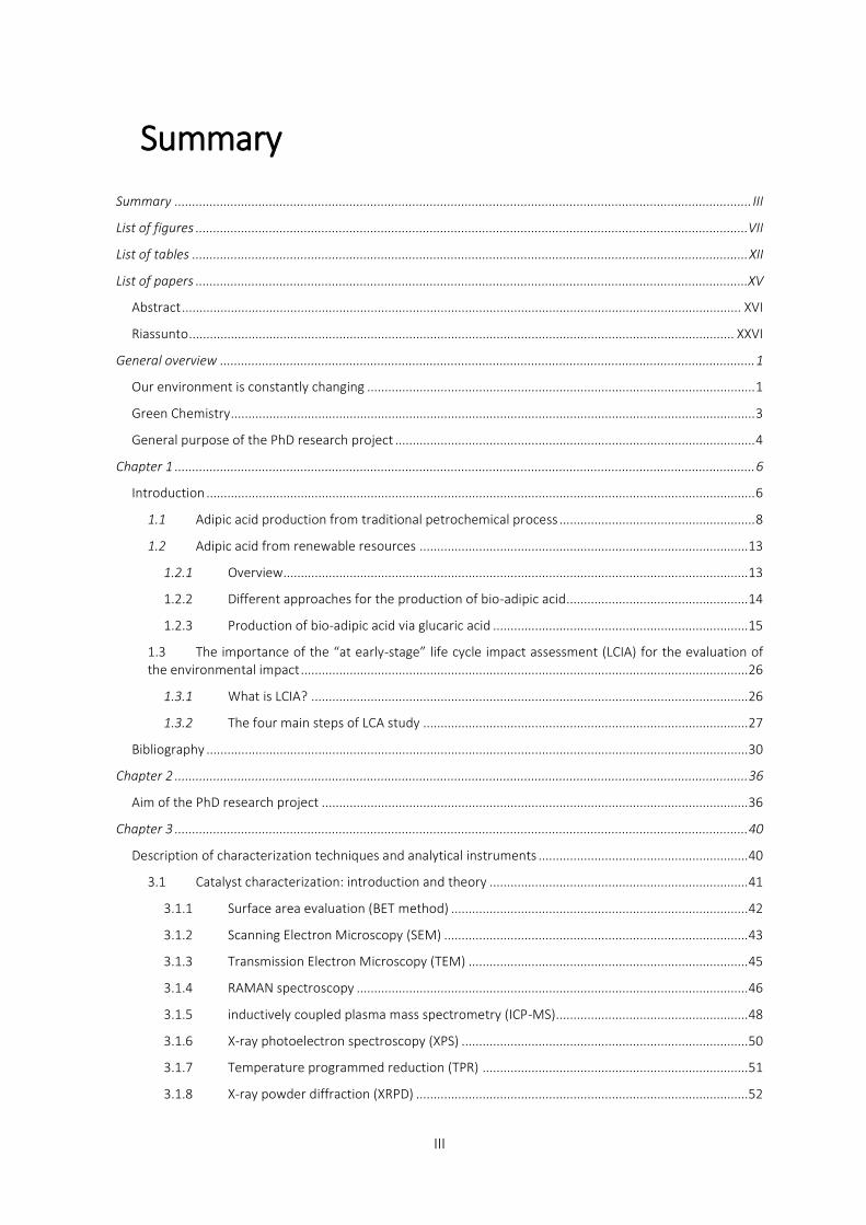
Summary Summary ..................................................................................................................................................................... III
List of figures .............................................................................................................................................................. VII
List of tables ............................................................................................................................................................... XII
List of papers ..............................................................................................................................................................XV
Abstract ................................................................................................................................................................ XVI
Riassunto ............................................................................................................................................................ XXVI
General overview ......................................................................................................................................................... 1
Our environment is constantly changing ............................................................................................................... 1
Green Chemistry ...................................................................................................................................................... 3
General purpose of the PhD research project ....................................................................................................... 4
Chapter 1 ...................................................................................................................................................................... 6
Introduction ............................................................................................................................................................. 6
1.1 Adipic acid production from traditional petrochemical process ........................................................ 8
1.2 Adipic acid from renewable resources .............................................................................................. 13
1.2.1 Overview..................................................................................................................................... 13
1.2.2 Different approaches for the production of bio-adipic acid .................................................... 14
1.2.3 Production of bio-adipic acid via glucaric acid ......................................................................... 15
1.3 The importance of the “at early-stage” life cycle impact assessment (LCIA) for the evaluation of the environmental impact ................................................................................................................................ 26
1.3.1 What is LCIA? ............................................................................................................................. 26
1.3.2 The four main steps of LCA study ............................................................................................. 27
Bibliography ........................................................................................................................................................... 30
Chapter 2 .................................................................................................................................................................... 36
Aim of the PhD research project .......................................................................................................................... 36
Chapter 3 .................................................................................................................................................................... 40
Description of characterization techniques and analytical instruments ............................................................ 40
3.1 Catalyst characterization: introduction and theory .......................................................................... 41
3.1.1 Surface area evaluation (BET method) ..................................................................................... 42
3.1.2 Scanning Electron Microscopy (SEM) ....................................................................................... 43
3.1.3 Transmission Electron Microscopy (TEM) ................................................................................ 45
3.1.4 RAMAN spectroscopy ................................................................................................................ 46
3.1.5 inductively coupled plasma mass spectrometry (ICP-MS)....................................................... 48
3.1.6 X-ray photoelectron spectroscopy (XPS) .................................................................................. 50
3.1.7 Temperature programmed reduction (TPR) ............................................................................ 51
3.1.8 X-ray powder diffraction (XRPD) ............................................................................................... 52

IV
3.2 Analytical techniques .......................................................................................................................... 53
3.2.1 UV-Visible analysis (UV-Vis) ....................................................................................................... 53
3.2.2 Gas-chromatographic analysis (GC) .......................................................................................... 54
3.2.3 Nuclear Magnetic Resonance (NMR) ........................................................................................ 56
Bibliography ........................................................................................................................................................... 57
Chapter 4 .................................................................................................................................................................... 58
Development of the analytical method ............................................................................................................... 58
4.1 Development and calibration of Ultraviolet-Visible for the evaluation of muconic acid conversion 60
4.1.1 Ultraviolet-Visible analysis calibration for sodium muconate acid in water .......................... 61
4.1.2 Ultraviolet-Visible analysis calibration for t,t-muconic acid in water ..................................... 63
4.1.3 Ultraviolet-Visible analysis calibration for t,t-muconic acid in ethanol .................................. 64
4.2 Development and calibration of gas-chromatographic method (GC) using different columns and detectors for the evaluation of selectivity. ..................................................................................................... 65
4.2.1 Analysis calibration using SUPELCOWAX 10 column ............................................................... 66
4.2.2 Analysis calibration using SP-2380 column .............................................................................. 70
4.3 Application of the developed analytical method .............................................................................. 77
4.3.1 Data elaboration ........................................................................................................................ 77
4.3.2 Optimization of the Fischer’s esterification reaction ............................................................... 82
4.3.3 Influence of Fischer esterification on stereoisomers ............................................................... 83
4.3.4 Stereoisomer separation: set up of the chromatographic parameter for SUPELCOWAX column 85
4.3.5 Stereoisomer separation: set up of the chromatographic parameter for SP-2380 column .. 86
4.3.6 Material balance ........................................................................................................................ 88
Conclusion ......................................................................................................................................................... 91
Bibliography ........................................................................................................................................................... 92
Chapter 5 .................................................................................................................................................................... 93
Muconic acid hydrogenation using commercial Pt and Pd catalysts.................................................................. 93
5.1 Overview on heterogeneous catalyzed hydrogenation reaction ..................................................... 94
5.1.1 Hydrogenation equipment ........................................................................................................ 96
5.2 Set up of the hydrogenation reactor ................................................................................................. 97
5.2.1 Stainless-steel autoclave for high pressure reactions.............................................................. 97
5.2.2 Low pressure reactor .............................................................................................................. 101
5.3 Evaluation of the starting operating parameters ........................................................................... 102
5.3.1 Hydrogen solubility in water in function of pressure and temperature .............................. 102
5.3.2 Control of kinetic regime ........................................................................................................ 104
5.4 Pt/AC 5% commercial catalyst ......................................................................................................... 108
5.4.1 t,t-MA hydrogenation in water .............................................................................................. 108

V
5.4.2 Influence of pressure .............................................................................................................. 108
5.4.3 Fresh and used catalyst characterization .............................................................................. 112
5.4.4 t,t-MA hydrogenation in synthetic fermentation broth ....................................................... 115
5.4.5 t,t-MA hydrogenation in light alcoholic solvent .................................................................... 117
5.5 Pd/AC 5% commercial catalyst ........................................................................................................ 121
5.6 Fresh catalyst characterization ........................................................................................................ 121
5.6.1 Hydrogenation reaction in stainless steel autoclave ............................................................ 125
5.6.2 Hydrogenation reaction in glass reactor ............................................................................... 138
5.6.3 Used catalyst characterization ............................................................................................... 140
Conclusion........................................................................................................................................................... 149
Bibliography ........................................................................................................................................................ 150
Chapter 6 .................................................................................................................................................................. 152
Mechanism identification and regression of kinetic parameters .................................................................... 152
6.1 State of art ........................................................................................................................................ 153
6.2 Materials and Methods.................................................................................................................... 154
6.2.1 Experimental ........................................................................................................................... 154
6.2.2 Kinetic modelling..................................................................................................................... 155
6.2.3 LHHW models and nonlinear regression .............................................................................. 156
6.3 Results and discussion ..................................................................................................................... 158
6.3.1 Preliminary study at constant temperature .......................................................................... 158
6.3.2 Refined mechanism and model.............................................................................................. 161
Conclusion........................................................................................................................................................... 169
Regression model and code ............................................................................................................................... 170
Bibliography ........................................................................................................................................................ 184
Chapter 7 .................................................................................................................................................................. 186
t,t-MA and Na-Muc hydrogenation using Pd/AC home-made catalyst ........................................................... 186
7.1 Overview about the synthesis of colloidal metal nanoparticles .................................................... 187
7.2 Pd/AC 1% catalyst: activated carbon effect .................................................................................... 189
7.2.1 Catalyst synthesis .................................................................................................................... 189
7.2.2 Catalyst characterization ........................................................................................................ 190
7.2.3 Hydrogenation reaction in glass reactor ............................................................................... 193
7.3 Pd/AC 1% catalyst: effect of the amount of stabilizer ................................................................... 195
7.3.1 Catalyst synthesis .................................................................................................................... 195
7.3.2 Fresh catalyst characterization .............................................................................................. 196
7.3.3 Hydrogenation reaction in glass reactor ............................................................................... 203
Conclusion........................................................................................................................................................... 211
Bibliography ........................................................................................................................................................ 212

VI
Chapter 8 .................................................................................................................................................................. 213
Life cycle impact assessment analysis (LCIA) and economic feasibility study ................................................. 213
8.1 Overview about LCIA study of adipic acid ....................................................................................... 214
8.2 LCIA study: methods and system boundaries definition ............................................................... 215
8.2.1 Method .................................................................................................................................... 215
8.2.2 System boundaries.................................................................................................................. 215
8.3 Adipic acid from oil .......................................................................................................................... 216
8.3.1 N2O evaluation ........................................................................................................................ 217
8.3.2 Glutaric and succinic acid evaluation ..................................................................................... 217
8.4 Bio-derived adipic acid ..................................................................................................................... 218
8.4.1 Glucose production from maize starch ................................................................................. 218
8.4.2 Muconic acid hydrogenation to bio-adipic acid .................................................................... 219
8.4.3 ReCiPe 2016, method used for environmental impact evaluation ...................................... 223
8.5 Results and discussion ..................................................................................................................... 223
8.5.1 ReCiPe midpoint (H) results ................................................................................................... 223
8.6 How to decrease the environmental impact? ................................................................................ 231
Waste wood hydrolysis and sugar fermentation .................................................................. 232
8.6.2 Muconic acid production ........................................................................................................ 233
8.6.3 Results ..................................................................................................................................... 235
8.7 LCA study conclusions ...................................................................................................................... 237
8.9 Economic feasibility analysis ........................................................................................................... 238
8.9.1 Base case scenario .................................................................................................................. 239
8.9.2 Sustainability analysis ............................................................................................................. 240
8.9.3 Cost distribution and process bottleneck analysis ................................................................ 241
8.10 Conclusion about the economic feasibility of the bio-process ...................................................... 242
Bibliography ........................................................................................................................................................ 244
General conclusion and future perspective ...................................................................................................... 247
Acknowledgements ............................................................................................................................................ 251
VII
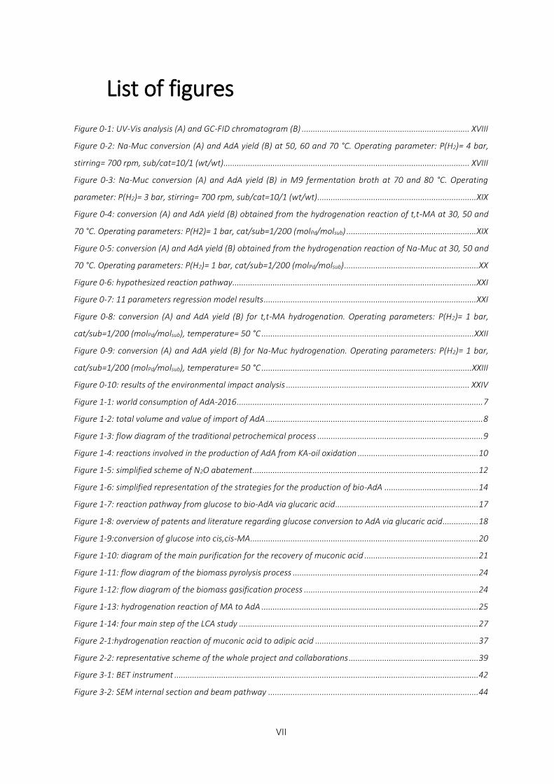
List of figures
Figure 0-1: UV-Vis analysis (A) and GC-FID chromatogram (B) ........................................................................... XVIII
Figure 0-2: Na-Muc conversion (A) and AdA yield (B) at 50, 60 and 70 °C. Operating parameter: P(H2)= 4 bar,
stirring= 700 rpm, sub/cat=10/1 (wt/wt).............................................................................................................. XVIII
Figure 0-3: Na-Muc conversion (A) and AdA yield (B) in M9 fermentation broth at 70 and 80 °C. Operating
parameter: P(H2)= 3 bar, stirring= 700 rpm, sub/cat=10/1 (wt/wt) ....................................................................... XIX
Figure 0-4: conversion (A) and AdA yield (B) obtained from the hydrogenation reaction of t,t-MA at 30, 50 and
70 °C. Operating parameters: P(H2)= 1 bar, cat/sub=1/200 (molPd/molsub) .......................................................... XIX
Figure 0-5: conversion (A) and AdA yield (B) obtained from the hydrogenation reaction of Na-Muc at 30, 50 and
70 °C. Operating parameters: P(H2)= 1 bar, cat/sub=1/200 (molPd/molsub) ............................................................ XX
Figure 0-6: hypothesized reaction pathway ............................................................................................................. XXI
Figure 0-7: 11 parameters regression model results ............................................................................................... XXI
Figure 0-8: conversion (A) and AdA yield (B) for t,t-MA hydrogenation. Operating parameters: P(H2)= 1 bar,
cat/sub=1/200 (molPd/molsub), temperature= 50 °C ............................................................................................... XXII
Figure 0-9: conversion (A) and AdA yield (B) for Na-Muc hydrogenation. Operating parameters: P(H2)= 1 bar,
cat/sub=1/200 (molPd/molsub), temperature= 50 °C .............................................................................................. XXIII
Figure 0-10: results of the environmental impact analysis .................................................................................. XXIV
Figure 1-1: world consumption of AdA-2016 .............................................................................................................. 7
Figure 1-2: total volume and value of import of AdA ................................................................................................. 8
Figure 1-3: flow diagram of the traditional petrochemical process .......................................................................... 9
Figure 1-4: reactions involved in the production of AdA from KA-oil oxidation ...................................................... 10
Figure 1-5: simplified scheme of N2O abatement ..................................................................................................... 12
Figure 1-6: simplified representation of the strategies for the production of bio-AdA .......................................... 14
Figure 1-7: reaction pathway from glucose to bio-AdA via glucaric acid ................................................................ 17
Figure 1-8: overview of patents and literature regarding glucose conversion to AdA via glucaric acid ................ 18
Figure 1-9:conversion of glucose into cis,cis-MA ...................................................................................................... 20
Figure 1-10: diagram of the main purification for the recovery of muconic acid ................................................... 21
Figure 1-11: flow diagram of the biomass pyrolysis process ................................................................................... 24
Figure 1-12: flow diagram of the biomass gasification process .............................................................................. 24
Figure 1-13: hydrogenation reaction of MA to AdA ................................................................................................. 25
Figure 1-14: four main step of the LCA study ........................................................................................................... 27
Figure 2-1:hydrogenation reaction of muconic acid to adipic acid ......................................................................... 37
Figure 2-2: representative scheme of the whole project and collaborations .......................................................... 39
Figure 3-1: BET instrument ........................................................................................................................................ 42
Figure 3-2: SEM internal section and beam pathway .............................................................................................. 44

VIII
Figure 3-3: TEM instrument ....................................................................................................................................... 45
Figure 3-4: RAMAN instrument ................................................................................................................................. 46
Figure 3-5: diagram of Rayleigh and Raman scattering process ............................................................................. 47
Figure 3-6: ICP-MS apparatus.................................................................................................................................... 48
Figure 3-7:ICP detectable chemical element ............................................................................................................ 50
Figure 3-8: XPS apparatus ......................................................................................................................................... 50
Figure 3-9: TPR apparatus ......................................................................................................................................... 51
Figure 3-10: UV-Vis instrument and spectrum ......................................................................................................... 53
Figure 3-11: GC instrument ....................................................................................................................................... 54
Figure 4-1: chromatogram obtained from HPLC analysis developed by Vardon et al. ........................................... 59
Figure 4-2: UV-Vis spectra of t,t-MA, (2E)-hexenedioic acid and AdA ..................................................................... 61
Figure 4-3: Na-Muc calibration in water ................................................................................................................... 62
Figure 4-4: calibration of t,t-MA in water ................................................................................................................. 63
Figure 4-5: calibration of t,t-MA in ethanol .............................................................................................................. 64
Figure 4-6: reaction scheme of Fischer’s esterification ............................................................................................ 65
Figure 4-7: calibration of (3E)HxDME ....................................................................................................................... 68
Figure 4-8: calibration of DMA .................................................................................................................................. 70
Figure 4-9: calibration of (2E)HxDME (SP-2380 column) ......................................................................................... 73
Figure 4-10: calibration of (3E)HxDME (SP-2380 column) ....................................................................................... 75
Figure 4-11: calibration of DMA (SP-2380 column) .................................................................................................. 77
Figure 4-12:evaluation of the DMA and (3E)HxDME formation during esterification reaction ............................. 83
Figure 4-13: chromatogram of esterified t,t-MA, AdA and (3E)-hexenedioic acid for isomerization evaluation .. 84
Figure 4-14: chromatographic separation of DMA, DMM and (3E)HxDME ........................................................... 85
Figure 4-15: chromatogram from SP 2380 column .................................................................................................. 87
Figure 5-1: picture and schematic representation of autoclave reactor ................................................................. 97
Figure 5-2: TPR analysis of the commercial Pt/C 5% (black line) and carbon support (red line) ........................... 99
Figure 5-3: glass reactor configuration .................................................................................................................. 101
Figure 5-4: hydrogen concentration in water at different temperatures and pressures ..................................... 104
Figure 5-5: Sodium muconate conversion evaluation at 250, 500 and 700 rpm T=60 °C, P(H2)= 4 bar, reaction
time= 60 min, sub/cat= 10 (wt/wt) and [MA]= 7∙10-2M ....................................................................................... 107
Figure 5-6: dependence of conversion and AdA yield on the hydrogen pressure at 70°C, cat/sub=200 (wt/wt), [Na-
Muc]=7.56E-02 M ................................................................................................................................................... 108
Figure 5-7: substrate/catalyst ratio optimization performed at T=60 °C, stirring rate =500 rpm, P(H2)=4 bar . 109
Figure 5-8: conversion of Na-Muc at different temperatures. Stirring=500 rpm, P(H2)=4 bar, sub/cat=24
(molsub/molPd), [Na-Muc]=7·10-2M ......................................................................................................................... 110
Figure 5-9: yields of the different compounds at different temperatures and AdA yield .................................... 111
Figure 5-10: results of the recycling test ................................................................................................................ 112

IX
Figure 5-11: Characterization by TEM of A) fresh and B) used catalyst ............................................................... 112
Figure 5-12: EDX mapping analysis of the (A-C) fresh Pt/C 5% catalyst and (B-D) the pre-treated ones ........... 113
Figure 5-13: Characterization by SEM of fresh (A, B) and used catalyst (C, D) in different zones ...................... 114
Figure 5-14: XRPD of Pt/AC 5% ............................................................................................................................... 114
Figure 5-15: conversion of sodium muconate (A) and AdA yield (B) in M9 fermentation broth ......................... 115
Figure 5-16: conductivity measurement on Pt/AC 5% in M9 ................................................................................ 116
Figure 5-17: t,t-MA conversion in EtOH at different temperatures ...................................................................... 117
Figure 5-18: yield of the reaction products (A,B,C,D,E) and AdA at different temperatures in EtOH at P(H2)=4 bar,
[t,t-MA]=0.054 M (10 mL) ...................................................................................................................................... 118
Figure 5-19: comparison of the conversion (A) and AdA yield (B) in water and EtOH at T=70 °C P(H2)= 4 bar,
stirring= 500 rpm .................................................................................................................................................... 119
Figure 5-20: conversion (A) and AdA yield (B) in MeOH at T=70 °C and P(H2) = 4 bar ........................................ 120
Figure 5-21:comparison of the results in term of t,t-MA conversion (A) and AdA yield (B) in alcoholic solvent 120
Figure 5-22: XRD pattern of commercial fresh Pd/AC 5% ..................................................................................... 122
Figure 5-23: TEM of fresh Pd/AC 5% catalyst (A) and EDX maps of the image (B, C).......................................... 122
Figure 5-24: SEM images of fresh Pd/AC 5% at 40 KX (A) and 250 KX (B) ........................................................... 123
Figure 5-25: TEM images(A), evaluation of the lattice fringe of Pd(111) specie (B) and particle size distribution (C)
for fresh commercial Pd/AC 5% catalyst ................................................................................................................ 124
Figure 5-26: XPS analysis on fresh commercial Pd/AC 5% catalyst ...................................................................... 125
Figure 5-27: conversion and YAdA evaluation at different cat/sub (molPd/molsub) ratio for t,t-MA and Na-Muc
................................................................................................................................................................................. 127
Figure 5-28: Initial activity at different pressure for t,t-MA (orange) and Na-Muc (green) hydrogenation....... 129
Figure 5-29: Pressure effects on conversion and yield using Na-Muc as substrate ............................................. 130
Figure 5-30: Pressure effects on conversion and yield using t,t-MA as substrate ............................................... 131
Figure 5-31: effect of Na-Muc concentration at different pressure ..................................................................... 132
Figure 5-32: effect of temperature during t,t-MA hydrogenation ........................................................................ 133
Figure 5-33: yield of the intermediates and AdA during t,t-MA hydrogenation reaction at different temperatures
................................................................................................................................................................................. 134
Figure 5-34: effect of temperature on conversion (A) and YAdA (B) during Na-Muc hydrogenation ................. 135
Figure 5-35: yield of the intermediates and AdA during Na-Muc hydrogenation reaction at different temperatures
................................................................................................................................................................................. 135
Figure 5-36: Arrhenius’ plot for the apparent activation energy evaluation ....................................................... 137
Figure 5-37: conversion of t,t-MA (solid line) and Na-Muc (dash line) at different temperatures ..................... 137
Figure 5-38: control of the kinetic regime during t,t-MA (orange) and Na-Muc (green) .................................... 139
Figure 5-39: Na-Muc conversion at different cat/sub ratios ................................................................................ 139
Figure 5-40: XPS and deconvolution of Pd species at different reaction times .................................................... 141
Figure 5-41: comparison of XPS results for Pd element during t,t-MA hydrogenation ....................................... 142
X
Figure 5-42: Pd(0) percentage during the hydrogenation reaction ...................................................................... 142
Figure 5-43: C deconvolution of catalyst samples recovered during t,t-MA hydrogenation ............................... 143
Figure 5-44: comparison of C species in the catalyst used for t,t-MA hydrogenation ......................................... 144
Figure 5-45: reduction of C=O and Csp3 specie during the hydrogenation reaction of t,t-MA ........................... 144
Figure 5-46: XPS and deconvolution of Pd species during Na-Muc hydrogenation reaction .............................. 145
Figure 5-47: comparison of XPS results for Pd element during Na-Muc hydrogenation ..................................... 146
Figure 5-48: Pd(0) percentage during the hydrogenation reaction ...................................................................... 147
Figure 5-49: C deconvolution of catalyst’s sample recovered during Na-Muc hydrogenation ........................... 147
Figure 5-50: comparison of C species in the catalyst used for Na-Muc hydrogenation ...................................... 148
Figure 6-1: reaction scheme with all possible monounsaturated intermediate isomers. The species reported are
trans,trans-muconic acid (MA), α,β cis-hexenedioc acid (cHDA), α,β trans-hexenedioic acid (tHDA), β,γ cis-
hexenedioic acid (cHDAbg), β,γ trans-hexenedioic acid (tHDAbg) and adipic acid (AA) ..................................... 156
Figure 6-2: hydrogenation at different temperatures ........................................................................................... 159
Figure 6-3: comparison between experimental and calculated values from model A (left) and B (right) .......... 160
Figure 6-4: hypothesized reaction scheme of model LHHW_17P ......................................................................... 163
Figure 6-5: concentration profiles for the hydrogenation of ttMA on Pt/C 5% catalyst at 4 bar of hydrogen. Results
of the regression with model LHHW_17P .............................................................................................................. 166
Figure 6-6: sensitivity analysis on the parameters of model LHHW_13P ............................................................. 167
Figure 6-7: concentration profiles for the hydrogenation of ttMA on Pt/C 5% catalyst at 4 bar of hydrogen. Results
of the regression with model LHHW_11P .............................................................................................................. 168
Figure 7-1: different types of colloids ..................................................................................................................... 187
Figure 7-2: Lamer's diagram................................................................................................................................... 187
Figure 7-3: 3 steps fro the synthesis of the home-made catalysts ....................................................................... 189
Figure 7-4: N2 adsorption isotherm for the differen carbon support .................................................................... 191
Figure 7-5: pore size distribution of the activated carbon support ...................................................................... 191
Figure 7-6: TEM of Pd/KB 1% .................................................................................................................................. 192
Figure 7-7: TEM of Pd/G60 1% ............................................................................................................................... 192
Figure 7-8: TEM of Pd/Norit 1%.............................................................................................................................. 192
Figure 7-9: t,t-MA conversion (A) and YAdA (B) .................................................................................................... 193
Figure 7-10: yield of reaction intermediates and AdA during t,t-MA hydrogenation .......................................... 194
Figure 7-11: Na-Muc conversion (A) and YAdA (B) ................................................................................................ 194
Figure 7-12: yield of reaction intermediates and AdA during Na-Muc hydrogenation ...................................... 195
Figure 7-13: N2 adsorptioin isotherm of KB series ................................................................................................. 197
Figure 7-14: pore size distribution of KB series ...................................................................................................... 197
Figure 7-16:TEM of 10_0.65PVA ............................................................................................................................ 198
Figure 7-15: TEM of 10_0.3PVA ............................................................................................................................. 198
Figure 7-17: TEM of 10_1.2PVA ............................................................................................................................. 198

XI
Figure 7-18: TEM of 10_0.0PVA ............................................................................................................................. 199
Figure 7-19: Pd/C ratio evaluated from the Survay spectra .................................................................................. 199
Figure 7-20: (Csp3+C-O)/Csp2 ratio of KB series catalysts .................................................................................... 200
Figure 7-21: Pd(0)/Pd(II) ratio of KB series ............................................................................................................ 201
Figure 7-22: Pd (A) and C (B) deconvolution for the different KB samples ........................................................... 202
Figure 7-23: conversion (A) and AdA yield (B) during t,t-MA hydrogentation with KB series catalysts .............. 203
Figure 7-24: initial activity (A) and AdA yield after 30 min of reaction ................................................................ 204
Figure 7-25: deconvolution of C species after 15 min ........................................................................................... 205
Figure 7-26: deconvolution of C specie after 90 min ............................................................................................. 206
Figure 7-27: Pd deconvolution afte 90 min ............................................................................................................ 206
Figure 7-28: conversion (A) and AdA yield (B) during Na-Muc hydrogentation with KB series catalysts ........... 207
Figure 7-29: initial activity of KB series during Na-Muc hydrogenation and AdA yield at 30 min ...................... 207
Figure 7-30: deconvolution of C specie after 30 min ............................................................................................. 208
Figure 7-31: Pd deconvolution after 30 min .......................................................................................................... 209
Figure 7-32: C deconvolution after 90 min ............................................................................................................ 209
Figure 7-33: Pd deconvolution after 30 min .......................................................................................................... 210
Figure 7-34: variation of Pd(0)/Pd(II) ratio at different reaction times ................................................................ 210
Figure 8-1: system boundaries ............................................................................................................................... 215
Figure 8-2: industrial process for the production of oil-based AdA ...................................................................... 216
Figure 8-3: reactions involved for the production of AdA from oil ....................................................................... 216
Figure 8-4: block diagram for the production of and purification of AdA ............................................................ 219
Figure 8-5: detailed flow sheet for the production of bio-AdA (red: utilities, green: directly recycles, blue: recycles
with the use of other unit operation or waste water treatment) ......................................................................... 220
Figure 8-6: global warming .................................................................................................................................... 224
Figure 8-7: human carcinogenic (A) and non-carcinogenic (B) toxicity ................................................................ 225
Figure 8-8: land use (A) and water consumption (B) ............................................................................................. 226
Figure 8-9: mineral (A) and fossil (B) scarcity ........................................................................................................ 227
Figure 8-10: terrestrial (A), freshwater (B), and marine (C) ecotoxicity ............................................................... 228
Figure 8-11: ionizing radiation (A), fine particulate matter (B) and terrestrial acidification (C) ......................... 230
Figure 8-12: freshwater (A) and marine (B) eutrophication ................................................................................. 231
Figure 8-13: reaction pathway from wood biomass to cis,cis-MA ....................................................................... 232
Figure 8-14: LCA results comparison among oil derived AdA, Bio-AdA from starch and bio-AdA from waste wood
................................................................................................................................................................................. 235
XII
List of tables
Table 0-1: initial activity after 10 minutes of reaction on Pd/AC 1% home-made catalyst ................................. XXIII
Table 1-1: Physico-chemical properties of AdA .......................................................................................................... 7
Table 1-2:Overview of the results achieved in oxidation of glucose (conversion (X) to glucaric acid and yield (Y))
.................................................................................................................................................................................... 15
Table 1-3: overview of the literature data about the production of muconic acid ................................................. 19
Table 1-4:overview on the scientific literature about MA hydrogenation to bio-AdA ............................................ 25
Table 3-1: summary of the main techniques used for the characterization of a solid material ............................ 41
Table 4-1: Calibration data of Na-Muc in water ....................................................................................................... 62
Table 4-2: Calibration data of t,t-MA in water ......................................................................................................... 63
Table 4-3: Calibration data of t,t-MA in ethanol ...................................................................................................... 64
Table 4-4:calibration data of (3E)HxDME ................................................................................................................. 66
Table 4-5:chromatographic results for (3E)HxDME calibration ............................................................................... 67
Table 4-6: results for (3E)HxDME calibration ........................................................................................................... 67
Table 4-7: sample preparation for DMA calibration ................................................................................................ 69
Table 4-8: chromatographic results for DMA calibration ........................................................................................ 69
Table 4-9: results for DMA calibration ...................................................................................................................... 69
Table 4-10: sample preparation for (2E)HxDME calibration (SP-2380 column) ..................................................... 72
Table 4-11:chromatographic results for (2E)HxDME calibration (SP-2380 column) .............................................. 72
Table 4-12: sample preparation and chromatographic results for (3E)HxDME calibration (SP-2380 column) .... 74
Table 4-13: results for (3E)HxDME calibration (SP-2380 column) ........................................................................... 74
Table 4-14: samples preparation and chromatographic results for DMA calibration (SP-2380 column) ............. 76
Table 4-15: results for DMA calibration (SP-2380 column) ...................................................................................... 76
Table 4-16:diluition table for UV-Vis sample preparation ....................................................................................... 78
Table 4-17: results of GC analysis.............................................................................................................................. 80
Table 4-18: retention times for SUPELCOWAX 10 column ....................................................................................... 86
Table 4-19: retention time using SP 2380 column .................................................................................................... 87
Table 4-20: mass balance evaluation ........................................................................................................................ 89
Table 5-1: hydrogen concentration in function of temperature and pressure evaluated with Henry’s Law ...... 103
Table 5-2: parameters used for mass transfer evaluation .................................................................................... 107
Table 5-3: results of the catalyst/substrate ratio optimization ............................................................................ 109
Table 5-4: conductivity tests on M9 broth and catalyst washing ......................................................................... 116
Table 5-5: elemental analysis on fresh Pd/AC 5% ................................................................................................. 123
Table 5-6: evaluation of the percentage of Pd(0) and Pd(II) in the fresh catalyst ............................................... 125
Table 5-7: Results for catalyst/substrate ratio optimization ................................................................................ 126

XIII
Table 5-8: value of the initial activity at different hydrogen pressures ................................................................ 129
Table 5-9: results of the different concentration and pressure on Na-Muc conversion and YAdA ..................... 132
Table 5-10: data for the construction of the Arrhenius’ plot ................................................................................ 136
Table 5-11: check of kinetic regime for t,t-MA hydrogenation ............................................................................. 138
Table 5-12: check of kinetic regime for Na-Muc hydrogenation .......................................................................... 138
Table 5-13: percentage of Pd(II) and Pd(0) at different reaction time ................................................................. 140
Table 5-14: Binding energy for the different C groups .......................................................................................... 143
Table 5-15: percentage of different C species in the catalyst used for t,t-MA hydrogenation ........................... 143
Table 5-16: percentage of Pd(II) and Pd(0) at different reaction time ................................................................. 145
Table 5-17: Binding energy for the different C groups .......................................................................................... 147
Table 5-18: percentage of different C species in the catalyst used for Na-Muc hydrogenation ......................... 148
Table 6-1: generic equations for the simplified mechanism with intermediate pseudo component. Dual site L-H
model according to Yang and Hougen tables, n=2 without H2 dissociation, n=3 with dissociation .................. 159
Table 6-2: concentration of the different compound at T=60 °C .......................................................................... 160
Table 6-3: generic equations for the refined mechanism with intermediates: dual site L-H model according to
Yang and Hougen tables, n=2 without H2 dissociation, n=3 with dissociation ................................................... 161
Table 6-4: calculated parameters for the three models, adsorption constants Ki are in L/mol .......................... 162
Table 6-5: experimental data used for the regression of parameter ................................................................... 163
Table 6-6: Calculated values of the model parameters with 95% confidence interval and regression metrics . 165
Table 7-1: list of prepared catalysts ....................................................................................................................... 190
Table 7-2: results of BET analysis on activated carbon supports .......................................................................... 191
Table 7-3: list of KB series samples prepared with different amount of PVA ....................................................... 196
Table 7-4: BET results of KB series catalyst ............................................................................................................ 196
Table 7-5: atomic percentage of C, O and Pd in the KB sample ........................................................................... 199
Table 7-6: Binding energy for the C species ........................................................................................................... 200
Table 7-7: percentage of the different C species of KB series catalysts ............................................................... 200
Table 7-8: BE of the detected Pd species ............................................................................................................... 201
Table 7-9: Pd(II) and Pd(0) species within the KB series ........................................................................................ 201
Table 7-10: binding energy of the species after 15 min of reaction ..................................................................... 204
Table 7-11: composition of C specie after 15 min of reaction with t,t-MA .......................................................... 205
Table 7-12: species detected from the survey spectrum on KB 0.65 sample after 90 min of reaction ............... 205
Table 7-13: results of the C deconvolution of KB 0.65PVA after 90 minutes of reaction .................................... 206
Table 7-14: results of Pd deconvolution of KB 0.65PVA after 90 minutes of reaction ......................................... 206
Table 7-15: element detected from a used sample after 30 min of reaction ....................................................... 208
Table 7-16: C species detected from the used sample after 30 min ..................................................................... 208
Table 7-17: Pd species detected after 30 min ........................................................................................................ 209
Table 7-18: element detected from a used sample after 90 min of reaction ....................................................... 209
XIV
Table 7-19: C species detected from the used sample after 90 min ..................................................................... 209
Table 7-20: Pd species detected after 30 min ........................................................................................................ 210
Table 8-1: amount of chemicals for MA production .............................................................................................. 218
Table 8-2: chemicals and materials for 1 kg of muconic acid ............................................................................... 234
Table 8-3: LCA results comparison among oil derived AdA, Bio-AdA from starch and bio-AdA from waste wood
................................................................................................................................................................................. 236
Table 8-4: chemicals and utilities cost ................................................................................................................... 238
Table 8-5: results of the economical feasibility using different scenarios ............................................................ 240
Table 8-6: impact of utilities, chemicals and capital on the production cost of bio-AdA from glucose .............. 241
XV
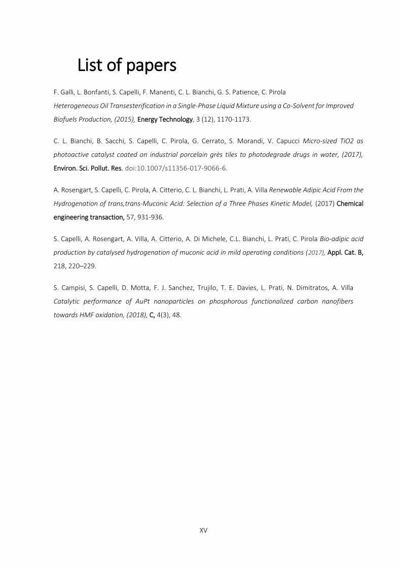
List of papers
F. Galli, L. Bonfanti, S. Capelli, F. Manenti, C. L. Bianchi, G. S. Patience, C. Pirola
Heterogeneous Oil Transesterification in a Single-Phase Liquid Mixture using a Co-Solvent for Improved
Biofuels Production, (2015), Energy Technology, 3 (12), 1170-1173.
C. L. Bianchi, B. Sacchi, S. Capelli, C. Pirola, G. Cerrato, S. Morandi, V. Capucci Micro-sized TiO2 as
photoactive catalyst coated on industrial porcelain grès tiles to photodegrade drugs in water, (2017),
Environ. Sci. Pollut. Res. doi:10.1007/s11356-017-9066-6.
A. Rosengart, S. Capelli, C. Pirola, A. Citterio, C. L. Bianchi, L. Prati, A. Villa Renewable Adipic Acid From the
Hydrogenation of trans,trans-Muconic Acid: Selection of a Three Phases Kinetic Model, (2017) Chemical
engineering transaction, 57, 931-936.
S. Capelli, A. Rosengart, A. Villa, A. Citterio, A. Di Michele, C.L. Bianchi, L. Prati, C. Pirola Bio-adipic acid
production by catalysed hydrogenation of muconic acid in mild operating conditions (2017), Appl. Cat. B,
218, 220–229.
S. Campisi, S. Capelli, D. Motta, F. J. Sanchez, Trujilo, T. E. Davies, L. Prati, N. Dimitratos, A. Villa
Catalytic performance of AuPt nanoparticles on phosphorous functionalized carbon nanofibers
towards HMF oxidation, (2018), C, 4(3), 48.
Abstract
XVI
Abstract
The awareness of the negative impacts of human activities against environment and public health have
pushed western governments to support long-term programs aimed at mitigating pollution and
reducing resource consumptions.1 In this spirit, both industry and academia are searching for new
solutions towards a “green” manufacturing practice, and the concept of “biorefinery” is taking place,
as a renewable counterpart of the ill-famed oil industry. Biorefineries are supposed to produce entire
classes of chemicals and fuels just as a real refinery.2 The great difference is that the carbon source
derives from renewable resources, following the natural cycle of CO2, which is captured from
atmosphere and fixed into living organisms (plants, algae, bacteria).3 Adipic acid (AdA) production was
chosen as base case due to the continuous increasing demand and the lack of some experimental data
necessary for further developments.4 The current AdA production covers a market of 3.7 million tons
per year (with a 4.1% of yearly growth)5 and increasing applications of AdA in various end-use
industries, automobiles, textiles, consumer goods, electrical and electronics, wires and cables and food
and packaging industry is expected to boost the AdA production during the forecast period (2017-
2025).6 Despite 70 years of technological maturity, the traditional benzene-based processes still raise
serious safety and environmental concerns.7 For these reasons, both private and public research
institutions have pursued alternative bio (and chemical) routes for AdA production.8 However, none of
these processes has reached industrialization yet, also due to the oil-price fall in 2014. This event
evidenced the main weakness of drop-in biorefineries: the need to compete in costs with a well-
established and optimized technology. A novel approach to process development is therefore required
for the case of bulk bio-derived chemical with low added value. Conceptual design acquires particular
importance from the early stage of process development, to produce reliable cost estimates and
projections, and to define a strategy for R&D. Due to the extensive and interdisciplinary literature
available, the first task was to collect and reorganize the accessible knowledge, identifying the current
alternative processes. A two steps biological-chemical process was considered worth of more detailed
investigation for its good yields and sustainability potential.9 This process consists in a first
fermentation to produce muconic acid (MA), starting from either glucose (from cellulose)10 or benzoic
acid (from lignin).11 In the second step the so produced MA is catalytically hydrogenated to AdA.
This doctoral thesis deals with the study of the hydrogenation of MA (a double unsaturated
dicarboxylic acid) to AdA with particular attention to understand the reaction mechanism. Moreover,
thanks to the collaboration with Politecnico di Milano, a first estimate of the kinetic parameters was
Abstract
XVII
performed, and a process superstructure was designed. This lead to a first economic and
environmental feasibility analysis that allowed to highlight the bottle neck of this new process.
Chapter 1 introduces the subject of the thesis including a discussion on the application of AdA. Chapter
2 describes the aim of the thesis. Chapter 3 illustrates the analytical instrument used during the
experimental work. Chapter 4 accurately describes the analytical method developed for the evaluation
of conversion and selectivity. Chapter 5 talks about the experimental details and the results obtained
using noble metals (Pt and Pd) supported commercial catalysts. After the collection of the first
experimental data, a regression of the kinetic parameter and a modelling of the reaction pathway was
performed as reported in Chapter 6. Chapter 7 describes the experimental details for the preparation
of home-made catalysts and their characterization. Moreover, the results obtained from the
hydrogenation of muconic acid and sodium muconate are reported. Finally, Chapter 8 provides a first
study about the environmental and economic feasibility analysis of the new purposed process.
The first experimental chapter describes the development of the analytical method used for the
evaluation of the conversion and products yield.
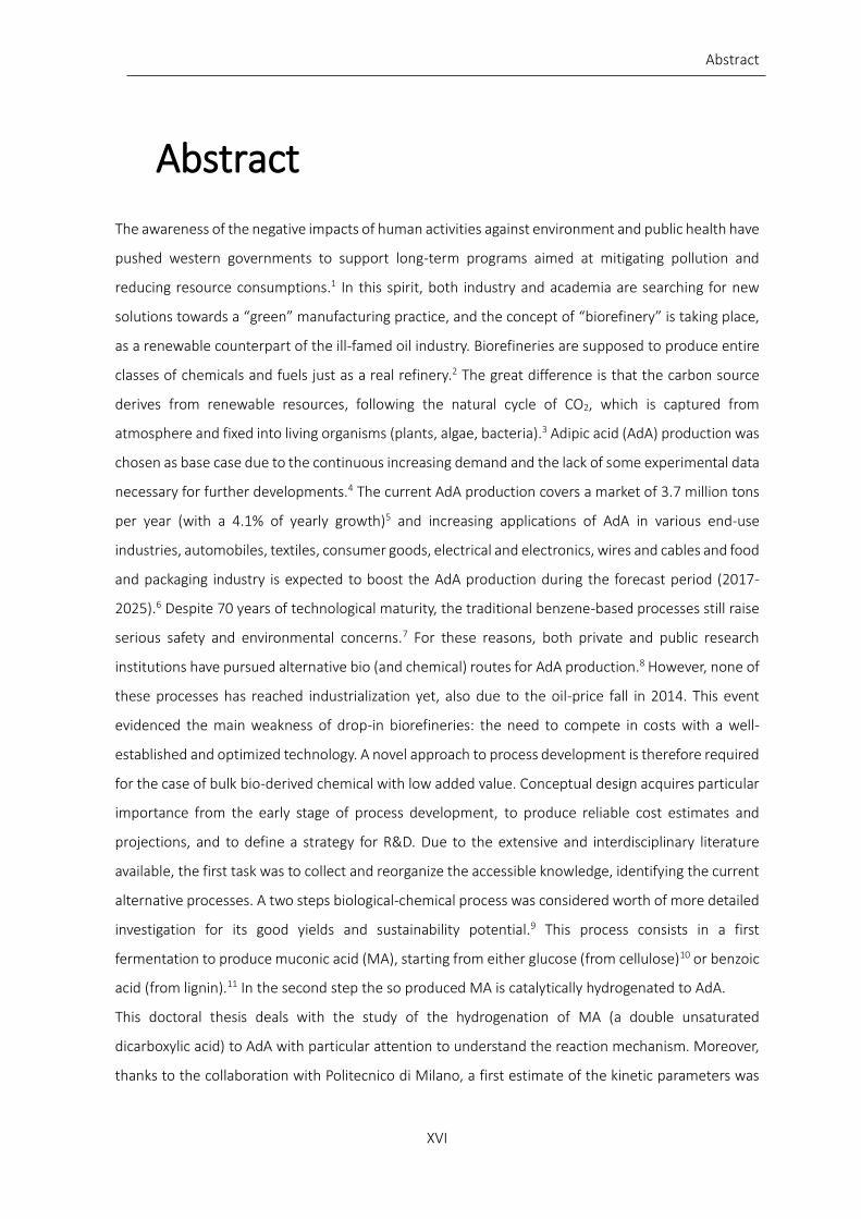
The conversion of the reaction was evaluated by UV-Vis analysis. A sample, collected after the catalyst
filtration, was analysed in a spectrophotometer T60 UV-Visible Spectrophotometer PRIXMA from 400
to 190 nm. The maximum absorption was at 264 nm (Figure 0-1 A). The calibration of the analysis was
done with sodium muconate (Na-Muc) prepared starting from commercial t,t-muconic acid (t,t-MA).
The selectivity was estimated by gas-chromatographic analyses. The aqueous collected sample was
dried in oven at 70 °C. The obtained white solid was then esterified with methanol in large excess and
sulphuric acid (50 µL) under blind stirring condition at 70 °C for 48 h. Derivatized methyl esters were
analysed by GC (Master GC Fast Gas Chromatograph Dani Instrument) equipped with TCD (or FID)
detector operating in split mode (1:3). Two different chromatographic columns were used during the
PhD period working at different operating conditions and detectors.
Supelcowax 10 column. The GC was outfitted with an Aldrich Supelcowax 10 (60 m, 0.53 mm, film
thickness 1 µm), and helium (15 mL∙min-1 column flow) was used as carrier gas. The GC-TCD method
consisted of an inlet temperature of 210 °C and TCD transfer line at 240 °C. A starting temperature of
60 °C was set and then ramped at 18 °C min-1 to a temperature of 120 °C. Then from 120 °C to 160 °C
ramped at 20 °C∙min-1. From 160 °C to 260 °C the temperature increases at 15 °C∙min-1 and held from
1 minute to purge the column. Butanol was used as internal standard.
SP-2380 column. The GC was outfitted with an Aldrich SP-2380 column (60 m, 0.53 mm 0.20 µm).
Helium, air and hydrogen was used to feed the column and the FID detector. The analysis was
performed using an isothermal analysis at 180 °C (Figure 0-1 B).
Abstract
XVIII
The second experimental chapter describes the results obtained during the hydrogenation reaction of
muconic acid and sodium muconate using noble metal supported commercial catalyst.
Hydrogenation reactions were conducted in a stainless-steel autoclave (at medium pressure of static
hydrogen) or in a glass reactor (at 1-1.2 bar of static hydrogen) equipped with an external jacket that
allowed to keep the reaction temperature constant. After the reaction (or after the collection of the
sample during the catalytic test) the catalyst was filtered, and the reactant solution was recovered for
the evaluation of conversion and selectivity. The conversion of the reaction was evaluated by UV-Vis
analysis. A sample, collected after the catalyst filtration, was analysed in a spectrophotometer from
400 to 190 nm. The maximum absorption was at 264 nm. The selectivity was estimated by gas-
chromatographic analyses after a derivatization of the reaction products.
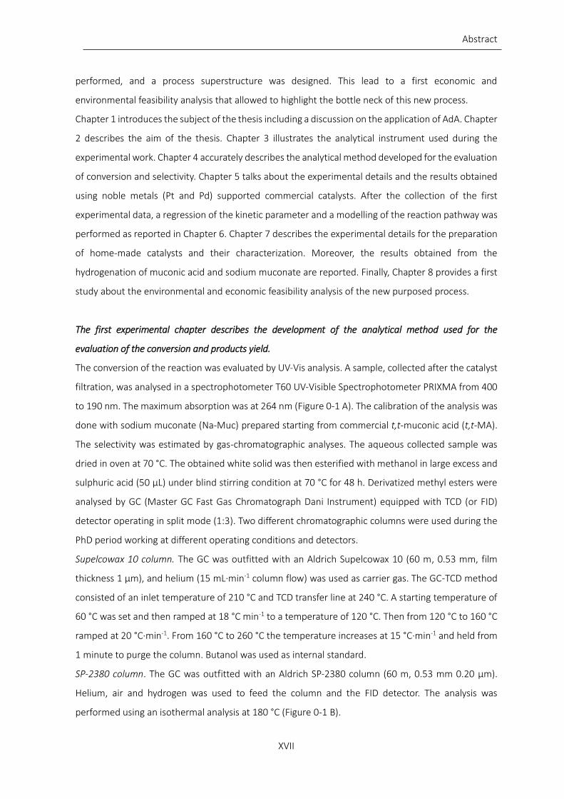
Pt/AC 5% commercial catalyst (Sigma Aldrich) was used after a pre-activation step made in the
autoclave at 200 °C for 3 h at 6 bar of hydrogen. Exploring different temperatures, hydrogen pressures
and amount of catalyst the most interesting results were obtained varying the temperature.
Increasing the temperature from 50 °C to 70 °C both Na-Muc conversion and AdA yield increase. After
60 min of reaction at 70 °C full conversion and yield to AdA was obtained (Figure 0-2).
200 250 300 350 400 450 500
0,0
0,2
0,4
0,6
0,8
1,0
1,2
1,4
Abs
.
wavelength (nm)
t,t-MA
(2E)-hexenedioic acid
AdA
4 5 6 7 8 9
0
50
100
150
200
Vo
ltag
e (
mV
)
Retention time (min)
Figure 0-1: UV-Vis analysis (A) and GC-FID chromatogram (B)
A B
0 20 40 60 80 100 120 1400
20
40
60
80
100
Co
nve
rsio
n (
%)
Reaction time (min)
70°C
50°C
60°C
0 30 60 90 120 150 180 210 2400
20
40
60
80
100
Y(%
)
Reaction time (min)
70°C
50°C
60°C
Figure 0-2: Na-Muc conversion (A) and AdA yield (B) at 50, 60 and 70 °C. Operating parameter: P(H2)= 4 bar, stirring= 700 rpm, sub/cat=10/1 (wt/wt)
A B
Abstract
XIX
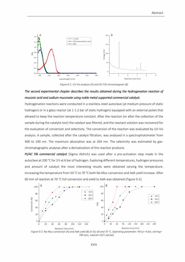
Recycling test showed the possibility to reuse the catalyst up to 10 times without loss in activity and
selectivity. Moreover, hydrogenation reaction was performed on Na-Muc using a synthetic
fermentation broth as reaction media. The minimal salt medium (M9) contains essential salts and
nitrogen suitable for recombinant E. Coli strains with the presence of large amount of NaOH.
The results showed that the conversion was not affected by temperature variation, but AdA yield was
higher increasing the temperature. The washings of the catalyst with water revealed that the salts
contained in the fermentation broth were absorbed on the catalyst surface blocking the active site to
the substrate. In fact, the reaction was slower than the one conducted in distilled water and the
maximum yield was about 80% after 3 hours of reaction (Figure 0-3).
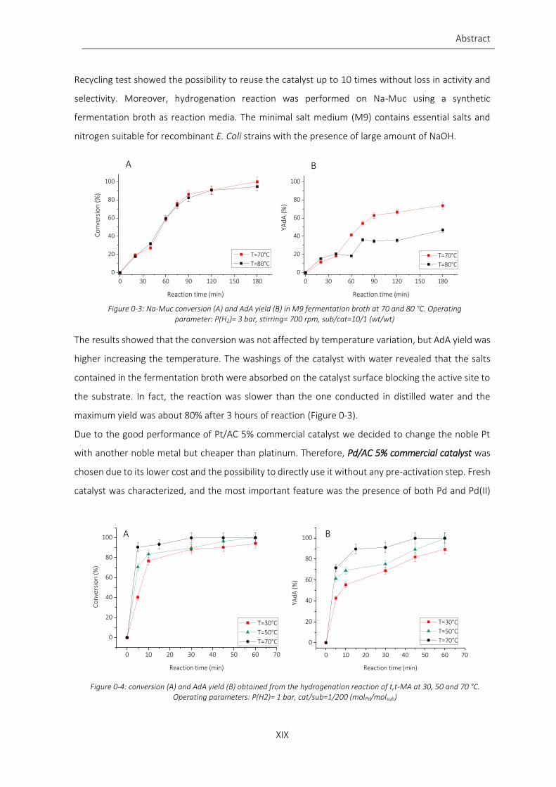
Due to the good performance of Pt/AC 5% commercial catalyst we decided to change the noble Pt
with another noble metal but cheaper than platinum. Therefore, Pd/AC 5% commercial catalyst was
chosen due to its lower cost and the possibility to directly use it without any pre-activation step. Fresh
catalyst was characterized, and the most important feature was the presence of both Pd and Pd(II)
0 30 60 90 120 150 180
0
20
40
60
80
100
120
YAd
A (
%)
Reaction time (min)
T=70°C
T=80°C
0 30 60 90 120 150 180
0
20
40
60
80
100
120
Co
nve
rsio
n (
%)
Reaction time (min)
T=70°C
T=80°C
Figure 0-3: Na-Muc conversion (A) and AdA yield (B) in M9 fermentation broth at 70 and 80 °C. Operating parameter: P(H2)= 3 bar, stirring= 700 rpm, sub/cat=10/1 (wt/wt)
0 10 20 30 40 50 60 70
0
20
40
60
80
100
Co
nve
rsio
n (
%)
Reaction time (min)
T=30°C
T=50°C
T=70°C
0 10 20 30 40 50 60 70
0
20
40
60
80
100
YAd
A (
%)
Reaction time (min)
T=30°C
T=50°C
T=70°C
Figure 0-4: conversion (A) and AdA yield (B) obtained from the hydrogenation reaction of t,t-MA at 30, 50 and 70 °C. Operating parameters: P(H2)= 1 bar, cat/sub=1/200 (molPd/molsub)
A B
A B

Abstract
XX
species on the catalyst surface in a ratio of about 1:1. Hydrogenation reactions were made with t,t-
MA and Na-Muc as substrates varying the pressure, the temperature and the amount of catalyst,
keeping constant the substrate concentration to 1.42E-02 M. Hydrogen pressure was varied from 1
to 3 bar, but the initial activity was not largely affected to this parameters as well as AdA yield.
Different results were obtained increasing the temperature from 30 °C to 70 °C. t,t-MA conversion did
not depend from the temperature except for short reaction time (Figure 0-4 A). On the other hand,
AdA yield was higher increasing the temperature (Figure 0-4 B).
Performing the reaction using the same operating parameters with Na-Muc the results were quite
different. In particular the conversion of Na-Muc at 30 °C was very slow and the yield to AdA reached
a maximum value of 90% at 70 °C (Figure 0-5). Therefore, the hydrogenation reaction differently
occurs on Na-Muc and t,t-MA. The evaluation of the initial activity confirmed this behaviour. The
calculated activation energy was: 3685 kJ/mol for the reduction of t,t-MA and 36170 kJ/mol for the
hydrogenation of Na-Muc. Apparent activation energy for Na-Muc is one order of magnitude greater
than the one related to the hydrogenation of t,t-MA. The characterization of used catalyst at different
reaction times revealed that during the reaction the Pd(II) specie was reduced to metal Pd and this
change in the oxidation state was faster using t,t-MA as substrate. Therefore, it was possible to
hypothesize that the hydrogenation of t,t-MA was faster due to the presence of higher amount of
metal Pd.
Starting from the collected data, a kinetic model was proposed as described in the chapter 6. We
considered the equations representing the absorption/desorption processes of all the species,
including hydrogen. It was not possible to establish the mechanism of H2 absorption process, so both
dissociated and un-dissociated hydrogen absorption was considered. Moreover, the kinetic equations
were proposed on the basis of the ones reported in the work of Yang e Hougen.12 Hence, different
A
Figure 0-5: conversion (A) and AdA yield (B) obtained from the hydrogenation reaction of Na-Muc at 30, 50 and 70 °C. Operating parameters: P(H2)= 1 bar, cat/sub=1/200 (molPd/molsub)
0 20 40 60 80 100
0
20
40
60
80
100
0 20 40 60 80 100
0
20
40
60
80
100
Conv
ersi
on (%
)
Reaction time (min)
T=30°C
T=50°C
T=70°C
YAdA
(%)
Reaction time (min)
T=30°C
T=50°C
T=70°C
B
Abstract
XXI
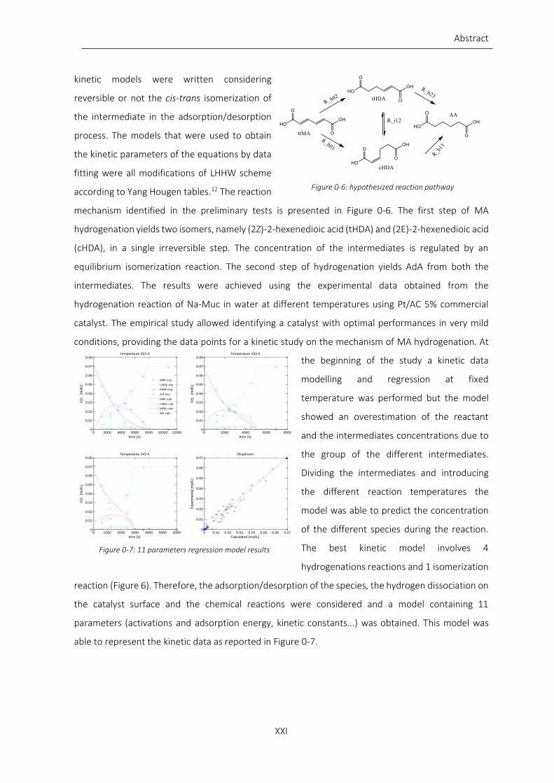
kinetic models were written considering
reversible or not the cis-trans isomerization of
the intermediate in the adsorption/desorption
process. The models that were used to obtain
the kinetic parameters of the equations by data
fitting were all modifications of LHHW scheme
according to Yang Hougen tables.12 The reaction
mechanism identified in the preliminary tests is presented in Figure 0-6. The first step of MA
hydrogenation yields two isomers, namely (2Z)-2-hexenedioic acid (tHDA) and (2E)-2-hexenedioic acid
(cHDA), in a single irreversible step. The concentration of the intermediates is regulated by an
equilibrium isomerization reaction. The second step of hydrogenation yields AdA from both the
intermediates. The results were achieved using the experimental data obtained from the
hydrogenation reaction of Na-Muc in water at different temperatures using Pt/AC 5% commercial
catalyst. The empirical study allowed identifying a catalyst with optimal performances in very mild
conditions, providing the data points for a kinetic study on the mechanism of MA hydrogenation. At
the beginning of the study a kinetic data
modelling and regression at fixed
temperature was performed but the model
showed an overestimation of the reactant
and the intermediates concentrations due to
the group of the different intermediates.
Dividing the intermediates and introducing
the different reaction temperatures the
model was able to predict the concentration
of the different species during the reaction.
The best kinetic model involves 4
hydrogenations reactions and 1 isomerization
reaction (Figure 6). Therefore, the adsorption/desorption of the species, the hydrogen dissociation on
the catalyst surface and the chemical reactions were considered and a model containing 11
parameters (activations and adsorption energy, kinetic constants...) was obtained. This model was
able to represent the kinetic data as reported in Figure 0-7.
0 2000 4000 6000 8000 10000 120000
0.01
0.02
0.03
0.04
0.05
0.06
0.07
0.08Temperature 323 K
time [s]
C(t
)
[mol/L]
0 2000 4000 6000 80000
0.01
0.02
0.03
0.04
0.05
0.06
0.07
0.08Temperature 333 K
time [s]
C(t
)
[mol/L]
0 1000 2000 3000 4000 5000 60000
0.01
0.02
0.03
0.04
0.05
0.06
0.07
0.08Temperature 343 K
time [s]
C(t
)
[mol/L]
ttMA exp
cHDA exp
tHDA exp
AA exp
ttMA calc
cHDA calc
tHDA calc
AA calc
0 0.01 0.02 0.03 0.04 0.05 0.06 0.070
0.01
0.02
0.03
0.04
0.05
0.06
0.07Dispersion
Calculated [mol/L]
Experim
enta
l [m
ol/L]
Figure 0-7: 11 parameters regression model results
Figure 0-6: hypothesized reaction pathway

Abstract
XXII
Due to the good performance of the Pd based catalyst, 7 catalysts were synthesized using the sol-
immobilization method. The method allows to synthesize supported NPs of noble metal controlling
the shape and the surface properties. Pd NPs were synthesized staring from the potassium chloride
precursor and using PVA an NaBH4 as stabilizing and reducing agent, respectively. 3 activated carbon
supports having different surface area were used as support. The detailed about the synthesis of the
home-made catalysts is described in chapter 7. Using t,t-MA as substrate no significant differences
among the catalysts were observed: full conversion of MA was obtained after 30 minutes of reaction,
while complete yield toward AdA was achieved after 60 minutes only with KB 0.65PVA (Figure 0-8).
Due to the good performance of the KB activated carbon support in the hydrogenation of t,t-MA and
Na-Muc (Figure 0-9 A and B) the influence of the amount of PVA used during the catalyst preparation
was studied. Therefore, different Pd/AC 1% using this carbon support were prepared varying the
weight ratio between the stabilizer and the metal (polyvinyl alcohol_PVA) from 0 to 1.2. The most
significant results were obtained using Na-Muc. Considering the YAdA all the curves showed an
induction period due to the production of a high amount of monounsaturated intermediate (Figure
0-9 D). Finally, the initial activity at 10 minutes of reaction was calculated dividing the reacted amount
of Na-Muc (mol) for the amount of Pd (mol) used for the reaction and the reaction time (sec). The
results reported in Table 1 shows that increasing the amount of PVA, the initial activity increases. This
behaviour might be explained considering that a larger amount of PVA helps the stabilization of small
nanoparticles which are more active than larger ones.
Figure 0-8: conversion (A) and AdA yield (B) for t,t-MA hydrogenation. Operating parameters: P(H2)= 1 bar, cat/sub=1/200
(molPd/molsub), temperature= 50 °C
0 20 40 60 80 100
0
20
40
60
80
100
Co
nve
rsio
n (
%)
Reaction time (min)
KB 0.65PVA
G60 0.65PVA
Norit_0.65PVA
t,t-MA
A
0 20 40 60 80 100
0
20
40
60
80
100t,t-MA
YAd
A (
%)
Reaction time (min)
KB 0.65PVA
G60 0.65PVA
Norit 0.65PVA
B
A B

Abstract
XXIII
Table 0-1: initial activity after 10 minutes of reaction on Pd/AC 1% home-made catalyst
Sample Initial activity (s-1)
KB_0.0PVA 0.11 KB_0.1PVA 0.10 KB_0.3PVA 0.13 KB_0.65PVA 0.19 KB_1.2PVA 0.25
Finally, an environmental and economic analysis compared the traditional petrochemical process with
two purposed bio processes for the production of AdA from glucose. The first bio process started from
the production of starch from maize culture, while the second used wood biomass as glucose source.
Detailed analysis of the results (Figure 0-10) revealed the advantages and weaknesses of the
innovative bio-processed. ReCiPe method was adopted for the evaluation of 18 environmental impact
categories. The results show that the traditional petrochemical process has a lower environmental
impact in all the categories except for the global warming. Firstly, industrial process for the production
of glucose from starch was considered and the results were largely affected by the cultivation, the
production of maize starch and all the respective waste treatments. Since the purpose is to produce
0 20 40 60 80 100
0
20
40
60
80
100
Conv
ersi
on (%
)
Reaction time (min)
Norit
KB 0.65PVA
G60 0.65PVA
Na-muc
0 20 40 60 80 100
0
20
40
60
80
100Na-muc
YAdA
(%)
Reaction time (min)
Norit 0.65PVA
KB 0.65PVA
G60 0.65PVA
0 20 40 60 80 100
0
20
40
60
80
100
Conv
ersi
on (%
)
Reaction time (min)
KB 0.0PVA
KB 0.1PVA
KB 0.3PVA
KB 0.65PVA
KB 1.2PVA
0 20 40 60 80 100
0
20
40
60
80
100
YAdA
(%)
Reaction time (min)
KB 0.1PVA
KB 0.3PVA
KB 0.65PVA
KB 1.2PVA
A B
C D
Figure 0-9: conversion (A) and AdA yield (B) for Na-Muc hydrogenation. Operating parameters: P(H2)= 1 bar, cat/sub=1/200 (molPd/molsub), temperature= 50 °C

Abstract
XXIV
glucose from waste wood, a second study was performed starting from the hydrolysis of wood and its
further conversion to glucose.
Figure 0-10: results of the environmental impact analysis
In this case the study started from the production process of bio-ethanol since no hydrolysis plant was
present in the software. Moreover, an average wood humidity was considered using literature data
for the yield of the process. Despite these limitations, the results obtained without considering cooling
water recycle and steam production from the process water were extremely different from the first
study. The global warming decreases from 22.9 to 13.6 Kg CO2 eq. that is the half of the value obtained
from the oil-derived process. All the results can be further improved introducing recycles of chemicals
and water, which will lead to a process capable of quasi- self-sustaining from energy demand point of
view and the purification products demand.
The economic study considered a base case scenario for a plant for 10000 metric ton/year of AdA,
located in America, with an annual productivity of 8150 h. The utilities and the cost of the chemicals
were referred to a plant located in America. From the base case scenario 4 other scenarios were
hypothesized considering the variation of glucose and AdA price, the variation of plant size and strain
yield and product concentration. The economic analysis in different scenarios confirmed that a bio-
AdA production is affected by the availability of cheap feedstock. In this specific case, the AdA process
Glo
bal
war
min
g
Stra
tosp
her
ic o
zon
e d
eple
tio
n
Ion
izin
g ra
dia
tio
n
Ozo
ne
form
atio
n, H
um
an h
ealt
h
Fin
e p
arti
cula
te m
atte
r fo
rmat
ion
Ozo
ne
form
atio
n, T
erre
stri
al e
cosy
stem
s
Terr
estr
ial a
cid
ific
atio
n
Fres
hw
ater
eu
tro
ph
icat
ion
Mar
ine
eutr
op
hic
atio
n
Terr
estr
ial e
coto
xici
ty
Fres
hw
ater
eco
toxi
city
Mar
ine
eco
toxi
city
Hu
man
car
cin
oge
nic
to
xici
ty
Hu
man
no
n-c
arci
no
gen
ic t
oxi
city
Lan
d u
se
Min
eral
res
ou
rce
scar
city
Foss
il re
sou
rce
scar
city
Wat
er c
on
sum
pti
on
0
5
10
20
25
30
3572.0
72.2
72.4
72.6
72.8
73.0 Oil-AdA
Bio-AdA from starch
Bio-AdA from waste wood
Ozone fo
rmat
ion, H
uman
healt
h
Fine p
artic
ulate m
atte
r form
atio
n
Ozone fo
rmat
ion, T
errest
rial e
cosy
stem
s
Terrest
rial a
cidifi
catio
n
Fresh
water e
utrophica
tion
Min
eral r
esourc
e scar
city
Foss
il reso
urce sc
arcit
y0.00
0.04
0.08
0.12
23456789
10
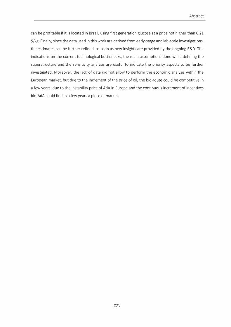
Abstract
XXV
can be profitable if it is located in Brazil, using first generation glucose at a price not higher than 0.21
$/kg. Finally, since the data used in this work are derived from early-stage and lab-scale investigations,
the estimates can be further refined, as soon as new insights are provided by the ongoing R&D. The
indications on the current technological bottlenecks, the main assumptions done while defining the
superstructure and the sensitivity analysis are useful to indicate the priority aspects to be further
investigated. Moreover, the lack of data did not allow to perform the economic analysis within the
European market, but due to the increment of the price of oil, the bio-route could be competitive in
a few years. due to the instability price of AdA in Europe and the continuous increment of incentives
bio-AdA could find in a few years a piece of market.
Riassunto
XXVI
Riassunto
I governi occidentali, consapevoli dell’impatto negativo delle attività umane sulla salute dell’ambiente
e il benessere delle persone, hanno elargito programmi a lungo termine, atti a mitigare l’inquinamento
e a ridurre il consumo di risorse energetiche e materiali.1 Contestualmente, sia l’industria che il mondo
accademico stanno incanalando i loro sforzi verso la ricerca di nuove soluzioni “green”. Un esempio
concreto sono le bio-raffinerie, sviluppate come controparte delle nocive industrie petrolchimiche,
che sono in grado di produrre intere classi di composti chimici e combustibili come una vera e propria
raffineria.2 La differenza sostanziale tra una raffineria e una bio-raffineria è la fonte di carbonio che,
nel caso di quest’ultima, deriva da risorse rinnovabili: l’anidride carbonica viene catturata
dall’atmosfera e fissata all’interno di alcuni microorganismi e piante, seguendo così il suo ciclo
naturale.3 L’acido adipico (AdA) è stato scelto come caso base, data la sua continua crescente
domanda e la mancanza di alcuni dati importanti per un ulteriore sviluppo in campo bio.4 La domanda
attuale di AdA copre un mercato di 3.7 milioni di tonnellate all’anno con una domanda che cresce del
circa 4.1%5 a causa delle prosperanti industrie automobilistiche, di vernici, tessili, dei beni di consumo,
elettriche ed elettroniche, di cablaggio e di imballaggio che continueranno a stimolarne la domanda
nel periodo 2017-2025.6 Nonostante i 70 anni di maturità tecnologica, il processo tradizionale di
produzione dell’AdA basato sull’utilizzo di benzene è tutt’ora al centro di controversie riguardanti la
sicurezza e l’impatto ambientale.7 Per tali ragioni sia le istituzioni di ricerca private che pubbliche
hanno perseguito strade alternative bio (e chimiche)8 per la produzione di tale composto chimico, ma
sfortunatamente, nessuno di tali processi ha raggiunto l’industrializzazione a causa della caduta del
prezzo del greggio nel 2014. Questo evento mise in luce la principale debolezza delle bio-raffinerie,
ovvero la necessità di competere in termini di costo con le tecnologie oramai consolidate e
ottimizzate. Nel caso di prodotti chimici di massa derivanti da processi bio si rende necessario lo
sviluppo di un approccio nuovo e innovativo: il design concettuale acquisisce quindi un ruolo di
fondamentale importanza nella fase iniziale di sviluppo di processo e le capacità di stimare
consistentemente costi e proiezioni e definire saldamente le strategie di ricerca e sviluppo sono i punti
chiave della buona riuscita del progetto. Data l’enorme quantità di letteratura disponibile e
l’interdisciplinarietà del progetto, il primo passo è stato la raccolta e l’organizzazione di tutta la
conoscenza accessibile e l’identificazione delle alternative di processo attuali e attuabili. A tale
riguardo si è deciso di scegliere un processo a due step che prevede un passaggio biotecnologico
seguito da uno puramente chimico in grado di dare buone rese e una potenziale sostenibilità
Riassunto
XXVII
ambientale ed economica.9 Più nel dettaglio il processo scelto consiste in una prima fermentazione
per la produzione di acido muconico (MA) partendo da glucosio (derivante dal trattamento della
cellulosa)10 o da acida benzoico (derivante dalla lignina).11 Successivamente l’MA così prodotto viene
idrogenato tramite processi catalitici ad AdA. La Tesi di Dottorato riguarda lo studio della reazione di
idrogenazione dell’acido muconico (un acido dicarbossilico di-insaturo) ad acido adipico con
particolare attenzione al meccanismo di reazione. Inoltre, grazie alla collaborazione con un gruppo di
ricerca del Politecnico di Milano è stata eseguita un prima stima dei parametri cinetici di reazione ed
è stata sviluppata la superstruttura dell’intero nuovo processo. Questo ha permesso di poter
effettuare una prima stima di fattibilità economica e di evidenziare i colli di bottiglia del nuovo
processo. Il Capitolo 1 fornisce un’introduzione all’oggetto della ricerca e la discussione dei principali
utilizzi e processi di produzione dell’AdA. Nel Capitolo 2 viene descritto lo scopo della tesi, mentre
all’interno del Capitolo 3 sono introdotti e descritti gli strumenti utilizzati durante la parte
sperimentale del lavoro. Il Capitolo 4 descrive accuratamente il metodo analitico sviluppato per la
valutazione della conversione e della resa dei prodotti e la sua consistenza. Nel Capitolo 5 vengono
riportate le procedure sperimentali e i risultati ottenuti utilizzando catalizzatori commerciali a base di
metalli nobili (Pt e Pd). Dopo la raccolta dei primi dati sperimentali si è proceduto alla regressione
cinetica dei parametri di reazione e alla modellizzazione del meccanismo di reazione (Capitolo 6). Nel
Capitolo 7 viene descritta la procedura di sintesi di catalizzatori a base di nanoparticelle di Pd
supportate su carboni attivi e i risultati ottenuti riguardo l’idrogenazione dell’MA e del sodio muconato
in ambiente acquoso. Infine, il Capitolo 8 riguarda lo studio di sostenibilità ambientale ed economica
del nuovo processo.
Il primo capitolo sperimentale descrive lo sviluppo del metodo analitico utilizzato per la valutazione della
conversione e delle rese di reazione.
La conversione della reazione è stata valutata utilizzando un’analisi UV-Vis; nel dettaglio un campione
prelevato dopo la filtrazione del catalizzatore eterogeneo è stato analizzato in uno spettrofotometro
T60 PRIXMA tra i 400 e i 190 nm. L’assorbimento massimo ottenuto si trova alla lunghezza d’onda di
264 nm ed è imputabile solamente all’MA (Figura 1 A). La calibrazione dell’analisi è stata eseguita con
sodio muconato (Na-Muc) preparata partendo da acido t,t-muconico (t,t-MA) e con acido t,t-MA puro.
La selettività dei prodotti di reazione è stata determinata servendosi di un’analisi gas cromatografica.
Il campione filtrato è stato essiccato in forno a 70 °C e il solido bianco così ottenuto è stato esterificato
in metanolo utilizzando un eccesso di acido solforico a 70 °C per 48 ore. I metilesteri così prodotti
sono stati analizzati tramite l’utilizzo di un gas cromatografo (Master Dani GC) fornito sia di rivelatore
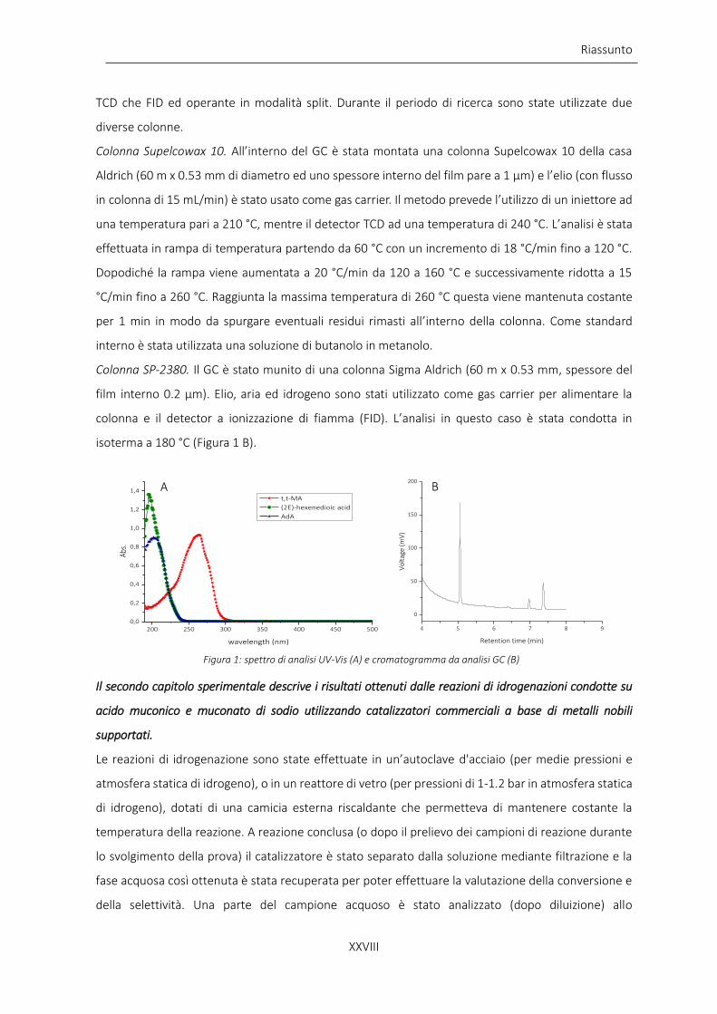
Riassunto
XXVIII
TCD che FID ed operante in modalità split. Durante il periodo di ricerca sono state utilizzate due
diverse colonne.
Colonna Supelcowax 10. All’interno del GC è stata montata una colonna Supelcowax 10 della casa
Aldrich (60 m x 0.53 mm di diametro ed uno spessore interno del film pare a 1 µm) e l’elio (con flusso
in colonna di 15 mL/min) è stato usato come gas carrier. Il metodo prevede l’utilizzo di un iniettore ad
una temperatura pari a 210 °C, mentre il detector TCD ad una temperatura di 240 °C. L’analisi è stata
effettuata in rampa di temperatura partendo da 60 °C con un incremento di 18 °C/min fino a 120 °C.
Dopodiché la rampa viene aumentata a 20 °C/min da 120 a 160 °C e successivamente ridotta a 15
°C/min fino a 260 °C. Raggiunta la massima temperatura di 260 °C questa viene mantenuta costante
per 1 min in modo da spurgare eventuali residui rimasti all’interno della colonna. Come standard
interno è stata utilizzata una soluzione di butanolo in metanolo.
Colonna SP-2380. Il GC è stato munito di una colonna Sigma Aldrich (60 m x 0.53 mm, spessore del
film interno 0.2 µm). Elio, aria ed idrogeno sono stati utilizzato come gas carrier per alimentare la
colonna e il detector a ionizzazione di fiamma (FID). L’analisi in questo caso è stata condotta in
isoterma a 180 °C (Figura 1 B).
Il secondo capitolo sperimentale descrive i risultati ottenuti dalle reazioni di idrogenazioni condotte su
acido muconico e muconato di sodio utilizzando catalizzatori commerciali a base di metalli nobili
supportati.
Le reazioni di idrogenazione sono state effettuate in un’autoclave d'acciaio (per medie pressioni e
atmosfera statica di idrogeno), o in un reattore di vetro (per pressioni di 1-1.2 bar in atmosfera statica
di idrogeno), dotati di una camicia esterna riscaldante che permetteva di mantenere costante la
temperatura della reazione. A reazione conclusa (o dopo il prelievo dei campioni di reazione durante
lo svolgimento della prova) il catalizzatore è stato separato dalla soluzione mediante filtrazione e la
fase acquosa così ottenuta è stata recuperata per poter effettuare la valutazione della conversione e
della selettività. Una parte del campione acquoso è stato analizzato (dopo diluizione) allo
200 250 300 350 400 450 500
0,0
0,2
0,4
0,6
0,8
1,0
1,2
1,4
Abs
.
wavelength (nm)
t,t-MA
(2E)-hexenedioic acid
AdA
4 5 6 7 8 9
0
50
100
150
200
Vo
ltag
e (m
V)
Retention time (min)
Figura 1: spettro di analisi UV-Vis (A) e cromatogramma da analisi GC (B)
A B

Riassunto
XXIX
spettrofotometro, mentre la selettività e stata determinata dopo una derivatizzazione dei prodotti di
reazione.
Il catalizzatore commerciale Pt/AC 5% (Sigma Aldrich) è stato utilizzato dopo un a pre-attivazione in
situ condotta a 200 °C per 3 ore a 6 bar di idrogeno. Le reazioni sono state effettuate variando la
temperatura, la pressione di idrogeno e la quantità di catalizzatore; i risultati più interessanti sono
stati ottenuti variando la temperatura di reazione. Aumentando la temperatura da 50 a 70 °C sia la
conversione del muconato di sodio che la resa in acido adipico aumentano. Dopo 1 ora di reazione a
70 °C si è ottenuta una completa conversione del substrato e una resa totale ad acido adipico (Figura
2).
Dai test di riciclo del catalizzatore si è evinto che è possibile utilizzare il catalizzatore per almeno 10
volte senza perdere in conversione e resa. Inoltre, per non escludere completamente la possibilità di
poter effettuare la reazione di idrogenazione direttamente all’interno del brodo di fermentazione, è
stato effettuato un test catalitico su un brodo sintetico composto dal cosiddetto “minimal salt media
M9”, un insieme di sali essenziali e composti azotati adatti a ceppi batterici ricombinanti del tipo E.
Coli, e da una grande quantità di idrossido di sodio. I risultati ottenuti hanno mostrato che la
0 20 40 60 80 100 120 1400
20
40
60
80
100
Co
nve
rsio
n (
%)
Reaction time (min)
70°C
50°C
60°C
0 30 60 90 120 150 180 210 2400
20
40
60
80
100
Y(%
)
Reaction time (min)
70°C
50°C
60°C
Figura 2: conversione Na-Muc (A) e resa in AdA (B) a 50, 60, 70 °C. Parametri operativi: P(H2)= 4 bar, agitazione= 700 rpm, sub /cat=10/1 (massa/massa)
0 30 60 90 120 150 180
0
20
40
60
80
100
120
YAd
A (
%)
Reaction time (min)
T=70°C
T=80°C
0 30 60 90 120 150 180
0
20
40
60
80
100
120
Co
nve
rsio
n (
%)
Reaction time (min)
T=70°C
T=80°C
Figura 3: conversione Na-Muc (A) e resa in AdA (B) all’interno del brodo di fermentazione a 70 e 80 °C. Parametri ooperativi: P(H2)= 3 bar, agitazione= 700 rpm, sub/cat= 10/1 (massa/massa)
A B
A B

Riassunto
XXX
conversione sembra non dipendere dalla temperatura del brodo di fermentazione, ma la resa in AdA
aumenta all’aumentare della temperatura. La reazione si è rivelata più lenta rispetto a quella condotta
in acqua distillata e la massima resa ottenuta è stata dell’80% circa dopo 3 ore di reazione.
Visti i buoni risultati ottenuti utilizzando il catalizzatore commerciale Pt/AC 5% si è optato per
cambiare il costoso catalizzatore a base di platino con un più economico catalizzatore commerciale di
palladio (Pd/AC 5%) che, oltretutto, non necessita di pre-attivazione. Il catalizzatore fresco è stato
caratterizzato utilizzando le principali tecniche e, grazie all’analisi XPS, si è dedotta la presenza di Pd(0)
e Pd(II) in superficie in equa quantità. La reazione di idrogenazione è stata condotta sia su t,t-MA che
sul Na-Muc variando la pressione, la temperatura e la quantità di catalizzatore, e tenendo costante la
concentrazione di partenza dei substrati a 1.42E-02 M. La pressione dell’idrogeno è stata variata da 1
a 3 bar; in tali condizioni l’attività iniziale resta pressoché costante così come la resa in AdA. Risultati
differenti sono stati ottenuti variando la temperatura da 30 °C a 70 °C. La conversione di t,t-MA non
dipende dalla temperatura, fatta eccezione per tempi brevi di reazione (Figura 4 A), mentre la resa in
AdA aumenta all’aumentare della temperatura (Figura 4 B).
0 10 20 30 40 50 60 70
0
20
40
60
80
100
Conv
ersi
on (%
)
Reaction time (min)
T=30°C
T=50°C
T=70°C
0 10 20 30 40 50 60 70
0
20
40
60
80
100
YAdA
(%)
Reaction time (min)
T=30°C
T=50°C
T=70°C
Figura 5: conversione (A) e resa in AdA (B) ottenute dall’idrogenazione di t,t-MA a 30, 50 e 70 °C. Parametri operativi:P(H2)= 1 bar, cat/sub= 1/200 (molPd/molsub)
0 20 40 60 80 100
0
20
40
60
80
100
0 20 40 60 80 100
0
20
40
60
80
100
Conv
ersi
on (%
)
Reaction time (min)
T=30°C
T=50°C
T=70°C
YAdA
(%)
Reaction time (min)
T=30°C
T=50°C
T=70°C
Figura 4: conversione (A) e resa in AdA (B) ottenuti dall’idrogenazione di Na-Muc a 30, 50 e 70 °C. Parametri operativi: P(H2)= 1 bar, cat/sub= 1/200 (molPd/molsub)
A B
A B
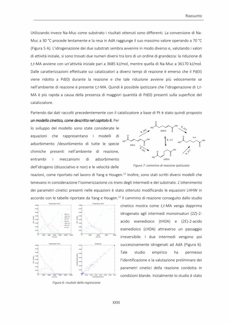
Riassunto
XXXI
Utilizzando invece Na-Muc come substrato i risultati ottenuti sono differenti. La conversione di Na-
Muc a 30 °C procede lentamente e la resa in AdA raggiunge il suo massimo valore operando a 70 °C
(Figura 5 A). L’idrogenazione dei due substrati sembra avvenire in modo diverso e, valutando i valori
di attività iniziale, si sono trovati due numeri diversi tra loro di un ordine di grandezza: la riduzione di
t,t-MA avviene con un’attività iniziale pari a 3685 kJ/mol, mentre quella di Na-Muc a 36170 kJ/mol.
Dalle caratterizzazioni effettuate sui catalizzatori a diversi tempi di reazione è emerso che il Pd(II)
viene ridotto a Pd(0) durante la reazione e che tale riduzione avviene più velocemente se
nell’ambiente di reazione è presente t,t-MA. Quindi è possibile ipotizzare che l’idrogenazione di t,t-
MA è più rapida a causa della presenza di maggiori quantità di Pd(0) presenti sulla superficie del
catalizzatore.
Partendo dai dati raccolti precedentemente con il catalizzatore a base di Pt è stato quindi proposto
un modello cinetico, come descritto nel capitolo 6. Per
lo sviluppo del modello sono state considerate le
equazioni che rappresentano i modelli di
adsorbimento /desorbimento di tutte le specie
chimiche presenti nell’ambiente di reazione,
entrambi i meccanismi di adsorbimento
dell’idrogeno (dissociativo e non) e le velocità delle
reazioni, come riportato nel lavoro di Yang e Hougen.12 Inoltre, sono stati scritti diversi modelli che
tenevano in considerazione l’isomerizzazione cis-trans degli intermedi e del substrato. L’ottenimento
dei parametri cinetici presenti nelle equazioni è stato ottenuto modificando le equazioni LHHW in
accordo con le tabelle riportate da Yang e Hougen.12 Il cammino di reazione conseguito dallo studio
cinetico mostra come t,t-MA venga dapprima
idrogenato agli intermedi monoinsaturi (2Z)-2-
acido esenedioico (tHDA) e (2E)-2-acido
esenedioico (cHDA) attraverso un passaggio
irreversibile. I due intermedi vengono poi
successivamente idrogenati ad AdA (Figura 6).
Tale studio empirico ha permesso
l’identificazione e la valutazione preliminare dei
parametri cinetici della reazione condotta in
condizioni blande. Inizialmente lo studio è stato
0 2000 4000 6000 8000 10000 120000
0.01
0.02
0.03
0.04
0.05
0.06
0.07
0.08Temperature 323 K
time [s]
C(t
)
[mol/L]
0 2000 4000 6000 80000
0.01
0.02
0.03
0.04
0.05
0.06
0.07
0.08Temperature 333 K
time [s]
C(t
)
[mol/L]
0 1000 2000 3000 4000 5000 60000
0.01
0.02
0.03
0.04
0.05
0.06
0.07
0.08Temperature 343 K
time [s]
C(t
)
[mol/L]
ttMA exp
cHDA exp
tHDA exp
AA exp
ttMA calc
cHDA calc
tHDA calc
AA calc
0 0.01 0.02 0.03 0.04 0.05 0.06 0.070
0.01
0.02
0.03
0.04
0.05
0.06
0.07Dispersion
Calculated [mol/L]
Experim
enta
l [m
ol/L]
Figura 7: cammino di reazione ipotizzato
Figura 6: risultati della regressione

Riassunto
XXXII
effettuato su dati raccolti a temperatura costante, ma il modello sovrastimava la concentrazione degli
intermedi a causa del raggruppamento di questi ultimi in una sola specie. Dividendo gli intermedi e
introducendo anche i dati ottenuti a diverse temperature il modello è in grado di predire la
concentrazione di tutte le specie. Il miglior modello cinetico sviluppato prevede 4 reazioni di
idrogenazione ed una di isomerizzazione. Considerando tutti gli step di reazione è quindi stato scritto
un modello contenente 11 parametri (energie di attivazione, energie di adsorbimento, costanti
cinetiche…) e che riesce a sovrapporsi ai dati sperimentali (Figura 7).
Considerando gli ottimi risultati ottenuti utilizzando il catalizzatore a base di Pd si è deciso di
sintetizzare 7 catalizzatori utilizzando il metodo del “sol-immobilization”; tale metodo permette di
sintetizzare nanoparticelle di Pd supportate su un materiale controllandone le dimensioni e le
proprietà superficiali. Le nanoparticelle di Pd sono state sintetizzate partendo dal precursore K2PdCl4,
utilizzando polivinilalcol (PVA) come agente stabilizzante e NaBH4 come agente riducente. Per la
sintesi di questi catalizzatori sono stati utilizzati 3 diversi carboni attivi aventi aree superficiali molto
diverse. I dettagli sulla sintesi dei catalizzatori sono descritti all’interno del capitolo 7. Conducendo la
reazione di idrogenazione su t,t-MA non si sono riscontrate grandi differenze in termini di
conversione, mentre una completa resa ad AdA è stata ottenuta solo per il catalizzatore preparato
utilizzando KB come carbone attivo di supporto (Figura 8 A e B). Anche nel caso di idrogenazione del
Na-Muc il carbone attivo KB è risultato quello in grado di produrre una maggiore quantità di AdA
(Figura 9 A e B). Considerati i buoni risultati ottenuti con il carbone KB, si è deciso di investigare come
la quantità di PVA utilizzato durante la sintesi possa inficiare sulla conversione e sulla resa in AdA; per
tale motivo si sono sintetizzati 5 diversi catalizzatori variando il rapporto in peso PVA/metallo tra 0 e
1.2. I risultati migliori sono stati ottenuti utilizzando come substrato Na-Muc. Tutte le curve di
conversione mostrano un periodo di induzione nella produzione di AdA tra gli 0 e i 15 minuti dovuta
all’iniziale produzione di grandi quantità di intermedio monoinsaturo (Figura 9 D). Infine, l’attività
iniziale valutata dopo 10 minuti di reazione mostra come, al crescere della quantità di PVA utilizzato
durante la sintesi, aumenti anche il suo valore. Questo andamento può essere spiegato considerando
che un’elevata quantità di PVA aiuta il processo di stabilizzazione di nanoparticelle più piccole che
sono più attive rispetto a quelle più grandi.

Riassunto
XXXIII
Tabella 1: attività iniziale dopo 10 minuti di reazione con Pd/AC 1% sintetizzati
Sample Initial activity (s-1)
KB_0.0PVA 0.11 KB_0.1PVA 0.10 KB_0.3PVA 0.13
KB_0.65PVA 0.19 KB_1.2PVA 0.25
0 20 40 60 80 100
0
20
40
60
80
100
Conv
ersi
on (%
)
Reaction time (min)
Norit
KB 0.65PVA
G60 0.65PVA
Na-muc
0 20 40 60 80 100
0
20
40
60
80
100Na-muc
YAdA
(%)
Reaction time (min)
Norit 0.65PVA
KB 0.65PVA
G60 0.65PVA
0 20 40 60 80 100
0
20
40
60
80
100
Conv
ersi
on (%
)
Reaction time (min)
KB 0.0PVA
KB 0.1PVA
KB 0.3PVA
KB 0.65PVA
KB 1.2PVA
0 20 40 60 80 100
0
20
40
60
80
100
YAdA
(%)
Reaction time (min)
KB 0.1PVA
KB 0.3PVA
KB 0.65PVA
KB 1.2PVA
A B
C D
Figura 9: conversione (A) e resa in AdA (B) durante l’idrogenazione di Na-Muc. Parametri operativi: P(H2)= 1 bar, cat/sub= 1/200 (molPd/molsub), temperatura= 50 °C
A
0 20 40 60 80 100
0
20
40
60
80
100
Co
nve
rsio
n (
%)
Reaction time (min)
KB 0.65PVA
G60 0.65PVA
Norit_0.65PVA
t,t-MA
A
0 20 40 60 80 100
0
20
40
60
80
100t,t-MA
YAd
A (
%)
Reaction time (min)
KB 0.65PVA
G60 0.65PVA
Norit 0.65PVA
B
Figura 8: conversione (A) e resa in AdA (B) durante l’idrogenazione di t,t-MA. Parametri operativi: P(H2)= 1 bar, cat/sub= 1/200 (molPd/molsub), temperatura= 50 °C
A B

Riassunto
XXXIV
Infine, è stata effettuata un’analisi ambientale ed economica per confrontare il processo tradizionale
petrolchimico di produzione di AdA con quello bio (partendo da glucosio) da noi proposto. Si è deciso
di considerare due processi bio che si differenziano solamente per la parte di produzione del glucosio:
il primo (in verde) parte dalla piantagione mais, mentre il secondo (in rosa) converte il legno di scarto.
Per la valutazione degli impatti ambientali è stato utilizzato il metodo ReCiPe che considera 18 diverse
categorie di impatto: i risultati dettagliati mostrati in Figura 10 rivelano i vantaggi e le debolezze del
nuovo processo bio. Innanzitutto, bisogna premettere che i risultati ottenuti partendo dalla
piantagione di mais sono ampiamente influenzati da tutte le utenze, l’acqua e i fertilizzanti utilizzati
durante la coltivazione e, di conseguenza, dal trattamento di tutte le acque di scarto derivanti dalla
conversione del mais in amido. Siccome l’idea principale è quella di produrre AdA da glucosio
derivante dagli scarti del legno, nel secondo processo bio si è considerata invece l’idrolisi del legno e
la sua successiva trasformazione in glucosio. Nell’ultimo caso, data l’assenza all’interno del software
del processo specifico di idrolisi, si è partiti da un impianto di produzione di bio-etanolo considerando
un’umidità media del legno e utilizzando rese di processo riportate in letteratura. Nonostante tali
limitazioni, i risultati ottenuti senza considerare ricicli delle acque di raffreddamento e di generazione
del vapore d’acqua dalle acque di processo, sono molto diversi rispetto a quelli ottenuti nel primo
caso. Per esempio, il riscaldamento globale decresce da 22.9 a 13.6 Kg CO2 eq., che è la metà del
valore ottenuto per il processo tradizionale. Tutti i risultati ottenuti sono ampiamente migliorabili
introducendo ricicli di alcuni composti chimici e dell’acqua; tali accorgimenti potrebbero rendere il
nuovo processo bio completamente auto sostiene sia dal punto di vista energetico che nella
purificazione dei prodotti di reazione. Lo studio di fattibilità economica parte da uno scenario di base
che prevede un impianto con capacità produttiva di 10000 ton/anno di acido adipico situato in nord
America con una produttività annua di 8150 ore. Il costo delle utenze e dei composti chimici necessari
fa riferimento ai prezzi americani. Partendo dallo scenario di base sono stati ipotizzati ulteriori 4
scenari considerando la variazione del prezzo del glucosio e del AdA, la modifica delle dimensioni
dell’impianto, della concentrazione dei prodotti e della resa dei ceppi batterici. L’analisi economica su
tali scenari ha confermato che la produzione del bio-AdA è influenzata dalla disponibilità di materie
prime economiche; nel caso specifico l’impianto potrebbe portare profitto se situato in Brasile ed
utilizza glucosio di prima generazione avente un prezzo non superiore a 0.21 $/kg. Siccome i risultati
derivano da uno studio che si trova ancora nella fase inziale di investigazione in laboratorio, i risultati
potranno essere ulteriormente ottimizzati durante le future fasi della ricerca. Tale studio ha permesso
di valutare i punti deboli di questa tecnologia e l’analisi di sensitività ha fornito indicazioni sugli aspetti
prioritari da investigare. Inoltre, data la mancanza di alcuni dati fondamentali riguardanti il continente
europeo, non è stato possibile effettuare un’analisi economica dettagliata riguardo alla possibilità di

Riassunto
XXXV
applicare tecnologia nel nuovo continente. Dato però il graduale aumento e l’instabilità del prezzo
dell’AdA il processo biotecnologico potrebbe risultare competitivo tra qualche anno.
Figura 10: risultati dello studio di impatto ambientale
1. European_commission. Environment & Climate Action_ Horizon 2020 programmes.
2. Wright, M. & Brown, R. C. Establishing the optimal sizes of different kinds of biorefineries. Biofuels, Bioprod. Biorefining 1, 191–200 (2007).
3. MacDowell, N. et al. An overview of CO2 capture technologies. Energy Environ. Sci. (2010). doi:10.1039/c004106h
4. Pyne, M. E. et al. An engineered Aro1 protein degradation approach for increased cis,cis -muconic acid biosynthesis in Saccharomyces cerevisiae. Appl. Environ. Microbiol. (2018). doi:10.1128/AEM.01095-18
5. Marketsandmarkets. Adipic Acid Market- Global Trends & Forecast to 2019. (2014). Available at: http://www.marketsandmarkets.com/Market-Reports/adipic-acid-269.html.
6. Adipic acid prices, markets & analysis. Available at: https://www.icis.com/chemicals/adipic-acid/.
7. Mainhardt, H. & Kruger, D. N2O emissions from adipic acid and nitric acid production. Good Pract. Guid. Uncertain. Manag. Natl. Greenh. Gas Invent. 183–195
8. Bart, J. C. J. & Cavallaro, S. Transiting from Adipic Acid to Bioadipic Acid. 1, Petroleum-Based Processes. Ind. Eng. Chem. Res. 54, 1–46 (2015).
9. Vardon, D. R. et al. cis,cis-Muconic acid: separation and catalysis to bio-adipic acid for nylon-6,6 polymerization. Green Chem. 18, 3397–3413 (2016).
10. Johnson, C. W. et al. Enhancing muconic acid production from glucose and lignin-derived aromatic compounds via increased protocatechuate decarboxylase activity. Metab. Eng. Commun. 3, 111–119 (2016).
11. Mizuno, S., Yoshikaw, N., Seki, M., Mikawa, T. & Imada, Y. Microbial production of cis,cis-muconic acid from benzoic acid. Appl. Microbiol. Biotechnol 28, (1988).
12. Yang, K. H. & Hougen, O. A. Determination of mechanism of catalyzed gaseous reactions. Chem. Eng. Prog. 46, 146–157 (1950).
Glo
bal w
arm
ing
Stra
tosp
heri
c oz
one
depl
etio
n
Ioni
zing
rad
iatio
n
Ozo
ne fo
rmat
ion,
Hum
an h
ealt
h
Fine
par
ticul
ate
mat
ter
form
atio
n
Ozo
ne fo
rmat
ion,
Ter
rest
rial
eco
syst
ems
Terr
estr
ial a
cidi
ficat
ion
Fres
hwat
er e
utro
phic
atio
n
Mar
ine
eutr
ophi
catio
n
Terr
estr
ial e
coto
xici
ty
Fres
hwat
er e
coto
xici
ty
Mar
ine
ecot
oxic
ity
Hum
an c
arci
noge
nic
toxi
city
Hum
an n
on-c
arci
noge
nic
toxi
city
Land
use
Min
eral
res
ourc
e sc
arci
ty
Foss
il re
sour
ce s
carc
ity
Wat
er c
onsu
mpt
ion
0
5
10
20
25
30
3572.0
72.2
72.4
72.6
72.8
73.0 Oil-AdA
Bio-AdA from starch
Bio-AdA from waste wood
Ozone fo
rmatio
n, Hum
an health
Fine particu
late m
atter f
ormatio
n
Ozone fo
rmatio
n, Terre
strial e
cosy
stem
s
Terrestr
ial acid
ificatio
n
Fresh
water e
utrophica
tion
Minera
l reso
urce sc
arcity
Fossil r
esourc
e scarc
ity0.00
0.04
0.08
0.12
23456789
10

1
General overview
Our environment is constantly changing
Our environment is constantly changing. There is no denying that. This is the sentence that
inspire this PhD research project.
In the last few years several natural disasters occurred, warming and cooling periods are becoming
more and more frequent and different types of weather patterns and much more are affecting our
daily life. All across the world, people are facing a wealth of new and challenging environmental
problems every day. Some of them are quite small and only affect a few ecosystems, but others are
greatly changing the landscape of what we already know. Currently many environmental processes
must be considered, and they are briefly described below.
1. Climate Change: problem that occurs due to rise in global warming which causes the
increment of atmosphere temperature by realising harmful gases by industry and burning
fossil fuels. The effects of the climate change are different such as modification in seasons,
melting of polar ice and frequent occurrence of floods and new diseases.
2. Global Warming: is the result of human practices like emission of greenhouse gases (CO2,
NOx, CO...). Global warming leads to rising temperatures of the oceans and the earth’s surface
causing excessive snow or desertification and other unpleasant weather phenomena.

General overview
2
3. Pollution: water and air pollution are one of the main topics discussed during several
conferences and congresses. Water pollution is caused by acid rain, oil spill and urban runoff,
while air pollution is manly related to gas emission by industries and factories and the
combustion of fossil fuel.
4. Natural resource depletion: fossil fuel consumption results in greenhouse gasses emission. In
the las few years people are taking efforts to shift to renewable sources (solar energy, wind
or biomass energy…) but the cost for their installation are often non-competitive.
5. Deforestation: our forests are natural sinks of carbon dioxide and produce fresh oxygen.
Deforestation simply means clearing of green cover and make that land available for
residential, industrial or commercial purpose.
6. Ocean acidification: it is a direct impact of excessive production of CO2. 25% of the total CO2
is produced by humans.1 The ocean acidity has increased by the last 250 years but by 2100, it
may shoot up by 150%.2
7. Water pollution: water is becoming an economic and political issue as the human population
fights for this resource. Desalting processes are becoming more and more important.
8. Overpopulation: population of the planet is increasing a lot due to the presence of more and
more specific disease treatments. This caused the depletion of sources like fuel, food and
water and the consequence increment of intensive agricultures productions.
9. Ozone layer depletion: it is attributed to pollution caused by chlorine and bromide found in
Chloro-floro carbons (CFC’s). The CFC’s are banned in many industries and consumer
products. Ozone layer is valuable because it prevents harmful UV radiation from reaching the
earth.
10. Acid rains: occurs due to the presence of pollutants in the atmosphere. Acid rain is a known
environmental problem that can have serious effect on human health, wildlife and aquatic
species
11. Waste disposal: the over consumption of resources and creation of plastics are creating a
global crisis of waste disposal. Plastic, fast food, packaging and cheap electronic wastes
threaten the well-being of humans. Waste disposal is one of urgent current environmental
problem.
All these described problems must be considered during the development of new industrial processes
and might be taken in to account also to improve the existing ones.
One of the most important rules to design a sustainable process are defined by Anastas and Warner.3
They identified 12 principles to follow to make a new process as greener as possible. Among these
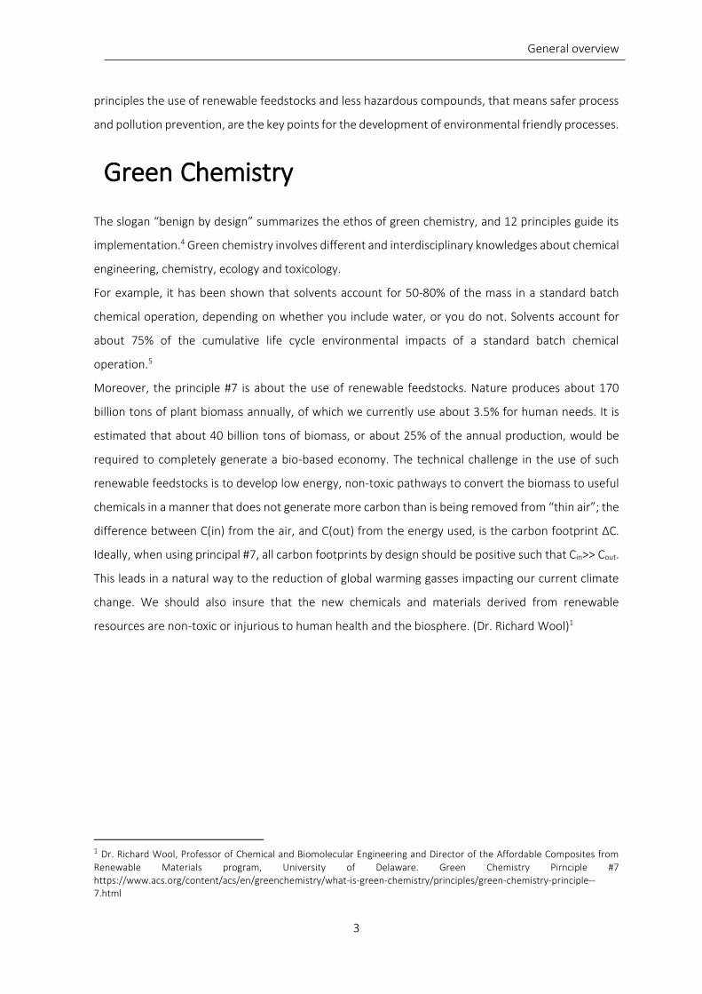
General overview
3
principles the use of renewable feedstocks and less hazardous compounds, that means safer process
and pollution prevention, are the key points for the development of environmental friendly processes.
Green Chemistry
The slogan “benign by design” summarizes the ethos of green chemistry, and 12 principles guide its
implementation.4 Green chemistry involves different and interdisciplinary knowledges about chemical
engineering, chemistry, ecology and toxicology.
For example, it has been shown that solvents account for 50-80% of the mass in a standard batch
chemical operation, depending on whether you include water, or you do not. Solvents account for
about 75% of the cumulative life cycle environmental impacts of a standard batch chemical
operation.5
Moreover, the principle #7 is about the use of renewable feedstocks. Nature produces about 170
billion tons of plant biomass annually, of which we currently use about 3.5% for human needs. It is
estimated that about 40 billion tons of biomass, or about 25% of the annual production, would be
required to completely generate a bio-based economy. The technical challenge in the use of such
renewable feedstocks is to develop low energy, non-toxic pathways to convert the biomass to useful
chemicals in a manner that does not generate more carbon than is being removed from “thin air”; the
difference between C(in) from the air, and C(out) from the energy used, is the carbon footprint ΔC.
Ideally, when using principal #7, all carbon footprints by design should be positive such that Cin>> Cout.
This leads in a natural way to the reduction of global warming gasses impacting our current climate
change. We should also insure that the new chemicals and materials derived from renewable
resources are non-toxic or injurious to human health and the biosphere. (Dr. Richard Wool)1
1 Dr. Richard Wool, Professor of Chemical and Biomolecular Engineering and Director of the Affordable Composites from Renewable Materials program, University of Delaware. Green Chemistry Pirnciple #7 https://www.acs.org/content/acs/en/greenchemistry/what-is-green-chemistry/principles/green-chemistry-principle--7.html
General overview
4
General purpose of the PhD research project
To develop new and greener chemical processes different approaches can be used.
Biotechnologist, chemists and chemical engineers are involved in different part of the
research, but the key point is to group all the results of the different approaches trying to find
the best compromise in terms of human health, environmental health and economic return.
This multidisciplinary thesis tries to put together different chemical scientific disciplines: physical
chemistry, theoretical chemistry, engineering chemistry, environmental chemical study and
biochemistry/biotechnology. It is not always simple to be on the same page. Often the results
considered good for a chemist, are not so good for the engineer and are completely unsuitable and
useless for a theoretical chemist. However, the key of the success is the common starting point:
improve the knowledge about the production of bio adipic acid starting from renewable sources. This
implies that the final aim is to develop an industrial process, so all the efforts are funneled to reach
this goal. This work starts from the basic research (i.e. catalytic study, development of analytical
method, characterization of the different catalysts, variation of the operating conditions...) and ends
with the development of an ideal bio adipic acid industrial process.
All this work is the results of a constructive collaboration with different professional figures and I want
to thank:
Alessandro ROSENGART, Ph.D., M.Sci in Chemical and Industrial Process Engineering (Politecnico di
Milano);
Alberto VILLA, Assistant professor, Chemistry Department, Università degli Studi di Milano;
Luca BRAMBILLA, Assistant Professor, Department of biotechnology and bioscience (Università degli
Studi di Milano Bicocca);
Nikolaos DIMITRATOS, Research Fellow, School of Chemistry (Cardiff University).

General overview
5
1. McMichael, A. J. & Woodruff, R. E. Climate Change and Human Health. in Encyclopedia of World
Climatology (ed. Oliver, J. E.) 209–213 (Springer Netherlands, 2005). doi:10.1007/1-4020-3266-8_41
2. Kerr, R. A. Ocean Acidification Unprecedented, Unsettling. Science 328, 1500–1501 (2010).
3. Anastas, P. T. & Warner, J. C. Green chemistry: theory and practice. (New York: Oxford University Press, 1998).
4. Anastas, P. T. & Zimmerman, J. B. Peer Reviewed: Design Through the 12 Principles of Green Engineering. Environ. Sci. Technol. 37, 94A–101A (2003).
5. Rani, B., Singh, U. & Maheshwari, R. K. Role of emerging green chemistry for human comfort and
economic intensification. Unique Res. J. Chem. 1, 1–15 (2013).

6
Chapter 1
Introduction
Climate change, limited oil reserves and geopolitical concerns combine to motivate an urgent quest
for alternatives to fossil derived fuels and commodity chemicals (the Grand Challenges).1 In this sense,
industrial innovation has already accepted the responsible practice of low energy use and minimal
waste generation, to align economic and environmental sustainability.2 As a further step, a growing
number of chemical industries are developing alternative processes that are based on renewable
sources.3 Much effort has been done in this direction for the development of a bio-based and
environmental friendly adipic acid (AdA) production.4 AdA is a strategic commodity chemical, widely
used as monomer in the synthesis of polyamides (PA-6,6), polyesters and other specialty products:
PA-6,6 accounts for about 85.4% of the total AdA demand, while other relevant applications are
polyurethanes (5%), and adipic esters (4%).5 In the geographical side, Asia-Pacific (APAC) accounted
for 36.5% of the overall the global adipic acid market.6
AdA is a crystalline powder, odorless and with a lethal dose concentration (LD50) of 3600 mg/kg. The
main physico-chemical properties are reported in Table 1-1.

Chapter 1- Introduction
7
Table 1-1: Physico-chemical properties of AdA
Physico-chemical properties
CAS number 124-04-9*
Chemical formula HOOC(CH2)4COOH*
Molar mass 146.14 g/mol*
Odour Odourless*
Melting point 152 °C*
Boiling point 337.5 °C*
Solubility in water 23 g/L at 25 °C§
logPow 0.081#
Flash point 196 °C§
Hazard statements H319§
Precautionary statements P305+P351+P338§
*http://www.sciencelab.com/msds.php?msdsId=9927423
§Sigma Aldrich
#Fisher chemical
Global AdA annual demand was estimated at 3750.8 metric tons in 2021 with a growth rate of 3–5%
per year.6,7 and its world consumption is reported in Figure 1-1.8
Figure 1-1: world consumption of AdA-2016
So far, the totality of the commercialized AdA derives from oil, mostly from the relatively expensive
benzene fraction.9 In Figure 1-2 the total amount of AdA and the value of import is reported.10
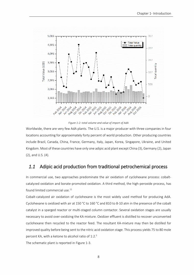
Chapter 1- Introduction
8
Figure 1-2: total volume and value of import of AdA
Worldwide, there are very few AdA plants. The U.S. is a major producer with three companies in four
locations accounting for approximately forty percent of world production. Other producing countries
include Brazil, Canada, China, France, Germany, Italy, Japan, Korea, Singapore, Ukraine, and United
Kingdom. Most of these countries have only one adipic acid plant except China (3), Germany (2), Japan
(2), and U.S. (4).
1.1 Adipic acid production from traditional petrochemical process
In commercial use, two approaches predominate the air oxidation of cyclohexane process: cobalt-
catalyzed oxidation and borate-promoted oxidation. A third method, the high-peroxide process, has
found limited commercial use.11
Cobalt-catalyzed air oxidation of cyclohexane is the most widely used method for producing AdA.
Cyclohexane is oxidized with air at 150 °C to 160 °C and 810 to 8-10 atm in the presence of the cobalt
catalyst in a sparged reactor or multi-staged column contactor. Several oxidation stages are usually
necessary to avoid over-oxidizing the KA mixture. Oxidizer effluent is distilled to recover unconverted
cyclohexane then recycled to the reactor feed. The resultant KA-mixture may then be distilled for
improved quality before being sent to the nitric acid oxidation stage. This process yields 75 to 80 mole
percent KA, with a ketone to alcohol ratio of 1:2.5
The schematic plant is reported in Figure 1-3.
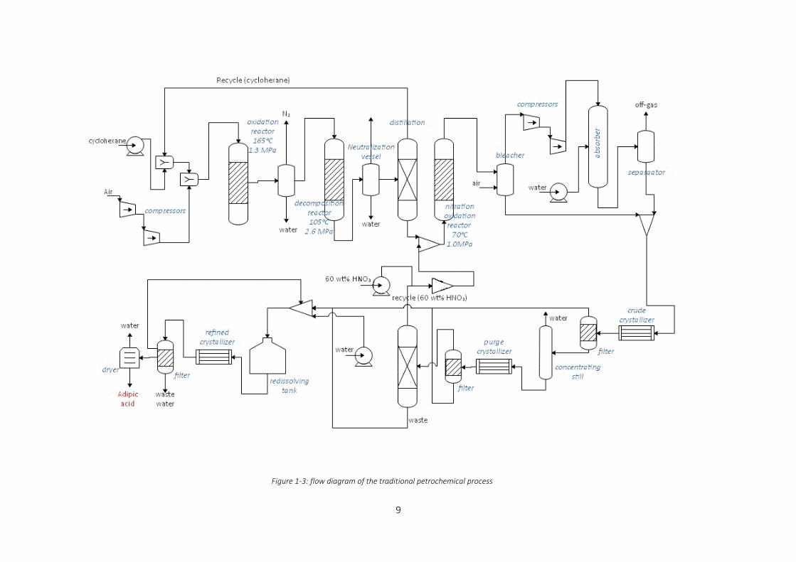
9
Figure 1-3: flow diagram of the traditional petrochemical process

Chapter 1- Introduction
10
The second step in commercial production of AdA is nitric acid oxidation of the cyclohexanol-
cyclohexanone mixture.12 Figure 1-4 shows the main reactions which occurs during the AdA synthesis
process.
OOH
HNO3+
HOOH
O
O
+ N2O + H2O + +NOx + Byproducts
OOH
+
CychlohexaneKA-oil mixture
KA-oil mixture Adipic acid
Figure 1-4: reactions involved in the production of AdA from KA-oil oxidation
As the reaction is highly exothermic, heat of reaction is usually dissipated by maintaining a high ratio
(40:1) of nitric acid to KA-mixture.13 Nitric acid (50% to 60%) and a copper-vanadium catalyst are
added to the KA-mixture in a reactor vessel at 60 °C- 80 °C and 0.1- 0.4 MPa. Conversion yields of 92%-
96% are attainable when using high-purity KA feedstock. Upon reaction, nitric acid is reduced to
nitrogen oxides: NO2, NO, N2O, and N2. The dissolved oxides are stripped from the reaction product
using air in a bleaching column and subsequently recovered as nitric acid in an absorption tower.13,14
The stripped AdA/nitric acid solution is chilled and sent to a crystallizer, where crystals of AdA are
formed. The crystals are separated from the mother liquor in a centrifuge and transported to the AdA
drying and/or melting facilities. The mother liquor is separated from the remaining uncrystallised AdA
in the product still and recycled to the reactors.
During the reaction many intermediates are formed such as succinic and glutaric acid.15
The hazards related to this process mainly derives from the use of nitric acid, as it is a strong acid and
a powerful oxidant, so the plant must be constructed of durable materials, more expensive than
normal steels. Moreover, a large amount of nitrogen oxides and nitrous oxide are produced during
the oxidation process. The real emission coefficient of nitrous oxide measured at the Nobeoka Works
of Asahi Chemical is 0.25 kgN2O/kgAdA (survey by Myiazaki Prefecture in 1994) because part of nitric
acid becomes N2 and NOx.16 The mixture of nitrogen oxides (reactions by-products) can be re-oxidized
to HNO3, except nitrous oxide (N2O), which, for environmental protection reasons, had to be
eliminated in catalytic or thermal processes.17 The nitrogen oxides (NO, NO2) are the main causes of
acid rain and under suitable atmospheric conditions favour the photochemical smog that leads to the
formation of ozone in the troposphere resulting harmful to living beings. NOx can be almost
Chapter 1- Introduction
11
completely recovered by water adsorption in a multistage column, yielding a nitric acid solution.18 The
main reactions are reported below.
2 NO + O2 → 2 NO2
3 NO2 + H2O → 2HNO3 + NO
This route allows the recovery of nitric acid which can be reused within the process itself. The greater
cost is in the low temperatures and high pressures needed to maximize the efficiency of the process.
Nitrous oxide is a greenhouse gas due to its strong IR absorption and relatively non-toxic, but it has a
number of recognized ill effects on human health, whether through breathing it in or by contact of
the liquid with skin or eyes.19,20 In the troposphere it also acts as a catalyst in the cycles of ozone
destruction, contributing to its decline. Before the introduction of the most recent N2O abatement
technology, AdA plants alone were the responsible of the 10% of anthropogenic nitrous pollution
worldwide.16 The most important N2O abatement technologies in order to decrease its emission in
the AdA plants are thermal destruction of N2O, conversion of N2O into recoverable NO and catalytic
dissociation of N2O to N2 and O2 (most common).17 The catalytic abatement involves highly exothermic
reactions:21,22
2 O* ↔ O2 + 2*
N2O + * → N2O * → N2+ O*
N2O + O* → N2 + O2 + *
The simplified flow sheet of the catalytic bed reactor is reported in Figure 1-5
There are several classes of catalysts that can be used in this process.23 Since the reaction is highly
exothermic, there are several problems to deal with, as the sintering of the catalyst, the need for
special heat-resistant expensive materials for reactors and troubles regarding the environmental
regulation. However, the development and the optimization of N2O abatement technology allows to
fully convert nitrous oxide (i.e. using copper/ceria based catalyst) at 550 °C.24

Chapter 1- Introduction
12
Cat
bed
Cat
bed
Cat
bed
Off gas
from AdA
Water Steam
Vent
Heated off
Gas from AdA
Purified Gas: low
conc. of N2O
Figure 1-5: simplified scheme of N2O abatement
Chapter 1- Introduction
13
1.2 Adipic acid from renewable resources
1.2.1 Overview
Bio adipic acid (bio-AdA) market size is likely to see significant growth as planned capacities come
online over the next few years. The bio-AdA market is still at the infancy stage as few companies have
focused on research to commercialize production. Companies such as Verdezyne, DSM, BioAmeber,
Ameris, Aemethis, Genomatica and Rennovia have successfully designed production technology to
develop 100% bio-AdA and would be commercializing the product over the coming years. AdA market
price trend is expected to remain stable between 1.6 $ to 1.9 $ per kilo. Increasing nylon 6,6 demand
for durable application such as automobiles, textile, carpets, tire-cod and technical fibers is likely to
drive bio-AdA market. Industry participants are vying to manufacture 100% bio-based nylon for
industrial applications owing to stringent government policies over environmental concerns. Global
nylon 6,6 market was estimated at over 1.3 million tons in 2013 and is likely to grow at a CAGR of over
4% from 2016 to 2023. In 2013, Rennovia announced successful completion of 100% bio-based nylon
6,6. It is based on combination of Rennovia’s RENNLON bio based AdA and hexamethylene diamine
(HMD). Rennovia is able to manufacture both the products through its patented chemical catalytic
process technology. Rennovia bio-AdA production is carried out through anaerobic oxidation of
glucose to obtain glucaric acid which further goes hydro-oxygenation. Rennovia products are
estimated to be cost competitive in comparison to petrochemical based products. The company is
targeting to commercialize bio-based AdA market with an initial capacity of 135 kilo tons per year by
the end of 2018.
Verdezyne is invested in research to develop bio-AdA through fermentation technique using yeast
microorganism which can utilize plant-based oil, alkanes or sugar as feedstock. In 2013, the company
announced collaboration with Malaysia’s biotechnology investment group, Biotechcorp (Malaysian
Biotechnology Corporation). This would help the company to access Malaysia as the prime location to
set up biotechnological production facility and it is likely to procure local feedstock such as palm fatty
acids and palm kernel oil distillates for manufacturing the end product. Companies are focusing on
green alternative routes to mitigate the risks as this could prove to be more beneficial in terms of cost
and also would be entitled for government incentives in the form of subsidies and loan guarantees.
Technologies developed from Rennovia and Verdezyne can prove to be cost effective as both the
process requires glucose as feedstock, available at competitive market rates in comparison to
cyclohexane. However, there are significant challenges to be met in terms of high yield and catalyst
productivity. Growing preference of bio polyurethane market in applications such as construction,

Chapter 1- Introduction
14
electronics and automotive is likely to drive bio-AdA market growth. It also finds applications in food
and medical industries. It is used as flavour and gelling aid for food preparations. Stringent norms by
Food and Drug Administration (FDA) over nitrogen dioxide emission from conventional adipic acid are
likely to favour bio based adipic acid market growth. Its polymeric coatings are used in hydrophilic
drugs and other controlled drug release formulations for medical applications. With established
companies such as Invista, BASF, Honeywell and PetroChina in the conventional space and several
innovative start-ups developing sustainable technology, adipic acid market share may fragment over
the next five years.
1.2.2 Different approaches for the production of bio-adipic acid
Bio-AdA productions strategies can be summarized as reported in Figure 1-6.
Lignocellulosic biomass or lipids-amino acids reach compounds can be converted to muconic acid
(MA), glucaric acid and other acids thanks to biotechnology approaches that use modified bacteria
and fungi. These intermediates can be further converted to AdA using chemical approaches. Among
the many green routes proposed for new “bio-derived building blocks”, the ones that allow AdA
production are the most interesting from an economical point of view. These syntheses, though
appealing from an economic base, present a series of difficulties that still hinder the diffusion of sugar
derived AdA. Several patents and scientific publications have shown the feasibility of the synthesis,
exploring a wide range of different technologies to perform the transformations.
Feedstocks Microbial Classis
Chemicals Products
Lignoellulosic biomass
Amino acids
Lipids
Bacteria
Fungi
Muconic acid
Glucaric acid
Adipic acid
Nylon
Polyester
Figure 1-6: simplified representation of the strategies for the production of bio-AdA

Chapter 1- Introduction
15
1.2.3 Production of bio-adipic acid via glucaric acid
Little scientific research has yet been carried out to explain catalytic routes to selectively oxidise
glucose to glucaric acid and most of the available literature efforts on the much easier selective
oxidation towards gluconic acid.25–28 Glucaric acid itself has a widely market potential with uses
ranging from detergents,29 to food and polymers.30 Very importantly, the dicarboxylic acid
functionalisation also makes it an attractive bio-derived precursor to AdA, which could be used as a
more sustainable alternative to fossil-fuel derived AdA in nylon production plants. A wide range of
other biodegradable polymers are also possible including methacrylates31 and other ester/amide
polymers.32
A large market opportunity has presented glucaric acid with the increase in governmental taxes on
phosphates in detergents in Europe and more regulation can be expected in the future to fully
eradicate the use of phosphates in detergent.33 Since the 1970s, significant amounts of scientific
evidence have linked these phosphates to eutrophication and subsequent decrease in water quality.34
This realization led to the economic disincentive policies in the EU and outright bans in the U.S. on
phosphates in detergents.35 Glucaric acid is a fascinating drop-in substitute for these banned
substances due to its chelating properties in sequestering metal ions in building detergents.36 The
current supply of glucaric acid is very limited and not sufficient for such large market, however, if
glucaric acid could be produced at large scale and with competitive cost, this multi-billion-dollar
market would be available soon. Table 1-2 outlines the catalytic oxidation studies of glucose to glucaric
acid from scientific literature, while in Figure 1-7 are shown the main catalytic reactions.
Table 1-2:Overview of the results achieved in oxidation of glucose (conversion (X) to glucaric acid and yield (Y))
Authors Year Catalyst P (bar) T (°C) X (%) Y (%)
Smith et al.14 2012 NaNO2 (HNO3) 1.25-1.5 (O2) 25-30 NA 45
Lee et al.37 2016 5%Pt/C 13.8 (O2) 80 100 74
Jin et al.38 2016 0.91%Pt
0.95%Pd/TiO2 1 (O2) 45 100 40
Solmi et al.39 2017 0.71%Au 0.2%Bi/C 10 (O2) 60 100 31
Thaburet et al.40 2001 TEMPO (NaOCl) 5 NA 90
Figure 1-8 gives an overview of the patent literature involved in the main synthesis glucose/bio-AdA.
In the upper part the reactive transformations are reported, while the lower part lists the separation
equipment proposed for glucaric acid.

Chapter 1- Introduction
16
Despite the presence of many patents regarding the bio-AdA production via glucaric acid, some
general considerations about the process are mandatory.
i. As for the variety of reaction conditions and of separation processes, a conceptual design
approach is necessary to explore all the possible combinations. More information about the
economic feasibility and the sustainability of the process are required, also to drive research
in the direction of the more promising solutions.
ii. None of the patents reported have any medium-large scale application.
iii. The actual bottlenecks of this technology are the purifications
iv. When glucaric acid is targeted, overoxidation and C-C breaking become a real problem.
Despite of this, the oxidative selective oxidation of glucose to glucaric acid continues to attract
important industrial interest aligned with the ultimate production of bio-derived adipic acid
or for its direct use and the development of very selective systems is still the key.

Chapter 1- Introduction
17
O
OH
OH
OH
OH
CH2OH
GLUCOSE
O OH
OH
OHHO
O
P
O
OH
HO
GLUCOSE-6-PHOSPHATE
myo-inositol-1-phosphate synthase (ino1)
HO
HO OH
P
OH
OH
O
OHHO
MYO-INOSITOL-1-PHOSPHATE
phosphatase (suhB)
HO
HO OH
OH
OH
OH
MYO-INOSITOL
myo-inositol oxygenase (miox)
O CH3
CH3
H3C CH3
O
HOD-GLUCURONIC ACID
uronate dehydrogenase (udh)
HO
O
OH
OH
OH
OH
O
OH
D-GLUCARIC ACID
HO
OH
O
O
ADIPIC ACID
Ru, Rh, Pd,Pt, Ir
Figure 1-7: reaction pathway from glucose to bio-AdA via glucaric acid

Chapter 1- Introduction
18
41
42 43 44
45
43 46
47
48
Rennovia process
WO 2013090031A2 (catalytic oxydation Pt/C +O
2)
Kiely process
US 29187398 B2 (Nitric acid STR reactor)
Tianjin Polytechnic process
(electrocatalytic oxydation)
Rennovia process
US 8669397B2 (2014) WO2013173372 (Multiphase Pt Rh/SiO2 + HBr+ H2)
*extra info on Li Wu Tsu 2014
Glucaric acid Adipic acid Glucose Oxydation
Hydro-deoxygenation
Purification
Simulated moving bed anion exchange chromatography
(US20100317823A1)
Diffusion dialysis
(US20080033205 A1)
Exsiccation (glucaric acid and lactone recovery
Concentration (nitric acid and ether recovery)
Solvent extraction with di-isopropyl ether (nitro-
oxidation) Membrane
electrodialysis
Figure 1-8: overview of patents and literature regarding glucose conversion to AdA via glucaric acid
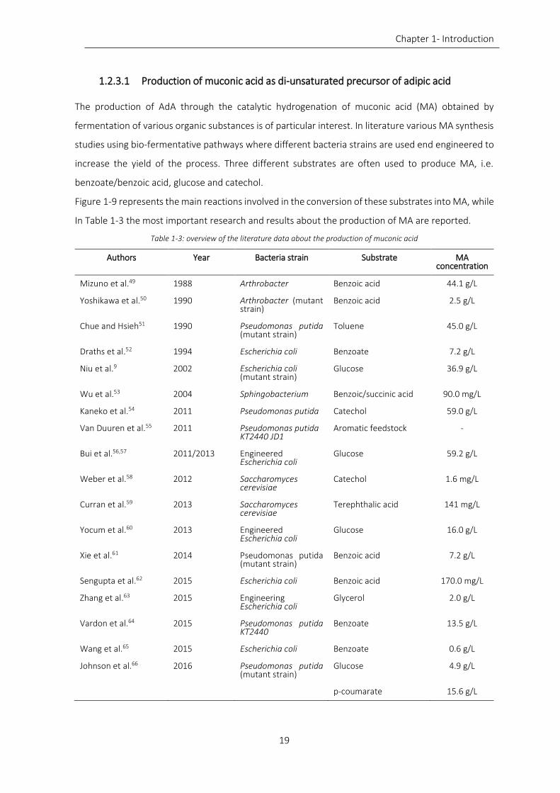
Chapter 1- Introduction
19
1.2.3.1 Production of muconic acid as di-unsaturated precursor of adipic acid
The production of AdA through the catalytic hydrogenation of muconic acid (MA) obtained by
fermentation of various organic substances is of particular interest. In literature various MA synthesis
studies using bio-fermentative pathways where different bacteria strains are used end engineered to
increase the yield of the process. Three different substrates are often used to produce MA, i.e.
benzoate/benzoic acid, glucose and catechol.
Figure 1-9 represents the main reactions involved in the conversion of these substrates into MA, while
In Table 1-3 the most important research and results about the production of MA are reported.
Table 1-3: overview of the literature data about the production of muconic acid
Authors Year Bacteria strain Substrate MA concentration
Mizuno et al.49 1988 Arthrobacter Benzoic acid 44.1 g/L
Yoshikawa et al.50 1990 Arthrobacter (mutant strain)
Benzoic acid 2.5 g/L
Chue and Hsieh51 1990 Pseudomonas putida (mutant strain)
Toluene 45.0 g/L
Draths et al.52 1994 Escherichia coli Benzoate 7.2 g/L
Niu et al.9 2002 Escherichia coli (mutant strain)
Glucose 36.9 g/L
Wu et al.53 2004 Sphingobacterium Benzoic/succinic acid 90.0 mg/L
Kaneko et al.54 2011 Pseudomonas putida Catechol 59.0 g/L
Van Duuren et al.55 2011 Pseudomonas putida KT2440 JD1
Aromatic feedstock -
Bui et al.56,57 2011/2013 Engineered Escherichia coli
Glucose 59.2 g/L
Weber et al.58 2012 Saccharomyces cerevisiae
Catechol 1.6 mg/L
Curran et al.59 2013 Saccharomyces cerevisiae
Terephthalic acid 141 mg/L
Yocum et al.60 2013 Engineered Escherichia coli
Glucose 16.0 g/L
Xie et al.61 2014 Pseudomonas putida (mutant strain)
Benzoic acid 7.2 g/L
Sengupta et al.62 2015 Escherichia coli Benzoic acid 170.0 mg/L
Zhang et al.63 2015 Engineering Escherichia coli
Glycerol 2.0 g/L
Vardon et al.64 2015 Pseudomonas putida KT2440
Benzoate 13.5 g/L
Wang et al.65 2015 Escherichia coli Benzoate 0.6 g/L
Johnson et al.66 2016 Pseudomonas putida (mutant strain)
Glucose 4.9 g/L
p-coumarate 15.6 g/L

Chapter 1- Introduction
20
O
OH
OH
OH
OH
CH2OH
E4P + PEP
DAHP sythase
HO O
O
O OH
OH
OH
HP
OH
OH
O2-DEHYDRO-3-DEOXY-D-ARABINO-HEPTONATE-7-PHOSPHATE (DAHP)
O
HO
HOOH
O
OH3-DEHYDROQUINATE (DHQ)
DHQ synthase
O
OH
OH
OHO
3-DEHYDROSHIKIMIC ACID (DHS)OH
OH
OHO
PROTOCATECHUATE
3-dehydroshikimicacid dehydratase
OH
OH
CATECHOL
protocatechuatedecarboxylase
OH
OHO
O
cis, cis-MUCONIC ACID
catechol 1,2dioxygenase
OH
OH
O
PHENOL
BENZOIC ACID
GLUCOSE
Figure 1-9:conversion of glucose into cis,cis-MA

Chapter 1- Introduction
21
Despite the literature deeply describes the different ways for the production of MA, only few patents
reported its production on medium scale.67–69 These patents are already expired and applied old
purification technology. With the development of new and more sustainable technology for the
recovery of chemicals from fermentation broth, the production of MA from glucose might be the best
choice for bio-AdA production.
In a recent paper Vardon et al. reported the steps for the recovery of MA achieving a purification yield
of 81.4% with a MA final purity of 99.8%.70
In Figure 1-10 are schematically reported the main steps of the purification process used to obtain
MA having a high purity.
Muconate removed
0.8 g Protein removal
Active Carbon cleanup
(1 h)
Crystallization (T=5 °C)
EtOH purification
1 L of Culture broth 34.5 g muconate
Negligible amount loss Retained broth
muconate 1.2 g
Waste salts 1.0 g
Purified crystals 28.1 g MA
Protein free broth muconate 33.7 g
Color free broth Muconate 33.7 g
Crystallized salt + MA 29.1 g
Figure 1-10: diagram of the main purification for the recovery of muconic acid

Chapter 1- Introduction
22
1.2.3.2 Catalytic hydrogenation of muconic acid to bio-adipic acid
The hydrogenation reaction involving double bonds needs a catalyst and a reducing agent to occur. It
is well known that noble metal based catalysts are the most common materials for hydrogenation
reactions71 while molecular gaseous hydrogen is the most common used reducing agent.
Heterogeneous catalysis is more common in industry due to the easy recovery of the solid powder
after the reaction (i.e. simple filtration is often applied to achieve this purpose). The noble-metal
catalysts are prepared depositing a metal precursor on a fine inactive powder, called support. The
support is a cheap, porous, bulky, usually granular material, such as alumina, titanium dioxide,
activated carbon (AC), and calcium carbonate. For example, platinum on carbon is produced by
reduction of chloroplatinic acid in situ carbon.72 In many cases, highly surface modifications involve
selective “poisons”. Thus, a wisely chosen catalyst can be used to hydrogenate only some functional
groups without affecting others (selective hydrogenation reactions). For example it is possible to
hydrogenate maleic acid to succinic acid without touching the carboxylic groups.73 The addition of
hydrogen to double or triple bonds in hydrocarbons is a redox reaction that is thermodynamically
favourable. The addition of hydrogen to alkenes has a Gibbs free energy change of -101 kJ/mol.74
However, the reaction rate for most hydrogenation reactions is null without using a catalyst. The
mechanism of metal-catalysed hydrogenation of double and triple bonds has been widely studied.75
On a solid surface, the accepted mechanism for hydrogenation reaction is the Horiuti-Polanyi
mechanism71,76 that occurs in three different steps:
i. binding of the unsaturated bond, and hydrogen dissociation into atomic hydrogen onto the
catalyst surface;
ii. addition of one atom of hydrogen (reversible step);
iii. addition of the second atom of hydrogen (irreversible step under hydrogenating conditions).
During the second step, the metal-intermediate formed is a saturated compound that is free to rotate
and then break down, detaching the alkene from the catalyst. Consequently, the contact with a
hydrogenation catalyst inevitably causes cis-trans isomerization, because it is thermodynamically
favourable. This might be a problem in partial hydrogenation reaction, while in complete one the
produces trans-alkene is eventually hydrogenated.
The second reagent in this kind of reaction is obviously hydrogen gas. The hydrogenation process
often occurs under pressure, usually transported from the cylinders and sometimes improved by
“booster pumps”. Gaseous hydrogen is mainly produced industrially from hydrocarbons by steam
reforming (SR) process.77 SR method involves a catalytic conversion of steam and hydrocarbons to
hydrogen and carbon oxides. The reactions reported below describe the syngas generation (mixture

Chapter 1- Introduction
23
of CO and H2), CO2 and H2 production from water-gas shift reaction (WGS) and H2 consumption by
methanation reactions.
To prevent cooking formation on the surface of the catalyst, the operating parameters of this reaction
are high temperature, pressure up to 3.5 MPa and steam-to-carbon ratios of 3.5.78
After the reformer, the gas mixture passes through a heat recovery step and is fed into a WGS reactor
where additional hydrogen is produced. Then the mixture passes either through a CO2 removal and
methanation leaving hydrogen with a purity near 100%.79 The CO2 emissions can be strongly reduced
using appropriate CO2 capture and storage (CCS) techniques, through which carbon dioxide is
captured and injected in geological reservoirs or the ocean.80 It is estimated that the hydrogen
production cost, corresponding to plants with a design capacity of 379.4 kg/day, at 90% capacity factor
and a natural gas cost of 10.00 $/MMBtu, are 2.27 $/kg and 2.08 $/kg with and without carbon capture
and sequestration, respectively.78
Although hydrocarbons are currently the main feedstock used for hydrogen production, the need to
increase the integration of renewable technologies will become inevitable. As the fossil fuels are
deteriorating and greenhouse effect is creating greater attention, the share of renewable
technologies will rise in the near future while in long term, is expected to dominate over conventional
technologies.81–83 There are many processes for H2 production from renewable resources such as
biomass process and biological process. Biomass is a renewable source of primary energy derived
from animals and plants materials crop residues, wood from forests and forest residues, grass,
industrial residues, and a host of other materials.84 Biomass stems from plants is organic matter in
which the energy of sunlight is stored in chemical bonds via photosynthesis.85 Although, CO2 is
released when biomass is used for energy production, this amount of gaseous emission is equal to the
amount absorbed by organisms when they were still living.86 Biological and thermochemical methods
are the two hydrogen production processes from biomass. Although biological processes are more
environmentally friend and less energy intensive (as they operate under mild conditions), they provide
low rates and yields of H2 depending on the raw materials used.87 On the other hand, thermochemical
processes are much faster and offer higher stoichiometric yield of hydrogen with gasification being a
promising option based on economic and environmental considerations.88 Thermochemical processes
are the method through which biomass can be transformed into hydrogen and hydrogen-rich
gases.89,90 Thermochemical technology mainly includes gasification and pyrolysis. Both conversion
Syngas generation CnHm + nH2O → nCO + (n+1/2m)H2 (non catalytic)
WGS reaction CO + H2O → CO2 + H2
Methanation reaction CO + 3H2 → CH4 + H2O

Chapter 1- Introduction
24
processes produce, among other gaseous products, CH4 and CO which can be further treated for more
hydrogen production through SR and WGS reaction. Biomass pyrolysis occurs at a range temperature
of 377-527 °C at 10.5 MPa and liquid oils, solid charcoal and gaseous compounds are produced by
heating the biomass.88 Biomass pyrolysis takes place in anaerobic conditions except in cases where
partial combustion allows to provide the thermal energy needed for the process.91 CH4 and other
hydrocarbon gases produced can be converted to hydrogen applying WGS reaction. After CO is
converted into CO2 and H2, the desired purified H2 is obtained by pressure swing adsorption (PSA).92
The flow diagram of the pyrolysis process is shown in Figure 1-11.
The yield of H2 production from biomass pyrolysis depends on the type of raw materials, the type of
the catalyst used, time of residence, and the working temperature.88,93 The H2 production cost using
biomass pyrolysis technique is expected to be in the range of 1.25 $/kg to 2.20 $/kg, depending on
the facility size and biomass type.94 Biomass gasification is the thermochemical conversion of biomass
into syngas in a gasifier where air, oxygen and/or steam are used as medium. It takes place at
temperatures between 500 °C and 1400 °C and working pressures from atmospheric to 33 bar.92 After
the transformation of biomass into syngas, the gas mixture is further treated in the same way as the
product gas of the pyrolysis process, as shown in Figure 1-12. The H2 yield is mainly affect by biomass
type, particle size, temperature, steam-to-biomass ratio, and type of catalyst used.89,95 In steam
Figure 1-11: flow diagram of the biomass pyrolysis process
H2O
Pyrolysis CSR WGS
reaction PSA system
Biomass
Bio-fuel CO+H2 CO2+H2
CO2
H2
Sorbent regenerator
Gas clean up Shift
conversion
CO2
absorption Gasifier
Air separation
Steam
Biomass
Air
O2
N2
Ash
S Sorbent regenerator
CO2
H2
Figure 1-12: flow diagram of the biomass gasification process
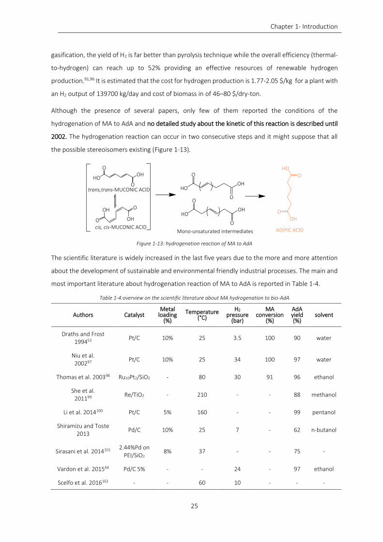
Chapter 1- Introduction
25
gasification, the yield of H2 is far better than pyrolysis technique while the overall efficiency (thermal-
to-hydrogen) can reach up to 52% providing an effective resources of renewable hydrogen
production.91,96 It is estimated that the cost for hydrogen production is 1.77-2.05 $/kg for a plant with
an H2 output of 139700 kg/day and cost of biomass in of 46–80 $/dry-ton.
Although the presence of several papers, only few of them reported the conditions of the
hydrogenation of MA to AdA and no detailed study about the kinetic of this reaction is described until
2002. The hydrogenation reaction can occur in two consecutive steps and it might suppose that all
the possible stereoisomers existing (Figure 1-13).
HOOH
O
O
OH
OHO
O
cis, cis-MUCONIC ACID
trans,trans-MUCONIC ACID HOOH
O
O
HOOH
O
OOH
HOO
O
ADIPIC ACIDMono-unsaturated intermediates
Figure 1-13: hydrogenation reaction of MA to AdA
The scientific literature is widely increased in the last five years due to the more and more attention
about the development of sustainable and environmental friendly industrial processes. The main and
most important literature about hydrogenation reaction of MA to AdA is reported in Table 1-4.
Table 1-4:overview on the scientific literature about MA hydrogenation to bio-AdA
Authors Catalyst Metal
loading (%)
Temperature (°C)
H2 pressure
(bar)
MA conversion
(%)
AdA yield (%)
solvent
Draths and Frost 199452
Pt/C 10% 25 3.5 100 90 water
Niu et al. 200297
Pt/C 10% 25 34 100 97 water
Thomas et al. 200398 Ru10Pt2/SiO2 - 80 30 91 96 ethanol
She et al. 201199
Re/TiO2 - 210 - - 88 methanol
Li et al. 2014100 Pt/C 5% 160 - - 99 pentanol
Shiramizu and Toste 2013
Pd/C 10% 25 7 - 62 n-butanol
Sirasani et al. 2014101 2.44%Pd on
PEI/SiO2 8% 37 - - 75 -
Vardon et al. 201564 Pd/C 5% - - 24 - 97 ethanol
Scelfo et al. 2016102 - - 60 10 - - -
Chapter 1- Introduction
26
Among all these scientific publications, only few of them reported the possibility to recycle the catalyst
or cite the possibility of a non-negligible deactivation of the catalyst. Therefore, a detailed kinetic
study starting from the basis is needed to better understand and go insight this reaction. Moreover,
a modelling and data regression study is mandatory to evaluate all the kinetic parameters (activation
energy, adsorption energy…) allowing the optimization of the reaction and the sizing of the reactor.
1.3 The importance of the “at early-stage” life cycle impact
assessment (LCIA) for the evaluation of the environmental
impact
1.3.1 What is LCIA?
LCIA is a method to evaluate environmental impacts related with all the stages of a product's life from
raw material extraction through materials processing, assembly, distribution, use, repair and
maintenance, and disposal or recycling. Designers use this technique to help critique their old and
new industrial processes and/or products. LCIAs can help avoid a narrow outlook on environmental
concerns by:
i. collecting an inventory of relevant material and energy inputs (without forgetting the material
and all the stuffs required for the construction of the plant) and environmental releases;
ii. estimating the potential impacts related with identified inputs and releases;
iii. interpreting and understanding the results to help make a more informed decision.
The main aim of the life cycle assessment (LCA) is to compare the full range of environmental effects
assignable to products and services by quantifying all inputs and outputs of material flows and
calculating how these material flows affect the environment. This information is used to improve
processes, provide a sound basis for informed decisions and support policy.
The procedures of LCA is included in ISO 14000 environmental management standards, in ISO
14040:2006, and 14044:2006. (ISO 14044 replaced earlier versions of ISO 14041 to ISO 14043).103,104
Although LCA is a global method for assessing impacts of a product on the environment, there are
some limitations to consider. First, it is only to evaluate the potential impacts (and not real or
measured) of a product or service. Moreover, the results are strictly dependent on data availability,
the complexity of the study and the quality of the information. Therefore, achieving this kind of study
requires an important level of knowledge and skills.

Chapter 1- Introduction
27
LCA is becoming more and more important for industry. Like the economic impact the environmental
impact is mainly determined in the early stage of development. The challenge in this context is that
the ecological impact is hard to predict, if the product has not been fully designed yet and if the
production processes are not well known. For the economic impact many empirical formulas exist,
whereas for the ecological impact such equations are still missing. Therefore, a life cycle impact
assessment tool has been developed which supports the developer during all stages of development.
1.3.2 The four main steps of LCA study
According to the ISO 14040 and 14044 standards, a LCA is carried out in four distinct phases as shown
in Figure 1-14. The phases are often interdependent in that the results of one phase will inform how
other phases are completed.
1. Goal and scope definition
The LCA study starts with an explicit declaration of the aim and scope of the study, which includes the
context of the study and reported how the results are to be communicated. The goal must be clearly
defined and consistent with the selected application.
In this sense the goal and scope document would include technical details such as:
i. the functional unit: it defines what exactly is being studied and quantifies the service delivered
by the product system, providing a reference to which the inputs and outputs can be related.
4. Interpretation
1. Goal and scope definition
2. Inventory analysis 3. Life cycle impact assessment
• Technical inputs and outputs of all processes
• Emission (to air, water and soil)
• Resource use (land, water, fossils, metals)
• Climate change • Ozone
depletion • Photochemical
ozone creation
• Human toxicity Ecotoxicity
• Eutrophication • Acidification • Land stress • Water stress • Resource
depletion
Human health
Biodiversity/ ecosystem services
Natural resources
Figure 1-14: four main step of the LCA study
Chapter 1- Introduction
28
Further, the functional unit is a central basis that enables alternative goods, or services, to be
compared and analyzed.105 Therefore, if we want to compare the environmental impact of
two different processes to produce AdA, the functional unit will be 1 kg of AdA. The functional
flow would be all the different items required for that function. For example, considering the
traditional petrochemical process, reactors, N2O absorber, decanter and concentrator will be
taken in to account, while for the bio process fermenter, activated carbon washing,
ultrafiltration and other operations will be considered;
ii. the system boundaries: they are delimitations of which processes that should be included in
the analysis of a product system;106
iii. any assumptions and limitations;
iv. the allocation methods: it is used to partition the environmental load of a process when
several products or functions share the same process. The choice of the allocation is a key
point of the study because different methods may give different results;
v. the impact categories chosen for example human toxicity, smog, global warming,
eutrophication…
2. Inventory analysis
Life Cycle Inventory (LCI) analysis involves creating an inventory of flows from and to nature for a
product system. The inventory flows must include raw materials, water and energy and all the
products that are released in air, water and land. To build this type of document, a flow chart diagram
of all unit processes is mandatory where all the inputs and outputs and their amount within the system
boundaries are clearly defined. The data must be related to the functional unit defined in the goal and
scope definition. All unit processes are linked through intermediate product flows, which makes the
process system model linear with respect to the quantity of function it provides. The environmental
exchanges are typically assumed to be linearly related to one of the product flows of the unit
process.105 The choices and assumptions made during system modelling, especially with respect to
the system boundaries and what processes to include within these boundaries, are often decisive for
the result of the LCA study.107
3. Life cycle-impact assessment
Inventory analysis is followed by impact assessment. This phase of LCA is aimed at evaluating the
significance of potential environmental impacts based on the LCI flow results. Classical life cycle
impact assessment (LCIA) consists of the following mandatory elements:
i. selection of impact categories, characterization models, and category indicators;

Chapter 1- Introduction
29
ii. the classification stage, where the inventory parameters are organized and allocated to
specific impact categories;
iii. impact measurement, where the categorized LCI flows are characterized, using one of many
possible LCIA methodologies.
Several different LCIA elements may be considered depending on the scope and final aim of the LCA
study:
i. normalization: the results of the different impact categories are usually compared with the
total impacts in the region of interest, the Europe for example;
ii. grouping: where the impact categories are sorted and possibly ranked;
iii. weighting: all the different environmental impacts are summed up to obtain a single score for
the total environmental impact.
LCI can also be considered the different phases of the development, production, use, and disposal of
a product. For example it is possible to consider the “first impacts” that includes the extraction of raw
material, the conversion of raw materials into a product, the transportation... Therefore the “use
impact” may be quantify considering the facilities (water, energy…), the maintenance, repairs and
renovations. Finally, the “end of life impact” may include the demolition and processing of waste and
recyclable materials.
4. Interpretation
The interpretation allows identifying, quantifying and evaluating all the information obtained during
the LCI and/or LCIA process. The result of the interpretation phase is a set of recommendations and
conclusions.
According to ISO 14040:2006 the interpretation should include:
the identification of all the significant topics based on the results of the LCI and LCIA phases;
evaluation of the study considering sensitivity and consistency checks;
conclusions, limitations and recommendations.
A key purpose of performing life cycle interpretation is to determine the level of confidence in the
final results and communicate them in a fair, complete, and accurate manner. Understanding the
results of an LCA is not as simple. The evaluation of the single contribution for each impact category
must be clear and complete. Moreover, a consistency estimation of the study is recommended, and
the conclusions should be based on a clear understanding of how the LCA was conducted and the
results were developed.

Chapter 1- Bibliography
30
Bibliography
1. Peñuelas, J. & Carnicer, J. Climate Change and Peak Oil: The Urgent Need for a Transition to a Non-Carbon-Emitting Society. Ambio 39, 85–90 (2010).
2. Bocken, N. M. P., Short, S. W., Rana, P. & Evans, S. A literature and practice review to develop sustainable business model archetypes. J. Clean. Prod. 65, 42–56 (2014).
3. Clark, J. H., Farmer, T. J., Hunt, A. J. & Sherwood, J. Opportunities for Bio-Based Solvents Created as Petrochemical and Fuel Products Transition towards Renewable Resources. Int. J. Mol. Sci. 16, 17101–17159 (2015).
4. Vardon, D. R. et al. Adipic acid production from lignin. Energy Environ. Sci. 8, 617–628 (2015).
5. Oppenheim, J. P., Dickerson, G. L. & Staff, U. B. Adipic Acid. in Encyclopedia of Chemical Technology (ed. Kirk-Othmer) 1–27 (Jhon Wiley & Sons, 2014). doi:10.1002/0471238961.0104091604012209.a01.pub2
6. Technavio. Global Adipic Acid Market - Drivers and Forecasts by Technavio. (2017). Available at: https://www.businesswire.com/news/home/20170516006527/en/Global-Adipic-Acid-Market---Drivers-Forecasts.
7. Bart, J. C. J. & Cavallaro, S. Transiting from adipic acid to bioadipic acid. Part II. Biosynthetic pathways. Ind. Eng. Chem. Res. 54, 567–576 (2015).
8. IHS Markit. Adipic acid. (2017).
9. Niu, W., Draths, K. M. & Frost, J. W. Benzene-Free Synthesis of Adipic Acid. Biotechnol. Prog. 18, 201–211 (2002).
10. Zauba technology and data. Total volume and value of imports. (2017). Available at: https://www.zauba.com/importanalysis-adipic+acid-report.html.
11. Castellan, A., Bart, J. C. J. & Cavallaro, S. Industrial production and use of adipic acid. Catal. Today 9, 237–254 (1991).
12. Castellan, A. Industrial production and use of adipic acid. Catal. Today 9, 237–254 (1991).
13. Luedeke, V. D. Adipic acid. in Encyclopedia of Chemical Processing and Design (ed. J. J. McKetta and W. A. Cunningham) 128–146 (Marcel Dekker, Inc., 1977).
14. Smith, T. N. et al. Modifications in the nitric acid oxidation of d-glucose. Carbohydr. Res. 350, 6–13 (2012).
15. Zhou, W. Y., Hu, B. C., Zhao, L. R. & Liu, Z. L. Qualitative and Quantitative Analysis of the By-Products in the Course of Cyclohexanone Production by HPLC-MS/MS. J, Chin Mass Spectr. Soc 30, 31 (2009).
16. Thiemens, M. H. & Trogler, W. C. Nylon Production: An Unknown Source of Atmospheric Nitrous Oxide. Science (80-. ). 251, 932 LP-934 (1991).
17. Shimizu, A., Tanaka, K. & Fujimori, M. Abatement technologies for N2O emissions in the adipic acid industry. Chemosph. - Glob. Chang. Sci. 2, 425–434 (2000).
18. Suchak, N. J. & Joshi, J. B. Simulation and optimization of NOx absorption system in nitric acid manufacture. AIChE J. 40, 944–956 (1994).
19. Jay, M. Nitrous oxide: recreational use, regulation and harm reduction. Drugs and Alcohol Today 8, 22–25 (2008).
20. Jevtovic-Todorovic, V., Beals, J., Benshoff, N. & Olney, J. W. Prolonged exposure to inhalational anesthetic nitrous oxide kills neurons in adult rat brain. Neuroscience 122, 609–616 (2003).
Chapter 1- Bibliography
31
21. Reimer, R. A., Slaten, C. S., Seapan, M., Lower, M. W. & Tomlinson, P. E. Abatement of N2O emissions produced in the adipic acid industry. Environ. Prog. 13, 134–137 (1994).
22. Kapteijn, F., Rodriguez-Mirasol, J. & Moulijn, J. A. Heterogeneous catalytic decomposition of nitrous oxide. Appl. Catal. B Environ. 9, 25–64 (1996).
23. Santiago, M., Hevia, M. A. G. & Pérez-Ramírez, J. Evaluation of catalysts for N2O abatement in fluidized-bed combustion. Appl. Catal. B Environ. 90, 83–88 (2009).
24. Liu, Z., He, C., Chen, B. & Liu, H. CuO-CeO2 mixed oxide catalyst for the catalytic decomposition of N2O in the presence of oxygen. Catal. Today 297, 78–83 (2017).
25. Dimitratos, N., Lopez-Sanchez, J. A. & Hutchings, G. J. Selective liquid phase oxidation with supported metal nanoparticles. Chem. Sci. 3, 20–44 (2012).
26. Besson, M., Gallezot, P. & Pinel, C. Conversion of Biomass into Chemicals over Metal Catalysts. Chem. Rev. 114, 1827–1870 (2014).
27. Corma, A. & Garcia, H. Supported gold nanoparticles as catalysts for organic reactions. Chem. Soc. Rev. 37, 2096–2126 (2008).
28. Sheldon, R. A. Green and sustainable manufacture of chemicals from biomass: state of the art. Green Chem. 16, 950–963 (2014).
29. Bessemer, A. C. & van Bekkum, H. Calcium sequestering agents based on carbohydrates. in Carbohydrates as Organic Raw Materials III (ed. H.van Bekkum, H. Roper, F. V.) (Wiley-VCH Verlag GmbH, 2007).
30. Mehtiö, T. et al. Production and applications of carbohydrate-derived sugar acids as generic biobased chemicals. Crit. Rev. Biotechnol. 36, 904–916 (2016).
31. Gallagher, J. J., Hillmyer, M. A. & Reineke, T. M. Degradable Thermosets from Sugar-Derived Dilactones. Macromolecules 47, 498–505 (2014).
32. Wu, Y., Enomoto-Rogers, Y., Masaki, H. & Iwata, T. Synthesis of Crystalline and Amphiphilic Polymers from d-Glucaric Acid. ACS Sustain. Chem. Eng. 4, 3812–3819 (2016).
33. Köhler, J. Detergent Phosphates: An EU Policy Assessment. J. Bus. Chem. 3, 15–30 (2006).
34. Mitchell, D. Eutrophication of Lake Water Microcosms: Phosphate versus Nonphosphate Detergents. Science (80-. ). 174, 827 LP-829 (1971).
35. Litke, D. W. Review of phosphorus control measures in the United States and their effects on water quality. Available at: http://agris.fao.org/agris-search/search.do?recordID=US201300035749.
36. Saeed, K., Priecel, P. & Lopez-Sanchez, J. Catalytic routes towards bio-renewable glucaric acid. Chimica oggi 35, (2017).
37. Lee, J., Saha, B. & Vlachos, D. G. Pt catalysts for efficient aerobic oxidation of glucose to glucaric acid in water. Green Chem. 18, 3815–3822 (2016).
38. Jin, X. et al. Synergistic Effects of Bimetallic PtPd/TiO2 Nanocatalysts in Oxidation of Glucose to Glucaric Acid: Structure Dependent Activity and Selectivity. Ind. Eng. Chem. Res. 55, 2932–2945 (2016).
39. Solmi, S., Morreale, C., Ospitali, F., Agnoli, S. & Cavani, F. Oxidation of d -Glucose to Glucaric Acid Using Au/C Catalysts. ChemCatChem 9, 2797–2806 (2017).
40. Thaburet, J.-F., Merbouh, N., Ibert, M., Marsais, F. & Queguiner, G. TEMPO-mediated oxidation of maltodextrins and d-glucose: effect of pH on the selectivity and sequestering ability of the resulting polycarboxylates. Carbohydr. Res. 330, 21–29 (2001).
41. Archer, R. et al. Processes for the production of adipic acid from D-glucose via hydro-deoxygenation and water concentration reduction in synthesis of hexamethylene diamine and caprolactam (2013).
Chapter 1- Bibliography
32
42. Donen, S., Hash, K., Smith, T. & Jensen, K. Nitric acid oxidation processes. (2013).
43. Boussie, T. R. et al. Production of adipic acid and derivatives from carbohydrate-containing materials. (2009).
44. Salem, G. F., Zhu, G., Hagmeyer, A. G. & Dias, E. L. Reduction catalysts. (2012).
45. Bin, D. et al. Controllable oxidation of glucose to gluconic acid and glucaric acid using an electrocatalytic reactor. Electrochim. Acta 130, 170–178 (2014).
46. Kiely, D. E. & Hash, K. R. Method of oxidization using nitric acid. (2006).
47. Koter, S. Ion-Exchange Membranes for Electrodialysis. A Patents Review. Recent Patents on Chemical Engineering 4, (2011).
48. Reeves, J. B. Use of Nitrobenzene Oxidation for Study of Lignin Composition with an Improved Method for Product Extraction1,2. J. Dairy Sci. 69, 71–76 (1986).
49. Mizuno, S., Yoshikaw, N., Seki, M., Mikawa, T. & Imada, Y. Microbial production of cis,cis-muconic acid from benzoic acid. Appl. Microbiol. Biotechnol 28, (1988).
50. Yoshikawa, N., Mizuno, S., Ohta, K. & Suzuki, M. Microbial production of cis,cis-muconic acid. J. Biotechnol. 14, 203–210 (1990).
51. Chua, J. W. & Hsieh, J.-H. Oxidative bioconversion of toluene to 1,3-butadiene-1,4-dicarboxylic acid (cis,cis-muconic acid). World J. Microbiol. Biotechnol. 6, 127–143 (1990).
52. Draths, K. M. & Frost, J. W. Environmentally compatible synthesis of adipic acid from D-glucose. J. Am. Chem. Soc. 116, 399–400 (1994).
53. Wu, C.-M., Lee, T.-H., Lee, S.-N., Lee, Y.-A. & Wu, J.-Y. Microbial synthesis of cis,cis-muconic acid by Sphingobacterium sp. GCG generated from effluent of a styrene monomer (SM) production plant. Enzyme Microb. Technol. 35, 598–604 (2004).
54. Kaneko, A., Ishii, Y. & Kirimura, K. High-yield Production of cis , cis -Muconic Acid from Catechol in Aqueous Solution by Biocatalyst. Chem. Lett. 40, 381–383 (2011).
55. van Duuren, J. B. J. H. et al. Generation of a catR deficient mutant of P. putida KT2440 that produces cis, cis-muconate from benzoate at high rate and yield. J. Biotechnol. 156, 163–172 (2011).
56. Bui, V., Lau, M. K. & Macrare, D. Methods for producing isomers of muconic acid and muconate salts. (2011).
57. Bui, V., Lau, M. K., Macrare, D. & Schweitzer, D. Methods for producing isomers of muconic acid and muconate salts. (2013).
58. Weber, C. et al. Biosynthesis of cis,cis-Muconic Acid and Its Aromatic Precursors, Catechol and Protocatechuic Acid, from Renewable Feedstocks by Saccharomyces cerevisiae. Appl Env. Microbiol 78, 8421–8430 (2012).
59. Curran, K. A., Leavitt, J. M., Karim, A. S. & Alper, H. S. Metabolic engineering of muconic acid production in Saccharomyces cerevisiae. Metab. Eng. 15, 55–66 (2013).
60. Yocum, R. R. et al. Production of muconic acid from genetically engineered microorganisms. (2013).
61. Xie, N.-Z. et al. Optimization of medium composition for cis,cis-muconic acid production by a Pseudomonas sp. mutant using statistical methods. Preparative biochemistry & biotechnology 44, (2014).
62. Sengupta, S., Jonnalagadda, S., Goonewardena, L. & Juturu, V. Metabolic engineering of a novel muconic acid biosynthesis pathway via 4-hydroxybenzoic acid in Escherichia coli. Appl. Environ. Microbiol. 81, 8037–43 (2015).
63. Zhang, H., Li, Z., Pereira, B. & Stephanopoulos, G. Engineering E. coli–E. coli cocultures for production of

Chapter 1- Bibliography
33
muconic acid from glycerol. Microb. Cell Fact. 14, 134 (2015).
64. Vardon, D. R. et al. Adipic acid production from lignin. Energy Environ. Sci. 8, 617–628 (2015).
65. Wang, J. & Zheng, P. Muconic acid production from glucose using enterobactin precursors in Escherichia coli. J. Ind. Microbiol. Biotechnol. 42, 701–709 (2015).
66. Johnson, C. W. et al. Enhancing muconic acid production from glucose and lignin-derived aromatic compounds via increased protocatechuate decarboxylase activity. Metab. Eng. Commun. 3, 111–119 (2016).
67. Frost, J. W. & Draths, K. M. Bacterial cell tranformants for production of cis, cis-muconic acid and catechol, (1993).
68. Imada, Y., Yoshikawa, N., Mizuno, S. & Takashi, M. Process for preparing muconic acid, (1984).
69. Maxwell, P. C. Production of muconic acid, (1982).
70. Vardon, D. R. et al. cis,cis-Muconic acid: separation and catalysis to bio-adipic acid for nylon-6,6 polymerization. Green Chem. 18, 3397–3413 (2016).
71. Horiuti, I. & Polanyi, M. Exchange reactions of hydrogen on metallic catalysts. Trans. Faraday Soc. 30, 1164–1172 (1934).
72. Nishimura, S. Handbook of Heterogeneous Catalytic Hydrogenation for Organic Synthesis. (2001).
73. Amoa, K. Catalytic Hydrogenation of Maleic Acid at Moderate Pressures. J. Chem. Educ. 84, 1948 (2007).
74. Atkins, P. W. & Atkins, P. W. Shriver & Atkins’ inorganic chemistry. (Oxford University Press ; W.H. Freeman and Co., 2006).
75. Kubas, G. J. Metal Dihydrogen and σ-Bond Complexes. (Springer US, 2001). doi:10.1007/b113929.
76. Gallezot, P. Hydrogenation - Heterogeneous. in Encyclopedia of Catalysis (Jhon Wiley & Sons, 2003).
77. Rylander, P. N. Hydrogenation and Dehydrogenation. in Ullman’s Encyclopedia of Industrial Chemistry (Wiley-VCH, 2005). doi:10.1002/14356007.a13_487.
78. Nikolaidis, P. & Poullikkas, A. A comparative overview of hydrogen production processes. Renew. Sustain. Energy Rev. 67, 597–611 (2017).
79. Steinberg, M. & Cheng, H. C. Modern and prospective technologies for hydrogen production from fossil fuels. Int. J. Hydrogen Energy 14, 797–820 (1989).
80. Damen, K., Troost, M. van, Faaij, A. & Turkenburg, W. A comparison of electricity and hydrogen production systems with CO2 capture and storage. Part A: Review and selection of promising conversion and capture technologies. Prog. Energy Combust. Sci. 32, 215–246 (2006).
81. Hites, R. A. Persistent Organic Pollutants in the Great Lakes: An Overview BT - Persistent Organic Pollutants in the Great Lakes. in (ed. Hites, R. A.) 1–12 (Springer Berlin Heidelberg, 2006). doi:10.1007/698_5_038.
82. Ćosić, B., Krajačić, G. & Duić, N. A 100% renewable energy system in the year 2050: The case of Macedonia. Energy 48, 80–87 (2012).
83. Mathiesen, B. V, Lund, H. & Karlsson, K. 100% Renewable energy systems, climate mitigation and economic growth. Appl. Energy 88, 488–501 (2011).
84. Demirbaş, A. Biomass resource facilities and biomass conversion processing for fuels and chemicals. Energy Convers. Manag. 42, 1357–1378 (2001).
85. McKendry, P. Energy production from biomass (part 1): overview of biomass. Bioresour. Technol. 83, 37–46 (2002).
86. Flamos, A., Georgallis, P. G., Doukas, H. & Psarras, J. Using Biomass to Achieve European Union Energy
Chapter 1- Bibliography
34
Targets—A Review of Biomass Status, Potential, and Supporting Policies. Int. J. Green Energy 8, 411–428 (2011).
87. Balat, H. & Kırtay, E. Hydrogen from biomass – Present scenario and future prospects. Int. J. Hydrogen Energy 35, 7416–7426 (2010).
88. Demirbaş, A. Yields of hydrogen-rich gaseous products via pyrolysis from selected biomass samples. Fuel 80, 1885–1891 (2001).
89. Wang, Z. et al. Gasification of biomass with oxygen-enriched air in a pilot scale two-stage gasifier. Fuel 150, 386–393 (2015).
90. Liu, S. et al. Hydrogen production via catalytic pyrolysis of biomass in a two-stage fixed bed reactor system. Int. J. Hydrogen Energy 39, 13128–13135 (2014).
91. Parthasarathy, P. & Narayanan, K. S. Hydrogen production from steam gasification of biomass: Influence of process parameters on hydrogen yield – A review. Renew. Energy 66, 570–579 (2014).
92. Iribarren, D., Susmozas, A., Petrakopoulou, F. & Dufour, J. Environmental and exergetic evaluation of hydrogen production via lignocellulosic biomass gasification. J. Clean. Prod. 69, 165–175 (2014).
93. Duman, G., Uddin, M. A. & Yanik, J. Hydrogen production from algal biomass via steam gasification. Bioresour. Technol. 166, 24–30 (2014).
94. Ni, M., Leung, D. Y. C., Leung, M. K. H. & Sumathy, K. An overview of hydrogen production from biomass. Fuel Process. Technol. 87, 461–472 (2006).
95. Fremaux, S., Beheshti, S.-M., Ghassemi, H. & Shahsavan-Markadeh, R. An experimental study on hydrogen-rich gas production via steam gasification of biomass in a research-scale fluidized bed. Energy Convers. Manag. 91, 427–432 (2015).
96. Balat, M. Hydrogen-rich gas production from biomass via pyrolysis and gasification processes and effects of catalyst on hydrogen yield. Energy Sources, Part A Recover. Util. Environ. Eff. 30, 552–564 (2008).
97. Niu, W., Draths, K. M. & Frost, J. W. Benzene-Free synthesis of adipic acid. Biotechnol. Prog. 18, 201–211 (2002).
98. Thomas, J. M. et al. Bimetallic nanocatalysts for the conversion of muconic acid to adipic acid. Chem. Commun. (Camb). 1126–1127 (2003). doi:10.1039/b300203a.
99. She, X., Brown, H. M., Zhang, X., Ahring, B. K. & Wang, Y. Selective hydrogenation of trans,trans-muconic acid to adipic acid over a titania-supported rhenium catalyst. ChemSusChem 4, 1071–1073 (2011).
100. Li, X. et al. Highly efficient chemical process to convert mucic acid into adipic acid and DFT studies of the mechanism of the rhenium-catalyzed deoxydehydration. Angew. Chemie - Int. Ed. 53, 4200–4204 (2014).
101. Sirasani, G., Tong, L. & Balskus, E. P. A biocompatible alkene hydrogenation merges organic synthesis with microbial metabolism. Angew. Chemie - Int. Ed. 53, 7785–7788 (2014).
102. Scelfo, S., Pirone, R. & Russo, N. Highly efficient catalysts for the synthesis of adipic acid from cis,cis-muconic acid. Catal. Commun. 84, 98–102 (2016).
103. ISO, 2006a. ISO 14040 International Standard. In: Environmental Management – Life Cycle Assessment – Principles and Framework. International Organisation for Standardization, Geneva, Switzerland.
104. ISO, 2006b. ISO 14044 International Standard. In: Environmental Management – Life Cycle Assessment – Requirements and Guidelines. International Organisation for Standardisation, Geneva, Switzerland.
105. Rebitzer, G. et al. Life cycle assessment: Part 1: Framework, goal and scope definition, inventory analysis, and applications. Environ. Int. 30, 701–720 (2004).
106. Finnveden, G. et al. Recent developments in Life Cycle Assessment. J. Environ. Manage. 91, 1–21 (2009).

Chapter 1- Bibliography
35
107. Heijungs, R. et al. Environmental life cycle assessment of products. Vol. I: Guide and Vol. II: Backgrounds. (Centre of Environmental Science, 1992).

36
Chapter 2
Aim of the PhD research project
The aim of this PhD research project is to study, starting from the bottom, the bio-production of AdA
from renewable source (i.e. hydrolysed lignin and cellulose). Since the MA production is widely studied
and reported in literature (see Chapter 2), we decided to focus the research on the hydrogenation
reaction of MA to bio-AdA.
This reaction might occur in several steps and different reaction equilibria could be established among
the regent itself and the different intermediates. Observing the compounds shown in Figure 2-1 it is
possible to observe the unquestionable similarity among them.
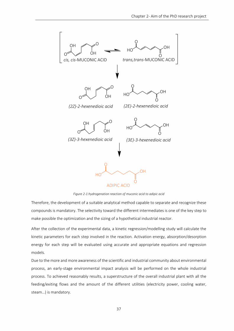
Chapter 2- Aim of the PhD research project
37
HOOH
O
O
OH
OHO
O
cis, cis-MUCONIC ACID trans,trans-MUCONIC ACID
OHHO
O
OADIPIC ACID
OH
OHO
O
HOOH
O
O
OH
OHO
O
HOOH
O
O
(2Z)-2-hexenedioic acid (2E)-2-hexenedioic acid
(3Z)-3-hexenedioic acid (3E)-3-hexenedioic acid
Figure 2-1:hydrogenation reaction of muconic acid to adipic acid
Therefore, the development of a suitable analytical method capable to separate and recognize these
compounds is mandatory. The selectivity toward the different intermediates is one of the key step to
make possible the optimization and the sizing of a hypothetical industrial reactor.
After the collection of the experimental data, a kinetic regression/modelling study will calculate the
kinetic parameters for each step involved in the reaction. Activation energy, absorption/desorption
energy for each step will be evaluated using accurate and appropriate equations and regression
models.
Due to the more and more awareness of the scientific and industrial community about environmental
process, an early-stage environmental impact analysis will be performed on the whole industrial
process. To achieved reasonably results, a superstructure of the overall industrial plant with all the
feeding/exiting flows and the amount of the different utilities (electricity power, cooling water,
steam…) is mandatory.
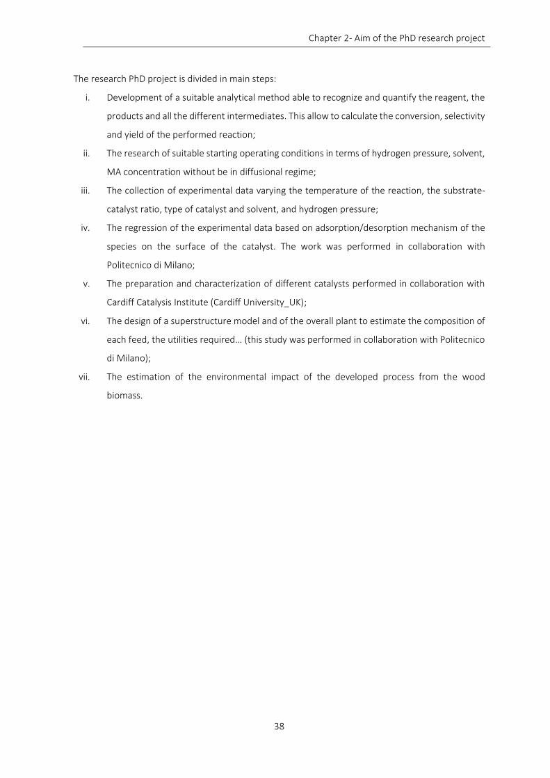
Chapter 2- Aim of the PhD research project
38
The research PhD project is divided in main steps:
i. Development of a suitable analytical method able to recognize and quantify the reagent, the
products and all the different intermediates. This allow to calculate the conversion, selectivity
and yield of the performed reaction;
ii. The research of suitable starting operating conditions in terms of hydrogen pressure, solvent,
MA concentration without be in diffusional regime;
iii. The collection of experimental data varying the temperature of the reaction, the substrate-
catalyst ratio, type of catalyst and solvent, and hydrogen pressure;
iv. The regression of the experimental data based on adsorption/desorption mechanism of the
species on the surface of the catalyst. The work was performed in collaboration with
Politecnico di Milano;
v. The preparation and characterization of different catalysts performed in collaboration with
Cardiff Catalysis Institute (Cardiff University_UK);
vi. The design of a superstructure model and of the overall plant to estimate the composition of
each feed, the utilities required… (this study was performed in collaboration with Politecnico
di Milano);
vii. The estimation of the environmental impact of the developed process from the wood
biomass.
Chapter 2- Aim of the PhD research project
39
Figure 2-2: representative scheme of the whole project and collaborations
Syn
thet
ic t
,t-M
A
Development of analytical method
Design and set-up of the reactor
Leakage test
Best conditions to operate in kinetic
regime
Optimization of the operating conditions
(catalyst pre-treatment, cat/sub, rpm...)
Preliminary commercial catalyst characterizations
Data collection at different operating
conditions (T, solvent, catalyst)
Data regression and kinetic model development
Commercial noble catalyst
Design of the super structure of the bio-
process
LCA
an
alys
is
Life cycle assessment for the traditional and the new bio-process
Home-made noble metal catalyst synthesis
catalyst characterizations
Protocol optimization
Data collection at different operating
conditions (T, pressure, solvent, catalyst)
40
Chapter 3
Description of characterization
techniques and analytical instruments
Catalyst characterization, if properly utilized, can be both the cornerstone of the science of catalysis
and the "catalyst in its own right for industrial progress". As a long-term research effort, its goal should
be an understanding of the catalytic act on a molecular level, a clear explanation of the nature of the
individual catalyst sites and of their interdependence and interaction with each other as well as with
the reactants. It must also provide an incentive for the development of instrumental capabilities and
chemical techniques which are the tools for this research effort. A basic knowledge of catalysis and
the ability to conceptualize a working hypothesis is a most desirable prerequisite for such studies.1
Synthetize a good catalyst and follow/evaluate the reagent conversion and products evolution play a
key role in the design of a new industrial process. This chapter describes the techniques used for
catalyst characterization and products recognition, the starting point for a robust work.

Chapter 3- Description of characterization techniques and analytical instruments
41
3.1 Catalyst characterization: introduction and theory
In general, catalyst characterization involves two main steps: the investigation of the porous nature
of the catalyst support (physical properties) and the properties of the active sites that are dispersed
on the surface of the support (Table 3-1).
Table 3-1: summary of the main techniques used for the characterization of a solid material
Catalyst texture
Physical properties Chemical properties
Result Technique Result Technique
Geometry and shape Chemical composition -Electron spectroscopy -Atomic adsorption
Total specific surface area
-Gas physisorption -Mercury porosimetry
Degree of dispersion
-Selective chemisorption -X-ray -Electron microscopy -Magnetisation analysis
True density -X-ray analysis -Neutron diffraction
Degree of dispersion
-Selective chemisorption -X-Ray -Electron microscopy -Magnetisation analysis
Bulk and apparent density
-Mercury porosimetry -Liquid displacement
Surface Energy
-Thermal analysis test -Temperature programmed desorption and reaction calorimetry
-Pore specific volume -Porosity
-Mercury porosimetry -Gas adsorption
Acid-base sites -Selective chemisorption -Temperature programmed desorption
Pore size and mean pore size
-Mercury porosimetry -Gas Adsorption
Redox sites
-Spectroscopic methods -Temp. programmed reduction -Temp. Programmed oxidation
Particle size
-Sieves -Laser scattering -Sedimentation -Electrical sensing zone -Etc.
-Catalytic properties -Activity -Selectivity
Reactor tests and simulation
Surface structure -Optical microscopy -Electron microscopy -X-Ray analysis
Surface change Z potential
The complete and accurate knowledge of the properties of a catalyst is fundamental for evaluating its
performances. The catalysts used in this work were characterized using several techniques to
investigate their physical and chemical properties.
The techniques used to characterize the catalysts were:
- Physisorption of gas using Brunauer–Emmett–Teller (BET) method: for the evaluation of
surface area and pore size distribution;

Chapter 3- Description of characterization techniques and analytical instruments
42
- Scanning Electron Microscopy (SEM) and Transmission Electron Microscopy (TEM): for the
evaluation of nanoparticles morphology;
- RAMAN spectroscopy: observation of vibrational, rotational, and other low-frequency modes
in a system;
- Inductively coupled plasma mass spectrometry (ICP-MS): for the detection and quantification
of metal inside a solution;
- X-ray Photoelectron Spectroscopy (XPS): metal oxidation state and metal exposure;
- Temperature Programmed Reduction (TPR): evaluation of the reduction temperature of
commercial Pt/AC 5% catalyst;
- X-Ray Powder Diffraction (XRPD): evaluation of crystal domain of metal and carbon support.
3.1.1 Surface area evaluation (BET method)
Adsorption methods may be used to provide information about the
total surface area of a catalyst and the pore size distribution. The
interaction between the adsorbate and the adsorbent may be
chemical (chemisorption) or physical (physisorption) and ideally
should be a surface-specific interaction. Physical adsorption is used
in the BET method to determine total surface areas.2 This
technique was developed by Brunauer, Emmett and Teller3 ( the
acronyms of their surname is in fact BET) and allows determining
the surface area that is commonly expressed as m2/g. The BET
theory is applied to systems of multilayer adsorption and usually
uses probing gases that do not chemically react with material
surfaces as adsorbates to quantify specific surface area. Nitrogen is the most commonly employed
gaseous adsorbate used for surface probing by BET methods. For this reason, standard BET analysis is
most often conducted at the boiling temperature of N2 (77 K). Specific surface area is a scale-
dependent property, with no single true value of specific surface area definable, and thus quantities
of specific surface area determined through BET theory may depend on the adsorbate molecule
utilized and its adsorption cross section. The concept of the theory is an extension of the Langmuir
theory,4 which is a theory for monolayer molecular adsorption, to multilayer adsorption with the
following hypotheses:
- gas molecules are physically adsorbed on a solid in layers infinitely;
- there is no interaction between each adsorption layer;
- the Langmuir theory can be applied to each layer.
Figure 3-1: BET instrument
Chapter 3- Description of characterization techniques and analytical instruments
43
The resulting BET equation is reported in Eq.1:
𝑉
𝑉𝑚=
𝑐𝑝
𝑝0
[1 −𝑝
𝑝0] [1 + (𝑐 − 1)𝑝
𝑝0] (Eq.3-1)
where:
V = volume of adsorbed gas at pressure p;
p° = gas saturation pressure, at temperature T;
p/p° = relative pressure;
Vm= the monolayer adsorbed gas quantity;
c = BET constant, expressed by Eq.2.
𝑐 = 𝑒𝑥𝑝 (𝑞1 − 𝑞𝐿
𝑅𝑇) (Eq.3-2)
where:
q1 = heat of adsorption of the first layer;
qL = heat of adsorption of the second and higher layers.
For the Vm calculation the Eq.3-1 must be linearized and the linear relationship of this equation is
maintained only in the range of 0.05 p< p0 < 0.35.
𝑝𝑝0
𝑉 [(1 −𝑝
𝑝0)]=
1
𝑐𝑉𝑚+
𝑝𝑝0 (𝑐 − 1)
𝑐𝑉𝑚 (Eq.3-3)
Eq.3-3 is an adsorption isotherm and can be plotted as a straight line with 1 / V[(p°/p) − 1] on the y-
axis and p/p0 on the x-axis according to experimental results. The specific surface area is determined
on the Vm basis:
𝑆𝑢𝑟𝑓𝑎𝑐𝑒 𝑎𝑟𝑒𝑎 (𝑆. 𝐴. ) =𝑉𝑚𝑁𝐴𝑉𝐴𝑚𝑜𝑙
𝑉𝑚𝑜𝑙 (Eq.3-4)
where:
NAV = Avogadro’s number;
Amol= adsorption cross section (for N2 = 16.2 Å2);
Vmol= molar volume of gas (22414 mL/mol);
3.1.2 Scanning Electron Microscopy (SEM)
The scanning electron microscope (SEM) uses a focused beam of high-energy electrons to generate a
variety of signals at the surface of solid specimens. The signals that derive from electron-sample
interactions reveal information about the sample including external morphology (texture), chemical

Chapter 3- Description of characterization techniques and analytical instruments
44
composition, and crystalline structure and orientation of materials making up the sample. In most
applications, data are collected over a selected area of the surface of the sample, and a 2-dimensional
image is generated that displays spatial variations in these properties. Areas ranging from
approximately 1 cm to 5 microns in width can be imaged in a scanning mode using conventional SEM
techniques. The SEM is also capable of performing analyses of selected point locations on the sample;
this approach is especially useful in qualitatively or semi-quantitatively determining chemical
compositions (using EDS), crystalline structure, and crystal orientations (using EBSD).
Accelerated electrons in an SEM
transmit significant amounts of kinetic
energy, and this energy is dissipated as
a variety of signals produced by
electron-sample interactions when
the incident electrons are decelerated
in the solid sample. These signals
consist of secondary electrons (that
produce SEM images), backscattered
electrons (BSE), diffracted
backscattered electrons (EBSD that
are used to determine crystal
structures and orientations of
minerals), photons (characteristic X-rays that are used for elemental analysis and continuum X-rays),
visible light (cathodoluminescence-CL), and heat. Secondary electrons and backscattered electrons
are commonly used for imaging samples: secondary electrons are most valuable for showing
morphology and topography on samples and backscattered electrons are most valuable for showing
contrasts in composition in multiphase samples. Measurement of the energy of photons emitted from
the sample is a common method to get analytical capabilities. Examples are the energy-dispersive X-
ray spectroscopy (EDS) detectors used in elemental analysis and CL systems that analyses the intensity
and spectrum of electron-induced luminescence. In SEM systems using these detectors it is common
to colour code these extra signals and superimpose them, so that differences in the distribution of the
various components of the sample can be seen clearly and compared. SEM analysis is considered to
be "non-destructive"; that is, X-rays generated by electron interactions do not lead to volume loss of
the sample, so it is possible to analyse the same material repetitively.
Electron source
Anode
Condenser lense
Scan coil
Objective lense
Sample
Secondary Electron detector
Electron beam
Figure 3-2: SEM internal section and beam pathway

Chapter 3- Description of characterization techniques and analytical instruments
45
3.1.3 Transmission Electron Microscopy (TEM)
TEM type of electron microscope that has three essential
systems:
1. an electron gun, which produces the electron beam,
and the condenser system, which focuses the beam onto the
object;
2. the image-producing system, consisting of the
objective lens, movable specimen stage, and intermediate
and projector lenses, which focus the electrons passing
through the specimen to form a real, highly magnified image;
3. the image-recording system, which converts the
electron image into some form perceptible to the human eye. The image-recording system
usually consists of a fluorescent screen for viewing and focusing the image and a digital
camera for permanent records. In addition, a vacuum system, consisting of pumps and their
associated gauges and valves, and power supplies are required.
The source of electrons, the cathode, is a heated V-shaped tungsten filament or, in high-performance
instruments, a sharply pointed rod of a material such as lanthanum hexaboride. The filament is
surrounded by a control grid, with a central aperture arranged on the axis of the column; the apex of
the cathode is arranged to lie at or just above or below this aperture. The cathode and control grid
are at a negative potential equal to the desired accelerating voltage and are insulated from the rest
of the instrument. The final electrode of the electron gun is the anode, which takes the form of a disk
with an axial hole. Electrons leave the cathode and shield, accelerate toward the anode, and, if the
stabilization of the high voltage is adequate, pass through the central aperture at a constant energy.
The control and alignment of the electron gun are critical in ensuring satisfactory operation. The
intensity and angular aperture of the beam are controlled by the condenser lens system between the
gun and the specimen. A single lens may be used to converge the beam onto the object, but, more
commonly, a double condenser is employed. In this the first lens is strong and produces a reduced
image of the source, which is then imaged by the second lens onto the sample. The use of a small spot
size minimizes disturbances in the specimen due to heating and irradiation.
The specimen grid is carried in a small holder in a movable specimen stage. The objective lens is usually
of short focal length (1–5 mm) and produces a real intermediate image that is further magnified by
the projector lens or lenses. A single projector lens may provide a range of magnification of 5:1, and
by the use of interchangeable pole pieces in the projector a wider range of magnifications may be
Figure 3-3: TEM instrument
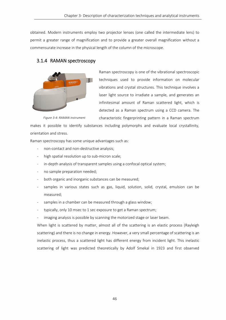
Chapter 3- Description of characterization techniques and analytical instruments
46
obtained. Modern instruments employ two projector lenses (one called the intermediate lens) to
permit a greater range of magnification and to provide a greater overall magnification without a
commensurate increase in the physical length of the column of the microscope.
3.1.4 RAMAN spectroscopy
Raman spectroscopy is one of the vibrational spectroscopic
techniques used to provide information on molecular
vibrations and crystal structures. This technique involves a
laser light source to irradiate a sample, and generates an
infinitesimal amount of Raman scattered light, which is
detected as a Raman spectrum using a CCD camera. The
characteristic fingerprinting pattern in a Raman spectrum
makes it possible to identify substances including polymorphs and evaluate local crystallinity,
orientation and stress.
Raman spectroscopy has some unique advantages such as:
- non-contact and non-destructive analysis;
- high spatial resolution up to sub-micron scale;
- in-depth analysis of transparent samples using a confocal optical system;
- no sample preparation needed;
- both organic and inorganic substances can be measured;
- samples in various states such as gas, liquid, solution, solid, crystal, emulsion can be
measured;
- samples in a chamber can be measured through a glass window;
- typically, only 10 msec to 1 sec exposure to get a Raman spectrum;
- imaging analysis is possible by scanning the motorized stage or laser beam.
When light is scattered by matter, almost all of the scattering is an elastic process (Rayleigh
scattering) and there is no change in energy. However, a very small percentage of scattering is an
inelastic process, thus a scattered light has different energy from incident light. This inelastic
scattering of light was predicted theoretically by Adolf Smekal in 1923 and first observed
Figure 3-4: RAMAN instrument
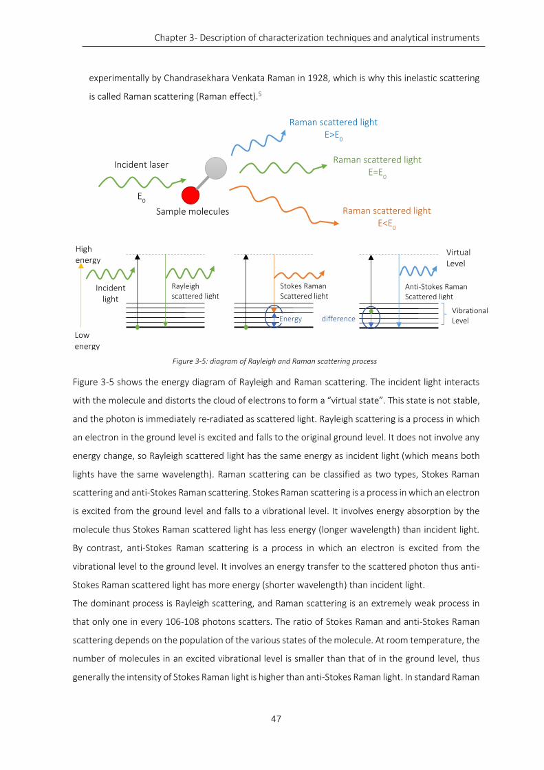
Chapter 3- Description of characterization techniques and analytical instruments
47
experimentally by Chandrasekhara Venkata Raman in 1928, which is why this inelastic scattering
is called Raman scattering (Raman effect).5
Figure 3-5 shows the energy diagram of Rayleigh and Raman scattering. The incident light interacts
with the molecule and distorts the cloud of electrons to form a “virtual state”. This state is not stable,
and the photon is immediately re-radiated as scattered light. Rayleigh scattering is a process in which
an electron in the ground level is excited and falls to the original ground level. It does not involve any
energy change, so Rayleigh scattered light has the same energy as incident light (which means both
lights have the same wavelength). Raman scattering can be classified as two types, Stokes Raman
scattering and anti-Stokes Raman scattering. Stokes Raman scattering is a process in which an electron
is excited from the ground level and falls to a vibrational level. It involves energy absorption by the
molecule thus Stokes Raman scattered light has less energy (longer wavelength) than incident light.
By contrast, anti-Stokes Raman scattering is a process in which an electron is excited from the
vibrational level to the ground level. It involves an energy transfer to the scattered photon thus anti-
Stokes Raman scattered light has more energy (shorter wavelength) than incident light.
The dominant process is Rayleigh scattering, and Raman scattering is an extremely weak process in
that only one in every 106-108 photons scatters. The ratio of Stokes Raman and anti-Stokes Raman
scattering depends on the population of the various states of the molecule. At room temperature, the
number of molecules in an excited vibrational level is smaller than that of in the ground level, thus
generally the intensity of Stokes Raman light is higher than anti-Stokes Raman light. In standard Raman
Incident laser
Sample molecules
E0
Raman scattered light E>E
0
Raman scattered light E=E
0
Raman scattered light E<E
0
Incident light
High energy
Low energy
Rayleigh scattered light
Stokes Raman Scattered light
Energy difference arises
Anti-Stokes Raman Scattered light
Virtual Level
Vibrational Level
Figure 3-5: diagram of Rayleigh and Raman scattering process

Chapter 3- Description of characterization techniques and analytical instruments
48
measurement, Rayleigh scattered light is rejected using a filter and only the Stokes Raman scattering
is recorded for simplicity. The intensity of anti-Stokes Raman light increases relative to Stokes
scattering as the temperature rises, thus the intensity ratio of anti-Stokes and Stokes light can be used
to measure the temperature of a sample.
Raman shifts are typically reported in wavenumbers, which have units of inverse length, as this value
is directly related to energy. In order to convert between spectral wavelength and wavenumbers of
shift in the Raman spectrum, the following formula can be used:
∆𝜔 =1
𝜆0
−1
𝜆1
(Eq.3-5)
Where:
∆𝜔= Raman shift expressed in wavenumber;
λ0= excitation wavelength;
λ1= Raman spectrum wavelength.
Most commonly, the unit chosen for expressing wavenumber in Raman spectra is inverse centimeters
(cm−1). Since wavelength is often expressed in units of nanometers (nm), the formula above can scale
for this unit conversion explicitly, giving:
Different parameters can be selected during the analysis and they affect the final spectrum. The
parameters of the analysis (time of scan, number of scans, wavelength region...) are chosen to
highlight a selected region or to enhance the signal.
3.1.5 inductively coupled plasma mass spectrometry (ICP-MS)
The ICP-MS instrument measures most of the elements
in the periodic table. The elements shown in color in
Figure 3-7 can be analyzed by ICP-MS with detection
limits a at or below the ppt range. Elements that are in
white are either not measurable by ICP-MS (the upper
right-hand side) or do not have naturally occurring
isotopes. Most analyses performed on ICP-MS
instrumentation are quantitative; however, it also can
work as an excellent semi-quantitative instrument. By
using a semi-quantitative software package, an
∆𝜔(𝑐𝑚−1) =1
𝜆0(𝑛𝑚)−
1
𝜆1(𝑛𝑚)∙
(107𝑛𝑚)
(𝑐𝑚) (Eq.3-6)
Figure 3-6: ICP-MS apparatus
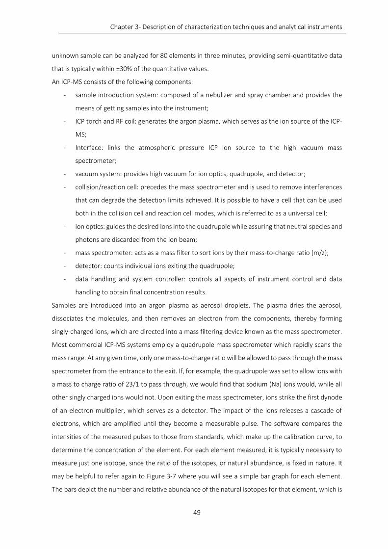
Chapter 3- Description of characterization techniques and analytical instruments
49
unknown sample can be analyzed for 80 elements in three minutes, providing semi-quantitative data
that is typically within ±30% of the quantitative values.
An ICP-MS consists of the following components:
- sample introduction system: composed of a nebulizer and spray chamber and provides the
means of getting samples into the instrument;
- ICP torch and RF coil: generates the argon plasma, which serves as the ion source of the ICP-
MS;
- Interface: links the atmospheric pressure ICP ion source to the high vacuum mass
spectrometer;
- vacuum system: provides high vacuum for ion optics, quadrupole, and detector;
- collision/reaction cell: precedes the mass spectrometer and is used to remove interferences
that can degrade the detection limits achieved. It is possible to have a cell that can be used
both in the collision cell and reaction cell modes, which is referred to as a universal cell;
- ion optics: guides the desired ions into the quadrupole while assuring that neutral species and
photons are discarded from the ion beam;
- mass spectrometer: acts as a mass filter to sort ions by their mass-to-charge ratio (m/z);
- detector: counts individual ions exiting the quadrupole;
- data handling and system controller: controls all aspects of instrument control and data
handling to obtain final concentration results.
Samples are introduced into an argon plasma as aerosol droplets. The plasma dries the aerosol,
dissociates the molecules, and then removes an electron from the components, thereby forming
singly-charged ions, which are directed into a mass filtering device known as the mass spectrometer.
Most commercial ICP-MS systems employ a quadrupole mass spectrometer which rapidly scans the
mass range. At any given time, only one mass-to-charge ratio will be allowed to pass through the mass
spectrometer from the entrance to the exit. If, for example, the quadrupole was set to allow ions with
a mass to charge ratio of 23/1 to pass through, we would find that sodium (Na) ions would, while all
other singly charged ions would not. Upon exiting the mass spectrometer, ions strike the first dynode
of an electron multiplier, which serves as a detector. The impact of the ions releases a cascade of
electrons, which are amplified until they become a measurable pulse. The software compares the
intensities of the measured pulses to those from standards, which make up the calibration curve, to
determine the concentration of the element. For each element measured, it is typically necessary to
measure just one isotope, since the ratio of the isotopes, or natural abundance, is fixed in nature. It
may be helpful to refer again to Figure 3-7 where you will see a simple bar graph for each element.
The bars depict the number and relative abundance of the natural isotopes for that element, which is

Chapter 3- Description of characterization techniques and analytical instruments
50
sometimes referred to as the isotopic fingerprint of the element. ICP-MS can be used to measure the
individual isotopes of each element; this capability brings value to laboratories interested in one
specific isotope of an element or in the ratio between two isotopes of an element.
Figure 3-7:ICP detectable chemical element
3.1.6 X-ray photoelectron spectroscopy (XPS)
XPS is a surface-sensitive quantitative spectroscopic
technique that measures the elemental composition at the
parts per thousand range, chemical state, empirical formula,
and electronic state of the elements that exist within a
material. XPS spectra are obtained by irradiating a material
with a beam of X-rays while at the same time measuring the
kinetic energy and number of electrons that are emitted
from the top 0 to 10 nm of the material being analyzed. XPS
requires high vacuum (P =10−8 mbar) or ultra-high vacuum
(UHV; P< 10−9 mbar) conditions. XPS can be used to analyze
the surface chemistry of a material in its initial state, or after some treatment, for example: exposure
to heat to study the changes due to heating, exposure to reactive gases or solutions, and exposure to
ion beam implant.
XPS is able to detect all elements with an atomic number (Z) between lithium (Z=3) and lawrencium
(Z=103). This limitation means that it cannot detect hydrogen (Z=1) or helium (Z=2). Detection limits
Figure 3-8: XPS apparatus

Chapter 3- Description of characterization techniques and analytical instruments
51
for most of the elements is 1000 ppm. Detections limits of parts per million (ppm) are possible but
require special conditions: concentration at top surface or very long collection time (overnight).
XPS technique is based on the analysis of the kinetic energy distribution of core level photoelectrons
emitted as the result of irradiation with monochromatic or narrow band X-rays2. Under optimum
conditions, the quantitative accuracy of the atomic percent (at%) values calculated from the Major
XPS Peaks is 90-95% for each major peak. If a high-level quality control protocol is used, the accuracy
can be further improved. Under routine work conditions, where the surface is a mixture of
contamination and expected material, the accuracy ranges from 80-90% of the value reported in
atomic percent values. The quantitative accuracy for the weaker XPS signals, that have peak intensities
10-20% of the strongest signal, are 60-80% of the true value, and depend upon the amount of effort
used to improve the signal-to-noise ratio (for example by signal averaging). The major interest is the
study of the “chemical shift” which reflects the oxidation state, and the chemical environment of the
emitter. Several problems can be occurred during the application of quantitative analysis to complex
systems (such as catalysts): sample charging, the choice of calibration procedures and the collection
time can widely affect the measurement. For this reason, XPS is widely used in catalyst research to
provide general qualitative analyses, to investigate the depth profile distribution of active species, to
obtain estimates of dispersion, clustering and other morphological variations, to study metal-metal
and metal-support interactions and to study the chemical states of additives, poisons and transition
metal ions in zeolites. Proven measurement techniques and models for interpolation are available.6,7
3.1.7 Temperature programmed reduction (TPR)
The aims of TPR techniques are:
- to find the most efficient reduction conditions;
- to identify the supported precursor phases and their
interactions with the support;
- to characterize complex systems, as bimetallic or
doped catalyst, to determine the role of the second
component ant to establish alloy formation or promotion
effects.
In the TPR technique a metal supported catalyst is treated using a programmed temperature ramp
while a reducing gas mixture flows into the sample chamber (usually, hydrogen diluted in some inert
gas as nitrogen or argon. The reduction rates are continuously measured by monitoring the change in
composition of the reactive mixture after the sample chamber. The decrease in H2 concentration in
the effluent gas with respect to the initial one suggests that the reduction process is occurring. An
Figure 3-9: TPR apparatus
Chapter 3- Description of characterization techniques and analytical instruments
52
interesting application of this technique is that the TPR analysis may be used to obtain evidence for
the interaction between the atoms of two metallic components, in the case of bimetallic system or
alloy as already cited. In general, TPR studies are carried out under low partial pressure of the reactive
gas. In this way it is possible to observe the intermediate reactions, depending from analytical
conditions as temperature rate, flow rate and concentration of reactive gas. The TPR method is used
for qualitative and quantitative analysis and the collected spectra are characteristic of a given solid.
3.1.8 X-ray powder diffraction (XRPD)
XRPD is a fast analytical technique mainly used for phase identification of a crystalline material and
can provide information on unit cell dimensions. The analyzed material is homogenized, and average
bulk composition is determined.
X-ray diffraction is based on constructive interference of monochromatic X-rays and a crystalline
sample. These X-rays are generated by a cathode ray tube, filtered to produce monochromatic
radiation, collimated to concentrate, and directed toward the sample. When conditions satisfy Bragg's
Law8 (Eq. 3-7)
𝑛𝜆 = 2𝑑 ∙ 𝑠𝑖𝑛𝜃 (Eq.3-7)
where:
n= is an integer;
𝜆 =wavelength of the radiation (nm);
d= distance between two adjacent planes (nm);
Θ= scattering angle (°).
the interaction of the incident rays with the sample produces constructive interference (and a
diffracted ray). This law relates the wavelength of electromagnetic radiation to the diffraction angle
and the lattice spacing in a crystalline sample. These diffracted X-rays are then detected, processed
and counted. By scanning the sample through a range of 2θ angles, all possible diffraction directions
of the lattice should be attained due to the random orientation of the powdered material. Conversion
of the diffraction peaks to d-spacings allows identification of the mineral because each mineral has a
set of unique d-spacings. Typically, this is achieved by comparison of d-spacings with standard
reference patterns. X-ray diffractometers consist of three basic elements: an X-ray tube, a sample
holder, and an X-ray detector. X-rays are generated in a cathode ray tube by heating a filament to
produce electrons, accelerating the electrons toward a target by applying a voltage, and bombarding
the target material with electrons. When electrons have sufficient energy to displace inner shell
electrons of the target material, characteristic X-ray spectra are produced. These spectra consist of
several components, the most common are Kα and Kβ. Filtering, by foils or crystal monochrometers, is

Chapter 3- Description of characterization techniques and analytical instruments
53
required to produce monochromatic X-rays needed for diffraction. Kα1and Kα2 are sufficiently close in
wavelength such that a weighted average of the two is used. Copper is the most common target
material for single-crystal diffraction, with Cu-Kα radiation = 1.5418 Å. These X-rays are collimated and
directed onto the sample. As the sample and detector are rotated, the intensity of the reflected X-
rays is recorded. When the geometry of the incident X-rays impacting the sample satisfies the Bragg
Equation, constructive interference occurs and a peak in intensity appears. A detector records and
processes this X-ray signal and converts the signal to a count rate which is then output to a device
such as a printer or computer monitor. The geometry of an X-ray diffractometer is such that the
sample rotates in the path of the collimated X-ray beam at an angle θ while the X-ray detector is
mounted on an arm to collect the diffracted X-rays and rotates at an angle of 2θ. The instrument used
to maintain the angle and rotate the sample is called a goniometer. For typical powder patterns, data
is collected at 2θ from ~5° to 70°, angles that are preset in the X-ray scan.
3.2 Analytical techniques
3.2.1 UV-Visible analysis (UV-Vis)
Ultraviolet–visible spectroscopy or ultraviolet–visible
spectrophotometry (UV–Vis or UV/Vis) refers to absorption
spectroscopy or reflectance spectroscopy in the ultraviolet-
visible spectral region. The absorption or reflectance in the
visible range directly affects the perceived color of the
chemicals involved. In this region of the electromagnetic
spectrum, atoms and molecules undergo electronic
transitions. UV/Vis spectroscopy is routinely used in analytical
chemistry for the quantitative determination of different
analytes, such as transition metal ions, highly conjugated
organic compounds, and biological macromolecules.
Spectroscopic analysis is commonly carried out in solution, but solids and gases may also be studied.
Molecules containing π-electrons or non-bonding electrons (n-electrons) can absorb energy in the
form of ultraviolet or visible light to excite these electrons to higher anti-bonding molecular orbitals.
The more easily excited the electrons (i.e. lower energy gap between the HOMO and the LUMO), the
longer the wavelength of light it can absorb. There are four possible types of transitions (π–π*, n–π*,
σ–σ*, and n–σ*), and they can be ordered as follows: σ–σ* > n–σ* > π–π* > n–π*.9
The reference law is the Lambert-Beer law (Eq.3-8):10
Figure 3-10: UV-Vis instrument and spectrum

Chapter 3- Description of characterization techniques and analytical instruments
54
𝐴 = 휀𝑖 ∙ 𝐶𝑖 ∙ 𝑙 (Eq.3-8)
where:
A= the absorbance of the species;
ε (L∙mol-1∙cm)= the molar attenuation coefficient or absorptivity of the attenuating species i in the
material sample;
Ci (mol/L)= the concentration of the attenuating species i in the material sample;
l (cm)= the path length of the beam of light through the material sample.
The path length is normally equal to 1, so the law represents the equation of a centered line in the
origin and angular coefficient equal to ε.
The Beer–Lambert Law is useful for characterizing many compounds but does not hold as a universal
relationship for the concentration and absorption of all substances
3.2.2 Gas-chromatographic analysis (GC)
Gas chromatography is a term used to describe the group of
analytical separation techniques used to analyze volatile
substances in the gas phase.
A gas chromatograph is based on a gas flow-through narrow tube
known as the column, through which different chemical
components of a sample pass in a gas stream (carrier gas, mobile
phase) at different rates depending on their various chemical and
physical properties and their interaction with a specific column
filling (stationary phase). As the chemicals exit the end of the
column, they are detected and identified electronically by using a
detector. The function of the stationary phase in the column is to separate different molecules,
affecting the exit time (retention time). Other parameters that can be used to alter the order or time
of retention are the carrier gas flow rate, column length and the temperature. In a GC analysis, a
known volume of gaseous or liquid analyte is introduced into the injector of the column, usually using
a micro syringe. The injector has a temperature of 50 °C above the boiling point of the most low-
boiling compound, therefore the injected liquid solution is instantaneously vaporized into the injector.
As the carrier gas transports the analyte molecules through the column, this motion is inhibited by
the adsorption of the analyte molecules either onto the column walls or onto the stationary phase.
The rate at which the molecules progress along the column depends on the strength of adsorption,
which depends on the type of molecule and on the solid stationary phase materials. Since each type
of molecule has a different rate of progression, the various components of the analyte mixture are
Figure 3-11: GC instrument

Chapter 3- Description of characterization techniques and analytical instruments
55
separated as they progress along the column and reach the end of the column at different times
(retention time). A detector is used to monitor the outlet stream from the column; thus, the time at
which each component reaches the outlet and the amount of that component can be determined.
Generally, substances are identified (qualitatively) by the order in which they emerge (elute) from the
column and by the retention time of the analyte in the column.
Nowadays may different detectors can be coupled with a GC instrument and the most commonly used
are:
- Flame ionization detector (FID);
- Thermo conductivity detector (TCD);
- Mass detector (MS).
During this PhD work all these three kinds of detector was used to obtain different information.
FID: in this detector electrodes are placed adjacent to a flame fueled by air/hydrogen mixture near
the exit of the column, and when carbon containing compounds exit the column they are pyrolyzed
by the flame. This detector works only for organic / hydrocarbon containing compounds due to the
ability of the carbons to form cations and electrons upon pyrolysis which generates a current between
the electrodes.11 The increase in current is converted and appears as a peak in a chromatogram. FIDs
have low detection limits (a few picograms per second) but they are unable to generate ions from
carbonyl containing carbons.11 FID compatible carrier gasses include helium, hydrogen, nitrogen, and
argon.
TCD: compares the thermal conductivity of two gas flows – the pure carrier (reference) gas and the
sample. Changes in the temperature of the electrically-heated wires in the detector are affected by
the thermal conductivity of the gas which flows around this. The changes in this thermal conductivity
are sensed as a change in electrical resistance and are measured. With this detector is possible to
detect water (using proper column and filament parameters).
FID and TCD detectors required standards injection to establish which compound is exiting from the
column. This recognition is not always simple, especially if new reaction is performed. For the
recognition of unknown compound is possible to couple to the GC instrument a mass detector (MS).
The compound exiting from the column are fed into the MS analyzer where the compounds are
ionized and fragmented. There are several ion sources available; each has advantages and
disadvantages for particular applications. For example, electron ionization (EI) gives a high degree of
fragmentation, yielding highly detailed mass spectra which when skillfully analyzed can provide
important information for structural elucidation/characterization and facilitate identification of
unknown compounds by comparison to mass spectral libraries obtained under identical operating
conditions.

Chapter 3- Description of characterization techniques and analytical instruments
56
3.2.3 Nuclear Magnetic Resonance (NMR)
NMR spectroscopy is an analytical chemistry technique used in quality control and research for
determining the content and purity of a sample as well as its molecular structure. For example, NMR
can quantitatively analyze mixtures containing known compounds. For unknown compounds, NMR
can either be used to match against spectral libraries or to infer the basic structure directly. Once the
basic structure is known, NMR can be used to determine molecular conformation in solution as well
as studying physical properties at the molecular level such as conformational exchange, phase
changes, solubility, and diffusion. In order to achieve the desired results, a variety of NMR techniques
are available. The principle behind NMR is that many nuclei have spin and all nuclei are electrically
charged. If an external magnetic field is applied, an energy transfer is possible between the base
energy to a higher energy level (generally a single energy gap). The energy transfer takes place at a
wavelength that corresponds to radio frequencies and when the spin returns to its base level, energy
is emitted at the same frequency. The signal that matches this transfer is measured in many ways and
processed in order to yield an NMR spectrum for the nucleus concerned.
The specific resonant frequency of the energy transition is dependent on the effective magnetic field
at the nucleus. This field is affected by electron shielding which is in turn dependent on the chemical
environment. As a result, information about the nucleus' chemical environment can be derived from
its resonant frequency. In general, the more electronegative the nucleus is, the higher the resonant
frequency. Other factors such as ring currents (anisotropy) and bond strain affect the frequency shift.
It is customary to adopt tetramethylsilane (TMS) as the proton reference frequency. This is because
the precise resonant frequency shift of each nucleus depends on the magnetic field used. The
frequency is not easy to describe so it was decided to define chemical shift as follows to yield a more
convenient number.
𝐶ℎ𝑒𝑚𝑖𝑐𝑎𝑙 𝑠ℎ𝑖𝑓𝑡 (𝛿) = (𝜈 − 𝜈0)/𝜈0 (Eq.3-9)
The chemical shift, using this equation, is not dependent on the magnetic field and it is convenient to
express it in ppm where (for proton) TMS is set to ν0 thereby giving it a chemical shift of zero.
Chapter 3- Bibliography
57
Bibliography
1. Haensel, V. & Haensel, H. S. The Role of Catalyst Characterization in Process Development. in Characterization and Catalyst development 2–11 (1989). doi:10.1021/bk-1989-0411.ch001
2. Haber, J., Block, J. H. & Delmon, B. Manual of method and procedures for catalyst characterization. Pure Apll. Chem. 67, 1257–1306 (1995).
3. Brunauer, S., Emmett, P. H. & Teller, E. Adsorption of Gases in Multimolecular Layers. J. Am. Chem. Soc. 60, 309–319 (1938).
4. Langmuir, I. The adsorption of gases on plane surfaces of glass, mica and platinum. J. Am. Chem. Soc. 40, 1361–1403 (1918).
5. Singh, R. C. V. Raman and the Discovery of the Raman Effect. Phys. Perspect. 4, 399–420 (2002).
6. Bagus, P. S., Ilton, E. S. & Nelin, C. J. The interpretation of XPS spectra: Insights into materials properties. Surf. Sci. Rep. 68, 273–304 (2013).
7. Lascovich, J. C., Giorgi, R. & Scaglione, S. Evaluation of the sp2/sp3 ratio in amorphous carbon structure by XPS and XAES. Appl. Surf. Sci. 47, 17–21 (1991).
8. Bragg, W. H. & Bragg, W. L. The reflection of X-rays by crystals. Proc. R. Soc. London. Ser. A 88, 428 LP-438 (1913).
9. Skoog, D. A., Holler, F. J. & Crouch, S. R. Principles of Instrumental Analysis. (Thomson Brooks/Cole, 2007).
10. Buijs, K. & Maurice, M. J. Some considerations on apparent deviations from lambert-beer’s law. Anal. Chim. Acta 47, 469–474 (1969).
11. Harris, D. C. Gas chromatogrphy. in Quantitative chemical analysis 657–712 (W.H. freeman and Company, 1999).

58
Chapter 4
Development of the analytical method
The development of a suitable analytical method able to allow the evaluation of conversion and
selectivity is mandatory, even if sometimes different analytical techniques are required to obtain the
results. In this chapter the description of the different characterization techniques is reported as well
as the analytical methods used to calculate the conversion and the selectivity. Due to laboratory
facilities, we have decided to develop a gas chromatographic method able to separate the reaction
products (adipic acid, Z and E hexenedioic acids, cis,cis-muconic acid). In this chapter the analytical
method used for the evaluation of conversion and selectivity is detailly described. The conversion was
evaluated by UV-Vis analysis while the selectivity though gas chromatographic analysis after
derivatization of the reaction products.

Chapter 4- Development of the analytical method
59
No specific analytical method for the separation and quantification of MA (and its isomers), the
monounsaturated intermediates, and AdA is present in literature. Vardon et al1. reported a high
performance liquid chromatography (HPLC) to separate AdA and the by products utilizing a
Phenomenex Rezex RFQ Fast Fruit H+ column. The system operated at 85 °C with isocratic mobile
phase elution t 1.0 ml/min. In this case by-products were identified by co-elution at the same
retention time with pure compounds. The spectra obtained with HPLC method is reported in Figure
4-1. MA is very close to ethanol peak and a better resolution is mandatory to correctly evaluate the
conversion (key parameter for any industrial application). No mention about (3E)-hexenedioic acid is
present. Another research group has mentioned a gas chromatography/mass spectrometry (GC-MS)
for the analysis and separation of AdA, dimethyl ester, 2-hexenedioic acid dimethyl ester, and 2, 4-
hexadienedioic acid dimethyl ester using a DB-1 MS column.2 Despite this sentence no operating
conditions were reported.
Therefore, a development of a suitable and robust analytical method is mandatory. Due to laboratory
facilities, we have decided to develop a gas chromatographic method able to separate the reaction
products (adipic acid, Z and E hexenedioic acids, cis,cis-muconic acid, and trans,trans-muconic acid).
Figure 4-1: chromatogram obtained from HPLC analysis developed by Vardon et al.
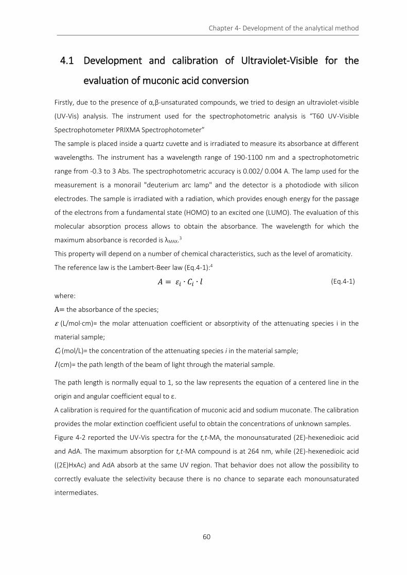
Chapter 4- Development of the analytical method
60
4.1 Development and calibration of Ultraviolet-Visible for the
evaluation of muconic acid conversion
Firstly, due to the presence of α,β-unsaturated compounds, we tried to design an ultraviolet-visible
(UV-Vis) analysis. The instrument used for the spectrophotometric analysis is “T60 UV-Visible
Spectrophotometer PRIXMA Spectrophotometer”
The sample is placed inside a quartz cuvette and is irradiated to measure its absorbance at different
wavelengths. The instrument has a wavelength range of 190-1100 nm and a spectrophotometric
range from -0.3 to 3 Abs. The spectrophotometric accuracy is 0.002/ 0.004 A. The lamp used for the
measurement is a monorail "deuterium arc lamp" and the detector is a photodiode with silicon
electrodes. The sample is irradiated with a radiation, which provides enough energy for the passage
of the electrons from a fundamental state (HOMO) to an excited one (LUMO). The evaluation of this
molecular absorption process allows to obtain the absorbance. The wavelength for which the
maximum absorbance is recorded is λMAX.3
This property will depend on a number of chemical characteristics, such as the level of aromaticity.
The reference law is the Lambert-Beer law (Eq.4-1):4
𝐴 = 휀𝑖 ∙ 𝐶𝑖 ∙ 𝑙 (Eq.4-1)
where:
A= the absorbance of the species;
ε (L/mol∙cm)= the molar attenuation coefficient or absorptivity of the attenuating species i in the
material sample;
Ci (mol/L)= the concentration of the attenuating species i in the material sample;
l (cm)= the path length of the beam of light through the material sample.
The path length is normally equal to 1, so the law represents the equation of a centered line in the
origin and angular coefficient equal to ε.
A calibration is required for the quantification of muconic acid and sodium muconate. The calibration
provides the molar extinction coefficient useful to obtain the concentrations of unknown samples.
Figure 4-2 reported the UV-Vis spectra for the t,t-MA, the monounsaturated (2E)-hexenedioic acid
and AdA. The maximum absorption for t,t-MA compound is at 264 nm, while (2E)-hexenedioic acid
((2E)HxAc) and AdA absorb at the same UV region. That behavior does not allow the possibility to
correctly evaluate the selectivity because there is no chance to separate each monounsaturated
intermediates.
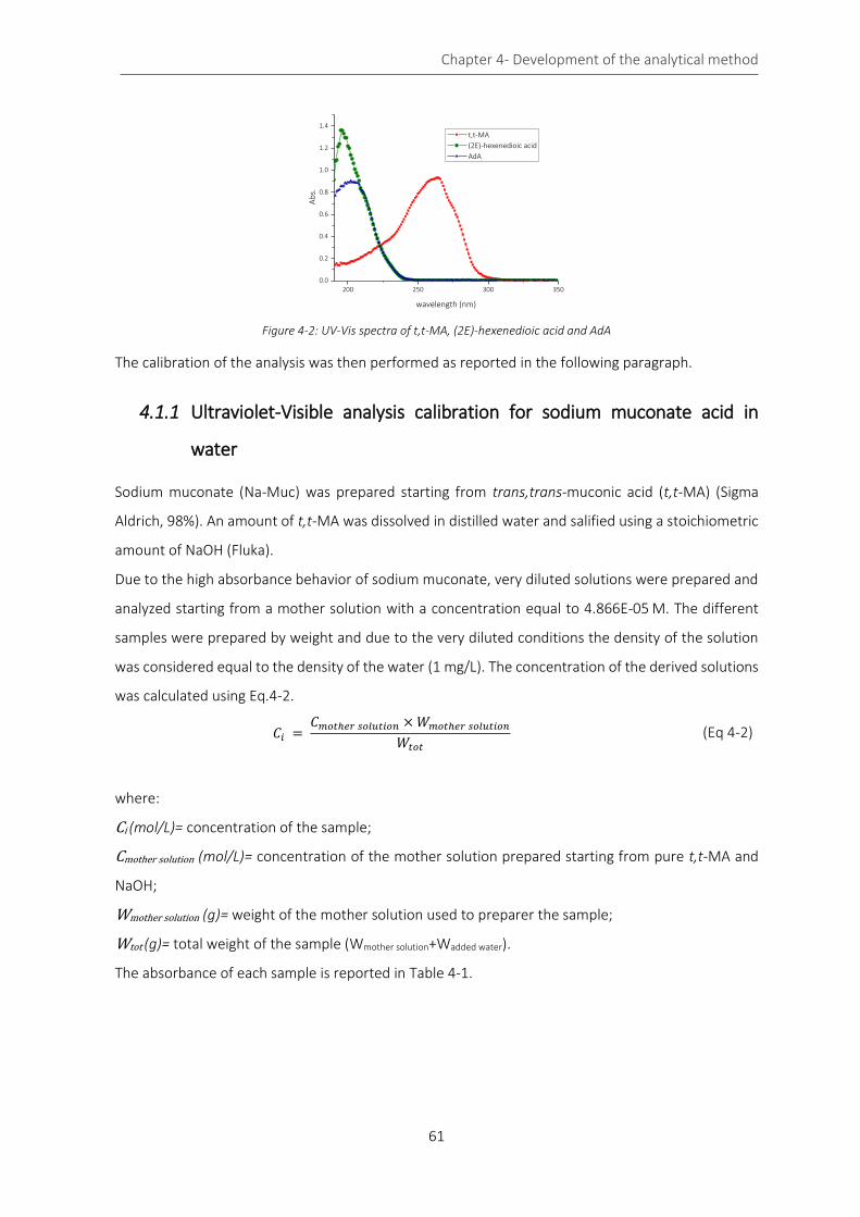
Chapter 4- Development of the analytical method
61
Figure 4-2: UV-Vis spectra of t,t-MA, (2E)-hexenedioic acid and AdA
The calibration of the analysis was then performed as reported in the following paragraph.
4.1.1 Ultraviolet-Visible analysis calibration for sodium muconate acid in
water
Sodium muconate (Na-Muc) was prepared starting from trans,trans-muconic acid (t,t-MA) (Sigma
Aldrich, 98%). An amount of t,t-MA was dissolved in distilled water and salified using a stoichiometric
amount of NaOH (Fluka).
Due to the high absorbance behavior of sodium muconate, very diluted solutions were prepared and
analyzed starting from a mother solution with a concentration equal to 4.866E-05 M. The different
samples were prepared by weight and due to the very diluted conditions the density of the solution
was considered equal to the density of the water (1 mg/L). The concentration of the derived solutions
was calculated using Eq.4-2.
𝐶𝑖 = 𝐶𝑚𝑜𝑡ℎ𝑒𝑟 𝑠𝑜𝑙𝑢𝑡𝑖𝑜𝑛 × 𝑊𝑚𝑜𝑡ℎ𝑒𝑟 𝑠𝑜𝑙𝑢𝑡𝑖𝑜𝑛
𝑊𝑡𝑜𝑡
(Eq 4-2)
where:
Ci (mol/L)= concentration of the sample;
Cmother solution (mol/L)= concentration of the mother solution prepared starting from pure t,t-MA and
NaOH;
Wmother solution (g)= weight of the mother solution used to preparer the sample;
Wtot (g)= total weight of the sample (Wmother solution+Wadded water).
The absorbance of each sample is reported in Table 4-1.
200 250 300 350
0.0
0.2
0.4
0.6
0.8
1.0
1.2
1.4
Ab
s.wavelength (nm)
t,t-MA
(2E)-hexenedioic acid
AdA
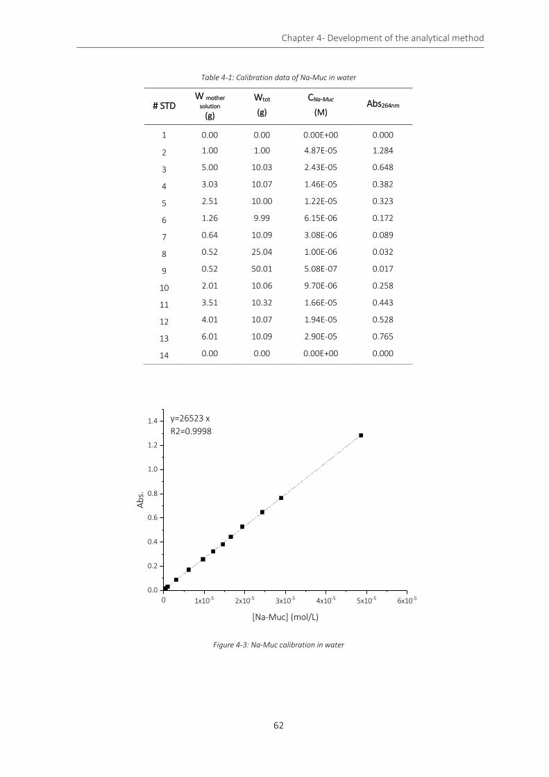
Chapter 4- Development of the analytical method
62
Table 4-1: Calibration data of Na-Muc in water
0 1x10⁻⁵ 2x10⁻⁵ 3x10⁻⁵ 4x10⁻⁵ 5x10⁻⁵ 6x10⁻⁵
0.0
0.2
0.4
0.6
0.8
1.0
1.2
1.4
Ab
s.
[Na-Muc] (mol/L)
y=26523 x
R2=0.9998
Figure 4-3: Na-Muc calibration in water
# STD W mother
solution
(g)
Wtot
(g)
CNa-Muc
(M) Abs264nm
1 0.00 0.00 0.00E+00 0.000
2 1.00 1.00 4.87E-05 1.284
3 5.00 10.03 2.43E-05 0.648
4 3.03 10.07 1.46E-05 0.382
5 2.51 10.00 1.22E-05 0.323
6 1.26 9.99 6.15E-06 0.172
7 0.64 10.09 3.08E-06 0.089
8 0.52 25.04 1.00E-06 0.032
9 0.52 50.01 5.08E-07 0.017
10 2.01 10.06 9.70E-06 0.258
11 3.51 10.32 1.66E-05 0.443
12 4.01 10.07 1.94E-05 0.528
13 6.01 10.09 2.90E-05 0.765
14 0.00 0.00 0.00E+00 0.000
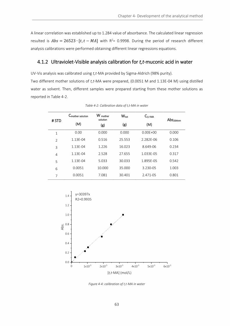
Chapter 4- Development of the analytical method
63
A linear correlation was established up to 1.284 value of absorbance. The calculated linear regression
resulted is 𝐴𝑏𝑠 = 26523 ∙ [𝑡, 𝑡 − 𝑀𝐴] with R2= 0.9998. During the period of research different
analysis calibrations were performed obtaining different linear regressions equations.
4.1.2 Ultraviolet-Visible analysis calibration for t,t-muconic acid in water
UV-Vis analysis was calibrated using t,t-MA provided by Sigma-Aldrich (98% purity).
Two different mother solutions of t,t-MA were prepared, (0.0051 M and 1.13E-04 M) using distilled
water as solvent. Then, different samples were prepared starting from these mother solutions as
reported in Table 4-2.
0 1x10⁻⁵ 2x10⁻⁵ 3x10⁻⁵ 4x10⁻⁵ 5x10⁻⁵ 6x10⁻⁵
0.0
0.2
0.4
0.6
0.8
1.0
1.2
1.4
Ab
s.
[t,t-MA] (mol/L)
y=30397x
R2=0.9935
Figure 4-4: calibration of t,t-MA in water
Table 4-2: Calibration data of t,t-MA in water
# STD
Cmother solution
(M)
W mother
solution
(g)
Wtot
(g)
Ct,t-MA
(M) Abs264nm
1 0.00 0.000 0.000 0.00E+00 0.000
2 1.13E-04 0.516 25.553 2.282E-06 0.106
3 1.13E-04 1.226 16.023 8.649-06 0.234
4 1.13E-04 2.528 27.655 1.033E-05 0.317
5 1.13E-04 5.033 30.033 1.895E-05 0.542
6 0.0051 10.000 35.000 3.230-05 1.003
7 0.0051 7.081 30.401 2.471-05 0.801
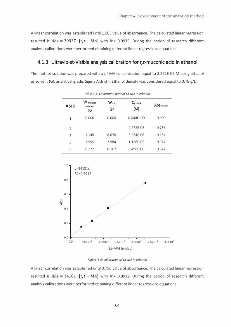
Chapter 4- Development of the analytical method
64
A linear correlation was established until 1.003 value of absorbance. The calculated linear regression
resulted is 𝐴𝑏𝑠 = 30937 ∙ [𝑡, 𝑡 − 𝑀𝐴] with R2= 0.9935. During the period of research different
analysis calibrations were performed obtaining different linear regressions equations.
4.1.3 Ultraviolet-Visible analysis calibration for t,t-muconic acid in ethanol
The mother solution was prepared with a t,t-MA concentration equal to 2.272E-05 M using ethanol
as solvent (GC analytical grade, Sigma Aldrich). Ethanol density was considered equal to 0.79 g/L.
0.0 5.0x10⁻⁶ 1.0x10⁻⁵ 1.5x10⁻⁵ 2.0x10⁻⁵ 2.5x10⁻⁵ 3.0x10⁻⁵
0.0
0.2
0.4
0.6
0.8
1.0
Ab
s.
[t,t-MA] (mol/L)
y=34181x
R2=0.9912
Figure 4-5: calibration of t,t-MA in ethanol
A linear correlation was established until 0.756 value of absorbance. The calculated linear regression
resulted is 𝐴𝑏𝑠 = 34181 ∙ [𝑡, 𝑡 − 𝑀𝐴] with R2= 0.9912. During the period of research different
analysis calibrations were performed obtaining different linear regressions equations.
Table 4-3: Calibration data of t,t-MA in ethanol
# STD W mother
solution
(g)
Wtot
(g)
Ct,t-MA
(M) Abs264nm
1 0.000 0.000 0.000E+00 0.000
2 - - 2.272E-05 0.756
3 1.149 8.070 3.234E-06 0.154
4 1.995 3.984 1.138E-05 0.317
5 0.122 8.167 6.498E-06 0.542

Chapter 4- Development of the analytical method
65
4.2 Development and calibration of gas-chromatographic method
(GC) using different columns and detectors for the evaluation of
selectivity.
In general, the quantification of dicarboxylic acids is a critical challenge due to the low instrument
sensitivity toward these compounds. Moreover, the separation of stereoisomers and chemical
compounds that differ only for the presence or not of a double bond is not always a simple goal to
achieve. On this way, the application of Fischer’s esterification to dicarboxylic acid could increase the
volatility of these chemicals during the GC analysis, allowing a good quantification and analysis
reproducibility. For this reason, a Fischer’s esterification was performed on each dicarboxylic acid. The
general reaction scheme and the mechanism is reported in
Figure 4-6. The Lewis or Brønstedt acid-catalyzed esterification of carboxylic acids with alcohols to give
esters is a typical reaction in which the products and reactants are in equilibrium.
The equilibrium may be influenced by either removing one product from the reaction mixture (for
example. removal of the water by azeotropic distillation or absorption by molecular sieves) or by
employing an excess of one reactant. Addition of a proton (e.g.: p-TsOH. H2SO4) or a Lewis acid leads
to a more reactive electrophile. Nucleophilic attack of the alcohol gives a tetrahedral intermediate in
which there are two equivalent hydroxyl groups. One of these hydroxyl groups is eliminated after a
proton shift (tautomerism) to give water and ester.
R OH
O
+
R OQ
O
+ H2O
R OH
OH+
R OH
O
R OH
O
H H O
QH
O
QH
O
OR
O
H
Q
H
tautomerism
H
O
H
R O
O
H
H
Q
O
H
OQR
+ H2O
R OQ
O
+ H2O
- H+
Figure 4-6: reaction scheme of Fischer’s esterification

Chapter 4- Development of the analytical method
66
In the following paragraphs analysis calibration and analytical method validation is reported.
4.2.1 Analysis calibration using SUPELCOWAX 10 column
The analysis was calibrated using the dimethyl adipate (DMA) (Sigma Aldrich, >99.8%) and (3E)-
hexenedioic dimethyl ester ((3E)HxDME) (Sigma Aldrich, 99%) were used as standard compound.
The instrument used for gas chromatographic analysis was “Master GC Fast Gas Chromatograph” (by
Dani Instruments S.p.A) equipped with thermal conductivity detector (TCD). The sample (0.3 μL) was
injected using a Hamilton syringe and subsequently vaporized at a temperature of 290 °C with a split
ratio 1:3. Helium carrier flow was 15 mL/min. The chromatographic column used for the analysis was
a SUPELCOWAX 10 (Sigma Aldrich) 60 meters long with a diameter of 0.53 mm and thickness of the
inner coating film of 1 μm in PEG. The instrument operates in a temperature ramp starting from 60
°C. The temperature ramp was the following:
from 60 °C to 120 °C with a ramp of 18 °C/min;
from 120 °C to 160 °C with a ramp of 20 °C/min;
from 160 °C to 260 °C with a ramp of 15 °C/min;
isotherm at 260 °C for 1 minute.
Each analysis lasts 13 minutes.
The analysis was carried out using a TCD detector set at 240 °C.
A solution of butanol in methanol 0.035 (wt/wt) (Sigma Aldrich 99.9%) was used as internal standard.
4.2.1.1 Calibration of (3E)-hexenedioic dimethyl ester
0.259 g of (3E)-hexenedioic dimethyl ester ((3E)HxDME) were solubilized in 15.164 g of MeOH
obtaining a solution with a weight ratio of 1.708E-02. The solution of the internal standard was
prepared using 0.662 g of ButOH in 18.893 g of MeOH obtaining a solution with a weight ratio of
3.502E-02. Different solutions were then prepared for the calibration analyses using MeOH as solvent
(Table 4-4). MeOH and ButOH density was considered 0.791 and 0.81 g/mL, respectively.
Table 4-4:calibration data of (3E)HxDME
# STD
Wsol.(3E)HxDME
(g) Wsol.ButOH
(g) WMeOH
(g) WtotMeOH
(g) W(3E)HxDME
(g) WButOH
(g)
1 4.010 0.507 0.000 4.430 6.85E-02 1.77E-02
2 5.06E-01 1.007 6.022 7.490 8.64E-03 3.53E-02
3 1.531 0.508 2.005 4.000 2.61E-02 1.78E-02

Chapter 4- Development of the analytical method
67
The total amount of ButOH and (3E)HxDME was evaluated using the Eq.4-4
𝑎𝑚𝑜𝑢𝑛𝑡𝑖 = 𝑊𝑠𝑜𝑙,𝑖 ∙ 𝑤𝑒𝑖𝑔ℎ𝑡 𝑟𝑎𝑡𝑖𝑜𝑖 (Eq.4-3)
𝑡𝑜𝑡𝑎𝑙 𝑎𝑚𝑜𝑢𝑛𝑡 𝑜𝑓 𝑀𝑒𝑂𝐻 = 𝑊𝑀𝑒𝑂𝐻 + ∑ 𝑊𝑠𝑜𝑙,𝑖 − 𝑎𝑚𝑜𝑢𝑛𝑡𝑖 (Eq.4-4)
where:
amounti (g) = amount of (3E)HxDME or ButOH;
Wsol,i (g)= amount of the mother solution used for the sample preparation;
Weight ratioi = 1.708E-02 and 3.502E-02 for (3E)HxDME and ButOH, respectively;
total amount of MeOH (g)= total weight of MeOH contained in the sample;
WMeOH (g) = MeOH added for the sample preparation.
Table 4-5:chromatographic results for (3E)HxDME calibration
# STD AButoOH A(3E)HxDME A(3E)HxDME /AButoOH
1 18.068 56.731 3.139
20.666 67.518 3.267
20.336 65.514 3.221
average 3.203
2 23.718 4.731 0.199
22.947 4.652 0.202
23.699 4.834 0.204
average 0.202
3 21.424 27.379 1.278
22.16 26.334 1.188
20.183 25.8 1.278
average 1.248
Table 4-6: results for (3E)HxDME calibration
The concentration of (3E)HxDME was evaluated using the Eq.4-5
# STD A(3E)HxDME /AButoOH C(3E)HxDME
(mol/L)
CMeOH
(mol/L) C(3E)HxDME /CButoOH
1 3.203 7.07E-02 4.26E-02 1.66
2 0.202 5.27E-03 5.00E-02 1.05E-01
3 1.248 2.99E-02 4.73E-02 0.63

Chapter 4- Development of the analytical method
68
𝐶(3𝐸)𝐻𝑥𝐷𝑀𝐸 =
𝑊(3𝐸)𝐻𝑥𝐷𝑀𝐸
𝑀𝑊𝐻𝑥𝐷𝑀𝐸∙ 1000(
𝑚𝐿𝐿
)
𝑊𝑀𝑒𝑂𝐻
𝜌𝑀𝑒𝑂𝐻+
𝑊𝐵𝑢𝑡𝑂𝐻
𝜌𝐵𝑢𝑡𝑂𝐻
(Eq.4-5)
where:
W(3E)HxDME (g) = amount of (3E)HxDME calculated with Eq.3;
MW(3E)HxDME (g/mol) = 172.18;
WMeOH (g) = amount of MeOH calculated with Eq.4;
MWButOH (g/mol) = 74.12;
ρMeOH (g/mL) = density of methanol;
ρMeOH (g/mL) = density of butanol;
A= chromatographic area.
An analogue equation was used to evaluate ButOH concentration.
The calibration curve obtained is reported in Figure 4-7.
0.0 0.3 0.5 0.8 1.0 1.3 1.5 1.8 2.00.0
0.5
1.0
1.5
2.0
2.5
3.0
3.5
4.0
A(3
E)H
xDM
E/A
Bu
tOH
C(3E)HxDME/CButOH
y=1.934x
R2=0.999
Figure 4-7: calibration of (3E)HxDME
A linear correlation was established. The calculated linear regression equation is 𝐴(3𝐸)𝐻𝑥𝐷𝑀𝐸 /
𝐴𝐵𝑢𝑡𝑂𝐻 = 1.934 ∙ 𝐶(3𝐸)𝐻𝑥𝐷𝑀𝐸 /𝐶𝐵𝑢𝑡𝑂𝐻 with R2=0.999. During the period of research different
analysis calibrations were performed obtaining different linear regressions equations.
4.2.1.2 Calibration of dimethyl adipate
0.363 g of dimethyl adipate (DMA) were solubilized in 20.295 g of MeOH obtaining a solution with a
weight ratio of 1.787E-02. The solution of the internal standard was prepared using 0.662 g of ButOH
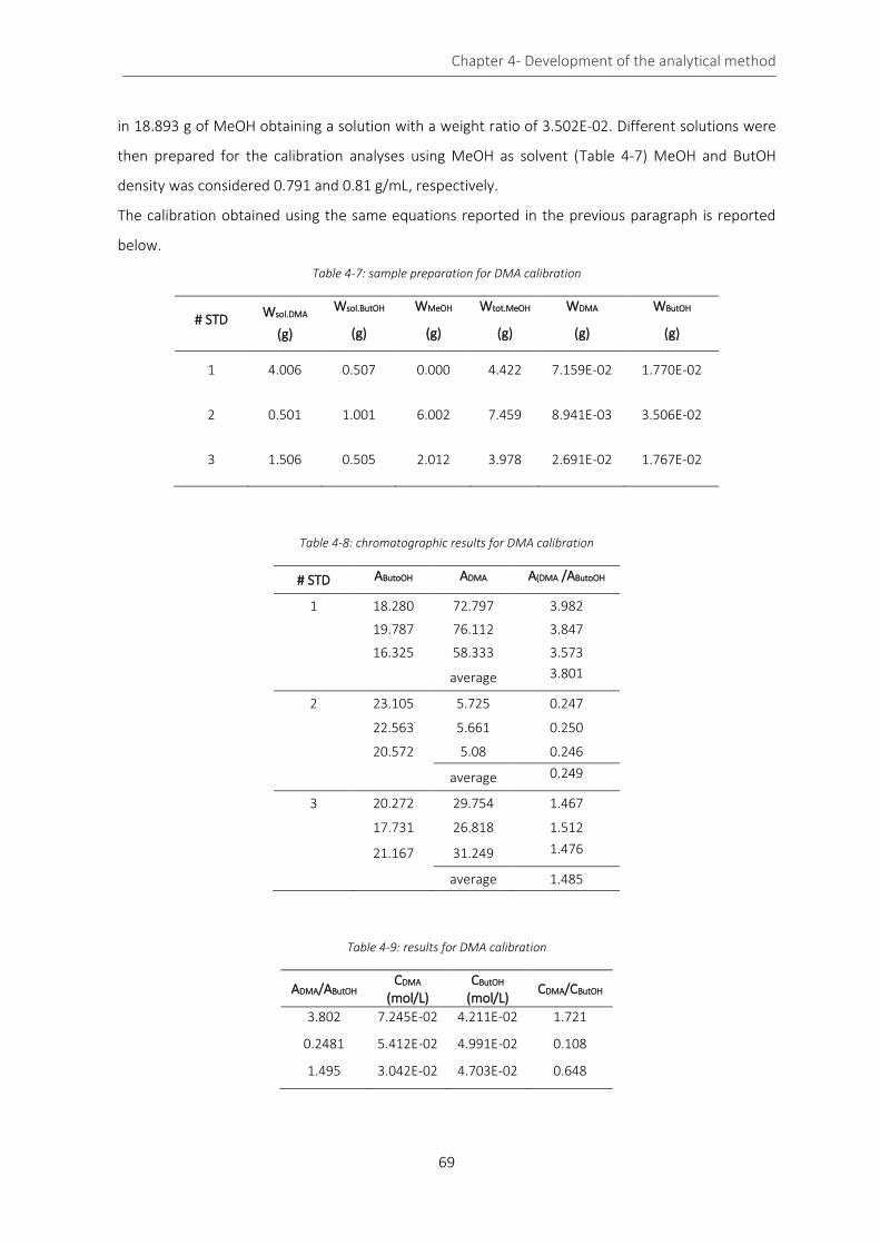
Chapter 4- Development of the analytical method
69
in 18.893 g of MeOH obtaining a solution with a weight ratio of 3.502E-02. Different solutions were
then prepared for the calibration analyses using MeOH as solvent (Table 4-7) MeOH and ButOH
density was considered 0.791 and 0.81 g/mL, respectively.
The calibration obtained using the same equations reported in the previous paragraph is reported
below.
Table 4-7: sample preparation for DMA calibration
# STD Wsol.DMA
(g)
Wsol.ButOH
(g)
WMeOH
(g)
Wtot.MeOH
(g)
WDMA
(g)
WButOH
(g)
1 4.006 0.507 0.000 4.422 7.159E-02 1.770E-02
2 0.501 1.001 6.002 7.459 8.941E-03 3.506E-02
3 1.506 0.505 2.012 3.978 2.691E-02 1.767E-02
Table 4-8: chromatographic results for DMA calibration
# STD AButoOH ADMA A(DMA /AButoOH
1 18.280 72.797 3.982 19.787 76.112 3.847 16.325 58.333 3.573
average 3.801
2 23.105 5.725 0.247
22.563 5.661 0.250
20.572 5.08 0.246
average 0.249
3 20.272 29.754 1.467
17.731 26.818 1.512
21.167 31.249 1.476
average 1.485
Table 4-9: results for DMA calibration
ADMA/AButOH CDMA
(mol/L) CButOH
(mol/L) CDMA/CButOH
3.802 7.245E-02 4.211E-02 1.721
0.2481 5.412E-02 4.991E-02 0.108
1.495 3.042E-02 4.703E-02 0.648

Chapter 4- Development of the analytical method
70
0.0 0.3 0.5 0.8 1.0 1.3 1.5 1.8 2.00.0
0.5
1.0
1.5
2.0
2.5
3.0
3.5
4.0
AD
MA/A
Bu
tOH
CDMA/CButOH
y=2.219x
R2=0.999
Figure 4-8: calibration of DMA
A linear correlation was established. The calculated linear regression equation is 𝐴𝐷𝑀𝐴 /𝐴𝐵𝑢𝑡𝑂𝐻 =
2.219 ∙ 𝐶𝐷𝑀𝐴 /𝐶𝐵𝑢𝑡𝑂𝐻 with R2= 0.999. During the period of research different analysis calibrations
were performed obtaining different linear regressions equations.
4.2.2 Analysis calibration using SP-2380 column
SP-2380 (Sigma Aldrich) column is a highly polar cyan-siloxane column commonly used for separation
of geometric (cis/trans) fatty acid methyl ester (FAME) isomers as a group. The stationary phase is
stabilized with poly (90% biscyanopropyl/10% cyanopropyl-phenyl siloxane). The possibility to work in
isotherm analysis to separate geometric isomers allowed performing several analyses in short period
time. A SP®-2380 Capillary GC Column L × I.D. 60 m × 0.25 mm, film thickness 0.20 μm column was
used during the last year of the research work.
We decided to use FID detector due to its higher sensibility compared with the TCD one.
Dimethyl glutarate (>99%, Fluka) was used as internal standard allowing the quantification of the
different products.
The analysis was performed setting the following parameters:
- Oven temperature: 180 °C (isothermal condition);
- Injector temperature= 220 °C;
- Injector He gas flow= 1.8 mL/min;
- Split= 90;
- Detector temperature: 220 °C;
Chapter 4- Development of the analytical method
71
- Detector He flow= 43 mL/min;
- Detector air flow= 310 mL/min;
- Detector H2 flow= 38 mL/min;
- Injection volume= 1.5 µL;
- Time of analysis= 8 min.
4.2.2.1 Calibration of (2E)hexenedioic dimethyl ester
The calibration of (2E)hexenedioic acid ((2E)HxDME) was performed using a standard purchase from
Sigma Aldrich (purity >99.9%).
0.0329 g of (2E)hexenedioic acid ((2E)HxDME) were solubilized in 11.256 g (14.23 mL) of MeOH.
(2E)HxDME concentration is equal to 1.34E-05 M. It is useless to prepare concentrated solution
because the amount of the compound in the reaction mixture is very low. DMG and (2E)HxDME
molecular weight is equal to 160.17 g/mol and 172.18 g/mol, respectively, while MeOH density was
considered equal to 0.791 g/mL. The density of the mother solution was considered equal to the
density of MeOH.
Different standard solutions were prepared starting from the mother solution and then analyzed by
GC-FID analysis. The results are reported in the following tables.
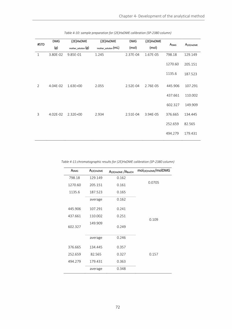
Chapter 4- Development of the analytical method
72
Table 4-10: sample preparation for (2E)HxDME calibration (SP-2380 column)
#STD DMG
(g)
(2E)HxDME
mother_solution (g)
(2E)HxDME
mother_solution (mL)
DMG
(mol)
(2E)HxDME
(mol) ADMG A(2E)HxDME
1 3.80E-02 9.85E-01 1.245 2.37E-04 1.67E-05 798.18
1270.60
1135.6
129.149
205.151
187.523
2 4.04E-02 1.63E+00 2.055 2.52E-04 2.76E-05 445.906
437.661
602.327
107.291
110.002
149.909
3 4.02E-02 2.32E+00 2.934 2.51E-04 3.94E-05 376.665
252.659
494.279
134.445
82.565
179.431
Table 4-11:chromatographic results for (2E)HxDME calibration (SP-2380 column)
ADMG A(2E)HxDME A(2E)HxDME /AButOH mol(2E)HxDME/molDMG
798.18 129.149 0.162 0.0705
1270.60 205.151 0.161
1135.6 187.523 0.165
average 0.162
445.906 107.291 0.241
0.109 437.661 110.002 0.251
602.327 149.909
0.249
average 0.246
376.665 134.445 0.357
0.157 252.659 82.565 0.327
494.279 179.431 0.363
average 0.348
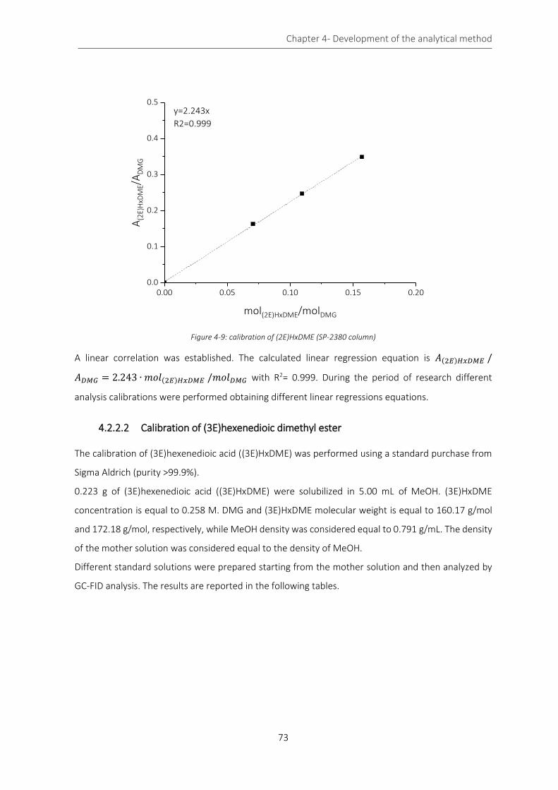
Chapter 4- Development of the analytical method
73
0.00 0.05 0.10 0.15 0.200.0
0.1
0.2
0.3
0.4
0.5
A(2
E)H
xDM
E/A
DM
G
mol(2E)HxDME/molDMG
y=2.243x
R2=0.999
Figure 4-9: calibration of (2E)HxDME (SP-2380 column)
A linear correlation was established. The calculated linear regression equation is 𝐴(2𝐸)𝐻𝑥𝐷𝑀𝐸 /
𝐴𝐷𝑀𝐺 = 2.243 ∙ 𝑚𝑜𝑙(2𝐸)𝐻𝑥𝐷𝑀𝐸 /𝑚𝑜𝑙𝐷𝑀𝐺 with R2= 0.999. During the period of research different
analysis calibrations were performed obtaining different linear regressions equations.
4.2.2.2 Calibration of (3E)hexenedioic dimethyl ester
The calibration of (3E)hexenedioic acid ((3E)HxDME) was performed using a standard purchase from
Sigma Aldrich (purity >99.9%).
0.223 g of (3E)hexenedioic acid ((3E)HxDME) were solubilized in 5.00 mL of MeOH. (3E)HxDME
concentration is equal to 0.258 M. DMG and (3E)HxDME molecular weight is equal to 160.17 g/mol
and 172.18 g/mol, respectively, while MeOH density was considered equal to 0.791 g/mL. The density
of the mother solution was considered equal to the density of MeOH.
Different standard solutions were prepared starting from the mother solution and then analyzed by
GC-FID analysis. The results are reported in the following tables.

Chapter 4- Development of the analytical method
74
Table 4-12: sample preparation and chromatographic results for (3E)HxDME calibration (SP-2380 column)
#STD DMG
(g) (3E)HxDME
mother_solution (µL)
MeOH (µL)
DMG (mol)
(3E)HxDME (mol)
ADMG A(3E)HxDME
1 2.08E-02 170 430 1.29E-04 4.39-05 1627.342
1197.833
807.015
492.988
361.656
223.315
2 1.51E-02 200 400 9.42E-05 5.16E-05 886.641
1118.37
14871.53
420.343
561.842
7324.091
3 1.03E-02 140 460 6.43E-05 3.61E-05 4852.977
3055.243
3262.192
2449.083
1567.744
1723.621
4 1.19E-02 302 200 7.43E-05 9.83E-06 390.345
277.731
101.714
46.765
33.461
11.342
5 1.39E-02 570 350 8.67E-05 1.86E-05 59.764
54.983
62.057
8.707
9.815
12.227
Table 4-13: results for (3E)HxDME calibration (SP-2380 column)
A(3E)HxDME /AButOH mol(3E)HxDME/molDMG
average
0.303 0.302 0.278 0.294
0.338
average
0.474 0.502 0.492 0.489
0.547
average
0.505 0.513 0.528 0.515
0.562
average
0.119 0.120 0.111 0.117
0.132
average
0.146 0.178 0.197 0.173
0.214

Chapter 4- Development of the analytical method
75
0.0 0.1 0.2 0.3 0.4 0.5 0.60.0
0.1
0.2
0.3
0.4
0.5
0.6
A(3
E)H
xDM
E/A
DM
G
mol(3E)HxDME/molDMG
y=0.843x
R2=0.995
Figure 4-10: calibration of (3E)HxDME (SP-2380 column)
A linear correlation was established. The calculated linear regression equation is 𝐴(3𝐸)𝐻𝑥𝐷𝑀𝐸 /
𝐴𝐷𝑀𝐺 = 0.843 ∙ 𝑚𝑜𝑙(3𝐸)𝐻𝑥𝐷𝑀𝐸 /𝑚𝑜𝑙𝐷𝑀𝐺 with R2= 0.995. During the period of research different
analysis calibrations were performed obtaining different linear regressions equations.
4.2.2.3 Calibration of dimethyl adipate
The calibration of dimethyl adipate (DMA) was performed using a standard purchase from Sigma
Aldrich (purity >99.9%) dissolved in MeOH
DMG and DMA molecular weight is equal to 160.17 g/mol and 174.19 g/mol, respectively. Different
standard solutions were prepared and then analyzed by GC-FID analysis. The results are reported in
the following tables.

Chapter 4- Development of the analytical method
76
Table 4-14: samples preparation and chromatographic results for DMA calibration (SP-2380 column)
#STD DMG
(g) DMA
(g) MeOH
(g) DMG (mol)
DMA (mol)
ADMG ADMA
1 0.079 0.147 0.698 4.98E-04 8.45E-04 137.75 292.84
321.73 687.05
136.24 293.71
2 0.045 0.100 0.644 2.82E-04 5.76E-04 231.48 562.57
481.87 1179.65
1026.43 2533.73
3 0.074 0.098 1.00 4.60E-04 5.65E-04 637.55 956.20
611.02 915.68
493.70 725.97
4 0.093 0.082 1.31 5.83E-04 4.71E-04 1411.03 1409.62
542.82 535.89
630.66 613.88
5 0.075 0.045 0.879 4.71E-04 2.64E-04 715.04 484.34
1354.94 941.849
1758.70 1219.6
Table 4-15: results for DMA calibration (SP-2380 column)
molDMA/molDMG ADMA/ADMG
1.698 2.126 2.136
2.156
average 2.139
2.0449 2.430 2.448 2.468
average 2.449
1.229 1.500 1.499 1.470
average 1.490
0.8072 0.999 0.987 0.973
average 0.986
0.5597 0.677 0.695 0.693
average 0.689

Chapter 4- Development of the analytical method
77
0.0 0.3 0.5 0.8 1.0 1.3 1.5 1.8 2.0 2.3 2.5 2.8 3.00.0
0.5
1.0
1.5
2.0
2.5
3.0
AD
MA/A
DM
G
molDMA/molDMG
y=1.2713x
R2=0.998
Figure 4-11: calibration of DMA (SP-2380 column)
A linear correlation was established. The calculated linear regression equation is 𝐴𝐷𝑀𝐴 /𝐴𝐷𝑀𝐺 =
1.2713 ∙ 𝑚𝑜𝑙𝐷𝑀𝐴 /𝑚𝑜𝑙𝐷𝑀𝐺 with R2=0.998. During the period of research different analysis
calibrations were performed obtaining different linear regressions equations.
4.3 Application of the developed analytical method
The application of this analytical method involves many different passages and the possibility to loss
material during the steps is tangible. For this reason, the material balance evaluation is mandatory to
verify the concrete possibility to use this analytical method. Due to the equilibrium reaction of
Fischer’s reaction, an optimization of the esterification was required to correctly evaluate the
selectivity. In the next paragraphs the application of the developed analytical method, its optimization
and material balance calculation are described.
4.3.1 Data elaboration
4.3.1.1 Evaluation of the conversion through UV-Vis analysis
After the end of the reaction 1 g of the reacted mixture is used for the UV analysis sample preparation.
Two or three dilutions are necessary to read an absorbance below 1. The samples are prepared
weighting the reacted mixture and water (or ethanol).
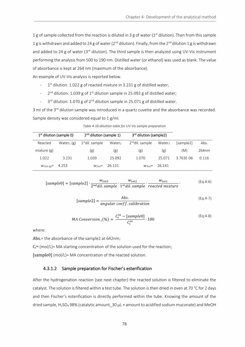
Chapter 4- Development of the analytical method
78
1 g of sample collected from the reaction is diluted in 3 g of water (1st dilution). Then from this sample
1 g is withdrawn and added to 24 g of water (2nd dilution). Finally, from the 2nd dilution 1 g is withdrawn
and added to 24 g of water (3rd dilution). The third sample is then analyzed using UV-Vis instrument
performing the analysis from 500 to 190 nm. Distilled water (or ethanol) was used as blank. The value
of absorbance is kept at 264 nm (maximum of the absorbance).
An example of UV-Vis analysis is reported below.
- 1st dilution: 1.022 g of reacted mixture in 3.231 g of distilled water;
- 2nd dilution: 1.039 g of 1st dilution sample in 25.092 g of distilled water;
- 3rd dilution: 1.070 g of 2nd dilution sample in 25.071 g of distilled water.
3 ml of the 3rd dilution sample was introduced in a quartz cuvette and the absorbance was recorded.
Sample density was considered equal to 1 g/ml.
Table 4-16:diluition table for UV-Vis sample preparation
1st dilution (sample 0) 2nd dilution (sample 1) 3rd dilution (sample2)
Reacted
mixture (g)
Water1 (g) 1stdil. sample
(g)
Water2
(g)
2nddil. sample
(g)
Water3
(g)
[sample2]
(M)
Abs.
264nm
1.022 3.231 1.039 25.092 1.070 25.071 3.763E-06 0.116
w1tot (g)= 4.253 w2tot= 26.131 w3tot= 26.141
[𝑠𝑎𝑚𝑝𝑙𝑒0] = [𝑠𝑎𝑚𝑝𝑙𝑒2] ∙𝑤𝑡𝑜𝑡3
2𝑛𝑑𝑑𝑖𝑙. 𝑠𝑎𝑚𝑝𝑙𝑒∙
𝑤𝑡𝑜𝑡2
1𝑠𝑡𝑑𝑖𝑙. 𝑠𝑎𝑚𝑝𝑙𝑒∙
𝑤𝑡𝑜𝑡1
𝑟𝑒𝑎𝑐𝑡𝑒𝑑 𝑚𝑖𝑥𝑡𝑢𝑟𝑒∙ (Eq.4-6)
[𝑠𝑎𝑚𝑝𝑙𝑒2] =𝐴𝑏𝑠.
𝑎𝑛𝑔𝑢𝑙𝑎𝑟 𝑐𝑜𝑒𝑓𝑓. 𝑐𝑎𝑙𝑖𝑏𝑟𝑎𝑡𝑖𝑜𝑛
(Eq.4-7)
𝑀𝐴 𝐶𝑜𝑛𝑣𝑒𝑟𝑠𝑖𝑜𝑛 𝑖(%) = 𝐶𝑖
𝑖𝑛 − [𝑠𝑎𝑚𝑝𝑙𝑒0]
𝐶𝑖𝑖𝑛
∙ 100 (Eq.4-8)
where:
Abs.= the absorbance of the sample2 at 642nm;
Ciin (mol/L)= MA starting concentration of the solution used for the reaction;
[sample0] (mol/L)= MA concentration of the reacted solution.
4.3.1.2 Sample preparation for Fischer’s esterification
After the hydrogenation reaction (see next chapter) the reacted solution is filtered to eliminate the
catalyst. The solution is filtered within a test tube. The solution is then dried in oven at 70 °C for 2 days
and then Fischer’s esterification is directly performed within the tube. Knowing the amount of the
dried sample, H2SO4 98% (catalytic amount_30 µL + amount to acidified sodium muconate) and MeOH
Chapter 4- Development of the analytical method
79
(in large excess) was added in the tube. Fischer’s esterification was performed in the oven at 70 °C for
48 h. Finally, the sample is cooled and, after the addition of the internal standard, is analyzed by GC
method.
An example of the evaluation of the amount of H2SO4 and MeOH to use during the esterification
reaction is reported below.
Dried powder recovered= 0.086 g
𝐻2𝑆𝑂4 𝑛𝑒𝑢𝑡𝑟. =𝑑𝑟𝑖𝑒𝑑 𝑝𝑜𝑤𝑑𝑒𝑟 (𝑔) ∗ 𝑀𝑊𝐻2𝑆𝑂4
∙ 0.98
𝑀𝑊𝑁𝑎−𝑚𝑢𝑐 ∙ 𝜌𝐻2𝑆𝑂4
= 2.39 ∙ 10−2 (Eq.4-9)
where:
H2SO4 neutrl (mL) = is the amount of sulphuric acid required to acidify sodium muconate;
MWH2SO4 (g/mol)= 98.08;
MWNa-muc (g/mol)= 188.1;
ρH2SO4 (g/mL)= 1.84.
Therefore, the total amount of H2SO4 is equal to the sum of the acid necessary to neutralize sodium
muconate and the catalytic amount required for the reaction. In this case the total amount is equal to
53.9 µL.
Methanol amount is instead evaluated as reported below.
Considering methanol/muconic acid ratio (mL/g) equal to 73, the amount of MeOH required for the
esterification reaction is
𝑀𝑒𝑂𝐻 =𝑑𝑟𝑖𝑒𝑑 𝑝𝑜𝑤𝑑𝑒𝑟 ∙ 𝑀𝑊𝑀𝐴 ∙ 𝑀𝑒𝑂𝐻 𝑀𝐴⁄ 𝑟𝑎𝑡𝑖𝑜
𝑀𝑊𝑁𝑎−𝑚𝑢𝑐
= 5.8 (Eq.4-10)
where:
MWMA (g/mol)= 142.1;
MeOH/MA ratio= 73 (mLMeOH/gMA).
4.3.1.3 Gas chromatographic analysis with SUPELCOWAX-10 column
After esterification reaction the sample is ready for gas chromatographic analysis. In the case of
SUPELCOWAX-10 column a solution of butanol (ButOH) (Sigma Aldrich, analytical grade) in methanol
was used as internal standard. Sample preparation and data elaboration are reported below.
Internal standard solution (STD) was prepared weighting 0.713 g of ButOH and 18.019 g of MeOH. The
weight ratio ButOH/MeOH is equal to 3.955E-02.
Therefore, 1.026 g of standard solution were added to the cool esterified sample.

Chapter 4- Development of the analytical method
80
STD (g)
ButOH (g)
ButOH (mol)
1.026 4.056E-02 5.472E-04
ButOH (g) was calculated knowing the ButOH/MeOH ratio:
𝐵𝑢𝑡𝑂𝐻(𝑔) = 𝑆𝑇𝐷 (𝑔) ∙ (𝐵𝑢𝑡𝑂𝐻
𝑀𝑒𝑂𝐻)
𝑟𝑎𝑡𝑖𝑜 (Eq.4-11)
while ButOH (mol) was simply derived dividing ButOH (g) for the molecular weight of ButOH (74.12
g/mol)
GC analysis was performed injecting the sample three times to control data reproducibility and
minimize analysis error. A are the chromatographic areas.
Table 4-17: results of GC analysis
Rt= 3.5 min Rt= 8.5 min
# AButOH ADMA ADMA/AButOH
1 173.259 24.254 0.140
2 180.560 25.610 0.141
3 178.908 24.987 0.139
average 0.140
Rt= 3.5 min Rt= 9.1 min
# AButOH A(2Z)HxDME A(2Z)HxDME/AButOH
1 173.259 0.000 0.000
2 180.560 0 .000 0.000
3 178.908 0.000 0.000
average 0.000
Rt= 3.5 min Rt= 9.3 min
# AButOH A(2E)HxDME A(2E)HxDME/AButOH
1 173.259 3.242 0.019
2 180.560 4.031 0.022
3 178.908 3.656 0.020
average 0.020
Rt= 3.5 min Rt= 9.7 min
# AButOH ADMM ADMM/AButOH
1 173.259 9.210 0.053
2 180.560 10.021 0.055
3 178.908 9.765 0.054
average 0.054

Chapter 4- Development of the analytical method
81
GC analysis is able to separate DMM, but this compound is not completely soluble in methanol at
room temperature. During the cooling down process DMM precipitated is clearly visible on the
bottom of the tube. For this reason, a good quantification is only possible using UV-Vis analysis.
After the collection of the chromatographic areas is possible to evaluate the selectivity of the reaction.
Due to the lack of (2Z)HxDME standard, the evaluation of the selectivity toward this compound was
performed using the same response factor of the (2Z)HxDME compound.
Using the calibration, it was possible to calculate the molar ratio between the compound and the
internal standard.
In general, the molar ratio is evaluated with the following equation
𝑚𝑜𝑙𝑖 𝑚𝑜𝑙𝐵𝑢𝑡𝑂𝐻⁄ =𝐴 𝐴𝐵𝑢𝑡𝑂𝐻⁄
𝑟𝑒𝑠𝑝𝑜𝑛𝑠𝑒 𝑓𝑎𝑐𝑡𝑜𝑟 (Eq.4-12)
where the response factor is the angular coefficient of the calibrations.
molDMA/molButOH mol(2Z)HxDME /molButOH mol(2E)HxDME /molButOH
6.307E-02 0.000 9.675E-03
The evaluation of the mole for each compound was performed using the following equation:
𝑚𝑜𝑙𝑖 = 𝑚𝑜𝑙𝑖 𝑚𝑜𝑙𝐵𝑢𝑡𝑂𝐻⁄ ∙ 𝑚𝑜𝑙𝐵𝑢𝑡𝑂𝐻 (Eq.4-13)
Finally, the selectivity of each compound was evaluated using Eq.14
𝑆𝑒𝑙𝑒𝑐𝑡𝑖𝑣𝑖𝑡𝑦𝑛 (%) =𝑚𝑜𝑙𝑛
∑ 𝑚𝑜𝑙𝑖 + 𝑚𝑜𝑙𝑛
∙ 100 (Eq.4-14)
where:
Selectivityn =is the selectivity of the n compound;
moln= is the number of moles of the considered reaction product;
∑ moli=is the sum of the moles of all the other reaction products.
SelDMA
(%) Sel(2Z)HxDME
(%) Sel(2E)HxDME
(%)
86.70 0.00 13.30
DMA (mol)
(2Z)HxDME (mol)
(2E)HxDME (mol)
3.451E-05 0.000 5.295E-06
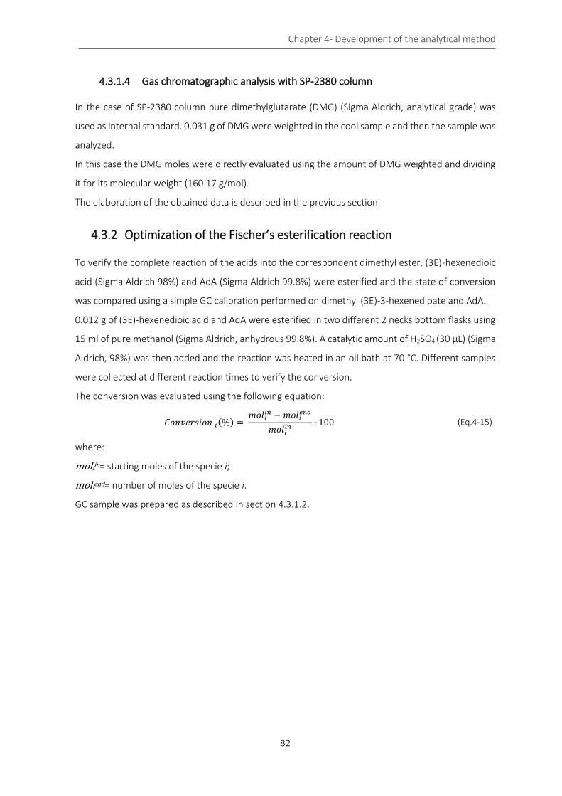
Chapter 4- Development of the analytical method
82
4.3.1.4 Gas chromatographic analysis with SP-2380 column
In the case of SP-2380 column pure dimethylglutarate (DMG) (Sigma Aldrich, analytical grade) was
used as internal standard. 0.031 g of DMG were weighted in the cool sample and then the sample was
analyzed.
In this case the DMG moles were directly evaluated using the amount of DMG weighted and dividing
it for its molecular weight (160.17 g/mol).
The elaboration of the obtained data is described in the previous section.
4.3.2 Optimization of the Fischer’s esterification reaction
To verify the complete reaction of the acids into the correspondent dimethyl ester, (3E)-hexenedioic
acid (Sigma Aldrich 98%) and AdA (Sigma Aldrich 99.8%) were esterified and the state of conversion
was compared using a simple GC calibration performed on dimethyl (3E)-3-hexenedioate and AdA.
0.012 g of (3E)-hexenedioic acid and AdA were esterified in two different 2 necks bottom flasks using
15 ml of pure methanol (Sigma Aldrich, anhydrous 99.8%). A catalytic amount of H2SO4 (30 µL) (Sigma
Aldrich, 98%) was then added and the reaction was heated in an oil bath at 70 °C. Different samples
were collected at different reaction times to verify the conversion.
The conversion was evaluated using the following equation:
𝐶𝑜𝑛𝑣𝑒𝑟𝑠𝑖𝑜𝑛 𝑖(%) = 𝑚𝑜𝑙𝑖
𝑖𝑛 − 𝑚𝑜𝑙𝑖𝑒𝑛𝑑
𝑚𝑜𝑙𝑖𝑖𝑛
∙ 100 (Eq.4-15)
where:
moliin= starting moles of the specie i;
moliend= number of moles of the specie i.
GC sample was prepared as described in section 4.3.1.2.
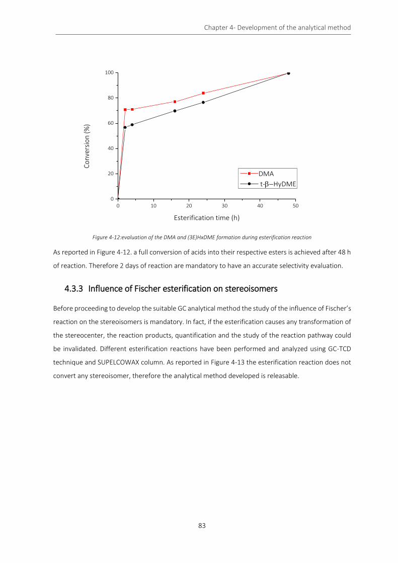
Chapter 4- Development of the analytical method
83
0 10 20 30 40 50
0
20
40
60
80
100
Co
nve
rsio
n (
%)
Esterification time (h)
DMA
t-HyDME
Figure 4-12:evaluation of the DMA and (3E)HxDME formation during esterification reaction
As reported in Figure 4-12. a full conversion of acids into their respective esters is achieved after 48 h
of reaction. Therefore 2 days of reaction are mandatory to have an accurate selectivity evaluation.
4.3.3 Influence of Fischer esterification on stereoisomers
Before proceeding to develop the suitable GC analytical method the study of the influence of Fischer’s
reaction on the stereoisomers is mandatory. In fact, if the esterification causes any transformation of
the stereocenter, the reaction products, quantification and the study of the reaction pathway could
be invalidated. Different esterification reactions have been performed and analyzed using GC-TCD
technique and SUPELCOWAX column. As reported in Figure 4-13 the esterification reaction does not
convert any stereoisomer, therefore the analytical method developed is releasable.
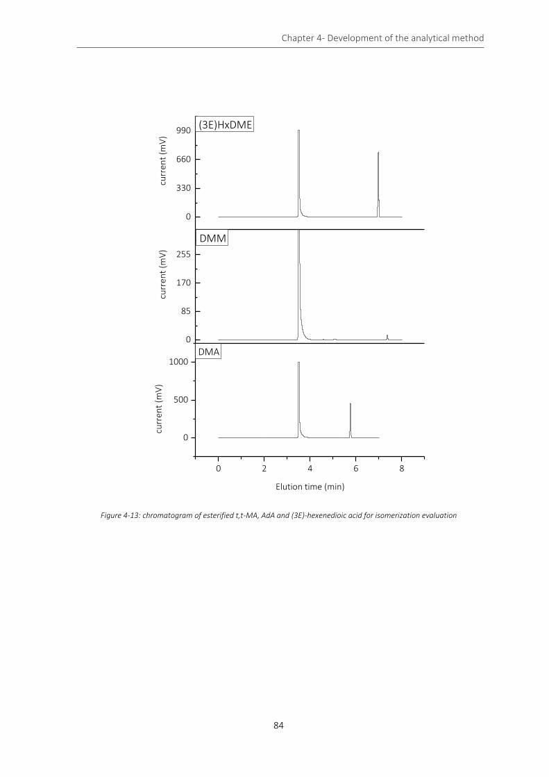
Chapter 4- Development of the analytical method
84
Figure 4-13: chromatogram of esterified t,t-MA, AdA and (3E)-hexenedioic acid for isomerization evaluation
0 2 4 6 8
0
500
1000
0
85
170
255
0
330
660
990
Elution time (min)
DMA
curr
ent
(mV
)cu
rren
t (m
V)
DMM
curr
ent
(mV
)
(3E)HxDME
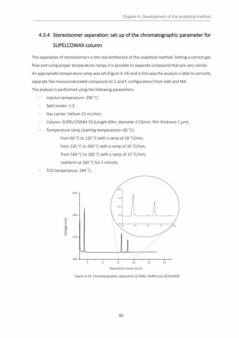
Chapter 4- Development of the analytical method
85
4.3.4 Stereoisomer separation: set up of the chromatographic parameter for
SUPELCOWAX column
The separation of stereoisomers is the real bottleneck of this analytical method. Setting a correct gas
flow and using proper temperature ramps it is possible to separate compound that are very similar.
An appropriate temperature ramp was set (Figure 4-14) and in this way the analysis is able to correctly
separate the monounsaturated compound (in Z and E configuration) from AdA and MA.
The analysis is performed using the following parameters:
- Injector temperature: 290 °C;
- Split mode= 1:3;
- Gas carrier: Helium 15 mL/min;
- Column: SUPELCOWAX 10 (Length 60m; diameter 0.53mm; film thickness 1 μm);
- Temperature ramp (starting temperature= 60 °C):
from 60 °C to 120 °C with a ramp of 18 °C/min;
from 120 °C to 160 °C with a ramp of 20 °C/min;
from 160 °C to 260 °C with a ramp of 15 °C/min;
isotherm at 260 °C for 1 minute;
- TCD temperature: 240 °C.
4 6 8 10 12 14
540
570
600
630
Volta
ge (m
V)
Retention time (min)
8.0 8.5 9.0 9.5 10.0540
550
560
570
580
Figure 4-14: chromatographic separation of DMA, DMM and (3E)HxDME
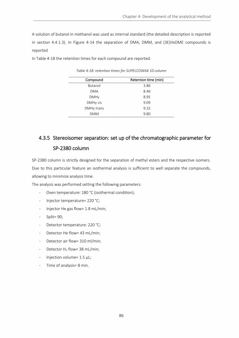
Chapter 4- Development of the analytical method
86
A solution of butanol in methanol was used as internal standard (the detailed description is reported
in section 4.4.1.3). In Figure 4-14 the separation of DMA, DMM, and (3E)HxDME compounds is
reported
In Table 4-18 the retention times for each compound are reported.
Table 4-18: retention times for SUPELCOWAX 10 column
Compound Retention time (min)
Butanol 3.86
DMA 8.46
DMHy 8.95
DMHy cis 9.09
DMHy trans 9.32
DMM 9.80
4.3.5 Stereoisomer separation: set up of the chromatographic parameter for
SP-2380 column
SP-2380 column is strictly designed for the separation of methyl esters and the respective isomers.
Due to this particular feature an isothermal analysis is sufficient to well separate the compounds,
allowing to minimize analysis time.
The analysis was performed setting the following parameters:
- Oven temperature: 180 °C (isothermal condition);
- Injector temperature= 220 °C;
- Injector He gas flow= 1.8 mL/min;
- Split= 90;
- Detector temperature: 220 °C;
- Detector He flow= 43 mL/min;
- Detector air flow= 310 ml/min;
- Detector H2 flow= 38 mL/min;
- Injection volume= 1.5 µL;
- Time of analysis= 8 min.
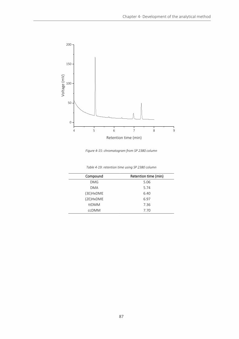
Chapter 4- Development of the analytical method
87
4 5 6 7 8 9
0
50
100
150
200
Vo
ltag
e (m
V)
Retention time (min)
Figure 4-15: chromatogram from SP 2380 column
Table 4-19: retention time using SP 2380 column
Compound Retention time (min)
DMG 5.06
DMA 5.74
(3E)HxDME 6.40
(2E)HxDME 6.97
ttDMM 7.36
ccDMM 7.70
Chapter 4- Development of the analytical method
88
4.3.6 Material balance
An analytical method can be considered robust and valid if all the operative steps and the analyses
are sufficiently accurate, and if it remains unaffected by small, but deliberate variations in method
parameters. In this sense the material balance can help to establish if all the steps performed before
analyzing the sample, and the results of the analyses are adequately precise for this kind of evaluation.
In the following table an example of material balance is reported. The material balance was performed
on two different reactions and at different reaction time.
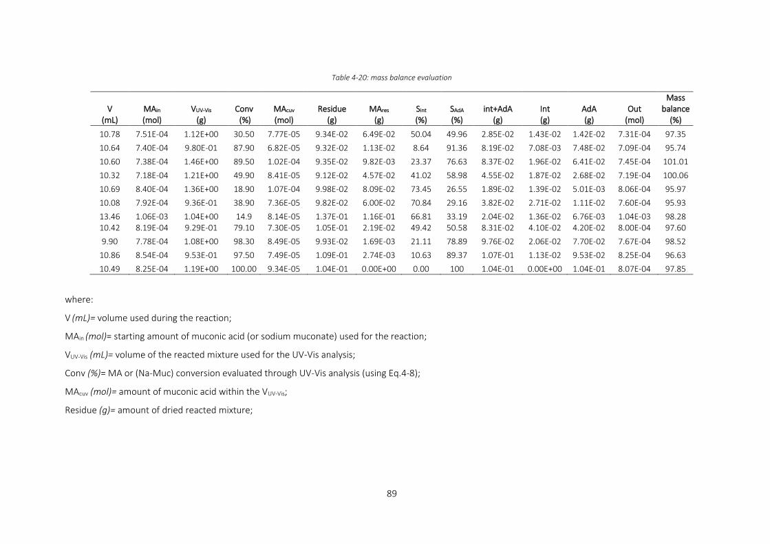
89
Table 4-20: mass balance evaluation
V (mL)
MAin (mol)
VUV-Vis
(g) Conv (%)
MAcuv (mol)
Residue (g)
MAres
(g) Sint (%)
SAdA (%)
int+AdA (g)
Int (g)
AdA (g)
Out (mol)
Mass balance
(%)
10.78 7.51E-04 1.12E+00 30.50 7.77E-05 9.34E-02 6.49E-02 50.04 49.96 2.85E-02 1.43E-02 1.42E-02 7.31E-04 97.35
10.64 7.40E-04 9.80E-01 87.90 6.82E-05 9.32E-02 1.13E-02 8.64 91.36 8.19E-02 7.08E-03 7.48E-02 7.09E-04 95.74
10.60 7.38E-04 1.46E+00 89.50 1.02E-04 9.35E-02 9.82E-03 23.37 76.63 8.37E-02 1.96E-02 6.41E-02 7.45E-04 101.01
10.32 7.18E-04 1.21E+00 49.90 8.41E-05 9.12E-02 4.57E-02 41.02 58.98 4.55E-02 1.87E-02 2.68E-02 7.19E-04 100.06
10.69 8.40E-04 1.36E+00 18.90 1.07E-04 9.98E-02 8.09E-02 73.45 26.55 1.89E-02 1.39E-02 5.01E-03 8.06E-04 95.97
10.08 7.92E-04 9.36E-01 38.90 7.36E-05 9.82E-02 6.00E-02 70.84 29.16 3.82E-02 2.71E-02 1.11E-02 7.60E-04 95.93
13.46 1.06E-03 1.04E+00 14.9 8.14E-05 1.37E-01 1.16E-01 66.81 33.19 2.04E-02 1.36E-02 6.76E-03 1.04E-03 98.28 10.42 8.19E-04 9.29E-01 79.10 7.30E-05 1.05E-01 2.19E-02 49.42 50.58 8.31E-02 4.10E-02 4.20E-02 8.00E-04 97.60
9.90 7.78E-04 1.08E+00 98.30 8.49E-05 9.93E-02 1.69E-03 21.11 78.89 9.76E-02 2.06E-02 7.70E-02 7.67E-04 98.52
10.86 8.54E-04 9.53E-01 97.50 7.49E-05 1.09E-01 2.74E-03 10.63 89.37 1.07E-01 1.13E-02 9.53E-02 8.25E-04 96.63
10.49 8.25E-04 1.19E+00 100.00 9.34E-05 1.04E-01 0.00E+00 0.00 100 1.04E-01 0.00E+00 1.04E-01 8.07E-04 97.85
where:
V (mL)= volume used during the reaction;
MAin (mol)= starting amount of muconic acid (or sodium muconate) used for the reaction;
VUV-Vis (mL)= volume of the reacted mixture used for the UV-Vis analysis;
Conv (%)= MA or (Na-Muc) conversion evaluated through UV-Vis analysis (using Eq.4-8);
MAcuv (mol)= amount of muconic acid within the VUV-Vis;
Residue (g)= amount of dried reacted mixture;
Chapter 4- Development of the analytical method
90
MAres (g)= amount of MA (or sodium muconate) in the residue;
Sint (%)= selectivity towards the intermediates evaluated through GC analysis;
SAdA (%)= selectivity towards AdA evaluated through GC analysis;
Int+AdA (g)= sum of the amount of intermediates and AdA;
Int (g)= amount of intermediates in the reaction products;
AdA (g)= amount of intermediates in the reaction products;
Out (g)= is the sum of the total number of moles in the products;
Balance (%)= mass balance.
The equations used to calculate the mass balance (%) are reported below.
𝑀𝐴𝑖𝑛(𝑚𝑜𝑙) =𝑉 (𝑚𝐿)
1000 (𝑚𝑙𝐿
)∙ 𝐶𝑀𝐴(
𝑚𝑜𝑙
𝐿)
(Eq.4-16)
𝑀𝐴𝑐𝑢𝑣 (𝑚𝑜𝑙) = 𝑉𝑈𝑉−𝑉𝑖𝑠 ∙ 𝑀𝐴𝑖𝑛
𝑉𝑡𝑜𝑡
(Eq.4-17)
𝑀𝐴𝑟𝑒𝑠(𝑔) = 𝑟𝑒𝑠𝑖𝑑𝑢𝑒 ∙ (1 −𝐶𝑜𝑛𝑣 (%)
100)
(Eq.4-18)
𝑖𝑛𝑡 + 𝐴𝑑𝐴 (𝑔) = 𝑟𝑒𝑠𝑖𝑑𝑢𝑒 − 𝑀𝐴𝑟𝑒𝑠 (Eq.4-19)
𝐼𝑛𝑡 (𝑔) = (𝑖𝑛𝑡 + 𝐴𝑑𝐴) ∙𝑆𝑖𝑛𝑡
100
(Eq.4-20)
𝐴𝑑𝐴 (𝑔) = (𝑖𝑛𝑡 + 𝐴𝑑𝐴) ∙𝑆𝐴𝑑𝐴
100
(Eq.4-21)
𝑂𝑢𝑡 (𝑚𝑜𝑙) = 𝑀𝐴𝑟𝑒𝑠
𝑀𝑊𝑀𝐴
+𝐼𝑛𝑡
𝑀𝑊𝑖𝑛𝑡
+ 𝐴𝑑𝐴
𝑀𝑊𝐴𝑑𝐴
+ 𝑀𝐴𝑐𝑢𝑣 (Eq.4-22)
𝐵𝑎𝑙𝑎𝑛𝑐𝑒 (%) = 𝑜𝑢𝑡
𝑀𝐴𝑖𝑛
∙ 100 (Eq.4-23)
As reported in Table 4-20 the Mass balance is always between 96 and 101%, therefore, the developed
method can be considered valid and robust.

Chapter 4- Development of the analytical method
91
Conclusion
A robust analytical method was developed to evaluate the conversion of MA and the selectivity
towards the different reaction intermediates.
In particular, MA (or sodium muconate) conversion was evaluated using UV-Vis analysis due to the
low solubility of dimethyl muconate in MeOH at room temperature. Different calibrations curves were
performed changing solvent and substrate.
The selectivity was evaluated by GC analysis after a derivatization of reaction products. In fact, even
if carboxylic acid can be separated and revealed during gas chromatographic analyses, the response
of the instrument toward these compounds is not linear and reproducible. A Fischer’s esterification
reaction was then performed and optimized allowing a good selectivity evaluation. Different
calibrations were performed, and two different gas chromatographic columns were used during the
period of the project. The developed gas chromatographic method is able to separate AdA from
monounsaturated intermediates and MA, and it is also able to separate the different stereo isomers.
This allows to achieve a detailed study on the reaction pathway and the development of a regression
model.
Using SUPELCOWAX 10 column a temperature ramp and TCD detector are mandatory to reach
suitable results. Instead, using SP-2380 column an isothermal analysis and FID detector are sufficient
to separate all the reaction products and reveal them. Finally, the mass balance range between 96
and 101% suggest that the developed analytical method is sufficiently robust.

Chapter 4- Bibliography
92
Bibliography
1. Vardon, D. R. et al. Adipic acid production from lignin. Energy Environ. Sci. 8, 617–628 (2015).
2. She, X., Brown, H. M., Zhang, X., Ahring, B. K. & Wang, Y. Selective hydrogenation of trans,trans-muconic acid to adipic acid over a titania-supported rhenium catalyst. ChemSusChem 4, 1071–1073 (2011).
3. Skoog, D. A., Holler, F. J. & Crouch, S. R. Principles of Instrumental Analysis. (Thomson Brooks/Cole, 2007).
4. Buijs, K. & Maurice, M. J. Some considerations on apparent deviations from lambert-beer’s law. Anal. Chim. Acta 47, 469–474 (1969).

93
Chapter 5
Muconic acid hydrogenation using
commercial Pt and Pd catalysts
This chapter describes the results obtained using commercial Pt and Pd catalyst supported on
activated carbon. Initially, two different reactors were designed allowing to explore different range of
hydrogen pressure. We decided to use a stainless-steel autoclave (with a working volume of 10 mL)
for high pressurized reactions while a glass reactor (with a working volume of 100 mL) was used for
atmospheric hydrogenation at low temperature (allowing to increase the volume of the solution used
during the reaction).
Moreover, an optimization of initial operating parameters was performed as well as the check of the
kinetic and diffusional regime.
Finally, recycling tests and catalyst characterization pre and post used was performed to understand
the reaction mechanism and how the catalyst works during the reaction. A part of the chapter was
published on Applied Catalysis B Journal (DOI: 10.1016/j.apcatb.2017.06.060).

Chapter 5- Muconic acid hydrogenation using commercial Pt and Pd catalysts
94
5.1 Overview on heterogeneous catalyzed hydrogenation reaction
Heterogeneous catalysts are preferable to homogenous counterparts for industrial application due to
the facility of the recovering from the reaction mixture.1 In fact, in these types of reactions the catalyst
and the reagents exist in two different phases, so a simple filtration can be often performed to
separate liquid products from the catalyst.2
The properties required for an industrial heterogeneous catalyst are:
high activity and selectivity: they depend on the choice of the metal and the support, the
amount of the metal anchored on the support;
fast filtration rate;
recycle capability;
high stability.
Activity and selectivity are greatly dependent on the choice of metal. This influences the strength of
adsorption of reactants, the rate of desorption of reaction products and the rate of chemical reactions.
The most frequently used metals for heterogeneous catalytic hydrogenation are palladium, platinum,
rhodium, nickel, cobalt and ruthenium.3 Heterogeneous catalyst may be supported or unsupported,
the former directly uses the active phase in the reaction media, while in the latter the metallic active
phase is anchored to a support (i.e. carbon, metal oxides…). Examples of unsupported catalysts
include cobalt and Raney nickel. These are made by chemically dissolving the aluminum out of nickel-
aluminum or cobalt-aluminum alloys and they are used for the reduction of nitriles, oximes and
carbonyl functions. On the contrary in the supported catalysts, the metal is deposited on an inert (or
not) material such as carbon, graphite, alumina or inorganic salts. For example, supported Pd catalysts
are used for the reduction of carbon-carbon multiple bonds, multiple bond isomerization and
hydrogenolysis while supported Pt is used for carbon-carbon and carbon-heteroatom double bonds.4
Supported catalysts present advantages such as easy separation from the reaction medium and more
effective use of the metal surface, as the metal is generally deposited as nanoparticles (between 1 to
10 nm in diameter). Its interaction with the support can also influence the properties of the catalyst,
as well as providing stabilization against particle conglomeration/sintering.5 The metal may be present
in oxidic or reduced form, depending on the method of catalyst preparation. Oxidic type catalysts are
reduced in situ to reach the metal 0 oxidation state and therefore frequently show an induction
period.6

Chapter 5- Muconic acid hydrogenation using commercial Pt and Pd catalysts
95
A peculiar feature of Pt and Pd is that they are active under very mild pressure and temperature
conditions.7 Therefore, they are often used in the liquid-phase hydrogenation reaction at room
temperature and atmospheric, or only slightly, pressure of hydrogen.8
The use of high reaction temperatures and pressure is generally favorable for increasing the reaction
rate, but in case of reaction that involves different phases (such as a gas and a liquid) elevated
temperatures mean lower gas solubility (Henry’s law). Therefore, in the case of hydrogenation
reaction, a compromise between pressure and temperature must be considered. The amounts of
catalyst to be used may also be reduced under these conditions, unless the catalyst is deactivated, as
is often the case with unsupported platinum metals.
Hydrogenation reactions under mild conditions are advantageous to study the conversion and thus
achieve selective hydrogenation. For fast hydrogenations, care must be taken to guarantee that the
reaction does not occur too violently, particularly in a large-scale hydrogenation. Therefore, an
accurate study about the optimization of the amount of catalyst, the hydrogen pressure and the
reaction temperature must be performed.
Heterogeneous catalytic hydrogenations reactions can be divided in three main groups depending on
the hydrogen source.9
- Ex-situ hydrogen sources
In these kind of reactions, the hydrogen is supplied from an external source (such as a cylinder) or is
produced within the plant and then fed using proper gas lines.
- Hydrogen transfer reaction
Hydrogen can be extracted ("transferred") from "hydrogen-donors" instead of H2 gas. Hydrogen
donors, which often serve as solvents include hydrazine, dihydronaphthalene, dihydroanthracene,
isopropanol, and formic acid.10
Transfer hydrogenation is useful for the asymmetric reduction of ketones, aldehydes, and imines.
Non-noble metal catalyst can be used in this reaction such as molybdenum oxide, super acid catalyst,
zeolites, acid resins…
- Electrochemical reaction
Electrochemical hydrogenation and hydrogenolysis (ECH) does not require external hydrogen source
and offers a sustainable way to produce chemicals at room temperature and pressure when matching
with renewable electricity sources. Bio-based chemicals can be produced in isolated locations where
hydrogen is not readily available. Another advantage of electrochemical reactions is that the reaction
on the electrocatalyst can be controlled by current or potential changes.11
Chapter 5- Muconic acid hydrogenation using commercial Pt and Pd catalysts
96
5.1.1 Hydrogenation equipment
Nowadays bench chemist has three main different choices of hydrogenation equipment:
- Batch reactor under atmospheric conditions
Batch reactor under atmospheric condition is the simplest and common configuration used in
teaching laboratories. This process is commonly performed by adding solid catalyst to a round bottom
flask (or a jacket glass reactor) of dissolved reactant. The hydrogen gas is then supplied from a H2
cylinder after an evacuation using helium. The resulting three phases mixture is stirred to promote
mixing.
- Batch reactor at high temperature and/or pressure
Pressurized system is widely used in hydrogenation of aromatic system or hydrogenolysis reactions.
In these cases, catalyst is added to a solution of reactant under an inert atmosphere in an autoclave.
Hydrogen is added directly from a cylinder. Heat may also be used, as the pressure compensates for
the associated reduction in gas solubility.
- Flow reactor
Flow hydrogenation is used to increase the process scale. This technique involves a continuous flowing
of dissolved reactant over a fixed bed catalyst in the presence of hydrogen. This technique allows to
reach high pressure (100 bar) and temperature.
- Industrial reactor
Catalytic hydrogenation is performed in tubular plug-flow reactor (PFR) packed with a supported
catalyst. Temperature and pressure can be high, although this depends on the catalyst. Catalyst
loading is typically much lower than in laboratory batch hydrogenation. Usually various promoters are
added to the metal to improve activity, selectivity and stability.
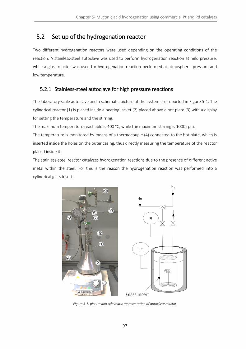
Chapter 5- Muconic acid hydrogenation using commercial Pt and Pd catalysts
97
5.2 Set up of the hydrogenation reactor
Two different hydrogenation reactors were used depending on the operating conditions of the
reaction. A stainless-steel autoclave was used to perform hydrogenation reaction at mild pressure,
while a glass reactor was used for hydrogenation reaction performed at atmospheric pressure and
low temperature.
5.2.1 Stainless-steel autoclave for high pressure reactions
The laboratory scale autoclave and a schematic picture of the system are reported in Figure 5-1. The
cylindrical reactor (1) is placed inside a heating jacket (2) placed above a hot plate (3) with a display
for setting the temperature and the stirring.
The maximum temperature reachable is 400 °C, while the maximum stirring is 1000 rpm.
The temperature is monitored by means of a thermocouple (4) connected to the hot plate, which is
inserted inside the holes on the outer casing, thus directly measuring the temperature of the reactor
placed inside it.
The stainless-steel reactor catalyzes hydrogenation reactions due to the presence of different active
metal within the steel. For this is the reason the hydrogenation reaction was performed into a
cylindrical glass insert.
PI
He
H2
TC
Glass insert
Figure 5-1: picture and schematic representation of autoclave reactor
Chapter 5- Muconic acid hydrogenation using commercial Pt and Pd catalysts
98
On the head of the reactor there are two conduits, both of which have a Teflon ring at the base.
The right-hand duct has an "open and close" valve (5) through which the reagent mixture is injected
using a syringe. The left duct has a pressure gauge (6) for measuring the pressure; this instrument has
a sensitivity of 0.4 bar and a maximum measurement fixed at 10 bar.
Another "open and close" valve (7) is positioned for the gas intake into the reactor. A three-way valve
(8) above the previous one has the function of switching the helium and hydrogen flow inside the
reactor. Helium is used both for inerting and quenching the reaction. In the picture two other valves
are reported: one with a pin (9) and the other "open and close" (10); they are safety valves which can
be respectively used to introduce and remove hydrogen.
The plant can not work in continuous for practical reasons, so each point of the kinetics is obtained
by performing a new test in the same operating conditions by varying only the reaction time.
5.2.1.1 Pre-treatment of the catalyst
The hydrogenation reaction requires a well-activated catalyst, so the noble metal that catalyzes the
reaction must not be in oxidized form and therefore a pretreatment reduction is mandatory.
An amount of known catalyst of about 100 mg was charged inside the glass insert, equipped with a
magnetic stirrer, which was placed inside the reactor.
Once the reactor was closed, a switch on in the reaction environment is started: 4/5 cycles of loading
and removal of hydrogen were then performed to ensure complete reducing environment. Once
completed, the activation step was performed: hydrogen fully charges the reactor at the desired
pressure (6 bar) and at the reduction temperature of 200 °C (obtained from TPR analyses described
in the following paragraph) for 3 hours.
In any case, the catalyst is placed on the bottom of the reactor, therefore it reaches the set
temperature. Once the catalyst activation phase was completed, the reactor was cooled to room
temperature.
5.2.1.2 Temperature programmed reduction (TPR)
TPD/R/O 1100 ThermoQuest Instruments was used for TPR study. An amount 40 mg of catalyst was
dried in oven and then analyzed. The sample was pre-treated with argon flow from room temperature
to 200 °C with a temperature ramp of 30 °C·min-1 and maintained at this temperature for 60 min. The
analysis was then conducted from 50 °C to 900 °C at 8 °C·min-1 at 1 bar. The gaseous mixture was
5.04% of hydrogen in argon and it was fluxed within the instrument at 14 mL·min-1.
The peaks in Figure 5-2 correspond to the material's reduction temperatures.

Chapter 5- Muconic acid hydrogenation using commercial Pt and Pd catalysts
99
The peak at 200-210 °C can be correlated to the platinum reduction temperature, so it was used in
the pre-treatment step to make it active in the reduction of muconic acid to AdA. The second peak is
due to the reduction-degradation of carbon; in fact, it is almost superimposable to the peak of pure
carbon (red line). The shift is probably caused by platinum interactions. The TPR profile shows that
the catalyst needs an activation at 200 °C. The chosen pressure (6 bar) is higher than that used during
TPR analysis in order to guarantee a complete activation.
Three hours are a reasonable time to be sure to have a total activation of the catalyst.
A well activated catalyst is a positive starting point to obtain good results.
0 100 200 300 400 500 600 700 8000
200
400
600
800
1000
1200
1400
Det
ecto
r (m
V)
Temperature (°C)
Pt/AC 5%
AC
5.2.1.3 Hydrogenation reaction of muconic acid
A known amount of about 10 g of reagent solution was weighed and loaded with a syringe by opening
the valve 5 and inserting the needle inside the right duct. This operation was mandatory for different
reasons: to prevent the spreading of the solution, to avoid catalyst re-oxidation and to prevent catalyst
burning due to the presence of carbon support that is extremely pyrophoric. Once the solution has
been charged inside the reactor, hydrogen cycles were carried out to eliminate each other gasses in
the reaction environment. Then hydrogen is charged to the desired pressure (1-4 bar), and the stirring
rate (700-1200 rpm) and temperature (40-70 °C) were set. Once the kinetic test was complete, the
heating was switched off and the hydrogen was discharged by opening the valve 10 and venting the
hydrogen outside. To be sure of having removed the hydrogen, quenching was carried out with
Figure 5-2: TPR analysis of the commercial Pt/C 5% (black line) and carbon support (red line)
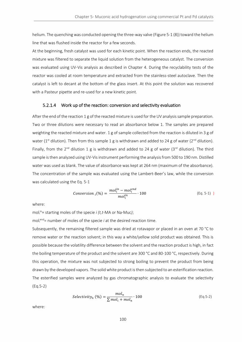
Chapter 5- Muconic acid hydrogenation using commercial Pt and Pd catalysts
100
helium. The quenching was conducted opening the three-way valve (Figure 5-1 (8)) toward the helium
line that was flushed inside the reactor for a few seconds.
At the beginning, fresh catalyst was used for each kinetic point. When the reaction ends, the reacted
mixture was filtered to separate the liquid solution from the heterogeneous catalyst. The conversion
was evaluated using UV-Vis analysis as described in Chapter 4. During the recyclability tests of the
reactor was cooled at room temperature and extracted from the stainless-steel autoclave. Then the
catalyst is left to decant at the bottom of the glass insert. At this point the solution was recovered
with a Pasteur pipette and re-used for a new kinetic point.
5.2.1.4 Work up of the reaction: conversion and selectivity evaluation
After the end of the reaction 1 g of the reacted mixture is used for the UV analysis sample preparation.
Two or three dilutions were necessary to read an absorbance below 1. The samples are prepared
weighting the reacted mixture and water. 1 g of sample collected from the reaction is diluted in 3 g of
water (1st dilution). Then from this sample 1 g is withdrawn and added to 24 g of water (2nd dilution).
Finally, from the 2nd dilution 1 g is withdrawn and added to 24 g of water (3rd dilution). The third
sample is then analyzed using UV-Vis instrument performing the analysis from 500 to 190 nm. Distilled
water was used as blank. The value of absorbance was kept at 264 nm (maximum of the absorbance).
The concentration of the sample was evaluated using the Lambert-Beer’s law, while the conversion
was calculated using the Eq. 5-1
𝐶𝑜𝑛𝑣𝑒𝑟𝑠𝑖𝑜𝑛 𝑖(%) = 𝑚𝑜𝑙𝑖
𝑖𝑛 − 𝑚𝑜𝑙𝑖𝑒𝑛𝑑
𝑚𝑜𝑙𝑖𝑖𝑛
∙ 100 )
(Eq. 5-1)
where:
moliin= starting moles of the specie i (t,t-MA or Na-Muc);
moliend= number of moles of the specie i at the desired reaction time.
Subsequently, the remaining filtered sample was dried at rotavapor or placed in an oven at 70 °C to
remove water or the reaction solvent; in this way a white/yellow solid product was obtained. This is
possible because the volatility difference between the solvent and the reaction product is high, in fact
the boiling temperature of the product and the solvent are 300 °C and 80-100 °C, respectively. During
this operation, the mixture was not subjected to strong boiling to prevent the product from being
drawn by the developed vapors. The solid white product is then subjected to an esterification reaction.
The esterified samples were analyzed by gas chromatographic analysis to evaluate the selectivity
(Eq.5-2)
𝑆𝑒𝑙𝑒𝑐𝑡𝑖𝑣𝑖𝑡𝑦𝑛 (%) =𝑚𝑜𝑙𝑛
∑ 𝑚𝑜𝑙𝑖 + 𝑚𝑜𝑙𝑛
∙ 100 (Eq.5-2)
where:
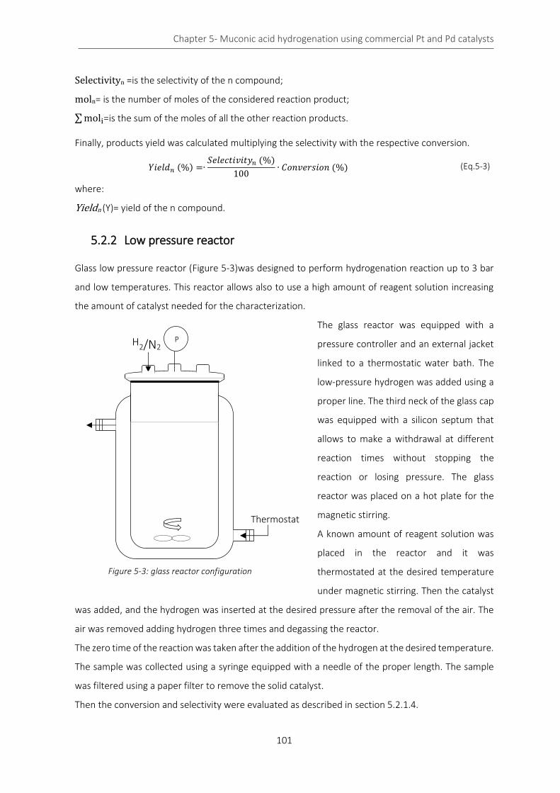
Chapter 5- Muconic acid hydrogenation using commercial Pt and Pd catalysts
101
Selectivityn =is the selectivity of the n compound;
moln= is the number of moles of the considered reaction product;
∑ moli=is the sum of the moles of all the other reaction products.
Finally, products yield was calculated multiplying the selectivity with the respective conversion.
𝑌𝑖𝑒𝑙𝑑𝑛 (%) =∙𝑆𝑒𝑙𝑒𝑐𝑡𝑖𝑣𝑖𝑡𝑦𝑛 (%)
100∙ 𝐶𝑜𝑛𝑣𝑒𝑟𝑠𝑖𝑜𝑛 (%) (Eq.5-3)
where:
Yieldn (Y)= yield of the n compound.
5.2.2 Low pressure reactor
Glass low pressure reactor (Figure 5-3)was designed to perform hydrogenation reaction up to 3 bar
and low temperatures. This reactor allows also to use a high amount of reagent solution increasing
the amount of catalyst needed for the characterization.
The glass reactor was equipped with a
pressure controller and an external jacket
linked to a thermostatic water bath. The
low-pressure hydrogen was added using a
proper line. The third neck of the glass cap
was equipped with a silicon septum that
allows to make a withdrawal at different
reaction times without stopping the
reaction or losing pressure. The glass
reactor was placed on a hot plate for the
magnetic stirring.
A known amount of reagent solution was
placed in the reactor and it was
thermostated at the desired temperature
under magnetic stirring. Then the catalyst
was added, and the hydrogen was inserted at the desired pressure after the removal of the air. The
air was removed adding hydrogen three times and degassing the reactor.
The zero time of the reaction was taken after the addition of the hydrogen at the desired temperature.
The sample was collected using a syringe equipped with a needle of the proper length. The sample
was filtered using a paper filter to remove the solid catalyst.
Then the conversion and selectivity were evaluated as described in section 5.2.1.4.
Thermostat
H2/N2
P
Figure 5-3: glass reactor configuration
Chapter 5- Muconic acid hydrogenation using commercial Pt and Pd catalysts
102
5.3 Evaluation of the starting operating parameters
Whenever a new reactor is designed, and a new reaction is performed, it is more advisable to select
suitable starting operating parameter to avoid mass transfer limitation or to use high pressure (that is
not suitable when pure hydrogen is used).
5.3.1 Hydrogen solubility in water in function of pressure and temperature
One of the most important parameter involved in hydrogenation reaction is hydrogen pressure. The
solubility of hydrogen in water strictly depends on pressure and temperature. Starting from a study
of Sander12 hydrogen concentration in water was evaluated at mild pressure and temperature. The
results of the study are reported in Table 5-1 and Figure 5-4.
Henry’s constant in function of temperature (T (K)) was calculated using Eq.5-4 in accordance with
Sander’s work.
𝐻(𝑇) = 𝐻𝑟𝑒𝑓 ∙ 𝑒[
𝑑𝐻
𝑑(1𝑇
)∙(
1𝑇
−1
𝑇𝑟𝑒𝑓)]
(Eq.5-4)
𝐶𝐻2(
𝑚𝑜𝑙
𝐿) = 𝐻(𝑇) ∙ 𝑃(𝑏𝑎𝑟) (Eq.5-5)
where:
H(T)= Henry’s constant at temperature T (expressed in Kelvin);
Href= Henry’s constant at 298.15 K;
dH/(d(1/T))= 530;12
Tref= 298.15 K;
P (bar)= considered pressure;
CH2 (mol/L)= hydrogen molar concentration in water.

Chapter 5- Muconic acid hydrogenation using commercial Pt and Pd catalysts
103
Table 5-1: hydrogen concentration in function of temperature and pressure evaluated with Henry’s Law
T [K] 298.15 303.15 308.15 313.15 318.15 323.15 328.15 333.15 338.15 343.15 348.15
H(T) 7.80E-04 7.57E-04 7.36E-04 7.16E-04 6.98E-04 6.80E-04 6.63E-04 6.47E-04 6.32E-04 6.18E-04 6.04E-04
P (bar) Hydrogen concentration in water (mol/L)
1 7.80E-04 7.57E-04 7.36E-04 7.16E-04 6.98E-04 6.80E-04 6.63E-04 6.47E-04 6.32E-04 6.18E-04 6.04E-04
1.2 9.36E-04 9.09E-04 8.84E-04 8.60E-04 8.37E-04 8.16E-04 7.96E-04 7.77E-04 7.58E-04 7.41E-04 7.25E-04
1.4 1.09E-03 1.06E-03 1.03E-03 1.00E-03 9.77E-04 9.52E-04 9.28E-04 9.06E-04 8.85E-04 8.65E-04 8.46E-04
1.6 1.25E-03 1.21E-03 1.18E-03 1.15E-03 1.12E-03 1.09E-03 1.06E-03 1.04E-03 1.01E-03 9.88E-04 9.67E-04
1.8 1.40E-03 1.36E-03 1.33E-03 1.29E-03 1.26E-03 1.22E-03 1.19E-03 1.16E-03 1.14E-03 1.11E-03 1.09E-03
2 1.56E-03 1.51E-03 1.47E-03 1.43E-03 1.40E-03 1.36E-03 1.33E-03 1.29E-03 1.26E-03 1.24E-03 1.21E-03
2.2 1.72E-03 1.67E-03 1.62E-03 1.58E-03 1.53E-03 1.50E-03 1.46E-03 1.42E-03 1.39E-03 1.36E-03 1.33E-03
2.4 1.87E-03 1.82E-03 1.77E-03 1.72E-03 1.67E-03 1.63E-03 1.59E-03 1.55E-03 1.52E-03 1.48E-03 1.45E-03
2.6 2.03E-03 1.97E-03 1.91E-03 1.86E-03 1.81E-03 1.77E-03 1.72E-03 1.68E-03 1.64E-03 1.61E-03 1.57E-03
2.8 2.18E-03 2.12E-03 2.06E-03 2.01E-03 1.95E-03 1.90E-03 1.86E-03 1.81E-03 1.77E-03 1.73E-03 1.69E-03
3 2.34E-03 2.27E-03 2.21E-03 2.15E-03 2.09E-03 2.04E-03 1.99E-03 1.94E-03 1.90E-03 1.85E-03 1.81E-03
3.2 2.50E-03 2.42E-03 2.36E-03 2.29E-03 2.23E-03 2.18E-03 2.12E-03 2.07E-03 2.02E-03 1.98E-03 1.93E-03
3.4 2.65E-03 2.58E-03 2.50E-03 2.44E-03 2.37E-03 2.31E-03 2.25E-03 2.20E-03 2.15E-03 2.10E-03 2.05E-03
3.6 2.81E-03 2.73E-03 2.65E-03 2.58E-03 2.51E-03 2.45E-03 2.39E-03 2.33E-03 2.28E-03 2.22E-03 2.18E-03
3.8 2.96E-03 2.88E-03 2.80E-03 2.72E-03 2.65E-03 2.58E-03 2.52E-03 2.46E-03 2.40E-03 2.35E-03 2.30E-03
4 3.12E-03 3.03E-03 2.95E-03 2.87E-03 2.79E-03 2.72E-03 2.65E-03 2.59E-03 2.53E-03 2.47E-03 2.42E-03
4.2 3.28E-03 3.18E-03 3.09E-03 3.01E-03 2.93E-03 2.86E-03 2.78E-03 2.72E-03 2.65E-03 2.59E-03 2.54E-03
4.4 3.43E-03 3.33E-03 3.24E-03 3.15E-03 3.07E-03 2.99E-03 2.92E-03 2.85E-03 2.78E-03 2.72E-03 2.66E-03
4.6 3.59E-03 3.48E-03 3.39E-03 3.30E-03 3.21E-03 3.13E-03 3.05E-03 2.98E-03 2.91E-03 2.84E-03 2.78E-03
4.8 3.74E-03 3.64E-03 3.53E-03 3.44E-03 3.35E-03 3.26E-03 3.18E-03 3.11E-03 3.03E-03 2.97E-03 2.90E-03
5 3.90E-03 3.79E-03 3.68E-03 3.58E-03 3.49E-03 3.40E-03 3.32E-03 3.24E-03 3.16E-03 3.09E-03 3.02E-03
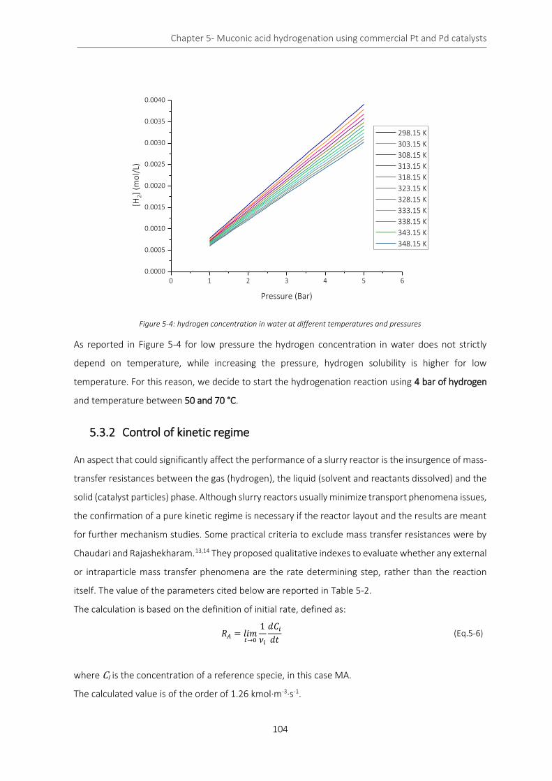
Chapter 5- Muconic acid hydrogenation using commercial Pt and Pd catalysts
104
0 1 2 3 4 5 6
0.0000
0.0005
0.0010
0.0015
0.0020
0.0025
0.0030
0.0035
0.0040
[H
2]
(mo
l/L)
Pressure (Bar)
298.15 K
303.15 K
308.15 K
313.15 K
318.15 K
323.15 K
328.15 K
333.15 K
338.15 K
343.15 K
348.15 K
Figure 5-4: hydrogen concentration in water at different temperatures and pressures
As reported in Figure 5-4 for low pressure the hydrogen concentration in water does not strictly
depend on temperature, while increasing the pressure, hydrogen solubility is higher for low
temperature. For this reason, we decide to start the hydrogenation reaction using 4 bar of hydrogen
and temperature between 50 and 70 °C.
5.3.2 Control of kinetic regime
An aspect that could significantly affect the performance of a slurry reactor is the insurgence of mass-
transfer resistances between the gas (hydrogen), the liquid (solvent and reactants dissolved) and the
solid (catalyst particles) phase. Although slurry reactors usually minimize transport phenomena issues,
the confirmation of a pure kinetic regime is necessary if the reactor layout and the results are meant
for further mechanism studies. Some practical criteria to exclude mass transfer resistances were by
Chaudari and Rajashekharam.13,14 They proposed qualitative indexes to evaluate whether any external
or intraparticle mass transfer phenomena are the rate determining step, rather than the reaction
itself. The value of the parameters cited below are reported in Table 5-2.
The calculation is based on the definition of initial rate, defined as:
𝑅𝐴 = 𝑙𝑖𝑚𝑡→0
1
𝜈𝑖
𝑑𝐶𝑖
𝑑𝑡 (Eq.5-6)
where Ci is the concentration of a reference specie, in this case MA.
The calculated value is of the order of 1.26 kmol∙m-3∙s-1.

Chapter 5- Muconic acid hydrogenation using commercial Pt and Pd catalysts
105
The contribution of gas-liquid mass transfer is evaluated by the index defined in Eq.5-7, which should
be lower than 0.1 to exclude its contribution to the overall kinetics.
𝛼1 =𝑅𝐴
𝑘𝑙𝑎𝐵𝐶𝐻2
∗ < 0.1 (Eq.5-7)
where:
klaB (s-1)= the overall mass transfer coefficient (gas side-film theory) for stirred reactors,
C*H2 (kmol·m-3) = the equilibrium concentration of hydrogen. Machado15,16 addressed the problem of
estimating the gas-liquid mass transfer coefficient for bench-scale stirred reactors.
The range of 0.05-0.5 s-1 was considered representative for the smaller hydrogenation reactors. Even
with the more conservative values, the system under study resulted in α1 values lower than 0.05. The
calculated value is 0.03 that is safely under the threshold to exclude gas-liquid resistance.
Liquid-liquid mass transfer limitation was excluded performing a series of hydrogenations under the
same conditions but varying the stirring speed from 250 to 700 rpm. The essays revealed that for
higher speed than 500 rpm the system is no more sensitive to stirring rate, hence no more liquid-
liquid transport is relevant on the overall kinetics Figure 5-5 the reactor can be considered a CSTR,
therefore the hydrogen concentration in liquid bulk is assumed constant.17
Liquid-solid mass transfer can be assessed by the index in equation 5-8.
𝛼2 =𝑅𝐴
𝑘𝑠𝑎𝑝𝐶𝐻2
∗ < 0.1 (Eq.5-8)
where:
ks (s-1) = the liquid-solid mass transfer coefficient;
ap (m2 ·m-3) = the interface area of liquid-solid boundary (external surface area of the catalyst per unit
volume.
The latter is defined by equation 5-9:
𝑎𝑝 =6𝑤
𝜌𝑝𝑑𝑝
(Eq.5-9)
Where:
w (kg·m-3) = the catalyst load;
ρP and dP (m)= particle density and diameter respectively.
Particles diameter was set using sieves and it was at about 40 µm (325 and 400 mesh –TYLER series)
The parameter ks is obtained using a literature correlation:18
𝑘𝑠𝑑𝑝
𝐷𝐻2𝐹𝑐
= 2 + 0.4 (𝑑𝑝
4𝜌𝑙3𝑒
𝜇𝑙3 )
0.25
(𝜇𝑙
𝜌𝑙𝐷𝐻2
)
0.33
(Eq.5-10)
where:

Chapter 5- Muconic acid hydrogenation using commercial Pt and Pd catalysts
106
𝐷𝐻2(m2·s-1) = the molecular diffusion of hydrogen in water;
Fc is a shape factor assumed to be 1 for spherical particles;
µl (P) and ρl (kg·m-3) = liquid viscosity and density respectively;
𝑒 = energy supplied to the liquid by the stirrer, given in equation 5-11
𝑒 =𝑁𝑝𝑛5𝑙5
𝑉
(Eq.5-11)
where:
Np = impeller power number;
l (m)= impeller diameter;
n (rps)= rotation speed.
The calculated value for α2 is 0.019, which allows excluding liquid-solid mass transfer limitations.
Finally, pore diffusion can be considered negligible if the parameter Φexp is lower than 0.2:
Φ 𝑒𝑥𝑝 = 𝑑𝑝 (𝜌𝑃𝑅𝐴
𝑤𝐷𝑒𝑐𝐻2
∗ )
0.5
< 0.2 (Eq.5-12)
where:
dp (m)= particle diameter;
w (kg·m-3) = catalyst load;
De =effective diffusivity calculated as
𝐷𝑒 =𝐷𝜀
𝜏
(Eq.5-13)
where:
= catalyst porosity;
= tortuosity factor.
The latter parameter is usually little characterized: it is a complex function of the type of charcoal, of
the adsorbed substrate, and the reaction medium, often regressed from indirect diffusion
measurements.19 Nonetheless, in carbon-supported platinum hydrogenation catalysts, the parameter
was estimated in the range between 3 and 7.20
The calculated φexp was lower than 0.04 even for the most conservative values of tortuosity in the
conditions of this study, allowing the exclusion of pore diffusion mass transfer.
In the case of Pt/AC 5% (Sigma Aldrich) the check on the mass transfer limitation was performed
applying the parameters reported in Table 5-2.
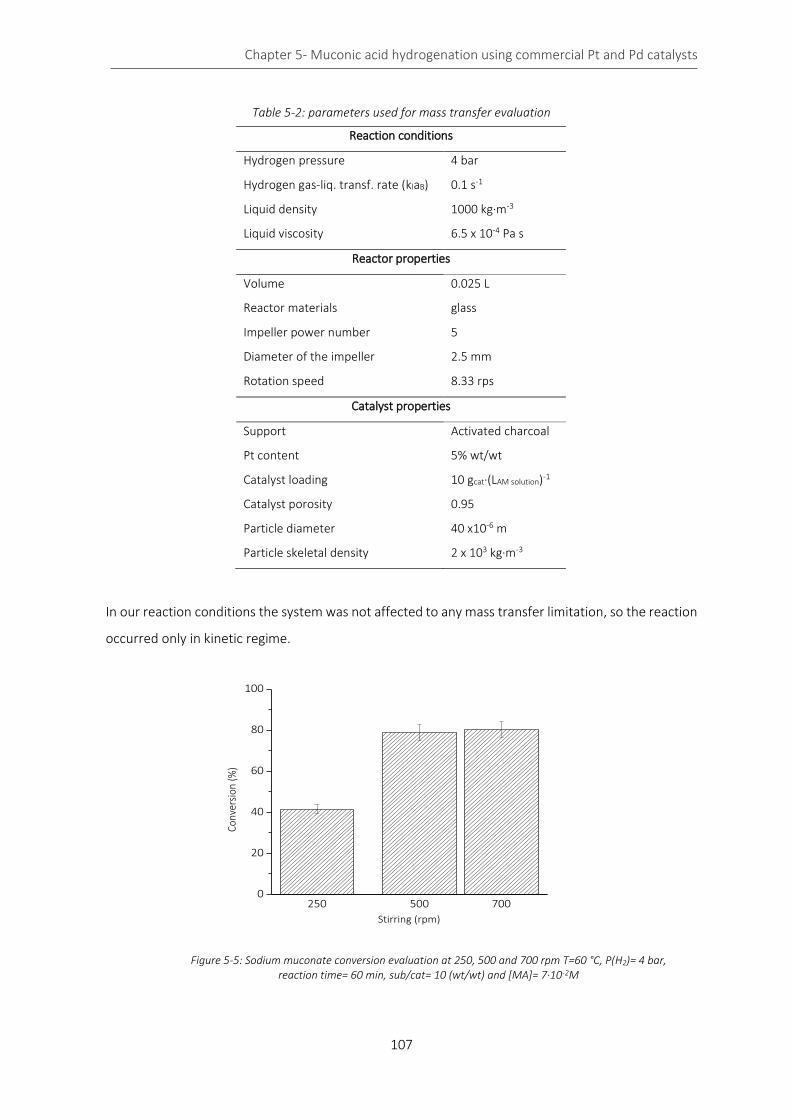
Chapter 5- Muconic acid hydrogenation using commercial Pt and Pd catalysts
107
Table 5-2: parameters used for mass transfer evaluation
In our reaction conditions the system was not affected to any mass transfer limitation, so the reaction
occurred only in kinetic regime.
250 500 7000
20
40
60
80
100
Conv
ersi
on (%
)
Stirring (rpm)
Reaction conditions
Hydrogen pressure 4 bar
Hydrogen gas-liq. transf. rate (klaB) 0.1 s-1
Liquid density 1000 kg·m-3
Liquid viscosity 6.5 x 10⁻⁴ Pa s
Reactor properties
Volume 0.025 L
Reactor materials glass
Impeller power number 5
Diameter of the impeller 2.5 mm
Rotation speed 8.33 rps
Catalyst properties
Support Activated charcoal
Pt content 5% wt/wt
Catalyst loading 10 gcat·(LAM solution)-1
Catalyst porosity 0.95
Particle diameter 40 x10-6 m
Particle skeletal density 2 x 10³ kg·m-3
Figure 5-5: Sodium muconate conversion evaluation at 250, 500 and 700 rpm T=60 °C, P(H2)= 4 bar, reaction time= 60 min, sub/cat= 10 (wt/wt) and [MA]= 7∙10-2M

Chapter 5- Muconic acid hydrogenation using commercial Pt and Pd catalysts
108
5.4 Pt/AC 5% commercial catalyst
5.4.1 t,t-MA hydrogenation in water
The first set of hydrogenation reaction was performed using Pt/AC 5% (Sigma Aldrich) on sodium
muconate solution. The catalyst was pre-treated at 200 °C for 3 h under 6 bar of static hydrogen. After
cooling, 10 mL of degassed muconate solution (0.07 M) were added to the reactor. The batch
hydrogenations were conducted at 50 °C, 60 °C and 70 °C at 2-4 bar of static hydrogen with a magnetic
stirring of 500 rpm up to 4 h.
Finally, experiments were performed at 70 °C, 4 bar of hydrogen and 500 rpm on cis,cis-muconic acid
using a synthetic salt solution which reproduces a clarified fermentation broth as the one of Niu et.al.21
This test considers the possibility to avoid a MA crystallization step before hydrogenation reaction,
preventing the solution acidification and the risk of MA isomerization. The synthetic fermentation
broth contained cis,cis-muconic acid (Sigma Aldrich) (28 g/L), Na2HPO4 (50 g/L), KH2PO4 (15 g/L), NaCl
(2.5 g/L) and NaOH (40 g/L).
After every reaction, the catalyst was removed by filtration and the solution analyzed as described in
paragraph 4.3.1. The filtrate was analyzed by ICP-OES to check a possible metal leaching.
5.4.2 Influence of pressure
Due to the influence of pressure on the hydrogen solubility in water, the impact of static hydrogen
pressure was studied to evaluate how conversion and yield are affected by it.
As reported in Figure 5-6 the conversion is slightly affected by the pressure, while the yield toward
adipic acid (YAdA) strongly depends on hydrogen pressure.
Figure 5-6: dependence of conversion and AdA yield on the hydrogen pressure at 70°C, cat/sub=200 (wt/wt), [Na-Muc]=7.56E-02 M
0 20 40 60 80 100 120 140 160 1800
20
40
60
80
100
YAd
A (
%)
Reaction time (min)
2 bar
4 bar
0 20 40 60 80 100 120 140 160 1800
20
40
60
80
100
Co
nve
rsio
n (
%)
Reaction time (min)
2 bar
4 bar
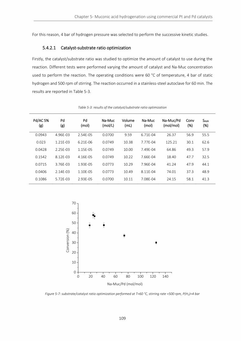
Chapter 5- Muconic acid hydrogenation using commercial Pt and Pd catalysts
109
For this reason, 4 bar of hydrogen pressure was selected to perform the successive kinetic studies.
5.4.2.1 Catalyst-substrate ratio optimization
Firstly, the catalyst/substrate ratio was studied to optimize the amount of catalyst to use during the
reaction. Different tests were performed varying the amount of catalyst and Na-Muc concentration
used to perform the reaction. The operating conditions were 60 °C of temperature, 4 bar of static
hydrogen and 500 rpm of stirring. The reaction occurred in a stainless-steel autoclave for 60 min. The
results are reported in Table 5-3.
Table 5-3: results of the catalyst/substrate ratio optimization
Pd/AC 5% (g)
Pd (g)
Pd (mol)
Na-Muc (mol/L)
Volume (mL)
Na-Muc (mol)
Na-Muc/Pd (mol/mol)
Conv (%)
SAdA
(%)
0.0943 4.96E-03 2.54E-05 0.0700 9.59 6.71E-04 26.37 56.9 55.5
0.023 1.21E-03 6.21E-06 0.0749 10.38 7.77E-04 125.21 30.1 62.6
0.0428 2.25E-03 1.15E-05 0.0749 10.00 7.49E-04 64.86 49.3 57.9
0.1542 8.12E-03 4.16E-05 0.0749 10.22 7.66E-04 18.40 47.7 32.5
0.0715 3.76E-03 1.93E-05 0.0773 10.29 7.96E-04 41.24 47.9 44.1
0.0406 2.14E-03 1.10E-05 0.0773 10.49 8.11E-04 74.01 37.3 48.9
0.1086 5.72E-03 2.93E-05 0.0700 10.11 7.08E-04 24.15 58.1 41.3
0 20 40 60 80 100 120 1400
10
20
30
40
50
60
70
Co
nve
rsio
n (
%)
Na-Muc/Pd (mol/mol)
Figure 5-7: substrate/catalyst ratio optimization performed at T=60 °C, stirring rate =500 rpm, P(H2)=4 bar

Chapter 5- Muconic acid hydrogenation using commercial Pt and Pd catalysts
110
5.4.2.2 Influence of temperature
Once the pressure and catalyst/substrate ratio were selected, different reactions were performed
varying the temperature. This parameter could affect the adsorption and desorption rate of the
species on the catalyst surface as well as the overall reaction rate. The results are reported in Figure
5-8. Na-Muc conversion is higher increasing the temperature. This behavior is common, a raise in the
temperature facilitates the reaction rate and the desorption and adsorption steps. Figure 5-9 shows
the yield and therefore the selectivity toward the monounsaturated compounds and AdA. For low
reaction time (2Z)HxAc is the predominant intermediates, while for long reaction time the two
0 20 40 60 80 100 120 140 160 180 2000
20
40
60
80
100
Co
nve
rsio
n (
%)
Reaction time (min)
70°C
50°C
60°C
0 20 40 60 80 100 120 140 160 180 2000
20
40
60
80
100
Co
nve
rsio
n (
%)
Reaction time (min)
50°C
0 20 40 60 80 100 120 140 160 180 2000
20
40
60
80
100C
on
ve
rsio
n (
%)
Reaction time (min)
60°C
0 20 40 60 80 100 120 140 160 180 2000
20
40
60
80
100
Co
nve
rsio
n (
%)
Reaction time (min)
70°C
Figure 5-8: conversion of Na-Muc at different temperatures. Stirring=500 rpm, P(H2)=4 bar, sub/cat=24 (molsub/molPd), [Na-Muc]=7·10-2M
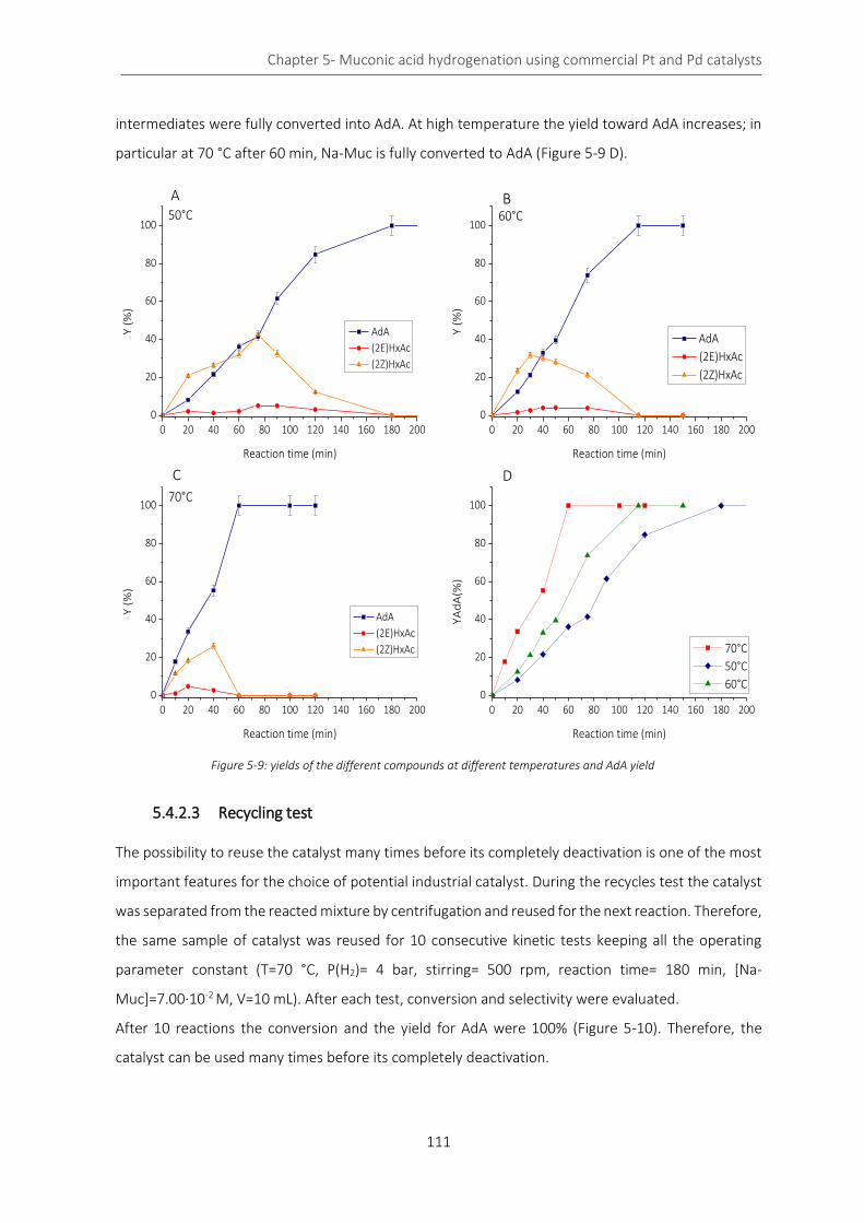
Chapter 5- Muconic acid hydrogenation using commercial Pt and Pd catalysts
111
intermediates were fully converted into AdA. At high temperature the yield toward AdA increases; in
particular at 70 °C after 60 min, Na-Muc is fully converted to AdA (Figure 5-9 D).
5.4.2.3 Recycling test
The possibility to reuse the catalyst many times before its completely deactivation is one of the most
important features for the choice of potential industrial catalyst. During the recycles test the catalyst
was separated from the reacted mixture by centrifugation and reused for the next reaction. Therefore,
the same sample of catalyst was reused for 10 consecutive kinetic tests keeping all the operating
parameter constant (T=70 °C, P(H2)= 4 bar, stirring= 500 rpm, reaction time= 180 min, [Na-
Muc]=7.00·10-2 M, V=10 mL). After each test, conversion and selectivity were evaluated.
After 10 reactions the conversion and the yield for AdA were 100% (Figure 5-10). Therefore, the
catalyst can be used many times before its completely deactivation.
0 20 40 60 80 100 120 140 160 180 2000
20
40
60
80
100
Y (
%)
Reaction time (min)
AdA
(2E)HxAc
(2Z)HxAc
70°C
0 20 40 60 80 100 120 140 160 180 2000
20
40
60
80
100
Y (
%)
Reaction time (min)
AdA
(2E)HxAc
(2Z)HxAc
60°C
0 20 40 60 80 100 120 140 160 180 2000
20
40
60
80
100
Y (
%)
Reaction time (min)
AdA
(2E)HxAc
(2Z)HxAc
50°C
0 20 40 60 80 100 120 140 160 180 2000
20
40
60
80
100
YA
dA
(%)
Reaction time (min)
70°C
50°C
60°C
Figure 5-9: yields of the different compounds at different temperatures and AdA yield
A B
C D

Chapter 5- Muconic acid hydrogenation using commercial Pt and Pd catalysts
112
1 2 3 4 5 6 7 8 9 100
20
40
60
80
100
(%)
Cycle (#)
Conversion
YAdA
Figure 5-10: results of the recycling test
5.4.3 Fresh and used catalyst characterization
5.4.3.1 Transmission electron microscopy coupled with Energy Dispersive X-ray
spectroscopy (TEM-EDX)
TEM images were obtained using Philips 208 Transmission Electron Microscope.
Figure 5-11: Characterization by TEM of A) fresh and B) used catalyst
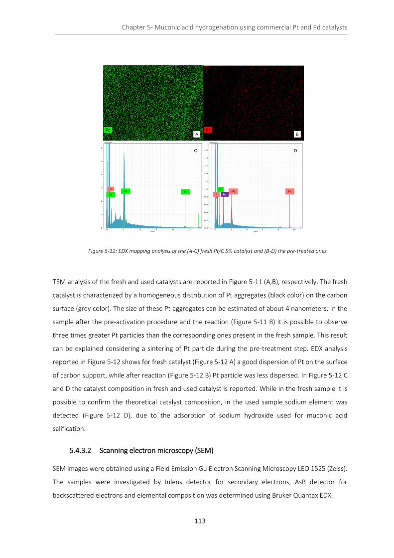
Chapter 5- Muconic acid hydrogenation using commercial Pt and Pd catalysts
113
TEM analysis of the fresh and used catalysts are reported in Figure 5-11 (A,B), respectively. The fresh
catalyst is characterized by a homogeneous distribution of Pt aggregates (black color) on the carbon
surface (grey color). The size of these Pt aggregates can be estimated of about 4 nanometers. In the
sample after the pre-activation procedure and the reaction (Figure 5-11 B) it is possible to observe
three times greater Pt particles than the corresponding ones present in the fresh sample. This result
can be explained considering a sintering of Pt particle during the pre-treatment step. EDX analysis
reported in Figure 5-12 shows for fresh catalyst (Figure 5-12 A) a good dispersion of Pt on the surface
of carbon support, while after reaction (Figure 5-12 B) Pt particle was less dispersed. In Figure 5-12 C
and D the catalyst composition in fresh and used catalyst is reported. While in the fresh sample it is
possible to confirm the theoretical catalyst composition, in the used sample sodium element was
detected (Figure 5-12 D), due to the adsorption of sodium hydroxide used for muconic acid
salification.
5.4.3.2 Scanning electron microscopy (SEM)
SEM images were obtained using a Field Emission Gu Electron Scanning Microscopy LEO 1525 (Zeiss).
The samples were investigated by Inlens detector for secondary electrons, AsB detector for
backscattered electrons and elemental composition was determined using Bruker Quantax EDX.
Figure 5-12: EDX mapping analysis of the (A-C) fresh Pt/C 5% catalyst and (B-D) the pre-treated ones

Chapter 5- Muconic acid hydrogenation using commercial Pt and Pd catalysts
114
Figure 5-13: Characterization by SEM of fresh (A, B) and used catalyst (C, D) in different zones
SEM analysis on fresh and used catalyst are reported in Figure 5-13, where two different particles of
the same sample were analyzed, i.e. A) and B) for fresh catalyst and C) and D) for the used one. Images
A) and C) were collected using secondary electron detectors, while B) and D) using backscattered
electrons detector. By making a comparison between the different zones it is possible conclude that
the catalyst is homogeneous for what concerns both its morphology and Pt distribution. Moreover,
the same observation previously discussed on the basis of TEM analysis is confirmed also by SEM.
5.4.3.3 X-ray powder diffraction (XRPD)
The XRPD analysis
Figure 5-14 shows the presence of very small
crystal domains (< 10 nm) of Pt (Sherrer’s
equation). The peak at 25° can be attributed
to the graphite crystal domains present in
the carbon support. The peak at 38° is
ascribable to Pt (111), while the peaks at 44°
and 77° are Pt (200) and Pt (220),
respectively.
Figure 5-14: XRPD of Pt/AC 5%
10 20 30 40 50 60 70 800
200
400
600
800
1000
*22
0
*20
0
Inte
nsi
ty (
cou
nt)
2(deg)
*11
1
*Pt
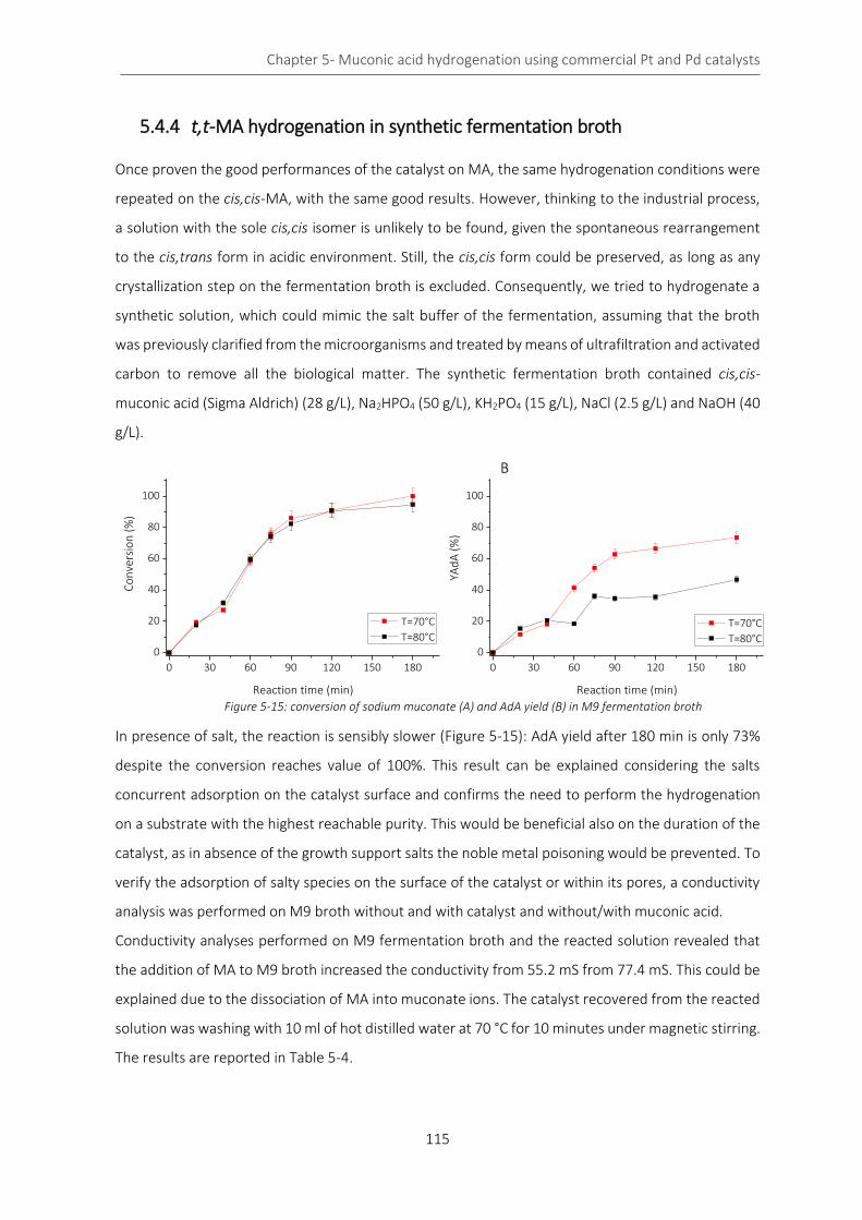
Chapter 5- Muconic acid hydrogenation using commercial Pt and Pd catalysts
115
5.4.4 t,t-MA hydrogenation in synthetic fermentation broth
Once proven the good performances of the catalyst on MA, the same hydrogenation conditions were
repeated on the cis,cis-MA, with the same good results. However, thinking to the industrial process,
a solution with the sole cis,cis isomer is unlikely to be found, given the spontaneous rearrangement
to the cis,trans form in acidic environment. Still, the cis,cis form could be preserved, as long as any
crystallization step on the fermentation broth is excluded. Consequently, we tried to hydrogenate a
synthetic solution, which could mimic the salt buffer of the fermentation, assuming that the broth
was previously clarified from the microorganisms and treated by means of ultrafiltration and activated
carbon to remove all the biological matter. The synthetic fermentation broth contained cis,cis-
muconic acid (Sigma Aldrich) (28 g/L), Na2HPO4 (50 g/L), KH2PO4 (15 g/L), NaCl (2.5 g/L) and NaOH (40
g/L).
In presence of salt, the reaction is sensibly slower (Figure 5-15): AdA yield after 180 min is only 73%
despite the conversion reaches value of 100%. This result can be explained considering the salts
concurrent adsorption on the catalyst surface and confirms the need to perform the hydrogenation
on a substrate with the highest reachable purity. This would be beneficial also on the duration of the
catalyst, as in absence of the growth support salts the noble metal poisoning would be prevented. To
verify the adsorption of salty species on the surface of the catalyst or within its pores, a conductivity
analysis was performed on M9 broth without and with catalyst and without/with muconic acid.
Conductivity analyses performed on M9 fermentation broth and the reacted solution revealed that
the addition of MA to M9 broth increased the conductivity from 55.2 mS from 77.4 mS. This could be
explained due to the dissociation of MA into muconate ions. The catalyst recovered from the reacted
solution was washing with 10 ml of hot distilled water at 70 °C for 10 minutes under magnetic stirring.
The results are reported in Table 5-4.
Figure 5-15: conversion of sodium muconate (A) and AdA yield (B) in M9 fermentation broth
0 30 60 90 120 150 180
0
20
40
60
80
100
120YA
dA
(%
)
Reaction time (min)
T=70°C
T=80°C
0 30 60 90 120 150 180
0
20
40
60
80
100
120
Co
nve
rsio
n (
%)
Reaction time (min)
T=70°C
T=80°C
B

Chapter 5- Muconic acid hydrogenation using commercial Pt and Pd catalysts
116
After 8 washes the water used during the washing has the same conductivity of distilled water (Figure
5-16). The washings help to clean the catalyst that might be adsorbed different salty species, blocking
the pores. The conductivity study was also performed on M9 broth in presence of Pt/AC catalyst
without the addition of MA. M9 growth support has a conductivity of 81.31 mS at 80 °C. After the
addition of Pt/AC 5% the conductivity decreases of
about 30% after 30 min, this means that the catalyst
adsorbs the different salts. When MA was added
higher values of conductivity were measure respect
to Pt+M9 sample. Therefore, MA must compete with
all the other species to reach and to be adsorbed on
the catalyst surface, that implies low reaction rate
and low conversion respect to the reaction
performed in distilled water.
Figure 5-16: conductivity measurement on Pt/AC 5% in M9 broth with t,t-MA during the catalyst washing test
Table 5-4: conductivity tests on M9 broth and catalyst washing
Conductivity (mS)
Distilled water (70 °C) 0.106
M9 broth (70 °C) 55.2
Filtered reacted solution (70 °C) 77.4
Washing with water (70 °C)
1st washing 24.2
2nd washing 5.7
3rd washing 1.4
4th washing 0.880
5th washing 0.366
6th washing 0.180
7th washing 0.152
8th washing 0.141
Pt in M9 no MA (80 °C)
M9 (80 °C) 82.31
Pt+M9 (30 min) 58.62
Pt+M9 (70 min) 61.21
Pt+M9 (110 min) 61.02
Pt+M9 (180 min) 60.83
Pt in M9 with MA (80 °C)
Pt+M9+MA (30 min) 86.6
Pt+M9+MA (60 min) 86.7
Pt+M9+MA (120 min) 91.3
Pt+M9+MA (180 min) 89.4
dist
illate
d w
ater
M9
brot
h
filte
red
reac
ted
solu
tion
1st w
ashi
ng2n
d w
ashi
ng3r
d w
ashi
ng4t
h w
ashi
ng5t
h w
ashi
ng6t
h w
ashi
ng7t
h w
ashi
ng8t
h w
ashi
ng --
0
20
40
60
80
Cond
uctiv
ity (m
S)

Chapter 5- Muconic acid hydrogenation using commercial Pt and Pd catalysts
117
5.4.5 t,t-MA hydrogenation in light alcoholic solvent
Hydrogenation of t,t-MA was tested using ethanol and methanol. In this case, due to the higher
solubility of muconic acid in organic solvent, no salification was performed. The reactions occurred in
the stainless-steel autoclave at different temperature keeping constant all the other operating
parameters.
- H2 pressure= 4 bar;
- Temperature= 50-90 °C;
- Stirring= 500 rpm;
- Catalyst: commercial Pt/AC 5% (0.1 g) pretreated at 200 °C for 3h at 6 bar of hydrogen;
- [t,t-MA]= 0.054 M (10 mL).
5.4.5.1 Ethanol
0 30 60 90 120 150 1800
20
40
60
80
100
Co
nve
rsio
n (
%)
Reaction time (min)
T=70°C
T=60°C
T=80°C
T=90°C
T=70°C
T=60°C
T=50°C
Figure 5-17: t,t-MA conversion in EtOH at different temperatures
As reported in Figure 5-17 the conversion rate is low at 50 °C, while for 60 and 70 °C the conversion
is more or less equal. Increasing the temperature, the conversion increases and after 15 min full
conversion of MA was reached.
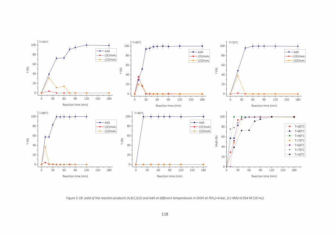
118
Figure 5-18: yield of the reaction products (A,B,C,D,E) and AdA at different temperatures in EtOH at P(H2)=4 bar, [t,t-MA]=0.054 M (10 mL)
0 30 60 90 120 150 180
0
20
40
60
80
100
Y (
%)
Reaction time (min)
AdA
(2E)HxAc
(2Z)HxAc
T=80°C
0 30 60 90 120 150 180
0
20
40
60
80
100
Y (
%)
Reaction time (min)
AdA
(2E)HxAc
(2Z)HxAc
T=50°C
0 30 60 90 120 150 180
0
20
40
60
80
100
AdA
(2E)HxAc
(2Z)HxAc
Y (
%)
Reaction time (min)
T=60°C
0 30 60 90 120 150 180
0
20
40
60
80
100
Y (
%)
Reaction time (min)
AdA
(2E)HxAc
(2Z)HxAc
T=90°C
0 30 60 90 120 150 180
0
20
40
60
80
100
Y (
%)
Reaction time (min)
AdA
(2E)HxAc
(2Z)HxAc
T=70°C
0 30 60 90 120 150 1800
20
40
60
80
100
YA
dA
(%
)
Reaction time (min)
T=60°C
T=80°C
T=90°C
T=70°C
T=60°C
T=70°C
T=50°C
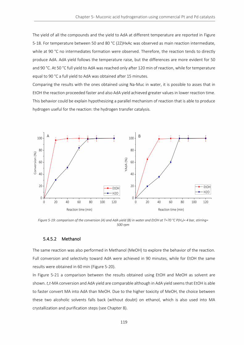
Chapter 5- Muconic acid hydrogenation using commercial Pt and Pd catalysts
119
The yield of all the compounds and the yield to AdA at different temperature are reported in Figure
5-18. For temperature between 50 and 80 °C (2Z)HxAc was observed as main reaction intermediate,
while at 90 °C no intermediates formation were observed. Therefore, the reaction tends to directly
produce AdA. AdA yield follows the temperature raise, but the differences are more evident for 50
and 90 °C. At 50 °C full yield to AdA was reached only after 120 min of reaction, while for temperature
equal to 90 °C a full yield to AdA was obtained after 15 minutes.
Comparing the results with the ones obtained using Na-Muc in water, it is possible to asses that in
EtOH the reaction proceeded faster and also AdA yield achieved greater values in lower reaction time.
This behavior could be explain hypothesizing a parallel mechanism of reaction that is able to produce
hydrogen useful for the reaction: the hydrogen transfer catalysis.
5.4.5.2 Methanol
The same reaction was also performed in Methanol (MeOH) to explore the behavior of the reaction.
Full conversion and selectivity toward AdA were achieved in 90 minutes, while for EtOH the same
results were obtained in 60 min (Figure 5-20).
In Figure 5-21 a comparison between the results obtained using EtOH and MeOH as solvent are
shown. t,t-MA conversion and AdA yield are comparable although in AdA yield seems that EtOH is able
to faster convert MA into AdA than MeOH. Due to the higher toxicity of MeOH, the choice between
these two alcoholic solvents falls back (without doubt) on ethanol, which is also used into MA
crystallization and purification steps (see Chapter 8).
Figure 5-19: comparison of the conversion (A) and AdA yield (B) in water and EtOH at T=70 °C P(H2)= 4 bar, stirring= 500 rpm
0 20 40 60 80 100 1200
20
40
60
80
100
Co
nve
rsio
n (
%)
Reaction time (min)
EtOH
H2O
0 20 40 60 80 100 1200
20
40
60
80
100
YA
dA
(%
)
Reaction time (min)
EtOH
H2O
A B

Chapter 5- Muconic acid hydrogenation using commercial Pt and Pd catalysts
120
Figure 5-21:comparison of the results in term of t,t-MA conversion (A) and AdA yield (B) in alcoholic solvent at 70 °C and P(H2) = 3 bar
0 30 60 90 120 150 1800
20
40
60
80
100
Co
nve
rsio
n (
%)
Reaction time (min)
0 30 60 90 120 150 180
0
20
40
60
80
100
Y (
%)
Reaction time (min)
AdA
(2E)HxAc
(2Z)HxAc
Figure 5-20: conversion (A) and AdA yield (B) in MeOH at T=70 °C and P(H2) = 4 bar
0 20 40 60 80 100 120 140 160 180
0
20
40
60
80
100
YAd
A (
%)
Reaction time (min)
EtOH
MeOH
0 20 40 60 80 100 120 140 160 180
0
20
40
60
80
100
Co
nve
rsio
n (
%)
Reaction time (min)
EtOH
MeOH
A B
A B

Chapter 5- Muconic acid hydrogenation using commercial Pt and Pd catalysts
121
5.5 Pd/AC 5% commercial catalyst
Palladium based catalysts are known as good catalyst for hydrogenation reactions.
The possibility to directly use the catalyst without pre-treatment,22,23 the high activity of the catalyst
at low temperature and atmospheric pressure24 and the lower price respect to the Pt based catalyst
make this material a good substitute of the expensive Pt/AC.25 A systematic study varying the
operating conditions was performed, trying to decrease the amount of catalyst as much as possible,
and working at low temperature (50-70 °C) and atmospheric pressure (1-3 bar). Moreover, a double
comparison between sodium muconate and t,t-MA hydrogenation was also performed to study the
different activity of the catalyst toward these compounds. MA production, recovery, and purification
processes affect the final chemical configuration of MA. MA is produced through bacterial
fermentation as cis,cis-sodium muconate but after its separation from the bacterial cells (for example
using acidic environment) it is converted to cis,cis and cis,trans-MA.26 Further purification step that
occurs in ethanol and hydrochloridric acid isomerizes almost completely the cis-cis form into trans-
trans configuration. Therefore, we decided to use sodium muconate and t,t-MA as substrate to study
and find the best choice regarding the starting substrate.
5.6 Fresh catalyst characterization
5.6.1.1 BET
Bet surface area of the fresh Pd/AC 5% commercial catalyst is 812.3 m2/g. The desorption pore
diameter was evaluated using BJH method27 and the result is 3.79 nm. The total pore volume for pores
with diameter less than 147.03 nm (at P/P0=0.9868) is 0.732 cc/g, while using the DR method28 the
cumulative desorption pore volume is 0.363 cc/g.
5.6.1.2 XRD
XRD pattern was collected using Bruker D8XR instrument. Figure 5-22 shows the results of the analysis
for the fresh catalyst. The broad peaks at 25° and 45 ° corresponds to the (002) and (101) planes of
low-graphitized carbonaceous structure, this indicates that the porous carbon material is disordered

Chapter 5- Muconic acid hydrogenation using commercial Pt and Pd catalysts
122
or amorphous.29,30 Other peaks were also observed at 2θ= 40°, 46° and 68 °, attributed to the (111),
(200) and (220) planes of the face-centred cubic (fcc) crystal structure of palladium oxide.31
10 20 30 40 50 60 70 80-100
0
100
200
300
400
500
600
700
§2
20
*10
3
*00
4
§2
00°1
10§
11
1
°10
1Inte
nsi
ty (
c. p
. s.)
2(
*00
2
°10
1
*graphite
° Pd§PdO
Figure 5-22: XRD pattern of commercial fresh Pd/AC 5%
5.6.1.3 SEM/EDX
SEM/EDX analysis was performed using a HITACHI analytical TableTop Microscope / Benchtop SEM
TM3030.
Figure 5-23: TEM of fresh Pd/AC 5% catalyst (A) and EDX maps of the image (B, C)
Pd NPs were well dispersed on the surface of the carbon support (Figure 5-23). This allows to perform
different reactions with different batch of catalyst without affecting reproducibility. Fresh catalyst is
composed by coal grains that have very different size (5-100 µm) (Figure 5-24).
A B
C

Chapter 5- Muconic acid hydrogenation using commercial Pt and Pd catalysts
123
An elemental analysis was also performed to evaluate the amount of different chemical element
present in the catalyst. A huge portion of particle was chosen allowing a good composition evaluation.
The results are reported in Table 5-5.
Table 5-5: elemental analysis on fresh Pd/AC 5%
Element AN
series
Norm
(wt%)
C atom
(at%)
Error
Carbon 6 K 89.78 98.06 6.1
Palladium 46 L 5.12 0.63 0.1
Copper 29 K 4.27 0.88 0.1
Sodium 11 K 0.44 0.25 0.0
Silicon 14 K 0.38 0.18 0.0
The activated carbon is not only composed by carbon and oxygen, but there is the presence of copper,
sodium and silicon in traces. The palladium amount is 5.12 % (error 0.1) that exactly corresponds to
the specification sheet of the home maker.
5.6.1.4 TEM
Transmission electron microscopy (TEM) and scanning transmission electron microscopy (STEM) were
performed on a JEOL JEM-2100 operating at 200 kV. Energy dispersive X-ray analysis (EDX) was done
using an Oxford Instruments X-MaxN 80 detector and the data analysed using the Aztec software.
Samples were prepared by dispersion in ethanol by sonication and deposited on 300 mesh copper
grids coated with holey carbon film.
At about 200 NPs were considered to evaluate the particle size distribution (PSD). The study was
performed using ImageJ program. The PSD was calculated using the Lognormal distribution.
2 4 6 8 10 12 14keV
0
2
4
6
8
10
12
14
16
18
20
cps/eV
C Pd Pd Pd
Si Na Cu Cu
Figure 5-24: SEM images of fresh Pd/AC 5% at 40 KX (A) and 250 KX (B)
A B

Chapter 5- Muconic acid hydrogenation using commercial Pt and Pd catalysts
124
Metal Pd particles are well dispersed on the carbon support Figure 5-25 (A and B) and their average
size is 3.3±0.3 nm (Figure 5-25 C) . Moreover, Figure 5-25 (B) revealed 0.225 nm spacing of the lattice
fringes which is consistent with the Pd(111) lattice plane.32
5.6.1.5 X-ray photoelectron spectroscopy (XPS)
X-ray photoelectron spectroscopy (XPS) was performed on a Thermo Scientific K-alpha+ spectrometer.
Samples were analyzed using a monochromatic Al x-ray source operating at 72 W (6 mA x 12 kV), with
the signal averaged over an oval-shaped area of approximately 600 x 400 microns. Data was recorded
at pass energies of 150 eV for survey scans and 40 eV for high resolution scan with a 1eV and 0.1 eV
step size respectively.
Charge neutralization of the sample was achieved using a combination of both low energy electrons
and argon ions (less than 1 eV) which gave a C(1s) binding energy of 284.8 eV.
All data were analyzed using CASAXPS (v2.3.17 PR1.1) using Scofield sensitivity factors and an energy
exponent of -0.6.
Figure 5-26 shows the fitted Pd 3d core-level XPS spectra of the fresh commercial Pd/AC 5%.
Each Pd species displayed two peaks due to the Pd 3d3/2 and Pd 3d5/2 transition. Pd(0) 3d5/2 core
electron binding energy is at 335.6 eV, while the Pd(0) 3d3/2 is at 340.54 eV. The Pd(II) peaks are at
1 2 3 4 5 6 7 8 9 100
20
40
60
80
100
120
140
Coun
t
Particle size (nm)
Figure 5-25: TEM images(A), evaluation of the lattice fringe of Pd(111) specie (B) and particle size distribution (C) for fresh commercial Pd/AC 5% catalyst
A B
C

Chapter 5- Muconic acid hydrogenation using commercial Pt and Pd catalysts
125
343.46 and 338.18 eV, and they are identified as 3d3/2 and 3d5/2 transition, respectively. These binding
energy values are in good agreement with that data reported in Chen et al. and Sanchez et al.32,33
As reported in Table 5-6, fresh Pd/AC catalyst is equally composed by Pd oxide and Pd metal. Despite
the active phase for hydrogenation reactions is the bare metal, it is possible to directly use the catalyst
avoiding the pre-treatment. In fact, in reducing conditions the metal oxide can be easily transform to
the active metal 0 state.
360 355 350 345 340 335 330
3000
4000
5000
6000
7000
8000
9000
10000
CP
S
Binding energy (eV)
Pd 3d_1_Pd 3d/2
Pd 3d_2_Pd 3d/2
Pd 3d_3_Pd 3d/2
Pd 3d_4_Pd 3d/2
Pd 3d_5_Pd 3d/2
Pd 3d_6_Pd 3d/2
Satellite_7_Pd 3d/2
Background_Pd 3d/2
Envelope_Pd 3d/2
Envelope_Pd 3d/2
Figure 5-26: XPS analysis on fresh commercial Pd/AC 5% catalyst
Table 5-6: evaluation of the percentage of Pd(0) and Pd(II) in the fresh catalyst
AreaPd(0) AreaPd(II) Sum AreaPd(0) (%) AreaPd(II) (%)
Pd3d5/2 3672 3222 6894 53.3 46.7
Pd3d3/2 3220 3098 6318 50.9 49.1
The ratio between Pd and PdO for the 3d5/2 and 3d3/2 configurations are 1.14 and 0.52, respectively.
5.6.1 Hydrogenation reaction in stainless steel autoclave
Hydrogenation reactions were performed both in autoclave and in glass reactor. Substrate/catalyst
ratio, temperature, stirring, substrate concentration and pressure were varied using t,t-MA an Na-
Muc as substrate and distilled water as solvent The tests at 2 and 3 bar of hydrogen were performed
in the autoclave. Tests at 1 bar were also performed in the glass reactor, allowing to use a large
amount of substrate and to collect a proper amount of post reaction catalyst to use for the
characterization.

Chapter 5- Muconic acid hydrogenation using commercial Pt and Pd catalysts
126
5.6.1.1 Catalyst to substrate ratio optimization
The catalyst/substrate ratio is one of the most important parameters because it affects the mass
transport and diffusion phenomena, and in industry, it might influence the cost of the process (in
particular if noble metals are involved in the reaction).
Different hydrogenation reactions were performed varying the amount of catalyst and keeping
constant all the other operating parameter. The reactions were performed using the following
operating parameter:
- temperature=70 °C;
- static pressure of hydrogen= 3 bar;
- concentration of t,t-MA and Na-Muc= 1.43E-02 M;
- magnetic stirring= 500 rpm;
- solvent= distilled water;
- catalyst= Pd/AC 5% (Sigma Aldrich);
- reaction time= 60 min;
- reactor= stainless steel reactor.
The catalyst/substrate ratio is expressed as mol of metal divided by the mol of substrate used for the
reaction. The results are reported in Table 5-7 and Figure 5-27.
Table 5-7: Results for catalyst/substrate ratio optimization
Cat/substrate
(molPd/molsub)
t,t-MA Na-Muc
Conversion
(%)
YAdA
(%)
Conversion
(%)
YAdA
(%)
1/10 99.42 99.09 98.87 98.69
1/100 99.13 99.13 92.82 69.79
1/200 99.62 99.49 97.68 41.89
1/500 98.65 98.23 90.12 37.26

Chapter 5- Muconic acid hydrogenation using commercial Pt and Pd catalysts
127
As reported in Figure 5-27 the fast hydrogenation of t,t-MA did not allow to study the dependence of
the conversion from the catalyst/substrate ratio: the conversion is high for all the tests. Different
results were obtained using Na-Muc, the conversion decreases reducing the amount of catalyst.
For high amount of catalyst, the conversion and the selectivity are higher than the results obtained
using lower amount of catalyst. With a cat/sub ratio equal to 1/200 the yield to AdA produced from
Na-Muc hydrogenation is the half respect to the one obtained using t,t-MA. The behaviour might be
explained considering the different pH of the substrate solution: t,t-MA has a pH equal 3.66 while Na-
Muc solution is a pH equal to 11.45. In fact, pH has a wide influence on the ionic state of MA. At low
pH AdA is completely undissociated while at high pH it is completely dissociated; this behaviour might
deeply affect the adsorption/desorption process the reactivity and therefore the reaction rate.34
We decided to perform the further hydrogenation reaction using the catalyst to substrate ratio equal
to 1/200 to allow a good and precise weight of the catalyst.
Figure 5-27: conversion and YAdA evaluation at different cat/sub (molPd/molsub) ratio for t,t-MA and Na-Muc
1/10 1/100 1/200 1/500
0
20
40
60
80
100
Co
nve
rsio
n (
%)
t,t-MA
Na-Muc
0
20
40
60
80
100
1/5001/2001/1001/10
YAd
A (
%)
t,t-MA
Na-Muc
1/10 1/100 1/200 1/500
0
20
40
60
80
100Na-Muc
(%)
Cat/Sub (mol/mol)
conv
AdA yield
1/10 1/100 1/200 1/500
0
20
40
60
80
100
Cat/Sub (mol/mol)
(%)
conv
AdA yieldt,t-MA
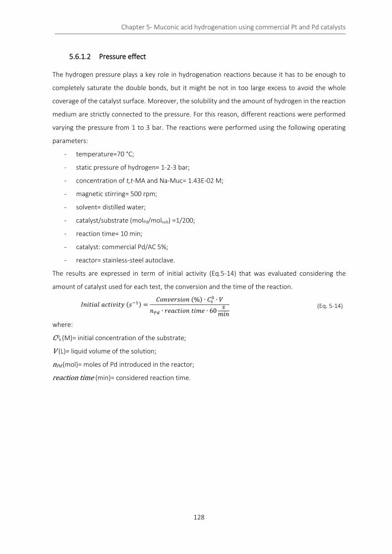
Chapter 5- Muconic acid hydrogenation using commercial Pt and Pd catalysts
128
5.6.1.2 Pressure effect
The hydrogen pressure plays a key role in hydrogenation reactions because it has to be enough to
completely saturate the double bonds, but it might be not in too large excess to avoid the whole
coverage of the catalyst surface. Moreover, the solubility and the amount of hydrogen in the reaction
medium are strictly connected to the pressure. For this reason, different reactions were performed
varying the pressure from 1 to 3 bar. The reactions were performed using the following operating
parameters:
- temperature=70 °C;
- static pressure of hydrogen= 1-2-3 bar;
- concentration of t,t-MA and Na-Muc= 1.43E-02 M;
- magnetic stirring= 500 rpm;
- solvent= distilled water;
- catalyst/substrate (molPd/molsub) =1/200;
- reaction time= 10 min;
- catalyst: commercial Pd/AC 5%;
- reactor= stainless-steel autoclave.
The results are expressed in term of initial activity (Eq.5-14) that was evaluated considering the
amount of catalyst used for each test, the conversion and the time of the reaction.
𝐼𝑛𝑖𝑡𝑖𝑎𝑙 𝑎𝑐𝑡𝑖𝑣𝑖𝑡𝑦 (𝑠−1) =𝐶𝑜𝑛𝑣𝑒𝑟𝑠𝑖𝑜𝑛 (%) ∙ 𝐶𝑠
0 ∙ 𝑉
𝑛𝑃𝑑 ∙ 𝑟𝑒𝑎𝑐𝑡𝑖𝑜𝑛 𝑡𝑖𝑚𝑒 ∙ 60𝑠
𝑚𝑖𝑛
(Eq. 5-14)
where:
C0s (M)= initial concentration of the substrate;
V (L)= liquid volume of the solution;
nPd (mol)= moles of Pd introduced in the reactor;
reaction time (min)= considered reaction time.
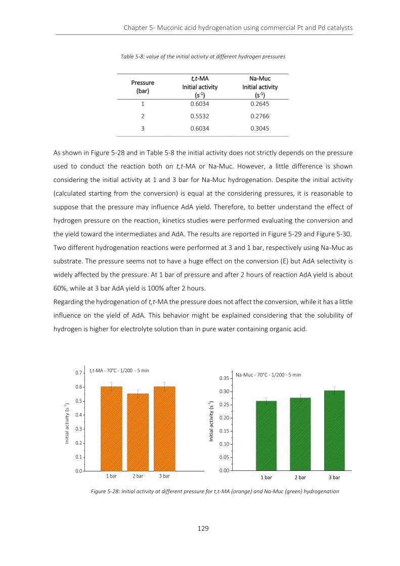
Chapter 5- Muconic acid hydrogenation using commercial Pt and Pd catalysts
129
Table 5-8: value of the initial activity at different hydrogen pressures
As shown in Figure 5-28 and in Table 5-8 the initial activity does not strictly depends on the pressure
used to conduct the reaction both on t,t-MA or Na-Muc. However, a little difference is shown
considering the initial activity at 1 and 3 bar for Na-Muc hydrogenation. Despite the initial activity
(calculated starting from the conversion) is equal at the considering pressures, it is reasonable to
suppose that the pressure may influence AdA yield. Therefore, to better understand the effect of
hydrogen pressure on the reaction, kinetics studies were performed evaluating the conversion and
the yield toward the intermediates and AdA. The results are reported in Figure 5-29 and Figure 5-30.
Two different hydrogenation reactions were performed at 3 and 1 bar, respectively using Na-Muc as
substrate. The pressure seems not to have a huge effect on the conversion (E) but AdA selectivity is
widely affected by the pressure. At 1 bar of pressure and after 2 hours of reaction AdA yield is about
60%, while at 3 bar AdA yield is 100% after 2 hours.
Regarding the hydrogenation of t,t-MA the pressure does not affect the conversion, while it has a little
influence on the yield of AdA. This behavior might be explained considering that the solubility of
hydrogen is higher for electrolyte solution than in pure water containing organic acid.
Pressure (bar)
t,t-MA Na-Muc
Initial activity (s-1)
Initial activity (s-1)
1 0.6034 0.2645
2 0.5532 0.2766
3 0.6034 0.3045
1 bar 2 bar 3 bar0.0
0.1
0.2
0.3
0.4
0.5
0.6
0.7
Init
ial a
ctiv
ity (
s-1)
t,t-MA - 70°C - 1/200 - 5 min
1 bar 2 bar 3 bar0.00
0.05
0.10
0.15
0.20
0.25
0.30
0.35Na-Muc - 70°C - 1/200 - 5 min
Init
ial a
ctiv
ity
(s-1
)
Figure 5-28: Initial activity at different pressure for t,t-MA (orange) and Na-Muc (green) hydrogenation

Chapter 5- Muconic acid hydrogenation using commercial Pt and Pd catalysts
130
0 20 40 60 80 100 120
0
20
40
60
80
100
Co
nve
rsio
n (
%)
Reaction time (min)
P= 3 bar
C
0 20 40 60 80 100 120
0
20
40
60
80
100P= 3 bar
Y (%
)
Reaction time (min)
(3E)HxAc
(2E)HxAc
AdA
c,c-MA
D
0 20 40 60 80 100 120
0
20
40
60
80
100
Co
nve
rsio
n (
%)
Reaction time (min)
P= 1 bar
A
0 20 40 60 80 100 120
0
20
40
60
80
100P= 1 barB
Y (%
)
Reaction time (min)
(3E)HxAc
(2E)HxAc
AdA
c,c-MA
0 20 40 60 80 100 120
0
20
40
60
80
100
Co
nve
rsio
n (
%)
Reaction time (min)
P= 3 bar
P=1 bar
E
0 20 40 60 80 100 120
0
20
40
60
80
100
YAd
A(%
)
Reaction time (min)
P=3 bar
P= 1 bar
F
Figure 5-29: Pressure effects on conversion and yield using Na-Muc as substrate

Chapter 5- Muconic acid hydrogenation using commercial Pt and Pd catalysts
131
0 10 20 30 40 50 60 70
0
20
40
60
80
100
Conv
ersi
on (%
)
Reaction time (min)
P= 1 bar
A
0 10 20 30 40 50 60 70
0
20
40
60
80
100 C
Conv
ersi
on (%
)
Reaction time (min)
P= 2 bar
0 10 20 30 40 50 60 70
0
20
40
60
80
100 E
P= 3 bar
Conv
ersi
on (%
)
Reaction time (min)
0 10 20 30 40 50 60 70
0
20
40
60
80
100 G
Conv
ersi
on (%
)
Reaction time (min)
P= 1 bar
P= 2 bar
P= 3 bar
0 10 20 30 40 50 60 70
0
20
40
60
80
100
P= 3 barF
Y (%
)
Reaction time (min)
(3E)HxAc
(2E)HxAc
AdA
c,c-MA
0 10 20 30 40 50 60 70
0
20
40
60
80
100
P= 2 barD
Y (%
)
Reaction time (min)
(3E)HxAc
(2E)HxAc
AdA
c,c-MA
0 10 20 30 40 50 60 70
0
20
40
60
80
100 BP= 1 bar
Y (%
)
Reaction time (min)
(3E)HxAc
(2E)HxAc
AdA
c,c-MA
0 10 20 30 40 50 60 70
0
20
40
60
80
100 H
Y A
dA(%
)
Reaction time (min)
P= 1 bar
P= 2 bar
P= 3 bar
Figure 5-30: Pressure effects on conversion and yield using t,t-MA as substrate
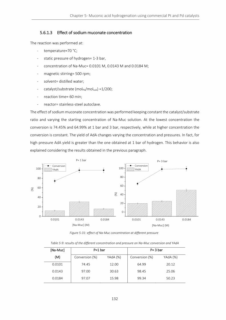
Chapter 5- Muconic acid hydrogenation using commercial Pt and Pd catalysts
132
5.6.1.3 Effect of sodium muconate concentration
The reaction was performed at:
- temperature=70 °C;
- static pressure of hydrogen= 1-3 bar,
- concentration of Na-Muc= 0.0101 M, 0.0143 M and 0.0184 M;
- magnetic stirring= 500 rpm;
- solvent= distilled water;
- catalyst/substrate (molPd/molsub) =1/200;
- reaction time= 60 min;
- reactor= stainless-steel autoclave.
The effect of sodium muconate concentration was performed keeping constant the catalyst/substrate
ratio and varying the starting concentration of Na-Muc solution. At the lowest concentration the
conversion is 74.45% and 64.99% at 1 bar and 3 bar, respectively, while at higher concentration the
conversion is constant. The yield of AdA changes varying the concentration and pressures. In fact, for
high pressure AdA yield is greater than the one obtained at 1 bar of hydrogen. This behavior is also
explained considering the results obtained in the previous paragraph.
Table 5-9: results of the different concentration and pressure on Na-Muc conversion and YAdA
[Na-Muc]
(M)
P=1 bar P= 3 bar
Conversion (%) YAdA (%) Conversion (%) YAdA (%)
0.0101 74.45 12.00 64.99 20.12
0.0143 97.00 30.63 98.45 25.06
0.0184 97.07 15.98 99.34 50.23
1 2 30
20
40
60
80
100
P= 1 bar
0.0101 0.0143 0.0184
(%)
Conversion
YAdA
0.0101
[Na-Muc] (M)
1 2 3
0
20
40
60
80
100
[Na-Muc] (M)
0.01840.01430.0101
(%)
Conversion
YAdA
P= 3 bar
Figure 5-31: effect of Na-Muc concentration at different pressure
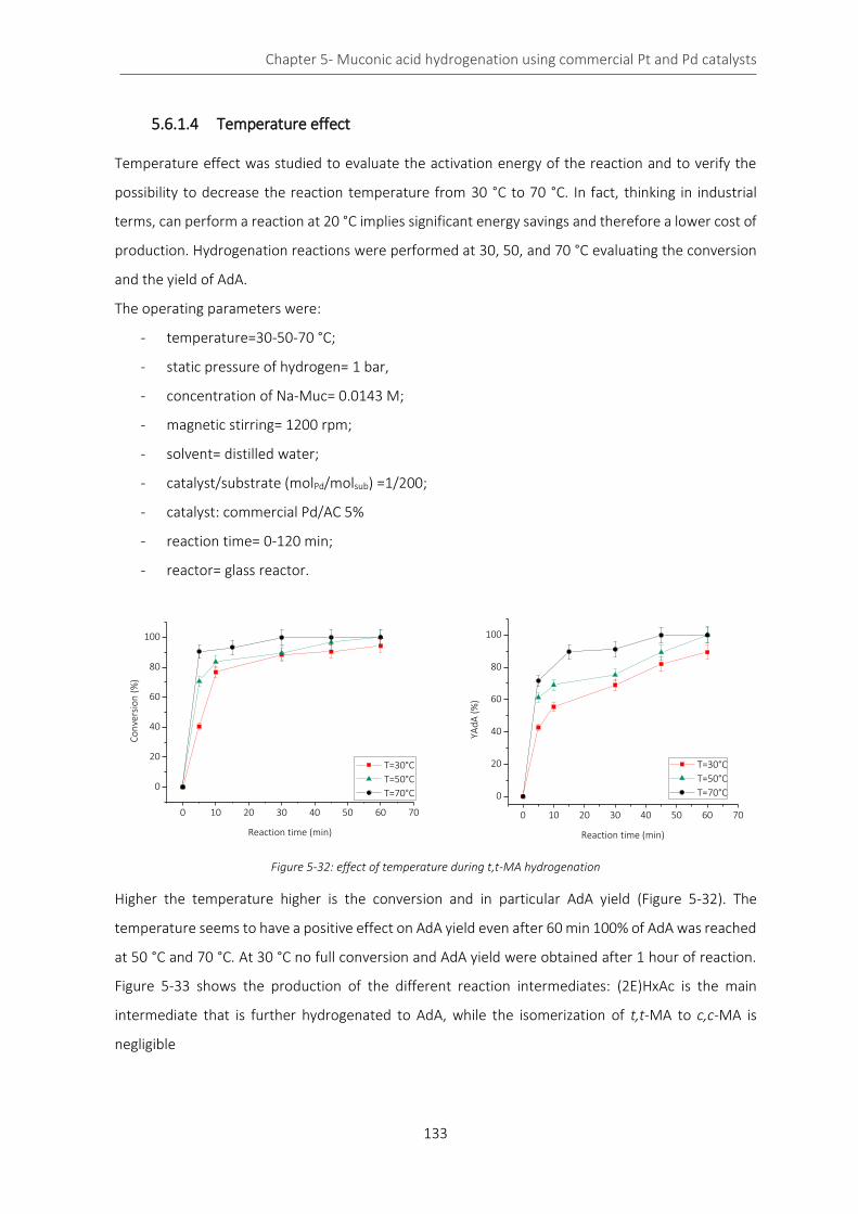
Chapter 5- Muconic acid hydrogenation using commercial Pt and Pd catalysts
133
5.6.1.4 Temperature effect
Temperature effect was studied to evaluate the activation energy of the reaction and to verify the
possibility to decrease the reaction temperature from 30 °C to 70 °C. In fact, thinking in industrial
terms, can perform a reaction at 20 °C implies significant energy savings and therefore a lower cost of
production. Hydrogenation reactions were performed at 30, 50, and 70 °C evaluating the conversion
and the yield of AdA.
The operating parameters were:
- temperature=30-50-70 °C;
- static pressure of hydrogen= 1 bar,
- concentration of Na-Muc= 0.0143 M;
- magnetic stirring= 1200 rpm;
- solvent= distilled water;
- catalyst/substrate (molPd/molsub) =1/200;
- catalyst: commercial Pd/AC 5%
- reaction time= 0-120 min;
- reactor= glass reactor.
0 10 20 30 40 50 60 70
0
20
40
60
80
100
Co
nve
rsio
n (
%)
Reaction time (min)
T=30°C
T=50°C
T=70°C
0 10 20 30 40 50 60 70
0
20
40
60
80
100
YAd
A (
%)
Reaction time (min)
T=30°C
T=50°C
T=70°C
Figure 5-32: effect of temperature during t,t-MA hydrogenation
Higher the temperature higher is the conversion and in particular AdA yield (Figure 5-32). The
temperature seems to have a positive effect on AdA yield even after 60 min 100% of AdA was reached
at 50 °C and 70 °C. At 30 °C no full conversion and AdA yield were obtained after 1 hour of reaction.
Figure 5-33 shows the production of the different reaction intermediates: (2E)HxAc is the main
intermediate that is further hydrogenated to AdA, while the isomerization of t,t-MA to c,c-MA is
negligible
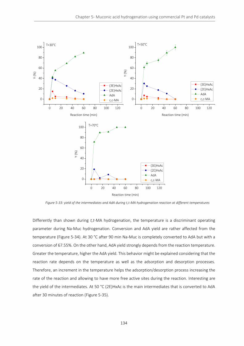
Chapter 5- Muconic acid hydrogenation using commercial Pt and Pd catalysts
134
Differently than shown during t,t-MA hydrogenation, the temperature is a discriminant operating
parameter during Na-Muc hydrogenation. Conversion and AdA yield are rather affected from the
temperature (Figure 5-34). At 30 °C after 90 min Na-Muc is completely converted to AdA but with a
conversion of 67.55%. On the other hand, AdA yield strongly depends from the reaction temperature.
Greater the temperature, higher the AdA yield. This behavior might be explained considering that the
reaction rate depends on the temperature as well as the adsorption and desorption processes.
Therefore, an increment in the temperature helps the adsorption/desorption process increasing the
rate of the reaction and allowing to have more free active sites during the reaction. Interesting are
the yield of the intermediates. At 50 °C (2E)HxAc is the main intermediates that is converted to AdA
after 30 minutes of reaction (Figure 5-35).
Figure 5-33: yield of the intermediates and AdA during t,t-MA hydrogenation reaction at different temperatures
0 20 40 60 80 100 120
0
20
40
60
80
100
Y (%
)
Reaction time (min)
(3E)HxAc
(2E)HxAc
AdA
c,c-MA
T=70°C
0 20 40 60 80 100 120
0
20
40
60
80
100T=50°C
Y (%
)
Reaction time (min)
(3E)HxAc
(2E)HxAc
AdA
c,c-MA
0 20 40 60 80 100 120
0
20
40
60
80
100T=30°C
Y (%
)
Reaction time (min)
(3E)HxAc
(2E)HxAc
AdA
c,c-MA

Chapter 5- Muconic acid hydrogenation using commercial Pt and Pd catalysts
135
Figure 5-35: yield of the intermediates and AdA during Na-Muc hydrogenation reaction at different temperatures
Figure 5-34: effect of temperature on conversion (A) and YAdA (B) during Na-Muc hydrogenation
0 20 40 60 80 100 120
0
20
40
60
80
100
Y %
)
Reaction time (min)
(3E)HxAc
(2E)HxAc
AdA
c,c-MA
T=30°C
0 20 40 60 80 100 120
0
20
40
60
80
100T= 50 °C
Y %
)
Reaction time (min)
(3E)HxAc
(2E)HxAc
AdA
c,c-MA
0 20 40 60 80 100 120
0
20
40
60
80
100
Y %
)
Reaction time (min)
(3E)HxAc
(2E)HxAc
AdA
c,c-MA
T= 70 °C
0 20 40 60 80 100
0
20
40
60
80
100
0 20 40 60 80 100
0
20
40
60
80
100
Conv
ersi
on (%
)
Reaction time (min)
T=30°C
T=50°C
T=70°C
YAdA
(%)
Reaction time (min)
T=30°C
T=50°C
T=70°C
B A
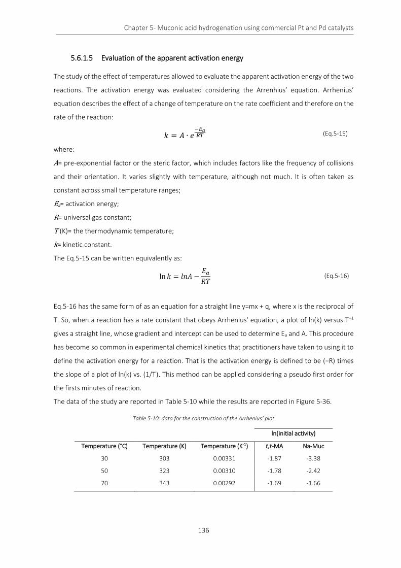
Chapter 5- Muconic acid hydrogenation using commercial Pt and Pd catalysts
136
5.6.1.5 Evaluation of the apparent activation energy
The study of the effect of temperatures allowed to evaluate the apparent activation energy of the two
reactions. The activation energy was evaluated considering the Arrenhius’ equation. Arrhenius’
equation describes the effect of a change of temperature on the rate coefficient and therefore on the
rate of the reaction:
𝑘 = 𝐴 ∙ 𝑒−𝐸𝑎𝑅𝑇 (Eq.5-15)
where:
A= pre-exponential factor or the steric factor, which includes factors like the frequency of collisions
and their orientation. It varies slightly with temperature, although not much. It is often taken as
constant across small temperature ranges;
Ea= activation energy;
R= universal gas constant;
T (K)= the thermodynamic temperature;
k= kinetic constant.
The Eq.5-15 can be written equivalently as:
ln 𝑘 = 𝑙𝑛𝐴 −𝐸𝑎
𝑅𝑇 (Eq.5-16)
Eq.5-16 has the same form of as an equation for a straight line y=mx + q, where x is the reciprocal of
T. So, when a reaction has a rate constant that obeys Arrhenius' equation, a plot of ln(k) versus T−1
gives a straight line, whose gradient and intercept can be used to determine Ea and A. This procedure
has become so common in experimental chemical kinetics that practitioners have taken to using it to
define the activation energy for a reaction. That is the activation energy is defined to be (−R) times
the slope of a plot of ln(k) vs. (1/T ). This method can be applied considering a pseudo first order for
the firsts minutes of reaction.
The data of the study are reported in Table 5-10 while the results are reported in Figure 5-36.
Table 5-10: data for the construction of the Arrhenius’ plot
ln(initial activity)
Temperature (°C) Temperature (K) Temperature (K-1) t,t-MA Na-Muc
30 303 0.00331 -1.87 -3.38
50 323 0.00310 -1.78 -2.42
70 343 0.00292 -1.69 -1.66
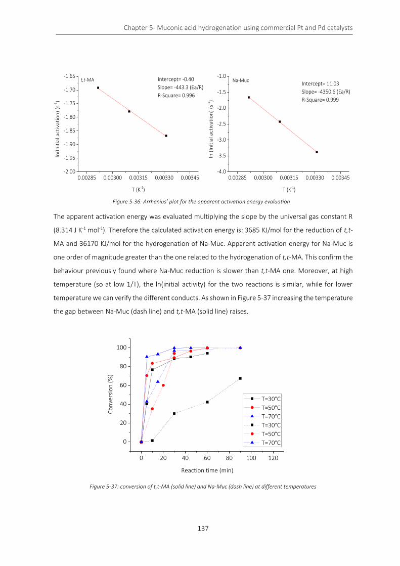
Chapter 5- Muconic acid hydrogenation using commercial Pt and Pd catalysts
137
The apparent activation energy was evaluated multiplying the slope by the universal gas constant R
(8.314 J K-1 mol-1). Therefore the calculated activation energy is: 3685 KJ/mol for the reduction of t,t-
MA and 36170 KJ/mol for the hydrogenation of Na-Muc. Apparent activation energy for Na-Muc is
one order of magnitude greater than the one related to the hydrogenation of t,t-MA. This confirm the
behaviour previously found where Na-Muc reduction is slower than t,t-MA one. Moreover, at high
temperature (so at low 1/T), the ln(initial activity) for the two reactions is similar, while for lower
temperature we can verify the different conducts. As shown in Figure 5-37 increasing the temperature
the gap between Na-Muc (dash line) and t,t-MA (solid line) raises.
0 20 40 60 80 100 120
0
20
40
60
80
100
Co
nve
rsio
n (
%)
Reaction time (min)
T=30°C
T=50°C
T=70°C
T=30°C
T=50°C
T=70°C
Figure 5-37: conversion of t,t-MA (solid line) and Na-Muc (dash line) at different temperatures
0.00285 0.00300 0.00315 0.00330 0.00345-2.00
-1.95
-1.90
-1.85
-1.80
-1.75
-1.70
-1.65Intercept= -0.40
Slope= -443.3 (Ea/R)
R-Square= 0.996
t,t-MA
ln(I
nit
ial a
ctiv
ati
on
) (s
-1)
T (K-1)
0.00285 0.00300 0.00315 0.00330 0.00345-4.0
-3.5
-3.0
-2.5
-2.0
-1.5
-1.0
ln (
Init
ial a
ctiv
ati
on
) (s
-1)
T (K-1)
Na-MucIntercept= 11.03
Slope= -4350.6 (Ea/R)
R-Square= 0.999
Figure 5-36: Arrhenius’ plot for the apparent activation energy evaluation

Chapter 5- Muconic acid hydrogenation using commercial Pt and Pd catalysts
138
5.6.2 Hydrogenation reaction in glass reactor
Hydrogenation reactions at different catalyst/substrate ratio were performed using the glass reactor.
This allowed better verifying the kinetic regime due to higher amount of substrate solution that it is
possible to introduce in the reactor, and therefore a larger amount of catalyst, decreasing the weight
error. The reactions were performed both on t,t-MA and Na-Muc solutions keeping constant all the
operating parameters except the amount of catalyst.
The operating parameters were:
- temperature=70 °C;
- static pressure of hydrogen= 1 bar,
- concentration of Na-Muc and t,t-MA= 0.0143 M;
- magnetic stirring= 1200 rpm;
- solvent= distilled water;
- catalyst/substrate (molPd/molsub) =1/10-1/700;
- reaction time= 10 min.
The results are reported in Table 5-11-12 and Figure 5-38.
Table 5-11: check of kinetic regime for t,t-MA hydrogenation
Cat/Sub (molPd/molsub) t,t-MA initial activity (s-1)
1/10 0.02762
1/100 0.27536
1/200 0.5363
1/500 0.5563
Table 5-12: check of kinetic regime for Na-Muc hydrogenation
Cat/Sub (molPd/molsub) Na-Muc initial activity (s-1)
1/200 0.2914
1/500 0.3274
1/700 0.3143

Chapter 5- Muconic acid hydrogenation using commercial Pt and Pd catalysts
139
From cat/sub ratio greater than 200 the initial activity is constant (Figure 5-38). Therefore, the
reaction is occurring in kinetic regime avoiding the interference of mass transfer limitation. It is
possible to reduce the amount of catalyst, but this implies a lower conversion. (Figure 5-39).
Industrially speaking, the choice of the amount of catalyst is a compromise between the production
and selectivity.
0 10 20 30 40 50 60 70
0
20
40
60
80
100
Co
nve
rsio
n (
%)
Reaction time (min)
1/200
1/500
1/700
Figure 5-39: Na-Muc conversion at different cat/sub ratios
1/200 1/500 1/7000.00
0.05
0.10
0.15
0.20
0.25
0.30
0.35
0.40Na-Muc - 70°C - 1 bar - 10 min
Init
ial a
ctiv
ity
(s-1
)
1/10 1/100 1/200 1/5000.0
0.1
0.2
0.3
0.4
0.5
0.6
Init
ial a
ctiv
ity
(s-1
)
t,t-MA - 70°C - 1 bar - 10 min
Figure 5-38: control of the kinetic regime during t,t-MA (orange) and Na-Muc (green)
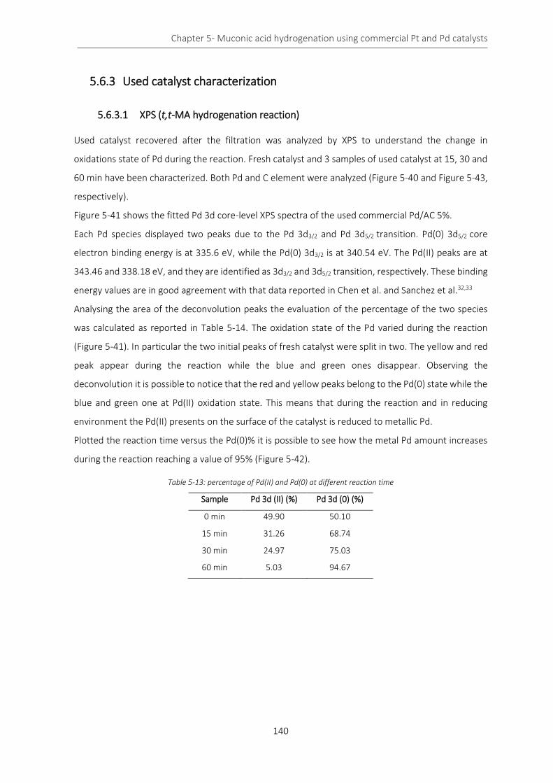
Chapter 5- Muconic acid hydrogenation using commercial Pt and Pd catalysts
140
5.6.3 Used catalyst characterization
5.6.3.1 XPS (t,t-MA hydrogenation reaction)
Used catalyst recovered after the filtration was analyzed by XPS to understand the change in
oxidations state of Pd during the reaction. Fresh catalyst and 3 samples of used catalyst at 15, 30 and
60 min have been characterized. Both Pd and C element were analyzed (Figure 5-40 and Figure 5-43,
respectively).
Figure 5-41 shows the fitted Pd 3d core-level XPS spectra of the used commercial Pd/AC 5%.
Each Pd species displayed two peaks due to the Pd 3d3/2 and Pd 3d5/2 transition. Pd(0) 3d5/2 core
electron binding energy is at 335.6 eV, while the Pd(0) 3d3/2 is at 340.54 eV. The Pd(II) peaks are at
343.46 and 338.18 eV, and they are identified as 3d3/2 and 3d5/2 transition, respectively. These binding
energy values are in good agreement with that data reported in Chen et al. and Sanchez et al.32,33
Analysing the area of the deconvolution peaks the evaluation of the percentage of the two species
was calculated as reported in Table 5-14. The oxidation state of the Pd varied during the reaction
(Figure 5-41). In particular the two initial peaks of fresh catalyst were split in two. The yellow and red
peak appear during the reaction while the blue and green ones disappear. Observing the
deconvolution it is possible to notice that the red and yellow peaks belong to the Pd(0) state while the
blue and green one at Pd(II) oxidation state. This means that during the reaction and in reducing
environment the Pd(II) presents on the surface of the catalyst is reduced to metallic Pd.
Plotted the reaction time versus the Pd(0)% it is possible to see how the metal Pd amount increases
during the reaction reaching a value of 95% (Figure 5-42).
Table 5-13: percentage of Pd(II) and Pd(0) at different reaction time
Sample Pd 3d (II) (%) Pd 3d (0) (%)
0 min 49.90 50.10
15 min 31.26 68.74
30 min 24.97 75.03
60 min 5.03 94.67
Chapter 5- Muconic acid hydrogenation using commercial Pt and Pd catalysts
141
Figure 5-40: XPS and deconvolution of Pd species at different reaction times

Chapter 5- Muconic acid hydrogenation using commercial Pt and Pd catalysts
142
348 342 336 330
348 342 336 330
Binding Energy (eV)
fresh
15 min
30 min
60 min
Figure 5-41: comparison of XPS results for Pd element during t,t-MA hydrogenation
0 10 20 30 40 50 60 70
0
20
40
60
80
100
Pd
(0
) (%
)
Reaction time (min)
Figure 5-42: Pd(0) percentage during the hydrogenation reaction
- - - Pd(0) - - - Pd(II) - - - Pd(0) - - - Pd(II)
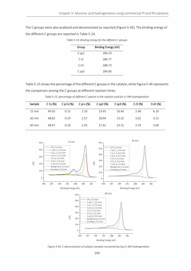
Chapter 5- Muconic acid hydrogenation using commercial Pt and Pd catalysts
143
The C groups were also analyzed and deconvoluted as reported (Figure 5-43). The binding energy of
the different C groups are reported in Table 5-14.
Table 5-14: Binding energy for the different C groups
Group Binding Energy (eV)
C sp2 284.29
C-O 286.77
C=O 288.73
C sp3 284.80
Table 5-15 shows the percentage of the different C groups in the catalyst, while Figure 5-44 represents
the comparison among the C groups at different reaction times.
Table 5-15: percentage of different C species in the catalyst used for t,t-MA hydrogenation
Sample C 1s (%) C pi b (%) C pi s (%) C sp2 (%) C sp3 (%) C-O (%) C=O (%)
15 min 49.05 0.15 2.10 23.65 16.40 2.48 6.16
30 min 48.82 0.19 2.57 28.94 13.32 3.02 3.12
60 min 48.67 0.18 2.45 27.61 14.31 3.79 3.00
300 297 294 291 288 285 282
0
1E4
2E4
3E4
4E4
5E4
CP
S
Binding Energy (eV)
CPS_C1s Scan
C sp2_1_C1s Scan
C pi s_2_C1s Scan
C pi b_3_C1s Scan
C-O_4_C1s Scan
C=O_5_C1s Scan
C sp3_6_C1s Scan
Background_C1s Scan
Envelope_C1s Scan
15 min
300 297 294 291 288 285 282
0
1E4
2E4
3E4
4E4
5E4
6E430 min
CP
S
Binding Energy (eV)
CPS_C1s Scan
C sp2_1_C1s Scan
C pi s_2_C1s Scan
C pi b_3_C1s Scan
C-O_4_C1s Scan
C=O_5_C1s Scan
C sp3_6_C1s Scan
Background_C1s Scan
Envelope_C1s Scan
300 297 294 291 288 285 282
0
1E4
2E4
3E4
4E4
5E4
6E460 min
CP
S
Binding Energy (eV)
CPS_C1s Scan
C sp2_1_C1s Scan
C pi s_2_C1s Scan
C pi b_3_C1s Scan
C-O_4_C1s Scan
C=O_5_C1s Scan
C sp3_6_C1s Scan
Background_C1s Scan
Envelope_C1s Scan
Figure 5-43: C deconvolution of catalyst samples recovered during t,t-MA hydrogenation
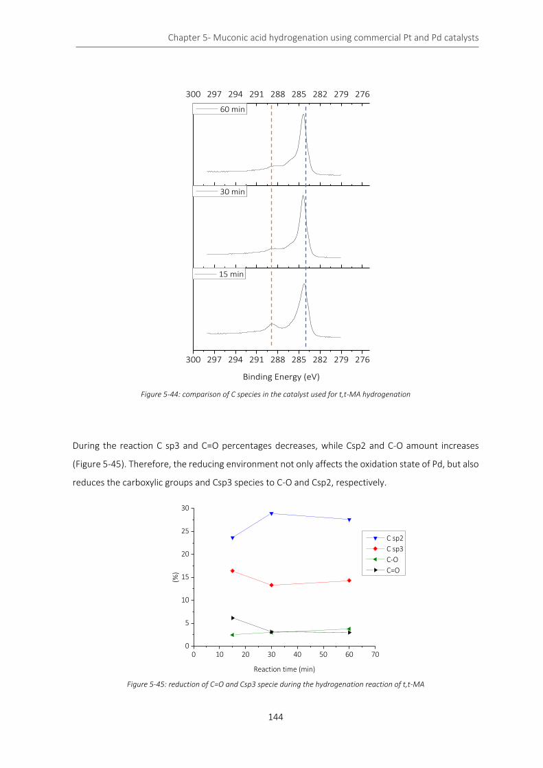
Chapter 5- Muconic acid hydrogenation using commercial Pt and Pd catalysts
144
300 297 294 291 288 285 282 279 276
300 297 294 291 288 285 282 279 276
Binding Energy (eV)
15 min
30 min
60 min
Figure 5-44: comparison of C species in the catalyst used for t,t-MA hydrogenation
During the reaction C sp3 and C=O percentages decreases, while Csp2 and C-O amount increases
(Figure 5-45). Therefore, the reducing environment not only affects the oxidation state of Pd, but also
reduces the carboxylic groups and Csp3 species to C-O and Csp2, respectively.
Figure 5-45: reduction of C=O and Csp3 specie during the hydrogenation reaction of t,t-MA
0 10 20 30 40 50 60 700
5
10
15
20
25
30
(%)
Reaction time (min)
C sp2
C sp3
C-O
C=O
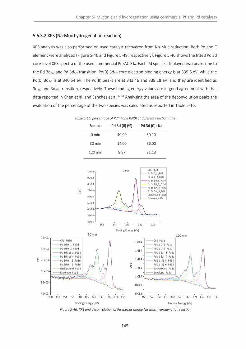
Chapter 5- Muconic acid hydrogenation using commercial Pt and Pd catalysts
145
5.6.3.2 XPS (Na-Muc hydrogenation reaction)
XPS analysis was also performed on used catalyst recovered from Na-Muc reduction. Both Pd and C
element were analyzed (Figure 5-46 and Figure 5-49, respectively). Figure 5-46 shows the fitted Pd 3d
core-level XPS spectra of the used commercial Pd/AC 5%. Each Pd species displayed two peaks due to
the Pd 3d3/2 and Pd 3d5/2 transition. Pd(0) 3d5/2 core electron binding energy is at 335.6 eV, while the
Pd(0) 3d3/2 is at 340.54 eV. The Pd(II) peaks are at 343.46 and 338.18 eV, and they are identified as
3d3/2 and 3d5/2 transition, respectively. These binding energy values are in good agreement with that
data reported in Chen et al. and Sanchez et al.32,33 Analysing the area of the deconvolution peaks the
evaluation of the percentage of the two species was calculated as reported in Table 5-16.
Table 5-16: percentage of Pd(II) and Pd(0) at different reaction time
Sample Pd 3d (II) (%) Pd 3d (0) (%)
0 min 49.90 50.10
30 min 14.00 86.00
120 min 8.87 91.13
Figure 5-46: XPS and deconvolution of Pd species during Na-Muc hydrogenation reaction
360 357 354 351 348 345 342 339 336 333 3306.0E3
8.0E3
1.0E4
1.2E4
1.4E4
1.6E4
1.8E4
CP
S
Binding Energy (eV)
CPS_Pd3d
Pd 3d 0_1_Pd3d
Pd 3d 0_2_Pd3d
Pd 3d Sat_3_Pd3d
Pd 3d Sat_4_Pd3d
Pd 3d (II)_5_Pd3d
Pd 3d (II)_6_Pd3d
Background_Pd3d
Envelope_Pd3d
120 min
348 344 340 336 3322E+03
3E+03
4E+03
5E+03
6E+03
7E+03
8E+03
9E+03
1E+04
CP
S
Binding Energy (eV)
CPS_Pd3d
Pd 3d 0_1_Pd3d
Pd 3d 0_2_Pd3d
Pd 3d (II)_5_Pd3d
Pd 3d (II)_6_Pd3d
Pd 3d Sat_4_Pd3d
Pd 3d Sat_3_Pd3d
Background_Pd3d
Envelope_Pd3d
0 min
360 357 354 351 348 345 342 339 336 333 3304E+03
5E+03
6E+03
7E+03
8E+03
9E+03
CP
S
Binding Energy (eV)
CPS_Pd3d
Pd 3d 0_1_Pd3d
Pd 3d 0_2_Pd3d
Pd 3d Sat_3_Pd3d
Pd 3d Sat_4_Pd3d
Pd 3d (II)_5_Pd3d
Pd 3d (II)_6_Pd3d
Background_Pd3d
Envelope_Pd3d
30 min
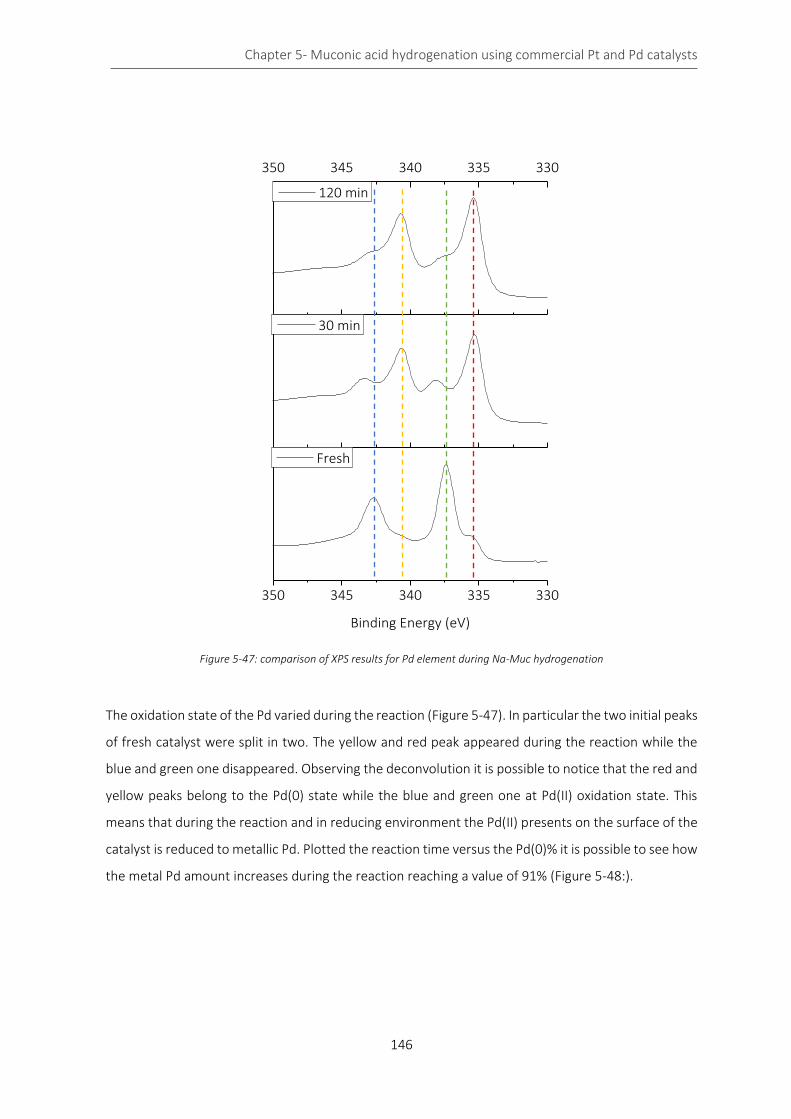
Chapter 5- Muconic acid hydrogenation using commercial Pt and Pd catalysts
146
350 345 340 335 330
350 345 340 335 330
Binding Energy (eV)
Fresh
30 min
120 min
Figure 5-47: comparison of XPS results for Pd element during Na-Muc hydrogenation
The oxidation state of the Pd varied during the reaction (Figure 5-47). In particular the two initial peaks
of fresh catalyst were split in two. The yellow and red peak appeared during the reaction while the
blue and green one disappeared. Observing the deconvolution it is possible to notice that the red and
yellow peaks belong to the Pd(0) state while the blue and green one at Pd(II) oxidation state. This
means that during the reaction and in reducing environment the Pd(II) presents on the surface of the
catalyst is reduced to metallic Pd. Plotted the reaction time versus the Pd(0)% it is possible to see how
the metal Pd amount increases during the reaction reaching a value of 91% (Figure 5-48:).
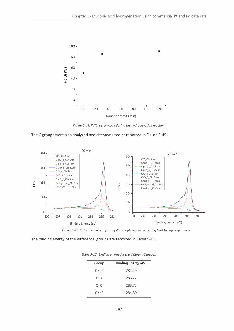
Chapter 5- Muconic acid hydrogenation using commercial Pt and Pd catalysts
147
0 20 40 60 80 100 120
0
20
40
60
80
100
Pd(0
) (%
)
Reaction time (min)
Figure 5-48: Pd(0) percentage during the hydrogenation reaction
The C groups were also analyzed and deconvoluted as reported in Figure 5-49:.
The binding energy of the different C groups are reported in Table 5-17.
Table 5-17: Binding energy for the different C groups
Group Binding Energy (eV)
C sp2 284.29
C-O 286.77
C=O 288.73
C sp3 284.80
300 297 294 291 288 285 282
0
1E4
2E4
3E4
4E4
CP
S
Binding Energy (eV)
CPS_C1s Scan
C sp2_1_C1s Scan
C pi s_2_C1s Scan
C pi b_3_C1s Scan
C-O_4_C1s Scan
C=O_5_C1s Scan
C sp3_6_C1s Scan
Background_C1s Scan
Envelope_C1s Scan
30 min
300 297 294 291 288 285 2820
1E4
2E4
3E4
4E4
5E4
6E4120 min
CP
S
Binding Energy (eV)
CPS_C1s Scan
C sp2_1_C1s Scan
C pi s_2_C1s Scan
C pi b_3_C1s Scan
C-O_4_C1s Scan
C=O_5_C1s Scan
C sp3_6_C1s Scan
Background_C1s Scan
Envelope_C1s Scan
Figure 5-49: C deconvolution of catalyst’s sample recovered during Na-Muc hydrogenation

Chapter 5- Muconic acid hydrogenation using commercial Pt and Pd catalysts
148
Table 5-18 shows the percentage of the different C groups in the catalyst while Figure 5-50 represents
the comparison among the C groups at different reaction times. No significative differences were
found between the catalyst recovered at 30 and 120 minutes of reaction. The catalyst is mainly
composed by C 1s specie while C=O is about 2%.
Table 5-18: percentage of different C species in the catalyst used for Na-Muc hydrogenation
Sample C 1s (%) C pi b (%) C pi s (%) C sp2 (%) C sp3 (%) C-O (%) C=O (%)
30 min 48.88 0.17 26.87 26.87 13.91 6.03 1.73
120 min 49.01 0.18 28.00 28.00 11.68 6.66 1.99
300 298 296 294 292 290 288 286 284 282 280
300 298 296 294 292 290 288 286 284 282 280
Binding Energy (eV)
30 min
120 min
Figure 5-50: comparison of C species in the catalyst used for Na-Muc hydrogenation
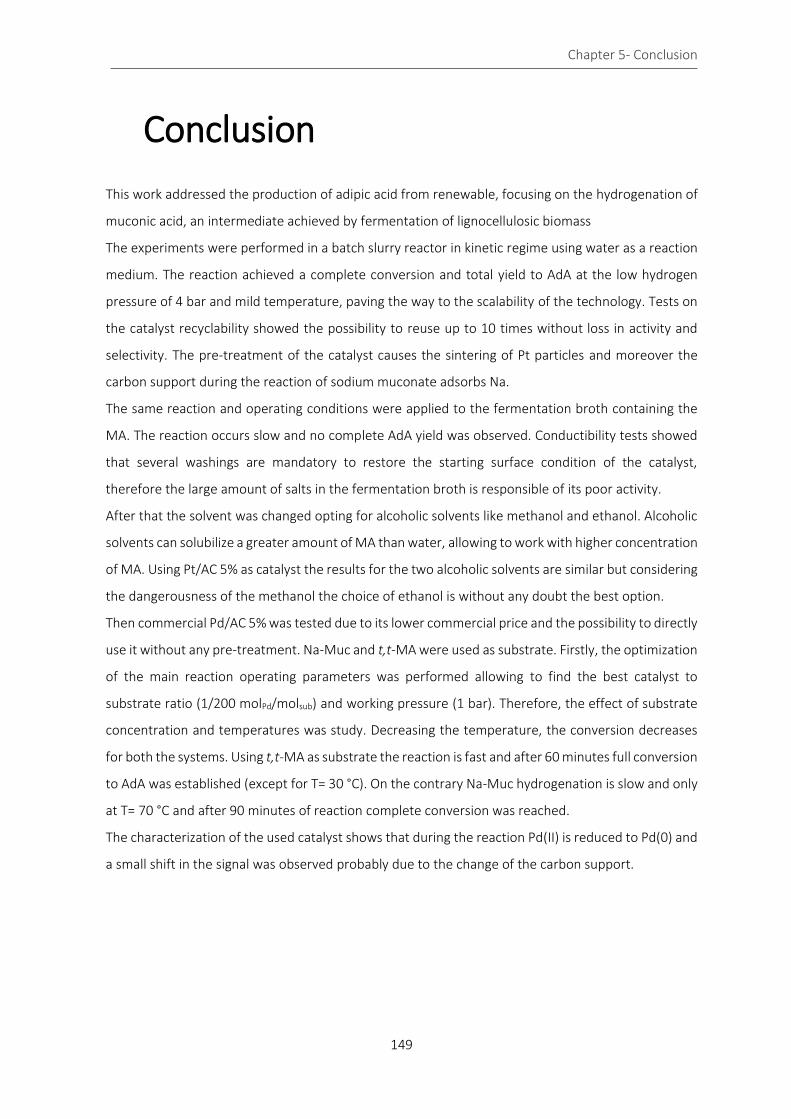
Chapter 5- Conclusion
149
Conclusion
This work addressed the production of adipic acid from renewable, focusing on the hydrogenation of
muconic acid, an intermediate achieved by fermentation of lignocellulosic biomass
The experiments were performed in a batch slurry reactor in kinetic regime using water as a reaction
medium. The reaction achieved a complete conversion and total yield to AdA at the low hydrogen
pressure of 4 bar and mild temperature, paving the way to the scalability of the technology. Tests on
the catalyst recyclability showed the possibility to reuse up to 10 times without loss in activity and
selectivity. The pre-treatment of the catalyst causes the sintering of Pt particles and moreover the
carbon support during the reaction of sodium muconate adsorbs Na.
The same reaction and operating conditions were applied to the fermentation broth containing the
MA. The reaction occurs slow and no complete AdA yield was observed. Conductibility tests showed
that several washings are mandatory to restore the starting surface condition of the catalyst,
therefore the large amount of salts in the fermentation broth is responsible of its poor activity.
After that the solvent was changed opting for alcoholic solvents like methanol and ethanol. Alcoholic
solvents can solubilize a greater amount of MA than water, allowing to work with higher concentration
of MA. Using Pt/AC 5% as catalyst the results for the two alcoholic solvents are similar but considering
the dangerousness of the methanol the choice of ethanol is without any doubt the best option.
Then commercial Pd/AC 5% was tested due to its lower commercial price and the possibility to directly
use it without any pre-treatment. Na-Muc and t,t-MA were used as substrate. Firstly, the optimization
of the main reaction operating parameters was performed allowing to find the best catalyst to
substrate ratio (1/200 molPd/molsub) and working pressure (1 bar). Therefore, the effect of substrate
concentration and temperatures was study. Decreasing the temperature, the conversion decreases
for both the systems. Using t,t-MA as substrate the reaction is fast and after 60 minutes full conversion
to AdA was established (except for T= 30 °C). On the contrary Na-Muc hydrogenation is slow and only
at T= 70 °C and after 90 minutes of reaction complete conversion was reached.
The characterization of the used catalyst shows that during the reaction Pd(II) is reduced to Pd(0) and
a small shift in the signal was observed probably due to the change of the carbon support.

Chapter 5- Bibliography
150
Bibliography
1. de Vries, J. G. & Jackson, S. D. Homogeneous and heterogeneous catalysis in industry. Catal. Sci. Technol. 2, 2009 (2012).
2. Beeck, O. Hydrogenation catalysts. Discuss. Faraday Soc. 8, 118–128 (1950).
3. Rylander, P. N. Catalytic Hydrogenation in Organic Synthesis. (Academic Press Limited, 1979).
4. Polkovnikov, B. D., Nefedov, O. M., Mikos, É. P. & Novitskaya, N. N. Sequence of hydrogenation of the double bonds of cycloheptatriene over palladium, platinum, and rhodium catalysts. Bull. Acad. Sci. USSR, Div. Chem. Sci. 17, 1175–1178 (1968).
5. Rodríguez-reinoso, F. The role of carbon materials in heterogeneous catalysis. Carbon N. Y. 36, 159–175 (1998).
6. Nerozzi, F. Heterogeneous Catalytic Hydrogenation. Platin. Met. Rev. 56, 236–241 (2012).
7. Upare, P. P. et al. Selective hydrogenation of levulinic acid to γ-valerolactone over carbon-supported noble metal catalysts. J. Ind. Eng. Chem. 17, 287–292 (2011).
8. Capelli, S. et al. Bio-adipic acid production by catalysed hydrogenation of muconic acid in mild operating conditions. Appl. Catal. B Environ. 218, 220–229 (2017).
9. Singh, U. K. & Vannice, M. A. Kinetics of liquid-phase hydrogenation reactions over supported metal catalysts — a review. Appl. Catal. A Gen. 213, 1–24 (2001).
10. van Es, T. & Staskun, B. Aldehydes from Aromatic Niriles: 4-Formylbenzenesulfonamide. in Organic synthesis database online (John Wiley and Sons, Inc., 2003). doi:https://doi.org/10.1002/0471264180.os051.06
11. Bard, A. J. & Faulkner, L. R. Electrochemical methods (Fundamentals and applications). (John Wiley and Sons, Inc., 2001).
12. Sander, R. Compilation of Henry’s law constant (version 4.0) for water as solvent. Atmos. Chem. Phys. 15, 4399–4981 (2015).
13. Chaudhari, R. V. et al. Kinetics of hydrogenation of maleic acid in a batch slurry reactor using a bimetallic Ru-Re/C catalyst. Chem. Eng. Sci. 58, 627–632 (2003).
14. Rajashekharam, M. V, Nikalje, D. D., Jaganathan, R. & Chaudhari, R. V. Hydrogenation of 2,4-Dinitrotoluene Using a Pd/Al2O3 Catalyst in a Slurry Reactor: A Molecular Level Approach to Kinetic Modeling and Nonisothermal Effects. Ind. Eng. Chem. Res. 36, 592–604 (1997).
15. Machado, R. M. Foundamentals of mass transfer and kinetics for the hydrogenation of nitrobenzene to aniline. ALR Appl. note 1, 1–14 (2007).
16. Fillion, B., Morsi, B. I., Heier, K. R. & Machado, R. M. Kinetics, Gas−Liquid Mass Transfer, and Modeling of the Soybean Oil Hydrogenation Process. Ind. Eng. Chem. Res. 41, 3052 (2002).
17. Hájek, J. & Murzin, D. Y. Liquid-Phase Hydrogenation of Cinnamaldehyde over a Ru−Sn Sol−Gel Catalyst. 1. Evaluation of Mass Transfer via a Combined Experimental/Theoretical Approach. Ind. Eng. Chem. Res. 43, 2030–2038 (2004).
18. Sano, Y., Yamaguchi, N. & Adachi, T. Mass transfer coefficients for suspended particles in agitated vessels and bubble columns. J. Chem. Eng. Japan 7, 255–261 (1974).
19. McKetta Jr., J. J. Encylopedia of Chemicals Processing and design: Volume 46-Pumps: Bypass to Reboilers. (Taylor & Francis, 1993).
20. Acres, G. J. K. & Cooper, B. J. Carbon-supported platinum metal catalysts for hydrogenation reactions. Mass transport effects in liquid phase hydrogenation over Pd/C. J. Appl. Chem. Biotechnol. 22, 769–785 (2018).
21. Niu, W., Draths, K. M. & Frost, J. W. Benzene-free synthesis of adipic acid. Biotechnol. Prog. 18, 201–211 (2002).
Chapter 5- Bibliography
151
22. Bard, A. J. & Faulkner, L. R. Electrochemical Methods: Fundamentals and Applications. (Jhon Wiley & Sons, 2000).
23. Ĉerveny, L. Palladium Catalysts In Hydrogenation Reactions. Chem. Eng. Commun. 83, 31–63 (1989).
24. Belskaya, O. B. et al. A Study of Pd/C Catalysts in the Liquid-phase Hydrogenation of 1,3,5-Trinitrobenzene and 2,4,6-Trinitrobenzoic Acid. Selection of Hydrogenation Conditions for Selective Production of 1,3,5-Triaminobenzene. Procedia Eng. 152, 110–115 (2016).
25. Cooper, J. & Beecham, J. A Study of Platinum Group Metals in Three-Way Autocatalysts. Platin. Met. Rev. 57, 281–288 (2013).
26. Carraher, J. M., Pfennig, T., Rao, R. G., Shanks, B. H. & Tessonnier, J.-P. cis,cis-Muconic acid isomerization and catalytic conversion to biobased cyclic-C 6 -1,4-diacid monomers. Green Chem. 21–25 (2017). doi:10.1039/C7GC00658F
27. Kumar, A. & Jena, H. M. Preparation and characterization of high surface area activated carbon from Fox nut (Euryale ferox) shell by chemical activation with H3PO4. Results Phys. 6, 651–658 (2016).
28. Jagiello, J. & Thommes, M. Comparison of DFT characterization methods based on N2, Ar, CO2, and H2 adsorption applied to carbons with various pore size distributions. Carbon N. Y. 42, 1227–1232 (2004).
29. Yang, G., Han, H., Li, T. & Du, C. Synthesis of nitrogen-doped porous graphitic carbons using nano-CaCO3as template, graphitization catalyst, and activating agent. Carbon N. Y. 50, 3755–3765 (2012).
30. Yu, W. et al. Nanosizing Pd on 3D porous carbon frameworks as effective catalysts for selective phenylacetylene hydrogenation. RSC Adv. 7, (2017).
31. Shang, S., Yang, X. & Tao, X. ming. Easy synthesis of carbon nanotubes with polypyrrole nanotubes as the carbon precursor. Polymer (Guildf). 50, 2815–2818 (2009).
32. Chen, X. et al. Non-covalently modified graphene supported ultrafine nanoparticles of palladium for hydrogen gas sensing. RSC ADVANCES 3, (2013).
33. Sanchez, F. et al. Hydrogen Generation from Additive-Free Formic Acid Decomposition Under Mild Conditions by Pd/C: Experimental and DFT Studies. Top. Catal. 61, 254–266 (2018).
34. Ebbesen, S. D., Mojet, B. L. & Lefferts, L. Effect of pH on the Nitrite Hydrogenation Mechanism over Pd/Al2O3 and Pt/Al2O3: Details Obtained with ATR-IR Spectroscopy. J. Phys. Chem. C 115, 1186–1194 (2011).

152
Chapter 6
Mechanism identification and
regression of kinetic parameters
In this chapter, the mechanism identification and kinetic model definition are described. The study
was developed using the results obtained from the hydrogenation reaction of sodium muconate in
water at different temperatures using Pt/AC 5% commercial catalyst.
The empirical study allowed identifying a catalyst with optimal performances in very mild conditions,
providing the data for the first kinetic study on the mechanism of muconic acid hydrogenation. At the
beginning of the study, the reaction was modelled using LHHW mechanism and kinetic parameters at
constant temperature were regressed. This reaction model showed an overestimation of the reactant
and the intermediate concentrations due to the group of the different intermediates. Divided the
intermediates and introducing the different reaction temperatures the model is able to predict the
concentration of the different species during the reaction. The results of this study are published in
Chemical Engineering Transaction Journal 57, 931-936 (2017).
Chapter 6- Mechanism identification and regression of kinetic parameters
153
6.1 State of art
Previous studies on muconic acid hydrogenation addressed only cis,cis-muconic acid (ccMA), without
considering that the cis,cis isomer is the most unstable of the three possible forms and spontaneously
evolves into the configurational isomer cis,trans (ctMA) in acidic environment at temperatures above
30 °C.1 Also, it has been extensively proven that both ccMA and ctMA tend to isomerize to trans,trans-
muconic acid (ttMA) in presence of metals that strongly bind hydrogen molecules.2,3 The choice of
ccMA for previous kinetic studies was motivated by the fact that the cis,cis isomer is the one produced
by the microorganism: this assumption still is not entirely acceptable from a full-process perspective.
Considering in fact the most plausible downstream operations for the ccMA rich fermentation broth,
the cis,cis form is unlikely to be preserved. Indeed, the filtered broth undergoes to a crystallization
step achieved by pH shift, and, due to the thermal deactivation of the bacteria and the evaporation
steps, an increase of temperature above 80 °C is required. The coupled conditions of acidic
environment and higher temperatures are therefore a realistic scenario, and the hydrogenation will
be possibly performed on a mixture of the three isomers. The presence of muconic lactones, which
actually can be formed in these conditions (and can reduce the hydrogenation selectivity), can be
avoided by shorter treatments.4
Therefore, trans,trans-muconic acid (ttMA) was selected as the model chemical for this hydrogenation
study. Even though a real application would probably deal with mixtures of MA isomers from the
purified broth (as assumed during the development of the superstructure in Chapter 3), the analysis
on the sole ttMA has several advantages. First, due to the lower solubility and higher heat of
formation, ttMA is the most recalcitrant isomer to react.5 Therefore, the reaction conditions valid for
ttMA apply also for the other isomers, leaving space for further optimizations. Second, the analytics
are simplified and accelerated, removing some of the other possible intermediates: 3-hexanedioic
acid, for example, is detected when hydrogenating ccMA,6 but it is not formed in measurable amounts
with ttMA.7 Finally, for the sake of the mechanism modelling, ttMA allows excluding the isomerization
equilibria of the reactant between cis,cis, cis,trans and trans,trans forms, reducing the number of
equations and parameters to regress. In this way, a deeper understanding of the reaction mechanism
is possible, removing parallel or concurrent pathways. All the analyses in water were performed on
sodium muconate salts, as ttMA is very insoluble in water in its acid form.
Chapter 6- Mechanism identification and regression of kinetic parameters
154
6.2 Materials and Methods
6.2.1 Experimental
The substrates were trans,trans-muconic acid (Sigma Aldrich, purity 98 %), Pt/C 5% (Taminco), butanol
(Sigma Aldrich, purity >99 %), sulfuric acid 98 % (Sigma Aldrich), sodium hydroxide (Sigma Aldrich,
purity >99 %), adipic acid (AA) (Sigma Aldrich), (2E)-2-hexenedioic acid (Sigma Aldrich, purity 98 %),
dimethyl adipate (Sigma Aldrich, purity ≥99 %). Reagents and solvent were used without further
purification.
The hydrogenation of MA was performed on the sodium muconate salt that was obtained adding to
the aqueous solution a stoichiometric amount of solid sodium hydroxide. The reaction was carried out
in a cylindrical batch autoclave equipped with two different gas lines. Helium was used to clean the
reactor and to quench the reaction, while hydrogen was used for catalyst pre-treatment and as
reagent for the hydrogenation reaction. The reaction took place in a cylindrical glass tube to avoid
that the Nickel contents in the steel could interfere. All the system was heated through an external
metal jacket and the temperature monitored with a thermocouple. The reaction mixture was stirred
with a magnetic stirrer at a stirring rate of 500 rpm. The catalyst (0.1 g) pre-treatment occurred in situ
at 6 bar of static hydrogen for 3 hours at 200 °C. The hydrogenation reaction was achieved in the
aqueous solution (10 mL, 0.7x10⁻² M). The hydrogenation tests were performed varying temperature
(40-70 °C) and keeping constant the hydrogen pressure, the amount of catalyst, the agitation speed
and reactor configuration. The reaction tests were performed in batch condition using a fresh catalyst
at the beginning of all the tests.
Sodium muconate conversion was evaluated by UV-Vis analysis. A reaction mixture sample collected
after the catalyst filtration was analysed in a spectrophotometer T60 UV-Visible Spectrophotometer
PRIXMA from 400 to 190 nm. The maximum absorption was at 264 nm. The calibration of the analysis
was performed with sodium muconate prepared from trans,trans-muconic acid. The selectivity
toward AA and monounsatured compounds was estimated by GC analyses on derivative methyl esters
(Master GC Fast Gas Cromatograph Dani Instrument equipped with an Aldrich Supelcowax 10: 60 m x
0.53 mm, film thickness 1 µm) with TCD detector operating in splitless mode. Butanol was used as
internal standard.
The recognition of the reaction intermediates was carried out with GC coupled with mass detector on
derivatized esterified products.

Chapter 6- Mechanism identification and regression of kinetic parameters
155
6.2.2 Kinetic modelling
The studied Pt/C 5 % catalyst outperformed all the others previously tested in terms of conversion
and selectivity (>99 %), even at milder pressure (4 bar). Therefore, the reaction was investigated to
characterize the kinetic parameters, which represent the basis for the scale up of laboratory data to
industry. Since trans,trans-muconic acid is a double unsaturated compound, it is reasonable to assume
a multi-step reaction, in which mono-unsaturated hexenedioic acid is formed as an intermediate
product and then is hydrogenated to AA. The presence of a solid catalyst in a slurry reactor involves
adsorption-desorption equilibria of the reacting species, thus Langmuir-Hinshelwood-Hougen-
Watson (LHHW) expressions were used to model the reaction rates.8,9 These models, originally
developed for gas phase reaction, proved to be effective also for liquid reactions, in which competitive
adsorption of hydrogen and organic molecules occurs.10,11
The macroscopic performance of a slurry reactor can be affected by the insurgence of mass-transfer
resistances among the gas (hydrogen), the liquid (water and reactants dissolved) and the solid
(catalyst particles) phases. Even though slurry reactors and the use of a catalyst in fine powder (40
µm) usually minimize transport phenomena issues, the validation of a pure kinetic regime was
necessary. Chaudari et al developed some qualitative indexes to assess whether any external or
intraparticle mass transfer phenomena are the rate determining step, taking care of the initial reaction
rate, of the stirring speed, and of the catalyst properties.10,12,13 The hydrogen concentration was
assumed to be constant throughout the reaction, given the fixed pressure and the exclusion of gas-
liquid mass transfer limitation. The nonlinear regression of model parameters, coupled with the
solution of the differential equations for the material balances in the reactor, were performed in C++
language applying Bzz-Math libraries.14 The library covers many fields of numerical analysis for
Windows and Linux users, includes parallel computations automatically enabled when possible, and
self-selects the best algorithms during computations. It is used in all continents and is the kernel of
many industrial solutions for process modeling, simulation, control, and optimization. In the simplified
mechanism, all the intermediates were considered as a single pseudo-component “IN”.
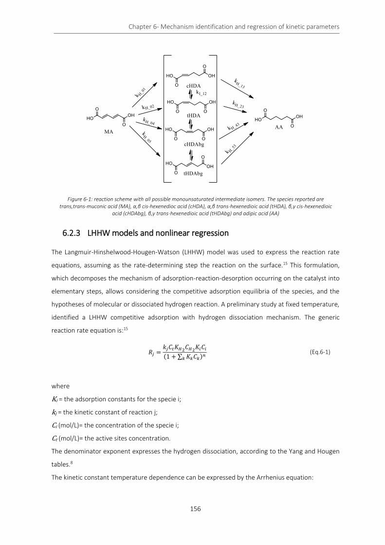
Chapter 6- Mechanism identification and regression of kinetic parameters
156
6.2.3 LHHW models and nonlinear regression
The Langmuir-Hinshelwood-Hougen-Watson (LHHW) model was used to express the reaction rate
equations, assuming as the rate-determining step the reaction on the surface.15 This formulation,
which decomposes the mechanism of adsorption-reaction-desorption occurring on the catalyst into
elementary steps, allows considering the competitive adsorption equilibria of the species, and the
hypotheses of molecular or dissociated hydrogen reaction. A preliminary study at fixed temperature,
identified a LHHW competitive adsorption with hydrogen dissociation mechanism. The generic
reaction rate equation is:15
𝑅𝑗 =𝑘𝑗𝐶𝑡𝐾𝐻2
𝐶𝐻2𝐾𝑖𝐶𝑖
(1 + ∑ 𝐾𝑘𝐶𝑘𝑘 )𝑛 (Eq.6-1)
where
Ki = the adsorption constants for the specie i;
kj = the kinetic constant of reaction j;
Ci (mol/L)= the concentration of the specie i;
Ct (mol/L)= the active sites concentration.
The denominator exponent expresses the hydrogen dissociation, according to the Yang and Hougen
tables.8
The kinetic constant temperature dependence can be expressed by the Arrhenius equation:
Figure 6-1: reaction scheme with all possible monounsaturated intermediate isomers. The species reported are trans,trans-muconic acid (MA), α,β cis-hexenedioc acid (cHDA), α,β trans-hexenedioic acid (tHDA), β,γ cis-hexenedioic
acid (cHDAbg), β,γ trans-hexenedioic acid (tHDAbg) and adipic acid (AA)
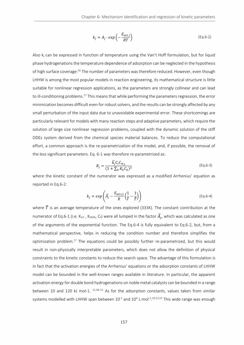
Chapter 6- Mechanism identification and regression of kinetic parameters
157
𝑘𝑗 = 𝐴𝑗 ∙ 𝑒𝑥𝑝 (−𝐸𝑎𝑡𝑡,𝑗
𝑅𝑇) (Eq.6-2)
Also kj can be expressed in function of temperature using the Van’t Hoff formulation, but for liquid
phase hydrogenations the temperature dependence of adsorption can be neglected in the hypothesis
of high surface coverage:16 The number of parameters was therefore reduced. However, even though
LHHW is among the most popular models in reaction engineering, its mathematical structure is little
suitable for nonlinear regression applications, as the parameters are strongly collinear and can lead
to ill-conditioning problems.17 This means that while performing the parameters regression, the error
minimization becomes difficult even for robust solvers, and the results can be strongly affected by any
small perturbation of the input data due to unavoidable experimental error. These shortcomings are
particularly relevant for models with many reaction steps and adaptive parameters, which require the
solution of large size nonlinear regression problems, coupled with the dynamic solution of the stiff
ODEs system derived from the chemical species material balances. To reduce the computational
effort, a common approach is the re-parametrization of the model, and, if possible, the removal of
the less significant parameters. Eq. 6-1 was therefore re-parametrized as:
𝑅𝑗 =𝑘�̃�𝐶𝑖𝐶𝐻2
(1 + ∑ 𝐾𝑘𝐶𝑘𝑘 )3 (Eq.6-3)
where the kinetic constant of the numerator was expressed as a modified Arrhenius’ equation as
reported in Eq.6-2:
𝑘𝑗 = 𝑒𝑥𝑝 (𝐴�̃� −𝐸𝑎𝑡𝑡,𝑖𝑗
𝑅(
1
𝑇−
1
�̅�)) (Eq.6-4)
where �̅� is an average temperature of the ones explored (333K). The constant contribution at the
numerator of Eq.6-1 (i.e. KH2 , KttMA, Ct) were all lumped in the factor 𝐴�̃�, which was calculated as one
of the arguments of the exponential function. The Eq.6-4 is fully equivalent to Eq.6-2, but, from a
mathematical perspective, helps in reducing the condition number and therefore simplifies the
optimization problem.17 The equations could be possibly further re-parametrized, but this would
result in non-physically interpretable parameters, which does not allow the definition of physical
constraints to the kinetic constants to reduce the search space. The advantage of this formulation is
in fact that the activation energies of the Arrhenius’ equations or the adsorption constants of LHHW
model can be bounded in the well-known ranges available in literature. In particular, the apparent
activation energy for double bond hydrogenations on noble metal catalysts can be bounded in a range
between 10 and 120 kJ mol-1. 12,18–21 As for the adsorption constants, values taken from similar
systems modelled with LHHW span between 10-1 and 104 L∙mol-1:19,22,23 This wide range was enough

Chapter 6- Mechanism identification and regression of kinetic parameters
158
to reduce sensibly the convergence time. The objective function to be minimized for the parameters
calculation was the sum of squared errors (SSE):
𝑆𝑆𝐸 = ∑(𝐶𝑖,𝑒𝑥𝑝 − 𝐶𝑖,𝑐𝑎𝑙𝑐)2
𝑖
(Eq.6-5)
where:
Ci,exp (mol/L)= experimental concentration of specie i;
Ci,calc (mol/L)= calculated concentration of specie i.
The model fitting quality was assessed comparing the final value of the SSE and the coefficient of
determination, defined as:
𝑅2% = 1 −𝑆𝑆𝐸
∑ (𝐶𝑖,𝑒𝑥𝑝 − 𝐶𝑖,𝑒𝑥�̃�)2
𝑖
(Eq.6-6)
where:
𝐶𝑖,𝑒𝑥�̃�= average experimental value.
The optimization method adopted to achieve the best parameters was based on the class of robust
minimization of BzzMath library in C++ language.17 The 95% confidence interval on the regressed
parameters were calculated using least square method analysis tools both in Matlab environment
(lsqnonlin function) and C++ (BzzMath nonLinReg), to confirm the results applying different solvers.
6.3 Results and discussion
6.3.1 Preliminary study at constant temperature
Since the main purpose of the study was to demonstrate the feasibility of MA hydrogenation in mild
conditions, lower pressures and lower temperatures were studied preferably. The reaction at 40 °C
(Figure 6-2) showed an induction period and did not achieve full conversion after 4 hours: this denotes
too slow kinetics for any practical application. A lag time is often detected in heterogeneous catalytic
systems at low temperatures, and it is due to the strong absorption of the organic species on the
active sites of the catalyst that gradually are deactivated. Low temperatures have not been sufficient
to sustain the desorption step, and full conversion cannot be achieved. Vardon et al.6 suggested a
similar explanation. An increase of temperature to 60 °C eliminated the lag time and allowed complete
conversion in only 1.5 hours. The kinetic study was then performed on the data at 60 °C, in line with
the suggestions of Scelfo et al.24 Many batches were necessary to provide a sufficient amount of
experimental data at different times. Also, the complex and time-demanding workout to characterize
the samples limited the number of the available points. To accelerate the data collection, the
Chapter 6- Mechanism identification and regression of kinetic parameters
159
intermediates were considered initially as a single pseudo-component, referred as “IN” in Table 6-1.
Two models based on LHHW adsorption mechanism were evaluated. Model A, considered the
dissociation of molecular hydrogen when it is adsorbed on the catalyst, while model B, assumed no
dissociation. The reaction rate equations are summarized in Table 6-1. Each hydrogenation step was
considered irreversible and rate-determining, if compared to the kinetics of adsorption and
desorption of all the species.
0 20 40 60 80 100 120 140 160 180 200
0
20
40
60
80
100
Co
nve
rsio
n (
%)
Reaction time (min)
40°C
50°C
60°C
70°C
Figure 6-2: hydrogenation at different temperatures
Table 6-1: generic equations for the simplified mechanism with intermediate pseudo component. Dual site L-H model according to Yang and Hougen tables, n=2 without H2 dissociation, n=3 with dissociation
Kinetic equation Reaction step
𝑅1 = 𝑘1𝐶𝑀𝐴𝐶𝐻2
(1 + 𝐾𝑀𝐴𝐶𝑀𝐴 + 𝐾𝐻 2𝐶𝐻2
+ 𝐾𝐼𝑁𝐶𝐼𝑁+𝐾𝐴𝐴𝐶𝐴𝐴)𝑛 MA hydrogenation to IN Eq.6-7
𝑅2 = 𝑘2𝐶𝐼𝑁𝐶𝐻2
(1 + 𝐾𝑀𝐴𝐶𝑀𝐴 + 𝐾𝐻 2𝐶𝐻2
+ 𝐾𝐼𝑁𝐶𝐼𝑁+𝐾𝐴𝐴𝐶𝐴𝐴)𝑛 IN hydrogenation to AA Eq.6-8
where:
k1= kinetic constant of MA hydrogenation to IN;
CMA (mol/L) = concentration of MA;
CH2 (mol/L) = concentration of H2;
KMA (m3/kmol) = adsorption constant of MA;
KH2 (m3/kmol) = adsorption constant of AA;
CIN (mol/L) = concentration of the intermediates;
KIN (m3/kmol) = adsorption constant of MA;

Chapter 6- Mechanism identification and regression of kinetic parameters
160
KAA (m3/kmol) = adsorption constant of AA;
CAA (mol/L) = concentration of AA;
k2 = kinetic constant for the hydrogenation of INT to AA.
Figure 6-3: comparison between experimental and calculated values from model A (left) and B (right)
In both the cases, the calculations failed to represent properly the experimental data. In particular,
the model showed an overestimation of the reactant and the intermediate concentrations. This trend,
common in both the models, introduced a doubt on the reliability of the experimental measures, later
confirmed by the material balances. A lack of molar quantities up to -20 % was observed during the
reaction, which reduced to 0 as long as the reactants were consumed. This peculiar trend could only
be explained by some errors in the quantification of the intermediate. After repeating the experiments
and increasing the resolution of the gas chromatograph, it was possible to identify two distinct
intermediates with different retention times. The analytical technique was then improved, so that all
the possible intermediates were considered (Table 6-2) in the following modelling.
Table 6-2: concentration of the different compound at T= 60 °C
Reaction time
(min)
CMA
(mol/L)
CcHDA
(mol/L)
CtHDA
(mol/L)
CAA
(mol/L)
0 7.00E-02 0.00E+00 0.00E+00 0.00E+00
20 5.69E-02 1.36E-03 8.25E-03 3.48E-03
40 4.28E-02 9.79E-03 9.50E-03 7.94E-03
60 2.93E-02 2.85E-03 1.53E-02 2.26E-02
90 1.46E-02 4.69E-03 2.00E-02 3.28E-02
120 1.19E-03 3.52E-03 1.10E-02 5.43E-02
180 1.75E-03 0.00E+00 0.00E+00 6.10E-02
240 1.00E-09 1.00E-09 1.00E-09 7.00E-02
A B

Chapter 6- Mechanism identification and regression of kinetic parameters
161
6.3.2 Refined mechanism and model
Since the hydrogenation catalyst promotes double bond rotation,3 all the four isomers are possible.
However, the β,γ unsaturated intermediates were not detected in significant amounts, therefore the
reaction scheme was simplified.
Three pathways were taken into consideration:
Model C: LHHW mechanism without hydrogen dissociation (n=2) with irreversible
isomerization of cHDA to tHDA;
Model D: LHHW mechanism with hydrogen dissociation (n=3) with irreversible isomerization
of cHDA to tHDA;
Model E: LHHW mechanism with hydrogen dissociation (n=3) with isomerization equilibrium
between cHDA and tHDA.
The equations used for modelling the reaction rates are reported in Table 6-3. Given the higher
number of species and reactions with respect to the first modelling attempt, the number of kinetic
parameters increases, resulting in different models which all performed a fairly good fitting (R2 higher
than 95% in all the cases). The residues were 0.0327, 0.0249 and 0.0226 for model C, D, and E,
respectively. The comparison of the residues of model C and D, equivalent in the number of
parameters, showed that hydrogen dissociates on the catalyst surface. Model E therefore assumes
the hydrogen dissociation and includes the isomerization reaction. Another tested model, analogous
to Model E but without dissociation, gave a poorer fit, confirming once again the dissociation of
hydrogen.
Table 6-3: generic equations for the refined mechanism with intermediates: dual site L-H model according to Yang and Hougen tables, n=2 without H2 dissociation, n=3 with dissociation
Kinetic equation Reaction step
𝑅𝐻_01 = 𝑘_ℎ01
∗ 𝐶1𝐶𝐻2
(1 + ∑ 𝐾𝑖𝐶𝑖)𝑛
MA hydrogenation to cHDA (Eq.6-9)
𝑅𝐻_02 = 𝑘_ℎ02
∗ 𝐶1𝐶𝐻2
(1 + ∑ 𝐾𝑖𝐶𝑖)𝑛
MA hydrogenation to tHDA (Eq.6-10)
𝑅𝐻_13 = 𝑘_ℎ13
∗ 𝐶1𝐶𝐻2
(1 + ∑ 𝐾𝑖𝐶𝑖)𝑛
cHDA hydrogenation to AdA (Eq.6-11)
𝑅𝐻_23 = 𝑘_ℎ23
∗ 𝐶2𝐶𝐻2
(1 + ∑ 𝐾𝑖𝐶𝑖)𝑛
tHDA hydrogenation to AdA (Eq.6-12)
𝑅𝐼_21 = 𝑘_𝑖21
∗ 𝐶2
(1 + ∑ 𝐾𝑖𝐶𝑖)𝑛
and
𝑅𝐼_12 = 𝑘_𝑖12
∗ 𝐶1
(1 + ∑ 𝐾𝑖𝐶𝑖)𝑛
Isomerization cHDA <-> tHDA (Eq.6-13)

Chapter 6- Mechanism identification and regression of kinetic parameters
162
Table 6-4: calculated parameters for the three models, adsorption constants Ki are in L/mol
KMA KcHDA KtHDA KAdA KH2 k_h01 k_h02 k_h13 k_h23 k_i12(i21)
C 67.36 77.17 2.14E-3 2.83 1.75E-1 6.61E-1 5.96E-1 4.60 5.09E-1 1.01E-3
D 15.90 2.60E-1 1.87E-2 3.25 2.33E-2 1.86E-1 1.70E-1 1.28 1.51E-1 1.00E-1
E 12.46 14.91 1.00E-5 2.92E-2 1.08E-2 1.13E-1 9.93E-2 9.52E-1 1.00E-5 2.27E-4
(5.14E-4)
Observing the parameter values of Table 6-4, however, it was clear that the model had to be further
refined. In fact, the trans configuration of the intermediate should be theoretically favored due to its
lower steric hindrance, however, comparing the two kinetic constants reported, the reaction seems
to move backward.
These results therefore served as an indication, before more experimental data became available. In
addition, the kinetic constants showed an undue variability from model to model, especially for model
D. However, it was impossible to compare the values to other published literature, since no data for
muconic acid and derivatives are available for benchmarking. Nonetheless, some confirmation on the
relative values of the adsorption constants can be found in Chaudhari et al.,22 who studied the kinetics
of hydrogenation of maleic acid to succinic acid in a slurry reactor, a similar system to MA. They
observed that the unsaturated acid adsorbs preferably, confirming the relative magnitude of the
calculated constants, even though their investigated temperatures were far higher than 230 °C.
6.3.2.1 Model regression with temperature dependence
The reaction mechanism identified in the preliminary tests is presented in Figure 6-4. The first step of
hydrogenation on ttMA yields two isomers, namely (2Z)-2-hexenedioic acid (tHDA) and (2E)-2-
hexenedioic acid (cHDA), in a single irreversible step. The concentration of the intermediates is
regulated by an equilibrium isomerization reaction. The second step of hydrogenation yields adipic
acid (AA) from both the intermediates.

Chapter 6- Mechanism identification and regression of kinetic parameters
163
Figure 6-4: hypothesized reaction scheme of model LHHW_17P
The experimental data used for the regression are reported in Table 6-5.
Table 6-5: experimental data used for the regression of parameter
Time
(s)
Temperature
(K)
ttMA
(mol/L)
cHDA
(mol/L)
tHDA
(mol/L)
AA
(mol/L)
H2
(mol/L)
0
323
6.96E-02 0.00E+00 0.00E+00 0.00E+00 2.73E-03
1200 4.80E-02 1.47E-03 1.45E-02 5.69E-03 2.73E-03
2400 3.55E-02 8.39E-04 1.82E-02 1.50E-02 2.73E-03
3600 2.07E-02 1.46E-03 2.22E-02 2.52E-02 2.73E-03
4500 7.56E-03 3.59E-03 2.96E-02 2.89E-02 2.73E-03
5400 6.47E-04 3.53E-03 2.26E-02 4.28E-02 2.73E-03
7200 0.00E+00 2.12E-03 8.51E-03 5.90E-02 2.73E-03
10800 6.96E-05 0.00E+00 0.00E+00 6.95E-02 2.73E-03
14400 0.00E+00 0.00E+00 0.00E+00 6.96E-02 2.73E-03
0
333
6.96E-02 0.00E+00 0.00E+00 0.00E+00 2.59E-03
1200 4.35E-02 1.13E-03 1.63E-02 8.67E-03 2.59E-03
1800 3.09E-02 1.83E-03 2.21E-02 1.48E-02 2.59E-03
2400 2.29E-02 2.76E-03 2.10E-02 2.29E-02 2.59E-03
3000 1.98E-02 2.82E-03 1.95E-02 2.75E-02 2.59E-03
4500 7.66E-04 2.72E-03 1.48E-02 5.13E-02 2.59E-03
6900 1.33E-03 0.00E+00 0.00E+00 7.00E-02 2.59E-03
9000 0.00E+00 0.00E+00 0.00E+00 7.00E-02 2.59E-03
0
343
6.96E-02 0.00E+00 0.00E+00 0.00E+00 2.47E-03
600 4.85E-02 6.87E-04 8.05E-03 1.24E-02 2.47E-03
1200 3.01E-02 3.32E-03 1.27E-02 2.34E-02 2.47E-03
2400 1.10E-02 1.86E-03 1.82E-02 3.85E-02 2.47E-03
3600 0.00E+00 0.00E+00 0.00E+00 6.96E-02 2.47E-03
6000 0.00E+00 0.00E+00 0.00E+00 6.96E-02 2.47E-03
7200 0.00E+00 0.00E+00 0.00E+00 6.96E-02 2.47E-03
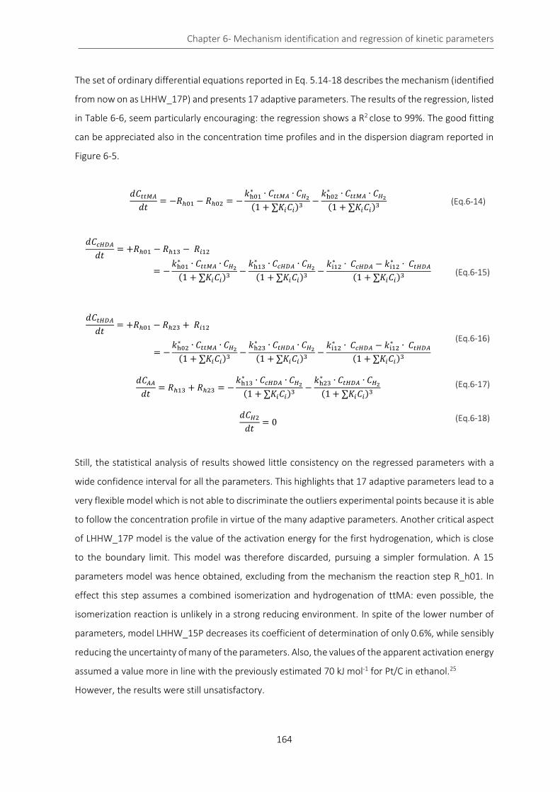
Chapter 6- Mechanism identification and regression of kinetic parameters
164
The set of ordinary differential equations reported in Eq. 5.14-18 describes the mechanism (identified
from now on as LHHW_17P) and presents 17 adaptive parameters. The results of the regression, listed
in Table 6-6, seem particularly encouraging: the regression shows a R2 close to 99%. The good fitting
can be appreciated also in the concentration time profiles and in the dispersion diagram reported in
Figure 6-5.
𝑑𝐶𝑡𝑡𝑀𝐴
𝑑𝑡= −𝑅ℎ01 − 𝑅ℎ02 = −
𝑘h01∗ ∙ 𝐶𝑡𝑡𝑀𝐴 ∙ 𝐶𝐻2
(1 + ∑𝐾𝑖𝐶𝑖)3
−𝑘h02
∗ ∙ 𝐶𝑡𝑡𝑀𝐴 ∙ 𝐶𝐻2
(1 + ∑𝐾𝑖𝐶𝑖)3
(Eq.6-14)
𝑑𝐶𝑐𝐻𝐷𝐴
𝑑𝑡= +𝑅ℎ01 − 𝑅ℎ13 − 𝑅𝑖12
= −𝑘h01
∗ ∙ 𝐶𝑡𝑡𝑀𝐴 ∙ 𝐶𝐻2
(1 + ∑𝐾𝑖𝐶𝑖)3
−𝑘h13
∗ ∙ 𝐶𝑐𝐻𝐷𝐴 ∙ 𝐶𝐻2
(1 + ∑𝐾𝑖𝐶𝑖)3
−𝑘i12
∗ ∙ 𝐶𝑐𝐻𝐷𝐴 − 𝑘i12∗ ∙ 𝐶𝑡𝐻𝐷𝐴
(1 + ∑𝐾𝑖𝐶𝑖)3
(Eq.6-15)
𝑑𝐶𝑡𝐻𝐷𝐴
𝑑𝑡= +𝑅ℎ01 − 𝑅ℎ23 + 𝑅𝑖12
= −𝑘h02
∗ ∙ 𝐶𝑡𝑡𝑀𝐴 ∙ 𝐶𝐻2
(1 + ∑𝐾𝑖𝐶𝑖)3
−𝑘h23
∗ ∙ 𝐶𝑡𝐻𝐷𝐴 ∙ 𝐶𝐻2
(1 + ∑𝐾𝑖𝐶𝑖)3
−𝑘i12
∗ ∙ 𝐶𝑐𝐻𝐷𝐴 − 𝑘i12∗ ∙ 𝐶𝑡𝐻𝐷𝐴
(1 + ∑𝐾𝑖𝐶𝑖)3
(Eq.6-16)
𝑑𝐶𝐴𝐴
𝑑𝑡= 𝑅ℎ13 + 𝑅ℎ23 = −
𝑘h13∗ ∙ 𝐶𝑐𝐻𝐷𝐴 ∙ 𝐶𝐻2
(1 + ∑𝐾𝑖𝐶𝑖)3
−𝑘h23
∗ ∙ 𝐶𝑡𝐻𝐷𝐴 ∙ 𝐶𝐻2
(1 + ∑𝐾𝑖𝐶𝑖)3
(Eq.6-17)
𝑑𝐶𝐻2
𝑑𝑡= 0 (Eq.6-18)
Still, the statistical analysis of results showed little consistency on the regressed parameters with a
wide confidence interval for all the parameters. This highlights that 17 adaptive parameters lead to a
very flexible model which is not able to discriminate the outliers experimental points because it is able
to follow the concentration profile in virtue of the many adaptive parameters. Another critical aspect
of LHHW_17P model is the value of the activation energy for the first hydrogenation, which is close
to the boundary limit. This model was therefore discarded, pursuing a simpler formulation. A 15
parameters model was hence obtained, excluding from the mechanism the reaction step R_h01. In
effect this step assumes a combined isomerization and hydrogenation of ttMA: even possible, the
isomerization reaction is unlikely in a strong reducing environment. In spite of the lower number of
parameters, model LHHW_15P decreases its coefficient of determination of only 0.6%, while sensibly
reducing the uncertainty of many of the parameters. Also, the values of the apparent activation energy
assumed a value more in line with the previously estimated 70 kJ mol-1 for Pt/C in ethanol.25
However, the results were still unsatisfactory.
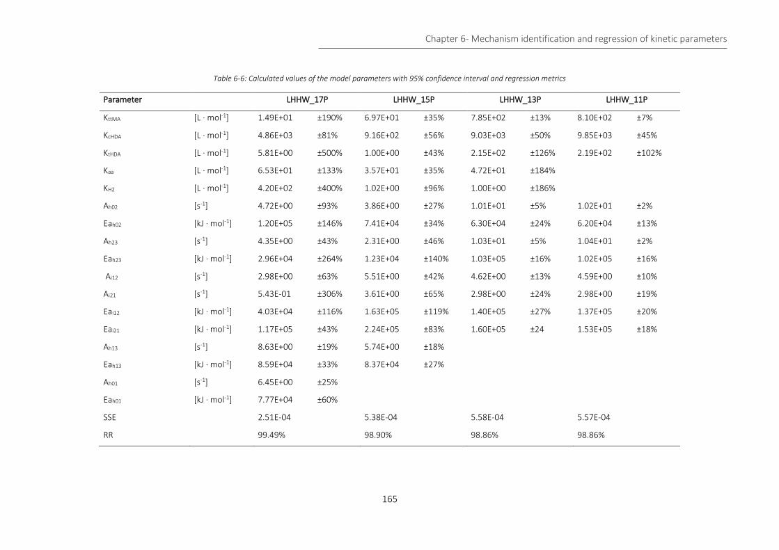
Chapter 6- Mechanism identification and regression of kinetic parameters
165
Table 6-6: Calculated values of the model parameters with 95% confidence interval and regression metrics
Parameter LHHW_17P LHHW_15P LHHW_13P LHHW_11P
KttMA [L ∙ mol-1] 1.49E+01 ±190% 6.97E+01 ±35% 7.85E+02 ±13% 8.10E+02 ±7%
KcHDA [L ∙ mol-1] 4.86E+03 ±81% 9.16E+02 ±56% 9.03E+03 ±50% 9.85E+03 ±45%
KtHDA [L ∙ mol-1] 5.81E+00 ±500% 1.00E+00 ±43% 2.15E+02 ±126% 2.19E+02 ±102%
Kaa [L ∙ mol-1] 6.53E+01 ±133% 3.57E+01 ±35% 4.72E+01 ±184%
KH2 [L ∙ mol-1] 4.20E+02 ±400% 1.02E+00 ±96% 1.00E+00 ±186%
Ah02 [s-1] 4.72E+00 ±93% 3.86E+00 ±27% 1.01E+01 ±5% 1.02E+01 ±2%
Eah02 [kJ ∙ mol-1] 1.20E+05 ±146% 7.41E+04 ±34% 6.30E+04 ±24% 6.20E+04 ±13%
Ah23 [s-1] 4.35E+00 ±43% 2.31E+00 ±46% 1.03E+01 ±5% 1.04E+01 ±2%
Eah23 [kJ ∙ mol-1] 2.96E+04 ±264% 1.23E+04 ±140% 1.03E+05 ±16% 1.02E+05 ±16%
Ai12 [s-1] 2.98E+00 ±63% 5.51E+00 ±42% 4.62E+00 ±13% 4.59E+00 ±10%
Ai21 [s-1] 5.43E-01 ±306% 3.61E+00 ±65% 2.98E+00 ±24% 2.98E+00 ±19%
Eai12 [kJ ∙ mol-1] 4.03E+04 ±116% 1.63E+05 ±119% 1.40E+05 ±27% 1.37E+05 ±20%
Eai21 [kJ ∙ mol-1] 1.17E+05 ±43% 2.24E+05 ±83% 1.60E+05 ±24 1.53E+05 ±18%
Ah13 [s-1] 8.63E+00 ±19% 5.74E+00 ±18%
Eah13 [kJ ∙ mol-1] 8.59E+04 ±33% 8.37E+04 ±27%
Ah01 [s-1] 6.45E+00 ±25%
Eah01 [kJ ∙ mol-1] 7.77E+04 ±60%
SSE 2.51E-04 5.38E-04 5.58E-04 5.57E-04
RR 99.49% 98.90% 98.86% 98.86%

Chapter 6- Mechanism identification and regression of kinetic parameters
166
Figure 6-5: concentration profiles for the hydrogenation of ttMA on Pt/C 5% catalyst at 4 bar of hydrogen. Results of the regression with model LHHW_17P
It is clear that the equilibrium is strongly shifted towards tHDA, therefore, the hydrogenation of the
cHDA intermediate is expected to have little effect on the overall mechanism. The reaction R_h13 was
therefore neglected, obtaining a more simplified model with 13 parameters, referred as LHHW_13P
with comparable residuals. Interestingly, the Arrhenius reaction rates parameters converged to
acceptable values with a reduction of the confidence interval, but the adsorption constants saw a
broadened confidence. Focusing on the adsorption constants of the dual site Langmuir Hinshelwood
model, it should be noted that the values are still comparable with the estimates for 2,4-
dinitrotoluene hydrogenation on carbon dispersed catalysts at similar temperatures.17
The large confidence interval for the adsorption constants depends on the fact that the denominator
parameters are the most correlated, as shown by a least square analysis performed with BzzMath
library tools. The t-test and p-test pointed KtHDA, KAA and KH2 as “redundant parameters”. This model
was further analyzed performing a sensitivity analysis on the parameters, whose results are shown in
Figure 6-6.
0 2000 4000 6000 8000 10000 120000
0.01
0.02
0.03
0.04
0.05
0.06
0.07
0.08Temperature 323 K
time [s]
C(t
)
[mol/L]
0 2000 4000 6000 80000
0.01
0.02
0.03
0.04
0.05
0.06
0.07
0.08Temperature 333 K
time [s]
C(t
)
[mol/L]
0 1000 2000 3000 4000 5000 60000
0.01
0.02
0.03
0.04
0.05
0.06
0.07
0.08Temperature 343 K
time [s]
C(t
)
[mol/L]
ttMA exp
cHDA exp
tHDA exp
AA exp
ttMA calc
cHDA calc
tHDA calc
AA calc
0 0.02 0.04 0.060
0.01
0.02
0.03
0.04
0.05
0.06
0.07Dispersion
Calculated [mol/L]
Experim
enta
l [m
ol/L]

Chapter 6- Mechanism identification and regression of kinetic parameters
167
Figure 6-6: sensitivity analysis on the parameters of model LHHW_13P
The parameters that minimally affect the regression results were, in order from the less relevant, KH2,
KAA and KtHDA. Provided the constant concentration of H2 and the lower value of the adsorption
constant (close to the lower limit) the contribution of the group KH2CH2 could be neglected (<<1). Also,
the group KAACAA was neglected, as the adsorption constants of saturated compounds was far lower
than saturated ones. The obtained model had therefore 11 parameters (identified as LHHW_11P),
resulting in a minimal reduction of the coefficient of determination. The statistical analysis showed
that KtDA was still affected by collinearity, but all the other values presented acceptable confidence
intervals as shown in Table 6-6. The concentration time profiles and in the dispersion diagram for
LHHW_11P are presented in Figure 6-7. In conclusion, the LHHW_11P model is to be preferred as
simple but sound in representing some of the experimental data.
-0.2 -0.15 -0.1 -0.05 0 0.05 0.1 0.15 0.2 0.250
0.01
0.02
0.03
0.04
0.05
0.06
%perturbation
%S
SE
0
Parameter Sensitivity
K
tMA
KcHDA
KtHDA
KAA
KH2
Ah02
Eath02
Ah23
Eath23
Ai12
Ai21
Eati21
Eati21
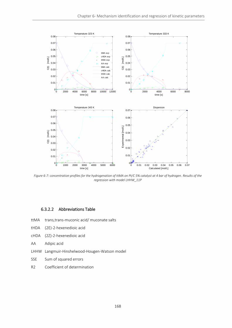
Chapter 6- Mechanism identification and regression of kinetic parameters
168
Figure 6-7: concentration profiles for the hydrogenation of ttMA on Pt/C 5% catalyst at 4 bar of hydrogen. Results of the regression with model LHHW_11P
6.3.2.2 Abbreviations Table
ttMA trans,trans-muconic acid/ muconate salts
tHDA (2E)-2-hexenedioic acid
cHDA (2Z)-2-hexenedioic acid
AA Adipic acid
LHHW Langmuir-Hinshelwood-Hougen-Watson model
SSE Sum of squared errors
R2 Coefficient of determination
0 2000 4000 6000 8000 10000 120000
0.01
0.02
0.03
0.04
0.05
0.06
0.07
0.08Temperature 323 K
time [s]
C(t
)
[mol/L]
0 2000 4000 6000 80000
0.01
0.02
0.03
0.04
0.05
0.06
0.07
0.08Temperature 333 K
time [s]
C(t
)
[mol/L]
0 1000 2000 3000 4000 5000 60000
0.01
0.02
0.03
0.04
0.05
0.06
0.07
0.08Temperature 343 K
time [s]
C(t
)
[mol/L]
ttMA exp
cHDA exp
tHDA exp
AA exp
ttMA calc
cHDA calc
tHDA calc
AA calc
0 0.01 0.02 0.03 0.04 0.05 0.06 0.070
0.01
0.02
0.03
0.04
0.05
0.06
0.07Dispersion
Calculated [mol/L]
Experim
enta
l [m
ol/L]
Chapter 6- Conclusion
169
Conclusion
Several models were used to interpret the experimental values, developed according to the LHHW
theory, which considers the species adsorption-desorption equilibria of the involved species. A dual-
step hydrogenation mechanism was demonstrated, characterized by hydrogen dissociation on the
metal. The mechanism is the following: ttMA is hydrogenated first to tHDA, that undergoes an
isomerization reaction to cHDA, promoted by the catalyst activation of the double bond. The
intermediates are further hydrogenated to AA. This led to the formulation of a first model with 17
adaptive parameters, able to fit the data but strongly affected by multicollinearity. The parameters
number was therefore reduced to 11, to achieve a final model with a good fit of the experimental data
and characterized by kinetic constants in line with previous literature estimates of similar systems.
This very first detailed study of the hydrogenation of muconic acid provided an insight of the kinetic
parameters, which currently are the sole reference values for this system. Even though the model was
able to fit satisfactorily the experimental data, some topics deserve further investigation.
- An aspect that has a key role in the hydrogenation dynamics is the adsorption/desorption of
the species on the catalyst. Even though LHHW model takes into account these phenomena,
the model has been questioned, as performs many simplifications. For this reason, a specific
study on the adsorption equilibria of muconates on the catalyst support needs to be
performed. The aim is including in the kinetic equations an explicit and detailed temperature-
dependent adsorption model. This will eventually reduce also the computational efforts for
the kinetic regression.
- The present model can be further refined exploring and modelling the effects of a wider range
of reaction conditions, collecting data on the effects of the catalyst amount, the initial species
concentration, a wider span of temperatures, and possibly different reactor configurations.
In this way the model could be better employed for simulating scaled-up applications, to
estimate the performance and the costs of an industrial hydrogenation process of muconic
acid.
In general, the hydrogenation model development and the optimization of the reaction conditions
gave very encouraging results, but the work is still at its beginning.

Chapter 6- Regression model and code
170
Regression model and code
Code for the regression of the kinetic parameters of a LHHW model in C++ language. The results are then compared with the least squares analysis on Matlab and plotted
1. Leastsquares17PModel4 (C++) 2. LHHW_17P_confidence_diss.m (MATLAB) 3. LHHW_17P_print_diss.m (MATLAB)
Function 1: Leastsquares17PModel4 (C++) Scope: Performs the SSE minimization to provide the kinetic parameters of a LHHW model of the hydrogenation of muconic acid to adipic acid. #define BZZ_COMPILER 3 #include "BzzMath.hpp" #define SSE_STD ////////////////////////////////////////////////////////////////////////////////////////////////////////////////////////////////////////////////////////////// // GLOBAL VARIABLES double ResMin(BzzVector &b); // Residues ycalc- yexp ->to be minimized BzzMatrix ModelOdeMB(BzzVector &b, int &flag); // Function for calculating the y calc to regress b parameters [n°models, n°pt exp, parameters, time, exp points] void MatBalModel4(BzzVector&y, double t, BzzVector &f); // mat bal function BzzVector bOdeMB; // adaptive parameters BzzVector tOdeMB; // t integration time points int numModels = 1; // Number of models int numX; // Nr columns input matrix int numY; // Nr input variables int numExperiments; // Nr experimental points double T; // Temperature int NumPar = 17; // Number of adaptive parameters in the model double R = 8.3144; // Universal gas constant J/mol/K BzzVector bGL(NumPar); // adaptive param of LHHV model, updated by function ModelOdeMB BzzMatrix X; // Input matrix acquired by file X.dat BzzMatrix Y; // Input matrix acquired by file Y.dat BzzMatrix Ycalc; // Calculated matrix by ModelOdeMB BzzVector yexp; FILE *risultati; // output file pointer double RR; // RR relative residual, or normalized SSE double SSE; // SSE sum of squared error ////////////////////////////////////////////////////////////////////////////////////////////////////////////////////////////////////////////////////////////// void main(void) { bzzOpenMP = 0; // parallel computation deactivation bzzWarningWindow = 0; // warning deactivation int maxIter = 10000; // max iterations robust BzzVector pOpt;

Chapter 6- Regression model and code
171
// print results risultati = fopen("myresults.txt", "w"); fprintf(risultati, " %s\n ", "CALCOLO PARAMETRI CINETICI IDROGENAZIONE ACIDO MUCONICO IN ACQUA"); fprintf(risultati, " %s\n ", "Modello a 17 parametri (serie 4HYDnodiss) vin SMART, 2 run davero"); printf(" %s\n ", "CALCOLO PARAMETRI CINETICI IDROGENAZIONE ACIDO MUCONICO IN ACQUA"); printf(" %s\n ", "Modello a 17 parametri (serie 4HYDnodiss) vin SMART, 2 run davero"); //data acquisition BzzMatrix inputX; Load(&inputX, "Xinput.dat"); BzzMatrix inputY; Load(&inputY, "Yinput.dat"); numExperiments = inputX.Rows(); // nr lines= nr experimental points fprintf(risultati, "%s\t %i\n", "numero pti sperimentali", numExperiments); printf("%s\t\t %i\n\n\n", "numero pti sperimentali", numExperiments); numY = inputY.Columns(); // Measured variables (they are 5: MucA, Hdioc cis, Hdioc trans, AdiA, Hydr) numX = inputX.Columns(); // Measured variables in X (they are 7: Temperature, measured time, e y0) BzzMatrix Xload(numExperiments, numX, 1, 1, inputX); X = Xload; BzzMatrix Yload(numExperiments, numY, 1, 1, inputY); // Exp points matrix. numExp lines, numY columns, taken from position 1,1, of input matrix inputY Y = Yload; Y.UseMatrixAsVector(&yexp); //vector experimental points ChangeDimensions(numExperiments, &tOdeMB); //vector tOdeMB is resized so that measure times correspond to the calculated times for (int i; i <= numExperiments; i = i + 1) { tOdeMB[i] = X[i][2]; } BzzMinimizationRobust mr; // Class minimization robust // 17 PARAMTETERS ++ CONSTRAINTS BzzVector bL(NumPar, 0., 0., 0., 0., 0., 0., 2.5e4, 0., 2.5e4, 0., 0., 0., 0., 0., 2.5e4, 0., 2.5e4); BzzVector bU(NumPar, 1.e6, 1.e6, 1.e6, 1.e6, 1.e6, 1.e6, 6.e4, 1.e6, 6.e4, 1.e6, 1.e6, 1.e6, 1.e6, 1.e6, 6.e4, 1.e6, 6.e4); BzzVector b0(NumPar, 49.439346, 0.434629, 109.909861, 0.000154, 533.932809, 0.259200, 25446.403051, 1.786284, 25069.625964, 13.748135, 11.788726, 94.644664, 55778.595363, 2.729225, 59999.836649, 1.730708, 25000.005689); //NO CONSTRAINTS //BzzVector bL(NumPar), bU(NumPar); // Search limits //BzzVector b0(NumPar);
//b0 = 1.; //bU = 1.e6;
//////////////////////////////////////////////////////////////////// // CALCULATION

Chapter 6- Regression model and code
172
//1 step printf("\n\n%-s\n", "PrimoStep..."); mr(b0, ResMin, bL, bU); // initialize object mr [1attempt, fun, min and max] mr(maxIter); // Call mr.BzzPrint("Results 1"); mr.GetSolution(&pOpt); // 2 Step printf("\n\n%-s\n", "SecondoStep..."); mr(pOpt, ResMin, bL, bU); mr(maxIter); mr.BzzPrint("Results 2"); mr.GetSolution(&pOpt); // 3 Step printf("\n\n%-s\n", "TerzoStep..."); mr(pOpt, ResMin, bL, bU); mr(maxIter); mr.BzzPrint("Results 3"); mr.GetSolution(&pOpt); //4 Step printf("\n\n%-s\n", "QuartoStep..."); mr(pOpt, ResMin, bL, bU); mr(maxIter); mr.BzzPrint("Results 4"); mr.GetSolution(&pOpt); //Plot screen pOpt.BzzPrint("\n\n\n\n%-s\n", "Parametri final:"); printf("%s\t %f\n", "SSE", SSE); // resudues and par printf("%s\t %f\n", "RR%", RR*100.); //plot to file myresults fprintf(risultati, "%s\t %f\n", "SSE", SSE); fprintf(risultati, "%s\t %f\n", "RR%", RR*100.); BzzMatrix rosematrice; rosematrice = Ycalc; int roserighe = rosematrice.Rows(); int rosecolonne = rosematrice.Columns(); int rosenmat, rosemmat; fprintf(risultati, "\n\n %s\t\n %i\t %i\n ", "matrice Ycalc ", roserighe, rosecolonne); for (int rosenmat = 1; rosenmat <= roserighe; rosenmat++) { for (int rosemmat = 1; rosemmat <= rosecolonne; rosemmat++) { fprintf(risultati, "%f\t", rosematrice[rosenmat][rosemmat]); } fprintf(risultati, "\n\n"); } } //END MAIN //////////////////////////////////////////////////////////////////////////////////////////////////////////////////////////////////////////////////////////////% Residues function (Objective fun to be minimized) double ResMin(BzzVector &b) { int flag;

Chapter 6- Regression model and code
173
Ycalc = ModelOdeMB(b, flag); // calculated points //Convergence check if (flag == 1) { bzzUnfeasible = 1; //printf("\n%-s\n","cambiamo il giro..."); return 0.; }
#ifdef SSE_STD BzzVector ycalc, diff, prod, prodnorm; Ycalc.UseMatrixAsVector(&ycalc); // big result matrix into vector diff = yexp - ycalc; // SSE difference ElementByElementProduct(diff, diff, &prod);// squared difference SSE = prod.GetSumElements(); // Sum of squared difference
#endif
#ifdef SSE_NORM //printf("%s\t %f\n", "RR", RR); BzzVector ycalc, diff, prod, prodnorm; Ycalc.UseMatrixAsVector(&ycalc); / diff = yexp - ycalc; int sz = diff.Size(); BzzVector diffnorm(sz); for (int i = 1; i <= sz; i = i + 1) { diffnorm[i] = fabs(diff[i] / (yexp[i] + 10.e-5)); } //system("pause"); //ElementByElementProduct(diffnorm, diffnorm, &prodnorm); double RR0; SSE = diffnorm.GetSumElements(); double szf = sz*1.; RR = RR0 / szf;
#endif return (SSE); } //////////////////////////////////////////////////////////////////////////////////////////////////////////////////////////////////////////////////////////////% Solution of the material balances (ODE integration) BzzMatrix ModelOdeMB(BzzVector &b, int &flag) // generates the calculated Ycalc values { flag = 0; bGL = b; int i = 1; BzzMatrix y0m(numExperiments, numY, 1, 3, X); // initial conditions matrix BzzVector y0(numY); // vector initial conditions, correspond to the 3rd column of inpit matrix X BzzVector yMin(numY), yy(numY); // min y=0. Positive value constraint BzzMatrix Ycalcload(numExperiments, numY); fprintf(risultati, "%s\n\n", "valori parziali parametri");

Chapter 6- Regression model and code
174
//17 PARAM fprintf(risultati, " %s\t %f\t %f\t %f\t %f\t %f\t %f\t %f\t %f\t %f\t %f\t %f\t %f\t %f\t %f\t %f\t %f\t %f\n ", "parametri regrediti", bGL[1], bGL[2], bGL[3], bGL[4], bGL[5], (bGL[6]), bGL[7], (bGL[8]), bGL[9], (bGL[10]), (bGL[11]), bGL[12], bGL[13], bGL[14], bGL[15], bGL[16], bGL[17]); // ODE SOLUTION BzzOdeStiff o; o.SetMinimumConstraints(&yMin); // Constraint y>=0 for (i = 1; i <= numExperiments; i = i + 1) { y0 = y0m.GetRow(i); o.SetInitialConditions(y0, 0., MatBalModel4HYD); T = X[i][1]; // Temperature considered, updated on the global yy = o(tOdeMB[i]); // Integration: each step corresponds to the experimental point. Integrates from 0 to tOdeMB[i] if (o.GetCalculationState() != 1 && o.GetCalculationState() != 2) { flag = 1; //If it does not converge } Ycalcload.SetRow(i, yy); } return (Ycalcload); } ////////////////////////////////////////////////////////////////////////////////////////////////////////////////////////////////////////////////////////////// // Regression models void MatBalModel4(BzzVector&y, double t, BzzVector &f) //LHHW with H2 dissociation ed R_h13 { // Model: 17 parameters // Idrogenazione irreversibile muconico solo a intermedio trans, equilibrio isomerizzazione trans cis, idrogenazione irreversibile del trans ad adipico // Le costanti sono LHHW CON formulazione Arrhenius // Dissociazione idrogeno esplicito // Si idrogena anche int CIS bOdeMB = bGL; double k333_h02 = bOdeMB[6]; double Ea333_h02 = bOdeMB[7]; double k333_h23 = bOdeMB[8]; double Ea333_h23 = bOdeMB[9]; double k333_i12 = bOdeMB[10]; double k333_i21 = bOdeMB[11]; double Ea333_i12 = bOdeMB[12]; double Ea333_i21 = bOdeMB[13]; double k333_h13 = bOdeMB[14]; double Ea333_h13 = bOdeMB[15]; double k333_h01 = bOdeMB[16]; double Ea333_h01 = bOdeMB[17]; double n = 3.; double hydcon = bOdeMB[5] * y[5]; double denexp1 = 1. + bOdeMB[1] * y[1] + bOdeMB[2] * y[2] + bOdeMB[3] * y[3] + bOdeMB[4] * y[4] + pow(hydcon, 0.5);//Adsorptions (denominator)

Chapter 6- Regression model and code
175
double R_h02 = exp(k333_h02 - Ea333_h02 / R*(1. / T - 1. / 333.)) * y[1] * y[5] / pow(denexp1, n); // Hydrog ttMA to tHDA double R_h23 = exp(k333_h23 - Ea333_h23 / R*(1. / T - 1. / 333.)) * y[3] * y[5] / pow(denexp1, n); // Hydrog tHDA to AA double R_i12 = -exp(k333_i12 - Ea333_i12 / R*(1. / T - 1. / 333.)) * y[2] / pow(denexp1, n) + exp(k333_i21 - Ea333_i21 / R*(1. / T - 1. / 333.)) * y[3] / pow(denexp1, n); // Isomer cHDA->tHDA double R_h13 = exp(k333_h13 - Ea333_h13 / R*(1. / T - 1. / 333.)) * y[2] * y[5] / pow(denexp1, n); // Hydrog cHDA to AA double R_h01 = exp(k333_h01 - Ea333_h01 / R*(1. / T - 1. / 333.)) * y[1] * y[5] / pow(denexp1, n); // Hydrog ttMA to cHDA f[1] = -R_h02 - R_h01; // tMA consumption f[2] = +R_i12 - R_h13 + R_h01; // formation consumption cHDA f[3] = R_h02 - R_h23 - R_i12; // formation consumption tHDA f[4] = R_h23 + R_h13; // formation AA f[5] = 0.; //Hydrogen constant composition } ///////////////////////////////////////////////////////////////////////////////////////////////////////////////// THE END ////////////////////////////////////
Input files: Xinput.dat 24 7 323.15 0 6.96E-02 0.00E+00 0.00E+00 0.00E+00 2.73E-03 323.15 1200 6.96E-02 0.00E+00 0.00E+00 0.00E+00 2.73E-03 323.15 2400 6.96E-02 0.00E+00 0.00E+00 0.00E+00 2.73E-03 323.15 3600 6.96E-02 0.00E+00 0.00E+00 0.00E+00 2.73E-03 323.15 4500 6.96E-02 0.00E+00 0.00E+00 0.00E+00 2.73E-03 323.15 5400 6.96E-02 0.00E+00 0.00E+00 0.00E+00 2.73E-03 323.15 7200 6.96E-02 0.00E+00 0.00E+00 0.00E+00 2.73E-03 323.15 10800 6.96E-02 0.00E+00 0.00E+00 0.00E+00 2.73E-03 323.15 14400 6.96E-02 0.00E+00 0.00E+00 0.00E+00 2.73E-03 333.15 0 6.96E-02 0.00E+00 0.00E+00 0.00E+00 2.59E-03 333.15 1200 6.96E-02 0.00E+00 0.00E+00 0.00E+00 2.59E-03 333.15 1800 6.96E-02 0.00E+00 0.00E+00 0.00E+00 2.59E-03 333.15 2400 6.96E-02 0.00E+00 0.00E+00 0.00E+00 2.59E-03 333.15 3000 6.96E-02 0.00E+00 0.00E+00 0.00E+00 2.59E-03 333.15 4500 6.96E-02 0.00E+00 0.00E+00 0.00E+00 2.59E-03 333.15 6900 6.96E-02 0.00E+00 0.00E+00 0.00E+00 2.59E-03 333.15 9000 6.96E-02 0.00E+00 0.00E+00 0.00E+00 2.59E-03 343.15 0 6.96E-02 0.00E+00 0.00E+00 0.00E+00 2.47E-03 343.15 600 6.96E-02 0.00E+00 0.00E+00 0.00E+00 2.47E-03 343.15 1200 6.96E-02 0.00E+00 0.00E+00 0.00E+00 2.47E-03 343.15 2400 6.96E-02 0.00E+00 0.00E+00 0.00E+00 2.47E-03 343.15 3600 6.96E-02 0.00E+00 0.00E+00 0.00E+00 2.47E-03 343.15 6000 6.96E-02 0.00E+00 0.00E+00 0.00E+00 2.47E-03 343.15 7200 6.96E-02 0.00E+00 0.00E+00 0.00E+00 2.47E-03
Input files: Yinput.dat 24 5 6.96E-02 0.00E+00 0.00E+00 0.00E+00 2.73E-03 4.80E-02 1.47E-03 1.45E-02 5.69E-03 2.73E-03 3.55E-02 8.39E-04 1.82E-02 1.50E-02 2.73E-03 2.07E-02 1.46E-03 2.22E-02 2.52E-02 2.73E-03 7.56E-03 3.59E-03 2.96E-02 2.89E-02 2.73E-03 6.47E-04 3.53E-03 2.26E-02 4.28E-02 2.73E-03

Chapter 6- Regression model and code
176
0.00E+00 2.12E-03 8.51E-03 5.90E-02 2.73E-03 6.96E-05 0.00E+00 0.00E+00 6.95E-02 2.73E-03 0.00E+00 0.00E+00 0.00E+00 6.96E-02 2.73E-03 6.96E-02 0.00E+00 0.00E+00 0.00E+00 2.59E-03 4.35E-02 1.13E-03 1.63E-02 8.67E-03 2.59E-03 3.09E-02 1.83E-03 2.21E-02 1.48E-02 2.59E-03 2.29E-02 2.76E-03 2.10E-02 2.29E-02 2.59E-03 1.98E-02 2.82E-03 1.95E-02 2.75E-02 2.59E-03 7.66E-04 2.72E-03 1.48E-02 5.13E-02 2.59E-03 1.33E-03 0.00E+00 0.00E+00 7.00E-02 2.59E-03 0.00E+00 0.00E+00 0.00E+00 7.00E-02 2.59E-03 6.96E-02 0.00E+00 0.00E+00 0.00E+00 2.47E-03 4.85E-02 6.87E-04 8.05E-03 1.24E-02 2.47E-03 3.01E-02 3.32E-03 1.27E-02 2.34E-02 2.47E-03 1.10E-02 1.86E-03 1.82E-02 3.85E-02 2.47E-03 0.00E+00 0.00E+00 0.00E+00 6.96E-02 2.47E-03 0.00E+00 0.00E+00 0.00E+00 6.96E-02 2.47E-03 0.00E+00 0.00E+00 0.00E+00 6.96E-02 2.47E-03
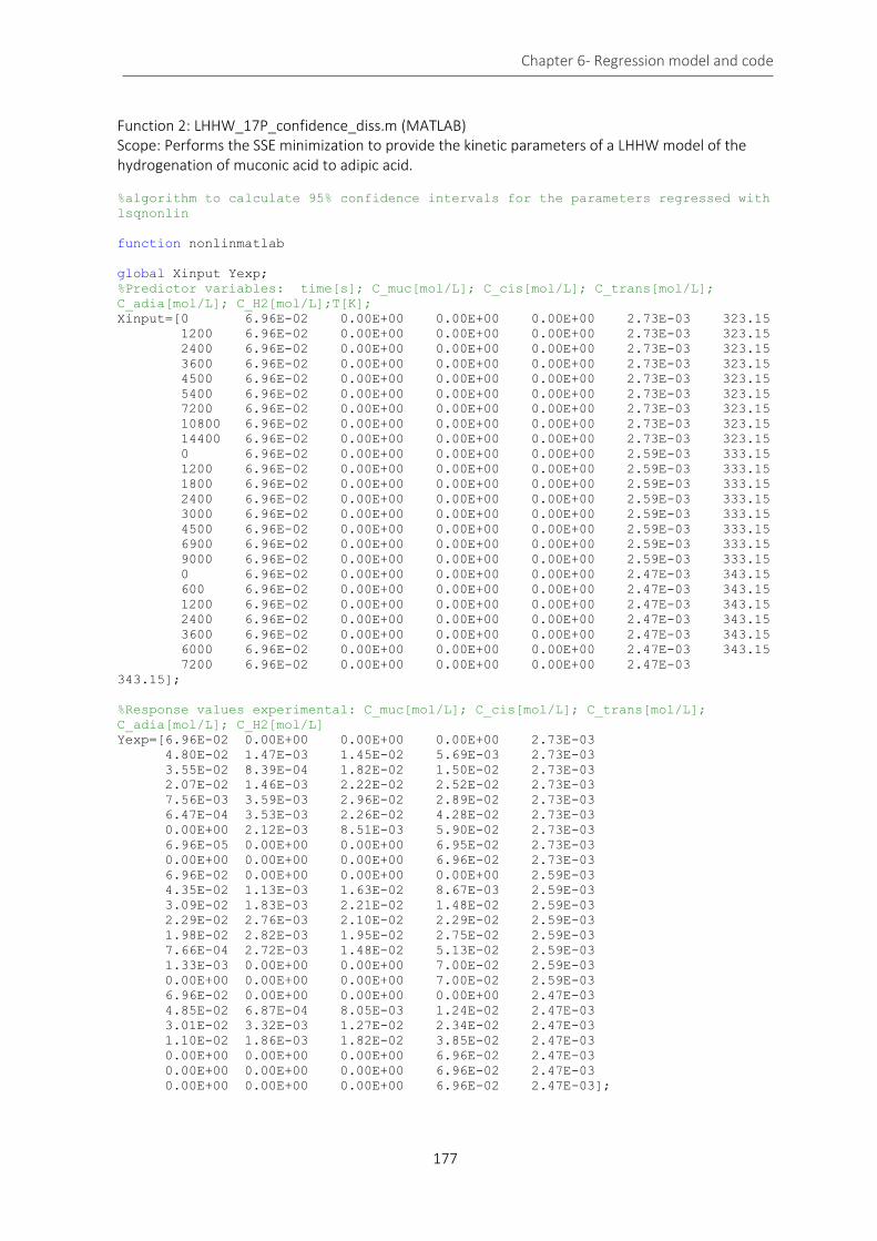
Chapter 6- Regression model and code
177
Function 2: LHHW_17P_confidence_diss.m (MATLAB) Scope: Performs the SSE minimization to provide the kinetic parameters of a LHHW model of the hydrogenation of muconic acid to adipic acid. %algorithm to calculate 95% confidence intervals for the parameters regressed with
lsqnonlin
function nonlinmatlab
global Xinput Yexp;
%Predictor variables: time[s]; C_muc[mol/L]; C_cis[mol/L]; C_trans[mol/L];
C_adia[mol/L]; C_H2[mol/L];T[K];
Xinput=[0 6.96E-02 0.00E+00 0.00E+00 0.00E+00 2.73E-03 323.15
1200 6.96E-02 0.00E+00 0.00E+00 0.00E+00 2.73E-03 323.15
2400 6.96E-02 0.00E+00 0.00E+00 0.00E+00 2.73E-03 323.15
3600 6.96E-02 0.00E+00 0.00E+00 0.00E+00 2.73E-03 323.15
4500 6.96E-02 0.00E+00 0.00E+00 0.00E+00 2.73E-03 323.15
5400 6.96E-02 0.00E+00 0.00E+00 0.00E+00 2.73E-03 323.15
7200 6.96E-02 0.00E+00 0.00E+00 0.00E+00 2.73E-03 323.15
10800 6.96E-02 0.00E+00 0.00E+00 0.00E+00 2.73E-03 323.15
14400 6.96E-02 0.00E+00 0.00E+00 0.00E+00 2.73E-03 323.15
0 6.96E-02 0.00E+00 0.00E+00 0.00E+00 2.59E-03 333.15
1200 6.96E-02 0.00E+00 0.00E+00 0.00E+00 2.59E-03 333.15
1800 6.96E-02 0.00E+00 0.00E+00 0.00E+00 2.59E-03 333.15
2400 6.96E-02 0.00E+00 0.00E+00 0.00E+00 2.59E-03 333.15
3000 6.96E-02 0.00E+00 0.00E+00 0.00E+00 2.59E-03 333.15
4500 6.96E-02 0.00E+00 0.00E+00 0.00E+00 2.59E-03 333.15
6900 6.96E-02 0.00E+00 0.00E+00 0.00E+00 2.59E-03 333.15
9000 6.96E-02 0.00E+00 0.00E+00 0.00E+00 2.59E-03 333.15
0 6.96E-02 0.00E+00 0.00E+00 0.00E+00 2.47E-03 343.15
600 6.96E-02 0.00E+00 0.00E+00 0.00E+00 2.47E-03 343.15
1200 6.96E-02 0.00E+00 0.00E+00 0.00E+00 2.47E-03 343.15
2400 6.96E-02 0.00E+00 0.00E+00 0.00E+00 2.47E-03 343.15
3600 6.96E-02 0.00E+00 0.00E+00 0.00E+00 2.47E-03 343.15
6000 6.96E-02 0.00E+00 0.00E+00 0.00E+00 2.47E-03 343.15
7200 6.96E-02 0.00E+00 0.00E+00 0.00E+00 2.47E-03
343.15];
%Response values experimental: C_muc[mol/L]; C_cis[mol/L]; C_trans[mol/L];
C_adia[mol/L]; C_H2[mol/L]
Yexp=[6.96E-02 0.00E+00 0.00E+00 0.00E+00 2.73E-03
4.80E-02 1.47E-03 1.45E-02 5.69E-03 2.73E-03
3.55E-02 8.39E-04 1.82E-02 1.50E-02 2.73E-03
2.07E-02 1.46E-03 2.22E-02 2.52E-02 2.73E-03
7.56E-03 3.59E-03 2.96E-02 2.89E-02 2.73E-03
6.47E-04 3.53E-03 2.26E-02 4.28E-02 2.73E-03
0.00E+00 2.12E-03 8.51E-03 5.90E-02 2.73E-03
6.96E-05 0.00E+00 0.00E+00 6.95E-02 2.73E-03
0.00E+00 0.00E+00 0.00E+00 6.96E-02 2.73E-03
6.96E-02 0.00E+00 0.00E+00 0.00E+00 2.59E-03
4.35E-02 1.13E-03 1.63E-02 8.67E-03 2.59E-03
3.09E-02 1.83E-03 2.21E-02 1.48E-02 2.59E-03
2.29E-02 2.76E-03 2.10E-02 2.29E-02 2.59E-03
1.98E-02 2.82E-03 1.95E-02 2.75E-02 2.59E-03
7.66E-04 2.72E-03 1.48E-02 5.13E-02 2.59E-03
1.33E-03 0.00E+00 0.00E+00 7.00E-02 2.59E-03
0.00E+00 0.00E+00 0.00E+00 7.00E-02 2.59E-03
6.96E-02 0.00E+00 0.00E+00 0.00E+00 2.47E-03
4.85E-02 6.87E-04 8.05E-03 1.24E-02 2.47E-03
3.01E-02 3.32E-03 1.27E-02 2.34E-02 2.47E-03
1.10E-02 1.86E-03 1.82E-02 3.85E-02 2.47E-03
0.00E+00 0.00E+00 0.00E+00 6.96E-02 2.47E-03
0.00E+00 0.00E+00 0.00E+00 6.96E-02 2.47E-03
0.00E+00 0.00E+00 0.00E+00 6.96E-02 2.47E-03];
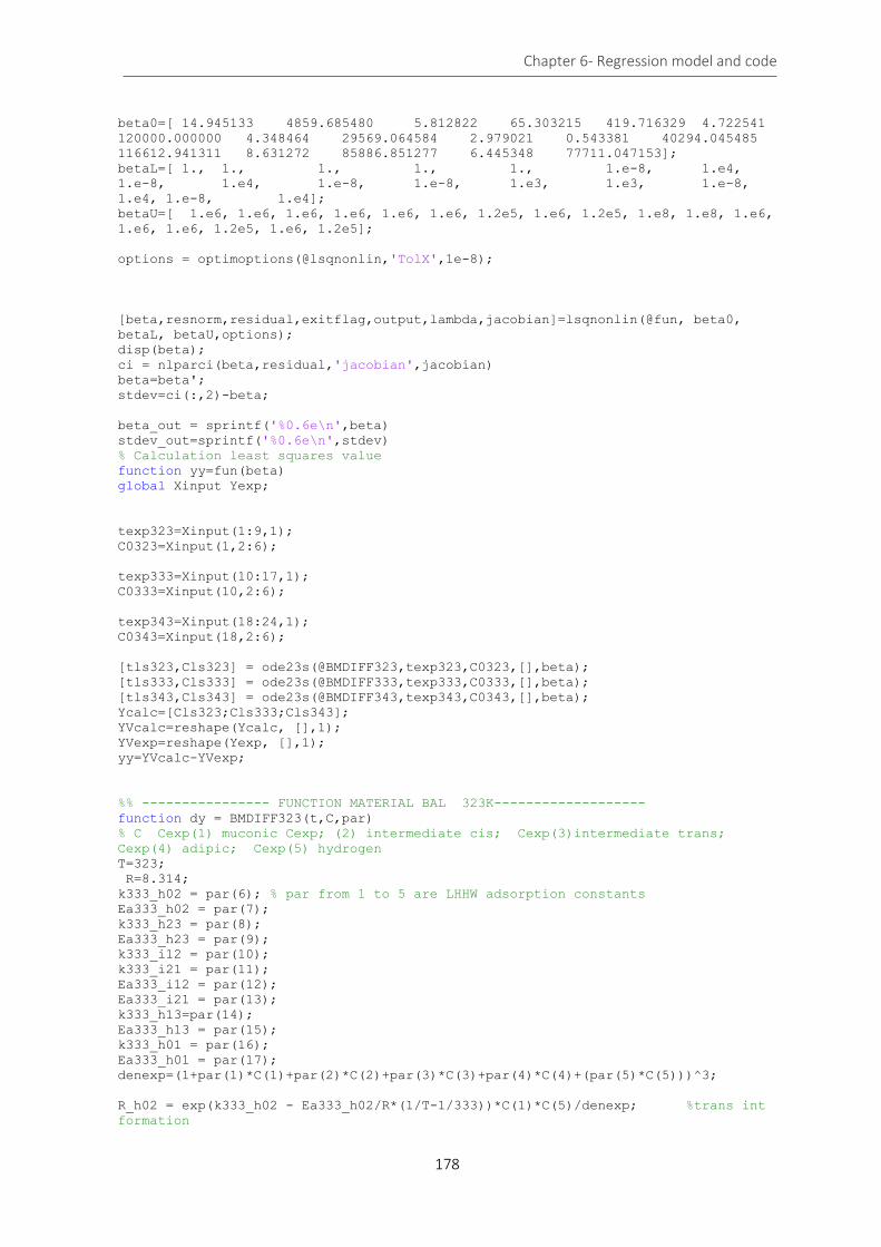
Chapter 6- Regression model and code
178
beta0=[ 14.945133 4859.685480 5.812822 65.303215 419.716329 4.722541
120000.000000 4.348464 29569.064584 2.979021 0.543381 40294.045485
116612.941311 8.631272 85886.851277 6.445348 77711.047153];
betaL=[ 1., 1., 1., 1., 1., 1.e-8, 1.e4,
1.e-8, 1.e4, 1.e-8, 1.e-8, 1.e3, 1.e3, 1.e-8,
1.e4, 1.e-8, 1.e4];
betaU=[ 1.e6, 1.e6, 1.e6, 1.e6, 1.e6, 1.e6, 1.2e5, 1.e6, 1.2e5, 1.e8, 1.e8, 1.e6,
1.e6, 1.e6, 1.2e5, 1.e6, 1.2e5];
options = optimoptions(@lsqnonlin,'TolX',1e-8);
[beta,resnorm,residual,exitflag,output,lambda,jacobian]=lsqnonlin(@fun, beta0,
betaL, betaU,options);
disp(beta);
ci = nlparci(beta,residual,'jacobian',jacobian)
beta=beta';
stdev=ci(:,2)-beta;
beta_out = sprintf('%0.6e\n',beta)
stdev_out=sprintf('%0.6e\n',stdev)
% Calculation least squares value
function yy=fun(beta)
global Xinput Yexp;
texp323=Xinput(1:9,1);
C0323=Xinput(1,2:6);
texp333=Xinput(10:17,1);
C0333=Xinput(10,2:6);
texp343=Xinput(18:24,1);
C0343=Xinput(18,2:6);
[tls323,Cls323] = ode23s(@BMDIFF323,texp323,C0323,[],beta);
[tls333,Cls333] = ode23s(@BMDIFF333,texp333,C0333,[],beta);
[tls343,Cls343] = ode23s(@BMDIFF343,texp343,C0343,[],beta);
Ycalc=[Cls323;Cls333;Cls343];
YVcalc=reshape(Ycalc, [],1);
YVexp=reshape(Yexp, [],1);
yy=YVcalc-YVexp;
%% ---------------- FUNCTION MATERIAL BAL 323K-------------------
function dy = BMDIFF323(t,C,par)
% C Cexp(1) muconic Cexp; (2) intermediate cis; Cexp(3)intermediate trans;
Cexp(4) adipic; Cexp(5) hydrogen
T=323;
R=8.314;
k333_h02 = par(6); % par from 1 to 5 are LHHW adsorption constants
Ea333_h02 = par(7);
k333_h23 = par(8);
Ea333_h23 = par(9);
k333_i12 = par(10);
k333_i21 = par(11);
Ea333_i12 = par(12);
Ea333_i21 = par(13);
k333_h13=par(14);
Ea333_h13 = par(15);
k333_h01 = par(16);
Ea333_h01 = par(17);
denexp=(1+par(1)*C(1)+par(2)*C(2)+par(3)*C(3)+par(4)*C(4)+(par(5)*C(5)))^3;
R_h02 = exp(k333_h02 - Ea333_h02/R*(1/T-1/333))*C(1)*C(5)/denexp; %trans int
formation
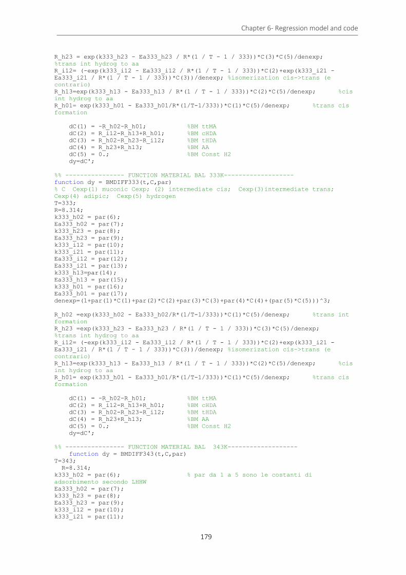
Chapter 6- Regression model and code
179
R_h23 = exp(k333_h23 - Ea333_h23 / R*(1 / T - 1 / 333))*C(3)*C(5)/denexp;
%trans int hydrog to aa
R_i12= (-exp(k333_i12 - Ea333_i12 / R*(1 / T - 1 / 333))*C(2)+exp(k333_i21 -
Ea333_i21 / R*(1 / T - 1 / 333))*C(3))/denexp; %isomerization cis->trans (e
contrario)
R_h13=exp(k333_h13 - Ea333_h13 / R*(1 / T - 1 / 333))*C(2)*C(5)/denexp; %cis
int hydrog to aa
R_h01= exp(k333_h01 - Ea333_h01/R*(1/T-1/333))*C(1)*C(5)/denexp; %trans cis
formation
dC(1) = -R_h02-R_h01; %BM ttMA
dC(2) = R_i12-R_h13+R_h01; %BM cHDA
dC(3) = R_h02-R_h23-R_i12; %BM tHDA
dC(4) = R_h23+R_h13; %BM AA
dC(5) = 0.; %BM Const H2
dy=dC';
%% ---------------- FUNCTION MATERIAL BAL 333K-------------------
function dy = BMDIFF333(t,C,par)
% C Cexp(1) muconic Cexp; (2) intermediate cis; Cexp(3)intermediate trans;
Cexp(4) adipic; Cexp(5) hydrogen
T=333;
R=8.314;
k333_h02 = par(6);
Ea333_h02 = par(7);
k333_h23 = par(8);
Ea333_h23 = par(9);
k333_i12 = par(10);
k333_i21 = par(11);
Ea333_i12 = par(12);
Ea333_i21 = par(13);
k333_h13=par(14);
Ea333_h13 = par(15);
k333_h01 = par(16);
Ea333_h01 = par(17);
denexp=(1+par(1)*C(1)+par(2)*C(2)+par(3)*C(3)+par(4)*C(4)+(par(5)*C(5)))^3;
R_h02 =exp(k333_h02 - Ea333_h02/R*(1/T-1/333))*C(1)*C(5)/denexp; %trans int
formation
R_h23 =exp(k333_h23 - Ea333_h23 / R*(1 / T - 1 / 333))*C(3)*C(5)/denexp;
%trans int hydrog to aa
R_i12= (-exp(k333_i12 - Ea333_i12 / R*(1 / T - 1 / 333))*C(2)+exp(k333_i21 -
Ea333_i21 / R*(1 / T - 1 / 333))*C(3))/denexp; %isomerization cis->trans (e
contrario)
R_h13=exp(k333_h13 - Ea333_h13 / R*(1 / T - 1 / 333))*C(2)*C(5)/denexp; %cis
int hydrog to aa
R_h01= exp(k333_h01 - Ea333_h01/R*(1/T-1/333))*C(1)*C(5)/denexp; %trans cis
formation
dC(1) = -R_h02-R_h01; %BM ttMA
dC(2) = R_i12-R_h13+R_h01; %BM cHDA
dC(3) = R_h02-R_h23-R_i12; %BM tHDA
dC(4) = R_h23+R_h13; %BM AA
dC(5) = 0.; %BM Const H2
dy=dC';
%% ---------------- FUNCTION MATERIAL BAL 343K-------------------
function dy = BMDIFF343(t,C,par)
T=343;
R=8.314;
k333_h02 = par(6); % par da 1 a 5 sono le costanti di
adsorbimento secondo LHHW
Ea333_h02 = par(7);
k333_h23 = par(8);
Ea333_h23 = par(9);
k333_i12 = par(10);
k333_i21 = par(11);

Chapter 6- Regression model and code
180
Ea333_i12 = par(12);
Ea333_i21 = par(13);
k333_h13=par(14);
Ea333_h13 = par(15);
k333_h01 = par(16);
Ea333_h01 = par(17);
denexp=(1+par(1)*C(1)+par(2)*C(2)+par(3)*C(3)+par(4)*C(4)+(par(5)*C(5)))^3;
R_h02 =exp(k333_h02 - Ea333_h02/R*(1/T-1/333))*C(1)*C(5)/denexp; %trans int
formation
R_h23 =exp(k333_h23 - Ea333_h23 / R*(1 / T - 1 / 333))*C(3)*C(5)/denexp;
%trans int hydrog to aa
R_i12= (-exp(k333_i12 - Ea333_i12 / R*(1 / T - 1 / 333))*C(2)+exp(k333_i21 -
Ea333_i21 / R*(1 / T - 1 / 333))*C(3))/denexp; %isomerization cis->trans (e
contrario)
R_h13=exp(k333_h13 - Ea333_h13 / R*(1 / T - 1 / 333))*C(2)*C(5)/denexp; %cis
int hydrog to aa
R_h01= exp(k333_h01 - Ea333_h01/R*(1/T-1/333))*C(1)*C(5)/denexp; %trans cis
formation
dC(1) = -R_h02-R_h01; %BM ttMA
dC(2) = R_i12-R_h13+R_h01; %BM cHDA
dC(3) = R_h02-R_h23-R_i12; %BM tHDA
dC(4) = R_h23+R_h13; %BM AA
dC(5) = 0.; %BM Const H2
dy=dC';

Chapter 6- Regression model and code
181
Function 3: LHHW_17P_print_diss.m (MATLAB) Scope: Calculates the concentration profiles of the species and plots them against the experimental values, given the regressed model parameters. %% PRINTING TOOL
%% REFERRED TO LHHW 17P
function fitDIFF
close all % per chiudere eventuali finestre di grafici
clear all
clc
global npoint;
%%%% Temperature 323
input='input_int'; % opens input dfile
C0323=xlsread(input,3,'B2:F2'); % conc matrix col1 ttMA, col2 cHDA,
col3 tHDA, col4 AA, col 5 H2
npoint=xlsread(input,3,'A20'); % nr exp points
rM=xlsread(input,3,'A2:F10'); % matrice input (grezza)
Cexp323=rM(1:npoint,2:end); % matrice concentrazione specie col1
muconico, col2 intermedio cis, col3 intermedio trans, col4 adipico, col 5 hydr
texp323 =rM(1:npoint,1); % vettore dei tempi sperimentali
Cexp_muc323=[texp323, Cexp323(1:npoint,1)];
Cexp_cis323=[texp323, Cexp323(1:npoint,2)];
Cexp_trans323=[texp323, Cexp323(1:npoint,3)];
Cexp_aad323=[texp323, Cexp323(1:npoint,4)];
%%%% Temperature 333
C0333=xlsread(input,4,'B2:F2'); conc matrix col1 ttMA, col2 cHDA, col3
tHDA, col4 AA, col 5 H2
npoint=xlsread(input,4,'A20'); % nr exp points
rM=xlsread(input,4,'A2:F9'); % matrice input (grezza)
Cexp333=rM(1:npoint,2:end); % matrice concentrazione specie col1
muconico, col2 intermedio cis, col3 intermedio trans, col4 adipico, col 5 hydr
texp333 =rM(1:npoint,1); % vettore dei tempi sperimentali
Cexp_muc333=[texp333, Cexp333(1:npoint,1)];
Cexp_cis333=[texp333, Cexp333(1:npoint,2)];
Cexp_trans333=[texp333, Cexp333(1:npoint,3)];
Cexp_aad333=[texp333, Cexp333(1:npoint,4)];
%%%% Temperature 343
C0343=xlsread(input,5,'B2:F2'); % initial conc ttMA, cHDA, tHDA, AA, H2
npoint=xlsread(input,5,'A20'); % nr exp points
rM=xlsread(input,5,'A2:F8'); % matrice input (grezza)
Cexp343=rM(1:npoint,2:end); % conc matrix col1 ttMA, col2 cHDA, col3
tHDA, col4 AA, col 5 H2
texp343 =rM(1:npoint,1); % exp times
Cexp_muc343=[texp343, Cexp343(1:npoint,1)];
Cexp_cis343=[texp343, Cexp343(1:npoint,2)];
Cexp_trans343=[texp343, Cexp343(1:npoint,3)];
Cexp_aad343=[texp343, Cexp343(1:npoint,4)];
% Insert final parameters
par=[14.945133 4859.685480 5.812822 65.303215 419.716329 4.722541
120000.000000 4.348464 29569.064584 2.979021 0.543381 40294.045485
116612.941311 8.631272 85886.851277 6.445348 77711.047153];
tsmooth323=[0:60:14400];
tsmooth333=[0:60:9000];
tsmooth343=[0:60:7200];
[tg323,Ctg323] = ode23s(@BMDIFF323,tsmooth323,C0323,[],par);
[tg333,Ctg333] = ode23s(@BMDIFF333,tsmooth333,C0333,[],par);
[tg343,Ctg343] = ode23s(@BMDIFF343,tsmooth343,C0343,[],par);
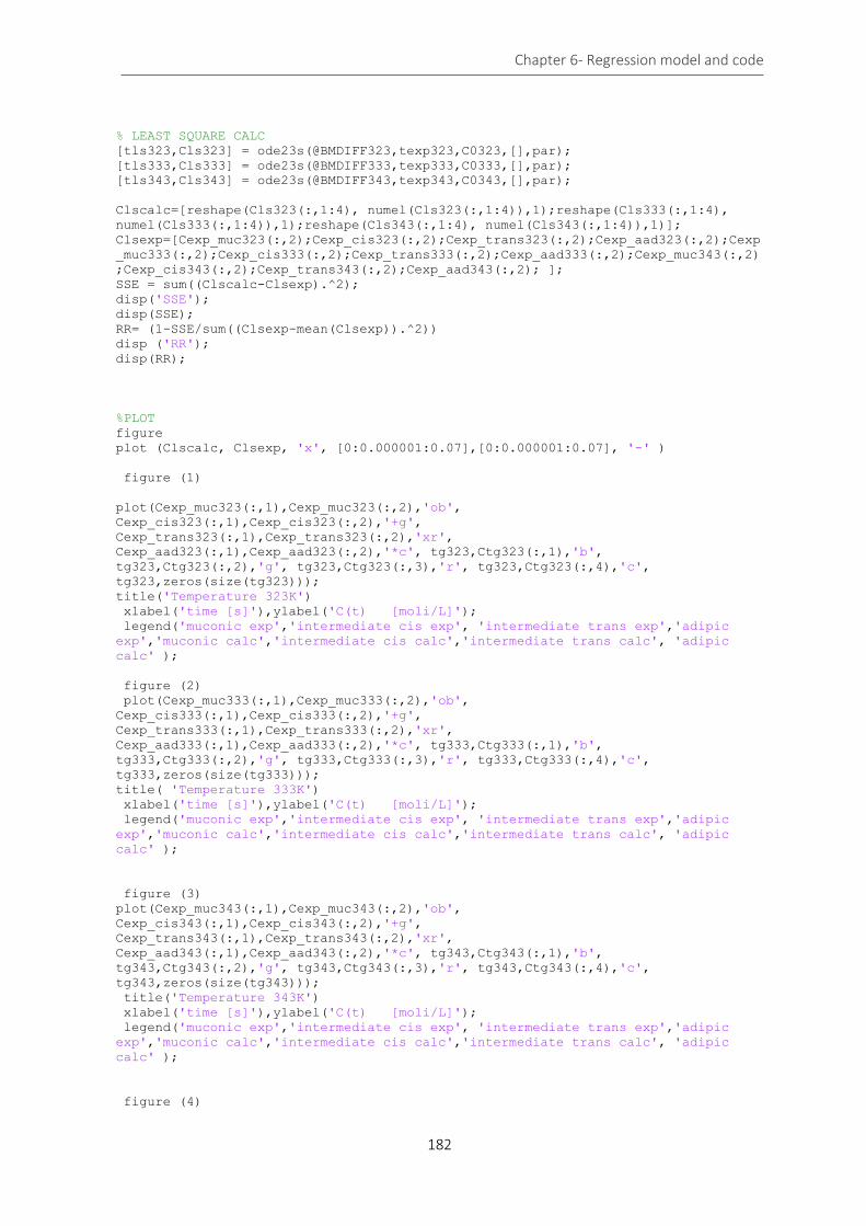
Chapter 6- Regression model and code
182
% LEAST SQUARE CALC
[tls323,Cls323] = ode23s(@BMDIFF323,texp323,C0323,[],par);
[tls333,Cls333] = ode23s(@BMDIFF333,texp333,C0333,[],par);
[tls343,Cls343] = ode23s(@BMDIFF343,texp343,C0343,[],par);
Clscalc=[reshape(Cls323(:,1:4), numel(Cls323(:,1:4)),1);reshape(Cls333(:,1:4),
numel(Cls333(:,1:4)),1);reshape(Cls343(:,1:4), numel(Cls343(:,1:4)),1)];
Clsexp=[Cexp_muc323(:,2);Cexp_cis323(:,2);Cexp_trans323(:,2);Cexp_aad323(:,2);Cexp
_muc333(:,2);Cexp_cis333(:,2);Cexp_trans333(:,2);Cexp_aad333(:,2);Cexp_muc343(:,2)
;Cexp_cis343(:,2);Cexp_trans343(:,2);Cexp_aad343(:,2); ];
SSE = sum((Clscalc-Clsexp).^2);
disp('SSE');
disp(SSE);
RR= (1-SSE/sum((Clsexp-mean(Clsexp)).^2))
disp ('RR');
disp(RR);
%PLOT
figure
plot (Clscalc, Clsexp, 'x', [0:0.000001:0.07],[0:0.000001:0.07], '-' )
figure (1)
plot(Cexp_muc323(:,1),Cexp_muc323(:,2),'ob',
Cexp_cis323(:,1),Cexp_cis323(:,2),'+g',
Cexp_trans323(:,1),Cexp_trans323(:,2),'xr',
Cexp_aad323(:,1),Cexp_aad323(:,2),'*c', tg323,Ctg323(:,1),'b',
tg323,Ctg323(:,2),'g', tg323,Ctg323(:,3),'r', tg323,Ctg323(:,4),'c',
tg323,zeros(size(tg323)));
title('Temperature 323K')
xlabel('time [s]'),ylabel('C(t) [moli/L]');
legend('muconic exp','intermediate cis exp', 'intermediate trans exp','adipic
exp','muconic calc','intermediate cis calc','intermediate trans calc', 'adipic
calc' );
figure (2)
plot(Cexp_muc333(:,1),Cexp_muc333(:,2),'ob',
Cexp_cis333(:,1),Cexp_cis333(:,2),'+g',
Cexp_trans333(:,1),Cexp_trans333(:,2),'xr',
Cexp_aad333(:,1),Cexp_aad333(:,2),'*c', tg333,Ctg333(:,1),'b',
tg333,Ctg333(:,2),'g', tg333,Ctg333(:,3),'r', tg333,Ctg333(:,4),'c',
tg333,zeros(size(tg333)));
title( 'Temperature 333K')
xlabel('time [s]'),ylabel('C(t) [moli/L]');
legend('muconic exp','intermediate cis exp', 'intermediate trans exp','adipic
exp','muconic calc','intermediate cis calc','intermediate trans calc', 'adipic
calc' );
figure (3)
plot(Cexp_muc343(:,1),Cexp_muc343(:,2),'ob',
Cexp_cis343(:,1),Cexp_cis343(:,2),'+g',
Cexp_trans343(:,1),Cexp_trans343(:,2),'xr',
Cexp_aad343(:,1),Cexp_aad343(:,2),'*c', tg343,Ctg343(:,1),'b',
tg343,Ctg343(:,2),'g', tg343,Ctg343(:,3),'r', tg343,Ctg343(:,4),'c',
tg343,zeros(size(tg343)));
title('Temperature 343K')
xlabel('time [s]'),ylabel('C(t) [moli/L]');
legend('muconic exp','intermediate cis exp', 'intermediate trans exp','adipic
exp','muconic calc','intermediate cis calc','intermediate trans calc', 'adipic
calc' );
figure (4)
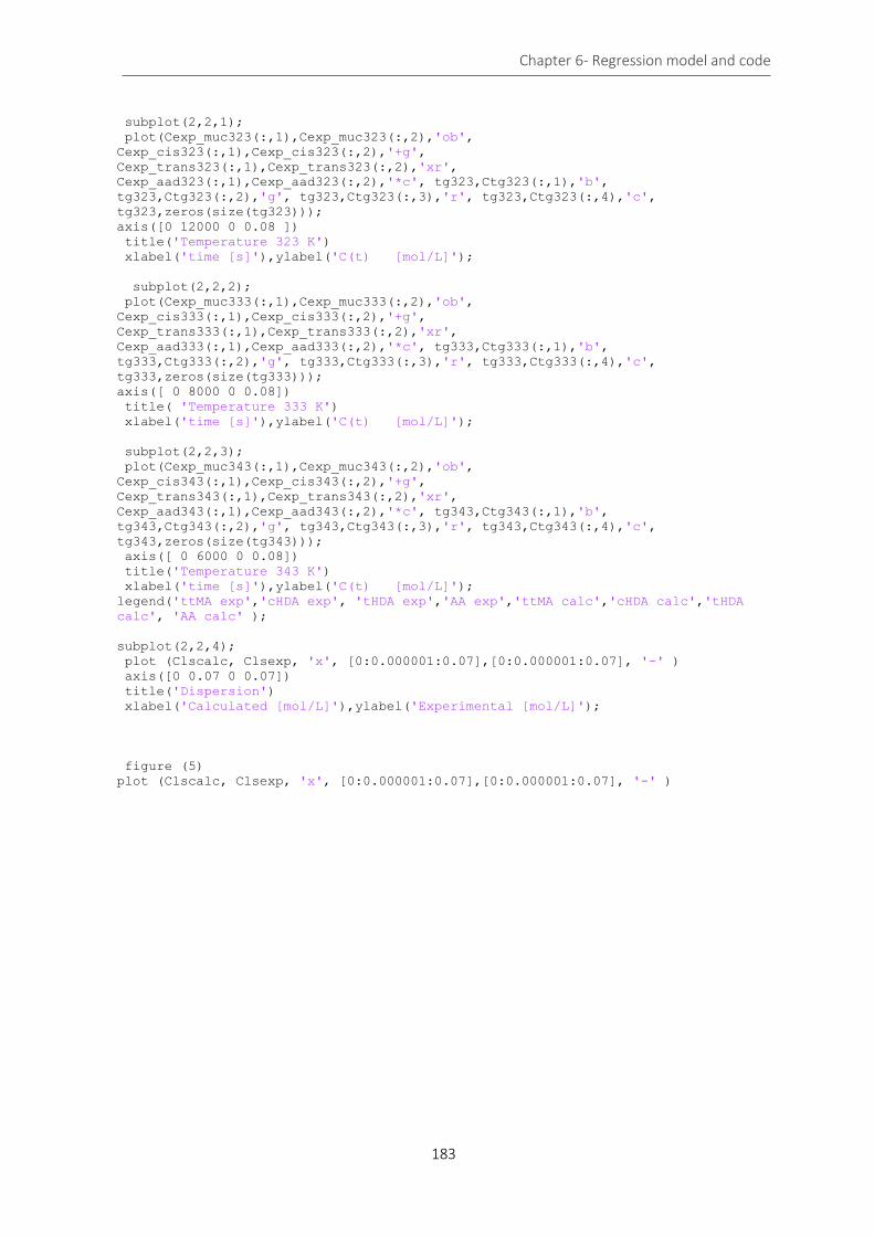
Chapter 6- Regression model and code
183
subplot(2,2,1);
plot(Cexp_muc323(:,1),Cexp_muc323(:,2),'ob',
Cexp_cis323(:,1),Cexp_cis323(:,2),'+g',
Cexp_trans323(:,1),Cexp_trans323(:,2),'xr',
Cexp_aad323(:,1),Cexp_aad323(:,2),'*c', tg323,Ctg323(:,1),'b',
tg323,Ctg323(:,2),'g', tg323,Ctg323(:,3),'r', tg323,Ctg323(:,4),'c',
tg323,zeros(size(tg323)));
axis([0 12000 0 0.08 ])
title('Temperature 323 K')
xlabel('time [s]'),ylabel('C(t) [mol/L]');
subplot(2,2,2);
plot(Cexp_muc333(:,1),Cexp_muc333(:,2),'ob',
Cexp_cis333(:,1),Cexp_cis333(:,2),'+g',
Cexp_trans333(:,1),Cexp_trans333(:,2),'xr',
Cexp_aad333(:,1),Cexp_aad333(:,2),'*c', tg333,Ctg333(:,1),'b',
tg333,Ctg333(:,2),'g', tg333,Ctg333(:,3),'r', tg333,Ctg333(:,4),'c',
tg333,zeros(size(tg333)));
axis([ 0 8000 0 0.08])
title( 'Temperature 333 K')
xlabel('time [s]'),ylabel('C(t) [mol/L]');
subplot(2,2,3);
plot(Cexp_muc343(:,1),Cexp_muc343(:,2),'ob',
Cexp_cis343(:,1),Cexp_cis343(:,2),'+g',
Cexp_trans343(:,1),Cexp_trans343(:,2),'xr',
Cexp_aad343(:,1),Cexp_aad343(:,2),'*c', tg343,Ctg343(:,1),'b',
tg343,Ctg343(:,2),'g', tg343,Ctg343(:,3),'r', tg343,Ctg343(:,4),'c',
tg343,zeros(size(tg343)));
axis([ 0 6000 0 0.08])
title('Temperature 343 K')
xlabel('time [s]'),ylabel('C(t) [mol/L]');
legend('ttMA exp','cHDA exp', 'tHDA exp','AA exp','ttMA calc','cHDA calc','tHDA
calc', 'AA calc' );
subplot(2,2,4);
plot (Clscalc, Clsexp, 'x', [0:0.000001:0.07],[0:0.000001:0.07], '-' )
axis([0 0.07 0 0.07])
title('Dispersion')
xlabel('Calculated [mol/L]'),ylabel('Experimental [mol/L]');
figure (5)
plot (Clscalc, Clsexp, 'x', [0:0.000001:0.07],[0:0.000001:0.07], '-' )
Chapter 6- Bibliography
184
Bibliography
1. Carraher, J. M., Matthiesen, J. E. & Tessonnier, J.-P. Comments on “Thermodynamics of cis,cis-muconic acid solubility in various polar solvents at low temperature range”. J. Mol. Liq. 224, 420–422 (2016).
2. Li, X. et al. Highly efficient chemical process to convert mucic acid into adipic acid and DFT studies of the mechanism of the rhenium-catalyzed deoxydehydration. Angew. Chemie - Int. Ed. 53, 4200–4204 (2014).
3. Frost, J. W., Miermont, A., Schweitzer, D. & Bui, V. Preparation of trans, trans muconic acid and trans, trans muconates. (2013).
4. Carraher, J. M., Pfennig, T., Rao, R. G., Shanks, B. H. & Tessonnier, J.-P. cis,cis-Muconic acid isomerization and catalytic conversion to biobased cyclic-C 6 -1,4-diacid monomers. Green Chem. 21–25 (2017). doi:10.1039/C7GC00658F
5. Matthiesen, J. E. et al. Electrochemical Conversion of Biologically Produced Muconic Acid: Key Considerations for Scale-Up and Corresponding Technoeconomic Analysis. ACS Sustain. Chem. Eng. 4, 7098–7109 (2016).
6. Vardon, D. R. et al. cis,cis-Muconic acid: separation and catalysis to bio-adipic acid for nylon-6,6 polymerization. Green Chem. 18, 3397–3413 (2016).
7. She, X., Brown, H. M., Zhang, X., Ahring, B. K. & Wang, Y. Selective hydrogenation of trans,trans-muconic acid to adipic acid over a titania-supported rhenium catalyst. ChemSusChem 4, 1071–1073 (2011).
8. Yang, K. H. & Hougen, O. A. Determination of mechanism of catalyzed gaseous reactions. Chem. Eng. Prog. 46, 146–157 (1950).
9. Rostrup-Nielsen, J. Chapter 5 Reaction kinetics/reactor design. Catal. Today 22, 295–311 (1994).
10. Chaudhari, R. V & Ramachandran, P. A. Three phase slurry reactors. AIChE J. 26, 177–201 (1980).
11. Piskun, A. S., van de Bovenkamp, H. H., Rasrendra, C. B., Winkelman, J. G. M. & Heeres, H. J. Kinetic modeling of levulinic acid hydrogenation to γ-valerolactone in water using a carbon supported Ru catalyst. Appl. Catal. A Gen. 525, 158–167 (2016).
12. Rajashekharam, M. V, Nikalje, D. D., Jaganathan, R. & Chaudhari, R. V. Hydrogenation of 2,4-Dinitrotoluene Using a Pd/Al2O3 Catalyst in a Slurry Reactor: A Molecular Level Approach to Kinetic Modeling and Nonisothermal Effects. Ind. Eng. Chem. Res. 36, 592–604 (1997).
13. Chaudhari, R. V et al. Kinetics of hydrogenation of maleic acid in a batch slurry reactor using a bimetallic Ru–Re/C catalyst. Chem. Eng. Sci. 58, 627–632 (2003).
14. Buzzi-Ferraris, G. & Manenti, F. Interpolation and Regression Models for chemical engineer: Solving Numerical Problems. (Jhon Wiley & Sons, 2010).
15. Froment, G. F., Bischoff, K. B. & De Wilde, J. Chemical reactor analysis and design. (Wiley New York, 2011).
16. Lylykangas, M. S., Rautanen, P. A. & Krause, A. O. I. Hydrogenation and Deactivation Kinetics in the Liquid-Phase Hydrogenation of Isooctenes on Pt/Al2O3. Ind. Eng. Chem. Res. 43, 1641–1648 (2004).
17. Buzzi-Ferraris, G. & Manenti, F. Interpolation and Regression Models for the Chemical Engineer: Solving Numerical Problems. (John Wiley & Sons, 2010).
18. Vardon, D. R. et al. Adipic acid production from lignin. Energy Environ. Sci. 8, 617–628 (2015).
19. Neri, G., Musolino, M. G., Milone, C. & Galvagno, S. Kinetic Modeling of 2,4-Dinitrotoluene Hydrogenation over Pd/C. Ind. Eng. Chem. Res. 34, 2226–2231 (1995).
20. Veldsink, J. W., Bouma, M. J., Schöön, N. H. & Beenackers, A. A. C. M. Heterogeneous Hydrogenation of Vegetable Oils: A Literature Review. Catal. Rev. 39, 253–318 (1997).
21. Jones, W. H. Catalysis in Organic Syntheses. (Elsevier Science, 2013).
22. Chaudhari, R. V. et al. Kinetics of hydrogenation of maleic acid in a batch slurry reactor using a bimetallic Ru-Re/C catalyst. Chem. Eng. Sci. 58, 627–632 (2003).
23. Zhang, Z., Jackson, J. E. & Miller, D. J. Kinetics of Aqueous-Phase Hydrogenation of Lactic Acid to

Chapter 6- Bibliography
185
Propylene Glycol. Ind. Eng. Chem. Res. 41, 691–696 (2002).
24. Scelfo, S., Pirone, R. & Russo, N. Highly efficient catalysts for the synthesis of adipic acid from cis,cis-muconic acid. Catal. Commun. 84, 98–102 (2016).
25. Vardon, D. R. et al. Adipic acid production from lignin. Energy Environ. Sci. 8, 617–628 (2015).
186
Chapter 7
t,t-MA and Na-Muc hydrogenation
using Pd/AC home-made catalyst
This chapter describes the results for t,t-MA hydrogenation reaction performed using Pd/AC 1%
home-made-catalyst. The catalysts were prepared using the colloidal-immobilization technique which
allow synthesizing noble metal nanoparticles that can be immobilized to a solid powder support.
Different carbon supports were used to prepare the catalyst and a reaction screening allowed to
choose the best catalyst to use for a deeper analysis. The home-made catalysts were characterize
using the most common techniques and a comparison between the best home-made catalyst and the
commercial Pd/AC 5% was finally performed.
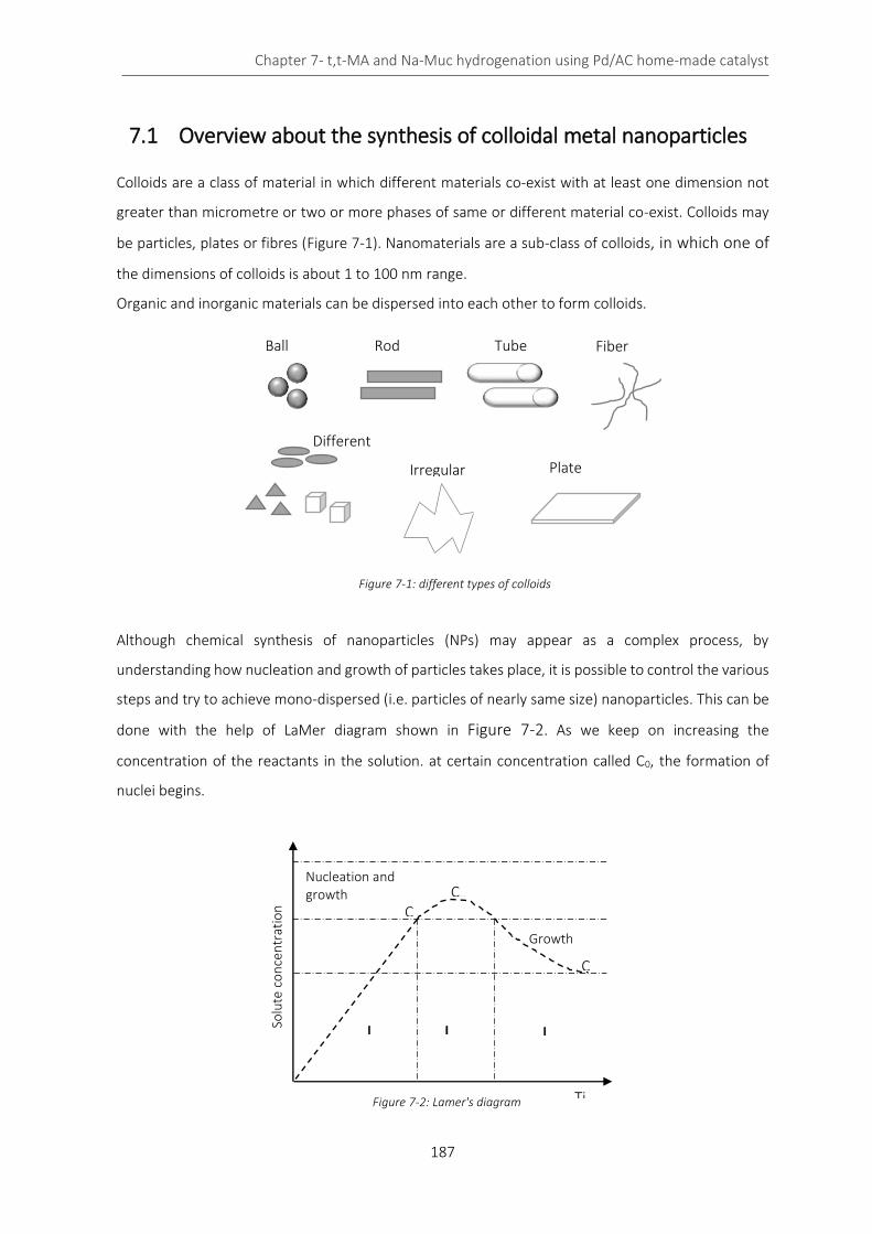
Chapter 7- t,t-MA and Na-Muc hydrogenation using Pd/AC home-made catalyst
187
7.1 Overview about the synthesis of colloidal metal nanoparticles
Colloids are a class of material in which different materials co-exist with at least one dimension not
greater than micrometre or two or more phases of same or different material co-exist. Colloids may
be particles, plates or fibres (Figure 7-1). Nanomaterials are a sub-class of colloids, in which one of
the dimensions of colloids is about 1 to 100 nm range.
Organic and inorganic materials can be dispersed into each other to form colloids.
Although chemical synthesis of nanoparticles (NPs) may appear as a complex process, by
understanding how nucleation and growth of particles takes place, it is possible to control the various
steps and try to achieve mono-dispersed (i.e. particles of nearly same size) nanoparticles. This can be
done with the help of LaMer diagram shown in Figure 7-2. As we keep on increasing the
concentration of the reactants in the solution. at certain concentration called C0, the formation of
nuclei begins.
Ball shaped
Different shapes
Rods
Tubes
Irregular shape
Fibers
Plates
Figure 7-1: different types of colloids
Figure 7-2: Lamer's diagram Ti
Solu
te c
on
cen
trat
ion
I I I
C
CN
C
Growth
Nucleation and
growth

Chapter 7- t,t-MA and Na-Muc hydrogenation using Pd/AC home-made catalyst
188
There is no precipitate at this concentration. Further increase in concentration increases nuclei
formation up to a concentration Cn, above which there is a “super saturation” between Cn and Cs.
Concentration Cn denotes the maximum rate of nuclei formation. When nuclei formation reduces,
again C0 the minimum concentration for nucleation is reached. No new nuclei can be formed, and
crystal growth reduces the concentration. At this concentration Cs equilibrium is obtained. If new
nuclei are formed during the growth of particles, particles with large size distribution are obtained.
Therefore, it is very important to adjust the concentration of the solute and its diffusion to obtain
more stable NPs and a constant rate grow of littler particles. Growth mode recognized as Ostwald
ripening. Experimentally it was found that there is sometimes aggregation of particles. Aggregation
also reduces the energy of the system. Thus Ostwald ripening and aggregation are competing
processes and either of them is responsible to reduce the surface free energy.1
Colloidal metal nanoparticles (NPs) can be prepared by two different approaches: the “top-down
method” which utilizes physical methods to subdivide the bulk meals and the “bottom-up method” in
which the solution-phase colloidal chemistry is employed. Colloidal chemical synthetic method cab be
used to synthesize uniform NPs with controlled particle size and shape in solution.2 In general there
are three main approaches to chemically produced metal NPs: chemical reduction of metal salt
precursors, controlled decomposition of organometallic compounds and metal-surfactant complexes,
and electrochemical synthesis. In all the above methods, a large variety of stabilizer (donor ligands,
polymers and surfactants) are used to control the growth of the initially forms nanocluster and to
prevent NPs agglomeration.
Colloidal methods are well established and simple wet chemistry precipitation processes where the
solutions of the different metal precursors, stabilizer and reducing agents are mixed under controlled
temperature. The schematic approach for producing NPs is reported below:
xMn+ + nxe- + stabilizer M0n (cluster) 3
After the NPs colloidal formation and stabilization, the support is added under vigorous stirring and
only after the solution is colourless the catalyst is filtered and dried in oven.
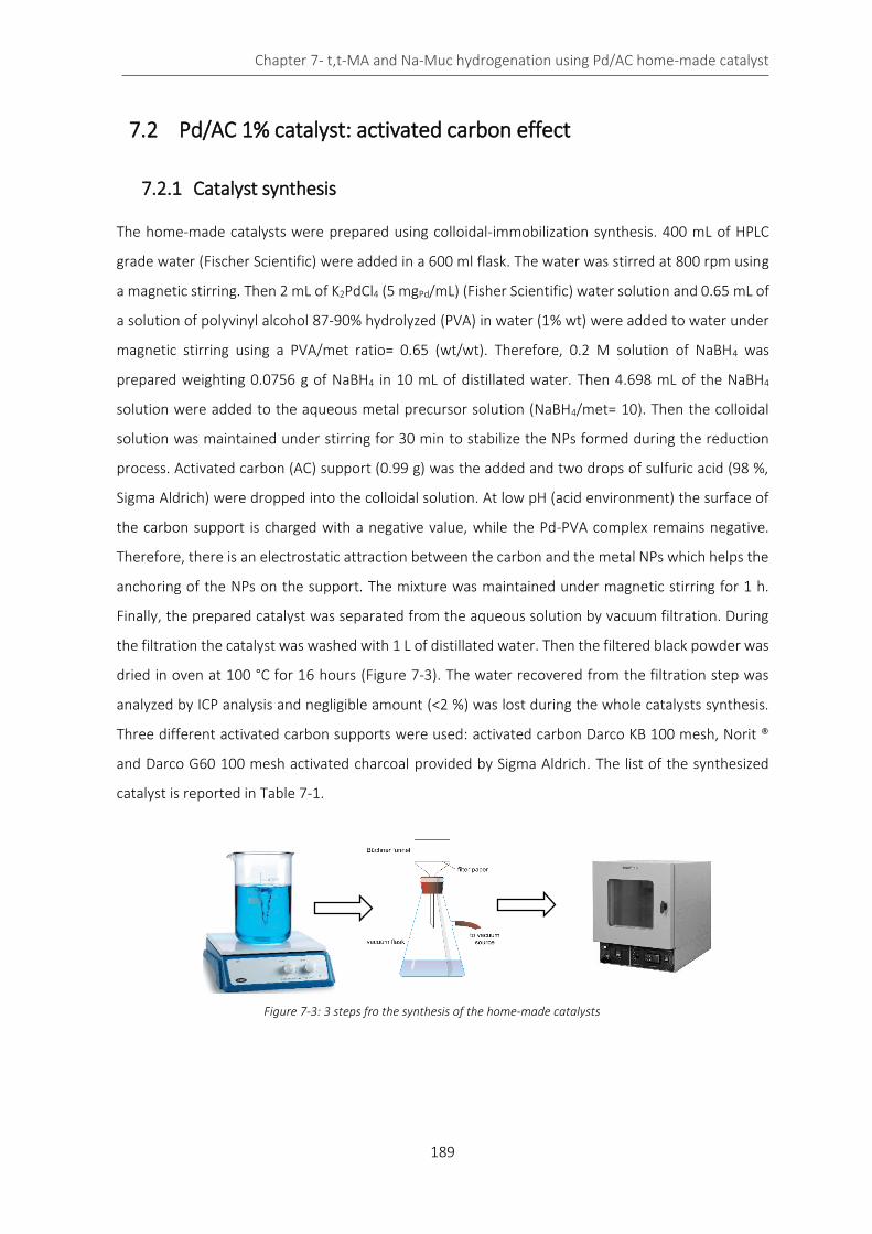
Chapter 7- t,t-MA and Na-Muc hydrogenation using Pd/AC home-made catalyst
189
7.2 Pd/AC 1% catalyst: activated carbon effect
7.2.1 Catalyst synthesis
The home-made catalysts were prepared using colloidal-immobilization synthesis. 400 mL of HPLC
grade water (Fischer Scientific) were added in a 600 ml flask. The water was stirred at 800 rpm using
a magnetic stirring. Then 2 mL of K2PdCl4 (5 mgPd/mL) (Fisher Scientific) water solution and 0.65 mL of
a solution of polyvinyl alcohol 87-90% hydrolyzed (PVA) in water (1% wt) were added to water under
magnetic stirring using a PVA/met ratio= 0.65 (wt/wt). Therefore, 0.2 M solution of NaBH4 was
prepared weighting 0.0756 g of NaBH4 in 10 mL of distillated water. Then 4.698 mL of the NaBH4
solution were added to the aqueous metal precursor solution (NaBH4/met= 10). Then the colloidal
solution was maintained under stirring for 30 min to stabilize the NPs formed during the reduction
process. Activated carbon (AC) support (0.99 g) was the added and two drops of sulfuric acid (98 %,
Sigma Aldrich) were dropped into the colloidal solution. At low pH (acid environment) the surface of
the carbon support is charged with a negative value, while the Pd-PVA complex remains negative.
Therefore, there is an electrostatic attraction between the carbon and the metal NPs which helps the
anchoring of the NPs on the support. The mixture was maintained under magnetic stirring for 1 h.
Finally, the prepared catalyst was separated from the aqueous solution by vacuum filtration. During
the filtration the catalyst was washed with 1 L of distillated water. Then the filtered black powder was
dried in oven at 100 °C for 16 hours (Figure 7-3). The water recovered from the filtration step was
analyzed by ICP analysis and negligible amount (<2 %) was lost during the whole catalysts synthesis.
Three different activated carbon supports were used: activated carbon Darco KB 100 mesh, Norit ®
and Darco G60 100 mesh activated charcoal provided by Sigma Aldrich. The list of the synthesized
catalyst is reported in Table 7-1.
Figure 7-3: 3 steps fro the synthesis of the home-made catalysts
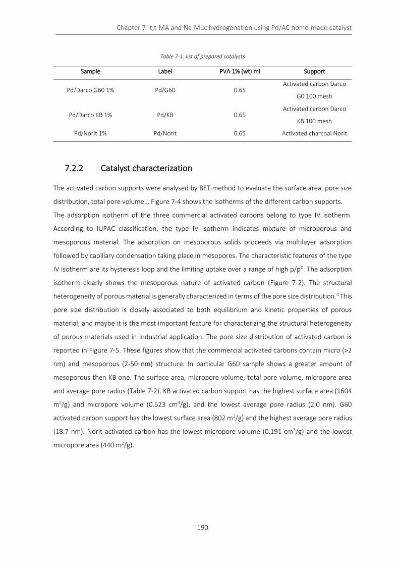
Chapter 7- t,t-MA and Na-Muc hydrogenation using Pd/AC home-made catalyst
190
Table 7-1: list of prepared catalysts
Sample Label PVA 1% (wt) ml Support
Pd/Darco G60 1% Pd/G60 0.65 Activated carbon Darco
G0 100 mesh
Pd/Darco KB 1% Pd/KB 0.65 Activated carbon Darco
KB 100 mesh
Pd/Norit 1% Pd/Norit 0.65 Activated charcoal Norit
7.2.2 Catalyst characterization
The activated carbon supports were analysed by BET method to evaluate the surface area, pore size
distribution, total pore volume… Figure 7-4 shows the isotherms of the different carbon supports.
The adsorption isotherm of the three commercial activated carbons belong to type IV isotherm.
According to IUPAC classification, the type IV isotherm indicates mixture of microporous and
mesoporous material. The adsorption on mesoporous solids proceeds via multilayer adsorption
followed by capillary condensation taking place in mesopores. The characteristic features of the type
IV isotherm are its hysteresis loop and the limiting uptake over a range of high p/p0. The adsorption
isotherm clearly shows the mesoporous nature of activated carbon (Figure 7-2). The structural
heterogeneity of porous material is generally characterized in terms of the pore size distribution.4 This
pore size distribution is closely associated to both equilibrium and kinetic properties of porous
material, and maybe it is the most important feature for characterizing the structural heterogeneity
of porous materials used in industrial application. The pore size distribution of activated carbon is
reported in Figure 7-5. These figures show that the commercial activated carbons contain micro (>2
nm) and mesoporous (2-50 nm) structure. In particular G60 sample shows a greater amount of
mesoporous then KB one. The surface area, micropore volume, total pore volume, micropore area
and average pore radius (Table 7-2). KB activated carbon support has the highest surface area (1604
m2/g) and micropore volume (0.523 cm3/g), and the lowest average pore radius (2.0 nm). G60
activated carbon support has the lowest surface area (802 m2/g) and the highest average pore radius
(18.7 nm). Norit activated carbon has the lowest micropore volume (0.191 cm3/g) and the lowest
micropore area (440 m2/g).
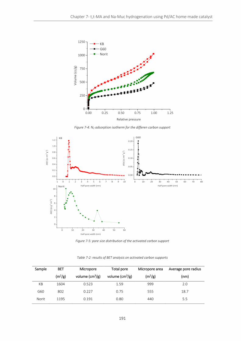
Chapter 7- t,t-MA and Na-Muc hydrogenation using Pd/AC home-made catalyst
191
Figure 7-4: N2 adsorption isotherm for the differen carbon support
Figure 7-5: pore size distribution of the activated carbon support
Table 7-2: results of BET analysis on activated carbon supports
Sample BET
(m2/g)
Micropore
volume (cm3/g)
Total pore
volume (cm3/g)
Micropore area
(m2/g)
Average pore radius
(nm)
KB 1604 0.523 1.59 999 2.0
G60 802 0.227 0.75 555 18.7
Norit 1195 0.191 0.80 440 5.5
-1 0 1 2 3 4 5 6 7 8 9 10
0.0
0.2
0.4
0.6
0.8
1.0
1.2
0 10 20 30 40 50 60 70 80
0.00
0.05
0.10
0.15
0.20
0 10 20 30 40 50 60
0
2
4
6
8
10
KB
dV(r
) (cc
nm
-1 g
-1)
Half pore width (nm)
G60
dV(r
) (cc
nm
-1 g
-1)
Half pore width (nm)Norit
dV(r
) (cc
g-1
nm-1
)
Half pore width (nm)
0.00 0.25 0.50 0.75 1.00 1.250
250
500
750
1000
1250
Vo
lum
e (c
c/g)
Relative pressure
KB
G60
Norit
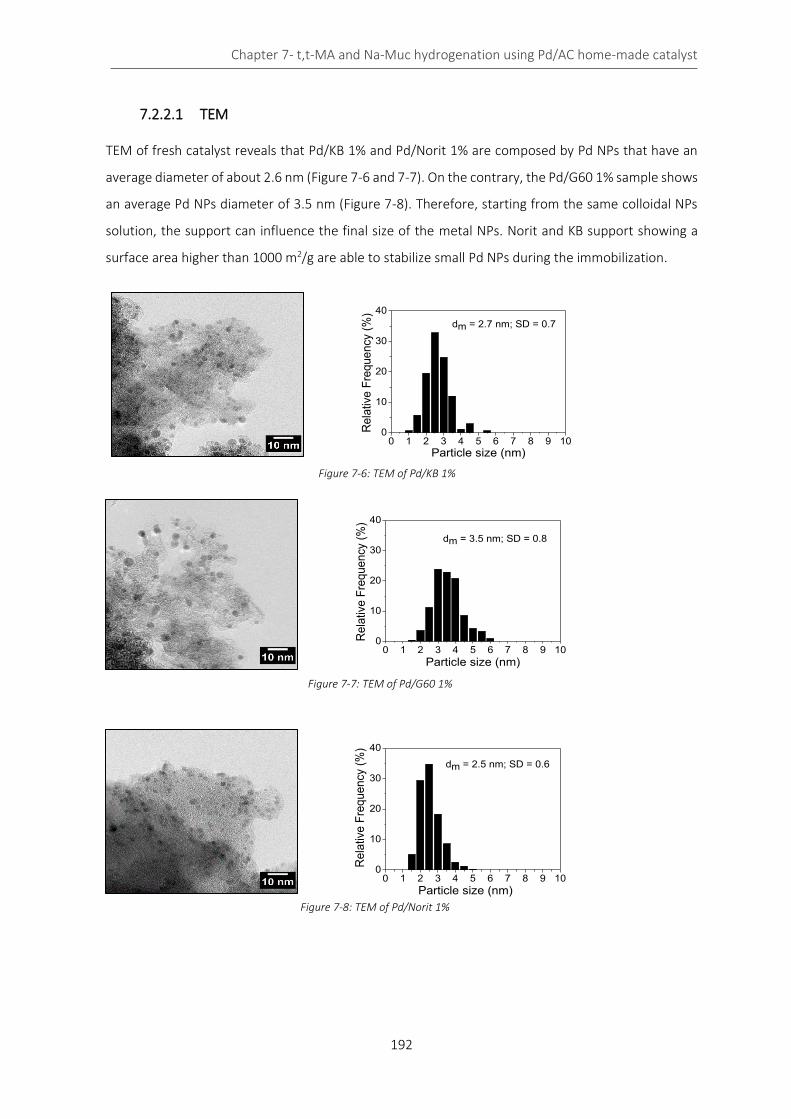
Chapter 7- t,t-MA and Na-Muc hydrogenation using Pd/AC home-made catalyst
192
7.2.2.1 TEM
TEM of fresh catalyst reveals that Pd/KB 1% and Pd/Norit 1% are composed by Pd NPs that have an
average diameter of about 2.6 nm (Figure 7-6 and 7-7). On the contrary, the Pd/G60 1% sample shows
an average Pd NPs diameter of 3.5 nm (Figure 7-8). Therefore, starting from the same colloidal NPs
solution, the support can influence the final size of the metal NPs. Norit and KB support showing a
surface area higher than 1000 m2/g are able to stabilize small Pd NPs during the immobilization.
0 1 2 3 4 5 6 7 8 9 100
10
20
30
40
Re
lative
Fre
qu
en
cy (
%)
Particle size (nm)
dm = 2.7 nm; SD = 0.7
Figure 7-6: TEM of Pd/KB 1%
0 1 2 3 4 5 6 7 8 9 100
10
20
30
40
dm = 2.5 nm; SD = 0.6
Rela
tive F
requency (
%)
Particle size (nm)
Figure 7-8: TEM of Pd/Norit 1%
0 1 2 3 4 5 6 7 8 9 100
10
20
30
40
dm = 3.5 nm; SD = 0.8
Rela
tive
Fre
quency
(%
)
Particle size (nm)
Figure 7-7: TEM of Pd/G60 1%
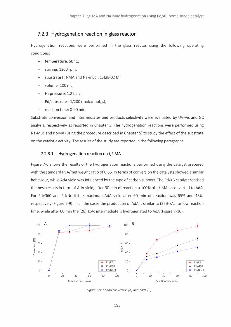
Chapter 7- t,t-MA and Na-Muc hydrogenation using Pd/AC home-made catalyst
193
7.2.3 Hydrogenation reaction in glass reactor
Hydrogenation reactions were performed in the glass reactor using the following operating
conditions:
temperature: 50 °C;
stirring: 1200 rpm;
substrate (t,t-MA and Na-muc): 1.42E-02 M;
volume: 100 mL;
H2 pressure: 1.2 bar;
Pd/substrate= 1/200 (molPd/molsub);
reaction time: 0-90 min.
Substrate conversion and intermediates and products selectivity were evaluated by UV-Vis and GC
analysis, respectively as reported in Chapter 3. The hydrogenation reactions were performed using
Na-Muc and t,t-MA (using the procedure described in Chapter 5) to study the effect of the substrate
on the catalytic activity. The results of the study are reported in the following paragraphs.
7.2.3.1 Hydrogenation reaction on t,t-MA
Figure 7-6 shows the results of the hydrogenation reactions performed using the catalyst prepared
with the standard PVA/met weight ratio of 0.65. In terms of conversion the catalysts showed a similar
behaviour, while AdA yield was influenced by the type of carbon support. The Pd/KB catalyst reached
the best results in term of AdA yield, after 90 min of reaction a 100% of t,t-MA is converted to AdA.
For Pd/G60 and Pd/Norit the maximum AdA yield after 90 min of reaction was 65% and 48%,
respectively (Figure 7-9). In all the cases the production of AdA is similar to (2E)HxAc for low reaction
time, while after 60 min the (2E)HxAc intermediate is hydrogenated to AdA (Figure 7-10).
0 20 40 60 80 100
0
20
40
60
80
100
Co
nve
rsio
n (
%)
Reaction time (min)
Pd/KB
Pd/G60
Pd/Norit
0 20 40 60 80 100
0
20
40
60
80
100
YAd
A (
%)
Reaction time (min)
Pd/KB
Pd/G60
Pd/Norit
Figure 7-9: t,t-MA conversion (A) and YAdA (B)
A B
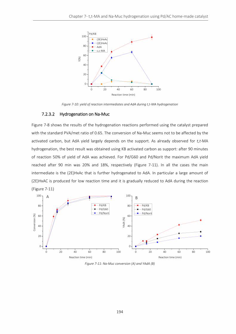
Chapter 7- t,t-MA and Na-Muc hydrogenation using Pd/AC home-made catalyst
194
Figure 7-10: yield of reaction intermediates and AdA during t,t-MA hydrogenation
7.2.3.2 Hydrogenation on Na-Muc
Figure 7-8 shows the results of the hydrogenation reactions performed using the catalyst prepared
with the standard PVA/met ratio of 0.65. The conversion of Na-Muc seems not to be affected by the
activated carbon, but AdA yield largely depends on the support. As already observed for t,t-MA
hydrogenation, the best result was obtained using KB activated carbon as support: after 90 minutes
of reaction 50% of yield of AdA was achieved. For Pd/G60 and Pd/Norit the maximum AdA yield
reached after 90 min was 20% and 18%, respectively (Figure 7-11). In all the cases the main
intermediate is the (2E)HxAc that is further hydrogenated to AdA. In particular a large amount of
(2E)HxAC is produced for low reaction time and it is gradually reduced to AdA during the reaction
(Figure 7-11)
Figure 7-11: Na-Muc conversion (A) and YAdA (B)
0 20 40 60 80 100
0
20
40
60
80
100
Y(%
)
Reaction time (min)
(3E)HxAc
(2E)HxAc
AdA
c,c-MA
Pd/KB
0 20 40 60 80 100
0
20
40
60
80
100
Co
nve
rsio
n (
%)
Reaction time (min)
Pd/KB
Pd/G60
Pd/Norit
0 20 40 60 80 100
0
20
40
60
80
100
YAd
A (
%)
Reaction time (min)
Pd/KB
Pd/G60
Pd/Norit
A B
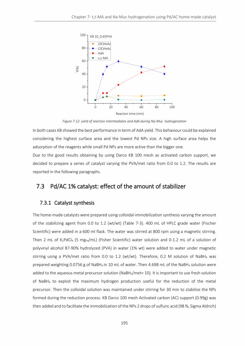
Chapter 7- t,t-MA and Na-Muc hydrogenation using Pd/AC home-made catalyst
195
Figure 7-12: yield of reaction intermediates and AdA during Na-Muc hydrogenation
In both cases KB showed the best performance in term of AdA yield. This behaviour could be explained
considering the highest surface area and the lowest Pd NPs size. A high surface area helps the
adsorption of the reagents while small Pd NPs are more active than the bigger one.
Due to the good results obtaining by using Darco KB 100 mesh as activated carbon support, we
decided to prepare a series of catalyst varying the PVA/met ratio from 0.0 to 1.2. The results are
reported in the following paragraphs.
7.3 Pd/AC 1% catalyst: effect of the amount of stabilizer
7.3.1 Catalyst synthesis
The home-made catalysts were prepared using colloidal-immobilization synthesis varying the amount
of the stabilizing agent from 0.0 to 1.2 (wt/wt) (Table 7-3). 400 mL of HPLC grade water (Fischer
Scientific) were added in a 600 ml flask. The water was stirred at 800 rpm using a magnetic stirring.
Then 2 mL of K2PdCl4 (5 mgPd/mL) (Fisher Scientific) water solution and 0-1.2 mL of a solution of
polyvinyl alcohol 87-90% hydrolyzed (PVA) in water (1% wt) were added to water under magnetic
stirring using a PVA/met ratio from 0.0 to 1.2 (wt/wt). Therefore, 0.2 M solution of NaBH4 was
prepared weighting 0.0756 g of NaBH4 in 10 mL of water. Then 4.698 mL of the NaBH4 solution were
added to the aqueous metal precursor solution (NaBH4/met= 10). It is important to use fresh solution
of NaBH4 to exploit the maximum hydrogen production useful for the reduction of the metal
precursor. Then the colloidal solution was maintained under stirring for 30 min to stabilize the NPs
formed during the reduction process. KB Darco 100 mesh Activated carbon (AC) support (0.99g) was
then added and to facilitate the immobilization of the NPs 2 drops of sulfuric acid (98 %, Sigma Aldrich)
0 20 40 60 80 100
0
20
40
60
80
100
Y(%
)
Reaction time (min)
(3E)HxAc
(2E)HxAc
AdA
c,c-MA
KB 10_0.65PVA
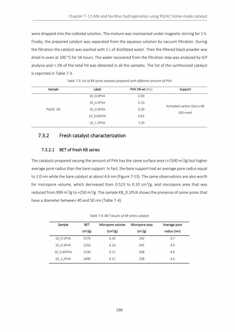
Chapter 7- t,t-MA and Na-Muc hydrogenation using Pd/AC home-made catalyst
196
were dropped into the colloidal solution. The mixture was maintained under magnetic stirring for 1 h.
Finally, the prepared catalyst was separated from the aqueous solution by vacuum filtration. During
the filtration the catalyst was washed with 1 L of distillated water. Then the filtered black powder was
dried in oven at 100 °C for 16 hours. The water recovered from the filtration step was analyzed by ICP
analysis and < 2% of the total Pd was detected in all the samples. The list of the synthesized catalyst
is reported in Table 7-3.
Table 7-3: list of KB series samples prepared with different amount of PVA
Sample Label PVA 1% wt (mL) Support
Pd/AC 1%
10_0.0PVA 0.00
Activated carbon Darco KB
100 mesh
10_0.1PVA 0.10
10_0.3PVA 0.30
10_0.65PVA 0.65
10_1.2PVA 1.20
7.3.2 Fresh catalyst characterization
7.3.2.1 BET of fresh KB series
The catalysts prepared varying the amount of PVA has the same surface area (≈1500 m2/g) but higher
average pore radius than the bare support. In fact, the bare support had an average pore radius equal
to 2.0 nm while the bare catalyst at about 4.6 nm (Figure 7-13). The same observations are also worth
for micropore volume, which decreased from 0.523 to 0.10 cm3/g, and micropore area that was
reduced from 999 m2/g to ≈250 m2/g. The sample KB_0.1PVA shows the presence of some pores that
have a diameter between 40 and 50 nm (Table 7-4).
Table 7-4: BET results of KB series catalyst
Sample BET
(m2/g)
Micropore volume
(cm3/g)
Micropore area
(m2/g)
Average pore
radius (nm)
10_0.1PVA 1570 0.10 242 4.7
10_0.3PVA 1550 0.10 245 4.6
10_0.65PVA 1530 0.11 268 4.6
10_1.2PVA 1490 0.11 258 4.6
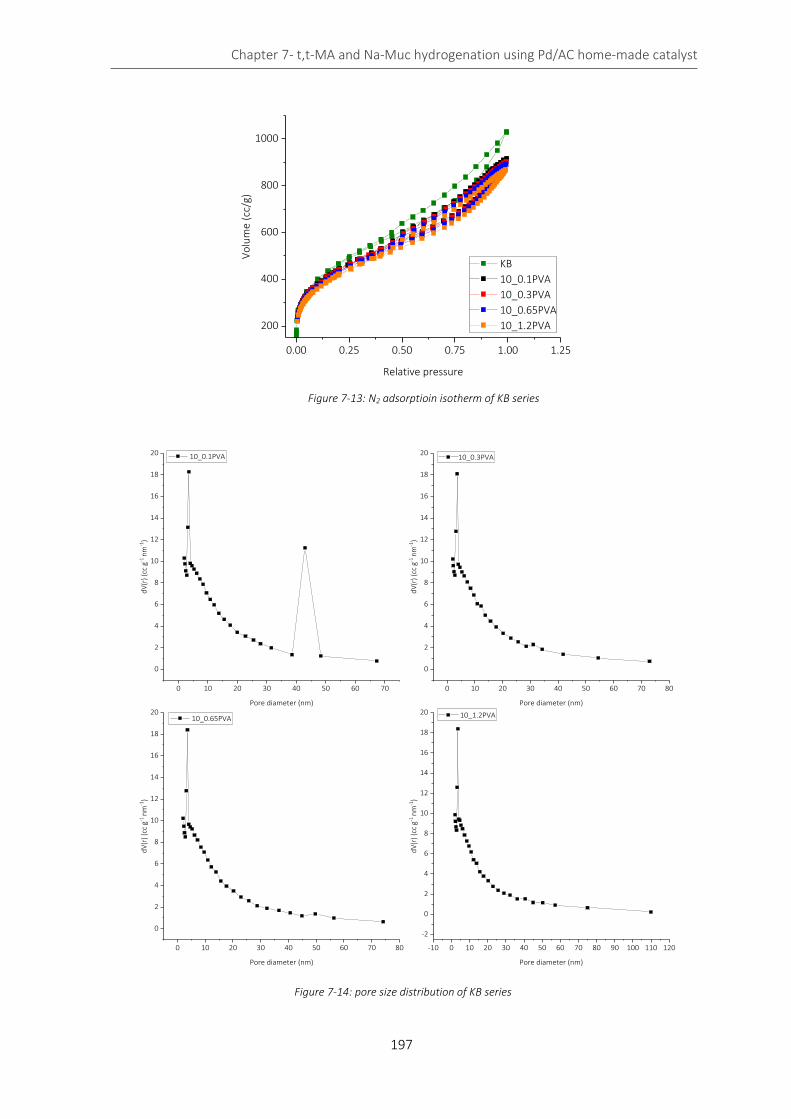
Chapter 7- t,t-MA and Na-Muc hydrogenation using Pd/AC home-made catalyst
197
Figure 7-13: N2 adsorptioin isotherm of KB series
Figure 7-14: pore size distribution of KB series
0 10 20 30 40 50 60 70
0
2
4
6
8
10
12
14
16
18
20
0 10 20 30 40 50 60 70 80
0
2
4
6
8
10
12
14
16
18
20
0 10 20 30 40 50 60 70 80
0
2
4
6
8
10
12
14
16
18
20
-10 0 10 20 30 40 50 60 70 80 90 100 110 120
-2
0
2
4
6
8
10
12
14
16
18
20
dV
(r)
(cc
g-1 nm
-1)
Pore diameter (nm)
10_0.1PVA
dV
(r)
(cc
g-1 nm
-1)
Pore diameter (nm)
10_0.3PVA
dV
(r)
(cc
g-1 nm
-1)
Pore diameter (nm)
10_0.65PVA
dV
(r)
(cc
g-1 nm
-1)
Pore diameter (nm)
10_1.2PVA
0.00 0.25 0.50 0.75 1.00 1.25
200
400
600
800
1000
Vo
lum
e (c
c/g)
Relative pressure
KB
10_0.1PVA
10_0.3PVA
10_0.65PVA
10_1.2PVA

Chapter 7- t,t-MA and Na-Muc hydrogenation using Pd/AC home-made catalyst
198
7.3.2.2 TEM
TEM images of KB series catalyst shows the presence of well dispersed Pd NPs on their surfaces.
Particles size is not the same for all the samples; in particular 10_0.3PVA and 10_1.2PVA have a similar
average particle diameter of 3.6 nm and 3.7 nm, respectively (Figure 7-15 and 7-17). The sample
10_0.65PVA shows a lower average particle size of 2.7 nm (Figure 7-16). Therefore, the PVA amount
influences the particle size: a low amount of PVA is not sufficiently able to stabilize, for example in
10_0.0PVA (Figure 7-18) wide NPs aggregates are immobilized on KB activated carbon surface.
0 1 2 3 4 5 6 7 8 9 100
10
20
30
40
dm = 3.6 nm; SD = 1.2
Re
lative
Fre
qu
en
cy (
%)
Particle size (nm)
Figure 7-16: TEM of 10_0.3PVA
0 1 2 3 4 5 6 7 8 9 100
10
20
30
40
Re
lative
Fre
qu
en
cy (
%)
Particle size (nm)
dm = 2.7 nm; SD = 0.7
Figure 7-15:TEM of 10_0.65PVA
0 1 2 3 4 5 6 7 8 9 100
10
20
30
40
dm = 3.7 nm; SD = 1.1
Re
lative
Fre
qu
en
cy (
%)
Particle size (nm)
Figure 7-17: TEM of 10_1.2PVA

Chapter 7- t,t-MA and Na-Muc hydrogenation using Pd/AC home-made catalyst
199
On the contrary a large excess of PVA slows down the immobilization process facilitating the
aggregation of the NPs that are in solution. Finally, the addition of sulfuric acid decreases the pH of
the solution decreasing the NPs stability. Therefore, lower is the immobilization rate, higher is the
possibility to form large aggregates.
Figure 7-18: TEM of 10_0.0PVA
7.3.2.3 XPS of fresh KB series
XPS analyses of the fresh KB series were performed and Pd and C spectra were elaborated.
The survey spectra were elaborated with CasaXPS software, and the atomic percentage for each
element was calculated. Due to the increment of PVA and the constant amount of Pd, the ratio
between Pd and C should decrease. Therefore, the Pd surface exposition decreases increasing the
amount of PVA; this behaviour might be explained considering that the higher is the amount of PVA
the greater is the presence of the stabilizer that is covering the catalyst surface. The results are
reported in Table 7-5 and Figure 7-19. The catalyst that has the highest Pd surface exposition is the
10_0.1PVA that has a Pd/C ratio equal to 0.039, while the 10_0.0PVA has the lowest value (0.012).
This difference might be explained considering the non-homogeneity of the catalyst and thus the
analysed sample could be no completely significative.
Table 7-5: atomic percentage of C, O and Pd in the KB sample
Sample C (%) O2 (%) Pd (%) Pd/C
10_0.0PVA 87.8 11.1 1.2 0.012
10_0.1PVA 82.9 13.8 3.2 0.039
10_0.3PVA 81.9 15.3 2.7 0.033
10_0.65PVA 82.8 14.8 2.4 0.029
10_1.2PVA 80.9 16.8 2.4 0.029
Figure 7-19: Pd/C ratio evaluated from the Survay spectra
10_0.0PVA 10_0.1PVA 10_0.3PVA 10_0.65PVA 10_1.2PVA0
1
2
3
4
5
6
Pd
(0)/
Pd
(II)
10_0.0PVA 10_0.1PVA 10_0.3PVA 10_0.65PVA 10_1.2PVA0.0
0.1
0.2
0.3
0.4
0.5
(Csp
3+C
-O)/
(C s
p2
)
10_0.0PVA 10_0.1PVA 10_0.3PVA 10_0.65PVA 10_1.2PVA0.000
0.005
0.010
0.015
0.020
0.025
0.030
0.035
0.040
Pd
/C

Chapter 7- t,t-MA and Na-Muc hydrogenation using Pd/AC home-made catalyst
200
From the deconvolution of C specie 4 different groups were detected: C sp2, C sp3, C=O and C-O at
284.09 eV, 284.80 eV, 287.66 eV and 287.71 eV, respectively (Table 7-6).
The percentage of the different C species evaluated from the C spectra were estimated and the results
are reported in Table 7-7. The last column shows the ratio between the sum of the percentage of the
Csp3 and C-O species, and the Csp2 that is ≈0.38. Csp2 was chosen as the reference species because
it is present only in the carbon support, therefore the C sp2 % is constant (33.7-37.4 %) while the C
sp3 and C-O should increase due to the presence of a larger amount of PVA. The only sample that
shows different results is the catalyst prepared without the PVA as reported in Figure 7-20.
Table 7-6: Binding energy for the C species
Specie Binding Energy (eV)
C sp2 284.09
C sp3 284.80
C=O 287.66
C-O 287.71
Table 7-7: percentage of the different C species of KB series catalysts
Sample
C 1s
(%)
C sp2
(%)
C sp3
(%)
C-O
(%)
C=O
(%)
Csp3+C-O
(%)
Csp3+C-O/C sp2
ratio
10_0.0PVA 50.5 37.4 9.9 1.2 0.9 11.2 0.30
10_0.1PVA 50.4 33.8 11.9 2.6 1.2 14.6 0.43
10_0.3PVA 50.2 33.7 12.2 1.3 2.6 13.5 0.40
10_0.65PVA 50.5 34.9 11.7 0.6 2.2 12.3 0.35
10_1.2PVA 50.8 34.9 10.2 2.6 1.6 12.7 0.37
10_0.0PVA 10_0.1PVA 10_0.3PVA 10_0.65PVA 10_1.2PVA
0.0
0.1
0.2
0.3
0.4
0.5
(Csp
3+C
-O)/
(C s
p2
)
Figure 7-20: (Csp3+C-O)/Csp2 ratio of KB series catalysts

Chapter 7- t,t-MA and Na-Muc hydrogenation using Pd/AC home-made catalyst
201
Regarding the deconvolution of Pd species, this metal displayed two different peaks (Figure 7-22 A)
ascribable to the Pd 3d3/2 and Pd 3d5/2 transition. Pd(0) 3d5/2 core electron binding energy is at 335.60
eV, while the Pd(0) 3d3/2 is at 340.54 eV. The Pd(II) peaks are at 338.15 eV and 343.47 eV, and they
are identified as 3d3/2 and 3d5/2 transition, respectively (Table 7-8). These binding energy values are in
good agreement with that data reported in Chen et al. and Sanchez et al.5,6
Table 7-8: BE of the detected Pd species
Specie Binding Energy (eV)
Pd 3d 5/2(0) 335.60
Pd 3d5/2 (II) 338.15
Pd 3d3/2 (0) 340.54
Pd 3d3/2 (II) 343.47
Moreover, the percentage of the different Pd species evaluated from the Pd spectra were estimated
and the results are reported Table 7-9. The 10_1.2PVA catalyst has the higher amount of Pd(II)
(32.2%), while the 10_0.1PVA has the lowest one (15.2%). Pd(0) specie percentage decreases
increasing the PVA amount. In particular, considering the 10_0.3PVA, 10_0.65PVA and 10_1.2PVA
samples, 10_0.65PVA sample show the highest value of Pd(0)/Pd(II) (Figure 7-21). We hypothesized
that smaller Pd NPs are more active toward the spontaneous passivation.
Table 7-9: Pd(II) and Pd(0) species within the KB series
Sample Pd (II) (%) Pd (0) (%) Pd(0)/Pd(II)
10_0.0PVA 18.5 81.5 4.4
10_0.1PVA 15.2 84.8 5.6
10_0.3PVA 26.9 72.1 2.7
10_0.65PVA 23.1 76.9 3.3
10_1.2PVA 32.2 67.8 2.1
10_0.0PVA 10_0.1PVA 10_0.3PVA 10_0.65PVA 10_1.2PVA0
1
2
3
4
5
6
Pd(0
)/Pd
(II)
10_0.0PVA 10_0.1PVA 10_0.3PVA 10_0.65PVA 10_1.2PVA0.0
0.1
0.2
0.3
0.4
0.5
(Csp
3+C-
O)/
(C s
p2)
10_0.0PVA 10_0.1PVA 10_0.3PVA 10_0.65PVA 10_1.2PVA0.000
0.005
0.010
0.015
0.020
0.025
0.030
0.035
0.040
Pd/C
Figure 7-21: Pd(0)/Pd(II) ratio of KB series

202
348 345 342 339 336 333 330
348 345 342 339 336 333 330
Binding energy (eV)
Pd(II) Pd(II)Pd(0)
10_0.0PVA
10_0.1PVA
10_0.3PVA
10_0.65PVA
10_1.2PVA Pd(0)
CPS
Figure 7-22: Pd (A) and C (B) deconvolution for the different KB samples
292 290 288 286 284 282 280
292 290 288 286 284 282 280
Binding Energy (mV)
10_0.0PVA
10_0.1PVA
10_0.3PVA
10_0.65PVA
C sp3
CPS
10_1.2PVA C sp2
A B

Chapter 7- t,t-MA and Na-Muc hydrogenation using Pd/AC home-made catalyst
203
7.3.3 Hydrogenation reaction in glass reactor
Hydrogenation reactions were performed in the glass reactor using the following operating
conditions:
temperature: 50 °C;
stirring: 1200 rpm;
substrate (t,t-ma and Na-muc): 1.42E-02 M;
volume: 100 ml;
H2 pressure: 1.2 bar;
Pd/substrate= 1/200 (molPd/molsub);
reaction time: 0-90 min.
Substrate conversion and intermediates and products selectivity were evaluated by UV-Vis and GC
analysis, respectively. The hydrogenation reactions were performed using Na-Muc and t,t-MA to study
the effect of the substrate on the catalytic activity. The results of the study are reported in the
following paragraphs.
7.3.3.1 t,t-MA hydrogenation
Using the same reaction conditions t,t-MA was hydrogenated using the catalysts synthesized with the
same activated carbon support but varying the PVA/met ratio from 0.0 to 1.2 (wt/wt). t,t-MA
conversion reaches 100% only after 20 minutes of reaction, except for KB 0.65 and 1.2 PVA (Figure 7-
22 A). Contrarywise, AdA yield is affected by the amount of PVA: KB 0.1 and 0.3 PVA samples show
the same trend, while for low reaction time KB 0.0 and 1.2 PVA catalysts has the highest value of AdA
yield (Figure 7-23 B). All the considered catalysts have an initial activity comparable with the one
obtained Pd/AC 5% commercial catalyst (≈0.2 s-1) (Figure 7-24 A).
0 20 40 60 80 100
0
20
40
60
80
100
YAd
A (
%)
Reaction time (min)
KB 0.0PVA
KB 0.1PVA
KB 0.3PVA
KB 0.65PVA
KB 1.2PVA
A
0 20 40 60 80 100
0
20
40
60
80
100 B
Co
nve
rsio
n (
%)
Reaction time (min)
KB 0.0PVA
KB 0.1PVA
KB 0.3PVA
KB 0.65PVA
KB 1.2PVA
0 20 40 60 80 100
0
20
40
60
80
100
YAd
A (
%)
Reaction time (min)
KB 0.0PVA
KB 0.1PVA
KB 0.3PVA
KB 0.65PVA
KB 1.2PVA
A
0 20 40 60 80 100
0
20
40
60
80
100 B
Co
nve
rsio
n (
%)
Reaction time (min)
KB 0.0PVA
KB 0.1PVA
KB 0.3PVA
KB 0.65PVA
KB 1.2PVA
A B
Figure 7-23: conversion (A) and AdA yield (B) during t,t-MA hydrogentation with KB series catalysts

Chapter 7- t,t-MA and Na-Muc hydrogenation using Pd/AC home-made catalyst
204
Comparing the YAdA at 30 min obtained using KB series catalysts with the result obtained with
commercial Pd/AC5% we can see that 0.1PVA, 0.3PVA and 1.2PVA have a yield (81%) higher than the
commercial catalyst (71%) (Figure 7-24 B).
7.3.3.2 Used catalyst characterization
Pd/AC 1% KB 10_0.65PVA was filtered from the reactant solution after 15 and 90 minutes of reaction.
The survey spectrum of used catalyst after 15 min of reaction shows the presence of C 1s (282.58 eV),
Pd 3d (337.54 eV) and O 1s (532.86 eV) species (Table 7-10). Pd 3d peak is very trivial to analyse for
further deconvolution, in fact the recovered catalyst was light grey, which means that some adipic
acid and intermediates species were covering the surface of the catalyst.
Table 7-10: binding energy of the species after 15 min of reaction
Specie Binding energy
(eV) Area Norm Area Group %
C 1s 284.58 2643 916.0 69.3
Pd 3d 337.54 201 4.48 0.3
O 1s 532.86 2883 400.9 30.4
Considering the deconvolution of C specie (Figure 7-25), 5 different C groups were found in the
sample: C sp2 (284.636 eV), C sp3 (285.754 eV), C-O (286.886 eV), C=O (289.187 eV) and C pi (290.798
eV). Csp2 specie is the 47.3% of the total C present on the catalyst surface, therefore we can
hypothesize that a lot of reagents and intermediates are adsorbed on the surface of the catalyst (Table
7-11).
Figure 7-24: initial activity (A) and AdA yield after 30 min of reaction
0.0PVA 0.1PVA 0.3PVA 0.65PVA 1.2PVA0
20
40
60
80
100
YAd
A (
%)
comm.0.0PVA 0.1PVA 0.3PVA 0.65PVA 1.2PVA0.00
0.03
0.06
0.09
0.12
0.15
0.18
0.21
Init
ial a
ctiv
ity
(s-1
)
comm.comm.
A B

Chapter 7- t,t-MA and Na-Muc hydrogenation using Pd/AC home-made catalyst
205
Table 7-11: composition of C specie after 15 min of reaction with t,t-MA
Specie Peak ID Binding energy
(eV) Area
Atom
(%)
C sp2 Pk01 284.636 39712 47.3
C sp3 Pk02 285.754 15020 17.9
C-O Pk03 286.886 11548 13.7
C=O Pk04 289.187 14093 16.8
C pi Pk05 290.798 3655 4.3
At 90 minutes of reaction C 1s, Pd 3d and O 1s signals were clearly detected in the range between 280
and 600 eV. From the evaluation of the area of the different species, C element was detected as the
major specie (84.1%). In this case atom percentage of Pd is not negligible (1.2%), therefore during the
reaction t,t-MA and the intermediates has been desorbed on the catalyst surface.
Table 7-12: species detected from the survey spectrum on KB 0.65 sample after 90 min of reaction
Considering the C species, 5 different carbon groups were detected (Figure 7-26): C sp2 (284.607 eV),
C sp3 (285.871 eV), C-O (287.559 eV), C=O (289.334 eV) and c pi (291.223 eV) (Table 7-12).
C=O percentage (5.1%) in the used catalyst at 90 minutes of reaction is slower than the ones at 15
minutes (16.8%). The reducing reaction environment helps not only the reduction of but also the
reduction of carboxylic group of the activated carbon (Table 7-13). The amount of C sp 3 specie
increases from 17.9% to 21.5% due to the reduction previously mentioned.
Specie Binding energy
(eV) Area Norm Area
Atom
(%)
C 1s 284.63 9706 1739.3 84.1
Pd 3d 335.976 2213 25.5 1.2
O 1s 532.851 4231 304.3 14.7
300 298 296 294 292 290 288 286 284 282 2800
250
500
750
1000
1250
1500
1750
CP
S
Binding energy (eV)
CPS
peak 01
peak 02
peak 03
peak 04
peak 05
Envelope
Figure 7-25: deconvolution of C species after 15 min
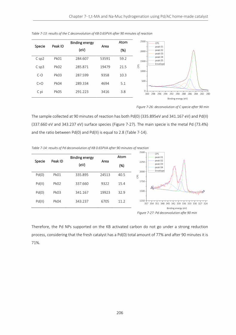
Chapter 7- t,t-MA and Na-Muc hydrogenation using Pd/AC home-made catalyst
206
Table 7-13: results of the C deconvolution of KB 0.65PVA after 90 minutes of reaction
Specie Peak ID Binding energy
(eV) Area
Atom
(%)
C sp2 Pk01 284.607 53591 59.2
C sp3 Pk02 285.871 19479 21.5
C-O Pk03 287.599 9358 10.3
C=O Pk04 289.334 4694 5.1
C pi Pk05 291.223 3416 3.8
The sample collected at 90 minutes of reaction has both Pd(0) (335.895eV and 341.167 eV) and Pd(II)
(337.660 eV and 343.237 eV) surface species (Figure 7-27). The main specie is the metal Pd (73.4%)
and the ratio between Pd(0) and Pd(II) is equal to 2.8 (Table 7-14).
Table 7-14: results of Pd deconvolution of KB 0.65PVA after 90 minutes of reaction
Specie Peak ID Binding energy
(eV) Area
Atom
(%)
Pd(0) Pk01 335.895 24513 40.5
Pd(II) Pk02 337.660 9322 15.4
Pd(0) Pk03 341.167 19923 32.9
Pd(II) Pk04 343.237 6705 11.2
Therefore, the Pd NPs supported on the KB activated carbon do not go under a strong reduction
process, considering that the fresh catalyst has a Pd(0) total amount of 77% and after 90 minutes it is
71%.
300 298 296 294 292 290 288 286 284 282 2800
500
1000
1500
2000
2500
CP
S
Binding energy (eV)
CPS
peak 01
peak 02
peak 03
peak 04
peak 05
Envelope
357 354 351 348 345 342 339 336 333 330 327 3241250
1500
1750
2000
2250
2500
CPS
Binding energy (eV)
CPS
peak 01
peak 02
peak 03
peak 04
Envelope
Figure 7-26: deconvolution of C specie after 90 min
Figure 7-27: Pd deconvolution afte 90 min
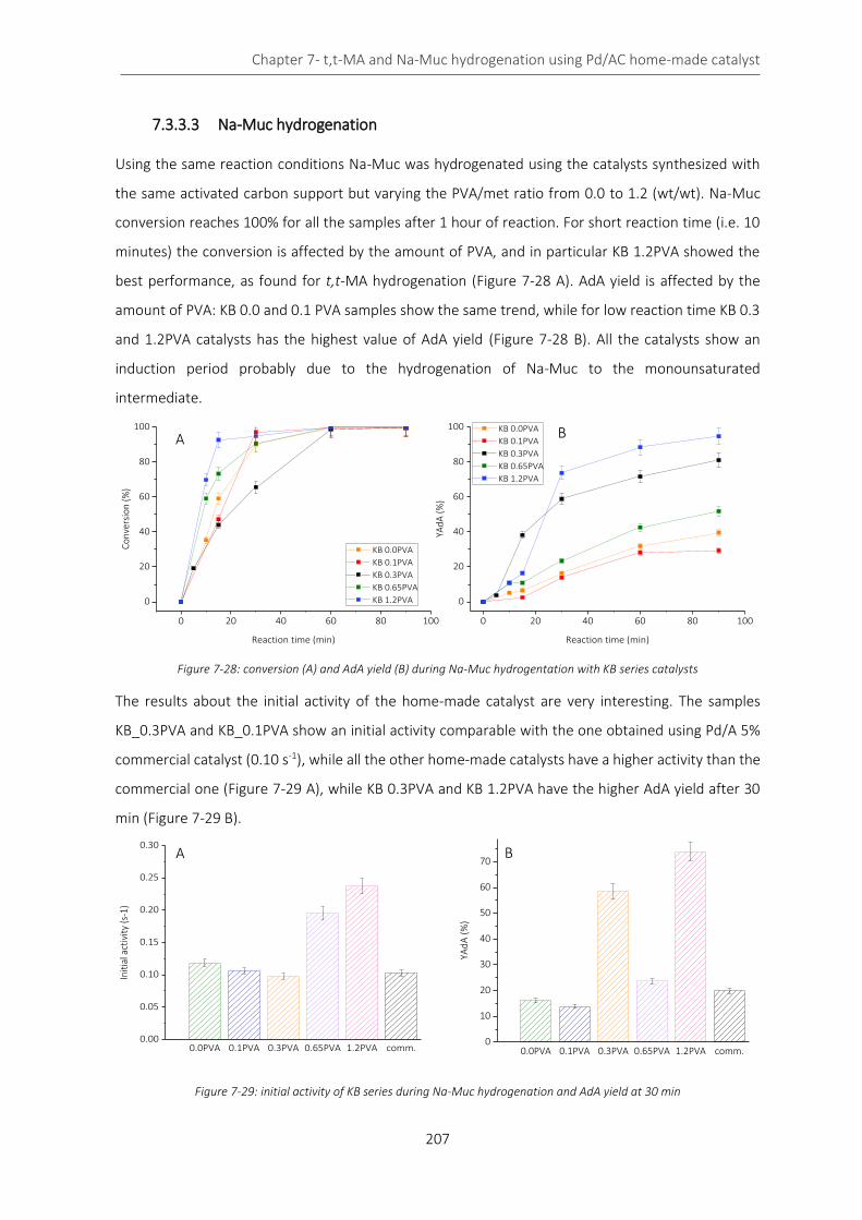
Chapter 7- t,t-MA and Na-Muc hydrogenation using Pd/AC home-made catalyst
207
7.3.3.3 Na-Muc hydrogenation
Using the same reaction conditions Na-Muc was hydrogenated using the catalysts synthesized with
the same activated carbon support but varying the PVA/met ratio from 0.0 to 1.2 (wt/wt). Na-Muc
conversion reaches 100% for all the samples after 1 hour of reaction. For short reaction time (i.e. 10
minutes) the conversion is affected by the amount of PVA, and in particular KB 1.2PVA showed the
best performance, as found for t,t-MA hydrogenation (Figure 7-28 A). AdA yield is affected by the
amount of PVA: KB 0.0 and 0.1 PVA samples show the same trend, while for low reaction time KB 0.3
and 1.2PVA catalysts has the highest value of AdA yield (Figure 7-28 B). All the catalysts show an
induction period probably due to the hydrogenation of Na-Muc to the monounsaturated
intermediate.
Figure 7-28: conversion (A) and AdA yield (B) during Na-Muc hydrogentation with KB series catalysts
The results about the initial activity of the home-made catalyst are very interesting. The samples
KB_0.3PVA and KB_0.1PVA show an initial activity comparable with the one obtained using Pd/A 5%
commercial catalyst (0.10 s-1), while all the other home-made catalysts have a higher activity than the
commercial one (Figure 7-29 A), while KB 0.3PVA and KB 1.2PVA have the higher AdA yield after 30
min (Figure 7-29 B).
Figure 7-29: initial activity of KB series during Na-Muc hydrogenation and AdA yield at 30 min
0 20 40 60 80 100
0
20
40
60
80
100
Con
vers
ion
(%)
Reaction time (min)
KB 0.0PVA
KB 0.1PVA
KB 0.3PVA
KB 0.65PVA
KB 1.2PVA
0 20 40 60 80 100
0
20
40
60
80
100YA
dA (
%)
Reaction time (min)
KB 0.0PVA
KB 0.1PVA
KB 0.3PVA
KB 0.65PVA
KB 1.2PVA
0.0PVA 0.1PVA 0.3PVA 0.65PVA 1.2PVA comm.0.00
0.05
0.10
0.15
0.20
0.25
0.30
Init
ial a
ctiv
ity
(s-1
)
0.0PVA 0.1PVA 0.3PVA 0.65PVA 1.2PVA comm.0
10
20
30
40
50
60
70
YAd
A (
%)
A B
A B
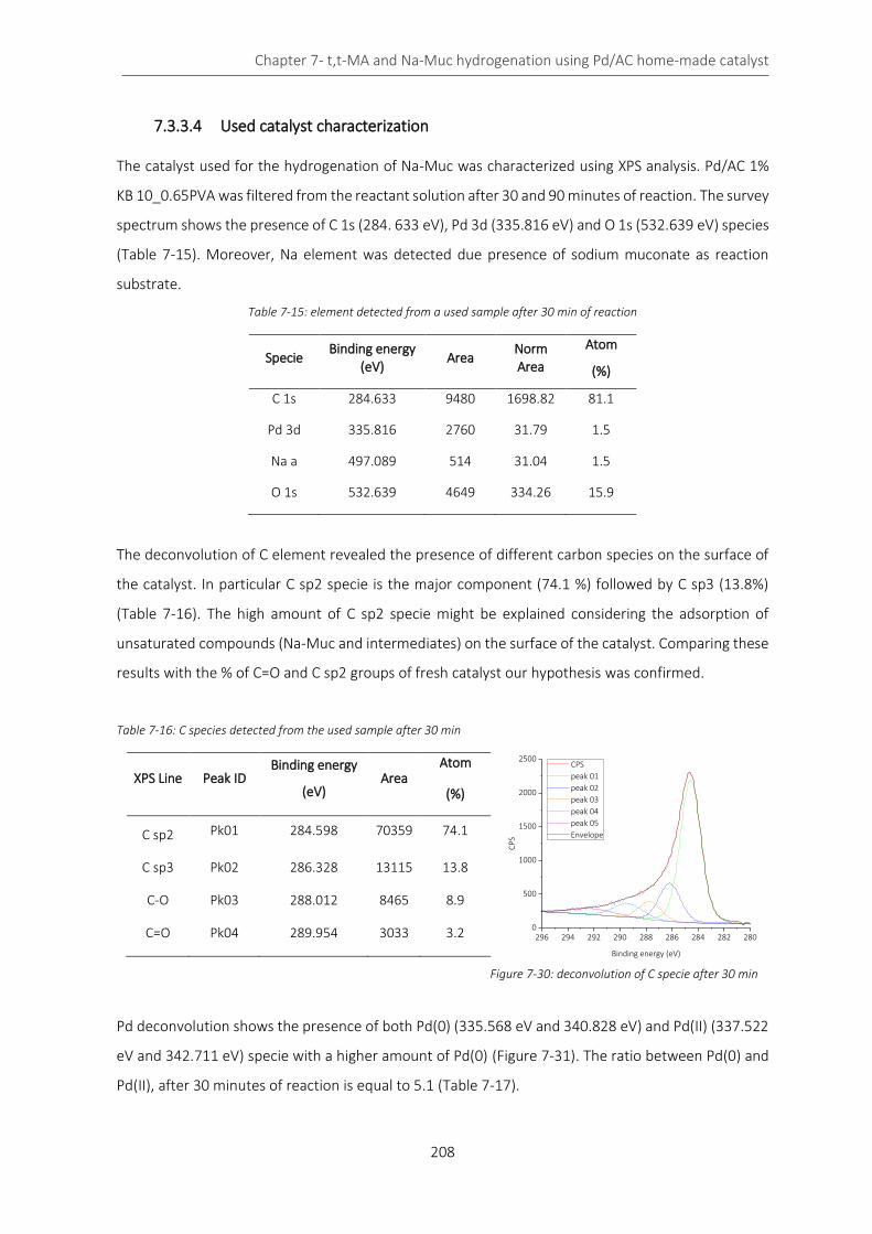
Chapter 7- t,t-MA and Na-Muc hydrogenation using Pd/AC home-made catalyst
208
7.3.3.4 Used catalyst characterization
The catalyst used for the hydrogenation of Na-Muc was characterized using XPS analysis. Pd/AC 1%
KB 10_0.65PVA was filtered from the reactant solution after 30 and 90 minutes of reaction. The survey
spectrum shows the presence of C 1s (284. 633 eV), Pd 3d (335.816 eV) and O 1s (532.639 eV) species
(Table 7-15). Moreover, Na element was detected due presence of sodium muconate as reaction
substrate.
Table 7-15: element detected from a used sample after 30 min of reaction
Specie Binding energy
(eV) Area
Norm Area
Atom
(%)
C 1s 284.633 9480 1698.82 81.1
Pd 3d 335.816 2760 31.79 1.5
Na a 497.089 514 31.04 1.5
O 1s 532.639 4649 334.26 15.9
The deconvolution of C element revealed the presence of different carbon species on the surface of
the catalyst. In particular C sp2 specie is the major component (74.1 %) followed by C sp3 (13.8%)
(Table 7-16). The high amount of C sp2 specie might be explained considering the adsorption of
unsaturated compounds (Na-Muc and intermediates) on the surface of the catalyst. Comparing these
results with the % of C=O and C sp2 groups of fresh catalyst our hypothesis was confirmed.
Table 7-16: C species detected from the used sample after 30 min
XPS Line Peak ID Binding energy
(eV) Area
Atom
(%)
C sp2 Pk01 284.598 70359 74.1
C sp3 Pk02 286.328 13115 13.8
C-O Pk03 288.012 8465 8.9
C=O Pk04 289.954 3033 3.2
Pd deconvolution shows the presence of both Pd(0) (335.568 eV and 340.828 eV) and Pd(II) (337.522
eV and 342.711 eV) specie with a higher amount of Pd(0) (Figure 7-31). The ratio between Pd(0) and
Pd(II), after 30 minutes of reaction is equal to 5.1 (Table 7-17).
296 294 292 290 288 286 284 282 2800
500
1000
1500
2000
2500
CP
S
Binding energy (eV)
CPS
peak 01
peak 02
peak 03
peak 04
peak 05
Envelope
Figure 7-30: deconvolution of C specie after 30 min

Chapter 7- t,t-MA and Na-Muc hydrogenation using Pd/AC home-made catalyst
209
Table 7-17: Pd species detected after 30 min
Specie Peak ID Binding energy
(eV) Area
Atom
(%)
Pd(0) Pk01 335.568 43844 49.5
Pd(II) Pk02 337.522 8604 9.7
Pd(0) Pk03 340.828 30346 34.2
Pd(II) Pk04 342.711 5807 6.6
The composition of the catalyst collected at the end of the reaction (90 min) did not show any changes
in the composition: Pd, C, O and Na element were detected during the analysis (Table 7-18).
Table 7-18: element detected from a used sample after 90 min of reaction
Specie Binding energy
(eV) Area
Norm Area
Atom
(%)
C 1s 284.649 6572 1177.72 80.7
Pd 3d 335.848 1953 22.49 1.5
Na a 496.517 369 22.28 1.5
O 1s 532.338 3293 236.71 16.3
The deconvolution of C element (Figure 7-32) revealed the presence of different C species on the
surface of the catalyst. The percentage of C sp2 group is 7% less than the one evaluated after 30
minutes of reaction while the C sp3 amount increased (Table 7-19). This behavior could be explained
considering that the during the hydrogenation reaction double bonds (C sp 2) are converted to single
bonds (C sp3).
Table 7-19: C species detected from the used sample after 90 min
XPS Line Peak ID Binding energy
(eV) Area
Area
(%)
C sp2 Pk01 284.575 49117 67.2
C sp3 Pk02 286.225 13435 18.4
C-O Pk03 287.798 5621 7.7
C=O Pk04 289.264 3072 4.2
C pi Pk05 290.985 1823 2.5 298 296 294 292 290 288 286 284 282 280
0
250
500
750
1000
1250
1500
1750
2000
CPS
Binding energy (eV)
CPS
peak 01
peak 02
peak 03
peak 04
peak 05
Envelope
355 350 345 340 335 330 325
1500
1750
2000
2250
2500
2750
3000
3250
CP
S
Binding energy (eV)
CPS
peak 01
peak 02
peak 03
peak 04
Envelope
Figure 7-31: Pd deconvolution after 30 min
Figure 7-32: C deconvolution after 90 min

Chapter 7- t,t-MA and Na-Muc hydrogenation using Pd/AC home-made catalyst
210
Pd deconvolution (Figure 7-33) shows the presence of both Pd(0) and Pd(II) specie with a higher
amount of Pd(0). The ratio between Pd(0) and Pd(II), after 90 minutes of reaction is equal to 2.71.
Table 7-20: Pd species detected after 30 min
Specie Peak ID Binding energy
(eV) Area
Area
(%)
Pd(0) Pk01 335.627 30848 43.3
Pd(II) Pk02 337.421 10549 14.8
Pd(0) Pk03 340.826 21237 29.8
Pd(II) Pk04 342.47 8609 12.1
Considering the Pd(0)/Pd(II) at different reaction times Pd(II) is reduced to Pd(0) during the first
moments of the reaction, while after 90 min the composition return to be similar to the first one.
Figure 7-34: variation of Pd(0)/Pd(II) ratio at different reaction times
0 min 30 min 90 min
0.0
0.4
0.8
1.2
1.6
2.0
2.4
2.8
3.2
3.6
4.0
4.4
4.8
5.2
Pd
(0)/
Pd
(II)
354 351 348 345 342 339 336 333 330 3271000
1250
1500
1750
2000
2250
2500
CPS
Binding energy (eV)
CPS
peak 01
peak 02
peak 03
peak 04
Envelope
Figure 7-33: Pd deconvolution after 30 min
Chapter 7- Conclusion
211
Conclusion
Na-Muc and t,t-MA were hydrogenated using catalyst prepared by sol-immobilization method. Pd NPs
were immobilized on three different activated carbon supports. KB Darco 100 mesh activated carbon
showed the best results in term of AdA yield, both during t,t-MA and Na-Muc conversion. Its best
behavior is probably due to the high surface area which help the adsorption and desorption process
and the low NPs dimension that are more active.
Therefore 5 catalysts were prepared varying the amount of stabilizer and keeping constant the KB
Darco activated carbon support and changing the amount of stabilizer (PVA). The catalysts had the
same surface area, while the Pd NP had different dimensions. Using the optimal amount of PVA (0.65
mL) the NPs had an average size of 2.7 nm, although using higher of lower amount of PVA the diameter
of the Pd NPs is higher. Low amount of stabilizer is not able to stabilize the NPs during their formation,
while high amount of PVA can interfere in the immobilization process.
t,t-MA and Na-Muc were hydrogenated and we obtained good results. t,t-MA hydrogenation quickly
occurs and the initial activity of the all home-made catalysts is equal to the commercial Pd/AC 5%
catalyst. The samples 10_0.0PVA and 10_0.65PVA showed an AdA yield equal to the commercial
catalyst after 30 min of reaction, while all the other home-made catalysts are better than the
commercial one.
Na-Muc hydrogenation reaction is slower than t,t-MA reduction. 10_0.0PVA, 10_0.65PVA and
10_1.2PVA presented higher activity than commercial Pd/AC 5% catalyst and they have more
capability to produce AdA. This behavior could be explained considering the different surface area of
the supports: KB activated carbon has a surface area that is twice respect to the commercial Pd/AC
5%.
In all the cases Pd(0) and Pd(II) species are presented on the catalyst surface and Pd(II) is reduced to
metal Pd during the reaction, increasing the catalyst activity.
These interesting results opened the possibility to optimize the design of this catalyst and to
understand the key catalyst feature for this kind of reaction.
Chapter 7- Bibliography
212
Bibliography
1. Zha, J. & Roggendorf, H. Sol-gel science, the physics and chemistry of sol-gel processing, Ed. by C. J. Brinker and G. W. Scherer, Academic Press, Boston 1990, xiv, 908 pp., bound?ISBN 0-12-134970-5. Adv. Mater. 3, 522–522 (1991).
2. Sharada, S. et al. Synthesis of palladium nanoparticles using continuous flow microreactor. Colloids Surfaces A Physicochem. Eng. Asp. 498, 297–304 (2016).
3. Jia, C.-J. & Schuth, F. Colloidal metal nanoparticles as a component of designed catalyst. Phys. Chem. Chem. Phys. 13, 2457–2487 (2011).
4. Ismadji, S. & Bhatia, S. K. Characterization of activated carbons using liquid phase adsorption. Carbon N. Y. 39, 1237–1250 (2001).
5. Chen, X. et al. Non-covalently modified graphene supported ultrafine nanoparticles of palladium for hydrogen gas sensing. RSC ADVANCES 3, (2013).
6. Sanchez, F. et al. Hydrogen Generation from Additive-Free Formic Acid Decomposition Under Mild Conditions by Pd/C: Experimental and DFT Studies. Top. Catal. 61, 254–266 (2018).
213
Chapter 8
Life cycle impact assessment analysis
(LCIA) and economic feasibility study
This chapter describes the life cycle impact assessment of the industrial process for the production of
adipic acid. Two different processes were considered: the conventional oil-based process and the bio-
based process. The traditional petrochemical process involves the oxidation of the KA-oil mixture
while the bio-based one the production of muconic acid starting from wood biomass and its further
hydrogenation to adipic acid. The comparison had been possible thanks to a deep study performed in
collaboration with Politecnico di Milano (Alessandro Rosengart et al. Process Synthesis for the
Production of Sustainable Adipic acid, Biotechnology and Biofuels, under review). We designed and
optimized the industrial process for the production of bio-adipic acid evaluating the materials and the
energy required for the process. This is obviously a preliminary study because no real industrial values
and process was taken into account for the bio-process description, but we decided to perform the
study placing in the worst operating conditions. Therefore, the values of the impact might change with
further detailed studies.

Chapter 8- Life cycle impact assessment analysis (LCIA) and economic feasibility study
214
8.1 Overview about LCIA study of adipic acid
There are several studies for the production of AdA starting from renewable sources, in particular
from lignin biomass.1–4 Lignocellulosic biomass is a versatile renewable resource for the production of
sustainable chemicals and materials; in fact polysaccharides are the first interest fraction for selective
conversion processes obtain from biomass.5 Xie at al. summed up all the different routes to obtain of
an important chemical intermediate in the production of bio-AdA such as muconic acid (MA). MA is a
high value-added bio-product produced by biotechnological pathway with different modified and
unmodified bacteria strains.2 Mizuno et.al produced 44.1 g/L of MA in 48 h using Arthrobacter sp. and
benzoate as feedstock 6, while in 2012 van Duuren et al. used P. Putida mutant strain BM014 in a fed-
batch reactor feeding benzoate as substrate. They obtained 32.4 g/L of MA with a molar yield of
100%.7 Vardon et al. in a recent work proposed the downstream process for the MA recovery from
the fermentation broth with a purity >98% using active carbon treatment, crystallization in acidic
environment and further purification with ethanol.8 The so produced and purified MA can be
converted to AdA in water in mild operating condition9 or in ethanol8 obtaining in both cases high
conversion (>99%) and selectivity (>99%). Considering that bio-AdA process technology is still at an
early development stage (TRL 1-4), it is important to keep updated the environmental results in terms
of MA productivity and AdA production. Up to now, only two studies are present in literature. Van
Duuren et al. performed a limited LCA study of bio-AdA production at the early stage7, therefore not
considering the new MA recovery strategies and AdA production and purification.8,10 Furthermore,
Aryapratama and Janssen 11 performed a prospective life cycle assessment of bio-based AdA
production from forest residues but without passing through MA production. The results of this study
show the benefit of the bio-based AdA on the eutrophication, photochemical ozone creation and
global warming but on the other side, it has a high impact on acidification.
Rosengart et al. proposed a detailed economical and feasibility study for the production of AdA from
glucose via MA pathway: mass balance and energy demand for each unit process are available and
they allow the exact evaluation of the amount of chemicals required for the obtainment of AdA and
the required energy for each step.12 The aim is to compare the environmental impact of the synthetic
process of AdA starting from non-renewable sources and wood biomass. Generally, this approach is
performed for the comparison of new industrial processes (bio-derived AdA) with the consolidated
one (oil-derived AdA); this way called “at early stage” helps researchers to verify the environmental
sustainability of an innovative chemical process.13

Chapter 8- Life cycle impact assessment analysis (LCIA) and economic feasibility study
215
8.2 LCIA study: methods and system boundaries definition
8.2.1 Method
The AdA production process from oil and from renewable sources was considered defining the system
boundaries reported in System boundaries definition paragraph. The assessment was performed
using SimaPro (version 8.4.0) an LCA software that uses a wide set of dedicated libraries. Among these,
the Ecoinvent3 database (version 2.2) was adopted while ReCiPe 2016 H (version 1.08) was selected
to cover eighteen impact categories. The functional unit in both cases is 1 kg of AdA produced at plant.
8.2.2 System boundaries
The system boundaries used for the LCA of the both processes are reported in Figure 8-1.
A cradle-to-gate study was performed considering the raw materials acquisition and all the production
processes required converting them into AdA. The purpose is to evaluate the environmental impact
of the processes involved in the production of AdA without considering its transformation to nylon or
other chemicals because it is exactly the same route. For the same reason disposal and recycling of
the derived AdA chemicals has been neglected. The geographical area selected for the study is the
rest of the World, reported in the software with the shortcut <RoW>. In order to operate with the
largest number of data present in SimaPro and to avoid limiting the location of the two industrial
processes to a single country in the world, global SimaPro data was chosen. Therefore, adopted
entries were represented with the shortcut <GLO> or <RoW> and they represent activities which are
considered to be an average valid for all countries in the world. It was used a Unit process version with
an allocation Default dataset.
Figure 8-1: system boundaries

Chapter 8- Life cycle impact assessment analysis (LCIA) and economic feasibility study
216
8.3 Adipic acid from oil
Oil derived AdA was present in SimaPro database as Adipic acid {RoW}| production | Alloc Def, U; the
flow sheet of the whole plant is reported in Figure 8-2.
The reactions involved in the production of AdA are reported in Figure 8-3.
Figure 8-3: reactions involved for the production of AdA from oil
The oxidation of the cyclohexanol-cyclohexanone mixture (KA oil) is carried out using nitric acid (60%)
in excess (at least seven times higher than the stoichiometric molar ratio) in the presence of a
homogeneous catalysts (Cu(II) and ammonium metavanadate); the temperature is low (50-80 °C),
since the reaction that occurs at atmospheric pressure is exothermic.14 The data reported in the
Rea
cto
r
Finishing reactor
NO
x st
rip
per
NOx absorber and N2O
treatment
cristallizator Co
nce
ntr
ato
r
Catalyst dissolution
Catalyst recover and by-products removal
KA oil
Off- gas Chimney
Catalyst make up
HNO3 make
up
Air
HNO3 recycle
DiacidsWaste
Mother liguor
Adipic acid (to purific and drying)
HNO3 from NOx absorption
Figure 8-2: industrial process for the production of oil-based AdA

Chapter 8- Life cycle impact assessment analysis (LCIA) and economic feasibility study
217
database were modified accordingly to new technologies that are able to reduce NOx from 90 to
99%.15,16 Since the most innovative technologies allow an abatement of N2O of 90-99%17, an average
value of 95% has been taken into account for the real emissions calculation. Moreover, in the database
no by-products were present, while in literature glutaric and succinic acid synthesis are always present
in AdA plant as by-products. The yield in AdA is normally 92% and for glutaric and succinic acid 2% of
yield for both the compounds was considered; as a consequence, the yield in CO2 is 4%. The final data
are reported in Table 8-1. By-products allocation was also considered and set to 96.4% for AdA, 1.7%
for succinic acid and 1.9% for glutaric acid. In this LCI since the catalyst is an ancillary product, it is
considered negligible compared to the rest of the inputs/outputs. Inputs and outputs (water, chemical
factory, heat and electricity) were supposed to be the same of the original process presents in SimaPro
database. Since the traditional petrochemical process for the synthesis of AdA is produced by industry
from more than 20 years, no uncertainties were considered.
8.3.1 N2O evaluation
A total conversion of cyclohexanol occurs: 60% is converted giving N2O since this pathway is more
favourable, while the remaining 40% is converted following the other path, releasing NO which is fully
recycled to give HNO3. These percentages have been assumed in the LCA study, but they strongly
depend on the operative condition, such as temperature, pressure, kind of reactor, amount of catalyst
and so on). 1 mole of cyclohexanol reacts with 2 moles of nitric acid to give 1 mole of AdA.
The amount of nitric acid, necessary for the process, can be calculated with the following relation,
taking into account that it is used as solution 50% w/w:
𝑚𝐻𝑁𝑂3= 𝑚𝑐𝑦𝑐𝑙𝑜ℎ𝑒𝑥𝑎𝑛𝑜𝑙 ∙ 𝑀𝑊𝑐𝑦𝑐𝑙𝑜ℎ𝑒𝑥𝑎𝑛𝑜𝑙 ∙ 2(𝑠𝑡𝑜𝑖𝑐ℎ𝑜𝑚𝑒𝑡𝑟𝑖𝑐 𝑐𝑜𝑒𝑓𝑓𝑖𝑐𝑖𝑒𝑛𝑡) ∙ 𝑀𝑊𝐻𝑁𝑂3
∙ 0.6
∙ 2(𝑠𝑜𝑙𝑢𝑡𝑖𝑜𝑛 50% 𝑤/𝑤) (Eq. 8-1)
N2O theoretical emissions are calculated from the stoichiometric reaction, so:
𝑚𝑁2𝑂 = 𝑚𝑜𝑙𝐻𝑁𝑂3∙ 𝑀𝑊𝑁2𝑂 ∙
1
2(𝑠𝑡𝑜𝑖𝑐ℎ𝑖𝑜𝑚𝑒𝑡𝑟𝑖𝑐 𝑐𝑜𝑒𝑓𝑓𝑖𝑐𝑖𝑒𝑛𝑡) (Eq. 8-2)
8.3.2 Glutaric and succinic acid evaluation
Nowadays glutaric and succinic acid are recovered by industries and sold (generally as a mixture), so
they are taken into account in the allocation of the process.
The actual amount of succinic acid (SAc) produced by the process is the following:
𝑚𝑆𝐴𝑐 = 𝑚𝑐𝑦𝑐𝑙𝑜ℎ𝑒𝑥𝑎𝑛𝑜𝑙 ∙ 𝑀𝑊𝑐𝑦𝑐𝑙𝑜ℎ𝑒𝑥𝑎𝑛𝑜𝑙 ∙ 𝑦𝑖𝑒𝑙𝑑 ∙ 𝑀𝑊𝑆𝐴𝑐 (Eq. 8-3)
For the glutaric acid (GAc) the same calculation has been performed:
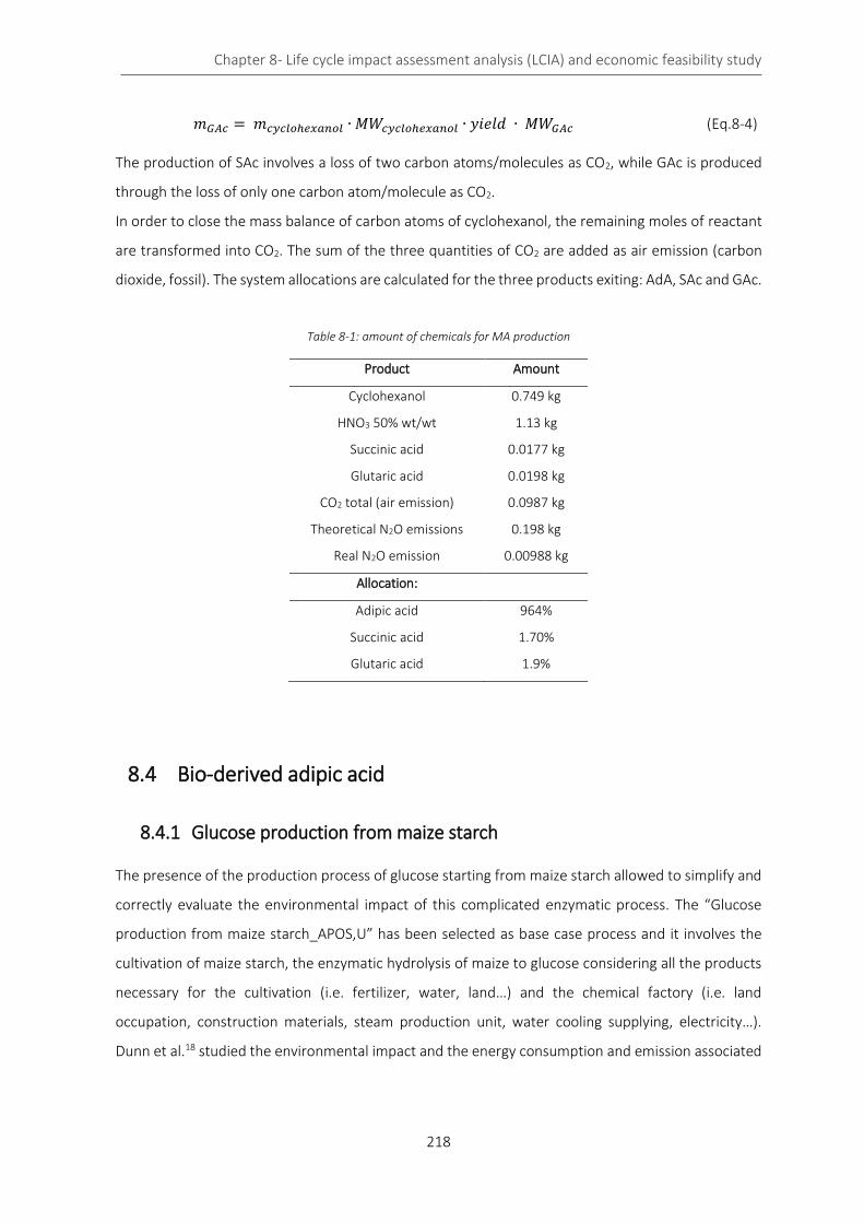
Chapter 8- Life cycle impact assessment analysis (LCIA) and economic feasibility study
218
𝑚𝐺𝐴𝑐 = 𝑚𝑐𝑦𝑐𝑙𝑜ℎ𝑒𝑥𝑎𝑛𝑜𝑙 ∙ 𝑀𝑊𝑐𝑦𝑐𝑙𝑜ℎ𝑒𝑥𝑎𝑛𝑜𝑙 ∙ 𝑦𝑖𝑒𝑙𝑑 ∙ 𝑀𝑊𝐺𝐴𝑐 (Eq.8-4)
The production of SAc involves a loss of two carbon atoms/molecules as CO2, while GAc is produced
through the loss of only one carbon atom/molecule as CO2.
In order to close the mass balance of carbon atoms of cyclohexanol, the remaining moles of reactant
are transformed into CO2. The sum of the three quantities of CO2 are added as air emission (carbon
dioxide, fossil). The system allocations are calculated for the three products exiting: AdA, SAc and GAc.
Table 8-1: amount of chemicals for MA production
Product Amount
Cyclohexanol 0.749 kg
HNO3 50% wt/wt 1.13 kg
Succinic acid 0.0177 kg
Glutaric acid 0.0198 kg
CO2 total (air emission) 0.0987 kg
Theoretical N2O emissions 0.198 kg
Real N2O emission 0.00988 kg
Allocation:
Adipic acid 964%
Succinic acid 1.70%
Glutaric acid 1.9%
8.4 Bio-derived adipic acid
8.4.1 Glucose production from maize starch
The presence of the production process of glucose starting from maize starch allowed to simplify and
correctly evaluate the environmental impact of this complicated enzymatic process. The “Glucose
production from maize starch_APOS,U” has been selected as base case process and it involves the
cultivation of maize starch, the enzymatic hydrolysis of maize to glucose considering all the products
necessary for the cultivation (i.e. fertilizer, water, land…) and the chemical factory (i.e. land
occupation, construction materials, steam production unit, water cooling supplying, electricity…).
Dunn et al.18 studied the environmental impact and the energy consumption and emission associated

Chapter 8- Life cycle impact assessment analysis (LCIA) and economic feasibility study
219
to the enzymatic hydrolysis process of starch. The reaction involves in the enzymatic hydrolysis of
starch is:
(C6H10O5) + nH2O nC6H12O6
8.4.2 Muconic acid hydrogenation to bio-adipic acid
The glucose obtained is further processed for the synthesis of cis,cis-MA. Despite the presence of pilot
plant production of bio-AdA from MA, no industrial mass balance or flow sheet process are available
for the completely synthetic process. As mentioned at the beginning of the chapter, Rosengart
developed a detailed economic and feasibility study for the production of bio-AdA via MA
hydrogenation. An evaluation of mass and energy balance was reported allowing the possibility to
perform a concrete environmental impact analysis which considers all the units operations requires
for the conversion of glucose into MA and the subsequent AdA production and purification. The whole
process is schematically reported in Figure 8-4 while the detailed one is reported in Figure 8-5.
8.4.2.1 Fermentation of glucose to c,c-MA
Glucose is converted into cis,cis-MA using a fermenter in which all the operating parameters must be
carefully controlled and monitored due to the sensitiveness of the system about temperature and pH
variations.
The reaction that occurs in the fermenter is:
7 𝑔𝑙𝑢𝑐𝑜𝑠𝑒 + 51
2𝑂2 → 3𝑐, 𝑐𝑀𝐴 + 33𝐻2𝑂 + 24𝐶𝑂2
Figure 8-4: block diagram for the production of and purification of AdA
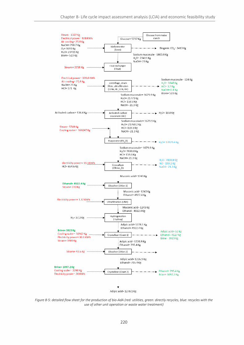
Chapter 8- Life cycle impact assessment analysis (LCIA) and economic feasibility study
220
Figure 8-5: detailed flow sheet for the production of bio-AdA (red: utilities, green: directly recycles, blue: recycles with the use of other unit operation or waste water treatment)

Chapter 8- Life cycle impact assessment analysis (LCIA) and economic feasibility study
221
The higher amount of water and CO2 produced during the fermentation requires a big fermenter and
all the utilities for the maintenance of the temperature are strictly correlated to the dimension of the
unit. In this case a system of parallel reactors is assumed, each of 1000 m3 (e.g. diameter 4 m, height
60 m, aspect ratio 15). For common biotechnology applications this volume is remarkable (100 m3 is
already considered “big”), however low added value fermentations are normally carried out in very
large-scale systems, as biogas or ethanol anaerobic fermentations. Big aerated fermenters with the
same scale assumed in this work have been successfully employed for succinic acid fermentations.19
8.4.2.2 Biomass deactivation (heat exchanger)
This step contains a single interval, representing a heat exchanger, which brings the raw fermentation
broth at 80 °C. The thermal treatment on the fermentation broth has three different effects. The first
is the deactivation of the bacteria. Increasing the temperature to 80 °C induces the pasteurization of
the fermentation broth, preventing any pathogenic risk. The second is the coagulation of the proteic
material present in the fermentation broth, which can be later removed via filtration.20 The third effect
is to promote the spontaneous isomerization of cis,cis-muconate salts to cis,trans-muconate, as
reported in the equation:21
𝑐𝑐𝑀𝐴 → 𝑐𝑡𝑀𝐴
The reaction is complete at 60 °C for 1.25 hours at pH 4, therefore HCl was used to acidify the
environment.
8.4.2.3 Bacteria removal (CENr, RF_CEN and UF)
After the deactivation the broth is processed to eliminate the biomass (i.e. all the solids product).
Thanks to three different steps: centrifuge (CENr), drum filter (RF_CEN) and ultrafiltration (UF). These
unit operations require a lot of energy and steam due to the high amount of products.
8.4.2.4 Activated carbon treatment (AC)
The purification of a clarified broth using granular activated carbon (GAC) in packed beds or slurry
reactors is often addressed as “decolorization treatment”. These removed impurities are a class of
diverse compounds covering aminoacids, polyphenols, and cell debris. In spite of their variety, the
impurities are removed thanks to the non-selective adsorption on the activated carbon internal
surface. Decolorization steps for high scale applications are quite similar for all the bio-processes: the
process specification applied for succinic acid or lactic acid can be transferred to the case of muconic
acid. In a moving bed column, the amount of muconic acid loss is negligible: the small amount of spent
carbon is rinsed with fresh water (returned to the main flux) and the adsorbed muconic acid is not
Chapter 8- Life cycle impact assessment analysis (LCIA) and economic feasibility study
222
relevant as shown by Vardon et al22. The consumption of utilities for this unit is negligible (all the
operating costs are implicitly carried by the regenerated carbon purchase).
8.4.2.5 Concentration (EV_D) and water separation (CRmw_D)
After the activated carbon treatment the so obtained muconic acid must be concentrated and
separated from water. The design specification of the evaporators was taken from Couper et al.23
using the indication of a thermal economy of 2.4 kg of water evaporated per kg of steam in a triple
effect configuration. The thermal stability of the products and the use of high pressure steam ensure
a temperature difference of 20 °C in each exchanger (in spite of the possible ebullioscopic rise),
avoiding more expensive vacuum systems. After the concentration cis,cis-sodium muconate is
therefore converted to c,c-MA using HCl. This step is one of the most important because the impurities
still present in the stream must be completed eliminated. The required purity of muconic acid usable
for the hydrogenation to AdA and the further nylon production is very high (>99.98%). Therefore,
muconic acid obtained after this step is 97%.
8.4.2.6 Dissolver (DISet 1)
The crystals of muconic acid recovered may contain co-crystals of other inorganic salts. Interval DISet
1assumes the dissolution of the intermediate crystals in ethanol, as suggested in the lab-procedure of
Vardon et al.22 Further studies could identify other alternative solvents for this step. The interval DISet
1 represents a coil jacketed stirred tank, to provide a 30 min residence time at 75 °C to ensure the
dissolution of the crystallized muconic acid in ethanol.23
8.4.2.7 Ultrafiltration (UFet)
Following Vardon et al.23 lab-scale procedure, a step of ultrafiltration after the ethanol dissolution is
necessary to remove the mineral crystals co-precipitated with muconic acid. The only reference for
muconic acid solubility in ethanol is the correlation of cis,cis-muconic acid of Scelfo et al.24 These data
are worth as a preliminary estimate. An average flow of 960 l/h/m2 at 4 bar transmembrane pressure
is assumed to size the module.
8.4.2.8 Hydrogenation reactor (Hydrog.)
For the hydrogenation in ethanol, the Pd/C catalyst performance of Vardon et al.22,25 are modelled:
Hydrog. assumes the reactant concentration coming from the upstream dissolution step. All the
intervals assume the application of a system of agitated jacketed reactors in parallel, with a volume
Chapter 8- Life cycle impact assessment analysis (LCIA) and economic feasibility study
223
of 10 m3 and a shape factor H/D of 4, to ensure the longer contact time between the gas and the liquid
phase.
8.4.2.9 Final purification steps
All the final purification steps involve a double step of crystallization and dissolution These last steps
of crystallization (interval CRaet2) allows the recovery of pure adipic acid. It is possible to see that the
superstructure is generated to include at least two crystallization steps for each possible configuration
(on muconic acid or adipic acid). This is an important difference from the flowsheets proposed
previously, assuming the recovery of 99.96% pure adipic acid (polymer grade) in a single step of
crystallization26,7. A single crystallization step is unlikely even for the oil-derived process, which
operates with more clean substrates.27 This final interval comprises a double cooler exchanger (cooling
water utility and brine), a draft tube crystallizer and a solid bowl centrifuge for the crystals harvest. A
complete product recovery is assumed (purge is negligible).
8.4.3 ReCiPe 2016, method used for environmental impact evaluation
LCA calculations were performed using the ReCiPe 2016 method (version 1.1) to evaluate the different
impacts in the production of AdA from oil and from renewable resources and elaborating/comparing
the results. In particular, 18 impact categories were considered and analysed in detail, trying to
highlight the differences between the two production processes. Moreover, thanks to the use of the
software SimaPro it is possible to understand which sub-processes, constituting the global process,
have a greater numerical impact value. In case the original method only reported a characterisation
value for one specific sub compartment, this value is taken as the characterisation value for all sub
compartments in this compartment. The characterisation values of the sub compartments "fresh
water" under water, "high population density" under air and "industrial soil" under soil were chosen
as factor for the sub compartment "unspecified". Please mind that the factors in Global warming differ
from the 100a time horizon in IPCC 2013 because climate-carbon feedback for non-CO2 green-house
gasses (GHGs) is included. For further details see the method's documentation.
8.5 Results and discussion
8.5.1 ReCiPe midpoint (H) results
Due to the early stage study of the bio-process the discussion of the results wants to be a critic about
the bottle neck of this new process. All the results about the 18 impact voices will be shown and

Chapter 8- Life cycle impact assessment analysis (LCIA) and economic feasibility study
224
discussed. To simplify the discussion and to establish which unit operations must be improved and
optimized, a step by step analysis was performed. In particular, all the figures describe the results
obtained for each impact voices for the oil-derived AdA and bio-AdA production process. Regarding
the bio-AdA process the chosen impact voice was divided for each unit operation.
8.5.1.1 Global warming
The voice “Global warming” expresses the change in global temperature caused by greenhouse gasses
produced by human activity; the reference unit used to measure this category is kg CO2 equivalent.
The raise of global temperature can cause desertification, spread of disease, rising of the level of sea,
and climatic disturbance. The climate change is one of the major environmental effects of economic
productivity, and one of the most difficult to handle because of its broad scale. Therefore, during LCA
study, this category is the most important and the CO2 eq. released by the new process should be as
low as possible. The global warming of bio-AdA production is lower than the oil-based one (Figure
8-6). We must consider that using ReCiPe method the biogenic CO2 is not considered in the calculation
due to its biological derivation. Despite the final value of global warming is not so different (blue and
green bar), we can observe that the step where there is the highest increment of CO2 is the
crystallization of sodium muconate to muconic acid. Performing a detailed analysis on this
crystallization step we found that the increment of kg CO2 eq. is due to the waste water treatment
used for slightly inorganic and organic contaminated water. Therefore, the introduction of recycle
able to separate the flow of water and NaCl (such as an evaporator) could decrease the impact of this
unit operation, positively affected the final result. Introducing the evaporation unit and deleting the
waste water treatment the CO2 eq. decreases at 11, underlying the importance of the recycling
process within an industrial process.
Figure 8-6: global warming

Chapter 8- Life cycle impact assessment analysis (LCIA) and economic feasibility study
225
8.5.1.2 Human carcinogenic and non-carcinogenic toxicity
The human toxicity potential is based on both the potential dose of a compound and its inherent
toxicity. This index reflects the potential harm of a unit of chemical released into the environment.
The considered chemicals are arsenic, sodium dichromate, hydrogen fluoride that mainly derive from
electricity production and fossil sources. These compounds are potentially dangerous to human
through inhalation, ingestion, and even contact. The unit is expressed as kg of 1,4-dichlorobenzene
equivalent (1,2-DB). Although in this case the CRmw_D step increases both the human carcinogenic
and non-carcinogenic toxicity the amount of the carcinogenic toxicity is one hundred time lower than
the non-carcinogenic one (Figure 8-7).
Figure 8-7: human carcinogenic (A) and non-carcinogenic (B) toxicity
8.5.1.3 Land use and water consumption
The study is based on the UNEP/SETAC land use assessment framework and focuses on occupation
impacts, i.e. the use of land. The damage is expressed as “potentially disappeared fraction of species”
(PDF) per m2 or m2 a (square metre of land per year).
Impact on the land due to agriculture, anthropogenic settlement and resource extraction are the main
voices involved in the evaluation. Obviously, the land use of the bio process is much more high due to
the cultivation of maize and the space occupied by the fermenter (3 fermenters in series). Regarding
the water consumption, the new bio-process shows negative value, which means that with the water
recycle occurring in the evaporator and in the first crystallizer it is possible to decrease a lot the whole
water consumption of the process. Optimizing all the operating unit and performing other possible
B A

Chapter 8- Life cycle impact assessment analysis (LCIA) and economic feasibility study
226
water recycling (i.e. cooling water and steam recovery) we could abate the water consumption to ≈0
(Figure 8-8).
Figure 8-8: land use (A) and water consumption (B)
8.5.1.4 Abiotic resource scarcity
This impact category is referred to the consumption of non-biological resources such as fossil fuels,
minerals, metals, water… The value of the abiotic resource consumption of a substance (e.g. lignite or
coal) is a measure of the scarcity of a substance. That means it depends on the amount of resources
and the extraction rate. It is formed by the amount of resources that are depleted and measured in
antimony equivalents in some models or water consumption (in m3), kg of mineral depletion and MJ
of fossil fuels. Considering the mineral resource scarcity (expressed in kg of Cu eq.) the oil-derived
process has a value of 0.2 while the bio one 0.075 (Figure 8-9). Studying all the different voices the
maize starch production is the process that has the highest score. The use of land, fertilizer and water
increase a lot the environmental impact about the mineral resources, while the score of fossil resource
mainly derived from ethylene production used during the transportation. We must keep in mind that
the bio-process starts from waste wood. Therefore, no cultivation is needed for the production so
these impact voices could be decreased considering the use of waste wood.
B A
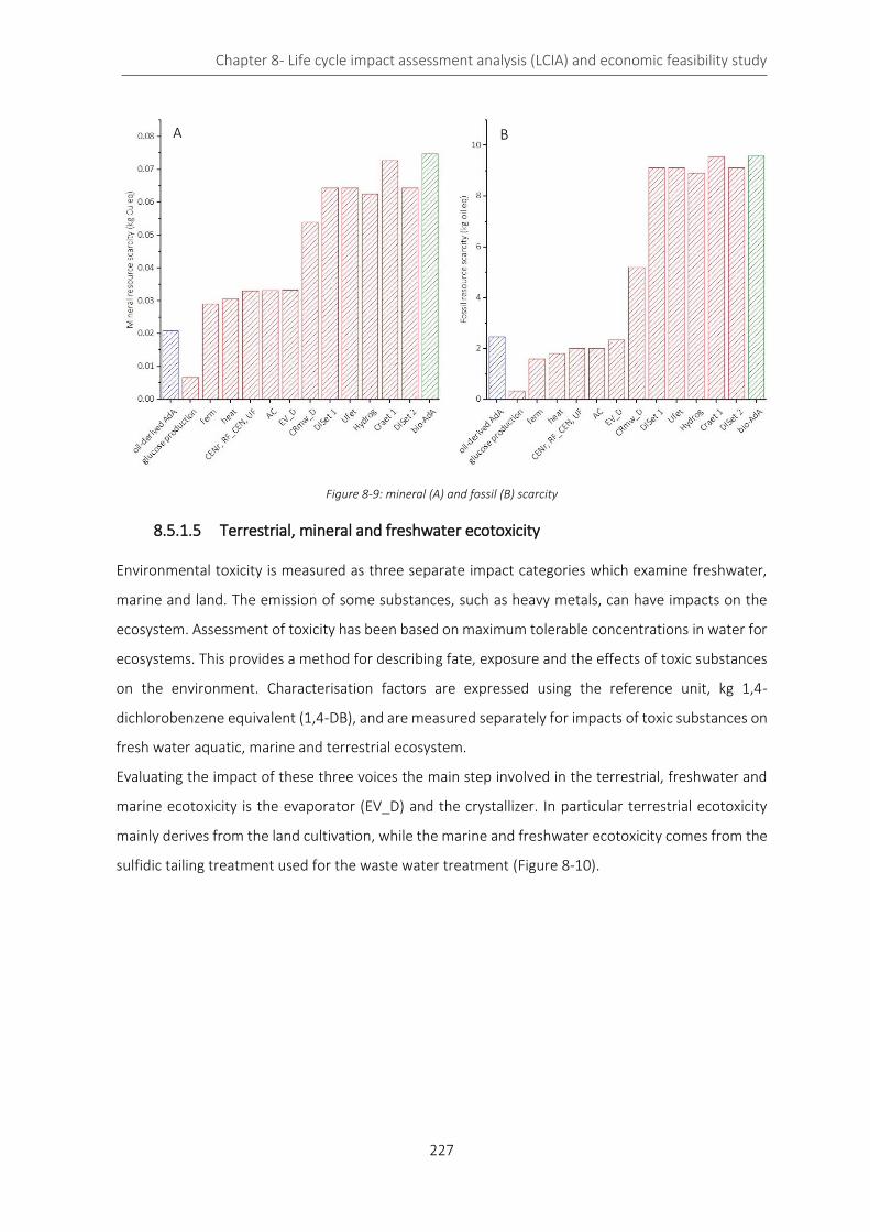
Chapter 8- Life cycle impact assessment analysis (LCIA) and economic feasibility study
227
Figure 8-9: mineral (A) and fossil (B) scarcity
8.5.1.5 Terrestrial, mineral and freshwater ecotoxicity
Environmental toxicity is measured as three separate impact categories which examine freshwater,
marine and land. The emission of some substances, such as heavy metals, can have impacts on the
ecosystem. Assessment of toxicity has been based on maximum tolerable concentrations in water for
ecosystems. This provides a method for describing fate, exposure and the effects of toxic substances
on the environment. Characterisation factors are expressed using the reference unit, kg 1,4-
dichlorobenzene equivalent (1,4-DB), and are measured separately for impacts of toxic substances on
fresh water aquatic, marine and terrestrial ecosystem.
Evaluating the impact of these three voices the main step involved in the terrestrial, freshwater and
marine ecotoxicity is the evaporator (EV_D) and the crystallizer. In particular terrestrial ecotoxicity
mainly derives from the land cultivation, while the marine and freshwater ecotoxicity comes from the
sulfidic tailing treatment used for the waste water treatment (Figure 8-10).
B A

Chapter 8- Life cycle impact assessment analysis (LCIA) and economic feasibility study
228
Figure 8-10: terrestrial (A), freshwater (B), and marine (C) ecotoxicity
8.5.1.6 Ionizing radiation, fine particulate matter formation and terrestrial acidification
Ionising radiation is an impact category in LCA related to the damage to ecosystem and human health
that is linked to the emissions of radionuclides through a product or building life cycle. In the building
area, they can be linked to the use of nuclear power in an electricity mix.
The category considers the radiation types α-, β-, γ-rays and neutrons. The characterization model
considers the emissions and calculation of their radiation behaviour and burden based on detailed
nuclear-physical knowledge. The unit the impact is given is kg of Cobalt-60 (Co-60 eq.) a radioactive
B A
C
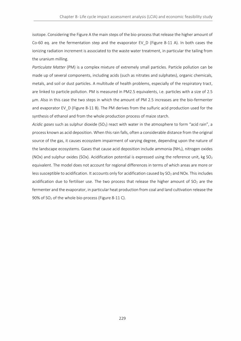
Chapter 8- Life cycle impact assessment analysis (LCIA) and economic feasibility study
229
isotope. Considering the Figure A the main steps of the bio-process that release the higher amount of
Co-60 eq. are the fermentation step and the evaporator EV_D (Figure 8-11 A). In both cases the
ionizing radiation increment is associated to the waste water treatment, in particular the tailing from
the uranium milling.
Particulate Matter (PM) is a complex mixture of extremely small particles. Particle pollution can be
made up of several components, including acids (such as nitrates and sulphates), organic chemicals,
metals, and soil or dust particles. A multitude of health problems, especially of the respiratory tract,
are linked to particle pollution. PM is measured in PM2.5 equivalents, i.e. particles with a size of 2.5
μm. Also in this case the two steps in which the amount of PM 2.5 increases are the bio-fermenter
and evaporator EV_D (Figure 8-11 B). The PM derives from the sulfuric acid production used for the
synthesis of ethanol and from the whole production process of maize starch.
Acidic gases such as sulphur dioxide (SO2) react with water in the atmosphere to form “acid rain”, a
process known as acid deposition. When this rain falls, often a considerable distance from the original
source of the gas, it causes ecosystem impairment of varying degree, depending upon the nature of
the landscape ecosystems. Gases that cause acid deposition include ammonia (NH3), nitrogen oxides
(NOx) and sulphur oxides (SOx). Acidification potential is expressed using the reference unit, kg SO2
equivalent. The model does not account for regional differences in terms of which areas are more or
less susceptible to acidification. It accounts only for acidification caused by SO2 and NOx. This includes
acidification due to fertiliser use. The two process that release the higher amount of SO2 are the
fermenter and the evaporator, in particular heat production from coal and land cultivation release the
90% of SO2 of the whole bio-process (Figure 8-11 C).
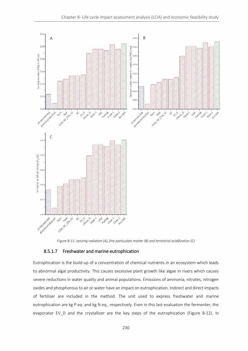
Chapter 8- Life cycle impact assessment analysis (LCIA) and economic feasibility study
230
Figure 8-11: ionizing radiation (A), fine particulate matter (B) and terrestrial acidification (C)
8.5.1.7 Freshwater and marine eutrophication
Eutrophication is the build-up of a concentration of chemical nutrients in an ecosystem which leads
to abnormal algal productivity. This causes excessive plant growth like algae in rivers which causes
severe reductions in water quality and animal populations. Emissions of ammonia, nitrates, nitrogen
oxides and phosphorous to air or water have an impact on eutrophication. Indirect and direct impacts
of fertiliser are included in the method. The unit used to express freshwater and marine
eutrophication are kg P eq. and kg N eq., respectively. Even in this last evaluation the fermenter, the
evaporator EV_D and the crystallizer are the key steps of the eutrophication (Figure 8-12). In
A B
C
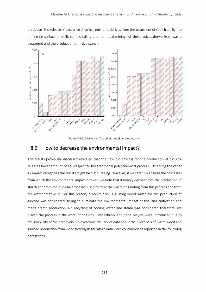
Chapter 8- Life cycle impact assessment analysis (LCIA) and economic feasibility study
231
particular, the release of excessive chemical nutrients derives from the treatment of spoil from lignite
mining (in surface landfill), sulfidic tailing and hard coal mining. All these voices derive from waste
treatment and the production of maize starch.
Figure 8-12: freshwater (A) and marine (B) eutrophication
8.6 How to decrease the environmental impact?
The results previously discussed revealed that the new bio-process for the production of bio-AdA
releases lower amount of CO2 respect to the traditional petrochemical process, Observing the other
17 impact categories the results might be discouraging. However, if we carefully analyse the processes
from which the environmental impact derives, we note that it mainly derives from the production of
starch and from the disposal processes used to treat the waste originating from this process and from
the water treatment. For this reason, a preliminary LCA using wood waste for the production of
glucose was considered, trying to eliminate the environmental impact of the land cultivation and
maize starch production. No recycling of cooling water and steam was considered therefore, we
placed the process in the worst conditions. Only ethanol and brine recycle were introduced due to
the simplicity of their recovery. To overcome the lack of data about the hydrolysis of waste wood and
glucose production from wood hydrolysis literature data were considered as reported in the following
paragraphs.
A B
Chapter 8- Life cycle impact assessment analysis (LCIA) and economic feasibility study
232
Waste wood hydrolysis and sugar fermentation
Wood may be a source of glucose and other sugars due to the presence of polysaccharides chains. Its
average composition is: 15-25% lignin, 23-32% hemicellulose and 38-50% cellulose.28 The cellulose
and hemicellulose can be hydrolysed to sugars that are microbially fermented into various products,
such as glucose.29 Glucose in cellulose is joined in a structure that is more difficult to depolymerize
than the other conventional sources of glucose like starch. Diluted acids (1% sulphuric acid) can be
used at high temperature (220 °C) to achieve yields of around 50-60%. The presence of water is
necessary for the obtainment of sugar monomers.30 After the hydrolysis, the glucose produced is
separated and neutralized. The remaining sulphuric acid is recycled. The glucose obtained from
hydrolysis, at a suitable value of pH, is fed to bacteria and cis,cis-sodium muconate is obtained from
glucose fermentation. Efforts were made by many researchers to obtain a bacterial strain that is able
to achieve the maximum possible productivity. According to Weber et al.31, the final recombinant E.
Coli strain produced 36.8 g/L of cis,cis-MA (as sodium salt), with a yield of 22% (mol/mol) within 48 h
of culturing under fed-batch fermenter conditions.(Figure 8-13)
Due to the peculiarity of the process, no related routes were available in SimaPro database but
comparable way to convert biomass into chemicals was found. In particular, bio-ethanol production
from wood was selected because it considers bio-mass treatment and fermentation processes. The
process modified in SimaPro database was: Ethanol, without water, in 95% solution state, from
fermentation {RoW}| ethanol production from wood | Alloc Def, U. In this process, ethanol is
produced by dilute acid pre-hydrolysis and simultaneous saccharification and co-fermentation of
lignocellulosic biomass. Process heat and power supply is ensured by the combustion of unconverted
solids such as lignin. The dataset includes the transport of wood from the forest to the distillery, and
the processing of wood to hydrated ethanol (95%) and electricity. Dehydration to anhydrous ethanol
is not included. The muconic acid production requires a fermenter similar to the one used for ethanol,
in fact the same apparatus and the same temperature/pressure conditions are assumed for the two
fermentations processes. Moreover, bacteria used for the production of sodium muconate were
supposed to have the same environmental impact than the ones used in the production of bio-ethanol
Wood biomass
Glucose 3-DAHP 3-DHQ
Biomass treatments
Figure 8-13: reaction pathway from wood biomass to cis,cis-MA
Chapter 8- Life cycle impact assessment analysis (LCIA) and economic feasibility study
233
and the types of emissions are considered the same as the reference ethanol fermentation. The main
difference is that the fermenter requires a different amount of wood and has a different amount of
emissions and sulfuric acid concentration. Considering all these differences and accordingly with
literature data,32-34 the different chemicals and materials required for the production of 1 Kg of MA
were evaluated and the results are reported in Table 8-2. At the end of the process, a dry solid is
obtained.
8.6.2 Muconic acid production
The functional unit is 1 kg of muconic acid.
A yield of 22% mol/mol is obtained starting from a water solution of glucose.
The glucose mass is calculated using Eq.8-5:
𝑚𝑔𝑙𝑢𝑐𝑜𝑠𝑒 =𝑚𝑀𝐴
𝑀𝑊𝑀𝐴
∙1
𝑦𝑖𝑒𝑙𝑑∙ 𝑀𝑊𝑔𝑙𝑢𝑐𝑜𝑠𝑒 (Eq.8-5)
Glucose is produced by cellulose and hemicellulose hydrolysis process, so an increase of weight of
10% occurs due to the addition of a molecule of water.
The composition of wood is assumed to be:35
- 50% cellulose, completely made up by glucose polymer;
- 30% hemicelluloses: its composition depends on the species of the considered plant;
- a composition of 33% of glucose, 33% of xylose and 34% of other sugars has been considered;
- 19% lignin;
- 1% ashes according to Sjostrom.36
An average hydrolysis yield of cellulose under acid condition of 55% was considered, while for the
hemicelluloses of 85% (under the same conditions).
Since for muconic acid synthesis only glucose is used, the actual quantity of useful wood is calculated:
5.2382 𝑘𝑔𝑔𝑙𝑢𝑐𝑜𝑠𝑒 𝑎𝑠 𝑝𝑜𝑙𝑦𝑚𝑒𝑟 = 𝑥 ∙ (0.5 ∙ 5 + 0.3 ∙ 0.85 ∙ 0.333)
𝑥 = 14.554 𝑘𝑔𝑑𝑟𝑦 𝑤𝑜𝑜𝑑 (Eq.8-6)
The mass of wet wood was calculated supposing that the humidity content is about 12% at 20 °C with
a relative humidity of 65%. This is an average value, but the water content strongly varies according
to the specific zone considered.34 The final volume of softwood included in the process input is
calculated taking into account a wood average density of 0.70 kg/L (considering humidity content of
12%).34
Among the inputs, woodchips are calculated considering that they make up the 0.551% of the total
wood present, as suggested by the original ethanol fermentation process.
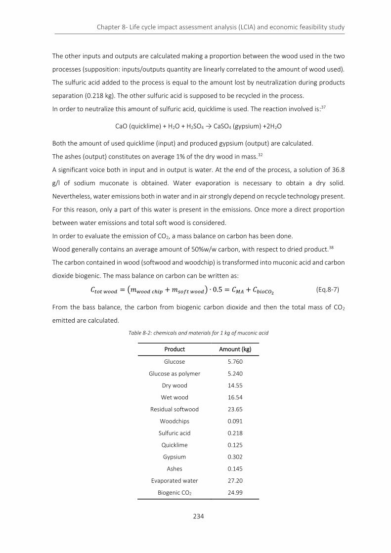
Chapter 8- Life cycle impact assessment analysis (LCIA) and economic feasibility study
234
The other inputs and outputs are calculated making a proportion between the wood used in the two
processes (supposition: inputs/outputs quantity are linearly correlated to the amount of wood used).
The sulfuric acid added to the process is equal to the amount lost by neutralization during products
separation (0.218 kg). The other sulfuric acid is supposed to be recycled in the process.
In order to neutralize this amount of sulfuric acid, quicklime is used. The reaction involved is:37
CaO (quicklime) + H2O + H2SO4 → CaSO4 (gypsium) +2H2O
Both the amount of used quicklime (input) and produced gypsium (output) are calculated.
The ashes (output) constitutes on average 1% of the dry wood in mass.32
A significant voice both in input and in output is water. At the end of the process, a solution of 36.8
g/l of sodium muconate is obtained. Water evaporation is necessary to obtain a dry solid.
Nevertheless, water emissions both in water and in air strongly depend on recycle technology present.
For this reason, only a part of this water is present in the emissions. Once more a direct proportion
between water emissions and total soft wood is considered.
In order to evaluate the emission of CO2, a mass balance on carbon has been done.
Wood generally contains an average amount of 50%w/w carbon, with respect to dried product.38
The carbon contained in wood (softwood and woodchip) is transformed into muconic acid and carbon
dioxide biogenic. The mass balance on carbon can be written as:
𝐶𝑡𝑜𝑡 𝑤𝑜𝑜𝑑 = (𝑚𝑤𝑜𝑜𝑑 𝑐ℎ𝑖𝑝 + 𝑚𝑠𝑜𝑓𝑡 𝑤𝑜𝑜𝑑) ∙ 0.5 = 𝐶𝑀𝐴 + 𝐶𝑏𝑖𝑜𝐶𝑂2 (Eq.8-7)
From the bass balance, the carbon from biogenic carbon dioxide and then the total mass of CO2
emitted are calculated.
Table 8-2: chemicals and materials for 1 kg of muconic acid
Product Amount (kg)
Glucose 5.760
Glucose as polymer 5.240
Dry wood 14.55
Wet wood 16.54
Residual softwood 23.65
Woodchips 0.091
Sulfuric acid 0.218
Quicklime 0.125
Gypsium 0.302
Ashes 0.145
Evaporated water 27.20
Biogenic CO2 24.99
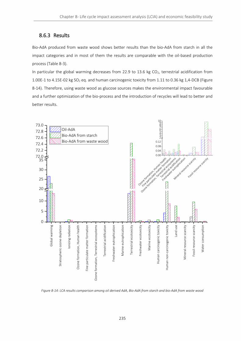
Chapter 8- Life cycle impact assessment analysis (LCIA) and economic feasibility study
235
8.6.3 Results
Bio-AdA produced from waste wood shows better results than the bio-AdA from starch in all the
impact categories and in most of them the results are comparable with the oil-based production
process (Table 8-3).
In particular the global warming decreases from 22.9 to 13.6 kg CO2, terrestrial acidification from
1.00E-1 to 4.15E-02 kg SO2 eq. and human carcinogenic toxicity from 1.11 to 0.36 kg 1,4-DCB (Figure
8-14). Therefore, using waste wood as glucose sources makes the environmental impact favourable
and a further optimization of the bio-process and the introduction of recycles will lead to better and
better results.
Figure 8-14: LCA results comparison among oil derived AdA, Bio-AdA from starch and bio-AdA from waste wood
Glo
bal
war
min
g
Stra
tosp
her
ic o
zon
e d
eple
tio
n
Ion
izin
g ra
dia
tio
n
Ozo
ne
form
atio
n, H
um
an h
ealt
h
Fin
e p
arti
cula
te m
atte
r fo
rmat
ion
Ozo
ne
form
atio
n, T
erre
stri
al e
cosy
stem
s
Terr
estr
ial a
cid
ific
atio
n
Fres
hw
ater
eu
tro
ph
icat
ion
Mar
ine
eutr
op
hic
atio
n
Terr
estr
ial e
coto
xici
ty
Fres
hw
ater
eco
toxi
city
Mar
ine
eco
toxi
city
Hu
man
car
cin
oge
nic
to
xici
ty
Hu
man
no
n-c
arci
no
gen
ic t
oxi
city
Lan
d u
se
Min
eral
res
ou
rce
scar
city
Foss
il re
sou
rce
scar
city
Wat
er c
on
sum
pti
on
0
5
10
20
25
30
3572.0
72.2
72.4
72.6
72.8
73.0 Oil-AdA
Bio-AdA from starch
Bio-AdA from waste wood
Ozone fo
rmat
ion, H
uman
healt
h
Fine p
artic
ulate m
atte
r form
atio
n
Ozone fo
rmat
ion, T
errest
rial e
cosy
stem
s
Terrest
rial a
cidifi
catio
n
Fresh
water e
utrophica
tion
Min
eral r
esourc
e scar
city
Foss
il reso
urce sc
arcit
y0.00
0.04
0.08
0.12
23456789
10

Chapter 8- Life cycle impact assessment analysis (LCIA) and economic feasibility study
236
Table 8-3: LCA results comparison among oil derived AdA, Bio-AdA from starch and bio-AdA from waste wood
Impact category Unit Oil-AdA Bio-AdA from
starch
Bio-AdA from waste
wood
Global warming kg CO2eq 2.66E+01 2.29E+01 1.36E+01
Stratospheric ozone depletion kg CFC11 eq 7.26E-04 7.39E-06 8.43E-06
Ionizing radiation kBq Co-60 eq 2.38E-01 1.05E+00 8.75E-01
Ozone formation, Human health kg NOx eq 1.79E-02 5.31E-02 2.61E-02
Fine particulate matter formation kg PM2.5 eq 1.28E-02 3.79E-02 1.60E-02
Ozone formation, Terrestrial ecosystems kg NOx eq 1.86E-02 5.55E-02 2.81E-02
Terrestrial acidification kg SO2 eq 3.36E-02 1.00E-01 4.15E-02
Freshwater eutrophication kg P eq 2.04E-03 9.16E-03 4.66E-03
Marine eutrophication kg N eq 1.26E-04 1.51E-02 3.45E-04
Terrestrial ecotoxicity kg 1,4-DCB 1.36E+01 7.24E+01 3.58E+01
Freshwater ecotoxicity kg 1,4-DCB 1.41E-01 6.48E-01 2.65E-01
Marine ecotoxicity kg 1,4-DCB 2.00E-01 9.17E-01 3.82E-01
Human carcinogenic toxicity kg 1,4-DCB 1.95E-01 1.11E+00 3.60E-01
Human non-carcinogenic toxicity kg 1,4-DCB 4.33E+00 2.38E+01 8.66E+00
Land use m2 a crop eq 1.16E-01 7.65E+00 2.33E+00
Mineral resource scarcity kg Cu eq 2.08E-02 7.48E-02 2.90E-02
Fossil resource scarcity kg oil eq 2.46E+00 9.58E+00 6.10E+00
Water consumption m3 6.69E-02 -1.13E+00 4.46E-01
Chapter 8- Life cycle impact assessment analysis (LCIA) and economic feasibility study
237
8.7 LCA study conclusions
The environmental impact of AdA production process from oil and renewable sources have been
compared. Detailed analysis of the results revealed the advantages and weaknesses of the innovative
bio-process. ReCiPe method was adopted for the evaluation of 18 environmental impact categories.
The results show that the traditional petrochemical process has a lower environmental impact in all
the categories except for the global warming. Firstly, industrial process for the production of glucose
from starch was considered and the results were largely affected by the cultivation, the production of
maize starch and all the respective waste treatments. Since the purpose is to produce glucose from
waste wood, a second study was performed starting from the hydrolysis of wood and its further
conversion to glucose. In this case the study started from the production process of bio-ethanol since
no hydrolysis plant is present in the software. Moreover, an average wood humidity was considered
using literature data for the yield of the process. Despite these limitations, the results obtained
without considering cooling water recycle and steam production from the process water were
extremely different from the first study. The global warming decreases from 22.9 to 13.6 Kg CO2 eq.
that is the half of the value obtained from the oil-derived process. All the results can be further
improved introducing recycles of chemicals and water, which will lead to a process capable of quasi-
self-sustaining from energy demand point of view and the purification products demand.
Since the data used in this work derive from early-stage and lab-scale investigations, using non-
optimized data, the estimates can be further refined, as soon as new insights are provided by the
ongoing R&D.

Chapter 8- Life cycle impact assessment analysis (LCIA) and economic feasibility study
238
8.9 Economic feasibility analysis
Thanks to the collaboration with Politecnico di Milano a sustainability economic analysis was
performed. The cost information can be retrieved from industrial quotes and estimates, from general
market overviews,39 or using equipment cost correlations40,41 and utilities cost correlations.42
The “best processing route” was selected according to its ability to generate profit, since industrial
innovation is determined first by economic drivers. Environmental impacts assessment and process
optimization will be performed on the optimal route, during stage 2 and 3 of process design as they
need a detailed process simulation to be meaningful.43 The objective function implemented considers
the annual incomes, deriving from the product sales, and the annual expenditures, related to capital
investment and to the operating costs (utilities and consumables). The sum of these contributions is
one formulation of the process economic potential44 and is a first indication of the profitability of the
process, providing also an order-of-magnitude estimate of the production cost. When the sum is equal
or greater than zero, the breakeven point is reached, and the process can be considered economically
feasible. As for the capital cost annuity estimation, an investment duration of 10 years and a MARR
(minimum attractive rate of return) of 7% is considered.45 Since the most updated available market
analysis were referred to 2014, this year was chosen as reference. Table 8-4 summarizes the main
2014 pricing information included in the problem.
Table 8-4: chemicals and utilities cost
Chemicals Price Notes
Glucose 0.428 $/kg 39
Sodium Benzoate 1.774 $/kg ICIS*
Adipic Acid 1.600 $/kg 40
Hydrogen (gas) 3.615 $/kg Electrolysis, 50kWh/kg
Utilities**
Electric power 0.0723 $/kWh US energy mix base
High pressure steam 0.0168 $/kg 8 bar steam, 170 °C
Low pressure steam 0.0160 $/kg 2 bar steam, 120 °C
Cooling water 2.09E-05 $/kg River water, 15 °C
Compressed air 0.07157 $/kg Compresses air
*The price refers to the oil derived feedstock. No commercial plants of renewable
sodium benzoate are available yet.
** The utilities cost estimates were derived from Ulrich & Vasudevan.35
Chapter 8- Life cycle impact assessment analysis (LCIA) and economic feasibility study
239
When performing conceptual estimation, the accuracy is around 30%:45 enough to quantify the
potential of the bio adipic acid biorefinery and rank the many processing alternatives. The base case
scenario and the results are reported in the following paragraphs. All the cots are based on the
chemicals and utilities reported in Figure 8-5.
8.9.1 Base case scenario
The base case solution considered a plant for 10000 metric ton/year of adipic acid, located in North
America, with an annual productivity of 8150 h. This scenario was identified in the results as SC_1.
8.9.1.1 Scenario with variation of AdA price
The following values from 2014 were considered, based on different locations: 1.60 $/kg for North
America (lower bound), 1.94 $/kg and 2.28 $/kg (intermediate values), and 2.61 $/kg for South
America (upper bound). Note that the high price for South America is due to the anti-dumping
resolution approved by the government of Brazil in December 2013.46 These four price values are
identified with the letters a, b, c, d respectively and are combined with the other scenarios (e.g.
SC_1_a, SC_1_b …).
8.9.1.2 Scenario with variation of glucose price
The price of glucose from 2014, varies with location too, which was considered through different
values: 0.428 $/kg for North America, 0.210 $/kg in South America (Brazil). The price of 0.428 $/kg
was considered in the base case scenario.
8.9.1.3 Scenario with variation of plant size
To get closer to the recommended size for a commodity chemical biorefinery, a capacity of 200000
ton/year, corresponding to 20-fold the base case size, was considered as well.47 This scenario was
identified as “SC_3”: this size is comparable to a medium sized plant for petrochemical-derived adipic
acid. The base-case scenario is sufficiently small to not consider raw-material supply chain. Existing
bio-gas plants distributed in rural areas have similar order of magnitude of feedstock requirement,
either from first or second generation biomass.48 The 200000 ton/year plant would require instead
around 950 kton/year of glucose, which is equivalent to a large scale sugarcane mill in Brazil or a
sawmill in US, assuming second generation biomass use.49 The optimal size of the plant according to
the local feedstock availability was not covered in this work.

Chapter 8- Life cycle impact assessment analysis (LCIA) and economic feasibility study
240
8.9.1.4 Scenario with variation of strain yield and product concentration
More favourable values have been assumed for fermentation yield and product concentration. This
was done to determine which of these has the biggest impact on the solution and then should be
targeted by future research. In the results, SC_4 assumes a higher product concentration (+30%), SC_5
a higher bioconversion selectivity, SC_6 the combination of both higher selectivity and concentration.
8.9.2 Sustainability analysis
The calculated economic potential can be used to provide a first estimate of the bio-derived adipic
acid production costs, assessing the level of maturity of the technology and the feasibility of the plant.
Under the conditions of the base-case scenario (SC_1 in Table 8-5), the optimal flowsheet is
economically feasible for a price of adipic acid of 3.60 $/kg. This value is more than double the
reference price of adipic acid in North America. Still, different market scenarios confirm the potential
of industrialization.
Table 8-5: results of the economical feasibility using different scenarios
Profit on sales ($/kg AdA)
SC_1 Base case -2.00 -1.66 -1.32 -0.99
SC_2 Sugar price (0.210 $/kg)* -1.00 -0.67 -0.33 0.00
SC_3 Scale up (200kton/year
AdA)
-0.93 -0.59 -0.25 0.08
SC_4 Concentration (+30%) -0.75 -0.41 -0.07 0.26
SC_5 Selectivity (93%) -0.76 -0.42 -0.08 0.25
SC_6 Selectivity (93%)+conc. -0.51 -0.17 0.17 0.50
AdA selling price ($/kg) a 1.6 b 1.94 c 2.28 d 2.61
Not feasible -20% to -5% -5% to 0% breakeven/profit
*This sugar price applies also to the following scenarios
For a benzoic acid-based process, on the other hand, the economic performances would be always
worse, requiring a selling price higher than 5.00 $/kg for the base case, and unacceptable price values
even in the most optimistic scenarios. As a general indication, the current benzoic acid route is not as
good as the glucose one for the industrial scale-up. Regarding the glucose-based process, the multi-
scenario analysis reported in Table 8-5 considers the price of glucose for a plant located in Brazil
(SC_2). In this case, when adipic acid is sold at 2.28 $/kg (SC_2_c), the estimated loss is within the
uncertainty of the cost estimates and profitability is reached at 2.61 $/kg (SC_2_d), which is the actual
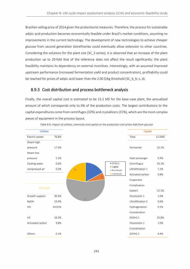
Chapter 8- Life cycle impact assessment analysis (LCIA) and economic feasibility study
241
Brazilian selling price of 2014 given the protectionist measures. Therefore, the process for sustainable
adipic acid production becomes economically feasible under Brazil’s market conditions, assuming no
improvements in the current technology. The development of new technologies to achieve cheaper
glucose from second generation biorefineries could eventually allow extension to other countries.
Considering the solutions for the plant size (SC_3 series), it is observed that an increase of the plant
production up to 20-fold that of the reference does not affect the result significantly: the plant
feasibility maintains its dependency on external incentives. Interestingly, with an assumed improved
upstream performance (increased fermentation yield and product concentration), profitability could
be reached for prices of adipic acid lower than the 2.00 $/kg threshold (SC_6_b, c, d).
8.9.3 Cost distribution and process bottleneck analysis
Finally, the overall capital cost is estimated to be 15.2 M$ for the base-case plant, the annualized
amount of which corresponds only to 6% of the production costs. The largest contributions to the
capital expenditures come from centrifuges (32%) and crystallizers (31%), which are the most complex
pieces of equipment in the process layout.
Table 8-6: impact of utilities, chemicals and capital on the production cost of bio-AdA from glucose
Utilities
Capital
Electric power 76.8% Total 12.5M$
Steam high
pressure 17.4% Fermenter 10.1%
Steam low
pressure 5.1% Heat exchanger 0.4%
Cooling water 0.6% Centrifugue 33.1%
compressed air 0.3% Ultrafiltration 1 7.2%
Activated carbon 0.8%
Evaporator
Chemicals Cristalization
(water) 12.1%
Growth support 30.4% Dissolution 1 1.0%
NaOH 19.4% Ultrafiltration 2 0.6%
HCl 24.02% Hydrogenation 9.2%
H2 16.3%
Crystalization
(EtOH) 1 10.6%
Activated carbon 9.8% Dissolution 2 1.0%
Others 0.1%
Crystalization
(EtOH) 2 8.4%

Chapter 8- Life cycle impact assessment analysis (LCIA) and economic feasibility study
242
8.10 Conclusion about the economic feasibility of the bio-process
This work applied a systematic methodology for early-stage process synthesis and design to obtain a
sustainable process design for the production of bio-derived AdA. A large number of reported
technologies associated with bio-conversions and downstream separation operations were employed
in the model of the process superstructure formulation. This included also the best and most updated
information about bio-catalytic and chemical conversions, related to the transformation of renewable
feedstocks to adipic acid. The main insights on the sustainable process design for adipic acid are: the
preference to the glucose feedstock (E. coli fermentation) instead of the benzoic acid feedstock (P.
putida fermentation); the need to reduce the product losses during the downstream purification; and
the advantages of converting the intermediate product (cis,cis-muconic acid) hydrogenation in an
organic solvent (ethanol). The economic analysis in different scenarios confirmed that a bio-adipic
acid production is affected by the availability of cheap feedstock. In this specific case, the adipic acid
process can be profitable if it is located in Brazil, using first generation glucose at a price not higher
than 0.21$/kg. Finally, since the data used in this work are derived from early-stage and lab-scale
investigations, the estimates can be further refined, as soon as new insights are provided by the
ongoing R&D. The indications on the current technological
bottlenecks, the main assumptions done while defining the
superstructure and the sensitivity analysis are useful to
indicate the priority aspects to be further investigated.
Moreover, the lack of data did not allow to perform the
economic analysis within the European market, but due to the
increment of the price of oil, the bio-route could be
competitive in a few years. Moreover, due to the instability
price of AdA in Europe and the continuous increment of
incentives bio-AdA could find in a few years a piece of market.
* https://www.icis.com/resources/news/2017/03/30/10093195/chemical-profile-europe-adipic-acid/

Chapter 8- Life cycle impact assessment analysis (LCIA) and economic feasibility study
243
List of symbols
AdA: adipic acid
3-DAHP: 3-Deoxy-D-arabino-heptulosonic acid 7-phosphate
DHQ: 3-dehydroquinate
LCI: Life Cycle Inventory
MA: muconic acid
ILCD: International Reference Life Cycle Data System
IPCC: Intergovernmental Panel on Climate Change

Chapter 8- Bibliography
244
Bibliography
1. Vardon, D. R. et al. Adipic acid production from lignin. Energy Environ. Sci. 8, 617–628 (2015).
2. Xie, N.-Z., Liang, H., Huang, R.-B. & Xu, P. Biotechnological production of muconic acid: current status and future prospects. Biotechnol. Adv. 32, 615–622 (2014).
3. Wu, C. M. et al. Microbial synthesis of cis,cis-muconic acid from benzoate by Sphingobacterium sp. mutants. Biochem. Eng. J. 29, 35–40 (2006).
4. Bart, J. C. J. & Cavallaro, S. Transiting from adipic acid to bioadipic acid. Part II. Biosynthetic pathways. Ind. Eng. Chem. Res. 54, 567–576 (2015).
5. Zakzeski, J., Bruijnincx, P. C., Jongerius, A. L. & Weckhuysen, B. M. The catalytic valorization of lignin for the production of renewable chemicals. Chem. Rev. 10, (2010).
6. Mizuno, S., Yoshikaw, N., Seki, M., Mikawa, T. & Imada, Y. Microbial production of cis,cis-muconic acid from benzoic acid. Appl. Microbiol. Biotechnol 28, (1988).
7. van Duuren, J. B. J. H. et al. Generation of a catR deficient mutant of P. putida KT2440 that produces cis, cis-muconate from benzoate at high rate and yield. J. Biotechnol. 156, 163–172 (2011).
8. Vardon, D. R. et al. cis,cis-Muconic acid: separation and catalysis to bio-adipic acid for nylon-6,6 polymerization. Green Chem. 18, 3397–3413 (2016).
9. Capelli, S. et al. Bio-adipic acid production by catalysed hydrogenation of muconic acid in mild operating conditions. Appl. Catal. B Environ. 218, 220–229 (2017).
10. Vardon, D. R. et al. Adipic acid production from lignin. Energy Environ. Sci. 8, 617–628 (2015).
11. Janssen, M., Aryapratama, R. & Tillman, A.-M. Prospective life cycle assessment of adipic acid production from forest residue. (2016). doi:10.13140/RG.2.2.36490.47049
12. Rosengart, A. et al. Process synthesis for bio-adipic acid 1 production via muconic acid route. Biotechnol. Biofuels, Under review
13. Cespi, D. et al. A simplified early stage assessment of process intensification: glycidol as a value-added product from epichlorohydrin industry wastes. Green Chem. 18, 4559–4570 (2016).
14. Castellan, A., Bart, J. C. J. & Cavallaro, S. Industrial production and use of adipic acid. Catal. Today 9, 237–254 (1991).
15. Shimizu, A., Tanaka, K. & Fujimori, M. Abatement technologies for N2O emissions in the adipic acid industry. Chemosph. - Glob. Chang. Sci. 2, 425–434 (2000).
16. Lee, S.-J., Ryu, I.-S., Kim, B.-M. & Moon, S.-H. A review of the current application of N2O emission reduction in CDM projects. Int. J. Greenh. Gas Control 5, 167–176 (2011).
17. Reimer, R. A., Slaten, C. S., Seapan, M., Lower, M. W. & Tomlinson, P. E. Abatement of N2O emissions produced in the adipic acid industry. Environ. Prog. 13, 134–137 (1994).
18. Dunn, J. B., Mueller, S., Wang, M. & Han, J. Energy consumption and greenhouse gas emissions from enzyme and yeast manufacture for corn and cellulosic ethanol production. Biotechnol. Lett. 34, 2259–2263 (2012).
19. Lubben, M. No Title https://www.bio.org/sites/default/files/WorldCongress/Marcel Lubben.pdf (accessed Oct 25, 2017).
20. Van De Graaf, M. J.; Vallianpoer, F.; Fiey, G.; Delattre, L.; Schulten, E. A. M. US20120238722A1
21. Babi, D. K.; Holtbruegge, J.; Lutze, P.; Gorak, A.; Woodley, J. M.; Gani, R. Comput. Chem. Eng. 81, 218 (2015).
22. Vardon, D. R.; Rorrer, N. A.; Salvachúa, D.; Settle, A. E.; Johnson, C. W.; Menart, M. J.; Cleveland, N. S.;

Chapter 8- Bibliography
245
Ciesielski, P. N.; Steirer, K. X.; Dorgan, J. R.; Beckham, G. T. Green Chem. 18 (11), 3397 (2016).
23. Couper, J. R.; Penney, W. R.; Fair, J. R. Chemical Process Equipment: Selection and Design; Elsevier Science (2012).
24. Scelfo, S.; Pirone, R.; Russo, N. Thermodynamics of cis,cis-muconic acid solubility in various polar solvents at low temperature range. J. Mol. Liq. 222 (Supplement C), 823-827 (2016).
25. Vardon, D. R.; Franden, M. A.; Johnson, C. W.; Karp, E. M.; Guarnieri, M. T.; Linger, J. G.; Salm, M. J.; Strathmann, T. J.; Beckham, G. T. Adipic acid production from lignin. Energy Environ. Sci. 8 (2), 617-628 (2015).
26. Matthiesen, J. E.; Suástegui, M.; Wu, Y.; Viswanathan, M.; Qu, Y.; Cao, M.; Rodriguez-Quiroz, N.; Okerlund, A.; Kraus, G.; Raman, D. R.; Shao, Z.; Tessonnier, Electrochemical Conversion of Biologically Produced Muconic Acid: Key Considerations for Scale-Up and Corresponding Technoeconomic AnalysisJ.-P. ACS Sustain. Chem. Eng. 4 (12), 7098-7109 (2016).
27. Castellan, A.; Bart, J. C. J.; Cavallaro, S. Industrial production and use of adipic acid. Catal. Today 9 (3), 237-254 (1991).
28. Anderson, A. B. THE COMPOSITION AND STRUCTURE OF WOOD ’. J. Chem. Educ. 35, 487–492 (1958).
29. Onda, A., Ochi, T. & Yanagisawa, K. Selective hydrolysis of cellulose into glucose over solid acid catalysts. Green Chem. 10, 1033–1037 (2008).
30. Kennedy, J. F. & Alanís, R. M. No Title. Carbohydr. Polym. 62, 301 (2005).
31. Weber, C. et al. Biosynthesis of cis,cis-Muconic Acid and Its Aromatic Precursors, Catechol and Protocatechuic Acid, from Renewable Feedstocks by Saccharomyces cerevisiae. Appl Env. Microbiol 78, 8421–8430 (2012).
32. Misra, M. K., Ragland, K. W. & Baker, A. J. Wood ash composition as a function of furnace temperature. Biomass and Bioenergy 4, 103–116 (1993).
33. SJÖSTRÖM, E. Chapter 10 - WOOD-BASED CHEMICALS AND PULPING BY-PRODUCTS BT - Wood Chemistry (Second Edition). in 225–248 (Academic Press, 1993). doi:https://doi.org/10.1016/B978-0-08-092589-9.50014-0
34. Bonamini, G. & Noferi, M. Umidità del legno strutturale. Problemi e soluzioni. L’edilizia 134, 72–77 (2004).
35. Anderson, A. B. The composition and structure of wood. J. Chem. Educ. 35, 487 (1958).
36. Sjöström, E. Chapter 1 - THE STRUCTURE OF WOOD BT - Wood Chemistry (Second Edition). in 1–20 (Academic Press, 1993). doi:https://doi.org/10.1016/B978-0-08-092589-9.50005-X.
37. National Lime association. Acid Neutralization with Lime for Environmental Control and Manufacturing Processes. Vol. 213 (1995).
38. Sjöström, E. Chapter 9 - CELLULOSE DERIVATIVES BT - Wood Chemistry (Second Edition). in 204–224 (Academic Press, 1993). doi:https://doi.org/10.1016/B978-0-08-092589-9.50013-9
39. Green, D. W. & Perry, R. H. Perry’s Chemical Engineers’ Handbook. (McGraw-Hill: New York, Chicago, San Francisco, Lisbon, London, Madrid, Mexico City, Milan, New Delhi, San Juan, Seoul, Singapore, Sydney, Toronto, 2007).
40. Couper, J. R., Penney, W. R. & Fair, J. R. Chemical Process Equipment. (Elsevier, 2012).
41. Turton, R., Bailie, R. C., Whiting, W. B. & Shaeiwitz, J. A. Analysis, Synthesis and Design of Chemical Processes. (Pearson Education, 2008).
42. Ulrich, G. D. & Vasudevan, P. T. How to Estimate Utility Costs. Chem. Eng. 113, 66–69 (2006).
43. Babi, D. K. et al. Sustainable process synthesis–intensification. Comput. Chem. Eng. 81, 218–244 (2015).
44. Douglas, J. M. A hierarchical decision procedure for process synthesis. AIChE J. 31, 353–362 (2018).

Chapter 8- Bibliography
246
45. Biegler, L. T., Grossmann, I. E. & Westerberg, A. W. Systematic methods of chemical process design. (Upper Saddle River, N.J. : Prentice Hall PTR, 1997).
46. Godinho, M. D. Secretaria de Comercio exterior: Circular n75 de 13 Dezembro 2013. (2015).
47. Wright, M. & Brown, R. C. Establishing the optimal sizes of different kinds of biorefineries. Biofuels, Bioprod. Biorefining 1, 191–200 (2007).
48. Walla, C. & Schneeberger, W. The optimal size for biogas plants. Biomass and Bioenergy 32, 551–557 (2008).
49. Neves, M. F., Trombin, V. G. & Consoli, M. A. Measurement of Sugar Cane Chain in Brazil. Int. Food Agribus. Manag. Rev. 13, 37–54 (2010).

247
General conclusion and future perspective
The Doctoral project presented in this Thesis addresses the feasibility study of a novel bioprocess for
the production of a drop-in commodity chemical, adipic acid. The topic belongs to the general
framework of renovation of the traditional oil-based industry toward a sustainable manufacturing, as
required by the most recent European Union policies. Bio adipic acid production process has been
chosen because it is characterized by a very early stage development. The lack of kinetic data and
operating parameters optimization, as well as economic feasibility had attracted our interest. The
peculiarity of this project is its interdisciplinarity: biotechnologists, chemists and engineers are invited
to collaborate to achieve good results and make wider the knowledge about bio adipic acid production
at scale industry.
This study follows the classical steps to achieve robust and reasonable results: a critic literature
analysis was performed with the purpose to establish the weak points of the new technology and
those not yet investigated. We decided to focus our attention on the kinetic study and operating
parameters optimization, since no studies were found in literature. The possibility to evaluate the
kinetic constants and activation energies opened the opportunity to start computational work about
the feasibility of this reaction at industrial scale, allowing to estimate the production costs and the
environmental impact. Finally, a great attention toward catalyst tuning helped to design a series of
catalysts (using green process) which have higher activity respect to commercial materials.
i. A new analytical method was developed able to correctly evaluate the conversion of the
substrate and the selectivity of the product and reaction intermediates. The most important
goal to achieve was the evaluation and chromatographic separation of cis/trans isomers and
compounds which differ only for one double bond. UV-Vis analysis allowed the calculation of
conversion, while GC/FID or TCD analysis valuated the selectivity.
ii. A first operating parameters optimization was completed with noble metal commercial
catalyst (metal loading 5%) in water. Pt and Pd supported on activated carbon were used and
with Pt catalyst a pre-activation step was performed before starting the reaction. The reaction
was performed in a stainless-steel autoclave for pressure from 2 to 6 bar, while for 1 bar of
hydrogen a bigger glass reactor was designed. In the optimum condition Pt/AC 5% is able to
fully convert sodium muconate in adipic acid. Pd/AC 5% catalyst was then chosen for further
studies due to its lower cost and the possibility to avoid catalyst pre-treatment. The
hydrogenation reaction provided good results at low hydrogen pressure (1.2 bar) and low
General conclusion and future perspective
248
temperature (50 °C). Used and fresh catalyst was characterized in collaboration with Cardiff
Catalysis Institute and some significant changes of the catalyst surface have been observed.
In particular, during the reaction, Pd(II) is reduced to Pd(0) increasing the activity of the
catalyst.
iii. After the collection of the first experimental data, in collaboration with Politecnico di Milano,
a kinetic model was designed, and the regression of the kinetic parameters was performed.
The cis/trans isomerization does not occur on the muconate, while the monounsaturated
intermediates are preferably in their trans configuration. The estimation of kinetic constants,
activation energies open the opportunity to model a hypothetic industrial reactor.
iv. Due to the good results obtained with Pd catalysts, a series of home-made catalysts was
prepared with 1% of metal loading. Metal NPs were prepared using a bottom-up approach
and sol-immobilization method allowed the deposition of Pd NPs on activated carbon support.
Hydrogenation reactions occurred on sodium muconate and t,t-muconic acid revealed that
some of the home-made catalyst had an initial activity equal or higher than the Pd/AC 5%
commercial catalyst. This open the opportunity to tune and optimize the synthesis of a
durable catalyst with optimum surface properties.
v. Finally, an environmental impact analysis was performed comparing the new bio adipic acid
production process with the traditional one. The results are comforting because the bio
process has a total global warming lower than to the more than optimized petrochemical
process. Economic analysis showed the possibility to produce bio adipic acid with a price that
is a little more expensive than the actual cost of oil based one. Further deeper studies will
allow to establish if the purposed technology can fully compete with adipic acid produced by
non-renewable sources.
The work is not finished and opens the possibility to further interesting researches.
i. In particular one of the first task is to optimize the bacteria strain (E. Coli or other strains) to
increase the production of muconic acid. The research group of Prof. Luca Brambilla of
Università di Milano Bicocca, interested in our topic, started the exploration of this difficult
issue and they are obtaining interesting results, but the work is only at the beginning.
ii. One of the main worry is the use of gaseous hydrogen as reduction agent. Although the new
technologies for hydrogen production are more and more sustainable, the use of this gas is
object of severe protocols. To make the process safer, researchers are exploring new ways for
General conclusion and future perspective
249
in-situ hydrogen production. One of the most interesting topic is the hydrogen transfer
catalysis. In particular conditions, a solvent (called donor), is able to offer a proton to an
acceptor species. Hydrogen transfer catalysis occurs in presence of a metal that could be a
homogeneous complex, or transition metal catalysts (Mn, Mo, Co, W…). The pro of this
reaction is the exclusion of gaseous hydrogen within the plant, but on the other hand
hydrogen transfer catalysis occurs with the consumption of the donor solvent and at higher
temperature and pressure respect to the classic hydrogenation. Therefore, further studies
will carry out to establish the optimum reaction and product purification conditions as well as
the life of the catalyst. Molybdenum and tungsten oxides were tested during the research
project, but the results are far from to be competitive with the reactions that use gaseous
hydrogen.
iii. The development of new technologies and unit operations more and more specific will allow
to minimize the use of utilities hypothetically exploiting all the resources within the company.
Bio-based adipic acid process is the ideal field for one of the first circular industrial plants,
capable to auto- maintain itself. Therefore, other studies about the possibility to recycle
chemicals and energy will allow to make the process greener and more competitive on the
market, maybe support from some international incentives.
Due to rising price of crude oil and the impact adipic acid has on the environment, the world is shifting
towards the use of bio-based adipic acid. Apart from providing a clean solution, bio-based adipic acid
is also economically viable against its synthetic counterpart.
Bio-based adipic acid market is expected to register significant growth on account of increasing
demand for production of industrial chemicals through sustainable means. The market is still in
nascent stages with companies focused R&D to develop manufacturing capabilities to produce bio-
based adipic acid on an industrial scale. Development of bio-based adipic acid as a substitute for
conventional adipic acid is expected to impact the latter’s demand in the market. Key factors
influencing the shift from adipic acid produced through crude oil could be attributed to growing
concerns regarding environmental impact and high feedstock prices of petrochemical based products.
Stringent regulations by Food and Drug Administration (FDA) regarding nitrogen dioxide emissions
from adipic acid are expected to act favorably for bio-based adipic acid market. The demand for bio-
based adipic acid in medical and food applications is expected to grow over the forecast period owing
to the above stated regulatory scenario.

General conclusion and future perspective
250
High investment and R&D costs associated with the production of bio-based adipic acid are expected
to pose challenges to the market participants.
For all these reasons the work done can be a useful starting point for the design of a sustainable and
competitive adipic acid production, but a lot of attempts must still be made to increase the possibility
to switch oil-based chemicals to bio-based ones.
251
Acknowledgements
I want to thank my supervisor Prof. Carlo Pirola and my co-supervisor Prof. Laura Prati for gave me
the opportunity to work in their lab on a very interesting project. I want also to thank Alberto Villa for
all the help during my last year of PhD, I learnt a lot about catalyst characterization an synthesis.
Finally, I want to thank Prof. Nikolaos Dimitratos who gave me the opportunity to work at Cardiff
Catalysis Institute for 5 months; I found an expert in characterization and catalyst synthesis, a lover of
Italy and Italian food (tiramisù) and a very English drinker.
Now it is time to switch the language to allow to my parents and friends to read the
acknowledgements.
Partendo dal mio gruppo di ricerca vorrei innanzitutto ringraziare i tesisti e i tirocinanti che si sono
intervallati e hanno lavorato e ottenuto risultati impensabili. Senza di voi questa tesi sarebbe
incompleta. Quindi ringrazio Luca, Emilio (il mio portafortuna), Ivan, Giulia, Michela, Marco, Gabri
(ricorderò per sempre la faccia di Riikka), Leila e Mavi. Non posso di certo non ricordare anche tutti i
tirocinanti e tesisti che sono passati in questi tre anni dal gruppo capanno, siete tanti, tantissimi e
ognuno di voi avrà sempre un posto speciale nei miei ricordi: Pacia e i suoi/nostri asfalti, Basha con
mille progetti (o forse nemmeno uno), Cipo in lotta continua con il sistema, Leila la fortunata del
gruppo, Emy il lavoratore instancabile, Nafi la nostra fotografa ufficiale, Dalma dall’anima oramai
canadese, Vale e la sua vita australiana, wikiPese e le sue continue polemiche, Gabri che non saprà
mai com’è il sapore di una lasagna o del cioccolato, Ale e Cri i due opposti sotto la stessa cappa, Fede
il mago del GC, Marco convertito da fotocatalista a impiantista, il Mammo produttore di aria arricchita,
Fede Sacco il mago del GC, Pigozzi sparito nel nulla, Jack che ha trovato la sua strada ad Amsterdam,
Sansone amante delle auto d’epoca, Richi Motta e i suoi mille disastri, Siro e Curdo con cui avrò piacere
di lavorare in futuro e la mia bresciana preferita Vane con i viaggi della speranza. Mi scuso se dovessi
aver dimenticato qualcuno, ma siete davvero in tanti.
Un ringraziamento importante va anche ai miei compagni di avventure e disavventure Fede, Alberto,
e Marta, come dimenticarsi Benedetta, senza di te questa tesi non esisterebbe.
Ma se questa è stata la mia famiglia UNIMI, non posso dimenticare di ringraziare anche gli ingegneri
(ma ricordatevi che ci sarà sempre un infiltrato) POLIMI. Ringrazio davvero di cuore Alessandro per
avermi aiutato e per aver collaborato a questo progetto, senza il tuo prezioso aiuto e qualche parola
veneta questa tesi sarebbe un groviera. Come dimenticare Anisolo, grazie per il sostegno che mi hai
Acknowledgements
252
sempre dato, ne abbiamo passate tante, forse troppe, ma ricorda che non sei stato assunto per fare
la guida turistica!
Un ringraziamento al gruppo di Cardiff, e siccome tra italiani, spagnoli e messicani ci si capisce posso
scrivere i ringraziamenti in italiano. Grazie a Marti, compagna di laboratorio e di avventure, di cinema
e di dolci; un grazie particolare ai coinquilini più diversi che io conosca Luca e Max, ora non avete più
scuse per cucinare sempre le stesse cose; un grazie particolare a Davide che mi ha seguito e
tramandato le sue conoscenze. Un grazie anche ad Anna, Giulia e Grazia, le anime femminili e
chiacchierone di questo grande gruppo; grazie a Keiko e Guillermo e infine al grandissimo Ricardo, il
messicano, ma un po' americano, che vorrebbe diventare italiano. Infine un grazie a Matteo, il ragazzo
più orgoglioso di essere trentino mai incontrato in vita mia (come potrò scordarmi la scena
dell’aeroporto) e a Stefano, mio futuri collega, che gentilmente mi ha ospitato i miei primi due giorni
rendendo il mio arrivo a Cardiff meno traumatico.
Un ringraziamento speciale va ai miei genitori e alle mie sorelle, agli zii e nonni che hanno accettato
questa mia scelta e mi hanno aiutata in questi 3 lunghi anni; un ringraziamento particolare a Fulvio,
compagno di vita e di avventure, sempre in grado di stupirmi e di essere presente in ogni momento.
Grazie anche ad Anna ed Armando che mi hanno sfamato e tenuto al fresco in questa torrida estate
di scrittura.
Un ringraziamento anche a Riccardo ed Elena, il reverendo Davide, Alberto, Paolo, Samu Franci e la
piccola Cate per tutte le risate e la spensieratezza che ci unisce durante le nostre serate.
Per ultimo, ma non in ordine di importanza, un grazie ai Carminis, che sanno sempre regalarmi grandi
emozioni e che mi trasportano in un’altra dimensione facendomi scordare gli imprevisti e le difficoltà
della settimana.