Networks, migration and investment : insiders and outsiders in ...

,„MIT LIBRARIES

3 9080 01917 6582

vmiSiMliiiliiil

Digitized by the Internet Archive

in 2011 with funding from

Boston Library Consortium IVIember Libraries

http://www.archive.org/details/networksmigratioOObane

.M415

0$

UtVVCT

Massachusetts Institute of TechnologyDepartment of EconomicsWorking Paper Series

NETWORKS, MIGRATION AND INVESTMENT: INSIDERS

AND OUTSIDERS IN TIRUPUR'S PRODUCTION CLUSTER

Abhijit Banerjee, MITKaivan Munshi, Univ. of Pennsylvania

Working Paper 00-08

June 2000

Room E52-251

50 Memorial Drive

Cambridge, MA 02142

This paper can be downloaded without charge from the

Social Science Research Network Paper Collection athttp://papers.ssm.coin/paper.taf?abstract id=XXXXXX

MSSACHUSEHS INSTITUTEOF TECHNOLOGY

OCT 2 5 2000

LIBRARIES

Massachusetts Institute of Technology

Department of EconomicsWorking Paper Series

NETWORKS, MIGRATION AND INVESTMENT: INSIDERS

AND OUTSIDERS IN TIRUPUR'S PRODUCTION CLUSTER

Abhijit Banerjee, MITKaivan Munshi, Univ. of Pennsylvania

Working Paper 00-08

June 2000

Room E52-251

50 Memorial Drive

Cambridge, MA 02142

This paper can be downloaded witiiout ciiarge from the

Social Science Research Network Paper Collection athttp://papers.ssm.com/paper.taf?abstract id=XXXXXX

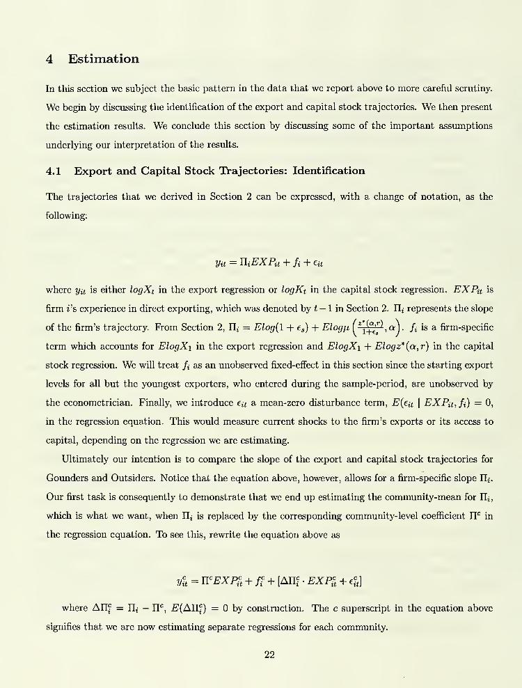
Networks, Migration and Investment:

Insiders and Outsiders in Tirupur's Production Cluster*

Abhijit Banerjee^ Kaivan Munshi*

March 2000

Abstract

This paper studies the effects of social network based lending. This is a pervasive phenomenon

in most of the developing world. Access to such network capital has an obvious influence on

investment. It also influences the pattern of migration since, ceteris paribus, migrants would prefer

to be in locations where they have access to their community's lending network. We show that

under reasonable conditions such lending will generate a rather specific pattern of migration and

investment. In particular, migrants to locations where they do not have access to their communty's

lending networks will tend to have higher ability than the traditional residents of that location, but

will invest less relative to their abihty. Under some conditions this generates the possibility that

migrants have higher ability but invest less in absolute terms than the local people. We test this

impUcation using data from the knitted garment industry in the South Indian town of Tirupur.

Comparing the growth rate of output (which, we argue, proxies well for ability) with investment

between garment firms owned by migrants to Tirupur and local people, we find that local people

have slower output growth but invest substantially more at all levels of experience. We also find a

positive correlation between investment and growth within any single community, consistent with

the view that capital access does not vary within each group.

'This project could not have been completed without the support and assistance that we received from the Export

Credit Guarantee Corporation of India (ECGC) and the PSG Institute of Management. Professor A. Govindan and T.

J. Sivan organized the survey and supervised the data collection. We thank Susan Athey, Esther Duflo, Anjini Kochar,

Nick Souleles and Petra Todd for helpful comments. Munshi's research was funded by NIH grant R01-HD37841. We are

responsible for any errors that may remain.

^Massachusetts Institute of Technology

^University of Pennsylvania

1 Introduction

There is a growing awareness that social networks play an important role in facilitating economic

activity when markets function imperfectly, particularly in the developing world. It is usually argued

that this is because long-term relationships, the possibihty of social sanctions, and the smooth flow

of information within the network make possible transactions that would not otherwise happen. This

view is supported by a ntmiber of studies, including Greif (1993), Udry (1994), and Townsend (1994)

in the context of capital markets.

In this paper we take a more macro approach: instead of looking at the internal functioning of

these networks we focus on the eflFects of networks on the functioning of the wider economy. In this we

follow a growing recent literature which emphasizes the possible distortions that arise from a reliance

on networks.^ To the best of our knowledge however there are no papers that tell us whether or not

these distortions can be of a magnitude that would make them worth taking seriously. This is what is

attempted here for the specific case of lending networks.'^ Using panel data that we gathered from the

knitted garment industry in Tirupur, a town in Southern India that produces about 70% of India's

exports, we will argue there is clear evidence of a large deviation from the first-best allocation.

At the heart of the case we make is the following set of observations. First, in a first-best world,

under the standard assumption of complementarity between ability and capital, higher ability people

will invest more in their firms.^ Second, lending networks tend to be local - in other words, they

provide privileged credit access to their members but only if their members locate where the network

has control. Therefore, in order to take fuU advantage of the lending network, one might have to invest

where one's network is established, rather than where one is most productive. Conversely, those who

choose to invest in an area where their network is weak, will presumably benefit from being in the place

best suited to their skills, at the cost of being more limited in their access to credit. Third, the previous

observation can be rephrased as follows: all those who choose to invest where the network is weak,

do so because this allows them to do what they are good at, while some of those who invest where

'See for example Greif (1993), Banerjee (1996), Kranton (1996), Banerjee and Newman (1998), Kranton and Minehart

(1998, 1999), and Jackson and Wolinsky (1996). Many of these papers are more after the subtle (though perhaps equally

important) distortions that arise out of the process of formation of networks or the pecuniary externalities arising from

the effect of networks on market prices.

Lending networks are networks whose main economic function is to facilitate credit market transactions. A reliance

on network-based lending is a ubiquitous feature of Indian corporate finance, particularly in the small-business sector,

and we will argue later that Tirupur is no exception to this rule.

'This observation is standard and goes back to Lucas (1978).

their network is strong do so despite being more productive at some other location. This implies that

those who invest where their network is weak are likely to be, on average, more able (in the sense of

being better matched to their chosen occupation) than those who invest where their network is strong.

Finally, the previous observation tells us that migrants in a new location, where their community's

network is yet to be established, are likely to be more able than the local people. However, for the

same reason, they may also invest less than the local people. In other words, comparing migrants

with non-migrants, in such a location, it is possible that the group (the migrants) with higher average

ability will also be the group that invests less. This is the opposite of what we would find in the

first-best case: it will only be observed in the data if network-generated distortions are large enough

to outweigh the standard complementarity effect. It is this prediction of network-based lending that

forms the basis of our empirical analysis.

Most of the observations that we provided above are in themselves well-known and widely accepted.

For example, it is generally recognized that people choose to migrate to places where they have access

to their community networks.'* The fact that a lack of social networks limits out-migration has also

been written about. ^ Finally, the fact that migrants have higher ability than the locals is common-

place in the migration literature. Borjas (1987) calls this "positive selection".^ Our framework unifies

these observations and uses their joint implications to provide empirical insights into the nature of

networks and their influence on migration and investment.

The reason for choosing Tirupur as the venue for the empirical work in this paper is that we can

take advantage of a recent change in the sociological composition of Tirupur's production cluster.

Until the late 1980s Tirupur was dominated by the Gounders, who are traditionally agriculturalists

from the area. However, in the last decade a number of people from all over the rest of India have

entered the Tirupur industry, attracted by its success as an export center. We will argue that at the

time when we observed them (in the mid 1990s) the Gounders had access to well-established lending in

Tirupur but the newcomers from outside probably had much more limited access to capital in Tirupur

^See Piore (1979) and Massey, Alarcon, Durand and Gonzalez (1987) for studies of Latin American migrants to the

U.S. that argue that migration tends to flow to areas where past migrants have already established a foothold. Carrington,

Detragiache and Vishwanath (1996) describe the support networks that were put in place for the later arrivals from the

American South during the Great Migration. Similarly, Timberg (1978) describes how social ties framed the expansion

of the Marwari community into specific cities in nineteenth-century India.

^Dasgupta (1987), among others, makes this point.

Borjas derives conditions under which a model where migration is constrained by the physical cost of moving will

generate positive selection. Our theory of positive selection differs from his in linking it to the distortionary effects of

networks.

than they would have had in their home basest It is this difference in the access to credit networks,

between insiders and outsiders, that we exploit in the empirical analysis.

The data shows that Gounders start their business with substantially more capital than the Out-

siders, and use substantially more capital per unit of production at every level of experience, consistent

with the view that they have better access to capital. We also find that output trajectories are steeper

for the Outsiders than for the Gounders.^ Starting with lower output levels, the Outsiders ultimately

surpass the Gounders after about five years of export experience, yet they continue to maintain lower

levels of capital stock. The fact that output grows faster for Outsiders than for Gounders despite the

fact that they invest less, we take as evidence that Outsiders have higher ability: this is certainly what

our theory predicts.^ Thus outsiders with higher ability invest less than the insiders, which suggests

in turn that there are substantial distortions in this industry.

The plan of the paper is as follows: Section 2 develops a model of lending networks and mi-

gration/location choice. The first goal of this section is to identify conditions under which lending

networks lead to positive selection. While our analysis shows that it is possible to find simple con-

ditions under which we get positive selection, it also points out that the simple intuition for positive

selection given above is incomplete - there are many quite convincing situations where we may not get

positive selection. The second goal of this section is to identify conditions under which we can identify

higher ability by comparing the growth trajectories of firms in the industry. The data used for the

empirical work is described next in Section 3. Section 4 discusses identification issues and presents the

regression results. Here we also present some evidence supporting the complementarity assumption

that underlies our empirical work. This section ends with a discussion of other possible interpreta-

tions of our results. Section 5 concludes the paper with a discussion on the poUcy implications of our

results. We recognize that demonstrating that there are distortions does not automatically establish

the feasibility of something better, and certainly does not of itself make a case for government inter-

^This assumption is supported by the historical and case-study evidence, mentioned above, which suggests that

communities tend to expand quite slowly into new locations.

*The fact that migrants have steeper earnings profiles is standard in the migration literature. Borjas (1987) calls

this one of the most convincing findings of the empirical literature on migration and cites studies by Chiswick (1978),

Carliner (1980) and De Preitas (1980). It is worth emphasizing, however, that these studies mainly focus on migration

from poor to rich countries. In such cases, there is a natural element of catch-up - the new migrants get educational and

other opportunities that they have never had. For example, migrants to the U.S. learn English, which makes them moreemployable. This kind of catch-up is less important with internal migration, and our results are therefore more likely to

be due to positive selection. What is striking about our case is that the steeper output profiles are associated with less

investment.

^But see the discussion in sub-section 2.7.

vention. However, we argue that in this specific context there may be a strong case for certain types

of government interventions in the financial sector.

2 A Simple Model of Location Choice and Investment

In this section, we formally develop the model suggested in the introduction. Specific assumptions

that we make will be inspired by the way the garment industry in Tirupur functions, as our goal

will be to use the model to interpret data from Tirupur. We first characterize the firm's production

and investment decision for a given interest rate and level of ability. We then go on to analyze the

location choice decision when networks are present. Finally, we bring the investment decision and

location choice together to derive the dynamics of output and investment for insiders and outsiders in

the industry.

2.1 Production and Investment

There is a large population of firms producing the same good. We adopt the normalization that the

price of the good is 1. Firms at any point of time have a stock of regular buyers. In each period firms

lose a fraction of this stock but acquire a random fraction of new buyers as well. This is captured by

writing the following equation for Xt+i, which should be thought of as the amount of sales that the

firm is sure to get in period * + 1 :

Xt+i=fXtXt{l+et).

We think of €f as a random shock distributed on [0, e*] with mean e and ^( as a number between

and 1. 4>{et) is the distribution of et and is assumed to be the same in all locations, while the shock

itself is assumed to be independent across people, and for the same person it is also assumed to be

independent over time.^° This equation is easy to interpret if we think of Xt(l+et) as the reahzed sales

in period t. Then this equation says that the minimum possible sales in the next period is a fraction

/i( of the current period's actual sales. This way of modeUng sales builds in a lot of persistence over

time which seems to fit the anecdotal evidence about the knitted garment export industry in Tirupur.

Our impression from talking to industry experts is that foreign buyers typically pick their exporters

and stick to them unless they have a bad experience.

'"We can assume that (/>(•) is the same for everyone because any fixed difference in the <^(-) is completely equivalent

to a difference in the ability a, which is introduced in the discussion below.

Capital is the only input used for production. Capital stock for period t is chosen at the beginning

of period t (when Xt is known but not Xt(H-ef)). Denote it by Kt. The technology used for production

is described by the equation

where a is the abihty of the entrepreneur in that particular industry. We assume that -gjAx > 0,

oo>B>^>B_>0 and Qrj.ftx'i. < 0. This equation represents the idea that a firm that uses

more capital per unit of sales retains more of its buyers. This is easy to interpret if we think of a

more capitalized firm as being more vertically integrated. We are then saying that vertical integration

allows better quahty control and increases buyer retention, and so does having an entrepreneur with

better skills. ^^ Finally, we assume that there are diminishing returns to capital.

The firm maximizes its expected discounted profits, which can be written as:

V{Xt) = maxE f2s'[Xt{l+et)-rKt]t=i

under the assumption that the owner of the firm is risk-neutral and discounts the future at rate 6, and

r is the interest rate that applies to the firm, which is assumed to be constant over time. The firm

takes as given Xi , the assured demand in the first period, and maximizes profits under the constraint

Imphcit in this way of writing the problem is the assumption that the firm can borrow as much as

it wants at an interest rate of r which, however, may be specific to the firm. This is a specific (though

standard) way of modeling a capital market imperfection: we could have alternatively assumed that

the firm is credit rationed or faces an increasing interest rate schedule.

Observe from the structure of the maximization problem that the value of V will double if we

simply double Xt and Kt for all t. It follows that

ViXt,r,a) ^ XtV{l,r,a).

"For instance, Cawthorne (1995) quotes one of the Tirupur exporters as saying, "I want to be like the spinning mills

here. That is my ambition. Then I will have all the stages (of production) as one operation. . . . With a large factory

you know exactly what is going on." While Cawthorne does not share his view, a large number of exporters that wespoke with expressed the same sentiment.

It is evident that V{l,r,a) must be increasing in a and decreasing in r (this can be verified by

differentiating the expression defining V{l,r,a) and applying the envelope theorem).

Using this decomposition of V{Xt,r,a), we can write the entrepreneur's maximand as

E{[Xt{l + et) - rKt] + 6Xt+iV{l,r,a)}

We maximize the maximand subject to the constraint above. Substituting in the expression for Xt+i

from the constraint equation, we can write the maximand as

E{Xt[{l + et)-r^^+6f^{^^-^^ya){l + et)V{l,r,a)]}

Writing ^ = 2;^, we write this as

Xt[{l+-e)-rzt + ^{zt,a)V{l,r,a)]

where Ji{zt,a) = E^i{j^^,a){l + et).

Maximizing this with respect to zt gives us

r ^ ^^{zt,a)V{l,r,a).

This determines z*{a,r), the optimal capital-output ratio for this particular firm.^^ Note that z* is

constant over time. It follows from the second-order condition for this maximization that an increase

in r leads to fall in z*. The effect of an increase in a on z*, when JI^^ > is unambiguously positive,

since an increase in a both raises JJ^ and V{1) (higher a means higher lifetime income).-'^ The effect

may be either positive or negative when Jl^^ < 0, since the positive effect on V(l) may or may not

dominate the negative effect on fl^

.

Note that this is telling us that ability and capital can be complements even if Ji^^ < and indeed

must be complements as long as Jiaz is small in absolute value relative to 72^. This is because higher

abihty people have a brighter future and therefore are willing to invest more in building up their

customer base.

Strictly this is not the capital-output ratio but rather the ratio of capital to the guaranteed amount of output.' We will find it convenient to state our conditions in terms of derivatives of the Ji function but it is worth noting that

these derivatives inherit the sign of the corresponding derivatives of thefj.

function.

2.2 Locations and Populations

We now extend the model to allow for location choice. We assume that there two locations, 1 and 2,

each with its own industry. Each person in the economy is associated with one of the two locations.

This is his community. Each person is also associated with a pair {a^,a'^), where a^ represents his

abihty in industry 1 and a^ his ability in industry 2. The population in each community is described by

a distribution function ^*(a\ a'^) i — 1,2, which is defined on the unit square and is assumed to have

no mass points. We assume that the two populations are exactly identical, i.e., ^^(a^, a^) = ^'^{a^,a'^)

for all pairs (0^,0^). The consequences of allowing the populations to be different are examined in

sub-section 2.5.

We will assume that the two locations are equivalent in all respects except perhaps in the way

their capital markets function. Specifically, we assume that the initial guaranteed level of demand in

the two locations, Xl and Xi, are equal. We have already set the price of the goods produced to be

equal to 1 in both locations.

These assumptions have the immediate impUcation that in a first-best world, where everybody faces

the same interest rate irrespective of location and community, people will simply choose the location

where their ability (i.e., their a) is higher. This particularly simple structure of the first-best outcome

makes it easy to identify the distortions generated by network-based lending. The impHcations of

relaxing these assumptions are discussed in sub-section 2.5.

2.3 Lending Networks

We have in mind a very simple model of lending networks. Enforcing credit contracts is costly.

Networks can lower the cost of lending because it is easier to enforce contracts when the borrower

belongs to the same community network as the lender. However, this only works when the borrower

is located where the network is based: the network only has enforcement power when the borrower is

at hand. In other words, there is no advantage to lending to a community member who has located

away from the network. ^^

' This says basically that networks are local, which is consistent with the historical evidence. While the Marwaris

spread all over India during the nineteenth century, a careful reading of their migration patterns reveals that each caste,

within the Marwaris, located in only a few locations (Timberg, 1978). For example, the Shekhavati Aggarwals were

dominant in Malwa, and had a substantial presence in Calcutta, Assam and the Indo-Gangetic plain. In contrast,

the Oswals dominated the Bombay Deccan, the Calcutta jute industry and had a significant presence in Bangalore,

Hyderabad and Tamil Nadu. Similarly, while the Nakarattars engaged in business throughout Southern India and

Southeast Asia, their internal capital markets had a local aspect as well. For example, Rudner (1994) describes how the

rate on community capital in Rangoon was set at a council meeting, once a week at a fixed time in the local temple.

The combination of these assumptions can be captured by assuming that when a borrower from

population 1 borrows at location 1, he pays rj, which is less than r^, which is what he would pay were

he to locate in location 2. Likewise, a borrower from population 2 pays r^ in location 2 and r2 > r^

in location 1. We make the assumption that the locations are symmetrical in the sense that rj = rj

and rf = rl- The consequences of not making this assumption are discussed in sub-section 2.5.

2.4 Location Choice

Before they choose how much to invest, people in our model have to decide where to locate. We will

focus on the decision of someone with ability vector (0^,0^), who was born in location 1 which allows

us to dispense with the marker for the location of birth. Strictly, this comparison can only tell us about

the movers and stayers from location 1 while we are really interested in how the stayers in location 1

compare with those who move to location 1 from location 2. However, under the assumption, made

above, that the two locations are perfectly symmetrical, the two comparisons coincide.

When individuals choose their location they know their own abilities and the interest rates in the

two locations, but do not have their actual orders for period 1. All they know is that their first-period

output in the two locations are given by the random variables Xl{l + e\) and X^(l + e^), where Xl

are Xf are known (and equal to each other), but e\ and ef are only revealed after location decisions

have been made and capital stocks have been chosen.

In order to understand the location decision we need to compare lifetime payoffs for the same person

in the two locations. We will, for the time being, assume that in either location the person would

choose to participate in the local industry. This would be true if an Inada-like condition holds for the

fi{-) function. The consequences of relaxing this assumption and therefore taking the participation

decision seriously are briefly discussed in a later sub-section.

Denote by V the individual's expected lifetime payoff if he were to choose location i. Because we

assume that the production technology does not vary across industries, V^ = F(X|,r%a*). For the

person who is marginal between going to 2 and staying in 1, it must be true that V{Xi,r'^,a'^) =

V{Xl,r^,a^), which, from above, implies X^V{l,r^,a^) = XlV{l,r^,a^), or

This implicitly defines a function a^ = f{a^), which tells us the lowest value of a^ for which

someone with attributes of (a^, o:'^) chooses 2. Since V{l,r^,a'') is increasing in «% it must be the

8

case that /(•) is an increasing function.

In a first-best world, since r^ = r^, f{a^) = a^. As a result, the distribution of abiUties among

those who move and those who stay will be identical. There is no positive selection.

In the case where r"^ > r^, since F(l,r%a*) is decreasing in r\ f{a^) > a^. The /() function

for this case is represented in Figure 1 by the curve AB. Those who are above the /(•) curve choose

industry 2, while the rest choose industry 1.

Insert Figure 1 here.

It is evident from Figure 1 that the people who are in the left-bottom corner of the square, i.e.,

people who have low ability along both dimensions, all remain in their home location. This is the

essence of the intuitive argument for positive selection offered in the introduction - those who migrate

do so because they are significantly better at the occupation that requires them to migrate, while

those who stay back do not have to be particularly good at the local occupation. And, indeed, it is a

force for positive selection. However, it is not enough to guarantee positive selection, except, as we will

see, in extreme cases. In general, we will need to impose restrictions on the distribution of abilities

(as described by the distribution function ^^(a^,a^)), as well as the shape of the /(•) curve.^^

To understand the role of the distribution of abilities, consider the case represented in Figure 2.

The distribution of abilities in this case has a substantial degree of concentration in the top right

corner of the unit square, suggesting that the correlation of abilities is the highest for high ability

people. From the position of the /(•) curve, it is clear that in this scenario most of the people with

high ability wiU stay back in industry 1. The average abihty of movers will clearly be lower than that

of the stayers.


Figure Sexplains why the /(•) curve matters. In this case, we assume that the distribution function

is uniform over the unit square, thereby eliminating any correlation between the two types of ability.

The /(•) curve as we have drawn it (ACB) almost coincides with the diagonal until a^ — 0.5, after

that it is almost vertical. The average ability of a mover in this case is the average of a^ over the

area ACBQ. The average ability of a stayer is the average of a^ over the area PACBRS which is the

Strictly, the /() curve only tells us about the movers and stayers from location 1 while we are interested in howthe stayers compare with those who move to location 1 from location 2. However, under the assumption that the two

locations are perfectly symmetrical, the two comparisons coincide.

average of the averages over PACDS and CBRD. Note that since the hne AC almost coincides with

the diagonal and CB is almost vertical, the average of a^ over ACBQ is essentially the same as the

average of a^ over PACDS. However, the average of a^ over CBRD is clearly higher than its average

over PACDS and therefore it follows that the average ability of the movers is unambiguously lower

than that of the stayers.


One case where the /(•) curve will have the shape it has in Figure 3 is where low ability people in

either industry do not use any capital. In this case, the difference in the price of capital is irrelevant

for this set of people. They simply choose the location where they have higher ability - the /(•)

curve therefore coincides with the 45° line in this range. High ability people, on the other hand,

need capital to benefit fully from their higher abilities. However, capital is so expensive in location

2 that no one uses it; whereas in location 1, capital is cheap, which helps high ability people. As a

result, productivity grows much faster with ability in location 1 than in location 2, generating a nearly

vertical /(•) curve. Intuitively, the problem here comes from the fact that there is strong ability-capital

complementarity. As a result, high ability people are severely penalized for moving to a location with

a higher rate of interest, which naturally reduces the share of high ability people among the movers.

In the rest of this sub-section we develop two sets of sufficient conditions which guarantee that the

movers from a certain location will have higher abiUty than those who stay there. Because we will be

interested in comparing average productivity rather than average abiUty, our goal will be to show that

the distribution of abilities of migrants first order stochastically dominates (FOSD) the distribution of

abilities among of those who stay back. While our formal arguments apply to movers and stayers from

location 1, because the two locations are perfectly symmetric the result also holds when we compare

those who move to location 1 with those who stay back in location 1. We therefore state our results in

terms of the comparison of migrants and local people at the same location, as this corresponds more

directly to our empirical analysis.

The intuition for the first set of conditions is very simple: increasing r^, keeping r^ fixed, moves the

/(•) curve up. As a result, for a high enough value of r'^ (with r^ fixed), the /(•) curve will pass through

the top-left-hand corner of the unit square {A'B' in Figure 1). When this happens, the distribution

of a^ among those who choose to move to 2 is entirely concentrated at a^ = 1.^^ By contrast, since

This actually assumes that the /(•) curve does not become vertical. The reader can verify by looking at the expression

10

almost no one moves, the distribution of a^ among those who choose to stay in industry 1 is almost

identical to the ex ante distribution in the population (i.e., the marginal distribution over values of

a^ that is generated by the joint distribution, ^{a^jO^)). This argument implies:^^

Clzdm 1 For a fixed value of r^ , there exists a high enough value of r^ such that the distribution of

ability in industry 1 among migrants first order stochastically dominates the distribution of ability in

the same industry among local people.

This result formalizes the argument for positive selection that was suggested in the introduction.

When the interest rate differential is very large, only those who have very high abihty will migrate.

The rest, including everyone who has medium or low abiUty in both occupations, will stay back,

depressing the average abiUty of stayers relative to migrants.

A limitation of this result is that it has precise predictions only about relatively extreme cases.

The next result formalizes the intuition, implied by the example in Figure 3, that we want to avoid

cases where the /() curve becomes very steep as ability increases. The proof, given in the Appendix,

first shows that under the conditions given below, the /(•) curve is everywhere flatter than the 45°

Une and then uses this property to prove the stated result.

Claim 2 Assume that djl{z,a)/da is a constant, that the elasticity of the function dji{z,a)/dz with

respect to z is greater than 1 and that ^^ {a^ , a^) and^ {a^,Q^) represent uniform distributions on the

unit square. Then the distribution of ability in industry 1 among migrants first order stochastically

dominates the distribution of ability in the same industry among local people.

Among these assumptions, the condition that djl{z, a)/da is a constant is there to limit the amount

of complementarity between ability and investment which helps us avoid a case such as the one in

Figure 3. Note that while this condition obviously imphes that d'^Jl{z,a)/dadz = 0, as pointed out in

Section 2.1 it does not necessarily imply the absence of complementarity between ability and capital.

The assumption of uniform distribution of abilities avoids the case in Figure 2. Finally, the assumption

that djl{z,a)/dz is elastic enough with respect to 2, directly implies that the demand for capital is

inelastic. This is to make sure that the higher interest rate at location 2 is sufficiently costly for the

for /'(•) derived in the Appendix that under the assumption that dEn{z^/{l + et),a^)/da is bounded above and below

(which has already been assumed), the /(•) curve remains bounded away from becoming vertical.

"^^The proof is obvious and is omitted.

11

movers. Otherwise the selection effect may not be strong enough to guarantee first order stochastic

dominance.

2.5 Discussion

We imposed a rather lengthy list of conditions in order to get this result. It is therefore worth

emphasizing that the conditions are more stringent than we actually need. For example, we do not

need the property that / () is everywhere flatter than the 45° line in order to prove Claim 2, though

our current proof does make use of this property. It can be directly checked from the proof of Claim

2 that in the case where /'(•) = 1 (i.e., the / (•) curve is a straight line parallel to the 45° line). Claim

2 continues to hold as long as r^ > r-^. By continuity, it also holds when /'(•) — 1 is allowed to be

positive, but is bounded above (once again as long as r"^ > r^). As a consequence, it can be shown

that as long as r-^ > r^, each of the other conditions of Claim 2 can be relaxed without changing the

result.

Prom the point of view of using this model to interpret our data, it is also useful to examine the

consequences of relaxing the strong symmetry assumptions that we have so far imposed. We now relax

each of the main assumptions in sequence.

1. Different ability distributions in the two locations: In general, more or less anything

can happen in this case. One interesting special case is when one of the populations has more ability

along both dimensions than the other. This would be the case, for example, if (say) population 2 has

a better outside option than population 1: in this case the low ability people in that population would

take their outside option and only relatively high ability people would invest in either of the industries.

It is clear that this will tend to widen the ability gap between those who move from location 2 to

location 1 and those who stay in location 1.

2. Asymmetric interest rates: The effect of relaxing the assumption of symmetric interest

rates is potentially quite complex. If one community has systematically higher interest rates than the

other - say, r2— r\ = r^ — rf > - the net effect can in principle go either way since people from

population 2 pay higher rates both if they migrate and if they stay. The one unambiguous effect is on

the decision to take the outside option. More of the people in population 2 (which faces higher rates)

will take the outside option and, as discussed in the previous paragraph, this has the effect of raising

the average ability of movers from that population. -^^

One resison why interest rates may be higher in one population than in the other is that ability levels are higher in

12

It is also possible that the differential between the interest rate paid by movers and the rate paid

by stayers may vary across populations. One might expect the differential to be large for communities

that have few connections outside their home base and small for widely dispersed communities. To fix

ideas, consider the case where starting with r^ — rj = rj — r2 we raise rf — rj and reduce rj — r^. This

makes it less likely that stayers in location 1 are strongly selected for industry 1 (because less people

move), but it also makes it less likely that those who move to location 1 from location 2 are strongly

selected for industry 1. In other words, both the movers and the stayers among those who finally join

industry 1 are Hkely to have lower ability and the net effect may be ambiguous.

3. Xi ^ Xl, i.e., industry 2 is a lot more profitable than industry 1:^^ In this case the

only people who would choose to stay in location 1 would be people with very high values of a^ .^° In

other words, the / (•) curve will move to position like A"B" in Figure 1. However, by the same logic

it is also true that only people with very high values of a^ will move to industry 1 from location 2.

Therefore the net effect of changes in Xi/X\ on the extent of positive selection can be either positive

or negative.

2.6 Investment eind Productivity

The main lesson from our investigation of location choice is that under reasonable conditions those

who move to a particular location may be more able than those who were "born" there. The effect

of this selective migration on investment is, however, ambiguous, since the ability bias exists precisely

because the movers face higher interest rates. As a result, it is quite possible that migrants, despite

having higher ability, invest less.

Turning next to productivity, there are clearly two effects. Movers have higher abihty but may

invest less. The net effect may be in either direction, but as we stated in the introduction, we are

interested in the case where movers invest less but have a higher average productivity. The next Claim

shows that under the conditions of Claim 2, this property holds for the person on the margin between

moving and staying (the proof is in the Appendix).

Claim 3 Assume that djl{z,a)/da is a constant and that the elasticity of the function djl{z,a)/dz

that population: this raises the demand for capital and therefore interest rates.

The case where the good produced by industry 2 carries a higher price than the good produced by industry 1 is

exactly the same.

The effect of raising X? , keeping X\ fixed, is actually somewhat subtle: it has the effect described in the text, but

raising Xl/Xl also flattens the /(•) curve, which acts as a countervailing effect. In the extreme cases, as in Figure 1,

the first effect must, however, dominate.

13

with respect to z is greater than 1. Then the person who is indifferent between moving and staying will

have a lower z but a higher Jl{z, a) if he moves.

This is, of course, at best illustrative: it applies only to the marginal person, while we are interested

in the average for the entire population of movers and stayers.'^^ However, it does establish the prima

facie plausibility of a negative relation between ability and investment.

2.7 Dynamics

With the results about investment and location choice in hand, we proceed to derive the capital

stock and production trajectories for a firm with ability a facing an interest rate r. Begin with the

accumulation process of someone who starts out expecting sales of at least Xi (note that we now allow

Xi to vary across firms). Then

X2 = Xi(l + 6i)/z(^^^,a).1 + ^1

Iterating on this formula we get

,^ /-. \ /-, N/•2*(a,r) . ,z*(a,r) .

Xt=Xi{l + ei) (l + et_i)M / ' \ a) ;x(—^^^,a).

Therefore,

t-l t-l ,. V

logXt = logXi + 5]log(l + 6,) + ^log^(^-^, a).

s=l s=l

Taking expectations, we get the dynamic path of evolution of output:

ElogXt = £;iogXi + it- l)£;iog(l + es) + (t - 1) E\ogtx{^^^^, a).

To get the corresponding equation for capital stock, we observe that Kt = Xf z*{a,r), which gives us

ElogKt = ElogXi + E\ogz*{a,r) + (t - l)^log(l + e,) + {t - 1) £;iog^(^J^^, a).

Moreover, as we will see, n is not exactly the right measure of productivity from the point of view our empirical

work - the correct measure is E{logfj.{-^,a'')}.

14

Because £^log(l + es) ought to be the same for everyone,^^ both capital stock and output grow faster if

and only if E log fj,{^j^f^, a) is higher. As observed above, /l(2*, a), may be higher for the outsiders

even if they have a lower z*. For the same reason, E log ij.{^-^^f^ , a), may also be higher for the

outsiders.

Since those who have a lower z* can have a higher Elogfi^^j;^^, a) only if they have higher

abiUty, if we observe that one group has a higher z* but a flatter trajectory for output we should

conclude that it has less ability but faces lower interest rates. This idea is the basis for the empirical

work reported in the following sections.

3 Institutional Background

3.1 The Setting

The setting for the empirical analysis is the South Indian town of Tirupur. In this sub-section and

the next, we try to explain why Tirupur's production cluster is ideally suited to test the implications

of network-based lending developed in the previous section.

Tirupur is located in Coimbatore district, in the modern Indian state of Tamil Nadu. This area was

traditionally known as Kongunad, one of the five big sub-divisions of the Tamil-speaking country, prior

to the arrival of the British. Kongunad is believed to have been colonized by the Vellala Gounders,

an elite cultivator caste, in the twelfth century (Beck, 1972). While Kongunad is quite dry, the soil

is fertile and there are significant reserves of subsoil water. Where well irrigation was available, high

agricultural yields have been obtained from early times.

Kongunad emerged as the most commercialized region in Tamil Nadu in the last quarter of the

nineteenth century with the advent of the railways, as cultivation shifted predominantly into cash

crops (particularly cotton). By the 1950s Coimbatore had 20% of its land allocated to cash crops,

which is the largest share of any district in Tamil Nadu, and this land was among the most valuable

in the state (Coimbatore District Gazetteer, 1951; Baker, 1984). While the Kongu Vellala Gounders

had always been wealthy, the cultivation of cash crops transformed this community into one of the

wealthiest in Tamil Nadu.

While Tirupur's association with the cotton trade goes at least as far back as the nineteenth

century, the first textile manufacturing unit was only established in the town in 1935. The Nakarat-

tars, a community traditionally involved in trading, initially dominated the industry. However, after

This is almost by construction: differences among people have been swept into thefj,

function.

15

a prolonged period of labor unrest in the mid-1960s, they were largely replaced by the Gounders

(Swaminathan and Jeyaranjan, 1994). The Gounders are a so-called "right hand" (valangkai) caste,

so they were traditionally confined to land-based activities; this was their first significant commercial

venture outside agriculture. For the next twenty years or so, the industry was dominated by the

Gounders and catered almost exclusively to the domestic market.

The export of knitted garments from Tirupur started to grow very rapidly around 1985, and in

the early 1990s the annual growth rate was above 50%. This generated an inflow of new entrepreneurs

from outside Tirupur. By the mid-1990s, which is when we observe the industry, about half of the

exporters were Gounders while the rest were from all over India. In our sample of exporters, 58% are

Gounders, 9% are Mudaliars, 10% are Chettiars, and the remaining 23% are from outside South India,

mainly from traditional trading communities such as Marwaris, Gujaratis and Khattri Punjabis.

Prom the point of view of our framework, Gounders in Tirupur are almost the perfect example

of local people. They have substantial presence in the area and extensive experience in the local

industry, both of which strengthen network lending. In contrast, the other communities are literally

outsiders, who only arrived in Tirupur in the 1990s with the surge in exports. These outsiders belong

to traditional trading communities with well established networks in other parts of the country but it

is probably too soon for these new entrants to have formed their own networks in Tirupur, though we

would expect such networks to ultimately emerge if the industry continues to provide high returns on

investment in the long-run. Por the time being at least, it seems plausible that the outsiders have to

forego the lower interest rates that they would receive if they located in one of their more established

business centers elsewhere in the country.

Our model would therefore tend to suggest that Gounders may have lower ability and will invest

more, at least relative to their ability. Several other factors reinforce this effect. Pirst, the Gounders

have almost no presence in trade or industry outside Tirupur and therefore their access to network

lending, were they to invest outside Tirupur, is likely to be very limited. As we have already observed

in sub-section 2.5, larger interest differentials between home and abroad tend to lower the average

ability of the population that stays back. Second, the outsiders in Tirupur are from traditional

business communities whereas the Gounders are, for the most part, new to industry. At least in terms

of understanding the process of exporting, the outsiders probably have an ability advantage. Third,

because the outsiders come from traditional business communities, their capital probably has many

alternative uses, while the Gounders can only invest their substantial agricultural wealth in the local

16

garment industry, or in agriculture or in the highly inefficient Indian financial sector. The interest

rates - for both movers and stayers - are probably higher for the outsiders than for the Gounders.

As we observed in sub-section 2.5, this tends to raise the average quality of outsiders in the industry

(and depress the amount they invest), relative to the Gounders.

3.2 The Industry

The industry produces knitted garments and is largely focused towards exporting. Most firms produce

t-shirts, targeted at low-end retail outlets in Europe and the United States. There are essentially three

types of firms in the industry: direct exporters, indirect exporters, and job-workers. Direct exporters

are the ones who receive orders from abroad. Once they have an order they often pass on a fraction

of the order to one or more indirect exporters. Indirect exporters are independent garment producers

who are entirely responsible for their share of the order, delivering the finished product to the direct

exporter prior to shipment.

Garment production is organized in a number of stages: the major stages are knitting, dyeing and

stitching, while the minor stages include calendaring (shrinkage control), printing and curing. The

direct and indirect exporters will typically own machinery for some stages of production, but not all of

them. For the rest of the stages they will employ job-workers, who are specialized producers owning

machinery for a single stage only.

Job-work and the use of indirect exporters allows for decentralization in the production process

and is one reason why there can be large variations in the output-capital ratio across direct exporters.

However, such decentralization has costs of its own. Quality appears to suffer and delays in shipment,

particularly during the peak production season, are more frequent. From our conversations with

bankers in Tirupur and officers in the Export Credit Guarantee Corporation (ECGC), a govermnent

agency that insures exporters, it appears that such delays often result in orders being rejected by

foreign buyers.

3.3 The Data

The main data source for this paper is a survey of six hundred direct exporters, indirect exporters

and job-workers carried out in 1995. Details of the entrepreneur's background, his access to bank

financing, as well as export (production) and investment information over a four-year period, 1991

to 1994, were collected from each firm. Some supplemental information was collected through a brief

17

re-survey in 1997.

Before turning to a description of the data, we briefly describe the sampUng procedure employed

in the 1995 Survey, which is non-standard. The Tirupur production cluster is a complex institution

comprising at least two thousand production units. Many of the units are unregistered, so there is no

"list" of firms in the town. Moreover, accurate maps are unavailable; Tirupur, like most small Indian

towns, is a maze of lanes and by-lanes. Under these circumstances we were unable to conduct a census

of all production units, which would have allowed us to randomly sample firms for the survey. We were

also unable to divide the town into a sufficiently large number of clusters, which would have allowed

us to survey a sample of clusters. Instead we divided the town into ten zones and allocated a fixed

number of days to survey firms within each zone.^^ We then proceeded from one zone to the next

until the entire town was covered, over a three month period. Ultimately, information was collected

from 300 indirect exporters and 147 direct exporters. The distribution of firms by community, in our

sample, is very even across the ten zones, suggesting that the sampUng was not biased towards any

community.'^^

3.4 Descriptive Statistics

The discussion that follows focuses for the most part on the one hundred and forty-seven direct ex-

porters in the 1995 Survey. Since we are particularly interested in comparing the investment behavior

and the export performance of the Gounders and the Outsiders, the sample is partitioned by com-

munity. We also divide firms into Young and Old units, where the cut-off separating these firms is

specified to be five years of export experience. Very few firms in our sample have more than ten years

of experience. Note that we have data over a four-year period, 1991 to 1994, for most of the variables

that we discuss.

We begin with the individual characteristics of the direct exporters in Columns 1-4 of Table 1.

Each exporter provides information on when he first arrived in Tirupur as well as when he received his

first direct export order. The entrepreneur's age and experience can then be computed at each point

in time over the sample-period: age is the number of years elapsed since he first arrived in Tirupur

while experience is the number of years since he became a direct exporter. The sample-statistics for

Production units in Tirupur are located for the most part in converted residential structures. There is no segregation

of homes and production units today, and firms are spread throughout the town. Since we were unable to identify any

spatial clustering in production activity, we surveyed the entire town.

There is a single exception - one zone had a relatively low proportion of Gounders. Dropping this zone does not

affect the estimated export and capital stock trajectories that we report later in Section 4.

18

the two communities are fairly similar, with the exception of the Old direct exporters, who have more

than five years of direct export experience. In this category, we see that the age variable is significantly

larger for the Gounders. This is consistent with the institutional background, which suggests that the

Gounders were established in Tirupur before the Outsiders arrived.

Turning to sources of finance, all the entrepreneurs and bankers we spoke to mentioned the impor-

tance of informal sources of capital in Tirupur. Family and community capital is a major component

of the financial structure of most firms that operate in India's small-business sector, and Tirupur does

not appear to be an exception to this pattern. Further, nidhis (informal credit institutions) and chit

funds (rotating savings and credit associations) have been used extensively in Kongunad since early

times (Baker, 1984), and continue to be an important source of capital today, particularly among

Gounder businessmen.

However, when it came to providing actual details of their own finances, we found that the surveyed

firms were generally unwilling to discuss the informal component of their finances. We speculate that

this is because many of these transactions, including the informal nidhis and chit funds, violate tax

laws and/or financial regulations.

They did, however, provide us with information about their bank credit. Bank credit is an impor-

tant source of credit for financing investments in machinery for both communities (Table 1). More

experienced exporters also appear to have greater access to bank credit. Notice, however, that there

is little difference between the two communities, both among the Young as well as the Old firms. This

last observation is useful in ruling out the possibility that the formal capital market treats Gounders

and Outsiders differently. The distinct investment behavior that we observe for these communities is

evidently due to their differential access to other sources of finance.^^

Partnership is another formal channel through which the firm can expand its capital base. It turns

out that as many as 25% of the Outsiders and 31% of the Gounders do have outside partners in their

firms. There were on average three outside partners in these firms (both for Gounders and Outsiders)

,

and the proprietor's share of the ownership was 44% for the Outsiders and 39% for the Gounders.

While there are small differences here that go in the right direction (Outsiders are more dependent

on a single person's personal assets), the two sets of firms basically look very similar. This is not

The fact that Gounders invest more overall but have the same proportion of bank capital, suggests that bank capital

tends to be complementary to other sources of finance rather than a substitute. This is consistent with many standard

models of imperfect capital markets (e.g., Holmstrom-Tirole, 1997) where the amount the bank lends is proportional to

the amount of private resources that the investor can raise.

19

surprising - partners are typically members of the extended family (29% say they are partners with

an immediate family member and another 51% name members of their extended family) and have

access to the same community network. We should therefore expect that the main difference between

Gounders and Outsiders will be in levels rather in the share owned by the partners - each Gounder

partner would be expected to bring more capital (in absolute amount) into the firm.

We also collected additional details about the exporter's background. It turns out that the Out-

siders received more schooling than the Gounders; the average years of education for the two com-

munities (with standard deviations in parentheses) are 13.41(2.62) versus 11.90(3.96). We can reject

the equality of means for the two communities with greater than 95% confidence. Further, 74% of

the Outsiders versus 57% of the Gounders belong to families with previous experience in the textile

industry. There is therefore some prima facie evidence to suggest that the Outsiders may have higher

"ability" in the sense of being better prepared to become successful producers.

With this background information in hand, we turn to the data on the investment and output

variables that lie at the heart of the empirical analysis. Note that Section 2 derived the production

trajectory as a function of ability and the interest rate. Total production is roughly measured by the

sum of direct exports and the indirect exporting that is done for others (very little is produced for the

domestic market). Because for a direct exporter indirect exporting is essentially a fallback when direct

orders are unavailable, the volume of direct exports may be a better measure of performance than total

production. This is supported by the evidence, presented later, that specialized indirect exporters of

either community operate with much less machinery of their own than the direct exporters, which

suggests in turn that direct exporters would not have invested nearly as much if they really intended

to focus on indirect exporting.

It is worth emphasizing, however, that all the results reported in this paper continue to hold if

we use total production rather than direct exports as a measure of production. The exact results are

available from the authors.

Looking now at direct exports. Table 1 shows that average exports for the two communities are

very similar for Young direct exporters, but among the Old exporters the levels are higher for the

Gounders. It will, however, be a mistake to infer from these simple averages that Gounders have

steeper trajectories with respect to experience; we will see in the next section that this gets reversed

once we introduce the necessary controls.

Turning next to investment, Gounders own significantly more machinery at each stage of the

20

direct exporter's life-cycle. Looking at the capital-export ratio, the difference between communities,

particularly for the Young exporters, is striking. Consistent with this evidence is the fact that Gounders

do a significantly greater fraction of indirect exporting. This presimiably reflects the fact that a direct

exporter will accept indirect orders from other exporters when his machinery is idle. AU exporters

accept less indirect exports as they become more experienced, yet Old Goimders continue to maintain

a substantial level of indirect exporting which suggests that their own orders are never sufficient to

keep their machinery running at full capacity. In contrast, the Old Outsiders in our sample focus

exclusively on direct exporting.

We also look at the capital stock that direct exporters have in the year prior to their first direct

order in Table 1. This is available for all direct exporters who commenced during the sample-period.

The distinction between the communities holds for the starting capital stock as well; Gounders start

with nearly three times as much capital as the Outsiders.

Finally, there are clear differences in the extent of vertical integration. Defining vertical integration

as ownership of machinery in all three major stages of production (knitting, dyeing and stitching),

we see that 15% of the Young Gounders are vertically integrated, as opposed to 7.5% for the Young

Outsiders. These numbers increase when we study partial vertical integration, which is defined as

ownership in two or more of these stages of production, but the difference between the two communities

remains.

We close this section by briefly describing the characteristics of the indirect exporters, who are very

different from the direct exporters in our sample. Looking at Colimins 5-8 in Table 1, the following

differences are readily discernible. First, they are younger. This is not surprising as many hope to

move up and receive direct orders of their own. Very few indirect exporters, particularly among the

Outsiders, remain in the business once they have crossed five years of age. Profit-margins are small for

these producers and most will leave the business if they do not receive direct export orders within a few

years. Second, the indirect exporters are much less reUant on bank finance than the direct exporters.

Capital stock and production are also far lower than the corresponding levels for the direct exporters.

Notice that there is Httle difference between Goimders and Outsiders among the indirect exporters.

Furthermore, firm characteristics hardly change with the exporter's age, although this pattern in the

data may be due to selected-exit among the older indirect exporters. Third, most of the indirect

exporters are Gounders. In contrast, the direct exporters are evenly divided between Gounders and

Outsiders. Migrants appear to come with the view that they want to be direct exporters.

21

4 Estimation

In this section we subject the basic pattern in the data that we report above to more careful scrutiny.

We begin by discussing the identification of the export and capital stock trajectories. We then present

the estimation results. We conclude this section by discussing some of the important assumptions

underlying our interpretation of the results.

4.1 Export and Capital Stock Trajectories: Identification

The trajectories that we derived in Section 2 can be expressed, with a change of notation, as the

following:

yu = UiEXPit + fi + Cit

where yu is either logXt in the export regression or logKt in the capital stock regression. EXPu is

firm i's experience in direct exporting, which was denoted by t — 1 in Section 2. Ilj represents the slope

of the firm's trajectory. Prom Section 2, Ilj = Elog{l + Cs) + Elogfi (^jf^,Oi]- fi is a firm-specific

term which accounts for ElogXi in the export regression and ElogX\ + Elogz*{a,r) in the capital

stock regression. We will treat fi as an unobserved fixed-effect in this section since the starting export

levels for all but the youngest exporters, who entered during the sample-period, are unobserved by

the econometrician. Finally, we introduce eu a mean-zero disturbance term, E{eit \ EXPit,fi) — 0,

in the regression equation. This would measure current shocks to the firm's exports or its access to

capital, depending on the regression we are estimating.

Ultimately our intention is to compare the slope of the export and capital stock trajectories for

Gounders and Outsiders. Notice that the equation above, however, allows for a firm-specific slope IXj.

Our first task is consequently to demonstrate that we end up estimating the community-mean for Ilj,

which is what we want, when 11, is replaced by the corresponding community-level coefficient n*^ in

the regression equation. To see this, rewrite the equation above as

yf,= W^EXP^, + /f + [An? • EXP^t + 6?,]

where AH? = Ili — 11'^, £'(An?) = by construction. The c superscript in the equation above

signifies that we are now estimating separate regressions for each community.

22

To show that an unbiased estimate of 11'^ is obtained, we begin by differencing out the fixed-effect

from the equation above. We take advantage of the fact that AII^ is a constant parameter for each

firm to derive the OLS estimate of n*^ as:

^ E{var{EXPi))

Since var{EXP[) is the same for all firms in a balanced panel, regardless of their experience in

the first year of the sample, AII^ and var{EXP^) are independent. The numerator of the second term

on the right side of the equation above can thus be written as JE(An^) E{var{EXP[)). We noted

earlier that £'(An?) = 0, hence an unbiased estimate of U^ is obtained.^^

Our next step is to verify that the estimated 11'^ coefficient correctly measures the experience-effect

that we are interested in. The first point to note is that ff only affects II'^ if it varies systematically

over time, since experience grows over time as well. In Section 2 we said nothing about how Xi,

the starting export level, or z*, varied across cohorts. Since the industry is in its growth phase, it

would seem reasonable to assume that successive cohorts vary in their ability and perhaps this effect

is different for the two communities. This would imply that z* and perhaps Xi, and by extension /f,

would vary over cohorts as well. 11'^ would be biased in this case if fixed-effects were not included in

the regression equation.

Further, when deriving the export and capital stock trajectories in Section 2 we did not allow for the

possibility that the entire industry could receive aggregate shocks, with a time trend. For instance, the

volume of orders from abroad could grow as more buyers learn about the Tirupur production cluster,

or as its reputation expands. Because experience also grows over time, the experience-effect could

simply proxy for a time-trend in the year effects. To see the problem that could arise, we introduce a

time-trend in the regression equation below:

With fixed-effects we are effectively differencing out each variable in the equation above from its

sample mean. While this procedure takes care of the cohort effects, it introduces a new problem. With

This is not strictly correct for the youngest firms who enter during the sample period. For example, if low-ability

firms enter later, and therefore have lower var(EXPi), then Allf and var(EXPi) will be positively correlated, biasing

n'^ upward.

23

a balanced panel, (EXP[^ — EXP[) = t — t, for all firms, regardless of their experience in the first

year of the sample, in year t (here EXP^, t are means, computed over the sample period). We cannot

separately identify the experience-effect and the time trend in the year effects when fixed-effects are

included in the regression equation.'^^

One way of getting around this problem is to simply assume that there is no time trend in the

year effects (as in Deaton and Paxson, 1994). However, we noted earUer that demand shocks, which

we associate with the year effects in our application, are very likely to be increasing over time in this

growing industry. Our identifying restriction instead is to assume that the time trend in the year

effects is common across communities. Since the time trend arises from expansion of foreign demand,

this would seem to be a reasonable assumption in this setting. Other community specific year effects

- variations in each community's supply of credit in a given year, for instance - are likely to be

uncorrelated with the time trend and can be included in the error term without biasing our results.

The differenced regression equation can then be written as

yf,- yl - (n^ + l){EXP^^ - EXP[) + (e^, - e^.),

where y^ , e? are sample means as usual. The difference in the slope of the trajectory in the two

regressions, estimated separately by community, now identifies the difference in the experience-effect

n'^, which is what ultimately interests us.

4.2 Export and Capital Stock Trajectories: Estimation

We saw in Section 3 that the Gounders held higher levels of capital on average than the Outsiders. We

also saw that the Older Gounders had higher exports than comparable Outsiders, whereas differences

between the two communities were insignificant among the Young exporters. We now subject these

patterns in the data to more careful scrutiny by comparing investment behavior and export outcomes

for the two communities at each point in the exporter's life-cycle. Firm fixed-effects will also be

included to account for unobserved cohort effects.

Exports and capital stock are regressed separately on experience in Table 2. To allow for variation

in these trajectories over the life-cycle, separate coefficients are estimated for Young and Old exporters.

^^See Deaton (1997), pp. 123-127, for a clear discussion on identifying age-effects (or experience-effects in our context)

with panel data, when cohort effects and year effects are present.

24

The cut-off separating these categories is specified as five years of direct export experience. We will

also present the corresponding nonparametric kernel estimates of these trajectories in Figures 4-7.

We begin with the simplest export regression, without fixed-effects, in Columns 1-2. Exports,

in logs, are increasing over time for both communities, although the trajectory is flatter for the

Old exporters. We cannot reject the null hypothesis, at the 5 percent significance level, that the

coefficients for the two communities are the same at both stages of the Ufe-cycle. While the constant

term, which measures the starting level of exports, is larger for the Gounders, this difference is also

not statistically significant. In general, the starting level of exports and the subsequent trajectories

for the two communities are statistically indistinguishable. This is more clearly demonstrated in the

corresponding nonparametric regression, presented in Figure 4. While the Older Gounders appear to

grow faster than the Old Outsiders, consistent with the patterns in Table 1, the 95% confidence-bands

for the two communities overlap throughout the exporter's life-cycle.


One explanation for the concavity in the export trajectory, for both communities, is that we have

failed to control for cohort effects in Columns 1-2. If older cohorts had lower starting exports, and

therefore lower average exports over the Ufe-cycle, then we would observe such a pattern in the data

even if the experience-effect was really linear. To control for these and other cohort effects,^® we

proceed to include firm fixed-effects in the regression equation.'^^ Notice now in Columns 3-4 of Table

2 that we cannot reject the null that the export-coefficient is constant over time, for both communities.

The trajectory is also steeper for the Outsiders, both among Young and Old exporters. Moreover, the

constant term in the Gounder regression is now significantly larger than the corresponding coefficient

for the Outsiders. Note that this constant term, which is computed as the average of the fixed-effects,

measures the starting level of exports for each community. These patterns in the data are once

more easy to visualize with the corresponding nonparametric regression, presented in Figure 5.^° The

See the discussion of cohort effects in the previous sub-section.

Year dummies do not appear in the fixed-effects regression. Recall that the experience-coefficient includes the time

trend in the year effects in this regression. Thus, while we could in principle include year dummies (only two would be

identified for the four years in the sample), these dummies would measure the deviation from this time trend. The year

dummies are thus orthogonal to the experience variable, by construction, so their omission does not affect the estimated

experience-coefficient.

^"To obtain the nonparametric kernel estimates in Figure 5 we first difference out the fixed-effects, after retaining

the constant term for each community as described above, from the nonparametric series approximation, presented in

Columns 3-4 (following an approach suggested by Porter, 1996). What we are doing essentially is to diff'erence out

the deviation from the mean fixed-effect, to allow for the possibility that the fixed-effects vary systematically across

25

Gounders begin with higher exports, but the Outsiders surge ahead after about five years of direct

exporting.


Turning to the capital-stock regression, we will see that much of the preceding discussion applies

here as well. Starting with the regression without fixed-effects, we see in Columns 5-6 of Table 2

that the capital-stock trajectory, in logs, is increasing and concave for both communities. While the

experience-coefficients for the two communities are statistically indistinguishable, the constant term

for the Gounders is larger and the difference between the communities is just significant. Because

the starting level for the Gounders is higher and the slope of the trajectories is the same for the

two communities, we would expect the Gounders to have a significantly higher level of capital stock

than the Outsiders throughout the life-cycle. This is precisely what we see with the nonparametric

estimates in Figure 6, except for a brief period around the five-year experience mark.


Introducing fixed-effects in the capital stock regression in Columns 7-8, the difference between the

communities widens. The trajectory is now linear for both communities and steeper for the Outsiders.

Finally, the constant term for the Gounders is significantly larger than the corresponding estimate

for the Outsiders. All of these patterns are observed in the corresponding nonparametric regression

presented in Figure 7. The Gounders begin with a higher level of capital stock and maintain this

advantage throughout the fife-cycle, although the trajectory is steeper for the Outsiders.


The patterns that we observe in the data can be easily interpreted, using the simple model presented

in Section 2. The export and capital-stock trajectories are both steeper for the Outsiders which, in

the context of our model, implies that E log fi{^-^f^ , a) must be greater for them.

cohorts within each community. We assume here that the first stage is flexible enough to capture the basic features of

the export trajectory, and indeed the linearity in the kernel estimates is consistent with the patterns that we obtain

with the series estimator. All the nonparametric regressions in this paper utilize the Epanechnikov kernel function.

Pointwise confidence intervals are computed using a method suggested by Hardle (1990). We assume that the estimated

fixed-efi'ects are "fixed" when computing the nonparametric confidence intervals since the kernel estimates converge muchmore slowly than the fixed-efi'ects.

26

Turning to z*, Table 1 shows that it is higher for the Gounders at every stage of the exporter's

hfe-cycle. We also regress log{z*) on the exporter's experience, separately by community, including

firm fixed-effects to control for cohort effects in Columns 9-10 of Table 2. The starting z*, measured

by the constant term, is just significantly larger for the Gounders. While z* dechnes with experience

for both communities, the decline is much sharper for the Outsiders. Turning to the corresponding

nonparametric regression in Figure 8, we see as expected that z* is significantly higher for the Gounders

at every level of experienced^


Because z* is higher for the Gounders, and £^log^( ^^^^'''',a) is higher for the Outsiders, it must

be that a is higher for them. This implies, in turn, that r must be lower for the Gounders in order to

generate a higher z*, under the standard assumption that a and z* are complements. Gounders face

lower interest rates and Outsiders have higher ability, which is precisely the prediction of the model of

networks and migration in Section 2. Network lending distorts the capital market because high ability

firms end up investing less.

4.3 Discussion of the Underlying Assumptions

It should be clear that the assumption that /x,^^ > is crucial for our interpretation of the results.

The effect of an increase in a on z* is unambiguously positive in this case; going back to the first-order

condition in the firm's investment decision, an increase in a both raises Ji^ and 1^(1). Consequently,

the interpretation of the export and capital stock trajectories that we provided above goes through.

Suppose instead,that Ji^^ < 0. Now the positive effect of a on V{1) may not dominate the negative

effect on Jt^. In this case, an increase in a could result in a decline in z*. Now the shallower export

and capital stock trajectory for the Gounders, as well as their higher z*, could be explained by lower

ability alone.

The reader will note that in contrast with what our model predicts, 2* is declining over the life-cycle for both

Gounders and Outsiders. This suggests that the fi function may not be the same for young and old firms: it is quite

plausible that fi may be less responsive to z for firms with higher levels of experience - because, for example, their

reputation may be much more secure. If we introduce the assumption thatfj.

varies with time (i.e.,fj,=

fj,{ ^ ,A^ . ,a, ()),

and in particular that /Xj falls as the firm ages, into the model in Section 2, it is easily checked that the basic analysis

still goes through. The value function is still linear in expected exports, and as long as /Xi2 > continues to hold for

all values of t, we can still explain why the Gounders have a higher z* but both capital and exports grow faster for

the outsiders. However, z' is no longer constant and will in fact decline over time, which fits the facts well. The one

compUcation it introduces is the possibility that the time paths of log-capital and log-exports may not be Unear, though

it does not rule out their being linear.

27

There are, however, at least three reasons to be skeptical of this explanation of the data. First,

ability-capital complementarity is a very standard assumption in the literature. Second, if all partic-

ipants in the industry face the same interest rate, then the fact that the Gounders seem to be able

to survive in the industry despite their lower ability and despite the fact that they spend more on

capital suggests that the Outsiders must earn huge rents. It seems puzzling that this would not have

attracted a much larger inflow of Outsiders over time.

Finally, if substitution effects are the entire story, the same kind of negative relation between z*

and Ji should also be found within each community. Note that, by contrast, in our story which is

based on different interest rates across communities, the relation between z* and p does not have to

be the same within and across communities. In the case where T^a^ is positive, the relation between z*

and Jt will be positive within the community (where interest rates ought to be similar across firms),

and yet could be negative across communities, as we have pointed out above.

The problem in estimating this relationship within the community is that z* is not observed by

the econometrician: what we observe instead is z* /{I + ej) in period t, and the slope of the export

trajectory Elog{\ + et) + Elogfx over the sample-period. We might expect (1 -I- et) to be serially

correlated, particularly at the level of the firm, in which case these variables have negative correlation

built into them by construction. To avoid this potential problem, we look at the correlation between

the exporter's capital stock before he got his first direct order (and therefore hopefully before he

learned et) and the slope of his export trajectory. Note that even if we have not been able to entirely

avoid this source of bias, it goes in the direction of making the correlation more negative.

The initial capital stock is available for firms that received their first order during the sample-

period. We estimate the export slope- Ki correlation in Columns 1-2 of Table 3, separately by

community. Higher initial capital is associated with a steeper slope for both communities, consistent

with the view that abiUty and capital are complements. By contrast, we have already seen that

Gounders have higher initial capital stock but have flatter trajectories than Outsiders, consistent with

the view that the correlation may be different between and across communities. While the results

are not reported here, we also estimated the export slope-z* correlation, where z* is measured as the

average capital-export ratio for the firm over the sample-period. A positive correlation was obtained

for both communities in this case as well.

Another assumption that is key to our interpretation is that capital is the one input whose price

28

varies across community lines.^^ Suppose instead that labor also mattered and, in particular, that

the Gounders had access to cheaper labor. This would be consistent with the view that the social

ties between the Goimder exporters and the local workers reduce information problems in the labor

market (as in Chari, 1997). Now the higher capital stock for the Gounders could simply reflect their

preferred access to a complementary input, labor, rather than a cheaper supply of capital itself.

One implication of this alternative view is that the Goimders should produce more per irnit of

capital, since the complementary input is eflFectively cheaper. To check this possibility we run a

regression with the capital-output ratio as the independent variable, which exactly parallels the capital-

export ratio regression reported in Table 2.^^ This is reported in Colmnns 3-4 of Table 3. The

corresponding nonparametric regression for the two communities is presented in Figure 9. Focusing on

the nonparametric regression, we see instead that the Gounders maintain a higher capital-production

ratio at every stage of the exporter's hfe-cycle, contradicting the cheap labor view.


Another related explanation for the distinct trajectories that we observe for the two commimities

rehes on differential access to the foreign buyers. Suppose, for example, that the older Gounder

exporters, who have aheady established themselves with their buyers, provide referrals for other

Goimders who are just beginning to export. Close community ties allow the young Gounders to

effectively begin with a reputation in this case. This would explain both the larger initial investment,

as well as the shallower export and capital stock trajectories, that we observe for that community.

Notice, however, in Figure 5 that the export trajectory is not just steeper for the Outsiders.

The Outsiders actually cross the Goimders in the absolute level of exports after about five years of

experience. So we do not simply see convergence between the two communities, as the Outsiders

gradually build up their own reputation, as the preceding argument would imply. Instead, the older

Outsiders achieve higher levels of exports, yet continue to maintain lower levels of capital stock, which

suggests that a more persistent distortion is present.

We close this section by studying an indirect implication of the view that the Gounders face lower

interest rates. If capital is sufficiently cheap for that community, its members would presumably

be prepared to accept the lower profit-margins associated with indirect exports, and so maintain a

Our model is consistent with there being several other variable inputs, as long as all of them have the same price for

both communities.

^^Here production is the sum of direct and indirect exports.

29

surplus stock of capital. Extra capital is particularly advantageous if the exporter needs to build a

reputation when he is young. Indeed, we see in Columns 5-6 of Table 3 and in Figure 10 that the

Gounders maintain a significantly higher level of indirect exports than the Outsiders at every stage

of the life-cycle. From Figure 10 we see that the Gounders start with about 25% of their production

as indirect exporters, with the corresponding statistic for Outsiders around 20%. By the end of their

life-cycle, the Outsiders focus entirely on direct orders whereas the Gounders remain with about 15%

of their production in the relatively low-paying indirect exports.


5 Conclusion

The evidence presented in last two sections seems to support our view that network-based lending

can generate significant distortions in the matching between ability and capital. We recognize that

demonstrating that there are distortions does not automatically establish the feasibility of something

better, and certainly does not of itself make a case for government intervention. It is possible, and

indeed likely, that if the government were to ban network-based lending, for example by implementing

a non-discrimination rule, investment in certain areas would collapse completely. On the other hand,

it is worth recognizing that network-based lending arises in part because more formal channels of

lending fail. The importance of credit networks in India is clearly not unconnected with the low rate

of returns paid by the banking sector and the financial sector more generally, which in turn is related

to the inefficiency of the (largely public) banking sector and the very poor enforcement of property

rights and low standards of shareholder protection. Taking seriously the idea that networks distort the

allocation of resources argues for measures to improve the functioning of the formal capital markets.^^

6 Appendix: Proof of Claims 2 and 4

We begin by characterizing the payoff function. From above,

^^A similar argument has been made by La Porta, Lopez-de-Silanes and Shleifer (1998) who suggest that large joint-

family-owned conglomerates - a particular manifestation of lending networks - arise because the formal capital markets

function badly and generate significant efficiency costs.

30

V{Xi,r\a') = m3xEf]6'-'[Xi{l + et)-r'Kt]

oo

= maxE 5]; 6*-^Xi[{l + q) - r'zt]

t=l

If z^ represents the optimal value of Zt in location i (we have already shown that it is constant over

time), we know from above that

t-i

1

Therefore

(-1

ViXlr\a^)=XiEj26'-'l[^izyil + e,),a')il+e,){l + et-r'z')

1

a

= Xi^S^-^Cp^y-^l + e - r'z')

i=l

where e is the mean of e^ and 7? = Efj,{z^/{1 + et),a')(l + et). It follows that

and

K.(Xi,r%aO=Xi^f-—-<574l + e-r^z,

(1-^)^

which imphes

V„(X;.r'.a') = nXi.r'..')^ = ^'^^'-jy"^-. (2)

We are interested in characterizing the /(•) function. f'{a^) = ^ can be derived by differentiating

equation (1) above and using equation (3) which gives us:

31

^ l-(57Z(z(r2,a2),a2)^ ^

1 - 67l(2(ri,ai),ai)

Since X^ = Xl and T^(l,r2,a2) = V{l,r^,a^), this is equivalent to

74(z(r2,a2),a2) 74(2(ri,ai),a^):/'

1 — ^{z{r'^,a^),a'^) 1 — ^(2;(ri,a^),Q:^)'

Using these expressions we can prove:

Lemma 4 Assume that JT^ is a constant and that the elasticity of the function JT^ with respect to z is

greater than 1. Then the slope of the /(•) function is everywhere less than 1.

Proof: Using the first assumption, it is easy to show that:

1-67Z2 {l-e-r^z'^)V{l,r\a^)f' = 1-^^ (l-e-ri2i)F(l,r2,Q2)

l-e-r2z21 — e — r^z^'

Recall that 2* is determined by the equation:

r' = 6E{fl,{^^,a')}V'{l,r\a').

By the assumptions we have already made, V^{l,r^,a^) = V^{l,r'^,a'^) and Jl^ is independent of of.

It follows that since r^ > r^, z^ > z'^. Moreover,

2

r2z2 E{ji,{^)}zJl

r'z^ E{TiA4^)]z^'

Therefore, how r2z2 compares with r^z^ depends on the elasticity of the function /IJ with respect to

z. If the elasticity is greater than 1, r22;2 ^jn bg smaller than r^z^ and conversely if the elasticity is

1 — 2 2less than 1. Combined with the fact that /' = Yzfzfifr) this gives us the result.

D

Using this Lemma, we now present:

Proof of Claim 2: Denote by 5(0:'^) the density of a^ values of those who go to 2 and by h{a^)

the density of a^ values of those who stay. Now, by the fact that 0^,0^ are uniformly distributed on

[0,1],

g{a^) = Kf-\a^)

h{a') = K'fia')

32

where K, K' are constants. It follows that:

and

Now

ff(a + e)=i + /"''(")e

5(a) /-H«)

h{a) ^fia)

f'{a) <l<r' (a)

and

Therefore

for all a. Therefore g FOSD h.D

f{a)>f-\a).

g(Q + e) h(a + e)

g{a) h{a)

Finally we present:

Proof of Claim 3: These conditions immediately tell us that the person who is indifferent

between the two locations would invest more if he were to invest in location 1: this follows from

the fact that under these conditions the first order condition for investment choice reduces to r* —

(57iz(2%ci')}V'*(l,r%a*), which implies that a higher r' is associated with less investment. Moreover,

since under these conditions it has already been shown that r^z'^ > r^z^ and

v(i r' an = l±l:ilil

it follows tha,t Jl^ > 7^^ (because the person is indifferent between the two locations, which impHes

V{l,r\a^) = V{l,r^,a'^))n

References

[1] Baker, Christopher (1984). An Indian Rural Economy, 1880-1955: The Tamilnad Countryside,

Delhi: Oxford University Press.

33

[2] Banerjee, Abhijit (1996). "Notes Towards a Theory of Industrialization in the Developing World,"

mimeo, M.I.T.

[3] Banerjee, Abhijit and Andrew Newman (1998). "Information, the Dual Economy, and Develop-

ment," The Review of Economic Studies, Vol. 65 (4), pp 631-53.

[4] Beck, Brenda (1972). Peasant Society in Konku: A Study of Left and Right Subcastes in South

India, New Delhi: Vikas Pubhshing House.

[5] Borjas, George (1987). "Self-Selection and the Earnings of Immigrants," American Economic

Review, Vol. 77 (4), pp 531-53.

[6] Carrington, William, Enrica Detragiache and Tara Vishwanath (1996). "Migration with Endoge-

nous Moving Costs," American Economic Review, Vol. 86 (4), pp 909-30.

[7] Cawthorne, Pamela (1995). "Of Networks and Markets: The Rise and Rise of a South Indian

Town, the Example of Tiruppur's Cotton Knitwear Industry," World Development, Vol. 23 (1),

pp 43-56.

[8] Chari, Sharad (1997). "Agrarian Questions in the Making of the Knitwear Industry in Tirupur,

India: A Historical Geography of the Industrial Present," in eds. David Goodman and Michael

Watts, Globalising Food, London: Routledge.

[9] Das Gupta, Monica (1987). "Informal Security Mechanisms and Population Retention in Rural

India," Economic Development & Cultural Change, Vol. 36 (1), pp 101-20.

[10] Deaton, Angus (1997). The Analysis of Household Surveys: A Microeconometric Approach to

Development Policy, Baltimore: The Johns Hopkins University Press.

[11] Deaton, Angus and Christina Paxson (1994). "Intertemporal Choice and Inequality," Journal of

Political Economy, Vol. 102 (3), pp 437-67.

[12] Greif, Avner (1993). "Contract Enforceability and Economic Institutions in Early Trade: the

Maghribi Traders' Coalition," American Economic Review, Vol. 83 (3), pp 525-48.

[13] Hardle, Wolfgang (1990). Applied Nonparametric Regression, Econometric Society Monographs,

Cambridge: Cambridge University Press.

34

[14] Holmstrom, Bengt and Jean Tirole (1997). "Financial Intermediation, Loanable Funds and the

Real Sector," Quarterly Journal of Economics, Vol. 112 (3), pp 663-91.

[15] Jackson, Matthew and Asher Wolinsky (1996). "A Strategic Model of Social and Economic Net-

works," Journal of Economic Theory, Vol. 71 (1), pp 44-74.

[16] Lucas, Robert (1978). "On the Size Distribution of Business Firms," The Bell Journal of Eco-

nomics, Vol. 9 (2), pp 508-23.

[17] Kranton, Rachel (1996). "Reciprocal Exchange: A Self-Sustaining System," American Economic

Review, Vol. 86 (4), pp 830-51.

[18] Kranton, Rachel and Deborah Minehart (1998). "A Theory of Buyer-Seller Networks," mimeo.

University of Maryland and Boston University

[19] Kranton, Rachel and Deborah Minehart (1999). "Competition for Goods in Buyer-Seller Net-

works," Cowles Foundation Discussion Paper #1232, Yale University.

[20] Massey, Douglas, Rafael Alarcon, Jorge Durand and Humberto Gonzalez (1987). Return to Azat-

lan: The Social Process of International Migration from Western Mexico, Berkeley: University

of California Press.

[21] Piore, Michael (1979). Birds of Passage: Migrant labor and industrial societies, Cambridge: Cam-

bridge University Press.

[22] Porter, Jack (1996). Essays in Econometrics, unpublished MIT Ph.D. dissertation.

[23] Rudner, David (1994). Caste and Capitalism in Colonial India: The Nattukottai Chettiars, Berke-

ley: University of Cahfornia Press.

[24] La Porta, Rafael, Florencio Lopez-de-Silanes and Andrei Shleifer (1998). "Corporate Ownership

Around the World," mimeo, Harvard University.

[25] Swaminathan, Padmini and J. Jeyaranjan (1994). "The Knitwear Cluster in Tiruppur: An Indian

Industrial District in the Making?" Working Paper No. 126, Madras Institute of Development

Studies.

35

[26] Timberg, Thomas (1978). The Marwaris: From Traders to Industrialists, New Delhi: Vikas

Publishing House.

[27] Townsend, Robert (1994). "Risk and Insurance in Village India," Econometrica, Vol. 62 (3), pp

171-84.

[28] Udry, Christopher (1994). "Risk and Insurance in a Rural Credit Market: An Empirical Investi-

gation in Northern Nigeria," Review of Economic Studies, Vol. 61(3), pp 495-526 .

36

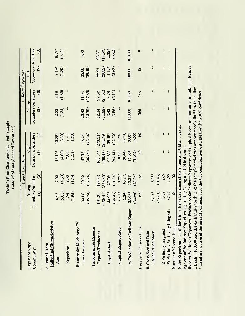
13C

Cs

oa

CO ^,—

v

kl £o3'3<t^

3O03 /-^ki t><u

TJa3oO

m î: CO4)g"S<4^

3Oen , V

I. lOlUT3d3oO

COh ss'S-*->

3Ooa^ m<u

T3c3Oo

en1^ 2oo'm-^3oEnu ^4)

XIB3oC3

c c

c a

X o

S-H ^.

to o

.-I «

0> 05-I CO

CO -*CO CO

C^l CO CD 00o CO p iq

i> Tf (>i 1-i

oo O CO oi <^«5 lO CO 00

to I> r-i O

Oloqin 00(N CO

C- OSIM in

<N 05S CD

oooo

oodo

00

qinCO CD CD

00 i-H

cm'IM

COCO

c6 s

CO Si

qCO

in

CO(m'

CO COCO CO

o ô CO

d 1-1

o»H

o COo CO

d CO

o

*00COoCD

oq CO CO

*

CO5?in

*in CO

CO00CM

*oooo

05CO

d CO t-^ r-i 00 CM COt>CO

CO

CM

00CO

COCOd d d d

*oi-H q

00

qCO

q00 Si

CO

*COCO

CM*COin T—

1

00COS*

*oq q

o

CO S t>' i-H COCO CO

oiCOd in

COd d in

tH CO

OC<3 C0C0t>00c^CV|c*ÔOit> C000t>iôOio00coco O^CQc^]'^^^ tH CO '^

1—I ^

<M

CM o CO in

qCO

q CM1—

(

cn in

CO in 1-H 1-H COCO

inCO

fH

dinCM

*•*

00in

-I SS « 9

Tisuee

es'-'

« 3

cc

<U Soa c<D «:

•c m(U S.

LI

M X c;

< H c

Ig,-2

ucca

c

.5 «

O * rH

d " J2CO «

CJ

u

O ^.00 o

2SCM 3,

ON r- COô t-^ inr-: d

r- m COq o\ t»

2cs

m

cS

aX

5 503

o dd o)—

1

-3en eu

CS td oo to^§ O3 ChTS o

£

32

C9

QBO

01

W3

euU

- >cs

— ^ tn

o

# ^ s

'S ^S cs

32

O)

w

a

o

o.

m

p.

O

u o

1^ 00

s 5DO 2 rH o"—

'

01o (M o*« d d d d•4->

so

entH s •* Si t^ Ga> CO i> <t COT3 n o CM og d d d d

h -*

I

1STQ

9 d

si9d

in o>CO lOCO od d

t-H CDTf Od d

;0 ;;j

O

i-H t> 05 05CO * CO COtH O 1—

t

Od d (D ci

* CO CO (N-I O "-HOdo o o

(N t~ CO -*(M in 1-1 in•* o * od d d d

(N O

.O '^

d d« _<u

g" &H H

IV

o15

o

O O a;00 in tH

d d

.a[14

o;z;

is - CO 05to i-l O 00

CO O 1-1odd

^7 CM 00 CO

2;

in T)"o oO CM

/^ CO ^* I-l

CO d

050000

m CO ;^

" d

^

doO

^ COO (N

COino

00 1-1

00CM

CO

8CO051-t

CM d d d

t> t- 1-1 O 1-1

-* t> OS o •*I> O CM O CM

00 COCM 05in 1-1

" t; -I

=^ in CM

o t>co oCO od d

1-1 Olin i-<

CO od d

CM COCO CMCO CO

d rH

lU

mO"doCO

O

l>o00

05CM

CMCMCOCM

CO d d r-i

« m :z;

00

ain

•z a <y

^ M 2 ^ ^"o "o "o "o "oO U O O O

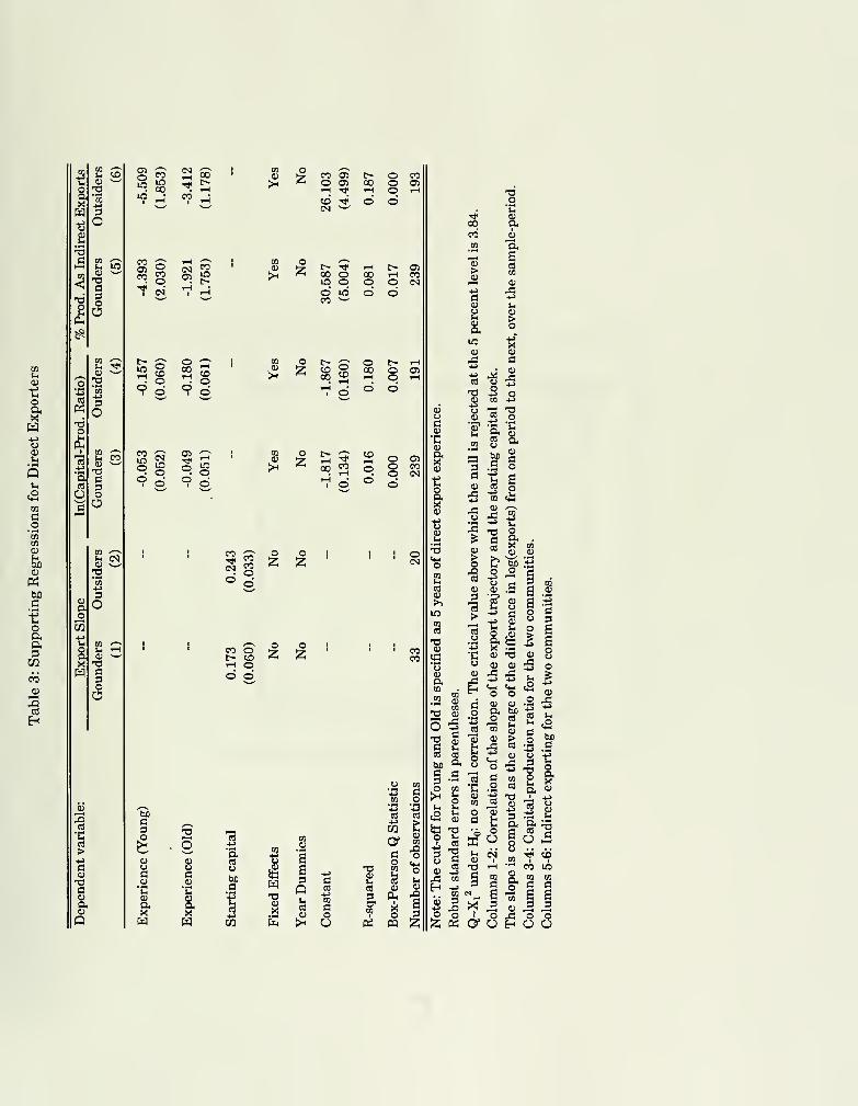
t.o

^

ao^

t.oaH

CO ^'3

-§

c<u

T3CaQ

11

COino

C3

•c

a

^ S^ S=? ^

CM ^

o2

o o : m

21 ><

9 d

q §9 d

2

o d

CO of- to"-I od d

o•z

uC

•c

0)

X

o

o

o•z

CO 05O 05

d Tt

00 olO od inCO "-^

II

00

d

00o

o00

«5

pd

o2;

o'Z

D

I

O COO 05O ^

C~ OS1-1 COO iM

O 05O ^

O 05O COo oq

c

esS

I

Xo

(1)

m

•s

* v>

o o

Q

«2

1 B R

C/

A/k

P.5

Figure 3«7 1

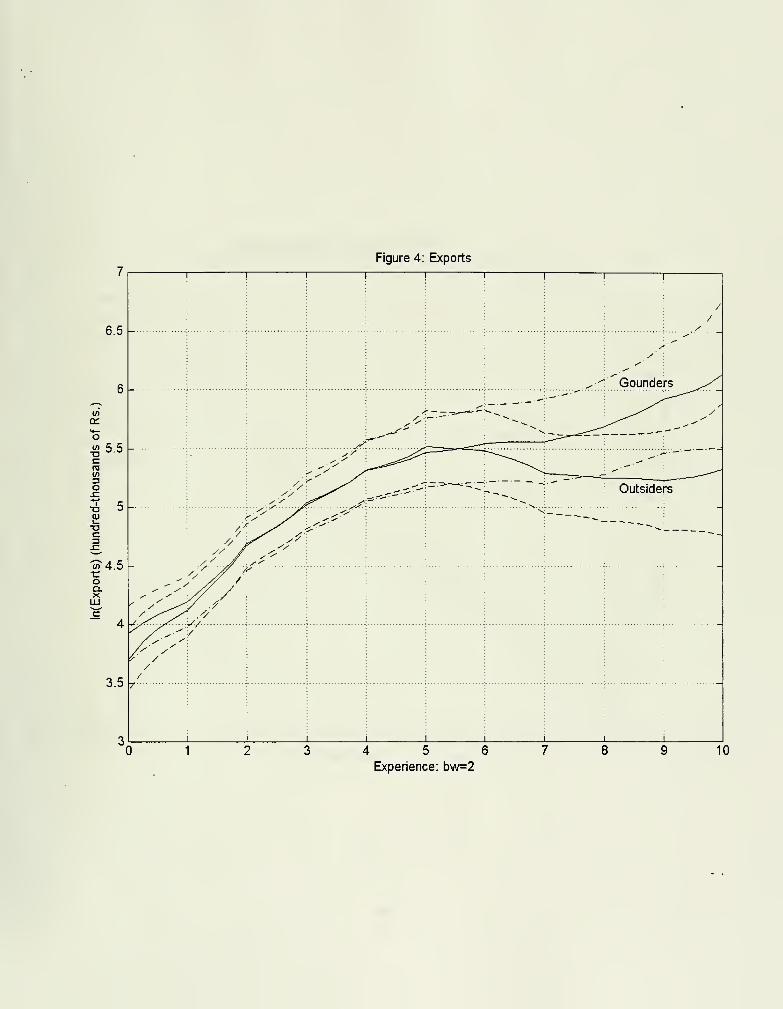
Figure 4: Exports

6.5 -

a:

«5.5cn

-6 50)

1?4.5•coQ.XLU

3.5

1 1 1 11 1

/

; ;i

; ^.^

..: :. ; ..-Hf^^ ^

.___^c

V,

: y '

y'

- ; \...^.^^l,^^f^....^^^^ll....

_ L.Zdi'i :

--^^-rr. ?v. - -

-^ ,—

^

Outsiders

/ ; ; : ;

7 :-

: ;

1 i i i i 1

4 5 6

Experience: bw=210

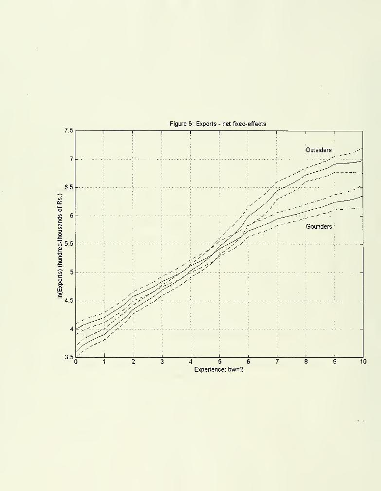
7.5

Figure 5: Exports - net fixed-effects

6.5

(A

cc

ra

o

-6 5.5cu

1? 5toQ.XUJ

4.5

3.5

1 1 1 1

Outsiders _^^'

; : : ^'C^^^:Z. ^ y.

; /'^///^-'''^ ^ ' Gounders

yA^yy^:^.

.y-yi^:-^

^•^'-

^y^ y;

^ ''^

^ ^— ^

y y y / ^X yy /''y y y y/> >""

i 1 1 1

4 5 6

Experience: bw=210

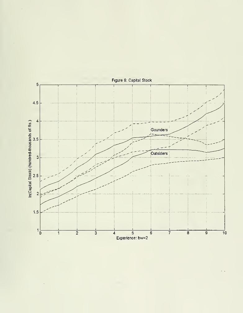
Figure 6: Capital Stocl<

4.5 -

01

a3.5

T5

T3

oo 2.5w2q.ns

O 2-y

1.5

1 1 1 1 1 1 1

: i /

: yr'- _

''. -^''': -^"

:'•

: ^:

'

: /- -^ -/^

": • -^ ^-.""""^

; / : /^ /

^ ^^^^: ^ /^

Gounders :

^,^-^''^; ^

^ ''

:' y''

: ^^^^

^^^^-^^^''lOutsiders

^'• -

r- ^^-^ -^-- ; :

.--''''" -^ • : •/^ -^ • :/ -^ : ;

-^ ; - ;^ '

i i i i i i i

4 5 6

Experience: bw=210

4.5

Figure 7: Capital Stock - net fixed-effects

4_.

01

<nT3

^3.5

T30)

Uo

o.ro

O

2.5

i

Gounders^--^

''-

— —^ ^^ ^ \

y' ^-^^""^ -^ : ^ ^ •

^ ^^-^^. . , y^ ,<.'

^ ^^ ^

^ ^ --^-^ ^-"•'''^ -^

-^' y^ -^ ^ "^ -.'•''^

^'^'~-'' ^^ ^^ -^^ ^^' 1

.^ y ^^.-^ y

-- - "J^ .-- ""'^ ,-'"' Outsiders^ ^^^^-^"^ ^ '^ ^^ y ^' 1^ -^

/ ^^/^,rf^

.' .^

/ ^^ yy

-^' ...^ i^''

>- / —y '

^ z.^^ ^^X /r^

^' ^^^ ^'-^ "

'H^-^''''''^""^ / y^ /

y j^ yy V--^ •*

-^ / ^^-^ ^/ y

<«^ ^x^ y^^ ^.-'•''''^ /y'^^.."^ y

y j^ ^'^^ ^^

^ "^ ^""""""^ /^.>-f^_ .V-;

^o^^^-^^^^ _J^ '-^

^ ^^ ^

1

1^^1

1 1 1 i 1 i 1 1 1 1

4 5 6

Experience: bw=210

Figure 8: Capital- Export Ratio - net fixed-effects

-1.5

-2

re

q:

-cox-2.5LU

I

re

'5.

re

O

-3.5

1 i

^ —^^ *^

v.

'^_

I1

: X.

1 t

• -^ x-

\ ^\

"V-

\ \\

.\. ...Xw. N.;

Gounders

:

i

Outsiders ;

~'.^^'-s,^;_- -

1

4 5 6

Experience: bw=210

-1.6

.1.8 =-

Figure 9: Capital-Production Ratio - net fixed-effects

-2.2 -

2-2.4

o0-2.6o

m5.-2,8re

O

-3.2

-3.4

-3.6

1 1 1 1 1 1

\ .—

_. ^N>*-^ '.,..>».

^^^^ ^; ~--..^ Gounders

^ ~^"" ^~^^^ ^ ^ '

''

"

^ ^^^^"-^: ^^ ^^"-^^ ^ ,^-—-"^

< ^ ^^"\ "^^^ ^ v; ^\. ^ """^^

^-.^^^-.^; r--^; ---"'^"~^-^..^.^-^...-v^ : , -.

^ >X^X ^

'

1 ^X^i- :

>.^ \ : ""^-v Outsiders

:

: : : ^ "^

^-v.

1 1 1 1 1 1 1

4 5 6

Experience: bw=210

Figure 10: Production as Indirect Exporter- net fixed-effects

Share

of

Production

as

Indirect

Exporter

(%)

o

en

ooi

o

en

o

c

/

1 1 1 I 1

N. : ;

-^^ '\ :

^^^ 'S^\: \ :

\^^ : ^ ;

::x^xX-^x:v^ \ :..":^ >^....\ ^>^^ X \ ;\ XX ^ X^ ^^^

^^ X "^x

Gounders_^'

^ \ ^,: \ V

"^ X,

N.

^ ^ '—

~

• '^ :

^ . -

s.' --^- -^ ; : :

X'~'--~^^;^\^^X^^^ Outsiders

^"^^5::::

-54 5 6

Experience: bw=2.5

10

5236 32

Date Due

Lib-26-67

MIT LIBRARIES

3 9080 01917 6582

„ -, . i'i!! i „

Networks, migration and investment : insiders and outsiders in ...

Documents

Transcript of Networks, migration and investment : insiders and outsiders in ...