arX

iv:1

111.

1750

v1 [

cs.D

S]

7 N

ov 2

011

Near Linear-Work Parallel SDD Solvers, Low-DiameterDecomposition, and Low-Stretch Subgraphs∗

Guy E. Blelloch Anupam Gupta Ioannis Koutis† Gary L. MillerRichard Peng Kanat Tangwongsan

Carnegie Mellon University and†University of Puerto Rico, Rio Piedras

Abstract

We present the design and analysis of a near linear-work parallel algorithm for solving symmetric diag-onally dominant (SDD) linear systems. On input of a SDDn-by-n matrixA with m non-zero entries and avectorb, our algorithm computes a vectorx such that‖x−A+b‖A ≤ ε · ‖A+b‖A in O(m logO(1) n log 1

ε )

work andO(m1/3+θ log 1ε ) depth for any fixedθ > 0.

The algorithm relies on a parallel algorithm for generatinglow-stretch spanning trees or spanning sub-graphs. To this end, we first develop a parallel decomposition algorithm that in polylogarithmic depth andO(|E|) work1, partitions a graph into components with polylogarithmic diameter such that only a small frac-tion of the original edges are between the components. This can be used to generate low-stretch spanningtrees with average stretchO(nα) in O(n1+α) work andO(nα) depth. Alternatively, it can be used to gen-erate spanning subgraphs with polylogarithmic average stretch inO(|E|) work and polylogarithmic depth.We apply this subgraph construction to derive a parallel linear system solver. By using this solver in knownapplications, our results imply improved parallel randomized algorithms for several problems, includingsingle-source shortest paths, maximum flow, minimum-cost flow, and approximate maximum flow.

1 Introduction

Solving a system of linear equationsAx = b is a fundamental computing primitive that lies at the core ofmanynumerical and scientific computing algorithms, including the popular interior-point algorithms. The special caseof symmetric diagonally dominant (SDD) systems has seen substantial progress in recent years; in particular,the ground-breaking work of Spielman and Teng showed how to solve SDD systems to accuracyε in timeO(m log(1ε )), wherem is the number of non-zeros in then-by-n-matrixA.2 This is algorithmically significantsince solving SDD systems has implications to computing eigenvectors, solving flow problems, finding graphsparsifiers, and problems in vision and graphics (see [Spi10, Ten10] for these and other applications).

In the sequential setting, the current best SDD solvers run inO(m log n(log log n)2 log(1ε )) time [KMP11].However, with the exception of the special case of planar SDDsystems [KM07], we know of no previous

∗Contact Address: 5000 Forbes Ave. Computer Science Department. Pittsburgh, PA 15213. E-mail:{guyb, anupamg,i.koutis, glmiller, yangp, ktangwon}@cs.cmu.edu.

1TheO(·) notion hides polylogarithmic factors.2The Spielman-Teng solver and all subsequent improvements are randomized algorithms. As a consequence, all algorithmsrelying

on the solvers are also randomized. For simplicity, we omit standard complexity factors related to the probability of error.

1

parallel SDD solvers that perform near-linear3 work and achieve non-trivial parallelism. This raises a naturalquestion:Is it possible to solve an SDD linear system ino(n) depth andO(m) work? This work answers thisquestion affirmatively:

Theorem 1.1 For any fixedθ > 0 and anyε > 0, there is an algorithmSDDSolve that on input ann× n SDDmatrixA with m non-zero elements and a vectorb, computes a vectorx such that‖x−A+b‖A ≤ ε · ‖A+b‖Ain O(m logO(1) n log 1

ε ) work andO(m1/3+θ log 1ε ) depth.

In the process of developing this algorithm, we give parallel algorithms for constructing graph decompo-sitions with strong-diameter guarantees, and parallel algorithms to construct low-stretch spanning trees andlow-stretch ultra-sparse subgraphs, which may be of independent interest. An overview of these algorithms andtheir underlying techniques is given in Section3.

Some Applications. Let us mention some of the implications of Theorem1.1, obtained by plugging it intoknown reductions.

— Construction of Spectral Sparsifiers.Spielman and Srivastava [SS08] showed that spectral sparsifiers canbe constructed usingO(log n) Laplacian solves, and using our theorem we get spectral and cut sparsifiers inO(m1/3+θ) depth andO(m) work.

— Flow Problems.Daitsch and Spielman [DS08] showed that various graph optimization problems, such asmax-flow, min-cost flow, and lossy flow problems, can be reduced to O(m1/2) applications4 of SDD solvesvia interior point methods described in [Ye97, Ren01, BV04]. Combining this with our main theorem impliesthat these algorithms can be parallelized to run inO(m5/6+θ) depth andO(m3/2) work. This gives the firstparallel algorithm witho(n) depth which is work-efficient to withinpolylog(n) factors relative to the sequentialalgorithm for all problems analyzed in [DS08]. In some sense, the parallel bounds are more interesting thanthe sequential times because in many cases the results in [DS08] are not the best known sequentially (e.g.max-flow)—but do lead to the best know parallel bounds for problems that have traditionally been hard toparallelize. Finally, we note that although [DS08] does not explicitly analyze shortest path, their analysisnaturally generalizes the LP for it.

Our algorithm can also be applied in the inner loop of [CKM+10], yielding aO(m5/6+θpoly(ε−1)) depthandO(m4/3poly(ε−1)) work algorithm for finding1− ε approximate maximum flows and1 + ε approximateminimum cuts in undirected graphs.

2 Preliminaries and Notation

We use the notationO(f(n)) to meanO(f(n) polylog(f(n))). We useA⊎B to denote disjoint unions, and[k]to denote the set{1, 2, . . . , k}. Given a graphG = (V,E), letdist(u, v) denote theedge-count distance(or hopdistance) betweenu andv, ignoring the edge lengths. When the graph has edge lengthsw(e) (also denoted bywe), let dG(u, v) denote theedge-length distance, the shortest path (according to these edge lengths) betweenu andv. If the graph has unit edge lengths, the two definitions coincide. We drop subscripts when the contextis clear. We denote byV (G) andE(G), respectively, the set of nodes and the set of edges, and usen = |V (G)|

3i.e. linear up to polylog factors.4hereO hideslogU factors as well, where it’s assumed that the edge weights areintegers in the range[1 . . . U ]

2

andm = |E(G)|. For an edgee = {u, v}, the stretch ofe on G′ is strG′(e) = dG′(u, v)/w(e). The totalstretchof G = (V,E,w) with respect toG′ is strG′(E(G)) =

∑e∈E(G) strG′(e).

GivenG = (V,E), a distance functionδ (which is eitherdist or d), and a partition ofV into C1 ⊎ C2 ⊎. . . ⊎ Cp, let G[Ci] denote the induced subgraph on setCi. Theweak diameterof Ci is maxu,v∈Ci

δG(u, v),whereas thestrong diameterof Ci is maxu,v∈Ci

δG[Ci](u, v); the former measures distances in the originalgraph whereas the latter measures distances within the induced subgraph. The strong (or weak) diameter of thepartition is the maximum strong (or weak) diameter over all the componentsCi’s.

Graph Laplacians. For a fixed, but arbitrary, numbering of the nodes and edges ina graphG = (V,E), theLaplacianLG of G is the|V |-by-|V | matrix given by

LG(i, j) =

{−wij if i 6= j∑

{j,i}∈E(G)wij if i = j,

When the context is clear, we useG andLG interchangeably. Given two graphsG andH and a scalarµ ∈ R,we sayG � µH if µLH − LG is positive semidefinite, or equivalentlyx⊤LGx ≤ µx⊤LHx for all vectorx ∈ R

|V |.

Matrix Norms, SDD Matrices. For a matrixA, we denote byA+ the Moore-Penrose pseudoinverse ofA (i.e.,A+ has the same null space asA and acts as the inverse ofA on its image). Given a symmetric positive semi-definite matrixA, theA-normof a vectorx is defined as‖x‖A =

√x⊤Ax. A matrixA is symmetric diagonally

dominant (SDD) if it is symmetric and for alli, Ai,i ≥∑

j 6=i |Ai,j |. Solving an SDD system reduces inO(m)

work andO(logO(1)m) depth to solving a graph Laplacian (a subclass of SDD matrices corresponding toundirected weighted graphs) [Gre96, Section 7.1].

Parallel Models. We analyze algorithms in the standard PRAM model, focusing on the work and depth param-eters of the algorithms. Bywork, we mean the total operation count—and bydepth, we mean the longest chainof dependencies (i.e., parallel time in PRAM).

Parallel Ball Growing. LetBG(s, r) denote the ball of edge-count distancer from a sources, i.e.,BG(s, r) ={v ∈ V (G) : distG(s, v) ≤ r}. We rely on an elementary form of parallel breadth-first search to computeBG(s, r). The algorithm visits the nodes level by level as they are encountered in the BFS order. More precisely,level 0 contains only the source nodes, level 1 contains the neighbors ofs, and each subsequent leveli + 1contains the neighbors of leveli’s nodes that have not shown up in a previous level. On standard parallelmodels (e.g.,CRCW), this can be computed inO(r log n) depth andO(m′ + n′) work, wherem′ andn’ arethe total numbers of edges and nodes, respectively, encountered in the search [UY91, KS97]. Notice that wecould achieve this runtime bound with a variety of graph (matrix) representations, e.g., using the compressedsparse-row (CSR) format. Our applications apply ball growing onr roughlyO(logO(1) n), resulting in a smalldepth bound. We remark that the idea of small-radius parallel ball growing has previously been employed inthe context of approximate shortest paths (see, e.g., [UY91, KS97, Coh00]). There is an alternative approachof repeatedly squaring a matrix, which can give a better depth bound for larger at the expenseof a much largerwork bound (aboutn3).

Finally, we state a tail bound which will be useful in our analysis. This bound is easily derived fromwell-known facts about the tail of a hypergeometric random variable [Chv79, Hoe63, Ska09].

Lemma 2.1 (Hypergeometric Tail Bound) LetH be a hypergeometric random variable denoting the numberof red balls found in a sample ofn balls drawn from a total ofN balls of whichM are red. Then, ifµ =

3

E [H] = nM/N , thenPr [H ≥ 2µ] ≤ e−µ/4

Proof: We apply the following theorem of Hoeffding [Chv79, Hoe63, Ska09]. For anyt > 0,

Pr [H ≥ µ+ tn] ≤(( p

p+ t

)p+t( 1− p

1− p− t

)1−p−t)n

,

wherep = µ/n. Usingt = p, we have

Pr [H ≥ 2µ] ≤(( p

2p

)2p( 1− p

1− 2p

)1−2p)n

≤(e−p ln 4

(1 +

p

1− 2p

)1−2p)n

≤(e−p ln 4 · ep

)n

≤ e−14pn,

where we have used the fact that1 + x ≤ exp(x). �

3 Overview of Our Techniques

In the general solver framework of Spielman and Teng [ST06, KMP10], near linear-time SDD solvers relyon a suitable preconditioning chain of progressively smaller graphs. Assuming that we have an algorithmfor generating low-stretch spanning trees, the algorithm as given in [KMP10] parallelizes under the followingmodifications: (i) perform the partial Cholesky factorization in parallel and (ii) terminate the preconditioningchain with a graph that is of size approximatelym1/3. The details in Section6 are the primary motivation ofthe main technical part of the work in this chapter, a parallel implementation of a modified version of Alon etal.’s low-stretch spanning tree algorithm [AKPW95].

More specifically, as a first step, we find an algorithm to embeda graph into a spanning tree with aver-age stretch2O(

√logn log logn) in O(m) work andO(2O(

√logn log logn) log ∆) depth, where∆ is the ratio of the

largest to smallest distance in the graph. The original AKPWalgorithm relies on a parallel graph decompo-sition scheme of Awerbuch [Awe85], which takes an unweighted graph and breaks it into components with aspecified diameter and few crossing edges. While such schemes are known in the sequential setting, they do notparallelize readily because removing edges belonging to one component might increase the diameter or evendisconnect subsequent components. We present the first nearlinear-work parallel decomposition algorithm thatalso gives strong-diameter guarantees, in Section4, and the tree embedding results in Section5.1.

Ideally, we would have liked for our spanning trees to have a polylogarithmic stretch, computable by a poly-logarithmic depth, near linear-work algorithm. However, for our solvers, we make the additional observationthat we do not really need a spanningtree with small stretch; it suffices to give an “ultra-sparse” graph withsmall stretch, one that has onlyO(m/polylog(n)) edges more than a tree. Hence, we present a parallel algo-rithm in Section5.2which outputs an ultra-sparse graph withO(polylog(n)) average stretch, performingO(m)work withO(polylog(n)) depth. Note that this removes the dependence oflog∆ in the depth, and reduces both

4

the stretch and the depth from2O(√logn log logn) to O(polylog(n)).5 When combined with the aforementioned

routines for constructing a SDD solver presented in Section6, this low-stretch spanning subgraph constructionyields a parallel solver algorithm.

4 Parallel Low-Diameter Decomposition

In this section, we present a parallel algorithm for partitioning a graph into components with low (strong)diameter while cutting only a few edges in each of thek disjoint subsets of the input edges. The sequentialversion of this algorithm is at the heart of the low-stretch spanning tree algorithm of Alon, Karp, Peleg, andWest (AKPW) [AKPW95].

For context, notice that the outer layer of the AKPW algorithm (more details in Section5) can be viewed asbucketing the input edges by weight, then partitioning and contracting them repeatedly. In this view, a numberof edge classes are “reduced” simultaneously in an iteration. Further, as we wish to output a spanning subtreeat the end, the components need to have low strong-diameter (i.e., one could not take “shortcuts” through othercomponents). In the sequential case, the strong-diameter property is met by removing components one afteranother, but this process does not parallelize readily. Forthe parallel case, we guarantee this by growing ballsfrom multiple sites, with appropriate “jitters” that conceptually delay when these ball-growing processes start,and assigning vertices to the first region that reaches them.These “jitters” terms are crucial in controlling theprobability that an edge goes across regions. But this probability also depends on the number of regions thatcould reach such an edge. To keep this number small, we use a repeated sampling procedure motivated byCohen’s(β,W )-cover construction [Coh93].

More concretely, we prove the following theorem:

Theorem 4.1 (Parallel Low-Diameter Decomposition)Given an input graphG = (V,E1 ⊎ . . . ⊎ Ek) withk edge classes and a “radius” parameterρ, the algorithmPartition(G, ρ), upon termination, outputs apartition ofV into componentsC = (C1, C2, . . . , Cp), each with centersi such that

1. the centersi ∈ Ci for all i ∈ [p],

2. for eachi, everyu ∈ Ci satisfiesdistG[Ci](si, u) ≤ ρ, and

3. for all j = 1, . . . , k, the number of edges inEj that go between components is at most|Ej | · c1·k log3 nρ ,

wherec1 is an absolute constant.

Furthermore,Partition runs inO(m log2 n) expected work andO(ρ log2 n) expected depth.

4.1 Low-Diameter Decomposition for Simple Unweighted Graphs

To prove this theorem, we begin by presenting an algorithmsplitGraph that works with simple graphs withonly oneedge class and describe how to build on top of it an algorithm that handles multiple edge classes.

The basic algorithm takes as input a simple, unweighted graph G = (V,E) and a radius (in hop count)parameterρ and outputs a partitionV into componentsC1, . . . , Cp, each with centersi, such that

5As an aside, this construction of low-stretch ultra-sparsegraphs shows how to obtain theO(m)-time linear system solver ofSpielman and Teng [ST06] without using their low-stretch spanning trees result [EEST05, ABN08].

5

(P1) Each center belongs to its own component. That is, the centersi ∈ Ci for all i ∈ [p];

(P2) Every component has radius at mostρ. That is, for eachi ∈ [p], everyu ∈ Ci satisfiesdistG[Ci](si, u) ≤ρ;

(P3) Given a technical condition (to be specified) that holdswith probability at least3/4, the probability thatan edge of the graphG goes between components is at most136

ρ log3 n.

In addition, this algorithm runs inO(m log2 n) expected work andO(ρ log2 n) expected depth. (These proper-ties should be compared with the guarantees in Theorem4.1.)

Consider the pseudocode of this basic algorithm in Algorithm 4.1. The algorithm takes as input an un-weightedn-node graphG and proceeds inT = O(log n) iterations, with the eventual goal of outputting apartition of the graphG into a collection of sets of nodes (each set of nodes is known as a component). LetG(t) = (V (t), E(t)) denote the graph at the beginning of iterationt. Since this graph is unweighted, the distancein this algorithm is always the hop-count distancedist(·, ·). For iterationt = 1, . . . , T , the algorithm picks a setof starting centersS(t) to grow balls from; as with Cohen’s(β,W )-cover, the number of centers is progressivelylarger with iterations, reminiscent of the doubling trick (though with more careful handling of the growth rate),to compensate for the balls’ shrinking radius and to ensure that the graph is fully covered.

Still within iteration t, it chooses a random “jitter” valueδ(t)s ∈R {0, 1, . . . , R} for each of the centers

in S(t) and grows a ball from each centers out to radiusr(t) − δ(t)s , wherer(t) = ρ

2 logn(T − t + 1). Let

X(t) be the union of these balls (i.e., the nodes “seen” from thesestarting points). In this process, the “jitter”should be thought of as a random amount by which we delay the ball-growing process on each center, sothat we could assign nodes to the first region that reaches them while being in control of the number of cross-component edges. Equivalently, our algorithm forms the components by assigning each vertexu reachable fromone of these centers to the center that minimizesdistG(t)(u, s) + δ

(t)s (ties broken in a consistent manner, e.g.,

lexicographically). Note that because of these “jitters,”some centers might not be assigned any vertex, not evenitself. For centers that are assigned some nodes, we includetheir components in the output, designating them asthe components’ centers. Finally, we constructG(t+1) by removing nodes that were “seen” in this iteration (i.e.,the nodes inX(t))—because they are already part of one of the output components—and adjusting the edge setaccordingly.

Analysis. Throughout this analysis, we make reference to various quantities in the algorithm and assume thereader’s basic familiarity with our algorithm. We begin by proving properties (P1)–(P2). First, we state aneasy-to-verify fact, which follows immediately by our choice of radius and components’ centers.

Fact 4.2 If vertexu lies in componentC(t)s , thendist (t)(s, u) ≤ r(t). Moreover,u ∈ B

(t)s .

We also need the following lemma to argue about strong diameter.

Lemma 4.3 If vertexu ∈ C(t)s , and vertexv ∈ V (t) lies on anyu-s shortest path inG(t), thenv ∈ C

(t)s .

Proof: Sinceu ∈ C(t)s , Fact4.2 implies u belongs toB(t)

s . But dist (t)(v, i) < dist(t)(u, i), and hencev

belongs toB(t)s andX(t) as well. This implies thatv is assigned tosomecomponentC(t)

j ; we claimj = s.

For a contradiction, assume thatj 6= s, and hencedist (t)(v, j) + δ(t)j ≤ dist

(t)(v, s) + δ(t)s . In this case

dist(t)(u, j) + δ

(t)j ≤ dist

(t)(u, v) + dist(t)(v, j) + δ

(t)j (by the triangle inequality). Now using the assumption,

6

Algorithm 4.1 splitGraph (G = (V,E), ρ) — Split an input graphG = (V,E) into components of hop-radius at mostρ.

LetG(1) = (V (1), E(1))← G. DefineR = ρ/(2 logn). Create empty collection of componentsC.Usedist (t) as shorthand fordistG(t) , and defineB(t)(u, r)

def= BG(t)(u, r) = {v ∈ V (t) | dist (t)(u, v) ≤ r}.

For t = 1, 2, . . . , T = 2 log2 n,

1. Randomly sampleS(t) ⊆ V (t), where|S(t)|| = σt = 12nt/T−1|V (t)| logn, or useS(t) = V (t) if |V (t)| < σt.

2. For each “center”s ∈ S(t), drawδ(t)s uniformly at random fromZ ∩ [0, R].

3. Letr(t) ← (T − t+ 1)R.

4. For each centers ∈ S(t), compute the ballB(t)s = B(t)(s, r(t) − δ

(t)s ).

5. LetX(t) = ∪s∈S(t)B(t)s .

6. Create components{C(t)s | s ∈ S(t)} by assigning eachu ∈ X(t) to the componentC(t)

s such thats minimizes

distG(t)(u, s) + δ(t)s (breaking ties lexicographically).

7. Add non-emptyC(t)s components toC.

8. SetV (t+1) ← V (t) \X(t), and letG(t+1) ← G(t)[V (t+1)]. Quit early ifV (t+1) is empty.

ReturnC.

this expression is at mostdist (t)(u, v) + dist(t)(v, s) + δ

(t)s = dist

(t)(u, s) + δ(t)s (sincev lies on the shortest

u-s path). But then,u would be also assigned toC(t)j , a contradiction. �

Hence, for each non-empty componentC(t)s , its centers lies within the component (since it lies on the

shortest path froms to anyu ∈ C(t)s ), which proves (P1). Moreover, by Fact4.2and Lemma4.3, the (strong)

radius is at mostTR, proving (P2). It now remains to prove (P3), and the work and depth bounds.

Lemma 4.4 For any vertexu ∈ V , with probability at least1 − n−6, there are at most68 log2 n pairs6 (s, t)such thats ∈ S(t) andu ∈ B(t)(s, r(t)),

We will prove this lemma in a series of claims.

Claim 4.5 For t ∈ [T ] andv ∈ V (t), if |B(t)(v, r(t+1))| ≥ n1−t/T , thenv ∈ X(t) w.p. at least1− n−12.

Proof: First, note that for anys ∈ S(t), r(t) − δs ≥ r(t) − R = r(t+1), and so ifs ∈ B(t)(v, r(t+1)), then

v ∈ B(t)s and hence inX(t). Therefore,

Pr[v ∈ X(t)

]≥ Pr

[S(t) ∩B(t)(v, r(t+1)) 6= ∅

],

which is the probability that a random subset ofV (t) of sizeσt hits the ballB(t)(v, r(t+1)). But,

Pr[S(t) ∩B(t)(v, r(t+1)) 6= ∅

]≥ 1−

(1− |B(t)(v,r(t+1))|

|V (t)|

)σt

,

which is at least1− n−12. �

Claim 4.6 For t ∈ [T ] andv ∈ V , the number ofs ∈ S(t) such thatv ∈ B(t)(s, r(t)) is at most34 log n w.p. atleast1− n−8.

6In fact, for a givens, there is a uniquet—if this s is ever chosen as a “starting point.”

7

Proof: For t = 1, the sizeσ1 = O(log n) and hence the claim follows trivially. Fort ≥ 2, we condition on allthe choices made in rounds1, 2, . . . , t− 2. Note that ifv does not survive inV (t−1), then it does not belong toV (t) either, and the claim is immediate. So, consider two cases, depending on the size of the ballB(t−1)(v, r(t))in iterationt− 1:

— Case 1.If |B(t−1)(v, r(t))| ≥ n1−(t−1)/T , then by Claim 3.5, with probability at least1 − n−12, we havev ∈ X(t−1), sov would not belong toV (t) and this meansno s ∈ S(t) will satisfy v ∈ B(t)(s, r(t)), provingthe claim for this case.

— Case 2.Otherwise,|B(t−1)(v, r(t))| < n1−(t−1)/T . We have

|B(t)(v, r(t))| ≤ |B(t−1)(v, r(t))| < n1−(t−1)/T

as B(t)(v, r(t)) ⊆ B(t−1)(v, r(t)). Now let X be the number ofs such thatv ∈ B(t)(s, r(t)), so X =∑s∈S(t) 1{s∈B(t)(v,r(t))}. Over the random choice ofS(t),

Pr[s ∈ B(t)(v, r(t))

]=|B(t)(v, r(t))||V (t)| ≤ 1

|V (t)|n1−(t−1)/T ,

which gives

E [X] = σt · Pr[s ∈ B(t)(v, r(t))

]≤ 17 log n.

To obtain a high probability bound forX, we will apply the tail bound in Lemma2.1. Note thatX is simplya hypergeometric random variable with the following parameters setting: total ballsN = |V (t)|, red ballsM = |B(t)(v, r(t))|, and the number balls drawn isσt. Therefore,Pr [X ≥ 34 log n] ≤ exp{−1

4 · 34 log n}, soX ≤ 34 log n with probability at least1− n−8.

Hence, regardless of what choices we made in rounds1, 2, . . . , t − 2, the conditional probability of seeingmore than34 log n differents’s is at mostn−8. Hence, we can remove the conditioning, and the claim follows.�

Lemma 4.7 If for each vertexu ∈ V , there are at most68 log2 n pairs (s, t) such thats ∈ S(t) and u ∈B(t)(s, r(t)), then for an edgeuv, the probability thatu belongs to a different component thanv is at most68 log2 n/R.

Proof: We define a centers ∈ S(t) as “separating”u andv if |B(t)s ∩{u, v}| = 1. Clearly, ifu, v lie in different

components then there is somet ∈ [T ] and some centers that separates them. For a centers ∈ S(t), this canhappen only ifδs = R − dist(s, u), sincedist(s, v) ≤ dist(s, u) − 1. As there areR possible values ofδs,this event occurs with probability at most1/R. And since there are only68 log2 n different centerss that canpossibly cut the edge, using a trivial union bound over them gives us an upper bound of68 log2 n/R on theprobability. �

To argue about (P3), notice that the premise to Lemma4.7 holds with probability exceeding1 − o(1) ≥3/4. Combining this with Lemma4.4 proves property (P3), where the technical condition is the premise toLemma4.7.

Finally, we consider the work and depth of the algorithm. These are randomized bounds. Each computationof B(t)(v, r(t)) can be done using a BFS. Sincer(t) ≤ ρ, the depth is bounded byO(ρ log n) per iteration,resulting inO(ρ log2 n) afterT = O(log n) iterations. As for work, by Lemma4.4, each vertex is reached byat mostO(log2 n) starting points, yielding a total work ofO(m log2 n).

8

4.2 Low-Diameter Decomposition for Multiple Edge Classes

Extending the basic algorithm to support multiple edge classes is straightforward. The main idea is as follows.Suppose we are given a unweighted graphG = (V,E), and the edge setE is composed ofk edge classesE1 ⊎ · · · ⊎ Ek. So, if we runsplitGraph on G = (V,E) andρ treating the different classes as one, thenproperty (P3) indicates that each edge—regardless of whichclass it came from—is separated (i.e., it goesacross components) with probabilityp = 136

ρ log3 n. This allows us to prove the following corollary, whichfollows directly from Markov’s inequality and the union bounds.

Corollary 4.8 With probability at least1/4, for all i ∈ [k], the number of edges inEi that are between

components is at most|Ei|272k log3 nρ .

The corollary suggests a simple way to usesplitGraph to provide guarantees required by Theorem4.1:as summarized in Algorithm4.2, we runsplitGraph on the input graph treating all edge classes as one and

repeat it if any of the edge classes had too many edges cut (i.e., more than|Ei|272k log3 nρ ). As the corollary

indicates, the number of trials is a geometric random variable with with p = 1/4, so in expectation, it willfinish after4 trials. Furthermore, although it could go on forever in the worst case, the probability does fallexponentially fast.

Algorithm 4.2 Partition (G = (V,E = E1 ⊎ · · · ⊎ Ek), ρ) — Partition an input graphG into componentsof radius at mostρ.

1. LetC = splitGraph((V,⊎Ei), ρ).

2. If there is somei such thatEi has more than|Ei|272·k log3 nρ edges between components, start over. (Recall

thatk was the number of edge classes.)

ReturnC.

Finally, we note that properties (P1) and (P2) directly giveTheorem4.1(1)–(2)—and the validation stepin Partition ensures Theorem4.1(3), settingc1 = 272. The work and depth bounds forPartition followfrom the bounds derived forsplitGraph and Corollary4.8. This concludes the proof of Theorem4.1.

5 Parallel Low-Stretch Spanning Trees and Subgraphs

This section presents parallel algorithms for low-stretchspanning trees and for low-stretch spanning subgraphs.To obtain the low-stretch spanning tree algorithm, we applythe construction of Alon et al. [AKPW95] (hence-forth, the AKPW construction), together with the parallel graph partition algorithm from the previous section.The resulting procedure, however, is not ideal for two reasons: the depth of the algorithm depends on the“spread”∆—the ratio between the heaviest edge and the lightest edge—and even for polynomial spread, boththe depth and the average stretch are super-logarithmic (both of them have a2O(

√logn·log logn) term). Fortu-

nately, for our application, we observe that we do not need spanning trees but merely low-stretch sparse graphs.In Section5.2, we describe modifications to this construction to obtain a parallel algorithm which computessparse subgraphs that give us only polylogarithmic averagestretch and that can be computed in polylogarithmicdepth andO(m) work. We believe that this construction may be of independent interest.

9

5.1 Low-Stretch Spanning Trees

Using the AKPW construction, along with thePartition procedure from Section4, we will prove the follow-ing theorem:

Theorem 5.1 (Low-Stretch Spanning Tree)There is an algorithmAKPW(G) which given as input a graphG = (V,E,w), produces a spanning tree inO(logO(1) n · 2O(

√logn·log logn) log∆) expected depth andO(m)

expected work such that the total stretch of all edges is bounded bym · 2O(√logn·log logn).

Algorithm 5.1 AKPW (G = (V,E,w)) — a low-stretch spanning tree construction.i. Normalize the edges so thatmin{w(e) : e ∈ E} = 1.ii. Let y = 2

√6 logn·log logn, τ = ⌈3 log(n)/ log y⌉, z = 4c1yτ log

3 n. InitializeT = ∅.iii. Divide E intoE1, E2, . . . , whereEi = {e ∈ E | w(e) ∈ [zi−1, zi)}.

LetE(1) = E andE(1)i = Ei for all i.

iv. For j = 1, 2, . . . , until the graph is exhausted,

1. (C1, C2, . . . , Cp) = Partition((V (j),⊎i≤jE(j)i ), z/4)

2. Add a BFS tree of each component toT .

3. Define graph(V (j+1), E(j+1)) by contracting all edges within the components and removingall self-loops (butmaintaining parallel edges). CreateE(j+1)

i fromE(j)i taking into account the contractions.

v. Output the treeT .

Presented in Algorithm5.1is a restatement of the AKPW algorithm, except that here we will use our parallellow-diameter decomposition for the partition step. In words, iterationj of Algorithm 5.1 looks at a graph(V (j), E(j)) which is a minor of the original graph (because components were contracted in previous iterations,and because it only considers the edges in the firstj weight classes). It usesPartition((V,⊎j≤kEj), z/4) todecompose this graph into components such that the hop radius is at mostz/4 and each weight class has only1/y fraction of its edges crossing between components. (Parametersy, z are defined in the algorithm and areslightly different from the original settings in the AKPW algorithm.) It then shrinks each of the componentsinto a single node (while adding a BFS tree on that component to T ), and iterates on this graph. Adding theseBFS trees maintains the invariant that the set of original nodes which have been contracted into a (super-)nodein the current graph are connected inT ; hence, when the algorithm stops, we have a spanning tree of the originalgraph—hopefully of low total stretch.

We begin the analysis of the total stretch and running time byproving two useful facts:

Fact 5.2 The number of edges|E(j)i | is at most|Ei|/yj−i.

Proof: If we could ensure that the number of weight classes in play atany time is at mostτ , the number ofedges in each class would fall by at least a factor ofc1τ log3 n

z/4 = 1/y by Theorem4.1(3) and the definitionof z, and this would prove the fact. Now, for the firstτ iterations, the number of weight classes is at mostτjust because we consider only the firstj weight classes in iterationj. Now in iterationτ + 1, the number ofsurviving edges ofE1 would fall to |E1|/yτ ≤ |E1|/n3 < 1, and hence there would only beτ weight classesleft. It is easy to see that this invariant can be maintained over the course of the algorithm. �

Fact 5.3 In iteration j, the radius of a component according to edge weights (in the expanded-out graph) is atmostzj+1.

10

Proof: The proof is by induction onj. First, note that by Theorem4.1(2), each of the clusters computed inany iterationj has edge-count radius at mostz/4. Now the base casej = 1 follows by noting that each edgein E1 has weight less thanz, giving a radius of at mostz2/4 < zj+1. Now assume inductively that the radiusin iterationj − 1 is at mostzj. Now any path withz/4 edges from the center to some node in the contractedgraph will pass through at mostz/4 edges of weight at mostzj , and at mostz/4+1 supernodes, each of whichadds a distance of2zj ; hence, the new radius is at mostzj+1/4 + (z/4 + 1)2zj ≤ zj+1 as long asz ≥ 8. �

Applying these facts, we bound the total stretch of an edge class.

Lemma 5.4 For anyi ≥ 1, strT (Ei) ≤ 4y2|Ei|(4c1τ log3 n)τ+1.

Proof: Let e be an edge inEi contracted during iterationj. Sincee ∈ Ei, we knoww(e) > zi−1. By Fact5.3,the path connecting the two endpoints ofe in F has distance at most2zj+1. Thus,strT (e) ≤ 2zj+1/zi−1 =

2zj−i+2. Fact5.2 indicates that the number of such edges is at most|E(j)i | ≤ |Ei|/yj−i. We conclude that

strT (Ei) ≤i+τ−1∑

j=i

2zj−i+2|Ei|/yj−i

≤ 4y2|Ei|(4c1τ log3 n)τ+1

�

Proof: [of Theorem5.1] Summing across the edge classes gives the promised bound onstretch. Now there are⌈logz ∆⌉ weight classesEi’s in all, and since each time the number of edges in a (non-empty) class drops by afactor ofy, the algorithm has at mostO(log∆+τ) iterations. By Theorem4.1and standard techniques, each it-eration doesO(m log2 n) work and hasO(z log2 n) = O(logO(1) n ·2O(

√logn·log logn)) depth in expectation.�

5.2 Low-Stretch Spanning Subgraphs

We now show how to alter the parallel low-stretch spanning tree construction from the preceding section to givea low-stretch spanningsubgraphconstruction that has no dependence on the “spread,” and moreover has onlypolylogarithmic stretch. This comes at the cost of obtaining a sparse subgraph withn − 1 + O(m/polylog n)edges instead of a tree, but suffices for our solver application. The two main ideas behind these improvementsare the following: Firstly, the number of surviving edges ineach weight class decreases by a logarithmic factorin each iteration; hence, we could throw in all surviving edges after they have been whittled down in a constantnumber of iterations—this removes the factor of2O(

√logn·log logn)from both the average stretch and the depth.

Secondly, if∆ is large, we will identify certain weight-classes withO(m/polylog n) edges, which by settingthem aside, will allow us to break up the chain of dependencies and obtainO(polylog n) depth; these edges willbe thrown back into the final solution, addingO(m/polylog n) extra edges (which we can tolerate) withoutincreasing the average stretch.

5.2.1 The First Improvement

Let us first show how to achieve polylogarithmic stretch withan ultra-sparse subgraph. Given parametersλ ∈Z>0 andβ ≥ c2 log

3 n (wherec2 = 2 ·(4c1(λ+1))12(λ−1)), we obtain the new algorithmSparseAKPW(G,λ, β)

11

by modifying Algorithm5.1as follows:

(1) use the altered parametersy = 1c2β/ log3 n andz = 4c1y(λ+ 1) log3 n;

(2) in each iterationj, callPartitionwith at mostλ+1 edge classes—keep theλ classesE(j)j , E

(j)j−1, . . . , E

(j)j−λ+1,

but then define a “generic bucket”E(j)0 := ∪j′≤j−λE

(j)j′ as the last part of the partition; and

(3) finally, output not just the treeT but the subgraphG = T ∪ (∪i≥1E(i+λ)i ).

Lemma 5.5 Given a graphG, parametersλ ∈ Z>0 andβ ≥ c2 log3 n (wherec2 = 2 · (4c1(λ+1))

12(λ−1)) the

algorithmSparseAKPW(G,λ, β) outputs a subgraph ofGwith at mostn−1+m(c2(log3 n/β))λ edges and total

stretch at mostmβ2 log3λ+3 n. Moreover, the expected work isO(m) and expected depth isO((c1β/c2)λ log2 n(log∆+

log n)).

Proof: The proof parallels that for Theorem5.1. Fact5.3 remains unchanged. The claim from Fact5.2 nowremains true only forj ∈ {i, . . . , i + λ − 1}; after that the edges inE(j)

i become part ofE(j)0 , and we only

give a cumulative guarantee on the generic bucket. But this does hurt us: ife ∈ Ei is contracted in iterationj ≤ i + λ − 1 (i.e., it lies within a component formed in iterationj), thenstr

G(e) ≤ 2zj−i+2. And the edges

of Ei that survive till iterationj ≥ i + λ have stretch1 because they are eventually all added toG; hence wedo not have to worry that they belong to the classE

(j)0 for those iterations. Thus,

strG(Ei) ≤i+λ−1∑

j=i

2zj−i+2 · |Ei|/yj−i ≤ 4y2(z

y)λ−1|Ei|.

Summing across the edge classes givesstrG(E) ≤ 4y2( zy )

λ−1m, which simplifies toO(mβ2 log3λ+3 n).Next, the number of edges in the output follows directly fromthe factT can have at mostn− 1 edges, and thenumber of extra edges from each class is only a1/yλ fraction (i.e.,|E(i+λ)

i | ≤ |Ei|/yλ from Fact5.2). Finally,the work remains the same; for each of the(log∆ + τ) distance scales the depth is stillO(z log2 n), but thenew value ofz causes this to becomeO((c1β/c2)λ log

2 n). �

5.2.2 The Second Improvement

The depth of theSparseAKPW algorithm still depends onlog∆, and the reason is straightforward: the graphG(j) used in iterationj is built by takingG(1) and contracting edges in each iteration—hence, it depends on allprevious iterations. However, the crucial observation is that if we hadτ consecutive weight classesEi’s whichare empty, we could break this chain of dependencies at this point. However, there may be no empty weightclasses; but having weight classes with relatively few edges is enough, as we show next.

Fact 5.6 Given a graphG = (V,E) and a subset of edgesF ⊆ E, letG′ = G\F be a potentially disconnectedgraph. IfG′ is a subgraph ofG′ with total stretchstr

G′(E(G′)) ≤ D, then the total stretch ofE onG := G′∪F

is at most|F |+D.

Consider a graphG = (V,E,w) with edge weightsw(e) ≥ 1, and letEi(G) := {e ∈ E(G) | w(e) ∈[zi−1, zi)} be the weight classes. Then,G is called(γ, τ)-well-spacedif there is a set ofspecialweight classes

12

{Ei(G)}i∈I such that for eachi ∈ I, (a) there are at mostγ weight classes before the following special weightclassmin{i′ ∈ I ∪ {∞} | i′ > i}, and (b) theτ weight classesEi−1(G), Ei−2(G), . . . , Ei−τ (G) precedingiare all empty.

Lemma 5.7 Given any graphG = (V,E), τ ∈ Z+, andθ ≤ 1, there exists a graphG′ = (V,E′) which is(4τ/θ, τ)-well-spaced, and|E′ \ E| ≤ θ · |E|. Moreover,G′ can be constructed inO(m) work andO(log n)depth.

Proof: Let δ = log∆log z ; note that the edge classes forG areE1, . . . , Eδ, some of which may be empty. Denote by

EJ the union∪i∈JEi. We constructG′ as follows: Divide these edge classes into disjoint groupsJ1, J2, . . . ⊆[δ], where each group consists of⌈τ/θ⌉ consecutive classes. Within a groupJi, by an averaging argument,there must be a rangeLi ⊆ Ji of τ consecutiveedge classes that contains at most aθ fraction of all the edgesin this group, i.e.,|ELi

| ≤ θ · |EJi | and|Li| ≥ τ . We formG′ by removing these the edges in all these groupsLi’s from G, i.e.,G′ = (V,E \ (∪iELi

)). This removes only aθ fraction of all the edges of the graph.

We claimG′ is (4τ/θ, τ)-well-spaced. Indeed, if we remove the groupLi, then we designate the smallestj ∈ [δ] such thatj > max{j′ ∈ Li} as a special bucket (if such aj exists). Since we removed the edges inELi

,the second condition for being well-spaced follows. Moreover, the number of buckets between a special bucketand the following one is at most

2⌈τ/θ⌉ − (τ − 1) ≤ 4τ/θ.

Finally, these computations can be done inO(m) work andO(log n) depth using standard techniques [JaJ92,Lei92]. �

Lemma 5.8 Let τ = 3log n/log y. Given a graphG which is(γ, τ)-well-spaced,SparseAKPW can be com-puted onG with O(m) work andO( c1c2γλβ log2 n) depth.

Proof: SinceG is (γ, τ)-well-spaced, each special bucketi ∈ I must be preceded byτ empty buckets. Hence,in iteration i of SparseAKPW, any surviving edges belong to bucketsEi−τ or smaller. However, these edgeshave been reduced by a factor ofy in each iteration and sinceτ > logy n

2, all the edges have been contracted

in previous iterations—i.e.,E(i)ℓ for ℓ < i is empty.

Consider any special bucketi: we claim that we can construct the vertex setV (i) thatSparseAKPW sees atthe beginning of iterationi, without having to run the previous iterations. Indeed, we can just take the MSTon the entire graphG = G(1), retain only the edges from bucketsEi−τ and lower, and contract the connectedcomponents of this forest to getV (i). And once we know this vertex setV (i), we can drop out the edges fromEi and higher buckets which have been contracted (these are nowself-loops), and execute iterationsi, i+1, . . .of SparseAKPW without waiting for the preceding iterations to finish. Moreover, given the MST, all this can bedone inO(m) work andO(log n) depth.

Finally, for each special bucketi in parallel, we start runningSparseAKPW at iterationi. Since there are atmostγ iterations until the next special bucket, the total depth isonly O(γz log2 n) = O( c1c2γλβ log2 n). �

Theorem 5.9 (Low-Stretch Subgraphs)Given a weighted graphG, λ ∈ Z>0, and β ≥ c2 log3 n (where

c2 = 2 · (4c1(λ+ 1))12(λ−1)), there is an algorithmLSSubgraph(G,β, λ) that finds a subgraphG such that

1. |E(G)| ≤ n− 1 +m(cLS

log3 nβ

)λ

13

2. The total stretch (of allE(G) edges) in the subgraphG is at most bymβ2 log3λ+3 n,

wherecLS (= c2+1) is a constant. Moreover, the procedure runs inO(m) work andO(λβλ+1 log3−3λ n) depth.If λ = O(1) andβ = polylog(n), the depth term simplifies toO(logO(1) n).

Proof: Given a graphG, we setτ = 3log n/log y andθ = (log3 n/β)λ, and apply Lemma5.7 to delete atmostθm edges, and get a(4τ/θ, τ)-well-spaced graphG′. Letm′ = |E′|. On this graph, we runSparseAKPWto obtain a graphG′ with n−1+m′(c2(log

3 n/β))λ edges and total stretch at mostm′β2 log3λ+3 n; moreover,Lemma5.8shows this can be computed withO(m) work and the depth is

O

(c1c2(4τ/θ)λβ log2 n

)= O(λβλ+1 log3−3λ n).

Finally, we output the graphG = G′ ∪ (E(G) \ E(G′)); this gives the desired bounds on stretch and thenumber of edges as implied by Fact5.6and Lemma5.5. �

6 Parallel SDD Solver

In this section, we derive a parallel solver for symmetric diagonally dominant (SDD) linear systems, using theingredients developed in the previous sections. The solverfollows closely the line of work of [ST03, ST06,KM07, KMP10]. Specifically, we will derive a proof for the main theorem (Theorem1.1), the statement ofwhich is reproduced below.

Theorem 1.1. For any fixedθ > 0 and anyε > 0, there is an algorithmSDDSolve that on inputan SDD matrixA and a vectorb computes a vectorx such that‖x−A+b‖A ≤ ε · ‖A+b‖A inO(m logO(1) n log 1

ε ) work andO(m1/3+θ log 1ε ) depth.

In proving this theorem, we will focus on Laplacian linear systems. As noted earlier, linear systems on SDDmatrices are reducible to systems on graph Laplacians inO(log(m + n)) depth andO(m + n) work [Gre96].Furthermore, because of the one-to-one correspondence between graphs and their Laplacians, we will use thetwo terms interchangeably.

The core of the near-linear time Laplacian solvers in [ST03, ST06, KMP10] is a “preconditioning” chain ofprogressively smaller graphs〈A1 = A,A2, . . . , Ad〉, along with a well-understood recursive algorithm, knownas recursive preconditioned Chebyshev method—rPCh, that traverses the levels of the chain and for each visitat leveli < d, performsO(1) matrix-vector multiplications withAi and other simple vector-vector operations.Each time the algorithm reaches leveld, it solves a linear system onAd using a direct method. Except forsolving the bottom-level systems, all these operations canbe accomplished in linear work andO(log(m+ n))depth. The recursion itself is based on a simple scheme; for each visit at leveli the algorithm makes at mostκ′irecursive calls to leveli+1, whereκ′i ≥ 2 is a fixed system-independent integer. Therefore, assumingwe havecomputed a chain of preconditioners, the total required depth is (up to a log) equal to the total number of timesthe algorithm reaches the last (and smallest) levelAd.

14

6.1 Parallel Construction of Solver Chain

The construction of the preconditioning chain in [KMP10] relies on a subroutine that on input a graphAi,constructs a slightly sparser graphBi which is spectrally related toAi. This “incremental sparsification” routineis in turn based on the computation of a low-stretch tree forAi. The parallelization of the low-stretch treeis actually the main obstacle in parallelizing the whole solver presented in [KMP10]. Crucial to effectivelyapplying our result in Section5 is a simple observation that the sparsification routine of [KMP10] only requires alow-stretch spanning subgraph rather than a tree.Then, with the exception of some parameters in its construction,the preconditioning chain remains essentially the same.

The following lemma is immediate from Section 6 of [KMP10].

Lemma 6.1 Given a graphG and a subgraphG of G such that the total stretch of all edges inG with respectto G ism ·S, a parameter on condition numberκ, and a success probability1− 1/ξ, there is an algorithm thatconstructs a graphH such that

1. G � H � κ ·G, and

2. |E(H)| = |E(G)|+ (cIS · S log n log ξ)/κ

in O(log2 n) depth andO(m log2 n) work, wherecIS is an absolute constant.

Although Lemma6.1 was originally stated withG being a spanning tree, the proof in fact works withoutchanges for an arbitrary subgraph. For our purposes,ξ has to be at mostO(log n) and that introduces anadditionalO(log log n) term. For simplicity, in the rest of the section, we will consider this as an extralog nfactor.

Lemma 6.2 Given a weighted graphG, parametersλ and η such thatη ≥ λ ≥ 16, we can construct inO(log2ηλ n) depth andO(m) work another graphH such that

1. G � H � 110 · logηλ n ·G

2. |E(H)| ≤ n− 1 +m · cPC/logηλ−2η−4λ (n),

wherecPC is an absolute constant.

Proof: Let G = LSSubgraph(G,λ, logη n). Then, Theorem5.9shows that|E(G)| is at most

n− 1 +m

(cLS · log3 n

β

)λ

= n− 1 +m

(cLS

logη−3 n

)λ

Furthermore, the total stretch of all edges inG with respect toG is at most

S = mβ2 logλ+3 n ≤ m log2η+3λ+3 n.

Applying Lemma6.1with κ = 110 log

ηλ n givesH such thatG � H � 110 log

ηλ n ·G and|E(H)| is at most

n− 1 +m ·(

cλLS

logλ(η−3) n+

10 · cIS log2η+3λ+5 n

logηλ n

)

≤ n− 1 +m · cPC

logηλ−2λ−3k−5 n

≤ n− 1 +m · cPC

logηλ−2η−4λ n.

15

�

We now give a more precise definition of the preconditioning chain we use for the parallel solver by givingthe pseudocode for constructing it.

Definition 6.3 (Preconditioning Chain) Consider a chain of graphs

C = 〈A1 = A,B1, A2, . . . , Ad〉,

and denote byni andmi the number of nodes and edges ofAi respectively. We say thatC is preconditioningchainfor A if

1. Bi = IncrementalSparsify(Ai).

2. Ai+1 = GreedyElimination(Bi).

3. Ai � Bi � 1/10 · κiAi, for some explicitly known integerκi. 7

As noted above, therPCh algorithm relies on finding the solution of linear systems onAd, the bottom-levelsystems. To parallelize these solves, we make use of the following fact which can be found in Sections 3.4. and4.2 of [GVL96].

Fact 6.4 A factorizationLL⊤ of the pseudo-inverse of ann-by-n LaplacianA, whereL is a lower triangularmatrix, can be computed inO(n) time andO(n3) work, and any solves thereafter can be done inO(log n) timeandO(n2) work.

Note that althoughA is not positive definite, its null space is the space spanned by the all1s vector when theunderlying graph is connected. Therefore, we can in turn drop the first row and column to obtain a semi-definitematrix on which LU factorization is numerically stable.

The routineGreedyElimination is a partial Cholesky factorization (for details see [ST06] or [KMP10])on vertices of degree at most2. From a graph-theoretic point of view, the routineGreedyElimination canbe viewed as simply recursively removing nodes of degree oneand splicing out nodes of degree two. Thesequential version ofGreedyElimination returns a graph with no degree1 or 2 nodes. The parallel versionthat we present below leaves some degree-2 nodes in the graph, but their number will be small enough to notaffect the complexity.

Lemma 6.5 If G hasn vertices andn− 1 +m edges, then the procedureGreedyElimination(G) returns agraph with at most2m− 2 nodes inO(n+m) work andO(log n) depthwhp.

Proof: The sequential version ofGreedyElimination(G) is equivalent to repeatedly removing degree1vertices and splicing out2 vertices until no more exist while maintaining self-loops and multiple edges (see,e.g., [ST03, ST06] and [Kou07, Section 2.3.4]). Thus, the problem is a slight generalization of parallel treecontraction [MR89]. In the parallel version, we show that while the graph has more than2m − 2 nodes, wecan efficiently find and eliminate a “large” independent set of degree two nodes, in addition to all degree onevertices.

We alternate between two steps, which are equivalent toRake andCompress in [MR89], until the vertexcount is at most2m− 2:Mark an independent set of degree 2 vertices, then

7The constant of1/10 in the condition number is introduced only to simplify subsequent notation.

16

1. Contract all degree1 vertices, and

2. Compress and/or contract out the marked vertices.

To find the independent set, we use a randomized marking algorithm on the degree two vertices (this is usedin place of maximal independent set for work efficiency): Each degree two node flips a coin with probability13of turning up heads; we mark a node if it is a heads and its neighbors either did not flip a coin or flipped a tail.

We show that the two steps above will remove a constant fraction of “extra” vertices. LetG is a multigraphwith n vertices andm+n−1 edges. First, observe that if all vertices have degree at least three thenn ≤ 2(m−1)and we would be finished. So, letT be any fixed spanning tree ofG; let a1 (resp.a2) be the number of verticesin T of degree one (resp. two) anda3 the number those of degree three or more. Similarly, letb1, b2, andb3 bethe number vertices inG of degree1, 2, and at least3, respectively, where the degree is the vertex’s degree inG.

It is easy to check that in expectation, these two steps removeb1+ 427b2 ≥ b1+

17b2 vertices. In the following,

we will show thatb1 + 17b2 ≥ 1

7∆n, where∆n = n− (2m− 2) = n− 2m+ 2 denotes the number of “extra”vertices in the graph. Consider non-tree edges and how they are attached to the treeT . Letm1, m2, andm3 bethe number of attachment of the following types, respectively:

(1) an attachment tox, a degree 1 vertex inT , wherex has at least one other attachment.

(2) an attachment tox, a degree 1 vertex inT , wherex has no other attachment.

(3) an attachment to a degree2 vertex inT .

As each edge is incident on two endpoints, we havem1 +m2 +m3 ≤ 2m. Also, we can lower boundb1andb2 in terms ofmi’s andai’s: we haveb1 ≥ a1 −m1/2−m2 andb2 ≥ m2 + a2 −m3. This gives

b1 +17b2 ≥ 2

7(a1 −m1/2 −m2) +17(m2 + a2 −m3)

= 27a1 +

17a2 − 1

7(m1 +m2 +m3)

≥ 27a1 +

17a2 − 2

7m.

Consequently,b1 + 17b2 ≥ 1

7(2a1 + a2 − 2m) ≥ 17 · ∆n, where to show the last step, it suffices to show that

n+2 ≤ 2a1+a2 for a treeT of n nodes. WLOG, we may assume that all nodes ofT have degree either one orthree, in which case2a1 = n+ 2. Finally, by Chernoff bounds, the algorithm will finish withhigh probabilityin O(log n) rounds. �

6.2 Parallel Performance of Solver Chain

Spielman and Teng [ST06, Section 5] gave a (sequential) time bound for solving a linear SDD system given apreconditioner chain. The following lemma extends their Theorem 5.5 to give parallel runtime bounds (workand depth), as a function ofκi’s andmi’s. We note that in the bounds below, them2

d term arises from the denseinverse used to solve the linear system in the bottom level.

Lemma 6.6 There is an algorithm that given a preconditioner chainC = 〈A1 = A,A2, . . . , Ad〉 for a matrixA, a vectorb, and an error toleranceε, computes a vectorx such that

‖x−A+b‖A ≤ ε · ‖A+b‖A,

17

with depth bounded by(∑

1≤i≤d

∏

1≤j<i

√κj

)log n log

(1ε

)≤ O

((∏

1≤j<d

√κj

)log n log

(1ε

))

and work bounded by ∑

1≤i≤d−1

mi ·∏

j≤i

√κj +m2

d

∏

1≤j<d

√κj

log

(1ε

).

To reason about Lemma6.6, we will rely on the following lemma about preconditioned Chebyshev iterationand the recursive solves that happen at each level of the chain. This lemma is a restatement of Spielman andTeng’s Lemma 5.3 (slightly modified so that the

√κi does not involve a constant, which shows up instead as

constant in the preconditioner chain’s definition).

Lemma 6.7 Given a preconditioner chain of lengthd, it is possible to construct linear operatorssolveAifor

all i ≤ d such that(1− e−2)A+

i � solveAi� (1 + e2)

and solveAiis a polynomial of degree

√κi involving solveAi+1 and4 matrices withmi non-zero entries (from

GreedyElimination).

Armed with this, we state and prove the following lemma:

Lemma 6.8 For ℓ ≥ 1, given any vectorb, the vectorsolveAℓ· b can be computed in depth

log n∑

ℓ≤i≤d

∏

ℓ≤j<i

√κj

and work ∑

ℓ≤i≤d−1

mi ·∏

ℓ≤j≤i

√κj +m2

d

∏

ℓ≤j<d

√κj

Proof: The proof is by induction in decreasing order onℓ. Whend = ℓ, all we are doing is a matrix multipli-cation with a dense inverse. This takesO(log n) depth andO(m2

d) work.

Suppose the result is true forℓ + 1. Then sincesolveAℓcan be expressed as a polynomial of degree

√κℓ

involving an operator that issolveAℓ+1multiplied by at most4 matrices withO(mℓ) non-zero entries. We have

that the total depth is

log n√κℓ +

√κℓ ·

log n

∑

ℓ+1≤i≤d

∏

ℓ+1≤j<i

√κj

= log n∑

ℓ≤i≤d

∏

ℓ≤j<i

√κj

and the total work is bounded by

√κℓmℓ +

√κℓ ·

∑

ℓ+1≤i≤d−1

mi ·∏

ℓ+1≤j≤i

√κj +m2

d

∏

ℓ+1≤j<d

√κj

=∑

ℓ≤i≤d−1

mi ·∏

ℓ≤j≤i

√κj +m2

d

∏

ℓ≤j<d

√κj .

18

�

Proof: [of Lemma6.6] Theε-accuracy bound follows from applying preconditioned Chebyshev tosolveA1 sim-ilarly to Spielman and Teng’s Theorem 5.5 [ST06], and the running time bounds follow from Lemma6.8whenℓ = 1. �

6.3 Optimizing the Chain for Depth

Lemma6.6shows that the algorithm’s performance is determined by thesettings ofκi’s andmi’s; however, aswe will be using Lemma6.2, the number of edgesmi is essentially dictated by our choice ofκi. We now showthat if we terminate chain earlier, i.e. adjusting the dimensionAd to roughlyO(m1/3 log ε−1), we can obtaingood parallel performance. As a first attempt, we will setκi’s uniformly:

Lemma 6.9 For any fixedθ > 0, if we construct a preconditioner chain using Lemma6.2 settingλ to someproper constant greater than 21,η = λ and extending the sequence untilmd ≤ m1/3−δ for someδ dependingon λ, we get a solver algorithm that runs inO(m1/3+θ log(1/ε)) depth andO(m log 1/ε) work asλ → ∞,whereε is the accuracy precision of the solution, as defined in the statement of Theorem1.1.

Proof: By Lemma6.1, we have thatmi+1—the number of edges in leveli+ 1—is bounded by

O(mi ·cPC

logηλ−2η−4λ) = O(mi ·

cPC

logλ(λ−6)),

which can be repeatedly apply to give

mi ≤ m ·(

cPC

logλ(λ−6) n

)i−1

Therefore, whenλ > 12, we have that for eachi < d,

mi ·∏

j≤i

√κ(nj) ≤ m ·

(cPC

logλ(λ−6) n

)i−1

·(√

logλ2n

)i

= O(m) ·(

cPC

logλ(λ−12)/2 n

)i

≤ O(m)

Now consider the term involvingmd. We have thatd is bounded by(2

3+ δ

)logm/ log (

1

cPClog nλ(λ−6)).

19

Combining with theκi = logλ2n, we get

∏

1≤j≤d

√κ(nj)

=(log nλ2/2

)( 23+δ) logm/ log (c lognλ(λ−6))

= exp

(log log n

λ2

2(2

3+ δ)

logm

λ(λ − 6) log log n− log cPC

)

≤ exp

(log log n

λ2

2(2

3+ δ)

logm

λ(λ − 7) log log n

)

(since log cPC ≥ − log n)

= exp

(log n

λ

λ− 7(1

3+

δ

2)

)

= O(m( 13+ δ

2) λ

λ−7 )

Sincemd = O(m13−δ), the total work is bounded by

O(m( 13+ δ

2) λ

λ−7+ 2

3−2δ) = O(m1+ 7

λ−7−δ λ−14

λ−7 )

So, settingδ ≥ 7λ−14 suffices to bound the total work byO(m). And, whenδ is set to 7

λ−14 , the total parallelrunning time is bounded by the number of times the last layer is called

∏

j

√κ(nj) ≤ O(m

( 13+ 1

2(λ−14)) λ

λ−7 )

≤ O(m13+ 7

λ−14+ λ

2(λ−14)(λ−7) )

≤ O(m13+ 7

λ−14+ 7

λ−14 )

≤ O(m13+ 14

λ−14 ) whenλ ≥ 21

Settingλ arbitrarily large suffices to giveO(m1/3+θ) depth. �

To match the promised bounds in Theorem1.1, we improve the performance by reducing the exponent onthe log n term in the total work fromλ2 to some large fixed constant while letting total depth still approachO(m1/3+θ).

Proof: [of Theorem1.1] Consider settingλ = 13 andη ≥ λ. Then,

ηλ− 2η − 4λ ≥ η(λ− 6) ≥ 7

13ηλ

We usec4 to denote this constant of713 , namelyc4 satisfies

cPC/ logηk−2η−4λ n ≤ cPC/ log

c4ηλ n

We can then pick a constant thresholdL and setκi for all i ≤ L as follows:

κ1 = logλ2n, κ2 = log(2c4)λ

2n, · · · , κi = log(2c4)

i−1λ2n

20

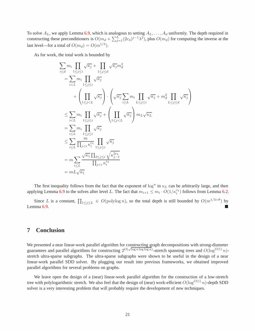
To solveAL, we apply Lemma6.9, which is analogous to settingAL, . . . , Ad uniformly. The depth required inconstructing these preconditioners isO(md +

∑Lj=1(2c4)

j−1λ2), plusO(md) for computing the inverse at the

last level—for a total ofO(md) = O(m1/3).

As for work, the total work is bounded by

∑

i≤d

mi

∏

1≤j≤i

√κj +

∏

1≤j≤d

√κjm

2d

=∑

i<L

mi

∏

1≤j≤i

√κj

+

∏

1≤j<L

√κj

·

√κj

∑

i≥L

mi

∏

L≤j≤i

√κj +m2

d

∏

L≤j≤d

√κj

≤∑

i<L

mi

∏

1≤j≤i

√κj +

∏

1≤j<L

√κj

mL

√κL

=∑

i≤L

mi

∏

1≤j≤i

√κj

≤∑

i≤L

m∏j<i κ

c4i

∏

1≤j≤i

√κj

= m∑

i≤L

√κ1∏

2≤j≤i

√κ2c4j−1∏

j<i κc4i

= mL√κ1

The first inequality follows from the fact that the exponent of logn in κL can be arbitrarily large, and thenapplying Lemma6.9 to the solves after levelL. The fact thatmi+1 ≤ mi · O(1/κc4i ) follows from Lemma6.2.

SinceL is a constant,∏

1≤j≤L ∈ O(polylog n), so the total depth is still bounded byO(m1/3+θ) byLemma6.9. �

7 Conclusion

We presented a near linear-work parallel algorithm for constructing graph decompositions with strong-diameterguarantees and parallel algorithms for constructing2O(

√logn log logn)-stretch spanning trees andO(logO(1) n)-

stretch ultra-sparse subgraphs. The ultra-sparse subgraphs were shown to be useful in the design of a nearlinear-work parallel SDD solver. By plugging our result into previous frameworks, we obtained improvedparallel algorithms for several problems on graphs.

We leave open the design of a (near) linear-work parallel algorithm for the construction of a low-stretchtree with polylogarithmic stretch. We also feel that the design of (near) work-efficientO(logO(1) n)-depth SDDsolver is a very interesting problem that will probably require the development of new techniques.

21

Acknowledgments

This work is partially supported by the National Science Foundation under grant numbers CCF-1018463, CCF-1018188, and CCF-1016799, by an Alfred P. Sloan Fellowship,and by generous gifts from IBM, Intel, andMicrosoft.

References

[ABN08] Ittai Abraham, Yair Bartal, and Ofer Neiman. Nearlytight low stretch spanning trees. InFOCS,pages 781–790, 2008.5

[AKPW95] Noga Alon, Richard M. Karp, David Peleg, and Douglas West. A graph-theoretic game and itsapplication to thek-server problem.SIAM J. Comput., 24(1):78–100, 1995.4, 5, 9

[Awe85] Baruch Awerbuch. Complexity of network synchronization. J. Assoc. Comput. Mach., 32(4):804–823, 1985.4

[BV04] S. Boyd and L. Vandenberghe.Convex Optimization. Camebridge University Press, 2004.2

[Chv79] V. Chvatal. The tail of the hypergeometric distribution. Discrete Mathematics, 25(3):285–287,1979.3, 4

[CKM+10] Paul Christiano, Jonathan A. Kelner, Aleksander Madry,Daniel Spielman, and Shang-Hua Teng.Electrical flows, laplacian systems, and faster approximation of maximum flow in undirectedgraphs. 2010.2

[Coh93] E. Cohen. Fast algorithms for constructing t-spanners and paths with stretch t. InProceedings ofthe 1993 IEEE 34th Annual Foundations of Computer Science, pages 648–658, Washington, DC,USA, 1993. IEEE Computer Society.5

[Coh00] Edith Cohen. Polylog-time and near-linear work approximation scheme for undirected shortestpaths.J. ACM, 47(1):132–166, 2000.3

[DS08] Samuel I. Daitch and Daniel A. Spielman. Faster approximate lossy generalized flow via interiorpoint algorithms.CoRR, abs/0803.0988, 2008.2

[EEST05] Michael Elkin, Yuval Emek, Daniel A. Spielman, andShang-Hua Teng. Lower-stretch spanningtrees. InProceedings of the thirty-seventh annual ACM symposium on Theory of computing, pages494–503, New York, NY, USA, 2005. ACM Press.5

[Gre96] Keith Gremban.Combinatorial Preconditioners for Sparse, Symmetric, Diagonally DominantLinear Systems. PhD thesis, Carnegie Mellon University, Pittsburgh, October 1996. CMU CSTech Report CMU-CS-96-123.3, 14

[GVL96] G. H. Golub and C. F. Van Loan.Matrix Computations. Johns Hopkins Press, 3rd edition, 1996.16

[Hoe63] Wassily Hoeffding. Probability Inequalities for Sums of Bounded Random Variables.Journal ofthe American Statistical Association, 58(301):13–30, 1963.3, 4

[JaJ92] Joseph JaJa.An Introduction to Parallel Algorithms. Addison-Wesley, 1992.13

22

[KM07] Ioannis Koutis and Gary L. Miller. A linear work,O(n1/6) time, parallel algorithm for solvingplanar laplacians. InSODA, pages 1002–1011, 2007.1, 14

[KMP10] Ioannis Koutis, Gary L. Miller, and Richard Peng. Approaching optimality for solving SDD linearsystems. InFOCS, pages 235–244, 2010.4, 14, 15, 16

[KMP11] Ioannis Koutis, Gary L. Miller, and Richard Peng. A nearlym log n time solver for SDD linearsystems. InFOCS, page (to appear), 2011.1

[Kou07] Ioannis Koutis.Combinatorial and algebraic algorithms for optimal multilevel algorithms. PhDthesis, Carnegie Mellon University, Pittsburgh, May 2007.CMU CS Tech Report CMU-CS-07-131. 16

[KS97] Philip N. Klein and Sairam Subramanian. A randomizedparallel algorithm for single-source short-est paths.J. Algorithms, 25(2):205–220, 1997.3

[Lei92] F. Thomson Leighton.Introduction to Parallel Algorithms and Architectures: Array, Trees, Hyper-cubes. Morgan Kaufmann Publishers Inc., San Francisco, CA, USA, 1992. 13

[MR89] Gary L. Miller and John H. Reif. Parallel tree contraction part 1: Fundamentals. In Silvio Micali,editor,Randomness and Computation, pages 47–72. JAI Press, Greenwich, Connecticut, 1989. Vol.5. 16

[Ren01] James Renegar.A mathematical view of interior-point methods in convex optimization. Society forIndustrial and Applied Mathematics, Philadelphia, PA, USA, 2001.2

[Ska09] Matthew Skala. Hypergeometric tail inequalities:ending the insanity, 2009.3, 4

[Spi10] Daniel A. Spielman. Algorithms, Graph Theory, and Linear Equations in Laplacian Matrices. InProceedings of the International Congress of Mathematicians, 2010.1

[SS08] Daniel A. Spielman and Nikhil Srivastava. Graph sparsification by effective resistances. InSTOC,pages 563–568, 2008.2

[ST03] Daniel A. Spielman and Shang-Hua Teng. Solving sparse, symmetric, diagonally-dominant linearsystems in timeO(m1.31). In FOCS, pages 416–427, 2003.14, 16

[ST06] Daniel A. Spielman and Shang-Hua Teng. Nearly-linear time algorithms for preconditioning andsolving symmetric, diagonally dominant linear systems.CoRR, abs/cs/0607105, 2006.4, 5, 14,16, 17, 19

[Ten10] Shang-Hua Teng. The Laplacian Paradigm: Emerging Algorithms for Massive Graphs. InTheoryand Applications of Models of Computation, pages 2–14, 2010.1

[UY91] Jeffrey D. Ullman and Mihalis Yannakakis. High-probability parallel transitive-closure algorithms.SIAM J. Comput., 20(1):100–125, 1991.3

[Ye97] Y. Ye. Interior point algorithms: theory and analysis. Wiley, 1997.2

23