Near Is My Shirt but Nearer Is My Skin. Ideology or Self-Interest as Determinants of Public Opinion...

1

Submission to Verein für Socialpolitik, Jahrestagung 2010,

Kiel, Germany

Near Is My Shirt, But Nearer Is My Skin: Ideology or Self-Interest as Determi-nants of Public Opinion on Fiscal Policy Issues Hans Pitlik, Gerhard Schwarz

(Austrian Institute of Economic Research WIFO, Vienna)

Barbara Bechter, Bernd Brandl

(University of Vienna, Department of Industrial Sociology)

Gerhard Schwarz (corresponding author and presenter)

Author contact information:

[email protected]

Austrian Institute of Economic Research (WIFO)

Arsenal Objekt 20, A-1030 Vienna, Austria

Phone: +43 1 798 26 01 - 263

Fax: +43 1 798 93 86

Abstract

Several empirical studies derive that personal positions with respect to policy measures are dominat-ed by ideology instead of narrow self-interest. In the present field study we carried out a telephone survey with 1.003 respondents all over Austria. Instead of only measuring self-interest indirectly, we requested respondents to assess directly whether they expect to be affected by policy measures. Our results indicate that such a subjectively measured narrow self-interest explains attitudes towards economic policies at least as good as ideological conviction. In some cases, however, ideology ap-pears to determine whether people feel affected by a proposed policy measure.

Key words: public opinion, sociotropic voting, ideology, self-interest, telephone surveys

This version: 01 March 2010

2

1 Introduction

Which factors determine public opinion on economic policy issues? How do people derive their per-sonal positions with respect to policy measures? Although these questions are at the heart of an understanding of voting behavior and, probably, for the making of economic policies in democratic societies (Page and Shapiro, 1983), Public Choice theory still lacks a unique conception about the process of individual preference formation and voter motivation. Somewhat simplifying, two broad lines of reasoning to explain opinion formation can be separated, an egocentric (self-interest) ap-proach and a sociotropic approach.

Simple rational choice theory claims that individual attitudes towards economic policies are deter-mined by narrow self-interest. Individuals know what is in their own interest and make choices ac-cordingly. Based on perceptions of the individual costs and benefits people develop expectations about the net effects of policies on their personal well-being. If the expected effect of a certain policy measure is positive, the respective citizen-voters are in favor of it. All that is required for an accurate determination of individual attitudes towards some specific policy measure is an assessment of the economic consequences on personal well-being. Hence, from this point of view individual opinion is exclusively shaped by egocentric motivation.

This view is often criticized. First, it is argued that an average person does not have the capability to calculate the individual costs and benefits of most policy measures. She/he usually lacks the technical knowledge and the information to gauge the personal consequences of certain policy measures on her/his personal well-being. Second, rational citizen-voters usually do not have an incentive to be-come informed about economic policy issues. As the cost of acquiring information are positive and the individual impact of an informed vote on final election outcomes is negligible, citizen-voters should remain rationally ignorant with respect to the effects of most policy issues.

Attitudes towards economic policies are then often driven by ideological convictions (Downs, 1957). Party ideologies serve as a substitute for the individual cost of acquiring political and economic in-formation. Yet such ideologically shaped opinions might still be consistent with self-interested beha-vior. Rational individuals 'choose' a certain ideology as an information short-cut, and their choice depends on which ideological party affiliation is expected to suit best to selfish motives. In many cases ideological and self-interested opinion formation are therefore not easily separable.

A somewhat different thinking dominates the sociotropic approach. According to this view, when forming opinions about economic policies, people have a normative view of the world in mind, i.e. a notion how it 'should' be (Denzau and North, 1994). Ideas and ideologies matter in particular in col-lective choices, as people do not have an incentive to collect information. According to the theory of low-cost decisions and expressive voting (see e.g. Kirchgässner and Pommerehne, 1993; Brennan and Lomansky, 1993) supporting or opposing a specific economic policy has no direct consequences for personal well-being, as individual action does not have an effect on the overall outcome. In such a situation it is almost without personal costs to express ideological convictions that are not necessarily in accordance with narrow self-interest. On the contrary, in the market sphere decisions which are only based on ideological judgments are associated with high costs as the consequences of a decision are borne by the decider. Hence, due to the low cost character of expressing preferences in the po-litical sphere, ideology and a personal conception of "the common good" are stronger motives in

3

individual voting behaviour and may thus explain opinion formation much better than pure self-interest.

Empirical investigations of individual and collective opinion formation so far often support the latter view. Studies from the fields of economics, sociology and political science show an increasing interest in the topic of self-interest and opinions on economic policy issues and address the question of the empirical relevance of former assumptions (see Citrin and Green, 1990; Sears and Funk, 1990; MacKuen et al., 1992; Mutz, 1993; Holbrook and Garand, 1996; Krause, 1997; Fuchs et al. 1998; Boeri and Tabellini, 2005). In general, these studies find (often based on the 1996 “Survey of Americans and Economists on the Economy”) that attitudes towards economic policy issues deviate with a sys-tematic bias from self-interest, i.e. the opinion whether a specific economic policy should be carried out is often not systematically related to egoistic motivations. Empirical studies for the U.S. (Walstad, 1997; Caplan, 2001, 2002, 2006) and for Germany (Heinemann et al., 2007) conclude that knowledge and ideology are of special relevance in explaining the bias, or are even the main determinants of opinion formation.

In a widely recognized recent paper, Blinder and Krueger (2004) use a specially designed telephone survey to address the problem of opinion formation on economic policy issues in the U.S. A main result of their study is that public opinion on the quality and adequacy of economic policies is mainly driven by ideological factors. With respect to policy issues like taxes, budget deficits, minimum wag-es, social security, and health insurance, ideology is the most consistently important determinant of individual preferences and policy acceptance, whereas objective measures of self-interest are the least important. These findings seem consistent with the idea that people use ideology as a short cut for deciding which position to take, especially when informing oneself is costly. Blinder and Krueger (2004) report that in many cases respondents in the telephone survey seem to have answered against their narrow self-interest, which is proxied by 'objective' variables, most notably household income.

Yet it is somewhat questionable whether narrow self-interest can be measured objectively. What matters eventually is what people believe to be in their self-interest. Blinder and Krueger have in mind a specific economic model on how certain individuals are affected by particular economic poli-cies. In general there is no guarantee that the Blinder-Krueger economic view of the world is identical to what respondents think about the working properties of an economy. Most probably, this is not the case, as laymen usually have a different view of the economic world (Caplan, 2001). If we want to know whether people systematically neglect their own self-interest in the process of opinion forma-tion on economic policies in favor of an ideologically defined common good, we should have a better, i.e. a subjective measure of self-interest. Put differently, in order to find out if narrow self-interest is really dominated by ideological convictions and ideas of 'the public good', it is important to know which policies people perceive to be in their self-interest or not. As ideology should serve as a simple rule-of-thumb in case of a lack of knowledge, people might express ideological preferences that ap-pear to be against their self-interest from the view of economists. However, in their own view res-pondents might express opinions on policy issues which they believe to be in their narrow interest. The main purpose of the present paper is to examine whether the often found dominance of ideolog-ical convictions survives if we measure self-interest more subjectively and directly.

The methodology of the present study closely follows Blinder and Krueger (2004). In autumn 2008 we carried out a telephone survey with 1.003 respondents all over Austria. The survey consisted of a

4

series of questions about personal opinions on a variety of fiscal policy issues. In contrast to Blinder-Krueger we not only asked for certain 'objective' measures that appear to be related to egocentric opinion formation. We additionally requested respondents directly to assess whether they expect to benefit from certain economic and fiscal policy measures. Hence, we need not speculate about a respondent's economic view of the world and whether he/she deviates from narrow self-interest; we simply asked them. All in all, our results show that – in contrast to Blinder and Krueger (2004) and several other investigations –subjectively measured narrow self-interest explains attitudes towards economic policies at least as good as ideological conviction.

A usual and often heard objection is that in interviews individuals can easily express opinions for an economic policy although they know that this policy will reduce their own well-being or income. Hence, doubts have been raised about whether the questions commonly asked in opinion polls show true preferences. This is certainly correct, but it does not invalidate our results. Taking part in a pub-lic opinion survey is comparable to the act of voting. In either case, individual action does not have individual consequences. Hence, both are certainly situations in which it is not individually costly to express socially desired or ideological preferences.

The paper proceeds as follows. In section 2 we present a very short overview on the political and methodological background of the study and the telephone survey. Section 3 reports some descrip-tive statistics. In section 4 we present the main results of our logit-regressions and discuss the results in the light of the two different approaches to opinion formation. Section 5 concludes.

2 Political and methodological background

In September 2008 we launched a telephone survey in Austria in order to replicate and verify the results of Blinder and Krueger (2004) that “ideology seems to play a stronger role in shaping opinion on economic policy issues than either self-interest or knowledge“ for the case of Austria. Of course we adapted the methodology; in particular we focus on ideology and self-interest only, leaving out knowledge as a possible determinant in the present study. 1.003 eligible Austrian voters were inter-viewed over the telephone. Fieldwork covered the last days of the campaign in federal elections for the Austrian National Council in 2008 and some of the first days after the elections.

One of the main topics discussed during the election campaign was whether and in which way a reform of the income tax should be put into practice.0F

1 The two parties which formed a grand coali-tion before as well as after the elections in principle agreed on the need for an income tax reform and that the reduction should amount to approximately € 3 bn, i.e. about 1% of GDP (Statistik Aus-tria, 2009). Although it was obvious that at least parts of the income tax reductions had to be fi-nanced by raising other taxes and/or by cutting expenditures in the federal budget, politicians’ statements on financing the income tax reform were at best very ambiguous. Against this back-ground we asked the participants of our survey which of the following ten policy measures would be appropriate for financing a reduction of the income tax1F

2:

• Raising the VAT

• Raising the petroleum tax

1 Note that in September 2008 there was still no open public debate about the possible consequences of the U.S. housing market and financial crisis on the Austrian economy. 2 To prevent order biases the sequence of categories was randomized.

5

• Raising profit taxes on public/private limited companies

• Raising environmental taxes on companies

• Impose a property or inheritance tax

• Raising the tax on capital returns

• Increasing public debt

• Cutting social security benefits

• Cutting subsidies for companies

• Cutting jobs in public administration

In stark contrast to Blinder and Krueger and other similar studies we did not only ask the respondents for socio-demographic characteristics, i.e. sex, age, occupation, personal income and education to assess whether they might be adversely affected by a certain policy measure, but also whether they believe this measure would have an adverse impact on them. This survey design enables us to find out how the perceived adverse impact of a policy measure influences its acceptance among the pub-lic.

To assess the effects of ideology on the acceptance of our policy measures we asked our intervie-wees to assign their political position on a five point Left-to-Right-Scale (LRS). Alternately the respon-dents could also choose “other” if they did not think the proposed scale matched their ideological position, or “refuse to answer” (the two latter categories were asked unprompted). Figure 1 shows the distribution of respondents' answers along the Left-to-Right-Scale. It is definitely clear that the by far largest group of people classifies itself as centrists, while the share of (moderate) leftists is slightly larger than the share of (moderate) rightists.

Figure 1: Ideological self-assignment based on the Left-to-Right-Scale

3 Descriptive Statistics

3.1 Acceptance of measures and subjective ('perceived') self-interest Descriptive analyses reveal a clear adverse correlation between the share of respondents who sup-pose a given policy measure is appropriate for financing a tax reform (acceptance) and the share of respondents who think this specific measure would have an adverse impact on them (Pearson’s Cor-relation Coefficient = -0.89). In other words: the more people expect to be adversely affected by a

Leftist Moderate Leftist Centrist Moderate Rightist Rightist Other (unprompted) Refused to answer

0%

5%

10%

15%

20%

25%

30%

35%

40%

45%

6

certain measure, the fewer people tend to accept this measure (see Figure 2). The least popular measure is a VAT increase, followed by an increase of the petroleum tax. Almost 80 % of the respon-dents think that raising profit taxes is an appropriate way to finance a personal income tax reduction, and about 70% think that savings by reducing jobs in public administration is an appropriate meas-ure.

Figure 2: Acceptance of policy measures and average perceived personal impact

Remarkably this strong correlation does not simply imply that people who fear an adverse impact on themselves oppose a certain measure while people who do not feel affected are in favor of it. Figure 3 clearly shows that the rates of acceptance show a similar pattern for both groups (Pearson’s Corre-lation Coefficient = 0.97), i.e. if many people feel negatively affected only few support a given meas-ure, even among those who do not expect an adverse impact on themselves, and vice versa. Howev-er, in all cases adversely affected persons are less likely to accept a certain measure than people who do not expect a negative impact. In eight out of ten cases the difference is significant (p<0.05). Only “cutting subsidies for companies” and “raising the VAT” do not show significant differences. In the latter case this is probably due to the fact that hardly anybody supports a higher VAT (4%), while a vast majority (89%) feels adversely affected by VAT increases so that there is hardly any room for a big differential among the groups.

0%

10%

20%

30%

40%

50%

60%

70%

80%

90%

100%

0% 20% 40% 60% 80% 100%

Reps

onde

ntes

who

thin

k a

give

n m

easu

re w

ould

aff

ect

them

neg

ativ

ely

Respondents who think a given measure is appropriate to finance a tax reform

Raising the VAT

Raising the petroleum tax

Raising profit taxes on public/private limited companiesRaising environmental taxes on companies

Impose a property or inheritance tax

Raising the tax on capital returns

Increasing public debt

Cutting social security benefits

Cutting subsidies for companies

Cutting jobs in public administration

7

Figure 3: Acceptance of policy measures by subjective ('perceived') impact

3.3 Acceptance of measures and ideological orientation Looking at the rates of acceptance according to ideological orientation based on the Left-to-Right-Scale2F

3 we find a similar pattern. The rates of acceptance are highly correlated for all displayed groups (see Figure 6), while the differences between the ideological groups are significant for the same eight policy measures as above. However, while people who assign themselves to the political centre or the right agree on average with 3.5 measures and 3.4 measures respectively, leftists agree with 4.2 political measures (which are significantly more).

Figure 6: Acceptance of policy measures by political self-assignment

3 For clarity the groups "left" and “moderately left” as well as “right” and “moderately right” were merged into the groups “(moderate) leftist” and “(moderate) rightist” respectively.

0%

10%

20%

30%

40%

50%

60%

70%

80%

90%

100%

Raising the VAT Raising the petroleum tax

Raising profit taxes on

corporations

Raising environmental

taxes on companies

Impose a property or

inheritance tax

Raising the tax on capital

returns




Cutting jobs in public

administration

People not expecting to be adversely affected People expecting to be adversely affected

0%

10%

20%

30%

40%

50%

60%

70%

80%

90%

Raising the VAT Raising the petroleum tax

Raising profit taxes on

corporations

Raising environmental

taxes on companies

Impose a property or

inheritance tax

Raising the tax on capital

returns




Cutting jobs in public

administration

(Moderate) Leftist Centrist (Moderate) Rightist

8

Figure 5 also shows that people who declare themselves as standing 'left' in general seem to prefer tax increases (except for VAT) compared to people with a centrist or rightist ideological orientation. With respect to spending cuts differences between the ideological groups seem to disappear. More-over, center and right ideology appear to be very closely related, while leftist ideology is much more distinct.

4 Results of logit regressions

4.1 Basic results To analyze more deeply the impact of perceived adverse impacts and ideological orientation we ran a set of logit regressions to reveal the main drivers of acceptance of policy measures as a dependent variable. We included the following possible determinants of acceptance into our models:

1. "Subjective" self-interest

• Expected adverse impact of the policy measure (dummy) 2. "Objective" self-interest

• Occupation (set of dummies: employee in the private sector, employee in the public sector, self-employed, retired; reference group: others)

• Personal net income (ordinal)

• Living in a big city (100,000 inhabitants and more, dummy) 3. Ideology

• (Moderately) leftist (dummy)3F

4 4. Control variables

• Sex (dummy)

• Age (ordinal)

• Educational level (ordinal)

Of course several of these variables are correlated. E.g., our survey shows that the higher the degree of education, the higher is the probability of adhering to a more left-wing ideology. However, tests of collinearity did not give any reason for concern. Interaction terms were not implemented given the methodological problems that their use causes in logit–models (see Ai and Norton, 2003). Seven of the ten models tested are properly specified, while for three models the chosen predictors are not meaningful, i.e. these three models fail in explaining the differences in the acceptance of the respec-tive policy measures. The remaining seven models yield Pseudo-R2 ranging from 0.16 – which we suppose to be acceptable – to rather limited 0.03.

Summing up results of our estimates we find that perceived adverse personal consequences of a policy measure have a significant impact on the acceptance of this measure in all seven properly spe-cified models (at the 95%-level, see Table 1). The signs of the coefficients are – as expected – nega-tive in all those cases, i.e. the acceptance of a policy measure is systematically lower among persons who expect to be adversely affected personally. This means that (perceived) self-interest clearly plays

4 As the descriptive results showed clear differences between (moderate) leftists on the one hand and centrists and (moderate) rightists on the other hand, the ordinary left-to-right-scale has been recoded into a dummy variable indicating whether a respondent declared herself as (moderately) left or not. Respondents who did not assign themselves to the left-to-right-scale (i.e. refused to answer or answered that the categories appropriate for them) were omitted from further analyses.

9

a remarkable if not dominant role – compared to ideology - in forming personal opinions on policy measures.

Personal net income, which is regularly used as a variable to proxy self-interest in many empirical investigations, is insignificant in all models. From an egoistic model of opinion formation, we would at least have expected that a higher net income is also associated with an increasing probability of acceptance of cuts in social benefits and a reduced acceptance of property tax increases in order to finance income tax reductions. With respect to occupation/profession as a determinant of objective self-interest, we find that public sector employees support profit tax and inheritance tax increases to a higher degree than other groups of persons. Somewhat surprisingly they do not oppose job cuts in the public sector significantly more often than other vocational groups. Interestingly people living in big cities (> 100.000 inhabitants) have a lower probability of accepting job cuts in the public sector than people from less urban areas. We suppose that this results from the large number of public sector employees living in the big cities where most of the workplaces in public administrations are located.

Remarkably, the share of opponents of higher petroleum taxes rises with the respondents’ age. This is counterintuitive as older people (above 65) are less likely to have access to cars (Herry and Sam-mer, 1998) and therefore are less prone to increased petroleum taxes. Consistently they also feel adversely affected by higher petroleum taxes to a lesser extent than younger peer groups. We guess this contradiction between the low rate of adverse consequences and the high rate of refuse reflects differences in the valuation of private transport among different peer groups and might therefore indicate that ideological positions beyond political attribution might play a significant role in the opi-nion formation.

Political ideology plays a significant role in five of the seven proper models. Ideological left-wingers are systematically likelier to accept tax rises as policy measures than self-declared right-wingers and centrists, even when we control for objective and subjective self-interest as well as a number of fur-ther socio-economic variables. Somewhat surprisingly left-wingers are not significantly more dismis-sive towards cutting social security benefits than centrists and rightists.

10

Table 1: Acceptance of policy measures by several determinants (logit models, full speci-fication) Sub-

jec-tive self-

inter-est

Objective self-interest Ide-

ology Control variables

Occupation

Pseu

do R

2

Expe

cted

adv

erse

con

sequ

ence

s of

mea

sure

Empl

oyee

in th

e pr

ivat

e se

ctor

Empl

oyee

in th

e pu

blic

sec

tor

Self-

empl

oyed

Retir

ed

Pers

onal

mon

thly

net

Inco

me

Livi

ng in

a b

ig c

ity

(Mod

erat

e) L

eftis

t

Sex

Age

Educ

atio

nal l

evel

Increasing VAT 0.14

Increasing the petroleum tax 0.16

Raising profit taxes on public/private limited companies 0.07

Raising environmental taxes on companies 0.08

Impose a property or inheritance tax 0.03

Raising the tax on capital returns 0.06

Increasing public debt 0.05

Cutting social security benefits 0.07

Cutting subsidies for companies 0.01

Cutting jobs in public administration 0.08 Expected adverse consequences of measure: 0 = No, 1 = Yes Occupation (Employee in the private sector/Employee in the public sector/Self-employed/Retired): 0 = No, 1 = Yes , Other = Reference group Living in a big city: 0 = No, 1 = Yes Personal monthly net income: 1 = none, 2 = Up to 1000 €, 3 = 1001 to 1500 €, 4 = 1501 to 2000 €, 5 = 2001 to 2500 €, 6 =2501 to 3000 €, 7 = More than 3000 € (Moderate) Leftist:0 = Rightist, moderate rightist, centrist, 1 = Moderate leftist, leftist Sex: 0 = Female, 1 = Male Age: 1 = 16 to 25 years, 2 = 26 to 35 years, 3 = 36 to 45 years, 4 = 46 to 55 years, 5 = 56 to 65 years, 6 = 65 years and older Educational level: 1 = Compulsory education attendance, 2 = Apprenticeship, 3 = Vocational school, 4 = Abitur (British A-Level), 5 = University (of applied sciences) … Positive coefficient, significant at the 95%-level … Negative coefficient, significant at the 95%-level … Variable not included in the model … Model misspecified, set of chosen predictors not meaningful (linktest, hat: p> 0.05) … Model misspecified, unobserved predictors or interactions probable (linktest, hatsq: p < 0.05)

4.2 Alternative specifications To get a picture on how subjective and objective self-interest and ideology mutually impair each oth-er we ran alternative specifications of the models introduced above. By omitting the subjective (‘per-ceived’) self- interest the indicators of objective self-interest become more important in explaining the acceptance of policy measures (Table 2). The number of significant cases of objective self-interest jumps from 4 to 10 out of 42 possible cases (6 variables x 7 valid models). Public sector employees, for example, now are less likely to accept job cuts in the public sector than other occupational groups, while self-employed are more in favor of lowering public security benefits than others. This shows that subjective (“perceived”) self-interest corresponds to people’s objective self-interest.

While in our basic model-setting ideology does not correspond significantly – and somewhat surpri-singly – with the proposition of cutting social security benefits, by omitting the perceived self-interest from the model ideology becomes a significant predictor of people’s attitudes towards this policy measure: leftists now are significantly less likely to acclaim to cutting social security benefits than centrists and rightists.

11

Table 2: Acceptance of policy measures by several determinants (logit models without ‘subjective’ – perceived - self-interest) Sub-

jec-tive self-

inter-est



Occupation

Pseu

do R

2

Expe

cted

adv

erse

con

sequ

ence

s of

mea

sure

Empl

oyee

in th

e pr

ivat

e se

ctor

Empl

oyee

in th

e pu

blic

sec

tor

Self-

empl

oyed

Retir

ed

Pers

onal

mon

thly

net

Inco

me

Livi

ng in

a b

ig c

ity

(Mod

erat

e) L

eftis

t

Sex

Age

Educ

atio

nal l

evel

Increasing VAT 0.13










Omitting ideology as a predictor changes the set of properly specified models somewhat (Table 3). While this modification does not change the impact of perceived self-interest, it moderately raises the number of cases where objective measures of self-interest have a significant impact on the ac-ceptance of policy measures from 4 out of 42 possible cases to 5 out of 48 (as now 8 models are properly specified). Three of these 5 cases occur in a specific model, i.e. apply to the acceptance of job cuts in the public sector. We therefore conclude that ideology and objective self-interest are only loosely related – at least as far as our set of objective measures is concerned.

12

Table 3: Acceptance of policy measures by several determinants (logit models without ideological orientation) Sub-

jec-tive self-

inter-est



Occupation

Pseu

do R

2

Expe

cted

adv

erse

con

sequ

ence

s of

mea

sure

Empl

oyee

in th

e pr

ivat

e se

ctor

Empl

oyee

in th

e pu

blic

sec

tor

Self-

empl

oyed

Retir

ed

Pers

onal

net

Inco

me

Livi

ng in

a b

ig c

ity

(Mod

erat

e) L

eftis

t

Sex

Age

Educ

atio

nal l

evel

Increasing VAT 0.10










Removing the objective measures of self-interest from our basic models leaves the impact of per-ceived self-interest on the acceptance of policy measures unchanged (Table 4). The number of cases where ideology plays a significant role goes up from 5 to 6 out of 7 properly specified models. As the set of properly specified models differs from our basic specification a significant influence of ideology emerges for two policy measures which did not show a significant impact of ideology in the basic setting. Leftists oppose cutting social security benefits significantly more often than centrists and rightists when subjective self-interest is not included in the model specification.

13

Table 4: Acceptance of policy measures by several determinants (logit models without ‘objective’ self-interest) Sub-

jec-tive self-

inter-est



Occupation

Pseu

do R

2

Expe

cted

adv

erse

con

sequ

ence

s of

mea

sure

Empl

oyee

in th

e pr

ivat

e se

ctor

Empl

oyee

in th

e pu

blic

sec

tor

Self-

empl

oyed

Retir

ed

Pers

onal

mon

thly

net

Inco

me

Livi

ng in

a b

ig c

ity

(Mod

erat

e) L

eftis

t

Sex

Age

Educ

atio

nal l

evel

Increasing VAT 0.09










Summarizing, people who expect adverse effects of a certain policy measure on themselves are less likely to assent to this specific measure. Subjective (perceived) self-interest therefore turns out to be a valid and robust indicator of the acceptance of policy measures – given that large proportions of the observed variance remain unexplained. The same holds true for ideology – given raising taxes is the topic. Leftists are clearly in favor of tax increases compared to centrists and rightists. Attitudes towards cutting public expenses seem to be unaffected by ideological orientation when subjective and/or objective measures of self-interest are taken into account. Only after removing variables representing self-interest from the models the impression of an ideological bias emerges, i.e. that leftists are more reluctant to cuts in public spending than centrists and rightists.

4.2 Ideology and perceived adverse affection To complete the picture and to find out whether ideology has an impact on the expectations of ad-verse impacts stemming from policy measures we ran similar logit regressions as above on the accep-tance of policy measures: the model specification stays in principle the same while – of course – the expected adverse impact is now the dependent variable.

In principle, we should not expect ideological convictions to have a significant impact on people’s perception of the consequences of specific policy measures: whether an action affects a person ad-

14

versely is not a question of ideology or political belief. Nevertheless, the results presented above indicate some interaction of ideology and (perceived) self-interest. All in all our models do not cope very well with this task. Only four out of ten models are properly specified (Table 5). This might be interpreted as an indication that in these cases ideology – on the one hand – does not contribute much in explaining perceived self interest, as the chosen set of predictors turns out to be not mea-ningful and/or unobserved predictors (including unobserved interaction effects) are indicated. In these cases the same is true for our objective measures of self-interest, suggesting that the concept of subjective self-interest covers objective interests beyond the scope of our dataset and/or only imagined interests.

Focusing on the four properly specified models we find that objective self-interest determines sub-ject self-interest in all four cases. Most times the coefficients’ signs are headed in the expected direc-tion. Still, it is astonishing that the self-employed feel less affected by increasing the capital return tax than other groups and, moreover, that the pensioners suppose to be less prone to cuts of social security benefits than other occupational groups as their (main) income, i.e. pensions are a social security benefit. Yet, we cannot exclude that the pensioners do not identify received pension pay-ments as a social transfer. Ideology is a significant predictor in two of the four properly specified models. This suggests that the political orientation might at least in some cases influence the percep-tion of political measures. However, we cannot reject the possibility that ideology only proxies objec-tive interests not operationalized in our models.

Table 5: Determinants of subjective (‘perceived’) adverse consequences of policy meas-ures (logit-models)

Objective self-interest Ideol-ogy

Control variables

Occupation

Pseu

do R

2

Empl

oyee

in th

e pr

ivat

e se

ctor

Empl

oyee

in th

e pu

blic

sec

tor

Self-

empl

oyed

Retir

ed

Pers

onal

mon

thly

net

Inco

me

Livi

ng in

a b

ig c

ity

(Mod

erat

e) L

eftis

t

Sex

Age

Educ

atio

nal l

evel

Increasing VAT 0.06


Raising profit taxes on public/private limited companies 0.03 Raising environmental taxes on companies 0.03






Cutting jobs in public administration 0.05 Occupation (Employee in the private sector/Employee in the public sector/Self-employed/Retired): 0 = No, 1 = Yes , Other = Reference group Living in a big city: 0 = No, 1 = Yes Personal monthly net income: 1 = none, 2 = Up to 1000 €, 3 = 1001 to 1500 €, 4 = 1501 to 2000 €, 5 = 2001 to 2500 €, 6 =2501 to 3000 €, 7 = More than 3000 € (Moderate) Leftist:0 = Rightist, moderate rightist, centrist, 1 = Moderate leftist, leftist Sex: 0 = Female, 1 = Male Age: 1 = 16 to 25 years, 2 = 26 to 35 years, 3 = 36 to 45 years, 4 = 46 to 55 years, 5 = 56 to 65 years, 6 = 65 years and older Educational level: 1 = Compulsory education attendance, 2 = Apprenticeship, 3 = Vocational school, 4 = Abitur (British A-Level), 5 = University (of applied sciences) … Positive coefficient, significant at the 95%-level … Negative coefficient, significant at the 95%-level … Variable not included in the model … Model misspecified, set of chosen predictors not meaningful (linktest, hat: p> 0.05) … Model misspecified, unobserved predictors or interactions probable (linktest, hatsq: p < 0.05)

15

5 Conclusions

Following Blinder and Krueger (2004) we conducted a survey among 1.003 eligible Austrian voters in order to test whether their findings and those of several others - namely that ideology is a more po-werful predictor of attitudes towards policy measures than self-interest – hold. Nevertheless we modified the methodology by introducing the concept of “subjective (perceived) self-interest”: we asked people if they think a specific measure will affect them adversely.

We find that subjective self-interest – in this specific case the expectation of personally adverse con-sequences of a policy measure – is the most important, if not dominant, identified determinant of the acceptance of policy measures. People who expect to personally face adverse consequences of a policy measure are less likely to find this measure appropriate.

Our results therefore do not suggest that “ideology seems to play a stronger role in shaping opinion on economic policy issues than either self-interest or knowledge“ (Blinder and Krueger, 2004) – given that our operationalizations of both – self-interest and ideology – differ from the operationalizations chosen by Blinder and Krueger and that we do not account for knowledge in our models. On the con-trary, our results indicate that (subjective, perceived) self-interest is the stable factor in opinion for-mation while the influence of ideology is vastly dependent on the nature of the tested policy meas-ure (tax raises vs. spending cuts).

Ideology too appears to play a part in the process of opinion forming, but only in certain contexts. In particular (moderate) leftists are more likely to accept tax raises as adequate policy measures than centrists and (moderate) rightists. Concerning cuts in public expenditures the political orientation is a significant predictor only after measures of objective and/or subjective self-interest are omitted from the analyses.

Some results related to the attitudes towards raising the petroleum tax among different age groups suggest that ideological concepts apart from political ideology might play a role in shaping opinions on policy measures, for example peer group related concepts of private transport.

However, we find that objective self-interest and ideology are only loosely related. Moreover, sub-jective (perceived) self-interest and ideology contribute to the acceptance of policy measures in pa-rallel; therefore not substituting each other at least as far as tax increases are concerned. This ad-dresses the question whether (political) ideology is the laymen’s shortcut to political opinion forma-tion, not because of some normative view of the world how it “should be”, but because ideology shapes the positive view of how the economy works.

Subjective and objective self-interest as well as ideology only explain a small fraction of the variation inherent in the formation of public opinions. For example 80% of those not feeling adversely affected think that raising profit taxes on corporations is an appropriate measure for financing a reform of the income tax, while still 60% among those who feel adversely affected agree with this measure. This of course raises the question on what determines the opinion formation of those 60% and how the relevant determinants can be measured.

16

References

Ai, C., Norton, E.C. (2003): Interaction Terms in Logit and Probit Models, Economics Letters 80, 123–

129.

Blinder, A.S. and Krueger, A.B. (2004): What does the public know about economic policy, and how

does it know it? NBER Working Paper Series, Working Paper 10787, National Bureau of Eco-

nomic Research.

Boeri, T. and Tabellini, G. (2005): Does information increase political support for pension reform?

CEPR Discussion Papers 5319.

Brennan, G. and Lomansky, L. (1993): Democracy and decisions: The pure theory of electoral prefer-

ence. Cambridge University Press, Cambridge.

Caplan, B. (2001): What makes people think like economists? Evidence from the Survey of Americans

and Economists on the Economy. Journal of Law and Economics 44, 395-426.

Caplan, B. (2002): Sociotropes, systematic bias, and political failure: Reflections on the Survey of

Americans and economists on the economy. Social Science Quarterly 83, 416-435.

Caplan, B. (2006): How do voters form positive economic beliefs? Evidence from the Survey of

Americans and economists on the economy. Public Choice 128, 367-381.

Citrin, J. and Green, D. (1990): The self-interest motive in American public opinion. In: Long, S. (ed.).

Research in Micropolitics, 3, p. 1-28.

Denzau, A.T. and North, D.C. (1994): Shared Mental Models: Ideologies and Institutions. Kyklos 47, 3-

31.

Downs, A. (1957): An Economic Theory of Democracy, New York.

Fuchs, V.R., Krueger, A.B. and Poterba, J.M. (1998): Economists’ view about parameters, values, and

policies: Survey results in Labor and Public Economics. Journal of Economic Literature 36,

1387-1425.

Herry and Sammer (1998): Mobilitätserhebung österreichischer Haushalte, Arbeitspaket A3-H2 im

Rahmen des Österreichischen Bundesverkehrswegeplan im Auftrag des BMWV.

Heinemann, F., Förg, M., Frey, D., Jonas, E., Rotfuß, W., Traut-Mattausch, E., Westerheide, P. (2007):

Psychologie, Wachstum und Reformfähigkeit, Zentrum für Europäische Wirtschaftsforschung.

17

Kirchgässner, G. and Pommerehne, W.W. (1993): Low-cost decisions as a challenge to Public Choice.

Public Choice 77, 107-115.

Krause, G. (1997): Voters, information heterogeneity, and the dynamics of aggregate economic ex-

pectations. American Journal of Political Science 41, 1170-1200.

Keeter, S., Miller, C., Kohut, A., Groves, R., Presser, S. (2000): Consequences of Reducing Nonre-

sponse in a National Telephone Survey.” Public Opinion Quarterly 64(2): 125-148

MacKuen, M., Erikson, R. and Stimson, J. (1992): Peasants or bankers? The American electorate and

the U.S. economy. American Political Science Review 86, 597-611.

Mutz, D. (1993): Direct and indirect routes to politicizing personal experience: does knowledge make

a difference? Public Opinion Quarterly 57, 483-502.

Page, B.I. and Shapiro, R.Y. (1983): Effects of public opinion on policy. American Political Science Re-

view 77, 175-190.

Sears, D. and Funk, C. (1990): Self-interest in Americans’ political opinions. In: Mansbridge, J. (ed.).

Beyond Self-Interest. Chicago University Press, Chicago, p. 147-170.

Statistik Austria (2009), Bruttoinlandsprodukt nach Wirtschaftssektoren, nominell.

http://www.statistik.at/web_de/static/bruttoinlandsprodukt_nach_wirtschaftssektoren_no

minell_019715.pdf

Survey of Americans and Economists on the Economy (1996). The Washington Post, Kaiser Family

Foundation and Harvard University.

Walstad, W. (1997): The effect of economic knowledge on public opinion of economic issues. Journal

of Economic Education 28, 195-205.

18

Annex 1 – List of Variables

19

Acceptance of policy measures (0 = No, 1 = Yes) f10_1x … Increasing VAT f10_2x … Increasing the petroleum tax f10_3x … Raising profit taxes on public/private limited companies f10_4x … Raising environmental taxes on companies f10_5x … Impose a property or inheritance tax f10_6x … Raising the tax on capital returns f10_7x … Increasing public debt f10_8x … Cutting social security benefits f10_9x … Cutting subsidies for companies f10_10x … Cutting jobs in public administration

Expected adverse consequences of measure (0 = No, 1 = Yes) f11_1x … Increasing VAT f11_2x … Increasing the petroleum tax f11_3x … Raising profit taxes on public/private limited companies f11_4x … Raising environmental taxes on companies f11_5x … Impose a property or inheritance tax f11_6x … Raising the tax on capital returns f11_7x … Increasing public debt f11_8x … Cutting social security benefits f11_9x … Cutting subsidies for companies f11_10x … Cutting jobs in public administration

Occupation (0 = No, 1 = Yes , Other = Reference group) s3_1x … Employee in the private sector s3_2x … Employee in the public sector s3_3x … Self-employed s3_4x … Retired

s4x … Personal monthly net income (1 = None, 2 = Up to 1000 €, 3 = 1001 to 1500 €, 4 = 1501 to 2000 €, 5 = 2001 to 2500 €, 6 =2501 to 3000 €, 7 = More than 3000 €)

GrStadt … Living in a big city (0 = No, 1 = Yes)

leftist … (Moderate) Leftist (0 = Rightist, moderate rightist, centrist, 1 = Moderate leftist, leftist)

s1x … Sex (0 = Female, 1 = Male)

s2x … Age (1 = 16 to 25 years, 2 = 26 to 35 years, 3 = 36 to 45 years, 4 = 46 to 55 years, 5 = 56 to 65 years, 6 = 65 years and older)

s7x … Educational level (1 = Compulsory education attendance, 2 = Apprenticeship, 3 = Vocational school, 4 = Abitur (British A-Level), 5 = University (of applied sciences))

20

Annex 2 – Acceptance of policy measures by several determinants (lo-git models, full speci-fication)

21

Collinearity Diagnostics SQRT R- Variable VIF VIF Tolerance Squared ---------------------------------------------------- f11_1x 1.04 1.02 0.9607 0.0393 s3_1x 2.38 1.54 0.4196 0.5804 s3_2x 1.76 1.33 0.5694 0.4306 s3_3x 1.74 1.32 0.5749 0.4251 s3_4x 4.02 2.01 0.2487 0.7513 s4x 1.70 1.30 0.5896 0.4104 GrStadt 1.11 1.05 0.9045 0.0955 leftist 1.06 1.03 0.9463 0.0537 s1x 1.24 1.11 0.8056 0.1944 s2x 2.55 1.60 0.3915 0.6085 s7x 1.27 1.13 0.7852 0.2148 ---------------------------------------------------- Mean VIF 1.81 Cond Eigenval Index --------------------------------- 1 6.6078 1.0000 2 1.1353 2.4125 3 1.0189 2.5466 4 1.0041 2.5652 5 0.7732 2.9234 6 0.5768 3.3846 7 0.4243 3.9465 8 0.1855 5.9685 9 0.1240 7.3007 10 0.0640 10.1625 11 0.0604 10.4619 12 0.0258 15.9941 --------------------------------- Condition Number 15.9941 Eigenvalues & Cond Index computed from scaled raw sscp (w/ intercept) Det(correlation matrix) 0.0816 Iteration 0: log likelihood = -108.88629 Iteration 1: log likelihood = -100.20432 Iteration 2: log likelihood = -94.379397 Iteration 3: log likelihood = -94.124386 Iteration 4: log likelihood = -94.122586 Iteration 5: log likelihood = -94.122585 Logistic regression Number of obs = 729 LR chi2(11) = 29.53 Prob > chi2 = 0.0019 Log likelihood = -94.122585 Pseudo R2 = 0.1356 ------------------------------------------------------------------------------ f10_1x | Coef. Std. Err. z P>|z| [95% Conf. Interval] -------------+---------------------------------------------------------------- f11_1x | -.7908343 .5486105 -1.44 0.149 -1.866091 .2844225 s3_1x | -.5523875 .6826995 -0.81 0.418 -1.890454 .785679 s3_2x | -.5168884 .9427688 -0.55 0.584 -2.364681 1.330904 s3_3x | -.5492724 .9475763 -0.58 0.562 -2.406488 1.307943 s3_4x | .8530472 1.060614 0.80 0.421 -1.225718 2.931812 s4x | -.2544873 .2294624 -1.11 0.267 -.7042252 .1952507 GrStadt | .3662238 .4539218 0.81 0.420 -.5234466 1.255894 leftist | -.5472242 .5102837 -1.07 0.284 -1.547362 .4529135 s1x | 1.723561 .5476459 3.15 0.002 .6501945 2.796927 s2x | -.4019306 .2272795 -1.77 0.077 -.8473903 .043529 s7x | .3744895 .1831893 2.04 0.041 .015445 .7335339 _cons | -2.809879 1.037068 -2.71 0.007 -4.842495 -.7772629 ------------------------------------------------------------------------------ Iteration 0: log likelihood = -108.88629 Iteration 1: log likelihood = -96.753467 Iteration 2: log likelihood = -94.495369 Iteration 3: log likelihood = -94.114269 Iteration 4: log likelihood = -94.092761 Iteration 5: log likelihood = -94.092673 Iteration 6: log likelihood = -94.092673 Logistic regression Number of obs = 729 LR chi2(2) = 29.59 Prob > chi2 = 0.0000 Log likelihood = -94.092673 Pseudo R2 = 0.1359 ------------------------------------------------------------------------------ f10_1x | Coef. Std. Err. z P>|z| [95% Conf. Interval] -------------+---------------------------------------------------------------- _hat | 1.209533 .8709117 1.39 0.165 -.4974224 2.916489 _hatsq | .0353261 .1425574 0.25 0.804 -.2440812 .3147334 _cons | .2683865 1.23363 0.22 0.828 -2.149484 2.686257 ------------------------------------------------------------------------------

22

Collinearity Diagnostics SQRT R- Variable VIF VIF Tolerance Squared ---------------------------------------------------- f11_2x 1.11 1.05 0.9001 0.0999 s3_1x 2.38 1.54 0.4200 0.5800 s3_2x 1.76 1.33 0.5694 0.4306 s3_3x 1.74 1.32 0.5756 0.4244 s3_4x 3.98 2.00 0.2511 0.7489 s4x 1.72 1.31 0.5822 0.4178 GrStadt 1.13 1.07 0.8814 0.1186 leftist 1.06 1.03 0.9397 0.0603 s1x 1.24 1.11 0.8071 0.1929 s2x 2.53 1.59 0.3947 0.6053 s7x 1.27 1.13 0.7881 0.2119 ---------------------------------------------------- Mean VIF 1.81 Cond Eigenval Index --------------------------------- 1 6.5431 1.0000 2 1.1420 2.3937 3 1.0181 2.5351 4 1.0037 2.5533 5 0.7946 2.8695 6 0.5778 3.3651 7 0.4235 3.9306 8 0.1906 5.8597 9 0.1451 6.7150 10 0.0722 9.5181 11 0.0611 10.3475 12 0.0282 15.2251 --------------------------------- Condition Number 15.2251 Eigenvalues & Cond Index computed from scaled raw sscp (w/ intercept) Det(correlation matrix) 0.0771 Iteration 0: log likelihood = -286.17024 Iteration 1: log likelihood = -246.59782 Iteration 2: log likelihood = -239.58293 Iteration 3: log likelihood = -239.51627 Iteration 4: log likelihood = -239.51621 Logistic regression Number of obs = 731 LR chi2(11) = 93.31 Prob > chi2 = 0.0000 Log likelihood = -239.51621 Pseudo R2 = 0.1630 ------------------------------------------------------------------------------ f10_2x | Coef. Std. Err. z P>|z| [95% Conf. Interval] -------------+---------------------------------------------------------------- f11_2x | -1.510956 .2863023 -5.28 0.000 -2.072098 -.949814 s3_1x | -.3752664 .3831196 -0.98 0.327 -1.126167 .3756342 s3_2x | .4073186 .4544541 0.90 0.370 -.4833952 1.298032 s3_3x | .19509 .5016955 0.39 0.697 -.7882151 1.178395 s3_4x | -.2120822 .5495433 -0.39 0.700 -1.289167 .8650028 s4x | -.1365356 .1242133 -1.10 0.272 -.3799893 .1069181 GrStadt | .3800618 .2614328 1.45 0.146 -.132337 .8924606 leftist | .7198616 .2481311 2.90 0.004 .2335337 1.20619 s1x | .2556429 .259412 0.99 0.324 -.2527953 .7640811 s2x | -.3066642 .1153993 -2.66 0.008 -.5328426 -.0804857 s7x | .2344837 .0991609 2.36 0.018 .0401318 .4288355 _cons | -.4213856 .5412651 -0.78 0.436 -1.482246 .6394745 ------------------------------------------------------------------------------ Iteration 0: log likelihood = -286.17024 Iteration 1: log likelihood = -252.11088 Iteration 2: log likelihood = -243.67399 Iteration 3: log likelihood = -239.49385 Iteration 4: log likelihood = -239.49121 Iteration 5: log likelihood = -239.49121 Logistic regression Number of obs = 731 LR chi2(2) = 93.36 Prob > chi2 = 0.0000 Log likelihood = -239.49121 Pseudo R2 = 0.1631 ------------------------------------------------------------------------------ f10_2x | Coef. Std. Err. z P>|z| [95% Conf. Interval] -------------+---------------------------------------------------------------- _hat | 1.053141 .2641497 3.99 0.000 .535417 1.570865 _hatsq | .0184931 .0826283 0.22 0.823 -.1434554 .1804416 _cons | .0171872 .2293618 0.07 0.940 -.4323536 .4667281 ------------------------------------------------------------------------------

23

Collinearity Diagnostics SQRT R- Variable VIF VIF Tolerance Squared ---------------------------------------------------- f11_3x 1.03 1.01 0.9709 0.0291 s3_1x 2.43 1.56 0.4120 0.5880 s3_2x 1.80 1.34 0.5568 0.4432 s3_3x 1.75 1.32 0.5710 0.4290 s3_4x 4.01 2.00 0.2495 0.7505 s4x 1.72 1.31 0.5828 0.4172 GrStadt 1.09 1.05 0.9140 0.0860 leftist 1.07 1.03 0.9383 0.0617 s1x 1.23 1.11 0.8107 0.1893 s2x 2.54 1.59 0.3936 0.6064 s7x 1.25 1.12 0.7980 0.2020 ---------------------------------------------------- Mean VIF 1.81 Cond Eigenval Index --------------------------------- 1 5.9407 1.0000 2 1.1425 2.2803 3 1.0471 2.3819 4 1.0037 2.4329 5 0.8483 2.6463 6 0.7116 2.8893 7 0.5669 3.2371 8 0.3994 3.8566 9 0.1664 5.9756 10 0.0788 8.6820 11 0.0617 9.8141 12 0.0329 13.4462 --------------------------------- Condition Number 13.4462 Eigenvalues & Cond Index computed from scaled raw sscp (w/ intercept) Det(correlation matrix) 0.0820 Iteration 0: log likelihood = -356.99586 Iteration 1: log likelihood = -333.35226 Iteration 2: log likelihood = -331.77852 Iteration 3: log likelihood = -331.74639 Iteration 4: log likelihood = -331.74632 Logistic regression Number of obs = 683 LR chi2(11) = 50.50 Prob > chi2 = 0.0000 Log likelihood = -331.74632 Pseudo R2 = 0.0707 ------------------------------------------------------------------------------ f10_3x | Coef. Std. Err. z P>|z| [95% Conf. Interval] -------------+---------------------------------------------------------------- f11_3x | -.9879703 .2336066 -4.23 0.000 -1.445831 -.5301097 s3_1x | .1011876 .3062727 0.33 0.741 -.4990958 .7014711 s3_2x | 1.542693 .5409684 2.85 0.004 .4824142 2.602971 s3_3x | -.4391373 .3988181 -1.10 0.271 -1.220806 .3425318 s3_4x | -.0317585 .4053246 -0.08 0.938 -.8261801 .7626631 s4x | .0746167 .0975634 0.76 0.444 -.116604 .2658373 GrStadt | .0029887 .224228 0.01 0.989 -.4364901 .4424674 leftist | .644791 .2394007 2.69 0.007 .1755743 1.114008 s1x | .028512 .2134862 0.13 0.894 -.3899133 .4469373 s2x | .0688365 .089909 0.77 0.444 -.1073818 .2450549 s7x | -.1912686 .0822071 -2.33 0.020 -.3523916 -.0301456 _cons | 1.30792 .4133036 3.16 0.002 .4978595 2.11798 ------------------------------------------------------------------------------ Iteration 0: log likelihood = -356.99586 Iteration 1: log likelihood = -332.76805 Iteration 2: log likelihood = -331.14356 Iteration 3: log likelihood = -331.1271 Iteration 4: log likelihood = -331.12709 Logistic regression Number of obs = 683 LR chi2(2) = 51.74 Prob > chi2 = 0.0000 Log likelihood = -331.12709 Pseudo R2 = 0.0725 ------------------------------------------------------------------------------ f10_3x | Coef. Std. Err. z P>|z| [95% Conf. Interval] -------------+---------------------------------------------------------------- _hat | 1.361018 .3556096 3.83 0.000 .6640359 2.058 _hatsq | -.1483315 .1285798 -1.15 0.249 -.4003433 .1036804 _cons | -.1564586 .247352 -0.63 0.527 -.6412596 .3283424 ------------------------------------------------------------------------------

24

Collinearity Diagnostics SQRT R- Variable VIF VIF Tolerance Squared ---------------------------------------------------- f11_4x 1.04 1.02 0.9621 0.0379 s3_1x 2.41 1.55 0.4154 0.5846 s3_2x 1.77 1.33 0.5656 0.4344 s3_3x 1.77 1.33 0.5647 0.4353 s3_4x 3.97 1.99 0.2522 0.7478 s4x 1.70 1.31 0.5867 0.4133 GrStadt 1.10 1.05 0.9074 0.0926 leftist 1.06 1.03 0.9443 0.0557 s1x 1.23 1.11 0.8137 0.1863 s2x 2.51 1.58 0.3986 0.6014 s7x 1.26 1.12 0.7923 0.2077 ---------------------------------------------------- Mean VIF 1.80 Cond Eigenval Index --------------------------------- 1 6.0124 1.0000 2 1.1299 2.3068 3 1.0830 2.3562 4 1.0044 2.4466 5 0.8085 2.7270 6 0.6419 3.0606 7 0.5794 3.2212 8 0.3969 3.8921 9 0.1699 5.9484 10 0.0787 8.7406 11 0.0621 9.8410 12 0.0329 13.5137 --------------------------------- Condition Number 13.5137 Eigenvalues & Cond Index computed from scaled raw sscp (w/ intercept) Det(correlation matrix) 0.0833 Iteration 0: log likelihood = -457.62466 Iteration 1: log likelihood = -420.68702 Iteration 2: log likelihood = -419.98995 Iteration 3: log likelihood = -419.9882 Iteration 4: log likelihood = -419.9882 Logistic regression Number of obs = 687 LR chi2(11) = 75.27 Prob > chi2 = 0.0000 Log likelihood = -419.9882 Pseudo R2 = 0.0822 ------------------------------------------------------------------------------ f10_4x | Coef. Std. Err. z P>|z| [95% Conf. Interval] -------------+---------------------------------------------------------------- f11_4x | -.5475382 .1919157 -2.85 0.004 -.9236861 -.1713903 s3_1x | -.0810252 .288915 -0.28 0.779 -.6472882 .4852378 s3_2x | .0798978 .3736966 0.21 0.831 -.6525341 .8123298 s3_3x | -.4413382 .3789141 -1.16 0.244 -1.183996 .3013199 s3_4x | .3428547 .349591 0.98 0.327 -.3423311 1.028041 s4x | -.083734 .0859076 -0.97 0.330 -.2521097 .0846418 GrStadt | .5192704 .1996851 2.60 0.009 .1278949 .9106459 leftist | .7841509 .2000342 3.92 0.000 .392091 1.176211 s1x | -.0977631 .1846844 -0.53 0.597 -.4597379 .2642116 s2x | -.3214198 .0818986 -3.92 0.000 -.4819381 -.1609016 s7x | .0711734 .0706943 1.01 0.314 -.0673849 .2097318 _cons | 1.553662 .3834563 4.05 0.000 .8021011 2.305222 ------------------------------------------------------------------------------ Iteration 0: log likelihood = -457.62466 Iteration 1: log likelihood = -420.90311 Iteration 2: log likelihood = -419.81692 Iteration 3: log likelihood = -419.79683 Iteration 4: log likelihood = -419.79682 Logistic regression Number of obs = 687 LR chi2(2) = 75.66 Prob > chi2 = 0.0000 Log likelihood = -419.79682 Pseudo R2 = 0.0827 ------------------------------------------------------------------------------ f10_4x | Coef. Std. Err. z P>|z| [95% Conf. Interval] -------------+---------------------------------------------------------------- _hat | .9065598 .1950661 4.65 0.000 .5242373 1.288882 _hatsq | .0892781 .1455341 0.61 0.540 -.1959635 .3745197 _cons | -.0155966 .1003413 -0.16 0.876 -.2122619 .1810687 ------------------------------------------------------------------------------

25

Collinearity Diagnostics SQRT R- Variable VIF VIF Tolerance Squared ---------------------------------------------------- f11_5x 1.03 1.01 0.9723 0.0277 s3_1x 2.37 1.54 0.4223 0.5777 s3_2x 1.76 1.33 0.5683 0.4317 s3_3x 1.74 1.32 0.5742 0.4258 s3_4x 3.95 1.99 0.2532 0.7468 s4x 1.71 1.31 0.5860 0.4140 GrStadt 1.10 1.05 0.9098 0.0902 leftist 1.06 1.03 0.9441 0.0559 s1x 1.24 1.11 0.8054 0.1946 s2x 2.53 1.59 0.3956 0.6044 s7x 1.28 1.13 0.7842 0.2158 ---------------------------------------------------- Mean VIF 1.80 Cond Eigenval Index --------------------------------- 1 6.2212 1.0000 2 1.1375 2.3386 3 1.0189 2.4710 4 1.0043 2.4889 5 0.7755 2.8324 6 0.5754 3.2882 7 0.5653 3.3175 8 0.3619 4.1460 9 0.1655 6.1315 10 0.0801 8.8120 11 0.0625 9.9779 12 0.0321 13.9251 --------------------------------- Condition Number 13.9251 Eigenvalues & Cond Index computed from scaled raw sscp (w/ intercept) Det(correlation matrix) 0.0838 Iteration 0: log likelihood = -489.28726 Iteration 1: log likelihood = -473.41377 Iteration 2: log likelihood = -473.3841 Iteration 3: log likelihood = -473.3841 Logistic regression Number of obs = 716 LR chi2(11) = 31.81 Prob > chi2 = 0.0008 Log likelihood = -473.3841 Pseudo R2 = 0.0325 ------------------------------------------------------------------------------ f10_5x | Coef. Std. Err. z P>|z| [95% Conf. Interval] -------------+---------------------------------------------------------------- f11_5x | -.37283 .1574895 -2.37 0.018 -.6815037 -.0641563 s3_1x | .4002692 .2618037 1.53 0.126 -.1128566 .913395 s3_2x | .7352641 .3410079 2.16 0.031 .0669009 1.403627 s3_3x | .0365507 .3557783 0.10 0.918 -.6607619 .7338633 s3_4x | .3398463 .3328856 1.02 0.307 -.3125975 .9922902 s4x | -.068361 .0818116 -0.84 0.403 -.2287088 .0919868 GrStadt | -.0698638 .1789291 -0.39 0.696 -.4205584 .2808307 leftist | .5251443 .1734097 3.03 0.002 .1852675 .8650211 s1x | .2607684 .1717603 1.52 0.129 -.0758755 .5974123 s2x | -.0316309 .0747601 -0.42 0.672 -.178158 .1148962 s7x | .1380685 .0654772 2.11 0.035 .0097355 .2664015 _cons | -.7675269 .3503394 -2.19 0.028 -1.454179 -.0808744 ------------------------------------------------------------------------------ Iteration 0: log likelihood = -489.28726 Iteration 1: log likelihood = -473.12081 Iteration 2: log likelihood = -473.09951 Iteration 3: log likelihood = -473.09951 Logistic regression Number of obs = 716 LR chi2(2) = 32.38 Prob > chi2 = 0.0000 Log likelihood = -473.09951 Pseudo R2 = 0.0331 ------------------------------------------------------------------------------ f10_5x | Coef. Std. Err. z P>|z| [95% Conf. Interval] -------------+---------------------------------------------------------------- _hat | 1.111876 .2388361 4.66 0.000 .6437663 1.579986 _hatsq | .2429436 .323668 0.75 0.453 -.3914339 .8773212 _cons | -.0309643 .1008395 -0.31 0.759 -.228606 .1666774 ------------------------------------------------------------------------------

26

Collinearity Diagnostics SQRT R- Variable VIF VIF Tolerance Squared ---------------------------------------------------- f11_6x 1.04 1.02 0.9606 0.0394 s3_1x 2.41 1.55 0.4156 0.5844 s3_2x 1.77 1.33 0.5660 0.4340 s3_3x 1.76 1.33 0.5681 0.4319 s3_4x 4.02 2.00 0.2488 0.7512 s4x 1.70 1.30 0.5872 0.4128 GrStadt 1.10 1.05 0.9076 0.0924 leftist 1.07 1.03 0.9385 0.0615 s1x 1.24 1.11 0.8084 0.1916 s2x 2.56 1.60 0.3910 0.6090 s7x 1.27 1.13 0.7857 0.2143 ---------------------------------------------------- Mean VIF 1.81 Cond Eigenval Index --------------------------------- 1 6.2672 1.0000 2 1.1401 2.3446 3 1.0257 2.4718 4 1.0044 2.4980 5 0.7930 2.8113 6 0.5722 3.3094 7 0.4821 3.6054 8 0.3788 4.0676 9 0.1640 6.1827 10 0.0791 8.9009 11 0.0617 10.0815 12 0.0317 14.0589 --------------------------------- Condition Number 14.0589 Eigenvalues & Cond Index computed from scaled raw sscp (w/ intercept) Det(correlation matrix) 0.0805 Iteration 0: log likelihood = -480.38912 Iteration 1: log likelihood = -451.92743 Iteration 2: log likelihood = -451.78962 Iteration 3: log likelihood = -451.78958 Logistic regression Number of obs = 700 LR chi2(11) = 57.20 Prob > chi2 = 0.0000 Log likelihood = -451.78958 Pseudo R2 = 0.0595 ------------------------------------------------------------------------------ f10_6x | Coef. Std. Err. z P>|z| [95% Conf. Interval] -------------+---------------------------------------------------------------- f11_6x | -.9141246 .1630814 -5.61 0.000 -1.233758 -.594491 s3_1x | .5229136 .2732954 1.91 0.056 -.0127355 1.058563 s3_2x | .5466482 .3485297 1.57 0.117 -.1364574 1.229754 s3_3x | -.145348 .3633141 -0.40 0.689 -.8574306 .5667345 s3_4x | -.1459627 .3434362 -0.43 0.671 -.8190853 .5271599 s4x | -.1425367 .0856735 -1.66 0.096 -.3104537 .0253802 GrStadt | .3580528 .1838861 1.95 0.052 -.0023573 .7184628 leftist | .3843174 .1799657 2.14 0.033 .0315912 .7370436 s1x | .2968322 .1778271 1.67 0.095 -.0517025 .6453669 s2x | .078526 .0777542 1.01 0.313 -.0738694 .2309215 s7x | .0291059 .0673666 0.43 0.666 -.1029303 .1611421 _cons | -.2724398 .3567181 -0.76 0.445 -.9715943 .4267147 ------------------------------------------------------------------------------ Iteration 0: log likelihood = -480.38912 Iteration 1: log likelihood = -451.56066 Iteration 2: log likelihood = -451.4532 Iteration 3: log likelihood = -451.45318 Logistic regression Number of obs = 700 LR chi2(2) = 57.87 Prob > chi2 = 0.0000 Log likelihood = -451.45318 Pseudo R2 = 0.0602 ------------------------------------------------------------------------------ f10_6x | Coef. Std. Err. z P>|z| [95% Conf. Interval] -------------+---------------------------------------------------------------- _hat | 1.081263 .1728643 6.25 0.000 .7424548 1.420071 _hatsq | .1675717 .2049359 0.82 0.414 -.2340953 .5692387 _cons | -.0450501 .1012269 -0.45 0.656 -.2434513 .153351 ------------------------------------------------------------------------------

27

Collinearity Diagnostics SQRT R- Variable VIF VIF Tolerance Squared ---------------------------------------------------- f11_7x 1.02 1.01 0.9814 0.0186 s3_1x 2.38 1.54 0.4204 0.5796 s3_2x 1.77 1.33 0.5657 0.4343 s3_3x 1.74 1.32 0.5751 0.4249 s3_4x 3.91 1.98 0.2559 0.7441 s4x 1.69 1.30 0.5910 0.4090 GrStadt 1.10 1.05 0.9111 0.0889 leftist 1.06 1.03 0.9475 0.0525 s1x 1.23 1.11 0.8163 0.1837 s2x 2.47 1.57 0.4041 0.5959 s7x 1.26 1.12 0.7968 0.2032 ---------------------------------------------------- Mean VIF 1.78 Cond Eigenval Index --------------------------------- 1 6.3674 1.0000 2 1.1330 2.3706 3 1.0164 2.5029 4 1.0043 2.5179 5 0.7725 2.8710 6 0.5773 3.3211 7 0.4475 3.7719 8 0.3426 4.3111 9 0.1649 6.2137 10 0.0776 9.0571 11 0.0631 10.0417 12 0.0333 13.8382 --------------------------------- Condition Number 13.8382 Eigenvalues & Cond Index computed from scaled raw sscp (w/ intercept) Det(correlation matrix) 0.0879 Iteration 0: log likelihood = -268.01122 Iteration 1: log likelihood = -255.02355 Iteration 2: log likelihood = -254.33376 Iteration 3: log likelihood = -254.3324 Iteration 4: log likelihood = -254.3324 Logistic regression Number of obs = 696 LR chi2(11) = 27.36 Prob > chi2 = 0.0041 Log likelihood = -254.3324 Pseudo R2 = 0.0510 ------------------------------------------------------------------------------ f10_7x | Coef. Std. Err. z P>|z| [95% Conf. Interval] -------------+---------------------------------------------------------------- f11_7x | -.9360231 .2350137 -3.98 0.000 -1.396641 -.4754048 s3_1x | .1809622 .3694938 0.49 0.624 -.5432323 .9051567 s3_2x | -.3814285 .5296132 -0.72 0.471 -1.419451 .6565942 s3_3x | -.4394001 .5587307 -0.79 0.432 -1.534492 .655692 s3_4x | -.0657797 .5080991 -0.13 0.897 -1.061636 .9300762 s4x | -.0183433 .1186364 -0.15 0.877 -.2508663 .2141798 GrStadt | .1075649 .261337 0.41 0.681 -.4046462 .619776 leftist | .4196343 .2503452 1.68 0.094 -.0710333 .910302 s1x | -.0775409 .2546968 -0.30 0.761 -.5767374 .4216556 s2x | -.1067965 .1099775 -0.97 0.332 -.3223485 .1087554 s7x | .0383986 .0974302 0.39 0.693 -.1525611 .2293584 _cons | -1.189522 .4933384 -2.41 0.016 -2.156447 -.2225964 ------------------------------------------------------------------------------ Iteration 0: log likelihood = -268.01122 Iteration 1: log likelihood = -256.16372 Iteration 2: log likelihood = -253.84873 Iteration 3: log likelihood = -253.84697 Iteration 4: log likelihood = -253.84697 Logistic regression Number of obs = 696 LR chi2(2) = 28.33 Prob > chi2 = 0.0000 Log likelihood = -253.84697 Pseudo R2 = 0.0528 ------------------------------------------------------------------------------ f10_7x | Coef. Std. Err. z P>|z| [95% Conf. Interval] -------------+---------------------------------------------------------------- _hat | 2.007756 1.032922 1.94 0.052 -.0167335 4.032245 _hatsq | .2797592 .2807236 1.00 0.319 -.270449 .8299673 _cons | .8059711 .8880234 0.91 0.364 -.9345228 2.546465 ------------------------------------------------------------------------------

28

Collinearity Diagnostics SQRT R- Variable VIF VIF Tolerance Squared ---------------------------------------------------- f11_8x 1.06 1.03 0.9406 0.0594 s3_1x 2.39 1.54 0.4190 0.5810 s3_2x 1.77 1.33 0.5641 0.4359 s3_3x 1.75 1.32 0.5706 0.4294 s3_4x 4.00 2.00 0.2497 0.7503 s4x 1.71 1.31 0.5835 0.4165 GrStadt 1.10 1.05 0.9097 0.0903 leftist 1.06 1.03 0.9442 0.0558 s1x 1.24 1.12 0.8036 0.1964 s2x 2.53 1.59 0.3950 0.6050 s7x 1.27 1.13 0.7891 0.2109 ---------------------------------------------------- Mean VIF 1.81 Cond Eigenval Index --------------------------------- 1 6.2722 1.0000 2 1.1370 2.3487 3 1.0293 2.4685 4 1.0098 2.4922 5 0.7689 2.8560 6 0.5968 3.2418 7 0.4953 3.5586 8 0.3595 4.1768 9 0.1634 6.1957 10 0.0735 9.2375 11 0.0623 10.0353 12 0.0318 14.0462 --------------------------------- Condition Number 14.0462 Eigenvalues & Cond Index computed from scaled raw sscp (w/ intercept) Det(correlation matrix) 0.0803 Iteration 0: log likelihood = -273.34912 Iteration 1: log likelihood = -255.6748 Iteration 2: log likelihood = -254.1837 Iteration 3: log likelihood = -254.17551 Iteration 4: log likelihood = -254.17551 Logistic regression Number of obs = 721 LR chi2(11) = 38.35 Prob > chi2 = 0.0001 Log likelihood = -254.17551 Pseudo R2 = 0.0701 ------------------------------------------------------------------------------ f10_8x | Coef. Std. Err. z P>|z| [95% Conf. Interval] -------------+---------------------------------------------------------------- f11_8x | -.9182604 .245707 -3.74 0.000 -1.399837 -.4366836 s3_1x | .1676866 .386877 0.43 0.665 -.5905784 .9259517 s3_2x | -.4410568 .5602256 -0.79 0.431 -1.539079 .6569653 s3_3x | .6927721 .4745904 1.46 0.144 -.237408 1.622952 s3_4x | -.016997 .5168362 -0.03 0.974 -1.029977 .9959833 s4x | -.1831846 .1234806 -1.48 0.138 -.4252022 .0588331 GrStadt | -.0593064 .2732316 -0.22 0.828 -.5948305 .4762177 leftist | -.5407952 .2935375 -1.84 0.065 -1.116118 .0345277 s1x | .4722305 .264573 1.78 0.074 -.0463231 .990784 s2x | -.1452428 .1087218 -1.34 0.182 -.3583336 .0678481 s7x | -.0015756 .0966527 -0.02 0.987 -.1910114 .1878601 _cons | -.6267806 .5063046 -1.24 0.216 -1.619119 .3655582 ------------------------------------------------------------------------------ Iteration 0: log likelihood = -273.34912 Iteration 1: log likelihood = -257.59448 Iteration 2: log likelihood = -253.30715 Iteration 3: log likelihood = -253.29626 Iteration 4: log likelihood = -253.29626 Logistic regression Number of obs = 721 LR chi2(2) = 40.11 Prob > chi2 = 0.0000 Log likelihood = -253.29626 Pseudo R2 = 0.0734 ------------------------------------------------------------------------------ f10_8x | Coef. Std. Err. z P>|z| [95% Conf. Interval] -------------+---------------------------------------------------------------- _hat | 1.871682 .6679095 2.80 0.005 .562603 3.18076 _hatsq | .2400832 .1759443 1.36 0.172 -.1047614 .5849278 _cons | .6707242 .5908411 1.14 0.256 -.4873032 1.828752 ------------------------------------------------------------------------------

29

Collinearity Diagnostics SQRT R- Variable VIF VIF Tolerance Squared ---------------------------------------------------- f11_9x 1.07 1.04 0.9323 0.0677 s3_1x 2.38 1.54 0.4197 0.5803 s3_2x 1.79 1.34 0.5599 0.4401 s3_3x 1.76 1.33 0.5692 0.4308 s3_4x 4.08 2.02 0.2449 0.7551 s4x 1.70 1.30 0.5899 0.4101 GrStadt 1.10 1.05 0.9112 0.0888 leftist 1.07 1.03 0.9389 0.0611 s1x 1.24 1.11 0.8085 0.1915 s2x 2.59 1.61 0.3854 0.6146 s7x 1.27 1.13 0.7871 0.2129 ---------------------------------------------------- Mean VIF 1.82 Cond Eigenval Index --------------------------------- 1 5.9151 1.0000 2 1.1927 2.2270 3 1.0899 2.3297 4 1.0035 2.4279 5 0.8087 2.7044 6 0.6845 2.9397 7 0.5782 3.1984 8 0.3894 3.8977 9 0.1664 5.9615 10 0.0778 8.7187 11 0.0619 9.7715 12 0.0319 13.6129 --------------------------------- Condition Number 13.6129 Eigenvalues & Cond Index computed from scaled raw sscp (w/ intercept) Det(correlation matrix) 0.0780 Iteration 0: log likelihood = -453.26151 Iteration 1: log likelihood = -448.90752 Iteration 2: log likelihood = -448.90581 Logistic regression Number of obs = 662 LR chi2(11) = 8.71 Prob > chi2 = 0.6485 Log likelihood = -448.90581 Pseudo R2 = 0.0096 ------------------------------------------------------------------------------ f10_9x | Coef. Std. Err. z P>|z| [95% Conf. Interval] -------------+---------------------------------------------------------------- f11_9x | .0068012 .217672 0.03 0.975 -.4198282 .4334305 s3_1x | -.3199154 .2651928 -1.21 0.228 -.8396838 .199853 s3_2x | -.4926285 .3475371 -1.42 0.156 -1.173789 .1885318 s3_3x | -.6283894 .3613006 -1.74 0.082 -1.336526 .0797469 s3_4x | -.5029098 .3425901 -1.47 0.142 -1.174374 .1685544 s4x | .1131987 .0822663 1.38 0.169 -.0480403 .2744376 GrStadt | -.0113556 .1816979 -0.06 0.950 -.3674769 .3447657 leftist | .1749939 .177729 0.98 0.325 -.1733486 .5233364 s1x | .1822719 .1761276 1.03 0.301 -.1629319 .5274756 s2x | .1122901 .0779601 1.44 0.150 -.0405088 .2650891 s7x | -.0392612 .067488 -0.58 0.561 -.1715352 .0930128 _cons | -.6913961 .3573799 -1.93 0.053 -1.391848 .0090557 ------------------------------------------------------------------------------ Iteration 0: log likelihood = -453.26151 Iteration 1: log likelihood = -448.42019 Iteration 2: log likelihood = -448.40718 Iteration 3: log likelihood = -448.40718 Logistic regression Number of obs = 662 LR chi2(2) = 9.71 Prob > chi2 = 0.0078 Log likelihood = -448.40718 Pseudo R2 = 0.0107 ------------------------------------------------------------------------------ f10_9x | Coef. Std. Err. z P>|z| [95% Conf. Interval] -------------+---------------------------------------------------------------- _hat | .4870005 .6162227 0.79 0.429 -.7207739 1.694775 _hatsq | -1.03008 1.038071 -0.99 0.321 -3.064663 1.004502 _cons | -.0093925 .1185666 -0.08 0.937 -.2417787 .2229938 ------------------------------------------------------------------------------

30

Collinearity Diagnostics SQRT R- Variable VIF VIF Tolerance Squared ---------------------------------------------------- f11_10x 1.06 1.03 0.9476 0.0524 s3_1x 2.37 1.54 0.4213 0.5787 s3_2x 1.79 1.34 0.5585 0.4415 s3_3x 1.73 1.32 0.5769 0.4231 s3_4x 3.93 1.98 0.2543 0.7457 s4x 1.71 1.31 0.5841 0.4159 GrStadt 1.09 1.05 0.9147 0.0853 leftist 1.06 1.03 0.9467 0.0533 s1x 1.24 1.12 0.8032 0.1968 s2x 2.51 1.58 0.3985 0.6015 s7x 1.26 1.12 0.7955 0.2045 ---------------------------------------------------- Mean VIF 1.80 Cond Eigenval Index --------------------------------- 1 5.9867 1.0000 2 1.1331 2.2985 3 1.1058 2.3268 4 1.0093 2.4355 5 0.7654 2.7966 6 0.6892 2.9472 7 0.5749 3.2269 8 0.3893 3.9217 9 0.1714 5.9095 10 0.0793 8.6895 11 0.0625 9.7839 12 0.0330 13.4777 --------------------------------- Condition Number 13.4777 Eigenvalues & Cond Index computed from scaled raw sscp (w/ intercept) Det(correlation matrix) 0.0829 Iteration 0: log likelihood = -423.31279 Iteration 1: log likelihood = -389.01683 Iteration 2: log likelihood = -388.30468 Iteration 3: log likelihood = -388.30315 Iteration 4: log likelihood = -388.30315 Logistic regression Number of obs = 708 LR chi2(11) = 70.02 Prob > chi2 = 0.0000 Log likelihood = -388.30315 Pseudo R2 = 0.0827 ------------------------------------------------------------------------------ f10_10x | Coef. Std. Err. z P>|z| [95% Conf. Interval] -------------+---------------------------------------------------------------- f11_10x | -.9673482 .2028759 -4.77 0.000 -1.364978 -.5697188 s3_1x | .2473249 .2852318 0.87 0.386 -.3117191 .8063689 s3_2x | -.5326851 .3639809 -1.46 0.143 -1.246074 .1807043 s3_3x | .796065 .4380097 1.82 0.069 -.0624184 1.654548 s3_4x | -.0301894 .3790557 -0.08 0.937 -.7731249 .7127461 s4x | .0422723 .0953207 0.44 0.657 -.1445529 .2290974 GrStadt | -.4976017 .1972875 -2.52 0.012 -.884278 -.1109253 leftist | -.2369422 .1955418 -1.21 0.226 -.6201971 .1463127 s1x | .3469719 .1969894 1.76 0.078 -.0391203 .7330641 s2x | .2400413 .0856197 2.80 0.005 .0722297 .4078529 s7x | .1448 .0741193 1.95 0.051 -.0004712 .2900712 _cons | -.3018396 .3715728 -0.81 0.417 -1.030109 .4264297 ------------------------------------------------------------------------------ Iteration 0: log likelihood = -423.31279 Iteration 1: log likelihood = -389.20229 Iteration 2: log likelihood = -388.29023 Iteration 3: log likelihood = -388.28598 Iteration 4: log likelihood = -388.28598 Logistic regression Number of obs = 708 LR chi2(2) = 70.05 Prob > chi2 = 0.0000 Log likelihood = -388.28598 Pseudo R2 = 0.0827 ------------------------------------------------------------------------------ f10_10x | Coef. Std. Err. z P>|z| [95% Conf. Interval] -------------+---------------------------------------------------------------- _hat | 1.036637 .2356121 4.40 0.000 .5748453 1.498428 _hatsq | -.0255112 .1376084 -0.19 0.853 -.2952188 .2441964 _cons | -.0004869 .1388518 -0.00 0.997 -.2726314 .2716576 ------------------------------------------------------------------------------

31

Annex 3 – Acceptance of policy measures by several determinants (lo-git models without ‘subjective’ – perceived - self-interest)

32

Collinearity Diagnostics SQRT R- Variable VIF VIF Tolerance Squared ---------------------------------------------------- s3_1x 2.37 1.54 0.4216 0.5784 s3_2x 1.75 1.32 0.5713 0.4287 s3_3x 1.73 1.32 0.5772 0.4228 s3_4x 3.96 1.99 0.2528 0.7472 s4x 1.71 1.31 0.5859 0.4141 GrStadt 1.10 1.05 0.9108 0.0892 leftist 1.06 1.03 0.9468 0.0532 s1x 1.24 1.11 0.8068 0.1932 s2x 2.53 1.59 0.3957 0.6043 s7x 1.27 1.13 0.7881 0.2119 ---------------------------------------------------- Mean VIF 1.87 Cond Eigenval Index --------------------------------- 1 5.7542 1.0000 2 1.1342 2.2524 3 1.0181 2.3773 4 1.0037 2.3944 5 0.7640 2.7444 6 0.5764 3.1595 7 0.4028 3.7798 8 0.1710 5.8005 9 0.0802 8.4693 10 0.0624 9.6035 11 0.0330 13.2099 --------------------------------- Condition Number 13.2099 Eigenvalues & Cond Index computed from scaled raw sscp (w/ intercept) Det(correlation matrix) 0.0859

33

Iteration 0: log likelihood = -108.88629 Iteration 1: log likelihood = -100.23238 Iteration 2: log likelihood = -95.264905 Iteration 3: log likelihood = -95.050224 Iteration 4: log likelihood = -95.048816 Iteration 5: log likelihood = -95.048816 Logistic regression Number of obs = 729 LR chi2(10) = 27.67 Prob > chi2 = 0.0020 Log likelihood = -95.048816 Pseudo R2 = 0.1271 ------------------------------------------------------------------------------ f10_1x | Coef. Std. Err. z P>|z| [95% Conf. Interval] -------------+---------------------------------------------------------------- s3_1x | -.5680755 .6884022 -0.83 0.409 -1.917319 .7811681 s3_2x | -.5264414 .9377107 -0.56 0.575 -2.364321 1.311438 s3_3x | -.5565995 .9471815 -0.59 0.557 -2.413041 1.299842 s3_4x | .8851626 1.043714 0.85 0.396 -1.160479 2.930804 s4x | -.2521256 .2333465 -1.08 0.280 -.7094763 .2052252 GrStadt | .4051542 .4524816 0.90 0.371 -.4816934 1.292002 leftist | -.5273115 .5033358 -1.05 0.295 -1.513831 .4592085 s1x | 1.78058 .5458372 3.26 0.001 .7107588 2.850401 s2x | -.3848149 .2244692 -1.71 0.086 -.8247664 .0551365 s7x | .3592026 .1828626 1.96 0.049 .0007985 .7176067 _cons | -3.55735 .9086245 -3.92 0.000 -5.338221 -1.776478 ------------------------------------------------------------------------------ Iteration 0: log likelihood = -108.88629 Iteration 1: log likelihood = -97.596125 Iteration 2: log likelihood = -95.442133 Iteration 3: log likelihood = -95.059658 Iteration 4: log likelihood = -95.03825 Iteration 5: log likelihood = -95.038163 Iteration 6: log likelihood = -95.038163 Logistic regression Number of obs = 729 LR chi2(2) = 27.70 Prob > chi2 = 0.0000 Log likelihood = -95.038163 Pseudo R2 = 0.1272 ------------------------------------------------------------------------------ f10_1x | Coef. Std. Err. z P>|z| [95% Conf. Interval] -------------+---------------------------------------------------------------- _hat | 1.129534 .9050492 1.25 0.212 -.6443296 2.903398 _hatsq | .0218086 .148243 0.15 0.883 -.2687424 .3123596 _cons | .1682096 1.296135 0.13 0.897 -2.372168 2.708587 ------------------------------------------------------------------------------ Iteration 0: log likelihood = -286.3125 Iteration 1: log likelihood = -257.0175 Iteration 2: log likelihood = -253.34084 Iteration 3: log likelihood = -253.32138 Iteration 4: log likelihood = -253.32138 Logistic regression Number of obs = 732 LR chi2(10) = 65.98 Prob > chi2 = 0.0000 Log likelihood = -253.32138 Pseudo R2 = 0.1152 ------------------------------------------------------------------------------ f10_2x | Coef. Std. Err. z P>|z| [95% Conf. Interval] -------------+---------------------------------------------------------------- s3_1x | -.3599865 .3666473 -0.98 0.326 -1.078602 .3586291 s3_2x | .3042289 .4384899 0.69 0.488 -.5551955 1.163653 s3_3x | .100799 .4821028 0.21 0.834 -.844105 1.045703 s3_4x | -.0081093 .523899 -0.02 0.988 -1.034932 1.018714 s4x | -.2068779 .1225336 -1.69 0.091 -.4470394 .0332836 GrStadt | .6828089 .2454939 2.78 0.005 .2016498 1.163968 leftist | .8063847 .238928 3.38 0.001 .3380945 1.274675 s1x | .3358355 .252586 1.33 0.184 -.1592239 .8308949 s2x | -.264673 .110831 -2.39 0.017 -.4818978 -.0474483 s7x | .2425665 .0975311 2.49 0.013 .0514091 .4337239 _cons | -1.746256 .4765749 -3.66 0.000 -2.680326 -.8121863 ------------------------------------------------------------------------------ Iteration 0: log likelihood = -286.3125 Iteration 1: log likelihood = -262.00338 Iteration 2: log likelihood = -253.25777 Iteration 3: log likelihood = -252.97681 Iteration 4: log likelihood = -252.97679 Logistic regression Number of obs = 732 LR chi2(2) = 66.67 Prob > chi2 = 0.0000 Log likelihood = -252.97679 Pseudo R2 = 0.1164 ------------------------------------------------------------------------------ f10_2x | Coef. Std. Err. z P>|z| [95% Conf. Interval] -------------+---------------------------------------------------------------- _hat | 1.343492 .4331273 3.10 0.002 .4945785 2.192406 _hatsq | .106141 .1267155 0.84 0.402 -.1422169 .3544988 _cons | .1910265 .3333545 0.57 0.567 -.4623363 .8443893 ------------------------------------------------------------------------------

34

Iteration 0: log likelihood = -364.06809 Iteration 1: log likelihood = -348.22308 Iteration 2: log likelihood = -347.24916 Iteration 3: log likelihood = -347.22475 Iteration 4: log likelihood = -347.22471 Logistic regression Number of obs = 691 LR chi2(10) = 33.69 Prob > chi2 = 0.0002 Log likelihood = -347.22471 Pseudo R2 = 0.0463 ------------------------------------------------------------------------------ f10_3x | Coef. Std. Err. z P>|z| [95% Conf. Interval] -------------+---------------------------------------------------------------- s3_1x | .1958493 .2982926 0.66 0.511 -.3887935 .7804921 s3_2x | 1.702324 .5370288 3.17 0.002 .6497673 2.754881 s3_3x | -.3934741 .3866977 -1.02 0.309 -1.151388 .3644394 s3_4x | .1676681 .391542 0.43 0.668 -.5997402 .9350763 s4x | .0345106 .0951809 0.36 0.717 -.1520406 .2210618 GrStadt | -.0202008 .2193554 -0.09 0.927 -.4501295 .4097279 leftist | .7184113 .2333886 3.08 0.002 .2609781 1.175845 s1x | .0002389 .2081508 0.00 0.999 -.4077293 .408207 s2x | .044689 .0870942 0.51 0.608 -.1260124 .2153905 s7x | -.1726222 .0801707 -2.15 0.031 -.3297539 -.0154905 _cons | 1.145212 .4027332 2.84 0.004 .35587 1.934555 ------------------------------------------------------------------------------ Iteration 0: log likelihood = -364.06809 Iteration 1: log likelihood = -347.9481 Iteration 2: log likelihood = -347.11725 Iteration 3: log likelihood = -347.09173 Iteration 4: log likelihood = -347.09167 Logistic regression Number of obs = 691 LR chi2(2) = 33.95 Prob > chi2 = 0.0000 Log likelihood = -347.09167 Pseudo R2 = 0.0466 ------------------------------------------------------------------------------ f10_3x | Coef. Std. Err. z P>|z| [95% Conf. Interval] -------------+---------------------------------------------------------------- _hat | 1.317153 .6369272 2.07 0.039 .0687988 2.565508 _hatsq | -.1090696 .2070462 -0.53 0.598 -.5148727 .2967336 _cons | -.1949229 .4461293 -0.44 0.662 -1.06932 .6794744 ------------------------------------------------------------------------------ Iteration 0: log likelihood = -471.03976 Iteration 1: log likelihood = -437.45033 Iteration 2: log likelihood = -436.9064 Iteration 3: log likelihood = -436.90538 Iteration 4: log likelihood = -436.90538 Logistic regression Number of obs = 705 LR chi2(10) = 68.27 Prob > chi2 = 0.0000 Log likelihood = -436.90538 Pseudo R2 = 0.0725 ------------------------------------------------------------------------------ f10_4x | Coef. Std. Err. z P>|z| [95% Conf. Interval] -------------+---------------------------------------------------------------- s3_1x | -.0936852 .2832717 -0.33 0.741 -.6488875 .4615172 s3_2x | .0431302 .3605978 0.12 0.905 -.6636284 .7498889 s3_3x | -.65691 .365887 -1.80 0.073 -1.374035 .0602154 s3_4x | .2485533 .343372 0.72 0.469 -.4244434 .9215501 s4x | -.0689992 .0838325 -0.82 0.410 -.2333078 .0953094 GrStadt | .4950018 .1930918 2.56 0.010 .1165488 .8734547 leftist | .8295875 .1966563 4.22 0.000 .4441482 1.215027 s1x | -.0781625 .181061 -0.43 0.666 -.4330356 .2767105 s2x | -.2979203 .0802392 -3.71 0.000 -.4551863 -.1406544 s7x | .0547376 .0691526 0.79 0.429 -.080799 .1902742 _cons | 1.347101 .3706489 3.63 0.000 .6206425 2.07356 ------------------------------------------------------------------------------ Iteration 0: log likelihood = -471.03976 Iteration 1: log likelihood = -437.49472 Iteration 2: log likelihood = -436.43123 Iteration 3: log likelihood = -436.41361 Iteration 4: log likelihood = -436.4136 Logistic regression Number of obs = 705 LR chi2(2) = 69.25 Prob > chi2 = 0.0000 Log likelihood = -436.4136 Pseudo R2 = 0.0735 ------------------------------------------------------------------------------ f10_4x | Coef. Std. Err. z P>|z| [95% Conf. Interval] -------------+---------------------------------------------------------------- _hat | .8234626 .2190753 3.76 0.000 .3940829 1.252842 _hatsq | .1667027 .1701867 0.98 0.327 -.1668571 .5002625 _cons | -.0200516 .097902 -0.20 0.838 -.211936 .1718328 ------------------------------------------------------------------------------

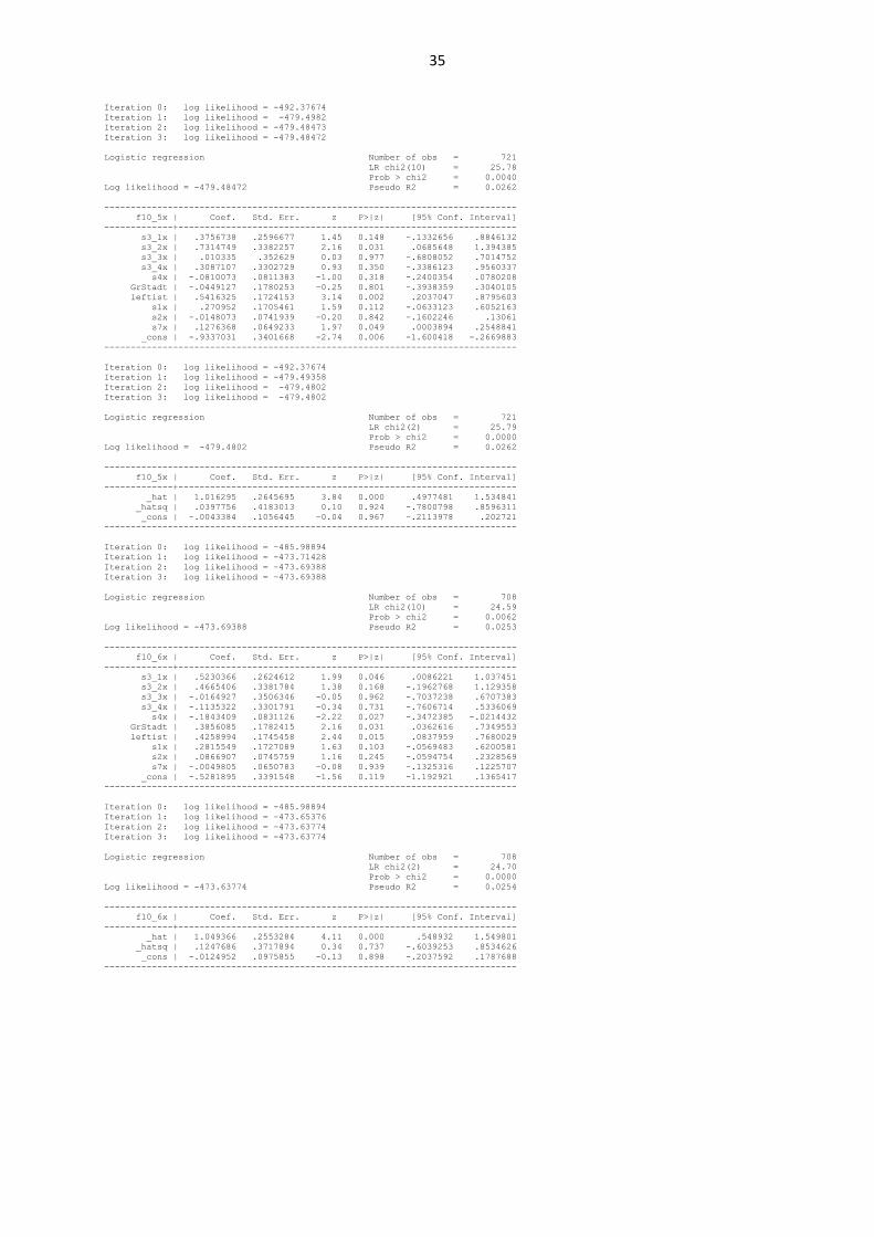
35

Iteration 0: log likelihood = -492.37674 Iteration 1: log likelihood = -479.4982 Iteration 2: log likelihood = -479.48473 Iteration 3: log likelihood = -479.48472 Logistic regression Number of obs = 721 LR chi2(10) = 25.78 Prob > chi2 = 0.0040 Log likelihood = -479.48472 Pseudo R2 = 0.0262 ------------------------------------------------------------------------------ f10_5x | Coef. Std. Err. z P>|z| [95% Conf. Interval] -------------+---------------------------------------------------------------- s3_1x | .3756738 .2596677 1.45 0.148 -.1332656 .8846132 s3_2x | .7314749 .3382257 2.16 0.031 .0685648 1.394385 s3_3x | .010335 .352629 0.03 0.977 -.6808052 .7014752 s3_4x | .3087107 .3302729 0.93 0.350 -.3386123 .9560337 s4x | -.0810073 .0811383 -1.00 0.318 -.2400354 .0780208 GrStadt | -.0449127 .1780253 -0.25 0.801 -.3938359 .3040105 leftist | .5416325 .1724153 3.14 0.002 .2037047 .8795603 s1x | .270952 .1705461 1.59 0.112 -.0633123 .6052163 s2x | -.0148073 .0741939 -0.20 0.842 -.1602246 .13061 s7x | .1276368 .0649233 1.97 0.049 .0003894 .2548841 _cons | -.9337031 .3401668 -2.74 0.006 -1.600418 -.2669883 ------------------------------------------------------------------------------ Iteration 0: log likelihood = -492.37674 Iteration 1: log likelihood = -479.49358 Iteration 2: log likelihood = -479.4802 Iteration 3: log likelihood = -479.4802 Logistic regression Number of obs = 721 LR chi2(2) = 25.79 Prob > chi2 = 0.0000 Log likelihood = -479.4802 Pseudo R2 = 0.0262 ------------------------------------------------------------------------------ f10_5x | Coef. Std. Err. z P>|z| [95% Conf. Interval] -------------+---------------------------------------------------------------- _hat | 1.016295 .2645695 3.84 0.000 .4977481 1.534841 _hatsq | .0397756 .4183013 0.10 0.924 -.7800798 .8596311 _cons | -.0043384 .1056445 -0.04 0.967 -.2113978 .202721 ------------------------------------------------------------------------------ Iteration 0: log likelihood = -485.98894 Iteration 1: log likelihood = -473.71428 Iteration 2: log likelihood = -473.69388 Iteration 3: log likelihood = -473.69388 Logistic regression Number of obs = 708 LR chi2(10) = 24.59 Prob > chi2 = 0.0062 Log likelihood = -473.69388 Pseudo R2 = 0.0253 ------------------------------------------------------------------------------ f10_6x | Coef. Std. Err. z P>|z| [95% Conf. Interval] -------------+---------------------------------------------------------------- s3_1x | .5230366 .2624612 1.99 0.046 .0086221 1.037451 s3_2x | .4665406 .3381784 1.38 0.168 -.1962768 1.129358 s3_3x | -.0164927 .3506346 -0.05 0.962 -.7037238 .6707383 s3_4x | -.1135322 .3301791 -0.34 0.731 -.7606714 .5336069 s4x | -.1843409 .0831126 -2.22 0.027 -.3472385 -.0214432 GrStadt | .3856085 .1782415 2.16 0.031 .0362616 .7349553 leftist | .4258994 .1745458 2.44 0.015 .0837959 .7680029 s1x | .2815549 .1727089 1.63 0.103 -.0569483 .6200581 s2x | .0866907 .0745759 1.16 0.245 -.0594754 .2328569 s7x | -.0049805 .0650783 -0.08 0.939 -.1325316 .1225707 _cons | -.5281895 .3391548 -1.56 0.119 -1.192921 .1365417 ------------------------------------------------------------------------------ Iteration 0: log likelihood = -485.98894 Iteration 1: log likelihood = -473.65376 Iteration 2: log likelihood = -473.63774 Iteration 3: log likelihood = -473.63774 Logistic regression Number of obs = 708 LR chi2(2) = 24.70 Prob > chi2 = 0.0000 Log likelihood = -473.63774 Pseudo R2 = 0.0254 ------------------------------------------------------------------------------ f10_6x | Coef. Std. Err. z P>|z| [95% Conf. Interval] -------------+---------------------------------------------------------------- _hat | 1.049366 .2553284 4.11 0.000 .548932 1.549801 _hatsq | .1247686 .3717894 0.34 0.737 -.6039253 .8534626 _cons | -.0124952 .0975855 -0.13 0.898 -.2037592 .1787688 ------------------------------------------------------------------------------

36

Iteration 0: log likelihood = -281.13036 Iteration 1: log likelihood = -274.51846 Iteration 2: log likelihood = -274.3273 Iteration 3: log likelihood = -274.32714 Logistic regression Number of obs = 722 LR chi2(10) = 13.61 Prob > chi2 = 0.1917 Log likelihood = -274.32714 Pseudo R2 = 0.0242 ------------------------------------------------------------------------------ f10_7x | Coef. Std. Err. z P>|z| [95% Conf. Interval] -------------+---------------------------------------------------------------- s3_1x | .3385971 .3608063 0.94 0.348 -.3685702 1.045764 s3_2x | -.2286306 .5028057 -0.45 0.649 -1.214112 .7568505 s3_3x | -.3241497 .5516205 -0.59 0.557 -1.405306 .7570067 s3_4x | .2000031 .4911313 0.41 0.684 -.7625966 1.162603 s4x | -.0065663 .1187813 -0.06 0.956 -.2393733 .2262408 GrStadt | .0851923 .2527334 0.34 0.736 -.4101561 .5805408 leftist | .5197652 .2365813 2.20 0.028 .0560744 .9834561 s1x | -.2004049 .2469172 -0.81 0.417 -.6843538 .283544 s2x | -.1345566 .1088282 -1.24 0.216 -.347856 .0787427 s7x | .0118766 .0938441 0.13 0.899 -.1720544 .1958075 _cons | -1.632392 .4788948 -3.41 0.001 -2.571009 -.6937758 ------------------------------------------------------------------------------ Iteration 0: log likelihood = -281.13036 Iteration 1: log likelihood = -274.66602 Iteration 2: log likelihood = -274.27437 Iteration 3: log likelihood = -274.27312 Iteration 4: log likelihood = -274.27312 Logistic regression Number of obs = 722 LR chi2(2) = 13.71 Prob > chi2 = 0.0011 Log likelihood = -274.27312 Pseudo R2 = 0.0244 ------------------------------------------------------------------------------ f10_7x | Coef. Std. Err. z P>|z| [95% Conf. Interval] -------------+---------------------------------------------------------------- _hat | .329735 2.071035 0.16 0.874 -3.729419 4.388889 _hatsq | -.1864166 .5711166 -0.33 0.744 -1.305785 .9329513 _cons | -.5716014 1.825433 -0.31 0.754 -4.149385 3.006182 ------------------------------------------------------------------------------ Iteration 0: log likelihood = -276.36333 Iteration 1: log likelihood = -266.03795 Iteration 2: log likelihood = -265.35992 Iteration 3: log likelihood = -265.35773 Iteration 4: log likelihood = -265.35773 Logistic regression Number of obs = 729 LR chi2(10) = 22.01 Prob > chi2 = 0.0150 Log likelihood = -265.35773 Pseudo R2 = 0.0398 ------------------------------------------------------------------------------ f10_8x | Coef. Std. Err. z P>|z| [95% Conf. Interval] -------------+---------------------------------------------------------------- s3_1x | .242549 .3761991 0.64 0.519 -.4947876 .9798856 s3_2x | -.2484771 .54983 -0.45 0.651 -1.326124 .8291699 s3_3x | .8996532 .4598787 1.96 0.050 -.0016924 1.800999 s3_4x | .2481632 .5107392 0.49 0.627 -.7528672 1.249194 s4x | -.1417068 .1207192 -1.17 0.240 -.3783121 .0948985 GrStadt | .0679913 .2654792 0.26 0.798 -.4523384 .5883211 leftist | -.5965709 .2887599 -2.07 0.039 -1.16253 -.0306119 s1x | .4693406 .2560559 1.83 0.067 -.0325197 .9712008 s2x | -.1515589 .1091757 -1.39 0.165 -.3655393 .0624216 s7x | -.00099 .0958896 -0.01 0.992 -.1889301 .1869501 _cons | -1.312198 .4829477 -2.72 0.007 -2.258758 -.3656378 ------------------------------------------------------------------------------ Iteration 0: log likelihood = -276.36333 Iteration 1: log likelihood = -266.49374 Iteration 2: log likelihood = -264.5536 Iteration 3: log likelihood = -264.55165 Iteration 4: log likelihood = -264.55165 Logistic regression Number of obs = 729 LR chi2(2) = 23.62 Prob > chi2 = 0.0000 Log likelihood = -264.55165 Pseudo R2 = 0.0427 ------------------------------------------------------------------------------ f10_8x | Coef. Std. Err. z P>|z| [95% Conf. Interval] -------------+---------------------------------------------------------------- _hat | 2.3941 1.093294 2.19 0.029 .251283 4.536917 _hatsq | .3813864 .2912207 1.31 0.190 -.1893957 .9521686 _cons | 1.16292 .9837907 1.18 0.237 -.7652744 3.091114 ------------------------------------------------------------------------------

37

Iteration 0: log likelihood = -458.04246 Iteration 1: log likelihood = -453.02463 Iteration 2: log likelihood = -453.02225 Logistic regression Number of obs = 669 LR chi2(10) = 10.04 Prob > chi2 = 0.4370 Log likelihood = -453.02225 Pseudo R2 = 0.0110 ------------------------------------------------------------------------------ f10_9x | Coef. Std. Err. z P>|z| [95% Conf. Interval] -------------+---------------------------------------------------------------- s3_1x | -.3260807 .2632399 -1.24 0.215 -.8420215 .1898601 s3_2x | -.5054093 .3447809 -1.47 0.143 -1.181168 .1703488 s3_3x | -.6688831 .3579875 -1.87 0.062 -1.370526 .0327595 s3_4x | -.5361216 .3387615 -1.58 0.114 -1.200082 .1278388 s4x | .1245927 .0820671 1.52 0.129 -.0362558 .2854412 GrStadt | -.0082001 .1813607 -0.05 0.964 -.3636605 .3472603 leftist | .1774838 .1765596 1.01 0.315 -.1685665 .5235342 s1x | .1725378 .1754773 0.98 0.325 -.1713915 .5164671 s2x | .1227652 .0769142 1.60 0.110 -.0279839 .2735143 s7x | -.0508847 .0672507 -0.76 0.449 -.1826937 .0809244 _cons | -.7086393 .3484193 -2.03 0.042 -1.391529 -.0257501 ------------------------------------------------------------------------------ Iteration 0: log likelihood = -458.04246 Iteration 1: log likelihood = -452.45237 Iteration 2: log likelihood = -452.43413 Iteration 3: log likelihood = -452.43413 Logistic regression Number of obs = 669 LR chi2(2) = 11.22 Prob > chi2 = 0.0037 Log likelihood = -452.43413 Pseudo R2 = 0.0122 ------------------------------------------------------------------------------ f10_9x | Coef. Std. Err. z P>|z| [95% Conf. Interval] -------------+---------------------------------------------------------------- _hat | .5114024 .5508109 0.93 0.353 -.5681672 1.590972 _hatsq | -.9807602 .9106213 -1.08 0.281 -2.765545 .8040248 _cons | -.0018004 .1135637 -0.02 0.987 -.2243813 .2207804 ------------------------------------------------------------------------------ Iteration 0: log likelihood = -429.76251 Iteration 1: log likelihood = -405.213 Iteration 2: log likelihood = -404.76707 Iteration 3: log likelihood = -404.7662 Logistic regression Number of obs = 719 LR chi2(10) = 49.99 Prob > chi2 = 0.0000 Log likelihood = -404.7662 Pseudo R2 = 0.0582 ------------------------------------------------------------------------------ f10_10x | Coef. Std. Err. z P>|z| [95% Conf. Interval] -------------+---------------------------------------------------------------- s3_1x | .2976663 .2778219 1.07 0.284 -.2468547 .8421873 s3_2x | -.765463 .3519123 -2.18 0.030 -1.455198 -.0757277 s3_3x | .8350654 .4311159 1.94 0.053 -.0099062 1.680037 s3_4x | .0206825 .3680803 0.06 0.955 -.7007416 .7421066 s4x | .068569 .0932661 0.74 0.462 -.1142292 .2513671 GrStadt | -.5791879 .1920034 -3.02 0.003 -.9555076 -.2028681 leftist | -.1989463 .1907554 -1.04 0.297 -.5728201 .1749275 s1x | .358933 .1920503 1.87 0.062 -.0174787 .7353446 s2x | .213842 .0834384 2.56 0.010 .0503057 .3773783 s7x | .1389475 .0723263 1.92 0.055 -.0028095 .2807044 _cons | -.4931833 .3619756 -1.36 0.173 -1.202642 .2162759 ------------------------------------------------------------------------------ Iteration 0: log likelihood = -429.76251 Iteration 1: log likelihood = -405.31488 Iteration 2: log likelihood = -404.69975 Iteration 3: log likelihood = -404.69799 Iteration 4: log likelihood = -404.69799 Logistic regression Number of obs = 719 LR chi2(2) = 50.13 Prob > chi2 = 0.0000 Log likelihood = -404.69799 Pseudo R2 = 0.0583 ------------------------------------------------------------------------------ f10_10x | Coef. Std. Err. z P>|z| [95% Conf. Interval] -------------+---------------------------------------------------------------- _hat | 1.110256 .3338269 3.33 0.001 .455967 1.764544 _hatsq | -.0682075 .1840123 -0.37 0.711 -.428865 .29245 _cons | -.0213566 .1643118 -0.13 0.897 -.3434018 .3006886 ------------------------------------------------------------------------------

38

Annex 4 – Acceptance of policy measures by several determinants (lo-git models without ideological orientation)

39

Collinearity Diagnostics SQRT R- Variable VIF VIF Tolerance Squared ---------------------------------------------------- f11_1x 1.04 1.02 0.9621 0.0379 s3_1x 2.41 1.55 0.4153 0.5847 s3_2x 1.80 1.34 0.5560 0.4440 s3_3x 1.67 1.29 0.5979 0.4021 s3_4x 3.94 1.99 0.2537 0.7463 s4x 1.69 1.30 0.5902 0.4098 GrStadt 1.09 1.04 0.9207 0.0793 s1x 1.21 1.10 0.8236 0.1764 s2x 2.51 1.58 0.3984 0.6016 s7x 1.28 1.13 0.7803 0.2197 ---------------------------------------------------- Mean VIF 1.86 Cond Eigenval Index --------------------------------- 1 6.2531 1.0000 2 1.1349 2.3473 3 1.0114 2.4865 4 1.0028 2.4971 5 0.6832 3.0254 6 0.4473 3.7389 7 0.1921 5.7056 8 0.1245 7.0882 9 0.0632 9.9504 10 0.0614 10.0907 11 0.0263 15.4290 --------------------------------- Condition Number 15.4290 Eigenvalues & Cond Index computed from scaled raw sscp (w/ intercept) Det(correlation matrix) 0.0883 Iteration 0: log likelihood = -139.05462 Iteration 1: log likelihood = -129.90606 Iteration 2: log likelihood = -124.82493 Iteration 3: log likelihood = -124.64751 Iteration 4: log likelihood = -124.64687 Iteration 5: log likelihood = -124.64687 Logistic regression Number of obs = 924 LR chi2(10) = 28.82 Prob > chi2 = 0.0013 Log likelihood = -124.64687 Pseudo R2 = 0.1036 ------------------------------------------------------------------------------ f10_1x | Coef. Std. Err. z P>|z| [95% Conf. Interval] -------------+---------------------------------------------------------------- f11_1x | -.4746259 .5240467 -0.91 0.365 -1.501739 .5524868 s3_1x | -.9755235 .5961048 -1.64 0.102 -2.143868 .1928205 s3_2x | -.8363936 .7757693 -1.08 0.281 -2.356873 .6840862 s3_3x | -1.105469 .8753234 -1.26 0.207 -2.821071 .6101335 s3_4x | .2119853 .8514097 0.25 0.803 -1.456747 1.880718 s4x | -.0700955 .1905369 -0.37 0.713 -.4435411 .30335 GrStadt | .1715122 .4013359 0.43 0.669 -.6150916 .9581161 s1x | 1.40822 .4464776 3.15 0.002 .5331396 2.283299 s2x | -.2596375 .1907051 -1.36 0.173 -.6334126 .1141376 s7x | .3460981 .1594046 2.17 0.030 .0336708 .6585255 _cons | -3.411415 .9180069 -3.72 0.000 -5.210675 -1.612155 ------------------------------------------------------------------------------ Iteration 0: log likelihood = -139.05462 Iteration 1: log likelihood = -126.36963 Iteration 2: log likelihood = -124.46229 Iteration 3: log likelihood = -124.28626 Iteration 4: log likelihood = -124.28322 Iteration 5: log likelihood = -124.28321 Logistic regression Number of obs = 924 LR chi2(2) = 29.54 Prob > chi2 = 0.0000 Log likelihood = -124.28321 Pseudo R2 = 0.1062 ------------------------------------------------------------------------------ f10_1x | Coef. Std. Err. z P>|z| [95% Conf. Interval] -------------+---------------------------------------------------------------- _hat | 1.765106 .8962089 1.97 0.049 .0085692 3.521643 _hatsq | .128206 .1457282 0.88 0.379 -.1574161 .413828 _cons | 1.013852 1.293131 0.78 0.433 -1.520637 3.548341 ------------------------------------------------------------------------------

40

Collinearity Diagnostics SQRT R- Variable VIF VIF Tolerance Squared ---------------------------------------------------- f11_2x 1.09 1.04 0.9184 0.0816 s3_1x 2.41 1.55 0.4156 0.5844 s3_2x 1.80 1.34 0.5564 0.4436 s3_3x 1.67 1.29 0.5986 0.4014 s3_4x 3.92 1.98 0.2554 0.7446 s4x 1.71 1.31 0.5833 0.4167 GrStadt 1.11 1.05 0.8989 0.1011 s1x 1.21 1.10 0.8236 0.1764 s2x 2.50 1.58 0.4002 0.5998 s7x 1.27 1.13 0.7865 0.2135 ---------------------------------------------------- Mean VIF 1.87 Cond Eigenval Index --------------------------------- 1 6.1975 1.0000 2 1.1428 2.3287 3 1.0112 2.4757 4 1.0018 2.4873 5 0.6939 2.9885 6 0.4450 3.7318 7 0.1976 5.5999 8 0.1487 6.4549 9 0.0725 9.2468 10 0.0610 10.0786 11 0.0280 14.8774 --------------------------------- Condition Number 14.8774 Eigenvalues & Cond Index computed from scaled raw sscp (w/ intercept) Det(correlation matrix) 0.0846 Iteration 0: log likelihood = -355.02402 Iteration 1: log likelihood = -312.69592 Iteration 2: log likelihood = -305.60197 Iteration 3: log likelihood = -305.53608 Iteration 4: log likelihood = -305.53603 Logistic regression Number of obs = 925 LR chi2(10) = 98.98 Prob > chi2 = 0.0000 Log likelihood = -305.53603 Pseudo R2 = 0.1394 ------------------------------------------------------------------------------ f10_2x | Coef. Std. Err. z P>|z| [95% Conf. Interval] -------------+---------------------------------------------------------------- f11_2x | -1.583581 .2536987 -6.24 0.000 -2.080821 -1.086341 s3_1x | -.5636687 .3366544 -1.67 0.094 -1.223499 .0961617 s3_2x | .0967693 .3931482 0.25 0.806 -.6737871 .8673257 s3_3x | -.1428504 .4443502 -0.32 0.748 -1.013761 .72806 s3_4x | -.3878565 .4743449 -0.82 0.414 -1.317555 .5418424 s4x | -.0627614 .108117 -0.58 0.562 -.2746668 .1491439 GrStadt | .3647034 .2327752 1.57 0.117 -.0915276 .8209344 s1x | .5097882 .2296693 2.22 0.026 .0596446 .9599319 s2x | -.3051157 .1014606 -3.01 0.003 -.5039749 -.1062566 s7x | .2603797 .0876504 2.97 0.003 .0885881 .4321712 _cons | -.3594961 .4711545 -0.76 0.445 -1.282942 .5639497 ------------------------------------------------------------------------------ Iteration 0: log likelihood = -355.02402 Iteration 1: log likelihood = -319.69515 Iteration 2: log likelihood = -309.367 Iteration 3: log likelihood = -305.53441 Iteration 4: log likelihood = -305.53274 Iteration 5: log likelihood = -305.53274 Logistic regression Number of obs = 925 LR chi2(2) = 98.98 Prob > chi2 = 0.0000 Log likelihood = -305.53274 Pseudo R2 = 0.1394 ------------------------------------------------------------------------------ f10_2x | Coef. Std. Err. z P>|z| [95% Conf. Interval] -------------+---------------------------------------------------------------- _hat | 1.019657 .2656996 3.84 0.000 .4988955 1.540419 _hatsq | .0065659 .0808924 0.08 0.935 -.1519804 .1651122 _cons | .0083471 .2318324 0.04 0.971 -.4460362 .4627303 ------------------------------------------------------------------------------

41

Collinearity Diagnostics SQRT R- Variable VIF VIF Tolerance Squared ---------------------------------------------------- f11_3x 1.03 1.01 0.9731 0.0269 s3_1x 2.44 1.56 0.4097 0.5903 s3_2x 1.83 1.35 0.5468 0.4532 s3_3x 1.68 1.30 0.5941 0.4059 s3_4x 3.93 1.98 0.2542 0.7458 s4x 1.72 1.31 0.5824 0.4176 GrStadt 1.07 1.04 0.9331 0.0669 s1x 1.21 1.10 0.8253 0.1747 s2x 2.49 1.58 0.4014 0.5986 s7x 1.26 1.12 0.7953 0.2047 ---------------------------------------------------- Mean VIF 1.87 Cond Eigenval Index --------------------------------- 1 5.5992 1.0000 2 1.1445 2.2118 3 1.0220 2.3406 4 1.0010 2.3651 5 0.7861 2.6689 6 0.6748 2.8805 7 0.4247 3.6309 8 0.1739 5.6736 9 0.0801 8.3619 10 0.0610 9.5817 11 0.0326 13.1072 --------------------------------- Condition Number 13.1072 Eigenvalues & Cond Index computed from scaled raw sscp (w/ intercept) Det(correlation matrix) 0.0896 Iteration 0: log likelihood = -445.86032 Iteration 1: log likelihood = -425.03488 Iteration 2: log likelihood = -424.07714 Iteration 3: log likelihood = -424.07136 Iteration 4: log likelihood = -424.07135 Logistic regression Number of obs = 847 LR chi2(10) = 43.58 Prob > chi2 = 0.0000 Log likelihood = -424.07135 Pseudo R2 = 0.0489 ------------------------------------------------------------------------------ f10_3x | Coef. Std. Err. z P>|z| [95% Conf. Interval] -------------+---------------------------------------------------------------- f11_3x | -.969981 .2075768 -4.67 0.000 -1.376824 -.563138 s3_1x | .0004965 .2753082 0.00 0.999 -.5390976 .5400907 s3_2x | 1.015674 .4290401 2.37 0.018 .1747707 1.856577 s3_3x | -.6341687 .3544241 -1.79 0.074 -1.328827 .0604897 s3_4x | -.1772715 .3605068 -0.49 0.623 -.8838518 .5293087 s4x | .0713204 .0881772 0.81 0.419 -.1015038 .2441445 GrStadt | -.0087045 .1944271 -0.04 0.964 -.3897746 .3723656 s1x | .1036337 .1865056 0.56 0.578 -.2619105 .4691779 s2x | .0666749 .0810085 0.82 0.410 -.0920988 .2254485 s7x | -.1506376 .0725813 -2.08 0.038 -.2928943 -.008381 _cons | 1.427926 .3719589 3.84 0.000 .6988999 2.156952 ------------------------------------------------------------------------------ Iteration 0: log likelihood = -445.86032 Iteration 1: log likelihood = -424.46887 Iteration 2: log likelihood = -423.26375 Iteration 3: log likelihood = -423.26167 Logistic regression Number of obs = 847 LR chi2(2) = 45.20 Prob > chi2 = 0.0000 Log likelihood = -423.26167 Pseudo R2 = 0.0507 ------------------------------------------------------------------------------ f10_3x | Coef. Std. Err. z P>|z| [95% Conf. Interval] -------------+---------------------------------------------------------------- _hat | 1.524637 .439697 3.47 0.001 .6628465 2.386427 _hatsq | -.2281285 .1753145 -1.30 0.193 -.5717387 .1154816 _cons | -.2312822 .27622 -0.84 0.402 -.7726634 .310099 ------------------------------------------------------------------------------

42

Collinearity Diagnostics SQRT R- Variable VIF VIF Tolerance Squared ---------------------------------------------------- f11_4x 1.03 1.01 0.9746 0.0254 s3_1x 2.42 1.56 0.4126 0.5874 s3_2x 1.80 1.34 0.5548 0.4452 s3_3x 1.69 1.30 0.5921 0.4079 s3_4x 3.90 1.98 0.2561 0.7439 s4x 1.70 1.30 0.5888 0.4112 GrStadt 1.08 1.04 0.9277 0.0723 s1x 1.20 1.10 0.8326 0.1674 s2x 2.47 1.57 0.4042 0.5958 s7x 1.26 1.12 0.7936 0.2064 ---------------------------------------------------- Mean VIF 1.86 Cond Eigenval Index --------------------------------- 1 5.6603 1.0000 2 1.1303 2.2378 3 1.0546 2.3167 4 1.0021 2.3766 5 0.7324 2.7801 6 0.6433 2.9662 7 0.4268 3.6416 8 0.1769 5.6569 9 0.0787 8.4831 10 0.0618 9.5727 11 0.0328 13.1380 --------------------------------- Condition Number 13.1380 Eigenvalues & Cond Index computed from scaled raw sscp (w/ intercept) Det(correlation matrix) 0.0913 Iteration 0: log likelihood = -579.39838 Iteration 1: log likelihood = -545.14665 Iteration 2: log likelihood = -544.79142 Iteration 3: log likelihood = -544.79112 Logistic regression Number of obs = 862 LR chi2(10) = 69.21 Prob > chi2 = 0.0000 Log likelihood = -544.79112 Pseudo R2 = 0.0597 ------------------------------------------------------------------------------ f10_4x | Coef. Std. Err. z P>|z| [95% Conf. Interval] -------------+---------------------------------------------------------------- f11_4x | -.5949641 .1689332 -3.52 0.000 -.9260671 -.263861 s3_1x | -.182352 .2538342 -0.72 0.473 -.6798579 .3151539 s3_2x | .1168218 .3244564 0.36 0.719 -.5191012 .7527447 s3_3x | -.3621152 .3352985 -1.08 0.280 -1.019288 .2950579 s3_4x | .2443964 .3072911 0.80 0.426 -.357883 .8466758 s4x | -.0720567 .0772025 -0.93 0.351 -.2233708 .0792574 GrStadt | .5983563 .1730874 3.46 0.001 .2591112 .9376014 s1x | -.0979215 .1595453 -0.61 0.539 -.4106245 .2147816 s2x | -.3052079 .072053 -4.24 0.000 -.4464291 -.1639868 s7x | .1083354 .0621328 1.74 0.081 -.0134426 .2301134 _cons | 1.52982 .3340545 4.58 0.000 .8750851 2.184555 ------------------------------------------------------------------------------ Iteration 0: log likelihood = -579.39838 Iteration 1: log likelihood = -545.14096 Iteration 2: log likelihood = -544.47975 Iteration 3: log likelihood = -544.47568 Iteration 4: log likelihood = -544.47568 Logistic regression Number of obs = 862 LR chi2(2) = 69.85 Prob > chi2 = 0.0000 Log likelihood = -544.47568 Pseudo R2 = 0.0603 ------------------------------------------------------------------------------ f10_4x | Coef. Std. Err. z P>|z| [95% Conf. Interval] -------------+---------------------------------------------------------------- _hat | .8709307 .2053518 4.24 0.000 .4684486 1.273413 _hatsq | .1391982 .1763267 0.79 0.430 -.2063959 .4847923 _cons | -.015834 .0887419 -0.18 0.858 -.189765 .158097 ------------------------------------------------------------------------------

43

Collinearity Diagnostics SQRT R- Variable VIF VIF Tolerance Squared ---------------------------------------------------- f11_5x 1.03 1.01 0.9746 0.0254 s3_1x 2.40 1.55 0.4159 0.5841 s3_2x 1.81 1.35 0.5512 0.4488 s3_3x 1.69 1.30 0.5929 0.4071 s3_4x 3.91 1.98 0.2555 0.7445 s4x 1.70 1.30 0.5889 0.4111 GrStadt 1.08 1.04 0.9288 0.0712 s1x 1.21 1.10 0.8239 0.1761 s2x 2.50 1.58 0.4001 0.5999 s7x 1.28 1.13 0.7828 0.2172 ---------------------------------------------------- Mean VIF 1.86 Cond Eigenval Index --------------------------------- 1 5.8640 1.0000 2 1.1362 2.2718 3 1.0116 2.4076 4 1.0010 2.4203 5 0.6843 2.9273 6 0.5735 3.1976 7 0.3836 3.9096 8 0.1717 5.8437 9 0.0801 8.5553 10 0.0619 9.7346 11 0.0320 13.5471 --------------------------------- Condition Number 13.5471 Eigenvalues & Cond Index computed from scaled raw sscp (w/ intercept) Det(correlation matrix) 0.0897 Iteration 0: log likelihood = -607.53773 Iteration 1: log likelihood = -594.13749 Iteration 2: log likelihood = -594.11257 Iteration 3: log likelihood = -594.11257 Logistic regression Number of obs = 899 LR chi2(10) = 26.85 Prob > chi2 = 0.0028 Log likelihood = -594.11257 Pseudo R2 = 0.0221 ------------------------------------------------------------------------------ f10_5x | Coef. Std. Err. z P>|z| [95% Conf. Interval] -------------+---------------------------------------------------------------- f11_5x | -.4001695 .1411858 -2.83 0.005 -.6768887 -.1234504 s3_1x | .3967122 .2338003 1.70 0.090 -.061528 .8549523 s3_2x | .5120379 .296031 1.73 0.084 -.0681722 1.092248 s3_3x | -.0191488 .319908 -0.06 0.952 -.646157 .6078593 s3_4x | .2284003 .2956028 0.77 0.440 -.3509704 .8077711 s4x | -.0524568 .0737282 -0.71 0.477 -.1969615 .0920479 GrStadt | .0849658 .1579498 0.54 0.591 -.22461 .3945417 s1x | .180612 .1515784 1.19 0.233 -.1164762 .4777002 s2x | -.0382935 .0670906 -0.57 0.568 -.1697887 .0932017 s7x | .1620153 .0588699 2.75 0.006 .0466325 .2773981 _cons | -.7255472 .3085521 -2.35 0.019 -1.330298 -.1207962 ------------------------------------------------------------------------------ Iteration 0: log likelihood = -607.53773 Iteration 1: log likelihood = -593.92866 Iteration 2: log likelihood = -593.90419 Iteration 3: log likelihood = -593.90419 Logistic regression Number of obs = 899 LR chi2(2) = 27.27 Prob > chi2 = 0.0000 Log likelihood = -593.90419 Pseudo R2 = 0.0224 ------------------------------------------------------------------------------ f10_5x | Coef. Std. Err. z P>|z| [95% Conf. Interval] -------------+---------------------------------------------------------------- _hat | 1.214743 .3878184 3.13 0.002 .4546328 1.974853 _hatsq | .2805059 .4338523 0.65 0.518 -.569829 1.130841 _cons | .0065248 .1003216 0.07 0.948 -.190102 .2031516 ------------------------------------------------------------------------------

44

Collinearity Diagnostics SQRT R- Variable VIF VIF Tolerance Squared ---------------------------------------------------- f11_6x 1.03 1.01 0.9734 0.0266 s3_1x 2.43 1.56 0.4120 0.5880 s3_2x 1.80 1.34 0.5545 0.4455 s3_3x 1.69 1.30 0.5922 0.4078 s3_4x 3.99 2.00 0.2508 0.7492 s4x 1.70 1.30 0.5900 0.4100 GrStadt 1.08 1.04 0.9271 0.0729 s1x 1.21 1.10 0.8249 0.1751 s2x 2.53 1.59 0.3956 0.6044 s7x 1.27 1.13 0.7867 0.2133 ---------------------------------------------------- Mean VIF 1.87 Cond Eigenval Index --------------------------------- 1 5.9202 1.0000 2 1.1414 2.2774 3 1.0139 2.4164 4 1.0014 2.4315 5 0.6845 2.9410 6 0.4956 3.4562 7 0.3996 3.8491 8 0.1717 5.8717 9 0.0786 8.6778 10 0.0614 9.8167 11 0.0317 13.6551 --------------------------------- Condition Number 13.6551 Eigenvalues & Cond Index computed from scaled raw sscp (w/ intercept) Det(correlation matrix) 0.0881 Iteration 0: log likelihood = -594.32321 Iteration 1: log likelihood = -565.77168 Iteration 2: log likelihood = -565.66553 Iteration 3: log likelihood = -565.66551 Logistic regression Number of obs = 873 LR chi2(10) = 57.32 Prob > chi2 = 0.0000 Log likelihood = -565.66551 Pseudo R2 = 0.0482 ------------------------------------------------------------------------------ f10_6x | Coef. Std. Err. z P>|z| [95% Conf. Interval] -------------+---------------------------------------------------------------- f11_6x | -.8951125 .1447197 -6.19 0.000 -1.178758 -.611467 s3_1x | .4372341 .2448566 1.79 0.074 -.042676 .9171441 s3_2x | .5459479 .3078542 1.77 0.076 -.0574352 1.149331 s3_3x | -.0251081 .3260715 -0.08 0.939 -.6641965 .6139804 s3_4x | -.2667711 .30728 -0.87 0.385 -.8690288 .3354867 s4x | -.1194084 .0769363 -1.55 0.121 -.2702008 .0313841 GrStadt | .2807228 .1629829 1.72 0.085 -.0387177 .6001634 s1x | .2823244 .1567624 1.80 0.072 -.0249243 .5895731 s2x | .1264928 .0696854 1.82 0.069 -.010088 .2630736 s7x | .0727424 .0604919 1.20 0.229 -.0458195 .1913044 _cons | -.5497192 .3167714 -1.74 0.083 -1.17058 .0711413 ------------------------------------------------------------------------------ Iteration 0: log likelihood = -594.32321 Iteration 1: log likelihood = -564.80966 Iteration 2: log likelihood = -564.74673 Iteration 3: log likelihood = -564.74672 Logistic regression Number of obs = 873 LR chi2(2) = 59.15 Prob > chi2 = 0.0000 Log likelihood = -564.74672 Pseudo R2 = 0.0498 ------------------------------------------------------------------------------ f10_6x | Coef. Std. Err. z P>|z| [95% Conf. Interval] -------------+---------------------------------------------------------------- _hat | 1.214831 .2124313 5.72 0.000 .798473 1.631188 _hatsq | .3280926 .2423167 1.35 0.176 -.1468394 .8030245 _cons | -.0533402 .0909631 -0.59 0.558 -.2316245 .1249442 ------------------------------------------------------------------------------

45

Collinearity Diagnostics SQRT R- Variable VIF VIF Tolerance Squared ---------------------------------------------------- f11_7x 1.02 1.01 0.9802 0.0198 s3_1x 2.43 1.56 0.4119 0.5881 s3_2x 1.82 1.35 0.5482 0.4518 s3_3x 1.69 1.30 0.5921 0.4079 s3_4x 3.91 1.98 0.2558 0.7442 s4x 1.69 1.30 0.5906 0.4094 GrStadt 1.08 1.04 0.9289 0.0711 s1x 1.21 1.10 0.8274 0.1726 s2x 2.45 1.57 0.4076 0.5924 s7x 1.26 1.12 0.7930 0.2070 ---------------------------------------------------- Mean VIF 1.86 Cond Eigenval Index --------------------------------- 1 6.0195 1.0000 2 1.1321 2.3059 3 1.0114 2.4396 4 1.0010 2.4523 5 0.6820 2.9708 6 0.4626 3.6073 7 0.3485 4.1558 8 0.1700 5.9511 9 0.0779 8.7926 10 0.0619 9.8608 11 0.0330 13.4967 --------------------------------- Condition Number 13.4967 Eigenvalues & Cond Index computed from scaled raw sscp (w/ intercept) Det(correlation matrix) 0.0921 Iteration 0: log likelihood = -344.06992 Iteration 1: log likelihood = -326.25427 Iteration 2: log likelihood = -325.27808 Iteration 3: log likelihood = -325.27629 Iteration 4: log likelihood = -325.27629 Logistic regression Number of obs = 874 LR chi2(10) = 37.59 Prob > chi2 = 0.0000 Log likelihood = -325.27629 Pseudo R2 = 0.0546 ------------------------------------------------------------------------------ f10_7x | Coef. Std. Err. z P>|z| [95% Conf. Interval] -------------+---------------------------------------------------------------- f11_7x | -1.022696 .2082488 -4.91 0.000 -1.430856 -.6145354 s3_1x | .4589042 .3341138 1.37 0.170 -.195947 1.113755 s3_2x | -.0772627 .4504489 -0.17 0.864 -.9601263 .8056008 s3_3x | -.1502098 .4942807 -0.30 0.761 -1.118982 .8185625 s3_4x | .0278132 .4557076 0.06 0.951 -.8653573 .9209838 s4x | -.0393377 .1077317 -0.37 0.715 -.2504879 .1718125 GrStadt | .105727 .231438 0.46 0.648 -.3478832 .5593371 s1x | -.1256128 .2233989 -0.56 0.574 -.5634666 .312241 s2x | -.1123279 .0973187 -1.15 0.248 -.303069 .0784132 s7x | .0774425 .0860864 0.90 0.368 -.0912838 .2461688 _cons | -1.164632 .4391874 -2.65 0.008 -2.025423 -.3038406 ------------------------------------------------------------------------------ Iteration 0: log likelihood = -344.06992 Iteration 1: log likelihood = -327.47914 Iteration 2: log likelihood = -324.12732 Iteration 3: log likelihood = -324.12505 Logistic regression Number of obs = 874 LR chi2(2) = 39.89 Prob > chi2 = 0.0000 Log likelihood = -324.12505 Pseudo R2 = 0.0580 ------------------------------------------------------------------------------ f10_7x | Coef. Std. Err. z P>|z| [95% Conf. Interval] -------------+---------------------------------------------------------------- _hat | 2.347366 .8980722 2.61 0.009 .5871771 4.107555 _hatsq | .3822891 .2494639 1.53 0.125 -.1066512 .8712294 _cons | 1.037413 .7425755 1.40 0.162 -.4180085 2.492834 ------------------------------------------------------------------------------

46

Collinearity Diagnostics SQRT R- Variable VIF VIF Tolerance Squared ---------------------------------------------------- f11_8x 1.04 1.02 0.9588 0.0412 s3_1x 2.40 1.55 0.4168 0.5832 s3_2x 1.81 1.34 0.5535 0.4465 s3_3x 1.67 1.29 0.5980 0.4020 s3_4x 3.90 1.97 0.2565 0.7435 s4x 1.71 1.31 0.5842 0.4158 GrStadt 1.08 1.04 0.9284 0.0716 s1x 1.22 1.10 0.8212 0.1788 s2x 2.49 1.58 0.4014 0.5986 s7x 1.27 1.13 0.7863 0.2137 ---------------------------------------------------- Mean VIF 1.86 Cond Eigenval Index --------------------------------- 1 5.9192 1.0000 2 1.1359 2.2828 3 1.0214 2.4073 4 1.0097 2.4213 5 0.6882 2.9327 6 0.5195 3.3756 7 0.3666 4.0181 8 0.1701 5.8990 9 0.0756 8.8472 10 0.0621 9.7600 11 0.0316 13.6898 --------------------------------- Condition Number 13.6898 Eigenvalues & Cond Index computed from scaled raw sscp (w/ intercept) Det(correlation matrix) 0.0884 Iteration 0: log likelihood = -347.07741 Iteration 1: log likelihood = -326.89581 Iteration 2: log likelihood = -325.35765 Iteration 3: log likelihood = -325.34791 Iteration 4: log likelihood = -325.34791 Logistic regression Number of obs = 909 LR chi2(10) = 43.46 Prob > chi2 = 0.0000 Log likelihood = -325.34791 Pseudo R2 = 0.0626 ------------------------------------------------------------------------------ f10_8x | Coef. Std. Err. z P>|z| [95% Conf. Interval] -------------+---------------------------------------------------------------- f11_8x | -.8951392 .2140296 -4.18 0.000 -1.31463 -.4756489 s3_1x | .2779367 .339948 0.82 0.414 -.388349 .9442225 s3_2x | -.8450812 .5282317 -1.60 0.110 -1.880396 .1902339 s3_3x | .6436228 .4158423 1.55 0.122 -.1714132 1.458659 s3_4x | -.1018392 .445303 -0.23 0.819 -.9746171 .7709386 s4x | -.109902 .1096884 -1.00 0.316 -.3248873 .1050834 GrStadt | -.2719653 .245954 -1.11 0.269 -.7540263 .2100956 s1x | .4569566 .2292226 1.99 0.046 .0076886 .9062246 s2x | -.0861864 .0963861 -0.89 0.371 -.2750996 .1027268 s7x | .0065798 .0861767 0.08 0.939 -.1623235 .1754831 _cons | -1.110157 .4537949 -2.45 0.014 -1.999579 -.2207355 ------------------------------------------------------------------------------ Iteration 0: log likelihood = -347.07741 Iteration 1: log likelihood = -327.68985 Iteration 2: log likelihood = -323.5615 Iteration 3: log likelihood = -323.55552 Iteration 4: log likelihood = -323.55552 Logistic regression Number of obs = 909 LR chi2(2) = 47.04 Prob > chi2 = 0.0000 Log likelihood = -323.55552 Pseudo R2 = 0.0678 ------------------------------------------------------------------------------ f10_8x | Coef. Std. Err. z P>|z| [95% Conf. Interval] -------------+---------------------------------------------------------------- _hat | 2.269489 .6690527 3.39 0.001 .95817 3.580809 _hatsq | .3430693 .1728311 1.98 0.047 .0043266 .681812 _cons | 1.016964 .6000035 1.69 0.090 -.1590216 2.192949 ------------------------------------------------------------------------------

47

Collinearity Diagnostics SQRT R- Variable VIF VIF Tolerance Squared ---------------------------------------------------- f11_9x 1.05 1.03 0.9503 0.0497 s3_1x 2.41 1.55 0.4146 0.5854 s3_2x 1.80 1.34 0.5542 0.4458 s3_3x 1.69 1.30 0.5908 0.4092 s3_4x 3.98 1.99 0.2516 0.7484 s4x 1.68 1.30 0.5960 0.4040 GrStadt 1.07 1.04 0.9304 0.0696 s1x 1.21 1.10 0.8257 0.1743 s2x 2.53 1.59 0.3947 0.6053 s7x 1.26 1.12 0.7909 0.2091 ---------------------------------------------------- Mean VIF 1.87 Cond Eigenval Index --------------------------------- 1 5.5871 1.0000 2 1.1907 2.1662 3 1.0527 2.3038 4 1.0018 2.3616 5 0.7362 2.7549 6 0.6616 2.9060 7 0.4227 3.6357 8 0.1750 5.6501 9 0.0786 8.4332 10 0.0621 9.4870 11 0.0316 13.3004 --------------------------------- Condition Number 13.3004 Eigenvalues & Cond Index computed from scaled raw sscp (w/ intercept) Det(correlation matrix) 0.0871 Iteration 0: log likelihood = -564.82395 Iteration 1: log likelihood = -560.84117 Iteration 2: log likelihood = -560.84009 Logistic regression Number of obs = 824 LR chi2(10) = 7.97 Prob > chi2 = 0.6320 Log likelihood = -560.84009 Pseudo R2 = 0.0071 ------------------------------------------------------------------------------ f10_9x | Coef. Std. Err. z P>|z| [95% Conf. Interval] -------------+---------------------------------------------------------------- f11_9x | -.1356998 .1878592 -0.72 0.470 -.503897 .2324974 s3_1x | -.224569 .2379905 -0.94 0.345 -.6910217 .2418838 s3_2x | -.4615312 .3041973 -1.52 0.129 -1.057747 .1346844 s3_3x | -.458881 .3228488 -1.42 0.155 -1.091653 .1738911 s3_4x | -.4429798 .3024844 -1.46 0.143 -1.035838 .1498787 s4x | .124634 .0749817 1.66 0.096 -.0223275 .2715955 GrStadt | .147615 .1618528 0.91 0.362 -.1696106 .4648405 s1x | .0588716 .1556521 0.38 0.705 -.246201 .3639442 s2x | .0747871 .0695112 1.08 0.282 -.0614524 .2110267 s7x | -.0581373 .0602323 -0.97 0.334 -.1761903 .0599158 _cons | -.4881742 .318784 -1.53 0.126 -1.112979 .1366311 ------------------------------------------------------------------------------ Iteration 0: log likelihood = -564.82395 Iteration 1: log likelihood = -560.64087 Iteration 2: log likelihood = -560.63474 Iteration 3: log likelihood = -560.63474 Logistic regression Number of obs = 824 LR chi2(2) = 8.38 Prob > chi2 = 0.0152 Log likelihood = -560.63474 Pseudo R2 = 0.0074 ------------------------------------------------------------------------------ f10_9x | Coef. Std. Err. z P>|z| [95% Conf. Interval] -------------+---------------------------------------------------------------- _hat | .6564606 .6426706 1.02 0.307 -.6031506 1.916072 _hatsq | -.7281998 1.139823 -0.64 0.523 -2.962212 1.505812 _cons | -.0121396 .1142327 -0.11 0.915 -.2360316 .2117525 ------------------------------------------------------------------------------

48

Collinearity Diagnostics SQRT R- Variable VIF VIF Tolerance Squared ---------------------------------------------------- f11_10x 1.05 1.02 0.9566 0.0434 s3_1x 2.40 1.55 0.4171 0.5829 s3_2x 1.82 1.35 0.5503 0.4497 s3_3x 1.67 1.29 0.5985 0.4015 s3_4x 3.87 1.97 0.2583 0.7417 s4x 1.70 1.30 0.5879 0.4121 GrStadt 1.07 1.03 0.9355 0.0645 s1x 1.22 1.10 0.8220 0.1780 s2x 2.47 1.57 0.4049 0.5951 s7x 1.25 1.12 0.7972 0.2028 ---------------------------------------------------- Mean VIF 1.85 Cond Eigenval Index --------------------------------- 1 5.6437 1.0000 2 1.1320 2.2329 3 1.0921 2.2733 4 1.0018 2.3735 5 0.6853 2.8698 6 0.6762 2.8890 7 0.4152 3.6870 8 0.1790 5.6154 9 0.0799 8.4065 10 0.0622 9.5218 11 0.0327 13.1399 --------------------------------- Condition Number 13.1399 Eigenvalues & Cond Index computed from scaled raw sscp (w/ intercept) Det(correlation matrix) 0.0907 Iteration 0: log likelihood = -534.64679 Iteration 1: log likelihood = -493.68571 Iteration 2: log likelihood = -492.86265 Iteration 3: log likelihood = -492.8599 Iteration 4: log likelihood = -492.8599 Logistic regression Number of obs = 884 LR chi2(10) = 83.57 Prob > chi2 = 0.0000 Log likelihood = -492.8599 Pseudo R2 = 0.0782 ------------------------------------------------------------------------------ f10_10x | Coef. Std. Err. z P>|z| [95% Conf. Interval] -------------+---------------------------------------------------------------- f11_10x | -.9848826 .1771747 -5.56 0.000 -1.332139 -.6376265 s3_1x | .0440389 .2533683 0.17 0.862 -.4525539 .5406318 s3_2x | -.6627014 .3201658 -2.07 0.038 -1.290215 -.0351879 s3_3x | .7905213 .4010881 1.97 0.049 .0044031 1.57664 s3_4x | -.1656646 .3317596 -0.50 0.618 -.8159015 .4845723 s4x | .0904708 .0861563 1.05 0.294 -.0783925 .259334 GrStadt | -.4831633 .1748094 -2.76 0.006 -.8257834 -.1405433 s1x | .2517451 .1730717 1.45 0.146 -.0874692 .5909595 s2x | .2286048 .075926 3.01 0.003 .0797925 .3774171 s7x | .1121376 .0659065 1.70 0.089 -.0170368 .241312 _cons | -.230011 .3332646 -0.69 0.490 -.8831976 .4231757 ------------------------------------------------------------------------------ Iteration 0: log likelihood = -534.64679 Iteration 1: log likelihood = -493.84606 Iteration 2: log likelihood = -492.84794 Iteration 3: log likelihood = -492.84303 Iteration 4: log likelihood = -492.84303 Logistic regression Number of obs = 884 LR chi2(2) = 83.61 Prob > chi2 = 0.0000 Log likelihood = -492.84303 Pseudo R2 = 0.0782 ------------------------------------------------------------------------------ f10_10x | Coef. Std. Err. z P>|z| [95% Conf. Interval] -------------+---------------------------------------------------------------- _hat | 1.031265 .2066476 4.99 0.000 .6262434 1.436287 _hatsq | -.0228766 .1244497 -0.18 0.854 -.2667935 .2210403 _cons | -.000017 .1227629 -0.00 1.000 -.2406279 .240594 ------------------------------------------------------------------------------

49

Annex 5 – Acceptance of policy measures by several determinants (lo-git models without ‘objective’ self-interest)

50

Collinearity Diagnostics SQRT R- Variable VIF VIF Tolerance Squared ---------------------------------------------------- f11_1x 1.03 1.01 0.9719 0.0281 leftist 1.03 1.01 0.9741 0.0259 s1x 1.03 1.01 0.9742 0.0258 s2x 1.07 1.04 0.9332 0.0668 s7x 1.06 1.03 0.9463 0.0537 ---------------------------------------------------- Mean VIF 1.04 Cond Eigenval Index --------------------------------- 1 4.5185 1.0000 2 0.6795 2.5788 3 0.4733 3.0898 4 0.1852 4.9397 5 0.1146 6.2797 6 0.0290 12.4873 --------------------------------- Condition Number 12.4873 Eigenvalues & Cond Index computed from scaled raw sscp (w/ intercept) Det(correlation matrix) 0.9004 Iteration 0: log likelihood = -109.97872 Iteration 1: log likelihood = -101.96287 Iteration 2: log likelihood = -99.899653 Iteration 3: log likelihood = -99.832951 Iteration 4: log likelihood = -99.832767 Logistic regression Number of obs = 761 LR chi2(5) = 20.29 Prob > chi2 = 0.0011 Log likelihood = -99.832767 Pseudo R2 = 0.0923 ------------------------------------------------------------------------------ f10_1x | Coef. Std. Err. z P>|z| [95% Conf. Interval] -------------+---------------------------------------------------------------- f11_1x | -.9351058 .5385789 -1.74 0.083 -1.990701 .1204893 leftist | -.4328064 .4963807 -0.87 0.383 -1.405695 .5400819 s1x | 1.338971 .5126939 2.61 0.009 .3341095 2.343833 s2x | -.272612 .131884 -2.07 0.039 -.5311 -.014124 s7x | .2781196 .1689839 1.65 0.100 -.0530827 .6093219 _cons | -3.295133 1.003557 -3.28 0.001 -5.262067 -1.328198 ------------------------------------------------------------------------------ Iteration 0: log likelihood = -109.97872 Iteration 1: log likelihood = -101.15758 Iteration 2: log likelihood = -99.75155 Iteration 3: log likelihood = -99.599853 Iteration 4: log likelihood = -99.596257 Iteration 5: log likelihood = -99.596254 Logistic regression Number of obs = 761 LR chi2(2) = 20.76 Prob > chi2 = 0.0000 Log likelihood = -99.596254 Pseudo R2 = 0.0944 ------------------------------------------------------------------------------ f10_1x | Coef. Std. Err. z P>|z| [95% Conf. Interval] -------------+---------------------------------------------------------------- _hat | 1.900437 1.295345 1.47 0.142 -.6383931 4.439267 _hatsq | .1380031 .1936901 0.71 0.476 -.2416225 .5176287 _cons | 1.349181 2.04309 0.66 0.509 -2.655201 5.353564 ------------------------------------------------------------------------------

51

Collinearity Diagnostics SQRT R- Variable VIF VIF Tolerance Squared ---------------------------------------------------- f11_2x 1.04 1.02 0.9624 0.0376 leftist 1.04 1.02 0.9648 0.0352 s1x 1.02 1.01 0.9766 0.0234 s2x 1.08 1.04 0.9222 0.0778 s7x 1.05 1.03 0.9496 0.0504 ---------------------------------------------------- Mean VIF 1.05 Cond Eigenval Index --------------------------------- 1 4.4541 1.0000 2 0.6918 2.5374 3 0.4649 3.0953 4 0.1952 4.7772 5 0.1608 5.2638 6 0.0332 11.5787 --------------------------------- Condition Number 11.5787 Eigenvalues & Cond Index computed from scaled raw sscp (w/ intercept) Det(correlation matrix) 0.8896 Iteration 0: log likelihood = -296.34904 Iteration 1: log likelihood = -260.22364 Iteration 2: log likelihood = -254.46831 Iteration 3: log likelihood = -254.41887 Iteration 4: log likelihood = -254.41885 Logistic regression Number of obs = 763 LR chi2(5) = 83.86 Prob > chi2 = 0.0000 Log likelihood = -254.41885 Pseudo R2 = 0.1415 ------------------------------------------------------------------------------ f10_2x | Coef. Std. Err. z P>|z| [95% Conf. Interval] -------------+---------------------------------------------------------------- f11_2x | -1.53728 .2608951 -5.89 0.000 -2.048625 -1.025935 leftist | .7001217 .2374996 2.95 0.003 .2346311 1.165612 s1x | .0642406 .2337293 0.27 0.783 -.3938604 .5223416 s2x | -.3512414 .074843 -4.69 0.000 -.497931 -.2045518 s7x | .2603965 .0897424 2.90 0.004 .0845046 .4362885 _cons | -.616775 .5139301 -1.20 0.230 -1.624059 .3905094 ------------------------------------------------------------------------------ Iteration 0: log likelihood = -296.34904 Iteration 1: log likelihood = -266.78085 Iteration 2: log likelihood = -256.58373 Iteration 3: log likelihood = -254.37987 Iteration 4: log likelihood = -254.3788 Logistic regression Number of obs = 763 LR chi2(2) = 83.94 Prob > chi2 = 0.0000 Log likelihood = -254.3788 Pseudo R2 = 0.1416 ------------------------------------------------------------------------------ f10_2x | Coef. Std. Err. z P>|z| [95% Conf. Interval] -------------+---------------------------------------------------------------- _hat | .9234887 .2941293 3.14 0.002 .3470058 1.499972 _hatsq | -.026105 .0925449 -0.28 0.778 -.2074897 .1552797 _cons | -.0303598 .245726 -0.12 0.902 -.5119739 .4512544 ------------------------------------------------------------------------------

52

Collinearity Diagnostics SQRT R- Variable VIF VIF Tolerance Squared ---------------------------------------------------- f11_3x 1.01 1.01 0.9871 0.0129 leftist 1.03 1.02 0.9662 0.0338 s1x 1.02 1.01 0.9767 0.0233 s2x 1.05 1.03 0.9495 0.0505 s7x 1.05 1.03 0.9512 0.0488 ---------------------------------------------------- Mean VIF 1.04 Cond Eigenval Index --------------------------------- 1 3.8425 1.0000 2 0.8640 2.1089 3 0.6231 2.4833 4 0.4479 2.9288 5 0.1787 4.6367 6 0.0438 9.3694 --------------------------------- Condition Number 9.3694 Eigenvalues & Cond Index computed from scaled raw sscp (w/ intercept) Det(correlation matrix) 0.9162 Iteration 0: log likelihood = -373.56199 Iteration 1: log likelihood = -356.4683 Iteration 2: log likelihood = -355.7343 Iteration 3: log likelihood = -355.73381 Logistic regression Number of obs = 714 LR chi2(5) = 35.66 Prob > chi2 = 0.0000 Log likelihood = -355.73381 Pseudo R2 = 0.0477 ------------------------------------------------------------------------------ f10_3x | Coef. Std. Err. z P>|z| [95% Conf. Interval] -------------+---------------------------------------------------------------- f11_3x | -1.045416 .2210326 -4.73 0.000 -1.478631 -.6121997 leftist | .6560987 .2292949 2.86 0.004 .206689 1.105508 s1x | .1049112 .1884771 0.56 0.578 -.2644971 .4743194 s2x | .0370932 .0581893 0.64 0.524 -.0769556 .1511421 s7x | -.1313119 .0722285 -1.82 0.069 -.2728771 .0102533 _cons | 1.538983 .3696323 4.16 0.000 .8145172 2.263449 ------------------------------------------------------------------------------ Iteration 0: log likelihood = -373.56199 Iteration 1: log likelihood = -356.7526 Iteration 2: log likelihood = -355.72093 Iteration 3: log likelihood = -355.72002 Iteration 4: log likelihood = -355.72002 Logistic regression Number of obs = 714 LR chi2(2) = 35.68 Prob > chi2 = 0.0000 Log likelihood = -355.72002 Pseudo R2 = 0.0478 ------------------------------------------------------------------------------ f10_3x | Coef. Std. Err. z P>|z| [95% Conf. Interval] -------------+---------------------------------------------------------------- _hat | .9102548 .5666 1.61 0.108 -.2002608 2.02077 _hatsq | .042681 .2574337 0.17 0.868 -.4618799 .5472418 _cons | .0330936 .3015073 0.11 0.913 -.5578498 .6240369 ------------------------------------------------------------------------------

53

Collinearity Diagnostics SQRT R- Variable VIF VIF Tolerance Squared ---------------------------------------------------- f11_4x 1.01 1.01 0.9899 0.0101 leftist 1.03 1.02 0.9681 0.0319 s1x 1.02 1.01 0.9794 0.0206 s2x 1.05 1.03 0.9494 0.0506 s7x 1.05 1.02 0.9528 0.0472 ---------------------------------------------------- Mean VIF 1.03 Cond Eigenval Index --------------------------------- 1 3.9283 1.0000 2 0.8081 2.2047 3 0.5967 2.5657 4 0.4421 2.9810 5 0.1815 4.6521 6 0.0432 9.5306 --------------------------------- Condition Number 9.5306 Eigenvalues & Cond Index computed from scaled raw sscp (w/ intercept) Det(correlation matrix) 0.9205 Iteration 0: log likelihood = -480.64598 Iteration 1: log likelihood = -449.17528 Iteration 2: log likelihood = -448.78019 Iteration 3: log likelihood = -448.77974 Logistic regression Number of obs = 719 LR chi2(5) = 63.73 Prob > chi2 = 0.0000 Log likelihood = -448.77974 Pseudo R2 = 0.0663 ------------------------------------------------------------------------------ f10_4x | Coef. Std. Err. z P>|z| [95% Conf. Interval] -------------+---------------------------------------------------------------- f11_4x | -.5766827 .1820406 -3.17 0.002 -.9334756 -.2198897 leftist | .8486372 .1915481 4.43 0.000 .4732099 1.224065 s1x | -.239531 .1619505 -1.48 0.139 -.5569481 .0778862 s2x | -.2404982 .051257 -4.69 0.000 -.3409601 -.1400363 s7x | .0724833 .0617258 1.17 0.240 -.0484971 .1934637 _cons | 1.210852 .3248965 3.73 0.000 .5740668 1.847638 ------------------------------------------------------------------------------ Iteration 0: log likelihood = -480.64598 Iteration 1: log likelihood = -449.1765 Iteration 2: log likelihood = -448.39067 Iteration 3: log likelihood = -448.38287 Iteration 4: log likelihood = -448.38287 Logistic regression Number of obs = 719 LR chi2(2) = 64.53 Prob > chi2 = 0.0000 Log likelihood = -448.38287 Pseudo R2 = 0.0671 ------------------------------------------------------------------------------ f10_4x | Coef. Std. Err. z P>|z| [95% Conf. Interval] -------------+---------------------------------------------------------------- _hat | .8434484 .2195117 3.84 0.000 .4132134 1.273683 _hatsq | .1577894 .1788003 0.88 0.378 -.1926527 .5082315 _cons | -.0184788 .098198 -0.19 0.851 -.2109434 .1739857 ------------------------------------------------------------------------------

54

Collinearity Diagnostics SQRT R- Variable VIF VIF Tolerance Squared ---------------------------------------------------- f11_5x 1.02 1.01 0.9772 0.0228 leftist 1.03 1.02 0.9692 0.0308 s1x 1.03 1.01 0.9748 0.0252 s2x 1.07 1.03 0.9375 0.0625 s7x 1.06 1.03 0.9442 0.0558 ---------------------------------------------------- Mean VIF 1.04 Cond Eigenval Index --------------------------------- 1 4.1338 1.0000 2 0.6974 2.4347 3 0.5533 2.7333 4 0.3971 3.2265 5 0.1764 4.8405 6 0.0420 9.9169 --------------------------------- Condition Number 9.9169 Eigenvalues & Cond Index computed from scaled raw sscp (w/ intercept) Det(correlation matrix) 0.9033 Iteration 0: log likelihood = -510.05745 Iteration 1: log likelihood = -495.94937 Iteration 2: log likelihood = -495.93416 Iteration 3: log likelihood = -495.93416 Logistic regression Number of obs = 748 LR chi2(5) = 28.25 Prob > chi2 = 0.0000 Log likelihood = -495.93416 Pseudo R2 = 0.0277 ------------------------------------------------------------------------------ f10_5x | Coef. Std. Err. z P>|z| [95% Conf. Interval] -------------+---------------------------------------------------------------- f11_5x | -.3850581 .1534353 -2.51 0.012 -.6857858 -.0843305 leftist | .5937061 .1667035 3.56 0.000 .2669733 .920439 s1x | .205526 .152556 1.35 0.178 -.0934784 .5045303 s2x | -.0256575 .0474216 -0.54 0.588 -.1186022 .0672872 s7x | .1144832 .0581587 1.97 0.049 .0004943 .228472 _cons | -.649659 .3092255 -2.10 0.036 -1.25573 -.0435881 ------------------------------------------------------------------------------ Iteration 0: log likelihood = -510.05745 Iteration 1: log likelihood = -495.9348 Iteration 2: log likelihood = -495.91818 Iteration 3: log likelihood = -495.91818 Logistic regression Number of obs = 748 LR chi2(2) = 28.28 Prob > chi2 = 0.0000 Log likelihood = -495.91818 Pseudo R2 = 0.0277 ------------------------------------------------------------------------------ f10_5x | Coef. Std. Err. z P>|z| [95% Conf. Interval] -------------+---------------------------------------------------------------- _hat | 1.033444 .2684348 3.85 0.000 .5073211 1.559566 _hatsq | .0749449 .4191144 0.18 0.858 -.7465042 .896394 _cons | -.0082145 .1048647 -0.08 0.938 -.2137455 .1973166 ------------------------------------------------------------------------------

55

Collinearity Diagnostics SQRT R- Variable VIF VIF Tolerance Squared ---------------------------------------------------- f11_6x 1.02 1.01 0.9773 0.0227 leftist 1.03 1.02 0.9668 0.0332 s1x 1.02 1.01 0.9770 0.0230 s2x 1.06 1.03 0.9431 0.0569 s7x 1.07 1.03 0.9370 0.0630 ---------------------------------------------------- Mean VIF 1.04 Cond Eigenval Index --------------------------------- 1 4.1843 1.0000 2 0.7031 2.4394 3 0.4993 2.8948 4 0.3963 3.2493 5 0.1744 4.8976 6 0.0425 9.9227 --------------------------------- Condition Number 9.9227 Eigenvalues & Cond Index computed from scaled raw sscp (w/ intercept) Det(correlation matrix) 0.9021 Iteration 0: log likelihood = -498.78239 Iteration 1: log likelihood = -476.98325 Iteration 2: log likelihood = -476.94036 Iteration 3: log likelihood = -476.94036 Logistic regression Number of obs = 728 LR chi2(5) = 43.68 Prob > chi2 = 0.0000 Log likelihood = -476.94036 Pseudo R2 = 0.0438 ------------------------------------------------------------------------------ f10_6x | Coef. Std. Err. z P>|z| [95% Conf. Interval] -------------+---------------------------------------------------------------- f11_6x | -.9054108 .1566653 -5.78 0.000 -1.212469 -.5983525 leftist | .4275392 .1721172 2.48 0.013 .0901958 .7648826 s1x | .1493957 .1557306 0.96 0.337 -.1558306 .454622 s2x | -.0317113 .0489434 -0.65 0.517 -.1276385 .0642159 s7x | .0364457 .0597729 0.61 0.542 -.0807071 .1535985 _cons | -.0099962 .3120964 -0.03 0.974 -.6216939 .6017015 ------------------------------------------------------------------------------ Iteration 0: log likelihood = -498.78239 Iteration 1: log likelihood = -476.98563 Iteration 2: log likelihood = -476.93957 Iteration 3: log likelihood = -476.93957 Logistic regression Number of obs = 728 LR chi2(2) = 43.69 Prob > chi2 = 0.0000 Log likelihood = -476.93957 Pseudo R2 = 0.0438 ------------------------------------------------------------------------------ f10_6x | Coef. Std. Err. z P>|z| [95% Conf. Interval] -------------+---------------------------------------------------------------- _hat | 1.007224 .2389596 4.22 0.000 .5388716 1.475576 _hatsq | .0143296 .3599623 0.04 0.968 -.6911835 .7198428 _cons | -.0026141 .1078196 -0.02 0.981 -.2139365 .2087084 ------------------------------------------------------------------------------

56

Collinearity Diagnostics SQRT R- Variable VIF VIF Tolerance Squared ---------------------------------------------------- f11_7x 1.01 1.00 0.9937 0.0063 leftist 1.03 1.01 0.9740 0.0260 s1x 1.02 1.01 0.9806 0.0194 s2x 1.05 1.02 0.9537 0.0463 s7x 1.05 1.03 0.9486 0.0514 ---------------------------------------------------- Mean VIF 1.03 Cond Eigenval Index --------------------------------- 1 4.2864 1.0000 2 0.6860 2.4997 3 0.4815 2.9835 4 0.3259 3.6264 5 0.1774 4.9150 6 0.0428 10.0098 --------------------------------- Condition Number 10.0098 Eigenvalues & Cond Index computed from scaled raw sscp (w/ intercept) Det(correlation matrix) 0.9256 Iteration 0: log likelihood = -279.51577 Iteration 1: log likelihood = -267.37835 Iteration 2: log likelihood = -266.82701 Iteration 3: log likelihood = -266.82623 Iteration 4: log likelihood = -266.82623 Logistic regression Number of obs = 724 LR chi2(5) = 25.38 Prob > chi2 = 0.0001 Log likelihood = -266.82623 Pseudo R2 = 0.0454 ------------------------------------------------------------------------------ f10_7x | Coef. Std. Err. z P>|z| [95% Conf. Interval] -------------+---------------------------------------------------------------- f11_7x | -.9793545 .2287156 -4.28 0.000 -1.427629 -.5310802 leftist | .4459179 .2413635 1.85 0.065 -.0271458 .9189816 s1x | -.0828876 .2280191 -0.36 0.716 -.5297968 .3640216 s2x | -.1258988 .0694697 -1.81 0.070 -.2620569 .0102593 s7x | .0006789 .087427 0.01 0.994 -.1706749 .1720327 _cons | -1.03917 .4429215 -2.35 0.019 -1.90728 -.1710593 ------------------------------------------------------------------------------ Iteration 0: log likelihood = -279.51577 Iteration 1: log likelihood = -267.48881 Iteration 2: log likelihood = -265.4534 Iteration 3: log likelihood = -265.45143 Logistic regression Number of obs = 724 LR chi2(2) = 28.13 Prob > chi2 = 0.0000 Log likelihood = -265.45143 Pseudo R2 = 0.0503 ------------------------------------------------------------------------------ f10_7x | Coef. Std. Err. z P>|z| [95% Conf. Interval] -------------+---------------------------------------------------------------- _hat | 3.224156 1.345735 2.40 0.017 .586564 5.861748 _hatsq | .6041812 .3604779 1.68 0.094 -.1023426 1.310705 _cons | 1.848255 1.164206 1.59 0.112 -.4335475 4.130057 ------------------------------------------------------------------------------

57

Collinearity Diagnostics SQRT R- Variable VIF VIF Tolerance Squared ---------------------------------------------------- f11_8x 1.02 1.01 0.9776 0.0224 leftist 1.03 1.01 0.9707 0.0293 s1x 1.03 1.01 0.9715 0.0285 s2x 1.07 1.03 0.9368 0.0632 s7x 1.05 1.03 0.9493 0.0507 ---------------------------------------------------- Mean VIF 1.04 Cond Eigenval Index --------------------------------- 1 4.2017 1.0000 2 0.6719 2.5007 3 0.5250 2.8290 4 0.3798 3.3261 5 0.1815 4.8110 6 0.0401 10.2381 --------------------------------- Condition Number 10.2381 Eigenvalues & Cond Index computed from scaled raw sscp (w/ intercept) Det(correlation matrix) 0.9060 Iteration 0: log likelihood = -293.05204 Iteration 1: log likelihood = -277.70434 Iteration 2: log likelihood = -276.89303 Iteration 3: log likelihood = -276.89044 Iteration 4: log likelihood = -276.89044 Logistic regression Number of obs = 753 LR chi2(5) = 32.32 Prob > chi2 = 0.0000 Log likelihood = -276.89044 Pseudo R2 = 0.0551 ------------------------------------------------------------------------------ f10_8x | Coef. Std. Err. z P>|z| [95% Conf. Interval] -------------+---------------------------------------------------------------- f11_8x | -.8916461 .2306819 -3.87 0.000 -1.343774 -.4395178 leftist | -.5738425 .2769361 -2.07 0.038 -1.116627 -.0310578 s1x | .3967038 .2282025 1.74 0.082 -.0505649 .8439726 s2x | -.1773823 .0688795 -2.58 0.010 -.3123837 -.0423809 s7x | -.0477612 .0844243 -0.57 0.572 -.2132299 .1177074 _cons | -.7666529 .4443284 -1.73 0.084 -1.637521 .1042149 ------------------------------------------------------------------------------ Iteration 0: log likelihood = -293.05204 Iteration 1: log likelihood = -278.69826 Iteration 2: log likelihood = -276.42016 Iteration 3: log likelihood = -276.41348 Iteration 4: log likelihood = -276.41348 Logistic regression Number of obs = 753 LR chi2(2) = 33.28 Prob > chi2 = 0.0000 Log likelihood = -276.41348 Pseudo R2 = 0.0568 ------------------------------------------------------------------------------ f10_8x | Coef. Std. Err. z P>|z| [95% Conf. Interval] -------------+---------------------------------------------------------------- _hat | 1.868984 .8955782 2.09 0.037 .1136825 3.624285 _hatsq | .2376046 .2383889 1.00 0.319 -.229629 .7048383 _cons | .7026791 .7846161 0.90 0.370 -.8351403 2.240498 ------------------------------------------------------------------------------

58

Collinearity Diagnostics SQRT R- Variable VIF VIF Tolerance Squared ---------------------------------------------------- f11_9x 1.02 1.01 0.9776 0.0224 leftist 1.04 1.02 0.9641 0.0359 s1x 1.02 1.01 0.9796 0.0204 s2x 1.07 1.03 0.9357 0.0643 s7x 1.05 1.02 0.9519 0.0481 ---------------------------------------------------- Mean VIF 1.04 Cond Eigenval Index --------------------------------- 1 3.8336 1.0000 2 0.8634 2.1072 3 0.6352 2.4567 4 0.4469 2.9289 5 0.1783 4.6363 6 0.0425 9.4933 --------------------------------- Condition Number 9.4933 Eigenvalues & Cond Index computed from scaled raw sscp (w/ intercept) Det(correlation matrix) 0.9065 Iteration 0: log likelihood = -474.35896 Iteration 1: log likelihood = -471.70413 Iteration 2: log likelihood = -471.70367 Logistic regression Number of obs = 693 LR chi2(5) = 5.31 Prob > chi2 = 0.3792 Log likelihood = -471.70367 Pseudo R2 = 0.0056 ------------------------------------------------------------------------------ f10_9x | Coef. Std. Err. z P>|z| [95% Conf. Interval] -------------+---------------------------------------------------------------- f11_9x | -.0288748 .2048817 -0.14 0.888 -.4304357 .372686 leftist | .1764816 .1714505 1.03 0.303 -.1595551 .5125184 s1x | .2385678 .1558459 1.53 0.126 -.0668847 .5440202 s2x | .0760276 .0491958 1.55 0.122 -.0203943 .1724495 s7x | -.0127043 .0598032 -0.21 0.832 -.1299164 .1045078 _cons | -.6820787 .3179047 -2.15 0.032 -1.305161 -.0589968 ------------------------------------------------------------------------------ Iteration 0: log likelihood = -474.35896 Iteration 1: log likelihood = -471.27498 Iteration 2: log likelihood = -471.27464 Logistic regression Number of obs = 693 LR chi2(2) = 6.17 Prob > chi2 = 0.0458 Log likelihood = -471.27464 Pseudo R2 = 0.0065 ------------------------------------------------------------------------------ f10_9x | Coef. Std. Err. z P>|z| [95% Conf. Interval] -------------+---------------------------------------------------------------- _hat | 1.956293 1.12327 1.74 0.082 -.2452754 4.157861 _hatsq | 1.816485 1.959265 0.93 0.354 -2.023604 5.656574 _cons | .0690417 .1571853 0.44 0.660 -.2390358 .3771193 ------------------------------------------------------------------------------

59

Collinearity Diagnostics SQRT R- Variable VIF VIF Tolerance Squared ---------------------------------------------------- f11_10x 1.01 1.00 0.9932 0.0068 leftist 1.03 1.01 0.9730 0.0270 s1x 1.03 1.01 0.9728 0.0272 s2x 1.06 1.03 0.9474 0.0526 s7x 1.05 1.03 0.9510 0.0490 ---------------------------------------------------- Mean VIF 1.03 Cond Eigenval Index --------------------------------- 1 3.8981 1.0000 2 0.7869 2.2257 3 0.6621 2.4264 4 0.4290 3.0143 5 0.1803 4.6492 6 0.0436 9.4548 --------------------------------- Condition Number 9.4548 Eigenvalues & Cond Index computed from scaled raw sscp (w/ intercept) Det(correlation matrix) 0.9193 Iteration 0: log likelihood = -433.47263 Iteration 1: log likelihood = -406.72292 Iteration 2: log likelihood = -406.22705 Iteration 3: log likelihood = -406.22683 Logistic regression Number of obs = 736 LR chi2(5) = 54.49 Prob > chi2 = 0.0000 Log likelihood = -406.22683 Pseudo R2 = 0.0629 ------------------------------------------------------------------------------ f10_10x | Coef. Std. Err. z P>|z| [95% Conf. Interval] -------------+---------------------------------------------------------------- f11_10x | -1.097461 .1955387 -5.61 0.000 -1.48071 -.7142124 leftist | -.3170437 .1899047 -1.67 0.095 -.6892501 .0551628 s1x | .4193061 .174868 2.40 0.016 .0765711 .762041 s2x | .2167636 .0544796 3.98 0.000 .1099856 .3235416 s7x | .1310754 .0663373 1.98 0.048 .0010566 .2610942 _cons | -.0715567 .3347001 -0.21 0.831 -.7275568 .5844433 ------------------------------------------------------------------------------ Iteration 0: log likelihood = -433.47263 Iteration 1: log likelihood = -405.34079 Iteration 2: log likelihood = -404.81169 Iteration 3: log likelihood = -404.81065 Iteration 4: log likelihood = -404.81065 Logistic regression Number of obs = 736 LR chi2(2) = 57.32 Prob > chi2 = 0.0000 Log likelihood = -404.81065 Pseudo R2 = 0.0661 ------------------------------------------------------------------------------ f10_10x | Coef. Std. Err. z P>|z| [95% Conf. Interval] -------------+---------------------------------------------------------------- _hat | 1.468805 .3189911 4.60 0.000 .8435939 2.094016 _hatsq | -.2974565 .1764526 -1.69 0.092 -.6432972 .0483841 _cons | -.0676197 .1632644 -0.41 0.679 -.387612 .2523726 ------------------------------------------------------------------------------

60

Annex 6 – Acceptance of policy measures by several determinants (lo-git models without ‘objective’ self-interest)

61

Collinearity Diagnostics SQRT R- Variable VIF VIF Tolerance Squared ---------------------------------------------------- f11_1x 1.03 1.01 0.9719 0.0281 leftist 1.03 1.01 0.9741 0.0259 s1x 1.03 1.01 0.9742 0.0258 s2x 1.07 1.04 0.9332 0.0668 s7x 1.06 1.03 0.9463 0.0537 ---------------------------------------------------- Mean VIF 1.04 Cond Eigenval Index --------------------------------- 1 4.5185 1.0000 2 0.6795 2.5788 3 0.4733 3.0898 4 0.1852 4.9397 5 0.1146 6.2797 6 0.0290 12.4873 --------------------------------- Condition Number 12.4873 Eigenvalues & Cond Index computed from scaled raw sscp (w/ intercept) Det(correlation matrix) 0.9004 Iteration 0: log likelihood = -109.97872 Iteration 1: log likelihood = -101.96287 Iteration 2: log likelihood = -99.899653 Iteration 3: log likelihood = -99.832951 Iteration 4: log likelihood = -99.832767 Logistic regression Number of obs = 761 LR chi2(5) = 20.29 Prob > chi2 = 0.0011 Log likelihood = -99.832767 Pseudo R2 = 0.0923 ------------------------------------------------------------------------------ f10_1x | Coef. Std. Err. z P>|z| [95% Conf. Interval] -------------+---------------------------------------------------------------- f11_1x | -.9351058 .5385789 -1.74 0.083 -1.990701 .1204893 leftist | -.4328064 .4963807 -0.87 0.383 -1.405695 .5400819 s1x | 1.338971 .5126939 2.61 0.009 .3341095 2.343833 s2x | -.272612 .131884 -2.07 0.039 -.5311 -.014124 s7x | .2781196 .1689839 1.65 0.100 -.0530827 .6093219 _cons | -3.295133 1.003557 -3.28 0.001 -5.262067 -1.328198 ------------------------------------------------------------------------------ Iteration 0: log likelihood = -109.97872 Iteration 1: log likelihood = -101.15758 Iteration 2: log likelihood = -99.75155 Iteration 3: log likelihood = -99.599853 Iteration 4: log likelihood = -99.596257 Iteration 5: log likelihood = -99.596254 Logistic regression Number of obs = 761 LR chi2(2) = 20.76 Prob > chi2 = 0.0000 Log likelihood = -99.596254 Pseudo R2 = 0.0944 ------------------------------------------------------------------------------ f10_1x | Coef. Std. Err. z P>|z| [95% Conf. Interval] -------------+---------------------------------------------------------------- _hat | 1.900437 1.295345 1.47 0.142 -.6383931 4.439267 _hatsq | .1380031 .1936901 0.71 0.476 -.2416225 .5176287 _cons | 1.349181 2.04309 0.66 0.509 -2.655201 5.353564 ------------------------------------------------------------------------------

62

Collinearity Diagnostics SQRT R- Variable VIF VIF Tolerance Squared ---------------------------------------------------- f11_2x 1.04 1.02 0.9624 0.0376 leftist 1.04 1.02 0.9648 0.0352 s1x 1.02 1.01 0.9766 0.0234 s2x 1.08 1.04 0.9222 0.0778 s7x 1.05 1.03 0.9496 0.0504 ---------------------------------------------------- Mean VIF 1.05 Cond Eigenval Index --------------------------------- 1 4.4541 1.0000 2 0.6918 2.5374 3 0.4649 3.0953 4 0.1952 4.7772 5 0.1608 5.2638 6 0.0332 11.5787 --------------------------------- Condition Number 11.5787 Eigenvalues & Cond Index computed from scaled raw sscp (w/ intercept) Det(correlation matrix) 0.8896 Iteration 0: log likelihood = -296.34904 Iteration 1: log likelihood = -260.22364 Iteration 2: log likelihood = -254.46831 Iteration 3: log likelihood = -254.41887 Iteration 4: log likelihood = -254.41885 Logistic regression Number of obs = 763 LR chi2(5) = 83.86 Prob > chi2 = 0.0000 Log likelihood = -254.41885 Pseudo R2 = 0.1415 ------------------------------------------------------------------------------ f10_2x | Coef. Std. Err. z P>|z| [95% Conf. Interval] -------------+---------------------------------------------------------------- f11_2x | -1.53728 .2608951 -5.89 0.000 -2.048625 -1.025935 leftist | .7001217 .2374996 2.95 0.003 .2346311 1.165612 s1x | .0642406 .2337293 0.27 0.783 -.3938604 .5223416 s2x | -.3512414 .074843 -4.69 0.000 -.497931 -.2045518 s7x | .2603965 .0897424 2.90 0.004 .0845046 .4362885 _cons | -.616775 .5139301 -1.20 0.230 -1.624059 .3905094 ------------------------------------------------------------------------------ Iteration 0: log likelihood = -296.34904 Iteration 1: log likelihood = -266.78085 Iteration 2: log likelihood = -256.58373 Iteration 3: log likelihood = -254.37987 Iteration 4: log likelihood = -254.3788 Logistic regression Number of obs = 763 LR chi2(2) = 83.94 Prob > chi2 = 0.0000 Log likelihood = -254.3788 Pseudo R2 = 0.1416 ------------------------------------------------------------------------------ f10_2x | Coef. Std. Err. z P>|z| [95% Conf. Interval] -------------+---------------------------------------------------------------- _hat | .9234887 .2941293 3.14 0.002 .3470058 1.499972 _hatsq | -.026105 .0925449 -0.28 0.778 -.2074897 .1552797 _cons | -.0303598 .245726 -0.12 0.902 -.5119739 .4512544 ------------------------------------------------------------------------------

63

Collinearity Diagnostics SQRT R- Variable VIF VIF Tolerance Squared ---------------------------------------------------- f11_3x 1.01 1.01 0.9871 0.0129 leftist 1.03 1.02 0.9662 0.0338 s1x 1.02 1.01 0.9767 0.0233 s2x 1.05 1.03 0.9495 0.0505 s7x 1.05 1.03 0.9512 0.0488 ---------------------------------------------------- Mean VIF 1.04 Cond Eigenval Index --------------------------------- 1 3.8425 1.0000 2 0.8640 2.1089 3 0.6231 2.4833 4 0.4479 2.9288 5 0.1787 4.6367 6 0.0438 9.3694 --------------------------------- Condition Number 9.3694 Eigenvalues & Cond Index computed from scaled raw sscp (w/ intercept) Det(correlation matrix) 0.9162 Iteration 0: log likelihood = -373.56199 Iteration 1: log likelihood = -356.4683 Iteration 2: log likelihood = -355.7343 Iteration 3: log likelihood = -355.73381 Logistic regression Number of obs = 714 LR chi2(5) = 35.66 Prob > chi2 = 0.0000 Log likelihood = -355.73381 Pseudo R2 = 0.0477 ------------------------------------------------------------------------------ f10_3x | Coef. Std. Err. z P>|z| [95% Conf. Interval] -------------+---------------------------------------------------------------- f11_3x | -1.045416 .2210326 -4.73 0.000 -1.478631 -.6121997 leftist | .6560987 .2292949 2.86 0.004 .206689 1.105508 s1x | .1049112 .1884771 0.56 0.578 -.2644971 .4743194 s2x | .0370932 .0581893 0.64 0.524 -.0769556 .1511421 s7x | -.1313119 .0722285 -1.82 0.069 -.2728771 .0102533 _cons | 1.538983 .3696323 4.16 0.000 .8145172 2.263449 ------------------------------------------------------------------------------ Iteration 0: log likelihood = -373.56199 Iteration 1: log likelihood = -356.7526 Iteration 2: log likelihood = -355.72093 Iteration 3: log likelihood = -355.72002 Iteration 4: log likelihood = -355.72002 Logistic regression Number of obs = 714 LR chi2(2) = 35.68 Prob > chi2 = 0.0000 Log likelihood = -355.72002 Pseudo R2 = 0.0478 ------------------------------------------------------------------------------ f10_3x | Coef. Std. Err. z P>|z| [95% Conf. Interval] -------------+---------------------------------------------------------------- _hat | .9102548 .5666 1.61 0.108 -.2002608 2.02077 _hatsq | .042681 .2574337 0.17 0.868 -.4618799 .5472418 _cons | .0330936 .3015073 0.11 0.913 -.5578498 .6240369 ------------------------------------------------------------------------------

64

Collinearity Diagnostics SQRT R- Variable VIF VIF Tolerance Squared ---------------------------------------------------- f11_4x 1.01 1.01 0.9899 0.0101 leftist 1.03 1.02 0.9681 0.0319 s1x 1.02 1.01 0.9794 0.0206 s2x 1.05 1.03 0.9494 0.0506 s7x 1.05 1.02 0.9528 0.0472 ---------------------------------------------------- Mean VIF 1.03 Cond Eigenval Index --------------------------------- 1 3.9283 1.0000 2 0.8081 2.2047 3 0.5967 2.5657 4 0.4421 2.9810 5 0.1815 4.6521 6 0.0432 9.5306 --------------------------------- Condition Number 9.5306 Eigenvalues & Cond Index computed from scaled raw sscp (w/ intercept) Det(correlation matrix) 0.9205 Iteration 0: log likelihood = -480.64598 Iteration 1: log likelihood = -449.17528 Iteration 2: log likelihood = -448.78019 Iteration 3: log likelihood = -448.77974 Logistic regression Number of obs = 719 LR chi2(5) = 63.73 Prob > chi2 = 0.0000 Log likelihood = -448.77974 Pseudo R2 = 0.0663 ------------------------------------------------------------------------------ f10_4x | Coef. Std. Err. z P>|z| [95% Conf. Interval] -------------+---------------------------------------------------------------- f11_4x | -.5766827 .1820406 -3.17 0.002 -.9334756 -.2198897 leftist | .8486372 .1915481 4.43 0.000 .4732099 1.224065 s1x | -.239531 .1619505 -1.48 0.139 -.5569481 .0778862 s2x | -.2404982 .051257 -4.69 0.000 -.3409601 -.1400363 s7x | .0724833 .0617258 1.17 0.240 -.0484971 .1934637 _cons | 1.210852 .3248965 3.73 0.000 .5740668 1.847638 ------------------------------------------------------------------------------ Iteration 0: log likelihood = -480.64598 Iteration 1: log likelihood = -449.1765 Iteration 2: log likelihood = -448.39067 Iteration 3: log likelihood = -448.38287 Iteration 4: log likelihood = -448.38287 Logistic regression Number of obs = 719 LR chi2(2) = 64.53 Prob > chi2 = 0.0000 Log likelihood = -448.38287 Pseudo R2 = 0.0671 ------------------------------------------------------------------------------ f10_4x | Coef. Std. Err. z P>|z| [95% Conf. Interval] -------------+---------------------------------------------------------------- _hat | .8434484 .2195117 3.84 0.000 .4132134 1.273683 _hatsq | .1577894 .1788003 0.88 0.378 -.1926527 .5082315 _cons | -.0184788 .098198 -0.19 0.851 -.2109434 .1739857 ------------------------------------------------------------------------------

65

Collinearity Diagnostics SQRT R- Variable VIF VIF Tolerance Squared ---------------------------------------------------- f11_5x 1.02 1.01 0.9772 0.0228 leftist 1.03 1.02 0.9692 0.0308 s1x 1.03 1.01 0.9748 0.0252 s2x 1.07 1.03 0.9375 0.0625 s7x 1.06 1.03 0.9442 0.0558 ---------------------------------------------------- Mean VIF 1.04 Cond Eigenval Index --------------------------------- 1 4.1338 1.0000 2 0.6974 2.4347 3 0.5533 2.7333 4 0.3971 3.2265 5 0.1764 4.8405 6 0.0420 9.9169 --------------------------------- Condition Number 9.9169 Eigenvalues & Cond Index computed from scaled raw sscp (w/ intercept) Det(correlation matrix) 0.9033 Iteration 0: log likelihood = -510.05745 Iteration 1: log likelihood = -495.94937 Iteration 2: log likelihood = -495.93416 Iteration 3: log likelihood = -495.93416 Logistic regression Number of obs = 748 LR chi2(5) = 28.25 Prob > chi2 = 0.0000 Log likelihood = -495.93416 Pseudo R2 = 0.0277 ------------------------------------------------------------------------------ f10_5x | Coef. Std. Err. z P>|z| [95% Conf. Interval] -------------+---------------------------------------------------------------- f11_5x | -.3850581 .1534353 -2.51 0.012 -.6857858 -.0843305 leftist | .5937061 .1667035 3.56 0.000 .2669733 .920439 s1x | .205526 .152556 1.35 0.178 -.0934784 .5045303 s2x | -.0256575 .0474216 -0.54 0.588 -.1186022 .0672872 s7x | .1144832 .0581587 1.97 0.049 .0004943 .228472 _cons | -.649659 .3092255 -2.10 0.036 -1.25573 -.0435881 ------------------------------------------------------------------------------ Iteration 0: log likelihood = -510.05745 Iteration 1: log likelihood = -495.9348 Iteration 2: log likelihood = -495.91818 Iteration 3: log likelihood = -495.91818 Logistic regression Number of obs = 748 LR chi2(2) = 28.28 Prob > chi2 = 0.0000 Log likelihood = -495.91818 Pseudo R2 = 0.0277 ------------------------------------------------------------------------------ f10_5x | Coef. Std. Err. z P>|z| [95% Conf. Interval] -------------+---------------------------------------------------------------- _hat | 1.033444 .2684348 3.85 0.000 .5073211 1.559566 _hatsq | .0749449 .4191144 0.18 0.858 -.7465042 .896394 _cons | -.0082145 .1048647 -0.08 0.938 -.2137455 .1973166 ------------------------------------------------------------------------------

66

Collinearity Diagnostics SQRT R- Variable VIF VIF Tolerance Squared ---------------------------------------------------- f11_6x 1.02 1.01 0.9773 0.0227 leftist 1.03 1.02 0.9668 0.0332 s1x 1.02 1.01 0.9770 0.0230 s2x 1.06 1.03 0.9431 0.0569 s7x 1.07 1.03 0.9370 0.0630 ---------------------------------------------------- Mean VIF 1.04 Cond Eigenval Index --------------------------------- 1 4.1843 1.0000 2 0.7031 2.4394 3 0.4993 2.8948 4 0.3963 3.2493 5 0.1744 4.8976 6 0.0425 9.9227 --------------------------------- Condition Number 9.9227 Eigenvalues & Cond Index computed from scaled raw sscp (w/ intercept) Det(correlation matrix) 0.9021 Iteration 0: log likelihood = -498.78239 Iteration 1: log likelihood = -476.98325 Iteration 2: log likelihood = -476.94036 Iteration 3: log likelihood = -476.94036 Logistic regression Number of obs = 728 LR chi2(5) = 43.68 Prob > chi2 = 0.0000 Log likelihood = -476.94036 Pseudo R2 = 0.0438 ------------------------------------------------------------------------------ f10_6x | Coef. Std. Err. z P>|z| [95% Conf. Interval] -------------+---------------------------------------------------------------- f11_6x | -.9054108 .1566653 -5.78 0.000 -1.212469 -.5983525 leftist | .4275392 .1721172 2.48 0.013 .0901958 .7648826 s1x | .1493957 .1557306 0.96 0.337 -.1558306 .454622 s2x | -.0317113 .0489434 -0.65 0.517 -.1276385 .0642159 s7x | .0364457 .0597729 0.61 0.542 -.0807071 .1535985 _cons | -.0099962 .3120964 -0.03 0.974 -.6216939 .6017015 ------------------------------------------------------------------------------ Iteration 0: log likelihood = -498.78239 Iteration 1: log likelihood = -476.98563 Iteration 2: log likelihood = -476.93957 Iteration 3: log likelihood = -476.93957 Logistic regression Number of obs = 728 LR chi2(2) = 43.69 Prob > chi2 = 0.0000 Log likelihood = -476.93957 Pseudo R2 = 0.0438 ------------------------------------------------------------------------------ f10_6x | Coef. Std. Err. z P>|z| [95% Conf. Interval] -------------+---------------------------------------------------------------- _hat | 1.007224 .2389596 4.22 0.000 .5388716 1.475576 _hatsq | .0143296 .3599623 0.04 0.968 -.6911835 .7198428 _cons | -.0026141 .1078196 -0.02 0.981 -.2139365 .2087084 ------------------------------------------------------------------------------

67

Collinearity Diagnostics SQRT R- Variable VIF VIF Tolerance Squared ---------------------------------------------------- f11_7x 1.01 1.00 0.9937 0.0063 leftist 1.03 1.01 0.9740 0.0260 s1x 1.02 1.01 0.9806 0.0194 s2x 1.05 1.02 0.9537 0.0463 s7x 1.05 1.03 0.9486 0.0514 ---------------------------------------------------- Mean VIF 1.03 Cond Eigenval Index --------------------------------- 1 4.2864 1.0000 2 0.6860 2.4997 3 0.4815 2.9835 4 0.3259 3.6264 5 0.1774 4.9150 6 0.0428 10.0098 --------------------------------- Condition Number 10.0098 Eigenvalues & Cond Index computed from scaled raw sscp (w/ intercept) Det(correlation matrix) 0.9256 Iteration 0: log likelihood = -279.51577 Iteration 1: log likelihood = -267.37835 Iteration 2: log likelihood = -266.82701 Iteration 3: log likelihood = -266.82623 Iteration 4: log likelihood = -266.82623 Logistic regression Number of obs = 724 LR chi2(5) = 25.38 Prob > chi2 = 0.0001 Log likelihood = -266.82623 Pseudo R2 = 0.0454 ------------------------------------------------------------------------------ f10_7x | Coef. Std. Err. z P>|z| [95% Conf. Interval] -------------+---------------------------------------------------------------- f11_7x | -.9793545 .2287156 -4.28 0.000 -1.427629 -.5310802 leftist | .4459179 .2413635 1.85 0.065 -.0271458 .9189816 s1x | -.0828876 .2280191 -0.36 0.716 -.5297968 .3640216 s2x | -.1258988 .0694697 -1.81 0.070 -.2620569 .0102593 s7x | .0006789 .087427 0.01 0.994 -.1706749 .1720327 _cons | -1.03917 .4429215 -2.35 0.019 -1.90728 -.1710593 ------------------------------------------------------------------------------ Iteration 0: log likelihood = -279.51577 Iteration 1: log likelihood = -267.48881 Iteration 2: log likelihood = -265.4534 Iteration 3: log likelihood = -265.45143 Logistic regression Number of obs = 724 LR chi2(2) = 28.13 Prob > chi2 = 0.0000 Log likelihood = -265.45143 Pseudo R2 = 0.0503 ------------------------------------------------------------------------------ f10_7x | Coef. Std. Err. z P>|z| [95% Conf. Interval] -------------+---------------------------------------------------------------- _hat | 3.224156 1.345735 2.40 0.017 .586564 5.861748 _hatsq | .6041812 .3604779 1.68 0.094 -.1023426 1.310705 _cons | 1.848255 1.164206 1.59 0.112 -.4335475 4.130057 ------------------------------------------------------------------------------

68

Collinearity Diagnostics SQRT R- Variable VIF VIF Tolerance Squared ---------------------------------------------------- f11_8x 1.02 1.01 0.9776 0.0224 leftist 1.03 1.01 0.9707 0.0293 s1x 1.03 1.01 0.9715 0.0285 s2x 1.07 1.03 0.9368 0.0632 s7x 1.05 1.03 0.9493 0.0507 ---------------------------------------------------- Mean VIF 1.04 Cond Eigenval Index --------------------------------- 1 4.2017 1.0000 2 0.6719 2.5007 3 0.5250 2.8290 4 0.3798 3.3261 5 0.1815 4.8110 6 0.0401 10.2381 --------------------------------- Condition Number 10.2381 Eigenvalues & Cond Index computed from scaled raw sscp (w/ intercept) Det(correlation matrix) 0.9060 Iteration 0: log likelihood = -293.05204 Iteration 1: log likelihood = -277.70434 Iteration 2: log likelihood = -276.89303 Iteration 3: log likelihood = -276.89044 Iteration 4: log likelihood = -276.89044 Logistic regression Number of obs = 753 LR chi2(5) = 32.32 Prob > chi2 = 0.0000 Log likelihood = -276.89044 Pseudo R2 = 0.0551 ------------------------------------------------------------------------------ f10_8x | Coef. Std. Err. z P>|z| [95% Conf. Interval] -------------+---------------------------------------------------------------- f11_8x | -.8916461 .2306819 -3.87 0.000 -1.343774 -.4395178 leftist | -.5738425 .2769361 -2.07 0.038 -1.116627 -.0310578 s1x | .3967038 .2282025 1.74 0.082 -.0505649 .8439726 s2x | -.1773823 .0688795 -2.58 0.010 -.3123837 -.0423809 s7x | -.0477612 .0844243 -0.57 0.572 -.2132299 .1177074 _cons | -.7666529 .4443284 -1.73 0.084 -1.637521 .1042149 ------------------------------------------------------------------------------ Iteration 0: log likelihood = -293.05204 Iteration 1: log likelihood = -278.69826 Iteration 2: log likelihood = -276.42016 Iteration 3: log likelihood = -276.41348 Iteration 4: log likelihood = -276.41348 Logistic regression Number of obs = 753 LR chi2(2) = 33.28 Prob > chi2 = 0.0000 Log likelihood = -276.41348 Pseudo R2 = 0.0568 ------------------------------------------------------------------------------ f10_8x | Coef. Std. Err. z P>|z| [95% Conf. Interval] -------------+---------------------------------------------------------------- _hat | 1.868984 .8955782 2.09 0.037 .1136825 3.624285 _hatsq | .2376046 .2383889 1.00 0.319 -.229629 .7048383 _cons | .7026791 .7846161 0.90 0.370 -.8351403 2.240498 ------------------------------------------------------------------------------

69

Collinearity Diagnostics SQRT R- Variable VIF VIF Tolerance Squared ---------------------------------------------------- f11_9x 1.02 1.01 0.9776 0.0224 leftist 1.04 1.02 0.9641 0.0359 s1x 1.02 1.01 0.9796 0.0204 s2x 1.07 1.03 0.9357 0.0643 s7x 1.05 1.02 0.9519 0.0481 ---------------------------------------------------- Mean VIF 1.04 Cond Eigenval Index --------------------------------- 1 3.8336 1.0000 2 0.8634 2.1072 3 0.6352 2.4567 4 0.4469 2.9289 5 0.1783 4.6363 6 0.0425 9.4933 --------------------------------- Condition Number 9.4933 Eigenvalues & Cond Index computed from scaled raw sscp (w/ intercept) Det(correlation matrix) 0.9065 Iteration 0: log likelihood = -474.35896 Iteration 1: log likelihood = -471.70413 Iteration 2: log likelihood = -471.70367 Logistic regression Number of obs = 693 LR chi2(5) = 5.31 Prob > chi2 = 0.3792 Log likelihood = -471.70367 Pseudo R2 = 0.0056 ------------------------------------------------------------------------------ f10_9x | Coef. Std. Err. z P>|z| [95% Conf. Interval] -------------+---------------------------------------------------------------- f11_9x | -.0288748 .2048817 -0.14 0.888 -.4304357 .372686 leftist | .1764816 .1714505 1.03 0.303 -.1595551 .5125184 s1x | .2385678 .1558459 1.53 0.126 -.0668847 .5440202 s2x | .0760276 .0491958 1.55 0.122 -.0203943 .1724495 s7x | -.0127043 .0598032 -0.21 0.832 -.1299164 .1045078 _cons | -.6820787 .3179047 -2.15 0.032 -1.305161 -.0589968 ------------------------------------------------------------------------------ Iteration 0: log likelihood = -474.35896 Iteration 1: log likelihood = -471.27498 Iteration 2: log likelihood = -471.27464 Logistic regression Number of obs = 693 LR chi2(2) = 6.17 Prob > chi2 = 0.0458 Log likelihood = -471.27464 Pseudo R2 = 0.0065 ------------------------------------------------------------------------------ f10_9x | Coef. Std. Err. z P>|z| [95% Conf. Interval] -------------+---------------------------------------------------------------- _hat | 1.956293 1.12327 1.74 0.082 -.2452754 4.157861 _hatsq | 1.816485 1.959265 0.93 0.354 -2.023604 5.656574 _cons | .0690417 .1571853 0.44 0.660 -.2390358 .3771193 ------------------------------------------------------------------------------

70

Collinearity Diagnostics SQRT R- Variable VIF VIF Tolerance Squared ---------------------------------------------------- f11_10x 1.01 1.00 0.9932 0.0068 leftist 1.03 1.01 0.9730 0.0270 s1x 1.03 1.01 0.9728 0.0272 s2x 1.06 1.03 0.9474 0.0526 s7x 1.05 1.03 0.9510 0.0490 ---------------------------------------------------- Mean VIF 1.03 Cond Eigenval Index --------------------------------- 1 3.8981 1.0000 2 0.7869 2.2257 3 0.6621 2.4264 4 0.4290 3.0143 5 0.1803 4.6492 6 0.0436 9.4548 --------------------------------- Condition Number 9.4548 Eigenvalues & Cond Index computed from scaled raw sscp (w/ intercept) Det(correlation matrix) 0.9193 Iteration 0: log likelihood = -433.47263 Iteration 1: log likelihood = -406.72292 Iteration 2: log likelihood = -406.22705 Iteration 3: log likelihood = -406.22683 Logistic regression Number of obs = 736 LR chi2(5) = 54.49 Prob > chi2 = 0.0000 Log likelihood = -406.22683 Pseudo R2 = 0.0629 ------------------------------------------------------------------------------ f10_10x | Coef. Std. Err. z P>|z| [95% Conf. Interval] -------------+---------------------------------------------------------------- f11_10x | -1.097461 .1955387 -5.61 0.000 -1.48071 -.7142124 leftist | -.3170437 .1899047 -1.67 0.095 -.6892501 .0551628 s1x | .4193061 .174868 2.40 0.016 .0765711 .762041 s2x | .2167636 .0544796 3.98 0.000 .1099856 .3235416 s7x | .1310754 .0663373 1.98 0.048 .0010566 .2610942 _cons | -.0715567 .3347001 -0.21 0.831 -.7275568 .5844433 ------------------------------------------------------------------------------ Iteration 0: log likelihood = -433.47263 Iteration 1: log likelihood = -405.34079 Iteration 2: log likelihood = -404.81169 Iteration 3: log likelihood = -404.81065 Iteration 4: log likelihood = -404.81065 Logistic regression Number of obs = 736 LR chi2(2) = 57.32 Prob > chi2 = 0.0000 Log likelihood = -404.81065 Pseudo R2 = 0.0661 ------------------------------------------------------------------------------ f10_10x | Coef. Std. Err. z P>|z| [95% Conf. Interval] -------------+---------------------------------------------------------------- _hat | 1.468805 .3189911 4.60 0.000 .8435939 2.094016 _hatsq | -.2974565 .1764526 -1.69 0.092 -.6432972 .0483841 _cons | -.0676197 .1632644 -0.41 0.679 -.387612 .2523726 ------------------------------------------------------------------------------

Near Is My Shirt but Nearer Is My Skin. Ideology or Self-Interest as Determinants of Public Opinion...

Documents

Transcript of Near Is My Shirt but Nearer Is My Skin. Ideology or Self-Interest as Determinants of Public Opinion...