Nature or nurture? Learning and female labour force dynamics

Nature or Nurture?

Learning and Female Labor Force Dynamics

Alessandra Fogli∗

Minneapolis Federal ReserveNYU and CEPR

Laura VeldkampNew York University

Stern School of Business

First version: February 2007This version: May 2007

Abstract

Much of the increase in female labor force participation in the post-war period has comefrom the entry of married women with young children. Accompanying this change has been arise in cultural acceptance of maternal employment. We argue that the concurrent S-shaped risein maternal participation and its cultural acceptance comes from generations of women engagedin Bayesian learning about the effects of maternal employment on children. Each generationupdates their parents’ beliefs by observing the children of employed women. When few womenparticipate in the labor force, most observations are uninformative and participation rises slowly.As information accumulates and the effects of labor force participation become less uncertain,more women participate, learning accelerates and labor force participation rises faster. As beliefsconverge to the truth, participation flattens out. Survey data, wage data and participation datasupport our mechanism and distinguish it from alternative explanations.

∗Corresponding author: [email protected], Research Department Federal Reserve Bank of Minneapolis, 90Hennepin Ave. Minneapolis, MN 55401, tel: (612) 204-5174. We thank seminar and conference participants atChicago GSB, Wisconsin Madison, Midwest Macro Meetings, Minneapolis Federal Reserve, Princeton, EuropeanUniversity in Florence, University of Southern California, the LAEF Households, Gender and Fertility conferenceand the NY/Philadelphia workshop on quantitative macro. We especially thank Stefania Albanesi for discussingour paper, Stefania Marcassa for excellent research assistance and Larry Jones, Patrick Kehoe, Raquel Bernal, LuigiGuiso, Roland Benabou and Ellen McGrattan for comments and suggestions. Laura Veldkamp thanks PrincetonUniversity for their hospitality and financial support through the Kenen fellowship. Keywords: female labor forceparticipation, preference formation, S-shaped learning, labor supply, information diffusion. JEL codes: E2, J21, Z1,N32.

One of the most dramatic economic changes of the last century has been the rise in female

labor force participation. Central to this rise has been the entry of married women with young

children. While only 6% of the mothers of preschool age children worked in the labor market in

1940, 60% of these mothers are employed today. This phenomenon took place at the same time as

a radical cultural change in the social acceptability of maternal employment. In just the last three

decades, the fraction of people who report that a preschool child is likely to suffer if her mother

works, has fallen by almost one-half. A large empirical literature has argued that such attitudes

and beliefs, broadly defined as culture, are an important determinant of labor force participation.1

We investigate where these cultural beliefs come from and how they interact with the labor force

participation decisions of women with young children.

We argue that beliefs are formed and evolve over time as women learn about the relative im-

portance of nature (innate ability) and nurture (the role of maternal employment) in determining

children’s outcomes. A crucial factor in a woman’s choice to work is the effect of her employment

on her children. The extent to which labor force participation trades off with children’s future

utility is unknown. Women pass down beliefs about the importance of nurture to their children.

Each generation updates those beliefs, using a set of observations on other children’s outcomes.

However, observations are only informative about the cost of labor force participation if women

in the previous generation work. Initially, very few women participate in the labor market; infor-

mation about the role of nurture diffuses slowly and beliefs are nearly constant. As information

accumulates and the effects of labor force participation become less uncertain, more women par-

ticipate, learning accelerates and labor force participation rises more quickly. As beliefs converge

to the truth, learning slows down and participation flattens out. This interaction between beliefs

and participation generates a simultaneous S-shaped evolution of women’s beliefs and of labor force

participation that mimics the data from the past century.

Why explore a learning theory? Existing theories based on technological innovation, falling

child care costs, the less physical nature of jobs and increases in women’s wages have had success1See Fernandez and Fogli (2005), Fernandez, Fogli, and Olivetti (2002), Fortin (2005), Alesina and Giuliano (2007).

1

in explaining features of participation.2 Adding learning to these forces allows them to reconcile

a broader set of facts: participation dynamics as well as labor supply elasticity, reported beliefs,

and cross-sectional participation differences due to ethnicity, wealth, ability, geography, marital

status and motherhood. In particular, our theory focuses on why the participation rates of married

women with children rose so much more than those of other women, even though the technological

and economic incentives for all women were changing. Furthermore, existing explanations already

rely on theories of what agents know. For example, a model where a new technology enables a

woman to complete housework and pursue a career typically assumes that the woman is aware of

the technology, knows its effect on her productivity, and understands the effect on her children of

outsourcing their care. This paper examines these kinds of unstated informational assumptions.

Finally, cultural change itself is economically important.3 While previous work has modeled culture

as a feature of preferences (Bisin and Verdier (2000), Benabou and Tirole (2006) Doepke and

Zilibotti (2007)), we argue that cultural change can be represented as Bayesian learning.

As a theoretical contribution, the model fills a gap between the literature on S-shaped learning

dynamics and on endogenous information. The S-shaped learning dynamic is similar to Amador

and Weill’s (2006) model where agents, arranged on a lattice, learn what their neighbors know.

But rather than studying the spread of information that agents are endowed with, we study an

environment where information is revealed only if a woman works. The fact that information and

actions are mutually interdependent delivers additional testable predictions. Not only do beliefs

predict actions, as in exogenous information models, but actions also predict changes in beliefs.

This idea that information is a by-product of economic activity appears in Van Nieuwerburgh

and Veldkamp (2006). But there was no S-shaped learning dynamic. Because the variable being

learned about was constantly changing, beliefs did not converge. Combining these two sets of ideas

generates new predictions that are supported by data.

Section 1 establishes our motivating facts. Female labor force participation and beliefs about the2See Greenwood, Seshadri, and Yorukoglu (2001), Goldin and Katz (2002), and Albanesi and Olivetti (2006) on

technologies, Attanasio, Low, and Sanchez-Marcos (2006) and Del Boca and Vuri (2007) on child care costs, andGoldin (1990), Jones, Manuelli, and McGrattan (2003) on nature of jobs.

3See Giuliano (2007), Guiso, Sapienza, and Zingales (2004), Tabellini (2005), Barro and McCleary (2006) andAlgan and Cahuc (2007).

2

welfare of children with working mothers have risen concurrently over the last century, following

an S-shaped time path. Furthermore, the change in participation rates of married women with

small children has been the major factor behind rising participation rates in the post-war period.

Finally, there is great uncertainty about the effect of maternal employment on young children.

Section 2 develops an overlapping generation model where a woman faces a trade-off between

entering the labor force to afford more consumption and staying out of the labor force to ensure

that her child reaches its potential. Women use Bayesian updating to learn about the importance

of maternal employment in determining children’s outcomes. The results (section 3) show how two

competing forces speed up, then slow down learning, creating the S-shaped participation dynamic.

Learning is slow at first because few women work, making data about labor force participation

scarce. As women learn, participation increases and speeds up learning. The offsetting force is that

as beliefs become more informed, new information affects them less.

To evaluate the quantitative predictions of the model, sections 4 and 5 use moments of the labor

force participation data and the distribution of wages from the census to calibrate and simulate a

dynamic learning model. We compare participation rates, survey responses, wages and endowments

predicted by the model to the data. The simulated time path of labor force participation looks

strikingly similar to the data, slightly over-predicting the increase. Wages and endowments of

working women change over time in the model because of a selection effect: The characteristics of

women who choose to work are changing. For endowments, the model under-predicts their level but

matches the size of their increase. For wages, the model matches the data well until 1980. At that

point, wages rise suddenly in the data, but not in the model. We show that adding a high-intensity

occupation that has a higher and more uncertain toll on children, but offers higher wages, can

match the increase in women’s wage. Although female wages increased after 1980, women’s labor

supply elasticity fell (Blau and Kahn 2005). Our model generates a declining elasticity. We show

this both analytically and quantitatively. Finally, we ask agents in our model the questions from

our survey data. Their replies match the level and evolution of the actual survey responses. Taken

together, these results show that Bayesian updating about cultural beliefs can help to reconcile a

broad set of facts about the experiences of female labor force participants.

3

Section 6 presents two pieces of evidence specific to our explanation. First, cultural beliefs have

a large causal effect on female labor force participation. Second, the surveys of cultural beliefs

reveal a pattern of decreasing uncertainty, indicative of learning.

In section 7, we use the model’s quantitative predictions to distinguish our learning theory from

other explanations. We do not argue that learning is a substitute explanation, but rather that

examining changes in beliefs that accompany changes in the economic environment can help to

match a broader set of facts. Section 8 concludes.

1 Motivating Facts: Beliefs, Participation and Child Development

Before proceeding with our theory, we document the rise in labor force participation and the cultural

change we are building the theory to explain. We also establish support for a critical assumption

of our model, that the effects of maternal employment on children is uncertain.

1940 1950 1960 1970 1980 1990 20000

20

40

60

80

100

Years

Per

cent

age

Married with ChildrenNon−married and Married w/o ChildrenNon−married with ChildrenTotal

Figure 1: Labor force participation among sub-groups of women.Details of the data are in appendix B.

1.1 Employment increase of women with young children

Figure 1 shows that the bulk of the increase in labor force participation over the last century came

from married women with children. Single mothers and women without children started with much

4

higher participation rates, which increased, but not dramatically. In contrast, the participation of

married women with children increased by more than three-fold. Even among this subgroup, the

largest increase came from women with children under 5 years of age. The participation rate for

this group was 6% in 1940 and rose 10-fold to 60% today. For this reason, we focus our theory

on the concerns and trade-offs that women with children face. The rest of our data analysis will

pertain to the group of women whose labor force participation showed the most change over the

last century: married women, with children under 5 years of age.4

1.2 Change in beliefs

1930 1940 1950 1960 1970 1980 1990 20000

20

40

60

80

100

Years

Per

cent

age

Female LFPSurvey Q1 (Fework)Survey Q2 (Fechld)Survey Q3 (Preschool)Survey Q4 (Fefam)

Figure 2: Labor force participation and average survey responses.Survey questions are about the effect of women’s labor force participation on children. Appendix B states each

question. A higher level indicates a more favorable attitude toward participation.

Surveys asking about female and maternal employment reveal a large shift in cultural beliefs.

The survey questions in figure 2 are about whether a married woman should work (fework), whether

she compromises her relationship with her children (fechld), whether pre-school age children, in

particular, suffer (preschool), and whether her family suffers (fefam). (Data details in appendix

B.) Increasing survey responses indicate that, over time, people believe that women’s labor force4We consider all married women with children under 5 who are between 25-54 years old. But the average age of

this subgroup is 32 and 90% are younger than 40. There are compositional changes in this group: The fraction ofmarried women with small children increases, then decreases. But these changes are far too small to account for theincrease in the participation rate.

5

participation is less harmful to families. What is striking about this graph is that the labor force

participation tracks the survey responses so closely and that both display an S shape. Greater

participation and cultural change are highly correlated.

Surveys specifically about employment in various stages of women’s lifecycle show that the

presence of a small child is crucial is pivotal. When asked if a woman should work full time outside

the home after marrying and before there are children, 70% say yes. But when that woman has

an infant, support falls to 10% (pooled data from (1988, 1994 and 2002). Whatever is determining

beliefs about the costs and benefits of labor force participation is not something that affects all

women equally. It hinges on the presence of children.

1.3 Psychological evidence on the true value of nurture

Our theory is based on the premise that the effect of mothers’ employment on children is uncertain.

This is realistic because even academic psychologists have not reached a consensus. Harvey (1999)

summarizes studies on the effects of early maternal employment on children’s development that

started in the early 60s and flourished in the 1980s when the children of the women interviewed in

the National Longitudinal Survey of Youth (NLSY) reached adulthood. She concludes that “their

results have been surprisingly mixed.” Her analysis of the data indicates that working more hours

is associated with slightly lower cognitive development and academic achievement scores before age

7.

More recent work by Hill, Waldfogel, Brooks-Gunn, and Han (2005) finds small but significant

negative effects of maternal employment on children’s cognitive outcomes for full-time employment

in the first year post-birth. Bernal and Keane (2006) concur: Having a full-time working mother

who uses informal child care during one of the first five years after childbirth is associated with

lower test scores. Belsky (1988) also finds that infants who were in non maternal care for more

than 20 hours per week were more aggressive and disobedient between ages 3 and 8. In sum, only

in the last 10 years have researchers begun to understand and agree on the effects of maternal

employment in early childhood. These facts motivate us to consider a model of women who are

uncertain about the effects of maternal employment on their young children.

6

2 The Model

We assume a discrete infinite horizon, t = 1, 2, ..., and we consider an overlapping generation

economy made up of a large finite number of agents living for two periods. Each agent is nurtured

in the first period and consumes and has one child in the second period of her life. Preferences of

an individual in family i born at time t−1 depend on their consumption cit and the potential wage

of their child wi,t+1.

U =c1−γit

1− γ+ β

w1−γi,t+1

1− γγ > 1 (1)

This utility function captures the idea that parents care about their child’s potential, but not the

choices they make.5

The budget constraint of the individual from family i born at time t− 1 is

cit = nitwit + ωit (2)

where ωit is an endowment which could represent a spouse’s income and nit ∈ {0, 1} is the discrete

labor force participation choice. If the agent works in the labor force, nit = 1.

The key feature of the model is that an individual’s earning potential is determined by a

combination of endowed ability and nurturing that cannot be disentangled. Endowed ability is an

unobserved normal random variable ai,t ∼ N(µa, σ2a). If a mother stays home with her child, the

child’s full natural ability is achieved. If the mother joins the labor force, some unknown amount

θ of the child’s ability will be lost. Wages depend exponentially on ability:

wi,t = exp(ai,t − ni,t−1θ) (3)

Information Sets The constant θ determines the importance of nurture and is not known when

making labor supply decisions. Young agents inherit their prior beliefs about θ from their parents’5Using utility over the future potential wage, rather than recursive utility shuts down an experimentation motive

where mothers participate in order to create information that their decedents can observe. Such a motive makes theproblem both intractable and unrealistic. Most parents do not gamble with their children’s future just to observewhat happens.

7

beliefs. In the first generation, initial beliefs are common, θ ∼ N(µ0, σ20). Each subsequent gen-

eration updates these beliefs by observing w’s. But, their signals are only informative about the

effect of maternal employment on wages if a mother actually worked. Note from equation (3) that

if ni,t−1 = 0, then wi,t is only reflecting innate ability and contains no information about θ.6

Each agent knows whether she was nurtured ni,t−1 and observes her potential wage wi,t at the

beginning of time t. We refer to w as the potential wage because it is observed, regardless of

whether the agent chooses to work.7 In addition, she observes both potential earnings and parental

employment decisions for J peers, randomly and independently chosen from the population. Ability

a is never observed so that θ can never be perfectly inferred from the wage. The set of family indices

for the outcomes observed by agent i is Ji. Agents use the information in observed potential wages

to update their prior, according to Bayes’ law.

Bayesian updating with J signals is equivalent to running a regression of children’s potential

wages on parents’ labor choices and then forming a linear combination of the estimated weight on

labor choices θ and the prior belief µt. Figure 3 shows the timing of information revelation and

decision-making.

At the end of each period t, the regression agents run to form their signal is

W − µa = Nθ + εi

where W and N are J × 1 vectors {log wj,t}jεJi and {ni,t−1}jεJi . Let ni,t be the sum of the labor

decisions for the set of families that (i, t) observes: ni,t =∑

jεJi ni,t. The resulting estimated

coefficient θ is normally distributed with mean µi,t =∑

jεJi(log wj,t − µa)nj,t/ni,t and variance

σ2i,t = σ2

a/ni,t.

6The fact that another woman’s mother chose to work is potentially an additional signal. But the informationcontent of this signal is very low because the outside observer does not know whether this person worked because theywere highly able, very poor, less uncertain or had low expectations for the value of theta. Since these observationscontain much more noise than wage signals, and the binary nature of the working decision makes updating muchmore complicated, we approximate beliefs by ignoring this small effect. Including it would only reinforce our resultsbecause low participation rates early on would discourage women from working and the increase in participationwould cause women to infer that others believe θ is lower, causing participation rates to increase faster.

7This assumption could be relaxed. If wi,t were only observed once agent (i,t) decided to work, then an informativesignal about θ would only be observed if both ni,t = 1 and ni,t−1 = 1. Since this condition is satisfied less frequently,such a model would make fewer signals observed and make learning slower.

8

Period t−1

Agent (i,t) born

inherits beliefs µi,t−1

Period tSee potential wage w

i,tSee J−1 other w

j,t

Update: form µi,t

Choose ni,t

Period t+1Consume c

i,tSee child outcome w

i,t+1

Figure 3: Model timing.

Posterior beliefs about the value of nurturing are normally distributed θ ∼ N(µi,t, σ2i,t). The

posterior mean is a linear combination of the estimated coefficient and the prior beliefs, where each

component’s weight is its relative precision:

µi,t =σ2

i,t

σ2i,t−1 + σ2

i,t

µi,t−1 +σ2

i,t−1

σ2i,t + σ2

i,t

µi,t (4)

The posterior precision (inverse of the variance) is the sum of the prior precision and the signal

precision. Thus posterior variance is

σ2i,t = (σ−2

i,t−1 + σ−2i,t )−1. (5)

Definition of equilibrium An equilibrium is a sequence of wages, distributions that characterize

beliefs about θ, work and consumption choices, for each individual i in each generation t such that:

1. Taking beliefs and wages as given, consumption and labor decisions maximize expected utility

(1) subject to the budget constraint (2).

2. Wages of agents born in period t − 1 are consistent with the labor choice of the parents, as

in (3).

3. An agent i born at date t− 1 chooses consumption and labor at date t. That optimization is

conditioned on beliefs µi,t, σi,t.

9

4. Priors µi,t−1, σi,t−1 are equal to the posterior beliefs of the parent, born at t − 1. Priors are

updated using observed wage outcomes Ji,t, according to Bayes’ law (4).

5. Distributions of elements Ji,t are consistent with distribution of optimal labor choices ni,(t−1).

3 Results

Substituting the budget constraint (2) and the law of motion for wages (3) into expected utility

(1) produces the following optimization problem for agent i born at date t− 1:

maxnit ε {0,1}

(nitwit + ωit)1−γ

1− γ+ βEai,t+1,θ

[exp ((ai,t+1 − ni,tθ)(1− γ))

1− γ

]. (6)

Taking the expectation over the unknown ability a and the importance of nurture θ delivers expected

utilities from each choice. If a woman stays out of the labor force, her expected utility is

EUOit =(ωit)1−γ

1− γ+

β

1− γexp

(µa(1− γ) +

12σ2

a(1− γ)2)

. (7)

If she participates in the labor force, her expected utility is

EUWit =(wit + ωit)1−γ

1− γ+

β

1− γexp

((µa − µi,t)(1− γ) +

12(σ2

a + σ2i,t)(1− γ)2

). (8)

The optimal policy is to join the labor force when the expected utility from employment is greater

than the expected utility from staying home (EUWit > EUOit). Define Nit ≡ EUWit −EUOit to

be the expected net benefit of labor force participation, conditional on information (µi,t, σi,t).

3.1 The Role of Beliefs in Labor Force Participation

We begin by establishing some intuitive properties of the labor force participation decision rule.

Women who think nurture is more important and those who are more uncertain about the impor-

tance of nurture are less likely to work.

10

Proposition 1 A higher expected value of nurture reduces the probability that a woman will par-

ticipate in the labor force, holding all else equal.

Proof: in appendix A.1. The logic of this result can be seen in equation (8). Increasing the expected

value of nurture decreases the net expected utility of labor force participation: ∂Ni,t/∂µi,t = −β,

times an term which is an exponential and thus must be non-negative. Since −β < 0, a higher µi,t

reduces the utility gain from labor force participation and therefore reduces the probability that a

woman will participate.

Proposition 2 Greater uncertainty about the value of nurture reduces the probability that a woman

will participate in the labor force, holding all else equal.

Proof: in appendix A.2. More uncertainty about the cost of maternal employment on children

makes labor force participation more risky. Participation falls because agents are risk-averse. Over

time as uncertainty falls, the net benefit of participating rises: ∂Ni,t/∂σi,t = (1 − γ)β, times an

term which is an exponential and thus must be non-negative. A higher risk aversion (more negative

(1− γ)) would amplify this effect.

Why the S-shape? The model generates an S-shaped labor force participation series because

beliefs move slowly at first, then faster, and then slow down. There are two competing forces that

generate this dynamic. One force is that as the number of women in the labor force increases, the

size of the updates to beliefs increases. The second, competing force is that as beliefs converge to

the truth, revisions in beliefs become smaller.

The information gleaned from observing others’ labor market outcomes can be described as

a signal with mean µi,t =∑

jεJi(log wj,t − µa)nj,t/ni,t and variance σ2i,t = σ2

a/ni,t. Let ρ be the

fraction of women who participate in the labor force. Then, the expected precision of this signal is

E[σ−2i,t ] = ρNσ2

a. A higher signal precision increases the expected magnitude of changes in beliefs.

This conditional variance of t beliefs is the difference between prior variance and posterior variance:

11

var(µi,t|µi,t−1) = σ2i,t−1 − σ2

i,t. Substituting in for posterior variance (5),

var(µi,t|µi,t−1) = σ2i,t−1 −

1σ−2

i,t−1 + σ−2i,t

. (9)

Since ∂var(µi,t|µi,t−1)/∂σ−2i,t > 0, the expected size of revisions is increasing in the precision of the

observed signals and therefore in the fraction of women who work. This is the first force: As beliefs

change more rapidly, so does labor force participation, early in the century.

The second force is the convergence of beliefs to the truth. Over time, the variance of beliefs

about θ declines. New information reduces posterior variance (equation 5): σ2i,t < σ2

i,t−1. As σ2

falls, the conditional variance of changes in beliefs falls as well: ∂var/∂σ2i,t−1 > 0.

The increase in signal quality early on in the century was the dominant force, causing learn-

ing to speed up. This effect diminished later on because the convergence of beliefs to the truth

reduces the effect of higher signal precision. This effect is about the cross-partial derivative:

∂2var/∂σ−2i,t ∂σ−2

i,t−1 = −2/(σ−2i,t−1 + σ−2

i,t )3 < 0. The convergence of beliefs is the dominant force,

slowing down learning later in the century both because higher prior precision makes belief revisions

smaller and because higher prior precision reduces the effect of more informative signals.

What starts the transition? The shift from agriculture to industrialization at the end of

the 19th century changed the nature of work. In agriculture, women allocated time continuously

between work and child-rearing. This was possible because home and work were in the same

location. Industrialization required women who took jobs to outsource their child care. Only at

that stage did people start to ask what effects outsourcing has on children. One might think that

with no women participating initially, the economy would be stuck in a zero-participation state

because no new information would be generated. The following proposition (proven in appendix

A.3) shows that zero labor force participation is not a steady state.

Proposition 3 In any period where the labor force participation rate is zero (∑

j nj,t−1 = 0), there

is a positive probability that at least one woman will work in the following period (∑

j nj,t ≥ 1).

12

Zero participation is a state that can persist for many periods and is exited each period with a

small probability. All it takes to escape a zero-participation state is for one extremely able woman

to be born. For a sufficiently able woman, working will be optimal, despite the uncertainty and

pessimism about the effect of working on her children.

Condition (8) also suggests circumstances in which such a woman is likely to emerge. When

the endowment ωjt is low, the cutoff ability level a∗ will be lower because the marginal value of

women’s income is higher. Thus, in times like the great depression or wars when husbands’ incomes

are lost, or when technologies reduce the cost of participation, the probability that a woman would

be sufficiently able to work rises. Thus, existing theories can provide a shock that hastens the

transition. But such exogenous shocks are not necessary for the transition to occur.

3.2 The Effect of Wages: Learning and Labor Supply Elasticity

One of the surprising features of this model is that it generates a decline in own-wage labor supply

elasticity, a subtle feature of the data. The wage elasticity of the labor supply is the marginal

change in the log probability that a woman participates due to a log change in the average wage.

Since wages make working more attractive, this elasticity is always positive. However, it declines

as women learn more about the effects of labor force participation on their children. (Proof in

appendix A.5.)

Proposition 4 As uncertainty about the value of nurture falls, the wage elasticity of an individual’s

labor force participation declines: ∂2 ln(Prob(Ni,t > 0))/∂σ2i,t∂ ln(mean(wi,t)) > 0, ∀(i, t).

Changing the average wage has two effects, each of which interacts with uncertainty. There is

a direct effect on the benefit of working and an indirect effect on the expected wage of children.

The direct effect of a decrease in uncertainty is to increase the number of women in the labor force.

When the economy starts from a higher participation rate, a larger increase in wages is needed to

achieve a given percentage increase in participation.

The indirect effect is that mothers expect a higher income for their children. This makes them

more willing to work because higher future income reduces the marginal utility cost of lowering

13

children’s income by working. Uncertainty amplifies this effect. Our utility function is such that

agents are more averse to risk when wage realizations are low than when they are high. Therefore,

they are much more responsive to a changes in the probability of catastrophic outcomes than to

average or excellent ones. When uncertainty increases, the probability of extreme outcomes rises.

When more probability is placed on the catastrophic outcomes, agents become more sensitive to

changes in the average wage. The higher probability of excellent outcomes reduces their sensitivity,

but by less. Therefore, when uncertainty increases, the sensitivity of marginal utility to changes in

the average wage rises. When the marginal utility of working is more sensitive to the wage, labor

supply is more elastic. Since both the direct and the indirect effect cause elasticity to increase with

uncertainty, as learning resolves uncertainty over time, the labor supply elasticity falls.

3.3 The Effect of Wealth

Another feature of the data that our learning model will explain is the change in the wealth of

employed women. To explain this effect, we need to show why women participate less when their

wealth level is higher.

Proposition 5 Greater initial wealth ωi,t reduces the probability that a woman will participate in

the labor force, holding all else equal.

Proof in appendix A.4. The effect of wealth on the value of participating in the labor force is

negative because more wealth reduces the marginal utility gain from additional labor income.

3.4 Survey responses in the model

One of the dimensions along which we will evaluate our model is to compare its predictions for

beliefs about the value of labor force participation to survey data about whether mothers should

participate in the labor force. To do this, we need a precise mapping between the survey responses

and model quantities. We establish this mapping by asking agents in our model whether they

believe, based on their observed information, that the average household’s utility U would be

14

higher if the mother worked. Agent j with beliefs µj,t, σj,t answers yes if

(∑

k∈Jj wk/J + exp(µω))1−γ

1− γ+

β

1− γexp

((µa − µj,t)(1− γ) +

12(σ2

a + σ2j,t)(1− γ)2

)

>exp(µω(1− γ))

1− γ+

β

1− γexp

(µa(1− γ) +

12σ2

a(1− γ)2)

. (10)

We use the mean of all the wage realizations observed by agent j at time t (∑

k∈Jj wk/J) to

estimated agent j’s belief about the average wage among women in the population.8

4 Calibration

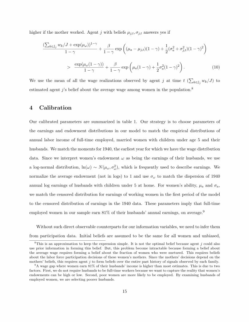
Our calibrated parameters are summarized in table 1. Our strategy is to choose parameters of

the earnings and endowment distributions in our model to match the empirical distributions of

annual labor income of full-time employed, married women with children under age 5 and their

husbands. We match the moments for 1940, the earliest year for which we have the wage distribution

data. Since we interpret women’s endowment ω as being the earnings of their husbands, we use

a log-normal distribution, ln(ω) ∼ N(µω, σ2ω), which is frequently used to describe earnings. We

normalize the average endowment (not in logs) to 1 and use σω to match the dispersion of 1940

annual log earnings of husbands with children under 5 at home. For women’s ability, µa and σa,

we match the censored distribution for earnings of working women in the first period of the model

to the censored distribution of earnings in the 1940 data. These parameters imply that full-time

employed women in our sample earn 81% of their husbands’ annual earnings, on average.9

Without such direct observable counterparts for our information variables, we need to infer them

from participation data. Initial beliefs are assumed to be the same for all women and unbiased,8This is an approximation to keep the expression simple. It is not the optimal belief because agent j could also

use prior information in forming this belief. But, this problem become intractable because forming a belief aboutthe average wage requires forming a belief about the fraction of women who were nurtured. This requires beliefsabout the labor force participation decisions of these women’s mothers. Since the mothers’ decisions depend on themothers’ beliefs, this requires agent j to form beliefs over the entire past history of signals observed by each family.

9A wage gap where women earn 81% of their husbands’ income is higher than most estimates. This is due to twofactors. First, we do not require husbands to be full-time workers because we want to capture the reality that women’sendowments can be high or low. Second, poor women are more likely to be employed. By examining husbands ofemployed women, we are selecting poorer husbands.

15

mean log ability µa -0.88 women’s earnings distributionstd log ability σa 0.57 women’s earnings distributionmean log endowment µω -0.28 average endowment = 1std log endowment σω 0.75 men’s earnings distributionoutcomes observed J 3 Prob(ni,t = ni,t−1)1970− 2000prior mean θ µ0 0.04 unbiased beliefsprior std θ σ0 1.38 1940 LFPtrue value of nurture θ 0.04 children’s test scores (Bernal and Keane 2006)intertemporal substitution γ 2 commonly used

Table 1: Parameter values for the simulated model and the calibration targets.

implying µ0 = θ. The alternative, a theory driven by initially biased beliefs, is difficult to rationalize.

The bias would have to be present in every country; otherwise, female labor force participation

would start out high and decrease in some countries. Uncertainty σ0 is chosen to match women’s

1940 labor force participation. The number of signals observed each period J matches the 42%

probability of a woman making a different labor participation decision than her mother. We use the

1970-2000 GSS data because matched mother-daughter data is only available for those years. The

rationale for matching this moment is that a woman who observes many signals will have posterior

beliefs potentially quite different from her mother’s and will have a higher chance of switching

outcomes.10 A seminal paper in the sociology literature (Marsden 1987) estimates that the average

American has three other people with whom he/she discusses important issues. Since J includes

the woman’s observation of her own wage, this implies J = 4. Section D explores alternative

calibrations. Setting J = 4 does not appreciably worsen the fit of the model.

The true value of nurture θ comes from evidence on the effect of maternal employment on

Peabody Individual Achievement Test scores of children and the correlation between the childhood

test scores and educational attainment (Bernal and Keane 2006), combined with estimates of the

college wage premium (Goldin and Katz 1999). One year of full time maternal employment plus

informal day care reduces test scores by roughly 3.4%. Maternal employment until age five trans-

lates into a 4% drop in children’s future annual wages. Appendix C provides more detail on the10This calibration strategy uses the counter-factual assumption that mothers’ and daughters’ abilities are uncor-

related. If we relax this assumption, we would need more signals (higher J) to match Prob(ni,t = ni,t−1). At thesame time, each correlated signal would reveal less independent information. The net effect on the rate of learning isambiguous.

16

estimation of all the calibration targets and discusses sample selection issues.

The model also needs an initial distribution of signals, which are observations of wages and

parental working decisions, in period 1 (1940). Our calibration determines the initial wages, but

not the maternal employment decisions. Those come from labor decisions in the previous period

(1930). To generate these, we simulate a 1930 period where we fix the labor supply equal to 3

percent, consistent with 1930 Census data and generate a set of signals from those outcomes.

5 Simulation Results

We simulate a model with 500,000 agents for 10 periods. To keep the benchmark model simple and

match it with the census data observed every ten years, we consider 10-year periods. Appendix D

considers a 20-year youth and staggered family timing.

5.1 S-shaped dynamics of participation and beliefs

1940 1960 1980 2000 20200

20

40

60

80

100

% w

ho b

elie

ve w

omen

sho

uld

wor

k

Survey Responses

1940 1960 1980 2000 20200

20

40

60

80

100

Parti

cipa

tion

Rat

e (%

)

Labor Force Participation

ModelData

ModelData

Figure 4: Labor force participation and survey responses in the model and data.LFP is the probability a woman participates in the labor force. The rise in survey responses means that womenbelieve labor force participation is less harmful to their children’s future outcomes over time.

Figure 4 shows that learning can explain the stylized facts that motivate the model. The first

(left panel) is the S-shaped rise in labor force participation in the simulated model. If we interpret

1 period as 10 years, then our model matches the realized labor force participation rates reasonably

well. Using the model to project forward in time, it forecasts that there will be a 62% participation

17

rate in 2005, after which the rate will change very little because learning has mostly converged. In

the data, the 2005 participation rate was 59%, meaning that our model under-predicts the increase

in labor force participation.

The second prediction of the model is that agents’ estimates of the value of nurture fall in an S-

shaped pattern. Figure 4 (right panel) plots the answers to the Census’ preschool question and the

simulated answers to the model survey question (equation 10). The preschool question measures

cultural acceptance of working women in our sample: mothers of preschool-age children. The

drawback of this particular question is that it misses data before 1977. The calibration appendix

describes how we use the fework question to infer the earlier data. The result is that the fraction of

respondents who support maternal employment and the evolution in that fraction are well-explained

by the model.

Taken together, these two graphs illustrate the model’s main mechanism: When labor force

participation is low, information about the cost of maternal employment on children is scarce, and

beliefs change slowly. The slow change in beliefs means a slow rise in the participation rate. As

that rate rises, more information is generated by working women whose children’s outcomes are

observed. Beliefs and participation change at a faster rate. Once information becomes sufficiently

abundant, beliefs and labor force participation converge, in unison.

5.2 Decline in uncertainty

One of the predictions that distinguishes the learning model from other explanations is that learning

entails a reduction in uncertainty, the conditional standard deviation of an agent’s posterior belief

σi,t. A common proxy for uncertainty is the dispersion in beliefs, measured as the cross-sectional

standard deviation of conditional means std(µi,t). The idea is that when there is lots of uncertainty,

there is also lots of disagreement about what the right answer is, meaning that agents’ beliefs µi,t

are dispersed. As uncertainty falls to zero, agents learn the truth and µi,t converges to θ. Since all

agents have identical beliefs in this full-information limit, belief dispersion approaches zero.

In the model, uncertainty declines monotonically (figure 5, right panel), but belief dispersion

increases then decreases (left panel). Belief dispersion starts out low because we assume that

18

1940 1960 1980 2000 20200

0.1

0.2

0.3

0.4Belief Dispersion

std t(µ

it)

1940 1960 1980 2000 20200

0.5

1

1.5

Average Uncertainty

mea

n t(σit)

Figure 5: Uncertainty and belief dispersion in the simulated model.Belief dispersion is the cross-sectional standard deviation of the beliefs: std(µi,t). Uncertainty is the average posteriorstandard deviation: mean(σi,t).

agents have common prior beliefs. Common beliefs, by definition, means no dispersion. As women

begin working, some agents observe labor market outcomes, while others do not. Furthermore,

the inferences that agents make from observing different labor market outcomes vary because the

unobserved innate ability of the workers they observe is different. As new information arrives,

beliefs diverge. Recall that what slows learning down at the end of the S-curve is that beliefs

converge to the truth. Since the true importance of nurture is the same for all agents, their beliefs

converge to each other and dispersion falls. The testable prediction here is that, in periods where

the increase in labor force participation is slowing down, differences in beliefs should be shrinking.

We test this prediction in the next section.

5.3 Wages and wealth of working women

Figure 6 shows the mean endowment and the mean wage of the subset of women who choose to

participate in the simulated model. We assumed that the unconditional distribution of endowments

and abilities is constant. What is changing is the nurture inputs and the selection of women who

work. In other words, this is primarily a selection effect.

The finding that women’s relative wages declined in the early part of the sample is surprising.

But this finding is supported by O’Neill (1984) who documents a widening of the male-female wage

gap in the mid-50’s to 70’s. She attributes it to the same selection effect that operates in our model.

What the model does not explain is why women’s wages rise, relative to men’s, after 1970. Appendix

19

1940 1960 1980 2000 2020

0.65

0.7

0.75

0.8

0.85

0.9

0.95

1Mean relative wage of employed women

1940 1960 1980 2000 2020

0.65

0.7

0.75

0.8

0.85

0.9

0.95

1Mean endowment of employed women

ModelData

ModelData

Figure 6: Average relative wage and endowed wealth for working women.Relative wage is the woman’s wage divided by her husband’s wage (wit/ωit). Mean relative wage is the relative wageaveraged over all employed women. Mean endowment is the average wage for the husband of an employed woman.

E works out an extended model with occupation choice that can explain this feature of the data.

Women face a decision between staying at home, entering a high-wage, highly time-consuming

occupation or a low-wage, less demanding job. Women start with a higher and more uncertain

expected cost of high-intensity employment. Over time, they resolve their uncertainty and many

choose careers that pay higher wages. In the calibrated sector choice model, the predictions for

total labor force participation are almost identical to the benchmark model. The difference is in

the wages – they fall and then rise, more like the data.

While learning can offer one explanation for increasing wages, there are obviously other factors

external to the model that have contributed to this trend. One of the robustness exercises in

appendix D feeds data on trending wages in to the model to see what effect they can have on

participation. The effect is negligible. Wage-based theories rely on a high estimated elasticity to

make wages matter. The implied elasticity in our model is low. Learning makes it even lower

because heterogeneity in beliefs makes fewer women marginal workers.

The endowment effect also relies on selection. In the data, women working at the beginning of

the century are married to poorer husbands than the women that are in the labor force today. The

same is true in the model: Poor women work first because their marginal utility of income is high.

As uncertainty about maternal employment diminishes, women with richer husbands join the labor

force. In the extended sector choice model, this effect is particularly pronounced in the 1970’s when

the increase in high-intensity employment induces richer women to enter the labor force.

20

5.4 Wage Elasticity of Labor Supply

One of the more puzzling changes in female labor force participation in the last 25 years is the

decline in labor supply elasticity. Blau and Kahn (2005) document that the elasticity of labor force

participation to their own wages decreased by 53% between 1980 and 2000.11 A related fact shows

up in our data: In the late 1980’s and throughout the 1990’s, women’s wages continued to increase

and yet labor force participation stagnated. A decline in wage elasticity is predicted by the model

(proposition 4). But, the magnitude of this decline in the calibrated model is small. Running a

regression similar to Blau and Kahn’s on our simulated model delivers a 1.2% elasticity decline.

Similarly, the estimated elasticity of female labor supply to husbands’ wages became less negative,

falling in magnitude by 47%. The same estimate in the model produces a decline of 2.5%.

One reason for the small change in elasticity has to do with how elasticity is estimated. In

theory, proposition 4 varies one woman’s wage and calculates the change in probability that she

will join the labor force. Empirically, such natural experiments are not observed. Instead, labor

economists regress labor force participation rates on wages to infer elasticities. Any non-wage

heterogeneity that decreases the covariance of wages and participation will reduce this estimate,

even if that added heterogeneity does not make any individual woman less responsive to her wage.

The non-wage sources of heterogeneity in the model are endowments and beliefs. Higher belief

dispersion reduces estimated elasticity.

In the model, belief dispersion rises in the beginning of the sample because agents start with

common priors and then observe different information resulting in different beliefs. This causes

own-wage elasticity to drop by 37% in the first 3 decades. So, the model does produce a large

decline in labor supply elasticity. It just does it too early. This has to do with assuming that

agents have a common prior in 1940, when the model starts.

In the extended model with occupation choice (appendix E), agents learn almost nothing about

the effect of high-intensity careers until the 1970’s. Then, as more women join such careers, more

signals about the effect of high-intensity maternal employment increase the dispersion in beliefs.11All elasticity estimates come from Blau and Kahn (2005), table 3, model 4.

21

Dispersion skyrockets in the 70’s and 80’s reducing labor supply elasticity by 22% between 1980

and 2000. It captures almost half of the observed decline.

6 Evidence on the Role of Beliefs and Learning

The evidence we have presented so far argues that cultural beliefs and participation are corre-

lated and that a model where changes in beliefs cause changes in participation rates is consistent

with various features of the participation data. This section presents direct evidence about the

relationship between cultural beliefs, learning and labor force participation.

6.1 Evidence of Causality: Culture Affects Participation

Fernandez and Fogli (2005) identify a causal effect of cultural beliefs on female labor force par-

ticipation. Using data on second generation American women, they show that cultural heritage

explains variation in participation.12 Labor force participation in the parents’ country of origin

explains 30% of the variation in hours worked across ancestries. Likewise, Fernandez, Fogli, and

Olivetti (2002) show that men who are born and raised by working mothers are more likely to

marry a working woman. Farre and Vella (2007) find that women who report being supportive

of female labor force participation are more likely to have daughters and daughters-in-law that

participate. In our model only women’s information matters. In reality, couples likely also use

husbands’ information to make joint labor decisions.

While this evidence points to causality, it does not distinguish between culture shaping prefer-

ences or transmitting information. The second piece of evidence speaks to this difference.

6.2 Evidence of Learning in Cultural Beliefs

If the learning hypothesis is correct, then uncertainty about the effects of labor force participation

on children should decline over time. As beliefs become less uncertain, they are also converging12Similar results, showing that ancestry affects labor choices can be found in Antecol (2000), Fortin (2005) and

Alesina and Giuliano (2007).

22

to the truth. This convergence results in falling cross-sectional dispersion of beliefs. This some

evidence of falling cross-sectional dispersion in beliefs in our survey data.

To measure belief dispersion, we use survey data that is not binary. The dispersion of yes-no

answers only reveals how far the average answer is from 50%. Instead, we have three sets of answers

that reflect an intensity of preference: preschool, fechild and fefam. All three begin in 1970 and

end in 2004. We assign a 1 to strongly agree, 2 to agree, 3 to disagree, and 4 to strongly disagree

and take the standard deviation of those replies. In the model, the survey question we pose to

agents is a binary one. Therefore, its answers cannot be directly compared. But we can look at the

changes in dispersion of beliefs (figure 5). Starting in the 1970’s, the dispersion rises slightly and

then falls. If we linearly interpolate between decades to get dispersion numbers for 1977 and 2004,

we find that the predicted belief dispersion falls by 5.5%.

For our benchmark survey measure of beliefs, preschool, dispersion falls by 2.5%, from 0.80 in

1977 to 0.78 in 2004. For fechld, dispersion falls by 9.4%, from 0.96 to 0.87. The exception to this

trend is fefam, for which the dispersion rises from 0.81 to 0.86. However, two features of the fefam

data do point to a decline in uncertainty. If we compare the number of agree or disagree responses

to the number of strongly agree and strongly disagree responses, the fraction of less certain replies

falls from 76% in 1977 to 71% in 2002. Second, the fraction of respondents who reply “I don’t

know” fell from 1.5% in 1977 to 1.2% in 2004. But, this is a small number of replies.

7 What Learning Adds to Existing Explanations

Other logical explanations for the increase in female labor force participation abound. This sections

examines four categories of explanations and argues that incorporating learning can add to the

explanatory power of each one.

7.1 Higher returns to employment

Rising wages, lower taxes or less discrimination encourage all women to join the labor force. Our

theory is one about why women with small children behaved so differently from other women.

23

In this sense, the two theories are complements. Wage-based explanations also have a hard time

reconciling the rising wages and stagnant female labor force participation in the last 20 years. For

example, Jones, Manuelli, and McGrattan (2003) use a high own-wage elasticity of female labor

supply to allow changing wages to have a large effect on participation. Although this elasticity falls

over time, it stays high enough to generate a continued increase in participation. Adding learning

could potentially reduce the elasticity enough to get participation rates to level off.

7.2 The cost of maternal employment declined

A second category of explanations are reasons why θ declined. For example, household appliances

(Greenwood and Guner 2005), innovations such as baby formula (Albanesi and Olivetti 2006) and

the availability of child care (Attanasio, Low, and Sanchez-Marcos 2006) all encouraged labor force

participation.

One shortcoming of the technology explanation is that it predicts that rich women who can

afford new technologies work first. This is at odds with the data (figure 6). Second, it does not

explain the fall in labor supply elasticity. If the availability of such goods and services is increasing

over time, a second effect should increase the labor supply elasticity: As wages rise, technology and

child care become more affordable. Being able to afford them makes working trade off less with

a nurturing home environment. Inside the model, this is like being able to sacrifice some labor

earnings to reduce θ. That means that not only does an increase in wage increase the benefit to

working, it also reduces its cost. This second effect makes labor supply more sensitive to the wage.

Finally, adding learning explains why women in the same place, at the same time, make different

decisions based on their parents’ ethnicity and labor force decisions.

Both the technology and learning mechanisms could be operating simultaneously. Perhaps

technological innovations and child care are endogenous. They arrive when there are enough work-

ing mothers demanding them, which reinforced the trend to higher participation. The increased

demand could come from a change in cultural beliefs about the costs of labor force participation.

24

7.3 Endogenous fertility

Concurrent with the increase in labor force participation was a decline in fertility. Women started

having fewer children at a later age. Of course, our empirical analysis is all conditional on women

who already have small children and having fewer children does not make the trade-off between

employment and nurturing disappear. But Goldin and Katz (2002) argue that these women acquired

more human capital and reduced the cost to their careers by postponing motherhood. Thus, the

skill composition of our sample has undoubtedly changed. At the same time, this effect does not

explain most of the increase in labor force participation. That increase started well before the

pill was available and continued long after the pill was widespread. Even conditional on having a

child and on educational attainment, participation still increased over the course of the century.

Furthermore, use of the pill itself was regulated by cultural beliefs about the role women should

play in society.

7.4 Preferences changed

The hardest alternative explanation to distinguish is a preference change. Perhaps women prefer

staying at home when lots of other women stay at home, or preferences change adaptively as a

consequence of previous history (Fernandez, Fogli, and Olivetti 2002). Three features of the data

help us argue that learning is going on. They don’t rule out simultaneous changes in preferences,

but they support a role for our theory. First, the questions in figure 2 are not about preferences.

They are about the effect of work on children. Second, a change in preferences does not entail a

fall in uncertainty. Third, and most importantly, changes in preferences would not cause the labor

supply elasticity to fall over time. It is uncertainty, combined with the concavity of the utility

function, that can generate the decreased sensitivity of participation to wages that we observe in

the data. Finally, our model can be interpreted as a rational theory of preference change. Such a

theory is useful because it isolates which preferences matter most for labor force participation, and

it offers a testable, systematic way of thinking about why preferences changed.

25

8 Conclusion

Our theory describes how cultural changes, such as an increase in female labor force participation,

can arise through learning from endogenous information. All kinds of cultural norms are adopted

because they are thought to be best practice at the time. If there is no experimentation with

alternatives, no new information is learned and the cultural norms stay fixed. Eventually, a few

people with extreme preferences or abilities deviate from these norms. In doing so, they provide

information that others can observe. This experimentation slowly begins to change beliefs, reducing

uncertainty about the desirability of the alternative practice, which encourages others to engage in

it. As more people deviate from the cultural norm, learning speeds up, social change quickens and

a social revolution takes hold.

Culture is a slow-moving variable. A key challenge for this theory is to explain why Bayesian

learning, usually so quick to converge, takes place so slowly. One possibility is that there is a

coordination component to culture. When women want to act like other women, they take actions

that are less reflective of their private information. These actions are then less informative to

others. This kind of mechanism has been used in monetary economics to slow price reactions to

monetary shocks. Introduced here, it would allow women to observe more information, without

speeding up the increase in labor force participation.

Another potential objection to the theory is that much information is derived from public

sources, rather than private interactions. An alternative model might be one where information

providers (magazine editors) want to provide high-demand information to their readers to maximize

their readership. In the 1940’s, women were so uncertain and therefore so averse to participation

that one article would not have changed their mind. Therefore, their demand for information was

low and little was provided. As a few women tried employment and generated information for

the women around them, participation started to rise. In the 1960’s many more women were near

the margin between participating or not. The information about children became more relevant to

their decision and therefore more valuable. In the 1960’s and 70’s, centralized information provision

can reinforce the decentralized learning in the model, causing participation to speed up more and

26

converge sooner. Such a reinforcement effect could help the model to better match the steep but

delayed entry of women with small children.

Of course, a few highly informative magazine articles, observed by all women in the mid-60’s

could cause participation to rise too quickly and level off in the 70’s. But this view understates

the difficulty of a woman making inference about what will happen to her children if she works.

We have modeled signals whose only source of noise is ability. In reality, women may observe more

signals with more unobserved factors such as: quality of nurturing, teacher quality, or peer effects.

This suggests that signals about the success of other children in the same situation as her own

are the most informative. Assessing how the environment of other children differs from her own

requires knowing a lot of information about their upbringing. Such detailed information is most

easily obtained by personal contact.

Modeling the local nature of information diffusion could also slow down learning in our model.

The idea that some kinds of information are transmitted mostly through families or close contacts

arises also in Piketty (1995). He argues that political beliefs are related to economic conditions,

but are very persistent across generations because agents learn from the experience of their family.

Signals from family or neighbors are likely to have correlated signal noise, which slows learning.

Also, local information transmission will slow the diffusion of information learned in one loca-

tion. Geographic or socioeconomic pockets of the country could get trapped for long periods in

low-participation equilibria where few women work and little is being learned about maternal em-

ployment, even as participation rates in the country rise. Large variation in participation rates

across U.S. counties suggests that information diffusion has a geographic component to it. Fu-

ture work will explore whether a spatial model of learning can explain the evolution of geographic

patterns of female labor force participation.

27

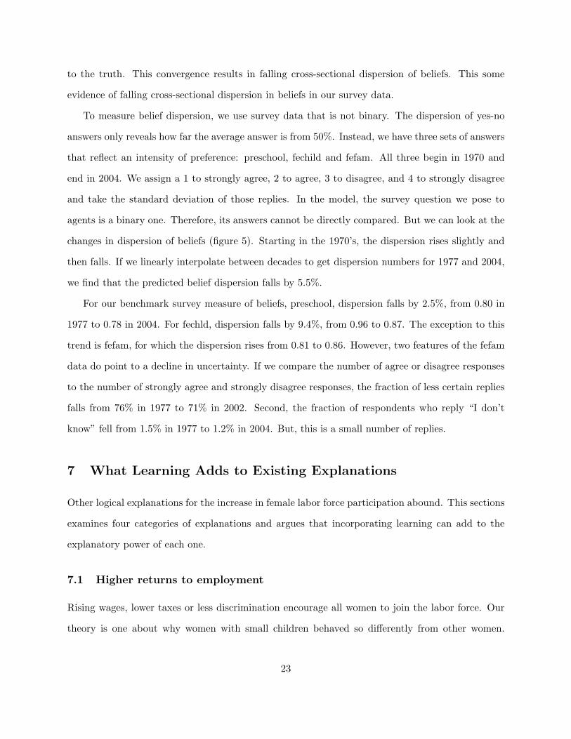
A Technical Appendix: Proofs

A.1 Proof of proposition 1

Step 1: Define a cutoff wage w such that all women who observe wi,t > w choose to join the labor force.A woman joins the labor force when EUWit − EUOit > 0. Note that ∂Ni,t/∂wit = (nitwit + ωit)

−γ > 0. SinceNi,t is monotonically increasing in the wage w, there is a unique w for each set of parameters, such that at w = w,Ni,t = 0.

Step 2: Describe the probability of labor force participation.Let Φ denote the cumulative density function for the unconditional distribution of wages in the population. This

is a log-normal c.d.f. Since the lognormal is unbounded and has positive probability on every outcomes, its c.d.f. istherefore strictly increasing in its argument. Then, the probability that a woman participates is 1 − Φ(w), which isthen strictly decreasing in w.

Step 3: The effect of beliefs on labor force participationTaking the partial derivative of the net utility gain from labor force participation yields ∂Ni,t/∂µi,t = −β. By

the implicit function theorem, ∂w/∂µi,t > 0. Thus, ∂(1 − Φ(w))/∂µi,t = (∂(1 − Φ(w))/∂w)(∂w/∂µi,t) < 0, whichcompletes the proof.


Steps 1 and 2 of the proof are as in appendix A.1.The benefit to participating is falling in uncertainty: ∂Ni,t/∂σi,t = (1−γ)β exp

�(µa − µi,t)(1− γ) + 1

2(σ2

a + σ2i,t)(1− γ)2

�.

Since γ > 1, β > 0 by assumption, and the exponential term must be non-negative, this means that ∂Ni,t/∂σ2i,t <

0. As before, the implicit function theorem tells us that ∂w/∂σ2i,t > 0. Thus, ∂(1 − Φ(w))/∂σ2

i,t = (∂(1 −Φ(w))/∂w)(∂w/∂σ2

i,t) < 0, which completes the proof.

A.3 Proof of proposition 3: Zero participation is not a steady state

Proof: For any arbitrary beliefs µjt, σjt and endowment ωjt, there is some finite level of ability a∗ and an associatedwage w∗ = exp(a∗), such that EUWit > EUOit > 0, ∀ajt ≥ a∗. The fact that ajt is normally distributed means thatProb(ajt ≥ a∗) > 0 for all finite a∗. Since woman j enters the labor force whenever EUWit > EUOit > 0, and thishappens with positive probability, njt = 1 with positive probability. Since this is true for all women j, it is also truethat

Pj njt ≥ 1 with positive probability.


Steps 1 and 2 of the proof are as in appendix A.1.The benefit to participating is falling in wealth: ∂Ni,t/∂ωi,t = (wi,t +ωi,t)

−γ− (ωi,t)−γ . This is negative because

(wi,t + ωi,t) > (ωi,t) holds as long as wi,t > 0. Since wi,t has a log-normal distribution, it is greater than zero withprobability one. As before, the implicit function theorem tells us that ∂w/∂ωi,t > 0. Thus, ∂(1 − Φ(w))/∂ωi,t =(∂(1− Φ(w))/∂w)(∂w/∂ωi,t) < 0, which completes the proof.


There are two effects of increasing the average wage that show up in elasticity: (1) the direct effect on increasingthe number of women whose wages are above the cutoff that determines whether they join the labor force or not;(2) the increase in the expected future wages of children affects the expected cost of joining the labor force. Weexamine how an increase in uncertainty σ affects each part separately, for a woman (i, t). We call the elasticity of thiswoman’s labor supply the conditional elasticity, because it is conditional on her endowment ωit and beliefs µit, σit.The last step shows that if σ increases the conditional elasticity for every woman, it increases the aggregate laborsupply elasticity as well.

Step 1: Direct own-wage effect. The probability that a woman participates is 1 − Φ(wit), which is thenstrictly decreasing in wit, as defined in appendix A.1. Rewrite the cumulative density function as the standard normalc.d.f. Φ of the log of wit, adjusted by the mean and standard deviation of log wages, µw and σw. The probability oflabor force participation, conditional on having endowment ωi and beliefs µit, σit is then 1− Φ(ln(wit)−µw/σw). Themarginal effect of increasing one’s own log wage is the standard normal probability density φ(ln(wit)− µw/σw) > 0.The conditional elasticity of labor force participation is ∂ ln(1 − Φ(·))/∂µw, since µw is the log average wage. The

28

conditional elasticity for woman (i, t) to a change in the mean of her own wage is therefore φ(ln(wit)− µw/σw)/(1−Φ(·)), which is a standard normal hazard function, H(ln(wit)− µw/σw).

Next, how does the decreasing uncertainty about the effect of nurture change this own-wage elasticity for woman(i, t) over time? Uncertainty affects (1 − Φ(ln(wit) − µw/σw)) through its effect on the cutoff wage wit. The proofof proposition A.2 tells us that ∂wit/∂σi,t > 0. Therefore, the effect of an increase in uncertainty is given by thecross-partial derivative ∂2 ln(1 − Φ(·))/∂µw∂wit > 0. This is positive because a standard normal hazard function isalways increasing in its argument.

Step 2: Indirect effect on children’s wages. This effect is the increase in the expected value of (µa −ni,tµi,t) = µw in the second term of (6). This indirect effect works through the effect of µw on ln(wit). Putting thetwo effects together gives us the total conditional elasticity of labor force participation to a change in average wage.Let CEit represent this conditional elasticity.

CEit = H

�ln(wit)− µw

σw

�+

∂ ln(1− Φ(·))∂ ln(wit)

∂ ln(wit)

∂µw

= H

�ln(wit)− µw

σw

�(1− ∂ ln(wit)

∂µw)

Lastly, we need to compute the derivative of the conditional elasticity with respect to uncertainty σ2i,t.

∂CEit

∂σ2i,t

= H

�ln(wit)− µw

σw

�(∂ ln(wit)

∂σ2i,t

)(1− ∂ ln(wit)

∂µw)−H

�ln(wit)− µw

σw

�∂2 ln(wit)

∂µw∂σ2i,t

.

Step 1 established that the first term is positive. Since hazard functions are always positive, the last remaining stepis to show that ∂2 ln(wit)/∂µw∂σ2

i,t < 0.Step 3: Show that ∂2 ln(wit)/∂µw∂σ2

i,t < 0. Note that

∂Ni,t/∂µw = β exp

�µa(1− γ) +

1

2σ2

a(1− γ)2��

exp

�(γ − 1)ni,tµi,t +

1

2n2

i,tσ2i,t(1− γ)2

�− 1

�.

This is positive because (γ − 1)ni,tµi,t + 12n2

i,tσ2i,t(1 − γ)2 > 0. This tells us that when expected wages are higher,

Ni,t, the net benefit of working is higher. This arises because the marginal utility cost of a reduction in expectedwages for children is lower if the expected level of those wages is higher. Differentiating this expression again withrespect to uncertainty yields:

∂2Ni,t

∂µw∂σ2i,t

= β exp

�µa(1− γ) +

1

2σ2

a(1− γ)2�

exp

�(γ − 1)ni,tµi,t +

1

2n2

i,tσ2i,t(1− γ)2

�1

2n2

i,t(1− γ)2 > 0.

Note also that ∂2Ni,t/∂µw∂w = 0 and ∂2Ni,t/∂σ2i,t∂w = 0. Therefore, applying the implicit function rule and

differentiating a second time tells us that

∂2 ln(wit)

∂µw∂σ2i,t

= −∂2Ni,t/∂µw∂σ2i,t

∂Ni,t/∂w+ 0.

Since the numerator is positive and the denominator is positive, the negative sign in front makes the cross-partialnegative.

Step 4: Convert conditional to aggregate elasticity. If the conditional elasticity for every woman (i, t)increases when their σit increases, then when every σit rises, the aggregate wage elasticity of labor rises as well. Theunconditional elasticity is

RCEitdF (ωit, µit, σit). Since we can reverse the order of differentiation and integration,

the result that the partial derivative of this term isR

∂CEit/∂ ln(wit)dF (ωit, µit, σit). Since the term inside theintegrand is positive for every (ωit, µit, σit), the whole expression is positive.

29

B Data Description

B.1 Survey data about beliefs

Data come from http://webapp.icpsr.umich.edu/GSS/ .

Attitudes We have 6 measures for individuals’ attitudes toward women working that have a time series dimension.

fehome Women should take care of running their homes and leave running the country up to men. (AGREE=1,DISAGREE=2, NOT SURE=8, NO ANSWER=9, NA=0). We generate a dummy variable fehome=1 ifFEHOME=1 and =0 if FEHOME=2. exclude observations for which FEHOME= 0 or FEHOME> 2.

The data span 1974-1998, with nine missing years. There are between 890 and 1884 responses per year, with16 years of observations, for a total 22,538 data points. The fraction of respondents who agree ranges from38% in 1977 to 14% in 1995.

fework Do you approve or disapprove of a married woman earning money in business or industry if she has ahusband capable of supporting her? (AGREE=1, DISAGREE=2, NOT SURE=8, NO ANSWER=9, NA=0).We generate dummy variable fework same as for fehome.

The data span 1972-1998, with ten missing years, for a total of 17 years with observations. There are between902 and 1,933 responses per year, and 24,401 total observations. The fraction of respondents who agree rangesfrom 48% in 1972 to 37% in 1996.

fechld A working mother can establish just as warm and secure a relationship with her children as a mother whodoes not work. (STRONGLY AGREE=1, AGREE=2, DISAGREE=3, STRONGLY DISAGREE=4, DON’TKNOW=8, NO ANSWER=9, NA=0). We use this variable as is, except observations with FECHLD= 0 andFECHLD> 4 which we treat as missing.

There is one set of observations in 1977, and then from 1995-2004, at least every two years, for a total of14 years in which data are available. There are between 897 and 1,948 responses per year, totalling 19,270observations. The average reply ranges from 2.5 in 1977 to 2.1 in 1994.

preschool A preschool child is likely to suffer if his or her mother works. (STRONGLY AGREE=1, AGREE=2,DISAGREE=3, STRONGLY DISAGREE=4, DON’T KNOW=8, NO ANSWER=9, NA=0). The only mod-ification we make to this variable is to treat observations with preschool= 0 and preschool> 4 as missing.


fefam It is much better for everyone involved if the man is the achiever outside the home and the woman takes careof the home and family. (STRONGLY AGREE=1, AGREE=2, DISAGREE=3, STRONGLY DISAGREE=4,DON’T KNOW=8, NO ANSWER=9, NA=0). The only modification we make to this variable is to treatobservations with FEFAM= 0 and FEFAM> 4 as missing.


Lifecycle Surveys We have 3 measures of acceptance of women working over life cycle. We do not have muchof times series dimension (only start in 1988), but they are interesting to show how the presence of a small child iscrucial in determining individuals’ attitudes.

Attitudes toward women working over life cycle: 3 stages of life cycle corresponding to 3 variables. We have these3 variables for only 3 years (1988, 1994, 2002). Not much variation over 14 years, but can be used to make cross-section point. First 9 tables show each variable in each year. Last 3 show the three variables when all observationsare pooled across years.

wrknokid Should a woman work outside the home after marrying and before there are children? (1=FULL,2=PART, 3=STAY HOME, 8=CAN’T CHOOSE, 9=NO ANSWER, 0=NA). Generate variable wrknokid=WRKNOKIDbut recode WRKNOKID=0 and WRKNOKID=9 as missing.

wrkbaby Should a woman work outside the home when there is a child under school age? (1=FULL, 2=PART,3=STAY HOME, 8=CAN’T CHOOSE, 9=NO ANSWER, 0=NA). Generate variable wrkbaby=WRKBABYbut recode WRKBABY=0 and WRKBABY=9 as missing.

30

wrksch Should a woman work outside the home after the youngest child starts school? (1=FULL, 2=PART,3=STAY HOME, 8=CAN’T CHOOSE, 9=NO ANSWER, 0=NA). Generate variable wrksch=WRKSCH butrecode WRKSCH=0 and WRKSCH=9 as missing.

Pre-1972 Data The attitudes data from GSS begin only in 1972. However, the increasing speed of female entryin the labor force (start of the S) precedes that date. To establish the contemporaneous S-shaped evolution of beliefs,it is vital to have more historical data.

We have one measure of beliefs that is collected infrequently, since the 1930’s. That is FEWORK. This data arefrom IPOLL databank, maintained by the Roper Center for Public Opinion Research. Unfortunately, the phrasingof the questions differs slightly over time. We describe below the questions and the replies.

August 1936 The Gallup Poll asked: “Should a married woman earn money if she has a husband capable ofsupporting her?” 18% said yes, 82% no. No uncertain or no response entries were allowed.

October 1938 The Gallup Poll asked: “Do you approve of a married woman earning money in business or industryif she has a husband capable of supporting her?” 22% approve, 78% disapprove.

November 1945 The Gallup Poll (AIPO) asked: “Do you approve or disapprove of a married woman holding ajob in business and industry if her husband is able to support her?” 62% disapprove, 18% approve. The restof the replies are miscellaneous open answers (e.g., if she has a good job, if she has no children, etc.).

June 1970 The Gallup Poll asked: “Do you approve of a married woman earning money in business or industry ifshe has a husband capable of supporting her?” 60% approve, 36% disapprove, 4% do not know.

Inferring pre-1977 preschool answers Figure 4 plots survey responses that are preschool replies from1977-2004. Before 1967, the only beliefs series we have is fework. There are 3 observations available before 1967 andthen regular observations starting in 1970. For each of the pre-1977 observations, we compute the growth rate fromone data point to the next. Then, we apply these same growth rates to project our preschool data back from 1977 tothe earlier observations. We believe that using one series to infer another is a reasonably accurate procedure becausefor years in which both survey questions are asked, the correlation in the replies is 74%.

B.2 Labor force participation and wage data

The wages data come from IPUMS (Integrated Public Use Microdata Series). It covers 1920-2005. It is every 10years until 2000, and yearly thereafter. The data are a 1-in-100 national random sample of the population until 2000.After 2000, it is the American Community Survey 2001 sample: a 1-in-232 (approximately) national random sampleof the population. We used only data on white women who are not agricultural workers and live with family membersin their household: (race=1, gq=1, farm=1, sex=2, excluding occ=810, 820, 830, 840, 123, 100). Residents of Hawaii(statefip=15) and Alaska (statefip=2) are excluded.

Labor Force Observations are dropped if the occupation is in agriculture or the respondent lives on a farm or inan institution. Ages range from 25-54. They are white, married women with spouse present and at least onechild under age 5 living in the household. Data are weighted using perwt (sample weights from census). Thereare no missing labor force observations.

Wages Data start in 1940. (Inctot and incwage start in 1940.) We deflated wages using the consumer price index(Series Id: CUUR0000SA0). The base year is 1982 − 84 = 100. Note that since the survey always asks aboutthe previous year’s wages, the 1940 wage data are really about 1939 wages.

We make three modifications to these data. First, we recode the labor force variable and the empstat (em-ployment status) variable as missing value if labforce=0 or empstat=0, meaning that the answer was N/A.Second, to account for the top-coding of the income variable, we multiply the top-coded values of INCWAGE(wage income) by a factor of 1.4. Finally, we take the log of each woman’s wage, then average across women.

Correcting sample bias There are two issues of sample bias. The first is the standard issue that the census isnot perfectly representative. The standard solution to this problem is to use the weights that the censusprovides on the frequency of various characteristics in the population. We weight all moments by the census-provided variable perwt. The second issue arises only for 1950 data. The weeks worked and income variablesare called “sample line” items in 1950 which means that they were collected only for 1 in 330 respondents.Therefore, we use a different weight “slwt” in 1950. When we look at husband’s characteristics in 1950, weweight the husband’s income using the women’s weight perwt, so that the moments of husbands’ wages are

31

the endowments of “representative” women. This is equivalent to restricting the sample to only sample lineindividuals since they are a flat sample in the population.

Dropped observations Also, since working FTYR this year is no guarantee of having worked the year before,andsince the earnings refer to the previous year, we also condition on having positive earnings in the previous yearfor both men and women.

Other data issues We take care of inflation by using CPI (Series Id: CUUR0000SA0), base year 1982-84=100. Werecode weeks and hours worked by assigning midpoints We generate a dummy FTYR =1 if (weekworkrec>= 50and hourworkrec>= 40) We need to condition for women to work full time year around because otherwise wefind an incredibly large difference between men and women annual earnings due to the large difference in theirlabor supply.

Hours and weeks worked The weeks worked variable (WKSWORK2) is an indicator variable that describes whichinterval the respondent’s answer fell in. We replace each indicator with the middle point of the reported interval.We do the same for hours worked (hrswork2). The reporting procedure changes in 1980. From 1980 on, weused the reported average hours per week (UHRSWORK).

Full time This is a dummy variable that indicates if two conditions are satisfied: 1) hrswork2 recoded ≥ 40, meaningthat the worker worked at least 40 hours per week; and 2) WKSWORK2 recoded ≥ 50, meaning that thewoman reports being employed for at least 50 weeks.

C Calibration Details

Throughout, we look at women 25-54, with their own child younger than 5 living in the household. We use individualsnot living in institution, not living in farm, not working in agriculture and white.

Abilities The distribution of women’s abilities is constructed so that their wages in the model match the distributionof women’s wages in the 1940 census data. σa = .57 is the standard deviation of log ability and µa =ln(earnings gap)− (σ2

a)/2 is the mean of log ability. These parameters match the initial ratio between averageearnings of working women to average earnings of all husbands (0.8 in the data) and to match the standarddeviation of log earnings of employed women in the data (0.53 in the data).

Selection effects in the model The distribution of observed wages in the data needs to be matched with thedistribution of wages for employed women in the model. Employed women are not a representative sample.They are disproportionately high-skill women. The calibration deals with this issue by matching the truncateddistribution of wages in the data to the same truncated sample in the model. In other words, we use the modelto back out how much selection bias there is.

Endowment distribution Data come from the census. We use wages in 1940 (first available year). From this, weconstruct two pools of matched data: One is only married women; the other is their husbands.

The log endowment is normal. For these two sets of wage data, we take the log of wages over previous year.For husbands, mean(log incwage husb ) = 7.043089 and std(log incwage husb) = .7348059. Therefore, we setσω = 0.73. We choose the mean log endowment µω = −(σ2

ω)/2 such that mean endowment is normalized to 1.

Initial labor force participation We need a period 0 participation rate that determines the period 1 wage distri-bution of women and a period 1 participation rate to start the simulation. Period zero FLFP=3%, period oneFLFP=6%. These are given from Census 1930 and 1940 for women, married, white, not living in farms, notliving in institutions, age 25-45 with a child younger than 5 living in the household.

True value of nurture To calibrate the θ parameter, we use micro evidence on the effect of maternal employmenton the future earnings of children. Our evidence on the effect of maternal employment comes from the NationalLongitudinal Survey of Youth (NLSY), in particular the Peabody Picture Vocabulary Test (PPVT) at age 4and the Peabody Individual Achievement Test (PIAT) for math and reading recognition scores measured atage 5 and 6. One year of full time maternal employment plus informal day care reduces test scores by roughly3.4% (Bernal and Keane 2006). If a mother works from one year after birth until age six, these five years ofemployment translate in to a score reduction of 17%.

The childhood test scores are significantly correlated with educational attainment at 18. A 1% increase in themath at age 6 is associated with .019 years of additional schooling. A 1% increase in the reading test score atage 6 is associated with .025 additional school years. Therefore, five years of maternal employment translatesinto between 0.32 (17*.019) and 0.42 (17*.025) fewer years of school.

32

The final step is to multiply the change in educational attainment by the returns to a college education. Weuse the returns to a year of college from 1940 to 1995 from Goldin and Katz (1999). Their estimates are thecomposition-adjusted log weekly wage for full-time/full-year, non agricultural, white males. Those estimatesare 0.1, 0.077, 0.091, 0.099, 0.089, 0.124, and 0.129 for the years 1939, 1949, 1959, 1969, 1979, 1989, and 1995.The average return to a year of college is 10%. Since maternal employment reduces education by 0.32-0.42years, the expected loss in terms of foregone yearly log earnings is about 4%, or θ = 0.04.

Number of signals J is calibrated to the probability that a mother and daughter make the same participationchoice. This probability comes from GSS data on married women with children under six who report thatthey work either full-time or are homemakers and who reported whether their mother worked for at least oneyear after having children and before they were six years of age.

D Robustness Checks

We explore the sensitivity of model outcomes to changes in four key sets of calibrated parameters, and to changes inmodel timing.

D.1 Changing Parameters

1940 1960 1980 20000

0.2

0.4

0.6

0.8

1Panel A: Number of signals j

LFP

1940 1960 1980 20000

0.2

0.4

0.6

0.8

1Panel B: Distribution prior beliefs µθ, σθ

LFP

1940 1960 1980 20000

0.2

0.4

0.6

0.8

1Panel C: Distribution of ability µ

a

LFP

1940 1960 1980 20000

0.2

0.4

0.6

0.8

1Panel D: Cost of maternal employment θ

LFP

Benchmarkj=2j=4

Benchmarkµθ=0.2, σθ=1.2

µθ=0.5, σθ=0.8

Benchmark

µa=0.24

µa=0.73

µat

=wt

Benchmarkθ=0.02θ=0.06

Figure 7: Sensitivity of labor force predictions to changes in parameter values.

Number of signals Since the number of signals is not something we can directly observe, it is important that ourresults not be too sensitive to it. Increasing the number of signals to 4 or decreasing it to 2 either speeds up orslows down learning. This can be seen in the steeper or flatter S-shapes in panel (a). Table 2 shows that thenumber of signals has mild effects on initial endowments and wages. These initial effects arise because moresignals make agents beliefs initially more different. Differences in beliefs, rather than differences in endowmentsor abilities then becomes a more important determinant of the participation decision. Since selection effectsdrive the average wage and endowment of working women, the number of signals affects this. The effect ismild. The number of signals has no effect on the ending endowment or wage.

33

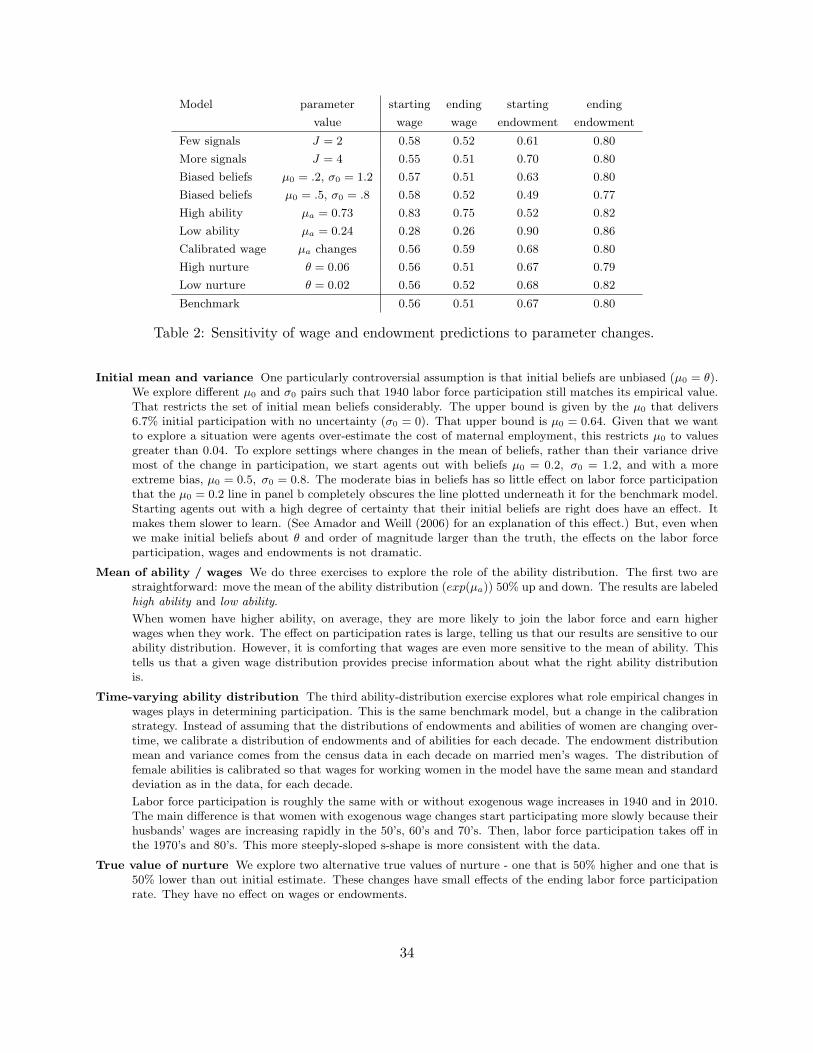
Model parameter starting ending starting ending

value wage wage endowment endowment

Few signals J = 2 0.58 0.52 0.61 0.80

More signals J = 4 0.55 0.51 0.70 0.80

Biased beliefs µ0 = .2, σ0 = 1.2 0.57 0.51 0.63 0.80

Biased beliefs µ0 = .5, σ0 = .8 0.58 0.52 0.49 0.77

High ability µa = 0.73 0.83 0.75 0.52 0.82

Low ability µa = 0.24 0.28 0.26 0.90 0.86

Calibrated wage µa changes 0.56 0.59 0.68 0.80

High nurture θ = 0.06 0.56 0.51 0.67 0.79

Low nurture θ = 0.02 0.56 0.52 0.68 0.82

Benchmark 0.56 0.51 0.67 0.80

Table 2: Sensitivity of wage and endowment predictions to parameter changes.

Initial mean and variance One particularly controversial assumption is that initial beliefs are unbiased (µ0 = θ).We explore different µ0 and σ0 pairs such that 1940 labor force participation still matches its empirical value.That restricts the set of initial mean beliefs considerably. The upper bound is given by the µ0 that delivers6.7% initial participation with no uncertainty (σ0 = 0). That upper bound is µ0 = 0.64. Given that we wantto explore a situation were agents over-estimate the cost of maternal employment, this restricts µ0 to valuesgreater than 0.04. To explore settings where changes in the mean of beliefs, rather than their variance drivemost of the change in participation, we start agents out with beliefs µ0 = 0.2, σ0 = 1.2, and with a moreextreme bias, µ0 = 0.5, σ0 = 0.8. The moderate bias in beliefs has so little effect on labor force participationthat the µ0 = 0.2 line in panel b completely obscures the line plotted underneath it for the benchmark model.Starting agents out with a high degree of certainty that their initial beliefs are right does have an effect. Itmakes them slower to learn. (See Amador and Weill (2006) for an explanation of this effect.) But, even whenwe make initial beliefs about θ and order of magnitude larger than the truth, the effects on the labor forceparticipation, wages and endowments is not dramatic.

Mean of ability / wages We do three exercises to explore the role of the ability distribution. The first two arestraightforward: move the mean of the ability distribution (exp(µa)) 50% up and down. The results are labeledhigh ability and low ability.

When women have higher ability, on average, they are more likely to join the labor force and earn higherwages when they work. The effect on participation rates is large, telling us that our results are sensitive to ourability distribution. However, it is comforting that wages are even more sensitive to the mean of ability. Thistells us that a given wage distribution provides precise information about what the right ability distributionis.

Time-varying ability distribution The third ability-distribution exercise explores what role empirical changes inwages plays in determining participation. This is the same benchmark model, but a change in the calibrationstrategy. Instead of assuming that the distributions of endowments and abilities of women are changing over-time, we calibrate a distribution of endowments and of abilities for each decade. The endowment distributionmean and variance comes from the census data in each decade on married men’s wages. The distribution offemale abilities is calibrated so that wages for working women in the model have the same mean and standarddeviation as in the data, for each decade.

Labor force participation is roughly the same with or without exogenous wage increases in 1940 and in 2010.The main difference is that women with exogenous wage changes start participating more slowly because theirhusbands’ wages are increasing rapidly in the 50’s, 60’s and 70’s. Then, labor force participation takes off inthe 1970’s and 80’s. This more steeply-sloped s-shape is more consistent with the data.

True value of nurture We explore two alternative true values of nurture - one that is 50% higher and one that is50% lower than out initial estimate. These changes have small effects of the ending labor force participationrate. They have no effect on wages or endowments.

34

D.2 Changing Model Timing

The model is designed to explain the labor force participation decisions of women with children under 5 years ofage. The majority of these women in the census data are between the ages of 25 and 35, with an average age of32. Whether women return to the labor force afterwards or not is not something our theory has anything to sayabout, nor is it relevant for the participation rates of our subgroup. This is part of the reason why we look at 10-yearperiods.

What our timing assumptions miss is that it takes about 20 years between when a child is born and when sheenters the labor force. Therefore, the decisions of mothers determine the information that others observe 20 years, not10 years later. This longer lag in the learning process slows down cultural change and allows us to add more signalsto the model, while still matching the data. To have a more realistic information lag, we explore two alternativetiming conventions.

Twenty-year periods We acknowledge that it takes twenty years for a child to grow up and their potentialwage to be observed. If we made the model have twenty-year instead of ten-year periods, without changing thenumber of signals, the results would be literally the ones we reported, with a re-labeling of years. But the longerperiods allow us to increase the information flow that women observe to address the criticism that information is toorestricted. We suppose that they observe three signals per decade, or six signals every 20-year period. This modelhas an almost-sized effect. What it loses is some of the S-shape in labor force participation. The reason is that theobservations are too far apart to capture the nuances of how participation increased.

1940 1960 1980 2000 20200

20

40

60

80

100

Part

icip

atio

n R

ate

(%

)

Labor Force Participation

ModelData

1940 1960 1980 2000 20200

20

40

60

80

100P

art

icip

atio

n R

ate

(%

)Labor Force Participation

ModelData

Figure 8: Twenty-year periods and staggered dynasties.

Staggered dynasties This model is one where a child grows up for 25 years and realizes her potential wageat 25. At the same time, the woman marries and starts having children. She is a married woman with a child under5 years of age until age 35, when she drops out of our sample. If started all families having children at the sametime, then in every 25 years, there would be 15 where there are no women with small children. Therefore, we staggerfamilies so that every year an equal number of children are born. The parameters are all equal to our benchmarkparameters, except that the number of signals observed every 25 years is 8. Those 8 signals come from wage andmaternal employment decisions of women from the current and last 10 cohorts.

The labor force participation rates measure participation of the 10 birth year cohorts that are between 25-35years old. The evolution of participation is illustrated in the right panel of figure 8.

Another alternative timing would be to have women start working at 20 and then start having children anddecide whether to remain in the labor force at age 25. But since women who have no children are not part of our dataset, we would not count 20-25 year-olds in the model participation rate either. The only affect that change wouldhave is to reveal potential wages 5 years earlier.

One interesting feature of this data is that it has 25-year cycles. The women begin learning and participationmore in 1940. The women who choose their participation 25 years later, in 1965 have observations that are moreinformative because the mothers of the women they observe worked with higher probability. That makes learningspeed up in 1965 and participation increase at a higher rate for the next few years. Again, in 1990, learning speedsup as women draw more informative signals. While out census data is sampled too infrequently to know whethersuch echo effects arise, one might think of the WWII era as a shock to the participation rate of women. 20-25 yearslater, was the cultural revolution of the 1960’s and a distinct increase in the rate of labor force participation. Thismodel give us a way to think about how these baby-boom echo effects might arise.

35

Finally, this model has a number of features that help to slow the increase in participation. One feature is a longerchildhood. That means that information that is generated from a woman participating today will not be revealedfor 25 years. A second feature is that participation rates include not only the current cohort, but also 10 years ofolder cohorts who made their participation decisions with less information and are therefore less likely to participate.A third feature is that signals are drawn from both current and 10 years of past cohorts. The potential wage andmaternal employment decisions of an older woman are less likely to be informative. These three features allow us tomore than double the rate of information flow, without making women learn the truth immediately. What we learnfrom this is the more realistic modeling of the timing of childbirth and introducing overlapping cohorts helps us toadd more persistence to the learning model.

E Extension: A Model with Occupation Choice

The prediction that women’s wages should decrease over time is squarely at odds with the data. In this section, weargue that this is not a problem with a learning explanation; it is a problem with assuming women have only onecareer choice. Allowing women the option to participate in a highly time-intensive but high-wage career, to havea normal career, or to nurture children, results in more women choosing the high-wage career over time. As thecomposition of career choices changes, wages rise.

The timing, the number of agents and preferences are the same as in the standard model. What is differs is thata woman has an additional career option. If she chooses a high-intensity career, she gets a known multiple w > 1 ofher baseline wage, but may further compromise her ability to nurture her child. Agents learn about two unknownparameters: the value of nurture θ and the toll on a child of high-intensity maternal employment θ.

The budget constraint of the individual from family i born at time t− 1 is

cit = (nit + hitw)wit + ωit (11)

where hit ∈ {0, 1} indicates the choice of a high-intensity career; ωit is an endowment which could represent a spouse’sincome, and nit ∈ {0, 1} is the choice to join a low-intensity career. If the agent works in the labor force, nit = 1. Ifshe works in a high intensity career, hit = 1. A woman can only have one career: nit + hit ≤ 1.

As before, endowed ability is ai,t ∼ N(µa, σ2a). If a mother stays home with her child, the child’s full natural

ability is achieved. If the mother chooses a low-intensity career, some unknown amount θ of the child’s ability willbe lost; for a high-intensity career, the loss is θ > θ. Wages depend exponentially on ability:

wi,t = exp(ai,t − ni,t−1θ − hi,t−1θ) (12)

Information Sets The constants θ and θ are not known when making labor supply decisions. In the firstgeneration, initial beliefs are θ ∼ N(µ0, σ

20) and θ ∼ N(µ0, σ

20). The errors in beliefs (µ0 − θ) and (µ − θ) are

independent. We assume that the high-intensity career is initially thought to be more detrimental to children:µ0 > µ0.

Each generation updates these beliefs by observing wages and nurturing decisions for themselves and for thesame set Ji of peers as in the original model. Ability a is never observed so that neither θ, nor θ can ever be perfectlyinferred from the wage. An important feature of (12) is that a wage is only informative about θ if the worker’s motherhad an intense career.

Bayesian updating with J signals is equivalent to running the following regression of children’s potential wageson mothers’ labor choices

Wit − µa = Nitθ + Hitθ + εit

where Wit, Nit and Hit are J × 1 vectors {log wj,t}jεJi , {ni,t−1}jεJi and {hi,t−1}jεJi . Then, agents form a linearcombination of the OLS-estimated θ or θ and the prior beliefs µt, µt. Let hi,t be the sum of the high-intensity careerschosen by the set of families that (i, t) observes: hi,t =

PjεJi hi,t. The resulting estimate of θ is normally distributed

with mean µi,t =P

jεJi(log wj,t − µa)hj,t/hi,t and variance σ2 = σ2a/hi,t.

Equilibrium1. Beliefs θ ∼ N(µi,t, σ

2i,t) and θ ∼ N(µi,t, σ

2i,t) are formed according to the rules in (4) and (5). Because

the unknown components of θ and θ are independent, updating occurs separately for high-intensity and low-intensity careers.

36

2. Substituting (11) and (12) into expected utility produces the following optimization problem. Choose nit, hit ε {0, 1} :nit + hit ≤ 1 to maximize:

((nit + hitwit)wit + ωit)1−γ

1− γ+

β

1− γEit

hexp

�(ai,t+1 − nitθ − hitθ)(1− γ)

�i+ L(1− nit − hit). (13)

3. Distributions of observed wage outcomes indexed by Ji,t are consistent with distribution of optimal laborchoices ni,(t−1) and hi,(t−1).

Solving for occupation choice For each possible career choice, we compute the expectation of (13), con-ditional on time t information (µit, σit, µit, σit). The expected value of staying out of the labor force, EUO and ofworking in a low-intensity career EUW are given by (7) and (8). The expected utility of a high-intensity career is

EUHit =(witw + ωit)

1−γ

1− γ+

β

1− γexp

�(µa − µi,t)(1− γ) +

1

2(σ2

a + σ2i,t)(1− γ)2

�. (14)

The optimal career choice for woman i in generation t is: (i) if EUOit > EUWit and EUOit > EUHit, thenstay home; (ii) if EUWit > EUOit and EUWit > EUHit, then work in a low-intensity career; (iii) otherwise, ifEUHit > EUOit and EUHit > EUWit, then work in a high-intensity career.

Calibration The census variable OCC1990 defines our high intensity occupations. This variable starts in 1950and the earlier classification (OCC1950) is not comparable. We consider high intensity the managerial and professionalspecialty occupation with the exclusion, (following Goldin and Katz 2002) of non-college teachers and those in healthassessment and treating occupations (nurses, dieticians, therapist, and physicians’ assistants).

The new model introduces four additional parameters: the true cost θ, the initial beliefs µ0 and σ0, and thewage premium w. For the true nurture cost of high-intensity careers, we calibrate the ratio θ/θ to the ratio of hoursworked by women in high-intensity to low-intensity professions. Duxbury and Higgins (2003) report that along manydimensions, professional careers are about twice as straining on households. First, the likelihood of having to doovernight job-related travel increases. 19% of non-professional and 40% of professional women report spending onenight a month away from home. 30% of non-professional and 60% of professional women bring work home. Finally,non-professional women do about 11.4 hours of unpaid overtime work per month, while professional women workabout 17.7 unpaid hours. As before, we calibrate to unbiased initial beliefs (µ0 = θ = 0.08) and we keep initialuncertainty at the same level as before (σ0 = 1.38) to match the same target: the initial labor force participationrate among married women with children under 5, in all careers.

This leaves only the wage premium for high-intensity careers. This comes from the census data. In each year, wecompute the average wage of full-time married women with small children in the high-intensity careers, as definedabove, and in all other careers. The ratio of these average wages is our wage premium in each year. It rises from1.19 in 1950 to 1.39 in 2005. To define full-time workers, the variable number of hours worked last week is replacedin 2000 and 2005 with usual hours worked in a week.

Simulation results In figure 9, labor force participation looks almost identical to the benchmark model. Itscomposition, not its level is changing. The high-intensity participation rises more gradually in the model than in thedata, but matches its start and end points well. The average wage and the average relative wage of women to theirhusbands both rise at the end of the sample. But this rise starts mostly in the 1990’s, rather than 1970’s. Of course,some of what the model misses are temporary shocks. Overall, the model does replicate the pattern of declining,then rising relative wages, even if the fall and rise are more moderate than in the data.

37

1940 1950 1960 1970 1980 1990 2000 20100

0.5

1LFP (total)

1940 1950 1960 1970 1980 1990 2000 20100

0.5

1High−intensity participation

1950 1960 1970 1980 1990 2000 20100.5

0.55

0.6

0.65

0.7Mean wages of working women

1950 1960 1970 1980 1990 2000 2010

0.65

0.7

0.75

0.8Mean relative wages of working women

ModelData

ModelData

ModelData

ModelData

Figure 9: Participation and wages in the occupation choice model.

38

References

Albanesi, S., and C. Olivetti (2006): “Home Production, Market Production and the GenderWage Gap: Incentives and Expectations,” Working Paper.

Alesina, A., and P. Giuliano (2007): “The Power of the Family,” Harvard University WorkingPaper.

Algan, Y., and P. Cahuc (2007): “Social attitudes and Macroeconomic performance: An epi-demiological approach,” Paris East and PSE Working Paper.

Amador, M., and P.-O. Weill (2006): “Learning from Private and Public Observations ofOthers’ Actions,” Working Paper.

Antecol, H. (2000): “An Examination of Cross-Country Differences in the Gender Gap in LaborForce Participation Rates,” Labour Economics, 7, 409–426.

Attanasio, O., H. Low, and V. Sanchez-Marcos (2006): “Explaining Changes in FemaleLabour Supply in a Life-Cycle Model,” Working Paper.

Barro, R., and R. McCleary (2006): “Religion and Economy,” Journal of Economic Perspec-tives, Spring.

Belsky, J. (1988): “The Effects of Infant Day Care Reconsidered,” Early Childhood ResearchQuarterly, 3, 235–272.

Benabou, R., and J. Tirole (2006): “Belief in a Just World and Redistributive Politics,” Quar-terly Journal of Economics, 121(2), 699–746.

Bernal, R., and M. Keane (2006): “Child Care Choices and Childrens Cognitive Achievement:The Case of Single Mothers,” Northwestern University, Working Paper.

Bisin, A., and T. Verdier (2000): “Beyond the Melting Pot”: Cultural Transmission, Marriage,and the Evolution of Ethnic and Religious Traits,” Quarterly Journal of Economics, 115(3),955–988.

Blau, F., and L. Kahn (2005): “Changes in the Labor Supply Behavior of Married Women:1980-2000,” NBER Working Paper 11230.

Del Boca, D., and D. Vuri (2007): “The Mismatch between labor supply and child care,”Journal of Population Economics, 4.

Doepke, M., and F. Zilibotti (2007): “Occupational Choice and the Spirit of Capitalism,”Working Paper.

Duxbury, L., and C. Higgins (2003): 2001 National Work-Life Conflict Study: Report I. HealthCanada.

Farre, L., and F. Vella (2007): “The Intergenerational Transmission of Gender Role Attitudesand its Implications for Female Labor Force Participation,” Georgetown Working Paper.

39

Fernandez, R., and A. Fogli (2005): “An Empirical Investigation of Beliefs, Work and Fertility,”NBER Working Paper 11268.

Fernandez, R., A. Fogli, and C. Olivetti (2002): “Marrying Your Mom: Preference Trans-mission and Women’s Labor and Education Choices,” NBER Working Paper 9234.

Fortin, N. (2005): “Gender Role Attitudes and the Labor Market Outcomes of Women AcrossOECD Countries,” Working Paper.

Giuliano, P. (2007): “Living Arrangements in Western Europe: Does Cultural Origin Matter?,”Journal of the European Economic Association, forthcoming.

Goldin, C. (1990): Understanding the Gender Gap. Oxford University Press.

Goldin, C., and L. Katz (1999): “The Returns to Skill in the United States across the TwentiethCentury,” NBER Working Paper # 7126.

(2002): “The Power of the Pill: Oral Contraceptives and Women’s Career and MarriageDecisions,” Journal of Political Economy, 100, 730–770.

Greenwood, J., and N. Guner (2005): “Social Change,” Economie d’avant gard, researchReport 9, University of Rochester.

Greenwood, J., A. Seshadri, and M. Yorukoglu (2001): “Engines of Liberation,” Economied’avant gard, research Report 2, University of Rochester.

Guiso, L., P. Sapienza, and L. Zingales (2004): “Cultural Biases in Economic Exchange,”NBER Working Paper 11005.

Harvey, E. (1999): “Short-Term and Long-Term Effects of Early Parental Employment on Chil-dren of the National Longitudinal Survey of Youth,” Developmental Psychology, 35(2), 445–459.

Hill, J., J. Waldfogel, J. Brooks-Gunn, and W. Han (2005): “Maternal Employment andChild Development: A Fresh Look Using Newer Methods,” Developmental Psychology, 41(6),833–850.

Jones, L., R. Manuelli, and E. McGrattan (2003): “Why Are Married Women Working SoMuch?,” Research Department Staff Report 317, Federal Reserve Bank of Minneapolis.

Marsden, P. (1987): “Core Discussion Networks of Americans,” American Sociological Review,52, 122–131.

O’Neill, J. (1984): “The Trend in the Male-Female Wage Gap in the United States,” .

Piketty, T. (1995): “Social Mobility and Redistributive Politics,” Quarterly Journal of Eco-nomics, 110, 551–583.

Tabellini, G. (2005): “Culture and Institutions: Economic Development in the Regions of Eu-rope,” CESifo Working Paper No.1492.

Van Nieuwerburgh, S., and L. Veldkamp (2006): “Learning Asymmetries in Real BusinessCycles,” Journal of Monetary Economics, 53(4), 753–772.

40

Nature or nurture? Learning and female labour force dynamics

Documents

Transcript of Nature or nurture? Learning and female labour force dynamics