Natural Resource Condition Assessment ZLWK DGGHQGXP

National Park Service U.S. Department of the Interior Natural Resource Program Center

Natural Resource Condition Assessment (with addendum) Fort Pulaski National Monument, Georgia Natural Resource Report NPS/NRPC/WRD/NRR—2009/103

ON THE COVER Fort Pulaski and its surrounding vegetation. Photograph by: Scott D. Klopfer, Conservation Management Institute, Virginia Tech

Natural Resource Condition Assessment (with addendum) Fort Pulaski National Monument, Georgia Natural Resource Report NPS/NRPC/WRD/NRR—2009/103 Jessica L. Dorr1, Scott D. Klopfer1, Ken M. Convery1, Rebecca M. Schneider1, Linsey C. Marr2, and John M. Galbraith3 1Conservation Management Institute Virginia Tech 1900 Kraft Drive, Suite 250 Blacksburg, VA 24061-0534 2Department of Civil and Environmental Engineering Virginia Tech 3Department of Crop and Soil Environmental Science Virginia Tech An addendum (appended to this report) was added in July 2009 to address the 3.3.1 Air Quality section of the Fort Pulaski National Monument (NM) Natural Resource Condition Assessment. The original air quality condition assessment utilized EPA criteria designated for pollutants that are considered problematic for human health. While these metrics are significant, it is important to note that a difference exists between air quality measurements pertaining to the human dimension and those pertaining to the natural resource dimension. Because the original condition assessment focused on the human dimensions of air quality, this addendum was developed to include air quality measures and target values from the perspective of natural resource planning and management. We used methods developed by the National Park Service (NPS) Air Resources Division (ARD) to evaluate air quality conditions within national parks. May 2009 U.S. Department of the Interior National Park Service Natural Resource Program Center Fort Collins, Colorado

The Natural Resource Publication series addresses natural resource topics that are of interest and applicability to a broad readership in the National Park Service and to others in the management of natural resources, including the scientific community, the public, and the NPS conservation and environmental constituencies. Manuscripts are peer-reviewed to ensure that the information is scientifically credible, technically accurate, appropriately written for the intended audience, and is designed and published in a professional manner. Natural Resource Reports are the designated medium for disseminating high priority, current natural resource management information with managerial application. The series targets a general, diverse audience, and may contain NPS policy considerations or address sensitive issues of management applicability. Examples of the diverse array of reports published in this series include vital signs monitoring plans; monitoring protocols; "how to" resource management papers; proceedings of resource management workshops or conferences; annual reports of resource programs or divisions of the Natural Resource Program Center; resource action plans; fact sheets; and regularly-published newsletters. Views, statements, findings, conclusions, recommendations and data in this report are solely those of the author(s) and do not necessarily reflect views and policies of the U.S. Department of the Interior, NPS. Mention of trade names or commercial products does not constitute endorsement or recommendation for use by the National Park Service. This report is available from the Southeast Regional Office and the Natural Resource Publications Management website (http://www.nature.nps.gov/publications/NRPM). Please cite this publication as: Dorr, J. L., S. D. Klopfer, K. M. Convery, R. M. Schneider, L. C. Marr, and J. M. Galbraith. 2009. Natural resource condition assessment with addendum, Fort Pulaski National Monument, Georgia. Natural Resource Report NPS/NRPC/WRD/NRR—2009/103. National Park Service, Fort Collins, Colorado. NPS D-172, May 2009

ii

http://www.nature.nps.gov/publications/NRPM

Contents Page

Tables ............................................................................................................................................. vi

Figures............................................................................................................................................ ix

Appendices ................................................................................................................................... xiii

Executive Summary ...................................................................................................................... xv

Acknowledgements ...................................................................................................................... xix

Abbreviations ................................................................................................................................ xx

1.0 Introduction ............................................................................................................................... 1

2.0 Park and Resources ................................................................................................................... 3

2.1 Bio-geographic and Physical Setting ................................................................................... 3 2.1.1 Park Location and Size ................................................................................................ 3 2.1.2 Park Plans and Objectives ........................................................................................... 3 2.1.3 Climate ......................................................................................................................... 4 2.1.4 Geology, Landforms, and Soils .................................................................................... 5 2.1.5 Surface Water and Wetlands ........................................................................................ 6

2.2 Regional and Historic Context ............................................................................................. 8 2.2.1 Regional History and Land Use ................................................................................... 8 2.2.2 Site History ................................................................................................................... 9

2.3 Unique and Significant Park Resources and Designations ................................................ 10 2.3.1 Unique Resources ....................................................................................................... 10 2.3.2 Special Designations .................................................................................................. 10

3.0 Condition Assessment (Interdisciplinary Synthesis) .............................................................. 11

3.1 Ecosystem Pattern and Process .......................................................................................... 12 3.1.1 Landscape Dynamics .................................................................................................. 12

3.1.1.a Current condition: ............................................................................................................ 12 3.1.1.b Resource threats and stressors: ........................................................................................ 18 3.1.1.c Critical knowledge or data gaps: ..................................................................................... 18 3.1.1.d Condition status summary ............................................................................................... 19 3.1.1.e Recommendations to park managers: .............................................................................. 19

3.1.2 Fire and Fuel Dynamics ............................................................................................. 20 3.1.2.a Current condition: ............................................................................................................ 20 3.1.2.b Resource threats and stressors: ........................................................................................ 25 3.1.2.c Critical knowledge or data gaps: ..................................................................................... 26 3.1.2.d Condition status summary: .............................................................................................. 27 3.1.2.e Recommendations to park managers: .............................................................................. 27

3.2 Human Use ......................................................................................................................... 28 3.2.1 Non-point Source Human Effects ............................................................................... 28

3.2.1.a Current condition: ............................................................................................................ 28 3.2.1.b Resource threats and stressors: ........................................................................................ 34 3.2.1.c Critical knowledge or data gaps: ..................................................................................... 34

iii

3.1.2.d Condition status summary: .............................................................................................. 34 3.2.1.e Recommendations to park managers: .............................................................................. 35

3.2.2 Visitor and Recreation Use ........................................................................................ 35 3.2.2.a Current condition: ............................................................................................................ 35 3.2.2.b Resource threats and stressors: ........................................................................................ 37 3.2.2.c Critical knowledge or data gaps: ..................................................................................... 37 3.1.2.d Condition status summary: .............................................................................................. 37 3.2.2.e Recommendations to park managers: .............................................................................. 38

3.3 Air and Climate .................................................................................................................. 38 3.3.1 Air Quality .................................................................................................................. 38

3.3.1.a Current condition: ............................................................................................................ 40 3.3.1.b Resource threats and stressors: ........................................................................................ 43 3.3.1.c Critical knowledge or data gaps: ..................................................................................... 43 3.1.2.d Condition status summary: .............................................................................................. 43 3.3.1.e Recommendations to park managers: .............................................................................. 44

3.3.2 Climate ....................................................................................................................... 44 3.3.2.a Current condition: ............................................................................................................ 44 3.3.2.b Resource threats and stressors: ........................................................................................ 63 3.3.2.c Critical knowledge or data gaps: ..................................................................................... 63 3.1.2.d Condition status summary: .............................................................................................. 63 3.3.2.e Recommendations to park managers: .............................................................................. 64

3.4 Water .................................................................................................................................. 64 3.4.1 Hydrology ................................................................................................................... 64

3.4.1.a Current condition: ............................................................................................................ 65 3.4.1.b Resource threats and stressors: ........................................................................................ 72 3.4.1.c Critical knowledge or data gaps: ..................................................................................... 76 3.1.2.d Condition status summary: .............................................................................................. 76 3.4.1.e Recommendations to park managers: .............................................................................. 76

3.4.2 Water Quality ............................................................................................................. 77 3.4.2.a Current condition: ............................................................................................................ 78 3.4.2.b Resource threats and stressors: ........................................................................................ 82 3.4.2.c Critical knowledge or data gaps: ..................................................................................... 83 3.1.2.d Condition status summary: .............................................................................................. 83 3.3.2.e Recommendations to park managers: .............................................................................. 84

3.5 Geology and Soils .............................................................................................................. 85 3.5.1 Geology and Soils ....................................................................................................... 85

3.5.1.a Current condition: ............................................................................................................ 85 3.5.1.b Resource threats and stressors: ...................................................................................... 100 3.5.1.c Critical knowledge or data gaps: ................................................................................... 100 3.1.2.d Condition status summary: ............................................................................................ 101 3.5.1.e Recommendations to park managers: ............................................................................ 101

3.6 Biological Integrity .......................................................................................................... 101 3.6.1 Focal Communities and At-risk Biota ...................................................................... 101

3.6.1.a Current condition: .......................................................................................................... 103 3.6.1.b Resource threats and stressors: ...................................................................................... 110 3.6.1.c Critical knowledge or data gaps: ................................................................................... 113 3.6.1.d Condition status summary ............................................................................................. 114 3.6.1.e Recommendations to park managers: ............................................................................ 114

4.0 Summary and Conclusion ..................................................................................................... 117

iv

v

Literature Cited ........................................................................................................................... 119

Appendices .................................................................................................................................. 128Addendum .................................................................................................................................. 181

Tables Page

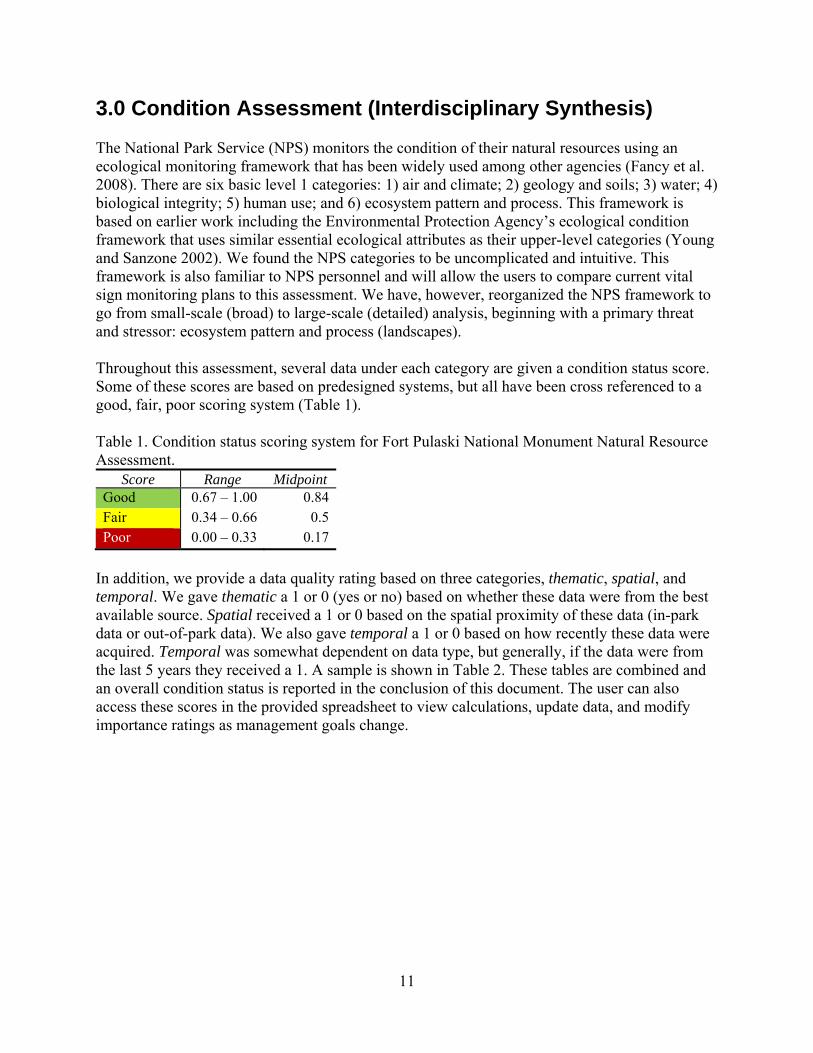
Table 1. Condition status scoring system for Fort Pulaski National Monument Natural

Resource Assessment. .................................................................................................. 11 Table 2. Example condition status table. Data quality was rated based on thematic (1 = best

source; 0 = not the best source), spatial (1 = inside park boundary; 0 = outside park boundary), and temporal (1 = recent; 0 = older than 5 years). The colors green, yellow, and red refer to good, fair, and poor scores respectively (see Table 1). ...................... 12

Table 3. Land cover (from 2001 C-CAP) totals and percent of total within Fort Pulaski National Monument boundary and in the subbasin study area containing FOPU and surrounding watersheds. ............................................................................................... 14

Table 4. Comparison of cover types (from 2001 C-CAP) within Fort Pulaski National Monument boundary, coastal study area, and coastal conservation areas. .................. 15

Table 5. Comparison of natural, semi-natural, and unnatural vegetation (reclassified from 2001 C-CAP) at Fort Pulaski National Monument and in the subbasin study area. .... 15

Table 6. Land cover change (from 1996 and 2001 C-CAP) in the subbasin study area containing Fort Pulaski National Monument and surrounding watersheds. ................ 18

Table 7. Landscape dynamics condition status summary within Fort Pulaski National Monument. Data quality was rated based on thematic (1 = best source; 0 = not the best source), spatial (1 = inside park boundary; 0 = outside park boundary), and temporal (1 = recent; 0 = older than 5 years). The colors green, yellow, and red refer to good, fair, and poor scores respectively (see Table 1). .......................................................... 19

Table 8. List of the coastal conservation areas, organizations, and contact information. ........ 20 Table 9. Wildfires reported at Fort Pulaski National Monument from 1/1/1972 to 12/31/2007,

at the National Fire and Aviation Management Web Application (National Wildfire Coordinating Group 2008). .......................................................................................... 21

Table 10. Fire condition status summary for Fort Pulaski National Monument. Data quality was rated based on thematic (1 = best source; 0 = not the best source), spatial (1 = inside park boundary; 0 = outside park boundary), and temporal (1 = recent; 0 = older than 5 years). The colors green, yellow, and red refer to good, fair, and poor scores respectively (see Table 1)............................................................................................. 27

Table 11. Schueler (2000) related percent impervious cover to management category. ......... 32 Table 12. Impervious surface totals for Fort Pulaski National Monument and each watershed/

subbasin within the study area. Management category from Schueler 2000. .............. 32 Table 13. Human effects condition status summary for Fort Pulaski National Monument. Data

quality was rated based on thematic (1 = best source; 0 = not the best source), spatial (1 = inside park boundary; 0 = outside park boundary), and temporal (1 = recent; 0 = older than 5 years). The colors green, yellow, and red refer to good, fair, and poor scores respectively (see Table 1).................................................................................. 34

Table 14. Number of National Park Service Fort visitors in ranked order. ............................. 37 Table 15. Visitor use condition status summary for Fort Pulaski National Monument. Data


vi

Table 16. The Air Quality Index (AQI) is a cross-agency U.S. Government venture whose purpose is to explain air quality health implications to the public. .............................. 39

Table 17. Air quality index in 2007 at monitoring sites near Fort Pulaski National Monument. Blank cells mean that the pollutant was not measured at the site ................................ 40

Table 18. Air quality condition status summary for Fort Pulaski National Monument. Data quality was rated based on thematic (1 = best source; 0 = not the best source), spatial (1 = inside park boundary; 0 = outside park boundary), and temporal (1 = recent; 0 = older than 5 years). The colors green, yellow, and red refer to good, fair, and poor scores respectively (see Table 1).................................................................................. 44

Table 19. List of recommended air quality organizations to participate with and promote regional approaches. ..................................................................................................... 44

Table 20. Classification used for Palmer Drought Severity Index (PDSI) values. .................. 52 Table 21. Saffir/Simpson Hurricane Scale (Blake et al. 2007). ............................................... 56 Table 22. Climate condition status summary for Fort Pulaski National Monument. Data


Table 23. Surface water detention correlation to National Wetland Inventory classification within Fort Pulaski NM. ............................................................................................... 65

Table 24. Coastal storm surge detention correlation to National Wetland Inventory classification within Fort Pulaski NM. ........................................................................ 66

Table 25. Streamflow maintenance correlation to National Wetland Inventory classification within Fort Pulaski NM. ............................................................................................... 67

Table 26. Nutrient transformation correlation to National Wetland Inventory classification within Fort Pulaski NM. ............................................................................................... 69

Table 27. Sediment and other particulate retention correlation to National Wetland Inventory classification within Fort Pulaski NM. ........................................................................ 70

Table 28. Shoreline stabilization correlation to National Wetland Inventory classification within Fort Pulaski NM. ............................................................................................... 71

Table 29. Hydrology condition status summary for Fort Pulaski National Monument. Data quality was rated based on thematic (1 = best source; 0 = not the best source), spatial (1 = inside park boundary; 0 = outside park boundary), and temporal (1 = recent; 0 = older than 5 years). The colors green, yellow, and red refer to good, fair, and poor scores respectively (see Table 1).................................................................................. 76

Table 30. Georgia water quality standards. .............................................................................. 80 Table 31. Standards for nutrient concentrations as developed for the National Coastal

Condition Report II (U.S. Environmental Protection Agency 2005). DIN refers to total dissolved inorganic nitrogen. DIP refers to total dissolved inorganic phosphorous. ... 80

Table 32. Potential for impairment of Fort Pulaski National Monument water resources. Adapted from McFarlin and Albers (2005). ................................................................ 84

Table 33. Water quality condition status summary within Fort Pulaski National Monument. Data quality was rated based on thematic (1 = best source; 0 = not the best source), spatial (1 = inside park boundary; 0 = outside park boundary), and temporal (1 = recent; 0 = older than 5 years). The colors green, yellow, and red refer to good, fair, and poor scores respectively (see Table 1). ................................................................. 84

vii

viii

Table 34. Recommendations to improve water quality and monitoring at Fort Pulaski National Monument from McFarlin and Albers (2005). ............................................................ 85

Table 35. Historical soil survey (USDA Bureau of Soils 1911) classification and approximate percent of total acreage for Fort Pulaski National Monument. .................................... 87

Table 36. Current soil survey (National Park Service 2006) classification, acreages, and percent of total acreage for Fort Pulaski National Monument. .................................... 88

Table 37. Potential erosion hazard (off-road, off-trial) according to soil characteristics at Fort Pulaski National Monument. ........................................................................................ 95

Table 38. Flooding frequency according to soil characteristics at Fort Pulaski National Monument .................................................................................................................... 97

Table 39. Drainage classes according to soil characteristics at Fort Pulaski National Monument. ................................................................................................................... 99

Table 40. Soil condition status summary for Fort Pulaski National Monument. Data quality was rated based on thematic (1 = best source; 0 = not the best source), spatial (1 = inside park boundary; 0 = outside park boundary), and temporal (1 = recent; 0 = older than 5 years). The colors green, yellow, and red refer to good, fair, and poor scores respectively (see Table 1)........................................................................................... 101

Table 41. List of available animal and plant surveys at Fort Pulaski National Monument. .. 102 Table 42. Management matrix used to categorize trend combinations. ................................. 106 Table 43. Species that utilize Fort Pulaski National Monument by taxa. .............................. 109 Table 44. Total number of species documented at Fort Pulaski National Monument, number

of high priority species from the GA Comprehensive Wildlife Conservation Strategy, and % of high priority species within Georgia that are found on FOPU. .................. 110

Table 45. Periwinkle density for fall collection sites on the Georgia Coastal LTER between 2003 and 2006. ........................................................................................................... 112

Table 46. Proportion of invasive species by taxa at Fort Pulaski National Monument. ........ 113 Table 47. Biotic community condition status summary for Fort Pulaski National Monument.

Data quality was rated based on thematic (1 = best source; 0 = not the best source), spatial (1 = inside park boundary; 0 = outside park boundary), and temporal (1 = recent; 0 = older than 5 years). The colors green, yellow, and red refer to good, fair, and poor scores respectively (see Table 1). ............................................................... 114

Table 48. Condition status scoring system for Fort Pulaski National Monument Natural Resource Assessment. ................................................................................................ 117

Table 49. Overall condition status summary for Fort Pulaski National Monument. Data quality was rated based on thematic (1 = best source; 0 = not the best source), spatial (1 = inside park boundary; 0 = outside park boundary), and temporal (1 = recent; 0 = older than 5 years). The colors green, yellow, and red refer to good, fair, and poor scores respectively (see Table 48).............................................................................. 118

Figures Page

Figure 1. Fort Pulaski National Monument is located on the coast of Georgia, just east of the

city of Savannah. ............................................................................................................ 4 Figure 2. Canal leading from Fort Pulaski National Monument ................................................ 6 Figure 3. Water resources and hydrologic units surrounding Fort Pulaski National Monument.

........................................................................................................................................ 8 Figure 4. The study area of major watersheds examined for the Fort Pulaski NM Natural

Resource Assessment. .................................................................................................. 13 Figure 5. Land cover (from 2001 C-CAP) in the subbasin study area containing Fort Pulaski

National Monument and surrounding watersheds. ...................................................... 16 Figure 6. Vegetation in the subbasin study area containing Fort Pulaski National Monument

and surrounding watersheds. ........................................................................................ 17 Figure 7. Wildfire sites and the dates they occurred, from 2000 to 2007 (GeoMAC 2008),

within 20 miles of Fort Pulaski National Monument. .................................................. 22 Figure 8. Simulated historical percent of low and mixed severity fires according to

LANDFIRE (USDA Forest Service 2006) in the region of Fort Pulaski National Monument. ................................................................................................................... 23

Figure 9. Simulated historical percent of replacement severity fires according to LANDFIRE (USDA Forest Service 2006) in the region of Fort Pulaski National Monument. ....... 24

Figure 10. Departure between current vegetation condition and reference vegetation condition according to LANDFIRE (USDA Forest Service 2006) in the region of Fort Pulaski National Monument. Fire Regime Condition Class I is low departure from historic vegetation; Condition Class II is moderate departure from historic vegetation; and Condition Class III is high departure from historic vegetation. ................................... 25

Figure 11. Wildfire fuel types according to LANDFIRE (USDA Forest Service 2006) in the region of Fort Pulaski National Monument. ................................................................ 26

Figure 12. A recent observed fire danger class map for the United States (USDA Forest Service 2008). .............................................................................................................. 28

Figure 13. Human population change in counties surrounding Fort Pulaski National Monument (U.S. Census Bureau 2008). ...................................................................... 30

Figure 14. Human population density (people per square kilometer, 2007) for counties surrounding Fort Pulaski National Monument (U.S. Census Bureau 2008). ............... 31

Figure 15. Impervious surface (from National Land Cover Database 2001) in the subbasin study area containing Fort Pulaski National Monument and surrounding watersheds. 33

Figure 16. Number of visitors per year to Fort Pulaski NM from 1935 to 2007. Data from NPS (2008b). ................................................................................................................ 36

Figure 17. Average monthly visitors (from the past 10 years, 1998 – 2007) to Fort Pulaski National Monument. Data from NPS (2008b). ............................................................ 36

Figure 18. Air quality monitoring sites near Fort Pulaski National Monument. Green indicates "Good" air quality, while yellow indicates "Moderate" air quality at these sites in 2007. ............................................................................................................................. 41

Figure 19. 8-hour average ozone (O3) exceedances for Fort Pulaski National Monument. .... 42 Figure 20. 24-hour average fine particulate matter (PM2.5) exceedances for Fort Pulaski

National Monument. .................................................................................................... 43

ix

Figure 21. Mean annual temperature for Savannah, GA from 1895 to 2007. The mean annual temperature is 64.95 °F. The trend is 0.2 °F increase per decade. ............................... 46

Figure 22. Mean temperature during winter for Savannah, GA from 1895 to 2007. The mean temperature was 50.24 °F. The trend is 0.10 °F increase per decade. ......................... 46

Figure 23. Spring temperature for Savannah, GA from 1895 to 2007. The mean temperature was 64.52 °F. The trend is 0.19 °F increase per decade. ............................................. 47

Figure 24. The summer temperature for Savannah, GA from 1895 to 2007. The mean temperature was 78.91 °F. The trend is 0.30 °F increase per decade. ......................... 47

Figure 25. The fall temperature for Savannah, GA from 1895 to 2007. The mean temperature is 66.22 °F. The trend is 0.20 °F increase per decade. ................................................. 48

Figure 26. Annual precipitation for Savannah, GA from 1895 to 2007. The mean annual precipitation is 48.26 inches with an increasing trend of 0.17 inches per decade. ...... 49

Figure 27. The winter precipitation for Savannah, GA from 1895 to 2007. The mean precipitation is 8.89 inches. The trend is 0.08 inches per decade. This figure was generated separately from the NOAA site but the data are from the same source as other figures below. ...................................................................................................... 50

Figure 28. The spring precipitation for Savannah, GA from 1895 to 2007. The mean precipitation is 9.89 inches. The trend is 0.15 inches per decade. ............................... 50

Figure 29. The summer precipitation for Savannah, GA from 1895 to 2007. The mean precipitation is 19.27 inches. The trend is -0.11 inches per decade. ............................ 51

Figure 30. The fall precipitation for Savannah, GA from 1895 to 2007. The mean precipitation is 10.13 inches. The trend is 0.06 inches per decade. .................................................. 51

Figure 31. PDSI value for Savannah, GA for 9-year periods from 1900 to 2007. .................. 53 Figure 32. The total growing degree days per year for Savannah, GA from 1896 to 2008. The

long term mean annual growing degree day total is 9146 (black line). The blue line indicates an increasing trend (R2= 0.31) ...................................................................... 54

Figure 33. The approximate date when 1200 GDD has been reached for each year. The decreasing trend indicates that this date is arriving earlier each year (trend is 0.4 days per decade). .................................................................................................................. 55

Figure 34. Total number of all storms per month (1851 – 2007) occurring within 100 nautical miles of Fort Pulaski National Monument. .................................................................. 57

Figure 35. Total number of major and minor storms per month (1851 – 2007) occurring within 100 nautical miles of Fort Pulaski National Monument. .................................. 58

Figure 36. Total number of storms by category per month (1851 – 2007) occurring within 100 nautical miles of Fort Pulaski National Monument. Tropical depressions (TD) have 38 mph sustained wind speeds or less, tropical storms (TS) have 39 to 73 mph wind speeds, and the remaining hurricane categories (1 – 4) are from Saffir/Simpson Hurricane Scale (Table 21). ......................................................................................... 59

Figure 37. Total number of all storms per decade (1851 – 2007) occurring within 100 nautical miles of Fort Pulaski National Monument. .................................................................. 60

Figure 38. Total number of major and minor storms per decade (1851 – 2007) occurring within 100 nautical miles of Fort Pulaski National Monument. .................................. 61

Figure 39. Total number of storms by category per decade (1851 – 2007) occurring within 100 nautical miles of Fort Pulaski National Monument. Tropical depressions (TD) have 38 mph sustained wind speeds or less, tropical storms (TS) have 39 to 73 mph

x

wind speeds, and the remaining hurricane categories (1 – 4) are from Saffir/Simpson Hurricane Scale (Table 21). ......................................................................................... 62

Figure 40. Surface water detention correlation to National Wetland Inventory classification within Fort Pulaski NM. ............................................................................................... 66

Figure 41. Coastal storm surge detention correlation to National Wetland Inventory classification within Fort Pulaski NM. ........................................................................ 67

Figure 42. Streamflow maintenance correlation to National Wetland Inventory classification within Fort Pulaski NM. ............................................................................................... 68

Figure 43. Nutrient transformation correlation to National Wetland Inventory classification within Fort Pulaski NM. ............................................................................................... 69

Figure 44. Sediment and other particulate retention correlation to National Wetland Inventory classification within Fort Pulaski NM. ........................................................................ 70

Figure 45. Shoreline stabilization correlation to National Wetland Inventory classification within Fort Pulaski NM. ............................................................................................... 72

Figure 46. Digital elevation model (DEM) of Fort Pulaski National Monument region showing mean sea level, and approximate two foot, and four foot storm surge. ......... 74

Figure 47. Federal Emergency Management Agency (FEMA, 2008) flood maps for the Fort Pulaski National Monument region, showing all areas are under flood hazard. .......... 75

Figure 48. Water resources and hydrologic units surrounding Fort Pulaski National Monument. ................................................................................................................... 78

Figure 49. Hazardous sites in Chatham County, surrounding Fort Pulaski National Monument. These sites are recorded by the Georgia Environmental Protection Division (EPD) and have released or are suspected to have released a regulated substance without a state sanctioned clean-up procedure. .................................................................................... 83

Figure 50. Extent of historical soil survey (USDA Bureau of Soils 1911) at Fort Pulaski National Monument. .................................................................................................... 87

Figure 51. Extent of current soil survey (National Park Service 2006) at Fort Pulaski National Monument. ................................................................................................................... 89

Figure 52. This aerial image (Google 2008) shows dredged spoil piles and the bike trail on McQueen’s island are now vegetated with shrubs and trees........................................ 91

Figure 53. White areas on fringes of nontidal dredged spoil deposits and uplands next to tidal marshes may indicate poor vegetation from low pH or high salinity, or poorly-vegetated sandy sediment washed free during extreme high tides (Google 2008). ..... 91

Figure 54. Cockspur Island (Google 2008), showing made land vegetated with scrub-shrub and forest trees, with an inset of the eroded sandy beach. ........................................... 92

Figure 55. Inset from Figure 54 showing shoreline erosion on the north shore of Cockspur Island (Google 2008). .................................................................................................. 92

Figure 56. Lower Coastal Plain Map, with arrow showing the location of Fort Pulaski National Monument. Barrier islands, also known as the Golden Isles, line the coast of Georgia. The Lower Coastal Plain extends for sixty-five to seventy miles between the Savannah and St. Marys Rivers and contains the remains of older and higher shorelines and dunes west of the present coast. Courtesy of V. J. Henry (Seabrook 2006). ........................................................................................................................... 93

Figure 57. This aerial image (Google 2008) with red lines indicate the location of Holocene barrier island dunes. The blue circle shows another Holocene-aged deposit on

xi

xii

Cockspur Island under the original fort (National Park Service 1995), while adjacent shrub and forest areas are recent dredged deposits. ..................................................... 94

Figure 58. Potential erosion hazard (off-road, off-trial) according to soil characteristics at Fort Pulaski National Monument. Slight means erosion is unlikely under ordinary climatic conditions; moderate means that some erosion is likely and that erosion-control measures may be needed; severe means that erosion is very likely, erosion-control measures advised; and very severe means that significant erosion is expected, loss of soil productivity and off-site damage likely................................................................. 96

Figure 59. Flooding frequency according to soil characteristics at Fort Pulaski National Monument. None means flooding is not probable; very rare means flooding is very unlikely; rare means flooding is unlikely but possible under unusual weather conditions; occasional means flooding occurs infrequently under normal weather conditions; frequent means flooding is likely to occur often; and very frequent means flooding is likely to occur very often under normal weather conditions. .................... 98

Figure 60. Drainage classes according to soil characteristics at Fort Pulaski National Monument. ................................................................................................................... 99

Figure 61. Hydric rating according to soil characteristics at Fort Pulaski National Monument. .................................................................................................................................... 100

Figure 62. USGS Breeding Bird Survey (BBS) Routes in the area surrounding Fort Pulaski National Monument that were chosen for the assessment. ........................................ 104

Figure 63. Number of periwinkles per square meter versus percent marsh biomass from a controlled study (Silliman and Bertness 2002). ......................................................... 111

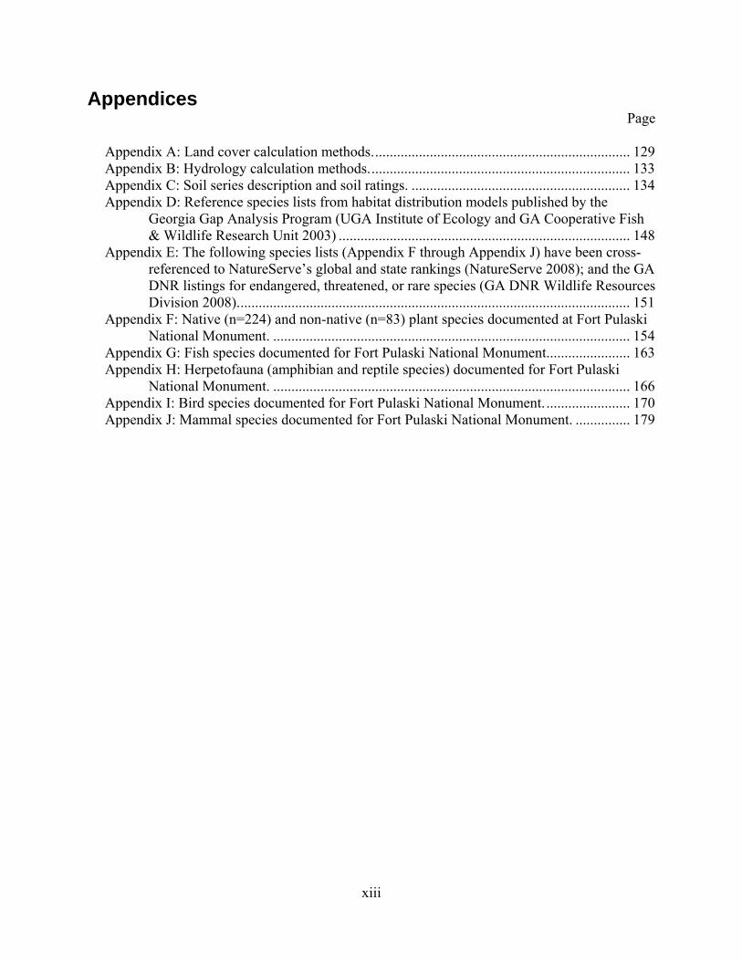
Appendices Page

Appendix A: Land cover calculation methods. ...................................................................... 129 Appendix B: Hydrology calculation methods. ....................................................................... 133 Appendix C: Soil series description and soil ratings. ............................................................ 134 Appendix D: Reference species lists from habitat distribution models published by the

Georgia Gap Analysis Program (UGA Institute of Ecology and GA Cooperative Fish & Wildlife Research Unit 2003) ................................................................................ 148

Appendix E: The following species lists (Appendix F through Appendix J) have been cross-referenced to NatureServe’s global and state rankings (NatureServe 2008); and the GA DNR listings for endangered, threatened, or rare species (GA DNR Wildlife Resources Division 2008). ........................................................................................................... 151

Appendix F: Native (n=224) and non-native (n=83) plant species documented at Fort Pulaski National Monument. .................................................................................................. 154

Appendix G: Fish species documented for Fort Pulaski National Monument....................... 163 Appendix H: Herpetofauna (amphibian and reptile species) documented for Fort Pulaski

National Monument. .................................................................................................. 166 Appendix I: Bird species documented for Fort Pulaski National Monument. ....................... 170 Appendix J: Mammal species documented for Fort Pulaski National Monument. ............... 179

xiii

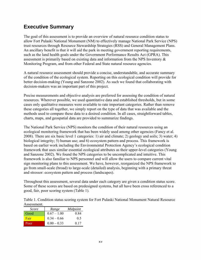
Executive Summary The goal of this assessment is to provide an overview of natural resource condition status to allow Fort Pulaski National Monument (NM) to effectively manage National Park Service (NPS) trust resources through Resource Stewardship Strategies (RSS) and General Management Plans. An ancillary benefit is that it will aid the park in meeting government reporting requirements, such as the land health goals under the Government Performance Results Act (GPRA). This assessment is primarily based on existing data and information from the NPS Inventory & Monitoring Program, and from other Federal and State natural resource agencies. A natural resource assessment should provide a concise, understandable, and accurate summary of the condition of the ecological system. Reporting on this ecological condition will provide for better decision-making (Young and Sanzone 2002). As such we found that collaborating with decision-makers was an important part of this project. Precise measurements and objective analysis are preferred for assessing the condition of natural resources. Wherever possible, we used quantitative data and established thresholds, but in some cases only qualitative measures were available to rate important categories. Rather than remove these categories all together, we simply report on the type of data that was available and the methods used to compare these data to a desired condition. In all cases, straightforward tables, charts, maps, and geospatial data are provided to summarize findings. The National Park Service (NPS) monitors the condition of their natural resources using an ecological monitoring framework that has been widely used among other agencies (Fancy et al. 2008). There are six basic level 1 categories: 1) air and climate; 2) geology and soils; 3) water; 4) biological integrity; 5) human use; and 6) ecosystem pattern and process. This framework is based on earlier work including the Environmental Protection Agency’s ecological condition framework that uses similar essential ecological attributes as their upper-level categories (Young and Sanzone 2002). We found the NPS categories to be uncomplicated and intuitive. This framework is also familiar to NPS personnel and will allow the users to compare current vital sign monitoring plans to this assessment. We have, however, reorganized the NPS framework to go from small-scale (broad) to large-scale (detailed) analysis, beginning with a primary threat and stressor: ecosystem pattern and process (landscapes). Throughout this assessment, several data under each category are given a condition status score. Some of these scores are based on predesigned systems, but all have been cross referenced to a good, fair, poor scoring system (Table 1). Table 1. Condition status scoring system for Fort Pulaski National Monument Natural Resource Assessment.

Score Range Midpoint Good 0.67 – 1.00 0.84Fair 0.34 – 0.66 0.5Poor 0.00 – 0.33 0.17

xv

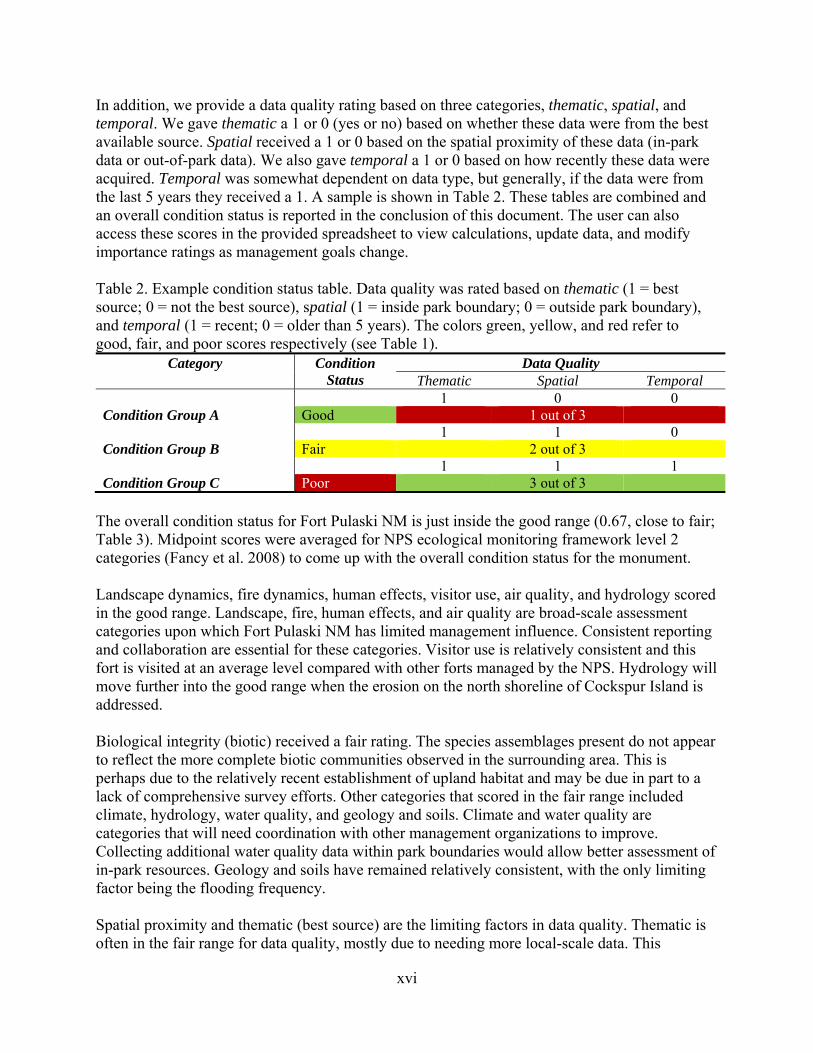
In addition, we provide a data quality rating based on three categories, thematic, spatial, and temporal. We gave thematic a 1 or 0 (yes or no) based on whether these data were from the best available source. Spatial received a 1 or 0 based on the spatial proximity of these data (in-park data or out-of-park data). We also gave temporal a 1 or 0 based on how recently these data were acquired. Temporal was somewhat dependent on data type, but generally, if the data were from the last 5 years they received a 1. A sample is shown in Table 2. These tables are combined and an overall condition status is reported in the conclusion of this document. The user can also access these scores in the provided spreadsheet to view calculations, update data, and modify importance ratings as management goals change. Table 2. Example condition status table. Data quality was rated based on thematic (1 = best source; 0 = not the best source), spatial (1 = inside park boundary; 0 = outside park boundary), and temporal (1 = recent; 0 = older than 5 years). The colors green, yellow, and red refer to good, fair, and poor scores respectively (see Table 1).

Category Condition Status

Data Quality Thematic Spatial Temporal

1 0 0 Condition Group A Good 1 out of 3 1 1 0 Condition Group B Fair 2 out of 3 1 1 1 Condition Group C Poor 3 out of 3

The overall condition status for Fort Pulaski NM is just inside the good range (0.67, close to fair; Table 3). Midpoint scores were averaged for NPS ecological monitoring framework level 2 categories (Fancy et al. 2008) to come up with the overall condition status for the monument. Landscape dynamics, fire dynamics, human effects, visitor use, air quality, and hydrology scored in the good range. Landscape, fire, human effects, and air quality are broad-scale assessment categories upon which Fort Pulaski NM has limited management influence. Consistent reporting and collaboration are essential for these categories. Visitor use is relatively consistent and this fort is visited at an average level compared with other forts managed by the NPS. Hydrology will move further into the good range when the erosion on the north shoreline of Cockspur Island is addressed. Biological integrity (biotic) received a fair rating. The species assemblages present do not appear to reflect the more complete biotic communities observed in the surrounding area. This is perhaps due to the relatively recent establishment of upland habitat and may be due in part to a lack of comprehensive survey efforts. Other categories that scored in the fair range included climate, hydrology, water quality, and geology and soils. Climate and water quality are categories that will need coordination with other management organizations to improve. Collecting additional water quality data within park boundaries would allow better assessment of in-park resources. Geology and soils have remained relatively consistent, with the only limiting factor being the flooding frequency. Spatial proximity and thematic (best source) are the limiting factors in data quality. Thematic is often in the fair range for data quality, mostly due to needing more local-scale data. This

xvi

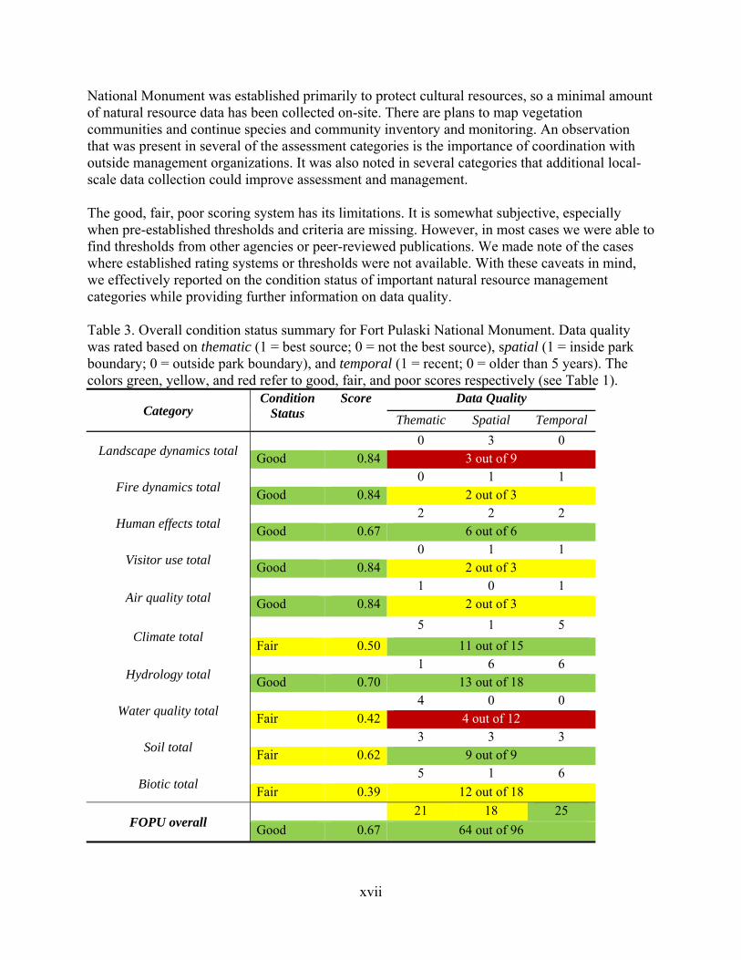
National Monument was established primarily to protect cultural resources, so a minimal amount of natural resource data has been collected on-site. There are plans to map vegetation communities and continue species and community inventory and monitoring. An observation that was present in several of the assessment categories is the importance of coordination with outside management organizations. It was also noted in several categories that additional local-scale data collection could improve assessment and management. The good, fair, poor scoring system has its limitations. It is somewhat subjective, especially when pre-established thresholds and criteria are missing. However, in most cases we were able to find thresholds from other agencies or peer-reviewed publications. We made note of the cases where established rating systems or thresholds were not available. With these caveats in mind, we effectively reported on the condition status of important natural resource management categories while providing further information on data quality. Table 3. Overall condition status summary for Fort Pulaski National Monument. Data quality was rated based on thematic (1 = best source; 0 = not the best source), spatial (1 = inside park boundary; 0 = outside park boundary), and temporal (1 = recent; 0 = older than 5 years). The colors green, yellow, and red refer to good, fair, and poor scores respectively (see Table 1).

Category Condition

Status Score Data Quality

Thematic Spatial Temporal

Landscape dynamics total 0 3 0

Good 0.84 3 out of 9

Fire dynamics total 0 1 1


Human effects total 2 2 2


Visitor use total 0 1 1


Air quality total 1 0 1


Climate total 5 1 5

Fair 0.50 11 out of 15

Hydrology total 1 6 6


Water quality total 4 0 0


Soil total 3 3 3


Biotic total 5 1 6


FOPU overall 21 18 25


xvii

xviii

This project provided a comprehensive amount of organized tabular data and many geospatial data layers and maps that will aid in the management of Fort Pulaski NM. These data are provided on an accompanying disk and can be used to compare current status to future conditions. This is merely a first step to compiling data and reporting on current condition status, data gaps, and threats and stressors. A well-established assessment protocol will include follow-up and future analysis.

Acknowledgements This project would not have been possible without the help of personnel from Fort Pulaski National Monument, NPS Southeast Region, Southeast Coast Network, Natural Resource Program Center, and various departments at Virginia Tech. We would like to thank the following people for their contribution to this assessment effort: Fort Pulaski National Monument Charles Fenwick Brent Rothschild Mike Weinstein Southeast Region Jim Long Southeast Coast Network Joe DeVivo Tony Curtis Christina Wright Natural Resource Program Center Jeff Albright Conservation Management Institute, Virginia Tech Shelia Crowe Jeff Dobson Jacob Hartwright Ginger Hicks David Palmer Laura Roghair Jeff Waldon Civil and Environmental Engineering, Virginia Tech Myles Killar Virginia Water Resources Research Center, Virginia Tech Dr. Stephen Schoenholtz

xix

Abbreviations AQI Air Quality Index BBS Breeding Bird Survey BOD Biological Oxygen Demand C-CAP Coastal Change Analysis Program CRD Coastal Resources Division DDT Dichloro-Diphenyl-Trichloroethane DEM Digital Elevation Model DIN Dissolved Inorganic Nitrogen DIP Dissolved Inorganic Phosphorus DNR Department of Natural Resources DO Dissolved Oxygen DRG Digital Raster Graphic EMAP Environmental Monitoring and Assessment Program EPA Environmental Protection Agency EPD Environmental Protection Division ERL Effects Range Low ESRI Environmental Systems Research Institute FDA Food and Drug Administration FEMA Federal Emergency Management Agency FOPU Fort Pulaski National Monument GA Georgia GAP Gap Analysis Program GCE Georgia Coastal Ecosystems GDD Growing Degree Days GeoMAC Geospatial Multi-Agency Coordination Group GIS Geographic Information System GMP General Management Plan GPRA Government Performance Results Act HUC Hydrologic Unit Code I&M Inventory and Monitoring LMER Land Margin Ecosystem Research LTER Long-Term Ecological Research MLRA Major Land Resource Area NB National Battlefield NCA National Coastal Assessment NHD National Hydrologic Data NM National Monument NOAA National Oceanic and Atmospheric Administration NPS National Park Service NRCS Natural Resources Conservation Service NTCHS National Technical Committee for Hydric Soils NWI National Wetlands Inventory PAHs Polycyclic Aromatic Hydrocarbons PCBs Polychlorinated Biphenyls PDSI Palmer Drought Severity Index

xx

xxi

PPM Parts per million RSS Resource Stewardship Strategies SC South Carolina SCP Southern Coastal Plain SSURGO Soil Survey Geographic TD Tropical Depression TS Tropical Storm U.S. United States UGA University of Georgia USACE United States Army Corps of Engineers USDA United States Department of Agriculture USGS United States Geological Survey

1.0 Introduction The goal of this assessment is to provide an overview of natural resource condition status to allow Fort Pulaski National Monument (NM) to effectively manage National Park Service (NPS) trust resources through Resource Stewardship Strategies (RSS) and General Management Plans. An ancillary benefit is that it will aid the park in meeting government reporting requirements, such as the land health goals under the Government Performance Results Act (GPRA). This assessment is primarily based on existing data and information from the NPS Inventory & Monitoring Program, and from other Federal and State natural resource agencies. A natural resource assessment should provide a concise, understandable, and accurate summary of the condition of the ecological system. Reporting on this ecological condition will provide for better decision-making (Young and Sanzone 2002). As such we found that collaborating with decision-makers was an important part of this project. An iterative process was implemented to collect and synthesize data and meet with NPS staff. We collaborated on what was important for their particular assessment, park, and watershed. Additional data was then collected and the process repeated itself to further refine and identify additional natural resource issues and objectives for this assessment. Precise measurements and objective analysis are preferred for assessing the condition of natural resources. Wherever possible, we used quantitative data and established thresholds, but in some cases only qualitative measures were available to rate important categories. Rather than remove these categories all together, we simply report on the type of data that was available and the methods used to compare these data to a desired condition. In all cases, straightforward tables, charts, maps, and geospatial data are provided to summarize findings.

1

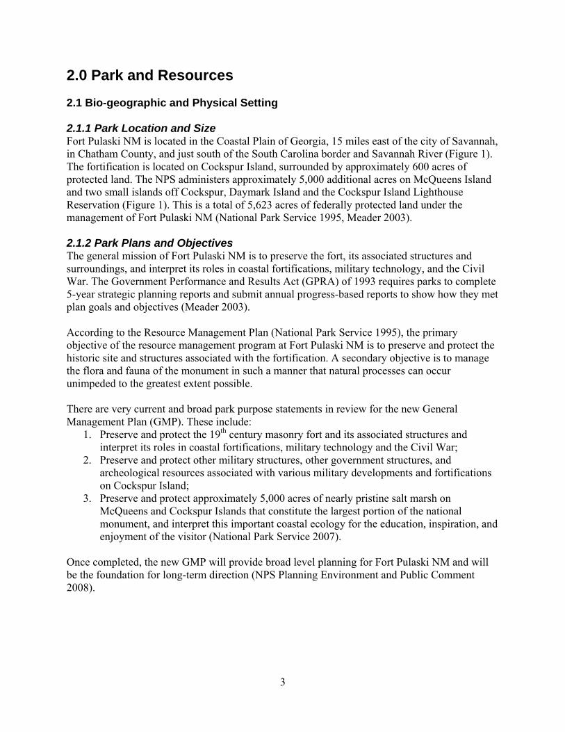
2.0 Park and Resources 2.1 Bio-geographic and Physical Setting 2.1.1 Park Location and Size Fort Pulaski NM is located in the Coastal Plain of Georgia, 15 miles east of the city of Savannah, in Chatham County, and just south of the South Carolina border and Savannah River (Figure 1). The fortification is located on Cockspur Island, surrounded by approximately 600 acres of protected land. The NPS administers approximately 5,000 additional acres on McQueens Island and two small islands off Cockspur, Daymark Island and the Cockspur Island Lighthouse Reservation (Figure 1). This is a total of 5,623 acres of federally protected land under the management of Fort Pulaski NM (National Park Service 1995, Meader 2003). 2.1.2 Park Plans and Objectives The general mission of Fort Pulaski NM is to preserve the fort, its associated structures and surroundings, and interpret its roles in coastal fortifications, military technology, and the Civil War. The Government Performance and Results Act (GPRA) of 1993 requires parks to complete 5-year strategic planning reports and submit annual progress-based reports to show how they met plan goals and objectives (Meader 2003). According to the Resource Management Plan (National Park Service 1995), the primary objective of the resource management program at Fort Pulaski NM is to preserve and protect the historic site and structures associated with the fortification. A secondary objective is to manage the flora and fauna of the monument in such a manner that natural processes can occur unimpeded to the greatest extent possible. There are very current and broad park purpose statements in review for the new General Management Plan (GMP). These include:

1. Preserve and protect the 19th century masonry fort and its associated structures and interpret its roles in coastal fortifications, military technology and the Civil War;

2. Preserve and protect other military structures, other government structures, and archeological resources associated with various military developments and fortifications on Cockspur Island;

3. Preserve and protect approximately 5,000 acres of nearly pristine salt marsh on McQueens and Cockspur Islands that constitute the largest portion of the national monument, and interpret this important coastal ecology for the education, inspiration, and enjoyment of the visitor (National Park Service 2007).

Once completed, the new GMP will provide broad level planning for Fort Pulaski NM and will be the foundation for long-term direction (NPS Planning Environment and Public Comment 2008).

3

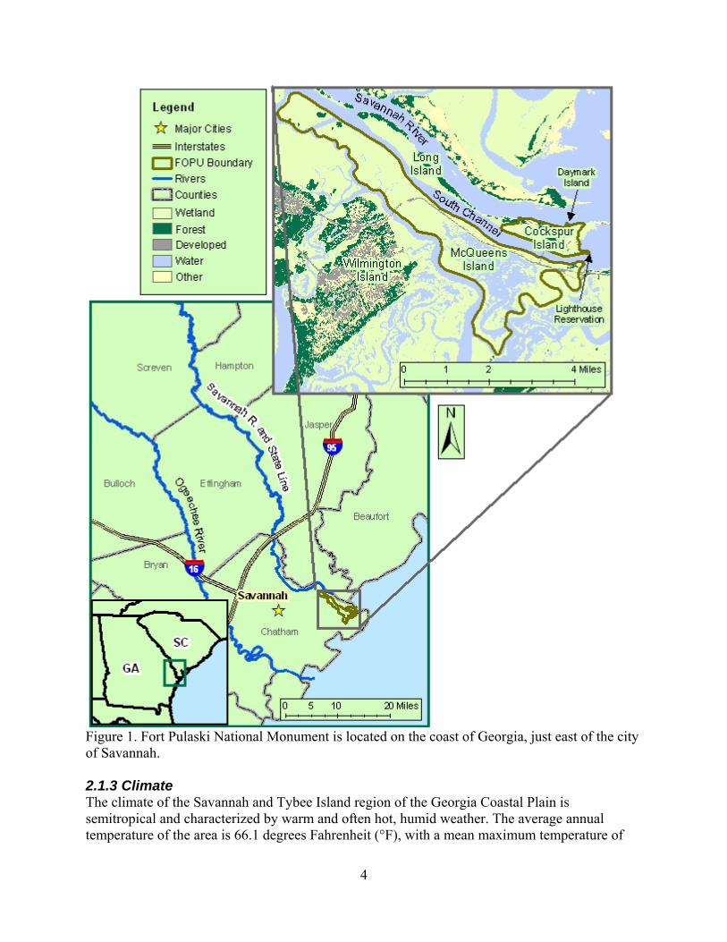
Figure 1. Fort Pulaski National Monument is located on the coast of Georgia, just east of the city of Savannah. 2.1.3 Climate The climate of the Savannah and Tybee Island region of the Georgia Coastal Plain is semitropical and characterized by warm and often hot, humid weather. The average annual temperature of the area is 66.1 degrees Fahrenheit (°F), with a mean maximum temperature of

4

76.6°F and a mean minimum temperature of 55.5°F. The warmest month on average is July, at 91°F. The coolest month on average is January, at 38.3°F (Georgia Automated Environmental Monitoring Network 2008). Lowest and highest recorded temperatures were 105°F in 1986 and 3°F in 1985 (The Weather Channel 2008). The wettest month has historically been August, with an average of 6.77 inches of precipitation. A great deal (49%) of the rain falls during the months of June through September. Tropical storms and hurricanes are a concern as this area is brushed or hit by a tropical system every 3.61 years (Hurricane City 2008). The growing season averages 260 days, with the last spring freeze normally occurring in early March and the first fall freeze normally occurring in late November (UGA State Climate Office 2008). 2.1.4 Geology, Landforms, and Soils The Coastal Plain region is composed of un-deformed sedimentary rock layers whose ages range from the Late Cretaceous to the present Holocene sediments of the coast. Beneath Coastal Plain sediments are harder igneous and metamorphic rocks, such as those found in the Piedmont. Usually referred to as the "basement," these hard rocks occur at greater and greater depths toward the south and east, reaching depths of up to 10,000 feet or more beneath the modern Georgia coast (Frazier 2007). Sediment from the upper Piedmont region eroded into the Coastal Plain over the past 100 million years. In addition to recent alluvium, organic and marine deposits make up some of the sediment found in the Coastal Plain (UGA Department of Geology 2008). Human-dredged and deposited sediments are abundant along the coastlines. Specifically, the coastal region near Fort Pulaski NM is a Holocene-aged deposit of organic, marine, and alluvial origin. More specifically Cockspur Island is primarily human-constructed with a system of dikes and drainage canals (Figure 2). Dredging in the Savannah River made up the spoil deposition which began with the fort construction (National Park Service 1995). Cockspur and Long Island to the northwest were combined into one island from sediment deposition after jetties were built and the placement of dredge materials during the late 19th and early 20th centuries. Due to these human activities, Cockspur Island, once mostly tidal marsh, is now 43% dry upland. Deposition of dredge material by the U.S. Army Corps of Engineers (USACE) continued until the 1980’s, halted by land-protection plans and a bill that passed in 1996 to prevent the USACE from continuing spoil deposition practices (Meader 2003).

5

Figure 2. Canal leading from Fort Pulaski National Monument Only 5% of McQueens Island is upland, with the remainder in native tidal salt marsh. These upland areas were filled for the development of U.S. Highway 80 and a railroad right of way that is now a pedestrian and bike trail. Land maps, circa 1862, show only the area inside the dikes of the fort as dry land on Cockspur and McQueens Island (National Park Service 1995). For all of the land area of Fort Pulaski (5,623 acres), several reports (National Park Service 1995, Meader 2003, National Park Service 2007) document close to 5,000 acres as salt marsh. According to Soil Survey Geographic (SSURGO) from the Natural Resources Conservation Service (NRCS) and NPS (National Park Service 2006), 81.5% of the soil is Tidal marsh, salty, 11.8% is water, and the remaining 6.7% is Made land. The parent material of Tidal marsh, salty is marine deposits, while tidal marshes make up the landform. The slope in this class is 0 to 2 percent. The area is very poorly drained since the depth to water table is about 0 inches and it is flooded two times per day. In addition, the typical profile is silty clay in both 0 to 10 inches and 10 to 60 inches. Made land is widely variable, from sandy to clayey with differing water capacity thresholds. As the name suggests, alterations of soil were performed by filing, removing, dredging, and dumping (National Park Service 2006, USDA Natural Resource Conservation Service 2006). 2.1.5 Surface Water and Wetlands The water bodies and waterways within or adjacent to Fort Pulaski NM include five saltwater ways: the Savannah River, the South Channel of the Savannah River, Bull River, Oyster Creek, and Lazaretto Creek (Figure 3). Three small bodies of freshwater include two unnamed water bodies, and a moat surrounding the fortification (McFarlin and Alber 2005).

6

The Savannah River and the South Fork, whose headwaters stretch to the Blue Ridge, are in the Lower Savannah Subbasin (National Hydrologic Data Hydrologic Unit Code [HUC] 03060109), or more specifically, the Savannah-Abercorn Creek Watershed (HUC 0306010906). The remaining waterways, Bull River, Oyster Creek, and Lazaretto Creek, are purely tidal in nature and are located in the Ogeechee Coastal Subbasin (HUC 03060204). Savannah (HUC 030601) and Ogeechee (HUC 030602) are two separate basins that coincide on the Fort Pulaski NM property (Figure 3). A large amount of the research and emphasis has been on the effects of pollution and water flows on the Savannah River (McFarlin and Alber 2005). The U.S. Army Corps of Engineers operates three dams and reservoirs upstream of Fort Pulaski: Hartwell, Richard B. Russell, and J. Strom Thurmond (U.S. Army Corps of Engineers 2008). Nearly 5,000 acres or 89% of Fort Pulaski NM are native tidal salt marsh. These wetlands are important globally and support key aquatic species such as shrimp, oysters, juvenile fish, and shellfish (National Park Service 2007). As development along the coast and threats of rising sea level from climate change continues, importance will be placed on maintaining wetlands.

7

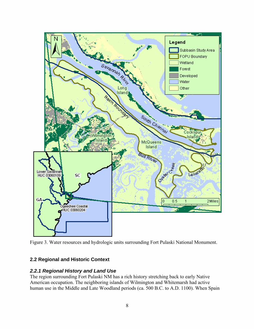
Figure 3. Water resources and hydrologic units surrounding Fort Pulaski National Monument. 2.2 Regional and Historic Context 2.2.1 Regional History and Land Use The region surrounding Fort Pulaski NM has a rich history stretching back to early Native American occupation. The neighboring islands of Wilmington and Whitemarsh had active human use in the Middle and Late Woodland periods (ca. 500 B.C. to A.D. 1100). When Spain

8

settled the area in the early 16th century, the Euchee Tribe was occupying adjacent Tybee Island (Meader 2003). Spanish missions left the area by 1684 due to the growth of Charles Town (later Charleston), the English colony to the north. Spain, France, and England disputed over Georgia until the city of Savannah was settled by the British (Meader 2003). Savannah was established in 1733 by General James Oglethorpe and 120 of his passengers, forming Georgia, the last of the 13 British Colonies. Savannah is a large city just 10 to 15 miles west of Fort Pulaski with an estimated population in 2006 of 127,889. The 2006 estimate marks a steady decline from the 2000 census of 131,510 individuals and the 1990 census of 137,560 (U.S. Census Bureau 2008). This is an incomplete statistic since suburban movement has affected many city populations across the country. If we look at the counties surrounding Savannah, there are significant population increases. Chatham County boasted an estimated 248,469 individuals in 2007, up 7% from the 2000 census of 232,048 individuals. Effingham County, to the northwest, is up 35%, from 37,535 in 2000 to 50,728 in 2007. Conversely, Jasper County, SC has grown only 6% to the 2007 estimate of 21,953 (U.S. Census Bureau 2008). The Savannah River basin as a whole had 523,100 individuals in 1995, with estimates of 60% growth to 900,000 individuals by 2050 (GA DNR Environmental Protection Division 2001). Similar to much of the United States, land use in the Savannah River basin is in flux. Forestry and its products are a major land use and commodity within the Savannah River basin, with approximately 2,420,300 acres of commercial forest land (GA DNR Environmental Protection Division 2001). Farmland has been decreasing since 1982. Almost 75% was pasture with the remainder in cotton, peanuts, tobacco, and grain. Poultry and livestock are also a large part of the agriculture in the Savannah River basin. Despite this, the closest areas, in Chatham and Effingham, had less than 15% of their counties in farmland (GA DNR Environmental Protection Division 2001). 2.2.2 Site History The first written account of Europeans on Cockspur Island (then Peeper Island) was in 1736, when John Wesley, the father of Methodism, and a small group from General James Oglethorpe’s ship made a short stop to give thanks. Before the first fort was built, goods were loaded and unloaded from ships on Cockspur Island. Fort George was built in the mid-1700’s to protect the colonies of Georgia and South Carolina from Spanish invasion from the south, but fell into disrepair in the 1770s. In 1794, Fort Green stood for a short period. A new system of fortification in America during the early 1800s would eventually lead to the construction of Fort Pulaski. By 1847, the primary components of the fortification we know today were complete (Meader 2003). Fort Pulaski was under Confederate control during the early part of the Civil War, from January 1861 to April 1862. On April 10, 1862, Union forces took control in the momentous battle that marked the end of masonry fortifications. Directly following the Civil War, plans were made to modernize Fort Pulaski, but these were quickly thwarted by plans for a new installation on Tybee Island. Fort Pulaski officially closed in 1873 with a caretaker on post and became a military

9

10

reservation that could be used in the future. After much neglect and alternative uses, Fort Pulaski officially became a national monument on October 15, 1924 (Meader 2003). Fort Pulaski was transferred from the War Department to the National Park Service in 1933. A great amount of work and money were needed for repairs and preservation of the fort. The New Deal programs in the 1930s and the Mission 66 program in the 1950s and 60s were the driving force behind rehabilitation and maintenance of this once great fort. Additional land was acquired and general park maintenance and management plans were established (Meader 2003). 2.3 Unique and Significant Park Resources and Designations 2.3.1 Unique Resources There are several significant historical park resources at Fort Pulaski NM. Chiefly it is the location where the end of masonry fortification was marked when this fort was breached by rifled cannons during the Civil War. This fort was also Robert E. Lee’s first project, overseeing construction after he graduated from West Point. There are several other significance statements of historical basis listed in the GMP review, but only one of natural resource significance: Fort Pulaski NM protects one of the largest federal holdings of native salt marsh (National Park Service 2007). This is a rather important statement and several other unique natural resources inevitably follow as a result. These include habitat for rare wildlife species, including important fish nurseries and coastal bird habitat. Salt marshes are an extremely productive natural environment (GA DNR Coastal Resources Division 2008b). Decaying grass particles from tidal marshes form the beginning of a complex food web that nourishes a long list of marine life. 2.3.2 Special Designations Although Fort Pulaski NM has no special designations at this time, there are plans to perform a formal wilderness assessment as part of their GMP process followed by a recommendation to Congress (National Park Service 2007). In fact, until there is a formal request, the NPS manages land that has wilderness characteristics in a manner required by the Wilderness Act. In addition, there has been some discussion of whether Fort Pulaski NM could meet the requirements of an Important Birding Area (Park Staff 2007).

3.0 Condition Assessment (Interdisciplinary Synthesis) The National Park Service (NPS) monitors the condition of their natural resources using an ecological monitoring framework that has been widely used among other agencies (Fancy et al. 2008). There are six basic level 1 categories: 1) air and climate; 2) geology and soils; 3) water; 4) biological integrity; 5) human use; and 6) ecosystem pattern and process. This framework is based on earlier work including the Environmental Protection Agency’s ecological condition framework that uses similar essential ecological attributes as their upper-level categories (Young and Sanzone 2002). We found the NPS categories to be uncomplicated and intuitive. This framework is also familiar to NPS personnel and will allow the users to compare current vital sign monitoring plans to this assessment. We have, however, reorganized the NPS framework to go from small-scale (broad) to large-scale (detailed) analysis, beginning with a primary threat and stressor: ecosystem pattern and process (landscapes). Throughout this assessment, several data under each category are given a condition status score. Some of these scores are based on predesigned systems, but all have been cross referenced to a good, fair, poor scoring system (Table 1). Table 1. Condition status scoring system for Fort Pulaski National Monument Natural Resource Assessment.


In addition, we provide a data quality rating based on three categories, thematic, spatial, and temporal. We gave thematic a 1 or 0 (yes or no) based on whether these data were from the best available source. Spatial received a 1 or 0 based on the spatial proximity of these data (in-park data or out-of-park data). We also gave temporal a 1 or 0 based on how recently these data were acquired. Temporal was somewhat dependent on data type, but generally, if the data were from the last 5 years they received a 1. A sample is shown in Table 2. These tables are combined and an overall condition status is reported in the conclusion of this document. The user can also access these scores in the provided spreadsheet to view calculations, update data, and modify importance ratings as management goals change.

11

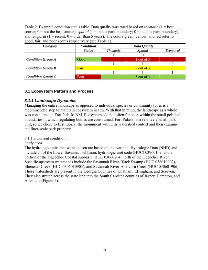
Table 2. Example condition status table. Data quality was rated based on thematic (1 = best source; 0 = not the best source), spatial (1 = inside park boundary; 0 = outside park boundary), and temporal (1 = recent; 0 = older than 5 years). The colors green, yellow, and red refer to good, fair, and poor scores respectively (see Table 1).



1 0 0 Condition Group A Good 1 out of 3 1 1 0 Condition Group B Fair 2 out of 3 1 1 1 Condition Group C Poor 3 out of 3

3.1 Ecosystem Pattern and Process 3.1.1 Landscape Dynamics Managing the entire landscape as opposed to individual species or community types is a recommended step to maintain ecosystem health. With that in mind, the landscape as a whole was considered at Fort Pulaski NM. Ecosystems do not often function within the small political boundaries in which regulating bodies are constrained. Fort Pulaski is a relatively small park unit, so we chose to first look at the monument within its watershed context and then examine the finer-scale park property. 3.1.1.a Current condition: Study area: The hydrologic units that were chosen are based on the National Hydrologic Data (NHD) and include all of the Lower Savannah subbasin, hydrologic unit code (HUC) 03960109, and a portion of the Ogeechee Coastal subbasin, HUC 03060204, north of the Ogeechee River. Specific upstream watersheds include the Savannah River-Black Swamp (HUC 036010902), Ebenezer Creek (HUC 0306010903), and Savannah River-Abercorn Creek (HUC 030601906). These watersheds are present in the Georgia Counties of Chatham, Effingham, and Screven. They also stretch across the state line into the South Carolina counties of Jasper, Hampton, and Allendale (Figure 4).

12

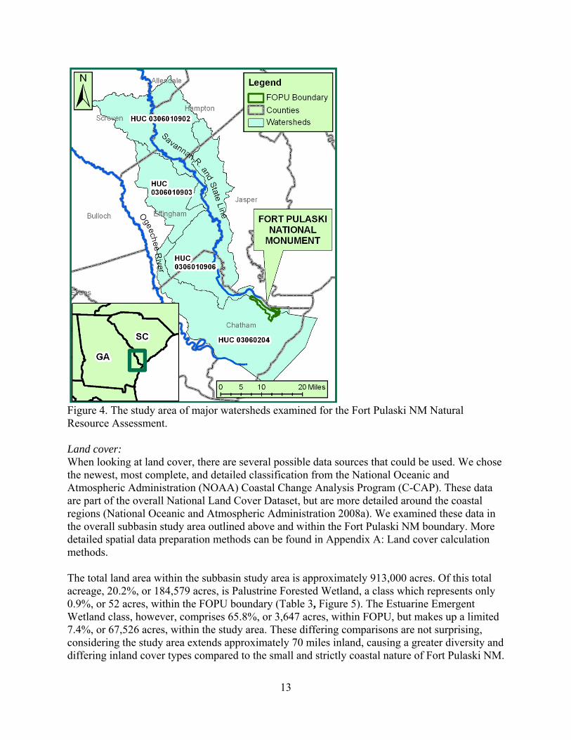
Figure 4. The study area of major watersheds examined for the Fort Pulaski NM Natural Resource Assessment. Land cover: When looking at land cover, there are several possible data sources that could be used. We chose the newest, most complete, and detailed classification from the National Oceanic and Atmospheric Administration (NOAA) Coastal Change Analysis Program (C-CAP). These data are part of the overall National Land Cover Dataset, but are more detailed around the coastal regions (National Oceanic and Atmospheric Administration 2008a). We examined these data in the overall subbasin study area outlined above and within the Fort Pulaski NM boundary. More detailed spatial data preparation methods can be found in Appendix A: Land cover calculation methods. The total land area within the subbasin study area is approximately 913,000 acres. Of this total acreage, 20.2%, or 184,579 acres, is Palustrine Forested Wetland, a class which represents only 0.9%, or 52 acres, within the FOPU boundary (Table 3, Figure 5). The Estuarine Emergent Wetland class, however, comprises 65.8%, or 3,647 acres, within FOPU, but makes up a limited 7.4%, or 67,526 acres, within the study area. These differing comparisons are not surprising, considering the study area extends approximately 70 miles inland, causing a greater diversity and differing inland cover types compared to the small and strictly coastal nature of Fort Pulaski NM.

13

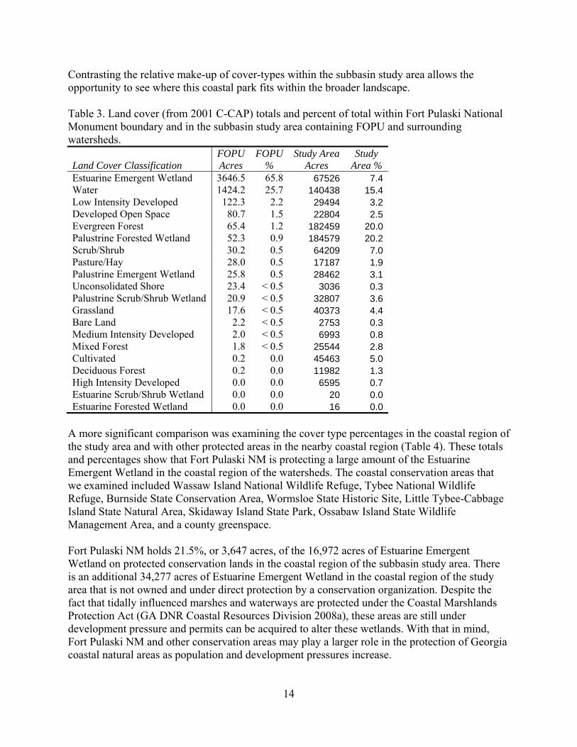
Contrasting the relative make-up of cover-types within the subbasin study area allows the opportunity to see where this coastal park fits within the broader landscape. Table 3. Land cover (from 2001 C-CAP) totals and percent of total within Fort Pulaski National Monument boundary and in the subbasin study area containing FOPU and surrounding watersheds.

Land Cover Classification FOPU Acres

FOPU %

Study Area Acres

Study Area %

Estuarine Emergent Wetland 3646.5 65.8 67526 7.4Water 1424.2 25.7 140438 15.4Low Intensity Developed 122.3 2.2 29494 3.2Developed Open Space 80.7 1.5 22804 2.5Evergreen Forest 65.4 1.2 182459 20.0Palustrine Forested Wetland 52.3 0.9 184579 20.2Scrub/Shrub 30.2 0.5 64209 7.0Pasture/Hay 28.0 0.5 17187 1.9Palustrine Emergent Wetland 25.8 0.5 28462 3.1Unconsolidated Shore 23.4 < 0.5 3036 0.3Palustrine Scrub/Shrub Wetland 20.9 < 0.5 32807 3.6Grassland 17.6 < 0.5 40373 4.4Bare Land 2.2 < 0.5 2753 0.3Medium Intensity Developed 2.0 < 0.5 6993 0.8Mixed Forest 1.8 < 0.5 25544 2.8Cultivated 0.2 0.0 45463 5.0Deciduous Forest 0.2 0.0 11982 1.3High Intensity Developed 0.0 0.0 6595 0.7Estuarine Scrub/Shrub Wetland 0.0 0.0 20 0.0Estuarine Forested Wetland 0.0 0.0 16 0.0

A more significant comparison was examining the cover type percentages in the coastal region of the study area and with other protected areas in the nearby coastal region (Table 4). These totals and percentages show that Fort Pulaski NM is protecting a large amount of the Estuarine Emergent Wetland in the coastal region of the watersheds. The coastal conservation areas that we examined included Wassaw Island National Wildlife Refuge, Tybee National Wildlife Refuge, Burnside State Conservation Area, Wormsloe State Historic Site, Little Tybee-Cabbage Island State Natural Area, Skidaway Island State Park, Ossabaw Island State Wildlife Management Area, and a county greenspace. Fort Pulaski NM holds 21.5%, or 3,647 acres, of the 16,972 acres of Estuarine Emergent Wetland on protected conservation lands in the coastal region of the subbasin study area. There is an additional 34,277 acres of Estuarine Emergent Wetland in the coastal region of the study area that is not owned and under direct protection by a conservation organization. Despite the fact that tidally influenced marshes and waterways are protected under the Coastal Marshlands Protection Act (GA DNR Coastal Resources Division 2008a), these areas are still under development pressure and permits can be acquired to alter these wetlands. With that in mind, Fort Pulaski NM and other conservation areas may play a larger role in the protection of Georgia coastal natural areas as population and development pressures increase.

14

Table 4. Comparison of cover types (from 2001 C-CAP) within Fort Pulaski National Monument boundary, coastal study area, and coastal conservation areas.

Land Cover Classification FOPU Acres

FOPU %

Coastal Area Acres

Coastal Area %

Coastal Conservation Acres

Coastal Conservation %

Estuarine Emergent Wetland 3646.5 65.8 51249 43.3 13325.2 61.8Water 1424.2 25.7 38501 32.5 3211.3 14.9Low Intensity Developed 122.3 2.2 3178 2.7 15.3 < 0.5Developed Open Space 80.7 1.5 3375 2.9 8.9 < 0.5Evergreen Forest 65.4 1.2 11865 10.0 2699.4 12.5Palustrine Forested Wetland 52.3 0.9 2209 1.9 729.0 3.4Scrub/Shrub 30.2 0.5 1214 1.0 131.9 0.6Pasture/Hay 28.0 0.5 85 < 0.5 2.9 < 0.5Palustrine Emergent Wetland 25.8 0.5 1406 1.2 233.5 1.1Unconsolidated Shore 23.4 < 0.5 1513 1.3 590.2 2.7Palustrine Scrub/Shrub Wetland 20.9 < 0.5 739 0.6 92.5 < 0.5Grassland 17.6 < 0.5 1172 1.0 232.0 1.1Bare Land 2.2 < 0.5 641 0.5 228.2 1.1Medium Intensity Developed 2.0 < 0.5 455 < 0.5 2.4 < 0.5Mixed Forest 1.8 < 0.5 497 < 0.5 31.6 < 0.5Deciduous Forest 0.2 0.0 136 < 0.5 13.1 < 0.5Cultivated 0.2 0.0 6 < 0.5 0.0 0.0High Intensity Developed 0.0 0.0 162 < 0.5 0.7 < 0.5Estuarine Scrub/Shrub Wetland 0.0 0.0 17 < 0.5 6.9 < 0.5Estuarine Forested Wetland 0.0 0.0 15 < 0.5 5.6 < 0.5Total 5543.1 100 118434 100 21560.5 100

Vegetation: In addition, we reclassified and examined the land cover data to quantify “natural vegetation,” “semi-natural vegetation,” and “unnatural vegetation” within the subbasin study area and within the monument boundary (Appendix A). Natural vegetation dominates the relative land area of the subbasin study area and an even greater relative area of Fort Pulaski NM (Table 5, Figure 6). Only 3% of the monument is in “unnatural vegetation,” while its subbasin study area is composed of almost 6% “unnatural vegetation.” Table 5. Comparison of natural, semi-natural, and unnatural vegetation (reclassified from 2001 C-CAP) at Fort Pulaski National Monument and in the subbasin study area.

Vegetation Classification FOPU Acres

FOPU %

Study Area Acres

Study Area %

Natural Vegetation 3860.8 94.3 638864 83.2Semi-natural Vegetation 109.0 2.7 85654 11.2Unnatural Vegetation 124.1 3.0 43168 5.6

15

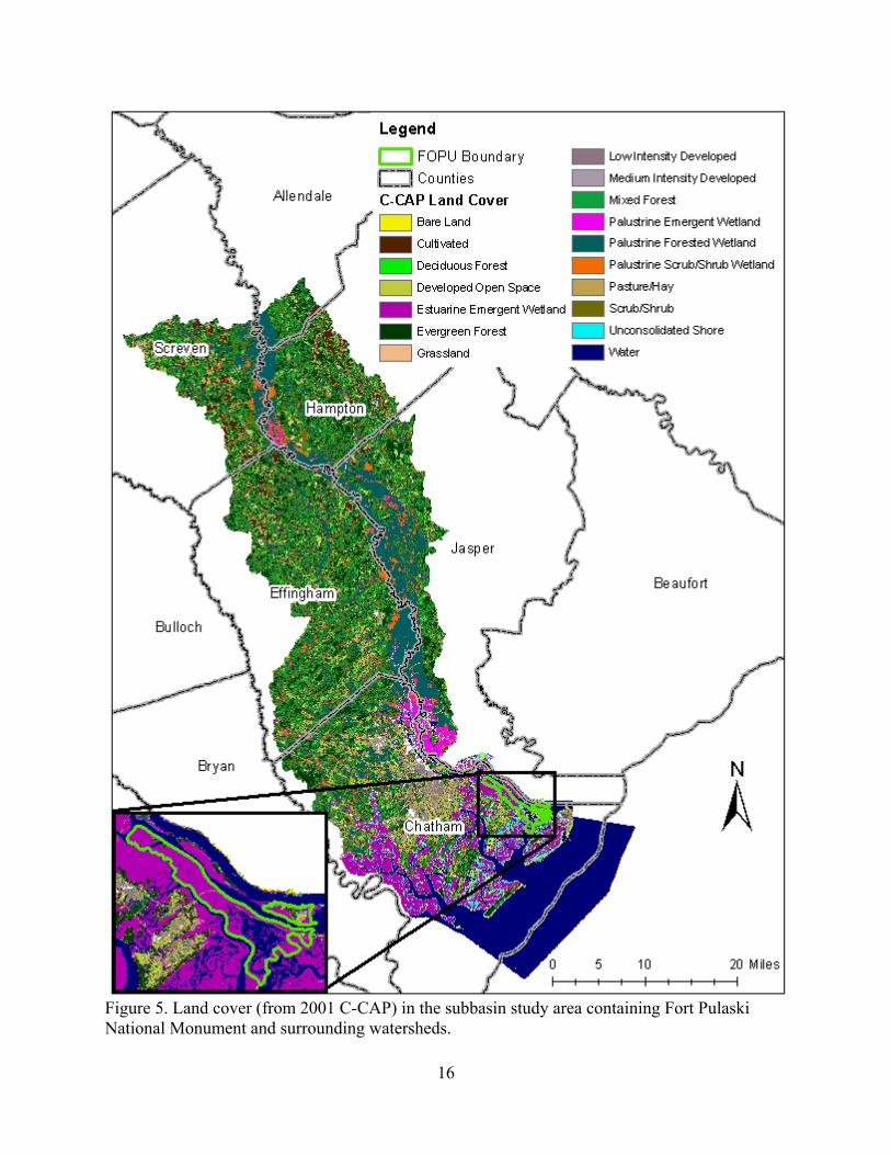
Figure 5. Land cover (from 2001 C-CAP) in the subbasin study area containing Fort Pulaski National Monument and surrounding watersheds.

16

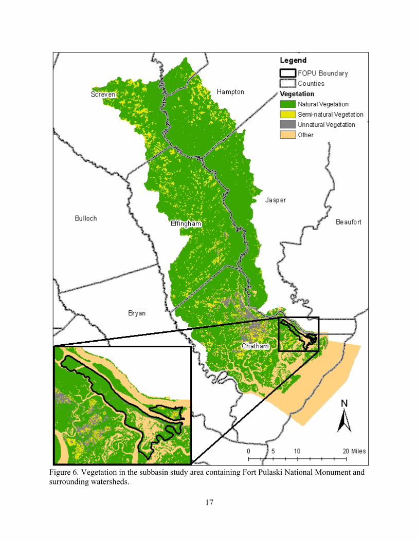
Figure 6. Vegetation in the subbasin study area containing Fort Pulaski National Monument and surrounding watersheds.

17

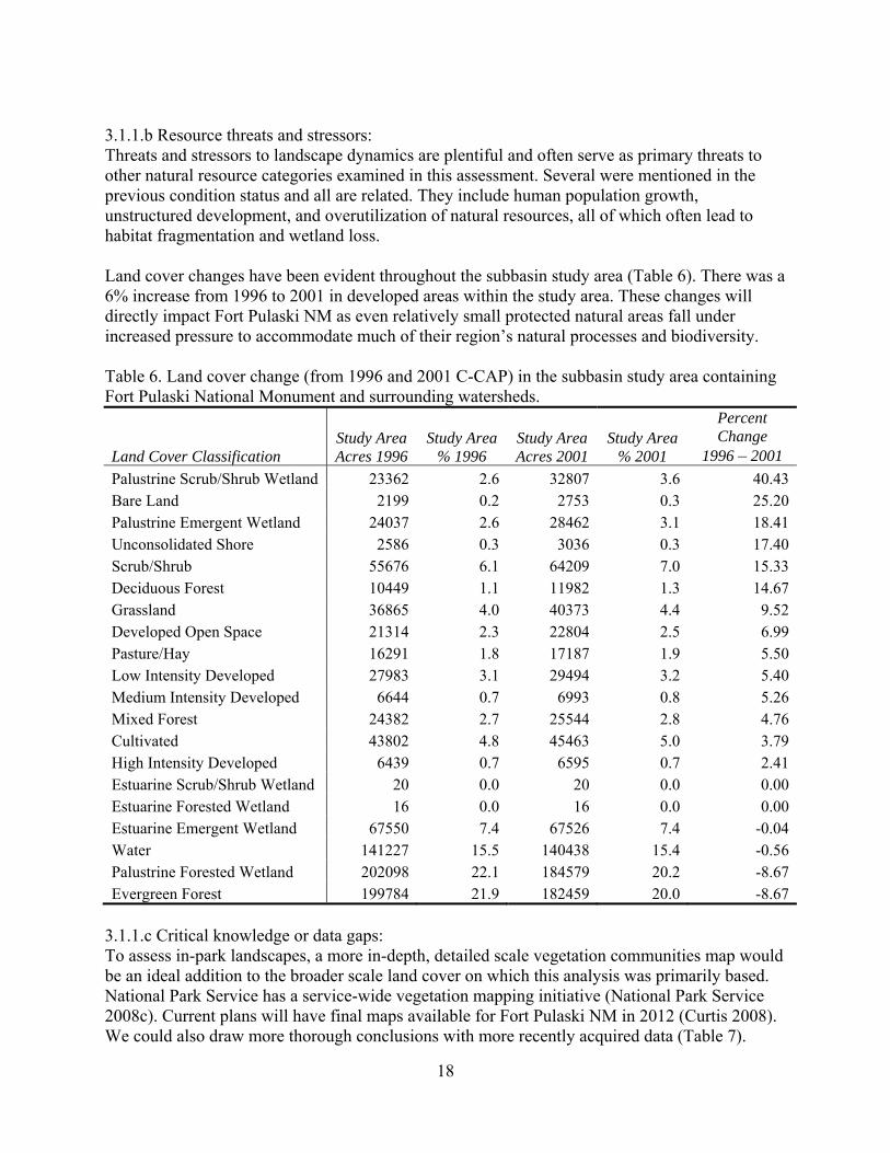
3.1.1.b Resource threats and stressors: Threats and stressors to landscape dynamics are plentiful and often serve as primary threats to other natural resource categories examined in this assessment. Several were mentioned in the previous condition status and all are related. They include human population growth, unstructured development, and overutilization of natural resources, all of which often lead to habitat fragmentation and wetland loss. Land cover changes have been evident throughout the subbasin study area (Table 6). There was a 6% increase from 1996 to 2001 in developed areas within the study area. These changes will directly impact Fort Pulaski NM as even relatively small protected natural areas fall under increased pressure to accommodate much of their region’s natural processes and biodiversity. Table 6. Land cover change (from 1996 and 2001 C-CAP) in the subbasin study area containing Fort Pulaski National Monument and surrounding watersheds.

Land Cover Classification Study Area Acres 1996

Study Area % 1996

Study Area Acres 2001

Study Area % 2001

Percent Change

1996 – 2001 Palustrine Scrub/Shrub Wetland 23362 2.6 32807 3.6 40.43Bare Land 2199 0.2 2753 0.3 25.20Palustrine Emergent Wetland 24037 2.6 28462 3.1 18.41Unconsolidated Shore 2586 0.3 3036 0.3 17.40Scrub/Shrub 55676 6.1 64209 7.0 15.33Deciduous Forest 10449 1.1 11982 1.3 14.67Grassland 36865 4.0 40373 4.4 9.52Developed Open Space 21314 2.3 22804 2.5 6.99Pasture/Hay 16291 1.8 17187 1.9 5.50Low Intensity Developed 27983 3.1 29494 3.2 5.40Medium Intensity Developed 6644 0.7 6993 0.8 5.26Mixed Forest 24382 2.7 25544 2.8 4.76Cultivated 43802 4.8 45463 5.0 3.79High Intensity Developed 6439 0.7 6595 0.7 2.41Estuarine Scrub/Shrub Wetland 20 0.0 20 0.0 0.00Estuarine Forested Wetland 16 0.0 16 0.0 0.00Estuarine Emergent Wetland 67550 7.4 67526 7.4 -0.04Water 141227 15.5 140438 15.4 -0.56Palustrine Forested Wetland 202098 22.1 184579 20.2 -8.67Evergreen Forest 199784 21.9 182459 20.0 -8.67

3.1.1.c Critical knowledge or data gaps: To assess in-park landscapes, a more in-depth, detailed scale vegetation communities map would be an ideal addition to the broader scale land cover on which this analysis was primarily based. National Park Service has a service-wide vegetation mapping initiative (National Park Service 2008c). Current plans will have final maps available for Fort Pulaski NM in 2012 (Curtis 2008). We could also draw more thorough conclusions with more recently acquired data (Table 7).

18

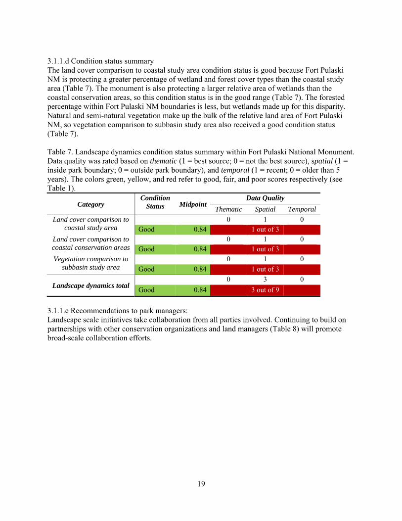
3.1.1.d Condition status summary The land cover comparison to coastal study area condition status is good because Fort Pulaski NM is protecting a greater percentage of wetland and forest cover types than the coastal study area (Table 7). The monument is also protecting a larger relative area of wetlands than the coastal conservation areas, so this condition status is in the good range (Table 7). The forested percentage within Fort Pulaski NM boundaries is less, but wetlands made up for this disparity. Natural and semi-natural vegetation make up the bulk of the relative land area of Fort Pulaski NM, so vegetation comparison to subbasin study area also received a good condition status (Table 7). Table 7. Landscape dynamics condition status summary within Fort Pulaski National Monument. Data quality was rated based on thematic (1 = best source; 0 = not the best source), spatial (1 = inside park boundary; 0 = outside park boundary), and temporal (1 = recent; 0 = older than 5 years). The colors green, yellow, and red refer to good, fair, and poor scores respectively (see Table 1).

Category Condition

Status MidpointData Quality

Thematic Spatial Temporal Land cover comparison to

coastal study area 0 1 0 Good 0.84 1 out of 3

Land cover comparison to coastal conservation areas

0 1 0 Good 0.84 1 out of 3

Vegetation comparison to subbasin study area

0 1 0 Good 0.84 1 out of 3

Landscape dynamics total 0 3 0 Good 0.84 3 out of 9

3.1.1.e Recommendations to park managers: Landscape scale initiatives take collaboration from all parties involved. Continuing to build on partnerships with other conservation organizations and land managers (Table 8) will promote broad-scale collaboration efforts.

19

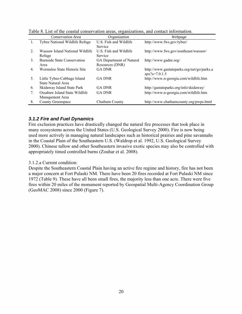
Table 8. List of the coastal conservation areas, organizations, and contact information. Conservation Area Organization Webpage

1. Tybee National Wildlife Refuge U.S. Fish and Wildlife Service

http://www.fws.gov/tybee/

2. Wassaw Island National Wildlife Refuge

U.S. Fish and Wildlife Service

http://www.fws.gov/southeast/wassaw/

3. Burnside State Conservation Area

GA Department of Natural Resources (DNR)

http://www.gadnr.org/

4. Wormsloe State Historic Site GA DNR http://www.gastateparks.org/net/go/parks.aspx?s=7.0.1.5

5. Little Tybee-Cabbage Island State Natural Area

GA DNR http://www.n-georgia.com/wildlife.htm

6. Skidaway Island State Park GA DNR http://gastateparks.org/info/skidaway/ 7. Ossabaw Island State Wildlife

Management Area GA DNR http://www.n-georgia.com/wildlife.htm

8. County Greenspace Chatham County http://www.chathamcounty.org/pwps.html 3.1.2 Fire and Fuel Dynamics Fire exclusion practices have drastically changed the natural fire processes that took place in many ecosystems across the United States (U.S. Geological Survey 2000). Fire is now being used more actively in managing natural landscapes such as historical prairies and pine savannahs in the Coastal Plain of the Southeastern U.S. (Waldrop et al. 1992, U.S. Geological Survey 2000). Chinese tallow and other Southeastern invasive exotic species may also be controlled with appropriately timed controlled burns (Zouhar et al. 2008). 3.1.2.a Current condition: Despite the Southeastern Coastal Plain having an active fire regime and history, fire has not been a major concern at Fort Pulaski NM. There have been 20 fires recorded at Fort Pulaski NM since 1972 (Table 9). These have all been small fires, the majority less than one acre. There were five fires within 20 miles of the monument reported by Geospatial Multi-Agency Coordination Group (GeoMAC 2008) since 2000 (Figure 7).

20

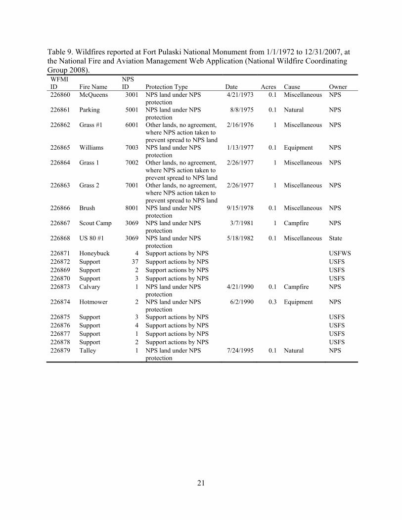
Table 9. Wildfires reported at Fort Pulaski National Monument from 1/1/1972 to 12/31/2007, at the National Fire and Aviation Management Web Application (National Wildfire Coordinating Group 2008). WFMI ID Fire Name

NPS ID Protection Type Date Acres Cause Owner

226860 McQueens 3001 NPS land under NPS protection

4/21/1973 0.1 Miscellaneous NPS

226861 Parking 5001 NPS land under NPS protection

8/8/1975 0.1 Natural NPS

226862 Grass #1 6001 Other lands, no agreement, where NPS action taken to prevent spread to NPS land

2/16/1976 1 Miscellaneous NPS

226865 Williams 7003 NPS land under NPS protection

1/13/1977 0.1 Equipment NPS

226864 Grass 1 7002 Other lands, no agreement, where NPS action taken to prevent spread to NPS land


226863 Grass 2 7001 Other lands, no agreement, where NPS action taken to prevent spread to NPS land


226866 Brush 8001 NPS land under NPS protection

9/15/1978 0.1 Miscellaneous NPS

226867 Scout Camp 3069 NPS land under NPS protection

3/7/1981 1 Campfire NPS

226868 US 80 #1 3069 NPS land under NPS protection

5/18/1982 0.1 Miscellaneous State

226871 Honeybuck 4 Support actions by NPS USFWS 226872 Support 37 Support actions by NPS USFS 226869 Support 2 Support actions by NPS USFS 226870 Support 3 Support actions by NPS USFS 226873 Calvary 1 NPS land under NPS

protection 4/21/1990 0.1 Campfire NPS

226874 Hotmower 2 NPS land under NPS protection

6/2/1990 0.3 Equipment NPS

226875 Support 3 Support actions by NPS USFS 226876 Support 4 Support actions by NPS USFS 226877 Support 1 Support actions by NPS USFS 226878 Support 2 Support actions by NPS USFS 226879 Talley 1 NPS land under NPS

protection 7/24/1995 0.1 Natural NPS

21

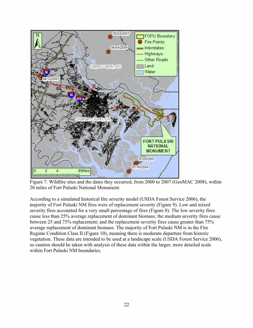
Figure 7. Wildfire sites and the dates they occurred, from 2000 to 2007 (GeoMAC 2008), within 20 miles of Fort Pulaski National Monument. According to a simulated historical fire severity model (USDA Forest Service 2006), the majority of Fort Pulaski NM fires were of replacement severity (Figure 9). Low and mixed severity fires accounted for a very small percentage of fires (Figure 8). The low severity fires cause less than 25% average replacement of dominant biomass; the medium severity fires cause between 25 and 75% replacement; and the replacement severity fires cause greater than 75% average replacement of dominant biomass. The majority of Fort Pulaski NM is in the Fire Regime Condition Class II (Figure 10), meaning there is moderate departure from historic vegetation. These data are intended to be used at a landscape scale (USDA Forest Service 2006), so caution should be taken with analysis of these data within the larger, more detailed scale within Fort Pulaski NM boundaries.

22

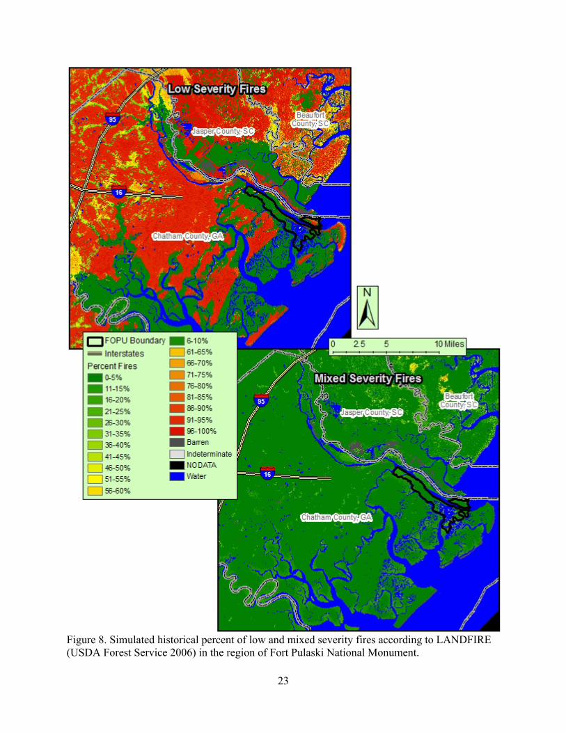
Figure 8. Simulated historical percent of low and mixed severity fires according to LANDFIRE (USDA Forest Service 2006) in the region of Fort Pulaski National Monument.

23

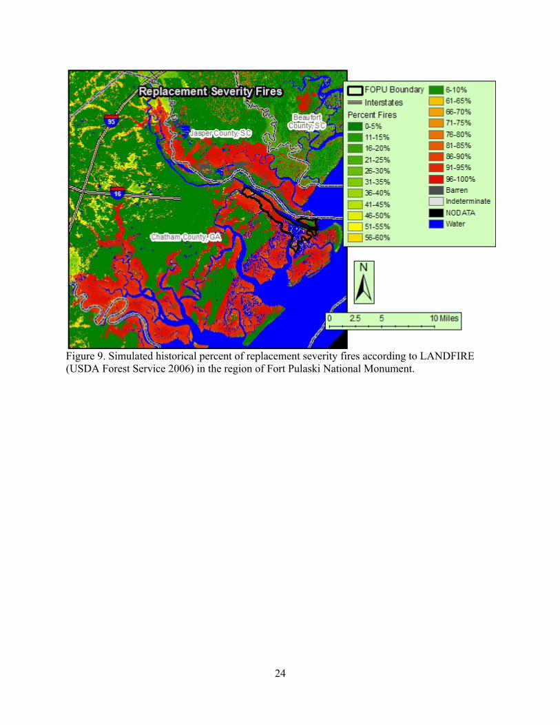
Figure 9. Simulated historical percent of replacement severity fires according to LANDFIRE (USDA Forest Service 2006) in the region of Fort Pulaski National Monument.

24

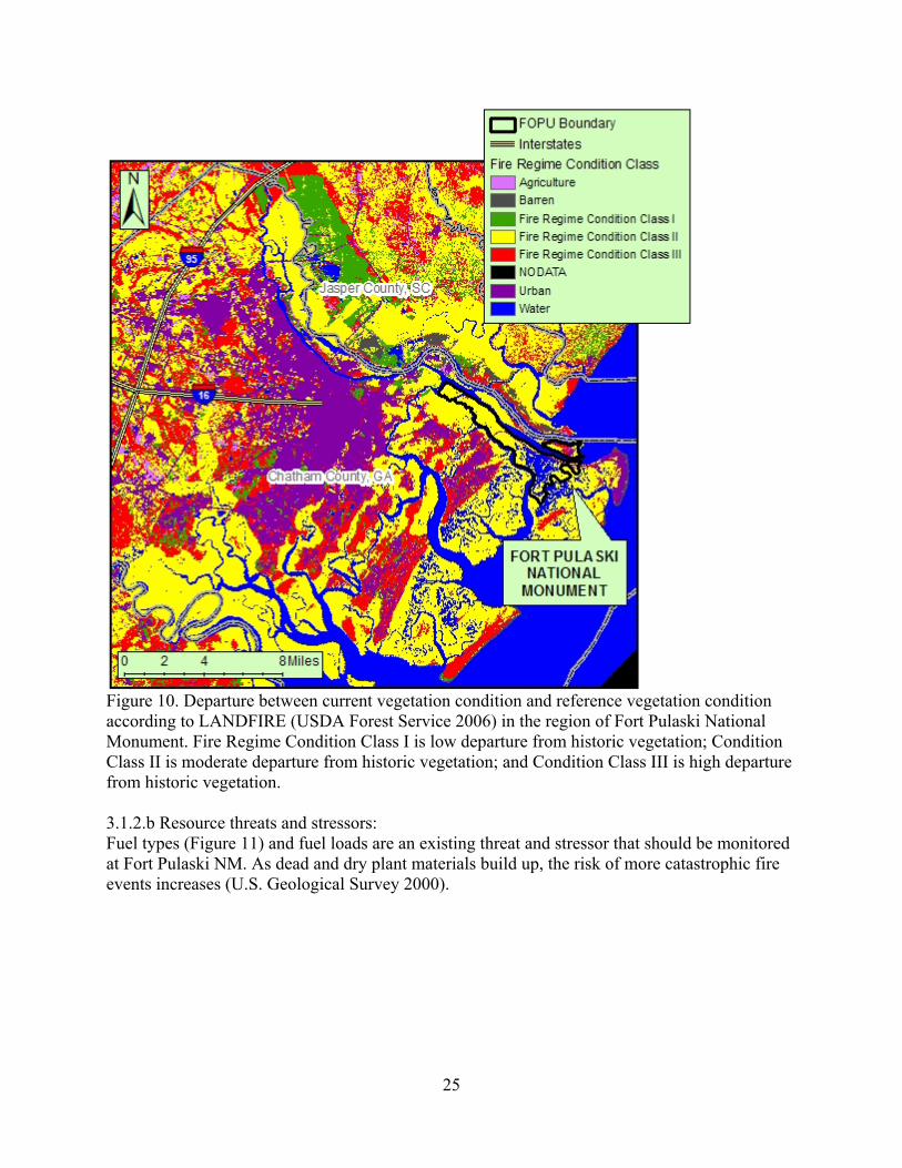
Figure 10. Departure between current vegetation condition and reference vegetation condition according to LANDFIRE (USDA Forest Service 2006) in the region of Fort Pulaski National Monument. Fire Regime Condition Class I is low departure from historic vegetation; Condition Class II is moderate departure from historic vegetation; and Condition Class III is high departure from historic vegetation. 3.1.2.b Resource threats and stressors: Fuel types (Figure 11) and fuel loads are an existing threat and stressor that should be monitored at Fort Pulaski NM. As dead and dry plant materials build up, the risk of more catastrophic fire events increases (U.S. Geological Survey 2000).

25

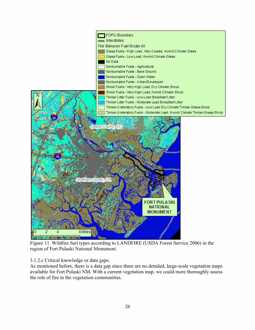
Figure 11. Wildfire fuel types according to LANDFIRE (USDA Forest Service 2006) in the region of Fort Pulaski National Monument. 3.1.2.c Critical knowledge or data gaps: As mentioned before, there is a data gap since there are no detailed, large-scale vegetation maps available for Fort Pulaski NM. With a current vegetation map, we could more thoroughly assess the role of fire in the vegetation communities.

26

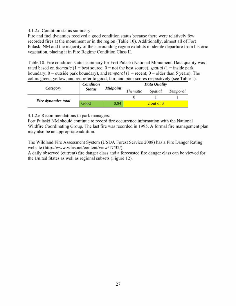
3.1.2.d Condition status summary: Fire and fuel dynamics received a good condition status because there were relatively few recorded fires at the monument or in the region (Table 10). Additionally, almost all of Fort Pulaski NM and the majority of the surrounding region exhibits moderate departure from historic vegetation, placing it in Fire Regime Condition Class II. Table 10. Fire condition status summary for Fort Pulaski National Monument. Data quality was rated based on thematic (1 = best source; 0 = not the best source), spatial (1 = inside park boundary; 0 = outside park boundary), and temporal (1 = recent; 0 = older than 5 years). The colors green, yellow, and red refer to good, fair, and poor scores respectively (see Table 1).

Category Condition



Fire dynamics total 0 1 1 Good 0.84 2 out of 3

3.1.2.e Recommendations to park managers: Fort Pulaski NM should continue to record fire occurrence information with the National Wildfire Coordinating Group. The last fire was recorded in 1995. A formal fire management plan may also be an appropriate addition. The Wildland Fire Assessment System (USDA Forest Service 2008) has a Fire Danger Rating website (http://www.wfas.net/content/view/17/32/). A daily observed (current) fire danger class and a forecasted fire danger class can be viewed for the United States as well as regional subsets (Figure 12).

27

Figure 12. A recent observed fire danger class map for the United States (USDA Forest Service 2008). 3.2 Human Use 3.2.1 Non-point Source Human Effects In the region of Fort Pulaski NM, human population and resulting development pressures are growing. This encroachment of human population and development is arguably the most important threat or stressor the monument must consider. Development may lead to increasing point and non-point source pollution, affecting air and water quality. Increased vehicle emissions can occur as more people move to the area. In-park biological integrity may also be stressed from these outside influences. 3.2.1.a Current condition: We examined two factors to assess the current condition of human effects in the Fort Pulaski NM area. First, census data was obtained from the U.S. Census Bureau and trends were analyzed. The second factor we examined was relative impervious surfaces within Fort Pulaski NM boundary and in the broad, subbasin study area. Human population: Although seemingly intuitive, several studies have quantitatively researched the relationship between human population and the degradation of the world’s natural resources (Jones and Clark

28

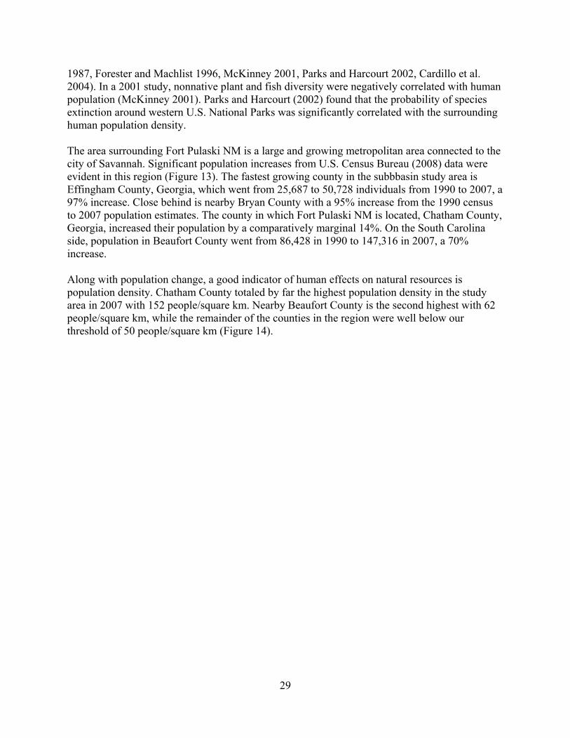
1987, Forester and Machlist 1996, McKinney 2001, Parks and Harcourt 2002, Cardillo et al. 2004). In a 2001 study, nonnative plant and fish diversity were negatively correlated with human population (McKinney 2001). Parks and Harcourt (2002) found that the probability of species extinction around western U.S. National Parks was significantly correlated with the surrounding human population density. The area surrounding Fort Pulaski NM is a large and growing metropolitan area connected to the city of Savannah. Significant population increases from U.S. Census Bureau (2008) data were evident in this region (Figure 13). The fastest growing county in the subbbasin study area is Effingham County, Georgia, which went from 25,687 to 50,728 individuals from 1990 to 2007, a 97% increase. Close behind is nearby Bryan County with a 95% increase from the 1990 census to 2007 population estimates. The county in which Fort Pulaski NM is located, Chatham County, Georgia, increased their population by a comparatively marginal 14%. On the South Carolina side, population in Beaufort County went from 86,428 in 1990 to 147,316 in 2007, a 70% increase. Along with population change, a good indicator of human effects on natural resources is population density. Chatham County totaled by far the highest population density in the study area in 2007 with 152 people/square km. Nearby Beaufort County is the second highest with 62 people/square km, while the remainder of the counties in the region were well below our threshold of 50 people/square km (Figure 14).

29

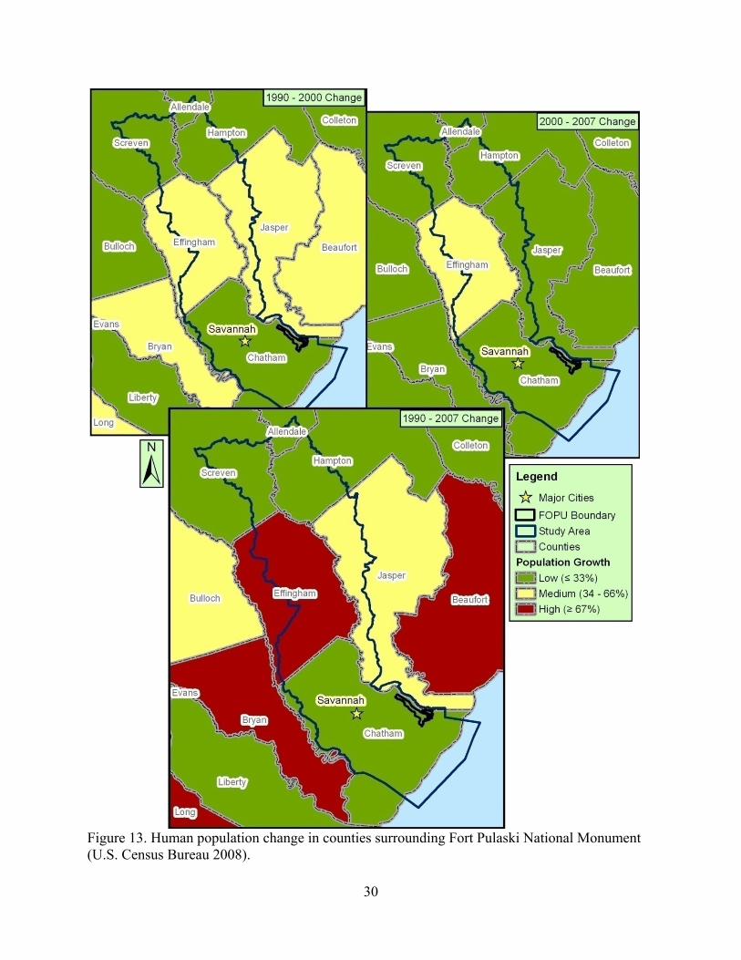
Figure 13. Human population change in counties surrounding Fort Pulaski National Monument (U.S. Census Bureau 2008).

30

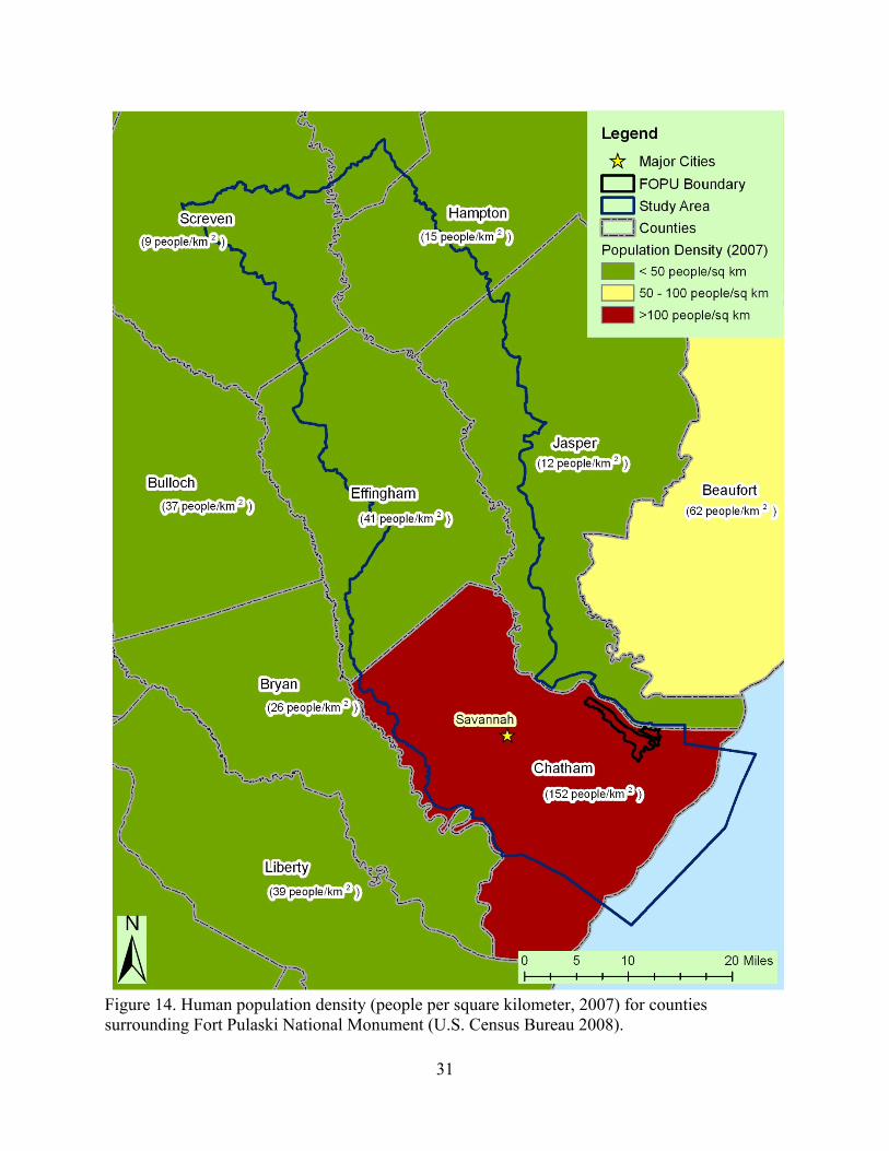
Figure 14. Human population density (people per square kilometer, 2007) for counties surrounding Fort Pulaski National Monument (U.S. Census Bureau 2008).

31

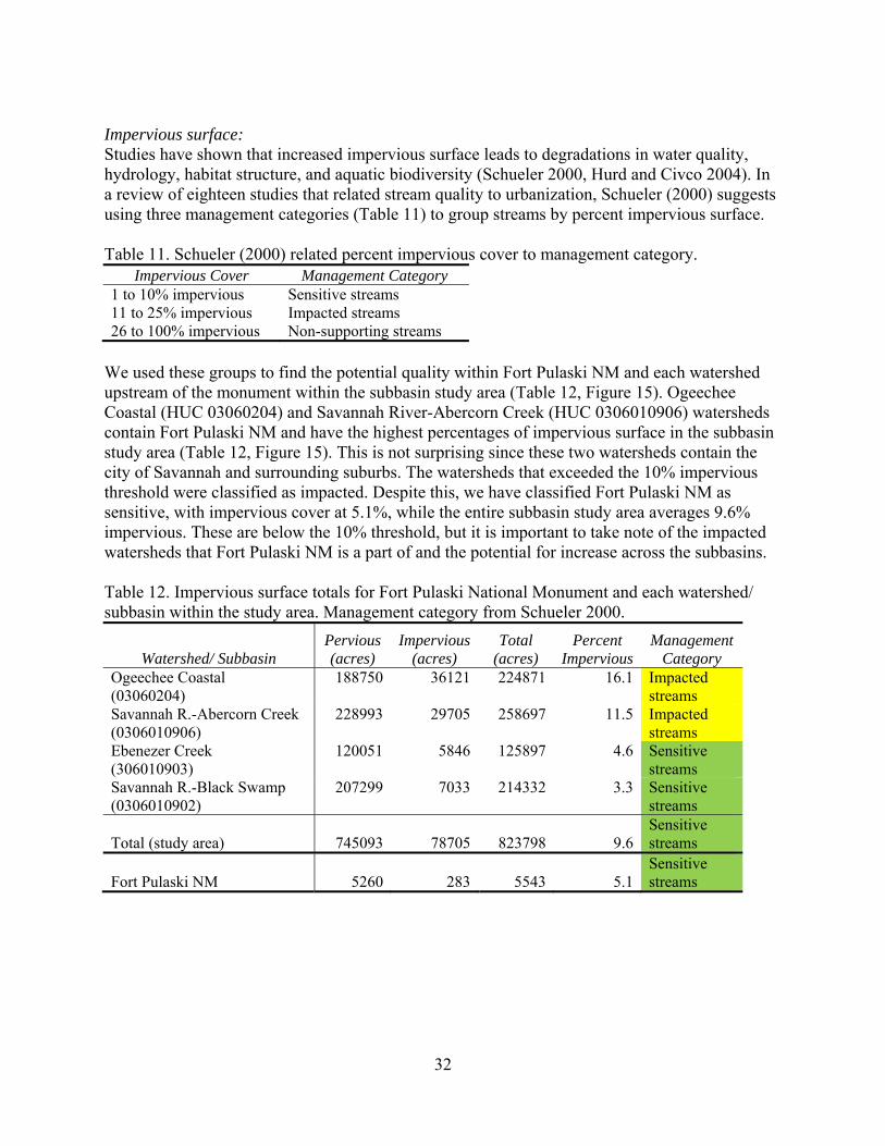
Impervious surface: Studies have shown that increased impervious surface leads to degradations in water quality, hydrology, habitat structure, and aquatic biodiversity (Schueler 2000, Hurd and Civco 2004). In a review of eighteen studies that related stream quality to urbanization, Schueler (2000) suggests using three management categories (Table 11) to group streams by percent impervious surface. Table 11. Schueler (2000) related percent impervious cover to management category.

Impervious Cover Management Category 1 to 10% impervious Sensitive streams 11 to 25% impervious Impacted streams 26 to 100% impervious Non-supporting streams

We used these groups to find the potential quality within Fort Pulaski NM and each watershed upstream of the monument within the subbasin study area (Table 12, Figure 15). Ogeechee Coastal (HUC 03060204) and Savannah River-Abercorn Creek (HUC 0306010906) watersheds contain Fort Pulaski NM and have the highest percentages of impervious surface in the subbasin study area (Table 12, Figure 15). This is not surprising since these two watersheds contain the city of Savannah and surrounding suburbs. The watersheds that exceeded the 10% impervious threshold were classified as impacted. Despite this, we have classified Fort Pulaski NM as sensitive, with impervious cover at 5.1%, while the entire subbasin study area averages 9.6% impervious. These are below the 10% threshold, but it is important to take note of the impacted watersheds that Fort Pulaski NM is a part of and the potential for increase across the subbasins. Table 12. Impervious surface totals for Fort Pulaski National Monument and each watershed/ subbasin within the study area. Management category from Schueler 2000.

Watershed/ Subbasin Pervious (acres)

Impervious (acres)

Total (acres)

Percent Impervious

Management Category

Ogeechee Coastal (03060204)

188750 36121 224871 16.1 Impacted streams

Savannah R.-Abercorn Creek (0306010906)

228993 29705 258697 11.5 Impacted streams

Ebenezer Creek (306010903)

120051 5846 125897 4.6 Sensitive streams

Savannah R.-Black Swamp (0306010902)

207299 7033 214332 3.3 Sensitive streams

Total (study area) 745093 78705 823798 9.6 Sensitive streams

Fort Pulaski NM 5260 283 5543 5.1 Sensitive streams

32

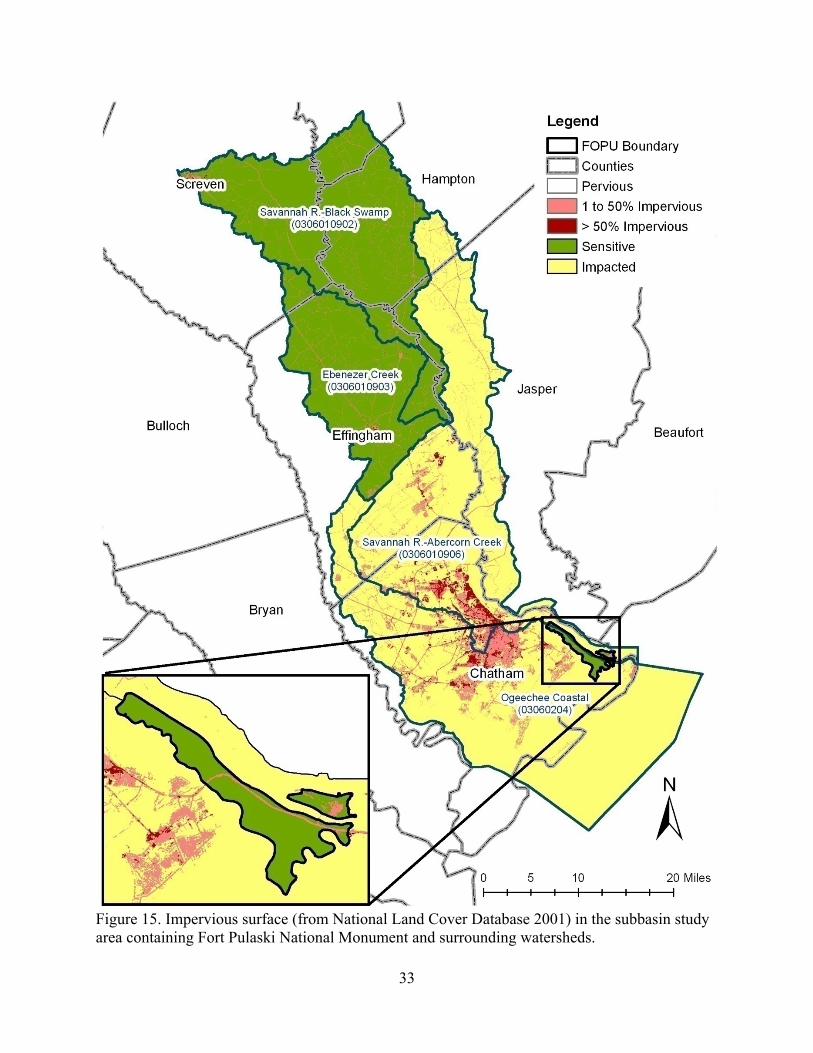
Figure 15. Impervious surface (from National Land Cover Database 2001) in the subbasin study area containing Fort Pulaski National Monument and surrounding watersheds.

33

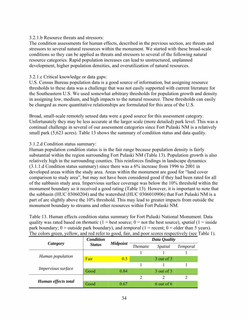
3.2.1.b Resource threats and stressors: The condition assessments for human effects, described in the previous section, are threats and stressors to several natural resources within the monument. We started with these broad-scale conditions so they can be applied as threats and stressors to several of the following natural resource categories. Rapid population increases can lead to unstructured, unplanned development, higher population densities, and overutilization of natural resources. 3.2.1.c Critical knowledge or data gaps: U.S. Census Bureau population data is a good source of information, but assigning resource thresholds to these data was a challenge that was not easily supported with current literature for the Southeastern U.S. We used somewhat arbitrary thresholds for population growth and density in assigning low, medium, and high impacts to the natural resource. These thresholds can easily be changed as more quantitative relationships are formulated for this area of the U.S. Broad, small-scale remotely sensed data were a good source for this assessment category. Unfortunately they may be less accurate at the larger scale (more detailed) park level. This was a continual challenge in several of our assessment categories since Fort Pulaski NM is a relatively small park (5,623 acres). Table 13 shows the summary of condition status and data quality. 3.1.2.d Condition status summary: Human population condition status is in the fair range because population density is fairly substantial within the region surrounding Fort Pulaski NM (Table 13). Population growth is also relatively high in the surrounding counties. This reinforces findings in landscape dynamics (3.1.1.d Condition status summary) since there was a 6% increase from 1996 to 2001 in developed areas within the study area. Areas within the monument are good for “land cover comparison to study area”, but may not have been considered good if they had been rated for all of the subbasin study area. Impervious surface coverage was below the 10% threshold within the monument boundary so it received a good rating (Table 13). However, it is important to note that the subbasin (HUC 03060204) and the watershed (HUC 0306010906) that Fort Pulaski NM is a part of are slightly above the 10% threshold. This may lead to greater impacts from outside the monument boundary to streams and other resources within Fort Pulaski NM. Table 13. Human effects condition status summary for Fort Pulaski National Monument. Data quality was rated based on thematic (1 = best source; 0 = not the best source), spatial (1 = inside park boundary; 0 = outside park boundary), and temporal (1 = recent; 0 = older than 5 years). The colors green, yellow, and red refer to good, fair, and poor scores respectively (see Table 1).

Category Condition



Human population 1 1 1 Fair 0.5 3 out of 3

Impervious surface 1 1 1 Good 0.84 3 out of 3

Human effects total 2 2 2 Good 0.67 6 out of 6

34

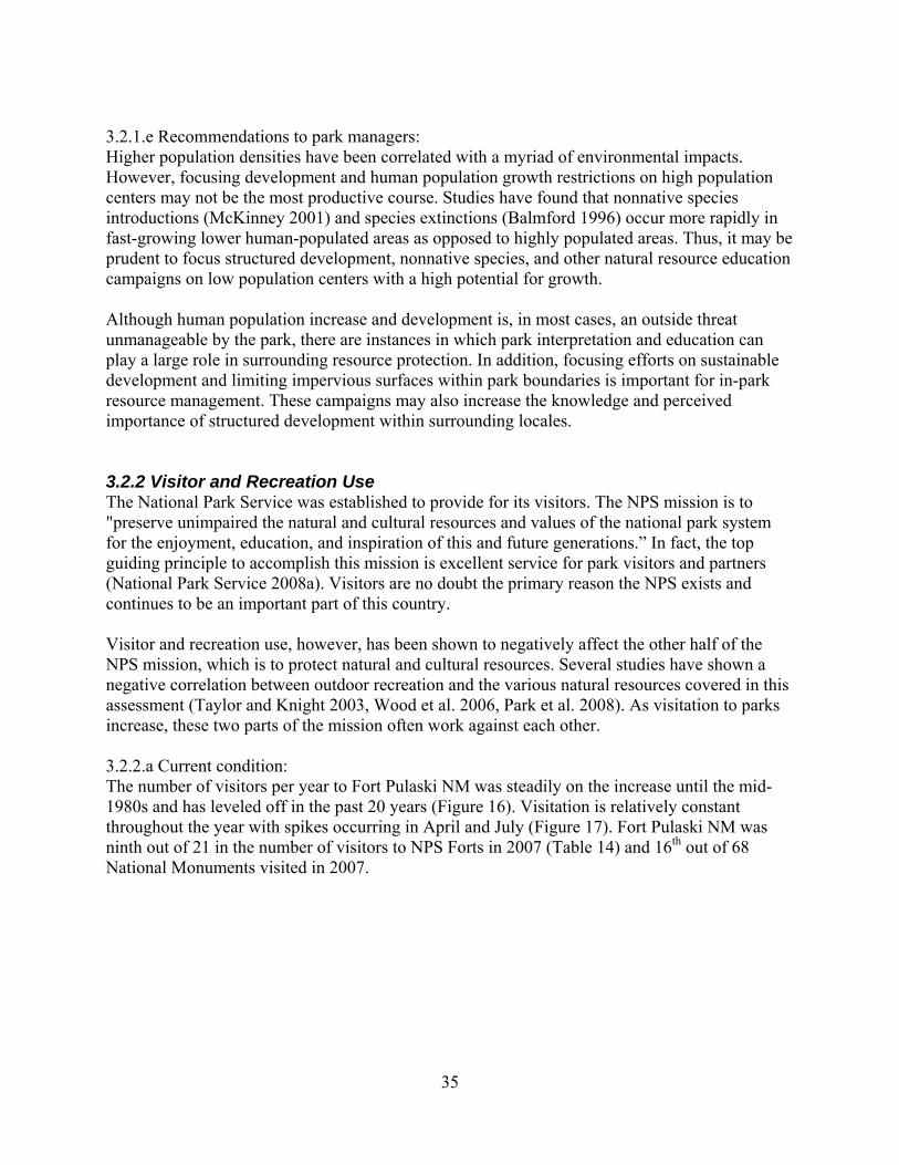
3.2.1.e Recommendations to park managers: Higher population densities have been correlated with a myriad of environmental impacts. However, focusing development and human population growth restrictions on high population centers may not be the most productive course. Studies have found that nonnative species introductions (McKinney 2001) and species extinctions (Balmford 1996) occur more rapidly in fast-growing lower human-populated areas as opposed to highly populated areas. Thus, it may be prudent to focus structured development, nonnative species, and other natural resource education campaigns on low population centers with a high potential for growth. Although human population increase and development is, in most cases, an outside threat unmanageable by the park, there are instances in which park interpretation and education can play a large role in surrounding resource protection. In addition, focusing efforts on sustainable development and limiting impervious surfaces within park boundaries is important for in-park resource management. These campaigns may also increase the knowledge and perceived importance of structured development within surrounding locales. 3.2.2 Visitor and Recreation Use The National Park Service was established to provide for its visitors. The NPS mission is to "preserve unimpaired the natural and cultural resources and values of the national park system for the enjoyment, education, and inspiration of this and future generations.” In fact, the top guiding principle to accomplish this mission is excellent service for park visitors and partners (National Park Service 2008a). Visitors are no doubt the primary reason the NPS exists and continues to be an important part of this country. Visitor and recreation use, however, has been shown to negatively affect the other half of the NPS mission, which is to protect natural and cultural resources. Several studies have shown a negative correlation between outdoor recreation and the various natural resources covered in this assessment (Taylor and Knight 2003, Wood et al. 2006, Park et al. 2008). As visitation to parks increase, these two parts of the mission often work against each other. 3.2.2.a Current condition: The number of visitors per year to Fort Pulaski NM was steadily on the increase until the mid-1980s and has leveled off in the past 20 years (Figure 16). Visitation is relatively constant throughout the year with spikes occurring in April and July (Figure 17). Fort Pulaski NM was ninth out of 21 in the number of visitors to NPS Forts in 2007 (Table 14) and 16th out of 68 National Monuments visited in 2007.

35

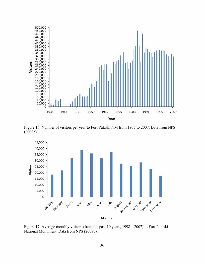
Figure 16. Number of visitors per year to Fort Pulaski NM from 1935 to 2007. Data from NPS (2008b).

020,00040,00060,00080,000100,000120,000140,000160,000180,000200,000220,000240,000260,000280,000300,000320,000340,000360,000380,000400,000420,000440,000460,000480,000500,000

1935 1943 1951 1959 1967 1975 1983 1991 1999 2007

Visitors

Year

Figure 17. Average monthly visitors (from the past 10 years, 1998 – 2007) to Fort Pulaski National Monument. Data from NPS (2008b).

0

5,000

10,000

15,000

20,000

25,000

30,000

35,000

40,000

45,000

Visitors

Months

36

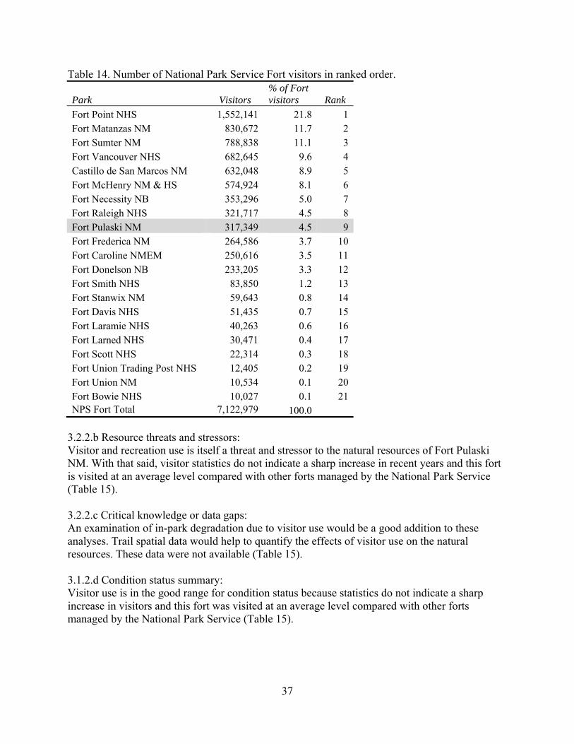
Table 14. Number of National Park Service Fort visitors in ranked order.

Park Visitors % of Fort visitors Rank

Fort Point NHS 1,552,141 21.8 1Fort Matanzas NM 830,672 11.7 2Fort Sumter NM 788,838 11.1 3Fort Vancouver NHS 682,645 9.6 4Castillo de San Marcos NM 632,048 8.9 5Fort McHenry NM & HS 574,924 8.1 6Fort Necessity NB 353,296 5.0 7Fort Raleigh NHS 321,717 4.5 8Fort Pulaski NM 317,349 4.5 9Fort Frederica NM 264,586 3.7 10Fort Caroline NMEM 250,616 3.5 11Fort Donelson NB 233,205 3.3 12Fort Smith NHS 83,850 1.2 13Fort Stanwix NM 59,643 0.8 14Fort Davis NHS 51,435 0.7 15Fort Laramie NHS 40,263 0.6 16Fort Larned NHS 30,471 0.4 17Fort Scott NHS 22,314 0.3 18Fort Union Trading Post NHS 12,405 0.2 19Fort Union NM 10,534 0.1 20Fort Bowie NHS 10,027 0.1 21NPS Fort Total 7,122,979 100.0

3.2.2.b Resource threats and stressors: Visitor and recreation use is itself a threat and stressor to the natural resources of Fort Pulaski NM. With that said, visitor statistics do not indicate a sharp increase in recent years and this fort is visited at an average level compared with other forts managed by the National Park Service (Table 15). 3.2.2.c Critical knowledge or data gaps: An examination of in-park degradation due to visitor use would be a good addition to these analyses. Trail spatial data would help to quantify the effects of visitor use on the natural resources. These data were not available (Table 15). 3.1.2.d Condition status summary: Visitor use is in the good range for condition status because statistics do not indicate a sharp increase in visitors and this fort was visited at an average level compared with other forts managed by the National Park Service (Table 15).

37

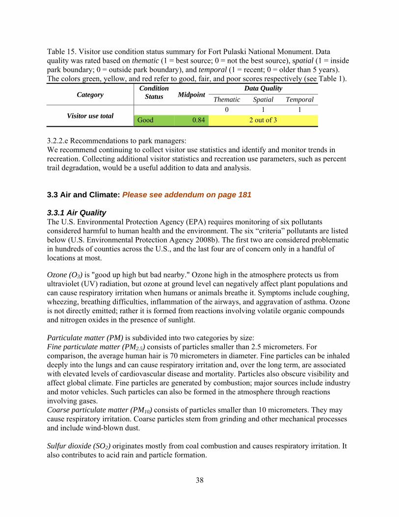
Table 15. Visitor use condition status summary for Fort Pulaski National Monument. Data quality was rated based on thematic (1 = best source; 0 = not the best source), spatial (1 = inside park boundary; 0 = outside park boundary), and temporal (1 = recent; 0 = older than 5 years). The colors green, yellow, and red refer to good, fair, and poor scores respectively (see Table 1).

Category Condition



Visitor use total 0 1 1 Good 0.84 2 out of 3

3.2.2.e Recommendations to park managers: We recommend continuing to collect visitor use statistics and identify and monitor trends in recreation. Collecting additional visitor statistics and recreation use parameters, such as percent trail degradation, would be a useful addition to data and analysis. 3.3 Air and Climate: Please see addendum on page 181 3.3.1 Air Quality The U.S. Environmental Protection Agency (EPA) requires monitoring of six pollutants considered harmful to human health and the environment. The six “criteria” pollutants are listed below (U.S. Environmental Protection Agency 2008b). The first two are considered problematic in hundreds of counties across the U.S., and the last four are of concern only in a handful of locations at most.

Ozone (O3) is "good up high but bad nearby." Ozone high in the atmosphere protects us from ultraviolet (UV) radiation, but ozone at ground level can negatively affect plant populations and can cause respiratory irritation when humans or animals breathe it. Symptoms include coughing, wheezing, breathing difficulties, inflammation of the airways, and aggravation of asthma. Ozone is not directly emitted; rather it is formed from reactions involving volatile organic compounds and nitrogen oxides in the presence of sunlight. Particulate matter (PM) is subdivided into two categories by size: Fine particulate matter (PM2.5) consists of particles smaller than 2.5 micrometers. For comparison, the average human hair is 70 micrometers in diameter. Fine particles can be inhaled deeply into the lungs and can cause respiratory irritation and, over the long term, are associated with elevated levels of cardiovascular disease and mortality. Particles also obscure visibility and affect global climate. Fine particles are generated by combustion; major sources include industry and motor vehicles. Such particles can also be formed in the atmosphere through reactions involving gases. Coarse particulate matter (PM10) consists of particles smaller than 10 micrometers. They may cause respiratory irritation. Coarse particles stem from grinding and other mechanical processes and include wind-blown dust. Sulfur dioxide (SO2) originates mostly from coal combustion and causes respiratory irritation. It also contributes to acid rain and particle formation.

38

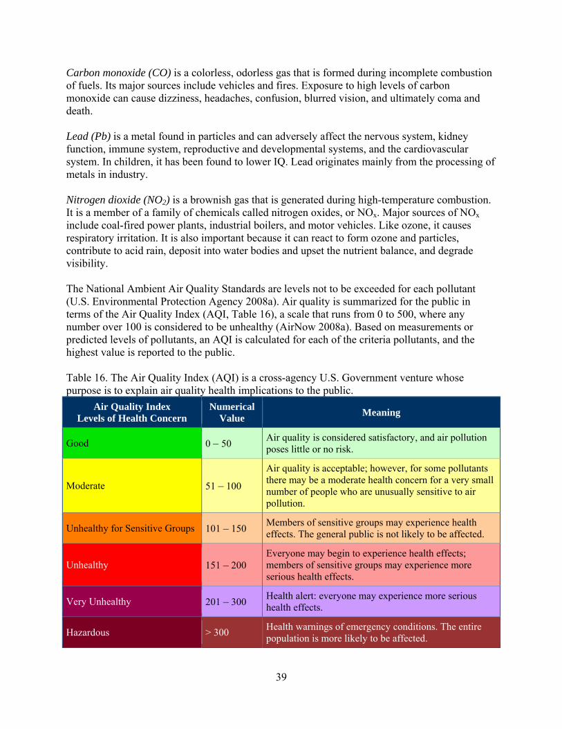
Carbon monoxide (CO) is a colorless, odorless gas that is formed during incomplete combustion of fuels. Its major sources include vehicles and fires. Exposure to high levels of carbon monoxide can cause dizziness, headaches, confusion, blurred vision, and ultimately coma and death. Lead (Pb) is a metal found in particles and can adversely affect the nervous system, kidney function, immune system, reproductive and developmental systems, and the cardiovascular system. In children, it has been found to lower IQ. Lead originates mainly from the processing of metals in industry. Nitrogen dioxide (NO2) is a brownish gas that is generated during high-temperature combustion. It is a member of a family of chemicals called nitrogen oxides, or NOx. Major sources of NOx include coal-fired power plants, industrial boilers, and motor vehicles. Like ozone, it causes respiratory irritation. It is also important because it can react to form ozone and particles, contribute to acid rain, deposit into water bodies and upset the nutrient balance, and degrade visibility. The National Ambient Air Quality Standards are levels not to be exceeded for each pollutant (U.S. Environmental Protection Agency 2008a). Air quality is summarized for the public in terms of the Air Quality Index (AQI, Table 16), a scale that runs from 0 to 500, where any number over 100 is considered to be unhealthy (AirNow 2008a). Based on measurements or predicted levels of pollutants, an AQI is calculated for each of the criteria pollutants, and the highest value is reported to the public. Table 16. The Air Quality Index (AQI) is a cross-agency U.S. Government venture whose purpose is to explain air quality health implications to the public.

Air Quality Index Levels of Health Concern

Numerical Value Meaning

Good 0 – 50 Air quality is considered satisfactory, and air pollution poses little or no risk.

Moderate 51 – 100

Air quality is acceptable; however, for some pollutants there may be a moderate health concern for a very small number of people who are unusually sensitive to air pollution.

Unhealthy for Sensitive Groups 101 – 150 Members of sensitive groups may experience health effects. The general public is not likely to be affected.

Unhealthy 151 – 200 Everyone may begin to experience health effects; members of sensitive groups may experience more serious health effects.

Very Unhealthy 201 – 300 Health alert: everyone may experience more serious health effects.

Hazardous > 300 Health warnings of emergency conditions. The entire population is more likely to be affected.

39

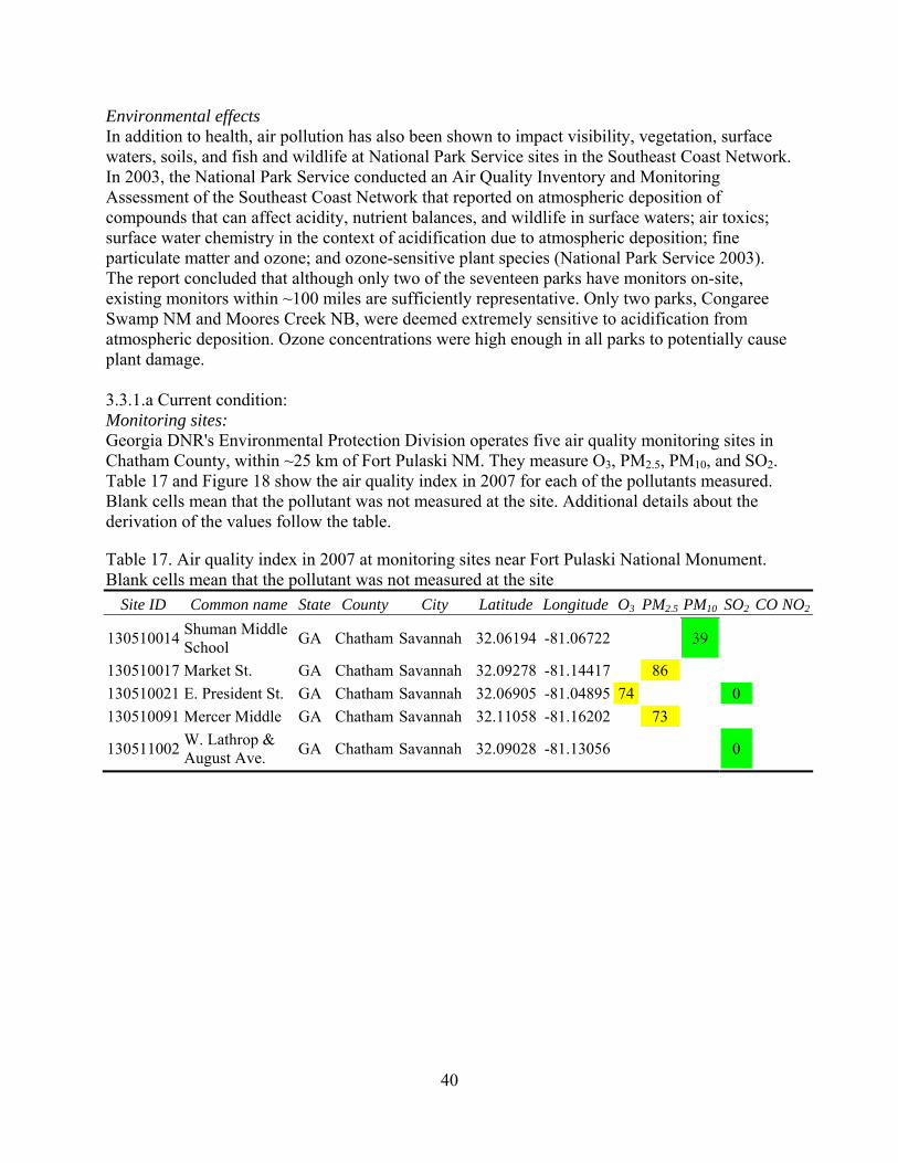
Environmental effects In addition to health, air pollution has also been shown to impact visibility, vegetation, surface waters, soils, and fish and wildlife at National Park Service sites in the Southeast Coast Network. In 2003, the National Park Service conducted an Air Quality Inventory and Monitoring Assessment of the Southeast Coast Network that reported on atmospheric deposition of compounds that can affect acidity, nutrient balances, and wildlife in surface waters; air toxics; surface water chemistry in the context of acidification due to atmospheric deposition; fine particulate matter and ozone; and ozone-sensitive plant species (National Park Service 2003). The report concluded that although only two of the seventeen parks have monitors on-site, existing monitors within ~100 miles are sufficiently representative. Only two parks, Congaree Swamp NM and Moores Creek NB, were deemed extremely sensitive to acidification from atmospheric deposition. Ozone concentrations were high enough in all parks to potentially cause plant damage. 3.3.1.a Current condition: Monitoring sites: Georgia DNR's Environmental Protection Division operates five air quality monitoring sites in Chatham County, within ~25 km of Fort Pulaski NM. They measure O3, PM2.5, PM10, and SO2. Table 17 and Figure 18 show the air quality index in 2007 for each of the pollutants measured. Blank cells mean that the pollutant was not measured at the site. Additional details about the derivation of the values follow the table.

Table 17. Air quality index in 2007 at monitoring sites near Fort Pulaski National Monument. Blank cells mean that the pollutant was not measured at the site

Site ID Common name State County City Latitude Longitude O3 PM2.5 PM10 SO2 CO NO2

130510014 Shuman Middle School GA Chatham Savannah 32.06194 -81.06722 39

130510017 Market St. GA Chatham Savannah 32.09278 -81.14417 86 130510021 E. President St. GA Chatham Savannah 32.06905 -81.04895 74 0 130510091 Mercer Middle GA Chatham Savannah 32.11058 -81.16202 73

130511002 W. Lathrop & August Ave. GA Chatham Savannah 32.09028 -81.13056 0

40

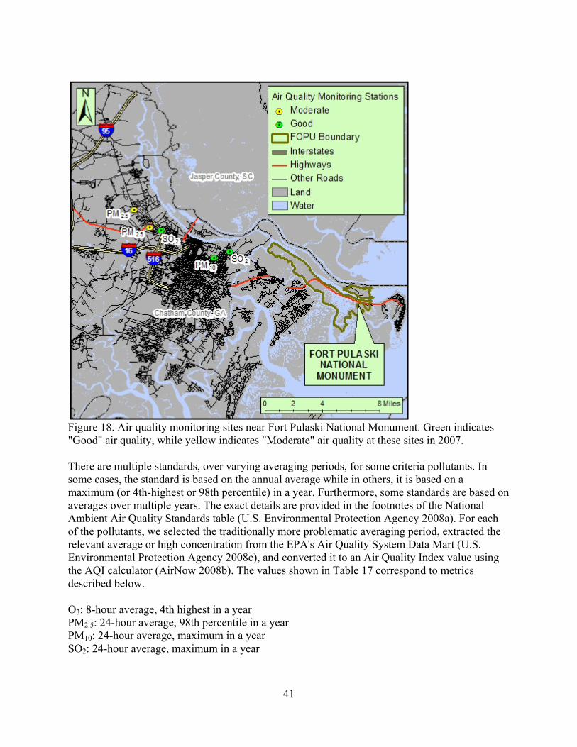
Figure 18. Air quality monitoring sites near Fort Pulaski National Monument. Green indicates "Good" air quality, while yellow indicates "Moderate" air quality at these sites in 2007. There are multiple standards, over varying averaging periods, for some criteria pollutants. In some cases, the standard is based on the annual average while in others, it is based on a maximum (or 4th-highest or 98th percentile) in a year. Furthermore, some standards are based on averages over multiple years. The exact details are provided in the footnotes of the National Ambient Air Quality Standards table (U.S. Environmental Protection Agency 2008a). For each of the pollutants, we selected the traditionally more problematic averaging period, extracted the relevant average or high concentration from the EPA's Air Quality System Data Mart (U.S. Environmental Protection Agency 2008c), and converted it to an Air Quality Index value using the AQI calculator (AirNow 2008b). The values shown in Table 17 correspond to metrics described below. O3: 8-hour average, 4th highest in a year PM2.5: 24-hour average, 98th percentile in a year PM10: 24-hour average, maximum in a year SO2: 24-hour average, maximum in a year

41

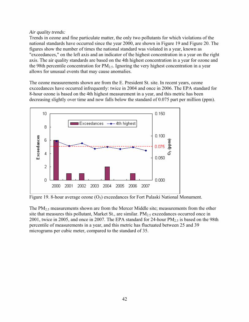
Air quality trends: Trends in ozone and fine particulate matter, the only two pollutants for which violations of the national standards have occurred since the year 2000, are shown in Figure 19 and Figure 20. The figures show the number of times the national standard was violated in a year, known as "exceedances," on the left axis and an indicator of the highest concentration in a year on the right axis. The air quality standards are based on the 4th highest concentration in a year for ozone and the 98th percentile concentration for PM2.5. Ignoring the very highest concentration in a year allows for unusual events that may cause anomalies. The ozone measurements shown are from the E. President St. site. In recent years, ozone exceedances have occurred infrequently: twice in 2004 and once in 2006. The EPA standard for 8-hour ozone is based on the 4th highest measurement in a year, and this metric has been decreasing slightly over time and now falls below the standard of 0.075 part per million (ppm).

Figure 19. 8-hour average ozone (O3) exceedances for Fort Pulaski National Monument. The PM2.5 measurements shown are from the Mercer Middle site; measurements from the other site that measures this pollutant, Market St., are similar. PM2.5 exceedances occurred once in 2001, twice in 2005, and once in 2007. The EPA standard for 24-hour PM2.5 is based on the 98th percentile of measurements in a year, and this metric has fluctuated between 25 and 39 micrograms per cubic meter, compared to the standard of 35.

42

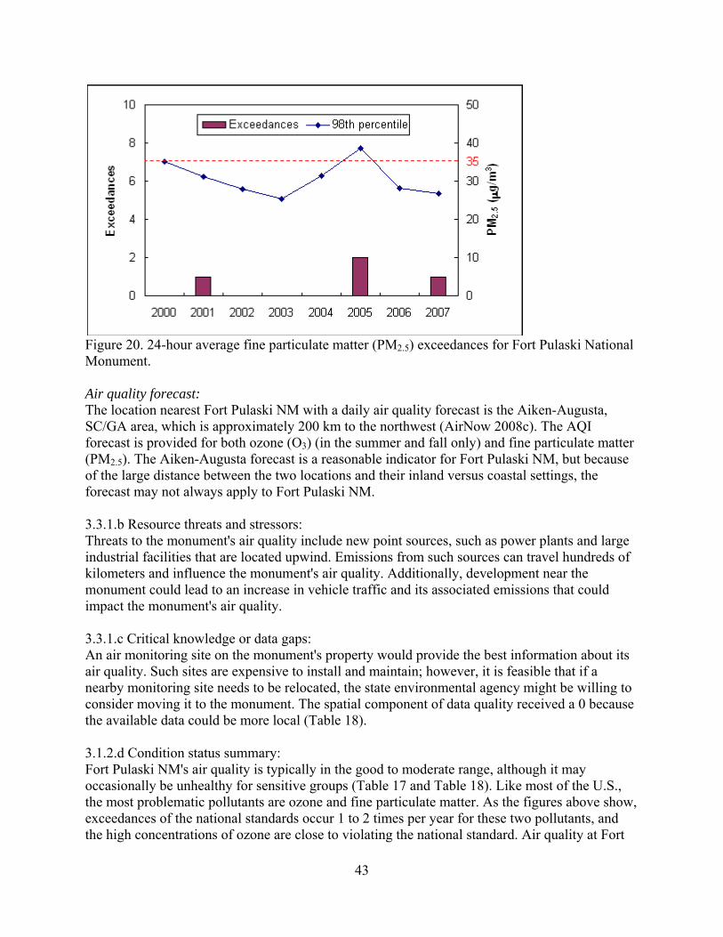
Figure 20. 24-hour average fine particulate matter (PM2.5) exceedances for Fort Pulaski National Monument. Air quality forecast: The location nearest Fort Pulaski NM with a daily air quality forecast is the Aiken-Augusta, SC/GA area, which is approximately 200 km to the northwest (AirNow 2008c). The AQI forecast is provided for both ozone (O3) (in the summer and fall only) and fine particulate matter (PM2.5). The Aiken-Augusta forecast is a reasonable indicator for Fort Pulaski NM, but because of the large distance between the two locations and their inland versus coastal settings, the forecast may not always apply to Fort Pulaski NM. 3.3.1.b Resource threats and stressors: Threats to the monument's air quality include new point sources, such as power plants and large industrial facilities that are located upwind. Emissions from such sources can travel hundreds of kilometers and influence the monument's air quality. Additionally, development near the monument could lead to an increase in vehicle traffic and its associated emissions that could impact the monument's air quality. 3.3.1.c Critical knowledge or data gaps: An air monitoring site on the monument's property would provide the best information about its air quality. Such sites are expensive to install and maintain; however, it is feasible that if a nearby monitoring site needs to be relocated, the state environmental agency might be willing to consider moving it to the monument. The spatial component of data quality received a 0 because the available data could be more local (Table 18). 3.1.2.d Condition status summary: Fort Pulaski NM's air quality is typically in the good to moderate range, although it may occasionally be unhealthy for sensitive groups (Table 17 and Table 18). Like most of the U.S., the most problematic pollutants are ozone and fine particulate matter. As the figures above show, exceedances of the national standards occur 1 to 2 times per year for these two pollutants, and the high concentrations of ozone are close to violating the national standard. Air quality at Fort

43

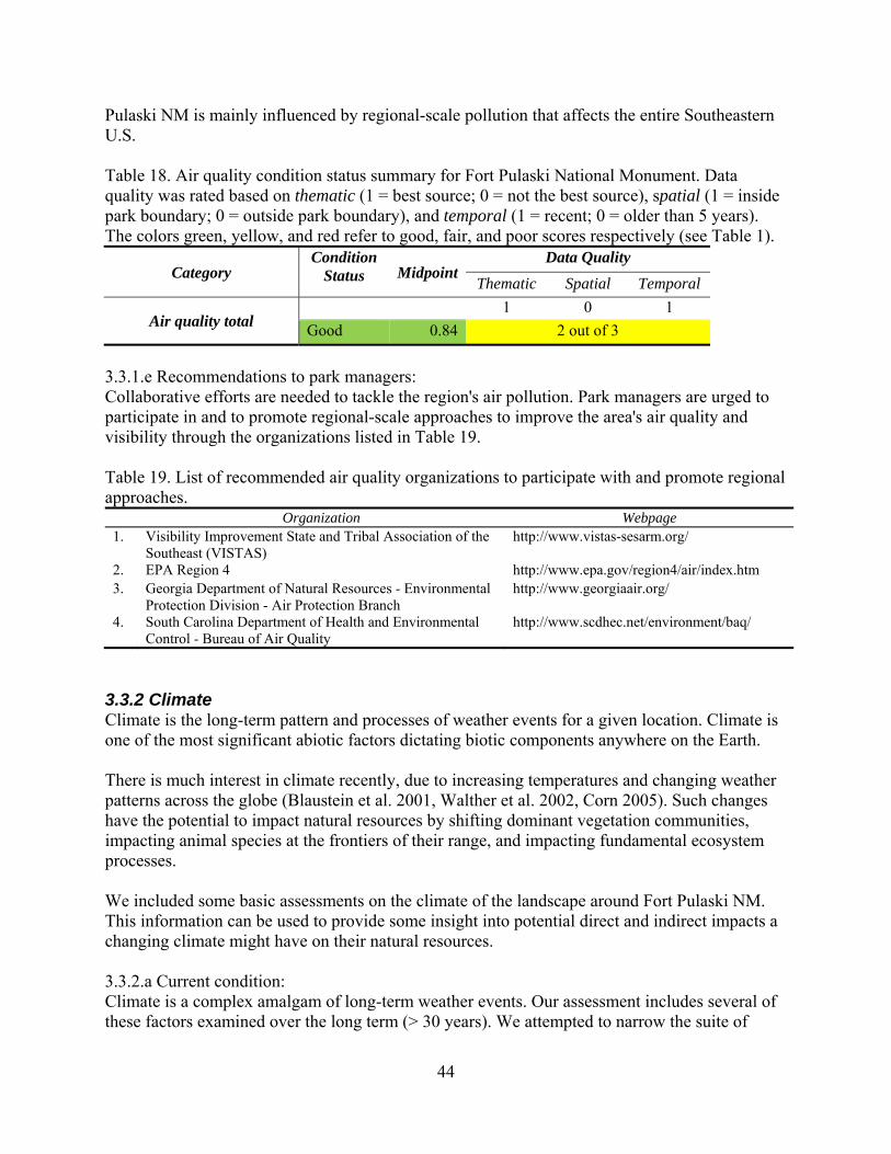
Pulaski NM is mainly influenced by regional-scale pollution that affects the entire Southeastern U.S. Table 18. Air quality condition status summary for Fort Pulaski National Monument. Data quality was rated based on thematic (1 = best source; 0 = not the best source), spatial (1 = inside park boundary; 0 = outside park boundary), and temporal (1 = recent; 0 = older than 5 years). The colors green, yellow, and red refer to good, fair, and poor scores respectively (see Table 1).

Category Condition



Air quality total 1 0 1 Good 0.84 2 out of 3

3.3.1.e Recommendations to park managers: Collaborative efforts are needed to tackle the region's air pollution. Park managers are urged to participate in and to promote regional-scale approaches to improve the area's air quality and visibility through the organizations listed in Table 19. Table 19. List of recommended air quality organizations to participate with and promote regional approaches.

Organization Webpage 1. Visibility Improvement State and Tribal Association of the

Southeast (VISTAS) http://www.vistas-sesarm.org/

2. EPA Region 4 http://www.epa.gov/region4/air/index.htm 3. Georgia Department of Natural Resources - Environmental

Protection Division - Air Protection Branch http://www.georgiaair.org/

4. South Carolina Department of Health and Environmental Control - Bureau of Air Quality

http://www.scdhec.net/environment/baq/

3.3.2 Climate Climate is the long-term pattern and processes of weather events for a given location. Climate is one of the most significant abiotic factors dictating biotic components anywhere on the Earth. There is much interest in climate recently, due to increasing temperatures and changing weather patterns across the globe (Blaustein et al. 2001, Walther et al. 2002, Corn 2005). Such changes have the potential to impact natural resources by shifting dominant vegetation communities, impacting animal species at the frontiers of their range, and impacting fundamental ecosystem processes. We included some basic assessments on the climate of the landscape around Fort Pulaski NM. This information can be used to provide some insight into potential direct and indirect impacts a changing climate might have on their natural resources. 3.3.2.a Current condition: Climate is a complex amalgam of long-term weather events. Our assessment includes several of these factors examined over the long term (> 30 years). We attempted to narrow the suite of

44

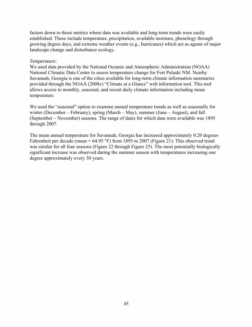
factors down to those metrics where data was available and long-term trends were easily established. These include temperature, precipitation, available moisture, phenology through growing degree days, and extreme weather events (e.g., hurricanes) which act as agents of major landscape change and disturbance ecology. Temperature: We used data provided by the National Oceanic and Atmospheric Administration (NOAA) National Climatic Data Center to assess temperature change for Fort Pulaski NM. Nearby Savannah, Georgia is one of the cities available for long-term climate information summaries provided through the NOAA (2008c) “Climate at a Glance” web information tool. This tool allows access to monthly, seasonal, and recent daily climate information including mean temperature. We used the “seasonal” option to examine annual temperature trends as well as seasonally for winter (December – February), spring (March – May), summer (June – August), and fall (September – November) seasons. The range of dates for which data were available was 1895 through 2007. The mean annual temperature for Savannah, Georgia has increased approximately 0.20 degrees Fahrenheit per decade (mean = 64.95 °F) from 1895 to 2007 (Figure 21). This observed trend was similar for all four seasons (Figure 22 through Figure 25). The most potentially biologically significant increase was observed during the summer season with temperatures increasing one degree approximately every 30 years.

45

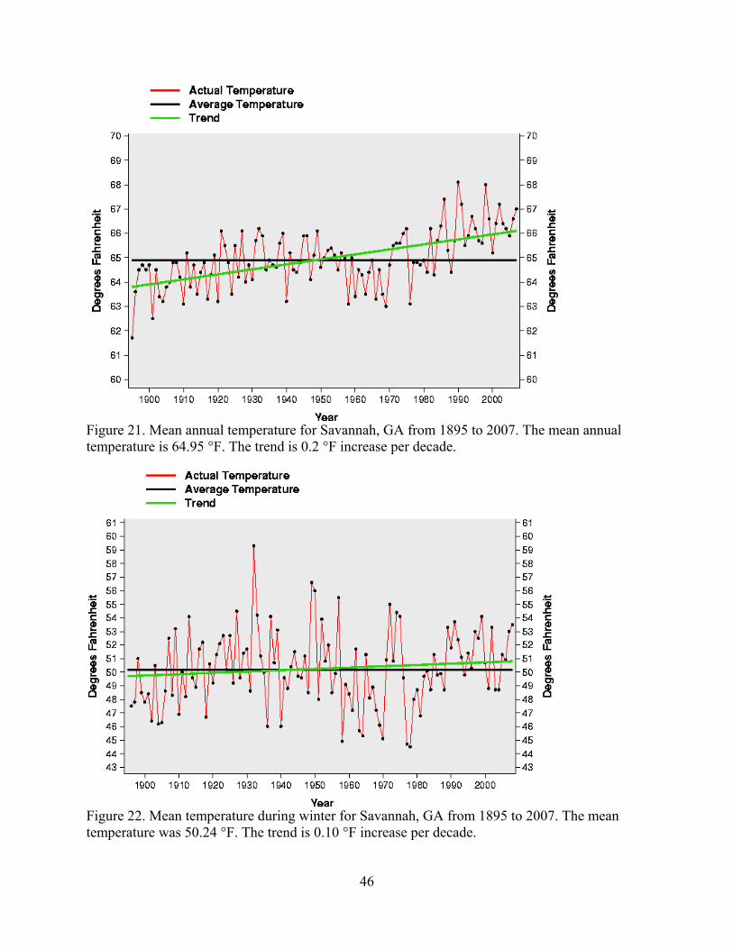
Figure 21. Mean annual temperature for Savannah, GA from 1895 to 2007. The mean annual temperature is 64.95 °F. The trend is 0.2 °F increase per decade.

Figure 22. Mean temperature during winter for Savannah, GA from 1895 to 2007. The mean temperature was 50.24 °F. The trend is 0.10 °F increase per decade.

46

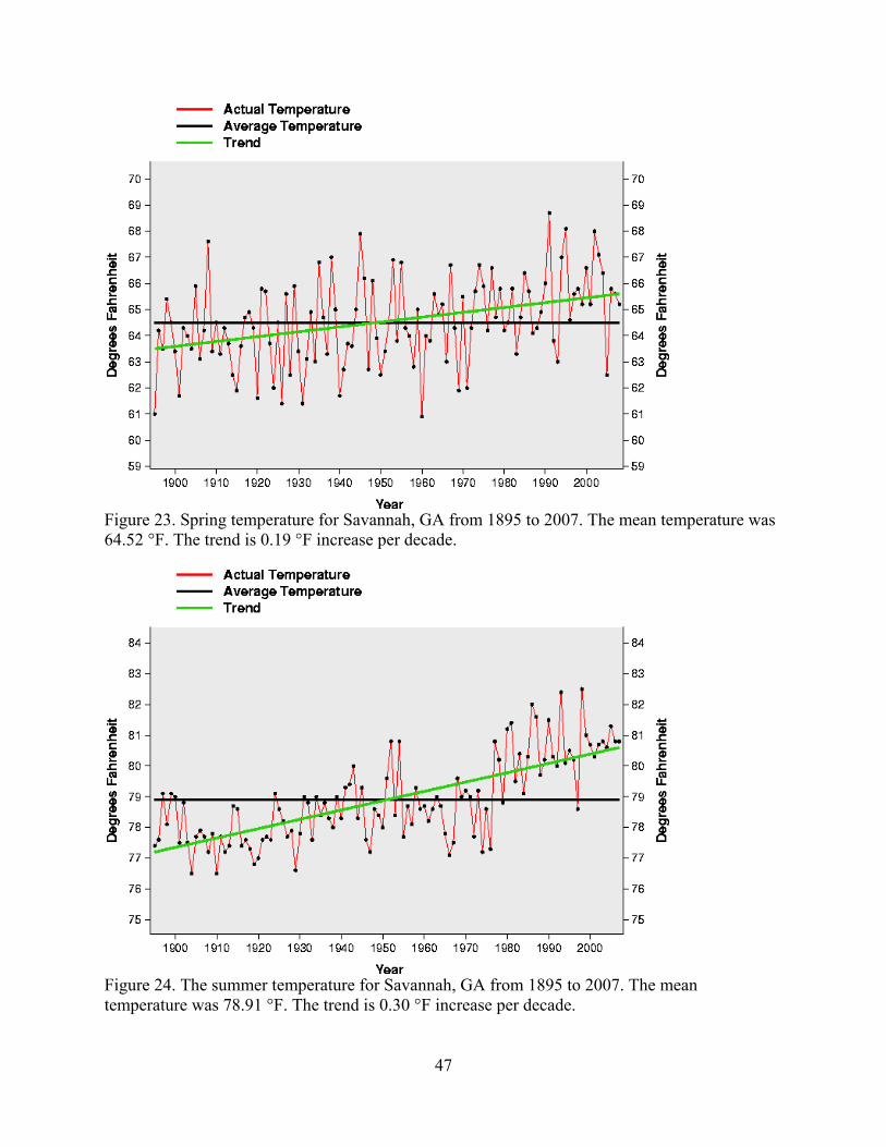
Figure 23. Spring temperature for Savannah, GA from 1895 to 2007. The mean temperature was 64.52 °F. The trend is 0.19 °F increase per decade.

Figure 24. The summer temperature for Savannah, GA from 1895 to 2007. The mean temperature was 78.91 °F. The trend is 0.30 °F increase per decade.

47

Figure 25. The fall temperature for Savannah, GA from 1895 to 2007. The mean temperature is 66.22 °F. The trend is 0.20 °F increase per decade. Since the upland habitats at Fort Pulaski NM developed over a similar timeframe, the present vegetation communities may be more reflective of this increasing thermal condition more so than similar older, longer-standing vegetation communities. Precipitation: Similar analyses were conducted for precipitation using data collected at Savannah, GA. The annual precipitation at Savannah shows great variation through time and has a slight increasing trend of approximately 0.17 inches per decade (Figure 26)

48

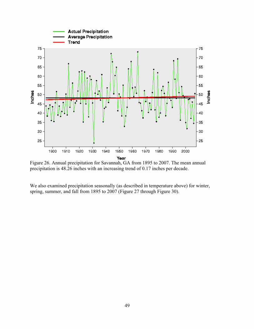
Figure 26. Annual precipitation for Savannah, GA from 1895 to 2007. The mean annual precipitation is 48.26 inches with an increasing trend of 0.17 inches per decade. We also examined precipitation seasonally (as described in temperature above) for winter, spring, summer, and fall from 1895 to 2007 (Figure 27 through Figure 30).

49

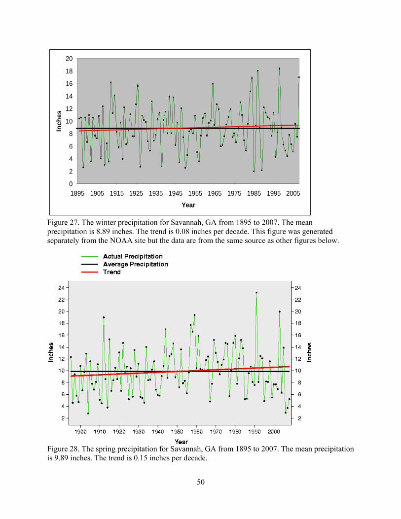
0

2

4

6

8

10

12

14

16

18

20

1895 1905 1915 1925 1935 1945 1955 1965 1975 1985 1995 2005

Year

Inch

es

Figure 27. The winter precipitation for Savannah, GA from 1895 to 2007. The mean precipitation is 8.89 inches. The trend is 0.08 inches per decade. This figure was generated separately from the NOAA site but the data are from the same source as other figures below.

Figure 28. The spring precipitation for Savannah, GA from 1895 to 2007. The mean precipitation is 9.89 inches. The trend is 0.15 inches per decade.

50

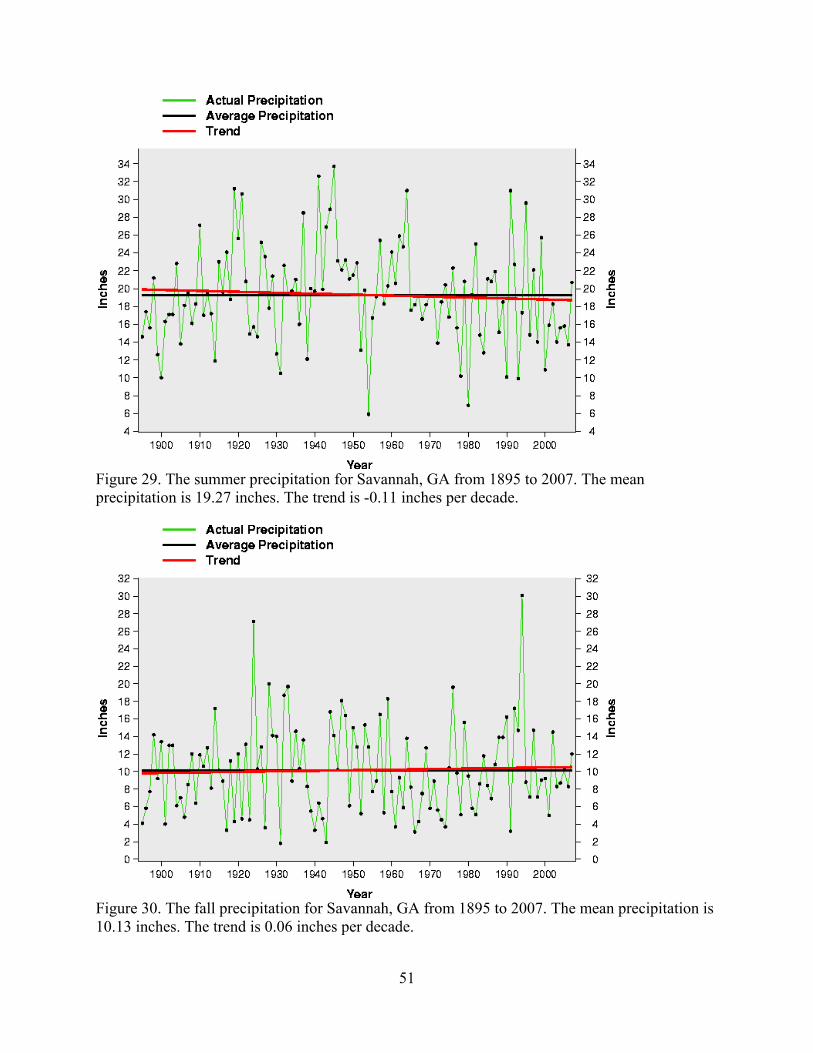
Figure 29. The summer precipitation for Savannah, GA from 1895 to 2007. The mean precipitation is 19.27 inches. The trend is -0.11 inches per decade.

Figure 30. The fall precipitation for Savannah, GA from 1895 to 2007. The mean precipitation is 10.13 inches. The trend is 0.06 inches per decade.

51

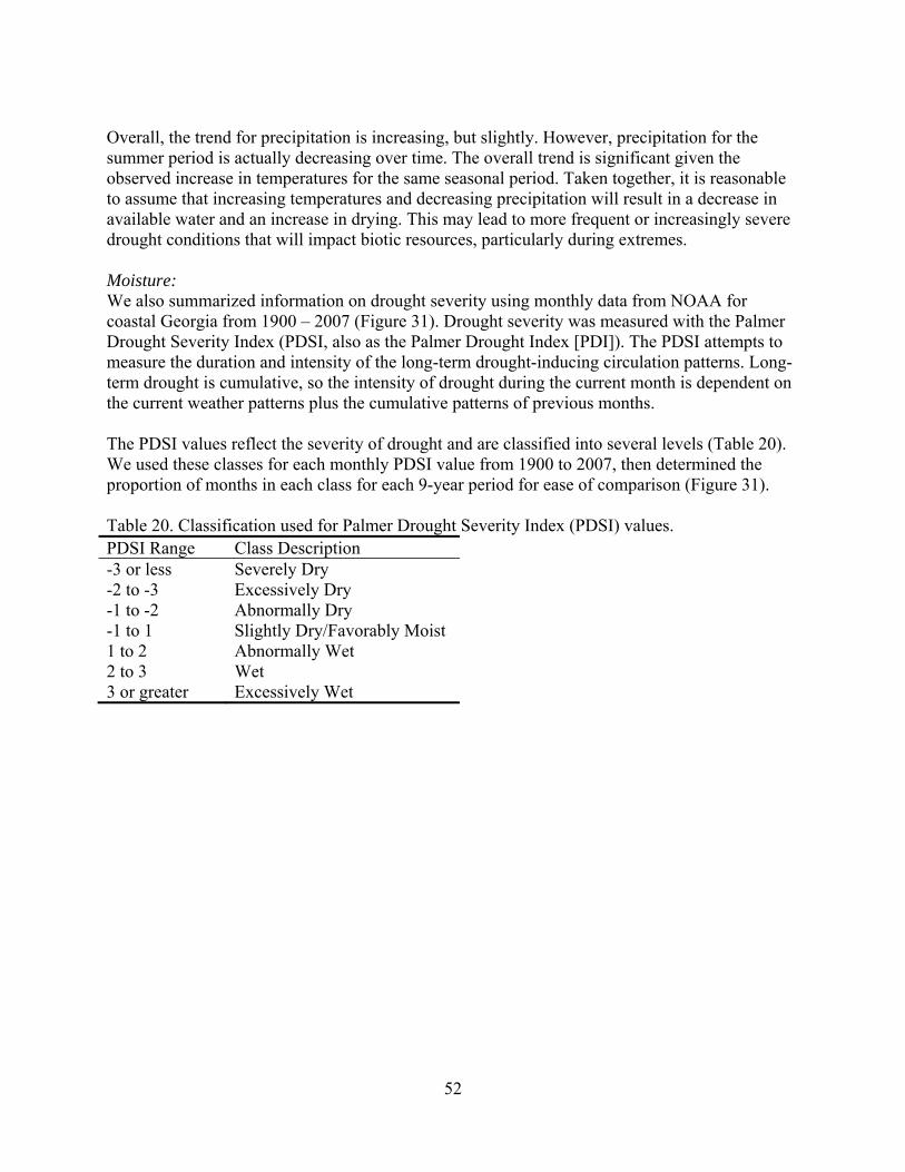
Overall, the trend for precipitation is increasing, but slightly. However, precipitation for the summer period is actually decreasing over time. The overall trend is significant given the observed increase in temperatures for the same seasonal period. Taken together, it is reasonable to assume that increasing temperatures and decreasing precipitation will result in a decrease in available water and an increase in drying. This may lead to more frequent or increasingly severe drought conditions that will impact biotic resources, particularly during extremes. Moisture: We also summarized information on drought severity using monthly data from NOAA for coastal Georgia from 1900 – 2007 (Figure 31). Drought severity was measured with the Palmer Drought Severity Index (PDSI, also as the Palmer Drought Index [PDI]). The PDSI attempts to measure the duration and intensity of the long-term drought-inducing circulation patterns. Long-term drought is cumulative, so the intensity of drought during the current month is dependent on the current weather patterns plus the cumulative patterns of previous months. The PDSI values reflect the severity of drought and are classified into several levels (Table 20). We used these classes for each monthly PDSI value from 1900 to 2007, then determined the proportion of months in each class for each 9-year period for ease of comparison (Figure 31). Table 20. Classification used for Palmer Drought Severity Index (PDSI) values. PDSI Range Class Description -3 or less Severely Dry -2 to -3 Excessively Dry -1 to -2 Abnormally Dry -1 to 1 Slightly Dry/Favorably Moist 1 to 2 Abnormally Wet 2 to 3 Wet 3 or greater Excessively Wet

52

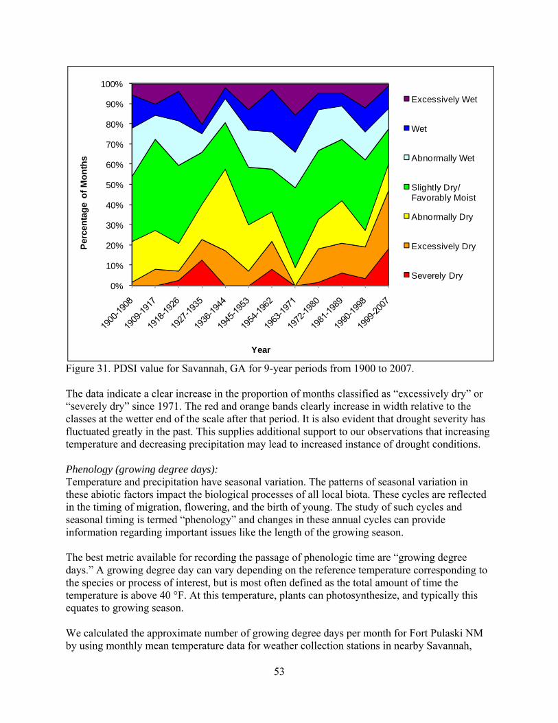
Figure 31. PDSI value for Savannah, GA for 9-year periods from 1900 to 2007.

0%

10%

20%

30%

40%

50%

60%

70%

80%

90%

100%Pe

rcen

tage

of M

onth

s

Year

Excessively Wet

Wet

Abnormally Wet

Slightly Dry/ Favorably Moist

Abnormally Dry

Excessively Dry

Severely Dry

The data indicate a clear increase in the proportion of months classified as “excessively dry” or “severely dry” since 1971. The red and orange bands clearly increase in width relative to the classes at the wetter end of the scale after that period. It is also evident that drought severity has fluctuated greatly in the past. This supplies additional support to our observations that increasing temperature and decreasing precipitation may lead to increased instance of drought conditions. Phenology (growing degree days): Temperature and precipitation have seasonal variation. The patterns of seasonal variation in these abiotic factors impact the biological processes of all local biota. These cycles are reflected in the timing of migration, flowering, and the birth of young. The study of such cycles and seasonal timing is termed “phenology” and changes in these annual cycles can provide information regarding important issues like the length of the growing season. The best metric available for recording the passage of phenologic time are “growing degree days.” A growing degree day can vary depending on the reference temperature corresponding to the species or process of interest, but is most often defined as the total amount of time the temperature is above 40 °F. At this temperature, plants can photosynthesize, and typically this equates to growing season. We calculated the approximate number of growing degree days per month for Fort Pulaski NM by using monthly mean temperature data for weather collection stations in nearby Savannah,

53

Georgia. Monthly temperature was available from 1896 to 2008 and was used to calculate the monthly growing degree day total with a simple formula:

GDD = (Tm – 40) Dm Where GDD = Growing degree days

Tm = monthly mean temperature Dm = number of days in month

The number of growing degrees days for each month were summed to determine the approximate number of growing degree days per year. These values were plotted against time (year) to illustrate the long-term trends in the numbers of growing degree days at Fort Pulaski NM (Figure 32).

Figure 32. The total growing degree days per year for Savannah, GA from 1896 to 2008. The long term mean annual growing degree day total is 9146 (black line). The blue line indicates an increasing trend (R2= 0.31) We observed an increase in the number of growing degree days that may indicate an increase in the growing season through time. To better illustrate this, we elected to examine the same data in terms of phenology. Much research has been completed equating phenological events to growing degree days (McMaster and Wilhelm 1997, University of Massachusetts Extension 2008, Virginia Tech FORSITE 2008). We attempted to put this in the context of a calendar year by selecting an arbitrary GDD threshold (1200 GDD) and estimating the date at which that number of growing degree days was achieved. This would be analogous to estimating the specific date a phenologic event was to occur (e.g., the blooming of dogwood trees). Since our source data is as monthly mean daily temperature, we calculated the total monthly accumulated GDD by multiplying the mean daily temperature by the number of days in the month. We then set a reference number of GDDs at 1200 to approximate a springtime

54

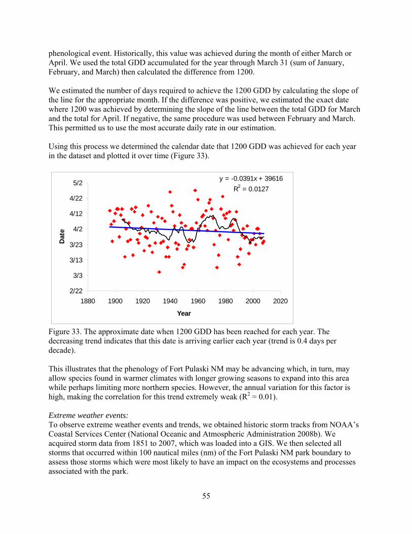
phenological event. Historically, this value was achieved during the month of either March or April. We used the total GDD accumulated for the year through March 31 (sum of January, February, and March) then calculated the difference from 1200. We estimated the number of days required to achieve the 1200 GDD by calculating the slope of the line for the appropriate month. If the difference was positive, we estimated the exact date where 1200 was achieved by determining the slope of the line between the total GDD for March and the total for April. If negative, the same procedure was used between February and March. This permitted us to use the most accurate daily rate in our estimation. Using this process we determined the calendar date that 1200 GDD was achieved for each year in the dataset and plotted it over time (Figure 33).

y = -0.0391x + 39616R2 = 0.0127

2/22

3/3

3/13

3/23

4/2

4/12

4/22

5/2

1880 1900 1920 1940 1960 1980 2000 2020

Year

Dat

e

Figure 33. The approximate date when 1200 GDD has been reached for each year. The decreasing trend indicates that this date is arriving earlier each year (trend is 0.4 days per decade). This illustrates that the phenology of Fort Pulaski NM may be advancing which, in turn, may allow species found in warmer climates with longer growing seasons to expand into this area while perhaps limiting more northern species. However, the annual variation for this factor is high, making the correlation for this trend extremely weak (R2 = 0.01). Extreme weather events: To observe extreme weather events and trends, we obtained historic storm tracks from NOAA’s Coastal Services Center (National Oceanic and Atmospheric Administration 2008b). We acquired storm data from 1851 to 2007, which was loaded into a GIS. We then selected all storms that occurred within 100 nautical miles (nm) of the Fort Pulaski NM park boundary to assess those storms which were most likely to have an impact on the ecosystems and processes associated with the park.

55

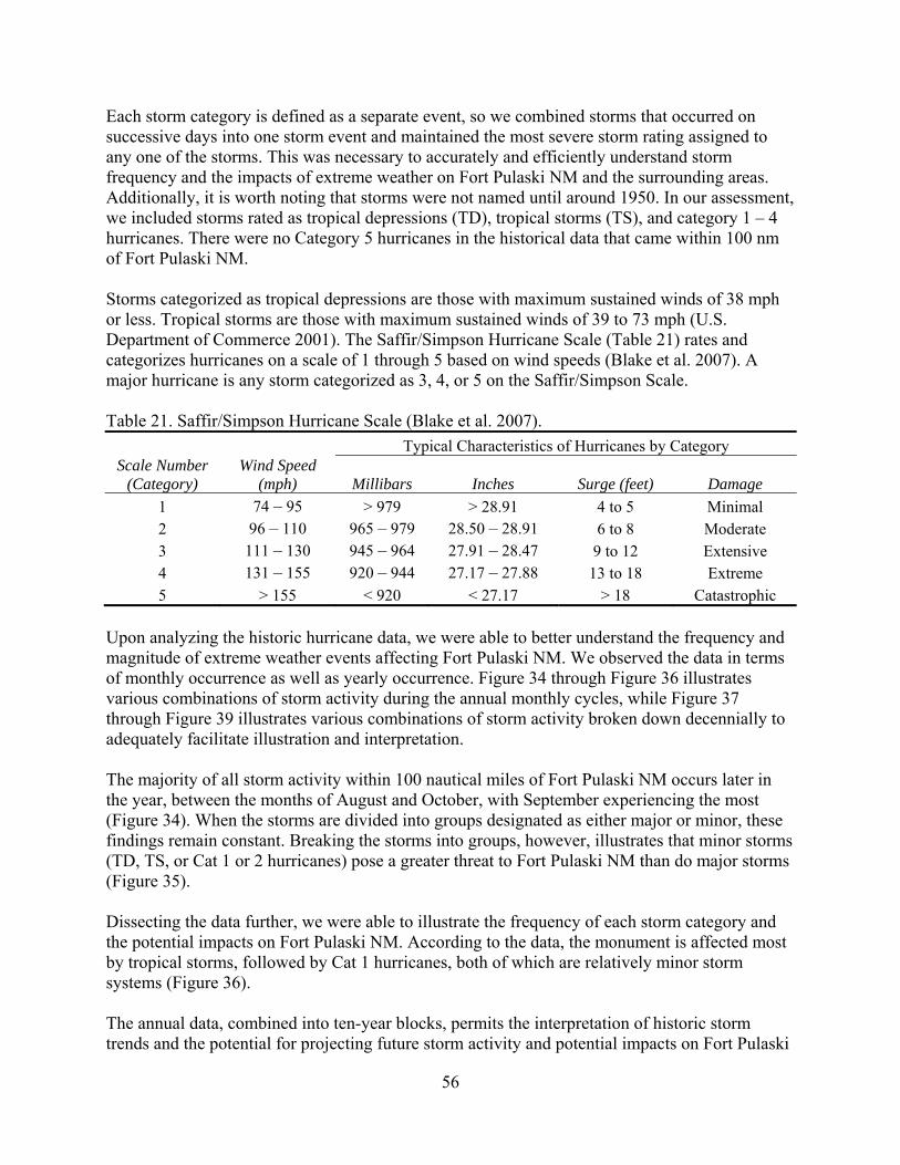
Each storm category is defined as a separate event, so we combined storms that occurred on successive days into one storm event and maintained the most severe storm rating assigned to any one of the storms. This was necessary to accurately and efficiently understand storm frequency and the impacts of extreme weather on Fort Pulaski NM and the surrounding areas. Additionally, it is worth noting that storms were not named until around 1950. In our assessment, we included storms rated as tropical depressions (TD), tropical storms (TS), and category 1 – 4 hurricanes. There were no Category 5 hurricanes in the historical data that came within 100 nm of Fort Pulaski NM. Storms categorized as tropical depressions are those with maximum sustained winds of 38 mph or less. Tropical storms are those with maximum sustained winds of 39 to 73 mph (U.S. Department of Commerce 2001). The Saffir/Simpson Hurricane Scale (Table 21) rates and categorizes hurricanes on a scale of 1 through 5 based on wind speeds (Blake et al. 2007). A major hurricane is any storm categorized as 3, 4, or 5 on the Saffir/Simpson Scale. Table 21. Saffir/Simpson Hurricane Scale (Blake et al. 2007). Typical Characteristics of Hurricanes by Category Scale Number

(Category) Wind Speed

(mph) Millibars Inches Surge (feet) Damage 1 74 – 95 > 979 > 28.91 4 to 5 Minimal 2 96 – 110 965 – 979 28.50 – 28.91 6 to 8 Moderate 3 111 – 130 945 – 964 27.91 – 28.47 9 to 12 Extensive 4 131 – 155 920 – 944 27.17 – 27.88 13 to 18 Extreme 5 > 155 < 920 < 27.17 > 18 Catastrophic

Upon analyzing the historic hurricane data, we were able to better understand the frequency and magnitude of extreme weather events affecting Fort Pulaski NM. We observed the data in terms of monthly occurrence as well as yearly occurrence. Figure 34 through Figure 36 illustrates various combinations of storm activity during the annual monthly cycles, while Figure 37 through Figure 39 illustrates various combinations of storm activity broken down decennially to adequately facilitate illustration and interpretation. The majority of all storm activity within 100 nautical miles of Fort Pulaski NM occurs later in the year, between the months of August and October, with September experiencing the most (Figure 34). When the storms are divided into groups designated as either major or minor, these findings remain constant. Breaking the storms into groups, however, illustrates that minor storms (TD, TS, or Cat 1 or 2 hurricanes) pose a greater threat to Fort Pulaski NM than do major storms (Figure 35). Dissecting the data further, we were able to illustrate the frequency of each storm category and the potential impacts on Fort Pulaski NM. According to the data, the monument is affected most by tropical storms, followed by Cat 1 hurricanes, both of which are relatively minor storm systems (Figure 36). The annual data, combined into ten-year blocks, permits the interpretation of historic storm trends and the potential for projecting future storm activity and potential impacts on Fort Pulaski

56

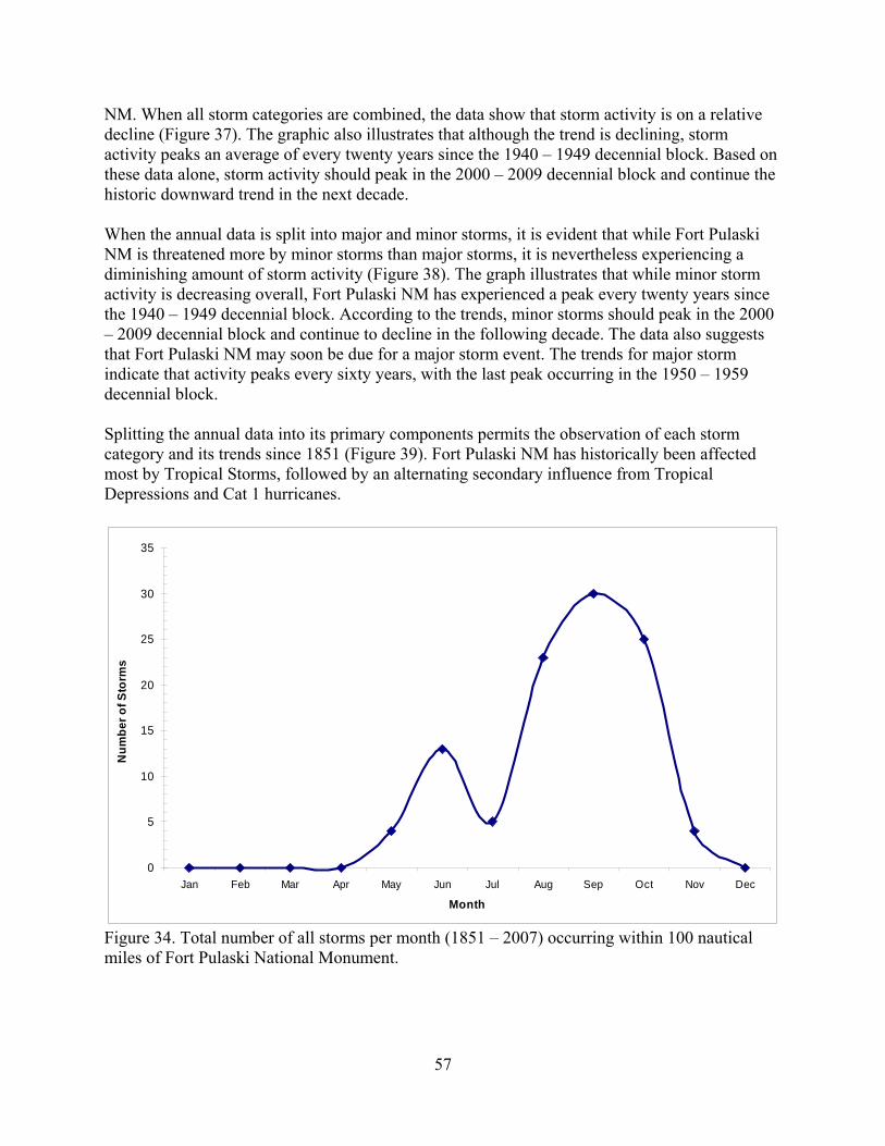
NM. When all storm categories are combined, the data show that storm activity is on a relative decline (Figure 37). The graphic also illustrates that although the trend is declining, storm activity peaks an average of every twenty years since the 1940 – 1949 decennial block. Based on these data alone, storm activity should peak in the 2000 – 2009 decennial block and continue the historic downward trend in the next decade. When the annual data is split into major and minor storms, it is evident that while Fort Pulaski NM is threatened more by minor storms than major storms, it is nevertheless experiencing a diminishing amount of storm activity (Figure 38). The graph illustrates that while minor storm activity is decreasing overall, Fort Pulaski NM has experienced a peak every twenty years since the 1940 – 1949 decennial block. According to the trends, minor storms should peak in the 2000 – 2009 decennial block and continue to decline in the following decade. The data also suggests that Fort Pulaski NM may soon be due for a major storm event. The trends for major storm indicate that activity peaks every sixty years, with the last peak occurring in the 1950 – 1959 decennial block. Splitting the annual data into its primary components permits the observation of each storm category and its trends since 1851 (Figure 39). Fort Pulaski NM has historically been affected most by Tropical Storms, followed by an alternating secondary influence from Tropical Depressions and Cat 1 hurricanes.

0

5

10

15

20

25

30

35

Jan Feb Mar Apr May Jun Jul Aug Sep Oct Nov Dec

Month

Num

ber o

f Sto

rms

Figure 34. Total number of all storms per month (1851 – 2007) occurring within 100 nautical miles of Fort Pulaski National Monument.

57

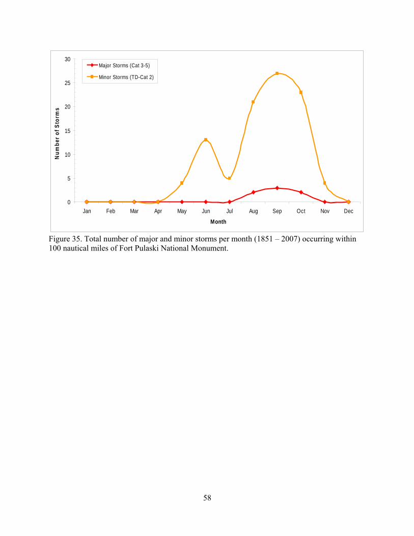
58

0

5

10

15

20

25

30


Month

Num

ber o

f Sto

rms

Major Storms (Cat 3-5)

Minor Storms (TD-Cat 2)

Figure 35. Total number of major and minor storms per month (1851 – 2007) occurring within 100 nautical miles of Fort Pulaski National Monument.

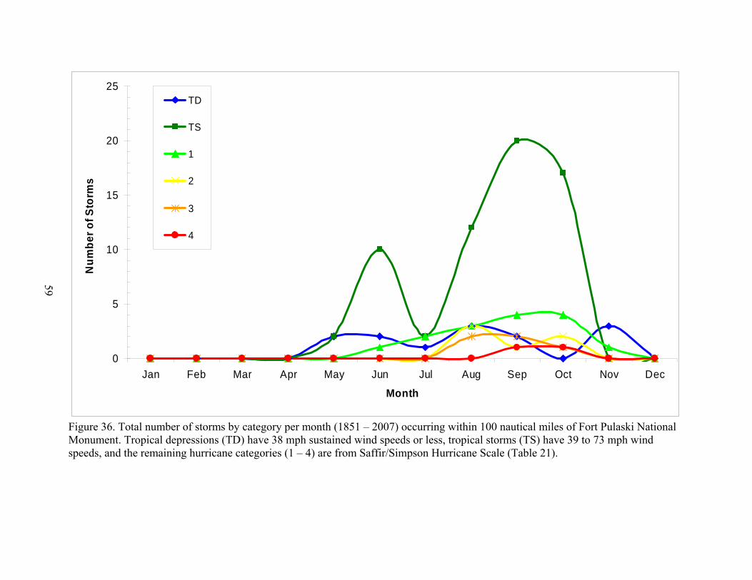
0

5

10

15

20

25


Month

Num

ber o

f Sto

rms

TD

TS

1

2

3

4

59

Figure 36. Total number of storms by category per month (1851 – 2007) occurring within 100 nautical miles of Fort Pulaski National Monument. Tropical depressions (TD) have 38 mph sustained wind speeds or less, tropical storms (TS) have 39 to 73 mph wind speeds, and the remaining hurricane categories (1 – 4) are from Saffir/Simpson Hurricane Scale (Table 21).

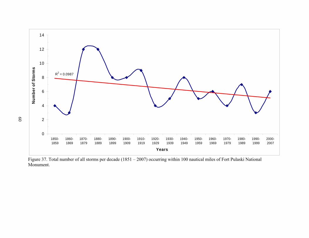
R2 = 0.0987

0

2

4

6

8

10

12

14

1850-1859

1860-1869

1870-1879

1880-1889

1890-1899

1900-1909

1910-1919

1920-1929

1930-1939

1940-1949

1950-1959

1960-1969

1970-1979

1980-1989

1990-1999

2000-2007

Years

Num

ber o

f Sto

rms

60

Figure 37. Total number of all storms per decade (1851 – 2007) occurring within 100 nautical miles of Fort Pulaski National Monument.

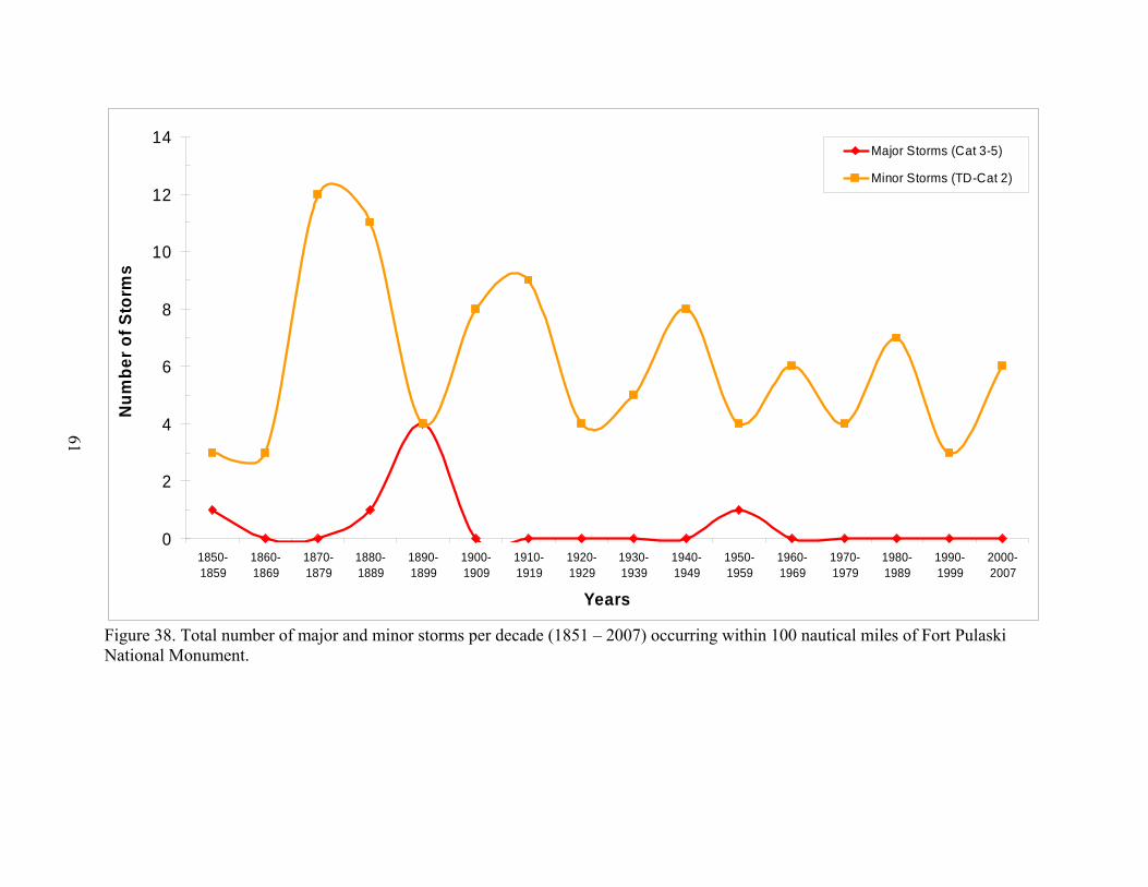
0

2

4

6

8

10

12

14

1850-1859

1860-1869

1870-1879

1880-1889

1890-1899

1900-1909

1910-1919

1920-1929

1930-1939

1940-1949

1950-1959

1960-1969

1970-1979

1980-1989

1990-1999

2000-2007

Years

Num

ber o

f Sto

rms

Major Storms (Cat 3-5)

Minor Storms (TD-Cat 2)

61

Figure 38. Total number of major and minor storms per decade (1851 – 2007) occurring within 100 nautical miles of Fort Pulaski National Monument.

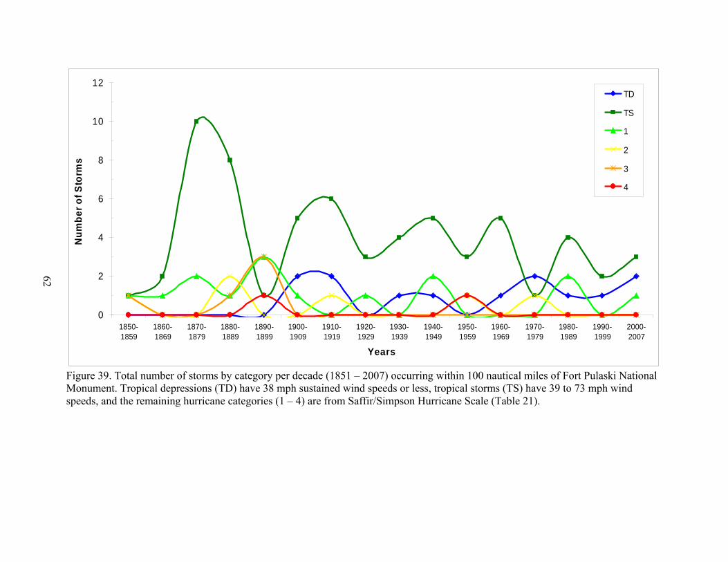
Figure 39. Total number of storms by category per decade (1851 – 2007) occurring within 100 nautical miles of Fort Pulaski National Monument. Tropical depressions (TD) have 38 mph sustained wind speeds or less, tropical storms (TS) have 39 to 73 mph wind speeds, and the remaining hurricane categories (1 – 4) are from Saffir/Simpson Hurricane Scale (Table 21).

0

2

4

6

8

10

12

1850-1859

1860-1869

1870-1879

1880-1889

1890-1899

1900-1909

1910-1919

1920-1929

1930-1939

1940-1949

1950-1959

1960-1969

1970-1979

1980-1989

1990-1999

2000-2007

Years

Num

ber o

f Sto

rms

TD

TS

1

2

3

4

62

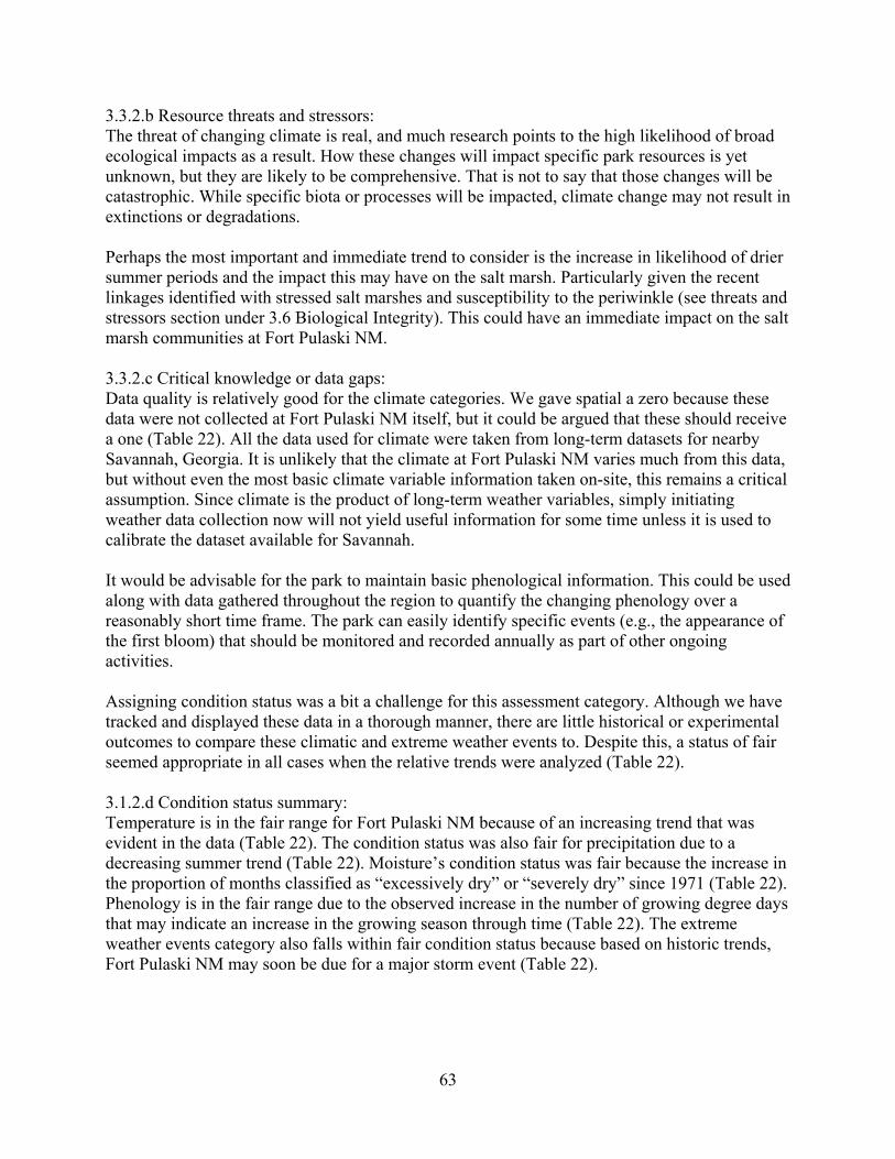
3.3.2.b Resource threats and stressors: The threat of changing climate is real, and much research points to the high likelihood of broad ecological impacts as a result. How these changes will impact specific park resources is yet unknown, but they are likely to be comprehensive. That is not to say that those changes will be catastrophic. While specific biota or processes will be impacted, climate change may not result in extinctions or degradations. Perhaps the most important and immediate trend to consider is the increase in likelihood of drier summer periods and the impact this may have on the salt marsh. Particularly given the recent linkages identified with stressed salt marshes and susceptibility to the periwinkle (see threats and stressors section under 3.6 Biological Integrity). This could have an immediate impact on the salt marsh communities at Fort Pulaski NM. 3.3.2.c Critical knowledge or data gaps: Data quality is relatively good for the climate categories. We gave spatial a zero because these data were not collected at Fort Pulaski NM itself, but it could be argued that these should receive a one (Table 22). All the data used for climate were taken from long-term datasets for nearby Savannah, Georgia. It is unlikely that the climate at Fort Pulaski NM varies much from this data, but without even the most basic climate variable information taken on-site, this remains a critical assumption. Since climate is the product of long-term weather variables, simply initiating weather data collection now will not yield useful information for some time unless it is used to calibrate the dataset available for Savannah. It would be advisable for the park to maintain basic phenological information. This could be used along with data gathered throughout the region to quantify the changing phenology over a reasonably short time frame. The park can easily identify specific events (e.g., the appearance of the first bloom) that should be monitored and recorded annually as part of other ongoing activities. Assigning condition status was a bit a challenge for this assessment category. Although we have tracked and displayed these data in a thorough manner, there are little historical or experimental outcomes to compare these climatic and extreme weather events to. Despite this, a status of fair seemed appropriate in all cases when the relative trends were analyzed (Table 22). 3.1.2.d Condition status summary: Temperature is in the fair range for Fort Pulaski NM because of an increasing trend that was evident in the data (Table 22). The condition status was also fair for precipitation due to a decreasing summer trend (Table 22). Moisture’s condition status was fair because the increase in the proportion of months classified as “excessively dry” or “severely dry” since 1971 (Table 22). Phenology is in the fair range due to the observed increase in the number of growing degree days that may indicate an increase in the growing season through time (Table 22). The extreme weather events category also falls within fair condition status because based on historic trends, Fort Pulaski NM may soon be due for a major storm event (Table 22).

63

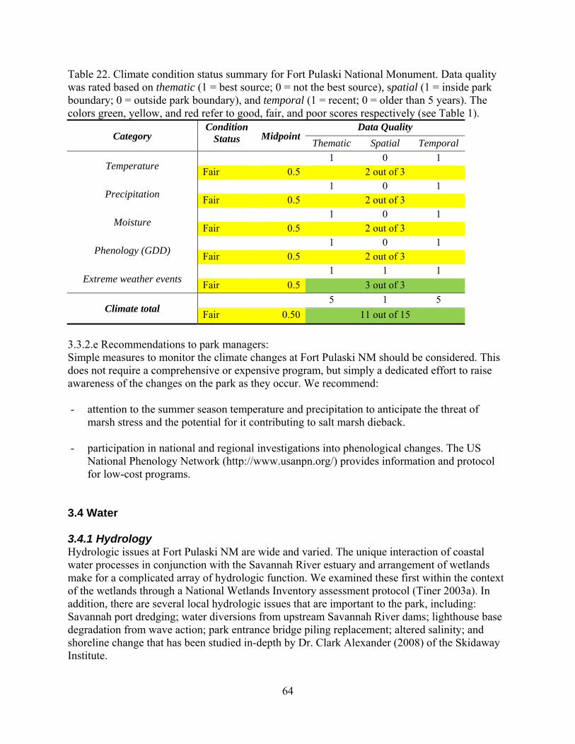
Table 22. Climate condition status summary for Fort Pulaski National Monument. Data quality was rated based on thematic (1 = best source; 0 = not the best source), spatial (1 = inside park boundary; 0 = outside park boundary), and temporal (1 = recent; 0 = older than 5 years). The colors green, yellow, and red refer to good, fair, and poor scores respectively (see Table 1).

Category Condition



Temperature 1 0 1 Fair 0.5 2 out of 3

Precipitation 1 0 1 Fair 0.5 2 out of 3

Moisture 1 0 1 Fair 0.5 2 out of 3

Phenology (GDD) 1 0 1 Fair 0.5 2 out of 3

Extreme weather events 1 1 1 Fair 0.5 3 out of 3

Climate total 5 1 5 Fair 0.50 11 out of 15

3.3.2.e Recommendations to park managers: Simple measures to monitor the climate changes at Fort Pulaski NM should be considered. This does not require a comprehensive or expensive program, but simply a dedicated effort to raise awareness of the changes on the park as they occur. We recommend: - attention to the summer season temperature and precipitation to anticipate the threat of

marsh stress and the potential for it contributing to salt marsh dieback. - participation in national and regional investigations into phenological changes. The US

National Phenology Network (http://www.usanpn.org/) provides information and protocol for low-cost programs.

3.4 Water 3.4.1 Hydrology Hydrologic issues at Fort Pulaski NM are wide and varied. The unique interaction of coastal water processes in conjunction with the Savannah River estuary and arrangement of wetlands make for a complicated array of hydrologic function. We examined these first within the context of the wetlands through a National Wetlands Inventory assessment protocol (Tiner 2003a). In addition, there are several local hydrologic issues that are important to the park, including: Savannah port dredging; water diversions from upstream Savannah River dams; lighthouse base degradation from wave action; park entrance bridge piling replacement; altered salinity; and shoreline change that has been studied in-depth by Dr. Clark Alexander (2008) of the Skidaway Institute.

64

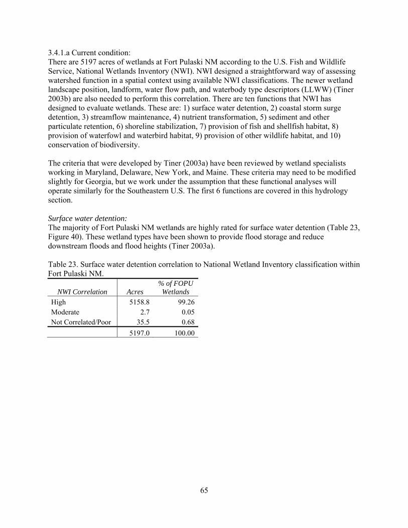
3.4.1.a Current condition: There are 5197 acres of wetlands at Fort Pulaski NM according to the U.S. Fish and Wildlife Service, National Wetlands Inventory (NWI). NWI designed a straightforward way of assessing watershed function in a spatial context using available NWI classifications. The newer wetland landscape position, landform, water flow path, and waterbody type descriptors (LLWW) (Tiner 2003b) are also needed to perform this correlation. There are ten functions that NWI has designed to evaluate wetlands. These are: 1) surface water detention, 2) coastal storm surge detention, 3) streamflow maintenance, 4) nutrient transformation, 5) sediment and other particulate retention, 6) shoreline stabilization, 7) provision of fish and shellfish habitat, 8) provision of waterfowl and waterbird habitat, 9) provision of other wildlife habitat, and 10) conservation of biodiversity. The criteria that were developed by Tiner (2003a) have been reviewed by wetland specialists working in Maryland, Delaware, New York, and Maine. These criteria may need to be modified slightly for Georgia, but we work under the assumption that these functional analyses will operate similarly for the Southeastern U.S. The first 6 functions are covered in this hydrology section. Surface water detention: The majority of Fort Pulaski NM wetlands are highly rated for surface water detention (Table 23, Figure 40). These wetland types have been shown to provide flood storage and reduce downstream floods and flood heights (Tiner 2003a). Table 23. Surface water detention correlation to National Wetland Inventory classification within Fort Pulaski NM.

NWI Correlation Acres % of FOPU

Wetlands High 5158.8 99.26Moderate 2.7 0.05Not Correlated/Poor 35.5 0.68 5197.0 100.00

65

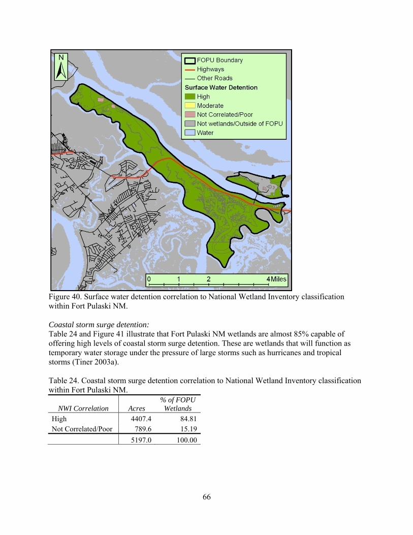
Figure 40. Surface water detention correlation to National Wetland Inventory classification within Fort Pulaski NM. Coastal storm surge detention: Table 24 and Figure 41 illustrate that Fort Pulaski NM wetlands are almost 85% capable of offering high levels of coastal storm surge detention. These are wetlands that will function as temporary water storage under the pressure of large storms such as hurricanes and tropical storms (Tiner 2003a). Table 24. Coastal storm surge detention correlation to National Wetland Inventory classification within Fort Pulaski NM.


Wetlands High 4407.4 84.81Not Correlated/Poor 789.6 15.19 5197.0 100.00

66

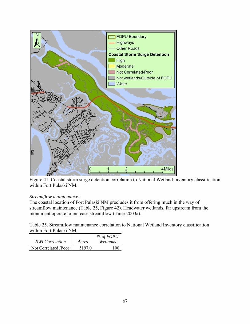
Figure 41. Coastal storm surge detention correlation to National Wetland Inventory classification within Fort Pulaski NM. Streamflow maintenance: The coastal location of Fort Pulaski NM precludes it from offering much in the way of streamflow maintenance (Table 25, Figure 42). Headwater wetlands, far upstream from the monument operate to increase streamflow (Tiner 2003a). Table 25. Streamflow maintenance correlation to National Wetland Inventory classification within Fort Pulaski NM.


Wetlands Not Correlated /Poor 5197.0 100

67

Figure 42. Streamflow maintenance correlation to National Wetland Inventory classification within Fort Pulaski NM. Nutrient transformation: Nutrient transformation occurs most readily in permanently flooded wetlands whereas temporarily flooded wetlands have only moderate potential (Tiner 2003a). Nutrients increase the biological oxygen demand (BOD) and therefore lower DO concentrations in water and have consistently ranked as one of the top causes of water degradation in the U.S. (U.S. Environmental Protection Agency 2008d). Sixty-six percent of the wetlands at Fort Pulaski NM are highly or moderately correlated with nutrient transformation (Table 26, Figure 43). The irregularly exposed wetlands and subtidal rivers/streams do not offer much in the way of nutrient transformation because they are continuously saturated and anaerobic.

68

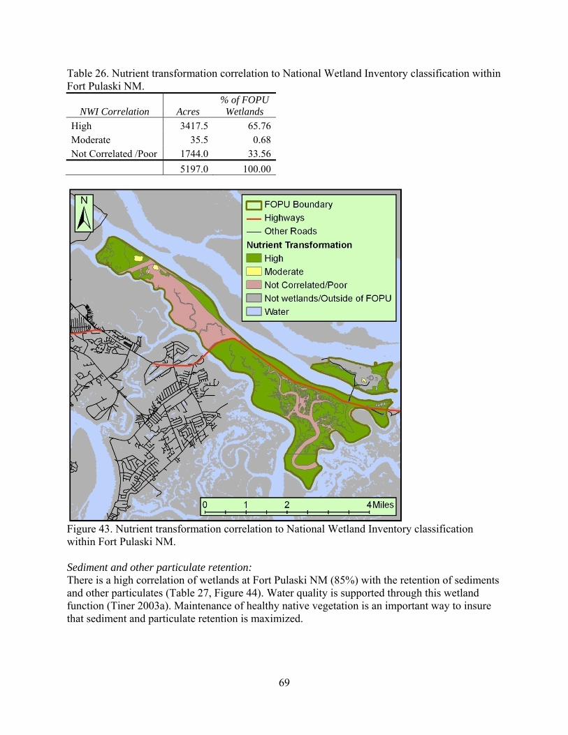
Table 26. Nutrient transformation correlation to National Wetland Inventory classification within Fort Pulaski NM.


Wetlands High 3417.5 65.76Moderate 35.5 0.68Not Correlated /Poor 1744.0 33.56 5197.0 100.00

Figure 43. Nutrient transformation correlation to National Wetland Inventory classification within Fort Pulaski NM. Sediment and other particulate retention: There is a high correlation of wetlands at Fort Pulaski NM (85%) with the retention of sediments and other particulates (Table 27, Figure 44). Water quality is supported through this wetland function (Tiner 2003a). Maintenance of healthy native vegetation is an important way to insure that sediment and particulate retention is maximized.

69

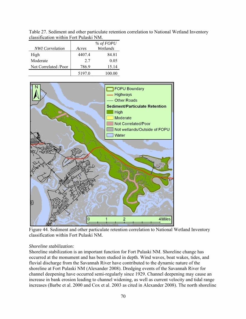
Table 27. Sediment and other particulate retention correlation to National Wetland Inventory classification within Fort Pulaski NM.


Wetlands High 4407.4 84.81Moderate 2.7 0.05Not Correlated /Poor 786.9 15.14 5197.0 100.00

Figure 44. Sediment and other particulate retention correlation to National Wetland Inventory classification within Fort Pulaski NM. Shoreline stabilization: Shoreline stabilization is an important function for Fort Pulaski NM. Shoreline change has occurred at the monument and has been studied in depth. Wind waves, boat wakes, tides, and fluvial discharge from the Savannah River have contributed to the dynamic nature of the shoreline at Fort Pulaski NM (Alexander 2008). Dredging events of the Savannah River for channel deepening have occurred semi-regularly since 1929. Channel deepening may cause an increase in bank erosion leading to channel widening, as well as current velocity and tidal range increases (Barbe et al. 2000 and Cox et al. 2003 as cited in Alexander 2008). The north shoreline

70

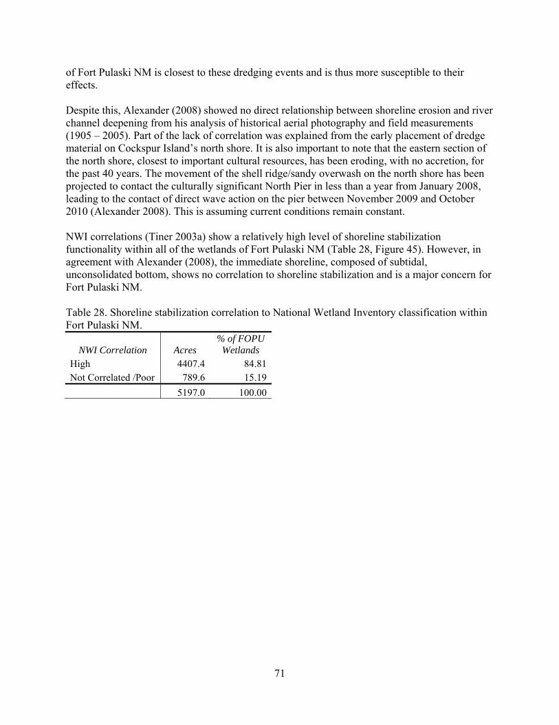
of Fort Pulaski NM is closest to these dredging events and is thus more susceptible to their effects. Despite this, Alexander (2008) showed no direct relationship between shoreline erosion and river channel deepening from his analysis of historical aerial photography and field measurements (1905 – 2005). Part of the lack of correlation was explained from the early placement of dredge material on Cockspur Island’s north shore. It is also important to note that the eastern section of the north shore, closest to important cultural resources, has been eroding, with no accretion, for the past 40 years. The movement of the shell ridge/sandy overwash on the north shore has been projected to contact the culturally significant North Pier in less than a year from January 2008, leading to the contact of direct wave action on the pier between November 2009 and October 2010 (Alexander 2008). This is assuming current conditions remain constant. NWI correlations (Tiner 2003a) show a relatively high level of shoreline stabilization functionality within all of the wetlands of Fort Pulaski NM (Table 28, Figure 45). However, in agreement with Alexander (2008), the immediate shoreline, composed of subtidal, unconsolidated bottom, shows no correlation to shoreline stabilization and is a major concern for Fort Pulaski NM. Table 28. Shoreline stabilization correlation to National Wetland Inventory classification within Fort Pulaski NM.


Wetlands High 4407.4 84.81Not Correlated /Poor 789.6 15.19 5197.0 100.00

71

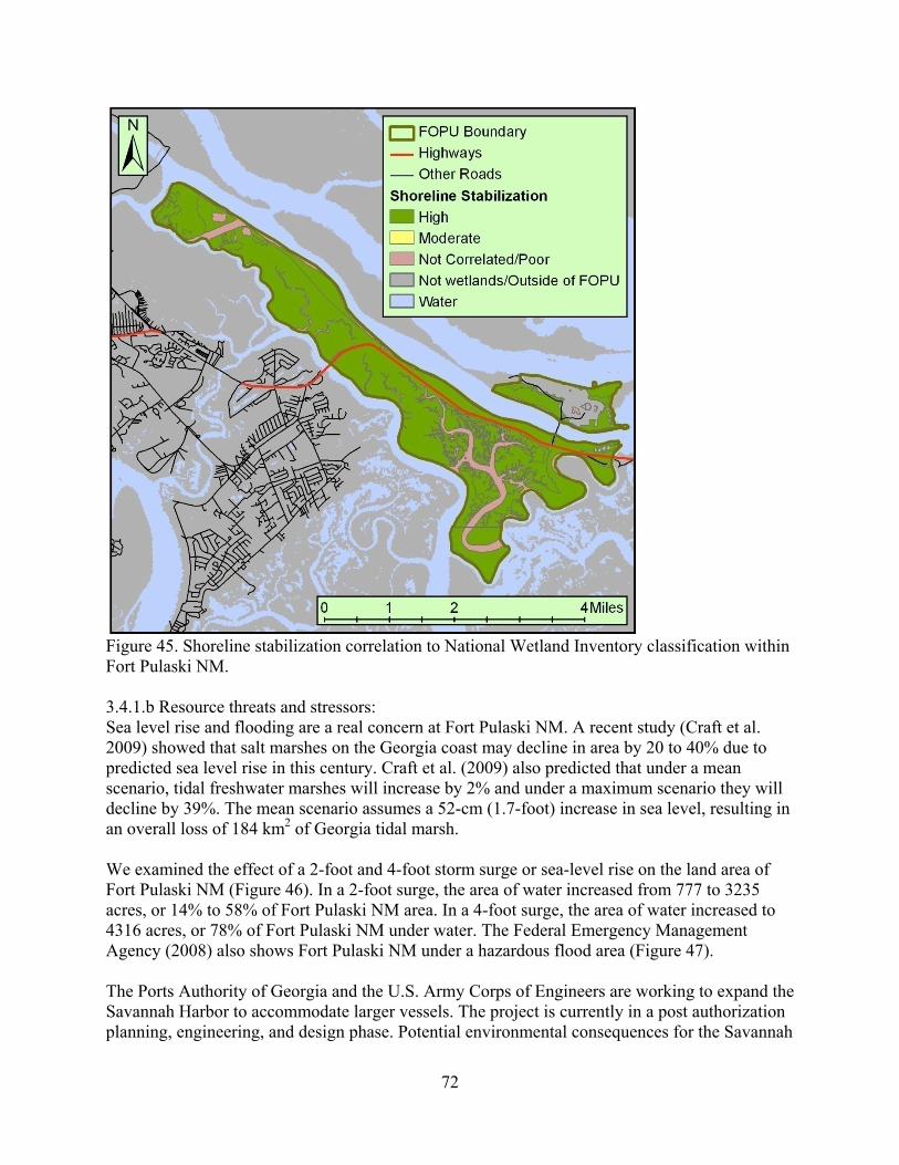
Figure 45. Shoreline stabilization correlation to National Wetland Inventory classification within Fort Pulaski NM. 3.4.1.b Resource threats and stressors: Sea level rise and flooding are a real concern at Fort Pulaski NM. A recent study (Craft et al. 2009) showed that salt marshes on the Georgia coast may decline in area by 20 to 40% due to predicted sea level rise in this century. Craft et al. (2009) also predicted that under a mean scenario, tidal freshwater marshes will increase by 2% and under a maximum scenario they will decline by 39%. The mean scenario assumes a 52-cm (1.7-foot) increase in sea level, resulting in an overall loss of 184 km2 of Georgia tidal marsh. We examined the effect of a 2-foot and 4-foot storm surge or sea-level rise on the land area of Fort Pulaski NM (Figure 46). In a 2-foot surge, the area of water increased from 777 to 3235 acres, or 14% to 58% of Fort Pulaski NM area. In a 4-foot surge, the area of water increased to 4316 acres, or 78% of Fort Pulaski NM under water. The Federal Emergency Management Agency (2008) also shows Fort Pulaski NM under a hazardous flood area (Figure 47). The Ports Authority of Georgia and the U.S. Army Corps of Engineers are working to expand the Savannah Harbor to accommodate larger vessels. The project is currently in a post authorization planning, engineering, and design phase. Potential environmental consequences for the Savannah

72

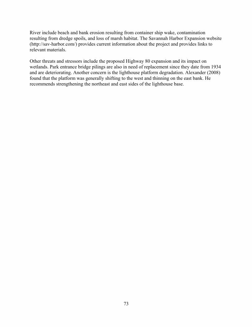
River include beach and bank erosion resulting from container ship wake, contamination resulting from dredge spoils, and loss of marsh habitat. The Savannah Harbor Expansion website (http://sav-harbor.com/) provides current information about the project and provides links to relevant materials. Other threats and stressors include the proposed Highway 80 expansion and its impact on wetlands. Park entrance bridge pilings are also in need of replacement since they date from 1934 and are deteriorating. Another concern is the lighthouse platform degradation. Alexander (2008) found that the platform was generally shifting to the west and thinning on the east bank. He recommends strengthening the northeast and east sides of the lighthouse base.

73

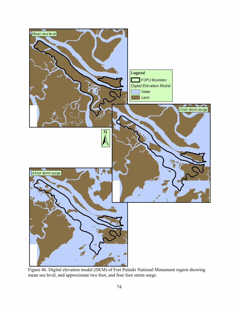
74

Figure 46. Digital elevation model (DEM) of Fort Pulaski National Monument region showing mean sea level, and approximate two foot, and four foot storm surge.

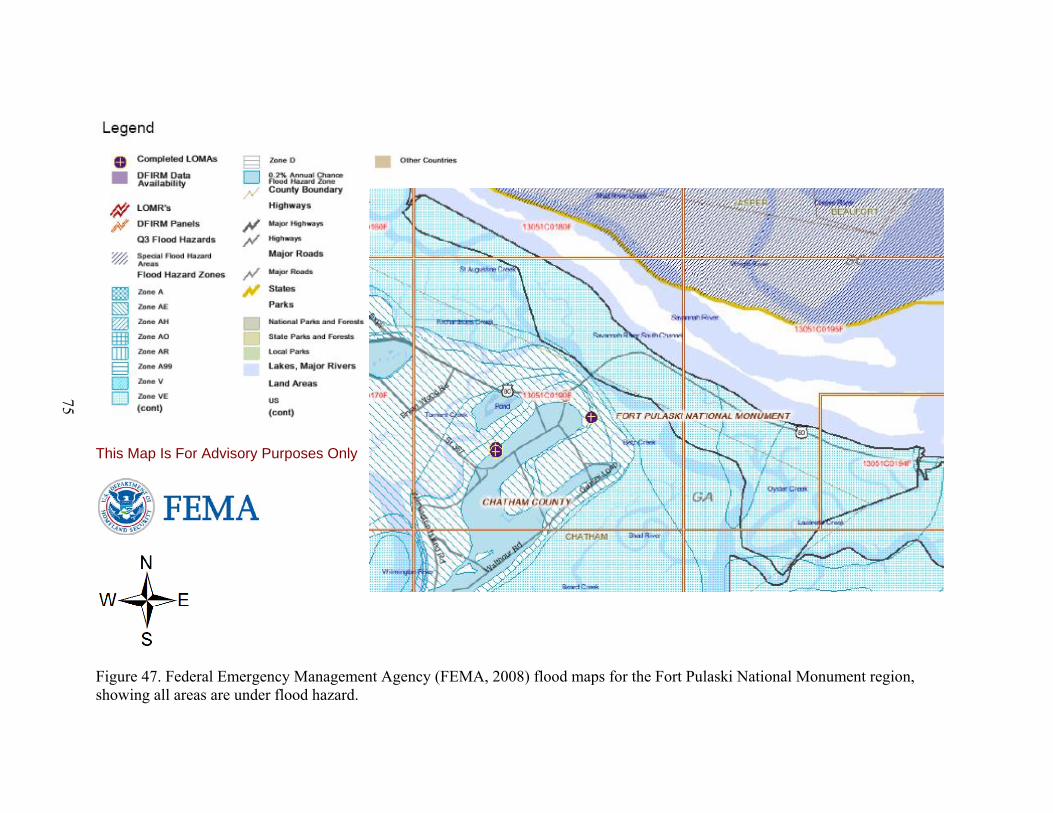
75

This Map Is For Advisory Purposes Only

Figure 47. Federal Emergency Management Agency (FEMA, 2008) flood maps for the Fort Pulaski National Monument region, showing all areas are under flood hazard.

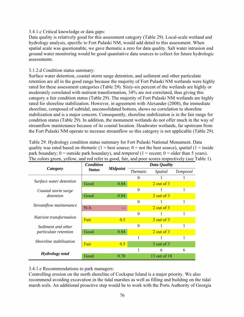
3.4.1.c Critical knowledge or data gaps: Data quality is relatively good for this assessment category (Table 29). Local-scale wetland and hydrology analysis, specific to Fort Pulaski NM, would add detail to this assessment. When spatial scale was questionable, we gave thematic a zero for data quality. Salt water intrusion and ground water monitoring would be good quanitative data sources to collect for future hydrologic assessments. 3.1.2.d Condition status summary: Surface water detention, coastal storm surge detention, and sediment and other particulate retention are all in the good range because the majority of Fort Pulaski NM wetlands were highly rated for these assessment categories (Table 29). Sixty-six percent of the wetlands are highly or moderately correlated with nutrient transformation, 34% are not correlated, thus giving this category a fair condition status (Table 29). The majority of Fort Pulaski NM wetlands are highly rated for shoreline stabilization. However, in agreement with Alexander (2008), the immediate shoreline, composed of subtidal, unconsolidated bottom, shows no correlation to shoreline stabilization and is a major concern. Consequently, shoreline stabilization is in the fair range for condition status (Table 29). In addition, the monument wetlands do not offer much in the way of streamflow maintenance because of its coastal location. Headwater wetlands, far upstream from the Fort Pulaski NM operate to increase streamflow so this category is not applicable (Table 29).

Table 29. Hydrology condition status summary for Fort Pulaski National Monument. Data quality was rated based on thematic (1 = best source; 0 = not the best source), spatial (1 = inside park boundary; 0 = outside park boundary), and temporal (1 = recent; 0 = older than 5 years). The colors green, yellow, and red refer to good, fair, and poor scores respectively (see

Table 1).

Category Condition



Surface water detention 0 1 1

Good 0.84 2 out of 3 Coastal storm surge

detention 0 1 1 Good 0.84 2 out of 3

Streamflow maintenance 0 1 1 N/A -- 2 out of 3

Nutrient transformation 0 1 1 Fair 0.5 2 out of 3

Sediment and other particulate retention

0 1 1 Good 0.84 2 out of 3

Shoreline stabilization 1 1 1 Fair 0.5 3 out of 3

Hydrology total 1 6 6 Good 0.70 13 out of 18

3.4.1.e Recommendations to park managers: Controlling erosion on the north shoreline of Cockspur Island is a major priority. We also recommend avoiding excavation in the tidal marshes as well as filling and building on the tidal marsh soils. An additional proactive step would be to work with the Ports Authority of Georgia

76

and Georgia Department of Transportation to minimize the effects of the Savannah Harbor dredging and Highway 80 expansion. 3.4.2 Water Quality Fort Pulaski NM is located at the mouth of the Savannah estuary, approximately 13 miles downstream of Savannah, Georgia (Figure 48). The 5,623-acre monument is composed of a series of small islands surrounded by tidally-influenced rivers and channels. According to national coastal land cover data (National Oceanic and Atmospheric Administration 2008a), Fort Pulaski NM water resources include 3,745 acres of wetland and 1,424 acres of open water. Because the Savannah basin drains over 9,850 sq mi (25,511 km²) of land, managers have little control over water quality within the monument boundaries(Cooney et al. 2005). In 2005, McFarlin and Alber completed a comprehensive water resource assessment of Fort Pulaski NM for the Water Resources Division of the National Park Service. The 187 page technical report (NPS/NRWRD/NRTR-2005/345) provides a thorough treatment of the water resources at and near Fort Pulaski NM, including background information, research methods, descriptions of pollutants and sources, and recommendations. In contrast to McFarlin and Alber (2005), this assessment provides a concise picture of the conditions and threats of the water resources at Fort Pulaski NM and is written for the non-expert resource manager. This section, in essence, is a summary of the information provided in McFarlin and Alber (2005) and McFarlin and Alber (2007), and their efforts are recognized. Readers wishing to learn more about the water resources and watershed conditions at Fort Pulaski NM are referred to those documents.

77

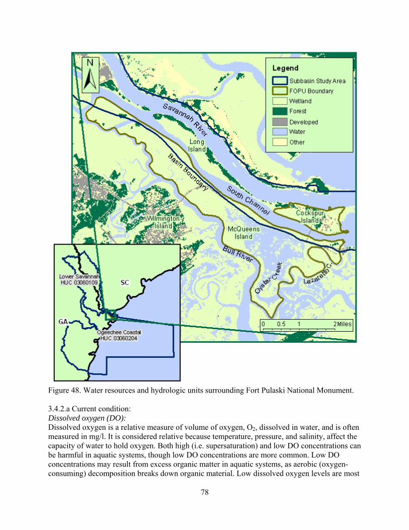
Figure 48. Water resources and hydrologic units surrounding Fort Pulaski National Monument. 3.4.2.a Current condition: Dissolved oxygen (DO): Dissolved oxygen is a relative measure of volume of oxygen, O2, dissolved in water, and is often measured in mg/l. It is considered relative because temperature, pressure, and salinity, affect the capacity of water to hold oxygen. Both high (i.e. supersaturation) and low DO concentrations can be harmful in aquatic systems, though low DO concentrations are more common. Low DO concentrations may result from excess organic matter in aquatic systems, as aerobic (oxygen-consuming) decomposition breaks down organic material. Low dissolved oxygen levels are most

78

prevalent during the warm summer months when water temperatures rise and mixing of the water column is reduced. McFarlin and Albers (2007) analyzed DO measurements taken from two distinct monitoring programs: the GA CRD Shellfish Monitoring Program and the NCA program (collected by GA CRD). In surface samples collected at four locations near Fort Pulaski NM as part of the Shellfish program, DO concentrations ranged from 2.7 to 10.7 mg/l and averaged 5.8 +-1.7 mg/l. These measurements were taken midday—and thus do not represent daily minimums—between March 2000 and April 2004. Thirty-one of 196 observations (16%) were below the GA EPD Recreational Water Quality Standard of 4 mg/l. Distinct seasonal variation occurred in DO concentrations with summertime minima and wintertime maxima; all observations of low DO occurred between May and October. Data collected by GA CRD for the NCA program sampled the entire water column during August or September, when DO minima often occur, during 2000, 2002, and 2003. McFarlin and Albers (2007) analyzed these data and determined that DO concentrations ranged from 3.32 to 5.23 mg/l and averaged 4.38 +- 0.57; samples collected near bottom averaged 4.03 +- 0.62. McFarlin and Albers (2005) considered DO levels near Fort Pulaski NM (estuary frontage and tidal creeks), to be a potential problem based on observations of low levels in the tidal creeks and the fact that all 21 samples below 2 meters within the Savannah harbor were less than the GA EPD Recreational Water Quality Standard of 4 mg/l. Georgia water quality standards are presented in Table 30. Dissolved oxygen elsewhere in the estuary was considered an existing problem, primarily based upon observations in the Savannah Harbor. The low DO concentrations observed were likely due to discharges of organic matter and/or nutrients associated with upstream industrial activity (McFarlin and Albers, 2007). Because algae blooms have occurred in the freshwater moat that surrounds the fort and two small ponds, DO was classified as a potential problem in these areas.

79

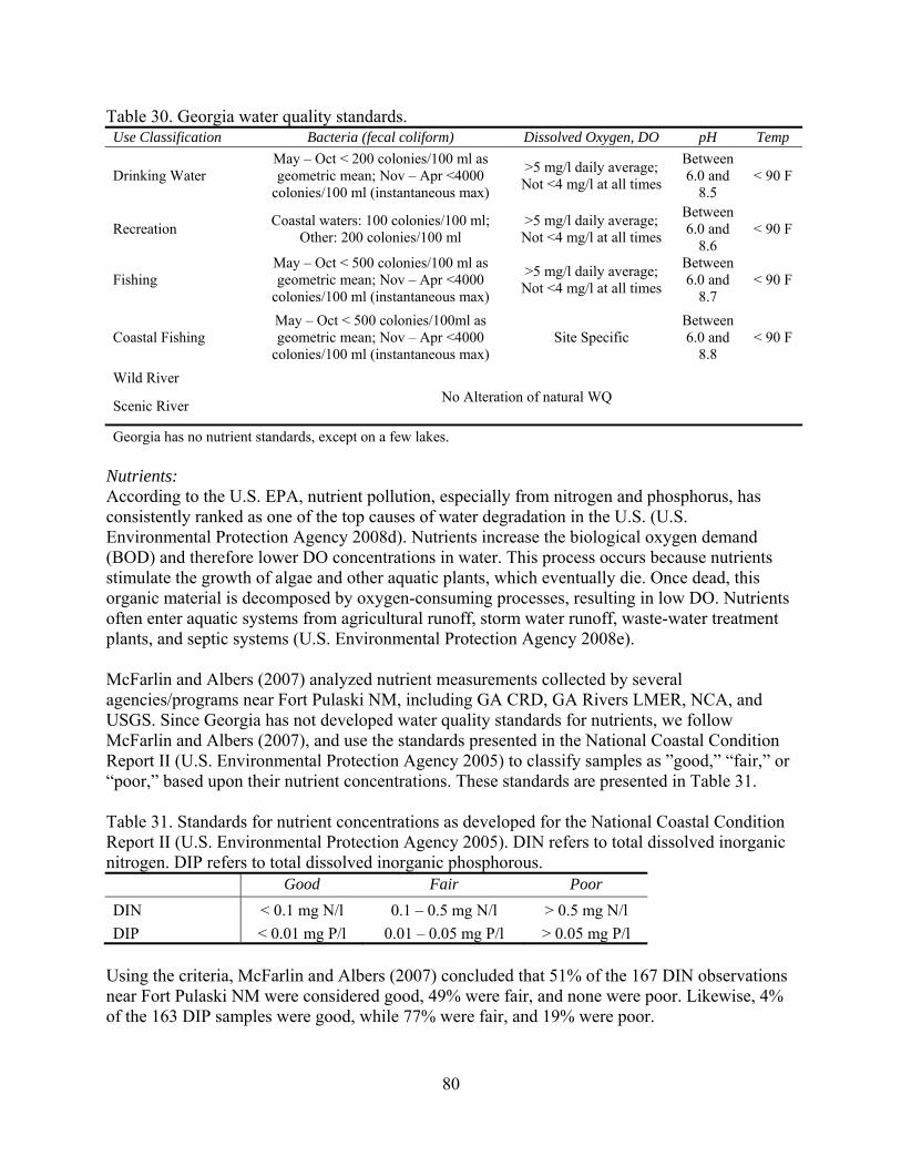
Table 30. Georgia water quality standards. Use Classification Bacteria (fecal coliform) Dissolved Oxygen, DO pH Temp

Drinking Water May – Oct < 200 colonies/100 ml as geometric mean; Nov – Apr <4000

colonies/100 ml (instantaneous max)

>5 mg/l daily average; Not <4 mg/l at all times

Between 6.0 and

8.5 < 90 F

Recreation Coastal waters: 100 colonies/100 ml; Other: 200 colonies/100 ml


Between 6.0 and

8.6 < 90 F

Fishing May – Oct < 500 colonies/100 ml as geometric mean; Nov – Apr <4000

colonies/100 ml (instantaneous max)


Between 6.0 and

8.7 < 90 F

Coastal Fishing May – Oct < 500 colonies/100ml as geometric mean; Nov – Apr <4000

colonies/100 ml (instantaneous max) Site Specific

Between 6.0 and

8.8 < 90 F

Wild River No Alteration of natural WQ Scenic River

Georgia has no nutrient standards, except on a few lakes. Nutrients: According to the U.S. EPA, nutrient pollution, especially from nitrogen and phosphorus, has consistently ranked as one of the top causes of water degradation in the U.S. (U.S. Environmental Protection Agency 2008d). Nutrients increase the biological oxygen demand (BOD) and therefore lower DO concentrations in water. This process occurs because nutrients stimulate the growth of algae and other aquatic plants, which eventually die. Once dead, this organic material is decomposed by oxygen-consuming processes, resulting in low DO. Nutrients often enter aquatic systems from agricultural runoff, storm water runoff, waste-water treatment plants, and septic systems (U.S. Environmental Protection Agency 2008e). McFarlin and Albers (2007) analyzed nutrient measurements collected by several agencies/programs near Fort Pulaski NM, including GA CRD, GA Rivers LMER, NCA, and USGS. Since Georgia has not developed water quality standards for nutrients, we follow McFarlin and Albers (2007), and use the standards presented in the National Coastal Condition Report II (U.S. Environmental Protection Agency 2005) to classify samples as ”good,” “fair,” or “poor,” based upon their nutrient concentrations. These standards are presented in Table 31. Table 31. Standards for nutrient concentrations as developed for the National Coastal Condition Report II (U.S. Environmental Protection Agency 2005). DIN refers to total dissolved inorganic nitrogen. DIP refers to total dissolved inorganic phosphorous.

Good Fair Poor DIN < 0.1 mg N/l 0.1 – 0.5 mg N/l > 0.5 mg N/l DIP < 0.01 mg P/l 0.01 – 0.05 mg P/l > 0.05 mg P/l

Using the criteria, McFarlin and Albers (2007) concluded that 51% of the 167 DIN observations near Fort Pulaski NM were considered good, 49% were fair, and none were poor. Likewise, 4% of the 163 DIP samples were good, while 77% were fair, and 19% were poor.

80

Based upon their analysis, McFarlin and Albers (2007) suggest that nutrient concentrations near Fort Pulaski NM (FOPU estuary frontage and FOPU tidal creeks) are an existing problem. Because algae blooms have occurred in the freshwater moat that surrounds the fort and two small ponds, nutrients are classified as a potential problem in these areas. Bacterial contamination (fecal coliform): Fecal coliform bacteria contamination is the most common form of bacterial contamination in many water bodies. Its presence in aquatic environments is a human health hazard and may indicate the presence of other dangerous pathogens as well. Fecal coliform bacteria often enter waterways through the direct discharge of untreated (or insufficiently treated) human waste and agricultural and municipal runoff. As reported by McFarlin and Albers (2007), fecal coliform measurements taken from 1991 to 2004 at four CRD shellfish stations near Fort Pulaski NM on Oyster Creek were generally low. In an analysis of data obtained at these stations, they found that only 9 of 584 monthly samples collected were above the GA criterion for recreational coastal water (100 CFU/100ml). More recent measurements, from 2002 to 2006, seem to indicate an improving trend; these samples measured less than 5 CFU/100 ml. Data collected upstream of the monument in the lower Savannah River basin revealed that 64% of samples (769 of 2,245 observations) exceeded EPA standards for bathing water (McFarlin and Albers, 2005). There is insufficient data to assess the condition of the freshwater moat and ponds at Fort Pulaski NM with respect to bacterial contamination. Based on these findings, bacterial contamination does not seem to be a problem in the Savannah Estuary near Fort Pulaski NM. There is, however, an existing bacterial contamination problem elsewhere within the watershed. Contaminants: Contaminants are substances such as metals, polycyclic aromatic hydrocarbons (PAHs), polychlorinated biphenyls (PCBs), and pesticides. These substances enter waterways through storm water runoff, industrial discharges, agricultural runoff, sewage treatment and atmospheric deposition. Once present in aquatic systems, they may concentrate in sediment and bottom-dwelling organisms. Many of these substances pose a risk to human health and aquatic systems. McFarlin and Albers (2007) reviewed contaminant data (GPA 1998) as part of their water resources and watershed assessment for Fort Pulaski NM. They concluded that contaminants near Fort Pulaski NM are a persistent problem. Water above and below the monument exceeded GA Water Quality Standards for copper (>2.9 mg/L) and nickel (>8.3 mg/L), and elevated levels of ammonia (max. 34,000 μg/L), manganese (max. 2,130 mg/L) and arsenic (~6.6 μg/L) were found. The concentrations reported for ammonia and manganese have been shown to cause toxic effects in marine organisms.

81

Other studies identified elevated contaminant levels near Fort Pulaski NM as well. As reported by McFarlin and Albers (2007), the EMAP and NCA programs collectively identified 47 contaminants in shrimp tissue. While none of these were above FDA guidelines, arsenic and PAHs were elevated under EPA Risk Guidelines. Loganathan et al. (2001) reported PCBs in fish tissue and DDT (2.11 ppb) in North Channel sediments above ERL values. Elevated concentrations of arsenic and PAH’s in oyster tissue was observed by Richardson and Sajwan (2001, 2002). Given these data, contaminants in the water near Fort Pulaski NM (estuary frontage and tidal creeks) are an existing problem. McFarlin and Albers (2005) concluded that toxic contaminants are a potential problem elsewhere in the estuary due to elevated concentrations of cadmium, copper, chromium, and arsenic in harbor sediments. The EPA's compilation of national recommended water quality criteria that includes contaminants is available at http://www.epa.gov/waterscience/criteria/wqctable. 3.4.2.b Resource threats and stressors: Threats and stressors to the water resources near Fort Pulaski NM are numerous. Water quality at Fort Pulaski NM is largely influenced by external factors, including point and nonpoint sources that originate beyond the monument boundaries. Point-source pollution originates from a single point or location, such as wastewater treatment plants and industrial outflows. Within the Savannah River watershed, there are numerous point sources of pollutants. For a current list of EPA approved discharge sites visit the EPA’s Envirofacts Warehouse, http://www.epa.gov/enviro/index.html. Nonpoint-source pollution is any contaminant that that does not originate from a point source. In the Savannah River watershed nonpoint sources include urban (i.e. storm water runoff) and agricultural runoff. Runoff often contains the same pollutants as point source discharges. However, since nonpoint sources of pollution do not come from any specific location, they are typically harder to control and pose more complex management challenges. As reported in the hydrology section of this report (3.4.1.b Resource threats and stressors:), the Savannah Harbor expansion project is underway. There are numerous potential environmental consequences to this project (http://sav-harbor.com/). An existing dredge disposal site is located near the monument. This site is known to contain arsenic and other heavy metals (Winger et al. 2000). Several industrial facilities upstream of Fort Pulaski NM are known to release contaminants into the groundwater or air (Figure 49). The Georgia Department of Natural Resources provides an inventory of hazardous sites within the state. Sites can be identified by name or location. This resource is available at http://www.gaepd.org/Documents/hazsiteinv.htmlhttp://www.gaepd.org/Documents/hazsiteinv.html.

82

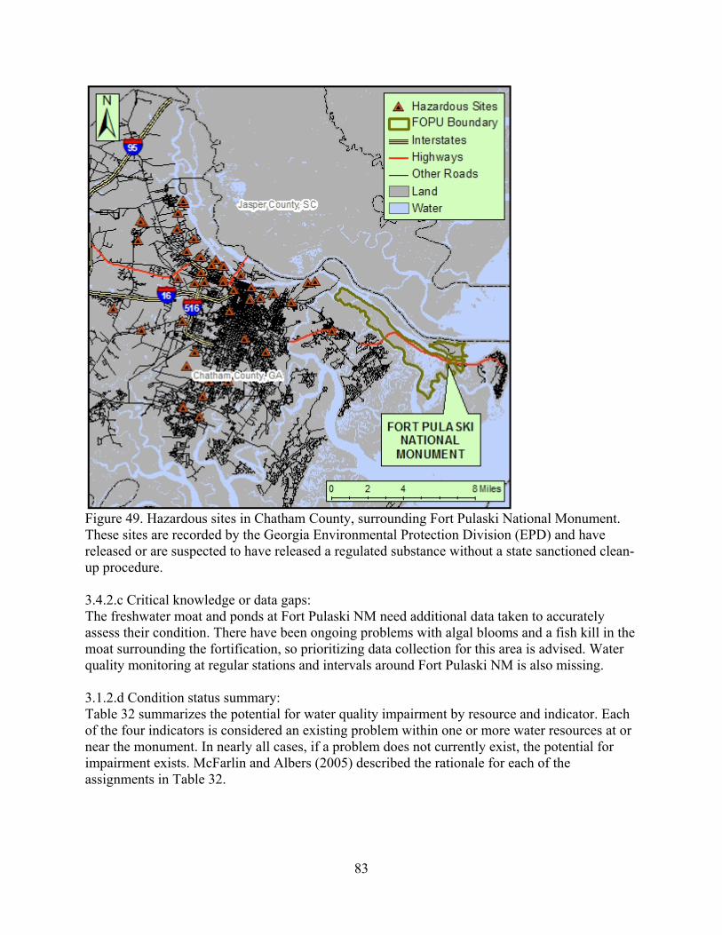
http://www.gaepd.org/Documents/hazsiteinv.html

Figure 49. Hazardous sites in Chatham County, surrounding Fort Pulaski National Monument. These sites are recorded by the Georgia Environmental Protection Division (EPD) and have released or are suspected to have released a regulated substance without a state sanctioned clean-up procedure. 3.4.2.c Critical knowledge or data gaps: The freshwater moat and ponds at Fort Pulaski NM need additional data taken to accurately assess their condition. There have been ongoing problems with algal blooms and a fish kill in the moat surrounding the fortification, so prioritizing data collection for this area is advised. Water quality monitoring at regular stations and intervals around Fort Pulaski NM is also missing. 3.1.2.d Condition status summary: Table 32 summarizes the potential for water quality impairment by resource and indicator. Each of the four indicators is considered an existing problem within one or more water resources at or near the monument. In nearly all cases, if a problem does not currently exist, the potential for impairment exists. McFarlin and Albers (2005) described the rationale for each of the assignments in Table 32.

83

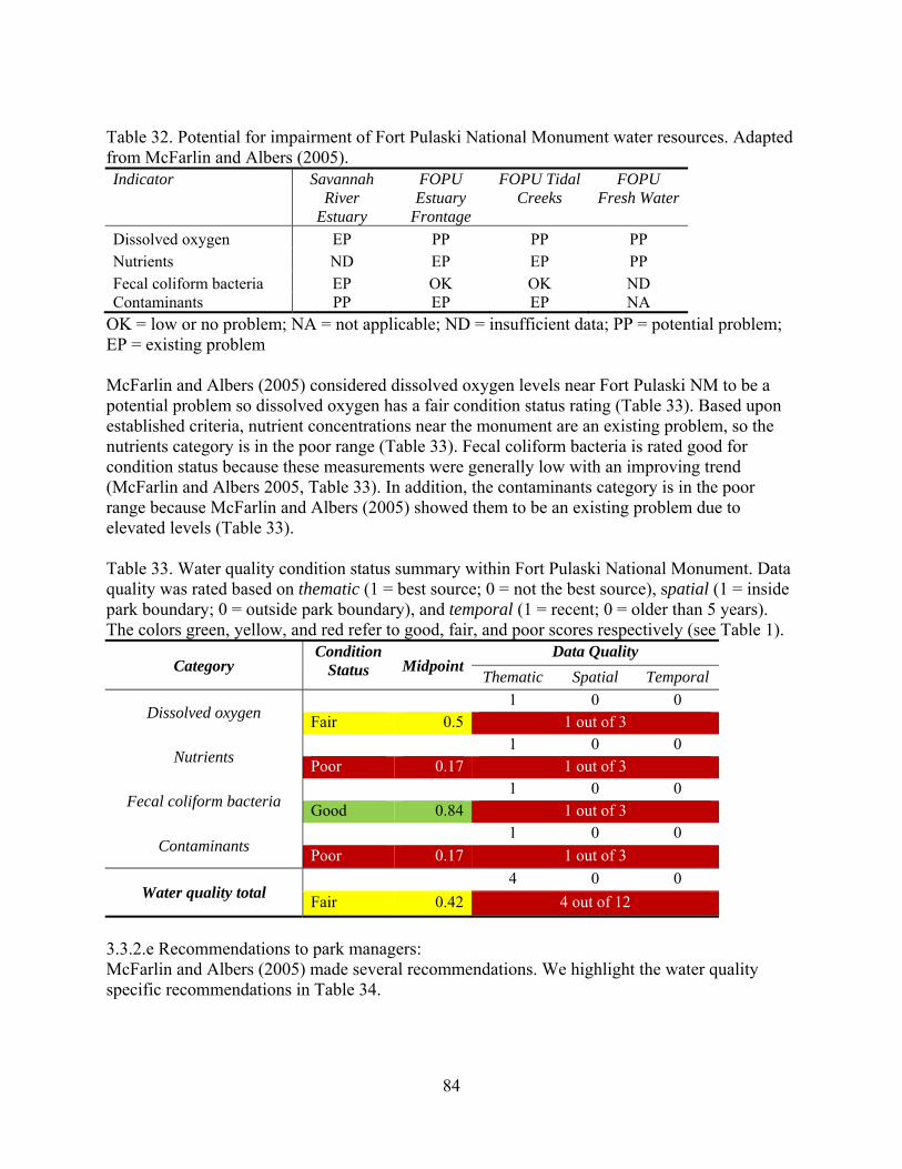
Table 32. Potential for impairment of Fort Pulaski National Monument water resources. Adapted from McFarlin and Albers (2005). Indicator Savannah

River Estuary

FOPU Estuary

Frontage

FOPU Tidal Creeks

FOPU Fresh Water

Dissolved oxygen EP PP PP PP Nutrients ND EP EP PP Fecal coliform bacteria EP OK OK ND Contaminants PP EP EP NA

OK = low or no problem; NA = not applicable; ND = insufficient data; PP = potential problem; EP = existing problem McFarlin and Albers (2005) considered dissolved oxygen levels near Fort Pulaski NM to be a potential problem so dissolved oxygen has a fair condition status rating (Table 33). Based upon established criteria, nutrient concentrations near the monument are an existing problem, so the nutrients category is in the poor range (Table 33). Fecal coliform bacteria is rated good for condition status because these measurements were generally low with an improving trend (McFarlin and Albers 2005, Table 33). In addition, the contaminants category is in the poor range because McFarlin and Albers (2005) showed them to be an existing problem due to elevated levels (Table 33). Table 33. Water quality condition status summary within Fort Pulaski National Monument. Data quality was rated based on thematic (1 = best source; 0 = not the best source), spatial (1 = inside park boundary; 0 = outside park boundary), and temporal (1 = recent; 0 = older than 5 years). The colors green, yellow, and red refer to good, fair, and poor scores respectively (see Table 1).

Category Condition



Dissolved oxygen 1 0 0 Fair 0.5 1 out of 3

Nutrients 1 0 0 Poor 0.17 1 out of 3

Fecal coliform bacteria 1 0 0 Good 0.84 1 out of 3

Contaminants 1 0 0 Poor 0.17 1 out of 3

Water quality total 4 0 0 Fair 0.42 4 out of 12

3.3.2.e Recommendations to park managers: McFarlin and Albers (2005) made several recommendations. We highlight the water quality specific recommendations in Table 34.

84

Table 34. Recommendations to improve water quality and monitoring at Fort Pulaski National Monument from McFarlin and Albers (2005). 1. Work towards improved regional cooperation 2. Initiate regular water quality monitoring at Fort Pulaski NM 3. Collect additional water quality information 4. Set up targeted monitoring for Harbor expansion and other modifications 5. Improve access to state and federal water quality data and improved metadata

3.5 Geology and Soils 3.5.1 Geology and Soils As outlined in the park and resources section of this report, the Coastal Plain region is composed of un-deformed sedimentary rock layers whose ages range from the Late Cretaceous to the present Holocene sediments of the coast. Sediment from the upper Piedmont region eroded into the Coastal Plain over the past 100 million years. Beneath Coastal Plain sediments are harder igneous and metamorphic rocks, such as those found in the Piedmont. Usually referred to as the "basement rocks," these hard rocks occur at greater and greater depths toward the south and east, reaching depths of up to 10,000 feet or more beneath the modern Georgia coast (Frazier 2007). In addition to recent alluvium, organic and marine deposits make up most of the sediment found in the Coastal Plain (UGA Department of Geology 2008). Specifically, the coastal region near Fort Pulaski is a Holocene-aged deposit of organic, marine, and alluvial origin with some human-dredged sediment deposited along the Savannah River and coastline. 3.5.1.a Current condition: We compared a 1911 soil survey (Table 35, Figure 50) to the current soil data from the Soil Survey Geographic Data Base (SSURGO, Table 36, Figure 51) to see if changes had occurred (USDA Natural Resource Conservation Service 2006). Current SSURGO data were compiled by the National Park Service. These soil data have a version date of December 21, 2006 and are available in GIS and database format (National Park Service 2006). The 1911 soil survey by the U.S. Department of Agriculture was obtained from an on-line collection at University of Alabama (USDA Bureau of Soils 1911). The 1911 soil data were aligned to digital raster graphics (DRG, 1:24,000 topographic maps), using the georeferencing tools in ArcGIS (ESRI 2006). We surveyed four DRG, 1:24,000 topographic maps that made up Fort Pulaski NM or were in close proximity to the boundary. These were all published in 1978 and included Fort Pulaski, Savannah, Tybee Island N, and Wassaw Sound. Published data was also used along with photo interpretation to assess both current soil resources and changes. The “Georgetown clay” making up about 10% of the area in the 1911 survey is an upland soil type from Central Texas that forms over limestone. The soil survey program was near its inception in 1911 and the Georgetown series as now identified does not occur on Cockspur Island. There is no limestone in the entire region (Frazier 2007). If there was a clay surface-textured soil found in the area that was not tidally influenced, it was probably a Savannah River terrace deposit or a recent marine terrace remnant, since the adjacent Intracoastal Waterway seen in the 2006 soil survey does not appear in the 1911 survey (Figure 50 and Figure 51). The absence of the nontidal upland area near the Intracoastal Waterway in the 2006 survey may be due to slow (about 12 inches per century) sea-level rise and expansion of the tidal marsh (Frazier

85

2007), or just archaic or inaccurate mapping in 1911. The Transquaking soil type identified on about 90% of the area in the 1911 survey is an organic soil from the upper East Coast in Maryland and is also not representative of the soils in the area. The Bohicket soil used and associated capers soils in the 2006 soil survey provide a better description of the soil resources. Bohicket and Capers do not have thick organic sediment at the surface. Overall, the difference in soils between 1911 and 2006 reflect updated versions of the soil series concepts and soil survey accuracy, along with additions of dredged spoils and some human alteration of soils through landscaping and development of roads and buildings. The Intracoastal Waterway cut-through was added on the northwestern end of McQueens Island after 1911 (Figure 50 and Figure 51), and is probably the source of the dredged material that now makes up the adjacent tree and shrub-covered areas. Figure 52, from Google Maps (2008), provides a close-up view. The close-up shows possible shoreline erosion along the Waterway caused by wakes of passing ships through the narrow channel. It also appears that Long Island and Cockspur Island were already joined in 1911 (Figure 50).

86

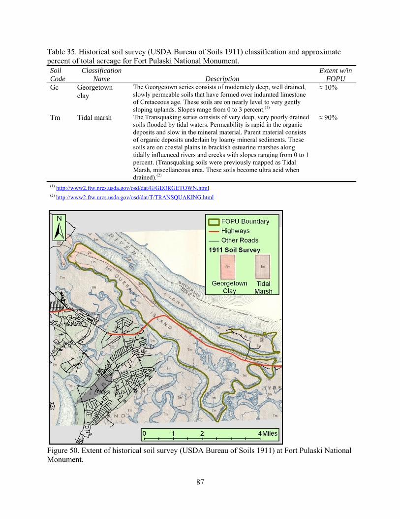
Table 35. Historical soil survey (USDA Bureau of Soils 1911) classification and approximate percent of total acreage for Fort Pulaski National Monument. Soil Code

Classification Name Description

Extent w/in FOPU

Gc Georgetown clay

The Georgetown series consists of moderately deep, well drained, slowly permeable soils that have formed over indurated limestone of Cretaceous age. These soils are on nearly level to very gently sloping uplands. Slopes range from 0 to 3 percent.(1)

≈ 10%

Tm Tidal marsh The Transquaking series consists of very deep, very poorly drained soils flooded by tidal waters. Permeability is rapid in the organic deposits and slow in the mineral material. Parent material consists of organic deposits underlain by loamy mineral sediments. These soils are on coastal plains in brackish estuarine marshes along tidally influenced rivers and creeks with slopes ranging from 0 to 1 percent. (Transquaking soils were previously mapped as Tidal Marsh, miscellaneous area. These soils become ultra acid when drained).(2)

≈ 90%

(1) http://www2.ftw.nrcs.usda.gov/osd/dat/G/GEORGETOWN.html (2) http://www2.ftw.nrcs.usda.gov/osd/dat/T/TRANSQUAKING.html

Figure 50. Extent of historical soil survey (USDA Bureau of Soils 1911) at Fort Pulaski National Monument.

87

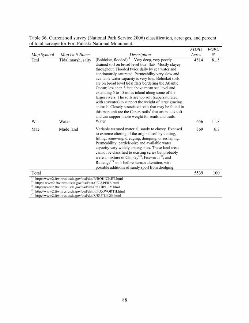
http://www2.ftw.nrcs.usda.gov/osd/dat/G/GEORGETOWN.html

http://www2.ftw.nrcs.usda.gov/osd/dat/T/TRANSQUAKING.html

Table 36. Current soil survey (National Park Service 2006) classification, acreages, and percent of total acreage for Fort Pulaski National Monument.

Map Symbol Map Unit Name Description FOPU Acres

FOPU %

Tml Tidal marsh, salty (Bohicket, flooded) 3 – Very deep, very poorly drained soil on broad level tidal flats. Mostly clayey throughout. Flooded twice daily by sea water and continuously saturated. Permeability very slow and available water capacity is very low. Bohicket soils are on broad level tidal flats bordering the Atlantic Ocean; less than 3 feet above mean sea level and extending 5 to 15 miles inland along some of the larger rivers. The soils are too soft (supersaturated with seawater) to support the weight of large grazing animals. Closely associated soils that may be found in this map unit are the Capers soils4 that are not as soft and can support more weight for roads and trails.

4514 81.5

W Water Water 656 11.8

Mae Made land Variable textured material, sandy to clayey. Exposed to extreme altering of the original soil by cutting, filling, removing, dredging, dumping, or reshaping. Permeability, particle-size and available water capacity vary widely among sites. These land areas cannot be classified to existing series but probably were a mixture of Chipley(5), Foxworth(6), and Rutledge(7) soils before human alteration, with possible additions of sandy spoil from dredging.

369 6.7

Total 5539 100(3) http://www2.ftw.nrcs.usda.gov/osd/dat/B/BOHICKET.html (4) http:// www2.ftw.nrcs.usda.gov/osd/dat/C/CAPERS.html (5) http://www2.ftw.nrcs.usda.gov/osd/dat/C/CHIPLEY.html (5) http://www2.ftw.nrcs.usda.gov/osd/dat/F/FOXWORTH.html (7) http://www2.ftw.nrcs.usda.gov/osd/dat/R/RUTLEGE.html

88

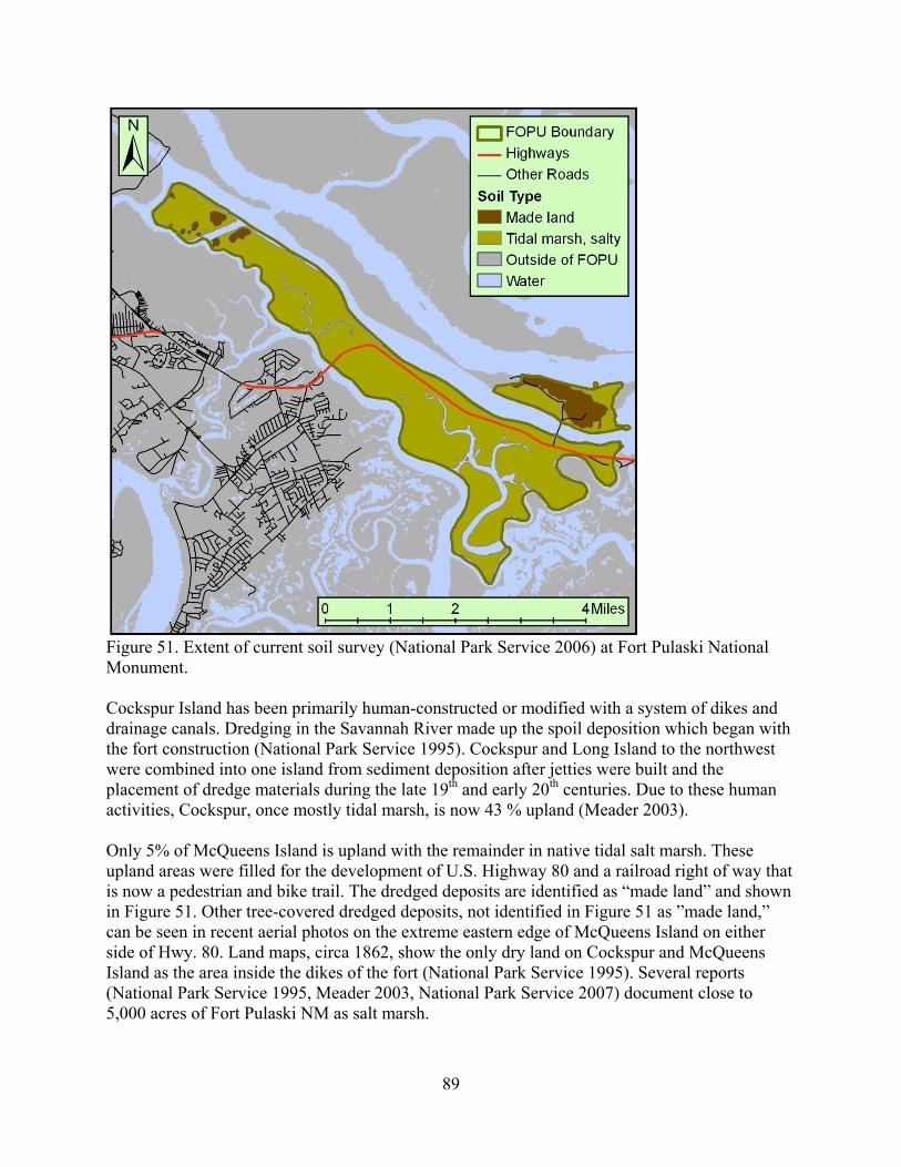
Figure 51. Extent of current soil survey (National Park Service 2006) at Fort Pulaski National Monument. Cockspur Island has been primarily human-constructed or modified with a system of dikes and drainage canals. Dredging in the Savannah River made up the spoil deposition which began with the fort construction (National Park Service 1995). Cockspur and Long Island to the northwest were combined into one island from sediment deposition after jetties were built and the placement of dredge materials during the late 19th and early 20th centuries. Due to these human activities, Cockspur, once mostly tidal marsh, is now 43 % upland (Meader 2003). Only 5% of McQueens Island is upland with the remainder in native tidal salt marsh. These upland areas were filled for the development of U.S. Highway 80 and a railroad right of way that is now a pedestrian and bike trail. The dredged deposits are identified as “made land” and shown in Figure 51. Other tree-covered dredged deposits, not identified in Figure 51 as ”made land,” can be seen in recent aerial photos on the extreme eastern edge of McQueens Island on either side of Hwy. 80. Land maps, circa 1862, show the only dry land on Cockspur and McQueens Island as the area inside the dikes of the fort (National Park Service 1995). Several reports (National Park Service 1995, Meader 2003, National Park Service 2007) document close to 5,000 acres of Fort Pulaski NM as salt marsh.

89

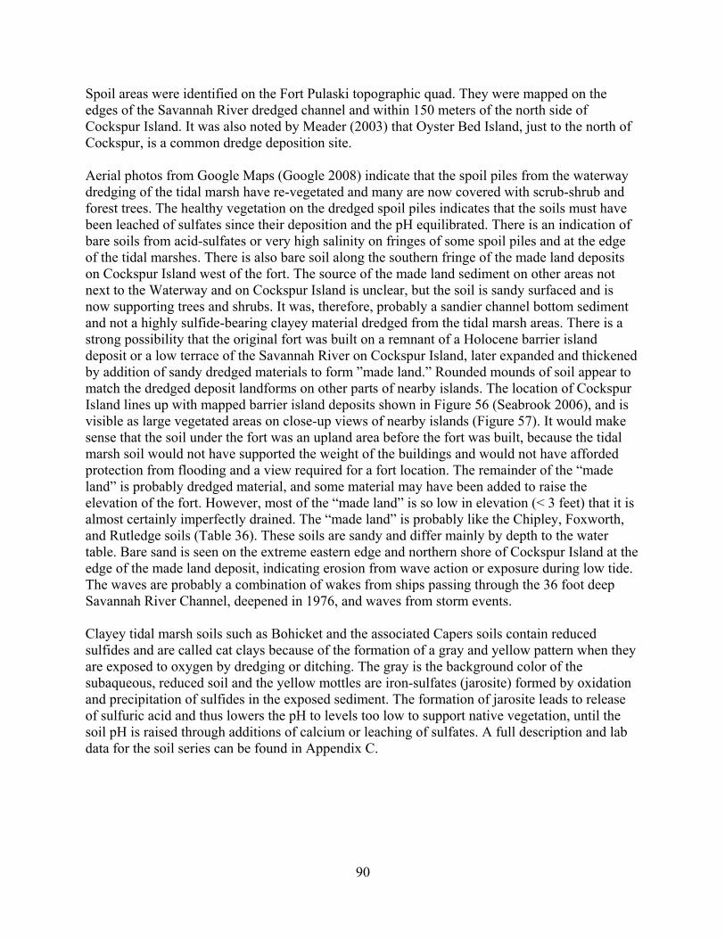
Spoil areas were identified on the Fort Pulaski topographic quad. They were mapped on the edges of the Savannah River dredged channel and within 150 meters of the north side of Cockspur Island. It was also noted by Meader (2003) that Oyster Bed Island, just to the north of Cockspur, is a common dredge deposition site. Aerial photos from Google Maps (Google 2008) indicate that the spoil piles from the waterway dredging of the tidal marsh have re-vegetated and many are now covered with scrub-shrub and forest trees. The healthy vegetation on the dredged spoil piles indicates that the soils must have been leached of sulfates since their deposition and the pH equilibrated. There is an indication of bare soils from acid-sulfates or very high salinity on fringes of some spoil piles and at the edge of the tidal marshes. There is also bare soil along the southern fringe of the made land deposits on Cockspur Island west of the fort. The source of the made land sediment on other areas not next to the Waterway and on Cockspur Island is unclear, but the soil is sandy surfaced and is now supporting trees and shrubs. It was, therefore, probably a sandier channel bottom sediment and not a highly sulfide-bearing clayey material dredged from the tidal marsh areas. There is a strong possibility that the original fort was built on a remnant of a Holocene barrier island deposit or a low terrace of the Savannah River on Cockspur Island, later expanded and thickened by addition of sandy dredged materials to form ”made land.” Rounded mounds of soil appear to match the dredged deposit landforms on other parts of nearby islands. The location of Cockspur Island lines up with mapped barrier island deposits shown in Figure 56 (Seabrook 2006), and is visible as large vegetated areas on close-up views of nearby islands (Figure 57). It would make sense that the soil under the fort was an upland area before the fort was built, because the tidal marsh soil would not have supported the weight of the buildings and would not have afforded protection from flooding and a view required for a fort location. The remainder of the “made land” is probably dredged material, and some material may have been added to raise the elevation of the fort. However, most of the “made land” is so low in elevation (< 3 feet) that it is almost certainly imperfectly drained. The “made land” is probably like the Chipley, Foxworth, and Rutledge soils (Table 36). These soils are sandy and differ mainly by depth to the water table. Bare sand is seen on the extreme eastern edge and northern shore of Cockspur Island at the edge of the made land deposit, indicating erosion from wave action or exposure during low tide. The waves are probably a combination of wakes from ships passing through the 36 foot deep Savannah River Channel, deepened in 1976, and waves from storm events. Clayey tidal marsh soils such as Bohicket and the associated Capers soils contain reduced sulfides and are called cat clays because of the formation of a gray and yellow pattern when they are exposed to oxygen by dredging or ditching. The gray is the background color of the subaqueous, reduced soil and the yellow mottles are iron-sulfates (jarosite) formed by oxidation and precipitation of sulfides in the exposed sediment. The formation of jarosite leads to release of sulfuric acid and thus lowers the pH to levels too low to support native vegetation, until the soil pH is raised through additions of calcium or leaching of sulfates. A full description and lab data for the soil series can be found in Appendix C.

90

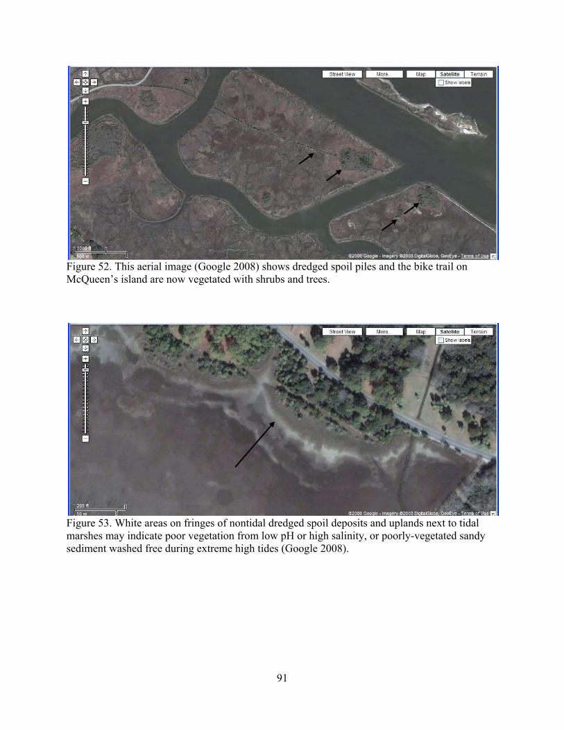
Figure 52. This aerial image (Google 2008) shows dredged spoil piles and the bike trail on McQueen’s island are now vegetated with shrubs and trees.

Figure 53. White areas on fringes of nontidal dredged spoil deposits and uplands next to tidal marshes may indicate poor vegetation from low pH or high salinity, or poorly-vegetated sandy sediment washed free during extreme high tides (Google 2008).

91

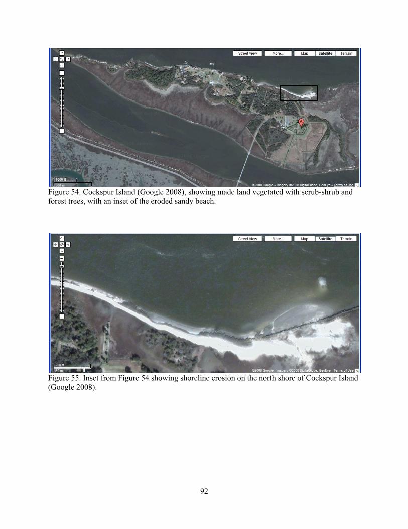
Figure 54. Cockspur Island (Google 2008), showing made land vegetated with scrub-shrub and forest trees, with an inset of the eroded sandy beach.

Figure 55. Inset from Figure 54 showing shoreline erosion on the north shore of Cockspur Island (Google 2008).

92

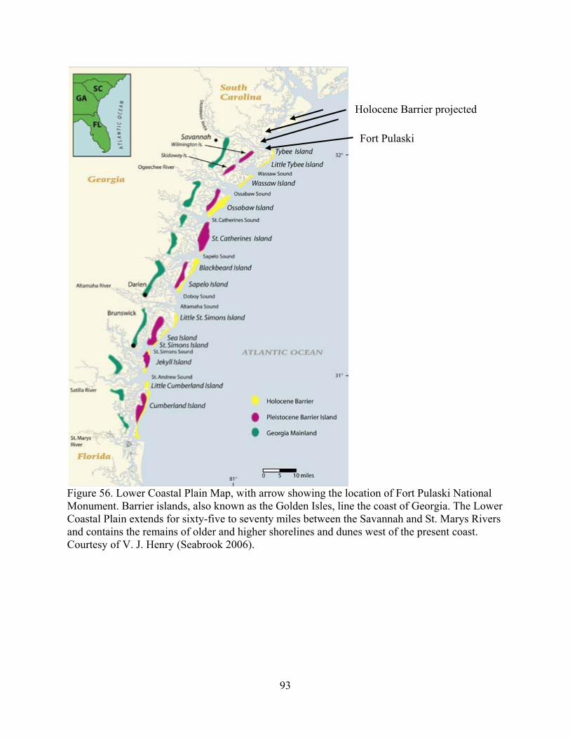
Figure 56. Lower Coastal Plain Map, with arrow showing the location of Fort Pulaski National Monument. Barrier islands, also known as the Golden Isles, line the coast of Georgia. The Lower Coastal Plain extends for sixty-five to seventy miles between the Savannah and St. Marys Rivers and contains the remains of older and higher shorelines and dunes west of the present coast. Courtesy of V. J. Henry (Seabrook 2006).

Holocene Barrier projected

Fort Pulaski

93

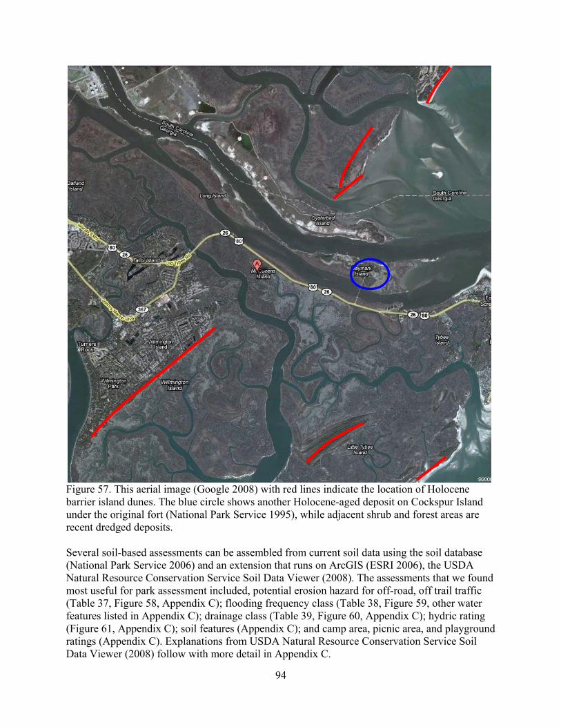
Figure 57. This aerial image (Google 2008) with red lines indicate the location of Holocene barrier island dunes. The blue circle shows another Holocene-aged deposit on Cockspur Island under the original fort (National Park Service 1995), while adjacent shrub and forest areas are recent dredged deposits. Several soil-based assessments can be assembled from current soil data using the soil database (National Park Service 2006) and an extension that runs on ArcGIS (ESRI 2006), the USDA Natural Resource Conservation Service Soil Data Viewer (2008). The assessments that we found most useful for park assessment included, potential erosion hazard for off-road, off trail traffic (Table 37, Figure 58, Appendix C); flooding frequency class (Table 38, Figure 59, other water features listed in Appendix C); drainage class (Table 39, Figure 60, Appendix C); hydric rating (Figure 61, Appendix C); soil features (Appendix C); and camp area, picnic area, and playground ratings (Appendix C). Explanations from USDA Natural Resource Conservation Service Soil Data Viewer (2008) follow with more detail in Appendix C.

94

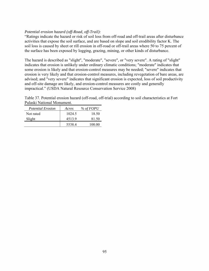
Potential erosion hazard (off-Road, off-Trail): “Ratings indicate the hazard or risk of soil loss from off-road and off-trail areas after disturbance activities that expose the soil surface, and are based on slope and soil erodibility factor K. The soil loss is caused by sheet or rill erosion in off-road or off-trail areas where 50 to 75 percent of the surface has been exposed by logging, grazing, mining, or other kinds of disturbance. The hazard is described as "slight", "moderate", "severe", or "very severe". A rating of "slight" indicates that erosion is unlikely under ordinary climatic conditions; "moderate" indicates that some erosion is likely and that erosion-control measures may be needed; "severe" indicates that erosion is very likely and that erosion-control measures, including revegetation of bare areas, are advised; and "very severe" indicates that significant erosion is expected, loss of soil productivity and off-site damage are likely, and erosion-control measures are costly and generally impractical.” (USDA Natural Resource Conservation Service 2008) Table 37. Potential erosion hazard (off-road, off-trial) according to soil characteristics at Fort Pulaski National Monument.

Potential Erosion Acres % of FOPU Not rated 1024.5 18.50Slight 4513.9 81.50 5538.4 100.00

95

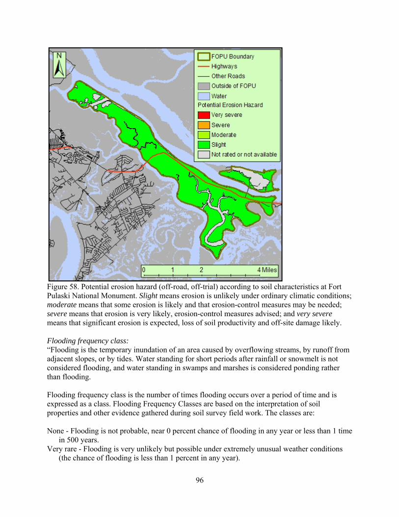
Figure 58. Potential erosion hazard (off-road, off-trial) according to soil characteristics at Fort Pulaski National Monument. Slight means erosion is unlikely under ordinary climatic conditions; moderate means that some erosion is likely and that erosion-control measures may be needed; severe means that erosion is very likely, erosion-control measures advised; and very severe means that significant erosion is expected, loss of soil productivity and off-site damage likely. Flooding frequency class: “Flooding is the temporary inundation of an area caused by overflowing streams, by runoff from adjacent slopes, or by tides. Water standing for short periods after rainfall or snowmelt is not considered flooding, and water standing in swamps and marshes is considered ponding rather than flooding. Flooding frequency class is the number of times flooding occurs over a period of time and is expressed as a class. Flooding Frequency Classes are based on the interpretation of soil properties and other evidence gathered during soil survey field work. The classes are: None - Flooding is not probable, near 0 percent chance of flooding in any year or less than 1 time

in 500 years. Very rare - Flooding is very unlikely but possible under extremely unusual weather conditions

(the chance of flooding is less than 1 percent in any year).

96

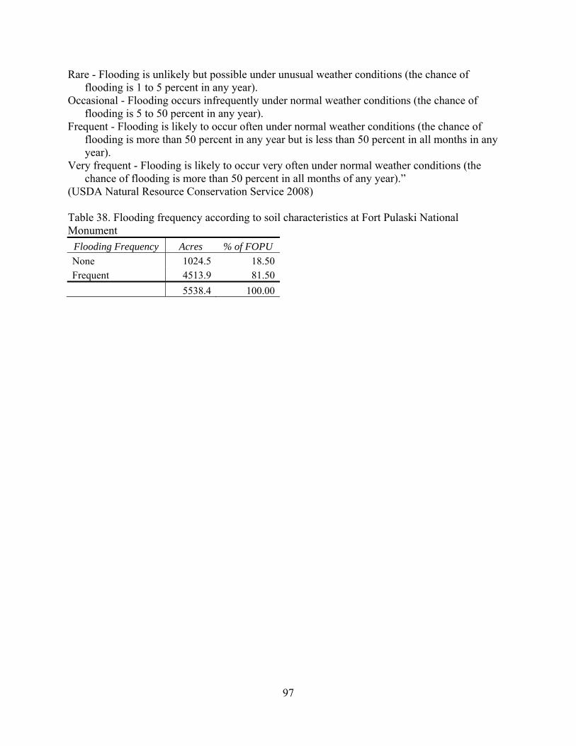
Rare - Flooding is unlikely but possible under unusual weather conditions (the chance of flooding is 1 to 5 percent in any year).

Occasional - Flooding occurs infrequently under normal weather conditions (the chance of flooding is 5 to 50 percent in any year).

Frequent - Flooding is likely to occur often under normal weather conditions (the chance of flooding is more than 50 percent in any year but is less than 50 percent in all months in any year).

Very frequent - Flooding is likely to occur very often under normal weather conditions (the chance of flooding is more than 50 percent in all months of any year).”

(USDA Natural Resource Conservation Service 2008) Table 38. Flooding frequency according to soil characteristics at Fort Pulaski National Monument

Flooding Frequency Acres % of FOPU None 1024.5 18.50Frequent 4513.9 81.50 5538.4 100.00

97

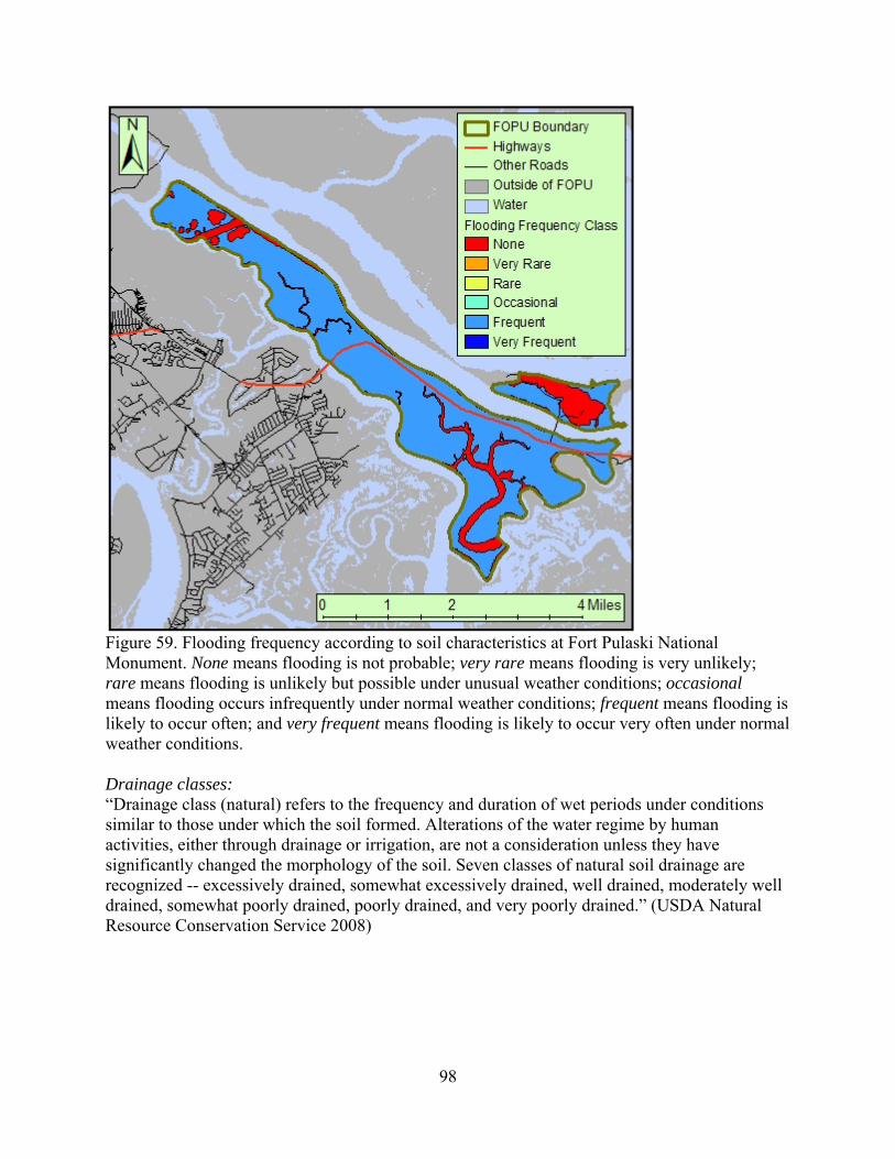
Figure 59. Flooding frequency according to soil characteristics at Fort Pulaski National Monument. None means flooding is not probable; very rare means flooding is very unlikely; rare means flooding is unlikely but possible under unusual weather conditions; occasional means flooding occurs infrequently under normal weather conditions; frequent means flooding is likely to occur often; and very frequent means flooding is likely to occur very often under normal weather conditions. Drainage classes: “Drainage class (natural) refers to the frequency and duration of wet periods under conditions similar to those under which the soil formed. Alterations of the water regime by human activities, either through drainage or irrigation, are not a consideration unless they have significantly changed the morphology of the soil. Seven classes of natural soil drainage are recognized -- excessively drained, somewhat excessively drained, well drained, moderately well drained, somewhat poorly drained, poorly drained, and very poorly drained.” (USDA Natural Resource Conservation Service 2008)

98

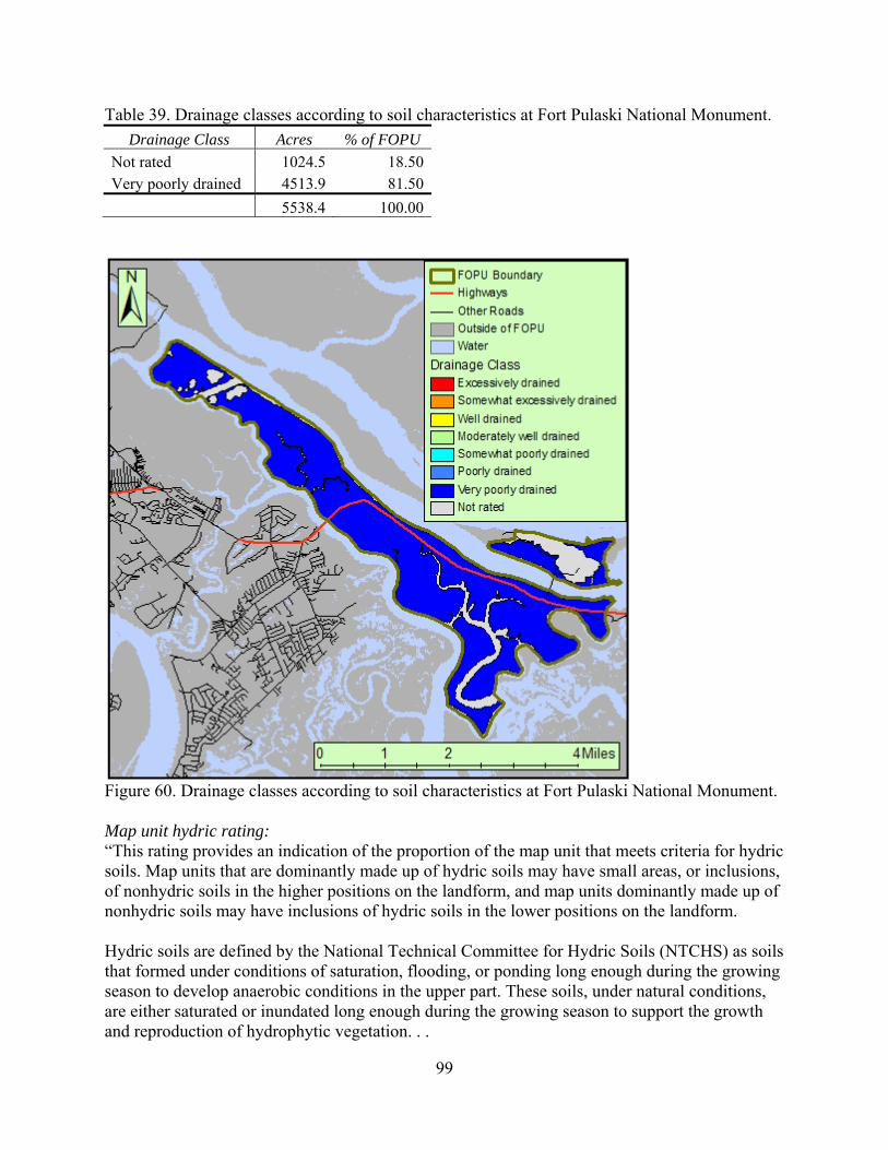
Table 39. Drainage classes according to soil characteristics at Fort Pulaski National Monument. Drainage Class Acres % of FOPU

Not rated 1024.5 18.50Very poorly drained 4513.9 81.50 5538.4 100.00

Figure 60. Drainage classes according to soil characteristics at Fort Pulaski National Monument. Map unit hydric rating: “This rating provides an indication of the proportion of the map unit that meets criteria for hydric soils. Map units that are dominantly made up of hydric soils may have small areas, or inclusions, of nonhydric soils in the higher positions on the landform, and map units dominantly made up of nonhydric soils may have inclusions of hydric soils in the lower positions on the landform. Hydric soils are defined by the National Technical Committee for Hydric Soils (NTCHS) as soils that formed under conditions of saturation, flooding, or ponding long enough during the growing season to develop anaerobic conditions in the upper part. These soils, under natural conditions, are either saturated or inundated long enough during the growing season to support the growth and reproduction of hydrophytic vegetation. . .

99

. . . If soils are wet enough for a long enough period of time to be considered hydric, they should exhibit certain properties that can be easily observed in the field. These visible properties are indicators of hydric soils. . . .” (USDA Natural Resource Conservation Service 2008)

Figure 61. Hydric rating according to soil characteristics at Fort Pulaski National Monument. 3.5.1.b Resource threats and stressors: One threat is the possible presence of acid-sulfate soils on the edges of made land deposits of dredge materials. This threat will diminish as sea level rises. Also, as sea level rises, high salinity may kill upland vegetation. In addition, erosion of shorelines may occur, especially the north shore of Cockspur Island, from rising sea levels and wakes of passing ships on the Savannah River. The threat of rising sea levels and erosion is covered in more depth in the Hydrology section (3.4.1 Hydrology). 3.5.1.c Critical knowledge or data gaps: Data quality is good in all cases (Table 40). Local-scale, specific soil analysis to Fort Pulaski NM may be appropriate to add detail to soil characteristics.

100

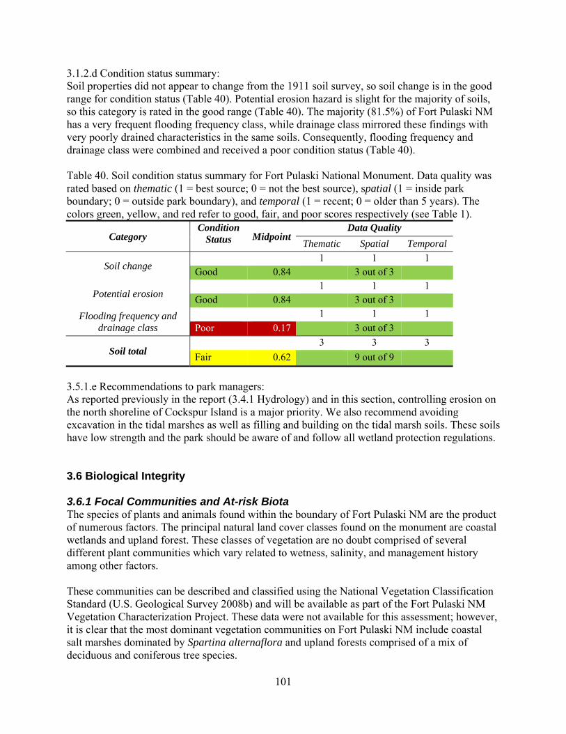
3.1.2.d Condition status summary: Soil properties did not appear to change from the 1911 soil survey, so soil change is in the good range for condition status (Table 40). Potential erosion hazard is slight for the majority of soils, so this category is rated in the good range (Table 40). The majority (81.5%) of Fort Pulaski NM has a very frequent flooding frequency class, while drainage class mirrored these findings with very poorly drained characteristics in the same soils. Consequently, flooding frequency and drainage class were combined and received a poor condition status (Table 40). Table 40. Soil condition status summary for Fort Pulaski National Monument. Data quality was rated based on thematic (1 = best source; 0 = not the best source), spatial (1 = inside park boundary; 0 = outside park boundary), and temporal (1 = recent; 0 = older than 5 years). The colors green, yellow, and red refer to good, fair, and poor scores respectively (see Table 1).

Category Condition



Soil change 1 1 1 Good 0.84 3 out of 3

Potential erosion 1 1 1 Good 0.84 3 out of 3

Flooding frequency and drainage class

1 1 1 Poor 0.17 3 out of 3

Soil total 3 3 3 Fair 0.62 9 out of 9

3.5.1.e Recommendations to park managers: As reported previously in the report (3.4.1 Hydrology) and in this section, controlling erosion on the north shoreline of Cockspur Island is a major priority. We also recommend avoiding excavation in the tidal marshes as well as filling and building on the tidal marsh soils. These soils have low strength and the park should be aware of and follow all wetland protection regulations. 3.6 Biological Integrity 3.6.1 Focal Communities and At-risk Biota The species of plants and animals found within the boundary of Fort Pulaski NM are the product of numerous factors. The principal natural land cover classes found on the monument are coastal wetlands and upland forest. These classes of vegetation are no doubt comprised of several different plant communities which vary related to wetness, salinity, and management history among other factors. These communities can be described and classified using the National Vegetation Classification Standard (U.S. Geological Survey 2008b) and will be available as part of the Fort Pulaski NM Vegetation Characterization Project. These data were not available for this assessment; however, it is clear that the most dominant vegetation communities on Fort Pulaski NM include coastal salt marshes dominated by Spartina alternaflora and upland forests comprised of a mix of deciduous and coniferous tree species.

101

The complete assemblage of species, plants and animals, at Fort Pulaski NM is a direct result of several different types of vegetation, land use, and hydrologic regimes that occur within its boundary. The two most important natural communities are the salt marsh and the maritime forest. However, the species assemblages observed on Fort Pulaski NM are certainly the product of other communities (natural or anthropogenic) around the monument. Ideally, an assessment of the biotic communities at Fort Pulaski NM would consist of the complete range of plants and animals known to occur within the monument as well as the full suite of species found on pristine tracts of similar habitat in the same landscape. The biotic assessment would be performed on the full spectrum of animals and plants from each taxonomic class. Species absences or species located that were not part of that suite of native species would represent decreases in biotic integrity from the reference scenario. Such a complete assessment is beyond the scope of this project. We can, however, use existing datasets for a few of these taxa to permit some insight as to the likely state of biotic communities at Fort Pulaski NM. There have been several investigations of animals and plants at Fort Pulaski NM over the past 35-plus years (Table 41). Table 41. List of available animal and plant surveys at Fort Pulaski National Monument. Year Community target for survey Author(s) 1970 Birds Author unknown (brochure) 1978/1979 flora and fauna Southeastern Wildlife Services, Inc. (referenced

in FOPU resource management plan) 1981 vertebrate and invertebrate fauna Southeastern Wildlife Services, Inc. (cited in

Tuberville, et al.) 1986 Birds Tucker, R. E. 1999 vertebrate animals Rabolli, C. and K. Ellington 1998 Flora Govus, Thomas, E. 2001 integrated pest management plan

(data in plan ~10yrs old) National Park Service

2005 Herpetofauna Tuberville, T. D., J. D. Willson, M. E. Dorcas, and J. W. Gibbons

These studies have been synthesized into a species information base by the NPS. With this system, users can extract predicted species lists for each park in the system including Fort Pulaski NM. We utilized this database to generate list of species (by taxa) expected to occur within Fort Pulaski NM. These lists were reviewed and corrected as necessary and used in this project as current species lists. Attempts at locating and utilizing appropriate reference datasets for comparison to Fort Pulaski NM community information were more problematic. Such information is either not readily available or is considered suspect for these purposes. Without defensible reference community assemblages, any assessments drawn using them would be suspect. We elected to focus on those communities for which the most defensible information was available. We also looked to the existing NPS Inventory and Monitoring (I&M) Vital Signs Program for the Southeast Coastal

102

Network to provide some guidance as to which species communities were considered important enough for future monitoring efforts. The I&M program has specifically identified forest breeding birds and amphibians as communities of interest for that program. Relatively sound community information can be obtained for these groups and work on and around Fort Pulaski NM for these communities has been done relatively recently. 3.6.1.a Current condition: Avian communities: The bird community at Fort Pulaski NM is reported to contain 64 species listed as “breeder”1. These species are associated with all the vegetation communities at Fort Pulaski NM. We elected to first compare this suite of species to that of known breeders from the surrounding landscape. The reference list of breeding birds was synthesized from data compiled as part of the ongoing USGS Breeding Bird Survey (BBS) effort (U.S. Geological Survey 2008c). We selected BBS routes from the surrounding landscape that had several years of survey data in them from 1966 – 2007 (Figure 62). We selected eight routes for building the reference species list.

1 There are a number of native species listed with breeding status “unknown” or exotic species that were omitted from this analysis.

103

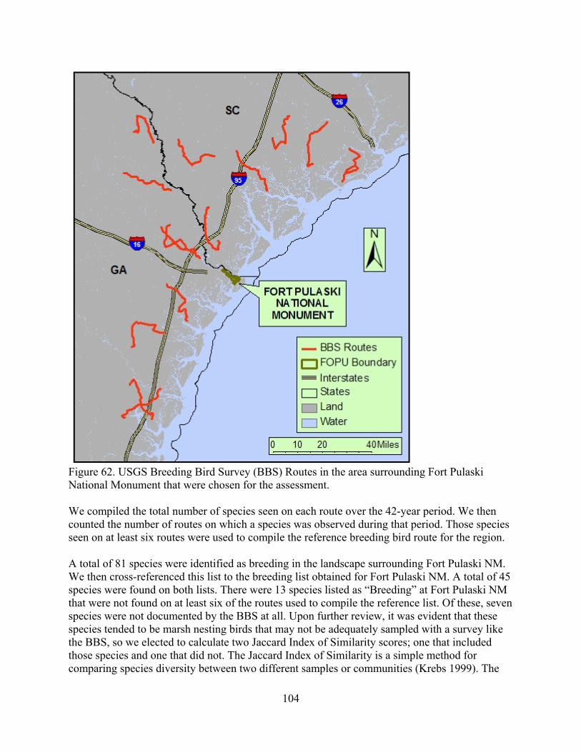
Figure 62. USGS Breeding Bird Survey (BBS) Routes in the area surrounding Fort Pulaski National Monument that were chosen for the assessment. We compiled the total number of species seen on each route over the 42-year period. We then counted the number of routes on which a species was observed during that period. Those species seen on at least six routes were used to compile the reference breeding bird route for the region. A total of 81 species were identified as breeding in the landscape surrounding Fort Pulaski NM. We then cross-referenced this list to the breeding list obtained for Fort Pulaski NM. A total of 45 species were found on both lists. There were 13 species listed as “Breeding” at Fort Pulaski NM that were not found on at least six of the routes used to compile the reference list. Of these, seven species were not documented by the BBS at all. Upon further review, it was evident that these species tended to be marsh nesting birds that may not be adequately sampled with a survey like the BBS, so we elected to calculate two Jaccard Index of Similarity scores; one that included those species and one that did not. The Jaccard Index of Similarity is a simple method for comparing species diversity between two different samples or communities (Krebs 1999). The

104

value is calculated by dividing the number of species found in both samples (a) by the number found in only one sample or the other (b,c): Sj = a /(a+b+c) The Jaccard Index of Similarity between the reference breeding bird list and the breeding bird list from Fort Pulaski NM was 0.45. If we removed those seven species thought to be under-represented in the reference list, the index score was determined to be 0.48. It is important to note that, 28 of the 36 species (~ 78%) on the reference list not in Fort Pulaski NM have been observed, but their breeding status has not been confirmed. Assuming those species were confirmed through additional survey efforts, then the similarity score for Fort Pulaski NM could be as high as 0.78. Another means for assessing the biotic condition of the birds at Fort Pulaski NM was to examine the population trends for each species. From a management perspective, Fort Pulaski NM would like to see each species either at, or moving towards, population levels desired for management. These levels will differ depending on the status of the species. For example, we assume that rare species populations would be desirable if they are increasing. The opposite would be true of exotic or nuisance species. Using the BBS data, we were able to establish observation trends for 45 species known to breed at Fort Pulaski NM. For each species, we calculated the number of times the species was observed each year over the course of the surveys, then calculated a regional average by dividing the total seen by the total number of routes that were completed in that year. In years that a route was completed but the species was not observed, we recorded a 0 value. We then plotted the mean number of observations against the years and used linear regression to create a trend line for each species. We used the statistical output to determine if the slope of the line was significantly different from 0. If so, it was classified as either “increasing” or “decreasing” for the period. We calculated this slope value for two periods. The first period was for the entire survey period (1966 – 2007). The second period was for the last 15 years only (1992 – 2007). Comparisons between these periods will allow us to determine if any non-significant long-term trends are changing more recently. We categorized trends as “acceptable” or “unacceptable” by using a simple management matrix for each class of species in the set (Table 42). These three classes were species of “concern,” “nuisance,” or “breeder.” These values were used to determine the overall management acceptability of population trends for the bird community.

105

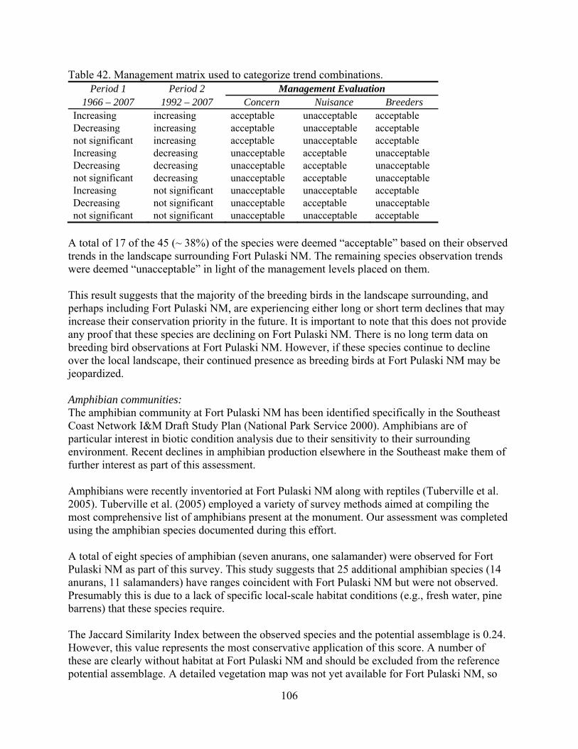
Table 42. Management matrix used to categorize trend combinations. Period 1 Period 2 Management Evaluation

1966 – 2007 1992 – 2007 Concern Nuisance Breeders Increasing increasing acceptable unacceptable acceptable Decreasing increasing acceptable unacceptable acceptable not significant increasing acceptable unacceptable acceptable Increasing decreasing unacceptable acceptable unacceptable Decreasing decreasing unacceptable acceptable unacceptable not significant decreasing unacceptable acceptable unacceptable Increasing not significant unacceptable unacceptable acceptable Decreasing not significant unacceptable acceptable unacceptable not significant not significant unacceptable unacceptable acceptable

A total of 17 of the 45 (~ 38%) of the species were deemed “acceptable” based on their observed trends in the landscape surrounding Fort Pulaski NM. The remaining species observation trends were deemed “unacceptable” in light of the management levels placed on them. This result suggests that the majority of the breeding birds in the landscape surrounding, and perhaps including Fort Pulaski NM, are experiencing either long or short term declines that may increase their conservation priority in the future. It is important to note that this does not provide any proof that these species are declining on Fort Pulaski NM. There is no long term data on breeding bird observations at Fort Pulaski NM. However, if these species continue to decline over the local landscape, their continued presence as breeding birds at Fort Pulaski NM may be jeopardized. Amphibian communities: The amphibian community at Fort Pulaski NM has been identified specifically in the Southeast Coast Network I&M Draft Study Plan (National Park Service 2000). Amphibians are of particular interest in biotic condition analysis due to their sensitivity to their surrounding environment. Recent declines in amphibian production elsewhere in the Southeast make them of further interest as part of this assessment. Amphibians were recently inventoried at Fort Pulaski NM along with reptiles (Tuberville et al. 2005). Tuberville et al. (2005) employed a variety of survey methods aimed at compiling the most comprehensive list of amphibians present at the monument. Our assessment was completed using the amphibian species documented during this effort. A total of eight species of amphibian (seven anurans, one salamander) were observed for Fort Pulaski NM as part of this survey. This study suggests that 25 additional amphibian species (14 anurans, 11 salamanders) have ranges coincident with Fort Pulaski NM but were not observed. Presumably this is due to a lack of specific local-scale habitat conditions (e.g., fresh water, pine barrens) that these species require. The Jaccard Similarity Index between the observed species and the potential assemblage is 0.24. However, this value represents the most conservative application of this score. A number of these are clearly without habitat at Fort Pulaski NM and should be excluded from the reference potential assemblage. A detailed vegetation map was not yet available for Fort Pulaski NM, so

106

we were unable to obtain the local scale information needed to exclude species for lack of habitat. We elected to use species-habitat distribution models published by the Georgia Gap Analysis Program (UGA Institute of Ecology and GA Cooperative Fish & Wildlife Research Unit 2003). These models were synthesized with a combination of literature review, historical records, and expert review. The resulting species-habitat models were applied to real landscapes using a land cover map. Predicted species distributions were then attributed to specific EMAP hexagons and mapped for the entire state (UGA Institute of Ecology and GA Cooperative Fish & Wildlife Research Unit 2003). Fort Pulaski NM is located within the EMAP hexagon number 2568. We extracted the frogs and salamanders species whose distributions placed them within this hexagon and used that as a reference list (Appendix D). A total of 25 species were identified from the GA-GAP models as occurring within the hexagon coincident with Fort Pulaski NM. Of these, seven species were documented at Fort Pulaski NM. In addition, the southern toad was found at Fort Pulaski NM although this species was not predicted to occur by the GA-GAP models. The Jaccard Similarity Index was calculated as 0.27 between Fort Pulaski NM amphibians and the GA-GAP derived reference set (Table 47). These indices reflect a relatively low overlap between the amphibians present at Fort Pulaski NM relative to similar habitats. That is, areas outside of the monument with similar habitat characteristics will have more species than were observed here. This, however, may be due to the relatively recent establishment of upland and freshwater habitats at Fort Pulaski NM. Since the monument is surrounded by salt water, the movement of amphibians from mainland populations and habitats to the islands is difficult. Therefore, although Fort Pulaski NM has relatively few frogs and salamanders, this may be due to its isolation from potential mainland immigrants rather than a degraded habitat condition. Reptile communities: We completed a community composition analysis for reptiles similar to our methods for amphibians. Reptiles were surveyed recently (Tuberville et al. 2005) along with amphibians using similar methods. A total of 17 reptiles were found on Fort Pulaski NM. The survey suggests the potential for 41 additional species with overlapping ranges (although habitat may not be found on the monument). This yields the most conservative Jaccard Similarity Index of 0.29. The list of 41 additional species is likely comprised of several species unlikely to occur within Fort Pulaski NM because of a lack of appropriate habitat. As with amphibians, we elected to utilize predicted distributions of reptile species from the GA-GAP (Appendix D). The GA-GAP models predict the occurrence of 50 species in all. All 17 species observed at Fort Pulaski NM are included, so the Jaccard Similarity Index was calculated at 0.34. As with amphibians, it is reasonable to conclude that many reptile species have not yet been able to colonize the relatively new upland habitats of Cockspur Island on Fort Pulaski NM. Therefore, our similarity indices would provide a low value. We decided to do a last comparison by

107

synthesizing a list of reptiles that would be expected to utilize the salt marsh habitats only and compare that to the list of reptiles for Fort Pulaski NM. Since the salt marsh communities have persisted over much longer periods of time, we expected that the species assemblage would more closely overlap a reference list. We generated a reference list of reptiles from Gibbons (1978 as cited in Wiegert and Freeman 1990). This list contains six species that are ubiquitous in coastal salt marshes throughout the Southeast. Of these six species, four have been documented at Fort Pulaski NM. Only the eastern mud turtle and yellow rat snake were not found (Jaccard Similarity Index = 0.67, Table 47). Mammal communities: The mammal community at Fort Pulaski NM is relatively small. There are 18 species on the monument including marine mammals and bats. Two species, the house mouse (Mus musculus) and black rat (Rattus rattus), are exotic species. We used the GA-GAP species distribution models as a reference list for comparison of mammals (Appendix D). GA-GAP models predicted the presence of 36 species in the Fort Pulaski NM area (did not include marine mammals). All 17 terrestrial species observed on Fort Pulaski NM were predicted by the GA-GAP models with a Jaccard Similarity Index of 0.47. Wiegert and Freeman (1990) also provided a list of salt marsh mammals (derived from Sanders 1978) found in the salt marshes of the Southeast. We identified those species on Fort Pulaski NM that were likely present due to the salt marsh and compared it to this list. All six salt marsh species present on Fort Pulaski NM were found on the reference list of 14 species with a Jaccard Similarity Index of 0.43 (Table 47). Other communities: There are several other key biotic communities that should be examined as part of this assessment. For the salt marsh vegetation communities, these include fish (especially breeding salt marsh species) and invertebrates (crabs and bivalves in particular). For both upland areas and salt marsh, plants are important as well. The biotic species list compiled from the NPS biotic database (Certified Organisms: NPSpecies 2008) indicates there are 40 fish species that utilize Fort Pulaski NM habitats for some period of their annual or seasonal life requisites (Table 43). Slusher (2009) performed an analysis of the aquatic condition for Fort Pulaski NM. The analysis compared native fish species documented on Fort Pulaski NM to native fish that occur in the watersheds based on NatureServe data. Percent similarity of native fish collected in the NPS unit was 0.13 (8/62).

108

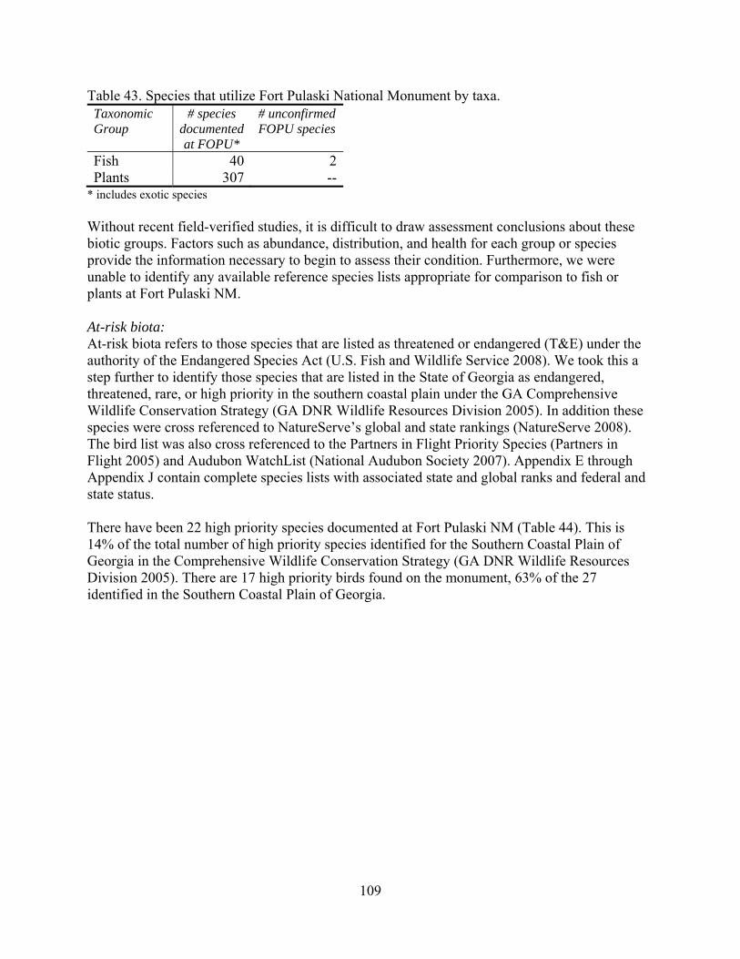
Table 43. Species that utilize Fort Pulaski National Monument by taxa. Taxonomic Group

# species documented at FOPU*

# unconfirmed FOPU species

Fish 40 2Plants 307 --

* includes exotic species Without recent field-verified studies, it is difficult to draw assessment conclusions about these biotic groups. Factors such as abundance, distribution, and health for each group or species provide the information necessary to begin to assess their condition. Furthermore, we were unable to identify any available reference species lists appropriate for comparison to fish or plants at Fort Pulaski NM. At-risk biota: At-risk biota refers to those species that are listed as threatened or endangered (T&E) under the authority of the Endangered Species Act (U.S. Fish and Wildlife Service 2008). We took this a step further to identify those species that are listed in the State of Georgia as endangered, threatened, rare, or high priority in the southern coastal plain under the GA Comprehensive Wildlife Conservation Strategy (GA DNR Wildlife Resources Division 2005). In addition these species were cross referenced to NatureServe’s global and state rankings (NatureServe 2008). The bird list was also cross referenced to the Partners in Flight Priority Species (Partners in Flight 2005) and Audubon WatchList (National Audubon Society 2007). Appendix E through Appendix J contain complete species lists with associated state and global ranks and federal and state status. There have been 22 high priority species documented at Fort Pulaski NM (Table 44). This is 14% of the total number of high priority species identified for the Southern Coastal Plain of Georgia in the Comprehensive Wildlife Conservation Strategy (GA DNR Wildlife Resources Division 2005). There are 17 high priority birds found on the monument, 63% of the 27 identified in the Southern Coastal Plain of Georgia.

109

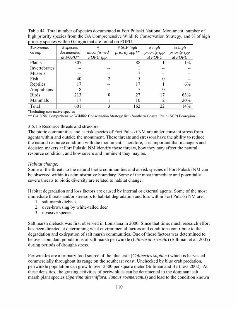
Table 44. Total number of species documented at Fort Pulaski National Monument, number of high priority species from the GA Comprehensive Wildlife Conservation Strategy, and % of high priority species within Georgia that are found on FOPU. Taxonomic Group

# species documented at FOPU*

# unconfirmed FOPU spp.

# SCP high priority spp**

# high priority spp

at FOPU

% high priority spp

at FOPU Plants 307 -- 88 1 1% Invertebrates -- -- 1 -- -- Mussels -- -- 7 -- -- Fish 40 2 5 0 -- Reptiles 17 -- 17 1 6% Amphibians 8 -- 7 0 -- Birds 213 0 27 17 63% Mammals 17 1 10 2 20% Total 601 3 162 22 14%

*Including non-native species ** GA DNR Comprehensive Wildlife Conservation Strategy list - Southern Coastal Plain (SCP) Ecoregion 3.6.1.b Resource threats and stressors: The biotic communities and at-risk species of Fort Pulaski NM are under constant stress from agents within and outside the monument. These threats and stressors have the ability to reduce the natural resource condition with the monument. Therefore, it is important that managers and decision makers at Fort Pulaski NM identify those threats, how they may affect the natural resource condition, and how severe and imminent they may be. Habitat change: Some of the threats to the natural biotic communities and at-risk species of Fort Pulaski NM can be observed within its administrative boundary. Some of the most immediate and potentially severe threats to biotic diversity are related to habitat change. Habitat degradation and loss factors are caused by internal or external agents. Some of the most immediate threats and/or stressors to habitat degradation and loss within Fort Pulaski NM are:

1. salt marsh dieback 2. over-browsing by white-tailed deer 3. invasive species

Salt marsh dieback was first observed in Louisiana in 2000. Since that time, much research effort has been directed at determining what environmental factors and conditions contribute to the degradation and extirpation of salt marsh communities. One of those factors was determined to be over-abundant populations of salt marsh periwinkle (Littoraria irrorata) (Silliman et al. 2005) during periods of drought-stress. Periwinkles are a primary food source of the blue crab (Calinectes sapidus) which is harvested commercially throughout its range on the southeast coast. Unchecked by blue crab predation, periwinkle population can grow to over 2500 per square meter (Silliman and Bertness 2002). At these densities, the grazing activities of periwinkles can be detrimental to the dominant salt marsh plant species (Spartina alterniflora, Juncus roemerianus) and lead to the condition known

110

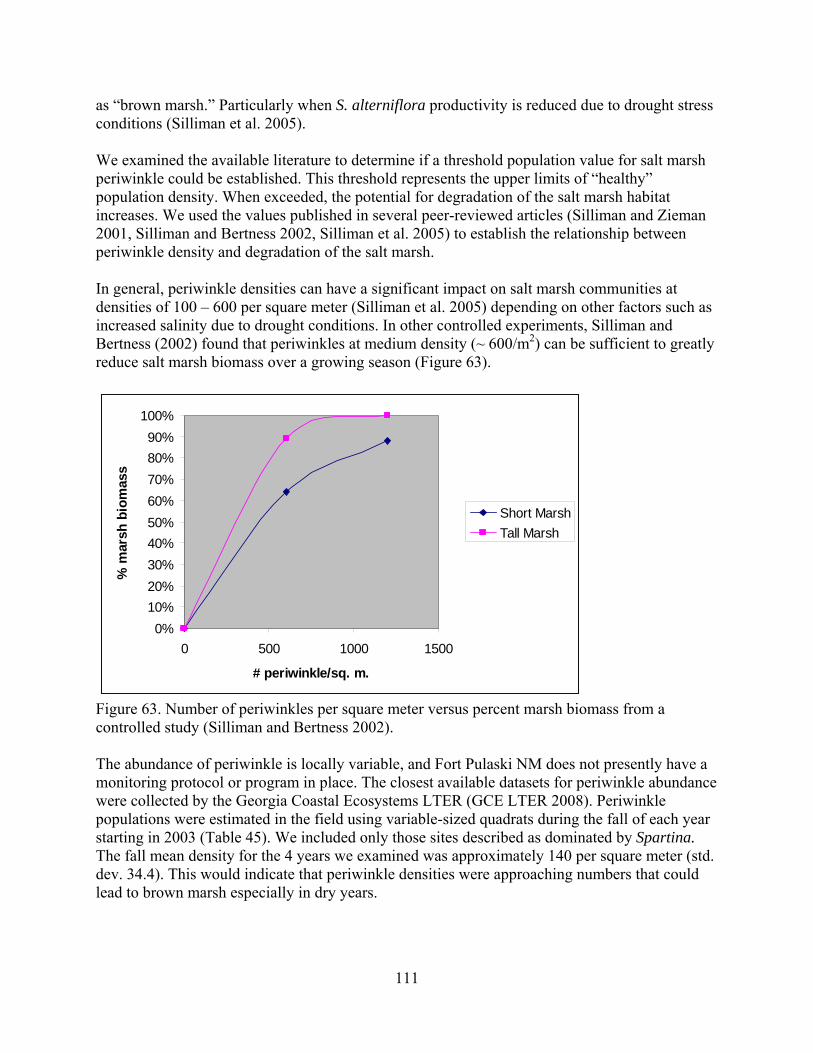
as “brown marsh.” Particularly when S. alterniflora productivity is reduced due to drought stress conditions (Silliman et al. 2005). We examined the available literature to determine if a threshold population value for salt marsh periwinkle could be established. This threshold represents the upper limits of “healthy” population density. When exceeded, the potential for degradation of the salt marsh habitat increases. We used the values published in several peer-reviewed articles (Silliman and Zieman 2001, Silliman and Bertness 2002, Silliman et al. 2005) to establish the relationship between periwinkle density and degradation of the salt marsh. In general, periwinkle densities can have a significant impact on salt marsh communities at densities of 100 – 600 per square meter (Silliman et al. 2005) depending on other factors such as increased salinity due to drought conditions. In other controlled experiments, Silliman and Bertness (2002) found that periwinkles at medium density (~ 600/m2) can be sufficient to greatly reduce salt marsh biomass over a growing season (Figure 63).

0%10%20%30%40%50%60%70%80%90%

100%

0 500 1000 1500

# periwinkle/sq. m.

% m

arsh

bio

mas

s

Short MarshTall Marsh

Figure 63. Number of periwinkles per square meter versus percent marsh biomass from a controlled study (Silliman and Bertness 2002). The abundance of periwinkle is locally variable, and Fort Pulaski NM does not presently have a monitoring protocol or program in place. The closest available datasets for periwinkle abundance were collected by the Georgia Coastal Ecosystems LTER (GCE LTER 2008). Periwinkle populations were estimated in the field using variable-sized quadrats during the fall of each year starting in 2003 (Table 45). We included only those sites described as dominated by Spartina. The fall mean density for the 4 years we examined was approximately 140 per square meter (std. dev. 34.4). This would indicate that periwinkle densities were approaching numbers that could lead to brown marsh especially in dry years.

111

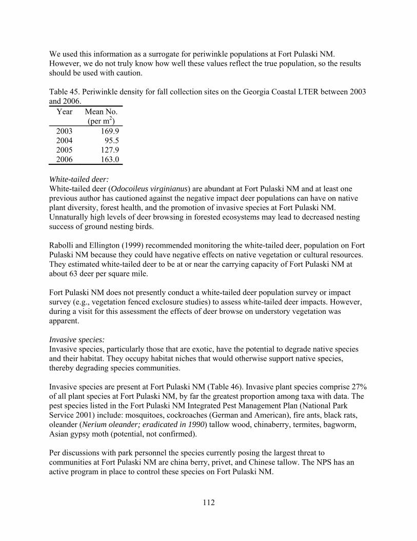
We used this information as a surrogate for periwinkle populations at Fort Pulaski NM. However, we do not truly know how well these values reflect the true population, so the results should be used with caution. Table 45. Periwinkle density for fall collection sites on the Georgia Coastal LTER between 2003 and 2006.

Year Mean No. (per m2)

2003 169.9 2004 95.5 2005 127.9 2006 163.0

White-tailed deer: White-tailed deer (Odocoileus virginianus) are abundant at Fort Pulaski NM and at least one previous author has cautioned against the negative impact deer populations can have on native plant diversity, forest health, and the promotion of invasive species at Fort Pulaski NM. Unnaturally high levels of deer browsing in forested ecosystems may lead to decreased nesting success of ground nesting birds. Rabolli and Ellington (1999) recommended monitoring the white-tailed deer, population on Fort Pulaski NM because they could have negative effects on native vegetation or cultural resources. They estimated white-tailed deer to be at or near the carrying capacity of Fort Pulaski NM at about 63 deer per square mile. Fort Pulaski NM does not presently conduct a white-tailed deer population survey or impact survey (e.g., vegetation fenced exclosure studies) to assess white-tailed deer impacts. However, during a visit for this assessment the effects of deer browse on understory vegetation was apparent. Invasive species: Invasive species, particularly those that are exotic, have the potential to degrade native species and their habitat. They occupy habitat niches that would otherwise support native species, thereby degrading species communities. Invasive species are present at Fort Pulaski NM (Table 46). Invasive plant species comprise 27% of all plant species at Fort Pulaski NM, by far the greatest proportion among taxa with data. The pest species listed in the Fort Pulaski NM Integrated Pest Management Plan (National Park Service 2001) include: mosquitoes, cockroaches (German and American), fire ants, black rats, oleander (Nerium oleander; eradicated in 1990) tallow wood, chinaberry, termites, bagworm, Asian gypsy moth (potential, not confirmed). Per discussions with park personnel the species currently posing the largest threat to communities at Fort Pulaski NM are china berry, privet, and Chinese tallow. The NPS has an active program in place to control these species on Fort Pulaski NM.

112

Table 46. Proportion of invasive species by taxa at Fort Pulaski National Monument. Taxonomic Group

# Native species

# Non-native species

% Non-native

Plants 224 83 27.0Fish -- -- --Herpetofauna 23 1 4.2Birds 211 2 0.9Mammals 15 2 11.7

External threats and stressors: There are many external threats to the biotic communities of Fort Pulaski NM, from factors external to the boundaries and management authority of the NPS. These factors have been covered extensively in previous sections and include:

1. Increased isolation due to human population growth and development, as discussed in the Human Use section.

2. Impact of 400,000 visitors per year, Visitor and Recreation Use section. 3. As mentioned the Water section, the Georgia Ports Authority and the U.S. Army Corps of

Engineers have plans to expand the Savannah harbor, which could result in several negative impacts to Fort Pulaski NM wildlife and their habitats.

4. Existing dredge disposal sites that were discussed in the Geology and Soils section. 5. A hazardous sites map was also discussed and provided in the Water section (Figure 49).

3.6.1.c Critical knowledge or data gaps: The biotic communities of Fort Pulaski NM may be unique in this landscape given the relatively recent establishment of upland habitat. Therefore, the species assemblages present do not appear to reflect the more complete biotic communities observed in the surrounding area. Relatively low similarity scores for all taxa may reflect the relatively low diversity on Fort Pulaski NM as a result. However, a lack of comprehensive survey efforts certainly contributes to some of the observed differences. Similarity index scores for birds, for example, may increase with more comprehensive data from within the monument. These surveys should not only focus on species inventory, but should also address abundance which, over time, will provide better information to complete biotic community assessments. Table 47 shows the summary of condition status and data quality. The following are specific knowledge gaps identified:

1. Unknown abundance of the majority of all faunal and floral species, especially plants, breeding fish and invertebrate species.

2. Unknown abundance (population size) and residency of most bird species (especially marshland birds).

3. Littoraria density in Spartina marsh areas. 4. Deer abundance and impact on upland vegetation communities.

113

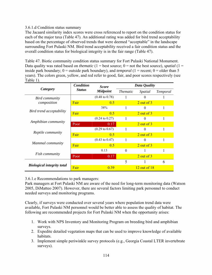
3.6.1.d Condition status summary The Jacaard similarity index scores were cross referenced to report on the condition status for each of the major taxa (Table 47). An additional rating was added for bird trend acceptability based on the percentage of observed trends that were deemed “acceptable” in the landscape surrounding Fort Pulaski NM. Bird trend acceptability received a fair condition status and the overall condition status for biological integrity is in the fair range (Table 47). Table 47. Biotic community condition status summary for Fort Pulaski National Monument. Data quality was rated based on thematic (1 = best source; 0 = not the best source), spatial (1 = inside park boundary; 0 = outside park boundary), and temporal (1 = recent; 0 = older than 5 years). The colors green, yellow, and red refer to good, fair, and poor scores respectively (see Table 1).

Category Condition

Status Score

Midpoint Data Quality


Bird community composition

(0.48 to 0.78) 1 0 1 Fair 0.5 2 out of 3

Bird trend acceptability 38% 1 0 1 Fair 0.5 2 out of 3

Amphibian community (0.24 to 0.27) 1 0 1 Poor 0.17 2 out of 3

Reptile community (0.29 to 0.67) 1 0 1 Fair 0.5 2 out of 3

Mammal community (0.43 to 0.47) 1 0 1 Fair 0.5 2 out of 3

Fish community 0.13 0 1 1 Poor 0.17 2 out of 3

Biological integrity total 5 1 6 Fair 0.39 12 out of 18

3.6.1.e Recommendations to park managers: Park managers at Fort Pulaski NM are aware of the need for long-term monitoring data (Watson 2005, DiMatteo 2007). However, there are several factors limiting park personnel to conduct needed surveys and monitoring programs. Clearly, if surveys were conducted over several years where population trend data were available, Fort Pulaski NM personnel would be better able to assess the quality of habitat. The following are recommended projects for Fort Pulaski NM when the opportunity arises:

1. Work with NPS Inventory and Monitoring Program on breeding bird and amphibian surveys.

2. Expedite detailed vegetation maps that can be used to improve knowledge of available habitats.

3. Implement simple periwinkle survey protocols (e.g., Georgia Coastal LTER invertebrate surveys).

114

115

4. Develop a more complete breeding fish survey in salt marsh areas. 5. Work with state and local natural resource agencies to determine the present abundance

of white-tailed deer 6. Use simple vegetation sampling and/or deer exclosure study to better understand impacts

to vegetation communities from deer browsing.

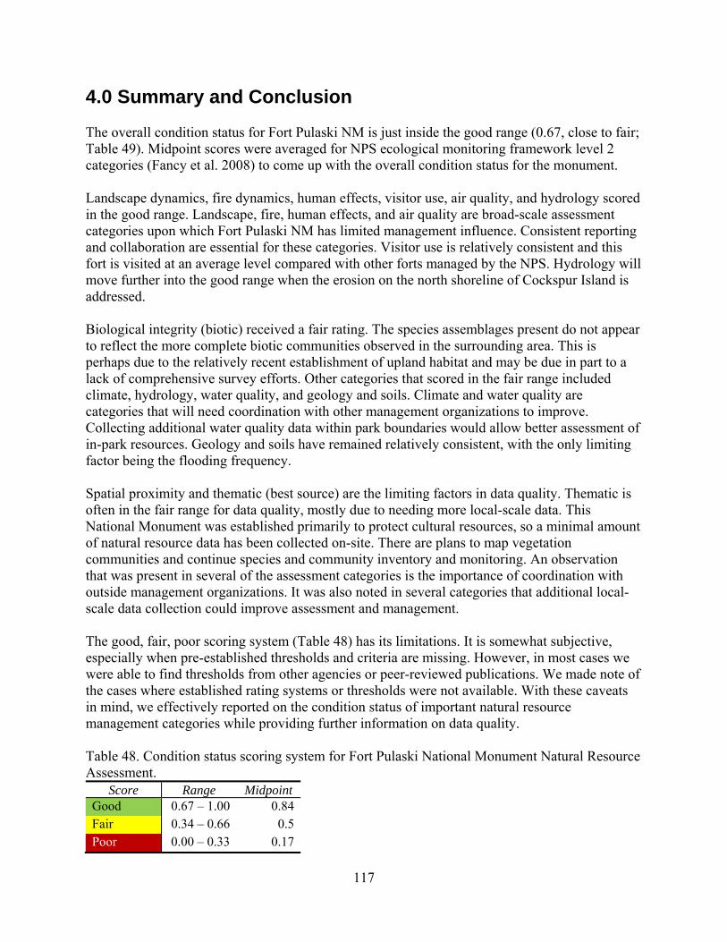
4.0 Summary and Conclusion The overall condition status for Fort Pulaski NM is just inside the good range (0.67, close to fair; Table 49). Midpoint scores were averaged for NPS ecological monitoring framework level 2 categories (Fancy et al. 2008) to come up with the overall condition status for the monument. Landscape dynamics, fire dynamics, human effects, visitor use, air quality, and hydrology scored in the good range. Landscape, fire, human effects, and air quality are broad-scale assessment categories upon which Fort Pulaski NM has limited management influence. Consistent reporting and collaboration are essential for these categories. Visitor use is relatively consistent and this fort is visited at an average level compared with other forts managed by the NPS. Hydrology will move further into the good range when the erosion on the north shoreline of Cockspur Island is addressed. Biological integrity (biotic) received a fair rating. The species assemblages present do not appear to reflect the more complete biotic communities observed in the surrounding area. This is perhaps due to the relatively recent establishment of upland habitat and may be due in part to a lack of comprehensive survey efforts. Other categories that scored in the fair range included climate, hydrology, water quality, and geology and soils. Climate and water quality are categories that will need coordination with other management organizations to improve. Collecting additional water quality data within park boundaries would allow better assessment of in-park resources. Geology and soils have remained relatively consistent, with the only limiting factor being the flooding frequency.

Spatial proximity and thematic (best source) are the limiting factors in data quality. Thematic is often in the fair range for data quality, mostly due to needing more local-scale data. This National Monument was established primarily to protect cultural resources, so a minimal amount of natural resource data has been collected on-site. There are plans to map vegetation communities and continue species and community inventory and monitoring. An observation that was present in several of the assessment categories is the importance of coordination with outside management organizations. It was also noted in several categories that additional local-scale data collection could improve assessment and management. The good, fair, poor scoring system (Table 48) has its limitations. It is somewhat subjective, especially when pre-established thresholds and criteria are missing. However, in most cases we were able to find thresholds from other agencies or peer-reviewed publications. We made note of the cases where established rating systems or thresholds were not available. With these caveats in mind, we effectively reported on the condition status of important natural resource management categories while providing further information on data quality. Table 48. Condition status scoring system for Fort Pulaski National Monument Natural Resource Assessment.


117

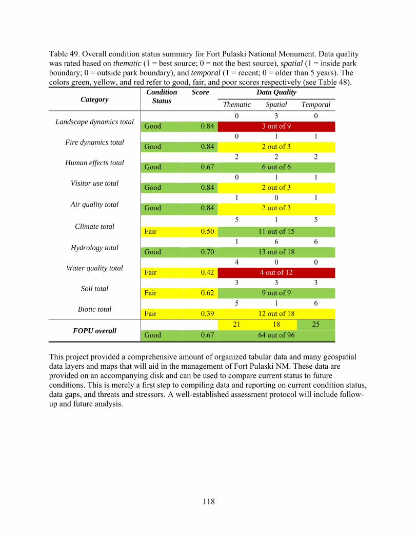
118

Table 49. Overall condition status summary for Fort Pulaski National Monument. Data quality was rated based on thematic (1 = best source; 0 = not the best source), spatial (1 = inside park boundary; 0 = outside park boundary), and temporal (1 = recent; 0 = older than 5 years). The colors green, yellow, and red refer to good, fair, and poor scores respectively (see Table 48).

Category Condition

Status Score Data Quality


Landscape dynamics total 0 3 0


Fire dynamics total 0 1 1


Human effects total 2 2 2


Visitor use total 0 1 1


Air quality total 1 0 1


Climate total 5 1 5


Hydrology total 1 6 6


Water quality total 4 0 0


Soil total 3 3 3


Biotic total 5 1 6


FOPU overall 21 18 25



Literature Cited AirNow. 2008a. Air quality index (AQI) - a guide to air quality and your health. A cross-agency

U.S. Government web site (http://airnow.gov/index.cfm?action=static.aqi). Accessed June 2008.

AirNow. 2008b. AQI calculator. (http://airnow.gov/index.cfm?action=aqi.conc_aqi_calc). Accessed June 2008.

AirNow. 2008c. Georgia air quality conditions & forecasts. (http://www.airnow.gov/index.cfm?action=airnow.showlocal&CityID=327). Accessed June 2008.

Alexander, C. 2008. Rates and processes of shoreline change at Ft. Pulaski National Monument. Applied Coastal Research Laboratory, Georgia Southern University and Skidaway Institute of Oceanography, Savannah, GA.

Balmford, A. 1996. Extinction filters and current resilience: the significance of past selection pressures for conservation biology. Trends in Ecology & Evolution 11:193-196.

Blake, E. S., E. N. Rappaport, and C. W. Landsea. 2007. The deadliest, costliest, and most intense United States tropical cyclones from 1851 to 2006 (and other frequently requested hurricane facts). National Weather Service, National Hurricane Center, Miami, Florida.

Blaustein, A. R., L. K. Belden, D. H. Olson, D. M. Green, T. L. Root, and J. M. Kiesecker. 2001. Amphibian breeding and climate change. Conservation Biology 15:1804-1809.

Cardillo, M., A. Purvis, W. Sechrest, J. L. Gittleman, J. Bielby, and G. M. Mace. 2004. Human population density and extinction risk in the world's carnivores. PLoS Biology 2:909 - 914.

Certified Organisms: NPSpecies. 2008. The National Park Service biodiversity database. Secure online version of certified organisms from (https://science1.nature.nps.gov/npspecies/web/main/start). Accessed 30 April 2008.

Cooney, T. W., P. A. Drewes, S. W. Ellisor, T. H. Lanier, and F. Melendez. 2005. Water resources data, South Carolina, water year 2005, volume 1, U.S. Geological Survey water-data report. SC-05-1.

Corn, P. S. 2005. Climate change and amphibians. Animal Biodiversity and Conservation 28:59-67.

119

Craft, C., J. Clough, J. Ehman, S. Joye, R. Park, S. Pennings, H. Guo, and M. Machmuller. 2009. Forecasting the effects of accelerated sea-level rise on tidal marsh ecosystem services. Frontiers in Ecology and the Environment. 7:73-78.

Curtis, T. 2008. NPS Southeast Coast Network Ecologist /Remote Sensing Specialist. E-mail Communication, June 16, 2008.

DiMatteo, A. 2007. National Parks Conservation Association natural resource assessment for Fort Pulaski National Monument. Masters Project. Duke University, Durham, NC.

ESRI. 2006. ArcInfo, ArcMap 9.2. Redlands, CA.

Fancy, S. G., J. E. Gross, and S. L. Carter. 2008. Monitoring the condition of natural resources in US National Parks. Environmental Monitoring and Assessment (In Press).

Federal Emergency Management Agency. 2008. Flood map viewer. (https://hazards.fema.gov/femaportal/wps/portal). Accessed December 2008.

Forester, D. J. and G. E. Machlist. 1996. Modeling human factors that affect the loss of biodiversity. Conservation Biology 10:1253-1263.

Frazier, W. J. 2007. Coastal plain geologic province. New Georgia Encyclopedia. Georgia Humanities Council and the University of Georgia Press. (http://www.georgiaencyclopedia.org/nge/Article.jsp?id=h-1161). Accessed August 2008.

GA DNR Coastal Resources Division. 2008a. Coastal Marshlands Protection Act. (http://crd.dnr.state.ga.us/content/displaycontent.asp?txtDocument=85&txtPage=2). Accessed August 2008.

GA DNR Coastal Resources Division. 2008b. Georgia Department of Natural Resources. Georgia's salt marshes. (http://crd.dnr.state.ga.us/content/displaycontent.asp?txtDocument=22). Accessed August 2008

GA DNR Environmental Protection Division. 2001. Savannah River basin management plan.

GA DNR Wildlife Resources Division. 2005. Georgia comprehensive wildlife conservation strategy. (http://www1.gadnr.org/cwcs/Documents/strategy.html). Accessed June 2008.

GA DNR Wildlife Resources Division. 2008. Georgia rare species and natural community information - protected species lists.

120

(http://georgiawildlife.dnr.state.ga.us/documentdetail.aspx?docid=89&pageid=2&category=conservation). Accessed October 2008.

GCE LTER. 2008. Georgia coastal ecosystems long term ecological research data. (http://gce-lter.marsci.uga.edu/public/data/data.htm). Accessed June 2008.

GeoMAC. 2008. Geospatial multi-agency coordination, wildland fire support. U.S. Department of Interior and U.S. Department of Agriculture. (http://www.geomac.gov/). Accessed June 2008.

Georgia Automated Environmental Monitoring Network. 2008. Climate averages for Chatham County, GA, Savannah International Airport (1951 to 2003). (http://www.griffin.uga.edu/aemn/cgi-bin/AEMN.pl?site=GASK&report=cl). Accessed May 2008.

Google. 2008. Google maps. (http://maps.google.com/). Accessed November, 2008.

Govus, T., E. 1998. Fort Pulaski National Monument inventory final report, part A: plants. Prepared for the National Park Service, Southeast Region.

Hurd, J. D. and D. L. Civco. 2004. Surface water quality and impervious surface quantity: a preliminary study. Center for Land use Education And Research, Department of Natural Resources Management & Engineering, College of Agriculture and Natural Resources, The University of Connecticut.

Hurricane City. 2008. Savannah, Georgia's history with tropical systems. (http://www.hurricanecity.com/city/savannah.htm). Accessed May 2008.

Jones, R. C. and C. C. Clark. 1987. Impact of watershed urbanization on stream insect communities. Journal of the American Water Resources Association 23:1047-1055.

Krebs, C. J. 1999. Ecological methodology. Second edition. Addison-Wesley Educational Publishers, Inc.

Leica Geosystems Geospatial Imaging. 2004. ERDAS Imagine 8.7. Norcross, GA.

Loganathan, B. G., K. S. Sajwan , J. P. Richardson, C. S. Chetty and D. A. Owen. 2001. Persistent organichlorine concentrations in sediment and fish from Atlantic coastal and brackish waters off Savannah,Georgia, USA. Marine Pollution Bulletin 42:246-250.

McFarlin, C. and M. Alber. 2005. Assessment of coastal water resources and watershed condition at Fort Pulaski National Monument, Georgia. Department of Marine Sciences, University of Georgia, for the National Park Service, U.S. Department of Interior, Water

121

Resources Division, Natural Resource Program Center, Technical Report NPS/NRWRD/NRTR-2005/345.

McFarlin, C. and M. Alber. 2007. Coastal watershed condition assessment of Fort Pulaski National Monument. Proceedings of the 2007 Georgia Water Resources Conference, March 27-29, 2007. University of Georgia.

McKinney, M. L. 2001. Effects of human population, area, and time on non-native plant and fish diversity in the United States. Biological Conservation 100:243-252.

McMaster, G. S. and W. W. Wilhelm. 1997. Growing degree-days: one equation, two interpretations. Agricultural and Forest Meteorology 87:291-300.

Meader, J. F. 2003. Fort Pulaski National Monument administrative history. Cultural Resources Division, Southeast Regional Office, National Park Service, Atlanta, GA.

National Audubon Society. 2007. WatchList. (http://web1.audubon.org/science/species/watchlist/). Accessed June 2008.

National Oceanic and Atmospheric Administration. 2008a. Coastal change analysis program, land cover analysis. (http://www.csc.noaa.gov/crs/lca/ccap.html). Accessed April 2008.

National Oceanic and Atmospheric Administration. 2008b. Coastal Services Center, historical hurricane tracks. (http://maps.csc.noaa.gov/hurricanes/index.jsp). Accessed September 2008.

National Oceanic and Atmospheric Administration. 2008c. U.S. climate at a glance. (http://www.ncdc.noaa.gov/oa/climate/research/cag3/cag3.html). Accessed July 2008.

National Park Service. 1995. Resource management plan, Fort Pulaski National Monument.

National Park Service. 2000. NPS, Southeast coastal inventory and monitoring network draft study plan.

National Park Service. 2001. Integrated pest management plan, Fort Pulaski National Monument.

National Park Service. 2003. Air quality monitoring considerations for the Southeast Coast Network. (http://www.nature.nps.gov/air/permits/aris/networks/secn.cfm). Accessed December 2008.

National Park Service. 2006. NPS - Soil survey geographic (SSURGO) database for Fort Pulaski National Monument, Georgia. Survey area version 5, survey area version date

122

12/21/2006. (http://science.nature.nps.gov/nrdata/datastore.cfm?ID=43769). Accessed July 2008.

National Park Service. 2007. Fort Pulaski National Monument, general management plan news (Newsletter #3 - Spring 2007).

National Park Service. 2008a. NPS mission. (http://www.nps.gov/aboutus/mission.htm). Accessed November 2008.

National Park Service. 2008b. NPS stats, National Park Service public use statistics office. (http://www.nature.nps.gov/stats/). Accessed November 2008.

National Park Service. 2008c. Vegetation mapping inventory. (http://science.nature.nps.gov/im/inventory/veg/index.cfm). Accessed November 2008.

National Wildfire Coordinating Group. 2008. National fire and aviation management web application. (http://fam.nwcg.gov/fam-web/). Accessed June 2008.

NatureServe. 2008. NatureServe explorer. (http://www.natureserve.org/explorer/ranking.htm). Accessed August 2008.

NPS Planning Environment and Public Comment. 2008. Fort Pulaski National Monument general management plan. (http://parkplanning.nps.gov/projectHome.cfm?parkId=379&projectId=11163). Accessed November 2008.

Park, L. O., R. E. Manning, J. L. Marion, S. R. Lawson, and C. Jacobi. 2008. Managing visitor impacts in parks: a multi-method study of the effectiveness of alternative management practices. Journal of Park & Recreation Administration 26:97-121.

Park Staff. 2007. Personal communication, meeting with park staff. 18 September 2007.

Parks, S. A. and A. H. Harcourt. 2002. Reserve size, local human density, and mammalian extinctions in U.S. protected areas. Conservation Biology 16:800-808.

Partners in Flight. 2005. Species assessment database. (http://www.rmbo.org/pif/scores/scores.html). Accessed August 2008.

Rabolli, C. and K. Ellington. 1999. Fort Pulaski National Monument inventory final report, part B: vertebrate animals. Prepared for: National Park Service, Southeast Region.

123

Richardson, J. P. and K. Sajwan. 2001. Baseline monitoring and analysis of health of the salt marsh ecosystem of Fort Pulaski National Monument, using sediment, oysters and water samples. Prepared for Fort Pulaski National Monument, National Park Service.

Richardson, J. P. and K. Sajwan. 2002. Baseline monitoring and analysis of health of the salt marsh ecosystem of Fort Pulaski National Monument, using sediment, oysters and water samples; year II. Prepared for Fort Pulaski National Monument, National Park Service.

Schueler, T. 2000. The importance of imperviousness. Pages 1-12 in T. Schueler and H. Holland, editors. The practice of watershed protection. Center for Watershed Protection. Ellicott City, MD.

Seabrook, C. 2006. Lower coastal plain and coastal islands. New Georgia Encyclopedia. Georgia Humanities Council and the University of Georgia Press. (http://www.georgiaencyclopedia.org/nge/Article.jsp?id=h-2123). Accessed November 2008.

Silliman, B. R. and M. D. Bertness. 2002. A trophic cascade regulates salt marsh primary production. Proceedings of the National Academy of Sciences of the United States of America 99:10500 - 10505.

Silliman, B. R., J. v. d. Koppel, M. D. Bertness, L. E. Stanton, and I. A. Mendelssohn. 2005. Drought, snails, and large-scale die-off of southern U.S. salt marshes. Science 310:1803 - 1806.

Silliman, B. R. and J. C. Zieman. 2001. Ecology. 82:2830-2845.

Slusher, J. 2009. Analysis of aquatic conditions in Fort Pulaski National Monument. In Nibbelink, N.P., J.M. Long, K.T. McAbee, J.C. Wilson, and L. Brons. Watershed-based condition and threat assessment for fish and aquatic habitat in southeastern National Park Service Units. Task Agreement J5028000705 Final Report. National Park Service, Atlanta, Georgia.

Taylor, A. R. and R. L. Knight. 2003. Wildlife responses to recreation and associated visitor perception. Ecological Applications 13:951-963.

The Weather Channel. 2008. Savannah, GA weather facts. (http://www.weather.com/weather/wxclimatology/monthly/graph/USGA0506?from=search). Accessed May 2008.

Tiner, R. W. 2003a. Correlating enhanced National Wetlands Inventory data with wetland functions for watershed assessments: a rationale for northeastern U.S. wetlands., U.S. Fish and Wildlife Service, National Wetlands Inventory Program, Region 5, Hadley, MA.

124

Tiner, R. W. 2003b. Dichotomous keys and mapping codes for wetland landscape position, landform, water flow path, and waterbody type descriptors. U.S. Fish and Wildlife Service, National Wetlands Inventory Program, Northeast Region, Hadley, MA.

Tuberville, T., J. Willson, M. Dorcas, and J. Gibbons. 2005. Herpetofaunal species richness of southeastern National Parks. Southeastern Naturalist 4.

Tucker, R. E. 1986. Preliminary list of birds of Fort Pulaski National Monument. National Park Service USDOI.

U.S. Army Corps of Engineers. 2008. US Army Corps of Engineers, Savannah District. (http://www.sas.usace.army.mil/). Accessed September 2008.

U.S. Census Bureau. 2008. American fact finder. (http://factfinder.census.gov/home/saff/main.html?_lang=en). Accessed August 2008.

U.S. Department of Commerce. 2001. Hurricanes, unleashing nature's fury, a preparedness guide. National Oceanic and Atmospheric Administration and National Weather Service.

U.S. Environmental Protection Agency. 2005. National coastal condition report II (2005), EPA-620/R-03/002., Office of Water, Washington, DC. (http://www.epa.gov/owow/oceans/nccr/). Accessed August 2008.

U.S. Environmental Protection Agency. 2008a. National Ambient Air Quality Standards (NAAQS). (http://www.epa.gov/air/criteria.html). Accessed July 2008.

U.S. Environmental Protection Agency. 2008b. Six Common Air Pollutants. (http://www.epa.gov/air/urbanair/). Accessed July 2008.

U.S. Environmental Protection Agency. 2008c. Technology transfer metwork (TTN), air quality system (AQS) data mart. (http://www.epa.gov/ttn/airs/aqsdatamart/index.htm). Accessed July 2008.

U.S. Environmental Protection Agency. 2008d. Water quality criteria for nitrogen and phosphorus pollution, basic information. (http://www.epa.gov/waterscience/criteria/nutrient/basic.htm). Accessed July 2008.

U.S. Environmental Protection Agency. 2008e. Water quality criteria for nitrogen and phosphorus pollution. (http://www.epa.gov/waterscience/criteria/nutrient/) Accessed July 2008.

U.S. Fish and Wildlife Service. 2008. Endangered species program, Endangered Species Act of 1973. (http://www.fws.gov/Endangered/ESA/content.html). Accessed November 2008.

125

U.S. Geological Survey. 2000. Fire ecology in the southeastern United States.

U.S. Geological Survey. 2008a. 7.5-minute digital elevation model (DEM). From GeoCommunity (http://www.geocomm.com/). Accessed December, 2008.

U.S. Geological Survey. 2008b. National vegetation classification standard (NVCS). (http://biology.usgs.gov/npsveg/nvcs.html). Accessed November 2008.

U.S. Geological Survey. 2008c. North American breeding bird survey data. Patuxent Wildlife Research Center, Laurel, MD. (http://www.pwrc.usgs.gov/bbs/results/). Accessed August 2008.

UGA Department of Geology. 2008. Georgia geology. (http://www.gly.uga.edu/default.php?PK=0&iPage=5). Accessed October 2008.

UGA Institute of Ecology and GA Cooperative Fish & Wildlife Research Unit. 2003. A GAP analysis of Georgia.

UGA State Climate Office. 2008. Savannah, Georgia climate information. (http://climate.engr.uga.edu/savannah/index.html). Accessed May 2008.

University of Massachusetts Extension. 2008. Monitoring: growing degree days and plant phenology. (http://www.umassgreeninfo.org/fact_sheets/ipmtools/gdd_phrenology.html). Accessed November 2008.

USDA Bureau of Soils. 1911. Historical soil survey maps. (http://alabamamaps.ua.edu/historicalmaps/soilsurvey/index.html). Accessed August 2008.

USDA Forest Service. 2006. LANDFIRE: 14047990, 64779257, 14896850, and 43476636: USDA Forest Service, Missoula MT.

USDA Forest Service. 2008. Wildland fire assessment system. (http://www.wfas.net/). Accessed November 2008.

USDA Natural Resource Conservation Service. 2006. Soil data mart. Soil survey area: Bryan and Chatham Counties, Georgia, version 5, December 21, 2006. (http://soildatamart.nrcs.usda.gov/Survey.aspx?County=GA051). Accessed September 2008.

USDA Natural Resource Conservation Service. 2008. Soil data viewer. (http://soildataviewer.nrcs.usda.gov/). Accessed August 2008.

126

127

Virginia Tech FORSITE. 2008. Forestry outreach site. Scientific investigations, phenology and growing degree days. (http://www.cnr.vt.edu/dendro/forsite/si6.htm). Accessed October 2008.

Waldrop, T. A., D. L. White, and S. M. Jones. 1992. Fire regimes for pine-grassland communities in the southeastern United States. Forest Ecology and Management 47:195-210.

Walther, G.-R., E. Post, P. Convey, A. Menzel, C. Parmesan, T. J. C. Beebee, J.-M. Fromentin, O. Hoegh-Guldberg, and F. Bairlein. 2002. Ecological responses to recent climate change. Nature 416:389-395.

Watson, K. 2005. Avian conservation implementation plan Fort Pulaski National Monument. United States Fish and Wildlife Service.

Wiegert, R. G. and B. J. Freeman. 1990. Tidal salt marshes of the southeast Atlantic coast: a community profile. U.S. Fish and Wildlife Service, Biological Report. 85 (7.29).

Winger, P. V., P. J. Lasier, D. H. White, and J. T. Segina. 2000. Effects of contaminants in dredge material from the lower Savannah River. Archives of Environmental Contamination and Toxicology 38:128-136.

Wood, K. T., S. R. Lawson, and J. L. Marion. 2006. Assessing recreation impacts to cliffs in Shenandoah National Park: integrating visitor observation with trail and recreation site measurements. Journal of Park & Recreation Administration 24:86-110.

Young, T. F. and S. Sanzone. 2002. A framework for assessing and reporting on ecological condition.

Zouhar, K., J. K. Smith, S. Sutherland, and M. L. Brooks. 2008. Wildland fire in ecosystems, fire and nonnative invasive plants. General Technical Report RMRS-GTR-42-volume 6. U.S. Department of Agriculture, Forest Service, Rocky Mountain Research Station, Ogden, UT.

Appendices Page

Appendix A: Land cover calculation methods. ...................................................................... 129 Appendix B: Hydrology calculation methods. ....................................................................... 133 Appendix C: Soil series description and soil ratings. ............................................................ 134 Appendix D: Reference species lists from habitat distribution models published by the

Georgia Gap Analysis Program (UGA Institute of Ecology and GA Cooperative Fish & Wildlife Research Unit 2003) ................................................................................ 148

Appendix E: The following species lists (Appendix F through Appendix J) have been cross-referenced to NatureServe’s global and state rankings (NatureServe 2008); and the GA DNR listings for endangered, threatened, or rare species (GA DNR Wildlife Resources Division 2008). ........................................................................................................... 151

Appendix F: Native (n=224) and non-native (n=83) plant species documented at Fort Pulaski National Monument. .................................................................................................. 154

Appendix G: Fish species documented for Fort Pulaski National Monument....................... 163 Appendix H: Herpetofauna (amphibian and reptile species) documented for Fort Pulaski

National Monument. .................................................................................................. 166 Appendix I: Bird species documented for Fort Pulaski National Monument. ....................... 170 Appendix J: Mammal species documented for Fort Pulaski National Monument. ............... 179

128

Appendix A: Land cover calculation methods. We used “Extract by Mask” in ArcToolbox (ESRI 2006) to clip each land cover dataset to the study areas. In some cases when the study areas went into another state, multiple datasets were mosaiced (combined) in ERDAS Imagine (Leica Geosystems Geospatial Imaging 2004). In some cases we performed grid reclassification and relabeling of class name to simplify and to make the raster files that were produced more useable. NOAA Coastal Change Analysis Program Classification Scheme (National Oceanic and Atmospheric Administration 2008a): Uplands Consisting of areas above sea level where saturated soils and standing water are absent. Also, the Hydrologic regime is not sufficiently wet to support vegetation associated with wetlands. Upland features are divided into classes such as High, Medium, Low Intensity Development, Cultivated land, Grassland, Pasture/ Hay, Barren land, Scrub/Shrub, Dwarf Shrub, Deciduous, Evergreen and Mixed Forest. 2- Developed, High Intensity – Includes highly developed areas where people reside or work in high numbers. Impervious surfaces account for 80 to 100 percent of the total cover. Characteristic land cover features: Large commercial/industrial complexes and associated parking, commercial strip development, large barns, hangars, interstate highways, and runways. 3- Developed, Medium Intensity – Includes areas with a mixture of constructed materials and vegetation. Impervious surfaces account for 50 to 79 percent of the total cover. Characteristic land cover features: Small buildings such as single family housing units, farm outbuildings, and large sheds. 4- Developed, Low Intensity – Includes areas with a mixture of constructed materials and vegetation. Impervious surfaces account for 21 to 49 percent of total cover. Characteristic land cover features: Same as Medium Intensity Developed with the addition of streets and roads with associated trees and grasses. If roads or portions of roads are present in the imagery they are represented as this class in the final land cover product. 5- Developed, Open Space – Includes areas with a mixture of some constructed materials, but mostly vegetation in the form of lawn grasses. Impervious surfaces account for less than 20 percent of total cover. Characteristic land cover features: Parks, lawns, athletic fields, golf courses, and natural grasses occurring around airports and industrial sites. 6- Cultivated Crops – Areas used for the production of annual crops. Crop vegetation accounts for greater than 20 percent of total vegetation. This class also includes all land being actively tilled. Characteristic land cover features: Crops (corn, soybeans, vegetables, tobacco, and cotton), orchards, nurseries, and vineyards.

129

7- Pasture/Hay – Areas of grasses, legumes, or grass-legume mixtures planted for livestock grazing or the production of seed or hay crops, typically on a perennial cycle and not tilled. Pasture/hay vegetation accounts for greater than 20 percent of total vegetation. Characteristic land cover features: Crops such as alfalfa, hay, and winter wheat. 8- Grassland/Herbaceous – Areas dominated by grammanoid or herbaceous vegetation, generally greater than 80 percent of total vegetation. These areas are not subject to intensive management such as tilling, but can be utilized for grazing. Characteristic land cover features: Prairies, meadows, fallow fields, clear-cuts with natural grasses, and undeveloped lands with naturally occurring grasses. 9- Deciduous Forest – Areas dominated by trees generally greater than 5 meters tall and greater than 20 percent of total vegetation cover. More than 75 percent of the tree species shed foliage simultaneously in response to seasonal change. Characteristic species: Maples (Acer), Hickory (Carya), Oaks (Quercus), and Aspen (Populus tremuloides). 10- Evergreen Forest – Areas dominated by trees generally greater than 5 meters tall and greater than 20 percent of total vegetation cover. More than 75 percent of the tree species maintain their leaves all year. Canopy is never without green foliage. Characteristic species: Longleaf pine (Pinus palustris), slash pine (Pinus ellioti), shortleaf pine (Pinus echinta), loblolly pine (Pinus taeda), and other southern yellow (Picea); various spruces and balsam fir (Abies balsamea); white pine (Pinus strobus), red pine (Pinus resinosa), and jack pine (Pinus banksiana); hemlock (Tsuga canadensis); and such western species as Douglas-fir (Pseudotsuga menziesii), redwood (Sequoia sempervirens), ponderosa pine (Pinus monticola), Sitka spruce (Picea sitchensis), Engelmann spruce (Picea engelmanni), western red cedar (Thuja plicata), and western hemlock (Tsuga heterophylla). 11- Mixed Forest – Areas dominated by trees generally greater than 5 meters tall, and greater than 20 percent of total vegetation cover. Neither deciduous nor evergreen species are greater than 75 percent of total tree cover. Characteristic species: Those listed in 9 and 10. 12- Scrub/Shrub – Areas dominated by shrubs less than 5 meters tall with shrub canopy typically greater than 20 percent of total vegetation. This class includes tree shrubs, young trees in an early successional stage, or trees stunted from environmental conditions. Characteristic species: Those listed in 9 and 10 as well as chaparral species such as chamise (Adenostoma fasciculatum), chaparral honeysuckle (Lonicera interrupta), scrub oak (Quercus beberidifolia), sagebrush (artemisia tridentate), and manzanita (Arctostaphylos spp.). Wetlands Areas dominated by saturated soils and often standing water. Wetlands vegetation is adapted to withstand long-term immersion and saturated, oxygen-depleted soils. These are divided into two salinity regimes: Palustrine for freshwater wetlands and Estuarine for saltwater wetlands. These

130

are further divided into Forested, Shrub/Scrub, and Emergent wetlands. Unconsolidated Shores are also included as wetlands. 13- Palustrine Forested Wetland – Includes all tidal and nontidal wetlands dominated by woody vegetation greater than or equal to 5 meters in height, and all such wetlands that occur in tidal areas in which salinity due to ocean-derived salts is below 0.5 percent. Total vegetation coverage is greater than 20 percent. Characteristic species: Tupelo (Nyssa), Cottonwoods (Populus deltoids), Bald Cypress (Taxodium distichum), American elm (Ulmus Americana), Ash (Fraxinus), and tamarack. 14- Palustrine Scrub/Shrub Wetland – Includes all tidal and non tidal wetlands dominated by woody vegetation less than 5 meters in height, and all such wetlands that occur in tidal areas in which salinity due to ocean-derived salts is below 0.5 percent. Total vegetation coverage is greater than 20 percent. The species present could be true shrubs, young trees and shrubs, or trees that are small or stunted due to environmental conditions (Cowardin et al. 1979). Characteristic species: Alders (Alnus spp.), willows (Salix spp.), buttonbush (Cephalanthus occidentalis), red osier dogwood (Cornus stolonifera), honeycup (Zenobia pulverenta), spirea (Spiraea douglassii), bog birch (Betula pumila), and young trees such as red maple (Acer rubrum) and black spruce (Picea mariana). 15- Palustrine Emergent Wetland (Persistent) – Includes all tidal and nontidal wetlands dominated by persistent emergent vascular plants, emergent mosses or lichens, and all such wetlands that occur in tidal areas in which salinity due to ocean-derived salts is below 0.5 percent. Plants generally remain standing until the next growing season. Total vegetation cover is greater than 80 percent. Characteristic species: Cattails (Typha spp.), sedges (Carex spp.), bulrushes (Scirpus spp.), rushes (Juncus spp.), saw grass (Cladium jamaicaense), and reed (Phragmites australis). 16- Estuarine Forested Wetland – Includes all tidal wetlands dominated by woody vegetation greater than or equal to 5 meters in height, and all such wetlands that occur in tidal areas in which salinity due to ocean-derived salts is equal to or greater than 0.5 percent. Total vegetation coverage is greater than 20 percent. Characteristic species: Red Mangrove (Rhizophora mangle), Black Mangrove (Avicennia germinans) and White Mangrove (Languncularia racemosa) 17- Estuarine Scrub / Shrub Wetland – Includes all tidal wetlands dominated by woody vegetation less than 5 meters in height, and all such wetlands that occur in tidal areas in which salinity due to ocean-derived salts is equal to or greater than 0.5 percent. Total vegetation coverage is greater than 20 percent. Characteristic species: Sea-myrtle (Baccharis halimifolia) and marsh elder (Iva frutescens). 18- Estuarine Emergent Wetland – Includes all tidal wetlands dominated by erect, rooted, herbaceous hydrophytes (excluding mosses and lichens). Wetlands that occur in tidal areas in which salinity due to ocean-derived salts is equal to or greater than 0.5 percent and that are present for most of the growing season in most years. Perennial plants usually dominate these wetlands. Total vegetation cover is greater than 80 percent.

131

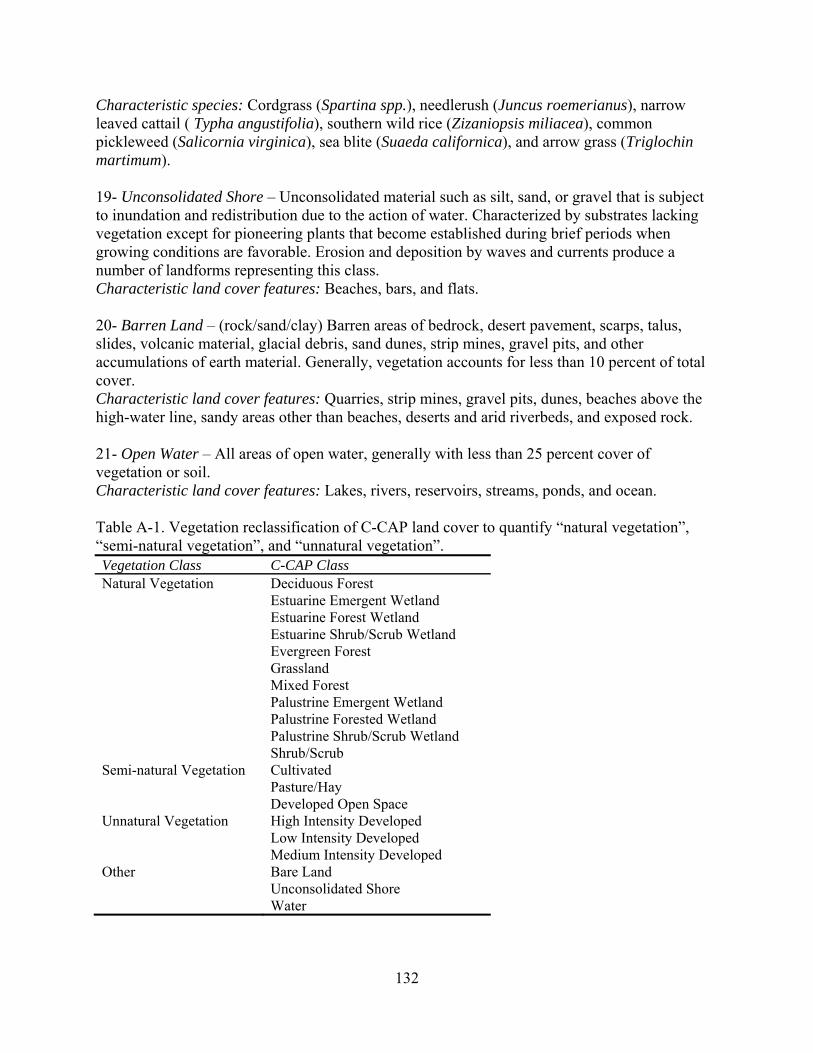
132

Characteristic species: Cordgrass (Spartina spp.), needlerush (Juncus roemerianus), narrow leaved cattail ( Typha angustifolia), southern wild rice (Zizaniopsis miliacea), common pickleweed (Salicornia virginica), sea blite (Suaeda californica), and arrow grass (Triglochin martimum). 19- Unconsolidated Shore – Unconsolidated material such as silt, sand, or gravel that is subject to inundation and redistribution due to the action of water. Characterized by substrates lacking vegetation except for pioneering plants that become established during brief periods when growing conditions are favorable. Erosion and deposition by waves and currents produce a number of landforms representing this class. Characteristic land cover features: Beaches, bars, and flats. 20- Barren Land – (rock/sand/clay) Barren areas of bedrock, desert pavement, scarps, talus, slides, volcanic material, glacial debris, sand dunes, strip mines, gravel pits, and other accumulations of earth material. Generally, vegetation accounts for less than 10 percent of total cover. Characteristic land cover features: Quarries, strip mines, gravel pits, dunes, beaches above the high-water line, sandy areas other than beaches, deserts and arid riverbeds, and exposed rock. 21- Open Water – All areas of open water, generally with less than 25 percent cover of vegetation or soil. Characteristic land cover features: Lakes, rivers, reservoirs, streams, ponds, and ocean. Table A-1. Vegetation reclassification of C-CAP land cover to quantify “natural vegetation”, “semi-natural vegetation”, and “unnatural vegetation”. Vegetation Class C-CAP Class Natural Vegetation Deciduous Forest Estuarine Emergent Wetland Estuarine Forest Wetland Estuarine Shrub/Scrub Wetland Evergreen Forest Grassland Mixed Forest Palustrine Emergent Wetland Palustrine Forested Wetland Palustrine Shrub/Scrub Wetland Shrub/Scrub Semi-natural Vegetation Cultivated Pasture/Hay Developed Open Space Unnatural Vegetation High Intensity Developed Low Intensity Developed Medium Intensity Developed Other Bare Land Unconsolidated Shore Water

Appendix B: Hydrology calculation methods. The 7.5-minute Digital Elevation Model (DEM) raster datasets were produced by the U.S. Geological Survey (2008a), and were obtained from the GeoCommunity website. We used “Extract by Mask” in ArcToolbox (ESRI 2006) to clip each DEM raster to the park boundaries. In some instances, the study areas of interest were contained in multiple quadrangles. In such cases, each raster dataset was clipped to the park boundary using the “Extract by Mask” tool and subsequently merged into one dataset using “Mosaic to New Raster” in ArcToolbox. Having clipped the DEM data to the park boundaries, the data were then reclassified, symbolized, and labeled to illustrate mean sea level, two-foot storm surges, and four-foot storm surges. Each reclassification permitted the analysis of changes in the acreage and percentage of land/water extent in each of the figures.

133

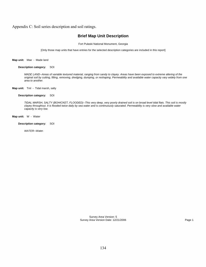
Appendix C: Soil series description and soil ratings. Brief Map Unit Description Fort Pulaski National Monument, Georgia

[Only those map units that have entries for the selected description categories are included in this report]

Map unit: Mae - Made land

Description category: SOI

MADE LAND--Areas of variable textured material, ranging from sandy to clayey. Areas have been exposed to extreme altering of the original soil by cutting, filling, removing, dredging, dumping, or reshaping. Permeability and available water capacity vary widely from one area to another.

Map unit: Tml - Tidal marsh, salty


TIDAL MARSH, SALTY (BOHICKET, FLOODED)--This very deep, very poorly drained soil is on broad level tidal flats. This soil is mostly clayey throughout. It is flooded twice daily by sea water and is continuously saturated. Permeability is very slow and available water capacity is very low.

Map unit: W - Water


WATER--Water.

Survey Area Version: 5 Survey Area Version Date: 12/21/2006 Page 1

134

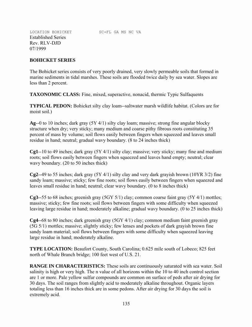
LOCATION BOHICKET SC+FL GA MS NC VA Established Series Rev. RLV-DJD 07/1999 BOHICKET SERIES The Bohicket series consists of very poorly drained, very slowly permeable soils that formed in marine sediments in tidal marshes. These soils are flooded twice daily by sea water. Slopes are less than 2 percent.

TAXONOMIC CLASS: Fine, mixed, superactive, nonacid, thermic Typic Sulfaquents

TYPICAL PEDON: Bohicket silty clay loam--saltwater marsh wildlife habitat. (Colors are for moist soil.)

Ag--0 to 10 inches; dark gray (5Y 4/1) silty clay loam; massive; strong fine angular blocky structure when dry; very sticky; many medium and coarse pithy fibrous roots constituting 35 percent of mass by volume; soil flows easily between fingers when squeezed and leaves small residue in hand; neutral; gradual wavy boundary. (8 to 24 inches thick)

Cg1--10 to 49 inches; dark gray (5Y 4/1) silty clay; massive; very sticky; many fine and medium roots; soil flows easily between fingers when squeezed and leaves hand empty; neutral; clear wavy boundary. (20 to 50 inches thick)

Cg2--49 to 55 inches; dark gray (5Y 4/1) silty clay and very dark grayish brown (10YR 3/2) fine sandy loam; massive; sticky; few fine roots; soil flows easily between fingers when squeezed and leaves small residue in hand; neutral; clear wavy boundary. (0 to 8 inches thick)

Cg3--55 to 68 inches; greenish gray (5GY 5/1) clay; common coarse faint gray (5Y 4/1) mottles; massive; sticky; few fine roots; soil flows between fingers with some difficulty when squeezed leaving large residue in hand; moderately alkaline; gradual wavy boundary. (0 to 25 inches thick)

Cg4--68 to 80 inches; dark greenish gray (5GY 4/1) clay; common medium faint greenish gray (5G 5/1) mottles; massive; slightly sticky; few lenses and pockets of dark grayish brown fine sandy loam material; soil flows between fingers with some difficulty when squeezed leaving large residue in hand; moderately alkaline.

TYPE LOCATION: Beaufort County, South Carolina; 0.625 mile south of Lobeco; 825 feet north of Whale Branch bridge; 100 feet west of U.S. 21.

RANGE IN CHARACTERISTICS: These soils are continuously saturated with sea water. Soil salinity is high or very high. The n value of all horizons within the 10 to 40 inch control section are 1 or more. Pale yellow sulfur compounds are common on surface of peds after air drying for 30 days. The soil ranges from slightly acid to moderately alkaline throughout. Organic layers totaling less than 16 inches thick are in some pedons. After air drying for 30 days the soil is extremely acid.

135

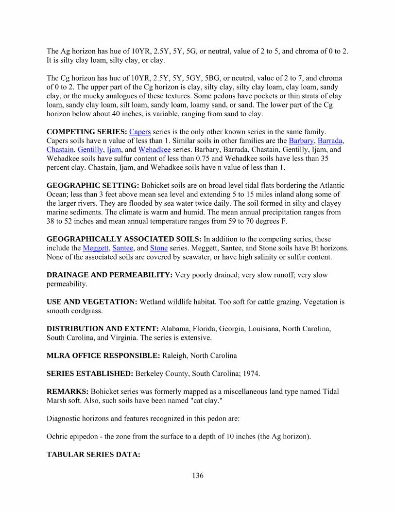
The Ag horizon has hue of 10YR, 2.5Y, 5Y, 5G, or neutral, value of 2 to 5, and chroma of 0 to 2. It is silty clay loam, silty clay, or clay.

The Cg horizon has hue of 10YR, 2.5Y, 5Y, 5GY, 5BG, or neutral, value of 2 to 7, and chroma of 0 to 2. The upper part of the Cg horizon is clay, silty clay, silty clay loam, clay loam, sandy clay, or the mucky analogues of these textures. Some pedons have pockets or thin strata of clay loam, sandy clay loam, silt loam, sandy loam, loamy sand, or sand. The lower part of the Cg horizon below about 40 inches, is variable, ranging from sand to clay.

COMPETING SERIES: Capers series is the only other known series in the same family. Capers soils have n value of less than 1. Similar soils in other families are the Barbary, Barrada, Chastain, Gentilly, Ijam, and Wehadkee series. Barbary, Barrada, Chastain, Gentilly, Ijam, and Wehadkee soils have sulfur content of less than 0.75 and Wehadkee soils have less than 35 percent clay. Chastain, Ijam, and Wehadkee soils have n value of less than 1.

GEOGRAPHIC SETTING: Bohicket soils are on broad level tidal flats bordering the Atlantic Ocean; less than 3 feet above mean sea level and extending 5 to 15 miles inland along some of the larger rivers. They are flooded by sea water twice daily. The soil formed in silty and clayey marine sediments. The climate is warm and humid. The mean annual precipitation ranges from 38 to 52 inches and mean annual temperature ranges from 59 to 70 degrees F.

GEOGRAPHICALLY ASSOCIATED SOILS: In addition to the competing series, these include the Meggett, Santee, and Stone series. Meggett, Santee, and Stone soils have Bt horizons. None of the associated soils are covered by seawater, or have high salinity or sulfur content.

DRAINAGE AND PERMEABILITY: Very poorly drained; very slow runoff; very slow permeability.

USE AND VEGETATION: Wetland wildlife habitat. Too soft for cattle grazing. Vegetation is smooth cordgrass.

DISTRIBUTION AND EXTENT: Alabama, Florida, Georgia, Louisiana, North Carolina, South Carolina, and Virginia. The series is extensive.

MLRA OFFICE RESPONSIBLE: Raleigh, North Carolina

SERIES ESTABLISHED: Berkeley County, South Carolina; 1974.

REMARKS: Bohicket series was formerly mapped as a miscellaneous land type named Tidal Marsh soft. Also, such soils have been named "cat clay."

Diagnostic horizons and features recognized in this pedon are:

Ochric epipedon - the zone from the surface to a depth of 10 inches (the Ag horizon).

TABULAR SERIES DATA:

136

http://ortho.ftw.nrcs.usda.gov/osd/dat/C/CAPERS.html

http://ortho.ftw.nrcs.usda.gov/osd/dat/B/BARBARY.html

http://ortho.ftw.nrcs.usda.gov/osd/dat/B/BARRADA.html

http://ortho.ftw.nrcs.usda.gov/osd/dat/C/CHASTAIN.html

http://ortho.ftw.nrcs.usda.gov/osd/dat/G/GENTILLY.html

http://ortho.ftw.nrcs.usda.gov/osd/dat/I/IJAM.html

http://ortho.ftw.nrcs.usda.gov/osd/dat/W/WEHADKEE.html

http://ortho.ftw.nrcs.usda.gov/osd/dat/M/MEGGETT.html

http://ortho.ftw.nrcs.usda.gov/osd/dat/S/SANTEE.html

http://ortho.ftw.nrcs.usda.gov/osd/dat/S/STONE.html

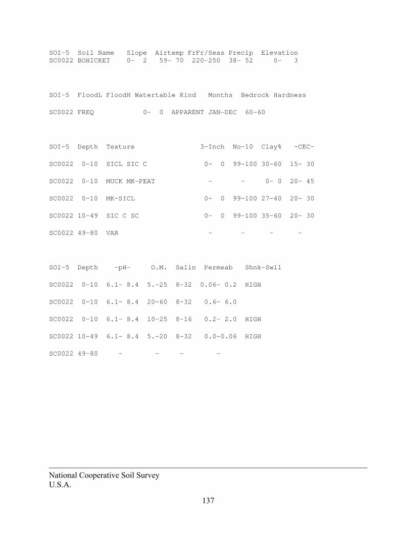
137

SOI-5 Soil Name Slope Airtemp FrFr/Seas Precip Elevation SC0022 BOHICKET 0- 2 59- 70 220-250 38- 52 0- 3

SOI-5 FloodL FloodH Watertable Kind Months Bedrock Hardness

SC0022 FREQ 0- 0 APPARENT JAN-DEC 60-60

SOI-5 Depth Texture 3-Inch No-10 Clay% -CEC-

SC0022 0-10 SICL SIC C 0- 0 99-100 30-60 15- 30

SC0022 0-10 MUCK MK-PEAT - - 0- 0 20- 45

SC0022 0-10 MK-SICL 0- 0 99-100 27-40 20- 30

SC0022 10-49 SIC C SC 0- 0 99-100 35-60 20- 30

SC0022 49-80 VAR - - - -

SOI-5 Depth -pH- O.M. Salin Permeab Shnk-Swll

SC0022 0-10 6.1- 8.4 5.-25 8-32 0.06- 0.2 HIGH

SC0022 0-10 6.1- 8.4 20-60 8-32 0.6- 6.0

SC0022 0-10 6.1- 8.4 10-25 8-16 0.2- 2.0 HIGH

SC0022 10-49 6.1- 8.4 5.-20 8-32 0.0-0.06 HIGH

SC0022 49-80 - - - -

National Cooperative Soil Survey U.S.A.

138

Potential Erosion Hazard (Off-Road, Off-Trail)

Aggregation Method: Dominant Condition Tie-break Rule: Higher

Fort Pulaski National Monument, Georgia Survey Area Version and Date: 5 - 12/21/2006

Map symbol Map unit name

Component name and % composition Rating reasons Rating

Mae Made land Not rated Made land 100%

Tml Tidal marsh, salty Slight Tidal marsh, salty 100%

W Water Not rated Water 100%

Application Version: 5.2.0016 12/10/2008

Page 1 of 2

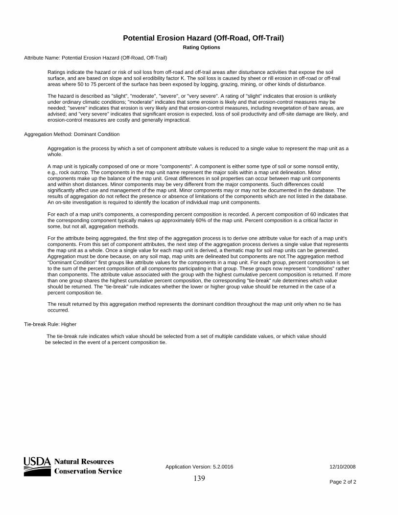
Potential Erosion Hazard (Off-Road, Off-Trail)

Rating Options

Attribute Name: Potential Erosion Hazard (Off-Road, Off-Trail)

Ratings indicate the hazard or risk of soil loss from off-road and off-trail areas after disturbance activities that expose the soil surface, and are based on slope and soil erodibility factor K. The soil loss is caused by sheet or rill erosion in off-road or off-trail areas where 50 to 75 percent of the surface has been exposed by logging, grazing, mining, or other kinds of disturbance.

The hazard is described as "slight", "moderate", "severe", or "very severe". A rating of "slight" indicates that erosion is unlikely under ordinary climatic conditions; "moderate" indicates that some erosion is likely and that erosion-control measures may be needed; "severe" indicates that erosion is very likely and that erosion-control measures, including revegetation of bare areas, are advised; and "very severe" indicates that significant erosion is expected, loss of soil productivity and off-site damage are likely, and erosion-control measures are costly and generally impractical.

Aggregation Method: Dominant Condition

Aggregation is the process by which a set of component attribute values is reduced to a single value to represent the map unit as a whole.

A map unit is typically composed of one or more "components". A component is either some type of soil or some nonsoil entity, e.g., rock outcrop. The components in the map unit name represent the major soils within a map unit delineation. Minor components make up the balance of the map unit. Great differences in soil properties can occur between map unit components and within short distances. Minor components may be very different from the major components. Such differences could significantly affect use and management of the map unit. Minor components may or may not be documented in the database. The results of aggregation do not reflect the presence or absence of limitations of the components which are not listed in the database. An on-site investigation is required to identify the location of individual map unit components.

For each of a map unit's components, a corresponding percent composition is recorded. A percent composition of 60 indicates that the corresponding component typically makes up approximately 60% of the map unit. Percent composition is a critical factor in some, but not all, aggregation methods.

For the attribute being aggregated, the first step of the aggregation process is to derive one attribute value for each of a map unit's components. From this set of component attributes, the next step of the aggregation process derives a single value that represents the map unit as a whole. Once a single value for each map unit is derived, a thematic map for soil map units can be generated. Aggregation must be done because, on any soil map, map units are delineated but components are not.The aggregation method "Dominant Condition" first groups like attribute values for the components in a map unit. For each group, percent composition is set to the sum of the percent composition of all components participating in that group. These groups now represent "conditions" rather than components. The attribute value associated with the group with the highest cumulative percent composition is returned. If more than one group shares the highest cumulative percent composition, the corresponding "tie-break" rule determines which value should be returned. The "tie-break" rule indicates whether the lower or higher group value should be returned in the case of a percent composition tie.

The result returned by this aggregation method represents the dominant condition throughout the map unit only when no tie has occurred.

Tie-break Rule: Higher

The tie-break rule indicates which value should be selected from a set of multiple candidate values, or which value should be selected in the event of a percent composition tie.

139


Page 2 of 2

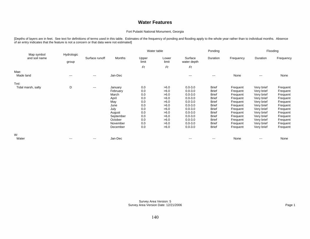
140

Water Features Fort Pulaski National Monument, Georgia

[Depths of layers are in feet. See text for definitions of terms used in this table. Estimates of the frequency of ponding and flooding apply to the whole year rather than to individual months. Absence of an entry indicates that the feature is not a concern or that data were not estimated]

Water table Ponding Flooding Map symbol Hydrologic and soil name Surface runoff Months Upper Lower Surface Duration Frequency Duration Frequency group limit limit water depth Ft Ft Ft Mae: Made land --- --- Jan-Dec --- --- None --- None

Tml: Tidal marsh, salty D --- January 0.0 >6.0 0.0-3.0 Brief Frequent Very brief Frequent February 0.0 >6.0 0.0-3.0 Brief Frequent Very brief Frequent March 0.0 >6.0 0.0-3.0 Brief Frequent Very brief Frequent April 0.0 >6.0 0.0-3.0 Brief Frequent Very brief Frequent May 0.0 >6.0 0.0-3.0 Brief Frequent Very brief Frequent June 0.0 >6.0 0.0-3.0 Brief Frequent Very brief Frequent July 0.0 >6.0 0.0-3.0 Brief Frequent Very brief Frequent August 0.0 >6.0 0.0-3.0 Brief Frequent Very brief Frequent September 0.0 >6.0 0.0-3.0 Brief Frequent Very brief Frequent October 0.0 >6.0 0.0-3.0 Brief Frequent Very brief Frequent November 0.0 >6.0 0.0-3.0 Brief Frequent Very brief Frequent December 0.0 >6.0 0.0-3.0 Brief Frequent Very brief Frequent

W: Water --- --- Jan-Dec --- --- None --- None

Survey Area Version: 5 Survey Area Version Date: 12/21/2006 Page 1

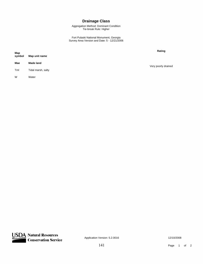
141

Drainage Class

Aggregation Method: Dominant Condition Tie-break Rule: Higher



Rating

Mae Made land

Very poorly drained Tml Tidal marsh, salty

W Water


Page 1 of 2

142

Drainage Class Rating Options

Attribute Name: Drainage Class

Drainage class (natural) refers to the frequency and duration of wet periods under conditions similar to those under which the soil formed. Alterations of the water regime by human activities, either through drainage or irrigation, are not a consideration unless they have significantly changed the morphology of the soil. Seven classes of natural soil drainage are recognized -- excessively drained, somewhat excessively drained, well drained, moderately well drained, somewhat poorly drained, poorly drained, and very poorly drained. These classes are defined in the "Soil Survey Manual."

Aggregation Method: Dominant Condition




For the attribute being aggregated, the first step of the aggregation process is to derive one attribute value for each of a map unit's components. From this set of component attributes, the next step of the aggregation process derives a single value that represents the map unit as a whole. Once a single value for each map unit is derived, a thematic map for soil map units can be generated. Aggregation must be done because, on any soil map, map units are delineated but components are not.The aggregation method "Dominant Condition" first groups like attribute values for the components in a map unit. For each group, percent composition is set to the sum of the percent composition of all components participating in that group. These groups now represent "conditions" rather than components. The attribute value associated with the group with the highest cumulative percent composition is returned. If more than one group shares the highest cumulative percent composition, the corresponding "tie-break" rule determines which value should be returned. The "tie-break" rule indicates whether the lower or higher group value should be returned in the case of a percent composition tie.

The result returned by this aggregation method represents the dominant condition throughout the map unit only when no tie has occurred.

Tie-break Rule: Higher



Page 2 of 2

143

Map Unit Hydric Rating

Aggregation Method: Absence/Presence Tie-break Rule: Lower



Rating

Mae Made land Unknown Hydric

Tml Tidal marsh, salty All Hydric

W Water Not Hydric


Page 1 of 2

144

Map Unit Hydric Rating Rating Options

Attribute Name: Map Unit Hydric Rating

This rating provides an indication of the proportion of the map unit that meets criteria for hydric soils. Map units that are dominantly made up of hydric soils may have small areas, or inclusions, of nonhydric soils in the higher positions on the landform, and map units dominantly made up of nonhydric soils may have inclusions of hydric soils in the lower positions on the landform.

Hydric soils are defined by the National Technical Committee for Hydric Soils (NTCHS) as soils that formed under conditions of saturation, flooding, or ponding long enough during the growing season to develop anaerobic conditions in the upper part (Federal Register, 1994). These soils, under natural conditions, are either saturated or inundated long enough during the growing season to support the growth and reproduction of hydrophytic vegetation.

The NTCHS definition identifies general soil properties that are associated with wetness. In order to determine whether a specific soil is a hydric soil or nonhydric soil, however, more specific information, such as information about the depth and duration of the water table, is needed. Thus, criteria that identify those estimated soil properties unique to hydric soils have been established (Federal Register, 2002). These criteria are used to identify map unit components that normally are associated with wetlands. The criteria used are selected estimated soil properties that are described in "Soil Taxonomy" (Soil Survey Staff, 1999) and "Keys to Soil Taxonomy" (Soil Survey Staff, 2003) and in the "Soil Survey Manual" (Soil Survey Division Staff, 1993).

If soils are wet enough for a long enough period of time to be considered hydric, they should exhibit certain properties that can be easily observed in the field. These visible properties are indicators of hydric soils. The indicators used to make onsite determinations of hydric soils are specified in "Field Indicators of Hydric Soils in the United States" (Hurt and others, 2002).

Aggregation Method: Absence/Presence




For the attribute being aggregated, the first step of the aggregation process is to derive one attribute value for each of a map unit's components. From this set of component attributes, the next step of the aggregation process derives a single value that represents the map unit as a whole. Once a single value for each map unit is derived, a thematic map for soil map units can be generated. Aggregation must be done because, on any soil map, map units are delineated but components are not.The aggregation method "Absence/Presence" returns a value that indicates if, for all components of a map unit, a condition is always present, never present, partially present, or whether the condition's presence or absence is unknown. The exact phrases used for a particular attribute may vary from what is shown below.

"Always present" means that the corresponding condition is present in all of a map unit's components.

"Never present" means that the corresponding condition is not present in any of a map unit's components.

"Partially present" means that the corresponding condition is present in some but not all of a map unit's components, or that the presence or absence of the corresponding condition cannot be determined for one or more components of the map unit.

"Unknown presence" means that for components where presence or absence can be determined, the corresponding condition is never present, but the presence or absence of the corresponding condition cannot be determined for one or more components.

The result returned by this aggregation method quantifies the degree to which the corresponding condition is present throughout the map unit.

Tie-break Rule: Lower



Page 2 of 2

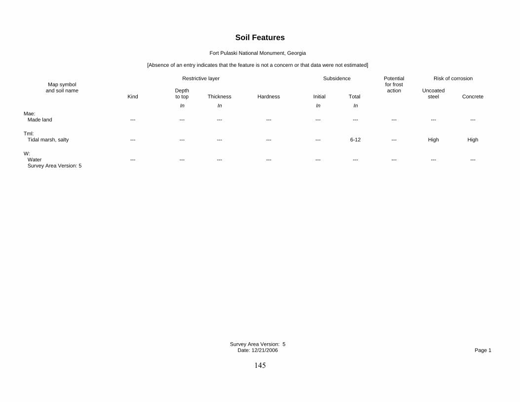
145

Soil Features Fort Pulaski National Monument, Georgia

[Absence of an entry indicates that the feature is not a concern or that data were not estimated]

Restrictive layer Subsidence Potential Risk of corrosion Map symbol for frost and soil name Depth action Uncoated Kind to top Thickness Hardness Initial Total steel Concrete In In In In Mae: Made land --- --- --- --- --- --- --- --- ---

Tml: Tidal marsh, salty --- --- --- --- --- 6-12 --- High High

W: Water --- --- --- --- --- --- --- --- --- Survey Area Version: 5 Survey Area Version: 5 Date: 12/21/2006 Page 1

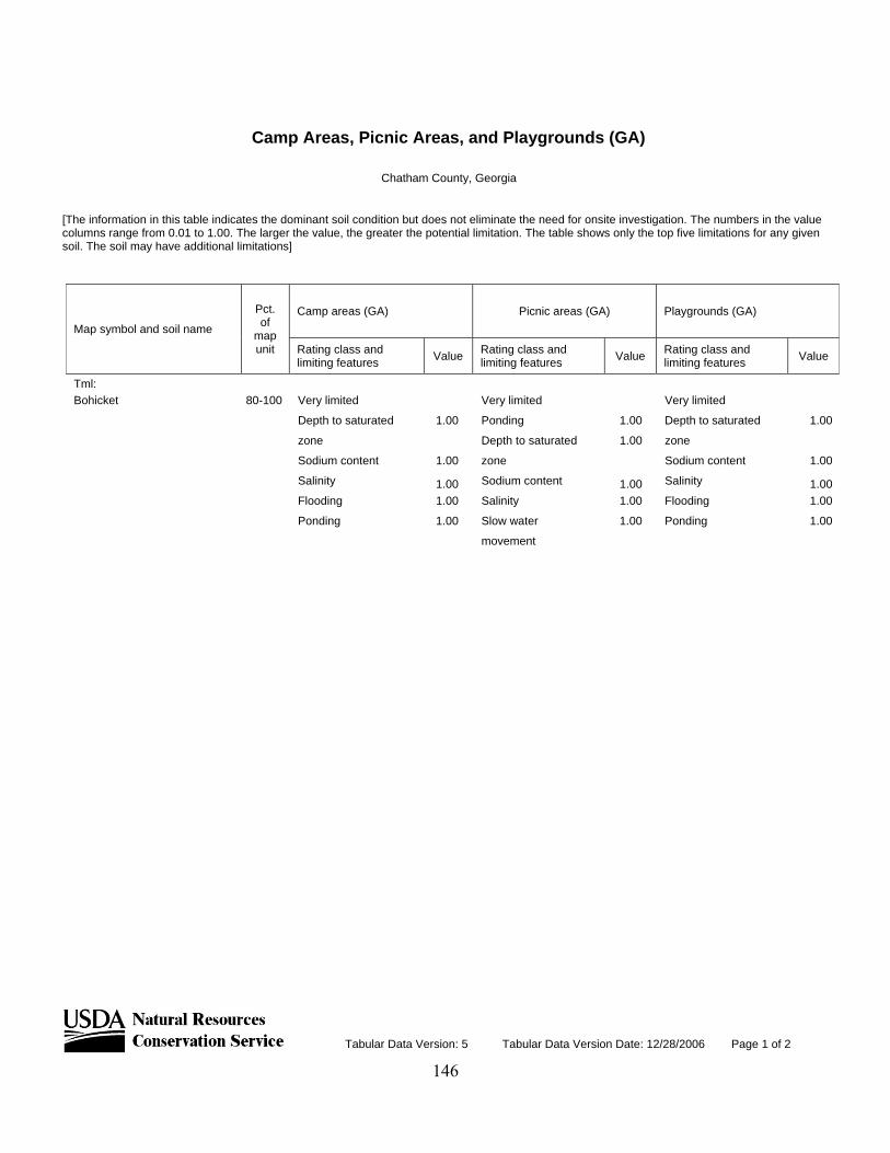
Chatham County, Georgia

[The information in this table indicates the dominant soil condition but does not eliminate the need for onsite investigation. The numbers in the value columns range from 0.01 to 1.00. The larger the value, the greater the potential limitation. The table shows only the top five limitations for any given soil. The soil may have additional limitations]

Camp Areas, Picnic Areas, and Playgrounds (GA)

Tabular Data Version: 5 Tabular Data Version Date: 12/28/2006 Page 1 of 2

Map symbol and soil name

Pct. of

map unit

Camp areas (GA) Picnic areas (GA) Playgrounds (GA)

Rating class and limiting features Value Rating class and

limiting features Value Rating class and limiting features Value

Tml: Bohicket 80-100 Very limited Very limited Very limited

Depth to saturated 1.00 Ponding 1.00 Depth to saturated 1.00

zone Depth to saturated 1.00 zone

Sodium content 1.00 zone Sodium content 1.00

Salinity 1.00 Sodium content 1.00 Salinity 1.00

Flooding 1.00 Salinity 1.00 Flooding 1.00

Ponding 1.00 Slow water 1.00 Ponding 1.00

movement

146

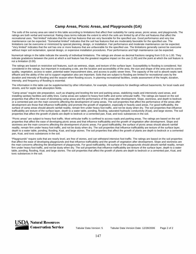
147

Camp Areas, Picnic Areas, and Playgrounds (GA) The soils of the survey area are rated in this table according to limitations that affect their suitability for camp areas, picnic areas, and playgrounds. The ratings are both verbal and numerical. Rating class terms indicate the extent to which the soils are limited by all of the soil features that affect the recreational uses. “Not limited” indicates that the soil has features that are very favorable for the specified use. Good performance and very low maintenance can be expected. “Somewhat limited” indicates that the soil has features that are moderately favorable for the specified use. The limitations can be overcome or minimized by special planning, design, or installation. Fair performance and moderate maintenance can be expected. “Very limited” indicates that the soil has one or more features that are unfavorable for the specified use. The limitations generally cannot be overcome without major soil reclamation, special design, or expensive installation procedures. Poor performance and high maintenance can be expected.

Numerical ratings in the table indicate the severity of individual limitations. The ratings are shown as decimal fractions ranging from 0.01 to 1.00. They indicate gradations between the point at which a soil feature has the greatest negative impact on the use (1.00) and the point at which the soil feature is not a limitation (0.00).

The ratings are based on restrictive soil features, such as wetness, slope, and texture of the surface layer. Susceptibility to flooding is considered. Not considered in the ratings, but important in evaluating a site, are the location and accessibility of the area, the size and shape of the area and its scenic quality, vegetation, access to water, potential water impoundment sites, and access to public sewer lines. The capacity of the soil to absorb septic tank effluent and the ability of the soil to support vegetation also are important. Soils that are subject to flooding are limited for recreational uses by the duration and intensity of flooding and the season when flooding occurs. In planning recreational facilities, onsite assessment of the height, duration, intensity, and frequency of flooding is essential.

The information in this table can be supplemented by other information, for example, interpretations for dwellings without basements, for local roads and streets, and for septic tank absorption fields.

“Camp areas” require site preparation, such as shaping and leveling the tent and parking areas, stabilizing roads and intensively used areas, and installing sanitary facilities and utility lines. Camp areas are subject to heavy foot traffic and some vehicular traffic. The ratings are based on the soil properties that affect the ease of developing camp areas and the performance of the areas after development. Slope, stoniness, and depth to bedrock or a cemented pan are the main concerns affecting the development of camp areas. The soil properties that affect the performance of the areas after development are those that influence trafficability and promote the growth of vegetation, especially in heavily used areas. For good trafficability, the surface of camp areas should absorb rainfall readily, remain firm under heavy foot traffic, and not be dusty when dry. The soil properties that influence trafficability are texture of the surface layer, depth to a water table, ponding, flooding, saturated hydraulic conductivity (Ksat), and large stones. The soil properties that affect the growth of plants are depth to bedrock or a cemented pan, Ksat, and toxic substances in the soil.

“Picnic areas” are subject to heavy foot traffic. Most vehicular traffic is confined to access roads and parking areas. The ratings are based on the soil properties that affect the ease of developing picnic areas and that influence trafficability and the growth of vegetation after development. Slope and stoniness are the main concerns affecting the development of picnic areas. For good trafficability, the surface of picnic areas should absorb rainfall readily, remain firm under heavy foot traffic, and not be dusty when dry. The soil properties that influence trafficability are texture of the surface layer, depth to a water table, ponding, flooding, Ksat, and large stones. The soil properties that affect the growth of plants are depth to bedrock or a cemented pan, Ksat, and toxic substances in the soil.

“Playgrounds” require soils that are nearly level, are free of stones, and can withstand intensive foot traffic. The ratings are based on the soil properties that affect the ease of developing playgrounds and that influence trafficability and the growth of vegetation after development. Slope and stoniness are the main concerns affecting the development of playgrounds. For good trafficability, the surface of the playgrounds should absorb rainfall readily, remain firm under heavy foot traffic, and not be dusty when dry. The soil properties that influence trafficability are texture of the surface layer, depth to a water table, ponding, flooding, Ksat, and large stones. The soil properties that affect the growth of plants are depth to bedrock or a cemented pan, Ksat, and toxic substances in the soil.

Tabular Data Version: 5 Tabular Data Version Date: 12/28/2006 Page 2 of 2

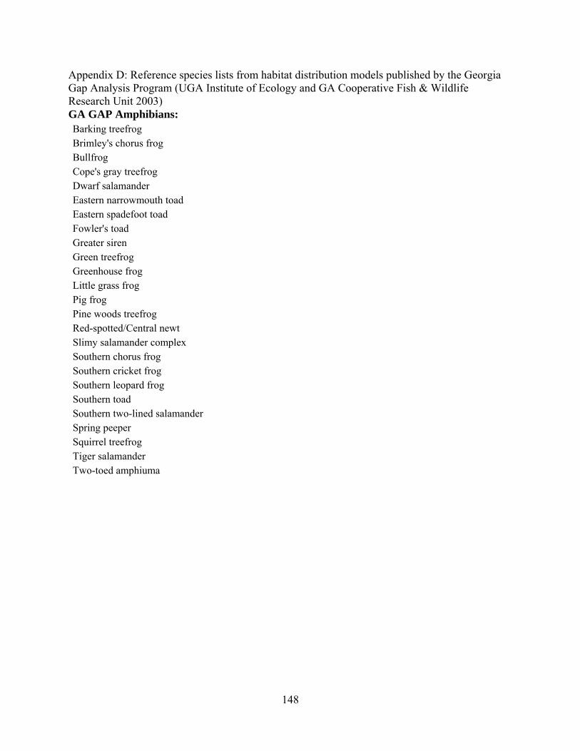
Appendix D: Reference species lists from habitat distribution models published by the Georgia Gap Analysis Program (UGA Institute of Ecology and GA Cooperative Fish & Wildlife Research Unit 2003) GA GAP Amphibians: Barking treefrog Brimley's chorus frog Bullfrog Cope's gray treefrog Dwarf salamander Eastern narrowmouth toad Eastern spadefoot toad Fowler's toad

Southern leopard frog

Greater siren Green treefrog Greenhouse frog Little grass frog Pig frog Pine woods treefrog Red-spotted/Central newt Slimy salamander complex Southern chorus frog Southern cricket frog

Southern toad Southern two-lined salamander Spring peeper Squirrel treefrog Tiger salamander Two-toed amphiuma

148

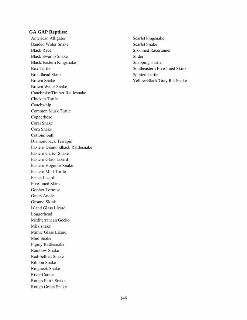
Eastern Glass Lizard

GA GAP Reptiles:American Alligator Banded Water Snake Black Racer Black Swamp Snake Black/Eastern Kingsnake Box Turtle Broadhead Skink Brown Snake Brown Water Snake Canebrake/Timber Rattlesnake Chicken Turtle Coachwhip Common Musk Turtle Copperhead Coral Snake Corn Snake Cottonmouth Diamondback Terrapin Eastern Diamondback Rattlesnake Eastern Garter Snake

Eastern Hognose Snake Eastern Mud Turtle Fence Lizard Five-lined Skink Gopher Tortoise Green Anole Ground Skink Island Glass Lizard Loggerhead Mediterranean Gecko Milk snake Mimic Glass Lizard Mud Snake Pigmy Rattlesnake Rainbow Snake Red-bellied Snake Ribbon Snake Ringneck Snake River Cooter Rough Earth Snake Rough Green Snake

Scarlet kingsnake Scarlet Snake Six-lined Racerunner Slider Snapping Turtle Southeastern Five-lined Skink Spotted Turtle Yellow/Black/Gray Rat Snake

149

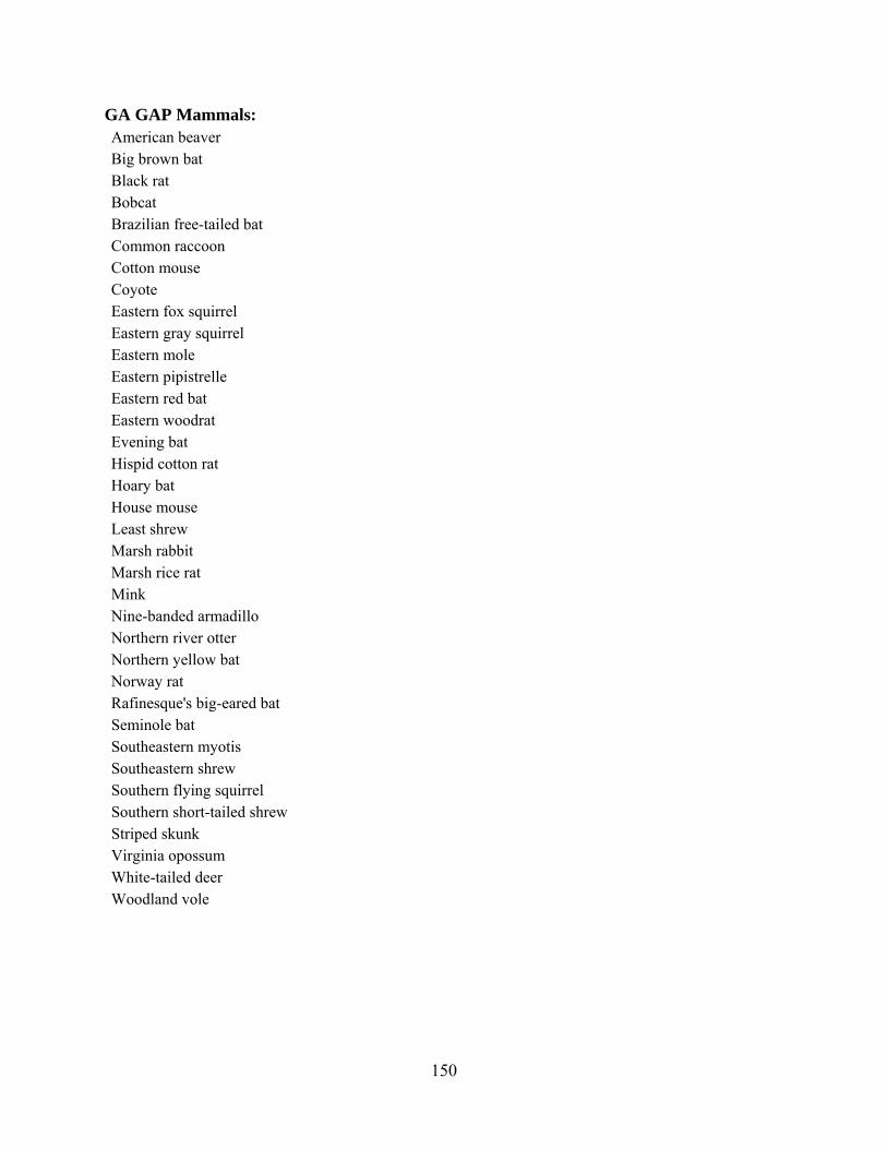
GA GAP Mammals: American beaver Big brown bat Black rat Bobcat Brazilian free-tailed bat Common raccoon Cotton mouse Coyote

Marsh rice rat

Eastern fox squirrel Eastern gray squirrel Eastern mole Eastern pipistrelle Eastern red bat Eastern woodrat Evening bat Hispid cotton rat Hoary bat House mouse Least shrew Marsh rabbit

Mink Nine-banded armadillo Northern river otter Northern yellow bat Norway rat Rafinesque's big-eared bat Seminole bat Southeastern myotis Southeastern shrew Southern flying squirrel Southern short-tailed shrew Striped skunk Virginia opossum White-tailed deer Woodland vole

150

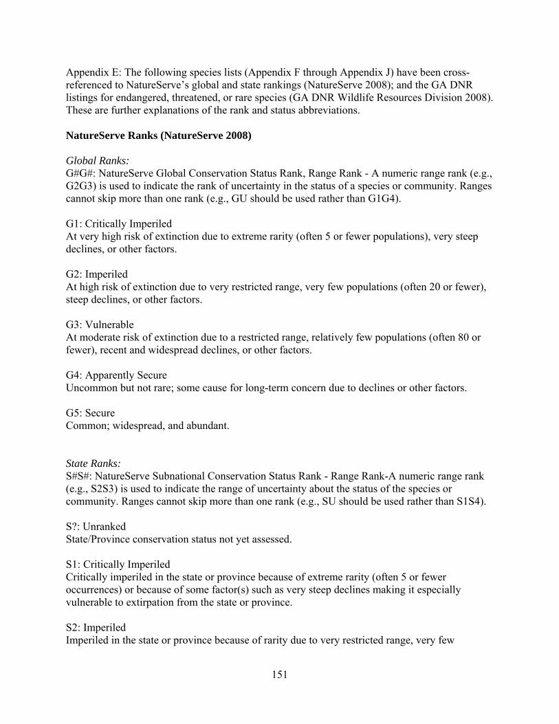
Appendix E: The following species lists (Appendix F through Appendix J) have been cross-referenced to NatureServe’s global and state rankings (NatureServe 2008); and the GA DNR listings for endangered, threatened, or rare species (GA DNR Wildlife Resources Division 2008). These are further explanations of the rank and status abbreviations. NatureServe Ranks (NatureServe 2008) Global Ranks: G#G#: NatureServe Global Conservation Status Rank, Range Rank - A numeric range rank (e.g., G2G3) is used to indicate the rank of uncertainty in the status of a species or community. Ranges cannot skip more than one rank (e.g., GU should be used rather than G1G4). G1: Critically Imperiled At very high risk of extinction due to extreme rarity (often 5 or fewer populations), very steep declines, or other factors. G2: Imperiled At high risk of extinction due to very restricted range, very few populations (often 20 or fewer), steep declines, or other factors. G3: Vulnerable At moderate risk of extinction due to a restricted range, relatively few populations (often 80 or fewer), recent and widespread declines, or other factors. G4: Apparently Secure Uncommon but not rare; some cause for long-term concern due to declines or other factors. G5: Secure Common; widespread, and abundant. State Ranks: S#S#: NatureServe Subnational Conservation Status Rank - Range Rank-A numeric range rank (e.g., S2S3) is used to indicate the range of uncertainty about the status of the species or community. Ranges cannot skip more than one rank (e.g., SU should be used rather than S1S4). S?: Unranked State/Province conservation status not yet assessed. S1: Critically Imperiled Critically imperiled in the state or province because of extreme rarity (often 5 or fewer occurrences) or because of some factor(s) such as very steep declines making it especially vulnerable to extirpation from the state or province. S2: Imperiled Imperiled in the state or province because of rarity due to very restricted range, very few

151

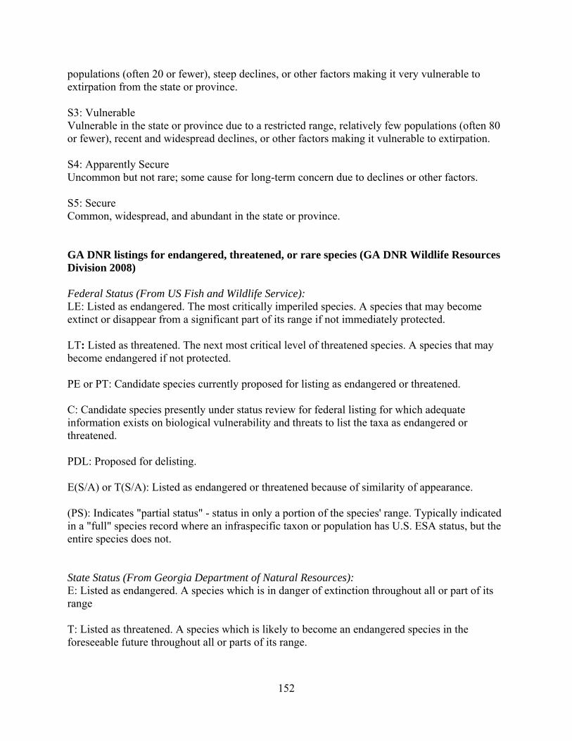
populations (often 20 or fewer), steep declines, or other factors making it very vulnerable to extirpation from the state or province. S3: Vulnerable Vulnerable in the state or province due to a restricted range, relatively few populations (often 80 or fewer), recent and widespread declines, or other factors making it vulnerable to extirpation. S4: Apparently Secure Uncommon but not rare; some cause for long-term concern due to declines or other factors. S5: Secure Common, widespread, and abundant in the state or province. GA DNR listings for endangered, threatened, or rare species (GA DNR Wildlife Resources Division 2008) Federal Status (From US Fish and Wildlife Service): LE: Listed as endangered. The most critically imperiled species. A species that may become extinct or disappear from a significant part of its range if not immediately protected. LT: Listed as threatened. The next most critical level of threatened species. A species that may become endangered if not protected. PE or PT: Candidate species currently proposed for listing as endangered or threatened. C: Candidate species presently under status review for federal listing for which adequate information exists on biological vulnerability and threats to list the taxa as endangered or threatened. PDL: Proposed for delisting. E(S/A) or T(S/A): Listed as endangered or threatened because of similarity of appearance. (PS): Indicates "partial status" - status in only a portion of the species' range. Typically indicated in a "full" species record where an infraspecific taxon or population has U.S. ESA status, but the entire species does not. State Status (From Georgia Department of Natural Resources): E: Listed as endangered. A species which is in danger of extinction throughout all or part of its range T: Listed as threatened. A species which is likely to become an endangered species in the foreseeable future throughout all or parts of its range.

152

153

R: Listed as rare. A species which may not be endangered or threatened but which should be protected because of its scarcity. U: Listed as unusual (and thus deserving of special consideration). Plants subject to commercial exploitation would have this status

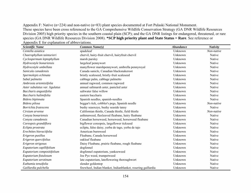
Appendix F: Native (n=224) and non-native (n=83) plant species documented at Fort Pulaski National Monument. These species have been cross referenced to the GA Comprehensive Wildlife Conservation Strategy (GA DNR Wildlife Resources Division 2005) high priority species in the southern coastal plain (SCP); and the GA DNR listings for endangered, threatened, or rare species (GA DNR Wildlife Resources Division 2008). *SCP high priority plant and State Status = Rare. See reference or Appendix E for explanation of abbreviations. Scientific Name Common Name(s) Abundance Nativity Centella asiatica

spadeleaf Unknown Non-native Chaerophyllum tainturieri chervil, hairy-fruit chervil, hairyfruit chervil Unknown Native Cyclospermum leptophyllum marsh parsley Unknown Native Hydrocotyle bonariensis largeleaf pennywort Unknown Native Hydrocotyle umbellata manyflower marshpennywort, umbrella pennyroyal Unknown Native Sanicula canadensis Canada sanicle, Canadian blacksnakeroot Unknown Native Spermolepis echinata bristly scaleseed, bristly-fruit scaleseed Unknown Native Sabal palmetto cabbage palm, cabbage palmetto Unknown Native Ambrosia artemisiifolia annual ragweed, common ragweed Unknown Native Aster subulatus var. ligulatus annual saltmarsh aster, panicled aster Unknown Native Baccharis angustifolia saltwater false willow Unknown Native Baccharis halimifolia eastern baccharis Unknown Native Bidens bipinnata Spanish needles, spanish-needles Unknown Native Bidens pilosa beggar's tick, cobbler's pegs, Spanish needle Unknown Non-native Borrichia frutescens bushy seaoxeye, bushy seaside tansy Unknown Native Cirsium arvense Californian thistle, Canada thistle, field thistle Unknown Non-native Conyza bonariensis asthmaweed, flaxleaved fleabane, hairy fleabane Unknown Native Conyza canadensis Canadian horseweed, horseweed, horseweed fleabane Unknown Native Coreopsis grandiflora bigflower coreopsis, largeflower tickseed Unknown Native Eclipta prostrata eclipta, false daisy, yerba de tago, yerba de tajo Unknown Native Erechtites hieraciifolia American burnweed Unknown Native Erigeron pusillus Fleabane, Canada horseweed Unknown Native Erigeron quercifolius oakleaf fleabane Unknown Native Erigeron strigosus Daisy Fleabane, prairie fleabane, rough fleabane Unknown Native Eupatorium capillifolium dogfennel Unknown Native Eupatorium compositifolium dogfennel eupatorium, yankeeweed Unknown Native Eupatorium fistulosum Joe Pye weed, trumpetweed Unknown Native Eupatorium serotinum late eupatorium, lateflowering thoroughwort Unknown Native Euthamia tenuifolia slender goldentop Unknown Native Gaillardia pulchella firewheel, Indian blanket, Indianblanket, rosering gaillardia Unknown Native

154

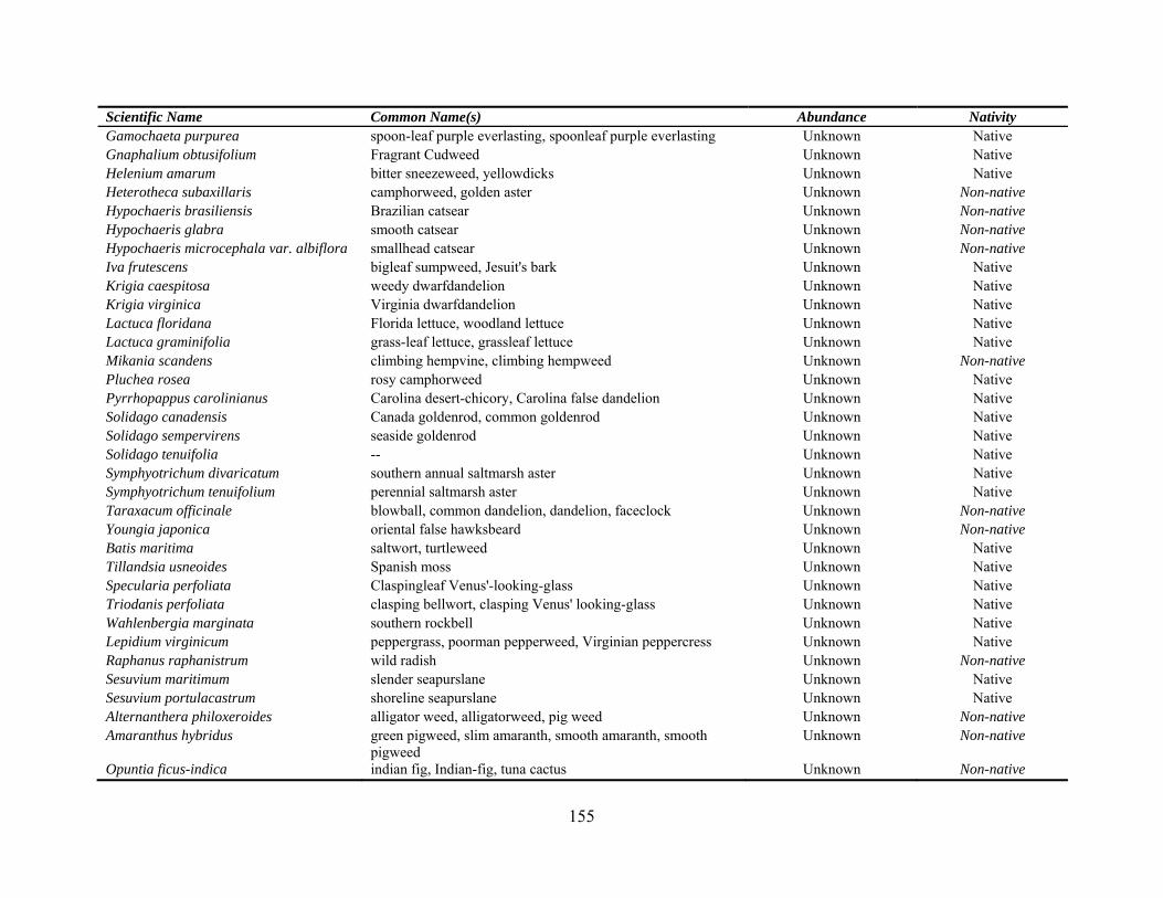
Scientific Name Common Name(s) Abundance Nativity Gamochaeta purpurea spoon-leaf purple everlasting, spoonleaf purple everlasting Unknown Native Gnaphalium obtusifolium Fragrant Cudweed Unknown Native Helenium amarum bitter sneezeweed, yellowdicks Unknown Native Heterotheca subaxillaris camphorweed, golden aster Unknown Non-native Hypochaeris brasiliensis Brazilian catsear Unknown Non-native Hypochaeris glabra smooth catsear Unknown Non-native Hypochaeris microcephala var. albiflora smallhead catsear Unknown Non-native Iva frutescens bigleaf sumpweed, Jesuit's bark Unknown Native Krigia caespitosa weedy dwarfdandelion Unknown Native Krigia virginica Virginia dwarfdandelion Unknown Native Lactuca floridana Florida lettuce, woodland lettuce Unknown Native Lactuca graminifolia grass-leaf lettuce, grassleaf lettuce Unknown Native Mikania scandens climbing hempvine, climbing hempweed Unknown Non-native Pluchea rosea rosy camphorweed Unknown Native Pyrrhopappus carolinianus Carolina desert-chicory, Carolina false dandelion Unknown Native Solidago canadensis Canada goldenrod, common goldenrod Unknown Native Solidago sempervirens seaside goldenrod Unknown Native Solidago tenuifolia -- Unknown Native Symphyotrichum divaricatum southern annual saltmarsh aster Unknown Native Symphyotrichum tenuifolium perennial saltmarsh aster Unknown Native Taraxacum officinale blowball, common dandelion, dandelion, faceclock Unknown Non-native Youngia japonica oriental false hawksbeard Unknown Non-native Batis maritima saltwort, turtleweed Unknown Native Tillandsia usneoides Spanish moss Unknown Native Specularia perfoliata Claspingleaf Venus'-looking-glass Unknown Native Triodanis perfoliata clasping bellwort, clasping Venus' looking-glass Unknown Native Wahlenbergia marginata southern rockbell Unknown Native Lepidium virginicum peppergrass, poorman pepperweed, Virginian peppercress Unknown Native Raphanus raphanistrum wild radish Unknown Non-native Sesuvium maritimum slender seapurslane Unknown Native Sesuvium portulacastrum shoreline seapurslane Unknown Native Alternanthera philoxeroides alligator weed, alligatorweed, pig weed Unknown Non-native Amaranthus hybridus green pigweed, slim amaranth, smooth amaranth, smooth

pigweed Unknown Non-native

Opuntia ficus-indica indian fig, Indian-fig, tuna cactus Unknown Non-native

155

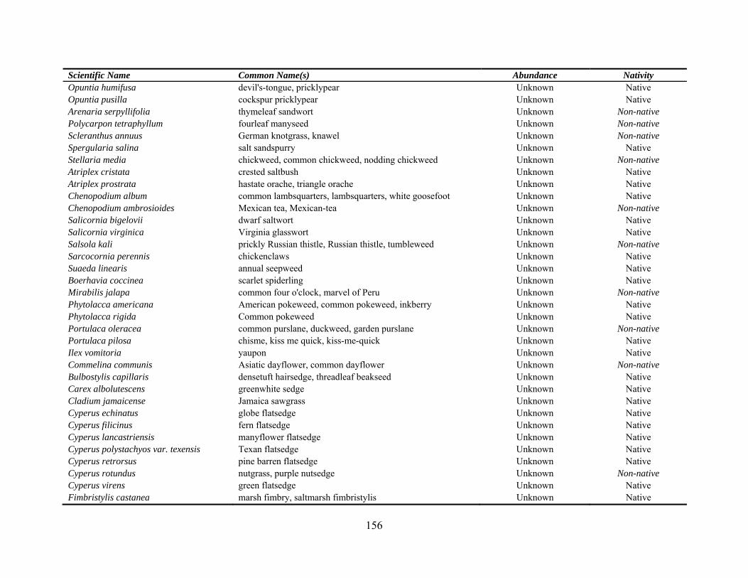
Scientific Name Common Name(s) Abundance Nativity Opuntia humifusa devil's-tongue, pricklypear Unknown Native Opuntia pusilla cockspur pricklypear Unknown Native Arenaria serpyllifolia thymeleaf sandwort Unknown Non-native Polycarpon tetraphyllum fourleaf manyseed Unknown Non-native Scleranthus annuus German knotgrass, knawel Unknown Non-native Spergularia salina salt sandspurry Unknown Native Stellaria media chickweed, common chickweed, nodding chickweed Unknown Non-native Atriplex cristata crested saltbush Unknown Native Atriplex prostrata hastate orache, triangle orache Unknown Native Chenopodium album common lambsquarters, lambsquarters, white goosefoot Unknown Native Chenopodium ambrosioides Mexican tea, Mexican-tea Unknown Non-native Salicornia bigelovii dwarf saltwort Unknown Native Salicornia virginica Virginia glasswort Unknown Native Salsola kali prickly Russian thistle, Russian thistle, tumbleweed Unknown Non-native Sarcocornia perennis chickenclaws Unknown Native Suaeda linearis annual seepweed Unknown Native Boerhavia coccinea scarlet spiderling Unknown Native Mirabilis jalapa common four o'clock, marvel of Peru Unknown Non-native Phytolacca americana American pokeweed, common pokeweed, inkberry Unknown Native Phytolacca rigida Common pokeweed Unknown Native Portulaca oleracea common purslane, duckweed, garden purslane Unknown Non-native Portulaca pilosa chisme, kiss me quick, kiss-me-quick Unknown Native Ilex vomitoria yaupon Unknown Native Commelina communis Asiatic dayflower, common dayflower Unknown Non-native Bulbostylis capillaris densetuft hairsedge, threadleaf beakseed Unknown Native Carex albolutescens greenwhite sedge Unknown Native Cladium jamaicense Jamaica sawgrass Unknown Native Cyperus echinatus globe flatsedge Unknown Native Cyperus filicinus fern flatsedge Unknown Native Cyperus lancastriensis manyflower flatsedge Unknown Native Cyperus polystachyos var. texensis Texan flatsedge Unknown Native Cyperus retrorsus pine barren flatsedge Unknown Native Cyperus rotundus nutgrass, purple nutsedge Unknown Non-native Cyperus virens green flatsedge Unknown Native Fimbristylis castanea marsh fimbry, saltmarsh fimbristylis Unknown Native

156

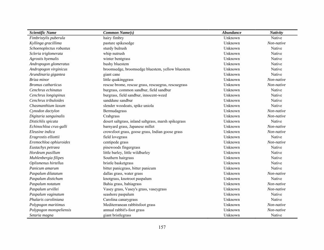
Scientific Name Common Name(s) Abundance Nativity Fimbristylis puberula hairy fimbry Unknown Native Kyllinga gracillima pasture spikesedge Unknown Non-native Schoenoplectus robustus sturdy bulrush Unknown Native Scleria triglomerata whip nutrush Unknown Native Agrostis hyemalis winter bentgrass Unknown Native Andropogon glomeratus bushy bluestem Unknown Native Andropogon virginicus broomsedge, broomsedge bluestem, yellow bluestem Unknown Native Arundinaria gigantea giant cane Unknown Native Briza minor little quakinggrass Unknown Non-native Bromus catharticus rescue brome, rescue grass, rescuegras, rescuegrass Unknown Non-native Cenchrus echinatus burgrass, common sandbur, field sandbur Unknown Native Cenchrus longispinus burgrass, field sandbur, innocent-weed Unknown Native Cenchrus tribuloides sanddune sandbur Unknown Native Chasmanthium laxum slender woodoats, spike uniola Unknown Native Cynodon dactylon Bermudagrass Unknown Non-native Digitaria sanguinalis Crabgrass Unknown Non-native Distichlis spicata desert saltgrass, inland saltgrass, marsh spikegrass Unknown Native Echinochloa crus-galli barnyard grass, Japanese millet Unknown Non-native Eleusine indica crowsfoot grass, goose grass, Indian goose grass Unknown Non-native Eragrostis elliottii field lovegrass Unknown Native Eremochloa ophiuroides centipede grass Unknown Non-native Eustachys petraea pinewoods fingergrass Unknown Native Hordeum pusillum little barley, little wildbarley Unknown Native Muhlenbergia filipes Southern hairgrass Unknown Native Oplismenus hirtellus bristle basketgrass Unknown Native Panicum amarum bitter panicgrass, bitter panicum Unknown Native Paspalum dilatatum dallas grass, water grass Unknown Non-native Paspalum distichum knotgrass, knotroot paspalum Unknown Native Paspalum notatum Bahia grass, bahiagrass Unknown Non-native Paspalum urvillei Vasey grass, Vasey's grass, vaseygrass Unknown Non-native Paspalum vaginatum seashore paspalum Unknown Native Phalaris caroliniana Carolina canarygrass Unknown Native Polypogon maritimus Mediterranean rabbitsfoot grass Unknown Non-native Polypogon monspeliensis annual rabbit's-foot grass Unknown Non-native Setaria magna giant bristlegrass Unknown Native

157

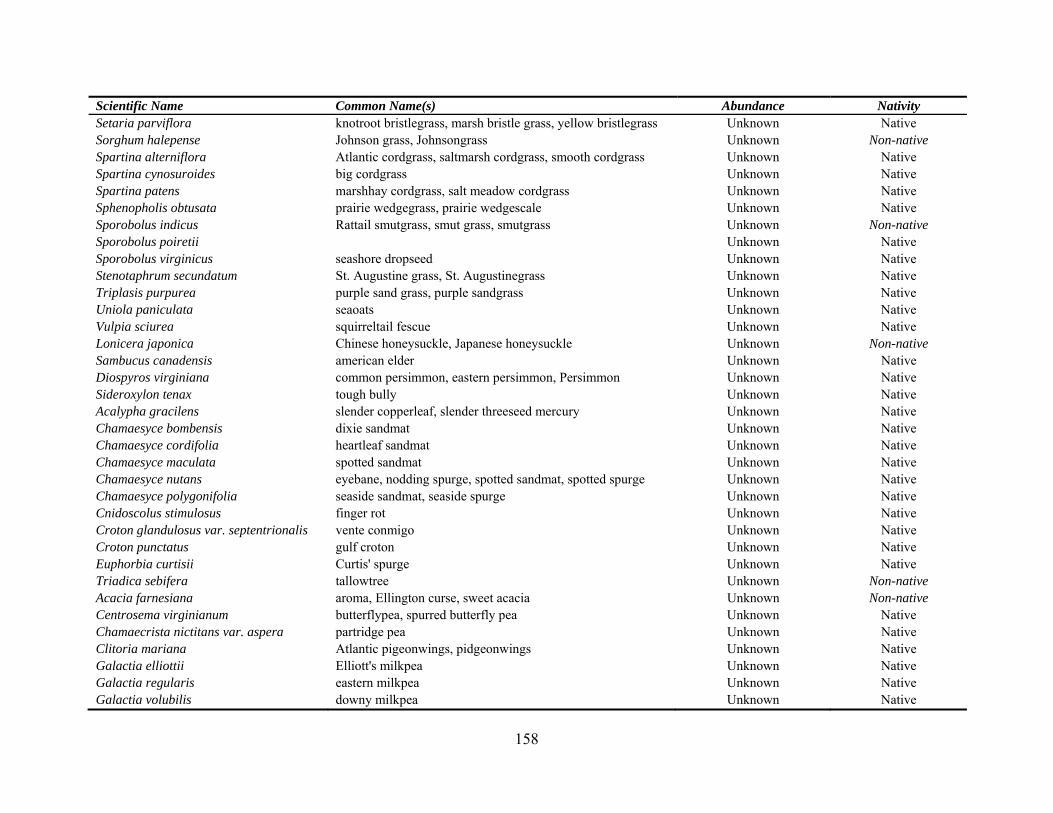
Scientific Name Common Name(s) Abundance Nativity Setaria parviflora knotroot bristlegrass, marsh bristle grass, yellow bristlegrass Unknown Native Sorghum halepense Johnson grass, Johnsongrass Unknown Non-native Spartina alterniflora Atlantic cordgrass, saltmarsh cordgrass, smooth cordgrass Unknown Native Spartina cynosuroides big cordgrass Unknown Native Spartina patens marshhay cordgrass, salt meadow cordgrass Unknown Native Sphenopholis obtusata prairie wedgegrass, prairie wedgescale Unknown Native Sporobolus indicus Rattail smutgrass, smut grass, smutgrass Unknown Non-native Sporobolus poiretii Unknown Native Sporobolus virginicus seashore dropseed Unknown Native Stenotaphrum secundatum St. Augustine grass, St. Augustinegrass Unknown Native Triplasis purpurea purple sand grass, purple sandgrass Unknown Native Uniola paniculata seaoats Unknown Native Vulpia sciurea squirreltail fescue Unknown Native Lonicera japonica Chinese honeysuckle, Japanese honeysuckle Unknown Non-native Sambucus canadensis american elder Unknown Native Diospyros virginiana common persimmon, eastern persimmon, Persimmon Unknown Native Sideroxylon tenax tough bully Unknown Native Acalypha gracilens slender copperleaf, slender threeseed mercury Unknown Native Chamaesyce bombensis dixie sandmat Unknown Native Chamaesyce cordifolia heartleaf sandmat Unknown Native Chamaesyce maculata spotted sandmat Unknown Native Chamaesyce nutans eyebane, nodding spurge, spotted sandmat, spotted spurge Unknown Native Chamaesyce polygonifolia seaside sandmat, seaside spurge Unknown Native Cnidoscolus stimulosus finger rot Unknown Native Croton glandulosus var. septentrionalis vente conmigo Unknown Native Croton punctatus gulf croton Unknown Native Euphorbia curtisii Curtis' spurge Unknown Native Triadica sebifera tallowtree Unknown Non-native Acacia farnesiana aroma, Ellington curse, sweet acacia Unknown Non-native Centrosema virginianum butterflypea, spurred butterfly pea Unknown Native Chamaecrista nictitans var. aspera partridge pea Unknown Native Clitoria mariana Atlantic pigeonwings, pidgeonwings Unknown Native Galactia elliottii Elliott's milkpea Unknown Native Galactia regularis eastern milkpea Unknown Native Galactia volubilis downy milkpea Unknown Native

158

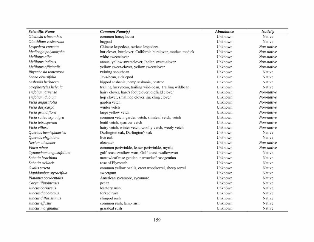
Scientific Name Common Name(s) Abundance Nativity Gleditsia triacanthos common honeylocust Unknown Native Glottidium vesicarium bagpod Unknown Native Lespedeza cuneata Chinese lespedeza, sericea lespedeza Unknown Non-native Medicago polymorpha bur clover, burclover, California burclover, toothed medick Unknown Non-native Melilotus alba white sweetclover Unknown Non-native Melilotus indicus annual yellow sweetclover, Indian sweet-clover Unknown Non-native Melilotus officinalis yellow sweet-clover, yellow sweetclover Unknown Non-native Rhynchosia tomentosa twining snoutbean Unknown Native Senna obtusifolia Java-bean, sicklepod Unknown Native Sesbania herbacea bigpod sesbania, hemp sesbania, peatree Unknown Native Strophostyles helvula trailing fuzzybean, trailing wild-bean, Trailing wildbean Unknown Native Trifolium arvense hairy clover, hare's foot clover, oldfield clover Unknown Non-native Trifolium dubium hop clover, smallhop clover, suckling clover Unknown Non-native Vicia angustifolia garden vetch Unknown Non-native Vicia dasycarpa winter vetch Unknown Non-native Vicia grandiflora large yellow vetch Unknown Non-native Vicia sativa ssp. nigra common vetch, garden vetch, slimleaf vetch, vetch Unknown Non-native Vicia tetrasperma lentil vetch, sparrow vetch Unknown Non-native Vicia villosa hairy vetch, winter vetch, woolly vetch, wooly vetch Unknown Non-native Quercus hemisphaerica Darlington oak, Darlington's oak Unknown Native Quercus virginiana live oak Unknown Native Nerium oleander oleander Unknown Non-native Vinca minor common periwinkle, lesser periwinkle, myrtle Unknown Non-native Cynanchum angustifolium gulf coast swallow-wort, Gulf coast swallowwort Unknown Native Sabatia brachiata narrowleaf rose gentian, narrowleaf rosegentian Unknown Native Sabatia stellaris rose of Plymouth Unknown Native Oxalis stricta common yellow oxalis, erect woodsorrel, sheep sorrel Unknown Native Liquidambar styraciflua sweetgum Unknown Native Platanus occidentalis American sycamore, sycamore Unknown Native Carya illinoinensis pecan Unknown Native Juncus coriaceus leathery rush Unknown Native Juncus dichotomus forked rush Unknown Native Juncus diffusissimus slimpod rush Unknown Native Juncus effusus common rush, lamp rush Unknown Native Juncus marginatus grassleaf rush Unknown Native

159

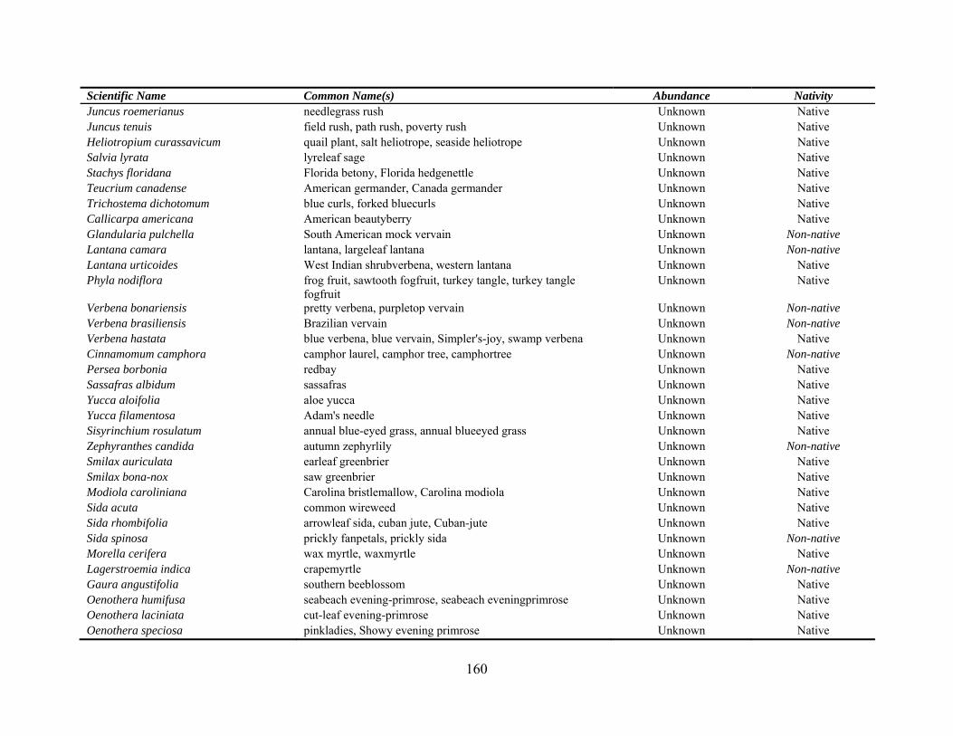
Scientific Name Common Name(s) Abundance Nativity Juncus roemerianus needlegrass rush Unknown Native Juncus tenuis field rush, path rush, poverty rush Unknown Native Heliotropium curassavicum quail plant, salt heliotrope, seaside heliotrope Unknown Native Salvia lyrata lyreleaf sage Unknown Native Stachys floridana Florida betony, Florida hedgenettle Unknown Native Teucrium canadense American germander, Canada germander Unknown Native Trichostema dichotomum blue curls, forked bluecurls Unknown Native Callicarpa americana American beautyberry Unknown Native Glandularia pulchella South American mock vervain Unknown Non-native Lantana camara lantana, largeleaf lantana Unknown Non-native Lantana urticoides West Indian shrubverbena, western lantana Unknown Native Phyla nodiflora frog fruit, sawtooth fogfruit, turkey tangle, turkey tangle

fogfruit Unknown Native

Verbena bonariensis pretty verbena, purpletop vervain Unknown Non-native Verbena brasiliensis Brazilian vervain Unknown Non-native Verbena hastata blue verbena, blue vervain, Simpler's-joy, swamp verbena Unknown Native Cinnamomum camphora camphor laurel, camphor tree, camphortree Unknown Non-native Persea borbonia redbay Unknown Native Sassafras albidum sassafras Unknown Native Yucca aloifolia aloe yucca Unknown Native Yucca filamentosa Adam's needle Unknown Native Sisyrinchium rosulatum annual blue-eyed grass, annual blueeyed grass Unknown Native Zephyranthes candida autumn zephyrlily Unknown Non-native Smilax auriculata earleaf greenbrier Unknown Native Smilax bona-nox saw greenbrier Unknown Native Modiola caroliniana Carolina bristlemallow, Carolina modiola Unknown Native Sida acuta common wireweed Unknown Native Sida rhombifolia arrowleaf sida, cuban jute, Cuban-jute Unknown Native Sida spinosa prickly fanpetals, prickly sida Unknown Non-native Morella cerifera wax myrtle, waxmyrtle Unknown Native Lagerstroemia indica crapemyrtle Unknown Non-native Gaura angustifolia southern beeblossom Unknown Native Oenothera humifusa seabeach evening-primrose, seabeach eveningprimrose Unknown Native Oenothera laciniata cut-leaf evening-primrose Unknown Native Oenothera speciosa pinkladies, Showy evening primrose Unknown Native

160

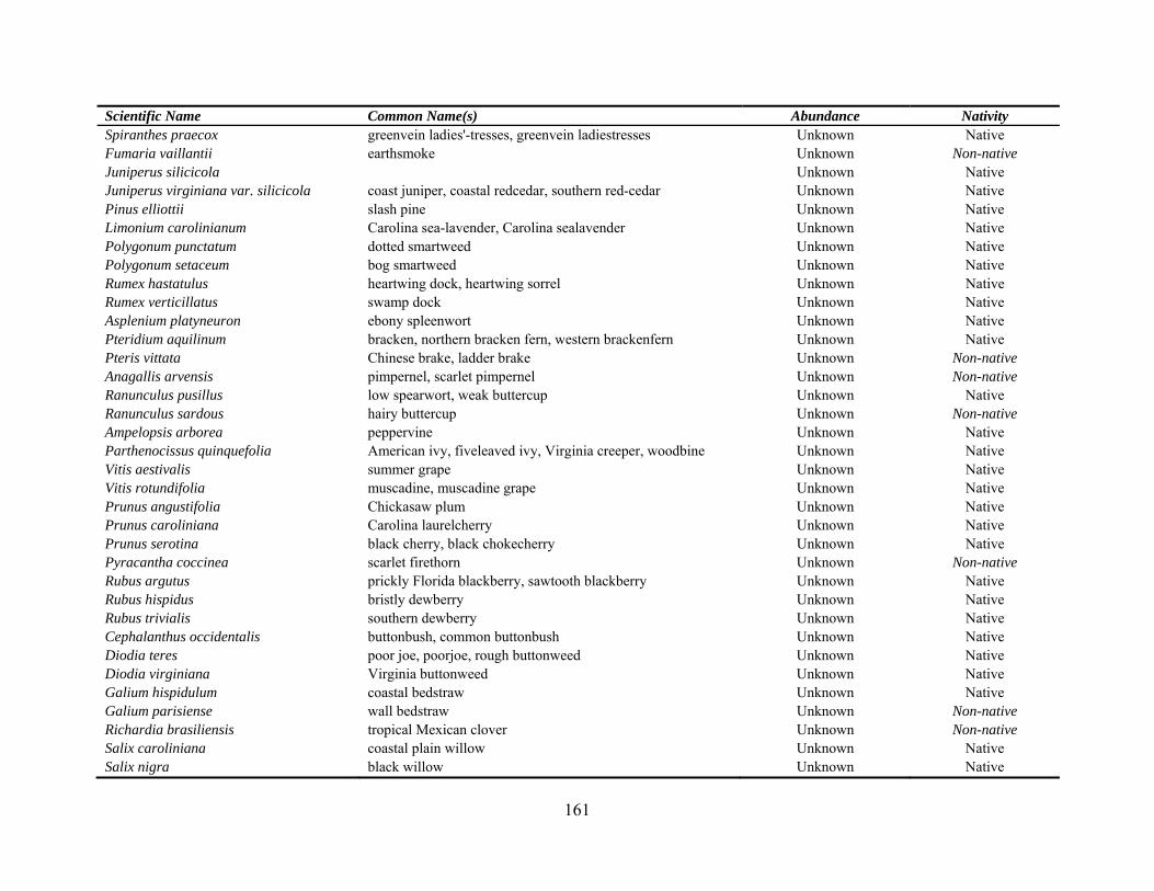
Scientific Name Common Name(s) Abundance Nativity Spiranthes praecox greenvein ladies'-tresses, greenvein ladiestresses Unknown Native Fumaria vaillantii earthsmoke Unknown Non-native Juniperus silicicola Unknown Native Juniperus virginiana var. silicicola coast juniper, coastal redcedar, southern red-cedar Unknown Native Pinus elliottii slash pine Unknown Native Limonium carolinianum Carolina sea-lavender, Carolina sealavender Unknown Native Polygonum punctatum dotted smartweed Unknown Native Polygonum setaceum bog smartweed Unknown Native Rumex hastatulus heartwing dock, heartwing sorrel Unknown Native Rumex verticillatus swamp dock Unknown Native Asplenium platyneuron ebony spleenwort Unknown Native Pteridium aquilinum bracken, northern bracken fern, western brackenfern Unknown Native Pteris vittata Chinese brake, ladder brake Unknown Non-native Anagallis arvensis pimpernel, scarlet pimpernel Unknown Non-native Ranunculus pusillus low spearwort, weak buttercup Unknown Native Ranunculus sardous hairy buttercup Unknown Non-native Ampelopsis arborea peppervine Unknown Native Parthenocissus quinquefolia American ivy, fiveleaved ivy, Virginia creeper, woodbine Unknown Native Vitis aestivalis summer grape Unknown Native Vitis rotundifolia muscadine, muscadine grape Unknown Native Prunus angustifolia Chickasaw plum Unknown Native Prunus caroliniana Carolina laurelcherry Unknown Native Prunus serotina black cherry, black chokecherry Unknown Native Pyracantha coccinea scarlet firethorn Unknown Non-native Rubus argutus prickly Florida blackberry, sawtooth blackberry Unknown Native Rubus hispidus bristly dewberry Unknown Native Rubus trivialis southern dewberry Unknown Native Cephalanthus occidentalis buttonbush, common buttonbush Unknown Native Diodia teres poor joe, poorjoe, rough buttonweed Unknown Native Diodia virginiana Virginia buttonweed Unknown Native Galium hispidulum coastal bedstraw Unknown Native Galium parisiense wall bedstraw Unknown Non-native Richardia brasiliensis tropical Mexican clover Unknown Non-native Salix caroliniana coastal plain willow Unknown Native Salix nigra black willow Unknown Native

161

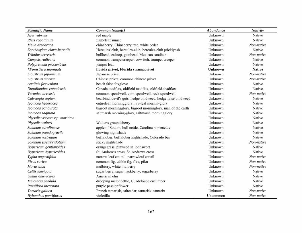
162

Scientific Name Common Name(s) Abundance Nativity Acer rubrum red maple Unknown Native Rhus copallinum flameleaf sumac Unknown Native Melia azedarach chinaberry, Chinaberry tree, white cedar Unknown Non-native Zanthoxylum clava-herculis Hercules' club, hercules-club, hercules-club pricklyash Unknown Native Tribulus terrestris bullhead, caltrop, goathead, Mexican sandbur Unknown Non-native Campsis radicans common trumpetcreeper, cow-itch, trumpet creeper Unknown Native Polypremum procumbens juniper leaf Unknown Native *Forestiera segregate florida privet, Florida swampprivet Unknown Native Ligustrum japonicum Japanese privet Unknown Non-native Ligustrum sinense Chinese privet, common chinese privet Unknown Non-native Agalinis fasciculata beach false foxglove Unknown Native Nuttallanthus canadensis Canada toadflax, oldfield toadflax, oldfield-toadflax Unknown Native Veronica arvensis common speedwell, corn speedwell, rock speedwell Unknown Non-native Calystegia sepium bearbind, devil's guts, hedge bindweed, hedge false bindweed Unknown Native Ipomoea hederacea entireleaf morningglory, ivy-leaf mornin-glory Unknown Native Ipomoea pandurata bigroot morningglory, bigroot morninglory, man of the earth Unknown Native Ipomoea sagittata saltmarsh morning-glory, saltmarsh morningglory Unknown Native Physalis viscosa ssp. maritima Unknown Native Physalis walteri Walter's groundcherry Unknown Native Solanum carolinense apple of Sodom, bull nettle, Carolina horsenettle Unknown Native Solanum pseudogracile glowing nightshade Unknown Native Solanum rostratum buffalobur, buffalobur nightshade, Colorado bur Unknown Native Solanum sisymbriifolium sticky nightshade Unknown Non-native Hypericum gentianoides orangegrass, pinweed st. johnswort Unknown Native Hypericum hypericoides St. Andrew's cross, St. Andrews cross Unknown Native Typha angustifolia narrow-leaf cat-tail, narrowleaf cattail Unknown Non-native Ficus carica common fig, edible fig, fiku, piku Unknown Non-native Morus alba mulberry, white mulberry Unknown Non-native Celtis laevigata sugar berry, sugar hackberry, sugarberry Unknown Native Ulmus americana American elm Unknown Native Melothria pendula drooping melonnettle, Guadeloupe cucumber Unknown Native Passiflora incarnata purple passionflower Unknown Native Tamarix gallica French tamarisk, saltcedar, tamarisk, tamarix Unknown Non-native Hybanthus parviflorus violetilla Uncommon Non-native

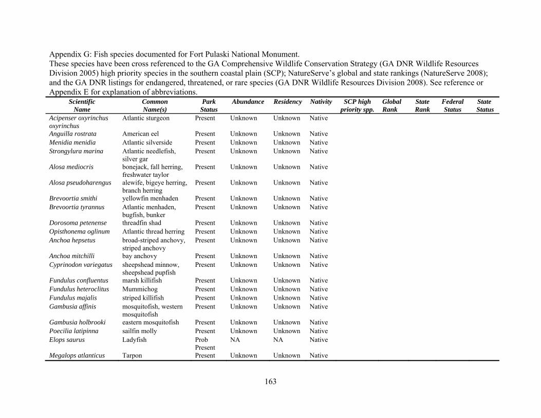
Appendix G: Fish species documented for Fort Pulaski National Monument. These species have been cross referenced to the GA Comprehensive Wildlife Conservation Strategy (GA DNR Wildlife Resources Division 2005) high priority species in the southern coastal plain (SCP); NatureServe’s global and state rankings (NatureServe 2008); and the GA DNR listings for endangered, threatened, or rare species (GA DNR Wildlife Resources Division 2008). See reference or Appendix E for explanation of abbreviations.

Scientific Common Name(s)

Park Status

Abundance Residency Nativity SCP high priority spp.

Global Rank

State Federal State Name Rank Status Status

Acipenser oxyrinchus oxyrinchus

Atlantic sturgeon Present Unknown Unknown Native

Anguilla rostrata American eel Present Unknown Unknown Native Menidia menidia Atlantic silverside Present Unknown Unknown Native Strongylura marina Atlantic needlefish,

silver gar Present Unknown Unknown Native

Alosa mediocris bonejack, fall herring, freshwater taylor

Present Unknown Unknown Native

Alosa pseudoharengus alewife, bigeye herring, branch herring


Brevoortia smithi yellowfin menhaden Present Unknown Unknown Native Brevoortia tyrannus Atlantic menhaden,

bugfish, bunker Present Unknown Unknown Native

Dorosoma petenense threadfin shad Present Unknown Unknown Native Opisthonema oglinum Atlantic thread herring Present Unknown Unknown Native Anchoa hepsetus broad-striped anchovy,

striped anchovy Present Unknown Unknown Native

Anchoa mitchilli bay anchovy Present Unknown Unknown Native Cyprinodon variegatus sheepshead minnow,

sheepshead pupfish Present Unknown Unknown Native

Fundulus confluentus marsh killifish Present Unknown Unknown Native Fundulus heteroclitus Mummichog Present Unknown Unknown Native Fundulus majalis striped killifish Present Unknown Unknown Native Gambusia affinis mosquitofish, western

mosquitofish Present Unknown Unknown Native

Gambusia holbrooki eastern mosquitofish Present Unknown Unknown Native Poecilia latipinna sailfin molly Present Unknown Unknown Native Elops saurus Ladyfish Prob

Present NA NA Native

Megalops atlanticus Tarpon Present Unknown Unknown Native

163

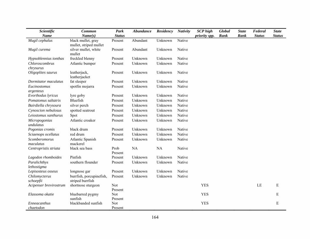
Scientific Common Name(s)

Park Status


Global Rank

State Federal State Name Rank Status Status

Mugil cephalus black mullet, gray mullet, striped mullet

Present Abundant Unknown Native

Mugil curema silver mullet, white mullet

Present Abundant Unknown Native

Hypsoblennius ionthas freckled blenny Present Unknown Unknown Native Chloroscombrus chrysurus

Atlantic bumper Present Unknown Unknown Native

Oligoplites saurus leatherjack, leatherjacket


Dormitator maculatus fat sleeper Present Unknown Unknown Native Eucinostomus argenteus

spotfin mojarra Present Unknown Unknown Native

Evorthodus lyricus lyre goby Present Unknown Unknown Native Pomatomus saltatrix Bluefish Present Unknown Unknown Native Bairdiella chrysoura silver perch Present Unknown Unknown Native Cynoscion nebulosus spotted seatrout Present Unknown Unknown Native Leiostomus xanthurus Spot Present Unknown Unknown Native Micropogonias undulatus

Atlantic croaker Present Unknown Unknown Native

Pogonias cromis black drum Present Unknown Unknown Native Sciaenops ocellatus red drum Present Unknown Unknown Native Scomberomorus maculatus

Atlantic Spanish mackerel


Centropristis striata black sea bass Prob Present

NA NA Native

Lagodon rhomboides Pinfish Present Unknown Unknown Native Paralichthys lethostigma

southern flounder Present Unknown Unknown Native

Lepisosteus osseus longnose gar Present Unknown Unknown Native Chilomycterus schoepfii

burrfish, porcupinefish, striped burrfish


Acipenser brevirostrum shortnose sturgeon Not Present

YES LE E

Elassoma okatie bluebarred pygmy sunfish

Not Present

YES E

Enneacanthus chaetodon

blackbanded sunfish Not Present

YES E

164

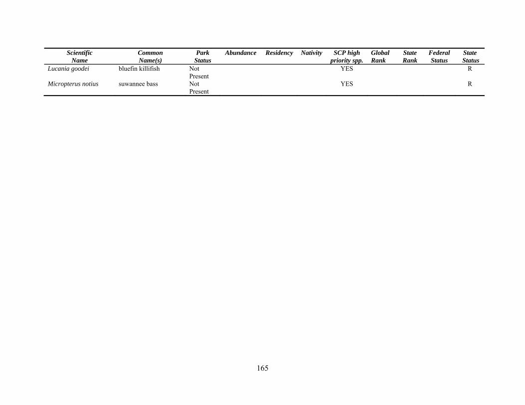
165

Status Scientific

Name Common Name(s)

Park Status


Global Rank

State Rank

Federal Status

State

Lucania goodei bluefin killifish Not Present

YES R

Micropterus notius suwannee bass Not Present

YES R

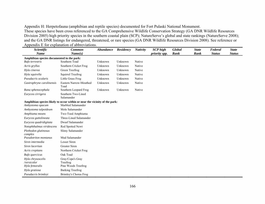
Appendix H: Herpetofauna (amphibian and reptile species) documented for Fort Pulaski National Monument. These species have been cross referenced to the GA Comprehensive Wildlife Conservation Strategy (GA DNR Wildlife Resources Division 2005) high priority species in the southern coastal plain (SCP); NatureServe’s global and state rankings (NatureServe 2008); and the GA DNR listings for endangered, threatened, or rare species (GA DNR Wildlife Resources Division 2008). See reference or Appendix E for explanation of abbreviations.

Scientific Name

Common Name(s)


Global Rank

State Federal State Rank Status Status

Amphibian species documented in the park: Bufo terrestris Southern Toad Unknown Unknown Native Acris gryllus Southern Cricket Frog Unknown Unknown Native Hyla cinerea Green Treefrog Unknown Unknown Native Hyla squirella Squirrel Treefrog Unknown Unknown Native Pseudacris ocularis Little Grass Frog Unknown Unknown Native Gastrophryne carolinensis Eastern Narrow-Mouthed

Toad Unknown Unknown Native

Rana sphenocephala Southern Leopard Frog Unknown Unknown Native Eurycea cirrigera Southern Two-Lined

Salamander

Amphibian species likely to occur within or near the vicinity of the park: Ambystoma opacum Marbled Salamander Ambystoma talpoideum Mole Salamander Amphiuma means Two-Toed Amphiuma Eurycea guttolineata Three-Lined Salamander Eurycea quadridigitata Dwarf Salamander Notophthalmus viridescens Red Spotted Newt Plethodon glutinosus complex

Slimy Salamander

Pseudotriton montanus Mud Salamander Siren intermedia Lesser Siren Siren lacertian Greater Siren Acris crepitans Northern Cricket Frog Bufo quercicus Oak Toad Hyla chrysoscelis /versicolor

Gray/Cope's Gray Treefrog

Hyla femoralis Pine Woods Treefrog Hyla gratiosa Barking Treefrog Pseudacris brimleyi Brimley's Chorus Frog

166

Scientific Name

Common Name(s)


Global Rank

State Rank

Federal Status

State Status

Pseudacris crucifer Spring Peeper Pseudacris nigrita Southern Chorus Frog Pseudacris ornata Ornate Chorus Frog Pseudacris triseriata Upland Chorus Frog Rana catesbeiana Bullfrog Rana clamitans Green Frog Rana grylio Pig Frog Scaphiopus holbrookii Eastern Spadefoot Toad

Priority amphibian species not documented in the park: Rana capito Gopher Frog YES G3G4 S3 R Ambystoma cingulatum Flatwoods Salamander YES G2G3 S2 LT T Desmognathus auriculatus Southern Dusky

Salamander YES G5 S3

Necturus punctatus Dwarf Waterdog YES G4 S2 Notophthalmus perstriatus Striped Newt YES G2G3 S2 T Stereochilus marginatus Many-Lined Salamander YES G5 S3 Pseudobranchus striatus Dwarf Siren YES G5 S3

Reptile species documented in the park: Alligator mississippiensis Alligator Unknown Unknown Native Ophisaurus ventralis Eastern Glass Lizard Unknown Unknown Native Coluber constrictor Black Racer Unknown Unknown Native Elaphe guttata Corn Snake Unknown Unknown Native Elaphe obsolete Eastern Ratsnake Unknown Unknown Native Lampropeltis getula Eastern Kingsnake Unknown Unknown Native Nerodia fasciata Southern Water Snake Unknown Unknown Native Opheodrys aestivus Rough Greensnake Unknown Unknown Native Anolis carolinensis Green Anole Unknown Unknown Native Norops sagrei Brown Anole Unknown Unknown Non-

native

Eumeces inexpectatus Southeastern Five-Lined Skink

Unknown Unknown Native

Scincella lateralis Ground Skink, Little Brown Skink

Unknown Unknown Native

Agkistrodon piscivorus Cottonmouth Unknown Unknown Native Crotalus adamanteus Eastern Diamond-Backed

Rattlesnake Unknown Unknown Native

167

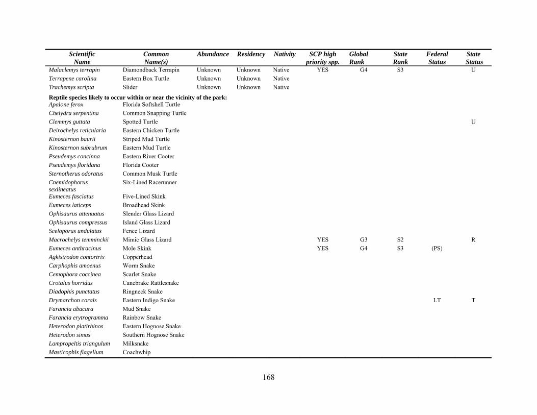
Scientific Name

Common Name(s)

Abundance Residency Nativity SCP high Global Rank

State Rank

Federal Status

State Status priority spp.

Malaclemys terrapin Diamondback Terrapin Unknown Unknown Native YES G4 S3 U Terrapene carolina Eastern Box Turtle Unknown Unknown Native Trachemys scripta Slider Unknown Unknown Native

Reptile species likely to occur within or near the vicinity of the park: Apalone ferox Florida Softshell Turtle Chelydra serpentina Common Snapping Turtle Clemmys guttata Spotted Turtle U Deirochelys reticularia Eastern Chicken Turtle Kinosternon baurii Striped Mud Turtle Kinosternon subrubrum Eastern Mud Turtle Pseudemys concinna Eastern River Cooter Pseudemys floridana Florida Cooter Sternotherus odoratus Common Musk Turtle Cnemidophorus sexlineatus

Six-Lined Racerunner

Eumeces fasciatus Five-Lined Skink Eumeces laticeps Broadhead Skink Ophisaurus attenuatus Slender Glass Lizard Ophisaurus compressus Island Glass Lizard Sceloporus undulatus Fence Lizard Macrochelys temminckii Mimic Glass Lizard YES G3 S2 R Eumeces anthracinus Mole Skink YES G4 S3 (PS) Agkistrodon contortrix Copperhead Carphophis amoenus Worm Snake Cemophora coccinea Scarlet Snake Crotalus horridus Canebrake Rattlesnake Diadophis punctatus Ringneck Snake Drymarchon corais Eastern Indigo Snake LT T Farancia abacura Mud Snake Farancia erytrogramma Rainbow Snake Heterodon platirhinos Eastern Hognose Snake Heterodon simus Southern Hognose Snake Lampropeltis triangulum Milksnake Masticophis flagellum Coachwhip

168

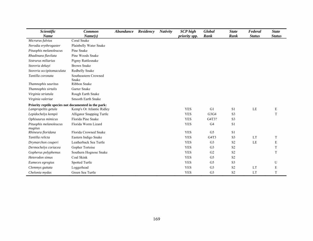
169

Scientific Name

Common Name(s)


Global Rank

State Rank

Federal Status

State Status

Micrurus fulvius Coral Snake Nerodia erythrogaster Plainbelly Water Snake Pituophis melanoleucus Pine Snake Rhadinaea flavilata Pine Woods Snake Sistrurus miliarius Pigmy Rattlesnake Storeria dekayi Brown Snake Storeria occipitomaculata Redbelly Snake Tantilla coronata Southeastern Crowned

Snake Thamnophis sauritus Ribbon Snake Thamnophis sirtalis Garter Snake Virginia striatula Rough Earth Snake Virginia valeriae Smooth Earth Snake Priority reptile species not documented in the park: Lampropeltis getula Kemp's Or Atlantic Ridley YES G1 S1 LE E Lepidochelys kempii Alligator Snapping Turtle YES G3G4 S3 T Ophisaurus mimicus Florida Pine Snake YES G4T3? S3 Pituophis melanoleucus mugitus

Florida Worm Lizard YES G4 S1

Rhineura floridana Florida Crowned Snake YES G5 S1 Tantilla relicta Eastern Indigo Snake YES G4T3 S3 LT T Drymarchon couperi Leatherback Sea Turtle YES G3 S2 LE E Dermochelys coriacea Gopher Tortoise YES G3 S2 T Gopherus polyphemus Southern Hognose Snake YES G2 S2 T Heterodon simus Coal Skink YES G5 S2 Eumeces egregius Spotted Turtle YES G5 S3 U Clemmys guttata Loggerhead YES G3 S2 LT E Chelonia mydas Green Sea Turtle YES G3 S2 LT T

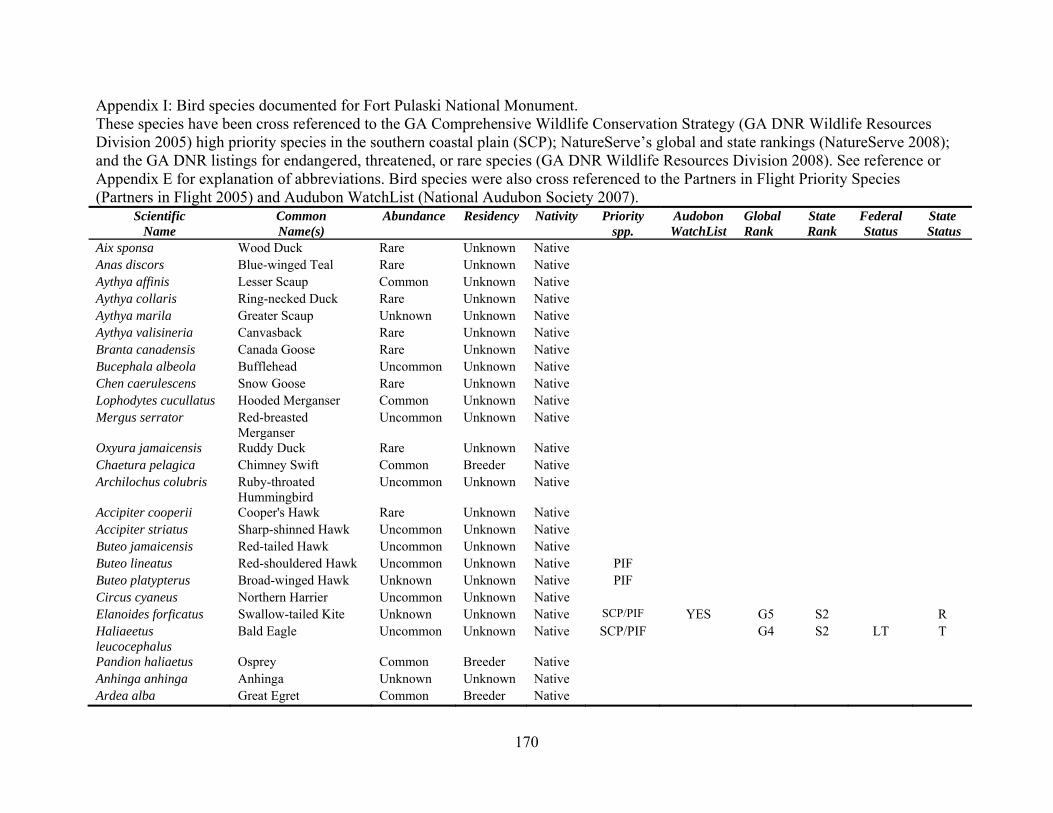
Appendix I: Bird species documented for Fort Pulaski National Monument. These species have been cross referenced to the GA Comprehensive Wildlife Conservation Strategy (GA DNR Wildlife Resources Division 2005) high priority species in the southern coastal plain (SCP); NatureServe’s global and state rankings (NatureServe 2008); and the GA DNR listings for endangered, threatened, or rare species (GA DNR Wildlife Resources Division 2008). See reference or Appendix E for explanation of abbreviations. Bird species were also cross referenced to the Partners in Flight Priority Species (Partners in Flight 2005) and Audubon WatchList (National Audubon Society 2007).

Scientific Name

Common Name(s)

Abundance Residency Nativity Priority spp.

Audobon WatchList

Global Rank


Aix sponsa Wood Duck Rare Unknown Native Anas discors Blue-winged Teal Rare Unknown Native Aythya affinis Lesser Scaup Common Unknown Native Aythya collaris Ring-necked Duck Rare Unknown Native Aythya marila Greater Scaup Unknown Unknown Native Aythya valisineria Canvasback Rare Unknown Native Branta canadensis Canada Goose Rare Unknown Native Bucephala albeola Bufflehead Uncommon Unknown Native Chen caerulescens Snow Goose Rare Unknown Native Lophodytes cucullatus Hooded Merganser Common Unknown Native Mergus serrator Red-breasted

Merganser Uncommon Unknown Native

Oxyura jamaicensis Ruddy Duck Rare Unknown Native Chaetura pelagica Chimney Swift Common Breeder Native Archilochus colubris Ruby-throated

Hummingbird Uncommon Unknown Native

Accipiter cooperii Cooper's Hawk Rare Unknown Native Accipiter striatus Sharp-shinned Hawk Uncommon Unknown Native Buteo jamaicensis Red-tailed Hawk Uncommon Unknown Native Buteo lineatus Red-shouldered Hawk Uncommon Unknown Native PIF Buteo platypterus Broad-winged Hawk Unknown Unknown Native PIF Circus cyaneus Northern Harrier Uncommon Unknown Native Elanoides forficatus Swallow-tailed Kite Unknown Unknown Native SCP/PIF YES G5 S2 R Haliaeetus leucocephalus

Bald Eagle Uncommon Unknown Native SCP/PIF G4 S2 LT T

Pandion haliaetus Osprey Common Breeder Native Anhinga anhinga Anhinga Unknown Unknown Native Ardea alba Great Egret Common Breeder Native

170

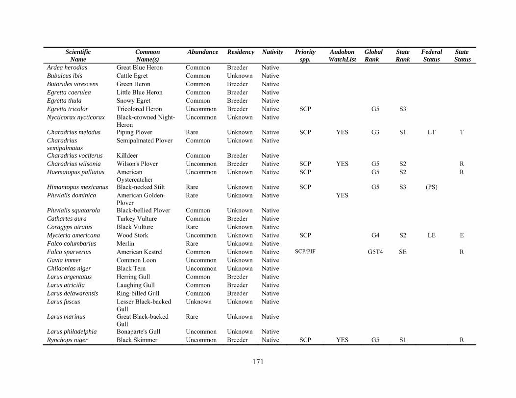
Scientific Name

Common Name(s)


Audobon WatchList

Global Rank


Ardea herodias Great Blue Heron Common Breeder Native Bubulcus ibis Cattle Egret Common Unknown Native Butorides virescens Green Heron Common Breeder Native Egretta caerulea Little Blue Heron Common Breeder Native Egretta thula Snowy Egret Common Breeder Native Egretta tricolor Tricolored Heron Uncommon Breeder Native SCP G5 S3 Nycticorax nycticorax Black-crowned Night-

Heron Uncommon Unknown Native

Charadrius melodus Piping Plover Rare Unknown Native SCP YES G3 S1 LT T Charadrius semipalmatus

Semipalmated Plover Common Unknown Native

Charadrius vociferus Killdeer Common Breeder Native Charadrius wilsonia Wilson's Plover Uncommon Breeder Native SCP YES G5 S2 R Haematopus palliatus American

Oystercatcher Uncommon Unknown Native SCP G5 S2 R

Himantopus mexicanus Black-necked Stilt Rare Unknown Native SCP G5 S3 (PS) Pluvialis dominica American Golden-

Plover Rare Unknown Native YES

Pluvialis squatarola Black-bellied Plover Common Unknown Native Cathartes aura Turkey Vulture Common Breeder Native Coragyps atratus Black Vulture Rare Unknown Native Mycteria americana Wood Stork Uncommon Unknown Native SCP G4 S2 LE E Falco columbarius Merlin Rare Unknown Native Falco sparverius American Kestrel Common Unknown Native SCP/PIF G5T4 SE R Gavia immer Common Loon Uncommon Unknown Native Chlidonias niger Black Tern Uncommon Unknown Native Larus argentatus Herring Gull Common Breeder Native Larus atricilla Laughing Gull Common Breeder Native Larus delawarensis Ring-billed Gull Common Breeder Native Larus fuscus Lesser Black-backed

Gull Unknown Unknown Native

Larus marinus Great Black-backed Gull

Rare Unknown Native

Larus philadelphia Bonaparte's Gull Uncommon Unknown Native Rynchops niger Black Skimmer Uncommon Breeder Native SCP YES G5 S1 R

171

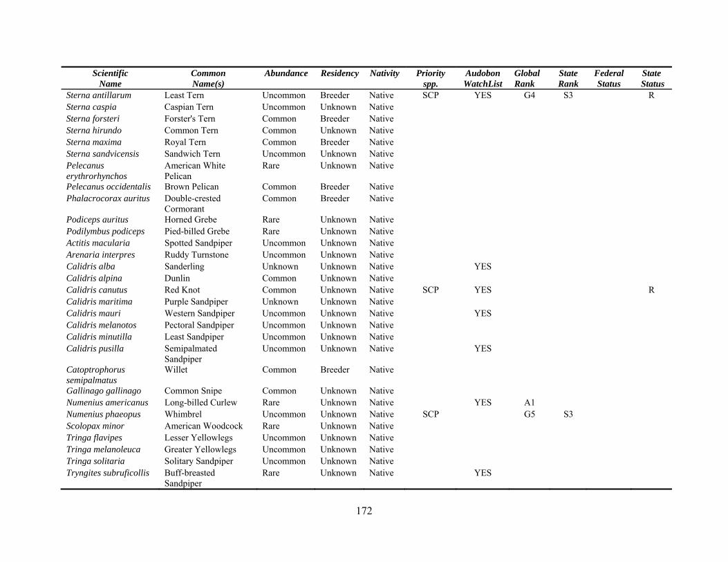
Scientific Name

Common Name(s)


Audobon WatchList

Global Rank


Sterna antillarum Least Tern Uncommon Breeder Native SCP YES G4 S3 R Sterna caspia Caspian Tern Uncommon Unknown Native Sterna forsteri Forster's Tern Common Breeder Native Sterna hirundo Common Tern Common Unknown Native Sterna maxima Royal Tern Common Breeder Native Sterna sandvicensis Sandwich Tern Uncommon Unknown Native Pelecanus erythrorhynchos

American White Pelican

Rare Unknown Native

Pelecanus occidentalis Brown Pelican Common Breeder Native Phalacrocorax auritus Double-crested

Cormorant Common Breeder Native

Podiceps auritus Horned Grebe Rare Unknown Native Podilymbus podiceps Pied-billed Grebe Rare Unknown Native Actitis macularia Spotted Sandpiper Uncommon Unknown Native Arenaria interpres Ruddy Turnstone Uncommon Unknown Native Calidris alba Sanderling Unknown Unknown Native YES Calidris alpina Dunlin Common Unknown Native Calidris canutus Red Knot Common Unknown Native SCP YES R Calidris maritima Purple Sandpiper Unknown Unknown Native Calidris mauri Western Sandpiper Uncommon Unknown Native YES Calidris melanotos Pectoral Sandpiper Uncommon Unknown Native Calidris minutilla Least Sandpiper Uncommon Unknown Native Calidris pusilla Semipalmated

Sandpiper Uncommon Unknown Native YES

Catoptrophorus semipalmatus

Willet Common Breeder Native

Gallinago gallinago Common Snipe Common Unknown Native Numenius americanus Long-billed Curlew Rare Unknown Native YES A1 Numenius phaeopus Whimbrel Uncommon Unknown Native SCP G5 S3 Scolopax minor American Woodcock Rare Unknown Native Tringa flavipes Lesser Yellowlegs Uncommon Unknown Native Tringa melanoleuca Greater Yellowlegs Uncommon Unknown Native Tringa solitaria Solitary Sandpiper Uncommon Unknown Native Tryngites subruficollis Buff-breasted

Sandpiper Rare Unknown Native YES

172

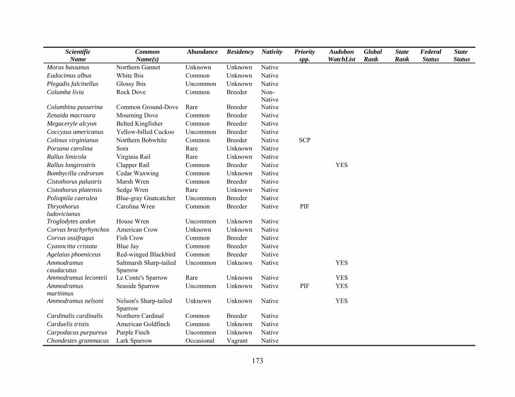
Scientific Name

Common Name(s)


Audobon WatchList

Global Rank


Morus bassanus Northern Gannet Unknown Unknown Native Eudocimus albus White Ibis Common Unknown Native Plegadis falcinellus Glossy Ibis Uncommon Unknown Native Columba livia Rock Dove Common Breeder Non-

Native

Columbina passerina Common Ground-Dove Rare Breeder Native Zenaida macroura Mourning Dove Common Breeder Native Megaceryle alcyon Belted Kingfisher Common Breeder Native Coccyzus americanus Yellow-billed Cuckoo Uncommon Breeder Native Colinus virginianus Northern Bobwhite Common Breeder Native SCP Porzana carolina Sora Rare Unknown Native Rallus limicola Virginia Rail Rare Unknown Native Rallus longirostris Clapper Rail Common Breeder Native YES Bombycilla cedrorum Cedar Waxwing Common Unknown Native Cistothorus palustris Marsh Wren Common Breeder Native Cistothorus platensis Sedge Wren Rare Unknown Native Polioptila caerulea Blue-gray Gnatcatcher Uncommon Breeder Native Thryothorus ludovicianus

Carolina Wren Common Breeder Native PIF

Troglodytes aedon House Wren Uncommon Unknown Native Corvus brachyrhynchos American Crow Unknown Unknown Native Corvus ossifragus Fish Crow Common Breeder Native Cyanocitta cristata Blue Jay Common Breeder Native Agelaius phoeniceus Red-winged Blackbird Common Breeder Native Ammodramus caudacutus

Saltmarsh Sharp-tailed Sparrow

Uncommon Unknown Native YES

Ammodramus leconteii Le Conte's Sparrow Rare Unknown Native YES Ammodramus maritimus

Seaside Sparrow Uncommon Unknown Native PIF YES

Ammodramus nelsoni Nelson's Sharp-tailed Sparrow

Unknown Unknown Native YES

Cardinalis cardinalis Northern Cardinal Common Breeder Native Carduelis tristis American Goldfinch Common Unknown Native Carpodacus purpureus Purple Finch Uncommon Unknown Native Chondestes grammacus Lark Sparrow Occasional Vagrant Native

173

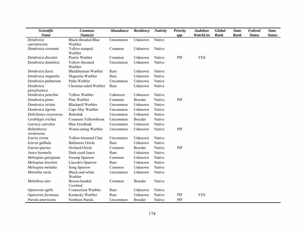
Scientific Name

Common Name(s)


Audobon WatchList

Global Rank

State Rank

Federal Status

State Status

Dendroica caerulescens

Black-throated Blue Warbler

Uncommon Unknown Native

Dendroica coronata Yellow-rumped Warbler

Common Unknown Native

Dendroica discolor Prairie Warbler Common Unknown Native PIF YES Dendroica dominica Yellow-throated

Warbler Uncommon Unknown Native

Dendroica fusca Blackburnian Warbler Rare Unknown Native Dendroica magnolia Magnolia Warbler Rare Unknown Native Dendroica palmarum Palm Warbler Uncommon Unknown Native Dendroica pensylvanica

Chestnut-sided Warbler Rare Unknown Native

Dendroica petechia Yellow Warbler Unknown Unknown Native Dendroica pinus Pine Warbler Common Breeder Native PIF Dendroica striata Blackpoll Warbler Uncommon Unknown Native Dendroica tigrina Cape May Warbler Uncommon Unknown Native Dolichonyx oryzivorus Bobolink Uncommon Unknown Native Geothlypis trichas Common Yellowthroat Uncommon Breeder Native Guiraca caerulea Blue Grosbeak Uncommon Unknown Native Helmitheros vermivorus

Worm-eating Warbler Uncommon Unknown Native PIF

Icteria virens Yellow-breasted Chat Uncommon Unknown Native Icterus galbula Baltimore Oriole Rare Unknown Native Icterus spurius Orchard Oriole Common Breeder Native PIF Junco hyemalis Dark-eyed Junco Rare Unknown Native Melospiza georgiana Swamp Sparrow Common Unknown Native Melospiza lincolnii Lincoln's Sparrow Rare Unknown Native Melospiza melodia Song Sparrow Common Unknown Native Mniotilta varia Black-and-white


Molothrus ater Brown-headed Cowbird

Common Breeder Native

Oporornis agilis Connecticut Warbler Rare Unknown Native Oporornis formosus Kentucky Warbler Rare Unknown Native PIF YES Parula americana Northern Parula Uncommon Breeder Native PIF

174

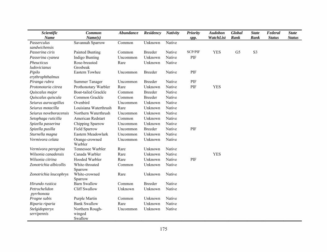
Scientific Name

Common Name(s)


Audobon WatchList

Global Rank

State Rank

Federal Status

State Status

Passerculus sandwichensis

Savannah Sparrow Common Unknown Native

Passerina ciris Painted Bunting Common Breeder Native SCP/PIF YES G5 S3 Passerina cyanea Indigo Bunting Uncommon Unknown Native PIF Pheucticus ludovicianus

Rose-breasted Grosbeak

Rare Unknown Native

Pipilo erythrophthalmus

Eastern Towhee Uncommon Breeder Native PIF

Piranga rubra Summer Tanager Uncommon Breeder Native PIF Protonotaria citrea Prothonotary Warbler Rare Unknown Native PIF YES Quiscalus major Boat-tailed Grackle Common Breeder Native Quiscalus quiscula Common Grackle Common Breeder Native Seiurus aurocapillus Ovenbird Uncommon Unknown Native Seiurus motacilla Louisiana Waterthrush Rare Unknown Native Seiurus noveboracensis Northern Waterthrush Uncommon Unknown Native Setophaga ruticilla American Redstart Common Unknown Native Spizella passerina Chipping Sparrow Uncommon Unknown Native Spizella pusilla Field Sparrow Uncommon Breeder Native PIF Sturnella magna Eastern Meadowlark Uncommon Unknown Native Vermivora celata Orange-crowned


Vermivora peregrina Tennessee Warbler Rare Unknown Native Wilsonia canadensis Canada Warbler Rare Unknown Native YES Wilsonia citrina Hooded Warbler Rare Unknown Native PIF Zonotrichia albicollis White-throated

Sparrow Common Unknown Native

Zonotrichia leucophrys White-crowned Sparrow

Rare Unknown Native

Hirundo rustica Barn Swallow Common Breeder Native Petrochelidon pyrrhonota

Cliff Swallow Unknown Unknown Native

Progne subis Purple Martin Common Unknown Native Riparia riparia Bank Swallow Rare Unknown Native Stelgidopteryx serripennis

Northern Rough-winged Swallow

Uncommon Unknown Native

175

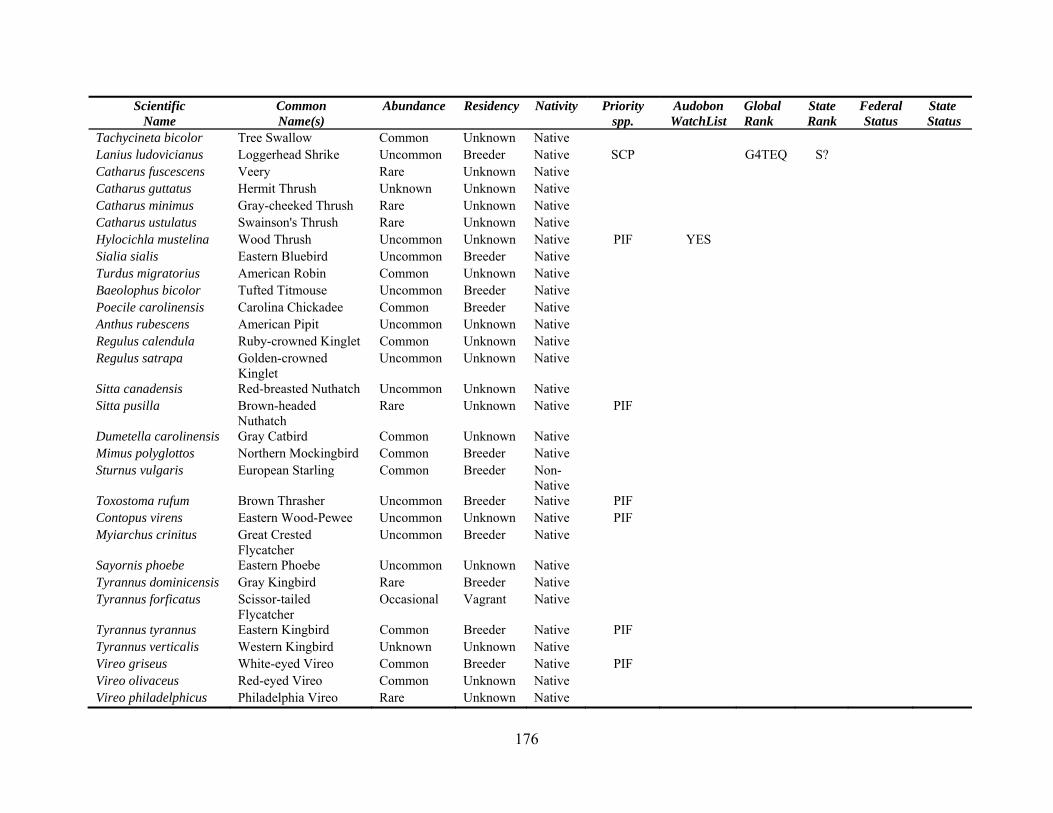
Scientific Name

Common Name(s)


Audobon WatchList

Global Rank

State Rank

Federal Status

State Status

Tachycineta bicolor Tree Swallow Common Unknown Native Lanius ludovicianus Loggerhead Shrike Uncommon Breeder Native SCP G4TEQ S? Catharus fuscescens Veery Rare Unknown Native Catharus guttatus Hermit Thrush Unknown Unknown Native Catharus minimus Gray-cheeked Thrush Rare Unknown Native Catharus ustulatus Swainson's Thrush Rare Unknown Native Hylocichla mustelina Wood Thrush Uncommon Unknown Native PIF YES Sialia sialis Eastern Bluebird Uncommon Breeder Native Turdus migratorius American Robin Common Unknown Native Baeolophus bicolor Tufted Titmouse Uncommon Breeder Native Poecile carolinensis Carolina Chickadee Common Breeder Native Anthus rubescens American Pipit Uncommon Unknown Native Regulus calendula Ruby-crowned Kinglet Common Unknown Native Regulus satrapa Golden-crowned

Kinglet Uncommon Unknown Native

Sitta canadensis Red-breasted Nuthatch Uncommon Unknown Native Sitta pusilla Brown-headed

Nuthatch Rare Unknown Native PIF

Dumetella carolinensis Gray Catbird Common Unknown Native Mimus polyglottos Northern Mockingbird Common Breeder Native Sturnus vulgaris European Starling Common Breeder Non-

Native

Toxostoma rufum Brown Thrasher Uncommon Breeder Native PIF Contopus virens Eastern Wood-Pewee Uncommon Unknown Native PIF Myiarchus crinitus Great Crested

Flycatcher Uncommon Breeder Native

Sayornis phoebe Eastern Phoebe Uncommon Unknown Native Tyrannus dominicensis Gray Kingbird Rare Breeder Native Tyrannus forficatus Scissor-tailed

Flycatcher Occasional Vagrant Native

Tyrannus tyrannus Eastern Kingbird Common Breeder Native PIF Tyrannus verticalis Western Kingbird Unknown Unknown Native Vireo griseus White-eyed Vireo Common Breeder Native PIF Vireo olivaceus Red-eyed Vireo Common Unknown Native Vireo philadelphicus Philadelphia Vireo Rare Unknown Native

176

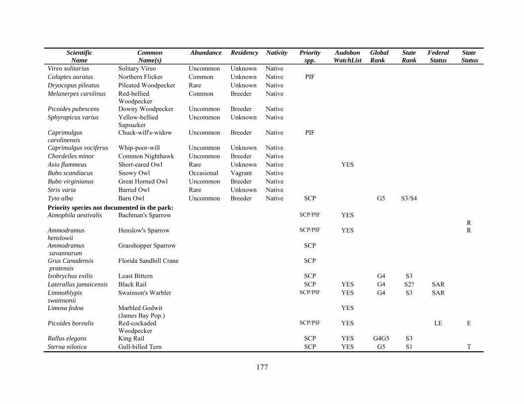
Scientific Name

Common Name(s)


Audobon WatchList

Global Rank

State Rank

Federal Status

State Status

Vireo solitarius Solitary Vireo Uncommon Unknown Native Colaptes auratus Northern Flicker Common Unknown Native PIF Dryocopus pileatus Pileated Woodpecker Rare Unknown Native Melanerpes carolinus Red-bellied

Woodpecker Common Breeder Native

Picoides pubescens Downy Woodpecker Uncommon Breeder Native Sphyrapicus varius Yellow-bellied

Sapsucker Uncommon Unknown Native

Caprimulgus carolinensis

Chuck-will's-widow Uncommon Breeder Native PIF

Caprimulgus vociferus Whip-poor-will Uncommon Unknown Native Chordeiles minor Common Nighthawk Uncommon Breeder Native Asio flammeus Short-eared Owl Rare Unknown Native YES Bubo scandiacus Snowy Owl Occasional Vagrant Native Bubo virginianus Great Horned Owl Uncommon Breeder Native Strix varia Barred Owl Rare Unknown Native Tyto alba Barn Owl Uncommon Breeder Native SCP G5 S3/S4 Priority species not documented in the park: Aimophila aestivalis Bachman's Sparrow SCP/PIF YES

R Ammodramus henslowii

Henslow's Sparrow SCP/PIF YES R

Ammodramus savannarum

Grasshopper Sparrow SCP

Grus Canadensis pratensis

Florida Sandhill Crane SCP

Ixobrychus exilis Least Bittern SCP G4 S3 Laterallus jamaicensis Black Rail SCP YES G4 S2? SAR Limnothlypis swainsonii

Swainson's Warbler SCP/PIF YES G4 S3 SAR

Limosa fedoa Marbled Godwit (James Bay Pop.)

YES

Picoides borealis Red-cockaded Woodpecker

SCP/PIF YES LE E

Rallus elegans King Rail SCP YES G4G5 S3 Sterna nilotica Gull-billed Tern SCP YES G5 S1 T

177

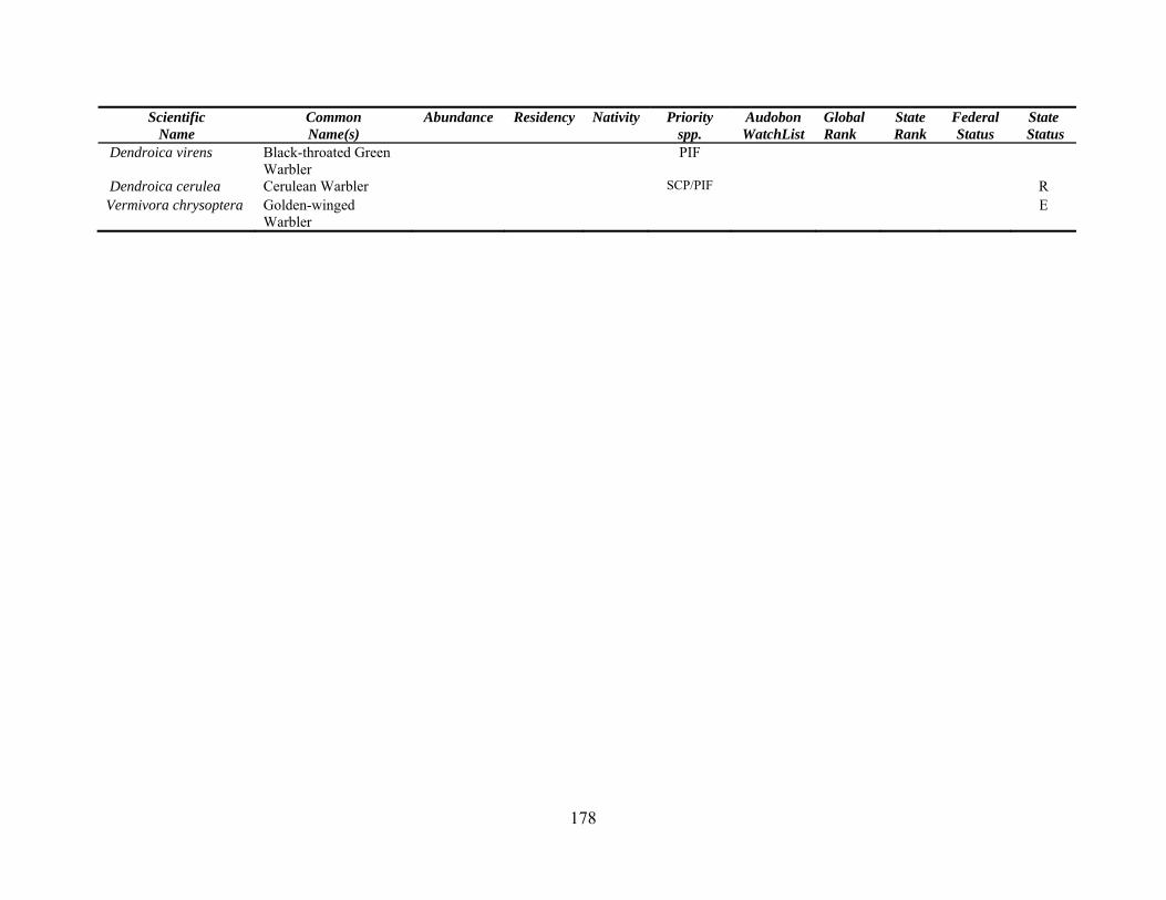
178

Scientific Name

Common Name(s)


Audobon WatchList

Global Rank

State Rank

Federal Status

State Status

Dendroica virens Black-throated Green Warbler

PIF

Dendroica cerulea Cerulean Warbler SCP/PIF R Vermivora chrysoptera Golden-winged

Warbler E

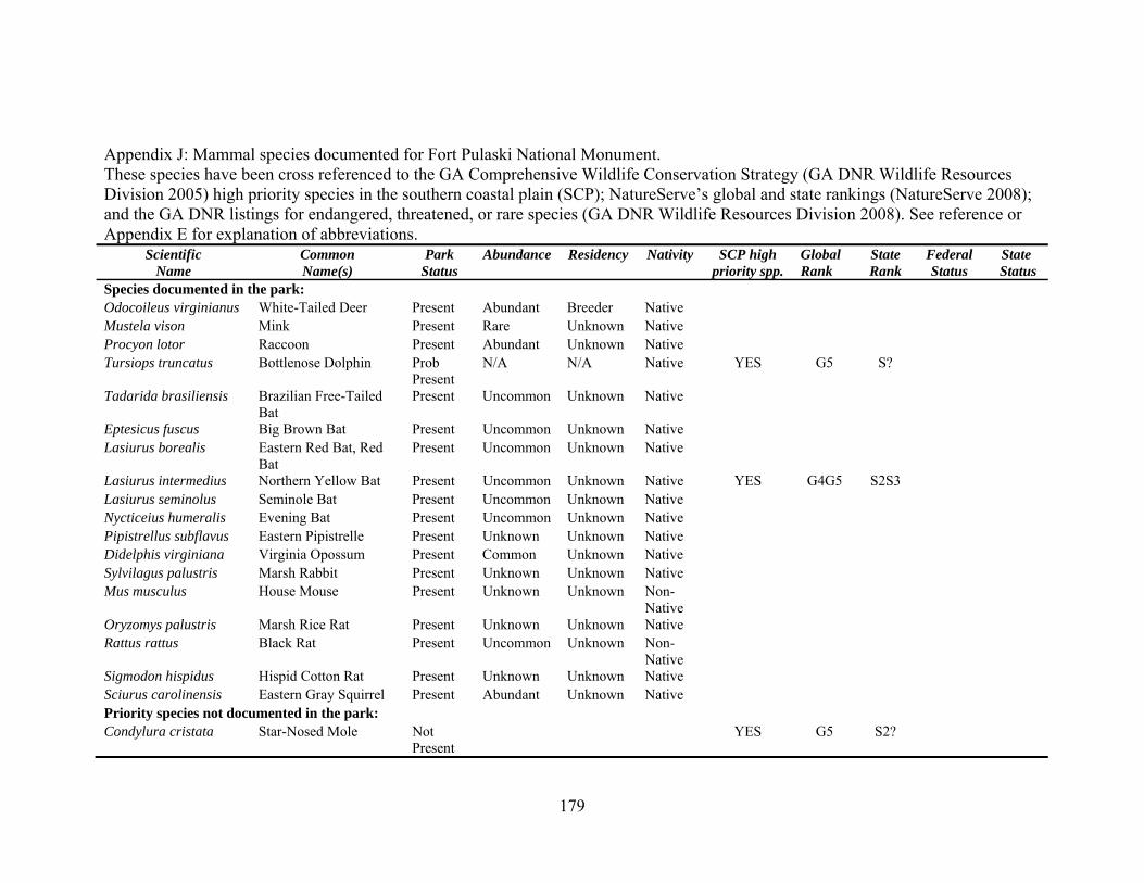
Appendix J: Mammal species documented for Fort Pulaski National Monument. These species have been cross referenced to the GA Comprehensive Wildlife Conservation Strategy (GA DNR Wildlife Resources Division 2005) high priority species in the southern coastal plain (SCP); NatureServe’s global and state rankings (NatureServe 2008); and the GA DNR listings for endangered, threatened, or rare species (GA DNR Wildlife Resources Division 2008). See reference or Appendix E for explanation of abbreviations.

Scientific Name

Common Name(s)

Park Status

Abundance Residency Nativity SCP high Global Rank

State Federal State priority spp. Rank Status Status

Species documented in the park: Odocoileus virginianus White-Tailed Deer Present Abundant Breeder Native Mustela vison Mink Present Rare Unknown Native Procyon lotor Raccoon Present Abundant Unknown Native Tursiops truncatus Bottlenose Dolphin

Prob Present

N/A N/A Native YES G5 S?

Tadarida brasiliensis Brazilian Free-Tailed Bat

Present Uncommon Unknown Native

Eptesicus fuscus Big Brown Bat Present Uncommon Unknown Native Lasiurus borealis Eastern Red Bat, Red

Bat Present Uncommon Unknown Native

Lasiurus intermedius Northern Yellow Bat Present Uncommon Unknown Native YES G4G5 S2S3 Lasiurus seminolus Seminole Bat Present Uncommon Unknown Native Nycticeius humeralis Evening Bat Present Uncommon Unknown Native Pipistrellus subflavus Eastern Pipistrelle Present Unknown Unknown Native Didelphis virginiana Virginia Opossum Present Common Unknown Native Sylvilagus palustris Marsh Rabbit Present Unknown Unknown Native Mus musculus House Mouse Present Unknown Unknown Non-

Native

Oryzomys palustris Marsh Rice Rat Present Unknown Unknown Native Rattus rattus Black Rat Present Uncommon Unknown Non-

Native

Sigmodon hispidus Hispid Cotton Rat Present Unknown Unknown Native Sciurus carolinensis Eastern Gray Squirrel Present Abundant Unknown Native Priority species not documented in the park: Condylura cristata Star-Nosed Mole Not

Present YES G5 S2?

179

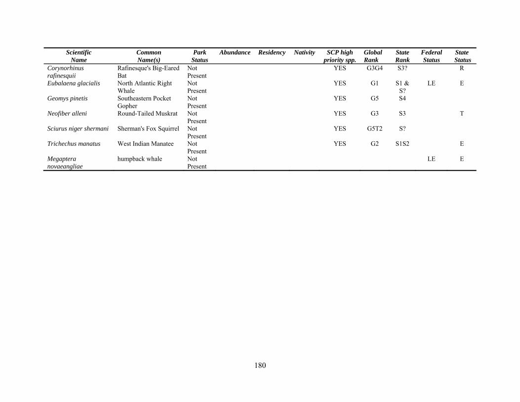
180

Status Scientific

Name Common Name(s)

Park Status


Global Rank

State Rank

Federal Status

State

Corynorhinus rafinesquii

Rafinesque's Big-Eared Bat

Not Present

YES G3G4 S3? R

Eubalaena glacialis North Atlantic Right Whale

Not Present

YES G1 S1 & S?

LE E

Geomys pinetis Southeastern Pocket Gopher

Not Present

YES G5 S4

Neofiber alleni Round-Tailed Muskrat Not Present

YES G3 S3 T

Sciurus niger shermani Sherman's Fox Squirrel Not Present

YES G5T2 S?

Trichechus manatus West Indian Manatee Not Present

YES G2 S1S2 E

Megaptera novaeangliae

humpback whale Not Present

LE E

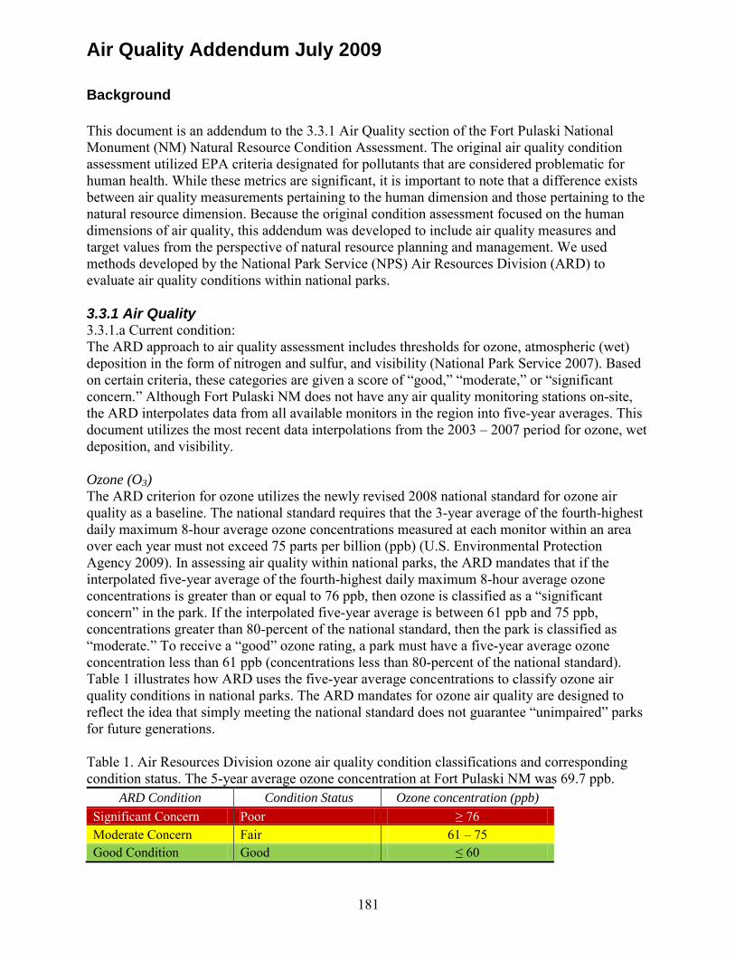
181

Background This document is an addendum to the 3.3.1 Air Quality section of the Fort Pulaski National Monument (NM) Natural Resource Condition Assessment. The original air quality condition assessment utilized EPA criteria designated for pollutants that are considered problematic for human health. While these metrics are significant, it is important to note that a difference exists between air quality measurements pertaining to the human dimension and those pertaining to the natural resource dimension. Because the original condition assessment focused on the human dimensions of air quality, this addendum was developed to include air quality measures and target values from the perspective of natural resource planning and management. We used methods developed by the National Park Service (NPS) Air Resources Division (ARD) to evaluate air quality conditions within national parks. 3.3.1 Air Quality 3.3.1.a Current condition: The ARD approach to air quality assessment includes thresholds for ozone, atmospheric (wet) deposition in the form of nitrogen and sulfur, and visibility (National Park Service 2007). Based on certain criteria, these categories are given a score of “good,” “moderate,” or “significant concern.” Although Fort Pulaski NM does not have any air quality monitoring stations on-site, the ARD interpolates data from all available monitors in the region into five-year averages. This document utilizes the most recent data interpolations from the 2003 – 2007 period for ozone, wet deposition, and visibility. Ozone (O3) The ARD criterion for ozone utilizes the newly revised 2008 national standard for ozone air quality as a baseline. The national standard requires that the 3-year average of the fourth-highest daily maximum 8-hour average ozone concentrations measured at each monitor within an area over each year must not exceed 75 parts per billion (ppb) (U.S. Environmental Protection Agency 2009). In assessing air quality within national parks, the ARD mandates that if the interpolated five-year average of the fourth-highest daily maximum 8-hour average ozone concentrations is greater than or equal to 76 ppb, then ozone is classified as a “significant concern” in the park. If the interpolated five-year average is between 61 ppb and 75 ppb, concentrations greater than 80-percent of the national standard, then the park is classified as “moderate.” To receive a “good” ozone rating, a park must have a five-year average ozone concentration less than 61 ppb (concentrations less than 80-percent of the national standard). Table 1 illustrates how ARD uses the five-year average concentrations to classify ozone air quality conditions in national parks. The ARD mandates for ozone air quality are designed to reflect the idea that simply meeting the national standard does not guarantee “unimpaired” parks for future generations. Table 1. Air Resources Division ozone air quality condition classifications and corresponding condition status. The 5-year average ozone concentration at Fort Pulaski NM was 69.7 ppb.

ARD Condition Condition Status Ozone concentration (ppb) Significant Concern Poor ≥ 76 Moderate Concern Fair 61 – 75 Good Condition Good ≤ 60

Air Quality Addendum July 2009

ir Quality Addendum 1

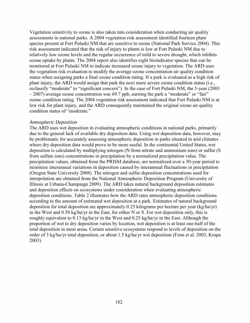
Vegetation sensitivity to ozone is also taken into consideration when conducting air quality assessments in national parks. A 2004 vegetation risk assessment identified fourteen plant species present at Fort Pulaski NM that are sensitive to ozone (National Park Service 2004). This risk assessment indicated that the risk of injury to plants is low at Fort Pulaski NM due to relatively low ozone levels and the regular occurrence of mild to severe drought, which inhibits ozone uptake by plants. The 2004 report also identifies eight bioindicator species that can be monitored at Fort Pulaski NM to indicate increased ozone injury to vegetation. The ARD uses the vegetation risk evaluation to modify the average ozone concentration air quality condition status when assigning parks a final ozone condition rating. If a park is evaluated as a high risk of plant injury, the ARD would assign that park the next more severe ozone condition status (i.e., reclassify “moderate” to “significant concern”). In the case of Fort Pulaski NM, the 5-year (2003 – 2007) average ozone concentration was 69.7 ppb, earning the park a “moderate” or “fair” ozone condition rating. The 2004 vegetation risk assessment indicated that Fort Pulaski NM is at low risk for plant injury, and the ARD consequently maintained the original ozone air quality condition status of “moderate.” Atmospheric Deposition The ARD uses wet deposition in evaluating atmospheric conditions in national parks, primarily due to the general lack of available dry deposition data. Using wet deposition data, however, may be problematic for accurately assessing atmospheric deposition in parks situated in arid climates where dry deposition data would prove to be more useful. In the continental United States, wet deposition is calculated by multiplying nitrogen (N from nitrate and ammonium ions) or sulfur (S from sulfate ions) concentrations in precipitation by a normalized precipitation value. The precipitation values, obtained from the PRISM database, are normalized over a 30-year period to minimize interannual variations in deposition caused by interannual fluctuations in precipitation (Oregon State University 2008). The nitrogen and sulfur deposition concentrations used for interpolation are obtained from the National Atmospheric Deposition Program (University of Illinois at Urbana-Champaign 2009). The ARD takes natural background deposition estimates and deposition effects on ecosystems under consideration when evaluating atmospheric deposition conditions. Table 2 illustrates how the ARD rates atmospheric deposition conditions according to the amount of estimated wet deposition at a park. Estimates of natural background deposition for total deposition are approximately 0.25 kilograms per hectare per year (kg/ha/yr) in the West and 0.50 kg/ha/yr in the East, for either N or S. For wet deposition only, this is roughly equivalent to 0.13 kg/ha/yr in the West and 0.25 kg/ha/yr in the East. Although the proportion of wet to dry deposition varies by location, wet deposition is at least one-half of the total deposition in most areas. Certain sensitive ecosystems respond to levels of deposition on the order of 3 kg/ha/yr total deposition, or about 1.5 kg/ha/yr wet deposition (Fenn et al. 2003, Krupa 2003).

182

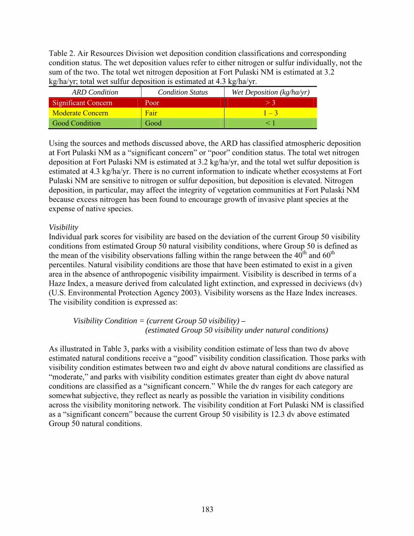
Table 2. Air Resources Division wet deposition condition classifications and corresponding condition status. The wet deposition values refer to either nitrogen or sulfur individually, not the sum of the two. The total wet nitrogen deposition at Fort Pulaski NM is estimated at 3.2 kg/ha/yr; total wet sulfur deposition is estimated at 4.3 kg/ha/yr.

ARD Condition Condition Status Wet Deposition (kg/ha/yr) Significant Concern Poor > 3 Moderate Concern Fair 1 – 3 Good Condition Good < 1

Using the sources and methods discussed above, the ARD has classified atmospheric deposition at Fort Pulaski NM as a “significant concern” or “poor” condition status. The total wet nitrogen deposition at Fort Pulaski NM is estimated at 3.2 kg/ha/yr, and the total wet sulfur deposition is estimated at 4.3 kg/ha/yr. There is no current information to indicate whether ecosystems at Fort Pulaski NM are sensitive to nitrogen or sulfur deposition, but deposition is elevated. Nitrogen deposition, in particular, may affect the integrity of vegetation communities at Fort Pulaski NM because excess nitrogen has been found to encourage growth of invasive plant species at the expense of native species. Visibility Individual park scores for visibility are based on the deviation of the current Group 50 visibility conditions from estimated Group 50 natural visibility conditions, where Group 50 is defined as the mean of the visibility observations falling within the range between the 40th and 60th percentiles. Natural visibility conditions are those that have been estimated to exist in a given area in the absence of anthropogenic visibility impairment. Visibility is described in terms of a Haze Index, a measure derived from calculated light extinction, and expressed in deciviews (dv) (U.S. Environmental Protection Agency 2003). Visibility worsens as the Haze Index increases. The visibility condition is expressed as:

Visibility Condition = (current Group 50 visibility) – (estimated Group 50 visibility under natural conditions)

As illustrated in Table 3, parks with a visibility condition estimate of less than two dv above estimated natural conditions receive a “good” visibility condition classification. Those parks with visibility condition estimates between two and eight dv above natural conditions are classified as “moderate,” and parks with visibility condition estimates greater than eight dv above natural conditions are classified as a “significant concern.” While the dv ranges for each category are somewhat subjective, they reflect as nearly as possible the variation in visibility conditions across the visibility monitoring network. The visibility condition at Fort Pulaski NM is classified as a “significant concern” because the current Group 50 visibility is 12.3 dv above estimated Group 50 natural conditions.

183

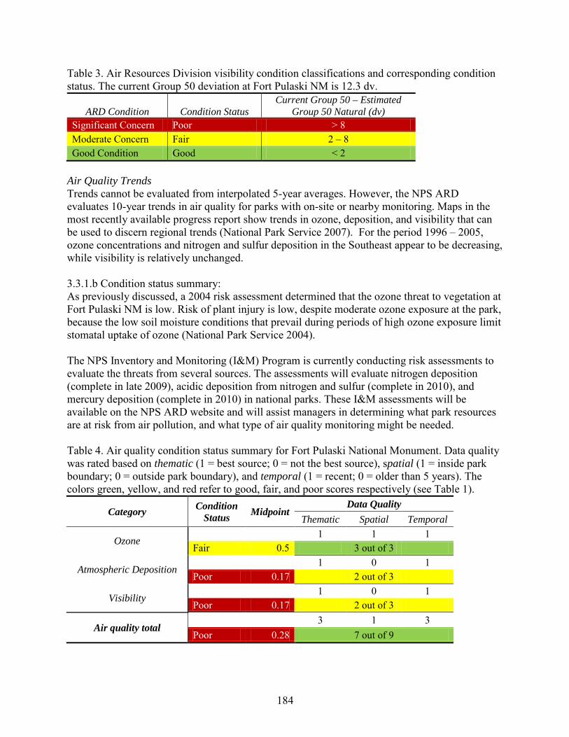
Table 3. Air Resources Division visibility condition classifications and corresponding condition status. The current Group 50 deviation at Fort Pulaski NM is 12.3 dv.

ARD Condition Condition Status Current Group 50 – Estimated

Group 50 Natural (dv) Significant Concern Poor > 8 Moderate Concern Fair 2 – 8 Good Condition Good < 2

Air Quality Trends Trends cannot be evaluated from interpolated 5-year averages. However, the NPS ARD evaluates 10-year trends in air quality for parks with on-site or nearby monitoring. Maps in the most recently available progress report show trends in ozone, deposition, and visibility that can be used to discern regional trends (National Park Service 2007). For the period 1996 – 2005, ozone concentrations and nitrogen and sulfur deposition in the Southeast appear to be decreasing, while visibility is relatively unchanged. 3.3.1.b Condition status summary: As previously discussed, a 2004 risk assessment determined that the ozone threat to vegetation at Fort Pulaski NM is low. Risk of plant injury is low, despite moderate ozone exposure at the park, because the low soil moisture conditions that prevail during periods of high ozone exposure limit stomatal uptake of ozone (National Park Service 2004). The NPS Inventory and Monitoring (I&M) Program is currently conducting risk assessments to evaluate the threats from several sources. The assessments will evaluate nitrogen deposition (complete in late 2009), acidic deposition from nitrogen and sulfur (complete in 2010), and mercury deposition (complete in 2010) in national parks. These I&M assessments will be available on the NPS ARD website and will assist managers in determining what park resources are at risk from air pollution, and what type of air quality monitoring might be needed. Table 4. Air quality condition status summary for Fort Pulaski National Monument. Data quality was rated based on thematic (1 = best source; 0 = not the best source), spatial (1 = inside park boundary; 0 = outside park boundary), and temporal (1 = recent; 0 = older than 5 years). The colors green, yellow, and red refer to good, fair, and poor scores respectively (see Table 1).

Category Condition Status Midpoint


Ozone 1 1 1 Fair 0.5 3 out of 3

Atmospheric Deposition 1 0 1 Poor 0.17 2 out of 3

Visibility 1 0 1 Poor 0.17 2 out of 3

Air quality total 3 1 3 Poor 0.28 7 out of 9

184

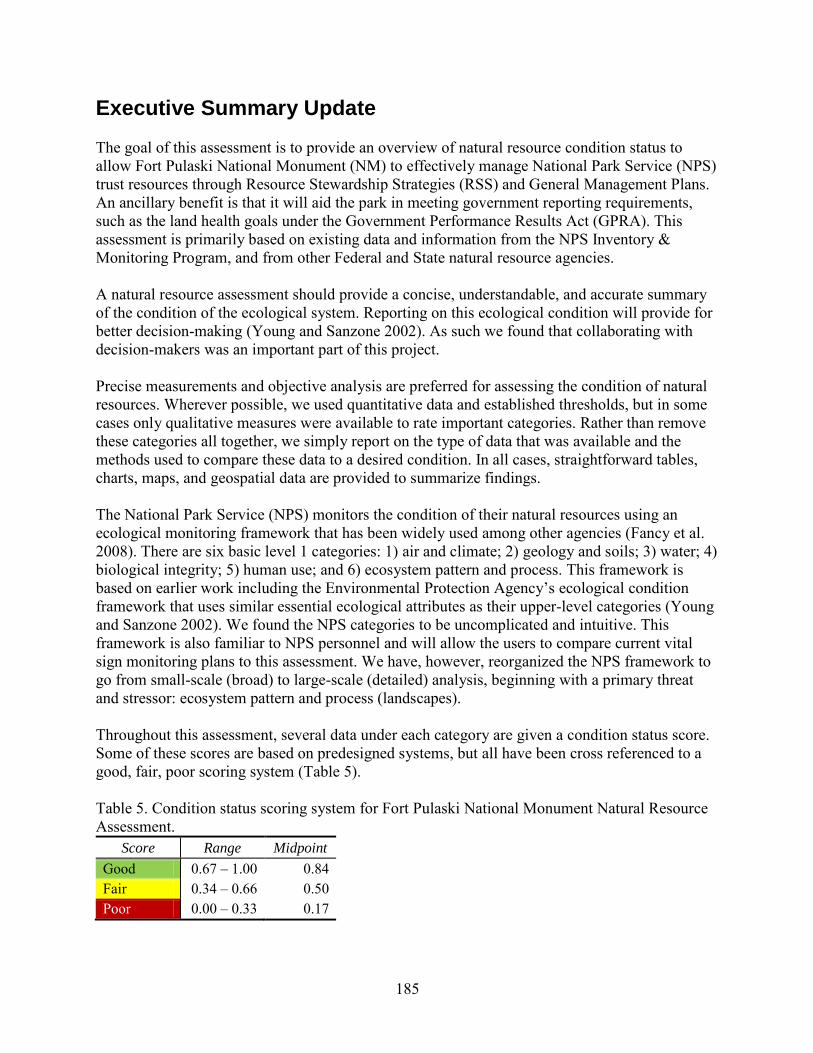
Executive Summary Update The goal of this assessment is to provide an overview of natural resource condition status to allow Fort Pulaski National Monument (NM) to effectively manage National Park Service (NPS) trust resources through Resource Stewardship Strategies (RSS) and General Management Plans. An ancillary benefit is that it will aid the park in meeting government reporting requirements, such as the land health goals under the Government Performance Results Act (GPRA). This assessment is primarily based on existing data and information from the NPS Inventory & Monitoring Program, and from other Federal and State natural resource agencies. A natural resource assessment should provide a concise, understandable, and accurate summary of the condition of the ecological system. Reporting on this ecological condition will provide for better decision-making (Young and Sanzone 2002). As such we found that collaborating with decision-makers was an important part of this project. Precise measurements and objective analysis are preferred for assessing the condition of natural resources. Wherever possible, we used quantitative data and established thresholds, but in some cases only qualitative measures were available to rate important categories. Rather than remove these categories all together, we simply report on the type of data that was available and the methods used to compare these data to a desired condition. In all cases, straightforward tables, charts, maps, and geospatial data are provided to summarize findings. The National Park Service (NPS) monitors the condition of their natural resources using an ecological monitoring framework that has been widely used among other agencies (Fancy et al. 2008). There are six basic level 1 categories: 1) air and climate; 2) geology and soils; 3) water; 4) biological integrity; 5) human use; and 6) ecosystem pattern and process. This framework is based on earlier work including the Environmental Protection Agency’s ecological condition framework that uses similar essential ecological attributes as their upper-level categories (Young and Sanzone 2002). We found the NPS categories to be uncomplicated and intuitive. This framework is also familiar to NPS personnel and will allow the users to compare current vital sign monitoring plans to this assessment. We have, however, reorganized the NPS framework to go from small-scale (broad) to large-scale (detailed) analysis, beginning with a primary threat and stressor: ecosystem pattern and process (landscapes). Throughout this assessment, several data under each category are given a condition status score. Some of these scores are based on predesigned systems, but all have been cross referenced to a good, fair, poor scoring system (Table 5). Table 5. Condition status scoring system for Fort Pulaski National Monument Natural Resource Assessment.

Score Range Midpoint Good 0.67 – 1.00 0.84 Fair 0.34 – 0.66 0.50 Poor 0.00 – 0.33 0.17

185

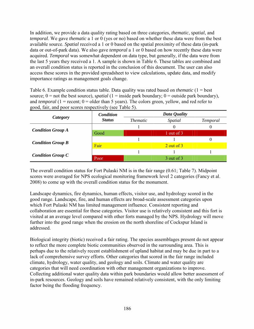
In addition, we provide a data quality rating based on three categories, thematic, spatial, and temporal. We gave thematic a 1 or 0 (yes or no) based on whether these data were from the best available source. Spatial received a 1 or 0 based on the spatial proximity of these data (in-park data or out-of-park data). We also gave temporal a 1 or 0 based on how recently these data were acquired. Temporal was somewhat dependent on data type, but generally, if the data were from the last 5 years they received a 1. A sample is shown in Table 6. These tables are combined and an overall condition status is reported in the conclusion of this document. The user can also access these scores in the provided spreadsheet to view calculations, update data, and modify importance ratings as management goals change. Table 6. Example condition status table. Data quality was rated based on thematic (1 = best source; 0 = not the best source), spatial (1 = inside park boundary; 0 = outside park boundary), and temporal (1 = recent; 0 = older than 5 years). The colors green, yellow, and red refer to good, fair, and poor scores respectively (see Table 5).



Condition Group A 1 0 0 Good 1 out of 3

Condition Group B 1 1 0 Fair 2 out of 3

Condition Group C 1 1 1 Poor 3 out of 3

The overall condition status for Fort Pulaski NM is in the fair range (0.61; Table 7). Midpoint scores were averaged for NPS ecological monitoring framework level 2 categories (Fancy et al. 2008) to come up with the overall condition status for the monument. Landscape dynamics, fire dynamics, human effects, visitor use, and hydrology scored in the good range. Landscape, fire, and human effects are broad-scale assessment categories upon which Fort Pulaski NM has limited management influence. Consistent reporting and collaboration are essential for these categories. Visitor use is relatively consistent and this fort is visited at an average level compared with other forts managed by the NPS. Hydrology will move further into the good range when the erosion on the north shoreline of Cockspur Island is addressed. Biological integrity (biotic) received a fair rating. The species assemblages present do not appear to reflect the more complete biotic communities observed in the surrounding area. This is perhaps due to the relatively recent establishment of upland habitat and may be due in part to a lack of comprehensive survey efforts. Other categories that scored in the fair range included climate, hydrology, water quality, and geology and soils. Climate and water quality are categories that will need coordination with other management organizations to improve. Collecting additional water quality data within park boundaries would allow better assessment of in-park resources. Geology and soils have remained relatively consistent, with the only limiting factor being the flooding frequency.

186

The only category in this assessment to receive a poor rating was air quality. Despite a fair ozone exposure score, the poor rating was a result of high levels of estimated atmospheric deposition and poor visibility due to a high Haze Index score. Similar to landscape, fire, and human effects, air quality is a broad-scale assessment category upon which Fort Pulaski NM has limited management influence. Spatial proximity and thematic (best source) are the limiting factors in data quality. Thematic is often in the fair range for data quality, mostly due to needing more local-scale data. This National Monument was established primarily to protect cultural resources, so a minimal amount of natural resource data has been collected on-site. There are plans to map vegetation communities and continue species and community inventory and monitoring. An observation that was present in several of the assessment categories is the importance of coordination with outside management organizations. It was also noted in several categories that additional local-scale data collection could improve assessment and management. The good, fair, poor scoring system has its limitations. It is somewhat subjective, especially when pre-established thresholds and criteria are missing. However, in most cases we were able to find thresholds from other agencies or peer-reviewed publications. We made note of the cases where established rating systems or thresholds were not available. With these caveats in mind, we effectively reported on the condition status of important natural resource management categories while providing further information on data quality.

187

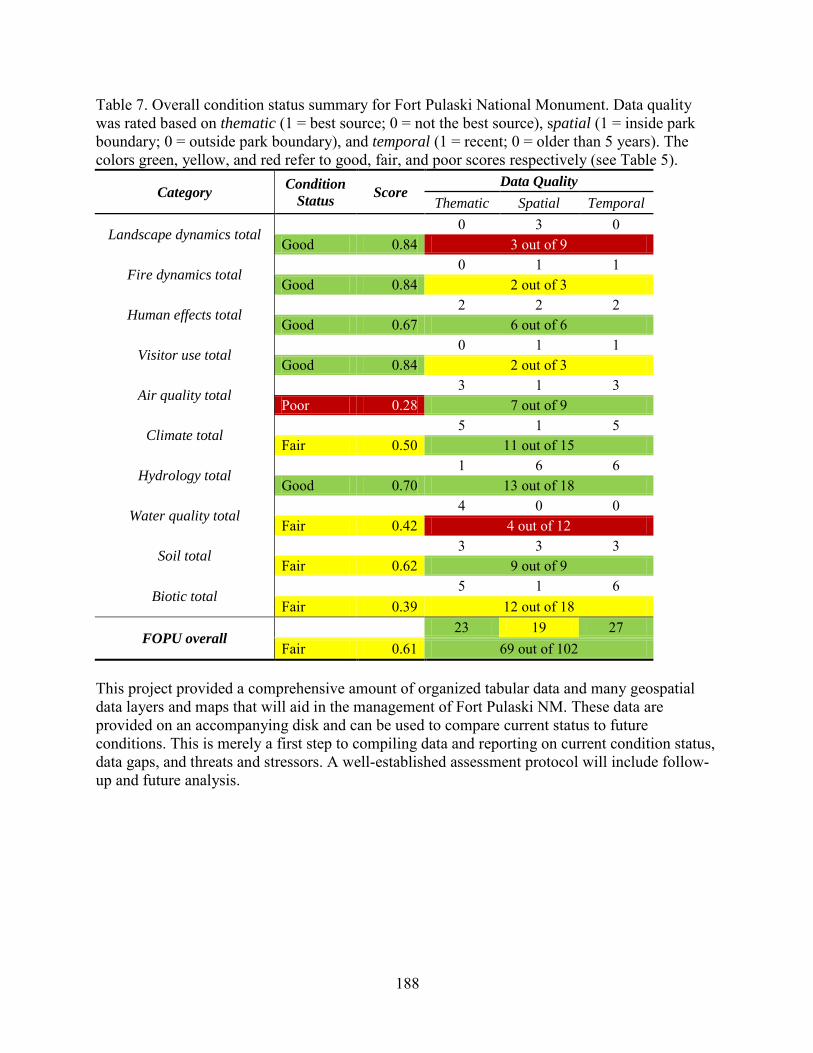
Table 7. Overall condition status summary for Fort Pulaski National Monument. Data quality was rated based on thematic (1 = best source; 0 = not the best source), spatial (1 = inside park boundary; 0 = outside park boundary), and temporal (1 = recent; 0 = older than 5 years). The colors green, yellow, and red refer to good, fair, and poor scores respectively (see Table 5).

Category Condition Status Score


Landscape dynamics total 0 3 0 Good 0.84 3 out of 9

Fire dynamics total 0 1 1 Good 0.84 2 out of 3

Human effects total 2 2 2 Good 0.67 6 out of 6

Visitor use total 0 1 1 Good 0.84 2 out of 3

Air quality total 3 1 3 Poor 0.28 7 out of 9

Climate total 5 1 5 Fair 0.50 11 out of 15

Hydrology total 1 6 6 Good 0.70 13 out of 18

Water quality total 4 0 0 Fair 0.42 4 out of 12

Soil total 3 3 3 Fair 0.62 9 out of 9

Biotic total 5 1 6 Fair 0.39 12 out of 18

FOPU overall 23 19 27 Fair 0.61 69 out of 102


188

Literature Cited Fancy, S. G., J. E. Gross, and S. L. Carter. 2008. Monitoring the condition of natural resources in

US National Parks. Environmental Monitoring and Assessment (In Press).

Fenn, M. E., J. S. Baron, E. B. Allen, H. M. Reuth, K. R. Nydick, L. Geiser, W. D. Bowman, J. O. Sickman, T. Meixner, D. W. Johnson, and P. Neitlich. 2003. Ecological Effects of Nitrogen Deposition in the Western United States. BioScience 53:404-420.

Krupa, S. V. 2003. Effects of atmospheric ammonia (NH3) on terrestrial vegetation: a review. Environmental Pollution 124:179-221.

National Park Service. 2004. Assessing the Risk of Foliar Injury From Ozone On Vegetation In Parks In the Southeast Coast Network. (http://www.nature.nps.gov/air/Pubs/pdf/03Risk/secnO3RiskOct04.pdf). Accessed June 2009.

National Park Service. 2007. 2006 Annual Performance & Progress Report: Air Quality in National Parks. (http://www.nature.nps.gov/air/Pubs/pdf/gpra/GPRA_AQ_ConditionsTrendReport2006.pdf). Accessed June 2009.

Oregon State University. 2008. Prism Climate Group. (http://www.prism.oregonstate.edu/). Accessed June 2009.

U.S. Environmental Protection Agency. 2003. Guidance for Estimating Natural Visibility Conditions Under the Regional Haze Program. EPA-454/B-03-005. Office of Air Quality Planning and Standards, United States Environmental Protection Agency, Research Triangle Park, NC. (http://www.epa.gov/ttn/oarpg/t1/memoranda/rh_envcurhr_gd.pdf). Accessed June 2009.

U.S. Environmental Protection Agency. 2009. Ground-level Ozone Air Quality Standards. (http://www.epa.gov/air/ozonepollution/standards.html). Accessed June 2009.

University of Illinois at Urbana-Champaign. 2009. National Atmospheric Deposition Program. (http://nadp.sws.uiuc.edu/). Accessed June 2009.

Young, T. F. and S. Sanzone. 2002. A framework for assessing and reporting on ecological condition.

189

The Department of the Interior protects and manages the nation’s natural resources and cultural heritage; provides scientific and other information about those resources; and honors its special responsibilities to American Indians, Alaska Natives, and affiliated Island Communities. NPS D-172, May 2009

National Park Service U.S. Department of the Interior

Natural Resource Program Center 1201 Oakridge Drive, Suite 150 Fort Collins, CO 80525

www.nature.nps.gov

EXPERIENCE YOUR AMERICA TM

Natural Resource Condition Assessment ZLWK DGGHQGXP

Documents

Transcript of Natural Resource Condition Assessment ZLWK DGGHQGXP