This article appeared in a journal published by Elsevier. The attachedcopy is furnished to the author for internal non-commercial researchand education use, including for instruction at the authors institution

and sharing with colleagues.

Other uses, including reproduction and distribution, or selling orlicensing copies, or posting to personal, institutional or third party

websites are prohibited.

In most cases authors are permitted to post their version of thearticle (e.g. in Word or Tex form) to their personal website orinstitutional repository. Authors requiring further information

regarding Elsevier’s archiving and manuscript policies areencouraged to visit:

http://www.elsevier.com/copyright

Author's personal copy

Myocardial border detection from ventriculograms using support vectormachines and real-coded genetic algorithms

Miguel Vera a, Antonio Bravo b,�, Ruben Medina c

a Laboratorio de Fısica, Departamento de Ciencias, Universidad de Los Andes-Tachira, San Cristobal 5001, Venezuelab Grupo de Bioingenierıa, Decanato de Investigacion, Universidad Nacional Experimental del Tachira, San Cristobal 5001, Venezuelac Grupo de Ingenierıa Biomedica (GIBULA), Facultad de Ingenierıa, Universidad de Los Andes, Merida 5101, Venezuela

a r t i c l e i n f o

Article history:

Received 23 December 2008

Accepted 17 February 2010

Keywords:

Human heart

Anatomical landmarks

Myocardial border

Left ventricle

Patterns classification

Support vectors machines

Real-coded genetic algorithms

Deformable models

a b s t r a c t

In this research a two step method for left ventricle segmentation based on landmark detection and

evolutionary snakes is reported. The proposed approach is applied to human heart angiograms. Several

anatomical landmarks located on the left ventricle are obtained using support vector machines. The

training stage is performed based on a set of windows of size 31� 31 including landmarks and non-

landmarks pixel patterns. The support vector machines use a radial basis function kernel and the

structural risk minimization principle as the inference rule. During the training stage, no false positives

are obtained and during the detection stage a 97.94% of recognition is attained. The estimated landmark

location is used for constructing an approximate myocardial border. This contour is a deformable model

that is optimized using a real-coded genetic algorithm. A validation is performed by comparing the

estimated contours with respect to contours manually traced by two cardiologists. From this validation

stage the maximum of the average contour error considering 6 angiographic sequences (a total of 178

images) is 4.93%.

& 2010 Elsevier Ltd. All rights reserved.

1. Introduction

In clinical routine, cardiologists use heart cavities images forthe assessment of morphology and function of the heart [1]. Thesemedical images provide enough information about the size andshape of heart cavities during the cardiac cycle. Left ventricleplays a major role in the heart dynamics. The accurate descriptionof ventricular shape and their quantitative analysis are important,since cardiovascular disease (CVD) accounts for one third of thedeaths in the world [2].

X-rays-based contrast cineangiography provides a projectedimage of cardiac structures [3]. Left ventricle images are obtainedafter the injection of a contrast medium in the cavities of the heartaiming at enhancing the contrast with respect to other tissues.Ventriculographic image analysis requires a precise description ofventricular shape in order to quantify the parameters associatedwith the cardiovascular function [4,5] or alternatively, forperforming the visualization of this anatomical structure [6].

Several left ventricular cavity detection methods are based ontracing a curve that delimits this heart structure and enablesquantification of this image region [7]. Other methods are basedon pattern recognition techniques where clustering methods are

applied. These methods allow splitting the image in a non-overlapped set of regions whose union is the complete image [8].Additionally, there are methods that consider the contour featuresand region information for extracting the ventricular contours [9].

Recently, robust methods for X-ray ventriculographic imagesegmentation have been proposed. A left ventricle boundarydelineation system based on anatomical knowledge about thecardiac cavity has been reported [10]. A ventricular contourdetector based on neural networks (NN) has been reported in [11].Other contribution reports a ventricular cavity automatic seg-mentation method based on active appearance models (AAMs)and dynamic programming (DP) [9]. Additionally, an unsuper-vised clustering approach for left ventricle segmentation based ona region growing technique is reported in [12]. These methodshave been validated using clinical data by comparison of theestimated contour with respect to the reference contour traced bythe cardiologist. Sui et al. [10] reported a mean absolute contourerror of 3 mm. A total of 375 clinical cases were processed. Suzukiet al. [11] have obtained an average contour error at end-diastoleof 6.2%. Oost et al. [9] included 140 images in the validation toobtain the average border positioning error smaller than 1.45 mm,and the contour error of 4.1% and 12.8% for end-diastole (ED) andfor end-systole (ES), respectively. Bravo and Medina [12] haveestimated the segmentation error for 437 images extracted frommono-plane and bi-plane ventriculographic sequences. Theaverage contour error was 6.67% at ED and 12.44% at ES. The

ARTICLE IN PRESS

Contents lists available at ScienceDirect

journal homepage: www.elsevier.com/locate/cbm

Computers in Biology and Medicine

0010-4825/$ - see front matter & 2010 Elsevier Ltd. All rights reserved.

doi:10.1016/j.compbiomed.2010.02.009

� Corresponding author. Tel.: +58 2763532454.

E-mail addresses: abravo@unet.edu.ve, antonio.j.bravo@gmail.com (A. Bravo).

Computers in Biology and Medicine 40 (2010) 446–455

Author's personal copyARTICLE IN PRESS

average area error was 8.58% at ED and 3.32% at ES. In general,these methods provided an accurate representation of ventricularborders, however, they are not yet fully validated and accepted byclinicians as a gold standard.

In several segmentation techniques, a previous stage could berequired for detecting an initial set of landmark points locatednear the shape to detect [13]. In medical imaging, landmarksdetection represents a useful stage for extracting information thatdescribes an anatomical structure. In the case of cardiac imaging,the apex, the basal regions and the aortic valve are usefullandmarks for defining the left ventricle shape. The extractedimage landmarks are used in various applications of cardiac imageanalysis, such as segmentation [14], shape-model construction[15] and motion analysis [16].

The objective of this work is to develop an approach based onmachine learning for detecting the left ventricle (LV) border fromX-ray angiograms. The algorithm includes two stages: First, anapproximation of the ventricular contour is obtained by means ofthe support vector machines by detecting several anatomicallandmarks located on the left ventricle boundaries. In the secondstage, an active contour model is used for representing the leftventricle border. An energy functional is constructed for repre-senting the contour energy, and the final optimal contour shapecorresponds to the minimum of this functional. A scheme basedon real-coded genetic algorithms is used for obtaining theminimal energy condition.

2. Related work

Approaches based on genetic algorithms (GA) have beenproposed to detect the left ventricle shape in image modalitiessuch as magnetic resonance (MR) and echocardiographic images.An automated system to optimize the set of parameters of leftventricle identification process has been proposed by Angelieet al. [17]. Two approaches are implemented, the first is based ona simple GA (SGA) and the second is based on a steady state GA(2SGA). The performance of the method is evaluated quantita-tively using the similarity criterion. MR images are used in thetest phase. The objective is to measure the similarity degreebetween the automatically outlined contours and gold standardtraced by a cardiologist. The attained similarity degrees are 59.5%and 66.7% for SGA and 2SGA, respectively.

Segmentation approaches based on deformable models havebecome a common application in 2-D and 3-D image analysis[18,19]. Deformable models and deformable surfaces haveenabled segmentation, registering and tracking of anatomicalstructures from multidimensional medical images [7,20,21]. Themodel fitting process is a dynamical process whose objective is tooptimize the time-varying model formulation (energy model).This optimization process has been implemented using adiscretization and numerical solution [22], basic physical rules[23], and a probabilistic framework [24].

Genetic algorithms (GA) have been used for more than 10years to optimize active contours [25,26]. An automatic approachfor left ventricle contour detection from 2-D echocardiographicimages was presented by Mishra et al. [27]. The LV contours wereobtained using an optimization process for updating an activecontour model considering all images in a sequence. A preproces-sing stage based on Gaussian filtering, thresholding and morpho-logical filtering was used to obtain an approximation of the cavityregion which was used as initialization for the active contourmodel. The initial state of the active contour model was optimizedusing a genetic algorithm. A comparison among the area enclosedby the ground truth contour and the contour obtained by the

method was presented as a correlation coefficient. The correlationin an angiographic image sequence was 0.9232.

3. Theory

3.1. Background in support vector machine

Support vector machine (SVM) is a methodology based on theVapnik–Chervonenkis learning theory and the structural riskminimization principle [28]. SVMs are efficient non-parametricclassification and regression tools [29,30]. In classificationproblems SVMs are used for constructing a discriminant functionto separate classes using vectors nearest to the decision boundary.The examples or training set for a two-class classification problemcan be represented as: D¼ fðxi; yiÞg

li ¼ 1 �RN

� fþ1;�1g, where yi

is the class associated to input pattern xi.The classification task (from D) addresses the general problem

of finding a discrimination function defined from an input spaceRN into an unordered set of classes {+1,�1}. This discriminationfunction in some m-dimensional feature space is a separatinghyper-plane expressed as follows:

f ðxÞ ¼ signðw � xþbÞ; ð1Þ

where w is the normal to the hyper-plane, b is the bias, JwJ is theEuclidean norm of w, and jbj=JwJ is the perpendicular distancefrom the origin to the hyper-plane.

The SVM objective is to find the hyper-plane with minimumnorm JwJ2 that optimally separates the data. The classificationproblem using linear machines trained on non-separable exam-ples [31,32], can be formulated as a quadratic programmingproblem where the optimal solution is obtained using Lagrangemultipliers. This solution can be written as

w¼Xl

i ¼ 1

liyixi; ð2Þ

where fl1; . . . ; llg are positive Lagrange multipliers. In (2), theexamples (xi) for which li40 are known as support vectors andcorrespond to the critical elements of the training set (the nearestpoints in the training set to the hyper-plane).

In real classification tasks a linear SVM classifier is notappropriate because the classes are generally separated by anon-linear function [32]. In this case, the examples are projectedto a feature space of higher dimensions (possibly infinite) via anon-linear mapping function Uð�Þ. This projection process isapplied to transform the non-linear problem in the N-space to alinear problem in the M-space (feature space). The SVM solutioncan be written as

f ðxÞ ¼ signXl

i ¼ 1

yiliUðxiÞ �UðxÞþb

!; ð3Þ

where x is the data to classify and xi are the support vectors.In the feature space a linear classification is performed. For

that reason, the so-called kernel function (K) is introduced tocompute scalar products of the form FðxiÞ �FðxjÞ:

Kðxi;xjÞ �FðxiÞ �FðxjÞ: ð4Þ

Using (3) and (4) the SVM real classifier is expressed as

f ðxÞ ¼ signXl

i ¼ 1

yiliðKðx;xiÞÞþb

!: ð5Þ

In summary, the SVMs training process consists of obtainingthe support vectors that define the optimal separating hyper-plane (2). In order to classify an input data non-considered in thetraining set, the classifier (5) is used.

M. Vera et al. / Computers in Biology and Medicine 40 (2010) 446–455 447

Author's personal copyARTICLE IN PRESS

3.2. Real-coded genetic algorithms

Genetic algorithms (GAs) provide a general search approachmotivated by an analogy to natural selection [33]. Given a searchspace or population, the objective is to identify the best memberor individual in this population. A best individual is defined as theone that optimizes an objective function (so called adaptationfunction or fitness). An initial population is used to start the GA.This population is evolved to create a new population. Eachsuccessive population is called a generation. There are threeoperations for creating a new generation: (a) evaluation of allmembers of the population according to a fitness function; (b)selection of these individuals in the current population attainingthe higher fitness values and; (c) creation of new individuals byapplying reproduction operators, such as crossover and mutation,to the selected individuals [34].

The individuals or chromosomes in GAs are often representedusing a binary representation given by bit strings because theycan be easily manipulated by reproduction operators. The binaryrepresentation can become redundant when a parameter with acardinality different from a power of two is coded. An additionaldrawback arises when the optimization process requires acontinuous search space with large dimensions, and the binaryrepresentation using fixed length bit strings would sacrifice theaccuracy of the solution. These limitations are the main reasonsfor developing algorithms using real-coded chromosome repre-sentations [35,36].

In optimization problems with variables represented in acontinuous domain, the most natural representation is realcoding, where each gene in the chromosome represents a variable[37,38]. A GA that uses this kind of representation is known as areal-coded genetic algorithm (RCGA). Herrera et al. [39] reviewthe main reproduction strategies for real-coded genetic algo-rithms that have been proposed in the literature.

3.3. Deformable models

A deformable model is a geometrical parametric contourlocated in the image plane ðx; yÞAR2. This contour could berepresented as a controlled continuity spline expressed asvðsÞ ¼ ðxðsÞ; yðsÞÞ>, where x and y are vectors of coordinatefunctions and sA ½0;1� is the parametric domain [22]. The energyassociated with this deformable model can be described accordingto the following functional:

E¼

Zs½EinternalðvðsÞÞþEimageðvðsÞÞ�ds: ð6Þ

The internal energy is given by the Eq. (7), the subscripts of varray denote the derivation operation. The weighting factors aand b represent the elasticity and rigidity coefficients associatedwith the deformable model. These coefficients are used forweighting the smoothness and the bending properties of themodel. The spline internal energy imposes the smoothnessrestriction.

Einternal ¼ajvsðsÞj

2þbjvssðsÞj2

2: ð7Þ

The image energy is constructed according to (8). Thisfunctional is based on the border detection theory proposed in[40], where the intensity changes can be detected by finding themaximum or the minimum of Gs � I that represents the convolu-tion of an image I with a bidimensional Gaussian distributionfunction Gs. The image energy pushes the deformable modeltoward the contour that constitutes the target features.

Eimage ¼�jrGs � Ij; ð8Þ

where s is the spread parameter (standard deviation) of theGaussian kernel.

According to variational calculus [41,42], the contour v thatminimizes the deformable model energy (6) must satisfy theEuler–Lagrange equation. This equation can be represented bytwo independent differential Eq. (9).

axssþbxssssþ@Eimage

@x¼ 0;

ayssþbyssssþ@Eimage

@y¼ 0: ð9Þ

Several approaches have been proposed to find the optimalcontour [22–24].

4. Myocardial borders detection approach

4.1. Data source

The data used in this research are sequences of mono-planeventriculographic images that have been acquired using a digitalflat-panel X-rays system (InnovaTM 4150, General Electric MedicalSystem). In the experimental setup, six databases acquired fromdifferent patients are considered. Each database contains 38images. These images are acquired using the right anterioroblique (RAO 303) view. Each image has a resolution of 420�420 pixels with a pixel size of ð0:285� 0:285Þmm. Each pixelvalue is represented by 8 bits. Fig. 1 shows a pair of angiographicimages of the left ventricle acquired using the RAO 303 view.

4.2. SVM left ventricle landmarks detection approach

In this case, the learning task involves classifying pixelpatterns that represent left ventricle landmarks in ventriculo-grams. This is a classification problem where a sample pixelpattern is classified as belonging to one of the possible categoriesor classes. Our approach uses densitometric information and asupport vector machine (SVM) for the reliable localization oflandmarks in ventriculographic images. American Heart Associa-tion (AHA) establishes fifteen anatomical landmarks for the leftventricle shape definition on the angiographic images acquiredfrom RAO 303 view. In Fig. 2, several standardized landmarks areshown.

4.2.1. Training set selection

The selected landmarks correspond to the apex (AP), the basalregions (BA2, BP3, BP4) and the aortic valve sides (VA, VP). Thedataset of landmarks patterns is constructed from severalventriculographic image sequences. A manual process performed

Fig. 1. Left ventricle images according to the RAO view. End-systole (left). End-

diastole (right).

M. Vera et al. / Computers in Biology and Medicine 40 (2010) 446–455448

Author's personal copyARTICLE IN PRESS

by a cardiologist is applied to locate l� l pixel patternscorresponding to each LV landmark. Two criteria are consideredto choose the pixel pattern size: (1) odd size, (2) good definition ofAP, VA and VP landmarks in the pattern selected by cardiologist.The second criterion is considered because the apex and valveslandmarks are morphologically more complex. A pixel patternsize of 31� 31 pixels is established. A total of 50 patternsconstitutes each landmark dataset. These patterns are extractedfrom three different angiographic images sequences according tothe following procedure: thirty four set of landmarks areextracted from of two databases (angiographic sequences) andsixteen are extracted from of remaining database.

A similar procedure is used for obtaining a dataset of 1200 non-landmark pixel patterns extracted without including any landmarkinformation. Each training set is formed in a 1:24 relation where foreach pattern that represents an anatomical landmark, twenty fournon-landmark patterns are introduced. Class +1 is assigned for alandmark and class �1 for the non-landmark pattern.

4.2.2. Training a support vector machine

In this section, six SVMs using the MatLab 7.0 library forsupport vector machines are designed. The idea is to construct theSVM classifier using one of the most popular parametric kernelssuch as the Gaussian radial basis function (10). This implementa-tion considers a unique parameter sRBF. Additionally, ours SVMsclassifiers consider a misclassification tolerance parameter C thatpenalizes the most undesirable errors. If the hyperplane con-structed cannot correctly separate the groups, the misclassifica-tion tolerance controls the distance that exists between the twoclasses, landmarks and non-landmarks. A large value of thisparameter corresponds to higher penalty errors. Whereas C

decreases the distance between the classes increases.

Kðxi;xjÞ ¼ e�Jxi�xjJ2=2s2

RBF : ð10Þ

Each SVM is trained using a training set of 1250 patterns (seeSection 4.2.1). The training process is used for constructing adecision surface that enables classification of input pixel patternsas left ventricle landmarks or non-landmarks.

The bootstrapping step is applied. The decision surface obtainedduring the training process is used to classify pixel patterns that donot contain landmarks. The false positives obtained in this processare incorporated to the dataset of non-landmark pixel patterns andthey are used in subsequent training phases. This bootstrappingprocess helps to characterize and to define the non-landmark classfor obtaining the decision surface that better separates the classes.

4.2.3. Left ventricle landmarks extraction

The landmark extraction problem can be defined as follows:given a ventriculographic image considered as input data, thelocation of the left ventricle landmarks should be estimated. Inthis case, each anatomical landmark on the image is encoded bymeans of a 31� 31 pixels neighborhood whose center representsthe exact location of the landmark.

This approach detects left ventricle landmarks by exhaustivelyscanning an image for landmark-like patterns. This processinvolves splitting the original image into overlapping sub-images.For one ventriculographic image a total of 152,100 sub-images orpixels patterns are established. These pattern windows areclassified using the SVM (see Section 4.2.2).

4.3. Left ventricle initial contour

The set of points obtained using the SVM landmark detectionapproach are used to construct an approximate contour of the leftventricle. Each landmark is identified by the center point of the 31�31 pattern considered. After all landmark points are identified, theyare joined clockwise starting from the VA landmark point and endingin the VP landmark point. Identification of the VA landmark isperformed using prior knowledge about the upper part of the aorticvalve localization in ventriculographic images. Five additional pointsare estimated using a linear interpolation method from the previouslycalculated points (AP, BA2, BP3, BP4, VA, VP). The five new points areobtained as follows: the midpoint of the line described by VA and BA2landmarks is computed. This midpoint is used to construct a new lineperpendicular to the line described by VA and BA2 landmarks. Themaximum image gradient is searched over this perpendicular line,and the first new point of the set is the one located at the maximumgradient along the line. The remaining points are similarly obtainedbetween the corresponding pair of landmarks: BA2-AP, AP-BP4, BP4-BP3, and BP3-VP. At the end, a new set of eleven points is available todescribe the initial LV contour. This set of points is used to generatethe parameterized contour using the b-spline method [43]. A finaldiscrete set of evenly distributed n points is determined by re-sampling the parameterized contour. This contour is used asinitialization for a deformable model-based segmentation algorithm.

4.4. RCGA left ventricle border detector

The proposed real-coded genetic algorithm has the followingfeatures: it is based on the GA simple structure [34], it uses linearcrossover and it considers a non-uniform mutation operator. Thealgorithm uses a selection mechanism based on a tournament. Theelitism is not implemented. The RCGA algorithm main features are:

RCGA codification: The chromosomes are made up by a float-value vector with 2� n elements. Each chromosome repre-sents a left ventricle contour (c) including n points of (x,y)coordinates. ðx; yÞAS, where S is the search space whichcorresponds with the image plane. As the image resolution is420� 420 each gene (x coordinate or y coordinate) belongs tothe interval [1,420]. Each coordinate pair ðxi; yiÞ1r irn, thatdefine a contour is denoted as vi1r irn. The chromosomefor the left ventricle detection algorithm where the contourhas n points will take the form:

c¼ fv1;v2; . . . ;vn�1;vng;c¼ fðx1;y1Þ;ðx2;y2Þ; . . . ;ðxn�1;yn�1Þ;ðxn;ynÞg:

ð11Þ

Objective function: This function corresponds to the argumentof the functional in (6).

ObjFunc¼ EinternalþEimage; ð12Þ

Fig. 2. Several AHA standard anatomical landmarks.

M. Vera et al. / Computers in Biology and Medicine 40 (2010) 446–455 449

Author's personal copyARTICLE IN PRESS

ObjFunc¼ajcsj

2þbjcssj2

2�jrGs � Ij; ð13Þ

where a and b were defined in (7). RCGA initialization: An evenly distributed set of n points is

established as the initial left ventricle contour (see Section 4.3).The initial left ventricle contour is codified according to theprevious paragraph. This chromosome (initial LV contour) isaltered at random to generate M individuals representing theinitial population. Each chromosome component (xi,yi) is alteredaccording to (14).

xi7Dxi;

yi7Dyi; ð14Þ

where Dxiand Dyi

are random integers in [0,hc] and hc

represents the size of the neighborhood where a gene i can bealtered. The sign (plus + or minus �) is chosen with probability0.5. Selection mechanism: Tournament selection is used. k-indivi-

duals are taken at random from the current population andthen the individual which has the maximum value of theobjective function is chosen. Linear crossover: From two chromosomes c1 ¼ ðv1

1 . . . v1nÞ and

c2 ¼ ðv21 . . . v

2nÞ selected as parents, three chromosomes

hk¼ ðuk

1; . . . ;uknÞ8k¼ 1;2;3, are calculated according to (15).

u1i ¼

12 v1

i þ12v2

i ;

u2i ¼

32 v1

i �12v2

i ; 8i¼ 1 . . .n:

u3i ¼�

12 v1

i þ32v2

i : ð15Þ

The selection mechanism is applied to obtain the two bestchromosomes in hk

¼ ðuk1; . . . ;u

knÞ8k¼ 1;2;3. These chromo-

somes are used for replacing the parents in the currentpopulation and for creating a new generation [44].According to the minimization experiments reported in [39], thelinear crossover is one of the best crossover operators for RCGAs.This operator uses the knowledge about the previously analyzedregions of the search space to obtain the next generation. For thisreason, the linear crossover is chosen as reproduction operator inthe proposed evolutionary snake. The main drawback of thiscrossover operator is that it requires more fitness functionevaluations with respect to other operators. Non-uniform mutation: The objective is to incorporate a

mutation adaptive mechanism. For the first generationsa uniform search is required while a very local searchis desirable as the algorithm evolves. Non-uniform mutationis implemented [45]. For a chromosome c¼ ðv1 . . . vnÞ

other chromosome c0 ¼ ðv01 . . . v0nÞ is obtained according

to (16).

v0i ¼ vi7dDgie; ð16Þ

where the sign 7 is chosen with probability 0.5 and Dgiis

given by (17), 8i¼ 1 . . .n.

Dgi¼ hm 1�dð1�g=gmaxÞ

bh i

; ð17Þ

where g is the current generation, gmax is the maximumgenerations number, d is a random number in [0,1], b is set to5 according to [39]. Dgi

is defined in [0,hm].

5. Results

5.1. Landmarks detection process

Training of the support vector machine was performed usingthe MatLab Support Vector Machine toolbox developed by Gunn

[46] from the Information: Signals, Images and Systems (ISIS)Research Group at the University of Southampton. The SVMclassifier was trained considering sRBF ¼ 0:002 and C=10.

The landmark detection stage was implemented in MatLab. Thesupport vectors obtained in the training stage were used forconstructing the decision surface that was used for discriminatingif each pixel pattern (see Section 4.2.3) from the original image was aleft ventricle landmark or non-landmark. The proposed approachhas been tested with six ventriculogram databases. These ventricu-lograms were acquired at several instants of the cardiac cycle.During the training procedure no false positives were obtained.

From the total of 228 images contained in the six angiographicsequences, only 178 were used during the test phase. Theremaining fifty images were used in the training process. Theset of test had a total of 1068 left ventricle landmarks (sixlandmarks per image). In the test stage, a landmark recognitionrate of 97.94% is obtained. The test involved 27,073,800 pixelspatterns (152,100 sub-images for each image in the sequences).These 22 false detections were obtained in five ventriculographicimages at end-systole phase or close to end-systole phase.Generally, when the left ventricle cavity advances to end-systole,its contour evolves to a triangular shape with vertices in the apex(AP) and the aortic valve sides (VA, VP). In this sense, the falsenegatives produced by the support vector machines occur becauseit is difficult to recognize the basal regions (BA2, BP3, BP4).However, for a total of 178 images, the false detections occurredin only five images, thus providing a 97.19% of recognition.

Results concerning the left ventricle landmarks detection stepfor three ventriculograms sequences (from end-systole to end-diastole) are shown in Fig. 3. The estimated anatomical landmarksare indicated by the white boxes.

Validation of the landmark detection approach was performedby quantifying the absolute error (in mm) between the estimatedleft ventricle landmark location with respect to the left ventriclelandmark located by a cardiologist. Square pixels with a size of0:285� 0:285 mm were considered. The average error obtained(mean7standard deviation) for the six LV landmarks in the sixventriculograms sequences in the RAO view (a total of 178 imagesand 1068 landmarks) was 2:4771:6 mm, with a maximum valueof 4.85 mm and a minimum value of 1.14 mm. The maximumerror represented 17 pixels. This error could be due to the lack ofimage transformations as rotation and scale changes for pixelspatterns in the landmark detection process.

5.2. Myocardial border detector

For each image in each ventriculographic sequence themyocardial landmark location was used to generate a leftventricle approximate contour according to the proceduredescribed in Section 4.3, where n was the chromosome size inthe real-coded genetic algorithm. The RCGA was used to optimizethe deformable model.

Two of the six sequences analyzed were used to train andinitialize the RCGA parameter set as follows. The detection processwas applied by varying each parameter value. For each parameter, acomparison between the resulting contour and the contour tracedby the cardiologist was obtained. This comparison was made usingthe metrics described in (18) and (19). The optimal parametersvalues obtained using this test procedure are presented in Table 1.

From the initial approximate left ventricle contour, a popula-tion of 60 individuals was generated using (14). Results of theRCGA for the end-diastole RAO image were estimated. The bestvalue of the contour energy function in generations 40 and 100are 8330 and 7817, respectively. The online measure was 8244,the offline measure was 8337, and the best individual was found

M. Vera et al. / Computers in Biology and Medicine 40 (2010) 446–455450

Author's personal copyARTICLE IN PRESS

in the generation 89. The online metric measures the performanceat a time instant t. This online measure was the fitness average ofall individuals at a time t. The offline or best-so-far metricmeasures the convergence to an optimal solution at a time t. Theoffline measure was the average of the best fitness value at eachiteration. Fig. 4 shows the best-so-far measure evolution.

Fig. 5 shows an initial contour of the population used fordetecting the myocardial contour from the end-diastole RAOimage and the optimized contour found in generation 89.

5.3. Scheme of validation

Validation of the segmentation method was performed byquantifying the error between the left ventricle shape obtainedwith respect to the left ventricle shape traced by two cardiolo-gists. The methodology proposed by Suzuki et al. [11] forevaluating the performance was used. Suzuki’s quantitativeevaluation methodology is based on calculating two metrics that

Fig. 3. Left ventricle image sequences. The bounding boxes represent the estimated anatomical landmarks.

Table 1Optimal parameters for the RCGA algorithm.

Parameter Meaning Value

a Elasticity coefficient 1

b Rigidity coefficient 1

n Chromosome size 51

M Population size 60

hc Neighborhood size for the crossover 5

hm Neighborhood size for the mutation 5

k Tournament size 4

pc Crossover probability 1

pm Mutation probability 0.01

gmax Maximum generation size 120

t Algorithm execution times 6

Fig. 4. Convergence to the optimal contour.

M. Vera et al. / Computers in Biology and Medicine 40 (2010) 446–455 451

Author's personal copyARTICLE IN PRESS

represent the contour error (EC) and the area error (EA). Eqs. (18)and (19) show the contour and area errors expressions.

EC ¼

Px;yARE

½aPðx;yÞ aDðx;yÞ�Px;yARE

aDðx;yÞ; ð18Þ

EA ¼

Px;yARE

aDðx;yÞ�P

x;yAREaPðx;yÞ

��� ���Px;yARE

aDðx;yÞ; ð19Þ

where

aDðx;yÞ ¼1; ðx; yÞARD;

0; otherwise;

(ð20Þ

aPðx;yÞ ¼1; ðx; yÞARP ;

0; otherwise;

(ð21Þ

where RE is the region corresponding to the image support, RD isthe region enclosed by the contour traced by the cardiologist, RP isthe region enclosed by the contour obtained by our segmentationapproach, and is the exclusive OR operator.

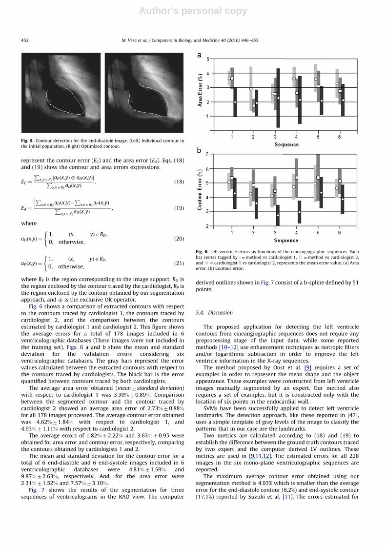
Fig. 6 shows a comparison of extracted contours with respectto the contours traced by cardiologist 1, the contours traced bycardiologist 2, and the comparison between the contoursestimated by cardiologist 1 and cardiologist 2. This figure showsthe average errors for a total of 178 images included in 6ventriculographic databases (These images were not included inthe training set). Figs. 6 a and b show the mean and standarddeviation for the validation errors considering sixventriculographic databases. The gray bars represent the errorvalues calculated between the extracted contours with respect tothe contours traced by cardiologists. The black bar is the errorquantified between contours traced by both cardiologists.

The average area error obtained (mean7standard deviation)with respect to cardiologist 1 was 3:30%70:89%. Comparisonbetween the segmented contour and the contour traced bycardiologist 2 showed an average area error of 2:73%70:88%for all 178 images processed. The average contour error obtainedwas 4:62%71:84% with respect to cardiologist 1, and4:93%71:11% with respect to cardiologist 2.

The average errors of 1:82%72:22% and 3:63%70:95 wereobtained for area error and contour error, respectively, comparingthe contours obtained by cardiologists 1 and 2.

The mean and standard deviation for the contour error for atotal of 6 end-diastole and 6 end-systole images included in 6ventriculographic databases were 4:81%71:59% and9:87%72:63%, respectively. And, for the area error were2:31%71:52% and 7:57%73:10%.

Fig. 7 shows the results of the segmentation for threesequences of ventriculograms in the RAO view. The computer

derived outlines shown in Fig. 7 consist of a b-spline defined by 51points.

5.4. Discussion

The proposed application for detecting the left ventriclecontours from cineangiographic sequences does not require anypreprocessing stage of the input data, while some reportedmethods [10–12] use enhancement techniques as isotropic filtersand/or logarithmic subtraction in order to improve the leftventricle information in the X-ray sequences.

The method proposed by Oost et al. [9] requires a set ofexamples in order to represent the mean shape and the objectappearance. These examples were constructed from left ventricleimages manually segmented by an expert. Our method alsorequires a set of examples, but it is constructed only with thelocation of six points in the endocardial wall.

SVMs have been successfully applied to detect left ventriclelandmarks. The detection approach, like these reported in [47],uses a simple template of gray levels of the image to classify thepatterns that in our case are the landmarks.

Two metrics are calculated according to (18) and (19) toestablish the difference between the ground truth contours tracedby two expert and the computer derived LV outlines. Thesemetrics are used in [9,11,12]. The estimated errors for all 228images in the six mono-plane ventriculographic sequences arereported.

The maximum average contour error obtained using oursegmentation method is 4.93% which is smaller than the averageerror for the end-diastole contour (6.2%) and end-systole contour(17.1%) reported by Suzuki et al. [11]. The errors estimated for

Fig. 5. Contour detection for the end-diastole image. (Left) Individual contour in

the initial population. (Right) Optimized contour.

Fig. 6. Left ventricle errors as functions of the cineangiographic sequences. Each

bar center tagged by 3¼method vs cardiologist 1, &¼method vs cardiologist 2,

and B¼ cardiologist 1 vs cardiologist 2, represents the mean error value. (a) Area

error. (b) Contour error.

M. Vera et al. / Computers in Biology and Medicine 40 (2010) 446–455452

Author's personal copyARTICLE IN PRESS

images at ED and ES are smaller than the errors reported in [12]for these cardiac instants.

The average of the area and the contour errors for the ED phaseobtained in this research are close to values reported in [9] (EC =4.1% and EA = 1.9%), while the errors at ES phase are smaller withrespect to EC = 12.8% and EA = 6.4% estimated in [9].

Intra-observer variability is not assessed for the proposedmethod. Nevertheless, the inter-observer variability is of 2% withrespect to area error and 4% with respect to contour error.According to Chalana and Kim [48], it is possible to diminish theinter-observer variability, if an average contour is calculated fromthe contours traced by cardiologists. This average contourrepresents the gold-standard contour to use in the comparisonstage. As a further work, the Chalana and Kim methodology couldbe incorporated to the validation stage.

Fig. 7 shows contours obtained with the left ventriclesegmentation approach. The worst cases are due to the shadowin the images (first row), the inhomogeneity between the bloodand contrast agent (second row), and the low contrast (third row).

The genetic snake approach can be compared with a differentsnake algorithm with the same initialization method. Thecomparison method [49] works from an approximate contourdefined by anatomical landmarks extracted using the procedure

described in Section 4.2, but it uses a normalized gradient descentprocedure in an iterative optimization process in order to obtainthe optimal contour that provides the minimum energy value.Five ventriculographic sequences were used in the experimentalsetup reported in [49]. An average contour error EC of 5.97% andan average area error EA of 3.71% were reached. These values arevery close to errors obtained using the currently reportedapproach. In this sense, the procedure described in Section 4.3and reported in [49, p. 796] can be considered as an efficientmethodology for snakes algorithms initialization.

6. Conclusions

A contour detection method in cardiac images has beenpresented. The method considers the relationship between neighborpixels and densitometric information. This method is based onseveral useful emergent computational techniques, enabling theautomatic detection of the LV in X-rays cineangiograms. Several realmono-plane ventriculogram sequences are used to validate themethod. The approach is useful for detection of the myocardialcontour in images affected by noise where boundaries are missing ordiffuse such as images without logarithmic subtraction or enhance-

Fig. 7. Contour detection for three RAO view image sequences. In each row three cardiac instants are shown for three different image sequences. Ground truth contours are

indicated by a black dashdotted line. Contours extracted using the proposed approach are indicated by a white dashdotted line.

M. Vera et al. / Computers in Biology and Medicine 40 (2010) 446–455 453

Author's personal copyARTICLE IN PRESS

ment. The algorithm provides an accurate left ventricle contour,nevertheless it is necessary to incorporate a methodology useful todiminish the inter-observer variability.

The approach is based on real-value encoding of individuals ofthe genetic algorithm. The genes comprising an individual orchromosome represent the points that define the candidates ofthe left ventricle optimal contour. The proposed contour detectionmethod incorporates an automatic approach based on supportvector machines for the extraction of several left ventricleanatomical landmarks. The SVM classification approach does notrequire any preprocessing of the input data and it is useful asinitialization stage the active contour models.

As a further research, we propose the application of thisalgorithm for performing the detection of the left ventriclecontour in images acquired according to the conventional leftanterior oblique (LAO) 603 view. A more complete validation isalso necessary, including control subjects as well as cardiacpatients. The validation stage could also include a comparison ofestimated parameters describing the cardiac function, such as thevolume and the ejection fraction with respect to results obtainedusing other imaging modalities including magnetic resonanceimaging or multi-slice computerized tomography.

Conflict of interest statement

None declared.

Acknowledgments

The authors would like to thank the CDCHT from Universidadde Los Andes (projects NUTA C-24-07-02-C and I-1075-07-02B),Investigation Dean’s Office of Universidad Nacional Experimentaldel Tachira and LOCTI Grant PR0100401 for their support to thisproject. Authors would also like to thank the Centro MedicoCaracas in Caracas, Venezuela, and the Centro de Cardiologıa ofHospital Universitario de Los Andes in Merida, Venezuela forproviding the human ventriculographic databases.

References

[1] M.L. Marcus, K.C. Dellsperger, Determinants of systolic and diastolicventricular function, in: M. Marcus, H. Schelbert, D. Skorton, G. Wolf (Eds.),Cardiac Imaging. A Companion to Braunwald’s Heart Disease, W.B. SaundersCompany, Philadelphia, USA, 1991, pp. 24–38.

[2] WHO, Reducing risk and promoting healthy life, The World Health Report2002, Geneva, World Health Organization (Julio 2002).

[3] A. Macovski, Medical Imaging Systems, Prentice-Hall, New-Jersey, 1983.[4] J. Kennedy, S. Trenholme, I. Kaiser, S. Wash, Left ventricular volume and mass

from single-plane cineangiocardiogram. A comparison of anteroposterior andright anterior oblique methods, American Heart Journal 80 (3) (1970) 343–352.

[5] O. Ratib, Quantitative analysis of cardiac function, in: I. Bankman (Ed.),Handbook of Medical Imaging: Processing and Analysis, Academic Press, SanDiego, 2000, pp. 359–374.

[6] R. Medina, M. Garreau, J. Toro, J.L. Coatrieux, D. Jugo, Three-dimensionalreconstruction of left ventricle from two angiographic views: an evidencecombination approach, IEEE Transactions on Systems, Man, and Cybernetic-s—Part A: Systems and Humans 34 (3) (2004) 359–370.

[7] C. Kervrann, F. Heitz, Statistical deformable model-based segmentation ofimage motion, IEEE Transactions on Image Processing 8 (4) (1999) 583–588.

[8] R. Medina, M. Garreau, D. Jugo, C. Castillo, J. Toro, Segmentation of ventricularangiographic images using fuzzy clustering, in: Proceedings of the 17thAnnual International Conference of the IEEE EMBS, Montreal, 1998, pp.405–406.

[9] E. Oost, G. Koning, M. Sonka, P.V. Oemrawsingh, J.H.C. Reiber, B.P.F. Lelieveldt,Automated contour detection in X-ray left ventricular angiograms usingmultiview active appearance models and dynamic programming, IEEETransactions on Medical Imaging 25 (9) (2006) 1158–1171.

[10] L. Sui, R. Haralick, F. Sheehan, A knowledge-based boundary delineationsystem for contrast ventriculograms, IEEE Transactions on InformationTechnology in Biomedicine 5 (2) (2001) 116–132.

[11] K. Suzuki, I. Horiba, N. Sugie, M. Nanki, Extraction of left ventricular contoursfrom left ventriculograms by means of a neural edge detector, IEEETransactions on Medical Imaging 23 (3) (2004) 330–339.

[12] A. Bravo, R. Medina, An unsupervised clustering framework for automaticsegmentation of left ventricle cavity in human heart angiograms, Computer-ized Medical Imaging and Graphics 32 (5) (2008) 396–408.

[13] K.S. Fu, J.K. Mui, A survey on image segmentation, Pattern Recognition 13 (1)(1981) 3–16.

[14] J. Bosch, S. Mitchell, B. Lelieveldt, F. Nijland, O. Kamp, M. Sonka, J. Reiber,Automatic segmentation of echocardiographic sequences by active appear-ance motion models, IEEE Transactions on Medical Imaging 21 (11) (2002)1374–1383.

[15] A. Frangi, D. Rueckert, J. Schnabel, W. Niessen, Automatic construction ofmultiple-object three-dimensional statistical shape models: application tocardiac modeling, IEEE Transactions on Medical Imaging 21 (9) (2002) 1151–1166.

[16] R. Chandrashekara, R. Mohiaddin, D. Rueckert, Analysis of 3-D myocardialmotion in tagged MR images using nonrigid image registration, IEEETransactions on Medical Imaging 23 (10) (2004) 1245–1250.

[17] E. Angelie, P.J.H. de Koning, M.G. Danilouchkine, H.C. van Assen, G. Koning,R.J. van der Geest, J.H.C. Reiber, Optimizing the automatic segmentation ofthe left ventricle in magnetic resonance images, Medical Physics 32 (2)(2005) 369–375.

[18] T. McInerney, D. Terzopoulos, Deformable models in medical image analysis:a survey, Medical Image Analysis 1 (2) (1996) 91–108.

[19] J. Montagnat, H. Delingette, N. Ayache, A review of deformable surfaces:topology, geometry and deformation, Image and Vision Computing 19 (14)(2001) 1023–1040.

[20] O. Gerard, A.C. Billon, J.-M. Rouet, M. Jacob, M. Fradkin, C. Allouche, Efficientmodel-based quantification of left ventricular function in 3-Dechocardiography, IEEE Transactions on Medical Imaging 21 (9) (2002)1059–1068.

[21] A. Gueziec, N. Ayache, Smoothing and matching of 3-D space curves,International Journal of Computer Vision 12 (1) (1994) 79–104.

[22] M. Kass, A. Witkin, D. Terzopoulos, Snakes: active contours models,International Journal of Computer Vision 1 (1987) 321–331.

[23] S. Lobregt, M. Viergever, A discrete dynamic contour model, IEEE Transac-tions on Medical Imaging 14 (1) (1995) 12–24.

[24] L.H. Staib, J.S. Duncan, Boundary finding with parametrically deformablemodels, IEEE Transaction on Pattern Recognition Analysis and MachineIntelligence 14 (11) (1992) 1061–1075.

[25] L. MacEachern, T. Manku, Genetic algorithms for active contour optimization,in: Proceedings of the IEEE International Symposium on Circuits and Systems,Montreal, 1998, pp. 229–232.

[26] T.F. Cootes, C.J. Taylor, D.H. Cooper, J. Graham, Active shape models-theirtraining and application, Computer Vision and Image Understanding 61 (1)(1995) 38–59.

[27] A. Mishra, P. Dutta, M. Ghosh, A GA based approach for boundary detection ofleft ventricle with echocardiographic image sequences, Image and VisionComputing 21 (11) (2003) 967–976.

[28] V. Vapnik, The Nature of Statistical Learning Theory, Springer-Verlag, NewYork, 1995.

[29] E. Osuna, R. Freund, F. Girosi, Training support vector machines: anapplication to face detection, in: Conference on Computer Vision and PatternRecognition (CVPR ’97), San Juan, Puerto Rico, 1997, pp. 130–136.

[30] A.J. Smola, Learning with kernels, Ph.D. Thesis, Technische Universitat Berlin,Germany, 1998.

[31] C. Burges, A tutorial on support vector machines for pattern recognition,Knowledge Discovery and Data Mining 2 (2) (1998) 121–167.

[32] E. Osuna, R. Freund, F. Girosi, Support vector machines: training andapplications, Technical Report, Artificial Intelligence Laboratory, Massachu-setts Institute of Technology, 1997.

[33] J.H. Holland, Adaptation in Natural and Artificial Systems, The University ofMichigan Press, Michigan, 1975.

[34] D. Goldberg, Genetic Algorithms in Search, Optimization, and MachineLearning, Addison-Wesley, Alabama, 1989.

[35] D. Goldberg, Real-coded genetic algorithms, virtual alphabets, and blocking,Complex Systems 5 (1) (1991) 139–167.

[36] N.J. Radcliffe, Non-linear genetic representations, in: R. Manner, B. Manderick(Eds.), Parallel Problem Solving from Nature, vol. 2, Elsevier SciencePublishers, Amsterdam, 1992, pp. 259–268.

[37] H. Muhlenbein, D. Schlierkamp-Voosen, Predictive models for the breedergenetic algorithm I. Continuous parameter optimization, EvolutionaryComputation 1 (1) (1999) 25–49.

[38] F. Herrera, M. Lozano, J.L. Verdegay, Tunning fuzzy logic controllers bygenetic algorithm, International Journal of Approximate Reasoning 12 (2)(1995) 295–315.

[39] F. Herrera, M. Lozano, J.L. Verdegay, Tackling real-coded genetic algorithms:operators and tools for behavioral analysis, Artificial Intelligence Review 12(4) (1998) 265–319.

[40] D. Marr, E. Hildreth, Theory of the edge detection, Proceedings of the RoyalSociety of London 207 (1980) 187–217.

[41] S. Mikhlin, Variational Methods in Mathematical Physics, Pergamon Press,New York, 1964.

[42] K. Washizu, Variational Methods in Elasticity Plasticity, Pergamon Press, NewYork, 1968.

M. Vera et al. / Computers in Biology and Medicine 40 (2010) 446–455454

Author's personal copyARTICLE IN PRESS

[43] B.A. Barsky, Computer Graphics and Geometric Modeling Using Beta-Splines,Springer-Verlag, USA, 1988.

[44] A. Wrigth, Genetic algorithms for real parameter optimization, in: G. Rawlin(Ed.), Foundations of Genetic Algorithms, vol. 1, Morgan Kaufmann, SanMateo, 1991, pp. 205–218.

[45] Z. Michalewicz, Genetic Algorithms+Data Structures=Evolution Programs,Springer-Verlag, New York, 1992.

[46] S. Gunn, Support vector machines for classification and regression, TechnicalReport, Information: Signals, Images, Systems (ISIS) Research Group,University of Southampton, 1997.

[47] M. Hearst, S. Dumais, E. Osuna, J. Platt, B. Scholkopf, Trends & controversies:support vector machines, IEEE Intelligent Systems and Their Applications 13(4) (1998) 18–28.

[48] V. Chalana, Y. Kim, A methodology for evaluation of boundary detectionalgorithms on medical images, IEEE Transactions on Medical Imaging 16 (5)(1997) 642–652.

[49] A. Bravo, M. Vera, R. Medina, Edge detection in ventriculograms usingsupport vector machine classifiers and deformable models, in: L. Rueda, D.Mery, J. Kittler (Eds.), CIARP of Lecture Notes in Computer Science, vol. 4756,Springer, Berlin, 2007, pp. 793–802.

M. Vera et al. / Computers in Biology and Medicine 40 (2010) 446–455 455