Mutual Information-based selection of optimal spatial-temporal patterns forsingle-trial EEG-based BCIs

Kai Keng Anga,∗, Zheng Yang China, Haihong Zhanga, Cuntai Guana

aInstitute for Infocomm Research, Agency for Science, Technology and Research (A*STAR), 1 Fusionopolis Way, #21-01 Connexis,Singapore 138632.

Abstract

The Common Spatial Pattern (CSP) algorithm is effective in decoding the spatial patterns of the corresponding neu-ronal activities from electroencephalogram (EEG) signal patterns in Brain-Computer Interfaces (BCIs). However, itseffectiveness depends on the subject-specific time segment relative to the visual cue and on the temporal frequencyband that is often selected manually or heuristically. This paper presents a novel statistical method to automaticallyselect the optimal subject-specific time segment and temporal frequency band based on the mutual information betweenthe spatial-temporal patterns from the EEG signals and the corresponding neuronal activities. The proposed methodcomprises four progressive stages: multi-time segment and temporal frequency band-pass filtering, CSP spatial filtering,mutual information-based feature selection and Naıve Bayesian classification. The proposed mutual information-basedselection of optimal spatial-temporal patterns and its one-versus-rest multi-class extension were evaluated on single-trialEEG from the BCI Competition IV Datasets IIb and IIa respectively. The results showed that the proposed methodyielded relatively better session-to-session classification results compared against the best submission.

Keywords:Brain-computer interface (BCI), electroencephalogram (EEG), mutual information, feature selection, Bayesianclassification.

1. Introduction

Electroencephalography (EEG) studies have shown thatmotor imagery results in an amplitude suppression calledevent-related desynchronization (ERD) or in an amplitudeenhancement called event-related synchronization (ERS)of brain oscillations over sensorimotor areas [1]. Hence,EEG-based Brain-Computer Interfaces (BCIs) are capa-ble of discriminating different types of neural activitiesconsequent to the performance of motor imagery, such asthe imagination of left-hand, right-hand, foot or tonguefrom the EEG signals. Methods in the literature used fordiscriminating different classes of motor imagery includebut not limited to, Common Spatial Pattern (CSP) algo-rithm [2, 3], methodologies based on ERD/ERS [4, 5, 6, 7],power spectral density models [1, 8, 9, 10, 11, 12], Autore-gressive models [1, 8, 13, 14, 15, 16], Independent Com-ponent Analysis [17, 9, 18], two-equivalent-dipole sourcemodel [19, 18], neural time series prediction [20, 21], phasesynchronization [22], time-frequency distribution [10] andtime-frequency-spatial pattern [23].

∗Corresponding authorEmail addresses: kkang@i2r.a-star.edu.sg (Kai Keng Ang),

zychin@i2r.a-star.edu.sg (Zheng Yang Chin),hhzhang@i2r.a-star.edu.sg (Haihong Zhang),ctguan@i2r.a-star.edu.sg (Cuntai Guan)

The CSP algorithm [3] is a commonly used statisticalmethod for discriminating the spatial patterns for twoclasses of motor imagery in EEG-based BCIs [2, 24, 25,26, 27, 1]. The effectiveness of the CSP algorithm dependson the temporal frequency band-pass filtering of the EEGsignals, the time segment of the EEG taken relative to thevisual cue, and the subset of CSP filters used [2]. Typi-cally, general settings such as a broad frequency band of7-30 Hz, time segment of 1 s after cue, and 2 or 3 subsetsof CSP filters are used [2]. Although the performance ofCSP can be enhanced by subject-specific parameters [28],these settings are often selected manually or heuristically[2, 26].

To address the issue of selecting optimal temporal fre-quency band for the CSP algorithm, several approacheswere proposed. The Common Spatio-Spectral Pattern(CSSP) optimized a simple filter that employed a one time-delayed sample with the CSP algorithm [27]. However, theflexibility of this simple filter was very limited, hence theCommon Sparse Spectral-Spatial Pattern (CSSSP) wasproposed to perform simultaneous optimization of an ar-bitrary Finite Impulse Response (FIR) filter within theCSP algorithm [26]. This simultaneous optimization wascomputationally expensive [25, 24], which motivated theSPECtrally-weighted Common Spatial Pattern (SPEC-CSP) algorithm [25] to alternately optimize the temporalfilter in the frequency domain and then the spatial filter in

Preprint submitted to Pattern Recognition May 6, 2011

an iterative procedure. The Iterative Spatio-Spectral Pat-tern Learning (ISSPL) [24] algorithm was then proposedto improve upon SPEC-CSP without relying on statisticalassumptions by optimizing all the temporal filters simulta-neously under a common optimization framework insteadof individually in SPEC-CSP. However, its convergence hasyet to be proven theoretically.

In this paper, a novel statistical method is proposed toautomatically select the optimal subject-specific time seg-ment and temporal frequency band based on the mutualinformation between the spatial-temporal patterns fromthe EEG signals and corresponding neuronal activities.A preliminary version of this work known as the FilterBank Common Spatial Pattern (FBCSP) algorithm waspresented in a conference proceeding [29] to select tempo-ral frequency band-pass filtering parameters for CSP usinga filter bank. However, the FBCSP algorithm has the fol-lowing limitations: Firstly, it was proposed for two-classmotor imagery. Secondly, the subject-specific time seg-ment was selected manually. Last but not least, it didnot address the details on the estimation of the mutualinformation that was employed as the criteria in featureselection. Subsequently, the Discriminative Common Spa-tial Pattern (DCSP) was proposed in [30] to select thesubject-specific filter bank based on a simpler approach ofusing the fisher ratio of the spectral power from a singlespecific channel of EEG data.

Section 2 describes the proposed method and the de-tails on multi-time segment and temporal frequency fil-tering, mutual information-based feature selection, NaıveBayesian classification for two-class motor imagery, anda one-versus-rest approach for multi-class motor imagery.The proposed method extends our preliminary work in [29]to automatically select the optimal subject-specific timesegment for multi-class motor imagery, and addresses thedetails on the estimation of the mutual information. Sec-tion 3 presents the experimental results of the proposedmethod and its multi-class extension on the BCI Compe-tition IV Datasets IIb and IIa respectively. The previousversion of this work was submitted to the BCI Competi-tion IV for these two datasets and yielded relatively thebest session-to-session classification results on the unseenevaluation data. The results of using the proposed methodare compared to FBCSP and DCSP. Finally, section 4 con-cludes this paper.

2. Mutual Informational-based selection of opti-mal spatial-temporal patterns

The proposed mutual information-based selection ofoptimal spatial-temporal patterns is illustrated in Fig.1. The proposed methodology comprises four progressivestages of statistical signal processing and pattern recog-nition on the EEG data: multi-time segment and tempo-ral band-pass filtering using a filter bank, CSP spatial fil-tering, CSP feature selection and classification of selected

CSP features. The CSP projection matrix for each tem-poral filter band, the discriminative CSP features, and theclassifier model are computed from training data labeledwith the respective motor imagery action. These param-eters computed from the training phase are then used tocompute the single-trial motor imagery action during theevaluation phase.

2.1. Multi-time segment and temporal frequency band-passfiltering

The first stage employs a filter bank that decomposesthe multi-time segments of EEG using causal digital band-pass filters such as Butterworth or Chebyshev Type II. Inthis work, a total of 3 time segments and a total of 9temporal band-pass filters are used in this work. The timesegments are: 0.5 to 2.5 s, 1.0 to 3.0 s, and 1.5 to 3.5 sfrom the onset of the visual cue given to the subject toperform motor imagery. The temporal band-pass filtersare: 4-8 Hz, 8-12 Hz,. . . , 36-40 Hz. Various configurationsof time segments and filter bank are as effective, but thesetime segments and band-pass frequency ranges are usedbecause they cover most of the manual or heuristicallyselected settings used in the literature.

2.2. Optimal spatial filtering using CSPThe second stage performs CSP spatial filtering. Spatial

filtering is performed using the CSP algorithm by linearlytransforming the EEG using

Z = WT E, (1)

where E ∈ Rc×τ denotes the ith single-trial band-pass fil-tered EEG; Z ∈ Rc×τ denotes E after spatial filtering,W ∈ Rc×c denotes the CSP projection matrix; c is thenumber of channels; τ is the number of EEG samples perchannel; and T denotes the transpose operator.

The CSP algorithm computes the transformation matrixW by solving the eigenvalue decomposition problem

Σ1W = (Σ1 + Σ2)WD, (2)

where Σ1 and Σ2 are estimates of the covariance matricesof the band-pass filtered EEG of the respective motor im-agery action, D is the diagonal matrix that contains theeigenvalues of Σ1.

The spatial filtered signal Z in equation (1) using Wb,d

from equation (2) thus maximizes the differences in thevariance of the 2 classes of band-pass filtered EEG. Sinceonly the first and last m columns of W are used to performspatial filtering,

Z = WT E, (3)

where W represents the first and last m columns of W.The choice for m depends on the data and is discussedfurther in section 3.

In the proposed mutual information-based selection ofoptimal spatial-temporal patterns, each pair of band-passand spatial filters for a specific time segment computes

2

Figure 1: Methodology of mutual information-based selection of optimal spatial-temporal patterns for the training and evaluation phases.

the CSP features that are specific to the time segmentand band-pass frequency range. Since the spatial filtersfrom different band-pass filtered EEG and different timesegments are not the same, let Eb,d,i ∈ Rc×τ denotes theith single-trial EEG from the bth band-pass filter of the dth

time segment, Zb,d,i ∈ Rc×τ denotes Eb,d,i after spatialfiltering, and Wb,d ∈ Rc×c denotes the CSP projectionmatrix. Then the CSP features of the ith trial for theEEG from the bth band-pass filter of the dth time segmentare then given by

vb,d,i = log(diag

(Zb,d,iZT

b,d,i

)/tr

[Zb,d,iZT

b,d,i

]), (4)

where vb,d,i ∈ R1×2m; diag(·) returns the diagonal ele-ments of the square matrix; tr[·] returns the sum of thediagonal elements in the square matrix.

Equation (4) can also be written in the form [3]

vb,d,i,k = log

(var

(Zb,d,i,k

)/

2m∑

l=1

var(Zb,d,i,l

)), (5)

where vb,d,i,k is the kth feature in vb,d,i, and Zb,d,i,k is thekth row of Zb,d,i.

Instead of using equation 5, the features can be simpli-fied to

vb,d,i,k =

((Z2

b,d,i,k

)/

2m∑

l=1

(Z2

b,d,i,l

)). (6)

The feature vector for the ith trial from the dth timesegment is formed using

vd,i = [v1,d,i,v2,d,i, . . . ,v9,d,i] , (7)

where vd,i ∈ R1×(9∗2m).

Denoting the training data and the true class labels asVd and y respectively to make a distinction from the eval-uation data,

Vd = [vTd,1, v

Td,2, . . . , v

Td,nt

]T , (8)

y = [y1, y2, . . . , ynt ]T , (9)

where Vd ∈ Rnt×(9∗2m); y ∈ Rnt×1; vd,i and yi denotethe feature vector and true class label from the ith train-ing trial, i=1,2,. . . ,nt; and nt denotes the total number oftrials in the training data.

2.3. Optimal Mutual Information-based Feature selection

The third stage selects discriminative CSP features fromthe training data Vd for the subject’s task. Various featureselection algorithms can be used in this stage. Based onthe study performed on the BCI Competition III DatasetIVa [29], the 10×10-fold cross-validation results of us-ing the Mutual Information-based Best Individual Feature(MIBIF) yielded better results than other feature selectionalgorithms and hence is used in this work.

2.3.1. MIBIF algorithmThe MIBIF algorithm is described as follows:

• Step 1: For each dth time segment, initialize set offeatures Fd and set of selected features Sd.

Initialize Fd =[fTd,1, f

Td,2, . . . , f

Td,9∗2m

]= Vd from the

training data whereby fTd,j ∈ Rnt×1 is the jth column

vector of Vd. Initialize Sd = ∅.

• Step 2: Compute the mutual information of each fea-ture fd,j with the class label ω = {1, 2}Compute I (fd,j ; ω) ∀j = 1, 2, . . . (9 ∗ 2m) using [31]

3

I (fd,j ; ω) = H (ω)−H (ω|fd,j) , (10)

where H (ω) = −2∑

ω=1

P (ω) log2 P (ω); and the condi-

tional entropy is

H (ω|fd,j) = −2∑

ω=1

p (ω|fd,j) log2 p (ω|fd,j)

= −2∑

ω=1

nt∑

i=1

p (ω|fd,j,i) log2 p (ω|fd,j,i) , (11)

where fd,j,i is the jth feature value of the ith trial fromfd,j ; and nt denotes the total number of trials in thetraining data.

The probability p (ω|fd,j,i) can be computed usingBayes rule given in equations (12) and (13).

p (ω|fd,j,i) =p (fd,j,i|ω)P (ω)

p (fd,j,i), (12)

where p(ω|fd,j,i) is the conditional probability of classω given fd,j,i; p(fd,j,i|ω) is the conditional probabilityof fd,j,i given class ω; P (ω) is the prior probability ofclass ω; and

p (fd,j,i) =2∑

ω=1

p (fd,j,i|ω) P (ω) . (13)

The conditional probability p(fj,i|ω) can be estimatedusing a Parzen Window [32] given by

p (fd,j,i|ω) =1

nω

∑

r∈Iω

φ (fd,j,i − fd,j,r, h) , (14)

where nω is the number of trials in the training databelonging to class ω; Iω is the set of indices of thetraining data trials belonging to class ω; fd,j,r is thefeature value of the rth trial from fd,j and φ is asmoothing kernel function with a smoothing parame-ter h given in equations (23) and (24) respectively.

• Step 3: Sort all the features in descending order ofmutual information computed in step 2 and selectthe first k features. Mathematically, this step is per-formed as follows till |Sd| = k

Fd = Fd\fd,j ,Sd = Sd ∪ fd,j |I (fd,j ; ω) = max

j=1..(9∗2m),fd,j∈Fd

I (fd,j ; ω) , (15)

where \ denotes set theoretic difference; ∪ denotes setunion; and | denotes given the condition.

The parameter k in the MIBIF algorithm denotes thenumber of best individual features to select. Based on thestudy performed on the BCI Competition III Dataset IVain [29], the 10×10-fold cross-validation results of using theMIBIF algorithm with k = 1 to 4 yielded the averagedaccuracies of 88.36 ± 0.70, 89.16 ± 0.77, 89.93 ± 0.73 and90.31 ± 0.67 respectively. Since the study showed thatk = 4 yielded a higher averaged accuracy, this setting isused in this work.

2.3.2. MISFS algorithmInstead of setting k number of features to select, the

Mutual Information-based Sequential Forward Selection(MISFS) algorithm [33] can be used to select features tillthere are no further increase in the mutual information.

The MISFS algorithm is described as follows:

• Step 1 & 2: Initialize and compute the mutual infor-mation of each feature.

These are the same as steps 1 & 2 of the MIBIFalgorithm.

• Step 3: Select the first feature.

Select the first feature that maximizes I(fd,j ;ω) using(16) from step 3 of the MIBIF algorithm.

• Step 4: Perform sequential feature selection

Repeat

(a) Compute I(fd,j ∪ Sd;ω) ∀fd,j ∈ Fd [33](b) Select next feature using

Fd = Fd\fd,j ,Sd = Sd ∪ fd,j |I (fd,j ∪ Sd; ω) = max

j=1..(9∗2m),fd,j∈Fd

I (fd,j ∪ Sd;ω) , (16)

Until 4I(Sd; ω) ≈ 0, where the increase in mutualinformation is close to zero.

2.4. Optimal Time segment

After the features are selected in Sd for all the timesegments, the average mutual information of the selectedfeatures of the dth time segment is computed using

I(Sd;ω) =

∑

fd,j∈Sd

I(fd,j ; ω)

/|Sd|, (17)

and the optimal time segment is selected using

dopt = arg maxd=1...nd

I(Sd; ω), (18)

where nd denotes the total number of time segments used.

4

It is possible to perform feature selection on all the fre-quency bands and all the time segments. However, theselection of an optimal time segment has the advantage incomputing the results using a shorter time segment. To il-lustrate this point, if the features computed from the timesegments 0.5 to 2.5 s, 1.0 to 3.0 s and 1.5 to 3.5 s and allthe frequency bands are grouped together to perform fea-ture selection, then a 3 s EEG evaluation data is neededto compute the result. This is because all the time seg-ments included a length of 3 s of EEG starting from 0.5 to3.5s. On the other hand, if only one of the time segmentsis selected, then 2 s of EEG evaluation data is needed tocompute the result since the length of each time segmentis 2 s.

2.5. Classification of optimal spatial-temporal features

The fourth stage employs a classification algorithm tomodel and classify the selected CSP features. Note thatsince the CSP features come in pairs, the correspondingpair of features is also included if it is not selected. Af-ter performing feature selection and optimal time segmentselection, the feature selected training data is denoted asX ∈ Rnt×nf where nt denotes the number of trials in thetraining data and nf ranges from 4 to 8. nf=4 if all 4features selected are from 2 pairs of CSP features. nf=8if all 4 features selected are from 4 pairs of CSP features,since their corresponding pair is included.

Various classification algorithms can be used at thisstage. Based on the study performed on the BCI Competi-tion III dataset IVa [29], the 10×10-fold cross-validation ofusing the Naıve Bayesian Parzen Window (NBPW) classi-fier [34], Fisher Linear Discriminant [35], Support VectorMachine [36], Classification And Regression Tree [37], k-nearest neighbor [38], Rough set-based Neuro-Fuzzy Sys-tem [39] and Dynamic Evolving Neural-Fuzzy InferenceSystem [40] yielded the averaged accuracies of 90.31±0.67,89.88 ± 0.85, 90.01 ± 0.82, 85.84 ± 1.40, 88.67 ± 0.85,87.46± 1.38 and 88.59±0.96 respectively. Since the studyshowed the NBPW classifier yielded better results, andthe FLD classifier is often used in BCI research, these twoclassifiers are used in this work.

2.5.1. NBPW classifierThe classification rule of the NBPW classifier is de-

scribed as follows:Given that X =

[xT

1 , xT2 , . . . , xT

nt

]T denotes the entiretraining data of nt trials, xi =

[xi,1, xi,2, . . . , xi,nf

]de-

notes the training data with the nf selected features fromthe ith trial, X =

[xT

1 ,xT2 , . . . ,xT

ne

]T denotes the entireevaluation data of ne trials, xl =

[xl,1, xl,2, . . . , xl,nf

]de-

notes the evaluation data with nf selected features fromthe lth trial; the NBPW classifier estimates p(xl|ω) andP (ω) from training data samples X and predicts the classω with the highest posterior probability p(ω|xl) usingBayes rule

p (ω|xl) =p (xl|ω)P (ω)

p (xl), (19)

where p(ω|xl) is the conditional probability of class ω givenevaluation trial xl; p(xl|ω) is the conditional probabilityof xl given class ω; P (ω) is the prior probability of classω; and p(xl) is

p (xl) =2∑

ω=1

p (xl|ω) P (ω) . (20)

The computation of p(ω|xl) is rendered feasible by anaıve assumption that all the features xl,1, xl,2, . . . , xl,d areconditionally independent given class ω in

p (xl|ω) =d∏

j=1

p (xl,j |ω) . (21)

The NBPW classifier employs a Parzen Window [32] toestimate the conditional probability p(xl,j |ω) in

p (xl,j |ω) =1

nω

∑

i∈Iω

φ (xl,j − xi,j , h) , (22)

where xi,j denotes the jth feature of the ith trial from thetraining data; nω is the number of data samples belongingto class ω; Iω is the set of indices of the trials of the train-ing data belonging to class ω; and φ is a smoothing kernelfunction with a smoothing parameter h. The NBPW clas-sifier employs the univariate Gaussian kernel given by

φ (y, h) =1√2π

e−(

y2

2h2

), (23)

and normal optimal smoothing strategy [41] given by

hopt =(

43nω

)1/5σ, (24)

where σ denotes the standard deviation of y from (23).The classification rule of the NBPW classifier is given

by

yl = arg maxω=1,2

p (ω|xl) . (25)

where yl denotes the predicted label of the lth evaluationtrial.

2.5.2. FLD classifierThe classification rule of the FLD classifier is given by

ω ={ ∈ ω′ ~wT x ≥ ~w0

/∈ ω′ ~wT x < ~w0(26)

where class ω′ is discriminated against the rest; ~w is anadjustable weight vector for class ω′; and ~w0 is a bias.

5

The FLD classifier maximizes the ratio of between-classscatter to within-class scatter given by

J (~w) =~wT Sb ~w~wT Sw ~w

(27)

where Sb is the between class scatter matrix; and Sw isthe within class scatter matrix.

2.6. One-Versus-Rest (OVR) multi-class extensionGiven that ω, ω′ ∈ {1, 2, 3, 4} represents the left, right,

foot and tongue motor imagery in the BCI CompetitionIV Dataset IIa, the OVR approach computes the CSP fea-tures that discriminates each class from the rest of theclasses [42]. For the 4 classes of motor imagery in theBCI Competition IV Dataset IIa, 4 OVR classifiers are re-quired. The classification rule of the NBPW classifier isthus extended from equation (25) to

yl = arg maxω=1,2,3,4

pOVR (ω|xl) , (28)

where pOVR (ω|xl) is the probability of classifying thelth evaluation trial between class ω and class ω′ ={1, 2, 3, 4}\ω; and \ denotes the set theoretic differenceoperation.

3. Experimental study

The experiment is performed using the BCI Competi-tion IV Datasets IIa and IIb, which comprised of trainingand evaluation data from 9 subjects each. For Dataset IIa,the training and evaluation data from one subject eachconsisted 1 session of single-trial EEG for four-class motorimagery of left-hand, right-hand, foot and tongue. Thedata in each session is comprised of 288 single-trials from22 channels. For Dataset IIb, the training data of one sub-ject consisted 3 sessions of single-trial EEG for two-classhand motor imagery whereas the evaluation data consisted2 sessions. The data in each session is comprised of 120single-trials from 3 bipolar channels. Details of the pro-tocols of Datasets IIa and IIb are available in [17] and[43] respectively. The choice of m pairs of CSP features isset to 2 for Dataset IIa and 1 for IIb. The former is se-lected because a greater choice of m did not significantlyimprove classification accuracy [3, 44]. The latter is se-lected because there are only 3 channels of EEG available,thus Wb,d ∈ R3×3 in equation (1) limited the maximumselection of m = 1 for Wb.

3.1. Cross-validation on training dataThe experiment is performed in two parts. In the first

part, 10×10-fold cross-validations are performed using theproposed method on the training data from Datasets IIaand IIb to select the parameter k. In each fold of thisprocedure, the selection of optimal time segment (0.5 to2.5 s, 1.0 to 3.0 s, and 1.5 to 3.5 s from the onset of thevisual cue) and temporal frequency and the training of

the spatial filters and classifier are performed on 9 partsof the training data. The classification accuracy of theproposed mutual information-based selection of optimalspatial-temporal patterns (denoted OSTP) is evaluated onthe remaining part for the time segment of 0 to 4s of EEGafter the onset of the visual. The experiment is performedfor a range of k=1 to 4 to select the optimal setting forthe second part of the experiment.

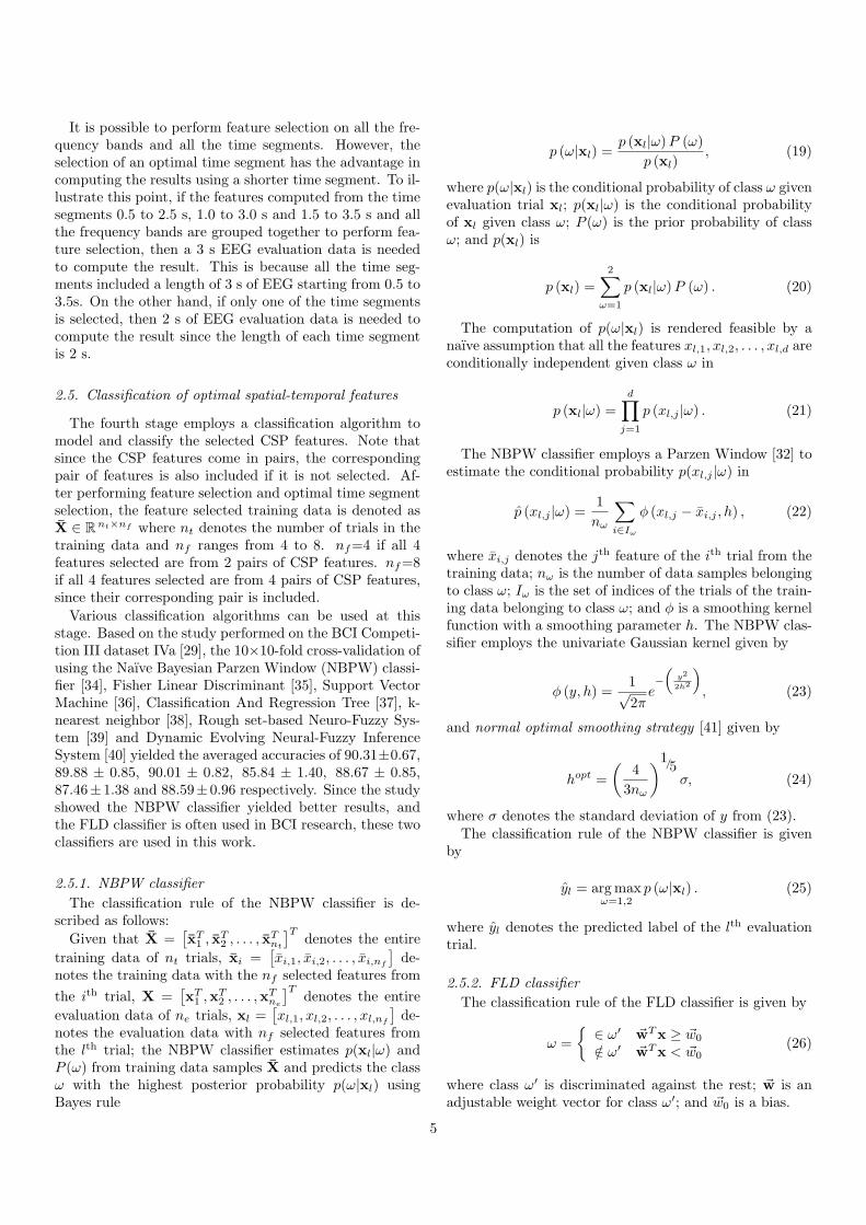
Tables 3.1 and 3.1 show the results of 10×10-fold cross-validation performed on Datasets IIa and IIb respectivelyof OSTP using the MIBIF algorithm whereby k=1 to 4 andthe NBPW classifier. The results in table 3.1 showed thatk=4 yielded higher averaged accuracy of 71.73%. The re-sults in table 3.1 showed that k=3 yielded higher averagedaccuracy of 78.25%, and k = 4 yielded the same result ask = 3. Based on these two sets of results, the value of k=4is selected for the next part of the experiment.

3.2. Session-to-session transferIn the second part of the experiment, session-to-session

transfers are performed using the proposed method on thetraining data of Datasets IIa and IIb to the evaluationdata. For this procedure, the selection of the optimaltime segment (0.5 to 2.5 s, 1.0 to 3.0 s, and 1.5 to 3.5s from the onset of the visual cue), temporal frequencyband, the training of the spatial filters and the classifier areperformed using the entire training data. The session-to-session performance of the proposed OSTP is computed onthe evaluation data that is recorded on another day. Thesession-to-session transfer is more challenging since brainsignals of the subjects can change substantially from thetraining data to the evaluation data that was recorded ona separate day [45].

Since the Kappa coefficient was used as a performancemeasure in the BCI Competition IV, it is used in this partof the experiment to measure the maximum Kappa valueevaluated on the entire single-trial EEG from the onsetof the fixation cross. The Kappa coefficient considers thedistribution of wrong classifications and the frequency ofoccurrence is normalized [46]. The Kappa coefficient κ [47]is given by

κ =Pa − Pc

1− Pc(29)

where Pa is the proportion of agreement, which is equalto the classification accuracy; and Pc is the proportionof chance agreement, which is equal to the accuracy of atrivial or random classifier.

For example, an accuracy of 50% in a two-class problemis equivalent to an accuracy of 25% in a four class problem,making it difficult to do a fair comparison of multi-classproblems using classification accuracies; but the Kappavalue is zero in both cases indicating random performance.The Kappa values and the standard error are calculatedusing the bci4eval function from the BioSig Toolbox [48].The Kappa value is computed from the onset of the fix-ation cross to the end of the cue for every every point intime across all the trials of the evaluation data.

6

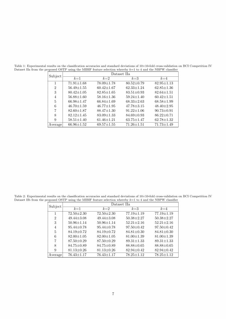
Table 1: Experimental results on the classification accuracies and standard deviations of 10×10-fold cross-validation on BCI Competition IVDataset IIa from the proposed OSTP using the MIBIF feature selection whereby k=1 to 4 and the NBPW classifier

Subject Dataset IIak=1 k=2 k=3 k=4

1 71.91±1.68 78.09±1.78 80.52±0.79 82.95±1.132 56.49±1.55 60.42±1.67 62.33±1.24 62.85±1.363 80.42±1.05 82.85±1.65 83.51±0.93 82.64±1.514 56.88±1.60 58.16±1.36 59.24±1.40 60.42±1.515 66.98±1.47 66.84±1.69 68.33±2.63 68.58±1.996 46.70±1.59 46.77±1.95 47.78±3.15 48.40±2.957 82.60±1.87 88.47±1.30 91.22±1.06 90.73±0.918 82.12±1.45 83.09±1.33 84.69±0.93 86.22±0.719 58.51±1.40 61.46±1.21 63.75±1.47 62.78±1.32

Average 66.96±1.52 69.57±1.55 71.26±1.51 71.73±1.49

Table 2: Experimental results on the classification accuracies and standard deviations of 10×10-fold cross-validation on BCI Competition IVDataset IIb from the proposed OSTP using the MIBIF feature selection whereby k=1 to 4 and the NBPW classifier

Subject Dataset IIak=1 k=2 k=3 k=4

1 72.50±2.30 72.50±2.30 77.19±1.19 77.19±1.192 49.44±3.08 49.44±3.08 50.38±2.27 50.38±2.273 50.96±1.14 50.96±1.14 52.21±2.16 52.21±2.164 95.44±0.78 95.44±0.78 97.50±0.42 97.50±0.425 84.19±0.72 84.19±0.72 84.81±0.30 84.81±0.306 82.00±1.05 82.00±1.05 81.00±1.39 81.00±1.397 87.50±0.29 87.50±0.29 89.31±1.33 89.31±1.338 84.75±0.89 84.75±0.89 88.88±0.65 88.88±0.659 81.13±0.26 81.13±0.26 82.94±0.42 82.94±0.42

Average 76.43±1.17 76.43±1.17 78.25±1.12 78.25±1.12

7

The performance of the proposed OSTP using theMIBIF algorithm with k=4 and the NBPW classifier iscompared with OSTP using the FLD classifier (denotedFLD), OSTP using the MISFS algorithm (denoted SFS),manual selection of time segment and frequency on thetraining data (denoted Manual), our previous works DCSP[30] and FBCSP [29], and results of the 2nd, 3rd and 4th

placed submissions for the competition. Note that theresults from the 2nd, 3rd and 4th placed submissions areonly available in 2 significant figures from [49]. The follow-ing paragraphs provide a brief description on the methodsemployed by the other competitors (please refer to [49] formore details).

For Dataset IIa, the 2nd placed submission performedCSP on band-pass filtered EEG between 8-30 Hz, thenclassified the CSP features using Linear DiscriminantAnalysis (LDA) and Bayesian classifier. The 3rd placedsubmission performed CSP on band-pass filtered EEG be-tween 8-25 Hz with channel selection based on a recur-sive elimination scheme and EOG removal with linear re-gression, then classified the CSP features using ensemblemulti-class classifiers with three SVM classifiers. The 4th

placed submission performed CSP on spectrally filteredNeural Time Series Prediction Preprocessing employing a1 s time window, then classified the CSP features usingLDA and SVM [21, 50].

For Dataset IIb, the 2nd placed submission performedCSP on various band-pass filtered EEG with various timewindow segment from 1 to 3 s and EOG removal, thenclassified the CSP features using LDA. The 3rd placed sub-mission performed CSP on spectrally filtered Neural TimeSeries Prediction Preprocessing employing a 1 s time win-dow, then classified the CSP features using LDA and SVM[21, 50]. The 4th placed submission performed a waveletpacket transform using channels C3 and C4, performedfrequency band selection, then classified the extracted fea-ture vector using LDA.

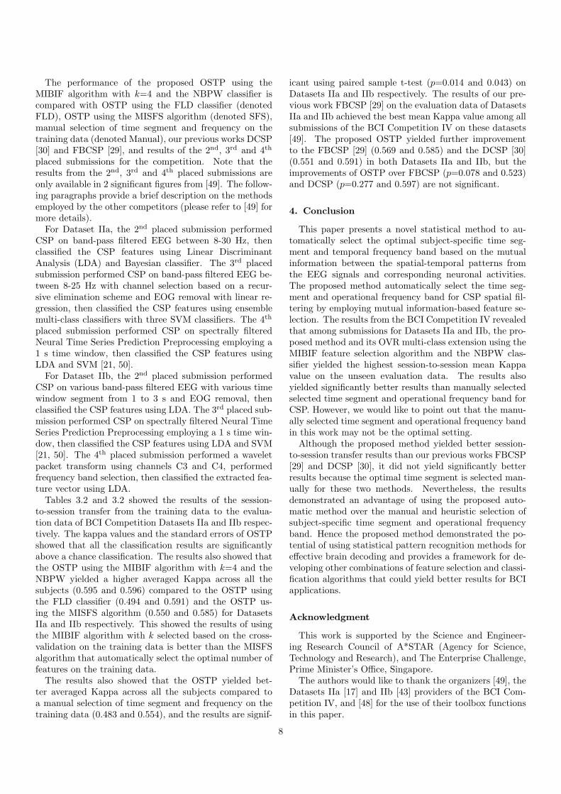
Tables 3.2 and 3.2 showed the results of the session-to-session transfer from the training data to the evalua-tion data of BCI Competition Datasets IIa and IIb respec-tively. The kappa values and the standard errors of OSTPshowed that all the classification results are significantlyabove a chance classification. The results also showed thatthe OSTP using the MIBIF algorithm with k=4 and theNBPW yielded a higher averaged Kappa across all thesubjects (0.595 and 0.596) compared to the OSTP usingthe FLD classifier (0.494 and 0.591) and the OSTP us-ing the MISFS algorithm (0.550 and 0.585) for DatasetsIIa and IIb respectively. This showed the results of usingthe MIBIF algorithm with k selected based on the cross-validation on the training data is better than the MISFSalgorithm that automatically select the optimal number offeatures on the training data.

The results also showed that the OSTP yielded bet-ter averaged Kappa across all the subjects compared toa manual selection of time segment and frequency on thetraining data (0.483 and 0.554), and the results are signif-

icant using paired sample t-test (p=0.014 and 0.043) onDatasets IIa and IIb respectively. The results of our pre-vious work FBCSP [29] on the evaluation data of DatasetsIIa and IIb achieved the best mean Kappa value among allsubmissions of the BCI Competition IV on these datasets[49]. The proposed OSTP yielded further improvementto the FBCSP [29] (0.569 and 0.585) and the DCSP [30](0.551 and 0.591) in both Datasets IIa and IIb, but theimprovements of OSTP over FBCSP (p=0.078 and 0.523)and DCSP (p=0.277 and 0.597) are not significant.

4. Conclusion

This paper presents a novel statistical method to au-tomatically select the optimal subject-specific time seg-ment and temporal frequency band based on the mutualinformation between the spatial-temporal patterns fromthe EEG signals and corresponding neuronal activities.The proposed method automatically select the time seg-ment and operational frequency band for CSP spatial fil-tering by employing mutual information-based feature se-lection. The results from the BCI Competition IV revealedthat among submissions for Datasets IIa and IIb, the pro-posed method and its OVR multi-class extension using theMIBIF feature selection algorithm and the NBPW clas-sifier yielded the highest session-to-session mean Kappavalue on the unseen evaluation data. The results alsoyielded significantly better results than manually selectedselected time segment and operational frequency band forCSP. However, we would like to point out that the manu-ally selected time segment and operational frequency bandin this work may not be the optimal setting.

Although the proposed method yielded better session-to-session transfer results than our previous works FBCSP[29] and DCSP [30], it did not yield significantly betterresults because the optimal time segment is selected man-ually for these two methods. Nevertheless, the resultsdemonstrated an advantage of using the proposed auto-matic method over the manual and heuristic selection ofsubject-specific time segment and operational frequencyband. Hence the proposed method demonstrated the po-tential of using statistical pattern recognition methods foreffective brain decoding and provides a framework for de-veloping other combinations of feature selection and classi-fication algorithms that could yield better results for BCIapplications.

Acknowledgment

This work is supported by the Science and Engineer-ing Research Council of A*STAR (Agency for Science,Technology and Research), and The Enterprise Challenge,Prime Minister’s Office, Singapore.

The authors would like to thank the organizers [49], theDatasets IIa [17] and IIb [43] providers of the BCI Com-petition IV, and [48] for the use of their toolbox functionsin this paper.

8

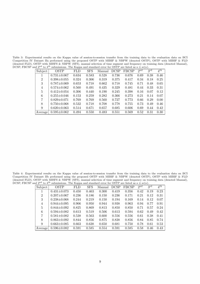
Table 3: Experimental results on the Kappa value of session-to-session transfer from the training data to the evaluation data on BCICompetition IV Dataset IIa performed using the proposed OSTP with MIBIF & NBPW (denoted OSTP), OSTP with MIBIF & FLD(denoted FLD), OSTP with MISFS & NBPW (SFS), manual selection of time segment and frequency on training data (denoted Manual),DCSP, FBCSP and 2nd to 4th submissions. The Kappa and standard error for OSTP are listed as κ± se(κ).

Subject OSTP FLD SFS Manual DCSP FBCSP 2nd 3rd 4th

1 0.731±0.067 0.634 0.583 0.528 0.736 0.676 0.69 0.38 0.462 0.398±0.055 0.324 0.306 0.319 0.375 0.417 0.34 0.18 0.253 0.787±0.069 0.653 0.718 0.662 0.718 0.745 0.71 0.48 0.654 0.574±0.062 0.560 0.491 0.435 0.329 0.481 0.44 0.33 0.315 0.412±0.054 0.306 0.440 0.190 0.245 0.398 0.16 0.07 0.126 0.255±0.046 0.153 0.259 0.282 0.366 0.273 0.21 0.14 0.077 0.829±0.071 0.769 0.769 0.560 0.727 0.773 0.66 0.29 0.008 0.750±0.068 0.532 0.718 0.708 0.778 0.755 0.73 0.49 0.469 0.620±0.063 0.514 0.671 0.657 0.685 0.606 0.69 0.44 0.42

Average 0.595±0.062 0.494 0.550 0.483 0.551 0.569 0.52 0.31 0.30

Table 4: Experimental results on the Kappa value of session-to-session transfer from the training data to the evaluation data on BCICompetition IV Dataset IIb performed using the proposed OSTP with MIBIF & NBPW (denoted OSTP), OSTP with MIBIF & FLD(denoted FLD), OSTP with MISFS & NBPW (SFS), manual selection of time segment and frequency on training data (denoted Manual),DCSP, FBCSP and 2nd to 4th submissions. The Kappa and standard error for OSTP are listed as κ± se(κ).

Subject OSTP FLD SFS Manual DCSP FBCSP 2nd 3rd 4th

1 0.431±0.073 0.450 0.463 0.300 0.419 0.356 0.42 0.19 0.232 0.207±0.067 0.236 0.186 0.150 0.236 0.171 0.21 0.12 0.313 0.238±0.068 0.244 0.219 0.150 0.194 0.169 0.14 0.12 0.074 0.944±0.095 0.906 0.950 0.944 0.938 0.963 0.94 0.77 0.915 0.844±0.092 0.825 0.869 0.813 0.850 0.850 0.71 0.57 0.246 0.594±0.082 0.613 0.519 0.506 0.613 0.594 0.62 0.49 0.427 0.581±0.082 0.538 0.563 0.600 0.556 0.556 0.61 0.38 0.418 0.863±0.092 0.844 0.856 0.875 0.838 0.856 0.84 0.85 0.749 0.663±0.085 0.663 0.638 0.650 0.681 0.750 0.78 0.61 0.53

Average 0.596±0.082 0.591 0.585 0.554 0.591 0.585 0.58 0.46 0.43

9

References

[1] G. Pfurtscheller, C. Neuper, Motor imagery and direct brain-computer communication, Proc. IEEE 89 (7) (2001) 1123–1134.

[2] B. Blankertz, R. Tomioka, S. Lemm, M. Kawanabe, K.-R.Muller, Optimizing Spatial filters for Robust EEG Single-TrialAnalysis, IEEE Signal Process. Mag. 25 (1) (2008) 41–56.

[3] H. Ramoser, J. Muller-Gerking, G. Pfurtscheller, Optimal spa-tial filtering of single trial EEG during imagined hand move-ment, IEEE Trans. Rehabil. Eng. 8 (4) (2000) 441–446.

[4] H. Yuan, A. Doud, A. Gururajan, B. He, Cortical Imaging ofEvent-Related (de)Synchronization During Online Control ofBrain-Computer Interface Using Minimum-Norm Estimates inFrequency Domain, IEEE Trans. Neural Syst. Rehabil. Eng.16 (5) (2008) 425–431.

[5] X. Liao, D. Yao, D. Wu, C. Li, Combining Spatial Filters for theClassification of Single-Trial EEG in a Finger Movement Task,IEEE Trans. Biomed. Eng. 54 (5) (2007) 821–831.

[6] B. Blankertz, G. Dornhege, M. Krauledat, K.-R. Muller,V. Kunzmann, F. Losch, G. Curio, The Berlin brain-computerinterface: EEG-based communication without subject training,IEEE Trans. Neural Syst. Rehabil. Eng. 14 (2) (2006) 147–152.

[7] G. Pfurtscheller, C. Neuper, Future prospects of ERD/ERS inthe context of brain-computer interface (BCI) developments, in:C. Neuper, W. Klimeschm (Eds.), Progress in Brain Research:Event-Related Dynamics of Brain Oscillations, Vol. 159, Else-vier, 2006, pp. 433–437.

[8] P. Herman, G. Prasad, T. M. McGinnity, D. Coyle, Compara-tive Analysis of Spectral Approaches to Feature Extraction forEEG-Based Motor Imagery Classification, IEEE Trans. NeuralSyst. Rehabil. Eng. 16 (4) (2008) 317–326.

[9] M. Naeem, C. Brunner, R. Leeb, B. Graimann, G. Pfurtscheller,Seperability of four-class motor imagery data using independentcomponents analysis, J. Neural Eng. 3 (3) (2006) 208–216.

[10] L. Qin, B. He, A wavelet-based time-frequency analysis ap-proach for classification of motor imagery for brain-computerinterface applications, J. Neural Eng. 2 (4) (2005) 65–72.

[11] T. Wang, J. Deng, B. He, Classifying EEG-based motor imagerytasks by means of time-frequency synthesized spatial patterns,Clin. Neurophysiol. 115 (12) (2004) 2744–2753.

[12] T. Wang, B. He, An efficient rhythmic component expressionand weighting synthesis strategy for classifying motor imageryEEG in a brain-computer interface, J. Neural Eng. 1 (1) (2004)1–7.

[13] D. J. McFarland, D. J. Krusienski, W. A. Sarnacki, J. R. Wol-paw, Emulation of computer mouse control with a noninvasivebrain-computer interface, J. Neural Eng. 5 (2) (2008) 101–110.

[14] A. Schlogl, F. Lee, H. Bischof, G. Pfurtscheller, Character-ization of four-class motor imagery EEG data for the BCI-competition 2005, J. Neural Eng. 2 (4) (2005) L14–L22.

[15] D. P. Burke, S. P. Kelly, P. de Chazal, R. B. Reilly, C. Finucane,A parametric feature extraction and classification strategy forbrain-computer interfacing, IEEE Trans. Neural Syst. Rehabil.Eng. 13 (1) (2005) 12–17.

[16] J. R. Wolpaw, D. J. McFarland, Control of a two-dimensionalmovement signal by a noninvasive brain-computer interface inhumans, Proc. Acad. Nat. Sci. 101 (51) (2004) 17849–17854.

[17] C. Brunner, M. Naeem, R. Leeb, B. Graimann, G. Pfurtscheller,Spatial filtering and selection of optimized components in fourclass motor imagery EEG data using independent componentsanalysis, Pattern Recog. Lett. 28 (8) (2007) 957–964.

[18] L. Qin, L. Ding, B. He, Motor imagery classification by meansof source analysis for brain-computer interface applications, J.Neural Eng. 1 (3) (2004) 135–141.

[19] B. Kamousi, Z. Liu, B. He, Classification of motor imagery tasksfor brain-computer interface applications by means of two equiv-alent dipoles analysis, IEEE Trans. Neural Syst. Rehabil. Eng.13 (2) (2005) 166–171.

[20] D. Coyle, G. Prasad, T. M. McGinnity, A time-series predictionapproach for feature extraction in a brain-computer interface,IEEE Trans. Neural Syst. Rehabil. Eng. 13 (4) (2005) 461–467.

[21] D. Coyle, A. Satti, G. Prasad, T. M. McGinnity, Neural time-series prediction preprocessing meets common spatial patternsin a brain-computer interface, in: Proc. 30th Annu. Int. Conf.IEEE Eng. Med. Biol. Soc., Vancouver, BC Canada, 2008, pp.2626–2629.

[22] C. Brunner, R. Scherer, B. Graimann, G. Supp,G. Pfurtscheller, Online Control of a Brain-Computer In-terface Using Phase Synchronization, IEEE Trans. Biomed.Eng. 53 (12) (2006) 2501–2506.

[23] N. Yamawaki, C. Wilke, Z. Liu, B. He, An enhanced time-frequency-spatial approach for motor imagery classification,IEEE Trans. Neural Syst. Rehabil. Eng. 14 (2) (2006) 250–254.

[24] W. Wu, X. Gao, B. Hong, S. Gao, Classifying Single-Trial EEGDuring Motor Imagery by Iterative Spatio-Spectral PatternsLearning (ISSPL), IEEE Trans. Biomed. Eng. 55 (6) (2008)1733–1743.

[25] R. Tomioka, G. Dornhege, G. Nolte, B. Blankertz, K. Aihara,K.-R. Muller, Spectrally weighted common spatial pattern al-gorithm for single trial EEG classification, Mathematical engi-neering technical reports (2006).

[26] G. Dornhege, B. Blankertz, M. Krauledat, F. Losch, G. Curio,K.-R. Muller, Combined Optimization of Spatial and TemporalFilters for Improving Brain-Computer Interfacing, IEEE Trans.Biomed. Eng. 53 (11) (2006) 2274–2281.

[27] S. Lemm, B. Blankertz, G. Curio, K.-R. Muller, Spatio-SpectralFilters for Improving the Classification of Single Trial EEG,IEEE Trans. Biomed. Eng. 52 (9) (2005) 1541–1548.

[28] B. Blankertz, G. Dornhege, M. Krauledat, K.-R. Muller, G. Cu-rio, The non-invasive Berlin Brain-Computer Interface: Fastacquisition of effective performance in untrained subjects, Neu-roImage 37 (2) (2007) 539–550.

[29] K. K. Ang, Z. Y. Chin, H. Zhang, C. Guan, Filter Bank Com-mon Spatial Pattern (FBCSP) in Brain-Computer Interface, in:Proc. IEEE Int. Joint Conf. Neural Netw., Hong Kong, 2008,pp. 2391–2398.

[30] K. P. Thomas, C. Guan, C. T. Lau, A. P. Vinod, K. K. Ang, ANew Discriminative Common Spatial Pattern Method for MotorImagery Brain-Computer Interfaces, IEEE Trans. Biomed. Eng.56 (11) (2009) 2730–2733.

[31] N. Kwak, C.-H. Choi, Input feature selection by mutual infor-mation based on Parzen window, IEEE Trans. Pattern Anal.Mach. Intell. 24 (12) (2002) 1667–1671.

[32] E. Parzen, On Estimation of a Probability Density Functionand Mode, Annals Math. Statist. 33 (3) (1962) 1065–1076.

[33] R. Battiti, Using mutual information for selecting features insupervised neural net learning, IEEE Trans. Neural Netw. 5 (4)(1994) 537–550.

[34] K. K. Ang, C. Quek, Rough Set-based Neuro-Fuzzy System,in: Proc. IEEE Int. Joint Conf. Neural Netw., Vancouver, BC,Canada, 2006, pp. 742–749.

[35] R. O. Duda, P. E. Hart, D. G. Stork, Pattern Classification,2nd Edition, John Wiley, New York, 2001.

[36] V. N. Vapnik, Statistical learning theory, Adaptive and learn-ing systems for signal processing, communications, and control,Wiley, New York, 1998.

[37] L. Breiman, J. H. Friedman, R. A. Olshen, C. J. Stone,Classification and regression trees, The Wadsworth statis-tics/probability series, Wadsworth International Group, Bel-mont, CA, 1984.

[38] T. Cover, P. Hart, Nearest neighbor pattern classification, IEEETrans. Inf. Theory 13 (1) (1967) 21–27.

[39] K. K. Ang, C. Quek, Rough set-based Neuro-Fuzzy System:Towards increasing interpretability without compromising ac-curacy , VDM Verlag, Germany, 2009.

[40] N. K. Kasabov, Q. Song, DENFIS: dynamic evolving neural-fuzzy inference system and its application for time-series pre-diction, IEEE Trans. Fuzzy Syst. 10 (2) (2002) 144–154.

[41] A. W. Bowman, A. Azzalini, Applied Smoothing Techniques forData Analysis: The Kernel Approach with S-Plus Illustrations,Oxford University Press, New York, 1997.

[42] G. Dornhege, B. Blankertz, G. Curio, K.-R. Muller, Increase

10

Information Transfer Rates in BCI by CSP Extension to Multi-class, in: S. Thrun, L. Saul, B. Schlkopf (Eds.), Advances inNeural Information Processing Systems, Vol. 16, MIT Press,Cambridge, MA, 2004.

[43] R. Leeb, F. Lee, C. Keinrath, R. Scherer, H. Bischof,G. Pfurtscheller, Brain-Computer Communication: Motivation,Aim, and Impact of Exploring a Virtual Apartment, IEEETrans. Neural Syst. Rehabil. Eng. 15 (4) (2007) 473–482.

[44] J. Muller-Gerking, G. Pfurtscheller, H. Flyvbjerg, Designing op-timal spatial filters for single-trial EEG classification in a move-ment task, Clin. Neurophysiol. 110 (5) (1999) 787–798.

[45] P. Shenoy, M. Krauledat, B. Blankertz, R. P. N. Rao, K.-R.Muller, Towards adaptive classification for BCI, J. Neural Eng.3 (1) (2006) R13.

[46] A. Schlogl, J. Kronegg, J. Huggins, S. Mason, Evaluation Cri-teria for BCI Research, in: Toward Brain-computer Interfacing,MIT Press, USA, 2007, pp. 327–342.

[47] J. Cohen, A coefficient of agreement for nominal scales, Educ.Psychol. Meas. 20 (1) (1960) 37–46.

[48] A. Schlogl, C. Brunner, BioSig: A Free and Open Source Soft-ware Library for BCI Research, Computer 41 (10) (2008) 44–50.

[49] B. Blankertz, BCI Competition IV, http//www.bbci.de/

competition/iv/ (2008).[50] D. Coyle, Neural network based auto association and time-series

prediction for biosignal processing in brain-computer interfaces,IEEE Comput. Intell. Mag. 4 (4) (2009) 47–59.

11