
MUTUAL FUND PERFORMANCE IN EMERGING MARKETS: THE CASE OF THAILAND By TEERAPAN SUPPA-AIM A Thesis...
323
MUTUAL FUND PERFORMANCE IN EMERGING MARKETS: THE CASE OF THAILAND By TEERAPAN SUPPA-AIM A Thesis submitted to THE UNIVERSITY OF BIRMINGHAM For the Degree of DOCTOR OF PHILOSOPHY Department of Accounting and Finance Birmingham Business School The University of Birmingham March 2010
Transcript of MUTUAL FUND PERFORMANCE IN EMERGING MARKETS: THE CASE OF THAILAND By TEERAPAN SUPPA-AIM A Thesis...

MUTUAL FUND PERFORMANCE IN EMERGING MARKETS:
THE CASE OF THAILAND
By
TEERAPAN SUPPA-AIM
A Thesis submitted to
THE UNIVERSITY OF BIRMINGHAM
For the Degree of
DOCTOR OF PHILOSOPHY
Department of Accounting and Finance
Birmingham Business School
The University of Birmingham
March 2010

University of Birmingham Research Archive
e-theses repository This unpublished thesis/dissertation is copyright of the author and/or third parties. The intellectual property rights of the author or third parties in respect of this work are as defined by The Copyright Designs and Patents Act 1988 or as modified by any successor legislation. Any use made of information contained in this thesis/dissertation must be in accordance with that legislation and must be properly acknowledged. Further distribution or reproduction in any format is prohibited without the permission of the copyright holder.

Synopsis
The rate of growth of investment in mutual funds has increased dramatically over the past
decade. Many studies have developed models for performance evaluation and have examined
whether fund managers provide value added for investors. Most of these studies, however,
have focused on the developed markets and only a few examine whether the findings carry
over to emerging markets as well.
This thesis specifically investigates mutual funds in one of the emerging economies,
Thailand, using a more extensive dataset than previous studies; it controls for investment
policy and tax-purpose differences, as unique characteristics of mutual funds in Thailand. We
scrutinize how fund managers perform and what strategy they use in managing their
portfolios; and ask whether any fund characteristics can explain fund performance. We also
explore the impact of liquidity on performance and performance measures.
We find in this context that mutual fund managers, as a whole, do not have selectivity
or timing ability and they do not give value added to investors. Most of the fund managers in
Thailand invest heavily in small and growth stocks. Flexible fund managers are, in
comparison, more active and adjust their portfolios dynamically according to economic
information.
There is persistence in performance in general mutual funds. This evidence is
statistically and economically significant although it derives mainly from poorly performing
funds which continue to perform badly. Size, age and fund family also have explanatory
power in fund performance but it is specific to investment policy and the evidence is not
economically significant. Net cash flows, in general, have no impact on fund performance.
However, the significant amount of cash inflows can severely lower performance in mutual

fund since the fund managers are unable to allocate their portfolio immediately and leave
large amounts in their cash position.
Liquidity also plays a major role in mutual fund performance. We find that funds
which contain more illiquid assets in their portfolios perform better and this suggests that
there is a liquidity premium in mutual funds. As a result, a liquidity-augmented model which
includes one liquidity factor is proposed. Results from this proposed model show that our
liquidity factor, as measured by stock turnover ratio, has explanatory power for fund
performance, in particular in low liquidity portfolios. However, our liquidity factor is unable
completely to explain the liquidity premium in mutual funds because the evidence of a
liquidity premium is still present.
Finally, the study reveals the policy implications of introducing the tax-benefit funds
scheme in Thailand. We find that the tax-benefit funds perform significantly better than
general funds and this is also true even when controlled for other fund characteristics. The
tax-benefit fund managers are more passive than managers of general funds but they do not
employ any different strategy from that used by managers of general funds. Tax-benefit funds
are more sensitive to cash flows and contain slightly more illiquid stocks in their underlying
assets. Thus, the superior performance in tax-benefit funds is not only attributable to the
liquidity premium, but also to the fund managers’ superior ability, as well as to the long-term
restrictions which help tax-benefit fund managers to reduce nondiscretionary trading cost in
these funds.

To my parents Paiboon and Thararat Ungphakorn

Acknowledgement
My econometrics tutor once told me that doing a PhD is like walking through a dark tunnel.
You never see the light until you are approaching the end. Now, I am at the end of my
journey; when I look back I find that I am highly indebted to many people who supported me
as I went along. First and foremost, I am very much indebted to my supervisor, Professor
Ranko Jelic. He is the person who gave me the chance to pursue a doctoral degree at the
University of Birmingham. He also provided excellent guidance and the best possible support
during my studies. My deep gratitude also goes to Professor Mike Theobald and my
examiners, Professor Victor Murinde and Dr.Natasha Todorovic, for their time reading this
thesis and giving me valuable suggestions and comments.
I am also indebted to Associate Professor Prapruke Ussahawanitchakit and Dr.
Julsuchada Sirisom. They are my inspiration and were the ones who originally made me think
about pursuing a PhD. During my research, they always give me great advice, support and
encouragement.
My deep gratitude should also go to the Royal Thai Government and Mahasarakham
University for their sponsorship. My ambition would never have been realised without their
financial support.
I am grateful to the Association of Investment Management Companies and the
Security Exchange Commission in Thailand for kindly providing me with data.
I would like to thank Marleen Vanstockem, Gabrielle Kelly and Ron Bishton as well
as all the members of staffs and fellow PhD students at the Birmingham Business School for
their help, friendship and support since I began this work. Because of the comfort, I have not
felt like a stranger though I am thousands of miles away from home.

I want to thank Dr. Kathryn Boniface, Maz Davies, Prof. Steven Gough and Dr. Parth
Narendran as well as the staffs at the University Medical Practice and Selly Oak Hospital.
They provided me with the best medication and took care for me throughout my studies.
Indeed, I owe them my life.
I also want to thank Chris Sherman, Cathie Bartlam, Grace Houses Birmingham and
all of my housemates for their warmth and support. They make the house a home to me.
My appreciation goes to the Scott and Obeda families for their hospitality on every
visit. Special thanks to Kim Scott for her lovely cooking; and to Joseph and Rebecca Scott for
making me smile.
I would like to give my gratitude to Dr. Eve Richards for her biggest help. She is
always there for me and reads my work without any complaints.
I much appreciated the invaluable friendship of Trairong Swatdikun, Vissanu
Zumitzavan, Dr.Yan Wang, Polwat Lerskullawat and Hadiza Sa’id, who were always right
there for me whenever I needed them.
Lastly, I also want to thank my dearest family – father, mother, grandmother and
brother – for their endless love and unending support. It is surely because of their greatest
love that I was able to start this journey and this is what has carried me through to its end.

TABLE OF CONTENTS
Page
Synopsis
Dedication
Acknowledgement
Table of Contents
List of Tables
List of Figures
CHAPTER ONE: INTRODUCTION……………………………………….………......1-12
1.1 Background and motivation of the study ...................................................................1
1.2 Aims of the study .......................................................................................................5
1.3 Contributions of the study..........................................................................................6
1.4 Methodology of the study ..........................................................................................9
1.5 Organisation of the study .........................................................................................11
CHAPTER TWO: LITERATURE SURVEY……………………………….………...13-91
2.1 Introduction ..............................................................................................................13
2.2 Performance measures .............................................................................................14
2.2.1 The early stage of performance measurement .....................................................15
2.2.2 Risk-adjusted non-regression approaches ............................................................17
2.2.3 Regression-based approaches ..............................................................................21
2.2.3.1 Single-factor model......................................................................................21
2.2.3.2 Multifactor models .......................................................................................22
2.2.3.3 Conditional measures ...................................................................................26
2.2.4 Timing ability.......................................................................................................27
2.2.5 Non-benchmark performance evaluation approaches..........................................30
2.2.6 Empirical studies in mutual fund performance ....................................................33
2.3 Persistence in performance ......................................................................................41
2.4 Flow related performance ........................................................................................45
2.4.1 Future flows and performance .............................................................................46
2.4.2 Past flows and performance .................................................................................47
2.5 Style Analysis ..........................................................................................................50

2.6 Empirical studies on emerging markets ...................................................................52
2.7 Conclusions and suggestions for further research....................................................59
CHAPTER THREE: INSTITUTIONAL BACKGROUNDS AND SAMPLE
SELECTION…...………………………………………….……………….…………..92-124
3.1 Introduction ..............................................................................................................93
3.2 An overview of the mutual fund business in Thailand ............................................96
3.2.1 Mutual fund development ....................................................................................96
3.2.2 Mutual fund classification..................................................................................101
3.2.2.1 The tax-benefit funds .................................................................................106
3.2.3 Organisational structure .....................................................................................111
3.2.4 Net asset values, fees and charges of mutual funds ...........................................115
3.3 Mutual fund data ....................................................................................................116
3.3.1 The Sample.........................................................................................................116
3.3.2 Survivorship bias................................................................................................121
3.4 Conclusions and suggestions for further research..................................................122
CHAPTER FOUR: PERFORMANCE OF THAI MUTUAL FUNDS….………...125-188
4.1 Introduction ............................................................................................................126
4.2 Previous evidence and hypotheses .........................................................................131
4.3 Data and Methodology...........................................................................................139
4.3.1 Mutual fund sample............................................................................................139
4.3.2 Performance measures .......................................................................................140
4.3.2.1 The Jensen measure....................................................................................140
4.3.2.2 Market timing.............................................................................................141
4.3.2.3 Four-factor model.......................................................................................142
4.3.2.4 Conditional measure...................................................................................143
4.3.3 Benchmarks and variables..................................................................................144
4.4 Empirical results.....................................................................................................146
4.4.1 Performance .......................................................................................................148
4.4.1.1 Overall performance...................................................................................148
4.4.1.2 Selectivity and market timing abilities.......................................................157

4.4.2 Investment strategy of fund managers ...............................................................159
4.4.3 Sub-period analysis ............................................................................................166
4.4.4 General and tax-benefit mutual funds ................................................................170
4.4.5 Mutual fund styles and performance..................................................................172
4.5 Robustness of the results........................................................................................176
4.5.1 Multifactor model...............................................................................................176
4.5.2 Value-weighted portfolio method ......................................................................179
4.5.3 Frequency of data...............................................................................................181
4.5.4 Dummy variable market timing measure...........................................................182
4.6 Conclusions............................................................................................................186
CHAPTER FIVE: DETERMINANTS OF MUTUAL FUND PERFORMANCE 189-232
5.1 Introduction ............................................................................................................190
5.2 Previous evidence and hypotheses .........................................................................193
5.2.1 Persistence in performance ................................................................................193
5.2.2 Fund size ............................................................................................................194
5.2.3 Net cash flows ....................................................................................................196
5.2.4 Fund longevity ...................................................................................................197
5.2.5 Family size .........................................................................................................198
5.2.6 Evidence from emerging markets and hypotheses.............................................198
5.3 Data and methodology ...........................................................................................201
5.3.1 Fund sample .......................................................................................................201
5.3.2 Fund performance benchmarks ..........................................................................203
5.3.3 Fund characteristics............................................................................................204
5.3.4 Methodology ......................................................................................................206
5.3.4.1 Multidimensional (panel) regression..........................................................206
5.3.4.2 Trading strategies .......................................................................................209
5.4 Empirical results.....................................................................................................211
5.4.1 Persistence in performance ................................................................................214
5.4.2 Mutual fund size.................................................................................................217
5.4.3 Net cash flows ....................................................................................................219
5.4.4 Fund longevity ...................................................................................................222
5.4.5 Family size .........................................................................................................223

5.5 Robustness of the results........................................................................................226
5.6 Conclusions............................................................................................................230
CHAPTER SIX: THE LIQUIDITY PREMIUM, SHARE RESTRICTION AND
MUTUAL FUND PERFORMANMCE…………………………………..….……...233-273
6.1 Introduction ............................................................................................................234
6.2 Literature and hypotheses ......................................................................................237
6.3 Data and Methodology...........................................................................................243
6.3.1 The sample .........................................................................................................243
6.3.2 Measuring mutual funds’ asset illiquidity..........................................................244
6.3.3 Liquidity-augmented performance measure ......................................................246
6.4 Empirical results.....................................................................................................248
6.4.1 Liquidity premium .............................................................................................248
6.4.2 Liquidity-augmented performance measure ......................................................254
6.4.3 Liquidity premium in tax-benefit funds .............................................................261
6.5 Robustness of the results........................................................................................264
6.5.1 Autoregressive model as a proxy of liquidity ....................................................264
6.5.2 January effect .....................................................................................................268
6.6 Conclusions............................................................................................................271
CHAPTER SEVEN: CONCLUSIONS……………………………….….………….274-283
7.1 Introduction ............................................................................................................274
7.2 Key findings ...........................................................................................................275
7.2.1 Literature survey on mutual fund performance..................................................275
7.2.2 Empirical study of Thai mutual fund performance ............................................277
7.2.3 Empirical study of the determinants of mutual fund performance ....................278
7.2.4 Empirical study of the effect of liquidity on mutual fund performance ............280
7.3 Policy Implications ................................................................................................281
7.4 Limitations of the study and suggestions for further research ...............................282
References
Appendices

LIST OF TABLES
Page
Table 2.1 Summary of main theories and empirical studies related in mutual fund
performance in developed markets ..........................................................................................61
Table 2.2 Summary of main theories and empirical studies related in mutual fund
performance in emerging markets............................................................................................87
Table 3.1 Thai mutual funds classified by investment policies .............................................106
Table 3.2 The differences between General, RMF and LTF funds .......................................109
Table 3.3 Growth of tax-benefit and general mutual funds from 2000 to 2007 ....................110
Table 3.4 Number and total asset values owned by asset management companies...............113
Table 3.5 Concentration ratio.................................................................................................114
Table 3.6 Fund sample selection............................................................................................118
Table 3.7 Number of funds in the sample for each year ........................................................119
Table 3.8 Fund characteristics ...............................................................................................121
Table 3.9 Survivorship bias....................................................................................................122
Table 4.1 Descriptive statistics of weekly returns for fund portfolios...................................140
Table 4.2 Descriptive statistics and correlation matrix of the risk factors............................146
Table 4.3 An overview of the performance of mutual fund portfolios .................................151
Table 4.4 The Jensen performance measure ..........................................................................153
Table 4.5 The market timing performance measure ..............................................................158
Table 4.6 Fund factor sensitivities .........................................................................................162
Table 4.7 Fund strategies using Cahart’s four-factor model..................................................165
Table 4.8 Performance measure: Sub-period analysis ...........................................................169
Table 4.9 Performance differences across fund characteristics .............................................171
Table 4.10 Cross-sectional coefficients of mutual fund characteristics.................................172
Table 4.11 Performance of style portfolios............................................................................175
Table 4.12 Cahart’s four-factor performance measure ..........................................................178
Table 4.13 Performance of value-weighted portfolios...........................................................180
Table 4.14 Fund’s factor sensitivities of value weighted portfolios ......................................180
Table 4.15 Fund strategies of value weighted portfolios .......................................................181
Table 4.16 Performance using monthly return data ...............................................................183
Table 4.17 The dummy variable market timing performance measure .................................185

Table 5.1 Previous evidence of the relationship between fund performance and fund attributes
in emerging markets...............................................................................................................201
Table 5.2 Summary statistics of mutual fund returns ............................................................202
Table 5.3 Summary statistics of fund attributes.....................................................................206
Table 5.4 Summary statistics of mutual fund performance ...................................................208
Table 5.5 Correlation matrix ..................................................................................................208
Table 5.6 Multidimensional (panel) analysis for determinants of fund performance............212
Table 5.7 Performance of trading strategy portfolios based on past performance.................216
Table 5.8 Performance of trading strategy portfolios based on fund size..............................218
Table 5.9 Performance of trading strategy portfolios based on net cash flows .....................221
Table 5.10 Performance of trading strategy portfolios based on fund longevity...................223
Table 5.11 Performance of trading strategy portfolios based on size of fund family............225
Table 5.12 Multivariate regression (Cross-section time-series average) ...............................228
Table 6.1 Descriptive statistics of the mutual fund sample ...................................................244
Table 6.2 Descriptive statistics for illiquid assets..................................................................249
Table 6.3 Descriptive statistics for the returns of liquidity portfolios ...................................251
Table 6.4 Performance using traditional single-factor measure.............................................253
Table 6.5 Descriptive statistics and correlation matrix of risk factors...................................255
Table 6.6 Performance using liquidity-augmented measure..................................................259
Table 6.7 Illiquid assets in general vs. tax-benefit funds.......................................................262
Table 6.8 Probit regression ....................................................................................................263
Table 6.9 First-order serial correlation...................................................................................266
Table 6.10 The January effect ................................................................................................269

LIST OF FIGURES
Page
Figure 1.1 Research methodology ...........................................................................................10
Figure 3.1 Worldwide mutual fund assets and the growth in the number of mutual funds,
2003-2007 ................................................................................................................................94
Figure 3.2 Growth of number of funds for Asia/Pacific countries, 2000-2007 .......................98
Figure 3.3 Growth of mutual fund asset values for Asia/Pacific countries, 2000-2007 ..........98
Figure 3.4 Growth in Thai mutual funds 2000-2007 .............................................................100
Figure 3.5 Savings to GDP classified by investment type in Thailand, 2000-2007 ..............100
Figure 3.6 Number of funds and total asset values (TNAs) classified by type (closed-ended
vs. open-ended) ......................................................................................................................102
Figure 3.7 Number of fund classified by policy 2000-2007 ..................................................105
Figure 3.8 Total Net Asset values (TNAs) classified by fund policy 2000-2007..................105
Figure 3.9 Benefits and requirements of retirement mutual funds (RMF) ............................108
Figure 3.10 Benefits and requirements of Long-term equity mutual funds (LTF) ................108
Figure 3.11 Number and asset value of RMF and LTF funds, 2000-2007 ............................110
Figure 3.12 Structure of the Thai mutual fund business ........................................................111
Figure 4.1 Frequency distributions of unconditional and conditional estimates ...................155
Figure 4.2 Scatter plots for size and book-to-market t-statistics............................................173

LIST OF APPENDICES
A.1 Mutual fund growth classified by investment policy, 2000-2007
A.2 Summary statistics of individual funds returns in the sample
1
CHAPTER ONE
INTRODUCTION
1
1.1 Background and motivation of the study
For a long time, mutual fund investment has played an important role in the financial market
and its popularity has increased dramatically over the past decade. This can be seen from the
sharp rise in worldwide mutual fund assets from $14 trillion in 2003 to $26 trillion in 2007
(ICI, 2008). In the US, mutual fund companies are the largest institutional investors in the
stock market and hold more than a quarter of the stocks (ibid.). Pozen and Crane (1998) claim
that around half the households in the US invest in mutual funds. The welcome given to
mutual funds is attributed to its various benefits, such as its diversification, professional
management, liquidity and flexibility and convenience. In addition, mutual fund investment is
important to the equity market and to the growth of the economy, since they are held by
institutional investors who hold a significant portion of capital assets.
Despite the popularity and importance of mutual fund investment, the notion of
modern portfolio theory (MPT), which explains the relationship between risk and expected
returns and also the famous efficient market hypothesis (EMH), which suggests that stock
prices fully reflect information are also a challenge to the studies in mutual funds and shift
the fund performance measurement from the calculation of crude returns to detailed
explorations of the risk and returns methods. More recently, studies in mutual funds have
become central to the performance of mutual funds. Some studies try to find a model in
evaluating mutual fund performance. Others explore whether fund managers can create value

2
added for investors and ways to succeed in this. Other studies still investigate whether mutual
fund performance can be explained or forecast by any particular factors. More recently, there
has been extensive research into mutual fund performance employing various research
methods and different datasets from a number of different study periods.
Nonetheless, due to the availability of the most of the data, these studies tend to be
conducted within the developed markets and only minor studies have focused on the mutual
funds in emerging markets. In addition, studies in the emerging markets still take the
prevailing approach and concentrate on showing how fund managers perform, neglecting
other relevant issues. Therefore, we still know too little about mutual fund investment in
emerging markets and this impedes the development of this industry.
In spite of the limited evidence about the behaviour of mutual funds in emerging
markets, mutual fund investment in these areas has grown markedly over the past decade at a
quicker pace than even the developed markets have shown. The growth in mutual fund
investment is influential because it shapes the future development in the securities market and
has important policy implications. The high proportion of institutional investors creates more
timely information and therefore makes the market more efficient. However, it tends also to
encourage irrational behaviour, such as herding, which makes the market more volatile.
Additionally, the excessive growth is liable to inflate stock prices and makes the market more
vulnerable, since it does not have enough capacity to anticipate the high inflows (Borensztein
and Gelos, 2001).
Furthermore, mutual fund industries in emerging markets display some unique
characteristics which are different from those in developed markets and these, too, challenge
the assumptions in this respect. For instance, mutual funds in emerging markets are less
competitive and information is less publicly available than elsewhere. Investors are more

3
passive and likely to make their decision on the basis of familiarity. Moreover, mutual funds
in some countries are used as part of the national financial policy, which differentiates mutual
fund styles even further. For example, in Thailand, the government gives favourable tax
treatment to a specific type of mutual fund in order to encourage retirement and long-term
savings. Thus, these conditions potentially impact on performance and stock selection
strategy, as well as decision behaviour.
More importantly, while most of the theoretical models which we use to evaluate
mutual fund performance are based on the assumption of efficient markets, emerging markets
fail to meet these assumptions. Returns in emerging markets suffer from several chronic
conditions such as high volatility, high trading cost, non-normality, and infrequent trading
(Bekaert and Harvey, 2002). Furthermore, there is still some doubt whether the factors
documented in developed markets can also explain stock returns in emerging markets (for
example, Claessens et al., 1995; Fama and French, 1998; Rouwenhorst, 1999; Barry et al.,
2002; van der Hart et al., 2002).
Thus, the study of mutual funds in emerging markets is overdue for those who need a
fuller understanding of their investment conditions. In addition, this would allow an out-of-
sample test to challenge existing asset pricing models and lead to the development of new
empirical models.
This study seeks to shed light on mutual fund investment in emerging markets and
specifically focuses on three issues: performance, determinants of performance and the role
of liquidity on performance and performance measure. Since mutual fund data from all
emerging markets are segmented and hard to obtain and also that policies and regulations are
different for each country, the scope of the present study rests solely on an emerging country,
namely, Thailand and it is treated as a case study typical of the emerging markets as a whole.

4
Although the characteristics of emerging markets are relatively diverse, Thailand can
represent the rest of the emerging countries, those in Asia in particular. This is because the
Thai stock market exhibits several behaviours which are consistent with the average for
emerging markets. For example, while the ten-year annualized growth of emerging markets
ranged from -0.03% (Taiwan) to 20.45% (India), the Thai stock market grew by 12.36% per
year and this figure is comparable to the growth of the MSCI Emerging Markets index1,
11.69% (MSCI, 2010). Also, Lim and Brooks showed that Thailand obtained a World Bank
FSDI equity market efficiency index of around 4 and this is close to the average of 4.42
among 33 emerging countries (cited in Gregoriou, 2009.). Allen and Chimhini (ibid.) reveal
that Asian equity markets are highly correlated.
In addition, Thai mutual funds play an important role in the capital market and
Thailand’s economy is among the three fastest growing in the Asia/Pacific region. The data
on mutual funds and the stock market, as well as other relevant information from Thailand,
are sufficiently accessible and more complete than from many other emerging countries and
thus allow us to make more comprehensive investigations of mutual funds in emerging
markets.
1 The MSCI Emerging markets index is a free float-adjusted market capitalisation weighted index which is
designed to measured equity market performance in emerging markets. As of June 2009, the index consists of indices for 22 countries: Brazil, Chile, China, Colombia, the Czech Republic, Egypt, Hungary, India, Indonesia, Israel, Korea, Malaysia, Mexico, Morocco, Peru, the Philippines, Poland, Russia, South Africa, Taiwan, Thailand and Turkey (MSCI, 2010).

5
1.2 Aims of the study
The main objective of this thesis is to comprehensively explore the performance of mutual
funds in an emerging market. This fills one of the gaps in mutual fund literature, since studies
in this region are scarce, based on the prevailing approach and survey a small number of
funds over only a short period. It should not be forgotten that emerging markets are unlike
developed markets in several ways. Subsequently, this thesis uses a more comprehensive
dataset of mutual funds in Thailand as a case study to represent its emerging market.
Subsequently, the thesis has four main purposes. The first relates to the comprehensive
evaluation of the performance of mutual funds in emerging markets and assesses style and
strategy used by fund managers in order to accomplish this. This study explores fund
performance at aggregated, style and fund levels and employs various models which evolved
in developed markets to estimate performance. Additionally, this study compares the results
with evidence from developed markets.
The second aim of this thesis is to investigate whether Thai mutual fund performance
can be explained by any of its characteristics. The study examines statistic and economic
importance of fund characteristics to its performance. In the literature, evidence is sparse and
mixed on developed markets, let alone that on emerging markets. Rather than focusing on
one particular characteristic, this study draws on the evidence from five important
characteristics in the literature, which offer theoretical and empirical support. They comprise
past performance, flows, longevity, fund size and family fund size. The study investigates the
characteristics separately and also combines them into a group and then performs
multidimensional regression, allowing for time variation.
The third aim of this thesis is to investigate the impact of liquidity on mutual fund
performance, for this is one of the main concerns in emerging markets. This study measures

6
the liquidity of assets contained in the portfolio, using a model in hedge fund literature. The
study also offers an auxiliary performance measure to capture this effect and assesses how
important it is to mutual fund performance in Thailand.
The fourth aim of this thesis is to investigate and discuss policy implications in
Thailand which adopt tax-advantaged types of mutual fund in order to encourage retirement
and long-term savings. In this thesis, the performance and characteristics of these tax-
advantaged funds are also investigated in a separate group and compared to those of general
mutual funds.
1.3 Contributions of the study
This thesis makes several meaningful contributions to the literature and the practical
perspective. First, it is conducted in a different setting from most previous studies. Thus, it
provides an out-of-sample test for the theories and empirical models so far established.
Second, this study fills one of the gaps in mutual fund studies by asking whether the
findings in developed markets carry over to emerging markets. This is important because,
even though emerging markets display several characteristics which are not found in
developed markets, the literature on mutual funds in emerging markets is relatively thin and
incomplete.
Third, this study uses a more extensive dataset than has been used in any previous
mutual fund studies of emerging markets. We employ a novel mutual fund dataset in
Thailand, consisting of both weekly and monthly data and including both equity and flexible
funds. This is the first time a mutual fund study has used data on both weekly and monthly

7
returns to tackle a problem. The high data frequency not only helps to validate our results, but
also allows us to advance some analysis. For example, in Chapter 5, the fund weekly data are
used to calculate the risk-adjusted abnormal return for each year from 2000-2007. Then, it
turns into a panel data allowing us to perform a multidimensional (panel) regression on fund
characteristics.
Furthermore, this is the first empirical study of an emerging market which includes
flexible funds in the sample. In theory, a flexible fund is in some ways similar to equity funds
since its main assets are also stocks. However, a proportion of its holdings can be more varied
over time, subject to the fund manager’s decision. Thus, this study includes flexible funds in
the sample and puts them into a separate category and it is hoped to provide a more
comprehensive account of portfolio behaviour.
Fourth, this study applies new methodologies which have never been applied to
emerging markets. For instance, Chapter 5 explores the determinants of risk-adjusted mutual
fund performance using multidimensional regression in addition to the common approach,
which is to use a zero-cost trading strategy. This alternative methodology can explore several
factors simultaneously while controlling the effect between one and another. Using the two
methods allows us to examine determinants of fund performance statistically and
economically and it provides more meaningful results. Moreover, in Chapter 6, we apply a
model in the hedge fund literature in measuring the illiquid assets contained in a portfolio in
our mutual fund data. This is the first empirical study to use such a model outside the hedge
fund literature.
Fifth, this study explores new issues which have not hitherto been observed in
previous studies. This is the first study in Thailand which explores the stock selection
strategies and style of fund managers (Chapter 4). In Chapter 5, we consider a broader range

8
of characteristics than previous studies in emerging markets have done in determining mutual
fund performance and also include more new factors, namely fund longevity and family size,
in the analysis. In Chapter 6, we look at the effect of liquidity on the mutual fund
performance because liquidity is one of the major concerns in emerging markets. Leaving
aside emerging markets, the liquidity effect is negligible in all mutual fund literature, even
though this issue has been widely documented by writers of asset pricing. The study also puts
forward an auxiliary model based on the liquidity effect in measuring mutual fund
performance.
Sixth, this study can claim several new findings. This is the first mutual fund study to
expose the evidence of a liquidity premium and emphasise the inclusion of including a
liquidity factor in the fund performance measure (Chapter 6). This study also provides new
findings about emerging markets. In Chapter 4, the study reveals the style of fund managers
in these markets and shows that they rely on medium capitalisation strategy. This chapter also
relates the sensitivity of data frequency to the fund performance. In addition, Chapter 5 gives
the first evidence from the emerging markets of short-term persistence in performance among
poorly performing funds.
Seventh, the study is the only one which gives important policy implications,
reporting them in turn in each empirical chapter. This is the first study on Thailand which
discusses the effect of the Thai government’s encouragement of individual savings by
adopting special fund styles which give favourable tax treatment. We reveal the policy
implications of this action by assessing these specific funds in a separate group from general
funds, before comparing and discussing the results from the two groups.
Finally, in its practical aspects, this study will, it is hoped, be useful for individuals
and institutional investors in selecting mutual funds. It also helps fund managers to identify

9
their positions and gives ideas on the strategies which they should follow in order to
maximise returns for their investors.
1.4 Methodology of the study
In the light of mutual fund performance analysis, our methodology involves a particular set of
quantitative procedures comprising: a review of the literature; identifying research problems
and hypotheses; the collection of data; analysis of data; interpretation of the empirical results;
and the drawing of conclusions.
Figure 1.1 illustrates the logical methodological process of this study. Once the
general research topic is decided, the process begins by reviewing the literature from various
sources, including books, journals, working papers, articles, websites and in-class handouts.
After reviewing the literature, the specific research problems and hypotheses are identified.
Then, the next step is to plan the research design in order to disentangle the problem. The
empirical models are formulated on the basis of the formulation in the literature review.
Subsequently, in Step 3, the data are collected. This study employs secondary data from
different sources. The two main sources are the Association of Investment Management
Companies (AIMC) and the Thompson Reuter Datastream. AIMC supplies data on mutual
funds, such as net asset values (NAVs) and total asset values (TNAs). The Thompson Reuter
Datastream provides other relevant data, such as stock market returns, stock characteristics
and other economic data. The Securities Exchange Commission Thailand (SEC), Bank of
Thailand (BOT) and Stock Exchange of Thailand (SET) give further information, such as
news, policies and regulations.

10
Then, in Step 4, the data are used empirically to test econometrics models and
hypotheses by means of statistical software packages, namely, STATA 10.0 and EViews 5.0.
Step 5 is to verify whether the model is statistically adequate. If the answer is ‘No’, then Step
2-4 must be repeated; if ‘YES’, then the thesis can proceed to the next step, which is to
interpret the results from the previous steps by relating them to the theory and previous
empirical evidence and finally draw some conclusions and offer suggestions for further
research.
Figure 1.1 Research methodology
No
Yes
(1) Review of literature and identify research problem/hypothesis
(6) Results and findings
(4) Model estimation and/or testing hypothesis
(3) Data collection
(2) Formulation of theoretical/empirical models
(5) Is the model statistically adequate?

11
1.5 Organisation of the study
This thesis is organised into seven chapters. Chapter One presents a general introduction to
the study. This provides an overview of the thesis, including the background and motivation
for the study, its main objectives, promising contributions, the methodology and the structure
of the thesis.
Chapter Two critically reviews the literature on mutual fund performance. The
chapter begins with the performance measures proposed in the literature, together with
empirical results for developed markets. Then the chapter continues by reviewing the key
issues related to performance, including persistence, flows and style analysis. Next, the
chapter presents evidence from the emerging markets and finally draws some conclusions and
raises some issues for further research.
Chapter Three describes the institutional background of mutual funds in Thailand and
a sample selection of the remaining study. The first part of the chapter reviews the
development, characteristics and regulations of Thai mutual funds and also provides some
relevant statistical information about them. The latter part details the sample data which will
be used for the following chapters and points out the possibilities of bias in the sample data.
At the end, the chapter draws some conclusions and points out some concerns to do with
institutional aspects, which can be tested in the following chapters.
Chapter Four presents the first of three empirical studies of mutual fund performance.
This chapter employs various models drawn from the literature which has been widely
conducted in developed markets to test mutual funds in Thailand as a case study of an
emerging market. The study focuses on the performance, strategy and style used by the fund
manager, controlling for investment policy and the unique characteristics of the funds. The

12
study also performs several robustness tests, including alternative models, portfolio formation
and data frequency.
Chapter Five presents the second empirical study. This aims to investigate the effects
of the characteristics of mutual fund performance, focusing on five of them, namely past
performance, fund longevity, flows of funds, fund size and family fund size. The study
investigates each characteristic separately, using constructed trading strategy portfolios
corresponding to the characteristics of the portfolios and investigating their performance.
Also, the study investigates for all characteristics simultaneously, using multidimensional
regression while controlling for time variation in the estimation.
Chapter Six presents the third empirical study, which aims to investigate the
relationship between liquidity and performance. In the first part, the study investigates the
role of the liquidity of the assets contained in the portfolio on the estimation of mutual fund
performance. In the second part, it proposes an alternative performance measure to capture
the liquidity premium in mutual fund performance and then discusses the importance of the
auxiliary model to mutual fund performance.
Finally, Chapter Seven summarises and draws conclusions from the previous
chapters. The study also discusses the policy implications and makes suggestions for future
research.

13
CHAPTER TWO
LITERATURE SURVEY
2
2.1 Introduction
The growth of investments in mutual funds around the world has widely increased during the
past few decades, leading to fierce competition in the industry. Investors now have a wide
range of products to choose from, which makes their investment decision more complicated
than before. Although there are many factors in their decisions, performance still seems to be
a determining factor (see Ippolito, 1992; Capon et al., 1996; Sirri and Tufano, 1998). As a
result, from the investors’ point of view, it is important not only to know how the portfolio
managers perform, but also to understand their investment policies. Similarly, at the macro
level, it is worth examining the performance of fund managers as a whole to see whether they
provide value added to portfolios or they are just sweeping benefits from investors.
However, superior performance in the past does not necessarily mean that it will
continue into the future. This is because superior performance may be due to either a
manager’s skill or good luck. Therefore, it is interesting to understand the characteristics of
funds and to know what caused the performance; this helps investors to understand how to
select their fund manager.
This literature survey chapter is organised as follows. Section 2.2 surveys the writings
related to performance measures and empirical evidence to do with them in the developed
markets. Section 2.3 surveys the literature on persistence in mutual fund performance.

14
Section 2.4 surveys the literature on flows and their relation to performance. Section 2.5
surveys the literature on style analysis. Section 2.6 gives empirical evidence on emerging
markets and, finally, section 2.6 draws some conclusions and makes suggestions for further
research. At the end of this chapter, Tables 2.1 and 2.2 summarise the main theoretical and
empirical studies related to mutual fund performance in developed and emerging markets, in
turn.
2.2 Performance measures
It is typical that when one has made a decision, one wonders what its consequences will be.
Therefore, once an investor has given money to a fund manager to invest on his/her behalf,
he/she should have the right to know what sort of performance they have obtained. Does the
fund manager offer superior or inferior performance? How does the fund manager perform
compared to peers? And what sort of strategy is used?
Performance evaluation measures the skill of an asset manager and its principal idea
is to compare the returns with an alternative appropriate portfolio to that which was obtained
in a particular case. The emergence of modern portfolio theory (MPT) by Markowitz (1952),
who quantifies how rational investors make decisions based on expected return and risk, has
brought much development to portfolio performance measurement. It moves performance
measurement from crude measures toward more precise, risk-adjusted measures. Up to now,
many researchers have proposed various methods for evaluating portfolio performance in
order to find a model which could give a precise and reliable measure (e.g. Jensen, 1968;
Grinblatt and Titman, 1993; Ferson and Schadt, 1996; Cahart, 1997; Daniel et al., 1997).

15
Although these researchers use different methods to evaluate portfolio performance,
they all aim to provide an appropriate method by which to distinguish superior managers
from others. However, it is difficult for a user to decide which model is the best suited for the
performance evaluation is a given case. Therefore, while many researchers have proposed
different methods for performance evaluation, some researchers also enquire which model
gives the best evaluation technique. (e.g. Grinblatt and Titmann, 1994; Kothari and Warner,
2001; Fletcher and Forbes, 2002; Otten and Bams, 2004). An appropriate model depends not
only on the method used for measurement, but also depends on the appropriateness of the
measure to the data and the market being evaluated. This section will first introduce various
methods of portfolio performance measurement which have been discussed in the literature,
partially following Grinblatt and Titman (Jarrow et al., 1995). We divide performance
measures into three classes: first, performance measures in the early stage (Section 2.2.1),
second, measures which require benchmark returns (Section 2.2.2 - 2.2.4) and, third,
measures which evaluate portfolios based on their composition and do not necessarily require
a benchmark portfolio (Section 2.2.5). Following this, we highlight empirical evidence of
fund performance in developed markets in Section 2.2.6.
2.2.1 The early stage of performance measurement
In the early stage, the past few decades, performance evaluation was made by focusing fund
performance on the returns of the portfolio. The two methods which can measure the return
on a portfolio are the ‘money-weighted return method’ and the ‘time-weighted return
method’. The money-weighted return (otherwise called the internal rate of return) is the
discount rate which makes the final value of portfolio equal the sum of initial value and cash
flows occurring during the period. Alternatively, the time-weighted return method is the

16
geometric mean return of the portfolio’s sub periods. This measure assumes that all
distributed cash flows, such as dividend, are reinvested. As return is the key aspect of
performance measurement, some criticisms can be made of the choice of method when
measuring return. For example, Sharpe and Alexander (1990) suggest that the time-weighted
return method is preferable because this method is not strongly influenced by the size and
timing of cash flows, which managers are unable to control. Spaulding (2003) reveals that
when a portfolio is measured in a short period and has few cash flows, the choice of return
method is not different. Campisi (2004) argues that the money-weighted return method is
more appropriate for measuring active investments. Nevertheless, the time-weighted return
method is still widely used in practice in the investment fund industry and it is believed that
increasing the measurement interval improves the precision of the calculation.
In term of risk measurement, there are two possible choices for measuring risk,
namely, ‘total risk’ and ‘systematic risk’. Total risk is the overall risk of a portfolio including
both systematic and unsystematic risk and is measured by the portfolio’s standard deviation
of portfolio. In contrast, systematic risk (or market risk) is measured by the portfolio’s beta
coefficient, which is the sensitivity of the portfolio’s return to changes in the return on the
market portfolio. The choice of risk measures depends on the way in which the portfolio is
diversified. If the portfolio is well diversified, then using systematic risk is preferable.
Thus, it is advisable in the early stages of mutual fund performance evaluation to use
the basic approach, directly comparing the return on portfolios to other portfolios with the
same risk (benchmark portfolio). This evaluation technique is straightforward and still widely
used among investors and practitioners. However, it could potentially be misleading and
biased, because to be truly comparable it requires the benchmark portfolio to have same risks
and constraints.

17
2.2.2 Risk-adjusted non-regression approaches
The revolution of performance evaluation owes much to the capital asset pricing theory
(CAPM) which was developed simultaneously by Sharpe (1964), Lintner (1965) and Mossin
(1966), based on Markowitz’s mean-variance portfolio theory. The capital asset pricing
theory shows a linear relationship between systematic risk and expected return. It is stated
that the expected returns of any assets are a function of systematic risk (beta) of the market
risk premium, shown in the following equation:
ptftmtpftpt RRERRE εβ +−+= ])([)( (2.1)
where )( ptRE is the expected return on portfolio p at time t, ftR is the risk-free rate of return
at time t, pβ is systematic risk for portfolio p, )( mtRE is the expected return on the market
portfolio at time t and ptε is the random component of the portfolio return.
Many scholars have proposed their portfolio performance measures based on the
implication of CAPM. Among several non-regression measures, the two focal measures are
the Treynor and Sharpe ratios. Treynor (1965) introduced the ‘Reward-to-Volatility ratio’, or
so-called Treynor ratio, which was based on the security market line (SML). The Reward-to-
Volatility ratio corresponds to the slope of the line connecting the risky asset to the risk free
asset. The Reward-to-Volatility is defined by:
p
fp
p
RRETR
β
−=
)( (2.2)
where pTR is the Reward-to-Volatility ratio of portfolio p, )( pRE is the expected return of
portfolio p, fR is the risk free rate of return and pβ is the portfolio’s systematic risk which is
the relation of portfolio returns to those of the market.

18
In order to discover whether our portfolio has a superior or inferior performance, we
need to compare portfolio returns with the benchmark returns. The benchmark returns give
the average return if an alternative portfolio with identical risk had been chosen. For this
result, the benchmark portfolio should be identified to precede the calculation. The
benchmark of the Reward-to-Volatility ratio is the slope of the SML, which equals the excess
return of the market portfolio (market risk premium). If the Reward-to-Volatility ratio of the
portfolio is greater than the market excess returns, the portfolio lies above the SML and,
hence, has outperformed the market benchmark. In contrast, if the ratio is lower than the
market excess return, then the portfolio has underperformed the market.
Sharpe (1966) also proposed the ‘Reward-to-Variability ratio’, called the Sharpe ratio.
In contrast to Treynor (1965)’s ratio, which based on the SML, this technique is drawn from
the capital market line (CML) and measures the excess returns of a portfolio relative to the
total risk of the portfolio, which is measured by its standard deviation. The benchmark of this
measure is based on the slope of the CML, which is the market risk premium divided by its
standard deviation. If the portfolio’s Reward-to-Variability ratio is larger than this figure,
then the portfolio’s own superior performance is compared to the benchmark and vice-versa.
The Reward-to-Variability ratio is defined by:
p
fp
p
RRESR
σ
−=
)( (2.3)
where pSR is the Reward-to-Variability ratio of portfolio p, )( pRE is the expected rate of
return of portfolio p, fR is the risk-free rate of return and pσ is the standard deviation of the
portfolio’s return during the measurement period.

19
The difference between the Reward-to-Volatility ratio and the Reward-to-Variability
ratio is the use of risk measurement. The appropriate risk measure depends on the investor’s
portfolio. If the investor has many other assets in his/her portfolio, then using systematic risk
is more relevant. Conversely, if the investor has only a few assets or relies dependently on
this portfolio, then total risk will give more accuracy. Grenblatt and Titman (Jarrow et al.,
1995) argue that the Reward-to-Variability ratio is not appropriate because managers rarely
manage the entire savings of an investor and investors hardly ever put all their wealth in a
single portfolio.
Conversely, the Reward-to-Volatility ratio uses systematic risk, which is drawn from
the CAPM and leads to Roll’s (1977) critique of the choice of market benchmark. Roll argues
that using the CAPM as a benchmark is inconsistent, since the market portfolio is
unobservable and, as a result, using different benchmark portfolios gives different results.
However, Stambaugh (1982) and, Kandel and Stambaugh (1987) show that the choice of
benchmark is not an empirical problem as long as there is a high correlation between the
benchmark and true market portfolios (cited in Campbell et al., 1997 ).
Additionally, Sortino and Price (1994) introduce the Sortino ratio as a modified
version of the Sharpe ratio. The Sortino ratio focuses on the downside risk. It measures
returns in excess of the minimum acceptable return (MAR) and, instead of the total risk as in
the Sharpe ratio, uses the semi-standard deviation. Therefore, the Sortino ratio can be viewed
as a goal-oriented measure because returns are adjusted with the minimum rate they want to
achieve, instead of the risk-free rate returns. The high Sortino ratio can be interpreted as
meaning that the fund has a low risk of large loss. The Sortino ratio is defined by:

20
∑<
=
−
−=
0
0
2)(1
)(
MARRptt
pt
p
p
MARRT
MARRERatioSortino (2.4)
where )( pRE is the expected rate of return of portfolio p and MAR is minimum acceptable
rate of return.
Besides to the above ratios, the Information ratio (IR) is also being used widely in
practice these days. The information ratio or so-called appraisal ratio is an expected return of
an active portfolio compared to its tracking error. The tracking error measures how closely
the portfolio follows its benchmark and is defined as the standard deviation of the difference
between the portfolio and the benchmark. The Information ratio is defined by:
)(
)(
bp
bp
RR
RREIR
−
−=
σ (2.5)
where pR is the return of the portfolio; and bR is the return of the benchmark. The
information ratio tells us whether the return we received is sufficient in relation to the amount
of risk taken and, thus, a high Information ratio is preferable. Nevertheless, it is argued that
this ratio does not take systematic risk into account. It is not desirable to compare portfolios
which have different degree of diversification (Le Sourd, 2007).
Additionally, the main drawback of using ratios for performance evaluation is that it
helps only by comparing whether a fund performance is better or worse than its peers.
Furthermore, it is impossible to interpret whether these signs of superior/inferior performance
are statistically significant or have any economic meaning.

21
2.2.3 Regression-based approaches
2.2.3.1 Single-factor model
One of the most popular performance measures is the single-factor model, which was
proposed by Michael Jensen (1968). This measure also uses the implication of the CAPM by
measuring portfolio performance as the difference between the return of a portfolio and the
return explained by the market model. The mathematical formula of Jensen’s alpha is as
follows:
ptftmtppftpt RRERRE εβα +−+=− ])([)( (2.6)
where )( ptRE is the expected return on portfolio p at time t, ftR is the risk-free rate of return
at time t, pβ is the systematic risk for portfolio p, )( mtRE is the expected return on the
market portfolio at time t, ptε is the random component of the portfolio return at time t and
pα is the an intercept of estimated regression, or called Jensen’s alpha. Jensen’s alpha
represents the performance of a mutual fund portfolio which is an additional unit return
generated from the manager’s performance.
If the market is semi-strong form efficient2 in Fama’s sense (1970), the Jensen’s alpha
of a passive portfolio, in which return is measured before all expenses, is expected to be
zero. Hence, positive alphas represent the portfolio’s superior performance to the benchmark
portfolio and negative alphas represent the reverse.
2 Fama (1970) identifies three forms of efficient market according to the degree of information reflected in the
prices. These are the weak form, the semi-strong form and the strong form of efficiency. Weak form efficiency is shown when prices reflect historical price information and, therefore, make it impossible to outperform the market using past return information. Semi-strong form efficiency is shown when prices not only reflect past prices but also other public information (i.e. past price, earnings, dividends and accounting statements). Therefore, fundamental analysis is irrelevant. Strong form efficiency is shown when prices reflect all public and private information and investors cannot benefit more than the market does.

22
Jensen’s alpha is widely used for performance, since it has strong theoretical support
as well as being simple to calculate and interpret. This is because this measure contains a
benchmark which allows portfolios with different levels of risk to be compared. More
importantly, the regression approach affords both statistics and economic meaning to the
performance evaluation.
Nevertheless, in a similar vein to Treynor’s ratio, the single-factor measure is still
concerned by Roll’s (1977) criticism of benchmark appropriateness. Furthermore, several
studies show that expected returns cannot be completely explained by a single risk factor; for
example, Ross, 1976; Fama and French, 1992, 1993). Ferson and Schadt (1996) also suggest
that this measure would bias performance upwardly, since portfolio systematic risk is
assumed to be fixed over the evaluation period.
2.2.3.2 Multifactor models
A great deal of theoretical and empirical evidence in asset pricing suggests that expected
returns can be explained by more than one variable3. Thus, performance measuring has been
extended to a multifactor model. The multifactor model allows a set of variables to explain
the returns of the portfolio. The set of variables can be obtained from macroeconomic,
financial market and firm characteristics. It is believed that using the factor model will
improve performance measurement since it comprises several risk factors. The factor model
is defined as follows:
3 For example, Amihud and Mendelson (1986), Chen et al. (1986); Connor and Korajczyk (1988); Fama and
French (1993); Jagadeesh and Titman (1993); Brennan and Subrahmanyam (1996); Brenan et al. (1998); Acharya and Pederson (2005)

23
∑=
++=K
K
ptktpkipt FR1
εβα (2.7)
where ptR is the return on portfolio p at time t; pkβ is the sensitivity of portfolio p’s return to
factor k; ktF is the return of factor k at time t; ptε is the random error components of portfolio
p at time t; and pα is the expected return for portfolio p if the expected value of the factors
equals zero.
Campbell et al. (1997) reviews the two approaches, statistical and theoretical, to
selecting the factors included in the model. The statistical approach is based on the Arbitrage
Pricing Theory (APT). The APT model was proposed by Ross (1976) as an alternative asset
pricing model. It is based on the law of one price and relaxes the strong assumptions of the
CAPM model, given that returns are sensitive to other factors, not only means and variances.
Ross suggests that there are ‘K’ common macroeconomic sources affecting asset returns.
However, this does not specify how many factors there are. Lehmann and Modest (1988) use
factor analysis and Connor and Korajczyk (1988) employ principal components to investigate
the APT-based multifactor model. They conclude that there is little sensitivity when the
number of factor rises to more than five.
Alternatively, factors in the model can be selected using the theoretical approach. This
approach selects factors based on theoretical arguments that can capture systematic risk.
These factors can be either economic variables or firm characteristics. Chen et al. (1986)
argue that stock returns are affected by any factors influencing the change in future cash
flows. They go on to propose a five-factor model which includes expected inflation,
unexpected inflation, term structure of the interest rate, default premium and industrial
production, and they find that these factors have a significant explanatory influence on
pricing.

24
The more practical and better-known approach for multifactor models is to use firm
characteristics as risk factors. This employs firm characteristics which have empirical
evidence to show that they can explain cross-section returns and then form portfolios based
on these characteristics. These models are also widely used among practitioners because they
make it simple to construct benchmark portfolios and are informative.
Elton et al. (1993) proposed for their evaluation a three-index model including return
on large stock, small stock and bond indexes. Their model is presented as follows:
ptftBtpBftStpSftLtpLpftpt RRRRRRRR εβββα +−+−+−+=− )()()( (2.8)
where LtR is the return on large stock index at time t, StR is the return on small stock index at
time t, BtR is the return on bond index at time t, ptR is the expected return on portfolio p at
time t, ftR is the risk-free rate of return at time t and ptε is the random error of the portfolio
return at time t.
Fama and French (1993) propose a 3-factor model comprising, besides the return on
market portfolio, two additional variables related to firm size and book-to-market ratio which
provide empirical evidence of the power to explain a cross-section of average returns (Fama
and French, 1992). As a result, fund managers who employ this strategy should not qualify as
informed or skilled managers. Fama and French (1993) construct variables related to size and
book-to-market ratio, called SMB and HML respectively. Each year from 1963 to 1991,
NYSE, Amex and NASDAQ stocks are ranked in size and split into two groups (Small and
Big) based on median NYSE size. NYSE, Amex and NASDAQ stocks are also ranked on the
basis of book-to-market ratio and broken into three groups (30% each for High and Low and
40% for Medium). This allows six value weighted portfolios to be constructed (S/L, S/M,
S/H, B/L, B/M, B/H). The SML variable is constructed by the average of the three small cap
stock portfolios minus the average of the three big cap stock portfolios. Similarly, the HML is

25
the average of the two high book-to-market stock portfolios minus the average of the two low
book-to-market stock portfolios. Fama and French’s three-factor model is as follows:
pttptpftmtppftpt HMLSMBRRRR εβββα +++−+=− 210 )( (2.9)
where SMB is the difference in return between a small cap portfolio and a large cap portfolio
and HML is the difference in return between a portfolio of high book-to-market and a
portfolio of low book-to-market.
In addition to Fama and French’s three-factor model, Mark Cahart (1997) shows that
fund managers employ momentum strategy in order to earn abnormal return. The momentum
anomaly was pointed out by Jegadeesh and Titman (1993). He finds that stocks which
perform best (worst) over a three- to twelve-month period tend to continue to perform well
(poorly) over a subsequent period. Therefore, if fund managers employ this phenomenon in
order to earn abnormal returns, it should not be counted as value added. Subsequently, Cahart
proposed his four-factor model which includes 3 factors from Fama and French (1992) and
one extra variable to capture the momentum anomaly. His momentum variable is the equally
weighted portfolio of the stock’s highest 30% eleven-month returns, lagged one month,
minus the equally weighted portfolio of stocks with the lowest 30% eleven-month returns,
lagged one month. Cahart’s (1997) four-factor model is expressed as follows:
pttptptpftmtppftpt YRPRHMLSMBRRRR εββββα ++++−+=− 1)( 3210 (2.10)
where YRPR1 is the difference in return between a portfolio of past winners and a portfolio
of past losers.
Although there is criticism that both Fama and French’s three-factor model and
Cahart’s four-factor model are not based on any theoretical framework, these models are
commonly used in portfolio performance and many studies show evidence that these

26
multifactor models, in particular Cahart’s four-factor model, do a good job in performance
measurement (see, for example, Fletcher and Forbes, 2002; Otten and Bams, 2004; Hubner,
2007).
2.2.3.3 Conditional measures
Ferson and Schadt (1996) argue that the performance measures mentioned above are based
on unconditional expected returns and risk, meaning that the portfolio’s betas are fixed for
the whole observation period. This could make performance unreliable because many
empirical studies show that risks and returns are predictable over time using economic
variables such as dividend, interest rate, etc. Hence, they build their conditional model on the
basis of three assumptions. First, many studies have rejected the CAPM due to the
conditional returns and evidence suggesting that the risks and returns of stocks and bonds are
predictable, using dividend yields, interest rates and also other economic variables. Second,
the traditional measures assume that investors have unconditional expectations and any
information used by fund managers can be considered an abnormal performance. However, if
the market is semi-strong form efficient, as defined by Fama (1970), meaning that market
prices are fully reflected in all public information, thus, a manager who adjusts a portfolio
dynamically according to the readily available information should not be viewed as having
superior performance. Finally, betas are a functional form. This is because there is a time-
varying factor in betas, which is due to three sources: first, the changing in betas of the
underlying assets, second, the portfolio’s re-weighting by active managers and, third, the
major fund flows into or out of a portfolio which can consequently change the weight of a
passive portfolio.

27
As a result, Ferson and Schadt (1996) mitigate the drawback of traditional measures
by incorporating interaction variables in order to capture time-varying expectations. These
interaction variables are a vector of the predetermined economic variables. They assume that
the conditional beta is a linear function of a vector of the predetermined variables. In addition
to the conditional betas, these predetermined variables can also be incorporated with the
portfolio alpha in order to allow time-varying in abnormal performance. The relationship of
the conditional beta and alpha is defined, respectively, by:
1
/
0)( −+= tpptp ZZ βββ (2.11)
1
/
0)( −+= tpptp ZZ ααα (2.12)
where )( tp Zβ are the conditional betas of portfolio p at time t and 1−tZ is a vector of the
public information variables lagged t-1 period.
This conditional beta can be used to replace any of the betas in the unconditional
model to capture a dynamic strategy on the part of a fund manager. Many studies incorporate
the conditional beta and alpha for the portfolio performance evaluation and suggest that using
a conditional model economically and statistically improves portfolio performance and makes
performance more neutral (see Ferson and Schadt, 1996; Ferson and Warther, 1996; Sawicki,
2001; Roy and Deb, 2003).
2.2.4 Timing ability
Fama (1972) suggests that performance can be broken down into two components: selectivity
ability – the ability to select superior stocks at the given risk level; and timing ability – the
ability to forecast the market’s movement or anticipate the market direction.

28
As expected return on a portfolio is linearly related to its beta, a successful market
timer will shift the portfolio beta according to the market situation. If the market is expected
to rise, a manager will increase the beta on the portfolio. Conversely, if the market is
expected to fall, a manager will lower the beta on the portfolio. Therefore, a manager who
has market timing ability may perform poorly under the standard constant beta measurement.
Timing ability can be measured by decomposing performance into timing and
selecting abilities. The two best-known approaches in measuring timing ability are, first, the
‘quadratic regression method’ proposed by Treynor and Mazuy in 1966 (Treynor and Mazuy,
1966). This model is built on the assumption that the characteristic line is not straight since
the steepness will be different according to its volatility. For example, if we think that the
market is falling, we will then shift our stocks from more to less volatility. Therefore, the
quadratic regression model is defined as follows:
ptftmtp
k
j
jtjpftpt RRRRR εγβα +−++=− ∑=
2
1
)()( (2.13)
where jβ is the loading on factor j. pγ is the manager’s ability to time the market movement
and pα is the expected return for portfolio p generated from the manager’s selectivity skills.
If a manager has successfully timed the market, then the coefficient of the quadratic
term ( pγ ) will be positive and significant. In contrast, if a manager has no timing ability, then
the relationship between the portfolio return and market return will be linear and the
quadratic term will be zero.
Alternatively, market timing ability can be measured by the ‘dummy variable
regression method’, which was developed by Henriksson and Merton (Henriksson and
Merton, 1981). They view market timing as the payoff to a call option. Hence they use a
dummy variable to capture the up and down market situation. A successful market timer will

29
raise the beta value when the market is up (Rm > Rf), which appears as a steeper slope of the
characteristic line. In contrast, when the market is down (Rm < Rf), they will lower the beta
risk. The dummy variable regression model is as follows:
ptftmttp
k
j
jtjpftpt RRDRRR εγβα +−−+=− ∑=
)()(1
(2.14)
where tD =0 if the market is up (Rmt-Rft ≥0), tD = 1 if the market is down (Rmt - Rft < 0)
The pγ is the difference between up-market beta and down-market beta which
estimates the manager’s timing ability. If the pγ is positive and significant, then portfolio
manager has successfully timed the market.
Although both quadratic regression and dummy variable regression methods can be
used to assess the portfolio manager’s timing ability, the difference between the two models
is that the quadratic regression method allows the portfolio’s beta to fluctuate over many
values, depending on the size of the market return, while the dummy variable regression
allows the beta to be varied only between up and down the market (Sharpe and Alexander,
1990).
Fund managers can also time the volatility in the market by reducing the market risk
exposure when the volatility in market increases. Busse (1999) proposed the market volatility
model as:
ptmmttmt
k
j
jtjpftpt rRRR εσσλβα +−++=− ∑=
)()(1
(2.15)
where mσ is the market volatility. The λ coefficient indicates market timing volatility. If the
manager successfully times market volatility, the coefficient will be negative and significant.

30
Nonetheless, there are some arguments regarding the potential bias in the market
timing measures. Goetzmann et al. (2000) show that the model can be misspecified when a
manager’s decision horizon is different from the evaluation horizon. However, Fama and
French’s three-factor model improves the market timing model specifications, Coles et al.
(2006) also show that the wrong model or the wrong benchmark can lead to severe bias in the
estimation.
2.2.5 Non-benchmark performance evaluation approaches
Performance can also be measured using the semi-parametric approach. The models with
under this approach require stock holding data. The first study using this approach was
conducted by Grinblatt and Titman (1989). The authors introduce a ‘Positive Period
Weighting measure’ (PPW) to evaluate mutual fund performance. This measure is based on
the intuition that if a manager has the ability to beat the market, then his/her performance will
be repeated over several periods. Therefore, the measure uses the excess returns of a portfolio
over several periods and assigns a non-negative weighting to each of them. The positive
period weighting is defined as follows:
∑=
=T
t
ptt RwPPW1
(2.16)
Given: 0≥tw , ∑ =T
t
tw 1 and ∑=
=T
t
Btt Rw1
0
where ptR is the excess return of the portfolio at period t, BtR is the excess return of the
benchmark portfolio at period t and tw is the weighting attributed to the return at period t.
Nonetheless, the drawback of this measure is that the weights of portfolio returns are required
for each period which is rather difficult in practice.

31
Grinblatt and Titman (1993) propose a performance measurement method based on
the composition of the portfolio. The intuition behind this method is that the portfolio
manager will give greater weight to the stocks which are expected to earn higher return and
will give less weight to other stocks. This change of portfolio composition implies the
performance of the fund manager. Therefore, the portfolio performance is defined by:
∑∑= =
−−=n
t
T
t
ktiitit TxxrGT1 1
, /))(( (2.17)
where itr is the returns of stock i at time t, itx is the weighting of stock i at time t and T is the
number of the period.
Using this approach, a passive portfolio with buy-and-hold strategy is expected to
yield zero return. Then, if an active fund manager can accurately outguess the market, then
the return will be positive. However, the model is not adjusted to take account of risk and
requires comprehensive information about the portfolio holdings. Therefore, they are not
widely used in either academic or practical applications.
Based on the work of Grinblatt and Titman (1993), Daniel et al.’s study (1997)
(DGTW) develops a portfolio characteristic-based approach for performance evaluation by
matching each stock contained in the fund with the ‘benchmark stocks’. For each quarter, all
stocks are quintiles-sorted on the basis of market capitalization, book-to-market value and
past year returns. Then value weighted portfolios are constructed corresponding to these
characteristics, which results in 125 portfolios. The DGTW measures fund performance by
decomposing fund characteristics into three sorts of component, namely, Characteristic
selectivity (CS), Characteristic timing (CT) and Average Style (AS). The CS measures the
ability of the fund manager to pick stocks which beat their matching characteristic-based
benchmarks. The CT measures the ability of fund managers to hold stocks with

32
characteristics at times when these characteristics bring optimal returns. Finally, the AS
measures the tendency of fund managers to hold stocks with optimal characteristics over a
long time period. The CS, CT and AS are calculated by:
∑=
−−−=
N
j
b
tjttjt
tjRRwCS1
1, )( 1, (2.18)
∑=
−−−− −=
N
j
b
ttj
b
ttjt
tjtj RwRwCT1
5,1, )( 5,1, (2.19)
∑=
−−=
N
j
b
ttjt
tjRwAS1
5,5, (2.20)
where jtR is return on stock j at time t and ktjb
tR −, is the return on the benchmark portfolio to
which stock j was allocated in the period t-k. The ktjw −, is the weight of stock j in the
portfolio at time t-k. If the value is positive, then a fund manager can outperform its
benchmarks. Subsequently, the overall DGTW performance approach is measured by the sum
of these three characteristics.
ttt ASCTCSDGTW ++= (2.21)
Daniel et al. (1997) argue that the characteristics-based approach is superior to
parametric measures because mutual fund style drifts over time and, therefore, stock returns
can be better explained by characteristics. Furthermore, this approach increases the statistical
power of the test. Nonetheless, the major drawback of this approach is that it requires a
comprehensive dataset including information on stock holdings in the funds. Furthermore,
some funds also hold other assets besides stocks, for example, bonds and cash. Thus, this
measure rarely carries over outside the US market to where data are less complete.
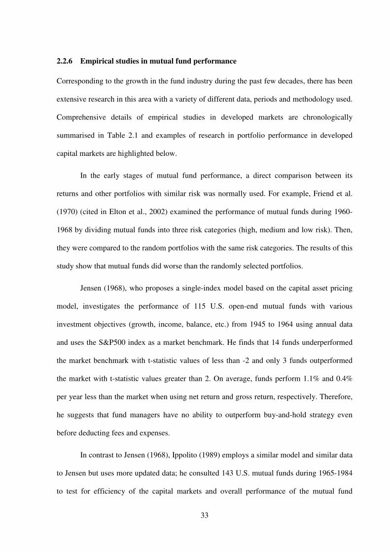
33
2.2.6 Empirical studies in mutual fund performance
Corresponding to the growth in the fund industry during the past few decades, there has been
extensive research in this area with a variety of different data, periods and methodology used.
Comprehensive details of empirical studies in developed markets are chronologically
summarised in Table 2.1 and examples of research in portfolio performance in developed
capital markets are highlighted below.
In the early stages of mutual fund performance, a direct comparison between its
returns and other portfolios with similar risk was normally used. For example, Friend et al.
(1970) (cited in Elton et al., 2002) examined the performance of mutual funds during 1960-
1968 by dividing mutual funds into three risk categories (high, medium and low risk). Then,
they were compared to the random portfolios with the same risk categories. The results of this
study show that mutual funds did worse than the randomly selected portfolios.
Jensen (1968), who proposes a single-index model based on the capital asset pricing
model, investigates the performance of 115 U.S. open-end mutual funds with various
investment objectives (growth, income, balance, etc.) from 1945 to 1964 using annual data
and uses the S&P500 index as a market benchmark. He finds that 14 funds underperformed
the market benchmark with t-statistic values of less than -2 and only 3 funds outperformed
the market with t-statistic values greater than 2. On average, funds perform 1.1% and 0.4%
per year less than the market when using net return and gross return, respectively. Therefore,
he suggests that fund managers have no ability to outperform buy-and-hold strategy even
before deducting fees and expenses.
In contrast to Jensen (1968), Ippolito (1989) employs a similar model and similar data
to Jensen but uses more updated data; he consulted 143 U.S. mutual funds during 1965-1984
to test for efficiency of the capital markets and overall performance of the mutual fund

34
performance to see whether active funds yield enough return to compensate for the higher fee
charged. His results show that 12 funds significantly outperformed and only 4 funds
significantly underperformed the market. He concludes that, on the net of fees and expenses
apart from the load fees basis, mutual funds, overall, have outperformed passive funds and
are large enough to compensate for the load charges, a result which is consistent with the
concept of costly information in an efficient market (Grossman and Stiglitz, 1980).
Grinblatt and Titmann (1989) studied funds during 1975 to 1984 using both actual
returns and gross returns. They employ Jensen’s single-index measure with four sets of
benchmarks. They find significantly superior performance among growth funds when gross
returns data are employed but evidence of this vanishes when using actual returns. Hence,
they conclude that growth funds outperformed the market but the evidence disappeared
because of its high expenses.
Cumby and Glen (1990) investigate 15 U.S.-based international funds during the
period 1982-1988. They employ Jensen’s measure and the Positive Period Weighting
proposed by Grinblatt and Titmann (1989) and find positive alphas in only 3 funds though
even these are not statistically significant. They also look into market timing ability as a part
of their mutual fund performance study. Using Treynor and Mazuy’s timing model, they find
evidence of negative market timing ability. Similarly, Malkiel (1995) examines fund
performance in the U.S market during the period 1972-1991 using Jensen’s single-factor
model. He finds the average alpha equals to -0.6% with very low t-statistic value. He reveals
that, on average, mutual funds have underperformed benchmark both before and after fees
and expenses have been deducted.
Gruber (1996) analyses common equity fund performance from 1985 to 1994 using a
relative return to the market, Jensen’s measure and multifactor model. The multifactor model

35
includes four variables, namely market return premium, difference in return between small
and large cap stocks, difference in return between growth and value and bond return
premium. Using 270 mutual funds, he finds that mutual funds underperform the market by
1.56% and 0.65% per year using respectively a single factor model and a multifactor model.
Similar to the studies above, in the U.K., Blake and Timmermann (1998) investigate a
large dataset of unit trusts for the period 1972-1995 using the three-index method, which
includes T-bills and bond and dividend yield. They find an average inferior performance of
1.8% per annum. Quigley and Sinquefield (2000) also reveal similar evidence in the UK
funds for the period 1978-1997.
Some studies examine performance in more detail by decomposing performance into
selectivity and timing ability. Studies related to the market timing ability include Treynor and
Mazuy (1966)’s study of the market timing ability of 57 U.S. mutual funds between 1953 and
1962 using a quadratic regression approach. They find that only 1 out of 57 funds exhibited
significant market timing.
Kon (1983) suggests that a fund manager has timing ability if he adjusts risk level
ahead of the market movements. Hence, he tests the timing ability by investigating the
stationarity of the fund’s systematic risk. He employs 37 funds from 1960 to 1976 and
concludes that some funds have significant timing ability but this is not the case at overall
level.
In contrast, Bollen and Busse (2001) argue that active fund managers adjust their
portfolio at high frequency. Hence, they employ mutual fund daily data from 1984 to 1995.
They find that, using daily data, 40% of funds have positive market timing ability.
Matallin-Saez (2006) examines the performance of mutual funds in Spain and tests
the effect of omitting a relevant benchmark. He uses a range of performance methods,

36
including Jensen’s measure, several multi-index models and Treynor and Mazuy’s market
timing, and judges that the performance of Spanish mutual funds is inferior and has negative
market timing but that these results are not statistically significant. He also confirms that the
effect of omitting the benchmark is that it leads to more perverse market timing.
While there was much evidence of inferiority in mutual fund performance from earlier
times, studies in mutual fund performance have become much more comprehensive in the last
decade. Recently, more completed data and sophisticated measures have been used. In 1996,
Ferson and Schadt argued that the all the single- and multifactor measures are biased, since
portfolio risk and returns are fixed through time (known as the unconditional measure). For
this reason, they propose in their model a conditional measure which allows time-varying.
They use both measures to investigate the performance of 67 mutual funds in the U.S. market
during the period 1968-1990. They employ 5 predetermined variables for their conditional
measure – including 1-month Treasury bills, dividend yield, slope of term structure, quality
of spread in the bond market and a dummy variable for the January effect – and incorporate it
with Jensen’s single factor measure. Their results show negative Jensen’s alphas in overall
fund performance. However, the alphas shift and become more positive when predetermined
variables are included. They also apply their conditional method to Treynor and Mazuy’s
(1966) and Henriksson and Merton’s (1981) market timing measures and use 3 self-
constructed buy-and-hold portfolios to test the market timing models, as well as data from 67
mutual funds. They conclude that the unconditional market timing models are misspecified,
since the results show negative market timing performance even if they are in the buy-and-
hold strategy portfolios. When the conditional market timing measures are replaced, the
negative timing coefficients are removed. Therefore, they confirm that using their conditional
model brings both statistical and economic significance and makes the performance of the
funds look better.

37
In a similar way, Sawicki and Ong (2000), apply both unconditional and conditional
Jensen’s measures, as well as Treynor and Mazuy’s market timing model to investigate
Australian funds between 1983 and 1995 They find weak evidence of positive performance
and negative market timing performance. In consistent to Ferson and Schadt (1996), they
confirm the statistical significance of incorporating lagged information variables in the
model, in particular with regard to dividend yield. They also confirm that the conditional
model shifts the alphas to the right and makes funds look better. Dahlquist (2000) explores
Swedish fund performance in broad fund classifications from 1993 to 1997, using a
conditional measure. He finds superior performance only for funds in the equity class.
Daniel et al. (1997) use their proposed characteristic-based performance measure to
examine more than 2500 US funds over the period 1975-1994. In contrast to the conventional
belief that fund managers are unable to outperform the market, they reveal that fund
managers have selectivity ability but no timing ability. However, the abnormal performance
is relatively small, 0.8% per annum, and close to its management fee. The evidence of
abnormal performance is stronger in growth-oriented funds.
Their results are also confirmed by Chen et al. (2000), who examine mutual funds
during 1975 to 1995. They conclude that fund managers have selectivity ability. They employ
stock held and trading data in mutual funds and reveal that fund managers did not hold
outperforming stocks but the stocks which they bought significantly outperformed the stock
which they sold by 2% per year. However, selectivity ability vanishes because fund managers
usually hold stocks for longer than a year.
In the similar vein, Wermers (2000) decomposes mutual fund performance during
1975 and 1994. He shows that fund managers have stock selectivity skill but style and high
expenses fade out any signs of abnormal return. On average, stocks held in the funds

38
outperform the market by 1.3% per year but their net fund return is 1% lower than the
market. The differences are attributed to the lower return for the non-stock holding
component, 0.7%, and the remaining 1.6% is split between expense ratio and transaction cost.
Kosowski et al. (2006) also find that, over the period 1975-2002, the average net
return alpha is around 0.5% below the market benchmark. Nonetheless, among these funds,
there are some fund managers who significantly outperform the market. Subsequently, they
examine whether the superior performance in some fund managers is due to skill or luck.
They employ a bootstrapping technique to analyse their data since they argue that the return
alphas of funds are non-normal. Their findings show that abnormal performance in fund
managers is not solely due to luck. The top 20% funds earn abnormal return because of
managers’ skills but this is not enough to cover expenses. In contrast, only the top 5% funds
really have positive abnormal performance which are large enough to compensate for their
expenses. This evidence is strong for growth-oriented funds.
Using similar measures to Kosowski et al., Cuthbertson et al. (2008) investigate
evidence of abnormal return using UK data. In contrast to the US findings, they find that the
superior performances of UK funds are due to luck rather than skill.
While most of the writings on performance are focused on equity portfolios, Comer
(2006) proposes an investigation into hybrid fund market timing performance. He uses a
multi-index model which is incorporated with quadratic variables for stock and bond returns.
He reveals little evidence of timing ability over the period 1981-1991 but during the period
1992-2000, he claims that funds exhibit statistically significant timing ability.
As a variety of performance measures have been proposed in the literature and
evidence of fund performance is still mixed, it is still not certain which of them provides a
valid performance measure and several studies have been conducted to answer this question.

39
For example, Grinblatt and Titman (1994) investigate the sensitivity of fund performance to
the choice of benchmarks and performance measures and also the relationship between fund
performance and fund attributes. They use 4 benchmarks and 3 measures to examine 109
passive portfolios which are formed on the basis of stock characteristics and also 279 mutual
funds between 1974 and 19844. They find that mutual fund performance is more sensitive to
the choice of benchmarks than measurement methods are. The CRSP value-weighted index is
the most inefficient benchmark because it admits size-related bias. The P8 index appears to
be the most reliable index in this study. In contrast, the choices of performance measure are
not sensitive to fund performance since few funds in this study exhibit positive market
timing.
Kothari and Warner (2001) also study the properties of performance measures for
mutual funds. They employ simulation procedures to simulate funds whose characteristics
mimic actual funds and test 5 different performance measures, both regression-based and
characteristic-based measures. They find that performance measures are unreliable and have
little ability to detect any large magnitude of abnormal performance, in particular funds
whose styles are different from the value-weighted benchmark market portfolio.
Fletcher and Forbes (2002) investigate the validity of different benchmarks used to
evaluate performance using the U.K. market. They use a similar approach to that of Grinblatt
and Titmann (1994), employing passive portfolios, formed on the basis of industry and stock
characteristics and 724 UK unit trusts, to test the specification of two performance measures
across five different benchmarks. They find that all five benchmarks have some bias.
Cahart’s (1997) four-factor model has the smallest degree of mispricing, although it does not
4The four benchmarks are the CRSP value-weighted, CRSP equally-weighted, 10-Factor (Lehman and Modest,
1988) and P8 (Grinblatt and Titmann, 1988) indices and the three performance measures are Jensen’s (1968), Treynor-Mazuy’s (1966) and Positive Period Weighting (1989)

40
fully capture the return on small stocks. Furthermore, it is found that using the conditional
model yields similar inferences to the unconditional model.
Otten and Bams (2004) use a different approach in order to explore which model is
best suited to measuring mutual fund performance. They employ a step-wise process to
examine the added value of additional variables, such as size, book-to-market, momentum,
bond index and a vector of information variables. They use a richer dataset than that used in
previous studies and analyse the data on both aggregate and style levels. They find that
conditional factor models are statistically superior to these unconditional models and that
Cahart’s four-factor model is the best model to explain mutual fund returns. They conclude
that conditional models add strong economic and statistical importance to the performance
measurement.
In a nutshell, this section reviews mutual fund performance measures as well as the
empirical evidence of mutual fund performance in developed markets over time. It may be
concluded that, in developed markets, mutual funds, as a whole, are unable to beat the market
although some studies suggest that growth-oriented funds perform better than others. The
inferiority in performance is not because fund managers have no ability, but is due mainly to
its high transaction costs and expenses. Subsequently, many researchers suggest that
investors should invest in passive index funds with low costs. Furthermore, some studies look
into performance from the viewpoint of the ability to forecast market direction. Most studies
find very little evidence of market timing, or even perverse market timing in mutual fund
performance. Evidence from a number of empirical studies exposes the fact that mutual fund
performance is sensitive not only to the measurement model but also to the benchmark and
data used.

41
2.3 Persistence in performance
Persistence in performance is another issue which has been widely discussed in the literature.
This is because we all want to know whether any sort of performance will be repeated in the
future. In other words, we want to know whether choosing funds based on an ex-ante
performance measure can earn abnormal returns in the future. Cuthberson et al. (2006) claim
that the concept of persistence is different from predictability, in the sense that persistence
implies that a winner (loser) will continue to be a winner (loser), meaning that there is only a
positive correlation, whereas the concept of predictability allows both positive and negative
correlation.
More importantly, the performance persistence issue is also evidence for rejecting
market efficiency. In an efficient market, prices change according only to new information,
which means that stock prices follow the random walk hypothesis. As a result, if a market is
efficient, performance persistence should not exist. However, Grossman and Stiglitz (1980)
aruge that the market should not fully reflect all information because if it did there would be
no reward for the costly search for new information.
There have been a number of studies so far on persistence in performance. However,
most of them investigate persistence in performance as part of the study of mutual fund
performance and, more importantly, the evidence in this topic is still mixed. We can classify
methods which are widely used in the persistence in the performance literature into four
broad groups. These are discussed below.
First, rank correlation: this approach is to split the fund performance into two time
periods and then use rank correlation to investigate the relationship between the performance
in the two periods. This approach is used in the early studies on persistence. For instance,

42
Sharpe (1966) estimates the Reward-to-Variability ratios for the periods 1944-1953 and
1954-1963. The rank correlation coefficient of the two periods is 0.36. He concludes that past
performance can predict future performance, though it is not the best predictor. Blake et al.
(1993) use this approach to investigate persistence in bond mutual funds by dividing their 10-
year sample into two 5-year periods and three 3-year periods. They find no evidence of
predictability using past performance. Nonetheless, the drawback of this approach is that it is
crude and unable to investigate performance persistence over a short horizon. Results
estimated using this approach could differ on the breakpoint for the two periods. Besides, this
approach does not provide any economic meaning in the results.
Second is the Winner-winner/Winner-loser method: this ranks funds based on pre-
and post- periods and then measures the association between the two periods (pre- and post-
period). Goetzmann and Ibbotson (1994) survey 728 funds over the period 1976-1988. They
measure performance using a variety of time periods and performance horizons and put each
fund into the category of either winner or loser, based on its median. They show that if a
manager outperforms in the first period, he/she is likely to outperform in a subsequent period,
which supports the concept of persistence in performance.
Brown and Goetzmann (1995) also employ this approach to analyse performance
persistence on a yearly basis from 1976 to 1988. They find that, over 12 year periods, 8 years
show evidence of persistence in performance. However, they show that this evidence is more
likely due to repeat-losers rather than repeat-winners.
Similarly, Malkiel (1995) tests persistence in performance over the period 1971-1979
by constructing a two-way table presenting a number of winners (losers) which carries over
to the year following. The author concludes that there is persistence in performance in most

43
years during the 1970s. Nonetheless, the author notes that this result might be influenced by
survivorship bias.
This approach mitigates some drawbacks from the first approach, as it can estimate
performance on the thinner periods and the bias due to breakpoint specification is removed.
However, some concern regarding economic meaning is still presented.
The third method is regression procedure: persistence in performance can be
estimated using a cross-sectional regression procedure which regresses current performance
on its lags. Hendricks et al. (1993) estimate the quarterly performance of mutual funds over
the period 1976-1988 and employ time-average cross-section regression to examine
persistence in performance. They find a positive persistence in performance for four quarters
and reversal thereafter. In contrast, Dahlquist et al. (2000) employ a year-fixed effect,
controlled for several factors, to estimate persistence in performance in Sweden. They find no
evidence of performance persistence.
Fourth, the trading strategy portfolio: this approach mitigates the drawback of the
above three approaches allowing for measures of both statistical and economic significance.
In order to construct a trading strategy portfolio, first of all, the ‘sorting rules’ must be
established. This includes specifying the sorting criteria and the number of factions. Once the
funds are placed in a group according to the trading rules, a portfolio of funds is formed on
the basis of either the equal weight or the value weighted method. Then the ‘holding period’
is specified. Portfolios are held up to the holding period and then rebalanced by repeating the
portfolio formation process. This procedure would provide a set of time-series portfolios
which can be used to test ‘forward-looking’ performance. However, a criticism of this
approach is the decision for the sorting criteria. This is because funds are heterogeneous in
that they contain great variation. Sorting them into narrower groups would help to reduce the

44
variation in fund characteristics but, at the same time it would also reduce the power of the
test. Therefore, to apply this approach, researchers need to trade off between the power of the
test and the heterogeneity of funds.
Hendricks et al. (1993) employ a trading strategy portfolio to examine the economic
significance of the hot hand phenomenon in mutual funds. They sort mutual funds into octile
portfolios based on previous net returns ranging from one to eight quarterly periods and
estimate the forward-looking performance of each portfolio using a single-factor model with
various benchmarks. They conclude that selecting funds based on the past four quarterly
returns outperforms the benchmark portfolio, suggesting short-term persistence in
performance. They also find that funds which perform well (poorly) will give superior
(inferior) performance in the near future, suggesting the “hot hands” (“icy hands”)
phenomenon. Nonetheless, the authors report that evidence of the “icy hands” phenomenon is
stronger than for the “hot hands”.
Elton et al. (1996) use a similar approach to investigate the performance of mutual
funds over the period 1977-1993, controlling for survivorship bias. Consistent with
Hendricks et al., they confirm that there is short-term persistence in mutual fund
performance. In addition, when risk-adjusted performance is used to rank funds, they find
persistence in performance in both short and long run periods.
Cahart (1997) argues that evidence of the “hot hands” phenomenon is a result of the
momentum strategy employed by the fund manager. He surveys equity funds over the period
1962-1993 which are free from survivorship bias and constructs portfolios based on previous
returns. Subsequently, he estimates performance using a single-factor model and his proposed
four-factor model, which includes an additional factor capturing momentum strategy in fund
managers. He shows that common factors in stock return, particular size and momentum, can

45
explain short-term persistence in performance. However, there is still some evidence of
persistence among worse performing funds which is still to be explained. Similarly, Daniel et
al. (1997) show that when the momentum effect is controlled, the persistence in fund
performance disappears.
In the U.K., Blake and Timmermann (1998) employ a large dataset over the period
1972-1995 and use a trading strategy portfolio approach to investigate persistence in
performance in the UK. They find some evidence of persistence in performance among the
best and worst performing funds.
Instead of the methods in the studies above, Bollen and Busse (2005) consider the daily
return data of 230 mutual funds between 1985 and 1995, controlling for survivorship bias, to
estimate persistence in mutual fund performance. The authors rank funds quarterly based on
past return, constructing decile portfolios to estimate performance using various models.
They find short-term persistence in performance even when the momentum factor is
included. Nonetheless, performance persistence is short-lived and disappears over time.
2.4 Flow related performance
In the competitive market, it is expected that informed investors will allocate their cash to
high performing funds and withdraw their cash from poorly performing funds. Therefore,
outperforming funds would expect to receive high cash flows in the subsequent period.
Nevertheless, if the fund experiences a great deal of cash flow, the cash position of the
portfolio will increase, which results in a lower return in the near future. Finally, the market
will reach equilibrium. Thus, according to this equilibrium process, the study of investment
flow related performance can be viewed from two separate standpoints: first, looking at the

46
relationship between performance and subsequent flows; and, second, looking at the
relationship between performance and the lagged flows. These two situations can be
examined using two common approaches; trading strategy portfolio or a cross-section
regression approach.
2.4.1 Future flows and performance
If investors are rational and well informed, they will assign their money to high performing
funds, but not if they are not. Therefore, one would expect to see a positive relationship
between past return and future cash flows. Capon et al. (1996) survey over 3000 investors in
the US using both questionnaires and telephone interviews. They reveal that financial
performance is the primary factor in investment decisions, although other non-performance
factors are also considered. Ippolito (1992) observes investor reaction to the signals of quality
in mutual funds. 143 mutual funds over the period 1965-1984 are analysed, using a pooled
cross-section regression model. He shows that investors move their money toward good
performers and away from poor performers. Investors, however, react disproportionately in
that they respond more strongly to well performing funds than to poorly performing funds.
Sirri and Tufano (1998) examine the relationship between performance and flows as
well as the implications of the costly search for mutual fund flows. They examine a large
dataset of mutual funds over the period 1971-1990. In the first part of their study, they
employ a cross-section time-series regression to examine relationships. They reveal
asymmetric purchasing decisions based on past performance information. Investors invest in
the funds which perform well in the past and flee from poorly performing funds. Moreover,
they find that investors prefer funds which are small, less risky and charge lower fees.

47
Furthermore, Del Guercio and Tkac (2002), Lynch and Musto (2003), Berk and Green
(2004), Elton et al. (2004), Bollen (2007), Huang et al. (2007) also find that flows move into
and out of funds in response to past performance. Most of these studies also confirm the
convex relationship between flows and past performance.
In contrast, Warther (1995) studies the relationship between fund flows and returns at
the macro level. The author divides fund flows into anticipated and unanticipated flows. The
study finds that no relation exists between flows and lagged returns. However, returns are
correlated with unexpected cash flows but unrelated to expected flows, which supports the
view that there is a positive relation between flows and subsequent returns.
Outside the US, Sawicki (2001) examines performance and flow in Australia. She
uses cross-section regression to estimate the relationship between flows and past performance
controlling for size-, style- and year-effect. Her findings are consistent with the US finding
that investors respond to past performance. However, results reveal that small and young
funds influence the asymmetry effect on the relationship between performance and flow.
2.4.2 Past flows and performance
Flows could have a negative relation to performance in the subsequent period because, when
large amounts of cash flow into the portfolio, fund managers are unable to adjust their
portfolio immediately and this subsequently results in a lowering of mutual fund returns.
Edelen (1999) investigates the relation of flows to mutual fund performance. In his study, he
argues that mutual funds managers are engaged with liquidity-motivated trading which
causes the lowering in performance of mutual funds and also of the market timing ability of
fund managers. He samples 166 funds from 1985 to 1990 in order to investigate this
hypothesis. He finds that funds statistically perform 1.6% lower than the market benchmark

48
per year. However, once the effect of liquidity-motivated trading is controlled, performance
become statistically insignificant, at -0.2% per year, and the evidence of perverse market
timing is removed.
Nonetheless, Benson and Faff (2006) analyse the relevance of flows in performance
evaluation, using Australian international equity funds during the 1990s and considering both
flows relative to fund size and flows relative to sector flows. They point out that only flows
relative to sector flows reduce the perverse negative timing in funds and these have no impact
on abnormal returns.
In contrast, many studies document the opposite finding; that is, the positive relation
between flows and the subsequent returns. Gruber (1996) explores the reason why there is
still growth in the mutual fund industry even though much evidence indicates that fund
managers do not add value. He investigates the returns on newly invested money in 227
mutual funds over the period 1985-1994. He shows that the average return on new cash flows
is higher than the average return of all funds. He suggests that this is the “smart money
effect”, referring to investors’ ability to select outperforming funds.
Zheng (1999) extends Gruber’s study by investigating a large mutual fund sample
between 1970 and 1993. He employs a benchmark-free performance measure, as proposed by
Grinblatt and Titmann (1993), as well as the trading strategies approach. The author reveals
that funds with new cash inflows perform better than funds with cash outflows in the
subsequent period. However, the smart money effect is a short-lived phenomenon and
investors cannot beat the market by investing in funds with high cash flows except in small
funds. In addition, he concludes that this effect is not due to style or macroeconomic
information but rather explained by fund specific information.

49
. Similarly, Sapp and Tiwari (2004) argue that the previous studies by Gruber and
Zheng take momentum anomaly into account. Thus, they investigate whether the smart model
effect can be explained by momentum strategy. They employ Cahart’s four-factor model to
control for the momentum phenomenon and examine funds for the period 1970-2000, using
trading strategies and cross-section regression methods. Using a model without controlling
for momentum, they find evidence of the smart money effect. However, the evidence
disappears when the stock return momentum is controlled. They also use cross section
regression to examine whether this is because an investor has the ability to identify
momentum funds or simply chases past returns. The authors indicate that investors are naïve
and are responding only to past returns.
Outside the U.S., Gharghori et al. (2007) examine whether the smart money effect
exists in the Australian market. They survey 239 equity funds over the period 1990-2004 to
construct trading strategy portfolios. Subsequently, they investigate the performance of these
trading strategies portfolios using Jensen’s single-factor, Fama and French’s three-factor and
Cahart’s four-factor measures and allowing for time variation in risk exposures. They reveal
that there is a smart money effect in Australia even when the momentum effect is controlled.
Moreover, using cross-section regression, their results indicate that investors select funds on
the basis of past performance rather than funds which use momentum strategy.
Keswani and Stolin (2008) investigate the smart money effect using UK data. They
employ a more comprehensive dataset than previous studies do. Their data cover the period
1991-1999 and contain exact cash inflow and outflow information for both individual and
institutional investors. They confirm that both individual and institutional investors are smart,
although this is revealed by the cash inflows rather than the cash outflows of the funds.

50
2.5 Style Analysis
Mutual fund style helps investors to select funds based on their risk preference. The
appropriate style enables an investor to effectively diversify. In the performance evaluation
aspect, mutual fund style also allows us to identify the appropriate benchmark. Moreover,
numerous studies find that the performance of funds varies across mutual fund styles.
Therefore, mutual fund style is important only in the selection process of mutual funds. In
general, mutual funds state their investment objectives in the prospectus, but only in a vague
manner. Studies reveal that some funds do not follow their style objectives and change their
style in order to make their performance look better. Nonetheless, in the major markets, there
are some investment service companies, such as Morningstar and Lipper, which provide style
classification information.
In classifying mutual fund style, there are two broad methods: the holdings-based
method and the returns-based method. The holding-based method classifies funds on the
basis of their holding characteristics. This method is widely used among practitioners. The
main drawback of this method is that it needs to indicate the boundaries in differentiating
characteristics which may not be clear. Furthermore, the results can be biased, due to
window-dressing (Cuthbertson et al., 2006). The most common use of this approach is to
investigate the characteristics of stocks contained in the fund. Morningstar, Inc. implements
this approach to construct their style box classification. In their style box, funds are classified
into 9 groups in the basis of size (large, medium, small) and style (value, blend, growth)
based on the investment-weighted scores of the stocks held in the funds.
Alternatively, a returns-based classification style can be used for style analysis. This
approach investigates the style of a mutual fund indirectly from its return. The advantage of

51
this method is that the model is parsimonious, and simple to use. The simplest way to
investigate this is to use the coefficients of factor loadings in the multifactor models, such as
the Fama and French three-factor model, to investigate mutual fund style.
The key study in style analysis using the return-based approach was conducted by
Sharpe (1992). The study advocates the ‘asset class factor model’, which divides the return of
a portfolio into style and selection components. Sharpe uses the returns of twelve broad asset
classes (constituting both stock and bond, both domestic and international markets) to form
an asset class factor model and applies them to particular US mutual funds. His asset class
factor model is defined by:
pnpnppp FFFR εβββ ~]~
...~~
[~
2211 ++++= (2.6)
Given: 1~
0 ≤≤ pnβ
and: ∑=
=n
p
pn
1
1~β
where pR~
is the return on asset p, nF~
is the return on asset class n, nβ is the sensitivity of pR~
to factor pR~
and pε~ is the non-factor component of the return on asset p.
Unlike ordinary regression, this regression follows a quadratic programming
algorithm which requires constraints to the regression, given that all coefficients are non-
negative and summed equal to one. It is possible to interpret coefficients as an asset class
weighting.
The sum of the terms in the bracket represents the return generated from the style
portfolio and the random error term ( pε~ ), which means that the returns which are not
explained by the portfolio benchmark represent the value-added return generated from the
portfolio manager’s selection.

52
Sharpe’s asset class factor model can be used not only in a portfolio’s style analysis
but also for performance evaluation (see Christopherson, 1997; diBartolomeo and Witkowski,
1997; Bogle, 1998; Buetow et al., 2000; Karatepe and Gokgoz, 2006). Nevertheless, Le
Sourd (2007) point out two major drawbacks of Sharpe’s asset class factor models. These are,
first, that using a quadratic programming algorithm could distort the results of standard
regression because some standard properties are unsatisfied and, second, that the abnormal
return generated from this model does not have a risk-adjusted basis.
2.6 Empirical studies on emerging markets
The term ‘emerging markets’ was first introduced by the World Bank in the 1980s and
defined as countries which are in the transition from developing to developed economies.
More recently, the study of emerging markets has become more controversial and a number
of studies reveal several differences between them and developed markets. Harvey (1995)
claims that emerging markets exhibit high volatility and low correlation with developed
markets. However, the standard asset pricing model fails to explain cross-section returns in
this market, since emerging markets are not integrated with the world economy and there is a
time variation in risk exposure. Bekaert and Harvey (2002, 2003) also argue that emerging
markets are inefficient. Emerging markets usually suffer from infrequent trading; high
transaction cost; and abnormal distribution of returns.
In addition, some researchers investigate the stock selection strategies in emerging
markets and reveal that stock returns in emerging markets are predictable owing to certain
fundamental characteristics. Claessens et al. (1995) investigate cross-section returns in 19
developing markets over the period 1986-1993 using several variables including, market

53
returns, earning-to-price, price-to-book value, size, dividend, turnover, and exchange rate.
They reveal that, in addition to market risk, firm size and turnover have explanatory power in
stock returns in many countries, although the signs are reversed in the evidence from the US.
Conversely, Fama and French (1998) argue that the results in Claessens et al. are due
to the sensitivity to outliers. They examine the value and growth premium in 16 emerging
markets for 1987-1995. They reveal that the evidence from developed markets is inconsistent
with the value and size premium in emerging markets. Nonetheless, they point to the
unreliability of their results, since the sample period is short and the returns are highly
volatile. Using a longer sample period, Rouwenhorst (1999) examines the return factors in 20
emerging markets over the period 1982-1997. In comparison to Fama and French, he
concludes that return factors in emerging markets are similar to those in the US and in
developed markets in that they exhibit momentum and small and value premium. Similarly,
van der Hart et al. (2003) survey 32 emerging markets. They argue that stock returns can be
explained by value, momentum and earning revisions but not for size, liquidity and mean
reversion. Nonetheless, Griffin et al. (2003), examining momentum strategy in 39 markets,
show evidence of momentum strategy among Asian markets.
In addition, some studies investigate the return factors in some specific emerging
markets. For instance, Drew and Veeraraghanvan (2002) find a size and value premium in
Malaysia; and Brown et al. (2008) reveal a momentum and a value premium in Hong Kong
and Singapore, respectively.
In the mutual fund literature, in contrast to the extensive evidence from developed
markets, studies in emerging market are scarce. Details of the empirical evidence in emerging
markets are chronologically presented in Table 2.2 and its main details are described below.

54
For his PhD thesis Elsiefy (2001) investigates the risk and return characteristics of 7
equity funds in Egyptian markets over the period 1996-1999. He employs several
performance measures, including the CAPM-based models; market timing models; and
Fama’s decomposition of returns (Fama, 1972). He reveals that over the period of his study
Egyptian funds do not outperform the market. However, the number of underperforming
funds is different for different measures used in the evaluation. Funds do not diversify and
therefore he suggests that using total risk is more appropriate in the Egyptian context. In
addition, he shows that performance does not change with the market conditions.
Roy and Deb (2003) take 89 Indian mutual funds over 4 years, 1999-2003 and
examine the importance of using a conditional performance model which allows time-varying
according to the economic conditions. They evaluate mutual fund performance and market
timing models, using both unconditional and conditional single-factor models. Their
conditional model includes 5 lagged information variables, namely, t-bill, dividend yield, the
term structure of interest rates, a dummy variable for the month of April and a dummy
variable for the tech rally. Inconsistently with the evidence from the US, their results suggest
that, as a whole, Indian mutual funds are unable to beat the market. The conditional version
makes funds look better and evidence of negative market timing is not present.
Soo-Wah (2007) explores 40 Malaysian funds over the period 1996-2000 using
single-factor and market timing models. He also tests for benchmark sensitivity by employing
two choices of benchmark: KLCI and the EMAS index. He finds inferior performance and
poor market timing in these Malaysian funds. However, the choice of benchmark does not
impact on performance evaluation, which contradicts the findings in developed markets (e.g.
Grinblatt and Titman, 1994 ). Similarly, Fauziah Md and Mansor (2007) study mutual fund
performance in Malaysia, using a longer sample period (1991-2001) than Soo-Wah used in
his study; they employ the measures of Sharpe, Jensen and Treynor. Unlike Soo-Wah, they

55
reveal that funds perform below the market and find no evidence of persistence in
performance.
Another study in Malaysia was conducted by Fikriyah et al. (2007). These writers
observe the difference in performance between conventional and Islamic funds over the
period 1992-2001. Their sample is 65 funds, including 14 Islamic funds. Like the studies
above, they employ standard measures, including the Sharpe, Jensen and Market timing
models. Subsequently, they reveal that Islamic funds are less risky than conventional funds
and perform better in bearish market conditions. Conversely, in bullish market conditions,
conventional funds seem to perform better.
In the Thai market, as far as is known, only a few studies in fund performance have
been published, some being in the form of scholars’ dissertations. Results from these studies
are, for example, those of Plabplatern (1997), who uses the portfolio holdings method to
investigate the performance of Thai mutual funds from 1993 to 1997. He uses the quarterly
data of 63 closed end funds. All funds have superior performance and half of them bear
evidence of market timing. In contrast, Sakranan (1998), who uses a similar approach and
time period, 1995-1997, to examine mutual fund performance, draws a different conclusion:
that only 2 out of 98 funds show selectivity skills. Pornchaiya (2000) uses Jensen’s single-
factor measure to explore 77 funds over the period 1996-1999. He reveals that only two funds
have superior performance, which is inconsistent with the two Thai studies listed above.
Vongniphon (2002) studies return and risk in 18 equity funds, using a longer and
more up-to-date sample, from 1994 to 2000. He employs Sharpe and Treynor measures and
also confirms the inferior performance of these funds. Likewise, Jenwikai (2005) uses Sharpe
and Treynor measures to compare the performance of 62 equity funds to his self-constructed

56
buy-and-hold portfolios. He reveals that equity funds perform worse than portfolios with buy-
and-hold strategy.
The most recent and extensive research in mutual fund performance in Thailand is
Nitibhon’s (2004) dissertation. He considers 114 equity funds in Thailand from 2000 to 2004
and investigates performance using various methods including: Jensen’s alpha (1968),
Cahart’s 4-factor model (1996), Ferson and Schadt’s conditional model (1996) and Daniel’s
characteristic-based performance measures (1997). He reveals that Thai mutual funds
perform better than the market but not enough to generate statistically abnormal returns.
However, he reveals that using a conditional approach creates fairly similar results to those
obtained from using unconditional models, which is inconsistent with the conclusions of Roy
and Deb (2003), who examine funds in India,
Furthermore, there are some researchers who concentrate their studies solely on
market timing performance, for example Srisuchart (2001) and Chunhachinda and
Tangprasert (2004), who explore timing ability in the Thai mutual funds. Srisuchart explores
equity and bond funds in the 1990s and Chunhachinda and Tangprasert examine 65 equity
funds over 2001-2003. Both of these studies yield the same conclusion: that Thai equity fund
managers have market timing ability. These results are also comparable to those of
Khanthavit (2001), who employs an alternative technique in examining market timing ability
in Thai closed end funds in the 1990s. He uses a Markov-switching technique and reveals that
fund managers exhibit both selectivity and market timing abilities, although overall
performance is not significant. However, these find managers tend to use their market timing
ability when the market is up and their selectivity ability when the market is down.
Nonetheless, issues outside mutual fund performance evaluation have received less
attention. Fauziah Md and Mansor (2007) look at the issue of persistence in performance in

57
the Malaysian context as part of their study of mutual fund performance. They estimate
performance annually over the period 1991-2001 and examine the correlation between past
and current performance. They do not find persistence in performance for mutual funds in
Malaysia. However, this contrasts with the evidence in Thailand. Watcharanaka (2003)
reveals persistence in performance in Thai mutual funds over the period 1992-2002, using a
cross-section regression approach in examining 62 funds. Nitibhon (2004) also examines
persistence in performance for the Thai mutual funds. In his study, he constructs decile
portfolios on the basis of past year returns and estimates performance using unconditional
and conditional single-factor models. He reveals that only the top decile portfolios (high past
returns) show significant positive performance.
Some studies explore mutual fund style in relation to performance. These include:
Ferruz and Ortiz (2005), who investigate whether Indian mutual funds correspond to their
classification. They employ factor analysis and cluster analysis and conclude that funds are
very close to one another. Similarly, Acharya and Sidana (2007) employ cluster analysis to
mutual funds in India over the period 2002-2006 and reveal the inconsistency between
investment style and the returns obtained by mutual funds. In Malaysia, Lau (2007) applies
Sharpe factor analysis to 43 funds over the period 1996-2000. He reveals that funds which
contain large and high liquidity stocks perform better than others.
Regarding the factors related to fund performance in Thailand, Prasomsak (2001)
investigates 77 mutual funds over the period 1998-2000, using fixed-effect regression of fund
raw returns on market returns size, turnover and fund style. He claims that fund returns are
positively correlated with market returns but negatively related to fund size and turnover.
This finding is in contrast to the findings of Nitibhon (2004), who employs cross-section
analysis and regress fund performance on size, value and growth factors. He reveals that fund
returns are positively related to size and growth stocks.

58
In addition, the evidence from Taiwan suggests that large funds perform better than
small funds (Shu et al., 2002). Tng Cheong (2007) explores the effect of fund size and
expenses on mutual fund performance in Singapore over the period 1999-2004. He reveals
that large funds perform insignificantly better than small funds and there is no difference in
fund returns between high and low expenses funds.
A study in the flows of mutual funds was conducted by Shu et al. (2002). They
investigate the investment flows of mutual funds in Taiwan over the period 1996-1990 and
reveal the difference of behaviour between small- and large-amount investors. Both small-
and large-amount investors tend to buy funds on the basis of short-term performance.
However, large-amount investors are more rational and redeem funds on the basis of
performance. In Thailand, Nitibhon (2004) estimates mutual fund flows of decile portfolios
rank on the basis of the past year’s returns. He claims that flows are not induced by the prior
year return and suggests no evidence of a smart money effect in Thai mutual funds.
Reviewing the evidence from the emerging markets makes it clear that: first, mutual
fund literature in this region concentrates mainly on performance evaluation. With various
techniques and different samples, most of these studies claim no abnormal returns in mutual
fund performance. Nevertheless, because these studies tend to use a small number of funds
and survey a short sample period, their results are still questionable. This is also because, as
mentioned above, emerging markets are highly volatile and there is a certain amount of
evidence of structural breaks.
Second, the evidence suggests that emerging markets are inefficient and display
several characteristics which distinguish them from to developed markets. In addition, there
are other factors outside the market risk which have explanatory in stock returns, for
example, size, value and momentum premium. Nevertheless, mutual fund studies in emerging

59
markets mostly employ standard CAPM-based measures, such as the Sharpe ratio and
Jensen’s alpha and none of these studies take these effects into consideration.
Third, we know very little about other issues related to mutual fund performance.
Evidence on persistence and flows, as well as other factors related to performance, is
relatively small and still mixed.
2.7 Conclusions and suggestions for further research
To summarise, this chapter surveys several issues related to mutual fund performance which
have been discussed in the literature. Topics connected with fund performance have been
greatly extended in the past few decades. Many researchers have advocated a variety of
performance measures as well as performance-related issues, in order to gain insightful
information about fund performance. However, the results are still mixed. This is partly
because of the differences in settings and study periods.
Most of the studies in mutual funds are central to investigating whether fund
managers are able to give value added to investors. With regard to the measure used, one can
conclude that fund managers do not offer abnormal returns, due to their fees and expenses.
Nonetheless, more recent studies have altered their research to identify and predict
outperforming funds by looking at their characteristics. The evidence suggests that funds in
one particular style can perform better than those in others. Similarly, a number of
characteristics, such as past returns, fees and expenses, and fund flows show evidence that
style has the power to explain fund performance.

60
Unlike the markets in developed countries, the emerging markets have attracted little
research in this area. While mutual fund performance in developed markets has been
comprehensively investigated by means of varied and sophisticated measures, studies in
emerging markets are still scarce and questionable. This is because the unique characteristics
of emerging markets are ignored. These studies unhesitatingly employ techniques derived
from the developed markets to estimate the performance in emerging markets. Further,
studies in the emerging markets rely mainly on the principal approaches, which retain some
limitations. To give an example, these measures are based on only one risk factor and the risk
factor given is fixed through the evaluation period, which incurs some critiques of being
negatively biased as regards portfolio performance, notably when a manager employs
dynamic strategy. In addition, mutual fund studies in emerging markets usually survey short
periods and cover only a small number of funds. More importantly, these studies primarily
pay attention to performance itself, without looking at other aspects of fund performance, for
example, style analysis, persistence, fund flows and the other determinants of performance.
Consequently, all the above problems prevent us from fully understanding the mutual fund
business in emerging markets and hence many puzzles still remained unsolved.
Thus, on the basis of the foregoing survey in the theory and evidence relating to
mutual fund performance, the present study puts forward three main promising research
ideas. First, there is a need to apply richer models in the literature to countries in the
emerging market which have different characteristics from developed markets, and to
examine whether the models and findings in developed market are comparable. Second, the
liquidity effect is one of the major concerns in emerging markets which needs further
investigation, while performance models for mutual funds in emerging markets also need to
be developed. Third, factors related to performance need to be investigated further.

61
Table 2.1 Summary of main theories and empirical studies related in mutual fund performance in developed markets
Author(s) Objectives Data & Sample Methodology Conclusion
Sharpe (1966) Extend Treynor’s work and propose the Reward-to-Variability ratio (R/V).
34 US mutual funds 1954-1963
Treynor and R/V (Sharpe) ratios to examine performance. Rank correlation between two periods (1944-53 and 1954-63) for persistence in performance.
This study proposes a new performance measure and shows that the theoretical measure can apply to the practice. The difference in performance is due solely to differences in investment objectives which support the view of market efficient. Past performance partly explains future performance.
Treynor and Mazuy (1966)
Propose a model for measuring market timing ability (TM) and empirically investigate whether fund manager have the ability to anticipate major turns in the stock market
57 US mutual funds (Growth and Balanced funds) 1953-1962
TM market timing model No statistically evidence that funds managers have successfully outguessed the market.
Jensen (1968) Propose single-index measure (Jensen) to evaluate performance
115 US mutual funds 1945-1964
Jensen measure Funds, on average, are unable to outperform the market benchmark even before deducting fee and expenses. At fund level, only 3 funds statistically outperformed the market.
Ippolito (1989) Test for market efficiency and evaluate the overall efficiency the mutual fund industry
143 US mutual funds 1965-1984
Jensen measure to evaluate performance and pool cross-section time-series regression to
Using net of fee returns data, mutual funds returns are comparable to index funds referring to the presence of costly information. Portfolio

62
Author(s) Objectives Data & Sample Methodology Conclusion
investigate impact of turnover, expenses and fees on performance.
turnover and management fee are unrelated to fund performance.
Grinblatt and Titman (1989)
Compare returns of active and passive funds using quarterly holdings data.
US mutual funds 1975 – 1985 Use two types of returns: actual returns (net of transaction costs) and gross returns (with transaction costs). The gross returns are constructed using quarterly data of portfolio holdings
The study estimate performance using Jensen measures with 4 sets of benchmark portfolios: (1) CRSP equal weighted (2) CRSP value weighted (3) F10 (Lehman and Modest, 1988) (4) P8 portfolios based on size, yield and past returns (Grinblatt and Titman, 1988)
Mutual funds display significant positive abnormal return when using gross returns, especially in aggressive-growth, growth and small funds. However, the superior performance is diminished when actual returns are used. Transaction costs are negatively related to fund size. Using gross return, performance is negatively to fund size. Survivorship bias in mutual fund performance is small (>0.5% pa)
Cumby and Glen (1990)
Evaluate performance of international funds
15 US international funds 1982-1988
Jensen and Positive Period Weighting
No abnormal returns. Only 3 funds have positive performance.
Sharpe (1992) Propose a technique to determine mutual fund styles and performance
395 US funds 1985-1989
Use 12 asset classes and employ quadratic programming regression, which constrains the coefficients summed to 1 and each coefficient is lie between 0 and 1
Asset class factor model can help investment process by providing a view of investment decision and fund manager strategy.

63
Author(s) Objectives Data & Sample Methodology Conclusion
Ippolito (1992) Evaluate consumer reactions to signals of quality in the market for investment management
143 US mutual funds 1965-1984
Pooled regression and fixed effect of growth on past performance residuals
Investors react disproportionately. They move money in the industry toward good performers and away from poor performers
Fama and French (1993)
Examine factors to predict return of stock and bonds. (Fama-French 3-factor model: FF)
Stock returns in NYSE, AMEX, NASDAQ 1963-1991
Construct 25 mimicking portfolios based on size and book-to-market (B/M). Regress bond and stock factors of the mimicking portfolios
At least 3 stock market factors (market risk, size, B/M) and 2 bond market factors (maturity and default risk) can explain stock returns. Stocks have shared variation due to stock market factors and linked to bond returns through share variation on bond factor.
Grinblatt and Titman (1993)
Propose new performance measure and apply to study of mutual fund performance
155 US mutual funds 1975 – 1985
Introduce a new performance measure. The measure does not require benchmark but use portfolio holding information instead. The author then compare results of this measure to Jensen with 4 sets of benchmark: 1. CRSP equal weighted 2. CRSP value weighted 3. F10 (Lehman&Modest,1988) 4. P8 (Grinblatt&Titman,1988)
Results from this measure are similar to Jensen measure with P8 benchmark portfolio. In general, mutual funds have positive performance, especially in aggressive growth funds. There is also some evidence of persistency, particular among positive abnormal returns funds.

64
Author(s) Objectives Data & Sample Methodology Conclusion
Grinblatt and Titman (1994)
Sensitivity of performance techniques to benchmark choices and the determinants of mutual fund performance
279 US mutual funds 1974-1984 And 109 self- constructed passive portfolios based industries and characteristics
3 performance measures; Jensen, PPW, TM with 4 set of benchmarks: 1. CRSP equal weighted 2. CRSP value weighted 3. F10 (Lehman&Modest,1988) 4. P8 (Grinblatt&Titman,1988) Cross-section regression is used to examine determinants of mutual fund performance.
Mutual fund performance is more sensitive to benchmarks than choice of measures. Inefficient benchmark leads to unbiased performance estimation. Among 4 benchmarks, CRSP value weight is the highest inefficient whereas P8 is the most reliable. The 3 measures display high cross-sectional correlation. This is due to funds have no timing ability and all 3 measure yield similar conclusion for fund performance. Using P8 benchmark, performance of mutual fund is undistinguished from zero. Very few funds have positive timing ability. Fund performance is positively related to portfolio turnover but not to size or to expenses.
Malkiel (1995) Investigate performance, survivorship bias and performance persistence
239 mutual funds 1971-1991
Employ Jensen measure with 2 benchmarks for mutual fund performance. For persistence in performance, the author divide sample into two sub-periods as well as employ simulation of strategies.
Mutual funds insignificantly underperform the benchmark portfolio for both before and after expenses are included. Performance is negatively related to expense ratio. Performance persistence is existed during 1970s. Impact of the survivorship bias is more important than previous studies.

65
Author(s) Objectives Data & Sample Methodology Conclusion
Fletcher (1995) Evaluate selectivity and market timing performance
65 UK unit trusts 1980 – 1989
TM and HM market timing measures with four sets of benchmark portfolio.
UK trusts exhibit positive selectivity performance and negative timing performance across all benchmarks. Performance is sensitive to the choice of benchmarks.
Ferson and Schadt (1996)
Propose a conditional model which incorporate information variables
67 US mutual funds 1968-1990
Incorporate five lagged time varying information variables into Jensen, Four-Factor, TM and HM market timing.
The conditional model shifts funds to the right and become neutral. Time varying information variables are statistically and economically significant. There is an evidence of persistence in performance on the extreme performing mutual funds.
Ferson and Warther (1996)
Evaluate performance using the conditional performance
63 US mutual funds 1968-1990
Conditional version of Jensen and TM market timing models. The time varying variables are dividend yield and T-bills.
Using unconditional version, 60% of funds have negative performance and 60% of funds have negative market timing.The buy-and-hold portfolio also has statistically significant negative market timing which implying to the model misspecification. Using conditional model, alphas are centered near zero and the interaction variables are significant. The misspecification in market timing is also disappeared.
Elton et al. (1996)
Examines mutual fund predictability
188 US mutual funds 1977-1993
Use four-index model to evaluate performance and construct decile portfolios of funds formed based on
Past performance can predict future risk-adjusted performance for both short- and long-run. Poor performance funds are due to the

66
Author(s) Objectives Data & Sample Methodology Conclusion
1- and 3-year past performance.
high expenses. Successful funds increase their revenue by increasing their size, not expenses.
Capon et al. (1996)
Investigate fund characteristics which are perceived as relevant for mutual fund investors’ investment decision
3,000 US investors in 1991
Survey method: telephone interview 3,000 investors in the U.S. The survey focuses on 3 set of variables: information sources, selection criteria and purchase. Then, cluster analysis is used to analyse set of groups based on the use of information sources and selection criteria and examine mutual fund behaviour across the groups.
Most mutual funds investors are naïve and uninformed about their mutual fund investment. Although financial performance is the main factor for investment decision, investors also consider non-performance related variables (multi-attribute). Very small group of investors are defined as a knowledgeable investor.
Ciccotello (1996)
Relationship of size and mutual fund performance
US Equity funds 1982-1992
Rank funds into quintile on the basis of size and examine 5- and 10-year returns
Historical returns of large funds are superior to small funds. Only evidence from aggressive growth funds that size can explain fund return. Performance is decline with fund size.
Carhart (1997) Explain persistence of mutual fund by stock common factors and investment costs
US Equity funds 1962-1993
Trading strategies: form 10 deciles portfolios based on past year reported returns and
Short-term persistence in equity mutual funds is explained by stock returns common factors (the use of momentum strategy) and investment

67
Author(s) Objectives Data & Sample Methodology Conclusion
evaluate performance using Jensen measure and his proposed 4-factor model (Cahart) which include momentum factor in addition to the FF model.
costs. Therefore, no skilled of informed fund managers in the fund market.
Kothari and Warner (1997)
Empirical properties of performance measure
Construct 50 Random portfolios each month from 1964-1991
Use several measures including: Sharpe, Jensen, Treynor, Appraisal ratio FF and market timing models, and Track performance over 3-year periods.
Benchmark can lead to model misspecification. FF model is better than Jensen model
Lawrence et al. (1997)
Assess asset selection and timing abilities of portfolio managers
130 Canadian funds 1981-1988
Conditional APT model with time-varying risk premia and observable macroeconomic factors
Performance is negative and time varying beta increase values of the performance. Many funds exhibit dynamic behaviour
Cai et al. (1997)
Comprehensive study of Japanese mutual funds
1,151 Japanese funds 1978 - 1992
Employ Jensen, PPW and FF using both unconditional and conditional measures. Analyse at funds and portfolio levels.
Funds underperform the benchmarks by 3.6%-10.8% and fund managers tend to invest more in large and low B/M ratio stocks. FF benchmark is the most appropriate measure although the conclusion is robust to the methodologies and benchmarks used. The underperforming may be explained by the tax dilution effected caused by inflows of funds.

68
Author(s) Objectives Data & Sample Methodology Conclusion
Daniel et al. (1997)
Develop and apply a new measure of mutual fund performance (DGTW: Characteristic-based benchmark)
UK funds 1975-1994
Develop the characteristic-based benchmark to measure fund performance (DGTW measure). The measure constructs 125 benchmarks based on size, b/m and past return; and matches them with portfolio holding of funds. The DGTW measure decomposes funds returns into 3 componemts: characteristic style (CS), characteristic timing (CT) and average style (AS)
The measure gives more insight details in performance and it is useful for funds which change their styles through time. They apply the measure to the US funds over the period 1975-1994 and reveal that aggressive and growth funds have selectivity ability but not characteristic timing ability.
Detzel and Robert (1998)
Examine whether style boxes of the Morningstar classification as useful in determining a mutual fund’s size and style equity class
All US equity mutual funds classified by Morningstar 1993-2004
Estimate funds using 4-factor model, rank and sort funds into 9 portfolios. Then estimate a prediction model by regress return of funds on dummy variables of future equity classes.
Both Morningstar style and size/style class do not predict mutual fund future returns. Growth funds are more stable than value and blend funds. Large-cap funds are more stable than mid and small cap funds. Fund managers are more likely to change their style and fund classification drift considerably. As a result, active fund investors need to monitor their portfolio regularly.

69
Author(s) Objectives Data & Sample Methodology Conclusion
Blake and Timmermann (1998)
Performance of UK unit trust manager and investigate evidence of the survivorship bias
2300 UK funds (survived and dead) 1972-1995
Multi-index model which include 3 variables: T-bills, bond, and dividend yield, both unconditional and conditional versions
UK unit trusts underperform the market by 1.8% pa. Results on unconditional are very similar to conditional model. Mutual fund performance varies across different asset categories. There is also evidence of persistence in performance and survivourship bias. Unit trusts outperform during their first year of existence and underperform when it closes to its termination date.
Sirri and Tufano (1998)
Examine performance and flows relationship and the implication of costly search for mutual fund flows
690 US mutual funds 1971-1990
Cross-section time-series regression, flows are regressed on past return, risk, and expenses, controlled for size and sectoral flows. Quintile portfolios are constructed to examine the different relationship across different performance level. Costly search is measured by size of family, marketing expenditure, and media coverage are included in the model to investigate implication of search cost
Consumers are asymmetrically based their purchase decision on prior performance information. They invest in funds that perform well in the prior period and flee from poor performing funds on the different rate. Consumers prefer funds with lower fees, less risk and small funds. Flows are also related to sectoral flows. They predict that, according to search cost, consumers would purchase funds that are easier or less costly for them to identify. They use 3 measure of cost to check this hypothesis and find that funds in

70
Author(s) Objectives Data & Sample Methodology Conclusion
for fund flows larger family grow more quickly but they are unable to observe that these funds have stronger performance-flow relationship. Funds that charge higher fee grow more slowly and there is a strong positive relationship of fee and performance (marketing effects performance) and, finally, they can’t detect relationship of media and flows, as well as the spill-over effect.
Zheng (1999) Investigate investors’ ability in forecasting mutual fund performance (Smart money)
1,826 US mutual funds 1970-1993
PPW and Trading strategies methods; The trading strategy is conducted by forming portfolios according to money flows and measure performance using raw return, excess return, Jensen, and FF measures for both unconditional and conditional versions.
The study confirms smart money effect but only for short-term period and this effect reverses after 30 months. In small funds sample, funds with positive net cash flows outperform the market in the subsequently period.
Edelen (1999) Relation between fund’s risk-adjusted return and volume of liquidity-motivated trading (flows)
166 US mutual funds 1985-1990
Cross-section regression of abnormal returns as a function of cash in/out flows
Inferior performing and negative market timing are due to the cost of liquidity-motivated trading. Mutual funds underperform 1.6% per year (statistically significant) but after controlling for the effects of flow-

71
Author(s) Objectives Data & Sample Methodology Conclusion
related liquidity trading, average alpha reduces insignificantly to -0.2%
Dahlquist et al. (2000)
Study the relation between fund performance and fund attributes in Swedish market
Swedish mutual funds: 80 general equity funds 46 public savings equity funds 42 bond funds 42 money market funds 1993-1997
Jensen measure (unconditional and conditional versions) and Cross section analysis of alphas and fund attributes (size, fees, turnover, commission, flows, lagged performance)
Conditional model suggests that performance of regular equity is insignificantly positive. Equity funds with public savings, money and bond funds perform less well. Larger equity funds and high fee funds perform less well. Larger bond funds perform better. Active funds perform better than passive equity funds. There is a positive relation between lagged performance and current flows. There is an evidence of persistence in performance in money market funds.
Wermers (2000)
Examine whether fund managers have ability to select outperforming stocks that justify trading costs and expenses
US funds 1975-1994
DGTW and decompose fund returns and costs into several components using data in portfolio holding, fund’s expenses and turnover ratio
Funds hold stocks that outperform the market by 1.3% pa (0.7% of this figure is due to fund managers’ skill) but they underperform the market by 1% pa on the net return basis. The differences are attributed to the non-stock holdings 0.7% and cost/expenses 1.6%.

72
Author(s) Objectives Data & Sample Methodology Conclusion
Sawicki and Ong (2000)
Examine performance of managed funds in Australia using conditional model
97 Australian balanced and equity funds 1983-1995
Use Jensen and TM measures, and incorporate with lagged information variable. Compare different of performance and persistence across fund type.
At all fund level, both models show insignificantly positive performance and evidence of the negative market timing. There are more superior funds than inferior funds. Conditional model shifts alphas to the right and makes funds look better. Dividend yield exhibits a statistically significant variable. Little evidence of persistence in performance.
Kothari and Warner (2001)
Study ability to detect abnormal performance of performance measures
50 Random selected equity mutual funds in 1996 and form simulated portfolios whose characteristics mimic actual funds.
Simulation procedure: The simulated funds contain 75 stocks each month from January 1966-December 1994, total 348 simulated funds. Portfolios are reformed annually. Use 5 models: Jensen, FF, Cahart and 2 characteristic-based measures, and examine distributional properties of performance measures
Mutual fund performance measures are reliable and have little ability to detect economically large magnitude, especially for a fund whose style characteristics differ from value-weighted market portfolio.
Sawicki (2001) Examine investor response to past performance in the Australian wholesale funds market
55 Australian Balanced wholesale funds 1980-1995
Reclassify funds into three categories based on equity exposure and OLS regression estimation is used for regress flow on
There is a statistically positive significant relationship between flow and recent performance but no evidence of the convexity. Small and young funds potentially drive

73
Author(s) Objectives Data & Sample Methodology Conclusion
lagged performance, controlled for size, growth and time-series correlation. Then, piecewise linear regression is used to measure the sensitivity of growth to performance in different regions.
the asymmetric effect.
Brown et al. (2001)
Explore reason of underperforming of mutual funds in Japan
1,275 Japanese equity funds 1978-1995
Generalized Style Classification (GSC) (Brown and Goetzman, 1997) for style classification and use style analysis (Sharpe, 1992) with a tax variable to control to control tax dilution effect.
The underperformance of Japanese mutual funds is because of the dilution effect. When tax dilution effect is controlled, alpha of Japanese mutual funds are indistinguishable from zero.
Chan et al. (2002)
Analyse product offered by mutual funds by looking at its characteristics and the information given
3,336 US mutual funds 1976-1997
Two style identification measures; characteristic-based and holding-based
Size and book-to-Market provide useful descriptors for fund style. Fund styles tend to cluster around a broad index although they are consistence in following their style. There is an evidence of style shifted among poor past performance. The approach based on portfolio characteristics does a better job in predicting future fund performance.

74
Author(s) Objectives Data & Sample Methodology Conclusion
Sawicki and Finn (2002)
Investigate size- and age-effects to the fund performance
55 Australian wholesale funds 1980-1995
Reclassify funds into 3 groups based on objectives and asset allocation. Then they estimate a model using piecewise regression, allowing slope and intercept are varied for size and age. Nine difference performance measures are used for a lagged performance variable
The test confirms for the size- and age-effects where investors response to small young funds than large old funds. The results also show that small funds react disproportionately to high performance.
Fletcher and Forbes (2002)
Explore validity of different benchmark specifications
724 UK equity unit trusts 1982-1996
Form 2 groups of passive portfolios which are 10 industry portfolios and 27 securities portfolios formed based on size, book-to-market, and momentum. Then, estimate performance using various models: Excess return, APT Four-factor, FF and Cahart with both unconditional and conditional measures.
All five benchmark specifications have some degree of mispricing but the Cahart model does a reasonable job in explaining cross-sectional return although it still unable to capture returns in small stocks completely. UK unit trusts do not outperform passive strategy. 80% of unit trusts show negative performance and many trusts are negatively and statistically significant. Results also show evidence of significant time variation in performance. The results on beta exposures

75
Author(s) Objectives Data & Sample Methodology Conclusion
suggest that unit trusts have significant and positive market beta coefficient. SMB and HML factors are also positive and significant but momentum factor in Cahart model is close to zero which differs to the US results.
Otten and Schweitzer (2002)
Compare behaviour of European and the US mutual fund market
Aggregate data on 2,096 US and 506 European funds from 6 countries 1991-2007
Sharpe Style analysis and Structure-conduct-performance paradigm
European mutual fund industry is still lagged behind the US in term of size and the market importance. Banks are the main distribution channel in the continental European countries while broker and direct sales are the main distribution channels in the US. Furthermore, US mutual funds performance is poorer than European mutual funds.
Del Guercio and Tkac (2002)
Comparing flow and performance relation between mutual funds and pension funds
562 pension funds and 483 mutual funds during 1987-94
Pooled time-series cross-section regression of fund flows and lagged performance. The study measures flows using dollar flows, percentage flows and change in number of clients; measures performance using both raw and risk adjusted methods.
Pension fund flows are positively related to risk-adjusted performance and negatively related to tracking error. Mutual fund flows are related to unadjusted-risk performance and unrelated to tracking error. Quantitative performance is less important in pension funds. Flow-performance relationship in pension funds is linear which different to the convexity relationship in mutual funds.

76
Author(s) Objectives Data & Sample Methodology Conclusion
Brown et al. (2003)
Analyse their relative performance of Japanese and foreign funds
3,072 Japanese equity funds 1998-2002
Generalized Style Classification and Sharpe’s asset allocation
Both Japanese and foreign funds are similar in style. Funds insignificantly underperform the benchmarks. Before the de-regulation, Japanese funds yielded superior performance but then become inferior after that due to the huge inflows and style shifts.
Drew and Stanford (2003)
Performance of Australian superannuation funds
148 Australian superannuation funds 1991-1999
Four-index model (Gruber, 1996)
Australian funds underperform the market by 0.5% to 0.93% pa. Results support the importance of four-factor model although it fails to capture impact of investment style.
Abel and Fletcher (2004)
Examine performance of UK emerging market unit trust and impact of the choice of model
56 UK unit trust with emerging market objective 1993 – 2003
13 models of the stochastic discount factor (including both local and emerging market indexes)
No evidence of superior performance and the choice of model does not impact on performance
Otten and Bams (2004)
Examine statistical and economic importance of adding more factor to the Jensen’s model
2436 US mutual funds 1962-2000
Jensen, FF, Cahart models with unconditional and conditional in alpha and betas. Use step-wise process to examine importance of the model.
Conditional models add statistic and economic relevances to performance measurement. The Cahart model is the best in explaining mutual fund returns. At the aggregated level, alphas do not change much between unconditional and conditional models. At style level, moving to the richer models have large impacts on the alphas in income funds.

77
Author(s) Objectives Data & Sample Methodology Conclusion
In overall, US mutual funds generate insignificant negative performance. Size and B/M factors have explanatory power for all style portfolios. Momentum factor has explanatory power for only three style portfolios. The growth/income portfolio is not statistically exposed to the momentum factor. Conditional model improves performance of funds and makes funds, in overall, look better except income/growth and income portfolios which conditional model decrease performance.
Klapper et al. (2004)
Structure, growth, and determinants of mutual funds growth in different countries
Aggregate mutual funds Aggregate data from 40 countries 1992-1998
Panel OLS regression and analyse developed and developing countries separately
Equity funds dominate in Anglo-American countries and bond funds dominate in continental Europe and mid-income countries. Capital market development and its stability are the main determinant of mutual fund growth. However, market microstructure factors are more concerned in developed countries while macroeconomic factors are more concerned in developing countries.

78
Author(s) Objectives Data & Sample Methodology Conclusion
Chen et al. (2004)
Examine relationship of size and fund performance
3439 US funds 1962-1999
Estimate performance using 1-, 3-, and 4-factor and use cross-section time-series regression
Performance is inversely correlated with fund size suggesting that liquidity plays important role in diseconomies of scale. However, performance increases with family size.
Sapp and Tiwari (2004)
Examine whether smart money effect is a result of momentum effect and if this is the case, are investors chase funds with momentum style or just simply chase funds with high past returns?
US funds 1970-2000 (cash flows is based on quarterly data)
Trading strategy: performance of portfolios constructed based on net cash flows. Performance is estimated using Cahart’s four factor model. Then, Cross-sectional regression to explore the determinants of cash flows of funds and portfolios based on momentum loadings are used to investigate the second question.
Smart money effect is explained by momentum phenomenon. Investors do not have ability to identify momentum style of mutual funds, they are naively chase funds with high past returns.
Khorana et al. (2005)
Study a combination of fundamental economic and regulatory forces that help to explain where the fund industry has flourished
Aggregated data from 56 countries 1996-2001
Cross-sectional, regress fund size on variables related to law, supply, demand and market characteristics
Fund industry is larger in countries with stronger rules, law and regulation and where investors’ right are better protected, and the countries which wealthier and have more educated populations, old industry, low trading cost, pension plan. Law regulation, supply, and demand affect the size of industry.
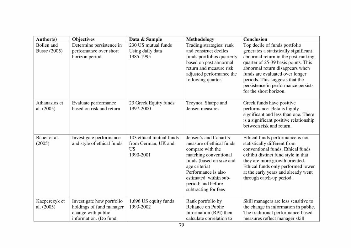
79
Author(s) Objectives Data & Sample Methodology Conclusion
Bollen and Busse (2005)
Determine persistence in performance over short horizon period
230 US mutual funds Using daily data 1985-1995
Trading strategies: rank and construct deciles funds portfolios quarterly based on past abnormal return and measure risk adjusted performance the following quarter.
Top decile of funds portfolio generates a statistically significant abnormal return in the post-ranking quarter of 25-39 basis points. This abnormal return disappears when funds are evaluated over longer periods. This suggests that the persistence in performance persists for the short horizon.
Athanasios et al. (2005)
Evaluate performance based on risk and return
23 Greek Equity funds 1997-2000
Treynor, Sharpe and Jensen measures
Greek funds have positive performance. Beta is highly significant and less than one. There is a significant positive relationship between risk and return.
Bauer et al. (2005)
Investigate performance and style of ethical funds
103 ethical mutual funds from German, UK and US 1990-2001
Jensen’s and Cahart’s measure of ethical funds compare with the matching conventional funds (based on size and age criteria) Performance is also estimated within sub-period; and before subtracting for fees
Ethical funds performance is not statistically different from conventional funds. Ethical funds exhibit distinct fund style in that they are more growth oriented. Ethical funds only performed lower at the early years and already went through catch-up period.
Kacperczyk et al. (2005)
Investigate how portfolio holdings of fund manager change with public information. (Do fund
1,696 US equity funds 1993-2002
Rank portfolio by Reliance on Public Information (RPI) then calculate correlation to
Skill managers are less sensitive to the change in information in public. The traditional performance-based measures reflect manager skill

80
Author(s) Objectives Data & Sample Methodology Conclusion
managers use public information or their own skills?)
investigate relationship of RPN and size, expenses, and age. Regress RPI in performance and flows with control variables
Benson and Faff (2006)
Examine impact of fund family characteristics on fund flows
1,418 Australian funds 1995-2006
Unbalanced panel time series data and pooled regression Regress fund flows on fund characteristics and fund family characteristics. Dummy variable for top performing fund is also incorporated to test whether top performing funds enjoy greater flows.
Investors favour fund families which are old, large, and implement specialisation strategies. Top performing funds within a family receive significantly greater flows. These imply that funds do not operate as a single entity but as a member of complex organisation.
Luis Ferruz et al. (2006)
Evaluate performance of Spanish mutual funds
225 Spanish equity funds 1994 – 2002
Conditional Jensen measure which incorporate 7 predetermined variables: dividend yields, T-bills, bond yield, variable that represent inverse relative wealth, term structure, quality spread, and dummy variable of January effect
Funds display negative alphas but performance improves when using conditional measure. The conditional measure also improves explanatory power of the model

81
Author(s) Objectives Data & Sample Methodology Conclusion
Bergstresser et al. (2006)
What benefits do broker-channel mutual fund consumers enjoy in exchange for these loads and 12b-1 fees?
1998-2002 Compare characteristics of brokers funds and direct funds using T-test and multiple regression
Brokers focus on smaller, younger funds that are not converted by major rating services. However, Broker channel funds fail to provide tangible advantages and consumers pay extra fee to buy funds with higher fee and expenses funds. Broker fund underperform direct funds
Bauer et al. (2006)
Examine performance, persistence, and effect on fees on performance
143 New Zealand mutual funds including domestic and international equity funds and balanced funds 1990-2003
Jensen, 4-factor, TM and conditional models with 3 information variables (90 day T-bill, dividend yield, Term structure). For persistence in performance, rank and construct portfolios based on previous return. For fund characteristics, use cross-section regression to regress fund characteristics (size, fee, age, load) with performance.
Mutual funds insignificantly underperform the market and no evidence of market timing ability. Performance is still not statistic significant when using 4-factor model. Momentum is a driver in international funds but reverse to the domestic funds. There is more exposure to small cap and growth oriented funds. When predetermined variables are included, performance of balance funds is negatively significant. There is evidence of short term persistence in performance but this is driven by underperforming funds (icy hand). Equity fund performance is positively related to size and expense ratios and negatively related to load funds.

82
Author(s) Objectives Data & Sample Methodology Conclusion
Comer (2006) Propose multifactor market timing for hybrid funds and examine whether it is superior than TM measure
56 Balanced and Flexible funds 1981-2000
The proposed timing measure follows multifactor by Lehman and Modest which include 4 stocks, 4 bond indices and 2 additional variables which are quadratic returns of stock and bonds. Then, estimate and compare results to TM measure
TM measure is biased because there is correlation between bond and quadratic term. Multifactor market timing shows a superiority power than TM market timing and not spurious. With Multifactor market timing, there is a small evidence of market timing during 1981-1991. During 1992-2000, hybrid funds have an evidence of significant market timing and balanced funds is a driver of timing ability.
Benson and Faff (2006)
Investigate importance of flows to the measuring fund performance of international funds
93 Australian international equity funds 1989-1999
Use the conditional TM model plus a variable in exchange rate, lagged net flow of funds and lagged sector flow. Evaluate mutual funds at both aggregate and fund levels.
Australian international funds are unable to outperform the market and have negative market timing. The results show the significance of incorporating fund flows. The flow variables improve fund performance and increase R-square of the estimation.
Matallin-Saez (2006)
Performance and seasonality of Spanish mutual
220 Spanish mutual funds 1998-2004
Multi-index model plus a quadratic term variable capturing timing and a dummy variable for seasonality.
Performance of Spanish mutual funds is not significant from zero. There is evidence of seasonality but no evidence of market timing. The omission of style benchmarks leads to greater evidence of negative market timing and positive seasonality.

83
Author(s) Objectives Data & Sample Methodology Conclusion
Kosowski et al. (2006)
Examine mutual fund performance that explicitly control for luck
US mutual funds 1975-2002
Use various performance models and use information criteria to choose the most appropriate model which is appeared to be 4-factor model. Conditional and unconditional versions give very similar result. Therefore, results will focus on unconditional four-factor model. Then Bootstrap analysis is employed to look at the extreme value.
Performance of best/worst managers is not solely due to luck. There is a superior performance among growth oriented funds and no evidence of ability among managers of income-oriented funds.
James and Karceski (2006)
Performance differences between retail and institutional funds and performance differences of the degree of investor oversight
US funds 1991-2001
Performance is estimated using 5-factor model (Cahart + international equity factor) Cross-section regression: Regress performance on fund characteristics; and flows on performance
Large institutional funds outperform other funds and they are less sensitive to the past returns. Institutional funds with low degree of oversight perform worse than other funds both before and adjusting for expenses.
Steven (2007)
Apply theory performance model to the practitioners approach
US mutual funds 1927-2005
FF Only few funds outperform the market benchmark.

84
Author(s) Objectives Data & Sample Methodology Conclusion
Heaney et al. (2007)
Investigate time-changing in alpha performance
74 Australian equity international funds 1995-2005
Investigate both fund and industry level using equal weight and value weight to calculate portfolio of funds. For performance, use International CAPM (ICAPM) with a quadratic term for market timing variables and 4 information variables, and allow both alpha and beta to change over time with information variables. 24- and 36- month rolling windows are used for investigate variation in alphas.
International equity funds have negative and significant performance in traditional model. When information variables are incorporated, performance is insignificant different from zero. There is an evidence of time variation in alphas, means that, over the study period, the alphas is not constant.
Gharghori et al. (2007)
Examine whether smart money effect exists in Australia and to examine whether momentum explain this effect. And to find determinants of cash flows
239 Australian equity funds 1990-2004
Trading strategies portfolios are constructed on the basis of cash flows. Then, Jensen, FF, Cahart, both unconditional and conditional versions are estimated. Subgroup of funds is classified by size are also constructed to control for size effect. Then, cross-section time-series average is used for
Evidence of smart money and it is slightly stronger in small funds. Momentum effect does not explain smart money in Australia. Past returns and past cash flow of funds can explain cash flows of funds.

85
Author(s) Objectives Data & Sample Methodology Conclusion
examine determinants of cash flows.
Bollenn (2007) Explore investor decision making in Social Responsible (SR) funds
205 SR funds 1980-2002
Control the differences in portfolio composition by using matching procedure to match SR funds to conventional funds with risk exposure criteria. Then compare SR funds with matched conventional funds. OLS regression estimating is used to estimate flow-performance relation, using net flows as a dependent variable and past dummy variables of performance as independent variables.
SR funds have lower monthly volatility and investors in SR fund are more sensitive to positive returns and less sensitive to negative returns than convention funds. This implies that preference of SR investors can be presented by conditional multi-attribute utility function
Geoffrey and Travis (2007)
Examine investor timing ability of their cash using cash flow data
7,125 US mutual funds 1991-2004
Investor timing performance (performance gap) is calculated by the differences between geometric returns and dollar weighted returns. Positive results mean investors have negative
Investor timing decisions reduce investor average returns by 1.56% annually. The poor timing is significantly associated with better performing funds. The underperforming is negatively correlated with value-style funds but positively correlated with momentum-style funds. Load fees, turnover and age are positively

86
Author(s) Objectives Data & Sample Methodology Conclusion
timing performance. Cross section regression is used to examine determinant of performance gap.
correlated with underperforming funds.
Hubner (2007) Examine performance of performance measures
72 US mutual funds 1993-2004
Compare Information ratio and the alpha with his Generalized Treynor Ratio (GTR). FF and Cahart’s are used to calculate the performance
GTR measure provides superior results. Using FF and Cahart model to generate the alphas increases in the adjusted R-squares compared to the simple market model.
Keswani and Stolin (2008)
Investigate smart money effect in the UK using cash inflows and outflows data and differentiate between individual and institutional investors
UK funds 1992-2000 (cash flows is based on monthly data)
Estimate performance of money flow-based portfolios using Cahart’s four factors model
There is smart money effect in the UK and this is not driven by momentum phenomenon. The effect is attributed by buying decision in both individual and institutional investor. They re-investigate smart money effect in the US for the period post-1991 and reveal comparable results.

87
Table 2.2 Summary of main theories and empirical studies related in mutual fund performance in emerging markets
Author Objectives Data Methodology Results
Plabplatern (1997)
Selectivity and market timing abilities
63 Thai Closed end funds 1993-1997
Portfolio holding Almost all funds have positive selectivity. 25 out of 63 have evidence of market timing
Sakranan (1998)
Performance of mutual funds
34 Thai equity funds 1995-1997
Portfolio holding approach
Only 2 funds have selectivity skills and all funds have market timing ability. No persistence in performance.
Pornchaiya (2000)
Performance 77 Thai closed and open end funds 1996-1999
Jensen measure Overall underperform: All closed end funds have negative alphas, and only 2 out of 55 open-end funds have positive performance.
Srisuchart (2001)
Market timing Thai close and open funds (Equity and Fixed income funds) 1990-2001
Jensen, TM, HM, Kon&Jen (switching regression), Kon
Equity funds have better market timing ability while fixed income funds are better in selectivity ability.
Prasomsak (2001)
Determinants of equity funds’ returns
33 Thai Equity open end funds and 11 Thai close end funds 1998-2000
Use market model for calculate return and employ cross-section regression with fixed effect
Market returns, size, turnover are related to funds’ returns but fund type and turnover are not. Returns are positively correlated with market’s returns and small funds are likely to have higher return.
Khanthavit (2001)
Performance 35 Thai Close end funds 1990-2000
Markov-Switching which is a technique to accommodate the switching strategies of the
In overall, fund managers do not have ability to beat the market but this is not because they do not have market timing or stock selection

88
Author Objectives Data Methodology Results
funds with respect to the state of the market
ability. That is because they choose to concentrate on a certain ability with respect to the market condition
Elsiefy (2001) Examine risk and return characteristics of mutual funds, optimal portfolios selection and the impact on economic factors on stock market and mutual funds
7 Egyptian equity funds 1996 - 1999
3 performance evaluation, measures; CAPM, market timing and decomposition of returns. The Arbitrage Pricing Theory (APT) model is employed to investigate the relationship between economic factors and performance. The economic factors used are: inflation, exchange rate, interest rate, government borrowing gross domestic product.
Overall, funds underperformed the market regardless to any benchmark used. However, number of underperforming funds is not the same for three measures. Funds are not diversified and market conditions do not affect the fund performance. Results from APT model suggest that fundamental economic variables fail to explain returns in Egyptian market.
Shu et al. (2002)
Different in the behaviour of investors who invest small amounts of money and those who invest large amount
Taiwanese mutual funds 1996-1999
Use Fama-Macbeth method to estimate relationship between mutual fund flows and past performance and set of control variables (e.g. Size, fee, turnover, and stand deviation). Fund flows are inflows, outflows and net flows.
Small amount investors mostly invest in large funds. They make a purchase based on short-term past performance and redeem funds to realise short term profits. On the other hand, large amount investors tend to buy small funds and insensitive to short-term performance but they tend to buy winners and sell losers.

89
Author Objectives Data Methodology Results
Vongniphon (2002)
Return and risk of open-equity funds
18 Thai equity funds 1994-1996 and 1997-2000
Sharpe and Treynor measures
During the study period, Thai equity funds underperform the market.
Roy and Deb (2003)
Effect of incorporating lagged information variables into the evaluation
89 Indian mutual funds 1999-2003
Jensen and TM, MH for both unconditional and conditional versions. Conditional model includes four predetermined variables, T-bills, dividend yield, term structure, dummy variable for April and dummy variable for tech rally.
Mutual funds outperform the market and using lagged information variables improve performance and the alpha performance shifts to the right
Watcharanaka (2003)
Determinants of the cash flows of funds, persistence and fee effects
62 Thai open equity funds 1999-2001
Cross-section regression of cash flows on several characteristics
NAV is positively related to fund flows. Size and interest rate are negatively related to fund flows. No evidence of persistence in performance.
Pakut et al. (2003)
Investigate the seasonal behaviour, specifically Month-of-the-Year Effect and Day-of-the-Week Effect
Thai stock market returns 1990-1999
Time series regression with dummy variable of each month
No evidence of Month-of-the-Year but Day-of-the-Week effect persists. Stock returns are positive and high on Friday while negative and low on Monday.
Friis and Smit (2004)
Relationship between performance of fund
30 South African companies within 57 unit
Use market excess return to estimate performance
Managers with qualifications perform better than those managers

90
Author Objectives Data Methodology Results
managers and their qualification.
trusts 1996-2002
and questionnaire method to collect fund manager qualification. The regress performance with fund manager qualification.
without qualification
Nitibhon (2004)
Performance of Thai Equity funds
114 Thai open-end funds 2000-2004
Jensen, Cahart for both unconditional and conditional versions, and Portfolio holding approach
Funds present no statistic significant abnormal return. No evidence in persistence in performance.
Chunhachinda and Tangprasert (2004)
Timing abilities of Thai mutual funds
65 Thai open end equity funds 2001-2003
TM, Volatility timing model (Busse, 1999)
mmmimi rrr σσγβα +−++= )(()( )
Use GARCH (1,1) to estimate because the degree of autocorrelation and heteroscedasticity
Using Weekly data 54% exhibit market timing ability 55% exhibit volatility timing ability Using Monthly data: 4% exhibit market timing ability 12% exhibit volatility timing ability
Jenwikai (2005)
Performance of an investment portfolio and compare performance of investment portfolio and a mutual fund
62 Thai Equity funds 1991-2004
Sharpe and Treynor measures
Investment portfolio has better returns than the mutual fund with regard to market conditions.
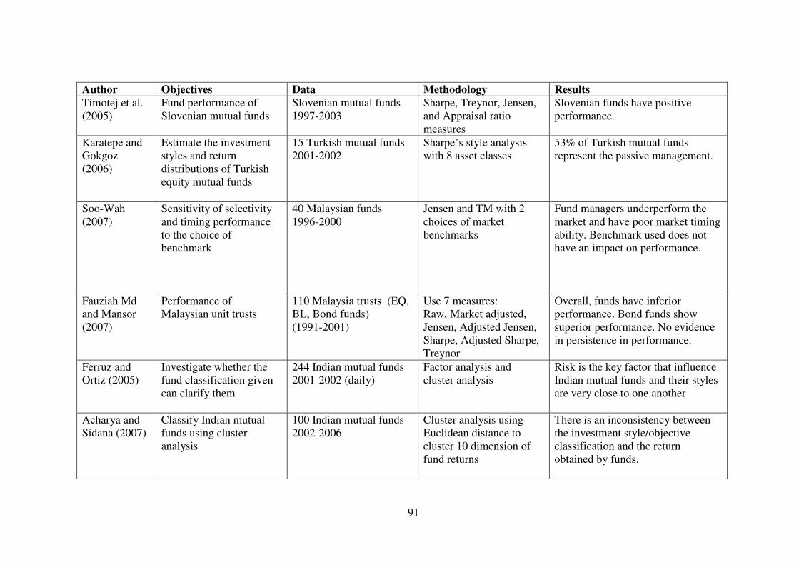
91
Author Objectives Data Methodology Results
Timotej et al. (2005)
Fund performance of Slovenian mutual funds
Slovenian mutual funds 1997-2003
Sharpe, Treynor, Jensen, and Appraisal ratio measures
Slovenian funds have positive performance.
Karatepe and Gokgoz (2006)
Estimate the investment styles and return distributions of Turkish equity mutual funds
15 Turkish mutual funds 2001-2002
Sharpe’s style analysis with 8 asset classes
53% of Turkish mutual funds represent the passive management.
Soo-Wah (2007)
Sensitivity of selectivity and timing performance to the choice of benchmark
40 Malaysian funds 1996-2000
Jensen and TM with 2 choices of market benchmarks
Fund managers underperform the market and have poor market timing ability. Benchmark used does not have an impact on performance.
Fauziah Md and Mansor (2007)
Performance of Malaysian unit trusts
110 Malaysia trusts (EQ, BL, Bond funds) (1991-2001)
Use 7 measures: Raw, Market adjusted, Jensen, Adjusted Jensen, Sharpe, Adjusted Sharpe, Treynor
Overall, funds have inferior performance. Bond funds show superior performance. No evidence in persistence in performance.
Ferruz and Ortiz (2005)
Investigate whether the fund classification given can clarify them
244 Indian mutual funds 2001-2002 (daily)
Factor analysis and cluster analysis
Risk is the key factor that influence Indian mutual funds and their styles are very close to one another
Acharya and Sidana (2007)
Classify Indian mutual funds using cluster analysis
100 Indian mutual funds 2002-2006
Cluster analysis using Euclidean distance to cluster 10 dimension of fund returns
There is an inconsistency between the investment style/objective classification and the return obtained by funds.

92
CHAPTER 3
INSTITUTIONAL BACKGROUNDS AND SAMPLE SELECTION
3
Abstract
This chapter reviews the institutional environment of mutual funds in Thailand and describes the
sample which will be used in subsequent chapters. The business of mutual funds has grown
dramatically in this country and gained in importance. Thai mutual funds include a special type
called tax-benefit funds, which give investors favourable tax treatment, conditional upon long-
term investment. The Thai mutual fund market is less competitive and controlled by a few bank-
owned management companies. Furthermore, information related to performance is not publicly
available and the banks are the main distribution channel, implying that investors value service
rather than performance. The latter part of this chapter sets out to justify the sample selection
which will be used in the rest of the thesis. In total we consider 230 Thai mutual funds,
comprising both equity and flexible funds over the period 2000-2007. The data are free from
survivorship bias.

93
3.1 Introduction
A mutual fund, or as the UK often refers to it, a unit trust, is an investment fund type of
collective investment scheme (CIS) – a term which includes all forms of retail investment fund,
regardless of their legal structure – by pooling money from investors to invest in a diversified
portfolio of stocks, bonds and/or other assets and hiring a professional fund manager to manage
the portfolio. The mutual fund form of investment is long established and provides several
benefits to investors, such as diversification, professional management, liquidity, flexibility and
convenience. Undoubtedly mutual fund investment has become significant all over the world and
its popularity and consequently the demand for it have steadily risen. According to the
Investment Company Institute (2008), by the end of 2007, assets of mutual fund investment
worldwide totalled more than 26 trillion US dollars, with more than 66,350 funds. These
amounts rose by more than 78% of the total in 2003 (Figure 3.1). Despite the growth of the
mutual fund industry worldwide, the size and institutional arrangement of mutual fund
investment are different in each country, which may influence the characteristics of fund
managers and investors, as well as the performance of the mutual funds. Klapper et al. (2004)
investigate the determinant of mutual fund development in both developed and emerging
countries. They point out that mutual fund investors in developed countries are concerned with
market microstructure, while those in emerging countries are focused more on macroeconomic
factors. Furthermore, they find that mutual funds are more developed in countries with more
stable capital markets. Similarly, Khorana et al. (2005) examine mutual fund investment in 56
countries and reveal that the mutual fund industry is larger in countries which have stronger laws
and regulations, and where populations are wealthier and better educated.

94
Figure 3.1 Worldwide mutual fund assets and the growth in the number of mutual funds,
2003-2007
Source: Investment Company Institute (2008)
In emerging markets, mutual funds have gained more recognition in the past decade
alone. After the Asian financial crisis, investors sought more secure forms of investment and
mutual funds investment is believed to be among these. Likewise, governments in many
emerging countries promote retail investment funds in order to boost investment in the capital
market as well as to encourage long-term savings. Subsequently, mutual fund investment in
emerging countries has grown significantly during the past decade. In the Asia Pacific region,
mutual fund assets in emerging markets, such as those of the Philippines, India and Thailand,
experienced higher growth than those of developed countries, such as Japan and New Zealand
(Figure 3.4).
Notwithstanding the growth in the mutual fund industry, the mutual fund business in each
country is unique in some respects, in emerging markets in particular, where mutual funds serve
26
22
1816
14
66,350
61,855
56,868
54,98254,569
40,000
45,000
50,000
55,000
60,000
65,000
70,000
2003 2004 2005 2006 2007
0
5
10
15
20
25
30
AUM No. of funds
No. of funds USD trillion
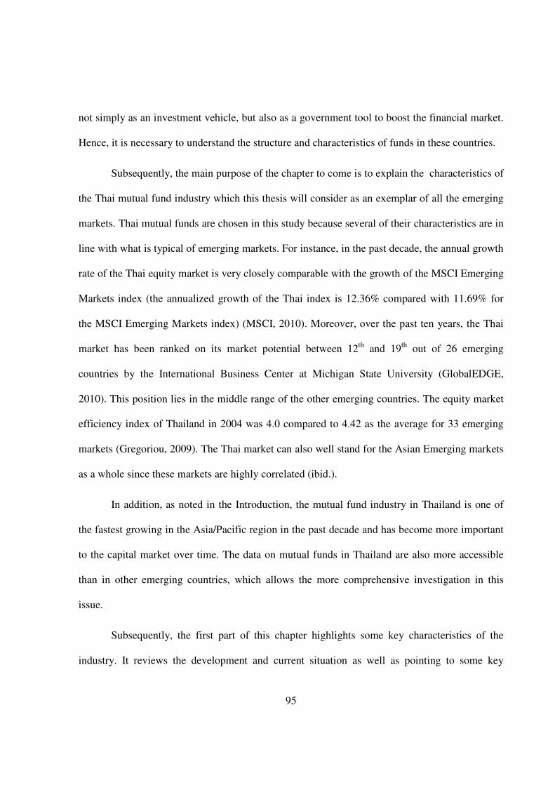
95
not simply as an investment vehicle, but also as a government tool to boost the financial market.
Hence, it is necessary to understand the structure and characteristics of funds in these countries.
Subsequently, the main purpose of the chapter to come is to explain the characteristics of
the Thai mutual fund industry which this thesis will consider as an exemplar of all the emerging
markets. Thai mutual funds are chosen in this study because several of their characteristics are in
line with what is typical of emerging markets. For instance, in the past decade, the annual growth
rate of the Thai equity market is very closely comparable with the growth of the MSCI Emerging
Markets index (the annualized growth of the Thai index is 12.36% compared with 11.69% for
the MSCI Emerging Markets index) (MSCI, 2010). Moreover, over the past ten years, the Thai
market has been ranked on its market potential between 12th and 19th out of 26 emerging
countries by the International Business Center at Michigan State University (GlobalEDGE,
2010). This position lies in the middle range of the other emerging countries. The equity market
efficiency index of Thailand in 2004 was 4.0 compared to 4.42 as the average for 33 emerging
markets (Gregoriou, 2009). The Thai market can also well stand for the Asian Emerging markets
as a whole since these markets are highly correlated (ibid.).
In addition, as noted in the Introduction, the mutual fund industry in Thailand is one of
the fastest growing in the Asia/Pacific region in the past decade and has become more important
to the capital market over time. The data on mutual funds in Thailand are also more accessible
than in other emerging countries, which allows the more comprehensive investigation in this
issue.
Subsequently, the first part of this chapter highlights some key characteristics of the
industry. It reviews the development and current situation as well as pointing to some key

96
motivating aspects related to the study. Then, in the latter part, this chapter seeks to justify the
sample of mutual funds from which its conclusions are drawn.
The overview is meant to improve understanding of the mutual fund environment in
Thailand and allow readers to compare and contrast it with that of mutual fund investment in
other countries. Furthermore, it will help to set up testable hypotheses from the institutional point
of view. Therefore, it is hoped to benefit both academics who wish to conduct research related to
mutual funds in Thailand and practitioners who are dealing with these funds.
The rest of this chapter is organised as follows. The next section, 3.2, provides an
overview of the mutual fund business in Thailand. Section 3.3 gives some motivating aspects
related to the institutional environment. Section 3.4 describes the mutual fund sample which will
be used in this study. Section 3.5 draws some conclusions from the details presented.
3.2 An overview of the mutual fund business in Thailand
3.2.1 Mutual fund development
The mutual fund business in Thailand was formally initiated in 1975, when the government of
Thailand and the International Finance Corporation (IFC) collaborated to establish the first
management company in Thailand, named the Mutual Fund Public Co., Ltd. This was no more
than a management company in Thailand between 1975 and 1992. During this period, the
company operated 22 funds; 12 domestic and 10 international funds. In 1992, the Congress
approved the Securities and Exchange Act BE 2535 (AD 1992), which allows wholly-owned
subsidiaries of banks and other financial institutions to operate mutual fund business. This
allowed several new management companies to be set up. At the end of 2007, Thailand had 21

97
management companies, made up of 821 mutual funds, with total assets valued at more than
1,400 billion Baht (SEC, 2008).
Within the Asia Pacific region, the Thai mutual fund industry has in the past decade been
one of the fastest growing, even though the contribution of this industry to the economy still lags
behind the contribution made in other parts of the region. Klapper et al. (2004) in their study of
the growth of mutual funds around the world reveal that Thai mutual fund assets grew by more
than 35% between 1993 and 1998. This brings Thailand to third place in the Asia/Pacific
continent, after New Zealand and Hong Kong. This growth figure is also higher than in such
developed countries as the US (22.4%) and the UK (20.9%) during the same period. In contrast,
Klapper et al point out that the total assets of Thai mutual funds were only 1.04% of GDP, which
was the second lowest figure for the Asia/Pacific region and much lower than that of the US
(41.95%) and the UK (15.07%). Additionally, the Investment Companies Institute (ICI) Fact
Book (2008) provides more recent data of mutual fund development in some major countries.
Combining data from the Security Exchange Commission of Thailand and the ICI Fact Book
allows us to compare the growth and importance of the mutual fund business in Thailand to those
of other countries within the same region. Figures 3.2 and 3.3 exhibit mutual fund growth in the
Asia/Pacific region in terms of the number of funds and asset values, respectively, from 2000 to
2007. They show clearly that the Thai mutual fund business had the fastest growth. Over the
period, mutual funds in Thailand experienced the highest growth in term of fund quantity (Figure
3.2) and the second highest growth, after the Philippines, in term of asset growth (Figure 3.3).

98
Figure 3.2 Growth of number of funds for Asia/Pacific countries, 2000-2007
0
0.5
1
1.5
2
2.5
3
3.5
4
2000 2001 2002 2003 2004 2005 2006 2007
% G
row
th (in
hundre
ds)
Hong Kong India Japan South KoreaNew Zealand Philippines Taiwan Thailand
Source: ICI Fact Book (2008) and SEC (2008)
Figure 3.3 Growth of mutual fund asset values for Asia/Pacific countries, 2000-2007
0
5
10
15
20
25
2000 2001 2002 2003 2004 2005 2006 2007
% G
row
th (in
hundre
ds)
Hong Kong India Japan South Korea
New Zealand Philippines Taiwan Thailand
Source: ICI Fact Book (2008) and SEC (2008)

99
More recent data on Thai mutual fund development are provided by the Security
Exchange Commission of Thailand (2008). Figure 3.4 illustrates the remarkable growth of
mutual fund investment in Thailand between 2000 and 2007. Mutual fund total assets rose by
more than ten-fold in those seven years, from 130 billion Baht in 2000 to more than 1,400 billion
Baht by the end of 2007. In spite of the growth in asset values, the number of funds also
increased from 225 funds in 2000 to 821 funds by the end of 2007, nearly four times the original
total in seven years. Similarly, Figure 3.5 reveals the proportion of investment in asset
management to GDP, which rose from 7.9% in 2000 to 24.1% in 2007, while the proportion of
bank savings to GDP dropped slightly, from 71.7% in 2000 to 50.8% in 2007.
Nonetheless, the high growth of mutual fund business in Thailand began in earnest only
in 2003-2004, after the tax-benefit mutual fund types were introduced. The tax-benefit mutual
fund will be further described in section 3.2.2.1, below. Nevertheless, this evidence attests to the
strong increase in demand and importance over a fairly short period in relation to other countries
in the same region.

100
Figure 3.4 Growth in Thai mutual funds 2000-2007
130 142198
1,041
775
485440
1,426
821
716
584
416
319
224225
279
0
200
400
600
800
1,000
1,200
1,400
1,600
2000 2001 2002 2003 2004 2005 2006 2007
TN
As (in
Billion B
aht)
0
100
200
300
400
500
600
700
800
900
Num
ber
of fu
nds
TNAs Number of funds
Source: Security Exchange Commission of Thailand (2008)
Figure 3.5 Savings to GDP classified by investment type in Thailand, 2000-2007
71.769.5 69.2
65.861.5
57.6 56.3
50.8
4.0 4.6 5.1 5.8 6.4 6.8 6.6 7.6
7.9 8.6 9.814.3 14.2
17.820.0
24.1
0
10
20
30
40
50
60
70
80
2000 2001 2002 2003 2004 2005 2006 2007 Year
% t
o G
DP
Bank Deposit Life insurance Asset management
Source: Security Exchange Commission of Thailand (2008)

101
3.2.2 Mutual fund classification
In Thailand, mutual funds can be broadly classified into closed-ended funds and open-ended
funds. The former kind offers a fixed number of shares, which cannot be redeemed until the
maturity date. Therefore, closed-ended funds are traded in the exchange market in order to
provide investors with liquidity. Closed-ended funds can be sold at either a discount or a
premium, which is determined by the supply and demand in the market.
In contrast, the latter kind, open-ended funds, offers unlimited numbers of shares which
can be sold or redeemed at any time through the fund’s management company or selling agents.
Open-ended funds are bought and sold at their own price, called the Net Asset Value (NAV),
which is determined by the total value of the fund’s assets at current market value minus current
liabilities and divided by the number of shares.
The 1990s saw a number of closed-end funds in the Thai market. However, their value
dropped substantially over the financial crisis. A decade later, open-ended funds began to gain
more recognition, owing to a government campaign emphasizing its advantages benefits over
closed-ended funds, in that they provide more flexibility and liquidity. Consequently, the number
of open-ended funds has increased sharply and some closed-ended funds have been converted to
open-ended funds. Below, Figure 3.6 shows the growth of open-ended compared to closed-ended
funds. It reveals that, over the past decade, the growth of open-ended funds is much greater
higher than closed-ended funds. Currently, more than 90% of the mutual funds in Thailand fall
into the open-ended category, accounting for more than 80% of all mutual funds’ assets (SEC,
2008).

102
Figure 3.6 Number of funds and total asset values (TNAs) classified by type (closed-ended
vs. open-ended)
0
200
400
600
800
1,000
1,200
1,400
TN
As (
in b
illi
on
Bah
t)
0
100
200
300
400
500
600
700
800
Nu
mb
er
of
fun
ds
TNAs (Closed) 12,053 10,027 8,931 142,066 151,997 197,544 218,436 249,169
TNAs (Open) 117,465 131,956 188,758 298,139 332,982 577,848 822,261 1,177,232
Number (Closed) 35 18 17 17 28 62 65 70
Number (Open) 191 206 262 302 388 522 651 751
2000 2001 2002 2003 2004 2005 2006 2007
Source: Security Exchange Commission of Thailand (2008)
In most developed countries, mutual funds managers provide information relating to their
investment policy and investment style5. This informs investor about their investment strategy
and helps investors to select funds based on their own preferences. In contrast, information on
investment style is not provided in Thailand.
The Association of Investment Management Companies (AIMC) – an organization
responsible for overseeing management companies in Thailand - largely classifies Thai mutual
5 Investment policy is classified by asset class, for example, equity funds, bond funds and balanced funds.
Investment style is classified by the types of stock which are selected to go into the portfolio, for example, growth funds and value funds.

103
funds only on the basis of the investment policies under five broad classifications. First, Equity
funds are mutual funds which invest primarily in equity instruments. Second, Fixed income funds
are funds which have the investment policy of investing in debt instruments, such as government
bonds and corporate bonds. Fixed income funds can also be classified according to the duration
of their assets; for example, short-term fixed income funds invest in debt instruments which have
less than one year’s time-to-maturity and long-term fixed income funds invest in debt
instruments which have more than one year’s time-to maturity. Third, Mixed funds are mutual
funds which invest in a combination of different classes of asset, namely, balanced funds and
flexible funds, where the portfolio holding depends on the fund manager’s decision. The
difference between these two mixed funds is only the proportional requirement of the portfolio
holding. Fourth, Property funds are mutual funds which primarily invest in property and, finally,
other funds are mutual funds which do not fall into any of the previous groups, for example,
foreign investment funds, index funds, guaranteed funds, sector funds and funds of funds.
Figures 3.7 and 3.8, respectively, show the changes in the number of funds and the asset
values classified by investment policies according to their AIMC category. These reveal that
equity, mixed and fixed income funds were of equal importance in the Thai mutual fund business
until 2005, when fixed income funds started to play the major part in the market. The annual
growth made by mutual funds classified by investment policy is also provided in Appendix A.1.
In addition, Table 3.1 provides more information by presenting mutual funds as fractions
numerically classified by investment policy. We see that in 2000-2001, around two-thirds of the
market capitalization (67.31%) was held by fixed income funds, even though equity funds were
the highest in quantity (45.33%), followed by fixed income funds (38.67%) and mixed funds
(15.56%). After this, mixed funds gained more public interest and they controlled the market

104
between 2002 and 2004. Indeed, from 2000 to the present, mixed funds have increased their
overall dominance in the market. More than half of the mutual fund market is dominated by
fixed income funds in terms of both assets and numbers of funds. By the end of 2007, fixed
income funds accounted for 66.37% of the total mutual fund assets and 57.13% of the total fund
quantity. Mixed funds accounted for 18.70% of total mutual fund assets and 14.01% of the
quantity of funds. Equity funds accounted for 10.95% of total mutual fund assets and 26.92% of
the quantity.
These figures are in contrast to the data before the Asian crisis as presented by Klapper et
al. (2004). He shows that between 1993 and 1998, equity funds in Thailand represented 59% of
all mutual fund assets and bond funds accounted for around 37% of mutual fund assets. This
suggests that, before the Asian crisis, equity funds were most important but, after it, equity funds
became less significant, giving way to fixed income funds. Nevertheless, Klapper et al. (2004)
suggest that equity funds in middle-income countries are less important than those in high-
income countries for three main reasons: lack of confidence in investors’ local markets; low risk
tolerance among investors; and the use of overseas funds by more sophisticated investors.

105
Figure 3.7 Number of fund classified by policy 2000-2007
0
50
100
150
200
250
300
350
400
450
500
2000 2001 2002 2003 2004 2005 2006 2007
N
Equity MIXED Fixed Income Properties and Others
Source: Security Exchange Commission of Thailand (2008)
Figure 3.8 Total Net Asset values (TNAs) classified by fund policy 2000-2007
0
100
200
300
400
500
600
700
800
900
1,000
2000 2001 2002 2003 2004 2005 2006 2007
TN
As
(in
bil
lio
n B
ah
t)
Equity MIXED Fixed Income Properties and Others
Source: Security Exchange Commission of Thailand (2008)

106
Table 3.1 Thai mutual funds classified by investment policies The table presents the percentages of Thai mutual funds classified by investment policy from 2000 to 2007 by asset values (panel A) and by number of funds (panel B).
2000 2001 2002 2003 2004 2005 2006 2007
Panel A: Asset values
Equity 19.7% 17.0% 13.8% 18.9% 16.5% 10.7% 8.6% 11.0%
Fixed income 67.3% 65.5% 47.2% 21.4% 24.1% 50.5% 61.5% 66.4%
Mixed 12.4% 17.0% 38.0% 58.7% 58.5% 35.6% 25.5% 18.7%
Others 0.6% 0.5% 1.0% 1.0% 0.9% 3.0% 4.5% 4.0%
100% 100% 100% 100% 100% 100% 100% 100%
Panel B: Numbers of funds as %
Equity 45.3% 41.5% 35.5% 31.0% 31.7% 25.9% 22.9% 26.9%
Fixed income 38.7% 35.3% 34.4% 29.2% 29.3% 46.4% 56.7% 57.1%
Mixed 15.6% 22.8% 28.7% 37.6% 37.5% 25.5% 18.6% 14.0%
Others 0.4% 0.5% 1.4% 2.2% 1.4% 2.2% 1.8% 2.0%
100% 100% 100% 100% 100% 100% 100% 100%
3.2.2.1 The tax-benefit funds
The immense change in mutual fund investment in Thailand occurred in 2002, when the
government announced the establishment of a new mutual fund scheme, called the Retirement
Mutual Fund (RMF), as a way of encouraging people to save for their retirement. This aim of
this scheme was also to satisfy the demand of the World Bank’s ‘three pillars’ pension system by
providing an alternative form of retirement savings6. The RMF funds are offered in all the
mutual fund investment policies so that investors can choose the funds which take account of
their attitudes to risk. The RMF funds give up to 15% income tax relief (or 300,000 Baht,
whichever is the smaller7) as well as capital gains tax exemption, but, at the same time, they
6 This scheme relates to the third pillar of the three proposed by the World Bank (1994). The first pillar is public
pensions, the second is occupational pensions and the third is personal pensions 7
The amount was raised to THB500,000 at the beginning of 2008

107
make some stipulations: a minimum continuous investment of 5,000 Baht (or 3% of annual
income, whichever is the smaller) for 5 years and the chance to redeem the fund only after the
age of 55.
Since the successful establishment of RMF funds, it has experienced significant new cash
flows. Subsequently, these affected the growth not only of the RMF mutual funds but the mutual
fund industry as a whole. This can be seen from the emergence of many new mutual funds and
the growth of asset values in recent years. Therefore, in 2004, the government announced
another new mutual fund scheme aiming to strengthen the capital market by increasing the
proportion of institutional investors in the market for long-term investments. The new mutual
fund scheme was called the Long-Term Mutual Fund (LTF). Like the RMF funds, the LTF fund
also offered the same 15% income tax relief, only with slightly different requirements: this fund
does not require a continuous investment but it cannot be redeemed until the end of its first 5
years. Furthermore, the LTF funds can be redeemed twice a year, on dates specified in the
prospectus8. In addition, since the aim of LTF funds is to promote long-term investment in the
capital market, LTF funds are available only as equity mutual funds. Below, Figures 3.9 and 3.10
summarise the requirements and benefits of the RMF and LTF funds in turn. Then Table 3.2 sets
out the main differences between general, RMF and LTF funds.
8 From December 2008, this condition was relaxed and investors can now redeem their funds at any time.

108
Figure 3.9 Benefits and requirements of retirement mutual funds (RMF)
Source: Author
Figure 3.10 Benefits and requirements of Long-term equity mutual funds (LTF)
Source: Author
Requirements for LTF: Invest before 2016 and hold for at least 5 years
Benefits: - Up to 15% income tax credit (Maximum 500,000 Baht)
- Exemption from capital gains tax
YES NO
No tax benefit Penalty fee: 1.5% per month of tax benefit claimed
Requirements for RMF: (1) Minimum annual investment of 5,000 (or 3% of income, whichever is less) (2) Invest for 5 unbroken years
(3) Redeem after the age of 55
Benefits: - Up to 15% income tax credit (Maximum 500,000 Baht)
- Exemption from capital gains tax
YES,
Satisfies (1), (2) and (3) NO
Benefits:
- Exemption from capital gains tax
No tax benefit
YES,
Satisfies (1), (2)

109
The RMF and LTF funds received much public attention, among high-income investors
in particular, because they reduced the high income tax normally due. Figure 3.11 and Table 3.3
represents the growth of RMF and LTF funds in comparison to general funds. As of December
2007, there were 75 RMF funds and 53 LTF funds. The total asset values of the RMF funds were
around 38 billion Baht and of LFT funds were around 49 billion Baht. These values altogether
account for approximately 6% of all mutual fund assets. Although this considers only a small
fraction of the market, the growth of RMF and LTF funds has risen remarkably over time and
has been much faster than the growth of general mutual funds.
Table 3.2 The differences between General, RMF and LTF funds The table presents the main differences between general funds, retirement mutual funds (RMF) and long-term mutual funds (LTF). a The ceiling was raised to 500,000 Baht from January 2008 b Conditions for the redemption date were relaxed from December 2008.
Characteristics General funds RMF funds LTF funds
1. Investment policy
Any (Equity, Mixed or
Bond funds)
Any (Equity, Mixed or
Bond funds)
Equity fund only
2. Tax benefits No Income tax credit (15% of total income, max. 300,000 Baht a)
Income tax credit (15% of total income, max. 300,000 Baht a)
3. Minimum investment
No 3% of annual income or THB5,000
(whichever is less)
No
4. Frequency of investments
No 5 consecutive years No
5. Holding period No Until the age of 55 5 years
6. Switching between funds
Yes Yes Yes
7. Specified redemption date
No No Yes (twice a year, on a specified date b )

110
Figure 3.11 Number and asset value of RMF and LTF funds, 2000-2007
0
9
4246
80
94
104
128
0
10
20
30
40
50
60
2000 2001 2002 2003 2004 2005 2006 2007
TN
As (in
billion B
aht)
0
20
40
60
80
100
120
140
Num
ber
of fu
nds
RMF LTF Number of RMF<F funds
Source: Security Exchange Commission of Thailand (2008)
Table 3.3 Growth of tax-benefit and general mutual funds from 2000 to 2007 The table presents the growth of general mutual funds and the two types of tax-benefit fund, Retirement mutual funds (RMF) and long-term equity funds (LTF) from 2000 to 2007. Panel A, columns 2-4 present the Total Net Asset values (TNAs). Columns 5-7 present the number of funds. Panel B shows the average annual growth rate of asset values and the number of funds.
Year TNAs (in Million Baht) Number of funds
RMF LTF GENERAL RMF LTF GENERAL
Panel A: Asset values and Numbers of funds
2000 -- -- 117,465.00 -- -- 191
2001 -- -- 131,441.74 -- -- 197
2002 2,836.21 -- 185,921.79 42 -- 220
2003 7,281.59 -- 290,857.41 46 -- 256
2004 12,237.88 5,633.94 320,744.12 58 22 330
2005 18,455.88 14,176.47 559,392.12 64 30 458
2006 25,475.24 25,186.42 796,786.12 70 34 581
2007 38,016.85 49,408.05 1,139,215.39 75 53 676
Panel B: Annual Growth rate
2001-02 -- -- 11.90% -- -- 3.14%
2003-07 72.58% 86.92% 45.31% 12.49% 34.61% 25.45%
Source: Security Exchange Commission of Thailand (2008)

111
3.2.3 Organisational structure
In Thailand, mutual funds are highly regulated. Mutual fund licenses are issued by the Ministry
of Finance. Once a mutual fund is registered, it becomes a separate legal entity from the
management company which set it up. Mutual funds are regulated by the Securities Exchange
Commission of Thailand (SEC) under the Securities Act of 1992 (B.E. 2535). Several
organisations are involved with the operation of mutual funds, as shown in the diagram of Figure
3.12.
Figure 3.12 Structure of the Thai mutual fund business
Source: Author
Investors Securities
SEC
Mutual Fund
Management Company
Broker
Custodian
Selling
Agent
AIMC Supervisors
$ $

112
The fund management company is the institution which initiates the mutual fund. This is
also called the mutual fund family or mutual fund complex. In Thailand, a fund management
company is usually a subsidiary of either the bank or some other financial institution. The
management company is responsible for the general operation of the fund and hires a fund
manager to manage the fund portfolio according to the objectives and policies described in the
prospectus. An asset management company generally offers an array of mutual funds from which
investors can select funds at will and also allows investors to switch between funds at low cost.
However, if a mutual fund company grew too big, it would probably control the market and
subsequently reduce market competition. As of December 2007, there were 21 management
companies in Thailand; a company can own anything from 2 to 68 mutual funds (on average, 35
funds) with total asset values of around 68 billion Baht (Table 3.4).

113
Table 3.4 Number and total asset values owned by asset management companies The table presents the asset values and numbers of mutual funds in Thailand at the end of 2007 classified by asset management company. TNA refers to the total asset values and N refers to the number of mutual funds.
Closed-ended Open-ended Total
TNA N TNA N TNA N
Panel A: Asset management company 1. Aberdeen Asset Management 0.0 0 22,198.4 14 22,198.4 14 2. Asset Plus Fund Management 94.1 1 18,599.9 30 18,694.0 31 3. Ayudhya JF Asset Management 694.7 1 42,765.4 47 43,460.1 48 4. BBL Asset Management 0.0 0 136,092.8 47 136,092.8 47 5. BT Asset Management 2,216.5 4 13,848.0 23 16,064.5 27 6. Finansa Asset Management 0.0 0 3,419.1 5 3,419.1 5 7. ING Funds (Thailand) 16,216.5 6 40,270.0 46 56,486.5 52 8. Kasikorn Asset Management 2,111.3 1 229,783.6 2 231,894.8 3 9. Krungthai Asset Management 26,257.1 37 19,423.6 31 45,680.7 68 10. Manulife Asset Management 0.0 0 3,035.1 5 3,035.1 5 11. MFC Asset Management 162,038.8 7 25,048.9 56 187,087.7 63 12. One Asset Management 4,427.2 3 11,200.1 32 15,627.3 35 13. Phillip Asset Management 0.0 0 423.5 3 423.5 3 14. PrimaVest Asset Management 656.5 1 25,170.5 29 25,827.0 30 15. SCB Asset Management 8,590.2 1 292,904.2 64 301,494.4 65 16. Seamico Asset Management 0.0 0 160.1 2 160.1 2 17. Siam City Asset Management 13,674.1 5 20,242.6 25 33,916.7 30 18. Thanachart Fund management 0.0 0 70,853.3 53 70,853.3 53 19. TISCO Asset Management 58.5 1 14,533.7 39 14,592.2 40 20. TMB Asset Management 11,216.5 1 127,167.5 51 138,384.0 52 21. UOB Asset Management 917.0 1 60,091.8 51 61,008.8 52 Panel B: Summary Statistics Mean 11,865.2 3.3 56,058.7 31.2 67,923.9 34.5 Standard deviation 35,121.1 8 78,361.4 20 83,595.8 22.1 Minimum 0.0 0 160.1 2 160.1 2 Maximum 162,038.8 37 292,904.2 64 301,494.4 68
Table 3.5, below, gives the concentration ratios of the four largest fund companies at the
end of 2007. The concentration ratio determines the market structure of the industry calculated
by the size of the largest firms (usually the four largest) in relation to the whole industry. The
concentration ratio of the Thai mutual fund industry is well over 60%, implying that the market
is highly controlled by a few particular fund companies. Furthermore, these companies are bank-
owned companies. This is also consistent with previous results from Kasikorn Research (2005),

114
stating that funds are concentrated in 5 major asset companies and that the large-bank-owned
asset companies hold a high market share.
Table 3.5 Concentration ratio
The table presents the concentration ratio at the end of 2007 calculated as the asset values of the four biggest asset management companies in relation to the total of mutual fund assets.
Concentration ratio
Closed-ended mutual funds 87.57% Open-ended mutual funds 66.76% Total (Closed- and Open-ended funds) 60.21%
The fund company sells its own mutual funds to investors or uses a selling agent (or
distribution channel). The selling agent/distribution channel provides the link between the
mutual fund and the investors and charges a percentage of the price as commission. In contrast to
the developed markets, where brokers and direct sales are the main distribution channels, the
main distribution channels in Thailand are the banks and the brokers. The Security Exchange
Commission of Thailand (2000) reveals that banks are the main distribution channels and
account for a market share of more than two thirds. Generally, Thailand mutual fund brokers are
financial institutions, such as security or insurance companies. Bank-owned asset management
companies use banks as their distribution channels, while non-bank-owned asset management
companies use a greater variety of distribution channels. However, banks have many branches
and, therefore, bank-owned mutual funds are more accessible (Kasikorn research, 2005).
There are also institutions which provide a link between mutual funds and the stock
market. These include brokers and custodians. A broker trades securities on behalf of the mutual
funds, while a custodian holds the assets of mutual funds. As a legal requirement, a custodian is

115
responsible for making and receiving payments for the fund assets bought and sold, as well as
paying for the fund’s expenses. There is also the registrar who is accountable for the related
administration.
On top of this, there are three main government entities involved with the operation of
mutual funds. First, the Association of Investment Management Companies (AIMC) is an
association which is charged with supervising all asset management companies; it sets guidelines
for reporting standards. This organisation provides the most complete information on all mutual
funds operating in Thailand. Second, supervisors are responsible for supervising fund managers
and making sure that their actions are aligned with each fund’s objective. Finally, the Securities
and Exchange Commission of Thailand (SEC), under the Securities and Exchange Act BE 2535,
oversees not only management companies, but also selling agents, brokers, custodians,
supervisors and AIMC. As a part of the SEC regulations, all mutual funds are required to
register with the SEC and must provide a prospectus describing such necessary details as the
name, type, fees and expenses of each fund. Furthermore, they have to report their financial
statements monthly, as well as any other relevant information regarding changes to their
portfolio.
3.2.4 Net asset values, fees and charges of mutual funds
In Thailand, management companies offer only one share class9. Mutual funds are bought and
sold at the net asset values (NAVs) which are determined by the current market values minus
9 In some countries, management companies offer multiple share class. Each class is different in term of how
investors pay fees. However, all classes represent only one portfolio.

116
liabilities and any prior charges. These prior charges involve the general operation costs of
mutual funds, such as management fees, trustee fees, registrar fees and advisory fees. These fees
are deducted as a percentage of the fund’s asset values and regarded as indirect charges to the
customers.
There are also some fees – the load fee, exchange fee and unit transfer fee – which are
associated with particular transactions and are directly collected from investors at the time of the
transaction. The load fee is a percentage charge for the purchase or sale of mutual funds; it can
be viewed as the commission paid to the brokers. There are two general types of load fee, front-
end fees (or sale charges), which are paid when investors buy shares in a fund; and back-end fees
(or deferred sale charges), which are paid when investors redeem funds. The exchange fee (or
switching fee) is the fee charged for exchanging or transferring funds within the same fund
family; and the transfer fee is charged for transferring to another fund family. Even though it is
impossible to obtain data on mutual fund fees in Thailand, a study by Kasikorn Research (2005)
suggests that fees and charges are not very different from one Thai mutual fund to another.
Watcharanaka (2003) reveals that Thai mutual funds fees are around 1.5% (ranging between
0.9% and 1.7%).
3.3 Mutual fund data
3.3.1 The Sample
Data pertaining to Thai mutual funds are obtained from the Association of Investment
Management Companies (AIMC). Our sample period is from June 2000 to August 2007 because
the AIMC does not retain data on anything before this period. Over our sample period, there

117
were 966 funds in the initial sample, in which defunct funds are also included. AIMC classifies
mutual funds on the basis of investment policy. We excluded closed-end funds, fixed-income
funds and funds which changed their policy over the study period. Subsequently, our sample size
was narrowed down to 357 funds. We also eliminated funds with a specific policy – for instance,
guaranteed funds, international funds, index funds, sector funds – since they have a different
kind of risk exposure and, as a result, they would require different benchmarks to measure their
performance. This reduced our final sample to 230 funds. Since in Thailand only one class of
share is offered, this number of reported funds not overstated. Table 3.6 shows how the final
sample was derived from the initial sample.
Accordingly, our sample comprises 3 kinds of mutual fund investment policy, namely,
equity funds, flexible funds and balanced funds. Balanced funds are treated among the flexible
funds because they are relatively similar in term of their strategy and asset holding. The total of
230 funds is made up of 166 equity funds and 64 flexible funds, including both general funds and
two tax-benefits fund plans (RMF and LTF funds). Since the two tax-benefits plans reveal
similar concepts and purposes, both RMF and LTF funds are treated as a single category, called
‘tax-benefit funds’.

118
Table 3.6 Fund sample selection The table shows how the initial sample was reduced to the final sample used in this study. The data are obtained from the AIMC from June 2000 to August 2007. The data are free from survivorship bias. a Fixed income funds are funds which invest predominantly in money and bond markets. b Special funds are funds with a specific policy, including guaranteed funds, international funds, index funds and sector funds.
Fund numbers
Total number of funds served by the AIMC over the period June 2000 - August2007 966
Funds deleted:
Closed-ended funds 125
Funds which changed their investment policy 12
Fixed income fundsa 472
Special fundsb 127
Final number of funds to be used 230
Table 3.7 outlines the number of funds in the sample for each year from 2000 to 2007.
Column 3-6 shows the number of funds classified by investment and tax-benefit policy. Over the
study period, the number of funds ranges from 103 to 194 funds. Thus, we are confident that this
study is robust in regard to sample size. At the end of study period, our data account for around a
quarter of all funds in the market10
. However, this represents a small fraction of the whole.
Because fixed income funds have dominated the mutual funds business for the past few years,
our sample includes both equity and flexible funds, which play a major role in the capital market.
10 As of June 2007, there were 821 funds with total assets of 1,426 billion Baht (SEC, 2008)

119
Table 3.7 Number of funds in the sample for each year The table presents the number of funds in the sample in each year from June 2000 to August 2007. Column 3-6 number of funds is classified by investment policy.
Year ALL Number of funds
General equity General flexible Tax equity Tax flexible
2000 103 84 19 -- --
2001 104 83 21 -- --
2002 125 85 26 7 7
2003 135 89 31 7 8
2004 164 92 39 23 10
2005 177 99 39 28 11
2006 183 98 41 33 11
2007 194 101 38 45 10
The Association of Investment Management Companies (AIMC) provides weekly data of
the total net asset values (TNAs) and net asset values (NAVs). NAVs account for capital gains
dividends (reinvested) and administration fees (subtracted). The weekly NAVs data are then
calculated to give the weekly continuously compounded returns as in the equation below.
)ln(1,
,
,
−
=tp
tp
tpNAV
NAVR (3.1)
where Rp,t is the continuously compounded return of mutual fund p at time t and NAVp,t is the
net asset value (NAV) of mutual fund p at time t.
This study employs weekly return data in the analysis, unlike many studies of mutual
fund performance. Los (1998) argues that fund managers make decisions and trade on a weekly
basis. Thus, using weekly data can increase the precision with which the styles and strategies
used by fund managers are identified. Nevertheless, monthly data are also used in testing the
robustness of the results. In addition, weekly data make an adequate time-series in estimating
risk-adjusted performance on a yearly basis. This makes our analysis of the determinants of
mutual fund performance more comprehensive and enables us to control for the year effect.

120
A summary of fund characteristics during the period studied is presented in Table 3.8.
Panel A shows the fund characteristics classified on the basis of investment policy. The sample is
dominated by equity funds, as it is clear that a number of funds in column 2 and total asset values
(TNAs) in column 4 account for nearly two-thirds of the sample. Nonetheless, the average size
of the flexible funds is larger. The average size of the flexible funds asset values is somewhat
below 700 million baht, compared to 430 million for equity funds. The average life of a fund in
our sample is 227 weeks or about 4 years. Furthermore, the last column shows evidence of large
positive cash flows during 2000-2007 in both equity and flexible funds, although equity funds
enjoyed greater cash inflows than these flexible funds did. The insight details in fund
characteristics are in Panel B, which classifies mutual funds into 4 sub-samples: general equity
funds, general flexible funds, tax-benefits equity funds and tax-benefit flexible funds. Although
both tax-benfit equity and flexible funds are smaller and have less asset value than general funds,
they received higher cash inflows during the period studied. In particular, the tax-benefits equity
funds received almost ten times as much in cash inflows than the general equity funds.

121
Table 3.8 Fund characteristics The table reports the characteristics of Thai mutual funds grouped by investment policy and tax purpose. Age refers to the life (in weeks) of mutual funds from June 2000 to August 2007. N and TNA respectively refer to the number of funds and the total net assets in THB million, in August 2007. Size refers to the average market capitalization (in THB million). NCF refers to the net cash flows of funds in the sample period. The table shows means and medians (in parentheses).
N Age TNA Size NCF
Panel A: Classified by investment policy
Equity funds 166 230.51 82,598.58 428.85 75.74
(204) (205.8) (-5.94)
Flexible funds 64 216.39 35,826.53 699.78 39.25
(231.5) (293) (-2.23)
All funds 230 226.60 118,425.11 503.91 112.19
(218) (232.5) (-10.08)
Panel B: Classified by investment policy and tax purpose
General Equity funds 120 279.28 51,594.70 467.18 9.34
(373) (240.2) (-21.02)
Tax-benefits Equity funds 46 105.98 31,003.88 330.99 86.70
(107) (156.2) (8.14)
General Flexible funds 50 227.04 27,098.32 722.59 22.40
(234) (306.5) (-5.05)
Tax-benefits Flexible 14 178.36 8,728.21 618.31 23.24
(218) (168.3) (7.85)
3.3.2 Survivorship bias
The survivorship bias is pointed out by Brown et al. (1992), in that if the funds which are unable
to survive for the whole period of the study (dead/defunct funds) are eliminated from the sample,
it can upwardly bias the performance measurement. A number of studies consider the effect of
this phenomenon. Evidence of overestimation are, for instance, in Elton et al (1996), who
estimate this bias in the US mutual fund market as 0.9% per annum and Otten and Bams (2004),
who document a severe bias of survival in alpha overestimation of up to 0.64% per year.
Moreover, look-ahead bias may arise if we include only funds with a longer period of time in the
test. The data provided by AIMC in their database include all defunct, surviving and new funds.

122
Thus, our sample is not affected by these biases. Nevertheless, Table 3.9 reveals the difference in
annual returns between all funds (including dead and surviving funds) and surviving funds in our
sample. The differences, in column 8, are quite small in our sample, (0.4% per year). This
suggests that the survivorship bias is less severe in Thailand than in the developed market.
Nonetheless, in order to ensure that our sample is not affected by these biases, all new, dead and
surviving funds are included in the sample.
Table 3.9 Survivorship bias The table compares the mean returns of all funds and surviving funds in the sample. Fund returns are calculated on the basis of an equally weighted portfolio of funds in a particular style. The return data are annualised and net of expenses. SD refers to standard deviation. N refers to number of funds. Column 2-4 reports summary statistics of all fund samples, including dead funds. Column 5-7 reports the summary statistics of the surviving fund sample. The survivor bias, in column 8, is calculated by subtracting the mean return of the surviving fund portfolios from the mean returns of all fund portfolios.
All funds Surviving funds Survivor
Mean SD N Mean SD N bias
Panel A: All sample
ALL 0.1142 0.0277 230 0.1180 0.0282 193 0.004
Panel B: Classified by investment and tax policies
General Equity 0.1164 0.0301 120 0.1195 0.0300 102 0.003
Tax Equity 0.2120 0.0226 46 0.2078 0.0223 43 -0.004
General Flexible 0.0892 0.0219 50 0.0951 0.0234 37 0.006
Tax Flexible 0.1760 0.0213 14 0.1426 0.0207 11 -0.033
3.4 Conclusions and suggestions for further research
This chapter gives an overview of the mutual fund business in Thailand as well as describing the
data used for the remaining study. In sum, the establishment of mutual fund investment in
Thailand dates as far back as the 1970s, although its development began only in the past decade.

123
Nonetheless, its growth and importance have become more significant over time. Currently, the
mutual fund business in Thailand is among the fastest growing in the Asia/Pacific region.
With this rapid growth, the mutual fund business in Thailand possesses some
characteristics which distinguish it from other major markets. Subsequently, on an overview of
the Thai mutual fund industry in Section 3.2, we find two key motivation aspects based on the
institutional characteristics which can be seen by students of Thai mutual funds.
The first institutional motivation relates to the unique fund styles. Thailand has two types
of exclusive tax-benefit mutual fund: retirement mutual funds (RMF) and long-term equity funds
(LTF). These tax-benefit funds allow investors to enjoy income tax shelter for up to 15% of their
income when it is tied up in a long-term investment agreement. Mutual funds of this kind have
become popular and received great cash inflows compared to general funds. Nonetheless, their
unique requirements suggest that the clientèle for them is not the same as for general mutual
funds. Similarly, significant cash inflows over time potentially impact on a fund’s systematic risk
and subsequently its performance (For example, see Warther (1995), Ferson and Schadt (1996),
Edelen (1999)).
Nevertheless, reviewing the literature on Thai mutual funds in Chapter 2 shows that none
of the studies in Thailand takes these fund types into account and examines them specifically.
Thus, it is still unknown how these tax-benefit funds perform in relation to general funds and
whether tax-benefit fund managers are able to make use of the restrictions imposed by the tax-
benefit funds to earn addition returns. As a result, general and tax-benefit funds should be
considered separately in order to compare and contrast the differences in the performance of fund
managers and strategy which they use. Moreover, the policy implications of the two tax benefit
schemes should be examined.

124
The second institutional motivation relates to the mutual fund environment in Thailand.
Despite its rapid growth, this business is still immature. The Thai mutual fund business is not
competitive and is highly controlled by a few bank-owned fund companies. More importantly,
information related to each investment style and its past performance is not publicly available.
Mutual fund advisors or league tables do not exist.
Furthermore, mutual funds are broadly classified only by investment policy (for example,
equity, flexible and bond funds). As a result, it is difficult for investors to make any decision
based on performance. Therefore, it would be advisable to investigate what strategy and style
they apply within this less competitive market. In addition, it would be interesting to follow how
less well-informed or uninformed investors behave in this kind of market.
In order to investigate such issues, this study takes 230 funds from 2000 to 2007 as a
sample. The sample comprises equity, flexible and balanced funds. Flexible and balanced funds
are combined in a single group. This study also further classifies funds into either general and
tax-benefit funds in order to compare and to investigate the impact of the restrictions imposed on
the tax-benefit funds. Finally, the sample includes defunct, new and surviving funds and, hence,
is free from survivorship and look-ahead biases.

125
CHAPTER 4
PERFORMANCE OF THAI MUTUAL FUNDS
4
Abstract
This chapter looks in some depth at the performance of mutual funds in Thailand during the
period 2000-2007. We find no evidence of stock selection or market timing ability in Thai fund
managers. Flexible fund managers adjust their portfolios dynamically, using information from
treasury bills and dividend yield, while equity fund managers are more passive. Fund investment
styles are fairly homogeneous. Most of them follow medium capitalisation, blend investment
style and relatively passive. Large-cap blend funds style yields marginally superior risk-adjusted
returns. The performance of tax-benefit funds is superior and statistically different from that of
general funds. Finally, mutual fund performance measures are found to be sensitive to data
frequency and the model used.

126
4.1 Introduction
In the past few decades, fund performance measurement has become a popular area in the
financial literature. A number of studies have introduced various extensive performance
evaluation techniques and sought to measure the performance of funds to see whether fund
managers can earn more than the expected returns. Furthermore, understanding mutual fund
performance is a key to portfolio management. It allows fund managers to recognise their
position and helps investors to understand fund managers’ strategies and to select the portfolio
which best meets their preferences.
However, due to the demand and the availability of data, studies in mutual fund
performance are based mainly in the US and other developed markets. In emerging markets,
these studies are limited and inconclusive. Possibly due to the lack of data available and the
regulatory differences in each country, only a few studies have investigated whether findings
from these developed markets carry over to the emerging markets.
This concern is potentially important, because mutual fund investment in emerging
markets has lately extended to a remarkable degree. Furthermore, these emerging markets have
distinctive characteristics which are different from those in developed markets, for example, in
their volatility, liquidity, inefficiency and regulatory arrangement (Beakaert and Harvey, 2002).
Thus, evidence from the developed markets may not give the best explanation of mutual fund
performance in emerging markets.
In addition, most of the studies in mutual performance in this region are still based on
prevailing performance measures – such as the Sharpe, Treynor and Jensen ratios –which are
based on one fixed risk factor. This undermines the robustness of their results, since many

127
researchers argue that asset returns can be explained by other factors in addition to market risk;
and these factors are unstable over time (Fama and French, 1992; 1998; Ferson and Warther,
1996; Rouwenhorst, 1999; Barry et al. 1992). Furthermore, most of these studies employ a small
sample and survey fund performance over the 1990s, which is relatively out-dated. As a result,
there is an unclear picture of the performance in emerging markets of mutual funds.
Thailand is one of the emerging countries where mutual fund investment did not gain
much public attention until quite recently. However, for many years now Thai mutual funds have
been exceptionally welcomed and their growth has rapidly increased. For instance, the ratio of
investment in asset management to GDP was only 7.9% in 2000 but within seven years had risen
to 24.1%. This is contrast to the dropping ratio of bank savings to GDP, which was 71.7% in
2000 and went down to 50.8% in 2007 (SEC, 2008)11
. Furthermore, the asset values of mutual
fund investment increased ten-fold and a number of funds increased four-fold within seven years
(SEC, 2008). The mutual fund business in Thailand is still relatively new and immature, despite
being fast-growing. One of the main concerns is the availability of information on mutual funds.
This is because, in Thailand, complete information about mutual funds can be obtained only
from the Association of Investment Management Companies (AIMC). However, this institution
provides only the raw returns, standard deviation, and information ratios of mutual funds.
Furthermore, unlike developed markets, Thai mutual funds are classified only by investment
policy (such as equity funds, fixed income funds and flexible funds) and provide no detail of
investment styles (such as growth funds and value funds). Thus an unclear picture of mutual fund
investment in Thailand emerges, leading to investors hesitating to invest there. A research survey
11 See for Chapter 3, Figure 3.3

128
by the Securities Exchange Commission Thailand (SEC, 2000) suggests familiarity in the fund
company is as important as its performance in buying mutual funds. About 70% of mutual fund
investors purchase mutual funds through commercial banks and invest for more than a one-year
period. Similarly, Kasikorn Research (2005) finds that investment companies which are owned
by large commercial banks dominate the mutual fund market although they do not make higher
profits than the others. They suggest that this is because bank-owned investment companies have
larger distribution channels and investors are more reliant on well-known bank-owned
investment companies.
In addition, Thai mutual funds have two unique types of fund: retirement mutual funds
(RMF funds) and long-term equity funds (LTF funds), which were established in 2002 and 2004,
respectively. These form part of the government plan to enhance stability in the capital market
and also to encourage long-term and individual retirement savings for investors. These two types
of fund can be viewed as ‘tax-benefit funds’ because they offer investors a full tax deduction to
contributions of up to 15% of annual income (or maximum THB 300,000), in exchange for
making a long-term investment in them12
. Subsequently, tax-benefit funds have drawn much
attention in Thailand, especially among middle- and high-income investors. Nonetheless, in
order to gain the tax benefits, the funds carrying them require a longer investment horizon and
this may also cause changes in fund managers’ strategies and could generate a liquidity return
premium (Aragon, 2007).
Even though tax-benefit funds exhibit different characteristics from those of general
funds and they have become more important to the mutual fund business in Thailand, no studies
12 See Chapter 3, Section 3.2.2 for details

129
have separately investigated these tax-benefit funds specifically. Furthermore, as in other
emerging countries, the studies of mutual fund performance in Thailand are still limited; based
on a conventional approach; and use scanty information. For example, the most extensive search
has been produced by Nitibhon (2004); this investigates Thai equity mutual fund performance
over a 4-year period, using various performance measures. He concludes that equity mutual
funds in Thailand produce no statistically significant abnormal returns. However, he does not
look at tax-benefit funds separately nor divide his results according the strategies being used by
fund managers. Hence, his work does not offer a clear understanding of mutual fund
performance in Thailand.
Even though the efficient market hypothesis (EMH) suggests no abnormal return in an
efficient market, the vast investment in mutual fund assets has led to a great many mutual fund
studies worldwide. However, these studies predominantly use data from the developing
countries. In emerging markets, the rapid growth also brings a huge demand for information
about mutual funds but, unfortunately, research on this issue is still insufficient. Moreover, the
unique characteristics of mutual funds and also the differences in industry environment and
investor preferences have brought up the question whether the findings about them from the
developed markets can carry over to the emerging markets. For these reasons, a study of mutual
fund performance in an emerging market is to be recommended.
Accordingly, in this chapter, I critically assess some evidence of the mutual fund
performance in the Thai market. The underlying purpose of this study is to revisit mutual fund
performance in an emerging market, using Thailand as a case study. This seeks to address three
main issues: first, how do Thai mutual fund managers perform on the risk-adjusted basis?

130
Second, what strategies do fund managers employ in adjusting their portfolio? And, third, are
performance and strategy used different for general funds and tax-benefit funds?
This study contributes to the literature on mutual fund performance in several ways. First,
it fills a gap in studies of mutual fund performance, which has rarely been examined outside the
developed markets. This study applies models from the literature to a specific emerging market,
Thailand, and also compares and contrasts the findings from the previous literature to see
whether results from the US and other developed markets carry over to emerging markets.
Second, this study uses a more recent and complete dataset than do previous studies in Thailand
and the dataset is free from survivorship bias. Third, we include both equity and flexible funds in
our dataset and control for the different investment policies by looking at the performance of
each separately. This also allows us to compare the differences in performance and strategy to be
observed between the two fund styles. Fourth, this study examines the performance of tax-
benefits fund types separately and compares results between one and another. This gives us a
clearer understanding of the policy implications of these types of mutual fund which can provide
evidence for policy makers in Thailand, as well as those in other countries who wish to
implement this kind of policy for themselves. Finally, this study also examines the sensitivity of
performance measures, portfolio formation methods and also the frequency of the data used.
In total, this study considers 230 Thai mutual funds from June 2000 to August 2007 and
evaluates performance using both unconditional and conditional measures. I find, first, that,
consistently with the evidence from developed markets, Thai mutual funds, as a whole, do not
have abnormal return or timing ability. Mutual funds insignificantly underperform the market by
1.12% per year, somewhat lower when using conditional measures. However, the performance
over the period studied is not stable. Mutual funds perform better and very close to zero before

131
2002 but then worsen afterwards. Second, the multifactor model is economically and statistically
significant for mutual fund performance in Thailand. Third, the style of Thai fund managers is
fairly homogeneous and passive. They favour mid-cap and blend (value and growth) style stocks,
even though large-cap and blend funds perform better than other fund styles. Fourth, fund
managers adjust their portfolios dynamically using macroeconomic factors. However, flexible
fund managers are more likely to use dynamic strategies than are equity fund managers. Fifth,
the performance of tax-benefit funds is higher than and significantly different from that of
general funds. Finally, the performance of mutual funds is sensitive to the models and time
intervals used in the study but not to the portfolio formation method.
The rest of the chapter is organised as follows. Section 4.2 gives a literature survey of
mutual fund performance in both developed and emerging markets. Section 4.3 describes the
data and the rationale of the models used in this paper. Section 4.4 presents the empirical results
of the research. Section 4.5 presents the results of robustness tests and, finally, section 4.6 draws
some conclusions and makes suggestions for future research.
4.2 Previous evidence and hypotheses
In an efficient capital market, stock prices reflect all available information. Therefore, it is not
possible to earn at a greater rate than the market by using information, in particular when
transaction costs are considered (Fama, 1970). Examining the performance of fund managers is
one approach to investigating market efficiency. Related studies related in mutual fund
performance include that of Jensen (1968) finds that using net returns and gross returns,
respectively, that, during 1945-1964, US funds perform 1.1% and 0.4% per year less than the

132
market and only 39 funds have positive alphas. Similarly, Grinblatt and Titman (1989), Ippolito
(1989), Cumby and Glen (1990) and Malkiel (1995) use Jensen’s performance measure to
investigate US mutual funds and draw the same conclusion: that mutual fund performance is
indistinguishable from zero. Outside the US, Cai et al. (1997) have investigated mutual fund
performance in Japan from 1981 to 1992 and find severe underperformance. In the UK, Blake
and Timmermann (1998) have investigated unit trusts for the period 1972 to 1995 and find
inferior performance of 1.8% per annum.
Writers who examine the market timing ability of mutual fund managers include Treynor
and Mazuy (1966), Kon (1983), Ferson and Warther (1996), Rao (2000), Matallin-Saez (2006),
and Benson and Faff (2006). Their studies suggest that there is no evidence of market timing
ability in fund managers. However, the findings are in contrast to the conclusions of Comer
(2006), who discovers significant timing ability in the US hybrid funds during the 1990s.
Studies in mutual fund performance in emerging markets include that of Roy and Deb
(2003) who investigate the performance of 89 Indian mutual funds and produce evidence of their
outperforming the market and this is similar to the empirical evidence from Slovenian mutual
funds produced by Timotej et al. (2005). In contrast, Fauziah Md. and Mansor (2007) and Soo-
Wah (2007) study the performance of mutual funds in Malaysia. Their results suggest that
Malaysian mutual funds are unable to beat the market. Soo-Wah (2007) also finds evidence of
poor market timing on the part of Malaysian fund managers. In Thailand, some empirical
research has been done on mutual fund performance, using a wide range of data and
methodology, although most of these studies are based on dissertations. For example, Plabplatern
(1997) finds overall positive performance and 25 funds show market timing ability. Pornchiya
(2000) applies Jensen’s traditional model to equity funds for the period 1996-1999 and concludes

133
that equity funds in Thailand are unable to outperform the market. Srisuchart (2001), Karinchai
(2001) and Vongniphon (2002) use Jensen’s traditional approach to measure performance and
draw a similar conclusion: that mutual funds in Thailand do not provide abnormal returns.
Sakavongsivimol (2002) finds that 4 fund companies provide positive returns, while the returns
of another 6 fund companies are not different from zero. Khanthavit (2001) concludes that Thai
fund managers perform indistinguishably from zero. He suggests that this is not because they do
not have selectivity or timing ability but because they choose to concentrate on timing ability
during bullish markets and concentrate on the ability to be selective in bearish markets. In
addition, Sakranan (1998) and Chunhachinda and Tungprasert (2004) find evidence of timing
ability among fund managers in Thailand.
Reviewing the literature on mutual fund performance reveals mixed findings. In
particular, studies of mutual fund performance in emerging markets are still narrow in scope, use
short periods of observation and survey limited numbers of funds. Their claims are tested later in
the first two hypotheses:
H4.1: Thai mutual fund managers do not have selectivity ability
H4.2: Thai mutual fund managers do not have market timing ability
Roll (1977, 1978) argues that the market portfolio is unobservable and, therefore, that
Jensen’s measure can be sensitive to different portfolio benchmarks. Grinblatt and Titman
(1994), Fletcher (1995) and Kothari and Warner (1997) investigate performance using different
benchmarks and confirm that performance is sensitive to the benchmark used, although this is
contrast to evidence from emerging markets. Soo-Wah (2007) suggests that the benchmark used
has no impact on mutual fund performance in Malaysia.

134
The more recent studies have evaluated mutual fund performance using multi-benchmark
models and are moving toward more sophisticated performance measures. For example, Gruber
(1996) employs a multifactor model and finds that mutual funds under-perform the benchmark
by 0.65% per year. Ferson and Schadt (1996) examine 67 open-ended funds in the US market,
using their proposed measure, which includes 5 time-varying variables. Their results show
insignificantly positive performance. They also reveal that the use of their measure improves
fund performance and that the additional variables, such as treasury bill, dividend yield and term
structure in particular, are statistically significant in the model. Similarly, Cahart (1997) suggests
a four-factor model which includes three variables in addition to the market benchmark capturing
size, book-to-market and momentum strategies. He concludes that there is only slight evidence
that any mutual fund manager can beat the market. Size and momentum factors account for most
of the explanation in US mutual fund returns.
In Australia, Sawicki and Ong (2000) employ Ferson and Schadt’s conditional measure.
They find positive performance in Australian funds between 1983 and 1995 and confirm the
statistical significance of incorporating lagged information variables, in particular the dividend
yield, in the model. They confirm that the conditional model shifts the alphas to the right and
makes funds look better. In contrast, Gharghori et al. (2007) find that incorporating the
conditional measure slightly lowers the apparent performance in equity funds in Australia.
Kothari and Warner (1997) and Fletcher and Forbes (2002) support the claim that
multifactor models are superior to Jensen’s single index model and give a better explanation of
cross-section returns. Similarly, Otten and Bams (2004) reveal that Cahart’s four-factor model is
the best available to explain mutual fund returns and the conditional model gives statistical and
economic importance to the performance measurement.

135
The additional variables used in multifactor measures provide evidence of explaining
stock returns not only in the developed markets, but also in the emerging markets. For instance,
Fama and French (1993, 1998) suggest that the size and value premium is evident in developed
markets, as well as in emerging markets. Rouwenhorst (1999) also concludes that emerging
market stock exhibits momentum and that small and value stocks outperform growth stocks.
Similarly, Drew and Veeraraghavan (2002) suggest that there is a size and value premium in
Malaysia. Brown et al. (2008) reveal the momentum premium in Hong Kong and the value
premium in Singapore, while Taiwan shows a reversed value premium. In contrast, Griffin et al.
(2003) examine momentum strategy in 39 international markets and conclude that Asian markets
provide the weakest evidence of this.
As a result, the multifactor models are potentially applicable also to the emerging
markets. Nevertheless, only a few studies in emerging markets have employed multifactor
models for assessing mutual fund performance. Roy and Deb (2003) adopt Ferson and Schadt’s
conditional measure for Indian mutual funds. They conclude that the performance of mutual
funds in India improves when the conditional variables are incorporated. Only one study using
multifactor measures in Thailand has been conducted, the one by Nitibhon (2004). Its results
show insignificantly positive returns of equity funds. It also reveals that there is no evidence of
momentum strategies among Thai fund managers and that only winning fund managers adjust
their portfolios dynamically according to the return of the risk-free rate. Therefore, a further
three hypotheses may be posited:

136
H4.3: Thai fund managers employ dynamic strategies in adjusting their portfolios.
H4.4: Thai fund managers employ size, book-to-market and momentum strategies in
adjusting their portfolios.
H4.5: Fund style has an impact on mutual fund performance.
There are also hypotheses which are drawn from the institutional perspective of
introducing the tax-benefit mutual funds in 2002. These tax-benefit funds have encouraged the
immense growth of the Thai mutual fund business. They give up to 15% tax relief but they are
also restricted as long-term investments. Effectively, these funds can also be viewed as load
mutual funds charging an indirect back-end fee, which is the fee charged for redeeming funds.
Ippolito (1989) reveals that load mutual funds perform 3.5% higher than no-load funds do.
In theory, the restriction in tax-benefit funds is likely to have a positive impact on fund
performance for two main reasons. First, it reduces the ‘cost of liquidity-motivated trading’.
General open-ended mutual funds give flexibility to investors, since they are allowed to buy and
redeem their shares at any time. However, this benefit can be costly because it forces a fund
manager to engage in uninformed trading. Consider a fund manager with a target efficient
portfolio; when there are significant cash inflows into the portfolio, a larger cash position is
created, which results in the lowering of the portfolio beta. Conversely, when fund managers
experience a cash outflow shock, they are also forced to liquidate their portfolio immediately and
cannot trade on private information efficiently. Subsequently, fund flows will have a negative
impact on fund performance. Nonetheless, the tax-benefit funds restrict investors from
liquidating their share for a certain time period and, therefore, the negative impact of doing so is
expected to lessen.

137
Studies of the impact of fund flows on performance include the following: Warther
(1995) finds a negative relation between fund beta and money flows. Edelen (1999) shows that
once the effect of liquidity trading is controlled, the mutual fund’s abnormal return increases
from -1.6% to -0.2%. Nonetheless, Benson and Faff (2006) analyse the relevance of flows to
performance evaluation, using Australian international equity funds during the 1990s. They point
out that only flows relative to sector flows reduce the perverse negative timing in mutual funds
and they have no impact on abnormal returns.
The second reason for the possible impact of restriction on performance is that it creates a
longer investment horizon. Amihud and Mendelson (1986) note the ‘clientèle effect’ in which
longer horizon investors have a positive relation to the expected returns because they hold less in
liquid assets and the return increases with illiquidity. This is consistent with the conventional
belief in mutual fund literature that active fund managers are unable to outperform a passive buy-
and-hold portfolio. Nonetheless, the impact of a longer investment horizon on mutual fund
performance has never been studied thoroughly, since mutual funds typically do not have
restrictions attached to them.
Restrictions are indeed more common on hedge fund investments than on mutual funds.
They include such features as lockup provision, a redemption notice period, redemption
frequency and minimum investment. Therefore, studies on the impact of restrictions on
performance in the hedge fund literature are well documented. Liang (1999) finds that hedge
fund performance is positively related to the lockup period. Similarly, Bali et al. (2007) reveal
the higher expected return in hedge funds with lockup provision than those without. Liang and
Park (2007) argue that the higher returns in lockup hedge funds can be explained by the
illiquidity premium. Aragon (2007) finds that hedge funds with lockup restrictions outperform

138
non-lockup funds by 4%-7% per year. He also reveals a positive relation between share
restriction and illiquidity assets and suggests that the outperforming in lockup hedge funds is to
be attributed to the share illiquidity premium. Liang and Park (2008) show that onshore hedge
funds impose a higher degree of share restriction. Nevertheless, offshore hedge funds collect a
higher illiquidity premium, 4.4% per year, compared to 2.7% per year for onshore funds.
Moreover, Agarwal et al. (2008) suggest that share restrictions are important drivers of hedge
fund returns. In contrast to the findings above, Joenväärä and Tolonen (2008), who find that
hedge funds with lockup generate 3.8%-5.4% lower Sharpe ratios than non-lockup funds do in
the period from 1995 to 2006.
Although mutual funds do not commonly impose restrictions, theory and empirical
evidence from the hedge fund literature above suggest the positive relation between restriction
and fund performance. Therefore, one could expect that the restrictions imposed on the tax-
benefit funds in Thailand would yield similar results. However, because the tax-benefit funds are
types of fund unique to Thailand, this issue has never been addressed before. Accordingly, the
two following hypotheses based on the institutional framework are:
H4.6: There is no difference in mutual fund performance between two sub-periods.
H4.7: Performance of tax-benefit mutual funds is different from that of general mutual
funds

139
4.3 Data and Methodology
4.3.1 Mutual fund sample
This study considers equity and flexible open-ended mutual funds in Thailand from June 2000 to
August 2007. In total, there are 230 mutual funds, made up of 166 equity funds and 64 flexible
funds. Data on weekly funds data are collected from the AIMC and used to calculate continuous
weekly returns13
. The sample is free from survivorship bias, since the sample includes both
surviving and dead funds.
In order to assess the performance of Thai mutual funds, this study analyses mutual funds
at three levels; overall level, investment policy level and individual level. The first two levels use
the equally weighted portfolio approach to combine funds together. For the overall level, all 230
mutual funds are included. Similarly, for the investment policy level, mutual funds are formed on
the basis of their investment policy, as either equity or flexible funds, which results in two
investment policy portfolios. At the individual level, mutual funds with less than 24-week
observations are excluded in order to ensure that estimation is robust for the sample size.
Because of this filter, survivorship and look-ahead biases may arise. Nevertheless, results in the
previous chapter (see Table 3.9) reveal that the differences are rather small compared to the
evidence in developed markets. Thus, we expect these biases to be very low.
Table 4.1 presents descriptive statistics of returns for mutual fund portfolios which
calculate with an equally weighted approach. Panel A shows the results from aggregate and
13 See Chapter 3, Section 3.4 for details.

140
investment policy levels; and Panel B shows the results of portfolios which are further classified
into either general or tax-benefit fund styles.
Table 4.1 Descriptive statistics of weekly returns for fund portfolios The table reports descriptive statistics of the weekly returns for fund portfolios from June 2000 to August 2007. Portfolios are constructed using the equally weighted method. SD refers to standard deviation. N refers to the number of funds included in the portfolio.
Mean SD Min Max N
Panel A: Aggregated and investment policy portfolios
Aggregated portfolio 0.00208 0.02775 -0.1175 0.09483 230
Equity funds portfolio 0.00220 0.02972 -0.1251 0.09979 166
Flexible funds portfolio 0.00176 0.02194 -0.0876 0.07091 64 PANEL B: General vs. Tax-benefit funds portfolios
General equity funds portfolio 0.00212 0.03012 -0.1251 0.09979 120
General flexible funds portfolio 0.00165 0.02191 -0.0876 0.07091 50
Tax-benefit general funds portfolio 0.00370 0.02255 -0.0716 0.06795 46
Tax-benefit general funds portfolio 0.00311 0.02133 -0.0647 0.05983 14
4.3.2 Performance measures
4.3.2.1 The Jensen measure
The first measure we use in measuring mutual fund performance is the Jensen measure. This
measure is a well-known performance measure, which is widely used among academics and
practitioners. Its method is a single factor regression and was proposed by Jensen (1968), who
built this model based solely on the Capital Asset Pricing Model (CAPM). Jensen’s estimated
regression equation is as follows:
tftmtppftpt RRRR εβα +−+=− )( (4.1)
where (Rpt – Rft) and (Rmt – Rft) are, respectively, the excess return on portfolio p and on the
benchmark portfolio over the risk-free rate (Rft) at time t; βp is the parameter estimating the

141
unconditional beta of portfolio p; εit is the random error of portfolio p. The intercept of this
model, pα , is called Jensen’s alpha. It measures the ability of the fund manager to forecast future
returns. A fund with buy-and-hold strategy is expected to yield a zero intercept. If a fund
manager performs better (worse) than the relative benchmark returns, then the Jensen’s alpha
will be positive (negative).
4.3.2.2 Market timing
Market timing ability is the ability of a fund manager to adjust his portfolio according to market
conditions. We use the work of Treynor and Mazuy (1966) in measuring market timing which
allows the fund risk factor to fluctuate over time based on the size of market return. If the fund
manager is able to time the market, he will incur raised portfolio risk when the market is going
up and lowered portfolio risk when the market slows down. Consequently, the fund’s market
beta is not linear. Treynor and Mazuy (1966) capture this non-linear relationship by including a
square term of the market returns as follows:
tftmtpftmtppftpt RRRRRR εγβα +−+−+=− 2)()( (4.2)
where Rpt and Rmt is the returns of fund and market portfolio, respectively. This study also
considers the dummy variable market timing approach as a check of robustness in results. The
dummy variable market timing approach allows the beta to be changed only between up and
down market conditions (Henriksson and Merton, 1981).
ptftmttpftmtmpftpt RRDRRRR εγβα +−−−+=− )()( (4.3)

142
where tD = 1 if the market is down (Rmt - Rft < 0), and zero otherwise. The coefficient of the
square term (γp) in both Equations (4.2) and (4.3) represents the timing ability of the fund
manager. If the fund manager is able to predict the direction of the market correctly, the
coefficient will be positive and significant, but if he is not, the opposite result will occur.
4.3.2.3 Four-factor model
A number of studies argue that there are other factors outside market returns which can explain
the cross-sectional returns of stocks. For instance, Fama and French (1992, 1993) examine the
cross-section average returns on 25 stock portfolios which are sorted by size and book-to-market
value (BE/ME). They find that cross-section stock returns can be best explained by the return of
the market portfolio and two mimicking portfolios related to the size and value premium.
Jegadeesh and Titman (1993, 2001) also point out the momentum anomaly by which cross-
section stock can be explained by the prior year return.
In consequence, Cahart (1997) extends Jensen’s single index model to a multifactor
model by proposing the four-factor model, which incorporates a variable to capture size and
value risk premiums, as well as the momentum effect. Cahart’s four-factor model is:
tttptpftmtppftpt YRPRHMLSMBRRRR εβββα ++++−+=− 1)( 32 (4.4)
where SMBt is the size premium factor, which is the difference between returns on small stock
portfolios and large stock portfolios. HMLt is the value premium, which is the difference in
return between a portfolio of high BE/ME stocks (growth stock) and a portfolio of low BE/ME
stocks (value stock portfolio). PR1YR is the difference in returns between a portfolio of a past
year (winner) and a portfolio of a past year (loser).

143
4.3.2.4 Conditional measure
Ferson and Schadt (1996) argue that there is a time variation in risk and returns which is due to
three main factors: first, the change in betas of the underlying assets; second, the change in
portfolio weight of the value; and third, the alteration in portfolio weights by the fund manager.
Therefore, the unconditional performance measures mentioned above are biased, since it is
assumed that the risk factors are fixed over time. However, if a fund manager follows active
strategies and adjust his portfolio according to the change in macro economic conditions, the
performance measure will be upwardly biased and unreliable. Furthermore, in the semi-strong
form of the efficient market, the use of readily available public information should not be judged
a superior performance. For this reason, Ferson and Schadt (1996) propose a conditional model
which assumes that portfolio conditional beta is a linear function of a set of public information
variables.
1
/
01 −− += tpptp ZZ βββ (4.5)
where Zt-1 represents a vector of predetermined variables lagged t period. These variables are
public information variables which previous studies have shown to have predictability power for
the returns and risks of stocks and bonds. There are a number of macroeconomic variables which
could be used; for example, dividend yields, yield spread, interest rate and seasonal effect. By
multiplying the market return to 1−tp Zβ the conditional Jensen measure is obtained:
ttftmtpftmtppftpt ZRRRRRR εδβα +−′+−+=− − ])[()( 10 (4.6)
where Zt-1 is the information variables at time t-1, which is the interaction term to capture the
variability in beta; and δp is the vector of parameter which measures how much the conditional
beta varies with respect to the vector of public information variables.

144
4.3.3 Benchmarks and variables
Since our data are local mutual funds which invest primarily in the stock exchange of Thailand,
the Stock Exchange of Thailand Index (SET index) is chosen as a market benchmark portfolio.
The SET index is value-weighted, comprising all stocks listed in the Stock Exchange of Thailand
(SET). Its returns are extracted from the DataStream database14
.
Nevertheless, performance can be sensitive to the choice of benchmark (Grinblatt and
Titman, 1994; Kothari and Warner, 1997). We also consider the SET50 and SET100 indices as
alternative benchmarks but the results are not different when the choice of benchmark changes.
This is because the SET50 and SET100 indices cover more than 75% of Thai market
capitalization. Moreover, the bond index is also considered as a benchmark for measuring
flexible fund performance. However, we disregard this index because the data are only available
from 2002, which is not enough to cover our study period.
The Bank of Thailand’s 7-day repurchase rate (Repo rate) is used as a risk-free rate
factor, since its maturity date is close to that of our mutual fund data. The data are also collected
from the DataStream database. These data are displayed in an annual yield and we subsequently
adjust to the weekly continuous returns using the following formula:
1)1(52,, −+= ftaftw RR (4.7)
14 The return index represents the theoretical aggregate growth in value of the constituents of the index. The index
constituents are deemed to return an aggregate daily dividend, which is included as an incremental amount to the daily change in price index. The calculation is as follows:
+=
−
−n
DY
PI
PIRIRI
t
t
tt*100
1**1
1
where tRI = return index on day t; 1−tRI = return index on previous day; tPI = price index on day t;
1−tPI = price index on previous day; DY = dividend yield of the price index; n = number of days in the financial
year (normally 260)

145
where ftaR , is the 7-day repurchase annual rate
In order to estimate Ferson and Schadt’s conditional measure, this study employs 3
predetermined economic variables, namely, treasury-bill yield, dividend yield and a dummy
variable of the January effect. The choice of our variables is based on the evidence from previous
studies, which reveal the importance of these variables in the conditional model for both
developed and emerging markets (see, for example, Ferson and Schadt (1996); Cai et al. (1997);
Ferson and Harvey (1999); Roy and Deb (2003); Nitibhon (2004)). In addition, choosing these
macroeconomic variables is also in line with a study by Klapper et al (2004), who suggest that
investors in emerging markets focus on this information more than they do on market
microstructure factors. A vector of predetermined variable is defined:
[ ]1111 −−−− = tttt JANDYTBZ (4.8)
The conditioning predetermined variables are the 7-day repurchase rate (TBt-1), dividend yield of
the value weighted SET index (DYt-1) and the January dummy variable (JANt-1). These data are
obtained from DataStream database.
To estimate Cahart’s four-factor model, as specified in Equation 4.3, SMB, HML and
PR1YR variables are self-constructed following Fama and French (1992, 1993) and Cahart
(1997), using Thai stock data. We include all the stocks listed in the Stock Exchange of
Thailand, excluding those stocks with negative book-to-market value. At the beginning of each
year all stocks are allocated into either small (S) or big (B) groups using the median of the
market capitalization. Stocks are also assigned to High (H), medium (M) and low (L) book-to-
market value, based on 30%, 40% and 30% breakpoints, respectively. Thus, we obtain six groups
of stocks based on size and BE/ME and form the six value weighted portfolios according to this
(SH, SM, SL, BH, BM, BL). These portfolios are then re-balanced at the start of every year. The

146
return of small minus big portfolios (SMB) is calculated from the difference between the average
of three small portfolios (SH, SM, SL) and three large portfolios (BM, BH, BL). The return of
the mimicking portfolio related to value premium, HML, is calculated from the difference
between the average of two high BE/ME portfolios (SH, BH) and low BE/ME portfolios (SL,
BL). Likewise, the portfolio mimicking momentum strategy, PR1YR, is constructed following
the method of Cahart (1997), which is to take the difference between the equally-weighted
portfolios of previously high and low returns. The summary statistics and correlation matrixes of
the variables used in this study are presented below.
Table 4.2 Descriptive statistics and correlation matrix of the risk factors The table gives descriptive statistics and the correlation matrix for the risk factors. Rm is the excess returns of SET index. SD is the standard deviation of the returns. SMB, HML and PR1YR are the returns of the portfolios mimicking size, value and momentum premium, respectively. TB and DY refer respectively to the 7-day-treasury-bill yield and the dividend yield from the Thai stock market.
Descriptive statistics Correlation matrix
Variable Mean return SD Rm SMB HML PR1YR TB DY
Rm 0.0023 0.0330 1 - - - - -
SMB 0.0027 0.0230 -0.252 1 - - - -
HML -0.0029 0.0366 -0.069 0.518 1 - - -
PR1YR 0.0081 0.0262 -0.023 0.119 0.088 1 - -
TB 0.0004 0.0002 -0.030 0.019 -0.055 -0.316 1 -
DY 2.9420 0.8790 0.011 0.013 -0.091 -0.543 0.765 1
4.4 Empirical results
This study analyses mutual funds based on portfolios and individual funds. At portfolio level, an
all-fund portfolio and two style portfolios are estimated. The advantage of using the portfolio
method is that it outlines an overall picture of mutual fund performance as well as letting us

147
directly compare the differences between fund styles. However, the limitation of using the
portfolio method is that it pools and uses the average return of these mutual funds without
considering its variations. In addition, the results may be sensitive to the methods for portfolio
construction. In this study, we base our results on the equally weighted method, which assumes
that we invest the same amount of money in each fund. Nevertheless, in section 4.5.2 we test the
sensitivity in results for the portfolio construction method.
Although the portfolios of mutual funds give a brief outline of mutual fund performance,
it is unable to differentiate funds which perform well from the rest. As a result, the present study
also analyses mutual performance at individual level in order to provide a clearer picture of
mutual fund performance. At the individual level, mutual funds with less than 24-week
observations are excluded from the results in order to avoid sample size bias. Also, a small
sample is unlikely to follow normal distribution and may bring more chance of hypothesis-
testing errors, even though excluding some funds from the sample may have the consequences of
survivorship and look-ahead bias. We expect this effect to be small, in any case. The Ordinary
Least Square (OLS) estimation is used for the analysis. This section shows empirically the
results of Thai mutual fund performance. Section 4.4.1 discusses the performance of mutual
funds in terms of both selectivity and timing abilities. Section 4.4.2 analyses the strategies used
by fund managers. Section 4.4.3 analyses the performance of funds within two sub-periods.
Section 4.4.4 compares differences in performance between general and tax-benefit funds and
section 4.4.5 examines mutual fund style and also investigates performance according to style.

148
4.4.1 Performance
4.4.1.1 Overall performance
This section examines the overall performance of Thai mutual fund managers by first looking at
the summary statistics of mutual fund returns in comparison to market returns and the returns of
treasury-bills and then examines risk-adjusted performance using Jensen’s measure in both
unconditional and conditional approaches. The data are analysed on both portfolio and individual
levels.
Table 4.3 gives the summary statistics of returns for fund portfolios in each category. The
table analyses the basic performance of mutual funds for the whole sample period (columns 2-5)
as well as the 2 sub-periods, June 2000 to December 2001 (columns 6-9) and January 2002 to
August 2007 (columns 10-13) using raw returns, total risk, excess returns and the Sharpe ratio.
The summary statistics of individual funds are in Appendix A.2. The inequality of the two
unequal sub-periods is mainly due to two factors. First, there is a big difference in economic
situation between the two periods. The market was quite slow during 2000-2001 and the GDP
growth rate was only 2.2% in 2001. This contrasts with 2002, when the market picked up and
become a bullish market with a GDP growth rate of well over 5% in 2002, rising to 7% in 2003.
Second, there was a dramatic change in the environment for mutual fund investment from the
beginning of 2002, when tax-benefits funds were introduced. These created enormous public
interest in mutual fund investment, which subsequently brought large cash inflows into the
industry. The evidence of this can be seen in Table 4.1, where positive cash flows are shown to
be mainly caused by tax-benefit funds.

149
The results from panel A suggest that, overall, mutual funds generate average raw returns
of 11.42% per year, which is below the average return from the market (15.18% per year).
Equity funds produce average returns higher than flexible funds, 12.13% compared to 9.59% p.a.
The variability of mutual funds returns over a 7-year period are presented in column 3. Although
the returns of mutual funds are lower than the market returns, their returns are also less volatile
than investment in the stock market. The Sharpe ratio, in column 5, shows the measurement of
excess returns compared to the total risk (standard deviation). This measure gives the unit of
reward received when taking an extra unit of risk. The results suggest that investment in the
stock market earns a Sharpe ratio of 0.066, which is slightly higher than either the equity or
flexible funds (0.059 and 0.060 respectively). Therefore, it can be concluded that during the
period 2000 – 2007, mutual fund managers still performed less well than the market, after
adjusting for total risk. Columns 6-9 give evidence of the returns in the period from 2000 to
2002, which betrays evidence of the economic recession. The average losses on the stock market
are well below 10% per annum in this sub-period. However, in the bear market mutual funds
perform particularly well in relation to the market. Equity and flexible funds yield -8.62% and -
4.65% per annum respectively. Similarly, the variability of mutual funds is considerably lower
than that of the market. These make the Sharpe ratios of mutual funds superior to the market. In
contrast to the period after 2002, when the market was markedly going up, the average raw
returns from the market were more than 23% per year. The mutual funds show lower mean
returns and standard deviation. The Sharpe ratio of the overall market was 0.118, which was
higher than either the equity or the flexible fund portfolio (0.101 and 0.096, respectively)
Mutual funds are further classified into tax-benefit and general fund styles, which are
shown in panel B. Between 2002 and 2007, tax-benefit funds produced higher returns than

150
general funds for both equity and flexible fund styles. The average raw return from tax-benefit
equity funds was 21.2% per year, compared to 10% in general equity funds. Similarly, the return
for tax-benefit flexible fund portfolios was 17.55% per year, while it was 13% in general flexible
funds. The Sharpe ratios in the last column also confirm that tax-benefit funds portfolios
outperform general funds in this period.
In sum, the findings of basic performance lead us to conclude that Thai mutual funds
underperform the market when raw returns and the Sharpe ratio are considered. Flexible funds
have lower raw returns than equity funds but their returns are also less volatile. Therefore,
flexible fund portfolios have a greater Sharpe ratio than equity fund portfolios. Although, the
Sharpe ratio are commonly used in practice and the results show that both funds underperform
the market benchmark, the Sharpe ratio can only be used in ranking funds in relation to their
peers but it provides no statistic or economic meanings. Therefore, the results of the Jensen
model, using both unconditional and conditional measures, are presented in Table 4.4. This
model, based on the capital asset pricing model, gives an intercept (alpha) estimation, which
refers to the fund performance in relation to the benchmark return. Using this measure allows us
to explore mutual fund performance without comparing other funds.
151
Table 4.3 An overview of the performance of mutual fund portfolios The table reports the descriptive statistics of the mutual funds returns in the sample between June 2000 and August 2007. Funds are grouped by investment policy and construct equally weighted portfolios. Mean return is the percentage of annualized return. Mean excess return is the weekly return in the excess of 7-day treasury bills. The Sharpe ratio is the proportion of mean excess return to standard deviation. In panel A, SET represents the returns of the SET index; ALL represents a portfolio of all the mutual funds in our sample; EQUITY stands for a portfolio of equity funds; FLEXIBLE for a portfolio of flexible funds. In Panel B, GEN-EQ stands for a portfolio of general equity funds; GEN-FLEX for a portfolio of general flexible funds; TAX-EQ for a portfolio of tax-benefits equity funds; and TAX-FLEX for a portfolio of tax-benefits flexible funds.
Whole sample period June 2000 - December 2001 January 2002 - August 2007
Mean Return (% pa)
Standard Deviation
Mean Excess Return
Sharpe ratio
Mean Return (% pa)
Standard Deviation
Mean Excess Return
Sharpe ratio
Mean Return (% pa)
Standard Deviation
Mean Excess Return
Sharpe ratio
Panel A: SET index; aggregated and investment policy portfolios
SET index 15.18 3.30 0.228 0.069 -10.31 4.13 -0.24 -0.058 23.44 3.02 0.357 0.118
ALL 11.42 2.78 0.164 0.059 -7.93 3.29 -0.19 -0.058 17.46 2.61 0.262 0.100
EQUITY 12.13 2.97 0.176 0.059 -8.62 3.52 -0.20 -0.058 18.66 2.80 0.281 0.101
FLEXIBLE 9.59 2.19 0.132 0.060 -4.65 2.47 -0.12 -0.050 13.89 2.11 0.202 0.096
Panel B: General vs. Tax-benefit portfolios
GEN-EQ 11.64 3.01 0.167 0.056 -8.62 3.52 -0.20 -0.058 18.00 2.85 0.271 0.095
GEN-FLEX 8.92 2.19 0.120 0.055 -4.65 2.47 -0.12 -0.050 13.01 2.11 0.187 0.089
TAX-EQ 21.20 2.26 0.326 0.145 -- -- -- -- 21.20 2.26 0.322 0.143
TAX-FLEX 17.55 2.13 0.267 0.125 -- -- -- -- 17.55 2.13 0.263 0.123

152
Table 4.4 summarises performance using Jensen models based on both unconditional and
conditional measures. Results at portfolio level are presented in panels A and B. This suggests
that, at both overall and investment policy levels, mutual funds do not have abnormal returns.
The alpha of the all-fund portfolio is statistically insignificant below the market by 0.023 percent
per week or about 1.19 percent per annum15
. At the investment policy level, the average
performance of the flexible fund was -0.015% per week (-0.78% p.a.), which was better than the
equity fund (-0.023% per week or -1.19% p.a.). Performance estimated with the conditional
measure is presented in columns 4 and 5. When time-varying predetermined variables are
included, the alphas are still insignificant even though there are somewhat below the
unconditional measure. With the conditional measure, mutual funds averagely insignificantly
under-perform 0.034% per week below the market (-1.75% p.a.).
The adjusted R-squares vary from 93% to 95%. These very high adjusted R-squares are
consistent with the literature (e.g. Ferson and Schadt 1996; Sawick and Ong, 2000) and can be
interpreted to show that fund managers employ a passive strategy, following the market closely
but not performing so well. Since the data used in this study do not include fees and expenses,
the underperforming may be due to the expenses and fees, as pointed out in Jensen (1968) and
Malkiel (1995). Nevertheless, because the available data are limited, this study is unable to
further investigate the performance of mutual funds before deducting fees and expenses.
15Annual Percentage is calculated using a compounded annual return

153
Table 4.4 The Jensen performance measure The table reports the results of estimations of Jensen’s unconditional and conditional measures at overall level, investment policy level and individual level in panels A, B and C, respectively. The measure estimates funds for June 2000 to August 2007, using ordinary least square. T-statistics, adjusted for heteroscedasticity, using White’s (1980), in parentheses ( ). Portfolio levels in panels A and B are calculated using the equally weighted method. Alpha indicates the abnormal returns of the portfolio. R2 represents the adjusted correlation coefficient. The conditional measure, in columns 4-5, is estimated using 3 time-varying variables; treasury-bill yield, dividend yield and the dummy variable of the January effect. The Wald test, in the last column, is under the null hypothesis that additional variables in the conditional measure are jointly equal to zero. Panel C presents the number of funds with positive and negative abnormal returns. The number of funds with negative abnormal returns is presented in square parentheses [ ]. Funds with less than 24-week observations are excluded. Sig 5% refers to the number of funds for which abnormal performances are significant at a 5% level.
Unconditional Conditional Wald test
Alpha R2 Alpha R2 (p-value)
Panel A: Overall level
ALL -0.00023 0.949 -0.00034 0.95 1.14 (0.33)
(-0.69) (-1.1)
Panel B: Investment policy level
EQUITY -0.00023 0.941 -0.00037 0.942 1.5 (0.22)
(-0.61) (-1.04)
FLEXIBLE -0.00015 0.934 -0.0003 0.939 3.89 (0.01)
(-0.5) (-1.14)
Panel C: Individual level (Number of positive and negative [ ] funds)
All Sig 5% All Sig 5%
All funds 83 [122] 14 [9] 69 [136] 14 [12]
Equity funds 64 [82] 13 [4] 52 [94] 11 [4]
Flexible funds 19 [40] 1 [5] 14 [42] 3 [8]
There is some evidence from previous studies to suggest that the predetermined economic
variables in the conditional measures are statistically significant in measuring mutual fund
performance (Ferson and Schadt, 1996; Roy and Deb, 2003; Otten and Bams, 2004). In order to
test the statistical significance of the conditional measure for Thai mutual fund performance, the
Wald test is employed. The null hypothesis of this test is that the time-varying coefficients of all
predetermined variables in the conditional measure are jointly equal to zero. The values and the

154
p-values (in parentheses) of Wald test are presented in the last column. The results suggest that
the hypothesis of the Wald test cannot be rejected for all fund portfolios. However, it is highly
significant for the flexible funds portfolio (p-value equals 0.0093). This implies that flexible fund
managers employ macroeconomic information and adjust their portfolio dynamically and also
that the conditional measure is statistically important in evaluating flexible funds, but not equity
funds.
Panel C estimates mutual fund performance individually. We show figures for a number
of positive and negative funds. Since funds with less than 24-week observations are eliminated,
there remain 205 mutual funds for estimations at this level. The results suggest that only a few
funds was statistically significant. Only 14 and 9 out of 205 funds performed in a way which was
positively or negatively significant to the market (6.83% and 4.4% respectively). Nevertheless,
there are more negative than positive performance funds. 83 funds produced positive alpha
returns, while 122 funds had negative alphas. Similarly, a conditional measure does not improve
the mutual fund performance at this fund level and the number of positive funds marginally
decreased in both equity and flexible funds. With the unconditional measure, there are 83
positive and 122 negative performing funds, whereas with the conditional measure there are 69
positive and 136 negative performing funds. Moreover, the number of funds with statistically
significant performance perceptibly increases. However, using the conditional measure, the
performance of 14 and 12 funds is respectively positively and negatively significant. Figures for
summary frequency distributions of unconditional and conditional estimates are shown below in
Figure 4.1.

155
Figure 4.1 Frequency distributions of unconditional and conditional estimates
These figures present frequency distributions of the mutual performance estimated by unconditional (Jensen, 1968) and conditional (Ferson and Schadt, 1996) measures. The performance for each fund is estimated over the period June 2000-August 2007.
02
04
06
08
01
00
Fre
qu
en
cy
-1 -.5 0 .5Unconditional alpha
02
04
06
08
01
00
Fre
qu
en
cy
-1.5 -1 -.5 0 .5Conditional alpha

156
A study by Ferson and Schadt (1996) suggests that the unconditional performance
measure leads to negative performance because the betas of mutual funds are negatively related
to the expected market return, which moves together with its volatility. Therefore, when time-
variation in beta is controlled, mutual fund performance will improve and shift the alphas to the
right. Studies by Ferson and Warther (1996), Sawicki and Ong (2000) and Roy and Deb (2003)
also confirm these findings. However, our results are in contrast to these findings and indicate
that moving from unconditional to conditional measures slightly lowers mutual fund
performance and does not give much change in the distribution of alphas. As a result, we can
conclude that these inconsistent findings may be due to the positive covariance between the
mutual fund betas and the expected market return. Our findings are similar to those of Blake and
Timmermann (1998) and Otten and Bams (2004), who conclude that the conditional measure
does not much change mutual fund performance and to that of Ghargohri et al. (2007), who also
find slightly poorer performance when applying a conditional measure to Australian mutual
funds.
Thus, the results from this section lead us to conclude that mutual funds in Thailand do
not, overall, show abnormal returns during the period studied. This is consistent with previous
studies of Thailand, such as those of Srisuchart (2001) and Vongniphon (2002), which examine
mutual fund performance during the 1990s and find it to be insignificantly inferior. Furthermore,
our study finds that using Ferson and Schadt’s conditional measure is statistically significant in
flexible funds but brings no economic significance to any of them. This is because the alphas are
only slightly lower when moving from Jensen’s unconditional measure to a conditional one. This
is also comparable to Nitibhon (2004), who employs both Jensen’s measure and a conditional
measures to Thai mutual funds during the period 2000-2004 and concludes that they show no

157
statistically significant abnormal return and the results from conditional performance measure
are not much different from those produced by Jensen’s measure.
4.4.1.2 Selectivity and market timing abilities
Timing ability is the ability of a fund manager to adjust his portfolio’s risk according to the
expected change in economic situation. The timing ability model separates timing ability from
selectivity ability and if the manager has timing ability the square term of the market return
should be positive and significant. Table 4.5 presents evidence of market timing ability using
Treynor and Mazuy’s model (1966). There is no evidence of timing ability among Thai mutual
fund managers, since the slope coefficients for the quadratic term of the return on market
portfolio (gamma) are insignificant in both the equity and flexible funds portfolios. This result is
consistent for both the unconditional and the conditional Jensen’s measure. The individual level
in panel C also confirms this result, for only 36 out of 205 funds are statistically significant and
only 15 of those can guess the market correctly. This is similar to most previous studies of
market timing in mutual funds in developed markets, which find that significant timing ability is
apparent in only a few funds (see, for example, Treynor and Mazuy (1966), Ferson and Warther
(1996) and Matallin-Saez (2006). However, this contradicts previous finding in Thailand by
Chunhachinda and Tungprasert (2004), who reveal that, during the period 2001-2003, half of
Thai equity fund managers showed timing ability.
Moreover, market timing ability is poorer when the conditional measure is used. With the
unconditional measure, the slope coefficients of equity and flexible fund portfolios are 0.41 and
0.02, respectively. They become 0.305 and -0.068, respectively, when the conditional measure is

158
applied. Again, this conflicts with the findings of Ferson and Schadt (1996) and Ferson and
Warther (1996), who claim that perverse market timing ability is removed when the conditional
measure is used. As pointed out in the previous section, the possible explanation of this is that
the covariance between mutual fund betas and the expected market returns may be positive, an
indication which moves in the opposite direction to the US market.
Table 4.5 The market timing performance measure The table reports the results of estimations of timing ability using Jensen’s unconditional and conditional measures at overall level, investment policy level and individual level in panels A, B and C, respectively. The measure estimates funds for June 2000 to August 2007 using ordinary least square. T-statistics, adjusted for heteroscedasticity using White’s (1980), in parentheses ( ). Portfolio levels in panels A and B are calculated using the equally weighted method. Alpha indicates the abnormal returns of the portfolio. Gamma is the coefficient of the quadratic variable representing market timing ability. R2 represents the adjusted correlation coefficient. The conditional measure, in columns 5-7, is estimated using 3 time-varying variables; Treasury-bill yield, dividend yield and the dummy variable of the January effect. Panel C presents the number of funds with positive and negative market timing ability. The number of funds with negative market timing ability is presented in square parentheses [ ]. Funds with less than 24-week observations are excluded. Sig 5% refers to the number of funds for which market timing ability is significant at a 5% level.
Unconditional Conditional
Alpha Gamma R2 Alpha Gamma R2
Panel A: Overall level
ALL -0.00059 0.328 0.95 -0.00059 0.248 0.95
(-1.45) (1.08) (-1.47) (0.86)
Panel B: Investment policy level
EQUITY -0.00069 0.41 0.94 -0.00068 0.305 0.94
(-1.53) (1.33) (-1.54) (1.03)
FLEXIBLE -0.00017 0.0235 0.93 -0.00024 -0.0676 0.94
(-0.38) (0.05) (-0.59) (-0.2)
Panel C: Individual level (Number of positive and negative [ ] market timing)
All funds 103[102] 103[102]
All funds with 5% sig. 15[21] 5[18]
Equity funds 85[61] 86[60]
Equity funds with 5% sig. 15[14] 5[12]
Flexible 18[41] 16[42]
Flexible funds with 5% sig. 0[7] 0[6]

159
4.4.2 Investment strategy of fund managers
To understand the investment strategy of fund managers and the sources which generate excess
return in mutual funds, this study employs the multi-factor model and examines its risk factor
loadings. This study consider two multi-factor models: Cahart’s four factor model (Cahart, 1997)
and the conditional measure (Ferson and Schadt, 1996). The conditional measure captures time
varying strategies among fund managers by letting the market risk vary over time in relation to
economic conditions. Therefore, employing the conditional measure allows us to explore the
dynamic strategy of fund managers.
Nevertheless, to ensure that the set of economic variables used in this study can predict
the returns in the Thai market, the weekly excess returns of the market are regressed with four
lagged values of macroeconomic variables, which were normally used in previous studies as a
set of information variables. These variables include Treasury bill yield (TB), dividend yield
(DY), slope of term structure (TERM) and a dummy of the January effect (JAN). The slope of
term structure (TERM) is a constant maturity 10-year government bond yielding less than the
three-month Treasury bill. Definitions and sources of data for the other variables are as explained
in section 4.3.3, above. The method of Ordinary Least Square (OLS) with robust standard errors
is used. The estimated regression and the t-statistics (in parentheses) are presented:
1111, 0158.0175.0587.0258.000058.0 −−−−+−+−−= tttttm JANTERMDYTBR R2=0.03
(-0.04) (-2.26) (1.77) (-0.73) (2.01)
This estimation confirms that all the predetermined variables which are used in this study
have predictability power for the market return for the sample period. Treasury bill yield is
160
negatively correlated with the market return at a 5% significance level. Dividend yield and the
January effect dummy are positively correlated at 10% and 5% significant levels, respectively.
Therefore, if a fund manager uses economic variables to adjust his/her portfolio rightly, the
coefficients of predetermined variables in the model must be significant with the signs given
above. The adjusted R-square for the regression is quite low, equalling 0.03. However, this is
consistent with the study by Cai et al. (1997), who show that the Japanese market returns one
period ahead can be explained by dividend yield, short-term interest rate and term spread with
around 6% R-square value.
Table 4.6 highlights the beta coefficients estimated from both unconditional and
conditional measures. The beta of each portfolio represents the sensitivity or risk of the portfolio
in relation to the overall market. The value of beta indicates the change of portfolio returns for a
unit change of the market return. While the unconditional measure assumes beta to be fixed over
the period studied, the conditional measure allows betas to dynamically change over time. The
second column of Table 4.6 presents beta coefficients estimated from Jensen’s conditional
model. All beta coefficients are positive and highly and statistically significant for both equity
and flexible funds. The estimated beta coefficient of the flexible funds portfolio is 0.64, which is
lower than the equity funds portfolio (0.88). Therefore, this proves that flexible funds are less
closely correlated to the market as its degree of asset combination rises. Columns 2 to 6 present
the beta coefficients estimated from the conditional measure. This measure assumes that fund
managers actively adjust their portfolio according to the macroeconomic conditions and allow
the market risk to vary over time. Hence, the factor loadings of these variables show us whether
fund managers adjust their portfolios dynamically using these economic variables.

161
The results in columns 3-6 of Table 4.6 indicate that fund managers employ dynamic
strategies and use macroeconomic information correctly. Treasury bill and dividend yield are the
most commonly used by fund managers. This can imply that fund managers would increase the
market risk exposure when dividend yield increases and do the opposite for the treasury bill
yield. The treasury bill yield is negatively significant at a 10% level in the equity funds portfolio,
while it is 5% significant in the flexible funds portfolio. Furthermore, dividend yield is also
positively highly significant but only in the flexible funds portfolio. Similarly, at the individual
level, 26 (17%) and 39 (27%) equity funds statistically respond to the Treasury bill and dividend
yield, respectively, compared to 14 (24%) and 21 (36%) for the flexible funds. Therefore, it can
be concluded that both equity and flexible funds managers employ dynamic strategies but the
flexible fund managers are more active than the equity fund managers. Nonetheless, this is
consistent with the studies in developed markets although in not as pronounced a form as they
exhibit. For example, in the US market, Ferson and Schadt (1996) and Ferson and Warther
(1996) find that dividend yield and Treasury bill yields are important predictors and Sawicki and
Ong (2000) find that Australian fund managers adjust their portfolios according to dividend yield
information. More importantly, this is also comparable to the study of mutual fund performance
in Thailand by Nitibhon (2004), who suggests that winning fund managers adjust their portfolio
according to Treasury bill and dividend yield.

162
Table 4.6 Fund factor sensitivities This table reports the beta coefficients estimated from Jensen’s unconditional and conditional measures. The beta coefficients of unconditional beta (βp) are presented in the second column and are estimated from the following regression: rpt = αp+ βp rmt+εt where rpt and rmt are, respectively, the excess return on portfolio p and on the benchmark portfolio over the risk-free rate at time t. The last four columns present the beta coefficients estimated using the conditional measure from the following regression: rpt = αp+ β0p rmt+ β1p (rmt *TBt-1)+ β2p (rmt *DIVt-1)+ β3p (rmt *JANt-1)+εt where TB, DIV, JAN are the treasury-bill yield, dividend yield, and dummy variable of the January effect, respectively. The regressions are estimated for June 2000 to August 2007 using ordinary least square. T-statistics, adjusted for heteroscedasticity using White’s (1980) model, are in parentheses ( ). Portfolio levels in panels A and B are calculated using the equally weighted method. Panel C presents the number of funds with positive and negative coefficients. The number of funds with negative coefficients is reported in square parentheses [ ]. Funds with less than 24 weeks observations are excluded. Sig 5% refers to the number of funds for which the coefficient is significant at a 5% level. *Significant at the 10% level. **Significant at the 5% level. ***Significant at the 1% level.
Unconditional Conditional
β β rm β t-bill β div β jan
Panel A: Overall level
ALL 0.82*** 0.784*** -1.55* 3.65 0.0254
(51.08) (13.19) (-1.67) (1.23) (0.68)
Panel B: Investment policy level
EQUITY 0.875*** 0.836*** -1.86* 4.17 0.0417
(48.78) (12.88) (-1.84) (1.29) (0.97)
FLEXIBLE 0.643*** 0.52*** -1.86** 7.75*** -0.027
(39.81) (10.66) (-2.33) (3.24) (-0.49)
Panel C: Individual level (Number of positive and negative [ ] funds)
All funds 203[2] 193[12] 61[144] 136[69] 121[83]
All funds with 5% sig. 201[0] 159[6] 12[28] 45[15] 18[5]
Equity funds 146[1] 142[4] 40[106] 100[46] 89[56]
Equity funds with 5% sig. 146[0] 119[2] 6[20] 30[9] 7[4]
Flexible 57[2] 51[8] 21[38] 36[23] 32[27]
Flexible funds with 5% sig. 55[0] 40[4] 6[8] 15[6] 11[1]

163
In addition, a number of studies in asset pricing argue that some factors outside the
market risk can also explain the returns of securities. This evidence is robust not only in
developed but also in emerging markets (Fama and French, 1993, 1998; Rouwenhorst, 1999;
Brown et al., 2008). Thus, fund managers may adjust their portfolios according to these factors.
Moreover, many studies have confirmed the superiority of the multifactor model to the
traditional single factor measure (Kothari and Warner, 1997; Fletcher and Forbes, 2002; Otten
and Bams, 2004). Therefore, in addition to the conditional measure, this study also employs
Cahart’s four-factor model as a representative of the multifactor models, capturing the size,
book-to-market and momentum strategies, in addition to the market benchmark.
Evidence of using additional risk factors among Thai fund managers is highlighted in
Table 4.7. Panels A and B estimate Cahart’s four-factor model, using unconditional and
conditional measures, respectively. With the unconditional four-factor model, in panel A, both
equity and flexible funds portfolios are the more exposed to growth stocks as the slope
coefficients of the HML factor, representing the value premium of high book-to market stocks, at
-0.033 and -0.027, respectively. These two values are statistically significant at a 1% level. The
SMB factor, representing the size premium of small stock, is also positively significant for the
equity funds portfolio, which implies that equity fund managers favour small over large cap
stocks. However, the momentum factor (PR1YR) is not statistically significant and is close to
zero in any portfolio. This means that fund managers give more weight to small and growth
stocks in their portfolios and less to the momentum strategy. Moreover, the equity funds
portfolio is more significant for these coefficients than the flexible funds portfolio, implying that
equity fund managers rely on risk factors based on stock characteristics more than do flexible
fund managers.

164
Our findings differ from much of the previous evidence in developed markets, which
suggests the widespread use of momentum strategies (Grinblatt et al., 1995 ; Daniel et al., 1997;
Cahart, 1997; Otten and Bams, 2004; Bauer et al., 2006; Gharghori et al., 2007). However, they
are similar to those in a study by Fletcher and Forbes (2002), who reveal that the momentum
factor is close to zero for UK unit trusts. Similarly, Griffin (2003) suggests that Asian markets
offer the weakest evidence of momentum strategy, while Nitibhon (2004) finds no evidence of
momentum strategy among Thai mutual fund managers.
Panel B of Table 4.7 displays the conditional version of the four-factor model, where
each coefficient is the linear combination of the average unconditional beta and a vector of beta-
responsive coefficients with respect to the factors16
. When the conditional variables are
included, the explanatory powers of all risk factors disappear. There remains only the size factor
in the flexible funds portfolio, which remains statistically significant. Therefore, this confirms
that flexible fund managers employ economic information to a higher degree than equity fund
managers do.
16
ptmtp
YRPR
p
tmtp
HML
ptmtp
SMB
ptmtp
Rm
pptp
YRPRz
HMLzSMBzRzR
εββ
ββββββα
+′++
′++′++′++=
−
−−−
,1
1
,1,1,1,
1)(
)()()(

165
Table 4.7 Fund strategies using Cahart’s four-factor model Table reports the estimation of Cahart’s four-factor model using unconditional and conditional measures, in panels A and B, respectively. The unconditional regressions, panel A, are estimated as follows: rpt = αp+ β0p rmt+ β1p SMBt + β2p HMLt + β3p PR1YRt +εt where αp is abnormal returns of portfolio; SMBt is the size premium factor, which is the difference between returns on small stock portfolios and large stock portfolios; HMLt is the value premium which is the difference in return between a portfolio of high BE/ME stocks and a portfolio of low BE/ME stocks; PR1YR is the difference in returns between a portfolio of a past year winner and a portfolio of a past year loser. In panel B, regressions are estimated using conditional measure. Each coefficient is a linear combination of the average unconditional beta and a vector of information variables as follows:
ptmtp
YRPR
p
tmtp
HML
ptmtp
SMB
ptmtp
Rm
pptp
YRPRz
HMLzSMBzRzR
εββ
ββββββα
+′++
′++′++′++=
−
−−−
,1
1
,1,1,1,
1)(
)()()(
where Zt-1 is the vector of information variables including treasury-bill yield, dividend yield, and the dummy variable of the January effect. The regression estimates the funds portfolio for June 2000 to August 2007 using the equally weighted method. T-statistics, adjusted for heteroscedasticity using White’s (1980) model, are in parentheses ( ). The R2 in the last column is the adjusted correlation coefficient. *Significant at the 10% level. **Significant at the 5% level. ***Significant at the 1% level.
αp β rm β SMB β HML β PR1YR R2
Panel A: Unconditional measure
ALL -0.00201 0.82*** 0.032** -0.030*** 0.002 0.95
(-1.09) (50.8) (2.1) (-3.21) (0.86)
EQUITY -0.00194 0.88*** 0.040** -0.033*** 0.001 0.942
(-0.95) (48.54) (2.34) (-3.31) (0.72)
FLEXIBLE -0.00258 0.65*** 0.025 -0.027*** 0.002 0.935
(-1.35) (40.45) (1.6) (-2.97) (1.13)
Panel B: Conditional measure
ALL -0.00051 3.717** 5.522 3.505 -0.050 0.95
(-0.18) (2.31) (1.45) (1.21) (-0.94)
EQUITY -0.00034 3.904** 5.180 3.886 -0.055 0.943
(-0.1) (2.11) (1.18) (1.17) (-0.91)
FLEXIBLE -0.00103 7.304*** 6.604** 2.855 -0.054 0.939
(-0.47) (5.19) (1.98) (1.13) (-1.17)

166
In sum, this section illustrates the strategies used by fund managers in Thailand which are
different for different fund investment policies. Fund managers exploit both macroeconomic
information variables and other risk factors outside the overall market risk, as stated in the
capital asset pricing model. Both equity and flexible fund managers dynamically adjust their
portfolio using Treasury bill yield and dividend yield information. However, flexible fund
managers are more active, likely to use these dynamic strategies and more reliant on economic
variables. In contrast, equity fund managers rely less on macroeconomic information but tend to
prefer to take advantage of risk premium factors by inclining toward small and glamour (growth)
stocks.
4.4.3 Sub-period analysis
Evaluation over a long horizon as a single period may not give a clear idea of the performance of
managers because of the possible existence of structural changes in the market. Several
researcher have found evidence in structural breaks in emerging markets (Beakaert and Harvey,
2000; 2002; Chaudhuri and Wu, 2003). Heaney et al. (2007), who investigate time changing in
alpha for Australian international equity funds, also reveal the evidence of inconsistent
performance through the evaluation period. Furthermore, emerging markets are more volatile
than developed markets.
In Table 4.3, the returns from the stock market in Thailand were approximately -10% per
annum between 2000 and 2001 and rose to more than 23% per annum during the period 2002-
2007. In addition, their policies and regulations also change over time and these have the
potential to destabilise the returns in these markets. Therefore, the study splits the sample period

167
into 2 sub-periods, from June 2000 to December 2001 and from January 2002 to August 2007.
The two main reasons for splitting the period in this way are the differences in market conditions
and the introduction of new policies for mutual fund investment.
Panel A in Table 4.8 gives the overall performance for both sub-periods. The mutual
funds performance and its goodness of fit of the first period (June 2000 – December 2001) are
given in columns 2-5 and the results from the second period (January 2002 – August 2007) are
given in columns 6-9. Although the performances of the two sub-periods are both insignificant,
results show that mutual funds perform better in the first sub-period and become poorer in the
second sub-period. In the first period, with the Jensen measure, investment in mutual funds
produces an abnormal return close to zero (-0.0004% per week or -0.21% p.a.) and it then shrank
to -2.06% in the next period. This is consistent with the conditional measure, by which
performance decreased from 0.38% to -2.11% per year. Similarly, this is robust across
investment policy level for both the equity and flexible funds portfolios. In particular, in the
flexible funds portfolio, a performance of 0.68% per year (0.013% per week) was diminished
and went down by more than 2% per year and this is even statistically significant at a 10% level
when the conditional measure is applied.
Performance at the individual level in panel C also yields similar conclusions to the
aggregated portfolio level. While only one fund performs positively significantly in the first
period, there are more extreme funds in the second period. There are 24 and 40 funds which
perform statistically significantly using unconditional and conditional measures, respectively.
Furthermore, the amount of positive funds drops in the second period significantly and this
remains robust across mutual fund styles and performance measures. For instance, more than

168
50% of funds have positive performance in the first period, although the proportion of positive
funds declines to below 40% in the second period.
In addition, the Chow (analysis of variance) test is performed in order to test the stability
of the parameters for the entire sample. Results show that the test statistics are high in both
unconditional and conditional measures. Using the unconditional measure, F-statistics for the
Chow stability test are 5.60, 5.36 and 22.78 for the all-funds, equity funds and flexible funds
portfolios, respectively, and there is also similarity to the conditional measure. Therefore, it can
be concluded that the performance of mutual funds in Thailand is unstable throughout the period
studied.

169
Table 4.8 Performance measure: Sub-period analysis The table reports the results of estimations of Jensen’s unconditional and conditional measures at overall level, investment policy level and individual level in panels A, B and C, respectively. Columns 2-5 report the estimation for June 2000 to December 2001 and columns 6-9 report the estimation for January 2002 to August 2007. T-statistics, adjusted for heteroscedasticity, using White’s (1980) model, are in parentheses ( ). Portfolio levels in panels A and B are calculated using the equally weighted method. Alpha indicates the abnormal returns of the portfolio. R2 represents the adjusted correlation coefficient. The conditional measure is estimated using 3 time-varying variables: treasury-bill yield, dividend yield and the dummy variable of the January effect. Panel C presents the number of funds with positive and negative abnormal returns. The number of funds with negative abnormal returns is presented in square parentheses [ ]. Funds with less than 24-week observations are excluded. Sig 5% refers to the number of funds for which abnormal performances are significant at a 5% level.
June 2000 – December 2001 January 2002 – August 2007
Unconditional Conditional Unconditional Conditional
Alpha R2 Alpha R2 Alpha R2 Alpha R2
Panel A: Overall level
ALL -0.00004 0.941 0.00007 0.94 -0.00040 0.955 -0.00041 0.955
(-0.05) (0.08) (-1.24) (-1.29)
Panel B: Investment policy level
EQUITY -0.00007 0.931 -0.00009 0.94 -0.00041 0.948 -0.00043 0.955
(-0.07) (-0.09) (-1.1) (-1.16)
FLEXIBLE 0.00013 0.89 0.00077 0.94 -0.00042 0.961 -0.00046* 0.955
(0.14) (0.85) (-1.75) (-1.95)
Panel C: Individual level (Number of positive and negative [ ] funds)
All Sig 5% All Sig 5% All Sig 5% All Sig 5%
All funds 54 [51] 1 [0] 64 [41] 1 [0] 79 [125] 12 [12] 95 [109] 29 [11]
Equity funds 40 [44] 0 [0] 51 [33] 0 [0] 61 [84] 11 [5] 75 [70] 24 [4]
Flexible funds 14 [7] 1 [0] 13 [8] 1 [0] 18 [41] 1 [7] 20 [39] 5 [7]

170
4.4.4 General and tax-benefit mutual funds
Tax-benefit funds are fund style unique to Thailand. They are different from general funds in
term of their restrictions, which require a longer holding period than all others. For the fund
managers, the restrictions are beneficial and, therefore, have a positive effect on fund
performance. This is due to two main reasons; first, that restrictions tend to reduce the cost of
liquidity-motivated trading and, second, that they allow fund managers to put more weight on
illiquid assets and to earn illiquidity rents. Hence, this section distinguishes tax-benefit funds
from general funds and investigates the performance of the two groups.
To test whether the performances are statistically different between funds, equally
weighted portfolios are formed, based on the tax purpose, and the performances of both
portfolios are estimated using either unconditional or conditional measures. Nonetheless, since
tax-benefit funds began in 2002, for consistency, we estimate the performances of all funds from
the beginning of 2002 to August 2007. The results in Table 4.9 suggest that, with the
unconditional measure, the returns of the tax-benefit funds portfolio equals 0.04% per week
(over 2% pa.) compared to -0.06% per week (-3% pa.) from general funds. The cross-equation
test in column 4 tests whether the constant terms (performance) in the two estimations are
identical. The test confirms that returns from tax-benefit funds are statistically higher than
general funds with regard to any performance measures used.

171
Table 4.9 Performance differences across fund characteristics This table reports the abnormal performance of general and tax-benefit funds portfolios using Jensen’s unconditional and conditional measures. The measures estimate for June 2002 to August 2007 using Ordinary Least Square (OLS). T-statistics, adjusted for heteroscedasticity using White’s (1980) model, are in parentheses ( ). The conditional measure is estimated using 3 time-varying variables; Treasury-bill yield, dividend yield and the dummy variable of the January effect. *Significant at the 10% level. **Significant at the 5% level. ***Significant at the 1% level.
Tax-benefit funds
portfolio (1) General funds portfolio (2) (1)-(2)
Unconditional 0.00044 -0.00057* 0.00101***
(1.32) (-1.92) (3.41)
Conditional 0.00028 -0.0006** 0.00088***
(0.92) (-1.99) (3.31)
Furthermore, this study also confirms the robustness of these results by using the cross-
section regression method to estimate the relationship between the performance of mutual funds
and tax style while controlling for fund characteristics. To begin with, the alphas of each fund are
estimated over the period 2002-2007. Subsequently, we perform a cross-section regression of
performance on a dummy variable of tax-benefit funds and four controlled variables; including
size, fund net cash flows, age and investment policy. Table 4.10 illustrates the results generated
from the Ordinarily Least Square estimation. We find that the dummy variables for tax-benefit
funds are positively significant to fund performance and this result is robust for both
unconditional and conditional performance. Therefore, this can be interpreted to suggest that tax-
benefit funds perform statistically differently from other mutual funds, which is consistent with
the results in Table 4.9.
This supports the conclusion that tax-benefit funds significantly outperform general
funds. The plausible explanation of this is that the restrictions tax-benefit funds could bring a
liquidity premium, as pointed out in the literature, for example, Edelen (1999) and Aragon
(2007). Nonetheless, the evidence of liquidity premium still calls for further investigation.

172
Table 4.10 Cross-sectional coefficients of mutual fund characteristics This table reports the slope coefficients for the cross-sectional regression of mutual fund performance on five mutual fund characteristics. Size refers to total asset values of mutual funds at the end of period. NNCF refers to the normalized net cash flows of mutual funds. Age refers to week-observations of mutual funds. Tax refer to a dummy variables for the tax-benefit fund style, equal to 1 if a tax-benefit fund, otherwise=0. Style refers to a dummy variable for mutual fund investment policy, equal to 1 if an equity fund, otherwise=0. To calculate performance, both unconditional and conditional measures are used. The conditional measure is estimated using 3 time-varying variables: treasury-bill yield, dividend yield and the dummy variable of the January effect. The measures are estimated using Ordinary Least Square (OLS). T-statistics, adjusted for heteroscedasticity using White’s (1980) model, are in parentheses ( ). *Significant at the 10% level. **Significant at the 5% level. ***Significant at the 1% level.
Tax Size NNCF Age Style R2
Unconditional 0.109** 0.00982 -8.00E-05 7.20E-05 0.00857 0.015
(2.18) (0.49) (-0.72) (0.39) (0.32)
Conditional 0.125*** 0.00334 -5.90E-05 -5.40E-06 0.00449 0.032
(2.74) (0.14) (-0.55) (-0.04) (0.2)
4.4.5 Mutual fund styles and performance
Unlike many developed countries, Thailand classifies mutual funds only on the basis of
investment policy, as, equity funds, flexible funds and bond funds. Specific information about
style policy is not provided. Thus, there is still a puzzle regarding the style which fund managers
follow and the differences in performance across fund styles. The present study puts forward a
simpler method to analyse mutual fund style, that of using the factor loadings in Fama and
French’s three factor model (1993) and investigates style in two dimensions, size and
value/growth. Our style classification approach is similar to Morningstar’s style box in that it
contains nine groups based on three investment styles and three fund size categories.
Nevertheless, our approach is the returns based classification where the Morningstar’s style box
is based on the holding assets.
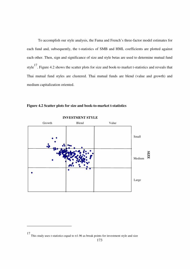
173
To accomplish our style analysis, the Fama and French’s three-factor model estimates for
each fund and, subsequently, the t-statistics of SMB and HML coefficients are plotted against
each other. Then, sign and significance of size and style betas are used to determine mutual fund
style17
. Figure 4.2 shows the scatter plots for size and book-to market t-statistics and reveals that
Thai mutual fund styles are clustered. Thai mutual funds are blend (value and growth) and
medium capitalization oriented.
Figure 4.2 Scatter plots for size and book-to-market t-statistics
17 This study uses t-statistics equal to ±1.96 as break points for investment style and size
Small
Medium
Large
INVESTMENT STYLE
Value Blend Growth
SIZ
E

174
This study further investigates whether there is any difference in performance across
mutual fund styles. Accordingly, mutual funds are categorised in one of nine styles: large-
cap/growth, large-cap/blend, large-cap/value, mid-cap/growth, mid-cap/blend, mid-cap/value,
small-cap/growth, small-cap/blend and small-cap/value. These styles are based on the SMB and
HML estimates in Fama and French’s three-factor model. The sign and significance value of t-
statistics are used as the break point. Funds are grouped into style portfolios and performances
are estimated using unconditional and conditional measures. The results are shown in Table 4.11.
Large-cap fund portfolio gives marginally abnormal returns. The large-cap and glamour fund
yields the lowest performance of all the nine styles and significant at 10% level. In contrast,
large-cap/blend funds give the highest return and outperform the market at 10% level. While
most of funds rely on the mid-cap/blend style, this style provides no abnormal returns and this
style is relatively passive. This finding contrasts with the evidence in developed markets, which
shows that growth funds perform better than funds of other styles (for example, see Grinblatt and
Titmann, 1989 and 1993; Daniel et al. 1997).
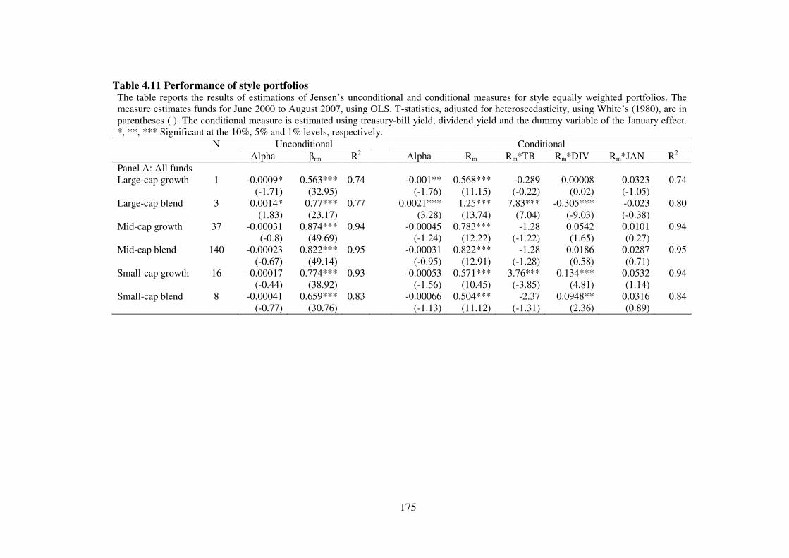
175
Table 4.11 Performance of style portfolios The table reports the results of estimations of Jensen’s unconditional and conditional measures for style equally weighted portfolios. The measure estimates funds for June 2000 to August 2007, using OLS. T-statistics, adjusted for heteroscedasticity, using White’s (1980), are in parentheses ( ). The conditional measure is estimated using treasury-bill yield, dividend yield and the dummy variable of the January effect. *, **, *** Significant at the 10%, 5% and 1% levels, respectively.
N Unconditional Conditional
Alpha βrm R2 Alpha Rm Rm*TB Rm*DIV Rm*JAN R2
Panel A: All funds Large-cap growth 1 -0.0009* 0.563*** 0.74 -0.001** 0.568*** -0.289 0.00008 0.0323 0.74
(-1.71) (32.95) (-1.76) (11.15) (-0.22) (0.02) (-1.05) Large-cap blend 3 0.0014* 0.77*** 0.77 0.0021*** 1.25*** 7.83*** -0.305*** -0.023 0.80
(1.83) (23.17) (3.28) (13.74) (7.04) (-9.03) (-0.38) Mid-cap growth 37 -0.00031 0.874*** 0.94 -0.00045 0.783*** -1.28 0.0542 0.0101 0.94
(-0.8) (49.69) (-1.24) (12.22) (-1.22) (1.65) (0.27) Mid-cap blend 140 -0.00023 0.822*** 0.95 -0.00031 0.822*** -1.28 0.0186 0.0287 0.95 (-0.67) (49.14) (-0.95) (12.91) (-1.28) (0.58) (0.71) Small-cap growth 16 -0.00017 0.774*** 0.93 -0.00053 0.571*** -3.76*** 0.134*** 0.0532 0.94
(-0.44) (38.92) (-1.56) (10.45) (-3.85) (4.81) (1.14) Small-cap blend 8 -0.00041 0.659*** 0.83 -0.00066 0.504*** -2.37 0.0948** 0.0316 0.84 (-0.77) (30.76) (-1.13) (11.12) (-1.31) (2.36) (0.89)

176
4.5 Robustness of the results
4.5.1 Multifactor model
Many studies in the developed markets confirm the importance of using a multifactor model for
performance evaluation and this is now commonly used. Yet the study of fund performance in
emerging markets is still mostly based on standard traditional measures, such as the Sharpe,
Treynor and Jensen models. For example, in Thailand, extensive search has produced only one
study, that by Nitibhon (2004), which investigates mutual fund performance in Thailand using a
multifactor model.
For this reason, this study employs a multifactor model – the four-factor model of Cahart
(1997) – to validate its results. This model adds three variables to Jensen’s measure to capture
size, value and momentum risk premiums. Performance, estimated by means of Cahart’s four-
factor model in Table 4.12, is consistent with Jensen’s model in showing that, as a whole, mutual
funds do not have abnormal returns. Neither an equity nor a flexible funds portfolio produces a
significant return. However, the performance generated by Cahart’s four-factor model provides
interesting results. With this model, the overall although funds still yield no statistically
abnormal returns, value of inferior return is enlarged to 0.021 percent per week or nearly 10% a
year, compared to an inferior performance of 1.19% using Jensen’s measure. Therefore, the
figures are economically significant because its size is considerable. This implies the heavy use
of other risk factors besides market risk. This conclusion is confirmed by column 4 where the P-
values of the Wald test are highly significant in both equity and flexible funds portfolios. This
indicates the significance of the additional variables in the multifactor model.

177
The results of the conditional version of Cahart’s four-factor model are presented in
columns 5-8. For the multifactor model, the conditional measure greatly improves fund
performance from -0.2% per week using the unconditional measure to only -0.05% per week.
This result contrasts with that using the Jensen measure, which suggests that performance is
lower when the conditional measure is used. The results in panel C also confirm the results from
panels A and B: a lowering in mutual funds performance using the multifactor model. 65 funds
are shown to have a superior return, compared to 83 funds when using the Jensen measure and a
number of significantly performing funds are removed.
Therefore, this lets us conclude that mutual fund performance is sensitive to the model
used, although estimating fund performance using Cahart’s four-factor model is consistent with
the Jensen measure and still gives the same conclusion as before: that there are no abnormal
returns in the Thai mutual funds. Nevertheless, the multifactor model shows evidence of
economic and statistical significance. In addition, extending to the multifactor model relaxes the
criticism of the Capital Asset Pricing Model (CAPM) that a market portfolio is unobservable.
The use of the multifactor model also allows us to understand the strategies used by fund
managers by examining the factor loadings in the model. So far, studies in emerging markets
using the multifactor model are still limited. As a result, it is urged that the future study of fund
performance in emerging markets should move forward to the multifactor model.
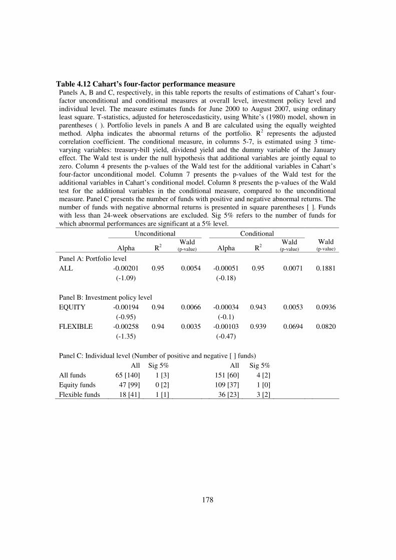
178
Table 4.12 Cahart’s four-factor performance measure Panels A, B and C, respectively, in this table reports the results of estimations of Cahart’s four-factor unconditional and conditional measures at overall level, investment policy level and individual level. The measure estimates funds for June 2000 to August 2007, using ordinary least square. T-statistics, adjusted for heteroscedasticity, using White’s (1980) model, shown in parentheses ( ). Portfolio levels in panels A and B are calculated using the equally weighted method. Alpha indicates the abnormal returns of the portfolio. R2 represents the adjusted correlation coefficient. The conditional measure, in columns 5-7, is estimated using 3 time-varying variables: treasury-bill yield, dividend yield and the dummy variable of the January effect. The Wald test is under the null hypothesis that additional variables are jointly equal to zero. Column 4 presents the p-values of the Wald test for the additional variables in Cahart’s four-factor unconditional model. Column 7 presents the p-values of the Wald test for the additional variables in Cahart’s conditional model. Column 8 presents the p-values of the Wald test for the additional variables in the conditional measure, compared to the unconditional measure. Panel C presents the number of funds with positive and negative abnormal returns. The number of funds with negative abnormal returns is presented in square parentheses [ ]. Funds with less than 24-week observations are excluded. Sig 5% refers to the number of funds for which abnormal performances are significant at a 5% level.
Unconditional Conditional
Alpha R2 Wald
(p-value) Alpha R2 Wald
(p-value) Wald
(p-value)
Panel A: Portfolio level
ALL -0.00201 0.95 0.0054 -0.00051 0.95 0.0071 0.1881
(-1.09) (-0.18)
Panel B: Investment policy level
EQUITY -0.00194 0.94 0.0066 -0.00034 0.943 0.0053 0.0936
(-0.95) (-0.1)
FLEXIBLE -0.00258 0.94 0.0035 -0.00103 0.939 0.0694 0.0820
(-1.35) (-0.47)
Panel C: Individual level (Number of positive and negative [ ] funds)
All Sig 5% All Sig 5%
All funds 65 [140] 1 [3] 151 [60] 4 [2]
Equity funds 47 [99] 0 [2] 109 [37] 1 [0]
Flexible funds 18 [41] 1 [1] 36 [23] 3 [2]

179
4.5.2 Value-weighted portfolio method
This fund performance study is mainly based on the equally weighted method, which assumes
that the same amount of money is invested in each fund and, thus, that the returns of each mutual
fund will affect the returns of the portfolio equally. To identify whether performance is sensitive
to the method of portfolio formation, the value-weighted portfolios are computed by weighting
returns with their total asset values (TNAs). This means that the returns from large mutual funds
have more influence on the returns of the portfolio than those from small funds. The results using
the TNAs weighted method, in Table 4.13, are consistent with the equally weighted method,
which gives no abnormal return. However, performance estimated by means of the TNA
weighted method is better and very close to zero, implying that large mutual funds perform better
than small mutual funds and their performances are close to zero. The P-Values of the Wald test,
presented in the last column, are significant over different portfolio styles and this is inconsistent
with the previous results in Table 4.4. Tables 4.14 and 4.15 highlight the strategies used by fund
managers, which are also consistent with the equally weighted method. Nonetheless, the
evidence of employing size, book-to-market and momentum strategies as well as predetermined
economic variables, is slightly stronger than it is for the equally weighted portfolios. Therefore,
it can be concluded that although the method of constructing portfolios is not sensitive to fund
performance, it is sensitive to the significance of parameters in performance models, implying
that there are differences in engaging strategies between large and small funds.

180
Table 4.13 Performance of value-weighted portfolios This table reports the results of estimations of Jensen’s unconditional and conditional measures using the value weighted portfolio method. The measure estimates funds for June 2000 to August 2007, using ordinary least square. T-statistics, adjusted for heteroscedasticity, using White’s (1980) model, are in parentheses ( ). Alpha indicates the abnormal returns of the portfolio. R2 represents the adjusted correlation coefficient. The conditional measure, in columns 4-5, is estimated using 3 time-varying variables: treasury-bill yield, dividend yield and the dummy variable of the January effect. The Wald test, in the last column, is under the null hypothesis that additional variables in the conditional measure are jointly equal to zero.
Unconditional Conditional Wald test
Alpha R2 Alpha R2 (p-value)
ALL -0.00004 0.955 -0.00019 0.956 2.37 (0.07)
(-0.15) (-0.67)
EQUITY 0.00002 0.953 -0.00013 0.954 3.70 (0.01)
(0.05) (-0.41)
FLEXIBLE -0.00008 0.871 -0.00033 0.876 10.87 (0.00)
(-0.17) (-0.7)
Table 4.14 Fund’s factor sensitivities of value weighted portfolios This table reports the beta coefficients estimated from Jensen’s unconditional and conditional measures using value-weighted portfolio method. The beta coefficients of unconditional beta (βp), estimated from the following regression are presented in the second column: rpt = αp+ βp rmt+εt where rpt and rmt are, respectively, the excess return on portfolio p and on the benchmark portfolio over the risk-free rate at time t. The last four columns present beta coefficients estimated using a conditional measure from the following regression: rpt = αp+ β0p rmt+ β1p (rmt *TBt-1)+ β2p (rmt *DIVt-1)+ β3p (rmt *JANt-1)+εt where TB, DIV, JAN are treasury-bill yield, dividend yield, and dummy variable of the January effect, respectively. The regressions are estimated for June 2000 to August 2007 using ordinary least square. T-statistics, adjusted for heteroscedasticity using White’s (1980) model, are in parentheses ( ). *Significant at the 10% level. **Significant at the 5% level. ***Significant at the 1% level.
Unconditional Conditional
βp β rm β t-bill β div β jan
ALL 0.809*** 0.755*** -2.07*** 5.2** 0.024
(56.4) (15.59) (-2.64) (2.16) (0.64)
EQUITY 0.854*** 0.825*** -2.44*** 4.74* 0.027
(54.04) (15.03) (-2.83) (1.74) (0.67)
FLEXIBLE 0.707*** 0.535*** -2.52*** 10.5*** 0.00866
(35.87) (11.58) (-2.77) (5.46) (0.2)

181
Table 4.15 Fund strategies of value weighted portfolios This table reports beta coefficients estimated from Cahart’s four factor model using the value-weighted portfolio method. SMB refers to a small-minus-big stock portfolio. HML refers to a high-minus-low book-to-market stock portfolio. PR1YR refers to the difference in return between portfolios of past years, winner and loser. The measure estimates funds for June 2000 to August 2007, using ordinary least square. T-statistics, adjusted for heteroscedasticity, using White’s model (1980), are in parentheses ( ). The Wald test, in the last column, is under the null hypothesis that additional variables are jointly equal to zero. *Significant at the 10% level. **Significant at the 5% level. ***Significant at the 1% level.
βrm βSMB βHML βPR1YR R2
ALL 0.813*** 0.0324** -0.0312*** 0.00163 0.956 (56.12) (2.11) (-3.24) (0.81) EQUITY 0.858*** 0.0394** -0.0344*** 0.00066 0.954 (54.03) (2.44) (-3.39) (0.32) FLEXIBLE 0.711*** 0.036* -0.034*** 0.00411* 0.872 (35.1) (1.72) (-2.91) (1.7)
4.5.3 Frequency of data
Whereas most previous studies use monthly data for performance evaluation, our analyses are
based on weekly returns. A fund’s beta may change with the return interval when the return is
measured in continuous time dates, due to the trading frequency. Goetzmann et al. (2000) reveal
that mutual fund performance is sensitive to the horizon period of the data. Thus, to verify the
sensitivity of fund performance to the time interval used in the study, in Table 4.16, we re-
estimate mutual fund performance using monthly returns data for the overall level (panel A),
investment policy level (panel B) and individual level (Panel B).
Using monthly data, mutual funds still provide no abnormal returns though its
performance is slightly more than the market returns. The results in Panel B show positive
insignificant performance for both equity and flexible portfolios, regardless of any performance
measure or portfolio formation used. Adjusted R-squares vary from 0.78-0.82, which is slightly
lower than they are with a weekly horizon. The individual level, in panel C, also gives a similar
conclusion: that there are more positive than negative funds. Moreover, the factor exposures of
182
conditional models contrast with the findings using weekly data. Only the dummy variable of the
January effect is positively significant with this estimation. This result can refer to the
investment horizon of fund managers, showing that they are likely to rebalance their portfolio
dynamically over a week’s horizon and, therefore, the use of a monthly interval is unable to
capture fund managers’ strategies. For this reason, it can be concluded that mutual fund
performance is sensitive to the time interval used. This has implications for future research as
regards the time horizon used in performance evaluation.
4.5.4 Dummy variable market timing measure
This study employs the dummy variable measure (Henriksson and Merton, 1981) to test
robustness in fund managers’ timing ability. Henriksson and Merton argue that beta risk changes
up and down according to the condition of the market. Subsequently, they incorporate a dummy
variable to capture up and down markets18
. The results in Table 4.16 are those from the dummy
variable market timing measure which are consistent with the quadratic market timing measure.
Coefficients of the dummy variables are not statistically significant in any portfolio. Moreover,
at individual level, shown in Panel C, only a small number of funds have significant timing
ability. This confirms that fund managers do not display market timing ability.
18 See Section 2.2.4 for details

183
Table 4.16 Performance using monthly return data The table reports the results of estimations of Jensen’s unconditional and conditional measures at overall level, investment policy level and individual level in panels A, B and C, respectively. The measure estimates funds for June 2000 to August 2007, using ordinary least square. T-statistics, adjusted for heteroscedasticity, using White’s (1980)model, shown in parentheses ( ). Portfolio levels in panels A and B are calculated using the equally weighted method (EW) and value-weighted method (VW). R2 represents the adjusted correlation coefficient. The conditional measure, in columns 5-10, is estimated using 3 time-varying variables: treasury-bill yield, dividend yield and the dummy variable of the January effect. Panel C presents the number of funds with positive and negative abnormal returns. The number of funds with negative abnormal returns is presented in square parentheses [ ]. Funds with less than 24-week observations are excluded. Sig 5% refers to the number of funds for which abnormal performances are significant at a 5% level. *Significant at the 10% level. **Significant at the 5% level. ***Significant at the 1% level.
Unconditional Conditional
Alpha βrm R2 Alpha Rm Rm*TB Rm*DIV Rm*JAN R2
Panel A: Overall level EW-ALL 0.00065 0.713*** 0.78 0.00092 0.92*** -49.6 -0.061 0.207** 0.80 (0.21) (15.44) (0.29) (8.42) (-0.95) (-1.11) (2.38) VW-ALL 0.00106 0.7*** 0.80 0.00099 0.914*** -71.3 -0.0455 0.191** 0.81 (0.36) (16.06) (0.34) (9.42) (-1.42) (-0.9) (2.33) Panel B: Investment policy level EW-EQUITY 0.00079 0.76*** 0.77 0.00098 0.978*** -57.8 -0.0593 0.211* 0.79 (0.23) (15.09) (0.28) (8.15) (-1) (-0.97) (2.2) VW-EQUITY 0.00154 0.742*** 0.79 0.00161 0.987*** -76.4 -0.0515 0.157* 0.81 (0.48) (15.98) (0.5) (9.05) (-1.38) (-0.92) (1.75) EW-FLEXIBLE 0.00052 0.564*** 0.79 0.00028 0.696*** -50.7 -0.0319 0.24*** 0.82 (0.22) (15.92) (0.12) (9.67) (-1.3) (-0.88) (3.78) VW-FLEXIBLE 0.00043 0.602*** 0.79 -0.00045 0.725*** -82.6* -0.00503 0.269*** 0.82 (0.17 (14.8) (-0.18) (10.15) (-1.96) (-0.13) (3.78)

184
Unconditional Conditional
Alpha βrm Alpha Rm Rm*TB Rm*DIV Rm*JAN
Panel C: Individual level (Number of positive and negative [ ] funds) All funds 137 [68] 203 [2] 137 [68] 181 [24] 52 [53] 79 [126] 177 [23] All funds with 5% sig. 10 [0] 196 [0] 16 [3] 114 [1] 3 [6] 4 [10] 129 [5] Equity funds 105 [41] 146 [0] 104 [42] 128 [18] 35 [111] 56 [90] 124 [18] Equity funds with 5% sig. 9 [0] 143 [0] 13 [1] 88 [1] 3 [4] 2 [8] 93 [5] Flexible 32 [27] 57 [2] 33 [26] 56 [6] 17 [42] 23 [36] 53 [5] Flexible funds with 5% sig. 1 [0] 53 [0] 3 [2] 26 [0] 0 [2] 2 [2] 36 [0]

185
Table 4.17 The dummy variable market timing performance measure The table reports the results of estimations of dummy variable timing ability (Henriksson and Merton, 1981) using unconditional and conditional measures at overall level, investment policy level and individual level in panels A, B and C, respectively. The measure estimates funds for June 2000 to August 2007 using ordinary least square. T-statistics, adjusted for heteroscedasticity using White’s (1980), are in parentheses ( ). Portfolio levels in panels A and B are calculated using the equally weighted method. Alpha indicates the abnormal returns of the portfolio. Dummy is the coefficient of the dummy variable representing market timing ability. R2 represents the adjusted correlation coefficient. The conditional measure, in column 5-7, is estimated using 3 time-varying variables; Treasury-bill yield, dividend yield and the dummy variable of the January effect. Panel C presents the number of funds with positive and negative market timing ability. Number of funds with negative market timing ability is presented in parentheses [ ]. Funds with less than 24-week observations are excluded. Sig 5% refers to the number of funds for which market timing ability is significant at a 5% level.
Unconditional Conditional
Alpha Dummy R2 Alpha Dummy R2
Panel A: Overall level
ALL -0.00037 -0.011 0.95 -0.00026 0.067 0.95
(-0.56) (-0.20) (-0.44) (0.14)
Panel B: Investment policy level
EQUITY -0.00056 -0.026 0.94 -0.00042 -0.0039 0.94
(-0.79) (-0.44) (-0.64) (-0.07)
FLEXIBLE 0.00044 0.047 0.94 0.00046 0.625 0.94
(0.64) (0.76) (0.82) (1.42)
Panel C: Individual level (Number of positive and negative [ ] market timing)
All funds 128[81] 118[86]
All funds with 5% sig. 21[0] 24[0]
Equity funds 77[69] 73[73]
Equity funds with 5% sig. 18[0] 19[0]
Flexible 47[12] 45[13]
Flexible funds with 5% sig. 3[0] 5[0]

186
4.6 Conclusions
It is acknowledged that mutual fund investment in emerging markets has grown substantially
in the past few years. Nonetheless, not many studies in fund performance have been
conducted in this setting and most of these studies still use conventional measures; survey
only short periods and examine a small number of funds. Therefore, this chapter reviews
mutual fund performance in Thailand in some depth, using survivorship-bias-free data from
2000-2007, which is the most extensive period to be reviewed in mutual fund performance
studies in Thailand. This chapter examines many aspects of fund performance, including
performance in selectivity and timing ability, the strategies and styles of fund managers and
mutual fund characteristics in relation to performance. In addition, this study also takes into
account the style of tax-benefit funds and reviews the differences between these and general
funds. Several models of mutual funds are used in this study and analysed at both aggregate,
style and individual levels. The findings are, first, that mutual fund managers do not have
stock selection ability or timing ability. On average, mutual funds insignificantly
underperform the market benchmark. The inferiority is 1.2% using an unconditional measure,
reducing to 1.75% with a conditional measure. In addition, the number of negative funds is
also greater than of positive funds at the individual level. Second, equity and flexible fund
managers employ different strategies to adjust their portfolios. Flexible fund managers tend
to adjust their portfolios dynamically by employing macroeconomic variables, namely,
treasury-bill and dividend yield. In contrast, equity fund managers select stocks on the basis
of stock characteristics and are likely to put more emphasis on small and growth stocks,
although there is no evidence of the momentum strategies used. Third, performance is
unstable throughout the period studied. Mutual funds performed better in the first part of the
period when the market was down but worsened in the subsequent period when the market

187
peaked and significant cash flows were approached. Fourth, the performances of tax-benefit
funds and general funds are statistically significant. Tax-benefit funds perform better than
these general funds. Fifth, fund managers styles are homogenous. They are rather passive and
mid-cap and blend (value and growth) oriented most funds. Finally, although the performance
of mutual funds is not sensitive to portfolio formation, it is sensitive to the time interval and
the model used. Cahart’s four-factor model gives statistical and economic significance in
fund performance.
These results provide practical implications for both Thai investors and fund
managers. While most of these funds are based on a passive strategy and provide no
abnormal return to investors, concentrating on small and value oriented funds is likely to
provide a better return. Flexible fund managers align themselves to their main objectives in
that they adjust their portfolios more actively on the basis of the economic information and,
thus, suit active investors better. Tax-benefit funds not only provide income tax relief, but
also earn a higher return than general funds. Therefore, this can be beneficial to the long-term
passive investors. Nevertheless, the performance of funds also depends on the market
conditions and for this reason performance in the past does not guarantee future performance.
Furthermore, the implication for fund managers is that they should be more style-specific.
The use of momentum strategy is also worth their consideration.
Our findings show both similarities and contradictions to the literature. The similarity
is that both show evidence of no selectivity ability or timing ability among fund managers in
Thailand. Moreover, predetermined variables in the conditional model are individually and
jointly significant, although it lowers fund performance, contrary to the study of Ferson and
Schadt (1996). Another contradiction is that, while evidence in the US reveals that growth
funds perform better than others, in Thailand their performance is low compared to funds of
other styles. However, the performance of tax-benefits funds is significantly different from

188
that of general funds. This may be due to the lock-up provision period of the tax-benefit
funds, which generate the liquidity premium (Edelen, 1999; Aragon, 2007).
Evidently these contradictions call for further studies, in order to find out what exactly
causes them. More study of tax-benefit fund style should consider what factors make them
perform better than general funds. The inclusion of benchmark and risk-free rate return to the
performance measures is also required, as some evidence suggests that these can affect the
results (Coles et al., 2006). Finally, the sensitivity of fund performance toward performance
measures and data frequency found in this study require further investigation in order to
evaluate as precisely as possible the mutual fund performance in emerging markets.

189
CHAPTER 5
DETERMINANTS OF MUTUAL FUND PERFORMANCE
5
Abstract
This study examines the relationship between Thai mutual fund performance and the
following five characteristics: past return, size, net flows, fund longevity and family size. We
base fund performance on risk-adjusted approaches and determine the relationship both
statistically and in economic terms. We find evidence of persistence in fund performance
only in general funds. The persistence in performance is mainly a result in poorly performing
funds. Lagged cash flows shock has a negative impact on the performance of tax-benefit
funds. Fund size, family size and fund longevity can explain fund performance in some
specific policies but these are not enough to earn abnormal return based on these
characteristics. In addition, we reveal the superior performance of tax-benefit funds even
when we control for fund characteristics and year effect.

190
5.1 Introduction
Regardless of data and measure used, the prevailing empirical evidence suggests that fund
managers, as a group, are unable to outperform the market, in particular after allowing for
fees and expenses (see, Jensen, 1968; Malkiel, 1995; Ferson and Schadt, 1996; Wermers,
2000). Nonetheless, when we consider this at the fund level, there are some funds which
outperform others. Kosowski et al. (2006) add that the performance of fund managers is not
entirely due to luck. A number of studies examine whether we can identify the finds with
superior performance and many fund characteristics are considered to be potential
determinants. For example, Hendricks et al. (1993), Brown and Goetzman (1995) and Gruber
(1996) suggest reasons for persistence in fund performance over a short horizon. However,
Cahart (1997) argues that this is due to the use of momentum strategy on the part of fund
managers. Indro et al. (1999) and Chen et al. (2004) suggest that fund size reflects the
implicit transaction cost and, therefore, has a negative impact on fund performance. In
addition, Warther (1995) and Edelen (1999) suggest the negative relation between return and
cash flows. In contrast, Gruber (1996) and Zheng (1999) reveal a positive relation between
returns and past flows and suggest a ‘smart money effect’ in fund performance. Furthermore,
some other factors, such as longevity, size of the management company, fees, expenses and
turnover have been identified in this regard in the literature. Nonetheless, most of these
studies focus on only one particular factor or investigate particular factors only as a small part
of their studies of mutual fund performance. More importantly, these studies are conducted
within a developed market setting, where the context is different from that of the emerging
markets in many ways, for instance, size, growth and competitiveness. This all makes
evidence on this issue still scarce and ambiguous.

191
Thus, this study aims to investigate relation between fund performance and fund
characteristics using data on Thai mutual funds. In addition to the fact that it is conducted in
an emerging market where little is known about mutual fund performance, this study will also
contribute to mutual fund literature in several ways. First, it examines a more extensive list of
characteristics and employs a wider dataset than any previous study of emerging markets. We
examine 5 characteristics which have been widely discussed in the literature including past
performance, net cash flows, fund size, fund family size and fund longevity. We use the more
complete dataset and also control for the effect from mutual fund investment policy
differences. Thus, this study is the most comprehensive study in mutual fund determinants in
an emerging market so far.
Second, in contrast to most previous studies of emerging markets, we focus on mutual
fund performance on a risk-adjusted basis. This study employs both unconditional and
conditional versions of Jensen’s alpha. The conditional model allows for time-varying in the
market risk factor.
Third, this is the first study which applies not one but two measures to disentangle the
problem; multivariate (panel) regression controlling for time-variation effect and zero-cost
trading strategy. This allows us to explore several determinants both separately and
simultaneously and also to highlight what is significant both statistically and economically.
In total, this study considers up to 230 mutual funds from 2000-2007, including both
equity and flexible funds. It examines a larger dataset and a longer period than previous
studies in Thailand. In addition, we control for the impact of the mutual fund investment
policy and tax-purpose fund style by further classifying funds into four groups; general equity
funds (EQN), tax-benefit equity funds (EQT), general flexible funds (FLN) and tax-benefit
flexible funds (FLT). The tax-benefit funds require a longer investment horizon than do the

192
general funds, resulting in clientele differences19
. Subsequently, this study will not only
benefit investors and fund managers, but can also be used to suggest policy implications in
order to scrutinize the characteristics of tax-benefit funds.
We find that the determinants of fund performance are subject to the fund investment
policies. We find strong persistence in the performance of general funds. However, this is
mainly attributable to poorly performing funds which continue to perform badly from one
period to the next. Lagged year net cash flows do not explain fund performance as a whole.
However, the cash flows shock in tax-benefit funds inversely affects fund performance. Fund
size is negatively related to general flexible funds and positively related to tax-benefit
flexible funds. General funds which belong to large management companies outperform those
of small companies; and finally, young general equity funds tend to perform better than old
ones. Nevertheless, selecting funds on the basis of size, family size and longevity does not
confer any economic benefit.
The rest of the present chapter is organised as follows. Section 5.2 gives previous
empirical evidence and hypotheses. Section 5.3 describes the data and methodology used.
Empirical results are provided in section 5.4 and the final section, 5.5, gives a conclusion and
suggestions for further research.
19 Tax-benefit funds are a special type of funds in Thailand which require long-term investment and investors
will receive up to 15% tax relief (or maximum THB 300,000). See Chapter 3 for details.

193
5.2 Previous evidence and hypotheses
A number of studies have investigated the relationships of various mutual funds
characteristics and fund performance in order to identify whether mutual fund performance
can be explained by any particular characteristics. This section begins with a review of
previous theoretical and empirical studies of each characteristic; include size, past returns, net
flows, fund age and family size. Then this section goes on to offer hypotheses which will be
tested in the study, concerning mutual fund characteristics. .
5.2.1 Persistence in performance
Persistence in performance occurs when past performance is positively correlated with
current performance. Persistence in performance implies that prices reflect information and,
therefore, it becomes evidence for rejecting the semi-strong form efficient hypothesis (EMH),
since this claims that price does not fully reflect available information. Studies of persistence
in mutual fund performance are well documented. In the literature, a number of studies bear
evidence of short-term persistence, particularly among poorly performing funds (see, for
example Hendricks et al., 1993; Goetzmann and Ibbotson, 1994). However, Brown and
Goetzmann (1995) argue that the persistence in performance is due to survivorship bias.
Grinblatt and Titman (1992) and Elton (1996) reveal evidence of persistence in a longer
horizon. However, Cahart (1997) suggests that persistence in the performance of mutual
funds is due to employing momentum strategies, as pointed out by Jagadeesh and Titmann
(1993). Cahart shows that, after controlling for this effect, evidence of persistence is
removed. Nonetheless, the recent study by Ferreira et al. (2009), who investigate the
determinants of mutual funds using cross-country data over the period 1997-2007, reveal that

194
fund performance can be explained by returns in the previous quarter, suggesting short-term
persistence in performance. They reveal that this evidence is stronger in the US domestic
funds than in non-US domestic funds.
In the UK, Blake and Timmermann (1998) also reveal persistence in UK unit trusts
and their findings are using a 24-month previous return. This is comparable to Otten and
Bams (2002), who reveal persistence in mutual fund performance in the UK but not in other
European countries. Furthermore, Annaert et al. (2003) find evidence of persistence in
European funds and Bauer et al. (2006) also reveal persistence in the performance of New
Zealand mutual funds. These findings contrast with those in a study of Swedish data by
Dahlquist et al. (2000) using Swedish data and Prather et al. (2004), who document the
reverse effect of persistence in US funds during 1996-2000.
5.2.2 Fund size
There are extensive studies about the relationship between the size of mutual funds and
performance, where the findings are still mixed. Large funds have an advantage over small
funds in term of economies of scale because large funds can spread fixed cost and have
access to more resources. In addition, managers of large funds will have better investment
opportunities than managers of small funds and the brokerage commission is likely to be
reduced with the amount of the transaction (Ciccotello, 1996).
However, some studies argue that fund size could have a negative impact on
performance. For instance, Indro et al. (1999) suggest that fund size reflects implicit
transaction costs and subsequently diminishing marginal returns. Fund size increases the cost
of acquiring and trading on information, as the activities of a fund draw market attention.
Therefore, larger funds face more difficulty in exploiting information asymmetry.

195
Furthermore, small funds also present stronger evidence of persistent performance (see
Gruber, 1996; Berk and Green, 2004).
Grinblatt and Titmann (1989) investigate US mutual funds during 1975-1984. They
find abnormal performance in small funds using returns data. Elton et al. (1996) also reveal
that larger funds perform better than smaller funds when the data are controlled by
survivorship bias. Similarly, Payne et al. (1999) find that the risk-adjusted performance of the
US mutual funds between 1993 and 1995 is positively related to fund size. Indro et al. (1999)
claim that mutual fund performance increases with size. However, the marginal return
diminishes when it reaches its optimum size. Using European mutual fund data, Otten and
Bams (2002) find a positive relationship between size and performance of mutual funds.
Annaert et al. (2003) also examine the relationship of European equity mutual funds
performance with different characteristics during 1995-1998 and reveal a positive
relationship with fund size. Similarly, Bauer et al. (2006) reveal a positive relationship among
New Zealand data.
In contrast to the findings above, Droms and Walker (1994) find no relationship in
international mutual funds between size and performance. Ciccotello (1996) employs mutual
funds with different investment objectives. He finds that fund size cannot explain fund
performance with the exception of funds in aggressive/growth objectives where size has an
inverse impact on performance. Dahlquist et al. (2000) point out that, in Sweden, small equity
funds perform better than large equity funds, although the reverse relation holds for bond
mutual funds. Similarly, Chen et al. (2004) examine a large set of US mutual funds from
1962 to 1999 and reveals a negative relationship between size and performance. They suggest
that this reverse relationship is related to liquidity constraints. In addition, Edelen et al.
(2007) also reveal that the evidence of negative relationship between size and performance is
a result of high trading cost. In contrast to Chen et al., Ferreira et al. (2009) argue that the

196
negative relationship exists only in the US market. Outside the US, large funds outperform
small funds.
5.2.3 Net cash flows
The net cash flow of a fund represents the net growth in fund assets. Nonetheless, the
movement of cash in and out of a fund would inversely affect portfolio beta and,
subsequently, performance. This is because, when a fund receives large cash inflows, it is not
possible for a manager to allocate the new money immediately. This makes a larger cash
position in the portfolio and subsequently lowers the mutual fund’s beta. Conversely, large
cash outflows require fund managers to liquidate assets, even though they may have private
information. Therefore, it prevents a fund manager from trading on information and causes
him to show negative market timing ability. The effect of flows to fund performance is
regarded as ‘liquidity-motivated trading’ and it impacts on the risk and return estimation.
Warther (1995) suggests that, during 1976-1970, t-statistics for the slope coefficient of
changes in beta on the changes in net cash flows were between -2.8 to -3.8. This negative is a
highly significantly way of representing the negative relation between the net flows and
portfolio beta (cited in Ferson and Schadt, 1996). Also, Edelen (1999) suggests the negative
relation between fund abnormal returns and investor flows. He suggests that this, due to
liquidity-motivated trading, lowers a fund’s abnormal return by 1.5% - 2% per year.
Furthermore, Benson and Faff (2006) study the relevance of money flows to equity fund
performance, using Australian data. They find evidence supporting Warther’s (1995) and
Edelen’s (1999) view that money flows and fund betas are negatively related and fund flows
negatively impact on fund performance.

197
However, some studies find evidence that money flows into funds which had high
returns in the preceding period, or “smart money”. This refers to the ability of investors to
pick superior find managers. A number of studies show evidence of the smart money effect.
For example, Gruber (1996) finds that the returns from funds with high net cash inflows are
higher than from those with average net cash inflows. Zheng (1999) also reveals that funds
with positive cash flows outperform in the following period funds with negative cash flows.
More specifically, she reveals that this finding is more pronounced in small funds.
Nevertheless, Sapp and Tiwari (2004) argue that the smart money effect is explained by the
stock momentum phenomenon. They show that, after controlling for stock return momentum,
the smart money effect disappears.
Outside the US, Dahquist et al. (2000) find little evidence in Sweden of the relation
between lagged flows and performance. However, Gharghori et al. (2007) investigate the
smart money effect using Australian funds. They find evidence of it which cannot be
explained by the stock return momentum. Ferreira et al. (2009) also confirm the above
findings. They suggest that the smart money effect is evident in both US and non-US funds.
5.2.4 Fund longevity
The relationship between longevity and fund performance has received little scholarly
attention in previous studies. Funds normally experience higher costs at first because they
have fewer connections and money has to be spent on advertising. Therefore, we could
expect that old funds would outperform young funds. Nevertheless, one could argue that
managers of young funds are more active. This is confirmed by Blake and Timmermann
(1998), who reveal that funds are likely to perform best during their first year of existence.
Similarly, Otten and Bams (2002) find a negative correlation between performance and fund

198
age in some European countries during the period 1991-1998. Nevertheless, Prather et al.
(2004) and Ferreira et al. (2009) find no relationship between age and fund performance.
5.2.5 Family size
Mutual funds are operated under a management company, or “fund family”, which holds an
array of mutual funds. Therefore, a mutual fund is not an independent entity but is operated
as part of a family. A fund family could impact on the decision of a fund manager and,
therefore, potentially impact on fund performance. A larger family is superior to a small
family in terms of increased economies of scale in operation, as it can share the resources of
the whole family (Khorana and Servaes, 1999, 2005). A larger fund family also has better
research quality. Furthermore, it reduces the search cost for investors due to its ease of
recognition (Gaspar et al., 2006). Nevertheless, Chen et al (2002) find that that the size of a
fund family does not significantly impact on fund performance. In contrast, Guedj and
Papastakaikoudi (2004) reveal evidence of persistence of performance among large fund
families. In addition, Chen et al (2004) and Ferreira et al. (2009) reveal the positive and
significant relation to fund performance of both US and international funds.
5.2.6 Evidence from emerging markets and hypotheses
The relationship between fund performance and fund characteristics are less researched in
emerging markets. This is primarily due to the fact that mutual fund data are much less
accessible than those of other financial intermediaries. Among a limited number of studies,
Mei-Chen (2006) examines the determinants of mutual fund performance over different
investment periods. He estimates performance using the Sharpe ratio and looking at different
characteristics in Taiwan. The characteristics include net asset values, current yield, turnover

199
and expenses ratios. He shows that performance is positively related to net asset values but
inversely related to the expenses ratio. Similarly, Tng Cheong (2007) finds insignificant
evidence of positive relationship in size and performance using mutual fund data from
Singapore.
In Thailand, a study of the relationship between performance and mutual fund
characteristics is conducted by Prasomsak (2001). He employs fixed-effect regression to
investigate the performance of 77 mutual funds over the period 1998-2000. He calculates
performance using raw returns and looks at market returns, fund size, turnovers and fund
type. He reveals that fund returns are positively correlated with market returns and negatively
related to size and turnover. The type of fund does not correlate with fund returns.
Watcharanaka (2003) investigates persistence in the performance of 62 Thai open equity
funds for the period 1999-2002 using cross-section regression. She reveals a negative
persistence in performance; that is, high return funds tend to perform worse in the following
period. In addition, she does not find any relationship between returns and mutual fund
expenses. Nitibhon (2004) also uses cross-sectional analysis to investigate how performance
is generated, focusing on two characteristics, size and the book-to-market value of stock held.
He finds that, over the period 2000-2004, performance is positively related to size and growth
stocks. In addition, he investigates persistence in performance and flows of funds. By
examining the performance of decile portfolios, he reveals that, unlike what is observed in the
US, only the top decile portfolio outperformed the market. However, the spread between top
and bottom portfolios is not statistically significant. In addition, he shows that the
outperforming in the top decile portfolio is not the result of momentum strategy but rather
because the fund manager has put more weight on growth stocks. Similarly, he finds that
investment in funds with high flows does not provide superior returns. Researchers in
Kasikorn research centre (2005) investigate the performance of the 5 largest fund companies

200
in relation to other companies. They find that large fund companies do not perform better
than small ones.
Table 5.1 summarises the findings in the previous literature on emerging markets as
well as the expected signs according to the theory and evidence in developed countries. It is
clear that, in emerging markets, research on this issue has so far received very little attention
and the evidence is still scanty. These studies examine only one or two characteristics and
tend to look at this issue as a part of a performance measurement study. Some of the
characteristics, such as fund age and family size, have never been investigated. Furthermore,
some studies do not consider the time-variation over the study period or differences in mutual
fund style.
Nevertheless, the issue of determinants in fund performance is important to investors
because it can be the first point of guidance in selecting funds and can also help fund
managers to manage their portfolio more efficiently. Therefore, this study aims to test the
same hypotheses as the previous literature; that is, to look at the relationship between mutual
fund performance and its characteristics. However, this study looks at this relationship in the
context of a emerging market where previous studies are hardly to be found. We test a more
extensive list of mutual fund characteristics and investigate its relationship comprehensively
by looking at each characteristic individually and also as part of a group in order to control
for the effect of one characteristic on the others. Altogether, we look at five characteristics,
namely, size, past returns, net flows, fund longevity and family size. Hence, five hypotheses
are tested:
H5.1: Fund past performance is related to fund current performance
H5.2: Fund size is related to fund performance
H5.3: Fund age is related to fund performance

201
H5.4: Fund net flow is related to fund performance
H5.5: Fund family size is related to fund performance
Table 5.1 Previous evidence of the relationship between fund performance and fund
attributes in emerging markets
The table summarises evidence of a relationship between fund performance and the five fund attributes, namely size, past returns, age, flows and family size. ‘+’ indicates a positive relationship. ‘-’ refers to a negative relationship. ‘0’ indicates no relationship.
Past
returns Size Age Flows Family
size
Prasomsak (2001) -
Nitibhon (2004) 0 + 0
Watcharanaka (2003) -
Kasikorn research centre (2005) 0
Mei-Chen (2006) +
Tng Cheong (2007) +
Author’s expected sign 0 +/- +/- +/- +/-
5.3 Data and methodology
5.3.1 Fund sample
Our sample includes equity and flexible mutual funds in Thailand over the period 2000-2007.
We exclude international funds, index funds, sector funds, property funds and fund with any
specific purpose. This makes 230 funds in our initial sample (made up of 166 equity funds
and 64 flexible funds). Details of our sample selection are in Chapter 3. In addition, we
impose one extra condition for this study: funds in order to be included must have been in
operation at least 12 weeks over the sample period. The reason behind this is to reduce small
sample size bias in the estimating mutual performance.
As a result, our final sample is reduced to 215 funds, made up of 155 equity funds
(118 general funds and 37 tax-benefit funds) and 60 flexible funds (48 general funds and 12

202
tax-benefit funds.) The tax-benefit funds offer tax relief while requiring a long-term
investment and result in differences in their characteristics. Subsequently, our sample can be
classified into four broad groups: general equity funds, general flexible funds, tax-benefit
equity funds and tax-benefit flexible funds. Table 5.2 below provides summary statistics of
the mutual fund returns in each year. The table shows that the number of funds rose sharply
over the years and there is great variation in mutual fund returns over the study period. Funds
lost up to 19% per annum during the recession period but earned around 70% during the bull
market. Additionally, Panel B reveals that returns are also different across investment policy.
Table 5.2 Summary statistics of mutual fund returns The table presents the summary statistics of fund returns from 2000-2007. Mean refers to the mean of annualised returns. SD refers to standard deviation of the returns. N refers to the number of funds operated in the year. Panel A gives the summary statistics of the whole fund sample and Panel B gives the summary statistics of the funds classified by investment and tax policies
2000 2001 2002 2003 2004 2005 2006 2007
Panel A: Whole sample
- Mean -0.1944 0.0333 0.1587 0.7670 -0.0957 0.0340 -0.0341 0.1547
- SD 0.07 0.07 0.11 0.50 0.19 0.09 0.08 0.08
- N 103 105 127 138 169 177 190 206
Panel B: Classified by fund investment and tax policies
General Equity funds
- Mean -0.2094 0.0398 0.1966 0.8266 -0.1454 0.0292 -0.0434 0.1752
- SD 0.05 0.06 0.09 0.55 0.23 0.11 0.07 0.07
- N 84 84 86 92 95 99 100 106
General Flexible funds
- Mean -0.1282 0.0076 0.1004 0.5748 -0.0579 0.0206 -0.0428 0.1033
- SD 0.10 0.09 0.10 0.34 0.09 0.05 0.10 0.07
- N 19 21 27 31 39 39 46 43
Tax-benefit Equity funds
- Mean -- -- 0.0314 0.9595 0.0071 0.0640 -0.0004 0.1576
- SD -- -- 0.08 0.19 0.04 0.06 0.06 0.09
- N -- -- 7 7 24 28 32 44
Tax-benefit Flexible funds
- Mean -- -- 0.0440 0.6582 -0.0253 0.0486 -0.0132 0.1479
- SD -- -- 0.10 0.35 0.05 0.04 0.04 0.07
- N -- -- 7 8 11 11 12 13

203
5.3.2 Fund performance benchmarks
In this study, we consider two different risk-adjusted performance measures: the traditional
Jensen’s alpha ( )tradα and conditional Jensen’s alpha ( )conα . The traditional Jensen’s alpha
measure is a single-factor model based on the Capital Asset Pricing model proposed by
Jensen (1968). Jensen’s measure is expressed as:
tmtpppt RR εβα ++= (5.1)
where Rpt is the excess return on portfolio p over risk-free rate; Rmt is the excess return on the
market benchmark portfolio over the risk-free rate t; εit is the random error term. The model
interception is the traditional Jensen’s alpha representing the performance of a fund.
The conditional Jensen’s model is estimated on the basis of work by Ferson and
Schadt (1996). They argue that the beta estimated by the Jensen model is downwardly biased
because the beta is unstable over time. They incorporate time varying variables in addition to
the previous model. The conditional Jensen’s measure is:
ttftmtpftmtppftpt ZRRRRRR εδβα +−′+−+=− − ])[()( 10 (5.2)
where Zt-1 is the predetermined information variables; and δp is the vector of parameter. The
interception is the conditional Jensen’s Alpha representing the performance of the fund.
In this study, the 7-day Bank of Thailand’s repurchase rate is used to represent the
return of a risk free rate and the return of SET index is used as the market benchmark. These
data are both obtained from the Thompson Datastream database. For the conditional Jensen’s
model, three predetermined information variables are used: 7-day treasury bills yield,
dividend yield and a dummy variable of the January effect. This selection is selected on the
basis of evidence that it can explain the stock return during our study period. Once again,
these data are obtained from the Thompson Datastream database.

204
5.3.3 Fund characteristics
In this study, we examine 5 fund characteristics, namely, size, persistence (past return), net
cash flows, fund longevity and fund family size. Summary statistics for these fund
characteristics are reported in Table 5.3. Mutual fund size is measured by the total asset
values (TNAs). This study assesses TNAs in two ways: TNAs at the beginning of the year
and average TNAs across the year. We focus on the TNAs at the beginning of the year in
order to avoid look-ahead bias. We obtain this data from the Association of Investment
Management Companies (AIMC) in Thailand. Table 5.3 reveals that the average size of
mutual funds is around 490 million Baht, but they are subject to great variation. Average
general funds size is slightly larger than tax-benefit funds. This is because tax-benefit funds
were established only in early 2002.
Net cash flows are the net amount of cash that a fund has received or paid during a
given period. Since the data on cash flows data are not publicly available, we implicitly
calculate the net cash flows based on a fund’s total net asset values by assuming that the
flows occur at the end of period. The net cash flows (NCF) and normalised net cash flows
(NNCF) are calculated following Equations 5.3 and 5.4, respectively.
1,
,1,,
,
)1(*
−
− +−=
tp
tptptp
tpTNA
RTNATNANCF (5.3)
1,
,
,
−
=tp
tp
tpTNA
NCFNNCF (5.4)
where TNAp,t is the total net asset values of fund p at the end of period t and Rp,t is the
cumulative return of the fund for the period t. The average cash flows of the funds in our
sample is 64 million Baht. However, this comes with the massive variation of 490 million
Baht. The tax-benefit funds receive much greater cash flows than the general funds. This

205
reveals the popularity of the tax-benefit funds over the study period. Tax-benefit flexible
funds received the highest average net cash flows while general equity funds received the
smallest net cash flows.
Fund longevity or fund age is measured by the length of time (in months) that the
fund has been operating since its registration date (inception date). We obtained a fund’s
inception date from the Security Exchange Commission Thailand (SEC) and then we match it
manually them to our mutual fund sample. The average age of our sample is 90 months, or
around 7 years. As expected, tax-benefit funds are much younger than general funds, since
the scheme began only in early 2002.
Finally, family size is measured by either the total net asset values (TNAs) of the
management company at the beginning of the year or the number of funds which belonged to
the company at the beginning of the year. These figures are obtained from the Security
Exchange Commission Thailand (SEC). We construct a dummy variable corresponding to
family size in order to separate the large management companies from the small management
companies. The dummy variable equals one if a fund belongs to the five largest companies in
a particular year and zero otherwise.

206
Table 5.3 Summary statistics of fund attributes The table presents the summary statistics of mutual fund attributes. The table shows mean and standard deviation (in parentheses). TNA refers to total asset value and NCF refers to net cash flows (in million Baht). Age refers to a fund’s longevity since its inception date (in months). DFAM is a dummy variable which equals one if the fund belongs to the five largest fund companies and zero otherwise. Panel A presents the summary statistics of funds in the whole sample. Panel B presents summary statistics for funds according to its investment style.
N TNA NCF AGE DFAM
Panel A: Whole sample
ALL 215 491.0447 63.8253 90.1429 0.3782
(800.03) (490.54) (60.70) (0.49)
Panel B: Classified by fund investment and tax policies
General Equity funds 118 443.6516 31.1268 123.5750 0.3552
(638.82) (472.66) (53.317) (0.48)
Tax-benefit Equity funds 37 383.5389 163.8508 29.6596 0.3910
(743.19) (316.97) (28.01) (0.49)
General Flexible funds 48 695.9902 73.2570 77.6800 0.4225
(1145.07) (598.63) (51.71) (0.49)
Tax-benefit Flexible funds 12 436.9128 178.9287 51.1429 0.3750
(747.38) (479.42) (18.19) (0.49)
5.3.4 Methodology
This study employs two approaches to investigate the relationship between performance and
the five characteristics, a multidimensional (panel) analysis (section 5.3.4.1) and trading
strategies (section 5.3.4.2).
5.3.4.1 Multidimensional (panel) regression
While previous studies normally use monthly return data, this study employ weekly return
data. The benefit of higher frequency in our dataset is that it allows us to investigate this issue
using an alternative approach: multidimensional or panel regression. We use the panel
regression approach to examine the determinants of fund performance both separately and as
a group while controlling for style specifics and year variation.
207
To estimate panel regression, we first estimate the risk-adjusted performance of each
fund every year from 2000-2007, using both traditional and conditional measures as stated in
Equations 5.1 and 5.2. We restrict this to funds with a minimum of 12 weekly returns in the
estimation; hence, survivorship bias may arise (see Brown et al., 1992). Nonetheless, the
evidence in Chapter 3 reveals that the bias in our data is expected to be relatively small. Table
5.4 reports summary statistics for mutual fund returns over the study period. For the period
2000-2007, mutual funds, on average, generated returns of around 8% per annum but they
still slightly underperformed for about 1%-2% in relation to the market. Nonetheless,
variations in returns are high, which is consistent with what is shown in Table 5.2 and reveals
the fluctuation in returns each year.
Table 5.5 reports the correlation between fund returns and the four following
characteristics: size, net flows, age and family size. As expected, the returns estimated using
unconditional and conditional measures are highly correlated. Therefore, this study will base
its results on the unconditional performance measure. However, we also report results from
the conditional measure in order to confirm the robustness of the results. The rest of the
variables have a relatively low correlation. The highest figure is 0.285, which comes from the
correlation between size and net flows. Therefore, our estimation is less likely to suffer from
multicollinearity.

208
Table 5.4 Summary statistics of mutual fund performance The table shows the summary statistics of mutual fund returns from 2000-2007 using traditional and conditional Jensen’s measures (in columns 4 and 5, respectively). Panel A gives the summary statistics for the whole sample. Panel B gives the summary statistics for funds within each investment style. The table shows mean and standard deviation (in parentheses).
N Excess return Alpha
tradα conα
Panel A: Whole sample
ALL 215 0.080 -0.00033 -0.00031
(0.322) (0.00284) (0.00312)
Panel B: Classified by investment and tax policies
General Equity funds 118 0.088 -0.00044 -0.00053
(0.367) (0.00335) (0.00354)
Tax-benefit Equity funds 37 0.088 0.00039 0.00052
(0.218) (0.00155) (0.00161)
General Flexible funds 48 0.051 -0.00040 -0.00016
(0.239) (0.00156) (0.00240)
Tax-benefit Flexible funds 12 0.099 0.00010 0.00031
(0.253) (0.00117) (0.00138)
Table 5.5 Correlation matrix The table presents a correlation matrix of fund performance and the four fund attributes.
tradα and tradα refer to traditional and conditional Jensen’s performance, respectively. TNA
and NCF refer to total asset value and net cash flows (in million Baht). Age refers to a fund’s longevity since its inception date (in months). DFAM is a dummy variable which equals one if the fund belongs to the five largest fund companies and zero otherwise.
tradα conα TNA NCF AGE DFAM
tradα 1.000 0.915 -0.042 -0.057 -0.028 0.020
conα - 1.000 -0.027 -0.100 -0.047 0.024
TNA - - 1.000 0.285 -0.105 0.150
NCF - - - 1.000 -0.098 0.065
AGE - - - - 1.000 0.138
DFAM - - - - - 1.000

209
Next, we estimate the panel regressions controlling for fixed-year effect (year
dummies) to account for cross-sectional dependence. The fixed-year effect is chosen over the
random effect because we assume there is some unobserved heterogeneity which correlated
with time. The model is presented as:
tpt
ititt
i
ititpt
CHARAC
tDSTYLEDTAXYEARPERF
εβ
αααα
+′+
+++= ∑=
109
8
1
0 (5.5)
where PERFpt represents the risk-adjusted performance of mutual fund p in year t estimated
using an unconditional measure. YEARit captures the fixed-effect model account for year-
specific fund performance. DTAXit is a dummy variable of a fund of tax-benefit style, equal
to 1 if fund i is a tax-benefit fund and zero otherwise. DSTYLEit is a dummy variable of fund
investment style, equal to 1 if fund i is an equity fund and zero otherwise. CHARACp is a set
of five mutual fund characteristics, namely, total net asset values of the fund; past year’s
performance; age of mutual fund; annual net cash flows; and a dummy variable
corresponding to family size. We estimate this regression for the full sample and also
separately for each investment and tax-benefit policy in order to control for heterogeneity in
mutual fund style.
5.3.4.2 Trading strategies
The alternative approach to examining the relationship between performance and fund
characteristics is to construct zero-cost trading strategy portfolios corresponding to each of
five characteristics: past returns, size, net flows, fund age and family size. Even though the
long-short strategy is not allowed in practice, this measure gives a meaningful result because
it also measures the economic significance of the fund determinants.

210
Nevertheless, this approach assumes that no transaction cost is involved in the
portfolio rebalancing. However, in practice, transaction costs can have a significant impact on
performance, in particular with active funds which trade more frequently. The transaction
costs are all costs associated with trading, both explicitly and implicitly. The main transaction
costs are commissioning and the bid/ask spread. The transaction cost can reduce the profit
from mutual funds and this becomes more significant with an active portfolio. Berk and
Green (2004) and Edelen et al. (2007) reveal that trading costs bear a significantly negative
relation to the fund performance, of large funds, most of all.
To conduct our trading strategies approach, our sorting rule is 30:70:30 and the
holding period is for one year. That is, at the beginning of each year, funds are ranked
according to their characteristics. Funds which lie above the 30th percentile (HIGH) and
below the 70th percentile (LOW) are used in constructing the HIGH and LOW portfolios
respectively. The portfolio is on an equally-weighted basis. Subsequently, these portfolios are
held for one year and then re-constructed by repeating the process.
We follow the process above to construct a trading strategy portfolio for all
characteristics except family size. Since the family size is a dummy variable, its HIGH
portfolio based on family size is defined as an equally weighted portfolio of funds which
belong to the five largest fund companies (HIGH) and the LOW portfolio is an equally
weighted portfolio of the remaining companies (LOW). Again, this is held for one year and
the process is repeated.
The trading strategies portfolios are constructed using the whole fund sample as well
as funds according to investment style. Therefore, for each characteristic, we have two
portfolios (a HIGH and a LOW) constructed within the five fund groups; the whole sample
(ALL), general equity funds (EQN), tax-benefit equity funds (EQT), general flexible funds
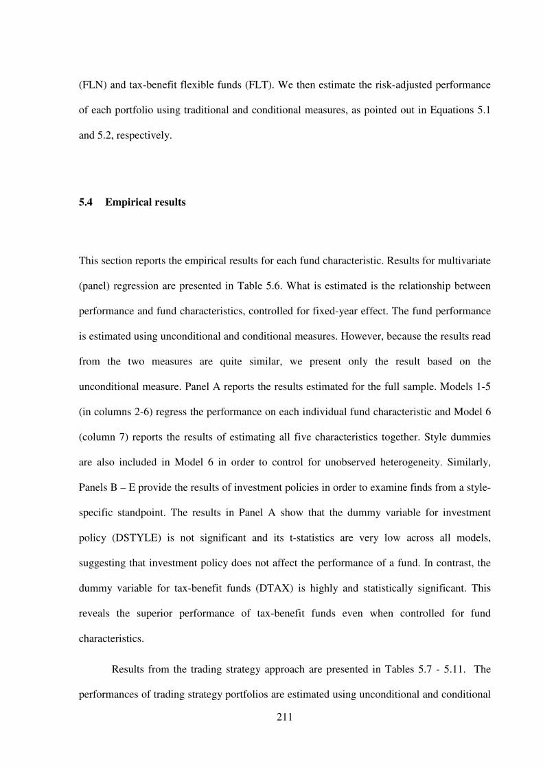
211
(FLN) and tax-benefit flexible funds (FLT). We then estimate the risk-adjusted performance
of each portfolio using traditional and conditional measures, as pointed out in Equations 5.1
and 5.2, respectively.
5.4 Empirical results
This section reports the empirical results for each fund characteristic. Results for multivariate
(panel) regression are presented in Table 5.6. What is estimated is the relationship between
performance and fund characteristics, controlled for fixed-year effect. The fund performance
is estimated using unconditional and conditional measures. However, because the results read
from the two measures are quite similar, we present only the result based on the
unconditional measure. Panel A reports the results estimated for the full sample. Models 1-5
(in columns 2-6) regress the performance on each individual fund characteristic and Model 6
(column 7) reports the results of estimating all five characteristics together. Style dummies
are also included in Model 6 in order to control for unobserved heterogeneity. Similarly,
Panels B – E provide the results of investment policies in order to examine finds from a style-
specific standpoint. The results in Panel A show that the dummy variable for investment
policy (DSTYLE) is not significant and its t-statistics are very low across all models,
suggesting that investment policy does not affect the performance of a fund. In contrast, the
dummy variable for tax-benefit funds (DTAX) is highly and statistically significant. This
reveals the superior performance of tax-benefit funds even when controlled for fund
characteristics.
Results from the trading strategy approach are presented in Tables 5.7 - 5.11. The
performances of trading strategy portfolios are estimated using unconditional and conditional

212
measures. Its abnormal returns and t-statistics (in parentheses) are shown in columns 2-3 and
5-6, respectively. Once again, the results are consistent across performance measures and,
therefore, we based our analysis on the unconditional measure. Columns 4 and 7 report the
differences in performance between the HIGH and the LOW portfolios and test whether it is
statistically different from zero.
Subsequently, sections 5.4.1 - 5.4.5 reveal the relationship between performance and
the following fund characteristics: past performance, size, net cash flows, age and size of
fund family respectively.
Table 5.6 Multidimensional (panel) analysis for determinants of fund performance The table shows the estimated results of annual fund performance regressed on fund attributes allowing for fixed-year effects. Coefficients and t-statistics (in parentheses) are reported, adjusted for heteroscedasticity using White’s (1980) model. Fund performances are calculated using an unconditional single-factor measure. lnTNA is the natural logarithm of average total asset value (TNA) of a fund in the year. PERFt-1 is the one-year lagged performance. NNCF refers to normalized net cash flows. lnAge is the natural logarithm of number of months since the fund’s inception date. DFamily is a dummy variable for family size, equal to 1 if belongs to the five largest companies, otherwise=0. Dstyle is a dummy for investment style, equal to 1 if an equity fund, otherwise=0. Dtax is a dummy variable for tax-benefit style, equal to 1 if a tax-benefit fund, otherwise=0. * Significant at a 10 % level. ** Significant at a 5% level. *** Significant at a 1% level
Variable Model 1 Model 2 Model 3 Model 4 Model 5 Model 6
Panel A: All funds PERF t-1 0.223*** 0.211*** (3.93) (3.31) lnTNA 0.0001 0.00003 (1.59) (0.3) NNCF t-1 0.0002** 0.0001 (2.19) (1.18) lnAge -0.00021* -0.00013 (-1.74) (-1.2) DFamily 0.00026** 0.0005*** (2.04) (2.58) DStyle 0.00003 -0.00005 0.00003 -0.00001 -0.00006 0.0001 (0.17) (-0.36) (0.17) (-0.09) (-0.41) (0.49) Dtax 0.0009*** 0.0011*** 0.0071*** 0.0008*** 0.0010*** 0.005*** (5.7) (7.6) (4.33) (4.69) (7.63) (2.76) R2 0.13 0.11 0.11 0.11 0.11 0.13

213
Variable Model 1 Model 2 Model 3 Model 4 Model 5 Model 6
Panel B: General Equity funds PERF t-1 0.231*** 0.986*** (3.57) (2.76) lnTNA 0.00023** 0.00013 (2.09) (1.01) NNCF t-1 0.0002 0.00003 (1.17) (0.17) lnAge -0.00032* -0.00027* (-1.7) (-1.74) DFamily 0.00026 0.00044* (1.46) (1.9) R2 0.13 0.10 0.10 0.10 0.10 0.13 Panel C: Tax-benefit Equity funds PERF t-1 0.0541 0.1639 (0.42) (0.96) lnTNA -0.00012 0.00005 (-1.12) (0.46) NNCF t-1 -0.00007 -0.00019 (-0.7) (-1.25) lnAge -0.00047 -0.00036 (-1.43) (-0.81) DFamily 0.00021 0.00032 (0.95) (1.07) R2 0.37 0.4 0.06 0.41 0.39 0.14 Panel D: General Flexible funds PERF t-1 0.302*** 0.266*** (3.8) (3.67) lnTNA -0.00007 -0.00021** (-0.74) (-2.21) NNCF t-1 0.0001 0.00021 (0.75) (1.63) lnAge 0.00003 0.00022 (0.18) (1.23) DFamily 0.00033** 0.0005** (1.97) (2.11) R2 0.27 0.22 0.21 0.22 0.23 0.35 Panel E: Tax-benefit flexible funds PERF t-1 0.0451 0.1453 (0.3) (0.98) lnTNA 0.00013** 0.00029* (2.1) (2.00) NNCF t-1 0.00008 -0.00001 (0.37) (-0.06) lnAge 0.00047** 0.00012 (2.68) (0.5) DFamily 0.00019 -0.0005 (0.84) (-1.28) R2 0.55 0.53 0.40 0.50 0.50 0.53

214
5.4.1 Persistence in performance
Table 5.6, Model 1, estimates whether fund performance is correlated with its performance in
the past year. The fund performance is estimated using a risk-adjusted unconditional
approach. The result shows that current performance increases with past performance and this
is highly and statistically significant. In addition, this is shown in Model 6 when other
characteristics are also included. Thus, we can conclude that there is evidence of performance
persistence in our fund sample. Nevertheless, since our sample is dominated by general
equity funds, we control for investment and tax policies and investigate the relationship
separately for each individual fund style.
Panels B to E show the results estimated at policy level. We find that the performance
of general equity and flexible funds can also be explained by the past year’s performance
(Panels B and D). In contrast, we do not find this evidence in any tax-benefit funds and its t-
statistical values are very low. Therefore, we suggest that there is persistence in the
performance of general mutual funds.
We also examine whether this evidence is robust and of any economic importance.
Table 5.7 presents evidence from the trading strategy approach. The table shows the
abnormal performance of trading strategy portfolios constructed on the basis of the past
year’s performance. We view past performance in two ways: risk adjusted returns (Panel A)
and raw returns (Panel B). In Panel A, the high past year’s returns portfolio insignificantly
outperforms the market. In contrast, the low past year’s returns portfolio underperforms the
market and is statistically significant at the 5% level. This makes the difference between the
two high and low past returns portfolios equal 0.13% per week or around 6% per annum. This
difference is highly and statistically significant. Consistent with the results in Table 5.7, we
find that persistence in performance is attributed to the evidence for general funds only, but

215
not to the tax-benefit funds. In contrast, results suggest that in tax-benefit funds the
differences in the high and the low past year’s returns portfolios are relatively small.
The results from Panel B, which estimates the performance of portfolios based on the
past year’s raw returns are comparable to the results in Panel A. For general funds, high past
year’s return portfolios do not earn abnormal returns, while low past year’s returns portfolios
generate significantly inferior performance. The differences between the two portfolios are
positively and highly significant but we do not find this evidence for the tax-benefit funds
portfolio.
Consequently, we can conclude that there is persistence in performance in Thai
mutual funds over our estimation period. This evidence is statistically and economically
important. However, it holds good only for general funds. In addition, our results suggest that
this result of persistence in performance applies only to poorly performing funds which
continue to perform badly. Past outperforming funds do not generate an abnormal return in a
subsequent period. Our results are consistent with several previous studies in developed
markets (for example, Grinblatt and Titmann, 1992; Hendricks et al., 1993; Goetzmann and
Ibbotson, 1994; Blake and Timmermann, 1998; Annaert et al., 2003; and Bauer, 2006).
However, this is in contrast to the evidence in Thailand suggested by Nitibhon (2004). He
shows that the first decile portfolio of funds has superior abnormal return but the long-short
strategy does not generate abnormal return. He also reveals that the superior performance in
the top decile portfolio is not due to the use of momentum strategy by fund managers.
Nevertheless, in our study, we do not observe whether the evidence of persistence is due to
the use of momentum strategy, as pointed out by Cahart (1997), and therefore this issue calls
for further investigation.

216
Table 5.7 Performance of trading strategy portfolios based on past performance The table presents performance estimated from trading strategy portfolios based on a past year’s returns using an unconditional Jensen’s measure (1968) and Ferson and Schadt’s conditional measure (1996). High refers to the equally weighted portfolio of the 30% highest past return portfolios and Low refers to the equally weighted portfolio of the 30% lowest past return portfolios. Panel A estimates using the past year’s raw returns and Panel B estimates using the past year’s risk-adjust single factor returns. T-statistics, adjusted for heteroscedasticity, using White’s (1980) model are in parentheses ( ). High-Low is the performance difference between the high and low portfolios and its t-statistics in parentheses ( ) test whether the performance is significant from zero. All refers to all funds, EQN to general equity funds, EQT to tax-benefit equity fund, FLN to general flexible funds and FLT to tax-benefit flexible funds. * significant at 10% ** significant at 5% *** significant at 1%
Unconditional Conditional
High Low High-Low High Low High-Low
Panel A: Single-factor measure
ALL 0.00023 -0.0011** 0.0013*** 0.00008 -0.0011*** 0.0012***
(0.6) (-2.54) (3.48) (0.21) (-2.85) (3.25)
EQN 0.00022 -0.00126** 0.0015*** 0.00007 -0.0014*** 0.0015***
(0.51) (-2.44) (3.29) (0.17) (-3.05) (3.29)
EQT -0.0006 -0.0002 -0.00046 -0.00048 0.00021 -0.0004
(-1.23) (-0.51) (-0.99) (-0.99) (0.53) (-0.86)
FLN 0.00002 -0.0011*** 0.0011** -0.00017 -0.001*** 0.0009**
(0.07) (-2.77) (2.5) (-0.61) (-2.96) (2.15)
FLT -0.00038 0.00013 -0.00007 -0.00054 0.00009 -0.00015
(-0.85) (0.38) (-0.2) (-1.53) (0.27) (-0.49)
Panel B: Raw returns
ALL 0.0002 -0.00072* 0.00091** 0.00003 -0.00042 0.00071*
(0.43) (-1.63) (2.14) (0.06) (-1.06) (1.77)
EQN 0.00021 -0.00087* 0.0011*** 0.00005 -0.001** 0.0011***
(0.44) (-1.8) (2.94) (0.13) (-2.45) (3.01)
EQT 0.0007* 0.0012*** -0.00048 0.00071* 0.0011*** -0.00038
(1.66) (2.97) (-1.28) (1.69) (2.75) (-1.03)
FLN 0.00012 -0.00058 0.000706 -0.00018 -0.00025 0.00008
(0.2) (-1.33) (1.04) (-0.34) (-0.64) (0.12)
FLT -0.00149** 0.00072 -0.0022*** -0.0013** 0.00042 -0.0018**
(-2.49) (1.63) (-2.83) (-2.3) (1.06) (-2.36)

217
5.4.2 Mutual fund size
Models 1 and 6 in Table 5.6 estimate the relationship between performance and mutual fund
size as measured by the natural logarithm of total net asset values at the beginning of the
year. We do not find this relationship in the whole sample estimation. However, the results in
Panels B- E reveal that size can explain fund performance to some extent but there are some
important differences across fund policies. We find that fund size is positively related to
performance in general equity funds and tax-benefit flexible funds. However, the evidence in
general funds is removed when other characteristics are included in the model. This is
probably due to the correlation between fund size and net cash flows. Conversely, we find a
negative relationship in flexible funds.
Table 5.8 reports the abnormal returns estimated from trading strategy portfolios
based on fund size. Panel A provides the results based on TNAs at the beginning of the year.
Results based on the average TNAs are also used to confirm the validity and are presented in
Panel B. Results from both panels are consistent and suggest that strategy portfolios based on
size do not yield abnormal performance. Therefore, even when there is evidence suggesting a
relationship between some mutual fund styles, this is not strong enough to be able to earn
abnormal returns on the basis of mutual fund size.
Our results are comparable to those of Nitibhon (2004), who applies cross-section
regression and reveals the positive relation in size and performance in Thai equity funds. In
addition, our results are also comparable to findings in other emerging markets which show
that performance increases with fund size ((Mei-Chen, 2006; Tng Cheong, 2007).
Nonetheless, it contrasts with most of the evidence in the US, which suggests a
negative relationship between size and fund performance (for instance, Indro et al. 1999;
Chen et al., 2004; Ferreira et al., 2009). Indro et al. (1999) pointed out that if a fund is larger

218
than marginal in size, there will be a negative impact on performance due to the diseconomies
of scales and liquidity constraints. Therefore, we conclude that the mutual funds in our
sample may not be large enough to reach marginal size.
Table 5.8 Performance of trading strategy portfolios based on fund size The table presents performance estimated from trading strategy portfolios based on fund size using an unconditional Jensen’s measure (1968) and Ferson and Schadt’s conditional measure (1996). Fund size is calculated using average total net asset values (Panel A) and total net asset values at the beginning of the year (Panel B). High refers to the equally weighted portfolio of the 30% largestportfolio and Low to the equally weighted portfolio of the 30% smallestportfolio. T-statistics, adjusted for heteroscedasticity, using White’s (1980) model are in parentheses ( ). High-Low represents the performance difference between the high and low portfolios and their t-statistics in parentheses ( ) test whether the performance is significant from zero. All refers to all funds, EQN to general equity funds, EQT to tax-benefit equity funds, FLN to general flexible funds and FLT to tax-benefit flexible funds. * significant at 10%, ** significant at 5% , *** significant at 1%
Single-factor Conditional
High Low High-Low High Low High-Low
Panel A: Average total net asset values
ALL -0.00009 -0.00038 0.00029 -0.00015 -0.00045 0.00030
(-0.3) (-0.93) (1.04) (-0.52) (-1.19) (1.04)
EQN -0.00013 -0.00058 0.000446 -0.0002 -0.00074 0.00055
(-0.41) (-1.16) (1.31) (-0.62) (-1.61) (1.59)
EQT 0.0010*** 0.0005 0.000439 0.0010*** 0.00061 0.00031
(2.63) (1.12) (1.04) (2.68) (1.38) (0.74)
FLN -0.00015 0.00007 -0.00022 -0.00039 -0.0003 -0.00009
(-0.43) (0.2) (-0.53) (-1.23) (-1) (-0.22)
FLT 0.00041 -0.00015 0.000474 0.00035 -0.00022 0.00057
(1.59) (-0.29) (1.05) (1.45) (-0.43) (1.3)
Panel B: Total net asset values at beginning of the period
ALL -0.00032 -0.00014 -0.00018 -0.00043 -0.00022 -0.00021
(-1) (-0.35) (-0.71) (-1.36) (-0.58) (-0.84)
EQN -0.00021 -0.00033 0.00011 -0.0003 -0.00051 0.00021
(-0.62) (-0.68) (0.34) (-0.87) (-1.14) (0.65)
EQT 0.00093** 0.00079** 0.000133 0.00098** 0.0008** 0.00019
(2.12) (2.03) (0.31) (2.26) (2.03) (0.45)
FLN -0.0003 -0.0003 0.00000 -0.00051* -0.00039 -0.00011
(-0.93) (-0.78) (0.01) (-1.81) (-1.18) (-0.3)
FLT -0.00021 0.00014 -0.00006 -0.00015 0.00029 -0.00004
(-0.78) (0.31) (-0.13) (-0.62) (0.67) (-0.09)

219
5.4.3 Net cash flows
This section presents evidence of the relationship between net cash flows and fund
performance. The net cash flows of funds are measured by the normalised net cash flows
(NNCFt-1) based on a one-year lagged period. On the basis of panel regression estimation
(Table 5.6), we find that, for a full sample (panel A), the coefficient of lagged net cash flows
equals 0.0002 and this is significant at the 5% level. However, this evidence is removed when
all characteristics are combined, in Model 6. This is possibly due to its correlation with fund
size. This relationship is also considered within the policy specifics in Panels B-E and we do
not find any statistically significant evidence in any fund group. Although it is insignificant,
the results suggest that performance is positively related with the past year’s net cash flows in
general funds but negatively related in tax-benefit funds.
Additionally, results from the trading strategy portfolios based on lagged cash flows
in Table 5.9 (Panel A) also reveal similar findings that, for the whole sample, high and low
past year cash flows portfolios do not perform significantly differently. However, when
investment policy is taken into account, the difference in general flexible funds is positively
and highly significant, implying the ‘smart money effect’ – that is, flexible fund investors
have the ability to identify superior funds in the subsequent period (Zheng, 1999).
However, this is in contrast to the evidence from tax-benefit funds. The results
suggest that tax-benefit funds with high net cash flows perform lower than funds with low net
cash flows. The figures are highly and statistically significant and account for up to 0.16%
and 0.14% per week on tax-benefit equity and flexible funds, respectively.
In addition, we also consider the effect of current cash flows on fund performance.
The results are presented in Table 5.9, Panel B. We do not find any difference in performance
between the high and the low current cash flow portfolios. This is consistent with Nitibhon
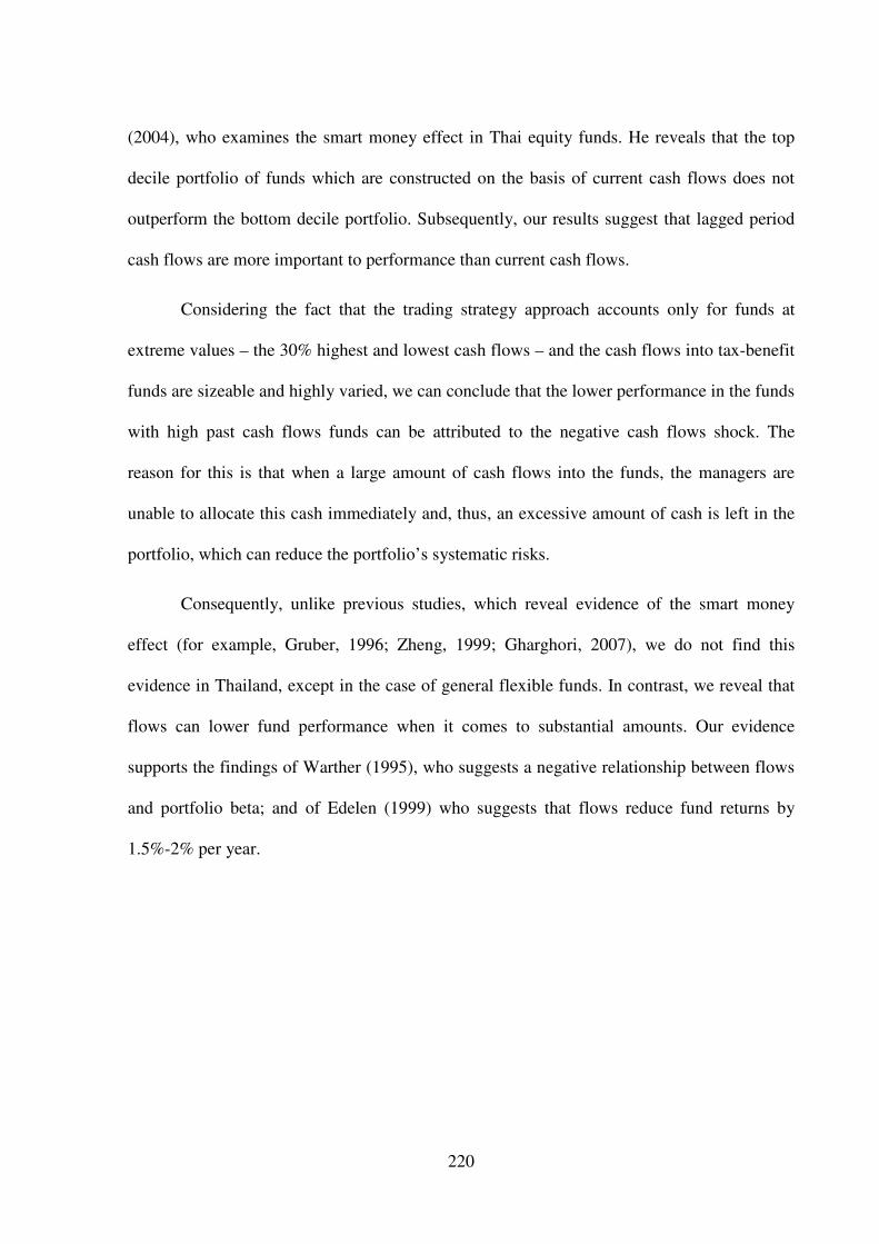
220
(2004), who examines the smart money effect in Thai equity funds. He reveals that the top
decile portfolio of funds which are constructed on the basis of current cash flows does not
outperform the bottom decile portfolio. Subsequently, our results suggest that lagged period
cash flows are more important to performance than current cash flows.
Considering the fact that the trading strategy approach accounts only for funds at
extreme values – the 30% highest and lowest cash flows – and the cash flows into tax-benefit
funds are sizeable and highly varied, we can conclude that the lower performance in the funds
with high past cash flows funds can be attributed to the negative cash flows shock. The
reason for this is that when a large amount of cash flows into the funds, the managers are
unable to allocate this cash immediately and, thus, an excessive amount of cash is left in the
portfolio, which can reduce the portfolio’s systematic risks.
Consequently, unlike previous studies, which reveal evidence of the smart money
effect (for example, Gruber, 1996; Zheng, 1999; Gharghori, 2007), we do not find this
evidence in Thailand, except in the case of general flexible funds. In contrast, we reveal that
flows can lower fund performance when it comes to substantial amounts. Our evidence
supports the findings of Warther (1995), who suggests a negative relationship between flows
and portfolio beta; and of Edelen (1999) who suggests that flows reduce fund returns by
1.5%-2% per year.

221
Table 5.9 Performance of trading strategy portfolios based on net cash flows The table presents performance estimated from trading strategy portfolios based on past year net cash flows funds, using an unconditional Jensen’s measure (1968) and Ferson and Schadt’s conditional measure (1996). Net cash flows are calculated assuming that flows occur at the beginning of the period. Results from the current net cash flows are presented in Panel A and results from the lagged year net cash flows are presented in Panel B. High refers to the equally weighted portfolio of the funds with 30% highest net cash flows and Low refers to the equally weighted portfolio of funds with the 30% lowest net cash flows. T-statistics, adjusted for heteroscedasticity, using White’s (1980) model are in parentheses ( ). High-Low is the performance difference between the high and low portfolios and its t-statistics in parentheses ( ) test whether the performance is significant from zero. All refers to all funds, EQN to general equity funds. EQT to tax-benefit equity funds, FLN to general flexible funds and FLT to tax-benefit flexible funds. * significant at 10%, ** significant at 5%, *** significant at 1%
Single-factor Conditional
High Low High-Low High Low High-Low
Panel A: lagged year net cash flows
ALL -0.0002 0.00021 -0.00046 -0.00019 -0.00015 -0.0005
(-0.45) (0.78) (-1.22) (-0.44) (-0.62) (-1.34)
EQN -0.00021 -0.00024 0.00002 -0.00034 -0.00028 -0.00006
(-0.55) (-0.53) (0.12) (-0.95) (-0.66) (-0.35)
EQT -0.00022 0.00075** -0.0016*** -0.00038 0.00077** -0.002***
(-0.38) (1.99) (-3.2) (-0.72) (2.05) (-3.5)
FLN 0.00043 -0.00032 0.0015*** 0.00039 -0.00052 0.0015***
(1.16) (-0.64) (4.34) (1.07) (-1.25) (4.35)
FLT -0.00093** 0.00028 -0.0014*** -0.0010** 0.00029 -
0.0014***
(-2.36) (0.59) (-2.63) (-2.58) (0.68) (-2.92)
Panel B: Current net cash flows
ALL -0.00045 0.00001 -0.00046 -0.00052 -0.00009 -0.00043
(-1.12) (0.01) (-1.28) (-1.31) (-0.29) (-1.2)
EQN -0.00074 -0.00004 -0.0007 -0.00094* -0.00011 -0.0008*
(-1.41) (-0.11) (-1.56) (-1.78) (-0.31) (-1.81)
EQT 0.00051 0.00016 0.000328 0.00054 0.00018 0.000324
(1.55) (0.39) (0.91) (1.59) (0.47) (0.93)
FLN -0.00075 0.00017 -0.00092 -0.00086 -0.00006 -0.0008
(-0.99) (0.55) (-1.16) (-1.2) (-0.21) (-1.01)
FLT 0.00047* -0.0003 0.000684 0.00041* -0.00047 0.0009**
(1.76) (-0.59) (1.6) (1.69) (-0.97) (2.15)

222
5.4.4 Fund longevity
We measure the longevity of funds by the operation period of mutual funds since its
registration date. The results from the panel regression, Table 5.6 (Model 4), present weak
evidence that young funds perform better than old funds. This evidence even disappears when
all the characteristics are combined in Model 6. In addition, the results from Panels B-E
suggest that the negative relationship in young funds is only applicable to general equity
funds. There is no evidence of it in any other fund category.
Subsequently, we examine whether fund age can be used as a criterion in determining
outperforming funds. The results in Table 5.10 show that the differences between old and
young funds are small and not enough to be significant for any fund policies. Thus, we
conclude that fund longevity does not explain mutual fund performance. This differs from the
conclusions of Blake and Timmermann (1988), who find that UK unit trusts perform better in
the early stage of their operation; and from Otten and Bams (2002), who reveal a negative
correlation in some European funds. However, our results are comparable to those of recent
studies such as Prather et al. (2004), who find no relationship between age and performance
in US funds; and Ferreira et al. (2009), who suggest that, after controlling for size, age does
not provide explanatory power in the case of domestic funds.
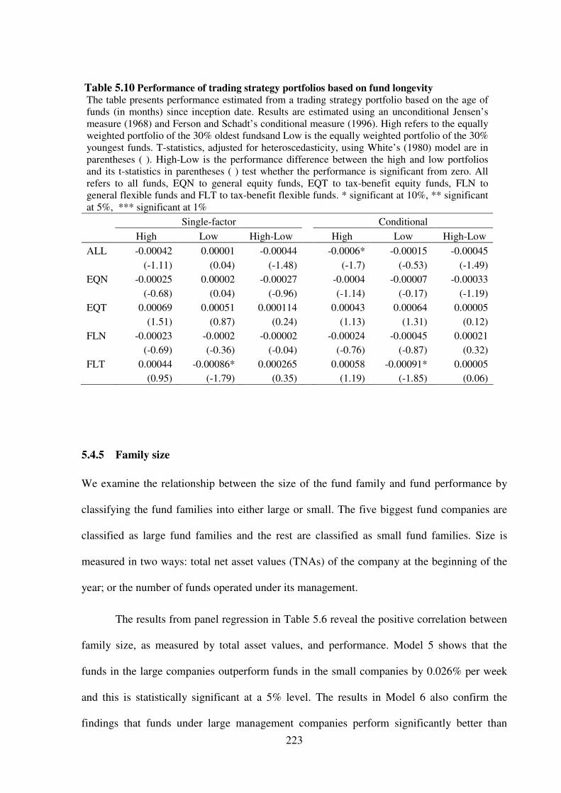
223
Table 5.10 Performance of trading strategy portfolios based on fund longevity The table presents performance estimated from a trading strategy portfolio based on the age of funds (in months) since inception date. Results are estimated using an unconditional Jensen’s measure (1968) and Ferson and Schadt’s conditional measure (1996). High refers to the equally weighted portfolio of the 30% oldest fundsand Low is the equally weighted portfolio of the 30% youngest funds. T-statistics, adjusted for heteroscedasticity, using White’s (1980) model are in parentheses ( ). High-Low is the performance difference between the high and low portfolios and its t-statistics in parentheses ( ) test whether the performance is significant from zero. All refers to all funds, EQN to general equity funds, EQT to tax-benefit equity funds, FLN to general flexible funds and FLT to tax-benefit flexible funds. * significant at 10%, ** significant at 5%, *** significant at 1%
Single-factor Conditional
High Low High-Low High Low High-Low
ALL -0.00042 0.00001 -0.00044 -0.0006* -0.00015 -0.00045
(-1.11) (0.04) (-1.48) (-1.7) (-0.53) (-1.49)
EQN -0.00025 0.00002 -0.00027 -0.0004 -0.00007 -0.00033
(-0.68) (0.04) (-0.96) (-1.14) (-0.17) (-1.19)
EQT 0.00069 0.00051 0.000114 0.00043 0.00064 0.00005
(1.51) (0.87) (0.24) (1.13) (1.31) (0.12)
FLN -0.00023 -0.0002 -0.00002 -0.00024 -0.00045 0.00021
(-0.69) (-0.36) (-0.04) (-0.76) (-0.87) (0.32)
FLT 0.00044 -0.00086* 0.000265 0.00058 -0.00091* 0.00005
(0.95) (-1.79) (0.35) (1.19) (-1.85) (0.06)
5.4.5 Family size
We examine the relationship between the size of the fund family and fund performance by
classifying the fund families into either large or small. The five biggest fund companies are
classified as large fund families and the rest are classified as small fund families. Size is
measured in two ways: total net asset values (TNAs) of the company at the beginning of the
year; or the number of funds operated under its management.
The results from panel regression in Table 5.6 reveal the positive correlation between
family size, as measured by total asset values, and performance. Model 5 shows that the
funds in the large companies outperform funds in the small companies by 0.026% per week
and this is statistically significant at a 5% level. The results in Model 6 also confirm the
findings that funds under large management companies perform significantly better than

224
others. However, the results at the policy level suggest that this evidence is typical of general
funds. General equity and flexible funds which belong to large management companies
perform significantly better. However, we do not find significant evidence from tax-benefit
funds.
We investigate the economic importance of family size to fund performance and show
the results in Table 5.11. The table compares the differences between large and small family
fund portfolios. In Panel A, family size is classified by the TNAs of a fund company and in
Panel B, family size is classified by number of funds owned by a company. We do not find
significant evidence from funds of any fund policy.
Thus, we can conclude that there is a positive relationship between family size and
performance in general funds, which agrees with the findings of previous studies such as
Indro et al. (1999) and Ferreira et al. (2009). However the performance differences between
large and small fund companies are not economically significant, which endorses the
evidence in Thailand of large fund companies not outperforming small companies (Kasikorn
Research, 2005)

225
Table 5.11 Performance of trading strategy portfolios based on size of fund family The table presents performance of portfolio based on size of fund family. Size is measured by total net asset values of company (Panel A) number of funds in the family (Panel B). Results are estimated using an unconditional Jensen’s measure (1968) and Ferson and Schadt’s conditional measure (1996). High refers to the equally weighted portfolio of funds belong the five largest management companies and Low to the equally weighted portfolio of remaining funds. T-statistics, adjusted for heteroscedasticity, using White’s (1980) model are in parentheses ( ). High-Low is the performance difference between the high and low portfolios and its t-statistics in parentheses ( ) test whether the performance is significant from zero. All refers to all funds, EQN to general equity funds, EQT to tax-benefit equity funds, FLN to general flexible funds and FLT to tax-benefit flexible funds. * significant at 10%, ** significant at 5%, *** significant at 1%
Single-factor Conditional
High Low High-Low High Low High-Low
Panel A: Total net asset values
ALL -0.00007 -0.00029 0.000224 -0.00011 -0.00044 0.000329
(-0.22) (-0.7) (0.65) (-0.36) (-1.16) (0.95)
EQN -0.00013 -0.00038 0.000253 -0.00017 -0.0006 0.000426
(-0.36) (-0.79) (0.61) (-0.48) (-1.37) (1.03)
EQT 0.00121** 0.00079* 0.000134 0.00083* 0.0006 -0.00004
(2.53) (1.66) (0.34) (1.9) (1.42) (-0.11)
FLN -0.00013 -0.0003 0.000173 -0.00022 -0.00053 0.000315
(-0.42 ) (-0.67) (0.35) (-0.74) (-1.38) (0.7)
FLT 0.00025 -0.00006 0.00015 0.00016 -0.00004 0.00007
(0.98) (-0.17) (0.44) (0.65) (-0.11) (0.2)
Panel B: Number of funds
ALL -0.00041 -0.00008 -0.00033 -0.00054 -0.0002 -0.00034
(-1.05) (-0.27) (-1.18) (-1.48) (-0.73) (-1.18)
EQN -0.00059 -0.00008 -0.00051 -0.00076* -0.00026 -0.0005
(-1.29) (-0.23) (-1.42) (-1.78) (-0.77) (-1.4)
EQT 0.00074 0.00063* 0.00006 0.00051 0.00061* 0.000018
(1.59) (1.75) (0.19) (1.27) (1.74) (0.06)
FLN -0.00022 -0.00022 0.00000 -0.00035 -0.00043 0.00008
(-0.8) (-0.42) (0) (-1.32) (-0.96) (0.16)
FLT 0.00031 -0.00036 0.000454 0.00021 -0.00031 0.000328
(1.17) (-1.08) (1.65) (0.81) (-0.92) (1.22)

226
5.5 Robustness of the results
In order to test the robustness of the results, these estimates use a cross-section time-series
average regression approach following Fama and Macbeth (1973), who suggest that the error
terms are likely to be correlated over time and that using pooled regression could violate the
OLS assumptions. Therefore, they suggest an alternative approach in estimating cross-section
regression in panel data which treats each fund-year observation non-independently. The
Fama-Macbeth approach is in two steps. The first step is to perform a cross-section
regression of fund performance in fund characteristics for each period. The model is
expressed as:
.,...2,1; teachforNpCHARACPERF tptptpt =+′+= εβα (5.5)
where PERFpt represents the performance of mutual fund p in period t estimated with the use
of either a traditional or conditional measure; CHARACp is a set of five mutual fund
characteristics, namely: total net asset values of the fund; past year’s performance; age of
mutual fund; annual net cash flows; and a dummy variable corresponding to family size. We
also include two other controlled variables; mutual fund style and tax benefit purpose.
The second step is to estimate the coefficients by obtaining the average coefficients of
the first step. Moreover, the standard deviations of coefficients estimated in the first step are
used to generate sampling errors. The mathematical expressions for estimated coefficients
and sampling errors are:
∑=
=T
t
tT 1
ˆ1ˆ ββ (5.6)
∑=
−=T
t
tT 1
2
2
2 )ˆˆ(1
)ˆ( βββσ (5.7)

227
Nevertheless, if the independent variables are not correlated over time, the Fama-Macbeth
procedure will be numerically equivalent to a pooled regression with the correction of
standard errors.
The results are presented in Table 5.12 and are estimated using the whole sample
(Panel A) and a sub sample for each fund style (Panel B). For the whole sample, another two
controlled variables are included capturing the effects of difference in fund styles.
Past performance (PERFt-1) is positively related to current performance. The slope
coefficients equal 0.19 and 0.26 using unconditional and conditional measures, respectively.
Nonetheless, evidence of persistence in performance is observed in general funds. The results
in panel B show that the slope coefficients of past returns are positively significant in both
general equity and flexible funds, but not in tax-benefit funds. The slope coefficient of
normalised net cash flows (NNCFt-1) is negatively significant, suggesting a negative
relationship of flows and performance. However, the results in panel B suggest that this is
generated from general equity funds. Furthermore, the slope coefficients of the normalised
net cash flows are negative in general funds but positive in tax-benefit funds. The effect of
fund age (lnAGE) is shown only in the general flexible funds which show a positive
relationship with fund performance. We do not find evidence that mutual fund size (lnSIZE)
and fund family (FAMILY) can explain fund performance. Thus, results based on Fama-
Macbeth approach show some support and some conflict with the findings in Section 5.4. We
find persistence in fund performance; but fund performance is not explained by fund size or
fund family size and these findings are comparable to our empirical findings in Section 5.4.
Nevertheless, results on net flows and fund age are not robust across the measure. Hence, we
conclude that the relationship between performance and fund characteristics estimated by a
cross-section approach can be sensitive to the measure used and this calls for further
investigation.

228
Table 5.12 Multivariate regression (Cross-section time-series average) The table shows the Fama-Macbeth (1973) estimates of annual fund performance regressed on fund attributes. Fund performances are calculated using traditional and conditional Jensen measures. lnSIZE is the natural logarithm of average total asset values (TNAs) of a fund in a year. PERFt-1 refers to the one-year lagged performance, NNCF to normalized net cash flows. lnAge is the natural logarithm of the number of months since the fund’s inception date. DFamily is a dummy variable for family size, equal to 1 if it belongs to the five largest companies, otherwise=0. DSTYLE is a dummy for investment style, equal to 1 if the fund is an equity fund, otherwise=0. DTAX is a dummy variable for tax-benefit style, equal to 1 if a tax-benefit fund, otherwise=0. The sample extends from June 2000 to August 2007. T-statistics are in parentheses ( ). * Significant at a 10 % level. ** Significant at a 5% level. *** Significant at a 1% level
Constant lnSIZE PERFt-1 NNCFt-1 lnAge DFamily DSTYLE DTAX R2
Panel A: Whole sample
Traditional 0.0000 0.0000 0.1860** -0.0006** -0.0002 0.0004 0.0003 0.0015 0.20
(0) (0.37) (2.55) (-3.11) (-0.84) (1.42) (1.29) (1.77)
Conditional 0.0005 0.0000 0.2600** -0.0004 -0.0002 0.0004 0.0003 0.0014 0.25
(0.36) (0.1) (3.01) (-1.46) (-0.74) (1.38) (1.23) (1.61)

229
Table 5.12 Multivariate regression (Cross-section time-series average) Cont’d
Constant lnSIZE PERFt-1 NNCFt-1 lnAge DFamily R2
Panel B: Classified by fund style
General Equity funds
- Traditional 0.0015 0.0002 0.3580** -0.0016* -0.0007 0.0003 0.28
(0.91) (0.91) (3.46) (-2.14) (-1.38) (0.93)
- Conditional 0.0008 0.0002 0.2670** -0.0016** -0.0006 0.0002 0.20
(0.58) (1.09) (3.05) (-2.78) (-1.41) (0.85)
Tax-benefit Equity funds
- Traditional -0.0145 -0.0020 0.3780* 0.0020 0.0066 0.0003 0.75
(-1.1) (-1.98) (2.37) (1.43) (1.36) (0.33)
- Conditional -0.0189 -0.0020 0.4000 0.0024 0.0078 0.0004 0.71
(-1.32) (-1.7) (1.74) (1.34) (1.42) (0.41)
General Flexible funds
- Traditional -0.0021 -0.0001 0.3540** 0.0008 0.0006** 0.0001 0.40
(-1.62) (-0.48) (2.96) (1.18) (3.14) (0.3)
- Conditional -0.0025* -0.0001 0.1690 -0.0001 0.0007** -0.0001 0.44
(-2.02) (-0.97) (0.98) (-0.27) (2.82) (-0.37)
Tax-benefit Flexible funds
- Traditional -0.0117 -0.0009 0.1270 0.0014 0.0040 0.0006 0.80
(-0.87) (-1.11) (0.43) (1.78) (1.01) (0.43)
- Conditional -0.0176 -0.0007 0.1090 0.0008 0.0055 -0.0001 0.78
(-0.95) (-1.35) (0.3) (1.2) (1.01) (-0.09)

230
5.6 Conclusions
In addition to the abundant literature on mutual fund performance, the growth and popularity
of mutual fund investment have led to another question to the mutual fund study. This is how
one can distinguish a superior performing fund from others. The present study explored this
question and examined the relationship of fund performance to an extensive set of mutual
fund characteristics. We examined five fund characteristics, making this the most
comprehensive study of them in emerging markets so far. The five characteristics consisted
of size, past performance, net cash flows, fund longevity and family size. Additionally, we
focused on fund performance on a risk-adjusted basis and disentangled the problem using
both multidimensional (panel) regression and the trading strategies portfolios. The former
approach allowed us to investigate the fund characteristics as a group, allowing the
association with characteristics to be controlled. In contrast, the latter approach, using the
trading strategies portfolios, allowed us to examine whether selecting funds based on these
characteristics is economically important. Therefore, the results of combining these two
approaches would provide us with more meaningful results than previous studies have done.
We find evidence of specific determinants of mutual fund performance for individual
investment policies. There is persistence in performance in general funds but not in tax-
benefit funds. This persistence is both statistically and economically significant. However,
persistence is evident only from poorly performing funds, which continue to perform poorly
in the next period; this is consistent with the empirical evidence in the US literature
(Hendricks et al., 1993; Goetzmann and Ibbotson, 1994; Bauer et al., 2006; Ferreira et al.,
2009).

231
The relationship between size and fund performance is also subject to policy specifics
and the evidence is stronger in flexible funds than in equity funds. Small general flexible
funds tend to perform better and, in contrast, small tax-benefit flexible funds tend to perform
worse than others. Nonetheless, the effect of fund size is not strong enough for investors to
earn abnormal returns on this basis. This is inconsistent with the contention in the US of
diseconomies of scale (Indro, 1999; Chen et al., 2004; Ferreira et al., 2009).
Net cash flows have very little impact on fund performance as a whole, which
contradicts the evidence of the smart money effect (Gruber, 1996; Zheng, 1999 Gharghori et
al., 2007; Keswani and Stolin, 2008). In addition, we find that tax-benefit funds with
relatively high cash flows perform significantly lower than funds with low cash flows. This
finding confirms the view of Warther (1995) and Edelen (1999), who suggest that cash flows
shock can lead to inferior performance in the next period because it is lower the portfolio’s
beta risk.
Young funds perform better than old funds among general equity funds and general
funds which belong to large fund companies also tend to perform better. However, these two
attributes are not economically significant and, therefore, investors are unable to earn
abnormal returns on the basis of these characteristics. In addition, we find that our results
could be sensitive to the regression method used in the analysis.
Thus, from our results we conclude that it is difficult on the basis of their
characteristics to select funds which earn abnormal returns, even though their performance
can be explained by some particular characteristics. Nevertheless, our results suggest three
important findings and some practical implications. The main three findings are: first, we find
strong evidence of persistence in performance in the Thai general mutual funds, which is a
primary reason to reject the efficient market hypothesis. Nevertheless, we do not consider the

232
use of momentum strategy in fund managers in this study (Jegadeesh and Titmann, 1993;
Cahart, 1996). This issue calls further investigation in a subsequent study.
Second, we find that tax-benefit funds with high cash flows perform significantly
lower than those with low cash flows. Thus, we argue that the cash flows shock is negatively
affected in fund performance. While cash flows into the funds in developed markets are quite
stable over time, emerging market mutual funds experience high and vulnerable cash flows.
In Thailand, tax-benefit funds received exceptionally high cash flows due to the government
campaign featuring long-term and retirement savings (Table 5.3). Thus, fund managers need
to be more responsive to this impact. In addition, the subject requires detailed exploration of
the effect of cash flows on performance in emerging markets.
Third, evidence on the panel regression confirms the highly significant outperforming
of tax-benefit mutual funds even when it is controlled for fund characteristics. Therefore, we
may conclude that superior performance can be a result of their own unique characteristics
which are restricted the long-term investment; or it can even be attributed to better skills on
the part of the fund managers and, subsequently, this requires a further examination to see
what causes them.
The practical implications from this study are that it is difficult to make a fund
selection on the basis of fund characteristics, such as size, family size and fund longevity
because these characteristics do not impact on fund returns. Nevertheless, short-term past
performance can be a good criterion in selecting funds. Investors should look at short-term
risk-adjusted performance and try to avoid funds which have performed poorly in the
previous year. Fund managers, in particular managers of tax-benefit funds, need to be more
responsive to cash flows. Cash flow prediction and a controlling policy for cash flows may be
required in order to avoid negative performance due to the cash flow shock.

233
CHAPTER SIX
THE LIQUIDITY PREMIUM, SHARE RESTRICTION AND MUTUAL FUND
PERFORMANCE
6
Abstract
This study looks at the relationship between liquidity and mutual fund performance in
Thailand, using a return-based stale price measure to quantify the liquidity of the assets
contained in the portfolio (Getmansky et al., 2004). We find evidence of an illiquidity
premium in Thai mutual funds. Thailand’s tax-benefit funds contain slightly – but not
statistically significantly – more illiquid assets than do general funds. Subsequently, the study
proposes a liquidity-augmented performance measure to capture the premium in liquid assets
as it is measured by the share turnover ratio. We find that our liquidity factor has explanatory
power for mutual fund returns and its magnitude increases with the degree of illiquidity. With
the liquidity-augmented measure, mutual fund returns are reduced and evidence of abnormal
returns in low liquid portfolios is removed but the evidence of a liquidity premium is still
present. This suggests the importance of the liquidity factor in the fund performance even
though share turnover ratio is not a good proxy for the liquidity premium. Finally, the results
are robust as regards the method used in quantifying illiquidity assets and are not affected by
seasonality.

234
6.1 Introduction
The role of liquidity in asset pricing and stock returns has attracted growing interest over the
past decade. Nonsynchronous trading is an example of illiquidity which impacts on the
estimation of stock returns. Previous studies find nonsynchronous trading results in the bias
beta estimation in the capital asset pricing model (see, for example, Scholes and Williams,
1977; Dimson, 1979; Lo and Mackinlay, 1988, 1990). Furthermore, less liquid assets are
likely to generate a return premium due to the clientele effect. Many studies have investigated
the relationship between liquidity and asset returns and confirmed the liquidity premium,
admitting also that liquidity can explain cross-sectional returns (see, for example, Amihud
and Mendelson, 1986; Brennan et al., 1998; Datar et al. 1998; Rouwenhorst, 1999; Amihud,
2002; Pastor and Stambaugh, 2003; Acharya and Pedersen, 2005; Liu, 2006). However, these
studies still focus on the security context and we still know very little about the way in which
liquidity influences other financial assets. More recently, few studies document the fact that
liquidity also impacts on hedge fund returns. In the seminal article of Getmansky et al.
(2004), the writers suggest that hedge fund returns are serially correlated not only because of
nonsynchronous trading but also because of the illiquidity of the stocks contained in their
portfolios. Aragon (2007) also shows that hedge funds with lockup restrictions perform better
than nonlockup funds and that those lockup hedge funds generate an illiquidity premium of
4%-7% per year.
Nonetheless, the impact on liquidity has never so far been extended to the mutual
fund literature, although its underlying assets are dominated by stocks. More importantly,
since empirical evidence suggests that liquidity leads to inconsistency in estimating risk and
return, it could equally influence the measurement of mutual fund performance, since most
prevailing performance measures are based on the standard capital asset pricing model.

235
In addition, liquidity is one of the major concerns in emerging markets. Several
researchers reveal that emerging markets often feature low liquidity and infrequent trading
(Harvey, 1995; Bekaert and Harvey, 2003). Therefore, emerging markets would seem to be
an ideal setting for investigating the evidence of a liquidity premium. Subsequently, the aim
of this chapter is to investigate the role of liquidity in mutual fund performance and
performance measures in an emerging market.
This study will, it is hoped, make several contributions. First, it extends the
knowledge of the role of liquidity in asset returns in the context of mutual funds. This, to the
best of our knowledge, is the first empirical study of this area in the mutual fund literature.
Second, we adopt an alternative approach in measuring mutual fund liquidity. The return-
based stale price measure allows us to quantify liquidity in funds’ underlying assets,
implicitly using fund return data (Getmansky et al., 2004). This measure has been proposed
and used in the hedge fund literature but hitherto it has never been applied to other financial
assets. Thus, this also allows us to investigate how to verify a model outside the hedge fund
literature. Third, we propose an auxiliary mutual fund performance measure which includes
one additional liquidity factor and we investigate whether liquidity is an important factor in
this performance measure. Our proposed performance measure can be viewed as a factor
model which would allow investors to understand how fund managers allocate their
portfolios and how to identify the source of the return premium which they receive. Fourth,
we employ data from one of the emerging economies. Since emerging markets are less liquid
and suffer from chronically infrequent trading, this would allow a powerful test and provide
useful evidence about the liquidity premium. Finally, we outline the policy implications
related to the long-term investment policy of the tax-benefit funds scheme in Thailand.
We consider Thai mutual fund data from 2002 to 2007 consisting of 211 mutual
funds, made up of 152 equity funds and 59 flexible funds, and observe the liquidity premium

236
in the funds using a return-based stale price measure, as proposed by Getmansky et al.
(2004), which suggests that the true observed return is a function of unobserved economic
returns. Subsequently, to capture liquidity premium in the funds, we propose a liquidity-
augmented performance measure which includes a liquidity factor as measured by share
turnover.
We find that the liquidity of assets contained in the mutual fund portfolio plays an
important part in mutual fund returns. The highest liquidity mutual fund portfolio
significantly underperforms the market in contrast to the lowest liquidity mutual fund
portfolio, which significantly outperforms the market. Our proposed liquidity-augmented
model makes performance slightly lower, particularly that of illiquid portfolios. We find that
our liquidity factor has explanatory power in all but two of the most liquid portfolios. This
suggests that low liquidity mutual funds allocate their portfolios on the basis of illiquidity
assets in order to obtain the liquidity premium. Nevertheless, evidence of liquidity premium
still persists when our liquidity factor is incorporated. Thus, turnover seems not to be the best
factor by which to explain the liquidity premium in Thai mutual funds. Finally, we look at
policy implications by considering the differences in liquidity between general and tax-
benefit funds. We hypothesize that, due to restrictions imposed on the tax benefit funds, these
mutual funds would invest in illiquid assets more than general funds would and,
subsequently, would earn a liquidity premium. We find that the tax-benefit funds contain
more illiquidity assets, but not enough to be statistically significant. Therefore, the evidence
of outperforming in tax-benefit funds does not result from the illiquidity premium alone.
The rest of this chapter is organised as follows. Section 6.2 gives a literature survey
and hypotheses for the study. Section 6.3 describes the data and methodology used. Section
6.4 presents the empirical results. Section 6.5 provides the results of a robustness test and,
finally, Section 6.6 draws some conclusions and makes suggestions for future research.

237
6.2 Literature and hypotheses
The effect of infrequent or nonsynchronous trading has long been discussed in the finance
literature. This effect is observed when stock prices trade at different time intervals but are
recorded at intervals of the same interval length (i.e. daily closing prices). Subsequently, this
creates bias in the movement and co-movement of stock returns, resulting in serial correlation
and cross serial correlation. Dimson (1979) shows that betas estimated from UK stock returns
over the period 1955-1974 increase with trading frequency, suggesting the bias in beta
estimation. Therefore, stock with infrequent trading will have a beta estimated downward
bias while stock with frequently traded stocks will have a beta estimated upward bias.
Subsequently, to capture this effect, he proposed the ‘aggregated coefficient method’, which
includes leads and lags variables in order, and found that the bias in estimated betas is
eliminated once this method is used.
Investment portfolios also have an impact from nonsynchronous trading through the
computation of the net asset values (NAVs). Bhargava et al. (1998), Goetzmann et al. (2001)
and Boudoukh et al. (2002) suggest that the net asset values of mutual funds reflect stale
prices due to the nonsynchronous trading effects on the prices of their underlying assets.
However, they suggest that this effect transfers wealth from buy-and-hold investors to those
who engage with a timing forecast.
Getmansky et al. (2004) argue that nonsynchronous trading is part of the cause of
serial correlation in hedge funds. Hedge funds can also have high serial correlation even
when their underlying stocks are synchronous, if these stocks are not actively traded. They
observe plausible sources of serial correlation in hedge fund returns and show that time-
varying expected returns, time-varying leverage and incentive fees with high water marks are

238
insufficient to explain the serial correlation in hedge fund returns. Thus, evidence of serial
correlation is most likely to be explained by illiquidity and smoothed returns. They propose
an econometric model followed a moving average process in quantifying illiquidity and
smoothing returns and empirically investigate a large hedge fund dataset during the period
1977-2001. Their results confirm that illiquidity exposure and smoothing returns are sources
of serial correlation in hedge fund returns.
Illiquidity also has an impact on asset returns, referring to implicit transaction cost
(i.e. the maximum expected return that an investor is willing to exchange for a zero
transaction cost). Amihud and Mendelson (1986) proposed a model by which, in equilibrium,
expected returns increase with illiquidity, as measured by the bid-ask spread. They also
showed that there is a ‘clientele effect’ in which longer horizon investors have a positive
relation to expected returns because they hold more in illiquid assets. They also find a
positive and concave relationship between expected return and transaction cost. In addition,
they test their hypothesis using data for the period 1961-1980 and find that their results are
consistent with their model.
In contrast, Eleswarapu and Reinganum (1993) re-investigate the relationship between
return and bid-ask spread, using the same methodology as in Amihud and Mendelson (1986).
They find, in contrast to Amihud and Mendelson, a positive relationship only during the
month of January. Therefore, they argue that the liquidity premium is merely a seasonal
phenomenon.
Instead of using the bid-ask spread as a measure of liquidity premium, Brennan and
Subrahmanyam (1996) employ intraday transaction data to measure liquidity. They find,
consistent with Amihud and Mendelson (1986), a positive and significant relationship

239
between return and illiquidity in assets, after adjusting for Fama and French’s three-factor
model.
Nonetheless, liquidity normally refers to the ability to trade large quantities quickly at
low cost without moving the price. Thus, liquidity can be viewed in several dimensions, such
as the quantity, speed and cost of trading. The literature mentioned above investigates
liquidity only in the trading cost dimension. However, there are also some studies which
investigate the effect of liquidity by looking at other dimensions. For example, Brennan et al.
(1998), Datar et al. (1998) and Rowenhorst (1999) look at liquidity in the trading quantity
dimension. Brennan et al. measure liquidity using trading volume. They suggest a negative
relationship between stock returns and trading volume. Similarly, Datar et al. employ a share
turnover ratio, which is the number of shares traded divided by the number of shares
outstanding. They argue that the share turnover ratio is an ideal proxy for liquidity because it
has strong theoretical support and the data are easy to obtain. Their results reveal that, over
the period 1963-1991, stock returns were negatively related to the turnover ratio even after
controlling for size and book-to-market risk premium and there is no evidence of seasonal
effect.
In the Asia-Pacific region, where there are few studies on liquidity, Rowenhorst
(1999) examines the factors which drive a cross-sectional return in 1,705 firms across 20
emerging markets over the period 1982-1997. Having constructed 30% top and bottom
turnover-sorted portfolios, they conclude that there is no evidence of a relationship between
expected return and share turnover. However share turnover is positively correlated with
other risk factors. In contrast, a more recent study by Bekaert et al. (2007) suggests that local
market liquidity is an important driver of expected returns in emerging markets.

240
With this evidence of a liquidity premium, a few more recent studies have tried to
incorporate a liquidity risk factor into an asset pricing model. One of the main papers to do
this is by Pastor and Stambaugh (2003), who propose liquidity beta in measuring liquidity
risk. This views liquidity as the price reaction to trading volume. In their study, liquidity beta
is the stock sensitivity to innovation in aggregate liquidity. They look at liquidity at the
aggregated market level and find a 7.5% per annum return spread in the expected return
between low and high liquidity stocks. Hence, they incorporate their liquidity factor into
Fama and French’s 3-factor model and conclude that, over the period 1966-1999, the risk
factor explains half the profit in a momentum strategy.
Liu (2006), in contrast, investigates liquidity using a proposed measure which he
argues is able to capture liquidity in several dimensions rather than one particular specific
dimension, as in previous studies. His liquidity factor is measured by the standardized
turnover-adjusted number of zero daily trading volumes over the previous 12 months. Then
he proposes a liquidity-augmented capital asset pricing model, which incorporates his
proposed liquidity risk factor. He finds that, over the period 1960-2003, his liquidity risk
measure positively correlates with other liquidity measures and the low liquid stock deciles
portfolio outperforms by 0.7% per month. The liquidity premium in January is 2% higher
than in other months. In particular, he finds that liquidity risk is an important factor in asset
pricing models and it can well explain cross-section return, unlike Fama and French’s 3-
factor model.
Outside the US market, Chan and Faff (2005) investigate the importance of the
liquidity premium in the asset pricing model, using Australian data from 1990 to 1998. They
quantify stock liquidity using the share turnover ratio and then construct a 4-factor model in a
similar way to Fama and French (1993), but with one additional factor, the liquidity factor,
which is measured by share turnover. They find evidence to support their model.

241
More recently, there have been some studies on the role of liquidity in the investment
fund literature. However, these studies are conducted using hedge fund data. This is because
certain hedge funds impose restrictions which can apply to the more illiquid underlying assets
in their portfolios20
. Studies which relate to liquidity and performance in hedge funds are, for
example, by Aragon (2007), who investigates the relationship between share lock-up
restrictions and the illiquidity assets of hedge funds between 1994 and 2001. He finds that
hedge funds with lock-up restrictions outperform non-lockup funds by 4%-7% per year. He
also reveals a positive relationship between share restriction and illiquid underlying assets.
He suggests that the outperforming in lock-up hedge funds is to be attributed to the share
illiquidity premium. Similarly, Liang and Park (2008) investigate the illiquidity premium in
hedge funds but, for their part, focus on the differences between onshore and offshore funds.
They argue that show onshore hedge funds impose a higher degree of share restriction, due to
the difference in legal structure. Nevertheless, offshore hedge funds collect a higher
illiquidity premium, 4.4% per year compared to 2.7% per year for onshore funds.
Thus, on the basis of previous studies, we can conclude that the evidence on the
liquidity premium shows it to be an important factor in asset pricing. Asset illiquidity could
also lead to biased estimation by underestimating risk and overestimating returns.
Nevertheless, empirical evidence on the role of liquidity is mostly conducted using stock
returns data. It is less clear whether the relationship of liquidity to asset returns also holds
good for mutual funds and how important it is to performance measurement. As with the
evidence on stock returns, we expect that mutual funds which contain high illiquid stocks as
their underlying assets could associate with the illiquidity returns premium. And thus,
20 General restrictions on hedge funds include lockup provision, redemption notice period, redemption
frequency and minimum investment.

242
incorporating the liquidity factor into the performance model would give less bias in the
estimations of performance. Therefore, the two following hypotheses are tested:
H6.1: A liquidity premium is associated with mutual fund performance
H6.2: The liquidity factor is an important factor in mutual fund performance measures
The last hypothesis is drawn from the institutional characteristics of Thai mutual
funds. In addition to conventional mutual funds, Thailand has two further unique types of
mutual fund, namely, Retirement mutual funds (RMF funds) and Long-term equity funds
(LTF funds). These two unique types (hereafter, tax-benefit funds) are different from general
mutual funds in term of their restrictions. In principle, tax-benefit mutual funds require a
longer holding period to fulfill the conditions for tax relief. For instance, investors are
required to hold LTF funds for at least 5 years and RMF funds until the age of 5521
. These
restrictions on tax-benefit funds create a longer investment horizon and therefore could create
a higher expected return, due to holding more illiquid assets, as pointed out in Amihud and
Mendelson (1986). Furthermore, although the restrictions in Thai tax-benefit funds are
unique, we find that they are similar to the restrictions imposed on hedge funds. The studies
on the impact of restrictions in the hedge funds literature are well documented. Liang (1999)
studies the performance of hedge funds during the 1990s. He finds that hedge fund
performance is positively related to the lockup period. Similarly, Bali et al. (2007) reveal the
higher expected return on hedge funds with lockup provision than on non-lockup funds.
Liang and Park (2007, 2008) and Aragon (2007) argue that the higher returns in lockup hedge
funds can be explained by the illiquidity premium because the restrictions allow fund
21 See chapter 3 for details

243
managers to manage illiquid assets more efficiently. Similarly, Agarwal et al. (2008) suggest
that share restrictions are important drivers of hedge fund returns. However, in contrast to the
findings above, Joenväärä and Tolonen (2008) investigate the impact of share restrictions on
risk taking and on hedge fund performance in the period from 1995 to 2006. They reveal that
hedge funds with lockup generate 3.8%-5.4% lower Sharpe ratios than non-lockup funds do.
The theoretical and empirical evidence above supports a positive relationship between
restrictions and fund performance because the restriction is not only a lower nondiscretionary
trading cost, but it also allows fund managers to put more weight on illiquid assets and to
manage these assets more efficiently. Therefore, one could expect that the restrictions
imposed on tax-benefit funds in Thailand would yield a similar result. More importantly, the
results in Chapter 4 reveal that tax-benefit funds outperform general funds. Therefore, we test
whether the evidence of outperforming in tax-benefit funds noted in Chapter 4 is a result of
fund managers’ skills in identifying mispricing in securities or of a liquidity premium as
compensation for the long-term investment restriction. Thus, we test the third hypothesis:
H6.3: Tax-benefit funds hold more illiquid assets than general mutual funds do.
6.3 Data and Methodology
6.3.1 The sample
This study was initially based on 230 Thai mutual funds, comprising equity and flexible
funds over the period 2000-2007. Details of our sample selection are outlined in Chapter 3.
Nevertheless, we impose an additional restriction in this study in that funds have to have at
least a 12-week period included in the sample order to mitigate the history bias. We also
narrow down the estimation period to one from January 2002-August 2007. This is done for

244
two main reasons: first, mutual funds exhibit different characteristics in the period before
2002 and, second, tax-benefit funds were launched in 2002 and we want to make all the
sampled funds consistent with one another. Our final sample in this study consisted of 211
mutual funds, made up of 152 general funds and 59 tax-benefit funds. Descriptive statistics
are presented in Table 6.1. The table shows that our data are dominated by equity funds, to
which more than two-thirds of the total asset values belong. However, the average asset
values across our sample period indicate that the average size of equity funds is slightly lower
than that of flexible funds (equity funds have average asset values equal to 558 million Baht
compared to 647 million Baht in flexible funds). The average life of equity funds is
approximately 4 years, which is about the same as for flexible funds.
Table 6.1 Descriptive statistics of the mutual fund sample This table reports the characteristics of the mutual fund sample from January 2002 to August 2007. TNA refers to the total net asset values (in million Baht).
Mean Median Std. Dev. Min. Max.
Panel A: ALL funds (N=211) TNAs (all) 110,096.56 TNAs (average/fund) 583.14 276.21 873.65 2.00 6312.70 Age (in weeks) 207.89 252 93.61 12 292 Panel B: Equity funds (N=152) TNAs (all) 82,020.98 TNAs (average/fund) 558.09 276.39 854.97 2.00 6312.70 Age (in weeks) 208.28 269 95.21 12 292 Panel C: Flexible funds (N=59) TNAs (all) 28,075.58 TNAs (average/fund) 647.66 271.43 924.46 20.89 4970.82 Age (in weeks) 206.86 250 90.13 33 292
6.3.2 Measuring mutual funds’ asset illiquidity
The mutual funds’ asset illiquidity can ideally be measured by looking at the individual fund
assets directly. Nevertheless, since portfolio holding data are not available in Thailand, we
alter the method and follow an econometrics model proposed by Getmansky et al. (2004). In

245
this study, the writers argue that the high serial correlation in hedge fund returns is explained
by illiquidity exposure and smoothed returns. Subsequently, they quantify illiquidity by
distinguishing between fund reported returns ( o
tR ) and true returns ( tR ). They argue that the
true (economic) returns ( tR ) are the flows of information which determine the asset price in
a frictionless market. However the effect of nonsynchronous trading causes the flows in
information to take longer until they are fully impounded in the price. This means that the
true (economic) return ( tR ) is unobserved in the current period but it is partially incorporated
in the reported returns ( o
tR ). Since the true returns could take up to k periods until the
information is impounded, the reported return in period t satisfies the following equation:
k
j
ktkttt
o
t
andkj
RRRRR
θθθθ
θ
θθθθ
...1
,...,1,0],1,0[
...
210
22110
+++=
=∈
++++= −−−
(6.1)
where o
tR is the fund’s reported returns and tR is the fund’s economic return in period t. The
condition of coefficients sum to one implies that the information in period t is reflected to the
returns, but it could take up to k+1 periods. Thus, the parameter 0θ can be viewed as
indicating the speed at which information reflects the reported returns and it can be a proxy
for asset liquidity. The larger 0θ can be interpreted as a high liquid portfolio. In contrast, the
smaller 0θ signifies that the fund is illiquid and exhibits return smoothing. We impose a 12-
week filter in order to obtain a reliable estimation22
. Subsequently, we estimate the MA (2)
model using estimated by maximum likelihood, assuming that demeaned economic returns
are mean-zero with normal random variables. Our estimated MA(2) model is expressed:
22 The 12-week filter is chosen to ensure consistency with the literature. However, the results could be
sensitive to filter choice; this is an issue which could be investigated in future research.

246
210
22110
1 θθθ
θθθ
++=
++= −− ttt
o
t RRRR (6.2)
6.3.3 Liquidity-augmented performance measure
We construct our liquidity-augmented performance measure based on Cahart’s 4-factor
model (1996), plus an additional factor capturing liquidity premium. Thus, our liquidity-
augmented measure contains five risk factors, namely, market risk, size and book-to-market
factors as proposed by Fama and French (1992, 1993); momentum variable to capture the
one-year momentum anomaly (Jegadeesh and Titman, 1993); and one liquidity factor to
capture the liquidity premium. The expected return of portfolio p from the liquidity-
augmented model is:
)()1(
)()())(()(
54
321
LIQEYRPRE
HMLESMBERRERRE
pp
ppfmpfp
ββ
βββ
++
++−=− (6.3)
where E(Rp) is the expected return of portfolio p, Rf is the risk-free rate of return, Rm is the
return of the market and SMB, HML and PR1YR are the returns of mimicking portfolios for
size, book-to-market and one year momentum in the stock returns factors. The last factor,
LIQ, is a mimicking portfolio capturing the liquidity premium in our augmented liquidity
model. Consequently, we estimate mutual fund performance using the capital asset pricing
model (CAPM) and our proposed liquidity-augmented factor model:
ptftmtpptftpt RRRR εβα +−+=− )(1 (6.4)
pttp
tptptpftmtpptftpt
LIQ
YRPRHMLSMBRRRR
εβ
ββββα
++
+++−+=−
5
4321 1)( (6.5)
We use the returns of the stock exchange of Thailand index (SET index) as a return of
the market (Rm). This is the value-weighted index for all Thai securities traded in the Stock
Exchange of Thailand. We use the government of Thailand’s 7-day repurchase rate as a

247
return of the risk-free rate. All the data for securities returns and their relevant characteristics,
such as market value, book-to-market ratio and number of shares, are collected from the
Datastream database.
Size and book-to-market mimicking portfolios are constructed following Fama and
French (1993), using data from the Thai stock market. At the beginning of the year, stocks
are equally divided into small (S) and big (B) groups, based on market value. We also rank
stocks by their book-to-market ratios, divided on a 30:40:30 split and assigned into one of
three groups, high (H), medium (M) and low (L).
For the liquidity factor, we measure liquidity using a share turnover ratio which can
be viewed as the trading quantity dimension of liquidity. The share turnover ratio used as a
liquidity factor occurs in previous studies, for example, Datar et al. (1998) and Chan and Faff
(2005). They argue that share turnover ratio is an appropriate liquidity factor because it has
strong theoretical support and they confirm that the share turnover ratio can explain stock
returns. Our share turnover ratio is calculated by the volume of shares traded in a month
divided by the quantity of shares outstanding in the month. Then, we calculate the average
monthly share turnover ratio over the year. For each year, we rank stock based on the average
turnover ratio on the year and break it down into very liquid (V), moderately liquid (O) and
illiquid (I), based on the 30:40:30 split.
Subsequently, we construct 18 value-weighted portfolios corresponding in size, book-
to-market and liquid characteristics (S/H/V, S/H/O, S/H/I, S/M/V, /M/O, S/M/I, S/L/V,
S/L/O, S/L/I, B/H/V, B/H/O, B/H/I, B/M/V, B/M/O, B/M/I, B/L/V, B/L/O and B/L/I).
Mimicking the portfolio for size (SMB) is the difference between the simple average of 9
small portfolios and the average 9 big portfolios. Mimicking the portfolio for book-to-market
(HML) is the difference between the simple average of 6 high book-to-market portfolios and

248
6 low book-to-market portfolios. Similarly, mimicking the portfolio for liquidity (LIQ) is the
difference between the average of 6 illiquid portfolios and very liquid portfolios. This process
is repeated at the beginning of each year from 2002-2007. Thus, this construction approach
ensures that all three factors are orthogonalized with each other and the effect of the two
other factors on the mimicking portfolios is minimized.
For the momentum portfolio, using Thai stock returns, we construct our momentum
portfolio (PR1YR) following Cahart (1996), who suggests that persistence in mutual fund
returns is explained by the use of momentum strategy. The PR1YR portfolio is the equally
weighted portfolio returns of stocks with the top 30 percent highest past year returns minus
the equally weighted portfolio returns of stocks with the 30% lowest past year returns.
6.4 Empirical results
6.4.1 Liquidity premium
We quantify illiquidity exposure using the econometric model suggested by Getmansky et al.
(2004). In their model, true returns are a finite moving average of economic (unobserved)
returns. Subsequently, we employ the maximum likelihood procedure to estimate an MA(2)
model with the constraint that coefficients are summed to one as expressed in Equation 6.2.
We estimate each mutual fund over the period January 2002 to August 2007. There is only
one general equity fund (EQN099) which yielded parameter estimates: 0θ̂ = 43.76, 1θ̂ = -
14.06 and 2θ̂ = -28.79, suggesting that the estimation for this fund is severely misspecified.
Therefore, we remove this fund from any remaining analysis which relates to the MA(2)
estimation. Table 6.2 summarises the values estimated from the model.

249
In panel A, the mean value of 0θ̂ , 0.9232, implies that, on average, 92.32% of the true
current weekly returns were reported and the remaining 7.68% were distributed over the
following two weeks )ˆˆ( 21 θθ + , which suggests illiquidity. Equity funds present a smaller
average value of 0θ̂ than flexible funds (0.9016 compared to 0.9784), indicating that equity
funds contain more illiquid asset than flexible funds. Nevertheless, illiquidity exposures
deviate more in flexible funds than they do in equity funds. These results are consistent with
the results of Getmansky et al. (2004) and Ding et al. (2008), who suggest that the
average 0θ̂ in hedge funds equals 0.92 and 0.90. For a robustness check, we also quantify asset
illiquidity using the first-order serial correlation ( 1ρ̂ ) in replacing the model of Getmansky et
al. The 1ρ̂ coefficient signifies the degree of asset illiquidity and, therefore, the high value
implies the high illiquid assets contained in the fund. Summary statistics of the first-order
serial correlation are presented in Table 6.2, Panel B, below.
Table 6.2 Descriptive statistics for illiquid assets The table reports the descriptive statistics for estimated illiquid assets contained in the mutual fund sample. N refers to the number of funds. Panel A shows the descriptive
statistics for illiquid assets as proxy by 0θ̂ based on the return-based stale price model
(Getmansky et al., 2004). Panel B shows the descriptive statistics for illiquid assets as proxy
estimated by the first-order serial correlation ( 1ρ̂ )
N Mean Median Std. Dev. Min Max
Panel A: Return-based stale price model ( 0θ̂ )
All funds 210 0.9232 0.9189 0.2871 -0.6238 3.5427 Equity funds 151 0.9016 0.9190 0.1859 -0.2597 2.1334 Flexible funds 59 0.9784 0.9189 0.4510 -0.6238 3.5427
Panel B: First-order serial correlation ( 1ρ̂ )
All funds 211 -0.0259 -0.0198 0.1027 -0.4799 0.5382 Equity funds 152 -0.0253 -0.0199 0.0757 -0.3893 0.2126 Flexible funds 59 -0.0275 -0.0176 0.1522 -0.4799 0.5382

250
In order to investigate the role of liquidity on mutual fund returns, we rank mutual
funds from the highest liquidity (highest 0θ̂ ) to the lowest liquidity (lowest 0θ̂ ) and then form
a deciles portfolio using both equally weighted and value-weighted methods. The summary
statistics of returns for equally weighted deciles portfolios and value-weighted deciles
portfolios are reported in Table 6.3 panels A and B, respectively.
During 2002 and 2007, the top two highest liquidity portfolios generated relatively
low mean returns compared to other portfolios, using both equal weight and value weight
methods. Using the equal weight method, the highest liquidity portfolio (1st deciles portfolio)
has an average return of well below 9% per annum compared to the annual return of more
than 18% in the lowest liquidity portfolio (10th deciles portfolio), even though the lowest
liquidity portfolio does not present the highest return. Panel B presents the mean returns
estimated from the value-weighted deciles portfolios. The results are somewhat similar, but
are slightly lower than for the equally weighted method in Panel A. Therefore, the evidence
from this deciles portfolio shows the preliminary evidence that the liquidity of assets
contained in mutual funds has an impact on the mutual fund returns.

251
Table 6.3 Descriptive statistics for the returns of liquidity portfolios The table reports the descriptive statistics of the returns of liquidity portfolios between January 2002 and August 2007. In Panel A, liquidity portfolios are calculated using the equally weighted method. In Panel B, liquidity portfolios are calculated using the value-weighted method.
Portfolios Mean Median Std. Dev. Min Max
Panel A: Equally weighted portfolios
1-High liquidity 0.00170 0.00242 0.02213 -0.1133 0.06735
2 0.00242 0.00286 0.02850 -0.0847 0.08022
3 0.00279 0.00378 0.02676 -0.0885 0.08374
4 0.00377 0.00556 0.02913 -0.0860 0.09533
5 0.00352 0.00323 0.02859 -0.0867 0.09519
6 0.00364 0.00499 0.02731 -0.0834 0.09298
7 0.00367 0.00484 0.02551 -0.0762 0.08218
8 0.00340 0.00461 0.02684 -0.0793 0.07611
9 0.00359 0.00535 0.02395 -0.0653 0.07382
10-Low liquidity 0.00353 0.00142 0.01777 -0.0611 0.06843
Panel B: Value-weighted portfolios
1-High liquidity 0.00167 0.00199 0.01986 -0.0822 0.06413
2 0.00184 0.00148 0.02502 -0.0760 0.06761
3 0.00319 0.00484 0.02380 -0.0767 0.08020
4 0.00389 0.00585 0.02927 -0.0856 0.09552
5 0.00374 0.00541 0.02897 -0.0873 0.09731
6 0.00392 0.0065 0.02798 -0.0868 0.09789
7 0.00366 0.00513 0.02711 -0.0807 0.08820
8 0.00342 0.00436 0.02583 -0.0742 0.07889
9 0.00290 0.00475 0.02711 -0.0835 0.08901
10-Low liquidity 0.00332 0.00122 0.01733 -0.0611 0.06843
Nevertheless, the mean returns in Table 6.3 do not take risk into account.
Subsequently, we employ the capital asset pricing model in adjusting for market risk (Jensen,
1968)23
. The capital asset pricing model is a single factor model in which the returns of
mutual fund portfolio are regressed on the return of the market portfolio. Interception or the
alpha estimate represents risk-adjusted performance. The Ordinary Least Square (OLS)
adjusted for heteroscedasticity using White’s (1980) method is used in the estimation. Table
23 We also consider the conditional performance model, which allows time varying in betas (Fama and Schadt,
1996) whose results (not reported) are similar.

252
6.4 shows the results for each deciles portfolio. Equally weighted and value-weighted deciles
portfolios are estimated in Columns 2-4 and 5-7, correspondingly and these results are quite
similar.
The results show that, using the equally weighed method to construct the portfolio,
the 1st deciles portfolio, the most liquid, has the lowest negative alpha figure -0.13% per week
or around 6.5% per annum which is statistically significant at the 5% level. Similarly, the 2nd
deciles portfolios also underperform at around 6% per annum, which is also statistically
significant at the 10% level. There is no evidence of abnormal returns in the 3rd to the 9th
portfolios. However, the lowest liquidity deciles portfolio, the 10th, statistically outperforms
the market with more than 7% per annum. The D10-1 portfolio is the return premium
generated from buying low liquidity by selling high liquidity funds. The performance
estimated from this portfolio is positive and significant at the 5% level.
Thus, this reveals that the performance of mutual funds portfolios increases with the
illiquidity assets in mutual funds. Performance runs from negatively significant in the high
liquid portfolios to positively significant in the low liquid portfolios. This signifies the
liquidity premium in mutual funds. This evidence is consistent with the theoretical and
previous empirical studies, which suggest a liquidity premium in stock returns (see, for
example, Amihud and Mendelson, 1986; Datar et al., 1998; Pastor and Stambaugh, 2003).
This is also consistent with the hedge fund literature, which suggests that funds with
restrictions hold more illiquid assets and perform better than funds without restrictions, due to
the illiquidity premium (see, for example, Aragon, 2007; Liang and Park, 2007).
Furthermore, the fact that the GLM measure is able to capture the return premium in mutual
funds means that the 0θ̂ in GLM measure is a good proxy for mutual fund liquidity.

253
Considering the market risk factor estimates which are presented in Columns 3 and 6,
the values are all highly significant, ranging from 0.43 to 0.92 across the portfolios.
Similarly, the adjusted R-squares are high and vary from 53% to 96%. The lowest beta
coefficient and adjusted R-square are exhibited in the lowest and highest liquidity portfolios.
Therefore, we suggest that there is a bias in beta estimation but do not confirm whether it is
downwardly biased, as Dimson (1979) and Asness et al. (2001) claim; they conclude that
betas estimated from infrequently traded stocks are downwardly biased.
Table 6.4 Performance using traditional single-factor measure The table reports the results of estimations of the traditional single-factor measure. The measure estimates the liquidity portfolios for January 2002 to August 2007, using ordinary least square. T-statistics, adjusted for heteroscedasticity, using White’s method (1980) are in parentheses ( ).Columns 2-4 and 5-7 give results for portfolios calculated using equally weighted and value-weighted methods, respectively. Alpha indicates abnormal returns in a portfolio. Rm is the excess return on the market benchmark. R2 represents the adjusted R-squares. * Significant at a 10% level. ** Significant at a 5% level. *** Significant at a 1% level
Equally weighted Value-weighted
Portfolios alpha Rm R2 alpha Rm R2
1-High liquidity -0.00125** 0.691*** 0.89 -0.00103* 0.618*** 0.89 (-2.73) (30.32) (-2.52) (35.44) 2 -0.00122* 0.886*** 0.88 -0.00149*** 0.796*** 0.92 (-2.11) (48.39) (-3.55) (53.07) 3 -0.0007 0.843*** 0.91 -0.000021 0.762*** 0.94 (-1.44) (47.61) (-0.06) (48.95) 4 -0.000088 0.945*** 0.96 0.000010 0.949*** 0.96 (-0.26) (76.16) (0.03) (75.8) 5 -0.00025 0.921*** 0.95 -0.000066 0.93*** 0.94 (-0.66) (61.47) (-0.16) (51.01) 6 0.000004 0.883*** 0.95 0.00021 0.903*** 0.95 (0.01) (65.14) (0.57) (55.01) 7 0.00023 0.828*** 0.96 0.000057 0.874*** 0.95 (0.77) (73.44) (0.16) (61.64) 8 -0.00018 0.868*** 0.95 0.000007 0.821*** 0.92 (-0.55) (71.58) (0.02) (39.66) 9 0.00035 0.772*** 0.95 -0.0007 0.872*** 0.94 (1.09) (65.09) (-1.85) (55.21) 10-Low liquidity 0.00151* 0.429*** 0.53 0.00142 0.397*** 0.48 (2.17) (12.1) (1.94) (10.98) D10-1 0.00228** -0.262*** 0.24 0.00196* -0.221*** 0.17 (2.82) (-6.11) (2.35) (-5.11)

254
6.4.2 Liquidity-augmented performance measure
Evidence from the previous section suggests a bias in beta estimation and also a liquidity
premium in mutual fund performance. Thus, we propose a liquidity-augmented model to
estimate mutual fund performance and examine whether our alternative model can explain
the illiquidity premium in mutual fund performance. Our model, as shown in Equation 6.5,
incorporates one extra variable to capture the liquidity premium in addition to Cahart’s 4-
factor model. The liquidity factor in our model is measured by the share turnover ratio, which
is calculated by the number of shares traded over the period in relation to total amount of
shares outstanding. Thus, our liquidity factor will capture liquidity from the viewpoint of the
quantity of trading. Nonetheless, the share turnover ratio is confirmed for its ability to explain
stock returns (Datar et al., 1998; Chan and Faff, 2005).
All risk factor variables are self-constructed, as explained in section 6.3, using Thai
stock data. Below, Table 6.5 provides descriptive statistics and a correlation matrix for the
five risk factors included in the model: market excess return (Rm-Rf), mimicking portfolios
for size (SMB), book-to-market (HML), 1-year-momentum (PR1YR) and liquidity risk
premium (LIQ), our proposed additional factor.
According to panel A of Table 6.5, over the period 2002-2007, the average excess
return of the market (Rm-Rf) is 0.36% per week, which equals around 19% per annum. The
return for size premium (SMB) is small, well below 1% per annum. The return for the book-
to-market premium (HML) is negative and below 20%. Therefore, this suggests that in the
Thai stock market, during our study period, size does not generate much return premium.
Growth stocks generate higher returns than value stocks. These findings contrast with
evidence from the developed markets, which generally shows that value and small stocks
earn higher returns (for example, Fama and French, 1993; Cahart, 1997; Daniel et al., 1997).
Additionally, the one-year momentum strategy (PR1YR) gives a high returns premium of

255
almost 60% per annum. This is consistent with the findings of Jegadeesh (1992), who shows
the momentum anomaly in the stock returns. Finally, our liquidity premium gives a positive
returns premium of well over 9% per annum. We also test whether the mean returns of the
five risk factors are statistically significantly different from zero. Results show that the
returns of market, book-to-market and momentum return premium are statistically different
from zero but not in the size and liquidity premiums.
Panel B presents the correlation matrix of our variables. The table reports only a high
positive correlation between the excess market returns and the liquidity factor. Other than
this, the correlations are relatively small. Our results are consistent with those of Fama and
French (1993), who report that the correlation between SMB and HML equals -0.08 and of
Chan and Faff (2005), who also report low correlation between their risk factors.
Table 6.5 Descriptive statistics and correlation matrix of risk factors The table reports the descriptive statistics (Panel A) and correlation matrix (Panel B) for risk factors. Rm is the excess returns of SET index. SMB, HML, PR1YR and LIQ are the returns of the portfolios mimicking size, value, momentum and liquidity premium, respectively. * Significant at a 10% level. ** Significant at a 5% level. *** Significant at a 1% level.
Rm SMB HML PR1YR LIQ
Panel A: Descriptive statistics Mean 0.0036 0.0002 -0.0045 0.0114 0.0018 Median 0.0041 -0.0010 -0.0041 0.0118 0.0041 Std. Dev. 0.0302 0.0142 0.0163 0.0221 0.0328 Min -0.0887 -0.0314 -0.0844 -0.0646 -0.1159 Max 0.0867 0.0780 0.0987 0.0847 0.1346 Skewness -0.2410 1.2052 0.6465 0.0072 -0.1370 Kurtosis 3.4081 7.2487 10.7945 3.9335 3.8516 t-statistics (Ho: mean=0) 2.02** 0.23 -4.73*** 8.82*** 0.93 Panel B: Correlation matrix Rm 1 - - - - SMB -0.3827 1 - - - HML -0.1872 -0.0563 1 - - PR1YR 0.0638 0.0028 -0.1051 1 - LIQ 0.7022 0.0432 -0.048 0.0328 1

256
Subsequently, we estimate the performance of each deciles portfolio, using our
proposed liquidity-augmented performance measure in order to investigate whether it can
capture the liquidity premium in mutual fund performance. Results from the estimation are
shown in Table 6.6. Column 2 presents the alpha, which is the risk-adjusted performance
estimated from the model. It reveals that, using the liquidity-augmented measure, the
performances of the top three highest liquidity portfolios are -0.16%, -0.13% and -0.11% per
week, respectively, and these are still negatively significant. The most liquid portfolio still
has the lowest performance and is statistically significant at the 5% level, while the second
and the third deciles portfolios are also statistically significant at the 10% level. We do not
find evidence of significant abnormal performance in any other portfolios. The positive
returns are presented only in the two lowest liquid portfolios; the 9th deciles portfolio has a
risk-adjusted performance equal to 0.027% and the 10th deciles portfolio has a risk-adjusted
performance equal to 0.11%, but these are not statistically significant. The performance of the
long-short portfolio (D10-1) is positively significant at the 5% level.
In Column 3, market coefficients (Rm) are highly significant in all the deciles
portfolios and vary across portfolios. The slopes of the market risk factor are slightly lower in
the extreme portfolios. Column 4 presents a coefficient for size premium (SMB) and the
results show that it is not statistically significant in any portfolio. The t-statistics for SMB
coefficients are relatively low, ranging from -0.69 to 0.82. The value stock premium factor,
HML, in Column 5 is negative and statistically significant at a 5% level in 7 out of 10
portfolios. This indicates that some fund managers adjust their portfolios based on their book-
to-market value and put more weight on value stocks than on growth stocks. Moreover, there
is no evidence of the use of momentum strategy by fund managers. The momentum factor,
PR1YR, is not statistically significant in any portfolio. Lastly, our liquidity variables (LIQ) in
Column 7 are all positive with the t-statistics ranging from 1.07 (in the 2nd decile) to 4.19 (in

257
the 8th decile). The two portfolios which yield insignificant liquidity factors are the two
highest liquidity portfolios. Furthermore, we find that the liquidity coefficients increase from
the high to the low liquidity portfolios. The coefficients run from 0.035 in the highest
liquidity portfolio to 0.08 in the lowest. This evidence suggests that some fund managers
allocate more of their assets to illiquid stocks in order to earn the illiquidity premium.
The results are then compared with those in Table 6.4 in order to examine the change
for alphas in the liquidity-augmented model in relation to the single-factor model. When the
liquidity augmented measure was used, the performance of the highest liquidity portfolio (1st
deciles) went down from -6.5% to -8.5% per annum. Likewise, the performance of the lowest
liquidity portfolio (10th deciles) went down from 7.8% to 5.7% per annum. In addition, the
adjusted R-squares rose to some extent.
Panel B shows the results estimated from the value-weighted portfolios. The results
are quite similar to the equally weighted portfolios in panel A, which suggests that the
performances are negatively and statistically significant in the high liquidity portfolios and
that the low liquidity portfolios give no abnormal return although its performance is
marginally better than the market. The liquidity factor is positive and significant across all
deciles portfolios, except the two most liquid portfolios in which the coefficients are also
positive but insignificant.
Our results reveal that the liquidity factor can explain the liquidity premium in mutual
fund performance. In particular, the liquidity factor in our proposed model is statistically
significant and more important in the less liquid portfolios. This signifies that the less liquid
portfolios invest more in illiquid assets and earn illiquidity rents. Our results are consistent
with the conclusions of Datar (1998), Amihud (2002), Chan and Faff (2005) and Liu (2006),
who suggest that liquidity can explain the returns of stocks and also with those of Bakaert et

258
al. (2007), who suggest that liquidity in the local market is an important driver of returns in
emerging markets. In addition, our results show that the model of Getmansky et al. can also
apply in the mutual fund context in measuring the illiquid assets contained in fund portfolios.
The results show that performance estimated by the liquidity-augmented model goes
down by approximately 2% per annum. This figure can be attributed to the growth and
liquidity return premium. Nonetheless, we find that evidence of a liquidity premium is still to
be observed in the liquidity-augmented model. This indicates that our liquidity factor is
unable to fully capture the liquidity premium in mutual funds. This may be the case that our
factor explains only one dimension of liquidity, as pointed out by Liu (2006).

259
Table 6.6 Performance using liquidity-augmented measure The table reports the results of estimations of the liquidity-augmented measure. The measure estimates liquidity portfolios for January 2002 to August 2007, using ordinary least square. T-statistics, adjusted for heteroscedasticity, using White’s method (1980) are in parentheses ( ).Panels A and B give results for portfolios calculated using equally weighted and value-weighted methods, respectively. Alpha indicates the abnormal returns of the portfolio. Rm is the excess return on the market benchmark. SMB is the size premium factor. HML is the value premium factor. PR1YR is the difference in returns between a portfolio of a past year’s winner and a past year’s loser. LIQ is the liquidity premium factor. R2 represents adjusted R-squares. * Significant at 10% level. ** Significant at 5% level. *** Significant at 1% level
Portfolios Alpha Rm SMB HML PR1YR LIQ R2
Panel A: Equally weighted 1-High liquidity -0.00164** 0.66*** 0.00639 -0.0532* 0.0174 0.035 0.893 (-2.57) (27.01) (0.16) (-1.93) (0.49) (1.45) 2 -0.00131* 0.858*** -0.00907 -0.0377 -0.00341 0.0292 0.88 (-1.94) (21.27) (-0.17) (-1.43) (-0.18) (1.07) 3 -0.00108* 0.812*** 0.0317 -0.0249 0.0253 0.0435** 0.907 (-1.92) (28.90) (0.82) (-0.89) (1.25) (2.09) 4 -0.00046 0.891*** -0.0156 -0.0605*** 0.0164 0.0582*** 0.962 (-1.11) (42.53) (-0.51) (-2.68) (0.94) (3.23) 5 -0.00036 0.877*** -0.00528 -0.0742*** -0.0136 0.0477** 0.95 (-0.79) (33.36) (-0.15) (-2.91) (-0.75) (2.42) 6 -0.0002 0.839*** -0.0161 -0.0611** 0.00094 0.0453** 0.956 (-0.49) (37.00) (-0.49) (-2.4) (0.05) (2.53) 7 -8.50E-06 0.778*** -0.0196 -0.0589*** 0.00492 0.0523*** 0.963 (-0.02) (39.27) (-0.68) (-2.7) (0.33) (3.39) 8 -0.00044 0.799*** -0.0238 -0.0756*** 0.0031 0.0736*** 0.958 (-1.25) (34.22) (-0.69) (-3.26) (0.2) (4.19) 9 0.00027 0.719*** 0.0017 -0.0539** -0.00763 0.0636*** 0.952 (0.76) (31.28) (0.05) (-2.16) (-0.5) (3.32) 10-Low liquidity 0.0011 0.369*** 0.02 0.00675 0.0452 0.0813* 0.538 (1.32) (5.86) (0.26) (0.09) (1.16) (1.69) D10-1 0.00229** -0.29*** 0.0132 0.0597 0.0245 0.0459 0.237 (2.24) (-4.13) (0.15) (0.71) (0.47) (0.83)

260
Portfolios Alpha Rm-Rf SMB HML PR1YR LIQ R2
Panel B: Value-weighted 1-High liquidity -0.00124** 0.611*** 0.00713 -0.0569** -0.00215 0.00389 0.886 (-2.5) (25.73) (0.2) (-2.19) (-0.08) (0.19) 2 -0.00154*** 0.772*** 0.00848 -0.0448* -0.0103 0.0284 0.924 (-3.09) (25.68) (0.22) (-1.91) (-0.61) (1.24) 3 -0.00063 0.731*** 0.00342 -0.0402* 0.0422** 0.0334* 0.937 (-1.43) (29.21) (0.11) (-1.76) (2.17) (1.79) 4 -0.00035 0.888*** -0.022 -0.0625*** 0.0161 0.0668*** 0.963 (-0.87) (42.89) (-0.72) (-2.79) (0.94) (3.84) 5 -0.00028 0.865*** -0.0265 -0.0865*** -0.00524 0.0672*** 0.944 (-0.6) (29.4) (-0.7) (-3.06) (-0.27) (3.23) 6 -0.00021 0.846*** -0.0325 -0.078*** 0.0152 0.0551*** 0.952 (-0.47) (33.07) (-0.91) (-2.85) (0.8) (2.97) 7 -0.00027 0.797*** -0.0452 -0.0924*** 0.00475 0.0773*** 0.953 (-0.65) (34.29) (-1.32) (-3.35) (0.27) (4.32) 8 -0.00008 0.738*** -0.042 -0.0593** -0.00343 0.0908*** 0.925 (-0.19) (22.97) (-0.96) (-2.23) (-0.18) (4.81) 9 -0.00103** 0.807*** -0.066* -0.0903*** 0.00621 0.057*** 0.946 (-2.27) (31.63) (-1.83) (-3.41) (0.3) (2.67) 10-Low liquidity 0.00118 0.339*** 0.027 -0.00612 0.0241 0.0806* 0.484 (1.33) (5.24) (0.35) (-0.08) (0.57) (1.66) D10-D1 0.00197 -0.271*** 0.0194 0.0505 0.023 0.0763 0.18 (1.91) (-3.74) (0.21) (0.58) (0.45) (1.4)

261
6.4.3 Liquidity premium in tax-benefit funds
Since tax benefit funds are a special type of mutual fund in Thailand which differs from the
conventional funds in term of its investment horizon, tax-benefit funds require a longer
investment period (for example, a minimum of 5 years in LTF funds). Subsequently, we
hypothesize that there is a clientele effect in the tax-benefit funds and that tax-benefit fund
investors require a return premium to compensate for their longer investment. Moreover, due
to their restrictions, tax-benefit fund managers have more opportunity to invest more in
illiquid assets, resulting in an illiquidity premium. The evidence in Chapter 4 suggests that
tax-benefit funds outperform general funds by around 5% per year (Table 4.9). Hence, we
test whether there is any difference in the degree of asset liquidity contained in the funds
between general and tax-benefit funds. We employ a straightforward method by using
0θ̂ estimated for all funds and test the mean difference between two types, the results being
shown in Table 6.7. Columns 2-6 compare the number of funds and risk-adjusted
performance estimated by Jensen’s alpha. The number of general funds is roughly three times
that of the tax-benefit funds. However, the tax-benefit funds, on average, outperform the
market, whereas the general funds underperform the market. The t-statistics, in Column 6,
compare the mean differences in fund performance between the two groups and reveal that
tax-benefit funds statistically highly outperform general funds. Nevertheless, at style level,
this is due only to the results from equity funds and there is no statistical evidence from the
flexible funds group.
Columns 7-9 give the average 0θ̂ for each mutual fund style as well as comparing the
mean differences between general and tax-benefit fund styles. The results suggest that the
average 0θ̂ of tax-benefit funds equals 0.88, which is somewhat lower than 0.94 in general
funds, implying that tax-benefit funds have more illiquidity assets than general funds. The t-

262
statistics in Column 4 equal 1.91, which is also significant at the 10% level. However, at style
level, the average 0θ̂ of general equity funds equals 0.91 compared to 0.86 in tax-benefit
funds. This gives a t-statistic value of 2.16, which is statistically significant at a 5% level. In
contrast, the t-statistics value comparing flexible funds is only 0.53. Thus, the evidence that
tax-benefit funds managers invest more in illiquid assets than general funds can be conclusive
only for equity funds. We find no evidence of it in the flexible funds.
Table 6.7 Illiquid assets in general vs. tax-benefit funds
The table reports the number of funds (N), performance (Alpha) and 0θ̂ of the fund sample.
Performance is estimated using the traditional single-factor model. 0θ̂ is estimated using the
model suggested by Getmansky et al. (2004). Mean and standard deviation (in parentheses) are reported. General refers to general funds. Tax refers to tax-benefit funds. T-stat refers to the t-statistics for the mean differences between the two samples. * Significant at a 10% level. ** Significant at a 5% level. *** Significant at a 1% level.
N Risk-adjusted returns 0θ̂
General Tax General Tax t-stat General Tax t-stat
All 161 49 -0.00072 0.0003 -3.4*** 0.9362 0.8801 1.91* (0.0021) (0.0012) (0.3220) (0.1041) Equity 114 37 -0.00074 0.0005 -3.0*** 0.9145 0.8616 2.16** (0.0024) (0.0013) (0.2061) (0.0917) Flexible 47 12 -0.00069 -0.0002 -1.65 0.9889 0.9374 0.63 (0.001) (0.0006) (0.5023) (0.1226)
Nonetheless, the difference in illiquidity may derive from other fund characteristics.
Thus, to confirm the robustness of the above results, we perform the probit regression and
control for fund characteristics, namely, the size, age and style of funds. The results are
presented in Table 6.8. We estimate the probit analysis of the tax-benefit funds in which the
value equals one if it is a tax-benefit fund and zero otherwise. Subsequently, the result is not
statistically significant. The results from models 1-3 reveal the probability that tax-benefit
funds increase by 0.54% per each decrease in one standard deviation in the estimated 0θ̂ .

263
However, Mutual fund age is negatively highly significant in our probit analysis. However,
this is not a surprising result because tax-benefit funds began only in early 2002.
Models 4-6, in Table 6.8, replace 0θ̂ to the first-order serial correlation ( 1ρ̂ ). The
results are consistent with the model using 0θ̂ confirming that, after controlling for fund
characteristics, the degree of illiquidity asset contained in the tax-benefit funds is no different
from that contained in the general funds.
Since tax-benefit funds contain only marginally more illiquid assets than general
funds, we conclude that the superior performance in tax-benefit funds is only a result of the
liquidity premium, but can also be attributed to other reasons, such as the lower
nondiscretionary trading cost and the superior ability of tax-benefit fund manager to identify
mispriced stocks.
Table 6.8 Probit regression The table reports the estimation from a probit analysis of tax-benefit funds. The value equalling one of the funds is tax-benefit and zero otherwise. θ0 and ρ1 refer to the estimates of the fund’s liquidity level, as measured by Getmansky et al. (2004) and first-order serial correlation, respectively. STYLE is a dummy variable for the mutual fund style, which equals one if flexible funds are in question and zero otherwise. lnAge refers to the natural logarithm of the fund’s age since its inception date (in weeks). lnTNA refers to the natural logarithm of a fund’s average net asset value (in million Baht). Heteroscedasticity consistent t-statistics are in parentheses ( ). * Significant at a 10% level. ** Significant at a 5% level. *** Significant at a 1% level.
Model θ0 ρ1 STYLE LnAGE lnTNA
1 -0.535 (-1.47) 2 -0.522 0.112 (-1.45) (0.51) 3 0.00892 0.0984 -0.47*** 0.0258 (0.03) (0.43) (-3.41) (0.32) 4 0.445 (0.49) 5 0.442 0.138 (0.48) (0.63) 6 -0.251 0.0962 -0.475*** 0.0247 (-0.26) (0.43) (-3.55) (0.31)

264
6.5 Robustness of the results
6.5.1 Autoregressive model as a proxy of liquidity
We measure asset illiquidity using first-order serial correlation ( 1ρ̂ ) in replacing the 0θ̂ in the
measure of Getmansky et al. The first-order serial correlation ( 1ρ̂ ) signifies the asset
illiquidity in funds. The greater value of the 1ρ̂ estimation indicates the higher illiquidity asset
contained in the fund. We estimate the 1ρ̂ of each fund in our sample using an AR(1) model.
Subsequently, we rank mutual funds from high 1ρ̂ to low 1ρ̂ and construct deciles portfolios.
The first deciles portfolio contains mutual funds with the highest 1ρ̂ , which implies the high
liquidity portfolios, whereas the last deciles portfolio contains funds with the lowest 1ρ̂
which implies the low liquidity portfolio. The results are provided in Table 6.9. Column 6.4
displays the coefficients estimated from the single-factor model. Panel A presents the results
estimated from the equally weighted portfolios. Consistent with Getmansky et al.’s model,
the most liquid portfolio, 1st deciles, underperforms the market and yields the lowest
performance whereas the most illiquid portfolio, 10th deciles, yields the highest performance
and is the only portfolio to outperform the market (alpha equals 0.045% per week).
Nonetheless, none of these portfolios has a statistically abnormal performance. Our liquidity-
augmented performance measure is estimated and the results are presented in Columns 5-11.
The alphas estimated from the liquidity-augmented model, in Column 5, are somewhat
similar to the single factor measure. The lowest liquidity portfolio is the only portfolio with
positive alpha performance. The liquidity factor is positive and highly significant in 5 out of
10 portfolios and, in particular, those portfolios are the 5 most illiquid portfolios. The
coefficients for market risk are low in the extreme portfolios, compared to the others.
Moreover, the adjusted R-square values slightly increase when the factors model is
incorporated.

265
Panel B of Table 6.9 estimates mutual fund performance for the value-weighted
portfolios. In contrast to the previous estimations, there is no evidence of a liquidity
premium. The portfolios of funds do not provide abnormal returns, with the exception of the
6th deciles portfolio, which statistically underperforms the market. Both highest and lowest
liquid portfolios perform worse than the market but this is not statistically significant.
Nevertheless, the liquidity factors in the illiquid portfolios, Column 10, are highly and
statistically significant, confirming the importance of this factor to the performance measure.
In addition, using 1ρ̂ as a proxy of illiquidity indicates the biased estimation in return
and risk premium in mutual funds and suggests the illiquidity premium in funds with low
liquidity assets. Although the liquidity-augmented measure slightly changes mutual
performance, it gives statistical importance to the mutual fund measure. Results estimated
from the first-order serial correlation support the findings in Getmansky et al.’s estimation,
though not so strongly. As a result, we can conclude that our results in quantifying asset
illiquidity are not sensitive to the method.
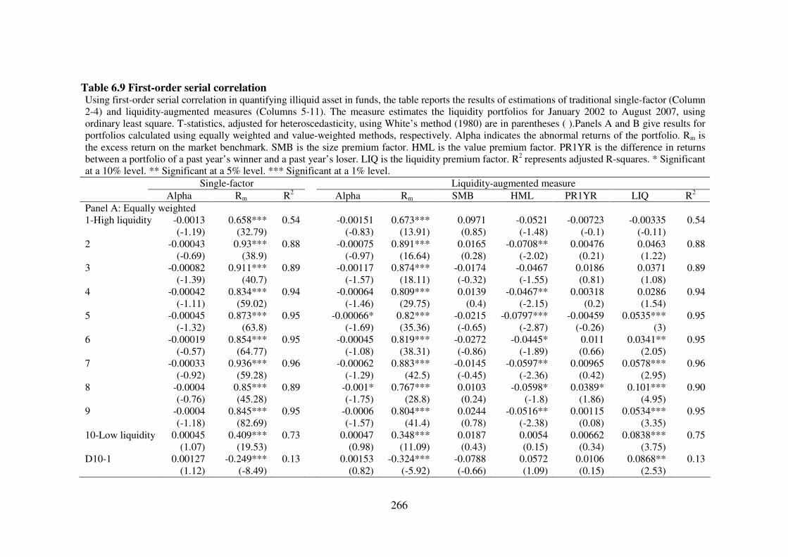
266
Table 6.9 First-order serial correlation Using first-order serial correlation in quantifying illiquid asset in funds, the table reports the results of estimations of traditional single-factor (Column 2-4) and liquidity-augmented measures (Columns 5-11). The measure estimates the liquidity portfolios for January 2002 to August 2007, using ordinary least square. T-statistics, adjusted for heteroscedasticity, using White’s method (1980) are in parentheses ( ).Panels A and B give results for portfolios calculated using equally weighted and value-weighted methods, respectively. Alpha indicates the abnormal returns of the portfolio. Rm is the excess return on the market benchmark. SMB is the size premium factor. HML is the value premium factor. PR1YR is the difference in returns between a portfolio of a past year’s winner and a past year’s loser. LIQ is the liquidity premium factor. R2 represents adjusted R-squares. * Significant at a 10% level. ** Significant at a 5% level. *** Significant at a 1% level.
Single-factor Liquidity-augmented measure
Alpha Rm R2 Alpha Rm SMB HML PR1YR LIQ R2
Panel A: Equally weighted 1-High liquidity -0.0013 0.658*** 0.54 -0.00151 0.673*** 0.0971 -0.0521 -0.00723 -0.00335 0.54 (-1.19) (32.79) (-0.83) (13.91) (0.85) (-1.48) (-0.1) (-0.11) 2 -0.00043 0.93*** 0.88 -0.00075 0.891*** 0.0165 -0.0708** 0.00476 0.0463 0.88 (-0.69) (38.9) (-0.97) (16.64) (0.28) (-2.02) (0.21) (1.22) 3 -0.00082 0.911*** 0.89 -0.00117 0.874*** -0.0174 -0.0467 0.0186 0.0371 0.89 (-1.39) (40.7) (-1.57) (18.11) (-0.32) (-1.55) (0.81) (1.08) 4 -0.00042 0.834*** 0.94 -0.00064 0.809*** 0.0139 -0.0467** 0.00318 0.0286 0.94 (-1.11) (59.02) (-1.46) (29.75) (0.4) (-2.15) (0.2) (1.54) 5 -0.00045 0.873*** 0.95 -0.00066* 0.82*** -0.0215 -0.0797*** -0.00459 0.0535*** 0.95 (-1.32) (63.8) (-1.69) (35.36) (-0.65) (-2.87) (-0.26) (3) 6 -0.00019 0.854*** 0.95 -0.00045 0.819*** -0.0272 -0.0445* 0.011 0.0341** 0.95 (-0.57) (64.77) (-1.08) (38.31) (-0.86) (-1.89) (0.66) (2.05) 7 -0.00033 0.936*** 0.96 -0.00062 0.883*** -0.0145 -0.0597** 0.00965 0.0578*** 0.96 (-0.92) (59.28) (-1.29) (42.5) (-0.45) (-2.36) (0.42) (2.95) 8 -0.0004 0.85*** 0.89 -0.001* 0.767*** 0.0103 -0.0598* 0.0389* 0.101*** 0.90 (-0.76) (45.28) (-1.75) (28.8) (0.24) (-1.8) (1.86) (4.95) 9 -0.0004 0.845*** 0.95 -0.0006 0.804*** 0.0244 -0.0516** 0.00115 0.0534*** 0.95 (-1.18) (82.69) (-1.57) (41.4) (0.78) (-2.38) (0.08) (3.35) 10-Low liquidity 0.00045 0.409*** 0.73 0.00047 0.348*** 0.0187 0.0054 0.00662 0.0838*** 0.75 (1.07) (19.53) (0.98) (11.09) (0.43) (0.15) (0.34) (3.75) D10-1 0.00127 -0.249*** 0.13 0.00153 -0.324*** -0.0788 0.0572 0.0106 0.0868** 0.13 (1.12) (-8.49) (0.82) (-5.92) (-0.66) (1.09) (0.15) (2.53)

267
Single-factor Liquidity-augmented measure
Alpha Rm R2 Alpha Rm SMB HML PR1YR LIQ R2
Panel B: Value-weighted 1-High liquidity -0.00027 0.536*** 0.78 0.00073 0.558*** 0.00834 -0.0489 -0.11*** -0.0267 0.79 (-0.5) (20.01) (1.31) (12.91) (0.16) (-1.31) (-4.65) (-0.98) 2 -0.00034 0.926*** 0.89 -0.00088 0.88*** 0.0151 -0.101*** 0.0141 0.0503 0.89 (-0.58) (37.04) (-1.27) (17.6) (0.27) (-2.82) (0.59) (1.4) 3 -0.00045 0.869*** 0.89 -0.00119 0.821*** -0.017 -0.0547* 0.0514** 0.0488 0.89 (-0.8) (37.93) (-1.62) (17.05) (-0.32) (-1.87) (2.06) (1.42) 4 -0.00021 0.826*** 0.94 -0.00024 0.785*** 0.0139 -0.0579*** -0.0155 0.05*** 0.95 (-0.59) (61.76) (-0.61) (30.80) (0.45) (-2.76) (-0.96) (2.68) 5 -0.00072** 0.885*** 0.95 -0.00088** 0.825*** -0.0285 -0.0788*** -0.00757 0.0613*** 0.95 (-1.98) (59.69) (-2.13) (30.93) (-0.77) (-2.67) (-0.43) (3) 6 0.00016 0.9*** 0.96 3.90E-05 0.854*** -0.0338 -0.0511** -0.0018 0.0456*** 0.96 (0.53) (71.6) (0.11) (42.64) (-1.1) (-2.06) (-0.12) (2.91) 7 -0.00023 0.933*** 0.95 -0.00055 0.872*** -0.0381 -0.0769*** 0.00827 0.0608*** 0.96 (-0.64) (63.97) (-1.29) (39.29) (-1.11) (-2.97) (0.46) (3.48) 8 2.30E-05 0.83*** 0.91 -0.00082* 0.721*** -0.0526 -0.0794*** 0.0591*** 0.116*** 0.92 (0.05) (37.31) (-1.94) (23.03) (-1.19) (-2.62) (2.81) (6.14) 9 -0.00068 0.83*** 0.91 -0.00027 0.79*** -0.0371 -0.0666** -0.0545** 0.0384 0.91 (-1.38) (35.41) (-0.49) (20.85) (-0.81) (-2.15) (-2.55) (1.63) 10-Low liquidity -0.0007 0.32*** 0.41 -0.00092 0.267*** 0.0142 0.0395 0.04 0.0752** 0.41 (-0.99) (11.96) (-1.04) (6.36) (0.18) (0.87) (1.17) (2.39) D10-1 -0.00091 -0.215*** 0.17 -0.0021** -0.289*** 0.0054 0.0881 0.146*** 0.102** 0.23 (-1.08) (-5.96) (-2.09) (-5.35) (0.06) (1.35) (3.93) (2.53)

268
6.5.2 January effect
Elesnarapu and Reinganum (1993) argue that the evidence of a liquidity premium is due to
the seasonal effect. Therefore, in order to ensure that our results are not driven by this effect,
we re-estimate our model with a variable capturing the January effect. We use a dummy
which equals one if the data are collected from the month of January and zero otherwise. In
Table 6.10, Panels A and B accordingly present the results estimated from equally weighted
and value-weighted portfolios. Columns 2-4 give the coefficients estimated from the single
factor model. The t-statistics estimated from the dummy variable for the January effect in
Column 4 are relatively low, ranging from -0.91 to 1.18, suggesting that our results are not
influenced by the seasonal effect. Similarly, Column 11 shows the coefficients of the January
effect dummy, estimated from our liquidity-augmented model and none of the portfolios has
a significant coefficient. Furthermore, we still find evidence of an illiquidity premium. The
high liquid fund portfolios yield statistically negative performance compared to the
statistically positive performance in the low liquidity portfolio and the liquidity factor is
positive and significant in the portfolio with illiquid assets. The results are consistent for both
equally weighted portfolios (Panel A) and the value-weighted portfolio (Panel B). Hence, we
conclude that our results are not sensitive to the January effect.

269
Table 6.10 The January effect The table reports the results of estimations of traditional single-factor (Columns 2-4) and liquidity-augmented measures (Columns 5-11). The measure estimates liquidity portfolios for January 2002 to August 2007, using ordinary least square. T-statistics, adjusted for heteroscedasticity, using White’s method (1980) are in parentheses ( ).Panels A and B give results for portfolios calculated using equally weighted and value-weighted methods, respectively. Alpha indicates the abnormal returns of the portfolio. Rm is the excess return on the market benchmark. SMB is the size premium factor. HML is the value premium factor. PR1YR is the difference in returns between a portfolio of a past year’s winner and a past year’s loser. LIQ is the liquidity premium factor. JAN is the dummy variable for the January effect which equals one if the data are obtained from the month of January and zero otherwise. * Significant at a 10% level. ** Significant at a 5% level. *** Significant at a 1% level
Jensen Liquidity-augmented
Portfolios Alpha Rm Jan Alpha Rm SMB HML PR1YR LIQ Jan
Panel A: Equally weighted 1-High -0.00105*** 0.693*** -0.00242 -0.00142*** 0.661*** 0.00484 -0.0527* 0.0139 0.0347 -0.0021 (-2.62) (29.97) (-0.91) (-2.79) (26.86) (0.12) (-1.89) (0.43) (1.46) (-0.88) 2 -0.00121* 0.886*** -0.00019 -0.00129* 0.858*** -0.00915 -0.0377 -0.00361 0.0292 -0.00012 (-1.93) (48.23) (-0.16) (-1.76) (21.24) (-0.17) (-1.42) (-0.19) (1.07) (-0.1) 3 -0.0008 0.842*** 0.0011 -0.00124** 0.811*** 0.0329 -0.0253 0.028 0.0438** 0.00161 (-1.52) (47.64) (0.96) (-2.07) (28.62) (0.84) (-0.9) (1.37) (2.1) (1.26) 4 -7.20E-05 0.945*** -0.00019 -0.00047 0.891*** -0.0155 -0.0606*** 0.0167 0.0583*** 0.00018 (-0.2) (76.19) (-0.16) (-1.1) (42.44) (-0.5) (-2.67) (0.95) (3.23) (0.14) 5 -0.00032 0.921*** 0.00077 -0.00045 0.877*** -0.00464 -0.0744*** -0.0122 0.0478** 0.00086 (-0.78) (61.43) (0.73) (-0.93) (33.3) (-0.13) (-2.92) (-0.67) (2.42) (0.81) 6 -0.0001 0.882*** 0.00126 -0.00036 0.839*** -0.015 -0.0614** 0.00341 0.0455** 0.00147 (-0.28) (65.65) (1.18) (-0.82) (36.9) (-0.45) (-2.42) (0.2) (2.54) (1.36) 7 0.00029 0.828*** -0.00077 5.00E-05 0.778*** -0.02 -0.0587*** 0.00398 0.0522*** -0.00056 (0.94) (73.04) (-0.91) (0.14) (39.36) (-0.69) (-2.68) (0.26) (3.38) (-0.6) 8 -0.0002 0.867*** 0.00025 -0.0005 0.799*** -0.0234 -0.0757*** 0.00399 0.0737*** 0.00053 (-0.58) (71.95) (0.2) (-1.34) (34.09) (-0.68) (-3.26) (0.26) (4.18) (0.43) 9 0.00035 0.772*** -8.10E-05 0.00026 0.719*** 0.00176 -0.0539** -0.00751 0.0637*** 7.60E-05 (1.08) (65.84) (-0.06) (0.73) (31.39) (0.05) (-2.15) (-0.5) (3.31) (0.05) 10-Low 0.0017** 0.43*** -0.00216 0.00125 0.37*** 0.0189 0.00711 0.0427 0.0811* -0.0015 (2.3) (12.22) (-0.84) (1.41) (5.91) (0.24) (0.1) (1.09) (1.69) (-0.61) D1-D10 0.00226*** -0.262*** 0.00027 0.00223** -0.29*** 0.0136 0.0595 0.0254 0.046 0.00057 (2.7) (-6.07) (0.08) (2.22) (-4.12) (0.16) (0.71) (0.5) (0.83) (0.18)

270
Jensen Liquidity-augmented
Portfolios Alpha Rm-Rf Jan Alpha Rm-Rf SMB HML PR1YR LIQ Jan
Panel B: Value-weighted 1-High -0.00093** 0.619*** -0.00119 -0.00112** 0.612*** 0.00631 -0.0566** -0.00402 0.0037 -0.00111 (-2.35) (35.13) (-0.61) (-2.47) (25.67) (0.18) (-2.16) (-0.16) (0.18) (-0.59) 2 -0.0013*** 0.797*** -0.00231 -0.0013** 0.773*** 0.00678 -0.0443* -0.0142 0.028 -0.00231 (-3) (53.35) (-1.46) (-2.52) (25.97) (0.18) (-1.89) (-0.83) (1.22) (-1.46) 3 -0.00002 0.762*** -0.00007 -0.00069 0.731*** 0.00381 -0.0403* 0.0431** 0.0335* 0.00053 (-0.04) (48.98) (-0.05) (-1.49) (29.06) (0.12) (-1.76) (2.18) (1.79) (0.34) 4 -0.00001 0.949*** 0.00022 -0.00041 0.887*** -0.0216 -0.0627*** 0.0172 0.0669*** 0.00061 (-0.02) (75.85) (0.19) (-0.97) (42.58) (-0.7) (-2.79) (0.98) (3.83) (0.47) 5 -0.00006 0.93*** -0.00003 -0.0003 0.865*** -0.0264 -0.0866*** -0.00499 0.0672*** 0.00015 (-0.15) (50.94) (-0.02) (-0.6) (29.41) (-0.7) (-3.05) (-0.25) (3.23) (0.11) 6 0.00007 0.902*** 0.00172 -0.00043 0.845*** -0.0309 -0.0786*** 0.0188 0.0554*** 0.0021* (0.17) (55.57) (1.41) (-0.93) (33.34) (-0.86) (-2.86) (1) (2.99) (1.74) 7 0.00009 0.874*** -0.00039 -0.00026 0.797*** -0.0453 -0.0924*** 0.00456 0.0773*** -0.00011 (0.24) (61.16) (-0.37) (-0.6) (34.22) (-1.32) (-3.34) (0.26) (4.32) (-0.1) 8 -0.00004 0.82*** 0.00056 -0.00016 0.738*** -0.0414 -0.0594** -0.00217 0.091*** 0.00075 (-0.09) (39.85) (0.32) (-0.36) (22.98) (-0.95) (-2.22) (-0.12) (4.79) (0.44) 9 -0.00071* 0.871*** 0.00016 -0.00107** 0.807*** -0.0658* -0.0903*** 0.00682 0.0571*** 0.00036 (-1.82) (55.35) (0.1) (-2.25) (31.52) (-1.82) (-3.4) (0.33) (2.66) (0.23) 10-Low 0.00165** 0.398*** -0.00279 0.00142 0.34*** 0.0252 -0.00556 0.0202 0.0802* -0.00234 (2.12) (11.07) (-1.31) (1.5) (5.3) (0.32) (-0.07) (0.48) (1.66) (-1.15) D1-D10 0.00209** -0.22*** -0.0016 0.0021* -0.271*** 0.0185 0.0508 0.0209 0.0761 -0.00126 (2.38) (-5.07) (-0.56) (1.96) (-3.73) (0.2) (0.58) (0.41) (1.39) (-0.44)

271
6.6 Conclusions
Previous studies suggest that liquidity plays an important role in asset pricing because it
could result in a bias in beta risk and return estimation. Also, illiquid assets are likely to
generate a return premium through the clientele effect. A number of previous studies has
documented the relationship between liquidity and stock returns. This study extends the
investigation into the role of liquidity to an alternative setting, an emerging market mutual
fund. This is necessary because most of its underlying mutual assets are stocks. In addition,
liquidity is a main concern in emerging markets and, therefore, investigating this issue in this
region would provide a powerful test and bring up useful evidence. To achieve this, this study
estimates the illiquid assets contained in mutual funds using the return-based stale price
model which was proposed by Getmansky et al. (2004). The model implicitly measures
illiquidity based on the observed returns and has been used only in the hedge fund literature.
We explore whether funds with high illiquid assets are able to earn illiquidity rents. Our
results suggest superior performance in illiquid fund portfolios, while liquid funds yield
inferior performance. The performance increases with the degree of illiquid assets which is
contained in the portfolio. We also find that the beta coefficients estimated from liquidity
portfolios are varied and relatively low in the extreme portfolios. Thus, we suggest that there
is evidence of a liquidity premium in mutual fund returns which is consistent with the
evidence in stock markets (Datar, 1998; Amihud, 2002; Chan and Faff, 2005; and Liu, 2006).
The variable in beta estimation across liquidity portfolio also implies the possibility of bias in
the beta estimation (Dimson, 1979).
As a result, we propose a liquidity-augmented performance measure. This liquidity-
augmented measure is a five-factor model which includes a liquidity variable capturing the

272
liquidity premium in stock returns, in addition to the variables of market, size, value/growth
and momentum. The liquidity measured by the share turnover ratio can explain the quantity
dimension in the liquidity. Next, all variables are self-constructed using Thai stock data. We
find that the liquidity-augmented model brings mutual fund performance down by roughly
2% per year. This is attributed to the growth and liquidity premiums. The coefficients of the
liquidity premium variable increase through the degree of illiquid assets contained in the
portfolios and are statistically significant in all funds except for two high liquid portfolios.
Thus, we confirm the evidence of liquidity rents in mutual funds and the explanatory power
in our liquidity factor. Nevertheless, we find that, using our proposed liquidity-augmented
measure, the low liquidity funds portfolios still outperform the high liquidity funds portfolios
and suggest that there is still evidence of a liquidity premium. This suggests that the share
turnover is not a good proxy for liquidity, which contradicts the findings in Datar (1998) and
Chan and Faff (2005). Nonetheless, the factor is of statistical importance in measuring mutual
fund performance and it helps to identify the sources of the return premium and also to
understand how fund managers allocate their portfolios.
In addition, we investigate the policy implications of tax-benefit funds which are a
unique mutual fund style in Thailand and require a longer investment horizon. The long-term
restriction gives fund managers an opportunity to put more weight on illiquid stocks in order
to exploit the illiquidity premium. Therefore, we specifically investigate the differences in
liquidity level between general and tax-benefit funds. We find that tax-benefit funds have
more illiquid assets than general funds but, after controlling for fund characteristics, this
result is not statistically significant. Therefore, the evidence of superior performance in tax-
benefit funds is not a result from illiquidity rents alone. The higher return in tax-benefit funds
may be attributed to other reasons, such as managerial skills and the lowering in trading cost

273
as the long-term restrictions can make the funds more passive than general funds are.
Nevertheless, this calls for further investigation at a later date.
We check for robustness in the results and find that our results are not sensitive to the
measure used in estimating asset illiquidity in funds and also are not influenced by seasonal
effect. Thus, we can confirm the evidence of a liquidity premium in Thai mutual funds as
well as the importance of including a liquidity factor in the performance measure.
Findings from this study make practical implications to both Thai fund investors and
fund managers. For investors, selecting funds which are illiquid stocks oriented could provide
them superior returns. In addition, the multi-factor model should be considered in
performance measurement since it can help investors to select funds which meet their
preferences. For fund managers, even the tax-benefit fund managers already perform
relatively well compared to their peers, they could perform even better by making use of their
long-term restrictions to invest more on illiquid stocks and to earn more illiquidity premium.
However, this study employs a share turnover ratio which can capture a quantity
dimension only in liquidity and is tested in only one of the emerging economies.
Thus, further research is called for the more study on the effect of liquidity on
investment portfolio; and to investigate the liquidity in other dimensions, such as the speed
and cost of trading. Further research is also called for to seek a more appropriate proxy in
explaining the liquidity premium in emerging market returns.

274
CHAPTER SEVEN
CONCLUSIONS
7
7.1 Introduction
The growth of mutual fund investment and its importance to various economies has become
more significant in the past few decades. The distinctive characteristics of emerging markets
make it vital to seek more understanding of mutual fund performance in this area; the present
thesis has this aim, using the Thai market as a case study. We have surveyed the literature
relating to performance measures which have been proposed in the past few decades as well
as empirical evidence from both developed and emerging markets. Subsequently, we carried
out three empirical studies connected to mutual funds in Thailand. The first relates to the
comprehensive evaluation of Thai mutual fund performance based on existing models in the
literature. We used a longer and more comprehensive dataset than previous studies did and
disentangled several issues which are still unclear or have not even been discussed in the Thai
literature, including the performance, style, and strategy used in Thai fund managers. The
second empirical study relates to whether any of the fund characteristics can help to explain
fund performance. The present study considered five important characteristics and used both
time-series and cross-section techniques to tackle this issue. The third relates to the role of
liquidity in mutual fund performance, since liquidity is one of the main concerns in emerging
markets. We examined the effect of liquidity in assets contained in the portfolio in relation to
fund performance and then we proposed an auxiliary performance measure to capture the
liquidity premium. Additionally, in each empirical study, we specifically examined the tax-

275
benefit mutual funds. This is an explicit fund type in Thailand, which has received immense
cash flows in the past few years. This mutual fund type gives favourable tax treatment and, at
the same time, it entails long-term investment restriction. Thus, we look at these funds as a
discrete group and reveal their policy implications.
Accordingly, this chapter presents the conclusions and key findings of the study as well
as providing some research suggestions. The chapter is organised as follows. Section 7.2
summarises the key findings in the study based on our empirical analysis. In Section 7.3, we
bring results from our analysis together and discuss policy implications. Finally, Section, 7.4,
discusses the limitations of the study and suggests areas which might benefit from further
research.
7.2 Key findings
7.2.1 Literature survey on mutual fund performance
We reviewed existing performance measures and empirical results as well as other relevant
issues in mutual fund performance which have been widely discussed over a decade. The
mutual fund performance measures are largely influenced by the modern portfolio theory.
The criticisms of the validity of the Capital Asset Pricing model and the evidence suggesting
that other variables outside the market risk can also explain stock returns have amplified
more recent models to become richer and more informative. These models not only help to
evaluate performance more efficiently but also allow us to examine further the style and
strategy which a fund manager follows. Empirical evidence suggests that fund managers
adjust portfolios dynamically on the basis of economic information; invest heavily in small
and value stocks; and make use of momentum strategy. Nevertheless, in most cases, they are
unable to outperform the market, at least, once fees and expenses have been deducted. This

276
indicates that fund managers do not give value added to investors and this is partly due to the
high fees and expenses charged. The other two crucial concerns which are widely discussed
in the mutual fund literature are persistence in performance and the effect of fund flows on
fund performance. Nevertheless, the results in these studies are still mixed.
With regard to the extensive literature on mutual fund performance, we find that these
studies are concentrated in the US and other developed countries and research within the
emerging regions is still scant, even though they are in many respects unlike the developed
markets. For example, emerging markets suffer from infrequent trading, inefficiency and high
volatility and high trading cost. More importantly, the mutual fund industries in emerging
markets are distinctive from those in the developed markets in terms of growth,
competitiveness, and organisational structure and information availability. Moreover, it is
still questionable whether the findings in the developed markets carry over to the emerging
markets.
The gap between the studies in developed and emerging countries is also owing to the
sample size and the models used in the studies. Most studies of the mutual funds in emerging
markets employ a short sample period, although these markets provide evidence of structural
breaks. Furthermore, these studies are still based on the prevailing approaches, such as the
Sharpe ratio, Treynor ratio and Jensen’s alpha, which involve many criricisms: for instance,
evidence from both the developed and the emerging markets suggests that there are other
factors which can explain stock returns and the risk factor is not constant over time.
In addition, the literature on mutual funds in emerging markets reveals that the main
concern in this region lies in performance evaluation. Very little has been written on other
issues related to mutual fund performance, such as style and performance determination.
Hence, these prevent a fuller understanding of the mutual find business.

277
Thus, this study chooses to examine mutual funds in emerging markets, using
Thailand as a case study, and comes up with three promising research ideas. First, we apply
performance measures in the existing literature to the mutual funds in Thailand and
investigate its performance comprehensively. Second, we examine the factors related to
mutual fund performance. Third, we examine the effect of liquidity, as one of the main
concerns in emerging markets in regard to mutual fund performance, and elaborate an
auxiliary performance measure.
7.2.2 Empirical study of Thai mutual fund performance
In Chapter Four, we examine the performance of Thai mutual funds using some of the
measures proposed in the literature. We investigate both the selectivity and timing abilities of
Thai fund managers and also investigate some of their styles and strategies. Finally, we
compare and contrast the results with those of existing studies. Our results reveal that Thai
fund managers as a whole do not have selectivity or timing ability. Therefore, over the
sample period, they do not give value added to investors. Additionally, we applied
performance measures which are seldom found in the emerging market literature and reveal
that these richer performance models are also statistically important in performance
evaluation, but not large enough to lead to abnormal returns. Nevertheless, the use of these
models makes it easier to scrutinize the behaviour of fund managers.
Results from style analysis reveal that a large proportion of Thai fund managers invest
heavily in small and growth stocks, although this style provides the worst performance of all
four fund styles. This is in contrast to the previous studies in developed markets, which
indicate that growth funds perform better than other fund styles.
We also employ conditional performance measures to investigate whether fund
managers are active and adjust their portfolio dynamically, using macroeconomic

278
information. In contrast to the findings in the literature which suggest that fund managers
actively adjust their portfolios in response to changes in economic conditions and that
conditional measures shift mutual fund performance toward zero, we find that, in Thailand,
only flexible fund managers adjust their portfolio dynamically using Treasury bills and
dividend yield. We also find that performances are unstable over the estimation period and
that the results are sensitive to the frequency of data and measures used in the evaluation.
Subsequently, our results are comparable to those of previous writers on both the
emerging and the developed markets in that no abnormal performance is shown. Our results
also extend the mutual fund literature in emerging markets and show that Thai fund managers
are more passive than their counterparts and that strategies are not very different in developed
and developing markets. Fund managers’ strategies are also different across fund types and it
is found that the richer models used in developed markets also well explain the mutual fund
returns behaviours in emerging markets.
7.2.3 Empirical study of the determinants of mutual fund performance
The findings in Chapter Four reveal that fund managers as a whole do not make abnormal
returns. However, some fund managers perform better than others. Thus, the next question is
whether we can learn to identify them. In Chapter Five, we shed light on whether abnormal
performing funds can be differentiated from others, using their particular characteristics. This
study looks at five main characteristics, namely, past performance, size, fund flows, fund
longevity and family size.
In addition to the prevailing studies, this chapter investigates fund characteristics
individually and as a group; and examines its importance from both statistical and economic
standpoints. We find that fund performance in Thailand based on risk-adjusted measures can

279
be explained by some of these characteristics, even though these are investment and tax
policy specific.
General funds reveal persistence in performance. There is a positive relationship
between the past year’s and current performances and its degrees are of both statistical and
economic importance. Nonetheless, this relationship applies to poorly performing funds,
which continue to perform badly from one period to the next. This is in contrast to the
previous evidence in emerging markets, which finds no evidence of performance persistence.
However, it is comparable to the several studies in developed markets which show evidence
of persistence in performance, especially among poorly performing funds.
Fund size is negatively related to general flexible fund performance and negatively
related to tax-benefit flexible fund performance. In contrast, fund family size is positively
related to the performance of both general equity and flexible funds. In addition, the
performance of general equity funds performance also decreases with the funds’ age. Even
though the fund performance can be statistically explained by these characteristics, selecting
funds on the basis of these strategies is unable to yield abnormal returns.
Another key finding in this study relates to the impact of fund flows on mutual fund
performance, about which little is known in emerging markets. In the panel regression, we do
not find a relationship in lagged year net cash flows and fund performance. However, in the
trading strategy portfolio, we find that tax-benefit funds with high net cash flows significantly
underperform. This is evidence of the negative net cash flows shock in tax-fund managers.
Since there is a large amount of cash inflow, fund managers are unable to allocate large
amounts of cash immediately, causing a lowering of the portfolio’s systematic risk and,
therefore, a poorer performance. Thus, we show evidence against the view of the smart
money effect in mutual fund performance and argue that, in emerging markets, cash flows

280
have little impact on fund performance but cash flows shock can result in inferior
performance in a subsequent period.
7.2.4 Empirical study of the effect of liquidity on mutual fund performance
In Chapter Six we examine the role of liquidity on mutual fund performance. Liquidity is one
of the main concerns in emerging markets and a number of studies reveal the effect of
liquidity on stock returns. However, the impact of liquidity has rarely been discussed in the
mutual fund literature. We apply a return-based stale price measure in the hedge fund
literature to quantify the degree of illiquid assets contained in the portfolio (Getmansky et al.,
2004). Inconsistently with the evidence in the literature, we find that portfolios of funds
which contain more illiquid assets perform significantly higher and suggest that there is a
liquidity premium in mutual fund performance. Subsequently, we propose an auxiliary
performance measure, which includes an additional variable to capture the liquidity premium,
in addition to the size, value and momentum premium. In our auxiliary model, liquidity is
measured by the share turnover ratio, which can capture liquidity in the trading quantity
dimension. We construct a liquidity variable, using three-way sorting on size, book-to-market
and share turnover ratio. The liquidity factor is the average returns of illiquid portfolios
minus the average returns of very liquid portfolios. The results of using the auxiliary model
suggest that the liquidity variable has explanatory power regarding mutual fund returns and is
statistically significant in portfolios of funds with a high degree of illiquid assets. This
suggests the importance of the liquidity factor to mutual fund performance, even though there
is some liquidity premium left unexplained, which may have resulted from the premium from
other dimensions of liquidity. Nonetheless, we find that our results are robust across the
measures used in estimating illiquid assets in the portfolios and are not influenced by any
seasonal effect.

281
7.3 Policy Implications
In 2002, the Thai government adopted a tax-benefit fund scheme called Retirement Mutual
Funds (RMF) and later, in 2004, it introduced another tax-benefit fund scheme called Long-
term Equity Funds (LTF). These two fund styles have a similar purpose: to promote long-
term and retirement savings. These funds impose a restriction on long-term investment while
giving favourable tax treatment. Consequently, these fund styles have become popular and
have received substantial cash flows. Since the tax-benefit funds focus on long-term investors
and impose restrictions in terms of the investment period, these may influence the funds’
performance as well as the behaviour and investment strategy of fund managers. The long-
term investment period is likely to make fund managers rely more on passive strategy. In
addition, the restrictions imposed on the funds are likely to have a positive impact on
performance because they reduce liquidity-motivated trading and also allow fund managers
to put more weight on illiquid assets, so as to earn an illiquidity premium.
Thus, we discuss the policy implications of these fund styles by examining these
funds in a discrete category, called tax-benefit funds, and comparing them with general funds.
Results are reported in each empirical chapter. In the first and second empirical chapters, we
find that tax-benefit funds, as a whole, perform significantly better than general funds, even
when controlled for size, net cash flows, age and style differences. We also find that tax-
benefit funds display different characteristics from general funds in explaining mutual fund
performance. In contrast to general funds, we do not find evidence of persistence in tax-fund
performance. Although tax-benefit funds perform better than general funds, we find that the
impact of high unexpected cash flows can result in inferior mutual fund performance in a
subsequent period because fund managers cannot adjust their portfolios immediately.

282
Furthermore, we investigate whether the superior performance in the tax-benefit funds
is a result of the liquidity premium. We examine the degree of illiquid assets contained in the
tax-benefit portfolio in relation to general funds. The results reveal that tax-benefit funds hold
slightly more illiquid assets than general funds do. Thus, we conclude that the superior
performance in tax-benefit funds is only partly attributable to the liquidity premium. The
superior performance in tax-benefit funds can also be a consequence of their long-term
lockup restriction, which allows fund managers to manage their portfolios more efficiently
and to reduce the cost of nondiscretionary trading. Also, it can be explained by the superior
skills of the tax-benefit fund manager themselves. Nonetheless, the intense growth in the tax-
benefit funds nowadays is something which Thai fund managers should be aware of and
prepare for, because they cause large cash flows into the funds which could inversely affect
fund performance.
7.4 Limitations of the study and suggestions for further research
The main limitations of this study are three-fold. First, it considers only one emerging
market, which cannot represent the emerging market as a whole. Even though these markets
share many of their main characteristics, some of them have their own unique characteristics
and regulations. Therefore, the findings may not fully cover all emerging markets. Second,
with regard to data availability, the data can be traced back only for the past seven years,
possibly not long enough to capture the market cycle. Third, some relevant information is not
available, such as fees and expenses, trading information and cash inflows and outflows.
Hence, some analyses cannot be applied.
Accordingly, we highlight some further research ideas on the basis of findings from
this study as well as the previous literature. First, research into mutual funds should be

283
conducted within other emerging countries as well as at the aggregated level. This would
provide more understanding of this part of the mutual fund industry.
Second, this study shows that liquidity, which is one of the main concerns in
emerging markets, influences the mutual fund performance measure. However, we focus only
on liquidity in the trading quantity dimension and, therefore, the effect of liquidity in other
dimensions is left unexplained. Furthermore, some further study of mutual funds in emerging
markets needs to put more emphasis on other characteristics of emerging markets, such as
their inefficiency, non-normality, volatility and structure breaks; and to examine how this
affects the performance and performance measures. There is also a need to develop a
performance model specifically for this region.
Third, further research can engage in examining the behaviour of mutual fund
investors in emerging markets. This study shows that much information about mutual funds is
not publicly available. For instance, there is no information on fund styles nor comprehensive
league tables to allow the comparison of mutual funds in the market. Subsequent investors
are likely to be uninformed. Thus, it is still not clear how these investors make their decisions
and whether these decisions are smart in the sense of providing superior returns in subsequent
periods.

284
REFERENCES
Abel, E. and Fletcher, J. (2004) An empirical examination of UK emerging market unit trust performance. Emerging Markets Review, 5 389-408
Acharya, D. and Sidana, G. (2007) Classifying mutual funds in India: Some results from
clustering. Indian Journal of Economics and Business, 6 (1): 71-79 Acharya, V. V. and Pedersen, L. H. (2005) Asset pricing with liquidity risk. Journal of
Financial Economics, 77 (2): 375-410 Agarwal, V., Daniel, N. D. and Nail, N. Y. (2008) Role of managerial incentives and
discretion in hedge fund performance. Journal of Finance, Forthcoming Amihud, Y. (2002) Illiquidity and stock returns: Cross-section and time-series effects.
Journal of Financial Markets, 5 (1): 31-56 Amihud, Y. and Mendelson, H. (1986) Asset pricing and the bid-ask spread. Journal of
Financial Economics, 17 (2): 223-249 Annaert, J., Van Den Broeck, J. and Vander Vennet, R. (2003) Determinants of mutual fund
underperformance: A Bayesian stochastic frontier approach. European Journal of
Operational Research, 151 (3): 617-632 Aragon, G. O. (2007) Share restrictions and asset pricing: Evidence from the hedge fund
industry. Journal of Financial Economics, 83 (1): 33-58 Asness, C. S., Robert, K. J. and John, L. M. (2001) Do hedge funds hedge? Journal of
Portfolio Management, 28 (1): 6-19 Athanasios, G. N., John, A. P. and John, L. (2005) Performance of mutual funds. Managerial
Finance, 31 (2): 101 Bali, T. G., Gokcan, S. and Liang, B. (2007) Value at risk and the cross-section of hedge fund
returns. Journal of Banking and Finance, 31 (4): 1135-1166 Bauer, R., Koedijk, K. and Otten, R. (2005) International evidence on ethical mutual fund
performance and investment style. Journal of Banking and Finance, 29 (7): 1751-1767
Bauer, R., Otten, R. and Rad, A. T. (2006) New Zealand mutual funds: Measuring
performance and persistence in performance. Accounting and Finance, 46 (3): 347 Bekaert, G. and Harvey, C. R. (2002) Research in emerging markets finance: Looking to the
future. Emerging Markets Review, 3 (4): 429-448 Bekaert, G. and Harvey, C. R. (2003) Emerging markets finance. Journal of Empirical
Finance, 10 (1-2): 3-56

285
Bekaert, G., Harvey, C. R. and Lundblad, C. (2007) Liquidity and expected returns: Lessons
from emerging markets. The Review of Financial Studies, 20 (6): 1783-1831 Benson, K. L. and Faff, R. W. (2006) Conditional performance evaluation and the relevance
of money flows for Australian international equity funds. Pacific-Basin Finance
Journal, 14 (3): 231-249 Bergstresser, D., Chalmers, J. M. R. and Tufano, P. (2009) Assessing the costs and benefits
of brokers in the mutual fund industry. The Review of Financial Studies, 22 (10): 4129-4156
Berk, J. B. and Green, R. C. (2004) Mutual fund flows and performance in rational markets.
Journal of Political Economy, 112 (6): 1269-1295 Bhargava, R., Bose, A. and Dubofsky, D. A. (1998) Exploiting international stock market
correlations with open-end international mutual funds. Journal of Business Finance
and Accounting, 25 (5/6): 765-773 Blake, C. R., Elton, E. J. and Gruber, M. J. (1993) The performance of bond mutual funds.
Journal of Business, 66 (3): 371 Blake, D. and Timmermann, A. (1998) Mutual fund performance: Evidence from the UK.
European Finance Review, 2 55-77 Bogle, J. C. (1998) The implications of style analysis for mutual fund performance
evaluation. Journal of Portfolio Management, 24 (4): 34-43 Bollen, N. P. B. (2007) Mutual fund attributes and investor behavior. Journal of Financial
and Quantitative Analysis, 42 (3): 683-708 Bollen, N. P. B. and Busse, J. A. (2001) On the timing ability of mutual fund managers.
Journal of Finance, 56 (3): 1075 Bollen, N. P. B. and Busse, J. A. (2005) Short-term persistence in mutual fund performance.
The Review of Finance Studies, 18 (2): 569-597 Bollenn, N. P. B. (2007) Mutual fund attributes and investor behavior. Journal of Financial
and Quantitative Analysis, 42 (3): 683-708 Borensztein, E. R. and Gelos, R. G. (2001) A panic-prone pack? The behavior of emerging
market mutual funds. Working paper, IMF Boudoukh, J., Richardson, M., Subrahmanyan, M., et al. (2002) Stale prices and strategies for
trading mutual funds. Financial Analysts Journal, 58 (4): 53 Brennan, M. J., Chordia, T. and Subrahmanyam, A. (1998) Alternative factor specifications,
security characteristics, and the cross-section of expected stock returns. Journal of
Financial Economics, 49 (3): 345-373

286
Brennan, M. J. and Subrahmanyam, A. (1996) Market microstructure and asset pricing: On the compensation for illiquidity in stock returns. Journal of Financial Economics, 41 (3): 441-464
Brooks, C. (2008) Introductory econometrics for finance, Cambridge: Cambridge
University Press. Brown, S., Ghon Rhee, S. and Zhang, L. (2008) The return to value in Asian stock markets.
Emerging Markets Review, 9 (3): 194-205 Brown, S. J., Goetzmann, W., Ibbotson, R. G., et al. (1992) Survivorship bias in performance
studies. The Review of Financial Studies, 5 (4): 553-580 Brown, S. J. and Goetzmann, W. N. (1995) Performance persistence. The Journal of
Finance, 50 (2): 679 Brown, S. J., Goetzmann, W. N., Hiraki, T., et al. (2001) The Japanese open-end fund puzzle.
Journal of Business, 74 (1): 59 Brown, S. J., Goetzmann, W. N., Hiraki, T., et al. (2003) An analysis of the relative
performance of Japanese and foreign money management. Pacific-Basin Finance
Journal, 11 (4): 393-412 Buetow, G. W., Johnson, R. R. and Runkle, D. E. (2000) The inconsistency of return–based
style analysis. Journal of Portfolio Management, 26 (3): 61-77 Busse, J. A. (1999) Volatility timing in mutual funds: Evidence from daily returns. The
Review of Financial Studies, 12 (5): 1009-1041 Cai, J., Chan, K. C. and Yamada, T. (1997) The performance of Japanese mutual funds. The
Review of Financial Studies, 10 (2): 237-273 Campbell, J. Y., Lo, A. W. and Mackinlay, A. C. (1997) The econometrics of financial
markets, Princeton, N.J. ; Chichester: Princeton University Press. Campisi, S. (2004) The case for money-weighted performance attribution. Journal of
Portfolio Management, 8 (3): Capon, N., Fitzsimons, G. J. and Prince, R. A. (1996) An individual level analysis of the
mutual fund investment decision. Journal of Financial Services Research, 10 (1): 59-82
Carhart, M. M. (1997) On persistence in mutual fund performance. Journal of Finance, 52
(1): 57-82 Chan, H. W. and Faff, R. W. (2005) Asset pricing and the illiquidity premium. Financial
Review, 40 (4): 429-458 Chan, L. K. C., Chen, H.-L. and Lakonishok, J. (2002) On mutual fund investment styles.
The Review of Financial Studies, 15 (5): 1407-1437

287
Chen, H.-L., Jegadeesh, N. and Wermers, R. (2000) The value of active mutual fund
management: An examination of the stockholdings and trades of fund managers. Journal of Financial and Quantitative Analysis, 35 (3): 343-368
Chen, J., Hong, H., Ming, H., et al. (2004) Does fund size erode mutual fund performance?
The role of liquidity and organization. American Economic Review, 94 (5): 1276-1302
Chen, N.-F., Roll, R. and Ross, S. A. (1986) Economic forces and the stock market. Journal
of Business, 59 (3): 383-403 Christopherson, J. A. (1997) Equity style classifications. Journal of Portfolio Management,
21 (3): 32-43 Chunhachinda, P. and Tangprasert, S. (2004) Market and volatility timing ability: New
evidence of mutual funds in Thailand. Thammasat Review, 161-185 Ciccotello, C. S. (1996) Equity fund size and growth: Implications for performance and
selection. Financial Services Review, 5 (1): 1 Claessens, S., Dasgupta, S. and Glen, J. D. (1995) The cross-section of stock returns:
Evidence from emerging markets. Working paper, World Bank policy research Coles, J. L., Daniel, N. D. and Nardari, F. (2006) Does the choice of model or benchmark
affect inference in measuring mutual fund performance? Working Paper, Arizona State University
Comer, G. (2006) Hybrid mutual funds and market timing performance. Journal of
Business, 79 (2): 771-797 Connor, G. and Korajczyk, R. A. (1988) Risk and return in an equilibrium APT : Application
of a new test methodology. Journal of Financial Economics, 21 (2): 255-289 Cumby, R. E. and Glen, J. D. (1990) Evaluating the performance of international mutual
funds. Journal of Finance, 45 (2): 497-521 Cuthbertson, K., Nitzsche, D. and O'sullivan, N. (2006) Mutual fund performance.
Working paper, Social Science Research Network Cuthbertson, K., Nitzsche, D. and O'sullivan, N. (2008) UK mutual fund performance: Skill
or luck? Journal of Empirical Finance, 15 (4): 613-634 Dahlquist, M., Engstrom, S. and Soderlind, P. (2000) Performance and characteristics of
Swedish mutual funds. Journal of Financial and Quantitative Analysis, 35 (3): 409-423
Daniel, K., Grinblatt, M., Titman, S., et al. (1997) Measuring mutual fund performance with
characteristic-based benchmarks. Journal of Finance, 52 (3): 1035-1058

288
Datar, V. T., Y. Naik, N. and Radcliffe, R. (1998) Liquidity and stock returns: An alternative test. Journal of Financial Markets, 1 (2): 203-219
Del Guercio, D. and Tkac, P. A. (2002) The determinants of the flow of funds of managed
portfolios: Mutual funds vs. Pension funds. Journal of Financial and Quantitative
Analysis, 37 (4): 523-557 Detzel, F. L. and Robert, A. W. (1998) Explaining persistance in mutual fund performance.
Financial Services Review, 7 (1): 45 Dibartolomeo, D. and Witkowski, E. (1997) Mutual fund misclassification: Evidence based
on style analysis. Financial Analysts Journal, 53 (5): 32-43 Dimson, E. (1979) Risk measurement when shares are subject to infrequent trading. Journal
of Financial Economics, 7 (2): 197-226 Ding, B., Getmansky, M., Liang, B., et al. (2008) Investor flows and share restrictions in
the hedge fund industry. Working paper, Social Science Research Network Drew, M. E. and Stanford, J. D. (2003) Returns from investing in Australian equity
superannuation funds, 1991-1999. Service Industries Journal, 23 (4): 12-24 Drew, M. E. and Veeraraghavan, M. (2002) A closer look at the size and value premium in
emerging markets: Evidence from the Kuala Lumpur stock exchange. Asian
Economic Journal, 16 (4): 337-351 Droms, W. G. and Walker, D. A. (1994) Investment performance of international mutual
funds. Journal of Financial Research, 17 (1): 1 Edelen, R. M. (1999) Investor flows and the assessed performance of open-end mutual funds.
Journal of Financial Economics, 53 (3): 439 Edelen, R. M., Evans, R. and Kadlec, G. B. (2007) Scale effects in mutual fund
performance: The role of trading costs. Working paper, Boston College Eleswarapu, V. R. and Reinganum, M. R. (1993) The seasonal behavior of the liquidity
premium in asset pricing. Journal of Financial Economics, 34 (3): 373-386 Elsiefy, E. A. E.-L. (2001) Portfolio performance evaluation and selection: Theory and
evidence from the Egyptian emerging capital market. PhD, University of Birmingham
Elton, E. J., Gruber, M. J. and Blake, C. R. (1996) The persistence of risk-adjusted mutual
fund performance. Journal of Business, 69 (2): 133-157 Elton, E. J., Gruber, M. J. and Brown, S. J. (2002) Modern portfolio theory and investment
analysis, New York: Wiley. Elton, E. J., Gruber, M. J. and Busse, J. A. (2004) Are investors rational? Choices among
index funds. Journal of Finance, 59 (1): 261-288

289
Elton, E. J., Gruber, M. J., Das, S., et al. (1993) Efficiency with costly information: A
reinterpretation of evidence from managed portfolios. The Review of Financial
Studies, 6 (1): 1-22 Fama, E. F. (1970) Efficient capital markets: A review of theory and empirical work. Journal
of Finance, 25 (2): 383-417 Fama, E. F. (1972) Components of investment performance. Journal of Finance, 27 (3):
551-567 Fama, E. F. and French, K. R. (1992) The cross-section of expected stock returns. Journal of
Finance, 47 (2): 427-465 Fama, E. F. and French, K. R. (1993) Common risk factor in the return on stocks and bonds.
Journal of Financial and Economics, 33 3-56 Fama, E. F. and French, K. R. (1998) Value versus growth: The international evidence.
Journal of Finance, 53 (6): 1975-1999 Fama, E. F. and Macbeth, J. D. (1973) Risk, return, and equilibrium: Empirical tests. Journal
of Political Economy, 81 (3): 607 Fauziah Md, T. and Mansor, I. (2007) Malaysian unit trust aggregate performance.
Managerial Finance, 33 (2): 102 Ferreira, M., Minuel, A. F. and Ramos, S. B. (2009) The determinants of mutual fund
performance: A cross-country study, Working paper, Social Science Research Network
Ferruz, L. and Ortiz, C. (2005) Does mutual fund management in India correspond to its
investment objective classification?, Working paper, Social Science Research Network
Ferson, W. E. and Schadt, R. W. (1996) Measuring fund strategy and performance in
changing economic conditions. Journal of Finance, 51 (2): 425-461 Ferson, W. E. and Warther, V. A. (1996) Evaluating fund performance in a dynamic market.
Financial Analysts Journal, 52 (6): 20 Fikriyah, A., Taufiq, H. and Shamsher, M. (2007) Investigation of performance of Malaysian
Islamic unit trust funds. Managerial Finance, 33 (2): 142 Fletcher, J. (1995) An examination of the selectivity and market timing performance of UK
unit trusts. Journal of Business Finance and Accounting, 22 (1): 143-156 Fletcher, J. and Forbes, D. (2002) U.K. Unit trust performance: Does it matter which
benchmark or measure is used? Journal of Financial Services Research, 21 (3): 195-218

290
Friis, L. B. and Smit, E. V. M. (2004) Are some fund managers better than others? Manager characteristics and fund performance. South African Journal of Business
Management, 35 (3): 31-40 Gaspar, J.-M., Massa, M. and Matos, P. (2006) Favoritism in mutual fund families? Evidence
on strategic cross-fund subsidization. Journal of Finance, 61 (1): 73-104 Geoffrey, C. F. and Travis, R. A. S. (2007) Mutual fund flows and investor returns: An
empirical examination of fund investor timing ability. Journal of Banking and
Finance, 31 (9): 2796 Getmansky, M., Lo, A. W. and Makarov, I. (2004) An econometric model of serial
correlation and illiquidity in hedge fund returns. Journal of Financial Economics, 74 (3): 529-609
Gharghori, P., Mudumba, S. and Veeraraghavan, M. (2007) How smart is money? An
investigation into investor behaviour in the Australian managed fund industry. Pacific-Basin Finance Journal, 15 (5): 494-513
GlobalEdge (2010) Market potential index for emerging markets [online].
http://globaledge.msu.edu/resourcedesk/mpi/ [Accessed 11 February 2010] Goetzmann, W. N. and Ibbotson, R. G. (1994) Do winners repeat? Journal of Portfolio
Management, 20 (2): 9-18 Goetzmann, W. N., Ivkovic, Z. and Rouwenhorst, K. G. (2001) Day trading international
mutual funds: Evidence and policy solutions. Journal of Financial and Quantitative
Analysis, 36 (3): 287-309 Goetzmann, W. N., Jr, J. I. and Ivkovic, Z. (2000) Monthly measurement of daily timers.
Journal of Financial and Quantitative Analysis, 35 (3): 257-290 Gregoriou, G. N. (2009) Emerging markets: Performance, analysis and innovation, Boca
Raton, FL.: CRC Press, Taylor and Francis Group. Griffin, J. M., J., X. J. and Martin, S. (2003) Momentum investing and business cycle risk:
Evidence from pole to pole. Journal of Finance, 58 (6): 2515-2547 Grinblatt, M. and Titman, S. (1989) Mutual fund performance: An analysis of quarterly
portfolio holdings. Journal of Business, 62 (3): 393 Grinblatt, M. and Titman, S. (1992) The persistence of mutual fund performance. Journal of
Finance, 47 (5): 1977-1984 Grinblatt, M. and Titman, S. (1993) Performance measurement without benchmarks: An
examination of mutual fund returns. Journal of Business, 66 (1): 47-68 Grinblatt, M. and Titman, S. (1994) A study of monthly mutual fund returns and performance
evaluation techniques. Journal of Financial and Quantitative Analysis, 29 (3): 419-444
291
Grinblatt, M., Titman, S. and Wermers, R. (1995) Momentum investment strategies, portfolio
performance, and herding: A study of mutual fund behavior American Economic
Review, 85 (5): 1088-1105 Grossman, S. J. and Stiglitz, J. E. (1980) On the impossibility of informationally efficient
markets. American Economic Review, 70 (3): 393 Gruber, M. J. (1996) Another puzzle: The growth in actively managed mutual funds. Journal
of Finance, 51 (3): 783-810 Guedj, I. and Papastakaikoudi, J. (2004) Can mutual funds families affect the performance
of their funds? Working paper, MIT Harvey, C. R. (1995) Predictable risk and returns in emerging markets. The Review of
Financial Studies, 8 (3): 773-816 Heaney, R., Hallahan, T., Josev, T., et al. (2007) Time-changing alpha? The case of
Australian international mutual funds. Australian Journal of Management, 32 (1): 95
Hendricks, D., Patel, J. and Zeckhauser, R. (1993) Hot hands in mutual funds: Short-run
persistence of relative performance, 1974-1988. Journal of Finance, 48 (1): 93-130 Henriksson, R. D. and Merton, R. C. (1981) On market timing and investment performance.
ii. Statistical procedures for evaluating forecasting skills. Journal of Business, 54 (4): 513-533
Huang, J., Wei, K. D. and Yan, H. (2007) Participation costs and the sensitivity of fund flows
to past performance. Journal of Finance, 62 (3): 1273-1311 Hubner, G. (2007) How do performance measures perform? Journal of Portfolio
Management, 33 (4): 64-74 Investment Company Institute (2008) Mutual fund fact book [online].
http://www.ici.org/stats/mf/ww_03_08.html#TopOfPage [Accessed 14 February 2009]
Indro, D. C., Jiang, C. X., Hu, M. V., et al. (1999) Mutual fund performance: Does fund size
matter? Financial Analysts Journal, 55 (3): 74-87 Ippolito, R. A. (1989) Efficiency with costly information: A study of mutual fund
performance, 1965-1984. Quarterly Journal of Economics, 104 (1): 1 Ippolito, R. A. (1992) Consumer reaction to measures of poor quality: Evidence from the
mutual fund industry. Journal of Law and Economics, 35 (1): 45-70 James, C. and Karceski, J. (2006) Investor monitoring and differences in mutual fund
performance. Journal of Banking and Finance, 30 (10): 2787-2808

292
Jarrow, R. A., Maksimovic, V. and Ziemba, W. T. (1995) Finance, Amsterdam ; Oxford: Elsevier.
Jegadeesh, N. and Titman, S. (1993) Returns to buying winners and selling losers:
Implications for stock market efficiency. Journal of Finance, 48 65-97 Jegadeesh, N. and Titman, S. (2001) Profitability of momentum strategies: An evaluation of
alternative explanations. Journal of Finance, 56 699-720 Jensen, M. C. (1968) The performance of mutual funds in the period 1945-1964. Journal of
Finance, 23 (2): 389-416 Jenwikai, W. (2005) Comparison performance between investment portfolio and mutual
fund. Master of Business Administration, Kasetsart University Joenvaara, J. and Tolonen, P. (2008) Share restrictions, risk taking and hedge fund
performance. University of Oulu Kacperczyk, M., Sialm, C. and Lu, Z. (2005) On the industry concentration of actively
managed equity mutual funds. Journal of Finance, 60 (4): 1983-2011 Kandel, S. and Stambaugh, R. F. (1987) On correlations and inferences about mean-variance
efficiency. Journal of Financial Economics, 18 (1): 61-90 Karatepe, Y. and Gokgoz, F. (2006) Style analysis of Turkish equity mutual funds.
International Research Journal of Financial and Economics, (2): 88-106 Karinchai, J. (2001) The comparison of risk, rate of return and performance of mutual
funds in Thailand, classified by investment policies. Master dissertation, Kasetsart University
Kasikorn Research (2005) Mutual funds in Thailand and factors affected on investor
decisions [online]. http://www.kasikornresearch.com/portal/site/KResearch/rsh_d/?id=5190&cid=12 [Accessed 6 January 2009]
Keswani, A. and Stolin, D. (2008) Which money is smart? Mutual fund buys and sells of
individual and institutional investors. Journal of Finance, 63 (1): 85-118 Khanthavit, A. (2001) A Markov-Switching model for mutual fund performance
evaluation. Working paper, Thammasat University Khorana, A. and Servaes, H. (1999) The determinants of mutual fund starts. The Review of
Financial Studies, 12 (5): 1043 Khorana, A., Servaes, H. and Tufano, P. (2005) Explaining the size of the mutual fund
industry around the world. Journal of Financial Economics, 78 (1): 145-185 Klapper, L., Sulla, V. and Vittas, D. (2004) The development of mutual funds around the
world. Emerging Markets Review, 5 (1): 1-38

293
Kon, S. J. (1983) The market-timing performance of mutual fund managers. Journal of
Business, 56 (3): 323-347 Kosowski, R., Timmermann, A., Wermers, R., et al. (2006) Can mutual fund stars really pick
stocks? New evidence from a bootstrap analysis. Journal of Finance, 61 (6): 2551-2595
Kothari, S. P. and Warner, J. B. (1997) Evaluating mutual fund performance Working
paper, Social Science Research Network Kothari, S. V. and Warner, J. B. (2001) Evaluating mutual fund performance. Journal of
Finance, 56 (5): Lau, W.-Y. (2007) An integrated framework for style analysis: How is it useful to Malaysian
equity trust investors? Managerial Finance, 33 (2): 122 Lawrence, K., Simon, L. and Minh Chau, T. (1997) Performance attribution using an APT
with prespecified macrofactors and time-varying risk premia and betas. Journal of
Financial and Quantitative Analysis, 32 (2): 205 Le Sourd, V. (2007) Performance measurement for traditional investment. Working
Paper, EDHEC Risk and Asset Management Research Centre Lehmann, B. N. and Modest, D. M. (1988) The empirical foundations of the arbitrage pricing
theory. Journal of Financial Economics, 21 (2): 213-254 Liang, B. (1999) On the performance of hedge funds. Financial Analysts Journal, 55 (4):
72-85 Liang, B. and Park, H. (2007) Risk measures for hedge funds: A cross-sectional approach.
European Financial Management, 13 (2): 333-370 Liang, B. and Park, H. (2008) Share restrictions, liquidity premium, and offshore hedge
funds. Working paper, University of Massachusetts at Amherst Lintner, J. (1965) The valuation of risk assets and the selection of risky investments in stock
portfolios and capital budgets. Review of Economics and Statistics, 47 (1): 13-37 Liu, W. (2006) A liquidity-augmented capital asset pricing model. Journal of Financial
Economics, 82 (3): 631-671 Lo, A. W. and Mackinlay, A. C. (1988) Stock market prices do not follow random walks:
Evidence from a simple specification test. The Review of Financial Studies, 1 (1): 41-66
Lo, A. W. and Mackinlay, A. C. (1990) Data-snooping biases in tests of financial asset
pricing models. The Review of Financial Studies, 3 (3): 431-467

294
Los, C. A. (1998) Nonparametric efficiency testing of Asian stock markets using weekly
data. Working paper, Centre for research in financial studies Luis Ferruz, A., María Vargas, M. and José, L. S. (2006) Evaluation of performance and
conditional information: The case of Spanish mutual funds. Applied Financial
Economics, 16 (11): 803 Lynch, A. W. and Musto, D. K. (2003) How investors interpret past fund returns. Journal of
Finance, 58 (5): 2033-2058 Malkiel, B. G. (1995) Returns from investing in equity mutual funds 1971 to 1991. Journal
of Finance, 50 (2): 549-572 Markowitz, H. (1952) Portfolio selection. Journal of Finance, 7 (1): 77-91 Matallin-Saez, J. C. (2006) Seasonality, market timing and performance amongst benchmarks
and mutual fund evaluation. Journal of Business Finance and Accounting, 33 (9/10): 1484-1507
Mei-Chen, L. (2006) An examination of the determinants of mutual fund performance over
different investment horizons. International Journal of Management, 23 (1): 147 Mossin, J. (1966) Equilibrium in a capital asset market. Econometrica, 34 (4): 768-783 MSCI Barra (2010) MSCI index performance [online].
http://www.mscibarra.com/products/indices/international_equity_indices/gimi/stdindex/performance.html [Accessed 11 February 2010]
Nitibhon, C. (2004) An analysis of performance, persistence and flows of Thai equity
funds. Master dissertation, Chulalongkorn University Otten, R. and Bams, D. (2002) European mutual fund performance. European Financial
Management, 8 (1): 75 Otten, R. and Bams, D. (2004) How to measure mutual fund performance: Economic versus
statistical relevance. Journal of Accounting and Finance, 44 203-222 Otten, R. and Schweitzer, M. (2002) A comparison between the European and the US Mutual
fund industry. Managerial Finance, 28 (1): 14 Pakut, G., Pamornmas, C. and Taweekittikul, Y. (2003) Month-of-the-year effect and day-of-
the-week effect in Thai stock exchange. Journal of Commerce-Burapha Review, 2 (1): 49-61
Pastor, L. and Stambaugh, R. F. (2003) Liquidity risk and expected stock returns. Journal of
Political Economy, 111 (3): 642-685 Payne, T. H., Prather, L. and Bertin, W. (1999) Value creation and determinants of equity
fund performance. Journal of Business Research, 45 (1): 69-74

295
Plabplatern, D. (1997) Closed-end fund performance. Master dissertation, Chulalongkorn University
Pornchaiya, S. (2000) Performance evaluation of Thai mutual fund: Case study in equity
fund 1996-1999. Master dissertation, Thammasat University Pozen, R. C. and Crane, S. D. (1998) The mutual fund business, Cambridge, Mass. ;
London: MIT Press. Prasomsak, S. (2001) Determinants of equity funds' returns. Master dissertation,
Chulalongkorn University Prather, L., Bertin, W. J. and Henker, T. (2004) Mutual fund characteristics, managerial
attributes, and fund performance. Review of Financial Economics, 13 (4): 305-326 Quigley, G. and Sinquefield, R. A. (2000) Performance of UK equity unit trusts. Journal of
Asset Management, 1 (1): 72-92 Rao, S. P. U. (2000) Market timing and mutual fund performance. American Business
Review, 18 (2): 75 Roll, R. (1977) A critique of the asset pricing theory's tests part i: On past and potential
testability of the theory. Journal of Financial Economics, 4 (2): 129-176 Roll, R. (1978) Ambiguity when performance is measured by the securities market line.
Journal of Finance, 33 (4): 1051-1069 Ross, S. A. (1976) The arbitrage theory of capital asset pricing. Journal of Economic
Theory, 13 341-360 Rouwenhorst, K. G. (1999) Local return factors and turnover in emerging stock markets.
Journal of Finance, 54 (4): 1439-1464 Roy, B. and Deb, S. S. (2003) The conditional performance of Indian mutual funds: An
empirical study Working paper, Social Science Research Network Sakavongsivimol, P. (2002) Market timing and mutual fund performance. Master
dissertation, Chulalongkorn University Sakranan, A. (1998) Measuring mutual fund performance. Master dissertation,
Chulalongkorn University Sapp, T. and Tiwari, A. (2004) Does stock return momentum explain the smart money effect?
Journal of Finance, 59 (6): 2605-2622 Sawicki, J. (2001) Investors' differential response to managed fund performance. Journal of
Financial Research, 24 (3): 367 Sawicki, J. and Finn, F. (2002) Smart money and small funds. Journal of Business Finance
and Accounting, 29 (5/6): 825

296
Sawicki, J. and Ong, F. (2000) Evaluating managed fund performance using conditional
measures: Australian evidence. Pacific-Basin Finance Journal, 8 505-528 Scholes, M. and Williams, J. (1977) Estimating betas from nonsynchronous data. Journal of
Financial Economics, 5 (3): 309-327 Securities Exchange Commission Thailand (2000) Knowledge and understanding of
mutual fund investors in Thailand [online]. http://www.sec.or.th/infocenter/report/Content_0000000273.jsp?categoryID=CAT0000291&lang=th [Accessed 8 January 2007]
Security Exchange Commission Thailand (2008) Mutual fund statistics [online].
http://www.sec.or.th/infocenter/report/Content_0000000138.jsp?categoryID=CAT0000569&lang=th [Accessed 18 August 2008]
Sharpe, W. F. (1964) Capital asset prices: A theory of market equilibrium under conditions of
risk. Journal of Finance, 19 (3): 425-442 Sharpe, W. F. (1966) Mutual fund performance. Journal of Business, 39 (1): 119-138 Sharpe, W. F. (1992) Asset allocation: Management style and performance measurement.
Journal of Portfolio Management, 18 (2): 7 Sharpe, W. F. and Alexander, G. J. (1990) Investments, Englewood Cliffs, N.J.: Prentice
Hall. Shu, P.-G., Yeh, Y.-H. and Yamada, T. (2002) The behavior of Taiwan mutual fund investor-
-performance and fund flows. Pacific-Basin Finance Journal, 10 583-600 Sirri, E. R. and Tufano, P. (1998) Costly search and mutual fund flows. Journal of Finance,
53 (5): 1589 Soo-Wah, L. (2007) Malaysian unit trust funds' performance during up and down market
conditions. Managerial Finance, 33 (2): 154 Sortino, F. A. and Price, L. N. (1994) Performance measurement in a downside risk
framework. Journal of Investing, 3 (3): 59-64 Spaulding, D. (2003) Is the modified Dietz formula money-weighted or time-weighted?
Journal of Performance Measurement, 7 (3): Srisuchart, S. (2001) Evaluation of Thai mutual fund performance (market timing ability
investigation). Master dissertation, Thammasat University Stambaugh, R. F. (1982) On the exclusion of assets from tests of the two-parameter model :
A sensitivity analysis. Journal of Financial Economics, 10 (3): 237-268 Steven, L. P. (2007) Using three-factor theory to assess investment performance. Journal of
Financial Planning, 20 (6): 66

297
Timotej, J., Marko, K., Boris, P., et al. (2005) An example of emerging markets: Slovenian
mutual funds1. Nase Gospodarstvo : NG, 51 (1/2): 33 Tng Cheong, S. (2007) Effects of expenditures and size on mutual fund performance.
Singapore Management Review, 29 (1): 31 Treynor, J. L. (1965) How to rate management of investment funds. Harvard Business
Review, 43 (1): 63-75 Treynor, J. L. and Mazuy, K. K. (1966) Can mutual funds outguess the market? Harvard
Business Review, 44 (4): 131-136 Van Der Hart, J., Slagter, E. and Van Dijk, D. (2003) Stock selection strategies in emerging
markets. Journal of Empirical Finance, 10 (1-2): 105-132 Vongniphon, P. (2002) Risk and return of Thai equity funds. Master dissertation,
Chulalongkorn University Warther, V. A. (1995) Aggregate mutual fund flows and security returns. Journal of
Financial Economics, 39 (2-3): 209-235 Watcharanaka, B. (2003) Fund flows, persistence, and fee effect. Chulalongkorn University Wermers, R. (2000) Mutual fund performance: An empirical decomposition into stock-
picking talent, style. Journal of Finance, 55 (4): 1655 White, H. (1980) A heteroskedasticity-consistent covariance matrix estimator and a direct test
for heteroskedasticity. Econometrica, 48 (4): 817-838 Zheng, L. (1999) Is money smart? A study of mutual fund investors' fund selection ability.
Journal of Finance, 54 (3): 901-933

298
Appendix A.1 Mutual fund growth classified by investment policy, 2000-2007
The table present mutual fund asset values in million baht (column 2-6) and number of funds (column 7-11) classified by investment policy from 2000-2007. Growth of asset values and number of funds are presented in panel B.
Year Total asset values Number of funds
Equity Fixed
income Mixed Others Total Equity Fixed
income Mixed Others Total
Panel A: Total net asset values and number of funds 2000 25,529 87,179 16,066 744 129,518 102 87 35 1 226 2001 24,192 92,967 24,067 757 141,983 93 79 51 1 224 2002 27,222 93,368 75,077 2,022 197,690 99 96 80 4 279 2003 83,384 94,168 258,186 4,468 440,205 99 93 120 7 319 2004 79,928 116,798 283,832 4,421 484,979 132 122 156 6 416 2005 82,565 391,315 275,672 23,500 775,392 151 271 149 13 584 2006 89,752 639,880 264,807 46,259 1,040,697 164 406 133 13 716 2007 156,240 946,697 266,744 56,720 1,426,401 221 469 115 16 821 Panel B: Annual growth 2001 -5.24% 6.64% 49.80% 1.75% 9.62% -8.82% -9.20% 45.71% 0.00% -0.88% 2002-04 71.56% 8.44% 155.26% 95.67% 57.36% 13.26% 16.53% 45.62% 120.24% 23.10% 2005-07 28.69% 115.50% -2.03% 183.67% 43.72% 19.25% 62.49% -9.59% 46.58% 25.88% 2001-07 42.22% 54.07% 72.78% 119.97% 44.69% 12.67% 32.55% 21.97% 71.49% 20.87%

299
Appendix A.2 Summary statistics of individual funds in the sample, June 2000-August 2007
CODE Name COMPANY Obs Mean SD Min Max
EQN001 1 A.M. Global Emerging Market Equity Fund ONEAM 88 0.0019 0.0241 -0.0971 0.0557
EQN002 1 A.M. Set 50 ONEAM 192 0.0028 0.0285 -0.0855 0.0792
EQN003 1 A.M. Valued Stock Fund-Dividend Fund ONEAM 114 0.0015 0.0226 -0.0756 0.0718
EQN004 Aberdeen Growth Fund ABERDEEN 373 0.0041 0.0296 -0.1757 0.0925
EQN005 Aberdeen Siam Leaders Fund ABERDEEN 179 0.0030 0.0204 -0.0583 0.0505
EQN006 Aberdeen Small Cap Fund ABERDEEN 114 0.0038 0.0146 -0.0424 0.0353
EQN007 Aberdden Thai Equity Dividend Fund ABERDEEN 17 -0.0022 0.0309 -0.1053 0.0320
EQN008 Adkinson Growth Open-Ended Fund MFC 373 0.0019 0.0348 -0.1532 0.0988
EQN009 Asia Panpol Fund UOBAM 373 0.0004 0.0545 -0.8643 0.0834
EQN010 AYF Star Capital Fund AYF 373 0.0009 0.0368 -0.2068 0.1077
EQN011 AYF Star Capital Fund 70/30 AYF 21 0.0035 0.0174 -0.0292 0.0452
EQN012 AYF Dividend Stock Fund AYF 20 0.0045 0.0166 -0.0279 0.0362
EQN013 AYF Dividend Stock Fund 70/30 AYF 21 0.0032 0.0123 -0.0266 0.0284
EQN014 AYF Star Equity Fund AYF 185 0.0010 0.0257 -0.0720 0.0616
EQN015 Bualuang Capital Open-End Fund BBLAM 373 0.0017 0.0314 -0.1099 0.1020
EQN016 Bualuang Infrastructure Open-End Fund BBLAM 373 0.0041 0.0264 -0.1041 0.0992
EQN017 Buakaew Open-End Fund BBLAM 373 0.0036 0.0295 -0.1077 0.1021
EQN018 Buakaew 2 Open-End Fund BBLAM 373 0.0036 0.0296 -0.1099 0.1007
EQN019 Buakaew Income Fund BBLAM 373 0.0023 0.0312 -0.1574 0.0999
EQN020 Bangkok Metropolitan Open-Ended Fund MFC 373 0.0017 0.0394 -0.4008 0.1012
EQN021 Sub Bualuang Open-End Fund BBLAM 373 0.0035 0.0294 -0.1092 0.0996
EQN022 Bualuang Thanakom Open-End Fund BBLAM 373 0.0024 0.0360 -0.1879 0.1712
EQN023 Bualuang Top-Ten Fund BBLAM 373 0.0038 0.0288 -0.0984 0.1070
EQN024 Dynamic Eastern One Open-Ended Fund MFC 373 0.0023 0.0335 -0.1336 0.1088
EQN025 AYF Star Dynamic Fund AYF 194 0.0005 0.0261 -0.0753 0.0755
EQN026 AYF Star Dynamic Fund AYF 181 0.0002 0.0237 -0.0720 0.0637

300
Code Name COMPANY Obs Mean SD Min Max
EQN027 Finansa SET 50 Dividend Plus Fund FAM 93 0.0016 0.0272 -0.0877 0.0618
EQN028 Finansa Enhanced Equity Fund FAM 13 0.0092 0.0414 -0.0794 0.0762
EQN029 Global Balanced Fund Of Funds ONEAM 270 0.0008 0.0103 -0.0418 0.0435
EQN030 IB Premier Fund PRIMAVEST 199 0.0025 0.0293 -0.0998 0.1102
EQN031 ING Thai Equity Fund(Corporate 14) ING FUNDS 20 0.0086 0.0260 -0.0347 0.0672
EQN032 ING Thai Balance Fund ING FUNDS 373 0.0034 0.0625 -0.5508 0.5599
EQN033 IFCT Ruam Thoon Fund MFC 373 0.0028 0.0316 -0.1158 0.1126
EQN034 K Equity Fund KASSET 373 0.0022 0.0331 -0.1633 0.1087
EQN035 Kiatnakin Fund UOBAM 373 0.0006 0.0525 -0.8138 0.0835
EQN036 Krungsri-Primavest Equity Fund PRIMAVEST 174 0.0001 0.0278 -0.1070 0.0723
EQN037 Kamrai Permpoon Open-Ended Fund UOBAM 373 0.0022 0.0328 -0.1606 0.0837
EQN038 Kamrai Permpoon Open-Ended Fund 2 UOBAM 158 0.0013 0.0261 -0.0893 0.0749
EQN039 Krungsri-Primavest Value Fund PRIMAVEST 174 0.0004 0.0238 -0.0958 0.0646
EQN040 K SET 50 Index Fund KASSET 121 0.0020 0.0275 -0.0871 0.0790
EQN041 Krung Thai Dividend Selected Fund KTAM 368 0.0003 0.0243 -0.1039 0.0731
EQN042 Krung Thai-Trinity Fund KTAM 197 0.0011 0.0312 -0.1553 0.0880
EQN043 K Valued Stock Fund KASSET 11 0.0029 0.0564 -0.1362 0.0697
EQN044 Max Equity Fund SCIA 156 0.0019 0.0259 -0.0911 0.0727
EQN045 MFC Global Equity Fund MFC 268 0.0004 0.0185 -0.0661 0.0605
EQN046 MFC Set 50 Fund MFC 166 0.0017 0.0278 -0.0907 0.0780
EQN047 Thanachart Fundamental Plus THANACHART 181 0.0015 0.0256 -0.0927 0.0713
EQN048 NPAT Progressive Fund ONEAM 185 0.0037 0.0342 -0.1186 0.1016
EQN049 N-SET Fund THANACHART 202 0.0029 0.0270 -0.0798 0.0783
EQN050 One Plus One Fund ONEAM 373 0.0026 0.0313 -0.1187 0.1018
EQN051 One High Yield Fund ONEAM 185 0.0037 0.0348 -0.1200 0.1021
EQN052 One FAS Prosperity Fund ONEAM 373 0.0026 0.0311 -0.1190 0.1047
EQN053 One Fundamental Fund ONEAM 1 0.0023 . 0.0023 0.0023

301
Code Name COMPANY Obs Mean SD Min Max
EQN054 One Multiple Growth Fund ONEAM 373 0.0024 0.0310 -0.1191 0.1024
EQN055 ONE Prosperous Fund ONEAM 85 -0.0014 0.0347 -0.1040 0.1009
EQN056 ONE Prime Fund ONEAM 373 0.0026 0.0315 -0.1200 0.1027
EQN057 ONE Progressive Fund ONEAM 300 0.0028 0.0321 -0.1226 0.1040
EQN058 ONE UB2 Fund ONEAM 193 0.0037 0.0357 -0.1199 0.1044
EQN059 ONE UB3 Fund ONEAM 373 0.0026 0.0317 -0.1213 0.1056
EQN060 ONE UB4 Fund ONEAM 204 0.0029 0.0359 -0.1175 0.1056
EQN061 ONE UB Growth Fund ONEAM 2 -0.0142 0.0235 -0.0308 0.0024
EQN062 ONE Wealth Builder Fund ONEAM 204 0.0029 0.0353 -0.1157 0.1034
EQN063 Om Sin Provincial Development Capital Fund THANACHART 122 0.0015 0.0209 -0.0620 0.0534
EQN064 Primavest Equity Dividend Fund PRIMAVEST 21 0.0078 0.0341 -0.0550 0.0965
EQN065 Pi-Boon Sab Dividend Fund THANACHART 373 0.0022 0.0308 -0.1426 0.0965
EQN066 Perm Poon Sab Dividend Fund THANACHART 373 0.0019 0.0322 -0.1543 0.0961
EQN067 Ruang Khao Equity Class Fund KASSET 373 0.0032 0.0330 -0.1669 0.1064
EQN068 Ruang Khao Equity Distribution Class KASSET 367 0.0023 0.0327 -0.1622 0.1080
EQN069 Ruang Khao2 Fund KASSET 373 0.0020 0.0347 -0.1658 0.1089
EQN070 Ruang Khao3 Fund KASSET 373 0.0021 0.0334 -0.1668 0.1089
EQN071 Ruang Khao4 Fund KASSET 373 0.0019 0.0347 -0.1928 0.1045
EQN072 Ruang Khao High Income Fund KASSET 373 0.0022 0.0317 -0.1621 0.0983
EQN073 Ruang Khao High Income 2 Fund KASSET 328 0.0023 0.0350 -0.1776 0.0978
EQN074 Ruam Pattana Two Open-Ended Fund MFC 373 0.0024 0.0359 -0.1726 0.1342
EQN075 Roong Roj Open-Ended Fund MFC 373 0.0024 0.0334 -0.1443 0.0980
EQN076 Sub Anan Open-End Fund MFC 373 0.0019 0.0355 -0.1548 0.1309
EQN077 SCB Dhana Ananta Open-Ended Fund SCBAM 373 0.0026 0.0322 -0.1463 0.1121
EQN078 SCB Dividend Stock Open End Fund SCBAM 202 0.0008 0.0222 -0.0950 0.0777
EQN079 SCB Munkhong Open-Ended Fund SCBAM 373 0.0029 0.0314 -0.1425 0.1106
EQN080 SCB Munkhong 2 Open-Ended Fund SCBAM 373 0.0027 0.0318 -0.1474 0.1150
EQN081 SCB Munkhong 3 Open-Ended Fund SCBAM 373 0.0028 0.0316 -0.1447 0.1107
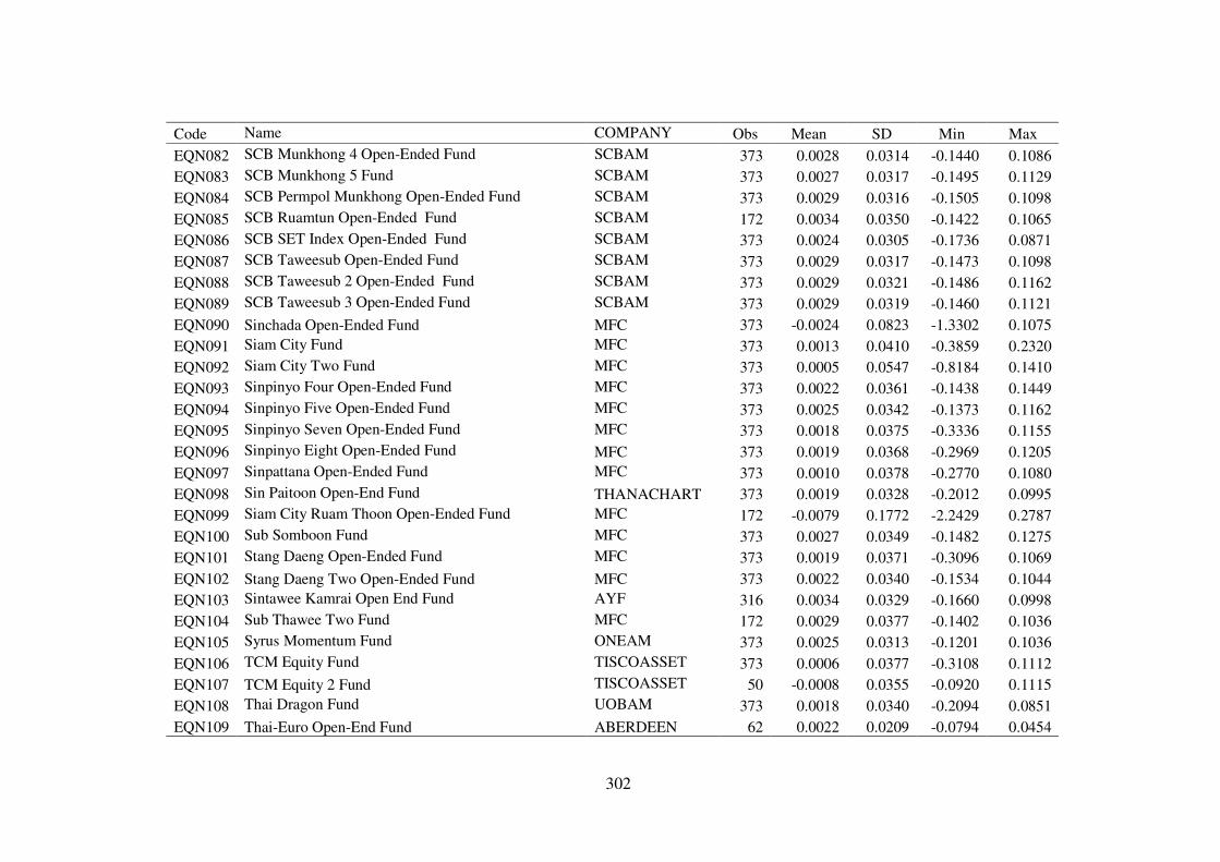
302
Code Name COMPANY Obs Mean SD Min Max
EQN082 SCB Munkhong 4 Open-Ended Fund SCBAM 373 0.0028 0.0314 -0.1440 0.1086
EQN083 SCB Munkhong 5 Fund SCBAM 373 0.0027 0.0317 -0.1495 0.1129
EQN084 SCB Permpol Munkhong Open-Ended Fund SCBAM 373 0.0029 0.0316 -0.1505 0.1098
EQN085 SCB Ruamtun Open-Ended Fund SCBAM 172 0.0034 0.0350 -0.1422 0.1065
EQN086 SCB SET Index Open-Ended Fund SCBAM 373 0.0024 0.0305 -0.1736 0.0871
EQN087 SCB Taweesub Open-Ended Fund SCBAM 373 0.0029 0.0317 -0.1473 0.1098
EQN088 SCB Taweesub 2 Open-Ended Fund SCBAM 373 0.0029 0.0321 -0.1486 0.1162
EQN089 SCB Taweesub 3 Open-Ended Fund SCBAM 373 0.0029 0.0319 -0.1460 0.1121
EQN090 Sinchada Open-Ended Fund MFC 373 -0.0024 0.0823 -1.3302 0.1075
EQN091 Siam City Fund MFC 373 0.0013 0.0410 -0.3859 0.2320
EQN092 Siam City Two Fund MFC 373 0.0005 0.0547 -0.8184 0.1410
EQN093 Sinpinyo Four Open-Ended Fund MFC 373 0.0022 0.0361 -0.1438 0.1449
EQN094 Sinpinyo Five Open-Ended Fund MFC 373 0.0025 0.0342 -0.1373 0.1162
EQN095 Sinpinyo Seven Open-Ended Fund MFC 373 0.0018 0.0375 -0.3336 0.1155
EQN096 Sinpinyo Eight Open-Ended Fund MFC 373 0.0019 0.0368 -0.2969 0.1205
EQN097 Sinpattana Open-Ended Fund MFC 373 0.0010 0.0378 -0.2770 0.1080
EQN098 Sin Paitoon Open-End Fund THANACHART 373 0.0019 0.0328 -0.2012 0.0995
EQN099 Siam City Ruam Thoon Open-Ended Fund MFC 172 -0.0079 0.1772 -2.2429 0.2787
EQN100 Sub Somboon Fund MFC 373 0.0027 0.0349 -0.1482 0.1275
EQN101 Stang Daeng Open-Ended Fund MFC 373 0.0019 0.0371 -0.3096 0.1069
EQN102 Stang Daeng Two Open-Ended Fund MFC 373 0.0022 0.0340 -0.1534 0.1044
EQN103 Sintawee Kamrai Open End Fund AYF 316 0.0034 0.0329 -0.1660 0.0998
EQN104 Sub Thawee Two Fund MFC 172 0.0029 0.0377 -0.1402 0.1036
EQN105 Syrus Momentum Fund ONEAM 373 0.0025 0.0313 -0.1201 0.1036
EQN106 TCM Equity Fund TISCOASSET 373 0.0006 0.0377 -0.3108 0.1112
EQN107 TCM Equity 2 Fund TISCOASSET 50 -0.0008 0.0355 -0.0920 0.1115
EQN108 Thai Dragon Fund UOBAM 373 0.0018 0.0340 -0.2094 0.0851
EQN109 Thai-Euro Open-End Fund ABERDEEN 62 0.0022 0.0209 -0.0794 0.0454

303
Code Name COMPANY Obs Mean SD Min Max
EQN110 TFAM Equity Fund KASSET 246 0.0048 0.0287 -0.0832 0.0691
EQN111 Thana One Fund ONEAM 373 0.0026 0.0313 -0.1186 0.1024
EQN112 Tisco Equity Dividend Fund TISCOASSET 322 0.0000 0.0593 -0.8996 0.1088
EQN113 Tisco Equity Growth Fund TISCOASSET 373 0.0024 0.0313 -0.1334 0.0965
EQN114 Thanaphum Open-Ended Fund MFC 373 0.0028 0.0342 -0.1566 0.1091
EQN115 Theerasub Open-Ended Fund MFC 373 -0.0002 0.0475 -0.6160 0.1064
EQN116 Thunvivatana Fund KASSET 361 0.0010 0.0341 -0.2476 0.1013
EQN117 United Open-Ended Fund MFC 373 0.0025 0.0340 -0.1385 0.1119
EQN118 UOB Smart Active 100 UOBAM 117 0.0024 0.0258 -0.0874 0.0764
EQN119 Udom Sab - Dividend Fund THANACHART 373 0.0018 0.0328 -0.1515 0.0937
EQN120 Udom Sab - Dividend 2 Fund THANACHART 373 0.0021 0.0319 -0.1417 0.0970
EQT001 1 A.M. Selective Growth Long Term Equity Fund ONEAM 114 0.0015 0.0254 -0.0867 0.0783
EQT002 1 A.M. Selective Long Term Equity Fund ONEAM 148 0.0015 0.0249 -0.0858 0.0789
EQT003 1 A.M. Smart Long Term Equity Fund ONEAM 6 -0.0009 0.0021 -0.0052 0.0003
EQT004 Aberdeen Long Term Equity Fund ABERDEEN 145 0.0037 0.0196 -0.0588 0.0521
EQT005 ABN Amro Equities RMF UOBAM 106 0.0068 0.0300 -0.0854 0.0699
EQT006 Aberdeen Smart Capital RMF ABERDEEN 245 0.0047 0.0200 -0.0577 0.0649
EQT007 AJF Set50 Long Term Equity Fund AYF 96 0.0014 0.0252 -0.0816 0.0600
EQT008 Asset Plus Equity RMF ASSETFUND 137 0.0017 0.0193 -0.0593 0.0725
EQT009 Asset Plus Long-Term Equity Fund ASSETFUND 141 0.0015 0.0206 -0.0829 0.0713
EQT010 AYF Equity RMF AYF 56 0.0041 0.0220 -0.0737 0.0605
EQT011 AYF Dividend Stock Long Term Equity Fund 70/30 AYF 7 0.0015 0.0138 -0.0199 0.0244
EQT012 AYF Dividend Stock Long Term Equity Fund AYF 142 0.0020 0.0178 -0.0695 0.0383
EQT013 AYF Equity LTF AYF 56 0.0041 0.0217 -0.0720 0.0606
EQT014 Bualuang Equity RMF BBLAM 244 0.0048 0.0255 -0.1024 0.0890
EQT015 Bualuang Long-Term Equity Fund BBLAM 143 0.0023 0.0227 -0.1012 0.0731
EQT016 Bualuang Long-Term Equity Fund 75/25 BBLAM 12 0.0075 0.0251 -0.0293 0.0606
EQT017 Equity Pro LTF SEAMICOASSET 4 -0.0054 0.0450 -0.0510 0.0559
EQT018 K Equity 70:30 LTF KASSET 88 0.0024 0.0198 -0.0599 0.0514

304
Code Name Company OBS Mean SD Min Max
EQT019 K Equity Dividend LTF KASSET 146 0.0018 0.0261 -0.0839 0.0687
EQT020 K Equity LTF KASSET 146 0.0024 0.0258 -0.0849 0.0686
EQT021 K Equity RMF KASSET 33 0.0064 0.0195 -0.0412 0.0570
EQT022 Krungsri-Primavest Long Term Equity Fund PRIMAVEST 144 0.0019 0.0246 -0.0849 0.0721
EQT023 Krungsri-Primavest LTF Dividend 70/30 PRIMAVEST 36 0.0023 0.0197 -0.0540 0.0491
EQT025 Krung Thai Shariah Long-Term Equity Fund KTAM 32 0.0069 0.0173 -0.0330 0.0529
EQT026 Krung Thai Shariah Retirement Mutual Fund KTAM 32 0.0068 0.0175 -0.0331 0.0532
EQT027 Krung Thai Long-Term Equity Fund KTAM 142 0.0014 0.0245 -0.0878 0.0762
EQT028 Krung Thai Long-Term Equity Fund70/30 KTAM 27 0.0102 0.0209 -0.0249 0.0563
EQT029 MFC Activity Long Term Equity Fund MFC 106 0.0018 0.0246 -0.0803 0.0747
EQT030 Max Dividend Long Term Equity Fund SCIA 146 0.0013 0.0132 -0.0448 0.0294
EQT031 Max Equity Retirement Mutual Fund SCIA 140 0.0018 0.0262 -0.0906 0.0712
EQT032 Max Long Term Equity Perfect SCIA 71 0.0004 0.0276 -0.0907 0.0576
EQT033 MFC Value Long Term Equity Fund MFC 144 0.0020 0.0239 -0.0778 0.0761
EQT034 Nasset Equity Retirement Mutual Fund THANACHART 279 0.0035 0.0245 -0.0819 0.0740
EQT035 The Retire Equity RMF KASSET 9 0.0061 0.0325 -0.0419 0.0657
EQT036 SCB Dividend Stock 70/30 Long Term Equity Fund SCBAM 146 0.0014 0.0158 -0.0528 0.0491
EQT037 SCB Stock Plus Long Term Equity Fund SCBAM 146 0.0022 0.0218 -0.0742 0.0680
EQT038 SCB Mai Stock Long Term Equity Fund SCBAM 95 0.0036 0.0229 -0.0700 0.0562
EQT039 SCB Inter Long Term Equity Fund SCBAM 6 0.0000 0.0275 -0.0449 0.0371
EQT040 SCB Smart Long Term Equity Fund SCBAM 6 0.0061 0.0214 -0.0187 0.0453
EQT041 SCB Target Long Term Equity Fund SCBAM 6 -0.0012 0.0292 -0.0499 0.0386
EQT042 SCB Equity RMF SCBAM 285 0.0032 0.0230 -0.0761 0.0695
EQT043 Tisco Equity Growth Retirement Fund TISCOASSET 252 0.0036 0.0285 -0.0956 0.0924
EQT044 UOB Equities RMF UOBAM 159 0.0023 0.0246 -0.0816 0.0753
EQT045 Valued Stock Retirement Mutual Fund ONEAM 292 0.0039 0.0252 -0.0823 0.0780
EQT046 Wealth Dividend LTF 70:30 KASSET 9 0.0063 0.0265 -0.0307 0.0533
EQT047 Wealth LTF KASSET 9 0.0075 0.0346 -0.0418 0.0671
FLN001 Aberdeen Privilege Fund ABERDEEN 212 0.0002 0.0220 -0.1386 0.0347
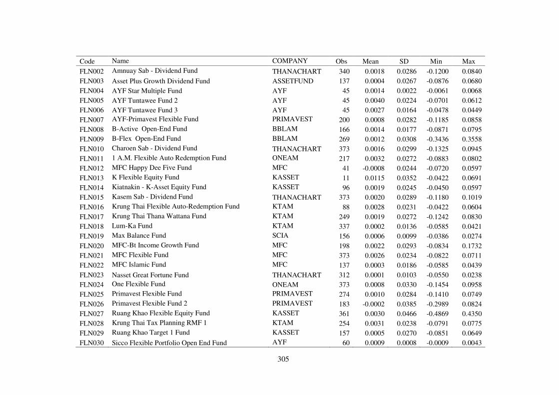
305
Code Name COMPANY Obs Mean SD Min Max
FLN002 Amnuay Sab - Dividend Fund THANACHART 340 0.0018 0.0286 -0.1200 0.0840
FLN003 Asset Plus Growth Dividend Fund ASSETFUND 137 0.0004 0.0267 -0.0876 0.0680
FLN004 AYF Star Multiple Fund AYF 45 0.0014 0.0022 -0.0061 0.0068
FLN005 AYF Tuntawee Fund 2 AYF 45 0.0040 0.0224 -0.0701 0.0612
FLN006 AYF Tuntawee Fund 3 AYF 45 0.0027 0.0164 -0.0478 0.0449
FLN007 AYF-Primavest Flexible Fund PRIMAVEST 200 0.0008 0.0282 -0.1185 0.0858
FLN008 B-Active Open-End Fund BBLAM 166 0.0014 0.0177 -0.0871 0.0795
FLN009 B-Flex Open-End Fund BBLAM 269 0.0012 0.0308 -0.3436 0.3558
FLN010 Charoen Sab - Dividend Fund THANACHART 373 0.0016 0.0299 -0.1325 0.0945
FLN011 1 A.M. Flexible Auto Redemption Fund ONEAM 217 0.0032 0.0272 -0.0883 0.0802
FLN012 MFC Happy Dee Five Fund MFC 41 -0.0008 0.0244 -0.0720 0.0597
FLN013 K Flexible Equity Fund KASSET 11 0.0115 0.0352 -0.0422 0.0691
FLN014 Kiatnakin - K-Asset Equity Fund KASSET 96 0.0019 0.0245 -0.0450 0.0597
FLN015 Kasem Sab - Dividend Fund THANACHART 373 0.0020 0.0289 -0.1180 0.1019
FLN016 Krung Thai Flexible Auto-Redemption Fund KTAM 88 0.0028 0.0231 -0.0422 0.0604
FLN017 Krung Thai Thana Wattana Fund KTAM 249 0.0019 0.0272 -0.1242 0.0830
FLN018 Lum-Ka Fund KTAM 337 0.0002 0.0136 -0.0585 0.0421
FLN019 Max Balance Fund SCIA 156 0.0006 0.0099 -0.0386 0.0274
FLN020 MFC-Bt Income Growth Fund MFC 198 0.0022 0.0293 -0.0834 0.1732
FLN021 MFC Flexible Fund MFC 373 0.0026 0.0234 -0.0822 0.0711
FLN022 MFC Islamic Fund MFC 137 0.0003 0.0186 -0.0585 0.0439
FLN023 Nasset Great Fortune Fund THANACHART 312 0.0001 0.0103 -0.0550 0.0238
FLN024 One Flexible Fund ONEAM 373 0.0008 0.0330 -0.1454 0.0958
FLN025 Primavest Flexible Fund PRIMAVEST 274 0.0010 0.0284 -0.1410 0.0749
FLN026 Primavest Flexible Fund 2 PRIMAVEST 183 -0.0002 0.0385 -0.2989 0.0824
FLN027 Ruang Khao Flexible Equity Fund KASSET 361 0.0030 0.0466 -0.4869 0.4350
FLN028 Krung Thai Tax Planning RMF 1 KTAM 254 0.0031 0.0238 -0.0791 0.0775
FLN029 Ruang Khao Target 1 Fund KASSET 157 0.0005 0.0270 -0.0851 0.0649
FLN030 Sicco Flexible Portfolio Open End Fund AYF 60 0.0009 0.0008 -0.0009 0.0043

306
Code Name COMPANY Obs Mean SD Min Max
FLN031 SCB Capital Stable Protection 1 Open End Fund SCBAM 57 0.0016 0.0057 -0.0223 0.0163
FLN032 SCB Prime Open-Ended Fund SCBAM 373 0.0030 0.0279 -0.1428 0.1024
FLN033 SCB Prime Growth Fund SCBAM 373 0.0029 0.0293 -0.1521 0.1069
FLN034 Sinwattana Fund KASSET 187 0.0005 0.0025 -0.0093 0.0067
FLN035 TCM Flexible Portfolio Fund TISCOASSET 373 0.0023 0.0607 -0.7309 0.7053
FLN036 Thanachart Flexible Fund-2 THANACHART 6 0.0111 0.0272 0.0000 0.0665
FLN037 Thanachart Flexible Fund-2 Series 2 THANACHART 1 0.0000 0.0000 0.0000
FLN038 Tisco Flexible Fund TISCOASSET 373 0.0021 0.0300 -0.1248 0.0854
FLN039 Thai Opportunity Fund KTAM 284 0.0020 0.0267 -0.1427 0.0777
FLN040 UOB Select Fin4cast/1 UOBAM 33 -0.0003 0.0059 -0.0215 0.0203
FLN041 UOB Select Set 50/1 UOBAM 50 0.0012 0.0021 -0.0066 0.0067
FLN042 Buakwan Open-End Fund BBLAM 352 0.0021 0.0317 -0.3393 0.3593
FLN043 ING Thai Balanced Fund ING FUNDS 373 0.0007 0.0562 -0.5460 0.5197
FLN044 Karnchana Anan Open-End Fund MFC 373 0.0014 0.0212 -0.1367 0.0558
FLN045 Pai-Boon Sab Dividend Fund THANACHART 354 0.0016 0.0207 -0.0983 0.0642
FLN046 Ruang Khao Balanced Class KASSET 373 0.0022 0.0204 -0.0973 0.0644
FLN047 Ruang Khao Balanced Distribution Class KASSET 345 0.0012 0.0207 -0.0975 0.0647
FLN048 Ruang Khao Balanced Fund KASSET 373 0.0008 0.0216 -0.1033 0.0613
FLN049 Sa-Thien Sab Dividend Fund THANACHART 373 0.0013 0.0209 -0.1254 0.0658
FLN050 Tisco Balanced Growth Fund TISCOASSET 211 0.0023 0.0194 -0.0637 0.0457
FLT001 Asset Plus Mixed RMF ASSETFUND 137 0.0016 0.0253 -0.0807 0.0833
FLT002 Bualuang Flexible RMF BBLAM 244 0.0034 0.0200 -0.0980 0.0765
FLT003 Finansa Retirement Mutual Fund FAM 62 0.0019 0.0165 -0.0489 0.0404
FLT004 Finansa Mixed Retirement Mutual Fund FAM 73 0.0010 0.0145 -0.0331 0.0392
FLT005 Ruang Khao Flexible Balanced RMF KASSET 281 0.0018 0.0114 -0.0312 0.0363
FLT006 Ruang Khao Flexible Equity RMF KASSET 281 0.0042 0.0303 -0.0870 0.0963
FLT007 Flexible Plus Retirement Mutual Fund ONEAM 191 0.0015 0.0253 -0.0839 0.0643
FLT008 K Balanced RMF KASSET 11 0.0034 0.0122 -0.0142 0.0251
FLT009 K Flexible Equity RMF KASSET 11 0.0115 0.0350 -0.0419 0.0692

307
Code Name COMPANY Obs Mean SD Min Max
FLT010 Max Balance Retirement Mutual Fund SCIA 148 0.0003 0.0096 -0.0344 0.0229
FLT011 MFC Retirment Value Fund MFC 258 0.0038 0.0259 -0.0791 0.0778
FLT012 Primavest Flexible Retirement Mutual Fund PRIMAVEST 250 0.0033 0.0264 -0.0848 0.0765
FLT013 SCB Flexible Fund RMF SCBAM 285 0.0022 0.0162 -0.0551 0.0516
FLT014 Tisco Flexible Portfolio Retirement Fund TISCOASSET 252 0.0032 0.0278 -0.0975 0.0815

308