J

Ma

Aa

b

c

a

ARA

KAMFS

1

Bsmkcdh(osv

ttwo

0d

ARTICLE IN PRESSG ModelAG-473; No. of Pages 10

International Journal of Applied Earth Observation and Geoinformation xxx (2011) xxx–xxx

Contents lists available at SciVerse ScienceDirect

International Journal of Applied Earth Observation andGeoinformation

jo u r n al hom epage: www.elsev ier .com/ locate / jag

ultiscale mapping of burn area and severity using multisensor satellite datand spatial autocorrelation analysis

. Lanortea,∗, M. Daneseb, R. Lasaponaraa, B. Murgantec

CNR-IMAA, Tito Scalo, Potenza, ItalyCNR-IBAM, Tito Scalo, Potenza, ItalyUniversity of Basilicata, Potenza, Italy

r t i c l e i n f o

rticle history:eceived 22 March 2011ccepted 3 September 2011

eywords:STERODIS

ire severity

a b s t r a c t

Traditional methods of recording fire burned areas and fire severity involve expensive and time-consuming field surveys. Available remote sensing technologies may allow us to develop standardizedburn-severity maps for evaluating fire effects and addressing post fire management activities. This paperfocuses on multiscale characterization of fire severity using multisensor satellite data. To this aim, bothMODIS (Moderate Resolution Imaging Spectroradiometer) and ASTER (Advanced Spaceborne ThermalEmission and Reflection Radiometer) data have been processed using geo-statistic analyses to capturepattern features of burned areas.

patial autocorrelation statistics Even if in last decades different authors tried to integrate geo-statistics and remote sensing imageprocessing, methods used since now are only variograms, semivariograms and kriging. In this paper, wepropose an approach based on the use of spatial indicators of global and local autocorrelation. Spatial auto-correlation statistics, such as Moran’s I and Getis–Ord Local Gi index, were used to measure and analyzedependency degree among spectral features of burned areas. This approach enables the characterizationof pattern features of a burned area and improves the estimation of fire severity.

© 2011 Elsevier B.V. All rights reserved.

. Introduction

Fire represents one of the main disturbances of Mediterraneanasin, bringing profound transformations at different temporal andpatial scales which affect ecosystems, landscapes and environ-ents. Immediately after a fire, there are its direct effects (also

nown as immediate effects or first-order fire effects), which areombustion direct consequences, namely fuel consumption, pro-uction of smoke and ash and heating of soil. Whereas, since a fewours up to many decades after a fire, there are long-term resultsalso known as second-order fire-effects), which are indirect resultsf fire, namely alteration in vegetation structure and composition,oil erosion, changes in nutrient levels, micro-climate, hydrology,egetation succession.

In the Mediterranean Basin, composition and structure of vege-ation have been and are generally strongly shaped by fires, whichend to operate as a selective force, increasing species diversity, as

Please cite this article in press as: Lanorte, A., et al., Multiscale mappispatial autocorrelation analysis. Int. J. Appl. Earth Observ. Geoinf. (201

ell as a filter favouring the dominance of some species rather thanf other ones (Grace et al., 2006; Pausas and Verdú, 2008).

∗ Corresponding author.E-mail address: alanorte@imaa.cnr.it (A. Lanorte).

303-2434/$ – see front matter © 2011 Elsevier B.V. All rights reserved.oi:10.1016/j.jag.2011.09.005

Effects of fires on soil, plants, landscape and ecosystems dependon many factors (among them fire frequency and plant resistance).Burn severity is a qualitative indicator of the effects of fire onecosystems, since it affects forest floor, canopy, etc. Assessing andmapping burn severity is important to monitor fire effects, to modeland evaluate post-fire dynamics and to estimate the ability of veg-etation to recover after fire (generally indicated as fire-resilience).In an operational context, burn severity estimation is critical forshort-term mitigation and rehabilitation treatments. Traditionalmethods of recording fire severity involve expensive and time-consuming field surveys. The use of satellite remote sensing canhelp in overcoming such drawbacks.

Remote sensing technologies can provide useful data forfire management, from risk estimation (Rauste et al., 1997;Lasaponara, 2005), fuel mapping (Lasaponara and Lanorte, 2006,2007a,b), fire detection (Lasaponara et al., 2003), to post firemonitoring (Lasaponara, 2006), including burn area and severityestimation (Gitas and Desantis, 2009; Hall et al., 2008; Richards,1995). Methods generally used to estimate fire severity fromsatellite are based on spectral indexes, obtained as a combination

ng of burn area and severity using multisensor satellite data and1), doi:10.1016/j.jag.2011.09.005

of bands which emphasize changes induced by fire in vegetationspectral behaviour. Several vegetation indexes were used, suchas SVI (Simple Vegetation Index), TVI (Transformed DifferenceVegetation Index), SAVI (Soil Adjusted Vegetation Index), NDVI

ING ModelJ

2 rth O

(B

prtktmaad

gbdpfiaae

aafitaG

2

u(

iavgs

nslMiwattgwooa

hssssicd

ARTICLEAG-473; No. of Pages 10

A. Lanorte et al. / International Journal of Applied Ea

Normalized Difference Vegetation Index) and NBR (Normalizedurn Difference).

Maps obtained by difference between pre- and post-fire indexesrovide a measure of change used to quantify biomass loss, carbonelease, smoke production, etc. (Xiao et al., 2003). Such evalua-ions are generally performed on fire perimeter maps (a priorinown), mainly using fixed threshold values to classify and maphe different levels of burn severity. Nevertheless, as suggested by

any authors, such fixed threshold values are generally not suit-ble for fragmented landscapes and inadequate for vegetation typesnd geographic regions different from those for which they wereevised (Key and Benson, 2006; Key, 2006; Zhu et al., 2006).

In order to overcome such limitations, a new approach, based oneo-statistical analyses applied to satellite data, is herein proposedoth to estimate burn area perimeter and to evaluate the differentegree of burn severity. The use of robust geo-statistical analyses torocess satellite data is relatively recent, even if, in last decades dif-erent authors tried to integrate geo-statistics and remote sensingmage processing (Curran et al., 1998), but methods used since nowre only variograms, semivariograms and kriging (some examplesre Hyppänen, 1996; Atkinson and Lewis, 2000; López-Granadost al., 2005).

In this paper, we propose a more robust spatial statistics analysispproach, based on the use of spatial indicators of global and localutocorrelation to capture feature pattern, to map areas affected byre and to estimate the degree of fire severity. For the purpose ofhis study, ASTER and MODIS derived indexes were processed for

significant test area located in southern Italy using Moran’s I andetis–Ord Local Gi index (see Moran, 1948; Getis and Ord, 1994).

. Satellite data

In the present study satellite MODIS and ASTER data have beensed. MODIS is a key instrument aboard Terra (EOS AM) and AquaEOS PM) satellites.

These data will improve our understanding of global dynam-cs and processes occurring on land, in oceans, and in lowertmosphere. MODIS is playing a vital role in the development ofalidated, global, interactive Earth system models able to predictlobal change accurately enough, to assist policy makers in makingound decisions concerning the protection of our environment.

Terra’s orbit around the Earth is timed so that it passes fromorth to south across the equator in the morning, while Aqua passesouth to north over the equator in the afternoon. Terra MODIS,aunched on December 18, 1999 and Aqua MODIS, launched on

ay 4, 2002, are viewing the entire Earth’s surface, acquiring datan 36 spectral bands ranging in wavelength from 0.4 �m to 14.4 �m,

ith a high radiometric sensitivity (12 bit).Two bands are imagedt a nominal resolution of 250 m at nadir, five bands at 500 m, andhe remaining 29 bands at 1 km. A ±55-degree scanning pattern athe EOS orbit of 705 km achieves a 2330-km swath and provideslobal coverage every one to two days.MODIS bands used in thisork are the first seven ones, corresponding to a spatial resolution

f 250 and 500 m. These spectral bands are suitable for the studyf vegetation characteristics. MODIS data used for this study werecquired on 14 July 2007 and 30 July 2007.

ASTER is a high resolution imaging instrument flying on Terra. Itas the highest spatial resolution (15 meters VNIR) of all five sen-ors on Terra and collects data in the visible/near infrared (VNIR),hort wave infrared (SWIR), and thermal infrared bands (TIR). Eachubsystem is pointable in the crosstrack direction. The VNIR sub-

Please cite this article in press as: Lanorte, A., et al., Multiscale mappispatial autocorrelation analysis. Int. J. Appl. Earth Observ. Geoinf. (201

ystem of ASTER is quite unique. One telescope of the VNIR systems nadir looking and two ones are backward looking, allowing theonstruction of three-dimensional digital elevation models (DEM)ue to the stereo capability of different looking angles.

PRESSbservation and Geoinformation xxx (2011) xxx–xxx

ASTER has a revisit period of 16 days, to any one location on theglobe, with a revisit time at the equator of four days. ASTER collectsapproximately 8 min of data per orbit (rather than continuously).Among the 14 ASTER bands in this work we only considered thethree channels in the VNIR region. For the purpose of our study,two MODIS and two ASTER multispectral images were acquired on14 July 2007 and 30 July 2007, respectively before and after a fireoccurrence (22 July 2007).

3. Classic methods: the NBR index

After a fire, the spectral behaviour of vegetation changes dueto consumption of fuel, presence of ash, reduced transpiration ofvegetation and increased surface temperature. All these effectsincrease reflectance in mid-infrared and reduce surface reflectancein near-infrared. This is the reason because NBR index (formula 1)is computed on the basis of the two burn sensitive bands, infrared(NIR) and shortwave infrared (SWIR). For this reason, it may be oneof the best indexes to detect a burn area.

NBR = NIR − SWIRNIR + SWIR

(1)

Maps obtained by the difference between pre- and post-fire indexes(formula (2)) provide a measure of change which then can be usedto estimate biomass loss, carbon release, aerosols production, etc.(Miller and Thode, 2007). Moreover, the difference in pre/post-burn NBR index could reflect surface change and characterize burnseverity degree.

dNBR = NBRprefire − NBRpostfire (2)

Some authors suggest the use of relative dNBR (formula (3)) inorder to overcome the drawback linked to misclassification of lowvegetated pixels that could arise using the absolute change imagederived through dNBR (Miller et al., 2009). They argue that absolutechange may be inappropriate to estimate ecological impacts of fireand may misclassify burn severity, especially using fixed thresholdvalues in fragmented ecosystems with different vegetation types.Image differences could produce a misclassification in burn severityespecially for low vegetated pixel characterized by small variationsof pre/post-burn NBR index. The use of relative dNBR is recom-mended to map fire severity of historic fires, for which field datamay not be available.

RdNBR = dNBR[abs (NBRprefire)]1/2 (3)

Moreover, the use of a relative index, here called RdNBR (3), willalso enable us to make comparable burn severity estimation acrossspace and time, that is a key issue for a landscape level analysis.

4. Spatial autocorrelation statistics

4.1. Spatial autocorrelation: basic concepts

The spatial autocorrelation concept is based on the first geog-raphy law introduced by Tobler (1970) “Everything is related toeverything else, but nearest things are more related than distantthings”. In other terms, considering the occurrences of a spatialvariable (events), spatial autocorrelation measures the degree ofdependency among events, considering at the same time their sim-ilarity and their distance relationships.

In absence of spatial autocorrelation, the complete spatial ran-domness hypothesis is valid: the probability to have an event inone point with defined (x, y) coordinates is independent on the

ng of burn area and severity using multisensor satellite data and1), doi:10.1016/j.jag.2011.09.005

probability to have another event belonging to the same variable.The presence of spatial autocorrelation modifies that probability;fixed a neighbourhood for each event, it is possible to understandhow much it is modified from the presence of other elements inside

ARTICLE IN PRESSG ModelJAG-473; No. of Pages 10

A. Lanorte et al. / International Journal of Applied Earth Observation and Geoinformation xxx (2011) xxx–xxx 3

lation

ta

-

-

-

c1s

-

-

-

-

t

E(I) = −(

1N − 1

)(9)

where N is the number of events in the whole distribution.

Fig. 1. Possible spatial distributions. (a) Positive spatial autocorre

hat neighbourhood.A distribution can show three types of spatialutocorrelation (O’Sullivan and Unwin, 2002):

the variable shows positive spatial autocorrelation (Fig. 1a) whenevents are near and similar (clustered distribution);

the variable shows negative spatial autocorrelation (Fig. 1b)when, even if events are near, they are not similar (uniform dis-tribution);

the variable shows null autocorrelation (Fig. 1c) when there areno spatial effects, neither about the position of events, or theirproperties (random distribution).

The presence of autocorrelation in a spatial distribution isaused by two effects, that could be clearly defined (Gatrell et al.,996; Bailey and Gatrell, 1995), but that could not be separatelytudied in the practice:

first order effects depend on properties of study region and mea-sures how the expected value (average of the quantitative valueassociated to each spatial event) varies in the space with the fol-lowing expression:

��(s) = limds→0

{E(Y(ds))

ds

}(4)

where ds is neighbourhood around s, E (·) is the expected averageand Y(ds) is events number in neighbourhood;

second order effects express local interactions between eventsin a fixed neighbourhood, which tend to the distance betweenevents i and j. These effects are measured with covariance varia-tions expressed by the limit:

�(sisj) =lim

dsidsj → 0

{E(Y(dsi)Y(dsj))

dsidsj

}(5)

where symbols are similar to those used in equation 1.As clarified by the definition of first and second order effects, the

study of spatial autocorrelation requests to know in more detail: the quantitative nature of dataset, also called intensity of the spa-tial process, that is how strong a variable happens in the space(Murgante et al., 2008; Danese et al., 2009; Murgante and Danese,2011), with the aim to understand if events are similar or dissim-ilar;

the geometric nature of dataset. This needs the conceptualizationof geometric relationships, usually done by the use of matrixes: (i)a distance matrix is defined to consider at which distance eventsinfluence each other (distance band); (ii) a contiguity matrix isuseful to know if events influence each other; (iii) a matrix of

Please cite this article in press as: Lanorte, A., et al., Multiscale mappispatial autocorrelation analysis. Int. J. Appl. Earth Observ. Geoinf. (201

spatial weights expresses how strong this influence is.

Concerning the distance matrix, a method should be establishedo calculate distances in module and direction.

, (b) negative spatial autocorrelation and (c) null autocorrelation.

For this concern Euclidean distance (3), is the most used module.

dE(si, sj) =√

(xi − xj)2 + (yi − yj)

2 (6)

For what concerns direction, existing methods take their name fromthe game of chess. They are called tower contiguity (Fig. 2a), bishopcontiguity (Fig. 2b) and queen contiguity (Fig. 2c).

Concerning the spatial weight matrix wij, most diffused methodsto calculate it are the “Inverse Distance” method and the “FixedDistance Band” method. In the first one, weights vary in inverserelation to the distance dz

ijamong events:

wij = dzij (7)

where z is a number smaller then 0.The “Fixed Distance Band” method defines a critical distance

beyond which two events will never be adjacent. If the areas towhich i and j belong are contiguous, wij will be equal to 1, otherwisewij will be equal to 0.

4.2. Global indicators of spatial autocorrelation

Global indicators of autocorrelation measure if and how muchthe dataset is autocorrelated throughout the study region.

One of the principal global indicators of autocorrelation is theMoran’s index I (Moran, 1948), defined in formula (8)

I =N∑

i

∑jwij(Xi − X)(Xj − X)(∑

i

∑jwij

)∑i(Xi − X)

2(8)

where N is the total pixel number, Xi and Xj are intensities in pointsi and j (with i /= j), X is the average value, wij is an element of theweight matrix.

If I ∈ [−1; 1]; if I ∈ [−1; 0] there is a negative autocorrelation; ifI ∈ [0; 1] there is a positive autocorrelation. Theoretically, if I con-verges to 0 there is null autocorrelation, in most of the cases, insteadof 0 the value used to affirm the presence of null autocorrelation isgiven in equation (9):

ng of burn area and severity using multisensor satellite data and1), doi:10.1016/j.jag.2011.09.005

Fig. 2. (a) Tower contiguity, (b) bishop contiguity and (c) queen contiguity.

ARTICLE IN PRESSG ModelJAG-473; No. of Pages 10

4 A. Lanorte et al. / International Journal of Applied Earth Observation and Geoinformation xxx (2011) xxx–xxx

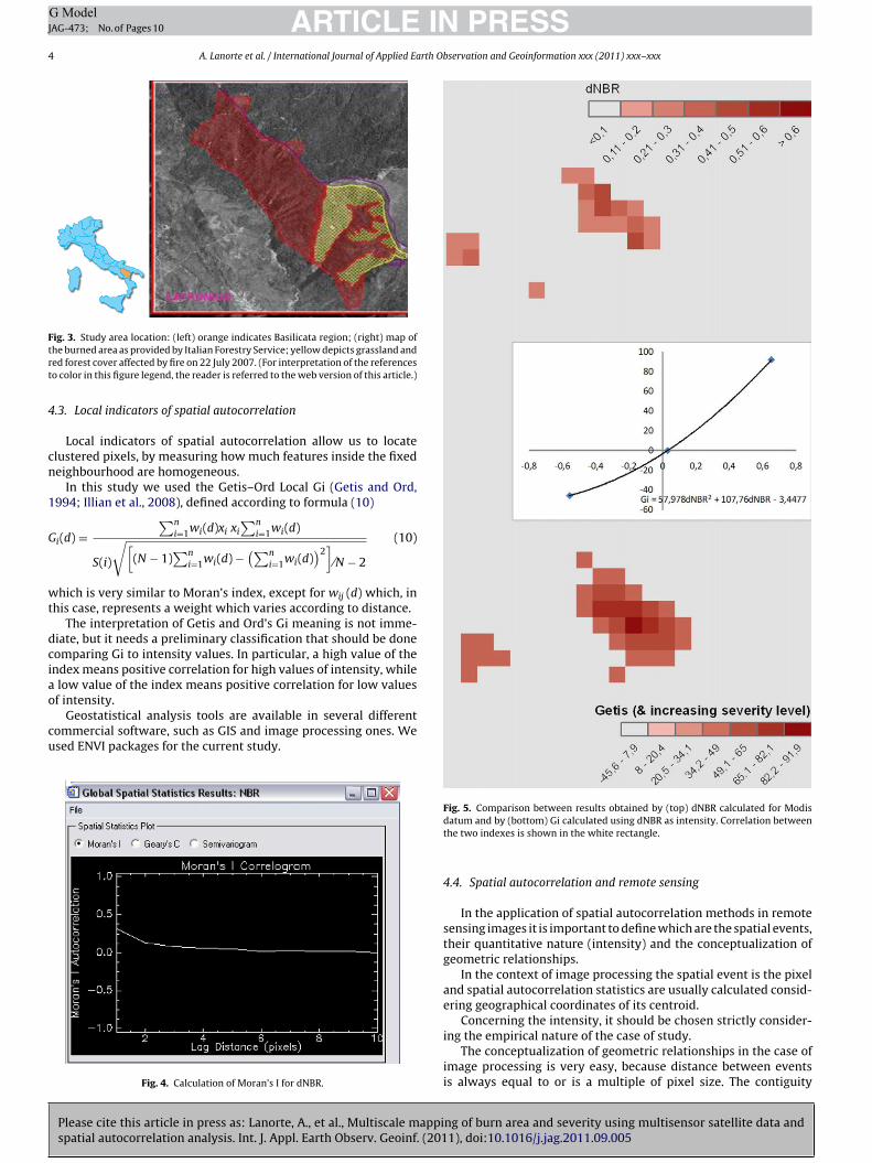
Fig. 3. Study area location: (left) orange indicates Basilicata region; (right) map oftrt

4

cn

1

G

wt

dciao

cu

he burned area as provided by Italian Forestry Service; yellow depicts grassland anded forest cover affected by fire on 22 July 2007. (For interpretation of the referenceso color in this figure legend, the reader is referred to the web version of this article.)

.3. Local indicators of spatial autocorrelation

Local indicators of spatial autocorrelation allow us to locatelustered pixels, by measuring how much features inside the fixedeighbourhood are homogeneous.

In this study we used the Getis–Ord Local Gi (Getis and Ord,994; Illian et al., 2008), defined according to formula (10)

i(d) =∑n

i=1wi(d)xi xi

∑ni=1wi(d)

S(i)

√[(N − 1)

∑ni=1wi(d) −

(∑ni=1wi(d)

)2]⁄N − 2

(10)

hich is very similar to Moran’s index, except for wij (d) which, inhis case, represents a weight which varies according to distance.

The interpretation of Getis and Ord’s Gi meaning is not imme-iate, but it needs a preliminary classification that should be doneomparing Gi to intensity values. In particular, a high value of thendex means positive correlation for high values of intensity, while

low value of the index means positive correlation for low values

Please cite this article in press as: Lanorte, A., et al., Multiscale mappispatial autocorrelation analysis. Int. J. Appl. Earth Observ. Geoinf. (201

f intensity.Geostatistical analysis tools are available in several different

ommercial software, such as GIS and image processing ones. Wesed ENVI packages for the current study.

Fig. 4. Calculation of Moran’s I for dNBR.

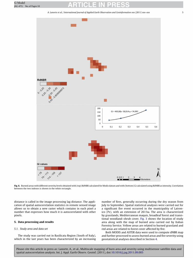
Fig. 5. Comparison between results obtained by (top) dNBR calculated for Modis

datum and by (bottom) Gi calculated using dNBR as intensity. Correlation betweenthe two indexes is shown in the white rectangle.

4.4. Spatial autocorrelation and remote sensing

In the application of spatial autocorrelation methods in remotesensing images it is important to define which are the spatial events,their quantitative nature (intensity) and the conceptualization ofgeometric relationships.

In the context of image processing the spatial event is the pixeland spatial autocorrelation statistics are usually calculated consid-ering geographical coordinates of its centroid.

Concerning the intensity, it should be chosen strictly consider-

ng of burn area and severity using multisensor satellite data and1), doi:10.1016/j.jag.2011.09.005

ing the empirical nature of the case of study.The conceptualization of geometric relationships in the case of

image processing is very easy, because distance between eventsis always equal to or is a multiple of pixel size. The contiguity

ARTICLE IN PRESSG ModelJAG-473; No. of Pages 10

A. Lanorte et al. / International Journal of Applied Earth Observation and Geoinformation xxx (2011) xxx–xxx 5

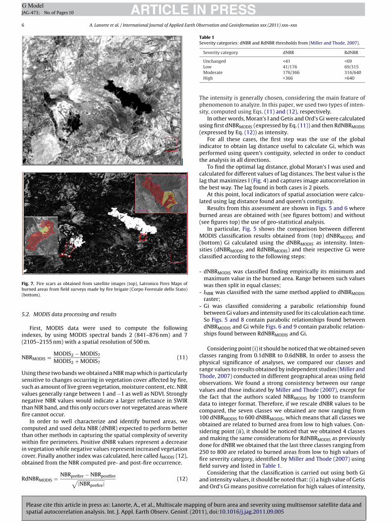
Fig. 6. Burned areas with different severity levels obtained with (top) RdNBR calculated for Modis datum and with (bottom) Gi calculated using RdNBR as intensity. Correlationb

dcanp

5

5

w

etween the two indexes is shown in the white rectangle.

istance is called in the image processing lag distance. The appli-ation of spatial autocorrelation statistics in remote sensed imagellows us to obtain a new raster which contains in each pixel aumber that expresses how much it is autocorrelated with otherixels.

. Data processing and results

Please cite this article in press as: Lanorte, A., et al., Multiscale mappispatial autocorrelation analysis. Int. J. Appl. Earth Observ. Geoinf. (201

.1. Study area and data set

The study was carried out in Basilicata Region (South of Italy),hich in the last years has been characterized by an increasing

number of fires, generally occurring during the dry season fromJuly to September. Spatial statistical analyses were carried out fora significant fire event occurred in the municipality of Latron-ico (Pz), with an extension of 261 ha. The area is characterizedby grasslands, Mediterranean maquis, broadleaf forest and transi-tional woodland–shrub cover. Fig. 3 shows the location of studyarea along with the map of burned area carried out by ItalianForestry Service. Yellow areas are related to burned grassland and

ng of burn area and severity using multisensor satellite data and1), doi:10.1016/j.jag.2011.09.005

red areas are related to forest cover affected by fire.Both MODIS and ASTER data were used to compute dNBR map

and further processed to assess burned areas and fire severity usinggeostatistical analyses described in Section 4.

ARTICLE IN PRESSG ModelJAG-473; No. of Pages 10

6 A. Lanorte et al. / International Journal of Applied Earth Observation and Geoinformation xxx (2011) xxx–xxx

Fig. 7. Fire scars as obtained from satellite images (top), Latronico Fires Maps ofb(

5

i(

N

Ussvntfi

ctwico

R

Table 1Severity categories: dNBR and RdNBR thresholds from (Miller and Thode, 2007).

Severity category dNBR RdNBR

Unchanged <41 <69Low 41/176 69/315

field survey and listed in Table 1.

urned areas from field surveys made by fire brigate (Corpo Forestale dello Stato)bottom).

.2. MODIS data processing and results

First, MODIS data were used to compute the followingndexes, by using MODIS spectral bands 2 (841–876 nm) and 72105–2155 nm) with a spatial resolution of 500 m.

BRMODIS = MODIS2 − MODIS7

MODIS2 + MODIS7(11)

sing these two bands we obtained a NBR map which is particularlyensitive to changes occurring in vegetation cover affected by fire,uch as amount of live green vegetation, moisture content, etc. NBRalues generally range between 1 and −1 as well as NDVI. Stronglyegative NBR values would indicate a larger reflectance in SWIRhan NIR band, and this only occurs over not vegetated areas wherere cannot occur.

In order to well characterize and identify burned areas, weomputed and used delta NBR (dNBR) expected to perform betterhan other methods in capturing the spatial complexity of severityithin fire perimeters. Positive dNBR values represent a decrease

n vegetation while negative values represent increased vegetationover. Finally another index was calculated, here called IMODIS (12),btained from the NBR computed pre- and post-fire occurrence.

Please cite this article in press as: Lanorte, A., et al., Multiscale mappispatial autocorrelation analysis. Int. J. Appl. Earth Observ. Geoinf. (201

dNBRMODIS = NBRprefire − NBRpostfire√|NBRprefire|

(12)

Moderate 176/366 316/640High >366 >640

The intensity is generally chosen, considering the main feature ofphenomenon to analyze. In this paper, we used two types of inten-sity, computed using Eqs. (11) and (12), respectively.

In other words, Moran’s I and Getis and Ord’s Gi were calculatedusing first dNBRMODIS (expressed by Eq. (11)) and then RdNBRMODIS(expressed by Eq. (12)) as intensity.

For all these cases, the first step was the use of the globalindicator to obtain lag distance useful to calculate Gi, which wasperformed using queen’s contiguity, selected in order to conductthe analysis in all directions.

To find the optimal lag distance, global Moran’s I was used andcalculated for different values of lag distances. The best value is thelag that maximizes I (Fig. 4) and captures image autocorrelation inthe best way. The lag found in both cases is 2 pixels.

At this point, local indicators of spatial association were calcu-lated using lag distance found and queen’s contiguity.

Results from this assessment are shown in Figs. 5 and 6 whereburned areas are obtained with (see figures bottom) and without(see figures top) the use of geo-statistical analysis.

In particular, Fig. 5 shows the comparison between differentMODIS classification results obtained from (top) dNBRMODIS and(bottom) Gi calculated using the dNBRMODIS as intensity. Inten-sities (dNBRMODIS and RdNBRMODIS) and their respective Gi wereclassified according to the following steps:

- dNBRMODIS was classified finding empirically its minimum andmaximum value in the burned area. Range between such valueswas then split in equal classes;

- INBR was classified with the same method applied to dNBRMODISraster;

- Gi was classified considering a parabolic relationship foundbetween Gi values and intensity used for its calculation each time.So Figs. 5 and 8 contain parabolic relationships found betweendNBRMODIS and Gi while Figs. 6 and 9 contain parabolic relation-ships found between RdNBRMODIS and Gi.

Considering point (i) it should be noticed that we obtained sevenclasses ranging from 0.1dNBR to 0.6dNBR. In order to assess thephysical significance of analyses, we compared our classes andrange values to results obtained by independent studies (Miller andThode, 2007) conducted in different geographical areas using fieldobservations. We found a strong consistency between our rangevalues and those indicated by Miller and Thode (2007), except forthe fact that the authors scaled NBRMODIS by 1000 to transformdata to integer format. Therefore, if we rescale dNBR values to becompared, the seven classes we obtained are now ranging from100 dNBRMODIS to 600 dNBRMODIS, which means that all classes weobtained are related to burned area from low to high values. Con-sidering point (ii), it should be noticed that we obtained 4 classesand making the same considerations for RdNBRMODIS as previouslydone for dNBR we obtained that the last three classes ranging from250 to 800 are related to burned areas from low to high values offire severity category, identified by Miller and Thode (2007) using

ng of burn area and severity using multisensor satellite data and1), doi:10.1016/j.jag.2011.09.005

Considering that the classification is carried out using both Giand intensity values, it should be noted that: (i) a high value of Getisand Ord’s Gi means positive correlation for high values of intensity,

ARTICLE IN PRESSG ModelJAG-473; No. of Pages 10

A. Lanorte et al. / International Journal of Applied Earth Observation and Geoinformation xxx (2011) xxx–xxx 7

F ted fob

thipft

oht

(t

ig. 8. Burned areas with different severity levels obtained with (top) dNBR calculaetween the two indexes is shown in the white rectangle.

hus providing pixels strongly affected by fire and characterized byigh fire severity level, (ii) while a low value of Getis and Ord’s Gi

ndex means positive correlation for low values of intensity, thusroviding pixels characterized by low levels of fire severity or unaf-ected by fire. The correlation between the two indexes is shown inhe white rectangle in Fig. 5.

From a visual inspection of Fig. 5, we can notice that resultsbtained by (top) dNBRMODIS exhibit some pixels which could notave been affected by fire. A similar behaviour can be observed in

Please cite this article in press as: Lanorte, A., et al., Multiscale mappispatial autocorrelation analysis. Int. J. Appl. Earth Observ. Geoinf. (201

he results of (bottom) Gi calculated using dNBR as intensity.In Fig. 5 (top and bottom), some problems appear to be present:

i) the overestimation of burned area, and (ii) the presence of addi-ional pixels classified as burned area. The overestimation of burned

r Aster datum and with (bottom) Gi calculated using dNBR as intensity. Correlation

area is due to pixel size which is not adequate for detecting afire-affected area of about 200 ha. Of course, the whole pixel isclassified as burned even if only a small part of it is affected byfire.

To check reliability of obtained results, we also considered inten-sity obtained by means of Eq. (10), which should be able to betterclassify fire affected pixels. Such results are shown in Fig. 6 whereburned areas are obtained with (see bottom) and without (see top)the use of geo-statistical analysis. Areas with different fire sever-

ng of burn area and severity using multisensor satellite data and1), doi:10.1016/j.jag.2011.09.005

ity levels were obtained with (top) RdNBR calculated for MODISimages and with (bottom) Gi calculated using RdNBR as inten-sity. Correlation between the two indexes is shown in the whiterectangle.

ARTICLE IN PRESSG ModelJAG-473; No. of Pages 10

8 A. Lanorte et al. / International Journal of Applied Earth Observation and Geoinformation xxx (2011) xxx–xxx

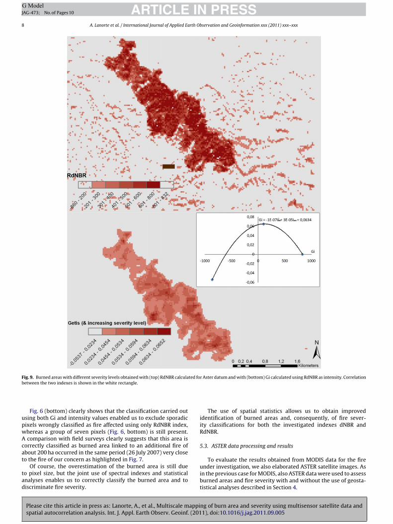
Fig. 9. Burned areas with different severity levels obtained with (top) RdNBR calculated for Aster datum and with (bottom) Gi calculated using RdNBR as intensity. Correlationb

upwAcat

tad

etween the two indexes is shown in the white rectangle.

Fig. 6 (bottom) clearly shows that the classification carried outsing both Gi and intensity values enabled us to exclude sporadicixels wrongly classified as fire affected using only RdNBR index,hereas a group of seven pixels (Fig. 6, bottom) is still present.

comparison with field surveys clearly suggests that this area isorrectly classified as burned area linked to an additional fire ofbout 200 ha occurred in the same period (26 July 2007) very closeo the fire of our concern as highlighted in Fig. 7.

Please cite this article in press as: Lanorte, A., et al., Multiscale mappispatial autocorrelation analysis. Int. J. Appl. Earth Observ. Geoinf. (201

Of course, the overestimation of the burned area is still dueo pixel size, but the joint use of spectral indexes and statisticalnalyses enables us to correctly classify the burned area and toiscriminate fire severity.

The use of spatial statistics allows us to obtain improvedidentification of burned areas and, consequently, of fire sever-ity classifications for both the investigated indexes dNBR andRdNBR.

5.3. ASTER data processing and results

To evaluate the results obtained from MODIS data for the fire

ng of burn area and severity using multisensor satellite data and1), doi:10.1016/j.jag.2011.09.005

under investigation, we also elaborated ASTER satellite images. Asin the previous case for MODIS, also ASTER data were used to assessburned areas and fire severity with and without the use of geosta-tistical analyses described in Section 4.

ING ModelJ

rth Ob

Aw

N

ItNcN

R

Siai

edscrAr

pwMooomMwas(tbcu

Riw

ssasbf

sG

Mbsca

os

ARTICLEAG-473; No. of Pages 10

A. Lanorte et al. / International Journal of Applied Ea

ASTER data were used to compute NBR based indexes usingSTER 3 (760–860 nm) and 7 (2235–2285 nm) spectral channels,ith a spatial resolution of 30 m, using formula (13).

BRASTER = ASTER2 − ASTER7

ASTER2 + ASTER7(13)

n this case NBRASTER values were multiplied by 1000 and convertedo integer format to follow Miller and Thode (2007) and compareBRASTER. As in the previous case for MODIS, another index was cal-ulated, here called RdNBRASTER (see formula (14)), obtained fromBR computed pre- and post-fire occurrence.

dNBRASTER = NBRprefire − NBRpostfire√|NBRprefire/1000|

(14)

ince we scaled NBR by 1000 to transform data to integer format,n formula 14 the pre-fire NBR must be divided by 1000. Taking thebsolute value of pre-fire, NBR in the denominator allows comput-ng the square-root without changing the sign of original dNBR.

Fig. 8 depicts Aster burned areas with different severity lev-ls obtained by dNBRaster (top) and Gi (bottom) calculated usingNBRaster as intensity. Correlation between the two indexes ishown in the white rectangle. Results were found with the samelassification method used for MODIS images. Again, a parabolicelationship was found between intensity and Getis and Ord’s Gi.pplying this relationship, significant values of Gi were found cor-esponding to dNBRaster classes.

As previously done for MODIS data investigations, consideringoint (i) of Section 5.2 we obtained several fire severity classes,hose range values were compared with results obtained fromiller and Thode (2007). We found a strong consistency between

ur classes and range values indicated by Miller and Thode (2007)n the basis of field surveys. In particular, the last five classes webtained were higher than 200 and therefore they correspond tooderate and high fire severity according to severity category byiller and Thode (2007) herein listed in Table 1. Nevertheless, whene applied this classification to the whole ASTER dNBRaster image,

high number of pixels were identified as burned area with fireeverity levels ranging from moderate to high. As it is shown in Fig. 8bottom), also in the case of ASTER dNBRaster images, the applica-ion of spatial statistics enabled us to improve both the detection ofurned areas and the assessment of fire severity levels. The classifi-ation of Gi (bottom), calculated using dNBR as intensity, excludednburned areas.

Finally, Fig. 9 shows different severity levels obtained bydNBRASTER (top) and Gi (bottom) calculated using RdNBRASTER as

ntensity. Correlation between the two indexes is shown in thehite rectangle.

The visual comparison between bottom and top of Fig. 9 clearlyhows that the classification carried out using both Gi and inten-ity values enabled us to exclude sporadic pixels wrongly classifieds burned areas using only RdNBR index. A comparison with fieldurveys clearly suggests that (i) this area is correctly classified asurned area and (ii) fire severity categories well identified the dif-erent levels of fire severity.

In particular, both mapping of the entire burned area and corre-ponding to different levels of fire severity, have been reached withPS tracking.

Results from all performed analyses pointed out that, for bothODIS and ASTER images, a parabolic relationship was found

etween intensity and Getis and Ord’s Gi. Applying this relation-hip, significant values of Gi were found corresponding to dNBRlasses. Obtained results enable us to recognize fire burned areas

Please cite this article in press as: Lanorte, A., et al., Multiscale mappispatial autocorrelation analysis. Int. J. Appl. Earth Observ. Geoinf. (201

nd quantitatively characterize fire patterns and burn severity.Of course, the use of Aster images limited the overestimation

f burned areas due to a most adequate pixel size for investigatedmall fires (around 200 ha). Finally, the joint use of spectral indexes

PRESSservation and Geoinformation xxx (2011) xxx–xxx 9

and statistical analyses enables us to correctly detect burned areasand to assess fire severity using both investigated indices dNBR andRdNBR.

6. Conclusions

In this paper, we propose a robust statistical approach, based onthe use of spatial indicators of global and local autocorrelation, todetect burned area and estimate fire severity. Spatial autocorrela-tion statistics, such as Moran’s I and Getis–Ord Local Gi index (seeMoran, 1948; Getis and Ord, 1994), were used to capture patternfeatures of burned areas.

We focused on the multiscale analyses using both MODIS(Moderate Resolution Imaging Spectroradiometer) and ASTER(Advanced Spaceborne Thermal Emission and Reflection Radiome-ter) data to identify burned areas and characterize burn severity.Pre- and post-fire satellite MODIS and ASTER images were pro-cessed for a significant test area in Southern Italy. Spectral indexesgenerally used for fire severity estimation were analyzed and pro-cessed with and without using geostatistical analyses.

The comparison of results obtained for both MODIS and ASTERimages with and without the use of spatial autocorrelation statisticsclearly pointed out the improvements achieved using both globaland local spatial autocorrelation statistics. Our results showed thatthese statistics applied to MODIS and ASTER data allowed us (i) todetect burned areas and (ii) to discriminate fire severity.

The new approach is independent on sensors used for the eval-uation as well as on vegetation cover types affected by fire, beingthe value obtained really close to those obtained by independentstudies carried out in diverse geographic regions and land covertypes.

Assessing and mapping burn severity is important for monitor-ing fire effects, modeling and evaluating post-fire dynamics andestimating vegetation resilience, which is the ability of vegetationto recover after fire. The availability of satellite high resolutionimagery provides the opportunity to obtain useful information forfire management, from risk evaluation to post-fire damage estima-tion.

The herein proposed approach could be directly incorporatedinto mapping process from local up to global scale.

References

Atkinson, P.M., Lewis, P., 2000. Geostatistical classification for remote sensing: anintroduction. Computers & Geosciences 26, 362–371.

Curran, P., Atkinson, P.M., 1998. Geostatistics remote sensing. Progress in PhysicalGeography 22 (1), 61-78.

Bailey, T.C., Gatrell, A.C., 1995. Interactive Spatial Data Analysis. Longman HigherEducation, Harlow.

Danese, M., Lazzari, M., Murgante, B., 2009. Geostatistics in historical macroseismicdata analysis. Transactions on Computational Sciences Journal VI LNCS vol. 5730,324–341, doi:10.1007/978-3-642-10649-1 19.

Gatrell, A.C., Bailey, T.C., Diggle, P.J., Rowlingson, B.S., 1996. Spatial point patternanalysis and its application in geographical epidemiology. Transaction of Insti-tute of British Geographer 21, 256–271.

Getis, A., Ord, J.K., 1994. The analysis of spatial association by use of distance statis-tics. Geographical Analysis 24, 189–206.

Gitas, I., Desantis, A., 2009. Remote sensing of burn severity. In: Chuvieco, E. (Ed.),Earth Observation of Wildland Fires in Mediterranean Ecosystems, vol. 129.Springer-Verlag, Berlin/Heidelberg, doi:10.1007/978-3-642-01754-4 10.

Grace, J.B., Keeley, J.E., 2006. A structural equation model analysis of postfire plantdiversity in California shrublands. Ecological Applications 16, 503–514.

Hall, R.J., Freeburn, J.T., de Groot, W.J., Pritchard, J.M., Lynham, T.J., Landry, R., 2008.Remote sensing of burn severity: experience from western Canada boreal fires.International Journal of Wildland Fire 17 (4), 476–489, doi:10.1071/WF08013.

Hyppänen, H., 1996. Spatial autocorrelation and optimal spatial resolution of opti-cal remote sensing data in boreal forest environment. International Journal of

ng of burn area and severity using multisensor satellite data and1), doi:10.1016/j.jag.2011.09.005

Remote Sensing 17 (17), 3441–3452.Illian, J., Penttinen, A., Stoyan, H., Stoyan, D., 2008. Statistical Analysis and Modelling

of Spatial Point Patterns. Wiley.Key, C.H., 2006. Ecological and sampling constraints on defining landscape fire sever-

ity. Fire Ecology 2 (2), pp. 178–203.

ING ModelJ

1 rth O

K

L

L

L

L

L

L

L

M

M

ARTICLEAG-473; No. of Pages 10

0 A. Lanorte et al. / International Journal of Applied Ea

ey, C.H., Benson, N.C., 2006. Landscape assessment: Ground measure of severity,the Composite Burn Index, and remote sensing of severity, the Normalized BurnRatio, in: Lutes, DC, Keane, R.E., Caratti, J.F., Key, C.H., Benson, N.C., Sutherland, S.,Gangi, L.J. (Eds.) FIREMON: Fire Effects Monitoring and Inventory System. USDAForest Service, Rocky Mountain Research Station, Ogden, UT. Gen. Tech. Rep.RMRS-GTR-164-CD: LA 1–51, 2006.

asaponara, R., 2005. Inter-comparison of AVHRR-based fire danger estimationmethods. International Journal of Remote Sensing vol. 26 (5), 853–870.

asaponara, A., Lanorte:, 1., 2007a. VHR QuickBird data for fuel type characterizationin fragmented landscape. Ecological Modelling vol. 204, 79–84.

asaponara, R., Lanorte:, A., 2007b. Remotely sensed characterization of forest fueltypes by using satellite ASTER data. International Journal of Applied Earth Obser-vations and Geoinformation vol. 9, 225–234.

asaponara, R., Lanorte, A., 2006. Multispectral fuel type characterization based onremote sensing data and Prometheus model. Forest Ecology and Managementvol. 234, S226.

asaponara, R., Cuomo, V., Macchiato, M.F., Simoniello, T., 2003. A self-adaptivealgorithm based on AVHRR multitemporal data analysis for small active firedetection. International Journal of Remote Sensing 24 (8), 1723–1749.

asaponara, R., 2006. Estimating spectral separability of satellite derived parametersfor burned areas mapping in the Calabria Region by using SPOT-Vegetation data.Ecological Modelling vol. 196, 265–270.

ópez-Granados, F., Jurado-Expósito, M., Pena-Barragán, J.M., García-Torres, L., 2005.Using geostatistical and remote sensing approaches for mapping soil properties.European Journal of Agronomy 23, 279–289.

Please cite this article in press as: Lanorte, A., et al., Multiscale mappispatial autocorrelation analysis. Int. J. Appl. Earth Observ. Geoinf. (201

iller, J.D., Thode, A.E., 2007. Quantifying burn severity in a heterogeneous land-scape with a relative version of the delta Normalized Burn Ratio (dNBR). RemoteSensing of Environment 109, 66–80.

iller, J.D., Knapp, E.E., Key, C.H., Skinner, C.N., Isbell, C.J., Creasy, R.M., Sherlock,J.W., 2009. Calibration and validation of the relative differenced Normalized

PRESSbservation and Geoinformation xxx (2011) xxx–xxx

Burn Ratio (RdNBR) to three measures of fire severity in the Sierra Nevada andKlamath Mountains, CA, USA. Remote Sensing of Environment 113 (3), 645–656.

Moran, P., 1948. The interpretation of statistical maps. Journal of the Royal StatisticalSociety 10, 243–251.

Murgante, B., Las Casas, G., Danese, M., 2008. The periurban city: geo-statisticalmethods for its definition. In: Coors, M., Rumor, V., Fendal, E.M., Zlatanova, ST.(Eds.), Urban and Regional Data Management. Taylor & Francis Group, London,pp. 473–485.

Murgante, B., Danese, M., 2011. Urban versus Rural: the decrease of agriculturalareas and the development of urban zones analyzed with spatial statistics. Inter-national Journal of Agricultural and Environmental Information Systems 2 (2),16–28, doi:10.4018/jaeis.2011070102.

O’Sullivan, D., Unwin, D., 2002. Geographic Information Analysis. John Wiley & Sons.Pausas, J.G., Verdú, M., 2008. Fire reduces morphospace occupation in plant com-

munities. Ecology 89 (8), 2181–2186.Rauste, Y., Herland, E., Frelander, H., Soine, K., Kuoremaki, T., Ruokari, A., 1997.

Satellite-based forest fire detection for fire control in boreal forests. Interna-tional Journal of Remote Sensing 18, 2641–2656.

Richards, G., 1995. A general mathematical framework for modeling twodimen-sional wildland fire spread. International Journal of Wildland Fire 5 (2),63–72.

Tobler, W.R., 1970. A computer model simulating urban growth in the detroit region.Economic Geography 46, 234–240.

Xiao, X., Braswell, B., Zhang, Q., Boles, S., Frolking, S., Moore III, B., 2003. Sensitivityof vegetation indices to atmospheric aerosols: continental-scale observations in

ng of burn area and severity using multisensor satellite data and1), doi:10.1016/j.jag.2011.09.005

Northern Asia. Remote Sensing Environment 84, 385–392.Zhu, Z., Key, C., Ohlen, D., Benson, N., 2006. Evaluate sensitivities of burn-severity

mapping algorithms for different ecosystems and fire histories in the UnitedStates. Final Report to the Joint Fire Science Program, Project JFSP 01-1-4-12,October 12, 35 pp., 2006.