Multiproxy dendroclimatology: a pilot study in northern Finland

1 The Holocene 13,6 (2003) pp. 831–8412

31234567891011121318192526

27 Multiproxy dendroclimatology: a pilot28 study in northern Finland29 Danny McCarroll,1* Risto Jalkanen,2 Sheila Hicks,3

30 Mervi Tuovinen,4 Mary Gagen,1 Frank Pawellek,1 Dieter Eckstein,5

31 Uwe Schmitt,5 Jyrki Autio4 and Olavi Heikkinen4

32 (1Department of Geography, University of Wales Swansea, Swansea SA2 8PP,33 Wales, UK; 2Finnish Forest Research Institute, Rovaniemi Research Station, PO34 Box 16, FIN-96301, Rovaniemi, Finland; 3Department of Geosciences, PO Box35 3000, 90014 University of Oulu, Finland; 4Department of Geography, PO Box36 3000, 90014 University of Oulu, Finland; 5Institute for Wood Biology,37 University of Hamburg, Leuschnerstrasse 91, D-21031, Hamburg, Germany)

38 Received 1 October 2001; revised manuscript accepted 25 April 2003

39

Abstract: Ten potential proxy measures of past climate were recovered from Scots pine (Pinus sylvestris) atthree sites on a latitudinal transect close to the pine limit in northern Finland (earlywood, latewood and annualring width; earlywood, latewood and maximum density; stable carbon isotope ratio; height increment; needleproduction; pollen deposition). Cambium dynamics were also monitored. The aim was to determine how climateinfluences each potential proxy and to decide which proxies are potentially useful for reconstructing climate.Height increment, needle and pollen production are strongly influenced by the temperature of the previousJuly, which is when the bud forms, but needle and particularly flower development may also be influencedby spring frosts. Maximum and latewood densities provide proxies of net photosynthesis. �13C is controlledmainly by summer sunshine, reflecting the influence of photon flux on photosynthetic rate, and moisture stresswhich reduces stomatal conductance. By combining proxies, the strength of climate correlations is increasedand the range of extractable parameters extended. The multiproxy approach provides a powerful means ofextracting climatic information from long tree-ring chronologies.

40

Key words: Tree rings, multiproxy approach, height increment, needle production, pollen, carbon isotopes,northern forests, treeline, cambium dynamics, pinning, dendrochronology, dendroclimatology,palaeoclimate, Finland.

5657

58 Introduction

59 Knowledge of Quaternary climatic and environmental change has60 been revolutionized in recent decades by intensive, multiproxy61 investigation of ocean and ice cores (Imbrie and Imbrie, 1979;62 Broecker and Denton, 1990; Lowe and Walker, 1999; Stauffer,63 2000). Ocean cores, however, usually lack the temporal resolution64 required to record Holocene climatic changes while ice cores rec-65 ord changes near the poles rather than on the continents where66 people live. To reconstruct the spatial pattern of Holocene climatic67 changes, and perhaps predict the consequences of future change,68 requires natural palaeoclimate archives from the continents. Loess69 profiles provide long chronologies but their distribution is restric-70 ted and the temporal resolution poor (Derbyshire et al., 1988).71 Peat profiles provided the first continuous records of Holocene

17 *Author for correspondence (e-mail: [email protected])

1 Arnold 20032 10.1191/0959683603hl668rp

1 HOL: the holocene2 18-08-03 12:13:06 Rev 16.04x HOL$$$668P

72climatic change (Barber, 1981) but uncertainties of dating, and73the uneven rate of accumulation, still limit the resolution of the74signals that can be extracted (Barber et al., 1994; Kilian et al.,752000). Lake sediments provide better resolution (Beaulieu and76Reille, 1992; Reille et al., 2000), but rarely approach an annual77signal (Peglar, 1993). Perhaps the greatest potential for recon-78structing Holocene climate at annual resolution lies in long tree-79ring chronologies (Hughes and Graumlich, 1996; Jones et al.,801998; Briffa, 2000).81Long tree-ring chronologies can be constructed using long-lived82trees (Schulman, 1958; Lara and Villalba, 1993) or by piecing83together subfossil logs of shorter-lived species. The latter84approach has been applied in Europe to construct long chrono-85logies for oak and conifers (Schweingruber, 1993). The work is86meticulous and laborious, requiring great care to ensure that each87tree is confidently cross-dated (Fritts, 1976), but the result is a88continuous tree-ring chronology that can extend for several

1 832 The Holocene 13 (2003)2

3

89 millennia. These chronologies have two advantages over most90 other natural archives. First, the exact dating of each ring provides91 perfect annual resolution. Second, each part of the chronology is92 represented by several overlapping trees, so it is possible to define93 the variability of a measurement as well as the average value.94 Whereas most natural archives provide uncertainly dated and95 qualitative records of past climate, trees have the potential to pro-96 vide quantitative estimates of specific climate parameters with97 statistically defined confidence limits and perfect annual resol-98 ution. To date, however, most attempts to extract climatic infor-99 mation have relied on simple inexpensive measures such as ring100 widths or, to a lesser extent, relative densities rather than using101 the multiproxy approach that has proved so successful in the study102 of ocean and ice cores.103 The aim of this project was to investigate the potential of a104 range of proxy measures of climate that might be extracted from105 the long Scots pine (Pinus sylvestris L.) chronologies that have106 recently been constructed using living and subfossil trees from107 shallow lakes in northern Fennoscandia. These now provide con-108 tinuous, annually resolved records covering much of the Holocene109 (Zetterberg et al., 1996; Lindholm et al., 1999; Briffa, 2000; Lind-110 holm and Eronen, 2000; Grudd et al., 2002; Eronen et al., 2002).111 Pine pollen accumulation rates, which may be recoverable from112 associated sediments are included for comparison. No attempt is113 made here to reconstruct past climate; rather the emphasis is on114 defining the way that climate influences each proxy and on115 determining their potential for use in palaeoclimate reconstruc-116 tion. Rather than using a long period with monthly climate data117 of varying quality, this pilot study focuses on the recent period118 for which high-quality, homogeneous, daily climate data are avail-119 able. A pilot study is necessary because several of the proxies120 tested here are expensive and/or time-consuming to derive. Four121 key questions are addressed:

122 (1) How strong is the common (and therefore potentially climate)123 signal retained by each proxy?124 (2) What climate parameters are strongly correlated with each125 proxy?126 (3) Can proxies be combined to provide a better estimate of127 individual climate parameters?128 (4) Does combining proxies extend the range of climate129 parameters that can be extracted?130

131 Sample collection and data treatment

132 Ten Pinus sylvestris trees were felled at each of three sites on a133 latitudinal transect in the far north of Finland, close to the northern134 limits of Scots pine (Figure 1; Table 1). Ring width, density and135 �13C measurements used discs from close to breast height; the136 measurements of annual height increment and needle production137 used the remainder of the stem. Annual, earlywood and latewood138 width, and earlywood, latewood and maximum density, were mea-139 sured using X-ray densitometry following standard procedures140 (Schweingruber, 1988). �13C ratios were measured on latewood141 cellulose following the procedures described by McCarroll and142 Pawellek (1998; 2001). Annual height increment and needle143 production (number of short shoots on the new height growth) are144 recovered by longitudinal dissection of the interwhorl stem sec-145 tions (Aalto and Jalkanen, 1998; Kurkela and Jalkanen, 1990;146 Jalkanen et al., 1994). Annual pine pollen deposition for 16 years147 was measured in the centre of small mires using modified Tauber148 traps and following the guidelines of the Pollen Monitoring Pro-149 gramme (Hicks, 2001). Cambium dynamics were monitored using150 the pinning technique.151 Width measurements were detrended by division with a straight152 or negative exponential best-fit line followed by a 32-year spline


661662

663

100 km

500 km

Tundra & Arctic /Alpine

Birch

Birch & Pine

Pine dominant

Pine & Spruce

Vegetation Zones of Lapland

Sampling sites

Climate station

KaamanenKaamanen

KevoKevoKevo

Kaamanen

Laanila

Rovaniemi

Arctic Circle

Ivalo

N

Nor

way

Sw

eden

Finland

664

665Figure 1 Location of the field sites and meteorological station.

725726

727Table 1 Site characteristics. Climate data are average values of the normal728period 1961–1990729730731

732Site Latitude Longitude Altitude Annual Mean July Mean733name (m) precip. temp. (°C) annual

(mm) temp. (°C)746747748

749Kevo 69°40′N 27°05′E 110 410 12.7 –1.9 756

757Kaamanen 69°07′N 27°15′E 155 430 13.0 –1.5 764

765Laanila 68°30′N 27°30′E 220 460 13.1 –1.6772

153(using ARSTAN software). Density values were detrended using154the difference from a straight best-fit line and expressed relative155to the tree mean. �13C ratios were first corrected for changes in156�13C of the atmosphere and then treated in the same way as the157density values (McCarroll and Pawellek, 2001). Height increment,158needle production and pollen deposition values have not been159treated. Daily meteorological data were obtained from Ivalo, near160Laanila (Figure 1).161Summary statistics of the 10 proxies are presented in Table 2.162Signal strength was calculated using the correlation-based alterna-163tive to analysis of variance (Wigley et al., 1984; Briffa and Jones,1641989). The Expressed Population Signal (EPS) is a function of the165number of trees and the mean between-tree correlation coefficient,166values <0.85 usually being considered too low. Given the small167samples used here, it is notable that some of the proxies yielded168very high EPS values, suggesting that the common signal is very169strong and that they may therefore be useful for reconstructing170climate for periods where few subfossil trees are available.171Some of the proxies are clearly linked and are thus strongly172correlated with each other, as exemplified using the combined173results from all sites (Table 3). A likely explanation for the poor174correlation between height increment, needle production and the175other proxies is that height growth takes place early in the grow-176ing season using stored photosynthates. In much of the analyses177that follow, therefore, height increment and needle production are178shifted by one year and pollen deposition is included both shifted179and unshifted (Table 4).

180Comparison with climate data

181Simple linear correlation coefficients (r-values) between each182proxy (with EPS �0.85) and mean monthly temperatures of the

1 Danny McCarroll et al.: Multiproxy dendroclimatology: a pilot study 8332

3775776

777 Table 2 Summary statistics for the 10 potential proxies at each site and for the three sites combined. 1st and 2nd order refer to autocorrelation, mean r778 is the mean between-tree correlation coefficient and is used in calculating the expressed population signal (EPS) which is a measure of the strength of779 the common (and therefore potentially climatic) signal780781782

Early Late Ring Early Late density Max. �13C Height Needle Pollenwidth width width density density increment production deposition

801802803

804 Laanila805

806 N 5 5 5 5 5 8 10 10817

818 Mean 1.00 0.99 0.99 270 619 732 –23.94 21.92 143 2158829

830 Median 0.99 0.96 0.97 268 624 740 –23.98 22.25 142 1347841

842 Stand dev. 0.15 0.21 0.16 14 72 78 0.40 6.61 33 2369853

854 Minimum 0.65 0.59 0.72 241 463 560 –24.87 8.00 71 357865

866 Maximum 1.31 1.47 1.55 303 754 866 –23.00 35.00 214 9943877

878 1st order –0.20 –0.09 –0.01 0.19 0.44 0.49 0.17 0.66 0.45 –0.07889

890 2nd order –0.03 –0.23 –0.07 0.13 0.34 0.36 0.03 0.37 0.31 –0.23901

902 Mean r 0.61 0.50 0.22 0.82 0.80 0.73 0.58 0.48913

914 EPS 0.89 0.83 0.59 0.96 0.95 0.96 0.93 0.90925

926 Kaamanen927

928 N 5 5 5 5 5 5 10 10939

940 Mean 0.99 0.99 1.00 217 597 696 –23.70 17.39 143 1298951

952 Median 0.97 0.95 0.97 216 591 695 –23.87 16.60 139 842963

964 Stand dev. 0.17 0.22 0.11 16 61 67 0.72 3.98 25 1199975

976 Minimum 0.74 0.67 0.85 185 491 583 –24.74 11.30 100 246987

988 Maximum 1.41 1.58 1.29 254 696 816 –21.78 26.80 203 4741999

1000 1st order 0.37 0.21 –0.01 0.17 0.20 0.13 0.35 0.57 0.46 –0.111011

1012 2nd order 0.20 –0.13 –0.28 –0.05 0.06 –0.02 0.13 0.29 0.09 –0.301023

1024 Mean r 0.69 0.46 0.49 0.65 0.66 0.85 0.4 0.351035

1036 EPS 0.92 0.81 0.83 0.90 0.91 0.97 0.87 0.851047

1048 Kevo1049

1050 N 5 5 5 5 5 7 10 101061

1062 Mean 1.00 0.98 1.01 185 524 614 –24.22 15.61 124 9581073

1074 Median 0.98 0.93 0.99 185 534 620 –24.29 16.00 125 7211085

1086 Stand dev. 0.16 0.26 0.16 11 70 77 0.58 4.99 26 8291097

1098 Minimum 0.70 0.58 0.74 166 395 462 –25.13 7.40 71 1351109

1110 Maximum 1.35 1.80 1.38 216 643 745 –22.29 26.50 175 26641121

1122 1st order 0.05 0.28 0.40 0.25 0.07 0.08 0.14 0.47 0.49 –0.261133

1134 2nd order 0.15 0.11 0.13 0.02 –0.02 –0.08 –0.18 0.01 0.09 –0.321145

1146 Mean r 0.59 0.66 0.45 0.81 0.82 0.82 0.5 0.281157

1158 EPS 0.88 0.91 0.80 0.96 0.96 0.97 0.91 0.81169

1170 Combined sites1171

1172 N 15 15 15 15 15 20 30 301183

1184 Mean 1.00 0.99 1.00 224 580 681 –23.98 18.31 137 14711195

1196 Median 0.99 0.95 1.00 222 588 686 –24.10 18.12 139 10991207

1208 Stand dev. 0.14 0.20 0.12 11 64 70 0.50 4.34 25 13801219

1220 Minimum 0.71 0.64 0.82 201 454 541 –24.83 11.00 96 3121231

1232 Maximum 1.30 1.42 1.31 250 693 797 –22.61 29.43 197 57831243

1244 1st order –0.04 0.19 0.03 0.15 0.25 0.25 0.24 0.48 0.42 –0.121255

1256 2nd order 0.09 –0.15 –0.17 –0.01 0.14 0.10 –0.02 0.08 0.06 –0.311267

1268 Mean r 0.48 0.42 0.31 0.71 0.69 0.67 0.38 0.331279

1280 EPS 0.93 0.92 0.87 0.97 0.97 0.98 0.95 0.941291

12941295

1296 Table 3 Correlation between the proxies. Values significant at p < 0.05 and p � 0.01 are bold and underlined respectively. Data are for all three sites com-1297 bined129812991300

Early width Late width Ring width Early density Late density Max. density �13C Height incr. Needle prod.131013111312

1313 Earlywood w.1314

1315 Latewood w. 0.301317

1318 Ring w. 0.81 0.591321

1322 Earlywood d. −0.03 0.08 0.101326

1327 Latewood d. 0.12 0.26 0.37 0.151332

1333 Maximum d. 0.15 0.31 0.40 0.14 1.001339

1340 �13C 0.30 0.21 0.36 –0.04 0.70 0.711347

1348 Height 0.06 0.01 0.23 –0.04 0.20 0.19 0.051356

1357 Needle p. 0.18 0.01 0.15 0.15 0.10 0.09 –0.16 0.911366

1367 Pollen d. 0.04 –0.11 0.07 0.72 0.37 0.39 0.05 0.43 0.431377


1 834 The Holocene 13 (2003)2

313801381

1382 Table 4 Correlation between the proxies after height increment, needle production and pollen deposition are shifted so that they represent the year prior1383 to the other proxies. Values significant at p < 0.05 and p < 0.01 are bold and underlined respectively. Data are for all three sites combined138413851386

Early width Late width Ring width Early density Late density Max. density �13C Height incr. Needle prod.(shifted) (shfited)

139813991400

1401 Earlywood w.1402

1403 Latewood w. 0.301405

1406 Ring w. 0.81 0.591409

1410 Earlywood d. –0.03 0.08 0.101414

1415 Latewood d. 0.12 0.26 0.37 0.151420

1421 Maximum d. 0.15 0.31 0.40 0.14 1.001427

1428 �13C 0.30 0.21 0.36 –0.04 0.70 0.711435

1436 Height (s) 0.06 0.16 0.32 –0.39 0.65 0.64 0.581444

1445 Needle p. (s) 0.18 0.19 0.40 –0.33 0.60 0.60 0.47 0.911454

1455 Pollen d. (s) 0.04 0.41 0.34 –0.07 0.44 0.42 0.45 0.43 0.4314651466

183 current and previous biological years are presented in Figure 2.184 Considerable care is required in interpreting the statistical signifi-185 cance of large sets of correlation coefficients presented in this186 way. For example, if a statistical significance level of p < 0.05 is668669

670

Sep

tA

ugJul

Jun

MayApr

Mar

FebJan

Dec

NovOct

Sep

tA

ugJul

Jun

MayApr

Mar

FebJan

Dec

NovOct

Sep

tA

ugJul

Jun

MayApr

Mar

FebJan

Dec

NovOct

Sep

tA

ugJul

Jun

MayApr

Mar

FebJan

Dec

NovOct

-0.71

0.71

0

0

0

0

0

-0.71

0.71

-0.71

0.71

-0.71

0.71

-0.71

0.71

Earlywood width

Latewood width

Annual ring width

Stable carbon isotopes

Height increment

Needle production

Latewood density Pine pollendeposition

Maximum density

Laanila

P<0.05

P<0.01 P<0.002

Kaamanen

Kevo

671

672 Figure 2 Simple linear correlation coefficients between the proxies from each of the three sites and the mean monthly temperature of the biological year673 before and during which each tree ring was formed.


187accepted, then 5% of the values identified as significant are likely188to be spurious. In the interpretation that follows, therefore, little189emphasis is given to relationships which are significant at p >1900.01.


3

191 The results suggest that the mean monthly temperature that is192 likely to be most easily reconstructed is that of July (Figure 3).193 Taking the results from the three sites combined, the correlation194 is significant (p < 0.05) for all of the proxies with the exception195 of earlywood width. The strongest correlations are obtained using196 height increment (r = 0.87) and needle production (0.84). The cor-197 relations with latewood and maximum density (r = 0.67) and with198 �13C (0.58) are lower though statistically still highly significant199 (p < 0.002). The correlation with ring width is significant at only200 p < 0.01 and latewood width and earlywood density at only201 p < 0.05. The correlation with pine pollen deposition is high (0.70)202 but given the smaller sample size is significant at p < 0.01. The203 pollen series is rather short for parametric correlation, but the non-204 parametric Spearman rank correlation coefficient of 0.68 confirms205 the influence of July temperature.206 The large differences, between the proxies, in the magnitude207 of the correlation with July temperature (Figure 3) is critical in208 determining their potential for palaeoclimate reconstruction. The209 usual procedure for using a proxy measure to reconstruct palaeo-210 temperatures is to define the relationship between the independent211 (e.g., July temperature) and dependent (e.g., ring width) variables212 using standard regression (of y on x). Inverse calibration (i.e.,213 regress x on y) is then used to translate proxy measurements into214 temperature estimates. A well-known weakness of this approach215 is that it results in underestimation of the extremes (Birks, 1995;216 Robertson et al., 1999). The magnitude of this bias is determined

676677

678

5

10

15

20

25

30

35

50

70

90

110

130

150

170

190

210

0.4

0.6

0.8

1.0

1.2

1.4

1.6

9 11 13 15 17 199 11 13 15 17 19190

200

210

220

230

240

250

260

0.6

0.7

0.8

0.9

1.0

1.1

1.2

1.3

1.4

-25

-24

-23

-22

500

550

600

650

700

750

800

850

400

450

500

550

600

650

700

750

Mean July temperature Mean July temperature

Height

r = 0.87

Needle production

r = 0.84

Maximum density

r = 0.67

Latewood density

r = 0.67

Stable carbon isotopes

r = 0.58

Latewood width

r = 0.38

Earlywood density

r = -0.37

Ring widths

r = 0.47

679

680 Figure 3 The relationship between potential proxies and mean July temperature. Data are for all three sites combined.


217by the difference between the best-fit lines representing the218regression of x on y and of y on x, which in turn is determined219by the degree of correlation between the two variables. Unfortu-220nately, there is a lack of clear guidance as to how high the corre-221lation needs to be to provide acceptable results. Here we follow222McCarroll and Pawellek (2001) in defining an acceptable corre-223lation coefficient (r-value) as 0.71, on the basis that the inde-224pendent variable explains half of the variance in the dependent225variable. Although many palaeoclimate reconstructions have been226based on weaker correlations, the value 0.71 may still be rather227low.228Taking 0.71 as the minimum acceptable r-value for quantitative229palaeoclimate reconstruction, only the mean temperature of July230could be reconstructed and the only useful proxies are height231increment and needle production. Even these proxies do not yield232r-values >0.71 at all of the sites. Since there is limited potential233for using the individual proxies to reconstruct monthly mean tem-234peratures, two alternatives are appropriate; determine the climate235parameter that most strongly controls each proxy and reconstruct236that, or combine proxies to improve the estimate of monthly mean237temperature values.238Moving temporal windows of varying size can be used to deter-239mine the correlation between each proxy and the mean tempera-240ture of different parts of the growing season (McCarroll and Paw-241ellek, 2001). The technique was applied here using overlapping242windows varying in size from 20 to 100 days covering May to

1 836 The Holocene 13 (2003)2

3683684

685

Ring width

Latewood density

Height incrementJuly

Days after May 1st

0 10 20 30 40 50 60 70 80 90 100 110 120 130 140 150

0

0.71

δ13C

686

687 Figure 4 Correlation between potential proxies and the mean temperature of moving temporal windows of varying duration (n days) for the three northern688 sites. The window size shown for each proxy is that which yielded the highest correlation coefficients. The lines represent the upper surface of overlapping689 histograms, where each bar represents the correlation coefficient for a period of n days. The vertical lines of the histograms are removed for clarity. This690 technique demonstrates the length and part of the summer that influences each of the potential proxies.

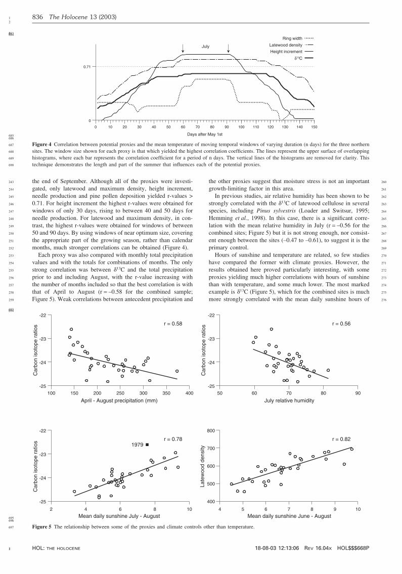
243 the end of September. Although all of the proxies were investi-244 gated, only latewood and maximum density, height increment,245 needle production and pine pollen deposition yielded r-values >246 0.71. For height increment the highest r-values were obtained for247 windows of only 30 days, rising to between 40 and 50 days for248 needle production. For latewood and maximum density, in con-249 trast, the highest r-values were obtained for windows of between250 50 and 90 days. By using windows of near optimum size, covering251 the appropriate part of the growing season, rather than calendar252 months, much stronger correlations can be obtained (Figure 4).253 Each proxy was also compared with monthly total precipitation254 values and with the totals for combinations of months. The only255 strong correlation was between �13C and the total precipitation256 prior to and including August, with the r-value increasing with257 the number of months included so that the best correlation is with258 that of April to August (r = –0.58 for the combined sample;259 Figure 5). Weak correlations between antecedent precipitation and

693694

695

4 5 6 7 8 9 10

400

500

600

700

800

2 4 6 8 10

-25

-24

-23

-22

-25

-24

-23

-22

-25

-24

-23

-22

50 60 70 80 90100 150 200 250 300 350 400

Late

woo

d de

nsity

Car

bon

isot

ope

ratio

sC

arbo

n is

otop

e ra

tios

Car

bon

isot

ope

ratio

s

April - August precipitation (mm) July relative humidity

Mean daily sunshine July - August Mean daily sunshine June - August

r = 0.58 r = 0.56

r = 0.78 r = 0.821979

696

697 Figure 5 The relationship between some of the proxies and climate controls other than temperature.


260the other proxies suggest that moisture stress is not an important261growth-limiting factor in this area.262In previous studies, air relative humidity has been shown to be263strongly correlated with the �13C of latewood cellulose in several264species, including Pinus sylvestris (Loader and Switsur, 1995;265Hemming et al., 1998). In this case, there is a significant corre-266lation with the mean relative humidity in July (r = –0.56 for the267combined sites; Figure 5) but it is not strong enough, nor consist-268ent enough between the sites (–0.47 to –0.61), to suggest it is the269primary control.270Hours of sunshine and temperature are related, so few studies271have compared the former with climate proxies. However, the272results obtained here proved particularly interesting, with some273proxies yielding much higher correlations with hours of sunshine274than with temperature, and some much lower. The most marked275example is �13C (Figure 5), which for the combined sites is much276more strongly correlated with the mean daily sunshine hours of


3

277 July and August (r = 0.78) than with temperature of the same per-278 iod (0.59). For the combined sites, latewood and maximum den-279 sity are also more strongly correlated with sunshine hours of June280 to August (r = 0.82 and 0.80) than with temperature of the same281 period (0.78 and 0.76). The difference is most marked at the282 southernmost site Laanila, where the sunshine hours of May to283 August yield r-values of 0.80 and 0.78. The relationship between284 temperature and sunshine is reversed at the northernmost site,285 where temperature of June to August yields r-values of 0.77 and286 0.77 compared to 0.73 and 0.72 for sunshine hours of the same287 period. It is notable that the correlations between annual height288 increment and needle production are much more strongly corre-289 lated with temperature than with hours of sunshine, with July tem-290 perature yielding 0.87 and 0.84 for the combined sites and July291 sunshine only 0.58 and 0.50.

292 How does climate influence the293 proxies?

294 Earlywood width295 The strongest correlation is with late summer (August/September)296 temperature of the previous season, suggesting that earlywood is297 formed mainly from reserves. At the southernmost site the298 temperature of early July of the current season is also important.

299 Latewood width300 The strongest correlation is with mid- to late-summer temperature301 of the current season. July has a stronger influence than August.302 The climate signal is weak and only preserved at the southern-303 most site.

304 Annual ring width305 The strongest climate signal is the temperature of July, but this306 was present only at the southernmost site (Laanila, r = 0.64). At307 these timberline sites ring width, averaged from a small number308 of young trees, provides a poor proxy for palaeotemperatures. The309 highest correlations were obtained from windows of 40 to 50 days310 covering most of July and part of August. The cambium dynamics311 results showed the most intense activity between the middle of312 June and end of July.

313 Earlywood density314 Inconsistent between trees and retaining no clear climate signals.

315 Latewood density316 Strongly correlated with the temperature and sunshine hours of317 late June to late August. Probably represents a proxy measure of318 net photosynthesis over most of the growing season. Can be used319 to reconstruct the mean temperature of July and August (r-value320 0.76 for the three sites combined).

321 Maximum density322 Very strongly correlated with mean latewood density and provid-323 ing the same climatic information.

324 Stable carbon isotope ratios325 The strongest correlation is with mean daily sunshine hours of326 July and August combined (r = 0.78 for the combined sites),327 the correlation with temperature of the same period being much328 weaker (0.59). This may reflect the influence of photon flux on329 photosynthetic rate and therefore on the internal concentration330 of CO2. Secondary controls are summer precipitation, which331 influences moisture stress and therefore stomatal conductance,332 and February temperature, which controls the depth of winter333 freezing and therefore the supply of soil moisture in the334 early summer.


335Annual height increment336Height growth occurs early in the season using reserves from the337previous summer. The correlation with July temperature is very338high, yielding 0.87 for the combined sites. A negative correlation339with the temperature of the November prior to the year in which340the reserves accumulated may relate to respiratory losses caused341by elevated late-autumn temperatures. Potentially a very powerful342proxy for reconstructing July temperatures.

343Needle production344Closely linked to annual height increment and providing little345extra climatic information. In the far north, needle initials may be346damaged by spring frosts, but the effect is not strong or consistent347enough for a frost signal to be extracted.

348Pollen deposition349Since male flowers are enclosed within the same buds that pro-350duce new height and branch growth, the two parameters are351related and the primary control is the temperature of the previous352July (Hicks, 2001). The temperature of the current spring deter-353mines the degree of frost damage and therefore the proportion of354flowers that survive. At the northernmost site, the spring tempera-355ture effect extends into June, whereas further south March and356April are more important. Pollen deposition is also influenced by357the weather conditions when the pollen is released, so there is a358correlation with the temperature of June. Where pine pollen depo-359sition can be obtained at near-annual resolution it provides a360potentially powerful tool for reconstructing palaeotemperatures as361well as vegetation dynamics.

362Combining proxies

363Where the primary controls on two or more proxies are similar,364they might be combined to provide a more reliable estimate of365that common control. The best results are likely to be obtained366where the other controlling factors are different, and therefore367tend to cancel each other. Combining proxies that have very simi-368lar controlling factors is less likely to improve the estimate since369they will be subject to similar sources of ‘error’. Several of the370potential proxies are controlled by, or correlated with, summer371temperature, but the length and timing of the part of the summer372that is important varies. In each case, there is a strong correlation373with the temperature of July of either the previous or current sea-374son (Figure 3). The estimate of July temperature is therefore most375likely to be improved by combining proxies.376A simple way to test the effectiveness of combining various377proxies is to use them independently to estimate July temperature378(inverse calibration), then average the results, with each proxy379weighted according to the percentage of its variance that is380explained by July temperature. The correlation between the esti-381mated values and the measured values provides the ‘effective cor-382relation’ between July temperature and the combined proxies. The383higher the effective correlation the more reliable, and less biased,384will be the reconstructed values that use this calibration set.385For the combined sites, the two proxies that are most strongly386correlated with July temperature are annual height increment and387needle production, but if these are combined the effective corre-388lation (0.88) is little better than that obtained using height389increment on its own. These proxies are so closely related that390sources of error are not reduced when they are combined. Simi-391larly, if latewood and maximum density are combined the effec-392tive correlation with July temperature is no improvement.393Combining proxies that are not very similar yields much better394results. At the central site, Kaamanen, for example, neither height395increment nor latewood density yielded correlation coefficients396sufficiently high to be used for reconstructing July temperatures

1 838 The Holocene 13 (2003)2

3700701

702

99

10

11

12

13

14

15

16

17

18

10 11 12 13 14 15 16 17 18

18

17

16

15

14

13

12

11

10

99 10 11 12 13 14 15 16 17 18

Latewood density

Height increment

99

10

11

12

13

14

15

16

17

18

10 11 12 13 14 15 16 17 18

Est

imat

e

Est

imat

eE

stim

ate

Mean July temperatureMean July temperature

Height increment and latewood density combined

r = 0.67

r = 0.63

r = 0.79

703

704 Figure 6 At the central site, Kaamanen, neither height increment nor latewood density explain more than half of the variance in mean July temperatures705 (r-values <0.71). However, when they are combined, by calculating the predicted July temperatures and taking a weighted average, the ‘effective correlation’706 between the predicted and measured values is much higher.

397 (0.67 and 0.63, respectively), but when they are combined the398 effective correlation rises to 0.78 (Figure 6). This is because399 height increment is influenced by temperatures prior to July, and400 latewood density by temperatures after July (Figure 4), so when401 they are combined these ‘errors’ are partly cancelled and the402 strength of the July signal is enhanced. The correlation between403 height increment and July temperature for the combined sites is404 so strong that combining it with other proxies yields no improve-405 ment. However, if height increment were unavailable then com-406 bining ring widths, latewood density and �13C would yield an407 acceptable effective correlation of 0.73 (Figure 7).408 Even very weak signals can be considerably enhanced. At the409 northern site, Kevo, for example, the temperature of February is410 weakly but significantly correlated with ring width, �13C and411 needle production (r-values 0.34, 0.47 and 0.55, respectively).412 However, these three do not share strong correlations with other413 months, so that when they are combined the February temperature414 signal is enhanced, yielding an effective correlation of 0.64.415 Although not strong enough for palaeoclimate reconstruction, this416 illustrates how even rather weak signals can be enhanced signifi-417 cantly using a multiproxy approach.418 As well as using the similarities in response of the different419 proxies to the same climatic controls, differences in response can420 also be used to good effect. For example, both latewood density421 and �13C are correlated with summer temperature and sunshine,

708709

710

9 181716151413121110

9

18

17

16

15

14

13

12

11

10

Mean July temperature

r = 0.73Est

imat

ed J

uly

tem

pera

ture

711

712 Figure 7 The correlation between estimated and measured mean July tem-713 peratures provides the ‘effective correlation’ coefficient when two or more714 proxies are combined. Note that the effective correlation based on ring715 widths, latewood density and �13C is much higher than the correlation716 obtained using any of the three proxies independently (see Figure 3).


422but �13C is also sensitive to soil moisture and therefore to summer423precipitation. If �13C is regressed on latewood density, therefore,424the correlation is strong (r = 0.70) but there are three marked425residuals with higher than expected �13C (Figure 8). These three426years (1979, 1980 and 1985) had the three driest summers (June–427August precipitation) in the series. The probability of randomly428identifying the three driest years from a sample of 35 is429p = 0.00015.

430Conclusions

431The results of this pilot study show that there is great potential432for using a multiproxy approach to dendroclimatology. If 0.71 is433taken as the minimum acceptable correlation coefficient on which434to base quantitative palaeoclimate reconstructions, and the com-435bined sites are taken to simulate the sort of sample that might be436produced by taking subfossil trees from several lakes over a wide437area, then the individual proxies could potentially be used to438reconstruct mean July temperature (annual height increment or439needle production, r-values 0.87 and 0.84), mean temperature of440July and August (latewood density or maximum density, r-values4410.78 and 0.76) and hours of sunshine in July and August (�13C,442r-value 0.78). By combining different proxies, the strength of the443climate signals can be enhanced and the range of extractable cli-444mate signals increased. High-correlation coefficients in the cali-445bration set are essential if quantitative palaeoclimate reconstruc-446tions are to be reliable. The key is to combine proxies that are447not too similar, so that they respond to the climate parameter of

718719

720

400 500 600 700

-25

-24

-23

-22

Latewood density

δ13C

3 driest summers

721

722Figure 8 When �13C values are regressed on latewood density values the723residuals represent the dry summers (June–August precipitation).


3

448 interest but the other controls differ, and thus tend to cancel each449 other. The difference in response of two proxies that share some450 controls but not others can also yield a useful climate signal. For451 example, when �13C values are regressed on latewood density the452 positive residuals represent the very dry summers (Figure 8). This453 combination has potential for reconstructing drought frequency454 and severity, even in areas where ring widths are insensitive to455 variations in precipitation.456 A possible extension of the multiproxy approach might be to457 resolve past changes in climate that have led to periods of458 enhanced or reduced tree growth. For example, an extended459 growth season but without unusually hot summers would be460 expected to produce an increase in annual ring width and latewood461 density but no concomitant increase in annual height increment462 or in the �13C of latewood cellulose. A growth reduction caused463 by moisture stress rather than low temperatures would show a464 decline in ring width and latewood density but an increase in the465 �13C of latewood cellulose. An increase in midsummer tempera-466 ture, but over a shorter growing season, would be expected to467 show a marked increase in annual height increment but no con-468 comitant increase in latewood density. A period with very sunny469 but cool summers would show reduced annual height increment470 but an increase in latewood density and in the �13C of latewood471 cellulose. The multiproxy approach provides, therefore, a more472 holistic view of changing climate and the potential to reconstruct473 synoptic changes as well as variations in individual parameters.474 Having demonstrated the great potential of the multiproxy475 approach, and identified those proxies most likely to be useful in476 this area, the results need now to be applied to much longer series,477 using trees of varying age and covering a greater latitudinal range.478 This is critical in order to determine whether the response of the479 various proxies to climate remains stable over time and space.480 Longer series, preferably pre-dating widespread human disturb-481 ance in this area, are also required to examine the behaviour of482 some of the relatively new proxies in relation to tree age. This483 will determine whether they can be used reliably to reconstruct484 the low-frequency changes in climate that are so difficult to485 extract using ring widths (Cook et al., 1995).486 Perhaps the greatest potential of the multiproxy approach lies487 not just in the way it has been applied here, using correlation and488 statistical inference, but in mechanistic modelling of the influence489 of climate on tree growth and function. Such models would ide-490 ally include measurements of the stable isotopes of oxygen and/or491 hydrogen as well as carbon, which has only recently become feas-492 ible for large numbers of samples (McCarroll and Loader, 2004).493 Mechanistic modelling might help circumvent the problem of494 using the last century as the calibration period for reconstructing495 past climate. The last century is the only period with reliable cli-496 matic records, but it has witnessed changes in atmospheric compo-497 sition, pollution, fertilization and land management that may have498 changed the way that trees respond to climate (Briffa et al.,499 1998a; 1998b).500 Long and continuous tree-ring chronologies, with perfect501 annual resolution, constructed over many years of careful502 research, now provide natural archives of information on past503 changes of climate in areas of the Earth where those changes are504 particularly interesting. A multiproxy approach provides a power-505 ful means of tapping the unrivalled potential of trees not as506 palaeothermometers but as sensitive monitors of synoptic507 climatology.

508 Acknowledgements

509 This work was conducted as part of the EU-funded FOREST510 (ENV4-CT95-0063) and PINE (EVK-CT-2002) projects and511 supported in part by the British Natural Environment Research


512Council (GR9/03098) and the Academy of Finland (Project No.5133423). We also gratefully acknowledge the support of the Thule514Institute at the University of Oulu. We would like to thank our515many friends who worked on other parts of the FOREST transect516for inspiring debates and pleasant company. Our Scientific Officer517Denis Peter gave lots of help and advice and provided the chance518to discuss our preliminary results with Keith Briffa. Several519people have helped with the sample preparation and measure-520ments, including Krystyna Flynn, Eleanor Pettigrew, Quentin521Dresser, Mari Sonninen, Tarmo Aalto, Jean-Louis Edouard and522Frederic Guibal. Mary Gagen, Neil Loader and Iain Robertson523provided many helpful comments.

524References

525Aalto, T. and Jalkanen, R. 1998: The needle trace method. Finnish Forest526Research Institute Research Papers 681, 36 pp.527Barber, K.E. 1981: Peat stratigraphy and climate change. Rotterdam:528Balkema.529Barber, K.E., Chambers, F.M., Maddy, D., Stoneman, R. and Brew,530J.S. 1994: A sensitive high-resolution record of late-Holocene climatic531change from a raised bog in northern England. The Holocene 4, 198–205.532Beaulieu, J-L. and Reille, M. 1992: The last climatic cycle at La Grande533Pile (Vosges, France): a new pollen profile. Quaternary Science Reviews53411, 431–38.535Birks, H.J.B. 1995: Quantitative palaeoenvironmental reconstructions. In536Maddy, D. and Brew, J.S., editors, Statistical modelling of Quaternary537science data, Technical Guide 5, Cambridge: Quaternary Research Associ-538ation, 161–254.539Briffa, K.R. 2000: Annual climate variability in the Holocene: interpreting540the message of ancient trees. Quaternary Science Reviews 19, 87–105.541Briffa, K. and Jones, P.D. 1989: Basic chronology statistics and542assessment. In Cook, E.R. and Kairiukstis, L.A., editors, Methods of543dendrochronology: applications in the environmental sciences, Dordrecht:544Kluwer Academic.545Briffa, K.R., Osborn, T.J., Schweingruber, F.H., Harris, I.C., Jones,546P.D., Shiyatov, S.G. and Vaganov, E.A. 2001: Low-frequency tempera-547ture variations from a northern tree ring density network. Journal of Geo-548physical Research, Atmospheres 106, 2929–41.549Briffa, K., Schweingruber, F.H., Jones, P.D., Osborn, T.J., Harris,550I.C., Shiyatov, S.G., Vaganov, E.A. and Grudd, H. 1998a: Trees tell551of past climates: but are they speaking less clearly today? Philosophical552Transactions of the Royal Society of London 353B, 65–73.553Briffa, K., Schweingruber, F.H., Jones, P.D., Osborn, T.J., Shiyatov,554S.G. and Vaganov, E.A. 1998b: Reduced sensitivity of recent tree-growth555to temperature at high northern latitudes. Nature 391, 678–82.556Broecker, W.S. and Denton, G.H. 1990: What drives glacial cycles?557Scientific American 262, 42–50.558Cook, E.R., Briffa, K.R., Meko, D.M., Graybill, D.A. and Funkhouser,559G. 1995: The ‘segment length curse’ in long tree-ring chronology develop-560ment for palaeoclimatic studies. The Holocene 5, 229–37.561Derbyshire, E., Billard, A., Van-Vliet Lanoe, B., Lautrodou, J-P. and562Cremaschi, M. 1988: Loess and palaeoenvironment: some results of a563European joint programme of research. Journal of Quaternary Research5643, 147–69.565Eronen, M., Zetterberg, P., Briffa, W.R., Lindholm, M., Merilainen,566J. and Timonen, M. 2002: The supra-long Scots pine tree-ring record for567Finnish Lapland: Part 1, chronology construction and initial inferences.568The Holocene 12, 673–80.569Fritts, H. 1976: Tree rings and climate. London: Academic Press.570Grudd, H., Briffa, K.R., Karlen, W., Bartholin, T.S., Jones, P.D. and571Kromer, B. 2002: A 7400-year tree-ring chronology in northern Swedish572Lapland: natural climatic variability expressed on annual to millennial tim-573escales. The Holocene 12, 657–65.574Hemming, D.L., Switsur, V.R., Waterhouse, J.S., Heaton, T.H.E. and575Carter, A.H.C. 1998: Climate and the stable carbon isotope composition576of tree ring cellulose: an intercomparison of three tree species. Tellus 50B,57725–32.578Hicks, S. 2001: The use of annual arboreal pollen deposition values for579delimiting tree-lines in the landscape and exploring models of pollen dis-580persal. Review of Palaeobotany and Palynology 117, 1–29.

1 840 The Holocene 13 (2003)2

3

581 Hicks, S., Amman, B., Latalowa, M., Pardoe, H. and Tinsley, H., edi-582 tors 1996: European pollen monitoring programme: project description583 and guidelines. Finland: Oulu University Press, 28 pp.584 Hicks, S., Tinsley, H., Pardoe, H. and Cundill, P. 1999: Supplement to585 the guidelines. European Pollen Monitoring Programme. Finland: Oulu586 University Press, 24 pp.587 Hughes, M.K. and Graumlich, L.J. 1996: Multimillennial dendroclimatic588 studies from the western United States. In Jones, P.D., Bradley, R.S. and589 Jouzel, J., editors, Climate variations and forcing mechanisms of the last590 2000 years, Berlin: Springer, 109–24.591 Imbrie, J. and Imbrie, K.P. 1979: Ice ages: solving the mystery. Lon-592 don: Macmillan.593 Jalkanen, R., Aalto, T., Innes, J., Kurkela, T. and Townsend, I. 1994:594 Needle retention and needle loss of Scots pine in recent decades at Thet-595 ford and Alice Holt, England. Canadian Journal of Forest Research 24(4),596 863–67.597 Jones, P.D., Briffa, K.R., Barnett, T.P. and Tett, S.F.B. 1998: High-598 resolution palaeoclimatic records for the last millennium: interpretation,599 integration and comparison with General Circulation Model control-run600 temperatures. The Holocene 8, 455–72.601 Kilian, M.R., van Geel, B. and van der Plicht, J. 2000: 14C AMS wiggle602 matching of raised bog deposits and models of peat accumulation. Quat-603 ernary Science Reviews 19, 1011–33.604 Kurkela, T. and Jalkanen, R. 1990: Revealing past needle retention in605 Pinus spp. Scandinavian Journal of Forest Research 5(4), 481–85.606 Lara, A. and Villalba, R. 1993: A 3,600-year temperature reconstruction607 from Fitzroya cupressoides tree rings in southern South America. Science608 260, 1104–106.609 Lindholm, M. and Eronen, M. 2000: A reconstruction of mid-summer610 temperatures from ring widths of Scots pine since ad 50 in northern611 Finland. Geografiska Annaler 82A, 527–35.612 Lindholm, M., Eronen, M., Timonen, M. and Merilainen, J. 1999: A613 ring-width chronology of Scots pine from northern Lapland covering the614 last two millennia. Annales Botanici Fennici 36, 119–26.615 Loader, N.J. and Switsur, V.R. 1995: Reconstructing past environmental616 change using stable isotopes in tree rings. Botanical Journal of Scotland617 48, 65–78.618 Lowe, J.J. and Walker, M.J.C. 1999: Reconstructing Quaternary619 environments (second edition). Harlow, Essex: Addison Wesley Longman.660


620McCarroll, D. and Loader, N.J. 2004: Stable isotopes in tree rings.621Quaternary Science Reviews, in press.622McCarroll, D. and Pawellek, F. 1998: Stable carbon isotope ratios of623latewood cellulose in Pinus sylvestris from northern Finland: variability624and signal strength. The Holocene 8, 693–702.625—— 2001: Stable carbon isotope ratios of Pinus sylvestris from northern626Finland and the potential for extracting a climate signal from long Fennos-627candian chronologies. The Holocene 11, 517–26.628Peglar, S.M. 1993: The mid-Holocene Ulmus decline at Diss Mere,629Norfolk, UK: a year-by-year pollen stratigraphy from annual laminations.630The Holocene 3, 1–13.631Reille, M., de Beaulieu, J-L., Svodobova, H., Andrieu-Ponel, V. and632Goeury, C. 2000: Pollen analytical biostratigraphy of the last five climatic633cycles from a long continental sequence from the Velay region (Massif634Central, France). Journal of Quaternary Science 15, 665–85.635Robertson, I., Lucy, D., Baxter, L., Pollard, A.M., Aykroyd, R.G.,636Barker, A.C., Carter, A.H.C., Switsur, V.R. and Waterhouse, J.S.6371999: A kernel-based Bayesian approach to climatic reconstruction. The638Holocene 9, 495–500.639Schulman, E. 1958: Bristlecone pine, oldest known living thing. National640Geographic Magazine 113, 354–72.641Schweingruber, F.H. 1987: Tree rings: basics and applications of642dendrochronology. Dordrecht: Reidel, 276 pp.643—— 1988: Radiodensitometry. In Cook, E.R. and Kairiukstis, L.A.,644editors, Methods of dendrochronology, Dordrecht: Kluwer, 55–63.645—— 1993: Trees and wood in dendrochronology. Berlin: Springer-646Verlag, 402 pp.647Stauffer, B. 2000: Long term climate records from polar ice. Space648Science Reviews 94, 321–36.649Wigley, T.M.L., Briffa, K.R. and Jones, P.D. 1984: On the average value650of correlated time series, with applications in dendroclimatology and651hydrometeorology. Journal of Climate and Applied Meteorology 23,652201–13.653Zetterberg, P., Eronen, M. and Lindholm, M. 1996: Construction of654a 7500-year tree-ring record for Scots pine (Pinus sylvestris L.)655in northern Fennoscandia and its application to growth variation and656palaeoclimatic studies. In Spiecker, H., Mielikainen, K., Kohl, M. and657Skovsgaard, J.P., editors, Growth trends in European forests, European658Forest Instutute Research Report 5, Berlin: Springer-Verlag,6597–18.

Multiproxy dendroclimatology: a pilot study in northern Finland

Documents

Transcript of Multiproxy dendroclimatology: a pilot study in northern Finland