�����������������

Citation: Kordon, F.; Maier, A.;

Swartman, B.; Privalov, M.;

El-Barbari, J.S.; Kunze, H. Multi-Stage

Platform for (Semi-)Automatic

Planning in Reconstructive Orthopedic

Surgery. J. Imaging 2022, 8, 108.

https://doi.org/10.3390/

jimaging8040108

Academic Editors: Terry Peters

and Elvis C.S. Chen

Received: 28 February 2022

Accepted: 8 April 2022

Published: 12 April 2022

Publisher’s Note: MDPI stays neutral

with regard to jurisdictional claims in

published maps and institutional affil-

iations.

Copyright: © 2020 by the authors.

Licensee MDPI, Basel, Switzerland.

This article is an open access article

distributed under the terms and

conditions of the Creative Commons

Attribution (CC BY) license (https://

creativecommons.org/licenses/by/

4.0/).

Journal of

Imaging

Article

Multi-Stage Platform for (Semi-)Automatic Planning inReconstructive Orthopedic SurgeryFlorian Kordon 1,2,3,* , Andreas Maier 1,2 , Benedict Swartman 4, Maxim Privalov 4, Jan Siad El-Barbari 4

and Holger Kunze 1,3

1 Pattern Recognition Lab, Friedrich-Alexander University Erlangen-Nuremberg, 91058 Erlangen, Germany;andreas.maier@fau.de (A.M.); holger.hk.kunze@siemens-healthineers.com (H.K.)

2 Erlangen Graduate School in Advanced Optical Technologies (SAOT), Friedrich-Alexander UniversityErlangen-Nuremberg, 91052 Erlangen, Germany

3 Advanced Therapies, Siemens Healthcare GmbH, 91031 Forchheim, Germany4 Department for Trauma and Orthopaedic Surgery, BG Trauma Center, Ludwigshafen,

67071 Ludwigshafen, Germany; benedict.swartman@bgu-ludwigshafen.de (B.S.);maxim.privalov@bgu-ludwigshafen.de (M.P.); jan.elbarbari@bgu-ludwigshafen.de (J.S.E.-B.)

* Correspondence: florian.kordon@fau.de

Abstract: Intricate lesions of the musculoskeletal system require reconstructive orthopedic surgeryto restore the correct biomechanics. Careful pre-operative planning of the surgical steps on 2Dimage data is an essential tool to increase the precision and safety of these operations. However, theplan’s effectiveness in the intra-operative workflow is challenged by unpredictable patient and devicepositioning and complex registration protocols. Here, we develop and analyze a multi-stage algorithmthat combines deep learning-based anatomical feature detection and geometric post-processing toenable accurate pre- and intra-operative surgery planning on 2D X-ray images. The algorithm allowsgranular control over each element of the planning geometry, enabling real-time adjustments directlyin the operating room (OR). In the method evaluation of three ligament reconstruction tasks effect onthe knee joint, we found high spatial precision in drilling point localization (ε < 2.9 mm) and lowangulation errors for k-wire instrumentation (ε < 0.75◦) on 38 diagnostic radiographs. Comparableprecision was demonstrated in 15 complex intra-operative trauma cases suffering from strong implantoverlap and multi-anatomy exposure. Furthermore, we found that the diverse feature detection taskscan be efficiently solved with a multi-task network topology, improving precision over the single-taskcase. Our platform will help overcome the limitations of current clinical practice and foster surgicalplan generation and adjustment directly in the OR, ultimately motivating the development of novel2D planning guidelines.

Keywords: computer-assisted surgery; surgical planning; reconstructive orthopedic surgery; ligamentreconstruction; deep learning; multi-task learning; X-ray images

1. Introduction

Joint injuries and the following structural instability are challenging patterns in ortho-pedics, usually caused by events of dislocation or unnatural motion and tears of restrainingligaments [1–4]. The destabilizing event comes with various implications for the patient’shealth and well-being, causing significant joint pain, functional impairment, symptomaticgiving way, osteochondral lesions, or damage to the articular cartilage [3,5–13]. For particu-larly severe lesions, the biomechanically correct joint function is restored by surgical recon-struction to relieve the patient’s symptoms and restore long-term stability [1,7,12,14–20].

An essential instrument to elevate the safety and accuracy of surgical reconstruction isthe careful planning and outcome verification on 2D image data. Fundamentally, a surgicalplan involves interrelating several salient features of the patient anatomy, such as osseous

J. Imaging 2022, 8, 108. https://doi.org/10.3390/jimaging8040108 https://www.mdpi.com/journal/jimaging

J. Imaging 2022, 8, 108 2 of 29

landmarks and anatomical axes, and performing a geometric construction for the under-lying task. For example, reconstruction surgery of the Medial Patellofemoral Ligament(MPFL) necessitates a precise fixation of the substitute graft on the femoral surface. Specif-ically, the physiological correct ligament insertion point that guarantees joint isometrycan be approximated by the construction of the Schoettle Point [21] on a 2D true-lateralradiograph. This construction builds on two anatomical keypoints on the distal femursurface and a subsection of the posterior cortex of the femoral shaft to ultimately localizethe optimal point for tunnel drilling. Another application is the careful placement andangulation of k-wires inserted into the patient anatomy for transtibial Posterior CruciateLigament (PCL) reconstruction surgery, guiding the subsequent tunnel drilling [22–25].High precision in the tunnel’s placement is essential to prevent any defects in joint biome-chanics after reconstruction and unnecessary graft abrasion [26]. It also protects from earlybreakout of the bone cortex with the risk of damaging nearby vascular structures [27–31].

For such reconstructive applications, surgical planning promises elevated treatmentsafety and standardized assessment with a physiologically-grounded rationale. However,several clinical and technical challenges complicate the plan’s intra-operative application.

1. Most planning methods rely on the combination of salient proxy structures. Thisindirect description implies a greater number of error sources, which translates tohigher observer-variability if the planning is done manually;

2. Certain surgical planning can have a high level of geometric complexity. Sufficientlyprecise manual execution is only possible with tailored software tools or otherwiserequires great amounts of time and labor;

3. The ability to register pre-operative planning and intra-operative live data is highlycomplex due to the variable configuration of the joint and arbitrary relation betweenpatient, table, and imaging system;

4. Ad-hoc modifications of the surgical plan are essential to compensate for motionduring the intervention;

5. Manual interaction with a computer-assisted planning system is undesirable dueto the surgery’s sterile setting. At the same time, the planning system should offergranular controls to correct each construction step with real-time visualization.

We propose a versatile platform for (semi-)automatic 2D planning and verificationin reconstructive orthopedic surgery that addresses most of the above challenges. Ourmethod involves three sequential stages: (i) First, a deep learning system detects therelevant anatomical structures for the underlying surgical task on 2D image data. Thedetection problem for each type of anatomical feature is solved in parallel using a multi-tasklearning (MTL) scheme; (ii) Second, the identified structures are transferred to geometricrepresentations, such as keypoint coordinates and line segments. If needed, post-processingcan be used to derive additional information required by the planning geometry; (iii) Third,the objects are combined and interrelated using a pre-defined blueprint describing theplanning geometry and calculation of the planning result. By mimicking each manualstep of the clinically established procedure, we align the automatic planning process toclinical practice as close as possible. This interpretable relation between anatomy andplanning geometry reduces the hurdle of acceptance that the practitioner must overcome.Additionally, if needed, the segmentation of the relevant bone can be used for a registrationof the planning result on subsequent live images. This allows an easier transfer of theapproach into an intra-operative workflow.

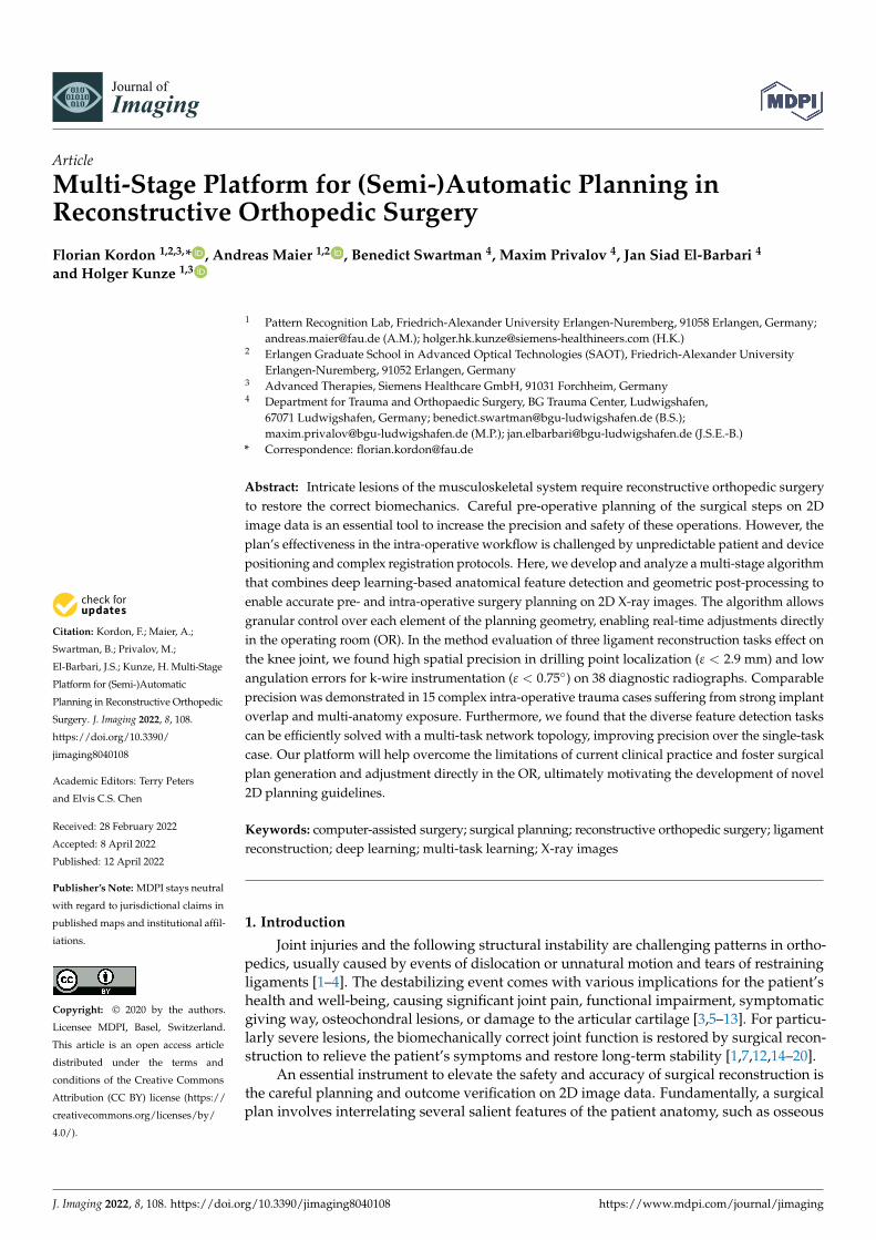
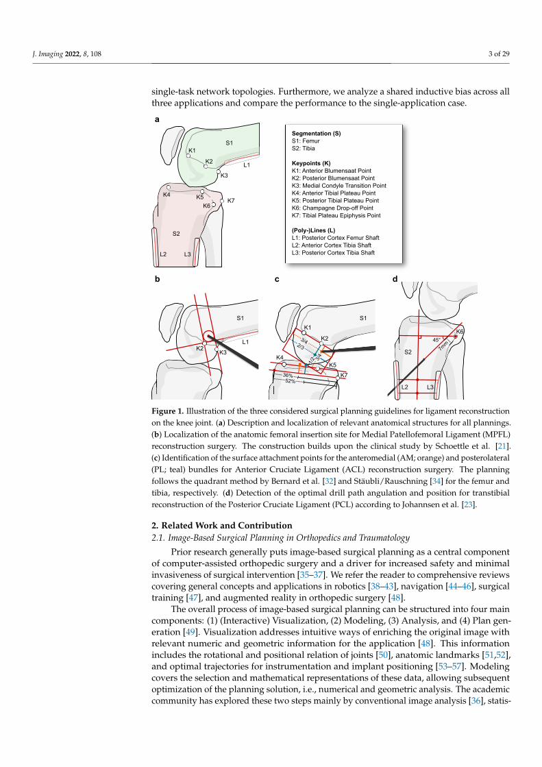
We evaluate our approach on three kinds of ligament reconstruction surgery on theknee joint (Figure 1): (i) Localization of the optimal graft fixation point (Schoettle Point)for tunnel drilling in MPFL reconstruction surgery [21]; (ii) Localization of anteromedial(AM) and posterolateral (PL) bundle attachment points on the femur and tibia for AnteriorCruciate Ligament (ACL) reconstruction [32–34]; (iii) Finding the optimal guidewire ori-entation and insertion point for transtibial PCL reconstruction [23,24]. We study differentstrategies for separating the anatomical features into individual tasks for each applicationand evaluate different levels of parameter sharing using multi-head, multi-decoder, and

J. Imaging 2022, 8, 108 3 of 29

single-task network topologies. Furthermore, we analyze a shared inductive bias across allthree applications and compare the performance to the single-application case.

S1

K1

K2

36%

2/3

1/2 3/

4

3/4

52%

K4K5

K7

S1

Segmentation (S)S1: FemurS2: Tibia

Keypoints (K)K1: Anterior Blumensaat PointK2: Posterior Blumensaat PointK3: Medial Condyle Transition PointK4: Anterior Tibial Plateau PointK5: Posterior Tibial Plateau PointK6: Champagne Drop-off PointK7: Tibial Plateau Epiphysis Point

(Poly-)Lines (L)L1: Posterior Cortex Femur ShaftL2: Anterior Cortex Tibia ShaftL3: Posterior Cortex Tibia Shaft

K1

K2

K3

K4 K5

K6K7

L1

L2 L3

S2

S1

K2K3

L1

K645°

7mm

L2 L3

S2

a

db c

Figure 1. Illustration of the three considered surgical planning guidelines for ligament reconstructionon the knee joint. (a) Description and localization of relevant anatomical structures for all plannings.(b) Localization of the anatomic femoral insertion site for Medial Patellofemoral Ligament (MPFL)reconstruction surgery. The construction builds upon the clinical study by Schoettle et al. [21].(c) Identification of the surface attachment points for the anteromedial (AM; orange) and posterolateral(PL; teal) bundles for Anterior Cruciate Ligament (ACL) reconstruction surgery. The planningfollows the quadrant method by Bernard et al. [32] and Stäubli/Rauschning [34] for the femur andtibia, respectively. (d) Detection of the optimal drill path angulation and position for transtibialreconstruction of the Posterior Cruciate Ligament (PCL) according to Johannsen et al. [23].

2. Related Work and Contribution2.1. Image-Based Surgical Planning in Orthopedics and Traumatology

Prior research generally puts image-based surgical planning as a central componentof computer-assisted orthopedic surgery and a driver for increased safety and minimalinvasiveness of surgical intervention [35–37]. We refer the reader to comprehensive reviewscovering general concepts and applications in robotics [38–43], navigation [44–46], surgicaltraining [47], and augmented reality in orthopedic surgery [48].

The overall process of image-based surgical planning can be structured into four maincomponents: (1) (Interactive) Visualization, (2) Modeling, (3) Analysis, and (4) Plan gen-eration [49]. Visualization addresses intuitive ways of enriching the original image withrelevant numeric and geometric information for the application [48]. This informationincludes the rotational and positional relation of joints [50], anatomic landmarks [51,52],and optimal trajectories for instrumentation and implant positioning [53–57]. Modelingcovers the selection and mathematical representations of these data, allowing subsequentoptimization of the planning solution, i.e., numerical and geometric analysis. The academiccommunity has explored these two steps mainly by conventional image analysis [36], statis-

J. Imaging 2022, 8, 108 4 of 29

tical shape modeling and machine learning [58], and, more recently, via deep learning [59].The prevailing representation and analysis methods are semantic segmentation of the targetsurface in 3D, landmarking of salient regions using numerical keypoints, the fusion ofimage information with simulated joint kinematics [39,60], and registration using cameradata, markers, or anatomic surface information [48].

Despite the wide adoption of pre-operative plans in various types of orthopedicsurgery, their application to trauma interventions, such as ligament reconstruction, islimited [35,37,48]. For these cases, diagnostic 3D-scans are rarely used and require complex3D/2D registration of localized intra-operative fluoroscopic data with the pre-operativevolume. On the other hand, planning on diagnostic 2D radiographs has limited value in theoperating room due to limitations in patient positioning and the arbitrary relation betweenthe patient, table, and imaging device. In these scenarios, intra-operative planning on 2Dimage data become an increasingly attractive alternative [21,61].

2.2. Multi-Task Learning and Task Weighting

In MTL, data samples from multiple related tasks are used together to build a learningsystem with shared inductive bias [62]. By leveraging similarities in data and their un-derlying formation process, the goal is to discover more generalized and potent featuresthat ultimately lead to better performance than independent single-task learning (STL)inference [62]. For feature-based MTL, the shared inductive bias is typically realized bysoft or hard parameter sharing [62–65]. In the soft case, the parameters for each task areseparated but constrained using a distance penalty. In hard parameter-sharing, the inter-action between tasks is structured by using a meta learner with shared parameters andindividual learners with task-specific parameters [66].

For most MTL problems, the update policy for the meta-learner parameters shouldbe designed to prevent any dominance of certain tasks over others. For task balancing,several weighting heuristics have been proposed, most of them being based on a weightedsummation of the task-specific losses [67]. Gradient normalization (GradNorm) dynam-ically approximates the gradient magnitude of the shared representation w.r.t. for eachtask and aims to level the individual training rates [68]. Liu et al. [69] simplify this idea bydirectly balancing the task losses’ rate of change over training time without consideringgradient magnitude. Kendall et al. [70] propose task uncertainty as a proxy for each task’sweight, whereas Sener and Koltun [71] formulate MTL as a multi-objective optimizationbased on Pareto-optimal updates. Multiple solutions consider analysis and manipulationof individual gradient directions. Yu et al. [72] project the task gradients onto the normalplane of conflicting tasks, thus avoiding opposing gradient directions and establishinga stable update trajectory. Wang et al. [73] update this formulation by explicitly adaptinggradients for cases of positive similarity to better capture the diverse and often highly com-plex task interactions. A different implementation of this rationale is probabilistic maskingof gradients with a conflicting sign using a drop-out-style operation [74], or weighting thetasks such that their aggregated gradient has equal projections onto individual tasks [75].

We use GradNorm task balancing [68] in this work as it shows competitive performancefor more related tasks and is easy to implement at little to no computational overhead.

2.3. Contribution

Our method builds on previous work [50,54,55] and extends them in several ways:

1. This work establishes a multi-stage workflow that covers all necessary steps for image-based surgical planning on 2D X-ray images. The workflow is designed to mimic theclinically-established manual planning process, enabling granular control over eachanatomical feature contributing to the planning geometry;

2. We evaluate the model for three trauma-surgical planning applications on both diag-nostic as well as intra-operative X-ray images of the knee joint. The numeric resultsmatch clinical requirements and encourage further clinical evaluation;

J. Imaging 2022, 8, 108 5 of 29

3. We empirically show that the detection of anatomical landmarks benefits from a MTLsetting. We confirm that explicit task weighting significantly reduces the landmarklocalization error, and illustrate that a multi-head network topology achieves similarperformance to task-specific decoders, which are computationally much more expensive.

4. Our study demonstrates that sharing tasks across anatomically related applications doesnot significantly improve performance compared to the single-application variant.

2.4. Article Structure

In Section 3, we present the multi-stage algorithm for (semi-)automatic orthopedicsurgery planning and provide details on each step. Furthermore, we describe the differentMTL schemes considered in this work, their training protocols, the pre- and intra-operativedatasets used, and finally the evaluation metrics for reporting the results. In Section 4, wepose several research questions that are investigated through a series of experiments. Afterthat, we discuss the observations and findings in Section 5 and summarize our contributionin Section 6.

3. Materials and Methods3.1. (Semi-)Automatic Workflow for 2D Surgical Planning3.1.1. Multi-Stage Planning Algorithm

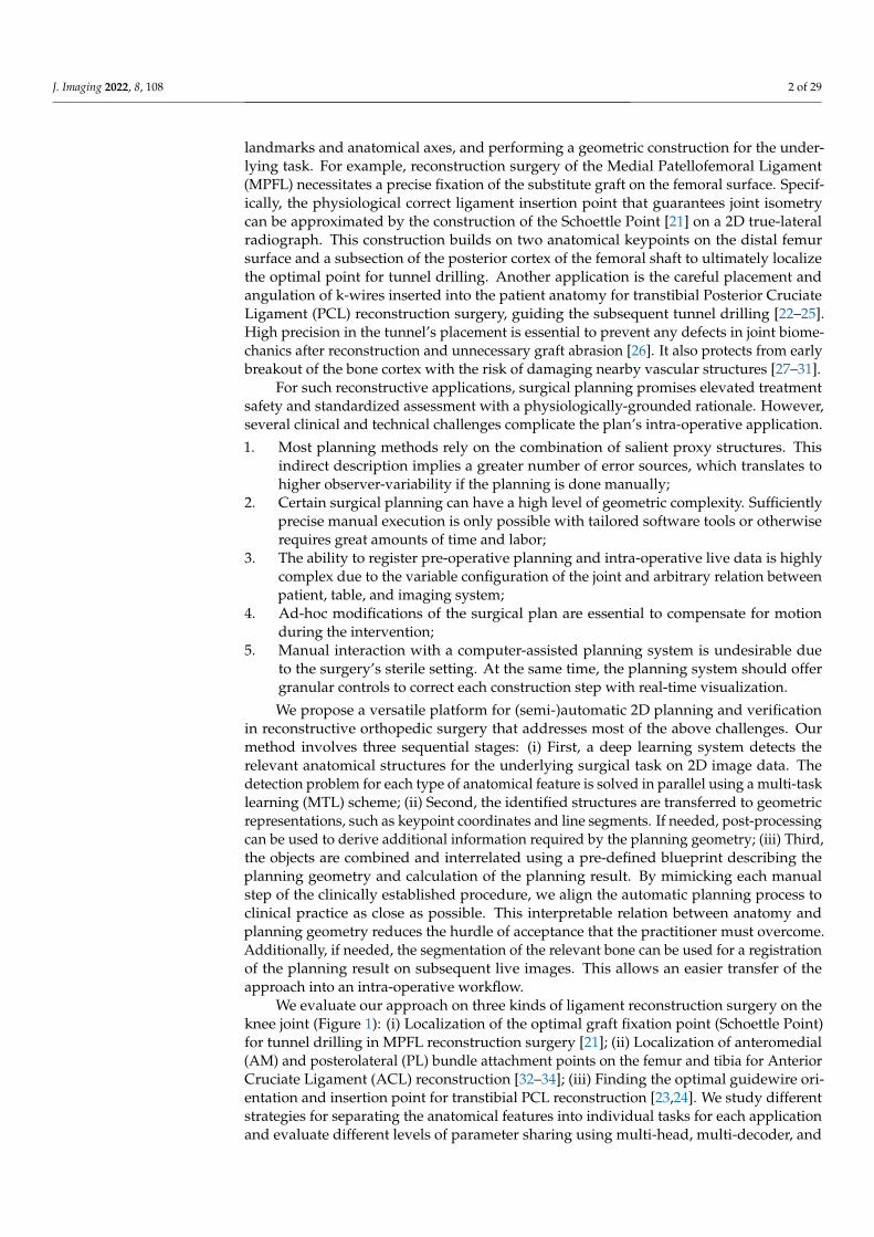
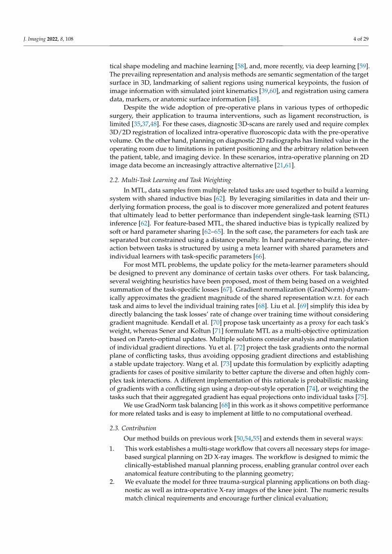
In the following, we describe a multi-stage algorithm that automatically models,analyzes, and visualizes a 2D orthopedic surgery plan. The general workflow is illustratedin Figure 2.

Before any geometric processing, a planning blueprint for the target surgical applica-tion needs to be defined, describing the necessary sequential construction steps. Based onthis blueprint, we can derive the relevant anatomical features and group them according tothe underlying task type. Furthermore, any post-processing that builds upon these featurescan be defined, e.g., the calculation of intersection points, or the extraction of relevantparts of a bone outline. In this work, we focus on three main feature and spatial task types(excluding any secondary features generated by post-processing) that are employed bymost surgical planning procedures:

1. Semantically coherent regions. Segmentation of connected regions that share certaincharacteristics, mostly bones and tools;

2. Anatomical keypoints. Point-like landmarks that pinpoint features of interest on thebone surface;

3. Elongated structures. Straight and curved lines that describe edges, ridges, or thatrefer to indirect features, such as anatomical axes.

After task configuration, in Stage A) , an MTL algorithm extracts all relevant anatom-ical structures in parallel, sorted by their task type. Second, in Stage B), the featuresare translated from their original inference encoding to geometrically interpretable ob-jects/descriptors. For example, the heatmap encoding of a keypoint is converted to itsgeometric equivalent of x and y coordinates, using the spatial argmax operation or a least-squares curve fitting. Stage C) finally describes the automatic processing of the individualplanning steps and its overlay on the input image. The user can interact with the plan-ning result to correct any misalignment, and the planning is updated in real-time. In thefollowing, we provide details on the individual stages.

J. Imaging 2022, 8, 108 6 of 29

1)

2)

PCL

Stage C) Geometric Construction

Multi-task network

Overlay (Manual modification)

(Repeat construction)

Stage A) 2D Anatomical Feature Extraction

Stage B) Transfer to Geometric Objects and Post-processing

Automatic processing of individual planning steps

1) 2) 3)

Anatomical features

Meta Learner Individual Learners

t=1 t=2

(ii) Configuration

Planning geometry

(i) Planning blueprint

Required post-processing

Feature and task composition

Input Output

t=3

Relevant contour masking Smooth intersection

Pixel-wise segmentation Contour extraction Keypoint coordinates Spatial likelihood map1)

2)

ACL

1)

2)

3)

MPFL

Figure 2. Overview of the automatic planning workflow. After selecting a planning blueprint anda corresponding configuration, the target X-ray image is processed in three consecutive stages. Afterextraction the 2D anatomical features with a multi-task network, they are transformed to theircorresponding geometric descriptors. The individual construction steps defined in the planningblueprint are automatically calculated by interrelating the extracted geometry (here, steps 1–3 inStage C)). If needed, the user can manually modify the planning by adjusting individual controlpoints upon real-time updates of the complete plan.

3.1.2. Stage A) MTL for Joint Extraction of Anatomical Features

Following the MTL paradigm, we want to find a functional mapping f tθ : X → Y t

from the input space X to multiple task solution spaces {Y t}t∈[T] [62,71]. θ is a set oftrainable parameters and T is the number of tasks. The data that are required to approx-imate this mapping in a supervised learning manner are characterized by M datapoints{xi, y1

i , . . . , yTi }i∈[M], where yT

i is the individual label for task t.We further consider a hard parameter-sharing strategy and split the parameters θ

into a single set of shared parameters θsh and task-specific parameter sets {θt}t∈[T] [66].Specifically, we define a meta learner gθsh : X → Z and individual learners for each taskht

θt : Z → Y t that by their composition htθt ◦ gθsh yield function

f tθsh ,θt : X → Y t. (1)

This learning scheme allows to leverage dependencies and similarities between thetasks, and to retain task-specific discriminative capacity. Specifically, for the extractionof anatomical features, the salient structures used for localizing certain landmarks maybe of similar importance when trying to solve a segmentation task of the complete bone.In addition, most structures relevant for surgical planning share the same underlyinganatomical processes. For the optimization of each task with gradient descent, a distinct

J. Imaging 2022, 8, 108 7 of 29

loss function Lt(·, ·) : Y t × Y t → R+0 is used. Although each loss function dictates the

updates for the individual learners, the parameter updates for the meta learner are derivedby their weighted linear combination. The general optimization problem can be written as

minθsh ; θ1,...,θT

T

∑t=1

wt

[1M

M

∑i=1Lt(

f tθsh ,θt(xi), yt

i

)]. (2)

wt is a scalar weight for the loss function for the tth task.Although the choice for the task’s loss function in theory only depends on the task

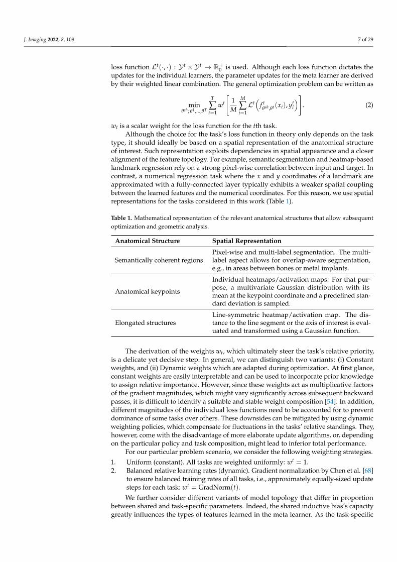
type, it should ideally be based on a spatial representation of the anatomical structureof interest. Such representation exploits dependencies in spatial appearance and a closeralignment of the feature topology. For example, semantic segmentation and heatmap-basedlandmark regression rely on a strong pixel-wise correlation between input and target. Incontrast, a numerical regression task where the x and y coordinates of a landmark areapproximated with a fully-connected layer typically exhibits a weaker spatial couplingbetween the learned features and the numerical coordinates. For this reason, we use spatialrepresentations for the tasks considered in this work (Table 1).

Table 1. Mathematical representation of the relevant anatomical structures that allow subsequentoptimization and geometric analysis.

Anatomical Structure Spatial Representation

Semantically coherent regionsPixel-wise and multi-label segmentation. The multi-label aspect allows for overlap-aware segmentation,e.g., in areas between bones or metal implants.

Anatomical keypoints

Individual heatmaps/activation maps. For that pur-pose, a multivariate Gaussian distribution with itsmean at the keypoint coordinate and a predefined stan-dard deviation is sampled.

Elongated structuresLine-symmetric heatmap/activation map. The dis-tance to the line segment or the axis of interest is eval-uated and transformed using a Gaussian function.

The derivation of the weights wt, which ultimately steer the task’s relative priority,is a delicate yet decisive step. In general, we can distinguish two variants: (i) Constantweights, and (ii) Dynamic weights which are adapted during optimization. At first glance,constant weights are easily interpretable and can be used to incorporate prior knowledgeto assign relative importance. However, since these weights act as multiplicative factorsof the gradient magnitudes, which might vary significantly across subsequent backwardpasses, it is difficult to identify a suitable and stable weight composition [54]. In addition,different magnitudes of the individual loss functions need to be accounted for to preventdominance of some tasks over others. These downsides can be mitigated by using dynamicweighting policies, which compensate for fluctuations in the tasks’ relative standings. They,however, come with the disadvantage of more elaborate update algorithms, or, dependingon the particular policy and task composition, might lead to inferior total performance.

For our particular problem scenario, we consider the following weighting strategies.

1. Uniform (constant). All tasks are weighted uniformly: wt = 1.2. Balanced relative learning rates (dynamic). Gradient normalization by Chen et al. [68]

to ensure balanced training rates of all tasks, i.e., approximately equally-sized updatesteps for each task: wt = GradNorm(t).

We further consider different variants of model topology that differ in proportionbetween shared and task-specific parameters. Indeed, the shared inductive bias’s capacitygreatly influences the types of features learned in the meta learner. As the task-specific

J. Imaging 2022, 8, 108 8 of 29

complexity shrinks, more general features need to be extracted, leading to superior solutionsfor similar tasks that benefit from each other or inferior solutions for conflicting tasks. Weanalyze this trade-off using two model topologies that facilitate different levels of parametersharing and compare them to a single-task earning baseline.

1. Single-task baseline. For comparison, a STL baseline of independent encoder-decoderstructures is optimized. Here, no parameters are shared;

2. Multi-head topology. Both the encoder and decoder parameters are shared betweenthe tasks in this variant. The output of the decoder is fed into task-specific predictionheads, which involve significantly less dedicated parameters and, thus, require a multi-purpose feature decoding. We argue that such a constrained decoder might benefitlearning for highly similar tasks;

3. Multi-decoder topology. After feature extraction in a shared feature encoder, the latentrepresentation is used as input for the task-specific decoders and prediction heads. Inother words, an abstract representation has to be found that serves the reconstructionfor different kinds of tasks.

3.1.3. Stage B) Extraction of Geometric Objects and Post-Processing

In Stage A), the multi-task network infers all anatomical features via specific spatialencodings. These encodings ensure an efficient optimization of the MTL scheme but cannotbe directly used for the geometrical construction defined in the planning blueprint. Forthat reason, the feature representations are subsequently transformed to more general de-scriptors using a common set of operations shared between different planning applications.

For the three main tasks (Section 3.1.2), the representation transformations are asfollows. The pixel-wise segmentation on the input image is interpreted as subsets Skwith k ∈ {0, . . . , K} that represent coherent regions of interest, e.g., bones, implants, softtissue, or background. Due to the multi-label definition, the subsets do not have to bedisjoint, which allows to identify region overlap. This is an important trait in the context oftransmissive imaging, which assumes an additive model of the pixel intensities and, thus,perceivable superimposition. The segmentation results are further represented as closedpolygons, facilitating further spatial analysis and shape relations. The inferred heatmapsdirectly encode the positional likelihood of the anatomical keypoint. The equivalentx and y coordinates are extracted by a spatial argmax operation or by a least-squarescurve fitting in case predicted heatmaps suffer from large local intensity variation. Theheatmap representation of an elongated structure is converted to a polyline by the followingsteps. First, the heatmap is interpreted as a 2D point cloud, and each point is assignedan importance weighting based on the predicted likelihood. By selecting the points witha weight above the threshold of 1σ, we extract only the most descriptive points for thetarget structure. Finally, we obtain the 2D polyline by interconnecting a set of equidistantpoints sampled from a smooth parametric B-spline which interpolates the selected points.If we are interested in a particular region of an object’s contour C, we alternatively interpretthe structure’s heatmap as a weighted mask that reduces the contour to a certain subsectionC ′ ⊂ C.

3.1.4. Stage C) Geometric Construction of Individual Planning Steps

Once the geometric descriptions and groupings are created, they are interrelated basedon the planning geometry provided in the planning blueprint (Appendix B). Accordingto the manual workflow, this interrelation is distributed over several steps, each targetinga single anatomical structure. The final result is then overlaid on the input image toprovide visual guidance for the user. After close inspection and visual alignment of theplanning to the underlying anatomy, the user might want to modify some parts of theplanning geometry retrospectively. The design choice of our multi-stage approach naturallysupports this use case. After manually adjusting any of the contained geometric objects,the geometric calculations in Stage 3) can be repeated at little computational cost, enablingreal-time visualization of the planning on live images.

J. Imaging 2022, 8, 108 9 of 29

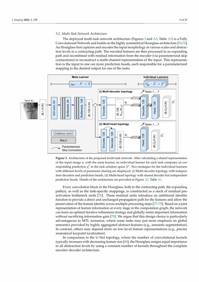
3.2. Multi-Task Network Architecture

The deployed multi-task network architecture (Figures 3 and A3, Table A1) is a FullyConvolutional Network and builds on the highly symmetrical Hourglass architecture [54,76].An Hourglass first captures and encodes the input morphology at various scales and abstrac-tion levels in a contracting path. The encoded features are then processed in an expandingpath and recombined with residual information from the encoder (via parameterized skipconnections) to reconstruct a multi-channel representation of the input. This representa-tion is the input to one ore more prediction heads, each responsible for a parameterizedmapping to the desired output for one of the tasks.

3x3

conv

, 64

Bot

tlene

ck, 6

4

Bot

tlene

ck, 1

28

ReLU

Parameterized Skip Connection

(B,C

t,H,W

)

(B,C

t,H,W

)

Dec

oder

, 128

Tasks 1,...,T(B

,128

,H,W

)

Hea

d, 1

28

Enc

oder

, 128

Hea

d, 1

28

(i) Multi-decoder topology

Meta Learner Individual Learners

(ii) Multi-head topology

instance norm

Dec

oder

, 128

Tasks 1,...,T

(B,1

,H,W

)

(B,1

28,H

,W)

Enc

oder

, 128

(B,1

28,

H/1

6,W

/16)

Input

Figure 3. Architecture of the proposed multi-task network. After calculating a shared representationof the input image xi with the meta learner, an individual learner for each task computes an cor-responding prediction yT

i in the task solution space Y t. Two strategies for the individual learnerswith different levels of parameter sharing are displayed: (i) Multi-decoder topology with indepen-dent decoders and prediction heads, (ii) Multi-head topology with shared decoder but independentprediction heads. Details of the architecture are provided in Figure A3, Table A1.

Every convolution block in the Hourglass, both in the contracting path, the expandingpath(s), as well as the task-specific mappings, is constructed as a stack of residual pre-activation bottleneck units [76]. These residual units introduce an additional identityfunction to provide a direct and unchanged propagation path for the features and allow thepreservation of the feature identity across multiple processing steps [77–79]. Based on a jointrepresentation of feature information at every stage in the computation graph, the networkcan learn an optimal iterative refinement strategy and globally retain important informationwithout sacrificing information gain [79]. We argue that this design choice is particularlyadvantageous in MTL scenarios, where some tasks may put more emphasis on globalsemantics provided by highly aggregated abstract features (e.g., semantic segmentation).In contrast, others may depend more on low-level feature representations (e.g., preciseanatomical keypoint localization).

In comparison to the U-Net topology, where the number of convolutional kernelstypically increases with decreasing feature size [80], the Hourglass assigns equal importanceto all abstraction levels by using a constant number of kernels throughout the completeencoder–decoder architecture.

J. Imaging 2022, 8, 108 10 of 29

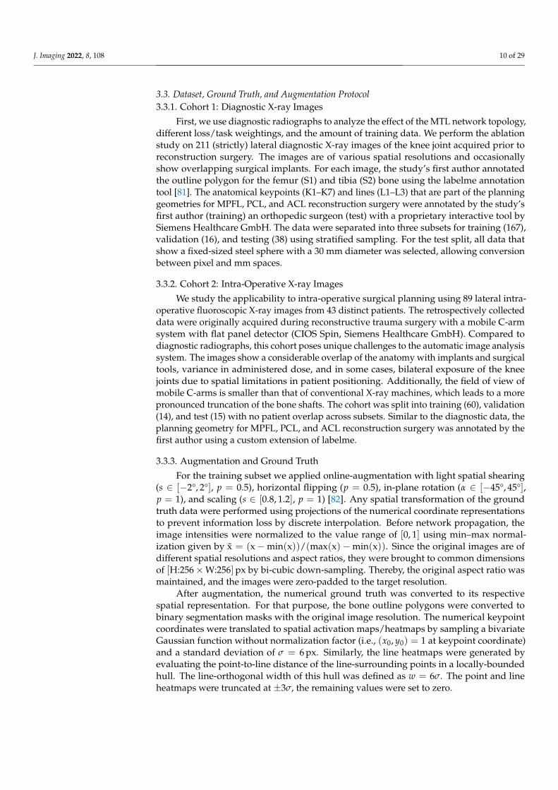
3.3. Dataset, Ground Truth, and Augmentation Protocol3.3.1. Cohort 1: Diagnostic X-ray Images

First, we use diagnostic radiographs to analyze the effect of the MTL network topology,different loss/task weightings, and the amount of training data. We perform the ablationstudy on 211 (strictly) lateral diagnostic X-ray images of the knee joint acquired prior toreconstruction surgery. The images are of various spatial resolutions and occasionallyshow overlapping surgical implants. For each image, the study’s first author annotatedthe outline polygon for the femur (S1) and tibia (S2) bone using the labelme annotationtool [81]. The anatomical keypoints (K1–K7) and lines (L1–L3) that are part of the planninggeometries for MPFL, PCL, and ACL reconstruction surgery were annotated by the study’sfirst author (training) an orthopedic surgeon (test) with a proprietary interactive tool bySiemens Healthcare GmbH. The data were separated into three subsets for training (167),validation (16), and testing (38) using stratified sampling. For the test split, all data thatshow a fixed-sized steel sphere with a 30 mm diameter was selected, allowing conversionbetween pixel and mm spaces.

3.3.2. Cohort 2: Intra-Operative X-ray Images

We study the applicability to intra-operative surgical planning using 89 lateral intra-operative fluoroscopic X-ray images from 43 distinct patients. The retrospectively collecteddata were originally acquired during reconstructive trauma surgery with a mobile C-armsystem with flat panel detector (CIOS Spin, Siemens Healthcare GmbH). Compared todiagnostic radiographs, this cohort poses unique challenges to the automatic image analysissystem. The images show a considerable overlap of the anatomy with implants and surgicaltools, variance in administered dose, and in some cases, bilateral exposure of the kneejoints due to spatial limitations in patient positioning. Additionally, the field of view ofmobile C-arms is smaller than that of conventional X-ray machines, which leads to a morepronounced truncation of the bone shafts. The cohort was split into training (60), validation(14), and test (15) with no patient overlap across subsets. Similar to the diagnostic data, theplanning geometry for MPFL, PCL, and ACL reconstruction surgery was annotated by thefirst author using a custom extension of labelme.

3.3.3. Augmentation and Ground Truth

For the training subset we applied online-augmentation with light spatial shearing(s ∈ [−2°, 2°], p = 0.5), horizontal flipping (p = 0.5), in-plane rotation (α ∈ [−45°, 45°],p = 1), and scaling (s ∈ [0.8, 1.2], p = 1) [82]. Any spatial transformation of the groundtruth data were performed using projections of the numerical coordinate representationsto prevent information loss by discrete interpolation. Before network propagation, theimage intensities were normalized to the value range of [0, 1] using min–max normal-ization given by x = (x−min(x))/(max(x)−min(x)). Since the original images are ofdifferent spatial resolutions and aspect ratios, they were brought to common dimensionsof [H:256×W:256]px by bi-cubic down-sampling. Thereby, the original aspect ratio wasmaintained, and the images were zero-padded to the target resolution.

After augmentation, the numerical ground truth was converted to its respectivespatial representation. For that purpose, the bone outline polygons were converted tobinary segmentation masks with the original image resolution. The numerical keypointcoordinates were translated to spatial activation maps/heatmaps by sampling a bivariateGaussian function without normalization factor (i.e., (x0, y0) = 1 at keypoint coordinate)and a standard deviation of σ = 6 px. Similarly, the line heatmaps were generated byevaluating the point-to-line distance of the line-surrounding points in a locally-boundedhull. The line-orthogonal width of this hull was defined as w = 6σ. The point and lineheatmaps were truncated at ±3σ, the remaining values were set to zero.

J. Imaging 2022, 8, 108 11 of 29

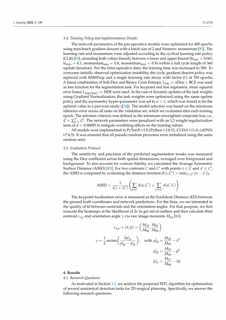
3.4. Training Policy and Implementation Details

The network parameters of the pre-operative models were optimized for 400 epochsusing mini-batch gradient descent with a batch size of 2 and Nesterov momentum [83]. Thelearning rate and momentum were adjusted according to the cyclical learning rate policy(CLR) [84], annealing both values linearly between a lower and upper bound (lrmin = 0.001,lrmax = 0.1, momentummin = 0.8, momentummax = 0.9) within a full cycle length of 360update iterations. For the intra-operative data, the training time was increased to 500. Toovercome initially observed optimization instability, the cyclic gradient descent policy wasreplaced with RMSProp and a single learning rate decay with factor 0.1 at 350 epochs.A linear combination of Soft-Dice and Binary Cross Entropy Lseg := sDice + BCE was usedas loss function for the segmentation task. For keypoint and line regression, mean squarederror losses L{kpt,line} := MSE were used. In the case of dynamic updates of the task weightsusing Gradient Normalization, the task weights were optimized using the same updatepolicy and the asymmetry hyper-parameter was set to α = 1, which was found to be theoptimal value in a previous study ([54]). The model selection was based on the minimuminference error across all tasks on the validation set, which we evaluated after each trainingepoch. The selection criterion was defined as the minimum unweighted composite loss, i.e.,L = ∑T

t=1 Lt. The network parameters were penalized with an L2 weight regularizationterm of d = 0.00005 to mitigate overfitting effects on the training subset.

All models were implemented in PyTorch v1.8 (Python v3.8.12, CUDA v11.0, cuDNNv7.6.5). It was ensured that all pseudo-random processes were initialized using the samerandom seed.

3.5. Evaluation Protocol

The sensitivity and precision of the predicted segmentation masks was measuredusing the Dice coefficient across both spatial dimensions, averaged over foreground andbackground. To also account for contour fidelity, we calculated the Average SymmetricSurface Distance (ASSD) [85]. For two contours C and C′ with points x ∈ C and x′ ∈ C′,the ASSD is computed by evaluating the distance function d(x, C′) = minx′∈C′‖x− x′‖2.

ASSD =1

|C|+ |C′|

(∑x∈C

d(x, C′) + ∑x′∈C′

d(x′, C)

)

The keypoint localization error is measured as the Euclidean Distance (ED) betweenthe ground truth coordinates and network predictions. For the lines, we are interested inthe quality of fit between centroids and the orientation angles. For that purpose, we firsttruncate the heatmaps at the likelihood of 2σ to get rid of outliers and then calculate theircentroid cx,y and orientation angle γ via raw image moments Mpq [86].

cx,y = (x, y) =(

M10

M00,

M01

M00

)

γ =12

arctan(

2µ′11µ′20 − µ′02

), with µ′20 =

M20

M00− x2

µ′02 =M02

M00− y2

µ′11 =M11

M00− xy

4. Results4.1. Research Questions

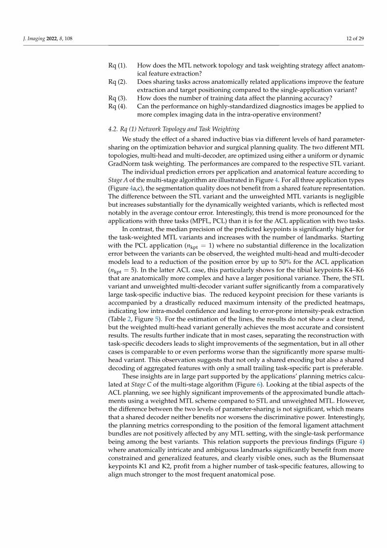
As motivated in Section 3.1, we analyze the proposed MTL algorithm for optimizationof several anatomical detection tasks for 2D surgical planning. Specifically, we answer thefollowing research questions:

J. Imaging 2022, 8, 108 12 of 29

Rq (1). How does the MTL network topology and task weighting strategy affect anatom-ical feature extraction?

Rq (2). Does sharing tasks across anatomically related applications improve the featureextraction and target positioning compared to the single-application variant?

Rq (3). How does the number of training data affect the planning accuracy?Rq (4). Can the performance on highly-standardized diagnostics images be applied to

more complex imaging data in the intra-operative environment?

4.2. Rq (1) Network Topology and Task Weighting

We study the effect of a shared inductive bias via different levels of hard parameter-sharing on the optimization behavior and surgical planning quality. The two different MTLtopologies, multi-head and multi-decoder, are optimized using either a uniform or dynamicGradNorm task weighting. The performances are compared to the respective STL variant.

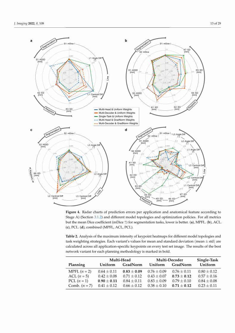
The individual prediction errors per application and anatomical feature according toStage A of the multi-stage algorithm are illustrated in Figure 4. For all three application types(Figure 4a,c), the segmentation quality does not benefit from a shared feature representation.The difference between the STL variant and the unweighted MTL variants is negligiblebut increases substantially for the dynamically weighted variants, which is reflected mostnotably in the average contour error. Interestingly, this trend is more pronounced for theapplications with three tasks (MPFL, PCL) than it is for the ACL application with two tasks.

In contrast, the median precision of the predicted keypoints is significantly higher forthe task-weighted MTL variants and increases with the number of landmarks. Startingwith the PCL application (nkpt = 1) where no substantial difference in the localizationerror between the variants can be observed, the weighted multi-head and multi-decodermodels lead to a reduction of the position error by up to 50% for the ACL application(nkpt = 5). In the latter ACL case, this particularly shows for the tibial keypoints K4–K6that are anatomically more complex and have a larger positional variance. There, the STLvariant and unweighted multi-decoder variant suffer significantly from a comparativelylarge task-specific inductive bias. The reduced keypoint precision for these variants isaccompanied by a drastically reduced maximum intensity of the predicted heatmaps,indicating low intra-model confidence and leading to error-prone intensity-peak extraction(Table 2, Figure 5). For the estimation of the lines, the results do not show a clear trend,but the weighted multi-head variant generally achieves the most accurate and consistentresults. The results further indicate that in most cases, separating the reconstruction withtask-specific decoders leads to slight improvements of the segmentation, but in all othercases is comparable to or even performs worse than the significantly more sparse multi-head variant. This observation suggests that not only a shared encoding but also a shareddecoding of aggregated features with only a small trailing task-specific part is preferable.

These insights are in large part supported by the applications’ planning metrics calcu-lated at Stage C of the multi-stage algorithm (Figure 6). Looking at the tibial aspects of theACL planning, we see highly significant improvements of the approximated bundle attach-ments using a weighted MTL scheme compared to STL and unweighted MTL. However,the difference between the two levels of parameter-sharing is not significant, which meansthat a shared decoder neither benefits nor worsens the discriminative power. Interestingly,the planning metrics corresponding to the position of the femoral ligament attachmentbundles are not positively affected by any MTL setting, with the single-task performancebeing among the best variants. This relation supports the previous findings (Figure 4)where anatomically intricate and ambiguous landmarks significantly benefit from moreconstrained and generalized features, and clearly visible ones, such as the Blumensaatkeypoints K1 and K2, profit from a higher number of task-specific features, allowing toalign much stronger to the most frequent anatomical pose.

J. Imaging 2022, 8, 108 13 of 29

Multi-Head & Uniform Weights

Multi-Decoder & Uniform Weights

Single-Task & Uniform Weights

Multi-Head & GradNorm Weights

Multi-Decoder & GradNorm Weights

0.985

0.99

0.995

1.0

0.35

0.4

0.45

0.5

1.252.5

3.755.0 1.25

2.5

3.75

5.0

1.25

2.5

3.75

5.0

0.20.4

0.60.8

0.2

0.4

0.6

0.8

Line

S2: ASSD[mm]

S2: mDice ↑

L3: Angle Diff[°]

K6: ED[mm]

L2: Centroid Diff[mm]

L3: Centroid Diff[mm]

L2: Angle Diff[°]

0.97

0.98

0.99

1.0

0.97

0.98

0.99

1.0

0.20.4

0.60.8

0.2

0.4

0.6

0.8

1.25

2.5

3.75

5.0

1.25

2.5

3.75

5.0

1.25

2.5

3.75

5.0

1.252.5

3.755.01.25

2.5

3.75

5.0

S2: ASSD[mm]

K4: ED[mm]

K5: ED[mm]

K7: ED[mm]

K1: ED[mm]

K2: ED[mm]

S1: ASSD[mm]

S2: mDice

S1: mDice ↑

0.985

0.99

0.995

1.0

0.25

0.3

0.35

0.4

1.0

2.0

3.0

4.0

1.0

2.0

3.0

4.0

1.0

2.0

3.0

4.0

0.125

0.25

0.375

0.5

Line

Segmentation

Segmentation

S1: mDice ↑

S1: ASSD[mm]

K2: ED[mm]

K3: ED[mm]

L1: Angle Diff[°]

L1: Centroid Diff[mm]

0.985

0.99

0.995

1.0

0.985

0.99

0.995

1.0

0.2

0.4

0.6

0.8

0.2

0.4

0.6

0.8

5.511.016.522.0

5.511.0

16.522.0

5.5

11.0

16.5

22.0

5.5

11.0

16.5

22.0

5.5

11.0

16.5

22.0

5.5

11.0

16.5

22.0

5.5

11.0

16.5

22.0

1.5

3.0

4.5

6.0

1.53.0

4.56.0

1.5 3.0 4.5 6.00.2

0.4

0.6

0.8

0.2

0.4

0.6

0.8

0.2

0.4

0.6

0.8

Keypoint

Line

S1: mDice ↑S2: mDice ↑

S1: ASSD[mm]

S2: ASSD[mm]

K1: ED[mm]

K2: ED[mm]

K3: ED[mm]

K4: ED[mm]

K5: ED[mm]

K6: ED[mm]

K7: ED[mm]

L1: Centroid Diff[mm]

L2: Centroid Diff[mm]

L3: Centroid Diff[mm]

L1: Angle Diff[°]

L2: Angle Diff[°]

L3: Angle Diff[°]

a

c d

b

Segmentation

Segmentation

Keypoint

Keypoint

Keypo

int

Figure 4. Radar charts of prediction errors per application and anatomical feature according toStage A) (Section 3.1.2) and different model topologies and optimization policies. For all metricsbut the mean Dice coefficient (mDice ↑) for segmentation tasks, lower is better. (a), MPFL. (b), ACL.(c), PCL. (d), combined (MPFL, ACL, PCL).

Table 2. Analysis of the maximum intensity of keypoint heatmaps for different model topologies andtask weighting strategies. Each variant’s values for mean and standard deviation (mean± std) arecalculated across all application-specific keypoints on every test set image. The results of the bestnetwork variant for each planning methodology is marked in bold.

Multi-Head Multi-Decoder Single-TaskPlanning Uniform GradNorm Uniform GradNorm Uniform

MPFL (n = 2) 0.64± 0.11 0.83± 0.09 0.76± 0.09 0.76± 0.11 0.80± 0.12ACL (n = 5) 0.42± 0.08 0.71± 0.12 0.43± 0.07 0.73± 0.12 0.57± 0.16PCL (n = 1) 0.90± 0.11 0.84± 0.11 0.83± 0.09 0.79± 0.10 0.84± 0.08Comb. (n = 7) 0.41± 0.12 0.66± 0.12 0.38± 0.10 0.71± 0.12 0.23± 0.11

J. Imaging 2022, 8, 108 14 of 29M

PF

LA

CL

PC

LC

ombi

ned

Multi-Head

Uniform UniformGradNorm GradNorm Uniform

Multi-Decoder Single-TaskGround Truth

K1K2 K3

K4K5

K6K7

K6

K2 K3

K1K2

K4K5

K7

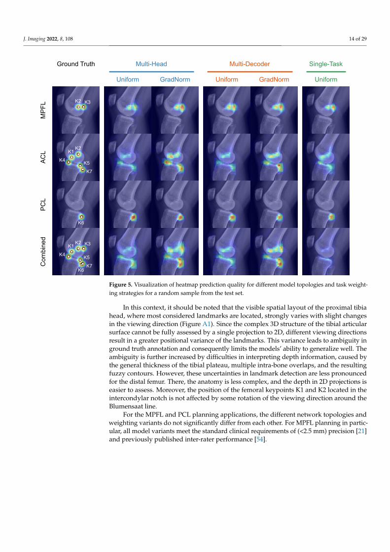
Figure 5. Visualization of heatmap prediction quality for different model topologies and task weight-ing strategies for a random sample from the test set.

In this context, it should be noted that the visible spatial layout of the proximal tibiahead, where most considered landmarks are located, strongly varies with slight changesin the viewing direction (Figure A1). Since the complex 3D structure of the tibial articularsurface cannot be fully assessed by a single projection to 2D, different viewing directionsresult in a greater positional variance of the landmarks. This variance leads to ambiguity inground truth annotation and consequently limits the models’ ability to generalize well. Theambiguity is further increased by difficulties in interpreting depth information, caused bythe general thickness of the tibial plateau, multiple intra-bone overlaps, and the resultingfuzzy contours. However, these uncertainties in landmark detection are less pronouncedfor the distal femur. There, the anatomy is less complex, and the depth in 2D projections iseasier to assess. Moreover, the position of the femoral keypoints K1 and K2 located in theintercondylar notch is not affected by some rotation of the viewing direction around theBlumensaat line.

For the MPFL and PCL planning applications, the different network topologies andweighting variants do not significantly differ from each other. For MPFL planning in partic-ular, all model variants meet the standard clinical requirements of (<2.5 mm) precision [21]and previously published inter-rater performance [54].

J. Imaging 2022, 8, 108 15 of 29

AM Bundle TibiaAM Bundle Femur PL Bundle Femur PL Bundle Tibia

0

10

MultiHead

MultiDecod.

SingleTask

0

20

MultiHead

MultiDecod.

SingleTask

0

20

MultiHead

MultiDecod.

SingleTask

0

25

50

MultiHead

MultiDecod.

SingleTask

Schoettle Point

ED

[mm

]

ED

[mm

]E

D [m

m]

ED

[mm

]

ED

[mm

]

ED

[mm

]

Bundle Insertion Guidewire Angle

0

2

4

MultiHead

MultiDecod.

SingleTask

Ang

le D

iff [°

]

0

25

50

MultiHead

MultiDecod.

SingleTask

0

5

d

a c

b

MultiHead

MultiDecod.

SingleTask

0

2

4

Schoettle Point

ED

[mm

] n n n nnnn

n nn

n n n nnnn

n nn

AM Bundle Femur

0

5

MultiHead

MultiDecod.

SingleTask

ED

[mm

] n n * *nnn

n nn

ED

[mm

]

Bundle Insertion

0

2

MultiHead

MultiDecod.

SingleTask

n n n nnnn

* nn

* n ******n*

******

* n * ***n**

* ***

* n * ***n*

** ***

n ** n ****n**

** ***

n ** n ****n**

** ***

n * n ****n*

n ****

Guidewire Angle

0

2

MultiHead

MultiDecod.

SingleTask

Ang

le D

iff [°

]

n * n nnnn

n nn

PL Bundle Femur

0

5

MultiHead

MultiDecod.

SingleTask

ED

[mm

] n n * nnnn

n nn

PL Bundle Tibia

0

5

10

MultiHead

MultiDecod.

SingleTask

ED

[mm

]

** n ** n

**n**** n

**

AM Bundle Tibia

0

10

MultiHead

MultiDecod.

SingleTask

ED

[mm

]

** * ** n

**n**** n

**

0

20

MultiHead

MultiDecod.

SingleTask

Topology

Multi-Head

Multi-Decod.

Single-task

Task Weighting Non-parametric Statistical Significance

Uniform Weights Not significant: p ≥ 0.05

Significant with level p < 0.05

Highly significant with level p < 0.001

GradNorm Weights * n * ***n*

** ***

n

*

**

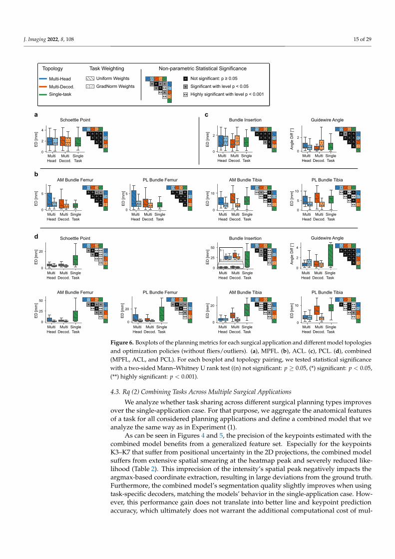
Figure 6. Boxplots of the planning metrics for each surgical application and different model topologiesand optimization policies (without fliers/outliers). (a), MPFL. (b), ACL. (c), PCL. (d), combined(MPFL, ACL, and PCL). For each boxplot and topology pairing, we tested statistical significancewith a two-sided Mann–Whitney U rank test ((n) not significant: p ≥ 0.05, (*) significant: p < 0.05,(**) highly significant: p < 0.001).

4.3. Rq (2) Combining Tasks Across Multiple Surgical Applications

We analyze whether task sharing across different surgical planning types improvesover the single-application case. For that purpose, we aggregate the anatomical featuresof a task for all considered planning applications and define a combined model that weanalyze the same way as in Experiment (1).

As can be seen in Figures 4 and 5, the precision of the keypoints estimated with thecombined model benefits from a generalized feature set. Especially for the keypointsK3–K7 that suffer from positional uncertainty in the 2D projections, the combined modelsuffers from extensive spatial smearing at the heatmap peak and severely reduced like-lihood (Table 2). This imprecision of the intensity’s spatial peak negatively impacts theargmax-based coordinate extraction, resulting in large deviations from the ground truth.Furthermore, the combined model’s segmentation quality slightly improves when usingtask-specific decoders, matching the models’ behavior in the single-application case. How-ever, this performance gain does not translate into better line and keypoint predictionaccuracy, which ultimately does not warrant the additional computational cost of mul-

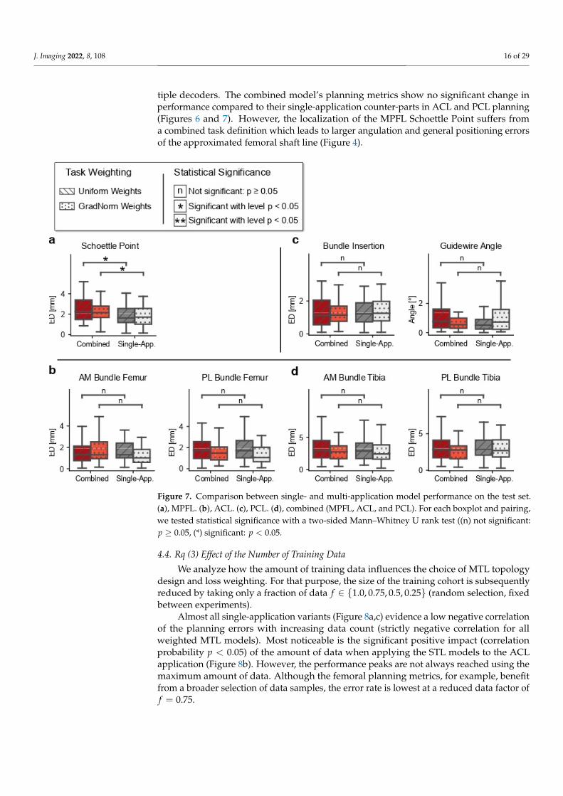
J. Imaging 2022, 8, 108 16 of 29

tiple decoders. The combined model’s planning metrics show no significant change inperformance compared to their single-application counter-parts in ACL and PCL planning(Figures 6 and 7). However, the localization of the MPFL Schoettle Point suffers froma combined task definition which leads to larger angulation and general positioning errorsof the approximated femoral shaft line (Figure 4).

Figure 7. Comparison between single- and multi-application model performance on the test set.(a), MPFL. (b), ACL. (c), PCL. (d), combined (MPFL, ACL, and PCL). For each boxplot and pairing,we tested statistical significance with a two-sided Mann–Whitney U rank test ((n) not significant:p ≥ 0.05, (*) significant: p < 0.05.

4.4. Rq (3) Effect of the Number of Training Data

We analyze how the amount of training data influences the choice of MTL topologydesign and loss weighting. For that purpose, the size of the training cohort is subsequentlyreduced by taking only a fraction of data f ∈ {1.0, 0.75, 0.5, 0.25} (random selection, fixedbetween experiments).

Almost all single-application variants (Figure 8a,c) evidence a low negative correlationof the planning errors with increasing data count (strictly negative correlation for allweighted MTL models). Most noticeable is the significant positive impact (correlationprobability p < 0.05) of the amount of data when applying the STL models to the ACLapplication (Figure 8b). However, the performance peaks are not always reached using themaximum amount of data. Although the femoral planning metrics, for example, benefitfrom a broader selection of data samples, the error rate is lowest at a reduced data factor off = 0.75.

J. Imaging 2022, 8, 108 17 of 29

0.25 0.5 0.75 1.0

0.2

0.3

0.25 0.5 0.75 1.0

0.25 0.5 0.75 1.0

10.0

0.25 0.5 0.75 1.0 0.25 0.5 0.75 1.01.0

10.0

0.25 0.5 0.75 1.0 0.25 0.5 0.75 1.0

10.0

3.04.0

6.0

0.25 0.5 0.75 1.0 0.25 0.5 0.75 1.0

10.0

3.0

4.0

6.0

0.25 0.5 0.75 1.0

0.25 0.5 0.75 1.0

1.0

1.2

1.4

1.61.8

0.25 0.5 0.75 1.0 0.25 0.5 0.75 1.0

1.0

0.6

2.0

0.25 0.5 0.75 1.0

Training Data Factor Training Data Factor Training Data Factor

Training Data Factor Training Data Factor Training Data Factor

Training Data Factor Training Data Factor Training Data Factor Training Data Factor

Training Data Factor Training Data Factor Training Data Factor Training Data Factor

0.25 0.5 0.75 1.01.0

10.0

0.25 0.5 0.75 1.0 0.25 0.5 0.75 1.01.0

10.0

0.25 0.5 0.75 1.0 0.25 0.5 0.75 1.0

10.0

0.25 0.5 0.75 1.0

0.25 0.5 0.75 1.0

10.0

2.0

3.04.0

6.0

0.25 0.5 0.75 1.0

0.25 0.5 0.75 1.0 0.25 0.5 0.75 1.0

10.0

0.25 0.5 0.75 1.01.0

10.0

0.25 0.5 0.75 1.0 0.25 0.5 0.75 1.0

1.0

10.0

0.25 0.5 0.75 1.0

STD

Training Data Factor Misc

0.25: n=430.50: n=830.75: n=1251.00: n=167

AM Bundle TibiaAM Bundle Femur PL Bundle Femur PL Bundle Tibia

Schoettle Point

ED

[mm

]E

D [m

m]

Bundle Insertion Guidewire Angle

Ang

le D

iff [°

]

d

a c

b

Schoettle Point

ED

[mm

]

AM Bundle Femur

ED

[mm

]

ED

[mm

]

ED

[mm

]E

D [m

m]

ED

[mm

]E

D [m

m]

ED

[mm

]

Bundle Insertion Guidewire Angle

Ang

le D

iff [°

]

PL Bundle Femur PL Bundle TibiaAM Bundle Tibia

Topology

Multi-Head

Multi-Decod.

Single-task

Task Weighting

Uniform Weights

GradNorm Weights

ED

[mm

]

ED

[mm

]ρ= -0.18 p=0.03

ρ= -0.17 p=0.04 ρ= -0.17 p=0.04ρ= -0.30 p=0.00 ρ= -0.31 p=0.00 ρ= -0.47 p=0.00 ρ= -0.45 p=0.00

ρ= +0.22 p=0.01

ρ= +0.21 p=0.01 ρ= +0.22 p=0.01

ρ= +0.20 p=0.01 ρ= +0.13 p=0.01

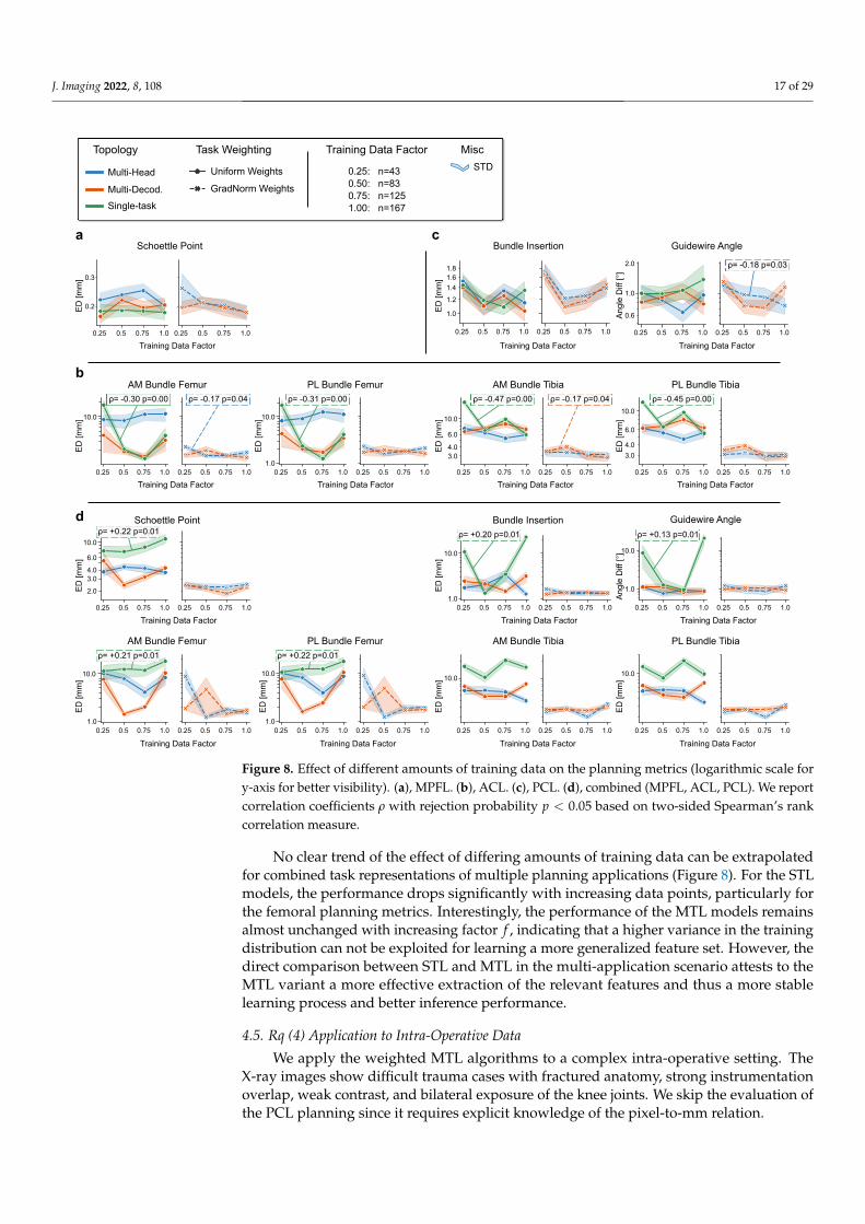
Figure 8. Effect of different amounts of training data on the planning metrics (logarithmic scale fory-axis for better visibility). (a), MPFL. (b), ACL. (c), PCL. (d), combined (MPFL, ACL, PCL). We reportcorrelation coefficients ρ with rejection probability p < 0.05 based on two-sided Spearman’s rankcorrelation measure.

No clear trend of the effect of differing amounts of training data can be extrapolatedfor combined task representations of multiple planning applications (Figure 8). For the STLmodels, the performance drops significantly with increasing data points, particularly forthe femoral planning metrics. Interestingly, the performance of the MTL models remainsalmost unchanged with increasing factor f , indicating that a higher variance in the trainingdistribution can not be exploited for learning a more generalized feature set. However, thedirect comparison between STL and MTL in the multi-application scenario attests to theMTL variant a more effective extraction of the relevant features and thus a more stablelearning process and better inference performance.

4.5. Rq (4) Application to Intra-Operative Data

We apply the weighted MTL algorithms to a complex intra-operative setting. TheX-ray images show difficult trauma cases with fractured anatomy, strong instrumentationoverlap, weak contrast, and bilateral exposure of the knee joints. We skip the evaluation ofthe PCL planning since it requires explicit knowledge of the pixel-to-mm relation.

J. Imaging 2022, 8, 108 18 of 29

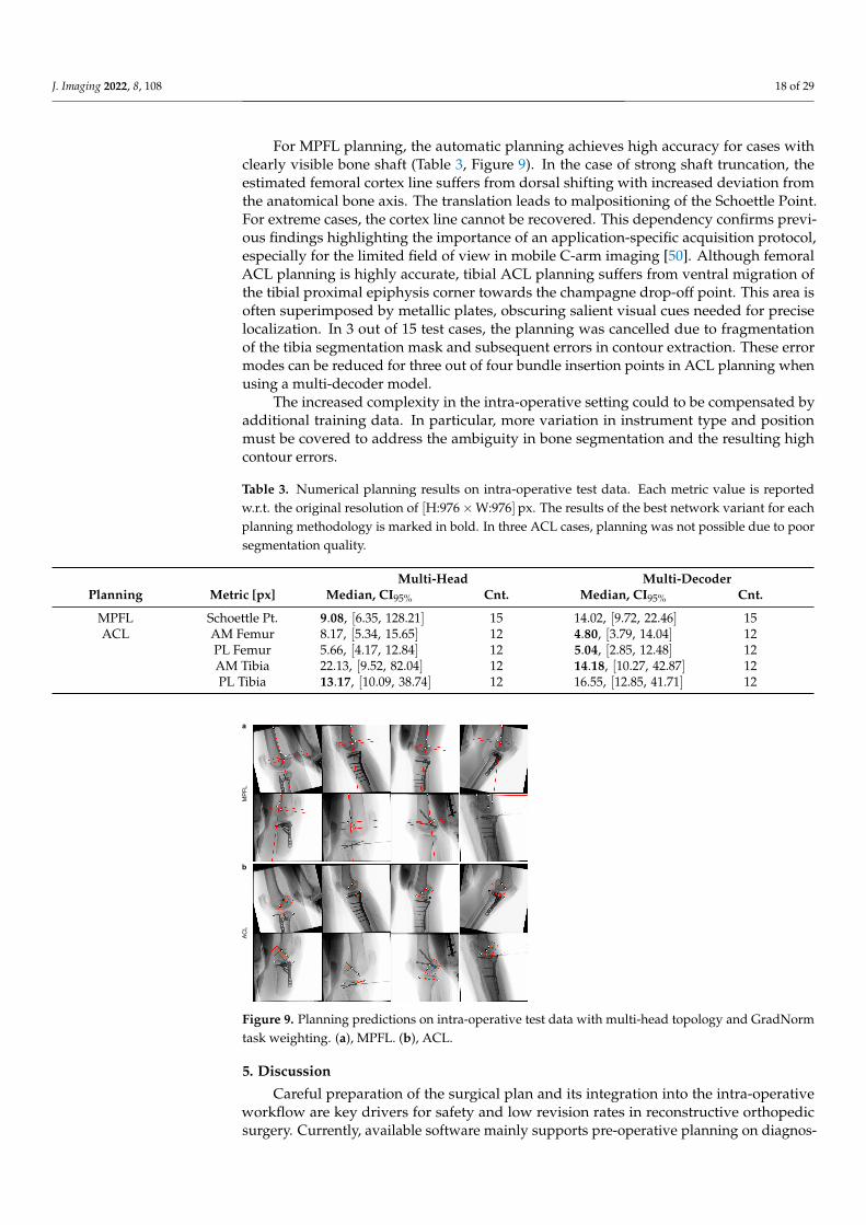
For MPFL planning, the automatic planning achieves high accuracy for cases withclearly visible bone shaft (Table 3, Figure 9). In the case of strong shaft truncation, theestimated femoral cortex line suffers from dorsal shifting with increased deviation fromthe anatomical bone axis. The translation leads to malpositioning of the Schoettle Point.For extreme cases, the cortex line cannot be recovered. This dependency confirms previ-ous findings highlighting the importance of an application-specific acquisition protocol,especially for the limited field of view in mobile C-arm imaging [50]. Although femoralACL planning is highly accurate, tibial ACL planning suffers from ventral migration ofthe tibial proximal epiphysis corner towards the champagne drop-off point. This area isoften superimposed by metallic plates, obscuring salient visual cues needed for preciselocalization. In 3 out of 15 test cases, the planning was cancelled due to fragmentationof the tibia segmentation mask and subsequent errors in contour extraction. These errormodes can be reduced for three out of four bundle insertion points in ACL planning whenusing a multi-decoder model.

The increased complexity in the intra-operative setting could to be compensated byadditional training data. In particular, more variation in instrument type and positionmust be covered to address the ambiguity in bone segmentation and the resulting highcontour errors.

Table 3. Numerical planning results on intra-operative test data. Each metric value is reportedw.r.t. the original resolution of [H:976×W:976]px. The results of the best network variant for eachplanning methodology is marked in bold. In three ACL cases, planning was not possible due to poorsegmentation quality.

Multi-Head Multi-DecoderPlanning Metric [px] Median, CI95% Cnt. Median, CI95% Cnt.

MPFL Schoettle Pt. 9.08, [6.35, 128.21] 15 14.02, [9.72, 22.46] 15ACL AM Femur 8.17, [5.34, 15.65] 12 4.80, [3.79, 14.04] 12

PL Femur 5.66, [4.17, 12.84] 12 5.04, [2.85, 12.48] 12AM Tibia 22.13, [9.52, 82.04] 12 14.18, [10.27, 42.87] 12PL Tibia 13.17, [10.09, 38.74] 12 16.55, [12.85, 41.71] 12

MPFL

ACL

a

b

Figure 9. Planning predictions on intra-operative test data with multi-head topology and GradNormtask weighting. (a), MPFL. (b), ACL.

5. Discussion

Careful preparation of the surgical plan and its integration into the intra-operativeworkflow are key drivers for safety and low revision rates in reconstructive orthopedicsurgery. Currently, available software mainly supports pre-operative planning on diagnos-

J. Imaging 2022, 8, 108 19 of 29

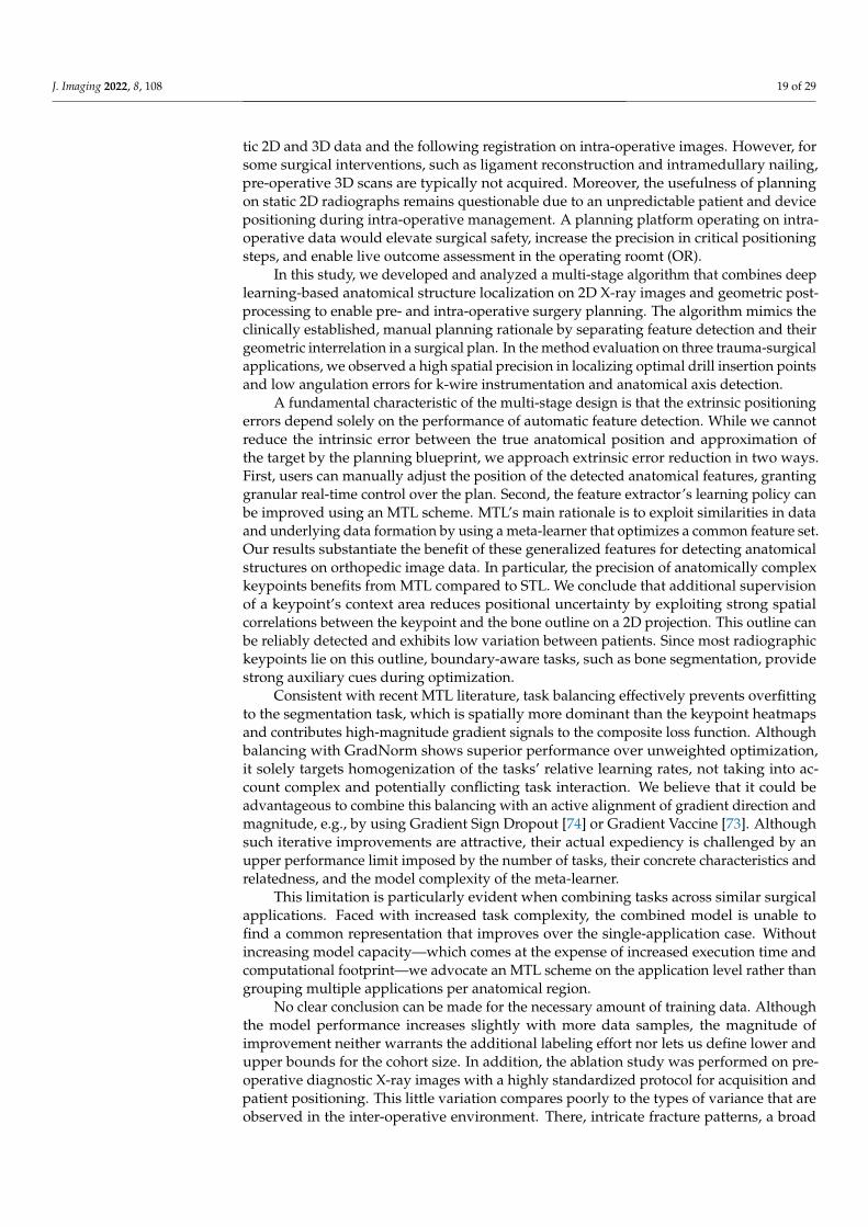
tic 2D and 3D data and the following registration on intra-operative images. However, forsome surgical interventions, such as ligament reconstruction and intramedullary nailing,pre-operative 3D scans are typically not acquired. Moreover, the usefulness of planningon static 2D radiographs remains questionable due to an unpredictable patient and devicepositioning during intra-operative management. A planning platform operating on intra-operative data would elevate surgical safety, increase the precision in critical positioningsteps, and enable live outcome assessment in the operating roomt (OR).

In this study, we developed and analyzed a multi-stage algorithm that combines deeplearning-based anatomical structure localization on 2D X-ray images and geometric post-processing to enable pre- and intra-operative surgery planning. The algorithm mimics theclinically established, manual planning rationale by separating feature detection and theirgeometric interrelation in a surgical plan. In the method evaluation on three trauma-surgicalapplications, we observed a high spatial precision in localizing optimal drill insertion pointsand low angulation errors for k-wire instrumentation and anatomical axis detection.

A fundamental characteristic of the multi-stage design is that the extrinsic positioningerrors depend solely on the performance of automatic feature detection. While we cannotreduce the intrinsic error between the true anatomical position and approximation ofthe target by the planning blueprint, we approach extrinsic error reduction in two ways.First, users can manually adjust the position of the detected anatomical features, grantinggranular real-time control over the plan. Second, the feature extractor’s learning policy canbe improved using an MTL scheme. MTL’s main rationale is to exploit similarities in dataand underlying data formation by using a meta-learner that optimizes a common feature set.Our results substantiate the benefit of these generalized features for detecting anatomicalstructures on orthopedic image data. In particular, the precision of anatomically complexkeypoints benefits from MTL compared to STL. We conclude that additional supervisionof a keypoint’s context area reduces positional uncertainty by exploiting strong spatialcorrelations between the keypoint and the bone outline on a 2D projection. This outline canbe reliably detected and exhibits low variation between patients. Since most radiographickeypoints lie on this outline, boundary-aware tasks, such as bone segmentation, providestrong auxiliary cues during optimization.

Consistent with recent MTL literature, task balancing effectively prevents overfittingto the segmentation task, which is spatially more dominant than the keypoint heatmapsand contributes high-magnitude gradient signals to the composite loss function. Althoughbalancing with GradNorm shows superior performance over unweighted optimization,it solely targets homogenization of the tasks’ relative learning rates, not taking into ac-count complex and potentially conflicting task interaction. We believe that it could beadvantageous to combine this balancing with an active alignment of gradient direction andmagnitude, e.g., by using Gradient Sign Dropout [74] or Gradient Vaccine [73]. Althoughsuch iterative improvements are attractive, their actual expediency is challenged by anupper performance limit imposed by the number of tasks, their concrete characteristics andrelatedness, and the model complexity of the meta-learner.

This limitation is particularly evident when combining tasks across similar surgicalapplications. Faced with increased task complexity, the combined model is unable tofind a common representation that improves over the single-application case. Withoutincreasing model capacity—which comes at the expense of increased execution time andcomputational footprint—we advocate an MTL scheme on the application level rather thangrouping multiple applications per anatomical region.

No clear conclusion can be made for the necessary amount of training data. Althoughthe model performance increases slightly with more data samples, the magnitude ofimprovement neither warrants the additional labeling effort nor lets us define lower andupper bounds for the cohort size. In addition, the ablation study was performed on pre-operative diagnostic X-ray images with a highly standardized protocol for acquisition andpatient positioning. This little variation compares poorly to the types of variance that areobserved in the inter-operative environment. There, intricate fracture patterns, a broad

J. Imaging 2022, 8, 108 20 of 29

array of surgical tools and implants, and greater out-of-plane rotation angles caused byspatially-constrained patient positioning introduce novel types of image characteristics. Inthis scenario, additional data may help to reduce model bias.

We see several limitations of our study. At the present stage, our method does notconsider the registration of an initial surgical plan on subsequent intra-operative live data.Although the lack of registration does not immediately impact the planning process, ithamstrings outcome evaluation and more advanced real-time guidance using fluoroscopyor periodical positioning checks with single shots. Furthermore, the method was onlyevaluated for surgical applications on the knee joint. Compared to the large femur and tibia,the bones of the wrist, elbow or foot are much smaller and have less pronounced contoursin the 2D projection due to strong inter-bone overlap. A further restriction of our methodis the disconnect between the optimization criterion and the actual planning target. Thealgorithm’s first stage solves the anatomical feature detection problem independently fromthe planning geometry, which can be seen as optimizing a proxy criterion with less anatomicand geometric constraints. However, such constraints could help rule out implausibleconfigurations and likely push the model to learn an abstract semantic representation ofthe actual planning target.

To address these shortcomings, future studies could investigate a combination ofanatomical feature extraction and subsequent plan generation with direct regression of theplanning target. The planning geometry can be implemented with differentiable functions,allowing gradient propagation from the actual target to the anatomical feature extractor. Inthis scenario, a consistency term between the geometric and direct target estimates can helpalign both estimates during optimization. Furthermore, previous studies have shown thatplanning methods are highly susceptible to rotational deviations between the underlyinganatomy and the standard projection [87,88]. We believe that extending our methodwith an automatic assessment [89,90] of this mismatch could assist in preventing targetmalpositioning and improve the planning’s reliability and clinical acceptance. Anotherdesirable extension is to combine our method with surgical tool recognition. In particular,knowledge of the k-wire direction and tip position would allow software-side securitycontrols and advanced guidance in the intra-operative execution of the plan [56].

However, already in its current stage, the presented approach offers a precise automatictool to support surgical intervention planning directly on intra-operative 2D data. Suchintra-operative plan generation is particularly relevant for trauma surgery, where pre-operative 3D images are often unavailable, limiting the application of many analysis andnavigation solutions operating on MRI [91–94] and CT [95–97] data. The proposed multi-stage planning algorithm was designed to separate automatic image analysis and geometricplan generation, allowing the user fine-grained control over each step of the proposed plan.This design decision ultimately improves user acceptance of the planning tool by allowinginaccuracies in the automatically proposed plan to be corrected for complex and rare injurypatterns. Furthermore, we were able to show empirically that parallel detection of allanatomical features relevant to the plan using a weighted MTL policy benefits positioningaccuracy, confirming the long-standing consensus in the MTL literature.

6. Conclusions

In this work, we specifically address the need for accurate X-ray guided 2D planningin the intra-operative environment for common injury patterns in reconstructive orthopedicsurgery. The proposed multi-stage algorithm separates automatic feature extraction and theactual planning step, which we consider a pivotal design choice that allows for real-timecontrol of individual planning components by the user. The detection step can be efficientlysolved with a lightweight MTL scheme, allowing short execution times and improvingspatial precision over the STL case. We believe that the developed platform will helpovercome the limitations of current clinical practice, where planning is done manually ondiagnostic 2D data with limited intra-operative value. Generating the surgical plan directlyin the OR will elevate surgical accuracy and ultimately motivate the development of novel

J. Imaging 2022, 8, 108 21 of 29

2D planning guidelines. Future work should explore the possibilities of end-to-end trainingof the feature extractor to provide gradient updates in each step of the planning geometry.Additionally, integrating the method with automatic mechanisms for image alignment andsurgical tool localization would assist the surgeon not only in planning, but also in imagedata acquisition and directly in surgical execution.

Author Contributions: Conceptualization, F.K., B.S. and H.K; methodology, F.K.; software, F.K.;validation, F.K.; formal analysis, F.K.; investigation, F.K.; resources, A.M., B.S., M.P., J.S.E.-B. and H.K.;data curation, F.K., B.S. and M.P.; writing—original draft preparation, F.K.; writing—review andediting, A.M., B.S., M.P., J.S.E.-B. and H.K.; visualization, F.K.; supervision, A.M. and H.K.; projectadministration, H.K.; funding acquisition, A.M. and H.K. All authors have read and agreed to thepublished version of the manuscript.

Funding: This research received no external funding.

Institutional Review Board Statement: Ethical review and approval were waived for this study, dueto the clinical data being obtained retrospectively from anonymized databases and not generatedintentionally for the study.

Informed Consent Statement: The acquisition of data from living patients had a medical indicationand informed consent was not required.

Data Availability Statement: The image data used for the evaluation of the software cannot bemade available. The methods and information presented here are based on research and are notcommercially available.

Acknowledgments: The authors gratefully acknowledge funding of the Erlangen Graduate Schoolin Advanced Optical Technologies (SAOT) by the Bavarian State Ministry for Science and Art. Theauthors acknowledge the support of Siemens Healthcare GmbH, Forchheim, Germany. The authorsacknowledge financial support by Deutsche Forschungsgemeinschaft and Friedrich-Alexander-Universität Erlangen-Nürnberg within the funding programme “Open Access Publication Funding”.

Conflicts of Interest: The authors declare no conflicts of interest.

Abbreviations

The following abbreviations are used in this manuscript:MPFL Medial Patellofemoral LigamentACL Anterior Cruciate LigamentPCL Posterior Cruciate LigamentAM AnteromedialPL PosterolateralOR Operating roomMTL Multi-task learningSTL Single-task learningGradNorm Gradient normalizationASSD Average symmetric surface distanceED Euclidean distance

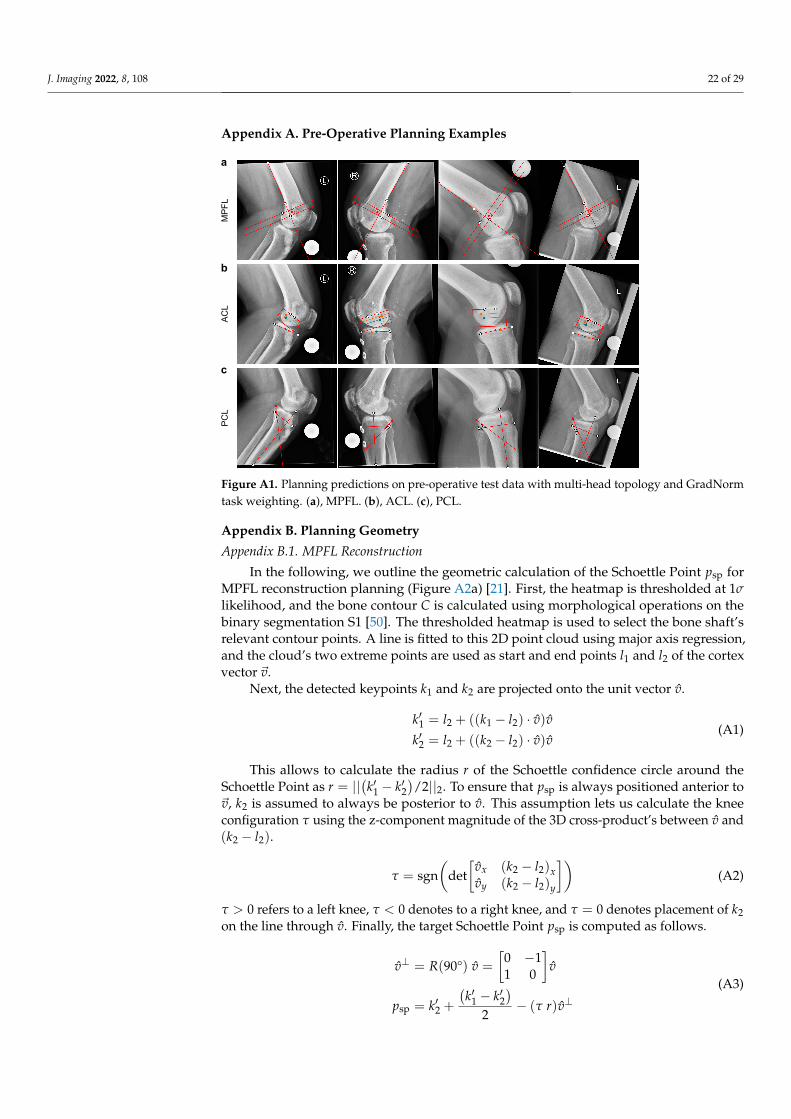
J. Imaging 2022, 8, 108 22 of 29

Appendix A. Pre-Operative Planning Examples

MPFL

ACL

PCL

a

b

c

Figure A1. Planning predictions on pre-operative test data with multi-head topology and GradNormtask weighting. (a), MPFL. (b), ACL. (c), PCL.

Appendix B. Planning Geometry

Appendix B.1. MPFL Reconstruction

In the following, we outline the geometric calculation of the Schoettle Point psp forMPFL reconstruction planning (Figure A2a) [21]. First, the heatmap is thresholded at 1σlikelihood, and the bone contour C is calculated using morphological operations on thebinary segmentation S1 [50]. The thresholded heatmap is used to select the bone shaft’srelevant contour points. A line is fitted to this 2D point cloud using major axis regression,and the cloud’s two extreme points are used as start and end points l1 and l2 of the cortexvector ~v.

Next, the detected keypoints k1 and k2 are projected onto the unit vector v.

k′1 = l2 + ((k1 − l2) · v)vk′2 = l2 + ((k2 − l2) · v)v

(A1)

This allows to calculate the radius r of the Schoettle confidence circle around theSchoettle Point as r = ||

(k′1 − k′2

)/2||2. To ensure that psp is always positioned anterior to

~v, k2 is assumed to always be posterior to v. This assumption lets us calculate the kneeconfiguration τ using the z-component magnitude of the 3D cross-product’s between v and(k2 − l2).

τ = sgn(

det[

vx (k2 − l2)xvy (k2 − l2)y

])(A2)

τ > 0 refers to a left knee, τ < 0 denotes to a right knee, and τ = 0 denotes placement of k2on the line through v. Finally, the target Schoettle Point psp is computed as follows.

v⊥ = R(90°) v =

[0 −11 0

]v

psp = k′2 +(k′1 − k′2

)2

− (τ r)v⊥(A3)

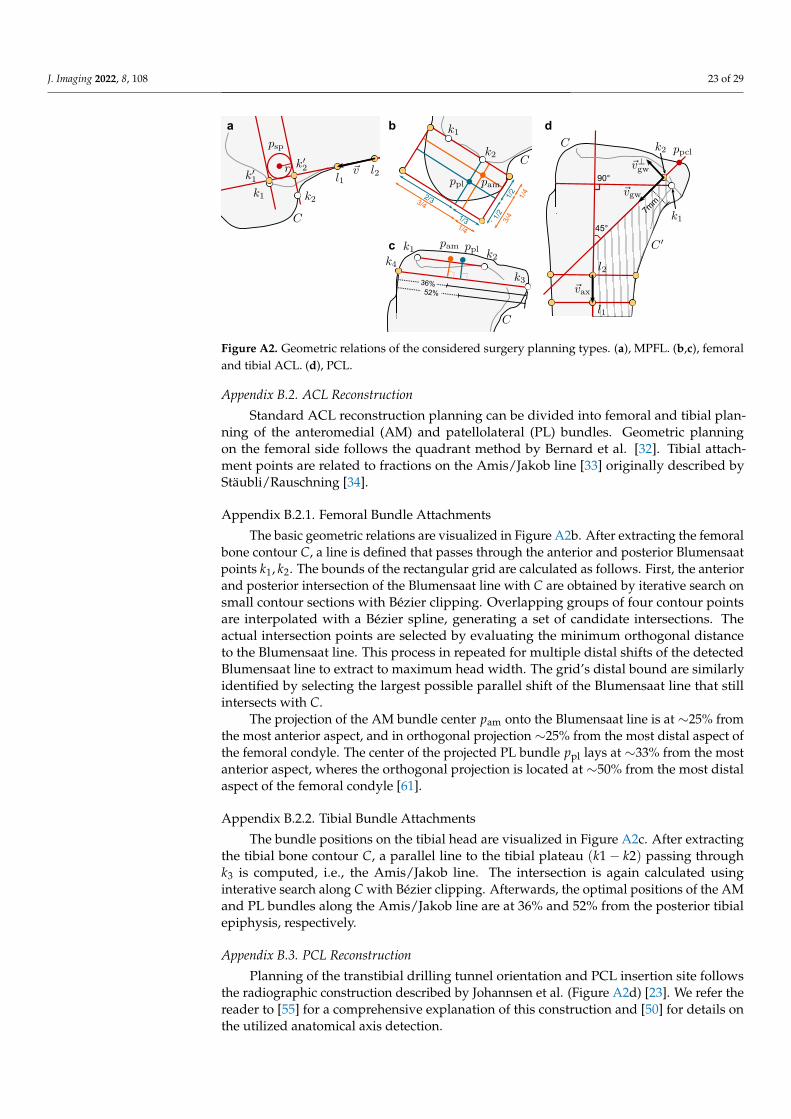
J. Imaging 2022, 8, 108 23 of 29

3/41/2

1/2

2/3

1/3

1/4

3/4

1/4

36%52%

b d

c

45°

90°

7mm

a

Figure A2. Geometric relations of the considered surgery planning types. (a), MPFL. (b,c), femoraland tibial ACL. (d), PCL.

Appendix B.2. ACL Reconstruction

Standard ACL reconstruction planning can be divided into femoral and tibial plan-ning of the anteromedial (AM) and patellolateral (PL) bundles. Geometric planningon the femoral side follows the quadrant method by Bernard et al. [32]. Tibial attach-ment points are related to fractions on the Amis/Jakob line [33] originally described byStäubli/Rauschning [34].

Appendix B.2.1. Femoral Bundle Attachments

The basic geometric relations are visualized in Figure A2b. After extracting the femoralbone contour C, a line is defined that passes through the anterior and posterior Blumensaatpoints k1, k2. The bounds of the rectangular grid are calculated as follows. First, the anteriorand posterior intersection of the Blumensaat line with C are obtained by iterative search onsmall contour sections with Bézier clipping. Overlapping groups of four contour pointsare interpolated with a Bézier spline, generating a set of candidate intersections. Theactual intersection points are selected by evaluating the minimum orthogonal distanceto the Blumensaat line. This process in repeated for multiple distal shifts of the detectedBlumensaat line to extract to maximum head width. The grid’s distal bound are similarlyidentified by selecting the largest possible parallel shift of the Blumensaat line that stillintersects with C.

The projection of the AM bundle center pam onto the Blumensaat line is at ∼25% fromthe most anterior aspect, and in orthogonal projection ∼25% from the most distal aspect ofthe femoral condyle. The center of the projected PL bundle ppl lays at ∼33% from the mostanterior aspect, wheres the orthogonal projection is located at ∼50% from the most distalaspect of the femoral condyle [61].

Appendix B.2.2. Tibial Bundle Attachments

The bundle positions on the tibial head are visualized in Figure A2c. After extractingthe tibial bone contour C, a parallel line to the tibial plateau (k1− k2) passing throughk3 is computed, i.e., the Amis/Jakob line. The intersection is again calculated usinginterative search along C with Bézier clipping. Afterwards, the optimal positions of the AMand PL bundles along the Amis/Jakob line are at 36% and 52% from the posterior tibialepiphysis, respectively.

Appendix B.3. PCL Reconstruction

Planning of the transtibial drilling tunnel orientation and PCL insertion site followsthe radiographic construction described by Johannsen et al. (Figure A2d) [23]. We refer thereader to [55] for a comprehensive explanation of this construction and [50] for details onthe utilized anatomical axis detection.

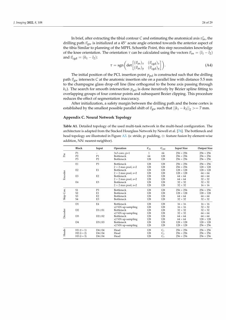
J. Imaging 2022, 8, 108 24 of 29

In brief, after extracting the tibial contour C and estimating the anatomical axis ~vax, thedrilling path ~vgw is initialized at a 45◦ acute angle oriented towards the anterior aspect ofthe tibia Similar to planning of the MPFL Schoettle Point, this step necessitates knowledgeof the knee orientation. The orientation τ can be calculated using the vectors ~vax = (l1 − l2)and ~vcgd = (k1 − l2):

τ = sgn(

det[(~vax)x (~vcgd)x(~vax)y (~vcgd)y

]). (A4)

The initial position of the PCL insertion point ppcl is constructed such that the drillingpath ~vgw intersects C at the anatomic insertion site on a parallel line with distance 5.5 mmto the champagne glass drop-off line (line orthogonal to the bone axis passing throughk1). The search for smooth intersection ppcl is done iteratively by Bézier spline fitting tooverlapping groups of four contour points and subsequent Bezier clipping. This procedurereduces the effect of segmentation inaccuracy.

After initialization, a safety margin between the drilling path and the bone cortex isestablished by the smallest possible parallel shift of ~vgw such that ||k1 − k2||2 >= 7 mm.

Appendix C. Neural Network Topology

Table A1. Detailed topology of the used multi-task network in the multi-head configuration. Thearchitecture is adapted from the Stacked Hourglass Network by Newell et al. [76]. The bottleneck andhead topology are illustrated in Figure A3. (s: stride, p: padding, ⊕: feature fusion by element-wiseaddition, NN: nearest-neighbor).

Block Input Operation Cin Cout Input Size Output Size

Pre P1 – 3x3 conv, p=1 1 64 256× 256 256× 256

P2 P1 Bottleneck 64 128 256× 256 256× 256P3 P2 Bottleneck 128 128 256× 256 256× 256

Enco

der

E1 P3 Bottleneck 128 128 256× 256 256× 2562× 2 max pool, s=2 128 128 256× 256 128× 128

E2 E1 Bottleneck 128 128 128× 128 128× 1282× 2 max pool, s=2 128 128 128× 128 64× 64

E3 E2 Bottleneck 128 128 64× 64 64× 642× 2 max pool, s=2 128 128 64× 64 32× 32

E4 E3 Bottleneck 128 128 32× 32 32× 322× 2 max pool, s=2 128 128 32× 32 16× 16

Skip

Con

.

S1 P3 Bottleneck 128 128 256× 256 256× 256S2 E1 Bottleneck 128 128 128× 128 128× 128S3 E2 Bottleneck 128 128 64× 64 64× 64S4 E3 Bottleneck 128 128 32× 32 32× 32

Dec

oder

D1 E4 Bottleneck 128 128 16× 16 16× 16x2 NN up-sampling 128 128 16× 16 32× 32

D2 D1⊕S1 Bottleneck 128 128 32× 32 32× 32x2 NN up-sampling 128 128 32× 32 64× 64

D3 D2⊕S2 Bottleneck 128 128 64× 64 64× 64x2 NN up-sampling 128 128 64× 64 128× 128

D4 D3⊕S3 Bottleneck 128 128 128× 128 128× 128x2 NN up-sampling 128 128 128× 128 256× 256

Hea

ds H1 (t = 1) D4⊕S4 Head 128 C1 256× 256 256× 256H2 (t = 2) D4⊕S4 Head 128 C2 256× 256 256× 256H3 (t = 3) D4⊕S4 Head 128 C3 256× 256 256× 256

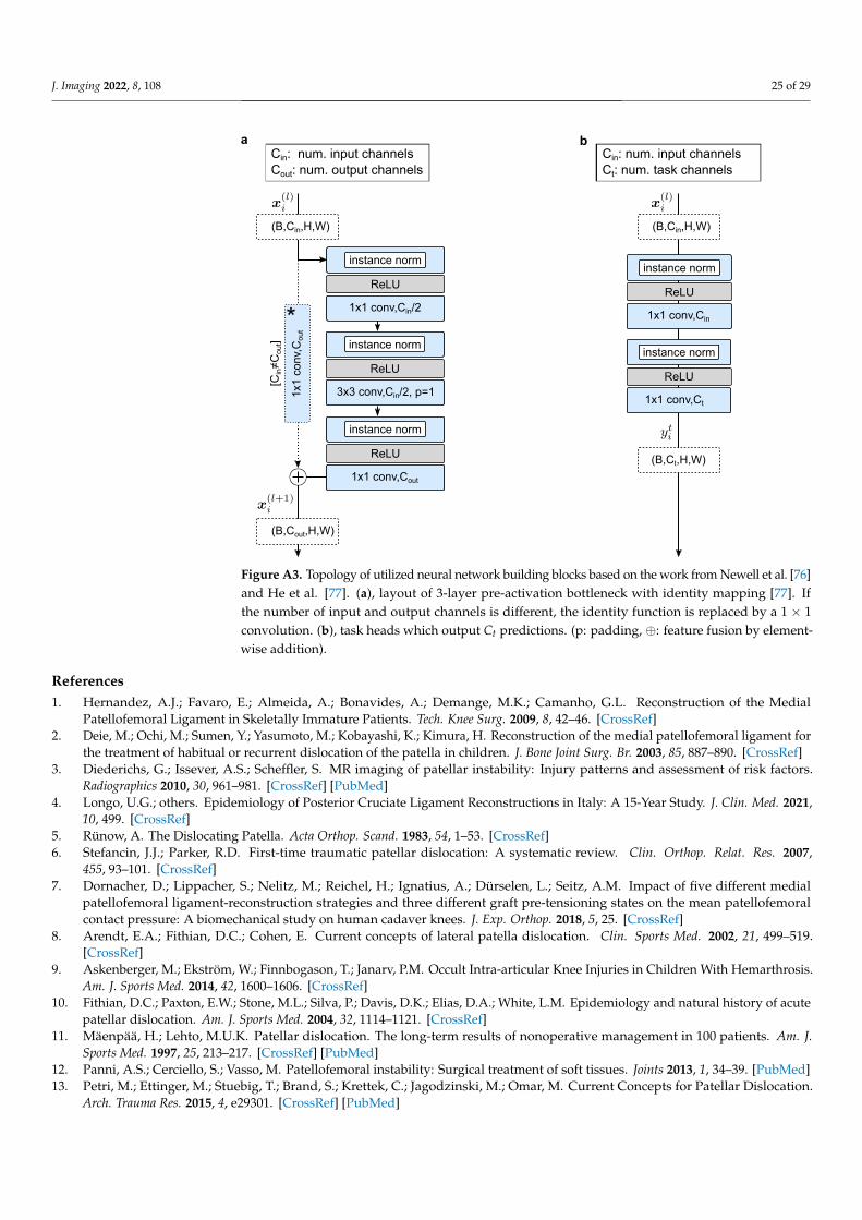
J. Imaging 2022, 8, 108 25 of 29

ReLU

1x1 conv,Cin/2

instance norm

ReLU

3x3 conv,Cin/2, p=1

instance norm

ReLU

1x1 conv,Cout

instance norm

(B,Cin,H,W)

(B,Cout,H,W)

(B,Cin,H,W)

(B,Ct,H,W)

ReLU

1x1 conv,Cin

instance norm

ReLU

1x1 conv,Ct

instance norm

Cin: num. input channels Cout: num. output channels

Cin: num. input channels Ct: num. task channels

a b

1x1

conv

,Cou

t *

[Cin≠C

out]

Figure A3. Topology of utilized neural network building blocks based on the work from Newell et al. [76]and He et al. [77]. (a), layout of 3-layer pre-activation bottleneck with identity mapping [77]. Ifthe number of input and output channels is different, the identity function is replaced by a 1 × 1convolution. (b), task heads which output Ct predictions. (p: padding, ⊕: feature fusion by element-wise addition).

References1. Hernandez, A.J.; Favaro, E.; Almeida, A.; Bonavides, A.; Demange, M.K.; Camanho, G.L. Reconstruction of the Medial

Patellofemoral Ligament in Skeletally Immature Patients. Tech. Knee Surg. 2009, 8, 42–46. [CrossRef]2. Deie, M.; Ochi, M.; Sumen, Y.; Yasumoto, M.; Kobayashi, K.; Kimura, H. Reconstruction of the medial patellofemoral ligament for

the treatment of habitual or recurrent dislocation of the patella in children. J. Bone Joint Surg. Br. 2003, 85, 887–890. [CrossRef]3. Diederichs, G.; Issever, A.S.; Scheffler, S. MR imaging of patellar instability: Injury patterns and assessment of risk factors.

Radiographics 2010, 30, 961–981. [CrossRef] [PubMed]4. Longo, U.G.; others. Epidemiology of Posterior Cruciate Ligament Reconstructions in Italy: A 15-Year Study. J. Clin. Med. 2021,

10, 499. [CrossRef]5. Rünow, A. The Dislocating Patella. Acta Orthop. Scand. 1983, 54, 1–53. [CrossRef]6. Stefancin, J.J.; Parker, R.D. First-time traumatic patellar dislocation: A systematic review. Clin. Orthop. Relat. Res. 2007,

455, 93–101. [CrossRef]7. Dornacher, D.; Lippacher, S.; Nelitz, M.; Reichel, H.; Ignatius, A.; Dürselen, L.; Seitz, A.M. Impact of five different medial

patellofemoral ligament-reconstruction strategies and three different graft pre-tensioning states on the mean patellofemoralcontact pressure: A biomechanical study on human cadaver knees. J. Exp. Orthop. 2018, 5, 25. [CrossRef]

8. Arendt, E.A.; Fithian, D.C.; Cohen, E. Current concepts of lateral patella dislocation. Clin. Sports Med. 2002, 21, 499–519.[CrossRef]

9. Askenberger, M.; Ekström, W.; Finnbogason, T.; Janarv, P.M. Occult Intra-articular Knee Injuries in Children With Hemarthrosis.Am. J. Sports Med. 2014, 42, 1600–1606. [CrossRef]

10. Fithian, D.C.; Paxton, E.W.; Stone, M.L.; Silva, P.; Davis, D.K.; Elias, D.A.; White, L.M. Epidemiology and natural history of acutepatellar dislocation. Am. J. Sports Med. 2004, 32, 1114–1121. [CrossRef]

11. Mäenpää, H.; Lehto, M.U.K. Patellar dislocation. The long-term results of nonoperative management in 100 patients. Am. J.Sports Med. 1997, 25, 213–217. [CrossRef] [PubMed]

12. Panni, A.S.; Cerciello, S.; Vasso, M. Patellofemoral instability: Surgical treatment of soft tissues. Joints 2013, 1, 34–39. [PubMed]13. Petri, M.; Ettinger, M.; Stuebig, T.; Brand, S.; Krettek, C.; Jagodzinski, M.; Omar, M. Current Concepts for Patellar Dislocation.

Arch. Trauma Res. 2015, 4, e29301. [CrossRef] [PubMed]

J. Imaging 2022, 8, 108 26 of 29

14. Amis, A.A.; Firer, P.; Mountney, J.; Senavongse, W.; Thomas, N.P. Anatomy and biomechanics of the medial patellofemoralligament. Knee 2003, 10, 215–220. [CrossRef]

15. Dragoo, J.L.; Nguyen, M.; Gatewood, C.T.; Taunton, J.D.; Young, S. Medial Patellofemoral Ligament Repair Versus Recon-struction for Recurrent Patellar Instability: Two-Year Results of an Algorithm-Based Approach. Orthop. J. Sports Med. 2017,5, 2325967116689465. [CrossRef] [PubMed]

16. Camp, C.L.; Krych, A.J.; Dahm, D.L.; Levy, B.A.; Stuart, M.J. Medial patellofemoral ligament repair for recurrent patellardislocation. Am. J. Sports Med. 2010, 38, 2248–2254. [CrossRef]

17. Buckens, C.F.M.; Saris, D.B.F. Reconstruction of the medial patellofemoral ligament for treatment of patellofemoral instability:A systematic review. Am. J. Sports Med. 2010, 38, 181–188. [CrossRef]

18. Nelitz, M.; Williams, S.R.M. Kombinierte Trochleaplastik und Rekonstruktion des medialen patellofemoralen Ligaments zurBehandlung der patellofemoralen Instabilität. Oper. Orthop. Traumatol. 2015, 27, 495–504. [CrossRef]

19. Shah, J.N.; Howard, J.S.; Flanigan, D.C.; Brophy, R.H.; Carey, J.L.; Lattermann, C. A systematic review of complications andfailures associated with medial patellofemoral ligament reconstruction for recurrent patellar dislocation. Am. J. Sports Med. 2012,40, 1916–1923. [CrossRef]

20. Vainionpää, S.; Laasonen, E.; Silvennoinen, T.; Vasenius, J.; Rokkanen, P. Acute dislocation of the patella. A prospective review ofoperative treatment. J. Bone Joint Surg. Br. 1990, 72, 366–369. [CrossRef]

21. Schöttle, P.B.; Schmeling, A.; Rosenstiel, N.; Weiler, A. Radiographic landmarks for femoral tunnel placement in medialpatellofemoral ligament reconstruction. Am. J. Sports Med. 2007, 35, 801–804. [CrossRef]

22. Chahla, J.; Nitri, M.; Civitarese, D.; Dean, C.S.; Moulton, S.G.; LaPrade, R.F. Anatomic Double-Bundle Posterior Cruciate LigamentReconstruction. Arthrosc. Tech. 2016, 5, e149–e156. [CrossRef] [PubMed]

23. Johannsen, A.M.; Anderson, C.J.; Wijdicks, C.A.; Engebretsen, L.; LaPrade, R.F. Radiographic landmarks for tunnel positioning inposterior cruciate ligament reconstructions. Am. J. Sports Med. 2013, 41, 35–42. [CrossRef] [PubMed]

24. LaPrade, R.F.; others. Double-Bundle Posterior Cruciate Ligament Reconstruction in 100 Patients at a Mean 3 Years’ Follow-up:Outcomes Were Comparable to Anterior Cruciate Ligament Reconstructions. Am. J. Sports Med. 2018, 46, 1809–1818. [CrossRef][PubMed]

25. Spiridonov, S.I.; Slinkard, N.J.; LaPrade, R.F. Isolated and combined grade-III posterior cruciate ligament tears treated withdouble-bundle reconstruction with use of endoscopically placed femoral tunnels and grafts: Operative technique and clinicaloutcomes. J. Bone Joint Surg. Am. 2011, 93, 1773–1780. [CrossRef] [PubMed]

26. Weimann, A.; Wolfert, A.; Zantop, T.; Eggers, A.K.; Raschke, M.; Petersen, W. Reducing the “killer turn” in posterior cruciateligament reconstruction by fixation level and smoothing the tibial aperture. Arthroscopy 2007, 23, 1104–1111. [CrossRef]

27. Jackson, D.W.; Proctor, C.S.; Simon, T.M. Arthroscopic assisted PCL reconstruction: A technical note on potential neurovascularinjury related to drill bit configuration. Arthroscopy 1993, 9, 224–227. [CrossRef]

28. Montgomery, S.R.; Johnson, J.S.; McAllister, D.R.; Petrigliano, F.A. Surgical management of PCL injuries: Indications, techniques,and outcomes. Curr. Rev. Musculoskelet. Med. 2013, 6, 115–123. [CrossRef]

29. Nicodeme, J.D.; Löcherbach, C.; Jolles, B.M. Tibial tunnel placement in posterior cruciate ligament reconstruction: A systematicreview. Knee Surg. Sports Traumatol. Arthrosc. 2014, 22, 1556–1562. [CrossRef]

30. Yao, J.; others. Effect of tibial drill-guide angle on the mechanical environment at bone tunnel aperture after anatomic single-bundle anterior cruciate ligament reconstruction. Int. Orthop. 2014, 38, 973–981. [CrossRef]

31. Bertollo, N.; Walsh, W.R. Drilling of Bone: Practicality, Limitations and Complications Associated with Surgical Drill-Bits. InBiomechanics in Applications; Klika, V., Ed.; IntechOpen: Rijeka, Croatia, 2011; Chapter 3. [CrossRef]

32. Bernard, M.; Hertel, P.; Hornung, H.; Cierpinski, T. Femoral insertion of the ACL. Radiographic quadrant method. J. Knee Surg.1997, 10, 14–21; discussion 21–22.

33. Amis, A.A.; Jakob, R.P. Anterior cruciate ligament graft positioning, tensioning and twisting. Knee Surg. Sports Traumatol. Arthrosc.1998, 6 (Suppl. 1), S2–S12. [CrossRef]

34. Stäubli, H.U.; Rauschning, W. Tibial attachment area of the anterior cruciate ligament in the extended knee position. Anatomyand cryosections in vitro complemented by magnetic resonance arthrography in vivo. Knee Surg. Sports Traumatol. Arthrosc. 1994,2, 138–146. [CrossRef] [PubMed]

35. Linte, C.A.; Moore, J.T.; Chen, E.C.; Peters, T.M. Image-Guided Procedures. In Bioengineering for Surgery; Elsevier: Amsterdam,The Netherlands, 2016; pp. 59–90. [CrossRef]

36. Kubicek, J.; Tomanec, F.; Cerny, M.; Vilimek, D.; Kalova, M.; Oczka, D. Recent Trends, Technical Concepts and Components ofComputer-Assisted Orthopedic Surgery Systems: A Comprehensive Review. Sensors 2019, 19, 5199. [CrossRef] [PubMed]

37. Joskowicz, L.; Hazan, E.J. Computer Aided Orthopaedic Surgery: Incremental shift or paradigm change? Med. Image Anal. 2016,33, 84–90. [CrossRef] [PubMed]

38. Bai, L.; Yang, J.; Chen, X.; Sun, Y.; Li, X. Medical Robotics in Bone Fracture Reduction Surgery: A Review. Sensors 2019, 19, 3593.[CrossRef] [PubMed]

39. Innocenti, B.; Bori, E. Robotics in orthopaedic surgery: Why, what and how? Arch. Orthop. Trauma Surg. 2021, 141, 2035–2042.[CrossRef]

40. Jinnah, A.H.; Luo, T.D.; Plate, J.F.; Jinnah, R.H. General Concepts in Robotics in Orthopedics. In Robotics in Knee and HipArthroplasty; Lonner, J.H., Ed.; Springer International Publishing: Cham, Switzerland, 2019; pp. 27–35. [CrossRef]

J. Imaging 2022, 8, 108 27 of 29

41. Karthik, K.; Colegate-Stone, T.; Dasgupta, P.; Tavakkolizadeh, A.; Sinha, J. Robotic surgery in trauma and orthopaedics. Bone JointJ. 2015, 97, 292–299. [CrossRef]

42. Stübig, T.; Windhagen, H.; Krettek, C.; Ettinger, M. Computer-Assisted Orthopedic and Trauma Surgery. Dtsch. Arztebl. Int. 2020,117, 793–800. [CrossRef]

43. Zhao, J.X.; Li, C.; Ren, H.; Hao, M.; Zhang, L.C.; Tang, P.F. Evolution and Current Applications of Robot-Assisted FractureReduction: A Comprehensive Review. Ann. Biomed. Eng. 2020, 48, 203–224. [CrossRef]

44. Ewurum, Chidozie H. and Guo, Yingying and Pagnha, Seang and Feng, Zhao and Luo, Xiongbiao. Surgical Navigation inOrthopedics: Workflow and System Review. In Intelligent Orthopaedics: Artificial Intelligence and Smart Image-Guided Technology forOrthopaedics; Zheng, G., Tian, W., Zhuang, X., Eds.; Springer Singapore: Singapore, 2018; pp. 47–63. [CrossRef]

45. Székely, G.; Nolte, L.P. Image guidance in orthopaedics and traumatology: A historical perspective. Med. Image Anal. 2016,33, 79–83. [CrossRef]

46. Zheng, G.; Nolte, L.P., Computer-Aided Orthopaedic Surgery: State-of-the-Art and Future Perspectives. In Intelligent Orthopaedics:Artificial Intelligence and Smart Image-guided Technology for Orthopaedics; Springer Singapore: Singapore, 2018; pp. 1–20. [CrossRef]

47. Wang, M.; Li, D.; Shang, X.; Wang, J. A review of computer-assisted orthopaedic surgery systems. Int. J. Med. Robot. 2020,16, 1–28. [CrossRef] [PubMed]

48. Casari, F.A.; Navab, N.; Hruby, L.A.; Kriechling, P.; Nakamura, R.; Tori, R.; de Lourdes Dos Santos Nunes, F.; Queiroz, M.C.;Fürnstahl, P.; Farshad, M. Augmented Reality in Orthopedic Surgery Is Emerging from Proof of Concept Towards Clinical Studies:A Literature Review Explaining the Technology and Current State of the Art. Curr. Rev. Musculoskelet. Med. 2021, 14, 192–203.[CrossRef] [PubMed]

49. Essert, C.; Joskowicz, L. Chapter 32 - Image-based surgery planning. In Handbook of Medical Image Computing and ComputerAssisted Intervention; Zhou, S.K., Rueckert, D., Fichtinger, G., Eds.; Academic Press, 2020; pp. 795–815. [CrossRef]

50. Kordon, F.; Maier, A.; Swartman, B.; Privalov, M.; El Barbari, J.S.; Kunze, H. Contour-Based Bone Axis Detection for X-ray GuidedSurgery on the Knee. In Medical Image Computing and Computer-Assisted Intervention (MICCAI); Martel, A.L.; Abolmaesumi, P.;Stoyanov, D.; Mateus D.; Zuluaga, M.A.; Zhou, S.K.; Racoceanu, D.; Joskowicz, L. Eds.; Springer: Cham, Switzerland, 2020;Volume 12266, pp. 671–680. [CrossRef]

51. Bier, B.; Unberath, M.; Zaech, J.N.; Fotouhi, J.; Armand, M.; Osgood, G.; Navab, N.; Maier, A. X-ray-transform InvariantAnatomical Landmark Detection for Pelvic Trauma Surgery. In Medical Image Computing and Computer-Assisted Intervention(MICCAI); Frangi, A.F., Schnabel, J.A., Davatzikos, C., Alberola-López, C., Fichtinger, G., Eds.; Springer International Publishing:Cham, Switzerland, 2018; Volume 11073, pp. 55–63. [CrossRef]

52. Lee, S.M.; Kim, H.P.; Jeon, K.; Lee, S.H.; Seo, J.K. Automatic 3D cephalometric annotation system using shadowed 2D image-basedmachine learning. Phys. Med. Biol. 2019, 64, 055002. [CrossRef] [PubMed]

53. Hsu, W.E.; Yu, C.H.; Chang, C.J.; Wu, H.K.; Yu, T.H.; Tseng, C.S. C-Arm Image-Based Surgical Path Planning Method for DistalLocking of Intramedullary Nails. Appl. Bionics Biomech. 2018, 2018, 4530386. [CrossRef] [PubMed]

54. Kordon, F.; others. Multi-task Localization and Segmentation for X-Ray Guided Planning in Knee Surgery. In Medical ImageComputing and Computer-Assisted Intervention (MICCAI); Shen, D.; Liu, T., Peters, T.M., Staib, L.H., Essert, C., Zhou, S., Yap, P.-T.,Khan, A., Eds.; Springer: Cham, Switzerland, 2019; Volume 11769, pp. 622–630. [CrossRef]

55. Kordon, F.; Maier, A.; Swartman, B.; Privalov, M.; El Barbari, J.S.; Kunze, H. Automatic Path Planning for Safe Guide PinInsertion in PCL Reconstruction Surgery. In Medical Image Computing and Computer-Assisted Intervention (MICCAI); de Bruijne, M.,Cattin, P.C., Cotin, S., Padoy, N., Speidel, S., Zheng, Y., Essert, C., Eds.; Springer International Publishing: Cham, Switzerland,2021; Volume 12904, pp. 560–570. [CrossRef]

56. Swartman, B.; Frere, D.; Wei, W.; Schnetzke, M.; Beisemann, N.; Keil, H.; Franke, J.; Grützner, P.; Vetter, S. 2D projection-basedsoftware application for mobile C-arms optimises wire placement in the proximal femur—An experimental study. Injury 2017,48, 2068–2073. [CrossRef]

57. Lisa Kausch.; Moritz Scherer.; Sarina Thomas.; André Klein.; Fabian Isensee.; Klaus Maier-Hein. Automatic image-based pediclescrew planning. In Medical Imaging 2021: Image-Guided Procedures, Robotic Interventions, and Modeling; Linte, C.A., Siewerdsen, J.H.,Eds.; SPIE: Bellingham, WA, USA, 2021, Volume 11598, pp. 406–414. [CrossRef]

58. Joskowicz, L., Future Perspectives on Statistical Shape Models in Computer-Aided Orthopedic Surgery: Beyond Statistical ShapeModels and on to Big Data. In Computer Assisted Orthopaedic Surgery for Hip and Knee: Current State of the Art in Clinical Applicationand Basic Research; Springer Singapore: Singapore, 2018; pp. 199–206. [CrossRef]

59. Kamiya, N., Deep Learning Technique for Musculoskeletal Analysis. In Deep Learning in Medical Image Analysis: Challenges andApplications; Springer International Publishing: Cham, Switzerland, 2020; pp. 165–176. [CrossRef]

60. Benos, L.; Stanev, D.; Spyrou, L.; Moustakas, K.; Tsaopoulos, D.E. A Review on Finite Element Modeling and Simulation of theAnterior Cruciate Ligament Reconstruction. Front. Bioeng. Biotechnol. 2020, 8, 967. [CrossRef]

61. Colombet, P.; Robinson, J.; Christel, P.; Franceschi, J.P.; Djian, P.; Bellier, G.; Sbihi, A. Morphology of anterior cruciate ligamentattachments for anatomic reconstruction: A cadaveric dissection and radiographic study. Arthroscopy 2006, 22, 984–992. [CrossRef]

62. Caruana, R., Multitask Learning. In Learning to Learn; Springer US: Boston, MA, USA, 1998; pp. 95–133. [CrossRef]63. Ruder, S. An Overview of Multi-Task Learning in Deep Neural Networks. arXiv 2017, arXiv:1706.05098.64. Thung, K.H.; Wee, C.Y. A brief review on multi-task learning. Multimed. Tools Appl. 2018, 77, 29705–29725. [CrossRef]65. Zhang, Y.; Yang, Q. An overview of multi-task learning. Natl. Sci. Rev. 2018, 5, 30–43. [CrossRef]

J. Imaging 2022, 8, 108 28 of 29

66. Baxter, J. A Model of Inductive Bias Learning. J. Artif. Int. Res. 2000, 12, 149–198. [CrossRef]67. Lin, B.; Ye, F.; Zhang, Y. A Closer Look at Loss Weighting in Multi-Task Learning. arXiv 2021, arXiv:2111.10603.68. Chen, Z.; Badrinarayanan, V.; Lee, C.Y.; Rabinovich, A. GradNorm: Gradient Normalization for Adaptive Loss Balancing in Deep

Multitask Networks. In Proceedings of the 35th International Conference on Machine Learning, Stockholm, Sweden, 10–15 July2018; Dy, J., Krause, A., Eds.; PMLR: Stockholm, Sweden, 10–15 July 2018; Volume 80, pp. 794–803.

69. Liu, S.; Johns, E.; Davison, A.J. End-To-End Multi-Task Learning With Attention. In Proceedings of the 2019 IEEE Conference onComputer Vision and Pattern Recognition (CVPR), Long Beach, CA, USA, 15–20 June 2019; pp. 1871–1880. [CrossRef]

70. Kendall, A.; Gal, Y.; Cipolla, R. Multi-Task Learning Using Uncertainty to Weigh Losses for Scene Geometry and Semantics. InProceedings of the 2018 IEEE Conference on Computer Vision and Pattern Recognition (CVPR), Salt Lake City, UT, USA, 18–23June 2018.

71. Sener, O.; Koltun, V. Multi-Task Learning as Multi-Objective Optimization. In Advances in Neural Information Processing Systems;Bengio, S., Wallach, H., Larochelle, H., Grauman, K., Cesa-Bianchi, N., Garnett, R., Eds.; Curran Associates, Inc.: Red Hook, NY,USA, 2018; Volume 31.

72. Yu, T.; Kumar, S.; Gupta, A.; Levine, S.; Hausman, K.; Finn, C. Gradient Surgery for Multi-Task Learning. In Advances in NeuralInformation Processing Systems; Larochelle, H., Ranzato, M., Hadsell, R., Balcan, M.F., Lin, H., Eds.; Curran Associates, Inc.: RedHook, NY, USA 2020; Volume 33, pp. 5824–5836.

73. Wang, Z.; Tsvetkov, Y.; Firat, O.; Cao, Y. Gradient Vaccine: Investigating and Improving Multi-task Optimization in MassivelyMultilingual Models. arXiv 2021, arXiv:2010.05874.

74. Chen, Z.; Ngiam, J.; Huang, Y.; Luong, T.; Kretzschmar, H.; Chai, Y.; Anguelov, D. Just Pick a Sign: Optimizing Deep MultitaskModels with Gradient Sign Dropout. In Advances in Neural Information Processing Systems; Larochelle, H., Ranzato, M., Hadsell, R.,Balcan, M.F., Lin, H., Eds.; Curran Associates, Inc.: Red Hook, NY, USA 2020; Volume 33, pp. 2039–2050.

75. Liu, L.; Li, Y.; Kuang, Z.; Xue, J.H.; Chen, Y.; Yang, W.; Liao, Q.; Zhang, W. Towards Impartial Multi-task Learning. In Proceedingsof the International Conference on Learning Representations, Virtual Event, 3–7 May 2021.

76. Newell, A.; Yang, K.; Deng, J. Stacked Hourglass Networks for Human Pose Estimation. In Computer Vision—ECCV 2016;Leibe, B., Matas, J., Sebe, N., Welling, M., Eds.; Springer: Cham, Switzerland, 2016; pp. 483–499.

77. He, K.; Zhang, X.; Ren, S.; Sun, J. Identity Mappings in Deep Residual Networks. In Computer Vision—ECCV 2016; Leibe, B.,Matas, J., Sebe, N., Welling, M., Eds.; Springer International Publishing: Cham, Switzerland, 2016; pp. 630–645.

78. He, K.; Zhang, X.; Ren, S.; Sun, J. Deep Residual Learning for Image Recognition. In Proceedings of the 2016 IEEE Conference onComputer Vision and Pattern Recognition (CVPR), Las Vegas, NV, USA, 27–30 June 2016, pp. 770–778. [CrossRef]

79. Greff, K.; Srivastava, R.K.; Schmidhuber, J. Highway and Residual Networks learn Unrolled Iterative Estimation. In Proceedingsof the 5th International Conference on Learning Representations, ICLR, Toulon, France, 24–26 April 2017.

80. Ronneberger, O.; P.Fischer.; Brox, T. U-Net: Convolutional Networks for Biomedical Image Segmentation. In Medical ImageComputing and Computer-Assisted Intervention (MICCAI); Springer: Berlin/Heidelberg, Germany, 2015; Volume 9351, pp. 234–241.

81. Wada, K. Labelme: Image Polygonal Annotation with Python; 2016. Available online: https://github.com/wkentaro/labelme(accessed on 28 February 2022).

82. Kordon, F.; Lasowski, R.; Swartman, B.; Franke, J.; Fischer, P.; Kunze, H. Improved X-Ray Bone Segmentation by Normalizationand Augmentation Strategies. In Bildverarbeitung für Die Medizin 2019; Handels, H., Deserno, T.M., Maier, A., Maier-Hein, K.H.,Palm, C., Tolxdorff, T., Eds.; Informatik Aktuell, Springer Fachmedien Wiesbaden: Wiesbaden, Germany, 2019; pp. 104–109.[CrossRef]

83. Sutskever, I.; Martens, J.; Dahl, G.; Hinton, G. On the Importance of Initialization and Momentum in Deep Learning. InProceedings of the 30th International Conference on International Conference on Machine Learning, Atlanta, GA, USA, 17–19June 2013.

84. Smith, L.N. Cyclical learning rates for training neural networks. In Proceedings of the 2017 IEEE Winter Conference onApplications of Computer Vision (WACV), Santa Rosa, CA, USA, 24–31 March 2017; pp. 464–472.

85. Akkus, Z.; Galimzianova, A.; Hoogi, A.; Rubin, D.L.; Erickson, B.J. Deep Learning for Brain MRI Segmentation: State of the Artand Future Directions. J. Digit. Imaging 2017, 30, 449–459. [CrossRef]

86. Hu, M.K. Visual pattern recognition by moment invariants. IEEE Trans. Inf. Theory 1962, 8, 179–187. [CrossRef]87. Ziegler, C.G.; Fulkerson, J.P.; Edgar, C. Radiographic Reference Points Are Inaccurate with and without a True Lateral Radiograph:

The Importance of Anatomy in Medial Patellofemoral Ligament Reconstruction. Am. J. Sports Med. 2016, 44, 133–142. [CrossRef]88. Sanchis-Alfonso, V.; Ramírez-Fuentes, C.; Montesinos-Berry, E.; Elía, I.; Martí-Bonmatí, L. Radiographic Location Does Not

Ensure a Precise Anatomic Location of the Femoral Fixation Site in Medial Patellofemoral Ligament Reconstruction. Orthop. J.Sports Med. 2017, 5, 2325967117739252. [CrossRef]

89. Kausch, L.; Thomas, S.; Kunze, H.; Privalov, M.; Vetter, S.; Franke, J.; Mahnken, A.H.; Maier-Hein, L.; Maier-Hein, K. Towardautomatic C-arm positioning for standard projections in orthopedic surgery. Int. J. Comput. Assist. Radiol. Surg. 2020,15, 1095–1105. [CrossRef]

90. Kausch, L.; Thomas, S.; Kunze, H.; Norajitra, T.; Klein, A.; El Barbari, J.S.; Privalov, M.; Vetter, S.; Mahnken, A.; Maier-Hein, L.;Maier-Hein, K.H. C-Arm Positioning for Spinal Standard Projections in Different Intra-operative Settings. In Medical ImageComputing and Computer-Assisted Intervention (MICCAI); de Bruijne, M., Cattin, P.C., Cotin, S., Padoy, N., Speidel, S., Zheng, Y.,Essert, C., Eds.; Springer International Publishing: Cham, Switzerland, 2021; pp. 352–362.

J. Imaging 2022, 8, 108 29 of 29

91. Cho, W.J.; Kim, J.M.; Kim, D.E.; Lee, J.G.; Park, J.W.; Han, Y.H.; Seo, H.G. Accuracy of the femoral tunnel position in robot-assistedanterior cruciate ligament reconstruction using a magnetic resonance imaging-based navigation system: A preliminary report.Int. J. Med. Robot. Comput. Assist. Surg. 2018, 14, e1933. [CrossRef]

92. Morita, K.; Kobashi, S.; Kashiwa, K.; Nakayama, H.; Kambara, S.; Morimoto, M.; Yoshiya, S.; Aikawa, S. Computer-aided SurgicalPlanning of Anterior Cruciate Ligament Reconstruction in MR Images. Procedia Comput. Sci. 2015, 60, 1659–1667. [CrossRef]

93. Morita, K. Computer-aided Diagnosis Systems Based on Medical Image Registration. Ph.D. Thesis, University of Hyogo, Kobe,Japan, 2019.

94. Raposo, C.; Barreto, J.P.; Sousa, C.; Ribeiro, L.; Melo, R.; Oliveira, J.P.; Marques, P.; Fonseca, F.; Barrett, D. Video-based computernavigation in knee arthroscopy for patient-specific ACL reconstruction. Int. J. Comput. Assist. Radiol. Surg. 2019, 14, 1529–1539.[CrossRef] [PubMed]

95. Choi, J.H.; Lim, S.; Kim, Y.; Lee, D.; Park, S.; Park, S.; Wang, J.H. 3D preoperative surgical planning software for anterior cruciateligament reconstruction. In Proceedings of the International Conference on Control, Automation and Systems (ICCAS), Gwangju,Korea, 20–23 October 2013; pp. 344–346. [CrossRef]

96. Le Huynh, M.; Kim, Y.H. A computer-aided and robot-assisted surgical system for reconstruction of anterior cruciate ligament.Int. J. Precis. Eng. Manuf. 2013, 14, 49–54. [CrossRef]

97. Kitamura, G.; Albers, M.B.V.; Lesniak, B.P.; Rabuck, S.J.; Musahl, V.; Andrews, C.L.; Ghodadra, A.; Fu, F. 3-Dimensional PrintedModels May Be a Useful Tool When Planning Revision Anterior Cruciate Ligament Reconstruction. Arthrosc. Sports Med. Rehab.2019, 1, e41–e46. [CrossRef]