MS_thesis presentation

MS Thesis Defense

Improved Adaptive Mobility of Courier nodes in

Underwater Wireless Sensor Networks

Supervisor: Dr. Nadeem Javaid Presented by: Muhammad Mohsin Raza Jafri

FA12 – REE – 024Department of Electrical Engineering

COMSATS Institute of Information Technology Islamabad, Pakistan

Nov 21, 2014

1

Outline• Introduction• Related Work and Motivation• Proposed Routing Schemes1. Adaptive Mobility of Courier nodes

in Threshold-optimized Dbr (AMCTD)2. improved Adaptive Mobility of

Courier nodes in Threshold-optimized Dbr (iAMCTD)

• Conclusion2

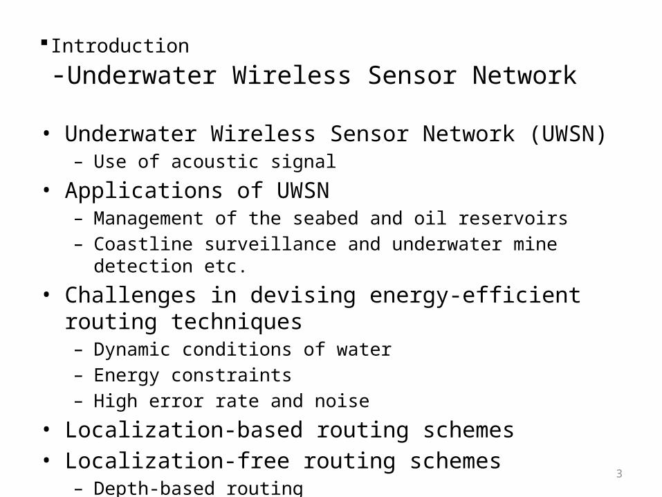
Introduction-Underwater Wireless Sensor Network

• Underwater Wireless Sensor Network (UWSN)– Use of acoustic signal

• Applications of UWSN– Management of the seabed and oil reservoirs– Coastline surveillance and underwater mine detection etc.

• Challenges in devising energy-efficient routing techniques– Dynamic conditions of water– Energy constraints– High error rate and noise

• Localization-based routing schemes• Localization-free routing schemes

– Depth-based routing3

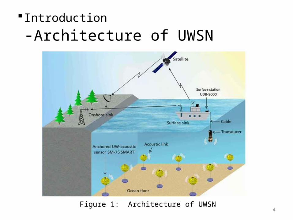
Introduction-Architecture of UWSN

4Figure 1: Architecture of UWSN

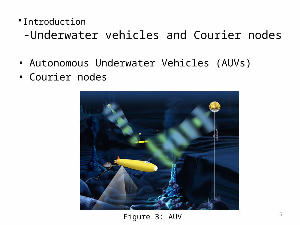
Introduction-Underwater vehicles and Courier nodes

• Autonomous Underwater Vehicles (AUVs)• Courier nodes

5Figure 3: AUV

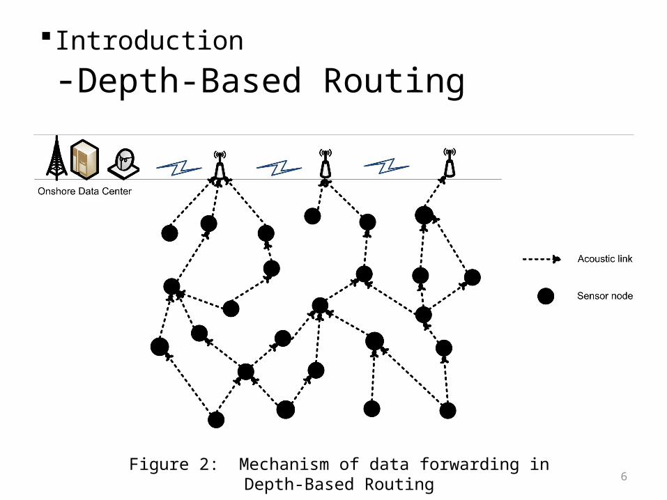
Introduction-Depth-Based Routing

6Figure 2: Mechanism of data forwarding in

Depth-Based Routing

Related work and Motivation-Related work

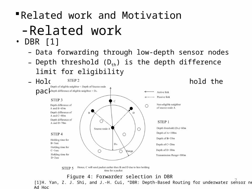
• DBR [1] – Data forwarding through low-depth sensor nodes– Depth threshold (Dth) is the depth difference limit for eligibility

– Holding time (HT) is the duration to hold the packet

7[1]H. Yan, Z. J. Shi, and J.-H. Cui, “DBR: Depth-Based Routing for underwater sensor networks,” in Ad Hoc and Sensor Networks, Wireless Networks, Next Generation Internet 2008, pp. 72–86, Springer, 2008.

Figure 4: Forwarder selection in DBR

Related work and Motivation-Related work• EEDBR [2]

– Use of residual energy information for data forwarder selection

• H2-DAB [3] – Implementation of dynamic addressing scheme among nodes

– Use of courier nodes

8

[2]A. Wahid, S. Lee, H.J. Jeong, and D. Kim, “EEDBR: Energy-Efficient Depth-Based Routing protocol for underwater wireless sensor networks,” in Advanced Computer Science and Information Technology, pp. 223–234, Springer, 2011.[3]M. Ayaz, A. Abdullah, I. Faye, and Y. Batira, “An efficient dynamic addressing based routing protocol for underwater wireless sensor networks,” Computer Communications, vol. 35, no. 4, pp. 475–486, 2012.

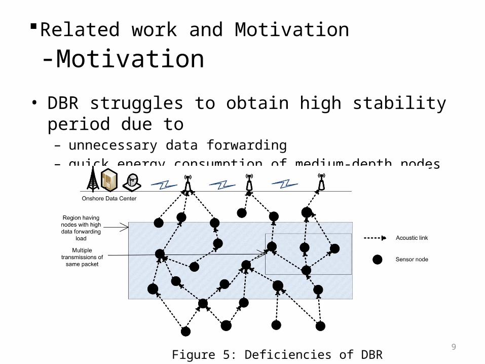
Related work and Motivation-Motivation• DBR struggles to obtain high stability period due to – unnecessary data forwarding– quick energy consumption of medium-depth nodes

9Figure 5: Deficiencies of DBR

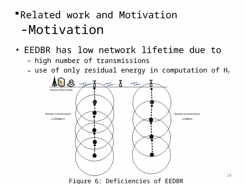
Related work and Motivation-Motivation• EEDBR has low network lifetime due to

– high number of transmissions– use of only residual energy in computation of HT

10Figure 6: Deficiencies of EEDBR

Proposed routing protocol: Adaptive Mobility of Courier nodes in Threshold-based Dbr -AMCTD

• Acoustic attenuation models• Network initialization• Data forwarding and variation in Dth

• Movement scheme of courier nodes• Performance evaluation

11

Proposed routing protocol: AMCTD-Acoustic attenuation models

• Attenuation A (l, f) can be computed by Thorp’s model [4] as follows:

10log(A(l, f))= k x 10log(l)+l x 10log( (f))where the first term denotes spreading loss and the second term is the absorption loss. k defines the geometry of the signal propagation.

• Calculation of ambient noise [5]N(f) = Nt (f) + Ns (f) + Nw (f) + Nth (f)

where Nt , Ns , Nw and Nth represent the noise due to turbulence, shipping, wind and thermal activities.

12

[4] M. Stojanovic , On the relationship between capacity and distance in an underwater acoustic communication channel, ACM Mobile Computing and Communications Review, 11, (4), (2007), 34–43.[5] A. F. Harris III, M. Zorzi , Modeling the underwater acoustic channel in ns2, in: Proceedings of the 2nd international conference on Performance evaluation methodologies and tools, ICST, 2007, p. 18.

Proposed routing protocol: AMCTD-Acoustic attenuation models

• Computation of Transmission Loss (TL) by MMPE [6] model

TL = m (f , s , d A , dB ) + w(t) + e(n)where:m( f , s , d A , dB): Propagation loss due to haphazard and

periodic constituentsf : Frequency of acoustic signal in kHzd A : Depth of sender node A in md B: Depth of receiver node B in ms: Euclidean distance between node A and node B in mw(t): Function to estimate loss due to wave movemente(n): Signal loss function caused by random noise error

13[6]K. B. Smith, “Convergence, stability, and variability of shallow water acoustic predictions using a split-step fourier parabolic equation model,” Journal of Computational Acoustics, vol. 9, no. 01, pp. 243–285, 2001.

Proposed routing protocol: AMCTD-Network initialization

• Gathering of nodes information by sink• Starting of sojourn movements of courier nodes• Calculation of HT

H T = (1 - WF) Htmax

where Htmax is the maximum holding time.• Calculation of Weight Function (WF)

Wi = Ti * Ri / Di * Ei

where Ri is the residual energy of node i, Di is the depth of node i, Ti is the Transmission range of node i and Ei is the initial energy of node i .– Higher the WF value of the node, lesser will be the

HT. 14

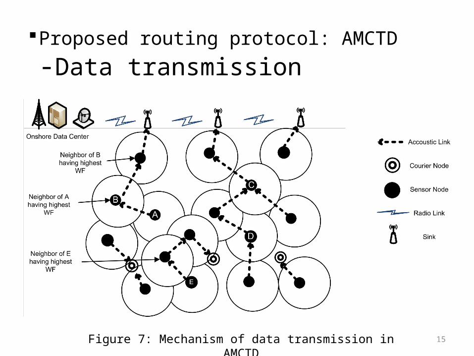
Proposed routing protocol: AMCTD-Data transmission

15Figure 7: Mechanism of data transmission in AMCTD

Proposed routing protocol: AMCTD-Data forwarding and Variation in Dth

• Variations in Dth

– load balancing by increasing number of eligible neighbors

– Assumptions are (1) Dth1=200m (2) Dth2=150m (3) Dth3=50m

• Revisions in WF calculation technique with change in node density– After the stability period, each node

calculates its WF as followsWi = Di * Ei / Ti * Ri

16

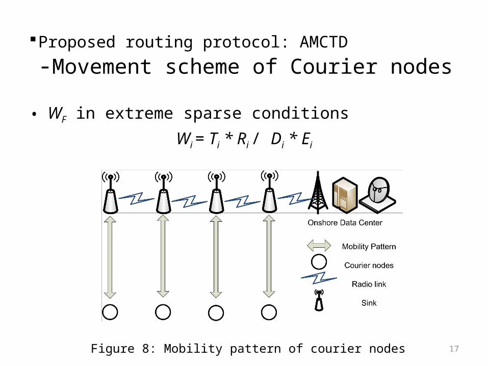
Proposed routing protocol: AMCTD-Movement scheme of Courier nodes• WF in extreme sparse conditions

Wi = Ti * Ri / Di * Ei

17Figure 8: Mobility pattern of courier nodes

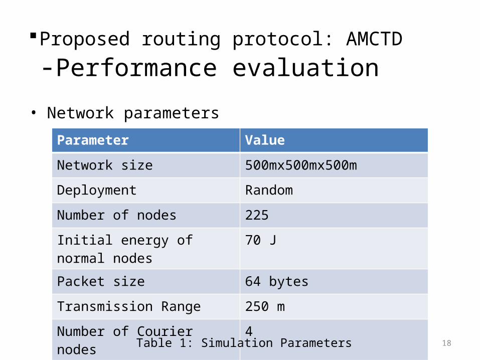
Proposed routing protocol: AMCTD-Performance evaluation

• Network parameters

18

Parameter ValueNetwork size 500mx500mx500mDeployment RandomNumber of nodes 225Initial energy of normal nodes

70 J

Packet size 64 bytesTransmission Range 250 mNumber of Courier nodes

4Table 1: Simulation Parameters

Proposed routing protocol: AMCTD-Network lifetime

19Figure 9: Comparison of Network lifetime in AMCTD, EEDBR and DBR

• Decrease in stability period of DBR and EEDBR due to increased data forwarding load on the medium-depth nodes as the number of nodes deployed in the low-depth region increases.

• Improved stability period of AMCTD as it requires less number of transmissions to deliver data packets to sink.

Proposed routing protocol: AMCTD-End-to-end delay of network

20Figure 10: Comparison of Delay in AMCTD, EEDBR and DBR

• AMCTD minimizes the delay by using mobility of courier nodes and weight functions.

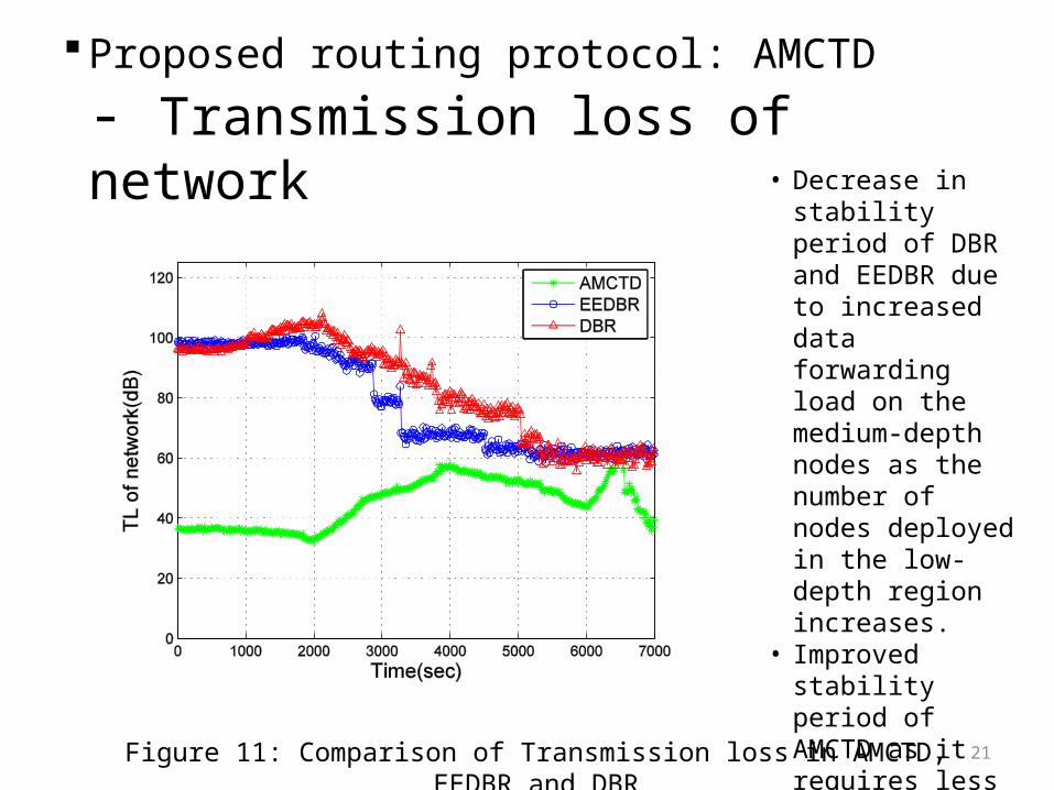
Proposed routing protocol: AMCTD- Transmission loss of network

21Figure 11: Comparison of Transmission loss in AMCTD, EEDBR and DBR

• Decrease in stability period of DBR and EEDBR due to increased data forwarding load on the medium-depth nodes as the number of nodes deployed in the low-depth region increases.

• Improved stability period of AMCTD as it requires less number of transmissions to deliver data packets to sink.

improved Adaptive Mobility of Courier nodes in Threshold-based Dbr -iAMCTD

• Motivations– Lack of on-demand data routing in AMCTD– Consideration of only two parameters in computation of HT

– Room for improvement in delay and TL

22

improved Adaptive Mobility of Courier nodes in Threshold-based Dbr -iAMCTD

• Proposed iAMCTD– Implementation of on-demand data routing

– Data forwarding phase– Improved mobility patterns of courier nodes

23

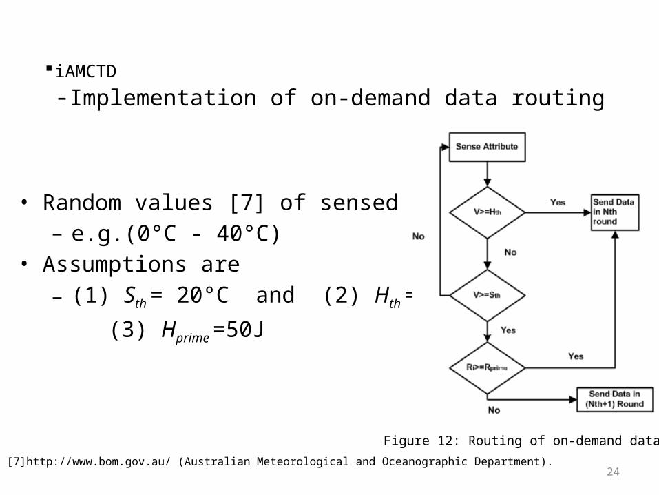
iAMCTD-Implementation of on-demand data routing

• Random values [7] of sensed attributes – e.g.(0°C - 40°C)

• Assumptions are– (1) Sth = 20°C and (2) Hth = 30° C

(3) Hprime =50J

24

Figure 12: Routing of on-demand data[7]http://www.bom.gov.au/ (Australian Meteorological and Oceanographic Department).

iAMCTD -Data forwarding phase

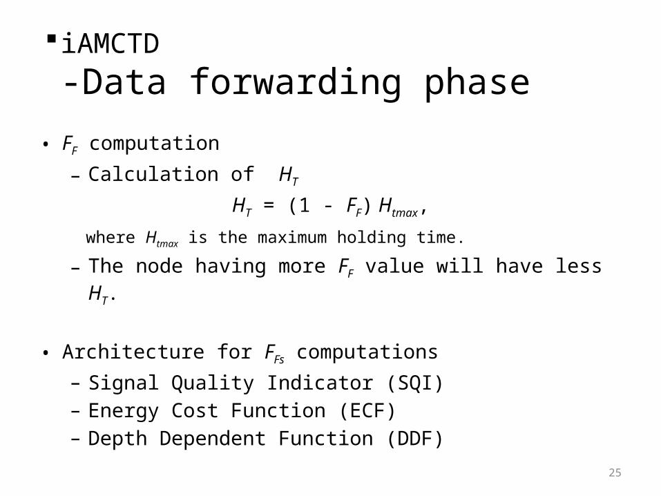
• FF computation– Calculation of HT

HT = (1 - FF) Htmax, where Htmax is the maximum holding time.– The node having more FF value will have less

HT.

• Architecture for FFs computations– Signal Quality Indicator (SQI)– Energy Cost Function (ECF)– Depth Dependent Function (DDF)

25


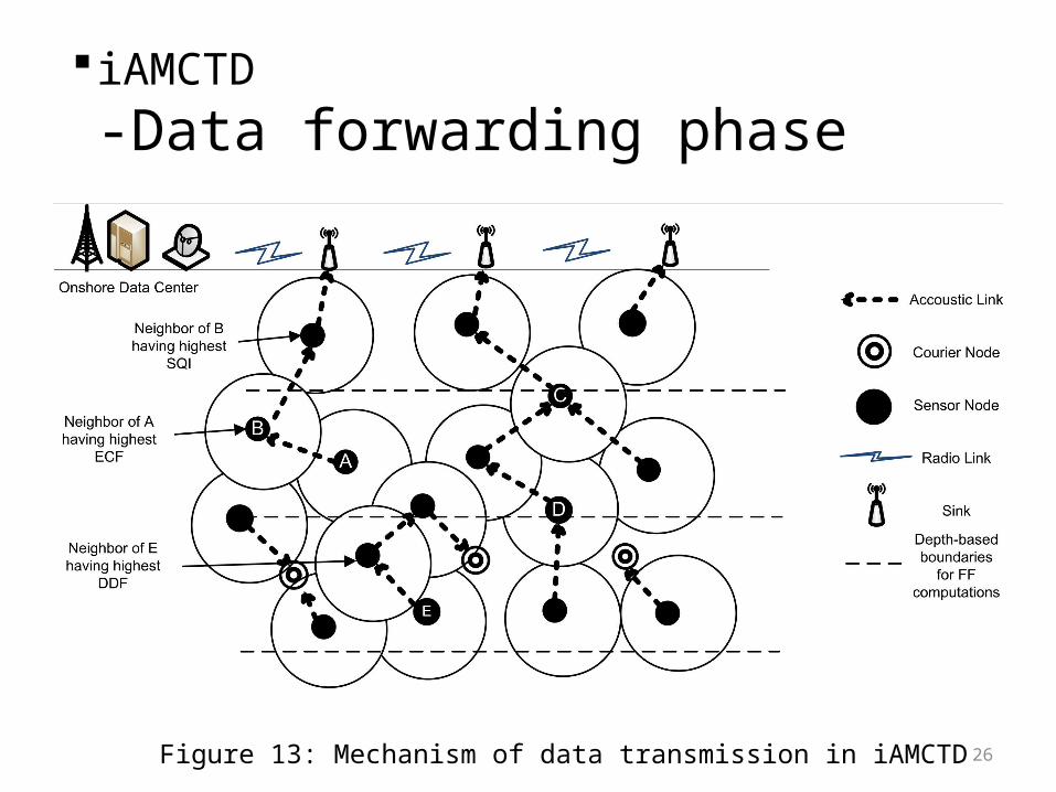
26Figure 13: Mechanism of data transmission in iAMCTD


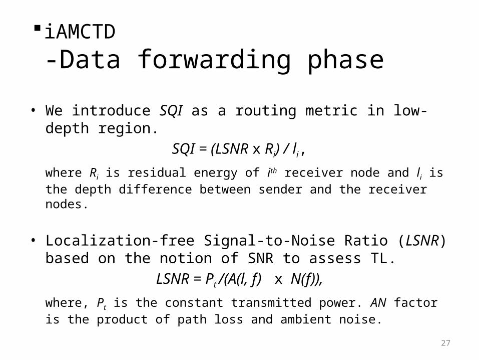
• We introduce SQI as a routing metric in low-depth region.

SQI = (LSNR x Ri) / li,where Ri is residual energy of ith receiver node and li is the depth difference between sender and the receiver nodes.

• Localization-free Signal-to-Noise Ratio (LSNR) based on the notion of SNR to assess TL.

LSNR = Pt /(A(l, f) x N(f)),where, Pt is the constant transmitted power. AN factor is the product of path loss and ambient noise.

27


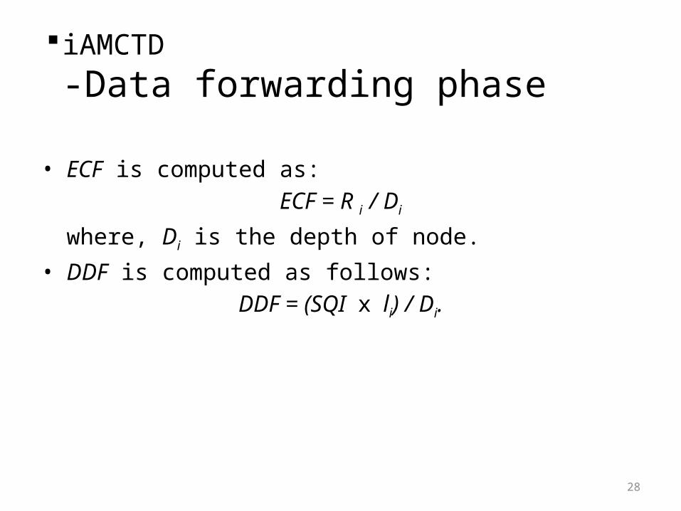
• ECF is computed as:ECF = R i / Di

where, Di is the depth of node.• DDF is computed as follows:

DDF = (SQI x li) / Di.

28

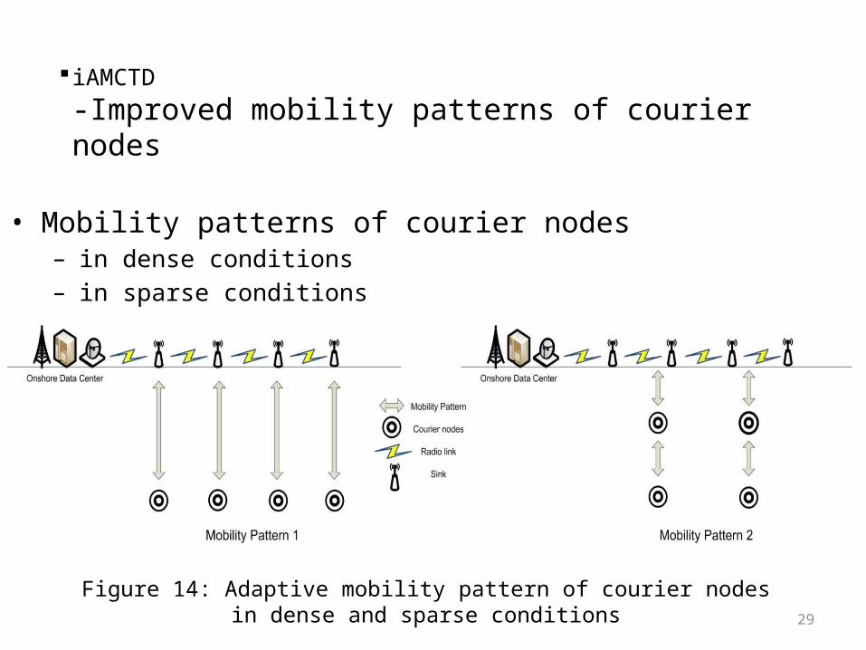
iAMCTD -Improved mobility patterns of courier nodes

• Mobility patterns of courier nodes– in dense conditions– in sparse conditions

29Figure 14: Adaptive mobility pattern of courier nodes

in dense and sparse conditions

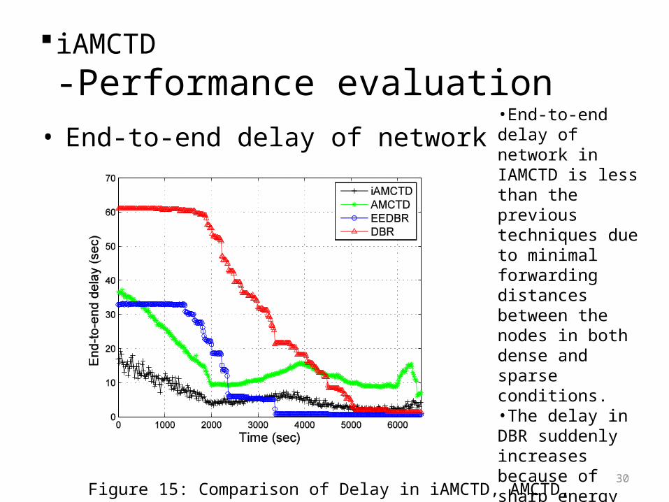
iAMCTD -Performance evaluation• End-to-end delay of network

30Figure 15: Comparison of Delay in iAMCTD, AMCTD, EEDBR and DBR

•End-to-end delay of network in IAMCTD is less than the previous techniques due to minimal forwarding distances between the nodes in both dense and sparse conditions. •The delay in DBR suddenly increases because of sharp energy depletion of medium-depth nodes, however in EEDBR, higher delay is caused due to prioritization of residual energy.

iAMCTD -Performance evaluation• Transmission loss of network

31Figure 16: Comparison of Transmission loss in iAMCTD, AMCTD, EEDBR and DBR

•In DBR, there are preferences of distant transmissions, however in EEDBR , again multiple transmissions increase the transmission loss between sender and the sink.

iAMCTD -Performance evaluation• Network throughput

32Figure 17: Comparison of throughput in iAMCTD, AMCTD, EEDBR and DBR

•The throughput of IAMCTD shows the amount of threshold-optimized data specifically for reactive networks.

•It removes the transmission of unnecessary data of network.

Conclusion• This thesis presents energy efficient routing schemes

for UWSNs by incorporating mobility of courier nodes and devising of WFs.

• AMCTD implements amendments in Dth and optimal WFs to achieve longer stability period.

• In iAMCTD, FFs calculation technique enhances network lifetime and reduces the TL.– In order to tackle flooding, path loss and propagation latency, it calculates optimal HT and use routing metrics; LSNR, SQI, ECF and DDF.

– Provides on-demand routing by formulating Hth, Sth and Rprime.

33

MS_thesis presentation

Documents

Transcript of MS_thesis presentation