MOSEK Modeling CookbookRelease 3.2.3

MOSEK ApS

15 November 2021

Contents

1 Preface 1

2 Linear optimization 32.1 Introduction . . . . . . . . . . . . . . . . . . . . . . . . . . . . . . . . . 32.2 Linear modeling . . . . . . . . . . . . . . . . . . . . . . . . . . . . . . . 72.3 Infeasibility in linear optimization . . . . . . . . . . . . . . . . . . . . . 112.4 Duality in linear optimization . . . . . . . . . . . . . . . . . . . . . . . . 13

3 Conic quadratic optimization 203.1 Cones . . . . . . . . . . . . . . . . . . . . . . . . . . . . . . . . . . . . . 203.2 Conic quadratic modeling . . . . . . . . . . . . . . . . . . . . . . . . . . 223.3 Conic quadratic case studies . . . . . . . . . . . . . . . . . . . . . . . . . 26

4 The power cone 304.1 The power cone(s) . . . . . . . . . . . . . . . . . . . . . . . . . . . . . . 304.2 Sets representable using the power cone . . . . . . . . . . . . . . . . . . 324.3 Power cone case studies . . . . . . . . . . . . . . . . . . . . . . . . . . . 33

5 Exponential cone optimization 375.1 Exponential cone . . . . . . . . . . . . . . . . . . . . . . . . . . . . . . . 375.2 Modeling with the exponential cone . . . . . . . . . . . . . . . . . . . . 385.3 Geometric programming . . . . . . . . . . . . . . . . . . . . . . . . . . . 415.4 Exponential cone case studies . . . . . . . . . . . . . . . . . . . . . . . . 45

6 Semidefinite optimization 506.1 Introduction to semidefinite matrices . . . . . . . . . . . . . . . . . . . . 506.2 Semidefinite modeling . . . . . . . . . . . . . . . . . . . . . . . . . . . . 546.3 Semidefinite optimization case studies . . . . . . . . . . . . . . . . . . . 62

7 Practical optimization 717.1 Conic reformulations . . . . . . . . . . . . . . . . . . . . . . . . . . . . . 717.2 Avoiding ill-posed problems . . . . . . . . . . . . . . . . . . . . . . . . . 747.3 Scaling . . . . . . . . . . . . . . . . . . . . . . . . . . . . . . . . . . . . 767.4 The huge and the tiny . . . . . . . . . . . . . . . . . . . . . . . . . . . . 787.5 Semidefinite variables . . . . . . . . . . . . . . . . . . . . . . . . . . . . 797.6 The quality of a solution . . . . . . . . . . . . . . . . . . . . . . . . . . . 807.7 Distance to a cone . . . . . . . . . . . . . . . . . . . . . . . . . . . . . . 82

8 Duality in conic optimization 84

i

8.1 Dual cone . . . . . . . . . . . . . . . . . . . . . . . . . . . . . . . . . . . 858.2 Infeasibility in conic optimization . . . . . . . . . . . . . . . . . . . . . . 868.3 Lagrangian and the dual problem . . . . . . . . . . . . . . . . . . . . . . 888.4 Weak and strong duality . . . . . . . . . . . . . . . . . . . . . . . . . . . 908.5 Applications of conic duality . . . . . . . . . . . . . . . . . . . . . . . . 938.6 Semidefinite duality and LMIs . . . . . . . . . . . . . . . . . . . . . . . 94

9 Mixed integer optimization 979.1 Integer modeling . . . . . . . . . . . . . . . . . . . . . . . . . . . . . . . 979.2 Mixed integer conic case studies . . . . . . . . . . . . . . . . . . . . . . 105

10 Quadratic optimization 10910.1 Quadratic objective . . . . . . . . . . . . . . . . . . . . . . . . . . . . . 10910.2 Quadratically constrained optimization . . . . . . . . . . . . . . . . . . . 11110.3 Example: Factor model . . . . . . . . . . . . . . . . . . . . . . . . . . . 114

11 Bibliographic notes 116

12 Notation and definitions 117

Bibliography 119

Index 121

ii

Chapter 1

Preface

This cookbook is about model building using convex optimization. It is intended as amodeling guide for the MOSEK optimization package. However, the style is intentionallyquite generic without specific MOSEK commands or API descriptions.

There are several excellent books available on this topic, for example the books byBen-Tal and Nemirovski [BenTalN01] and Boyd and Vandenberghe [BV04], which haveboth been a great source of inspiration for this manual. The purpose of this manualis to collect the material which we consider most relevant to our users and to presentit in a practical self-contained manner; however, we highly recommend the books as asupplement to this manual.

Some textbooks on building models using optimization (or mathematical program-ming) introduce various concepts through practical examples. In this manual we havechosen a different route, where we instead show the different sets and functions that canbe modeled using convex optimization, which can subsequently be combined into realis-tic examples and applications. In other words, we present simple convex building blocks,which can then be combined into more elaborate convex models. We call this approachextremely disciplined modeling. With the advent of more expressive and sophisticatedtools like conic optimization, we feel that this approach is better suited.

Content

We begin with a comprehensive chapter on linear optimization, including modeling ex-amples, duality theory and infeasibility certificates for linear problems. Linear problemsare optimization problems of the form

minimize 𝑐𝑇𝑥subject to 𝐴𝑥 = 𝑏,

𝑥 ≥ 0.

Conic optimization is a generalization of linear optimization which handles problems ofthe form:

minimize 𝑐𝑇𝑥subject to 𝐴𝑥 = 𝑏,

𝑥 ∈ 𝐾,

where 𝐾 is a convex cone. Various families of convex cones allow formulating differenttypes of nonlinear constraints. The following chapters present modeling with four typesof convex cones:

1

• quadratic cones ,

• power cone,

• exponential cone,

• semidefinite cone.

It is “well-known” in the convex optimization community that this family of cones issufficient to express almost all convex optimization problems appearing in practice.

Next we discuss issues arising in practical optimization, and we wholeheartedly recom-mend this short chapter to all readers before moving on to implementing mathematicalmodels with real data.

Following that, we present a general duality and infeasibility theory for conic prob-lems. Finally we diverge slightly from the topic of conic optimization and introducethe language of mixed-integer optimization and we discuss the relation between convexquadratic optimization and conic quadratic optimization.

2

Chapter 2

Linear optimization

In this chapter we discuss various aspects of linear optimization. We first introduce thebasic concepts of linear optimization and discuss the underlying geometric interpretations.We then give examples of the most frequently used reformulations or modeling tricks usedin linear optimization, and finally we discuss duality and infeasibility theory in somedetail.

2.1 Introduction

2.1.1 Basic notions

The most basic type of optimization is linear optimization. In linear optimization weminimize a linear function given a set of linear constraints. For example, we may wish tominimize a linear function

𝑥1 + 2𝑥2 − 𝑥3

under the constraints that

𝑥1 + 𝑥2 + 𝑥3 = 1, 𝑥1, 𝑥2, 𝑥3 ≥ 0.

The function we minimize is often called the objective function; in this case we havea linear objective function. The constraints are also linear and consist of both linearequalities and inequalities. We typically use more compact notation

minimize 𝑥1 + 2𝑥2 − 𝑥3

subject to 𝑥1 + 𝑥2 + 𝑥3 = 1,𝑥1, 𝑥2, 𝑥3 ≥ 0,

(2.1)

and we call (2.1) a linear optimization problem. The domain where all constraints aresatisfied is called the feasible set ; the feasible set for (2.1) is shown in Fig. 2.1.

For this simple problem we see by inspection that the optimal value of the problemis −1 obtained by the optimal solution

(𝑥⋆1, 𝑥

⋆2, 𝑥

⋆3) = (0, 0, 1).

3

x1 x2

x3

Fig. 2.1: Feasible set for 𝑥1 + 𝑥2 + 𝑥3 = 1 and 𝑥1, 𝑥2, 𝑥3 ≥ 0.

Linear optimization problems are typically formulated using matrix notation. The stan-dard form of a linear minimization problem is:

minimize 𝑐𝑇𝑥subject to 𝐴𝑥 = 𝑏,

𝑥 ≥ 0.(2.2)

For example, we can pose (2.1) in this form with

𝑥 =

⎡⎣ 𝑥1

𝑥2

𝑥3

⎤⎦ , 𝑐 =

⎡⎣ 12

−1

⎤⎦ , 𝐴 =[︀

1 1 1]︀.

There are many other formulations for linear optimization problems; we can have differenttypes of constraints,

𝐴𝑥 = 𝑏, 𝐴𝑥 ≥ 𝑏, 𝐴𝑥 ≤ 𝑏, 𝑙𝑐 ≤ 𝐴𝑥 ≤ 𝑢𝑐,

and different bounds on the variables

𝑙𝑥 ≤ 𝑥 ≤ 𝑢𝑥

or we may have no bounds on some 𝑥𝑖, in which case we say that 𝑥𝑖 is a free variable.All these formulations are equivalent in the sense that by simple linear transformationsand introduction of auxiliary variables they represent the same set of problems. Theimportant feature is that the objective function and the constraints are all linear in 𝑥.

2.1.2 Geometry of linear optimization

A hyperplane is a subset of R𝑛 defined as {𝑥 | 𝑎𝑇 (𝑥−𝑥0) = 0} or equivalently {𝑥 | 𝑎𝑇𝑥 =𝛾} with 𝑎𝑇𝑥0 = 𝛾, see Fig. 2.2.

Thus a linear constraint

𝐴𝑥 = 𝑏

4

a

x

aTx = γ

x0

Fig. 2.2: The dashed line illustrates a hyperplane {𝑥 | 𝑎𝑇𝑥 = 𝛾}.

with 𝐴 ∈ R𝑚×𝑛 represents an intersection of 𝑚 hyperplanes.Next, consider a point 𝑥 above the hyperplane in Fig. 2.3. Since 𝑥 − 𝑥0 forms an

acute angle with 𝑎 we have that 𝑎𝑇 (𝑥 − 𝑥0) ≥ 0, or 𝑎𝑇𝑥 ≥ 𝛾. The set {𝑥 | 𝑎𝑇𝑥 ≥ 𝛾} iscalled a halfspace. Similarly the set {𝑥 | 𝑎𝑇𝑥 ≤ 𝛾} forms another halfspace; in Fig. 2.3 itcorresponds to the area below the dashed line.

a

x

aTx > γ

x0

Fig. 2.3: The grey area is the halfspace {𝑥 | 𝑎𝑇𝑥 ≥ 𝛾}.

A set of linear inequalities

𝐴𝑥 ≤ 𝑏

corresponds to an intersection of halfspaces and forms a polyhedron, see Fig. 2.4.The polyhedral description of the feasible set gives us a very intuitive interpretation

of linear optimization, which is illustrated in Fig. 2.5. The dashed lines are normal tothe objective 𝑐 = (−1, 1), and to minimize 𝑐𝑇𝑥 we move as far as possible in the oppositedirection of 𝑐, to the furthest position where a dashed line intersect the polyhedron; anoptimal solution is therefore always either a vertex of the polyhedron, or an entire facetof the polyhedron may be optimal.

The polyhedron shown in the figure is nonempty and bounded, but this is not alwaysthe case for polyhedra arising from linear inequalities in optimization problems. In suchcases the optimization problem may be infeasible or unbounded, which we will discuss indetail in Sec. 2.3.

5

a1

a2a3

a4

a5

Fig. 2.4: A polyhedron formed as an intersection of halfspaces.

x⋆

a1

a2a3

a4

a5

c

Fig. 2.5: Geometric interpretation of linear optimization. The optimal solution 𝑥⋆ is ata point where the normals to 𝑐 (the dashed lines) intersect the polyhedron.

6

2.2 Linear modeling

In this section we present useful reformulation techniques and standard tricks whichallow constructing more complicated models using linear optimization. It is also a guidethrough the types of constraints which can be expressed using linear (in)equalities.

2.2.1 Maximum

The inequality 𝑡 ≥ max{𝑥1, . . . , 𝑥𝑛} is equivalent to a simultaneous sequence of 𝑛 in-equalities

𝑡 ≥ 𝑥𝑖, 𝑖 = 1, . . . , 𝑛

and similarly 𝑡 ≤ min{𝑥1, . . . , 𝑥𝑛} is the same as

𝑡 ≤ 𝑥𝑖, 𝑖 = 1, . . . , 𝑛.

Of course the same reformulation applies if each 𝑥𝑖 is not a single variable but a linearexpression. In particular, we can consider convex piecewise-linear functions 𝑓 : R𝑛 ↦→ Rdefined as the maximum of affine functions (see Fig. 2.6):

𝑓(𝑥) := max𝑖=1,...,𝑚

{𝑎𝑇𝑖 𝑥 + 𝑏𝑖}

a1x+ b1

a2x+ b2

a3x+ b3

Fig. 2.6: A convex piecewise-linear function (solid lines) of a single variable 𝑥. Thefunction is defined as the maximum of 3 affine functions.

The epigraph 𝑓(𝑥) ≤ 𝑡 (see Sec. 12) has an equivalent formulation with 𝑚 inequalities:

𝑎𝑇𝑖 𝑥 + 𝑏𝑖 ≤ 𝑡, 𝑖 = 1, . . . ,𝑚.

Piecewise-linear functions have many uses linear in optimization; either we have a convexpiecewise-linear formulation from the onset, or we may approximate a more complicated(nonlinear) problem using piecewise-linear approximations, although with modern non-linear optimization software it is becoming both easier and more efficient to directlyformulate and solve nonlinear problems without piecewise-linear approximations.

7

2.2.2 Absolute value

The absolute value of a scalar variable is a special case of maximum

|𝑥| := max{𝑥,−𝑥},

so we can model the epigraph |𝑥| ≤ 𝑡 using two inequalities

−𝑡 ≤ 𝑥 ≤ 𝑡.

2.2.3 The ℓ1 norm

All norms are convex functions, but the ℓ1 and ℓ∞ norms are of particular interest forlinear optimization. The ℓ1 norm of vector 𝑥 ∈ R𝑛 is defined as

‖𝑥‖1 := |𝑥1| + |𝑥2| + · · · + |𝑥𝑛|.

To model the epigraph

‖𝑥‖1 ≤ 𝑡, (2.3)

we introduce the following system

|𝑥𝑖| ≤ 𝑧𝑖, 𝑖 = 1, . . . , 𝑛,𝑛∑︁

𝑖=1

𝑧𝑖 = 𝑡, (2.4)

with additional (auxiliary) variable 𝑧 ∈ R𝑛. Clearly (2.3) and (2.4) are equivalent, in thesense that they have the same projection onto the space of 𝑥 and 𝑡 variables. Therefore,we can model (2.3) using linear (in)equalities

−𝑧𝑖 ≤ 𝑥𝑖 ≤ 𝑧𝑖,𝑛∑︁

𝑖=1

𝑧𝑖 = 𝑡, (2.5)

with auxiliary variables 𝑧. Similarly, we can describe the epigraph of the norm of anaffine function of 𝑥,

‖𝐴𝑥− 𝑏‖1 ≤ 𝑡

as

−𝑧𝑖 ≤ 𝑎𝑇𝑖 𝑥− 𝑏𝑖 ≤ 𝑧𝑖,𝑛∑︁

𝑖=1

𝑧𝑖 = 𝑡,

where 𝑎𝑖 is the 𝑖−th row of 𝐴 (taken as a column-vector).

Example 2.1 (Basis pursuit). The ℓ1 norm is overwhelmingly popular as a convexapproximation of the cardinality (i.e., number on nonzero elements) of a vector 𝑥. Forexample, suppose we are given an underdetermined linear system

𝐴𝑥 = 𝑏

8

where 𝐴 ∈ R𝑚×𝑛 and 𝑚 ≪ 𝑛. The basis pursuit problem

minimize ‖𝑥‖1subject to 𝐴𝑥 = 𝑏,

(2.6)

uses the ℓ1 norm of 𝑥 as a heuristic for finding a sparse solution (one with many zeroelements) to 𝐴𝑥 = 𝑏, i.e., it aims to represent 𝑏 as a linear combination of few columnsof 𝐴. Using (2.5) we can pose the problem as a linear optimization problem,

minimize 𝑒𝑇 𝑧subject to −𝑧 ≤ 𝑥 ≤ 𝑧,

𝐴𝑥 = 𝑏,(2.7)

where 𝑒 = (1, . . . , 1)𝑇 .

2.2.4 The ℓ∞ norm

The ℓ∞ norm of a vector 𝑥 ∈ R𝑛 is defined as

‖𝑥‖∞ := max𝑖=1,...,𝑛

|𝑥𝑖|,

which is another example of a simple piecewise-linear function. Using Sec. 2.2.2 we model

‖𝑥‖∞ ≤ 𝑡

as

−𝑡 ≤ 𝑥𝑖 ≤ 𝑡, 𝑖 = 1, . . . , 𝑛.

Again, we can also consider affine functions of 𝑥, i.e.,

‖𝐴𝑥− 𝑏‖∞ ≤ 𝑡,

which can be described as

−𝑡 ≤ 𝑎𝑇𝑖 𝑥− 𝑏 ≤ 𝑡, 𝑖 = 1, . . . , 𝑛.

Example 2.2 (Dual norms). It is interesting to note that the ℓ1 and ℓ∞ norms aredual. For any norm ‖ · ‖ on R𝑛, the dual norm ‖ · ‖* is defined as

‖𝑥‖* = max{𝑥𝑇𝑣 | ‖𝑣‖ ≤ 1}.

Let us verify that the dual of the ℓ∞ norm is the ℓ1 norm. Consider

‖𝑥‖*,∞ = max{𝑥𝑇𝑣 | ‖𝑣‖∞ ≤ 1}.

9

Obviously the maximum is attained for

𝑣𝑖 =

{︂+1, 𝑥𝑖 ≥ 0,−1, 𝑥𝑖 < 0,

i.e., ‖𝑥‖*,∞ =∑︀

𝑖 |𝑥𝑖| = ‖𝑥‖1. Similarly, consider the dual of the ℓ1 norm,

‖𝑥‖*,1 = max{𝑥𝑇𝑣 | ‖𝑣‖1 ≤ 1}.

To maximize 𝑥𝑇𝑣 subject to |𝑣1| + · · · + |𝑣𝑛| ≤ 1 we simply pick the element of 𝑥 withlargest absolute value, say |𝑥𝑘|, and set 𝑣𝑘 = ±1, so that ‖𝑥‖*,1 = |𝑥𝑘| = ‖𝑥‖∞. Thisillustrates a more general property of dual norms, namely that ‖𝑥‖** = ‖𝑥‖.

2.2.5 Homogenization

Consider the linear-fractional problem

minimize 𝑎𝑇 𝑥+𝑏𝑐𝑇 𝑥+𝑑

subject to 𝑐𝑇𝑥 + 𝑑 > 0,𝐹𝑥 = 𝑔.

(2.8)

Perhaps surprisingly, it can be turned into a linear problem if we homogenize the linearconstraint, i.e. replace it with 𝐹𝑦 = 𝑔𝑧 for a single variable 𝑧 ∈ R. The full newoptimization problem is

minimize 𝑎𝑇𝑦 + 𝑏𝑧subject to 𝑐𝑇𝑦 + 𝑑𝑧 = 1,

𝐹𝑦 = 𝑔𝑧,𝑧 ≥ 0.

(2.9)

If 𝑥 is a feasible point in (2.8) then 𝑧 = (𝑐𝑇𝑥 + 𝑑)−1, 𝑦 = 𝑥𝑧 is feasible for (2.9) with thesame objective value. Conversely, if (𝑦, 𝑧) is feasible for (2.9) then 𝑥 = 𝑦/𝑧 is feasible in(2.8) and has the same objective value, at least when 𝑧 ̸= 0. If 𝑧 = 0 and 𝑥 is any feasiblepoint for (2.8) then 𝑥 + 𝑡𝑦, 𝑡 → +∞ is a sequence of solutions of (2.8) converging to thevalue of (2.9). We leave it for the reader to check those statements. In either case weshowed an equivalence between the two problems.

Note that, as the sketch of proof above suggests, the optimal value in (2.8) may notbe attained, even though the one in the linear problem (2.9) always is. For example,consider a pair of problems constructed as above:

minimize 𝑥1/𝑥2

subject to 𝑥2 > 0,𝑥1 + 𝑥2 = 1.

minimize 𝑦1subject to 𝑦1 + 𝑦2 = 𝑧,

𝑦2 = 1,𝑧 ≥ 0.

Both have an optimal value of −1, but on the left we can only approach it arbitrarilyclosely.

10

2.2.6 Sum of largest elements

Suppose 𝑥 ∈ R𝑛 and that 𝑚 is a positive integer. Consider the problem

minimize 𝑚𝑡 +∑︀

𝑖 𝑢𝑖

subject to 𝑢𝑖 + 𝑡 ≥ 𝑥𝑖, 𝑖 = 1, . . . , 𝑛,𝑢𝑖 ≥ 0, 𝑖 = 1, . . . , 𝑛,

(2.10)

with new variables 𝑡 ∈ R, 𝑢𝑖 ∈ R𝑛. It is easy to see that fixing a value for 𝑡 determinesthe rest of the solution. For the sake of simplifying notation let us assume for a momentthat 𝑥 is sorted:

𝑥1 ≥ 𝑥2 ≥ · · · ≥ 𝑥𝑛.

If 𝑡 ∈ [𝑥𝑘, 𝑥𝑘+1) then 𝑢𝑙 = 0 for 𝑙 ≥ 𝑘+ 1 and 𝑢𝑙 = 𝑥𝑙− 𝑡 for 𝑙 ≤ 𝑘 in the optimal solution.Therefore, the objective value under the assumption 𝑡 ∈ [𝑥𝑘, 𝑥𝑘+1) is

obj𝑡 = 𝑥1 + · · · + 𝑥𝑘 + 𝑡(𝑚− 𝑘)

which is a linear function minimized at one of the endpoints of [𝑥𝑘, 𝑥𝑘+1). Now we cancompute

obj𝑥𝑘+1− obj𝑥𝑘

= (𝑘 −𝑚)(𝑥𝑘 − 𝑥𝑘+1).

It follows that obj𝑥𝑘has a minimum for 𝑘 = 𝑚, and therefore the optimum value of (2.10)

is simply

𝑥1 + · · · + 𝑥𝑚.

Since the assumption that 𝑥 is sorted was only a notational convenience, we concludethat in general the optimization model (2.10) computes the sum of 𝑚 largest entries in𝑥. In Sec. 2.4 we will show a conceptual way of deriving this model.

2.3 Infeasibility in linear optimization

In this section we discuss the basic theory of primal infeasibility certificates for linearproblems. These ideas will be developed further after we have introduced duality in thenext section.

One of the first issues one faces when presented with an optimization problem iswhether it has any solutions at all. As we discussed previously, for a linear optimizationproblem

minimize 𝑐𝑇𝑥subject to 𝐴𝑥 = 𝑏,

𝑥 ≥ 0.(2.11)

the feasible set

ℱ𝑝 = {𝑥 ∈ R𝑛 | 𝐴𝑥 = 𝑏, 𝑥 ≥ 0}

is a convex polytope. We say the problem is feasible if ℱ𝑝 ̸= ∅ and infeasible otherwise.

11

Example 2.3 (Linear infeasible problem). Consider the optimization problem:

minimize 2𝑥1 + 3𝑥2 − 𝑥3

subject to 𝑥1 + 𝑥2 + 2𝑥3 = 1,− 2𝑥1 − 𝑥2 + 𝑥3 = −0.5,− 𝑥1 + 5𝑥3 = −0.1,

𝑥𝑖 ≥ 0.

This problem is infeasible. We see it by taking a linear combination of the constraintswith coefficients 𝑦 = (1, 2,−1)𝑇 :

𝑥1 + 𝑥2 + 2𝑥3 = 1, / ·1− 2𝑥1 − 𝑥2 + 𝑥3 = −0.5, / ·2− 𝑥1 + 5𝑥3 = −0.1, / ·(−1)− 2𝑥1 − 𝑥2 − 𝑥3 = 0.1.

This clearly proves infeasibility: the left-hand side is negative and the right-hand sideis positive, which is impossible.

2.3.1 Farkas’ lemma

In the last example we proved infeasibility of the linear system by exhibiting an explicitlinear combination of the equations, such that the right-hand side (constant) is positivewhile on the left-hand side all coefficients are negative or zero. In matrix notation, sucha linear combination is given by a vector 𝑦 such that 𝐴𝑇𝑦 ≤ 0 and 𝑏𝑇𝑦 > 0. The nextlemma shows that infeasibility of (2.11) is equivalent to the existence of such a vector.

Lemma 2.1 (Farkas’ lemma). Given 𝐴 and 𝑏 as in (2.11), exactly one of the two state-ments is true:

1. There exists 𝑥 ≥ 0 such that 𝐴𝑥 = 𝑏.

2. There exists 𝑦 such that 𝐴𝑇𝑦 ≤ 0 and 𝑏𝑇𝑦 > 0.

Proof. Let 𝑎1, . . . , 𝑎𝑛 be the columns of 𝐴. The set {𝐴𝑥 | 𝑥 ≥ 0} is a closed convexcone spanned by 𝑎1, . . . , 𝑎𝑛. If this cone contains 𝑏 then we have the first alternative.Otherwise the cone can be separated from the point 𝑏 by a hyperplane passing through0, i.e. there exists 𝑦 such that 𝑦𝑇 𝑏 > 0 and 𝑦𝑇𝑎𝑖 ≤ 0 for all 𝑖. This is equivalent to thesecond alternative. Finally, 1. and 2. are mutually exclusive, since otherwise we wouldhave

0 < 𝑦𝑇 𝑏 = 𝑦𝑇𝐴𝑥 = (𝐴𝑇𝑦)𝑇𝑥 ≤ 0.

Farkas’ lemma implies that either the problem (2.11) is feasible or there is a certificateof infeasibility 𝑦. In other words, every time we classify model as infeasible, we can certifythis fact by providing an appropriate 𝑦, as in Example 2.3.

12

2.3.2 Locating infeasibility

As we already discussed, the infeasibility certificate 𝑦 gives coefficients of a linear combi-nation of the constraints which is infeasible “in an obvious way”, that is positive on oneside and negative on the other. In some cases, 𝑦 may be very sparse, i.e. it may havevery few nonzeros, which means that already a very small subset of the constraints isthe root cause of infeasibility. This may be interesting if, for example, we are debugginga large model which we expected to be feasible and infeasibility is caused by an errorin the problem formulation. Then we only have to consider the sub-problem formed byconstraints with index set {𝑗 | 𝑦𝑗 ̸= 0}.

Example 2.4 (All constraints involved in infeasibility). As a cautionary note considerthe constraints

0 ≤ 𝑥1 ≤ 𝑥2 ≤ · · · ≤ 𝑥𝑛 ≤ −1.

Any problem with those constraints is infeasible, but dropping any one of the inequal-ities creates a feasible subproblem.

2.4 Duality in linear optimization

Duality is a rich and powerful theory, central to understanding infeasibility and sensitivityissues in linear optimization. In this section we only discuss duality in linear optimizationat a descriptive level suited for practitioners; we refer to Sec. 8 for a more in-depthdiscussion of duality for general conic problems.

2.4.1 The dual problem

Primal problem

We consider as always a linear optimization problem in standard form:

minimize 𝑐𝑇𝑥subject to 𝐴𝑥 = 𝑏,

𝑥 ≥ 0.(2.12)

We denote the optimal objective value in (2.12) by 𝑝⋆. There are three possibilities:

• The problem is infeasible. By convention 𝑝⋆ = +∞.

• 𝑝⋆ is finite, in which case the problem has an optimal solution.

• 𝑝⋆ = −∞, meaning that there are feasible solutions with 𝑐𝑇𝑥 decreasing to −∞, inwhich case we say the problem is unbounded.

13

Lagrange function

We associate with (2.12) a so-called Lagrangian function 𝐿 : R𝑛 × R𝑚 × R𝑛+ → R that

augments the objective with a weighted combination of all the constraints,

𝐿(𝑥, 𝑦, 𝑠) = 𝑐𝑇𝑥 + 𝑦𝑇 (𝑏− 𝐴𝑥) − 𝑠𝑇𝑥.

The variables 𝑦 ∈ R𝑚 and 𝑠 ∈ R𝑛+ are called Lagrange multipliers or dual variables. For

any feasible 𝑥* ∈ ℱ𝑝 and any (𝑦*, 𝑠*) ∈ R𝑚 × R𝑛+ we have

𝐿(𝑥*, 𝑦*, 𝑠*) = 𝑐𝑇𝑥* + (𝑦*)𝑇 · 0 − (𝑠*)𝑇𝑥* ≤ 𝑐𝑇𝑥*.

Note the we used the nonnegativity of 𝑠*, or in general of any Lagrange multiplier as-sociated with an inequality constraint. The dual function is defined as the minimum of𝐿(𝑥, 𝑦, 𝑠) over 𝑥. Thus the dual function of (2.12) is

𝑔(𝑦, 𝑠) = min𝑥

𝐿(𝑥, 𝑦, 𝑠) = min𝑥

𝑥𝑇 (𝑐− 𝐴𝑇𝑦 − 𝑠) + 𝑏𝑇𝑦 =

{︂𝑏𝑇𝑦, 𝑐− 𝐴𝑇𝑦 − 𝑠 = 0,−∞, otherwise.

Dual problem

For every (𝑦, 𝑠) the value of 𝑔(𝑦, 𝑠) is a lower bound for 𝑝⋆. To get the best such boundwe maximize 𝑔(𝑦, 𝑠) over all (𝑦, 𝑠) and get the dual problem:

maximize 𝑏𝑇𝑦subject to 𝑐− 𝐴𝑇𝑦 = 𝑠,

𝑠 ≥ 0.(2.13)

The optimal value of (2.13) will be denoted 𝑑⋆. As in the case of (2.12) (which from nowon we call the primal problem), the dual problem can be infeasible (𝑑⋆ = −∞), have anoptimal solution (−∞ < 𝑑⋆ < +∞) or be unbounded (𝑑⋆ = +∞). Note that the roles of−∞ and +∞ are now reversed because the dual is a maximization problem.

Example 2.5 (Dual of basis pursuit). As an example, let us derive the dual of thebasis pursuit formulation (2.7). It would be possible to add auxiliary variables andconstraints to force that problem into the standard form (2.12) and then just applythe dual transformation as a black box, but it is both easier and more instructive todirectly write the Lagrangian:

𝐿(𝑥, 𝑧, 𝑦, 𝑢, 𝑣) = 𝑒𝑇 𝑧 + 𝑢𝑇 (𝑥− 𝑧) − 𝑣𝑇 (𝑥 + 𝑧) + 𝑦𝑇 (𝑏− 𝐴𝑥)

where 𝑒 = (1, . . . , 1)𝑇 , with Lagrange multipliers 𝑦 ∈ R𝑚 and 𝑢, 𝑣 ∈ R𝑛+. The dual

function

𝑔(𝑦, 𝑢, 𝑣) = min𝑥,𝑧

𝐿(𝑥, 𝑧, 𝑦, 𝑢, 𝑣) = min𝑥,𝑧

𝑧𝑇 (𝑒− 𝑢− 𝑣) + 𝑥𝑇 (𝑢− 𝑣 − 𝐴𝑇𝑦) + 𝑦𝑇 𝑏

is only bounded below if 𝑒 = 𝑢 + 𝑣 and 𝐴𝑇𝑦 = 𝑢− 𝑣, hence the dual problem is

maximize 𝑏𝑇𝑦subject to 𝑒 = 𝑢 + 𝑣,

𝐴𝑇𝑦 = 𝑢− 𝑣,𝑢, 𝑣 ≥ 0.

(2.14)

14

It is not hard to observe that an equivalent formulation of (2.14) is simply

maximize 𝑏𝑇𝑦subject to ‖𝐴𝑇𝑦‖∞ ≤ 1,

(2.15)

which should be associated with duality between norms discussed in Example 2.2.

Example 2.6 (Dual of a maximization problem). We can similarly derive the dual ofproblem (2.13). If we write it simply as

maximize 𝑏𝑇𝑦subject to 𝑐− 𝐴𝑇𝑦 ≥ 0,

then the Lagrangian is

𝐿(𝑦, 𝑢) = 𝑏𝑇𝑦 + 𝑢𝑇 (𝑐− 𝐴𝑇𝑦) = 𝑦𝑇 (𝑏− 𝐴𝑢) + 𝑐𝑇𝑢

with 𝑢 ∈ R𝑛+, so that now 𝐿(𝑦, 𝑢) ≥ 𝑏𝑇𝑦 for any feasible 𝑦. Calculating

min𝑢 max𝑦 𝐿(𝑦, 𝑢) is now equivalent to the problem

minimize 𝑐𝑇𝑢subject to 𝐴𝑢 = 𝑏,

𝑢 ≥ 0,

so, as expected, the dual of the dual recovers the original primal problem.

2.4.2 Weak and strong duality

Suppose 𝑥* and (𝑦*, 𝑠*) are feasible points for the primal and dual problems (2.12) and(2.13), respectively. Then we have

𝑏𝑇𝑦* = (𝐴𝑥*)𝑇𝑦* = (𝑥*)𝑇 (𝐴𝑇𝑦*) = (𝑥*)𝑇 (𝑐− 𝑠*) = 𝑐𝑇𝑥* − (𝑠*)𝑇𝑥* ≤ 𝑐𝑇𝑥*

so the dual objective value is a lower bound on the objective value of the primal. Inparticular, any dual feasible point (𝑦*, 𝑠*) gives a lower bound:

𝑏𝑇𝑦* ≤ 𝑝⋆

and we immediately get the next lemma.

Lemma 2.2 (Weak duality). 𝑑⋆ ≤ 𝑝⋆.

It follows that if 𝑏𝑇𝑦* = 𝑐𝑇𝑥* then 𝑥* is optimal for the primal, (𝑦*, 𝑠*) is optimal forthe dual and 𝑏𝑇𝑦* = 𝑐𝑇𝑥* is the common optimal objective value. This way we can usethe optimal dual solution to certify optimality of the primal solution and vice versa.

The remarkable property of linear optimization is that 𝑑⋆ = 𝑝⋆ holds in the mostinteresting scenario when the primal problem is feasible and bounded. It means that thecertificate of optimality mentioned in the previous paragraph always exists.

15

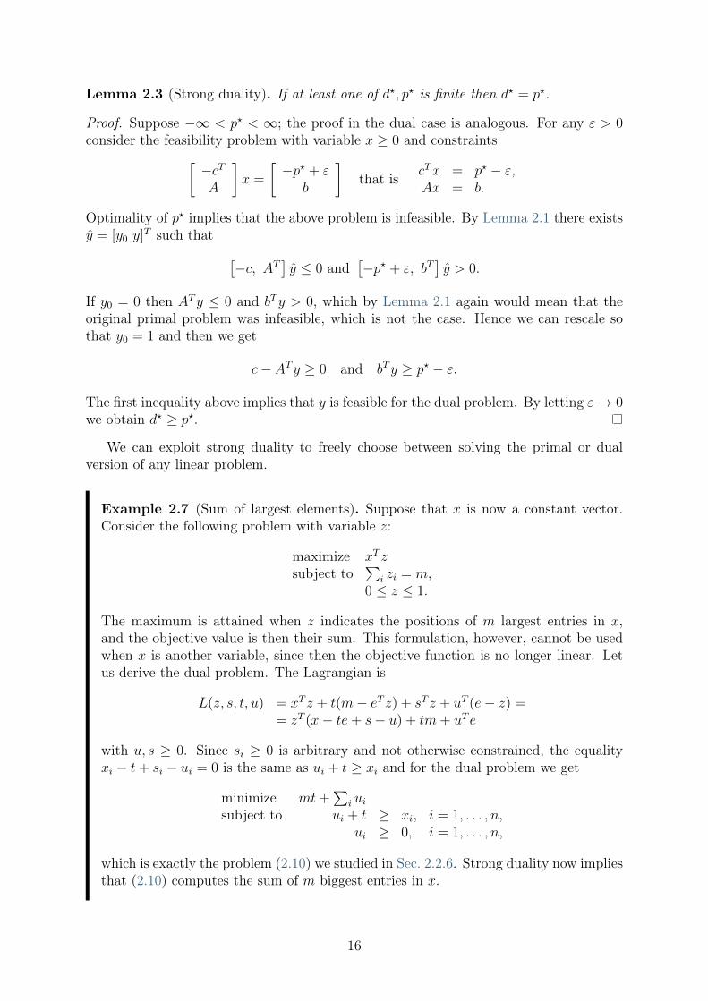
Lemma 2.3 (Strong duality). If at least one of 𝑑⋆, 𝑝⋆ is finite then 𝑑⋆ = 𝑝⋆.

Proof. Suppose −∞ < 𝑝⋆ < ∞; the proof in the dual case is analogous. For any 𝜀 > 0consider the feasibility problem with variable 𝑥 ≥ 0 and constraints[︂

−𝑐𝑇

𝐴

]︂𝑥 =

[︂−𝑝⋆ + 𝜀

𝑏

]︂that is 𝑐𝑇𝑥 = 𝑝⋆ − 𝜀,

𝐴𝑥 = 𝑏.

Optimality of 𝑝⋆ implies that the above problem is infeasible. By Lemma 2.1 there exists𝑦 = [𝑦0 𝑦]𝑇 such that [︀

−𝑐, 𝐴𝑇]︀𝑦 ≤ 0 and

[︀−𝑝⋆ + 𝜀, 𝑏𝑇

]︀𝑦 > 0.

If 𝑦0 = 0 then 𝐴𝑇𝑦 ≤ 0 and 𝑏𝑇𝑦 > 0, which by Lemma 2.1 again would mean that theoriginal primal problem was infeasible, which is not the case. Hence we can rescale sothat 𝑦0 = 1 and then we get

𝑐− 𝐴𝑇𝑦 ≥ 0 and 𝑏𝑇𝑦 ≥ 𝑝⋆ − 𝜀.

The first inequality above implies that 𝑦 is feasible for the dual problem. By letting 𝜀 → 0we obtain 𝑑⋆ ≥ 𝑝⋆.

We can exploit strong duality to freely choose between solving the primal or dualversion of any linear problem.

Example 2.7 (Sum of largest elements). Suppose that 𝑥 is now a constant vector.Consider the following problem with variable 𝑧:

maximize 𝑥𝑇 𝑧subject to

∑︀𝑖 𝑧𝑖 = 𝑚,

0 ≤ 𝑧 ≤ 1.

The maximum is attained when 𝑧 indicates the positions of 𝑚 largest entries in 𝑥,and the objective value is then their sum. This formulation, however, cannot be usedwhen 𝑥 is another variable, since then the objective function is no longer linear. Letus derive the dual problem. The Lagrangian is

𝐿(𝑧, 𝑠, 𝑡, 𝑢) = 𝑥𝑇 𝑧 + 𝑡(𝑚− 𝑒𝑇 𝑧) + 𝑠𝑇 𝑧 + 𝑢𝑇 (𝑒− 𝑧) == 𝑧𝑇 (𝑥− 𝑡𝑒 + 𝑠− 𝑢) + 𝑡𝑚 + 𝑢𝑇 𝑒

with 𝑢, 𝑠 ≥ 0. Since 𝑠𝑖 ≥ 0 is arbitrary and not otherwise constrained, the equality𝑥𝑖 − 𝑡 + 𝑠𝑖 − 𝑢𝑖 = 0 is the same as 𝑢𝑖 + 𝑡 ≥ 𝑥𝑖 and for the dual problem we get

minimize 𝑚𝑡 +∑︀

𝑖 𝑢𝑖

subject to 𝑢𝑖 + 𝑡 ≥ 𝑥𝑖, 𝑖 = 1, . . . , 𝑛,𝑢𝑖 ≥ 0, 𝑖 = 1, . . . , 𝑛,

which is exactly the problem (2.10) we studied in Sec. 2.2.6. Strong duality now impliesthat (2.10) computes the sum of 𝑚 biggest entries in 𝑥.

16

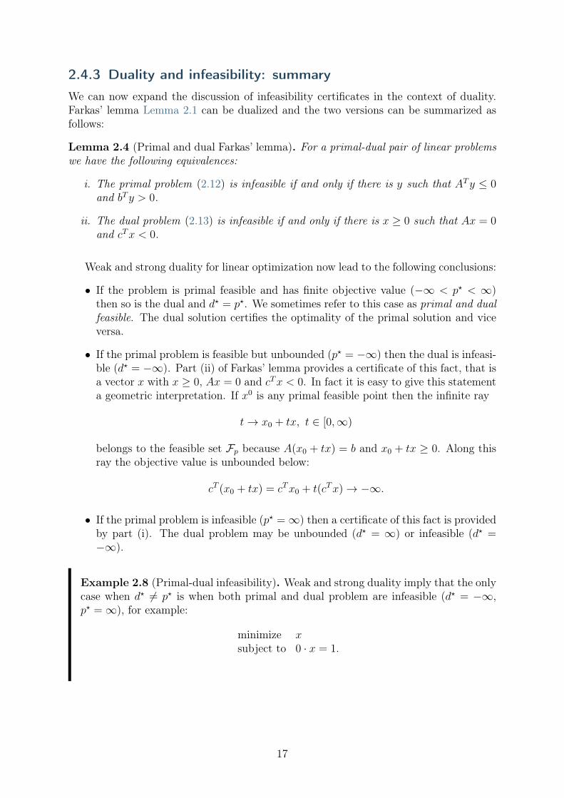
2.4.3 Duality and infeasibility: summary

We can now expand the discussion of infeasibility certificates in the context of duality.Farkas’ lemma Lemma 2.1 can be dualized and the two versions can be summarized asfollows:

Lemma 2.4 (Primal and dual Farkas’ lemma). For a primal-dual pair of linear problemswe have the following equivalences:

i. The primal problem (2.12) is infeasible if and only if there is 𝑦 such that 𝐴𝑇𝑦 ≤ 0and 𝑏𝑇𝑦 > 0.

ii. The dual problem (2.13) is infeasible if and only if there is 𝑥 ≥ 0 such that 𝐴𝑥 = 0and 𝑐𝑇𝑥 < 0.

Weak and strong duality for linear optimization now lead to the following conclusions:

• If the problem is primal feasible and has finite objective value (−∞ < 𝑝⋆ < ∞)then so is the dual and 𝑑⋆ = 𝑝⋆. We sometimes refer to this case as primal and dualfeasible. The dual solution certifies the optimality of the primal solution and viceversa.

• If the primal problem is feasible but unbounded (𝑝⋆ = −∞) then the dual is infeasi-ble (𝑑⋆ = −∞). Part (ii) of Farkas’ lemma provides a certificate of this fact, that isa vector 𝑥 with 𝑥 ≥ 0, 𝐴𝑥 = 0 and 𝑐𝑇𝑥 < 0. In fact it is easy to give this statementa geometric interpretation. If 𝑥0 is any primal feasible point then the infinite ray

𝑡 → 𝑥0 + 𝑡𝑥, 𝑡 ∈ [0,∞)

belongs to the feasible set ℱ𝑝 because 𝐴(𝑥0 + 𝑡𝑥) = 𝑏 and 𝑥0 + 𝑡𝑥 ≥ 0. Along thisray the objective value is unbounded below:

𝑐𝑇 (𝑥0 + 𝑡𝑥) = 𝑐𝑇𝑥0 + 𝑡(𝑐𝑇𝑥) → −∞.

• If the primal problem is infeasible (𝑝⋆ = ∞) then a certificate of this fact is providedby part (i). The dual problem may be unbounded (𝑑⋆ = ∞) or infeasible (𝑑⋆ =−∞).

Example 2.8 (Primal-dual infeasibility). Weak and strong duality imply that the onlycase when 𝑑⋆ ̸= 𝑝⋆ is when both primal and dual problem are infeasible (𝑑⋆ = −∞,𝑝⋆ = ∞), for example:

minimize 𝑥subject to 0 · 𝑥 = 1.

17

2.4.4 Dual values as shadow prices

Dual values are related to shadow prices, as they measure, under some nondegeneracyassumption, the sensitivity of the objective value to a change in the constraint. Consideragain the primal and dual problem pair (2.12) and (2.13) with feasible sets ℱ𝑝 and ℱ𝑑

and with a primal-dual optimal solution (𝑥*, 𝑦*, 𝑠*).Suppose we change one of the values in 𝑏 from 𝑏𝑖 to 𝑏′𝑖. This corresponds to moving

one of the hyperplanes defining ℱ𝑝, and in consequence the optimal solution (and theobjective value) may change. On the other hand, the dual feasible set ℱ𝑑 is not affected.Assuming that the solution (𝑦*, 𝑠*) was a unique vertex of ℱ𝑑 this point remains optimalfor the dual after a sufficiently small change of 𝑏. But then the change of the dualobjective is

𝑦*𝑖 (𝑏′𝑖 − 𝑏𝑖)

and by strong duality the primal objective changes by the same amount.

Example 2.9 (Student diet). An optimization student wants to save money on thediet while remaining healthy. A healthy diet requires at least 𝑃 = 6 units of protein,𝐶 = 15 units of carbohydrates, 𝐹 = 5 units of fats and 𝑉 = 7 units of vitamins. Thestudent can choose from the following products:

P C F V pricetakeaway 3 3 2 1 5vegetables 1 2 0 4 1bread 0.5 4 1 0 2

The problem of minimizing cost while meeting dietary requirements is

minimize 5𝑥1 + 𝑥2 + 2𝑥3

subject to 3𝑥1 + 𝑥2 + 0.5𝑥3 ≥ 6,3𝑥1 + 2𝑥2 + 4𝑥3 ≥ 15,2𝑥1 + 𝑥3 ≥ 5,𝑥1 + 4𝑥2 ≥ 7,𝑥1, 𝑥2, 𝑥3 ≥ 0.

If 𝑦1, 𝑦2, 𝑦3, 𝑦4 are the dual variables associated with the four inequality constraintsthen the (unique) primal-dual optimal solution to this problem is approximately:

(𝑥, 𝑦) = ((1, 1.5, 3), (0.42, 0, 1.78, 0.14))

with optimal cost 𝑝⋆ = 12.5. Note 𝑦2 = 0 indicates that the second constraint is notbinding. Indeed, we could increase 𝐶 to 18 without affecting the optimal solution. Theremaining constraints are binding.

Improving the intake of protein by 1 unit (increasing 𝑃 to 7) will increase the costby 0.42, while doing the same for fat will cost an extra 1.78 per unit. If the studenthad extra money to improve one of the parameters then the best choice would be toincrease the intake of vitamins, with shadow price of just 0.14.

If one month the student only had 12 units of money and was willing to relax oneof the requirements then the best choice is to save on fats: the necessary reduction of

18

𝐹 is smallest, namely 0.5 · 1.78−1 = 0.28. Indeed, with the new value of 𝐹 = 4.72 thesame problem solves to 𝑝⋆ = 12 and 𝑥 = (1.08, 1.48, 2.56).

We stress that a truly balanced diet problem should also include upper bounds.

19

Chapter 3

Conic quadratic optimization

This chapter extends the notion of linear optimization with quadratic cones. Conicquadratic optimization, also known as second-order cone optimization, is a straightfor-ward generalization of linear optimization, in the sense that we optimize a linear func-tion under linear (in)equalities with some variables belonging to one or more (rotated)quadratic cones. We discuss the basic concept of quadratic cones, and demonstrate thesurprisingly large flexibility of conic quadratic modeling.

3.1 Cones

Since this is the first place where we introduce a non-linear cone, it seems suitable tomake our most important definition:

A set 𝐾 ⊆ R𝑛 is called a convex cone if

• for every 𝑥, 𝑦 ∈ 𝐾 we have 𝑥 + 𝑦 ∈ 𝐾,

• for every 𝑥 ∈ 𝐾 and 𝛼 ≥ 0 we have 𝛼𝑥 ∈ 𝐾.

For example a linear subspace of R𝑛, the positive orthant R𝑛≥0 or any ray (half-line)

starting at the origin are examples of convex cones. We leave it for the reader to checkthat the intersection of convex cones is a convex cone; this property enables us to assemblecomplicated optimization models from individual conic bricks.

3.1.1 Quadratic cones

We define the 𝑛-dimensional quadratic cone as

𝒬𝑛 =

{︂𝑥 ∈ R𝑛 | 𝑥1 ≥

√︁𝑥22 + 𝑥2

3 + · · · + 𝑥2𝑛

}︂. (3.1)

The geometric interpretation of a quadratic (or second-order) cone is shown in Fig. 3.1for a cone with three variables, and illustrates how the boundary of the cone resemblesan ice-cream cone. The 1-dimensional quadratic cone simply states nonnegativity 𝑥1 ≥ 0.

20

Fig. 3.1: Boundary of quadratic cone 𝑥1 ≥√︀𝑥22 + 𝑥2

3 and rotated quadratic cone 2𝑥1𝑥2 ≥𝑥23, 𝑥1, 𝑥2 ≥ 0.

3.1.2 Rotated quadratic cones

An 𝑛−dimensional rotated quadratic cone is defined as

𝒬𝑛𝑟 =

{︀𝑥 ∈ R𝑛 | 2𝑥1𝑥2 ≥ 𝑥2

3 + · · · + 𝑥2𝑛, 𝑥1, 𝑥2 ≥ 0

}︀. (3.2)

As the name indicates, there is a simple relationship between quadratic and rotatedquadratic cones. Define an orthogonal transformation

𝑇𝑛 :=

⎡⎣ 1/√

2 1/√

2 0

1/√

2 −1/√

2 00 0 𝐼𝑛−2

⎤⎦ . (3.3)

Then it is easy to verify that

𝑥 ∈ 𝒬𝑛 ⇐⇒ 𝑇𝑛𝑥 ∈ 𝒬𝑛𝑟 ,

and since 𝑇 is orthogonal we call 𝒬𝑛𝑟 a rotated cone; the transformation corresponds to

a rotation of 𝜋/4 in the (𝑥1, 𝑥2) plane. For example if 𝑥 ∈ 𝒬3 and⎡⎣ 𝑧1𝑧2𝑧3

⎤⎦ =

⎡⎣ 1√2

1√2

01√2

− 1√2

0

0 0 1

⎤⎦ ·

⎡⎣ 𝑥1

𝑥2

𝑥3

⎤⎦ =

⎡⎣ 1√2(𝑥1 + 𝑥2)

1√2(𝑥1 − 𝑥2)

𝑥3

⎤⎦then

2𝑧1𝑧2 ≥ 𝑧23 , 𝑧1, 𝑧2 ≥ 0 =⇒ (𝑥21 − 𝑥2

2) ≥ 𝑥23, 𝑥1 ≥ 0,

and similarly we see that

𝑥21 ≥ 𝑥2

2 + 𝑥23, 𝑥1 ≥ 0 =⇒ 2𝑧1𝑧2 ≥ 𝑧23 , 𝑧1, 𝑧2 ≥ 0.

Thus, one could argue that we only need quadratic cones 𝒬𝑛, but there are many exampleswhere using an explicit rotated quadratic cone 𝒬𝑛

𝑟 is more natural, as we will see next.

21

3.2 Conic quadratic modeling

In the following we describe several convex sets that can be modeled using conic quadraticformulations or, as we call them, are conic quadratic representable.

3.2.1 Absolute values

In Sec. 2.2.2 we saw how to model |𝑥| ≤ 𝑡 using two linear inequalities, but in fact theepigraph of the absolute value is just the definition of a two-dimensional quadratic cone,i.e.,

|𝑥| ≤ 𝑡 ⇐⇒ (𝑡, 𝑥) ∈ 𝒬2.

3.2.2 Euclidean norms

The Euclidean norm of 𝑥 ∈ R𝑛,

‖𝑥‖2 =√︁𝑥21 + 𝑥2

2 + · · · + 𝑥2𝑛

essentially defines the quadratic cone, i.e.,

‖𝑥‖2 ≤ 𝑡 ⇐⇒ (𝑡, 𝑥) ∈ 𝒬𝑛+1.

The epigraph of the squared Euclidean norm can be described as the intersection of arotated quadratic cone with an affine hyperplane,

𝑥21 + · · · + 𝑥2

𝑛 = ‖𝑥‖22 ≤ 𝑡 ⇐⇒ (1/2, 𝑡, 𝑥) ∈ 𝒬𝑛+2𝑟 .

3.2.3 Convex quadratic sets

Assume 𝑄 ∈ R𝑛×𝑛 is a symmetric positive semidefinite matrix. The convex inequality

(1/2)𝑥𝑇𝑄𝑥 + 𝑐𝑇𝑥 + 𝑟 ≤ 0

may be rewritten as

𝑡 + 𝑐𝑇𝑥 + 𝑟 = 0,𝑥𝑇𝑄𝑥 ≤ 2𝑡.

(3.4)

Since 𝑄 is symmetric positive semidefinite the epigraph

𝑥𝑇𝑄𝑥 ≤ 2𝑡 (3.5)

is a convex set and there exists a matrix 𝐹 ∈ R𝑘×𝑛 such that

𝑄 = 𝐹 𝑇𝐹 (3.6)

22

(see Sec. 6 for properties of semidefinite matrices). For instance 𝐹 could be the Choleskyfactorization of 𝑄. Then

𝑥𝑇𝑄𝑥 = 𝑥𝑇𝐹 𝑇𝐹𝑥 = ‖𝐹𝑥‖22

and we have an equivalent characterization of (3.5) as

(1/2)𝑥𝑇𝑄𝑥 ≤ 𝑡 ⇐⇒ (𝑡, 1, 𝐹𝑥) ∈ 𝒬2+𝑘𝑟 .

Frequently 𝑄 has the structure

𝑄 = 𝐼 + 𝐹 𝑇𝐹

where 𝐼 is the identity matrix, so

𝑥𝑇𝑄𝑥 = 𝑥𝑇𝑥 + 𝑥𝑇𝐹 𝑇𝐹𝑥 = ‖𝑥‖22 + ‖𝐹𝑥‖22

and hence

(𝑓, 1, 𝑥) ∈ 𝒬2+𝑛𝑟 , (ℎ, 1, 𝐹𝑥) ∈ 𝒬2+𝑘

𝑟 , 𝑓 + ℎ = 𝑡

is a conic quadratic representation of (3.5) in this case.

3.2.4 Second-order cones

A second-order cone is occasionally specified as

‖𝐴𝑥 + 𝑏‖2 ≤ 𝑐𝑇𝑥 + 𝑑 (3.7)

where 𝐴 ∈ R𝑚×𝑛 and 𝑐 ∈ R𝑛. The formulation (3.7) is simply

(𝑐𝑇𝑥 + 𝑑,𝐴𝑥 + 𝑏) ∈ 𝒬𝑚+1 (3.8)

or equivalently

𝑠 = 𝐴𝑥 + 𝑏,𝑡 = 𝑐𝑇𝑥 + 𝑑,

(𝑡, 𝑠) ∈ 𝒬𝑚+1.(3.9)

As will be explained in Sec. 8, we refer to (3.8) as the dual form and (3.9) as the primalform. An alternative characterization of (3.7) is

‖𝐴𝑥 + 𝑏‖22 − (𝑐𝑇𝑥 + 𝑑)2 ≤ 0, 𝑐𝑇𝑥 + 𝑑 ≥ 0 (3.10)

which shows that certain quadratic inequalities are conic quadratic representable.

23

3.2.5 Simple sets involving power functions

Some power-like inequalities are conic quadratic representable, even though it need notbe obvious at first glance. For example, we have

|𝑡| ≤ √𝑥, 𝑥 ≥ 0 ⇐⇒ (𝑥, 1/2, 𝑡) ∈ 𝒬3

𝑟,

or in a similar fashion

𝑡 ≥ 1

𝑥, 𝑥 ≥ 0 ⇐⇒ (𝑥, 𝑡,

√2) ∈ 𝒬3

𝑟.

For a more complicated example, consider the constraint

𝑡 ≥ 𝑥3/2, 𝑥 ≥ 0.

This is equivalent to a statement involving two cones and an extra variable

(𝑠, 𝑡, 𝑥), (𝑥, 1/8, 𝑠) ∈ 𝒬3𝑟

because

2𝑠𝑡 ≥ 𝑥2, 2 · 1

8𝑥 ≥ 𝑠2, =⇒ 4𝑠2𝑡2 · 1

4𝑥 ≥ 𝑥4 · 𝑠2 =⇒ 𝑡 ≥ 𝑥3/2.

In practice power-like inequalities representable with similar tricks can often be expressedmuch more naturally using the power cone (see Sec. 4), so we will not dwell on theseexamples much longer.

3.2.6 Rational functions

A general non-degenerate rational function of one variable 𝑓(𝑥) = 𝑎𝑥+𝑏𝑔𝑥+ℎ

can always bewritten in the form 𝑓(𝑥) = 𝑝 + 𝑞

𝑔𝑥+ℎ, and when 𝑞 > 0 it is convex on the set where

𝑔𝑥 + ℎ > 0. The conic quadratic model of

𝑡 ≥ 𝑝 +𝑞

𝑔𝑥 + ℎ, 𝑔𝑥 + ℎ > 0, 𝑞 > 0

with variables 𝑡, 𝑥 can be written as:

(𝑡− 𝑝, 𝑔𝑥 + ℎ,√︀

2𝑞) ∈ 𝒬3𝑟.

We can generalize it to a quadratic-over-linear function 𝑓(𝑥) = 𝑎𝑥2+𝑏𝑥+𝑐𝑔𝑥+ℎ

. By performinglong polynomial division we can write it as 𝑓(𝑥) = 𝑟𝑥 + 𝑠 + 𝑞

𝑔𝑥+ℎ, and as before it is

convex when 𝑞 > 0 on the set where 𝑔𝑥 + ℎ > 0. In particular

𝑡 ≥ 𝑟𝑥 + 𝑠 +𝑞

𝑔𝑥 + ℎ, 𝑔𝑥 + ℎ > 0, 𝑞 > 0

can be written as

(𝑡− 𝑟𝑥− 𝑠, 𝑔𝑥 + ℎ,√︀

2𝑞) ∈ 𝒬3𝑟.

In both cases the argument boils down to the observation that the target function is asum of an affine expression and the inverse of a positive affine expression, see Sec. 3.2.5.

24

3.2.7 Harmonic mean

Consider next the hypograph of the harmonic mean,(︃1

𝑛

𝑛∑︁𝑖=1

𝑥−1𝑖

)︃−1

≥ 𝑡 ≥ 0, 𝑥 ≥ 0.

It is not obvious that the inequality defines a convex set, nor that it is conic quadraticrepresentable. However, we can rewrite it in the form

𝑛∑︁𝑖=1

𝑡2

𝑥𝑖

≤ 𝑛𝑡,

which suggests the conic representation:

2𝑥𝑖𝑧𝑖 ≥ 𝑡2, 𝑥𝑖, 𝑧𝑖 ≥ 0, 2𝑛∑︁

𝑖=1

𝑧𝑖 = 𝑛𝑡. (3.11)

Alternatively, in case 𝑛 = 2, the hypograph of the harmonic mean can be represented bya single quadratic cone:

(𝑥1 + 𝑥2 − 𝑡/2, 𝑥1, 𝑥2, 𝑡/2) ∈ 𝒬4. (3.12)

As this representation generalizes the harmonic mean to all points 𝑥1+𝑥2 ≥ 0, as impliedby (3.12), the variable bounds 𝑥 ≥ 0 and 𝑡 ≥ 0 have to be added seperately if so desired.

3.2.8 Quadratic forms with one negative eigenvalue

Assume that 𝐴 ∈ R𝑛×𝑛 is a symmetric matrix with exactly one negative eigenvalue, i.e.,𝐴 has a spectral factorization (i.e., eigenvalue decomposition)

𝐴 = 𝑄Λ𝑄𝑇 = −𝛼1𝑞1𝑞𝑇1 +

𝑛∑︁𝑖=2

𝛼𝑖𝑞𝑖𝑞𝑇𝑖 ,

where 𝑄𝑇𝑄 = 𝐼, Λ = Diag(−𝛼1, 𝛼2, . . . , 𝛼𝑛), 𝛼𝑖 ≥ 0. Then

𝑥𝑇𝐴𝑥 ≤ 0

is equivalent to

𝑛∑︁𝑗=2

𝛼𝑗(𝑞𝑇𝑗 𝑥)2 ≤ 𝛼1(𝑞

𝑇1 𝑥)2. (3.13)

This shows 𝑥𝑇𝐴𝑥 ≤ 0 to be a union of two convex subsets, each representable by aquadratic cone. For example, assuming 𝑞𝑇1 𝑥 ≥ 0, we can characterize (3.13) as

(√𝛼1𝑞

𝑇1 𝑥,

√𝛼2𝑞

𝑇2 𝑥, . . . ,

√𝛼𝑛𝑞

𝑇𝑛𝑥) ∈ 𝒬𝑛. (3.14)

25

3.2.9 Ellipsoidal sets

The set

ℰ = {𝑥 ∈ R𝑛 | ‖𝑃 (𝑥− 𝑐)‖2 ≤ 1}

describes an ellipsoid centred at 𝑐. It has a natural conic quadratic representation, i.e.,𝑥 ∈ ℰ if and only if

𝑥 ∈ ℰ ⇐⇒ (1, 𝑃 (𝑥− 𝑐)) ∈ 𝒬𝑛+1.

3.3 Conic quadratic case studies

3.3.1 Quadratically constrained quadratic optimization

A general convex quadratically constrained quadratic optimization problem can be writ-ten as

minimize (1/2)𝑥𝑇𝑄0𝑥 + 𝑐𝑇0 𝑥 + 𝑟0subject to (1/2)𝑥𝑇𝑄𝑖𝑥 + 𝑐𝑇𝑖 𝑥 + 𝑟𝑖 ≤ 0, 𝑖 = 1, . . . , 𝑝,

(3.15)

where all 𝑄𝑖 ∈ R𝑛×𝑛 are symmetric positive semidefinite. Let

𝑄𝑖 = 𝐹 𝑇𝑖 𝐹𝑖, 𝑖 = 0, . . . , 𝑝,

where 𝐹𝑖 ∈ R𝑘𝑖×𝑛. Using the formulations in Sec. 3.2.3 we then get an equivalent conicquadratic problem

minimize 𝑡0 + 𝑐𝑇0 𝑥 + 𝑟0subject to 𝑡𝑖 + 𝑐𝑇𝑖 𝑥 + 𝑟𝑖 = 0, 𝑖 = 1, . . . , 𝑝,

(𝑡𝑖, 1, 𝐹𝑖𝑥) ∈ 𝒬𝑘𝑖+2𝑟 , 𝑖 = 0, . . . , 𝑝.

(3.16)

Assume next that 𝑘𝑖, the number of rows in 𝐹𝑖, is small compared to 𝑛. Storing 𝑄𝑖

requires about 𝑛2/2 space whereas storing 𝐹𝑖 then only requires 𝑛𝑘𝑖 space. Moreover,the amount of work required to evaluate 𝑥𝑇𝑄𝑖𝑥 is proportional to 𝑛2 whereas the workrequired to evaluate 𝑥𝑇𝐹 𝑇

𝑖 𝐹𝑖𝑥 = ‖𝐹𝑖𝑥‖2 is proportional to 𝑛𝑘𝑖 only. In other words, if𝑄𝑖 have low rank, then (3.16) will require much less space and time to solve than (3.15).We will study the reformulation (3.16) in much more detail in Sec. 10.

3.3.2 Robust optimization with ellipsoidal uncertainties

Often in robust optimization some of the parameters in the model are assumed to beunknown exactly, but there is a simple set describing the uncertainty. For example, fora standard linear optimization problem we may wish to find a robust solution for allobjective vectors 𝑐 in an ellipsoid

ℰ = {𝑐 ∈ R𝑛 | 𝑐 = 𝐹𝑦 + 𝑔, ‖𝑦‖2 ≤ 1}.

A common approach is then to optimize for the worst-case scenario for 𝑐, so we get arobust version

minimize sup𝑐∈ℰ 𝑐𝑇𝑥

subject to 𝐴𝑥 = 𝑏,𝑥 ≥ 0.

(3.17)

26

The worst-case objective can be evaluated as

sup𝑐∈ℰ

𝑐𝑇𝑥 = 𝑔𝑇𝑥 + sup‖𝑦‖2≤1

𝑦𝑇𝐹 𝑇𝑥 = 𝑔𝑇𝑥 + ‖𝐹 𝑇𝑥‖2

where we used that sup‖𝑢‖2≤1 𝑣𝑇𝑢 = (𝑣𝑇𝑣)/‖𝑣‖2 = ‖𝑣‖2. Thus the robust problem (3.17)

is equivalent to

minimize 𝑔𝑇𝑥 + ‖𝐹 𝑇𝑥‖2subject to 𝐴𝑥 = 𝑏,

𝑥 ≥ 0,

which can be posed as a conic quadratic problem

minimize 𝑔𝑇𝑥 + 𝑡subject to 𝐴𝑥 = 𝑏,

(𝑡, 𝐹 𝑇𝑥) ∈ 𝒬𝑛+1,𝑥 ≥ 0.

(3.18)

3.3.3 Markowitz portfolio optimization

In classical Markowitz portfolio optimization we consider investment in 𝑛 stocks or assetsheld over a period of time. Let 𝑥𝑖 denote the amount we invest in asset 𝑖, and assume astochastic model where the return of the assets is a random variable 𝑟 with known mean

𝜇 = E𝑟

and covariance

Σ = E(𝑟 − 𝜇)(𝑟 − 𝜇)𝑇 .

The return of our investment is also a random variable 𝑦 = 𝑟𝑇𝑥 with mean (or expectedreturn)

E𝑦 = 𝜇𝑇𝑥

and variance (or risk)

(𝑦 − E𝑦)2 = 𝑥𝑇Σ𝑥.

We then wish to rebalance our portfolio to achieve a compromise between risk and ex-pected return, e.g., we can maximize the expected return given an upper bound 𝛾 on thetolerable risk and a constraint that our total investment is fixed,

maximize 𝜇𝑇𝑥subject to 𝑥𝑇Σ𝑥 ≤ 𝛾

𝑒𝑇𝑥 = 1𝑥 ≥ 0.

(3.19)

27

Suppose we factor Σ = 𝐺𝐺𝑇 (e.g., using a Cholesky or a eigenvalue decomposition). Wethen get a conic formulation

maximize 𝜇𝑇𝑥subject to (

√𝛾,𝐺𝑇𝑥) ∈ 𝒬𝑛+1

𝑒𝑇𝑥 = 1𝑥 ≥ 0.

(3.20)

In practice both the average return and covariance are estimated using historical data. Arecent trend is then to formulate a robust version of the portfolio optimization problemto combat the inherent uncertainty in those estimates, e.g., we can constrain 𝜇 to anellipsoidal uncertainty set as in Sec. 3.3.2.

It is also common that the data for a portfolio optimization problem is already givenin the form of a factor model Σ = 𝐹 𝑇𝐹 of Σ = 𝐼+𝐹 𝑇𝐹 and a conic quadratic formulationas in Sec. 3.3.1 is most natural. For more details see Sec. 10.3.

3.3.4 Maximizing the Sharpe ratio

Continuing the previous example, the Sharpe ratio defines an efficiency metric of a port-folio as the expected return per unit risk, i.e.,

𝑆(𝑥) =𝜇𝑇𝑥− 𝑟𝑓(𝑥𝑇Σ𝑥)1/2

,

where 𝑟𝑓 denotes the return of a risk-free asset. We assume that there is a portfolio with𝜇𝑇𝑥 > 𝑟𝑓 , so maximizing the Sharpe ratio is equivalent to minimizing 1/𝑆(𝑥). In otherwords, we have the following problem

minimize ‖𝐺𝑇 𝑥‖𝜇𝑇 𝑥−𝑟𝑓

subject to 𝑒𝑇𝑥 = 1,𝑥 ≥ 0.

The objective has the same nature as a quotient of two affine functions we studied in Sec.2.2.5. We reformulate the problem in a similar way, introducing a scalar variable 𝑧 ≥ 0and a variable transformation

𝑦 = 𝑧𝑥.

Since a positive 𝑧 can be chosen arbitrarily and (𝜇− 𝑟𝑓𝑒)𝑇𝑥 > 0, we can without loss of

generality assume that

(𝜇− 𝑟𝑓𝑒)𝑇𝑦 = 1.

Thus, we obtain the following conic problem for maximizing the Sharpe ratio,

minimize 𝑡subject to (𝑡, 𝐺𝑇𝑦) ∈ 𝒬𝑘+1,

𝑒𝑇𝑦 = 𝑧,(𝜇− 𝑟𝑓𝑒)

𝑇𝑦 = 1,𝑦, 𝑧 ≥ 0,

and we recover 𝑥 = 𝑦/𝑧.

28

3.3.5 A resource constrained production and inventory problem

The resource constrained production and inventory problem [Zie82] can be formulated asfollows:

minimize∑︀𝑛

𝑗=1(𝑑𝑗𝑥𝑗 + 𝑒𝑗/𝑥𝑗)

subject to∑︀𝑛

𝑗=1 𝑟𝑗𝑥𝑗 ≤ 𝑏,

𝑥𝑗 ≥ 0, 𝑗 = 1, . . . , 𝑛,

(3.21)

where 𝑛 denotes the number of items to be produced, 𝑏 denotes the amount of commonresource, and 𝑟𝑗 is the consumption of the limited resource to produce one unit of item 𝑗.The objective function represents inventory and ordering costs. Let 𝑐𝑝𝑗 denote the holdingcost per unit of product 𝑗 and 𝑐𝑟𝑗 denote the rate of holding costs, respectively. Further,let

𝑑𝑗 =𝑐𝑝𝑗𝑐

𝑟𝑗

2

so that

𝑑𝑗𝑥𝑗

is the average holding costs for product 𝑗. If 𝐷𝑗 denotes the total demand for product 𝑗and 𝑐𝑜𝑗 the ordering cost per order of product 𝑗 then let

𝑒𝑗 = 𝑐𝑜𝑗𝐷𝑗

and hence

𝑒𝑗𝑥𝑗

=𝑐𝑜𝑗𝐷𝑗

𝑥𝑗

is the average ordering costs for product 𝑗. In summary, the problem finds the optimalbatch size such that the inventory and ordering cost are minimized while satisfying theconstraints on the common resource. Given 𝑑𝑗, 𝑒𝑗 ≥ 0 problem (3.21) is equivalent to theconic quadratic problem

minimize∑︀𝑛

𝑗=1(𝑑𝑗𝑥𝑗 + 𝑒𝑗𝑡𝑗)

subject to∑︀𝑛

𝑗=1 𝑟𝑗𝑥𝑗 ≤ 𝑏,

(𝑡𝑗, 𝑥𝑗,√

2) ∈ 𝒬3𝑟, 𝑗 = 1, . . . , 𝑛.

It is not always possible to produce a fractional number of items. In such case 𝑥𝑗 shouldbe constrained to be integers. See Sec. 9.

29

Chapter 4

The power cone

So far we studied quadratic cones and their applications in modeling problems involving,directly or indirectly, quadratic terms. In this part we expand the quadratic and rotatedquadratic cone family with power cones, which provide a convenient language to expressmodels involving powers other than 2. We must stress that although the power conesinclude the quadratic cones as special cases, at the current state-of-the-art they requiremore advanced and less efficient algorithms.

4.1 The power cone(s)

𝑛-dimensional power cones form a family of convex cones parametrized by a real number0 < 𝛼 < 1:

𝒫𝛼,1−𝛼𝑛 =

{︁𝑥 ∈ R𝑛 : 𝑥𝛼

1𝑥1−𝛼2 ≥

√︀𝑥23 + · · · + 𝑥2

𝑛, 𝑥1, 𝑥2 ≥ 0}︁. (4.1)

The constraint in the definition of 𝒫𝛼,1−𝛼𝑛 can be expressed as a composition of two

constraints, one of which is a quadratic cone:

𝑥𝛼1𝑥

1−𝛼2 ≥ |𝑧|,𝑧 ≥

√︀𝑥23 + · · · + 𝑥2

𝑛,(4.2)

which means that the basic building block we need to consider is the three-dimensionalpower cone

𝒫𝛼,1−𝛼3 =

{︀𝑥 ∈ R3 : 𝑥𝛼

1𝑥1−𝛼2 ≥ |𝑥3|, 𝑥1, 𝑥2 ≥ 0

}︀. (4.3)

More generally, we can also consider power cones with “long left-hand side”. That is, for𝑚 < 𝑛 and a sequence of exponents 𝛼1, . . . , 𝛼𝑚 with 𝛼1 + · · ·+𝛼𝑚 = 1, we have the mostgeneral power cone object defined as

𝒫𝛼1,··· ,𝛼𝑚𝑛 =

{︁𝑥 ∈ R𝑛 :

∏︀𝑚𝑖=1 𝑥

𝛼𝑖𝑖 ≥

√︁∑︀𝑛𝑖=𝑚+1 𝑥

2𝑖 , 𝑥1, . . . , 𝑥𝑚 ≥ 0

}︁. (4.4)

The left-hand side is nothing but the weighted geometric mean of the 𝑥𝑖, 𝑖 = 1, . . . ,𝑚with weights 𝛼𝑖. As we will see later, also this most general cone can be modeled as acomposition of three-dimensional cones 𝒫𝛼,1−𝛼

3 , so in a sense that is the basic object ofinterest.

30

There are some notable special cases we are familiar with. If we let 𝛼 → 0 then in thelimit we get 𝒫0,1

𝑛 = R+ ×𝒬𝑛−1. If 𝛼 = 12

then we have a rescaled version of the rotatedquadratic cone, precisely:

(𝑥1, 𝑥2, . . . , 𝑥𝑛) ∈ 𝒫12, 12

𝑛 ⇐⇒ (𝑥1/√

2, 𝑥2/√

2, 𝑥3, . . . , 𝑥𝑛) ∈ 𝒬𝑛r .

A gallery of three-dimensional power cones for varying 𝛼 is shown in Fig. 4.1.

Fig. 4.1: The boundary of 𝒫𝛼,1−𝛼3 seen from a point inside the cone for 𝛼 =

0.1, 0.2, 0.35, 0.5.

31

4.2 Sets representable using the power cone

In this section we give basic examples of constraints which can be expressed using powercones.

4.2.1 Powers

For all values of 𝑝 ̸= 0, 1 we can bound 𝑥𝑝 depending on the convexity of 𝑓(𝑥) = 𝑥𝑝.

• For 𝑝 > 1 the inequality 𝑡 ≥ |𝑥|𝑝 is equivalent to 𝑡1/𝑝 ≥ |𝑥| and hence correspondsto

𝑡 ≥ |𝑥|𝑝 ⇐⇒ (𝑡, 1, 𝑥) ∈ 𝒫1/𝑝,1−1/𝑝3 .

For instance 𝑡 ≥ |𝑥|1.5 is equivalent to (𝑡, 1, 𝑥) ∈ 𝒫2/3,1/33 .

• For 0 < 𝑝 < 1 the function 𝑓(𝑥) = 𝑥𝑝 is concave for 𝑥 ≥ 0 and so we get

|𝑡| ≤ 𝑥𝑝, 𝑥 ≥ 0 ⇐⇒ (𝑥, 1, 𝑡) ∈ 𝒫𝑝,1−𝑝3 .

• For 𝑝 < 0 the function 𝑓(𝑥) = 𝑥𝑝 is convex for 𝑥 > 0 and in this range the inequality𝑡 ≥ 𝑥𝑝 is equivalent to

𝑡 ≥ 𝑥𝑝 ⇐⇒ 𝑡1/(1−𝑝)𝑥−𝑝/(1−𝑝) ≥ 1 ⇐⇒ (𝑡, 𝑥, 1) ∈ 𝒫1/(1−𝑝),−𝑝/(1−𝑝)3 .

For example 𝑡 ≥ 1√𝑥

is the same as (𝑡, 𝑥, 1) ∈ 𝒫2/3,1/33 .

4.2.2 𝑝-norm cones

Let 𝑝 ≥ 1. The 𝑝-norm of a vector 𝑥 ∈ R𝑛 is ‖𝑥‖𝑝 = (|𝑥1|𝑝 + · · · + |𝑥𝑛|𝑝)1/𝑝 and the𝑝-norm ball of radius 𝑡 is defined by the inequality ‖𝑥‖𝑝 ≤ 𝑡. We take the 𝑝-norm cone(in dimension 𝑛 + 1) to be the convex set{︀

(𝑡, 𝑥) ∈ R𝑛+1 : 𝑡 ≥ ‖𝑥‖𝑝}︀. (4.5)

For 𝑝 = 2 this is precisely the quadratic cone. We can model the 𝑝-norm cone by writingthe inequality 𝑡 ≥ ‖𝑥‖𝑝 as:

𝑡 ≥∑︁𝑖

|𝑥𝑖|𝑝/𝑡𝑝−1

and bounding each summand with a power cone. This leads to the following model:

𝑟𝑖𝑡𝑝−1 ≥ |𝑥𝑖|𝑝 ((𝑟𝑖, 𝑡, 𝑥𝑖) ∈ 𝒫1/𝑝,1−1/𝑝

3 ),∑︀𝑟𝑖 = 𝑡.

(4.6)

When 0 < 𝑝 < 1 or 𝑝 < 0 the formula for ‖𝑥‖𝑝 gives a concave, rather than convexfunction on R𝑛

+ and in this case it is possible to model the set{︂(𝑡, 𝑥) : 0 ≤ 𝑡 ≤

(︁∑︁𝑥𝑝𝑖

)︁1/𝑝, 𝑥𝑖 ≥ 0

}︂, 𝑝 < 1, 𝑝 ̸= 0.

We leave it as an exercise (see previous subsection). The case 𝑝 = −1 appears in Sec.3.2.7.

32

4.2.3 The most general power cone

Consider the most general version of the power cone with “long left-hand side” defined in(4.4). We show that it can be expressed using the basic three-dimensional cones 𝒫𝛼,1−𝛼

3 .Clearly it suffices to consider a short right-hand side, that is to model the cone

𝒫𝛼1,...,𝛼𝑚

𝑚+1 = {𝑥𝛼11 𝑥𝛼2

2 · · ·𝑥𝛼𝑚𝑚 ≥ |𝑧|, 𝑥1, . . . , 𝑥𝑚 ≥ 0} , (4.7)

where∑︀

𝑖 𝛼𝑖 = 1. Denote 𝑠 = 𝛼1 + · · · + 𝛼𝑚−1. We split (4.7) into two constraints

𝑥𝛼1/𝑠1 · · · 𝑥𝛼𝑚−1/𝑠

𝑚−1 ≥ |𝑡|, 𝑥1, . . . , 𝑥𝑚−1 ≥ 0,𝑡𝑠𝑥𝛼𝑚

𝑚 ≥ |𝑧|, 𝑥𝑚 ≥ 0,(4.8)

and this way we expressed 𝒫𝛼1,...,𝛼𝑚

𝑚+1 using two power cones 𝒫𝛼1/𝑠,...,𝛼𝑚−1/𝑠𝑚 and 𝒫𝑠,𝛼𝑚

3 .Proceeding by induction gives the desired splitting.

4.2.4 Geometric mean

The power cone 𝒫1/𝑛,...,1/𝑛𝑛+1 is a direct way to model the inequality

|𝑧| ≤ (𝑥1𝑥2 · · ·𝑥𝑛)1/𝑛, (4.9)

which corresponds to maximizing the geometric mean of the variables 𝑥𝑖 ≥ 0. In thisspecial case tracing through the splitting (4.8) produces an equivalent representation of(4.9) using three-dimensional power cones as follows:

𝑥1/21 𝑥

1/22 ≥ |𝑡3|,

𝑡1−1/33 𝑥

1/33 ≥ |𝑡4|,

· · ·𝑡1−1/(𝑛−1)𝑛−1 𝑥

1/(𝑛−1)𝑛−1 ≥ |𝑡𝑛|,

𝑡1−1/𝑛𝑛 𝑥

1/𝑛𝑛 ≥ |𝑧|.

4.2.5 Non-homogenous constraints

Every constraint of the form

𝑥𝛼11 𝑥𝛼2

2 · · ·𝑥𝛼𝑚𝑚 ≥ |𝑧|𝛽, 𝑥𝑖 ≥ 0,

where∑︀

𝑖 𝛼𝑖 < 𝛽 and 𝛼𝑖 > 0 is equivalent to

(𝑥1, 𝑥2, . . . , 𝑥𝑚, 1, 𝑧) ∈ 𝒫𝛼1/𝛽,...,𝛼𝑚/𝛽,𝑠𝑚+2

with 𝑠 = 1 −∑︀𝑖 𝛼𝑖/𝛽.

4.3 Power cone case studies

4.3.1 Portfolio optimization with market impact

Let us go back to the Markowitz portfolio optimization problem introduced in Sec. 3.3.3,where we now ask to maximize expected profit subject to bounded risk in a long-only

33

portfolio:

maximize 𝜇𝑇𝑥

subject to√𝑥𝑇Σ𝑥 ≤ 𝛾,

𝑥𝑖 ≥ 0, 𝑖 = 1, . . . , 𝑛,

(4.10)

In a realistic model we would have to consider transaction costs which decrease theexpected return. In particular if a really large volume is traded then the trade itself willaffect the price of the asset, a phenomenon called market impact. It is typically modeledby decreasing the expected return of 𝑖-th asset by a slippage cost proportional to 𝑥𝛽 forsome 𝛽 > 1, so that the objective function changes to

maximize

(︃𝜇𝑇𝑥−

∑︁𝑖

𝛿𝑖𝑥𝛽𝑖

)︃.

A popular choice is 𝛽 = 3/2. This objective can easily be modeled with a power cone asin Sec. 4.2:

maximize 𝜇𝑇𝑥− 𝛿𝑇 𝑡

subject to (𝑡𝑖, 1, 𝑥𝑖) ∈ 𝒫1/𝛽,1−1/𝛽3 (𝑡𝑖 ≥ 𝑥𝛽

𝑖 ),· · ·

In particular if 𝛽 = 3/2 the inequality 𝑡𝑖 ≥ 𝑥3/2𝑖 has conic representation (𝑡𝑖, 1, 𝑥𝑖) ∈

𝒫2/3,1/33 .

4.3.2 Maximum volume cuboid

Suppose we have a convex, conic representable set 𝐾 ⊆ R𝑛 (for instance a polyhedron,a ball, intersections of those and so on). We would like to find a maximum volumeaxis-parallel cuboid inscribed in 𝐾. If we denote by 𝑝 ∈ R𝑛 the leftmost corner and by𝑥1, . . . , 𝑥𝑛 the edge lengths, then this problem is equivalent to

maximize 𝑡subject to 𝑡 ≤ (𝑥1 · · ·𝑥𝑛)1/𝑛,

𝑥𝑖 ≥ 0,(𝑝1 + 𝑒1𝑥1, . . . , 𝑝𝑛 + 𝑒𝑛𝑥𝑛) ∈ 𝐾, ∀𝑒1, . . . , 𝑒𝑛 ∈ {0, 1},

(4.11)

where the last constraint states that all vertices of the cuboid are in 𝐾. The optimalvolume is then 𝑣 = 𝑡𝑛. Modeling the geometric mean with power cones was discussed inSec. 4.2.4.

Maximizing the volume of an arbitrary (not necessarily axis-parallel) cuboid inscribedin 𝐾 is no longer a convex problem. However, it can be solved by maximizing the solutionto (4.11) over all sets 𝑇 (𝐾) where 𝑇 is a rotation (orthogonal matrix) in R𝑛. In practiceone can approximate the global solution by sampling sufficiently many rotations 𝑇 orusing more advanced methods of optimization over the orthogonal group.

34

Fig. 4.2: The maximal volume cuboid inscribed in the regular icosahedron takes upapproximately 0.388 of the volume of the icosahedron (the exact value is 3(1 +

√5)/25).

4.3.3 𝑝-norm geometric median

The geometric median of a sequence of points 𝑥1, . . . , 𝑥𝑘 ∈ R𝑛 is defined as

argmin𝑦∈R𝑛

𝑘∑︁𝑖=1

‖𝑦 − 𝑥𝑖‖,

that is a point which minimizes the sum of distances to all the given points. Here ‖ · ‖can be any norm on R𝑛. The most classical case is the Euclidean norm, where thegeometric median is the solution to the basic facility location problem minimizing totaltransportation cost from one depot to given destinations.

For a general 𝑝-norm ‖𝑥‖𝑝 with 1 ≤ 𝑝 < ∞ (see Sec. 4.2.2) the geometric median isthe solution to the obvious conic problem:

minimize∑︀

𝑖 𝑡𝑖subject to 𝑡𝑖 ≥ ‖𝑦 − 𝑥𝑖‖𝑝,

𝑦 ∈ R𝑛.(4.12)

In Sec. 4.2.2 we showed how to model the 𝑝-norm bound using 𝑛 power cones.The Fermat-Torricelli point of a triangle is the Euclidean geometric mean of its ver-

tices, and a classical theorem in planar geometry (due to Torricelli, posed by Fermat),states that it is the unique point inside the triangle from which each edge is visible atthe angle of 120∘ (or a vertex if the triangle has an angle of 120∘ or more). Using (4.12)we can compute the 𝑝-norm analogues of the Fermat-Torricelli point. Some examples areshown in Fig. 4.3.

35

Fig. 4.3: The geometric median of three triangle vertices in various 𝑝-norms.

4.3.4 Maximum likelihood estimator of a convex density function

In [TV98] the problem of estimating a density function that is know in advance to beconvex is considered. Here we will show that this problem can be posed as a conicoptimization problem. Formally the problem is to estimate an unknown convex densityfunction 𝑔 : R+ → R+ given an ordered sample 𝑦1 < 𝑦2 < . . . < 𝑦𝑛 of 𝑛 outcomes of adistribution with density 𝑔.

The estimator 𝑔 ≥ 0 is a piecewise linear function

𝑔 : [𝑦1, 𝑦𝑛] → R+

with break points at (𝑦𝑖, 𝑥𝑖), 𝑖 = 1, . . . , 𝑛, where the variables 𝑥𝑖 > 0 are estimators for𝑔(𝑦𝑖). The slope of the 𝑖-th linear segment of 𝑔 is

𝑥𝑖+1 − 𝑥𝑖

𝑦𝑖+1 − 𝑦𝑖.

Hence the convexity requirement leads to the constraints

𝑥𝑖+1 − 𝑥𝑖

𝑦𝑖+1 − 𝑦𝑖≤ 𝑥𝑖+2 − 𝑥𝑖+1

𝑦𝑖+2 − 𝑦𝑖+1

, 𝑖 = 1, . . . , 𝑛− 2.

Recall the area under the density function must be 1. Hence,

𝑛−1∑︁𝑖=1

(𝑦𝑖+1 − 𝑦𝑖)

(︂𝑥𝑖+1 + 𝑥𝑖

2

)︂= 1

must hold. Therefore, the problem to be solved is

maximize∏︀𝑛

𝑖=1 𝑥𝑖

subject to 𝑥𝑖+1−𝑥𝑖

𝑦𝑖+1−𝑦𝑖− 𝑥𝑖+2−𝑥𝑖+1

𝑦𝑖+2−𝑦𝑖+1≤ 0, 𝑖 = 1, . . . , 𝑛− 2,∑︀𝑛−1

𝑖=1 (𝑦𝑖+1 − 𝑦𝑖)(︀𝑥𝑖+1+𝑥𝑖

2

)︀= 1,

𝑥 ≥ 0.

Maximizing∏︀𝑛

𝑖=1 𝑥𝑖 or the geometric mean (∏︀𝑛

𝑖=1 𝑥𝑖)1𝑛 will produce the same optimal

solutions. Using that observation we can model the objective as shown in Sec. 4.2.4.Alternatively, one can use as objective

∑︀𝑖 log 𝑥𝑖 and model it using the exponential cone

as in Sec. 5.2.

36

Chapter 5

Exponential cone optimization

So far we discussed optimization problems involving the major “polynomial” families ofcones: linear, quadratic and power cones. In this chapter we introduce a single new object,namely the three-dimensional exponential cone, together with examples and applications.The exponential cone can be used to model a variety of constraints involving exponentialsand logarithms.

5.1 Exponential cone

The exponential cone is a convex subset of R3 defined as

𝐾exp ={︀

(𝑥1, 𝑥2, 𝑥3) : 𝑥1 ≥ 𝑥2𝑒𝑥3/𝑥2 , 𝑥2 > 0

}︀∪

{(𝑥1, 0, 𝑥3) : 𝑥1 ≥ 0, 𝑥3 ≤ 0} . (5.1)

Thus the exponential cone is the closure in R3 of the set of points which satisfy

𝑥1 ≥ 𝑥2𝑒𝑥3/𝑥2 , 𝑥1, 𝑥2 > 0. (5.2)

When working with logarithms, a convenient reformulation of (5.2) is

𝑥3 ≤ 𝑥2 log(𝑥1/𝑥2), 𝑥1, 𝑥2 > 0. (5.3)

Alternatively, one can write the same condition as

𝑥1/𝑥2 ≥ 𝑒𝑥3/𝑥2 , 𝑥1, 𝑥2 > 0,

which immediately shows that 𝐾exp is in fact a cone, i.e. 𝛼𝑥 ∈ 𝐾exp for 𝑥 ∈ 𝐾exp and𝛼 ≥ 0. Convexity of 𝐾exp follows from the fact that the Hessian of 𝑓(𝑥, 𝑦) = 𝑦 exp(𝑥/𝑦),namely

𝐷2(𝑓) = 𝑒𝑥/𝑦[︂

𝑦−1 −𝑥𝑦−2

−𝑥𝑦−2 𝑥2𝑦−3

]︂is positive semidefinite for 𝑦 > 0.

37

Fig. 5.1: The boundary of the exponential cone 𝐾exp. On the left, the red isolines aregraphs of 𝑥2 → 𝑥2 log(𝑥1/𝑥2) for fixed 𝑥1, see (5.3). On the right, they are graphs of𝑥3 → 𝑥2𝑒

𝑥3/𝑥2 for fixed 𝑥2.

5.2 Modeling with the exponential cone

Extending the conic optimization toolbox with the exponential cone leads to new typesof constraint building blocks and new types of representable sets. In this section we listthe basic operations available using the exponential cone.

5.2.1 Exponential

The epigraph 𝑡 ≥ 𝑒𝑥 is a section of 𝐾exp:

𝑡 ≥ 𝑒𝑥 ⇐⇒ (𝑡, 1, 𝑥) ∈ 𝐾exp. (5.4)

5.2.2 Logarithm

Similarly, we can express the hypograph 𝑡 ≤ log 𝑥, 𝑥 ≥ 0:

𝑡 ≤ log 𝑥 ⇐⇒ (𝑥, 1, 𝑡) ∈ 𝐾exp. (5.5)

5.2.3 Entropy

The entropy function 𝐻(𝑥) = −𝑥 log 𝑥 can be maximized using the following representa-tion which follows directly from (5.3):

𝑡 ≤ −𝑥 log 𝑥 ⇐⇒ 𝑡 ≤ 𝑥 log(1/𝑥) ⇐⇒ (1, 𝑥, 𝑡) ∈ 𝐾exp. (5.6)

38

5.2.4 Relative entropy

The relative entropy or Kullback-Leiber divergence of two probability distributions isdefined in terms of the function 𝐷(𝑥, 𝑦) = 𝑥 log(𝑥/𝑦). It is convex, and the minimizationproblem 𝑡 ≥ 𝐷(𝑥, 𝑦) is equivalent to

𝑡 ≥ 𝐷(𝑥, 𝑦) ⇐⇒ −𝑡 ≤ 𝑥 log(𝑦/𝑥) ⇐⇒ (𝑦, 𝑥,−𝑡) ∈ 𝐾exp. (5.7)

Because of this reparametrization the exponential cone is also referred to as the relativeentropy cone, leading to a class of problems known as REPs (relative entropy problems).Having the relative entropy function available makes it possible to express epigraphs ofother functions appearing in REPs, for instance:

𝑥 log(1 + 𝑥/𝑦) = 𝐷(𝑥 + 𝑦, 𝑦) + 𝐷(𝑦, 𝑥 + 𝑦).

5.2.5 Softplus function

In neural networks the function 𝑓(𝑥) = log(1+𝑒𝑥), known as the softplus function, is usedas an analytic approximation to the rectifier activation function 𝑟(𝑥) = 𝑥+ = max(0, 𝑥).The softplus function is convex and we can express its epigraph 𝑡 ≥ log(1 + 𝑒𝑥) bycombining two exponential cones. Note that

𝑡 ≥ log(1 + 𝑒𝑥) ⇐⇒ 𝑒𝑥−𝑡 + 𝑒−𝑡 ≤ 1

and therefore 𝑡 ≥ log(1 + 𝑒𝑥) is equivalent to the following set of conic constraints:

𝑢 + 𝑣 ≤ 1,(𝑢, 1, 𝑥− 𝑡) ∈ 𝐾exp,

(𝑣, 1,−𝑡) ∈ 𝐾exp.(5.8)

5.2.6 Log-sum-exp

We can generalize the previous example to a log-sum-exp (logarithm of sum of exponen-tials) expression

𝑡 ≥ log(𝑒𝑥1 + · · · + 𝑒𝑥𝑛).

This is equivalent to the inequality

𝑒𝑥1−𝑡 + · · · + 𝑒𝑥𝑛−𝑡 ≤ 1,

and so it can be modeled as follows:∑︀𝑢𝑖 ≤ 1,

(𝑢𝑖, 1, 𝑥𝑖 − 𝑡) ∈ 𝐾exp, 𝑖 = 1, . . . , 𝑛.(5.9)

39

5.2.7 Log-sum-inv

The following type of bound has applications in capacity optimization for wireless networkdesign:

𝑡 ≥ log

(︂1

𝑥1

+ · · · +1

𝑥𝑛

)︂, 𝑥𝑖 > 0.

Since the logarithm is increasing, we can model this using a log-sum-exp and an expo-nential as:

𝑡 ≥ log(𝑒𝑦1 + · · · + 𝑒𝑦𝑛),𝑥𝑖 ≥ 𝑒−𝑦𝑖 , 𝑖 = 1, . . . , 𝑛.

Alternatively, one can also rewrite the original constraint in equivalent form:

𝑒−𝑡 ≤ 𝑠 ≤(︂

1

𝑥1

+ · · · +1

𝑥𝑛

)︂−1

, 𝑥𝑖 > 0.

and then model the right-hand side inequality using the technique from Sec. 3.2.7. Thisapproach requires only one exponential cone.

5.2.8 Arbitrary exponential

The inequality

𝑡 ≥ 𝑎𝑥11 𝑎𝑥2

2 · · · 𝑎𝑥𝑛𝑛 ,

where 𝑎𝑖 are arbitrary positive constants, is of course equivalent to

𝑡 ≥ exp

(︃∑︁𝑖

𝑥𝑖 log 𝑎𝑖

)︃

and therefore to (𝑡, 1,∑︀

𝑖 𝑥𝑖 log 𝑎𝑖) ∈ 𝐾exp.

5.2.9 Lambert W-function

The Lambert function 𝑊 : R+ → R+ is the unique function satisfying the identity

𝑊 (𝑥)𝑒𝑊 (𝑥) = 𝑥.

It is the real branch of a more general function which appears in applications such as diodemodeling. The 𝑊 function is concave. Although there is no explicit analytic formula for𝑊 (𝑥), the hypograph {(𝑥, 𝑡) : 0 ≤ 𝑥, 0 ≤ 𝑡 ≤ 𝑊 (𝑥)} has an equivalent description:

𝑥 ≥ 𝑡𝑒𝑡 = 𝑡𝑒𝑡2/𝑡

and so it can be modeled with a mix of exponential and quadratic cones (see Sec. 3.1.2):

(𝑥, 𝑡, 𝑢) ∈ 𝐾exp, (𝑥 ≥ 𝑡 exp(𝑢/𝑡)),(1/2, 𝑢, 𝑡) ∈ 𝒬r , (𝑢 ≥ 𝑡2).

(5.10)

40

5.2.10 Other simple sets

Here are a few more typical sets which can be expressed using the exponential andquadratic cones. The presentations should be self-explanatory; we leave the simple veri-fications to the reader.

Table 5.1: Sets representable with the exponential coneSet Conic representation𝑡 ≥ (log 𝑥)2, 0 < 𝑥 ≤ 1 (1

2, 𝑡, 𝑢) ∈ 𝒬3

r , (𝑥, 1, 𝑢) ∈ 𝐾exp, 𝑥 ≤ 1𝑡 ≤ log log 𝑥, 𝑥 > 1 (𝑢, 1, 𝑡) ∈ 𝐾exp, (𝑥, 1, 𝑢) ∈ 𝐾exp

𝑡 ≥ (log 𝑥)−1, 𝑥 > 1 (𝑢, 𝑡,√

2) ∈ 𝒬3r , (𝑥, 1, 𝑢) ∈ 𝐾exp

𝑡 ≤ √log 𝑥, 𝑥 > 1 (1

2, 𝑢, 𝑡) ∈ 𝒬3

r , (𝑥, 1, 𝑢) ∈ 𝐾exp

𝑡 ≤ √𝑥 log 𝑥, 𝑥 > 1 (𝑥, 𝑢,

√2𝑡) ∈ 𝒬3

r , (𝑥, 1, 𝑢) ∈ 𝐾exp

𝑡 ≤ log(1 − 1/𝑥), 𝑥 > 1 (𝑥, 𝑢,√

2) ∈ 𝒬3r , (1 − 𝑢, 1, 𝑡) ∈ 𝐾exp

𝑡 ≥ log(1 + 1/𝑥), 𝑥 > 0 (𝑥 + 1, 𝑢,√

2) ∈ 𝒬3r , (1 − 𝑢, 1,−𝑡) ∈ 𝐾exp

5.3 Geometric programming

Geometric optimization problems form a family of optimization problems with objectiveand constraints in special polynomial form. It is a rich class of problems solved byreformulating in logarithmic-exponential form, and thus a major area of applications forthe exponential cone 𝐾exp. Geometric programming is used in circuit design, chemicalengineering, mechanical engineering and finance, just to mention a few applications. Werefer to [BKVH07] for a survey and extensive bibliography.

5.3.1 Definition and basic examples

A monomial is a real valued function of the form

𝑓(𝑥1, . . . , 𝑥𝑛) = 𝑐𝑥𝑎11 𝑥𝑎2

2 · · ·𝑥𝑎𝑛𝑛 , (5.11)

where the exponents 𝑎𝑖 are arbitrary real numbers and 𝑐 > 0. A posynomial (positivepolynomial) is a sum of monomials. Thus the difference between a posynomial and astandard notion of a multi-variate polynomial known from algebra or calculus is that (i)posynomials can have arbitrary exponents, not just integers, but (ii) they can only havepositive coefficients.

For example, the following functions are monomials (in variables 𝑥, 𝑦, 𝑧):

𝑥𝑦, 2𝑥1.5𝑦−1𝑥0.3, 3√︀

𝑥𝑦/𝑧, 1 (5.12)

and the following are examples of posynomials:

2𝑥 + 𝑦𝑧, 1.5𝑥3𝑧 + 5/𝑦, (𝑥2𝑦2 + 3𝑧−0.3)4 + 1. (5.13)

A geometric program (GP) is an optimization problem of the form

minimize 𝑓0(𝑥)subject to 𝑓𝑖(𝑥) ≤ 1, 𝑖 = 1, . . . ,𝑚,

𝑥𝑗 > 0, 𝑗 = 1, . . . , 𝑛,(5.14)

41

where 𝑓0, . . . , 𝑓𝑚 are posynomials and 𝑥 = (𝑥1, . . . , 𝑥𝑛) is the variable vector.A geometric program (5.14) can be modeled in exponential conic form by making a

substitution

𝑥𝑗 = 𝑒𝑦𝑗 , 𝑗 = 1, . . . , 𝑛.

Under this substitution a monomial of the form (5.11) becomes

𝑐𝑒𝑎1𝑦1𝑒𝑎2𝑦2 · · · 𝑒𝑎𝑛𝑦𝑛 = exp(𝑎𝑇* 𝑦 + log 𝑐)

for 𝑎* = (𝑎1, . . . , 𝑎𝑛). Consequently, the optimization problem (5.14) takes an equivalentform

minimize 𝑡subject to log(

∑︀𝑘 exp(𝑎𝑇0,𝑘,*𝑦 + log 𝑐0,𝑘)) ≤ 𝑡,

log(∑︀

𝑘 exp(𝑎𝑇𝑖,𝑘,*𝑦 + log 𝑐𝑖,𝑘)) ≤ 0, 𝑖 = 1, . . . ,𝑚,(5.15)

where 𝑎𝑖,𝑘 ∈ R𝑛 and 𝑐𝑖,𝑘 ∈ R for all 𝑖, 𝑘. These are now log-sum-exp constraints wealready discussed in Sec. 5.2.6. In particular, the problem (5.15) is convex, as opposedto the posynomial formulation (5.14).

Example

We demonstrate this reduction on a simple example. Take the geometric problem

minimize 𝑥 + 𝑦2𝑧subject to 0.1

√𝑥 + 2𝑦−1 ≤ 1,

𝑧−1 + 𝑦𝑥−2 ≤ 1.

By substituting 𝑥 = 𝑒𝑢, 𝑦 = 𝑒𝑣, 𝑧 = 𝑒𝑤 we get

minimize 𝑡subject to log(𝑒𝑢 + 𝑒2𝑣+𝑤) ≤ 𝑡,

log(𝑒0.5𝑢+log 0.1 + 𝑒−𝑣+log 2) ≤ 0,log(𝑒−𝑤 + 𝑒𝑣−2𝑢) ≤ 0.

and using the log-sum-exp reduction from Sec. 5.2.6 we write an explicit conic problem:

minimize 𝑡subject to (𝑝1, 1, 𝑢− 𝑡), (𝑞1, 1, 2𝑣 + 𝑤 − 𝑡) ∈ 𝐾exp, 𝑝1 + 𝑞1 ≤ 1,

(𝑝2, 1, 0.5𝑢 + log 0.1), (𝑞2, 1,−𝑣 + log 2) ∈ 𝐾exp, 𝑝2 + 𝑞2 ≤ 1,(𝑝3, 1,−𝑤), (𝑞3, 1, 𝑣 − 2𝑢) ∈ 𝐾exp, 𝑝3 + 𝑞3 ≤ 1.

Solving this problem yields (𝑥, 𝑦, 𝑧) ≈ (3.14, 2.43, 1.32).

5.3.2 Generalized geometric models

In this section we briefly discuss more general types of constraints which can be modeledwith geometric programs.

42

Monomials

If 𝑚(𝑥) is a monomial then the constraint 𝑚(𝑥) = 𝑐 is equivalent to two posynomialinequalities 𝑚(𝑥)𝑐−1 ≤ 1 and 𝑚(𝑥)−1𝑐 ≤ 1, so it can be expressed in the language ofgeometric programs. In practice it should be added to the model (5.15) as a linearconstraint ∑︁

𝑘

𝑎𝑘𝑦𝑘 = log 𝑐.

Monomial inequalities 𝑚(𝑥) ≤ 𝑐 and 𝑚(𝑥) ≥ 𝑐 should similarly be modeled as linearinequalities in the 𝑦𝑖 variables.

In similar vein, if 𝑓(𝑥) is a posynomial and 𝑚(𝑥) is a monomial then 𝑓(𝑥) ≤ 𝑚(𝑥) isstill a posynomial inequality because it can be written as 𝑓(𝑥)𝑚(𝑥)−1 ≤ 1.

It also means that we can add lower and upper variable bounds: 0 < 𝑐1 ≤ 𝑥 ≤ 𝑐2 isequivalent to 𝑥−1𝑐1 ≤ 1 and 𝑐−1

2 𝑥 ≤ 1.

Products and positive powers

Expressions involving products and positive powers (possibly iterated) of posynomialscan again be modeled with posynomials. For example, a constraint such as

((𝑥𝑦2 + 𝑧)0.3 + 𝑦)(1/𝑥 + 1/𝑦)2.2 ≤ 1

can be replaced with

𝑥𝑦2 + 𝑧 ≤ 𝑡, 𝑡0.3 + 𝑦 ≤ 𝑢, 𝑥−1 + 𝑦−1 ≤ 𝑣, 𝑢𝑣2.2 ≤ 1.

Other transformations and extensions

• If 𝑓1, 𝑓2 are already expressed by posynomials then max{𝑓1(𝑥), 𝑓2(𝑥)} ≤ 𝑡 is clearlyequivalent to 𝑓1(𝑥) ≤ 𝑡 and 𝑓2(𝑥) ≤ 𝑡. Hence we can add the maximum operatorto the list of building blocks for geometric programs.

• If 𝑓, 𝑔 are posynomials, 𝑚 is a monomial and we know that 𝑚(𝑥) ≥ 𝑔(𝑥) then theconstraint 𝑓(𝑥)

𝑚(𝑥)−𝑔(𝑥)≤ 𝑡 is equivalent to 𝑡−1𝑓(𝑥)𝑚(𝑥)−1 + 𝑔(𝑥)𝑚(𝑥)−1 ≤ 1.

• The objective function of a geometric program (5.14) can be extended to includeother terms, for example:

minimize 𝑓0(𝑥) +∑︁𝑘

log𝑚𝑘(𝑥)

where 𝑚𝑘(𝑥) are monomials. After the change of variables 𝑥 = 𝑒𝑦 we get a slightlymodified version of (5.15):

minimize 𝑡 + 𝑏𝑇𝑦subject to

∑︀𝑘 exp(𝑎𝑇0,𝑘,*𝑦 + log 𝑐0,𝑘) ≤ 𝑡,

log(∑︀

𝑘 exp(𝑎𝑇𝑖,𝑘,*𝑦 + log 𝑐𝑖,𝑘)) ≤ 0, 𝑖 = 1, . . . ,𝑚,

(note the lack of one logarithm) which can still be expressed with exponential cones.

43

5.3.3 Geometric programming case studies

Frobenius norm diagonal scaling

Suppose we have a matrix 𝑀 ∈ R𝑛×𝑛 and we want to rescale the coordinate systemusing a diagonal matrix 𝐷 = Diag(𝑑1, . . . , 𝑑𝑛) with 𝑑𝑖 > 0. In the new basis the lineartransformation given by 𝑀 will now be described by the matrix 𝐷𝑀𝐷−1 = (𝑑𝑖𝑀𝑖𝑗𝑑

−1𝑗 )𝑖,𝑗.

To choose 𝐷 which leads to a “small” rescaling we can for example minimize the Frobeniusnorm

‖𝐷𝑀𝐷−1‖2𝐹 =∑︁𝑖𝑗

(︀(𝐷𝑀𝐷−1)𝑖𝑗

)︀2=∑︁𝑖𝑗

𝑀2𝑖𝑗𝑑

2𝑖 𝑑

−2𝑗 .

Minimizing the last sum is an example of a geometric program with variables 𝑑𝑖 (andwithout constraints).

Maximum likelihood estimation

Geometric programs appear naturally in connection with maximum likelihood estimationof parameters of random distributions. Consider a simple example. Suppose we have twobiased coins, with head probabilities 𝑝 and 2𝑝, respectively. We toss both coins and countthe total number of heads. Given that, in the long run, we observed 𝑖 heads 𝑛𝑖 times for𝑖 = 0, 1, 2, estimate the value of 𝑝.

The probability of obtaining the given outcome equals(︂𝑛0 + 𝑛1 + 𝑛2

𝑛0

)︂(︂𝑛1 + 𝑛2

𝑛1

)︂(𝑝 · 2𝑝)𝑛2 (𝑝(1 − 2𝑝) + 2𝑝(1 − 𝑝))𝑛1 ((1 − 𝑝)(1 − 2𝑝))𝑛0 ,

and, up to constant factors, maximizing that expression is equivalent to solving theproblem

maximize 𝑝2𝑛2+𝑛1𝑠𝑛1𝑞𝑛0𝑟𝑛0

subject to 𝑞 ≤ 1 − 𝑝,𝑟 ≤ 1 − 2𝑝,𝑠 ≤ 3 − 4𝑝,

or, as a geometric problem:

minimize 𝑝−2𝑛2−𝑛1𝑠−𝑛1𝑞−𝑛0𝑟−𝑛0

subject to 𝑞 + 𝑝 ≤ 1,𝑟 + 2𝑝 ≤ 1,

13𝑠 + 4

3𝑝 ≤ 1.

For example, if (𝑛0, 𝑛1, 𝑛2) = (30, 53, 16) then the above problem solves with 𝑝 = 0.29.

An Olympiad problem

The 26th Vojtěch Jarník International Mathematical Competition, Ostrava 2016. Let𝑎, 𝑏, 𝑐 be positive real numbers with 𝑎 + 𝑏 + 𝑐 = 1. Prove that(︂

1

𝑎+

1

𝑏𝑐

)︂(︂1

𝑏+

1

𝑎𝑐

)︂(︂1

𝑐+

1

𝑎𝑏

)︂≥ 1728

44

Using the tricks introduced in Sec. 5.3.2 we formulate this problem as a geometric pro-gram:

minimize 𝑝𝑞𝑟subject to 𝑝−1𝑎−1 + 𝑝−1𝑏−1𝑐−1 ≤ 1,

𝑞−1𝑏−1 + 𝑞−1𝑎−1𝑐−1 ≤ 1,𝑟−1𝑐−1 + 𝑟−1𝑎−1𝑏−1 ≤ 1,

𝑎 + 𝑏 + 𝑐 ≤ 1.

Unsurprisingly, the optimal value of this program is 1728, achieved for (𝑎, 𝑏, 𝑐, 𝑝, 𝑞, 𝑟) =(︀13, 13, 13, 12, 12, 12

)︀.

Power control and rate allocation in wireless networks

We consider a basic wireless network power control problem. In a wireless network with𝑛 logical transmitter-receiver pairs if the power output of transmitter 𝑗 is 𝑝𝑗 then thepower received by receiver 𝑖 is 𝐺𝑖𝑗𝑝𝑗, where 𝐺𝑖𝑗 models path gain and fading effects. Ifthe 𝑖-th receiver’s own noise is 𝜎𝑖 then the signal-to-interference-plus-noise (SINR) ratioof receiver 𝑖 is given by

𝑠𝑖 =𝐺𝑖𝑖𝑝𝑖

𝜎𝑖 +∑︀

𝑗 ̸=𝑖 𝐺𝑖𝑗𝑝𝑗. (5.16)

Maximizing the minimal SINR over all receivers (max min𝑖 𝑠𝑖), subject to boundedpower output of the transmitters, is equivalent to the geometric program with variables𝑝1, . . . , 𝑝𝑛, 𝑡:

minimize 𝑡−1

subject to 𝑝min ≤ 𝑝𝑗 ≤ 𝑝max, 𝑗 = 1, . . . , 𝑛,𝑡(𝜎𝑖 +

∑︀𝑗 ̸=𝑖 𝐺𝑖𝑗𝑝𝑗)𝐺

−1𝑖𝑖 𝑝

−1𝑖 ≤ 1, 𝑖 = 1, . . . , 𝑛.

(5.17)

In the low-SNR regime the problem of system rate maximization is approximated by theproblem of maximizing

∑︀𝑖 log 𝑠𝑖, or equivalently minimizing

∏︀𝑖 𝑠

−1𝑖 . This is a geometric

problem with variables 𝑝𝑖, 𝑠𝑖:

minimize 𝑠−11 · · · · 𝑠−1

𝑛

subject to 𝑝min ≤ 𝑝𝑗 ≤ 𝑝max, 𝑗 = 1, . . . , 𝑛,𝑠𝑖(𝜎𝑖 +

∑︀𝑗 ̸=𝑖 𝐺𝑖𝑗𝑝𝑗)𝐺

−1𝑖𝑖 𝑝

−1𝑖 ≤ 1, 𝑖 = 1, . . . , 𝑛.

(5.18)

For more information and examples see [BKVH07].

5.4 Exponential cone case studies

In this section we introduce some practical optimization problems where the exponentialcone comes in handy.

45

5.4.1 Risk parity portfolio

Consider a simple version of the Markowitz portfolio optimization problem introduced inSec. 3.3.3, where we simply ask to minimize the risk 𝑟(𝑥) =

√𝑥𝑇Σ𝑥 of a fully-invested

long-only portfolio:

minimize√𝑥𝑇Σ𝑥

subject to∑︀𝑛

𝑖=1 𝑥𝑖 = 1,𝑥𝑖 ≥ 0, 𝑖 = 1, . . . , 𝑛,

(5.19)

where Σ is a symmetric positive definite covariance matrix. We can derive from thefirst-order optimality conditions that the solution to (5.19) satisfies 𝜕𝑟

𝜕𝑥𝑖= 𝜕𝑟

𝜕𝑥𝑗whenever

𝑥𝑖, 𝑥𝑗 > 0, i.e. marginal risk contributions of positively invested assets are equal. Inpractice this often leads to concentrated portfolios, whereas it would benefit diversificationto consider portfolios where all assets have the same total contribution to risk:

𝑥𝑖𝜕𝑟

𝜕𝑥𝑖

= 𝑥𝑗𝜕𝑟

𝜕𝑥𝑗

, 𝑖, 𝑗 = 1, . . . , 𝑛. (5.20)

We call (5.20) the risk parity condition. It indeed models equal risk contribution fromall the assets, because as one can easily check 𝜕𝑟

𝜕𝑥𝑖= (Σ𝑥)𝑖√

𝑥𝑇Σ𝑥and

𝑟(𝑥) =∑︁𝑖

𝑥𝑖𝜕𝑟

𝜕𝑥𝑖

.

Risk parity portfolios satisfying condition (5.20) can be found with an auxiliary optimiza-tion problem:

minimize√𝑥𝑇Σ𝑥− 𝑐

∑︀𝑖 log 𝑥𝑖

subject to 𝑥𝑖 > 0, 𝑖 = 1, . . . , 𝑛,(5.21)

for any 𝑐 > 0. More precisely, the gradient of the objective function in (5.21) is zerowhen 𝜕𝑟

𝜕𝑥𝑖= 𝑐/𝑥𝑖 for all 𝑖, implying the parity condition (5.20) holds. Since (5.20) is

scale-invariant, we can rescale any solution of (5.21) and get a fully-invested risk parityportfolio with

∑︀𝑖 𝑥𝑖 = 1.

The conic form of problem (5.21) is:

minimize 𝑡− 𝑐𝑒𝑇 𝑠

subject to (𝑡,Σ1/2𝑥) ∈ 𝒬𝑛+1, (𝑡 ≥√𝑥𝑇Σ𝑥),

(𝑥𝑖, 1, 𝑠𝑖) ∈ 𝐾exp, (𝑠𝑖 ≤ log 𝑥𝑖).

(5.22)

5.4.2 Entropy maximization

A general entropy maximization problem has the form

maximize −∑︀𝑖 𝑝𝑖 log 𝑝𝑖subject to

∑︀𝑖 𝑝𝑖 = 1,𝑝𝑖 ≥ 0,𝑝 ∈ ℐ,

(5.23)

where ℐ defines additional constraints on the probability distribution 𝑝 (these are knownas prior information). In the absence of complete information about 𝑝 the maximum

46

entropy principle of Jaynes posits to choose the distribution which maximizes uncertainty,that is entropy, subject to what is known. Practitioners think of the solution to (5.23) asthe most random or most conservative of distributions consistent with ℐ.

Maximization of the entropy function 𝐻(𝑥) = −𝑥 log 𝑥 was explained in Sec. 5.2.Often one has an a priori distribution 𝑞, and one tries to minimize the distance between

𝑝 and 𝑞, while remaining consistent with ℐ. In this case it is standard to minimize theKullback-Leiber divergence

𝒟𝐾𝐿(𝑝||𝑞) =∑︁𝑖

𝑝𝑖 log 𝑝𝑖/𝑞𝑖

which leads to an optimization problem

minimize∑︀

𝑖 𝑝𝑖 log 𝑝𝑖/𝑞𝑖subject to

∑︀𝑖 𝑝𝑖 = 1,𝑝𝑖 ≥ 0,𝑝 ∈ ℐ.

(5.24)

5.4.3 Hitting time of a linear system

Consider a linear dynamical system

x′(𝑡) = 𝐴x(𝑡) (5.25)

where we assume for simplicity that 𝐴 = Diag(𝑎1, . . . , 𝑎𝑛) with 𝑎𝑖 < 0 with initialcondition x(0)𝑖 = 𝑥𝑖. The resulting dynamical system x(𝑡) = x(0) exp(𝐴𝑡) converges to0 and one can ask, for instance, for the time it takes to approach the limit up to distance𝜀. The resulting optimization problem is

minimize 𝑡

subject to√︁∑︀

𝑖 (𝑥𝑖 exp(𝑎𝑖𝑡))2 ≤ 𝜀,

with the following conic form, where the variables are 𝑡, 𝑞1, . . . , 𝑞𝑛:

minimize 𝑡subject to (𝜀, 𝑥1𝑞1, . . . , 𝑥𝑛𝑞𝑛) ∈ 𝒬𝑛+1,

(𝑞𝑖, 1, 𝑎𝑖𝑡) ∈ 𝐾exp, 𝑖 = 1, . . . , 𝑛.

See Fig. 5.2 for an example. Other criteria for the target set of the trajectories are alsopossible. For example, polyhedral constraints

𝑐𝑇x ≤ 𝑑, 𝑐 ∈ R𝑛+, 𝑑 ∈ R+

are also expressible in exponential conic form for starting points x(0) ∈ R𝑛+, since they

correspond to log-sum-exp constraints of the form

log

(︃∑︁𝑖

exp(𝑎𝑖x𝑖 + log(𝑐𝑖𝑥𝑖))

)︃≤ log 𝑑.

For a robust version involving uncertainty on 𝐴 and 𝑥(0) see [CS14].

47

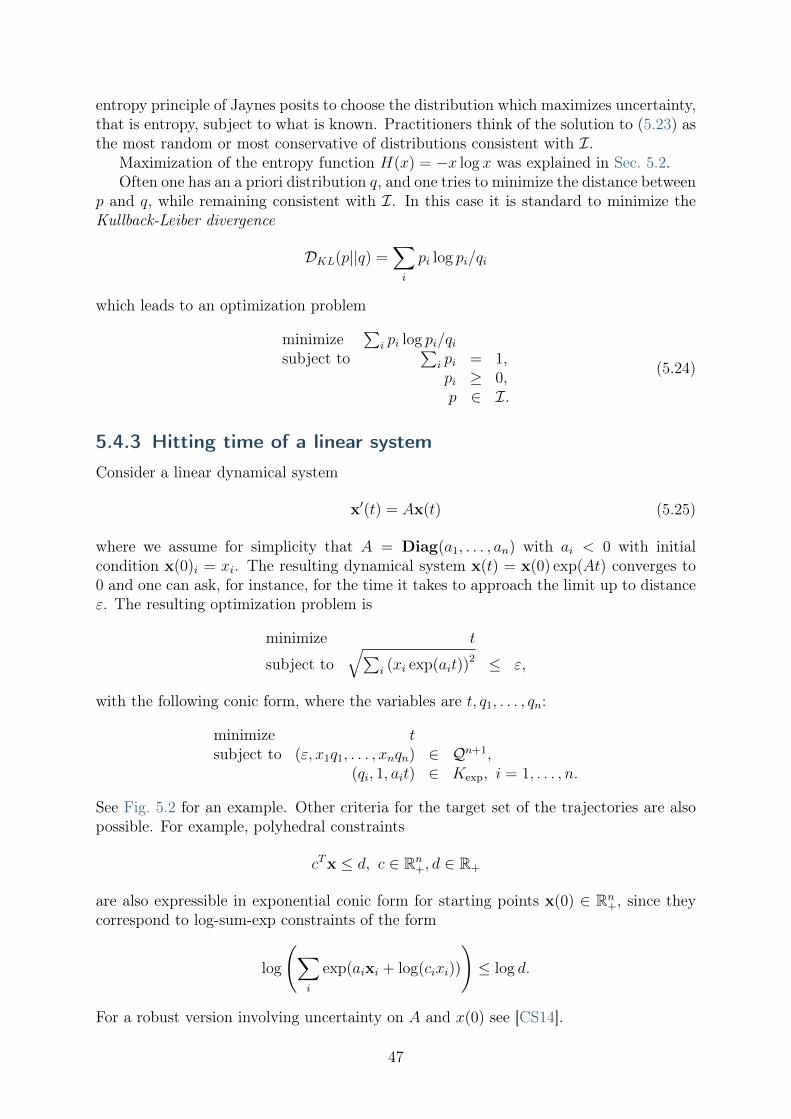
Fig. 5.2: With 𝐴 = Diag(−0.3,−0.06) and starting point 𝑥(0) = (2.2, 1.3) the trajectoryreaches distance 𝜀 = 0.5 from origin at time 𝑡 ≈ 15.936.

5.4.4 Logistic regression

Logistic regression is a technique of training a binary classifier. We are given a trainingset of examples 𝑥1, . . . , 𝑥𝑛 ∈ R𝑑 together with labels 𝑦𝑖 ∈ {0, 1}. The goal is to traina classifier capable of assigning new data points to either class 0 or 1. Specifically, thelabels should be assigned by computing

ℎ𝜃(𝑥) =1

1 + exp(−𝜃𝑇𝑥)(5.26)

and choosing label 𝑦 = 0 if ℎ𝜃(𝑥) < 12

and 𝑦 = 1 for ℎ𝜃(𝑥) ≥ 12. Here ℎ𝜃(𝑥) is interpreted

as the probability that 𝑥 belongs to class 1. The optimal parameter vector 𝜃 should belearned from the training set, so as to maximize the likelihood function:∏︁

𝑖

ℎ𝜃(𝑥𝑖)𝑦𝑖(1 − ℎ𝜃(𝑥𝑖))

1−𝑦𝑖 .

By taking logarithms and adding regularization with respect to 𝜃 we reach an uncon-strained optimization problem

minimize𝜃∈R𝑑 𝜆‖𝜃‖2 +∑︁𝑖

−𝑦𝑖 log(ℎ𝜃(𝑥𝑖)) − (1 − 𝑦𝑖) log(1 − ℎ𝜃(𝑥𝑖)). (5.27)

Problem (5.27) is convex, and can be more explicitly written as

minimize∑︀

𝑖 𝑡𝑖 + 𝜆𝑟subject to 𝑡𝑖 ≥ − log(ℎ𝜃(𝑥)) = log(1 + exp(−𝜃𝑇𝑥𝑖)) if 𝑦𝑖 = 1,

𝑡𝑖 ≥ − log(1 − ℎ𝜃(𝑥)) = log(1 + exp(𝜃𝑇𝑥𝑖)) if 𝑦𝑖 = 0,𝑟 ≥ ‖𝜃‖2,

involving softplus type constraints (see Sec. 5.2) and a quadratic cone. See Fig. 5.3 foran example.

48

Fig. 5.3: Logistic regression example with none, medium and strong regularization (small,medium, large 𝜆). The two-dimensional dataset was converted into a feature vector𝑥 ∈ R28 using monomial coordinates of degrees at most 6. Without regularization we getobvious overfitting.

49

Chapter 6

Semidefinite optimization

In this chapter we extend the conic optimization framework introduced before with sym-metric positive semidefinite matrix variables.

6.1 Introduction to semidefinite matrices

6.1.1 Semidefinite matrices and cones

A symmetric matrix 𝑋 ∈ 𝒮𝑛 is called symmetric positive semidefinite if

𝑧𝑇𝑋𝑧 ≥ 0, ∀𝑧 ∈ R𝑛.

We then define the cone of symmetric positive semidefinite matrices as

𝒮𝑛+ = {𝑋 ∈ 𝒮𝑛 | 𝑧𝑇𝑋𝑧 ≥ 0, ∀𝑧 ∈ R𝑛}. (6.1)

For brevity we will often use the shorter notion semidefinite instead of symmetric positivesemidefinite, and we will write 𝑋 ⪰ 𝑌 (𝑋 ⪯ 𝑌 ) as shorthand notation for (𝑋 −𝑌 ) ∈ 𝒮𝑛

+

((𝑌 −𝑋) ∈ 𝒮𝑛+). As inner product for semidefinite matrices, we use the standard trace

inner product for general matrices, i.e.,

⟨𝐴,𝐵⟩ := tr(𝐴𝑇𝐵) =∑︁𝑖𝑗

𝑎𝑖𝑗𝑏𝑖𝑗.

It is easy to see that (6.1) indeed specifies a convex cone; it is pointed (with origin𝑋 = 0), and 𝑋, 𝑌 ∈ 𝒮𝑛

+ implies that (𝛼𝑋 + 𝛽𝑌 ) ∈ 𝒮𝑛+, 𝛼, 𝛽 ≥ 0. Let us review a

few equivalent definitions of 𝒮𝑛+. It is well-known that every symmetric matrix 𝐴 has a

spectral factorization

𝐴 =𝑛∑︁

𝑖=1

𝜆𝑖𝑞𝑖𝑞𝑇𝑖 .

where 𝑞𝑖 ∈ R𝑛 are the (orthogonal) eigenvectors and 𝜆𝑖 are eigenvalues of 𝐴. Using thespectral factorization of 𝐴 we have

𝑥𝑇𝐴𝑥 =𝑛∑︁

𝑖=1

𝜆𝑖(𝑥𝑇 𝑞𝑖)

2,

50

which shows that 𝑥𝑇𝐴𝑥 ≥ 0 ⇔ 𝜆𝑖 ≥ 0, 𝑖 = 1, . . . , 𝑛. In other words,

𝒮𝑛+ = {𝑋 ∈ 𝒮𝑛 | 𝜆𝑖(𝑋) ≥ 0, 𝑖 = 1, . . . , 𝑛}. (6.2)

Another useful characterization is that 𝐴 ∈ 𝒮𝑛+ if and only if it is a Grammian matrix

𝐴 = 𝑉 𝑇𝑉 . Here 𝑉 is called the Cholesky factor of 𝐴. Using the Grammian representationwe have

𝑥𝑇𝐴𝑥 = 𝑥𝑇𝑉 𝑇𝑉 𝑥 = ‖𝑉 𝑥‖22,

i.e., if 𝐴 = 𝑉 𝑇𝑉 then 𝑥𝑇𝐴𝑥 ≥ 0 for all 𝑥. On the other hand, from the positivespectral factorization 𝐴 = 𝑄Λ𝑄𝑇 we have 𝐴 = 𝑉 𝑇𝑉 with 𝑉 = Λ1/2𝑄𝑇 , where Λ1/2 =Diag(

√𝜆1, . . . ,

√𝜆𝑛). We thus have the equivalent characterization

𝒮𝑛+ = {𝑋 ∈ 𝒮𝑛

+ | 𝑋 = 𝑉 𝑇𝑉 for some 𝑉 ∈ R𝑛×𝑛}. (6.3)

In a completely analogous way we define the cone of symmetric positive definite matricesas

𝒮𝑛++ = {𝑋 ∈ 𝒮𝑛 | 𝑧𝑇𝑋𝑧 > 0, ∀𝑧 ∈ R𝑛}

= {𝑋 ∈ 𝒮𝑛 | 𝜆𝑖(𝑋) > 0, 𝑖 = 1, . . . , 𝑛}= {𝑋 ∈ 𝒮𝑛

+ | 𝑋 = 𝑉 𝑇𝑉 for some 𝑉 ∈ R𝑛×𝑛, rank(𝑉 ) = 𝑛},

and we write 𝑋 ≻ 𝑌 (𝑋 ≺ 𝑌 ) as shorthand notation for (𝑋−𝑌 ) ∈ 𝒮𝑛++ ((𝑌 −𝑋) ∈ 𝒮𝑛

++).The one dimensional cone 𝒮1

+ simply corresponds to R+. Similarly consider

𝑋 =

[︂𝑥1 𝑥3

𝑥3 𝑥2

]︂with determinant det(𝑋) = 𝑥1𝑥2 − 𝑥2

3 = 𝜆1𝜆2 and trace tr(𝑋) = 𝑥1 + 𝑥2 = 𝜆1 + 𝜆2.Therefore 𝑋 has positive eigenvalues if and only if

𝑥1𝑥2 ≥ 𝑥23, 𝑥1, 𝑥2 ≥ 0,

which characterizes a three-dimensional scaled rotated cone, i.e.,[︂𝑥1 𝑥3

𝑥3 𝑥2

]︂∈ 𝒮2

+ ⇐⇒ (𝑥1, 𝑥2, 𝑥3

√2) ∈ 𝒬3

𝑟.

More generally we have

𝑥 ∈ R𝑛+ ⇐⇒ Diag(𝑥) ∈ 𝒮𝑛

+

and

(𝑡, 𝑥) ∈ 𝒬𝑛+1 ⇐⇒[︂

𝑡 𝑥𝑇

𝑥 𝑡𝐼

]︂∈ 𝒮𝑛+1

+ ,

where the latter equivalence follows immediately from Lemma 6.1. Thus both the linearand quadratic cone are embedded in the semidefinite cone. In practice, however, linearand quadratic cones should never be described using semidefinite constraints, which wouldresult in a large performance penalty by squaring the number of variables.

51

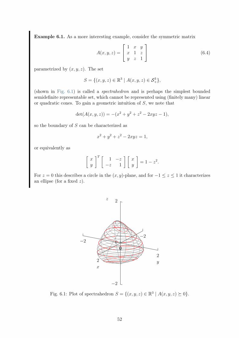
Example 6.1. As a more interesting example, consider the symmetric matrix

𝐴(𝑥, 𝑦, 𝑧) =

⎡⎣ 1 𝑥 𝑦𝑥 1 𝑧𝑦 𝑧 1

⎤⎦ (6.4)

parametrized by (𝑥, 𝑦, 𝑧). The set

𝑆 = {(𝑥, 𝑦, 𝑧) ∈ R3 | 𝐴(𝑥, 𝑦, 𝑧) ∈ 𝒮3+},

(shown in Fig. 6.1) is called a spectrahedron and is perhaps the simplest boundedsemidefinite representable set, which cannot be represented using (finitely many) linearor quadratic cones. To gain a geometric intuition of 𝑆, we note that

det(𝐴(𝑥, 𝑦, 𝑧)) = −(𝑥2 + 𝑦2 + 𝑧2 − 2𝑥𝑦𝑧 − 1),

so the boundary of 𝑆 can be characterized as

𝑥2 + 𝑦2 + 𝑧2 − 2𝑥𝑦𝑧 = 1,

or equivalently as [︂𝑥𝑦

]︂𝑇 [︂1 −𝑧

−𝑧 1

]︂ [︂𝑥𝑦

]︂= 1 − 𝑧2.

For 𝑧 = 0 this describes a circle in the (𝑥, 𝑦)-plane, and for −1 ≤ 𝑧 ≤ 1 it characterizesan ellipse (for a fixed 𝑧).

Fig. 6.1: Plot of spectrahedron 𝑆 = {(𝑥, 𝑦, 𝑧) ∈ R3 | 𝐴(𝑥, 𝑦, 𝑧) ⪰ 0}.

52

6.1.2 Properties of semidefinite matrices

Many useful properties of (semi)definite matrices follow directly from the definitions(6.1)-(6.3) and their definite counterparts.

• The diagonal elements of 𝐴 ∈ 𝒮𝑛+ are nonnegative. Let 𝑒𝑖 denote the 𝑖th standard

basis vector (i.e., [𝑒𝑖]𝑗 = 0, 𝑗 ̸= 𝑖, [𝑒𝑖]𝑖 = 1). Then 𝐴𝑖𝑖 = 𝑒𝑇𝑖 𝐴𝑒𝑖, so (6.1) implies that𝐴𝑖𝑖 ≥ 0.

• A block-diagonal matrix 𝐴 = Diag(𝐴1, . . . 𝐴𝑝) is (semi)definite if and only if eachdiagonal block 𝐴𝑖 is (semi)definite.

• Given a quadratic transformation 𝑀 := 𝐵𝑇𝐴𝐵, 𝑀 ≻ 0 if and only if 𝐴 ≻ 0and 𝐵 has full rank. This follows directly from the Grammian characterization𝑀 = (𝑉 𝐵)𝑇 (𝑉 𝐵). For 𝑀 ⪰ 0 we only require that 𝐴 ⪰ 0. As an example, if 𝐴 is(semi)definite then so is any permutation 𝑃 𝑇𝐴𝑃 .

• Any principal submatrix of 𝐴 ∈ 𝒮𝑛+ (𝐴 restricted to the same set of rows as columns)

is positive semidefinite; this follows by restricting the Grammian characterization𝐴 = 𝑉 𝑇𝑉 to a submatrix of 𝑉 .

• The inner product of positive (semi)definite matrices is positive (nonnegative). Forany 𝐴,𝐵 ∈ 𝒮𝑛

++ let 𝐴 = 𝑈𝑇𝑈 and 𝐵 = 𝑉 𝑇𝑉 where 𝑈 and 𝑉 have full rank. Then

⟨𝐴,𝐵⟩ = tr(𝑈𝑇𝑈𝑉 𝑇𝑉 ) = ‖𝑈𝑉 𝑇‖2𝐹 > 0,

where strict positivity follows from the assumption that 𝑈 has full column-rank,i.e., 𝑈𝑉 𝑇 ̸= 0.

• The inverse of a positive definite matrix is positive definite. This follows from thepositive spectral factorization 𝐴 = 𝑄Λ𝑄𝑇 , which gives us

𝐴−1 = 𝑄𝑇Λ−1𝑄

where Λ𝑖𝑖 > 0. If 𝐴 is semidefinite then the pseudo-inverse 𝐴† of 𝐴 is semidefinite.

• Consider a matrix 𝑋 ∈ 𝒮𝑛 partitioned as

𝑋 =

[︂𝐴 𝐵𝑇

𝐵 𝐶

]︂.

Let us find necessary and sufficient conditions for 𝑋 ≻ 0. We know that 𝐴 ≻ 0 and𝐶 ≻ 0 (since any principal submatrix must be positive definite). Furthermore, wecan simplify the analysis using a nonsingular transformation

𝐿 =

[︂𝐼 0𝐹 𝐼

]︂

53

to diagonalize 𝑋 as 𝐿𝑋𝐿𝑇 = 𝐷, where 𝐷 is block-diagonal. Note that det(𝐿) = 1,so 𝐿 is indeed nonsingular. Then 𝑋 ≻ 0 if and only if 𝐷 ≻ 0. Expanding 𝐿𝑋𝐿𝑇 =𝐷, we get [︂

𝐴 𝐴𝐹 𝑇 + 𝐵𝑇

𝐹𝐴 + 𝐵 𝐹𝐴𝐹 𝑇 + 𝐹𝐵𝑇 + 𝐵𝐹 𝑇 + 𝐶

]︂=

[︂𝐷1 00 𝐷2

]︂.

Since det(𝐴) ̸= 0 (by assuming that 𝐴 ≻ 0) we see that 𝐹 = −𝐵𝐴−1 and directsubstitution gives us [︂

𝐴 00 𝐶 −𝐵𝐴−1𝐵𝑇

]︂=

[︂𝐷1 00 𝐷2

]︂.

In the last part we have thus established the following useful result.

Lemma 6.1 (Schur complement lemma). A symmetric matrix

𝑋 =

[︂𝐴 𝐵𝑇

𝐵 𝐶

]︂.

is positive definite if and only if

𝐴 ≻ 0, 𝐶 −𝐵𝐴−1𝐵𝑇 ≻ 0.

6.2 Semidefinite modeling

Having discussed different characterizations and properties of semidefinite matrices, wenext turn to different functions and sets that can be modeled using semidefinite conesand variables. Most of those representations involve semidefinite matrix-valued affinefunctions, which we discuss next.

6.2.1 Linear matrix inequalities

Consider an affine matrix-valued mapping 𝐴 : R𝑛 ↦→ 𝒮𝑚:

𝐴(𝑥) = 𝐴0 + 𝑥1𝐴1 + · · · + 𝑥𝑛𝐴𝑛. (6.5)

A linear matrix inequality (LMI) is a constraint of the form

𝐴0 + 𝑥1𝐴1 + · · · + 𝑥𝑛𝐴𝑛 ⪰ 0 (6.6)

in the variable 𝑥 ∈ R𝑛 with symmetric coefficients 𝐴𝑖 ∈ 𝒮𝑚, 𝑖 = 0, . . . , 𝑛. As a simpleexample consider the matrix in (6.4),

𝐴(𝑥, 𝑦, 𝑧) = 𝐴0 + 𝑥𝐴1 + 𝑦𝐴2 + 𝑧𝐴3 ⪰ 0

with

𝐴0 = 𝐼, 𝐴1 =

⎡⎣ 0 1 01 0 00 0 0

⎤⎦ , 𝐴2 =

⎡⎣ 0 0 10 0 01 0 0

⎤⎦ , 𝐴3 =

⎡⎣ 0 0 00 0 10 1 0

⎤⎦ .

54

Alternatively, we can describe the linear matrix inequality 𝐴(𝑥, 𝑦, 𝑧) ⪰ 0 as

𝑋 ∈ 𝒮3+, 𝑥11 = 𝑥22 = 𝑥33 = 1,

i.e., as a semidefinite variable with fixed diagonal; these two alternative formulationsillustrate the difference between primal and dual form of semidefinite problems, see Sec.8.6.

6.2.2 Eigenvalue optimization

Consider a symmetric matrix 𝐴 ∈ 𝒮𝑚 and let its eigenvalues be denoted by

𝜆1(𝐴) ≥ 𝜆2(𝐴) ≥ · · · ≥ 𝜆𝑚(𝐴).

A number of different functions of 𝜆𝑖 can then be described using a mix of linear andsemidefinite constraints.

Sum of eigenvalues

The sum of the eigenvalues corresponds to𝑚∑︁𝑖=1

𝜆𝑖(𝐴) = tr(𝐴).

Largest eigenvalue

The largest eigenvalue can be characterized in epigraph form 𝜆1(𝐴) ≤ 𝑡 as

𝑡𝐼 − 𝐴 ⪰ 0. (6.7)

To verify this, suppose we have a spectral factorization 𝐴 = 𝑄Λ𝑄𝑇 where 𝑄 is orthogonaland Λ is diagonal. Then 𝑡 is an upper bound on the largest eigenvalue if and only if

𝑄𝑇 (𝑡𝐼 − 𝐴)𝑄 = 𝑡𝐼 − Λ ⪰ 0.

Thus we can minimize the largest eigenvalue of 𝐴.

Smallest eigenvalue

The smallest eigenvalue can be described in hypograph form 𝜆𝑚(𝐴) ≥ 𝑡 as

𝐴 ⪰ 𝑡𝐼, (6.8)

i.e., we can maximize the smallest eigenvalue of 𝐴.

Eigenvalue spread

The eigenvalue spread can be modeled in epigraph form

𝜆1(𝐴) − 𝜆𝑚(𝐴) ≤ 𝑡

by combining the two linear matrix inequalities in (6.7) and (6.8), i.e.,

𝑧𝐼 ⪯ 𝐴 ⪯ 𝑠𝐼,𝑠− 𝑧 ≤ 𝑡.

(6.9)

55

Spectral radius

The spectral radius 𝜌(𝐴) := max𝑖 |𝜆𝑖(𝐴)| can be modeled in epigraph form 𝜌(𝐴) ≤ 𝑡 usingtwo linear matrix inequalities

−𝑡𝐼 ⪯ 𝐴 ⪯ 𝑡𝐼.

Condition number of a positive definite matrix

Suppose now that 𝐴 ∈ 𝒮𝑚+ . The condition number of a positive definite matrix can be

minimized by noting that 𝜆1(𝐴)/𝜆𝑚(𝐴) ≤ 𝑡 if and only if there exists a 𝜇 > 0 such that

𝜇𝐼 ⪯ 𝐴 ⪯ 𝜇𝑡𝐼,

or equivalently if and only if 𝐼 ⪯ 𝜇−1𝐴 ⪯ 𝑡𝐼. If 𝐴 = 𝐴(𝑥) is represented as in (6.5) thena change of variables 𝑧 := 𝑥/𝜇, 𝜈 := 1/𝜇 leads to a problem of the form

minimize 𝑡subject to 𝐼 ⪯ 𝜈𝐴0 +

∑︀𝑚𝑖=1 𝑧𝑖𝐴𝑖 ⪯ 𝑡𝐼,

(6.10)

from which we recover the solution 𝑥 = 𝑧/𝜈. In essence, we first normalize the spectrumby the smallest eigenvalue, and then minimize the largest eigenvalue of the normalizedlinear matrix inequality. Compare Sec. 2.2.5.

6.2.3 Log-determinant

Consider again a symmetric positive-definite matrix 𝐴 ∈ 𝒮𝑚+ . The determinant

det(𝐴) =𝑚∏︁𝑖=1

𝜆𝑖(𝐴)

is neither convex or concave, but log det(𝐴) is concave and we can write the inequality

𝑡 ≤ log det(𝐴)

in the form of the following problem:[︂𝐴 𝑍𝑍𝑇 diag(𝑍)

]︂⪰ 0,

𝑍 is lower triangular,𝑡 ≤∑︀𝑖 log𝑍𝑖𝑖.

(6.11)

The equivalence of the two problems follows from Lemma 6.1 and subadditivity of deter-minant for semidefinite matrices. That is:

0 ≤ det(𝐴− 𝑍𝑇diag(𝑍)−1𝑍) ≤ det(𝐴) − det(𝑍𝑇diag(𝑍)−1𝑍)= det(𝐴) − det(𝑍).

On the other hand the optimal value det(𝐴) is attained for 𝑍 = 𝐿𝐷 if 𝐴 = 𝐿𝐷𝐿𝑇 is theLDL factorization of 𝐴.

The last inequality in problem (6.11) can of course be modeled using the exponentialcone as in Sec. 5.2. Note that we can replace that bound with 𝑡 ≤ (

∏︀𝑖 𝑍𝑖𝑖)

1/𝑚 to getinstead the model of 𝑡 ≤ det(𝐴)1/𝑚 using Sec. 4.2.4.

56

6.2.4 Singular value optimization

We next consider a non-square matrix 𝐴 ∈ R𝑚×𝑝. Assume 𝑝 ≤ 𝑚 and denote the singularvalues of 𝐴 by

𝜎1(𝐴) ≥ 𝜎2(𝐴) ≥ · · · ≥ 𝜎𝑝(𝐴) ≥ 0.

The singular values are connected to the eigenvalues of 𝐴𝑇𝐴 via

𝜎𝑖(𝐴) =√︀

𝜆𝑖(𝐴𝑇𝐴), (6.12)

and if 𝐴 is square and symmetric then 𝜎𝑖(𝐴) = |𝜆𝑖(𝐴)|. We show next how to optimizeseveral functions of the singular values.

Largest singular value

The epigraph 𝜎1(𝐴) ≤ 𝑡 can be characterized using (6.12) as

𝐴𝑇𝐴 ⪯ 𝑡2𝐼,

which from Schur’s lemma is equivalent to[︂𝑡𝐼 𝐴𝐴𝑇 𝑡𝐼

]︂⪰ 0. (6.13)

The largest singular value 𝜎1(𝐴) is also called the spectral norm or the ℓ2-norm of 𝐴,‖𝐴‖2 := 𝜎1(𝐴).

Sum of singular values

The trace norm or the nuclear norm of 𝑋 is the dual of the ℓ2-norm:

‖𝑋‖* = sup‖𝑍‖2≤1

tr(𝑋𝑇𝑍). (6.14)

It turns out that the nuclear norm corresponds to the sum of the singular values,

‖𝑋‖* =𝑚∑︁𝑖=1

𝜎𝑖(𝑋) =𝑛∑︁

𝑖=1

√︀𝜆𝑖(𝑋𝑇𝑋), (6.15)

which is easy to verify using singular value decomposition 𝑋 = 𝑈Σ𝑉 𝑇 . We have

sup‖𝑍‖2≤1

tr(𝑋𝑇𝑍) = sup‖𝑍‖2≤1

tr(Σ𝑇𝑈𝑇𝑍𝑉 )

= sup‖𝑌 ‖2≤1

tr(Σ𝑇𝑌 )

= sup|𝑦𝑖|≤1

𝑝∑︁𝑖=1

𝜎𝑖𝑦𝑖 =

𝑝∑︁𝑖=1

𝜎𝑖.

which shows (6.15). Alternatively, we can express (6.14) as the solution to

maximize tr(𝑋𝑇𝑍)

subject to[︂

𝐼 𝑍𝑇

𝑍 𝐼

]︂⪰ 0,

(6.16)

57

with the dual problem (see Example 8.8)

minimize tr(𝑈 + 𝑉 )/2

subject to[︂

𝑈 𝑋𝑇

𝑋 𝑉

]︂⪰ 0.

(6.17)

In other words, using strong duality we can characterize the epigraph ‖𝐴‖* ≤ 𝑡 with[︂𝑈 𝐴𝑇

𝐴 𝑉

]︂⪰ 0, tr(𝑈 + 𝑉 )/2 ≤ 𝑡. (6.18)

For a symmetric matrix the nuclear norm corresponds to the sum of absolute values ofeigenvalues, and for a semidefinite matrix it simply corresponds to the trace of the matrix.

6.2.5 Matrix inequalities from Schur’s Lemma

Several quadratic or quadratic-over-linear matrix inequalities follow immediately fromSchur’s lemma. Suppose 𝐴 : R𝑚×𝑝 and 𝐵 : R𝑝×𝑝 are matrix variables. Then

𝐴𝑇𝐵−1𝐴 ⪯ 𝐶

if and only if [︂𝐶 𝐴𝑇

𝐴 𝐵

]︂⪰ 0.

6.2.6 Nonnegative polynomials

We next consider characterizations of polynomials constrained to be nonnegative on thereal axis. To that end, consider a polynomial basis function

𝑣(𝑡) =(︀1, 𝑡, . . . , 𝑡2𝑛

)︀.

It is then well-known that a polynomial 𝑓 : R ↦→ R of even degree 2𝑛 is nonnegative onthe entire real axis

𝑓(𝑡) := 𝑥𝑇𝑣(𝑡) = 𝑥0 + 𝑥1𝑡 + · · · + 𝑥2𝑛𝑡2𝑛 ≥ 0, ∀𝑡 (6.19)

if and only if it can be written as a sum of squared polynomials of degree 𝑛 (or less), i.e.,for some 𝑞1, 𝑞2 ∈ R𝑛+1

𝑓(𝑡) = (𝑞𝑇1 𝑢(𝑡))2 + (𝑞𝑇2 𝑢(𝑡))2, 𝑢(𝑡) := (1, 𝑡, . . . , 𝑡𝑛). (6.20)

It turns out that an equivalent characterization of {𝑥 | 𝑥𝑇𝑣(𝑡) ≥ 0, ∀𝑡} can be given interms of a semidefinite variable 𝑋,

𝑥𝑖 = ⟨𝑋,𝐻𝑖⟩, 𝑖 = 0, . . . , 2𝑛, 𝑋 ∈ 𝒮𝑛+1+ . (6.21)

where 𝐻𝑛+1𝑖 ∈ R(𝑛+1)×(𝑛+1) are Hankel matrices

[𝐻𝑖]𝑘𝑙 =

{︂1, 𝑘 + 𝑙 = 𝑖,0, otherwise.

58

When there is no ambiguity, we drop the superscript on 𝐻𝑖. For example, for 𝑛 = 2 wehave

𝐻0 =

⎡⎣ 1 0 00 0 00 0 0

⎤⎦ , 𝐻1 =

⎡⎣ 0 1 01 0 00 0 0

⎤⎦ , . . . 𝐻4 =

⎡⎣ 0 0 00 0 00 0 1

⎤⎦ .

To verify that (6.19) and (6.21) are equivalent, we first note that

𝑢(𝑡)𝑢(𝑡)𝑇 =2𝑛∑︁𝑖=0

𝐻𝑖𝑣𝑖(𝑡),

i.e., ⎡⎢⎢⎢⎣1𝑡...𝑡𝑛

⎤⎥⎥⎥⎦⎡⎢⎢⎢⎣

1𝑡...𝑡𝑛

⎤⎥⎥⎥⎦𝑇

=

⎡⎢⎢⎢⎣1 𝑡 . . . 𝑡𝑛

𝑡 𝑡2 . . . 𝑡𝑛+1

...... . . . ...

𝑡𝑛 𝑡𝑛+1 . . . 𝑡2𝑛

⎤⎥⎥⎥⎦ .

Assume next that 𝑓(𝑡) ≥ 0. Then from (6.20) we have

𝑓(𝑡) = (𝑞𝑇1 𝑢(𝑡))2 + (𝑞𝑇2 𝑢(𝑡))2

= ⟨𝑞1𝑞𝑇1 + 𝑞2𝑞𝑇2 , 𝑢(𝑡)𝑢(𝑡)𝑇 ⟩

=∑︀2𝑛

𝑖=0⟨𝑞1𝑞𝑇1 + 𝑞2𝑞𝑇2 , 𝐻𝑖⟩𝑣𝑖(𝑡),

i.e., we have 𝑓(𝑡) = 𝑥𝑇𝑣(𝑡) with 𝑥𝑖 = ⟨𝑋,𝐻𝑖⟩, 𝑋 = (𝑞1𝑞𝑇1 +𝑞2𝑞

𝑇2 ) ⪰ 0. Conversely, assume

that (6.21) holds. Then

𝑓(𝑡) =2𝑛∑︁𝑖=0

⟨𝐻𝑖, 𝑋⟩𝑣𝑖(𝑡) = ⟨𝑋,2𝑛∑︁𝑖=0

𝐻𝑖𝑣𝑖(𝑡)⟩ = ⟨𝑋, 𝑢(𝑡)𝑢(𝑡)𝑇 ⟩ ≥ 0

since 𝑋 ⪰ 0. In summary, we can characterize the cone of nonnegative polynomials overthe real axis as

𝐾𝑛∞ = {𝑥 ∈ R𝑛+1 | 𝑥𝑖 = ⟨𝑋,𝐻𝑖⟩, 𝑖 = 0, . . . , 2𝑛, 𝑋 ∈ 𝒮𝑛+1

+ }. (6.22)

Checking nonnegativity of a univariate polynomial thus corresponds to a semidefinitefeasibility problem.

Nonnegativity on a finite interval

As an extension we consider a basis function of degree 𝑛,

𝑣(𝑡) = (1, 𝑡, . . . , 𝑡𝑛).

A polynomial 𝑓(𝑡) := 𝑥𝑇𝑣(𝑡) is then nonnegative on a subinterval 𝐼 = [𝑎, 𝑏] ⊂ R if andonly 𝑓(𝑡) can be written as a sum of weighted squares,

𝑓(𝑡) = 𝑤1(𝑡)(𝑞𝑇1 𝑢1(𝑡))

2 + 𝑤2(𝑡)(𝑞𝑇2 𝑢2(𝑡))

2

where 𝑤𝑖(𝑡) are polynomials nonnegative on [𝑎, 𝑏]. To describe the cone

𝐾𝑛𝑎,𝑏 = {𝑥 ∈ R𝑛+1 | 𝑓(𝑡) = 𝑥𝑇𝑣(𝑡) ≥ 0, ∀𝑡 ∈ [𝑎, 𝑏]}

we distinguish between polynomials of odd and even degree.

59

• Even degree. Let 𝑛 = 2𝑚 and denote

𝑢1(𝑡) = (1, 𝑡, . . . , 𝑡𝑚), 𝑢2(𝑡) = (1, 𝑡, . . . , 𝑡𝑚−1).

We choose 𝑤1(𝑡) = 1 and 𝑤2(𝑡) = (𝑡 − 𝑎)(𝑏 − 𝑡) and note that 𝑤2(𝑡) ≥ 0 on [𝑎, 𝑏].Then 𝑓(𝑡) ≥ 0,∀𝑡 ∈ [𝑎, 𝑏] if and only if

𝑓(𝑡) = (𝑞𝑇1 𝑢1(𝑡))2 + 𝑤2(𝑡)(𝑞

𝑇2 𝑢2(𝑡))

2

for some 𝑞1, 𝑞2, and an equivalent semidefinite characterization can be found as

𝐾𝑛𝑎,𝑏 = {𝑥 ∈ R𝑛+1 | 𝑥𝑖 = ⟨𝑋1, 𝐻

𝑚𝑖 ⟩ + ⟨𝑋2, (𝑎 + 𝑏)𝐻𝑚−1

𝑖−1 − 𝑎𝑏𝐻𝑚−1𝑖 −𝐻𝑚−1

𝑖−2 ⟩,𝑖 = 0, . . . , 𝑛, 𝑋1 ∈ 𝒮𝑚

+ , 𝑋2 ∈ 𝒮𝑚−1+ }.

(6.23)

• Odd degree. Let 𝑛 = 2𝑚 + 1 and denote 𝑢(𝑡) = (1, 𝑡, . . . , 𝑡𝑚). We choose 𝑤1(𝑡) =(𝑡− 𝑎) and 𝑤2(𝑡) = (𝑏− 𝑡). We then have that 𝑓(𝑡) = 𝑥𝑇𝑣(𝑡) ≥ 0,∀𝑡 ∈ [𝑎, 𝑏] if andonly if

𝑓(𝑡) = (𝑡− 𝑎)(𝑞𝑇1 𝑢(𝑡))2 + (𝑏− 𝑡)(𝑞𝑇2 𝑢(𝑡))2

for some 𝑞1, 𝑞2, and an equivalent semidefinite characterization can be found as

𝐾𝑛𝑎,𝑏 = {𝑥 ∈ R𝑛+1 | 𝑥𝑖 = ⟨𝑋1, 𝐻

𝑚𝑖−1 − 𝑎𝐻𝑚

𝑖 ⟩ + ⟨𝑋2, 𝑏𝐻𝑚𝑖 −𝐻𝑚

𝑖−1⟩,𝑖 = 0, . . . , 𝑛, 𝑋1, 𝑋2 ∈ 𝒮𝑚

+ }. (6.24)

6.2.7 Hermitian matrices

Semidefinite optimization can be extended to complex-valued matrices. To that end, letℋ𝑛 denote the cone of Hermitian matrices of order 𝑛, i.e.,

𝑋 ∈ ℋ𝑛 ⇐⇒ 𝑋 ∈ C𝑛×𝑛, 𝑋𝐻 = 𝑋, (6.25)

where superscript ’𝐻’ denotes Hermitian (or complex) transposition. Then 𝑋 ∈ ℋ𝑛+ if

and only if

𝑧𝐻𝑋𝑧 = (ℜ𝑧 − 𝑖ℑ𝑧)𝑇 (ℜ𝑋 + 𝑖ℑ𝑋)(ℜ𝑧 + 𝑖ℑ𝑧)

=

[︂ℜ𝑧ℑ𝑧

]︂𝑇 [︂ ℜ𝑋 −ℑ𝑋ℑ𝑋 ℜ𝑋

]︂ [︂ℜ𝑧ℑ𝑧

]︂≥ 0, ∀𝑧 ∈ C𝑛.

In other words,

𝑋 ∈ ℋ𝑛+ ⇐⇒

[︂ℜ𝑋 −ℑ𝑋ℑ𝑋 ℜ𝑋

]︂∈ 𝒮2𝑛

+ . (6.26)

Note that (6.25) implies skew-symmetry of ℑ𝑋, i.e., ℑ𝑋 = −ℑ𝑋𝑇 .

60

6.2.8 Nonnegative trigonometric polynomials

As a complex-valued variation of the sum-of-squares representation we consider trigono-metric polynomials; optimization over cones of nonnegative trigonometric polynomialshas several important engineering applications. Consider a trigonometric polynomialevaluated on the complex unit-circle

𝑓(𝑧) = 𝑥0 + 2ℜ(𝑛∑︁

𝑖=1

𝑥𝑖𝑧−𝑖), |𝑧| = 1 (6.27)

parametrized by 𝑥 ∈ R×C𝑛. We are interested in characterizing the cone of trigonometricpolynomials that are nonnegative on the angular interval [0, 𝜋],

𝐾𝑛0,𝜋 = {𝑥 ∈ R× C𝑛 | 𝑥0 + 2ℜ(

𝑛∑︁𝑖=1

𝑥𝑖𝑧−𝑖) ≥ 0, ∀𝑧 = 𝑒𝑗𝑡, 𝑡 ∈ [0, 𝜋]}.

Consider a complex-valued basis function

𝑣(𝑧) = (1, 𝑧, . . . , 𝑧𝑛).

The Riesz-Fejer Theorem states that a trigonometric polynomial 𝑓(𝑧) in (6.27) is non-negative (i.e., 𝑥 ∈ 𝐾𝑛

0,𝜋) if and only if for some 𝑞 ∈ C𝑛+1

𝑓(𝑧) = |𝑞𝐻𝑣(𝑧)|2. (6.28)

Analogously to Sec. 6.2.6 we have a semidefinite characterization of the sum-of-squaresrepresentation, i.e., 𝑓(𝑧) ≥ 0, ∀𝑧 = 𝑒𝑗𝑡, 𝑡 ∈ [0, 2𝜋] if and only if

𝑥𝑖 = ⟨𝑋,𝑇𝑖⟩, 𝑖 = 0, . . . , 𝑛, 𝑋 ∈ ℋ𝑛+1+ (6.29)

where 𝑇 𝑛+1𝑖 ∈ R(𝑛+1)×(𝑛+1) are Toeplitz matrices

[𝑇𝑖]𝑘𝑙 =

{︂1, 𝑘 − 𝑙 = 𝑖0, otherwise , 𝑖 = 0, . . . , 𝑛.

When there is no ambiguity, we drop the superscript on 𝑇𝑖. For example, for 𝑛 = 2 wehave

𝑇0 =

⎡⎣ 1 0 00 1 00 0 1

⎤⎦ , 𝑇1 =

⎡⎣ 0 0 01 0 00 1 0

⎤⎦ , 𝑇2 =

⎡⎣ 0 0 00 0 01 0 0

⎤⎦ .

To prove correctness of the semidefinite characterization, we first note that

𝑣(𝑧)𝑣(𝑧)𝐻 = 𝐼 +𝑛∑︁

𝑖=1

(𝑇𝑖𝑣𝑖(𝑧)) +𝑛∑︁

𝑖=1

(𝑇𝑖𝑣𝑖(𝑧))𝐻

i.e., ⎡⎢⎢⎢⎣1𝑧...𝑧𝑛

⎤⎥⎥⎥⎦⎡⎢⎢⎢⎣

1𝑧...𝑧𝑛

⎤⎥⎥⎥⎦𝐻

=

⎡⎢⎢⎢⎣1 𝑧−1 . . . 𝑧−𝑛

𝑧 1 . . . 𝑧1−𝑛

...... . . . ...

𝑧𝑛 𝑧𝑛−1 . . . 1

⎤⎥⎥⎥⎦ .

61

Next assume that (6.28) is satisfied. Then

𝑓(𝑧) = ⟨𝑞𝑞𝐻 , 𝑣(𝑧)𝑣(𝑧)𝐻⟩= ⟨𝑞𝑞𝐻 , 𝐼⟩ + ⟨𝑞𝑞𝐻 ,∑︀𝑛

𝑖=1 𝑇𝑖𝑣𝑖(𝑧)⟩ + ⟨𝑞𝑞𝐻 ,∑︀𝑛𝑖=1 𝑇

𝑇𝑖 𝑣𝑖(𝑧)⟩

= ⟨𝑞𝑞𝐻 , 𝐼⟩ +∑︀𝑛

𝑖=1⟨𝑞𝑞𝐻 , 𝑇𝑖⟩𝑣𝑖(𝑧) +∑︀𝑛

𝑖=1⟨𝑞𝑞𝐻 , 𝑇 𝑇𝑖 ⟩𝑣𝑖(𝑧)

= 𝑥0 + 2ℜ(∑︀𝑛

𝑖=1 𝑥𝑖𝑣𝑖(𝑧))

with 𝑥𝑖 = ⟨𝑞𝑞𝐻 , 𝑇𝑖⟩. Conversely, assume that (6.29) holds. Then

𝑓(𝑧) = ⟨𝑋, 𝐼⟩ +𝑛∑︁

𝑖=1

⟨𝑋,𝑇𝑖⟩𝑣𝑖(𝑧) +𝑛∑︁

𝑖=1

⟨𝑋,𝑇 𝑇𝑖 ⟩𝑣𝑖(𝑧) = ⟨𝑋, 𝑣(𝑧)𝑣(𝑧)𝐻⟩ ≥ 0.

In other words, we have shown that

𝐾𝑛0,𝜋 = {𝑥 ∈ R× C𝑛 | 𝑥𝑖 = ⟨𝑋,𝑇𝑖⟩, 𝑖 = 0, . . . , 𝑛, 𝑋 ∈ ℋ𝑛+1

+ }. (6.30)

Nonnegativity on a subinterval

We next sketch a few useful extensions. An extension of the Riesz-Fejer Theorem statesthat a trigonometric polynomial 𝑓(𝑧) of degree 𝑛 is nonnegative on 𝐼(𝑎, 𝑏) = {𝑧 | 𝑧 =𝑒𝑗𝑡, 𝑡 ∈ [𝑎, 𝑏] ⊆ [0, 𝜋]} if and only if it can be written as a weighted sum of squaredtrigonometric polynomials

𝑓(𝑧) = |𝑓1(𝑧)|2 + 𝑔(𝑧)|𝑓2(𝑧)|2

where 𝑓1, 𝑓2, 𝑔 are trigonemetric polynomials of degree 𝑛, 𝑛 − 𝑑 and 𝑑, respectively, and𝑔(𝑧) ≥ 0 on 𝐼(𝑎, 𝑏). For example 𝑔(𝑧) = 𝑧 + 𝑧−1 − 2 cos𝛼 is nonnegative on 𝐼(0, 𝛼), andit can be verified that 𝑓(𝑧) ≥ 0, ∀𝑧 ∈ 𝐼(0, 𝛼) if and only if

𝑥𝑖 = ⟨𝑋1, 𝑇𝑛+1𝑖 ⟩ + ⟨𝑋2, 𝑇

𝑛𝑖+1⟩ + ⟨𝑋2, 𝑇

𝑛𝑖−1⟩ − 2 cos(𝛼)⟨𝑋2, 𝑇

𝑛𝑖 ⟩,

for 𝑋1 ∈ ℋ𝑛+1+ , 𝑋2 ∈ ℋ𝑛

+, i.e.,

𝐾𝑛0,𝛼 = {𝑥 ∈ R× C𝑛 | 𝑥𝑖 = ⟨𝑋1, 𝑇

𝑛+1𝑖 ⟩ + ⟨𝑋2, 𝑇

𝑛𝑖+1⟩ + ⟨𝑋2, 𝑇

𝑛𝑖−1⟩

−2 cos(𝛼)⟨𝑋2, 𝑇𝑛𝑖 ⟩, 𝑋1 ∈ ℋ𝑛+1

+ , 𝑋2 ∈ ℋ𝑛+}.

(6.31)

Similarly 𝑓(𝑧) ≥ 0, ∀𝑧 ∈ 𝐼(𝛼, 𝜋) if and only if

𝑥𝑖 = ⟨𝑋1, 𝑇𝑛+1𝑖 ⟩ + ⟨𝑋2, 𝑇

𝑛𝑖+1⟩ + ⟨𝑋2, 𝑇

𝑛𝑖−1⟩ − 2 cos(𝛼)⟨𝑋2, 𝑇

𝑛𝑖 ⟩

i.e.,

𝐾𝑛𝛼,𝜋 = {𝑥 ∈ R× C𝑛 | 𝑥𝑖 = ⟨𝑋1, 𝑇

𝑛+1𝑖 ⟩ + ⟨𝑋2, 𝑇

𝑛𝑖+1⟩ + ⟨𝑋2, 𝑇

𝑛𝑖−1⟩

+2 cos(𝛼)⟨𝑋2, 𝑇𝑛𝑖 ⟩, 𝑋1 ∈ ℋ𝑛+1

+ , 𝑋2 ∈ ℋ𝑛+}.

(6.32)

6.3 Semidefinite optimization case studies

6.3.1 Nearest correlation matrix

We consider the set

𝑆 = {𝑋 ∈ 𝒮𝑛+ | 𝑋𝑖𝑖 = 1, 𝑖 = 1, . . . , 𝑛}

62

(shown in Fig. 6.1 for 𝑛 = 3). For 𝐴 ∈ 𝒮𝑛 the nearest correlation matrix is

𝑋⋆ = arg min𝑋∈𝑆

‖𝐴−𝑋‖𝐹 ,

i.e., the projection of 𝐴 onto the set 𝑆. To pose this as a conic optimization we definethe linear operator

svec(𝑈) = (𝑈11,√

2𝑈21, . . . ,√

2𝑈𝑛1, 𝑈22,√

2𝑈32, . . . ,√

2𝑈𝑛2, . . . , 𝑈𝑛𝑛),

which extracts and scales the lower-triangular part of 𝑈 . We then get a conic formulationof the nearest correlation problem exploiting symmetry of 𝐴−𝑋,

minimize 𝑡subject to ‖𝑧‖2 ≤ 𝑡,

svec(𝐴−𝑋) = 𝑧,diag(𝑋) = 𝑒,𝑋 ⪰ 0.

(6.33)

This is an example of a problem with both conic quadratic and semidefinite constraintsin primal form. We can add different constraints to the problem, for example a bound 𝛾on the smallest eigenvalue by replacing 𝑋 ⪰ 0 with 𝑋 ⪰ 𝛾𝐼.

6.3.2 Extremal ellipsoids

Given a polytope we can find the largest ellipsoid contained in the polytope, or thesmallest ellipsoid containing the polytope (for certain representations of the polytope).

Maximal inscribed ellipsoid

Consider a polytope

𝑆 = {𝑥 ∈ R𝑛 | 𝑎𝑇𝑖 𝑥 ≤ 𝑏𝑖, 𝑖 = 1, . . . ,𝑚}.

The ellipsoid

ℰ := {𝑥 | 𝑥 = 𝐶𝑢 + 𝑑, ‖𝑢‖ ≤ 1}

is contained in 𝑆 if and only if

max‖𝑢‖2≤1

𝑎𝑇𝑖 (𝐶𝑢 + 𝑑) ≤ 𝑏𝑖, 𝑖 = 1, . . . ,𝑚

or equivalently, if and only if

‖𝐶𝑎𝑖‖2 + 𝑎𝑇𝑖 𝑑 ≤ 𝑏𝑖, 𝑖 = 1, . . . ,𝑚.

Since Vol(ℰ) ≈ det(𝐶)1/𝑛 the maximum-volume inscribed ellipsoid is the solution to

maximize det(𝐶)subject to ‖𝐶𝑎𝑖‖2 + 𝑎𝑇𝑖 𝑑 ≤ 𝑏𝑖, 𝑖 = 1, . . . ,𝑚,

𝐶 ⪰ 0.

In Sec. 6.2.2 we show how to maximize the determinant of a positive definite matrix.

63

Minimal enclosing ellipsoid

Next consider a polytope given as the convex hull of a set of points,

𝑆 ′ = conv{𝑥1, 𝑥2, . . . , 𝑥𝑚}, 𝑥𝑖 ∈ R𝑛.

The ellipsoid

ℰ ′ := {𝑥 | ‖𝑃𝑥− 𝑐‖2 ≤ 1}

has Vol(ℰ ′) ≈ det(𝑃 )−1/𝑛, so the minimum-volume enclosing ellipsoid is the solution to

maximize det(𝑃 )subject to ‖𝑃𝑥𝑖 − 𝑐‖2 ≤ 1, 𝑖 = 1, . . . ,𝑚,

𝑃 ⪰ 0.

Fig. 6.2: Example of inner and outer ellipsoidal approximations of a pentagon in R2.

6.3.3 Polynomial curve-fitting

Consider a univariate polynomial of degree 𝑛,

𝑓(𝑡) = 𝑥0 + 𝑥1𝑡 + 𝑥2𝑡2 + · · · + 𝑥𝑛𝑡

𝑛.

Often we wish to fit such a polynomial to a given set of measurements or control points

{(𝑡1, 𝑦1), (𝑡2, 𝑦2), . . . , (𝑡𝑚, 𝑦𝑚)},

i.e., we wish to determine coefficients 𝑥𝑖, 𝑖 = 0, . . . , 𝑛 such that

𝑓(𝑡𝑗) ≈ 𝑦𝑗, 𝑗 = 1, . . . ,𝑚.

To that end, define the Vandermonde matrix

𝐴 =

⎡⎢⎢⎢⎣1 𝑡1 𝑡21 . . . 𝑡𝑛11 𝑡2 𝑡22 . . . 𝑡𝑛2...

......

...1 𝑡𝑚 𝑡2𝑚 . . . 𝑡𝑛𝑚

⎤⎥⎥⎥⎦ .

64

We can then express the desired curve-fit compactly as

𝐴𝑥 ≈ 𝑦,

i.e., as a linear expression in the coefficients 𝑥. When the degree of the polynomial equalsthe number measurements, 𝑛 = 𝑚, the matrix 𝐴 is square and non-singular (providedthere are no duplicate rows), so we can can solve

𝐴𝑥 = 𝑦

to find a polynomial that passes through all the control points (𝑡𝑖, 𝑦𝑖). Similarly, if 𝑛 > 𝑚there are infinitely many solutions satisfying the underdetermined system 𝐴𝑥 = 𝑦. Atypical choice in that case is the least-norm solution

𝑥ln = arg min𝐴𝑥=𝑦

‖𝑥‖2

which (assuming again there are no duplicate rows) equals

𝑥ln = 𝐴𝑇 (𝐴𝐴𝑇 )−1𝑦.

On the other hand, if 𝑛 < 𝑚 we generally cannot find a solution to the overdeterminedsystem 𝐴𝑥 = 𝑦, and we typically resort to a least-squares solution

𝑥ls = arg min ‖𝐴𝑥− 𝑦‖2

which is given by the formula (see Sec. 8.5.1)

𝑥ls = (𝐴𝑇𝐴)−1𝐴𝑇𝑦.

In the following we discuss how the semidefinite characterizations of nonnegative poly-nomials (see Sec. 6.2.6) lead to more advanced and useful polynomial curve-fitting con-straints.

• Nonnegativity. One possible constraint is nonnegativity on an interval,

𝑓(𝑡) := 𝑥0 + 𝑥1𝑡 + · · · + 𝑥𝑛𝑡𝑛 ≥ 0, ∀𝑡 ∈ [𝑎, 𝑏]

with a semidefinite characterization embedded in 𝑥 ∈ 𝐾𝑛𝑎,𝑏, see (6.23).

• Monotonicity. We can ensure monotonicity of 𝑓(𝑡) by requiring that 𝑓 ′(𝑡) ≥ 0 (or𝑓 ′(𝑡) ≤ 0), i.e.,

(𝑥1, 2𝑥2, . . . , 𝑛𝑥𝑛) ∈ 𝐾𝑛−1𝑎,𝑏 ,

or

−(𝑥1, 2𝑥2, . . . , 𝑛𝑥𝑛) ∈ 𝐾𝑛−1𝑎,𝑏 ,

respectively.

65

• Convexity or concavity. Convexity (or concavity) of 𝑓(𝑡) corresponds to 𝑓 ′′(𝑡) ≥ 0(or 𝑓 ′′(𝑡) ≤ 0), i.e.,

(2𝑥2, 6𝑥3, . . . , (𝑛− 1)𝑛𝑥𝑛) ∈ 𝐾𝑛−2𝑎,𝑏 ,

or

−(2𝑥2, 6𝑥3, . . . , (𝑛− 1)𝑛𝑥𝑛) ∈ 𝐾𝑛−2𝑎,𝑏 ,

respectively.

As an example, we consider fitting a smooth polynomial

𝑓𝑛(𝑡) = 𝑥0 + 𝑥1𝑡 + · · · + 𝑥𝑛𝑡𝑛

to the points {(−1, 1), (0, 0), (1, 1)}, where smoothness is implied by bounding |𝑓 ′𝑛(𝑡)|.

More specifically, we wish to solve the problem

minimize 𝑧subject to |𝑓 ′

𝑛(𝑡)| ≤ 𝑧, ∀𝑡 ∈ [−1, 1]𝑓𝑛(−1) = 1, 𝑓𝑛(0) = 0, 𝑓𝑛(1) = 1,

or equivalently

minimize 𝑧subject to 𝑧 − 𝑓 ′

𝑛(𝑡) ≥ 0, ∀𝑡 ∈ [−1, 1]𝑓 ′𝑛(𝑡) − 𝑧 ≥ 0, ∀𝑡 ∈ [−1, 1]𝑓𝑛(−1) = 1, 𝑓𝑛(0) = 0, 𝑓𝑛(1) = 1.

Finally, we use the characterizations 𝐾𝑛𝑎,𝑏 to get a conic problem

minimize 𝑧subject to (𝑧 − 𝑥1,−2𝑥2, . . . ,−𝑛𝑥𝑛) ∈ 𝐾𝑛−1

−1,1

(𝑥1 − 𝑧, 2𝑥2, . . . , 𝑛𝑥𝑛) ∈ 𝐾𝑛−1−1,1

𝑓𝑛(−1) = 1, 𝑓𝑛(0) = 0, 𝑓𝑛(1) = 1.

In Fig. 6.3 we show the graphs for the resulting polynomails of degree 2, 4 and 8, re-spectively. The second degree polynomial is uniquely determined by the three constraints𝑓2(−1) = 1, 𝑓2(0) = 0, 𝑓2(1) = 1, i.e., 𝑓2(𝑡) = 𝑡2. Also, we obviously have a lower boundon the largest derivative max𝑡∈[−1,1] |𝑓 ′

𝑛(𝑡)| ≥ 1. The computed fourth degree polynomialis given by

𝑓4(𝑡) =3

2𝑡2 − 1

2𝑡4

after rounding coefficients to rational numbers. Furthermore, the largest derivative isgiven by

𝑓 ′4(1/

√2) =

√2,

and 𝑓 ′′4 (𝑡) < 0 on (1/

√2, 1] so, although not visibly clear, the polynomial is nonconvex

on [−1, 1]. In Fig. 6.4 we show the graphs of the corresponding polynomials where weadded a convexity constraint 𝑓 ′′

𝑛(𝑡) ≥ 0, i.e.,

(2𝑥2, 6𝑥3, . . . , (𝑛− 1)𝑛𝑥𝑛) ∈ 𝐾𝑛−2−1,1.

66

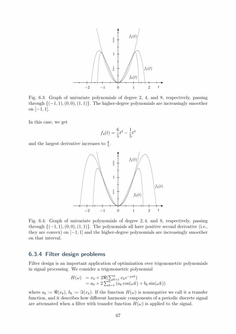
f2(t)

f4(t)

f8(t)

12

1

32

−2 −1 0 1 2 t

Fig. 6.3: Graph of univariate polynomials of degree 2, 4, and 8, respectively, passingthrough {(−1, 1), (0, 0), (1, 1)}. The higher-degree polynomials are increasingly smootheron [−1, 1].

In this case, we get

𝑓4(𝑡) =6

5𝑡2 − 1

5𝑡4

and the largest derivative increases to 85.

f2(t)

f4(t)

f8(t)12

1

32

−2 −1 0 1 2 t

Fig. 6.4: Graph of univariate polynomials of degree 2, 4, and 8, respectively, passingthrough {(−1, 1), (0, 0), (1, 1)}. The polynomials all have positive second derivative (i.e.,they are convex) on [−1, 1] and the higher-degree polynomials are increasingly smootheron that interval.

6.3.4 Filter design problems

Filter design is an important application of optimization over trigonometric polynomialsin signal processing. We consider a trigonometric polynomial

𝐻(𝜔) = 𝑥0 + 2ℜ(∑︀𝑛

𝑘=1 𝑥𝑘𝑒−𝑗𝜔𝑘)

= 𝑎0 + 2∑︀𝑛

𝑘=1 (𝑎𝑘 cos(𝜔𝑘) + 𝑏𝑘 sin(𝜔𝑘))

where 𝑎𝑘 := ℜ(𝑥𝑘), 𝑏𝑘 := ℑ(𝑥𝑘). If the function 𝐻(𝜔) is nonnegative we call it a transferfunction, and it describes how different harmonic components of a periodic discrete signalare attenuated when a filter with transfer function 𝐻(𝜔) is applied to the signal.

67

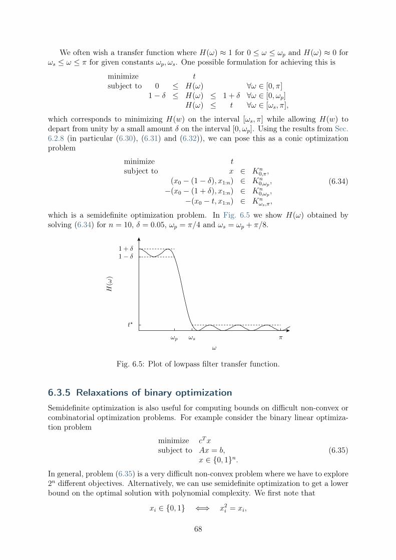
We often wish a transfer function where 𝐻(𝜔) ≈ 1 for 0 ≤ 𝜔 ≤ 𝜔𝑝 and 𝐻(𝜔) ≈ 0 for𝜔𝑠 ≤ 𝜔 ≤ 𝜋 for given constants 𝜔𝑝, 𝜔𝑠. One possible formulation for achieving this is

minimize 𝑡subject to 0 ≤ 𝐻(𝜔) ∀𝜔 ∈ [0, 𝜋]

1 − 𝛿 ≤ 𝐻(𝜔) ≤ 1 + 𝛿 ∀𝜔 ∈ [0, 𝜔𝑝]𝐻(𝜔) ≤ 𝑡 ∀𝜔 ∈ [𝜔𝑠, 𝜋],

which corresponds to minimizing 𝐻(𝑤) on the interval [𝜔𝑠, 𝜋] while allowing 𝐻(𝑤) todepart from unity by a small amount 𝛿 on the interval [0, 𝜔𝑝]. Using the results from Sec.6.2.8 (in particular (6.30), (6.31) and (6.32)), we can pose this as a conic optimizationproblem

minimize 𝑡subject to 𝑥 ∈ 𝐾𝑛

0,𝜋,(𝑥0 − (1 − 𝛿), 𝑥1:𝑛) ∈ 𝐾𝑛

0,𝜔𝑝,

−(𝑥0 − (1 + 𝛿), 𝑥1:𝑛) ∈ 𝐾𝑛0,𝜔𝑝

,

−(𝑥0 − 𝑡, 𝑥1:𝑛) ∈ 𝐾𝑛𝜔𝑠,𝜋,

(6.34)

which is a semidefinite optimization problem. In Fig. 6.5 we show 𝐻(𝜔) obtained bysolving (6.34) for 𝑛 = 10, 𝛿 = 0.05, 𝜔𝑝 = 𝜋/4 and 𝜔𝑠 = 𝜔𝑝 + 𝜋/8.

t?

1− δ1 + δ

H(ω

)

ωp ωs π

ω

Fig. 6.5: Plot of lowpass filter transfer function.

6.3.5 Relaxations of binary optimization

Semidefinite optimization is also useful for computing bounds on difficult non-convex orcombinatorial optimization problems. For example consider the binary linear optimiza-tion problem

minimize 𝑐𝑇𝑥subject to 𝐴𝑥 = 𝑏,

𝑥 ∈ {0, 1}𝑛.(6.35)

In general, problem (6.35) is a very difficult non-convex problem where we have to explore2𝑛 different objectives. Alternatively, we can use semidefinite optimization to get a lowerbound on the optimal solution with polynomial complexity. We first note that

𝑥𝑖 ∈ {0, 1} ⇐⇒ 𝑥2𝑖 = 𝑥𝑖,

68

which is, in fact, equivalent to a rank constraint on a semidefinite variable,

𝑋 = 𝑥𝑥𝑇 , diag(𝑋) = 𝑥.

By relaxing the rank 1 constraint on 𝑋 we get a semidefinite relaxation of (6.35),

minimize 𝑐𝑇𝑥subject to 𝐴𝑥 = 𝑏,

diag(𝑋) = 𝑥,𝑋 ⪰ 𝑥𝑥𝑇 ,

(6.36)

where we note that

𝑋 ⪰ 𝑥𝑥𝑇 ⇐⇒[︂

1 𝑥𝑇

𝑥 𝑋

]︂⪰ 0.

Since (6.36) is a semidefinite optimization problem, it can be solved very efficiently.Suppose 𝑥⋆ is an optimal solution for (6.35); then (𝑥⋆, 𝑥⋆(𝑥⋆)𝑇 ) is also feasible for (6.36),but the feasible set for (6.36) is larger than the feasible set for (6.35), so in general theoptimal solution of (6.36) serves as a lower bound. However, if the optimal solution 𝑋⋆

of (6.36) has rank 1 we have found a solution to (6.35) also. The semidefinite relaxationcan also be used in a branch-bound mixed-integer exact algorithm for (6.35).

We can tighten (or improve) the relaxation (6.36) by adding other constraints thatcut away parts of the feasible set, without excluding rank 1 solutions. By tightening therelaxation, we reduce the gap between the optimal values of the original problem and therelaxation. For example, we can add the constraints

0 ≤ 𝑋𝑖𝑗 ≤ 1, 𝑖 = 1, . . . , 𝑛, 𝑗 = 1, . . . , 𝑛,𝑋𝑖𝑖 ≥ 𝑋𝑖𝑗, 𝑖 = 1, . . . , 𝑛, 𝑗 = 1, . . . , 𝑛,

and so on. This will usually have a dramatic impact on solution times and memoryrequirements. Already constraining a semidefinite matrix to be doubly nonnegative (𝑋𝑖𝑗 ≥0) introduces additional 𝑛2 linear inequality constraints.

6.3.6 Relaxations of boolean optimization

Similarly to Sec. 6.3.5 we can use semidefinite relaxations of boolean constraints 𝑥 ∈{−1,+1}𝑛. To that end, we note that

𝑥 ∈ {−1,+1}𝑛 ⇐⇒ 𝑋 = 𝑥𝑥𝑇 , diag(𝑋) = 𝑒, (6.37)

with a semidefinite relaxation 𝑋 ⪰ 𝑥𝑥𝑇 of the rank-1 constraint.As a (standard) example of a combinatorial problem with boolean constraints, we

consider an undirected graph 𝐺 = (𝑉,𝐸) described by a set of vertices 𝑉 = {𝑣1, . . . , 𝑣𝑛}and a set of edges 𝐸 = {(𝑣𝑖, 𝑣𝑗) | 𝑣𝑖, 𝑣𝑗 ∈ 𝑉, 𝑖 ̸= 𝑗}, and we wish to find the cut of maximumcapacity. A cut 𝐶 partitions the nodes 𝑉 into two disjoint sets 𝑆 and 𝑇 = 𝑉 ∖ 𝑆, andthe cut-set 𝐼 is the set of edges with one node in 𝑆 and another in 𝑇 , i.e.,

𝐼 = {(𝑢, 𝑣) ∈ 𝐸 | 𝑢 ∈ 𝑆, 𝑣 ∈ 𝑇}.

The capacity of a cut is then defined as the number of edges in the cut-set, |𝐼|.

69

v0

v1

v2

v3 v4

v5v6

Fig. 6.6: Undirected graph. The cut {𝑣2, 𝑣4, 𝑣5} has capacity 9 (thick edges).

To maximize the capacity of a cut we define the symmetric adjacency matrix 𝐴 ∈ 𝒮𝑛,

[𝐴]𝑖𝑗 =

{︂1, (𝑣𝑖, 𝑣𝑗) ∈ 𝐸,0, otherwise,

where 𝑛 = |𝑉 |, and let

𝑥𝑖 =

{︂+1, 𝑣𝑖 ∈ 𝑆,−1, 𝑣𝑖 /∈ 𝑆.

Suppose 𝑣𝑖 ∈ 𝑆. Then 1 − 𝑥𝑖𝑥𝑗 = 0 if 𝑣𝑗 ∈ 𝑆 and 1 − 𝑥𝑖𝑥𝑗 = 2 if 𝑣𝑗 /∈ 𝑆, so we get anexpression for the capacity as

𝑐(𝑥) =1

4

∑︁𝑖𝑗

(1 − 𝑥𝑖𝑥𝑗)𝐴𝑖𝑗 =1

4𝑒𝑇𝐴𝑒− 1

4𝑥𝑇𝐴𝑥,

and discarding the constant term 𝑒𝑇𝐴𝑒 gives us the MAX-CUT problem

minimize 𝑥𝑇𝐴𝑥subject to 𝑥 ∈ {−1,+1}𝑛, (6.38)

with a semidefinite relaxation

minimize ⟨𝐴,𝑋⟩subject to diag(𝑋) = 𝑒,

𝑋 ⪰ 0.(6.39)

70

Chapter 7

Practical optimization

In this chapter we discuss various practical aspects of creating optimization models.

7.1 Conic reformulations

Many nonlinear constraint families were reformulated to conic form in previous chapters,and these examples are often sufficient to construct conic models for the optimizationproblems at hand. In case you do need to go beyond the cookbook examples, however, afew composition rules are worth knowing to guarantee correctness of your reformulation.

7.1.1 Perspective functions

The perspective of a function 𝑓(𝑥) is defined as 𝑠𝑓(𝑥/𝑠) on 𝑠 > 0. From any conicrepresentation of 𝑡 ≥ 𝑓(𝑥) one can reach a representation of 𝑡 ≥ 𝑠𝑓(𝑥/𝑠) by exchangingall constants 𝑘 with their homogenized counterpart 𝑘𝑠.

Example 7.1. In Sec. 5.2.6 it was shown that the logarithm of sum of exponentials

𝑡 ≥ log(𝑒𝑥1 + · · · + 𝑒𝑥𝑛),

can be modeled as: ∑︀𝑢𝑖 ≤ 1,

(𝑢𝑖, 1, 𝑥𝑖 − 𝑡) ∈ 𝐾exp, 𝑖 = 1, . . . , 𝑛.

It follows immediately that its perspective

𝑡 ≥ 𝑠 log(𝑒𝑥1/𝑠 + · · · + 𝑒𝑥𝑛/𝑠),

can be modeled as: ∑︀𝑢𝑖 ≤ 𝑠,

(𝑢𝑖, 𝑠, 𝑥𝑖 − 𝑡) ∈ 𝐾exp, 𝑖 = 1, . . . , 𝑛.

Proof. If [𝑡 ≥ 𝑓(𝑥)] ⇔ [𝑡 ≥ 𝑐(𝑥, 𝑟) + 𝑐0, 𝐴(𝑥, 𝑟) + 𝑏 ∈ 𝐾] for some linear functions𝑐 and 𝐴, a cone 𝐾, and artificial variable 𝑟, then [𝑡 ≥ 𝑠𝑓(𝑥/𝑠)] ⇔ [𝑡 ≥ 𝑠

(︀𝑐(𝑥/𝑠, 𝑟) +

71

𝑐0)︀, 𝐴(𝑥/𝑠, 𝑟) + 𝑏 ∈ 𝐾] ⇔ [𝑡 ≥ 𝑐(𝑥, 𝑟) + 𝑐0𝑠, 𝐴(𝑥, 𝑟) + 𝑏𝑠 ∈ 𝐾], where 𝑟 is taken as a new

artificial variable in place of 𝑟𝑠.

7.1.2 Composite functions

In representing composites 𝑓(𝑔(𝑥)), it is often helpful to move the inner function 𝑔(𝑥) toa separate constraint. That is, we would like 𝑡 ≥ 𝑓(𝑔(𝑥)) to be reformulated as 𝑡 ≥ 𝑓(𝑟)for a new variable 𝑟 constrained as 𝑟 = 𝑔(𝑥). This reformulation works directly as statedif 𝑔 is affine; that is, 𝑔(𝑥) = 𝑎𝑇𝑥 + 𝑏. Otherwise, one of two possible relaxations may beconsidered:

1. If 𝑓 is convex and 𝑔 is convex, then 𝑡 ≥ 𝑓(𝑟), 𝑟 ≥ 𝑔(𝑥) is equivalent to 𝑡 ≥{︃𝑓(𝑔(𝑥)) if 𝑔(𝑥) ∈ ℱ+,

𝑓min otherwise ,

2. If 𝑓 is convex and 𝑔 is concave, then 𝑡 ≥ 𝑓(𝑟), 𝑟 ≤ 𝑔(𝑥) is equivalent to 𝑡 ≥{︃𝑓(𝑔(𝑥)) if 𝑔(𝑥) ∈ ℱ−,

𝑓min otherwise ,

where ℱ+ (resp. ℱ−) is the domain on which 𝑓 is nondecreasing (resp. nonincreasing),and 𝑓min is the minimum of 𝑓 , if finite, and −∞ otherwise. Note that Relaxation 1provides an exact representation if 𝑔(𝑥) ∈ ℱ+ for all 𝑥 in domain, and likewise forRelaxation 2 if 𝑔(𝑥) ∈ ℱ− for all 𝑥 in domain.

Proof. Consider Relaxation 1. Intuitively, if 𝑟 ∈ ℱ+, you can expect clever solvers todrive 𝑟 towards −∞ in attempt to relax 𝑡 ≥ 𝑓(𝑟), and this push continues until 𝑟 ≥ 𝑔(𝑥)becomes active or else — in case 𝑔(𝑥) ̸∈ ℱ+ — until 𝑓min is reached. On the other hand,if 𝑟 ∈ ℱ− (and thus 𝑟 ≥ 𝑔(𝑥) ∈ ℱ−) then solvers will drive 𝑟 towards +∞ until 𝑓min isreached.

Example 7.2. Here are some simple substitutions.

• The inequality 𝑡 ≥ exp(𝑔(𝑥)) can be rewritten as 𝑡 ≥ exp(𝑟) and 𝑟 ≥ 𝑔(𝑥)for all convex functions 𝑔(𝑥). This is because 𝑓(𝑟) = exp(𝑟) is nondecreasingeverywhere.

• The inequality 2𝑠𝑡 ≥ 𝑔(𝑥)2 can be rewritten as 2𝑠𝑡 ≥ 𝑟2 and 𝑟 ≥ 𝑔(𝑥) for allnonnegative convex functions 𝑔(𝑥). This is because 𝑓(𝑟) = 𝑟2 is nondecreasingon 𝑟 ≥ 0.

• The nonconvex inequality 𝑡 ≥ (𝑥2 − 1)2 can be relaxed as 𝑡 ≥ 𝑟2 and 𝑟 ≥ 𝑥2 − 1.This relaxation is exact on 𝑥2 − 1 ≥ 0 where 𝑓(𝑟) = 𝑟2 is nondecreasing, i.e., onthe disjoint domain |𝑥| ≥ 1. On the domain |𝑥| ≤ 1 it represents the strongestpossible convex cut given by 𝑡 ≥ 𝑓min = 0.

72

Example 7.3. Some amount of work is generally required to find the correct reformu-lation of a nested nonlinear constraint. For instance, suppose that for 𝑥, 𝑦, 𝑧 ≥ 0 with𝑥𝑦𝑧 > 1 we want to write

𝑡 ≥ 1

𝑥𝑦𝑧 − 1.

A natural first attempt is:

𝑡 ≥ 1

𝑟, 𝑟 ≤ 𝑥𝑦𝑧 − 1,

which corresponds to Relaxation 2 with 𝑓(𝑟) = 1/𝑟 and 𝑔(𝑥, 𝑦, 𝑧) = 𝑥𝑦𝑧 − 1 > 0. Thefunction 𝑓 is indeed convex and nonincreasing on all of 𝑔(𝑥, 𝑦, 𝑧), and the inequality𝑡𝑟 ≥ 1 is moreover representable with a rotated quadratic cone. Unfortunately 𝑔 isnot concave. We know that a monomial like 𝑥𝑦𝑧 appears in connection with the powercone, but that requires a homogeneous constraint such as 𝑥𝑦𝑧 ≥ 𝑢3. This gives us anidea to try

𝑡 ≥ 1

𝑟3, 𝑟3 ≤ 𝑥𝑦𝑧 − 1,

which is 𝑓(𝑟) = 1/𝑟3 and 𝑔(𝑥, 𝑦, 𝑧) = (𝑥𝑦𝑧−1)1/3 > 0. This provides the right balance:all conditions for validity and exactness of Relaxation 2 are satisfied. Introducinganother variable 𝑢 we get the following model:

𝑡𝑟3 ≥ 1, 𝑥𝑦𝑧 ≥ 𝑢3, 𝑢 ≥ (𝑟3 + 13)1/3,

We refer to Sec. 4 to verify that all the constraints above are representable using powercones. We leave it as an exercise to find other conic representations, based on othertransformations of the original inequality.

7.1.3 Convex univariate piecewise-defined functions

Consider a univariate function with 𝑘 pieces:

𝑓(𝑥) =

⎧⎪⎨⎪⎩𝑓1(𝑥) if 𝑥 ≤ 𝛼1,

𝑓𝑖(𝑥) if 𝛼𝑖−1 ≤ 𝑥 ≤ 𝛼𝑖, for 𝑖 = 2, . . . , 𝑘 − 1,

𝑓𝑘(𝑥) if 𝛼𝑘−1 ≤ 𝑥,

Suppose 𝑓(𝑥) is convex (in particular each piece is convex by itself) and 𝑓𝑖(𝛼𝑖) = 𝑓𝑖+1(𝛼𝑖).In representing the epigraph 𝑡 ≥ 𝑓(𝑥) it is helpful to proceed via the equivalent represen-tation:

𝑡 =∑︀𝑘

𝑖=1 𝑡𝑖 −∑︀𝑘−1

𝑖=1 𝑓𝑖(𝛼𝑖),

𝑥 =∑︀𝑘

𝑖=1 𝑥𝑖 −∑︀𝑘−1

𝑖=1 𝛼𝑖,𝑡𝑖 ≥ 𝑓𝑖(𝑥𝑖) for 𝑖 = 1, . . . , 𝑘,𝑥1 ≤ 𝛼1, 𝛼𝑖−1 ≤ 𝑥𝑖 ≤ 𝛼𝑖 for 𝑖 = 2, . . . , 𝑘 − 1, 𝛼𝑘−1 ≤ 𝑥𝑘.

Proof. In the special case when 𝑘 = 2 and 𝛼1 = 𝑓1(𝛼1) = 𝑓2(𝛼1) = 0 the epigraph of 𝑓 isequal to the Minkowski sum {(𝑡1+𝑡2, 𝑥1+𝑥2) : 𝑡𝑖 ≥ 𝑓𝑖(𝑥𝑖)}. In general the epigraph over

73

two consecutive pieces is obtained by shifting them to (0, 0), computing the Minkowskisum and shifting back. Finally more than two pieces can be joined by continuing thisargument by induction.

As the reformulation grows in size with the number of pieces, it is preferable tokeep this number low. Trivially, if 𝑓𝑖(𝑥) = 𝑓𝑖+1(𝑥), these two pieces can be merged.Substituting 𝑓𝑖(𝑥) and 𝑓𝑖+1(𝑥) for max(𝑓𝑖(𝑥), 𝑓𝑖+1(𝑥)) is sometimes an invariant changeto facilitate this merge. For instance, it always works for affine functions 𝑓𝑖(𝑥) and𝑓𝑖+1(𝑥). Finally, if 𝑓(𝑥) is symmetric around some point 𝛼, we can represent its epigraphvia a piecewise function, with only half the number of pieces, defined in terms of a newvariable 𝑧 = |𝑥− 𝛼| + 𝛼.

Example 7.4 (Huber loss function). The Huber loss function

𝑓(𝑥) =

⎧⎪⎨⎪⎩−2𝑥− 1 if 𝑥 ≤ −1,

𝑥2 if − 1 ≤ 𝑥 ≤ 1,

2𝑥− 1 if 1 ≤ 𝑥,

is convex and its epigraph 𝑡 ≥ 𝑓(𝑥) has an equivalent representation

𝑡 ≥ 𝑡1 + 𝑡2 + 𝑡3 − 2,𝑥 = 𝑥1 + 𝑥2 + 𝑥3,𝑡1 = −2𝑥1 − 1, 𝑡2 ≥ 𝑥2

2, 𝑡3 = 2𝑥3 − 1,𝑥1 ≤ −1, −1 ≤ 𝑥2 ≤ 1, 1 ≤ 𝑥3,

where 𝑡2 ≥ 𝑥22 is representable by a rotated quadratic cone. No two pieces of 𝑓(𝑥)

can be merged to reduce the size of this formulation, but the loss function does satisfya simple symmetry; namely 𝑓(𝑥) = 𝑓(−𝑥). We can thus represent its epigraph by𝑡 ≥ 𝑓(𝑧) and 𝑧 ≥ |𝑥|, where

𝑓(𝑧) =

{︃𝑧2 if 𝑧 ≤ 1,

2𝑧 − 1 if 1 ≤ 𝑧.

In this particular example, however, unless the absolute value 𝑧 from 𝑧 ≥ |𝑥| is usedelsewhere, the cost of introducing it does not outweigh the savings achieved by goingfrom three pieces in 𝑥 to two pieces in 𝑧.

7.2 Avoiding ill-posed problems

For a well-posed continuous problem a small change in the input data should induce asmall change of the optimal solution. A problem is ill-posed if small perturbations ofthe problem data result in arbitrarily large perturbations of the solution, or even changethe feasibility status of the problem. In such cases small rounding errors, or solving theproblem on a different computer can result in different or wrong solutions.

In fact, from an algorithmic point of view, even computing a wrong solution is numer-ically difficult for ill-posed problems. A rigorous definition of the degree of ill-posedness is

74

possible by defining a condition number. This is an attractive, but not very practical met-ric, as its evaluation requires solving several auxiliary optimization problems. Thereforewe only make the modest recommendations to avoid problems

• that are nearly infeasible,

• with constraints that are linearly dependent, or nearly linearly dependent.

Example 7.5 (Near linear dependencies). To give some idea about the perils of nearlinear dependence, consider this pair of optimization problems:

maximize 𝑥subject to 2𝑥− 𝑦 ≥ −1,

2.0001𝑥− 𝑦 ≤ 0,

and

maximize 𝑥subject to 2𝑥− 𝑦 ≥ −1,

1.9999𝑥− 𝑦 ≤ 0.

The first problem has a unique optimal solution (𝑥, 𝑦) = (104, 2 · 104 + 1), while thesecond problem is unbounded. This is caused by the fact that the hyperplanes (here:straight lines) defining the constraints in each problem are almost parallel. Moreover,we can consider another modification:

maximize 𝑥subject to 2𝑥− 𝑦 ≥ −1,

2.001𝑥− 𝑦 ≤ 0,

with optimal solution (𝑥, 𝑦) = (103, 2 · 103 + 1), which shows how a small perturbationof the coefficients induces a large change of the solution.

Typical examples of problems with nearly linearly dependent constraints are dis-cretizations of continuous processes, where the constraints invariably become more cor-related as we make the discretization finer; as such there may be nothing wrong withthe discretization or problem formulation, but we should expect numerical difficulties forsufficiently fine discretizations.

One should also be careful not to specify problems whose optimal value is only achievedin the limit. A trivial example is

minimize 𝑒𝑥, 𝑥 ∈ R.

The infimum value 0 is not attained for any finite 𝑥, which can lead to unspecified be-haviour of the solver. More examples of ill-posed conic problems are discussed in Fig. 7.1and Sec. 8. In particular, Fig. 7.1 depicts some troublesome problems in two dimensions.In (a) minimizing 𝑦 ≥ 1/𝑥 on the nonnegative orthant is unattained approaching zerofor 𝑥 → ∞. In (b) the only feasible point is (0, 0), but objectives maximizing 𝑥 are notblocked by the purely vertical normal vectors of active constraints at this point, falsely

75

suggesting local progress could be made. In (c) the intersection of the two subsets isempty, but the distance between them is zero. Finally in (d) minimizing 𝑥 on 𝑦 ≥ 𝑥2

is unbounded at minus infinity for 𝑦 → ∞, but there is no improving ray to follow. Al-though seemingly unrelated, the four cases are actually primal-dual pairs; (a) with (b)and (c) with (d). In fact, the missing normal vector property in (b)—desired to certifyoptimality—can be attributed to (a) not attaining the best among objective values atdistance zero to feasibility, and the missing positive distance property in (c)—desired tocertify infeasibility—is because (d) has no improving ray.

Fig. 7.1: Geometric representations of some ill-posed situations.

7.3 Scaling

Another difficulty encountered in practice involves models that are badly scaled. Looselyspeaking, we consider a model to be badly scaled if

• variables are measured on very different scales,

• constraints or bounds are measured on very different scales.

For example if one variable 𝑥1 has units of molecules and another variable 𝑥2 measurestemperature, we might expect an objective function such as

𝑥1 + 1012𝑥2

and in finite precision the second term dominates the objective and renders the contri-bution from 𝑥1 insignificant and unreliable.

A similar situation (from a numerical point of view) is encountered when using pe-nalization or big-𝑀 strategies. Assume we have a standard linear optimization problem(2.12) with the additional constraint that 𝑥1 = 0. We may eliminate 𝑥1 completely fromthe model, or we might add an additional constraint, but suppose we choose to formulatea penalized problem instead

minimize 𝑐𝑇𝑥 + 1012𝑥1

subject to 𝐴𝑥 = 𝑏,𝑥 ≥ 0,

76

reasoning that the large penalty term will force 𝑥1 = 0. However, if ‖𝑐‖ is small wehave the exact same problem, namely that in finite precision the penalty term will com-pletely dominate the objective and render the contribution 𝑐𝑇𝑥 insignificant or unreliable.Therefore, the penalty term should be chosen carefully.

Example 7.6 (Risk-return tradeoff). Suppose we want to solve an efficient frontiervariant of the optimal portfolio problem from Sec. 3.3.3 with an objective of the form

maximize 𝜇𝑇𝑥− 1

2𝛾𝑥𝑇Σ𝑥

where the parameter 𝛾 controls the tradeoff between return and risk. The user mightchoose a very small 𝛾 to discount the risk term. This, however, may lead to numericalissues caused by a very large solution. To see why, consider a simple one-dimensional,unconstrained analogue:

maximize 𝑥− 1

2𝛾𝑥2, 𝑥 ∈ R

and note that the maximum is attained for 𝑥 = 1/𝛾, which may be very large.

Example 7.7 (Explicit redundant bounds). Consider again the problem (2.12), butwith additional (redundant) constraints 𝑥𝑖 ≤ 𝛾. This is a common approach for someoptimization practitioners. The problem we solve is then

minimize 𝑐𝑇𝑥subject to 𝐴𝑥 = 𝑏,

𝑥 ≥ 0,𝑥 ≤ 𝛾𝑒,

with a dual problem

maximize 𝑏𝑇𝑦 − 𝛾𝑒𝑇 𝑧subject to 𝐴𝑇𝑦 + 𝑠− 𝑧 = 𝑐,

𝑠, 𝑧 ≥ 0.

Suppose we do not know a-priori an upper bound on ‖𝑥‖∞, so we choose a very large𝛾 = 1012 reasoning that this will not change the optimal solution. Note that the largevariable bound becomes a penalty term in the dual problem; in finite precision such alarge bound will effectively destroy accuracy of the solution.

Example 7.8 (Big-M). Suppose we have a mixed integer model which involves a big-Mconstraint (see Sec. 9), for instance

𝑎𝑇𝑥 ≤ 𝑏 + 𝑀(1 − 𝑧)

77

as in Sec. 9.1.3. The constant 𝑀 must be big enough to guarantee that the constraintbecomes redundant when 𝑧 = 0, or we risk shrinking the feasible set, perhaps to thepoint of creating an infeasible model. On the other hand, the user might set 𝑀 to ahuge, safe value, say 𝑀 = 1012. While this is mathematically correct, it will lead to amodel with poorer linear relaxations and most likely increase solution time (sometimesdramatically). It is therefore very important to put some effort into estimating areasonable value of 𝑀 which is safe, but not too big.

7.4 The huge and the tiny

Some types of problems and constraints are especially prone to behave badly with verylarge or very small numbers. We discuss such examples briefly in this section.

Sum of squares

The sum of squares 𝑥21 + · · ·+𝑥2

𝑛 can be bounded above using the rotated quadratic cone:

𝑡 ≥ 𝑥21 + · · · + 𝑥2

𝑛 ⇐⇒ (1

2, 𝑡, 𝑥) ∈ 𝒬𝑛

r ,

but in most cases it is better to bound the square root with a quadratic cone:

𝑡′ ≥√︁

𝑥21 + · · · + 𝑥2

𝑛 ⇐⇒ (𝑡′, 𝑥) ∈ 𝒬𝑛.

The latter has slightly better numerical properties: 𝑡′ is roughly comparable with 𝑥 andis measured on the same scale, while 𝑡 grows as the square of 𝑥 which will sooner lead tonumerical instabilities.

Exponential cone

Using the function 𝑒𝑥 for 𝑥 ≤ −30 or 𝑥 ≥ 30 would be rather questionable if 𝑒𝑥 is supposedto represent any realistic value. Note that 𝑒30 ≈ 1013 and that 𝑒30.0000001− 𝑒30 ≈ 106, so atiny perturbation of the exponent produces a huge change of the result. Ideally, 𝑥 shouldhave a single-digit absolute value. For similar reasons, it is even more important to havewell-scaled data. For instance, in floating point arithmetic we have the “equality”

𝑒20 + 𝑒−20 = 𝑒20

since the smaller summand disappears in comparison to the other one, 1017 times bigger.For the same reason it is advised to replace explicit inequalities involving exp(𝑥) with

log-sum-exp variants (see Sec. 5.2.6). For example, suppose we have a constraint such as

𝑡 ≥ 𝑒𝑥1 + 𝑒𝑥2 + 𝑒𝑥3 .

Then after a substitution 𝑡 = 𝑒𝑡′ we have

1 ≥ 𝑒𝑥1−𝑡′ + 𝑒𝑥2−𝑡′ + 𝑒𝑥3−𝑡′

which has the advantage that 𝑡′ is of the same order of magnitude as 𝑥𝑖, and that theexponents 𝑥𝑖 − 𝑡′ are likely to have much smaller absolute values than simply 𝑥𝑖.

78

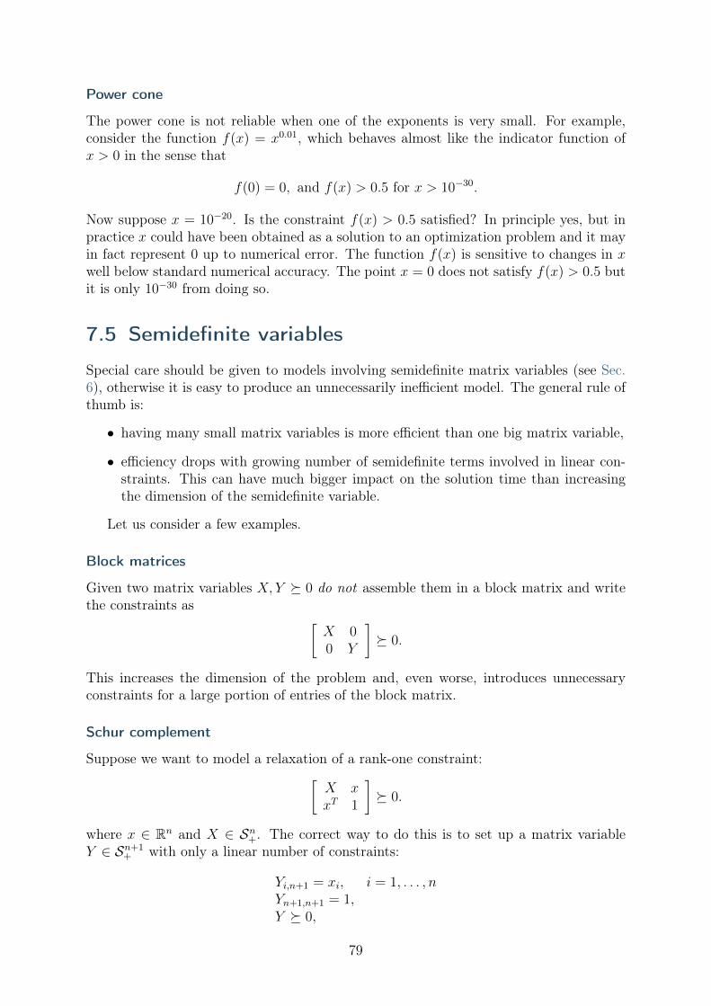
Power cone

The power cone is not reliable when one of the exponents is very small. For example,consider the function 𝑓(𝑥) = 𝑥0.01, which behaves almost like the indicator function of𝑥 > 0 in the sense that

𝑓(0) = 0, and 𝑓(𝑥) > 0.5 for 𝑥 > 10−30.

Now suppose 𝑥 = 10−20. Is the constraint 𝑓(𝑥) > 0.5 satisfied? In principle yes, but inpractice 𝑥 could have been obtained as a solution to an optimization problem and it mayin fact represent 0 up to numerical error. The function 𝑓(𝑥) is sensitive to changes in 𝑥well below standard numerical accuracy. The point 𝑥 = 0 does not satisfy 𝑓(𝑥) > 0.5 butit is only 10−30 from doing so.

7.5 Semidefinite variables

Special care should be given to models involving semidefinite matrix variables (see Sec.6), otherwise it is easy to produce an unnecessarily inefficient model. The general rule ofthumb is:

• having many small matrix variables is more efficient than one big matrix variable,

• efficiency drops with growing number of semidefinite terms involved in linear con-straints. This can have much bigger impact on the solution time than increasingthe dimension of the semidefinite variable.

Let us consider a few examples.

Block matrices

Given two matrix variables 𝑋, 𝑌 ⪰ 0 do not assemble them in a block matrix and writethe constraints as [︂

𝑋 00 𝑌

]︂⪰ 0.

This increases the dimension of the problem and, even worse, introduces unnecessaryconstraints for a large portion of entries of the block matrix.

Schur complement

Suppose we want to model a relaxation of a rank-one constraint:[︂𝑋 𝑥𝑥𝑇 1

]︂⪰ 0.

where 𝑥 ∈ R𝑛 and 𝑋 ∈ 𝒮𝑛+. The correct way to do this is to set up a matrix variable

𝑌 ∈ 𝒮𝑛+1+ with only a linear number of constraints:

𝑌𝑖,𝑛+1 = 𝑥𝑖, 𝑖 = 1, . . . , 𝑛𝑌𝑛+1,𝑛+1 = 1,𝑌 ⪰ 0,

79

and use the upper-left 𝑛×𝑛 part of 𝑌 as the original 𝑋. Going the other way around, i.e.starting with a variable 𝑋 and aligning it with the corner of another, bigger semidefinitematrix 𝑌 introduces 𝑛(𝑛 + 1)/2 equality constraints and will quickly have formidablesolution times.

Sparse LMIs

Suppose we want to model a problem with a sparse linear matrix inequality (see Sec.6.2.1) such as:

minimize 𝑐𝑇𝑥

subject to 𝐴0 +∑︀𝑘

𝑖=1 𝐴𝑖𝑥𝑖 ⪰ 0,

where 𝑥 ∈ R𝑘 and 𝐴𝑖 are symmetric 𝑛× 𝑛 matrices. The representation of this problemin primal form is:

minimize 𝑐𝑇𝑥

subject to 𝐴0 +∑︀𝑘

𝑖=1 𝐴𝑖𝑥𝑖 = 𝑋,𝑋 ⪰ 0,

and the linear constraint requires a full set of 𝑛(𝑛 + 1)/2 equalities, many of which arejust 𝑋𝑘,𝑙 = 0, regardless of the sparsity of 𝐴𝑖. However the dual problem (see Sec. 8.6) is:

maximize −⟨𝐴0, 𝑍⟩subject to ⟨𝐴𝑖, 𝑍⟩ = 𝑐𝑖, 𝑖 = 1, . . . , 𝑘,

𝑍 ⪰ 0,

and the number of nonzeros in linear constraints is just joint number of nonzeros in 𝐴𝑖.It means that large, sparse LMIs should almost always be dualized and entered in thatform for efficiency reasons.

7.6 The quality of a solution

In this section we will discuss how to validate an obtained solution. Assume we havea conic model with continuous variables only and that the optimization software hasreported an optimal primal and dual solution. Given such a solution, we might ask howto verify that it is indeed feasible and optimal.

To that end, consider a simple model

minimize −𝑥2

subject to 𝑥1 + 𝑥2 ≤ 3,𝑥22 ≤ 2,

𝑥1, 𝑥2 ≥ 0,

(7.1)

where a solver might approximate the solution as

𝑥1 = 0.0000000000000000 and 𝑥2 = 1.4142135623730951

and therefore the approximate optimal objective value is

−1.4142135623730951.

80

The true objective value is −√

2, so the approximate objective value is wrong by theamount

1.4142135623730951 −√

2 ≈ 10−16.

Most likely this difference is irrelevant for all practical purposes. Nevertheless, in generala solution obtained using floating point arithmetic is only an approximation. Most (ifnot all) commercial optimization software uses double precision floating point arithmetic,implying that about 16 digits are correct in the computations performed internally bythe software. This also means that irrational numbers such as

√2 and 𝜋 can only be

stored accurately within 16 digits.

Verifying feasibility

A good practice after solving an optimization problem is to evaluate the reported solution.At the very least this process should be carried out during the initial phase of buildinga model, or if the reported solution is unexpected in some way. The first step in thatprocess is to check that the solution is feasible; in case of the small example (7.1) thisamounts to checking that:

𝑥1 + 𝑥2 = 0.0000000000000000 + 1.4142135623730951 ≤ 3,𝑥22 = 2.0000000000000004 ≤ 2, (?)

𝑥1 = 0.0000000000000000 ≥ 0,𝑥2 = 1.4142135623730951 ≥ 0,

which demonstrates that one constraint is slightly violated due to computations in finiteprecision. It is up to the user to assess the significance of a specific violation; for examplea violation of one unit in

𝑥1 + 𝑥2 ≤ 1

may or may not be more significant than a violation of one unit in

𝑥1 + 𝑥2 ≤ 109.

The right-hand side of 109 may itself be the result of a computation in finite precision,and may only be known with, say 3 digits of accuracy. Therefore, a violation of 1 unit isnot significant since the true right-hand side could just as well be 1.001 · 109. Certainly aviolation of 4 · 10−16 as in our example is within the numerical tolerance for zero and wewould accept the solution as feasible. In practice it would be standard to see violationsof order 10−8.

Verifying optimality

Another question is how to verify that a feasible approximate solution is actually optimal,which is answered by duality theory, which is discussed in Sec. 2.4 for linear problemsand in Sec. 8 in full generality. Following Sec. 8 we can derive an equivalent version ofthe dual problem as:

maximize −3𝑦1 − 𝑦2 − 𝑦3subject to 2𝑦2𝑦3 ≥ (𝑦1 + 1)2,

𝑦1 ≥ 0.

81

This problem has a feasible point (𝑦1, 𝑦2, 𝑦3) = (0, 1/√

2, 1/√

2) with objective value−√

2, matching the objective value of the primal problem. By duality theory this provesthat both the primal and dual solutions are optimal. Again, in finite precision the dualobjective value may be reported as, for example

−1.4142135623730950

leading to a duality gap of about 10−16 between the approximate primal and dual objectivevalues. It is up to the user to assess the significance of any duality gap and accept orreject the solution as sufficiently good approximation of the optimal value.

7.7 Distance to a cone

The violation of a linear constraint 𝑎𝑇𝑥 ≤ 𝑏 under a given solution 𝑥* is obviously

max(0, 𝑎𝑇𝑥* − 𝑏).

It is less obvious how to assess violations of conic constraints. To this end suppose wehave a convex cone 𝐾. The (Euclidean) projection of a point 𝑥 onto 𝐾 is defined as thesolution of the problem

minimize ‖𝑝− 𝑥‖2subject to 𝑝 ∈ 𝐾.

(7.2)

We denote the projection by proj𝐾(𝑥). The distance of 𝑥 to 𝐾

dist(𝑥,𝐾) = ‖𝑥− proj𝐾(𝑥)‖2,

i.e. the objective value of (7.2), measures the violation of a conic constraint involving 𝐾.Obviously

dist(𝑥,𝐾) = 0 ⇐⇒ 𝑥 ∈ 𝐾.

This distance measure is attractive because it depends only on the set 𝐾 and not on anyparticular representation of 𝐾 using (in)equalities.

Example 7.9 (Surprisingly small distance). Let 𝐾 = 𝒫0.1,0.93 be the power cone defined

by the inequality 𝑥0.1𝑦0.9 ≥ |𝑧|. The point

𝑥* = (𝑥, 𝑦, 𝑧) = (0, 10000, 500)

is clearly not in the cone, in fact 𝑥0.1𝑦0.9 = 0 while |𝑧| = 500, so the violation of theconic inequality is seemingly large. However, the point

𝑝 = (10−8, 10000, 500)

belongs to 𝒫0.1,0.93 (since (10−8)0.1 · 100000.9 ≈ 630), hence

dist(𝑥*,𝒫0.1,0.93 ) ≤ ‖𝑥* − 𝑝‖2 = 10−8.

Therefore the distance of 𝑥* to the cone is actually very small.

82

Distance to certain cones

For some basic cone types the projection problem (7.2) can be solved analytically. De-noting [𝑥]+ = max(0, 𝑥) we have that:

• For 𝑥 ∈ R the projection onto the nonnegative half-line is projR+(𝑥) = [𝑥]+.

• For (𝑡, 𝑥) ∈ R× R𝑛−1 the projection onto the quadratic cone is

proj𝒬𝑛(𝑡, 𝑥) =

⎧⎪⎪⎨⎪⎪⎩(𝑡, 𝑥) if 𝑡 ≥ ‖𝑥‖2,12

(︁𝑡

‖𝑥‖2 + 1)︁

(‖𝑥‖2, 𝑥) if − ‖𝑥‖2 < 𝑡 < ‖𝑥‖2,0 if 𝑡 ≤ −‖𝑥‖2.

• For 𝑋 =∑︀𝑛

𝑖=1 𝜆𝑖𝑞𝑖𝑞𝑇𝑖 the projection onto the semidefinite cone is

proj𝒮𝑛+

(𝑋) =𝑛∑︁

𝑖=1

[𝜆𝑖]+𝑞𝑖𝑞𝑇𝑖 .

83

Chapter 8

Duality in conic optimization

In Sec. 2 we introduced duality and related concepts for linear optimization. Here wepresent a more general version of this theory for conic optimization and we illustrate itwith examples. Although this chapter is self-contained, we recommend familiarity withSec. 2, which some of this material is a natural extension of.

Duality theory is a rich and powerful area of convex optimization, and central tounderstanding sensitivity analysis and infeasibility issues. Furthermore, it provides asimple and systematic way of obtaining non-trivial lower bounds on the optimal value formany difficult non-convex problems.

From now on we consider a conic problem in standard form

minimize 𝑐𝑇𝑥subject to 𝐴𝑥 = 𝑏,

𝑥 ∈ 𝐾,(8.1)

where 𝐾 is a convex cone. In practice 𝐾 would likely be defined as a product

𝐾 = 𝐾1 × · · · ×𝐾𝑚

of smaller cones corresponding to actual constraints in the problem formulation. Theabstract formulation (8.1) encompasses such special cases as 𝐾 = R𝑛

+ (linear optimiza-tion), 𝐾𝑖 = R (unconstrained variable) or 𝐾𝑖 = 𝒮𝑛

+ (12𝑛(𝑛 + 1) variables representing the

upper-triangular part of a matrix).The feasible set for (8.1):

ℱ𝑝 = {𝑥 ∈ R𝑛 | 𝐴𝑥 = 𝑏} ∩𝐾

is a section of 𝐾. We say the problem is feasible if ℱ𝑝 ̸= ∅ and infeasible otherwise. Thevalue of (8.1) is defined as

𝑝⋆ = inf{𝑐𝑇𝑥 : 𝑥 ∈ ℱ𝑝},

allowing the special cases of 𝑝⋆ = +∞ (the problem is infeasible) and 𝑝⋆ = −∞ (theproblem is unbounded). Note that 𝑝⋆ may not be attained, i.e. the infimum is notnecessarily a minimum, although this sort of problems are ill-posed from a practicalpoint of view (see Sec. 7).

84

Example 8.1 (Unattained problem value). The conic quadratic problem

minimize 𝑥subject to (𝑥, 𝑦, 1) ∈ 𝒬3

𝑟,

with constraint equivalent to 2𝑥𝑦 ≥ 1, 𝑥, 𝑦 ≥ 0 has 𝑝⋆ = 0 but this optimal value isnot attained by any point in ℱ𝑝.

8.1 Dual cone

Suppose 𝐾 ⊆ R𝑛 is a closed convex cone. We define the dual cone 𝐾* as

𝐾* = {𝑦 ∈ R𝑛 : 𝑦𝑇𝑥 ≥ 0 ∀𝑥 ∈ 𝐾}. (8.2)

For simplicity we write 𝑦𝑇𝑥, denoting the standard Euclidean inner product, but every-thing in this section applies verbatim to the inner product of matrices in the semidefinitecontext. In other words 𝐾* consists of vectors which form an acute (or right) angle withevery vector in 𝐾. We see easily that 𝐾* is in fact a convex cone. The main example,associated with linear optimization, is the dual of the positive orthant:

Lemma 8.1 (Dual of linear cone).

(R𝑛+)* = R𝑛

+.

Proof. This is obvious for 𝑛 = 1, and then we use the simple fact

(𝐾1 × · · · ×𝐾𝑚)* = 𝐾*1 × · · · ×𝐾*

𝑚,

which we invite the reader to prove.

All cones studied in this cookbook can be explicitly dualized as we show next.

Lemma 8.2 (Duals of nonlinear cones). We have the following:

• The quadratic, rotated quadratic and semidefinite cones are self-dual:

(𝒬𝑛)* = 𝒬𝑛, (𝒬𝑛r )* = 𝒬𝑛

r , (𝒮𝑛+)* = 𝒮𝑛

+.

• The dual of the power cone (4.4) is

(𝒫𝛼1,··· ,𝛼𝑚𝑛 )* =

{︂𝑦 ∈ R𝑛 :

(︂𝑦1𝛼1

, . . . ,𝑦𝑚𝛼𝑚

, 𝑦𝑚+1, . . . , 𝑦𝑛

)︂∈ 𝒫𝛼1,··· ,𝛼𝑚

𝑛

}︂.

• The dual of the exponential cone (5.2) is the closure

(𝐾exp)* = cl{︀𝑦 ∈ R3 : 𝑦1 ≥ −𝑦3𝑒

𝑦2/𝑦3−1, 𝑦1 > 0, 𝑦3 < 0}︀.

85

Proof. We only sketch some parts of the proof and indicate geometric intuitions. First,let us show (𝒬𝑛)* = 𝒬𝑛. For (𝑡, 𝑥), (𝑠, 𝑦) ∈ 𝒬𝑛 we have

𝑠𝑡 + 𝑦𝑇𝑥 ≥ ‖𝑦‖2‖𝑥‖2 + 𝑦𝑇𝑥 ≥ 0

by the Cauchy-Schwartz inequality |𝑢𝑇𝑣| ≤ ‖𝑢‖2‖𝑣‖2, therefore 𝒬𝑛 ⊆ (𝒬𝑛)*. Geomet-rically we are just saying that the quadratic cone 𝒬𝑛 has a right angle at the apex, soany two vectors inside the cone form at most a right angle. Now suppose (𝑠, 𝑦) is apoint outside 𝒬𝑛. If (−𝑠,−𝑦) ∈ 𝒬𝑛 then −𝑠2 − 𝑦𝑇𝑦 < 0 and we showed (𝑠, 𝑦) ̸∈ (𝒬𝑛)*.Otherwise let (𝑡, 𝑥) = proj𝒬𝑛(𝑠, 𝑦) be the projection (see Sec. 7.7); note that (𝑠, 𝑦) and(𝑡,−𝑥) ∈ 𝒬𝑛 form an obtuse angle.

For the semidefinite cone we use the property ⟨𝑋, 𝑌 ⟩ ≥ 0 for 𝑋, 𝑌 ∈ 𝒮𝑛+ (see Sec.

6.1.2). Conversely, assume that 𝑍 ̸∈ 𝒮𝑛+. Then there exists a 𝑤 satisfying ⟨𝑤𝑤𝑇 , 𝑍⟩ =

𝑤𝑇𝑍𝑤 < 0, so 𝑍 ̸∈ (𝒮𝑛+)*.

As our last exercise let us check that vectors in 𝐾exp and (𝐾exp)* form acute angles.By definition of 𝐾exp and (𝐾exp)* we take 𝑥, 𝑦 such that:

𝑥1 ≥ 𝑥2 exp(𝑥3/𝑥2), 𝑦1 ≥ −𝑦3 exp(𝑦2/𝑦3 − 1), 𝑥1, 𝑥2, 𝑦1 > 0, 𝑦3 < 0,

and then we have

𝑦𝑇𝑥 = 𝑥1𝑦1 + 𝑥2𝑦2 + 𝑥3𝑦3 ≥ −𝑥2𝑦3 exp(𝑥3

𝑥2+ 𝑦2

𝑦3− 1) + 𝑥2𝑦2 + 𝑥3𝑦3

≥ −𝑥2𝑦3(𝑥3

𝑥2+ 𝑦2

𝑦3) + 𝑥2𝑦2 + 𝑥3𝑦3 = 0,

using the inequality exp(𝑡) ≥ 1 + 𝑡. We refer to the literature for full proofs of all thestatements.

Finally it is nice to realize that (𝐾*)* = 𝐾 and that the cones {0} and R are eachothers’ duals. We leave it to the reader to check these facts.

8.2 Infeasibility in conic optimization

We can now discuss infeasibility certificates for conic problems. Given an optimizationproblem, the first basic question we are interested in is its feasibility status. The theoryof infeasibility certificates for linear problems, including the Farkas lemma (see Sec. 2.3)extends almost verbatim to the conic case.

Lemma 8.3 (Farkas’ lemma, conic version). Suppose we have the conic optimizationproblem (8.1). Exactly one of the following statements is true:

1. Problem (8.1) is feasible.

2. Problem (8.1) is infeasible, but there is a sequence 𝑥𝑛 ∈ 𝐾 such that ‖𝐴𝑥𝑛−𝑏‖ → 0.

3. There exists 𝑦 such that −𝐴𝑇𝑦 ∈ 𝐾* and 𝑏𝑇𝑦 > 0.

Problems which fall under option 2. (limit-feasible) are ill-posed: an arbitrarily smallperturbation of input data puts the problem in either category 1. or 3. This fringecase should therefore not appear in practice, and if it does, it signals issues with theoptimization model which should be addressed.

86

Example 8.2 (Limit-feasible model). Here is an example of an ill-posed limit-feasiblemodel created by fixing one of the root variables of a rotated quadratic cone to 0.

minimize 𝑢subject to (𝑢, 𝑣, 𝑤) ∈ 𝒬3

𝑟,𝑣 = 0,𝑤 ≥ 1.

The problem is clearly infeasible, but the sequence (𝑢𝑛, 𝑣𝑛, 𝑤𝑛) = (𝑛, 1/𝑛, 1) ∈ 𝒬3𝑟 with

(𝑣𝑛, 𝑤𝑛) → (0, 1) makes it limit-feasible as in alternative 2. of Lemma 8.3. There is noinfeasibility certificate as in alternative 3.

Having cleared this detail we continue with the proof and example for the actuallyuseful part of conic Farkas’ lemma.

Proof. Consider the set

𝐴(𝐾) = {𝐴𝑥 : 𝑥 ∈ 𝐾}.

It is a convex cone. Feasibility is equivalent to 𝑏 ∈ 𝐴(𝐾). If 𝑏 ̸∈ 𝐴(𝐾) but 𝑏 ∈ cl(𝐴(𝐾))then we have the second alternative. Finally, if 𝑏 ̸∈ cl(𝐴(𝐾)) then the closed convex conecl(𝐴(𝐾)) and the point 𝑏 can be strictly separated by a hyperplane passing through theorigin, i.e. there exists 𝑦 such that

𝑏𝑇𝑦 > 0, (𝐴𝑥)𝑇𝑦 ≤ 0 ∀𝑥 ∈ 𝐾.

But then 0 ≤ −(𝐴𝑥)𝑇𝑦 = (−𝐴𝑇𝑦)𝑇𝑥 for all 𝑥 ∈ 𝐾, so by definition of 𝐾* we have−𝐴𝑇𝑦 ∈ 𝐾*, and we showed 𝑦 satisfies the third alternative. Finally, 1. and 3. aremutually exclusive, since otherwise we would have

0 ≤ (−𝐴𝑇𝑦)𝑇𝑥 = −𝑦𝑇𝐴𝑥 = −𝑦𝑇 𝑏 < 0

and the same argument works in the limit if 𝑥𝑛 is a sequence as in 2. That proves thelemma.

Therefore Farkas’ lemma implies that (up to certain ill-posed cases) either the problem(8.1) is feasible (first alternative) or there is a certificate of infeasibility 𝑦 (last alternative).In other words, every time we classify a model as infeasible, we can certify this fact byproviding an appropriate 𝑦. Note that when 𝐾 = R𝑛

+ we recover precisely the linearversion, Lemma 2.1.

Example 8.3 (Infeasible conic problem). Consider a minimization problem:

minimize 𝑥1

subject to −𝑥1 + 𝑥2 − 𝑥4 = 1,2𝑥3 − 3𝑥4 = −1,

𝑥1 ≥√︀𝑥22 + 𝑥2

3,𝑥4 ≥ 0.

87

It can be expressed in the standard form (8.1) with

𝐴 =

[︂−1 1 0 −10 0 2 −3

]︂, 𝑏 =

[︂1−1

]︂, 𝐾 = 𝒬3 × R+, 𝑐 = [1, 0, 0, 0]𝑇 .

A certificate of infeasibility is 𝑦 = [1, 0]𝑇 . Indeed, 𝑏𝑇𝑦 = 1 > 0 and −𝐴𝑇𝑦 =[1,−1, 0, 1] ∈ 𝐾* = 𝒬3 × R+. The certificate indicates that the first linear constraintalone causes infeasibility, which is indeed the case: the first equality together with theconic constraints yield a contradiction:

𝑥2 − 1 ≥ 𝑥2 − 1 − 𝑥4 = 𝑥1 ≥ |𝑥2|.

8.3 Lagrangian and the dual problem

Classical Lagrangian

In general constrained optimization we consider an optimization problem of the form

minimize 𝑓0(𝑥)subject to 𝑓(𝑥) ≤ 0,

ℎ(𝑥) = 0,(8.3)

where 𝑓0 : R𝑛 ↦→ R is the objective function, 𝑓 : R𝑛 ↦→ R𝑚 encodes inequality constraints,and ℎ : R𝑛 ↦→ R𝑝 encodes equality constraints. Readers familiar with the method ofLagrange multipliers or penalization will recognize the Lagrangian for (8.3), a function𝐿 : R𝑛 × R𝑚 × R𝑝 ↦→ R that augments the objective with a weighted combination of allthe constraints,

𝐿(𝑥, 𝑦, 𝑠) = 𝑓0(𝑥) + 𝑦𝑇ℎ(𝑥) + 𝑠𝑇𝑓(𝑥). (8.4)

The variables 𝑦 ∈ R𝑝 and 𝑠 ∈ R𝑚+ are called Lagrange multipliers or dual variables. The

Lagrangian has the property that 𝐿(𝑥, 𝑦, 𝑠) ≤ 𝑓0(𝑥) whenever 𝑥 is feasible for (8.1) and𝑠 ∈ R𝑚

+ . The optimal point satisfies the first-order optimality condition ∇𝑥𝐿(𝑥, 𝑦, 𝑠) = 0.Moreover, the dual function 𝑔(𝑦, 𝑠) = inf𝑥 𝐿(𝑥, 𝑦, 𝑠) provides a lower bound for the optimalvalue of (8.3) for any 𝑦 ∈ R𝑝 and 𝑠 ∈ R𝑚

+ , which leads to considering the dual problemof maximizing 𝑔(𝑦, 𝑠).

Lagrangian for a conic problem

We next set up an analogue of the Lagrangian theory for the conic problem (8.1)

minimize 𝑐𝑇𝑥subject to 𝐴𝑥 = 𝑏,

𝑥 ∈ 𝐾,

where 𝑥, 𝑐 ∈ R𝑛, 𝑏 ∈ R𝑚, 𝐴 ∈ R𝑚×𝑛 and 𝐾 ⊆ R𝑛 is a convex cone. We associate with(8.1) a Lagrangian of the form 𝐿 : R𝑛 × R𝑚 ×𝐾* → R

𝐿(𝑥, 𝑦, 𝑠) = 𝑐𝑇𝑥 + 𝑦𝑇 (𝑏− 𝐴𝑥) − 𝑠𝑇𝑥.

88

For any feasible 𝑥* ∈ ℱ𝑝 and any (𝑦*, 𝑠*) ∈ R𝑚 ×𝐾* we have

𝐿(𝑥*, 𝑦*, 𝑠*) = 𝑐𝑇𝑥* + (𝑦*)𝑇 · 0 − (𝑠*)𝑇𝑥* ≤ 𝑐𝑇𝑥*. (8.5)

Note the we used the definition of the dual cone to conclude that (𝑠*)𝑇𝑥* ≥ 0. The dualfunction is defined as the minimum of 𝐿(𝑥, 𝑦, 𝑠) over 𝑥. Thus the dual function of (8.1)is

𝑔(𝑦, 𝑠) = min𝑥

𝐿(𝑥, 𝑦, 𝑠) = min𝑥

𝑥𝑇 (𝑐− 𝐴𝑇𝑦 − 𝑠) + 𝑏𝑇𝑦 =

{︂𝑏𝑇𝑦, 𝑐− 𝐴𝑇𝑦 − 𝑠 = 0,−∞, otherwise.

Dual problem

From (8.5) every (𝑦, 𝑠) ∈ R𝑚 ×𝐾* satisfies 𝑔(𝑦, 𝑠) ≤ 𝑝⋆, i.e. 𝑔(𝑦, 𝑠) is a lower bound for𝑝⋆. To get the best such bound we maximize 𝑔(𝑦, 𝑠) over all (𝑦, 𝑠) ∈ R𝑚 × 𝐾* and getthe dual problem:

maximize 𝑏𝑇𝑦subject to 𝑐− 𝐴𝑇𝑦 = 𝑠,

𝑠 ∈ 𝐾*,(8.6)

or simply:

maximize 𝑏𝑇𝑦subject to 𝑐− 𝐴𝑇𝑦 ∈ 𝐾*.

(8.7)

The optimal value of (8.6) will be denoted 𝑑⋆. As in the case of (8.1) (which from nowon we call the primal problem), the dual problem can be infeasible (𝑑⋆ = −∞), have anoptimal solution (−∞ < 𝑑⋆ < +∞) or be unbounded (𝑑⋆ = +∞). As before, the value𝑑⋆ is defined as a supremum of 𝑏𝑇𝑦 and may not be attained. Note that the roles of −∞and +∞ are now reversed because the dual is a maximization problem.

Example 8.4 (More general constraints). We can just as easily derive the dual of aproblem with more general constraints, without necessarily having to transform theproblem to standard form beforehand. Imagine, for example, that some solver acceptsconic problems of the form:

minimize 𝑐𝑇𝑥 + 𝑐𝑓

subject to 𝑙𝑐 ≤ 𝐴𝑥 ≤ 𝑢𝑐,𝑙𝑥 ≤ 𝑥 ≤ 𝑢𝑥,𝑥 ∈ 𝐾.

(8.8)

Then we define a Lagrangian with one set of dual variables for each constraint appearingin the problem:

𝐿(𝑥, 𝑠𝑐𝑙 , 𝑠𝑐𝑢, 𝑠

𝑥𝑙 , 𝑠

𝑥𝑢, 𝑠

𝑥𝑛) = 𝑐𝑇𝑥 + 𝑐𝑓 − (𝑠𝑐𝑙 )

𝑇 (𝐴𝑥− 𝑙𝑐) − (𝑠𝑐𝑢)𝑇 (𝑢𝑐 − 𝐴𝑥)−(𝑠𝑥𝑙 )𝑇 (𝑥− 𝑙𝑥) − (𝑠𝑥𝑢)𝑇 (𝑢𝑥 − 𝑥) − (𝑠𝑥𝑛)𝑇𝑥

= 𝑥𝑇 (𝑐− 𝐴𝑇 𝑠𝑐𝑙 + 𝐴𝑇 𝑠𝑐𝑢 − 𝑠𝑥𝑙 + 𝑠𝑥𝑢 − 𝑠𝑥𝑛)+(𝑙𝑐)𝑇 𝑠𝑐𝑙 − (𝑢𝑐)𝑇 𝑠𝑐𝑢 + (𝑙𝑥)𝑇 𝑠𝑥𝑙 − (𝑢𝑐)𝑇 𝑠𝑥𝑢 + 𝑐𝑓

and that gives a dual problem

maximize (𝑙𝑐)𝑇 𝑠𝑐𝑙 − (𝑢𝑐)𝑇 𝑠𝑐𝑢 + (𝑙𝑥)𝑇 𝑠𝑥𝑙 − (𝑢𝑐)𝑇 𝑠𝑥𝑢 + 𝑐𝑓

subject to 𝑐 + 𝐴𝑇 (−𝑠𝑐𝑙 + 𝑠𝑐𝑢) − 𝑠𝑥𝑙 + 𝑠𝑥𝑢 − 𝑠𝑥𝑛 = 0,𝑠𝑐𝑙 , 𝑠

𝑐𝑢, 𝑠

𝑥𝑙 , 𝑠

𝑥𝑢 ≥ 0,

𝑠𝑥𝑛 ∈ 𝐾*.

89

Example 8.5 (Dual of simple portfolio). Consider a simplified version of the portfoliooptimization problem, where we maximize expected return subject to an upper boundon the risk and no other constraints:

maximize 𝜇𝑇𝑥subject to ‖𝐹𝑥‖2 ≤ 𝛾,

where 𝑥 ∈ R𝑛 and 𝐹 ∈ R𝑚×𝑛. The conic formulation is

maximize 𝜇𝑇𝑥subject to (𝛾, 𝐹𝑥) ∈ 𝒬𝑚+1,

(8.9)

and we can directly write the Lagrangian

𝐿(𝑥, 𝑣, 𝑤) = 𝜇𝑇𝑥 + 𝑣𝛾 + 𝑤𝑇𝐹𝑥 = 𝑥𝑇 (𝜇 + 𝐹 𝑇𝑤) + 𝑣𝛾

with (𝑣, 𝑤) ∈ (𝒬𝑚+1)* = 𝒬𝑚+1. Note that we chose signs to have 𝐿(𝑥, 𝑣, 𝑤) ≥ 𝜇𝑇𝑥since we are dealing with a maximization problem. The dual is now determined by theconditions 𝐹 𝑇𝑤 + 𝜇 = 0 and 𝑣 ≥ ‖𝑤‖2, so it can be formulated as

minimize 𝛾‖𝑤‖2subject to 𝐹 𝑇𝑤 = −𝜇.

(8.10)

Note that it is actually more natural to view problem (8.9) as the dual form andproblem (8.10) as the primal. Indeed we can write the constraint in (8.9) as[︂

𝛾0

]︂−[︂

0−𝐹

]︂𝑥 ∈ (𝑄𝑚+1)*

which fits naturally into the form (8.7). Having done this we can recover the dual asa minimization problem in the standard form (8.1). We leave it to the reader to checkthat we get the same answer as above.

8.4 Weak and strong duality

Weak duality

Suppose 𝑥* and (𝑦*, 𝑠*) are feasible points for the primal and dual problems (8.1) and(8.6), respectively. Then we have

𝑏𝑇𝑦* = (𝐴𝑥*)𝑇𝑦* = (𝑥*)𝑇 (𝐴𝑇𝑦*) = (𝑥*)𝑇 (𝑐− 𝑠*) = 𝑐𝑇𝑥* − (𝑠*)𝑇𝑥* ≤ 𝑐𝑇𝑥* (8.11)

so the dual objective value is a lower bound on the objective value of the primal. Inparticular, any dual feasible point (𝑦*, 𝑠*) gives a lower bound:

𝑏𝑇𝑦* ≤ 𝑝⋆

and we immediately get the next lemma.

90

Lemma 8.4 (Weak duality). 𝑑⋆ ≤ 𝑝⋆.

It follows that if 𝑏𝑇𝑦* = 𝑐𝑇𝑥* then 𝑥* is optimal for the primal, (𝑦*, 𝑠*) is optimal forthe dual and 𝑏𝑇𝑦* = 𝑐𝑇𝑥* is the common optimal objective value. This way we can usethe optimal dual solution to certify optimality of the primal solution and vice versa.

Complementary slackness

Moreover, (8.11) asserts that 𝑏𝑇𝑦* = 𝑐𝑇𝑥* is equivalent to orthogonality

(𝑠*)𝑇𝑥* = 0

i.e. complementary slackness. It is not hard to verify what complementary slacknessmeans for particular types of cones, for example

• for 𝑠, 𝑥 ∈ R+ we have 𝑠𝑥 = 0 iff 𝑠 = 0 or 𝑥 = 0,

• vectors (𝑠1, 𝑠), (𝑥1, �̃�) ∈ 𝒬𝑛+1 are orthogonal iff (𝑠1, 𝑠) and (𝑥1,−�̃�) are parallel,

• vectors (𝑠1, 𝑠2, 𝑠), (𝑥1, 𝑥2, �̃�) ∈ 𝒬𝑛+2r are orthogonal iff (𝑠1, 𝑠2, 𝑠) and (𝑥2, 𝑥1,−�̃�) are

parallel.

One implicit case is worth special attention: complementary slackness for a linearinequality constraint 𝑎𝑇𝑥 ≤ 𝑏 with a non-negative dual variable 𝑦 asserts that (𝑎𝑇𝑥* −𝑏)𝑦* = 0. This can be seen by directly writing down the appropriate Lagrangian for thistype of constraint. Alternatively, we can introduce a slack variable 𝑢 = 𝑏 − 𝑎𝑇𝑥 with aconic constraint 𝑢 ≥ 0 and let 𝑦 be the dual conic variable. In particular, if a constraintis non-binding in the optimal solution (𝑎𝑇𝑥* < 𝑏) then the corresponding dual variable𝑦* = 0. If 𝑦* > 0 then it can be related to a shadow price, see Sec. 2.4.4 and Sec. 8.5.2.

Strong duality

The obvious question is now whether 𝑑⋆ = 𝑝⋆, that is if optimality of a primal solutioncan always be certified by a dual solution with matching objective value, as for linearprogramming. This turns out not to be the case for general conic problems.

Example 8.6 (Positive duality gap). Consider the problem

minimize 𝑥3

subject to 𝑥1 ≥√︀𝑥22 + 𝑥2

3,𝑥2 ≥ 𝑥1, 𝑥3 ≥ −1.

The only feasible points are (𝑥, 𝑥, 0), so 𝑝⋆ = 0. The dual problem is

maximize −𝑦2subject to 𝑦1 ≥

√︀𝑦21 + (1 − 𝑦2)2,

with feasible points (𝑦, 1), hence 𝑑⋆ = −1.Similarly, we consider a problem

minimize 𝑥1

subject to

⎡⎣ 0 𝑥1 0𝑥1 𝑥2 00 0 1 + 𝑥1

⎤⎦ ∈ 𝒮3+,

91

with feasible set {𝑥1 = 0, 𝑥2 ≥ 0} and optimal value 𝑝⋆ = 0. The dual problem can beformulated as

maximize −𝑧2

subject to

⎡⎣ 𝑧1 (1 − 𝑧2)/2 0(1 − 𝑧2)/2 0 0

0 0 𝑧2

⎤⎦ ∈ 𝒮3+,

which has a feasible set {𝑧1 ≥ 0, 𝑧2 = 1} and dual optimal value 𝑑⋆ = −1.

To ensure strong duality for conic problems we need an additional regularity assump-tion. As with the conic version of Farkas’ lemma Lemma 8.3, we stress that this is atechnical condition to eliminate ill-posed problems which should not be formed in prac-tice. In particular, we invite the reader to think that strong duality holds for all wellformed conic problems one is likely to come across in applications, and that having aduality gap signals issues with the model formulation.

We say problem (8.1) is very nicely posed if for all values of 𝑐0 the feasibility problem

𝑐𝑇𝑥 = 𝑐0, 𝐴𝑥 = 𝑏, 𝑥 ∈ 𝐾

satisfies either the first or third alternative in Lemma 8.3.

Lemma 8.5 (Strong duality). Suppose that (8.1) is very nicely posed and 𝑝⋆ is finite.Then 𝑑⋆ = 𝑝⋆.

Proof. For any 𝜀 > 0 consider the feasibility problem with variable 𝑥 and constraints[︂−𝑐𝑇

𝐴

]︂𝑥 =

[︂−𝑝⋆ + 𝜀

𝑏

]︂𝑥 ∈ 𝐾

that is𝑐𝑇𝑥 = 𝑝⋆ − 𝜀,𝐴𝑥 = 𝑏,𝑥 ∈ 𝐾.

Optimality of 𝑝⋆ implies that the above problem is infeasible. By Lemma 8.3 and becausewe assumed very-nice-posedness there exists 𝑦 = [𝑦0 𝑦]𝑇 such that[︀

𝑐, −𝐴𝑇]︀𝑦 ∈ 𝐾* and

[︀−𝑝⋆ + 𝜀, 𝑏𝑇

]︀𝑦 > 0.

If 𝑦0 = 0 then −𝐴𝑇𝑦 ∈ 𝐾* and 𝑏𝑇𝑦 > 0, which by Lemma 8.3 again would mean thatthe original problem was infeasible, which is not the case. Hence we can rescale so that𝑦0 = 1 and then we get

𝑐− 𝐴𝑇𝑦 ∈ 𝐾* and 𝑏𝑇𝑦 ≥ 𝑝⋆ − 𝜀.

The first constraint means that 𝑦 is feasible for the dual problem. By letting 𝜀 → 0 weobtain 𝑑⋆ ≥ 𝑝⋆.

There are more direct conditions which guarantee strong duality, such as below.

Lemma 8.6 (Slater constraint qualification). Suppose that (8.1) is strictly feasible: thereexists a point 𝑥 ∈ int(𝐾) in the interior of 𝐾 such that 𝐴𝑥 = 𝑏. Then strong dualityholds if 𝑝⋆ is finite. Moreover, if both primal and dual problem are strictly feasible then𝑝⋆ and 𝑑⋆ are attained.

92

We omit the proof which can be found in standard texts. Note that the first problemfrom Example 8.6 does not satisfy Slater constraint qualification: the only feasible pointslie on the boundary of the cone (we say the problem has no interior). That problemis not very nicely posed either: the point (𝑥1, 𝑥2, 𝑥3) = (0.5𝑐20𝜀

−1 + 𝜀, 0.5𝑐20𝜀−1, 𝑐0) ∈ 𝒬3

violates the inequality 𝑥2 ≥ 𝑥1 by an arbitrarily small 𝜀, so the problem is infeasible butlimit-feasible (second alternative in Lemma 8.3).

8.5 Applications of conic duality

8.5.1 Linear regression and the normal equation

Least-squares linear regression is the problem of minimizing ‖𝐴𝑥−𝑏‖22 over 𝑥 ∈ R𝑛, where𝐴 ∈ R𝑚×𝑛 and 𝑏 ∈ R𝑚 are fixed. This problem can be posed in conic form as

minimize 𝑡subject to (𝑡, 𝐴𝑥− 𝑏) ∈ 𝒬𝑚+1,

and we can write the Lagrangian

𝐿(𝑡, 𝑥, 𝑢, 𝑣) = 𝑡− 𝑡𝑢− 𝑣𝑇 (𝐴𝑥− 𝑏) = 𝑡(1 − 𝑢) − 𝑥𝑇𝐴𝑇𝑣 + 𝑏𝑇𝑣

so the constraints in the dual problem are:

𝑢 = 1, 𝐴𝑇𝑣 = 0, (𝑢, 𝑣) ∈ 𝑄𝑚+1.

The problem exhibits strong duality with both the primal and dual values attained inthe optimal solution. The primal solution clearly satisfies 𝑡 = ‖𝐴𝑥− 𝑏‖2, and so comple-mentary slackness for the quadratic cone implies that the vectors (𝑢,−𝑣) = (1,−𝑣) and(𝑡, 𝐴𝑥−𝑏) are parallel. As a consequence the constraint 𝐴𝑇𝑣 = 0 becomes 𝐴𝑇 (𝐴𝑥−𝑏) = 0or simply

𝐴𝑇𝐴𝑥 = 𝐴𝑇 𝑏

so if 𝐴𝑇𝐴 is invertible then 𝑥 = (𝐴𝑇𝐴)−1𝐴𝑇 𝑏. This is the so-called normal equation forleast-squares regression, which we now obtained as a consequence of strong duality.

8.5.2 Constraint attribution

Consider again a portfolio optimization problem with mean-variance utility function,vector of expected returns 𝛼 and covariance matrix Σ = 𝐹 𝑇𝐹 :

maximize 𝛼𝑇𝑥− 12𝑐𝑥𝑇Σ𝑥

subject to 𝐴𝑥 ≤ 𝑏,(8.12)

where the linear part represents any set of additional constraints: total budget, sectorconstraints, diversification constraints, individual relations between positions etc. In theabsence of additional constraints the solution to the unconstrained maximization problemis easy to derive using basic calculus and equals

�̂� = 𝑐−1Σ−1𝛼.

93

We would like to understand the difference 𝑥*− �̂�, where 𝑥* is the solution of (8.12), andin particular to measure which of the linear constraints actually cause 𝑥* to deviate from�̂� and to what degree. This can be quantified using the dual variables.

The conic version of problem (8.12) is

maximize 𝛼𝑇𝑥− 𝑐𝑟subject to 𝐴𝑥 ≤ 𝑏,

(1, 𝑟, 𝐹𝑥) ∈ 𝒬r

with dual

minimize 𝑏𝑇𝑦 + 𝑠subject to 𝐴𝑇𝑦 = 𝛼 + 𝐹 𝑇𝑢,

(𝑠, 𝑐, 𝑢) ∈ 𝒬r ,𝑦 ≥ 0.

Suppose we have a primal-dual optimal solution (𝑥*, 𝑟*, 𝑦*, 𝑠*, 𝑢*). Complementary slack-ness for the rotated quadratic cone implies

(𝑠*, 𝑐, 𝑢*) = 𝛽(𝑟*, 1,−𝐹𝑥*)

which leads to 𝛽 = 𝑐 and

𝐴𝑇𝑦* = 𝛼− 𝑐𝐹 𝑇𝐹𝑥*

or equivalently

𝑥* = �̂�− 𝑐−1Σ−1𝐴𝑇𝑦*.

This equation splits the difference between the constrained and unconstrained solutionsinto contributions from individual constraints, where the weights are precisely the dualvariables 𝑦*. For example, if a constraint is not binding (𝑎𝑇𝑖 𝑥* − 𝑏𝑖 < 0) then by com-plementary slackness 𝑦*𝑖 = 0 and, indeed, a non-binding constraint has no effect on thechange in solution.

8.6 Semidefinite duality and LMIs

The general theory of conic duality applies in particular to problems with semidefinitevariables so here we just state it in the language familiar to SDP practitioners. Considerfor simplicity a primal semidefinite optimization problem with one matrix variable

minimize ⟨𝐶,𝑋⟩subject to ⟨𝐴𝑖, 𝑋⟩ = 𝑏𝑖, 𝑖 = 1, . . . ,𝑚,

𝑋 ∈ 𝒮𝑛+.

(8.13)

We can quickly repeat the derivation of the dual problem in this notation. The Lagrangianis

𝐿(𝑋, 𝑦, 𝑆) = ⟨𝐶,𝑋⟩ −∑︀𝑖 𝑦𝑖(⟨𝐴𝑖, 𝑋⟩ − 𝑏𝑖) − ⟨𝑆,𝑋⟩= ⟨𝐶 −∑︀𝑖 𝑦𝑖𝐴𝑖 − 𝑆,𝑋⟩ + 𝑏𝑇𝑦

94

and we get the dual problem

maximize 𝑏𝑇𝑦subject to 𝐶 −∑︀𝑚

𝑖=1 𝑦𝑖𝐴𝑖 ∈ 𝒮𝑛+.

(8.14)

The dual contains an affine matrix-valued function with coefficients 𝐶,𝐴𝑖 ∈ 𝒮𝑛 andvariable 𝑦 ∈ R𝑚. Such a matrix-valued affine inequality is called a linear matrix inequality(LMI). In Sec. 6 we formulated many problems as LMIs, that is in the form more naturallymatching the dual.

From a modeling perspective it does not matter whether constraints are given as linearmatrix inequalities or as an intersection of affine hyperplanes; one formulation is easilyconverted to other using auxiliary variables and constraints, and this transformation isoften done transparently by optimization software. Nevertheless, it is instructive to studyan explicit example of how to carry out this transformation. An linear matrix inequality

𝐴0 + 𝑥1𝐴1 + · · · + 𝑥𝑛𝐴𝑛 ⪰ 0

where 𝐴𝑖 ∈ 𝒮𝑚+ is converted to a set of linear equality constraints using a slack variable

𝐴0 + 𝑥1𝐴1 + · · · + 𝑥𝑛𝐴𝑛 = 𝑆, 𝑆 ⪰ 0.

Apart from introducing an explicit semidefinite variable 𝑆 ∈ 𝒮𝑚+ we also added 𝑚(𝑚+1)/2

equality constraints. On the other hand, a semidefinite variable 𝑋 ∈ 𝒮𝑛+ can be rewritten

as a linear matrix inequality with 𝑛(𝑛 + 1)/2 scalar variables

𝑋 =𝑛∑︁

𝑖=1

𝑒𝑖𝑒𝑇𝑖 𝑥𝑖𝑖 +

𝑛∑︁𝑖=1

𝑛∑︁𝑗=𝑖+1

(𝑒𝑖𝑒𝑇𝑗 + 𝑒𝑗𝑒

𝑇𝑖 )𝑥𝑖𝑗 ⪰ 0.

Obviously we should only use these transformations when necessary; if we have a problemthat is more naturally interpreted in either primal or dual form, we should be careful torecognize that structure.

Example 8.7 (Dualization and efficiency). Consider the problem:

minimize 𝑒𝑇 𝑧subject to 𝐴 + Diag(𝑧) = 𝑋,

𝑋 ⪰ 0.

with the variables 𝑋 ∈ 𝒮𝑛+ and 𝑧 ∈ R𝑛. This is a problem in primal form with

𝑛(𝑛 + 1)/2 equality constraints, but they are more naturally interpreted as a linearmatrix inequality

𝐴 +∑︁𝑖

𝑒𝑖𝑒𝑇𝑖 𝑧𝑖 ⪰ 0.

The dual problem is

maximize −⟨𝐴,𝑍⟩subject to diag(𝑍) = 𝑒,

𝑍 ⪰ 0,

in the variable 𝑍 ∈ 𝒮𝑛+. The dual problem has only 𝑛 equality constraints, which is a

vast improvement over the 𝑛(𝑛+ 1)/2 constraints in the primal problem. See also Sec.7.5.

95

Example 8.8 (Sum of singular values revisited). In Sec. 6.2.4, and specifically in(6.16), we expressed the problem of minimizing the sum of singular values of a non-symmetric matrix 𝑋. Problem (6.16) can be written as an LMI:

maximize∑︀

𝑖,𝑗 𝑋𝑖𝑗𝑧𝑖𝑗

subject to 𝐼 −∑︀𝑖,𝑗 𝑧𝑖𝑗

[︂0 𝑒𝑗𝑒

𝑇𝑖

𝑒𝑖𝑒𝑇𝑗 0

]︂⪰ 0.

Treating this as the dual and going back to the primal form we get:

minimize Tr(𝑈) + Tr(𝑉 )subject to 𝑆 = −1

2𝑋,[︂

𝑈 𝑆𝑇

𝑆 𝑉

]︂⪰ 0,

which is equivalent to the claimed (6.17). The dual formulation has the advantage ofbeing linear in 𝑋.

96

Chapter 9

Mixed integer optimization

In other chapters of this cookbook we have considered different classes of convex problemswith continuous variables. In this chapter we consider a much wider range of non-convexproblems by allowing integer variables. This technique is extremely useful in practice,and already for linear programming it covers a vast range of problems. We introducedifferent building blocks for integer optimization, which make it possible to model usefulnon-convex dependencies between variables in conic problems. It should be noted thatmixed integer optimization problems are very hard (technically NP-hard), and for manypractical cases an exact solution may not be found in reasonable time.

9.1 Integer modeling

A general mixed integer conic optimization problem has the form

minimize 𝑐𝑇𝑥subject to 𝐴𝑥 = 𝑏,

𝑥 ∈ 𝐾,𝑥𝑖 ∈ Z, ∀𝑖 ∈ ℐ,

(9.1)

where 𝐾 is a cone and ℐ ⊆ {1, . . . , 𝑛} denotes the set of variables that are constrainedto be integers.

Two major techniques are typical for mixed integer optimization. The first one is theuse of binary variables, also known as indicator variables, which only take values 0 and1, and indicate the absence or presence of a particular event or choice. This restrictioncan of course be modeled in the form (9.1) by writing:

0 ≤ 𝑥 ≤ 1 and 𝑥 ∈ Z.

The other, known as big-M, refers to the fact that some relations can only be modeledlinearly if one assumes some fixed bound 𝑀 on the quantities involved, and this constantenters the model formulation. The choice of 𝑀 can affect the performance of the model,see Example 7.8.

97

9.1.1 Implication of positivity

Often we have a real-valued variable 𝑥 ∈ R satisfying 0 ≤ 𝑥 < 𝑀 for a known upperbound 𝑀 , and we wish to model the implication

𝑥 > 0 =⇒ 𝑧 = 1. (9.2)

Making 𝑧 a binary variable we can write (9.2) as a linear inequality

𝑥 ≤ 𝑀𝑧, 𝑧 ∈ {0, 1}. (9.3)

Indeed 𝑥 > 0 excludes the possibility of 𝑧 = 0, hence forces 𝑧 = 1. Since a priori 𝑥 ≤ 𝑀 ,there is no danger that the constraint accidentally makes the problem infeasible. A typicaluse of this trick is to model fixed setup costs.

Example 9.1 (Fixed setup cost). Assume that production of a specific item 𝑖 costs 𝑢𝑖

per unit, but there is an additional fixed charge of 𝑤𝑖 if we produce item 𝑖 at all. Forinstance, 𝑤𝑖 could be the cost of setting up a production plant, initial cost of equipmentetc. Then the cost of producing 𝑥𝑖 units of product 𝑖 is given by the discontinuousfunction

𝑐𝑖(𝑥𝑖) =

{︂𝑤𝑖 + 𝑢𝑖𝑥𝑖, 𝑥𝑖 > 00, 𝑥𝑖 = 0.

If we let 𝑀 denote an upper bound on the quantities we can produce, we can thenminimize the total production cost of 𝑛 products under some affine constraint 𝐴𝑥 = 𝑏with

minimize 𝑢𝑇𝑥 + 𝑤𝑇 𝑧subject to 𝐴𝑥 = 𝑏,

𝑥𝑖 ≤ 𝑀𝑧𝑖, 𝑖 = 1, . . . , 𝑛𝑥 ≥ 0,𝑧 ∈ {0, 1}𝑛,

which is a linear mixed-integer optimization problem. Note that by minimizing theproduction cost, we drive 𝑧𝑖 to 0 when 𝑥𝑖 = 0, so setup costs are indeed included onlyfor products with 𝑥𝑖 > 0.

9.1.2 Semi-continuous variables

We can also model semi-continuity of a variable 𝑥 ∈ R,

𝑥 ∈ 0 ∪ [𝑎, 𝑏], (9.4)

where 0 < 𝑎 ≤ 𝑏 using a double inequality

𝑎𝑧 ≤ 𝑥 ≤ 𝑏𝑧, 𝑧 ∈ {0, 1}.

98

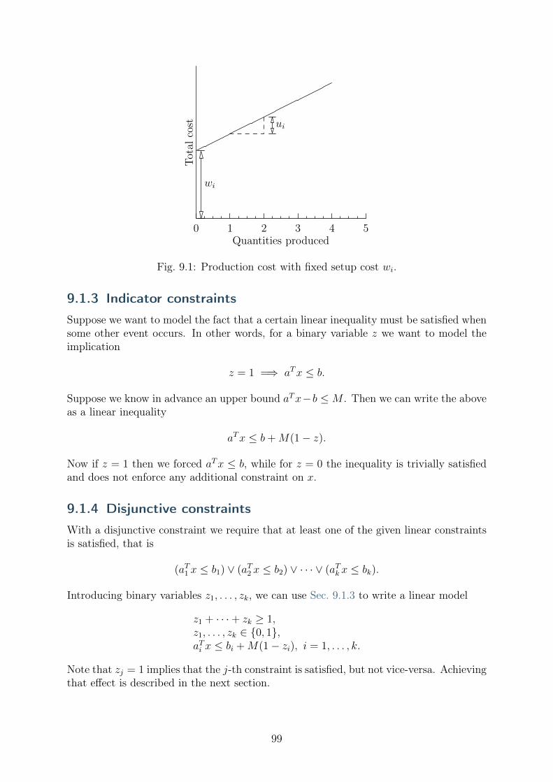
Total

cost

0 1 2 3 4 5Quantities produced

wi

ui

Fig. 9.1: Production cost with fixed setup cost 𝑤𝑖.

9.1.3 Indicator constraints

Suppose we want to model the fact that a certain linear inequality must be satisfied whensome other event occurs. In other words, for a binary variable 𝑧 we want to model theimplication

𝑧 = 1 =⇒ 𝑎𝑇𝑥 ≤ 𝑏.

Suppose we know in advance an upper bound 𝑎𝑇𝑥−𝑏 ≤ 𝑀 . Then we can write the aboveas a linear inequality

𝑎𝑇𝑥 ≤ 𝑏 + 𝑀(1 − 𝑧).

Now if 𝑧 = 1 then we forced 𝑎𝑇𝑥 ≤ 𝑏, while for 𝑧 = 0 the inequality is trivially satisfiedand does not enforce any additional constraint on 𝑥.

9.1.4 Disjunctive constraints

With a disjunctive constraint we require that at least one of the given linear constraintsis satisfied, that is

(𝑎𝑇1 𝑥 ≤ 𝑏1) ∨ (𝑎𝑇2 𝑥 ≤ 𝑏2) ∨ · · · ∨ (𝑎𝑇𝑘 𝑥 ≤ 𝑏𝑘).

Introducing binary variables 𝑧1, . . . , 𝑧𝑘, we can use Sec. 9.1.3 to write a linear model

𝑧1 + · · · + 𝑧𝑘 ≥ 1,𝑧1, . . . , 𝑧𝑘 ∈ {0, 1},𝑎𝑇𝑖 𝑥 ≤ 𝑏𝑖 + 𝑀(1 − 𝑧𝑖), 𝑖 = 1, . . . , 𝑘.

Note that 𝑧𝑗 = 1 implies that the 𝑗-th constraint is satisfied, but not vice-versa. Achievingthat effect is described in the next section.

99

9.1.5 Constraint satisfaction

Say we want to define an optimization model that will behave differently depending onwhich of the inequalities

𝑎𝑇𝑥 ≤ 𝑏 or 𝑎𝑇𝑥 ≥ 𝑏

is satisfied. Suppose we have lower and upper bounds for 𝑎𝑇𝑥 − 𝑏 in the form of 𝑚 ≤𝑎𝑇𝑥− 𝑏 ≤ 𝑀 . Then we can write a model

𝑏 + 𝑚𝑧 ≤ 𝑎𝑇𝑥 ≤ 𝑏 + 𝑀(1 − 𝑧), 𝑧 ∈ {0, 1}. (9.5)

Now observe that 𝑧 = 0 implies 𝑏 ≤ 𝑎𝑇𝑥 ≤ 𝑏 + 𝑀 , of which the right-hand inequalityis redundant, i.e. always satisfied. Similarly, 𝑧 = 1 implies 𝑏 + 𝑚 ≤ 𝑎𝑇𝑥 ≤ 𝑏. In otherwords 𝑧 is an indicator of whether 𝑎𝑇𝑥 ≤ 𝑏.

In practice we would relax one inequality using a small amount of slack, i.e.,

𝑏 + (𝑚− 𝜖)𝑧 + 𝜖 ≤ 𝑎𝑇𝑥 (9.6)

to avoid issues with classifying the equality 𝑎𝑇𝑥 = 𝑏.

9.1.6 Exact absolute value

In Sec. 2.2.2 we showed how to model |𝑥| ≤ 𝑡 as two linear inequalities. Now suppose weneed to model an exact equality

|𝑥| = 𝑡. (9.7)

It defines a non-convex set, hence it is not conic representable. If we split 𝑥 into positiveand negative part 𝑥 = 𝑥+ − 𝑥−, where 𝑥+, 𝑥− ≥ 0, then |𝑥| = 𝑥+ + 𝑥− as long as either𝑥+ = 0 or 𝑥− = 0. That last alternative can be modeled with a binary variable, and weget a model of (9.7):

𝑥 = 𝑥+ − 𝑥−,𝑡 = 𝑥+ + 𝑥−,0 ≤ 𝑥+, 𝑥−,

𝑥+ ≤ 𝑀𝑧,𝑥− ≤ 𝑀(1 − 𝑧),𝑧 ∈ {0, 1},

(9.8)

where the constant 𝑀 is an a priori known upper bound on |𝑥| in the problem.

9.1.7 Exact 1-norm

We can use the technique above to model the exact ℓ1-norm equality constraint𝑛∑︁

𝑖=1

|𝑥𝑖| = 𝑐, (9.9)

where 𝑥 ∈ R𝑛 is a decision variable and 𝑐 is a constant. Such constraints arise for instancein fully invested portfolio optimizations scenarios (with short-selling). As before, we split

100

𝑥 into a positive and negative part, using a sequence of binary variables to guaranteethat at most one of them is nonzero:

𝑥 = 𝑥+ − 𝑥−,0 ≤ 𝑥+, 𝑥−,

𝑥+ ≤ 𝑐𝑧,𝑥− ≤ 𝑐(𝑒− 𝑧),∑︀

𝑖 𝑥+𝑖 +

∑︀𝑖 𝑥

−𝑖 = 𝑐,𝑧 ∈ {0, 1}𝑛, 𝑥+, 𝑥− ∈ R𝑛.

(9.10)

9.1.8 Maximum

The exact equality 𝑡 = max{𝑥1, . . . , 𝑥𝑛} can be expressed by introducing a sequence ofmutually exclusive indicator variables 𝑧1, . . . , 𝑧𝑛, with the intention that 𝑧𝑖 = 1 picks thevariable 𝑥𝑖 which actually achieves maximum. Choosing a safe bound 𝑀 we get a model:

𝑥𝑖 ≤ 𝑡 ≤ 𝑥𝑖 + 𝑀(1 − 𝑧𝑖), 𝑖 = 1, . . . , 𝑛,𝑧1 + · · · + 𝑧𝑛 = 1,

𝑧 ∈ {0, 1}𝑛.(9.11)

9.1.9 Boolean operators

Typically an indicator variable 𝑧 ∈ {0, 1} represents a boolean value (true/false). In thiscase the standard boolean operators can be implemented as linear inequalities. In thetable below we assume all variables are binary.

Table 9.1: Boolean operatorsBoolean Linear𝑧 = 𝑥 OR 𝑦 𝑥 ≤ 𝑧, 𝑦 ≤ 𝑧, 𝑧 ≤ 𝑥 + 𝑦𝑧 = 𝑥 AND 𝑦 𝑥 ≥ 𝑧, 𝑦 ≥ 𝑧, 𝑧 + 1 ≥ 𝑥 + 𝑦𝑧 = NOT 𝑥 𝑧 = 1 − 𝑥𝑥 =⇒ 𝑦 𝑥 ≤ 𝑦At most one of 𝑧1, . . . , 𝑧𝑛 holds (SOS1, set-packing)

∑︀𝑖 𝑧𝑖 ≤ 1

Exactly one of 𝑧1, . . . , 𝑧𝑛 holds (set-partitioning)∑︀

𝑖 𝑧𝑖 = 1At least one of 𝑧1, . . . , 𝑧𝑛 holds (set-covering)

∑︀𝑖 𝑧𝑖 ≥ 1

At most 𝑘 of 𝑧1, . . . , 𝑧𝑛 holds (cardinality)∑︀

𝑖 𝑧𝑖 ≤ 𝑘

9.1.10 Fixed set of values

We can restrict a variable 𝑥 to take on only values from a specified finite set {𝑎1, . . . , 𝑎𝑛}by writing

𝑥 =∑︀

𝑖 𝑧𝑖𝑎𝑖𝑧 ∈ {0, 1}𝑛,∑︀

𝑖 𝑧𝑖 = 1.(9.12)

In (9.12) we essentially defined 𝑧𝑖 to be the indicator variable of whether 𝑥 = 𝑎𝑖. In somecircumstances there may be more efficient representations of a restricted set of values, forexample:

101

• (sign) 𝑥 ∈ {−1, 1} ⇐⇒ 𝑥 = 2𝑧 − 1, 𝑧 ∈ {0, 1},

• (modulo) 𝑥 ∈ {1, 4, 7, 10} ⇐⇒ 𝑥 = 3𝑧 + 1, 0 ≤ 𝑧 ≤ 3, 𝑧 ∈ Z,

• (fraction) 𝑥 ∈ {0, 1/3, 2/3, 1} ⇐⇒ 3𝑥 = 𝑧, 0 ≤ 𝑧 ≤ 3, 𝑧 ∈ Z,

• (gap) 𝑥 ∈ (−∞, 𝑎] ∪ [𝑏,∞) ⇐⇒ 𝑏 − 𝑀(1 − 𝑧) ≤ 𝑥 ≤ 𝑎 + 𝑀𝑧, 𝑧 ∈ {0, 1} forsufficiently large 𝑀 .

In a very similar fashion we can restrict a variable 𝑥 to a finite union of intervals⋃︀𝑖[𝑎𝑖, 𝑏𝑖]: ∑︀

𝑖 𝑧𝑖𝑎𝑖 ≤ 𝑥 ≤∑︀𝑖 𝑧𝑖𝑏𝑖,𝑧 ∈ {0, 1}𝑛,∑︀

𝑖 𝑧𝑖 = 1.(9.13)

9.1.11 Alternative as a bilinear equality

In the literature one often finds models containing a bilinear constraint

𝑥𝑦 = 0.

This constraint is just an algebraic formulation of the alternative 𝑥 = 0 or 𝑦 = 0 andtherefore it can be written as a mixed-integer linear problem:

|𝑥| ≤ 𝑀𝑧,|𝑦| ≤ 𝑀(1 − 𝑧),𝑧 ∈ {0, 1},

for a suitable constant 𝑀 . The absolute value can be omitted if both 𝑥, 𝑦 are nonnegative.Otherwise it can be modeled as in Sec. 2.2.2.

9.1.12 Equal signs

Suppose we want to say that the variables 𝑥1, . . . , 𝑥𝑛 must either be all nonnegative orall nonpositive. This can be achieved by introducing a single binary variable 𝑧 ∈ {0, 1}which picks one of these two alternatives:

−𝑀(1 − 𝑧) ≤ 𝑥𝑖 ≤ 𝑀𝑧, 𝑖 = 1, . . . , 𝑛.

Indeed, if 𝑧 = 0 then we have −𝑀 ≤ 𝑥𝑖 ≤ 0 and if 𝑧 = 1 then 0 ≤ 𝑥𝑖 ≤ 𝑀 .

9.1.13 Continuous piecewise-linear functions

Consider a continuous, univariate, piecewise-linear, non-convex function 𝑓 : [𝛼1, 𝛼5] ↦→ Rshown in Fig. 9.2. At the interval [𝛼𝑗, 𝛼𝑗+1], 𝑗 = 1, 2, 3, 4 we can describe the function as

𝑓(𝑥) = 𝜆𝑗𝑓(𝛼𝑗) + 𝜆𝑗+1𝑓(𝛼𝑗+1)

102

f(x)

xα1 α2 α3 α4 α5

Fig. 9.2: A univariate piecewise-linear non-convex function.

where 𝜆𝑗𝛼𝑗 + 𝜆𝑗+1𝛼𝑗+1 = 𝑥 and 𝜆𝑗 + 𝜆𝑗+1 = 1. If we add a constraint that only two(adjacent) variables 𝜆𝑗, 𝜆𝑗+1 can be nonzero, we can characterize every value 𝑓(𝑥) overthe entire interval [𝛼1, 𝛼5] as some convex combination,

𝑓(𝑥) =4∑︁

𝑗=1

𝜆𝑗𝑓(𝛼𝑗).

The condition that only two adjacent variables can be nonzero is sometimes called anSOS2 constraint. If we introduce indicator variables 𝑧𝑖 for each pair of adjacent variables(𝜆𝑖, 𝜆𝑖+1), we can model an SOS2 constraint as:

𝜆1 ≤ 𝑧1, 𝜆2 ≤ 𝑧1 + 𝑧2, 𝜆3 ≤ 𝑧2 + 𝑧3, 𝜆4 ≤ 𝑧4 + 𝑧3, 𝜆5 ≤ 𝑧4𝑧1 + 𝑧2 + 𝑧3 + 𝑧4 = 1, 𝑧 ∈ {0, 1}4,

so that we have 𝑧𝑗 = 1 =⇒ 𝜆𝑖 = 0, 𝑖 ̸= {𝑗, 𝑗 + 1}. Collectively, we can then model theepigraph 𝑓(𝑥) ≤ 𝑡 as

𝑥 =∑︀𝑛

𝑗=1 𝜆𝑗𝛼𝑗,∑︀𝑛

𝑗=1 𝜆𝑗𝑓(𝛼𝑗) ≤ 𝑡

𝜆1 ≤ 𝑧1, 𝜆𝑗 ≤ 𝑧𝑗 + 𝑧𝑗−1, 𝑗 = 2, . . . , 𝑛− 1, 𝜆𝑛 ≤ 𝑧𝑛−1,

𝜆 ≥ 0,∑︀𝑛

𝑗=1 𝜆𝑗 = 1,∑︀𝑛−1

𝑗=1 𝑧𝑗 = 1, 𝑧 ∈ {0, 1}𝑛−1,(9.14)

for a piecewise-linear function 𝑓(𝑥) with 𝑛 terms. This approach is often called thelambda-method.

For the function in Fig. 9.2 we can reduce the number of integer variables by using aGray encoding

00 10 11 01

α1 α2 α3 α4 α5

of the intervals [𝛼𝑗, 𝛼𝑗+1] and an indicator variable 𝑦 ∈ {0, 1}2 to represent the fourdifferent values of Gray code. We can then describe the constraints on 𝜆 using only twoindicator variables,

(𝑦1 = 0) → 𝜆3 = 0,(𝑦1 = 1) → 𝜆1 = 𝜆5 = 0,(𝑦2 = 0) → 𝜆4 = 𝜆5 = 0,(𝑦2 = 1) → 𝜆1 = 𝜆2 = 0,

103

which leads to a more efficient characterization of the epigraph 𝑓(𝑥) ≤ 𝑡,

𝑥 =∑︀5

𝑗=1 𝜆𝑗𝛼𝑗,∑︀5

𝑗=1 𝜆𝑗𝑓(𝛼𝑗) ≤ 𝑡,

𝜆3 ≤ 𝑦1, 𝜆1 + 𝜆5 ≤ (1 − 𝑦1), 𝜆4 + 𝜆5 ≤ 𝑦2, 𝜆1 + 𝜆2 ≤ (1 − 𝑦2),

𝜆 ≥ 0,∑︀5

𝑗=1 𝜆𝑗 = 1, 𝑦 ∈ {0, 1}2,

The lambda-method can also be used to model multivariate continuous piecewise-linearnon-convex functions, specified on a set of polyhedra 𝑃𝑘. For example, for the functionshown in Fig. 9.3 we can model the epigraph 𝑓(𝑥) ≤ 𝑡 as

𝑥 =∑︀6

𝑖=1 𝜆𝑖𝑣𝑖,∑︀6

𝑖=1 𝜆𝑖𝑓(𝑣𝑖) ≤ 𝑡,𝜆1 ≤ 𝑧1 + 𝑧2, 𝜆2 ≤ 𝑧1, 𝜆3 ≤ 𝑧2 + 𝑧3,

𝜆4 ≤ 𝑧1 + 𝑧2 + 𝑧3 + 𝑧4, 𝜆5 ≤ 𝑧3 + 𝑧4, 𝜆6 ≤ 𝑧4,

𝜆 ≥ 0,∑︀6

𝑖=1 𝜆𝑖 = 1,∑︀4

𝑖=1 𝑧𝑖 = 1,𝑧 ∈ {0, 1}4.

(9.15)

Note, for example, that 𝑧2 = 1 implies that 𝜆2 = 𝜆5 = 𝜆6 = 0 and 𝑥 = 𝜆1𝑣1 +𝜆3𝑣3 +𝜆4𝑣4.

Fig. 9.3: A multivariate continuous piecewise-linear non-convex function.

9.1.14 Lower semicontinuous piecewise-linear functions

The ideas in Sec. 9.1.13 can be applied to lower semicontinuous piecewise-linear functionsas well. For example, consider the function shown in Fig. 9.4. If we denote the one-sidedlimits by 𝑓−(𝑐) := lim𝑥↑𝑐 𝑓(𝑥) and 𝑓+(𝑐) := lim𝑥↓𝑐 𝑓(𝑥), respectively, the one-sided limits,then we can describe the epigraph 𝑓(𝑥) ≤ 𝑡 for the function in Fig. 9.4 as

𝑥 = 𝜆1𝛼1 + (𝜆2 + 𝜆3 + 𝜆4)𝛼2 + 𝜆5𝛼3,𝜆1𝑓(𝛼1) + 𝜆2𝑓−(𝛼2) + 𝜆3𝑓(𝛼2) + 𝜆4𝑓+(𝛼2) + 𝜆5𝑓(𝛼3) ≤ 𝑡,

𝜆1 + 𝜆2 ≤ 𝑧1, 𝜆3 ≤ 𝑧2, 𝜆4 + 𝜆5 ≤ 𝑧3,

𝜆 ≥ 0,∑︀5

𝑖=1 𝜆𝑖 = 1,∑︀3

𝑖=1 𝑧𝑖 = 1, 𝑧 ∈ {0, 1}3,(9.16)

where we have a different decision variable for the intervals [𝛼1, 𝛼2), [𝛼2, 𝛼2], and (𝛼2, 𝛼3].As a special case this gives us an alternative characterization of fixed charge modelsconsidered in Sec. 9.1.1.

104

f(x)

xα1 α2 α3

Fig. 9.4: A univariate lower semicontinuous piecewise-linear function.

9.2 Mixed integer conic case studies

9.2.1 Wireless network design

The following problem arises in wireless network design and some other applications.We want to serve 𝑛 clients with 𝑘 transmitters. A transmitter with range 𝑟𝑗 can serveall clients within Euclidean distance 𝑟𝑗 from its position. The power consumption of atransmitter with range 𝑟 is proportional to 𝑟𝛼 for some fixed 1 ≤ 𝛼 < ∞. The goal isto assign locations and ranges to transmitters minimizing the total power consumptionwhile providing coverage of all 𝑛 clients.

Denoting by 𝑥1, . . . , 𝑥𝑛 ∈ R2 locations of the clients, we can model this problem usingbinary decision variables 𝑧𝑖𝑗 indicating if the 𝑖-th client is covered by the 𝑗-th transmitter.This leads to a mixed-integer conic problem:

minimize∑︀

𝑗 𝑟𝛼𝑗

subject to 𝑟𝑗 ≥ ‖𝑝𝑗 − 𝑥𝑖‖2 −𝑀(1 − 𝑧𝑖𝑗), 𝑖 = 1, . . . , 𝑛, 𝑗 = 1, . . . , 𝑘,∑︀𝑗 𝑧𝑖𝑗 ≥ 1, 𝑖 = 1, . . . , 𝑛,

𝑝𝑗 ∈ R2, 𝑧𝑖𝑗 ∈ {0, 1}.(9.17)

The objective can be realized by summing power bounds 𝑡𝑗 ≥ 𝑟𝛼𝑗 or by directly boundingthe 𝛼-norm of (𝑟1, . . . , 𝑟𝑘). The latter approach would be recommended for large 𝛼.

This is a type of clustering problem. For 𝛼 = 1, 2, respectively, we are minimizing theperimeter and area of the covered region. In practical applications the power exponent 𝛼can be as large as 6 depending on various factors (for instance terrain). In the linear costmodel (𝛼 = 1) typical solutions contain a small number of huge disks covering most ofthe clients. For increasing 𝛼 large ranges are penalized more heavily and the disks tendto be more balanced.

105

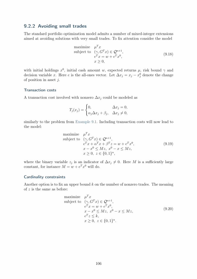
9.2.2 Avoiding small trades

The standard portfolio optimization model admits a number of mixed-integer extensionsaimed at avoiding solutions with very small trades. To fix attention consider the model

maximize 𝜇𝑇𝑥subject to (𝛾,𝐺𝑇𝑥) ∈ 𝒬𝑛+1,

𝑒𝑇𝑥 = 𝑤 + 𝑒𝑇𝑥0,𝑥 ≥ 0,

(9.18)

with initial holdings 𝑥0, initial cash amount 𝑤, expected returns 𝜇, risk bound 𝛾 anddecision variable 𝑥. Here 𝑒 is the all-ones vector. Let ∆𝑥𝑗 = 𝑥𝑗 − 𝑥0

𝑗 denote the changeof position in asset 𝑗.

Transaction costs

A transaction cost involved with nonzero ∆𝑥𝑗 could be modeled as

𝑇𝑗(𝑥𝑗) =

{︃0, ∆𝑥𝑗 = 0,

𝛼𝑗∆𝑥𝑗 + 𝛽𝑗, ∆𝑥𝑗 ̸= 0,

similarly to the problem from Example 9.1. Including transaction costs will now lead tothe model:

maximize 𝜇𝑇𝑥subject to (𝛾,𝐺𝑇𝑥) ∈ 𝒬𝑛+1,

𝑒𝑇𝑥 + 𝛼𝑇𝑥 + 𝛽𝑇 𝑧 = 𝑤 + 𝑒𝑇𝑥0,𝑥− 𝑥0 ≤ 𝑀𝑧, 𝑥0 − 𝑥 ≤ 𝑀𝑧,𝑥 ≥ 0, 𝑧 ∈ {0, 1}𝑛,

(9.19)

where the binary variable 𝑧𝑗 is an indicator of ∆𝑥𝑗 ̸= 0. Here 𝑀 is a sufficiently largeconstant, for instance 𝑀 = 𝑤 + 𝑒𝑇𝑥0 will do.

Cardinality constraints

Another option is to fix an upper bound 𝑘 on the number of nonzero trades. The meaningof 𝑧 is the same as before:

maximize 𝜇𝑇𝑥subject to (𝛾,𝐺𝑇𝑥) ∈ 𝒬𝑛+1,

𝑒𝑇𝑥 = 𝑤 + 𝑒𝑇𝑥0,𝑥− 𝑥0 ≤ 𝑀𝑧, 𝑥0 − 𝑥 ≤ 𝑀𝑧,𝑒𝑇 𝑧 ≤ 𝑘,𝑥 ≥ 0, 𝑧 ∈ {0, 1}𝑛.

(9.20)

106

Trading size constraints

We can also demand a lower bound on nonzero trades, that is |∆𝑥𝑗| ∈ {0} ∪ [𝑎, 𝑏] for all𝑗. To this end we combine the techniques from Sec. 9.1.6 and Sec. 9.1.2 writing 𝑝𝑗, 𝑞𝑗 forthe indicators of ∆𝑥𝑗 > 0 and ∆𝑥𝑗 < 0, respectively:

maximize 𝜇𝑇𝑥subject to (𝛾,𝐺𝑇𝑥) ∈ 𝒬𝑛+1,

𝑒𝑇𝑥 = 𝑤 + 𝑒𝑇𝑥0,𝑥− 𝑥0 = 𝑥+ − 𝑥−,𝑥+ ≤ 𝑀𝑝, 𝑥− ≤ 𝑀𝑞,𝑎(𝑝 + 𝑞) ≤ 𝑥+ + 𝑥− ≤ 𝑏(𝑝 + 𝑞),𝑝 + 𝑞 ≤ 𝑒,𝑥, 𝑥+, 𝑥− ≥ 0, 𝑝, 𝑞 ∈ {0, 1}𝑛.

(9.21)

9.2.3 Convex piecewise linear regression

Consider the problem of approximating the data (𝑥𝑖, 𝑦𝑖), 𝑖 = 1, . . . , 𝑛 by a piecewiselinear convex function of the form

𝑓(𝑥) = max{𝑎𝑗𝑥 + 𝑏𝑗, 𝑗 = 1, . . . 𝑘},

where 𝑘 is the number of segments we want to consider. The quality of the fit is measuredwith least squares as ∑︁

𝑖

(𝑓(𝑥𝑖) − 𝑦𝑖)2.

Note that we do not specify the locations of nodes (breakpoints), i.e. points where 𝑓(𝑥)changes slope. Finding them is part of the fitting problem.

As in Sec. 9.1.8 we introduce binary variables 𝑧𝑖𝑗 indicating that 𝑓(𝑥𝑖) = 𝑎𝑗𝑥𝑖 + 𝑏𝑗,i.e. it is the 𝑗-th linear function that achieves maximum at the point 𝑥𝑖. Following Sec.9.1.8 we now have a mixed integer conic quadratic problem

minimize ‖𝑦 − 𝑓‖2subject to 𝑎𝑗𝑥𝑖 + 𝑏𝑗 ≤ 𝑓𝑖, 𝑖 = 1, . . . , 𝑛, 𝑗 = 1, . . . , 𝑘,

𝑓𝑖 ≤ 𝑎𝑗𝑥𝑖 + 𝑏𝑗 + 𝑀(1 − 𝑧𝑖𝑗), 𝑖 = 1, . . . , 𝑛, 𝑗 = 1, . . . , 𝑘,∑︀𝑗 𝑧𝑖𝑗 = 1, 𝑖 = 1 . . . , 𝑛,

𝑧𝑖𝑗 ∈ {0, 1}, 𝑖 = 1, . . . , 𝑛, 𝑗 = 1, . . . , 𝑘,

(9.22)

with variables 𝑎, 𝑏, 𝑓, 𝑧, where 𝑀 is a sufficiently large constant.Frequently an integer model will have properties which formally follow from the prob-

lem’s constraints, but may be very hard or impossible for a mixed-integer solver to auto-matically deduce. It may dramatically improve efficiency to explicitly add some of themto the model. For example, we can enhance (9.22) with all inequalities of the form

𝑧𝑖,𝑗+1 + 𝑧𝑖+𝑖′,𝑗 ≤ 1,

which indicate that each linear segment covers a contiguous subset of the sample andadditionally force these segments to come in the order of increasing 𝑗 as 𝑖 increases fromleft to right. The last statement is an example of symmetry breaking.

107

Fig. 9.5: Convex piecewise linear fit with 𝑘 = 2, 3, 4 segments.

108

Chapter 10

Quadratic optimization

In this chapter we discuss convex quadratic and quadratically constrained optimization.Our discussion is fairly brief compared to the previous chapters for three reasons; (i)convex quadratic optimization is a special case of conic quadratic optimization, (ii) formost convex problems it is actually more computationally efficient to pose the problemin conic form, and (iii) duality theory (including infeasibility certificates) is much simplerfor conic quadratic optimization. Therefore, we generally recommend a conic quadraticformulation, see Sec. 3 and especially Sec. 3.2.3.

10.1 Quadratic objective

A standard (convex) quadratic optimization problem

minimize 12𝑥𝑇𝑄𝑥 + 𝑐𝑇𝑥

subject to 𝐴𝑥 = 𝑏,𝑥 ≥ 0,

(10.1)

with 𝑄 ∈ 𝒮𝑛+ is conceptually a simple extension of a standard linear optimization problem

with a quadratic term 𝑥𝑇𝑄𝑥. Note the important requirement that 𝑄 is symmetricpositive semidefinite; otherwise the objective function would not be convex.

10.1.1 Geometry of quadratic optimization

Quadratic optimization has a simple geometric interpretation; we minimize a convexquadratic function over a polyhedron., see Fig. 10.1. It is intuitively clear that thefollowing different cases can occur:

• The optimal solution 𝑥⋆ is at the boundary of the polyhedron (as shown in Fig.10.1). At 𝑥⋆ one of the hyperplanes is tangential to an ellipsoidal level curve.

• The optimal solution is inside the polyhedron; this occurs if the unconstrainedminimizer arg min𝑥

12𝑥𝑇𝑄𝑥 + 𝑐𝑇𝑥 = −𝑄†𝑐 (i.e., the center of the ellipsoidal level

curves) is inside the polyhedron. From now on 𝑄† denotes the pseudoinverse of 𝑄;in particular 𝑄† = 𝑄−1 if 𝑄 is positive definite.

• If the polyhedron is unbounded in the opposite direction of 𝑐, and if the ellipsoidlevel curves are degenerate in that direction (i.e., 𝑄𝑐 = 0), then the problem isunbounded. If 𝑄 ∈ 𝒮𝑛

++, then the problem cannot be unbounded.

109

• The problem is infeasible, i.e., {𝑥 | 𝐴𝑥 = 𝑏, 𝑥 ≥ 0} = ∅.

x⋆

a0

a1a2

a3

a4

Fig. 10.1: Geometric interpretation of quadratic optimization. At the optimal point 𝑥⋆

the hyperplane {𝑥 | 𝑎𝑇1 𝑥 = 𝑏} is tangential to an ellipsoidal level curve.

Possibly because of its simple geometric interpretation and similarity to linear opti-mization, quadratic optimization has been more widely adopted by optimization practi-tioners than conic quadratic optimization.

10.1.2 Duality in quadratic optimization

The Lagrangian function (Sec. 8.3) for (10.1) is

𝐿(𝑥, 𝑦, 𝑠) =1

2𝑥𝑇𝑄𝑥 + 𝑥𝑇 (𝑐− 𝐴𝑇𝑦 − 𝑠) + 𝑏𝑇𝑦 (10.2)

with Lagrange multipliers 𝑠 ∈ R𝑛+, and from ∇𝑥𝐿(𝑥, 𝑦, 𝑠) = 0 we get the necessary first-

order optimality condition

𝑄𝑥 = 𝐴𝑇𝑦 + 𝑠− 𝑐,

i.e. (𝐴𝑇𝑦 + 𝑠− 𝑐) ∈ ℛ(𝑄). Then

arg min𝑥

𝐿(𝑥, 𝑦, 𝑠) = 𝑄†(𝐴𝑇𝑦 + 𝑠− 𝑐),

which can be substituted into (10.2) to give a dual function

𝑔(𝑦, 𝑠) =

{︂𝑏𝑇𝑦 − 1

2(𝐴𝑇𝑦 + 𝑠− 𝑐)𝑄†(𝐴𝑇𝑦 + 𝑠− 𝑐), (𝐴𝑇𝑦 + 𝑠− 𝑐) ∈ ℛ(𝑄),

−∞ otherwise.

Thus we get a dual problem

maximize 𝑏𝑇𝑦 − 12(𝐴𝑇𝑦 + 𝑠− 𝑐)𝑄†(𝐴𝑇𝑦 + 𝑠− 𝑐)

subject to (𝐴𝑇𝑦 + 𝑠− 𝑐) ∈ ℛ(𝑄),𝑠 ≥ 0,

(10.3)

110

or alternatively, using the optimality condition 𝑄𝑥 = 𝐴𝑇𝑦 + 𝑠− 𝑐 we can write

maximize 𝑏𝑇𝑦 − 12𝑥𝑇𝑄𝑥

subject to 𝑄𝑥 = 𝐴𝑇𝑦 − 𝑐 + 𝑠,𝑠 ≥ 0.

(10.4)

Note that this is an unusual dual problem in the sense that it involves both primal anddual variables.

Weak duality, strong duality under Slater constraint qualification and Farkas infeasi-bility certificates work similarly as in Sec. 8. In particular, note that the constraints inboth (10.1) and (10.4) are linear, so Lemma 2.4 applies and we have:

i. The primal problem (10.1) is infeasible if and only if there is 𝑦 such that 𝐴𝑇𝑦 ≤ 0and 𝑏𝑇𝑦 > 0.

ii. The dual problem (10.4) is infeasible if and only if there is 𝑥 ≥ 0 such that 𝐴𝑥 = 0,𝑄𝑥 = 0 and 𝑐𝑇𝑥 < 0.

10.1.3 Conic reformulation

Suppose we have a factorization 𝑄 = 𝐹 𝑇𝐹 where 𝐹 ∈ R𝑘×𝑛, which is most interestingwhen 𝑘 ≪ 𝑛. Then 𝑥𝑇𝑄𝑥 = 𝑥𝑇𝐹 𝑇𝐹𝑥 = ‖𝐹𝑥‖22 and the conic quadratic reformulation of(10.1) is

minimize 𝑟 + 𝑐𝑇𝑥subject to 𝐴𝑥 = 𝑏,

𝑥 ≥ 0,(1, 𝑟, 𝐹𝑥) ∈ 𝒬𝑘+2

r ,

(10.5)

with dual problem

maximize 𝑏𝑇𝑦 − 𝑢subject to −𝐹 𝑇𝑣 = 𝐴𝑇𝑦 − 𝑐 + 𝑠,

𝑠 ≥ 0,(𝑢, 1, 𝑣) ∈ 𝒬𝑘+2

r .

(10.6)

Note that in an optimal primal-dual solution we have 𝑟 = 12‖𝐹𝑥‖22, hence the com-

plementary slackness for 𝒬𝑘+2r demands 𝑣 = −𝐹𝑥 and −𝐹 𝑇𝐹𝑣 = 𝑄𝑥, as well as

𝑢 = 12‖𝑣‖22 = 1

2𝑥𝑇𝑄𝑥. This justifies why some of the dual variables in (10.6) and (10.4)

have the same names - they are in fact equal, and so both the primal and dual solutionto the original quadratic problem can be recovered from the primal-dual solution to theconic reformulation.

10.2 Quadratically constrained optimization

A general convex quadratically constrained quadratic optimization problem is

minimize 12𝑥𝑇𝑄0𝑥 + 𝑐𝑇0 𝑥 + 𝑟0

subject to 12𝑥𝑇𝑄𝑖𝑥 + 𝑐𝑇𝑖 𝑥 + 𝑟𝑖 ≤ 0, 𝑖 = 1, . . . ,𝑚,

(10.7)

111

where 𝑄𝑖 ∈ 𝒮𝑛+. This corresponds to minimizing a convex quadratic function over an

intersection of convex quadratic sets such as ellipsoids or affine halfspaces. Note theimportant requirement 𝑄𝑖 ⪰ 0 for all 𝑖 = 0, . . . ,𝑚, so that the objective function is convexand the constraints characterize convex sets. For example, neither of the constraints

1

2𝑥𝑇𝑄𝑖𝑥 + 𝑐𝑇𝑖 𝑥 + 𝑟𝑖 = 0,

1

2𝑥𝑇𝑄𝑖𝑥 + 𝑐𝑇𝑖 𝑥 + 𝑟𝑖 ≥ 0

characterize convex sets, and therefore cannot be included.

10.2.1 Duality in quadratically constrained optimization

The Lagrangian function for (10.7) is

𝐿(𝑥, 𝜆) = 12𝑥𝑇𝑄0𝑥 + 𝑐𝑇0 𝑥 + 𝑟0 +

∑︀𝑚𝑖=1 𝜆𝑖

(︀12𝑥𝑇𝑄𝑖𝑥 + 𝑐𝑇𝑖 𝑥 + 𝑟𝑖

)︀= 1

2𝑥𝑇𝑄(𝜆)𝑥 + 𝑐(𝜆)𝑇𝑥 + 𝑟(𝜆),

where

𝑄(𝜆) = 𝑄0 +𝑚∑︁𝑖=1

𝜆𝑖𝑄𝑖, 𝑐(𝜆) = 𝑐0 +𝑚∑︁𝑖=1

𝜆𝑖𝑐𝑖, 𝑟(𝜆) = 𝑟0 +𝑚∑︁𝑖=1

𝜆𝑖𝑟𝑖.

From the Lagrangian we get the first-order optimality conditions

𝑄(𝜆)𝑥 = −𝑐(𝜆), (10.8)

and similar to the case of quadratic optimization we get a dual problem

maximize −12𝑐(𝜆)𝑇𝑄(𝜆)†𝑐(𝜆) + 𝑟(𝜆)

subject to 𝑐(𝜆) ∈ ℛ (𝑄(𝜆)) ,𝜆 ≥ 0,

(10.9)

or equivalently

maximize −12𝑤𝑇𝑄(𝜆)𝑤 + 𝑟(𝜆)

subject to 𝑄(𝜆)𝑤 = −𝑐(𝜆),𝜆 ≥ 0.

(10.10)

Using a general version of the Schur Lemma for singular matrices, we can also write (10.9)as an equivalent semidefinite optimization problem,

maximize 𝑡

subject to[︂

2(𝑟(𝜆) − 𝑡) 𝑐(𝜆)𝑇

𝑐(𝜆) 𝑄(𝜆)

]︂⪰ 0,

𝜆 ≥ 0.

(10.11)

Feasibility in quadratically constrained optimization is characterized by the followingconditions (assuming Slater constraint qualification or other conditions to exclude ill-posed problems):

• Either the primal problem (10.7) is feasible or there exists 𝜆 ≥ 0, 𝜆 ̸= 0 satisfying𝑚∑︁𝑖=1

𝜆𝑖

[︂2𝑟𝑖 𝑐𝑇𝑖𝑐𝑖 𝑄𝑖

]︂≻ 0. (10.12)

112

• Either the dual problem (10.10) is feasible or there exists 𝑥 ∈ R𝑛 satisfying

𝑄0𝑥 = 0, 𝑐𝑇0 𝑥 < 0, 𝑄𝑖𝑥 = 0, 𝑐𝑇𝑖 𝑥 = 0, 𝑖 = 1, . . . ,𝑚. (10.13)

To see why the certificate proves infeasibility, suppose for instance that (10.12) and(10.7) are simultaneously satisfied. Then

0 <∑︁𝑖

𝜆𝑖

[︂1𝑥

]︂𝑇 [︂2𝑟𝑖 𝑐𝑇𝑖𝑐𝑖 𝑄𝑖

]︂ [︂1𝑥

]︂= 2

∑︁𝑖

𝜆𝑖

(︂1

2𝑥𝑇𝑄𝑖𝑥 + 𝑐𝑇𝑖 𝑥 + 𝑟𝑖

)︂≤ 0

and we have a contradiction, so (10.12) certifies infeasibility.

10.2.2 Conic reformulation

If 𝑄𝑖 = 𝐹 𝑇𝑖 𝐹𝑖 for 𝑖 = 0, . . . ,𝑚, where 𝐹𝑖 ∈ R𝑘𝑖×𝑛 then we get a conic quadratic reformu-

lation of (10.7):

minimize 𝑡0 + 𝑐𝑇0 𝑥 + 𝑟0subject to (1, 𝑡0, 𝐹0𝑥) ∈ 𝒬𝑘0+2

r ,(1,−𝑐𝑇𝑖 𝑥− 𝑟𝑖, 𝐹𝑖𝑥) ∈ 𝒬𝑘𝑖+2

r , 𝑖 = 1, . . . ,𝑚.(10.14)

The primal and dual solution of (10.14) recovers the primal and dual solution of (10.7)similarly as for quadratic optimization in Sec. 10.1.3. Let us see for example, how a(conic) primal infeasibility certificate for (10.14) implies an infeasibility certificate in theform (10.12). Infeasibility in (10.14) involves only the last set of conic constraints. Wecan derive the infeasibility certificate for those constraints from Lemma 8.3 or by directlywriting the Lagrangian

𝐿 = −∑︀𝑖

(︀𝑢𝑖 + 𝑣𝑖(−𝑐𝑇𝑖 𝑥− 𝑟𝑖) + 𝑤𝑇

𝑖 𝐹𝑖𝑥)︀

= 𝑥𝑇(︀∑︀

𝑖 𝑣𝑖𝑐𝑖 −∑︀

𝑖 𝐹𝑇𝑖 𝑤𝑖

)︀+ (∑︀

𝑖 𝑣𝑖𝑟𝑖 −∑︀

𝑖 𝑢𝑖) .

The dual maximization problem is unbounded (i.e. the primal problem is infeasible) ifwe have ∑︀

𝑖 𝑣𝑖𝑐𝑖 =∑︀

𝑖 𝐹𝑇𝑖 𝑤𝑖,∑︀

𝑖 𝑣𝑖𝑟𝑖 >∑︀

𝑖 𝑢𝑖,2𝑢𝑖𝑣𝑖 ≥ ‖𝑤𝑖‖2, 𝑢𝑖, 𝑣𝑖 ≥ 0.

We claim that 𝜆 = 𝑣 is an infeasibility certificate in the sense of (10.12). We can assume𝑣𝑖 > 0 for all 𝑖, as otherwise 𝑤𝑖 = 0 and we can take 𝑢𝑖 = 0 and skip the 𝑖-th coordinate.Let 𝑀 denote the matrix appearing in (10.12) with 𝜆 = 𝑣. We show that 𝑀 is positivedefinite:

[𝑦, 𝑥]𝑇𝑀 [𝑦, 𝑥] =∑︀

𝑖

(︀𝑣𝑖𝑥

𝑇𝑄𝑖𝑥 + 2𝑣𝑖𝑦𝑐𝑇𝑖 𝑥 + 2𝑣𝑖𝑟𝑖𝑦

2)︀

>∑︀

𝑖

(︀𝑣𝑖‖𝐹𝑖𝑥‖2 + 2𝑦𝑤𝑇

𝑖 𝐹𝑖𝑥 + 2𝑢𝑖𝑦2)︀

≥∑︀𝑖 𝑣−1𝑖 ‖𝑣𝑖𝐹𝑖𝑥 + 𝑦𝑤𝑖‖2 ≥ 0.

113

10.3 Example: Factor model

Recall from Sec. 3.3.3 that the standard Markowitz portfolio optimization problem is

maximize 𝜇𝑇𝑥subject to 𝑥𝑇Σ𝑥 ≤ 𝛾,

𝑒𝑇𝑥 = 1,𝑥 ≥ 0,

(10.15)

where 𝜇 ∈ R𝑛 is a vector of expected returns for 𝑛 different assets and Σ ∈ 𝒮𝑛+ denotes

the corresponding covariance matrix. Problem (10.15) maximizes the expected returnof an investment given a budget constraint and an upper bound 𝛾 on the allowed risk.Alternatively, we can minimize the risk given a lower bound 𝛿 on the expected return ofinvestment, i.e., we can solve the problem

minimize 𝑥𝑇Σ𝑥subject to 𝜇𝑇𝑥 ≥ 𝛿,

𝑒𝑇𝑥 = 1,𝑥 ≥ 0.

(10.16)

Both problems (10.15) and (10.16) are equivalent in the sense that they describe the samePareto-optimal trade-off curve by varying 𝛿 and 𝛾.

Next consider a factorization

Σ = 𝑉 𝑇𝑉 (10.17)

for some 𝑉 ∈ R𝑘×𝑛. We can then rewrite both problems (10.15) and (10.16) in conicquadratic form as

maximize 𝜇𝑇𝑥subject to (1/2, 𝛾, 𝑉 𝑥) ∈ 𝒬𝑘+2

𝑟 ,𝑒𝑇𝑥 = 1,𝑥 ≥ 0,

(10.18)

and

minimize 𝑡subject to (1/2, 𝑡, 𝑉 𝑥) ∈ 𝒬𝑘+2

𝑟 ,𝜇𝑇𝑥 ≥ 𝛿,𝑒𝑇𝑥 = 1,𝑥 ≥ 0,

(10.19)

respectively. Given Σ ≻ 0, we may always compute a factorization (10.17) where 𝑉is upper-triangular (Cholesky factor). In this case 𝑘 = 𝑛, i.e., 𝑉 ∈ R𝑛×𝑛, so there islittle difference in complexity between the conic and quadratic formulations. However,in practice, better choices of 𝑉 are either known or readily available. We mention twoexamples.

114

Data matrix

Σ might be specified directly in the form (10.17), where 𝑉 is a normalized data-matrixwith 𝑘 observations of market data (for example daily returns) of the 𝑛 assets. When theobservation horizon 𝑘 is shorter than 𝑛, which is typically the case, the conic representa-tion is both more parsimonious and has better numerical properties.

Factor model

For a factor model we have

Σ = 𝐷 + 𝑈𝑇𝑅𝑈

where 𝐷 = Diag(𝑤) is a diagonal matrix, 𝑈 ∈ R𝑘×𝑛 represents the exposure of assets torisk factors and 𝑅 ∈ R𝑘×𝑘 is the covariance matrix of factors. Importantly, we normallyhave a small number of factors (𝑘 ≪ 𝑛), so it is computationally much cheaper to find aCholesky decomposition 𝑅 = 𝐹 𝑇𝐹 with 𝐹 ∈ R𝑘×𝑘. This combined gives us Σ = 𝑉 𝑇𝑉 for

𝑉 =

[︂𝐷1/2

𝐹𝑈

]︂of dimensions (𝑛 + 𝑘) × 𝑛. The dimensions of 𝑉 are larger than the dimensions of theCholesky factors of Σ, but 𝑉 is very sparse, which usually results in a significant reductionof solution time. The resulting risk minimization conic problem can ultimately be writtenas:

minimize 𝑑 + 𝑡subject to (1/2, 𝑡, 𝐹𝑈𝑥) ∈ 𝒬𝑘+2

𝑟 ,

(1/2, 𝑑, 𝑤1/21 𝑥1, · · · , 𝑤1/2

𝑛 𝑥𝑛) ∈ 𝒬𝑛+2𝑟 ,

𝜇𝑇𝑥 ≥ 𝛿,𝑒𝑇𝑥 = 1,𝑥 ≥ 0.

(10.20)

115

Chapter 11

Bibliographic notes

The material on linear optimization is very basic, and can be found in any textbook.For further details, we suggest a few standard references [Chvatal83], [BT97] and [PS98],which all cover much more that discussed here. [NW06] gives a more modern treatmentof both theory and algorithmic aspects of linear optimization.

Material on conic quadratic optimization is based on the paper [LVBL98] and thebooks [BenTalN01], [BV04]. The papers [AG03], [ART03] contain additional theoreticaland algorithmic aspects.

For more theory behind the power cone and the exponential cone we recommend thethesis [Cha09].

Much of the material about semidefinite optimization is based on the paper [VB96]and the books [BenTalN01], [BKVH07]. The section on optimization over nonnegativepolynomials is based on [Nes99], [Hac03]. We refer to [LR05] for a comprehensive surveyon semidefinite optimization and relaxations in combinatorial optimization.

The chapter on conic duality follows the exposition in [GartnerM12]Mixed-integer optimization is based on the books [NW88], [Wil93]. Modeling of piece-

wise linear functions is described in the survey paper [VAN10].

116

Chapter 12

Notation and definitions

R and Z denote the sets of real numbers and integers, respectively. R𝑛 denotes the set of𝑛-dimensional vectors of real numbers (and similarly for Z𝑛 and {0, 1}𝑛); in most caseswe denote such vectors by lower case letters, e.g., 𝑎 ∈ R𝑛. A subscripted value 𝑎𝑖 thenrefers to the 𝑖-th entry in 𝑎, i.e.,

𝑎 = (𝑎1, 𝑎2, . . . , 𝑎𝑛).

The symbol 𝑒 denotes the all-ones vector 𝑒 = (1, . . . , 1)𝑇 , whose length always followsfrom the context.

All vectors are interpreted as column-vectors. For 𝑎, 𝑏 ∈ R𝑛 we use the standard innerproduct,

⟨𝑎, 𝑏⟩ := 𝑎1𝑏1 + 𝑎2𝑏2 + · · · + 𝑎𝑛𝑏𝑛,

which we also write as 𝑎𝑇 𝑏 := ⟨𝑎, 𝑏⟩. We let R𝑚×𝑛 denote the set of 𝑚× 𝑛 matrices, andwe use upper case letters to represent them, e.g., 𝐵 ∈ R𝑚×𝑛 is organized as

𝐵 =

⎡⎢⎢⎢⎣𝑏11 𝑏12 . . . 𝑏1𝑛𝑏21 𝑏22 . . . 𝑏2𝑛...

... . . . ...𝑏𝑚1 𝑏𝑚2 . . . 𝑏𝑚𝑛

⎤⎥⎥⎥⎦For matrices 𝐴,𝐵 ∈ R𝑚×𝑛 we use the inner product

⟨𝐴,𝐵⟩ :=𝑚∑︁𝑖=1

𝑛∑︁𝑗=1

𝑎𝑖𝑗𝑏𝑖𝑗.

For a vector 𝑥 ∈ R𝑛 we have

Diag(𝑥) :=

⎡⎢⎢⎢⎣𝑥1 0 . . . 00 𝑥2 . . . 0...

... . . . ...0 0 . . . 𝑥𝑛

⎤⎥⎥⎥⎦ ,

i.e., a square matrix with 𝑥 on the diagonal and zero elsewhere. Similarly, for a squarematrix 𝑋 ∈ R𝑛×𝑛 we have

diag(𝑋) := (𝑥11, 𝑥22, . . . , 𝑥𝑛𝑛).

117

A set 𝑆 ⊆ R𝑛 is convex if and only if for any 𝑥, 𝑦 ∈ 𝑆 and 𝜃 ∈ [0, 1] we have

𝜃𝑥 + (1 − 𝜃)𝑦 ∈ 𝑆

A function 𝑓 : R𝑛 ↦→ R is convex if and only if its domain dom(𝑓) is convex and for all𝜃 ∈ [0, 1] we have

𝑓(𝜃𝑥 + (1 − 𝜃)𝑦) ≤ 𝜃𝑓(𝑥) + (1 − 𝜃)𝑓(𝑦).

A function 𝑓 : R𝑛 ↦→ R is concave if and only if −𝑓 is convex. The epigraph of a function𝑓 : R𝑛 ↦→ R is the set

epi(𝑓) := {(𝑥, 𝑡) | 𝑥 ∈ dom(𝑓), 𝑓(𝑥) ≤ 𝑡},

shown in Fig. 12.1.

epi(f)

f

Fig. 12.1: The shaded region is the epigraph of the function 𝑓(𝑥) = − log(𝑥).

Thus, minimizing over the epigraph

minimize 𝑡subject to 𝑓(𝑥) ≤ 𝑡

is equivalent to minimizing 𝑓(𝑥). Furthermore, 𝑓 is convex if and only if epi(𝑓) is aconvex set. Similarly, the hypograph of a function 𝑓 : R𝑛 ↦→ R is the set

hypo(𝑓) := {(𝑥, 𝑡) | 𝑥 ∈ dom(𝑓), 𝑓(𝑥) ≥ 𝑡}.

Maximizing 𝑓 is equivalent to maximizing over the hypograph

maximize 𝑡subject to 𝑓(𝑥) ≥ 𝑡,

and 𝑓 is concave if and only if hypo(𝑓) is a convex set.

118

Bibliography

[AG03] F. Alizadeh and D. Goldfarb. Second-order cone programming. Math. Pro-gramming, 95(1):3–51, 2003.

[ART03] E. D. Andersen, C. Roos, and T. Terlaky. On implementing a primal-dualinterior-point method for conic quadratic optimization. Math. Programming,February 2003.

[BT97] D. Bertsimas and J. N. Tsitsiklis. Introduction to linear optimization. AthenaScientific, 1997.

[BKVH07] S. Boyd, S.J. Kim, L. Vandenberghe, and A. Hassibi. A Tutorial on Geomet-ric Programming. Optimization and Engineering, 8(1):67–127, 2007. Avail-able at http://www.stanford.edu/ boyd/gp_tutorial.html.

[BV04] S. Boyd and L. Vandenberghe. Convex optimization. Cambridge UniversityPress, 2004. http://www.stanford.edu/ boyd/cvxbook/.

[CS14] Venkat Chandrasekaran and Parikshit Shah. Conic geometric programming.In Information Sciences and Systems (CISS), 2014 48th Annual Conferenceon, 1–4. IEEE, 2014.

[Cha09] Peter Robert Chares. Cones and interior-point algorithms for structed convexoptimization involving powers and exponentials. PhD thesis, Ecole polytech-nique de Louvain, Universitet catholique de Louvain, 2009.

[Chvatal83] V. Chvátal. Linear programming. W.H. Freeman and Company, 1983.

[GartnerM12] B. Gärtner and J. Matousek. Approximation algorithms and semidefiniteprogramming. Springer Science & Business Media, 2012.

[Hac03] Y. Hachez. Convex optimization over non-negative polynomials: structuredalgorithms and applications. PhD thesis, Université Catholique De Lovain,2003.

[LR05] M. Laurent and F. Rendl. Semidefinite programming and integer pro-gramming. Handbooks in Operations Research and Management Science,12:393–514, 2005.

[LVBL98] M. S. Lobo, L. Vanderberghe, S. Boyd, and H. Lebret. Applications of second-order cone programming. Linear Algebra Appl., 284:193–228, November 1998.

[NW88] G. L. Nemhauser and L. A. Wolsey. Integer programming and combinatorialoptimization. John Wiley and Sons, New York, 1988.

119

[Nes99] Yu. Nesterov. Squared functional systems and optimization problems. InH. Frenk, K. Roos, T. Terlaky, and S. Zhang, editors, High PerformanceOptimization. Kluwer Academic Publishers, 1999.

[NW06] J. Nocedal and S. Wright. Numerical optimization. Springer Science, 2ndedition, 2006.

[PS98] C. H. Papadimitriou and K. Steiglitz. Combinatorial optimization: algo-rithms and complexity. Dover publications, 1998.

[TV98] T. Terlaky and J.-Ph. Vial. Computing maximum likelihood estimators ofconvex density functions. SIAM J. Sci. Statist. Comput., 19(2):675–694,1998.

[VB96] L. Vandenberghe and S. Boyd. Semidefinite programming. SIAM Rev.,38(1):49–95, March 1996.

[VAN10] J. P. Vielma, S. Ahmed, and G. Nemhauser. Mixed-integer models for non-separable piecewise-linear optimization: unifying framework and extensions.Operations research, 58(2):303–315, 2010.

[Wil93] H. P. Williams. Model building in mathematical programming. John Wileyand Sons, 3rd edition, 1993.

[Zie82] H Ziegler. Solving certain singly constrained convex optimization problems inproduction planning. Operations Research Letters, 1982. URL: http://www.sciencedirect.com/science/article/pii/016763778290030X.

[BenTalN01] A. Ben-Tal and A. Nemirovski. Lectures on Modern Convex Optimization:Analysis, Algorithms, and Engineering Applications. MPS/SIAM Series onOptimization. SIAM, 2001.

120

Index

Aabsolute value, 8, 22, 100adjacency matrix, 69

Bbasis pursuit, 8, 14big-M, 77, 97binary optimization, 68, 69binary variable, 97Boolean operator, 101

Ccardinality constraint, 106Cholesky factorization, 23, 28, 51complementary slackness, 91condition number, 56cone

convex, 20distance to, 82dual, 85exponential, 36p-order, 32power, 29product, 84projection, 82quadratic, 19, 51rotated quadratic, 20, 51second-order, 19self-dual, 85semidefinite, 50

conic quadratic optimization, 19constraint, 3

disjunctive, 99indicator, 99redundant, 77

constraint attribution, 93constraint satisfaction, 100convex

cone, 20function, 118set, 118

covariance matrix, 28, 114CQO, 19curve fitting, 64cut, 69

Ddeterminant, 56disjunctive constraint, 99dual

cone, 85function, 14, 88norm, 9problem, 14, 89, 110

dualityconic, 83gap, 91linear, 13, 18quadratic, 110, 112strong, 15, 91weak, 15, 90

dynamical system, 47

Eeigenvalue optimization, 55ellipsoid, 26, 63, 109entropy, 38

maximization, 46relative, 39, 46

epigraph, 118exponential

cone, 36function, 38optimization, 36

Ffactor model, 23, 28, 115Farkas lemma, 12, 17, 86, 111, 112feasibility, 84feasible set, 3, 11, 84Fermat-Torricelli point, 35filter design, 67

121

functionconcave, 118convex, 118dual, 14, 88entropy, 38exponential, 38, 40Lagrange, 14, 88, 110, 112Lambert W, 40logarithm, 38, 41lower semicontinuous, 104piecewise linear, 7, 102power, 23, 32, 43, 105sigmoid, 48softplus, 39

Ggeometric mean, 33, 34, 36geometric median, 35geometric programming, 41GP, 41Grammian matrix, 51

Hhalfspace, 5harmonic mean, 25Hermitian matrix, 60hitting time, 47homogenization, 10, 28Huber loss, 74hyperplane, 4hypograph, 118

Iill-posed, 74, 75, 84, 87indicator

constraint, 99variable, 97

infeasibility, 84certificate, 11, 12, 86, 87, 111, 112locating, 13

inner product, 117matrix, 50

integer variable, 97inventory, 29

KKullback-Leiber divergence, 39, 47

LLagrange function, 14, 88, 110, 112Lambert W function, 40limit-feasibility, 87linear

matrix inequality, 54, 80, 94near dependence, 75optimization, 2

linear matrix inequality, 54, 80, 94linear-fractional problem, 10LMI, 54, 80, 94LO, 2log-determinant, 56log-sum-exp, 39log-sum-inv, 40logarithm, 38, 41logistic regression, 48lowpass filter, 67

MMarkowitz model, 27matrix

adjacency, 69correlation, 62covariance, 28, 114Grammian, 51Hermitian, 60inner product, 50positive definite, 50pseudo-inverse, 53, 109semidefinite, 50, 109, 111variable, 50

MAX-CUT, 70maximum, 7, 9, 43, 101maximum likelihood, 36, 44mean

geometric, 33harmonic, 25

MIO, 96monomial, 41

Nnearest correlation matrix, 62network

design, 105wireless, 45, 105

norm1-norm, 8, 100

122

2-norm, 22dual, 9Euclidean, 22Frobenius, 44infinity norm, 9nuclear, 57p-norm, 32, 35

normal equation, 93

Oobjective, 109objective function, 3optimal value, 3, 84

unattainment, 10, 84optimization

binary, 68boolean, 69eigenvalue, 55exponential, 36linear, 2mixed integer, 96p-order cone, 32power cone, 29practical, 70quadratic, 107robust, 26semidefinite, 48

overflow, 78

Ppenalization, 77perturbation, 74piecewise linear

function, 7regression, 107

pOCO, 32polyhedron, 5, 34, 109polynomial

curve fitting, 64nonnegative, 58, 59, 65trigonometric, 61, 62, 67

portfolio optimizationcardinality constraint, 106constraint attribution, 93covariance matrix, 28, 114duality, 90factor model, 23, 28, 115fully invested, 46, 100

market impact, 33Markowitz model, 27risk factor exposure, 115risk parity, 46Sharpe ratio, 28trading size, 107transaction costs, 106

posynomial, 41power, 23, 43power cone optimization, 29power control, 45precision, 78, 81principal submatrix, 53pseudo-inverse, 53

QQCQO, 26, 111QO, 22, 107quadratic

cone, 19duality, 110, 112optimization, 107rotated cone, 20

quadratic optimization, 22, 26

Rrate allocation, 45redundant constraints, 77regression

linear, 93logistic, 48piecewise linear, 107regularization, 48

regularization, 48relative entropy, 39, 46relaxation

semidefinite, 68, 69, 79Riesz-Fejer Theorem, 61risk parity, 46robust optimization, 26rotated quadratic cone, 20

Sscaling, 76Schur complement, 53, 58, 79, 112SDO, 48second-order cone, 19, 23semicontinuous variable, 98semidefinite

123

cone, 50optimization, 48relaxation, 68, 69, 79

setcovering, 101packing, 101partitioning, 101

setup cost, 98shadow price, 18Sharpe ratio, 28sigmoid, 48signal processing, 67signal-to-noise, 45singular value, 57, 96Slater constraint qualification, 92, 111, 112SOCO, 19softplus, 39SOS1, 101SOS2, 103spectrahedron, 52spectral factorization, 25, 50, 53spectral radius, 56sum of squares, 58, 61symmetry breaking, 107

Ttrading size, 107transaction costs, 106trigonometric polynomial, 61, 62, 67

Uunattainment, 75

Vvariable

binary, 97indicator, 97integer, 97matrix, 50semicontinuous, 98

verification, 80violation, 81volume, 34, 63

124