Some of the long-term changes in weather and climate extremes have occurred as expected

in the warming climate, but trends are not all uniform across the United States nor easily

detected amidst multiyear and decadal variations.

MONITORING AND UNDERSTANDING CHANGES

IN HEAT WAVES, COLD WAVES, FLOODS, AND DROUGHTS

IN THE UNITED STATESState of Knowledge

by Thomas C. PeTerson, riChard r. heim Jr., roberT hirsCh, dale P. Kaiser, harold brooKs, noah s. diffenbaugh, randall m. dole, Jason P. giovanneTTone,

KrisTen guirguis, Thomas r. Karl, riChard W. KaTz, KenneTh KunKel, dennis leTTenmaier, gregory J. mCCabe, ChrisToPher J. PaCioreK, Karen r. ryberg, siegfried sChuberT, viviane b. s. silva,

brooKe C. sTeWarT, aldo v. veCChia, gabriele villarini, russell s. vose, John Walsh, miChael Wehner, david WoloCK, Klaus WolTer, Connie a. Woodhouse, and donald Wuebbles

T he Global Change Research Act of 1990 requires the U.S. government to prepare a report that integrates, evaluates, and interprets scientific

analyses of effects of global climate change on both human and natural systems in the United States. The U.S. National Climate Assessment (www.globalchange .gov/what-we-do/assessment) must therefore address extremes because not only are extremes changing (e.g., Field et al. 2012; Coumou and Rahmstorf 2012) and anthropogenic climate change has a role in altering the probabilities of some of the extreme events (Peterson et al. 2012) but extreme events drive changes in natural and human systems much more than average climatic conditions (Peterson et al. 2008).

However, the domain of extremes is so broad, ranging from tornados less than 1 km across and

lasting only a few minutes to 1,000-km-wide droughts lasting many months, and the scientific literature is so diverse that it is not easy for the assessment writing teams to accurately cover all extremes. Therefore, to provide technical input to the U.S. National Climate Assessment writing team, four workshops were held where leading scientists in the field came together to assess or, more accurately, to determine how best to assess the state of the science in understanding the decadal- to century-scale variability and changes in various types of extreme events. After the workshops, the meeting participants produced papers synthesizing the state of the science on their set of extremes.

The f irst workshop focused on severe local storms, including tornadoes and extreme pre-cipitation (Kunkel et al. 2013). The third workshop

821june 2013AMeRICAn MeTeOROLOGICAL SOCIeTY |

examined extratropical storms, winds, and waves (Vose et al. 2013, manuscript submitted to Bull. Amer. Meteor. Soc.). The fourth workshop assessed historical and projected climate extremes in the United States simulated in phase 5 of the Coupled Model Intercomparison Project models (Wuebbles et al. 2013, manuscript submitted to Bull. Amer. Meteor. Soc.). While our workshop, the second workshop, focused on the large-scale phenomena of heat waves, cold waves, f loods, and drought and served as the basis for this paper, it also allowed the experts to discuss what information is required and what additional analyses we should preform so that we could incorporate their results into this article. As the peer-reviewed literature on these phenomena use many different approaches in assessing these extreme events, our paper as well must use different methodologies where appropriate.

Because the National Climate Assessment has different writing teams focusing on different regions (see Fig. 1), where appropriate this paper describes the geographic differences in the long-term behavior of heat waves, cold waves, floods, and droughts across the United States. While most of the information below comes from either our own or previous peer-reviewed publications’ quantitative analyses, there was one subjective assessment that the workshop facilitated: rating the state of the understanding of the physical factors that cause these extremes to change and the adequacy of the data to accurately reveal long-term variability and change in these extremes, in comparison to each other and in comparison to the extremes assessed in the other workshops.

Defining exactly what constitutes an extreme varies with the phenomenon. Some phenomena, such as hurricanes, tornadoes, floods, and droughts, are by their very definitions extreme events partly be-cause they are rare and have high impacts. However, other extremes, such as heavy precipitation, are simply points on the tails of the distribution of the observa-tions. Exactly how far out on the tail of the distribution one should go is often determined by the goal of the analysis. For example, while a 20-yr return period extreme may have far more societal relevant impacts than an extreme that might occur every year or two, if one is seeking to detect changes in extremes in a part of the world with only 50 yr of available daily data, then 20-yr return period events would provide too few data points for robust trends. Zwiers et al. (2012) provides more context on what constitutes an extreme.

HEAT WAVES AND COLD WAVES . Introduction. Episodes of extreme heat and cold can have serious societal, agricultural, economic, and ecological impacts across the United States, with heat being the number one weather-related killer (National Weather Service 2012; Borden and Cutter 2008). In addition to temperature, high humidity can increase the impacts of heat waves, while high winds can increase the impacts of cold waves (Sheridan and Kalkstein 2004; Steadman 1984; Stocks et al. 2004; Ames and Insley 1975). Many agricultural products exhibit direct temperature threshold responses (e.g., Schlenker and Roberts 2009; White et al. 2006) and can be indirectly affected through threshold responses of agricultural pests (Diffenbaugh et al.

AFFILIATIONS: PeTerson, heim, Karl, and vose—NOAA/National Climatic Data Center, Asheville, North Carolina; hirsCh—U.S. Geological Survey, Reston, Virginia; Kaiser—Carbon Dioxide Information Analysis Center, Oak Ridge National Laboratory, DOE, Oak Ridge, Tennessee; brooKs—National Severe Storms Laboratory, NOAA, Norman, Oklahoma; diffenbaugh—Stanford University, Stanford, California; dole and WolTer— NOAA/Earth System Research Laboratory, Boulder, Colorado; giovanneTTone—Institute for Water Resources, U.S. Army Corp of Engineers, Alexandria, Virginia; guirguis—Scripps Institution of Oceanography, University of California, San Diego, La Jolla, California, and University Corporation for Atmospheric Research, Boulder, Colorado; KaTz—National Center for Atmospheric Research, Boulder, Colorado; KunKel—Cooperative Institute for Climate and Satellites, Asheville, North Carolina; leTTenmaier—University of Washington, Seattle, Washington; mCCabe and WoloCK—USGS, Lawrence, Kansas; PaCioreK—Department of Statistics, University of California, Berkeley, Berkeley, California; ryberg and veCChia—U.S. Geological Survey, Bismarck, North Dakota; sChuberT— NASA

Goddard Space Flight Center, Greenbelt, Maryland; silva—Climate Services Division, NOAA/NWS/OCWWS, Silver Spring, Maryland; sTeWarT—STG, Asheville, North Carolina; villarini—IIHR–Hydroscience and Engineering, The University of Iowa, Iowa City, Iowa; Walsh—University of Alaska Fairbanks, Fairbanks, Alaska; Wehner—Lawrence Berkeley National Laboratory, Berkeley, California; Woodhouse—University of Arizona, Tucson, Arizona; Wuebbles—University of Illinois at Urbana–Champaign, Urbana, IllinoisCORRESPONDING AUTHOR: Thomas C. Peterson, NOAA/National Climatic Data Center, 151 Patton Avenue, Asheville, NC 28803E-mail: thomas.c.peterson@noaa.gov

The abstract for this article can be found in this issue, following the table of contents.DOI:10.1175/BAMS-D-12-00066.1

A supplement to this article is available online (10.1175/BAMS-D-12-00066.2)

In final form 30 November 2012©2013 American Meteorological Society

822 june 2013|

2008, and references therein). Ecological responses include limitation of invasive species by severe cold (Walther et al. 2002; Firth et al. 2011), large-scale forest biomass decline in response to severe heat (Toomey et al. 2011), and bleaching of corals by high ocean temperatures (Brown 1997). Physical characteristics and classification of the main types of heat and cold waves are given in the supplemen-tary material (SM; available online at http://dx.doi .org/10.1175/BAMS-D-12-00066.2) in Table ES1.

Heat and cold waves are typically defined as events exceeding specified temperature thresholds over some minimum number of days. Chosen thresholds may be statistical or absolute and in the case of the latter are geographically and sector dependent [e.g., the occurrence of nighttime lows > 80°F (~27°C) in Chicago, Illinois, being far more significant than in Houston, Texas]. Robust analysis of these events over time requires daily maximum and minimum tem-perature data from stations with records of sufficient length, quality, completeness, and temporal homoge-neity. Homogeneity of the daily temperature record is an especially difficult challenge because of stations

experiencing varying degrees of change over time in location, instrumentation, observing practices, and siting conditions. Details regarding the U.S. station networks used in this analysis, along with additional discussion of the issues and caveats involved in the use of daily temperature data, are given in the SM.

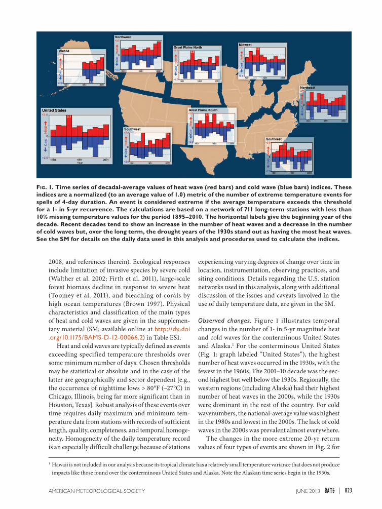
Observed changes. Figure 1 illustrates temporal changes in the number of 1- in 5-yr magnitude heat and cold waves for the conterminous United States and Alaska.1 For the conterminous United States (Fig. 1: graph labeled “United States”), the highest number of heat waves occurred in the 1930s, with the fewest in the 1960s. The 2001–10 decade was the sec-ond highest but well below the 1930s. Regionally, the western regions (including Alaska) had their highest number of heat waves in the 2000s, while the 1930s were dominant in the rest of the country. For cold wavenumbers, the national-average value was highest in the 1980s and lowest in the 2000s. The lack of cold waves in the 2000s was prevalent almost everywhere.

The changes in the more extreme 20-yr return values of four types of events are shown in Fig. 2 for

1 Hawaii is not included in our analysis because its tropical climate has a relatively small temperature variance that does not produce impacts like those found over the conterminous United States and Alaska. Note the Alaskan time series begin in the 1950s.

Fig. 1. Time series of decadal-average values of heat wave (red bars) and cold wave (blue bars) indices. These indices are a normalized (to an average value of 1.0) metric of the number of extreme temperature events for spells of 4-day duration. An event is considered extreme if the average temperature exceeds the threshold for a 1- in 5-yr recurrence. The calculations are based on a network of 711 long-term stations with less than 10% missing temperature values for the period 1895–2010. The horizontal labels give the beginning year of the decade. Recent decades tend to show an increase in the number of heat waves and a decrease in the number of cold waves but, over the long term, the drought years of the 1930s stand out as having the most heat waves. See the SM for details on the daily data used in this analysis and procedures used to calculate the indices.

823june 2013AMeRICAn MeTeOROLOGICAL SOCIeTY |

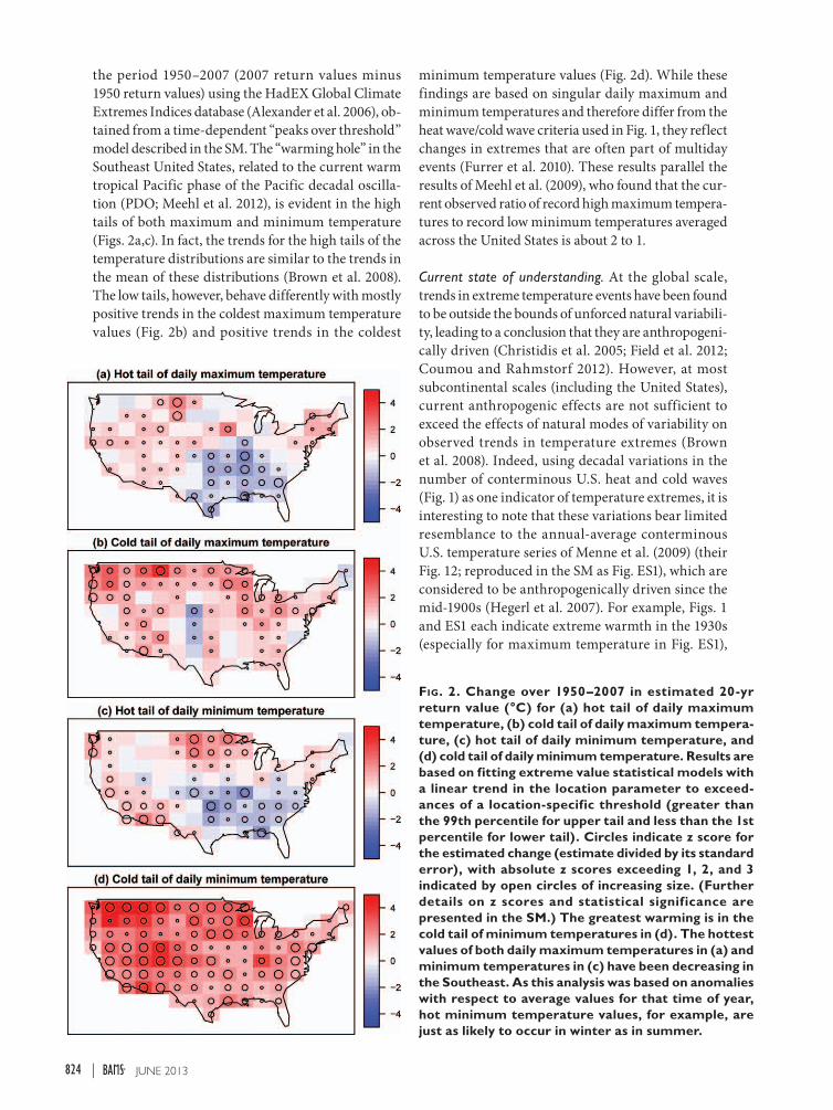
the period 1950–2007 (2007 return values minus 1950 return values) using the HadEX Global Climate Extremes Indices database (Alexander et al. 2006), ob-tained from a time-dependent “peaks over threshold” model described in the SM. The “warming hole” in the Southeast United States, related to the current warm tropical Pacific phase of the Pacific decadal oscilla-tion (PDO; Meehl et al. 2012), is evident in the high tails of both maximum and minimum temperature (Figs. 2a,c). In fact, the trends for the high tails of the temperature distributions are similar to the trends in the mean of these distributions (Brown et al. 2008). The low tails, however, behave differently with mostly positive trends in the coldest maximum temperature values (Fig. 2b) and positive trends in the coldest

minimum temperature values (Fig. 2d). While these findings are based on singular daily maximum and minimum temperatures and therefore differ from the heat wave/cold wave criteria used in Fig. 1, they reflect changes in extremes that are often part of multiday events (Furrer et al. 2010). These results parallel the results of Meehl et al. (2009), who found that the cur-rent observed ratio of record high maximum tempera-tures to record low minimum temperatures averaged across the United States is about 2 to 1.

Current state of understanding. At the global scale, trends in extreme temperature events have been found to be outside the bounds of unforced natural variabili-ty, leading to a conclusion that they are anthropogeni-cally driven (Christidis et al. 2005; Field et al. 2012; Coumou and Rahmstorf 2012). However, at most subcontinental scales (including the United States), current anthropogenic effects are not sufficient to exceed the effects of natural modes of variability on observed trends in temperature extremes (Brown et al. 2008). Indeed, using decadal variations in the number of conterminous U.S. heat and cold waves (Fig. 1) as one indicator of temperature extremes, it is interesting to note that these variations bear limited resemblance to the annual-average conterminous U.S. temperature series of Menne et al. (2009) (their Fig. 12; reproduced in the SM as Fig. ES1), which are considered to be anthropogenically driven since the mid-1900s (Hegerl et al. 2007). For example, Figs. 1 and ES1 each indicate extreme warmth in the 1930s (especially for maximum temperature in Fig. ES1),

Fig. 2. Change over 1950–2007 in estimated 20-yr return value (°C) for (a) hot tail of daily maximum temperature, (b) cold tail of daily maximum tempera-ture, (c) hot tail of daily minimum temperature, and (d) cold tail of daily minimum temperature. Results are based on fitting extreme value statistical models with a linear trend in the location parameter to exceed-ances of a location-specific threshold (greater than the 99th percentile for upper tail and less than the 1st percentile for lower tail). Circles indicate z score for the estimated change (estimate divided by its standard error), with absolute z scores exceeding 1, 2, and 3 indicated by open circles of increasing size. (Further details on z scores and statistical significance are presented in the SM.) The greatest warming is in the cold tail of minimum temperatures in (d). The hottest values of both daily maximum temperatures in (a) and minimum temperatures in (c) have been decreasing in the Southeast. As this analysis was based on anomalies with respect to average values for that time of year, hot minimum temperature values, for example, are just as likely to occur in winter as in summer.

824 june 2013|

but Fig. ES1 does not hint at the 1980s experiencing the most cold waves of any decade (Fig. 1). However, the post-2000 portion of the minimum temperature series in Fig. ES1 (the warmest stretch in the record) does correspond with the 2000s in Fig. 1, showing the smallest number of cold waves of any decade.

Atmospheric moisture plays an important role in heat waves. The impact of heat waves on humans is exacerbated by high humidity (e.g., the deadly 1995 Chicago heat wave; Karl and Knight 1997). Gaffen and Ross (1998) found significant increases in appar-ent temperature over parts of the United States from 1949 to 1995. Extremely high dewpoint temperatures recently observed in parts of the United States (e.g., NOAA 2011) can lead to extremely warm nights. Conversely, some of the most extreme, prolonged, and high-impact heat waves in the United States are bolstered by positive, reinforcing feedbacks related to low-humidity and drought conditions (e.g., over the central United States in summer 2012; NCDC 2012). Such heat/drought linkages are also discussed in the subsection on the current state of understanding in the “Droughts” section, while more detailed char-acteristics of atmospheric/land surface processes relating to both U.S. heat and cold waves are presented in Table ES1 in the SM.

Evidence indicates that the coldest air masses in North American source regions (mainly arctic and subarctic Canada) are warming on multidecadal time scales (Kalkstein et al. 1990; Hankes and Walsh 2011). While the Pacific decadal oscillation is known to affect Alaskan temperatures (Hartmann and Wendler 2005), warming of these source regions likely provides additional explanation for the decreasing trends in cold waves since the 1970s in Alaska and may relate to simi-lar trends over the Northwest and Southwest (Fig. 1), as only the coldest air masses are typically able to spill westward across the Rocky Mountains. East of the Rockies, the highest numbers of cold waves occurred in the 1980s. Strong warming of the coldest nights experienced over much of the United States since 1950 (Fig. 2d) is consistent with the aforementioned warming of the North American cold airmass source regions.

FLOODS. Introduction. Changes in river flooding can be caused by changes in atmospheric conditions (e.g., precipitation amount, type, and timing, as well as temperature), land use/land cover (e.g., agricultural practices, urbanization), and water management (e.g., dams, diversions, and levees). These changes can occur in tandem and make it difficult to determine the relative importance of each factor as drivers of observed changes in river flooding behavior. Given

the large changes that most of the watersheds across the United States have undergone during the twen-tieth century (e.g., Villarini et al. 2009a), ours and other analyses have taken measures to assure that results are not driven by changes in land use or water management.

Further compounding analyses’ complexity, watersheds have memory (due to moisture storage), so that extreme wetness or dryness can influence flood behavior over many years. Because of natural climate variability and basin memory, there is a potential for trendlike behavior that lasts multiple decades but when viewed in a longer context is only a single limb of an oscillation or part of a transient change (see Lettenmaier and Burges 1978; Cohn and Lins 2005; Koutsoyiannis and Montanari 2007). While century-scale records can help mitigate but not eliminate this issue, they also limit the ability to assess the role of drivers that may only dominate later in the record. For example, the effects of human influence on global temperature diverge from natural variability only after about 1950 (Hegerl et al. 2007).

Observed changes. Changes in the magnitude of peak annual river floods are shown in Fig. 3a for the subset of all watersheds with records on the order of 100 years that have experienced little or no land-use or water management changes. While much of the United States shows little or no change in flooding, some areas have spatially coherent changes. Flood magnitudes have been decreasing in the Southwest. Long-term data show an increase in flooding in the northern half of the eastern prairies and parts of the Midwest, especially when examined over the last several decades. Land management practices could be a contributing factor (e.g., Zhang and Schilling 2006; Schilling et al. 2008; Villarini et al. 2011), and this is an area with observed oscillatory behavior at a time scale on the order of a century (see Shapley et al. 2005; Vecchia 2008). Another area where increased f looding has been well documented is from the northern Appalachian Mountains to New England (Collins 2009; Villarini and Smith 2010; Smith et al. 2010; Hodgkins 2010; Hirsch and Ryberg 2012).

Current state of understanding. Days with heavy precipitation have been increasing significantly across the eastern United States, particularly in New England (Karl et al. 2009; Kunkel et al. 2013). Interestingly, this trend is not strongly related to changes in river flooding. Possible reasons for this mismatch include that flooding in most river basins larger than 1000 km2 generally respond to longer-

825june 2013AMeRICAn MeTeOROLOGICAL SOCIeTY |

duration precipitation events and because some of the changes in heavy precipitation occur during seasons that generally do not produce f loods (e.g., Small et al. 2006). For example, an area such as the northern Great Plains, where peak f looding most often occurs during spring snowmelt, tend to have their heaviest daily rainfall events during summer convective storms. Additionally, some of the great-est floods in the last few decades, such as the great upper Mississippi basin f lood of 1993 (Wahl et al. 1993), have been in response to seasonal and longer extreme events. However, examination of changes in long-term flooding (Fig. 3a) and corresponding changes in total annual precipitation (Fig. 3b) does reveal regional-scale similarity.

For some regions of the United States where snow-pack is an important component of the hydrologic system, there is evidence for earlier melt and changes in the rain-to-snow ratio (see Dettinger and Cayan 1995; Hodgkins et al. 2003). These changes may be influential in changing river flood behavior, but their nature could be either decreases or increases in flood magnitudes, depending on watershed characteristics. The Southwest United States shows a general decrease in flood magnitudes, possibly attributable to general drying and diminished snowpack that can be related to changes in greenhouse forcing (Hirsch and Ryberg 2012; Milly et al. 2005). For California in particular, narrow bands of concentrated water vapor transport referred to as atmospheric rivers drive many of the catastrophic floods, but more work needs to be done to reliably estimate their potential change (Dettinger 2011). While precipitation and flooding have been in-creasing in the northern half of the eastern prairies in recent decades, general circulation models do not show this as an area expected to have a substantial increase in runoff in the twentieth-century hindcast or the twenty-first-century forecast (Milly et al. 2005, 2008).

Total annual precipitation for the United States has increased on average about 5% over the past 50 years (Karl et al. 2009). Projections for future precipitation are less certain than projections for future tempera-ture but generally indicate that northern areas are likely to become wetter and southern areas, particu-larly in the Southwest, are likely to become drier (Karl

Fig. 3. Geographic distribution of century-scale changes in (a) flooding, (b) precipitation, and (c) droughts. In (a), the triangles are located at 200 stream gauges, which have record lengths of 85–127 years. The selection of these sites is described by Hirsch and Ryberg (2012). The color and size of the triangles are determined by the trend slope of a regression of the logarithm of the annual flood magnitude vs time for the entire period of record at the site, ending with water year 2008. In (b), trends in total annual precipitation as percentages for a 100-yr period end the same year as the flood data (2008) shown in (a). Precipitation data are from Global Historical Climatology Network (GHCN)-Daily (Menne et al. 2012) and Snowpack Telemetry (SNOTEL; Serreze et al. 1999) data. In (c), the number of months with the Palmer Hydrological Drought Index (PHDI) ≤ –2.0 (moderate to extreme drought) in the second half of the same 100-yr period used in (b) minus the first half (plotted by climate division, which is the source dataset) are shown. Note there are regional similarities between the figures, such as increases in floods and precipitation in the northeastern Great Plains and drying in the Southwest, but there is not a one-to-one correspondence.

826 june 2013|

et al. 2009). However, when con-sidering the issue of future river f lood hazard changes, it is im-portant to recognize that urban and rural land-use impacts and water management impacts have significant inf luence on f lood behavior (e.g., Villarini et al. 2009b; Vogel et al. 2011; Hirsch 2011; Zhang and Schilling 2006; Schilling et al. 2008; Villarini et al. 2011). In addition, while there have been large increases in f lood damages over the past century, one key driver of that is growth in the economic activ-ity situated in high flood hazard areas (Pielke and Downton 1999; Pielke 1999), which appears to be continuing.

DROUGHTS. Introduct ion. Drought is a very complex phe-nomenon that is dif f icult to define and measure. Drought is best represented by indicators that quantitatively appraise the total environmental moisture status or the imbalance between water supply and water demand, usually involving characteristics such as duration, intensity, size of the area affected, and impacts (World Meteorological Organization 1992; American Meteorological Society 1997; Heim 2002; Mishra and Singh 2010; Zwiers et al. 2011). As mul-tiple climate variables affect drought, drought-related datasets and products are derived from a broad set of variables. Drought indices are based on precipitation data (e.g., McKee et al. 1993; Guttman 1998), pre-cipitation and temperature data (e.g., Palmer 1965; Guttman 1998; Dai et al. 2004; Heim 2002), stream discharge records (Heim 2002; Flieg et al. 2006; Zwiers et al. 2011), and model-based soil moisture indicators (e.g., Koster et al. 2009) and other modeling techniques (e.g., Gutzler and Robbins 2010; Kao and Govindaraju 2010) and often have a particular focus such as agricultural droughts or hydrological droughts.

Observed changes. The PHDI (a monthly precipita-tion and mean temperature drought indicator based on computations using 1931–90 for the calibration period) was analyzed to assess observed changes in drought for the period 1900–2011. Based on the PHDI, each decade has experienced drought episodes

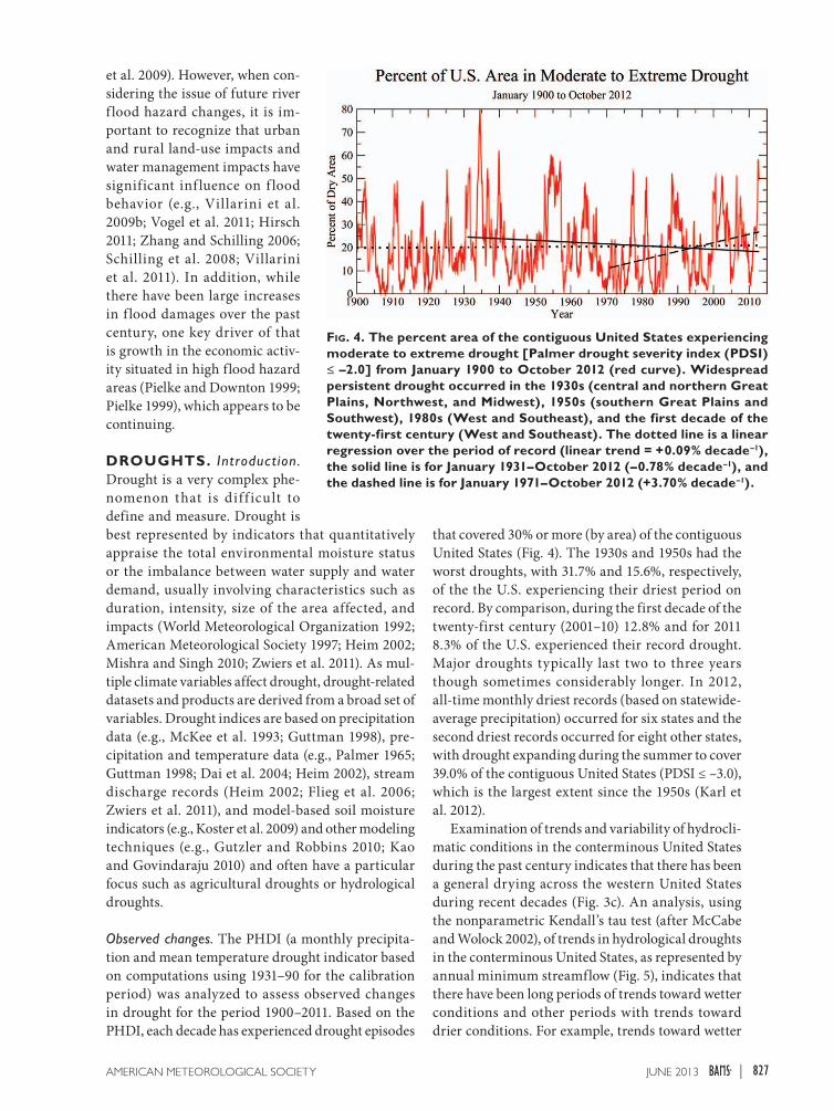
that covered 30% or more (by area) of the contiguous United States (Fig. 4). The 1930s and 1950s had the worst droughts, with 31.7% and 15.6%, respectively, of the the U.S. experiencing their driest period on record. By comparison, during the first decade of the twenty-first century (2001–10) 12.8% and for 2011 8.3% of the U.S. experienced their record drought. Major droughts typically last two to three years though sometimes considerably longer. In 2012, all-time monthly driest records (based on statewide-average precipitation) occurred for six states and the second driest records occurred for eight other states, with drought expanding during the summer to cover 39.0% of the contiguous United States (PDSI ≤ –3.0), which is the largest extent since the 1950s (Karl et al. 2012).

Examination of trends and variability of hydrocli-matic conditions in the conterminous United States during the past century indicates that there has been a general drying across the western United States during recent decades (Fig. 3c). An analysis, using the nonparametric Kendall’s tau test (after McCabe and Wolock 2002), of trends in hydrological droughts in the conterminous United States, as represented by annual minimum streamflow (Fig. 5), indicates that there have been long periods of trends toward wetter conditions and other periods with trends toward drier conditions. For example, trends toward wetter

Fig. 4. The percent area of the contiguous United States experiencing moderate to extreme drought [Palmer drought severity index (PDSI) ≤ –2.0] from January 1900 to October 2012 (red curve). Widespread persistent drought occurred in the 1930s (central and northern Great Plains, Northwest, and Midwest), 1950s (southern Great Plains and Southwest), 1980s (West and Southeast), and the first decade of the twenty-first century (West and Southeast). The dotted line is a linear regression over the period of record (linear trend = +0.09% decade–1), the solid line is for January 1931–October 2012 (–0.78% decade–1), and the dashed line is for January 1971–October 2012 (+3.70% decade–1).

827june 2013AMeRICAn MeTeOROLOGICAL SOCIeTY |

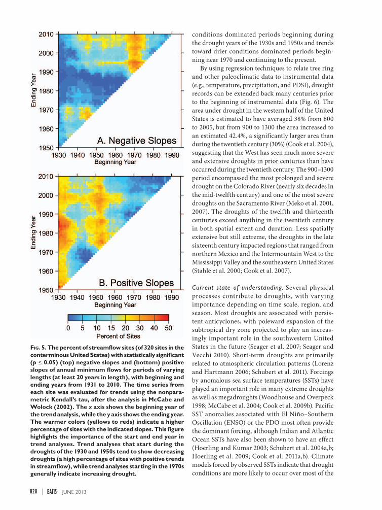
conditions dominated periods beginning during the drought years of the 1930s and 1950s and trends toward drier conditions dominated periods begin-ning near 1970 and continuing to the present.

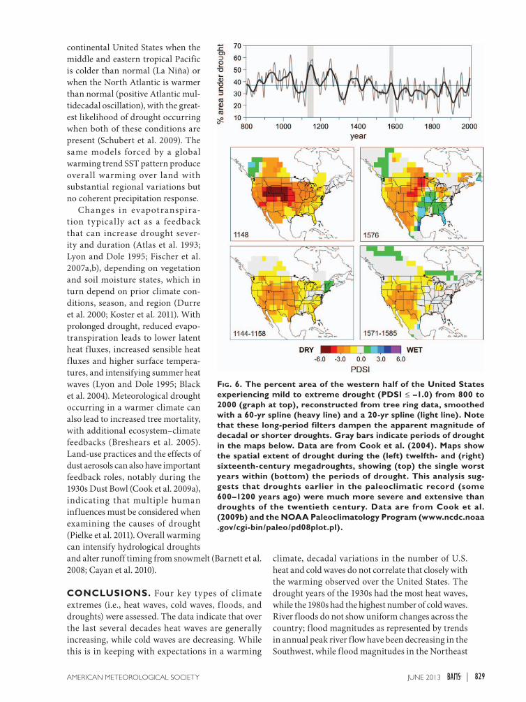
By using regression techniques to relate tree ring and other paleoclimatic data to instrumental data (e.g., temperature, precipitation, and PDSI), drought records can be extended back many centuries prior to the beginning of instrumental data (Fig. 6). The area under drought in the western half of the United States is estimated to have averaged 38% from 800 to 2005, but from 900 to 1300 the area increased to an estimated 42.4%, a significantly larger area than during the twentieth century (30%) (Cook et al. 2004), suggesting that the West has seen much more severe and extensive droughts in prior centuries than have occurred during the twentieth century. The 900–1300 period encompassed the most prolonged and severe drought on the Colorado River (nearly six decades in the mid-twelfth century) and one of the most severe droughts on the Sacramento River (Meko et al. 2001, 2007). The droughts of the twelfth and thirteenth centuries exceed anything in the twentieth century in both spatial extent and duration. Less spatially extensive but still extreme, the droughts in the late sixteenth century impacted regions that ranged from northern Mexico and the Intermountain West to the Mississippi Valley and the southeastern United States (Stahle et al. 2000; Cook et al. 2007).

Current state of understanding. Several physical processes contribute to droughts, with varying importance depending on time scale, region, and season. Most droughts are associated with persis-tent anticyclones, with poleward expansion of the subtropical dry zone projected to play an increas-ingly important role in the southwestern United States in the future (Seager et al. 2007; Seager and Vecchi 2010). Short-term droughts are primarily related to atmospheric circulation patterns (Lorenz and Hartmann 2006; Schubert et al. 2011). Forcings by anomalous sea surface temperatures (SSTs) have played an important role in many extreme droughts as well as megadroughts (Woodhouse and Overpeck 1998; McCabe et al. 2004; Cook et al. 2009b). Pacific SST anomalies associated with El Niño–Southern Oscillation (ENSO) or the PDO most often provide the dominant forcing, although Indian and Atlantic Ocean SSTs have also been shown to have an effect (Hoerling and Kumar 2003; Schubert et al. 2004a,b; Hoerling et al. 2009; Cook et al. 2011a,b). Climate models forced by observed SSTs indicate that drought conditions are more likely to occur over most of the

Fig. 5. The percent of streamflow sites (of 320 sites in the conterminous United States) with statistically significant (p ≤ 0.05) (top) negative slopes and (bottom) positive slopes of annual minimum flows for periods of varying lengths (at least 20 years in length), with beginning and ending years from 1931 to 2010. The time series from each site was evaluated for trends using the nonpara-metric Kendall’s tau, after the analysis in McCabe and Wolock (2002). The x axis shows the beginning year of the trend analysis, while the y axis shows the ending year. The warmer colors (yellows to reds) indicate a higher percentage of sites with the indicated slopes. This figure highlights the importance of the start and end year in trend analyses. Trend analyses that start during the droughts of the 1930 and 1950s tend to show decreasing droughts (a high percentage of sites with positive trends in streamflow), while trend analyses starting in the 1970s generally indicate increasing drought.

828 june 2013|

continental United States when the middle and eastern tropical Pacific is colder than normal (La Niña) or when the North Atlantic is warmer than normal (positive Atlantic mul-tidecadal oscillation), with the great-est likelihood of drought occurring when both of these conditions are present (Schubert et al. 2009). The same models forced by a global warming trend SST pattern produce overall warming over land with substantial regional variations but no coherent precipitation response.

Changes in evapotranspira-tion typically act as a feedback that can increase drought sever-ity and duration (Atlas et al. 1993; Lyon and Dole 1995; Fischer et al. 2007a,b), depending on vegetation and soil moisture states, which in turn depend on prior climate con-ditions, season, and region (Durre et al. 2000; Koster et al. 2011). With prolonged drought, reduced evapo-transpiration leads to lower latent heat fluxes, increased sensible heat fluxes and higher surface tempera-tures, and intensifying summer heat waves (Lyon and Dole 1995; Black et al. 2004). Meteorological drought occurring in a warmer climate can also lead to increased tree mortality, with additional ecosystem–climate feedbacks (Breshears et al. 2005). Land-use practices and the effects of dust aerosols can also have important feedback roles, notably during the 1930s Dust Bowl (Cook et al. 2009a), indicating that multiple human influences must be considered when examining the causes of drought (Pielke et al. 2011). Overall warming can intensify hydrological droughts and alter runoff timing from snowmelt (Barnett et al. 2008; Cayan et al. 2010).

CONCLUSIONS. Four key types of climate extremes (i.e., heat waves, cold waves, f loods, and droughts) were assessed. The data indicate that over the last several decades heat waves are generally increasing, while cold waves are decreasing. While this is in keeping with expectations in a warming

climate, decadal variations in the number of U.S. heat and cold waves do not correlate that closely with the warming observed over the United States. The drought years of the 1930s had the most heat waves, while the 1980s had the highest number of cold waves. River floods do not show uniform changes across the country; flood magnitudes as represented by trends in annual peak river flow have been decreasing in the Southwest, while flood magnitudes in the Northeast

Fig. 6. The percent area of the western half of the United States experiencing mild to extreme drought (PDSI ≤ –1.0) from 800 to 2000 (graph at top), reconstructed from tree ring data, smoothed with a 60-yr spline (heavy line) and a 20-yr spline (light line). Note that these long-period filters dampen the apparent magnitude of decadal or shorter droughts. Gray bars indicate periods of drought in the maps below. Data are from Cook et al. (2004). Maps show the spatial extent of drought during the (left) twelfth- and (right) sixteenth-century megadroughts, showing (top) the single worst years within (bottom) the periods of drought. This analysis sug-gests that droughts earlier in the paleoclimatic record (some 600–1200 years ago) were much more severe and extensive than droughts of the twentieth century. Data are from Cook et al. (2009b) and the NOAA Paleoclimatology Program (www.ncdc.noaa .gov/cgi-bin/paleo/pd08plot.pl).

829june 2013AMeRICAn MeTeOROLOGICAL SOCIeTY |

and north-central United States are increasing. Confounding the analysis of trends in f looding is multiyear and even multidecadal variability likely caused by both large-scale atmospheric circulation changes as well as basin-scale “memory” in the form of soil moisture. Droughts too have multiyear and longer variability. Instrumental data indicate that the Dust Bowl of the 1930s and the 1950s drought were the most widespread twentieth-century droughts in the United States, while tree ring data indicate that the megadroughts over the twelfth century exceeded anything in the twentieth century in both spatial extent and duration.

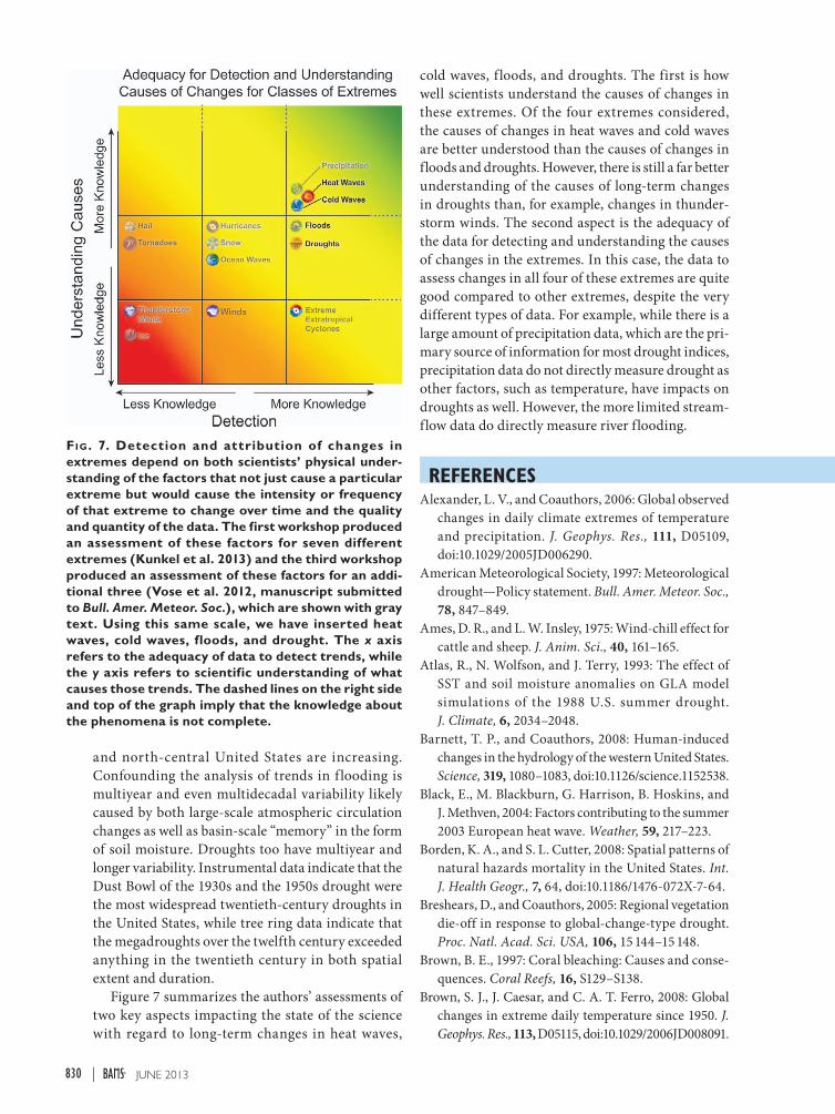
Figure 7 summarizes the authors’ assessments of two key aspects impacting the state of the science with regard to long-term changes in heat waves,

cold waves, f loods, and droughts. The first is how well scientists understand the causes of changes in these extremes. Of the four extremes considered, the causes of changes in heat waves and cold waves are better understood than the causes of changes in floods and droughts. However, there is still a far better understanding of the causes of long-term changes in droughts than, for example, changes in thunder-storm winds. The second aspect is the adequacy of the data for detecting and understanding the causes of changes in the extremes. In this case, the data to assess changes in all four of these extremes are quite good compared to other extremes, despite the very different types of data. For example, while there is a large amount of precipitation data, which are the pri-mary source of information for most drought indices, precipitation data do not directly measure drought as other factors, such as temperature, have impacts on droughts as well. However, the more limited stream-flow data do directly measure river flooding.

RefeRencesAlexander, L. V., and Coauthors, 2006: Global observed

changes in daily climate extremes of temperature and precipitation. J. Geophys. Res., 111, D05109, doi:10.1029/2005JD006290.

American Meteorological Society, 1997: Meteorological drought—Policy statement. Bull. Amer. Meteor. Soc., 78, 847–849.

Ames, D. R., and L. W. Insley, 1975: Wind-chill effect for cattle and sheep. J. Anim. Sci., 40, 161–165.

Atlas, R., N. Wolfson, and J. Terry, 1993: The effect of SST and soil moisture anomalies on GLA model simulations of the 1988 U.S. summer drought. J. Climate, 6, 2034–2048.

Barnett, T. P., and Coauthors, 2008: Human-induced changes in the hydrology of the western United States. Science, 319, 1080–1083, doi:10.1126/science.1152538.

Black, E., M. Blackburn, G. Harrison, B. Hoskins, and J. Methven, 2004: Factors contributing to the summer 2003 European heat wave. Weather, 59, 217–223.

Borden, K. A., and S. L. Cutter, 2008: Spatial patterns of natural hazards mortality in the United States. Int. J. Health Geogr., 7, 64, doi:10.1186/1476-072X-7-64.

Breshears, D., and Coauthors, 2005: Regional vegetation die-off in response to global-change-type drought. Proc. Natl. Acad. Sci. USA, 106, 15 144–15 148.

Brown, B. E., 1997: Coral bleaching: Causes and conse-quences. Coral Reefs, 16, S129–S138.

Brown, S. J., J. Caesar, and C. A. T. Ferro, 2008: Global changes in extreme daily temperature since 1950. J. Geophys. Res., 113, D05115, doi:10.1029/2006JD008091.

Fig. 7. Detection and attribution of changes in extremes depend on both scientists’ physical under-standing of the factors that not just cause a particular extreme but would cause the intensity or frequency of that extreme to change over time and the quality and quantity of the data. The first workshop produced an assessment of these factors for seven different extremes (Kunkel et al. 2013) and the third workshop produced an assessment of these factors for an addi-tional three (Vose et al. 2012, manuscript submitted to Bull. Amer. Meteor. Soc.), which are shown with gray text. Using this same scale, we have inserted heat waves, cold waves, floods, and drought. The x axis refers to the adequacy of data to detect trends, while the y axis refers to scientific understanding of what causes those trends. The dashed lines on the right side and top of the graph imply that the knowledge about the phenomena is not complete.

830 june 2013|

Cayan, D. R., T. Das, D. W. Pierce, T. P. Barnett, M. Tyree, and A. Gershunov, 2010: Future dryness in the southwest US and the hydrology of the early 21st century drought. Proc. Natl. Acad. Sci. USA, 107, 21 271–21 276.

Christidis, N., P. A. Stott, S. Brown, G. C. Hegerl, and J. Caesar, 2005: Detection of changes in temperature extremes during the second half of the 20th century. Geophys. Res. Lett., 32, L20716, doi:10.1029/2005GL023885.

Cohn, T. A., and H. F. Lins, 2005: Nature’s style: Naturally trendy. Geophys. Res. Lett., 32, L23402, doi:10.1029/2005GL024476.

Collins, M. J., 2009: Evidence for changing flood risk in New England since the late 20th century. J. Amer. Water Resour. Assoc., 45, 279–290.

Cook, B. I., R. L. Miller, and R. Seager, 2009a: Amplifi-cation of the North American “Dust Bowl” drought through human-induced land degradation. Proc. Natl. Acad. Sci. USA, 106, 4997–5001.

—, R. Seager, R. Heim Jr., R. Bose, C. Herwejer, and C. Woodhouse, 2009b: Megadroughts in North America: Placing IPCC projections of hydroclimatic change in a long-term paleoclimate context. J. Quat. Sci, 25, 48–61.

—, E. Cook, K. J. Anchukaitis, R. Seager, and R. L. Miller, 2011a: Forced and unforced variability of twentieth century North American droughts and pluvials. Climate Dyn., 37, 1097–1110.

—, R. Seager, and R. L. Miller, 2011b: Atmospheric circulation anomalies during two persistent North American droughts: 1932–39 and 1948–57. Climate Dyn., 36, 2339–2355.

Cook, E. R., C. A. Woodhouse, C. M. Eakin, D. M. Meko, and D. W. Stahle, 2004: Long-term aridity changes in the western United States. Science, 306, 1015–1018.

—, R. Seager, M. A. Cane, and D. W. Stahle, 2007: North American drought: Reconstructions, causes and consequences. Earth Sci. Rev., 81, 93–134.

Coumou, D., and S. Rahmstorf, 2012: A decade of weather extremes. Nat. Climate Change, 2, 491–496.

Dai, A., K. E. Trenberth, and T. Qian, 2004: A global data set of Palmer drought severity index for 1870–2002: Relationship with soil moisture and effects of surface warming. J. Hydrometeor., 5, 1117–1130.

Dettinger, M. D., 2011: Climate change, atmospheric rivers, and f loods in California—A multimodel analysis of storm frequency and magnitude changes. J. Amer. Water Resour. Assoc., 47, 514–523.

—, and D. R. Cayan, 1995: Large-scale atmospheric forcing of recent trends toward early snowmelt runoff in California. J. Climate, 8, 606–623.

Diffenbaugh, N. S., C. H. Krupke, M. A. White, and C. E. Alexander, 2008: Global warming presents new

challenges for maize pest management. Environ. Res. Lett., 3, 044007, doi:10.1088/1748-9326/3/4/044007.

Durre, I., J. M. Wallace, and D. P. Lettenmaier, 2000: Dependence of extreme daily maximum tempera-tures on antecedent soil moisture in the contigu-ous United States during summer. J. Climate, 13, 2641–2651.

Field, C. B., V. Barros, T. F. Stocker, and Q. Dahe, Eds., 2012: Managing the Risks of Extreme Events and Disasters to Advance Climate Change Adaptation. Cambridge University Press, 582 pp.

Firth, L. B., A. M. Knights, and S. S. Bell, 2011: Air tem-perature and winter mortality: Implications for the persistence of the invasive mussel, Perna viridis in the intertidal zone of the southeastern United States. J. Exp. Mar. Biol. Ecol., 400, 250–256.

Fischer, E. M., S. I. Seneverante, D. Luthi, and C. Schar, 2007a: Contributions of land-atmosphere coupling to recent European summer heat waves. Geophys. Res. Lett., 34, L06707, doi:10.1029/2006GL029068.

—, —, P. L. Vidale, D. Luthi, and C. Schar, 2007b: Soil moisture–atmosphere interactions during the 2003 European summer heat wave. J. Climate, 20, 5081–5099.

Flieg, A. K., L. M. Tallasken, H. Hisdal, and S. Demuth, 2006: A global evaluation of streamflow drought characteristics. Hydrol. Earth Syst. Sci., 10, 535–555.

Furrer, E. M., R. W. Katz, M. D. Walter, and R. Furrer, 2010: Statistical modeling of hot spells and heat waves. Climate Res., 43, 191–205.

Gaffen, D. J., and R. J. Ross, 1998: Increased summer-time heat stress in the US. Nature, 396, 529–530.

Guttman, N. B., 1998: Comparing the Palmer drought index and the standardized precipitation index. J. Amer. Water Resour. Assoc., 34, 113–121.

Gutzler, D. S., and T. O. Robbins, 2010: Climate variabil-ity and projected change in the western United States: Regional downscaling and drought statistics. Climate Dyn., 37, 835–849, doi:10.1007/s00382-010-0838-7.

Hankes, I. E., and J. E. Walsh, 2011: Characteris-tics of extreme cold air masses over the North American sub-Arctic. J. Geophys. Res., 116, D11102, doi:10.1029/2009JD013582.

Hartmann, B., and G. Wendler, 2005: The significance of the 1976 Pacific climate shift of Alaska. J. Climate, 18, 4824–4839.

Hegerl, G. C., and Coauthors, 2007: Understanding and attributing climate change. Climate Change 2007: The Physical Science Basis, S. Solomon et al., Eds., Cambridge University Press, 663–745.

Heim, R. R., Jr., 2002: A review of twentieth-century drought indices used in the United States. Bull. Amer. Meteor. Soc., 83, 1149–1165.

831june 2013AMeRICAn MeTeOROLOGICAL SOCIeTY |

Hirsch, R. M., 2011: A perspective on nonstationarity and water management. J. Amer. Water Resour. Assoc., 47, 436–446.

—, and K. R. Ryberg, 2012: Has the magnitude of f loods across the USA changed with global CO2 levels? Hydrol. Sci. J., 57, 1–9.

Hodgkins, G. A., 2010: Historical changes in annual peak f lows in Maine and implications for f lood-frequency analyses. U.S. Geological Survey Scien-tific Investigations Rep. 2010-5094, 38 pp. [Available online at http://pubs.usgs.gov/sir/2010/5094/pdf /sir2010-5094.pdf.]

—, R. W. Dudley, and T. G. Huntington, 2003: Changes in the timing of high river f lows in New England of the 20th century. J. Hydrol., 278, 244–252.

Hoerling, M., and A. J. Kumar, 2003: The perfect ocean for drought. Science, 299, 691–694.

—, X.-W. Quan, and J. Eischeid, 2009: Distinct causes for two principal U.S. droughts of the 20th century. Geophys. Res. Lett., 36, L19708, doi:10.1029/2009GL039860.

Kalkstein, L. S., P. C. Dunne, and R. S. Vose, 1990: Detection of climatic change in the western North American Arctic using a synoptic climatological approach. J. Climate, 3, 1153–1167.

Kao, S. C., and R. S. Govindaraju, 2010: A copula-based joint deficit index for droughts. J. Hydrol., 380, 121–134.

Karl, T. R., and R. W. Knight, 1997: The 1995 Chicago heat wave: How likely a recurrence? Bull. Amer. Meteor. Soc., 78, 1107–1119.

—, J. M. Melillo, and T. C. Peterson, Eds., 2009: Global Climate Change Impacts in the United States. Cambridge University Press, 188 pp.

—, and Coauthors, 2012: U.S. temperature and drought: Recent anomalies and trends. Eos, Trans. Amer. Geophys. Union, 93, 473–474.

Koster, R. D., Z. Guo, R. Yang, P. A. Dirmeyer, K. Mitchell, and M. J. Puma, 2009: On the nature of soil moisture in land surface models. J. Climate, 22, 4322–4335.

—, and Coauthors, 2011: The second phase of the global land–atmosphere coupling experiment: Soil moisture contributions to subseasonal forecast skill. J. Hydrometeor., 12, 805–822.

Koutsoyiannis, D., and A. Montanari, 2007: Statisti-cal analysis of hydroclimatic time series: Uncer-tainty and insights. Water Resour. Res., 43, W05429, doi:10.1029/2006WR005592.

Kunkel, K. E., and Coauthors, 2013: Monitoring and understanding changes in extreme storm statistics: State of knowledge. Bull. Amer. Meteor. Soc., 94, 499–514.

Lettenmaier, D. P., and S. J. Burges, 1978: Climate change: Detection and its impact on hydrologic design. Water Resour. Res., 14, 670–687.

Lorenz, D. J., and D. L. Hartmann, 2006: The effect of the MJO on the North American monsoon. J. Climate, 19, 333–343.

Lyon, B., and R. M. Dole, 1995: A diagnostic compari-son of the 1980 and 1988 U.S. summer heat wave–droughts. J. Climate, 8, 1658–1675.

McCabe, G. J., and D. M. Wolock, 2002: A step increase in streamflow in the conterminous United States. Geophys. Res. Lett., 29, 2185, doi:10.1029/2002GL015999.

—, M. A. Palecki, and J. L. Betancout, 2004: Pacific and Atlantic Ocean inf luences on multidecadal drought frequency in the United States. Proc. Natl. Acad. Sci. USA, 101, 4136–4141.

McKee, T. B., N. J. Doesken, and J. Kleist, 1993: The relationship of drought frequency and duration to time scales. Proc. Eighth Conf. on Applied Climatol-ogy, Anaheim, CA, Amer. Meteor. Soc., 179–184.

Meehl, G. A., C. Tebaldi, G. Walton, D. Easterling, and L. McDaniel, 2009: Relative increase of record high maximum temperatures compared to record low minimum temperatures in the U.S. Geophys. Res. Lett., 36, L23701, doi:10.1029/2009GL040736.

—, J. M. Arblaster, and G. Branstator, 2012: Mechanisms contributing to the warming hole and the consequent U.S. east–west differential of heat extremes. J. Climate, 25, 6394–6408.

Meko, D. M., M. D. Therrell, C. H. Baisan, and M. K. Hughes, 2001: Sacramento River flow reconstructed to A.D. 869 from tree rings. J. Amer. Water Resour. Assoc., 37, 1029–1040.

—, C. A. Woodhouse, C. H. Baisan, T. Knight, J. J. Lukas, M. K. Hughes, and M. W. Salzer, 2007: Medieval drought in the upper Colorado River basin. Geophys. Res. Lett., 34, L10705, doi:10.1029/2007GL029988.

Menne, M. J., C. N. Williams, and R. S. Vose, 2009: The U.S. Historical Climatology Network monthly temperature data, version 2. Bull. Amer. Meteor. Soc., 90, 993–1007.

—, I. Durre, R. S. Vose, B. E. Gleason, and T. G. Houston, 2012: An overview of the Global Histori-cal Climatology Network daily database. J. Atmos. Oceanic Technol., 29, 897–910.

Milly, P. C. D., K. A. Dunne, and A. V. Vecchia, 2005: Global pattern of trends in streamflow and water avail-ability in a changing climate. Nature, 438, 347–350.

—, J. Betancourt, M. Falkenmark, R. M. Hirsch, Z. W. Kundzewicz, D. P. Lettenmaier, and R. J. Stouffer, 2008: Stationarity is dead: Whither water management? Science, 319, 573–574.

832 june 2013|

Mishra, A. K., and V. P. Singh, 2010: A review of drought concepts. J. Hydrol., 391, 202–216.

National Weather Service, cited 2012: Heat: A major killer. [Available online at www.nws.noaa.gov/os /heat/index.shtml.]

NCDC, cited 2012: State of the climate, national over-view, July 2012. [Available online at www.ncdc.noaa .gov/sotc/national/2012/7.]

NOAA, cited 2011: State of the climate national over-view: July 2011. [Available online at www.ncdc.noaa.gov/sotc/national/2011/7.]

Palmer, W. C., 1965: Meteorological drought. U.S. Department of Commerce Weather Bureau Research Paper 45, 58 pp.

Peterson, T. C., and Coauthors, 2008: Why weather and climate extremes matter. Weather and Climate Extremes in a Changing Climate. Regions of Focus: North America, Hawaii, Caribbean, and U.S. Pacific Islands, T. R. Karl et al., Eds., U.S. Climate Change Science Program and the Subcommittee on Global Change Research, 11–33.

—, P. A. Stott, and S. Herring, Eds., 2012: Explaining extreme events of 2011 from a climate perspective. Bull. Amer. Meteor. Soc., 93, 1041–1067.

Pielke, R. A., Jr., 1999: Nine fallacies of floods. Climatic Change, 42, 413–438.

—, and M. Downton, 1999: U.S. trends in streamflow and precipitation: Using societal impact data to address an apparent paradox. Bull. Amer. Meteor. Soc., 80, 1435–1436.

Pielke, R. A., Sr., and Coauthors, 2011: Land use/land cover changes and climate: Modeling analysis and observational evidence. Climate Change, 2, 828–850.

Schilling, K. E., M. K. Jha, Y.-K. Zhang, P. W. Gassman, and C. F. Wolter, 2008: Impact of land use and land cover change on the water balance of a large agricultural watershed: Historical effects and future directions. Water Resour. Res., 44, W00A09, doi:10.1029/2007WR006644.

Schlenker, W., and M. J. Roberts, 2009: Nonlinear tem-perature effects indicate severe damages to US crop yields under climate change. Proc. Natl. Acad. Sci. USA, 106, 15 594–15 598.

Schubert, S. D., M. J. Suarez, P. J. Pegion, R. D. Koster, and J. T. Bacmeister, 2004a: Causes of long-term drought in the U.S. Great Plains. J. Climate, 17, 485–503.

—, —, —, —, and —, 2004b: On the cause of the 1930s Dust Bowl. Science, 33, 1855–1859.

—, and Coauthors, 2009: A U.S. CLIVAR project to assess and compare the responses of global climate models to drought-related SST forcing patterns: Overview and results. J. Climate, 22, 5251–5272.

—, H. Wang, and M. Suarez, 2011: Warm season subseasonal variability and climate extremes in the Northern Hemisphere: The role of stationary Rossby waves. J. Climate, 24, 4773–4792.

Seager, R., and G. A. Vecchi, 2010: Greenhouse warming and the 21st century hydroclimate of southwestern North America. Proc. Natl. Acad. Sci. USA, 107, 21 277–21 282.

—, and Coauthors, 2007: Model projections of an imminent transition to a more arid climate in south-western North America. Science, 316, 1181–1184.

Serreze, M., M. Clark, R. Armstrong, D. McGinnis, and R. Pulwarty, 1999: Characteristics of the western United States snowpack from Snowpack Telemetry (SNOTEL) data. Water Resour. Res., 35, 2145–2160.

Shapley, M. D., W. C. Johnson, D. R. Engstrom, and W. R. Osterkamp, 2005: Late-Holocene f looding and drought in the northern Great Plains, USA, reconstructed from tree rings, lake sediments, and ancient shorelines. Holocene, 15, 29–41.

Sheridan, S. C., and L. S. Kalkstein, 2004: Progress in heat watch–warning system technology. Bull. Amer. Meteor. Soc., 85, 1931–1941.

Small, D., S. Islam, and R. M. Vogel, 2006: Trends in precipitation and streamflow in the eastern U.S.: Paradox or perception? Geophys. Res. Lett., 33, L03403, doi:10.1029/2005GL024995.

Smith, J. A., M. L. Baeck, G. Villarini, and W. F. Krajewski, 2010: The hydrology and hydrometeo-rology of f looding in the Delaware River basin. J. Hydrometeor., 11, 841–859.

Stahle, D. W., E. R. Cook, M. K. Cleaveland, M. D. Therrell, D. M. Meko, H. D. Grissino-Mayer, E. Watson, and B. H. Luckman, 2000: Tree-ring data document 16th century megadrought over North America. Eos, Trans. Amer. Geophys. Union, 81, 121–125.

Steadman, R. G., 1984: A universal scale of apparent temperature. J. Climate Appl. Meteor., 23, 1674–1687.

Stocks, J. M., N. A. S. Taylor, M. J. Tipton, and J. E. Greenleaf, 2004: Human physiological responses to cold exposure. Aviat. Space Environ. Med., 75, 444–457.

Toomey, M., D. A. Roberts, C. Still, M. L. Goulden, and J. P. McFadden, 2011: Remotely sensed heat anomalies linked with Amazonian forest bio-mass declines. Geophys. Res. Lett., 38, L19704, doi:10.1029/2011GL049041.

Vecchia, A. V., 2008: Climate simulation and flood risk analysis for 2008-40 for Devils Lake, North Dakota. U.S. Geological Survey Scientific Investigations Rep. 2008-5011, 28 pp.

833june 2013AMeRICAn MeTeOROLOGICAL SOCIeTY |

Villarini, G., and J. A. Smith, 2010: Flood peak distri-butions for the eastern United States. Water Resour. Res., 46, W06504, doi:10.1029/2009WR008395.

—, F. Serinaldi, J. A. Smith, and W. F. Krajewski, 2009a: On the stationarity of annual f lood peaks in the continenta l United States during the 20th century. Water Resour. Res., 45, W08417, doi:10.1029/2008WR007645.

—, J. A. Smith, F. Serinaldi, J. Bales, P. D. Bates, and W. F. Krajewski, 2009b: Flood frequency analysis for nonstationary annual peak records in an urban drainage basin. Adv. Water Resour., 32, 1255–1266.

—, —, M. L. Baeck, and W. F. Krajewski, 2011: Examining f lood frequency distributions in the Midwest U.S. J. Amer. Water Resour. Assoc., 47, 447–463.

Vogel, R. M., C. Yaindl, and M. Walter, 2011: Non-stationarity: Flood magnification and recurrence reduction factors in the United States. J. Amer. Water Resour. Assoc., 47, 464–474.

Wahl, K. L., K. C. Vining, and G. J. Wiche, 1993: Precipi-tation in the upper Mississippi River basin, January 1 through July 31, 1993. U.S. Geological Survey Circular 1120-B, 13 pp.

Walther, G.-R., and Coauthors, 2002: Ecological respons-es to recent climate change. Nature, 416, 389–395.

White, M. A., N. S. Diffenbaugh, G. V. Jones, J. S. Pal, and F. Giorgi, 2006: Extreme heat reduces and shifts United States premium wine production in the 21st century. Proc. Natl. Acad. Sci. USA, 103, 11 217–11 222.

Woodhouse, C. A., and J. T. Overpeck, 1998: 2000 years of drought variability in the central United States. Bull. Amer. Meteor. Soc., 79, 2693–2714.

World Meteorological Organization, 1992: International meteorological vocabulary. 2nd ed. WMO Rep. 182, 784 pp.

Zhang, Y.-K., and K. E. Schilling, 2006: Increasing streamflow and baseflow in Mississippi River since the 1940s: Effect of land use change. J. Hydrol., 324, 412–422.

Zwiers, F. W., and Coauthors, 2011: Challenges in estimating and understanding recent changes in the frequency and intensity of extreme climate and weather events. Proc. World Climate Research Pro-gramme Open Science Conf., Denver, CO, WCRP, 45 pp. [Available online at http://library.wmo.int /pmb_ged/wcrp_2011-zwiers.pdf.]

—, G. C. Hegerl, S.-K. Min, and X. Zhang, 2012: Historical context. Bull. Amer. Meteor. Soc., 93, 1043–1047.

834 june 2013|