1

Molchanov Alexander M.

NUMERICAL METHODS FOR SOLVING THE NAVIER-STOKES

EQUATIONS

Moscow, 2018

2

Annotation

This book is intended for beginners in the field of Computational Fluid

Dynamics (CFD), studying in English. If you have never studied CFD before, if

you have never worked in the area, and if you have no real idea as to what the

discipline is all about, then this book is for you. Although the material has been

developed from first principles wherever possible, the book will be of greatest

benefit to those who are familiar with the ideas of calculus, elementary vector

and matrix algebra and basic numerical methods. The main purpose in writing

this book is to provide a simple, satisfying, and motivational approach toward

presenting the subject to the reader who is learning about CFD for the first time.

In the workplace, CFD is today a mathematically sophisticated discipline.

The book is focused on the problems related to aviation and aerospace topics.

However, the proposed methods can be easily applied to a wider sphere of

science.

3

Preface ................................................................................................................... 5

Navier-Stokes Equations ................................................................................... 5

Application of Computational Fluid Dynamics ................................................ 7

Advantages of a Theoretical Calculation .......................................................... 8

Disadvantages of a Theoretical Calculation ...................................................... 9

1. FLUID DYNAMICS ....................................................................................... 11

1.1. Some useful formulas. .............................................................................. 11

1.2. Fundamental Equations ............................................................................ 13

1.3. Continuity Equation ................................................................................. 14

1.4. Momentum Equation ................................................................................ 16

1.5. Energy Equation ....................................................................................... 21

1.6. Equation of State ...................................................................................... 24

1.7. Vector Form of Equations ........................................................................ 26

1.8. Orthogonal Curvilinear Coordinates ........................................................ 27

1.9. General transport equation ....................................................................... 32

1.10. One-Way and Two-Way Coordinates .................................................... 38

Problems .......................................................................................................... 41

2. DISCRETIZATION METHODS ................................................................... 41

2.1.The Task .................................................................................................... 41

2.2. Taylor-Series Formulation ....................................................................... 45

2.3. Control Volume Approach ....................................................................... 47

2.4. The basic rules derived from a physical sense of control volume method ......................................................................................................................... 51

2.5. Convergence ............................................................................................. 54

2.6.Approximation .......................................................................................... 55

2.7. Stability of a discretization scheme. ....................................................... 58

2.8. Convergence as a consequence of approximation and stability .............. 59

2.9. Spectral analysis of the difference problem ............................................. 60

2.10. Explicit, Crank-Nicolson, and Fully Implicit Schemes ......................... 63

4

2.11. TriDiagonal-Matrix Algorithm .............................................................. 65

2.12. Time-development method for steady state problems ........................... 68

Problems .......................................................................................................... 69

3. NUMERICAL SOLUTION OF THE NAVIER-STOKES EQUATIONS .... 69

3.1. Desirable Numerical Properties ............................................................... 69

3.2. MacCormack Explicit Method ................................................................. 72

3.3. The finite volume approximation of Navier-Stockes equations .............. 74

3.4. Splitting of inviscid fluxes ...................................................................... 76

3.5. Jacobian matrices, eigenvalues, eigenvectors .......................................... 81

3.6. Explicit and implicit Finite Volume Schemes ....................................... 83

3.7. Viscous fluxes .......................................................................................... 85

3.8. Ways to improve the numerical method .................................................. 87

Problems .......................................................................................................... 88

4. SOLUTION OF SYSTEMS OF LINEAR EQUATIONS WITH BLOCK COEFFICIENTS ................................................................................................. 89

4.1. Finite approximating difference/volume equation ................................... 89

4.2. Gauss-Seidel iteration method ................................................................. 91

4.3. Approximate Factorization (AF) .............................................................. 92

4.4. Modified Approximate Factorization (MAF) .......................................... 93

4.5. Block TriDiagonal-Matrix Algorithm ...................................................... 95

5. BOUNDARY CONDITIONS ......................................................................... 96

5.1. Characteristics. Riemann's invariants. ..................................................... 97

5.2. Types of boundary conditions ................................................................ 105

5.2.1. INLET ............................................................................................. 107

5.2.2. OUTLET ......................................................................................... 109

5.2.3. FREE STREAM BOUNDARY ...................................................... 110

5.2.4. WALL ............................................................................................. 113

5.2.5. PLANE (LINE) of SYMMETRY ................................................... 113

5.3. Ghost cells .............................................................................................. 114

5.3.1. Boundary conditions for inviscid fluxes ......................................... 116

5.3.2. Viscous Boundary Condition .......................................................... 119

5

6. COMPUTATIONAL RESULTS .................................................................. 123

6.1. Supersonic jet at high exit static pressure ratio ...................................... 123

6.2. Supersonic oxygen jet in high-temperature ambient. ........................... 125

6.3. Cold under-expanded and over-expanded air jets ................................ 127

6.4. Highly Under-Expanded Chemically Reacting Jets .............................. 132

6.5. Afterburning of exhaust plume. ............................................................. 137

REFERENCES .................................................................................................. 139

Preface

Navier-Stokes Equations The Navier-Stokes Equations are the basic governing equations for a viscous,

heat conducting fluid. It is a vector equation obtained by applying Second

Newton's Law of Motion to a fluid element and is also called the momentum

equation. It is supplemented by the mass conservation equation, also called

continuity equation and the energy equation. Usually, the term Navier-Stokes

equations is used to refer to all of these equations.

Navier-Stokes Equations are the governing equations of Computational Fluid

Dynamics (CFD). Computational Fluid Dynamics is the simulation of fluids

engineering systems using modeling (mathematical physical problem

formulation) and numerical methods (discretization methods, solvers, numerical

parameters, and grid generations, etc.). The process is as figure 0.1.

6

Figure 0.1. Process of Computational Fluid Dynamics

Firstly, we have a fluid problem. To solve this problem, we should know the

physical properties of fluid by using Fluid Mechanics. Then we can use

mathematical equations to describe these physical properties. This is Navier-

Stokes Equations. As the Navier-Stokes Equations are analytical, human can

understand it and solve them on a piece of paper. But if we want to solve these

equations with computer, we have to translate it to the discretized form. The

translators are numerical discretization methods, such as Finite Difference,

Finite Element, Finite Volume methods. Consequently, we also need to divide

our whole problem domain into many small parts because our discretization is

based on them. Then, we can write programs to solve them. The typical

languages are Fortran and C. Normally the programs are run on workstations or

supercomputers. In the end, we can get our simulation results. We can compare

and analyze the simulation results with experiments and the real problem. If the

results are not sufficient to solve the problem, we have to repeat the process

until find satisfied solution. This is the process of CFD.

Main objective of this book is to train readers the main methods of the

solution of the Navier-Stokes equations so that they without any assistance will

7

be able to create algorithmic programs for the solution of the main problems of

aerodynamics and thermophysics as well as other problems of Computational

Fluid Dynamics.

Besides, this book intends to provide the theoretical background required for

the effective use of commercial codes (ANSYS CFX, FLUENT, FlowVision,

etc.) based on the finite volume method.

The author did not intend to provide a brief review of all existing methods of

the solution of the Navier-Stokes equations, since he does not consider it

effective from a practical point of view. However, here are some most effective

methods (from the author’s point of view) described in detail.

The covers the following subject areas:

• Governing equations of viscous fluid flows

• Boundary conditions

• Finite volume discretisation for the key transport phenomena in fluid

flows: diffusion, convection and sources

• Discretisation procedures for unsteady phenomena

• Solution algorithms for systems of discretised equations

• Implementation of boundary conditions

Application of Computational Fluid Dynamics

Computational Fluid Dynamics (CFD) is the analysis of systems involving

fluid flow, heat transfer and associated phenomena such as chemical reactions

by means of computer-based simulation. The technique is very powerful and

spans a wide range of industrial and non-industrial application areas. Some

examples are:

• aerodynamics of aircraft and vehicles: lift and drag

8

• hydrodynamics of ships

• power plant: combustion in IC engines and gas turbines

• turbomachinery: flows inside rotating passages, diffusers etc.

• electrical and electronic engineering: cooling of equipment including micro-

circuits

• chemical process engineering: mixing and separation, polymer moulding

• external and internal environment of buildings: wind loading and heating/

ventilation

• marine engineering: loads on off-shore structures

• environmental engineering: distribution of pollutants and effluents

• hydrology and oceanography: flows in rivers, estuaries, oceans

• meteorology: weather prediction

• biomedical engineering: blood flows through arteries and veins

Advantages of a Theoretical Calculation

There are three methods in study of Fluid: theory analysis, experiment and

simulation (CFD). As a new method, CFD has many advantages compared to

experiments. Please refer table 1.

Table 1. Comparison of Simulation and Experiment Simulation (CFD) Experiment

Cost Cheap Expensive

Time Short Long

Scale Any Small/Middle

Information All Measured Point

9

Repeatable Yes Some

Safety Yes Some Dangerous

Disadvantages of a Theoretical Calculation

A computer analysis works out the implications of a mathematical model. The

experimental investigation, by contrast, observes the reality itself. A perfectly

satisfactory numerical technique can produce worthless results if an inadequate

mathematical model is employed.

For the purpose of discussing the disadvantages of a theoretical calculation, it

is, therefore, useful to divide all practical problems into two groups:

Group A: Problems for which an adequate mathematical description can be

written. (Examples: heat conduction, laminar flows, simple turbulent boundary

layers.)

Group В: Problems for which an adequate mathematical description has not

yet been worked out. (Examples: complex turbulent flows, certain non-

Newtonian flows, formation of nitric oxides in turbulent combustion, some two-

phase flows.)

Of course, the group into which a given problem falls will be determined by

what we are prepared to consider as an “adequate” description.

Disadvantages for Group A. It may be stated that, for most problems of Group

A, the theoretical calculation suffers from no disadvantages. The computer

solution then represents an alternative that is highly superior to an experimental

study. Occasionally, however, one encounters some disadvantages. If the

prediction has a very limited objective (such as finding the overall pressure drop

for a complicated apparatus), the computation may not be less expensive than an

experiment. For difficult problems involving complex geometry, strong

10

nonlinearities, sensitive fluid-property variations, etc., a numerical solution may

be hard to obtain and would be excessively expensive if at all possible.

Extremely fast and small-scale phenomena such as turbulence, if they are to

be computed in all their time-dependent detail by solving the unsteady Navier-

Stokes equations, are still beyond the practical reach of computational methods.

Finally, when the mathematical problem occasionally admits more than one

solution, it is not easy to determine whether the computed solution corresponds

to reality.

Research in computational methods is aimed at making them more reliable,

accurate, and efficient. The disadvantages mentioned here will diminish as this

research progresses.

Disadvantages for Group B. The problems of Group В share all the

disadvantages of Group A; in addition, there is the uncertainty about the extent

to which the computed results would agree with reality. In such cases, some

experimental backup is highly desirable.

Research in mathematical models causes a transfer of problems from Group В

into Group A. This research consists of proposing a model, working out its

implications by computer analysis, and comparing the results with experimental

data. Thus, computational methods play a key role in this research. A striking

example of this role can be found in the recent development of turbulence

models.

11

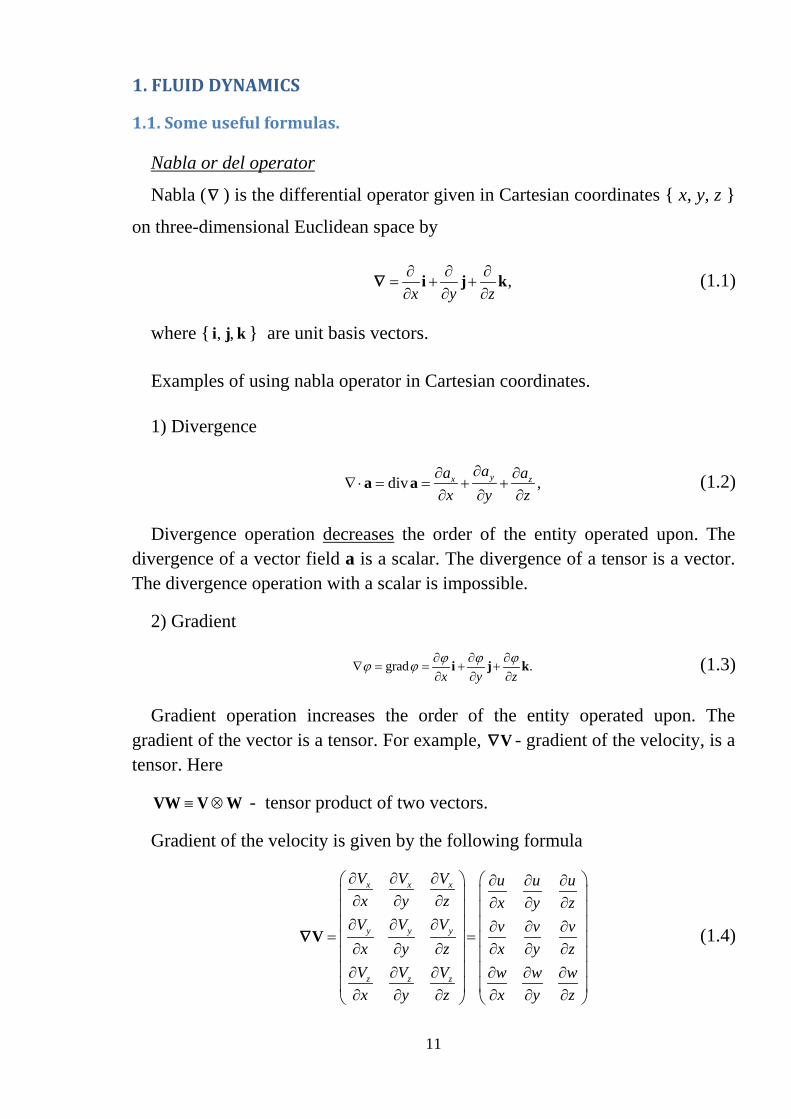
1. FLUID DYNAMICS

1.1. Some useful formulas.

Nabla or del operator

Nabla (∇ ) is the differential operator given in Cartesian coordinates x, y, z

on three-dimensional Euclidean space by

,x y z∂ ∂ ∂

= + +∂ ∂ ∂

i j k∇ (1.1)

where , ,i j k are unit basis vectors.

Examples of using nabla operator in Cartesian coordinates.

1) Divergence

div ,yx zaa a

x y z∂∂ ∂

∇ ⋅ = = + +∂ ∂ ∂

a a (1.2)

Divergence operation decreases the order of the entity operated upon. The divergence of a vector field a is a scalar. The divergence of a tensor is a vector. The divergence operation with a scalar is impossible.

2) Gradient

grad .x y zϕ ϕ ϕϕ ϕ ∂ ∂ ∂

∇ = = + +∂ ∂ ∂

i j k (1.3)

Gradient operation increases the order of the entity operated upon. The gradient of the vector is a tensor. For example, V∇ - gradient of the velocity, is a tensor. Here

≡ ⊗VW V W - tensor product of two vectors.

Gradient of the velocity is given by the following formula

x x x

y y y

z z z

V V V u u ux y z x y z

V V V v v vx y z x y zV V V w w wx y z x y z

∂ ∂ ∂ ∂ ∂ ∂ ∂ ∂ ∂ ∂ ∂ ∂ ∂ ∂ ∂ ∂ ∂ ∂

= = ∂ ∂ ∂ ∂ ∂ ∂ ∂ ∂ ∂ ∂ ∂ ∂ ∂ ∂ ∂ ∂ ∂ ∂

V∇ (1.4)

12

since the velocity components in the coordinate system (x,y,z) are denoted by (u,v,w)

3) Laplacian

( )2 div gradϕ ϕ ϕ ϕ∆ = ∇⋅∇ = ∇ = , (1.5)

where ϕ is a scalar.

The laplacian of a vector is also a vector:

2 2 2

2 2 2

2 2 22

2 2 2

2 2 2

2 2 2

x x x

y y y

z z z

a a ax y za a ax y za a ax y z

∂ ∂ ∂+ + ∂ ∂ ∂

∂ ∂ ∂ ∆ = ∇ = + +∂ ∂ ∂

∂ ∂ ∂ + + ∂ ∂ ∂

a a (1.6)

Laplacian operation does not change the order of the entity operated upon.

Einstein notation

Operations on Cartesian components of vectors and tensors may be expressed

very efficiently and clearly using index notation. Let x be a (three dimensional)

vector. Let e1,e2,e3 be a Cartesian basis. Denote the components of x in this

basis by (x1,x2,x3). Lower case Latin subscripts (i, j, k…) have the range (1,2,3).

The symbol xi denotes three components of a vector x1,x2,x3. The components of

the velocity vector are denoted by 1 2 3, , , ,u u u u v w⇔ .

Summation convention (Einstein convention or Einstein notation): If an

index is repeated in a product of vectors or tensors, summation is implied over

the repeated index. Thus the following formulas are valid

3

1 1 2 2 3 31

i i i ii

a b a b a b a b a bλ λ λ=

= ⇔ = ⇔ = + +∑ (1.7)

31 2

1 2 3

i

i

u uu u u v wx x x x x y z∂ ∂∂ ∂ ∂ ∂ ∂

≡ + + ≡ + +∂ ∂ ∂ ∂ ∂ ∂ ∂

(1.8)

Gauss’ divergence theorem. For a vector a this theorem states

13

V A

dV dA⋅ = ⋅∫∫∫ ∫∫a n a

∇ (1.9)

The physical interpretation of ⋅n a is the component of vector a in the

direction of the vector n normal to surface element dA. Thus the integral of the

divergence of a vector a over a volume is equal to the component of a in the

direction normal to the surface which bounds the volume summed (integrated)

over the entire bounding surface A.

1.2. Fundamental Equations

The fundamental equations of fluid dynamics are based on the following

universal laws of conservation:

Conservation of Mass,

Conservation of momentum,

Conservation of energy.

The equation that results from applying the Conservation of Mass law to a

fluid flow is called the continuity equation. The Conservation of Momentum law

is nothing more than Newton’s Second Law. When this law is applied to a fluid

flow, it yields a vector equation known as the momentum equation.

The Conservation of Energy law is identical to the First Law of

Thermodynamics, and the resulting fluid dynamic equation is named the energy

equation. In addition to the equations developed from these universal laws, it is

necessary to establish relationships between fluid properties in order to close the

system of equations. An example of such a relationship is the equation of state,

which relates the thermodynamic variables pressure p, density ρ, and

temperature T.

Historically, there have been two different approaches taken to derive the

equations of fluid dynamics: the phenomenological approach and the kinetic

theory approach. In the phenomenological approach, certain relations between

14

stress and rate of strain and heat flux and temperature gradient are postulated,

and the fluid dynamic equations are then developed from the conservation laws.

The required constants of proportionality between stress and rate of strain and

heat flux and temperature gradient (which are called transport coefficients) must

be determined experimentally in this approach. In the kinetic theory approach

(also called the mathematical theory of nonuniform gases), the fluid dynamic

equations are obtained with the transport coefficients defined in terms of certain

integral relations, which involve the dynamics of colliding particles. The

drawback of this approach is that the interparticle forces must be specified in

order to evaluate the collision integrals. Thus a mathematical uncertainty takes

the place of the experimental uncertainty of the phenomenological approach.

These two approaches will yield the same fluid dynamic equations if equivalent

assumptions are made during their derivations.

The derivation of the fundamental equations of fluid dynamics will not be

presented here. The fundamental equations given initially in this chapter were

derived for a uniform, homogeneous fluid without mass diffusion or finite-rate

chemical reactions. In order to include these later effects it is necessary to

consider extra relations, called the species continuity equations, and to add terms

to the energy equation to account for diffusion.

1.3. Continuity Equation

The Conservation of Mass law applied to a fluid passing through an

infinitesimal, fixed control volume (see Fig. 1.1) yields the following equation

of continuity:

( ) 0tρ ρ∂+ ⋅ =

∂V∇ (1.10)

where ρ is the fluid density, V is the fluid velocity

15

The first term in Eq. (1.10) represents the rate of increase of the density in the

control volume, and the second term represents the rate of mass flux passing out

of the control surface (which surrounds the control volume) per unit volume.

Figure 1.1. Control volume for Eulerian approach

It is convenient to use the substantial derivative

( )DDt tρ ρ ρ∂≡ + ⋅∂

V ∇ (1.11)

to change Eq. (1.10) into the form

( ) 0DDtρ ρ+ ⋅ =V∇ (1.12)

Equation (1.10) was derived using the Eulerian approach. In this approach, a

fixed control volume is utilized, and the changes to the fluid are recorded as the

fluid passes through the control volume. In the alternative Lagrangian approach,

the changes to the properties of a fluid element are recorded by an observer

moving with the fluid element. The Eulerian viewpoint is commonly used in

fluid mechanics.

We may use another form of Eq. (1.10):

( ) 0divtρ ρ∂+ =

∂V (1.13)

16

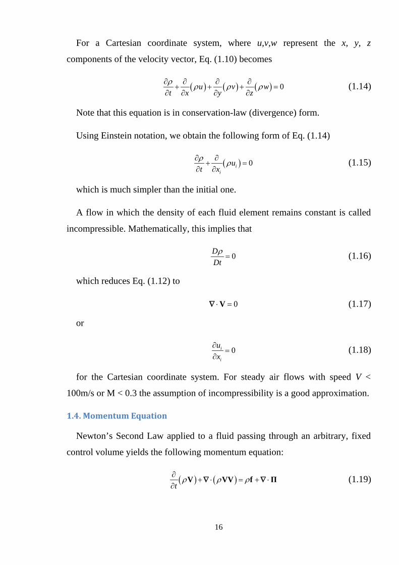
For a Cartesian coordinate system, where u,v,w represent the x, y, z

components of the velocity vector, Eq. (1.10) becomes

( ) ( ) ( ) 0u v wt x y zρ ρ ρ ρ∂ ∂ ∂ ∂+ + + =

∂ ∂ ∂ ∂ (1.14)

Note that this equation is in conservation-law (divergence) form.

Using Einstein notation, we obtain the following form of Eq. (1.14)

( ) 0ii

ut xρ ρ∂ ∂+ =

∂ ∂ (1.15)

which is much simpler than the initial one.

A flow in which the density of each fluid element remains constant is called

incompressible. Mathematically, this implies that

0DDtρ= (1.16)

which reduces Eq. (1.12) to

0⋅ =V∇ (1.17)

or

0i

i

ux∂

=∂

(1.18)

for the Cartesian coordinate system. For steady air flows with speed V <

100m/s or M < 0.3 the assumption of incompressibility is a good approximation.

1.4. Momentum Equation

Newton’s Second Law applied to a fluid passing through an arbitrary, fixed

control volume yields the following momentum equation:

( ) ( )tρ ρ ρ∂

+ ⋅ = + ⋅∂

V VV f Π∇ ∇ (1.19)

17

The first term in this equation represents the rate of increase of momentum

per unit volume in the control volume. The second term represents the rate of

momentum lost by convection (per unit volume) through the control surface.

Note that ρVV is a tensor, so that ( )ρ⋅ VV∇ is not a simple divergence. This

term can be expanded, however, as

( ) ( )( )ρ ρ ρ⋅ = ⋅ + ⋅VV V V V V∇ ∇ ∇ (1.20)

When this expression for ( )ρ⋅ VV∇ is substituted into Eq. (1.19), and the

resulting equation is simplified using the continuity equation (1.10), the

momentum equation reduces to

DDt t

ρ ρ ρ ρ∂≡ + ⋅ = + ⋅

∂V V V V f Π∇ ∇ (1.21)

The first term on the right-hand side of Eq. (1.21) is the body force per unit

volume. Body forces act at a distance and apply to the entire mass of the fluid.

The most common body force is the gravitational force. In this case, the force

per unit mass (f) equals the acceleration of gravity vector g:

ρ ρ=f g (1.22)

The second term on the right-hand side of Eq. (1.21) represents the surface

forces per unit volume. These forces are applied by the external stresses on the

fluid element. The stresses consist of normal stresses and shearing stresses and

are represented by the components of the stress tensor Π.

The momentum equation given above is quite general and is applicable to

both continuum and noncontinuum flows. It is only when approximate

expressions are inserted for the shear-stress tensor that Eq. (1.19) loses its

generality. For all gases that can be treated as a continuum, and most liquids, it

has been observed that the stress at a point is linearly dependent on the rates of

strain (deformation) of the fluid. A fluid that behaves in this manner is called a

Newtonian fluid. With this assumption, it is possible to derive a general

18

deformation law that relates the stress tensor to the pressure and velocity

components. In compact tensor notation, this relation becomes

, 1,2,3ji kij ij ij

j i k

uu up i, j,kx x x

δ µ δ µ ∂∂ ∂′Π = − + + + = ∂ ∂ ∂

(1.23)

where ijδ is the Kronecker delta function ( 1ij if i jδ = = and 0ij if i jδ = ≠ );

1 2 3, ,u u u represent the three components of the velocity vector V; x1,x2,x3 represent the three components of the position vector; µ is the coefficient of viscosity (dynamic viscosity), and µ' is the second coefficient of viscosity. The two coefficients of viscosity are related to the coefficient of bulk viscosity κ by the expression

23

κ µ µ′= + (1.24)

In general, it is believed that κ is negligible except in the study of the structure of shock waves and in the absorption and attenuation of acoustic waves. For this reason, we will ignore bulk viscosity for the remainder of the text. With κ = 0, the second coefficient of viscosity becomes

23

µ µ′ = − (1.25)

and the stress tensor may be written as

2 , 1,2,33

ji kij ij ij

j i k

uu up i, j,kx x x

δ µ δ ∂∂ ∂

Π = − + + − = ∂ ∂ ∂ (1.26)

The stress tensor is frequently separated in the following manner:

ij ij ijpδ τΠ = − + (1.27)

where τij represents the viscous stress tensor given by

2 , 1,2,33

ji kij ij

j i k

uu u i, j,kx x x

τ µ δ ∂∂ ∂

= + − = ∂ ∂ ∂ (1.28)

In vector form Eq. (1.28) is written as

19

( ) ( )23

Tµ = + − ⋅ τ V V V I∇ ∇ ∇ (1.29)

where I is the identity tensor, upper index T means tensor transposition.

Upon substituting Eq. (1.26) into Eq. (1.21), the famous Navier-Stokes

equation is obtained:

D pDt

ρ ρ= − + ⋅V f τ∇ ∇ (1.30)

Using Einstein notation and Eq. (1.27), we can obtain the following form of

Eq. (1.19) for a Cartesian coordinate system

( ) ( ) , 1, 2,3i i j ij ij ij

u u u p f it xρ ρ δ τ ρ∂ ∂

+ + − = =∂ ∂

(1.31)

or

( ) ( ) ( ) ( )

( ) ( ) ( ) ( )

( ) ( ) ( ) ( )

,

,

xx xy xz x

yx yy yz y

zx zy zz z

u uu p uv uw ft x y z

v vu vv p vz ft x y z

w wu wv ww p ft x y z

ρ ρ τ ρ τ ρ τ ρ

ρ ρ τ ρ τ ρ τ ρ

ρ ρ τ ρ τ ρ τ ρ

∂ ∂ ∂ ∂+ + − + − + − =

∂ ∂ ∂ ∂∂ ∂ ∂ ∂

+ − + + − + − =∂ ∂ ∂ ∂∂ ∂ ∂ ∂

+ − + − + + − =∂ ∂ ∂ ∂

(1.32)

This is the conservation-law form of the Navier-Stokes equations. Utilizing

Eq. (1.21), these equations can be rewritten in non-conservation form as

, 1, 2,3iji ij i

j i j

u u pu f it x x x

τρ ρ ρ

∂∂ ∂ ∂+ = − + =

∂ ∂ ∂ ∂ (1.33)

or

xyxx xzx

yx yy yzy

zyzx zzz

u u u u pu v w ft x y z x x y zv v v v pu v w ft x y z y x y zw w w w pu v w ft x y z z x y z

ττ τρ ρ ρ ρ ρ

τ τ τρ ρ ρ ρ ρ

ττ τρ ρ ρ ρ ρ

∂∂ ∂∂ ∂ ∂ ∂ ∂+ + + = − + + +

∂ ∂ ∂ ∂ ∂ ∂ ∂ ∂∂ ∂ ∂∂ ∂ ∂ ∂ ∂

+ + + = − + + +∂ ∂ ∂ ∂ ∂ ∂ ∂ ∂

∂∂ ∂∂ ∂ ∂ ∂ ∂+ + + = − + + +

∂ ∂ ∂ ∂ ∂ ∂ ∂ ∂

(1.34)

20

In equations (1.32) and (1.34) the components of the viscous stress tensor ijτ

are given by

2 2 22 , 2 , 2 ,3 3 3

, ,

xx yy zz

xy yx xz zx yz zy

u v w v u w w u vx y z y x z z x y

u v u w v wy x z x z y

τ µ τ µ τ µ

τ τ µ τ τ µ τ τ µ

∂ ∂ ∂ ∂ ∂ ∂ ∂ ∂ ∂= − − = − − = − − ∂ ∂ ∂ ∂ ∂ ∂ ∂ ∂ ∂

∂ ∂ ∂ ∂ ∂ ∂ = = + = = + = = + ∂ ∂ ∂ ∂ ∂ ∂

(1.35)

The Navier-Stokes equations form the basis upon which the entire science of

viscous flow theory has been developed. Strictly speaking, the term Navier-

Stokes equations refers to the components of the viscous momentum equation

[Eq. (1.33)]. However, it is common practice to include the continuity equation

and the energy equation in the set of equations referred to as the Navier-Stokes

equations.

If the flow is incompressible and the coefficient of viscosity (µ) is assumed

constant, Eq. (1.30) will reduce to the much simpler form

2D pDt

ρ ρ µ= − +V f V∇ ∇ (1.36)

It should be remembered that Eq. (1.36) is derived by assuming a constant viscosity, which may be a poor approximation for the nonisothermal flow of a liquid whose viscosity is highly temperature dependent. On the other hand, the viscosity of gases is only moderately temperature dependent, and Eq. (1.36) is a good approximation for the incompressible flow of a gas.

The term

1e2

jiij

j i

uux x

∂∂= + ∂ ∂

(1.37)

is called the rate of strain. It is a symmetric tensor. In continuum mechanics, the strain rate tensor is a physical quantity that describes the rate of change of the deformation of a material in the neighborhood of a certain point, at a certain moment of time.

So we can rewrite Eq. (1.28) using (1.37)

21

22e , 1,2,33

kij ij ij

k

u i, j,kx

τ µ δ ∂

= − = ∂ (1.38)

1.5. Energy Equation

The First Law of Thermodynamics applied to a fluid passing through an

infinitesimal, fixed control volume yields the following energy equation:

( ) ( ) ( )QE Et tρ ρ ρ∂ ∂

+ ⋅ = − ⋅ + ⋅ ⋅ ⋅∂ ∂

V f V Π Vq +∇ ∇ ∇ (1.39)

where E is the total energy per unit mass given by

2

...2

VE e potential energy= + + + (1.40)

and e is the internal energy per unit mass. The first term on the left-hand side

of Eq. (1.39) represents the rate of increase of E in the control volume, while the

second term represents the rate of total energy lost by convection through the

control surface. The first term on the right-hand side of Eq. (1.39) is the rate of

heat produced per unit volume by external agencies, while the second term ( ⋅q∇

) is the rate of heat lost by conduction (per unit volume) through the control

surface. Fourier’s law for heat transfer by conduction will be assumed, so that

the heat transfer q can be expressed as

Tλ= −q ∇ (1.41)

where λ is the coefficient of thermal conductivity and T is the temperature.

The third term on the right-hand side of Eq. (1.39) represents the work done on

the control volume (per unit volume) by the body forces, while the fourth term

represents the work done on the control volume (per unit volume) by the surface

forces. It should be obvious that Eq. (1.39) is simply the First Law of

Thermodynamics applied to the control volume. That is, the increase of energy

in the system is equal to heat added to the system plus the work done on the

system.

22

For a Cartesian coordinate system, Eq. (1.39) becomes

( ) ( )i i i ij j i ii

QE E u pu q u f ut t xρ ρ τ ρ∂ ∂ ∂

− + + + − =∂ ∂ ∂

(1.42)

which is in conservation-law form. We can write this equation in more detail

without using Einstein notation:

( ) ( )

( )

( )

x xx xy xz

y yx yy yz

z zx zy zz x y z

QE E u pu q u v wt t x

E v pv q u v wy

E w pw q u v w f u f v f wz

ρ ρ τ τ τ

ρ τ τ τ

ρ τ τ τ ρ ρ ρ

∂ ∂ ∂− + + + − − −

∂ ∂ ∂∂

+ + + − − −∂∂

+ + + − − − = + +∂

(1.43)

Using the continuity equation, the left-hand side of Eq. (1.39) can be replaced

by the following expression:

( ) ( )D E E EDt t

ρ ρ ρ∂= + ⋅∂

V∇ (1.44)

which is equivalent to

2

2D De D VEDt Dt Dt

ρ ρ ρ

= +

(1.45)

if only internal energy and kinetic energy are considered significant in Eq.

(1.40). Forming the scalar dot product of Eq. (1.30) with the velocity vector V

allows one to obtain

( )D pDt

ρ ρ⋅ = ⋅ − ⋅ + ⋅ ⋅V V f V V τ V∇ ∇ (1.46)

Now if Eqs. (1.44), (1.45) and (1.46) are combined and substituted into Eq.

(1.39), a useful variation of the original energy equation is obtained:

( ) ( )De QpDt t

ρ ∂+ ⋅ = − ⋅ ⋅ ⋅ − ⋅ ⋅

∂V τ V τ Vq +∇ ∇ ∇ ∇ (1.47)

Development of formula:

23

( ) ( ) ( ) ( )

( ) ( )

( )

( ) ( )

( ) ( )

QE E pt tDe D Q pDt Dt tDe pDtQ pt

De QpDt t

ρ ρ ρ

ρ ρ ρ

ρ ρ

ρ

ρ

∂ ∂+ ⋅ = − ⋅ + ⋅ − ⋅ ⋅ ⋅

∂ ∂∂

+ ⋅ = − ⋅ + ⋅ − ⋅ ⋅ ⋅∂

+ ⋅ − ⋅ + ⋅ ⋅

∂= − ⋅ + ⋅ − ⋅ ⋅ ⋅∂

∂+ ⋅ = − ⋅ ⋅ ⋅ − ⋅ ⋅

∂

V f V V τ V

VV f V V τ V

f V V τ V

f V V τ V

V τ V τ V

q +

q +

q +

q +

∇ ∇ ∇ ∇

∇ ∇ ∇

∇ ∇

∇ ∇ ∇

∇ ∇ ∇ ∇

The last two terms in Eq. (1.47) can be combined into a single term, since

( ) ( ) :⋅ ⋅ − ⋅ ⋅ = ≡ Φτ V τ V τ V∇ ∇ ∇ , (1.48)

where :τ V∇ is the double dot product of two tensors. This term is customarily called the dissipation function Ф and represents the rate at which mechanical energy is expended in the process of deformation of the fluid due to viscosity. After inserting the dissipation function, Eq. (1.47) becomes

De QpDt t

ρ ∂+ ⋅ = − ⋅ Φ

∂V q +∇ ∇ (1.49)

Using the definition of enthalpy

ph eρ

= + (1.50)

and the continuity equation, Eq. (1.49) can be rewritten as

Dh Dp QDt Dt t

ρ ∂= + − ⋅ Φ

∂q +∇ (1.51)

For a Cartesian coordinate system, the dissipation function, which is always

positive if 23

µ µ′ = − , becomes

2 2 22 2

22

2 2 2

23

iij

j

ux

u v w v u w vx y z x y y z

u w u v wz x x y z

τ

µ

∂Φ =

∂

∂ ∂ ∂ ∂ ∂ ∂ ∂ = + + + + + + ∂ ∂ ∂ ∂ ∂ ∂ ∂ ∂ ∂ ∂ ∂ ∂ + + − + + ∂ ∂ ∂ ∂ ∂

(1.52)

24

If the flow is incompressible, and if the coefficient of thermal conductivity is

assumed constant, Eq. (1.49) reduces to

2De Q TDt t

ρ λ∂= − ∇ Φ∂

+ (1.53)

1.6. Equation of State

In order to close the system of fluid dynamic equations it is necessary to

establish relations between the thermodynamic variables (p, ρ, T, e, h) as well as

to relate the transport properties ( µ, λ ) to the thermodynamic variables. For

example, consider a compressible flow without external heat addition or body

forces and use Eq. (1.14) for the continuity equation, Eqs. (1.34) for the three

momentum equations, and Eq. (1.43) for the energy equation. These five scalar

equations contain seven unknowns p, ρ, T, e, u, v, w, provided that the transport

coefficients µ, λ can be related to the thermodynamic properties in the list of

unknowns. It is obvious that two additional equations are required to close the

system. These two additional equations can be obtained by determining relations

that exist between the thermodynamic variables. Relations of this type are

known as equations of state. According to the state principle of

thermodynamics, the local thermodynamic state is fixed by any two independent

thermodynamic variables, provided that the chemical composition of the fluid is

not changing owing to diffusion or finite-rate chemical reactions. Thus for the

present example, if we choose e and p as the two independent variables, then

equations of state of the form

( ) ( ), , ,p p e T T eρ ρ= = (1.54)

are required.

For most problems in gas dynamics, it is possible to assume a perfect gas. A

perfect gas is defined as a gas whose intermolecular forces are negligible. A

perfect gas obeys the perfect gas equation of state,

p RTρ= (1.55)

25

where R is the gas constant. The intermolecular forces become important

under conditions of high pressure and relatively low temperature. For these

conditions, the gas no longer obeys the perfect gas equation of state, and an

alternative equation of state must be used. An example is the Van der Waals

equation of state,

( )2 1p a b RTρρ

+ − =

(1.56)

where a and b are constants for each type of gas.

For problems involving a perfect gas at relatively low temperatures, it is

possible to also assume a calorically perfect gas. A calorically perfect gas is

defined as a perfect gas with constant specific heats. In a calorically perfect gas,

the specific heat at constant volume cv, the specific heat at constant pressure cp,

and the ratio of specific heats γ all remain constant, and the following relations

exist:

, , , ,1 1

pv p v p

v

c R Re c T h c T c cc

γγγ γ

= = = = =− −

(1.57)

For air at standard conditions, R = 287 m2/(s2 K) and γ = 1.4. If we assume

that the fluid in our example is a calorically perfect gas, then Eqs. (1.54) become

( ) ( )11 ,

ep e T

Rγ

γ ρ−

= − = (1.58)

For fluids that cannot be considered calorically perfect, the required state

relations can be found in the form of tables, charts, or curve fits.

The coefficients of viscosity and thermal conductivity can be related to the

thermodynamic variables using kinetic theory. For example, Sutherland’s

formulas for viscosity and thermal conductivity are given by

3/2 3/2

1 32 4

,T TC CT C T C

µ λ= =+ +

(1.59)

26

where C1-C4 are constants for a given gas. For air at moderate temperatures,

C1 = 1.458×10-6 kg/(m s K1/2), C2 = 110.4 K, C3 = 2.495 ×10-3 (kg m)/(s3K3/2),

and C4 = 194 K. The Prandtl number

Pr pcµλ

= (1.60)

is often used to determine the coefficient of thermal conductivity к once ц. is

known. This is possible because the ratio (cp/Pr), which appears in the

expression

Pr

pcλ µ= (1.61)

is approximately constant for most gases. For air at standard conditions, Pr =

0.72.

1.7. Vector Form of Equations

Before applying a numerical algorithm to the governing fluid dynamic

equations, it is often convenient to combine the equations into a compact vector

form. For example, the compressible Navier-Stokes equations in Cartesian

coordinates without body forces, mass diffusion, finite-rate chemical reactions,

or external heat addition can be written as

0t x y z

∂ ∂ ∂ ∂+ + + =

∂ ∂ ∂ ∂U E F G (1.62)

where U, E, F, and G are vectors given by

uvwE

ρρρρρ

=

U (1.63)

27

( )

2

/

xx

yx

zx

xx yx zx x

uu pvuwuu E p u v w q

ρ

ρ τρ τ

ρ τρ ρ τ τ τ

+ − = − −

+ − − − +

E (1.64)

( )

2

/

xy

yy

zy

xy yy zy y

vuv

v pwv

v E p u v w q

ρρ τ

ρ τ

ρ τ

ρ ρ τ τ τ

− = + − − + − − − +

F (1.65)

( )

2

/

xz

yz

zz

xz yz zz z

wuwvw

w pw E p u v w q

ρρ τρ τ

ρ τρ ρ τ τ τ

− = − + − + − − − +

G (1.66)

The first row of the vector Eq. (1.62) corresponds to the continuity equation

as given by Eq. (1.14). Likewise, the second, third, and fourth rows are the

momentum equations, Eqs. (1.34), while the fifth row is the energy equation,

Eq. (1.43). With the Navier-Stokes equations written in this form, it is often

easier to code the desired numerical algorithm. Other fluid dynamic equations

that are written in conservation-law form can be placed in a similar vector form.

Vectors E, F and G are contains two parts: inviscid and viscous. And the

inviscid flux consists of two physically distinct parts, i.e., convective and

pressure fluxes. The former is associated with the flow (advection) speed, while

the latter with the acoustic speed; or respectively classified as the linear and

nonlinear fields.

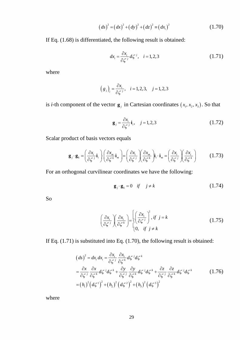
1.8. Orthogonal Curvilinear Coordinates

The basic equations of fluid dynamics are valid for any coordinate system.

We have previously expressed these equations in terms of a Cartesian coordinate

system. For many applications it is more convenient to use a different

28

orthogonal coordinate system. Let us define 1 2 3, ,ζ ζ ζ to be a set of

generalized orthogonal curvilinear coordinates whose origin is at point P and let

1 2 3, ,g g g be the corresponding unit vectors (see Fig. 1.2). The rectangular

Cartesian coordinates are related to the generalized curvilinear coordinates by

( )( )( )

1 2 3

1 2 3

1 2 3

, , ,

, , ,

, ,

x x

y y

z z

ζ ζ ζ

ζ ζ ζ

ζ ζ ζ

=

=

=

(1.67)

or using Einstein notation

( )1 2 3, , , 1,2,3i ix x iζ ζ ζ= = (1.68)

Figure 1.2. Orthogonal curvilinear coordinate system.

so if the Jacobian

( )( )1 2 3

, , ,, ,x y z

ζ ζ ζ∂

∂

is nonzero, then

( )1 2 3, , , 1,2,3j j x x x jζ ζ= = (1.69)

The elemental arc length ds in Cartesian coordinates is obtained from

29

( ) ( ) ( ) ( ) ( )2 2 2 2 2ids dx dy dz dx= + + ≡ (1.70)

If Eq. (1.68) is differentiated, the following result is obtained:

, 1,2,3jii j

xdx d iζζ∂

= =∂

(1.71)

where

( ) , 1,2,3, 1,2,3ij ji

xg i jζ∂

= = =∂

is i-th component of the vector jg in Cartesian coordinates ( )1 2 3, ,x x x . So that

, 1,2,3ij ij

x jζ∂

= =∂

g i (1.72)

Scalar product of basis vectors equals

i m i m i ij k i m i mj k j k j k

x x x x x xζ ζ ζ ζ ζ ζ

∂ ∂ ∂ ∂ ∂ ∂⋅ = ⋅ = ⋅ = ∂ ∂ ∂ ∂ ∂ ∂

g g i i i i (1.73)

For an orthogonal curvilinear coordinates we have the following:

0j k if j k⋅ = ≠g g (1.74)

So

2

,

0,

ii i jj k

x if j kx x

if j kζ

ζ ζ

∂= ∂ ∂ = ∂ ∂ ∂ ≠

(1.75)

If Eq. (1.71) is substituted into Eq. (1.70), the following result is obtained:

( )

( ) ( ) ( ) ( ) ( ) ( )

2

2 2 22 2 21 2 31 2 3

j ki ii i j k

j k j k j kj k j k j k

x xds dx dx d d

x x y y z zd d d d d d

h d h d h d

ζ ζζ ζ

ζ ζ ζ ζ ζ ζζ ζ ζ ζ ζ ζ

ζ ζ ζ

∂ ∂= =

∂ ∂∂ ∂ ∂ ∂ ∂ ∂

= + +∂ ∂ ∂ ∂ ∂ ∂

= + +

(1.76)

where

30

( )

( )

( )

2 2 22

1 1 1 1

2 2 22

2 2 2 2

2 2 22

3 3 3 3

x y zh

x y zh

x y zh

ζ ζ ζ

ζ ζ ζ

ζ ζ ζ

∂ ∂ ∂= + + ∂ ∂ ∂

∂ ∂ ∂= + + ∂ ∂ ∂

∂ ∂ ∂= + + ∂ ∂ ∂

(1.77)

The above formulas can now be used to derive the fluid dynamic equations in any

orthogonal curvilinear coordinate system. Examples include

Cartesian coordinates

1 1 1

2 2 2

3 3 3

, 1,, 1,, 1,

x h u uy h u vz h u w

ζζζ

= = == = == = =

Cylindrical coordinates

1 1 1

2 2 2

3 3 3

, 1,, ,, 1,

r

z

r h u uh r u u

z h u uθ

ζζ θζ

= = == = == = =

Spherical coordinates

1 1 1

2 2 2

3 3 3

, 1,, ,, sin ,

rr h u yuh r u uh r u u

θ

φ

ζζ θζ φ θ

= = == = == = =

Two-dimensional (2-D) or axisymmetric body intrinsic coordinates

( )

( ) ( )

1 1 1

2 2 2

3 3 3

, 1 ,, 1,

, cos ,m

h K u uh u v

h r u mw

ζ ξ ξ ηζ η

ζ φ ξ η α ξ

= = + =

= = =

= = + =

where ( )K ξ is the local body curvature, ( )r ξ is the cylindrical radius, and

0, for 2-D flow1, for axisymmetric flow

m =

These coordinate systems are illustrated in Fig. 1.3.

31

Figure 1.3. Curvilinear coordinate systems, (a) Cylindrical coordinates; (b) spherical coordinates; (c) 2-D or axisymmetric body intrinsic coordinates.

We will give the main equations in a cylindrical system of coordinates as an example:

( ) ( ) ( )1 0rr z

uu u ut r r z rθρ ρρ ρ ρ

θ∂ ∂ ∂ ∂

+ + + + =∂ ∂ ∂ ∂

, (1.78)

( ) ( ) ( ) ( )

( )

1

1

r r r rr r r z r zr

r r rr r

u u u p u u u ut r r z

u u u u Fr

θ θ

θ θ θθ

ρ ρ τ ρ τ ρ τθ

ρ ρ τ τ ρ

∂ ∂ ∂ ∂+ + − + − + −

∂ ∂ ∂ ∂

+ − − + =, (1.79)

( ) ( ) ( ) ( )

( )

1

2

r r z z

r r

u u u u u p u ut r r z

u u Fr

θ θ θ θ θ θθ θ θ

θ θ θ

ρ ρ τ ρ τ ρ τθ

ρ τ ρ

∂ ∂ ∂ ∂+ − + + − + −

∂ ∂ ∂ ∂

+ − =, (1.80)

32

( ) ( ) ( ) ( )

( )

1

1

z r z rz z z z z zz

r z rz z

u u u u u u u pt r r z

u u Fr

θ θρ ρ τ ρ τ ρ τθ

ρ τ ρ

∂ ∂ ∂ ∂+ − + − + + −

∂ ∂ ∂ ∂

+ − =, (1.81)

( ) ( )1r z rr r z z

E f f f f F u F u F ut r r z r

θθ θ

ρρ

θ∂ ∂ ∂ ∂

+ + + + = + +∂ ∂ ∂ ∂

(1.82)

where

2 123

r zrr r

u u uur r z

θτ µθ

∂ ∂ ∂ = − + − ∂ ∂ ∂ (1.83)

2

2 23

r zr

u u uur r z

θθθτ µ

η ∂ ∂ ∂

= − + + − ∂ ∂ ∂ (1.84)

2 1 23

r zzz r

u u uur r z

θτ µθ

∂ ∂ ∂ = − − + + ∂ ∂ ∂ (1.85)

1 rr

u u ur rθ

θ θτ µθ

∂ ∂ = + − ∂ ∂ (1.86)

z rrz

u ur z

τ µ ∂ ∂ = + ∂ ∂ (1.87)

1 zz

u ur z

θθτ µ

θ∂ ∂ = + ∂ ∂

(1.88)

1, ,r zT T Tq q qr r zθλ λ λ

θ∂ ∂ ∂

= − = − = −∂ ∂ ∂

(1.89)

,,

r r r r rr r z zr

r r z z

z z z r rz z z zz

f u H q u u uf u H q u u uf u H q u u u

θ θ

θ θ θ θ θ θθ θ

θ θ

ρ τ τ τρ τ τ τρ τ τ τ

= + − − −= + − − −

= + − − − (1.90)

1.9. General transport equation

All the main equations, which governs the time-dependent three-dimensional

fluid flow and heat transfer of a compressible Newtonian fluid, can be presented

in a single form.

33

For example, let’s consider the equation of momentum in a projection to an

axis x (1.32).

Eq. (1.32) it can be written as

( ) ( ) ( ) ( )

( ) ( ) ( ) ,xx xy xz x

u uu uv uwt x y z

p fx x y z

ρ ρ ρ ρ

τ τ τ ρ

∂ ∂ ∂ ∂+ + +

∂ ∂ ∂ ∂∂ ∂ ∂ ∂

= − + + + +∂ ∂ ∂ ∂

(1.91)

Using Eqs. (1.35) we obtain from Eq. (1.91)

( ) ( ) ( ) ( )

23 x

p u u uu uu uv uwt x y z x x x y y z z

u v w u v w fx x y x z x x x y z

ρ ρ ρ ρ µ µ µ

µ µ µ µ µ µ ρ

∂ ∂ ∂ ∂ ∂ ∂ ∂ ∂ ∂ ∂ ∂ + + + = − + + + ∂ ∂ ∂ ∂ ∂ ∂ ∂ ∂ ∂ ∂ ∂ ∂ ∂ ∂ ∂ ∂ ∂ ∂ ∂ ∂ ∂ + + + − + + + ∂ ∂ ∂ ∂ ∂ ∂ ∂ ∂ ∂ ∂

(1.92)

or

( ) ( ) ( )

( )23 x

pu div u div grad ut x

u v w div fx x y x z x x

ρ ρ µ

µ µ µ ρ

∂ ∂+ = − +

∂ ∂∂ ∂ ∂ ∂ ∂ ∂ ∂ + + + − + ∂ ∂ ∂ ∂ ∂ ∂ ∂

V

V (1.93)

We quote in Table 1.1. the conservative or divergence form of the system of

equations.

Table 1.1.

Equation

Continuity ( ) 0divtρ ρ∂+ =

∂V

x- Momentum ( ) ( ) ( ) Mxpu div u div grad u S

t xρ ρ µ∂ ∂

+ = − + +∂ ∂

V

y- Momentum ( ) ( ) ( ) Mypv div v div grad v S

t yρ ρ µ∂ ∂

+ = − + +∂ ∂

V

z- Momentum ( ) ( ) ( ) Mzpw div w div grad w S

t zρ ρ µ∂ ∂

+ = − + +∂ ∂

V

Energy ( ) ( ) ( ) Qe div e p div div grad Tt tρ ρ λ∂ ∂

+ = − + + +Φ∂ ∂

V V

34

where, for example

( )23Mx x

u v wS div fx x y x z x x

µ µ µ ρ∂ ∂ ∂ ∂ ∂ ∂ ∂ = + + − + ∂ ∂ ∂ ∂ ∂ ∂ ∂ V

There are significant commonalities between the various equations. If we

introduce a general variable φ the conservative form of all fluid flow equations,

including equations for scalar quantities such as temperature, can usefully be

written in the following form:

( ) ( ) ( ) St φρφ ρ φ φ∂

+ ⋅ = ⋅ Γ +∂

∇ ∇ ∇V (1.94)

In words

Rate of increase of φ of fluid element +

Net rate of flow of φ out of fluid element =

Rate of increase of φ due to diffusion

+

Rate of φincrease of due to sources

Here

Table 1.2

Equation φ Γ Sφ Continuity 1 0 0

x- Momentum u µ Mx

p Sx∂

− +∂

y- Momentum v µ My

p Sy∂

− +∂

z- Momentum w µ Mz

p Sz∂

− +∂

Energy e vcλ

Qp divt

∂− + +Φ

∂V

The equation (1.94) is the so-called transport equation for property φ . It

clearly highlights the various transport processes: the rate of change term and

the convective term on the left hand side and the diffusive term (Γ=diffusion

35

coefficient) and the source term respectively on the right hand side. In order to

bring out the common features we have, of course, had to hide the terms that are

not shared between the equations in the source terms. Note that equations (1.94)

can be made to work for the internal energy equation by changing e into T by

means of an equation of state.

The equation (1.94) is used as the starting point for computational procedures

in the finite volume method. By setting φ equal to 1, u, v, w and e (or T or E)

and selecting appropriate values for the diffusion coefficient Γ and source terms

we obtain special forms of Table 2.1 for each of the five partial differential

equations for mass, momentum and energy conservation. The key step of the

finite volume method, which is to be developed in the next Chapter, is the

integration of (1.94) over a three-dimensional control volume V yielding

( ) ( ) ( )V V V V

dV dV dV S dVt φρφ ρ φ φ∂

+ ⋅ = ⋅ Γ +∂∫∫∫ ∫∫∫ ∫∫∫ ∫∫∫∇ ∇ ∇V (1.95)

The volume integrals in the second term on the left hand side, the convective term, and in the first term on the right hand side, the diffusive term, are re-written as integrals over the entire bounding surface of the control volume by using Gauss’ divergence theorem. For a vector a this theorem states

V A

dV dA⋅ = ⋅∫∫∫ ∫∫a n a

∇ (1.96)

The physical interpretation of ⋅n a is the component of vector a in the

direction of the vector n normal to surface element dA. Thus the integral of the

divergence of a vector a over a volume is equal to the component of a in the

direction normal to the surface which bounds the volume summed (integrated)

over the entire bounding surface A. Applying Gauss’ divergence theorem,

equation (1.95) can be written as follows:

( ) ( ) ( )V A A V

dV dA dA S dVt φρφ ρ φ φ∂

+ ⋅ = ⋅ Γ +∂∫∫∫ ∫∫ ∫∫ ∫∫∫n n

∇V (1.97)

36

The order of integration and differentiation has been changed in the first term

on the left hand side of (1.97) to illustrate its physical meaning. This term

signifies the rate of change of the total amount of fluid property φ in the

control volume. The product ( )ρ φ⋅n V expresses the flux component of property

φ due to fluid flow along the outward normal vector n, so the second term on

the left hand side of (1.97), the convective term, is therefore the net rate of

decrease of fluid property φ of the fluid element due to convection.

A diffusive flux is positive in the direction of a negative gradient of the fluid

property φ , i.e. along direction -grad φ . For instance, heat is conducted in the

direction of negative temperature gradients. Thus, the product ( )φ⋅ −Γn ∇ is the

component of diffusion flux along the outward normal vector, and so out of the

fluid element. Similarly, the product ( )φ⋅ Γn ∇ , which is also equal to

( )( )φΓ − ⋅ −n ∇ , can be interpreted as a positive diffusion flux in the direction of

the inward normal vector -n, i.e. into the fluid element. The first term on the

right hand side of (1.97), the diffusive term, is thus associated with a flux into

the element and represents the net rate of increase of fluid property φ of the

fluid element due to diffusion. The final term on the right hand side of this

equation gives the rate of increase of property φ as a result of sources inside

the fluid element.

In words, relationship (1.97) for the fluid in the control volume can be expressed as follows:

Rate of increase of φ +

Net rate of decrease of φ due to convection across the boundaries

=

Rate of increase of φ due to diffusion across the boundaries

+

Net rate of creation of φ

This discussion clarifies that integration of the partial differential equation

generates a statement of the conservation of a fluid property for a finite size

(macroscopic) control volume.

37

Multiplying the continuity equation by φ and subtracting the obtained result

from equation (1.94), we can rewrite it in non-conservation form as

( ) ( ) St φφρ ρ φ φ∂+ ⋅ = ⋅ Γ +

∂∇ ∇ ∇V (1.98)

Analyzing the Eq. (1.98), we can receive several special cases.

1) If convective and diffusive terms are equal to zero, we have an ordinary

differential equation

Sddt

φφρ

= (1.99)

2) If convective and source terms are equal to zero, we have an equation of

parabolic type

t x x y y z zφ φ φ φρ ∂ ∂ ∂ ∂ ∂ ∂ ∂ = Γ + Γ + Γ ∂ ∂ ∂ ∂ ∂ ∂ ∂

(1.100)

3) If diffusive and source terms are equal to zero, we have an equation of

hyperbolic type

0u v wt x y zφ φ φ φ∂ ∂ ∂ ∂+ + + =

∂ ∂ ∂ ∂ (1.101)

4) In a case of steady-state flow, with the absence of convective and source

terms, a generalized equation is an elliptic one

0x x y y z z

φ φ φ ∂ ∂ ∂ ∂ ∂ ∂ Γ + Γ + Γ = ∂ ∂ ∂ ∂ ∂ ∂ (1.102)

5) For steady state 2D boundary layer approximation the equation (1.98) is

as follows

u vx y y y

ρ ρ ∂Φ ∂Φ ∂ ∂Φ

+ = Γ ∂ ∂ ∂ ∂ (1.103)

38

In such form this equation is also brought to parabolic type from the point of

view of longitudinal coordinate.

In each of these five cases different numerical methods are applied. The

boundary conditions differ as well.

Different terms of the equation (1.94) can play a defining role in different

areas of real flows at different timepoints.

Therefore, it is preferable to choose a method of numerical interpretation not

for all equation in general, but for its different parts.

From this point of view, it is convenient to use the interpretation of

properties of coordinates offered by S. Patankar [3], both spatial and temporary.

1.10. One-Way and Two-Way Coordinates

We shall now consider new concepts about the properties of coordinates and

then establish a connection between these and the standard mathematical

terminology.

Definitions. A two-way coordinate is such that the conditions at a given

location in that coordinate are influenced by changes in conditions on either side

of that location. A one-way coordinate is such that the conditions at a given

location in that coordinate are influenced by changes in conditions on only one

side of that location.

Examples. One-dimensional steady heat conduction in a rod provides an

example of a two-way coordinate. The temperature of any given point in the rod

can be influenced by changing the temperature of either end. Normally, space

coordinates are two-way coordinates. Time, on the other hand, is always a one-

way coordinate. During the unsteady cooling of a solid, the temperature at a

given instant can be influenced by changing only those conditions that prevailed

before that instant. It is a matter of common experience that yesterday’s events

39

affect today’s happenings, but tomorrow’s conditions have no influence on what

happens today.

Space as a one-way coordinate. What is more interesting is that even a space

coordinate can very nearly become one-way under the action of fluid flow. If

there is a strong unidirectional flow in the coordinate direction, then significant

influences travel only from upstream to downstream. The conditions at a point

are then affected largely by the upstream conditions, and very little by the

downstream ones. The one-way nature of a space coordinate is an

approximation. It is true that convection is a one-way process, but diffusion

(which is always present) has two-way influences. However, when the flow rate

is large, convection overpowers diffusion and thus makes the space coordinate

nearly one-way.

Parabolic, elliptic, hyperbolic. It appears that the mathematical terms

parabolic and elliptic, which are used for the classification of differential

equations, correspond to our computational concepts of one-way and two-way

coordinates. The term parabolic indicates a one-way behavior, while elliptic

signifies the two-way concept.

It would be more meaningful if situations were described as being parabolic

or elliptic in a given coordinate. Thus, the unsteady heat conduction problem,

which is normally called parabolic, is actually parabolic in time and elliptic in

the space coordinates. The steady heat conduction problem is elliptic in all

coordinates. A two-dimensional boundary layer is parabolic in the streamwise

coordinate and elliptic in the cross-stream coordinate.

Since such descriptions are unconventional, a connection with established

practice can perhaps be achieved by the following rule:

A situation is parabolic if there exists at least one one-way coordinate;

otherwise, it is elliptic.

40

A flow with one one-way space coordinate is sometimes called a boundary-

layer-type flow, while a flow with all two-way coordinates is referred to as a

recirculating flow.

What about the third category, namely, hyperbolic? It so happens that a

hyperbolic situation does not neatly fit into the computational classification. A

hyperbolic problem has a kind of one-way behavior, which is, however, not

along coordinate directions but along special lines called characteristics. There

are numerical methods that make use of the characteristic lines, but they are

restricted to hyperbolic problems.

Computational implications. The motivation for the foregoing discussion

about one-way and two-way coordinates is that, if a one-way coordinate can be

identified in a given situation, substantial economy of computer storage and

computer time is possible. Let us consider an unsteady two-dimensional heat

conduction problem. We shall construct a two-dimensional array of grid points

in the calculation domain. At any instant of time, there will be a corresponding

two-dimensional temperature field. Such a field will have to be handled in the

computer for each of the successive instants of time. However, since time is a

one-way coordinate, the temperature field at a given time is not affected by the

future temperature fields. Indeed, the entire unsteady problem can be reduced to

the required repetitions of one basic step, namely this: Given the temperature

field at time t, find the temperature field at time t + Δt. Thus, computer storage

will be needed only for these two temperature fields; the same storage space can

be used, over and over again, for all the time steps.

In this manner, starting with a given initial temperature field, we are able to

“march” forward to successive instants of time. During any time step, only one

two-dimensional array of temperatures forms the unknowns to be treated

simultaneously. They are decoupled from all future values of temperature, and

41

the previous values that influence them are known. Thus, we need to solve a

much simpler set of equations, with a consequent saving of computer time.

Problems

1. In conjunction with the spatially marching solutions of Eq. (1.62) for an

inviscid flow, the elements of the solution vector E are given as:

( )21 2 3 4 5, , , , /E u E u p E vu E wu E u E pρ ρ ρ ρ ρ ρ= = + = = = + (1.104)

Derive expressions for the primitive variables ρ, u, v, w and p in terms of E1, E2, E3, E4 and E5. Assume a calorically perfect gas (with constant γ).

2. Derive the momentum and energy equations for a viscous flow in integral form. Show that all three conservation equations continuity momentum, and energy can be put in a single generic integral form.

2. DISCRETIZATION METHODS

2.1.The Task

A numerical solution of a differential equation consists of a set of numbers

from which the distribution of the dependent variable φ can be constructed. In

this sense, a numerical method is akin to a laboratory experiment, in which a set

of instrument readings enables us to establish the distribution of the measured

quantity in the domain under investigation. The numerical analyst and the

laboratory experimenter both must remain content with only a finite number of

numerical values as the outcome, although this number can, at least in principle,

be made large enough for practical purposes.

Let us suppose that we decide to represent the variation of ϕ by a polynomial

in x,

42

20 1 2 ... m

ma a x a x a xφ = + + + + (2.1)

and employ a numerical method to find the finite number of coefficients

0 1 2, , , ..., ma a a a . This will enable us to evaluate ϕ at any location x by substituting

the value of x and the values of the a's into Eq. (2.1). This procedure is,

however, somewhat inconvenient if our ultimate interest is to obtain the values

of ϕ at various locations. The values of the a’s are, by themselves, not

particularly meaningful, and the substitution operation must be carried out to

arrive at the required values of φ . This leads us to the following thought: Why

not construct a method that employs the values of ϕ at a number of given points

as the primary unknowns? Indeed, most numerical methods for solving

differential equations do belong in this category, and therefore we shall limit our

attention to such methods.

Thus, a numerical method treats as its basic unknowns the values of the

dependent variable at a finite number of locations (called the grid points) in the

calculation domain. The method includes the tasks of providing a set of

algebraic equations for these unknowns and of prescribing an algorithm for

solving the equations.

In focusing attention on the values at the grid points, we have replaced the

continuous information contained in the exact solution of the differential

equation with discrete values. We have thus discretized the distribution of φ ,

and it is appropriate to refer to this class of numerical methods as discretization

methods.

The algebraic equations involving the unknown values of ϕ at chosen grid

points, which we shall now name the discretization equations, are derived from

the differential equation governing ϕ. In this derivation, we must employ some

assumption about how φ varies between the grid points. Although this “profile”

of φ could be chosen such that a single algebraic expression suffices for the

whole calculation domain, it is often more practical to use piecewise profiles

43

such that a given segment describes the variation of φ over only a small region

in terms of the φ values at the grid points within and around that region. Thus, it

is common to subdivide the calculation domain into a number of subdomains or

elements such that a separate profile assumption can be associated with each

subdomain.

In this manner, we encounter the discretization concept in another context.

The continuum calculation domain has been discretized. It is this systematic

discretization of space and of the dependent variables that makes it possible to

replace the governing differential equations with simple algebraic equations,

which can be solved with relative ease.

For simplicity, in this section it is assumed that the variable ϕ is a function of

the only independent variable x. However, the ideas developed here will also be

applicable in the case of the dependence of more than one independent variable.

Suppose that a differential boundary-value problem is given on some interval,

D on the x-axis. This means that one is given a differential equation (or system

of equations) which the solution must satisfy in the interval, D, and auxiliary

conditions on φ at one or both ends of this interval. The differential boundary-

value problem will be written in the symbolic form

L fφ = (2.2)

Where L is a given differential operator, and f is a given right-hand side.

Thus, for example, to write the problem

( )

( )

2 cos , 0 1,1

0 3

d x x xdxφ

φφ

+ = ≤ ≤ + =

(2.3)

in form (2.2) we need only take

44

( )( )

2 , 0 1,1

0

cos , 0 1,3

d x xdxL

x xf

φφφ

φ

+ ≤ ≤ +≡

≤ ≤≡

(2.4)

We will assume that the solution ( )xφ of problem (2.2) on the interval D,

exists. In order to calculate this solution by the numerical method, we must first

of all choose, on the interval D, a finite set of points which, in totality, we will

call a "net" and designate by the symbol Dh; then we set out to find, not the

solution, ( )xφ , of problem (2.2), but a table, [ ]hφ of values of the solution at the

points of the net Dh. It is assumed that the net depends on a parameter 0h x= ∆ > ,

which can take on positive values as small as desired. As the "step-size" h goes

to zero the net becomes steadily "finer". For example, if the interval D is [0,1]

and the number of grid nodes is equal to N, then we can assume that the step is

equal to h = 1/N, and take, as the net Dh, the totality of points

0 1 20, , 2 , , 1Nx x h x h x Nh= = = = = . The desired net [ ]hφ , in this case takes on, at

the points nx nh= of the net Dh .

For the approximate computation of the table [ ]hφ of solution- values, in the

case of problem (2.3), one could use, for example, the system of equations

( )1

2

0

cos , 0,1,..., 11

3

n n nn

n

x x n Nh

φ φφ

φ

+ − + = = − + =

(2.5)

obtained by substituting for the derivative ddxφ at the points of the net, the

difference approximation

( ) ( )x h xddx h

φ φφ + −

45

The solution ( ) ( )0 1 2, , ,...,hNφ φ φ φ φ= of system (2.5) is defined on the same net as

the desired net function [ ]hφ . It's values 1 2, ,..., Nφ φ φ at the points x1, x2, ... , xN are

consecutively calculated from Eq. (2.5) for n = 0, 1,.... N-1.

Suppose that for the approximate computation of the solution of the

differential boundary-value problem (2.2), i.e. for the approximation

computation of the net function [ ]hφ via Eq. (2.2), we have constructed a system

of equations which we will write symbolically, by analogy with Eq. (2.2), in the

form

( ) ( )h hhL fφ = (2.6)

Difference scheme (2.5) for differential boundary-value problem (2.4) may be

taken as example of this differencing process.

To write scheme (2.5) in form (2.6) we may set

( )

( ) ( )

12

0

, 0,1,..., 11

cos , 0,1,..., 13

n n nh

nh

h

x n NhL

nh n Nf

φ φφφ

φ

+ − + = − +=

= −=

(2.7)

2.2. Taylor-Series Formulation

The usual procedure for deriving finite-difference equations consists of

approximating the derivatives in the differential equation via a truncated Taylor

series. Let us consider the grid points shown in Fig. 2.1. For grid point 2, located

midway between grid points 1 and 3 such that 2 1 3 2x x x x x∆ = − = − , the Taylor-

series expansion around 2 gives

46

22

1 2

22

1 2

1 ...2

1 ...2

n nn n

n nn n

h hx x

h hx x

φ φφ φ

φ φφ φ

−

+

∂ ∂ = − + − ∂ ∂

∂ ∂ = + + − ∂ ∂

(2.8)

where h x= ∆ .

Truncating the series just after the third term, and adding and subtracting the

two equations, we obtain

1 1

2n n

nx hφ φ φ+ −∂ − ≈ ∂

(2.9)

and

2

1 12 2

2n n n

nx hφ φ φ φ+ − ∂ − +

≈ ∂ (2.10)

If in the second of the equations (1.108) we truncate the series just after the

second term, then we obtain:

1n n

nx hφ φ φ+∂ − ≈ ∂

(2.11)

The substitution of such expressions into the differential equation leads to the

finite-difference equation.

The method includes the assumption that the variation of φ is somewhat like

a polynomial in x, so that the higher derivatives are unimportant. This

assumption, however, leads to an undesirable formulation when, for example,

exponential variations are encountered. The Taylor-series formulation is

relatively straightforward but allows less flexibility and provides little insight

into the physical meanings of the terms.

47

Fig.2.1 Three successive grid points used for the Taylor-series expansion.

An expression given by Eq. (2.11) is called a forward difference; an

expression

1n n

nx hφ φ φ −∂ − ≈ ∂

(2.12)

is called a backward difference and finite difference approximation of

derivative given by Eq. (2.9) is called central difference.

2.3. Control Volume Approach

Often elementary textbooks on heat transfer derive the finite-difference

equation via the Taylor-series method and then demonstrate that the resulting

equation is consistent with a heat balance over a small region surrounding a grid

point. We have also seen that the control-volume formulation can be regarded as

a special version of the method of weighted residuals. The basic idea of the

control-volume formulation is easy to understand and lends itself to direct

physical interpretation. The calculation domain is divided into a number of

nonoverlapping control volumes such that there is one control volume

surrounding each grid point. The differential equation is integrated over each

control volume. Piecewise profiles expressing the variation of ϕ between the

grid points are used to evaluate the required integrals. Piecewise profiles

expressing the variation of ϕ between the grid points are used to evaluate the

required integrals

48

The discretization equation obtained in this manner expresses the

conservation principle for φ for the finite control volume, just as the differential

equation expresses it for an infinitesimal control volume.

The most attractive feature of the control-volume formulation is that the

resulting solution would imply that the integral conservation of quantities such

as mass, momentum, and energy is exactly satisfied over any group of control

volumes and, of course, over the whole calculation domain. This characteristic

exists for any number of grid points - not just in a limiting sense when the

number of grid points becomes large. Thus, even the coarse-grid solution

exhibits exact integral balances.

When the discretization equations are solved to obtain the grid-point values of

the dependent variable, the result can be viewed in two different ways. In the

finite-element method and in most weighted-residual methods, the assumed

variation of φ consisting of the grid-point values and the interpolation functions

(or profiles) between the grid points is taken as the approximate solution. In the

finite-difference method, however, only the grid-point values of φ are

considered to constitute the solution, without any explicit reference as to how φ

varies between the grid points. This is akin to a laboratory experiment where the

distribution of a quantity is obtained in terms of the measured values at some

discrete locations without any statement about the variation between these

locations. In our control-volume approach, we shall also adopt this view. We

shall seek the solution in the form of the grid-point values only. The

interpolation formulas or the profiles will be regarded as auxiliary relations

needed to evaluate the required integrals in the formulation. Once the

discretization equations are derived, the profile assumptions can be forgotten.

This viewpoint permits complete freedom of choice in employing, if we wish,

different profile assumptions for integrating different terms in the differential

equation.

49

To make the foregoing discussion more concrete, we shall now derive the

control-volume discretization equation for a simple situation.

Let us consider steady one-dimensional heat conduction governed by

0d dT Sdx dx

λ + =

(2.13)

where λ is the thermal conductivity, T is the temperature, and S is the rate of

heat generation per unit volume.

Figure 2.2 Grid-point cluster for the one-dimensional problem.

Preparation. To derive the discretization equation, we shall employ the grid-

point cluster shown in Fig. 2.2. We focus attention on the grid point P, which

has the grid points E and W as its neighbors. (E denotes the east side, i.e., the

positive x direction, while W stands for west or the negative x direction.) The

dashed lines show the faces of the control volume; their exact locations are

unimportant for the time being. The letters e and w denote these faces. For the

one-dimensional problem under consideration, we shall assume a unit thickness

in the у and z directions. Thus, the volume of the control volume shown is

1 1x∆ × × . If we integrate Eq. (2.13) over the control volume, we get

0e

e w w

dT dT Sdxdx dx

λ λ − + = ∫ (2.14)

Profile assumption. To make further progress, we need a profile assumption

or an interpolation formula. Two simple profile assumptions are shown in Fig.

50

2.3. The simplest possibility is to assume that the value of T at a grid point

prevails over the control volume surrounding it. This gives the stepwise profile

sketched in Fig. 2.3a. For this profile, the slope dT/dx is not defined at the

control-volume faces (i.e., at w or e). A profile that does not suffer from this

difficulty is the piecewise-linear profile (Fig. 2.3b). Here, linear interpolation

functions are used between the grid points.

(a) (b)

Figure 2.3. Two simple profile assumptions, (a) Stepwise profile; (b) piecewise-

linear profile.

The discretization equation. If we evaluate the derivatives dT/dx in Eq. (2.14)

from the piecewise-linear profile, the resulting equation will be

( ) ( )

0E P P We w

e w

T T T T S xx x

λ λδ δ− −

− + ∆ = (2.15)

where S is the average value of S over the control volume.

Treatment of the source term. Let's give some attention to the source term S in

Eq. (2.13). Often, the source term is a function of the dependent variable T itself,

and it is then desirable to acknowledge this dependence in constructing the

discretization equation. We can, however, formally account for only a linear

dependence because, as we shall see later, the discretization equations will be

solved by the techniques for linear algebraic equations. The procedure for

51

“linearizing” a given S ~ T relationship will be discussed in the next chapter.

Here, it is sufficient to express the average value S as

C P PS S S T= + (2.16)

where CS stands for the constant part of S, while PS is the coefficient of PT .

(Obviously, PS does not stand for S evaluated at point P.)

The appearance of PT in Eq. (2.16) reveals that, in expressing the average

value S, we have presumed that the value PT prevails over the control volume; in

other words, the stepwise profile shown in Fig. 3.3a has been used. (It should be

noted that we are free to use the stepwise profile for the source term while using

the piecewise-linear profile for the dT/dx term.)

With the linearized source expression, the discretization equation (2.15) will

be the following:

P P E E W Wa T a T a T b= + + (2.17)

where

( ) ( )

,

, ,

P E W P

e wE W C

e w

a a a S h

a a b S xx xλ λδ δ

= + −

= = = ∆ (2.18)

In general, it is convenient to think of Eq. (2.17) as having the form

P P nb nba T a T b= +∑ , (2.19)

where the subscript nb denotes a neighbor, and the summation is to be taken

over all the neighbors.

2.4. The basic rules derived from a physical sense of control volume method

The formulas from previous chapter provide sufficient background to allow

the formulation of the basic rules that our discretization equations should obey,

52

to ensure physical realism and overall balance. These seemingly simple rules

have far-reaching implications, and they will guide the development of methods

throughout this book.

Rule 1: Consistency at control-volume faces. When a face is common to

two adjacent control volumes, the flux across it must be represented by the same

expression in the discretization equations for the two control volumes.

Discussion. Obviously, the heat flux that leaves one control volume through a

particular face must be identical to the flux that enters the next control volume

through the same face. Otherwise, the overall balance would not be satisfied.

Although this requirement is easy to understand, subtle violations must be

watched for. For the control volume shown in Fig. 2.2, we could have evaluated

the interface heat fluxes λdT/dx from a quadratic profile passing through TW, TP,

and TE. The use of the same kind of formulation for the next control volume

implies that the gradient dT/dx at the common interface is calculated from

different profiles, depending on which control volume is being considered. The

resulting inconsistency in dT/dx (and hence in the heat flux) is sketched in Fig.

2.4.

Figure 2.4. Flux inconsistency resulting from quadratic profile.

53

Another practice that could lead to flux inconsistency is to assume that the

fluxes at the faces of a given control volume are all governed by the center-point

conductivity λP. Then the heat flux at the interface e (shown in Fig. 2.2) will be

expressed as λP (TP — TE)/(δx)e when the control volume surrounding the point P

is considered, and as λE (TP — TE)/(δx)e when the equation with E as the center

point is constructed. To avoid such inconsistencies, it is useful to remember that

an interface flux must be considered in its own right, and not as belonging to a

certain control volume.

Rule 2: Positive coefficients. Most situations of interest here will be such

that the value of a dependent variable at a grid point is influenced by the values

at neighboring grid points only through the processes of convection and

diffusion. Then it follows that an increase in the value at one grid point should,

with other conditions remaining unchanged, lead to an increase (and not a

decrease) in the value at the neighboring grid point. In Eq. (2.17), if an increase

in TE must lead to an increase in TP, it follows that the coefficients aE and aP

must have the same sign. In other words, for the general equation (2.19), the

neighbor coefficients anb and the center-point coefficient aP all must be of the

same sign. We can, of course, choose to make them all positive or all negative.

Let us decide to write our discretization equations such that the coefficients are

positive; then Rule 2 can be stated as follows:

All coefficients (aP and neighbor coefficients anb) must always be positive.

Comments. The coefficient definitions given in Eqs. (2.18) show that our

illustrative discretization equation [Eq. (2.17)] does obey the positive coefficient

rule. However there are numerous formulations that frequently violate this rule.

Usually, the consequence is a physically unrealistic solution. The presence of a

negative neighbor coefficient can lead to the situation in which an increase in a

boundary temperature causes the temperature at the adjacent grid point to

54

decrease. We shall accept only those formulations that guarantee positive

coefficients under all circumstances.

Rule 3: Negative-slope linearization of the source term. If we consider the

coefficient definitions in Eqs. (2.18), it appears that, even if the neighbor

coefficients are positive, the center-point coefficient aP can become negative via

the SP term. Of course, the danger can be completely avoided by requiring that

SP will not be positive. Thus, we formulate Rule 3 as follows:

When the source term is linearized as C P PS S S T= + , the coefficient SP must

always be less than or equal to zero.

Remarks. This rule is not as arbitrary as it sounds. Most physical processes do

have a negative-slope relationship between the source term and the dependent

variable. Indeed, if SP were positive, the physical situation could become

unstable. A positive SP implies that, as TP increases, the source term increases; if

an effective heat-removal mechanism is not available, this may, in turn, lead to

an increase in TP, and so on. Computationally, it is vital to keep SP negative so

that instabilities and physically unrealistic solutions do not arise. The source-

term linearization is further discussed in the next chapter. It is sufficient to note

here that, for computational success, the principle of negative SP is essential.

2.5. Convergence

We must give a precise meaning to the requirement that ( ) [ ]hh

φ φ→ , the

convergence requirement that we will impose on discretization schemes.

We will say that the solution ( )hφ of the difference boundary-value problem

(2.6) converges, as the net is refined, to the solution of a boundary- value

problem (2.2), if

[ ] ( ) 0 as 0hh

hφ φ− → → (2.20)

where ( ) ( )0 1 2, , ,...,hNφ φ φ φ φ= is the solution of system (2.6)

55

( ) ( )h hhL fφ =

The norm can be defined in various ways. One can, for example, take as the

norm of the maximum value of the module

[ ] ( ) ( )maxhn nh n

xφ φ φ φ− = − (2.21)

Another definition of the norm:

[ ] ( ) ( )1/2

2

0

1 Nh

n nhn

xN

φ φ φ φ=

− = − ∑ (2.22)

If in addition the inequality

[ ] ( )h kh

chφ φ− < (2.23)

is satisfied, where c > 0 and k > 0 are constants not depending on h, we will

say that convergence is of order hk, or that the numerical scheme has k'th order

accuracy.

The requirement that the numerical scheme be convergent is the fundamental

requirement which will be imposed on discretization scheme (2.6) for the

numerical solution of the differential boundary-value problem (2.2). When this

requirement is met then, with the aid of discretization scheme (2.6) , the solution

ϕ can be computed to any prescribed accuracy, if h is taken small enough. We

have rigorously formulated the concept of convergence and have come up to the

central question: i.e., how does one construct a convergent discretization scheme

(2.6) for computation of the solution of differential boundary-value problem

(2.2)? For one and the same differential boundary-value problem one can get

different discretization schemes (2.6), choosing different nets Dh, and replacing

the derivatives by various discretization approximations. Some of them may be

unsuitable for computation.

2.6.Approximation.

56

We now give a precise meaning to the concept of approximation of boundary

value problem (2.2)

L fφ = (2.24)

on the solution ϕ , by discretization scheme (2.6)

( ) ( )h hhL fφ = (2.25)

For this purpose one must state more precisely what is meant by the residual ( )hfδ

[ ] ( ) ( )h hh h

L f fφ δ= + , (2.26)

which forms when the net function [ ]hφ , the table of values of the required

solution ϕ, is substituted into Eq. (2.25); and one must make a precise statement

as to its magnitude.

Convergence of the magnitude of ( )hfδ to zero, as 0h → , we then take as the

definition of approximation.

We start with the consideration of an example of a discretization scheme for

the numerical solution of the differential problem

( )2

2 0, 0 1d da x xdx dxφ φ+ = ≤ ≤ (2.27)

As a discretization scheme for the approximate computation of [ ]hφ we use

the equation-set in form (2.25)

( ) ( )

( )

1 1 1 12

2 ,2

0

h n n n n nh n

h

L a xh h

f

φ φ φ φ φφ + − + −− + −= +

= (2.28)

By Taylor's formula we have:

57

( ) ( ) ( ) ( ) ( ) ( ) ( )

( ) ( ) ( ) ( ) ( ) ( ) ( )

( ) ( ) ( ) ( ) ( )

( ) ( ) ( ) ( ) ( )

2 3 41 1

2 3 41 2

2 31 3

2 31 4

1 1 12 6 241 1 12 6 241 12 61 12 6

IVn n n n n

IVn n n n n

n n n n

n n n n

x x x h x h x h h

x x x h x h x h h

x x x h x h h

x x x h x h h

φ φ φ φ φ φ ξ

φ φ φ φ φ φ ξ

φ φ φ φ φ ξ

φ φ φ φ φ ξ

−

+

−

+

′ ′′ ′′′= − + − +

′ ′′ ′′′= + + + +

′ ′′ ′′′= − + −

′ ′′ ′′′= + + +

(2.29)

where 1 2 3 4, , ,ξ ξ ξ ξ are certain points in the interval [ ]1 1,n nx x− + .

Let us determine [ ]h hL φ by substituting in the expression (2.28) the function

( )nxφ instead of the function nφ , ( )1nxφ − instead of 1nφ − , ( )1nxφ + instead of 1nφ + .

Therefore the expression

[ ] ( ) ( ) ( ) ( ) ( ) ( )1 1 1 12

2,

21,2,..., 1

n n n n nh nh

x x x x xL a x

h hn = N

φ φ φ φ φφ + − + −− + −

= +

− (2.30)

can be rewritten thus:

[ ] ( ) ( ) ( )

( ) ( ) ( ) ( ) ( ) ( ) ( )1 2 3 4 2

24 12

h n n nh

IV IV

n

L x a x x

a x h

φ φ φ

φ ξ φ ξ φ ξ φ ξ

′′ ′= +

′′′ ′′′+ ++ +

(2.31)

Taking Eq. (2.27) into account, we obtain

[ ] ( ) ( )h hh h

L f fφ δ= + (2.32)

where

( )( ) ( ) ( ) ( ) ( ) ( ) ( )1 2 3 42

24 12

IV IVh

nf h a xφ ξ φ ξ φ ξ φ ξ

δ ′′′ ′′′+ +

= +

(2.33)

If function ϕ has bounded derivatives, then we can write that

( ) 2hf Chδ ≤ (2.34)

where C is some constant, depending on ϕ, but not dependent on h.

58

Now we can define approximation. [4, p.98] We will say that the numeric

scheme ( ) ( )h hhL fφ = approximates the problem L fφ = on the solution ϕ if

( ) 0hfδ → as 0h → . If, moreover, the inequality

( )

h

h k

Ff chδ ≤ (2.35)

is satisfied, where c > 0 and k > 0 are constants, then we will say that the

approximation is of order hk, or order k with respect to the magnitude of h.

Thus the numeric scheme (2.28) for the problem (2.27) has the second order

of approximation.

2.7. Stability of a discretization scheme.

Suppose that, for the approximate solution of the boundary-value problem

L fφ = (2.36)

we have constructed the discretization scheme

( ) ( )h hhL fφ = , (2.37)

which approximates problem (2.36) on the solution φ to some order hk . This

means that the residual ( )hfδ

[ ] ( ) ( )h hh h

L f fφ δ= + (2.38)

which appears when the table, [ ]hφ , of values of the solution φ , is substituted

into Eq. (2.37), satisfies a bound of the form

( )1

h

h kf C hδΦ≤ (2.39)

where C1 is some constant not depending on h.

It can be shown, that approximation is not sufficient for convergence

generally. Stability is needed in addition.

59

We will call discretization scheme (2.37) stable if there exists numbers, h0 > 0

and δ > 0, such that for any h < h0 and any ε(h) such as

( )hε δ<

the difference problem

( ) ( ) ( )h h hhL z f ε= + (2.40)

obtained from problem (2.37) through the addition to the right-hand side of a

perturbation ( )hε , has one and only one solution ( )hz and moreover, this solution

deviates from the solution, ( )hφ , of the unperturbed problem (2.37) by a net

function ( ) ( )h hz φ− , satisfying the bound

( ) ( ) ( )h h hz Cφ ε− ≤ (2.41)

where C is some constant not depending on h.

Inequality Eq. (2.41) signifies that a small perturbation ( )hε , of the right-hand

side of discretization scheme (2.37) evokes a perturbation, ( ) ( )h hz φ− in the

solution, which is uniformly small with respect to h.

Suppose the operator hL is linear. We can prove that in this case the above

definition of stability is equivalent to the following:

Discretization scheme ( ) ( )h hhL fφ = is stable, if for any ( )hf , it has a unique

solution ( )hφ and

( ) ( )h hC fφ ≤ (2.42)

where C is some constant not depending on h.

2.8. Convergence as a consequence of approximation and stability

We show, now, that from approximation and stability follows convergence.

We will formulate the following theorem without proof.

60

Suppose that the discretization scheme ( ) ( )h h

hL fφ = approximates the problem

L fφ = on the solution φ to order hk , and is stable .

Then the solution, ( )hφ , of the difference problem ( ) ( )h hhL fφ = converges to [ ]h

φ ,

satisfying the bound

[ ] ( ) ( )1h

h kh

CC hφ φΦ

− ≤ (2.43)

where C and C1 are the numbers entering into bounds (2.39) and (2.41).

2.9. Spectral analysis of the difference problem

Here we develop the Von Neumann method, useful in a wide range of

circumstances for the study of difference problems with initial conditions.

Let us consider the following problem.

In an plane 0,D t x= ≥ −∞ < < ∞ we need to find a function ( ),t xφ , which

satisfies the equation

0ut xφ φ∂ ∂+ =

∂ ∂ (2.44)

and the boundary conditions

( ) ( )0, ,x g x xφ = −∞ < < ∞ (2.45)

Let u be greater than 0: u > 0 .

We use the following discretization scheme

( )

11

0

0,

, 0,1,2,...; 0, 1, 2,...

n n n nm m m m

m m

ut xg x n m

φ φ φ φ

φ

+− − −

+ = ∆ ∆ = = = ± ±

(2.46)

where

61

, 0,1,2,..., 0, 1, 2,...

n

m

t n t nx m x m= ∆ == ∆ = ± ±

(2.47)

It is possible to show that a condition of stability equation reference goes here

(2.42) in this case takes the form

( )1max max , 0,1,2,...nm mm m

C g nφ ≤ = (2.48)

i.e. that the solution of the problem (2.46) should satisfy the condition

( )01max max , 0,1,2,...n

m mm mC nφ φ≤ = (2.49)

Necessary spectral condition for stability. For the stability of problem (2.46)

with respect to starting data it is necessary that condition (2.49) be fulfilled, in

particular, when 0mφ is any harmonic

0 i mm e αφ = (2.50)

where i is imaginary unit, α is a real parameter. In this case the solution of

problem (2.46) for initial conditions (2.50) has the form

n n i mm e αφ λ= (2.51)

where ( )λ λ α= is determined by substituting expression (2.51) into the

homogeneous difference equation of problem (2.46):

( )1 1 1 ,i iu t e r re

xu tr const

x

α αλ − −∆= − − = − +

∆∆

= =∆

(2.52)

For the solution (2.51) we may write

( ) 0max maxnn

m mm mφ λ α φ= (2.53)

Therefore, if condition (2.49) is to be satisfied, it is necessary that, for all real

α, we have

62

( ) 1n

Cλ α ≤ (2.54)

Since this condition must be satisfied for any value of n, it is equivalent to

the condition

( ) 1λ α ≤ (2.55)

Precisely this is the necessary spectral condition of Von Neumann as applied

to the example under consideration.

Let us now use the above-formulated criterion to analyze the stability of

problem (2.44). The spectrum (2.52) constitutes a circle, with center at the point

(1 - r) and radius r, in the complex plane. In the case r < 1 this region lies inside

the unit circle (and is tangent to it at the point λ=1); for r = 1 it coincides with

the unit circle, and for r > 1 lies outside the unit circle (Fig. 2.5).

Correspondingly the necessary condition for stability equation reference goes

here is fulfilled for r ≤ 1, and not fulfilled when r > 1.

Fig. 2.5. Necessary spectral condition for stability

We can show that the necessary Von Neumann stability condition turns out

to be sensitive enough, in this particular case, so as to separate precisely the

region of stability from the region of instability.

If the necessary Von Neumann condition (2.55) is not satisfied then one

cannot expect stability for any reasonable choice of norms, and if it is satisfied

one may hope to achieve stability for some reasonably defined norms.

63

Parameter u trx∆

=∆

is called Courant-Friedrichs-Levy number

u tCFLx∆

=∆

(2.56)

and condition

1CFL ≤ (2.57)

is called Courant-Friedrichs-Levy condition.

A similar analysis for case u < 0 shows that for the discretization scheme

(2.46) the condition (2.55) is not satisfied at any values of parameters, and,

therefore, this scheme is always unstable. In this case, for a problem (2.44) the

following discretization scheme will be stable

1

1 0n n n nm m m mu

t xφ φ φ φ+

+− −+ =

∆ ∆ (2.58)

on the following condition

1u t

CFLx∆

= ≤∆

(2.59)

2.10. Explicit, Crank-Nicolson, and Fully Implicit Schemes

We will conduct an analysis of stability of a numerical scheme for a non-

stationary one-dimensional thermal conductivity equation

T TCt x x

ρ λ∂ ∂ ∂ = ∂ ∂ ∂ (2.60)

According to the Principle of frozen coefficients, the analysis of stability of

this nonlinear equation can be replaced with the analysis of the equation

2

2

T Tat x

∂ ∂=

∂ ∂ (2.61)

where

a constCλρ

= = (2.62)

We consider the following discretization scheme, approximating the heat

transfer equation (2.61):

64

( )1 1 1 1

1 1 1 12 2

2 21 0n n n n n n n n

m m m m m m m mT T T T T T T Ta f ft x x

+ + + ++ − + − − − + − +

− − + = ∆ ∆ ∆ (2.63)

For certain specific values of the weighting factor f, the discretization

equation reduces to one of different schemes for parabolic differential equations.

In particular, f = 0 leads to the explicit scheme, f =0.5 to the Crank-Nicolson

scheme, and f =1 to the fully implicit scheme. We shall briefly discuss these

schemes and finally indicate the fully implicit scheme as our preference.

Let us consider two special cases.

1) Explicit scheme, f = 0

Substitution of the expression n n i mmT e αλ= into the corresponding homogeneous

difference equation leads to the relation

2

1 2 0i ie ea

t x

α αλ −− − +− =

∆ ∆ (2.64)

Using Euler's formula

cos sinie iα α α= + (2.65)

we get from Eq. (2.64)

( ) ( ) 22 2

2 41 1 cos 1 sin2

a t a tx x

αλ α α∆ ∆= − − = −

∆ ∆ (2.66)

Solving the inequality (2.55) ( ) 1λ α ≤ , we get the necessary condition of

stability:

2

2xta

∆∆ ≤ (2.67)

2) Fully implicit scheme, f =1

Substitution of n n i mmT e αλ= into Eq. (2.63) gives

( )2

21 0i ie e

at x

α αλλ−− +−

− =∆ ∆

(2.68)

It leads to the expression

( )2

2

141 sin

2a tx

λ α α=∆

+∆

(2.69)

65

It is obvious that ( ) 1λ α ≤ at any positive value a, i.e. the necessary

condition of stability is satisfied at any time step.

We can formulate the following rule: implicit schemes more often stable in

comparison with explicit ones. But at the same time, the process of solution of a

system of linear algebraic equations, which derive from discretization of the

initial equations, becomes very complicated.

Eq. (2.63) can be rewritten as

1 1 11 12 2 21 2 n n n n

m m m ma t a t a tf T f T f T T

x x xδ δ δ+ + +

+ −

∆ ∆ ∆ + − − = ∆ ∆ ∆ ∆ (2.70)

where

( )1 12 2n n n nm m m m

a tT T T Tx + −

∆∆ = − +

∆ - (2.71)

the solution of explicit form of Eq. (2.63).

Then Eq. (2.70) takes the form

1 1 11 1

n n nm m m m m m ma T b T c T dδ δ δ+ + +

+ −= + + (2.72) where

2 21 2 ,m m m

nm m

a t a ta f b c fx x

d T

∆ ∆ = + = = ∆ ∆ = ∆

(2.73)

2.11. TriDiagonal-Matrix Algorithm

The solution of the discretization equations like (2.72) for the one-

dimensional situation can be obtained by the standard Gaussian-elimination

method. Because of the particularly simple form of the equations, the

elimination process turns into a convenient algorithm. This is sometimes called

the Thomas algorithm or the TDMA (TriDiagonal-Matrix Algorithm). The

designation TDMA refers to the fact that when the matrix of the coefficients of

these equations is written, all the nonzero coefficients align themselves along

three diagonals of the matrix.

66

For convenience in presenting the algorithm, it is necessary to use somewhat

different nomenclature. Suppose the grid points were numbered 1,2,3,...,N, with

points 1 and N denoting the boundary points. The discretization equations can be

written as

1 1i i i i i i ia b c d+ −Φ = Φ + Φ + (2.74)

where 1,2,..., 1,i N N= −

Thus, the function iΦ is related to the neighboring functions 1i+Φ and 1i−Φ . To

account for the special form of the boundary-point equations, let us set

1 0, 0Nc b= = (2.75)

so that the functions 0Φ and 1N+Φ will not have any meaningful role to play.

(When the function boundary values are given, these boundary-point equations

take a rather trivial form. For example, if 1Φ is given, we have

1 1 1 1 11, 0, 0,a b c d= = = = Φ .)

These conditions imply that 1Φ is known in terms of 2Φ . The equation for i=2

is a relation between 1Φ , 2Φ and 3Φ . But, since 1Φ can be expressed in terms of

2Φ , this relation reduces to a relation between 2Φ and 3Φ . In other words, 2Φ

can be expressed in terms of 3Φ . This process of substitution can be continued

until NΦ is formally expressed in terms of 1N+Φ . But, because 1N+Φ has no

meaningful existence, we actually obtain the numerical value of NΦ at this

stage. This enables us to begin the “back-substitution” process in which 1N−Φ is

obtained from NΦ , 2N−Φ from 1N−Φ , 2Φ from 3Φ , and 1Φ from 2Φ . This is the

essence of the TDMA.

Suppose, in the forward-substitution process, we seek a relation

1i i i iP Q+Φ = Φ + (2.76)

after we have just obtained

1 1 1i i i iP Q− − −Φ = Φ + (2.77)

Substitution of Eq. (2.77) into Eq. (2.74) leads to

67

( ) ( )

11

1 1

i i i ii i

i i i i i i

b c Q da c P a c P

−+

− −

+Φ = Φ +

− − (2.78)

which can be rearranged to look like Eq. (2.76). In other words, the

coefficients iP , and iQ then stand for

( ) ( )

1

1 1

,i i i ii i

i i i i i i

b c Q dP Qa c P a c P

−

− −

+= =

− − (2.79)

These are recurrence relations, since they give iP and iQ in terms of 1iP− and

1iQ − . To start the recurrence process, we note that Eq. (2.74) for i=1 is almost of

the form (2.76). Thus, the values of 1P and 1Q are given by

1 11 1

1 1

,b dP Qa a

= = (2.80)

[It is interesting to note that these expressions do follow from Eq. (2.79) after

the substitution 1 0c = .]

At the other end of the iP , iQ , sequence, we note that 0Nb = . This leads to

0NP = PN - 0, and hence from Eq. (2.76) we obtain

N NQ = Φ (2.81)

Now we are in a position to start the back substitution via Eq. (2.76).

Summary of the algorithm.

1. Calculate 1 1,P Q from Eq. (2.80).

2. Use the recurrence relations (2.79), to obtain ,i iP Q for 2,3,...,i N=

3. Set N NQ = Φ

4. Use Eq. (2.76) for 1, 2,...,3,2,1i N N= − − , to obtain 1 2 3 2 1, ,..., , ,N N− −Φ Φ Φ Φ Φ .

The tridiagonal-matrix algorithm is a very powerful and convenient equation

solver whenever the algebraic equations can be represented in the form of Eq.

(2.74). Unlike general matrix methods, the TDMA requires computer storage

and computer time proportional only to N, rather than to N2 or N3.

68

2.12. Time-development method for steady state problems

To calculate the solutions of many of the stationary problems of mathematical

physics, describing various equilibrium states, one considers these equilibria as

the results of the approach-to-steady-state of processes developing in time,

whose computational treatment is simpler than the direct calculation of the

equilibrium state itself.

We illustrate the use of the method of time-development via the example of

an algorithm for the computational solution of the Dirichlet problem for heat-

transfer equation

0Sx x y y

φ φ ∂ ∂ ∂ ∂ Γ + Γ + = ∂ ∂ ∂ ∂ (2.82)

This equation is elliptic. The Dirichlet boundary conditions are given by

( ),w x yφ ψ=

Consider the auxiliary nonstationary heat-flow problem

( ) ( )( )

0

,

0, , , ,

,w

St x x y yx y x y

x y

φ φ φρ

φ φ

φ ψ

∂ ∂ ∂ ∂ ∂ = Γ + Γ + ∂ ∂ ∂ ∂ ∂ =

=

(2.83)

where S and ( ),x yψ are the same as in problem (2.82), and ( )0 ,x yφ is

arbitrary.

Since the distribution of heat sources S (х,у), and the boundary temperature wφ

, are time-independent, it is natural to expect that the solution, ( ), ,t x yφ will

change more and more slowly with time, and that the temperature distribution

( ), ,t x yφ , in the limit as t →∞ , will evolve into the equilibrium temperature

distribution ( ),x yφ characterized by problem (2.82).

Therefore instead of stationary problem (2.82) one can solve nonstationary

problem (2.83) out to the time, t, when the solution stops changing within the

accuracy we require. This is the idea behind the solution of stationary problems

by the "time-development method ".

69

Problems 1. Determine the order of approximation of the difference scheme

( )1

1 1 , ,2

0,1,2,...; 0, 1, 2,...

n n n nni i i i

iu f t xt x

n i

φ φ φ φ++ −− −

− =∆ ∆

= = ± ± (2.84)

for Cauchy problem for equation

( ),u f t xt xφ φ∂ ∂− =

∂ ∂ (2.85)

2. Investigate stability of the difference scheme (2.84) for equation (2.85) for

two cases: 1) u>0; 2) u<0

3. NUMERICAL SOLUTION OF THE NAVIER-STOKES EQUATIONS

In chapter 1 the governing fluid dynamic equations were obtained. In a vector

form they are written as

0t x y z

∂ ∂ ∂ ∂+ + + =

∂ ∂ ∂ ∂U E F G (3.1)

where U, E, F, and G are vectors given by Eqs. (1.63)-(1.66).

3.1. Desirable Numerical Properties

The following is a list of desirable properties for a numerical method for

solving the Navier-Stokes equations.

1. Accuracy - second order or higher.

2. Efficiency - unrestricted time step size Δt.

3. No added numerical dissipation - to control numerical instability.

70

4. No dependence of the steady state solution on the choice of Δt.

5. Using of Upwind Schemes and splitting of inviscid fluxes.

6. Fully conservative to prevent numerical losses in mass, momentum and

energy.

A short discussion of each item follows.

1. First order accurate methods tend to be highly dissipative, which often

smears flow features that should be crisp and competes with the physically

relevant dissipative processes in the flow. Paradoxically, however, the use of

first order flux split procedures at isolated discontinuities in the flow can

improve numerical precision locally, but their use throughout the flow field

calculation will in general artificially increase dissipation and losses in

conserved quantities.

2. Navier-Stokes calculations of engineering interest still require thousands of

time steps to converge to steady state solutions. This is far too many and too

costly for practical use in aerodynamic design. Unrestricted choice of the size of

the time step could reduce the number of required iterations to a reasonable

twenty or less for steady state converging solutions. Unsteady solutions

following a time history of several cycles or more would require

correspondingly more iterations depending upon the temporal resolution

required.

3. The appearance of some numerical procedures for solving the Navier-

Stokes equations is dominated by the presence of explicit and implicit numerical

dissipative terms added to suppress the natural tendency of the procedures to be

unstable. All numerical procedures must be to some degree dissipative to control

numerical instabilities. Some inherently possess the needed dissipation through

the type of difference operators used to approximate the terms of the governing

differential equations. Others artificially add new viscous-like terms to the

approximating difference equations themselves. For the former, dissipation is

related to the eigenvalue-eigenvector structure of the governing equations.

Dissipation of each eigenvector is proportional to its own eigenvalue, almost

71

independently of the others. For the latter, the added terms may bear no relation

to the mathematical structure of the governing equations and some components

of the solution may be destroyed in the attempt to control unwanted growth in

another physically unrelated component.

4. The fourth item above is usually raised as a criticism of the predictor-

corrector methods. The finite difference operators in the predictor and corrector

steps are of different type, usually one-sided forward or backward difference

operators. As a steady state solution is approached, if by chance one step

satisfies the converged solution requirement of no solution change, the other,

using the same solution data differently, will most likely calculate a solution

change of the order of the truncation error of the difference equations. Reducing

solution change residuals to computer machine zero is therefore impossible and

a pseudo unsteady dancing of the numerical solution about the steady state

solution is obtained. This has generally been an unwanted nuisance, but it does

serve to indicate the margin of error present in the numerical solution. Methods

using the same difference approximations, usually central difference

approximations, for each step of the calculation have the advantage of being

able to converge to machine zero, orders of magnitude below the truncation

error present in the solution. This advantage enables these methods to converge

to the same steady solution independent of the time step size.

5. Interest in flux splitting procedures has grown rapidly since the pioneering

work of Steger and Warming in the late 1970's [Ref. 13]. These procedures take

into consideration the direction of information travel to compute fluxes and

therefore can approximate the physics of the governing equations more

realistically than otherwise. Splitting the flux vectors into subvectors whose

associated eigenvalues are of the same sign allows use of one-sided (upwind)

operators. These methods are more robust and computationlly efficient than

conventional spatially centered schemes. The schemes based on central space

discretizations which have a symmetry with respect to a change in sign of the

Jacobian eigenvalues does not distinguish upstream from downstream

72

influences. Hence the physical propagation of perturbations along

characteristics, typical of hyperbolic equations, is not considered in the

definition of the numerical model. The family of upwind schemes is directed

towards an introduction of the physical properties of the flow equations into the

discretized formulation and has led to the family of techniques known as

upwinding, covering a variety of approaches, such as flux vector splitting, flux

difference splitting and various 'flux controlling' methods.

6. Finally, the desirability of the last item, the conservation of mass,

momentum and energy by a numerical procedure, is self evident.

3.2. MacCormack Explicit Method

The MacCormack method [2] is a widely used scheme for solving fluid flow

equations. The basic algorithm is explicit predictor-corrector method. The

options are used when desired to increase the numerical efficiency or precision

of the calculation. It can be programmed quickly and all explicit boundary

conditions can be tested before the considerably larger efforts required for

implementing any of the listed options. Let's consider at first 2D case. Briefly,

the algorithm is as follows for advancing the numerical solution of Eq. (3.1) by

Δt in time at each mesh point i,j.

(1) predictor step

, ,

,

1, , ,

,n ni j i jn

i j

n n ni j i j i j

D Dt

x y+ +

+

∆ = −∆ + ∆ ∆

= + ∆

E FU

U U U

(3.2)

(2) corrector step

( )

1 1, ,1

,

1 1 1, , , ,

,

12

n ni j i jn

i j

n n n ni j i j i j i j

D Dt

x y

+ +− −+

+ + +

∆ = −∆ + ∆ ∆

= + + ∆

E FU

U U U U

(3.3)

In the above, forward difference operators are used in the predictor step and

backward difference operators are used in the corrector step. This choice could

73

have been reversed or one forward and one backward difference could have

been used in each. There are four different choices that should be cycled through

during the course of a calculation. Though not indicated in the above, the

viscous terms should be central differenced whenever possible. Let

inviscid part viscous part

′ ′′= +Ε Ε Ε

(3.4)

( )

( )

, 1, ,

, , 1,

i j i j i j

i j i j i j

Dforward difference operator

x xDx

backward difference operatorx x

+ +

− −

′ ′ ′−=′∂ ∆ ∆

′ ′ ′−∂ = ∆ ∆

Ε Ε ΕΕ

Ε Ε Ε (3.5)

However, the terms ux x

µ∂ ∂ ∂ ∂

and vx y

µ ∂ ∂ ∂ ∂

appearing in viscous part x′′∂

∂Ε

are differenced as follows. For a forward difference

( ) ( )

( ) ( )

1, 1, , , , 1,2

1, 1, 1 1, 1 , , 1 , 1

2

i j i j i j i j i j i j

i j i j i j i j i j i j

u u u uux x x

v v v vvx y x y

µ µµ

µ µµ

+ + −

+ + + + − + −

− − −∂ ∂ ∂ ∂ ∆

− − − ∂ ∂ ∂ ∂ ∆ ∆

(3.6)

For a backward difference

( ) ( )

( ) ( )

, 1, , 1, , 1,2

, , 1 , 1 1, 1, 1 1, 1

2

i j i j i j i j i j i j

i j i j i j i j i j i j

u u u uux x x

v v v vvx y x y

µ µµ

µ µµ

+ − −

+ − − − + − −

− − −∂ ∂ ∂ ∂ ∆

− − − ∂ ∂ ∂ ∂ ∆ ∆

(3.7)

McCormack's method is very convenient for practical use, but it has a number

of serious shortcomings. From the six above-stated requirements it possesses

only 1 and 6. As for other requirements:

(2) the method is explicit, therefore there are restrictions for a step Δt

(3) to obtain a stable solution it is necessary to add artificial numerical

dissipation

(4) the convergence on a predictor and correcter can be various (see above)

(5) the scheme does not consider the propagation of influence in inviscid

members, therefore some oscillations may appear

74

The latest work of McCormack [14] proposed an implicit version of this

scheme for lifting of restrictions on a step. But it has an inflexibility to set all

types of possible boundary conditions within the implicit part of the calculation.

Therefore the author abandoned this scheme.

3.3. The finite volume approximation of Navier-Stockes equations

The vector form of Navier-Stockes equations (Eq. (1.62) ) is written as

0t x y z

∂ ∂ ∂ ∂+ + + =

∂ ∂ ∂ ∂U E F G (3.8)

or in 2D case as

0t x y

∂ ∂ ∂+ + =

∂ ∂ ∂U E F (3.9)

Parameters E,F,G in the Eq. (3.8) can be interpreted as components of a

vector ( ) ( ), , , ,x y z= ≡ E F G

F F F F in the coordinate system (x,y,z). So, Eq. (3.8)

can be rewritten as

0divt

∂+ =

∂U

F (3.10)

This conservation equation may be written in an integral form for an arbitrary

control-volume V as follows:

0V V

dV div dVt∂

+ =∂ ∫∫∫ ∫∫∫U

F , (3.11)

where V is the volume of a control volume,

F represents both the inviscid and

viscous flux of the conserved quantities U through the control surfaces.

Using Gauss-Ostrogradsky theorem, we obtain from Eq. (3.11):

0V S

dV dSt∂

+ =∂ ∫∫∫ ∫∫U

F n (3.12)

where dSn is a vector element of the control surface with outward normal n .

We consider that a control volume V has the form of a parallelepiped with

sides parallel to the axes x,y,z, respectively ( )V x y z= ∆ ×∆ ×∆ . A two-dimensional

version of this control on the 0xy plane is shown in Fig. 3.1 (shaded area).

75

Fig.3.1. Two-dimensional finite-volume cell

For this cell volume, the flux quantity in Eq. (3.12) taking into account that

( ), ,= E F G

F is rewritten as an integral over each face thereby yielding

( ) ( )

( )

1/2 1/2 1/2 1/2

1/2 1/2 0

i i j jV y z x z

k kx y

dV dydz dxdzt

dxdy

+ − + −∆ ∆ ∆ ∆

+ −∆ ∆

∂+ − + −

∂

+ − =

∫∫∫ ∫∫ ∫∫

∫∫

U E E F F

G G (3.13)

Here the indices i,j,k represent the cell location. The vector U contains the

conservation variables which are defined at the center of the cell i,j,k. The fluxes

are defined at the cell interfaces which are represented by non-whole indices.

The vectors E,F and G represent the inviscid flux and viscous stress/transport

through the cell interfaces in the x,y,z directions, respectively.

The basic assumption is that each flux is constant over the entire face, i.e. for

example, for a flux along the axis x we have:

( ) ( )1/2 1/2 1/2 1/2i i i iy z

dydz y z+ − + −∆ ∆

− − ∆ ∆∫∫ E E E E (3.14)

In addition, we suppose that

, , , ,i j k i j kV

dV V x y z= ∆ ∆ ∆∫∫∫U U U (3.15)

where Ui,j,k is the value of vector U in the center of the cell.

So that Eq. (3.13) can be rewritten as

76

1/2, , 1/2, , , 1/2, , 1/2, , , 1/2 , , 1/2

, ,

0i j k i j k i j k i j k i j k i j k

i j kt x y z+ − + − + −− − −∂ + + + = ∂ ∆ ∆ ∆

E E F F G GU (3.16)

which is the finite volume approximation of the basic vector equation (3.8).

3.4. Splitting of inviscid fluxes.

As we know, the inviscid flux consist of two physically distinct parts, i.e.,

convective and pressure fluxes. The former is associated with the flow

(advection) speed, while the latter with the acoustic speed; or respectively

classified as the linear and nonlinear fields.

In this section we review the restrictions placed on spatial difference

approximations by the characteristic speeds (eigenvalues) of a hyperbolic

system.

To illustrate the basic notions we consider a one-dimensional system of

conservation laws

0t x

∂ ∂+ =

∂ ∂U E (3.17)

where U and E are m-component column vectors.

This equation is obtained from Eq. (1.62) in the one-dimensional case.

The finite volume approximation (3.16) reduces to

1/2 1/2i i

it x+ −∂ − + = ∂ ∆

U E E 0 (3.18)

Viscous terms are not taken into account. The system (3.17) can be rewritten as a quasi-linear system

( ) 0t x

∂ ∂+ =

∂ ∂U UUA (3.19)

where A is the Jacobian matrix ( ) ∂=∂

EUU

A . The system (3.19) is hyperbolic at

the point (x, t, U) if there exists a similarity transformation such that

77

1

21 =

0

0 m

=

λλ

λ

−

SAS Λ (3.20)

where Λ a diagonal matrix, the eigenvalues λl of A are real, and the norms of

S and S-1 are uniformly bounded.

For the purpose of a linear stability analysis, we assume that the coefficient

matrix A is “frozen”, that is, constant. By virture of Eq. (3.20), Eq. (3.19) can be

rewritten as

( ) ( )

1

1

0

0

t x

t x

−

−

∂ ∂+ = →

∂ ∂∂ ∂

+ =∂ ∂

U U

U U

S S

S S

Λ

Λ (3.21)

So that Eq. (3.19) is transformed to the uncoupled system

0, 1,2,3,...,l ll

u u l mt x

λ∂ ∂+ = =

∂ ∂ (3.22)

by defining a new vector

( )1 2 3, , ,..., Tmu u u u=U U= S (3.23)

where index T means matrix transposition.

Consequently, when analyzing the stability of numerical algorithms as applied

to the linearized version of the system (3.19), we need only examine the scalar

Eq. (3.22). For simplicity, the subscript l will be dropped.

So let's examine the model equation

0u ut x

λ∂ ∂+ =

∂ ∂ (3.24)

In Chapter 2 it was shown that for this type of equations only the following

difference schemes can be stable:

1

1

0, 0

0, 0

j j j

j j j

u u uif

t xu u u

ift x

δλ λ

δλ λ

−

+

−+ = >

∆ ∆−

+ = <∆ ∆

(3.25)

78

In summary, for one-sided spatial difference approximations we have the

following result: If ux∂∂

is approximated by the backward-difference operator,

then the resulting ordinary differential equation will be stable if and only if 0λ >

(i.e., the wave travels to the right). Conversely, if ux∂∂

is approximated by the

forward- difference operator, the resulting ordinary differential equation will be

stable if and only if 0λ < .

Proceeding from the above considerations, the difference analogue of

equation (3.24) should have the following form:

1 1 0

,2 2

i i i i iu u u u ut x x

δ λ λ

λ λ λ λλ λ

+ −− +

+ −

− −+ + =

∆ ∆ ∆+ −

= =

(3.26)

so if 0λ ≥ the backward-difference operator is used in Eq. (3.26), and if 0λ <

the forward- difference operator is used.

We can use difference approximations described by Eq. (3.26) for all

equations of the uncoupled system (3.22).

Using the above formulas, we split the diagonal matrix

+ −= +Λ Λ Λ (3.27) where +Λ and −Λ have diagonal elements lλ

+ and lλ− , respectively. Using

these diagonal matrices Eq. (3.26) can be rewritten in the following vector form

( ) ( )1 10

i i i ii

t x xδ − +

+ −− −

+ + =∆ ∆ ∆

U U U UU Λ Λ (3.28)

By substituting Eq. (3.23) in Eq. (3.28) and multiplying it from the left by 1−S

, we obtain the following equation:

( ) ( )1 1 0i i i ii

t x xδ + −− +− −

+ + =∆ ∆ ∆

U U U UU A A (3.29)

where 1 1= , =+ − + − − −A S S A S SΛ Λ . (We remember that matrix 1= −A S SΛ is “frozen”, i.e. constant).

Eq. (3.29) can be rewritten as

79

( ) ( )1 1 0i i i ii

t xδ

+ − + −+ −+ − +

+ =∆ ∆

U U U UU A A A A (3.30)

Comparing it with (3.18) we obtain formulas for convective flux vector E at

the cell interfaces

1/2 1

1/2 1

i i i

i i i

+ −+ +

+ −− −

= +

= +

E U UE U U

A AA A

(3.31)

The obtained result can be interpreted by the scheme shown in Fig.3.2.

Fig.3.2. Direction of information travel in time to surface i + 1/2, j.k

At the moment 1nt t += a part of the convective flux defined by i+UA comes to

the cell interface (i+1/2) from the left; and a part of the flux defined by 1i−

+A U

comes from the right. If, for example, all eigenvalues of the matrix A are

positive, then the matrix −Λ and, respectively, the matrix −A consists of only

zero elements. In this case, the effect on the parameters of the interface (i+1/2) is

exerted only by the nodes that are to the left of this interface.

The important formula (3.31) can be represented in a more general form. The

split fluxes can be written in terms of UL and UR (Fig.3.3).

80

Fig.3.3. Split vector flux

1) The Steger-Warming split vector flux is

1/2i L L R R+ −

+ = +E U UA A (3.32)

where the split Jacobians are evaluated also using the state vectors UL and UR.

2) The Modified-Steger-Warming split vector flux is

1/2 1/2 1/2i i L i R+ −

+ + += +E U UA A (3.33) where

( ) ( )1/2 1/2 1/21,2i i i L R+ + += = +U U U UA A (3.34)

3) The Roe split difference vector flux is

( ) ( )1/2 1/2ˆ0.5 0.5i L R i R L+ += + − −E E E A U U (3.35)

the Roe method uses a geometric averaging of the values UL and UR to form

1/2ˆ

i+A :

1/2R R L L

iR L

ρ ρ ρ ρρ

ρ ρ+

+=

+ (3.36)

1/2R R L L

iR L

u uu

ρ ρρ ρ+

+=

+ (3.37)

1/2R R L L

iR L

v vv

ρ ρρ ρ+

+=

+ (3.38)

1/2R R L L

iR L

w ww

ρ ρρ ρ+

+=

+ (3.39)

1/2R R L L

iR L

H HH

ρ ρρ ρ+

+=

+ (3.40)

where total enthalpy H is defined as

81

/H E p ρ= + (3.41)

Three approximations for UL and UR follow [6].

1) First order upwind:

1,L i R i+= =U U U U (3.42) 2) Second order upwind:

( ) ( )1 1 21 13 , 32 2L i i R i i− + += − = −U U U U U U (3.43)

3) Third order upwind biased:

( ) ( )1 1 1 21 13 6 , 3 68 8L i i i R i i i+ − + += + − = + −U U U U U U U U (3.44)

3.5. Jacobian matrices, eigenvalues, eigenvectors

The Jacobian matrix ∂=∂

EU

A is easily computed for calorically perfect gas and

found to be

( )

( )

2

2

0 1 0 0 02

0 00 0

u u v wuv v uuw w u

u H H u uv uw u

αβ γ β β β

αβ β β β γ

− − − − ∂ −= =

∂ −

− − − −

EU

A (3.45)

where

( )2 2 21 , 12

u v wα β γ= + + = − (3.46)

The following is true for calorically perfect gas:

p eβρ= (3.47)

The eigenvalues of A are

1 3 4

2 5

,,

uu a u a

λ λ λλ λ= = == + = −

(3.48)

where a is a speed of sound.

These eigenvalues of matrix A have an important physical meaning. In fact,

they characterize the propagation of influence in the flow of a compressible gas

82

in the direction of the x axis. Any point of the flow can propagate its influence

on the surrounding space in the following way:

• with speed u due to the movement of the flow itself - downstream;

• with speed u+a due to the movement of the flow itself and the propagation

of sound oscillations - downstream;

• with speed u-a due to the propagation of sound vibrations; if the speed u

exceeds the speed of sound a, this effect is pulled down and there is no upstream

effect.

The matrices S and S-1, which are included in similarity transformation (3.20)

, are given by

2 2 2 2 21

10 0 0

10 0 0

A

u v wa a a a aua a u v w

v

w

ua a u v w

αβ β β β β

αβ β β β β

ρ ρ

ρ ραβ β β β β

− −

− − − −

− = − + − − − −

S (3.49)

and

2 2

2 2

12 2

2 2

2 2

1 11 0 02 2

0 02 2

02 2

02 2

1 12 2 2 2

a au a u au

a av vva aw wwa a

ua uav wa a

ρ

ρ

α αα ρ ρβ β

−

+ − = + −

+ +

S (3.50)

We can use similar formulas for convective fluxes on all cell interfaces of the

control volume:

83

1/2, , , , 1, ,

, 1/2, , , , 1,

, , 1/2 , , , , 1

i j k i j k i j k

i j k i j k i j k

i j k i j k i j k

+ −+ +

+ −+ +

+ −+ +

= +

= +

= +

E U U

F U U

G U U

A A

B B

C C

(3.51)

where

, ,∂ ∂ ∂= = =∂ ∂ ∂

E F GU U U

A B C (3.52)

3.6. Explicit and implicit Finite Volume Schemes

We can use explicit representation of fluxes in Eq. (3.16). In this case

1/2, , 1/2, , , 1/2, , 1/2, , , 1/2 , , 1/2

, ,

0n n n n n ni j k i j k i j k i j k i j k i j k

i j kt x y z+ − + − + −− − −∂ + + + = ∂ ∆ ∆ ∆

E E F F G GU (3.53)

and the change in the solution at grid point i,j,k during the interval from time

n t∆ to time ( )1n t+ ∆ is determined as

1/2, , 1/2, , , 1/2, , 1/2, , , 1/2 , , 1/2, ,

n n n n n ni j k i j k i j k i j k i j k i j kn

i j k tx y z

+ − + − + − − − −∆ = −∆ + + ∆ ∆ ∆

E E F F G GU (3.54)

We use Eqs. (3.51) for inviscid fluxes and formulas similar to formulas (3.6),

(3.7) - for viscous parts.

Eq. (3.54) is very easy to use but it is numerically stable only for Courant–

Friedrichs–Lewy (CFL) numbers less than or equal to one. An estimate of the

condition on t∆ follows.

For one-dimensional case:

2

12

tu a

x xν

∆ ≤+

+∆ ∆

(3.55)

For two- dimensional case:

2 2 2 2

11 1 1 12

tu v

ax y x y x y

ν∆ ≤

+ + + + + ∆ ∆ ∆ ∆ ∆ ∆

(3.56)

Here ν is connected with the kinematic viscosity or ( )max , / Pr /µ λµ ρ .

To remove the CFL restriction on Δt requires an implicit procedure.

84

For simplicity, we consider the two-dimensional case. And let us devide

fluxes into inviscid and viscous parts:

inviscid viscouspart part

C V= +E E E (3.57)

If we focus on the inviscid problem for now, we can linearize the flux vector

using

1 1 1

1 1 1

,

,

nn n n n n nC

C C C

nn n n n n nC

C C C

δ δ

δ δ

+ + +

+ + +

∂ + = + ∂

∂ + = + ∂

EE E EU

FF F FU

U A U

U B U

(3.58)

Let us express inviscid fluxes in Eq. (3.16) as

( )( )

1 1

1 1

1 ,

1

n n n n nC C C C

n n n n nC C C C

α α α δ

α α α δ

+ +

+ +

= − + = +

= − + = +

E E E E

F F F F

A U

B U (3.59)

The parameter α determines the order of accuracy of the time derivative. For

α = 1/2 the time derivative is centered, Crank-Nicholson like, and second order

accurate, otherwise it is of first order. At α = 1 the method is fully implicit and

for α > 1 it is over relaxed, but may have better convergence properties

depending on the particular simulation.

We then split the fluxes according to the sign of the eigenvalues of the

Jacobians according to Eqs. (3.31)-(3.34):

1/2 1i i i+ −

+ += +E U UA A (3.60) So the first of the Eqs. (3.59) can be rewritten as

( ) ( ) ( ) ( )1 1, 1,1/2, 1/2, 1/2, 1/2,

n nn n nC C i j i ji j i j i j i j

α δ δ+ + − +++ + + +

= + + E E A U A U , (3.61)

where for explicit ( ) 1/2,

nC i j+

E we use one of the Eqs. (3.31)-(3.34).

Similar expressions are obtained for flux CF .

Upon substituting these equations in Eq. (3.16), for 2D case we obtain an

implicit finite volume representation:

1 1 1 1 1, , , , 1 , , 1 , 1, , 1, ,

n n n n n ni j i j i j i j i j i j i j i j i j i j i jδ δ δ δ δ+ + + + +

+ − + −+ + + + = ∆A U B U C U D U E U U (3.62)

where ,ni j∆U is solution change, calculated explicitly by (3.54), and

85

( ) ( ) ( ) ( )

( ) ( )

( ) ( )

, 1/2, 1/2, , 1/2 , 1/2

, ,, 1/2 , 1/2

, ,1/2, , 1/2, ,

,

,

n n n n

i j i j i j i j i j

n n

i j i ji j i j

n n

i j i ji j k i j k

t tx y

t ty yt tx x

α α

α α

α α

+ − + −

+ − + −

− +

+ −

− +

+ −

∆ ∆ = + − + − ∆ ∆∆ ∆

= = −∆ ∆∆ ∆

= = −∆ ∆

A I

B C

D E

A A B B

B B

A A

(3.63)

I - identity martix.

3.7. Viscous fluxes

The vectors of viscous fluxes , ,V V VE F G considering formula (1.62) are as

follows:

00 0

, ,xyxx xz

V yx V yy V yz

zx zy zz

xz yz zz zxx yx zx x xy yy zy yu v w qu v w q u v w q

ττ ττ τ τ

τ τ ττ τ ττ τ τ τ τ τ

−− − = − = − = − − − −

− − − +− − − + − − − +

E F G (3.64)

Obviously, they are not basically the functions of vector U itself, but of its

derivatives on spatial variables , ,x y zx y z∂ ∂ ∂

≡ ≡ ≡∂ ∂ ∂U U UU U U :

( ) ( ) ( ), , , , , , , ,V V x y z V V x y z V V x y z= = =E E U U U F F U U U G G U U U (3.65)

So we can linearize the viscous flux vector using

( ) ( ) ( )11 11

nn nnn nn n V V V

V V x y zx y z

δ δ δ++ ++

∂ ∂ ∂= + + + ∂ ∂ ∂

E E EE E U U UU U U

(3.66)

where, for example, ( ) ( ) ( )1 1n n nx x xδ + += −U U U

The papers [1,7] show that it is not necessary to consider all the members in

implicit representation (3.66). Only those terms that sigficantly determine the

flow and affect numerical stability need to be represented. In viscous fluxes the

mixed derivatives play significantly a smaller role than other members.

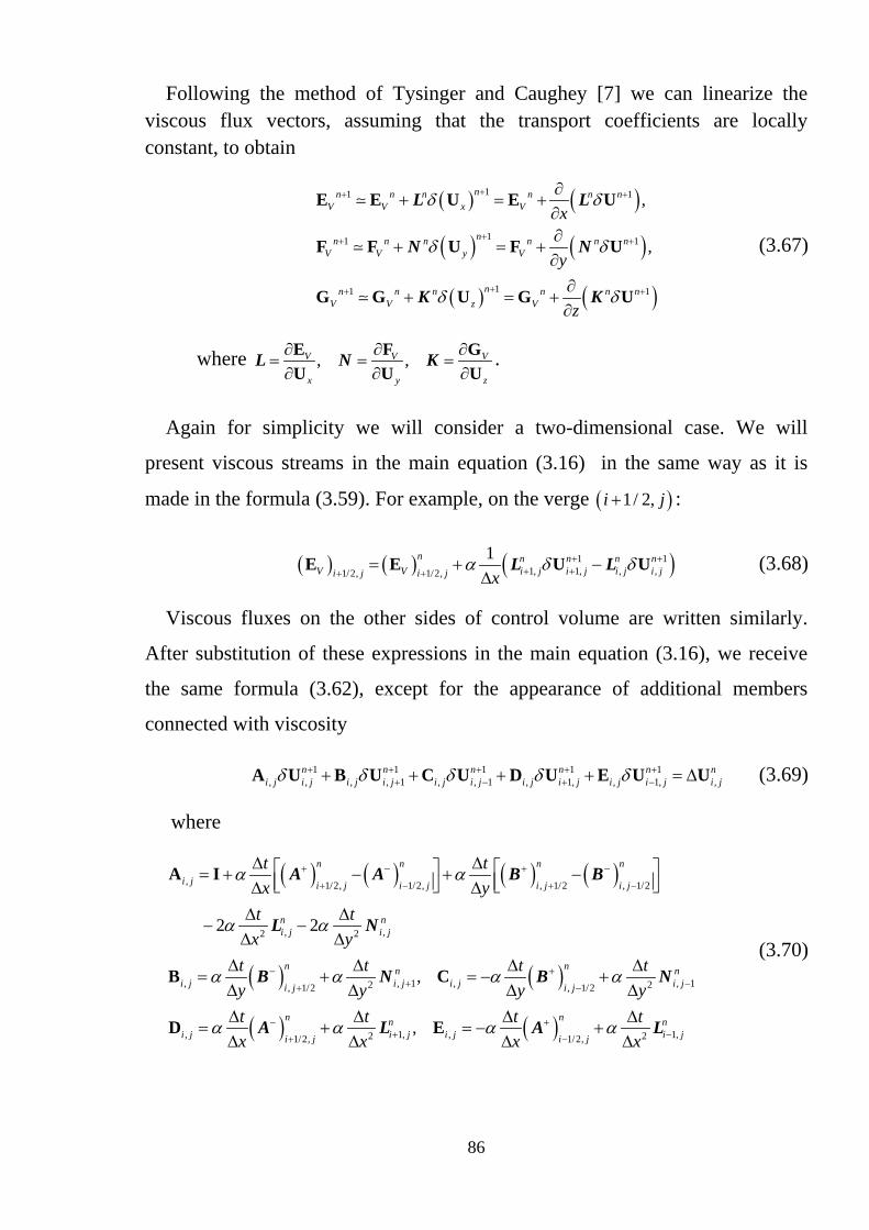
86

Following the method of Tysinger and Caughey [7] we can linearize the viscous flux vectors, assuming that the transport coefficients are locally constant, to obtain

( ) ( )

( ) ( )

( ) ( )

11 1

11 1

11 1

,

,

nn n n n n nV V x V

nn n n n n nV V y V

nn n n n n nV V z V

x

y

z

δ δ

δ δ

δ δ

++ +

++ +

++ +

∂+ = +

∂∂

+ = +∂∂

+ = +∂

E E U E U

F F U F U

G G U G U

L L

N N

K K

(3.67)

where , ,V V V

x y z

∂ ∂ ∂= = =∂ ∂ ∂E F GU U U

L N K .

Again for simplicity we will consider a two-dimensional case. We will

present viscous streams in the main equation (3.16) in the same way as it is

made in the formula (3.59). For example, on the verge ( )1/ 2,i j+ :

( ) ( ) ( )1 11, 1, , ,1/2, 1/2,

1n n n n nV V i j i j i j i ji j i j x

α δ δ+ ++ ++ +

= + −∆

E E U UL L (3.68)

Viscous fluxes on the other sides of control volume are written similarly.

After substitution of these expressions in the main equation (3.16), we receive

the same formula (3.62), except for the appearance of additional members

connected with viscosity

1 1 1 1 1, , , , 1 , , 1 , 1, , 1, ,

n n n n n ni j i j i j i j i j i j i j i j i j i j i jδ δ δ δ δ+ + + + +

+ − + −+ + + + = ∆A U B U C U D U E U U (3.69)

where

( ) ( ) ( ) ( )

( ) ( )

( )

, 1/2, 1/2, , 1/2 , 1/2

, ,2 2

, , 1 , , 12 2, 1/2 , 1/2

, 1,21/2,

2 2

,

n n n n

i j i j i j i j i j

n ni j i j

n nn ni j i j i j i ji j i j

n

i j ii j

t tx y

t tx y

t t t ty y y yt tx x

α α

α α

α α α α

α α

+ − + −

+ − + −

− ++ −+ −

−++

∆ ∆ = + − + − ∆ ∆∆ ∆

− −∆ ∆

∆ ∆ ∆ ∆= + = − +

∆ ∆ ∆ ∆∆ ∆

= +∆ ∆

A I

B C

D

A A B B

L N

B N B N

A L ( ), 1,21/2,,

nn nj i j i ji j

t tx x

α α+−−

∆ ∆= − +

∆ ∆E A L

(3.70)

87

3.8. Ways to improve the numerical method

When using the splitting of inviscid fluxes, the Modified-Steger-Warming

method Eq. (3.33) gives the best results.

But this approach is not suitable in the vicinity of strong shock waves. Close

to shock waves, the method needs to be switched to the original Steger-Warming

scheme ( Eq. (3.32) ) which is more dissipative.

To solve this problem the following pressure switch method [15] can be used

( ) ( )

1/2 ,

,i L R

+ −+

+ + − −+ −

= +

= =

E U UU U

A AA A A A

(3.71)

where

( )

( )1 ,

1L R

L R

z z

z z+

−

= − +

= + −

U U U

U U U (3.72)

( )2

1/2

0.56 1i

z+

=Γ +

(3.73)

The parameter Γ is determined by the normalized second differences of the

pressure

( ), 1, 1 1, 1, 1 , 1 , , 1 1, 1 1, 1, 1

2 2, , ,

1, , 1, , 1 , , 1, ,

1, , 1, , 1 , , 1

max e ,e ,e ,e ,e ,e ,e ,e ,e

e e e

2 2e ; e

2 2

i j i j i j i j i j i j i j i j i j i j

i j X i j Y i j

i j i j i j i j i j i jX i j Y i j

i j i j i j i j i j i j

p p p p p pp p p p p p

− − − − + − + + − + + +

+ − + −

+ − + −

Γ =

= +

− + − += =

+ + + +

(3.74)

For small values of e parameter 1 0.5z z= − = and modified Steger-Warming is

recovered from the Eq. (3.71). Close to shock waves the value of e is great,

0z = and the method is switched to the original Steger-Warming scheme.

As already known there are three types of approximations for UL and UR:

first order (see Eq. (3.42) ), second order (see Eq. (3.43) ), third order (see Eq.

(3.44) ).

Using first-order approximation gives a very robust solution, however, with a

significant error and «blur» of shocks. Using second and third orders provides

more correct solution, but with bucking failure at great pressure gradient.

88

The simple extrapolation formulae assume a smooth variation of U; however,

discontinuities in U are possible (i.e. shocks). There is a need for some

mechanism to sense such discontinuities and limit the variation of U in these

extrapolation formulas.

The following representation of fluxes is suggested:

( ) ( ) ( )

( ) ( ) ( )

1 1 1

1 1 2 1 2

1 11 3 2 ,2 8

1 11 3 22 8

L i i i i i i

R i i i i i i

θ θ

θ θ

− + −

+ + + + +

= +Φ ⋅ − + − ⋅ − − = +Φ ⋅ − + − ⋅ − −

U U U U U U U

U U U U U U U (3.75)

When 0Φ = we have first-order approximation; when 1Φ = we have second-

order approximation ( 1θ = ) or third-order approximation ( 0θ = ).

The following formula is used for Φ :

( )( )2

1/2

1max 0, ;6 1i

r z+

Φ = =Γ +

(3.76)

In cases when pressure gradient is great a numerical dissipation is added to

the scheme. The eigenvalues of the Jacobians , , ,+ − + +A A B B are calculated by

( )2 212

eλ λ λ± = ± + (3.77)

where e is supposed to be a small number used only to correct the sonic

glitch problem.

In the current work the parameter e is calculated by

( ) ( )1 2,A Be k u a e k v a= Γ + = Γ + (3.78)

The constants 1 2,k k are set within the range from 0.5 to 2.5 .

Problems

1. Define the Jacobian matrix ∂=∂

FU

B for calorically perfect gas .

2. Define the matrices 1, ,B B B−S SΛ included in the representation

1= B B B−B S SΛ (3.79)

89

4. SOLUTION OF SYSTEMS OF LINEAR EQUATIONS WITH BLOCK COEFFICIENTS

4.1. Finite approximating difference/volume equation A finite difference/volume equation, approximating the Eq. (3.16), is given by

Eq. (3.69)

1 1 1 1 1, , , , 1 , , 1 , 1, , 1, ,

n n n n n ni j i j i j i j i j i j i j i j i j i j i jδ δ δ δ δ+ + + + +

+ − + −+ + + + = ∆A U B U C U D U E U U

where , , , , ,, , , ,i j i j i j i j i jA B C D E are block matrix elements and ,ni j∆U is given by

Eq. (3.54). This system contains 5 unknown vectors and is described by a

pentadiagonal matrix of block coefficients.

The system contains seven unknown variables in a three-dimensional case.

Eq. (3.69) can also be expressed in full matrix form

[ ] [ ]δ⋅ =Μ U U∆ (4.1)

where

. . . . . . . . . .. . . . . . . . .

. . . . . . . . .

. . . . . . . . .. . . . . . . .

. . . . . . . .

. . . . . . . .

. . . . . . . .

. . . . . . . .

. . . . . . . . .

. . . . . . . . .

. . . . . . . . .

. . . . . . . . . .

x x xx x x x

x x x xx x x x

x x x x xx x x x x

x x x x xx x x x x

x x x xx x x x

x x x xx x x

=

Μ D B A C E

(4.2)

And the solution change vectors ∆U , calculated explicitly, and δU , calculated

implicitly, are given by

90

[ ] [ ]

1,

, 1

, ,

, 1

1,

. .

. ..

. .

. ..

,.

. .

. ..

. .

. .

i j

i j

i j i j

i j

i j

δ

δδ δ

δ

δ

+

+

−

−

= = ∆

U

UU UU U

U

U

∆ (4.3)

If a grid has dimension X YN N× , then vectors [ ]δU and [ ]∆U have the order of

X YN N× , and order of matrix M equals ( ) ( )X Y X YN N N N× × ×

Each element of a matrix M itself is a matrix of size 4 4× ; each element of vectors [ ]δU и [ ]∆U is also a vector consisting of 4 components.

The matrix is M sparse but it would be very expensive (computationally) to

solve the algebraic system. For instance, for a reasonable two-dimensional

calculation of transonic flow past an airfoil we could use approximately 400

points in the x direction and 200 points in the y direction. The resulting algebraic

system is a 320,000 x 320,000 matrix problem to be solved and although we

could take advantage of its banded sparse structure it would still be very costly

in terms of both CPU time and storage.

Unlike a one-dimensional problem, which is described by a block tridiagonal

matrix of coefficients and which is effectively solved by a Thomas algorithm

(TDMA) (see the paragraph 2.11), there are no such effective methods for two-

dimensional or three-dimensional matrices.

Therefore, most methods of the solution of a system with a pentadiagonal

matrix or a septa-diagonal matrix are bases on reducing these systems to block

tridiagonal inversions which can be performed in an efficient way through the

Thomas algorithm.

91

In the following paragraphs these methods will be described:

• Gauss-Seidel iteration with alternating sweeps

• Approximate Factorization method

• Modified Approximate Factorization method

All these methods are approximate and require several iterations.

4.2. Gauss-Seidel iteration method

Eq. (3.69) can be rewritten as

, , 1 , 1 1, 1, ,n

i j i j i j i j i j i jδ δ δ δ δ+ − + −+ + + + = ∆A U B U C U D U E U U (4.4)

where for convenience we have deleted the superscript n+1 on the δU 's and

the subscripts on the block 4 x 4 matrices.

Eq. (4.4) can be solved (see Fig. 4.1.) by line Gauss-Seidel iteration with

alternating sweeps in the backward and forward x-directions.

Figure 4.1. Sweep directions for line Gauss-Seidel iteration

For k = 1, 3, ...

Backward Sweep:

( ) ( ) ( ) ( ) ( )1, , 1 , 1 , 1, 1,k k k k kn

i j i j i j i j i j i jδ δ δ δ δ −+ − + −+ + = ∆ − −A U B U C U U D U E U (4.5)

and

92

Forward Sweep:

( ) ( ) ( ) ( ) ( )1 1 1 1, , 1 , 1 , 1, 1,k k k k kn

i j i j i j i j i j i jδ δ δ δ δ+ + + ++ − + −+ + = ∆ − −A U B U C U U D U E U (4.6)

To initiate the sweeps set ( )0,i jδ =U 0 . For the most applications only two

sweeps, one backward and one forward, per step, can be used.

The right parts of the equations (4.5) and (4.6) are taken from the previous

iteration and boundary conditions. Each of the matrixes in these equations is

three-diagonal and is solved by a TDMA (see paragraph 4.5)

4.3. Approximate Factorization (AF)

The matrix M in Eq. (4.1) is factored by

x y⋅M M M (4.7)

where

. . . . . . . . . .. . . . . . . . .

. . . . . . . .,. . . . . . . .

. . . . . . . .

. . . . . . . . .

. . . . . . . . . .

x yx y

x x x xx x x x x

x x x x x x

x x x x x xx x x x x

x x x x

= =

Μ ΜD A E B A C (4.8)

The matrix elements , , ,, ,i j i j i jB C D and ,i jE are defined as before in Eq. (3.70),

and

( ) ( ) ( )

( ) ( ) ( )

,2, 1/2, 1/2,

,2, , 1/2 , 1/2

2

2

n n nx i ji j i j i j

n n ny i ji j i j i j

t tx xt ty y

α α

α α

+ −

+ −

+ −

+ −

∆ ∆ = + − − ∆ ∆∆ ∆ = + − − ∆ ∆

A I

A I

A A L

B B N (4.9)

Each factor represents a block tridiagonal matrix.

Let us introduce the following notation

[ ] [ ]y δ δ⋅ =M U W (4.10)

Then from (4.7) we obtain:

[ ] [ ]x δ⋅ = ∆M W U (4.11)

93

This equation is as follows:

( ) 1 1 1, , 1, , 1, ,,n n n n

x i j i j i j i j i j i ji jδ δ δ+ + +

+ −+ + = ∆A W D W E W U (4.12)

Now we can solve Eq. (4.10):

( ) 1 1 1 1, , , 1 , , 1 ,,

n n n ny i j i j i j i j i j i ji j

δ δ δ δ+ + + ++ −+ + =A U B U C U W (4.13)

which is solved by a TDMA method too.

Upon matrix multiplication of the two factors in Eq. (4.7), none of the original

matrix elements are returned exactly and some zero elements of M become

significantly nonzero. This factorization error reduces accuracy and slows

algorithm convergence.

4.4. Modified Approximate Factorization (MAF)

The approximate factorization procedure can be modified to significantly

reduce the adverse effects of decomposition error. The modified procedure has

the property of Stone’s Strongly Implicit Method (SIP) [8] for matrix

decomposition of returning exactly the original nonzero elements of the matrix

M upon factor multiplication, although some originally zero elements become

nonzero. This modification was used by Bardina and Lombard [9] in 1987,

which they called their Diagonally Dominant Alternating Direction Implicit

(DDADI) procedure. When applied to the matrix M

[ ] 1x y

−′ ′⋅M M D M (4.14)

where

94

. . . . .. . . . .

. . . .. . . .. . . .. . . . .. . . . .

x

x xx x

x x x

x x xx x

x x

′ =

Μ D A E (4.15)

. . . . .. . . .

. . . .

. . . .

. . . .

. . . .

. . . . .

y

x xx x x

x x x

x x xx x x

x x

′ =

Μ B A C (4.16)

and diagonal matrix

. . . . . .. . . . . .. . . . . .. . . . . .. . . . . .. . . . . .. . . . . .

xx

x

xx

x

=

D A (4.17)

The block matrix elements appearing above are defined by Eq. (3.70).

Although the original nonzero elements of matrix M are returned exactly by

the above MAF decomposition procedure, other formerly zero elements are

disturbed and can contribute to both error and reduced convergence speed. The

following section describes an iterative procedure for eliminating or further

reducing this remaining decomposition error.

Removal of Decomposition Error

Eq. (4.14) can be expanded as follows.

[ ] 1x y

−′ ′⋅ = +M M D M M P (4.18)

The equation actually solved, instead of Eq.(3.69) or (4.1), is

95

[ ] [ ] [ ]δ δ⋅ + ⋅ =Μ U P U U∆ (4.19)

The difference between Eq. (4.1) and Eq. (4.19) is the decomposition error

term [ ]δ⋅P U . We now present an iterative procedure for removing this

decomposition error.

The decomposition error term is fed back into the matrix equation on the right

hand side for self cancellation. A k-step iterative modified approximate

factorization algorithm, MAFk (MAFk Algorithm), is defined as follows.

( ) ( ) [ ] ( )1k k kδ δ δ − ⋅ + ⋅ = + ⋅ Μ U P U U P U∆ (4.20)

where ( ) [ ]0 1,2,3,...kδ = = U 0

MAF1 is the same as Eq. (4.19) above. For this iterative procedure to work,

each MAF iteration must be numerically stable and the sequence must converge.

For it to be efficient, the number of iterations must be kept small, ideally at two.

A simplified stability analysis and examples showed the optimum value for the

maximum number of k sub-iterations per time step was shown to be two for

flows going to steady states.

4.5. Block TriDiagonal-Matrix Algorithm

The majority of the numerical methods described above resolve the solution

of difficult problems into repeated solutions of an equation system with a block

tri-diagonal matrix

1 1i i i i i i i+ −= + +Φ Φ Φa b c d (4.21)

where 1,2,..., 1,i N N= −

Here an unknown value of Φ and coefficient d are vectors which order is

equal 5 (for a 3-dimensional task) or 4 (for a two-dimensional task). Coefficients

, ,m m ma b c are (5x5) or (4x4) olrder matrixes respectively.

For the solution of a system it is possible to use an algorithm similar to

Thomas algorithm, described in paragraph 2.11. The only essential difference is

96

that a multiplication by an inverse matrix is used instead of division into

number.

The algorithm of the solution of system (4.21) is as follows

1. Calculate 1 1,P Q

1 11 1 1 1 1 1,− −= =P a b Q a d (4.22)

2. Use the recurrence relations

( )( ) ( )

11

11 1

,i i i i i

i i i i i i i

−−

−− −

= −

= − +

P a c P b

Q a c P c Q d (4.23)

to obtain ,i iP Q for 2,3,...,i N=

3. Set N N=Q Φ

4. Use

1i i i i+= +Φ ΦP Q (4.24) for 1, 2,...,3,2,1i N N= − − , to obtain 1 2 3 2 1, ,..., , ,N N− −Φ Φ Φ Φ Φ

5. BOUNDARY CONDITIONS

Setting boundary conditions for Navier-Stokes's equations is not a trivial

task. From a theoretical point of view it is the most difficult part of the problem

considered in this book.

At first sight, it seems that from the point of view of space variables we deal

with a typical boundary value problem, and for its decision it is necessary to set

all gasdynamic parameters on all the boundary of an estimated area.

Actually, it is not so.

Let’s consider, as an example, a compressed gas flow along an axis x with

speed u from left to right.

97

As mentioned above any point of the flow can propagate its influence on the

surrounding space as follows:

• with speed u due to movement of the flow - down the flow;

• with speed u+a due to movement of the flow and propagation of sound

vibrations - down the flow;

• with speed u-a due to propagation of sound vibrations; if speed u

exceeds the speed of sound a, there is no upwind influence.

Thus, in case of a supersonic flow from left to right, the right boundary of an

estimated area can't influence up the flow in any way; and setting boundary

conditions on it contradicts any physical sense.

If speed at the exit from an estimated area is subsonic, then extension of

influence up the flow is possible owing to propagation of sound vibrations, and

it is required to set boundary conditions on this boundary.

What boundary conditions are needed to be set on various types of boundary

of an estimated area?

The answer to this question is connected with ‘so-called’ characteristics.

5.1. Characteristics. Riemann's invariants.

It is supposed that on the boundaries of a computational domain it is possible

to neglect the influence of viscosity. (This assumption is fair for many types of

boundaries, except for cases when a boundary is a wall or a plane (line) of

symmetry.)

The Euler equations are a set of quasilinear hyperbolic equations governing

adiabatic and inviscid flow

Consider the following unsteady homogeneous hyperbolic equation

( ) ( ) ( )0, 0, ,u ua u u x x xt x

φ∂ ∂+ = = −∞ < < ∞

∂ ∂ (5.1)

98

Characteristics are the curves in x-t plane determined by the equation

( ) ( )( )( ),dx t

a u t x tdt

= (5.2)

If the solution ( ),u t x is differentiable, then it remains constant along the

characteristic ( )x t . Really

( )( ) ( ) ( ),

0du t x t dx tu u u ua u

dt t x dt t x∂ ∂ ∂ ∂

= + = + =∂ ∂ ∂ ∂

(5.3)

Now let’s consider a one-dimensional non-stationary problem of a

compressed inviscid gas flow along an axis x.

The main equations in this case are as follows:

( )

( ) ( )

( ) ( )

2

0

0

0

ut x

u u pt x

E uE upt x

ρ ρ

ρ ρ

ρ ρ

∂ ∂+ =

∂ ∂∂ ∂

+ + =∂ ∂∂ ∂

+ + =∂ ∂

(5.4)

It is a ‘so-called’ conservative form of the equations. The other form is obtained by subtracting the continuity equation from the second and third equations of the system and multiplied by u и E respectively:

( )

0

0

0

uut x x

u u put x xE Eu upt x x

ρ ρ ρ

ρ ρ

ρ ρ

∂ ∂ ∂+ + =

∂ ∂ ∂∂ ∂ ∂

+ + =∂ ∂ ∂∂ ∂ ∂

+ + =∂ ∂ ∂

(5.5)

If the gas is calorically perfect the total energy E can be expressed through

pressure and speed

2 21 12 2

pE e u uβρ

= + = + , (5.6)

where 1β γ= −

99

Hence:

2

dp pddE uduρβρ βρ

= − + (5.7)

Substituting Eq. (5.7) in the 3rd equation of (5.5), we obtain:

1 0p u p p u u p uu u u pt x t x t x x x

ρ ρ ρ ρβ β βρ∂ ∂ ∂ ∂ ∂ ∂ ∂ ∂ + − + + + + + = ∂ ∂ ∂ ∂ ∂ ∂ ∂ ∂

(5.8)

From here, considering the continuity and momentum equations, we receive

the energy equation through pressure:

0p u pp ut x x

γ∂ ∂ ∂+ + =

∂ ∂ ∂ (5.9)

Thus, we solve the considered equation in unknown vector

up

ρ =

W (5.10)

The system of equations in a vector form is as follows

0t x

∂ ∂+ =

∂ ∂W WA , (5.11)

where

0

0 1/0

uup u

ρρ

γ

=

Α (5.12)

The eigenvalues of this matrix are equal to 1 2 3, ,u u a u aλ λ λ= = − = +

The corresponding eigenvectors are

1 / /0 , 1 , 10

a a

a a

ρ ρ

ρ ρ

− −

(5.13)

100

Thus, in similarity transformation

1−=A S ΛS (5.14)

matrices are equal to

( )( )

2

1

1 / / 1 0 1/0 1 1 , 0 1/ 2 1/ 20 0 1/ 2 1/ 2

a a aa

a a a

ρ ρρ

ρ ρ ρ

−

− − = = −

−

S S (5.15)

(matrix 1−S is composed of eigenvectors, and S is found as the inverse for

it)

Considering Eq. (5.14) the vector equation (5.11) is transformed to so-called

characteristic form

0t x

∂ ∂+ =

∂ ∂W WS SΛ (5.16)

The characteristic variables ( )1 2 3, , Tξ ξ ξ=ξ are defined as follows (note the differential form)

d dξ W= S (5.17)

Substituting the definition of the characteristic variables in the characteristic form of the governing equations (5.16) leads to

0t x

∂ ∂+ =

∂ ∂ξ ξΛ (5.18)

which is also called the characteristic form of the governing equations and

has the advantage of decoupling the characteristic variables.

Each characteristic equation within Eq. (5.18) can be written as

0i iit x

ξ ξλ∂ ∂+ =

∂ ∂ (5.19)

As

101

( )( )

( )( )

22 /1 0 1/0 1/ 2 1/ 2 / 2 / 20 1/ 2 1/ 2 / 2 / 2

d dp aa dd d a du du dp a

a dp du dp a

ρρρ ρρ ρ

− − ≡ = − = −

+

ξ WS , (5.20)

then for the considered problem the characteristic variables are (up to a

numerical constant):

( )( )

21 0

2

3

/ ,/

/

d d d dp a dsd d du dp a

d d du dp a

ξ ξ ρξ ξ ρ

ξ ξ ρ−

+

≡ = − =

≡ = −

≡ = +

(5.21)

where s is an entropy, a is a speed of sound.

Notice that characteristic variables are strictly conserved during their

propagation along the characteristic; that is the quantity iξ , satisfying Eq. (5.19)

remains constant along the characteristic Ci, defined by

( )ii

dx tdt

λ= (5.22)

since along Ci

0i i i i ii

d dxdt t x t t xξ ξ ξ ξ ξλ∂ ∂ ∂ ∂= + = + =∂ ∂ ∂ ∂ ∂

(5.23)

The variables iξ are also called Riemann variables and Riemann invariants

when they remain constant. The system of equations in characteristic form can

also, be written as follows

( ) ( ) ( )

( ) ( ) ( ) ( )

( ) ( ) ( ) ( )

0 0 02

1 0,

1 0,

1 0,

t x

t x

t x

d d p d ua

d u d p d u aa

d u d p d u aa

ρ

ρ

ρ

+ + +

− − −

− = = ∂ + ∂

+ = = ∂ + + ∂

− = = ∂ + − ∂

(5.24)

with the definitions of the three characteristics

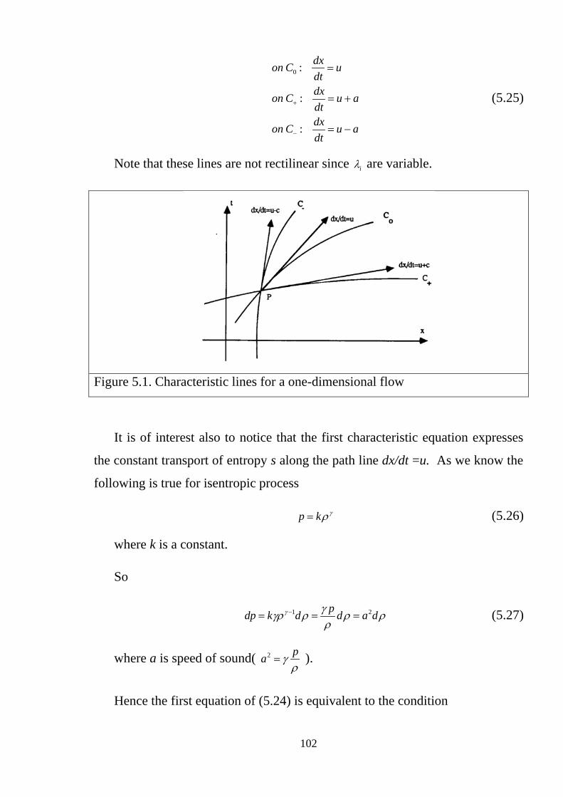
102

0 :

:

:

dxon C udtdxon C u adtdxon C u adt

+

−

=

= +

= −

(5.25)

Note that these lines are not rectilinear since iλ are variable.

Figure 5.1. Characteristic lines for a one-dimensional flow

It is of interest also to notice that the first characteristic equation expresses

the constant transport of entropy s along the path line dx/dt =u. As we know the

following is true for isentropic process

p k γρ= (5.26)

where k is a constant.

So

1 2pdp k d d a dγ γγρ ρ ρ ρρ

−= = = (5.27)

where a is speed of sound( 2 pa γρ

= ).

Hence the first equation of (5.24) is equivalent to the condition

103

( )0 0 along dxd s udt

= = (5.28)

Thus the entropy propagates along the path line and is conserved along this

characteristic, as long as discontinuities do not appear.

For isentropic flows, the Riemann or characteristic variables can be

integrated as follows, for either C+ or C-.;. For instance, on C+,

( )dp du u aa

ρξ ρρ ρ+ = + = +∫ ∫ (5.29)

where the isentropic relations

2 1,p k a kγ γρ γρ −= = (5.30)

can be introduced, k being a constant. This gives

21

u aξγ+ = +−

(5.31)

and similarly

21

u aξγ− = −−

(5.32)

for the two Riemann variables on the characteristics C+ and C-.

In the literature, another notation for invariants is often used:

0 0

21

21

R s

R u a

R u a

ξ

ξγ

ξγ

+ +

− −

≡ =

≡ = +−

≡ = −−

(5.33)

One can interpret the physical state at a given point in a one-dimensional

isentropic inviscid flow as resulting from the quantities transported along the

characteristics.

At a given point P(x, t) (Figure 5.2), the physical flow condition will be

determined by the entropy transported along C0 at speed u, that is along the

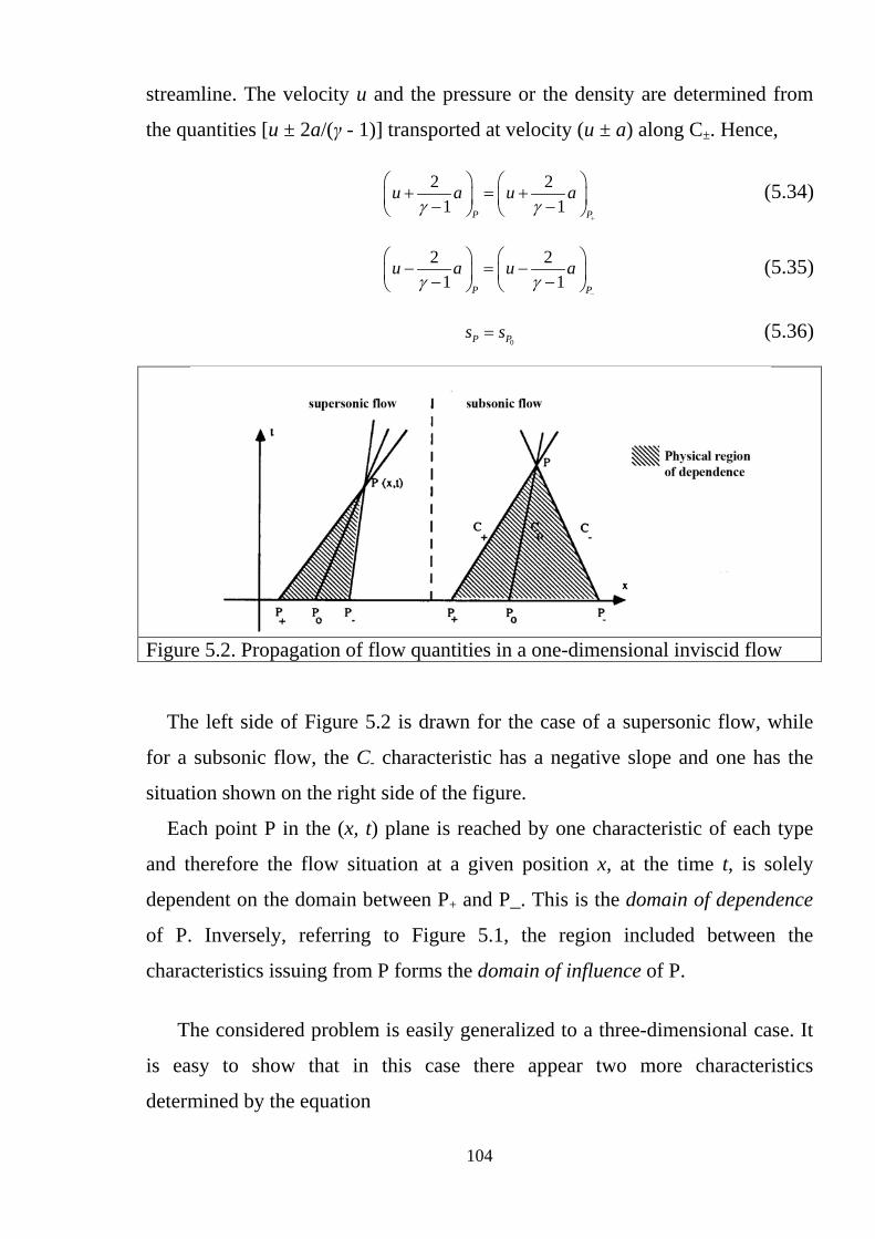
104

streamline. The velocity u and the pressure or the density are determined from

the quantities [u ± 2a/(γ - 1)] transported at velocity (u ± a) along C±. Hence,

2 21 1P P

u a u aγ γ

+

+ = + − −

(5.34)

2 21 1P P

u a u aγ γ

−

− = − − −

(5.35)

0P Ps s= (5.36)

Figure 5.2. Propagation of flow quantities in a one-dimensional inviscid flow

The left side of Figure 5.2 is drawn for the case of a supersonic flow, while

for a subsonic flow, the C- characteristic has a negative slope and one has the

situation shown on the right side of the figure.

Each point P in the (x, t) plane is reached by one characteristic of each type

and therefore the flow situation at a given position x, at the time t, is solely

dependent on the domain between P+ and P_. This is the domain of dependence

of P. Inversely, referring to Figure 5.1, the region included between the

characteristics issuing from P forms the domain of influence of P.

The considered problem is easily generalized to a three-dimensional case. It

is easy to show that in this case there appear two more characteristics

determined by the equation

105

( )dx tu

dt= , (5.37)

and the corresponding Riemann's invariants are

4 5,R v R w= = (5.38)

5.2. Types of boundary conditions

As a rule, boundary conditions are divided into 5 types.

1) INLET – boundary on which the velocity vector is directed inside an

estimated area

2) OUTLET – boundary on which the velocity vector is directed outside

from an estimated area

3) FREE STREAM BOUNDARY – boundary between an estimated area

and an external flow or quiescent space; the direction of a speed vector is

unknown here in advance

4) WALL – an impenetrable surface

5) The PLANE (LINE) of SYMMETRY – boundary relative to which all

parameters of a flow are symmetric.

The considerations from previous paragraph have a direct bearing on the

number of boundary conditions to be imposed in a one-dimensional inviscid

flow problem. Consider an inlet plane x = x0 , an outlet plane x = x1 and points P0

and P1 at a given time on these boundaries. The number of boundary conditions

to be imposed will depend on the way the information transported along the

characteristics interacts with the boundaries (Figure 5.3).

106

(a)

(b)

Figure 5.3. Boundary conditions for one-dimensional inviscid flows

(a) - supersonic flow, (b) ) - subsonic flow

At an inlet point P0, the characteristics C+ and C0 have speeds u and a + u,

which are always positive, for a flow in the positive x direction. Therefore, they

will always carry information from the boundaries towards the inside of the

domain. This requires the values of the transported quantities to be known at P0.

The third characteristic C- has a slope whose sign depends on the inlet Mach

number. For supersonic inlet flow conditions, C- will have a positive slope, but a

negative slope at subsonic inlet conditions.

In the first case, the information from the inlet surface enters the domain and

a corresponding boundary condition has to be imposed. On the other hand, at

subsonic inlet conditions, information from inside the domain reaches the

107

boundary along C- and no boundary condition associated with C- is allowed to

be fixed arbitrarily.

Similar considerations can be made at the outlet. Two characteristics, C+ and

C0 , always reach the outlet from inside the domain and therefore they determine

two of the three independent characteristic variables in the outlet plane from the

behaviour of the interior flow.

The third condition is dependent on the outlet flow Mach number. For

supersonic outlet velocities no boundary condition is to be imposed, while at

subsonic outlet velocities one boundary condition is to be fixed at the outlet

section.

We will consider these cases in more detail

5.2.1. INLET

We assume that this boundary is located perpendicular to an axis x, i.e. is on

a plane 0yz .

There are two possible options.

If a velocity component u is more than the speed of sound, all eigenvalues of

the matrix determining convective transport through the boundary

1 2 3 4 5, , , ,u u a u u u aλ λ λ λ λ= = + = = = − have a positive sign. That means that all

five characteristics are directed inside an estimated area, and propagation of

influence is directed only from the boundary inside.

In this case, the boundary is called a SUPERSONIC INLET, and it is

necessary to set all 5 parameters of a flow on it. Most often, they are 3

components of speed, temperature and pressure (or density).

In case of a supersonic inlet, usually there are no problems with setting

boundary conditions.

108

The option when u a< is more difficult. In this case, only 4 characteristics

are directed inside an estimated area, and the one – from the internal part of an

estimated area to the boundary.

Such border is called a SUBSONIC INLET, and 4 parameters of a flow are

set on it. The fifth parameter is defined by extrapolation from the internal part of

an estimated area.

Here are various possible options depending on a specific problem.

For example, for the solution of a problem of a flow in a pipe or problems of

expiration a flow from a subsonic nozzle, 3 components of speed and

temperature are most often set at an inlet.

The pressure at an inlet is determined from a condition of constancy of the

invariant connected with the eigenvalue u aλ = − , i.e. from a condition:

( )/ 0du dp aρ− = (5.39)

For this purpose we take an internal point which is next to a considered

boundary point, determine speed and pressure received during calculation in it,

and then, as a result of the solution of a differential analog of the equation (5.39)

we obtain the pressure in the boundary point.

In more detail this process is like that. We assume that on the n-th step by

time all parameters of the flow are known. It is required to determine pressure

on the boundary on the (n+1) - th step by time. We designate parameters on the

boundary with index b , and parameters of the next internal point – with index i .

From the equation (5.39) we obtain:

( )( )1 1n n n nb i b ip p a u uρ+ += + − (5.40)

The coefficient ( )aρ is taken as an average between two points and can be

found iteratively (2 iterations enough).

109

Let’s see another example: a flow in the combustion chamber of a rocket

engine. As a rule, pressure and temperature are known at the inlet of the

chamber.

In this case, speed at an inlet is easily found from a condition of constancy

of Riemann’s invariant of ( )

21

aR uγ

= −−

:

b iR R= (5.41)

The value iR is known on n-th step by time, the sound speed is determined

by pressure and temperature. From here we obtain bu .

It is possible to consider other variants of setting parameters on a subsonic

inlet. All of them are easily solved with the use of Riemann’s invariant.

5.2.2. OUTLET

In this case, it is also necessary to consider 2 options: SUPERSONIC

OUTLET and SUBSONIC OUTLET.

In case of a supersonic outlet, all 5 characteristics leave an estimated area.

Boundary conditions are not set, and the values of parameters on the boundary

are found from extrapolation from next points inside the estimated area. In this

case, it isn't even required to use Riemann’s invariants.

In case of a subsonic outlet, it is necessary to set one parameter of a flow on

the boundary - that is pressure, as a rule.

For jet flows, for flow past bodies with a gas flow and for a flow in a pipe

this pressure is supposed to be equal to the pressure of a surrounding area.

If we consider the right boundary of an estimated area, which is located

perpendicular to an axis x, the influence up the flow is determined by the

characteristic u aλ = − и and the corresponding Riemann’s invariant.

110

The other parameters of a flow are determined using Riemann’s invariants.

As before, we will designate parameters on the boundary with index b , and

parameters of the next internal point – with index i .

From the condition of constancy of Riemann’s invariants relating to the

characteristics directed down a flow, we obtain:

( ) ( )( ) ( ) ( )

1 1 2

1 1

/ 0

/ 0

n n n nb i b i

n n n nb i b i

p p a

u u p p a

ρ ρ

ρ

+ +

+ +

− − − =

− + − = (5.42)

From here:

( )

( )

11

2

11

n nb in n

b i

n nb in n

b i

p pa

p pu u

a

ρ ρ

ρ

++

++

−= +

−= −

(5.43)

As in the previous paragraph, on n-th step by time the values , ,n n ni i ip uρ are

known in the internal part of an estimated area; 1nbp + is set.

Further by formulas (5.43) we determine the values of parameters 1 1,n nb buρ + +

on the boundary on (n+1) - th step by time.

For the other speed components from (5.38) it appears:

1

1

n nb i

n nb i

v vw w

+

+

=

= (5.44)

5.2.3. FREE STREAM BOUNDARY

On this boundary, a speed component directed by normal to the boundary is

always subsonic. As it was already said, the direction of this speed can be any.

Therefore, the characteristics can be also directed inside or outside the estimated

area.

111

As a rule, such boundary separates an estimated area from an external stream

or quiescent space. It would seem that in this case it is possible to set the

boundary conditions coinciding with the parameters of an external stream.

In some cases it is acceptable, but it is more correct to use characteristic

variables.

As an example, we will consider the boundary which is above the estimated

area perpendicular to an axis y.

As always, we have 5 characteristics which in this case correspond to

eigenvalues 1 2 3 4 5, , , ,v v a v v v aλ λ λ λ λ= = + = = = −

Obviously, the second characteristic comes to the boundary from within an

estimated area, and the fifth one - from the external area. We will designate

parameters of the external area with index e (from the English word external).

We consider that the influence of an external stream is also caused by other

characteristics.

From the point of view of characteristic variables it means that there is a

relation between an external flow and the boundary:

( )

2/ 0,/ 0,

0,0

d dp adv dp adudw

ρρ

− =

− =

==

(5.45)

and between the internal area and the boundary–

( )/ 0dv dp aρ+ = (5.46)

The differential form of these equations is as follows:

112

( ) ( )( ) ( ) ( )( )( )( ) ( ) ( )

1 1 2

1 1

1

1

1 1

/ 0,

/ 0,

0,

0,

/ 0

n n n nb e b e

n n n nb e b e

n nb e

n nb e

n n n nb i b i

p p a

v v p p a

u u

w w

v v p p a

ρ ρ

ρ

ρ

+ +

+ +

+

+

+ +

− − − =

− − − =

− =

− =

− + − =

(5.47)

The solution to this system:

( )

( ) ( )( )

( ) ( )( )

1

1

1

1

12

12 21 12 2

1 1 12 2

n nb e

n nb e

n nn n n i e

b e i

n n n n nb i e i e

n n n n n nb e i e i e

u uw w

p pv v va

p p p a v v

p p a v va

ρ

ρ

ρ ρ ρ

+

+

+

+

+

=

=

−= + +

= + + −

= + − + −

(5.48)

The analysis of these formulas shows that even if an external stream is

quiescent, i.e. 0e e eu v w= = = , when a positive indignation of pressure approaches

the boundary, there appears a positive normal component of speed bv . Also, the

pressure on the boundary will change. Thus, parameters on the boundary will

differ from parameters of an external stream.

It is possible to set the boundary conditions coinciding with parameters of an

external stream only in case when it is known in advance that no indignations

happening in an internal part of the estimated area will reach the boundary.

All equations obtained for the boundaries located parallel to the coordinate

planes are easily applied to randomly located boundaries. Only instead of speeds

u,v,w it is necessary to use speed components which are normal and tangential to

the boundary.

113

For example, for the considered case instead of v we use nu - a speed

component normal to border; and instead of u, w we use a tangential

components of speed.

5.2.4. WALL

Walls can be with free slip. Then a normal component of speed on the

boundary is equal to zero, and for tangential components:

0tun

∂=

∂ (5.49)

where n∂∂

- normal derivative to a surface.

If there is no slip on a wall, then all speed components on the boundary are

equal to zero.

In both cases we assume for pressure:

0pn∂

=∂

(5.50)

The temperature on the wall can be set

b WT T= , (5.51)

or a wall can be adiabatic, then

0Tn

∂=

∂ (5.52)

Using characteristic variables near a wall is difficult, since a strong impact is

exerted by viscosity here.

Conditions (5.49), (5.50), (5.52) should be set implicitly. For this purpose, it

is very convenient to use so-called "ghost" cells, which will be considered in the

following section in detail.

5.2.5. PLANE (LINE) of SYMMETRY

From the mathematics point of view, this type of boundary is a special case

of a WALL when there is free slip and a wall is adiabatic.

114

5.3. Ghost cells

In this section for simplicity of description we will consider boundaries in

two-dimensional problems, however all obtained results are easily applied to

three-dimensional problems.

First of all, we will note that the control volumes located in close proximity

to the boundary of an estimated area can be designed in various ways.

Let’s consider this using an example of a lower boundary of a two-

dimensional grid.

Fig.5.4. Wall boundary, method I

Fig. 5.4. shows method I, when the boundary of an estimated area passes

through grid points. The near-boundary control volumes are twice less than next

volumes there. Such method is convenient when values of all flow parameters

are known, or they are directly set by boundary conditions, or determined using

characteristics. In this case, there is no need to write down the equations of

balances for near-boundary control volumes, since the values of parameters in

grid points of these cells are already known. In this example they are grid points

( ),1 , 1,2,..., Xi i N= .

The values of flow parameters in these grid point are used to determine

fluxes through the sides of next cells: ( ),2 , 1,2,..., Xi i N= ..

115

Fig.5.5 Wall boundary, method II

Method II presented in fig. 5.5 is based on the fact that the boundary of an

estimated area passes through the lower sides of near-boundary control volumes.

In that case, the values of flow parameters in near-boundary grid points are

unknown in advance, and the same balance equations are written for them as

well as for the other cells.

If flow parameters on the boundary are known, then by making up balances

the fluxes are easily determined by the lower sides of near-boundary cells.

The situation is worse for boundaries like WALL or SYMMETRY, on

which it is not parameters that are set but their derivatives. In order to use such

boundary conditions, it is necessary to enter relations between parameters in

several layers of near-boundary cells in implicit form.

The implementation of boundary conditions can be performed using “ghost”

cells. Ghost cells are not created by the grid generator. Instead, they are logically

created by the numerical code and are associated with a boundary face.

The values of its properties are set so that the flux calculation on the

boundary face yields the correct flux. For instance, for a wall boundary face, the

correct inviscid flux calculations should yield zero mass and energy fluxes and a

116

momentum flux equal to the pressure. The viscous flux for the wall boundary

face should yield a prescribed diffusion flux, viscous forces and heat fluxes.

Only one set of properties is not enough to satisfy all the constraints. In this

work, the properties of the ghost cell change according to the flux calculation

being performed. When the inviscid fluxes are being calculated, the ghost cells

hold properties such that the inviscid fluxes are correct at the boundaries. The

same happens at the viscous flux calculation.

5.3.1. Boundary conditions for inviscid fluxes

WALL and SYMMETRY

The inviscid flux for a symmetry face and a wall are the same. No mass and

energy fluxes and momentum flux given by the pressure only. That is

accomplished by setting the normal velocity to the wall to zero. This is easier to

achieve by working in the face coordinate frame.

For example, for the lower boundary (fig. 5.5) this condition is provided by

the fact that the normal component of velocity in a ghost cell is taken with the

opposite sign in relation to a near-boundary cell:

,0 ,1i iv v= − (5.53)

In this case, on the boundary:

( ),0 1/2 ,0 ,11 02i i iv v v+ = + =

This condition is written in a vector form:

,0 ,1, 1, 2,...,i i Xi N= =U WU (5.54)

where

117

1 0 0 00 1 0 00 0 1 00 0 0 1

= −

W (5.55)

If a boundary is located to the left of an estimated area, then for it we assume

in a ghost cell

0, 1, , 1,2,...j j Yu u j N= − = , (5.56)

and matrix W contains a negative unit on the second position.

Implicit Boundary Conditions

The global differential equation (3.69) for a two-dimensional problem is as

follows:

1 1 1 1 1, , , , 1 , , 1 , 1, , 1, ,

n n n n n ni j i j i j i j i j i j i j i j i j i j i jδ δ δ δ δ+ + + + +

+ − + −+ + + + = ∆A U B U C U D U E U U (5.57)

For increments δU on a wall, there are the same relation as for the main

vector U .

For example, for the lower wall boundary

1 1,0 ,1 , 1, 2,...,n n

i i Xi Nδ δ+ += =U W U , (5.58)

from here we obtain that at 1j = inviscid fluxes through the lower side are

calculated by the following formula

( ) ( ) ( ) ( )

( ) ( ) ( ) ( )

1 1, , 1, 1/2 , 1/2 , 1/2 , 1/2

1,, 1/2 , 1/2 , 1/2 , 1/2

,n n nn nC C i j i ji j i j i j i j

n n n nC C i ji j i j i j i j

α δ δ

α δ

+ ++ − ++ + + +

++ −− − − −

= + + = + +

G G U U

G G U

B B

B W B (5.59)

( ) ( ) ( ) ( ) ( )( ), 1/2 , 1/2 , 1/2 , 1/2 , 1/2

n n n n nC L R Ri j i j i j i j i j

v+ − + −− − − − −= + = +G U UB B B W B (5.60)

Eq. (5.57) for 1j = is as follows

118

1, , , 1, , , 1, , , , 1 ,

n n n n ni j i j i j i j i j k i j i j k i j i jδ δ δ δ+

+ − ++ + + = ∆A D E BU U U U U , (5.61)

here coefficients , , ,, ,i j i j i jD E B are calculated by the same formulas as for not

near-boundary grid points, and the contribution of convection CG to coefficient

,i jA is determined by a formula

( ) ( ) ( ), , , 1/2 , 1/2 , 1/2

n n ni j i j i j i j i j

ty

α+ − ++ − −

∆ → + − − ∆A A B B B W (5.62)

instead of

( ) ( ), , , 1/2 , 1/2

n ni j i j i j i j

ty

α+ −+ −

∆ → + − ∆A A B B

SUPERSONIC OUTPUT

For a boundary of this kind it is convenient to use ghost cells too. For

example, if an output is located on the right, then

1, , , 1, 2,...Nx j Nx j Yj N+ = =U U (5.63)

Implicit Boundary Conditions

For implicit form of boundary conditions at Xi N= we obtain :

( ) ( ) ( ) ( )

( ) ( ) ( ) ( )

1, ,1/2, , 1/2, , 1/2, , 1/2, ,

1 11, , , ,1/2, , 1/2, , 1/2, , 1/2, ,

,

,

n n n nC C i j ki j k i j k i j k i j k

n n nn nC C i j k i j ki j k i j k i j k i j k

α δ

α δ δ

++ −+ + + +

+ ++ − −− − − −

= + + = + +

F F U

F F U U

A A

A A (5.64)

The differential equation:

1, , , 1, , , 1 , , 1 ,

n n n n ni j i j i j i j i j i j i j i j i jδ δ δ δ+

− + −+ + + = ∆A U E U B U C U U (5.65)

And the contribution of convection CF to coefficient ,i jA is determined by a

formula

( ) ( ) ( ), , 1/2, , 1/2, , 1/2, ,

n n ni j i j i j k i j k i j k

tx

α+ − −+ − +

∆ → + − + ∆A A A A A (5.66)

119

Instead of

( ) ( ), , 1/2, , 1/2, ,

n ni j i j i j k i j k

tx

α+ −+ −

∆ → + − ∆A A A A

FREE STREAM BOUNDARY

Here it is also convenient to use ghost cells. In this case, the parameters in

these cells are assumed equal to the parameters of an external stream.

Ghost cells can be also used in other types of borders: INLET, SUBSONIC

OUTLET. But this method doesn't give great advantages in comparison with the

method of setting fluxes directly on the boundary.

5.3.2. Viscous Boundary Condition

WALL

There is no point in considering a wall with free slip as there is no viscosity

there.

On a wall without slip the following parameters are set:

0W W W

W in

u v wp p

= = ==

(5.67)

Here, parameters on a wall are designated by index W , and parameters in the

closest internal grid point of an estimated area are designated by the index in .

For an equation of energy there are different possible options of boundary

conditions:

1) Temperature can be set on a wall - WT

2) A wall can be adiabatic, then

W inT T= (5.68)

120

3) We also can use a non-catalytic wall in radiative equilibrium. That is

accomplished by setting the radiative flux equal to the convective heating

crossing the wall. The balance of heat is as follows

40

in WW W

T TTn

εσ λ −=

∆, (5.69)

where n∆ - a distance from grid point of a near-boundary cell to a wall by

normal, ε - wall emissivity, 0σ - Stefan-Boltsman's constant, Wλ - heat

conductivity coefficient of gas at a wall.

The equation in unknown WT (5.69) is solved iteratively at each moment of

time in each near-boundary cell.

Knowing the values of all parameters on a wall, we can determine them also

in the grid points of ghost cells. For example, for the lower boundary (see fig.

5.5) these values are determined by a formula

,0 ,12 , 1,2,...,i W i Xf f f i N= − = , (5.70)

where ( ), , , ,f u v w p T= - any parameter of a flow.

Implicit boundary conditions

To obtain an implicit form of boundary conditions on the lower wall we do

the following.

Viscous fluxes on the upper and lower edge of a near-boundary cell j=1 are

determined by a formula

( ) ( ) ( )

( ) ( ) ( )

, 1/2 , 1 ,, 1/2 , 1/2

, 1/2 , , 1, 1/2 , 1/2

1 ,

1

n n n nV V i j i j i ji j i j

n n n nV V i j i j i ji j i j

y

y

α δ δ

α δ δ

+ ++ +

− −− −

= + −∆

= + −∆

G G U U

G G U U

N

N (5.71)

where , 1ni jδ −U - an increment in a ghost cell.

It is necessary to express it somehow through increments in the main cells.

121

For this purpose, we introduce a vector

[ ], , , Tu v eρ=V (5.72)

Let

, 1 ,i j i jδ δ− =V VΩ (5.73)

Then

, 1 , 1 ,i j i j i jδ δ δ− −

∂ ∂= =∂ ∂U UU V VV V

Ω (5.74)

Note that considering that

V V Vy y∂ ∂ ∂

= =∂ ∂ ∂V V UG

UM M (5.75)

Using this, it is possible to approximate a viscous flux on the boundary as

, , 1i j i jV V y

−−=

∆V V

G M (5.76)

From here, considering (5.73)

( ) ( ) ( ) 1,, 1/2 , 1/2

n nVV V i ji j i j

Vy

α δ +− −

= + −∆MG G I Ω (5.77)

Finally we obtain:

( ) ( )

1, 1/2 ,, 1/2 , 1/2

1 nn ni jV V i ji j i j y

α δ +−− −

= +∆

G G N U (5.78)

where

( ), 1/2ni j V−

∂= −

∂VN M IU

Ω (5.79)

Thus, the differential equation for grid point 1j = is as follows

1, , , 1, , , 1, , , , 1 ,

n n n n ni j i j i j i j i j k i j i j k i j i jδ δ δ δ+

+ − ++ + + = ∆A D E BU U U U U (5.80)

122

And the contribution of a viscous flux VG to coefficient ,i jA is determined

by a formula

( ), 1/2, , , 1/22

nni ji j i j i j

ty

α−+

∆→ − +

∆A A N N (5.81)

instead of

( ), , , 1/2, , 1/2,2n n

i j i j i j k i j kt

yα

+ −

∆→ − +

∆A A N N

There is still an open issue of determining matrix Ω , included in a formula

(5.73). It is created with the use of relations (5.70) and depends on boundary

conditions for the energy equation.

1) Temperature set on a wall - WT

1 0 0 00 1 0 00 0 1 00 0 0 1

− = −

−

Ω (5.82)

2) Adiabatic wall

1 0 0 00 1 0 00 0 1 00 0 0 1

− = −

Ω (5.83)

3) An option with a radiation by a formula (5.69). After differentiating this

formula, we obtain

304 0in W

W W WT TT T

nδ δεσ δ λ −

− =∆

(5.84)

It can be shown that at small values of n∆ the first member in this equation

is significantly smaller than the second one and so can be neglected. Therefore:

,W in i jT T Tδ δ δ= = (5.85)

123

Considering a formula (5.70) we obtain

,0 ,1 ,2i W i i jT T T Tδ δ δ δ= − = (5.86)

Therefore, the formula for Ω coincides with (5.83)

6. COMPUTATIONAL RESULTS This chapter presents some calculation results obtained using the computer

program UNIVERSE-CFD, developed in the Moscow Aviation Institute [15].

This program used the Modified Approximate Factorization (MAF) (see Section

4.4) method with the additions described in Section 3.8 "Ways to improve the

numerical method".

6.1. Supersonic jet at high exit static pressure ratio

The first test aimed at checking the capabilities of the proposed numerical

method. For this purpose, simulation was performed for an air jet with the

following parameters: 54; 2000[ ]; / 10 ; 12; 288[ ]a a a e e eM T K p p M T K= = = = =

This flow is characterized by regions with very high pressure gradients and

high Mach numbers. The numerical computation of this variant is very

complicated when using shock-capturing method without grid adaptation.

Figure 6.1 presents the predicted Mach number field. For comparison we used

the results of Averenkova et al. [16], where the method of characteristics was

applied to the simulation of ideal gas jet structure. The 800x120 grid was used.

124

Figure 6.2 presents centerline pressure and density profiles. The results are

compared when using the 1-st approximation order of convective fluxes (dashed

lines) and the 2-st approximation order with limiter functions (solid lines). The

results of Ref. 16 are also presented.

After analyzing the results we can see that the use of the shock-capturing

numerical method allowed for obtaining quite a true picture of parameter

distribution in a supersonic jet with strong shocks. Using first approximation

order for convective fluxes results in a big «blur» of the solution in the vicinity

of strong shock waves if compared with second approximation order with

limiter function (see Eq. (3.75) ).

Figure 6.1. Mach number magnitude field and jet structure. 1 – attached shock, 2

– jet boundary, 3 – intercepting (barrel) shock, 4 – reflected shock.

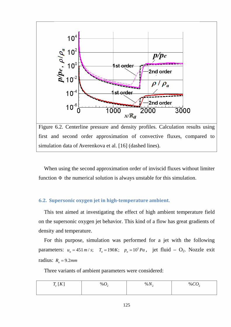
125

Figure 6.2. Centerline pressure and density profiles. Calculation results using

first and second order approximation of convective fluxes, compared to

simulation data of Averenkova et al. [16] (dashed lines).

When using the second approximation order of inviscid fluxes without limiter

function Φ the numerical solution is always unstable for this simulation.

6.2. Supersonic oxygen jet in high-temperature ambient.

This test aimed at investigating the effect of high ambient temperature field

on the supersonic oxygen jet behavior. This kind of a flow has great gradients of

density and temperature.

For this purpose, simulation was performed for a jet with the following

parameters: 5451 / ; 190 ; 10a a au m s T K p Pa= = = , jet fluid – O2. Nozzle exit

radius: 9.2aR mm=

Three variants of ambient parameters were considered:

[ ]eT K 2%O 2%N 2%CO

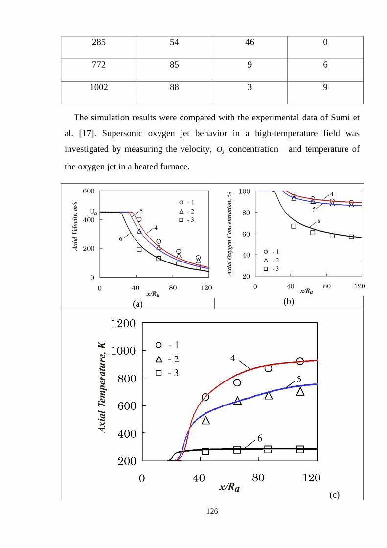
126

285 54 46 0

772 85 9 6

1002 88 3 9

The simulation results were compared with the experimental data of Sumi et

al. [17]. Supersonic oxygen jet behavior in a high-temperature field was

investigated by measuring the velocity, 2O concentration and temperature of

the oxygen jet in a heated furnace.

(a)

(b)

(c)

127

Figure 6.3. Centerline (a) velocity, (b) oxygen concentration and (c) temperature profiles. 1,2,3 – Sumi et al. [17] experiment: 1 - 1002eT K= , 2 - 772eT K= , 3 - 285eT K= ; 4,5,6 – simulations: 4 - 1002eT K= , 5 - 772eT K= , 6 - 285eT K=

Figures 6.3 present the distribution of velocity, the concentration of oxygen

and temperature on the jet axis at different ambient temperatures. The

comparison of the simulation results using the presented method with the

experimental data of Sumi et al. [17] shows a good agreement and also

demonstrates the fact that the attenuation of the jet is restrained as the ambient

temperature increases.

6.3. Cold under-expanded and over-expanded air jets

The simulation was performed for air jets having total temperature 0 300T K=

and nozzle exit Mach number 3.3aM = . The simulation results were compared

with the experimental data of Safronov and Khotulev [18].

Figures 6.4 present the simulation results and the experimental data for an

under-expanded jet with static pressure ratio / 1.5a ep p = , diameter of the profiled

nozzle 53.7aD mm= and nozzle exit half cone angle 10aθ = ° .

The simulation was performed using a 400x100 trapezoidal grid. Various

turbulence models were used:

1) standard K-ε model;

2) K-ε turbulence model with compressibility correction [22]

Using standard -K ε turbulence model considerably under-predicts the jet

length if compared with the experimental data, and also reduces a number of

shock diamonds; all shock waves are having significantly lower amplitude than

measured.

Using the turbulence model with compressibility correction gave results,

which are in a good agreement with the experimental data of Safronov,

Khotulev [18].

128

(a)

(b)

129

(c)

Figure 6.4. Centerline distribution of (a) normalized relative pitot pressure, (b) Mach number and (c) static pressure in jet with

0 300 , 3.3, / 1.5, 10a a e aT K M p p θ= = = = ° . Calculations using various turbulence models, compared to experiment. 1 – experiment; 2 – simulation with standard -K ε model; 3 – K-ε turbulence model with compressibility correction [22]

This test also investigates the influence of the grid resolution and the spatial

order of numerical scheme on the results of simulations.

Figures 6.5 show the influence of the grid resolution at various spatial orders

of numerical scheme. A 400х200 grid and a relatively coarse 200х60 grid were

compared. When using second and third approximation order the simulation

results were very similar for the both grids. Using a coarse 200х60 grid with

first order resulted in too large restraining of the waves and rapid amplitude

decay.

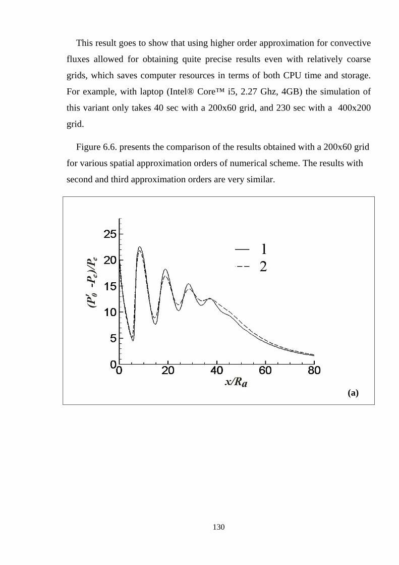
130

This result goes to show that using higher order approximation for convective

fluxes allowed for obtaining quite precise results even with relatively coarse

grids, which saves computer resources in terms of both CPU time and storage.

For example, with laptop (Intel® Core™ i5, 2.27 Ghz, 4GB) the simulation of

this variant only takes 40 sec with a 200х60 grid, and 230 sec with a 400х200

grid.

Figure 6.6. presents the comparison of the results obtained with a 200х60 grid

for various spatial approximation orders of numerical scheme. The results with

second and third approximation orders are very similar.

(a)

131

(b)

(c) Figure 6.5. Centerline distribution of normalized relative pitot pressure in jet with 0 300 , 3.3, / 1.5, 10a a e aT K M p p θ= = = = ° . Calculation results for various grids, using various spatial orders of numerical scheme: (a) - first order, (b) – second order, (c) – third order.

1 – 400x100 grid, 2 – 200x60 grid.

132

Figire 10. Test 4. Centerline distribution of normalized relative pitot pressure in jet with 0 300 , 3.3, / 1.5, 10a a e aT K M p p θ= = = = ° . Calculation results for various spatial orders of numerical scheme, using 200x60 grid: 1 - first order, 2 – second order, 3 – third order.

6.4. Highly Under-Expanded Chemically Reacting Jets

This test aims at the jets of combustion products exhausting from model

engines through sonic throats. The main features of these jets are high pressure

ratio and generation of a big normal shock wave (Mach disk).

The simulation results were compared with the experimenting data of two

model engines: kerosene-air (Chauveau et.al. [19] ) and hydrogen -air (Klavhun

et al. [20])

133

In the first test case the combustion chamber is fed with air and liquid

kerosene at normal temperature. The pressure and temperature in the

combusting chamber are 50 027 10 ; 1950p Pa T K≈ ⋅ ≈ respectively.

The contour of the sonic throat is smooth, as it is shown in Figure 6.7,

providing a uniform velocity profile at the jet origin.

PIV (Particles Image Velocimetry) was a technique to measure the velocity

field in a fluid flow. To apply PIV, the flow must be seeded with fine particles

that are supposed to follow precisely the fluid motion within the measurement

zone.

The following parameters at the nozzle exit are used in the simulation:

2 2 2 2

5792m/s; 1720K; 14.77 10 ;0.05535; 0.06001; 0.00007; 0.15116; 0.73341

a a a

O H O CO CO N

u T p PaY Y Y Y Y

= = = ⋅

= = = = =

The ambient is air at normal conditions.

Figire 6.7. Geometry of the sonic throat of kerosene-air engine.

Figure 6.8 presents the predicted and the experimental structure of the jet.

Direct processing of instantaneous PIV images allows for measuring the Mach

disk and other shocks geometry. The similar results were obtained through the

134

simulation based on the picture of velocity field. The comparison shows a good

agreement of the simulation results with the experimental data.

Figure 6.8. Jet structure obtained from an instantaneous PIV image (upper half)

[19] and velocity magnitude fields predicted by the simulation (lower half)

Figures 6.9, 6.10 show the axial distributions and radial profiles of velocity

obtained though simulation and compared with the experimental data.

The comparison showed a good agreement of simulation results with the

experimental data in all the areas of the flow except for Mach disk region. The

authors of the experiment explain that the observed discrepancies should be

attributed to the flow tracking problems and limited capabilities of the PIV

system.

135

Figire 6.9. Centerline velocity vs. distance from nozzle exit x in jet exhausting

from kerosene-air engine. 792m/s; 1720K; / 14.77a a a eu T p p= = = 1 – Chauveau et al. [19] experiment; 2 – simulation with standard -K ε model;

3 – simulation with K-ε turbulence model with compressibility correction [22]

(a)

(b)

(c)

(d)

136

(e)

Figure 6.10. Radial profiles of velocity magnitude in jet exhausting from kerosene-air engine. 792m/s; 1720K; / 14.77a a a eu T p p= = = (a) - 0.1x m= ; (b) - 0.15x m= ; (c) - 0.2x m= ; (d) - 0.25x m= ; (e) - 0.3x m= . Calculation results (lines) are compared to the experimental data (points). 1 – Chauveau et al.29 experiment; 2 – simulation with standard -K ε model; 3 – simulation with K-ε turbulence model with compressibility correction [22]

The second experiment used in this test was to show how well the presented

method describes the flow in Mach disk region.

The comparison was made using the experimental data of Klavhun et al. [20],

which involves the investigation of a sonic under-expanded jet exhausting from

a model engine. The jet facility consists of a small ceramic-lined combustion

chamber that contains a stoichiometric hydrogen-air flame, the products of

which are accelerated through a 3.15-mm-i.d. alumina tube into a low-pressure

chamber to form a reacting under-expanded jet. The pressure in the combusting

chamber is 50 1.6 10p Pa= ⋅ , the temperature in the combusting chamber is 0 2000T K= .

The low- pressure chamber has 50.11 10ep Pa= ⋅ . It is assumed that the jet reacts

chemically with the air present in this chamber.

A high-resolution OH laser-induced fluorescence (LIF) velocity measurement

technique was used in this experiment [20]. The approach for measuring

velocity is based on detection of the laser-induced fluorescence from a Doppler-

shifted OH absorption line.

The following parameters at the nozzle exit were used:

137

2

2 2 2

5871m/s; 1765K; 0.7 10 ;0.00023; 0.00006; 0.00205; 0.00509

0.00167; 0.33903; 0.65187

a a a

H O OH H

O H O N

u T p PaY Y Y Y

Y Y Y

= = = ⋅

= = = =

= = = Figure 6.11 presents centerline velocity distribution. The simulation results

are provided at constant and variable values of PrT, ScT. As it can be seen, those

are very similar, i.e. considering the variability of these criteria does not impact

much on the dynamic characteristics of the flow.

The comparison shows a good agreement of simulation results with the

experimental data in all flow regions including Mach disk region.

Figure 6.11 Centerline velocity vs. distance from nozzle exit in jet exhausting from hydrogen-air engine. 871m/s; 1765K; / 6.36a a a eu T p p= = = Calculation results for various Pr ,T TSc models (constant and variable), 1 – Klavhun et al. [20] experiment; 2 – simulation using constant PrT= ScT=0.7; 3 – simulation using variable PrT, ScT model

6.5. Afterburning of exhaust plume.

This test aimed at validating the presented method for investigating of

supersonic non-isobaric jets which contain unburned combustible species:

2 ,H CO . These species chemically react with the oxygen contained in air; their

afterburning causes a considerable increase of temperature.

138

This test included the simulation of jets exhausting from hot-gas generator,

described in Safronov and Khotulev[18, 21]. Pitot pressure and total temperature

were measured.

The numerical investigation for two gas generator operational modes was

performed using the same fuel.

Figure 6.12 presents centerline distribution of normalized relative pitot

pressure in over-expanded jet with the following parameters:

0 2860T K= , 4.0aM = , / 0.65a ep p =

Mass fractions of afterburning species are: 2

0.01; 0.29H COY Y= =

The simulation was carried out with the use of different turbulence models.

The simulation results with the presented turbulence model are in a good

agreement with the experimental data; using standard -K ε model considerably

under predicts the jet length; -K ε turbulent model with compressibility

correction of Sarkar et al. [23] slightly over predicts the jet length.

Figure 6.12. Centerline distribution of normalized relative pitot pressure in overexpanded jet with 0 2860 , 4.0, / 0.65a a eT K M p p= = = .

139

Calculations using various turbulence models, compared to experiment. 1 – Safronov experiment; 2 – simulation using standard -K ε model without compressibility correction; 3 – 3 – simulation with K-ε turbulence model with compressibility correction [22]; 4 – simulation with -K ε model with Sarkar et al.[23] compressibility correction

REFERENCES

1. MacCormack, R.W. Current Status of Numerical Solutions of the Navier-

Stokes Equations //AIAA-85-0032. - 1985. 14p.

2. MacCormack, R.W., The Effect of Viscosity in Hypervelocity Impact

Cratering // AIAA Paper No. 69-354. - 1969. 7p.

3. Patankar, S.V. Numerical Heat Transfer and Fluid Flow // Hemisphere

Publishing Corporation. - 1980. 197 pages.

4. Godunov S.K., Ryabenkii V.S. Difference Schemes: An Introduction to the

Underlying Theory // Elsevier, 1987 - Pages 488.

5. Tannehill J. C., Anderson D. A., Pletcher R. H. Computational Fluid

Mechanics and Heat Transfer. Taylor & Francis, 1997. 792 pp. ISBN 1 56032

045X.

6. MacCormack, R.W., and Pulliam, T. Assessment of A New Numerical

Procedure For Fluid Dynamics //AIAA Paper 98-2821. -1998. 9p.

7. Tysinger, T., and Caughey, D., “Implicit Multigrid Algorithm for the

Navier–Stokes Equations,” AIAA Paper 91-0242, 1991, pp.1-16.

8. Stone, H.L., “Iterative Solution of Implicit Approximations of

Multidimensional Partial Differential Equations,” Siam J. Numer. Anal., Vol. 5,

No. 3, Sept., 1968, pp. 530-558.

9. Bardina, J. and C.K. Lombard, “Three Dimensional Hyper sonic Flow

Simulations with the CSCM Implicit Upwind Navier-Stokes Method,” AIAA

Paper No. 87-11Ц, 1987.

140

10. Versteeg H. K. and Malalasekera W. An introduction to computational

fluid dynamics. The finite volume method // Pearson Education, Limited, 2011 -

Finite volume method - 552 pages

11. Wangda Zuo. Introduction of Computational Fluid Dynamics // FAU

Erlangen-Nürnberg, JASS 05, St. Petersburg, 205, 8 pages

12. Scalabrin L.C. Numerical Simulation of Weakly Ionized Hypersonic Flow

over Reentry Capsules //A dissertation submitted in partial fulfillment of the

requirements for the degree of Doctor of Philosophy (Aerospace Engineering) in

The University of Michigan. -2007. -182p.

13. Steger, J. and Warming, R. F. "Flux Vector Splitting of the Inviscid

Gasdynamics Equations with Application to Finite Difference Methods," NASA

TM-78605, 1979.

14. MacCormack, R. W,, "A Numerical Method for Solving the Equations of

Compressible Viscous Flow," AIAA Paper No. 81-0110.

15. Molchanov A.M. Numerical Simulation of Supersonic Chemically

Reacting Turbulent Jets. 2011. AIAA Paper 2011-3211, 37p.

16. Averenkova, G.P., Ashratov, E.A., Volkonskaya, T.G., et al. Supersonic

Jets of the Ideal Gas. In 2 parts. [in Russian] Moscow: Publishing House of

Moscow State University, 1970-1971. Part 1. 1970, 279p., Part 2, 1971, 170 p.

17. Sumi, I., Kishimoto, Y., Kikichi, Y. and Igarashi, H.,"Effect of high

temperature field on supersonic oxygen jet behavior," ISIJ International, Vol.

46, 2006, pp. 1312-1317.

18. Safronov A., Khotulev V. Results of experimenal researches of the

supersonic cold and hot jet // Physical-Chemical Kinetics in Gas Dynamics.

2008. V.6. http://chemphys.edu.ru/issues/2008-6/articles/280/

19. Chauveau, C., Davidenko, D. M., Sarh, B., Gökalp, I., Avrashkov, V.,

Fabre, C., “PIV Measurements in an Underexpanded Hot Free Jet,” 13th Int

Symp on Applications of Laser Techniques to Fluid Mechanics, Paper No.1161,

2006, pp.1-12.

141

20. Klavhun,K.G., Gauba, G., McDanial,J. C., "OH Laser-Induced

Fluorescence Velocimetry Technique for Steady, High-Speed, Reacting Flows,"

Journal of Propulsion and Power, Vol. 10, No. 6, 1994, pp.787-797.

21. Safronov A. The method of calculation of the jets of combustion products

at the rocket launch//Physical-Chemical Kinetics in Gas Dynamics. 2006. V.4.

http://chemphys.edu.ru/issues/2006-4/articles/100/

22. Molchanov, A.M., "A calculation of supersonic non-isobaric jets with

compressibility corrections in a turbulence model," Vestnik MAI, No.1, Vol.16,

2009, pp.38-48.

23. Sarkar, S., Erlebacher, G., Hussaini, M.Y. and Kreiss, H.O., "The analysis

and modeling of dilatational terms in compressible turbulence," Journal of Fluid

Mechanics, Vol. 227, 1991, pp.473–493.