1

MODULE VI

APPLICATION LAYER

4.1. DOMAIN NAME SYSTEM

The Domain Name System (DNS) is the method by which Internet addresses in

mnemonic form such as cse.cusat.ac.in are converted into the equivalent numeric

IP address such as 134.220.4.1. To the user and application process this translation is

a service provided either by the local host or from a remote host via the Internet. The

DNS server (or resolver) may communicate with other Internet DNS servers if it cannot

translate the address itself.

The system accesses the DNS through a resolver. The resolver gets the hostname and

returns the IP address or gets an IP address and looks up a hostname. The resolver returns

the IP address before asking the TCP to open a connection or sending a datagram using

UDP.

4.1.1. DNS Name Structure

DNS names are constructed hierarchically. The highest level of the hierarchy being the

last component or label of the DNS address. Labels can be up to 63 characters long and

are case insensitive. A maximum length of 255 characters is allowed. Labels must start

with a letter and can only consist of letters, digits and hyphens. The root of the DNS tree

is a special node with a null label. In the DNS we start from the leaf and "go up" till the

root.

2

Top-level domains can be classified as

• Generic

• Country

The seven 3-character generic domain names.

code meaning

com Commercial. Now international.

edu Educational.

gov Government.

int International Organization.

mil Military.

net Network related.

org Miscellaneous Organization.

The Internet scheme can accommodate a wide variety of organizations, and allows each

group to choose between geographical or organizational naming hierarchies. Most sites

follow the Internet scheme so they can attach their TCP/IP installations to the connected

Internet without changing names. The zone is a sub tree of the DNS that is administered

separately. A common zone is a second-level domain, "ac.il" for example. Thus a lot of

second-level domains divide their zone into smaller zones.

3

Whenever a new system is installed in a zone, the DNS administrator for the zone

allocates a name and an IP address for the new system and enters these into the name

server's database. A name server is said to have authority for one zone or multiple zones.

Often, server software executes on a dedicated processor, and this computing machine is

called the name Server.

The person responsible for a zone must provide a primary name server for that zone and

one or more secondary name servers. The main difference between a primary and a

secondary is that the primary loads all the information for the zone from disk files, while

the secondary obtain all the information from the primary. When a secondary obtains the

information from its primary it is called a zone transfer.

When a new host is added to the zone, the administrator adds the appropriate information

(name and IP address) to a disk file on the system running the primary. The primary

name server is then notified to reread its configuration files. The secondary query the

primary on regular basis (normally every 3 hours) and if the primary contains newer data,

the secondary obtains the new data using a zone transfer.

If the name server doesn't contain the information requested, it must contact another

name server. The root servers then know the name and location (i.e. IP address) of each

authoritative name servers for all the second-level domains. There are six root servers in

the world and every primary name server has to know the address of one of root server.

The country domains are of three characters. The country domain for India is in, United

Kingdom is uk etc. Every country in the world has a two letter domain name.

4

4.1.2. Resource Records

The Domain Name System provides a consistent name space that is used for referring to

resources. It is a distributed hierarchical system that can be used in many applications and

across multiple communications systems. It consists of three kinds of entities: name

servers, name resolvers, and resource records. Name servers answer queries using data

available to them. Name resolvers serve as an interface between user programs and the

Domain Name System. Resource records are the data associated with the names.

Resource records are used to store data about domain names and IP addresses.

Every domain has a set of resource records. Resource record is a five tuple. Format is

<domain_name> <time_to_live> <class> <type> <value>

If the domain name is only a host name, the default domain is appended. If it is left

empty, then the last specific name is used. If it is the @ symbol, the domain name of the

DNS server is used.

Time to live is an optional entry that specifies how long the record can be cached.

Class is the class of the record, and it is IN for Internet.

Type is the type of the record.

Value is the resource record data.

5

Some common resource record type

4.2. ELECTRONIC MAIL

Email is the most widely used Internet application. For some people, it is their most

frequent form of communication. Electronic mail is a natural use of networked

communication technology that developed along with the evolution of the Internet.

Message exchange in one form or another has existed from the early days of timesharing

computers. Network email was developed for the ARPANET shortly after it's creation,

and has now evolved into the powerful email technology that is the most used application

on the Internet today.

Email servers exchange messages using the SMTP protocol. Client applications log into

the servers to send and receive user's email with one of several protocols, including the

leading POP3, IMAP, and MAPI protocols.

Each internet domain has an associated email server that manages all addresses at that

domain. Each email address is expressed in the form "name@domain", and is unique at

that domain, as in " jane@twenty.net".

The key to this elegant architecture is its simple structure, where each domain has an

associated mail server that maintains the accounts for all users with addresses at that

domain. Therefore, any email server can easily use the Internet's domain name system to

find the IP address of any other mail server, connect to that server, and transfer email to

recipients at that domain using the standard SMTP protocol.

6

4.3. MIME

In the early days of the ARPANET, e-mail consisted exclusively of text messages written

in English and expressed in ASCII. For this environment, RFC 822 did the job

completely: it specified the headers but left the content entirely up to the users.

Nowadays, on the worldwide Internet, this approach is no longer adequate. The problems

include sending and receiving

• Messages in languages with accents (e.g., French and German).

• Messages in non-Latin alphabets (e.g., Hebrew and Russian).

• Messages in languages without alphabets (e.g., Chinese and Japanese).

• Messages not containing text at all (e.g., audio or images).

A solution was proposed in RFC 1341 and updated in RFCs 2045–2049. This solution,

called MIME (Multipurpose Internet Mail Extensions) is now widely used.

The basic idea of MIME is to continue to use the RFC 822 format, but to add structure to

the message body and define encoding rules for non-ASCII messages. By not deviating

from RFC 822, MIME messages can be sent using the existing mail programs and

protocols. All that has to be changed are the sending and receiving programs, which users

can do for themselves.

MIME is an Internet Standard for the format of e-mail. Virtually all human written

Internet e-mail and a fairly large proportion of automated e-mail is transmitted via SMTP

in MIME format. Internet e-mail is so closely associated with the SMTP and MIME

standards that it is sometimes called SMTP/MIME e-mail.

To insure that email messages containing images or other non-text information will be

delivered with maximum protection against corruption, MIME provides a way for non-

text information to be encoded as text. This encoding is known as base64, and appears to

be a source of frustration for many email users.

MIME defines five new message headers, as shown in figure. The first of these simply

tells the user agent receiving the message that it is dealing with a MIME message, and

which version of MIME it uses. Any message not containing a MIME-Version: header is

assumed to be an English plaintext message and is processed as such.

7

The Content-Description: header is an ASCII string telling what is in the message. This

header is needed so the recipient will know whether it is worth decoding and reading the

message. If the string says: “Photo of Barbara’s hamster” and the person getting the

message is not a big hamster fan, the message will probably be discarded rather than

decoded into a high-resolution color photograph.

The Content-Id: header identifies the content. It uses the same format as the standard

Message-Id: header.

The Content-Transfer-Encoding: tells how the body is wrapped for transmission through

a network that may object to most characters other than letters, numbers, and punctuation

marks. Five schemes (plus an escape to new schemes) are provided. The simplest scheme

is just ASCII text. ASCII characters use 7 bits and can be carried directly by the e-mail

protocol provided that no line exceeds 1000 characters.

The Content-Type: It specifies the nature of the message body.

4.4. MOBILE TELEPHONE SYSTEMS

4.4.1. Evolution of mobile telephone systems

Cellular is one of the fastest growing and most demanding telecommunications

applications. Today, it represents a continuously increasing percentage of all new

telephone subscriptions around the world. Currently there are more than 45 million

cellular subscribers worldwide, and nearly 50 percent of those subscribers are located in

the United States. It is forecasted that cellular systems using a digital technology will

become the universal method of telecommunications.

The concept of cellular service is the use of low-power transmitters where frequencies

can be reused within a geographic area. The idea of cell-based mobile radio service was

formulated in the United States at Bell Labs in the early 1970s. However, the Nordic

Header Meaning

MIME version Identifies the MIME version

Content description Human readable string telling what is in the

message

Content-Id Unique identifier

Content-Transfer-Encoding: How the body is wrapped for transmission

Content-Type Type and format of the content

8

countries were the first to introduce cellular services for commercial use with the

introduction of the Nordic Mobile Telephone (NMT) in 1981.

Cellular systems began in the United States with the release of the advanced mobile

phone service (AMPS) system in 1983. The AMPS standard was adopted by Asia, Latin

America, and Oceanic countries, creating the largest potential market in the world for

cellular.

In the early 1980s, most mobile telephone systems were analog rather than digital, like

today's newer systems. One challenge facing analog systems was the inability to handle

the growing capacity needs in a cost-efficient manner. As a result, digital technology was

welcomed. The advantages of digital systems over analog systems include ease of

signaling, lower levels of interference, integration of transmission and switching, and

increased ability to meet capacity demands.

4.4.2. Global System for Mobile Communication (GSM)

Throughout the evolution of cellular telecommunications, various systems have been

developed without the benefit of standardized specifications. This presented many

problems directly related to compatibility, especially with the development of digital

radio technology. The GSM standard is intended to address these problems.

From 1982 to 1985 discussions were held to decide between building an analog or digital

system. After multiple field tests, a digital system was adopted for GSM. The next task

was to decide between a narrow or broadband solution. In May 1987, the narrowband

time division multiple access (TDMA) solution was chosen.

The GSM Network

GSM provides recommendations, not requirements. The GSM specifications define the

functions and interface requirements in detail but do not address the hardware. The

reason for this is to limit the designers as little as possible but still to make it possible for

the operators to buy equipment from different suppliers. The GSM network is divided

into three major systems: the switching system (SS), the base station system (BSS), and

the operation and support system (OSS).

The basic GSM network is given below.

9

The Switching System

The switching system (SS) is responsible for performing call processing and subscriber-

related functions. The switching system includes the following functional units.

Home Location Register (HLR)—The HLR is a database used for storage and

management of subscriptions. The HLR is considered the most important database, as it

stores permanent data about subscribers, including a subscriber's service profile, location

information, and activity status. When an individual buys a subscription from one of the

PCS operators, he or she is registered in the HLR of that operator.

Mobile Services Switching Center (MSC)—The MSC performs the telephony

switching functions of the system. It controls calls to and from other telephone and data

systems. It also performs such functions as toll ticketing, network interfacing, common

channel signaling, and others.

Visitor Location Register (VLR)—The VLR is a database that contains temporary

information about subscribers that is needed by the MSC in order to service visiting

subscribers. The VLR is always integrated with the MSC. When a mobile station roams

into a new MSC area, the VLR connected to that MSC will request data about the mobile

station from the HLR. Later, if the mobile station makes a call, the VLR will have the

information needed for call setup without having to interrogate the HLR each time.

Authentication Center (AUC)—A unit called the AUC provides authentication and

encryption parameters that verify the user's identity and ensure the confidentiality of each

10

call. The AUC protects network operators from different types of fraud found in today's

cellular world.

Equipment Identity Register (EIR)—The EIR is a database that contains information

about the identity of mobile equipment that prevents calls from stolen, unauthorized, or

defective mobile stations. The AUC and EIR are implemented as stand-alone nodes or as

a combined AUC/EIR node.

The Base Station System (BSS)

All radio-related functions are performed in the BSS, which consists of base station

controllers (BSCs) and the base transceiver stations (BTSs).

BSC—The BSC provides all the control functions and physical links between the MSC

and BTS. It is a high-capacity switch that provides functions such as handover, cell

configuration data, and control of radio frequency (RF) power levels in base transceiver

stations. A number of BSCs are served by an MSC.

BTS—The BTS handles the radio interface to the mobile station. The BTS is the radio

equipment (transceivers and antennas) needed to service each cell in the network. A

group of BTSs are controlled by a BSC.

The Operation and Support System

The operations and maintenance center (OMC) is connected to all equipment in the

switching system and to the BSC. The implementation of OMC is called the operation

and support system (OSS). The OSS is the functional entity from which the network

operator monitors and controls the system. The purpose of OSS is to offer the customer

cost-effective support for centralized, regional and local operational and maintenance

activities that are required for a GSM network. An important function of OSS is to

provide a network overview and support the maintenance activities of different operation

and maintenance organizations.

• Message Center (MXE)—The MXE is a node that provides integrated voice,

fax, and data messaging. Specifically, the MXE handles short message service,

cell broadcast, voice mail, fax mail, e-mail, and notification.

• Mobile Service Node (MSN)—The MSN is the node that handles the mobile

intelligent network (IN) services.

11

• Gateway Mobile Services Switching Center (GMSC)—A gateway is a node

used to interconnect two networks. The gateway is often implemented in an MSC.

The MSC is then referred to as the GMSC.

• GSM Interworking Unit (GIWU)—The GIWU consists of both hardware and

software that provides an interface to various networks for data communications.

Through the GIWU, users can alternate between speech and data during the same

call. The GIWU hardware equipment is physically located at the MSC/VLR.

4.5. BLUETOOTH

Bluetooth is a global standard for wireless connectivity. Bluetooth technology facilitates

the replacement of the cables used to connect one device to another, with one universal

short-range radio link operating in the unlicensed 2.45 GHz ISM band. The main

objectives of Bluetooth technology can be described as follows,

• Cable replacement: Getting rid of the various types of cables and wires required

for interconnectivity between various devices would enable the lay man to use all

electronic devices without wasting time and money.

• Small size: the Bluetooth device is very small so that it can be attached to any

device required like the cell phones without adding much to the weight of the

system.

• Low cost: Bluetooth is aimed to be a low cost device approximately $5 in the near

future.

• Low power: The utilization of power is very less (within 100 mW) as it is short

range equipment and so it facilitates the use of small batteries for its usage.

4.5.1. Working of BLUETOOTH

Basically, Bluetooth is the term used to describe the protocol of a short range (10 meter)

frequency-hopping radio link between devices. These devices implementing the

Bluetooth technology are termed Bluetooth - enabled. Bluetooth can imitate a universal

bridge to attach the existing data networks, and also as a mechanism for forming ad-hoc

networks. Designed to operate in noisy frequency environments, the Bluetooth radio uses

a fast acknowledgement and frequency hopping scheme to make the link robust.

12

4.5.2. Bluetooth Architecture

Different layers are:

Bluetooth Radio: The Bluetooth Radio (layer) is the lowest defined layer of the

Bluetooth specification. It defines the requirements of the Bluetooth transceiver device

operating in the 2.4GHz ISM band. The Bluetooth air interface is based on three power

classes,

• Power Class 1: designed for long range (~100m), max output power of 20 dBm.

• Power Class 2: ordinary range devices (~10m), max output power of 4 dBm.

• Power Class 3 short range devices (~10cm), with a max output power of 0 dBm.

Baseband: The Base band is the physical layer of the Bluetooth. It manages physical

channels and links apart from other services like error correction, data whitening, hop

selection and Bluetooth security. As mentioned previously, the basic radio is a hybrid

spread spectrum radio. Typically, the radio operates in a frequency-hopping manner in

which the 2.4GHz ISM band is broken into 79 1MHz channels that the radio randomly

hops through while transmitting and receiving data. A Pico net is formed when one

Bluetooth radio connects to another Bluetooth radio.

LMP: The Link Manager Protocol is used by the Link Managers (on either side) for link

set-up and control.

13

HCI: The Host Controller Interface provides a command interface to the Baseband Link

Controller and Link Manager, and access to hardware status and control registers.

L2CAP: Logical Link Control and Adaptation Protocol supports higher level protocol

multiplexing, packet segmentation and reassembly, and the conveying of quality of

service information.

RFCOMM: The RFCOMM protocol provides emulation of serial ports over the

L2CAPprotocol. The protocol is based on the ETSI standard TS 07.10.

SDP: The Service Discovery Protocol provides a means for applications to discover

which services are provided by or available through a Bluetooth device. It also allows

applications to determine the characteristics of those available services.

MODULE 5

UDP - SIMPLE DEMULTIPLEXER (UDP)

The simplest transport protocol is one that extends the host-to-host delivery service of the underlying

network into a process-to-process communication service. There are likely to be many processes

running on any given host, so the protocol needs to add a level of demultiplexing, thereby allowing

multiple application process on each host to share the network. Aside from this requirement, the

transport protocol adds no other functionality to the best-effort service provided by the underlying

network. The Internet‟s Users Datagram protocol (UDP) is an example of such a transport protocol.

The only interesting issue in such a protocol is the form of the address used to identify the target

process. Although it is possible for a process to directly identify each other with an OS-assigned

process ID (pid), such an approach is only practical in a closed distributed system. in which a single

OS runs on all hosts and assigns each process a unique ID.A more common approach, and the one

used by UDP, is for process to indirectly identify each other using an abstract locater, often called a

port or mail box. The basic idea is for a source process to send a message to a port and for the

destination process to receive the message from a port.

The header for an end-to-end protocol that implements this demultiplexing function typically

contains an identifier (port) for both the sender (source)and the receiver(destination)of the message.

The UDP port field is only 16bits long. This means that there are up to 64K possible ports, clearly

not enough to identify all the processes on all the hosts in the Internet. Fortunately, ports are not

interpreted across the entire Internet, but only on a single host. That is, a process is really identified

by a port on some particular host-<port, host >pair. In fact, this pair constitutes the demultiplexing

key for the UDP protocol.

The next issue is how a process learns the port for the process to which it wants to send the message.

Typically a client process initiates a message exchange with a server process. Once a client has

contacted a server, the server knows the client‟s port (it was contained in the message header) and

can reply to it. The real problem, therefore, is how the client learns the server‟s port in the first place.

A common approach is for the server to accept messages at a well known port. That is, each server

receives its messages at some fixed port that is widely published, much like the emergency telephone

service available at the well-known number 911.In the Internet, for example, the domain name server

(DNS) receives messages at well-known port 53 on each host, the mail service listens of messages at

port 25,and the Unix talk program accepts messages at well known port 517,and so on. This mapping

is published periodically in an RFC and is available on the most Unix systems in file /etc/services.

Sometimes a well-known port to agree on some other port that they will use for subsequent

communication leaving the well-known port free for other clients.

An alternative strategy is to generalize this idea, so that there is only a single well-known port- the

one at which the “port mapper” service accepts messages. A client would send a message to the

port mapper‟s well known port asking for the port it should use to talk to the “whatever” service

and the port associated with different services over time, and for each host to use a different port

for the same service.

As just mentioned, a port is purely an abstraction. Exactly how it is implemented differs from system

to system, or more precisely, from OS to OS. For example, the socket API is an example

implementation of ports. Typically, a port is implemented by a message queue. When a message

arrives, the protocol l(eg.UDP) appends the message to the end of the queue. Should the queue be

full, the message is discarded. There is no flow-control mechanism that tells the sender to slow down.

When an application process wants to receive a message, one is removed from the front of the queue.

If the queue is empty, the process blocks until a message becomes available.

Finally, although UDP does not implement flow control or reliable/ordered delivery, it does a little

more work than to simplify demultiplexer messages to some application process- it also ensures the

correctness of the message by the use of a checksum.(The UDP checksum is optional in the current

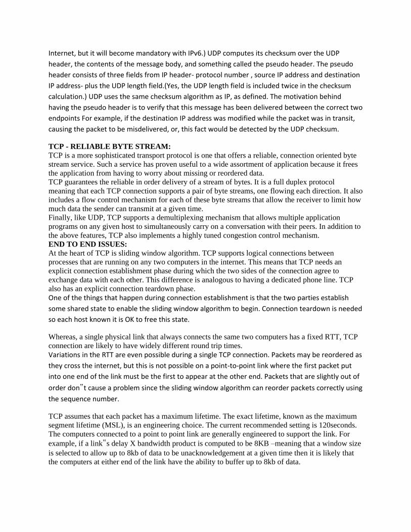
Internet, but it will become mandatory with IPv6.) UDP computes its checksum over the UDP

header, the contents of the message body, and something called the pseudo header. The pseudo

header consists of three fields from IP header- protocol number , source IP address and destination

IP address- plus the UDP length field.(Yes, the UDP length field is included twice in the checksum

calculation.) UDP uses the same checksum algorithm as IP, as defined. The motivation behind

having the pseudo header is to verify that this message has been delivered between the correct two

endpoints For example, if the destination IP address was modified while the packet was in transit,

causing the packet to be misdelivered, or, this fact would be detected by the UDP checksum.

TCP - RELIABLE BYTE STREAM:

TCP is a more sophisticated transport protocol is one that offers a reliable, connection oriented byte

stream service. Such a service has proven useful to a wide assortment of application because it frees

the application from having to worry about missing or reordered data.

TCP guarantees the reliable in order delivery of a stream of bytes. It is a full duplex protocol

meaning that each TCP connection supports a pair of byte streams, one flowing each direction. It also

includes a flow control mechanism for each of these byte streams that allow the receiver to limit how

much data the sender can transmit at a given time.

Finally, like UDP, TCP supports a demultiplexing mechanism that allows multiple application

programs on any given host to simultaneously carry on a conversation with their peers. In addition to

the above features, TCP also implements a highly tuned congestion control mechanism.

END TO END ISSUES:

At the heart of TCP is sliding window algorithm. TCP supports logical connections between

processes that are running on any two computers in the internet. This means that TCP needs an

explicit connection establishment phase during which the two sides of the connection agree to

exchange data with each other. This difference is analogous to having a dedicated phone line. TCP

also has an explicit connection teardown phase.

One of the things that happen during connection establishment is that the two parties establish

some shared state to enable the sliding window algorithm to begin. Connection teardown is needed

so each host known it is OK to free this state.

Whereas, a single physical link that always connects the same two computers has a fixed RTT, TCP

connection are likely to have widely different round trip times.

Variations in the RTT are even possible during a single TCP connection. Packets may be reordered as

they cross the internet, but this is not possible on a point-to-point link where the first packet put

into one end of the link must be the first to appear at the other end. Packets that are slightly out of

order don‟t cause a problem since the sliding window algorithm can reorder packets correctly using

the sequence number.

TCP assumes that each packet has a maximum lifetime. The exact lifetime, known as the maximum

segment lifetime (MSL), is an engineering choice. The current recommended setting is 120seconds.

The computers connected to a point to point link are generally engineered to support the link. For

example, if a link‟s delay X bandwidth product is computed to be 8KB –meaning that a window size

is selected to allow up to 8kb of data to be unacknowledgement at a given time then it is likely that

the computers at either end of the link have the ability to buffer up to 8kb of data.

Because the transmitting side of a directly connected link cannot send any faster than the

bandwidth of the link allows, and only one host is pumping data into the link, it is not possible to

unknowingly congest the link. Said another way, the load on the link is visible in the form of a queue

of packets at the sender. In contrast, the sending side of a TCP connection has no idea what links

will be traversed to reach the destination.

SEGMENT FORMAT

1

MODULE IV

TRANSPORT LAYER

4.1. FUNCTIONS OF THE TRANSPORT LAYER

Transport layer is the fourth layer in the OSI and TCP/IP models. The layer above it is

the Session layer in the OSI model and the Application layer in the TCP/IP model.

Protocols in the transport layer are responsible for providing a reliable and cost effective

data transport from an application program running on one machine to a program running

on another machine. Application layer programs interact with each other using the

services provided by the transport layer without being aware of the existence of lower

layers. For this the transport layer makes use of the services provided by the network

layer. The hardware or software within the transport layer that is used to implement the

services of the transport layer is called the transport entity.

To achieve these the transport layer may need to incorporate the following functions:

(a) Packetizing: Long messages sent by the application programs are divided into

smaller units. These units form the TPDU payload. Headers are added to these to

form TPDU.

(b) Addressing

(c) Multiplexing and splitting of transport connections - A number of transport

connections may be carried on one network connection and a transport connection

may be split between a numbers of different network connections.

(d) Providing reliability

• Sequencing

• Flow Control

• Error Control

4.2. NEED FOR TRANSPORT LAYER

• Transport layer is part of the subnet and is run by the carrier. Users have no

control over the subnet. Transport layer is put on top of the network layer to

improve the quality of service.

• Since the network layer employs connectionless protocol, lost packets and

mangled data are detected and compensated for by the transport layer.

• There are a variety of networks. So the network service primitive varies from

network to network. Transport layer makes it possible for the application

2

programs to be written using a standard set of primitives and these programs will

run on a variety of networks.

4.3. FUNCTIONS OF THE TRANSPORT LAYER

4.3.1. Service provided to the upper layer.

The Hardware /Software in the transport protocol provide the service to the upper

layer is called transport entity. The transport entity can be operating system kernel on

network interface card.

Figure 4.1. Network, transport and application layers

4.3.2. Quality of Service

The OSI transport service allows the user to specify preferred, acceptable, and

unacceptable values for QOS parameters at the time a connection is set up. Some of

the parameters also apply for connectionless transport. It is up to the transport layer to

examine these parameters, and depending on the kind of network service or services

available to it, determine whether it can provide the required service. The common

transport layer QOS parameters are

• Connection establishment delay - The amount of time elapsing between a

transport connection being requested and connection confirmation being

received by the user of the transport service.

• Connection establishment failure probability - This is chance of connection

not being established within the maximum establishment delay time.

• Throughput - This parameter measures the number of bytes of user data

transferred per second, measured over some time interval.

3

• Transit delay - This measures the time between a message being sent by the

transport user on the source machine and it being received by the transport

user on the destination machine.

• Residual error rate - This parameter measures the number of lost messages

as a fraction of total sent.

• Protection -This parameter provides a way for the transport user to specify

interest in having the transport layer provide protection against unauthorized

third parties reading or modifying the transmitted data.

• Priority - This parameter provides a way for transport user to indicate that

some of its connection is more important than other ones.

• Resilience - This gives the probability of the transport layer terminating a

connection due to internal problems or congestion.

4.3.3. Transport Service Primitives

Transport service primitives allow the transport users to access the transport service.

Each transport service has its own access primitives. The primitives for simple

transport service are given below.

Figure 4.2. Primitives for a simple transport service

To start with the server executes LISTEN primitive. When the client executes a

CONNECT primitive, the transport entity at the client sends a CONNECTION

REQUEST TPDU to the server. When the server receives this TPDU, it sends back a

CONNECTION ACCEPTED TPDU to the client. The connection is now established

and data is exchanged using SEND and RECEIVE primitives. When data transfer is

over a DISCONNECT primitive is executed. There are two types of disconnection.

• Asymmetric: Either transport user issues a DISCONNECT primitive. A

DISCONNECT TPDU is sent to the remote transport entity and when this

TPDU arrives the connection is released.

4

• Symmetric: Each direction is closed separately. When one side does a

DISCONNECT, it means that it has no data to send. But it can still accept data

from its partner. A connection is released only when both sides have done a

DISCONNECT.

Figure 4.3. State diagram for simple connection management

The message sent by transport entity to transport entity is called Transport Protocol

Data Unit (TPDU). TPDUs are contained in packets. Packets are contained in frames.

When a frame arrives, the DLL process the frame header and passes the contents of

the frame payload field up to the network entity. The network entity processes the

packet header and passes the contents of the packet payload up to the transport entity.

Figure 4.4. Nesting of TPDUs, packets, and frames

5

Berkeley Sockets

Figure 4.5. Socket primitives used in Berkeley UNIX for TCP

Servers execute the first four primitives. The SOCKET primitive create a new end

point within the transport entity. Newly created socket do not have addresses. These

are assigned using BIND primitive. In this socket model LISTEN is not a blocking

call. To block waiting for an incoming connection, the server executes an ACCEPT

primitive.

Client side also create socket by executing SOCKET primitive. Establish a

connection using CONNECT primitive. When it completes the client process is

unblocked and the connection is established. Both sides can use SEND and

RECEIVE to transmit and receive data. When both sides have executed CLOSE

primitive, the connection is released.

4.4. ELEMENTS OF THE TANSPORT PROTOCOL

The transport service is implemented by a transport protocol used between two

transport entities.

Transport protocols resemble the data link protocols: error control, sequencing, and flow

control.

There are major dissimilarities between DLL protocol and transport layer protocol.

• In the data link layer, it is not necessary for a router to specify which router it

wants to talk to. In the transport layer, explicit addressing of destination is

required.

• Initial connection setup is much more complicated in transport layer.

• The potential existence of storage capacity in the subnet requires special transport

protocols.

6

• Buffering and flow control are needed in both layers, but the presence of a large

and dynamically varying number of connections in the transport layer may require

a different approach than the data link layer approach (e.g., sliding window buffer

management).

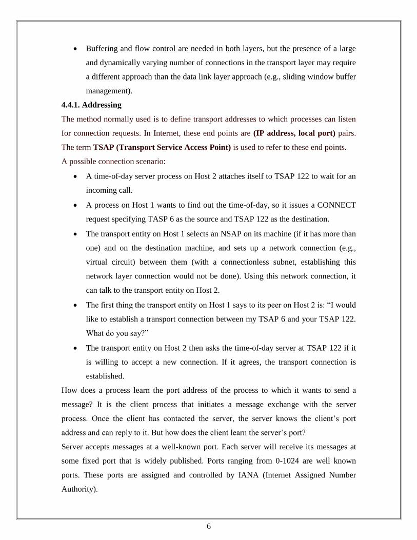
4.4.1. Addressing

The method normally used is to define transport addresses to which processes can listen

for connection requests. In Internet, these end points are (IP address, local port) pairs.

The term TSAP (Transport Service Access Point) is used to refer to these end points.

A possible connection scenario:

• A time-of-day server process on Host 2 attaches itself to TSAP 122 to wait for an

incoming call.

• A process on Host 1 wants to find out the time-of-day, so it issues a CONNECT

request specifying TASP 6 as the source and TSAP 122 as the destination.

• The transport entity on Host 1 selects an NSAP on its machine (if it has more than

one) and on the destination machine, and sets up a network connection (e.g.,

virtual circuit) between them (with a connectionless subnet, establishing this

network layer connection would not be done). Using this network connection, it

can talk to the transport entity on Host 2.

• The first thing the transport entity on Host 1 says to its peer on Host 2 is: “I would

like to establish a transport connection between my TSAP 6 and your TSAP 122.

What do you say?”

• The transport entity on Host 2 then asks the time-of-day server at TSAP 122 if it

is willing to accept a new connection. If it agrees, the transport connection is

established.

How does a process learn the port address of the process to which it wants to send a

message? It is the client process that initiates a message exchange with the server

process. Once the client has contacted the server, the server knows the client’s port

address and can reply to it. But how does the client learn the server’s port?

Server accepts messages at a well-known port. Each server will receive its messages at

some fixed port that is widely published. Ports ranging from 0-1024 are well known

ports. These ports are assigned and controlled by IANA (Internet Assigned Number

Authority).

7

A port mapper service accepts messages at a well-known port. Client sends a message to

the port mapper specifying the service name. Port mapper returns back the appropriate

TSAP.

In this model, service has stable TSAP address, which can be printed on paper and given

to new users when they join the network. Instead of every server listening at a well-

known TSAP, each machine that wishes to offer a service has a special server process

server that acts as a proxy. It listen a set of ports at the same time, waiting for a TCP

connection request. User begin by doing CONNECT request specifying the TSAP

address. If no server is waiting for them, they get a connection to the process server.

After it gets the incoming request the process server give this to the requested server. The

new server does the requested work.

8

In this model there exists a special process called a name server or directory server. To

find the TSAP address corresponding to a given service name, the user send a message

specifying the service name and the name server sends back the TSAP address. Then the

user releases the connection with the name server and establishes a new connection with

the desired service. In this model, when a new service is created, it must register itself

with the name server, giving both its service name and the address of its TSAP.

4.4.2. Establishing a Connection

Connection establishment begins when a Transport Service user (TS-user) issues a

T.CONNECT request primitive to the transport entity. The transport entity issues a CR-

TPDU (Connection Request Transport Protocol Data Unit) to its peer transport entity

who informs its user with a T.CONNECT indication primitive. The user can respond with

a T.CONNECT response primitive if the user is prepared to except the connection or a

T.DISCONNECT request primitive .The peer transport entity then issues a CC-TPDU

(Connection Confirm) or a DR-TPDU (Disconnect Request) respectively. This response

is conveyed to the initiating user by means of a T.CONNECT confirm primitive (for

success) or T.DISCONNECT indication primitive (for rejection) contain the reason for

the failure.

The CR-TPDU and the CC-TPDUs both contain information relating to the connection

being established.

9

The purpose of CC is to establish a connection with agreed-upon characteristics. These

characteristics are defined in the CC-TPDU.

A transport connection has three types of Identifiers:

• TSAP - Transport Service Access Point

• NSAP - Network Service Access Point

• Transport Connection I.D.

As there may be more than one user of the transport entity, a TSAP allows the transport

entity to multiplex data between users. This identifier must be passed down from the

transport user, and included in CC- and CR-TPDUs. The NSAP identifies the system on

which the transport entity is located. Each transport connection is given a unique

identifier used in all TPDUs. It allows the transport entity to multiplex multiple transport

connections on a single network.

The issue here is how to deal with the problem of delayed duplicates and establish

connections in a reliable way. The methods suggested are

a. Use throwaway TSAP addresses - Each time a TSAP address is needed, a new,

unique address is generated, typically based on the current time. When a

connection is released, the addresses are discarded forever.

b. Each connection is assigned a connection identifier (i.e., a sequence number

incremented for each connection established), chosen by the initiating party, and

put in each TPDU, including the one requesting the connection. After each

connection is released, each transport entity could update a table listing obsolete

connections as (peer transport entity, connection identifier) pair. Whenever a

connection request comes in, it could be checked against the table, to see if it

belonged to a previously released connection.

c. Kill off aged packets - here we ensure that no packet lives longer than some

known time. So we need is a mechanism to kill off very old packets that are still

wandering about. Methods are

• Restricted subnet design - prevents packets from looping

• Putting a hop counter in each packet.

• Time stamping each packet

d. When a host crashes and comes up again, the transport entity will remain idle for

T seconds (where T is the life time of a packet) so that all old TPDUs will die off.

10

4.4.3. Releasing a Connection

Releasing a connection is easier than establishing one. There are two types of connection

termination.

• Asymmetric - Either party issues a DISCONNECT, which results in a

DISCONNECT TPDU being sent and the transmission ends in both directions.

• Symmetric - Both parties issue DISCONNECT, closing only one direction at a

time.

A user requests connection release by sending a T.DISCONNECT request primitive to

the transport entity with the reason for closing the connection. The transport entity then

sends a Disconnect Request (DR) -TPDU to its peer transport entity. The transport entity

then ignores all subsequent TPDUs until receipt of a Disconnect Confirm (DC) -TPDU.

The peer transport entity on receipt of a DR-TPDU returns a DC-TPDU and issues a

T.DISCONNECT to the transport user. The transport connection is now closed.

Four protocol scenario for releasing a connection.

11

(a) Normal case of a three-way handshake. (b) Final ACK lost.

(c) Response lost. (d) Response lost and subsequent DRs lost.

4.4.4. Flow Control and Buffering

For flow control, a sliding window is needed on each connection to keep a fast

transmitter from overrunning a slow receiver (the same as the data link layer).

Since a host may have numerous connections, it is impractical to implement the same

data link buffering strategy (using dedicated buffers for each line).

The sender should always buffer outgoing TPDUs until they are acknowledged.

The receiver may not dedicate specific buffers to specific connections. Instead, a single

buffer pool may be maintained for all connections. When a TPDU comes in, if there is a

free buffer available, the TPDU is accepted, otherwise it is discarded.

However, for high-bandwidth traffic (e.g., file transfers), it is better if the receiver

dedicate a full window of buffers, to allow the data to flow at maximum speed.

12

4.4.5. Multiplexing

The reasons for multiplexing:

• To share the price of a virtual circuit connection: mapping multiple transport

connections to a single network connection (upward multiplexing).

• To provide a high bandwidth: mapping a single transport connection to multiple

network connections (downward multiplexing).

4.4.6. Crash Recovery

In case of a router crash, the two transport entities must exchange information after the

crash to determine which TPDUs were received and which were not. The crash can be

recovered by retransmitting the lost ones.

It is very difficulty to recover from a host crash.

Suppose that the sender is sending a long file to the receiver using a simple stop-and-wait

protocol. Part way through the transmission the receiver crashes.

13

When the receiver comes back up, it might send a broadcast TPDU to all other hosts,

requesting the other hosts to inform it of the status of all open connections before the

crash.

The sender can be in one of two states: one TPDU outstanding or no TPDUs outstanding.

4.5. TRANSPORT LAYER PROTOCOLS

The two primary protocols in this layer are

• Transmission Control Protocol (TCP)

• User Datagram Protocol (UDP)

4.5.1. Transmission Control Protocol (TCP)

4.5.1.1. TCP Header

Applications that require the transport protocol to provide reliable data delivery use TCP

because it verifies that data is delivered across the network accurately and in the proper

sequence. TCP is a reliable, connection-oriented, byte-stream protocol. TCP provides

reliability with a mechanism called Positive Acknowledgment with Re-transmission

(PAR). A system using PAR sends the data again, unless it hears from the remote system

that the data arrived okay. The unit of data exchanged between cooperating TCP modules

is called a segment. Each segment contains a checksum that the recipient uses to verify

that the data is undamaged. If the data segment is received undamaged, the receiver sends

a positive acknowledgment back to the sender. If the data segment is damaged, the

receiver discards it. After an appropriate time-out period, the sending TCP module re-

transmits any segment for which no positive acknowledgment has been received.

Every TCP segment begins with a fixed format 20-byte header followed by header

options. After the options data bytes may follow.

14

TCP Segment Header

TCP is responsible for delivering data received from IP to the correct application. The

application that the data is bound for is identified by a 16-bit number called the port

number. The Source Port and Destination Port is contained in the first word of the

segment header. These 16-bit Source Port and 16-bit Destination Port is used to identify

the application.

Sequence number and Acknowledge number perform their usual functions.

Header length tells how many 32-bit words are contained in the TCP header.

URG is set to 1 if urgent point is in use. The urgent pointer is used to indicate a byte

offset from the current sequence number at which the urgent data is to be found.

ACK bit is set to 1 to indicate that the acknowledge number is valid.

PSH indicate the pushed data. This field is used for requesting to deliver the data

immediately and not to buffer.

RST is used to reset the connection.

SYN bit is used to establish the connection.

FIN is used to release the connection.

Window size tells how many bytes may be sent starting at the byte acknowledged.

4.5.1.2. TCP Connection Establishment

TCP uses a three-way handshaking procedure to set-up a connection. A connection is

set up by the initiating side sending a segment with the SYN flag set and the proposed

initial sequence number in the sequence number field (seq = X). The receiver then returns

15

a segment with both the SYN and ACK flags set with the sequence number field set to its

own assigned value for the reverse direction (seq = Y) and and acknowledge field of X +

1 (ack = X + 1). On receipt of this, the initiating side makes a note of Y and returns a

segment with just the ACK flag set and an acknowledgement field of Y + 1.

4.5.1.3. TCP Connection Termination

When the user has sent all its data and wishes to close the connection it sends a CLOSE

primitive to TCP, which sends a segment with the FIN flag set. On receipt of this, the

peer TCP issues a CLOSING primitive flag to the user and returns an ACK segment. If

the peer TCP user has finished send all its data it sends a CLOSE primitive. If the user

still has some data to send it sends the data in a segment with the SEQ and FIN flags set.

On receipt of this segment the initiating TCP issues a TERMINATE primitive to the user

and returns an ACK for the data just received. When the peer TCP receives the ACK, it

returns a TERMINATE primitive to the user.

4.5.1.4. TCP Window Management

16

Suppose the receiver has 4096 byte buffer. IF the sender transmits a 2048 byte

segment that is correctly received, the receiver will acknowledge the segment.

Now it has only 2048 of buffer space. It will send a message with the new

window size indicated. Now sender transmits another 2048 bytes, which are

acknowledged, but the window size is 0 now. The sender must stop sending.

When the receiver has removed some data from the buffer and sends the new

window update to the sender.

4.5.2. User Datagram Protocol (UDP)

The User Datagram Protocol gives application programs direct access to a datagram

delivery service, like the delivery service that IP provides. This allows applications to

exchange messages over the network with a minimum of protocol overhead.

UDP is an unreliable, connectionless datagram protocol. “Unreliable" merely means that

there are no techniques in the protocol for verifying that the data reached the other end of

the network correctly. Within your computer, UDP will deliver data correctly. UDP uses

16-bit Source Port and Destination Port numbers in word 1 of the message header, to

deliver data to the correct applications process. Figure shows the UDP message format

17

UDP Header

The amount of data being transmitted is small; the overhead of creating connections and

ensuring reliable delivery may be greater than the work of re-transmitting the entire data

set. In this case, UDP is the most efficient choice for a Transport Layer protocol. UDP

can be used in applications that fit a query-response model. The response can be used as

a positive acknowledgment to the query. If a response isn't received within a certain time

period, the application just sends another query. Still other applications provide their own

techniques for reliable data delivery, and don't require that service from the transport

layer protocol. Imposing another layer of acknowledgment on any of these types of

applications is inefficient.

4.6. ASYNCHRONOUS TRANSFER MODE (ATM)

Asynchronous Transfer Mode (ATM) is a connection-oriented, unreliable, virtual circuit

packet switching technology. ATM technology includes:

• Scalable performance — ATM can send data across a network quickly and

accurately, regardless of the size of the network. ATM works well on both very

low and very high-speed media.

• Flexible, guaranteed Quality of Service (QoS) — ATM allows the accuracy and

speed of data transfer to be specified by the client. This feature distinguishes

ATM from other high-speed LAN technologies such as gigabit Ethernet. The QoS

feature of ATM also supports time dependent traffic. Traffic management at the

hardware level ensures that the level of service exists end-to-end. Each virtual

circuit in an ATM network is unaffected by traffic on other virtual circuits. Small

packet size and a simple header structure ensure that switching is done quickly

and that bottlenecks are minimized.

• Speed — ATM imposes no architectural speed limitations. Its pre-negotiated

virtual circuits, fixed-length cells, message segmentation and re-assembly in

hardware, and hardware-level switching all help support extremely fast

forwarding of data.

18

• Integration of different traffic types — ATM supports integration of voice, video,

and data services on a single network.

The ATM protocols are used in high-speed switching to local area networking. ATM is

used by the telecommunications community as a broadband carrier for Integrated

Services Digital Network (ISDN) networks and by the computer industry for high-speed

LAN.

4.6.1. The Protocol Reference Model

In a similar way to the OSI 7-layer model, ATM has also developed a protocol reference

model. Above the Physical Layer rests the ATM Layer and the ATM Adaptation Layer

(AAL).

The AAL and Physical layers are further divided into sublayers, and the functions of

these layers are shown below.

19

Responsibilities of ATM Layer

The ATM layer is responsible for transporting information across the network. ATM uses

virtual connections for information transport. The connections are deemed virtual

because although the users can connect end-to-end, connection is only made when a cell

needs to be sent. The connection is not dedicated to the use of one conversation.

4.6.2. ATM Cell Structure

At the core of the ATM architecture is a fixed length "cell." An ATM cell is a short, fixed

length block of data that contains a short header (5 bytes) with addressing information,

followed by the upper layer traffic, or "payload” (48 bytes).

Figure 1: Structure of ATM cell

Header

(5 bytes)

Payload

(48 bytes)

Formats of the ATM Cell Header

The ATM standards groups have defined two header formats. The User-Network

Interface (UNI) header format is defined by the UNI specification, and the Network-to-

Network Interface (NNI) header format is defined by the NNI specification.

20

The UNI specification defines communications between ATM endpoints (such as

workstations and routers) and switch routers in private ATM networks. The format of the

UNI cell header is shown in Figure 2.

Figure 2: UNI Header Format

The UNI header consists of the following fields:

GFC—4 bits of generic flow control that are used to provide local functions, such as

identifying multiple stations that share a single ATM interface. The GFC field is typically

not used and is set to a default value.

VPI—8 bits of virtual path identifier that is used, in conjunction with the VCI, to identify

the next destination of a cell as it passes through a series of switch routers on its way to

its destination.

VCI—16 bits of virtual channel identifier that is used, in conjunction with the VPI, to

identify the next destination of a cell as it passes through a series of switch routers on its

way to its destination.

PT—3 bits of payload type. The first bit indicates whether the cell contains user data or

control data. If the cell contains user data, the second bit indicates congestion, and the

third bit indicates whether the cell is the last in a series of cells that represent a single

AAL5 frame.

CLP—1 bit of congestion loss priority (cell loss priority) that indicates whether the cell

should be discarded if it encounters extreme congestion as it moves through the network.

HEC—8 bits of header error control that are a checksum calculated only on the header

itself.

21

The NNI specification defines communications between switch routers. The format of the

NNI header is shown in Figure 3.

Figure 3: NNI Header Format

The GFC field is not present in the format of the NNI header. Instead, the VPI field

occupies the first 12 bits, which allows switch routers to assign larger VPI values. With

that exception, the format of the NNI header is identical to the format of the UNI header.

4.6.3. ATM Adaptation Layer (AAL)

The ATM adaptation layer lies between the ATM layer and the higher layers which use

the ATM service. Its main purpose is to resolve any disparity between a service required

by the user and services available at the ATM layer. The ATM adaptation layer maps

user information into ATM cells and accounts for transmission errors. It also may

transport timing information so the destination can regenerate time dependent signals.

The goal of AAL is to provide useful services to application programs and to shield them

from the mechanics of chopping data up into cells at the source and reassembling them at

the destination.

The AAL service space is organized along three axes:

• Real-time service versus non-real-time service.

• Constant bit rate service versus variable bit rate service.

• Connection-oriented service versus connectionless service.

Different AALs were defined in supporting different traffic or service expected to be

used. The service classes and the corresponding types of AALs were as follows:

22

Class A - Constant Bit Rate (CBR) service: AAL1 supports a connection-oriented service

in which the bit rate is constant. Examples of this service include 64 Kbps voice, fixed-

rate uncompressed video and leased lines for private data networks.

Class B - Variable Bit Rate (VBR) service: AAL2 supports a connection-oriented service

in which the bit rate is variable but requires a bounded delay for delivery. Examples of

this service include compressed pocketsize voice or video. The requirement on bounded

delay for delivery is necessary for the receiver to reconstruct the original uncompressed

voice or video.

Class C - Connection-oriented data service: For connection-oriented file transfer and in

general, data network applications where a connection is set up before data is transferred,

this type of service has variable bit rate and does not require bounded delay for delivery.

Two AAL protocols were defined to support this service class, and have been merged

into a single type, called AAL3/4. But with its high complexity, the AAL5 protocol is

often used to support this class of service.

Class D - Connectionless data service: Examples of this service include datagram traffic

and in general, data network applications where no connection is set up before data is

transferred. Either AAL3/4 or AAL5 can be used to support this class of service.

The ATM adaptation layer is divided into two sub layers:

• Convergence Sub layer: This layer wraps the user-service data units in a header

and trailer that contain information used to provide the services required. The

information in the header and trailer depends on the class of information to be

transported but will usually contain error handling and data priority preservation

information.

• Segmentation and reassembly sub layer: This layer receives the convergence

sublayer protocol data unit and divides it up into pieces which it can place in an

ATM cell. It adds to each piece a header that contains information used to

reassemble the pieces at the destination.

AAL1

AAL-1 is used to transfer constant bit rate data that is time dependent. It must therefore

send timing information with the data so that the time dependency maybe recovered.

AAL-1 provides error recovery and indicates error information that could not be

recovered.

23

Convergence Sub layer: The functions provided at this layer differ depending on the

service provided. It provides bit error correction and may use explicit time stamps to

transfer timing information.

Segmentation and reassembly sub layer: At this layer the convergence sub layer -

protocol data unit is segmented and a header added. The header contains 3 fields (see

diagram below).

• Sequence Number used to detect cell insertion and cell loss.

• Sequence Number protection used to correct and errors that occur in the sequence

number.

• Convergence sub layer indication used to indicate the presence of the

convergence sub layer function.

AAL2

AAL-2 is used to transfer variable bit rate data that is time dependant. It sends timing

information along with the data so that the timing dependency may be recovered at the

destination. AAL-2 provides error recovery and indicates error information that could not

be recovered. As the source generates a variable bit rate some of the cells transferred

maybe useful and therefore additional features are required at the segmentation and

recovery layer.

Convergence sublayer: This layer provides for error correction and transports the timing

information from source to destination. Inserting time stamps or timing information into

the convergence sublayer - protocol data unit, achieves this.

Segmentation and recovery sublayer: The CS-PDU is segmented at this layer and a

header and trailer added to each piece. The header contains two fields.

• Sequence number is used to detect inserted or lost cells.

24

• Information type is one of the following:

o BOM, beginning of message

o COM, continuation of message

o EOM, end of message

The trailer also contains two fields

• Length indicator indicated the number of true data bytes in a partially full cell.

• CRC is a cyclic redundancy check used by the segmentation and reassembly

sublayer to correct errors.

AAL 3-4

AAL-3 is designed to transfer variable rate data that is time independent. It supports both

message mode and streaming mode services. Message mode services are transported in a

single ATM adaptation layer interface data unit, while streaming mode services require

one or more AAL-IDUs. AAL-3 can be further divided into two modes of operation:

Assured operation: Corrupted or lost convergence sublayer - protocol data units are

retransmitted and flow control is supported.

Non-assured operation: Error recovery is left to higher layers and flow control is optional

Convergence sublayer: The ATM adaptation layer 3 convergence sublayer is similar to

the ATM adaptation layer 2 convergence sublayer as both handle non real time data. The

ATM adaptation layer 3 convergence sublayer is therefore subdivided into two sections

1. The common part convergence sublayer. The AAL-2 CS also provides this. It appends

a header and trailer to the common part convergence sublayer - protocol data unit

payload.

The header contains 3 fields:

• Common part indicator indicates that the payload is part of the common part.

25

• Begin tag marks the start of the common part convergence sublayer - protocol

data unit.

• Buffer allocation size tells the receiver how much buffer space is required to

accommodate the message.

The trailer also contains 3 fields:

• Alignment is byte filler used to make the header and trailer the same length. i.e.

4bytes.

• End tag marks the end of the common part convergence sublayer - protocol data

unit.

• The length field holds the length of the common part convergence sublayer -

protocol data unit payload.

The service specific part. The functions provided at this layer depend on the services

requested. They generally include functions for error detection and recovery and may

also include special functions such as transparent delivery.

2. Segmentation and reassembly sublayer: At this layer the convergence sublayer -

protocol data unit is segmented into pieces which can be placed in ATM cells. A header

and trailer that contain information necessary for reassembly and error recovery are

appended to each piece. The header contains 3 fields:

Segment type indicates what part of a message is contained in the payload. It has one of

the following values:

• BOM: Begining of message

• COM: continuation of message

• EOM: End of message

• SSM: Single segment message

Sequence number used to detect cell insertion and cell loss.

Multiplexing identifier. This field is used to distinguish between data from different

connection that have been multiplexed onto a single ATM connection. The trailer

contains two fields:

Length indicator holds the number of useful data bytes in a partially full cell.

CYC is a cyclic redundancy check used for error detection and recovery.

26

MODULE III

NETWORK LAYER

NETWORK LAYER DESIGN ISSUES

The network layer has been designed with the following goals:

• The services provided should be independent of the routing technology. Users of

the service need not be aware of the physical implementation of the network. This

design goal has great importance when we consider the great variety of networks

in operation. In the area of public networks, networks in underdeveloped

countries are nowhere near that in the countries like the US or Ireland. The design

of the layer must not disable us from connecting to networks of different

technologies.

• The transport layer (that is the host computer) should be shielded from the

number, type and different topologies of the routers present. That is, all that the

transport layer wants is a communication link; it need not know how that link is

made.

• Finally, there is a need for some uniform addressing scheme for network

addresses.

Services provided to the Transport Layer

The network layer provides two different types of service,

• Connection oriented

• Connectionless.

A connection-oriented service is one in which the user is given a "reliable" end to end

connection. In a connection-less service, the user simply bundles his information

together, puts an address on it, and then sends it off, in the hope that it will reach its

destination. There is no guarantee that the bundle will arrive. So - a connection less

service is somewhat identical to the postal system. A letter sent, is then in the "postal

network" where it gets bounced around and hopefully will leave the network in the

correct place, that is, in the addressee's letter box. We can never be totally sure that the

letter will arrive, but we know that there is a high probability that it will, and so we place

our trust in the postal network.

With a connection oriented service, the user must pay for the length (i.e. the duration) of

his connection. Usually this will involve a fixed start up fee. Now, if the user intends to

send a constant stream of data down the line, he is given a reliable service for as long as

he wants. However, say the user wished to send only a packet or two of data - now the

cost of setting up the connection greatly overpowers the cost of sending. A telephone call

is the classic example of a connection oriented service.

Internal organization of the network layer

The subnet is organized in two different ways

• Virtual circuits: used in subnets whose primary service is connection-oriented.

• Datagrams correspond to the independent packets of the connectionless

organization.

Datagrams

Each datagram must contain the full destination address. The routers have a table telling

which outgoing line to use for each possible destination router. (These tables are also

needed in virtual circuit subnets for determining the route for a SETUP packet). Routes

are not worked out in advance. Successive packets may follow different routes.

Virtual Circuits

• Each router must maintain a table with one entry per open virtual circuit passing

through it.

• Each packet traveling through the subnet must contain a virtual circuit number field

in its header, in addition to sequence numbers, checksums, and the like.

• Whenever a host wants to create a new outbound virtual circuit, it chooses the lowest

circuit number not currently in use (locally), and put this number in the header of a

SETUP packet.

• The router does not forward this SETUP packet to the next router as is. Instead, router

chooses the lowest free VC number and substitutes that number for the one chosen by

the host, and then forwards the SETUP packet to router.

• Similarly, router chooses the lowest free number between it and the next router,

substitutes that number for the one chosen by router, and then forwards the setup

packet to the next router.

• When this SETUP packet finally arrives at the destination, the router there chooses

the lowest free inbound circuit number, substitutes that number for the one in the

packet, and pass it to the host.

Comparison between datagrams and virtual circuits

Issue Datagram Virtual Circuit

Addressing

Each packet contains the full

source and destination

addresses

Each packet contains a virtual circuit

number

Circuit Setup Not needed Required

Routing Each packet is routed

independently

Route is chosen when the virtual

circuit is setup, all packets follow this

route

State Information

Routers do not hold

information about

connections

Each VC requires router table space

per connection

Quality of Service Difficult Easy if enough resources can be

allocated in advance for each VC

Congestion Control Difficult Easy if enough resources can be

allocated in advance for each VC

Effect of router

failures

None, except for packets lost

during the crash

All virtual circuits that are passed

through the failed router are

terminated

ROUTING ALGORITHMS

Routing is the act of moving information across an internetwork from a source to a

destination. Along the way, at least one intermediate node typically is encountered.

Routing is often contrasted with bridging, which might seem to accomplish precisely the

same thing to the casual observer. The primary difference between the two is that

bridging occurs at Layer 2 (the datalink layer) of the OSI reference model, whereas

routing occurs at Layer 3 (the network layer).

Routing involves two basic activities: determining optimal routing paths and transporting

information groups (typically called packets) through an internetwork. In the context of

the routing process, the latter of these is referred to as packet switching.

The routing algorithm is that part of the network layer software responsible for deciding

which output line an incoming packet should be transmitted on.

Routing algorithms often have one or more of the following design goals:

• Correctness – are the packets getting to the right destination?

• Simplicity – the simpler the algorithm and steps, the easier to understand, to extend,

modify and improve. Routing algorithms also are designed to be as simple as

possible.

• Robustness – If something happens to the network (e.g. some lines go down, some

user in a machine starts sending out a huge amount of data, etc), does the algorithm

cater for that? This is good if a network is very dynamic and changes occur

frequently, which means that they should perform correctly in the face of unusual or

unforeseen circumstances, such as hardware failures, high load conditions, and

incorrect implementations. Because routers are located at network junction points,

they can cause considerable problems when they fail. The best routing algorithms are

often those that have withstood the test of time and that have proven stable under a

variety of network conditions.

• Stability – Does the routes change all the time? If the routes are unstable, even when

there are little changes to the network, the routers will incur the overhead of having to

keep changing their routing tables. This must be balanced with robustness of the

algorithm.

• Fairness – How well does the algorithm ensure all routers have the same share of

network utilization, and the same consideration when finding routes for them?

• Optimality – How well does the algorithm ensure that the cost (time, hops, distance,

etc) is kept to a minimal? This is balanced against fairness

Optimality principle: Optimality refers to the capability of the routing algorithm to

select the best route, which depends on the metrics and metric weightings used to make

the calculation. If a router k is on the optimal path from router i to router j, then the

optimal path from k to j is also falls along the same route.

The set of optimal routes from all sources to a given destination form a tree (called sink

tree) rooted at the destination.

In addition, routing algorithms must converge rapidly. Convergence is the process of

agreement, by all routers, on optimal routes. When a network event causes routes to

either go down or become available, routers distribute routing update messages,

stimulating recalculation of optimal routes and eventually causing all routers to agree on

these routes. Routing algorithms that converge slowly can cause routing loops.

Routing algorithms can be divided into two major classes:

• Nonadaptive algorithms or Static Routing algorithms

• Adaptive algorithms or Dynamic Routing algorithms

Static Routing Algorithms

Nonadaptive algorithms do not base their routing decisions on measurements or estimates

of the current traffic and topology. The choice of the route to use is computed in advance,

off-line, and downloaded to the routers when the network is booted (Static Routing).

1. Shortest Path Routing

This is the simplest and widely used technique. The basic idea:

• Build a graph of the subnet, with each node of the graph representing a router and

each arc of the graph representing a communication line.

• To choose a route between a given pair of routers, the algorithm finds the shortest

path between them.

Metrics for measuring the shortest path can be any one of the following,

• The number of hops.

• The geographic distance in kilometers.

• The mean queuing and transmission delay.

• A function of the distance, bandwidth, average traffic, communication cost, mean

queue length, measured delay, etc.

The Dijkstra’s algorithm is used to find the shortest path. The following steps are

performed:

1. The router builds a status record set for every node on the network. The record

contains three fields:

• Predecessor field - This field shows the previous node.

• Length field - This field shows the sum of the weights from the source to that

node.

• Label field - This field shows the status of node. Each node can have one status

mode: "permanent" or "tentative."

2. The router initializes the parameters of the status record set (for all nodes) and sets

their length to "infinity" and their label to "tentative."

3. The router sets a T-node. For example, if V1 is to be the source T-node, the router

changes V1's label to "permanent." When a label changes to "permanent," it never

changes again. A T-node is an agent and nothing more.

4. The router updates the status record set for all tentative nodes that are directly linked

to the T-node.

5. The router looks at all of the tentative nodes in the entire network and chooses the one

whose weight to V1 is lowest. That node is then the destination T-node.

6. If this node is not V2 (the intended destination), the router goes back to step 4.

7. If this node is V2, the router extracts its previous node from the status record set and

does this until it arrives at V1. This list of nodes shows the best route from V1 to V2.

Example: Dijkstra Algorithm

Here we want to find the best route between A and E (see below). You can see that there

are six possible routes between A and E (ABE, ACE, ABDE, ACDE, ABDCE, ACDBE),

and it's obvious that ABDE is the best route because its weight is the lowest. But life is

not always so easy, and there are some complicated cases in which we have to use

algorithms to find the best route.

1. As you see in the image below, the source node (A) has been chosen as T-node,

and so its label is permanent (we show permanent nodes with filled circles and T-

nodes with the --> symbol).

2. In this step, you see that the status record set of tentative nodes directly linked to

T-node (B, C) has been changed. Also, since B has less weight, it has been chosen

as T-node and its label has changed to permanent (see below).

3. In this step, like in step 2, the status record set of tentative nodes that have a direct

link to T-node (D, E), has been changed. Also, since D has less weight, it has

been chosen as T-node and its label has changed to permanent (see below).

4. In this step, we don't have any tentative nodes, so we just identify the next T-

node. Since E has the least weight, it has been chosen as T-node.

5. E is the destination, so we stop here.

Now we have to identify the route. The previous node of E is D, and the previous node of

D is B, and B's previous node is A. So the best route is ABDE. In this case, the total

weight is 4 (1+2+1).

2. Flooding

Another static routing algorithm is flooding. In flooding every incoming packet is sent

out on every outgoing line except the one it arrived on.

Measures for damming the flood:

• A hop counter is included in the header of each packet, which is decremented at each

hop. A packet is discarded when the counter reaches zero.

• A sequence number is included in each packet. Each router maintains a list per source

router telling which sequence numbers originating at that source have already been

seen. A packet is discarded when it contains a sequence number that is in the list.

Selective flooding - an incoming packet is sent on those lines that are going

approximately in the right direction.

Possible applications of flooding:

• In military applications, to withstand large numbers of routers crashes at any

instant.

• As a metric (always choose the shortest path) against which other routing

algorithms can be compared.

• In distributed database flooding used to update the databases concurrently.

Flow Based Routing

It takes into account of the load. It is suitable in some networks (e.g., a corporate network

for a retail store chain), in which the mean data flow between each pair of nodes is

relatively stable (approximately constant in time) and predictable.

Information known in advance:

• The subnet topology.

• The capacity for each line in the subnet.

• The average traffic (pkts/sec) between any pair of nodes.

Main calculations involved:

• Tentatively choose a routing algorithm.

• Apply the tentatively chosen routing algorithm to the known subnet topology to

select a path from each node to all other nodes.

• For each line, calculate the average flow according to the selected path and the

known average traffic between any pair of nodes.

• For each line, compute the mean packet delay on that line from queuing theory

(assuming a mean packet delay)

• For each line, calculate the flow-weight - the fraction of the total traffic using that

line.

• For the whole subnet, calculate mean packet delay according to the flow-weight

and the mean packet delay for each line.

The routing problem reduces to finding the routing algorithm (from a collection of known

single path routing algorithms) that produces the minimum average delay for the entire

subnet. Since the calculations can be done off-line, the fact that it may be time consuming

is not necessarily a serious problem.

Dynamic Routing Algorithms

Adaptive algorithms attempt to change their routing decisions to reflect changes in

topology and the current traffic. (Dynamic Routing).

1. Distance Vector Routing

A distance vector routing protocol advertises the number of hops to a network destination

(the distance) and the direction in which a packet can reach a network destination (the

vector). The distance vector algorithm, also known as the Bellman-Ford algorithm,

enables a router to pass route updates to its neighbors at regularly scheduled intervals.

Each neighbor then adds its own distance value and forwards the routing information on

to its immediate neighbors. The result of this process is a table containing the cumulative

distance to each network destination.

Distance vector routing protocols, the earliest dynamic routing protocols, are an

improvement over static routing, but have some limitations. When the topology of the

internetwork changes, distance vector routing protocols can take several minutes to detect

the change and make the appropriate corrections.

One advantage of distance vector routing protocols is simplicity. Distance vector routing

protocols are easy to configure and administer. They are well suited for small networks

with relatively low performance requirements. Most distance vector routing protocols use

a hop count as a routing metric. A routing metric is a number associated with a route that

a router uses to select the best of several matching routes in the IP routing table. The hop

count is the number of routers that a packet must cross to reach a destination.

Consider the following subnet

Router J receives the following delay vectors from its neighboring routers A, I, H and K.

Router J has calculated its delay to A, I, H and K as 8, 10, 12 and 6 respectively. This is

done by sending an ECHO packet to its neighbors and finding the round trip time.

From this information, router J computes its new routing table by finding the path with

the shortest delay to each router in the subnet.

For example:

For router B, if J takes the path through A the delay is 8+12 = 20

A I H K

A 0 24 20 21

B 12 36 31 28

C 25 18 19 36

D 40 27 8 24

E 14 7 30 22

F 23 20 19 40

G 18 31 6 31

H 17 20 0 19

I 21 0 14 22

J 9 11 7 10

K 24 22 22 0

L 29 33 9 9

If J takes the path through I the delay is 10+36 = 46

If J takes the path through H the delay is 12+31 = 43

If J takes the path through K the delay is 6+28 = 34

The path with shortest delay for J to reach B is through its neighbor A. Similarly for the

other routers also J calculates the path with minimum delay and updates its routing table

with the delay and the path to reach each router.

Now the routing table for J is

Delay Path

A 8 A

B 20 A

C 28 I

D 20 H

E 17 I

F 30 I

G 18 H

H 12 H

I 10 I

J 0 -

K 6 K

L 15 K

Routing Information Protocol (RIP) is the best known and most widely used of the

distance vector routing protocols. RIP version 1 (RIP v1), which is now outmoded, was

the first routing protocol accepted as a standard for TCP/IP. RIP version 2 (RIP v2)

provides authentication support, multicast announcing, and better support for classless

networks. The Windows Server 2003 Routing and Remote Access service supports both

RIP v1 and RIP v2 (for IPv4 only).

Using RIP, the maximum hop count from the first router to the destination is 15. Any

destination greater than 15 hops away are considered unreachable. This limits the

diameter of a RIP internetwork to 15. However, if you place your routers in a hierarchical

structure, 15 hops can cover a large number of destinations.

Link State Routing

• To replace Distance Vector Routing

• Problem with Distance Vector Routing – uses only delay at a node – doesn't

consider line capacity

Each router

1. Discover its neighbors and addresses – this is done by sending out HELLO

packets on start-up and receiving replies from neighbors.

2. Measure the cost to each neighbor – measure the round-trip time taken to send an

ECHO packet and to receive a reply.

3. Construct link state packets and send it to all routers – these link state packets

contains what each router knows about the cost to each of its neighbors.

4. Compute the shortest path to each router based on received link state packets from

other routers.

HIERARCHICAL ROUTING

In both link state and distance vector algorithms, every router has to save some

information about other routers. When the network size grows, the number of routers in

the network increases. Consequently, the size of routing table increases, and routers can't

handle network traffic efficiently. Hierarchical routing solves this problem.

In hierarchical routing network is divided into regions. Each region has a main router.

All routers need to know only about the routers in their region and the main routers in the

other regions. So routers just save one record in their table for every other region.

Suppose we use distance vector algorithms to find best routes between nodes. In the

situation depicted below, every node of the network has to save a routing table with 17

records. Here is a typical graph and routing table for router A.

Routing Table for Router A

In this example, we have classified our network into five regions.

Routing table for A in Hierarchical Routing

If A wants to send packets to any router in region 2 (D, E, F or G), it sends them to B. As

you can see, in this type of routing, the tables can be summarized, so network efficiency

improves. The above example shows two-level hierarchical routing. We can also use

three- or four-level hierarchical routing.

In three-level hierarchical routing, the network is classified into a number of clusters.

Each cluster is made up of a number of regions, and each region contains a number or

routers. Hierarchical routing is widely used in Internet routing and makes use of several

routing protocols.

ROUTING FOR MOBILE HOSTS

In this routing, nodes can move amongst regions or areas.

There are three kinds of nodes

• Stationary

• Migratory

• Mobile

The challenge is how to find a portable host that could potentially be anywhere. Each

mobile host has a home location, with a home agent. When the mobile host moves to a

new location, it registers with a foreign agent. The foreign agent lets home agent know

when a sender sends a packet to the mobile host. Home agent forwards packet to foreign

agent to pass to mobile host. Home agent also notifies sender to send subsequent packets

to mobile host's foreign agent.

BROADCAST ROUTING

Broadcasting is sending packets to more than one host in the subnet. The possible ways

are,

• Sender sends one packet to each possible destination

• Flooding

• Multi-destination Routing

• Reverse path forwarding – router will forward the packet to its outgoing links

only if the packet arrived on the shortest path back to the source.

• Using spanning tree (sink tree) – a node will forward the packet to all its

neighbors in the spanning tree.

MULTICAST ROUTING

Some hosts spread over a large network can be put into "multicast" groups – packets sent

out to a group is sent to every member of a group. E.g. news updates service where news

is sent to every user who subscribes. It can't use broadcast since some machines are not

meant to receive the packets. In a LAN, we are less security conscious and assume that

the supporting protocols for each machine will ignore all packets not meant for it. Here

we have a set of routers from very different networks. We can't trust that all routers (or

their administrators) will not illegally read the packets.

One way of doing multi-cast routing to a particular group:

• Compute a spanning tree joining all nodes – there may be more than one.

• Delete the links that do not lead to members of the group.

• Using this pruned spanning tree forward the packet to all the neighbors in the

pruned spanning tree.

CONGESTION CONTROL

What happens when there are more packets in a path than the routers can handle? This

situation is called congestion. At very high traffic, performance collapses completely and

almost no packets are delivered.

When too much traffic is offered, congestion sets in and performance degrades sharply

Congestion can be brought on by several factors. If all of a sudden, streams of packets

begin arriving on three or four input lines and all need the same output line, a queue will

build up. If there is insufficient memory to hold all of them, packets will be lost.

Regulating the average rate of data transmission is called traffic shaping.

Causes of congestion

• The input traffic rate exceeds the capacity of the output lines (Routers receiving

packets from multiple incoming lines, all meant for the same outgoing line).

• Slow processors for the routers - in this case, the packets from the multiple

incoming lines are coming in faster than the routers can process them and send

them back out.

• Low bandwidth lines

• The routers' buffer is too limited.

Difference between congestion control and flow control

Flow control is between sender and receiver. In flow control, it is about not having a fast

sender flood a slow receiver, when the slow receiver is not able to process the packets.

An example when we have a flow control problem but no congestion is a fast

supercomputer sends packets to a slow workstation. The packets are not delayed at any of

the routers, and so get to the workstation very quickly. Unfortunately, the workstation

can’t process the packets fast enough. In this case, there is no congestion (in the

network), but there is a flow problem (between the sender and receiver).

Congestion control makes sure that the subnet is able to carry the offered traffic. It is a

global issue that involves the behavior of all hosts, all routers, store and forwarding

processing within the routers etc.

CONGESTION CONTROL ALGORITHMS

Congestion control algorithms can be classified as

a. Open loop

• Attempts to solve the problem by good design

• Makes sure that congestion does not occur

• Once the system is up and running, midcourse corrections are not made

b. Closed loop

Have feedback on congestion in real-time, and respond. The different steps are:

1. Monitor for congestion - Explicit monitors detects congestions by having the

congested nodes send packets to notify others. Implicit monitors detect congestion by

inferring from local data, such as how long acknowledgments take to get back. Chief

metrics for monitoring the subnet for congestion are:

• percentage of all packets discarded for lack of buffer space

• average queue lengths

• number of packets that time out and are retransmitted

• average packet delay

• standard deviation of packet delay

2. Pass the information to appropriate places where actions can be taken. Usually the

best place to pass congestion information to is the source of the packets. The source is

most able to adjust to congestion (by re-routing, slowing down, etc). The different

methods to propagate the monitored congestion information are

• The router detecting the congestion sends a separate warning packet to the traffic

source.

• A bit or field can be reserved in each packet. When a router detects a congested

state, it fills in the field in all outgoing packets to warn the neighbors.

• Hosts or routers send probe packets out periodically to explicitly ask about

congestion and to route traffic around problem areas.

3. Adjust the system operations to correct the problem. The different methods to correct

congestion problem are:

• Increase the resource:

o Using an additional line to temporarily increase the bandwidth between

certain points.

o Splitting traffic over multiple routes.

o Using spare routers.

• Decrease the load:

o denying service to some users,

o degrading service to some or all users

o having users schedule their demands in a more predictable way.

Open Loop Solutions

Traffic Shaping

• Controlling congestion by controlling the rate of data transmission mainly at the

source of the packets.

• Having host transmit at uniform rate usually cause less congestion – network less

affected by bursts of packets.

• Requires an agreement between all senders, receivers and subnet on how the

network flow should be like - if for example, most hosts agrees to transmit at a

slow rate, but one decides it will transmit at the fast rate, then the fast host will

end up hogging the lines it uses.

Algorithms used for traffic shaping are

• Leaky Bucket Algorithm

• Token Bucket Algorithm

Leaky Bucket Algorithm

The leaky bucket algorithm is similar to how a leaky bucket behaves under a tap. The

drip from the leak is always constant regardless of how fast water is coming from a tap,

and if the bucket is full, then water will overflow and be discarded.

In a network using the leaky bucket algorithm, data coming from a host goes through an

interface. The interface stores up the packets from the source in memory and sends them

out in a constant rate. If the memory fills up, the packets will be discarded (the host will

re-transmit at a later time when it times out).

To handle variable size packets, instead of sending one packet per clock tick, a fixed

number of bytes are transmitted.

Token Bucket Algorithm

Here also we use an interface (bucket) to regulate the flow, but we want to allow a

slightly faster rate when the bucket is relatively full and slower when relatively empty.

We do this by having the interface generate tokens. A packet being sent through the

interface must consume a token. If there are no tokens, the packets must wait. By having

the interface generate the tokens at a regular interval, we can have the tokens saved up at

idle times, to be used for a burst when the packets come. And at busy times, the rate of

transmission is still constant since the tokens are generated at a constant rate.

Token bucket algorithm design

– Leaky bucket holds tokens

– Tokens generated by a clock, one token every ΔT seconds

– Bucket has a maximum size (capacity) of c tokens

– For a cell to be transmitted, it must remove one token from the bucket

Performance of the token bucket algorithm

Let s = burst length (seconds)

c = bucket capacity (bytes)

ρ = token arrival rate (bytes/second)

m = maximum source rate (bytes/second)

Then the maximum bytes sent from the token bucket during a burst is c + ρ × s

Maximum bytes the source can send during a burst is m × s

Setting the two equal and solving for s

s = c ÷ (m − ρ)

Closed Loop Solutions

The different closed loop solutions are

• Congestion control in virtual circuit subnets

• Choke packets

• Load shedding

Congestion Control in Virtual Circuit Subnets

• Admission control: once congestion has been signaled, no more virtual circuits

are set up until the problem has gone away.

• Allow new VC, but choose an alternate path: Suppose that a host attached to

router A wants to set up a connection to a host attached to router B. Normally, this

connection would pass through one of the congested routers. To avoid this

situation, we can redraw the subnet omitting the congested routers and all of their

lines. The dashed line shows a possible route for the virtual circuit that avoids the

congested routers.

• Negotiate an agreement between the host and subnet when a virtual circuit is set

up: This agreement specifies the volume and shape of the traffic, quality of

service required, and other parameters. The subnet will reserve resources along

the path when the circuit is set up. These resources can include table and buffer

space in the routers and bandwidth on the lines. In this way, congestion is unlikely

to occur on the new virtual circuits because all the necessary resources are

guaranteed to be available.

Choke Packets

This method can be used in either VCs or datagram subnets. Every router maintains a

variable for every outgoing line. The variable indicates how often the line is used. The

router will obviously know how often a particular outgoing line is being used. If the

variable goes above a threshold value, the line goes into a warning state. If an incoming

packet requires an outgoing line that is in warning state, a choke packet is sent back to

the source and the packet is till forwarded as normal. Source receiving choke packets

adjust their sending patterns by either slow down, or re-route through somewhere else.

Load Shedding

The strategy adopted is that, when routers can’t handle the load, just dump incoming

packets. But decision has to be made on which packets to dump, new or old packets. This

depends on what type the packets are. In some applications, it is better that new packets

get dumped. E.g. in interlaced image packets, packets sent out first (old packets) contain

the coarse-grain image, and then the later packets (new packets) fill in the details. So

getting the coarse-grain image without the details may still be usable, but having the

details without the coarse-grain image to work with is not. On the other hand, in some

applications, it is better that old packets get dumped. E.g. in file transfers, if any packets

are to be discarded, it would be better that the one sent out earlier (old packets). This is so

that the sender gets time out a lot sooner and re-transmits the file, rather than falsely

believing that since the earlier packets are getting acknowledged, that everything is OK.

Another strategy is to dump packets with low priority. Source label the priority of the

packets and put them in priority fields in the packet headers and routers can use these

priority fields and dump the low priority packets first.

Jitter Control

In some audio and video transmission, speed for each packet is not as important as having

a constant rate for all the packets. Routers can calculate if these packets are ahead or

behind the scheduled rate, and during congestion hold off packets currently ahead of the

schedule. This involves the packets having a time-stamp, and the routers using this time-

stamp to determine if the packet is ahead of the schedule or not.

INTERNET PROTOCOL

The Internet is a collection of many different networks. The central protocol, which holds

all the different networks together, is the Internet Protocol (or IP). The aim of IP is to

transport datagrams from source to destination inside and outside the same network.

The IPv4 (Internet Protocol) header

Fields in an IPv4 header:

• Version: specifies which version of IP.

• IHL: this header's length - minimum 160 bits.

• Type of Service: what type of service this packet requires (e.g. reliability, speed,

etc). Each router can try and satisfy this.

• Total length: this header's length - maximum 64Kb.

• Identification, DF, MF, Fragment Offset: for fragmenting packets that are too

large.

• Time to live: value to limit packet lifetime, so that it doesn't float around forever -

set by host and decreased by each router.

• Protocol: the protocol, which pass IP the data (e.g. TCP).

• Checksum: checksum for the header, to ensure there are no errors.

• Source and Destination Addresses: sender and receiver of the data.

• Options: other useful header fields not included above.

Lecture Plan – Computer Networks (RT 604)

Rajagiri School of Engineering & Technology 1

MODULE II

Lecture # 6

1. Synopsis

Data link layer – Design Issues

2. Target

At the completion of this lecture you should be able to answer questions like

1. What are the functions of the data link layer?

2. What are the design issues of the data link layer?

3. What is framing?

4. What are the different framing methods?

5. What is error control?

6. What are the requirements for error control?

7. What is flow control?

3. Introduction

In lecture 2 we discussed the different layers in the OSI reference model. In lecture 4

& 5 we discussed the different aspects of the physical layer. As stated above, in this

lecture, we plan to explore more on the next layer i.e. the data link layer. In particular,

we will emphasize the following

• Functions of the data link layer

• Services provided by the data link layer to the network layer

• Framing

• Error Control

• Flow Control

4. Revision / Prerequisites

Please refer lecture 2 for an introduction to the data link layer.

5.1. Data link Layer

The main task of the data link layer is to take a raw transmission facility and transform it

into a line that appears free of transmission errors in the network layer. It accomplishes

this task by having the sender break the input data up into data frames (typically a few

hundred bytes), transmit the frames sequentially, and process the acknowledgment frames

sent back by the receiver. Since the physical layer merely accepts and transmits a stream

Lecture Plan – Computer Networks (RT 604)

Rajagiri School of Engineering & Technology 2

of bits without any regard to meaning of structure, it is up to the data link layer to create

and recognize frame boundaries. This can be accomplished by attaching special bit

patterns to the beginning and end of the frame.

The data link layer should provide error control between adjacent nodes. The data link

layer provides the functional and procedural means to transfer data between network

entities and to detect and possibly correct errors that may occur in the Physical layer.

Examples of data link protocols are Ethernet for local area networks and PPP, HDLC and

ADCCP for point-to-point connections.

This layer is made up of two components. The first component is Logical Link Control.

This component determines where one frame of data ends and the next one starts.

The second component is Media Access Control. This component determines who is

allowed to access the media at any one time. There are generally two forms of media

access control: distributed and centralized.

5.2. Data Link Layer Design Issues

5.2.1 Services provided to the network layer

Figure 6.5.1. (a) Virtual Communication (b) Actual Communication

Functions of DLL

• Group the physical layer bit stream into units called frames

Lecture Plan – Computer Networks (RT 604)

Rajagiri School of Engineering & Technology 3

• Sender checksums the frame and sends checksum together with data. The

checksum allows the receiver to determine when a frame has been damaged in

transit

• Receiver recomputes the checksum and compares it with the received value. If

they differ, an error has occurred and the frame is discarded

• Perhaps return a positive or negative acknowledgment to the sender. A positive

acknowledgment indicates that the frame was received without errors, while a

negative acknowledgment indicates the opposite

• Flow control. Prevent a fast sender from overwhelming a slower receiver. For

example, a supercomputer can easily generate data faster than a PC can consume

it

• Provide service to the network layer

5.2.2. Framing

The DLL translates the physical layer's raw bit stream into discrete units (messages)

called frames.

Figure 6.5.2 Relationship between packets and frames

Breaking the bit stream up to frame is difficult. One way to achieve this framing is to

insert the time gap between frames. Network rarely make any guarantee about timing, so

it is possible to these time gap might be squeezed out, or other time gap can be inserted

during transmission. Different methods are used to mark the start and end of the frame.

Framing Methods

a) Length Count (Character Count):

Lecture Plan – Computer Networks (RT 604)

Rajagiri School of Engineering & Technology 4

Make the first field in the frame's header be the length of the frame. That way the receiver

knows how big the current frame is and can determine where the next frame ends.

Disadvantage: Receiver loses synchronization when bits become garbled. If the bits in the

count become corrupted during transmission, the receiver will think that the frame

contains fewer (or more) bits than it actually does. Although checksum will detect the

incorrect frames, the receiver will have difficulty resynchronizing to the start of a new

frame. This technique is not used anymore, since better techniques are available.

b) Bit Stuffing:

Use reserved bit patterns to indicate the start and end of a frame. For instance, use the 4-

bit sequence of 0111 to delimit consecutive frames. A frame consists of everything

between two delimiters.

Problem: What happens if the reserved delimiter happens to appear in the frame itself? If

we don't remove it from the data, the receiver will think that the incoming frame is

actually two smaller frames!

Solution: Use bit stuffing. Within the frame, replace every occurrence of two consecutive

1's with 110. E.g., append a zero bit after each pair of 1's in the data. This prevents 3

consecutive 1's from ever appearing in the frame.

Likewise, the receiver converts two consecutive 1's followed by a 0 into two 1's, but

recognizes the 0111 sequence as the end of the frame.

Example1: The frame ``1011101'' would be transmitted over the physical layer as

``0111101101010111''.

Example2:

Note: When using bit stuffing, locating the start/end of a frame is easy, even when frames

are damaged. The receiver simply scans arriving data for the reserved patterns. Moreover,

Lecture Plan – Computer Networks (RT 604)

Rajagiri School of Engineering & Technology 5

the receiver will resynchronize quickly with the sender as to where frames begin and end,

even when bits in the frame get garbled.

The main disadvantage with bit stuffing is the insertion of additional bits into the data

stream, wasting bandwidth. How much expansion? The precise amount depends on the

frequency in which the reserved patterns appear as user data.

c) Character stuffing:

Same idea as bit-stuffing, but operates on bytes instead of bits.

Use reserved characters to indicate the start and end of a frame. For instance, use the two-

character sequence DLE STX (Data-Link Escape, Start of Text) to signal the beginning

of a frame, and the sequence DLE ETX (End of Text) to flag the frame's end.

Problem: What happens if the two-character sequence DLE ETX happens to appear in the

frame itself?

Solution: Use character stuffing. Within the frame, replace every occurrence of DLE

with the two-character sequence DLE DLE. The receiver reverses the processes,

replacing every occurrence of DLE DLE with a single DLE.

Example: If the frame contained ``A B DLE D E DLE'', the characters transmitted over

the channel would be ``DLE STX A B DLE DLE D E DLE DLE DLE ETX''.

Disadvantage: character is the smallest unit that can be operated on; not all architectures

are byte oriented.

d) Encoding Violations:

Send a signal that doesn't conform to any legal bit representation. In Manchester

encoding, for instance, 1-bits are represented by a high-low sequence, and 0-bits by low-

high sequences. The start/end of a frame could be represented by the signal low-low or

high-high.

The advantage of encoding violations is that no extra bandwidth is required as in bit-

stuffing. The IEEE 802.4 standard uses this approach.

5.2.3. Error Control

Error control is concerned with insuring that all frames are eventually delivered (possibly

in order) to a destination.

Three Items are required for this.

Acknowledgements:

Lecture Plan – Computer Networks (RT 604)

Rajagiri School of Engineering & Technology 6

Typically, reliable delivery is achieved using the ``acknowledgments with

retransmission'' paradigm, whereby the receiver returns a special acknowledgment (ACK)

frame to the sender indicating the correct receipt of a frame.

In some systems, the receiver also returns a negative acknowledgment (NACK) for

incorrectly-received frames. This is nothing more than a hint to the sender so that it can

retransmit a frame right away without waiting for a timer to expire.

Timers:

One problem that simple ACK/NACK schemes fail to address is recovering from a frame

that is lost, and as a result, fails to solicit an ACK or NACK. What happens if an ACK or

NACK becomes lost?

Retransmission timers are used to resend frames that don't produce an ACK. When

sending a frame, schedule a timer to expire at some time after the ACK should have been

returned. If the timer goes off, retransmit the frame.

Sequence Numbers:

Retransmissions introduce the possibility of duplicate frames. To suppress duplicates, add

sequence numbers to each frame, so that a receiver can distinguish between new frames

and old copies.

5.2.4. Flow Control

Flow control deals with throttling the speed of the sender to match that of the receiver.

Usually, this is a dynamic process, as the receiving speed depends on such changing

factors as the load, and availability of buffer space.

One solution is to have the receiver extend credits to the sender. For each credit, the

sender may send one frame. Thus, the receiver controls the transmission rate by handing

out credits.

6. Summary

1. The main task of the data link layer is to take a raw transmission facility and

transform it into a line that appears free of transmission errors in the network

layer.

2. The DLL translates the physical layer's raw bit stream into discrete units

(messages) called frames.

3. Bit stuffing is to use reserved bit patterns to indicate the start and end of a frame.

Lecture Plan – Computer Networks (RT 604)

Rajagiri School of Engineering & Technology 7

4. Character stuffing uses reserved characters to indicate the start and end of a

frame.

5. Error control is concerned with insuring that all frames are eventually delivered

(possibly in order) to a destination.

6. Flow control deals with throttling the speed of the sender to match that of the

receiver.

University Questions

1. What are the three major service types provided by the LLC layer?

7. Exercise questions

1. What are the major functions of data link layer?

2. One way of detecting errors is to transmit data as a block of n rows of k bits per

row and adding parity bits to each row and each column. Will this scheme detect

all single errors? Double errors? Triple errors?

8. Programming / Computational assignments

1. The following data fragment occurs in the middle of a data stream for which the

character stuffing algorithm is used: DLE, STX, A, DLE, B, DLE, ETX. What is

the output after stuffing?

2. If the bit string 0111101111101111110 is bit stuffed, what is the output string?

Lecture Plan – Computer Networks (RT 604)

Rajagiri School of Engineering & Technology 8

Lecture # 7

1. Synopsis

Error Detection and Correction

2. Target

At the completion of this lecture you should be able to answer questions like

1. What is hamming distance?

2. What is the difference between error detection and correction?

3. How is error correction done using Hamming code?

4. What is Cyclic Redundancy Codes?

5. How is the checksum calculated in CRC?

3. Introduction

In lecture 6 we have discussed that one of the functions of the data link layer is to

perform error detection and correction. In this lecture we plan to explore some of the

techniques used for error detection and correction. Before we begin on this topic, a

revision of the topics that you have learned in your Data Communication paper may be

helpful. In this lecture, we will emphasize the following

• Error Correction using Hamming code

• Error Detection using Cyclic Redundancy Code

4. Revision / Prerequisites

Please refer 243 to 260 of Data Communication & Networking by Behrouz A. Forouzan.

5.1. Error Detection and Correction

In data communication, line noise is a fact of life (e.g., signal attenuation, natural

phenomenon such as lightning, and the telephone repairman). Moreover, noise usually

occurs as bursts rather than independent, single bit errors. For example, a burst of

lightning will affect a set of bits for a short time after the lightning strike.

There are two types of attacks against errors:

Error Detecting Codes:

Include enough redundancy bits to detect errors and use ACKs and retransmissions to

recover from the errors.

Error Correcting Codes:

Include enough redundancy to detect and correct errors.

Lecture Plan – Computer Networks (RT 604)

Rajagiri School of Engineering & Technology 9

To understand errors, consider the following:

1. Messages (frames) consist of m data (message) bits and r redundancy bits,

yielding an n = (m+r)-bit codeword.

2. Hamming Distance. Given any two codeword, we can determine how many of the

bits differ. Simply exclusive or (XOR) the two words, and count the number of 1

bits in the result.

3. If two codewords are d bits apart, d errors are required to convert one to the other.

4. A code's Hamming Distance is defined as the minimum Hamming Distance

between any two of its legal codeword (from all possible codewords).

5. In general, all possible data words are legal. However, by choosing check bits

carefully, the resulting codeword will have a large Hamming Distance. The larger

the Hamming distance, the better able the code can detect errors.

To detect d 1-bit errors requires having a Hamming Distance of at least d+1 bits.

To correct d errors requires 2d+1 bits. Intuitively, after d errors, the garbled messages is

still closer to the original message than any other legal codeword.

Parity Bits

A single parity bit is appended to each data block (e.g. each character in ASCII systems)

so that the number of 1 bits always adds up to an even (odd) number. 1000000(1)

1111101(0). The Hamming Distance for parity is 2, and it cannot correct even single-bit

errors (but can detect single-bit errors). As another example, consider a 10-bit code used

to represent 4 possible values: ``00000 00000'', ``00000 11111'', ``11111 00000'', and

``11111 11111''. Its Hamming distance is 5, and we can correct 2 single-bit errors:

For instance, ``10111 00010'' becomes ``11111 00000'' by changing only two bits.

However, if the sender transmits ``11111 00000'' and the receiver sees ``00011 00000'',

the receiver will not correct the error properly. Finally, in this example we are guaranteed

to catch all 2-bit errors, but we might do better: if ``00111 00111'' contains 4 single-bit

errors, we will reconstruct the block correctly.

Error correction is most useful in three contexts:

1. Simplex links (e.g., those that provide only one-way communication).

2. Long delay paths, where retransmitting data leads to long delays (e.g., satellites).

Lecture Plan – Computer Networks (RT 604)

Rajagiri School of Engineering & Technology 10

3. Links with very high error rates, where there is often one or two errors in each

frame. Without forward error correction, most frames would be damaged, and

retransmitting them would result in the frames becoming garbled again.

Error Correction using Hamming Code

Using Hamming code provides 100% certainty of detecting a single bit error in a code.

Additionally, the use of Hamming code allows the erroneous bit to be identified.

Hamming code has 11-bits comprising 7-bits of an ASCII code and an additional 4-bits

which are parity bits.

A 7-bit ASCII character may be represented by an 11-bit Hamming code in which the

additional 4 parity bits take the positions 1, 2, 4 and 8 in the binary sequence and are 0 or

1 according to specified criteria which allow not only a single error to be detected, but

also identified.

As an example take the ASCII code for the $ sign. This is 0100100. In an 11-bit

Hamming code sequence this bits fill the following positions:

0 1 0 0 1 0 0

Bit #: 1 2 3 4 5 6 7 8 9 10 11

The additional bits are filled according to the following criteria

• bit 1, 0 or 1 so that the total number of 1s in bits 1,3,5,7,9,11 is even

• bit 2, 0 or 1, so that the total number of 1s in bits 2,3,6,7,10,11 is even

• bit 4, 0 or 1, so that the total number of 1s in bits 4,5,6,7 is even

• bit 8, 0 or 1, so that the total number of 1s in bits 8,9,10,11 is even

The Hamming code for the $ sign is therefore: 00011001100

If a bit is changed during communication then checking if the conditions above are met

allows identification of the erroneous bit. For example, suppose the 6th bit is changed

from 0 to 1 so that the received code is 00011101100. Checking the parity bits:

• bit 1 - total number of 1s in bits 1,3,5,7,9,11 is even - passes test

• bit 2 - total number of 1s in bits 2,3,6,7,10,11 is odd - fails test

• bit 4 - total number of 1s in bits 4,5,6,7 is odd - fails test

• bit 8 - total number of 1s in bits 8,9,10,11 is even - passes test

Lecture Plan – Computer Networks (RT 604)

Rajagiri School of Engineering & Technology 11

Adding up the bit numbers of the failed tests gives 2 + 4 = 6 - correctly identifies the

erroneous bit.

Error Detection

Error correction is relatively expensive (computationally and in bandwidth). For example,

10 redundancy bits are required to correct 1 single-bit error in a 1000-bit message.

Detection? In contrast, detecting a single bit error requires only a single-bit, no matter

how large the message. The most popular error detection codes are based on polynomial

codes or cyclic redundancy codes (CRCs). Allows us to acknowledge correctly received

frames and to discard incorrect ones.

CRC (Cyclic Redundancy Code)Checksums

The most popular error detection codes are based on polynomial codes or cyclic

redundancy codes. Idea:

• Represent a k-bit frame as coefficients of a polynomial expansion ranging from

to , with the high-order bit corresponding to the coefficient of .

For example, represent the string ``11011'' as the polynomial:

• Perform modulo 2 arithmetic (e.g. XOR of the bits)

• Sender and receiver agree on a generator polynomial: G(x). (G(x) must be smaller

than the number of bits in the message.)

• Append a checksum to message; let's call the message M(x), and the combination

T(x). The checksum is computed as follows:

1. Let r be the degree of G(x), append r zeros to M(x). Our new polynomial

becomes

2. Divide by G(x) using modulo 2 arithmetic.

3. Subtract the remainder from giving us T(x).

• When receiver gets T(x), it divides T(x) by G(x); if T(x) divides cleanly (e.g., no

remainder), no error has occurred.

The presence of a remainder indicates an error.

Assume:

• the receiver gets T(x) + E(x), where each bit in E(x) corresponds to an error bit.

• k 1 bits indicate k single-bit errors.

Lecture Plan – Computer Networks (RT 604)

Rajagiri School of Engineering & Technology 12

• Receiver computes [T(x) + E(x)]/G(x) = E(x)/G(x).

Will detect:

• single bit errors. If a single-bit error occurs, G(x) will detect it if it contains more

than one term. If it contains only one term, it may or may not detect the error,

depending on the E(x) and G(x).

• two isolated single-bit errors. Consider two single-bit errors:

Example:

CRC Standards

There are currently three international standards:

Lecture Plan – Computer Networks (RT 604)

Rajagiri School of Engineering & Technology 13

University Questions

1. Describe any one method of error detection.

6. Summary

1. Hamming Distance is calculaed by exclusive or (XOR) the two words, and count

the number of 1 bits in the result.

2. If two codewords are d bits apart, d errors are required to convert one to the other.

3. The most popular error detection codes are based on polynomial codes or cyclic

redundancy codes (CRCs).

7. Exercise questions

1. Explain the difference between error detection and correction.

2. What is hamming distance?

3. What is cyclic redundancy code?

4. How is the checksum calculated in CRC?

5. Explain how error correction is done using hamming code.

8. Programming / Computational assignments

1. Assume that the Frame polynomial is x7+x5+1 and Generator Polynomial: x3+1.

When the polynomial code method is employed, what is the check summed frame

to be transmitted?

Lecture Plan – Computer Networks (RT 604)

Rajagiri School of Engineering & Technology 14

Lecture # 8

1. Synopsis:

Elementary Data Link Protocols

2. Target

At the completion of this lecture you should be able to answer questions like

1. Which are the elementary data link protocols?

2. Explain unrestricted simplex protocol.

3. Explain simplex Stop-and-wait protocol.

4. Explain Simplex protocol for noisy channel.

3. Introduction

In this lecture we will be discussing some elementary protocols in the data link layer. In

particular, we will emphasize the following

• An unrestricted simplex protocol

• Simplex stop-and-wait protocol

• Simplex protocol for noisy channel

4. Revision / Prerequisites

Prerequisite for this lecture is that you should have some knowledge of C programming.

5.1. Elementary Data Link Protocols

As far as the data link layer concerned, the packet passed across the interface to it from

the network layer. While the DLL accepts a packet, it encapsulates the packet into frame

by adding header and trailer to it. Thus frame consists of an embedded packet and some

control (header) information. The frame is then transmitted to the other DLL.

We will assume that there exist suitable library functions. The transmitting hardware

computes and appends the checksum, so that DLL software need not worry about it.

Initially the receiver has nothing to do. It sit simply and waiting for the frame arrival.

Library functions and predefined data structures are given below.

#define MAX_PKT 4 /* determines packet size in bytes */

typedef enum {false, true} boolean; /* boolean type */

typedef unsigned int seq_nr; /* sequence or ack numbers */

typedef struct {unsigned char data[MAX_PKT];} packet; /* packet

definition */

Lecture Plan – Computer Networks (RT 604)

Rajagiri School of Engineering & Technology 15

typedef enum {data, ack, nak} frame_kind; /* frame_kind definition */

typedef struct

{ /* frames are transported in this layer */

frame_kind kind; /* what kind of a frame is it? */

seq_nr seq; /* sequence number */

seq_nr ack; /* acknowledgement number */

packet info; /* the network layer packet */

} frame;

/* Wait for an event to happen; return its type in event. */

void wait_for_event(event_type *event);

/* Fetch a packet from the network layer for transmission on the

channel. */

void from_network_layer(packet *p);

/* Deliver information from an inbound frame to the network layer. */

void to_network_layer(packet *p);

/* Go get an inbound frame from the physical layer and copy it to r. */

void from_physical_layer(frame *r);

/* Pass the frame to the physical layer for transmission. */

void to_physical_layer(frame *s);

/* Start the clock running and enable the timeout event. */

void start_timer(seq_nr k);

/* Stop the clock and disable the timeout event. */

void stop_timer(seq_nr k);

/* Start an auxiliary timer and enable the ack_timeout event. */

void start_ack_timer(void);

/* Stop the auxiliary timer and disable the ack_timeout event. */

void stop_ack_timer(void);

Lecture Plan – Computer Networks (RT 604)

Rajagiri School of Engineering & Technology 16

/* Allow the network layer to cause a network_layer_ready event. */

void enable_network_layer(void);

/* Forbid the network layer from causing a network_layer_ready event.

*/

void disable_network_layer(void);

/* Macro inc is expanded in-line: Increment k circularly. */

#define inc(k) if (k < MAX_SEQ) k = k + 1; else k = 0

5.1.1. An Unrestricted Simplex Protocol

This is the simplest protocol in which data are transmitted in one direction only. Both the

transmitting and receiving network layers are always ready. Processing time is ignored

and infinite buffer space is available. Also it is assumed that the communication channel

between the data link layers never loses or damages frames.

The protocol consists of two distinct procedures a sender and a receiver. The sender runs

in the data link layer of the source machine and the receiver runs in the data link layer of

the destination machine.

/* Protocol 1 provides for data transmission in one direction only,

from sender to receiver. The communication channel is assumed to be

error free, and the receiver is assumed to be able to process all the

input infinitely fast. Consequently, the sender just sits in a loop

pumping data out onto the line as fast as it can. */

typedef enum {frame_arrival} event_type;

#include "protocol.h"

void sender1(void)

{

frame s; /* buffer for an outbound frame */

packet buffer; /* buffer for an outbound packet */

while (true)

{

from_network_layer(&buffer); /* go get something to send

*/

s.info = buffer; /* copy it into s for transmission */

Lecture Plan – Computer Networks (RT 604)

Rajagiri School of Engineering & Technology 17

to_physical_layer(&s); /* send it on its way */

}

}

void receiver1(void)

{

frame r;

event_type event; /* filled in by wait, but not used here */

while (true)

{

wait_for_event(&event); /*only possibility is frame_arrival*/

from_physical_layer(&r); /* go get the inbound frame */

to_network_layer(&r.info); /* pass the data to the network

layer */

}

}

5.1.2. A Simplex Stop-and-Wait Protocol

Stop-and-wait protocol provides for a one-directional flow of data from sender to

receiver. The communication channel is once again assumed to be error free, as in

protocol 1. However, this time, the receiver has only a finite buffer capacity and a finite

processing speed, so the protocol must explicitly prevent the sender from flooding the

receiver with data faster than it can be handled.

/* Protocol 2 (stop-and-wait) also provides for a one-directional flow

of data from sender to receiver. The communication channel is once

again assumed to be error free, as in protocol 1. However, this

time, the receiver has only a finite buffer capacity and a finite

procesing speed, so the protocol must explicitly prevent the sender

from flooding the receiver with data faster than it can be handled. */

typedef enum {frame_arrival} event_type;

#include "protocol.h"

void sender2(void)

{

frame s; /* buffer for an outbound frame */

packet buffer; /* buffer for an outbound packet */

Lecture Plan – Computer Networks (RT 604)

Rajagiri School of Engineering & Technology 18

event_type event; /* frame_arrival is the only possibility */

while (true)

{

from_network_layer(&buffer); /* go get something to send */

s.info = buffer; /* copy it into s for transmission */

to_physical_layer(&s); /* bye bye little frame */

wait_for_event(&event); /* do not proceed until given the

go ahead */

}

}

void receiver2(void)

{

frame r, s; /* buffers for frames */

event_type event; /* frame_arrival is the only possibility */

while (true)

{

wait_for_event(&event); /* only possibility is frame_arrival */

from_physical_layer(&r); /* go get the inbound frame */

to_network_layer(&r.info); /* pass the data to the network

layer */

to_physical_layer(&s); /* send a dummy frame to awaken

sender */

}

}

5.1.3. A Simplex Protocol for a Noisy Channel

This protocol allows unidirectional data flow over an unreliable channel.

/* Protocol 3 (par) allows unidirectional data flow over an unreliable

channel. */

#define MAX_SEQ 1 /* must be 1 for protocol 3 */

typedef enum {frame_arrival, cksum_err, timeout} event_type;

#include "protocol.h"

void sender3(void)

{

seq_nr next_frame_to_send; /* seq number of next outgoing frame */

Lecture Plan – Computer Networks (RT 604)

Rajagiri School of Engineering & Technology 19

frame s; /* scratch variable */

packet buffer; /* buffer for an outbound packet */

event_type event;

next_frame_to_send = 0; /* initialize outbound sequence numbers */

from_network_layer(&buffer); /* fetch first packet */

while (true)

{

s.info = buffer; /* construct a frame for transmission */

s.seq = next_frame_to_send; /*insert sequence number in frame*/

to_physical_layer(&s); /* send it on its way */

start_timer(s.seq); /* if answer takes too long, time out */

wait_for_event(&event); /* frame_arrival, cksum_err,

timeout */

if (event == frame_arrival)

{

from_physical_layer(&s); /* get the acknowledgement */

if (s.ack == next_frame_to_send)

{

from_network_layer(&buffer); /*get the next one

to send*/

inc(next_frame_to_send); /* invert

next_frame_to_send */

}

}

}

}

void receiver3(void)

{

seq_nr frame_expected;

frame r, s;

event_type event;

frame_expected = 0;

while (true)

{

Lecture Plan – Computer Networks (RT 604)

Rajagiri School of Engineering & Technology 20

wait_for_event(&event); /* possibilities: frame_arrival,

cksum_err */

if (event == frame_arrival)

{

/* A valid frame has arrived. */

from_physical_layer(&r); /* go get the newly arrived

frame */

if (r.seq == frame_expected)

{

/* This is what we have been waiting for. */

to_network_layer(&r.info); /* pass the data to the

network layer */

inc(frame_expected); /* next time expect the

other sequence nr */

}

s.ack = 1 - frame_expected; /* tell which frame is

being acked */

to_physical_layer(&s); /*only the ack field is use*/

}

}

}

6. Summary

1. Unrestricted Simplex Protocol is the simplest protocol in which data are

transmitted in one direction only and processing time is ignored and infinite

buffer space is available.

2. Stop-and-wait protocol provides for a one-directional flow of data from sender to

receiver but the receiver has only a finite buffer capacity and a finite processing

speed.

3. Simplex protocol for noisy channel allows unidirectional data flow over an

unreliable channel.

7. Exercise questions

Given below is a psuedo code of a data link layer protocol. Identify the protocol

void sender (void)

{

frame s;

Lecture Plan – Computer Networks (RT 604)

Rajagiri School of Engineering & Technology 21

packet buffer;

event_type event;

while (true)

{

from_network_layer(&buffer);

s.info = buffer;

to_physical_layer(&s);

wait_for_event(&event);

}

}

void receiver(void)

{

frame r,s;

event_type event;

while (true)

{

wait_for_event(&event);

from_physical_layer(&r);

to_network_layer(&r.info);

to_physical_layer(&s);

}

}

Lecture Plan – Computer Networks (RT 604)

Rajagiri School of Engineering & Technology 22

Lecture # 9

1. Synopsis:

Sliding Window Protocols

2. Target: At the completion of this lecture you should be able to answer questions like

1. Explain one bit sliding window protocol (Stop and wait)

2. Explain Go-back n protocol

3. Explain selective repeat protocol

3. Introduction

In lecture 8 we discussed the elementary data link protocols like unrestricted simplex

protocol, stop and wait protocol and simplex protocol for a noisy channel. In all these

protocols data frames were transmitted in one direction only. As stated above, in this

lecture, we plan to explore three protocols that are more robust. These protocols belong to

a class of protocols called sliding window protocols. In particular, we will emphasize the

following

1. One Bit Sliding Window Protocol

2. Go Back n Protocol

3. Selective Repeat Protocol

4. Revision / Prerequisites

Please refer to pages 202 to 206 of your textbook.

5.1. Sliding Window Protocols

Sliding window is used by most connection oriented network protocol, among others, the

Point-to-Point protocol (PPP) which many people use to establish their home PC as

temporary Internet node via a phone-line connection to an existing node. Sliding Window

Protocol assumes two-way communication (full duplex). It uses two types of frames:

1. Data

2. Ack (sequence number of last correctly received frame)

The basic idea of sliding window protocol is that both sender and receiver keep a

``window'' of acknowledgment. The sender keeps the value of expected acknowledgment;

while the receiver keeps the value of expected receiving frame. When it receives an

acknowledgment from the receiver, the sender advances the window. When it receives

the expected frame, the receiver advances the window. When communication links are

Lecture Plan – Computer Networks (RT 604)

Rajagiri School of Engineering & Technology 23

noisy and loss rate high, ACK schemes are preferred: a sender has to receive an

acknowledgment from each receiver of a message. If ACKs are not received, the message

is resent until an ACK has been received.

The idea of sliding windows is to keep track of the acknowledgements for each ID.

However, a scheme in which a sender send a single message (e.g. to multiple receivers in

a group) and then waits for all ACKs is to slow: a sender should be able to send a number

of messages and a separate thread should receive ACKs, and resend messages with ACKs

missing.

The senders and receivers each maintain a window of messages for which no ACKs have

been received: a window is essentially a sequence of message IDs, starting with a low

water mark and bounded by a high water mark. Whenever an ACK is received, the low

and high water marks are advanced by 1, this allows 1 more ACK to be received,

therefore sliding the window 1 to the right. When the window is full, an ACK is either

discarded, or some kind of flow control is used to throttle the sender until there is more

space available.

Sliding windows usually start out with a given size, however, more sophisticated

protocols will dynamically adapt the window size, trying to find an agreed-upon size

between sender and receiver.

The characteristics of sliding windows used at the sender and receiver usually involve

a. Error correction (by retransmission)

b. Flow control

c. Message ordering by sender (FIFO).

Example:

Lecture Plan – Computer Networks (RT 604)

Rajagiri School of Engineering & Technology 24

Figure 9.5.1. A sliding window of size 1, with a 3-bit sequence number (a) Initially

(b) After the first frame has been sent (c) After the first frame has been received (d)

After the first acknowledgement has been received

5.1.2. Protocol 4: One Bit Sliding Window Protocol (Stop And Wait)

One bit sliding window protocol is also called Stop-And-Wait protocol. In this protocol,

the sender sends out one frame, waits for acknowledgment before sending next frame,

thus the name Stop-And-Wait.

Problem with Stop-And-Wait protocol is that it is very inefficient. At any one moment,

only in frame is in transition. The sender will have to wait at least one round trip time

before sending next. The waiting can be long for a slow network such as satellite link.

/* Protocol 4 (sliding window) is bidirectional and is more robust than

protocol 3. */

#define MAX_SEQ 1 /* must be 1 for protocol 4 */

typedef enum {frame_arrival, cksum_err, timeout} event_type;

#include "protocol.h"

void protocol4 (void)

{

seq_nr next_frame_to_send; /* 0 or 1 only */

seq_nr frame_expected; /* 0 or 1 only */

frame r, s; /* scratch variables */

packet buffer; /* current packet being sent */

Lecture Plan – Computer Networks (RT 604)

Rajagiri School of Engineering & Technology 25

event_type event;

next_frame_to_send = 0; /* next frame on the outbound stream */

frame_expected = 0; /* number of frame arriving frame expected */

from_network_layer(&buffer); /* fetch a packet from the network

layer */

s.info = buffer; /* prepare to send the initial frame */

s.seq = next_frame_to_send; /* insert sequence number into frame */

s.ack = 1 - frame_expected; /* piggybacked ack */

to_physical_layer(&s); /* transmit the frame */

start_timer(s.seq); /* start the timer running */

while (true)

{

wait_for_event(&event); /* could be: frame_arrival, cksum_err,

timeout */

if (event == frame_arrival)

{ /* a frame has arrived undamaged. */

from_physical_layer(&r); /* go get it */

if (r.seq == frame_expected)

{ /* Handle inbound frame stream. */

to_network_layer(&r.info); /* pass packet to

network layer */

inc(frame_expected); /* invert sequence number

expected next */

}

if (r.ack == next_frame_to_send)

{ /* handle outbound frame stream. */

from_network_layer(&buffer); /* fetch new packet

from network layer */

inc(next_frame_to_send); /* invert sender's

sequence number */

}

}

s.info = buffer; /* construct outbound frame */

s.seq = next_frame_to_send; /*insert sequence number into it */

s.ack = 1 - frame_expected; /* seq number of last received

frame */

to_physical_layer(&s); /* transmit a frame */

Lecture Plan – Computer Networks (RT 604)

Rajagiri School of Engineering & Technology 26

start_timer(s.seq); /* start the timer running */

}

}

5.1.3. Protocol 5: Go back n

In Go back n protocol if there is one frame k missing, the receiver simply discard all

subsequent frames k+1, k+2, ..., sending no acknowledgments. So the sender will

retransmit frames from k onwards. Figure 3-15(a) on page 208. This effectively sets the

receiver window size to be 1. This can be a waste of bandwidth.

/* Protocol 5 (pipelining) allows multiple outstanding frames. The

sender may transmit up to MAX_SEQ frames without waiting for an ack.

In addition, unlike the previous protocols, the network layer is not

assumed to have a new packet all the time. Instead, the network layer

causes a network_layer_ready event when there is a packet to send. */

#define MAX_SEQ 7 /* should be 2^n - 1 */

typedef enum {frame_arrival, cksum_err, timeout, network_layer_ready}

event_type;

#include "protocol.h"

static boolean between(seq_nr a, seq_nr b, seq_nr c)

{

/* Return true if (a <=b < c circularly; false otherwise. */

if (((a <= b) && (b < c)) || ((c < a) && (a <= b)) || ((b < c) && (c

< a)))

return(true);

else

Lecture Plan – Computer Networks (RT 604)

Rajagiri School of Engineering & Technology 27

return(false);

}

static void send_data(seq_nr frame_nr, seq_nr frame_expected, packet

buffer[])

{

/* Construct and send a data frame. */

frame s; /* scratch variable */

s.info = buffer[frame_nr]; /* insert packet into frame */

s.seq = frame_nr; /* insert sequence number into frame */

s.ack = (frame_expected + MAX_SEQ) % (MAX_SEQ + 1); /*piggyback ack*/

to_physical_layer(&s); /* transmit the frame */

start_timer(frame_nr); /* start the timer running */

}

void protocol5(void)

{

seq_nr next_frame_to_send; /*MAX_SEQ > 1; used for outbound stream*/

seq_nr ack_expected; /* oldest frame as yet unacknowledged */

seq_nr frame_expected; /* next frame expected on inbound stream */

frame r; /* scratch variable */

packet buffer[MAX_SEQ+1]; /* buffers for the outbound stream */

seq_nr nbuffered; /* # output buffers currently in use */

seq_nr i; /* used to index into the buffer array */

event_type event;

enable_network_layer(); /* allow network_layer_ready events */

ack_expected = 0; /* next ack expected inbound */

next_frame_to_send = 0; /* next frame going out */

frame_expected = 0; /* number of frame expected inbound */

nbuffered = 0; /* initially no packets are buffered */

while (true)

{

wait_for_event(&event); /* four possibilities: see event_type

above */

switch(event)

{

Lecture Plan – Computer Networks (RT 604)

Rajagiri School of Engineering & Technology 28

case network_layer_ready: /* the network layer has a packet

to send */

/* Accept, save, and transmit a new frame. */

from_network_layer(&buffer[next_frame_to_send]); /* fetch new

packet */

nbuffered = nbuffered + 1; /* expand the sender's window */

send_data(next_frame_to_send, frame_expected, buffer);

/* transmit the frame */

inc(next_frame_to_send); /* advance sender's upper window

edge */

break;

case frame_arrival: /* a data or control frame has arrived */

from_physical_layer(&r); /* get incoming frame from physical

layer */

if (r.seq == frame_expected)

{ /* Frames are accepted only in order. */

to_network_layer(&r.info); /* pass packet to network

layer */

inc(frame_expected); /* advance lower edge of receiver's

window */

}

/* Ack n implies n - 1, n - 2, etc. Check for this. */

while (between(ack_expected, r.ack, next_frame_to_send))

{ /* Handle piggybacked ack. */

nbuffered = nbuffered - 1; /*one frame fewer buffered */

stop_timer(ack_expected); /* frame arrived intact; stop

timer */

inc(ack_expected); /* contract sender's window */

}

break;

case cksum_err: ; /* just ignore bad frames */

break;

case timeout: /*trouble; retransmit all outstanding frames */

next_frame_to_send = ack_expected; /* start retransmitting

here */

for (i = 1; i <= nbuffered; i++)

{

Lecture Plan – Computer Networks (RT 604)

Rajagiri School of Engineering & Technology 29

send_data(next_frame_to_send, frame_expected, buffer);

/* resend 1 frame */

inc(next_frame_to_send); /* prepare to send the next

one */

}

}

if (nbuffered < MAX_SEQ)

enable_network_layer();

else

disable_network_layer();

}

}

5.1.4. Protocol 6: Selective Repeat

Another strategy is to re-send only the ones that are actually lost or damaged. The

receiver buffers all the frames after the lost one. When the sender finally noticed the

problem (e.g. no ack for the lost frame is received within time-out limit), the sender

retransmits the frame in question.

/* Protocol 6 (nonsequential receive) accepts frames out of order, but passes packets to

the network layer in order. Associated with each outstanding frame is a timer. When the

timer goes off, only that frame is retransmitted, not all the outstanding frames, as in

protocol 5. */

#define MAX_SEQ 7 /* should be 2^n - 1 */

#define NR_BUFS ((MAX_SEQ + 1)/2)

Lecture Plan – Computer Networks (RT 604)

Rajagiri School of Engineering & Technology 30

typedef enum {frame_arrival, cksum_err, timeout, network_layer_ready,

ack_timeout} event_type;

#include "protocol.h"

boolean no_nak = true; /* no nak has been sent yet */

seq_nr oldest_frame = MAX_SEQ+1; /* init value is for the simulator */

static boolean between(seq_nr a, seq_nr b, seq_nr c)

{

/* Same as between in protocol5, but shorter and more obscure. */

return ((a <= b) && (b < c)) || ((c < a) && (a <= b)) || ((b < c) &&

(c < a));

}

static void send_frame(frame_kind fk, seq_nr frame_nr, seq_nr

frame_expected, packet buffer[])

{

/* Construct and send a data, ack, or nak frame. */

frame s; /* scratch variable */

s.kind = fk; /* kind == data, ack, or nak */

if (fk == data) s.info = buffer[frame_nr % NR_BUFS];

s.seq = frame_nr; /* only meaningful for data frames */

s.ack = (frame_expected + MAX_SEQ) % (MAX_SEQ + 1);

if (fk == nak) no_nak = false; /* one nak per frame, please */

to_physical_layer(&s); /* transmit the frame */

if (fk == data) start_timer(frame_nr % NR_BUFS);

stop_ack_timer(); /*no need for separate ack frame */

}

void protocol6(void)

{

seq_nr ack_expected; /* lower edge of sender's window */

seq_nr next_frame_to_send; /* upper edge of sender's window + 1 */

seq_nr frame_expected; /* lower edge of receiver's window */

seq_nr too_far; /* upper edge of receiver's window + 1 */

int i; /* index into buffer pool */

frame r; /* scratch variable */

packet out_buf[NR_BUFS]; /* buffers for the outbound stream */

Lecture Plan – Computer Networks (RT 604)

Rajagiri School of Engineering & Technology 31

packet in_buf[NR_BUFS]; /* buffers for the inbound stream */

boolean arrived[NR_BUFS]; /* inbound bit map */

seq_nr nbuffered; /*how many output buffers currently used*/

event_type event;

enable_network_layer(); /* initialize */

ack_expected = 0; /*next ack expected on the inbound stream*/

next_frame_to_send = 0; /* number of next outgoing frame */

frame_expected = 0; /* frame number expected */

too_far = NR_BUFS; /* receiver's upper window + 1 */

nbuffered = 0; /* initially no packets are buffered */

for (i = 0; i < NR_BUFS; i++) arrived[i] = false;

while (true)

{

wait_for_event(&event); /* five possibilities: see event_type

above */

switch(event)

{

case network_layer_ready: /* accept, save, and transmit a new

frame */

nbuffered = nbuffered + 1; /* expand the window */

from_network_layer(&out_buf[next_frame_to_send % NR_BUFS]);

/*fetch new packet */

send_frame(data, next_frame_to_send, frame_expected, out_buf);

/* transmit the frame */

inc(next_frame_to_send); /* advance upper window edge */

break;

case frame_arrival: /* a data or control frame has arrived */

from_physical_layer(&r); /* fetch incoming frame from

physical layer */

if (r.kind == data)

{

/* An undamaged frame has arrived. */

if ((r.seq != frame_expected) && no_nak)

send_frame(nak, 0, frame_expected, out_buf);

else

Lecture Plan – Computer Networks (RT 604)

Rajagiri School of Engineering & Technology 32

start_ack_timer();

if (between(frame_expected, r.seq, too_far) &&

(arrived[r.seq%NR_BUFS] == false))

{

/* Frames may be accepted in any order. */

arrived[r.seq % NR_BUFS] = true; /*mark buffer as full*/

in_buf[r.seq % NR_BUFS] = r.info; /* insert data into

buffer */

while (arrived[frame_expected % NR_BUFS])

{

/* Pass frames and advance window. */

to_network_layer(&in_buf[frame_expected % NR_BUFS]);

no_nak = true;

arrived[frame_expected % NR_BUFS] = false;

inc(frame_expected); /* advance lower edge of

receiver's window */

inc(too_far); /* advance upper edge of receiver's

window */

start_ack_timer(); /* to see if (a separate ack

is needed */

}

}

}

if((r.kind==nak) &&

etween(ack_expected,(r.ack+1)%(MAX_SEQ+1),next_frame_to_send))

send_frame(data, (r.ack+1) % (MAX_SEQ + 1),

frame_expected, out_buf);

while (between(ack_expected, r.ack,

next_frame_to_send))

{

nbuffered = nbuffered – 1;/*handle piggybacked ack*/

stop_timer(ack_expected % NR_BUFS); /* frame

arrived intact */

inc(ack_expected); /* advance lower edge of

sender's window */

}

Lecture Plan – Computer Networks (RT 604)

Rajagiri School of Engineering & Technology 33

break;

case cksum_err: if (no_nak) send_frame(nak, 0,

frame_expected,out_buf); break; /* damaged frame */

case timeout: send_frame(data, oldest_frame,

frame_expected, out_buf); break; /* we timed out */

case ack_timeout: send_frame(ack,0,frame_expected,

out_buf); /* ack timer expired; send ack */

}

if (nbuffered < NR_BUFS) enable_network_layer(); else

disable_network_layer();

}

}

University Questions

1. How is error control achieved using Sliding Window Protocol? Explain “Go-

Back-N” ARQ.

2. Under what circumstances can Selective Repeat ARQ be gainfully employed?

Why?

3. Discuss about one bit sliding window protocol.

6. Summary

1. The technique of temporarily delaying outgoing acknowledgements so that they

can be hooked onto the next outgoing data frame is called piggy backing.

2. One bit sliding window protocol is also called Stop-And-Wait protocol.

3. In Stop-And-Wait protocol protocol, the sender sends out one frame and waits for

acknowledgment before sending next frame.

4. In Go back n protocol if there is one frame k missing, the receiver simply discards

all subsequent frames k+1, k+2,..., sending no acknowledgments. So the sender

will retransmit frames from k onwards.

5. In Selective Repeat protocol the sender re-send only the ones that are actually lost

or damaged.

7. Exercise questions

1. Explain Selective repeat protocol.

2. What is piggybacking?

Lecture Plan – Computer Networks (RT 604)

Rajagiri School of Engineering & Technology 34

Lecture # 10

1. Synopsis:

LAN Protocols: Static & Dynamic channel allocation in LAN’s and WAN’s,

Multiple access protocols – ALOHA – Pure ALOHA – Slotted ALOHA

2. Target: At the completion of this lecture you should be able to answer questions like

1. Explain Medium Access Sublayer

2. Explain ALOHA systems

3. Compare Pure ALOHA and Slotted ALOHA

3. Introduction

In lecture 6 we discussed that the data link layer consists of Media Access Control. This

component determines who is allowed to access the media at any time.As stated above, in

this lecture, we plan to explore the MAC layer, the Static and Dynamic Channel

Allocation in LANs and MANs and the Multi Access Protocols like ALOHA system.

Before we begin on this topic, a revision of the Frequency Division Multiplexing and

Time Division Multiplexing that you have learned in your Data Communications paper

may be helpful. Once we finish this aspect, we will proceed towards exposition of items

listed in the synopsis. In particular, we will emphasize the following

• Medium Access Sublayer

• Static Channel allocation in LAN and MAN

• Dynamic Channel allocation in LAN and MAN

• Aloha System

4. Revision / Prerequisites

Multiplexing

Multiplexing is a transmission of multiple signals over a single communications or

computer channel. The multiplexer brings together several low speed communications

lines, transforms them into one high speed channel and reverses the operation at the other

end. The multiplexers also perform the concentration functions. Multiplexers are less

expensive than concentrators, but many of the earlier versions were not programmable

and thus did not have the flexibility of concentrators.

Lecture Plan – Computer Networks (RT 604)

Rajagiri School of Engineering & Technology 35

However today’s microprocessor equipped multiplexers perform much like

concentrators.

There are many applications in which several terminals are connected to a computer. If

each terminal is operating at 300 bits per second over a communications line (channel)

that can operate at 9600 bits per second, then we see a very inefficient operation. It has

been found that the capacity of a channel exceeds that required for a single signal. A

channel is an expensive resource. Hence, for its optimal utilization, the channel can be

shared in such a way so as to simultaneously transmit multiple signals over it. The

method of dividing a physical channel into many logical channels so

that a number of independent signals may be simultaneously transmitted on it is known as

multiplexing.

The electronic device that performs this task is known as a multiplexer.

A multiplexer takes several data communications lines or signals and converts them into

one data communications line or signal at the sending location. For example, as shown in

figure there may be 4 terminals connected to a multiplexer. The multiplexer takes the

signals from the 4 terminals and converts them into 1 large signal, which can be

transmitted over 1 communications line. Then, at the receiving location, a multiplexer

takes the 1 large signal and breaks it into the original 4 signals. Without multiplexers, you

would have to have 4 separate communications lines.

Figure 10.4.1

Thus, with multiplexing it is possible for a single transmission medium to concurrently

Lecture Plan – Computer Networks (RT 604)

Rajagiri School of Engineering & Technology 36

transmit data between several transmitters and receivers. There are two basic methods of

multiplexing channels. They are frequency division multiplexing and time division

multiplexing.

Frequency Division Multiple Access (FDMA)

With Frequency Division Multiple Access (FDMA) the entire available frequency band is

divided into bands each of which serves a single user. Every user is therefore equipped

with a transmitter for a given, predetermined, frequency band, and a receiver for each

band. The main advantage of FDMA is its simplicity--it does not require any

coordination or synchronization among the users since each can use its own frequency

band without interference. This, however, is also the cause of waste especially when the

load is momentarily uneven, since when one user is idle his share of the bandwidth

cannot be used by other users. It should be noted that if the users have uneven long term

demands, it is possible to divide the frequency range unevenly, i.e., proportional to the

demands. FDMA is also not flexible; adding a new user to the network requires

equipment modification (in every other user. The best example of FDM is the way we

receive various stations in a radio. Each radio station is assigned a frequency range within

a bandwidth of radio frequencies. Several radio stations may be transmitting speech

signals simultaneously over the physical channel that is "ether" in this case. A radio

receiver’s antenna receives signals transmitted by all the stations. Finally, the tuning dial

in the radio is used to isolate the speech signal of the station tuned. In FDM, the signals to

be transmitted must be analog signals. Thus, digital signals must be converted to analog

form if they are to use FDM.

Figure 10.4.2

Time Division Multiple Access (TDMA)

In the time division multiple access (TDMA) scheme the time axis is divided into time

Lecture Plan – Computer Networks (RT 604)

Rajagiri School of Engineering & Technology 37

slots, pre assigned to the different users. Every user is allowed to transmit freely during

the slot assigned to it, that is, during the assigned slot the entire system resources are

devoted to that user. The slot assignments follow a predetermined pattern that repeats

itself periodically; each such period is called a cycle or a frame. Whenever a node has a

frame to send, it transmits the frame's bits during its assigned time slot in the revolving

TDM frame.

In the most basic TDMA scheme every user has exactly one slot in every frame.

Moreover, communication between computers occurs in short, fast bursts. Each burst

would thus need the full channel bandwidth, which is available to a signal in TDM.

Besides this, TDM is generally more efficient as more subchannels can be derived

because it is upto the network designers to allocate time slots to different channels. It is

common to have 32 low speed terminals connected to one high speed line.

Whether or not to use multiplexing usually depends upon economics. The cost of high-

speed modems and multiplexers is very high compared to the cost of low-speed modems.

However, if line costs are high due to long distances, then multiplexing is cost effective.

One serious disadvantage with multiplexing relates to transmission line failure. If the line

goes out, everything is dead. With individual lines only one terminal is likely to be lost.

Figure 10.4.3.

Problems with FDMA & TDMA

Static conflict-free protocols such as the FDMA and TDMA protocols do not utilize the

shared channel very efficiently, especially when the system is lightly loaded or when the

Lecture Plan – Computer Networks (RT 604)

Rajagiri School of Engineering & Technology 38

loads of different users are asymmetric. The static and fixed assignment in these

protocols, cause the channel (or part of it) to be idle even though some users have data to

transmit. Dynamic channel allocation protocols are designed to overcome this drawback.

5.1. The Medium Access Sub layer

There are two types of network links: point-to-point links, and broadcast links. A point-

to-point link consists of a single sender on one end of the link, and a single receiver at the

other end of the link. Second type of link, a broadcast link, can have multiple sending and

receiving nodes all connected to the same, single, shared broadcast channel.

Traditional networks make use of point-to-point channels, that is, channels that are

dedicated to a (ordered) pair of users. These channels, beyond being very economical, are

advantageous due to their noninterference feature namely, that transmission between a

pair of nodes has no effect on the transmission between another pair of nodes even if

these two pairs have a common node. Point-to-point channels, however, require the

topology to be fixed, mostly determined at network design time. Subsequent topological

changes are quite hard (and costly) to implement.

When point-to-point channels are not economical, not available, or when dynamic

topologies are required broadcast channels can be used. Informally stated, a broadcast

channel is one in which more than a single receiver can potentially receive every

transmitted message.

Broadcast channels appear naturally in radio, satellite, and some local area networks.

This basic property has its advantages and disadvantages. If, indeed, a message is

destined to a large number of destinations then a broadcast channel is clearly superior.

However, in a typical case a message is destined to a single or a very small number of

destinations and wasteful processing results in all those switches for whom the message

is not intended. The transmissions over a broadcast channel interfere, in the sense that

one transmission coinciding in time with another may cause none of them to be received.

To make a transmission successful interference must be avoided or at least controlled.

The channel then becomes the shared resource whose allocation is critical for proper

operation of the network. This is done by Multiple Access Protocols. These protocols are

nothing but channel allocation schemes that posses desirable performance characteristics.

In terms of known networking models, such as the OSI reference model, these protocols

Lecture Plan – Computer Networks (RT 604)

Rajagiri School of Engineering & Technology 39

reside mostly within a special layer called the Medium Access Control (MAC) layer. The

MAC layer is between the Data Link Control (DLC) layer and the Physical Layer.

5.2. Static Channel Allocation in LANs and MANs

The different methods for static channel allocation are

• Frequency Division Multiplexing

• Time Division Multiplexing

5.3. Dynamic Channel Allocation in LANs and MANs

Dynamic allocation strategies, the channel allocation changes with time and is based on

current (and possibly changing) demands of the various users.

5.4. Multi access Protocols

Protocols that solve the resolution problem dynamically are called Multiple Access

(Multi access) Protocols.

Different types of multi-access protocols:

• Contention protocols resolve a collision after it occurs. These protocols execute

a collision resolution protocol after each collision

• Collision-free protocols ensure that a collision can never occur.

5.5. Contention Protocols

5.5.1. ALOHA

Aloha, also called the Aloha method refers to a simple communications scheme in which

each source (transmitter) in a network sends data whenever there is a frame to send. If

the frame successfully reaches the destination (receiver), the next frame is sent. If the

frame fails to be received at the destination, it is sent again. This protocol was originally

developed at the University of Hawaii for use with satellite communication systems in

the Pacific.

In a wireless broadcast system or a half-duplex two-way link, Aloha works perfectly. But

as networks become more complex, for example in an Ethernet system involving multiple

sources and destinations in which data travels many paths at once, trouble occurs because

data frames collide (conflict). The heavier the communications volume, the worse the

collision problems become. The result is degradation of system efficiency, because when

two frames collide, the data contained in both frames is lost.

Lecture Plan – Computer Networks (RT 604)

Rajagiri School of Engineering & Technology 40

Figure 10.5.1

5.5.2. Pure ALOHA

With Pure Aloha, stations are allowed access to the channel whenever they have data to

transmit. Because the threat of data collision exists, each station must either monitor its

transmission on the rebroadcast or await an acknowledgment from the destination station.

By comparing the transmitted packet with the received packet or by the lack of an

acknowledgement, the transmitting station can determine the success of the transmitted

packet. If the transmission was unsuccessful it is resent after a random amount of time to

reduce the probability of re-collision.

• Whenever a station has data, it transmits

• Sender finds out whether transmission was successful or experienced a collision

by listening to the broadcast from the central node

• Sender retransmits after some random time if there is a collision

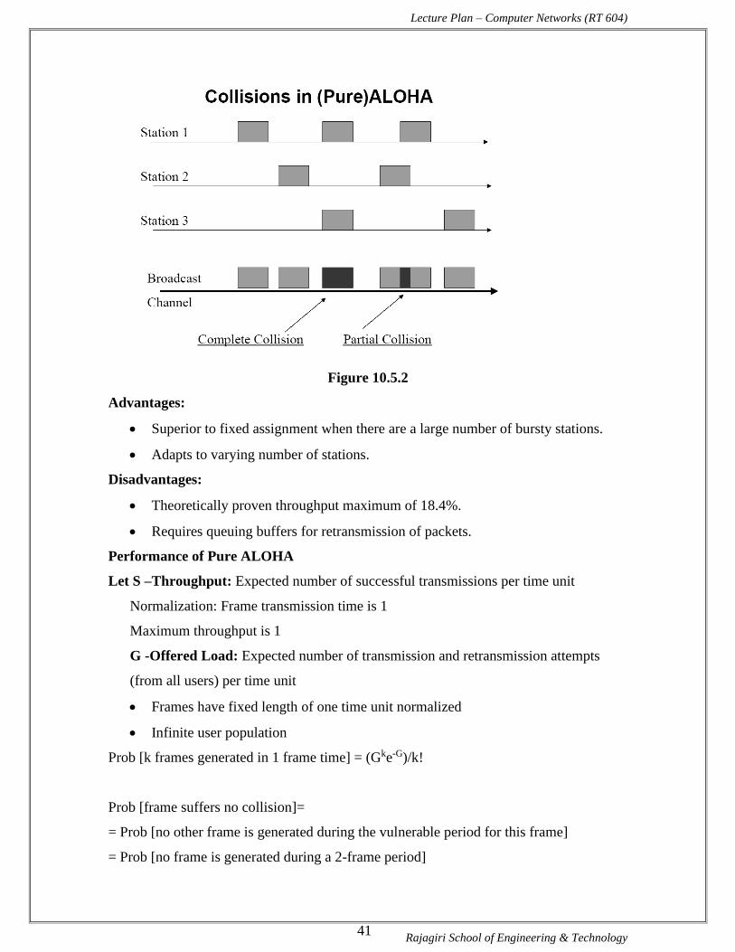
Lecture Plan – Computer Networks (RT 604)

Rajagiri School of Engineering & Technology 41

Figure 10.5.2

Advantages:

• Superior to fixed assignment when there are a large number of bursty stations.

• Adapts to varying number of stations.

Disadvantages:

• Theoretically proven throughput maximum of 18.4%.

• Requires queuing buffers for retransmission of packets.

Performance of Pure ALOHA

Let S –Throughput: Expected number of successful transmissions per time unit

Normalization: Frame transmission time is 1

Maximum throughput is 1

G -Offered Load: Expected number of transmission and retransmission attempts

(from all users) per time unit

• Frames have fixed length of one time unit normalized

• Infinite user population

Prob [k frames generated in 1 frame time] = (Gke-G)/k!

Prob [frame suffers no collision]=

= Prob [no other frame is generated during the vulnerable period for this frame]

= Prob [no frame is generated during a 2-frame period]

Lecture Plan – Computer Networks (RT 604)

Rajagiri School of Engineering & Technology 42

Throughput in ALOHA

Throughput will be maximum for G=0.5. So Effiency of Pure ALOHA is 18%.

5.5.3. Slotted ALOHA

• Aloha with an additional constraint

• Time is divided into discrete time intervals (=slot)

• Slot size equals fixed packet transmission time

• A station can transmit only at the beginning of a slot.

• When Packet ready for transmission, wait until start of next slot

• Packets overlap completely or not at all

Figure 10.5.3

Advantages:

• Doubles the efficiency of Aloha

• Adaptable to a changing station population

Disadvantages:

• Theoretically proven throughput maximum of 36.8%

Lecture Plan – Computer Networks (RT 604)

Rajagiri School of Engineering & Technology 43

• Requires queuing buffers for retransmission of packets

Performance of Slotted ALOHA

Prob [frame suffers no collision] = Prob [no other frame is generated during the

vulnerable period for this frame]

= Prob [no frame is generated during a 1-frame period]

Throughput in S-ALOHA:

Throughput will be maximum for G=1.0. So Effiency of Slotted ALOHA is 36%.

5.5.4. Comparison between Pure ALOHA & Slotted ALOHA.

Figure 10.5.4

University Questions

1. How is collision avoidance achieved in Slotted ALOHA?

2. How is Finite Population ALOHA different from pure ALOHA?

Lecture Plan – Computer Networks (RT 604)

Rajagiri School of Engineering & Technology 44

3. Draw the curve relating throughput with offered traffic for ALOHA system. What

does the curve convey?

4. Explain the improvements obtained in slotted ALOHA with suitable diagrams.

6. Summary

1. Multiple Access Protocols are channel allocation schemes that posses desirable

performance characteristics.

2. Multiple Access Protocols reside within a special layer called the Medium

Access Control (MAC) layer.

3. MAC layer is between the Data Link Control (DLC) layer and the Physical Layer.

4. Aloha method refers to a simple communications scheme in which each source in

a network sends data whenever there is a frame to send.

5. In Pure Aloha, stations are allowed access to the channel whenever they have data

to transmit.

7. Exercise questions

1. Describe ALOHA system

2. Describe MAC sub layer.

3. Compare Pure ALOHA and Slotted ALOHA

Lecture Plan – Computer Networks (RT 604)

Rajagiri School of Engineering & Technology 45

Lecture # 11

1. Synopsis

Carrier Sense Multiple Access protocols – persistent and non-persistent CSMA – CSMA

with collision detection – IEEE 802.3 standards for LAN

2. Target

At the completion of this lecture you should be able to answer questions like

1. Explain Carrier Sense Multiple Access protocol

2. Explain the different CSMA protocols

3. Explain CSMA with collision detection

4. Explain IEEE 802.3 (Ethernet) standards for LAN

3. Introduction

In lecture 10 we discussed the ALOHA method. But the best channel utilization that can

be achieved with slotted ALOHA is 1/e. In this lecture we will be discussing some

protocols for improving performance. In particular, we will emphasize the following

• Non-Persistent CSMA

• 1-Persistent CSMA

• p-Persistent CSMA

• CSMA with collision detection (CSMA/CD)

• IEEE 802.3 Standard for LAN

4. Revision / Prerequisites

Please refer lecture 10 for the contention protocols.

5.1. Carrier Sense Multiple Access Protocol (CSMA)

In both slotted and pure ALOHA, a node's decision to transmit is made independently of

the activity of the other nodes attached to the broadcast channel. Ethernet uses a

refinement of ALOHA, known as Carrier Sense Multiple Access (CSMA), which

improves performance when there is a higher medium utilization. When a Station has

data to transmit, the station first listens to the cable (using a transceiver) to see if a carrier

(signal) is being transmitted by another node. This may be achieved by monitoring

whether a current is flowing in the cable (each bit corresponds to 18-20 milliamps (mA)).

Lecture Plan – Computer Networks (RT 604)

Rajagiri School of Engineering & Technology 46

If a sender does not receive an acknowledgment after some period, it assumes that a

collision has occurred. After a collision a station backs off for a certain (random) time

and retransmits.

There are a number of variations of CSMA protocols:

• Non-Persistent CSMA

• 1-Persistent CSMA

• p-Persistent CSMA

5.2. Non-Persistent CSMA Protocol:

1. If the medium is idle, transmit immediately

2. If the medium is busy, wait a random amount of time and repeat Step 1

• Random back-off reduces probability of collisions

• Wasted idle time if the back-off time is too long

• May result in long access delays

• Better Channel utilization than 1 persistent.

5.3. 1-persistent CSMA Protocol:

When a station has to send data it first listens to the channel to see if anyone else is

transmitting. If the channel is busy the station waits until it becomes idle, When the

station detects an idle channel, it transmits a frame. If a collision occurs, the station waits

a random amount of time and starts all over again.

1. Check the medium.

2. if idle, send

3. else, wait until idle (continuously sense), then send

4. if collision, wait random amount of time, goto 1

There will always be a collision if two stations want to transmit simultaneously.

1-persistent CSMA transmits with probability 1 when it finds channel idle.

5.4. p-Persistent CSMA Protocol:

This protocol applies to slotted channels. When a station becomes ready to send it sends

the channel. If it is idle it transmits with a probability p.

1. If the medium is idle, transmit with probability p, and delay for one time unit with

probability (1 - p) (time unit = length of propagation delay).

2. If the medium is busy, continue to listen until medium becomes idle, then go to Step 1

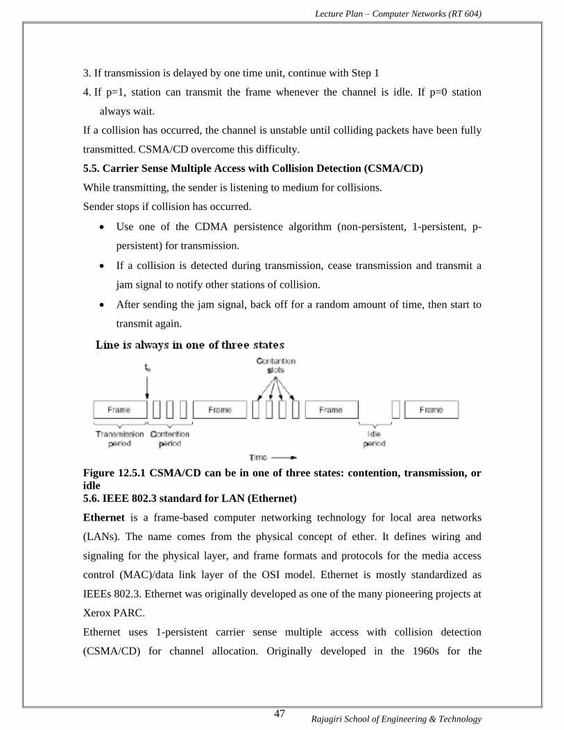
Lecture Plan – Computer Networks (RT 604)

Rajagiri School of Engineering & Technology 47

3. If transmission is delayed by one time unit, continue with Step 1

4. If p=1, station can transmit the frame whenever the channel is idle. If p=0 station

always wait.

If a collision has occurred, the channel is unstable until colliding packets have been fully

transmitted. CSMA/CD overcome this difficulty.

5.5. Carrier Sense Multiple Access with Collision Detection (CSMA/CD)

While transmitting, the sender is listening to medium for collisions.

Sender stops if collision has occurred.

• Use one of the CDMA persistence algorithm (non-persistent, 1-persistent, p-

persistent) for transmission.

• If a collision is detected during transmission, cease transmission and transmit a

jam signal to notify other stations of collision.

• After sending the jam signal, back off for a random amount of time, then start to

transmit again.

Figure 12.5.1 CSMA/CD can be in one of three states: contention, transmission, or

idle

5.6. IEEE 802.3 standard for LAN (Ethernet)

Ethernet is a frame-based computer networking technology for local area networks

(LANs). The name comes from the physical concept of ether. It defines wiring and

signaling for the physical layer, and frame formats and protocols for the media access

control (MAC)/data link layer of the OSI model. Ethernet is mostly standardized as

IEEEs 802.3. Ethernet was originally developed as one of the many pioneering projects at

Xerox PARC.

Ethernet uses 1-persistent carrier sense multiple access with collision detection

(CSMA/CD) for channel allocation. Originally developed in the 1960s for the

Lecture Plan – Computer Networks (RT 604)

Rajagiri School of Engineering & Technology 48

ALOHAnet in Hawaii using radio, the scheme is relatively simple compared to token ring

or master controlled networks. When one station wants to send some information, it

obeys the following algorithm:

Step 1: Start - If the wire is idle, starts transmitting, else go to step 4

Step 2: Transmitting - If detecting a collision, continue transmitting until the minimum

packet time is reached (to ensure that all other transmitters and receivers detect the

collision) then go to step 4.

Step 3: End successful transmission - Report success to higher network layers; exit

transmit mode.

Step 4: Wire is busy - Wait until wire becomes idle

Step 5: Wire just became idle - Wait a random time, then go to step 1, unless maximum

number of transmission attempts has been exceeded

Step 6: Maximum number of transmission attempt exceeded - Report failure to higher

network layers; exit transmit mode.

University Questions

1. Compare Non Persistent, 1-Persistent and p-Persistent CSMA.

2. What does part 802.3 of IEEE 802 standard describe?

3. Explain CSMA.

4. Explain different multiple access protocols.

6. Summary

1. Carrier Sense Protocols are protocols in which stations listen for a carrier and act

accordingly.

2. In 1-persistent CSMA the station transmits with a probability of 1 whenever it

finds the channel idle.

3. The p-persistent protocol applies to slotted channels.

4. CSMA/CD is used on LANs in the MAC layer.

5. Ethernet is a frame-based computer networking technology for local area

networks

7. Exercise questions

1. Name some of the multiple access protocols

2. Explain various contention protocols.

Lecture Plan – Computer Networks (RT 604)

Rajagiri School of Engineering & Technology 1

MODULE I

Lecture # 1

1. Synopsis

Introduction

2. Target

At the completion of this lecture you should be able to answer questions like

1. What is a computer network?

2. What is the need for a network?

3. What are the applications of computer network?

4. What is the need for a network standard?

3. Introduction

This being the first class of this course you will get a very basic idea of computer

networks. Before we begin on this topic, a revision of the concepts developed earlier

(subjects taught earlier etc or previous lectures) may be helpful. Once we finish this

aspect, we will proceed towards exposition of items listed in the synopsis. In particular,

we will emphasize the following

1. What is a computer network?

2. What is the need for a network?

3. What are the applications of computer network?

4. What is the need for a network standard?

4. Revision / Prerequisites

In your Data Communication paper you have come across multiplexing, the different

types of multiplexing like FDM, STDM etc. You have also learned about the different

techniques for transmitting digital data, the different transmission mode and different

kinds of switching like packet switching and circuit switching. The Data

Communication course RT506 is demanded as a prerequisite for this course.

5.1. What is a computer network?

Computer network is a collection of autonomous computers interconnected by a

single technology. Two computers are said to be interconnected if they are able to

exchange information. It is not necessary that the connection should be via a copper

Lecture Plan – Computer Networks (RT 604)

Rajagiri School of Engineering & Technology 2

wire. Fiber optics, microwaves, infrared, and communication satellites can also be

used to establish the connection.

5.2. Why Networks?

• Distribute computation among nodes

• Coordination between processes running on different nodes

• Remote I/O Devices

• Remote Data/File Access

• Personal communications (e-mail, chat, A/V)

• World Wide Web

5.3. Applications of networks

Business applications

Resource sharing by using client server model

In this model the data are stored on powerful computers called servers. Users have simpler

machines, called clients, on their desks, with which they access remote data.

A computer network can provide a powerful communication medium among employees.

Virtually every company that has two or more computers now has e-mail (electronic mail),

which employees generally use for a great deal of daily communication.

Home Applications

Access to remote information.

Person-to-person communication.

Lecture Plan – Computer Networks (RT 604)

Rajagiri School of Engineering & Technology 3

Interactive entertainment.

Electronic commerce.

5.4. Why Do We Need A Standard?

• Many types of connection media: telephone lines, optical fibers, cables, radios,

etc.

• Many different types of machines and operating systems

• Many different network applications

To reduce their design complexity, most networks are organized as a stack of layers

or levels, each one built upon the one below it. The number of layers, the name of

each layer, the contents of each layer, and the function of each layer differ from

network to network. The purpose of each layer is to offer certain services to the

higher layers, shielding those layers from the details of how the offered services are

actually implemented. In a sense, each layer is a kind of virtual machine, offering

certain services to the layer above it.

University Questions

1. Compare the advantages and disadvantages of Analog transmission with its digital

counterpart.

6. Summary

1. Computer network is a collection of autonomous computers interconnected by a

single technology.

2. Since many types of connection media can be used for communication between

many different types of machines that may have different operating systems and

may support different network applications a standard is essential for the

network of computers.

7. Exercise questions

1. What are the applications of computer network?

2. What are two reasons for using layered protocols?

8. Programming / Computational assignments

Lecture Plan – Computer Networks (RT 604)

Rajagiri School of Engineering & Technology 4

Lecture # 2

1. Synopsis:

ISO-OSI Reference Model

2. Target: At the completion of this lecture you should be able to answer questions like

1. What are the layers in the OSI model?

2. What is the function of the physical layer?

3. What is the function of the data link layer?

4. What is the function of the network layer?

5. What is the function of the transport layer?

6. What is the function of the session layer?

7. What is the function of the presentation layer?

8. What is the function of the application layer?

3. Introduction

In this lecture, we will emphasize the following

a. ISO-OSI Model

b. The functions of the seven layers in the OSI model

4. Revision / Prerequisites

In lecture 1 we have discussed the need for a standard for establishing a network

connection. In this lecture we will be discussing an important reference model that

was developed by the International Standards Organization (ISO). This model is

called the ISO OSI (Open Systems Interconnection) Reference model and was the

first step towards the international standardization of the protocols used in the various

layers.

5.1. ISO - OSI Model

One of the most important concepts in networking is the open-systems

interconnection (OSI) reference model. It serves as a framework within which

communication protocol standards are developed.

In 1977, International Standards Organization (ISO) began an ambitious project

to develop a single international standard set of communications protocols. By 1984,

Lecture Plan – Computer Networks (RT 604)

Rajagiri School of Engineering & Technology 5

ISO had defined an overall model of computer communications called the Reference

Model for Open Systems Interconnection, or OSI Model.

ISO also developed a comprehensive set of standards for the various layers of the OSI

model. The standards making up the OSI architecture were not widely implemented

in commercial products for computer networking. However, the OSI model is still

important. The concepts and terminology associated with the OSI model have become

widely accepted as a basis for discussing and describing network architectures. The

OSI model is often used in categorizing the various communications protocols that

are in common use today and also used for comparing one network architecture to

another.

• Model: It means that it is only theory. In fact the OSI model is not yet fully

implemented in real networks.

• Open System: It can communicate with any other system that follows the

specified standards, formats, and semantics.

• Protocols give rules that specify how the communication parties may

communicate.

• Supports two general types of protocols. They are

o Connection-Oriented:

▪ Sender and receiver first establish a connection, possibly negotiate

on a protocol (virtual circuit)

▪ Transmit the stream of data

▪ Release the connection when done

▪ e.g. Telephone connection

o Connectionless

▪ No advance setup is needed.

▪ Transmit the message (datagram) when sender is ready.

e.g. surface mail

5.2. The Seven Layers

• The OSI model defines the seven functional layers. Each layer performs a

different set of functions, and the intent was to make each layer as independent as

possible from all others.

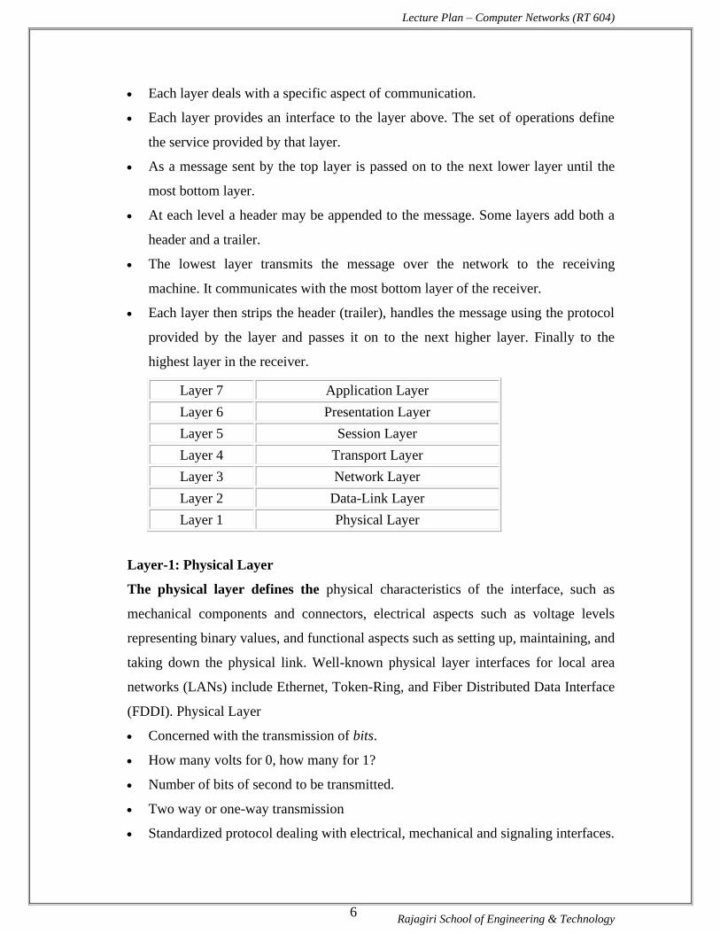
Lecture Plan – Computer Networks (RT 604)

Rajagiri School of Engineering & Technology 6

• Each layer deals with a specific aspect of communication.

• Each layer provides an interface to the layer above. The set of operations define

the service provided by that layer.

• As a message sent by the top layer is passed on to the next lower layer until the

most bottom layer.

• At each level a header may be appended to the message. Some layers add both a

header and a trailer.

• The lowest layer transmits the message over the network to the receiving

machine. It communicates with the most bottom layer of the receiver.

• Each layer then strips the header (trailer), handles the message using the protocol

provided by the layer and passes it on to the next higher layer. Finally to the

highest layer in the receiver.

Layer 7 Application Layer

Layer 6 Presentation Layer

Layer 5 Session Layer

Layer 4 Transport Layer

Layer 3 Network Layer

Layer 2 Data-Link Layer

Layer 1 Physical Layer

Layer-1: Physical Layer

The physical layer defines the physical characteristics of the interface, such as

mechanical components and connectors, electrical aspects such as voltage levels

representing binary values, and functional aspects such as setting up, maintaining, and

taking down the physical link. Well-known physical layer interfaces for local area

networks (LANs) include Ethernet, Token-Ring, and Fiber Distributed Data Interface

(FDDI). Physical Layer

• Concerned with the transmission of bits.

• How many volts for 0, how many for 1?

• Number of bits of second to be transmitted.

• Two way or one-way transmission

• Standardized protocol dealing with electrical, mechanical and signaling interfaces.

Lecture Plan – Computer Networks (RT 604)

Rajagiri School of Engineering & Technology 7

• Many standards have been developed, e.g. RS-232 (for serial communication

lines).

• Example: X.21

Layer-2: Data-Link Layer

The data link layer defines the rules for sending and receiving information across the

physical connection between two systems. This layer encodes and frames data for

transmission, in addition to providing error detection and control. Because the data

link layer can provide error control, higher layers may not need to handle such

services. However, when reliable media is used, there is a performance advantage by

not handling error control in this layer, but in higher layers. Bridges operate at this

layer in the protocol stack.

• Handles errors in the physical layer.

• Groups bits into frames and ensures their correct delivery.

• Adds some bits at the beginning and end of each frame plus the checksum.

• Receiver verifies the checksum.

• If the checksum is not correct, it asks for retransmission. (Send a control

message).

• Consists of two sub layers:

o Logical Link Control (LLC) defines how data is transferred over the cable

and provides data link service to the higher layers.

o Medium Access Control (MAC) defines who can use the network when

multiple computers are trying to access it simultaneously (i.e. Token passing,

Ethernet [CSMA/CD]).

Layer-3: Network Layer

The network layer defines protocols for opening and maintaining a path on the

network between systems. It is concerned with data transmission and switching

procedures, and hides such procedures from upper layers. Routers operate at the

network layer. The network layer can look at packet addresses to determine routing

methods. If a packet is addressed to a workstation on the local network, it is sent

directly there. If it is addressed to a network on another segment, the packet is sent to

a routing device, which forwards it on the network.

Lecture Plan – Computer Networks (RT 604)

Rajagiri School of Engineering & Technology 8

• Concerned with the transmission of packets.

• Choose the best path to send a packet (routing).

• It may be complex in a large network (e.g. Internet).

• Shortest (distance) route vs. route with least delay.

• Static (long term average) vs. dynamic (current load) routing.

• Two protocols are most widely used.

• X.25

o Connection Oriented

o Public networks, telephone, European PTT

o Send a call request at the outset to the destination

o If destination accepts the connection, it sends an connection identifier

• IP (Internet Protocol)

o Connectionless

o Part of Internet protocol suite.

o An IP packet can be sent without a connection being established.

o Each packet is routed to its destination independently.

Layer-4: Transport Layer

The transport layer provides a high level of control for moving information between

systems, including more sophisticated error handling, prioritization, and security

features. The transport layer provides quality service and accurate delivery by

providing connection-oriented services between two end systems. It controls the

sequence of packets, regulates traffic flow, and recognizes duplicate packets. The

transport layer assigns pocketsize information a traffic number that is checked at the

destination. If data is missing from the packet, the transport layer protocol at the

receiving end arranges with the transport layer of the sending system to have packets

re-transmitted. This layer ensures that all data is received and in the proper order.

• Network layer does not deal with lost messages.

• Transport layer ensures reliable service.

• Breaks the message (from sessions layer) into smaller packets, assigns sequence

number and sends them.

• Reliable transport connections are built on top of X.25 or IP.

Lecture Plan – Computer Networks (RT 604)

Rajagiri School of Engineering & Technology 9

• In case IP, lost packets arriving out of order must be reordered.

• TCP: (Transport Control Protocol) Internet transport protocol.

• TCP/IP Widely used for network/transport layer (UNIX).

• UDP (Universal Datagram Protocol) : Internet connectionless transport layer

protocol.

• Application programs that do not need connection-oriented protocol generally use

UDP.

Layer-5: Session Layer

The session layer coordinates the exchange of information between systems by using

conversational techniques, or dialogues. Dialogues are not always required, but some

applications may require a way of knowing where to restart the transmission of data if

a connection is temporarily lost, or may require a periodic dialog to indicate the end

of one data set and the start of a new one.

• Enhanced version of transport layer.

• Dialog control, synchronization facilities.

• Rarely supported (Internet suite does not).

Layer-6: Presentation Layer

Protocols at the presentation layer are part of the operating system and application the

user runs in a workstation. Information is formatted for display or printing in this

layer. Codes within the data, such as tabs or special graphics sequences, are

interpreted. Data encryption and the translation of other character sets are also

handled in this layer.

• Concerned with the semantics of the bits.

• Define records and fields in them.

• Sender can tell the receiver of the format.

• Makes machines with different internal representations to communicate.

• If implemented, the best layer for cryptography.

Layer-7: Application Layer

Applications access the underlying network services using defined procedures in this

layer. The application layer is used to define a range of applications that handle file

transfers, terminal sessions, network management, and message exchange.

Lecture Plan – Computer Networks (RT 604)

Rajagiri School of Engineering & Technology 10

• Collection of miscellaneous protocols for high level applications

• Electronic mail, file transfer, connecting remote terminals, etc.

• E.g. SMTP, FTP, Telnet, HTTP, etc.

Lecture Plan – Computer Networks (RT 604)

Rajagiri School of Engineering & Technology 11

5.3. Performance Parameters

Latency: Time required to transfer an empty message between relevant computers.

Sum total of

1. Delay introduced by the sender software.

2. Delay introduced by the receiver software.

3. Delay in accessing the network.

4. Delay introduced by the network.

Data transfer rate: is the speed at which data can be transferred between sender and

receiver in a network, once transmission has begun. (bit/sec)

Message transfer time = latency + (length of message) / (Data transfer rate).

Bandwidth: is the total volume of traffic that can be transferred across the network.

Max. Data rate (bit/sec) = carrier BW · log2 (1 + (signal/noise))

e.g. phone line BW = 3 kHz, S/N = 30 dB = 1000 Max. Data rate = 30 kbit/sec

Lecture Plan – Computer Networks (RT 604)

Rajagiri School of Engineering & Technology 12

University Questions

1. Draw the block diagram of an OSI reference model and briefly explain the

functions of each. (Nov 2005)

2. What are the advantages of layered architecture?

6. Summary

1. Open Systems Interconnection (OSI) reference model serves as a

framework within which communication protocol standards are developed.

2. Open System can communicate with any other system that follows the

specified standards, formats, and semantics.

3. Protocols are rules that specify how the communication parties may

communicate.

4. The physical layer defines the physical characteristics of the interface, such as

mechanical components and connectors, electrical aspects such as voltage

levels representing binary values, and functional aspects such as setting up,

maintaining, and taking down the physical link.

5. Examples of physical layer interfaces for local area networks (LANs) include

Ethernet, Token-Ring, and Fiber Distributed Data Interface (FDDI).

6. The data link layer encodes and frames data for transmission and also

provides error detection and control.

7. Bridges operate at the data link layer in the protocol stack.

8. Data link layer consists of two sub layers, Logical Link Control (LLC) and

Medium Access Control (MAC)

9. Logical Link Control (LLC) defines how data is transferred over the cable

and provides data link service to the higher layers.

10. Medium Access Control (MAC) defines who can use the network when

multiple computers are trying to access it simultaneously (i.e. Token passing,

Ethernet [CSMA/CD]).

11. The network layer defines protocols for opening and maintaining a path on the

network between systems.

Lecture Plan – Computer Networks (RT 604)

Rajagiri School of Engineering & Technology 13

12. The transport layer provides a high level of control for moving information

between systems, including more sophisticated error handling, prioritization,

and security features.

13. The transport layer provides quality service and accurate delivery by

providing connection-oriented services between two end systems.

14. The session layer coordinates the exchange of information between systems

by using conversational techniques, or dialogues.

15. Data encryption and the translation of other character sets are also handled in

the presentation layer.

16. Applications access the underlying network services using defined procedures

in the application layer.

7. Exercise questions

1. Describe OSI reference model.

2. Which of the OSI layers handles each of the following:

a. Breaking the transmitted bit stream into frames

b. Determining which route through the subnet to use

3. What is the principal difference between connectionless communication and

connection-oriented communication?

8. Programming / Computational assignments

1. Calculate the latency (from first bit sent to the last bit received) for a 10 Mbps

Ethernet with a single store-and –forward switch in the path, and a packet size of

5000 bits. Assume that each link introduces a propagation delay of 10 s and that

the switch begins retransmitting immediately after it has finished receiving the

packet.

Lecture Plan – Computer Networks (RT 604)

Rajagiri School of Engineering & Technology 14

Lecture # 3

1. Synopsis

TCP/IP Reference Model

2. Target

At the completion of this lecture you should be able to answer questions like

1. Which are the different layers in the TCP/IP Reference model?

2. Which are the application level protocols in the TCP/IP?

3. What is Domain Name Server?

4. What is the function of FTP?

5. What is the function of SMTP?

6. What is Hyper Text Transfer Protocol?

7. What is the function of the transport layer in the TCP/IP?

8. Which are the transport level protocols in TCP/IP?

9. What is the function of the Internet layer in TCP/IP?

10. Why is IP referred to as unreliable protocol?

11. What is the function of the Network Access layer?

12. What are the similarities of OSI and TCP/IP model?

13. How do the OSI and TCP/IP models differ?

3. Introduction

In lecture 1 we discussed about the need for a standard for establishing a network of

computers. Also in lecture 2 we discussed on such reference model, the ISO-OSI

reference model. As stated above, in this lecture, we plan to explore another important

reference model, the TCP/IP reference model. In this lecture we will emphasize the

following

a) TCP/IP Reference Model

b) Comparison of the OSI and TCP/IP models

4. Revision / Prerequisites

Before beginning this lecture you should go through the lecture 2, which explains the OSI

reference model. This will help you in comparing the two reference models.

Lecture Plan – Computer Networks (RT 604)

Rajagiri School of Engineering & Technology 15

5.1. TCP/IP Reference Model

The TCP/IP reference model is the network model used in the current Internet

architecture. It has its origins back in the 1960's with the grandfather of the Internet, the

ARPANET. The TCP/IP model does not exactly match the OSI model. There is no

universal agreement regarding how to describe TCP/IP with a layered model but it is

generally agreed that there are fewer levels than the seven layers of the OSI model.

Layers of the TCP/IP model are defined as follows:

Application layer

Like OSI Model, it contains all the higher-level protocols. In TCP/IP the Application

Layer also includes the OSI Presentation Layer and Session Layer. This includes all of

the processes that involve user interaction. The application determines the presentation of

the data and controls the session. In TCP/IP the terms socket and port are used to

describe the path over which applications communicate. There are numerous application

level protocols in TCP/IP, including Simple Mail Transfer Protocol (SMTP) and Post

Office Protocol (POP) used for e-mail, Hyper Text Transfer Protocol (HTTP) used for the

World-Wide-Web, and File Transfer Protocol (FTP). Most application level protocols are

associated with one or more port number.

The most widely known and implemented Application Layer protocols are:

Network Terminal Protocol (Telnet): Provides text communication for remote login

and communication across the network

File Transfer Protocol (FTP): Used to download and upload files across the network

Simple Mail Transfer Protocol (SMTP): Delivers electronic mail messages across the

network

Post Office Protocol, Version 3 (POP-3): Allows users to pick up e-mail across the

network from a central server

Domain Name Service (DNS): Maps IP addresses to Internet domain names

Hyper Text Transfer Protocol (HTTP): The protocol used by the World-Wide-Web to

exchange text, pictures, sounds, and other multi-media information via a graphical user

interface (GUI)

Routing Information Protocol (RIP): Used by network devices to exchange routing

information

Lecture Plan – Computer Networks (RT 604)

Rajagiri School of Engineering & Technology 16

Some protocols are used directly by users as applications, such as FTP and Telnet. Other

protocols are directly behind applications, such as SMTP and HTTP. Others, such as RIP

and DNS, happen indirectly or are used by the programs and operating system routines. A

system administrator must be aware of all of the protocols and how they interact with

each other and the lower TCP/IP layers.

Most of the application level protocols in TCP/IP are implemented as 7-bit ASCII stream

conversations. This means that the communication that takes place across the network is

formatted using upper and lower case alphabetic characters, numeric digits, and standard

punctuation. This was partly done because, historically, as a packet of information passed

across the Internet there was no predicting what type of system it would pass through. 7-

bit ASCII was chosen as a coding scheme that almost any computer or piece of

equipment would be able to handle. Any information that is not actually 7-bit ASCII is

first converted to ASCII, then transmitted across the network, and converted back to its

original form at the destination.

To really understand the rest of the reasons behind why application protocols are simple

text conversations it is important to understand a little of the history of TCP/IP, the

Internet, and UNIX.

The Internet and TCP/IP originally grew up on networks of UNIX computer systems. On

a classic UNIX system there was one central computer system with a number of "Dumb",

text display terminals connected to it. A user on one of the terminals typed in text

commands to run programs, which displayed text as output.

One of the first real network applications allowed a user on one UNIX computer to

communicate across a connection to a remote UNIX computer and run programs as if

directly connected to the remote system. This type of connection used Network Terminal

Protocol, which is now commonly called Telnet. The local system that the user is

connected to is called the client, and the remote computer is called the server. This was

one of the original Client-Server applications.

When a user wanted to communicate from their computer to a remote system, they would

Telnet to the remote and run a program on the remote system. For example, if they

wanted to send mail to someone on a remote computer, they could Telnet to the remote

system, run the mail receiving program, and type in a message to a particular user. If they

Lecture Plan – Computer Networks (RT 604)

Rajagiri School of Engineering & Technology 17

wanted to send a file from computer to computer, they would Telnet to the remote

system, start a Receive program running, then drop back to the local computer and start a

Send program to transmit the file.

Eventually there were certain programs that were left running all the time on the server

computers, E-Mail, File Transfer, and other common applications, so that a remote user

did not have to log onto the remote system and start them each time they wanted to use

them. These programs were left running in the background, using only a small amount of

resources, while they waited to be contacted. These are what is known in the UNIX world

as Daemons, and in the Windows world as Services. Just so that people could find the

correct Daemon to talk to, each common or well known program was given a specific

Port on the computer that it listened to while it was waiting for someone to contact it.

Programmers, being the basically lazy people they are, grew tired of all the Telnetting

from system to system. They began writing programs to do the Telnetting about for them.

These programs at first were barely more than a modified Telnet program that followed a

script to talk to a remote server. But these client applications grew in complexity and

sophistication, becoming much more popular than the manual method of Telnetting

around and typing in long text messages. Eventually there were mostly computers talking

to computers, but the conversations were still the original text messages developed when

it was people doing the conversing.

Now, the above description is not exactly the order of events, or exactly the way it all

happened, but it does give a rough idea of how the application protocols ended up the

way they are. The important thing to remember is that most application protocols are text

conversations that can be manually operated using a Telnet client program.

The text conversation aspect of application level protocols comes in very handy when

setting up, testing, and troubleshooting TCP/IP applications. It is usually possible, and

often quite easy, to use a simple Telnet client to contact a remote TCP/IP application and

send it commands and test data. For example, if you are having trouble sending an E-

Mail message to a particular person, it is quite easy to Telnet directly to the recipients

mail server and manually compose a message for delivery. Then the responses of the

remote system to each step of the procedure can be observed. This usually makes it much

easier to identify where and how a problem is occurring.

Lecture Plan – Computer Networks (RT 604)

Rajagiri School of Engineering & Technology 18

One downside of the text conversation aspect of TCP/IP application level protocols is

that it is fairly easy to eavesdrop on a conversation or to write a program to generate the

correct text messages so that one program can impersonate another. There have been

many solutions developed to address this problem. Pretty Good Privacy (PGP) is a

publicly available application that encrypts text messages before they are passed across

unsecured channels, and then un encrypts them at the destination. Secure Hyper Text

Transfer Protocol (SHTTP) and the Secure Sockets Layer (SSL) are designed to verify

the identities of computer systems at both ends of a World Wide Web conversation and to

encrypt information in transit between them. These are just a few of a broad range of

available applications that address the security issues.

Secure communications across TCP/IP is a broad topic and is beyond the scope of this

technical reference. Usually it is best to approach it on an application by application

basis, or as an individual solution such as a Firewall system.

Transport layer

In TCP/IP there are two Transport Layer protocols. The Transmission Control Protocol

(TCP) guarantees that information is received as it was sent. The User Datagram Protocol

(UDP) performs no end-to-end reliability checks.

Between the Internet layer and Application layer of the TCP/IP architecture model is the

Transport Layer. This layer has two primary protocols, the Transmission Control

Protocol (TCP) and the User Datagram Protocol (UDP).

TCP is a connection based protocol that provides error detection and correction with

reliable delivery of data packets. UDP is a connectionless protocol with low overhead.

When writing application software a developer normally chooses TCP or UDP based on

whether it is more important to have a reliable connection with bi-directional

communication and error management, or if it is more important to develop a low

overhead, streamlined application.

Internet Layer

In the OSI Reference Model the Network Layer isolates the upper layer protocols from

the details of the underlying network and manages the connections across the network.

The Internet Protocol (IP) is normally described as the TCP/IP Network Layer. Because

of the Inter-Networking emphasis of TCP/IP this is commonly referred to as the Internet

Lecture Plan – Computer Networks (RT 604)

Rajagiri School of Engineering & Technology 19

Layer. All upper and lower layer communications travel through IP as they are passed

through the TCP/IP protocol stack.

The Internet Layer of the TCP/IP architecture model resides just above the Network

Access Layer and below the Transport Layer. The primary concern of the protocol at this

layer is to manage the connections across networks as information is passed from source

to destination. The Internet Protocol (IP) is the primary protocol at this layer of the

TCP/IP architecture model.

IP is a connectionless protocol. This means it does not use a handshake to provide end-

to-end control of communications flow. It relies on other layers to provide this function if

it is required. IP also relies on other layers to provide error detection and correction.

Because of this IP is sometimes referred to as an unreliable protocol. This does not

mean that IP cannot be relied upon to accurately deliver data across a network; it simply

means that IP itself does not perform the error checking and correcting functions.

The functions that IP performs include:

• Defining a datagram and an addressing scheme

• Moving data between transport layer and network access layer protocols

• Routing datagram to remote hosts

• The fragmentation and reassembly of datagram

The only other protocol that is generally described as being at the Internet Layer of the

TCP/IP model is the Internet Control Message Protocol (ICMP), a protocol used to

communicate control messages between IP systems.

Network Access Layer (Host to Network Layer)

In TCP/IP the Data Link Layer and Physical Layer are normally grouped together.

TCP/IP makes use of existing Data Link and Physical Layer standards rather than

defining its own. Most RFCs that refer to the Data Link Layer describe how IP utilizes

existing data link protocols such as Ethernet, Token Ring, FDDI, HSSI, and ATM. The

characteristics of the hardware that carries the communication signal are typically defined

by the Physical Layer. This describes attributes such as pin configurations, voltage levels,

and cable requirements. Examples of Physical Layer standards are RS-232C, V.35, and

IEEE 802.3.

Lecture Plan – Computer Networks (RT 604)

Rajagiri School of Engineering & Technology 20

The Network Access layer is the lowest level of the TCP/IP protocol hierarchy. It is often

ignored by users as it is well hidden by the mid-level protocols such as IP, TCP, and

UDP, and higher level protocols such as SMTP, HTTP, and FTP. Functions performed at

the network access layer include encapsulation of IP datagram into frames to be

transmitted by the network, and mapping IP addresses to physical hardware addresses.

Much of the work that takes place at the network access layer is handled by software

applications and drivers that are unique to individual pieces of hardware. Configuration

often consists of simply selecting the appropriate driver for loading, and selecting TCP/IP

as the protocol for use. Many computers come with this driver software pre-loaded and

configured, or can automatically configure themselves via "plug-and-play" applications.

5.2. Comparison of the OSI and TCP/IP reference models

• Both are based on the concept of a stack of independent protocols.

• Functionality of the layers is similar.

• The layers up through and including transport layer are providing an end-to-

end transport service.

• Concepts, Interfaces, Protocols are the three concepts central to the OSI

model. Each layer provides some service for the layer above to it. A layer’s

interface tells the process above it how to access it.

• The TCP/IP model did not originally clearly distinguish between service,

interface, and protocol.

• The OSI reference model was devised before the protocols were invented.

• With the TCP/IP, protocol came first, and the model was really the description

of the existing protocol.

Lecture Plan – Computer Networks (RT 604)

Rajagiri School of Engineering & Technology 21

Figure: 3.1 TCP/IP and OSI Models

Figure 3.2. TCP/IP Protocol Suite

University Questions

1. Compare OSI and TCP/IP Reference Models.

6. Summary

Lecture Plan – Computer Networks (RT 604)

Rajagiri School of Engineering & Technology 22

1. The TCP/IP reference model is the network model used in the current Internet

architecture.

2. In TCP/IP the Application Layer also includes the OSI Presentation Layer and

Session Layer.

3. The numerous application level protocols in TCP/IP, includes Simple Mail

Transfer Protocol (SMTP) and Post Office Protocol (POP) used for e-mail, Hyper

Text Transfer Protocol (HTTP) used for the World-Wide-Web, and File Transfer

Protocol (FTP).

4. Network Terminal Protocol (Telnet) provides text communication for remote

login and communication across the network

5. File Transfer Protocol (FTP) is used to download and upload files across the

network

6. Simple Mail Transfer Protocol (SMTP) delivers electronic mail messages

across the network

7. Post Office Protocol, Version 3 (POP-3) allows users to pick up e-mail across

the network from a central server

8. Domain Name Service (DNS) is used to map IP addresses to Internet domain

names

9. Hyper Text Transfer Protocol (HTTP) is the protocol used by the World-Wide-

Web to exchange text, pictures, sounds, and other multi-media information via a

graphical user interface (GUI)

10. Routing Information Protocol (RIP) is used by network devices to exchange

routing information

11. In TCP/IP there are two Transport Layer protocols, the Transmission Control

Protocol (TCP) and the User Datagram Protocol (UDP).

12. TCP is a connection-based protocol that provides error detection and correction

with reliable delivery of data packets.

13. UDP is a connectionless protocol with low overhead.

14. The Internet Protocol (IP) is described as the TCP/IP Network Layer.

15. IP is a connectionless protocol.

16. IP is sometimes referred to as an unreliable protocol.

Lecture Plan – Computer Networks (RT 604)

Rajagiri School of Engineering & Technology 23

17. The Network Access layer is the lowest level of the TCP/IP protocol hierarchy.

18. Functions performed at the network access layer include encapsulation of IP

datagram into frames to be transmitted by the network, and mapping IP addresses

to physical hardware addresses.

7. Exercise questions

1. List two ways in which the OSI reference model and the TCP/IP reference model

are the same. List two ways in which they differ.

2. What is the main difference between TCP and UDP?

3. List two advantages and disadvantages of having international standards for

network protocols.

4. How many Layers does TCP/IP model consist of? Explain the function of each

layer.

Lecture Plan – Computer Networks (RT 604)

Rajagiri School of Engineering & Technology 24

Lecture # 4

1. Synopsis

Comparison Network hardware-Repeaters, Routers, Bridges, Gateways, Hub,

Cable Modem

2. Target

At the completion of this lecture you should be able to answer questions like

1. What are the different network topologies?

2. What is a repeater?

3. What is a router?

4. What is a bridge?

5. What is a gateway?

6. What is a Hub?

7. What is a Cable Modem?

8. Compare the different network hardware elements.

3. Introduction

In your previous paper on Data Communication you have come across the different types

of networks. As stated above, in this lecture, we plan to explore the different network

topologies and the network hardware elements. Before we begin on this topic, a revision

of the concepts like the different transmission technologies and the different types of

networks etc. will be helpful. Once we finish this aspect, we will proceed towards

exposition of items listed in the synopsis. In particular, we will emphasize the following

• Network Topologies

➢ Bus

➢ Star

➢ Ring

➢ Mesh

• Network Hardware

➢ Repeaters

➢ Router

➢ Bridge

➢ Gateway

Lecture Plan – Computer Networks (RT 604)

Rajagiri School of Engineering & Technology 25

➢ Hub

➢ Cable Modem

4. Revision / Prerequisites

4.1. Transmission Technology

There are two types of transmission technology.

▪ Broadcast links (Multiple Access).

▪ Point-to-point links.

Broadcast networks have a single communication channel that is shared by all the

machines on the network. Short messages, called packets in certain contexts, sent by any

machine are received by all the others. An address field within the packet specifies the

intended recipient. Upon receiving a packet, a machine checks the address field. If the

packet is intended for the receiving machine, that machine processes the packet; if the

packet is intended for some other machine, it is just ignored. Broadcast systems generally

also allow the possibility of addressing a packet to all destinations by using a special

code in the address field. When a packet with this code is transmitted, it is received and

processed by every machine on the network. This mode of operation is called

broadcasting. Some broadcast systems also support transmission to a subset of the

machines, something known as multicasting.

Point-to-point networks consist of many connections between individual pairs of

machines. To go from the source to the destination, a packet on this type of network may

have to first visit one or more intermediate machines. Often multiple routes, of different

lengths, are possible, so finding good ones is important in point-to-point networks. As a

general rule (although there are many exceptions), smaller, geographically localized

networks tend to use broadcasting, whereas larger networks usually are point-to-point.

Point-to-point transmission with one sender and one receiver is sometimes called

unicasting.

4.2. Types of Networks

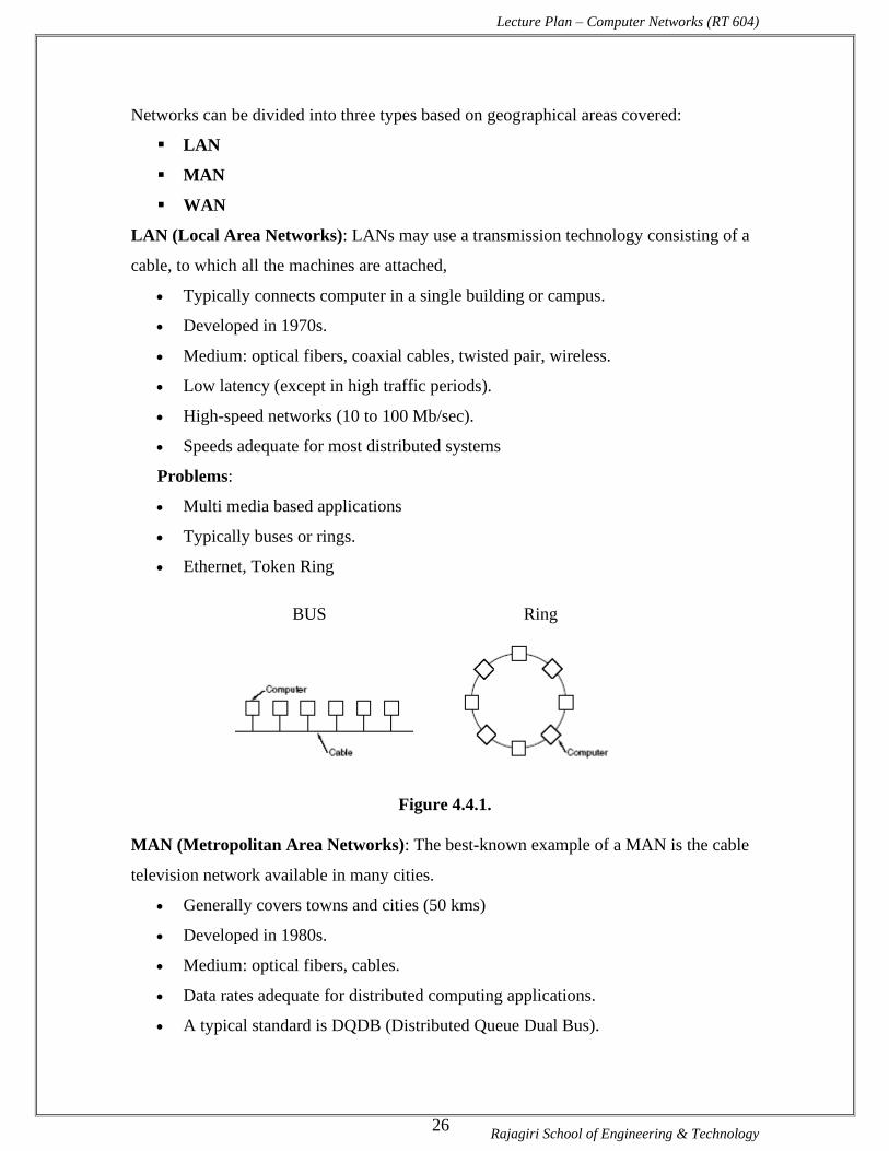
Lecture Plan – Computer Networks (RT 604)

Rajagiri School of Engineering & Technology 26

Networks can be divided into three types based on geographical areas covered:

▪ LAN

▪ MAN

▪ WAN

LAN (Local Area Networks): LANs may use a transmission technology consisting of a

cable, to which all the machines are attached,

• Typically connects computer in a single building or campus.

• Developed in 1970s.

• Medium: optical fibers, coaxial cables, twisted pair, wireless.

• Low latency (except in high traffic periods).

• High-speed networks (10 to 100 Mb/sec).

• Speeds adequate for most distributed systems

Problems:

• Multi media based applications

• Typically buses or rings.

• Ethernet, Token Ring

BUS Ring

Figure 4.4.1.

MAN (Metropolitan Area Networks): The best-known example of a MAN is the cable

television network available in many cities.

• Generally covers towns and cities (50 kms)

• Developed in 1980s.

• Medium: optical fibers, cables.

• Data rates adequate for distributed computing applications.

• A typical standard is DQDB (Distributed Queue Dual Bus).

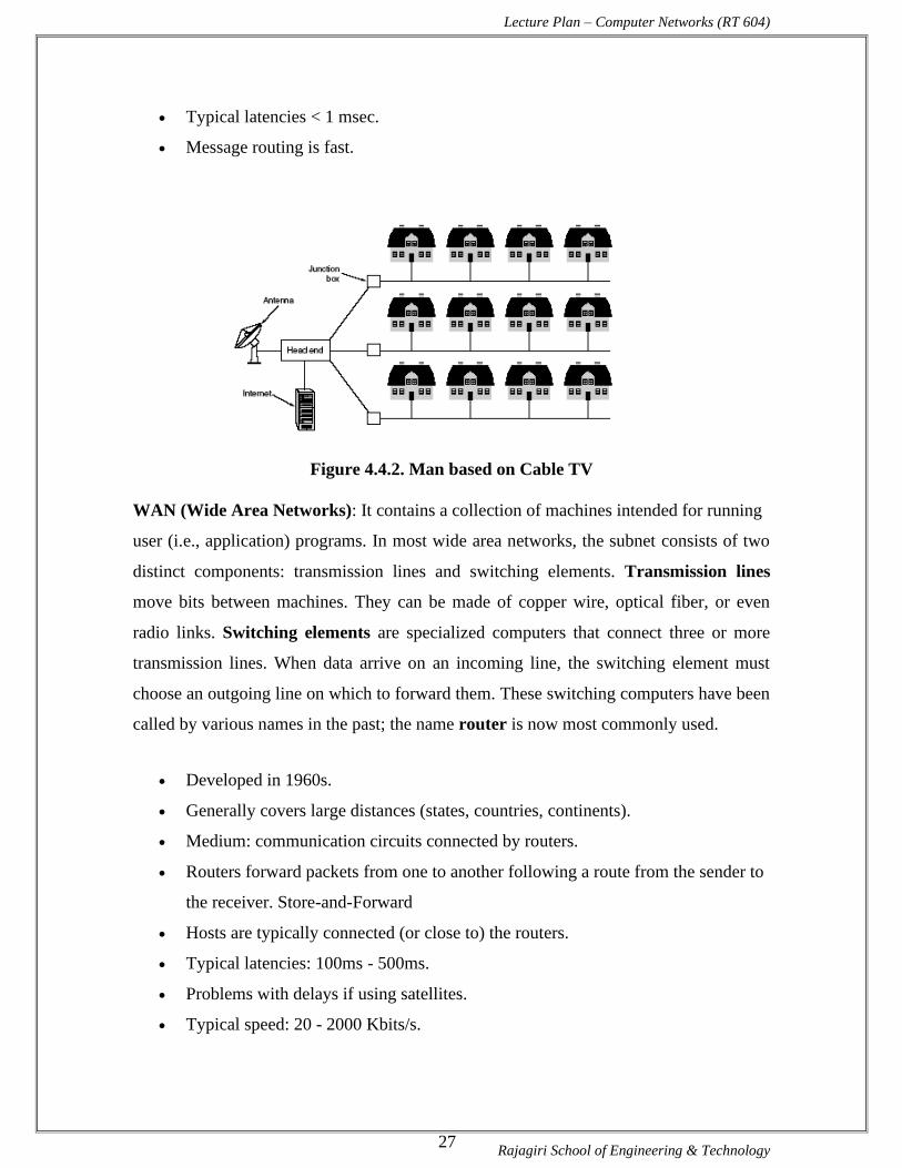
Lecture Plan – Computer Networks (RT 604)

Rajagiri School of Engineering & Technology 27

• Typical latencies < 1 msec.

• Message routing is fast.

Figure 4.4.2. Man based on Cable TV

WAN (Wide Area Networks): It contains a collection of machines intended for running

user (i.e., application) programs. In most wide area networks, the subnet consists of two

distinct components: transmission lines and switching elements. Transmission lines

move bits between machines. They can be made of copper wire, optical fiber, or even

radio links. Switching elements are specialized computers that connect three or more

transmission lines. When data arrive on an incoming line, the switching element must

choose an outgoing line on which to forward them. These switching computers have been

called by various names in the past; the name router is now most commonly used.

• Developed in 1960s.

• Generally covers large distances (states, countries, continents).

• Medium: communication circuits connected by routers.

• Routers forward packets from one to another following a route from the sender to

the receiver. Store-and-Forward

• Hosts are typically connected (or close to) the routers.

• Typical latencies: 100ms - 500ms.

• Problems with delays if using satellites.

• Typical speed: 20 - 2000 Kbits/s.

Lecture Plan – Computer Networks (RT 604)

Rajagiri School of Engineering & Technology 28

• Not (yet) suitable for distributed computing.

• New standards are changing the landscape.

In this model, each host is frequently connected to a LAN on which a router is present,

although in some cases a host can be connected directly to a router. The collection of

communication lines and routers (but not the hosts) form the subnet.

Figure 4.2.3. Network Components

Common requirements are:

• Connect networks of different types, different vendors.

• Provide common communication facilities and hide different hardware and

protocols of constituent networks.

• Needed for extensible open distributed systems

5.1. Network Topology

Figure 4.5.1. Network Topology

Lecture Plan – Computer Networks (RT 604)

Rajagiri School of Engineering & Technology 29

BUS Network: Bus network is a network architecture in which a set of clients is

connected via a shared communications line, called a bus. Bus networks are the simplest

way to connect multiple clients, but often have problems when two clients want to

communicate at the same time on the same bus.

Advantages

Easy to implement and extend

Well suited for temporary networks (quick setup)

Typically the cheapest topology to implement

Failure of one station does not affect others

Disadvantages

Difficult to administer/troubleshoot

Limited cable length and number of stations

A cable break can disable the entire network

Maintenance costs may be higher in the long run

Performance degrades as additional computers are added

Low security (all computers on the bus can see all data transmissions on the bus)

One virus in the network will affect all of them (but not as badly as a star or ring

network)

Star network: In its simplest form, star network consists of one central or hub computer

which acts as a router to transmit messages.

Advantages

Easy to implement and extend

Well suited for temporary networks

The failure of a non-central node will not affect the functionality of the network

Disadvantages

Limited cable length and number of stations

Maintenance costs may be higher in the long run

Failure of the central node can disable the entire network

One virus in the network will affect them all

Lecture Plan – Computer Networks (RT 604)

Rajagiri School of Engineering & Technology 30

Ring network: Ring network is a topology where each user is connected to two other

users. Popular example for such a network is the token ring network.

Advantages

All stations have equal access

Each node on the ring acts as a repeater, allowing ring networks to span greater distances

than other topologies

When a coaxial cable is used to create the ring network the service becomes much faster

Disadvantages

The most expensive topology

Mesh Network: Mesh network is a way to route data, voice and instructions between

nodes. It allows for continous connections and reconfiguration around blocked paths by

hopping from node to node until a connection can be established.

Mesh networks are self healing, i.e. the network can still operate even when a node

breaks down or a connection goes bad. Thus it a very reliable network. This is applicable

to wireless networks, wired networks and software interaction.

This network allows inexpensive peer network nodes to supply services to other nodes in

the same network.

Star-Bus Network: It is a combination of a star network and a bus network. A hub is

used to connect the nodes to the network.

5.2. Network Hardware

5.2.1. Network adapter: Interfaces a computer board with the network medium.

5.2.2.Repeaters

A repeater connects two segments of your network cable. It retimes and regenerates the

signals to proper amplitudes and sends them to the other segments. When talking about,

Ethernet topology, you are probably talking about using a hub as a repeater. Repeaters

require a small amount of time to regenerate the signal. This can cause a propagation

delay, which can affect network communication when there are several repeaters in a

row. Many network architectures limit the number of repeaters that can be used in a row.

Repeaters work only at the physical layer of the OSI network model.

Lecture Plan – Computer Networks (RT 604)

Rajagiri School of Engineering & Technology 31

Figure 4.5.2. Repeater

5.2.3. Bridges

A bridge is a simple device that split the physical network being shared by many

computers into smaller segments. A bridge generally has only two ports; bridges with

more than two ports are usually called switches. Bridges are normally used to connect

LAN segments within a limited geographic area (local bridges), like a building or a

campus. Bridges can be programmed to reject packets from particular networks.

Ethernet is the most commonly used physical network. On an Ethernet network, all the

connected computers share the same piece of "wire" (it's not physically the same piece,

but it is electrically). When two computers attempt to talk at the same time, they drown

each other out and create what's called a collision. The more computers you have on one

Ethernet, the bigger chance you'll have a collision.

Bridges split an Ethernet into multiple collision-domains. All the data on one side of the

bridge stays there, unless it's destined for a computer on the other side of the bridge,

lessening the overall load on each segment. Bridges forward all broadcast messages. Only

a special bridge called a translation bridge will allow two networks of different

architectures to be connected. Bridges do not normally allow connection of networks

with different architectures. It does not propagate noise signals and defective frames as it

was the case for repeaters (at the physical layer). It adaptively recognizes which machines

are reachable from a port. It reduces traffic on each port and it improves security since

each port will only transmit frames directed to nodes reachable from that port. All the

nodes reachable from a node through segments and bridges will receive broadcast

messages sent by that node.

Bridges don't care what protocol is being used on the network (TCP/IP, IPX, AppleTalk,

etc.) since they operate at the data-link level. This is both a benefit and a curse; since they

work at such a simple level, bridges are able to operate at blindingly fast speeds, but since

they will indiscriminately forward data, one has little control over their operation. This is

where routers come in.

5.2.4. HUB

Hubs can also be called either Multi port Repeaters or Concentrators. They are physical

hardware devices. Hubs are used to provide a Physical Star Topology. At the center of

Lecture Plan – Computer Networks (RT 604)

Rajagiri School of Engineering & Technology 32

the star is the Hub, with the network nodes located on the tips of the star. Hubs are a

crucial element to all star topology LANs. Hubs serve as a central device through which

data bound for a workstation travels. Hubs do not read any of the data passing through

them and are not aware of their source or destination. Essentially, a hub simply receives

incoming packets, possibly amplifies the electrical signal, and broadcasts these packets

out to all devices on the network - including the one that originally sent the packet. The

data may be distributed, amplified, regenerated, screened or cut off. The hierarchical use

of hubs removes the length limitation of the cables.

Hub joins multiple computers (or other network devices) together to form a single

network segment. On this network segment, all computers can communicate directly with

each other.

A hub includes a series of ports that each accepts a network cable. Small hubs network

four computers.

Hubs classify as Layer 1 devices in the OSI model. (Physical layer)

Three different types of hubs exist:

• Passive

• Active

• Intelligent

Passive hubs do not amplify the electrical signal of incoming packets before broadcasting

them out to the network. Active hubs, on the other hand, do perform this amplification, as

does a different type of dedicated network device called a repeater. They can also be

treated as concentrator when referring to a passive hub and multiport repeater when

referring to an active hub.

Intelligent hubs add extra features to an active hub that are of particular importance to

businesses. An intelligent hub typically is stackable (built in such a way that multiple

units can be placed one on top of the other to conserve space). It also typically includes

remote management capabilities

5.2.5. Router

A router is a box or a regular computer with at least two ports, used to connect also

dissimilar networks. A router is used to route data packets between two networks. It reads

the information in each packet to tell where it is going. It differs from bridges since it

Lecture Plan – Computer Networks (RT 604)

Rajagiri School of Engineering & Technology 33

operates at the network level. It will also use different addresses. For example a bridge

may use Ethernet addresses while a router uses IP addresses. Routers work at the network

layer - they actually understand the protocols being used to carry the data over the

network. And since they understand the protocols, they can use rules to decide what to do

with a specific piece of data. Because of this, routers are useful in linking networks that

are used for different purposes or by different organizations. One can apply rules or

filters to let certain data in, but keep other data out. Also to route data serving one

purpose over a certain set of network connections, while routing other data over other

connections. This convenience comes at a price. The more detail a router must acquire

about a specific piece of data before forwarding it on, the longer that piece of data is

delayed before being sent on to its destination. Also, the greater configurability of routers

requires faster, more expensive hardware.

It does all the transformations that may be required by the transfer of packets across the

networks it connects. Routing involves two basic activities: running routing algorithms to

determine routes, as expressed by routing tables, and using the routing tables to move

packets across the network. The latter activity is easier and it is called switching. Routing

tables contain information that will indicate for each packet on the basis of its final

destination (usually an IP address) where to go next (next-hop forwarding) as to the port

to be used and the physical address of the next router.

5.2.6. Gateways

A gateway can translate information between different network data formats or network

architectures. It can translate TCP/IP to AppleTalk so computers supporting TCP/IP can

communicate with Apple brand computers. Most gateways operate at the application

layer, but can operate at the network or session layer of the OSI model. Gateways will

start at the lower level and strip information until it gets to the required level and

repackage the information and work its way back toward the hardware layer of the OSI

model.

5.2.7. Cable Modem

The cable television companies have the high speed bandwidth to the homes. Cable

modems use the existing cable TV line to provide the high speed bandwidth. It is an

asymmetrical transfer rates with the upstream data transfer rate at 2 Mbps. The

Lecture Plan – Computer Networks (RT 604)

Rajagiri School of Engineering & Technology 34

downstream data transfer rate is a maximum of 30 Mbps. Most users connect the cable

modem to their 10 Mbps Ethernet NIC, and don't utilize the cable modems full

bandwidth. Switching to a 100 Mbps Ethernet NIC would give them full bandwidth.

Most cable companies use dynamic IP addressing: each time the user connects; they are

assigned a new IP address. Most cable TV companies are placing high performance web

proxy servers at the head end. These servers store the most commonly accessed web

pages and files locally at the head end. The user's web browser first checks the proxy

server to see if the file has been downloaded there. If it hasn't, then it goes out on the

Internet to download it. The storing of the web pages and files on the local proxy server

reduces the load on the communication servers (to the Internet), and gives the impression

of extremely fast Internet access.

Figure 4.5.3.

The cable modem is connected to the existing cable TV RG59 coax line, using a standard

RF connector. The output of the cable modem is a 10BaseT or 100BaseT Ethernet

connection to your NIC.

Cable Modem Advantages

• Fast data transfers, up to 30 Mbps if using a 100BaseT NIC

• Competitive pricing against competing technologies

• Easy to install - home prewired

Cable Modem Disadvantages

• The available bandwidth depends on the number of users on the local cable TV

line segment.

• There is an asymmetrical transfer rate. Upstream is slower than downstream.

• There can be a bottleneck at the communication server at the head end.

University Questions

1. What is the need for gateways?

2. List the advantages and disadvantages of BUS topology.

Lecture Plan – Computer Networks (RT 604)

Rajagiri School of Engineering & Technology 35

3. What are the various network topologies? Discuss with diagram.

4. Write the features of LAN and WAN.

5. Explain briefly the network components used in computer data communication

6. Distinguish clearly between Hubs, Bridges and Routers.

6. Summary

1. Bus network is a network architecture in which a set of clients is connected via a

shared communications line, called a bus.

2. Star network consists of one central or hub computer which acts as a router to

transmit messages.

3. Ring network is a topology where each user is connected to two other users.

4. Mesh network allows for continuous connections and reconfiguration around

blocked paths by hopping from node to node until a connection can be

established.

5. A repeater connects two segments of your network cable.

6. A bridge is a simple device that split the physical network being shared by many

computers into smaller segments.

7. A bridge generally has only two ports; bridges with more than two ports are

usually called switches.

8. Bridges are normally used to connect LAN segments within a limited geographic

area (local bridges), like a building or a campus. Bridges can be programmed to

reject packets from particular networks.

9. Hubs can also be called either Multi port Repeaters or Concentrators.

10. Hubs are physical hardware devices used to provide a Physical Star Topology.

11. A router is a box or a regular computer with at least two ports, used to connect

dissimilar networks and is used to route data packets between two networks.

12. A gateway can translate information between different network data formats or

network architectures.

13. Cable modems use the existing cable TV line to provide the high-speed

bandwidth.

7. Exercise questions

1. Differentiate between bridges and routers.

2. Write short notes on Gateways.

Lecture Plan – Computer Networks (RT 604)

Rajagiri School of Engineering & Technology 36

3. Write short note on Network Repeater.

4. What is unicasting?

5. What is multicasting?

Lecture # 5

1. Synopsis:

Transmission Media– ISDN system Architecture – Communication Satellites –

geostationary satellites - Medium Earth Orbit Satellites- Low earth orbit satellites–

Satellite v/s Fiber

2. Target

At the completion of this lecture you should be able to answer questions like

1. What are the different transmission media available?

2. Explain the different media for transmission.

3. What is ISDN?

4. Explain ISDN architecture.

3. Introduction

In lecture 4 we discussed about the different network topologies and the network

hardware elements. In your previous paper you have come across some media for

transmission. As stated above, in this lecture, we plan to explore the bounded,

unbounded and wireless transmission media. Also we will be discussing the ISDN

architecture. In this lecture, we will emphasize the following

• Transmission media

• ISDN

• ISDN Architecture

4. Revision / Prerequisites

Please refer to Data Communications by Forouzan for notes on different transmission

media.

5.1. Transmission Media

The media for transmission can be classified as

• Bound Media

• Unbound Media

Lecture Plan – Computer Networks (RT 604)

Rajagiri School of Engineering & Technology 37

• Wireless Media

5.1.1. Bound Media

Media is the path used for transferring data in a network. Bound Media consists of

physical substances used to transfer data. The following is a list of the types of bound

media and their susceptibility to EMI - (Electrical Magnetic Interference).

• Coaxial Cable - copper core, shielding, used in LANs, EMI

• Fiber Optic - light signal, glass core, no shielding (not required) No EMI

• Unshielded Twisted Pair (UTP) - No shielding, high EMI, very common, cheap

• Shielded Twisted Pair (STP) - Shielding, less EMI than UTP, IBM networks

Coaxial Cable

Coaxial cable consists of two conductors. The inner conductor is held inside an insulator

with the other conductor woven around it providing a shield. An insulating protective

coating called a jacket covers the outer conductor.

Figure 5.5.1 Coaxial Cable

The outer shield protects the inner conductor from outside electrical signals. The distance

between the outer conductor (shield) and inner conductor plus the type of material used

for insulating the inner conductor determine the cable properties or impedance. Typical

impedances for coaxial cables are 75 ohms for Cable TV, 50 ohms for Ethernet. The

excellent control of the impedance characteristics of the cable allow higher data rates to

be transferred than with twisted pair cable.

• Used extensively in LANs

• Single central conductor surrounded by a circular insulation layer and a

conductive shield

• High bandwidth: Upto 400 Mhz

• High quality of data transmission

Lecture Plan – Computer Networks (RT 604)

Rajagiri School of Engineering & Technology 38

• Max. Used data rates: 100 Mbits/s

• Problems: Signal loss at high frequencies

Twisted Pair Cable

Figure 5.5.2 Twisted Pair Cable

• Extensively used in telephone circuits, where several wires are insulated and

put together.

• Bandwidth: 250 KHz.

• Low signal to noise ratio (cross talk) -> Low data rate.

• Good for short-distance communications.

• Used in LAN (UTP or 10baseT).

Optical Fiber

Fiber optic cable has the ability to transmit more information, more quickly and over

longer distances. Fiber optic cable offers almost unlimited bandwidth and unique

advantages over all previously developed transmission media. The basic point-to-point

fiber optic transmission system consists of three basic elements: the optical transmitter,

the fiber optic cable and the optical receiver.

The Optical Transmitter: The transmitter converts an electrical analog or digital signal

into a corresponding optical signal. The source of the optical signal can be either a light

emitting diode, or a solid-state laser diode. The most popular wavelengths of operation

for optical transmitters are 850, 1300, or 1550 nanometers.

The Fiber Optic Cable: The cable consists of one or more glass fibers, which act as

waveguides for the optical signal. Fiber optic cable is similar to electrical cable in its

construction, but provides special protection for the optical fiber within. For systems

requiring transmission over distances of many kilometers, or where two or more fiber

optic cables must be joined together, an optical splice is commonly used.

Lecture Plan – Computer Networks (RT 604)

Rajagiri School of Engineering & Technology 39

The Optical Receiver: The receiver converts the optical signal back into a replica of the

original electrical signal. The detector of the optical signal is either a PIN-type

photodiode or avalanche-type photodiode.

Figure 5.5.3 Fiber Optic Cable

• High quality and high bandwidth data transmission applications.

• Use light instead of electric pulses for message transmission.

• Very high frequency ranges (20,000 Mhz).

• Single fiber can support over 30,000 telephone lines.

• Data transmission rates of 400 Mbits/s and more.

• Becoming very popular for MAN and LAN, also used for intercontinental

links.

• High signal to noise ratio, difficulty in tapping (security).

• Cost is the single biggest drawback (currently).

Advantages of Fiber Optic communication

Fiber optic transmission systems – a fiber optic transmitter and receiver, connected by

fiber optic cable – offer a wide range of benefits not offered by traditional copper wire or

coaxial cable. These include:

1. The ability to carry much more information and deliver it with greater fidelity than

either copper wire or coaxial cable.

2. Fiber optic cable can support much higher data rates, and at greater distances, than

coaxial cable, making it ideal for transmission of serial digital data.

3. The fiber is totally immune to virtually all kinds of interference, including lightning,

and will not conduct electricity. It can therefore come in direct contact with high voltage

electrical equipment and power lines. It will also not create ground loops of any kind.

Lecture Plan – Computer Networks (RT 604)

Rajagiri School of Engineering & Technology 40

4. As the basic fiber is made of glass, it will not corrode and is unaffected by most

chemicals. It can be buried directly in most kinds of soil or exposed to most corrosive

atmospheres in chemical plants without significant concern.

5. Since the only carrier in the fiber is light, there is no possibility of a spark from a

broken fiber. Even in the most explosive of atmospheres, there is no fire hazard, and no

danger of electrical shock to personnel repairing broken fibers.

6. Fiber optic cables are virtually unaffected by outdoor atmospheric conditions, allowing

them to be lashed directly to telephone poles or existing electrical cables without concern

for extraneous signal pickup.

7. A fiber optic cable, even one that contains many fibers, is usually much smaller and

lighter in weight than a wire or coaxial cable with similar information carrying capacity.

It is easier to handle and install, and uses less duct space. (It can frequently be installed

without ducts.)

8. Fiber optic cable is ideal for secure communications systems because it is very difficult

to tap but very easy to monitor. In addition, there is absolutely no electrical radiation

from a fiber

5.1.2. Unbound Media

Media is the path used for transferring data in a network. Unbound Media consists of the

wireless path used to transfer data. The following is a list of the types of unbound media

and their suseptability to EMI - (Electrical Magnetic Interference).

• Radio Waves

• Micro Waves - Terrestrial and Satellite

• Infrared

Microwave Transmission

Another popular transmission medium is microwave. This is a popular way of

transmitting data since it does not require the expense of laying cables. Microwave

systems use very high frequency radio signals to transmit data through space. However,

at microwave frequencies the electromagnetic waves cannot bend or pass through

obstacles like hills, etc. Hence microwave transmission is a line-of-sight method of

Lecture Plan – Computer Networks (RT 604)

Rajagiri School of Engineering & Technology 41

communication. In other words, the transmitter and receiver of a microwave system,

which are mounted on very high towers, should be in a line-of-sight. This may

not be possible for very long distance transmission due to physical constraints. Moreover,

the signals become weak after traveling a certain distance and require power

amplification.

In order to overcome the problems of line-of-sight and power amplification of weak

signals, microwave systems use repeaters at intervals of about 25 to 30 km in between the

transmitting and receiving stations. The first repeater is placed in line-of-sight of the

transmitting station and the last repeater is placed in line-of-sight of the receiving station.

Two consecutive repeaters are also placed in line-of-sight of each other. The data signals

are received, amplified, and re-transmitted by each of these stations.

Figure 5.5.4. Microwave Transmission

Advantages and Limitations of Microwave Transmission

Microwave systems permit data transmission rates of about 16 Giga (1 giga = 109) bits

per second. At such high frequency, a microwave system can carry 250,000 voice

channels at the same time.

Lecture Plan – Computer Networks (RT 604)

Rajagiri School of Engineering & Technology 42

However, the capital investment needed to install microwave links is very high and hence

they are mostly used to link big metropolitan cities that have heavy telephone traffic

between them.

5.1.3. Wireless Media

Figure 5.5.5.

• For WANs satellites provide global communication over the world, receiving

signals from transmitters and relaying them back to the receivers.

• With geostationary satellites senders and receivers always points the same

direction.

• High communication capacity. Big latency : 0.25 secs.

• For MANs microwave radio technology is widely used (2 to 24 Mbit/s).

• For LANs Spread Spectrum radio technology is becoming very popular (up to

2 Mbit/s).

• Infrared: Line of sight limitation.

Communication Satellite

Figure 5.5.6.

The main problem with microwave communications is that the curvature of the earth,

mountains, and other structures often block the line-of-sight. Due to this reason, several

Lecture Plan – Computer Networks (RT 604)

Rajagiri School of Engineering & Technology 43

repeater stations are normally required for long distance transmission, which increases

the cost of data transmission between two points. This problem is overcome by using

satellites which are relatively newer and more promising data transmission media.

A communication satellite is basically a microwave relay station placed precisely at

36,000 km above the equator where its orbit speed exactly matches the earth’s rotation

speed. Since a satellite is positioned in a geo-synchronous orbit, (i.e. the orbit where the

speed of the satellite matches the earth’s rotation speed), it appears to be stationary

relative to earth and always stays over the same point with respect to earth. This allows a

ground station to aim its antenna at a fixed point in the sky. The Indian satellite, INSAT-

1B, is positioned in such a way that it is accessible from any place in India.

Figure 5.5.7.

Communications through satellites are either passive or active. The first communications

satellites were passive. Signals from Earth were merely reflected from the orbiting

metallic sphere. Later types of satellites are active. Active communication satellites

receive signals from Earth, electronically strengthen the signals, and transmit the signals

to Earth.

This relaying of signals from one Earth Station to another is done through the satellite's

transponder. Most communications satellites have more than one transponder and

antenna so that they can relay several users of radio waves or signals at the same time.

Advantages and Limitations

The main advantage of satellite communication is that it is a single microwave relay

station visible from any point of a very large area on the earth. For example, satellites

Lecture Plan – Computer Networks (RT 604)

Rajagiri School of Engineering & Technology 44

used for national transmission are visible from all parts of the country. Thus transmission

and reception can be between any two randomly chosen places in that area. Moreover,

transmission and reception costs are independent of the distance between the two points.

In addition to this, a transmitting station can receive back its own transmission and check

whether the satellite has transmitted the information correctly. If an error is detected, the

data would be retransmitted.

A major drawback of satellite communications has been the high cost of placing the

satellite into its orbit. Moreover, a signal sent to a satellite is broadcasted to all receivers

within the satellite’s range. Hence necessary security measures need to be taken to

prevent unauthorized tampering of information.

Communications satellites are launched by rockets or carried into space by the Space

Shuttle. Once in space, small engines on the satellites guide the satellite into orbit and

help keep them there. Most communications satellites are placed in orbit at an altitude of

22,300 miles above the Earth. This is known as a geostationary or synchronous orbit.

This allows the satellite to orbit the Earth at the same speed as the rotation of the Earth.

As a result, the satellite appears to be stationary above the same location on Earth.

Communications satellites will be used to link all the regions and people of the world.

This is a giant step from the early uses of communication satellites. This global system

will consist of many satellites, positioned in geostationary orbit, providing high

bandwidth capacity; interconnect many highly specialized Earth Stations operating in

more than thirty countries. This network, already in progress by consortiums headed by

Motorola (Iridium) will provide the framework and capability for anyone in the world to

communicate with anyone else, regardless of location.

5.2. ISDN

ISDN stands for Integrated Services Digital Network. It is a design for a completely

digital telephone/telecommunications network. It is designed to carry voice, data, images,

and video, everything you could ever need. It is also designed to provide a single

interface (in terms of both hardware and communication protocols) for hooking up your

phone, your fax machine, your computer, your videophone, your video-on-demand

system (someday), and your microwave.

Lecture Plan – Computer Networks (RT 604)

Rajagiri School of Engineering & Technology 45

B-ISDN is Broadband ISDN. (The older ISDN is often called Narrowband ISDN.) This

is not simply faster ISDN, or ISDN with the copper to your home finally upgraded to

fiber. B-ISDN is a complete redesign. It is still capable of providing all the integrated

services (voice, data, video, etc.) through a single interface just like ISDN was supposed

to.

5.2.1 ISDN Architecture

ISDN components include terminals, terminal adapters (TA), network-termination

devices, line-termination equipment and exchange-termination equipment.

• ISDN terminals come in two types:

• Specialized ISDN terminals are referred to as terminal equipment type 1 (TE1).

• Non - ISDN terminals such as DTE that predate the ISDN standards are referred

to as terminal equipment type 2 (TE2).

TE1 are connected to the ISDN network through a four-wired twisted-pair digital link.

TE2 are connected to the ISDN network through a terminal adapter.

The ISDN TA can either be a stand-alone device or a board inside TE2. If implemented

as a stand-alone device, the TE2 is connected to the TA via a standard physical layer

interface.

Lecture Plan – Computer Networks (RT 604)

Rajagiri School of Engineering & Technology 46

Figure 5.5.8. Sample ISDN Configuration

University Questions

1. What is a low earth orbit satellite?

2. Explain the different types of satellites used as transmission media. (Nov 2005)

3. Explain in detail the ISDN system architecture.

4. Write notes on ISDN service.

5. What are the major differences between Basic Rate and Primary Rate interfaces of

ISDN?

6. Explain Ethernet Networks.

7. Explain the various physical media’s used in computer networks.

8. Compare analog and digital transmission with special reference to ISDN.

9. Write notes on fiber optic communication.

10. What are some of the physical media that Ethernet can run over?

11. What are the various IEEE standards? Briefly explain.

6. Summary

1. The different Bound media for transmission are co-axial cable, twisted pair cable

and optical fiber.

2. Unbound media for communication are radio waves, microwaves and infrared

3. Wireless media of transmission is with the help of communication satellites.

4. ISDN (Integrated Services Digital Network) is a design for a completely digital

telephone/telecommunications network to carry voice, data, images, and video, to

provide a single interface for hooking up your phone, your fax machine, your

computer, your videophone, your video-on-demand system (someday), and your

microwave

7. Exercise questions

1. Explain various transmission medias.

2. Write notes on fiber optic communication.

3. Write notes on coaxial cable.