Modified level set equation and its numerical assessment

Journal of Computational Physics 278 (2014) 1–30

Contents lists available at ScienceDirect

Journal of Computational Physics

www.elsevier.com/locate/jcp

Modified level set equation and its numerical assessment

Vladimir Sabelnikov a, Andrey Yu. Ovsyannikov b, Mikhael Gorokhovski c,∗a ONERA – The French Aerospace Lab., Chemin de la Hunière et des Joncherettes, BP 80100, FR-91123, Palaiseau, Franceb Center for Turbulence Research, Stanford University, Stanford, CA 94305, USAc Laboratoire de Mécanique des Fluides et d’Acoustique, École Centrale de Lyon, CNRS–Université Claude Bernard Lyon 1–INSA Lyon, Écully, France

a r t i c l e i n f o a b s t r a c t

Article history:Received 29 April 2013Received in revised form 15 July 2014Accepted 10 August 2014Available online 19 August 2014

Keywords:Computing interface motionLevel set methodsReinitializationEikonal equationSigned distance function

In the context of level set methods, the level set equation is modified by embedding a source term. The exact expression of this term is such that the eikonal equation is automatically satisfied, and also, this term is zero on the interface. Theoretically, it renders the reinitialization of level sets unnecessary, similarly to the extension velocity method. The exact expression of the source term makes also possible the derivation of its local approximate forms, of zero-, first- and higher-order accuracy. Application of those forms simplifies the realization of level set methods in comparison with the extension velocity method, but requires the return to the reinitialization procedure. Nevertheless, the advantage of local approximate forms of the proposed source term is that the number of reinitializations can be significantly reduced in comparison with the standard level set equation with the reinitialization procedure. Furthermore, with increasing the order of accuracy of approximation less number of reinitializations is needed. This leads to improvement of the interface resolution. The paper describes the new approach and an assessment of its performance in different test cases.

© 2014 Elsevier Inc. All rights reserved.

1. Introduction

In a variety of physical processes the discontinuity in physical properties is mimicked by the evolution of a fluid-interface. Examples include immiscible gas–liquid flows, premixed flames, solidification and melting phenomena, etc. In these exam-ples, the level set methods are often used for simulation of the moving interface. The most basic description of these methods, pioneered by Osher and Sethian in [1], can be found in books [2–4]. Essential is that the interface is embedded as the zero level set Σ = {x : G(x, t) = 0} of a continuous level set function G(x, t) evolving according to the following field-equation:

∂G

∂t+ u · ∇G = 0. (1)

This equation, with a given initial distribution G(x, t)|t=0 = G0(x), is often referred to as the level set equation, or the G-equation. Here u(x, t) is the flow velocity field. Geometric quantities such as the unit vector n, normal to the interface, and the interface curvature κ can be determined from the level set field:

* Corresponding author.E-mail address: [email protected] (M. Gorokhovski).

http://dx.doi.org/10.1016/j.jcp.2014.08.0180021-9991/© 2014 Elsevier Inc. All rights reserved.

http://dx.doi.org/10.1016/j.jcp.2014.08.018

http://www.ScienceDirect.com/

http://www.elsevier.com/locate/jcp

mailto:[email protected]

http://dx.doi.org/10.1016/j.jcp.2014.08.018

http://crossmark.crossref.org/dialog/?doi=10.1016/j.jcp.2014.08.018&domain=pdf

2 V. Sabelnikov et al. / Journal of Computational Physics 278 (2014) 1–30

n = ∇G

|∇G| , κ = ∇ · n. (2)

According to definition (2), the equivalent form of Eq. (1) can be written in terms of the normal velocity F = u · n:

∂G

∂t+ F |∇G| = 0. (3)

The well-known problem addressed to Eq. (1) is this: if the flow velocity is not constant, the level set function G may become strongly distorted, and then the numerical integration of (1) suffers from loss of accuracy in the prediction of the interface. Consequently, the relevant geometric quantities (2) are poorly computed. In level set methods this problem is remedied by the reinitialization procedure1 [5], i.e. by reconstructing the level set function such that it satisfies the eikonal equation:

|∇G| = 1, G|x∈Σ = 0. (4)

There are a number of numerical methods for reinitialization (or redistancing) of a given level set function to the corre-sponding signed distance function. The most popular methods fast marching methods [6–8], fast sweeping methods [9,10]and reinitialization methods [11–18] based on PDEs (partial differential equation). In this work, we address to the PDE-based reinitialization method, referred to as the reinitialization procedure. It relies on the evolutional form of Eq. (4) through an iterative process:

∂G

∂τ= sgn(G)

(1 − |∇G|), G(x, τ = 0) = G. (5)

The process runs numerically till an arbitrary level set function G becomes the signed distance function. In practice, G es-timates the solution to Eq. (1) at the given time. This estimate is not a signed distance function from the zero level set. Analytically, it is stated that in the limit τ → ∞, the solution of Eq. (5) tends to the unique viscosity solution of Eq. (4)without perturbation of the zero level set. However, practical computations have shown two difficulties concerning the reinitialization procedure given by Eq. (5).

(i) Perturbation of the front. In [12], it has been observed that after several iterations in discretized form of Eq. (5), the zero level set may move towards the nearest grid points which does not lie directly on the interface. The explanation of this effect [12] relies on the fact that in upwind methods, employed usually for integration of Eq. (5), the upwind differencing is performed according to the direction of the characteristics. This means that applying upwind differencing on grid points across the interface, the upwind property is violated, due to opposite directions of the characteristics propagation on the exterior and the interior. To overcome this drawback, the upwind fix across the zero level set was proposed in [12]; thereby the interface motion was effectively reduced. This approach was further developed in [13] for schemes of higher-order. In order to preserve area/volume during the level set reinitializations, a constraint was introduced in [14], in the form of the source term in Eq. (5). In [15,16], Eq. (5) was modified on the basis of the least-squares method allowing the displacement of the zero level set to be explicitly minimized within the reinitialization.

(ii) The convergence problem was addressed in [17]. For design of a stable scheme for (5), the sign function is usually smeared-out numerically. Such an approximation slows down the propagation speed of information from the zero level set. Since this information propagates along the normal direction, i.e. along the characteristics of the eikonal equation, the reduced speed of its propagation (less than one) requires, for the convergence, an increased number of iterations, much more than expected one for (5) with the unit propagation speed. Iterations become especially costly in the vicinity of the interface, where the smoothed sign function has intermediate values between −1 and 1.

In alternative to solving different forms of the reinitialization equation (5), there are other techniques, in which the reinitialization procedure is avoided, while the sign distance solution is preserved. As noted in [19] for example, one can obtain the signed distance as a solution to the evolutional equation if to correct properly the velocity field in Eq. (1), without changing the velocity on the interface. This idea was used in [20] for the formulation of the extension velocity method. In the extension velocity method, the main challenge is to introduce a new velocity field F ext which coincides with the flow velocity field on the interface and is constant in the normal to the interface direction. Namely, F ext is governed by the following boundary value problem:

∇ F ext · ∇G = 0 and F ext|∑ = F |∑ = (u · n)|∑. (6)

Then the G-equation written in terms of the normal velocity, i.e. Eq. (3), is solved with F ext , instead of F . Similar approach was proposed in [21]. The difference between the approach from [21] and the extension velocity method [20] concerns the way of computing of F ext . However, it has been mentioned in [22] that in complex flows, the computational cost of determining the extension velocity is high, and in some cases, the time-marching method for integration of Eq. (6) can lead to unexpected behavior. Further development of the extension velocity method was proposed and assessed in [22].

1 Appendix A contains demonstration of how the reinitialization procedure works. A simple flow produced by one-dimensional strain is selected to illustrate clearly the key point of this procedure. Namely, it consists in the use of two G-fields at successive time steps: (i) the first field, with |∇ G| > 1 is used to find the position of zero level set at current time; (ii) the second field, with |∇Grein| = 1, is constructed from the knowledge of this position.

V. Sabelnikov et al. / Journal of Computational Physics 278 (2014) 1–30 3

In this paper, we propose an approach,2 in which the aim is also to circumvent Eq. (5), but in the way which is different from [14–22]. We modify directly the level set equation by embedding a source term. The exact expression of this term is such that the eikonal equation is automatically satisfied. Furthermore, on the interface, this term is zero. Thus the new source term does not affect the interface motion. Therefore theoretically, when integrating the new form of the level set equation, the reinitialization procedure of the level set function is no longer necessary. In the meantime, the advantage of the new approach is this: the exact expression of the source term allows us to derive its local approximate forms, of zero-, first- and higher-order accuracy, in which there is no necessity in computing, at any time and any point, the interface propagation speed F |∑ = (u · n)|∑ . This simplifies the realization of the level set methods. Moreover, comparing to the standard approach with the reinitialization procedure, the approximate forms give the economies in the number of level set reinitializations. Due to reduced number of reinitializations, the interface may be better resolved. Hence, the objective of our paper is to describe and to assess this approach in different test cases.

2. The source term in the level set equation

We begin with considering the level set equation (1), supplemented by a source term proportional to the level set function:

∂G

∂t+ u · ∇G = A(x, t)G, (7)

where the coefficient A(x, t) is an arbitrary regular function which does not depend on G(x, t).

Claim. Taking Eq. (7) instead of Eq. (1), the evolution of the zero level set remains unaffected for any regular A(x, t).

To prove this claim, we note that the first order linear PDEs, (1) and (7), can be solved with the aid of the method of characteristics. Along the characteristics

dx

dt= u(x, t), (8)

PDEs (1) and (7) have the following forms, respectively:

dG

dt= 0,

dG

dt= A(x, t)G. (9)

Therefore, the temporal evolution of the zero level set, relevant to (7), is governed by

dG

dt

∣∣∣∣G=0

= (A(x, t)G

)∣∣G=0 = 0. (10)

It coincides with the first equation in (9). Thus the claim is proven.As seen from (10), the claim made above is still valid when the coefficient A is bounded. It is worthwhile to stress that

the claim refers to the zero level set only. The non-zero level sets from Eq. (7) and Eq. (1), as well as the corresponding distances between level sets, evolve differently. In the case of Eq. (7), the evolution of the non-zero level set depends on the choice of A(x, t). The same is in the vicinity of the zero level set: G , given by Eq. (7), versus G , given by Eq. (1), is determined by different values of first and higher order derivatives. Then due to the difference in truncation errors in discrete forms of Eq. (7) and Eq. (1), the level of accuracy in computing the zero level set is also different. In the next example, we show that the choice of A(x, t) affects the accuracy produced in computing the zero level set.

Example. Let us consider the test case in which the interface deformation is induced by a single vortex flow (details of this test case are given in Section 6.3). In Fig. 1 and Fig. 2, the numerical solution of Eq. (1) is compared with that of Eq. (7), where coefficient A is presumed in the following form: A(x, y, t) = −π sin(2πx) sin(2π y) cos(πt/T ). The mesh resolution in Fig. 1 is 128 × 128, and in Fig. 2 it is 512 × 512. It is seen in Fig. 2 that fine-grid simulations for both Eq. (1) and Eq. (7)give practically the same zero iso-contour (i.e. the interface predicted), although outside the interface, the level sets from Eq. (1) and Eq. (7) are very different. As to the coarse-grid simulation, it is clearly seen that the interface is better predicted in the framework of Eq. (7). Table 1 shows that the error in prediction of the zero level set is smaller when Eq. (7) is employed. Of course, it is also possible to choose such a source term coefficient A(x, t) that will degrade the accuracy of numerical solution compared to Eq. (1). The following question raised: What is the choice of A(x, t) which will provide a good accuracy in the prediction of the interface? From numerical practice, it is desirable to keep the level set as the signed distance function. So, in the next section we derive function A(x, t) in such a way that the eikonal equation is satisfied.

2 We reported this approach at ECCOMAS 2012 (see [23]).


Fig. 1. Single vortex test. 20 iso-contours of the level set function G = {−0.5, . . . , 0.5} at the time of the maximum deformation, and at the time of return to the initial shape (in the upper right-hand corner). On the left: no source term; on the right: with the source term. Grid resolution: 128 × 128.

Fig. 2. Single vortex test. 20 iso-contours of the level set function G = {−0.5, . . . , 0.5} at the moment of maximum deformation and at the moment of return to the initial shape (in the upper right-hand corner). On the left: no source term; on the right: with the source term. Grid resolution: 512 × 512.

Table 1L1 error in estimation of the interface measured by (56) for the standard level set equation and for the modified level set equation with the presumed source term.

Source term coefficient/Mesh 128 × 128 256 × 256 512 × 512

A = 0 (standard approach) 2.35 × 10−2 5.02 × 10−3 3.61 × 10−4

A = −π sin(2πx) sin(2π y) cos(πt/T ) 5.45 × 10−3 1.58 × 10−3 3.05 × 10−4

3. Distance preserving source term

In line with the claim made earlier, we introduce a new scalar field ϕ(x, t). Let us consider the following initial value problem (in suffix notation):

dϕ

dt= ∂ϕ

∂t+ uk

∂ϕ

∂xk= A(x, t)ϕ, (11)

ϕ(x, t = 0) = ϕ0(x),∣∣∇ϕ0(x)

∣∣ = 1. (12)

As in (1), here the moving interface is associated with the evolution of the zero level set ϕ(x f (t), t) = 0. In terms of the eikonal equation, we have at all times∣∣∇ϕ(x, t)

∣∣ = 1, t > 0 (13)

Thereby the expression for the unit vector, normal to the interface, is reduced to n = ∇ϕ . By use of constraint (13), the source term coefficient A(x, t), which is now a non-linear and non-local functional of the function ϕ(x, t) (see Eq. (19)


below) is determined as follows. Differentiating Eq. (11) with respect to xi , and then multiplying it by 2∇iϕ , where, by virtue of (13), ∇iϕ ≡ ∂ϕ/∂xi = ni and d

dt |∇ϕ|2 ≡ 0, we obtain (after summing over the suffix i) the equation for A(x, t):

ϕni∂ A(x, t)

∂xi+ A(x, t) = ni

∂uk

∂xink. (14)

We reiterate here that this equation is valid along a characteristics of the eikonal equation, i.e. along a straight line xϕ=0 =x + ϕn normal to zero-isosurface ϕ(x, t) = 0. Here xϕ=0 implies a point position, at which the characteristics, indexed by the position x, will land on the zero-isosurface.

For what follows, it is useful to rewrite Eq. (14) in the form of normal derivatives. To this end, we consider a distance nfrom the interface along the characteristics which are straight lines normally to the interface. It is clear that along such a line, the components of n(x, t) = ∇ϕ(x, t) do not change, i.e. ∂nk

∂n = 0; besides, by virtue of (13), ϕ aligns with n:

ϕ = n. (15)

Then Eq. (14) can be recast as

∂(An − uknk)

∂n= 0. (16)

The exact solution to Eq. (16) is straightforward:

A(x, t)n = uknk − (uknk)|n=0, (17)

where the condition ( )|n=0 denotes ( )|ϕ(x,t)=0. It is worthwhile to note that on the zero level set ϕ(x, t) = 0, Eq. (14) takes the following form:

A(xϕ=0, t) = nkni∂uk

∂xi

∣∣∣∣n=0

= nk∂uk

∂n

∣∣∣∣n=0

= ∂uknk

∂n

∣∣∣∣n=0

= ∂(u · n)

∂n

∣∣∣∣n=0

. (18)

It is seen that as n → 0, (17) tends to (18). In terms of the level set function ϕ , the exact expression (17) is

A(x, t)ϕ = [uk − (uk)|n=0

] ∂ϕ

∂xk. (19)

Then Eq. (7) takes the following form:

∂ϕ

∂t+ uk

∂ϕ

∂xk= (

uk − (uk)|n=0) ∂ϕ

∂xk. (20)

It is seen that the convection term in (20) is canceled by the first term in the right hand side. Thus, using the normal velocity F |n=0 = (uknk)|n=0, Eq. (20) can be written as

∂ϕ

∂t+ F |n=0|∇ϕ| = 0. (21)

Obviously, F ext = F |n=0 = (uknk)|n=0 satisfies (6), and therefore Eq. (21) is equivalent to the extension velocity method [20]. All level sets of ϕ propagate with the speed which is constant in the normal to the interface direction; thereby the distance between level sets is preserved with time. Hence by (21), theoretically, the reinitialization procedure is no longer necessary, but instead, the corresponding value of (uk)|n=0 is required to be found at each point and time. This may create numerical difficulties. Therefore we resort to the approximate forms of A in (19).

4. Local approximations to the source term coefficient in the narrow band

Around the interface of interest, we introduce a narrow band (NB) of a thickness defined by a distance n, and we expand the speed uknk in Eq. (17) in a Taylor series about n. This will provide a set of approximations to the source term coefficient A(x, t). Hereafter the zero-, first-, and second-order approximate forms are derived.

Expansions in a Taylor series for A(x, t) up to the second-order term

A(x, t) = A0 + A1n + A2n2 + O(n3), (22)

and for uknk , up to the third-order term

uknk = (uknk)|n=0 +(

∂uknk

∂n

)∣∣∣∣n=0

n + 1

2

(∂2uknk

∂n2

)∣∣∣∣n=0

n2 + 1

6

(∂3uknk

∂n3

)∣∣∣∣n=0

n3 + O(n4), (23)

lead in (17) to

A0 + A1n + A2n2 + O(n3) =

(∂uknk

∂n

)∣∣∣∣ + 1

2

(∂2uknk

2

)∣∣∣∣ n + 1

6

(∂3uknk

3

)∣∣∣∣ n2 + O(n3). (24)

n=0 ∂n n=0 ∂n n=0


By equating coefficients at coincident powers of n, the coefficients Ak can be expressed through derivatives ( ∂k+1ulnl∂nk+1 )|n=0,

k = 0, 1, 2. Therefore setting these expressions for Ak into (22),3 leads to successive approximate forms of A(x, t).

4.1. Zero-order local approximation

The zero-order coefficient in (24) is given by

A0 =(

∂uknk

∂n

)∣∣∣∣n=0

. (25)

The computation of A0 exactly on the zero level set is quite inconvenient for evaluating A, since the quantities are known on the grid points, and not on the zero level set. Therefore, without changing the order of approximation to A(x, t), we replace A0 by its approximation at a spatial point x belonging to the narrow band, x ∈ NB. Indeed, accurate to the first-order within the narrow band, the first derivative of uknk at the front in (25) can be represented by the first derivative of uknk at any x ∈ NB:(

∂uknk

∂n

)∣∣∣∣n=0

=(

∂uknk

∂n

)∣∣∣∣x+ O (n). (26)

Then an approximation to (25) takes the following form

AL A,0(x, t) =(

∂uknk

∂n

)∣∣∣∣x. (27)

Here AL A,0(x, t), is referred to as the zero-order local approximation.4

4.2. First-order local approximation

By including the first-order term in (24), we have:

A0 + A1n =(

∂uknk

∂n

)∣∣∣∣n=0

+ 1

2

(∂2uknk

∂n2

)∣∣∣∣n=0

n (28)

As previously noted, the fact that coefficients A0 and A1 are expressed by velocity derivatives, to be taken on the front, makes A(x, t) = A0 + A1n + O (n2) inconvenient for computation. An alternative is the same as for (25): without changing the order of approximation to A(x ∈ NB, t), coefficients A0 and A1 may be represented by their local approximations within the narrow band. Therefore at any x ∈ NB, the following Taylor expansions are used to leading order:(

∂uknk

∂n

)∣∣∣∣x=

(∂uknk

∂n

)∣∣∣∣n=0

+(

∂2uknk

∂n2

)∣∣∣∣n=0

n + O(n2), (29)

(∂uknk

∂n

)∣∣∣∣n=0

=(

∂uknk

∂n

)∣∣∣∣x−

(∂2uknk

∂n2

)∣∣∣∣n=0

n + O(n2), (29a)

(∂2uknk

∂n2

)∣∣∣∣x=

(∂2uknk

∂n2

)∣∣∣∣n=0

+ O (n). (30)

Then, substituting (29a), (30) into (28), the local approximation to A(x ∈ NB, t) takes the following form:

AL A,1(x, t) =(

∂uknk

∂n

)∣∣∣∣x− 1

2

(∂2uknk

∂n2

)∣∣∣∣xn (31)

Herein this is referred to as the first-order local approximation.

4.3. Second-order local approximation

From (24) we have

A(x, t) =(

∂uknk

∂n

)∣∣∣∣n=0

+ 1

2

(∂2uknk

∂n2

)∣∣∣∣n=0

n + 1

6

(∂3uknk

∂n3

)∣∣∣∣n=0

n2 + O(n3). (32)

3 For illustration, in Appendix B the expressions for Ak are derived directly from Eq. (14).4 This local approximation comes also directly from Eq. (14) by neglecting the first term.


Here again, without changing the order of this approximation to A(x ∈ NB, t), coefficients A0 = (∂uknk

∂n )|n=0, A1 =12 (

∂2uknk∂n2 )|n=0 and A2 = 1

6 (∂3uknk

∂n3 )|n=0 can be transformed into their local approximations using the first, second and third-order derivatives of uknk at any x ∈ NB. The following Taylor expansions are used(

∂uknk

∂n

)∣∣∣∣x=

(∂uknk

∂n

)∣∣∣∣n=0

+(

∂2uknk

∂n2

)∣∣∣∣n=0

n + 1

2

(∂3uknk

∂n3

)∣∣∣∣n=0

n2 + O(n3), (33)

(∂2uknk

∂n2

)∣∣∣∣x=

(∂2uknk

∂n2

)∣∣∣∣n=0

+(

∂3uknk

∂n3

)∣∣∣∣n=0

n + O(n3), (34)

(∂3uknk

∂n3

)∣∣∣∣x=

(∂3uknk

∂n3

)∣∣∣∣n=0

+ O (n). (35)

We find from (33)–(35):(∂uknk

∂n

)∣∣∣∣n=0

=(

∂uknk

∂n

)∣∣∣∣x−

(∂2uknk

∂n2

)∣∣∣∣xn + 1

2

(∂3uknk

∂n3

)∣∣∣∣xn2 + O

(n3), (33a)

(∂2uknk

∂n2

)∣∣∣∣n=0

=(

∂2uknk

∂n2

)∣∣∣∣x−

(∂3uknk

∂n3

)∣∣∣∣xn + O

(n2), (34a)

(∂3uknk

∂n3

)∣∣∣∣n=0

=(

∂3uknk

∂n3

)∣∣∣∣x+ O (n). (35a)

With expressions (33a)–(35a), the second-order local approximation to (32) is

AL A,2(x, t) =(

∂uknk

∂n

)∣∣∣∣x− 1

2

(∂2uknk

∂n2

)∣∣∣∣xn + 1

6

(∂3uknk

∂n3

)∣∣∣∣xn2. (36)

With the help of the following definitions nk = ∂ϕ∂xk

, ∂∂n = ∂ϕ

∂x j

∂∂x j

, and taking into account that along the characteristics ∂nk∂n = 0, ( ∂ϕ

∂xk)|n=0 = ∂ϕ

∂xkand n = ϕ expressions (27) and (31) can be incorporated into the level set equation (11) in the

following form5:

AL A,0(x, t) = ∂ϕ

∂x j

(∂uk

∂x j

)∂ϕ

∂xk, (37)

AL A,1(x, t) = AL A,0(x, t) − 1

2

∂ϕ

∂xl

∂ϕ

∂xm

(∂2uk

∂xl∂xm

)∂ϕ

∂xkϕ (38)

The second-order approximation (36) can be also rewritten in terms of ϕ:

AL A,2(x, t) = AL A,1(x, t) + 1

6

∂ϕ

∂xn

∂ϕ

∂xl

∂ϕ

∂xm

(∂3uk

∂xl∂xm∂xm

)∂ϕ

∂xkϕ2 (39)

This expression involves the third-order derivative of the velocity, and it is strongly non-linear. It can lead to significant difficulties in practical calculations. Therefore in subsequent sections, we address only to the zero-order (37) and the first-order (38) local approximations. Finally, the level set equation (11), in line with (37)–(38) in the narrow band, takes the following approximate forms, respectively:

∂ϕ

∂t+ uk

∂ϕ

∂xk= ∂ϕ

∂x j

(∂uk

∂x j

)∂ϕ

∂xkϕ, (40)

∂ϕ

∂t+ uk

∂ϕ

∂xk=

(∂uk

∂x j− 1

2ϕ

∂ϕ

∂xl

∂2uk

∂xl∂x j

)∂ϕ

∂x j

∂ϕ

∂xkϕ. (41)

Along with integration of Eqs. (40)–(41) the reinitialization procedure is needed, but in comparison with the standard approach (1) with (5), the number of reinitializations is expected to be reduced. Thus the objective in next section is to assess the numerical solution to (40) and (41) for different tests configuration. But before turning to this assessment, we indicate the particular case: a homogeneous strain flow.

5 In practice, however, |∇ϕ| is only approximately 1, and components of the normal are no longer nk = ∂kϕ . Then the primary definition nk = ∂kϕ/|∇ϕ|may provide a higher accuracy, but also, it may pose some difficulties in the design of the robust upwind scheme.


4.4. The case of the velocity prescribed by a homogeneous strain

If the flow is produced by a homogeneous strain, ui(x) = Likxk , where a matrix Lik = ∂ui/∂xk is at most dependent on the time, then the exact form of A(x, t) (19) becomes

A(x, t) = Lik∂ϕ

∂xi

∂ϕ

∂xk, (42)

with taking into account that [uk − (uk)n=0] = Lik∂ϕ∂xi

∂ϕ∂xk

ϕ . As follows directly from (22) Ak = 0, k ≥ 1, therefore the local approximations of all orders and the exact form of A(x, t) (42) in the whole domain are equivalent. Hereafter this prop-erty is used in setting simple test cases with a target to assess a suitable discretization of the non-linear source term in Eqs. (40), (41). It is worth noting that in the particular case of a homogeneous strain – in the pure rotation flow (a fluid subjected to a solid body rotation), Lik = −Lki , the source is equal identically to zero A(x, t) = 0, and the modified level set equation (11), (19) reduces to (1). In the pure rotation flow, the distance between any two given points remains constant in time, therefore if ϕ(x, t) is initially an exact distance function, then theoretically, ϕ(x, t) will maintain this property at all times.

It should be stressed that this conclusion doesn’t mean at all that in this case the reinitialization procedure will be not required in the calculations for the general interface. The well-known example is the rotation of Zalesak’s slotted disc, so called the Zalesak problem. In this example, since there are corners in the interface, the numerical error indicator E =||∇ϕ(x, t)| − 1| can be tripped even if ϕ(x, t) is initially an exact distance function at the grid points. The same conclusion is valid for the evolution of the surfaces with corners in the homogeneous strain, calculated by new approach (11), (42). The Zalesak test case, and more generally, interfaces with corners are not considered in this article.

5. Numerical implementation

In the 2D case, the computational domain Ω is discretized in both x and y directions (x1 and x2, respectively), using a uniform mesh with a constant spacing x and y : xi = (i − 1/2)x, y j = ( j − 1/2)y. The time discretization is presented also by a constant step: tn = nt . Grid values of the level set function are denoted as ϕn

i, j = ϕ(xi, y j, tn). Extensions for the 3D case of described herein numerical schemes are straightforward.

5.1. Narrow band approach

We used the adaptive narrow band approach [24–27]: the computation is performed only in a small band of cells around the interface6; all other cells are discarded. The narrow band moves with the interface, and it is reconstructed at each time step. Fig. 3 gives a sketch of the narrow band domain. The thickness of the narrow band is controlled by the parameter γtaken to be of several grid sizes. The influence of this thickness is analyzed in Section 6.3. The narrow band methods are used usually to reduce the computational cost. In our study, the narrow band approach was employed so as to match the locality of derived approximations (37)–(39).

We need the information from 3 grid points outside the narrow band, so as to build up the approximation in cells near to the band edge. For boundary conditions, we use the extrapolation in the normal direction from points inside the domain. To this end, for the buffer zone in Fig. 3, we solve the following PDE:

∂ϕ

∂τ+ Ibn · ∇ϕ = 0, (43)

where Ib is the indicator function for the buffer zone (it is 1 inside, and 0 outside). In order to avoid the development of spurious oscillations from edges of the narrow band, the cutoff function is used for both the velocity field and the source term:

c(ϕ) =

⎧⎪⎨⎪⎩

1 if |ϕ| ≤ β,

(|ϕ|−γ )2(2|ϕ|+γ −3β)

(γ −β)3 if β < |ϕ| ≤ γ ,

0 if |ϕ| > γ .

(44)

Then, the modified level set equation (7) is integrated in the following form:

∂ϕ

∂t+ c(ϕ)u · ∇ϕ = c(ϕ)Aϕ. (45)

Using the cut-off function both for the velocity and the source term allows us to prevent the error propagating from the edge of the narrow band.

6 For the test cases, in which the velocity field is given by a homogeneous strain, the simulation is done in a whole computational domain.


Fig. 3. Schematic of the narrow band computational domain.

5.2. Spatial discretization

To begin with, we consider the general form of the Hamilton–Jacobi equation:

∂ϕ

∂t+ H(x,∇ϕ) = 0. (46)

In semi-discrete form, Eq. (46) is

dϕi, j

dt= F (ϕi, j) = −H

(xi, y j,ϕ

+x,i, j,ϕ

−x,i, j,ϕ

+y,i, j,ϕ

−y,i, j

). (47)

Here the operator F (ϕ) denotes the numerical approximation of the convection term, i.e. −u · ∇ϕ for the standard level set equation (1), sgn(ϕ)(1 −|∇ϕ|) for the reinitialization equation (5), and −u ·∇ϕ + Aϕ for the modified level set equation (7). H is the numerical Hamiltonian function, ϕ±

x,i, j and ϕ±y,i, j are the finite-difference approximations to ( ∂ϕ

∂x )i, j and ( ∂ϕ∂ y )i, j ,

superscript “+” denotes a right-biased discretization and superscript “−” denotes a left-biased discretization.For example, the standard level set equation has the Hamiltonian H given by the convection term H = u1

∂ϕ∂x1

+ u2∂ϕ∂x2

. In this case a numerical Hamiltonian is given by the standard upwinding:

H(ϕ+

x ,ϕ−x ,ϕ+

y ,ϕ−y

) = max(u1,0)ϕ−x + min(u1,0)ϕ+

x + max(u2,0)ϕ−y + min(u2,0)ϕ+

y . (48)

For simplicity, we dropped the nodal index i, j in (48). For the computation of ϕ±x , ϕ±

y , we the 5th-order WENO scheme [28,29]. Details of the WENO scheme are given in Appendix C.

The reinitialization equation (5) has the following Hamiltonian: H = sgn(ϕ)(

√ϕ2

x + ϕ2y − 1). As in common practice,

a smoothed sign function is used in the discretization of (5):

sgn(ϕ) ≈ S(ϕ) = ϕ√ϕ2 + x2

. (49)

In this case, a numerical Hamiltonian is calculated by the Godunov flux-function [29]:

H(ϕ+

x ,ϕ−x ,ϕ+

y ,ϕ−y

) =

⎧⎪⎨⎪⎩

S(

√[max{(ϕ+

x )−, (ϕ−x )+}]2 + [max{(ϕ+

y )−, (ϕ−y )+}]2 − 1) if ϕ > 0,

S(

√[max{(ϕ+

x )+, (ϕ−x )−}]2 + [max{(ϕ+

y )+, (ϕ−y )−}]2 − 1) if ϕ < 0,

(50)

where (a)+ = max(a, 0) and (a)− = − min(a, 0).The question raised is: How to build up a proper numerical scheme for the approximation of the source term in

Eqs. (40)–(41)? Although the simplest way is to use the standard central difference scheme for all derivatives in the source term coefficient, our experience showed that the discretization of the source term by the central schemes leads often to an unstable behavior (see for example, Section 6.1.2). To design a stable scheme, we use numerical techniques developed specifically for the Hamilton–Jacobi equation. We notice that Eqs. (40)–(41) differ from the Hamilton–Jacobi type equation, since additionally to the dependence on ∇ϕ , those equations include the dependence on ϕ . For example, for zero-order local approximation we have


H = H(ϕ,∇ϕ) = −AL A,0ϕ = −ϕ∂ui

∂x j

∂ϕ

∂xi

∂ϕ

∂x j. (51)

Nevertheless, from our practice, the 5th-order WENO scheme [29], developed for time dependent Hamilton–Jacobi equations, is much more effective than the central difference schemes. In the case of zero- and first-order local approximations, we use the local Lax–Friedrichs function, as a numerical Hamiltonian:

H(ϕ+

x ,ϕ−x ,ϕ+

y ,ϕ−y

) = H

(ϕ+

x + ϕ−x

2,ϕ+

y + ϕ−y

2

)− α

(ϕ+

x ,ϕ−x

)ϕ+x − ϕ−

x

2− β

(ϕ+

y ,ϕ−y

)ϕ+y − ϕ−

y

2, (52)

where α(ϕ+x , ϕ−

x ) = max ϕx∈I(ϕ−x ,ϕ+

x )ϕy∈[C,D]

|H1(ϕx, ϕy)|, β(ϕ+y , ϕ−

y ) = max ϕx∈[A,B]ϕy∈I(ϕ−

y ,ϕ+y )

|H2(ϕx, ϕy)|.Here H1, H2 stand for the partial derivative of H with respect to ϕx and ϕy; [A, B] is a value range of ϕ±

x ; [C, D] is the value range of ϕ±

y ; I(a, b) = [min(a, b), max(a, b)].

5.3. Time discretization and stability

For time integration we use the 3rd-order TVD Runge–Kutta scheme [30]. The integration procedure consists in 3 stages:

ϕ(1) = ϕ(0) + t F(ϕ(0)

),

ϕ(2) = 3

4ϕ(0) + 1

4ϕ(1) + t

4F(ϕ(1)

),

ϕ(3) = 1

2ϕ(0) + 2

3ϕ(1) + 2t

3F(ϕ(2)

)(53)

where ϕ(0) = ϕn denotes the solution from the previous time step and ϕn+1 = ϕ(3) is the solution on the new time step, t is the time step (τ is attributed to the reinitialization equation). We discretized all terms explicitly. Then to preserve the stability, there is the restriction on the time step. The restriction on the convective time step is given by CFL condition:

t

( |u1|max

x+ |u2|max

y

)< 1, (54)

where |u1|max, |u2|max are the maximum magnitudes of velocities. The additional constraint on the time step is due to the source term, namely Mt < 1, where M = max |A(x, t)|. According to Eq. (19), the coefficient M is dependent on the velocity difference |u − (u)|n=0|. Then an estimate of M can be obtained using a Taylor-series expansion about ϕ , similar expansions in Section 4. For the zero-order local approximation (37), one has

M = max

∣∣∣∣∂uk

∂xi

∂ϕ

∂xi

∂ϕ

∂xk

∣∣∣∣ = max

∣∣∣∣Sik∂ϕ

∂xi

∂ϕ

∂xk

∣∣∣∣,where Sik = 1

2 (∂uk∂xi

+ ∂ui∂xk

) is the rate-of-strain tensor. In this case, using the eikonal equation, the resulting estimate of M is provided by:

M < |λ1| + |λ2| + |λ3|. (55)

Here λ1, λ2, and λ3 are the eigenvalues of the symmetric tensor Sik .Although the discretized evolution equations contain terms of the order tui(ϕ)2/(x)3 and tui(ϕ)2ϕ/(x)5

for the zero-order (37) and the first-order approximations (38), respectively, we have in the narrow band ϕ ≈ x, ui ≈x and ϕ ≈ Cx, C ≈ 10. This provides a stable integration in time. In fact, the stability of schemes under condition (55) is numerically confirmed by our experience in practice. However a formal stability analysis has not been performed yet.

5.4. Accuracy and parameters

The error of numerical solution is calculated by the difference between the numerical and the exact signed distance solution d(x) in the points adjacent to the zero level set:

E1 = ‖ϕ − d‖1 = 1

NΓ

∑Γ

|ϕi, j − di, j|, (56)

where NΓ is the number of grid points in Γ = {i, j : ϕi, jϕi±1, j < 0 or ϕi, jϕi, j±1 < 0}.The area enclosed by the zero level set is determined by the integral of the Heaviside function over the whole domain ∫

ΩH(−ϕ)dxdy, which is numerically approximated by the midpoint rule:∫

H(−ϕ)dxdy ≈∑i, j

Hε(−ϕi, j)xy. (57)

Ω


In this expression the smoothed Heaviside function Hε is given by

Hε(ϕ) =⎧⎨⎩

1 if ϕ > ε,12 [1 + ϕ

ε + 1π sin(

πϕε )] if |ϕ| ≤ ε,

0 if ϕ < −ε.

(58)

To estimate the number of iterations in the reinitialization procedure, we use the convergence criterion from [11]:

1

Nε

∑i, j:|ϕn

i, j |<ε

∣∣ϕn,υ+1i, j − ϕn,υ

i, j

∣∣ < τx2. (59)

Here Nε is the number of grid points, and |ϕni, j | < ε, ε = 1.5x determines the band thickness for the convergence of ϕ to

the signed distance function. In our simulation, the number of iterations is limited by Niter max = 50.

6. Computation and discussion

In this section, the results of computations from the non-modified level set equation with the reinitialization procedure are referred to as “the standard approach”. These results are compared with numerical solutions of Eq. (40) and Eq. (41)(also with the reinitialization procedure). Those are referred to as “the new approach”. Among them, the computations corresponding to the zero-order local approximation (40) are denoted by “source term 1”, and those for the first-order local approximation (41) by “source term 2”.

6.1. Homogeneous strain

We consider two simple cases:

6.1.1.Flow is one-dimensional, and it is produced by a homogeneous strain

u1 = −k(x1 − 0.5), u2 = 0. (60)

The initial distribution of the level set function is given by

ϕ0(x1) = −x1 + x0, x0 = 0.2. (61)

In this case, the exact signed distance solution is given by

d(x1) = −(x1 − 0.5) + (x0 − 0.5)e−kt . (62)

6.1.2.Flow is two-dimensional, and it is also stretched homogeneously, but, simultaneously, it is rotating. We prescribe the

following velocity components:

u1 = x1 − x2, u2 = 2x1 − x2. (63)

The initial distribution of the level set function is presumed by

ϕ0(x1, x2) =√

x21 + x2

2 − 0.15. (64)

In this case, the analytical solution to the standard level set equation can be written in characteristic variables:

ξ = x1(cos t − sin t) + x2 sin t, η = −2x1 sin t + x2(cos t + sin t). (65)

As may readily be verified:

ϕ(x1, x2, t) = ϕ0(ξ,η). (66)

Fig. 4(left) and Fig. 4(right) show the initial shape of the interface and the vector plot of the prescribed velocity field corresponding to these two cases, respectively. The analytical solutions (62) and (66) allow the mean computational error of the interface shape to be estimated by (56). In both cases, the computation was performed on a whole computational domain. In the framework of the new approach, the level sets were not reinitialized. The new approach was compared with results from the standard one, with and without the reinitialization procedure.

Results for the case 6.1.1: The computational domain is represented by a unit interval discretized on the uniform mesh, with resolution varying from 64 × 64 to 512 × 512. It is taken in (60) k = 2, the CFL number is chosen equal to 0.25, and iterations in the reinitialization procedure run with τ = 0.1x, as in [11]. At different times, Fig. 5 shows the level set function obtained by the standard approach without reinitialization (on the left), and by the new approach (on the right).


Fig. 4. Initial location of the interface and the velocity field produced by homogeneous strain; on the left – one-dimensional case (60); on the right – two-dimensional case (63).

Fig. 5. Level set function at different times in one-dimensional flow produced by a homogeneous strain; on the left: standard method without reinitializa-tion, on the right: new approach.

As expected, the new approach conserved the slope of level sets, whereas in the case of the standard approach, those level sets incline with time progressively as ∂ϕ/∂x1 ∼ ekt . In Fig. 6, the results from the new approach are compared with those from the standard one, but with reinitializations of level sets. It is seen that the standard approach requires about 40–50 iterations in the reinitialization procedure against zero iterations in the new approach. It is interesting to notice that although the eikonal equation is satisfied with both approaches, the new approach predicts much better the analytical position of the interface. This is demonstrated on the right part in Fig. 6. An improvement in the prediction of the front location is also confirmed in Table 2 for different grid resolutions: the error in computation by the new method is about 3–4 orders of magnitude less than in the standard method.

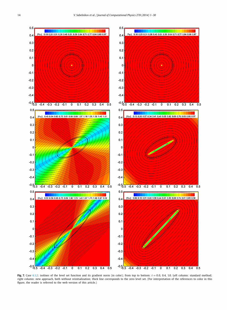
Results for the case 6.1.2: In this case the velocity field is divergence free, and in contrast to the previous case, the area enclosed by the interface should be conserved. First, we compare the new and the standard approaches, both without the reinitialization procedure. At different times, and for grid resolution 128 × 128, Fig. 7 shows the distributions of the level set and of norm of its gradient (in color). The standard approach without reinitialization is presented on the left, and the new approach on the right. Obviously, the new approach preserved the distance between level sets, and the gradient norm is equal to unity in most part of the computational domain. Noticeable exceptions represent points inside the zero level set, where discontinuities in ∇ϕ may appear on the intersection of normal to interface directions. In contrast, the standard approach displays a complex distribution around the zero-level set, with increased and decreased densities of level sets in the minor and major directions, respectively. For these two considered approaches, Fig. 8 shows the area enclosed by zero


Fig. 6. One-dimensional flow produced by a homogeneous strain; on the left: comparison of number of iterations in the reinitialization procedure; on the right: mean computational error in the interface location.

Table 2Case 6.1.1: L1 error computed by (56) for different meshes and methods at time t = 1.0.

Method/Mesh 64 128 256 512

Standard with reinitialization 1.23 × 10−5 6.75 × 10−7 4.82 × 10−7 3.00 × 10−8

New approach 8.58 × 10−10 1.05 × 10−10 1.30 × 10−11 1.62 × 10−12

level set. It is seen that after a certain time (t = 0.3 for 64 × 64; t = 0.5 for 128 × 128; t = 0.7 for 256 × 256), the flow is so stretched that due to approximations to source terms in (37)–(38), the new approach fails to keep this area constant. On the other hand, the solution from the standard approach without reinitializations exhibits large oscillations in computation of this area. Otherwise when the reinitialization procedure is activated in the standard approach, the numerical oscillations are suppressed, but, in comparison with the new approach, it incurs a supplementary loss of accuracy in the computation of area. This is shown in Fig. 9. Additionally to this comparison, the total number of iterations used in the reinitialization procedure is given in Fig. 10 for 128 × 128 grid points. This number in the standard approach is almost 40 against zero in the new approach. Fig. 11 and Fig. 12 assess different schemes for computation of the source term in the new approach. As noted earlier, we used the 5th-order WENO scheme with local Lax–Friedrichs approximation for the Hamiltonian, and we found that the use of the central schemes gives often the unstable numerical results. In Fig. 11, distribution of ϕ (isolines) and |∇ϕ| (in color) from 4th-order central scheme are compared versus 5th-order WENO scheme. 1D profile of ϕ along central line y = 0 is shown in Fig. 12. In these figures, the central difference scheme is presented on the left, and the WENO scheme on the right. It is seen that the central difference scheme produced oscillations in the points of discontinuity of ∇ϕ , while the use of the WENO scheme leads to the stable results.

We complete this subsection by answering one additional question: How the new approach is time-consuming in com-parison with the standard approach (1) but with no reinitializations of the level set. The results are summarized in Table 3. It is seen that the new approach is about twice more time-consuming than the standard approach without reinitializations.

6.2. Single vortex test

For this classical test, in which a circular interface is subjected to deformation by a single vortex flow, the conditions are taken from [31–33]. The initial zero level set is a circle centered at x1 = 0.5, x2 = 0.75 and its radius is 0.15. The interface in a computational domain Ω : [0, 1] × [0, 1] is deformed by the time-dependent velocity field given by the following stream function:

ψ(x1, x2) = 1

πsin2(πx1) sin2(πx2) cos(πt/T ) (67)

The maximum deformation is reached at time t = T /2, after which the interface is reversed to its initial circular shape at time t = T , when the flow returns to its initial state. In computation, T is taken to be 8. Our aim is to compare the interface resolution at t = T /2 and at t = T from standard and new approaches along with the zero-order and first-order local approximations for the source term coefficient, Eq. (37) and Eq. (38), respectively. In all computations, the CFL number (based on the maximum velocity) is set to 0.25. In the reinitialization procedure we use the convergence criterion (59) and the pseudo time step τ = 0.5x. The initial configuration and the reference solution at t = T /2, computed by the standard approach on the fine mesh, are shown in Fig. 13.


Fig. 7. Case 6.1.2: isolines of the level set function and its gradient norm (in color); from top to bottom: t = 0.0, 0.4, 1.0. Left column: standard method; right column: new approach, both without reinitialization; thick line corresponds to the zero level set. (For interpretation of the references to color in this figure, the reader is referred to the web version of this article.)


Fig. 8. Case 6.1.2: Evolution of the normalized area in new and standard approaches, both without reinitialization.

At time t = T /2, we compare the reference solution with computations on coarser grids containing 128 × 128 and 256 × 256 grid points. In this test problem, the local approximations Eq. (38) and Eq. (39) are valid only in the vicinity of the zero level set: the narrow band approach is used. To examine the influence of the band thickness, we considered three values of parameter γ = {24x, 12x, 6x}. The results of computations on 128 × 128 grid with the narrow band parameter γ = 12x are depicted in Fig. 14. Here, fifteen isolines of level set function are shown in the domain of narrow band; the thick red line represents the zero level set of ϕ at t = T /2 (the maximum stretching) and at t = T (return to initial shape). It is seen that both forms of local approximations, Eq. (38) and Eq. (39), give the interface configuration very similar to one from the standard method. When the grid resolution is further increased, as illustrated in Fig. 15 (256 × 256grid points are used in Fig. 15 instead of 128 × 128 grid points in Fig. 14), one can see that in cases “source term 1” and


Fig. 9. Case 6.1.2: Evolution of the normalized area in new and standard approaches, both with reinitialization.

“source term 2”, the stretched filament, and especially the returned shape of the interface at t = T become fairly better resolved than in the standard approach.

Although the convergence criterion in the reinitialization procedure for all approaches used herein is taken to be the same, the advantage of the new approach is seen when the average number of reinitializations and the L1 error (computed by Eq. (56) at t = T ) are compared for different approaches. This is reported in Table 4 and in Table 5, for 128 × 128 and 256 × 256 grid points, respectively. The results are given for different band thicknesses: γ = {24x, 12x, 6x}. In Table 4,


Fig. 10. Case 6.1.2: Number of iterations employed in reinitialization procedure for standard and new approach.

Fig. 11. Isolines of the level set function and its gradient norm (in color) for new approach at time t = 0.5. On the left: 4th-order central scheme; on the right: 5th-order Hamilton–Jacobi WENO scheme. (For interpretation of the references to color in this figure, the reader is referred to the web version of this article.)

it is seen that decreasing the band thickness for 128 × 128 grid points, one can improve the interface resolution using decreased number of reinitializations. In Table 5, this advantage is obvious for all band thicknesses used in computation.

6.3. Oscillating circle

This test case was proposed in [16]: in a computational domain Ω : [−5, 5] ×[−5, 5], the initially circular interface, with radius R = 3 and with center at x1 = 0, x2 = 0, is subject to a presumed velocity field, in which only the normal component is non-zero. The modulus of this component is defined by trigonometric functions of azimuth and time:

u = sn, s = cos(8Θ) sin(ωt), Θ = arctg

∣∣∣∣ x2

x1

∣∣∣∣, ω = 2π

T. (68)

The period of oscillation is set to T = 5. Parameters of simulation are chosen the same as in the original paper [16]. The time step t = 0.25x corresponds to CFL number of 0.25. In reinitialization procedure we use the convergence criterion (59) with ε = 5x and τ = 0.25x. The grid resolution is varying from 64 × 64 to 512 × 512 points. The normal vector nis approximated using the second-order central differences. To estimate the accuracy of different approaches and to compare our results with those from [16] we compute the mean shape error according to:


Fig. 12. 1D slice of the level set function along y = 0 for the new approach at time t = 0.5. On the left: 4th-order central scheme; on the right: 5th-order Hamilton–Jacobi WENO scheme.

Table 3Case 6.1.2: CPU time (in seconds) for the new and standard approaches with no reinitialization in both cases.

Method/Mesh 64 × 64 128 × 128 256 × 256 512 × 512

Standard 6.94 50.98 403.96 3225.7New approach 14.13 98.51 729.25 5559.0

Fig. 13. Single vortex test. On the left: initial circle and the initial velocity field plot; on the right: the reference solution at t = T /2 obtained by the standard approach on 1024 × 1024 computational grid without reinitialization of level sets.

Es = 1

NR

N∑k=1

(√x2

k + y2k − R

), (69)

where N is the number of sample points on the interface determined by linear interpolation between neighboring cells.The oscillating circle test is a particularly difficult one, since the interface shape is strongly coupled with the interface

motion. Small perturbations of the normal vector n to the interface may lead to errors in the level set function ϕ , and consequently, to a modification of the external velocity vector u. As noted in [16], this test case requires a large number of reinitializations of the level set function. Otherwise, when the standard approach is used without reinitializations, the interface shape suffers from strong oscillations. The results of computation and comparison between the appraising ap-proaches are illustrated in Fig. 16 and Fig. 17 at times t = 2.5 and t = 5.0, respectively. Time t = 5.0 corresponds to the return of convected interface back to its initial circled shape. Here, fifteen iso-lines of ϕ are shown in the narrow band domain (γ = 12x), and the thick line represents the zero level set. As to t = 2.5, all considered approaches give similar


Fig. 14. Single vortex test. Isolines of level set function at t = T /2 and t = T (in the upper right-hand corner) using the standard approach and the new approach (“source term 1” and “source term 2”) in the narrow band domain with γ = 12x. Here, 15 level sets of ϕ are shown in the narrow band domain; thick red line represents the zero level set of ϕ . Grid resolution: 128 × 128 points. (For interpretation of the references to color in this figure, the reader is referred to the web version of this article.)

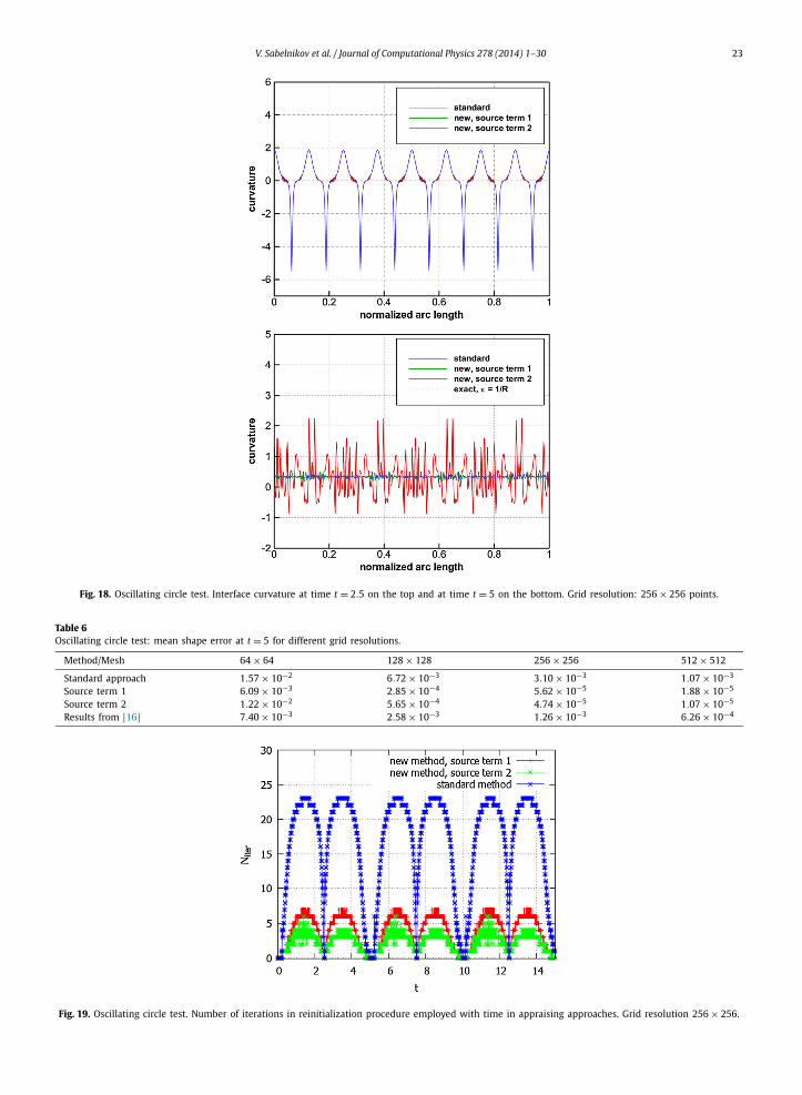
configuration. However, the returned circled shape at t = 5.0 is different, and is fairly better presented by the new approach. It is clearly seen in Fig. 17: the zero and first-order local approximations lead to the smoothed circled shape. In the next figure, Fig. 18, such an improvement is demonstrated by calculation of the curvature along the normalized arc length at t = 2.5 (on the top) and t = 5 (on the bottom). It is seen that spurious modes, developed in computation of the curvature by the standard approach, are remarkably reduced when the new approach is used.

This was observed for different grid resolutions: 64 × 64; 128 × 128; 256 × 256; 512 × 512. The mean shape error is given in Table 6 by the standard approach, and by the zero- and first-order local approximations. Starting from 128 × 128 grid points, the new approach gives the error an order less compared to other results. Additionally to this improved computation of the curvature, the number of iterations in the reinitialization procedure is approximately five times less in the new approach than in the standard one. This is shown in Fig. 19, in which the number of iterations used by zero- and first-order local approximations is confronted to results from the standard approach. As expected, it is seen in this figure that higher order local approximation requires less of reinitializations. Table 7 concludes the oscillating circle test: the mean number of iterations, the mean computational cost per time-step and the numerical error are given for the returned shape at t = 5.0applying the standard approach and the zero- and first-order local approximations. Computational efficiency of the latter is clearly seen.

6.4. Propagation of the premixed flame front

Another interesting example, wherein the interface configuration is coupled with its advancement, is the propagation of the premixed flame in the framework of the G-equation. In this formulation, the flame front is governed by the following evolution equation:

∂ϕ

∂t+ u · ∇ϕ = uF |∇ϕ|, (70)

with the following initial condition ϕ0(x, y) = −x + x0. Here uF is a proper speed of the flame front, u determines the external flow field, x0 corresponds to initial position of the flame front. It is assumed that ϕ(x, y, t) > 0 in the burnt gas.


Fig. 15. Single vortex test. Isolines of level set function at t = T /2 and t = T (in the upper right-hand corner) using the standard approach and the new approach (“source term 1” and “source term 2”) in the narrow band domain with γ = 12x. Here, 15 level sets of ϕ are shown in the narrow band domain; thick red line represents the zero level set of ϕ . Grid resolution: 256 × 256 points. (For interpretation of the references to color in this figure legend, the reader is referred to the web version of this article.)

Consequently, the flame propagates from the left to the right. At initial time, all level surfaces of ϕ(x, y, t) are planes normal to the x direction. Another form of (70) is this:

∂ϕ

∂t+ (u − uF n) · ∇ϕ = 0. (71)

It is seen that advection of ϕ is controlled by prescribed velocity field and by the front propagation speed, which in turn, depends on the normal vector n. In our calculation we presumed the shear velocity field:

u = λ(1 + ε cos(ky)

)cos(2ky), v = 0. (72)

As in the previous example, a computational domain Ω : [0, 1] × [0, 1] is discretized by uniform grid. Parameters of calcula-tions are as follows: the flame front speed is uF = 1.0, the shear intensity parameter is λ = 0.4, the intensity of modulation ε = 0.5 and the wave number is k = 8π . The flame front is initially located at x0 = 0.2. The final time of computation is t = 0.5. In Fig. 20, three plots of the premixed flame front at time t = 0.4 are shown from numerical integration on the mesh 64 × 64: results on the left are obtained by the standard approach with reinitialization; in the middle – by the zero-order local approximation; on the right – by the first-order local approximation. Below these plots, three fronts are compared with the reference solution from the standard approach using the fine grid with 512 × 512 points. It is seen that computations with the new approach (for both local approximations to the source term) give the flame front location closer to the reference solution than in the case of the standard approach. The same was observed for other times. The difference in a favor of the new approach is also seen from the curvature computation at the leading edge of the front in Fig. 21: the cusped zones of the front are better resolved. What is remarkable at the moment is the number of iterations employed in the reinitialization procedure. This number (averaged in time) is fairly different: 29.4 iterations for the standard approach, 16.4 iterations for zero-order local approximation and 15.2 iterations for the first-order local approximation.


Table 4Single vortex test. Influence of the narrow band thickness. Averaged number of iterations and L1 error computed by (56) at t = T for different approaches. Grid resolution: 128 × 128 points.

Parameter γ Standard “Source term 1” “Source term 2”

〈Niter〉 E1 〈Niter〉 E1 〈Niter〉 E1

γ = 24x 19.2 4.7145 × 10−2 18.5 4.9255 × 10−2 18.9 5.2405 × 10−2

γ = 12x 19.2 4.6767 × 10−2 9.6 2.8977 × 10−2 8.9 3.1349 × 10−2

γ = 6x 19.5 4.7873 × 10−2 8.7 2.7459 × 10−2 6.9 2.4487 × 10−2

Table 5Single vortex test. Influence of the narrow band thickness. Averaged number of iterations and L1 error computed by (56) at t = T for different approaches. Grid resolution: 256 × 256 points.

Parameter γ Standard “Source term 1” “Source term 2”

〈Niter〉 E1 〈Niter〉 E1 〈Niter〉 E1

γ = 24x 12.6 1.0617 × 10−2 10.3 5.4352 × 10−3 9.9 5.7632 × 10−3

γ = 12x 12.6 1.0628 × 10−2 7.8 5.3870 × 10−3 7.4 5.3065 × 10−3

γ = 6x 12.8 1.0809 × 10−2 7.1 5.3861 × 10−3 6.3 5.1724 × 10−3

Fig. 16. Oscillating circle test. Isolines of level set function are computed by standard and new approaches. New approach: zero-order local approximation – source term 1; first-order local approximation – source term 2; exact expression of the source term coefficient – source term 3. Here, 15 isolines of ϕ are shown in the narrow band domain with γ = 12x, thick red line represents the zero level set of ϕ . Grid resolution: 256 × 256 points. (For interpretation of the references to color in this figure legend, the reader is referred to the web version of this article.)

6.5. Merging test in the stagnation-point flow with the divergence-free velocity field

There are complicated situations when the interface is subject to extreme changes, e.g., merging or pinching off. Ver-sus the standard approach, the question raising is how the new approach may behave in such situations. For answering,


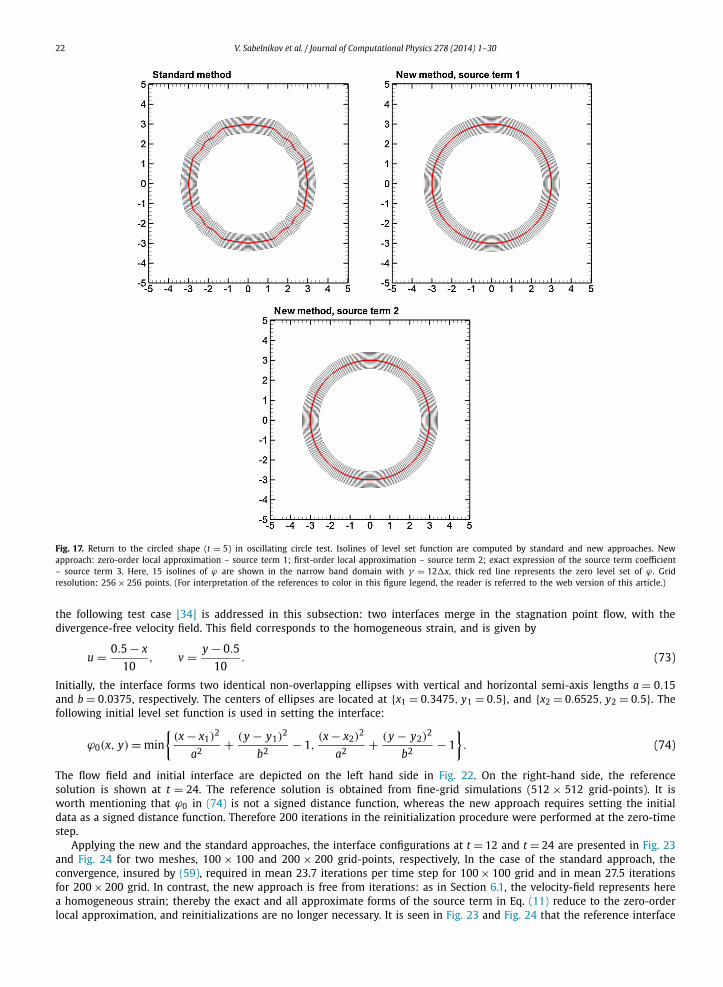
Fig. 17. Return to the circled shape (t = 5) in oscillating circle test. Isolines of level set function are computed by standard and new approaches. New approach: zero-order local approximation – source term 1; first-order local approximation – source term 2; exact expression of the source term coefficient – source term 3. Here, 15 isolines of ϕ are shown in the narrow band domain with γ = 12x, thick red line represents the zero level set of ϕ . Grid resolution: 256 × 256 points. (For interpretation of the references to color in this figure legend, the reader is referred to the web version of this article.)

the following test case [34] is addressed in this subsection: two interfaces merge in the stagnation point flow, with the divergence-free velocity field. This field corresponds to the homogeneous strain, and is given by

u = 0.5 − x

10, v = y − 0.5

10. (73)

Initially, the interface forms two identical non-overlapping ellipses with vertical and horizontal semi-axis lengths a = 0.15and b = 0.0375, respectively. The centers of ellipses are located at {x1 = 0.3475, y1 = 0.5}, and {x2 = 0.6525, y2 = 0.5}. The following initial level set function is used in setting the interface:

ϕ0(x, y) = min

{(x − x1)

2

a2+ (y − y1)

2

b2− 1,

(x − x2)2

a2+ (y − y2)

2

b2− 1

}. (74)

The flow field and initial interface are depicted on the left hand side in Fig. 22. On the right-hand side, the reference solution is shown at t = 24. The reference solution is obtained from fine-grid simulations (512 × 512 grid-points). It is worth mentioning that ϕ0 in (74) is not a signed distance function, whereas the new approach requires setting the initial data as a signed distance function. Therefore 200 iterations in the reinitialization procedure were performed at the zero-time step.

Applying the new and the standard approaches, the interface configurations at t = 12 and t = 24 are presented in Fig. 23and Fig. 24 for two meshes, 100 × 100 and 200 × 200 grid-points, respectively, In the case of the standard approach, the convergence, insured by (59), required in mean 23.7 iterations per time step for 100 × 100 grid and in mean 27.5 iterations for 200 × 200 grid. In contrast, the new approach is free from iterations: as in Section 6.1, the velocity-field represents here a homogeneous strain; thereby the exact and all approximate forms of the source term in Eq. (11) reduce to the zero-order local approximation, and reinitializations are no longer necessary. It is seen in Fig. 23 and Fig. 24 that the reference interface


Fig. 18. Oscillating circle test. Interface curvature at time t = 2.5 on the top and at time t = 5 on the bottom. Grid resolution: 256 × 256 points.

Table 6Oscillating circle test: mean shape error at t = 5 for different grid resolutions.

Method/Mesh 64 × 64 128 × 128 256 × 256 512 × 512

Standard approach 1.57 × 10−2 6.72 × 10−3 3.10 × 10−3 1.07 × 10−3

Source term 1 6.09 × 10−3 2.85 × 10−4 5.62 × 10−5 1.88 × 10−5

Source term 2 1.22 × 10−2 5.65 × 10−4 4.74 × 10−5 1.07 × 10−5

Results from [16] 7.40 × 10−3 2.58 × 10−3 1.26 × 10−3 6.26 × 10−4

Fig. 19. Oscillating circle test. Number of iterations in reinitialization procedure employed with time in appraising approaches. Grid resolution 256 × 256.


Table 7Oscillating circle test. Averaged number of iterations, computational cost per time-step and mean shape error. Grid resolution: 256 × 256 points.

Method 〈Niter〉 CPU time, seconds Shape error

Standard method 16.56 0.5758 3.10 × 10−3

Source term 1 3.89 0.1960 5.62 × 10−5

Source term 2 2.23 0.1745 4.74 × 10−5

Fig. 20. Premixed flame test. On the top: 15 isolines of the level set function in the narrow band at time t = 0.4. Interface location is represented by the thick line; on the bottom: three fronts put together. Red line depicts the standard method, green – the source term 1, blue – the source term 2. Dashed line depicts the reference solution. (For interpretation of the references to color in this figure legend, the reader is referred to the web version of this article.)

is much better represented by the new approach for both meshes used in computation, especially for 100 × 100 grid-points (contrary to the standard approach, where two ellipses are coalesced). The useful information on the area loss is given in Table 8. It is seen that in both approaches, a finer-grid is characterized by the decreased area lost; less of the area lost is measured in the case of the new approach, except a slight difference for 200 × 200 grid-points.

7. Final remarks

In this paper we proposed a new form of the level set equation (11) adding a source term such that the eikonal equation is automatically satisfied. On the interface, this source term is zero; thereby the zero level set is not affected by the embed-ded source term. In the exact formulation, the source term is determined by the non-local equation (19). From the strict equation, we proposed to derive the local approximate forms of the source term. These local approximations are specified for zero-, first- and second-order accuracy in the form of Eqs. (31)–(37), respectively.

The new form of the level set is assessed in different test cases where the velocity field is prescribed. First, the different test cases with one- and two-dimensional flows, produced by a homogeneous strain, were addressed. It should be noted that in the case of a homogeneous strain, all approximate forms coincide with the exact form of the source term. The results from the new approach were compared with the analytical solution and with the solution to the standard level set equation, with and without reinitializations. The numerical results showed that in comparison with the standard level set equation,


Fig. 21. Premixed flame test. Interface curvature at t = 0.4 for the standard and the new approach on 64 × 64 grid. Dashed line corresponds to the reference solution.

Fig. 22. Merging test. On the left: initial interfaces and flow field; on the right: resolved fine grid solution at t = 24.

Fig. 23. Merging test. Zero level set at t = 12 on the left and t = 24 on the right. The red line corresponds to the standard method, the blue line – to the new approach. Grid resolution 100 × 100. (For interpretation of the references to color in this figure legend, the reader is referred to the web version of this article.)

the modified level set equation enhanced both the computational efficiency and the accuracy in predicting the interface (namely, its location, shape and area). Additionally, the new approach was assessed by the test case, in which the interface undergoes merging in the stagnation point flow with the divergence-free velocity field. For this test case, results from the new and standard methods are compared with the reference fine-grid simulation for two merging ellipses. The advantage of the new method was clearly observed using a series of uniformly spaced meshes.


Fig. 24. Merging test. Zero level set at t = 12 on the left and t = 24 on the right. The red line corresponds to the standard method, the blue line – to the new approach. Grid resolution 200 × 200. (For interpretation of the references to color in this figure legend, the reader is referred to the web version of this article.)

Table 8Merging test. Area loss at t = 24 for different grid resolutions.

Method/Mesh 50 × 50 100 × 100 200 × 200

Standard 87.54% 14.59% 1.43%New 23.60% 5.92% 1.99%

It is worth noting that the test cases considered in this article don’t include the interfaces with corners. The well-known example of such a surface is the rotation of Zalesak’s slotted disc, so called the Zalesak problem. In a solid body rotation flow, which is a particular case of the homogeneous strain, the distance between any two given points remains constant in time, therefore if ϕ(x, t) is initially an exact distance function, then theoretically, ϕ(x, t) will maintain this property at all times. But, since there are corners in the interface, the numerical error indicator E = ||∇ϕ(x, t)| − 1| can be tripped even if ϕ(x, t) is initially an exact distance function at the grid points. The same conclusion is valid for the evolution of the surfaces with corners in the homogeneous strain, calculated with new approach (11), (42).

The new approach was also assessed for more general velocity fields. In the considered test cases, all approximate forms of the source term are valid only in the vicinity of the interface. Then in order to preserve the local character of the source term approximations, we used a narrow band approach. First, we performed simulations for the classical test case of the interface stretched by a single vortex. Compared to the standard approach with the reinitialization procedure, we observed that the use of approximate forms of the source term leads to a fairly better resolution of the interface. Moreover, the number of reinitializations is progressively decreased in comparison with the standard approach, according to the order of accuracy of the local approximation. The next test case was addressed to the oscillating circle. The particularity of this test case consists in the strong coupling between the interface shape and its dynamics. Here again, in comparison with the standard approach with the reinitialization procedure, the new approach allowed to resolve much better the curvature and the position of the interface. Furthermore, the spurious oscillations on the interface were effectively suppressed, and the number of reinitializations of level sets was significantly decreased. Another test case concerns the premixed flame. This test was motivated by its practical importance. A simple two-dimensional configuration with the presumed shear for the velocity field was considered. It was shown that relevant to the reference solution, and comparing to standard approach, the cusped zones of the flame front were better simulated by the new approach. Moreover, the number of iterations, used in the reinitialization procedure, was remarkable decreased by the new approach. In the future, we are motivated in revisiting this test but in a more complex configuration.

Overall, because of reduced cost and increased accuracy, and also because of ease of use, we believe that the new approach proposed in this paper can be effectively applied as a tool for the simulation of interface dynamics.

Acknowledgements

The authors are pleased to express their gratitude to Giovanni Russo for his useful comments and support of this work. A.O. and M.G. acknowledge support from CTR, Stanford University, and in particular, the hospitality of Parviz Moin during the Summer Program 2012. V.S. was supported by ONERA. He acknowledges also the support from the Nordic Institute for Theoretical Physics and in particular, the hospitality of Axel Brandenburg during the NORDITA Turbulent Combustion program 2010. A.O. and M.G. also acknowledge the support from the CANNEX program (ANR-13-TDMO-0003). Finally, the authors are very grateful to two Reviewers for their help and indeed valuable comments – we are deeply impressed by the work done by those Reviewers.


Appendix A. Simple illustration of the reinitialization procedure

Consider the case of non-rotational time-independent strain u = −kx, k ≡ const > 0. The one-dimensional level set equa-tion is

∂G

∂t− kx

∂G

∂x= 0, G(x, t = 0) = −x + x0 (A.1)

Its exact solution may readily be verified:

G(x, t) = −exp(kt)x + x0 (A.2)

It is seen that the norm of gradient of this solution grows exponentially:

∣∣∇G(x, t)∣∣ =

∣∣∣∣∂G

∂x

∣∣∣∣ = exp(kt)t→∞−−−→ ∞ (A.3)

and the position x f (t) of the zero level, G(x f (t), t) = 0, changes with time according to:

x f (t) = x0 exp(−kt) (A.4)

The exponential growth of level set gradients involves progressively the approximation error in G(x, t); it degrades the numerical accuracy for the zero level set. Our simple illustration of the reinitialization procedure deals with the explicit Euler scheme. In integration of (A.1), the advancement in time after the first time step gives

G(t) = G|t=0 + kx∂G

∂x

∣∣∣∣t=0

t = −x(1 + kt) + x0 (A.5)

∣∣∣∣∂G(t)

∂x

∣∣∣∣ = (1 + kt) > 1 (A.6)

Thereby according to (A.5), the position of the zero level G(x f (t)) = 0 moves from x0 to

x f (t) = x0

(1 + kt)(A.7)

After the second step, we have

G(2t) = G(t) + kx∂G

∂x

∣∣∣∣t=t

t = −x(1 + kt) + x0 − kx(1 + kt)t = −x(1 + kt)2 + x0 (A.8)

and the new position of zero level

x f (2t) = x f (t)

(1 + kt)= x0

(1 + kt)2(A.9)

After N = t/t steps, the recursion is

G(t = Nt) = −x(1 + kNt)N + x0 = −x

(1 + k

t

N

)N

+ x0 (A.10)

and discrete positions of the zero level set, G(x f (t)) = 0, are determined by:

x f (t = Nt) = x0

(1 + kNt)N= x0

(1 + k

t

N

)−N

(A.11)

Obviously, if N → ∞ (A.10), (A.11) reduce to (A.2), (A.4), respectively. Now after each single-step, let us reinitialize the level set. After the first step, G(t) field, given by solution (A.5), should be replaced by the new one, say Grein(t) field, in which the zero level is the same as in original field, i.e. it is determined by x f (t) from (A.7), and the norm of gradient of this new field should be equal to unity. To this end, Grein(t) is simply represented by translation of initial field G(x, t = 0) = −x + x0to

Grein(t) = −x + x f (t), (A.12)∣∣∣∣∂Grein(t)

∂x

∣∣∣∣ = 1 (A.13)

Then the second step will start from (A.12), and not from (A.5). Instead of (A.8), we have the level set equation:

G(2t) = Grein(t) + kx∂Grein

∂x

∣∣∣∣t=t

t = −x(1 + kt) + x f (t) (A.14)

∣∣∣∣∂ G(2t)∣∣∣∣ = (1 + kt) > 1 (A.15)

∂x


Note that the zero level in (A.14), −x f (2t)(1 + kt) + x f (t) = 0, has the same new position x f (2t), as the zero level in original field G(2t), and is determined by (A.9). The reinitialization of G(2t) is similar to reinitialization of G(t): it corresponds to translation of Grein(t) from (A.12) to

Grein(2t) = −x + x f (2t),

∣∣∣∣∂Grein(2t)

∂x

∣∣∣∣ = 1 (A.16)

The third step starts from (A.16):

G(3t) = Grein(2t) + kx∂Grein

∂x

∣∣∣∣t=2t

t = −x(1 + kt) + x f (2t) (A.17)

∣∣∣∣∂ G(3t)

∂x

∣∣∣∣ = (1 + kt) > 1 (A.18)

Here again the zero level position at t = 3t coincides with the zero level position x f (3t) in original field G(x f (3t)) = 0, and reinitialization of G(3t) consists in translation of Grein(2t) to

Grein(3t) = −x + x f (3t),

∣∣∣∣∂Grein(3t)

∂x

∣∣∣∣ = 1 (A.19)

Performing the reinitialization at each consecutive time step, we obtain after N time steps

Grein((N − 1)t

) = −x + x f((N − 1)t

),

∣∣∣∣∂Grein((N − 1)t)

∂x

∣∣∣∣ = 1 (A.20)

which represents the intermediate level set function in interval [(N − 1)t, Nt]. Then at t = Nt , the level sets are updated by the level set equation to

G(Nt) = −x(1 + kt) + x f((N − 1)t

),

∣∣∣∣∂ G(Nt)

∂x

∣∣∣∣ = (1 + kt) > 1 (A.21)

Thus at each time the reinitialization procedure is carried out by two stages: preliminary level set translation Gren(x, t) =−x + x f (t), | ∂Grein

∂x | = 1, and then computation of updated level set by the level set equation.

Appendix B. Derivation of local approximations from the exact equation for A

In Eq. (14) the following expansions in a Taylor series are used:

A = A0 + A1ϕ + . . . (B.1)

∂uk

∂xi=

(∂uk

∂xi

)∣∣∣∣n=0

+(

∂2uk

∂xi∂xl

)∣∣∣∣n=0

dxl + . . . (B.2)

where dxl = ∂ϕ∂xl

ϕ . Inserting these expansions into (14) yields

A0 + A1ϕ = −ϕ∂ϕ

∂xi

∂

∂xi(A0 + A1ϕ) + ∂ϕ

∂xi

[∂uk

∂xi

∣∣∣∣n=0

+ ∂2uk

∂xi∂xl

∣∣∣∣n=0

∂ϕ

∂xlϕ

]∂ϕ

∂xk(B.3)

By equating coefficients at coincident powers of ϕ , we write

A0 = ∂ϕ

∂xi

(∂uk

∂xi

)∣∣∣∣n=0

∂ϕ

∂xk=

(∂uknk

∂n

)∣∣∣∣n=0

(B.4)

A1 = −A1∂ϕ

∂xi

∂ϕ

∂xi+ ∂ϕ

∂xi

(∂2ui

∂xk∂xl

)∣∣∣∣n=0

∂ϕ

∂xk

∂ϕ

∂xl. (B.5)

From (B.5), taking into account that ∂ϕ∂xi

∂ϕ∂xi

= |∇ϕ|2 = 1, we obtain

A1 = 1

2

∂ϕ

∂xi

∂ϕ

∂xl

(∂2ui

∂xk∂xl

)∣∣∣∣n=0

∂ϕ

∂xk= 1

2

(∂2uknk

∂n2

)∣∣∣∣n=0

. (B.6)

It is seen that (B.4) and (B.6) are coincident with (28). The higher-order coefficients can be obtained by the same proceeding.It is worth to note that for velocity field produced by homogeneous strain all local approximations coincide with the

exact form of the source term. Let us consider the velocity field which is given by

uk(x, t) = Lkl(t)xl, k = 1,2,3 (B.7)


Here the components of the velocity gradient tensor, Lkl , depend at most on time. All spatial derivatives of the velocity of order higher than one are equal to zero, and consequently, all local approximations to the source term coefficient, as well as its exact form, are coincident, and are equal to the zero-order local approximation, i.e.:

uknk − (uknk)|n=0 = Lkl∂ϕ

∂xk

∂ϕ

∂xlϕ (B.8)

Indeed, consider a value of the velocity components on the interface ϕ(x f (t), t) = 0:

(uk)|n=0 = (uk)|x−ϕ∇ϕ = Lkl

(xl − ϕ

∂ϕ

∂xl

)(B.9)

Using (B.9) and property that nk = (nk)|n=0 along characteristics of the eikonal equation, we may rewrite the left hand side in (B.8) in the following form:

uknk − (uknk)|n=0 = (uk − (uk)|n=0

) ∂ϕ

∂xk=

(Lklxl − Lkl

[xl − ϕ

∂ϕ

∂xl

])∂ϕ

∂xk= Lkl

∂ϕ

∂xl

∂ϕ

∂xkϕ = AL A,0ϕ.

Appendix C. WENO scheme for left and right derivatives

Consider a specific grid point i. To find the left-biased derivative ϕ−x , set

v1 = ϕi−2 − ϕi−3

x, v2 = ϕi−1 − ϕi−2

x,

v3 = ϕi − ϕi−1

x, v4 = ϕi+1 − ϕi

x,

v5 = ϕi+2 − ϕi+1

x. (C.1)

And to find the right-biased derivative find ϕ+x , set

v1 = ϕi+3 − ϕi+2

x, v2 = ϕi+2 − ϕi+1

x,

v3 = ϕi+1 − ϕi

x, v4 = ϕi − ϕi−1

x,

v5 = ϕi−1 − ϕi−2

x. (C.2)

Next we define the smoothness indicators

IS1 = 13

12(v1 − 2v2 + v3)

2 + 1

4(v1 − 4v2 + 3v3)

2,

IS2 = 13

12(v2 − 2v3 + v4)

2 + 1

4(v2 − v4)

2,

IS3 = 13

12(v3 − 2v4 + v5)

2 + 1

4(3v3 − 4v4 + v5)

2, (C.3)

and the weights

αk = dk

(ε + ISk)2, ωk = αk

α1 + α2 + α3, k = 1,2,3. (C.4)

Here the optimal weights d1 = 0.1, d2 = 0.6, d3 = 0.3. To avoid division by zero we use ε = 10−6. Finally, we get

(ϕ±

x

)i = ω1

(v1

3− 7v2

6+ 11v3

6

)+ ω2

(−v2

6+ 5v3

6+ v4

3

)+ ω3

(v3

3+ 5v4

6− v5

6

). (C.5)

References

[1] S.J. Osher, J.A. Sethian, Fronts propagating with curvature dependent speed: algorithms based on Hamilton–Jacobi formulations, J. Comput. Phys. 79 (1988) 12–49.

[2] J.A. Sethian, Level Set Methods: Evolving Interfaces in Geometry, Fluid Mechanics, Computer Vision, and Materials Science, Cambridge University Press, Cambridge, UK, 1996.

[3] J.A. Sethian, Level Set Methods and Fast Marching Methods, Cambridge University Press, Cambridge, UK, 1999.[4] S. Osher, R. Fedkiw, Level Set Methods and Dynamic Implicit Surfaces, Springer-Verlag, New York, 2002.[5] D. Chopp, Computing minimal surface via level set curvature flow, J. Comput. Phys. 106 (1) (1993) 77–91.

http://refhub.elsevier.com/S0021-9991(14)00572-5/bib31s1








[6] J.A. Sethian, Fast marching level set methods for three dimensional photolithography development, Proc. SPIE 2726 (1996) 261–272.[7] J.A. Sethian, Fast marching methods, SIAM Rev. 41 (2) (1999) 199–235.[8] D.L. Chopp, Some improvements of the fast marching method, SIAM J. Sci. Comput. 23 (1) (2002) 230–244.[9] Y.R. Tsai, L.-T. Cheng, S. Osher, H.K. Zhao, Fast sweeping algorithms for a class of Hamilton–Jacobi equations, SIAM J. Numer. Anal. 41 (2) (2003)

673–694.[10] H. Zhao, A fast sweeping method for eikonal equations, Math. Comput. 74 (2005) 603–627.[11] M. Sussman, P. Smereka, S. Osher, A level set approach for computing solutions to incompressible two-phase flow, J. Comput. Phys. 114 (1994) 146–159.[12] G. Russo, P. Smereka, A remark on computing distance functions, J. Comput. Phys. 163 (2000) 51–67.[13] A. Du Chéné, C. Min, F. Gibou, Second-order accurate computation of curvatures in a level set framework using novel high-order reinitialization

schemes, J. Sci. Comput. 35 (2008) 114–131.[14] M. Sussman, E. Fatemi, Efficient, interface-preserving level set redistancing algorithm and its application to interfacial incompressible fluid flow, SIAM

J. Sci. Comput. 20 (4) (1999) 1165–1191.[15] D. Hartmann, M. Meinke, W. Schröder, Differential equation based constrained reinitialization for level set methods, J. Comput. Phys. 227 (2008)

6821–6845.[16] D. Hartmann, M. Meinke, W. Schröder, The constrained reinitialization equation for level set methods, J. Comput. Phys. 229 (2010) 1514–1535.[17] L.-T. Cheng, Y.R. Tsai, Redistancing by flow of time dependent eikonal equation, J. Comput. Phys. 227 (8) (2008) 4002–4017.[18] C. Min, On reinitializing level set functions, J. Comput. Phys. 229 (2010) 2764–2772.[19] H. Zhao, T. Chan, B. Merriman, S. Osher, A variational level set approach to multiphase motion, J. Comput. Phys. 127 (1996) 179–195.[20] D. Adalsteinsson, J.A. Sethian, The fast construction of extension velocities in level set methods, J. Comput. Phys. 148 (1999) 2–22.[21] J. Gomes, O. Faugeras, Reconciling distance functions and level sets, J. Vis. Commun. Image Represent. 11 (2000) 209–223.[22] D.L. Chopp, Another look at velocity extensions in the level set method, SIAM J. Sci. Comput. 31 (5) (2009) 3255–3273.[23] V. Sabel’nikov, A.Yu. Ovsyannikov, M. Gorokhovski, Modified level set equation for gas–liquid interfaces and its numerical solution, in: Proceedings of

6th European Congress on Computational Methods in Applied Sciences and Engineering, ECCOMAS 2012, Vienna, Austria, 2012, pp. 5597–5611.[24] D. Adalsteinsson, J.A. Sethian, A fast level set method for propagating interfaces, J. Comput. Phys. 118 (1995) 269–277.[25] D.P. Peng, B. Merriman, S. Osher, H.K. Zhao, M.J. Kang, A PDE-based fast local level set method, J. Comput. Phys. 155 (1999) 410–438.[26] P. Gomez, J. Hernandez, J. Lopez, On the reinitialization procedure in a narrow-band locally refined level set method for interfacial flows, Int. J. Numer.

Methods Eng. 63 (2005) 1478–1512.[27] M. Herrmann, A balanced force refined level set grid method for two-phase flows on unstructured flow solver grids, J. Comput. Phys. 227 (2008)

2674–2706.[28] G.-S. Jiang, C.-W. Shu, Efficient implementation of weighted ENO schemes, J. Comput. Phys. 126 (1996) 202–228.[29] G.-S. Jiang, D. Peng, Weighted ENO schemes for Hamilton–Jacobi equations, SIAM J. Sci. Comput. 21 (2000) 2126–2143.[30] C.-W. Shu, S.J. Osher, Efficient implementation of essentially non-oscillatory shock-capturing schemes, J. Comput. Phys. 77 (1988) 439–471.[31] J. Bell, P. Colella, H. Glaz, A second-order projection method for the incompressible Navier–Stokes equations, J. Comput. Phys. 85 (1989) 257.[32] W. Rider, D. Kothe, Reconstructing volume tracking, J. Comput. Phys. 141 (1998) 112–152.[33] D. Enright, R. Fedkiw, J. Ferziger, I. Mitchell, A hybrid particle level set method for improved interface capturing, J. Comput. Phys. 183 (2002) 83–116.[34] H. Samuel, A level set two-way wave equation approach for Eulerian interface tracking, J. Comput. Phys. 259 (2014) 617–635.





































Modified level set equation and its numerical assessment

Documents

Transcript of Modified level set equation and its numerical assessment