Energy and Environment Research; Vol. 5, No. 1; 2015 ISSN 1927-0569 E-ISSN 1927-0577

Published by Canadian Center of Science and Education

49

Modelling the Potential Impact of Climate Change on Agricultural Production in the Province of British Columbia

Liliana Perez1, Trisalyn A. Nelson2, Mathieu Bourbonnais2 & Aleck Ostry3 1 Département de géographie, Université de Montréal, Montreal, QC, Canada 2 Spatial Pattern Analysis and Research Laboratory, Department of Geography, University of Victoria, Victoria, BC, Canada 3 Department of Geography, University of Victoria, Victoria, BC, Canada

Correspondence: Trisalyn Nelson, Spatial Pattern Analysis and Research Laboratory, Department of Geography, University of Victoria, Victoria, BC, V8W 3R4, Canada. Tel: 1-250-472-5620. E-mail: trisalyn@uvic.ca

Received: September 23, 2013 Accepted: October 11, 2013 Online Published: April 8, 2015

doi:10.5539/eer.v5n1p49 URL: http://dx.doi.org/10.5539/eer.v5n1p49

The research is financed by a SSHRC Insight Development Grant

Abstract The goal of this research was to model the potential impact of climate change on food production, in the Fraser Valley and Peace River regions of British Columbia (BC), using historical crop yield and climate data. We identified eight indicator crops of importance for these regions of BC and utilized historical Census of Agriculture and climate data (temperature and precipitation) to model future potential impacts of climate change on agriculture. We developed three climate change scenarios for these eight indicators crops (extreme, moderate, and business as usual). Under the most extreme climate model scenario the Fraser Valley is expected to experience cooler summers and springs and wetter summers, with incremental increases in oat, blueberry and green bean yields by 2050. These same climate conditions were predicted to decrease the yields for raspberry crops by 2050, while barley and wheat crop yields remain steady. The business as usual scenario, where springs and summers are warmer and summers are wetter in the Fraser Valley, predicted increased barley, oat, wheat, and blueberry crop yields by 2050, while yields of raspberries were predicted to decrease and green bean yields are expected to be steady. Under the more conservative climate change scenario conditions, yields should remain steady for all crops, except green beans where yields will increase by 2050. Future climate conditions for the Peace River area were much different from the Fraser Valley. All three scenarios forecasted warmer and wetter springs and summers with decreased evapotranspiration and moisture deficits. These changes in climate conditions predicted declines in wheat, canola, and barley crop yields by 2050, while incremental increases in oat and dry pea crop yields could be expected by 2050. Keywords: climate change, food production, Fraser Valley, Peace River, indicator crops, crop yields

1. Introduction The climate has been changing over the last three decades and is expected continue to do so regardless of any mitigation strategy (Barker, 2007; IPCC, 2007). Temperatures are predicted to increase about 3–5 °C by the middle of the 21st century, while precipitation patterns (amount, seasonality, and intensity) are predicted to shift (Arnell et al., 2004; IPCC, 2007). Agriculture is a climate-dependent activity and hence is highly sensitive to climatic change and climate variability (Lobell & Field, 2007; Rivington et al., 2013). Crop yields are vulnerable to these changes in climate (Rivington et al., 2013; Thornton, Jones, Ericksen, & Challinor, 2011), which can jeopardize food security and economic sustainability that provide the necessary input for sustaining people’s livelihoods (FAO, 2012; FAO, WFP & IFAD, 2012). Agriculture is a key driver of national and local economies and largely depends on what can be grown and how efficiently it can be done, taking into consideration variations in climatic trends.

A literature review of the impact of climatic trends on crop yields (Bradshaw, Dolan, & Smit, 2004; Bryant et al., 2000; Joshi, Maharjan, & Luni, 2011; Lobell, Field, Cahill, & Bonfils, 2006) indicated that changes in growing season temperature and precipitation drive annual variation in average yields (Lobell & Field, 2007; Peng et al.,

www.ccsenet.org/eer Energy and Environment Research Vol. 5, No. 1; 2015

50

2004). Crop yields are a function of dynamic, nonlinear interactions between climate, soil water, management, and the physiology of the crop (Semenov & Porter, 1995). For example, changes in the variability of temperature can greatly influence dry matter production as both high and low temperatures decrease the rate of dry matter production and, at extremes, can cause production to cease (Grace, 1988; Ingver, Tamm, Tamm, Kangor, & Koppel,, 2010). Likewise, water deficit occurring immediately before flowering can lead to pollen sterility and will result in a drastic decline in grain yield (Ingver et al., 2010; Nguyen & Sutton, 2009; Thakur, Kumar, Malik, Berger, & Nayyar, 2010). Previous research relating predicted climatic variations to crop response have offered the potential to anticipate changes in crop production early enough to adjust critical decisions (Blench, 2003; Hansen, 2002; Letson et al., 2001).

To study the implications of climate change in British Columbia (BC) agriculture we selected eight indicator crops from three different food groups (grains, fruits, and vegetables). In the grains group we chose barley, spring wheat, oat, canola, and dry peas. Grains have been documented (Joshi et al., 2011; Subedi, Gregory, Summerfield, & Gooding, 1998; Thakur et al., 2010; Willenbockel, 2012) to be very vulnerable to changes in temperature and precipitation; therefore historical data on grain yields can serve as proxy to understand future effects of variable weather conditions. Likewise, fruits such as blueberries and raspberries, as well as vegetables such as green beans are susceptible to water deficit. When water supply is limited during the vegetative and yield formation periods, plant development is usually delayed, causing non-uniform growth and minimizing yield (Glass, Percival, & Proctor, 2005; Hall & Sobey, 2013; Petrova, Matev, & Haitova, 2012). Temporal yield data from fruit and vegetable crops are also used to study the relationship between climate change and agriculture in BC.

1.2 Goal

The goal of this research is to model the potential impact of climate change on BC`s food production, as represented by historical and future crop yield projections. To meet this goal we identify indicator crops of major importance for BC and utilize temporal Census of Agriculture data, available from Statistics Canada, to identify potential impacts of climate change on agriculture. We characterize climate relationships observed over time by relating archived climate information to annual agricultural yields. To reduce redundancy produced by correlated climate predictors, we use Principal Components Analysis (PCA) to derive a new set of uncorrelated climate variables. Quantitative historical values are then used to model potential future yields for 2020 and 2050 under different climate change scenarios.

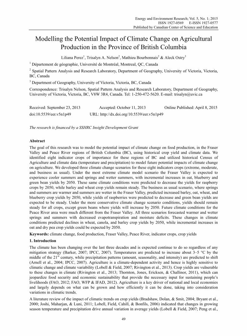
1.3 Study Area The province of BC in western Canada spans 944 735 km2 and has a diversity of landscapes, topography, climatic zones, and geographical features (Holland, 1976). As a result of the province's variety in landforms, agriculture and food industry are diverse. The province is divided into eight agricultural census regions (Figure 1). BC possesses unique agriculture policies directly related to local food production; in particular, the Agricultural Land Reserve (ALR) is a province-wide land preservation policy of nearly five million hectares of protected farmland where farming is encouraged and non-agricultural uses are controlled (Androkovich, Desjardins, Tarzwell, & Tsigaris, 2008; Hanna, 1997). ALR delimitation is based on soil and climate and represents 5% of BC land suitable for farming, with only 1% having the best soil with the highest capability for growing crops.

Table 1. Data summary on indicator crops Crop Region Years Source Barley

Peace River Fraser Valley

1991-2009 November 2011 Farm Survey. Statistics Canada, Agriculture Division, Crops Section.

Spring Wheat

Oat

Canola Peace River

1991-2009 November 2011 Farm Survey. Statistics Canada, Agriculture Division, Crops Section. Dry Peas 1995-2006

Green Beans Fraser Valley 1961-2009 Fruit and Vegetable Survey - 3407. Table 001-0013 Area, production and farm value of vegetables, annual.

Blueberries Fraser Valley 2002-2009

Fruit and Vegetable Survey - 3407. Table 001-0009 Area, production and farm value of fresh and processed fruits, by province, annual. Raspberries

www.ccsenet.org/eer Energy and Environment Research Vol. 5, No. 1; 2015

51

Figure 1. Map of the agricultural regions of British Columbia and the Agricultural Land Reserve of Fraser Valley and Peace River, where the indicator crops are grown.

1.4 Data

The crop yield data used in this paper were provided by Statistics Canada (Table 1). Agricultural Census data provided information on the area of farmland under cultivation for our indicator crops. Data from the farm surveys were disseminated at the provincial scale with no sub-provincial data available. Census and sample survey data were gathered by Statistics Canada from direct questionnaires supplied to farm owners in Canada. Total food production for a given product over a year is calculated by Statistics Canada using extrapolated data from sample surveys. Crop data descriptions are as follows.

1.4.1 Grains

Through Statistics Canada Field Crop Reporting Series, accurate and timely estimates of seeding intentions, seeded and harvested area, production, yield and farm stocks of the principal field crops in Canada were provided at the provincial level (Statistics Canada, 2012a). Field Crop Series data reported farms producing grains in all non-Atlantic provinces; farms were stratified by size and randomly sampled. In BC, grain crops grown in Peace River (Figure 1) were reported separately from the remainder of the province and account for 90% of total grain production excluding forage corn. A large proportion of some grain crops (e.g., oats and barley) are fed to livestock. The estimated proportion of livestock grain was removed from the production data, given that it is not be available for human consumption (Statistics Canada, 2012b).

1.4.2 Fruits and Vegetables

We used data from the annual Spring and Fall Survey of Fruits and Vegetables, conducted by Statistics Canada. Through stratified random samples this survey collected data to provide estimates of the total cultivated area, harvested area, total production, marketed production, and farm gate value of selected fruits and vegetables grown in Canada. The survey excluded farms producing only mushrooms, potatoes, and greenhouse vegetables, as well as farms that were on Indian reserves; likewise, small operations with less than one acre of fruit and less than one acre of vegetables were left out. Annual totals of production and planted area for all fruits, vegetables, and potatoes are released by Statistics Canada each year (Statistics Canada, 2012c; 2012d). Fruits and vegetables in BC are mostly grown in the Lower Mainland-Southwest area (Lower Mainland and Fraser Valley) (Figure 1).

1.4.3 Climate Data:

We used high spatial resolution topographically corrected climate information for BC sourced from the Climate Western North America database version 4.60 (CWNA) (Wang, Hamann, & Spittlehouse, 2010). CWNA utilizes

www.ccsenet.org/eer Energy and Environment Research Vol. 5, No. 1; 2015

52

the Parameter-elevation Regressions on Independent Slopes Model (PRISM) approach (Daly et al., 2008; Oregon State University, 2011) and uses up-sampling of climate models employing topography, climate stations, wind patterns, and rain shadow information to provide a continuous coverage of climate data for the province. Four datasets were used. The 49-year data spanning 1961-2009 was used to represent current climate. The three future climate scenarios were based on the Canadian Centre for Climate Modelling and Analysis (CCCma) B1, A1B, and A2 scenarios for the years 2020 and 2050. The future scenario B1 (AR4 – R4) represents the least extreme scenario, A1B (AR4 – R4) represents the business as usual scenario, and A2 (AR4 – R4) represents the most extreme scenario. Model selection was based on using the full range of possible scenarios that were available from respected institutions and were recommended by the Pacific Climate Impacts Consortium (Murdock & Splittlehouse, 2011).

2. Method 2.1 Climate variables

Selected temperature-based variables consisted of Spring and Summer mean temperature, Spring and Summer mean maximum temperature, and Spring and Summer mean minimum temperature. Hybrid climate metrics consisted of Spring and Summer climate moisture deficit and evapotranspiration. Finally, precipitation variables were Spring and Summer mean precipitation.

2.2 Principal Component Analysis

Climate variables such as temperature, precipitation, and evapotranspiration are highly correlated (Trenberth, 2005), leading to problems when applying regression techniques. After testing for correlation between the 12 climatic variables selected for this study, we used Principal Components Analysis (PCA) to derive a new set of uncorrelated climate variables in order to reduce the redundancy created by correlated predictors. PCA is a classical technique used to reduce the dimensionality of a dataset by transforming input data based on a correlation matrix into a set of linear uncorrelated eigenvalues, or principal components (PCs), equal to the number of input variables and accounts for the total variance present in the input data (Jolliffe, 2002). PCs are uncorrelated and ordered such that the kth PC has the kth largest variance among all PCs. The kth PC can be interpreted as the direction that maximizes the variation of the projections of the data points such that it is orthogonal to the first k −1 PCs (Abdi & Williams, 2010; Saporta & Niang, 2010). While the first few PCs account for the greatest proportion of the data variance, the last PCs may be as interesting as the first components, since the type or the direction of the shifts are a priori unknown (Abdi & Williams, 2010; Jolliffe, 2002; Saporta & Niang, 2010). PCA was conducted using climate variables from the Fraser Valley and Peace River regions. A total of twelve PCs were derived from climate variables in each region.

2.3 Generalized Linear Models

The principal component scores were employed as inputs in generalized linear models (GLMs) with a gamma distribution (Husak, Michaelsen, & Funk, 2007), which were used to predict future crop yields in the Fraser Valley and Peace River regions under different climate scenarios. The gamma distribution was chosen because it is bounded at zero and this takes into account that crops are always present.

First presented by Nelder and Wedderbum (1972), GLMs are a flexible generalization of ordinary linear regression, allowing the linear model to be related to the response variable via a link function and the magnitude of the variance of each measurement to be a function of its predicted value (Gotway & Stroup, 1997; Nelder & Wedderburn, 1972). GLMs permit analyzing data from non-normal distributions and account for non-linear relationships. In this study, the final GLM for each crop was chosen using stepwise model selection based on the second-order Akaike's information criterion (AICc), which includes a bias-correction term to account for a small sample size relative to the number of model parameters (Anderson, Burnham, & Thompson, 2000; Burnham & Anderson, 2002). The model with the lowest AICc score was considered the most parsimonious, thus minimizing estimate bias and optimizing precision (Burnham & Anderson, 2002). Significant PCs retained in final GLMs were assessed to determine which climate variables were influential in the prediction of future crop yields. Forecast of future crop yields for the Fraser Valley and Peace River regions were calculated using the climate scenarios B1, A1B, and A2 and values associated with the 90% confidence interval (CI) are presented as Kg/ha.

3. Results 3.1 Principal Component Analysis

Twelve PCs were drawn from the PCA for each region (Fraser Valley and Peace River). It should be noted that a common rule of thumb for selecting the quantity of PCs is to choose the smallest number of PCs such that a chosen percentage of total variation is exceeded. For the Fraser Valley data, the first 5 PCs cover more than 93%

www.ccsenet.org/eer Energy and Environment Research Vol. 5, No. 1; 2015

53

of the total variation in the data, while for the Peace River dataset the first 4 PCs account for over 92% of the total variation. However, if only four or five components had been chosen, it would have had a detrimental effect on the regression model given that final PCs often represent stable linear relationships between predictor variables that are of interest in climate modelling.

3.2 Generalized Linear Models

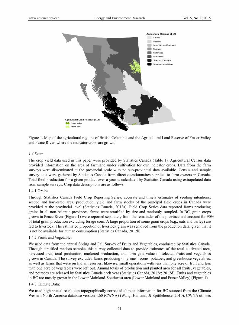
The overall variability in crop yields was high and the mean was relatively low, with a positively skewed gamma distribution. Out of the several models generated for each crop and region, a total of eleven models were selected based on their AICc. AICc values and the number of parameter (Ki) per model are reported in Table 2. The reported AICc corresponded to the lower value attained with K parameters, allowing us to determine which model among a set of models was most parsimonious.

Table 2. AICc-selected models for eight different crops in the regions of Fraser Valley and Peace River. CI represents the 90% confidence intervals of the predictions in Kg/ha.

Region Model AICc Scenario A2 ScenarioA1B Scenario B1

CI 2020 CI 2050 CI 2020 CI 2050 CI 2020 CI 2050

Fraser

Valley

Barley 308.12 2730.46

1946.16

3286.22

2013.67

3283.37

1958.96

5175.11

1897.92

2549.75

1838.76

2894.78

1931.5

Blueberr

y 154.79

8277.11

4972.32

11152.66

5887.77

11340.34

6020.75

19767.94

6817.69

8070.06

5507.2

9606.16

5787.11

Green

Beans 662.82

6515.77

4991.5

6816.78

6310.15

6940.28

6478.13

7205.26

6632.8

6999.72

6527.3

7828.04

6785.83

Oat 306.44 1958.47

1138.05

2321.59

1240.06

2241.29

1221.11

3543.06

1445.43

1695.69

1011.7

1964.69

1140.27

Raspberr

ies 157.78

6705.09

4906.72

6687.44

4080.86

7490.87

4163.05

8353.57

1826.83

7165.34

5145.11

7478.56

4727.45

Wheat 303.02 3187.07

2242.4

3296.26

2214.27

3213.95

2235.79

4165.57

1943.45

3008.59

2277.15

3086.12

2264.57

Peace

River

Barley 306.45 4192.23

2412.04

4872.51

2552.77

3458.75

2183.94

3251.29

2027.28

5828.67

2522.36

4221.64

2452.89

Canola 277.12 2043.51

807.86

2452.29

460.14

2430.58

741.19

2336.92

144.72

2346.43

371.7

2313.05

213.47

Dry Peas 204.44 2416.11

1698.82

2901.51

1698.19

2632.67

1496.62

3294.33

974.29

2768.15

1573.33

2881.91

1777.48

Oat 295.41 2902.79

1847.08

3756.58

2064.55

3101.85

1751.02

3499.09

1464.07

2834.79

1763.66

3143.49

1894.42

Wheat 291.97 3643.01

2364.98

4113.9

2254.54

3315.72

2053.81

3232.31

1721.37

4508.41

2455.48

3653.59

2121.15

Table 3. Future trends in climate variables under different emission scenarios Scenario A2

Region Climate change between 2009 and 2020 Tmax_sp

Tmax_sm

Tmin_sp

Tmin_sm

Tave_sp

Tave_sm

PPT_sp

PPT_sm

Eref_sp

Eref_sm

CMD_sp

CMD_sm

Fraser Valley

↓ ↓ ↓ ↓ ↓ ↓ ↓ ↑ ↓ ↓ ↑ ↓

Peace River

↑ ↓ ↑ ↑ ↑ ↑ ↑ ↑ ↑ ↓ ↓ ↓

Scenario A1B Region Climate change between 2009 and 2020

www.ccsenet.org/eer Energy and Environment Research Vol. 5, No. 1; 2015

54

Tmax_sp

Tmax_sm

Tmin_sp

Tmin_sm

Tave_sp

Tave_sm

PPT_sp

PPT_sm

Eref_sp

Eref_sm

CMD_sp

CMD_sm

Fraser Valley

↑ ↑ ↑ ↑ ↑ ↑ ↓ ↑ ↑ ↓ ↑ ↑

Peace River

↑ ↑ ↑ ↑ ↑ ↑ -- ↑ ↑ ↓ ↑ ↓

Scenario B1

Region Climate change between 2009 and 2020 Tmax_sp

Tmax_sm

Tmin_sp

Tmin_sm

Tave_sp

Tave_sm

PPT_sp

PPT_sm

Eref_sp

Eref_sm

CMD_sp

CMD_sm

Fraser Valley

↑ ↓ ↑ ↑ ↑ ↓ ↓ ↑ ↑ ↓ -- ↓

Peace River

↑ ↓ ↑ ↑ ↑ ↑ ↑ ↑ ↑ ↓ ↓ ↓

www.ccsenet.org/eer Energy and Environment Research Vol. 5, No. 1; 2015

55

www.ccsenet.org/eer Energy and Environment Research Vol. 5, No. 1; 2015

56

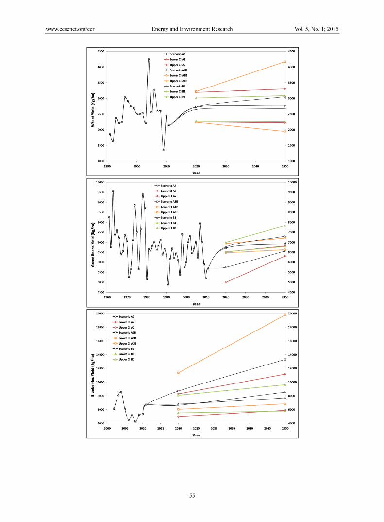
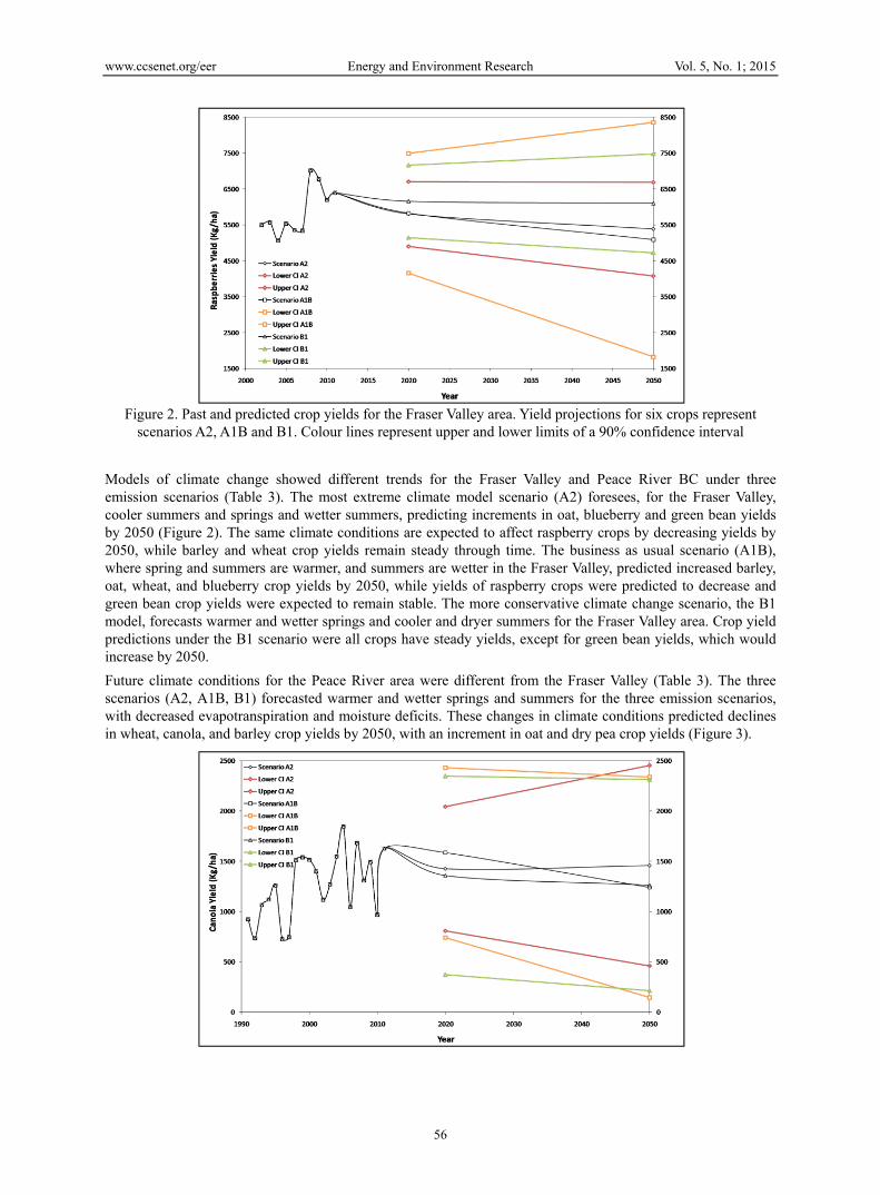
Figure 2. Past and predicted crop yields for the Fraser Valley area. Yield projections for six crops represent

scenarios A2, A1B and B1. Colour lines represent upper and lower limits of a 90% confidence interval

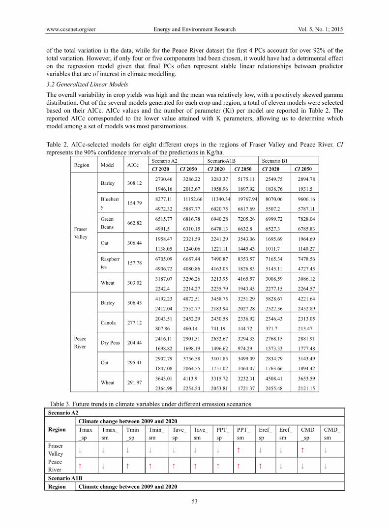
Models of climate change showed different trends for the Fraser Valley and Peace River BC under three emission scenarios (Table 3). The most extreme climate model scenario (A2) foresees, for the Fraser Valley, cooler summers and springs and wetter summers, predicting increments in oat, blueberry and green bean yields by 2050 (Figure 2). The same climate conditions are expected to affect raspberry crops by decreasing yields by 2050, while barley and wheat crop yields remain steady through time. The business as usual scenario (A1B), where spring and summers are warmer, and summers are wetter in the Fraser Valley, predicted increased barley, oat, wheat, and blueberry crop yields by 2050, while yields of raspberry crops were predicted to decrease and green bean crop yields were expected to remain stable. The more conservative climate change scenario, the B1 model, forecasts warmer and wetter springs and cooler and dryer summers for the Fraser Valley area. Crop yield predictions under the B1 scenario were all crops have steady yields, except for green bean yields, which would increase by 2050.

Future climate conditions for the Peace River area were different from the Fraser Valley (Table 3). The three scenarios (A2, A1B, B1) forecasted warmer and wetter springs and summers for the three emission scenarios, with decreased evapotranspiration and moisture deficits. These changes in climate conditions predicted declines in wheat, canola, and barley crop yields by 2050, with an increment in oat and dry pea crop yields (Figure 3).

www.ccsenet.org/eer Energy and Environment Research Vol. 5, No. 1; 2015

57

www.ccsenet.org/eer Energy and Environment Research Vol. 5, No. 1; 2015

58

Figure 3. Past and predicted crop yields for the Peace River area. Yield projections for six crops represent scenarios A2, A1B and B1. Colour lines represent upper and lower limits of a 90% confidence interval

4. Discussion As a result of a high correlation between our climate variable data, we generated twelve uncorrelated PCs to decrease the redundancy product of highly correlated predictors. The development of relationships between the PCs and historical dataset of crop yields allowed us to create a predictive model of yields based on future climate conditions. Despite the fact that it was hard to interpret the directionality of the relationships in our final GLM model coefficients due to the conversion of all climate variables into PCs, overall, the PCs explained a good proportion of the variance in the temperature and precipitation data. Previous studies (e.g., Challinor & Slingo, 2003) incorporating precipitation data in PCs have been found to correlate well with crop yields in other regions.

Underestimation of the uncertainty of a forecast can lead to excessive responses that are inconsistent with a decision maker’s risk tolerance, while overestimating uncertainty leads to under confidence and lost opportunity to prepare for adverse conditions or to take advantage of favourable conditions. Specifically for our model, climate variability and crop yield data errors were the major sources of uncertainty in yield forecasting. Likewise, the datasets used in this study showed a lot of variability in year to year crop yields, but less variability with the climate data, creating uncertainty in the long-term forecasting, especially since some of the yield/climate sample sizes were quite small. However, by using GLM as a predictive modeling technique, we were able to forecast yields using less data than what traditional techniques would require. GLMs tend to be more robust than other predictive modeling techniques and are less susceptible to the over-fitting that may occur with small datasets (McCullagh & Nelder, 1989).

Due to confidentiality procedures with the Census of Agriculture, it was not possible to obtain the exact location of farms (Statistics Canada, 2012c). With no spatially identifiable agricultural operations and yields available, the spatial distribution of crop yields (response variable) was not comprehensive. This poses a problem when associating yield data to climate variables in heterogeneous areas. For defining the relationships between climate and crop yields we utilized mean seasonal (spring and summer) values from 1961 to 2009. The use of these datasets in large areas such as the province of BC brings the uncertainty entailed in dynamical downscaling from coarse to fine resolution. This uncertainty in the regional climate response has been documented in numerous contexts (Christensen et al., 2007; Elía et al., 2008). With respect to modelling and statistical downscaling, uncertainties are also associated with imperfect knowledge and/or representation of physical processes, limitations due to the numerical approximation of the model's equations, simplifications and assumptions in the models, and/or approaches and internal model variability (Mearns et al., 2012). Likewise, it is essential to acknowledge that the observed regional climate is sometimes characterized by a high level of uncertainty due to measurement errors and sparseness of stations, especially in remote regions such as northern BC and in regions of complex topography.

www.ccsenet.org/eer Energy and Environment Research Vol. 5, No. 1; 2015

59

Similar to Challinor, Slingo, Wheeler, Craufurd, and Grimes (2003), our models showed that much of the inter-annual variability in crop yields can be explained simply using temperature and precipitation, and that this relationship is demonstrated at a regional scale. For most of the crops, the percent of deviance explained was over 45%. Where crops had lower deviance (e.g., Fraser Valley Green Beans, Wheat, Barley, and Oats) it is possible that they responded more to factors other than climate such as soil conditions and/or available carbon/nitrogen. Previous authors (Moen, Kaiser & Riha, 1994; Reilly et al., 2003) found that increasing within-year temperature variability had the greatest impact on yields if the growing season temperature is outside the optimum for growth. For BC it would be possible to examine whether years of low/high crop yields correlate with low/high temperature and precipitation.

Conclusion We predicted future crop yields for eight indicator crops under three future climate change scenarios for the Fraser Valley and Peace River regions of BC. In the Fraser Valley, the three climate scenarios predicted different trends in temperature and precipitation, resulting in a range of predicted crop responses. In the most extreme scenario, cooler springs and summers along with wetter summers should result in increased yields of oats, blueberries, and green beans, with decreased raspberry yields. In contrast, the three climate scenarios all predicted warmer and wetter springs and summers for the Peace River region, resulting in predictions of increased yields for oat and dry pea crops, with decreased yields of wheat, canola, and barley crops. Our results have important implications for policy as it is easier to mitigate the potential impacts of climate change on crop yields by instituting policy on farming reform or adaptations at a regional level rather than at the local scale. Using GLMs to model future crop yields allowed us to overcome issues with small sample sizes.

Acknowledgments This work was funded by a Social Science and Humanities Research Council (SSHRC) Insight grant to Dr. Aleck Ostry and Dr. Trisalyn Nelson.

References Abdi, H., & Williams, L. J. (2010). Principal component analysis. Wiley Interdisciplinary Reviews:

Computational Statistics 2, 433–459. http://dx.doi.org/10.1002%2Fwics.101

Anderson, D. R., Burnham, K. P., & Thompson, W. L. (2000). Null Hypothesis Testing: Problems, Prevalence, and an Alternative. The Journal of Wildlife Management, 64, 912–923. http://dx.doi.org/10.2307/3803199

Androkovich, R., Desjardins, I., Tarzwell, G., & Tsigaris, P. (2008). Land Preservation in British Columbia : An empirical analysis of the factors underlying public support and willingness to pay. Journal of Agricultural and Applied Economics, 40, 999–1013.

Arnell, N. W., Livermore, M. J. L., Kovats, S., Levy, P. E., Nicholls, R., Parry, M. L., & Gaffin, S. R. (2004). Climate and socio-economic scenarios for global-scale climate change impacts assessments: characterising the SRES storylines. Global Environmental Change, 14, 3–20. http://dx.doi.org/10.1016/j.gloenvcha.2003.10.004

Barker, T. (2007). Climate Change 2007: An Assessment of the Intergovernmental Panel on Climate Change. Change, 446, 12–17.

Blench, R. (2003). Forecasts and farmers: exploring the limitations. In K. L. O’Brien, & C. Vogel (Eds.), Coping with climate variability: The use of seasonal climate forecasts in southern Africa. (pp. 59–71). Ashgate Publishing, Ltd.

Bradshaw, B. E. N., Dolan, H., & Smit, B. (2004). Farm-level adaptation to climatic variability and change : crop diversification in the Canadian prairies. Climatic Change, 67, 119–141. http://dx.doi.org/10.1007/s10584-004-0710-z

Bryant, C. R., Smit, B., Brklacich, M., Johnston, T. R., Smithers, J., Chiotti, Q., & Singh, B. (2000). Adaptation in Canadian agriculture to climatic variability and change. Climatic Change, 45, 181–200. http://dx.doi.org/10.1007/978-94-017-3010-5_10

Burnham, K., & Anderson, D. (2002). Model selection and multi-model inference: A practical information-theoretic approach. Springer-Verlag, New York, NY, USA.

Challinor, A. J., Slingo, J. M., Wheeler, T. R., Craufurd, P. Q., & Grimes, I. F. (2003). Toward a combined seasonal weather and crop productivity forecasting system: Determination of the working spatial scale. Journal of Applied Meteorology, 42, 175–192.

www.ccsenet.org/eer Energy and Environment Research Vol. 5, No. 1; 2015

60

http://dx.doi.org/10.1175/1520-0450(2003)042<0175:TACSWA>2.0.CO;2

Christensen, J. H., Hewitson, B., Busuioc, A., Chen, A., Gao, X., Held, I., … Whetton, P. (2007). Regional climate projections. In Climate Change 2007: The Physical Science Basis. Contribution of Working Group I to the Fourth Assessment Report of the Intergovernmental Panel on Climate Change. (pp. 849–940). Cambridge University Press, Cambridge, UK.

Daly, C., Halbleib, M., Smith, J. I., Gibson, W. P., Doggett, M. K., Taylor, G. H., … Pasteris, P. P. (2008). Physiographically sensitive mapping of climatological temperature and precipitation across the conterminous United States. International Journal of Climatology, 28, 2031–2064. http://dx.doi.org/10.1002/joc.1688

Elía, R., Caya, D., Côté, H., Frigon, A., Biner, S., Giguère, M., … Plummer, D. (2008). Evaluation of uncertainties in the CRCM-simulated North American climate. Climate Dynamics, 30, 113–132. http://dx.doi.10.1007/s00382-007-0288-z

FAO. (2012). The state of food and agriculture 2012. Investing in agriculture for a better future. FAO, Roma, Italy.

FAO, WFP, IFAD. (2012). The State of Food Insecurity in the World 2012. Economic growth is necessary but not sufficient to accelerate reduction of hunger and malnutrition. FAO, Rome, Italy.

Glass, V. M., Percival, D. C., & Proctor, J. T. A. (2005). Tolerance of lowbush blueberries (Vaccinium angustifolium Ait .) to drought stress. I . Soil water and yield component analysis. Canadian Journal of Plant Science, 85, 911–917. http://dx.doi. 10.4141/P03-027

Gotway, C. A., & Stroup, W. W. (1997). A Generalized Linear Model approach to spatial data analysis and prediction. Journal of Agricultural, Biological, and Environmental Statistics, 2, 157–178. http://dx.doi.org/10.2307/1400401

Grace, J. (1988). Temperature as a determinant of plant productivity. Symposia of the Society for Experimental Biology, 42, 91–107. Retrieved from http://www.unboundmedicine.com/medline/citation/3270210/Temperature_as_a_determinant_of_plant_productivity_

Hall, H., & Sobey, T. (2013). Climatic requirements. In Funt, R. C., & Hall, H. K. (Eds.), Raspberries. Cabi.

Hanna, K. (1997). Regulation and land-use conservation: A case study of the British Columbia Agricultural Land Reserve. Journal of Soil and Water Conservation, 52, 166–170. Retrieved from http://www.jswconline.org/content/52/3/166.extract

Hansen, J. W. (2002). Realizing the potential benefits of climate prediction to agriculture: issues, approaches, challenges. Agricultural Systems, 74, 309–330. http://dx.doi.org/10.1016/S0308-521X(02)00043-4

Holland, S. S. (1976). Landforms of British Columbia: A physiographic outline. Retrieved from http://www.empr.gov.bc.ca/Mining/Geoscience/PublicationsCatalogue/BulletinInformation/BulletinsAfter1940/Documents/Bull48-txt.pdf

Husak, G., Michaelsen, J., & Funk, C. (2007). Use of the gamma distribution to represent monthly rainfall in Africa for drought monitoring applications. International Journal of Climatology, 27, 935–944. http://dx.doi.org/10.1002/joc.1441

Ingver, A., Tamm, I., Tamm, Ü., Kangor, T., & Koppel, R. (2010). The characteristics of spring cereals in changing weather in Estonia. Agronomy Research, 8, 553–562. Retrieved from http://agronomy.emu.ee/vol08Spec3/p08s306.pdf

IPCC. (2007). Climate Change 2007: Mitigation. Contribution of Working Group III to the Fourth Assessment Report of the Intergovernmental Panel on Climate Change, Climate Change 2007: Mitigation. Contribution of Working Group III to the Fourth Assessment Report of the Intergovernmental Panel on Climate Change. Cambridge University Press, Cambridge.

Jolliffe, I. T. (2002). Principal Component Analysis. Springer. Retrieved from http://f3.tiera.ru/2/M_Mathematics/MV_Probability/MVsa_Statistics%20and%20applications/Jolliffe%20I.%20Principal%20Component%20Analysis%20(2ed.,%20Springer,%202002)(518s)_MVsa_.pdf

Joshi, N. P., Maharjan, K. L., & Luni, P. (2011). Effect of climate variables on yield of major food-crops in Nepal: A time-series analysis. Journal of Contemporary India Studies: Space and Society, Hiroshima University, 1, 19–26. Retrieved from http://mpra.ub.uni-muenchen.de/35379/1/MPRA_paper_35379.pdf

www.ccsenet.org/eer Energy and Environment Research Vol. 5, No. 1; 2015

61

Letson, D., Llovet, I., Podestá, G., Royce, F., Brescia, V., Lema, D., & Parellada, G. (2001). User perspectives of climate forecasts: crop producers in Pergamino, Argentina. Climate Research, 19, 57–67. Retrieved from http://www.int-res.com/articles/cr2002/19/c019p057.pdf

Lobell, D. B., & Field, C. B. (2007). Global scale climate–crop yield relationships and the impacts of recent warming. Environmental Research Letters, 2, 014002. http://dx.doi.org/10.1088/1748-9326/2/1/014002

Lobell, D. B., Field, C. B., Cahill, K. N., & Bonfils, C. (2006). Impacts of future climate change on California perennial crop yields: Model projections with climate and crop uncertainties. Agricultural and Forest Meteorology, 141, 208–218. http://dx.doi.org/10.1016/j.agrformet.2006.10.006

McCullagh, P., & Nelder, J. A. (1989). Generalized Linear Models. Chapman and Hall/CRC.

Mearns, L. O., Arritt, R., Biner, S., Bukovsky, M. S., McGinnis, S., Sain, S., … Snyder, M. (2012). The North American Regional Climate Change Assessment Program: Overview of phase I results. Bulletin of the American Meteorological Society, 93, 1337–1362. http://dx.doi.org/10.1175/BAMS-D-11-00223.1

Moen, T. N., Kaiser, H. M., & Riha, S. J. (1994). Regional yield estimation using a crop simulation model: Concepts, methods, and validation. Agricultural Systems, 46, 79–92. http://dx.doi.org/10.1016/0308 -521X(94)90170-K

Murdock, T. Q., & Splittlehouse, D. L. (2011). Selecting and using climate change scenarios for British Columbia. Climate Impacts Consortium, University of Victoria 49.

Nelder, A. J. A., & Wedderburn, R. W. M. (1972). Generalized Linear Models. Journal of the Royal Statistical Society. Series A, 135, 370–384. http://dx.doi.org/10.2307/2344614

Nguyen, G. N., & Sutton, B. G. (2009). Water deficit reduced fertility of young microspores resulting in a decline of viable mature pollen and grain set in rice. Journal of Agronomy and Crop Science, 195, 11–18. http://dx.doi.org/10.1111/j.1439-037X.2008.00342.x

Oregon State University. (2011). PRISM Climate Group. Retrieved from http://www.prism.oregonstate.edu/

Peng, S., Huang, J., Sheehy, J. E., Laza, R. C., Visperas, R. M., Zhong, X., … Cassman, K. G. (2004). Rice yields decline with higher night temperature from global warming. Proceedings of the National Academy of Science (PNAS), 101, 9971–9975. http://dx.doi.org/10.1073/pnas.0403720101

Petrova, R., Matev, A., & Haitova, D. (2012). Influence of the irrigation rate on the vegetative development of green beans. Agrarni Nauki, 4, 107–112. Retrieved from http://www.cabdirect.org/abstracts/20133050891.html;jsessionid=AD9E7AD32CFF7CEA1CF7598899DDC54B

Reilly, J., Tubiello, F., McCarl, B., Abler, D., Darwin, R., Fuglie, K., … Rosenzweig, C. (2003). U.S. Agriculture and climate change: New results. Climatic Change, 57, 43–67. http://dx.doi.org/10.1023/A:1022103315424

Rivington, M., Matthews, K. B., Buchan, K., Miller, D. G., Bellocchi, G., & Russell, G. (2013). Climate change impacts and adaptation scope for agriculture indicated by agro-meteorological metrics. Agricultural Systems, 114, 15–31. http://dx.doi.org/10.1016/j.agsy.2012.08.003

Saporta, G., & Niang, N. (2010). Principal Component Analysis: Application to statistical process control. In:Govaert, G. (Ed.), Data Analysis. (pp. 1–23). Wiley. http://dx.doi.org/10.1002/9780470611777.ch1

Semenov, M. A., & Porter, J. R. (1995). Climatic variability and the modelling of crop yields. Agricultural and Forest Meteorology, 73, 265–283. http://dx.doi.org/10.1016/0168-1923(94)05078-K

Statistics Canada (2012a). Field Crop Reporting Series: Definitions, data sources and methods. Retrieved from www.statcan.gc.ca

Statistics Canada. (2012b). Field Crop Reporting Series-Catalogue no. 22-002-X. Retrieved from http://www.statcan.gc.ca/pub/22-002-x/22-002-x2011008-eng.pdf

Statistics Canada. (2012c). Fruits and Vegetables Survey: Definitions, data sources and methods. Retrieved from www.statcan.gc.ca

Statistics Canada. (2012d). Fruit and vegetable production-Catalogue no. 22-003-X. Retrieved from http://www.statcan.gc.ca/pub/22-003-x/22-003-x2011002-eng.pdf

Subedi, K. D., Gregory, P. J., Summerfield, R. J., & Gooding, M. J. (1998). Cold temperatures and boron deficiency caused grain set failure in spring wheat (Triticum aestivum L.). Field Crops Research, 57, 277–288. http://dx.doi.org/10.1016/S0378-4290(97)00148-2

www.ccsenet.org/eer Energy and Environment Research Vol. 5, No. 1; 2015

62

Thakur, P., Kumar, S., Malik, J. A., Berger, J. D., & Nayyar, H. (2010). Cold stress effects on reproductive development in grain crops: An overview. Environmental and Experimental Botany, 67, 429–443. http://dx.doi.org/10.1016/j.envexpbot.2009.09.004

Thornton, P. K., Jones, P. G., Ericksen, P. J., & Challinor, A. J. (2011). Agriculture and food systems in sub-Saharan Africa in a 4°C+ world. Philosophical transactions. Series A, Mathematical, physical, and engineering sciences, 369, 117–36. http://dx.doi.org/10.1098/rsta.2010.0246

Trenberth, K. E. (2005). Relationships between precipitation and surface temperature. Geophysical Research Letters, 32, 4. http://dx.doi.org/10.1029/2005GL022760

Wang, T., Hamann, A., & Splittlehouse, D. (2010). Climate Western North America. Retrieved from http://www.genetics.forestry.ubc.ca/cfcg/ClimateWNA/help.htm

Willenbockel, D. (2012). Extreme weather events and crop price spikes in a changing climate - Illustrative global simulation scenarios. Retrieved from http://www.iadb.org/intal/intalcdi/PE/2012/10653.pdf

Copyrights Copyright for this article is retained by the author(s), with first publication rights granted to the journal.

This is an open-access article distributed under the terms and conditions of the Creative Commons Attribution license (http://creativecommons.org/licenses/by/3.0/).