1

Modelling polar marine ecosystem functions guided by bacterial physiological and taxonomic traits

Hyewon Heather Kim1, 2, *, Jeff S. Bowman3, Ya-Wei Luo4, Hugh W. Ducklow5, Oscar M. Schofield6, Deborah K. Steinberg7, Scott C. Doney2

5 1Woods Hole Oceanographic Institution, Woods Hole, MA 02543, USA 2University of Virginia, Charlottesville, VA 22904, USA 3Scripps Institution of Oceanography, UC San Diego, La Jolla, CA, USA 4Xiamen University, Xiamen, China 5Lamont-Doherty Earth Observatory of Columbia University, Palisades, NY 10964, USA 10 6Rutgers University, New Brunswick, NJ 80901, USA 7Virginia Institute of Marine Science, William & Mary, Gloucester Point, VA 23062, USA

Correspondence to: Hyewon Heather Kim (hkim@whoi.edu)

Abstract Heterotrophic marine bacteria utilize organic carbon for growth and biomass synthesis. Thus, their physiological variability is 15 key to the balance between the production and consumption of organic matter and ultimately particle export in the ocean. Here we investigate a potential link between bacterial traits and ecosystem functions in the rapidly warming West Antarctic Peninsula (WAP) region based on a bacteria-oriented ecosystem model. Using a data assimilation scheme, we utilize the observations of bacterial groups with different physiological traits to constrain the group-specific bacterial ecosystem functions in the model. We then examine the association of the modelled bacterial and other key ecosystem functions with eight recurrent 20 modes representative of different bacterial taxonomic traits. Both taxonomy and physiological traits reflect the variability of bacterial carbon demand, net primary production, and particle sinking flux. Numerical experiments under perturbed climate conditions demonstrate a potential shift from low nucleic acid bacteria to high nucleic acid bacteria-dominated communities in the coastal WAP. Our study suggests that bacterial diversity via different taxonomic and physiological traits can guide the modelling of the polar marine ecosystem functions under climate change. 25

1 Introduction

Microbes regulate many key ecosystem functions in the marine food web. Unicellular primary producers fix organic carbon (i.e., an ecosystem function termed primary production), while heterotrophic marine bacteria and archaea (hereafter bacteria) utilize the fixed organic carbon for growth and biomass synthesis (i.e., an ecosystem function termed bacterial production, or BP; Azam et al. 1983). Thus, the variability in the abundance and activity of bacteria is central to understanding the balance 30 between production and consumption of organic matter and ultimately particle export in the ocean. In flow cytometric analyses, bacteria cluster into two groups of cells with different nucleic acid content, including high nucleic acid (HNA) and low nucleic acid (LNA) cells (Bouvier et al. 2007; Gasol et al. 1999). These two groups are suggested to represent lineages (Schattenhofer et al. 2011; Vila‐Costa et al. 2012) or physiological states (Bowman et al. 2017), where HNA cells are generally larger in both cell and genome size compared to LNA cells (Bouvier et al. 2007; Calvo-Díaz and Morán 2006). The significance of HNA 35 versus LNA cells in determining distinct ecosystem states and functions has been investigated, but much is still unknown. In

2

a recent study along the West Antarctic Peninsula (WAP), the high dimensionality of the bacterial community structure data was reduced via emergent self-organizing maps and subdivided into a small number of bacterial modes associated with specific taxonomic and functional traits (Bowman et al. 2017). Bowman et al. (2017) demonstrated that a combination of taxonomy, physiological structure (i.e., HNA and LNA cells), and abundance of bacterial communities explained up to 73% of the 40 variance in bulk BP. Their findings imply that physiological and taxonomic traits of bacteria may inform a predictive ecosystem model to further explore ecologically important questions including: Would these bacterial traits reflect other important ecosystem functions such as the net primary production and particle sinking flux? If so, what would be the potential mechanisms and how will the relationship between bacterial traits and ecosystem functions be impacted by climate change?

The WAP is a rapidly warming marine ecosystem, with resulting changes in physical, ecological, and biogeochemical 45 processes (Clarke et al. 2009; Cook et al. 2005; Ducklow et al. 2007; King 1994; Meredith and King 2005; Stammerjohn et al. 2008; Vaughan et al. 2003; Vaughan 2006; Whitehouse et al. 2008). Routine monitoring through the Palmer Long-Term Ecological Research project (Palmer LTER; since 1991) has revealed climate-driven variations in seasonal phytoplankton accumulation (Saba et al. 2014; Schofield et al. 2017), bacterial dynamics (Bowman and Ducklow 2015; Ducklow et al. 2012a; Kim and Ducklow 2016; Luria et al. 2017; Luria et al. 2014), nutrient drawdown (Kim et al. 2016), and micro- and 50 macrozooplankton dynamics (Garzio and Steinberg 2013; Steinberg et al. 2015; Thibodeau et al. 2019). The wealth of Palmer LTER observations has enabled the construction of a numerical marine ecosystem model for the coastal WAP region (i.e., the WAP-1D-VAR v1.0 model; Kim et al., 2021) by adapting the regional test-bed models of other ocean basins (Friedrichs 2001; Friedrichs et al. 2006, 2007; Luo et al. 2010, 2012). The WAP-1D-VAR v1.0 model is compared against roughly bi-weekly time-series observations over the growth season (October - March) near Palmer Station (64.77°S, 64.05°W; the mean depth 55 ~65 m, the bottom depth ~75 m) that record seasonal variations in ecological processes modulated by variations in surface light, mixed layer depth, and surface sea-ice cover. The WAP-1D-VAR v1.0 model utilizes a data assimilation scheme to minimize the misfits between model results and observational data via a variational adjoint method (Lawson et al. 1995) that assimiltes the available Palmer LTER data to objectively adjust the model parameters. Serving as a mechanistic model, assimilation of the Palmer LTER observations enables the model to constrain poorly-measured bacterial processes (e.g., 60 respiration, viral and grazing mortality, growth efficiency, carbon demand, and utilization of dissolved organic matter with varying lability) and to predict microbial system states in changing environments. Yet, incorporating molecular observations into a numerical ecosystem model is a challenge because of the difference in how levels of biological organization are treated in observations and models (Hellweger 2020) as well as the high dimensionality of microbial molecular observations. One argument is that molecular-level changes in microbial dynamics may not directly translate into a clear picture of changes in 65 community structure or resulting changes in bulk ecosystem functions.

In this study, we explore a potential link between bacterial traits and ecosystem functions in the warming coastal WAP, using a bacteria-oriented ecosystem model modified from the WAP-1D-VAR v1.0 model (Kim et al. 2021). The bacterial traits examined in this study include physiological and taxonomic traits. For physiological traits, our model explicitly simulates the time-evolving dynamics of two ubiquitous bacterial groups with differing nucleic acid contents, the HNA group and the LNA 70 group, by directly assimilating the group-specific carbon biomass obesrvations estimated by flow cytometry. For taxonomic traits, taxonomic modes derived from bacterial 16S rRNA gene sequence data (Bowman et al. 2017) are compared to final model results at the corresponding time points, with the assumption that bacterial taxonomy would provide information about bacterial ecosystem processes and structures. Our study indirectly incorporates bacterial molecular information into ecosystem-level dynamics, in contrast to genome-scale or gene-centric models predicting the time-evolving dynamics of microbial 75 molecular processes.

3

2 Material and Methods

2.1 Bacteria-oriented ecosystem model

The model is originally derived and modified from the one-dimensional (1-D) variational data assimilation planktonic ecosytem model for the coastal WAP region called the WAP-1D-VAR v1.0 model (Kim et al., 2021). The WAP-1D-VAR 80 v1.0 model tracks C, N, and P of its state variables with flexible stoichiometry. For our study, we modify the original model’s single bacterial compartment into HNA and LNA bacterial compartments and only discuss their C stocks and rates as well as other state variables that remain the same as the WAP-1D-VAR v1.0 model. The state variables in this modified model include HNA and LNA bacteria, diatoms, cryptophytes, microzooplankton, krill, labile dissolved organic carbon (DOC), semi-labile DOC (SDOC), ammonium (NH4), nitrate (NO3), phosphate (PO4), and particulate (carbon) detritus (Fig. 1). Refractory DOC 85 (RDOC) and higher trophic levels are implicit to serve as model closure terms (i.e., they are source or sink terms of other explicit state variables and their time derivativies are not calculated in the model). The model is forced by mixed layer depth (MLD), photosynthetically active radiation (PAR) at the ocean surface, surface sea-ice concentration, water-column temperature, and eddy diffusivity (Fig. S1) using a constant time step of 1 hour and a second-order Runge-Kutta scheme (Text S1-2). The model allows both L- and SDOC as substrate sources for bacteria, and it is nutrient quota of bacteria that allow the 90 lability of SDOC to vary. In contrast to LDOC pool that is entirely available for bacteria, a parameter controlling the lability of SDOC (rSDOC, Tables S2-6) regulates how much portion of SDOC can be taken up by bacteria. Bacterial C growth is determined by their cellular nutrient quota as well as available L- and SDOC concentrations (Kim et al., 2021).

The time derivative of C biomass for each bacterial group is determined as follows: dCHNA

dt = GCHNA,LDOC + GCHNA,SDOC – RCHNA – ECHNA,RDOC – ECHNA,SDOC – GZCHNA – MCHNA (1) 95

dCLNA

dt = GCLNA,LDOC + GCLNA,SDOC – RCLNA – ECLNA,RDOC – ECLNA,SDOC – GZCLNA – MCLNA (2)

where C is bacterial C biomass, GCLDOC is LDOC consumption, GCSDOC is SDOC consumption, RC is respiration, ECRDOC is RDOC excretion, ECSDOC is SDOC excretion, GZC is the amount of C biomass grazed by microzooplankton, and MCHNA is mortality caused by viral attack (unit: mmol C m-3 for C and mmol C m-3 d-1 for the rest terms). The sum of the first three terms on the right-hand side in Eqs. 1-2 is defined as BP for each bacterial group (i.e., BPHNA = GCHNA,LDOC + GCHNA,SDOC – RCHNA, 100 BPLNA = GCLNA,LDOC + GCLNA,SDOC – RCLNA). Both CHNA and CHNA are constrained by the group-specific C biomass data estimated via flow cytometry, while only bulk BP (i.e., BP = BPHNA + BPLNA), not the group-specific BP, is constrained by the observations due to the lack of the group-specific BP data at the study site. With the initial parameter values distinct to each bacterial group (Table 1), the model incorporates the observations of CHNA, CLNA, BP, and other state and rate variables to its built-in data assimilation scheme (Section 2.2) that optimizes the parameters and calculates the resulting C stock and flows of 105 each bacterial group (Eqs. 1-2). In other words, the partitioning of BP into HNA and LNA groups is purely determined by parameter optimization using the information about other ecosystem obesrvations.

2.2 Modelling framework

The modelling framework consists of the mechanistic and data-driven parts (Fig. 2). The mechanistic part represents prognostic, time-evolving microbial processes in the model (Fig. 1, Section 2.1) with its built-in data assimilation scheme via 110 a varitional adjoint method (Lawson et al., 1995). The data assimilation scheme minimizes the misfits between observations (i.e., assimilated data, Section 2.4) and model results by objectively optimizing a subset of model parameters (Friedrichs, 2001; Spitz et al., 2001; Ward et al., 2010; details in Text S3). The data-driven part represents the pairing of the optimized model results from the mechanistic part and the bacterial taxonomic “modes” derived from 16S rRNA gene sequence abundance data

4

(Bowman et al., 2017). We call this latter part data-driven because the high dimensionality of the bacterial community structure 115 data is reduced to a single taxonomic mode using an unsupervised machine learning algorithm called Kohonen’s self-organizing maps (Kohonen, 2001). Each taxonomic mode (mode hereafter) represents its specific taxonomic traits and is expressed as a single categorical variable without linear progression in-between. For example, mode 1 is not necessarily closer to mode 3 than it is to mode 7. Modes are not necesarly correlated to the physiological traits of bacteria (i.e., HNA and LNA C biomass) despite being derived from the same samples. In other words, the taxonomic and physiological traits are 120 independent of each other.

We select a nearshore Palmer LTER Station B (64.77°S, 64.05°W, ~65 m) in the coastal WAP as the modelling site. The Station B datasets consist of roughly bi-weekly physical, chemical, and biological profiles collected via a profiling Conductivity-Temperature-Density (CTD) rosette. Flow cyotometric data for HNA and LNA C biomass and 16S rRNA gene amplicon data for taxonomic modes come from Arthur Harbour Station B at 10 m depth (situated 1 km from the Station B) or 125 Palmer Station seawater intake at 6 m depth (Bowman et al., 2017). Three upper-ocean depth levels, 0, 10, and 20 m (with the layer thickness of 2, 16, and 4 m, respectively) are modelled for 4 consecutive growth seasons, including November 2010 - March 2011 (2010-11 hereafter), 2011-12, 2012-13, and 2013-14. However, the results from 10 m are only presented in detail because of the availability of the bacterial traits data at that depth. Despite the advantage of simulating the full water-column layers, it would be best to exclude the depth levels without bacterial traits observations, yet to include the adequate number of 130 depth levels to simulate seasonal MLD and light impacts on bacterial dynamics. Thus, we choose to model three layers, that is, 0, 10, and 20 m, in a 1-D (vertical) water column.

The 1-D modelling of the coastal WAP region is justifiable given that the WAP shows relatively weak net advection compared with the Antarctic Circumpolar Current (ACC) or the subpolar gyres (Meredith et al., 2008, 2013). In addition, the CTD observations at Palmer Station do not show abrupt changes in physical and biogeochemical tracers as a result of lateral 135 advection, with fairly homogeneous temperature and salinity distributions for the years and depths modelled in our study (Kim and Ducklow, 2016). There is a 6-month sampling gap in the Austral aumtum and winter months, so we optimize the model each year separately only for the Austral spring to summer months. This results in each year possessing its own uniquely optimized parameter set that drives the minimized model-observation misfits for the given year. We also optimize the model for the climatological year, referred to the climatological model, constructed by averaging 4-year observations (2010-11 to 140 2013-14; Text S4). We do not average the whole Palmer LTER multi-decadal period (since 1991) because of the lack of HNA and LNA C biomass data except those 4 years. Other modelling aspects (e.g., model initialization, spin-up, and bottom boundary conditions) are detailed in Text S4 and Kim et al (2021).

2.3 Assimilated data

We assimilate the Palmer LTER observations from 0, 10, and 20 m that correspond to the compartments and flows in 145 the model, including NO3, PO4, phytoplankton taxonomic specific chlorophyll (Chl) for diatoms and cryptophytes (Schofield et al., 2017), microzooplankton C biomass (Garzio et al., 2013), bulk primary production (PP), bulk BP, HNA bacterial C biomass, LNA bacterial C biomass, SDOC, particulate organic carbon (POC), and particulate organic nitrogen (PON). Though not available in 2011-12, because of the importance in constraining the group-specific phytoplankton dynamics, the 4-year climatological value of the group-specific Chl is assimlated for 2011-12. NO3 is not assimilated in 2010-11, while POC, PON, 150 and SDOC are not assimilated in 2012-13 and 2013-14 because of the lack of the observations in those years. Krill C biomass is not assimilated due to the strong patchiness of their distribution with many zero values that may hinder proper model optimization, while microzooplankton C biomass (2010-11) from a single year measurement is assimilated for all 4 model years to at least provide constraints on the parameter values for phytoplankton grazing. The model-observation misfits for

5

microzooplankton are not examined because of the discrepancy in the timing and location of those data assimilated compared 155 to our study.

SDOC is calculated by subtracting the background (RDOC) concentration (40.0 mmol m-3) from climatological total DOC concentration. POC (PON) is assimilated to represent the model detrital pool, but its measurements contained living biomass from bottle filter experiments. Climatological observations show that living phytoplankton and bacterial biomass account for 26% of total POC and 29% of total PON, so these fractions are used to exclude living biomass from the bulk 160 particulate material pool. When converting Chl to phytoplankton C biomass, the maximum Chl/N ratio is used along with the reference (Redfield) C/N ratio of 0.15. BP (mmol C m-3 d-1) is derived from 3H-leucine incorporation rate (pmol l-1 h-1) data using the conversion factor of 1.5 kg C mol-1 leucine incorporated (Ducklow, 2000). The bacterial group-specific C biomass (mmol C m-3) is estimated from bacterial abundance measured by flow cytometry (i.e., bulk bacterial C biomass multiplied by the fraction of each physiological group, fHNA or fLNA, with the conversion factor of 10 fg C cell-1; Fukuda et al. 1998). 165

2.4 Cost function and portability index

The total cost function is calculated to represent the misfit between observations and model results as follows: J = ∑ 1

Nm∑ ( a!m,n#am,n

σm)Nm

n=1Mm=1

2 (3)

where m and n represent assimilated data types and data points, respectively, M and Nm are the total number of assimilated data types and data points for data type m, respectively, σm is the target error for data type m, am,nis observations, and a#m,nis 170 model output. Hereafter, we present the total cost function as the total cost function normalized by M (J’ = J/M) and normalized costs of individual data types (J’m = J’m/M) as the model-observation misfit equivalent to a reduced Chi-square estimate of the model goodness of fit (i.e., J’ = 1 as a good fit from optimization, J’ >>1 as a poor fit due to underestimation of the error variance or the fit not fully capturing the data, and J’ <<1 as an overfitting of the data, fitting the noise, or overestimation of the error variance). The base-10 logarithm of Chl and PP is used in Eq. 3 to account for high productivity of the WAP waters 175 and the approximate log-normal distribution of those data types (Campbell 1995; Glover et al. 2018). The target error σmis calculated for each data type m as:

σm = am,n$$$$$ · CVm (4) where am,n$$$$$ is the climatological mean of the observations and CVmis the adjusted coefficient of variation (CV) of the observations of each data type over 0, 10, and 20 m (due to observational error and seasonal and interannual variations). 180 CVmfor the 4 modelled years in our study are higher than those across every measured depth within the mixed layer for an extended year period examined with the original WAP-1D-VAR v1.0 model (2002-03 to 2011-12; Kim et al., 2021) and are therefore reduced to the levels in the mixed layer to avoid an overestimated target error of each data type (Text S5). The rationale behind using the adjusted CV in the target error calculation is based on Luo et al. (2010), where all properties should be completely mixed in the mixed layer, a perfect measurement without significant errors should generate similar values at 185 every measured depth within the mixed layer, and the average CV of all depth profiles can be used as CV in the target error calculation. The standard deviation is used as target errors of the log-converted data types. The CV of the log-converted data type is estimated as the average of ± 1 standard deviation in log space converted back into normal space (Doney et al., 2003; Glover et al., 2018).

We compute the portability index (Friedrichs et al., 2007) to evaluate the broader applicability of the optimized model 190 parameter set for each year in predicting the dynamics of the other year as follows:

Portability index = J’c/J’x (5) where J’x is the normalized cross-validation total cost function when a model parameter set optimized for a given year is used to simulate another year, and J’c is the normalized total cost function of the climatological model. A portability index value

6

close to 1 indicates a more portable model, or a system that is not particularly sensitive to year-to-year variations in optimized 195 parameters, while an index value <<1 indicates a less portable model, or a system that is sensitive to year-to-year variations in optimized parameters.

2.5 Uncertainty analysis

The uncertainties of the optimized parameters are estimated using a finite difference approximation of the complete Hessian matrix during the iterative data assimilation process (i.e., the second derivatives of the cost function with respect to 200 the model parameters). When computed at the minimum of the cost function value, the square root of a diagonal element in the inversed Hessian matrix represents the logarithm of the relative uncertainty of the corresponding optimized parameter. The absolute uncertainty of the optimized parameter is calculated as pf ´ e±σi where pf is the value of the optimized parameter and σf is its relative uncertainty. We denote an optimized parameter with σf larger than 50% as an “optimized” parameter, while an optimized parameter with σf smaller than 50% is denoted as a “constrained” parameter (Tables S2-6). We then conduct Monte 205 Carlo experiments to examine the impact of the uncertainties of the constrained parameters on the modelled fields. The Monte Carlo experiments consist of 1) creating an ensemble of parameter sets (N = 1,000) by randomly sampling values within the uncertainty ranges of the constrained parameters and 2) then performing a model simulation using each parameter set. All uncertainty estimates are calculated following standard error propagation rules and presented herein as ± 1 standard deviation.

3 Results 210

3.1 Model skill assessment

The iterative optimization procedure reduced by 24-93% the misfits between observations and model results for each year and for the climatological year, compared to those obtained using the initial parameter values (Table 2). The optimized parameter sets satisfied the pre-set convergence criteria, including the local minima achieved by the total costs, low gradients of the total costs with respect to each optimized parameter, and positive eigenvalues of the Hessian matrix (details in Kim et 215 al., 2021). The total costs were reduced by optimizing only a subset of the parameters, 5-7 constrained and 3-6 optimized parameters (Tables S2-6). The optimized parameters in common across all years were αDA (the initial slope of photosynthesis versus irradiance curve of diatoms, mol C (g Chl a)-1 d-1 (W m-2)-1), μHNA (the maximum HNA bacterial growth rate, d-1), μLNA

(the maximum LNA bacterial growth rate, d-1), and gCR (the half-saturation density of cryptophytes in microzooplankton grazing, mmol C m-3). gHNA (the half-saturation density of HNA bacteria in microzooplankton grazing, mmol C m-3), gMZ (the 220 half-saturation density of microzooplankton in krill grazing, mmol C m-3), and μKR (the maximum krill growth rate, d-1) were next frequently optimized, at least for 4 years out of a total of 5 modelled years including the climatological year.

Because this study’s focus on the modelled bacterial and other ecosystem functions as a function of bacterial traits (Section 3.3) rather than of year (Figs. S2-5), we combined the observations and model results from all 4 years together for model skill assessment. According to the Taylor diagrams, model skills were overall similar among the 4 study years (Fig. 3a) 225 and the climatological year (Fig. 3b). Three core variables in this study, including HNA biomass, LNA biomass, and BP, had better model-observation agreements than other data types, with relatively high correlations, low centred (bias removed) root-mean-square difference (RMSD), and the normalized standard deviation closer to 1. These variables also had better fits to the 4-year seasonal cycles of the observations than other data types (Fig. S7). However, the model skill for HNA biomass slightly degraded in the climatological model (Fig. 3b), with the insignificant correlation (p = 0.61, versus r = 0.53 and p = 0.003 in 230 Fig. 3a), lower normalized standard deviation, and higher RMSD than the 4 years together (Fig. 3a). After optimization, the model captured best the temporal and spatial (depth) variability of PP, as shown by its high correlations (Fig. 3), but the models

7

tended to underestimate PP with relatively larger errors than for other data types (Fig. S7). By contrast, there were slight positive model biases for POC and PON (Fig. S7) and their variability was not well captured as shown by their negative correlations (Fig. 3). 235

Cross-validation cost analyses showed the increased model-observation misfits when a set of parameters optimized for one year was applied to simulate another year’s dynamics (Tables 2-3), suggesting that each year was best modelled using its own unique set of the optimized parameters. The magnitude of increase in the cost function varied by year pair, with the average portability index values indicating that the optimized model parameters for 2012-13 was most portable (0.76 ± 0.11), followed by those for 2013-14 (0.73 ± 0.17), 2010-11 (0.68 ± 0.08), and 2011-12 (0.61 ± 0.12; Table 3), though the differences 240 were not always significantly different among the years.

3.2 Bacterial carbon stocks and flows

C stocks and flows for each bacterial group represented significant seasonal and interannual variability (Figs. 4a, S8). Across years, HNA bacteria had significantly higher seasonal maximum values than their LNA counterparts when normalized by the group-specific biomass. These so-called cell-specific, seasonal maximum rates of the HNA group ranged from 0.10 ± 245 0.004 d-1 to 0.59 ± 0.24 d-1, 0.03 ± 0.001 d-1 to 0.18 ± 0.12 d-1, 0.07 ± 0.003 d-1 to 0.18 ± 0.08 d-1, 0.05 ± 0.002 d-1 to 0.57 ± 0.26 d-1, and 0.07 ± 0.03 d-1 to 0.36 ± 0.17 d-1 for LDOC uptake, SDOC uptake, respiration, BP, and grazing rates, respectively (Fig. 4). For the LNA group, the maximum cell-specific rates ranged from 0.01 ± 0.002 d-1 to 0.12 ± 0.02 d-1, 0.004 ± 0.002 d-

1 to 0.03 ± 0.01 d-1, 0.01 ± 0.001 d-1 to 0.02 ± 0.002 d-1, 0.01 ± 0.003 d-1 to 0.13 ± 0.02 d-1, and 0.02 ± 0.0004 d-1 to 0.17 ± 0.03 d-1 for LDOC uptake, SDOC uptake, respiration, BP, and grazing rates, respectively (Fig. 4). For each year, C stocks and flows 250 averaged over the growth season (Fig. 5) and those normalized by NPP (normalized by NPP in 1-day for C stocks; Fig. S9) summarized an annual snapshot of the group-specific bacterial dynamics. The annual mean LNA biomass was ~17 times larger than that of HNA biomass in 2011-12 (Fig. 5b), in contrast to relatively similar average biomass values of both groups in other years (Figs. 5a, c, d). Bacterial carbon demand (BCD; i.e., BCD = BP + bacterial respiration; blue arrows in Fig. 5) was mostly supported by LDOC (67-81%) for both bacterial groups. 255

The rest of the modelled C stocks and flows fell into one of the following categories: 1) the variable for a single year’s values were assimilated (i.e., microzooplankton C biomass); 2) the variables for which observational values for the given year were assimilated (i.e., nutrients, POC or detritus, and SDOC), and 3) the variables that were not assimilated at all (i.e., krill C biomass, LDOC, NH4, and particle sinking flux). There was little interannual variability in the average microzooplankton C biomass (Fig. 5). Even in the years where NO3, POC, and SDOC were not assimilated, their values were modelled similarly 260 to those modelled in other assimilated years (Fig. 5). Modelled LDOC and NH4 were also within the reasonable ranges of their typically small values (< 1 μM).

3.3 Bacterial physiological and taxonomic association with ecosystem functions

Each mode was dominated by unique bacterial taxa, thereby representing taxonomic traits (Fig. S10). Candidatus Pelagibacter was most abundant in mode 6 (Fig. S10c), Dokdonia sp. MED134 in mode 7 (Fig. S10d), Candidatus Thioglobus 265 singularis PS1 in mode 1 (Fig. S10e), Owenweeksia hongkongensis DSM 17368 in mode 2 (Fig. S10f), Rhodobacteraceae in mode 5 (Fig. S10g), and Planktomarina temperata RCA23 in mode 4 (Fig. S10h). To explore a potential link between the bacterial taxonomic traits and the key ecosystem functions, we first extracted the modelled NPP, POC sinking flux, and BCD from the ecosystem model (i.e., the “final optimized output” in Fig. 2) at the time of the bacterial samples and depth (10 m) placed into a single mode derived from the observations. We then performed a linear regression with the mode as a factor, 270 where the mode is a categorical predictor with 8 modes rather than an ordinal or continuous variable (i.e., equivalent to a one-

8

way ANOVA with 8 different categories). 27%, 37%, and 77% of the total variance in the modelled NPP, POC sinking flux, and BCD were explained by the bacterial taxonomic mode (Figs. 6a-c). In particular, modes 3, 5, and 7 were associated with 2-3 times higher NPP, POC sinking flux, and BCD, compared to when mode 4 dominated (two-sample t-test with unequal sample size, p = 0.02 for NPP and p < 0.001 for POC sinking flux and BCD), or to when mode 6 dominated (p = 0.03 for NPP, 275 p = 0.003 for POC sinking flux, and p < 0.001 for BCD).

The observed mode was also positively correlated to the observed fHNA (r2 = 0.52, p < 0.001; not shown). Thus, we examined a potential link between the bacterial physiological traits and the key ecosystem functions as described above, using a linear regression with the observed fHNA as a predictor and the modelled ecosystem functions as dependent variables. The observed fHNA was positively correlated to the modelled NPP (r2 = 0.34, p < 0.001; Fig. 6d), and to a stronger extent, to the 280 modelled POC sinking flux (r2 = 0.50, p < 0.001; Fig. 6e) and to the modelled BCD (r2 = 0.56, p < 0.001; Fig. 6f). The stepwise addition of one predictor variable to the other predictor variable (i.e., fHNA adding to mode or vice versa) did not improve the model performance (not shown). These results suggest a clear link between the modelled ecosystem functions and the bacterial taxonomic (modes) and physiological (fHNA) traits observations.

3.4 Climate change experiments 285

We explored the responses of the modelled bacterial dynamics and other ecosystem functions (Sections 3.2-3.3) to changing climates along the WAP (Fig. 7). Due to the varying portability of the optimized parameter sets among the 4 study years, we used the optimzied parameter set for the climatological year (Table S6) to simulate an overall WAP system response under perturbed ocean temperatures (i.e., +0.5°C and +1.0°C relative to observed temperatures) and sea-ice forcing fields (i.e., 5% and 10% loss of sea-ice concentrations relative to observed sea-ice concentrations). These experiments were conducted 290 under each perturbed condition separately (i.e., warming alone in Fig. S11 versus melting alone in Fig. S12) as well as simultaneously (i.e., climate change; Fig. 7). We only analyzed the results from the climate change experiments, given that despite different impacts of each forcing changes (i.e., the impact of warming on rate processes versus the impact of melting on light and photosynthesis but not MLD in our model) climate change would cause simultaneous changes in sea ice and water temperature along the WAP. 295

The climate change experiments resulted in a combination of changes in overall bacterial C stocks and rates, as well as the key ecosystem functions, and shifts in their seasonal timing (Fig. 7a), compared to the base state (the first row as the base state in Fig. 7a-b, while the second and third rows as anomalies under perturbed conditions in Fig. 7b). HNA bacterial C stock and rates responded more strongly to the perturbed climate conditions compared to their LNA counterparts. Under combined warming/melting (+1.0°C/-10%) conditions, there were the maximum increases of the HNA C stock and rates by 300 19-35% (29 ± 89% for biomass, 22 ± 67% for LDOC uptake, 35 ± 111% for SDOC uptake, 26 ± 79% for respiration, 25 ± 78% for BP, 29 ± 89% for viral mortality, 19 ± 26% for grazing, and 29 ± 89% for RDOC excretion), compared to the maximum increases of the LNA C stock and rates by 3-15% (3 ± 2% for biomass, 6 ± 11% for LDOC uptake, 15 ± 27% for SDOC uptake, 8 ± 3% for respiration, 7 ± 6% for BP, 3 ± 2% for viral mortality, 7 ± 18% for grazing, and 3 ± 2% for RDOC excretion). In contrast to bacterial C stocks and rates that increased consistently throughout the growth season, microzooplankton grazing 305 rates showed seasonally mixed responses for both HNA and LNA cases, with the maximum decreases of 8 ± 32% for HNA bacteria and of 4 ± 32% for LNA bacteria. Similarly, there were the maximum increases of NPP and POC sinking flux by 14 ± 15% and 3 ± 22%, and the maximum decreases of NPP and POC sinking flux by 4 ± 11% and 3 ± 13%, respectively. SDOC exhibited the maximum increase by 2 ± 1% early in the season but shortly became depleted strongly as the season progressed. LDOC decreased consistently in response to the perturbed conditions, with the maximum decrease by 10 ± 43%. 310

9

4 Discussion

4.1 Model skill assessment

Despite the important role that bacteria play in the ocean carbon cycle, the vast majority of mechanistic biogeochemical models neither include heterotrophic marine bacteria as a model state variable nor explicitly simulate their physiological processes. Most models parameterize the bacterial remineralization of the sinking organic matter with depth by 315 fitting the power law functions or other similarly-derived, empirical approaches (Buesseler et al., 2020; Cael and Bisson, 2018). Cellular functions, taxa, and functional gene expression of other prokaryotes, such as cyanobacteria (Hellweger, 2010; Martín-Figueroa et al., 2000; Miller et al., 2013), or a diverse suite of microbial functional groups (Coles et al., 2017; Dutkiewicz et al., 2020) have been modelled so far. However, our study is the first to explicitly model heterotrophic bacterial groups of different physiological traits and to link the key ecosystem functions to their taxonomic traits. 320

Only a subset of the parameters was optimized in our model to simulate microbial and ecological patterns for each study year, consistent with other data assimilation modelling studies (Friedrichs, 2001; Friedrichs et al., 2006, 2007; Luo et al., 2010, 2012). In general, optimization of this class of marine ecosystem models requires adjustment of a small number of independent parameters to achieve well-posed model solutions, because of the highly cross-correlated nature of the parameters in the inherently nonlinear model equations (Fennel et al., 2001; Harmon and Challenor, 1997; Matear, 1996; Prunet et al., 325 1996). In our study, most of the constrained parameters were directly associated with the bacterial processes, and there were overall better model-observation fits for the bacterial data types compared to other data types. These results provide confidence in the simulated bacterial C stocks and rates.

Optimization also sheds light on major unknown parameters in bacterial grazing processes involving gHNA and gLNA

(the half-saturation densities of HNA and LNA bacteria in microzooplankton grazing, respectively). Microzooplankton grazing 330 of the given bacterial group is simulated using a Holling Type 2 density-dependent grazing function with a preferential prey selection on diatoms, cryptophytes, and the other bacterial group, where a single microzooplankton maximum grazing rate is implemented for both bacterial groups for model simplicity purposes (Tables S2-6, Kim et al., 2021). Thus, it is the half-saturation density that determines the degree of preferential grazing by microzooplankton on the given bacterial group, the change of which may ultimately depend on the group-specific C biomass. Due to the lack of a priori knowledge on the relative 335 magnitude of gHNA and gLNA, we assigned the identical initial parameter value (Table 1) to let the data assimilation scheme determine the values that best fit the overall observations. Compared to gLNA, smaller optimized gHNA values (Tables S2-6) reflect preferential grazing of HNA cells by microzooplankton, consistent with previous speculations that grazers selectively remove larger and more active bacterial cells (Giorgio et al., 1996; Gonzalez et al., 1990; Sherr et al., 1992), so HNA bacteria (Garzio et al., 2013). Together with the higher mean cell-specific grazing rates for HNA bacteria (Section 3.2), our results 340 suggest preferential grazing of HNA cells by microzooplankton.

The portability index in our study reflects the extent to which a single model framework represented by its distinctly optimized parameters in the same model equations captures the observed variability in different years, given variable environmental forcing and the accompanying shift in plankton ecosystem structure. The model parameter set optimized for 2012-13 was most portable, while the model parameter set optimized for 2011-12 was the least portable (Table 3), where the 345 most (n = 7 out of total 11) and the least numbers (n = 5 out of total 11) of model parameters were constrained, respectively (Tables S3-4). The other two years exhibited the intermediate levels of model portability, with similar portability index values characterized by the same number of the constrained parameters (n = 6 out of total 10 for 2010-11 and n = 6 out of total 12 for 2013-14; Tables S2, S5). In other words, it is the number of the constrained parameters that matters most in driving high model portability, suggesting the connection between overfitting and the portability of the optimized parameter sets in our study. 350 Also, varying degrees of the model portability across the 4 study years rendered it difficult to choose one particular year’s

10

model solution to perform the climate change experimens (Sections 3.4, 4.4), consistent with the characteristics of the original WAP-1D-VAR v1.0 model. Instead, better model skill was found by utilizing the parameters from assimilating the climatological observations (i.e., the climatological model).

4.2 Bacterial carbon stocks and flows 355

The fact that cell-specific BP, respiration, and SDC uptake rates of HNA bacteria were significantly higher than those of LNA bacteria (Section 3.2) is mainly because of the way the parameter optimization was conducted (Text S3). The higher initial parameter values assigned for HNA bacterial growth, RDOC excretion, mortality, and respiration rates (Table 1) might drive not only their faster cell-specific growth rates but also their higher DOC uptake rates to coexist with their LNA counterparts when the loss rates were relatively large for HNA bacteria. Though driven by the model assumptions, the 360 important aspect of these results lies in the fact that the model can leverage such assumptions to examine the implications for the WAP food-web dynamics and biogeochemistry. As with phylogenetic groups (Fuchs et al., 2000; Teira et al., 2009; Yokokawa et al., 2004), cell-specific bacterial growth rates are expected to differ among distinct bacterial physiological groups, but there are limited studies focusing on group-specific cell activities (Gasol et al., 1999; Giorgio et al., 1996; Günter et al., 2008; Longnecker et al., 2005; Moràn et al., 2011). Moràn et al (2011) showed that HNA bacteria greatly outgrew LNA 365 bacteria in Waquoit Bay Estuary, with the cell-specific growth rate of up to 2.26 d-1 for HNA cells versus < 0.5 d-1 for LNA cells. Other studies have demonstrated that HNA bacteria might depend on phytoplankton substrates more than LNA bacteria (Li et al., 1995; Morán et al., 2007; Scharek and Latasa 2007). The hypothesis that WAP bacteria might rely on SDOC when limited by LDOC availability has received indirect support previously (Ducklow et al., 2011; Kim and Ducklow, 2016; Luria et al., 2017), providing the basis for bacterial SDOC utilization in our model formulation. 370

The model also captured the rest of the ecosystem variables fairly well. The modelled nutrient stocks were above the detection limits, indicating no evidence of macronutrient limitations at the study site. The WAP typically exhibits strong interannual variability in physical forcing and ecological and biogeochemical processes (Ducklow et al., 2007), but the lack of the strong interannual variability in the modelled microzooplankton C biomass is due to assimilating their climatological observations. One exception is krill C biomass that was modelled 3-8 times larger than the maximum value from the available 375 field measurement in 2017-2018 (0.57 mmol C m-3; not shown). It should be noted that there were inconsistences in the nature of the assimilated data types, including a single-year observation of microzooplankton C biomass (versus each year-specific observations of other variables) and two unassimilated data types (e.g., krill C biomass). Also, there can be compensating errors in krill grazing rate and metabolism values given that krill are mobile laterally. These observational limitations make it challenging to construct a complete bacterial C budget without significant uncertainties. A more complete assimilation of 380 zooplankton data should be the next effort to improve the model fits and minimize uncertainties in the bacterial variables. Another source of uncertainty in our study is that the model forcing does not seem to have sufficient information to capture small-scale and high-frquency sources of variability (e.g., local circulation and tidal flow near Palmer Station), resulting in relatively low standard deviation values of the modelled bacterial and ecosystem variables than those of the observations (e.g., Figs. 3, S2). By contrast, our model adequately captures seasonal variations in modelled ecosystem dynamics likely because 385 such high frequency processes do not strongly rectify into the seasonal cycles in the WAP ecosystem.

4.3 Bacterial physiological and taxonomic association with ecosystem functions

The positive associations of the observed fHNA with the modelled NPP and POC sinking flux suggest a relatively strong resource control on these actively-growing HNA cells compared to slowly-growing LNA cells. This is consistent with previous studies showing the increased HNA growth rates in response to enhanced phytoplankton-derived organic substrate 390 (Morán et al., 2010) and more abundant HNA cells in areas or periods where bacterial assemblages were predominantly

11

controlled by resources, rather than grazing (Morán et al., 2007). It has been hypothesized that due to minimal inputs of terrestrial organic matter, bacteria must ultimately rely on in situ NPP for organic matter source in the WAP (Ducklow et al., 2012b), supporting the importance of resource control on these actively-growing bacteiral populations.

In our study, modes 3, 5, and 7, characterized by copiotrophic taxa with large genomes and more 16S rRNA gene 395 copies (Bowman et al., 2017), were associated with high values of the modelled NPP, POC sinking flux, and BCD, while modes 4 and 6, characterized by taxa associated with more oligotrophic conditions, were associated with low values of the modelled NPP, POC sinking flux, and BCD. Dokdonia sp. MED134, a common bacterial species of the modes associated with high NPP, POC sinking flux, and BCD, is a proteorhodopsin-containing marine flavobacterium that grows faster with light (Gómez-Consarnau et al., 2007; Kimura et al., 2011) and in conditions under which resources are abundant (Gómez-Consarnau 400 et al., 2007). Given the coastal WAP being primarily light-limited (Ducklow et al., 2012), the correspondence of D. Dokdonia MED134 to high values of the modelled NPP suggests light-enhanced growth rates and cell yields from sufficient irradiance. By contrast, mode 4, dominated by Planktomarina temperata RCA23, is a slowly growing bacterium that specializes in using complex organic substrates (Giebel et al., 2013). These attributes are consistent with high occurrence of mode 4 during the periods of low values of the modelled NPP and POC sinking flux. Candidatus Pelagibacter, abundant in mode 6, is generally 405 known as an oligotrophic specialist with a low DOC requirement, but often observed during the Antarctic phytoplankton blooms (Delmont et al., 2014; Luria et al., 2014), the characteristics of which support its occurrence during the periods of high values of the modelled NPP. In summary, our study provides a novel numerical framework combining the dynamics of different ecosystem functions and microbial physiology and taxonomy. Certain modes represent distinct WAP ecosystem states, and the mode-state associations are reasonably explained from microbial perspectives. However, we did not investigate 410 a seasonal succession and development in mode itself, or the mode association of the key WAP ecosystem states. Future investigations should focus on including a few dominant or seasonally distinct modes in the data assimilation process, in order to fully resolve the seasonality of the mode-ecosystem state associations along the WAP.

4.4 Climate change experiments

The WAP has experienced significant atmospheric and ocean warming and resulting changes in marine ecological 415 processes, and further climate change is projected for the next several decades. The magnitudes of the perturbations used in the climate change experiments (+0.5º/+1.0ºC compared to observed temperature fields and -5%/-10% compared to observed sea-ice fields) are within the range of the long-term changes in temperature and sea-ice duration along the WAP continental shelf. The temperature of the ACC water that has direct access to the WAP shelf has shown a large increase after the 1980s, equivalent to a uniform warming of the upper 300 m layer by 0.7ºC (Ducklow et al., 2012). The trend in the annual ice season 420 duration is -1.5 days per year over 1979-80 to 2017-18 field season (Henley et al., 2019). The degree of melting (5-10%) chosen for the climate change experiments is translated into the shortening of the ice season duration by 1-3 days (not shown), falling within the range of the trend in Henley et al. (2019).

Under combined warming/melting conditions, we expected that increased NPP and phytoplankton accumulations early in the season would result in a significant build-up of all DOC pools. However, this was the case only for SDOC, and 425 bacteria were soon LDOC-limited due to their preferential LDOC uptake for their primary C source. Nonetheless, the growth of bacteria and increased bacterial rates under LDOC limitation was still possible because bacteria depended on SDOC to meet the rest of their C demand, resulting in the strong depletion of SDOC pool later in the season (Fig. 7b). In other words, bacteria were more likely resource-limited, in particular by the labile DOC pool, and SDOC subsequently played an increasingly important role. This change was particularly important in HNA bacteria, as shown by the relatively large increase of HNA 430 bacterial C demand via SDOC compared to LNA bacteria. Temperature is often regarded as a major factor regulating physiological rates by changing the rate of enzymatic reactions (Kirchman et al., 2009; White et al., 1991). In our study, the

12

modelled C stock and rates of HNA bacteria increased under the warming alone coditions (Fig. S11) but equally or more than under the melting alone conditions (i.e., increased photosynthesis and resource availability; Fig. S12). This suggests that temperature per se is not necessarily a more important limiting factor for bacterial growth, at least for HNA bacteria, than 435 resource availability (Ducklow et al., 2012a), and warming may rather enhance HNA bacterial utilization of the already increased organic matter from the increased phytoplankton productivity. Also, future climate may impact the (re)distribution of bacterial taxonomic groups, with a potential shift to more abundant HNA cells in the WAP bacterial communities owing to their preferential SDOC utilization.

The major limitation of our climate change experiments is the short duration of the simulations. An ideal set of climate 440 change simulations should be performed for longer-term periods as well as continuously across many years. However, our study could not accommodate these requirements because of the limited observations and existing data gaps in each year. Despite these challenges, we were able to validate the capacity of the climatological model to partly reproduce the already observed, climate-driven trends of some ecosystem variables along the WAP. Under each year’s forcing fields, the climatological model parameter set reproduced the interannual variability fairly well compared to the observed interannual 445 variability, except for only a few cases (e.g., overestimated BP and HNA biomass in 2011-12, underestimated PP in 2012-13 and 2013-14; Table S7). 2011-12 was characterized by the negative temperature anomaly (-0.13 ± 0.83ºC versus 0.03 ± 0.84ºC for the 4-year climatology) and the positive sea-ice anomaly (24 ± 38% versus 21 ± 29% for the 4-year climatology), with lower temperature and higher sea-ice concentrations than the other three years (all p < 0.05, two-sample t-test). This coldest year had the lowest values of BP, HNA biomass, and PP observations (Table S7), consistent with increases in the modelled 450 BP, HNA biomass, and PP under the combined warming/melting conditions. A combination of low HNA biomass, low PP, and low POC flux was also modelled in 2011-12, largely responsible for driving the positive association of the observed fHNA with the modelled NPP and POC sinking across years (Section 4.3). Sea ice did not retreat until mid-December in 2011-12 (Fig. S1), and as a result of subsequently low light levels PP was modelled to be low. The low modelled PP drove both low HNA biomass and low particle sinking flux, reinforcing the strong resource control on these fast-growing bacterial populations 455 and the conventional “high PP-high export” paradigm along the WAP.

Finally, our climate change simulations share similar results with those performed using the WAP-1D-VAR v1.0 model with one bacterial compartment (Kim et al., 2021). In the original WAP-1D-VAR v1.0 model, combined warming and reduced sea-ice conditions also increased NPP, net community production, POC sinking flux, bulk bacterial productivity and biomass, and SDOC, in contrast to LDOC that was strongly limited early in the season. This potential shift to a more productive 460 and efficient export system state is partially in agreement with the speculations suggested by previous studies that warming may induce more recycling favourable and microbial-dominated food webs (Moline et al., 2004; Sailley et al., 2013). Despite the increased productivity and plankton accumulations, LDOC may become strongly depleted and, therefore, bacteria may need to depend more on SDOC to meet a significant part of their C demand (i.e., an increasingly important role of SDOC for bulk bacterial communities). Most of these results convey the same story as our experiments, thereby adding confidence in the 465 results of the climate change experiments in our study. Yet, it should be noted that the increased complexity of bacterial dynamics in our study’s bacteria-oriented model adds two important contributions to the original WAP ecosystem model including: 1) the dominance of HNA bacteria over LNA bacteria in the warming WAP waters and 2) bacterial taxonomic (i.e., mode) and physiological (i.e., fHNA) traits being a significant indicator of the key WAP ecosystem functions.

5 Conclusions 470

Heterotrophic microbial diversity has seldom been considered in detail in the formulation and analysis of marine pelagic ecosystem models, reflecting in part the lack of suitable field data for model evaluation. Utilizing genomic products to prescribe

13

the taxonomic aspects of bacterial dynamics, our study demonstrates the association of bacterial abundance with different physiological states, bacterial community structure, and key ecosystem functions. The modelling approach in our study enables the observations in different bacterial populations to constrain the group-specific processes and model parameters that have 475 been poorly understood. These include the partitioning of BP specific to HNA and LNA groups, the partitioning of the bacterial uptake of DOC pools with different lability, and the half-saturation density of each bacterial group in microzooplankton grazing. The model also serves as an effective numerical platform to explore the WAP microbial response to changing climate conditions, where ocean warming and melting sea ice would induce a potential shift to the dominance of HNA bacteria in more productive waters due to their increasing dependence on SDOC. 480 Code availability

The model simulation results and codes are available in a NetCDF data structure and Fortran 90 at HHK’s GitHub data repository (https://github.com/hyewon-kim-whoi). 485 Data availability

Complete Palmer LTER time-series data used for data assimilation are available online (http://pal.lternet.edu/data). Surface downward solar radiation flux data used for physical forcing of the model simulations can be found in the National Centers for Environmental Prediction website (https://www.esrl.noaa.gov/psd/data/gridded/data.ncep.reanalysis.surface.html). The Tangent linear and Adjoint Model 490 Compiler (TAPENADE) used to construct an adjoint model is available online (http://www-sop.inria.fr/tropics/). Author contribution

HHK designed the study, performed the model simulations, and wrote the manuscript. JSB provided the observational data and helped data analyses and interpretation. HWD, OMS, and DKS provided observational data. YWL contributed the 495 model simulations. SCD supervised the study and significantly revised the manuscript. Competing interest

The authors declare that they have no conflict of interest. 500 Acknowledgements

This study leverages the wealth of marine biogeochemical data collected by Palmer LTER program along the WAP, and the authors thank the scientists, students, technicians, station support and logistical staff, and ship captains, officers and crew involved. This research was supported, in part, by the U.S. National Science Foundation Office of Polar Programs through award NSF PLR-1440435 and the U.S. National Aeronautics and Space Administration Ocean Biology and Biogeochemistry 505 Program through award NASA NNX14AL86G. HHK was also supported by the Investment in Science Fund and the Reuben F. and Elizabeth B. Richards Endowed Fund from Woods Hole Oceanographic Institution.

References

Azam, F. et al. 1983. “The Ecological Role of Water-Column Microbes in the Sea.” Marine Ecology Progress Series 10(3): 257–63. 510

14

Bertilsson, S., Berglund, O., Karl, D. M., & Chisholm, S. W. (2003). Elemental composition of marine Prochlorococcus and Synechococcus: Implications for the ecological stoichiometry of the sea. Limnology and Oceanography, 48(5), 1721–1731. https://doi.org/10.4319/lo.2003.48.5.1721

Bouvier, Thierry, Paul A. Del Giorgio, and Josep M. Gasol. 2007. “A Comparative Study of the Cytometric Characteristics of High and Low Nucleic-Acid Bacterioplankton Cells from Different Aquatic Ecosystems.” Environmental 515 Microbiology 9(8): 2050–66.

Bowman, Jeff S et al. 2017. “Bacterial Community Segmentation Facilitates the Prediction of Ecosystem Function along the Coast of the Western Antarctic Peninsula.” The ISME Journal 11(6): 1460–71.

Bowman, Jeff S., and Hugh W. Ducklow. 2015. “Microbial Communities Can Be Described by Metabolic Structure: A General Framework and Application to a Seasonally Variable, Depth-Stratified Microbial Community from the Coastal West 520 Antarctic Peninsula.” PLOS ONE 10(8): e0135868.

Calvo-Díaz, Alejandra, and Xosé Anxelu G. Morán. 2006. “Seasonal Dynamics of Picoplankton in Shelf Waters of the Southern Bay of Biscay.” Aquatic Microbial Ecology 42(2): 159–74.

Campbell, Janet W. 1995. “The Lognormal Distribution as a Model for Bio-Optical Variability in the Sea.” Journal of Geophysical Research: Oceans 100(C7): 13237–54. 525

Clarke, Andrew et al. 2009. “Spatial Variation in Seabed Temperatures in the Southern Ocean: Implications for Benthic Ecology and Biogeography.” Journal of Geophysical Research: Biogeosciences 114(G3). https://agupubs.onlinelibrary.wiley.com/doi/abs/10.1029/2008JG000886 (March 9, 2020).

Coles, V. J. et al. 2017. “Ocean Biogeochemistry Modeled with Emergent Trait-Based Genomics.” Science 358(6367): 1149–54. 530

Cook, A. J., A. J. Fox, D. G. Vaughan, and J. G. Ferrigno. 2005. “Retreating Glacier Fronts on the Antarctic Peninsula over the Past Half-Century.” Science 308(5721): 541–44.

Delmont, Tom O. et al. 2014. “Phaeocystis Antarctica Blooms Strongly Influence Bacterial Community Structures in the Amundsen Sea Polynya.” Frontiers in Microbiology 5: 646.

Doney, Scott C., David M. Glover, Scott J. McCue, and Montserrat Fuentes. 2003. “Mesoscale Variability of Sea-Viewing 535 Wide Field-of-View Sensor (SeaWiFS) Satellite Ocean Color: Global Patterns and Spatial Scales.” Journal of Geophysical Research: Oceans 108(C2). https://agupubs.onlinelibrary.wiley.com/doi/abs/10.1029/2001JC000843 (July 7, 2020).

Droop, M. R. (1974). The nutrient status of algal cells in continuous culture. Journal of the Marine Biological Association of the United Kingdom, 54(4), 825–855. https://doi.org/10.1017/S002531540005760X 540

Droop, M. R. (1983). 25 years of algal growth kinetics. A personal view. Botanica Marina. http://agris.fao.org/agris1110search/search.do?recordID=US201302597810

15

Ducklow, H. W. 2000. “Bacterial Production and Biomass in the Ocean.” In Microbial Ecology of the Oceans, Second Edition, John Wiley & Sons, Inc, 85–120.

Ducklow, Hugh et al. 2012. “The Marine System of the Western Antarctic Peninsula.” In Antarctic Ecosystems, John Wiley 545 & Sons, Ltd, 121–59. https://onlinelibrary.wiley.com/doi/abs/10.1002/9781444347241.ch5 (May 20, 2020).

Ducklow, Hugh W et al. 2007. “Marine Pelagic Ecosystems: The West Antarctic Peninsula.” Philosophical Transactions of the Royal Society B: Biological Sciences 362(1477): 67–94.

Ducklow, Hugh W. et al. 2011. “Response of a Summertime Antarctic Marine -bacterial Community to Glucose and Ammonium Enrichment.” http://agris.fao.org/agris-search/search.do?recordID=AV2012072112 (March 9, 2020). 550

———. 2012a. “Multiscale Control of Bacterial Production by Phytoplankton Dynamics and Sea Ice along the Western Antarctic Peninsula: A Regional and Decadal Investigation.” Journal of Marine Systems 98–99: 26–39.

———. 2012b. “Multiscale Control of Bacterial Production by Phytoplankton Dynamics and Sea Ice along the Western Antarctic Peninsula: A Regional and Decadal Investigation.” Journal of Marine Systems 98–99: 26–39.

Dutkiewicz, Stephanie et al. 2020. “Dimensions of Marine Phytoplankton Diversity.” Biogeosciences 17(3): 609–34. 555

Feist, Adam M. et al. 2009. “Reconstruction of Biochemical Networks in Microorganisms.” Nature Reviews. Microbiology 7(2): 129–43.

Fennel, Katja, Martin Losch, Jens Schröter, and Manfred Wenzel. 2001. “Testing a Marine Ecosystem Model: Sensitivity Analysis and Parameter Optimization.” Journal of Marine Systems 28(1): 45–63.

Friedrichs, M. A. M. 2001. “Assimilation of JGOFS EqPac and SeaWiFS Data into a Marine Ecosystem Model of the Central 560 Equatorial Pacific Ocean.” Deep Sea Research Part II: Topical Studies in Oceanography 49(1): 289–319.

Friedrichs, M. A. M. et al. 2007. “Assessment of Skill and Portability in Regional Marine Biogeochemical Models: Role of Multiple Planktonic Groups.” Journal of Geophysical Research: Oceans 112(C8).

Friedrichs, M. A. M., R. R. Hood, and J. D. Wiggert. 2006. “Ecosystem Model Complexity versus Physical Forcing: Quantification of Their Relative Impact with Assimilated Arabian Sea Data.” Deep Sea Research Part II: Topical 565 Studies in Oceanography 53(5): 576–600.

Fuchs, Bernhard M. et al. 2000. “Changes in Community Composition during Dilution Cultures of Marine Bacterioplankton as Assessed by Flow Cytometric and Molecular Biological Techniques.” Environmental Microbiology 2(2): 191–201.

Fukuda, Rumi, Hiroshi Ogawa, Toshi Nagata, and Isao Koike. 1998. “Direct Determination of Carbon and Nitrogen Contents of Natural Bacterial Assemblages in Marine Environments.” Applied and Environmental Microbiology 64(9): 3352–570 58.

Garzio, Lori M., Deborah K. Steinberg, Matthew Erickson, and Hugh W. Ducklow. 2013. “Microzooplankton Grazing along the Western Antarctic Peninsula.” https://darchive.mblwhoilibrary.org/handle/1912/6317 (March 9, 2020).

16

Garzio, Lori, and Deborah Steinberg. 2013. “Microzooplankton Community Composition along the Western Antarctic Peninsula.” Deep Sea Research Part I: Oceanographic Research Papers 77: 36–49. 575

Gasol, Josep M. et al. 1999. “Significance of Size and Nucleic Acid Content Heterogeneity as Measured by Flow Cytometry in Natural Planktonic Bacteria.” Applied and Environmental Microbiology 65(10): 4475–83.

Geider, R. J., MacIntyre, H. L., & Kana, T. M. (1997). Dynamic model of phytoplankton growth and acclimation: Responses of the balanced growth rate and the chlorophyll a: carbon ratio to light, nutrient-limitation and temperature. Marine Ecology Progress Series, 148(1/3), 187–200. JSTOR. 580

Giebel, Helge-Ansgar et al. 2013. “Planktomarina Temperata Gen. Nov., Sp. Nov., Belonging to the Globally Distributed RCA Cluster of the Marine Roseobacter Clade, Isolated from the German Wadden Sea.” International Journal of Systematic and Evolutionary Microbiology 63(Pt 11): 4207–17.

Giorgio, Paul A. del et al. 1996. “Bacterioplankton Community Structure: Protists Control Net Production and the Proportion of Active Bacteria in a Coastal Marine Community.” Limnology and Oceanography 41(6): 1169–79. 585

del Giorgio, Paul A., and Jonathan J. Cole. 1998. “Bacterial Growth Efficiency in Natural Aquatic Systems.” Annual Review of Ecology and Systematics 29(1): 503–41.

Glover, David M., Scott C. Doney, William K. Oestreich, and Alisdair W. Tullo. 2018. “Geostatistical Analysis of Mesoscale Spatial Variability and Error in SeaWiFS and MODIS/Aqua Global Ocean Color Data.” Journal of Geophysical Research: Oceans 123(1): 22–39. 590

Glover, David M., William J. Jenkins, and Scott C Doney. 2011. “10. Model Analysis and Optimization.” In Modeling Methods for Marine Science, Cambridge University Press.

Gómez-Consarnau, Laura et al. 2007. “Light Stimulates Growth of Proteorhodopsin-Containing Marine Flavobacteria.” Nature 445(7124): 210–13.

Gonzalez, J. M., E. B. Sherr, and B. F. Sherr. 1990. “Size-Selective Grazing on Bacteria by Natural Assemblages of Estuarine 595 Flagellates and Ciliates.” Applied and Environmental Microbiology 56(3): 583–89.

GÜnter, Jost et al. 2008. “High Abundance and Dark CO2 Fixation of Chemolithoautotrophic Prokaryotes in Anoxic Waters of the Baltic Sea.” Limnology and Oceanography 53(1): 14–22.

Harmon, Robin, and Peter Challenor. 1997. “A Markov Chain Monte Carlo Method for Estimation and Assimilation into Models.” Ecological Modelling 101(1): 41–59. 600

Hellweger, Ferdi L. 2010. “Resonating Circadian Clocks Enhance Fitness in Cyanobacteria in Silico.” Ecological Modelling 221(12): 1620–29.

———. 2020. “Combining Molecular Observations and Microbial Ecosystem Modeling: A Practical Guide.” Annual Review of Marine Science 12(1): 267–89.

17

Henley, Sian F. et al. 2019. “Variability and Change in the West Antarctic Peninsula Marine System: Research Priorities and 605 Opportunities.” Progress in Oceanography 173: 208–37.

Kim, Hyewon et al. 2016. “Climate Forcing for Dynamics of Dissolved Inorganic Nutrients at Palmer Station, Antarctica: An Interdecadal (1993–2013) Analysis.” Journal of Geophysical Research: Biogeosciences 121(9): 2369–89.

———. 2018. “Inter-Decadal Variability of Phytoplankton Biomass along the Coastal West Antarctic Peninsula.” Philosophical Transactions of the Royal Society A: Mathematical, Physical and Engineering Sciences 376(2122): 610 20170174.

Kim, Hyewon, and Hugh W. Ducklow. 2016. “A Decadal (2002–2014) Analysis for Dynamics of Heterotrophic Bacteria in an Antarctic Coastal Ecosystem: Variability and Physical and Biogeochemical Forcings.” Frontiers in Marine Science 3. https://www.frontiersin.org/articles/10.3389/fmars.2016.00214/full (March 2, 2020).

Kim, H. H., Luo, Y.-W., Ducklow, H. W., Schofield, O. M., Steinberg, D. K., and Doney, S. C.: WAP-1D-VAR v1.0: 615 Development and Evaluation of a One-Dimensional Variational Data Assimilation Model for the Marine Ecosystem Along the West Antarctic Peninsula, Geosci. Model Dev., https://doi.org/10.5194/gmd-2020-375, Accepted, 2021

Kimura, Hiroyuki, Curtis R. Young, Asuncion Martinez, and Edward F. DeLong. 2011. “Light-Induced Transcriptional Responses Associated with Proteorhodopsin-Enhanced Growth in a Marine Flavobacterium.” The ISME Journal 5(10): 1641–51. 620

King, J. C. 1994. “Recent Climate Variability in the Vicinity of the Antarctic Peninsula.” International Journal of Climatology 14(4): 357–69.

Kirchman, David L., Xosé Anxelu G. Morán, and Hugh Ducklow. 2009. “Microbial Growth in the Polar Oceans - Role of Temperature and Potential Impact of Climate Change.” Nature Reviews. Microbiology 7(6): 451–59.

Kohonen T. (2001). Self-Organzing Maps, 3rd edn.Springer: Berlin. 625

Lawson, Linda M., Yvette H. Spitz, Eileen E. Hofmann, and Robert Bryan Long. 1995. “A Data Assimilation Technique Applied to a Predator-Prey Model.” Bulletin of Mathematical Biology 57(4): 593–617.

Li, W. K. W., J. F. Jellett, and P. M. Dickie. 1995. “DNA Distributions in Planktonic Bacteria Stained with TOTO or TO-PRO.” Limnology and Oceanography 40(8): 1485–95.

Longnecker, K., B. F. Sherr, and E. B. Sherr. 2005. “Activity and Phylogenetic Diversity of Bacterial Cells with High and 630 Low Nucleic Acid Content and Electron Transport System Activity in an Upwelling Ecosystem.” Applied and Environmental Microbiology 71(12): 7737–49.

Luo, Ya-Wei et al. 2010. “Oceanic Heterotrophic Bacterial Nutrition by Semilabile DOM as Revealed by Data Assimilative Modeling.” Aquatic Microbial Ecology 60(3): 273–87.

———. 2012. “Interannual Variability of Primary Production and Dissolved Organic Nitrogen Storage in the North Pacific 635 Subtropical Gyre.” Journal of Geophysical Research: Biogeosciences 117(G3).

18

Luria, Catherine M. et al. 2017. “Seasonal Shifts in Bacterial Community Responses to Phytoplankton-Derived Dissolved Organic Matter in the Western Antarctic Peninsula.” Frontiers in Microbiology 8. https://www.ncbi.nlm.nih.gov/pmc/articles/PMC5675858/ (March 9, 2020).

Luria, Catherine M., Hugh W. Ducklow, and Linda A. Amaral-Zettler. 2014. “Marine Bacterial, Archaeal and Eukaryotic 640 Diversity and Community Structure on the Continental Shelf of the Western Antarctic Peninsula.” https://darchive.mblwhoilibrary.org/handle/1912/6966 (March 9, 2020).

Martín-Figueroa, E., F. Navarro, and F. J. Florencio. 2000. “The GS-GOGAT Pathway Is Not Operative in the Heterocysts. Cloning and Expression of GlsF Gene from the Cyanobacterium Anabaena Sp. PCC 7120.” FEBS letters 476(3): 282–86. 645

Matear, Richard J. 1996. “Parameter Optimization and Analysis of Ecosystem Models Using Simulated Annealing: A Case Study at Station P.” Oceanographic Literature Review 43(6). https://www.ingentaconnect.com/content/jmr/jmr/1995/00000053/00000004/art00003 (February 6, 2020).

McCarthy, J. (1980). Nitrogen. In: Morris I (ed) The physiological ecology of phytoplankton. Blackwell, Oxford 650

Meredith, Michael P., and John C. King. 2005. “Rapid Climate Change in the Ocean West of the Antarctic Peninsula during the Second Half of the 20th Century.” Geophysical Research Letters 32(19). https://agupubs.onlinelibrary.wiley.com/doi/abs/10.1029/2005GL024042 (March 9, 2020).

Meredith MP, Brandon MA, Wallace MI, Clarke A, Leng MJ, Renfrew IA, Van Lipzig NP, King JC. Variability in the freshwater balance of northern Marguerite Bay, Antarctic Peninsula: results from δ18O. Deep Sea Research Part II: 655 Topical Studies in Oceanography. 2008 Feb 1;55(3-4):309-22.

Meredith MP, Venables HJ, Clarke A, Ducklow HW, Erickson M, Leng MJ, Lenaerts JT, van den Broeke MR. The freshwater system west of the Antarctic Peninsula: spatial and temporal changes. Journal of Climate. 2013 Mar 1;26(5):1669-84.

Miller, Todd R., Lucas Beversdorf, Sheena D. Chaston, and Katherine D. McMahon. 2013. “Spatiotemporal Molecular Analysis of Cyanobacteria Blooms Reveals Microcystis-Aphanizomenon Interactions.” PLOS ONE 8(9): e74933. 660

Moline, Mark A. et al. 2004. “Alteration of the Food Web along the Antarctic Peninsula in Response to a Regional Warming Trend.” Global Change Biology 10(12): 1973–80.

Morán, Xosé Anxelu G., Antonio Bode, Luis Ángel Suárez, and Enrique Nogueira. 2007. “Assessing the Relevance of Nucleic Acid Content as an Indicator of Marine Bacterial Activity.” Aquatic Microbial Ecology 46(2): 141–52.

Moràn, Xosè Anxelu G., Hugh W. Ducklow, and Matthew Erickson. 2011. “Single-Cell Physiological Structure and Growth 665 Rates of Heterotrophic Bacteria in a Temperate Estuary (Waquoit Bay, Massachusetts).” Limnology and Oceanography 56(1): 37–48.

Prunet, Pascal, Jean-François Minster, Vincent Echevin, and Isabelle Dadou. 1996. “Assimilation of Surface Data in a One-Dimensional Physical-Biogeochemical Model of the Surface Ocean: 2. Adjusting a Simple Trophic Model to Chlorophyll, Temperature, Nitrate, and PCO2 Data.” Global Biogeochemical Cycles 10(1): 139–58. 670

19

Prunet, Pascal, Jean-François Minster, Diana Ruiz‐Pino, and I. Dadou. 1996. “Assimilation of Surface Data in a One-Dimensional Physical-Biogeochemical Model of the Surface Ocean: 1. Method and Preliminary Results.” Global Biogeochemical Cycles 10(1): 111–38.

Reed, Daniel C., Christopher K. Algar, Julie A. Huber, and Gregory J. Dick. 2014. “Gene-Centric Approach to Integrating Environmental Genomics and Biogeochemical Models.” Proceedings of the National Academy of Sciences of the 675 United States of America 111(5): 1879–84.

Saba, Grace K. et al. 2014. “Winter and Spring Controls on the Summer Food Web of the Coastal West Antarctic Peninsula.” Nature Communications 5(1): 1–8.

Sailley, Sévrine F. et al. 2013. “Carbon Fluxes and Pelagic Ecosystem Dynamics near Two Western Antarctic Peninsula Adélie Penguin Colonies: An Inverse Model Approach.” Marine Ecology Progress Series 492: 253–72. 680

Scharek, Renate, and Mikel Latasa. 2007. “Growth, Grazing and Carbon Flux of High and Low Nucleic Acid Bacteria Differ in Surface and Deep Chlorophyll Maximum Layers in the NW Mediterranean Sea.” Aquatic Microbial Ecology 46(2): 153–61.

Schattenhofer, Martha et al. 2011. “Phylogenetic Characterisation of Picoplanktonic Populations with High and Low Nucleic Acid Content in the North Atlantic Ocean.” Systematic and Applied Microbiology 34(6): 470–75. 685

Schofield, Oscar et al. 2017. “Decadal Variability in Coastal Phytoplankton Community Composition in a Changing West Antarctic Peninsula.” Deep Sea Research Part I: Oceanographic Research Papers 124: 42–54.

Sherr, Barry F., Evelyn B. Sherr, and Julie McDaniel. 1992. “Effect of Protistan Grazing on the Frequency of Dividing Cells in Bacterioplankton Assemblages.” Applied and Environmental Microbiology 58(8): 2381–85.

Spitz, Y H, J R Moisan, and M R Abbott. 2001. “Configuring an Ecosystem Model Using Data from the Bermuda Atlantic 690 Time Series (BATS).” Deep Sea Research Part II: Topical Studies in Oceanography 48(8–9): 1733–68.

Stammerjohn, S. E. et al. 2008. “Trends in Antarctic Annual Sea Ice Retreat and Advance and Their Relation to El Niño–Southern Oscillation and Southern Annular Mode Variability.” Journal of Geophysical Research: Oceans 113(C3). https://agupubs.onlinelibrary.wiley.com/doi/abs/10.1029/2007JC004269 (March 11, 2020).

Steinberg, Deborah K. et al. 2015. “Long-Term (1993–2013) Changes in Macrozooplankton off the Western Antarctic 695 Peninsula.” Deep Sea Research Part I: Oceanographic Research Papers 101: 54–70.

Teira, Eva, Sandra Martínez‐García, Christian Lønborg, and Xosé A. Álvarez‐Salgado. 2009. “Growth Rates of Different Phylogenetic Bacterioplankton Groups in a Coastal Upwelling System.” Environmental Microbiology Reports 1(6): 545–54.

Thibodeau, P. S., D. K. Steinberg, S. E. Stammerjohn, and C. Hauri. 2019. “Environmental Controls on Pteropod Biogeography 700 along the Western Antarctic Peninsula.” Limnology and Oceanography 64(S1): S240–56.

20

Vaughan, David et al. 2003. “Recent Rapid Regional Climate Warming on the Antarctic Peninsula.” Climatic Change 60: 243–74.

Vaughan, David G. 2006. “Recent Trends in Melting Conditions on the Antarctic Peninsula and Their Implications for Ice-Sheet Mass Balance and Sea Level.” Arctic, Antarctic, and Alpine Research 38(1): 147–52. 705

Vila‐Costa, Maria, Josep M. Gasol, Shalabh Sharma, and Mary Ann Moran. 2012. “Community Analysis of High- and Low-Nucleic Acid-Containing Bacteria in NW Mediterranean Coastal Waters Using 16S RDNA Pyrosequencing.” Environmental Microbiology 14(6): 1390–1402.

Ward, Ben A., Marjorie A. M. Friedrichs, Thomas R. Anderson, and Andreas Oschlies. 2010. “Parameter Optimisation Techniques and the Problem of Underdetermination in Marine Biogeochemical Models.” Journal of Marine Systems 710 81(1): 34–43.

White, Paul A., Jacob Kalff, Joseph B. Rasmussen, and Josep M. Gasol. 1991. “The Effect of Temperature and Algal Biomass on Bacterial Production and Specific Growth Rate in Freshwater and Marine Habitats.” Microbial Ecology 21(1): 99–118.

Whitehouse, M. J. et al. 2008. “Rapid Warming of the Ocean around South Georgia, Southern Ocean, during the 20th Century: 715 Forcings, Characteristics and Implications for Lower Trophic Levels.” Deep Sea Research Part I: Oceanographic Research Papers 55(10): 1218–28.

Yokokawa, Taichi, Toshi Nagata, Matthew T. Cottrell, and David L. Kirchman. 2004. “Growth Rate of the Major Phylogenetic Bacterial Groups in the Delaware Estuary.” Limnology and Oceanography 49(5): 1620–29.

Figures 720

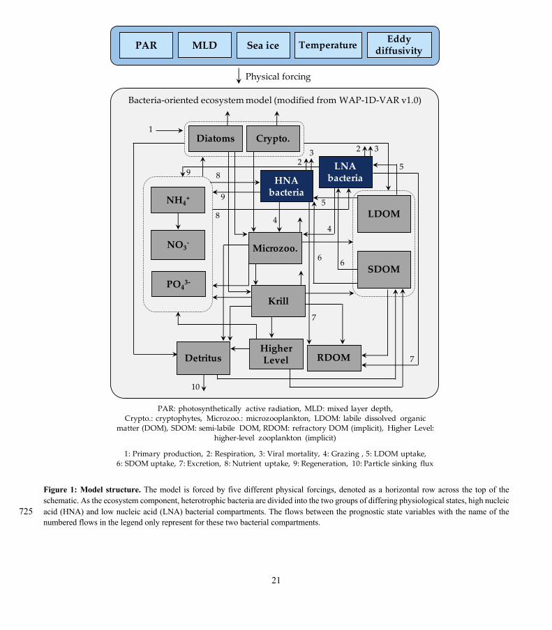
21

Figure 1: Model structure. The model is forced by five different physical forcings, denoted as a horizontal row across the top of the schematic. As the ecosystem component, heterotrophic bacteria are divided into the two groups of differing physiological states, high nucleic acid (HNA) and low nucleic acid (LNA) bacterial compartments. The flows between the prognostic state variables with the name of the 725 numbered flows in the legend only represent for these two bacterial compartments.

Bacteria-oriented ecosystem model (modified from WAP-1D-VAR v1.0)

2

5

4

3

6

7

1

8

9

10

2 3

4

5

6

7

8

9

PAR MLD Sea ice Temperature Eddy diffusivity

Physical forcing

Diatoms Crypto.

HNA bacteria

LNA bacteria

Microzoo.

Krill

LDOM

SDOM

RDOMHigher LevelDetritus

NH4+

NO3-

PO43-

PAR: photosynthetically active radiation, MLD: mixed layer depth, Crypto.: cryptophytes, Microzoo.: microzooplankton, LDOM: labile dissolved organic

matter (DOM), SDOM: semi-labile DOM, RDOM: refractory DOM (implicit), Higher Level: higher-level zooplankton (implicit)

1: Primary production, 2: Respiration, 3: Viral mortality, 4: Grazing , 5: LDOM uptake, 6: SDOM uptake, 7: Excretion, 8: Nutrient uptake, 9: Regeneration, 10: Particle sinking flux

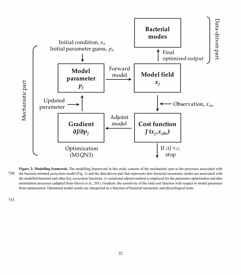
22

Figure 2: Modelling framewok. The modelling framework in this study consists of the mechanistic part as the processes associated with the bacteria-oriented ecosystem model (Fig. 1) and the data-driven part that represents how bacterial taxonomic modes are associated with 730 the modelled bacterial and other key ecosystem functions. A variational adjoint method is employed for the parameter optimization and data assimilation processes (adapted from Glover et al., 201). Gradient: the sensitivity of the total cost function with respect to model parameter from optimization. Optimized model results are interpreted as a function of bacterial taxonomic and physiological traits.

735

Model parameter

pj

Model fieldxj

Initial condition, x0Initial parameter guess, p0

Cost functionJ (xj ,xobs)

Observation, xobs

Gradient∂J/∂pj

If ΔJ < ɛ, stop

Optimization (M1QN3)

Forward model

Adjoint model

Updated parameter

Finaloptimized output

Bacterial modes

Mec

hani

stic

par

tD

ata-driven part

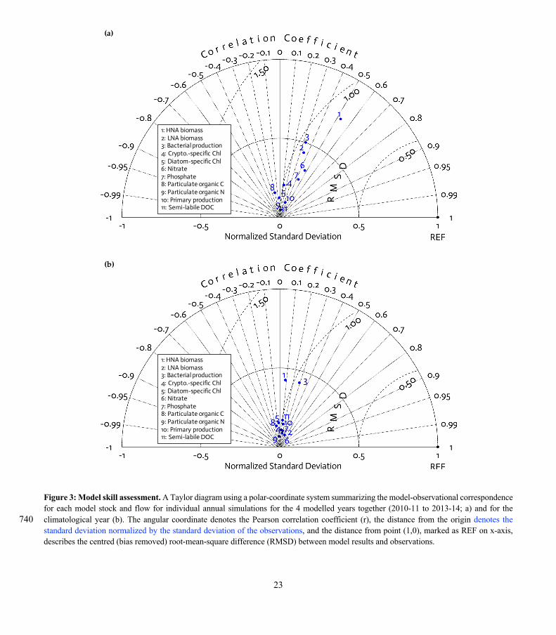
23

Figure 3: Model skill assessment. A Taylor diagram using a polar-coordinate system summarizing the model-observational correspondence for each model stock and flow for individual annual simulations for the 4 modelled years together (2010-11 to 2013-14; a) and for the climatological year (b). The angular coordinate denotes the Pearson correlation coefficient (r), the distance from the origin denotes the 740 standard deviation normalized by the standard deviation of the observations, and the distance from point (1,0), marked as REF on x-axis, describes the centred (bias removed) root-mean-square difference (RMSD) between model results and observations.

(a)

(b)

1: HNA biomass2: LNA biomass3: Bacterial production4: Crypto.-specific Chl5: Diatom-specific Chl6: Nitrate7: Phosphate8: Particulate organic C9: Particulate organic N10: Primary production11: Semi-labile DOC

1: HNA biomass2: LNA biomass3: Bacterial production4: Crypto.-specific Chl5: Diatom-specific Chl6: Nitrate7: Phosphate8: Particulate organic C9: Particulate organic N10: Primary production11: Semi-labile DOC

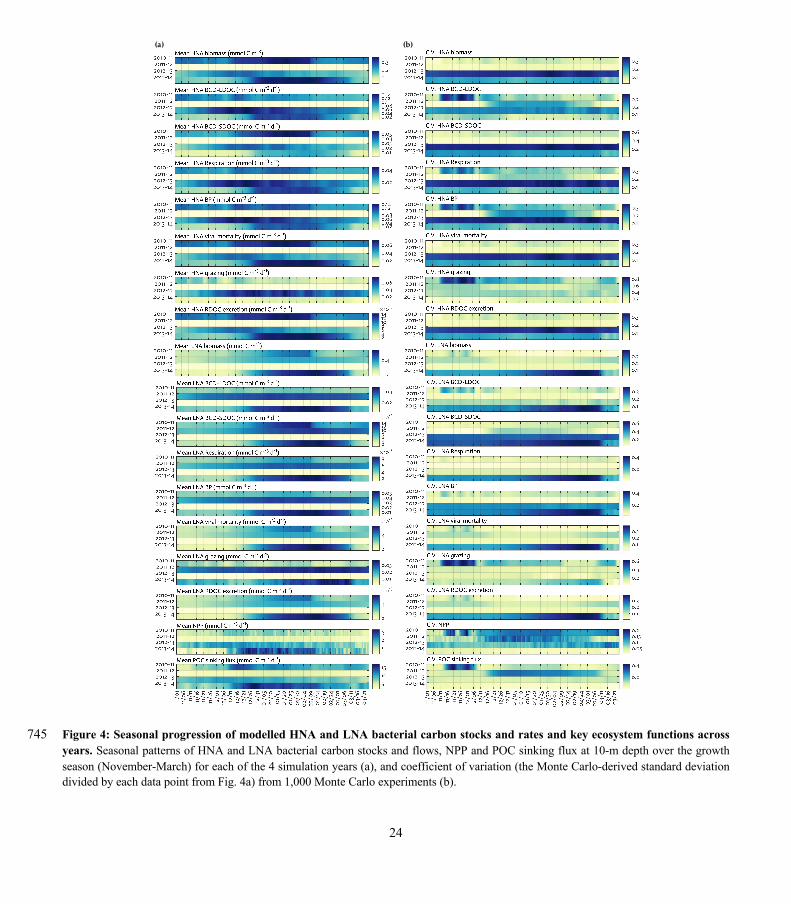
24

Figure 4: Seasonal progression of modelled HNA and LNA bacterial carbon stocks and rates and key ecosystem functions across 745 years. Seasonal patterns of HNA and LNA bacterial carbon stocks and flows, NPP and POC sinking flux at 10-m depth over the growth season (November-March) for each of the 4 simulation years (a), and coefficient of variation (the Monte Carlo-derived standard deviation divided by each data point from Fig. 4a) from 1,000 Monte Carlo experiments (b).

(a) (b)

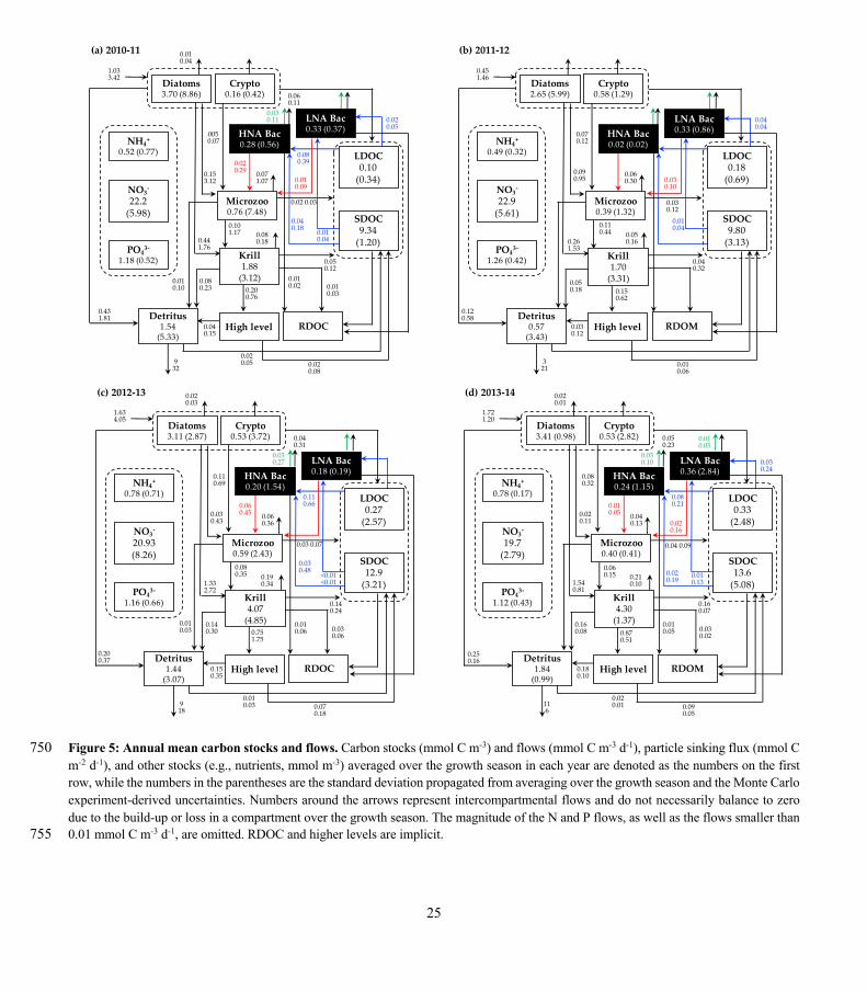
25

Figure 5: Annual mean carbon stocks and flows. Carbon stocks (mmol C m-3) and flows (mmol C m-3 d-1), particle sinking flux (mmol C 750 m-2 d-1), and other stocks (e.g., nutrients, mmol m-3) averaged over the growth season in each year are denoted as the numbers on the first row, while the numbers in the parentheses are the standard deviation propagated from averaging over the growth season and the Monte Carlo experiment-derived uncertainties. Numbers around the arrows represent intercompartmental flows and do not necessarily balance to zero due to the build-up or loss in a compartment over the growth season. The magnitude of the N and P flows, as well as the flows smaller than 0.01 mmol C m-3 d-1, are omitted. RDOC and higher levels are implicit. 755

0.030.11

0.010.10

0.071.07

0.010.04

0.080.39

0.010.02

932

0.080.180.44

1.76

0050.07

0.020.29

1.033.42

0.060.11

0.010.04

0.020.05

0.153.12 0.01

0.09

(a) 2010-11

0.040.180.10

1.17

0.02 0.03

0.050.12

0.080.23 0.20

0.760.010.03

0.040.15

0.020.05 0.02

0.08

0.431.81

0.060.30

321

0.050.160.26

1.53

0.070.12

0.451.46

0.010.04

0.040.04

0.090.95 0.03

0.10

(b) 2011-12

0.11 0.44

0.030.12

0.040.32

0.050.18 0.15

0.62

0.030.12

0.010.06

0.120.58

0.030.27

0.010.03

0.060.36

0.020.03

0.110.66

0.010.06

918

0.190.341.33

2.72

0.110.69

0.060.45

1.634.05

0.040.31

<0.01<0.01

0.030.43

(c) 2012-13

0.030.480.08

0.35

0.03 0.07

0.140.24

0.140.30 0.75

1.750.030.06

0.150.35

0.010.03 0.07

0.18

0.200.37

0.030.10

0.040.13

0.020.01

0.080.21

0.010.05

116

0.210.101.54

0.81

0.080.32

0.010.05

1.721.20

0.010.05

0.050.23

0.010.13

0.030.24

0.020.11 0.02

0.16

(d) 2013-14

0.020.19

0.06 0.15

0.04 0.09

0.160.07

0.160.08 0.87

0.510.030.02

0.180.10

0.020.01 0.09

0.05

0.250.16

RDOC

NO3-

22.2(5.98)

PO43-

1.18 (0.52) Krill1.88

(3.12)

Diatoms3.70 (8.86)

LNA Bac0.33 (0.37)

LDOC0.10

(0.34)

SDOC9.34

(1.20)

Detritus1.54

(5.33)

Crypto0.16 (0.42)

RDOM

NO3-

22.9(5.61)

PO43-

1.26 (0.42) Krill1.70

(3.31)

Diatoms2.65 (5.99)

LNA Bac0.33 (0.86)

High level

LDOC0.18

(0.69)

Microzoo0.39 (1.32)

SDOC9.80

(3.13)

HNA Bac0.02 (0.02)

Detritus0.57

(3.43)

Crypto0.58 (1.29)

RDOC

NO3-

20.93(8.26)

PO43-

1.16 (0.66) Krill4.07

(4.85)

Diatoms3.11 (2.87)

LNA Bac0.18 (0.19)

High level

LDOC0.27

(2.57)

Microzoo0.59 (2.43)

SDOC12.9

(3.21)

HNA Bac0.20 (1.54)

Detritus1.44

(3.07)

Crypto0.53 (3.72)

RDOM

NO3-

19.7(2.79)

PO43-

1.12 (0.43) Krill4.30

(1.37)

Diatoms3.41 (0.98)

LNA Bac0.36 (2.84)

High level

LDOC0.33

(2.48)

Microzoo0.40 (0.41)

SDOC13.6

(5.08)

HNA Bac0.24 (1.15)

Detritus1.84

(0.99)

Crypto0.53 (2.82)

Microzoo0.76 (7.48)

HNA Bac0.28 (0.56)

High level

NH4+

0.49 (0.32)NH4

+

0.52 (0.77)

NH4+

0.78 (0.71)NH4

+

0.78 (0.17)

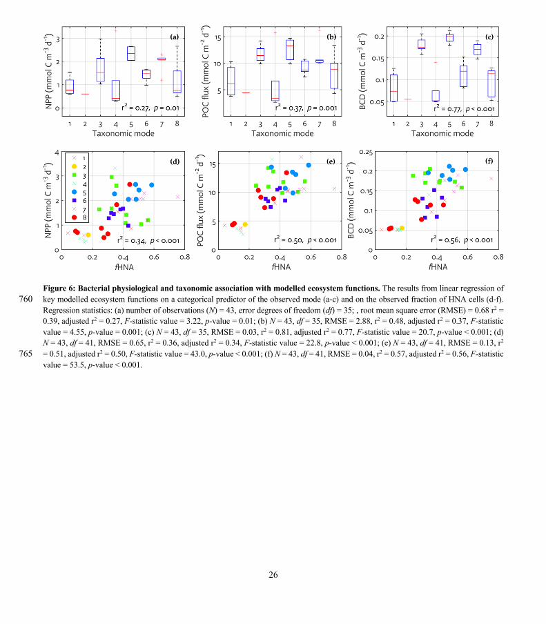
26

Figure 6: Bacterial physiological and taxonomic association with modelled ecosystem functions. The results from linear regression of key modelled ecosystem functions on a categorical predictor of the observed mode (a-c) and on the observed fraction of HNA cells (d-f). 760 Regression statistics: (a) number of observations (N) = 43, error degrees of freedom (df) = 35; , root mean square error (RMSE) = 0.68 r2 = 0.39, adjusted r2 = 0.27, F-statistic value = 3.22, p-value = 0.01; (b) N = 43, df = 35, RMSE = 2.88, r2 = 0.48, adjusted r2 = 0.37, F-statistic value = 4.55, p-value = 0.001; (c) N = 43, df = 35, RMSE = 0.03, r2 = 0.81, adjusted r2 = 0.77, F-statistic value = 20.7, p-value < 0.001; (d) N = 43, df = 41, RMSE = 0.65, r2 = 0.36, adjusted r2 = 0.34, F-statistic value = 22.8, p-value < 0.001; (e) N = 43, df = 41, RMSE = 0.13, r2 = 0.51, adjusted r2 = 0.50, F-statistic value = 43.0, p-value < 0.001; (f) N = 43, df = 41, RMSE = 0.04, r2 = 0.57, adjusted r2 = 0.56, F-statistic 765 value = 53.5, p-value < 0.001.

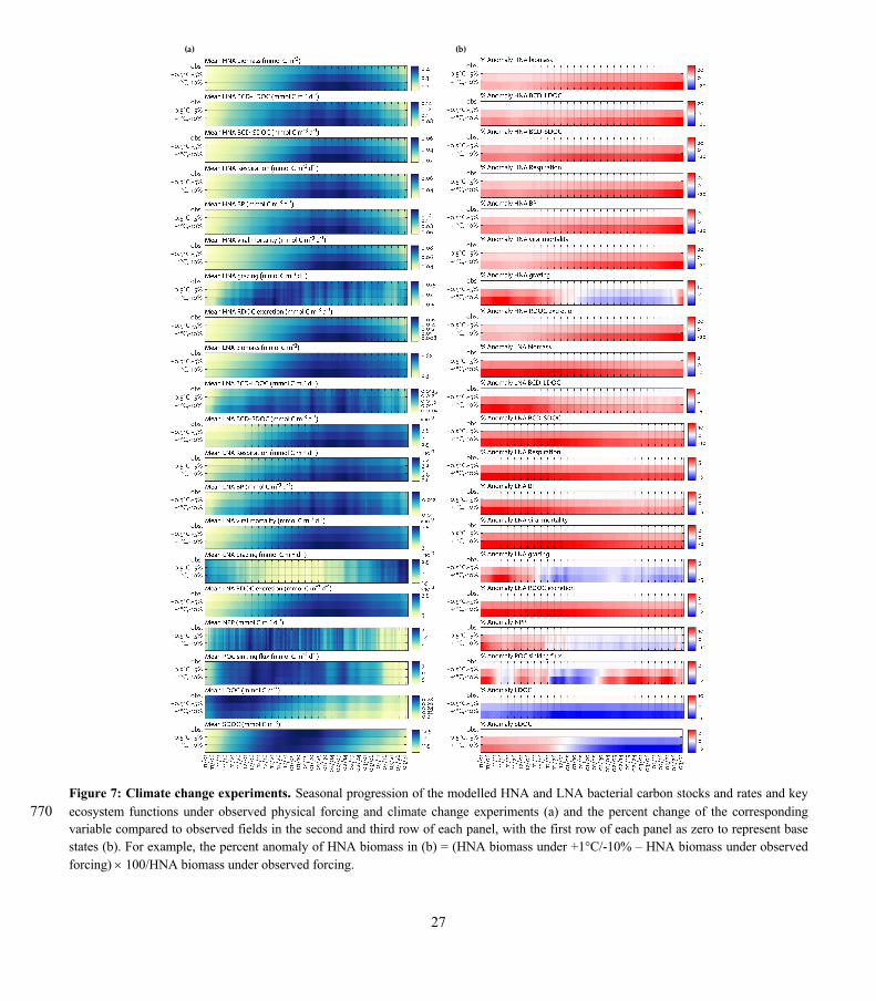
27

Figure 7: Climate change experiments. Seasonal progression of the modelled HNA and LNA bacterial carbon stocks and rates and key ecosystem functions under observed physical forcing and climate change experiments (a) and the percent change of the corresponding 770 variable compared to observed fields in the second and third row of each panel, with the first row of each panel as zero to represent base states (b). For example, the percent anomaly of HNA biomass in (b) = (HNA biomass under +1°C/-10% – HNA biomass under observed forcing) ´ 100/HNA biomass under observed forcing.

(a) (b)

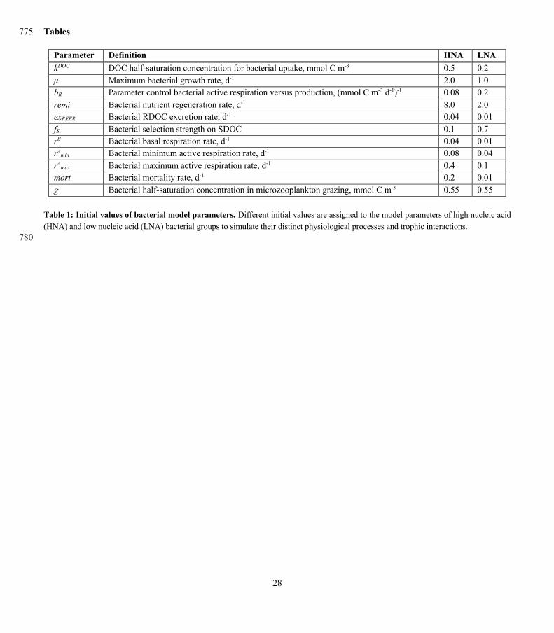
28

Tables 775

Parameter Definition HNA LNA kDOC DOC half-saturation concentration for bacterial uptake, mmol C m-3 0.5 0.2 μ Maximum bacterial growth rate, d-1 2.0 1.0 bR Parameter control bacterial active respiration versus production, (mmol C m-3 d-1)-1 0.08 0.2 remi Bacterial nutrient regeneration rate, d-1 8.0 2.0 exREFR Bacterial RDOC excretion rate, d-1 0.04 0.01 fS Bacterial selection strength on SDOC 0.1 0.7 rB Bacterial basal respiration rate, d-1 0.04 0.01 rAmin Bacterial minimum active respiration rate, d-1 0.08 0.04 rAmax Bacterial maximum active respiration rate, d-1 0.4 0.1 mort Bacterial mortality rate, d-1 0.2 0.01 g Bacterial half-saturation concentration in microzooplankton grazing, mmol C m-3 0.55 0.55

Table 1: Initial values of bacterial model parameters. Different initial values are assigned to the model parameters of high nucleic acid (HNA) and low nucleic acid (LNA) bacterial groups to simulate their distinct physiological processes and trophic interactions. 780

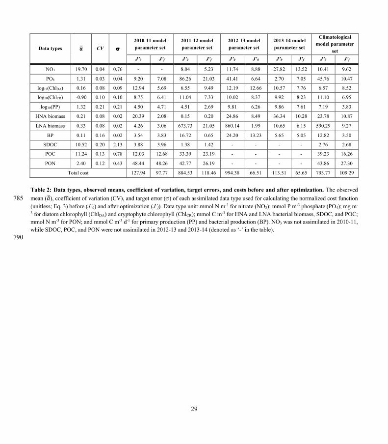
29

Data types 𝒂"# CV s 2010-11 model parameter set

2011-12 model parameter set

2012-13 model parameter set

2013-14 model parameter set

Climatological model parameter

set J’0 J’f J’0 J’f J’0 J’0 J’0 J’f J’0 J’f

NO3 19.70 0.04 0.76 - - 8.04 5.23 11.74 8.88 27.82 13.52 10.41 9.62

PO4 1.31 0.03 0.04 9.20 7.08 86.26 21.03 41.41 6.64 2.70 7.05 45.76 10.47

log10(ChlDA) 0.16 0.08 0.09 12.94 5.69 6.55 9.49 12.19 12.66 10.57 7.76 6.57 8.52

log10(ChlCR) -0.90 0.10 0.10 8.75 6.41 11.04 7.33 10.02 8.37 9.92 8.23 11.10 6.95

log10(PP) 1.32 0.21 0.21 4.50 4.71 4.51 2.69 9.81 6.26 9.86 7.61 7.19 3.83

HNA biomass 0.21 0.08 0.02 20.39 2.08 0.15 0.20 24.86 8.49 36.34 10.28 23.78 10.87

LNA biomass 0.33 0.08 0.02 4.26 3.06 673.73 21.05 860.14 1.99 10.65 6.15 590.29 9.27

BP 0.11 0.16 0.02 3.54 3.83 16.72 0.65 24.20 13.23 5.65 5.05 12.82 3.50

SDOC 10.52 0.20 2.13 3.88 3.96 1.38 1.42 - - - - 2.76 2.68

POC 11.24 0.13 0.78 12.03 12.68 33.39 23.19 - - - - 39.23 16.26

PON 2.40 0.12 0.43 48.44 48.26 42.77 26.19 - - - - 43.86 27.30

Total cost 127.94 97.77 884.53 118.46 994.38 66.51 113.51 65.65 793.77 109.29

Table 2: Data types, observed means, coefficient of variation, target errors, and costs before and after optimization. The observed mean (𝑎"#), coefficient of variation (CV), and target error (s) of each assimilated data type used for calculating the normalized cost function 785 (unitless; Eq. 3) before (J’0) and after optimization (J’f). Data type unit: mmol N m-3 for nitrate (NO3); mmol P m-3 phosphate (PO4); mg m-

3 for diatom chlorophyll (ChlDA) and cryptophyte chlorophyll (ChlCR); mmol C m-3 for HNA and LNA bacterial biomass, SDOC, and POC; mmol N m-3 for PON; and mmol C m-3 d-1 for primary production (PP) and bacterial production (BP). NO3 was not assimilated in 2010-11, while SDOC, POC, and PON were not assimilated in 2012-13 and 2013-14 (denoted as ‘-’ in the table). 790

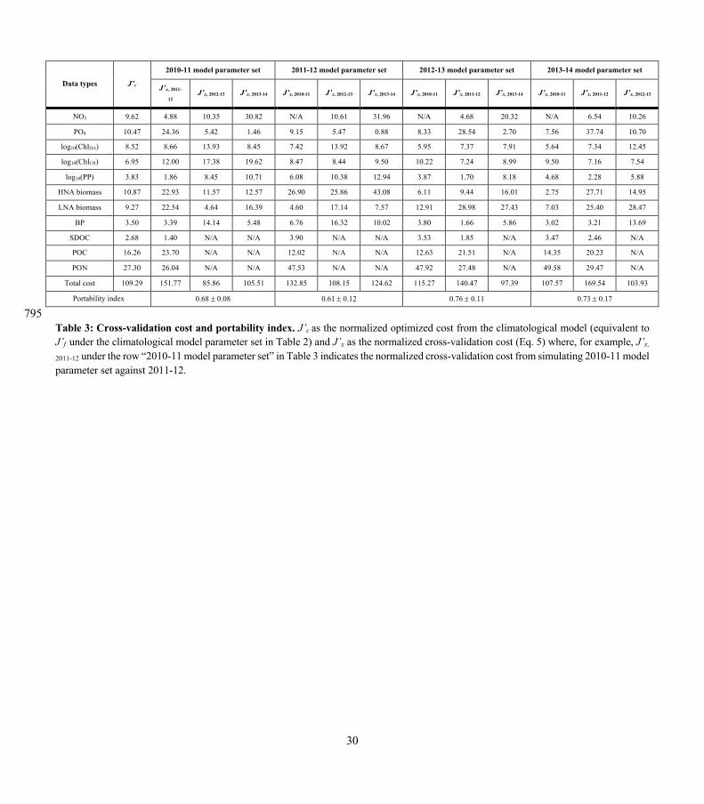
30

Data types J’c

2010-11 model parameter set 2011-12 model parameter set 2012-13 model parameter set 2013-14 model parameter set

J’x, 2011-

12 J’x, 2012-13 J’x, 2013-14 J’x, 2010-11 J’x, 2012-13 J’x, 2013-14 J’x, 2010-11 J’x, 2011-12 J’x, 2013-14 J’x, 2010-11 J’x, 2011-12 J’x, 2012-13

NO3 9.62 4.88 10.35 30.82 N/A 10.61 31.96 N/A 4.68 20.32 N/A 6.54 10.26

PO4 10.47 24.36 5.42 1.46 9.15 5.47 0.88 8.33 28.54 2.70 7.56 37.74 10.70

log10(ChlDA) 8.52 8.66 13.93 8.45 7.42 13.92 8.67 5.95 7.37 7.91 5.64 7.34 12.45

log10(ChlCR) 6.95 12.00 17.38 19.62 8.47 8.44 9.50 10.22 7.24 8.99 9.50 7.16 7.54

log10(PP) 3.83 1.86 8.45 10.71 6.08 10.38 12.94 3.87 1.70 8.18 4.68 2.28 5.88

HNA biomass 10.87 22.93 11.57 12.57 26.90 25.86 43.08 6.11 9.44 16.01 2.75 27.71 14.95

LNA biomass 9.27 22.54 4.64 16.39 4.60 17.14 7.57 12.91 28.98 27.43 7.03 25.40 28.47

BP 3.50 3.39 14.14 5.48 6.76 16.32 10.02 3.80 1.66 5.86 3.02 3.21 13.69

SDOC 2.68 1.40 N/A N/A 3.90 N/A N/A 3.53 1.85 N/A 3.47 2.46 N/A

POC 16.26 23.70 N/A N/A 12.02 N/A N/A 12.63 21.51 N/A 14.35 20.23 N/A

PON 27.30 26.04 N/A N/A 47.53 N/A N/A 47.92 27.48 N/A 49.58 29.47 N/A

Total cost 109.29 151.77 85.86 105.51 132.85 108.15 124.62 115.27 140.47 97.39 107.57 169.54 103.93

Portability index 0.68 ± 0.08 0.61 ± 0.12 0.76 ± 0.11 0.73 ± 0.17

795 Table 3: Cross-validation cost and portability index. J’c as the normalized optimized cost from the climatological model (equivalent to J’f under the climatological model parameter set in Table 2) and J’x as the normalized cross-validation cost (Eq. 5) where, for example, J’x,

2011-12 under the row “2010-11 model parameter set” in Table 3 indicates the normalized cross-validation cost from simulating 2010-11 model parameter set against 2011-12.