Modeling word and morpheme order in natural language as ...

Modeling word and morpheme order in natural language as anefficient tradeoff of memory and surprisal

Michael Hahn Judith Degen Richard FutrellStanford University Stanford University UC Irvine

[email protected] [email protected] [email protected]

January 9, 2021

Abstract

Memory limitations are known to constrain language comprehension and production, and have beenargued to account for crosslinguistic word order regularities. However, a systematic assessment of therole of memory limitations in language structure has proven elusive, in part because it is hard to ex-tract precise large-scale quantitative generalizations about language from existing mechanistic modelsof memory use in sentence processing. We provide an architecture-independent information-theoreticformalization of memory limitations which enables a simple calculation of the memory efficiency oflanguages. Our notion of memory efficiency is based on the idea of a memory–surprisal tradeoff : acertain level of average surprisal per word can only be achieved at the cost of storing some amount ofinformation about past context. Based on this notion of memory usage, we advance the Efficient TradeoffHypothesis: the order of elements in natural language is under pressure to enable favorable memory-surprisal tradeoffs. We derive that languages enable more efficient tradeoffs when they exhibit informa-tion locality: when predictive information about an element is concentrated in its recent past. We provideempirical evidence from three test domains in support of the Efficient Tradeoff Hypothesis: a reanalysisof a miniature artificial language learning experiment, a large-scale study of word order in corpora of54 languages, and an analysis of morpheme order in two agglutinative languages. These results suggestthat principles of order in natural language can be explained via highly generic cognitively motivatedprinciples and lend support to efficiency-based models of the structure of human language.

1 Introduction

Natural language is a powerful tool that allows humans to communicate, albeit under inherent cognitiveresource limitations. Here, we investigate whether human languages are grammatically structured in a waythat reduces the cognitive resource requirements for comprehension, compared to counterfactual languagesthat differ in grammatical structure.

The suggestion that the structure of human language reflects a need for efficient processing under re-source limitations has been present in the linguistics and cognitive science literature for decades (Yngve,1960; Berwick and Weinberg, 1984; Hawkins, 1994; Chomsky, 2005; Jaeger and Tily, 2011; Gibson et al.,

0This is a preprint of a paper in press at Psychological Review. A version including Supplementary Information (SI Appendix)is available at: https://psyarxiv.com/nu4qzc© 2021, American Psychological Association. This paper is not the copy of record and may not exactly replicate the final, au-

thoritative version of the article. Please do not copy or cite without authors’ permission. The final article will be available, uponpublication, via its DOI: 10.1037/rev0000269

1

2019; Hahn et al., 2020). The idea has been summed up in Hawkins’s (2004) Performance–Grammar Cor-respondence Hypothesis (PGCH), which holds that grammars are structured so that the typical utterance iseasy to produce and comprehend under performance constraints.

One major source of resource limitation in language processing is incremental memory use. When pro-ducing and comprehending language in real time, a language user must keep track of what they have alreadyproduced or heard in some kind of incremental memory store, which is subject to resource constraints. Thesememory constraints have been argued to underlie various locality principles which linguists have used topredict the orders of words within sentences and morphemes within words (e.g. Behaghel, 1932; Givon,1985; Bybee, 1985; Rijkhoff, 1990; Hawkins, 1994, 2004, 2014; Temperley and Gildea, 2018). The idea isthat language should be structured to reduce long-term dependencies of various kinds, by placing elementsthat depend on each other close to each other in linear order. That is, elements of utterances which are more‘relevant’ or ‘mentally connected’ to each other are closer to each other.

Our contribution is to present a new, highly general formalization of the relationship between sequentialorder and incremental memory in language processing, from which we can derive a precise and empiricallytestable version of the idea that utterance elements which depend on each other should be close to eachother. Our formalization allows us to predict the order of words within sentences, and morphemes withinwords directly by the minimization of memory usage.

We formalize the notion of memory constraints in terms of what we call the memory–surprisal trade-off: the idea that the ease of comprehension depends on the amount of computational resources invested intoremembering previous linguistic elements, e.g., words. Therefore, there exists a tradeoff between the quan-tity of memory resources invested, and the ease of language processing. The shape of this tradeoff dependson the grammar of a language, and in particular the way that it structures information in time. We char-acterize memory resources using the theory of lossy data compression (Cover and Thomas, 2006; Berger,2003).

Within our framework, we prove a theorem showing that lower memory requirements result when ut-terance elements that depend on each other statistically are placed close to each other. This theorem doesnot require any assumptions about the architecture or functioning of memory, except that it has a boundedcapacity. Using this concept, we introduce the Efficient Tradeoff Hypothesis: Order in natural language isstructured so as to provide efficient memory–surprisal tradeoff curves. We provide evidence for this hypoth-esis in three studies. We demonstrate that word orders with short dependencies do indeed engender lowerworking memory resource requirements in toy languages studied in the previous literature, and we showthat real word orders in corpora of 54 languages have lower memory requirements than would be expectedunder artificial baseline comparison grammars. Finally, we show that we can predict the order of morphemeswithin words in two languages using our principle of the minimization of memory usage.

Our work not only formalizes and tests an old idea in functional linguistics and psycholinguistics, italso opens up connections between those fields and the statistical analysis of natural language (Debowski,2011; Bentz et al., 2017; Lin and Tegmark, 2017), and more broadly, between linguistics and fields that havestudied information-processing costs and resource requirements in brains (e.g., Friston, 2010) and generalphysical systems (e.g., Still et al., 2012).

2 Background

A wide range of work has argued that information in natural language utterances is ordered in ways thatreduce memory effort, by placing elements close together when they depend on each other in some way.Here, we review these arguments from linguistic and cognitive perspectives.

2

2.1 Dependency locality and memory constraints in psycholinguistics

When producing and comprehending language in real time, a language user must keep track of what shehas already produced or heard in some kind of incremental memory store, which is subject to resource con-straints. An early example of this idea is Miller and Chomsky (1963), who attributed the unacceptabilityof multiple center embeddings in English to limitations of human working memory. Concurrent and subse-quent work studied how different grammars induce different memory requirements in terms of the numberof symbols that must be stored at each point to produce or parse a sentence (Yngve, 1960; Abney and John-son, 1991; Gibson, 1991; Resnik, 1992). In psycholinguistic studies, memory constraints typically manifestin the form of processing difficulty associated with long-term dependencies. For example, at the level ofword-by-word online language comprehension, there is observable processing difficulty at moments whenit seems that information about a word must be retrieved from working memory. This difficulty increaseswhen there is a great deal of time or intervening material between the point when a word is first encounteredand the point when it must be retrieved from memory (Gibson, 1998; Gibson and Thomas, 1999; Gibson,2000; McElree, 2000; Lewis and Vasishth, 2005; Bartek et al., 2011; Nicenboim et al., 2015; Balling andKizach, 2017). That is, language comprehension is harder for humans when words which depend on eachother for their meaning are separated by many intervening words. This idea is most prominently associatedwith the Dependency Locality Theory of human sentence processing (Gibson, 2000).

For example, Grodner and Gibson (2005) studied word-by-word reading times in a series of sentencessuch as (1) below.

(1) a. The administrator who the nurse supervised. . .

b. The administrator who the nurse from the clinic supervised. . .

c. The administrator who the nurse who was from the clinic supervised. . .

In these sentences, the distance between the noun administrator and the verb supervised is successivelyincreased. Grodner and Gibson (2005) found that as this distance increases, there is a concomitant increasein reading time at the verb supervised and following words.

The hypothesized reason for this reading time pattern is based on memory constraints. The idea goes: atthe word supervised, a comprehender who is trying to compute the meaning of the sentence must integratea representation of the verb supervised with a representation of the noun administrator, which is a directobject of the verb. This integration requires retrieving the representation of administrator from workingmemory. If this representation has been in working memory for a long time—for example as in Sentence 1cas opposed to 1a—then the retrieval is difficult or inaccurate, in a way that manifests as increased readingtime. Essentially, there exists a dependency between the words administrator and supervised, and moreexcess processing difficulty is incurred the more the two words are separated; this excess difficulty is calleda dependency locality effect.

The existence of dependency locality effects in human language processing, and their connection withworking memory, are well-established (Fedorenko et al., 2013). These locality effects in online processingmirror locality effects in word order, described below.

2.2 Locality and cross-linguistic universals of order

Dependency locality in word order means that there is a pressure for words which depend on each othersyntactically to be close to each other in linear order. There is ample evidence from corpus statistics indicat-ing that dependency locality is a real property of word order across many languages (Ferrer-i-Cancho, 2004;

3

Gildea and Temperley, 2007; Liu, 2008; Gildea and Temperley, 2010; Futrell et al., 2015a; Liu et al., 2017;Temperley and Gildea, 2018). Hawkins (1994, 2003) formulates dependency locality as the Principle of Do-main Minimization, and has shown that this principle can explain cross-linguistic universals of word orderthat have been documented by linguistic typologists for decades (Greenberg, 1963). Such a pressure can bemotivated in terms of the documented online processing difficulty associated with long-term dependenciesamong words: dependency locality in word order means that online processing is easier.

An example is order alternation in postverbal constituents in English. While NP objects ordinarily pre-cede PPs (2a, example from Staub et al. (2006)), this order is less preferred when the NP is very long (2c),in which case the inverse order becomes more felicitous (2d). The pattern in (2d) is known as Heavy NPShift (Ross, 1967; Arnold et al., 2000; Stallings and MacDonald, 2011). Compared to (2c), it reduces thedistance between the verb “ate” and the PP, while only modestly increasing the distance between the verband object NP.

(2) a. Lucy ate [the broccoli] with a fork.

b. ? Lucy ate with a fork [the broccoli].

c. Lucy ate [the extremely delicious, bright green broccoli] with a fork .

d. Lucy ate with a fork [the extremely delicious, bright green broccoli].

Locality principles have also appeared in a more general form in the functional linguistics literature,in the form of the idea that elements which are more ‘relevant’ to each other will appear closer to eachother in linear order in utterances (Behaghel, 1932; Givon, 1985; Givon, 1991; Bybee, 1985; Newmeyer,1992). Here, ‘elements’ can refer to words or morphemes, and the definition of ‘relevance’ varies. Forexample, Givon (1985)’s Proximity Principle states that elements are placed closer together in a sentenceif they are closer conceptually. Applying a similar principle, Bybee (1985) studied the order or morphemeswithin words across languages, and argued that (for example) morphemes that indicate the valence of a verb(whether it takes zero, one, or two objects) are placed closer to the verb root than morphemes that indicatethe plurality of the subject of the verb, because the valence morphemes are more ‘relevant’ to the verb root.

While these theories are widespread in the linguistics literature, there exists to date no quantifiabledefinition of ‘relevance’ or ‘being closer conceptually’. One of our contributions is to derive such a notionof ‘relevance’ from the minimization of memory usage during language processing.

2.3 Architectural assumptions

The connection between memory resources and locality principles relies on the idea that limitations inworking memory will give rise to difficulty when elements that depend on each other are separated at alarge distance in time. In previous work, this idea has been motivated in terms of specific assumptions aboutthe architecture of memory. For example, models of memory in sentence processing differ in whether theyassume limitations in storage capacity (e.g., ‘memory cost’ in the model of Gibson, 1998) or the precisionwith which specific elements can be retrieved from memory (e.g. Lewis and Vasishth, 2005). Furthermore, inorder to derive the connection between memory usage in such models and locality in word order, it has beennecessary to stipulate that memory representations or activations decay over time in some way to explainwhy longer dependencies are harder to process. The question remains of whether these assumptions aboutmemory architecture are necessary, or whether word orders across languages are optimized for memoryindependently of the implementation and architecture of human language processing.

4

In this work, we adopt an information-theoretic perspective on memory use in language processing,which abstracts away from the details of memory architecture. Within our framework, we will establish theconnection between memory resources and locality principles by providing general information-theoreticlower bounds on memory use. We quantify memory resources in terms of their information-theoretic ca-pacity measured in bits, following models proposed for working memory in other domains (Brady et al.,2008, 2009; Sims et al., 2012). Our result immediately entails a link between locality and boundedness ofmemory, following only from the stipulation that memory is finite in capacity. In particular, our model doesnot require any assumption that memory representations or activations decay over time (as was required inprevious work: Gibson, 1998; Lewis and Vasishth, 2005; Futrell et al., 2020b). We will then show empiricalevidence that the orders of words and morphemes in natural language are structured in a way that reducesour measure of memory use compared to the orders of counterfactual baseline languages.

The remainder of the paper is structured as follows. We first introduce the memory-surprisal tradeoff andintroduce our Efficient Tradeoff Hypothesis. Then, we test the Efficient Tradeoff Hypothesis in three studies.In Study 1, we qualitatively test the Hypothesis in a reanalysis of word orders emerging in a miniatureartificial language study (Fedzechkina et al., 2017). In Study 2, we quantitatively test the Hypothesis in alarge-scale study of the word order of 54 languages. In Study 3, we test the Hypothesis on morpheme orderin Japanese and Sesotho. Finally, we discuss the implications and limitations of the reported results.

3 Memory-Surprisal Tradeoff

In this section, we introduce the main concept and hypothesis of the paper. We provide a technical definitionof the memory–surprisal tradeoff curve, and we prove a theorem showing that more efficient memory–surprisal tradeoffs are possible in languages exhibiting information locality, i.e., in languages where wordsthat depend on each other are close to each other. This theorem establishes the formal link between memoryefficiency in online processing and locality in word order.

3.1 An information-theoretic model of online language comprehension

We begin developing our model by considering the process of language comprehension, where a listener isprocessing a stream of words uttered by an interlocutor. Experimental research has established three prop-erties of online language comprehension: (1) listeners maintain some information about the words receivedso far in incremental memory, (2) listeners form probabilistic expectations about the upcoming words (e.g.Altmann and Kamide, 1999; Staub and Clifton Jr, 2006; Kuperberg and Jaeger, 2016), and (3) words areeasy to process to the extent that they are predictable based on a listener’s memory of words received so far(Hale, 2001; Levy, 2008; Futrell et al., 2020b). See General Discussion for discussion of how our model isrelated to theories that do not explicitly make these assumptions.

We formalize these three observations into postulates intended to provide a simplified picture of whatis known about online language comprehension. Consider a listener comprehending a sequence of wordsw1, . . . ,wt , . . . ,wn, at an arbitrary time t.

1. Comprehension Postulate 1 (Incremental memory). At time t, the listener has an incremental memorystate mt that contains her stored information about previous words. The memory state is characterizedby a memory encoding function M such that mt = M(wt−1,mt−1).

2. Comprehension Postulate 2 (Incremental prediction). The listener has a subjective probability distribu-tion at time t over the next word wt as a function of the memory state mt . This probability distribution

5

is denoted P(wt |mt).

3. Comprehension Postulate 3 (Linking hypothesis). Processing a word wt incurs difficulty proportionalto the surprisal of wt given the memory state mt :1

Difficulty ∝− log2 P(wt |mt). (1)

The claim that processing difficulty should be directly proportional to surprisal comes from surprisal theory(Hale, 2001; Levy, 2008), an established psycholinguistic theory that can capture reading time effects relatedto garden-path disambiguation, antilocality effects, and effects of syntactic construction frequency. Surprisalis a robust linear predictor of reading times in large-scale eye-tracking studies based on naturalistic text(Smith and Levy, 2013; Goodkind and Bicknell, 2018; Frank and Hoeks, 2019; Aurnhammer and Frank,2019; Wilcox et al., 2020), and effects of surprisal have been observed for units as small as phonemes(Gwilliams et al., 2020). There are several converging theoretical arguments for surprisal as a measure ofprocessing cost (Levy, 2008; Smith and Levy, 2013). Surprisal theory is compatible with different viewson the mechanisms underlying prediction, and can reflect different mechanisms such as preactivation andintegration (Kuperberg and Jaeger, 2016). We do not assume that listeners explicitly compute a full-fledgeddistribution P(wt |mt); we view P(wt |mt) as a formalization of the probabilistic expectations that listenersform during comprehension.

Our expression (1) differs from the usual formulation of surprisal theory in that we consider predictabil-ity based on a (potentially lossy or noisy) memory representation mt , rather than predictability based onthe true complete context w1, . . . ,wt−1. The generalization to lossy memory representations is necessary tocapture empirically observed effects of memory limitations on language processing, such as dependencylocality and structural forgetting (Futrell et al., 2020b).

In this work, we are interested in using theories of processing difficulty to derive predictions about lan-guages as a whole, not about individual words or sentences. Therefore, we need a measure of the processingdifficulty associated with a language as a whole. For this, we consider the average surprisal per word in thelanguage. We call this quantity the average surprisal of a language given a memory encoding function M,denoted SM.

Crucially, the listener’s ability to predict upcoming words accurately depends on how much she remem-bers about previous words. As the precision of her memory increases, the accuracy of her predictions alsoincreases, and the average surprisal SM for each incoming word decreases. Taking an information-theoreticperspective, we can think about the amount of information (measured in bits) about previous words storedin the listener’s memory state. This quantity of information is given by the entropy of the memory state,which we denote HM. As the listener stores more and more bits of information about the previous wordsher memory state, she can achieve lower and lower surprisal values for the upcoming words. This tradeoffbetween memory and surprisal is the main object of study in this paper.

The memory–surprisal tradeoff curve answers the question: for a given amount of information aboutprevious words HM stored in the listener’s memory state, what is the lowest achievable average surprisalSM? Two example tradeoff curves are shown in Figure 1. In general, as the listener stores more informationabout previous words in her memory state, her lowest achievable average surprisal can only decrease. Sothe curve is always monotonically decreasing. However, the precise shape of the tradeoff curve depends onthe structure of the language being predicted. For example, Figure 1 shows how two hypothetical languagesmight engender different tradeoff curves, with Language A allowing more favorable tradeoffs than Language

1In this paper, all logarithms are taken to base 2. As choosing another basis (e.g., e) would only result in multiplication with aproportionality constant, this assumption does not impact the generality of this linking hypothesis.

6

4.5

4.0

3.5

3.0

0.0 0.5 1.0 1.5 2.0 2.5

Language A

Language B

Sur

pris

al

Memory (bits)

Figure 1: Example memory–surprisal tradeoff curves for two languages, A and B. Achieving an averagesurprisal of 3.5 bits requires storing at least 1.0 bits in language A, while it requires storing 2.0 bits in lan-guage B. Language A has a steeper memory–surprisal tradeoff than Language B, and requires less memoryresources to achieve the same level of processing difficulty.

B. That is, for Language A, it is possible to achieve lower processing difficulty while investing less memoryresources than in Language B.

3.2 Main hypothesis

Having conceptually introduced the memory–surprisal tradeoff, we can state the main hypothesis of thiswork, the Efficient Tradeoff Hypothesis.

Efficient Tradeoff Hypothesis:The order of elements in natural language is characterized by a distinctivelysteeper memory–surprisal tradeoff curve, compared to other possible orders.

A steep tradeoff curve corresponds to memory efficiency, in the sense that it is possible to achieve a lowlevel of processing difficulty (average surprisal SM) while storing a relatively small amount of informationabout previous words (entropy of memory HM). We hypothesize that this property is reflected in grammaticalstructure and usage preferences across languages.

3.3 Formal definition of the memory–surprisal tradeoff

Here we provide the technical definition of the memory–surprisal tradeoff curve. Let W be a stochastic pro-cess generating a stream of symbols extending indefinitely into the past and future: . . . ,w−2,w−1,w0,w1,w2, . . . .These symbols can represent words, morphemes, or other units for decomposing sentences into a sequenceof symbols. We model this process as stationary (Doob, 1953), that is, the joint probability distributions ofsymbols at different time points depend only on their relative positions in time, not their absolute positions(see SI Section 1.1.1 for more on this modeling assumption).

7

Let M be a memory encoding function. We consider memory and surprisal costs at an arbitrary timepoint t. Recall that the surprisal for a specific word wt after a past word sequence . . . ,wt−2,wt−1 encodedinto a memory state mt is:

− log2 P(wt |mt).

The average surprisal of the process W under the memory encoding function M is obtained by averagingover all possible past sequences . . . ,wt−2,wt−1 with associated memory states mt , and possible next wordswt :

SM ≡− ∑wt ,mt

P(mt)P(wt |mt) log2 P(wt |mt).

where wt ranges over possible symbols, and mt ranges over possible outputs of the memory encoding func-tion M. This quantity is known as the conditional entropy of wt given mt (Cover and Thomas, 2006, p.17):

SM = H[wt |mt ].

Because the process W is stationary, the average surprisal SM is independent of the choice of t (see SISection 1.1.2). The lowest possible average surprisal for W is attained when mt perfectly encodes all previousobserved words. This quantity is called the entropy rate of W (Cover and Thomas, 2006, pp. 74–75):

S∞ ≡ H[wt | . . . ,wt−2,wt−1],

which again is independent of t because W is stationary. We use the notation S∞ to suggest this idea of un-limited resources. The entropy rate of a stochastic process is the irreducible unpredictability of the process:the extent to which a stream of symbols remains unpredictable even for a predictor with unlimited resources.

Because the memory state mt is a function of the previous words . . . ,wt−2,wt−1, we can prove by theData Processing Inequality (Cover and Thomas, 2006, pp. 34–35) that the entropy rate must be less than orequal to the average surprisal for any memory encoding function M:

S∞ ≤ SM.

If the memory state mt stores all information about the previous words . . . ,wt−2,wt−1, then we haveSM = S∞.

Having defined average surprisal, we now turn to the question of how to define memory capacity. Theaverage amount of information stored in the memory states mt is the average number of bits required toencode mt . This is given by the entropy of the stationary distribution over memory states, HM:

HM ≡ H[mt ]

whereH[mt ] =−∑

mP(mt = m) log2 P(mt = m)

where m runs over all possible states of the memory encoding mt . Again, because W is stationary, thisquantity does not depend on the choice of t (see SI Section 1.1.2).

We will be imposing bounds on HM and studying the resulting values of SM.

Definition 1. The memory–surprisal tradeoff curve for a process W is the lowest achievable average sur-prisal SM for each value of HM. Let R denote an upper bound on the memory entropy HM; then the memory–surprisal tradeoff curve as a function of R is given by

D(R)≡ minM:HM≤R

SM, (2)

8

(a)

Hi, how are you?

I1

I2

I3

X-3 X-2 X-1 X0

t

It

It is sunny outside.

gave the attempt up.He

I4

(b)

T

A

B

T

t

It

t It

t

Bits of memory:

Excess surprisal incurred:

Figure 2: (a) Conditional mutual information It captures how much predictive information about the nextword is provided, on average, by the word t steps in the past. (b) Here we illustrate our theoretical result. Weplot It (top) and tIt (bottom) as functions of t. For any choice of T , a listener using B bits memory (bottom)to represent prior observations will incur at least A bits of extra surprisal beyond the entropy rate (top).

where the minimization is over all memory encoding functions M whose entropy HM is less than or equal toR.

The memory state mt is generally a lossy representation of the true context of words w1, . . . ,wt−1, mean-ing that mt does not contain all the possible information about w1, . . . ,wt−1. The mathematical theory oflossy representations is rate–distortion theory (for an overview and key results, see Cover and Thomas,2006, pp. 301–347); this theory has seen recent successful application in cognitive science and linguistics asa model of rational action under resource constraints (Brady et al., 2009; Sims et al., 2012; Sims, 2018; Za-slavsky et al., 2018; Schach et al., 2018; Zenon et al., 2019; Gershman, 2020). Rate–distortion theory studiescurves of the form of Eq. 2, which quantify tradeoffs between negative utility (‘distortion’) and information(‘rate’).

3.4 Information locality

The shape of the memory–surprisal tradeoff is determined in part by the grammatical structure of a language.Some hypothetical languages enable more efficient tradeoffs than others by allowing a listener to store fewerbits in memory to achieve the same level of average surprisal.

Here, we will demonstrate that the memory–surprisal tradeoff is optimized by languages with wordorders exhibiting a property called information locality. Information locality means that words that dependon each other statistically are located close to each other in time. We will argue that information localitygeneralizes the well-known word order principle of dependency locality.

We will make our argument by defining a lower bound on the memory–surprisal tradeoff curve (Eq. 2).This lower bound represents an unavoidable cost associated with a certain level of memory usage HM; thetrue average surprisal SM might be higher than this bound.

Our argument will make use of a quantity called mutual information. Mutual information is the mostgeneral measure of statistical association between two random variables. The mutual information between

9

two random variables X and Y , conditional on a third random variable Z, is defined as:

I[X : Y |Z]≡ ∑x,y,z

P(x,y,z) log2P(x,y|z)

P(x|z)P(y|z). (3)

Mutual information is always non-negative. It is zero when X and Y are conditionally independent given Z,and positive whenever X gives any information that makes the value of Y more predictable, or vice versa.

We will study the mutual information structure of natural language sentences, and in particular themutual information between words at certain distances in linear order. We define the notation It to mean themutual information between words at distance t from each other, conditional on the intervening words:

It ≡ I[wt : w0|w1, . . . ,wt−1].

This quantity, visualized in Figure 2(a), measures how much predictive information is provided about thecurrent word by the word t steps in the past. It is a statistical property of the language, and can be estimatedfrom large-scale text data.

Equipped with this notion of mutual information at a distance, we can now state our theorem:

Theorem 1. (Information locality bound) For any positive integer T , let M be a memory encoding functionsuch that

HM ≤T

∑t=1

tIt . (4)

Then we have a lower bound on the average surprisal under the memory encoding function M:

SM ≥ S∞ +∞

∑t=T+1

It . (5)

A formal proof based on the Comprehension Postulates 1–3 is given in SI Section 1.2. An intuitiveargument, forming the basis of the proof, is the following. Suppose that a comprehender predicting the t’thword wt uses an average of It bits of information coming from a previous word w0. Then these bits musthave been carried over t timesteps and thus have occupied memory for t timesteps. Since this happens forevery word in a sequence, there are, at any given point in time, t such packets of information, each withan average size of It bits, that have to be maintained, summing up to tIt . In the specific setting where Mencodes information from a contiguous span of the past T words, the total amount of encoded informationthus sums up to ∑

Tt=1 tIt , while information from longer contexts is lost, increasing surprisal by ∑

∞t=T+1 It .

While this informal argument specifically considers a memory encoding function that utilizes informationfrom a contiguous span of the past T words, the formal proof extends this to all memory encoding functionsM satisfying the Comprehension Postulates.

Interpretation The theorem means that a predictor with limited memory capacity will always be affectedby surprisal cost arising from long-term statistical dependencies of length greater than T , for some finite T .This is why we call the result ‘information locality’: processes are easier to predict when most statisticaldependencies are short-term (shorter than some T ). Below we explain in more detail how this interpretationmatches the mathematics of the theorem.

The quantities in the theorem are illustrated visually in Figure 2. Eq. 4 describes a memory encodingfunction which has enough capacity to remember the relevant information from at most T words in the

10

0

1

2

3

4

5

1 5 10t

Con

ditio

nal M

utua

l Inf

orm

atio

n (I

t)

Language

LessEfficientMoreEfficient

0

1

2

3

4

5

1 5 10t

t * It

Language


Figure 3: Left: It as a function of t, for two different hypothetical languages. It decays faster for the MoreEf-ficient language: Predictive information about the present observation is concentrated more strongly in therecent past. Right: t · It as a function of t for the same languages.

immediate past. The minimal amount of memory capacity which would be required to retain this informationis the sum ∑

Tt=1 tIt , reflecting the cost of holding It bits in memory for t timesteps up to t = T .

The information locality bound theorem says that the surprisal cost for this memory encoding functionis at least S∞ +∑

∞t=T+1 It (Eq. 5). The first term S∞ is the entropy rate of the process, representing the bits of

information in the process which could not have been predicted given any amount of memory. The secondterm ∑

∞t=T+1 It is the sum of all the relevant information contained in words more than T timesteps in the past

(see Figure 2(b)). These correspond to bits of information in the process which could have been predictedgiven infinite memory resources, but which were not, due to the limit on memory usage.

The theorem gives a lower bound on the memory–surprisal tradeoff curve, meaning that there is nomemory encoding function M with capacity HM which achieves lower average surprisal than Eq. 5. Interms of psycholinguistics, if memory usage is bounded by Eq. 4, then processing cost of at least Eq. 5is inevitable. Importantly, the bound holds for any memory encoding function M, including functions thatdo not specifically keep track of a window of the past T words. The information locality bound theoremdemonstrates in a highly general way that language comprehension requires less memory resources whenstatistical dependencies are mostly short-term.

Because processing long-term dependencies requires higher memory usage, the theorem also impliesthat a language can be easier to process when most of the predictive information about a word is concentratedclose to that word in time—that is, when It falls off rapidly as t→∞. When memory capacity is limited, thenthere must be some timescale T such that a listener appears to be affected by excess surprisal arising fromstatistical dependencies of length greater than T . A language avoids such cost to the extent that it avoidsdependencies with a time-span larger than T .

We illustrate the theorem in Figure 3. We consider two hypothetical languages, LessEfficient and More-Efficient, where It := 5t−1.5 for LessEfficient and It := 3.5t−2.5 for MoreEfficient.2 The curves of It , as a

2Although these are purely mathematical examples, the It curve for natural languages does seem empirically to fall off as a

11

3

4

5

6

5 10 15Memory

Sur

pris

al Language


Figure 4: Listener’s memory–surprisal tradeoff for the two hypothetical languages in Figure 3. Recall thatthe MoreEfficient language has a faster decay of conditional mutual information It . Correspondingly, thisfigure shows that a listener can achieve lower average surprisal at the same level of memory load.

function of the distance t, are shown in Figure 3 (left). In both cases, It converges to zero as t grows to infinity.However, It decays more quickly for language MoreEfficient. This means that predictive information aboutan observation is concentrated more strongly in the recent past. In Figure 3 (right), we show t ·It as a functionof t. Note that the area under the curve is equal to (4). This area is smaller for the MoreEfficient language, asIt decays more quickly there. In Figure 4, we show the resulting bounds on memory–surprisal tradeoffs ofthe two languages. As It decays faster for language MoreEfficient, it has a more efficient memory–surprisaltradeoff, allowing a listener to achieve strictly lower surprisal across a range of memory values.

3.5 Other kinds of memory bottlenecks

We derived the memory–surprisal tradeoff and the Information Locality Lower Bound by imposing a capac-ity limit on memory using the entropy HM. The entropy HM represents the average amount of informationthat can be stored in memory at any time. However, in some psycholinguistic theories, memory-relateddifficulty arises not because of a bound on memory capacity, but rather because of difficulties involved inretrieving information from memory (McElree, 2000; Lewis and Vasishth, 2005; Nicenboim and Vasishth,2018; Vasishth et al., 2019).

It turns out that it is possible to derive results closely analogous to ours by imposing a capacity limit onthe retrieval of information from memory, rather than the storage of information. Essentially, the constrainton the memory state in our Theorem 1 can be re-interpreted as a constraint on the capacity of a commu-nication channel linking short-term memory to working memory. This result constrains average surprisalfor memory models based on cue-based retrieval such as the ACT-R model of Lewis and Vasishth (2005).In fact, the theorem based on retrieval capacity gives a tighter bound than the theorem based on storagecapacity. For the full model and derivation, see SI Section 1.3.

power law as in these examples (Debowski, 2015).

12

A Orders: Short DependenciesOSV: [[Adjective Noun Postposition] Noun-CASE] Noun VerbSOV: [[Adjective Noun Postposition] Noun] Noun-CASE VerbB Orders: Long DependenciesSOV: Noun [[Adjective Noun Postposition] Noun-CASE] VerbOSV: Noun-CASE [[Adjective Noun Postposition] Noun] Verb

Figure 5: Production targets in the miniature artificial language from Fedzechkina et al. (2017). The languagehas head-final order, with free variation between SO and OS orders. When one of the arguments is muchlonger than the other, placing the longer one first (A orders) shortens syntactic dependencies, compared to Borders.

We believe that concepts analogous to the memory–surprisal tradeoff and the Information LocalityLower Bound are likely to be valid across a broad range of models of incremental processing and mem-ory.

4 Study 1: Memory and Dependency Length

So far, we have proven that there exists a tradeoff between memory invested and surprisal incurred duringlanguage processing, and that this tradeoff is optimized when languages have relatively short-term depen-dencies. In this section we qualitatively test the Efficient Tradeoff Hypothesis by reanalyzing the data fromFedzechkina et al. (2017). This is a miniature artificial language study that showed a bias for dependencylocality in production in artificial language learning. We will show that, as predicted, the languages whichwere favored in the artificial language learning experiment are those which optimize the memory–surprisaltradeoff.

4.1 Background: Fedzechkina et al. (2017)

Fedzechkina et al. (2017) conducted a miniature artificial language learning experiment in which participantswere exposed to videos describing simple events, paired with sentences in an artificial language of the formSubject–Object–Verb or Object–Subject–Verb, in equal proportion, with free variation between these twoword orders. The subject and the object were either simple nouns, or complex noun phrases with modifiers.Participants were trained to produce sentences in response to videos.

Crucially, Fedzechkina et al. (2017) set up the experiment such that in all training trials, either the subjectand the object were both simple, or they were both complex. Then, after participants were sufficiently skilledin the use of the artificial language, they were asked to produce sentences describing videos with mixedcomplexity of noun phrases. The possible word orders that could be produced in this mixed-complexitysetting are shown in Figure 5; the orders marked A would create short dependencies, and the orders markedB would create long dependencies.

Fedzechkina et al. (2017) found that participants favored the A orders over the B orders, despite the factthat there was no pattern in the participants’ training input which would have favored A over B. That is,when exposed to input which was ambiguous with respect to language A or B, participants favored languageA. Fedzechkina et al. (2017) explained this result in terms of dependency locality: because the A orderscreate short dependencies between the verb and its arguments and the B orders create long dependencies,participants preferred the A orders.

13

4.2 Calculating the memory–surprisal tradeoff for the artificial languages

The Efficient Tradeoff Hypothesis predicts that the favored language A has a steeper memory–surprisaltradeoff curve than the disfavored language B. Because of the controlled nature of this artificial language,we are able to test this hypothesis by exactly computing the bound on memory as given in Theorem 1. Infact, for this toy process, we can prove that the bound provided by the theorem is achievable, meaning thatour computations reflect the true memory–surprisal tradeoff curve, and not only a lower bound on it.

We only consider the head-final version of Fedzechkina et al. (2017)’s artificial language. This is becauseour bound on the memory–surprisal tradeoff curve is invariant under reversal of a language. That is, if wetake a language and reverse the order of all the words in all its sentences, we would measure the same lowerbound on the memory–surprisal tradeoff curve (for a proof, see SI Section 1.5). Therefore, strictly head-finaland strictly head-initial languages are equivalent under our bound.

We constructed a stochastic process representing the language consisting of sentences with the A ordersfrom Figure 5, and one language consisting of the B orders. Following the experimental setup of Fedzechkinaet al. (2017), we assigned equal probability to the two possible configurations per language, and used aseparate set of nouns (inanimate nouns) for the embedded noun in the long phrase.

We interpreted each of the two languages as a stationary processes, extending infinitely in both direc-tions, by concatenating independent samples drawn from the language, and separating them with a specialsymbol indicating sentence boundaries. We computed the bounds on memory and surprisal (4-5) from The-orem 1 from a chain of 1000 independently sampled sentences, for each of the two versions of the toylanguage.

4.3 Results

Figure 6 (left) shows the curve of the conditional mutual information It as a function of the distance t, forthe two languages A and B. The curves differ at t = 2 and t = 5: About 0.105 bits of predictive informationthat are at distance t = 2 in the A orders are moved to t = 5 in the B orders.

The source of the difference lies in predicting the presence and absence of a case marker on the secondargument. Conceptually, a comprehender may be in a state of uncertainty as to whether a subject or objectmight follow. Since surprisal is determined entirely by the statistical properties of distributions over word-forms, this uncertainty manifests as uncertainty about whether to expect an accusative case marker. 3 In theA orders, considering the last two words is sufficient to make this decision. In the B orders, it is necessary toconsider the word before the long second constituent, which is five words in the past.

The total amount of predictive information—corresponding to the area under the It curve—is the samefor both languages, indicating that both languages are equally predictable. However, the memory demandsdiffer between the two languages. Figure 6 (right) shows the minimal memory requirements for rememberingpredictive information at a distance t (t · It) as a function of t. As It decays faster in A orders, the total areaunder the curve differs between A and B, and is larger in B. Thus, achieving the same predictive accuracy inlanguage B requires more memory resources than in language A.

Figure 7 shows the resulting memory–surprisal tradeoff curve for the two versions of the artificial lan-guage from Fedzechkina et al. (2017), obtained by tracing out all values of T = 1,2, . . . in the theorem, andconnecting the points linearly.4 The curve shows that, at any desired level of surprisal, language A requires

3In other languages lacking case markers, similar uncertainty may manifest as uncertainty about wordform, since subjects andobjects often have very different distributions over wordforms.

4Linear interpolation is justified because rate-distortion curves such as the memory–surprisal tradeoff curve are convex (Berger,2003).

14

0.0

0.5

1.0

1.5

2.0

0 2 4 6t

Con

ditio

nal M

utua

l Inf

orm

atio

n (I

t)

Order

A (Short)B (Long)

0.0

0.5

1.0

1.5

2.0

0 2 4 6t

t * It

Order

A (Short)B (Long)

Figure 6: Left: Decay of conditional mutual information It , as a function of the distance t, for the twoversions in the artificial language. The areas under the two curves are identical, corresponding to the factthat both orders are equally predictable. However, mutual information decays faster in language A. Right:The minimal memory requirement tIt to store It bits of information for timespan t, as a function of t. Thearea under the B curve is larger, corresponding to larger memory demand for this order.

0.1

0.2

0.3

0.4

2.25 2.50 2.75 3.00 3.25Memory (bits)

Sur

pris

al (

bits

)

Order

A (Short)B (Long)

Figure 7: Tradeoff between listener memory and surprisal for the two versions of the artificial language fromFedzechkina et al. (2017). Language A requires less memory at the same level of surprisal.

15

at most as much memory as language B. To reach optimal surprisal, the empirically-favored language Arequires strictly less memory.

4.4 Discussion

In a reinterpretation of previous experimental findings, we showed that the languages which are favored in anartificial language learning experiment are those which optimize the memory–surprisal tradeoff. This is evi-dence that learners and/or speakers have a bias toward word orders that optimize the tradeoff. Furthermore,this result solidifies the link between the memory–surprisal tradeoff and more traditional notions from lin-guistics, such as dependency locality. We found that the word orders which are optimal from the perspectiveof dependency locality are also those orders which are optimal from the perspective of the memory–surprisaltradeoff, in the setting of a small controlled artificial language. In Study 2, we scale this approach up to largercorpora of real text.

5 Study 2: Large-Scale Evidence that Word Orders Optimize Memory-SurprisalTradeoff

To test whether word orders as found in natural language reflect optimization for the memory–surprisaltradeoff more generally, we compare the memory–surprisal tradeoffs of 54 actual languages to those ofcounterfactual baseline languages. These baseline languages differ from the actual languages only in theirword order rules. This method of comparison against counterfactual baseline languages was introduced byGildea and Temperley (2007, 2010) and has since been fruitfully applied to study optimization-based modelsof word order universals (Futrell et al., 2015a; Gildea and Jaeger, 2015; Hahn et al., 2020).

Here, we describe how we measure the memory–surprisal tradeoff in corpora, and how we generatecounterfactual baseline languages. We then compare the tradeoff in real corpora against the tradeoff in thecounterfactual baselines. For the majority of languages, we find that the real languages have more favorablememory–surprisal tradeoffs than the baselines, in line with the Efficient Tradeoff Hypothesis.

5.1 Measuring the memory–surprisal tradeoff in corpora

The key to evaluating the memory–surprisal tradeoff from corpus data is the set of quantities It , the mutualinformation between words at distance t conditional on the intervening words. These quantities can beplugged in to Theorem 1 to give a lower bound on the memory–surprisal tradeoff.

The quantities It can be estimated as the difference between the average surprisal of Markov modelshave access to windows of size t and t + 1. That is, if we have a t’th-order Markov model with averagesurprisal

St = H[wt |w1, . . . ,wt−1] (6)

and a (t +1)’th-order Markov model with average surprisal

St+1 = H[wt |w0, . . . ,wt−1],

then we can calculate It straightforwardly in the following way:

It = I[wt : w0|w1, . . . ,wt−1]

= St −St+1.

16

Mary has two green books

nsubj

obj

nummod

amod

Figure 8: An English sentence with dependency annotations, according to the Universal Dependencies 2.4standard (Nivre et al., 2017a). We visualize grammatical relations as arcs drawn from heads (e.g., the verb‘has’) to dependents (e.g., its object ‘book’).

Therefore, to evaluate It , all we need is a way of fitting Markov models of order t and t +1 and computingtheir average surprisals.

To fit Markov models to the data, we use neural language models. In particular, we use Recurrent Neu-ral Networks with Long Short-Term Memory architectures (Hochreiter and Schmidhuber, 1997). Neuralnetwork models are the basis of the state-of-the art in statistical modeling of language. Surprisal estimatesderived from such models have been shown to best predict reading times, compared to other models, e.g.,n-gram models (Frank and Bod, 2011; Goodkind and Bicknell, 2018). See SI Section 3.2 for details onhow these models were fit to data, and see SI Sections 3.4 and 3.5 for control studies using other methodsof estimating It (based on n-gram models and PCFG chart parsers). These control studies yield the samequalitative results as the neural network-based studies presented here.

For each language, we run the neural network estimator multiple times with different random seeds, tocontrol for variation in the random initialization of model parameters (see SI Section 3.2.3 for details).

In order to evaluate the average surprisal values St , we computed the empirical word-by-word surprisalvalues under the t’th-order Markov model for held-out data, different from the data that was used to trainthe model. By evaluating on held-out data, we avoid underestimating the value of St due to overfitting. Wechose held-out data based on existing splits of corpora, see section ‘Data’ below.

5.2 Data

We draw on syntactically annotated corpora, compiled by the Universal Dependencies project for severaldozen languages (Nivre et al., 2017a). These are annotated in the format of Dependency Grammar (Hays,1964; Hudson, 1984; Melcuk, 1988; Corbett et al., 1993; Tesniere and Kahane, 2015). In such dependencycorpora, sentences are annotated with dependency trees (Figure 8). These are directed trees describing thegrammatical relations among words. For example, the arcs labeled “obj” represent that the noun in questionis the direct object of the verb, rather than e.g. the subject or an indirect object. A dependency arc is drawnfrom a head (e.g. the verb ‘has’) to a dependent (e.g. its object ‘book’). Dependency trees can be definedin terms of many different syntactic theories (Corbett et al., 1993). Although there are some differences inhow different formalisms would draw trees for certain sentences, there is broad enough agreement aboutdependency trees that it has been possible to develop large-scale dependency-annotated corpora of text fromdozens of languages (Nivre et al., 2017b).

We computed memory–surprisal tradeoffs for all languages for which there are Universal Dependen-cies 2.4 treebanks with a total of at least 500 sentences of training data. We excluded data from historicallanguages, as these corpora often include poetry, translated text, or texts spanning several centuries.5 Thisresulted in 54 languages. We also excluded corpora that primarily contain code-switched text6 or text created

5Historical languages excluded: Ancient Greek, Classical Chinese, Coptic, Gothic, Latin, Old Church Slavonic, Old French.6Hindi English corpus

17

by non-native speakers.7

For each of these languages, we pooled all available corpora into one dataset. Most Universal Dependen-cies corpora have a predefined split into training, held-out (also known as development), and test partitions.In most cases, we used the predefined data split, separately pooling data from the different partitions. Forsome languages with little data, there is no predefined training partition, or the training partition is smallerthan the other partitions. In these cases, we redefined the split to obtain more training data. For these lan-guages, we pooled all the available partitions, used 100 randomly selected sentences as held-out data, andused the remainder as training data.8 We did not make use of the test partitions here. We provide the sizesof the resulting datasets in SI Section 3.1. The datasets ranged in size from 564 sentences (Armenian) to114,304 sentences (Czech), with a median of 5,255 sentences per language. For each language, we obtaina stationary process by concatenating the sentences from the corpus in random order, separated with anend-of-sentence symbol.

5.3 Defining baselines

Testing the Efficient Tradeoff Hypothesis requires comparing the memory–surprisal tradeoffs of real gram-mars to those of baseline grammars. The baseline grammars we construct are counterfactual ordering gram-mars that define consistent ordering rules similar to those found in actual languages (Figure 9). For instance,these grammars specify which dependents precede or follow their heads (e.g., whether objects follow orprecede verbs, whether adjectives follow or precede nouns), and the relative order of different dependentson the same side of the head (e.g., whether noun phrases have order adjective-numeral-noun or numeral-adjective-noun). Our formalism of ordering grammars was introduced in Hahn et al. (2020), adapting themethod of Gildea and Temperley (2007, 2010) to the setting of dependency corpora.

Universal Dependencies 2.4 defines 37 universal syntactic relations that are used to label dependencyarcs across all corpora. These relations encode cross-linguistically meaningful relations such as subjects(nsubj, see Figure 8) , objects (obj), and adjectival modifiers (amod). We define ordering grammars by as-signing a parameter aτ ∈ [−1,1] to every one of these 37 universal syntactic relations. Relations sometimeshave language-specific subtypes; we do not distinguish these subtypes. Following Gildea and colleagues,this parameter defines how dependents are ordered relative to their head: Given a head and a set of depen-dents, we order each dependent by the parameter aτ assigned to the syntactic relation linking it to the head.Dependents with negative weights are placed to the left of the head; dependents with positive weights areplaced to the right. Ordering grammars describe languages that have consistent word order. For instance, thesubject is consistently ordered before or after the verb, depending on whether the parameter ansub j for theverb-subject dependency is positive or negative.

We constructed baseline grammars by randomly sampling the parameters aτ. Such baseline grammarsdefine languages that have word order rules which are consistent but do not exhibit systematic preferencesfor patterns such as short dependencies.

We first constructed at least 10 baseline grammars for each of the 54 real languages. We then continuedto construct baseline grammars until a precision-based stopping criterion was reached. This criterion wasdesigned to ensure that enough grammars were sampled to reliably compare the tradeoff curves of real andbaseline grammars, without biasing results towards or against our hypothesis (see SI Section 3.2.3). Thestopping criterion compared what fraction of baseline grammars had strictly more (or strictly less) efficienttradeoff curves than the real ordering, and required a bootstrapped 95% confidence interval for that ratio to

7ESL for English, CFL for Chinese.8This affects Amharic, Armenian, Breton, Buryat, Cantonese, Faroese, Kazakh, Kurmanji, Naija, Thai, and Uyghur.

18

Mary has two green books

nsubj obj

nummod

amod

Mary

has

two

greenbooks

Hierarchical Structures

Maryhastwogreenbooks

Counterfactual Corpus

Annotated Corpus Grammar 1adjectival modifiers 0.3

numerals

subjects

objects

0.7

0.2

-0.8

Maryhas twogreenbooks


Grammar 2

Maryhas twogreen books


Grammar 3adjectival modifiers 0.3

numerals

subjects

objects

0.7

0.2

0.1

adjectival modifiers -0.3

numerals

subjects

objects

0.7

0.2

0.8

Figure 9: Estimating chance by constructing counterfactual grammars and languages: We start from anannotated dependency corpus of sentences annotated with syntactic dependencies (top left). We then extractthe raw dependency structures, stripping away word order information (bottom left). We construct baselineordering grammars that provide rules for ordering the words in such dependency structures (Grammars 1–3).Applying any such grammar to the dependency structures yields a counterfactual corpus of a hypotheticallanguage that has the same dependency structures as the actual language, but different word order rules.

have width ≤ 0.15. The resulting number of baseline grammars ranged from 10 (Italian and Romanian) to347 (Estonian).9

Due to the way ordering grammars are specified, certain kinds of rules cannot be modeled by our wordorder grammars. This includes rules sensitive to the category of the dependent, such as the difference be-tween postverbal nominal objects and preverbal pronominal objects in Romance languages. It also includesrules sensitive to larger context, e.g., the alternation between verb-final order in embedded clauses and verb-initial/verb-medial order in main clauses in German and Dutch. Furthermore, the model does not allow rulesspecifying interactions between different constituents, for instance, verb-second order, where exactly onedependent precedes the verb, and all others follow it. Finally, the model does not account for word orderfreedom, as all ordering choices are deterministic. In this sense, ordering grammars only represent an ap-proximation to the kinds of ordering rules found in natural language. Other models described in the literature(Futrell and Gibson, 2015; Wang and Eisner, 2016) mostly share these limitations.

To ensure that results are not due to the representational restrictions of the word order grammar for-malism, we also compared the baselines to the result of ordering the corpora according to grammars thatapproximate the real orders to the extent possible in the grammar formalism. These grammars have exactlythe same representational constraints as the baseline grammars while approximating the real orderings. Weexpect these grammars to have better memory–surprisal tradeoffs than comparable random baseline gram-mars across all languages. We created these ordering grammars by fitting them to the actual orderings ofeach language using the method of Hahn et al. (2020). They match the order of the actual language in thosecases where order of a relation is fully consistent; for relations where order is variable, they approximatethis by modeling the most frequent order. In representing word order rules, they have the same limitationsas baseline grammars have, for instance, they cannot specify rules sensitive to the category of the dependent

9Due to a scripting error, 846 grammars were generated for Erzya even though this was not required by the stopping criterion.

19

or to larger context.

5.4 Results

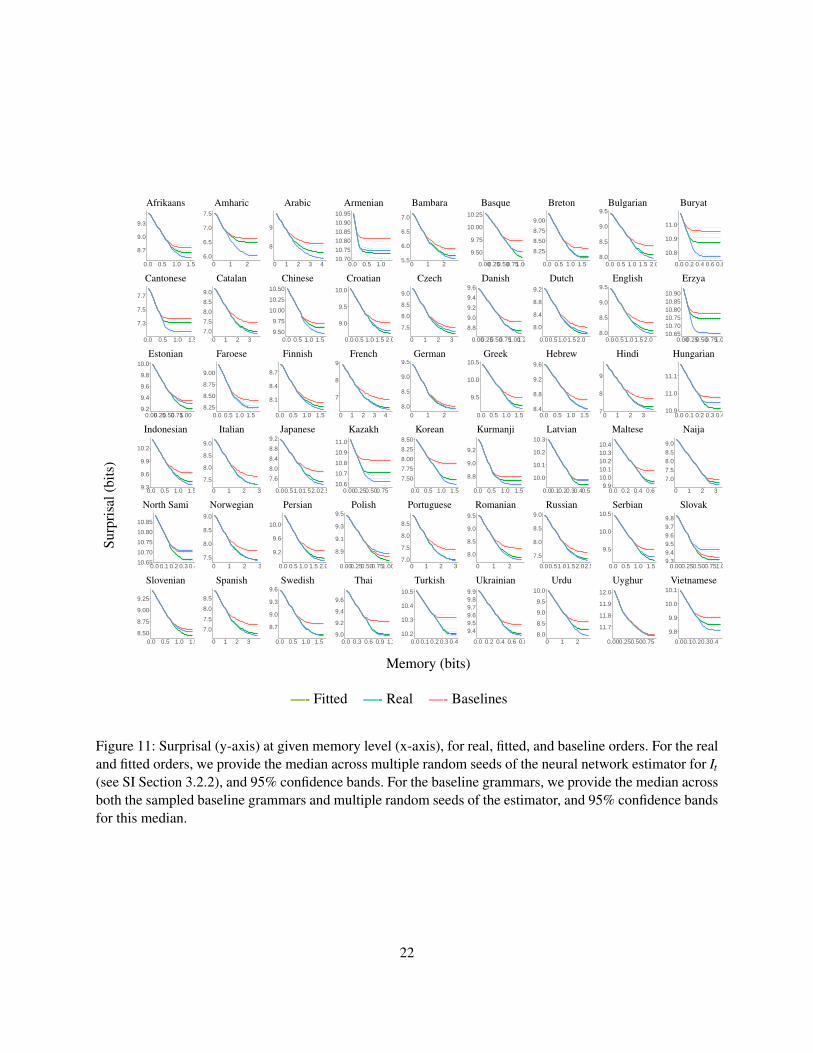
To test the Efficient Tradeoff Hypothesis, we compare the tradeoff curves for the real orders with those forrandom baseline grammars. In Figure 10, we show the estimated values of It for real and fitted orders andthe median of It across different baseline grammars. In most languages, I1 is distinctly larger for the actualand fitted orderings compared to the baseline orderings. This means that real orderings tend to concentratemore predictive information at the immediately preceding word than baseline grammars.

In Figure 11, we show the resulting bounds on the memory–surprisal tradeoff curves, showing surprisalsat given levels of memory, for real and baseline languages. We compute surprisal at 40 evenly spaced pointsof memory (selected individually for each language, between 0 and the maximal memory capacity HM

obtained using Theorem 1), over real orders and baseline grammars. At each point, we then compute themedian surprisal over all model runs for the real language, and over all baselines grammars. For each point,we compute an non-asymptotic and non-parametric 95% confidence interval for this median surprisal usingthe binomial test.

Numerically, the real language provides a better tradeoff than the median of the baselines across alllanguages, with four exceptions (Latvian, North Sami, Polish, Slovak). In order to quantify the degree ofoptimality of real orders, we further computed the area under the memory–surprisal tradeoff curve (AUC)for real and baseline orderings. Area under the curve (AUC) is a general quantity evaluating the efficiencyof a tradeoff curve (Bradley, 1997). A smaller area indicates a more efficient memory–surprisal tradeoff.In Figure 12, we plot the AUC for the real orderings, together with the distribution of AUCs for baselinegrammars. We quantify the degree of optimality by the fraction of baseline grammars for which the AUC ishigher than for the real orders: The real ordering is highly efficient if it results in a lower AUC than almostall baseline grammars. Numerically, the AUC is smaller in the real orderings than in at least 50% of baselinegrammars in all but three languages (Polish, Slovak, North Sami). We evaluated significance using a two-sided binomial test. In these three languages, the AUC is higher in the real orderings than in significantlyless than 50% (p < 0.01 in each language). In all other languages except for Latvian, the fraction of moreefficient baseline grammars was significantly less than 50%, at p = 0.01, where we applied Hochberg’sstep-up procedure (Hochberg, 1988) to control for multiple comparisons. In 42 of the 54 languages, the reallanguage was more efficient than all of the sampled baseline grammars.

The AUC for the fitted grammars is lower than more than 50% of random baseline grammars in all 54languages (p < 0.01, using two-sided Binomial test and Hochberg’s step-up procedure). Thus, we replicatethe result that ordering regularities of real languages provide more efficient tradeoffs than most possibleorder grammars even when comparing within the same word order grammar formalism.

5.5 Discussion

We have found that 50 out of 54 languages provide better memory–surprisal tradeoffs than random baselineswith consistent but counterfactual word order rules. Numerically, we observed differences in memory andsurprisal between real and baseline orders in the range of up to a few bits, often less than a bit (Figure 11).While one bit of memory seems like a small difference, this is a difference in cost at every word, whichaccumulates over a sentence. In a sentence with 20 words, the overall number of bits that have to be encodedover time (though not simultaneously) additionally might add up to 20 bits.

Four languages provide exceptions; these are Latvian (Baltic), North Sami (Uralic), Polish and Slovak(both Slavic). These four languages did not have significantly lower AUC values than half of the random

20

Con

ditio

nalM

utua

lInf

orm

atio

nI t

(bits

)

Afrikaans Amharic Arabic Armenian Bambara Basque Breton Bulgarian Buryat

0.00

0.25

0.50

0.75

1 2 3 40.00

0.25

0.50

0.75

1.00

1 2 3 40.0

0.5

1.0

1.5

1 2 3 40.00

0.05

0.10

0.15

0.20

1 2 3 40.0

0.3

0.6

0.9

1 2 3 40.0

0.2

0.4

0.6

0.8

1 2 3 40.00

0.25

0.50

0.75

1 2 3 40.0

0.5

1.0

1 2 3 40.0

0.1

0.2

1 2 3 4

Cantonese Catalan Chinese Croatian Czech Danish Dutch English Erzya

0.0

0.2

0.4

0.6

1 2 3 40.0

0.5

1.0

1.5

1 2 3 40.0

0.2

0.4

0.6

0.8

1 2 3 40.0

0.3

0.6

0.9

1 2 3 40.0

0.5

1.0

1.5

1 2 3 40.0

0.2

0.4

0.6

1 2 3 40.0

0.3

0.6

0.9

1 2 3 40.00

0.25

0.50

0.75

1.00

1.25

1 2 3 40.0

0.1

0.2

1 2 3 4

Estonian Faroese Finnish French German Greek Hebrew Hindi Hungarian

0.0

0.2

0.4

0.6

1 2 3 40.0

0.2

0.4

0.6

0.8

1 2 3 40.0

0.2

0.4

0.6

1 2 3 40.0

0.5

1.0

1.5

2.0

1 2 3 40.0

0.3

0.6

0.9

1.2

1 2 3 40.0

0.3

0.6

0.9

1.2

1 2 3 40.00

0.25

0.50

0.75

1.00

1 2 3 40.0

0.5

1.0

1.5

2.0

1 2 3 40.00

0.05

0.10

0.15

0.20

1 2 3 4

Indonesian Italian Japanese Kazakh Korean Kurmanji Latvian Maltese Naija

0.0

0.2

0.4

0.6

0.8

1 2 3 40.0

0.5

1.0

1.5

1 2 3 40.0

0.5

1.0

1.5

1 2 3 40.0

0.1

0.2

0.3

1 2 3 40.00

0.25

0.50

0.75

1.00

1 2 3 40.0

0.2

0.4

1 2 3 40.0

0.1

0.2

0.3

1 2 3 40.0

0.1

0.2

0.3

0.4

0.5

1 2 3 40.0

0.5

1.0

1.5

2.0

2.5

1 2 3 4

North Sami Norwegian Persian Polish Portuguese Romanian Russian Serbian Slovak

0.00

0.05

0.10

0.15

1 2 3 40.00

0.25

0.50

0.75

1.00

1.25

1 2 3 40.0

0.3

0.6

0.9

1 2 3 40.0

0.2

0.4

0.6

1 2 3 40.0

0.5

1.0

1.5

1 2 3 40.0

0.5

1.0

1 2 3 40.0

0.5

1.0

1 2 3 40.0

0.3

0.6

0.9

1 2 3 40.0

0.1

0.2

0.3

0.4

1 2 3 4

Slovenian Spanish Swedish Thai Turkish Ukrainian Urdu Uyghur Vietnamese

0.0

0.2

0.4

0.6

0.8

1 2 3 40.0

0.5

1.0

1.5

1 2 3 40.00

0.25

0.50

0.75

1 2 3 40.0

0.2

0.4

0.6

1 2 3 40.0

0.1

0.2

0.3

1 2 3 40.0

0.1

0.2

0.3

0.4

0.5

1 2 3 40.0

0.5

1.0

1.5

1 2 3 4

0.05

0.10

0.15

0.20

1 2 3 40.0

0.1

0.2

1 2 3 4

1

Distance t

– Fitted —- Real —- Baselines

Figure 10: Conditional mutual information It (y-axis) as a function of t (x-axis), for real, fitted and baselineorders. We plot the median over all sampled baseline grammars.

21

Surp

risa

l(bi

ts)


8.7

9.0

9.3

0.0 0.5 1.0 1.56.0

6.5

7.0

7.5

0 1 2

8

9

0 1 2 3 410.70

10.75

10.80

10.85

10.90

10.95

0.0 0.5 1.05.5

6.0

6.5

7.0

0 1 2

9.50

9.75

10.00

10.25

0.000.250.500.751.00

8.25

8.50

8.75

9.00

0.0 0.5 1.0 1.58.0

8.5

9.0

9.5

0.0 0.5 1.0 1.5 2.0

10.8

10.9

11.0

0.0 0.2 0.4 0.6 0.8


7.3

7.5

7.7

0.0 0.5 1.0 1.57.0

7.5

8.0

8.5

9.0

0 1 2 39.50

9.75

10.00

10.25

10.50

0.0 0.5 1.0 1.5

9.0

9.5

10.0

0.0 0.5 1.0 1.5 2.0

7.5

8.0

8.5

9.0

0 1 2 3

8.8

9.0

9.2

9.4

9.6

0.000.250.500.751.001.25

8.0

8.4

8.8

9.2

0.00.51.01.52.08.0

8.5

9.0

9.5

0.0 0.5 1.0 1.5 2.010.6510.7010.7510.8010.8510.90

0.000.250.500.751.00


9.2

9.4

9.6

9.8

10.0

0.000.250.500.751.008.25

8.50

8.75

9.00

0.0 0.5 1.0 1.5

8.1

8.4

8.7

0.0 0.5 1.0 1.5

7

8

9

0 1 2 3 48.0

8.5

9.0

9.5

0 1 2

9.5

10.0

10.5

0.0 0.5 1.0 1.58.4

8.8

9.2

9.6

0.0 0.5 1.0 1.57

8

9

0 1 2 310.9

11.0

11.1

0.0 0.1 0.2 0.3 0.4


9.3

9.6

9.9

10.2

0.0 0.5 1.0 1.5

7.5

8.0

8.5

9.0

0 1 2 3

7.6

8.0

8.4

8.8

9.2

0.00.51.01.52.02.510.6

10.7

10.8

10.9

11.0

0.000.250.500.75

7.50

7.75

8.00

8.25

8.50

0.0 0.5 1.0 1.5

8.8

9.0

9.2

0.0 0.5 1.0 1.5

10.0

10.1

10.2

10.3

0.00.10.20.30.40.59.9

10.010.110.210.310.4

0.0 0.2 0.4 0.6

7.07.58.08.59.0

0 1 2 3


10.65

10.70

10.75

10.80

10.85

0.0 0.1 0.2 0.3 0.47.5

8.0

8.5

9.0

0 1 2 3

9.2

9.6

10.0

0.0 0.5 1.0 1.5 2.0

8.9

9.1

9.3

9.5

0.000.250.500.751.007.0

7.5

8.0

8.5

0 1 2 3

8.0

8.5

9.0

9.5

0 1 2

7.5

8.0

8.5

9.0

0.00.51.01.52.02.5

9.5

10.0

10.5

0.0 0.5 1.0 1.59.39.49.59.69.79.8

0.000.250.500.751.00


8.50

8.75

9.00

9.25

0.0 0.5 1.0 1.5

7.0

7.5

8.0

8.5

0 1 2 3

8.7

9.0

9.3

9.6

0.0 0.5 1.0 1.59.0

9.2

9.4

9.6

0.0 0.3 0.6 0.9 1.210.2

10.3

10.4

10.5

0.0 0.1 0.2 0.3 0.4

9.49.59.69.79.89.9

0.0 0.2 0.4 0.6 0.88.0

8.5

9.0

9.5

10.0

0 1 2

11.7

11.8

11.9

12.0

0.000.250.500.75

9.8

9.9

10.0

10.1

0.00.10.20.30.4

1

Memory (bits)

—- Fitted —- Real —- Baselines

Figure 11: Surprisal (y-axis) at given memory level (x-axis), for real, fitted, and baseline orders. For the realand fitted orders, we provide the median across multiple random seeds of the neural network estimator for It(see SI Section 3.2.2), and 95% confidence bands. For the baseline grammars, we provide the median acrossboth the sampled baseline grammars and multiple random seeds of the estimator, and 95% confidence bandsfor this median.

22


13.7013.7513.8013.8513.9013.95 17.5 18.0 18.5 19.0 34.0 34.5 35.0 35.5 14.3 14.4 14.5 16.8 17.0 17.2 17.4 9.95 10.0010.0510.10 14.9 15.0 15.1 15.2 15.3 17.117.217.317.417.5 8.65 8.70 8.75 8.80


11.0 11.2 11.4 28.5 29.0 29.5 16.7016.7516.8016.8516.90 18.5 18.6 18.7 18.8 18.9 26.4 26.6 26.8 10.92 10.96 11.00 11.04 19.7 19.8 19.9 20.0 20.1 19.519.619.719.819.9 10.6 10.7


11.35 11.40 11.4515.6515.7015.7515.8015.8515.90 13.5513.6013.6513.70 31.5 32.0 32.5 33.0 23.0 23.1 23.2 15.9 16.0 16.1 14.5514.6014.6514.70 31.0 31.5 32.0 4.40 4.41 4.42 4.43


14.8014.8514.9014.9515.00 23.4 23.6 23.8 20.0 20.2 20.4 20.6 9.96 10.0010.0410.0812.2 12.3 12.4 12.5 12.6 14.3 14.4 14.5 5.335.345.355.365.37 6.73 6.75 6.77 26 27 28 29 30 31


4.20 4.22 4.24 22.923.023.123.223.3 19.1 19.2 19.3 19.4 19.5 9.4509.4759.5009.52523.2 23.4 23.6 23.8 23.4 23.6 23.8 24.0 19.5 19.6 19.7 19.8 15.9015.9516.0016.0516.10 9.10 9.15 9.20


12.8512.9012.9513.00 28.6 29.0 29.4 15.1 15.2 15.3 10.8510.9010.9511.00 4.39 4.40 4.41 7.48 7.50 7.52 7.54 23.8 24.0 24.2 24.4 10.2910.3010.3110.3210.33 4.66 4.68 4.70

1

Area under the Curve (AUC)


Figure 12: Histograms for the Area under the Curve (AUC) for the memory–surprisal tradeoffs for real,fitted, and random orders. We provide a kernel density smoothing estimate of the distribution of randombaseline orders. A smaller AUC value indicates a more efficient tradeoff. In most cases, the real and fittedorders provide more efficient tradeoffs than most or all baseline grammars.

23

●

●

●

●

●

●

●

●

●●

●

●

●

●

●

●

●

●

●

●

●

●

●

●

●

●

●

●●

●

●

●

●

●

●

●

●●

●

●

●

●

●

●

●

●

●●

● ●

●

●

●

Afrikaans

Amharic

Arabic

Armenian

Bambara

Basque

Breton

Bulgarian

BuryatCantonese

Catalan

ChineseCroatian

CzechDanishDutch

English

ErzyaEstonian

Faroese

Finnish

French

German

GreekHebrew

Hindi

Hungarian

Indonesian

Italian

Japanese

Kazakh

Kurmanji

Latvian

Maltese

Naija

North_Sami

NorwegianPersian

Polish

Portuguese Romanian

Russian

Serbian

Slovak

Slovenian

Spanish

SwedishThai

Turkish

Ukrainian

Urdu

Uyghur

Vietnamese●

●

0.0

0.5

1.0

0.1 0.2 0.3 0.4Branching Direction Entropy

Sur

pris

al D

iffer

ence

Type ● ●With Information Structure Without Information Structure

Figure 13: Word order freedom and strength of optimization: For each of the 54 languages, we show word or-der freedom as measured by branching entropy, and the difference between the real order’s surprisal and themedian surprisal of the baseline grammars, at the maximum memory value (see Figure 11). Languages withhigher branching direction entropy show a smaller reduction in surprisal compared to baseline orders. ForCzech, we also provide an estimate accounting for information strcuture (red dot), see below, ‘Controllingfor Information Structure‘, for more information.

baselines. One feature that unites these four languages is that they have strong word order freedom, as wewill see below in Figure 13. Word order freedom plausibly makes sentences less predictable, as the samesyntactic structure can receive different surface realizations. We thus hypothesized that word order freedomimpacts the memory–surprisal tradeoff, and that languages with more strongly fixed word order shoulddisplay more optimal memory–surprisal tradeoffs.

To test this hypothesis, we examined the correlation between word order freedom and the surprisaldifference between real and baseline orderings. To quantify word order freedom, we used a corpus-basedestimate, the branching direction entropy (Futrell et al., 2015b). This is the entropy of the ordering (head-first or dependent-first) of dependencies conditioned on the dependency label and the part-of-speech labelof head and dependent. These two quantities are plotted in Figure 13. We found that branching directionentropy was strongly correlated with the surprisal difference between real and baseline orderings (Spearmancorrelation −0.58, p < .0001).

This result might mean that optimization of word orders for memory–surprisal tradeoffs is indeedstronger in languages with more fixed word order, and that word order freedom leads to less efficientmemory–surprisal tradeoffs. A second possibility is that languages with seemingly free word order encodeother information in word order, in particular, information about information structure (e.g. Givon, 1988;Firbas, 1966, 1974; Myhill, 1985). Next, we test the latter hypothesis by examining whether the degree ofoptimization changes when taking into account information structure.

24

5.6 Controlling for Information Structure

In this section we address the question about word order freedom raised in the last section. We draw on acorpus of Czech with information structure annotation to determine whether real orders are more optimizedwhen comparing to baselines taking information structure into account.

Languages with flexible word order often show a strong influence of information structure on wordorder (Givon, 1988; Jacobs, 1988; Neeleman and van de Koot, 2016). Due to the difficulty of annotatinginformation structure, only relatively few datasets have annotations for information structure, and even fewerdatasets have both syntactic and information structure annotation. We draw on the Prague DependencyTreebank of Czech (Bohmova et al., 2003; Mikulova et al., 2006), which has both types of annotation.Czech is a language with relatively high degree of word order freedom, which is generally thought to bestrongly impacted by information structure (Firbas, 1966, 1974).

About one third of the Prague Dependency Treebank has annotation for topic-focus articulation (Mikulovaet al., 2006). Constituents are annotated for contrastiveness and for contextual boundedness, i.e., givenness.Contextually bound expressions are presumed as given in context so that their referent is uniquely deter-mined by the context; contextually bound expressions are contrastive if they choose from a contextuallygiven set of alternatives (Mikulova et al., 2006, Section 10.2). Three labels are used: “c” for contrastiveand contextually bound, “f” for contextually non-bound, “t” for non-contrastive contextually bound. Theselabels were diagnosed based on constituent order and intonation. Some constituents remain unmarked, thevast majority of which are function words such as adpositions, conjunctions, and auxiliaries; we introduce alabel “NA” for these. To define baselines, we extend the word order grammar formalism by defining separateweights for each combination of the 37 syntactic relations and these four information structure labels.

We obtained 38,727 training sentences and 5,228 held-out sentences. We created 20 baseline grammarswith information structure, 20 baseline grammars without it.

Results We show estimated tradeoffs and the distributions over AUC values in Figure 14. As this experi-ment was conducted only on the subset of the Prague Dependency Treebank that has information structureannotation, the numerical values are slightly different from those in Figure 11. We compare the real ordersboth with the same baselines as above, and with the baselines taking information structure into account.Baselines show a larger gap in efficiency between real and baseline grammars when the baselines conditionword order on information structure. This suggests that, among word orders that encode information struc-ture, the real order of Czech provides a very efficient memory–surprisal tradeoff, and that the strength ofoptimization is underestimated when comparing against baselines that do not take information structure intoaccount.

In Figure 13, we show how the data point for Czech changes when including information structure inthe word order modeling. When modeling information structure, branching direction entropy decreases,while the surprisal difference between real and baseline orders increases. This suggests that the weakeroptimization in free word order languages observed in Study 2 might in part be because ordering grammarsdo not take information structure into account. In general, we expect that conditioning word order on moresources of information will increase the set of possible word orders, and thus decrease predictability andincrease surprisal. As more corpora become available, it will be important to reproduce this finding on datafrom further languages. If this finding replicates, then this would mean that the impact of order freedom onthe strength of optimization observed in Study 2 is an artifact of the fact that languages differ in the degreeto which their word order encodes information structure, and that similar degrees of optimization mightactually hold across such different languages.

25

8.0

8.5

9.0

9.5

0 1 2Memory (bits)

Sur

pris

al (

bits

)

0.00

0.25

0.50

0.75

1.00

22.1 22.3 22.5 22.7Area under Curve

—- Fitted —- Real —- Baselines —- Baselines with Information Structure

Figure 14: Left: Memory-surprisal tradeoff for Czech with information structure. Right: AUC for Czech,for baselines without information structure and baselines with information structure. Optimization of realorders is stronger when considering information structure in baselines.

26

Discussion Using data from Czech, we found that the difference between the memory–surprisal tradeoffsof real and baseline orders increases if we choose baseline orderings that encode information structure, asreal orders do. We hypothesize that this in part explains why the observed strength of memory efficiencyoptimization is negatively correlated with the degree of word order freedom: Languages with flexible wordorder typically encode information structure in word order, which increases average surprisal. This doesnot mean that conditioning word order on information structure makes language less efficient in general.Rather, encoding information structure in word order may increase the information content transmitted tothe listener, which may in turn balance an increase in surprisal processing effort (Hahn et al., 2020). Due tothe difficulty and cost of annotating information structure, we could only evaluate this hypothesis on datafrom one language. As more annotated data becomes available, this should be replicated on data from furtherlanguages.

5.7 Interim summary

In this section, we tested the Efficient Tradeoff Hypothesis on dependency corpora from 54 languages, com-paring observed word orders to hypothetical baseline grammars. We found that, in 50 out of 54 languages,real orders provide more efficient memory–surprisal tradeoffs than most baseline grammars. This result alsoheld when comparing real and baseline orderings within a single grammar formalism. These results suggeststhat, across languages, word order favors information locality more strongly than most possible alternativeorders.

We also found that the degree of optimization was weaker in languages with high degrees of word orderfreedom. Using data from Czech that is annotated for both syntax and information structure, we providedevidence that this dependence on word order freedom is an artifact of the fact that languages with flexibleword order tend to encode information structure in word order.

Taken together, Studies 1 and 2 suggest that crosslinguistic word orders are in part impacted by a pressuretowards efficient memory–surprisal tradeoffs, and thus information locality. To test whether the EfficientTradeoff Hypothesis holds at different levels of representation, we consider morpheme order in Study 3.

6 Study 3: Morpheme Order

The Efficient Tradeoff Hypothesis should apply not just at the level of words, but at the level of any linguis-tic element. For instance, just as observed word orders exhibit information locality, the order of morphemeswithin words should also be structured so that morphemes which predict each other are close to each other.Here, we apply the Efficient Tradeoff Hypothesis to predict the order of morphemes within morphologicallycomplex words in two agglutinative languages. We study two agglutinative languages for which extensivecorpora with hand-annotated morphological segmentation and labeling are available: Japanese and Sesotho.We compare the memory–surprisal tradeoff of the actual morpheme orders in these languages with hy-pothetical baseline orderings. Furthermore, we construct hypothetical orderings that are optimized for theefficiency of the memory–surprisal tradeoff, and compare these to the actual morpheme orderings, to inves-tigate whether morpheme order in these languages can be predicted by optimization of tradeoff efficiency.Below, we first give brief sketches of the morphological patterns in these languages.

Verb Suffixes in Japanese In Japanese, verbs are marked with an extensive number of suffixes. For ex-ample, the following verb forms are marked with multiple suffixes:

27

(1) a. misee

rarePASSIVE

mashPOLITENESS

yooFUTURE

‘will be seen’b. mi

seetakuDESIDERATIVE

nakatNEGATION

taPAST

‘did not wish to see’

Based on corpus data and the linguistic literature on Japanese, we identified the following frequent verbsuffixes, occurring in the following order outwards from the verb root (see SI for details).

1. suru: obligatory suffix after Sino-Japanese words when they are used as verbs

2. Valence: causative (-ase-) (Hasegawa (2014, 142), Kaiser et al. (2013, Chapter 13))

3. Voice and Mood: passive (-are-, -rare-) (Hasegawa (2014, 152), Kaiser et al. (2013, Chapter 12)) andpotential (-e-, -are-, -rare-) (Kaiser et al., 2013, 398)

4. Politeness (-mas-) (Kaiser et al., 2013, 190).

5. Mood: desiderative (-ta-) (Kaiser et al., 2013, 238)

6. Negation (-n-)

7. Tense, Aspect, Mood, and Finiteness: past (-ta), future/hortative (-yoo) (Kaiser et al., 2013, 229),nonfiniteness (-te) (Kaiser et al., 2013, 186)

Verb Affixes in Sesotho Sesotho (also known as Southern Sotho) is a Southern Bantu language spokenprimarily in Lesotho and South Africa. Sesotho verbs are marked with both prefixes and suffixes (Demuth,1992). Common prefixes include markers for agreement with subjects and objects; object prefixes alwaysfollow subject prefixes (2-a). Common suffixes include markers changing valence and voice, and a moodsuffix (2-b).

(2) a. oaSUBJECT.AGREEMENT

diOBJECT.AGREEMENT

rekbuy

aINDICATIVE

‘(he) is buying (it)’ (Demuth, 1992)b. o

SUBJECT.AGREEMENT

phehcook

elAPPLICATIVE

aINDICATIVE

‘(he) cooks (food) for (him)’ (Demuth, 1992)

We identified affix morphemes and their ordering based on the analysis in Demuth (1992), supplementedwith information from grammars of Sesotho (Doke and Mofokeng, 1967; Guma, 1971). See SI for details.We identified the following prefixes:

1. Subject agreement: This morpheme encodes agreement with the subject, for person, number, and nounclass (the latter only in the 3rd person) (Doke and Mofokeng, 1967, §395). The annotation providedby Demuth (1992) distinguishes between ordinary subject agreement prefixes and agreement prefixesused in relative clauses; we distinguish these morpheme types here.

2. Negation (Doke and Mofokeng, 1967, §429)

28

3. Tense/aspect marker (Doke and Mofokeng, 1967, §400–424)

4. Object agreement or reflexive marker (Doke and Mofokeng, 1967, §459). Similar to subject agree-ment, object agreement denotes person, number, and noun class features of the object.

We identified the following suffixes:

1. Semantic derivation: reversive (e.g., ‘do’→ ‘undo’) (Doke and Mofokeng, 1967, §345)

2. Valence: Common valence-altering suffixes include causative, neuter/stative, applicative, and recipro-cal (Doke and Mofokeng, 1967, §307–338). See SI for details on their meanings.

3. Voice: passive (Doke and Mofokeng, 1967, §300)

4. Tense (Doke and Mofokeng, 1967, §369)

5. Mood (Doke and Mofokeng, 1967, §386–445)

6. Interrogative and relative markers, appended to verbs in certain interrogative and relative clauses(Doke and Mofokeng, 1967, §160, 271, 320, 714, 793).

6.1 Experiment

Data Selection and Processing For Japanese, we drew on Universal Dependencies data. In the tokeniza-tion scheme used for Japanese, most affixes are separated as individual tokens, effectively providing mor-pheme segmentations. We used the GSD corpus, Version 2.4, (Tanaka et al., 2016; Asahara et al., 2018), asit was the only corpus with a training set and freely available word forms. In the corpus, verb suffixes largelycorrespond to auxiliaries (with tag AUX); only a few morphemes tagged AUX are not standardly treated as suf-fixes (see SI), and one frequent suffix (-te) is labeled SCONJ. We selected verb forms by selecting all chainsof a verb (tag VERB) followed by any number of auxiliaries (tag AUX) from the training set of the corpus.When the suffix -te (tag SCONJ) followed such a chain, we added this. We labeled suffixes for underlyingmorphemes with the help of the lemmatization provided for each suffix in the corpus (see SI Section 4.3for details). The passive and potential (slot 3) markers are formally indistinguishable for many verbs. As wecannot systematically distinguish them on the basis of the available corpus annotation, we merge these intoa single underlying morpheme ‘Passive/Potential’.

We obtained 15,281 verb forms in the training set and 1,048 verb forms in the held-out set. Of the formsin the training set, 27% had two or more suffixes (modal group: two suffixes, accounting for 20% of forms;maximum seven suffixes). While predicting order naturally focuses on datapoints with more than one suffix,we include the other datapoints for estimating conditional mutual information It .

For Sesotho, we used the Demuth Corpus (Demuth, 1992) of child and child-directed speech, containingabout 13K utterances with 500K morphemes. The corpus has very extensive manual morphological segmen-tation and annotation; each verb form is segmented into morphemes, which are annotated for their function.Sesotho verbs carry both prefixes and suffixes. We extracted 37K verb forms (see SI 4.2 for details). Werandomly selected 5% to serve as held-out data and used the remaining 95% as training data. 93% of formshad two or more affixes (modal group: three affixes, accounting for 36% of forms; maximum eight affixes).

29

Estimating Memory-Surprisal Tradeoff We modeled incremental prediction on the level of morphemesequences. To do so, we represented each verb form as a sequence of a stem and affix morphemes, abstractingaway from morphophonemic interactions between neighboring morphemes. As in many languages, affixesin Japanese and Sesotho show morphophonemic interactions between neighboring morphemes; for instance,the Japanese politeness morpheme -mas- takes the form -masu when it is word-final, while it has the allo-morph -mase- when followed by the negation suffix -n. Modeling prediction on the level of morphemes, asopposed to phonemes, controls for these interactions.10

In analogy to Studies 1–2, we modeled verb forms as a stationary stochastic process by concatenatingthe verb forms from the corpus in random order.

We calculated It by estimating an n-gram model on the training set and then computing the averagesurprisal St as cross-entropy on the held-out set using Kneser-Ney smoothing. The model may overfit as thecontext size t increases, leading to higher cross-entropies for larger values of t. We mitigated overfitting forlarge t by estimating

St := mins≤t

Ss, (7)

where Ss is the cross-entropy of the s’th order Markov model on held-out data. This procedure ensures thatSt can only decrease as the context size t increases.

Parameterizing Alternative Orderings We parameterized alternative affix orderings by assigning a weightin [0,1] to each morpheme. Given such a grammar, affixes are ordered by the values assigned to their un-derlying morphemes. We considered all morphemes annotated in the corpora, including low-frequency onesgoing beyond the ones identified above (see SI for details).

To verify that this formalism is appropriate for capturing morpheme order in Japanese and Sesotho, wefitted models parameterized in this way to the observed orders. Ordering morphemes according to these fittedmodels recovered the observed order for almost all forms (98.6 % for Japanese, 99.93% for Sesotho prefixes,97.4% for Sesotho suffixes). Exceptions largely concern low-frequency affixes beyond those consideredhere. We take this as confirmation that the formalism is generally suited to capture morpheme order.

For each language, we constructed 40 baseline grammars by randomly sampling weights.

Creating Optimal Orders In order to create optimal orders to compare real orders to, we optimizedorderings for the AUC under the memory–surprisal tradeoff curve with an adaptation of the hill climbingmethod that Gildea and Jaeger (2015) used to optimize word order grammars for the length of syntacticdependencies and trigram surprisal.

We randomly initialized the assignment of weights to morphemes, and then iteratively change the as-signment to reduce AUC. In each iteration, we randomly chose one morpheme, and evaluate AUC for eachway of ordering it between two other morphemes. We then updated the weights to the ordering that yieldsthe lowest AUC. To speed up optimization, we restricted to morphemes occurring at least 10 times in thecorpus for 95% of iterations, and to 10% of possible orderings in each step. These choices vastly reducedcomputation time by reducing time spent on low-frequency morphemes. This optimization method is ap-proximate, as it only guarantees convergence to a local optimum (Gildea and Jaeger, 2015), not to a globallyoptimal assignment.

We ran this method for 1,000 iterations. Empirically, AUC converged after a few hundred iterations. Tocontrol for the randomness in initialization and the optimization steps, we ran this algorithm ten times. Dif-

10See SI Section 4.3 for qualitatively similar results when modeling prediction at the phoneme level.

30

Japanese Sesotho

97.5 98.0 98.5 80.2 80.4 80.6 80.8 81.00.00

0.25

0.50

0.75

1.00

0.00

0.25

0.50

0.75

1.00

Area under Curve

Den

sity Type

OptimizedRandomRealReverse

Figure 15: Areas under the curve for the memory–surprisal tradeoff for verb affixes in Japanese (left) andSesotho (right). For the baseline grammars, we show a Kernel Density estimate. In both Japanese andSesotho, real and optimized orderings lead to lower AUC than all of the 40 baseline samples.

ferent runs achieved almost the same AUC values (SD 0.0051 in Japanese, 0.0036 in Sesotho). For Sesotho,we ran the algorithm separately for prefixes and suffixes due to computational efficiency considerations.11

6.2 Results

In Figure 15, we compare the area under curve of the memory–surprisal tradeoff for Japanese and Sesothoverb forms under different orderings. Both observed orders and the approximately optimized grammarsshow lower AUCs than all 40 random baseline samples, in both languages. For comparison, we also showAUC for the order resulting from reversing all suffix chains in the observed orders; this results in high AUCeven exceeding most random grammars. These results show that Japanese and Sesotho affix orderings enableapproximately optimal memory–surprisal tradeoffs.

We now ask to what extent the observed morpheme ordering is predicted correctly by approximatelyoptimized grammars. In Table 1, we give summary statistics about the accuracy of optimized grammars inpredicting affix order in the corpus, together with random baseline figures. We evaluate accuracy using twomethods: In one method (‘Pairs’), we consider, for each verb form in the corpus, all pairs of prefixes (orsuffixes). We report the proportion of these pairs in the corpus for which the relative order of the two affixesis as predicted by the grammar. In the other method, (‘Full’), we report the proportion of verb forms in thecorpus that has exactly the affix ordering predicted by the grammar. In both measures, we average over allten approximately optimized grammars for each language.

Japanese results. In Japanese, by both measures, optimized grammars recover the observed orders withhigh accuracy. We compare the real grammar with the approximately optimized grammar that achieved thelowest AUC value in Table 2. We conducted an error analysis comparing the real Japanese morpheme orderagainst our approximately optimized orders. We extracted the pairs of morphemes whose relative order isincorrectly predicted, excluding pairs involving low-frequency morphemes not discussed here. Results are

11With the exception of the tense/aspect markers, none of the morpheme types discussed above can occur both as prefixes andsuffixes. Therefore, we do not expect this separation to impact results.

31

Prefixes SuffixesPairs Full Pairs Full

Japanese Optimized – – 0.953 (SD 0.011) 0.943 (SD 0.014)Baseline – – 0.497 (SD 0.287) 0.425 (SD 0.29)

Sesotho Optimized 0.988 (SD 0.0) 0.989 (SD 0.0) 0.756 (SD 0.014) 0.676 (SD 0.017)Baseline 0.672 (SD 0.305) 0.604 (SD 0.338) 0.423 (SD 0.204) 0.332 (SD 0.211)

Table 1: Accuracy of approximately optimized orderings, and of random baseline orderings, in predictingverb affix order in Japanese and Sesotho. ‘Pairs’ denotes the rate of pairs of morphemes that are orderedcorrectly, and ‘Full’ denotes the rate of verb forms where order is predicted entirely correctly. We showmeans and standard deviations over ten different runs of the optimization algorithm (‘Optimized’), and overdifferent random orderings (‘Random’).

Real OptimizedStem Stem

1 suru suru2 causative causative3 passive/potential passive/potential4 desiderative negation5 politeness future6 negation politeness7 future desiderative

past nonfinitenonfinite past

Table 2: Comparing order of Japanese affixes in the observed orders (left) and according to an approximatelyoptimized grammar (right). We organize the affixes in the real order into the seven slots described above.

shown in Table 3. The most frequent divergence for this grammar is that politeness and negation suffixes areconsistently ordered incorrectly; this affects 74 corpus examples (out of 15K total examples).

We also found that prediction was more accurate when modeling on the level of phonemes, suggestingthat divergence between model predictions and actual order might be related to phonological pressure (seeSI Section 4.3).

Sesotho results. We compare the real Sesotho grammar with the approximately optimized grammar thatachieved the lowest AUC value in Table 4. In Sesotho, for prefixes, all optimized grammars almost exactlyrecover the ordering described above. The only divergence among the high-frequency morphemes is thatnegation and the tense/aspect prefix are ordered incorrectly; this accounts for only 12 occurrences in thedata set, as the two prefixes rarely co-occur (Table 5, top).

For Sesotho suffixes, order is recovered at above-chance accuracies (Table 1, bottom), though withsome divergences. The most common error (Table 5, bottom) is that relative and interrogative suffixes areconsistently placed closer to the verb stem than the mood suffix. We conjecture that this happens becauseall Sesotho verbs uniformly have a mood suffix, suggesting that there might be lower mutual informationbetween the stem and the mood suffix than between the stem and these two suffixes. Furthermore, valence-changing suffixes are ordered farther away from the stem than various other suffixes, in contrast with the

32

Error Frequencypoliteness negation 74desiderative negation 14politeness future 9

Table 3: Errors in Japanese: We show pairs of morphemes that are ordered incorrectly by the approximatelyoptimized grammar with the lowest AUC value. We indicate the number of such pairs occurring in thecorpus. We only show errors where both morphemes are among the high-frequency ones studied here.

Real Optimized1 Subject Subject

Subject (rel.) Subject (rel.)2 Negation Tense/aspect3 Tense/aspect Negation4 Object Object

Stem Stem1 Reversive Passive2 Causative Reciprocal

Neuter Tense/aspectApplicative NeuterReciprocal Relative

3 Passive Causative4 Tense/aspect Applicative5 Mood Interrogative6 Interrogative Reversive

Relative Mood

Table 4: Comparing order of Sesotho affixes in the observed orders (left) and according to an approxima-tively optimized grammar (right). Note that order was separately optimized for prefixes and suffixes.

actual orders. Interestingly, we found that prediction was more accurate in this respect when estimating Itnaively on the training set (see SI Section 4.3), suggesting that the available corpus data does not sufficientlydetermine the optimal ordering.

6.3 Discussion

We have found that the ordering of verb affixes in Japanese and Sesotho provides approximately optimalmemory–surprisal tradeoffs, close to the efficiency of orderings computationally optimized for efficiency.We further found that parts of these languages’ ordering rules can be derived from optimizing order forefficient tradeoffs.

Here we argue that the memory–surprisal tradeoff provides an explanation of previously-existing typo-logical generalizations, and an operationalization of previous functionally-motivated explanations for them;in particular, we argue that the notion of mutual information operationalizes the concept of ‘relevance.’

One prominent typological generalization due to Bybee (1985, p. 24, 34–35) claims that there exists auniversal ordering of verbal inflectional morphemes across languages:

33

Error FrequencyNegation Tense/aspect 12

Error FrequencyMood Interrogative 2204Mood Relative 858Applicative Tense/aspect 347Causative Tense/aspect 174Neuter Tense/aspect 155Reversive Causative 100Applicative Passive 81Causative Passive 61Applicative Relative 49Causative Relative 41

Table 5: Errors in Sesotho prefixes (top) and suffixes (bottom). We show the ten most common errors whereboth morphemes are among the high-frequency ones studied here.

verb stem valence voice aspect tense mood subject agreement

Morphemes are claimed either to go in the order above (suffixes), or its reverse (prefixes). This hierarchymakes no statements as to which affixes are realized as prefixes or suffixes.

Japanese and Sesotho verb affixes are broadly in agreement with Bybee’s generalization. For instance,valence and voice suffixes are closer to the stem than tense/aspect/mood markers. Subject agreement inSesotho is farther away from the verb than tense/aspect/mood prefixes. This ordering is reproduced closelyby optimization in Japanese and for Sesotho prefixes, and to some extent also for Sesotho suffixes.

Bybee (1985, p. 37) argues further that morpheme order is determined by the degree of relevance be-tween the affix and the stem, that is, the degree to which “the semantic content of the first [element] directlyaffects or modifies the semantic content of the second” (p. 13). She argues that elements whose meaningsare more relevant to each other appear closer together. For instance, the meaning of a verb is impacted morestrongly by a causative affix than by a tense affix: Combining a verb with a causative marker results in aform that denotes a different action, whereas a tense affix only locates the action in time.

We conjecture that this notion of relevance is related to mutual information. If an affix has a strongerimpact on the meaning of the verb, it will typically not be applicable to all verbs. For instance, causativemarkers will only attach to verbs whose semantics is compatible with causation. In contrast, a past tensemarker can attach to all verbs that are compatible with actions that can have occurred in the past. Therefore,we expect that affixes that are more relevant to a verb stem will also tend to have higher mutual informa-tion with the verb stem. If they have higher mutual information with the verb stem, then the principle ofinformation locality predicts that they will go close to the verb stem.

7 General Discussion

We introduced a notion of memory efficiency in language processing: the memory–surprisal tradeoff. Wethen tested the resulting Efficient Tradeoff Hypothesis: Order of elements in natural language is character-ized by efficient memory–surprisal tradeoffs, compared to other possible orders. In Study 1, we showed that

34

the Efficient Tradeoff Hypothesis predicts the known preference for short dependencies. In Study 2, we usedcorpus data from 54 languages to show that real word orders provide more efficient tradeoffs than baselineorder grammars. In Study 3, we showed that in two languages (Japanese and Sesotho) the order of verbaffixes not only provides approximately optimal tradeoffs, but can also partly be predicted by optimizing forthe efficiency of the memory–surprisal tradeoff.

Here, we discuss the limitations of our results and the implications they have more broadly for the fieldsof psycholinguistics, typology, and information theory.

7.1 Role of Comprehension, Production, and Acquisition

Our results leave open the causal mechanism leading to the observed optimization, in particular, whetheroptimization is the result of minimizing effort during comprehension, production, or acquisition. One pos-sibility is that optimization reflects an effort on the side of the speaker to produce utterances that are easy tocomprehend by listeners, a strategy known as audience design (Clark and Murphy, 1982; Lindblom, 1990;Brennan and Williams, 1995). More efficient memory–surprisal tradeoffs are useful from the listener’s per-spective because they allow for better prediction with lower memory investment than less efficient tradeoffs.

Another possibility is that optimization reflects production-internal pressures to minimize effort on thespeaker’s part during sentence planning (Bock and Warren, 1985; Ferreira and Dell, 2000; MacDonald,2013; Fedzechkina and Jaeger, 2020). That is, instead of speakers optimizing for the benefit of listeners, theiterated application of production-internal heuristics that reduce speaker effort may result in more efficienttradeoffs (MacDonald, 2013). While our theory is stated in terms of the efficiency of language processing fora comprehender of language, we can show that an analogous memory–surprisal tradeoff exists in languageproduction, and that speakers with bounded memory capacity can minimize production errors when thelanguage has stronger information locality. For discussion including mathematical proofs, see SI Section1.4. Depending on the precise formalization of the production problem, the production-oriented version ofthe memory–surprisal tradeoff may or may not be identical the comprehension-oriented version we havepresented here. We leave the proper formulation of an information-theoretic model of production to futurework.

Finally, optimization may reflect biases that come into play during language learning. It is possible thatmemory efficiency makes languages more learnable, as learning should require less memory resources forlanguages with more efficient memory–surprisal tradeoffs. Evidence from artificial language learning ex-periments suggests that language acquisition is biased towards efficiency in communication and processing(e.g. Fedzechkina et al., 2012, 2017).

7.2 Relation to Models of Sentence Processing

There is a substantial literature proposing sentence processing models and quantitative memory metricsfor sentence processing. In this section, we discuss how our theoretical results relate to and generalize thesepreviously proposed models. We do not view our model as competing with or replacing any of these models;instead, our information-theoretic analysis captures aspects that are common to most of these models andshows how they arise from very general modeling assumptions.

In the Information Locality Bound Theorem, we proved a formal relationship between the entropy ofmemory HM and average surprisal SM. We made no assumptions about the architecture of incremental mem-ory, and so our result is general across all such architectures. Memory representations do not have to berational or optimal for our bound in Theorem 1 to hold. There is no physically realizable memory architec-ture that can violate this bound.

35

However, psycholinguistic theories may differ on whether the entropy of memory HM really is the rightmeasure of memory load, and on whether average surprisal SM really is the right predictor of processingdifficulty for humans. Therefore, in order to establish that our information-theoretic processing model gen-eralizes previous theories, we will establish two links:

• Our measure of memory usage generalizes theories that are based on counting numbers of objectsstored in incremental memory (e.g., Yngve, 1960; Miller and Chomsky, 1963; Frazier, 1985; Gibson,1998; Kobele et al., 2013; Graf and Marcinek, 2014; Graf et al., 2015; Gerth, 2015; Graf et al., 2017;De Santo, 2020). Furthermore, for theories where memory is constrained in its capacity for retrievalrather than storage (e.g., McElree et al., 2003; Lewis and Vasishth, 2005), the information localitybound will still hold.

• Our predictor of processing difficulty (i.e., average surprisal) reflects at least a component of thepredicted processing difficulty under other theories.

Below, we discuss the connections between our theory and existing theories of human sentence process-ing with regard to the points above.

Storage-Based Theories There is a long tradition of models of human language processing in whichdifficulty is attributed to high working memory load. These models go back to Yngve (1960)’s productionmodel, where difficulty was associated with moments when a large number of items have to be kept on aparser stack; this model correctly predicted the difficulty of center-embedded clauses, but problematicallypredicted that left-branching structures should be hard (Kimball, 1973). Other early examples include Millerand Chomsky (1963) and Frazier (1985)’s measure of syntactic complexity based on counting the numberof local nonterminal nodes. More recently, a line of literature has formulated complexity metrics based onhow many nodes are kept in incremental memory for how long during parsing, and used linear or rankedcombinations of these metrics to predict acceptability differences in complex embeddings (Kobele et al.,2013; Graf and Marcinek, 2014; Rambow and Joshi, 2015; Graf et al., 2015; Gerth, 2015; Graf et al., 2017;De Santo, 2020).

Our measure of memory complexity—i.e., the memory entropy HM—straightforwardly generalizes mea-sures based on counting items stored in memory. If each item stored in memory requires k bits of storage,then storing n items would require a capacity of nk bits in terms of memory entropy HM. In general, ifmemory entropy is HM and all items stored in memory take k bits each to store, then we can store HM/kitems. However, the memory entropy HM is more general as a measure of storage cost, because it allows thatdifferent items stored in memory might take different numbers of bits to store, and also that the memory rep-resentation might be able to compress the representations of multiple items when they are stored together, sothat the capacity required to store two items might be less than the sum of the capacity required to store eachindividual item. Previous work has argued that visual working memory is characterized by an information-theoretic capacity limit (Brady et al., 2008; Sims et al., 2012); we extend this idea to incremental memoryas used in language processing.

The Dependency Locality Theory The connection with the Dependency Locality Theory is particularlyinteresting. Our lower bound on memory usage, described in Theorem 1 Eq. 4, is formally similar to StorageCost in the Dependency Locality Theory (DLT) (Gibson, 1998, 2000). In that theory, storage cost at a giventimestep is defined as the number of predictions that are held in memory. Our bound on memory usage isstated in terms of mutual information, which indicates the amount of predictive information extracted from

36

the previous context and stored in memory. As the notion of ‘number of predictions’ is subsumed by thenotion of ‘amount of predictive information’, our measure generalizes DLT storage cost.

The other component of the DLT is integration cost, the amount of difficulty incurred by establishing along-term syntactic dependency. In our framework, DLT integration cost corresponds to surprisal given animperfect memory representation, following Futrell et al. (2020b).

There is one remaining missing link between our theory of processing difficulty and theories such as theDependency Locality Theory: our information locality theorem says that statistical dependencies should beshort-term, whereas psycholinguistic theories of locality have typically focused on the time-span of syntac-tic dependencies: words which depend on each other to determine the meaning or the well-formedness ofa sentence. Statistical dependencies, in contrast, mean that whenever one element of a sequence determinesor predicts another element in any way, those two elements should be close to each other in time.

If statistical dependencies, as measured using mutual information, can be identified with syntactic depen-dencies, then that would mean that information locality is straightforwardly a generalization of dependencylocality. Futrell et al. (2019) give theoretical and empirical arguments that this is so. They show that syn-tactic dependencies as annotated in dependency treebanks identify word pairs with especially high mutualinformation, and give a derivation showing that this is to be expected according to a formalization of thepostulates of dependency grammar. The connection between mutual information and syntactic dependencyhas also been explored in the literature on grammar induction and unsupervised chunking (Harris, 1955;de Paiva Alves, 1996; Yuret, 1998; McCauley and Christiansen, 2019; Clark and Fijalkow, 2020).

Cue-Based Retrieval Models Work within cue-based retrieval frameworks has suggested that workingmemory is not characterized by a decay in information over time, but rather an accumulation of interfer-ence among similar items stored in memory (Lewis and Vasishth, 2005, p. 408). In contrast, the formula formemory usage in Eq. 4 might appear to suggest that boundedness of memory entails that representationshave to decay over time. However, this is not the case: our theorem does not imply that a listener forgetswords beyond some amount of time T in the past. An optimal listener may well decide to remember infor-mation about words more distant than T , but in order to stay within the bounds of memory, she can only doso at the cost of forgetting some information about words closer than T . The Information Locality LowerBound still holds, in the sense that the long-term dependency will cause processing difficulty, even if thelong-term dependency is not itself forgotten. See SI Section 2.1–2.2 for a mathematical example illustratingthis phenomenon.

The ACT-R model of Lewis and Vasishth (2005) also does not have an explicit surprisal cost. Instead,surprisal effects are interpreted as arising because, in less constraining contexts, the parser is more likelyto make decisions that then turn out to be incorrect, leading to additional correcting steps. We view this asan algorithmic-level implementation of a surprisal cost: If a word wt is unexpected given the current stateof the working memory, then its current state must provide insufficient information to constrain the actualsyntactic state of the sentence, meaning that the parsing steps made to integrate wt are likely to include morebacktracking and correction steps. Thus, we argue that cue-based retrieval models predict that the surprisal− logP(wt |mt) will be part of the cost of processing word wt .

The Role of Surprisal There are more general reasons to believe that any realistic theory of sentenceprocessing must include surprisal as at least a component of the cost of processing a word, even if it isnot explicitly stated as such. There are both empirical and theoretical grounds for this claim. Empirically,surprisal makes a well-documented and robust contribution to processing difficulty in empirical studies ofreading times and event-related potentials (Smith and Levy, 2013; Frank et al., 2015a). Theoretically, sur-

37

prisal may represent an irreducible thermodynamic cost incurred by any information processing system(Landauer, 1961; Still et al., 2012; Zenon et al., 2019), and there are multiple converging theoretical argu-ments for why it should hold as a cost in human language processing in particular (see Levy, 2013, for areview).

A few prior models explicitly include both surprisal and memory components (Demberg and Keller,2009; Rasmussen and Schuler, 2018). The model proposed by Demberg and Keller (2009) assumes thatprocessing cost is composed of surprisal and a verification cost term similar to DLT integration cost. Ac-cording to this term, processing of a new word costs more effort when the relevant prediction has not beenaccessed for a longer time, or has low prior probability. While this model has separate costs for surprisaland for memory access, their overall effect is similar to surprisal conditioned on memory representationsgenerated by an encoding function M that stores predictions made from prior words and which decay overtime: Processing cost is dominated by surprisal when a word is predicted by information from the recentpast, while processing cost is increased when the relevant prediction stored in memory has been affected bymemory decay. In the model of Rasmussen and Schuler (2018), memory effects arise from interference in adistributed model of memory, whereas surprisal effects arise from the need to renormalize distributed repre-sentations of possible parse trees in proportion to their probability. The explanation of memory effects canbe viewed as a specific type of capacity constraint, forcing M to take values in a fixed-dimensional vectorspace.

Previous Information Locality Results Previous work has attempted to derive the principle of informa-tion locality from incremental processing models. Futrell et al. (2020b) describe a processing model wherelisteners make predictions (and incur surprisal) based on lossy memory representations. In particular, theyconsider loss models that delete, erase, or replace words in the past. Within this model, they were able toestablish a similar information locality result, by showing that the theoretical processing difficulty increaseswhen words with high pointwise mutual information are separated by large distances. Pointwise mutual in-formation is the extent to which a particular value predicts another value in a joint probability distribution.For example, if we have words w1 and w2 in a sentence, their pointwise mutual information is:

pmi(w1;w2)≡ logP(w2|w1)

P(w2).

Mutual information, as we defined it in Eq. 3, is the average pointwise mutual information over an entireprobability distribution.

Our information locality bound theorem differs from this previous result in three ways:

1. Futrell et al. (2020b) required an assumption that incremental memory is subject to decay over time.In contrast, we do not require any assumptions about incremental memory except that it has boundedcapacity (or that retrieval operations have bounded capacity; see above).

2. Our result is a precise bound, whereas the previous result was an approximation based on neglectinghigher-order interactions among words.

3. Our result is about the fall-off of the mutual information between words, conditional on the interven-ing words. The previous result was about the fall-off of pointwise mutual information between specificwords, without conditioning on the intervening words.

We would like to emphasize the last point: previous work defined information locality in terms of theunconditional mutual information between linguistic elements. In contrast, we advocate that conditional

38

mutual information is more relevant for measuring memory usage than unconditional mutual information.While the decay of conditional mutual information provably provides a lower bound on memory entropy, thedecay of unconditional mutual information does not. In SI Section 2.3, we provide an example of a stochasticprocess where unconditional mutual information does not decay with distance, but memory requirementsremain low.

Experience-Based and Connectionist Models Our model and results are compatible with work arguingthat memory strategies adapt to language structure and language statistics, and that experience shapes mem-ory performance in syntactic processing (e.g. MacDonald and Christiansen, 2002; Wells et al., 2009). Forinstance, MacDonald and Christiansen (2002) argue for a connectionist model in which network structureand language experience account for processing capacity. Such models use recurrent neural networks withsome fixed number of neurons, which can be understood as a specific kind of constrained memory. A casein point is the observation that forgetting effects in nested head-final dependencies are reduced or absentin head-final structures (Vasishth et al., 2010; Frank et al., 2015b; Frank and Ernst, 2019), which has beenmodeled using connectionist models (Engelmann and Vasishth, 2009; Frank et al., 2015b), which can beinterpreted as modeling surprisal conditioned on imperfect memory (Futrell et al., 2020b).

7.3 Limitations

Finiteness of Data As corpora are finite, estimates for It may not be reliable for larger values of t. Inparticular, we expect that models will underestimate It for large t, as models will not be able to extract andutilize all available information over longer distances. This means that we might not be able to consistentlyestimate the asymptotic values of the average surprisal SM as the memory capacity goes to infinity, i.e. theentropy rate S∞. We specifically expect this to happen in languages where less data is available (see SISection 3.1 for corpus sizes). We expect this bias to be roughly equal in magnitude across real and baselinelanguages for a given t, enabling us to compare across these languages at a given t.

The finiteness of data also has implications for the interpretation of the memory–surprisal tradeoffs athigher values of memory entropy HM. In Study 2, the lowest achieved surprisals are different for real andbaseline orderings. This does not necessarily mean that these orderings really have different entropy ratesS∞. It is logically possible that real and baseline languages actually have the same entropy rate S∞, but thatbaseline orderings spread the same amount of predictive information over a larger distance, making it harderfor models to extract given finite corpus data. What our results do imply is that real languages provide lowersurprisals in the setting of relatively small memory budgets. This result only depends on the estimates ofIt for small values of t, which are most trustworthy. To the extent that It is underestimated even for smallvalues of t, such a bias equally applies to different ordering grammars. We therefore expect that estimatingthe relative efficiency of different orderings at the same level of memory is still reliable (see SI Section 3.6for supporting experiments comparing estimation with different sample sizes).

Nature of the Bound Our theoretical result provides a lower bound on the tradeoff curve that holds acrossall ways of physically realizing a memory representation obeying the postulates (1–3). However, this boundmay be loose in two ways.

First, architectural properties of human memory might introduce additional constraints on possible rep-resentations. Depending on the role played by factors other than infomation-theoretic capacity, the tradeoffsachieved by these human memory representations need not be close to achieving the theoretical bounds.

39

Second, depending on properties of the stochastic process, the bound might be loose across all models;that is, there are processes where the bound is not attainable by any memory architecture. This can happenif there is strong uncertainty as to which aspects of the past observations will be relevant to the future. Weprovide an artificial example with analytical calculations in SI Section 2.1, but this example does not seemlinguistically natural.

Extralinguistic Context Comprehension Postulate 1 states that the memory state after receiving a word isdetermined by that word and the memory state before receiving this word. The assumption about informationflow disregards the role of information sources that are external to the linguistic material in the sentence.For instance, the interlocutors might have common knowledge of the weather, and the listener might usethis to construct predictions for the speaker’s utterances, even if no relevant information has been mentionedin the prior discourse. Such sources of information are disregarded in our model. They are also disregardedin many other models of memory in sentence processing. Taking extralinguistic context into account wouldlikely result in more efficient tradeoffs, as this can introduce additional cues helping to predict the futurebetter.

Limitations of Baseline Language Grammar Model In Study 2, baseline grammars are constructed in aformalism that cannot fully express some word order regularities found in languages. For instance, it cannotexpress orders that differ in main clauses and embedded clauses (see discussion there for further limitations).These limitations are common to most other order grammar formalisms considered in the literature; despitethese limitations, such word order models have demonstrated reasonably good fits to corpus data and humanjudgments of fluency (Futrell and Gibson, 2015; Wang and Eisner, 2016). These limitations do not affectthe estimated tradeoffs of real orders. However, the grammar model determines the baseline distribution,and thus impacts their comparison with real orders. For example, to the extent that strict word order de-creases surprisal, this baseline distribution will put more weight on relatively efficient baselines, potentiallyresulting in a smaller difference with real orders than for baseline distributions that allow more flexibility.This limitation does not hold in Study 3, where the formalism provides very close fit to observed morphemeorders.

7.4 Relation to linguistic typology

As a theory of linguistic typology, our Efficient Tradeoff Hypothesis aims to explain universals in terms offunctional efficiency (Haspelmath, 2008). We have shown that it derives two previous typological principles—dependency length minimization and the Proximity Principle—which have been claimed to explain typo-logical patterns such as Greenberg’s harmonic word order correlations (Greenberg, 1963; Dryer, 1992),universal tendencies to order phrases with respect to their length (Behaghel, 1909; Chang, 2009; Wasowand Arnold, 2003), and the order of morphemes within words (Givon, 1985; Bybee, 1985). The EfficientTradeoff Hypothesis explains these apparently disparate phenomena via a simple and easily operationaliz-able principle of information locality: elements with high mutual information are expected to be close toeach other.

The idea of information locality goes beyond the idea of dependency length minimization by claimingthat the strength of the pressure for words to be close to each other varies in proportion to their mutualinformation. This allows information locality to make predictions where dependency length minimizationdoes not, for example in the order of elements with the noun phrase, including adjective ordering. These

40

predictions have met with empirical success (Futrell, 2019; Hahn et al., 2018; Futrell et al., 2020a) (cf.Kirby et al., 2018).

Given the success of the memory–surprisal tradeoff in capturing previous generalizations and in makingnew ones, further work on using the tradeoff to predict more properties of languages seems promising. Inthis connection, we note that the memory–surprisal tradeoff is mathematically non-trivial, and its propertieshave not yet been fully explored. We have provided only a lower bound on the tradeoff and shown that itderives a principle of information locality. A fuller mathematical treatment may reveal further predictions tobe tested, perhaps expanding the empirical coverage of the theory.

One limitation of our current treatment of the memory–surprisal tradeoff is that its predictions are invari-ant with respect to word order reversal.12 That is, it does not make any direct predictions about what elementsshould go earlier or later in a sentence; rather, it only predicts what elements should be relatively close or farfrom each other. This limitation means that the theory might not capture widespread universals which arenot invariant to word order reversal, for example the fact that suffixes are generally preferred over prefixesin morphology (Cutler et al., 1985), or the fact that elements which are animate, given, definite, and frequenttend to go earlier in sentences (Bock and Warren, 1985). Similarly, any asymmetries between head-final andhead-initial constructions and languages are beyond the reach of our treatment. These order-asymmetricaluniversals have been explained in previous work using principles such as easy-first production (e.g., Bockand Warren, 1985; MacDonald, 2013) and the principle of Maximize Online Processing (MaxOP: Hawkins,2004, 2014).

However, this invariance to reversal applies only to our lower bound on the memory–surprisal tradeoffcurve; the true curve may not generally be invariant to word order reversal (cf. Crutchfield et al., 2009).Therefore, a more complete mathematical treatment might make predictions that are not invariant to wordorder reversal. We leave it to future work to derive these predictions and to determine if they match thetypological data and the intuitions underlying theories such as MaxOP.

7.5 Relation to information-theoretic studies of language

Our work opens up a connection between psycholinguistics, linguistic typology, and statistical studies oflanguage. Here, we survey the connections between our work and previous statistical studies.

The average surprisal of real and counterfactual word orders has been studied by Gildea and Jaeger(2015) and Hahn et al. (2020). Gildea and Jaeger (2015) found that, in five languages, real orders providelower trigram surprisal than baseline languages. This work can be viewed as instantiating our model in thecase where the encoding function M records exactly the past two words, and showing that these five lan-guages show optimization for surprisal under this encoding function. Hahn et al. (2020) compared surprisaland parseability for real and baseline orders as estimated using neural network models, arguing that word or-ders optimize a tradeoff between these quantities. The results of Experiment 2 complement this by showingthat real word orders optimize surprisal across possible memory capacities and memory encoding functions.

While we define information locality in terms of conditional mutual information, prior work has studiedhow unconditional mutual information decays with distance in natural language texts, at the level of ortho-graphic characters (Ebeling and Poschel, 1994; Lin and Tegmark, 2017) and words (Futrell et al., 2019).The link between memory and information locality provided by our Theorem 1 appears to be a novel con-tribution. The closest existing result is by Sharan et al. (2016), who show a link between excess entropyand approximability by n’th order Markov models, noting that processes with low excess entropy can beapproximated well with Markov models of low order.

12For a mathematical proof, see SI Section 1.5.

41

Our formalization of memory is related to studies of dynamic systems in the physics literature. Ourmemory–surprisal curve is closely related to the predictive information bottleneck introduced by Still(2014) and studied by Marzen and Crutchfield (2016); in particular, it is a version of the recursive informa-tion bottleneck (Still, 2014, §4). Hahn and Futrell (2019) empirically estimate the predictive informationbottleneck tradeoff of natural language using neural variational inference, providing an upper bound on thetrade-off, whereas the current paper provides a lower bound.

In the limit of optimal prediction, our formalization of memory cost is equivalent to the notion of sta-tistical complexity (Crutchfield and Young, 1989; Shalizi and Crutchfield, 2001); in our terminology, thestatistical complexity of a stochastic process is the minimum value of HM that achieves SM = S∞. Further-more, in the limit T → ∞, the quantity in Eq. 4 is equal to another quantity from the theory of statisticalcomplexity: excess entropy (Crutchfield and Young, 1989), the mutual information between the past andfuture of a sequence.

Our results are also closely related to information-theoretic scaling laws that characterize natural lan-guage, and in particular the Relaxed Hilberg Conjecture (Hilberg, 1990; Debowski, 2015; Debowski, 2020).The Relaxed Hilberg Conjecture is the claim that the average surprisal of a t’th-order Markov approximationto language decays as a power law in t:

St ≈ kt−α +S∞,

with the Hilberg exponent α ≈ 12 , and k a scaling factor. The Relaxed Hilberg Conjecture implies that

conditional mutual information It falls off with distance as

It = St −St+1

∝ t−α− (t +1)−α .

The steepness of the fall-off of mutual information depends on the value of the Hilberg exponent α. Asα gets small, the fall-off of mutual information is more rapid, corresponding to more information locality.Therefore, our Efficient Tradeoff Hypothesis can be read as a claim about the Hilberg exponent α for naturallanguage: that it is lower than would be expected in a comparable system not constrained by incrementalmemory.

8 Conclusion

In this work, we have provided evidence that human languages order elements in a way that reduces cogni-tive resource requirements, in particular memory effort. We provided an information-theoretic formalizationof memory requirements as a tradeoff of memory and surprisal. We showed theoretically that languageshave more efficient tradeoffs when they show stronger degrees of information locality. Information local-ity provides a formalization of various locality principles from the linguistic literature, including depen-dency locality (Gibson, 1998), domain minimization (Hawkins, 2004), and the proximity principle (Givon,1985). Using this result, we provided evidence that languages order words and morphemes in such a way asto provide efficient memory–surprisal tradeoffs. Therefore, the memory–surprisal tradeoff simultaneouslyprovides (1) a unified explanation of diverse typological phenomena which is rigorously grounded in thepsycholinguistics literature, (2) a theory which makes new successful quantitative predictions about wordand morpheme order within and across languages, and (3) a mathematical framework relating universals oflanguage to principles of efficient coding from information theory.

Our result shows that wide-ranging principles of order in natural language can be explained from highlygeneric cognitively-motivated information-theoretic principles. The locality properties we have discussed

42

are some of the most characteristic properties of natural language, setting natural language apart fromother codes studied in information theory. Therefore, our result raises the question of whether other dis-tinctive characteristics of language—for example, mildly context-sensitive syntax, duality of patterning, andcompositionality—might also be explained in terms of information-theoretic resource constraints.

References

Abney, S. P. and Johnson, M. (1991). Memory requirements and local ambiguities of parsing strategies.Journal of Psycholinguistic Research, 20(3):233–250.

Altmann, G. T. and Kamide, Y. (1999). Incremental interpretation at verbs: Restricting the domain ofsubsequent reference. Cognition, 73(3):247–264.

Arnold, J. E., Losongco, A., Wasow, T., and Ginstrom, R. (2000). Heaviness vs. newness: The effects ofstructural complexity and discourse status on constituent ordering. Language, 76(1):28–55.

Asahara, M., Kanayama, H., Tanaka, T., Miyao, Y., Uematsu, S., Mori, S., Matsumoto, Y., Omura, M., andMurawaki, Y. (2018). Universal dependencies version 2 for japanese. In Proceedings of the EleventhInternational Conference on Language Resources and Evaluation (LREC 2018).

Aurnhammer, C. and Frank, S. L. (2019). Evaluating information-theoretic measures of word prediction innaturalistic sentence reading. Neuropsychologia, 134:107198.

Balling, L. W. and Kizach, J. (2017). Effects of surprisal and locality on danish sentence processing: Aneye-tracking investigation. Journal of psycholinguistic research, 46(5):1119–1136.

Bartek, B., Lewis, R. L., Vasishth, S., and Smith, M. R. (2011). In search of on-line locality effectsin sentence comprehension. Journal of Experimental Psychology: Learning, Memory, and Cognition,37(5):1178.

Behaghel, O. (1909). Beziehungen zwischen umfang und reihenfolge von satzgliedern. IndogermanischeForschungen, 25:110–142.

Behaghel, O. (1932). Deutsche Syntax, vol. 4. Heidelberg: Winter.

Bentz, C., Alikaniotis, D., Cysouw, M., and Ferrer-i Cancho, R. (2017). The entropy of words—learnabilityand expressivity across more than 1000 languages. Entropy, 19(6):275.

Berger, T. (2003). Rate-distortion theory. Wiley Encyclopedia of Telecommunications.

Berwick, R. C. and Weinberg, A. (1984). The grammatical basis of linguistic performance. Cambridge,MA: MIT Press.

Bock, J. K. and Warren, R. K. (1985). Conceptual accessibility and syntactic structure in sentence formula-tion. Cognition, 21(1):47–67.

Bohmova, A., Hajic, J., Hajicova, E., and Hladka, B. (2003). The prague dependency treebank. In Treebanks,pages 103–127. Springer.

Bradley, A. P. (1997). The use of the area under the roc curve in the evaluation of machine learning algo-rithms. Pattern recognition, 30(7):1145–1159.

43

Brady, T. F., Konkle, T., and Alvarez, G. A. (2008). Efficient coding in visual short-term memory: Evidencefor an information-limited capacity. In Proceedings of the Annual Meeting of the Cognitive ScienceSociety, volume 30.

Brady, T. F., Konkle, T., and Alvarez, G. A. (2009). Compression in visual working memory: Using sta-tistical regularities to form more efficient memory representations. Journal of Experimental Psychology:General, 138(4):487.

Brennan, S. E. and Williams, M. (1995). The feeling of another’s knowing: Prosody and filled pauses as cuesto listeners about the metacognitive states of speakers. Journal of memory and language, 34(3):383–398.

Bybee, J. L. (1985). Morphology : a study of the relation between meaning and form. John Benjamins,Amsterdam.

Chang, F. (2009). Learning to order words: A connectionist model of heavy np shift and accessibility effectsin japanese and english. Journal of Memory and Language, 61(3):374–397.

Chomsky, N. (2005). Three factors in language design. Linguistic Inquiry, 36(1):1–61.

Clark, A. and Fijalkow, N. (2020). Consistent unsupervised estimators for anchored pcfgs. Transactions ofthe Association for Computational Linguistics, 8:409–422.

Clark, H. H. and Murphy, G. L. (1982). Audience design in meaning and reference. In Advances in psy-chology, volume 9, pages 287–299. Elsevier.

Corbett, G. G., Fraser, N. M., and McGlashan, S. (1993). Heads in Grammatical Theory. CambridgeUniversity Press, Cambridge.

Cover, T. M. and Thomas, J. (2006). Elements of Information Theory. John Wiley & Sons, Hoboken, NJ.

Crutchfield, J. P., Ellison, C. J., and Mahoney, J. R. (2009). Time’s barbed arrow: Irreversibility, crypticity,and stored information. Physical review letters, 103(9):094101.

Crutchfield, J. P. and Feldman, D. P. (2003). Regularities unseen, randomness observed: Levels of entropyconvergence. Chaos: An Interdisciplinary Journal of Nonlinear Science, 13(1):25–54.

Crutchfield, J. P. and Young, K. (1989). Inferring statistical complexity. Physical Review Letters, 63(2):105–108.

Cutler, A., Hawkins, J. A., and Gilligan, G. (1985). The suffixing preference: A processing explanation.Linguistics, 23(5):723–758.

Daniluk, M., Rocktaschel, T., Welbl, J., and Riedel, S. (2017). Frustratingly short attention spans in neurallanguage modeling. In 5th International Conference on Learning Representations, ICLR 2017, Toulon,France, April 24-26, 2017, Conference Track Proceedings.

de Paiva Alves, E. (1996). The selection of the most probable dependency structure in Japanese using mutualinformation. In 34th Annual Meeting of the Association for Computational Linguistics, pages 372–374.

De Santo, A. (2020). MG parsing as a model of gradient acceptability in syntactic islands. In Proceedingsof the Society for Computation in Linguistics, volume 3.

44

Debowski, L. (2011). Excess entropy in natural language: Present state and perspectives. Chaos: An Inter-disciplinary Journal of Nonlinear Science, 21(3):037105.

Debowski, Ł. (2015). The relaxed hilberg conjecture: A review and new experimental support. Journal ofQuantitative Linguistics, 22(4):311–337.

Debowski, Ł. (2020). Information theory meets power laws: Stochastic processes and language modesl.John Wiley & Sons.

Demberg, V. and Keller, F. (2009). A computational model of prediction in human parsing: Unifying localityand surprisal effects. In Proceedings of the Annual Meeting of the Cognitive Science Society, volume 31.

Demberg, V., Keller, F., and Koller, A. (2013). Incremental, predictive parsing with psycholinguisticallymotivated tree-adjoining grammar. Comput. Linguistics, 39(4):1025–1066.

Demuth, K. (1992). Acquisition of Sesotho. In The cross-linguistic study of language acquisition, pages557–638. Lawrence Erlbaum Associates.

Doke, C. M. and Mofokeng, S. M. (1967). Textbook of southern Sotho grammar. Longmans.

Doob, J. L. (1953). Stochastic processes. New York Wiley.

Dryer, M. S. (1992). The Greenbergian Word Order Correlations. Language, 68(1):81–138.

Ebeling, W. and Poschel, T. (1994). Entropy and Long-Range Correlations in Literary English. EurophysicsLetters (EPL), 26(4):241–246.

Engelmann, F. and Vasishth, S. (2009). Processing grammatical and ungrammatical center embeddings inEnglish and German: A computational model. In Proceedings of the Ninth International Conference onCognitive Modeling, Manchester, UK, pages 240–45.

Fedorenko, E., Woodbury, R., and Gibson, E. (2013). Direct evidence of memory retrieval as a source ofdifficulty in non-local dependencies in language. Cognitive Science, 37(2):378–394.

Fedzechkina, M., Chu, B., and Jaeger, T. F. (2017). Human information processing shapes language change.

Fedzechkina, M. and Jaeger, T. F. (2020). Production efficiency can cause grammatical change: Learn-ers deviate from the input to better balance efficiency against robust message transmission. Cognition,196:104115.

Fedzechkina, M., Jaeger, T. F., and Newport, E. L. (2012). Language learners restructure their input tofacilitate efficient communication. Proceedings of the National Academy of Sciences, 109(44):17897–17902.

Ferreira, V. S. and Dell, G. S. (2000). Effect of ambiguity and lexical availability on syntactic and lexicalproduction. Cognitive psychology, 40(4):296–340.

Ferrer-i-Cancho, R. (2004). Euclidean distance between syntactically linked words. Physical Review E,70:056135.

Firbas, J. (1966). On defining the theme in functional sentence analysis. Travaux Linguistiques de Prague,1:267–280.

45

Firbas, J. (1974). Some aspects of the czechoslovak approach to problems of functional sentence perspective.In Danes, F., editor, Papers on Functional Sentence Perspective, pages 11–37.

Frank, S. L. and Bod, R. (2011). Insensitivity of the Human Sentence-Processing System to HierarchicalStructure. Psychological Science, 22(6):829–834.

Frank, S. L. and Ernst, P. (2019). Judgements about double-embedded relative clauses differ between lan-guages. Psychological research, 83(7):1581–1593.

Frank, S. L. and Hoeks, J. C. J. (2019). The interaction between structure and meaning in sentence compre-hension. recurrent neural networks and reading times. In Proceedings of the 41st Annual Conference ofthe Cognitive Science Society, pages 337–343. [Sl: sn].

Frank, S. L., Otten, L. J., Galli, G., and Vigliocco, G. (2015a). The erp response to the amount of informationconveyed by words in sentences. Brain and language, 140:1–11.

Frank, S. L., Trompenaars, T., and Vasishth, S. (2015b). Cross-Linguistic Differences in Processing Double-Embedded Relative Clauses: Working-Memory Constraints or Language Statistics? Cognitive Science.

Frazier, L. (1985). Syntactic complexity. Natural language parsing: Psychological, computational, andtheoretical perspectives, pages 129–189.

Friston, K. (2010). The free-energy principle: a unified brain theory? Nature reviews neuroscience,11(2):127–138.

Futrell, R. (2019). Information-theoretic locality properties of natural language. In Proceedings of the FirstWorkshop on Quantitative Syntax (Quasy, SyntaxFest 2019), pages 2–15.

Futrell, R., Dyer, W., and Scontras, G. (2020a). What determines the order of adjectives in english? com-paring efficiency-based theories using dependency treebanks. In Jurafsky, D., Chai, J., Schluter, N., andTetreault, J. R., editors, Proceedings of the 58th Annual Meeting of the Association for ComputationalLinguistics, ACL 2020, Online, July 5-10, 2020, pages 2003–2012. Association for Computational Lin-guistics.

Futrell, R. and Gibson, E. (2015). Experiments with generative models for dependency tree linearization.In Proceedings of the 2015 Conference on Empirical Methods in Natural Language Processing, pages1978–1983, Lisbon, Portugal. Association for Computational Linguistics.

Futrell, R., Gibson, E., and Levy, R. (2020b). Lossy-context surprisal: An information-theoretic model ofmemory effects in sentence processing. Cognitive science, 44(3).

Futrell, R., Mahowald, K., and Gibson, E. (2015a). Large-scale evidence of dependency length minimizationin 37 languages. Proceedings of the National Academy of Sciences, 112(33):10336–10341.

Futrell, R., Mahowald, K., and Gibson, E. (2015b). Quantifying word order freedom in dependency corpora.In Proceedings of the Third International Conference on Dependency Linguistics (Depling 2015), pages91–100.

Futrell, R., Qian, P., Gibson, E., Fedorenko, E., and Blank, I. (2019). Syntactic dependencies correspondto word pairs with high mutual information. In Proceedings of the fifth international conference ondependency linguistics (depling, syntaxfest 2019), pages 3–13.

46

Gershman, S. J. (2020). Origin of perseveration in the trade-off between reward and complexity. bioRxiv.

Gerth, S. (2015). Memory Limitations in Sentence Comprehension: A Structural-based Complexity Metricof Processing Difficulty, volume 6. Universitatsverlag Potsdam.

Gibson, E. (1991). A computational theory of human linguistic processing: Memory limitations and pro-cessing breakdown. PhD thesis, Carnegie Mellon University Pittsburgh, PA.

Gibson, E. (1998). Linguistic complexity: Locality of syntactic dependencies. Cognition, 68(1):1–76.

Gibson, E. (2000). The dependency locality theory: A distance-based theory of linguistic complexity. InMarantz, A., Miyashita, Y., and O’Neil, W., editors, Image, Language, Brain: Papers from the First MindArticulation Project Symposium, pages 95–126.

Gibson, E., Futrell, R., Piandadosi, S. T., Dautriche, I., Mahowald, K., Bergen, L., and Levy, R. (2019). Howefficiency shapes human language. Trends in cognitive sciences.

Gibson, E. and Thomas, J. (1999). Memory limitations and structural forgetting: The perception of complexungrammatical sentences as grammatical. Language and Cognitive Processes, 14(3):225–248.

Gildea, D. and Jaeger, T. F. (2015). Human languages order information efficiently. arXiv:1510.02823 [cs].arXiv: 1510.02823.

Gildea, D. and Temperley, D. (2007). Optimizing Grammars for Minimum Dependency Length. In Pro-ceedings of the 45th Annual Meeting of the Association of Computational Linguistics, pages 184–191,Prague, Czech Republic. Association for Computational Linguistics.

Gildea, D. and Temperley, D. (2010). Do Grammars Minimize Dependency Length? Cognitive Science,34(2):286–310.

Givon, T. (1985). Iconicity, isomorphism and non-arbitrary coding in syntax. Iconicity in syntax, pages187–219.

Givon, T. (1988). The pragmatics of word-order: Predictability, importance and attention. In Hammond,M., Moravcsik, E., and Wirth, J., editors, Studies in Syntactic Typology, pages 243–284.

Givon, T. (1991). Markedness in grammar: distributional, communicative and cognitive correlates of syn-tactic structure. Stud Lang, 15:335–370.

Goodkind, A. and Bicknell, K. (2018). Predictive power of word surprisal for reading times is a linearfunction of language model quality. In Proceedings of the 8th Workshop on Cognitive Modeling andComputational Linguistics (CMCL 2018), pages 10–18.

Goodman, J. (1999). Semiring parsing. Comput. Linguistics, 25(4):573–605.

Graf, T., Fodor, B., Monette, J., Rachiele, G., Warren, A., and Zhang, C. (2015). A refined notion of memoryusage for minimalist parsing. In Proceedings of the 14th Meeting on the Mathematics of Language (MOL2015), pages 1–14, Chicago, USA. Association for Computational Linguistics.

Graf, T. and Marcinek, B. (2014). Evaluating evaluation metrics for minimalist parsing. In Proceedings ofthe Fifth Workshop on Cognitive Modeling and Computational Linguistics, pages 28–36.

47

Graf, T., Monette, J., and Zhang, C. (2017). Relative clauses as a benchmark for Minimalist parsing. Journalof Language Modelling, 5:57–106.

Greenberg, J. H. (1963). Some universals of grammar with particular reference to the order of meaningfulelements. Universals of language, 2:73–113.

Grodner, D. and Gibson, E. (2005). Consequences of the serial nature of linguistic input for sentenialcomplexity. Cognitive science, 29(2):261–290.

Guma, S. M. (1971). An outline structure of Southern Sotho. Shuter and Shooter.

Gwilliams, L., King, J.-R., Marantz, A., and Poeppel, D. (2020). Neural dynamics of phoneme sequencingin real speech jointly encode order and invariant content. bioRxiv.

Hahn, M., Degen, J., Goodman, N., Jurafsky, D., and Futrell, R. (2018). An information-theoretic expla-nation of adjective ordering preferences. In Proceedings of the 40th Annual Meeting of the CognitiveScience Society (CogSci).

Hahn, M. and Futrell, R. (2019). Estimating predictive rate-distortion curves via neural variational inference.Entropy, 21(7):640.

Hahn, M., Jurafsky, D., and Futrell, R. (2020). Universals of word order reflect optimization for commu-nicative efficiency. Proceedings of the National Academy of Sciences of the United States of America.

Hale, J. T. (2001). A probabilistic Earley parser as a psycholinguistic model. In Proceedings of the SecondMeeting of the North American Chapter of the Association for Computational Linguistics and LanguageTechnologies, pages 1–8.

Harris, Z. (1955). From phonemes to morphemes. Language, 31:190–222.

Hasegawa, Y. (2014). Japanese: A linguistic introduction. Cambridge University Press.

Haspelmath, M. (2008). Parametric versus functional explanations of syntactic universals. In Biberauer, T.,editor, The Limits of Syntactic Variation, pages 75–107. John Benjamins, Amsterdam.

Hawkins, J. A. (1994). A performance theory of order and constituency. Cambridge University Press,Cambridge.

Hawkins, J. A. (2003). Efficiency and complexity in grammars: Three general principles. The nature ofexplanation in linguistic theory, pages 121–152.

Hawkins, J. A. (2004). Efficiency and complexity in grammars. Oxford University Press, Oxford.

Hawkins, J. A. (2014). Cross-linguistic variation and efficiency. Oxford University Press, Oxford.

Hays, D. G. (1964). Dependency theory: A formalism and some observations. Language, 40:511–525.

Hilberg, W. (1990). Der bekannte grenzwert der redundanzfreien information in texten—eine fehlinterpre-tation der shannonschen experimente? Frequenz, 44:243–248.

Hochberg, Y. (1988). A sharper bonferroni procedure for multiple tests of significance. Biometrika,75(4):800–802.

48

Hochreiter, S. and Schmidhuber, J. (1997). Long short-term memory. Neural Computation, 9(8):1735–1780.

Hudson, R. A. (1984). Word grammar. Blackwell Oxford.

Jacobs, J. (1988). Probleme der freien wortstellung im deutschen. Sprache und Pragmatik. Arbeitsberichte,5:8–37.

Jaeger, T. F. and Tily, H. J. (2011). On language ‘utility’: Processing complexity and communicative effi-ciency. Wiley Interdisciplinary Reviews: Cognitive Science, 2(3):323–335.

Jelinek, F. and Lafferty, J. D. (1991). Computation of the probability of initial substring generation bystochastic context-free grammars. Comput. Linguistics, 17(3):315–323.

Kaiser, S., Ichikawa, Y., Kobayashi, N., and Yamamoto, H. (2013). Japanese: A comprehensive grammar.Routledge.

Kim, Y., Dyer, C., and Rush, A. M. (2019). Compound probabilistic context-free grammars for grammarinduction. In Korhonen, A., Traum, D. R., and Marquez, L., editors, Proceedings of the 57th Conferenceof the Association for Computational Linguistics, ACL 2019, Florence, Italy, July 28- August 2, 2019,Volume 1: Long Papers, pages 2369–2385. Association for Computational Linguistics.

Kimball, J. (1973). Seven principles of surface structure parsing in natural language. Cognition, 2(1):15–47.

Kirby, S., Culbertson, J., and Schouwstra, M. (2018). The origins of word order universals: Evidence fromcorpus statistics and silent gesture. In Proceedings of the 12th International Conference on the Evolutionof Language (Evolang12).

Kneser, R. and Ney, H. (1995). Improved backing-off for m-gram language modeling. In Acoustics, Speech,and Signal Processing, 1995. ICASSP-95., 1995 International Conference on, volume 1, pages 181–184.IEEE.

Kobele, G. M., Gerth, S., and Hale, J. (2013). Memory resource allocation in top-down minimalist parsing.In Formal Grammar, pages 32–51. Springer.

Kuperberg, G. R. and Jaeger, T. F. (2016). What do we mean by prediction in language comprehension?Language, cognition and neuroscience, 31(1):32–59.

Landauer, R. (1961). Irreversibility and heat generation in the computing process. IBM journal of researchand development, 5(3):183–191.

Levy, R. (2008). Expectation-based syntactic comprehension. Cognition, 106(3):1126–1177.

Levy, R. (2013). Memory and surprisal in human sentence comprehension. In van Gompel, R. P. G., editor,Sentence Processing, page 78–114. Hove: Psychology Press.

Lewis, R. L. and Vasishth, S. (2005). An activation-based model of sentence processing as skilled memoryretrieval. Cognitive Science, 29(3):375–419.

Lin, H. W. and Tegmark, M. (2017). Critical Behavior in Physics and Probabilistic Formal Languages.Entropy, 19(7):299.

49

Lindblom, B. (1990). On the communication process: Speaker-listener interaction and the development ofspeech. Augmentative and Alternative Communication, 6(4):220–230.

Liu, H. (2008). Dependency distance as a metric of language comprehension difficulty. Journal of CognitiveScience, 9(2):159–191.

Liu, H., Xu, C., and Liang, J. (2017). Dependency distance: A new perspective on syntactic patterns innatural languages. Physics of Life Reviews.

MacDonald, M. C. (2013). How language production shapes language form and comprehension. Frontiersin psychology, 4:226.

MacDonald, M. C. and Christiansen, M. H. (2002). Reassessing working memory: Comment on just andcarpenter (1992) and waters and caplan (1996).

Marzen, S. E. and Crutchfield, J. P. (2016). Predictive Rate-Distortion for Infinite-Order Markov Processes.Journal of Statistical Physics, 163(6):1312–1338.

McCauley, S. M. and Christiansen, M. H. (2019). Language learning as language use: A cross-linguisticmodel of child language development. Psychological Review, 126(1):1.

McElree, B. (2000). Sentence comprehension is mediated by content-addressable memory structures. Jour-nal of psycholinguistic research, 29(2):111–123.

McElree, B., Foraker, S., and Dyer, L. (2003). Memory structures that subserve sentence comprehension.Journal of Memory and Language, 48(1):67–91.

Melcuk, I. A. (1988). Dependency syntax: Theory and practice. SUNY Press.

Mikolov, T., Karafiat, M., Burget, L., Eernocky, J., and Khudanpur, Sanjeev (2010). Recurrent neural net-work based language model. In Proceedings of INTERSPEECH.

Mikulova, M., Bemova, A., Hajic, J., Hajicova, E., Havelka, J., Kolarova, V., Kucova, L., Lopatkova, M.,Pajas, P., Panevova, J., et al. (2006). Annotation on the tectogrammatical layer in the prague dependencytreebank, annotation manual.

Miller, G. A. and Chomsky, N. (1963). Finitary models of language users. In Handbook of MathematicalPsychology.

Myhill, J. (1985). Pragmatic and categorial correlates of vs word order. Lingua, 66:177–200.

Nederhof, M. and Satta, G. (2011). Computation of infix probabilities for probabilistic context-free gram-mars. In Proceedings of the 2011 Conference on Empirical Methods in Natural Language Processing,EMNLP 2011, 27-31 July 2011, John McIntyre Conference Centre, Edinburgh, UK, A meeting of SIGDAT,a Special Interest Group of the ACL, pages 1213–1221. ACL.

Neeleman, A. and van de Koot, H. (2016). Word order and information structure. In Fery, C. and Ishihara,S., editors, The Oxford Handbook of Information Structure.

50

Neubig, G. and Mori, S. (2010). Word-based partial annotation for efficient corpus construction. In Calzo-lari, N., Choukri, K., Maegaard, B., Mariani, J., Odijk, J., Piperidis, S., Rosner, M., and Tapias, D., editors,Proceedings of the International Conference on Language Resources and Evaluation, LREC 2010, 17-23May 2010, Valletta, Malta. European Language Resources Association.

Neubig, G., Nakata, Y., and Mori, S. (2011). Pointwise prediction for robust, adaptable japanese morpho-logical analysis. In The 49th Annual Meeting of the Association for Computational Linguistics: HumanLanguage Technologies, Proceedings of the Conference, 19-24 June, 2011, Portland, Oregon, USA - ShortPapers, pages 529–533. The Association for Computer Linguistics.

Newmeyer, F. J. (1992). Iconicity and generative grammar. Language, pages 756–796.

Nicenboim, B. and Vasishth, S. (2018). Models of retrieval in sentence comprehension: A computationalevaluation using bayesian hierarchical modeling. Journal of Memory and Language, 99:1–34.

Nicenboim, B., Vasishth, S., Gattei, C., Sigman, M., and Kliegl, R. (2015). Working memory differences inlong-distance dependency resolution. Frontiers in Psychology, 6:312.

Nivre, J., Agic, Z., Ahrenberg, L., Antonsen, L., Aranzabe, M. J., Asahara, M., Ateyah, L., Attia, M., Atutxa,A., Augustinus, L., Badmaeva, E., Ballesteros, M., Banerjee, E., Bank, S., Barbu Mititelu, V., Bauer, J.,Bengoetxea, K., Bhat, R. A., Bick, E., Bobicev, V., Borstell, C., Bosco, C., Bouma, G., Bowman, S., Bur-chardt, A., Candito, M., Caron, G., Cebiroglu Eryigit, G., Celano, G. G. A., Cetin, S., Chalub, F., Choi, J.,Cinkova, S., Coltekin, C., Connor, M., Davidson, E., de Marneffe, M.-C., de Paiva, V., Diaz de Ilarraza, A.,Dirix, P., Dobrovoljc, K., Dozat, T., Droganova, K., Dwivedi, P., Eli, M., Elkahky, A., Erjavec, T., Farkas,R., Fernandez Alcalde, H., Foster, J., Freitas, C., Gajdosova, K., Galbraith, D., Garcia, M., Gardenfors,M., Gerdes, K., Ginter, F., Goenaga, I., Gojenola, K., Gokırmak, M., Goldberg, Y., Gomez Guinovart, X.,Gonzales Saavedra, B., Grioni, M., Gr¯ uzıtis, N., Guillaume, B., Habash, N., Hajic, J., Hajic jr., J., Ha My,L., Harris, K., Haug, D., Hladka, B., Hlavacova, J., Hociung, F., Hohle, P., Ion, R., Irimia, E., Jelınek, T.,Johannsen, A., Jørgensen, F., Kasıkara, H., Kanayama, H., Kanerva, J., Kayadelen, T., Kettnerova, V.,Kirchner, J., Kotsyba, N., Krek, S., Laippala, V., Lambertino, L., Lando, T., Lee, J., Le Hong, P., Lenci,A., Lertpradit, S., Leung, H., Li, C. Y., Li, J., Li, K., Ljubesic, N., Loginova, O., Lyashevskaya, O.,Lynn, T., Macketanz, V., Makazhanov, A., Mandl, M., Manning, C., Maranduc, C., Marecek, D., Marhei-necke, K., Martınez Alonso, H., Martins, A., Masek, J., Matsumoto, Y., McDonald, R., Mendonca, G.,Miekka, N., Missila, A., Mititelu, C., Miyao, Y., Montemagni, S., More, A., Moreno Romero, L., Mori, S.,Moskalevskyi, B., Muischnek, K., Muurisep, K., Nainwani, P., Nedoluzhko, A., Nespore-Berzkalne, G.,Nguyen Thi, L., Nguyen Thi Minh, H., Nikolaev, V., Nurmi, H., Ojala, S., Osenova, P., Ostling, R., Øvre-lid, L., Pascual, E., Passarotti, M., Perez, C.-A., Perrier, G., Petrov, S., Piitulainen, J., Pitler, E., Plank,B., Popel, M., Pretkalnina, L., Prokopidis, P., Puolakainen, T., Pyysalo, S., Rademaker, A., Ramasamy,L., Rama, T., Ravishankar, V., Real, L., Reddy, S., Rehm, G., Rinaldi, L., Rituma, L., Romanenko, M.,Rosa, R., Rovati, D., Sagot, B., Saleh, S., Samardzic, T., Sanguinetti, M., Saulıte, B., Schuster, S., Seddah,D., Seeker, W., Seraji, M., Shen, M., Shimada, A., Sichinava, D., Silveira, N., Simi, M., Simionescu, R.,Simko, K., Simkova, M., Simov, K., Smith, A., Stella, A., Straka, M., Strnadova, J., Suhr, A., Suluba-cak, U., Szanto, Z., Taji, D., Tanaka, T., Trosterud, T., Trukhina, A., Tsarfaty, R., Tyers, F., Uematsu, S.,Uresova, Z., Uria, L., Uszkoreit, H., Vajjala, S., van Niekerk, D., van Noord, G., Varga, V., Villemontede la Clergerie, E., Vincze, V., Wallin, L., Washington, J. N., Wiren, M., Wong, T.-s., Yu, Z., Zabokrtsky,Z., Zeldes, A., Zeman, D., and Zhu, H. (2017a). Universal Dependencies 2.1.

51

Nivre, J., Agic, Z., Ahrenberg, L., Antonsen, L., Aranzabe, M. J., Asahara, M., Ateyah, L., Attia, M., Atutxa,A., Badmaeva, E., Ballesteros, M., Banerjee, E., Bank, S., Bauer, J., Bengoetxea, K., Bhat, R. A., Bick,E., Bosco, C., Bouma, G., Bowman, S., Burchardt, A., Candito, M., Caron, G., Cebiroglu Eryigit, G.,Celano, G. G. A., Cetin, S., Chalub, F., Choi, J., Cho, Y., Cinkova, S., Coltekin, C., Connor, M., de Marn-effe, M.-C., de Paiva, V., Diaz de Ilarraza, A., Dobrovoljc, K., Dozat, T., Droganova, K., Eli, M., Elkahky,A., Erjavec, T., Farkas, R., Fernandez Alcalde, H., Foster, J., Freitas, C., Gajdosova, K., Galbraith, D.,Garcia, M., Ginter, F., Goenaga, I., Gojenola, K., Gokırmak, M., Goldberg, Y., Gomez Guinovart, X.,Gonzales Saavedra, B., Grioni, M., Gruzıtis, N., Guillaume, B., Habash, N., Hajic, J., Hajic jr., J., Ha My,L., Harris, K., Haug, D., Hladka, B., Hlavacova, J., Hohle, P., Ion, R., Irimia, E., Johannsen, A., Jørgensen,F., Kasıkara, H., Kanayama, H., Kanerva, J., Kayadelen, T., Kettnerova, V., Kirchner, J., Kotsyba, N.,Krek, S., Kwak, S., Laippala, V., Lambertino, L., Lando, T., Le H`ong, P., Lenci, A., Lertpradit, S.,Leung, H., Li, C. Y., Li, J., Ljubesic, N., Loginova, O., Lyashevskaya, O., Lynn, T., Macketanz, V.,Makazhanov, A., Mandl, M., Manning, C., Manurung, R., Maranduc, C., Marecek, D., Marheinecke, K.,Martınez Alonso, H., Martins, A., Masek, J., Matsumoto, Y., McDonald, R., Mendonca, G., Missila, A.,Mititelu, V., Miyao, Y., Montemagni, S., More, A., Moreno Romero, L., Mori, S., Moskalevskyi, B.,Muischnek, K., Mustafina, N., Muurisep, K., Nainwani, P., Nedoluzhko, A., Nguy˜en Thi., L., Nguy˜enThi. Minh, H., Nikolaev, V., Nitisaroj, R., Nurmi, H., Ojala, S., Osenova, P., Øvrelid, L., Pascual, E., Pas-sarotti, M., Perez, C.-A., Perrier, G., Petrov, S., Piitulainen, J., Pitler, E., Plank, B., Popel, M., Pretkalnina,L., Prokopidis, P., Puolakainen, T., Pyysalo, S., Rademaker, A., Real, L., Reddy, S., Rehm, G., Rinaldi,L., Rituma, L., Rosa, R., Rovati, D., Saleh, S., Sanguinetti, M., Saulıte, B., Sawanakunanon, Y., Schuster,S., Seddah, D., Seeker, W., Seraji, M., Shakurova, L., Shen, M., Shimada, A., Shohibussirri, M., Silveira,N., Simi, M., Simionescu, R., Simko, K., Simkova, M., Simov, K., Smith, A., Stella, A., Strnadova, J.,Suhr, A., Sulubacak, U., Szanto, Z., Taji, D., Tanaka, T., Trosterud, T., Trukhina, A., Tsarfaty, R., Tyers,F., Uematsu, S., Uresova, Z., Uria, L., Uszkoreit, H., van Noord, G., Varga, V., Vincze, V., Washington,J. N., Yu, Z., Zabokrtsky, Z., Zeman, D., and Zhu, H. (2017b). Universal dependencies 2.0 – CoNLL2017 shared task development and test data. LINDAT/CLARIN digital library at the Institute of Formaland Applied Linguistics (UFAL), Faculty of Mathematics and Physics, Charles University.

Petrov, S. and Klein, D. (2007). Learning and inference for hierarchically split pcfgs. In Proceedingsof the Twenty-Second AAAI Conference on Artificial Intelligence, July 22-26, 2007, Vancouver, BritishColumbia, Canada, pages 1663–1666. AAAI Press.

Rambow, O. and Joshi, A. K. (2015). 12 a processing model for free word-order languages. Perspectives onsentence processing.

Rasmussen, N. E. and Schuler, W. (2018). Left-corner parsing with distributed associative memory producessurprisal and locality effects. Cognitive science, 42:1009–1042.

Resnik, P. (1992). Left-corner parsing and psychological plausibility. In Proceedings of the 14th conferenceon Computational linguistics-Volume 1, pages 191–197. Association for Computational Linguistics.

Rijkhoff, J. (1990). Explaining word order in the noun phrase. Linguistics, 28(1):5–42.

Roark, B. (2001). Probabilistic top-down parsing and language modeling. Comput. Linguistics, 27(2):249–276.

Ross, J. R. (1967). Constraints on variables in syntax. Dissertation.

52

Schach, S., Gottwald, S., and Braun, D. A. (2018). Quantifying motor task performance by bounded rationaldecision theory. Frontiers in neuroscience, 12:932.

Schadeberg, T. (2003). Derivation. In The Bantu Languages, edited by D. Nurse & G. Philippson, 71-89.Routledge, London.

Schijndel, M. V., Exley, A., and Schuler, W. (2013). A model of language processing as hierarchic sequentialprediction. topiCS, 5(3):522–540.

Shalizi, C. R. and Crutchfield, J. P. (2001). Computational mechanics: Pattern and prediction, structure andsimplicity. Journal of statistical physics, 104(3-4):817–879.

Shannon, C. E. (1951). Prediction and entropy of printed english. Bell system technical journal, 30(1):50–64.

Sharan, V., Kakade, S., Liang, P., and Valiant, G. (2016). Prediction with a Short Memory. arXiv:1612.02526[cs, stat]. arXiv: 1612.02526.

Sims, C. R. (2018). Efficient coding explains the universal law of generalization in human perception.Science, 360(6389):652–656.

Sims, C. R., Jacobs, R. A., and Knill, D. C. (2012). An ideal observer analysis of visual working memory.Psychological review, 119(4):807.

Smith, N. J. and Levy, R. (2013). The effect of word predictability on reading time is logarithmic. Cognition,128(3):302–319.

Snoek, J., Larochelle, H., and Adams, R. P. (2012). Practical bayesian optimization of machine learningalgorithms. In Advances in neural information processing systems, pages 2951–2959.

Srivastava, N., Hinton, G., Krizhevsky, A., Sutskever, I., and Salakhutdinov, R. (2014). Dropout: A simpleway to prevent neural networks from overfitting. The Journal of Machine Learning Research, 15(1):1929–1958.

Stallings, L. M. and MacDonald, M. C. (2011). It’s not just the “heavy np”: relative phrase length modulatesthe production of heavy-np shift. Journal of psycholinguistic research, 40(3):177–187.

Staub, A. and Clifton Jr, C. (2006). Syntactic prediction in language comprehension: Evidence from either...or. Journal of experimental psychology: Learning, memory, and cognition, 32(2):425.

Staub, A., Clifton Jr, C., and Frazier, L. (2006). Heavy np shift is the parser’s last resort: Evidence from eyemovements. Journal of memory and language, 54(3):389–406.

Still, S. (2014). Information Bottleneck Approach to Predictive Inference. Entropy, 16(2):968–989.

Still, S., Sivak, D. A., Bell, A. J., and Crooks, G. E. (2012). Thermodynamics of prediction. Physical reviewletters, 109(12):120604.

Stolcke, A. (1995). An efficient probabilistic context-free parsing algorithm that computes prefix probabili-ties. Comput. Linguistics, 21(2):165–201.

53

Takahashi, S. and Tanaka-Ishii, K. (2018). Cross entropy of neural language models at infinity—a newbound of the entropy rate. Entropy, 20(11):839.

Tanaka, T., Miyao, Y., Asahara, M., Uematsu, S., Kanayama, H., Mori, S., and Matsumoto, Y. (2016).Universal dependencies for japanese. In Proceedings of the Tenth International Conference on LanguageResources and Evaluation (LREC’16), pages 1651–1658.

Temperley, D. and Gildea, D. (2018). Minimizing Syntactic Dependency Lengths: Typological/CognitiveUniversal? Annu. Rev. Linguist, 4:1–15.

Tesniere, L. and Kahane, S. (2015). Elements of structural syntax. John Benjamins Publishing CompanyNew York.

Vaccari, O. and Vaccari, E. E. (1938). Complete course of Japanese conversation-grammar. Maruzen inKomm.

Vasishth, S., Nicenboim, B., Engelmann, F., and Burchert, F. (2019). Computational models of retrievalprocesses in sentence processing. Trends in Cognitive Sciences.

Vasishth, S., Suckow, K., Lewis, R. L., and Kern, S. (2010). Short-term forgetting in sentence comprehen-sion: Crosslinguistic evidence from verb-final structures. Language and Cognitive Processes, 25(4):533–567.

Wang, D. and Eisner, J. (2016). The Galactic Dependencies Treebanks: Getting more data by synthesizingnew languages. Transactions of the Association for Computational Linguistics, 4:491–505.

Wasow, T. and Arnold, J. (2003). Post-verbal constituent ordering in English. Determinants of grammaticalvariation in English, pages 119–54.

Wells, J. B., Christiansen, M. H., Race, D. S., Acheson, D. J., and MacDonald, M. C. (2009). Experienceand sentence processing: Statistical learning and relative clause comprehension. Cognitive psychology,58(2):250–271.

Wilcox, E. G., Gauthier, J., Hu, J., Qian, P., and Levy, R. P. (2020). On the predictive power of neurallanguage models for human real-time comprehension behavior. In Proceedings of CogSci 2020, pages1707–1713.

Xie, Z., Wang, S. I., Li, J., Levy, D., Nie, A., Jurafsky, D., and Ng, A. Y. (2017). Data noising as smoothingin neural network language models. arXiv preprint arXiv:1703.02573.

Yngve, V. H. (1960). A model and an hypothesis for language structure. Proceedings of the Americanphilosophical society, 104(5):444–466.

Yuret, D. (1998). Discovery of linguistic relations using lexical attraction. arXiv preprint cmp-lg/9805009.

Zaslavsky, N., Kemp, C., Regier, T., and Tishby, N. (2018). Efficient compression in color naming and itsevolution. Proceedings of the National Academy of Sciences, 115(31):7937–7942.

Zenon, A., Solopchuk, O., and Pezzulo, G. (2019). An information-theoretic perspective on the costs ofcognition. Neuropsychologia, 123:5–18.

54

Supplementary Information for: Modeling word and morphemeorder in natural language as an efficient tradeoff of memory and

surprisal

Michael Hahn, Judith Degen, Richard Futrell

September 15, 2020

Contents

1 Formal Analysis and Proofs 21.1 Mathematical Assumptions . . . . . . . . . . . . . . . . . . . . . . . . . . . . . . . . . . . 2

1.1.1 Ingredient 1: Language as a Stationary Stochastic Process . . . . . . . . . . . . . . 21.1.2 Ingredient 2: Postulates about Memory and Processing . . . . . . . . . . . . . . . . 31.1.3 Ingredient 3: No Mindreading . . . . . . . . . . . . . . . . . . . . . . . . . . . . . 4

1.2 Proof of the Theorem . . . . . . . . . . . . . . . . . . . . . . . . . . . . . . . . . . . . . . 41.3 Memory-Surprisal Tradeoff in a Model with Memory Retrieval . . . . . . . . . . . . . . . . 61.4 Information Locality in Language Production . . . . . . . . . . . . . . . . . . . . . . . . . 9

1.4.1 Information Locality Theorem in Production . . . . . . . . . . . . . . . . . . . . . 111.5 Proof of Left-Right Invariance . . . . . . . . . . . . . . . . . . . . . . . . . . . . . . . . . 12

2 Examples with Analytical Calculations 122.1 Window-Based Model not Optimal . . . . . . . . . . . . . . . . . . . . . . . . . . . . . . . 122.2 Tight Bound for Retrieval Model . . . . . . . . . . . . . . . . . . . . . . . . . . . . . . . . 132.3 Low memory requirements do not imply decay of unconditional mutual information . . . . . 14

3 Study 2 153.1 Corpus Size per Language . . . . . . . . . . . . . . . . . . . . . . . . . . . . . . . . . . . 153.2 Details for Neural Network Models . . . . . . . . . . . . . . . . . . . . . . . . . . . . . . 15

3.2.1 Choice of Hyperparameters . . . . . . . . . . . . . . . . . . . . . . . . . . . . . . 163.2.2 Estimation of average surprisal . . . . . . . . . . . . . . . . . . . . . . . . . . . . . 163.2.3 Number of Samples, Precision-Based Stopping Criterion . . . . . . . . . . . . . . . 17

3.3 Samples Drawn per Language . . . . . . . . . . . . . . . . . . . . . . . . . . . . . . . . . 183.4 N-Gram Models . . . . . . . . . . . . . . . . . . . . . . . . . . . . . . . . . . . . . . . . . 19

3.4.1 Method . . . . . . . . . . . . . . . . . . . . . . . . . . . . . . . . . . . . . . . . . 193.4.2 Results . . . . . . . . . . . . . . . . . . . . . . . . . . . . . . . . . . . . . . . . . 20

3.5 Chart Parsing Control . . . . . . . . . . . . . . . . . . . . . . . . . . . . . . . . . . . . . . 233.5.1 Deriving PCFGs from Dependency Corpora . . . . . . . . . . . . . . . . . . . . . . 243.5.2 Estimating It with Chart Parsing . . . . . . . . . . . . . . . . . . . . . . . . . . . . 243.5.3 Results . . . . . . . . . . . . . . . . . . . . . . . . . . . . . . . . . . . . . . . . . 25

1

3.6 Dependence on Corpus Size . . . . . . . . . . . . . . . . . . . . . . . . . . . . . . . . . . 27

4 Study 3 274.1 Determining Japanese Verb Suffixes . . . . . . . . . . . . . . . . . . . . . . . . . . . . . . 274.2 Determining Sesotho Verb Affixes . . . . . . . . . . . . . . . . . . . . . . . . . . . . . . . 294.3 Experiment . . . . . . . . . . . . . . . . . . . . . . . . . . . . . . . . . . . . . . . . . . . 32

1 Formal Analysis and Proofs

In this section, we prove the Information Locality Bound Theorem and related theoretical results referencedin the main paper.

1.1 Mathematical Assumptions

We first make explicit how we formalize language processing for proving the theorem. This is a formallyfully rigorous statement of the model described in main paper (Section ‘An information-theoretic model ofonline language comprehension’).

1.1.1 Ingredient 1: Language as a Stationary Stochastic Process

We represent language as a stochastic process of words W = . . .w−2w−1w0w1w2 . . . , extending indefinitelyboth into the past and into the future (Doob, 1953). The symbols wt belong to a common set, representingthe words or morphemes of the language. Formally, a stochastic process is a probability distribution overinfinite sequences . . .w−2w−1w0w1w2 . . . (Doob, 1953). As t runs over the set of integers Z, it will some-times be convenient to write such an infinite sequence as (wt)t∈Z. This distribution gives rise to probabilitydistributions over finite subsequences

P(wt , . . . ,wt+T ) (1)

for integers t,T , and to conditional probabilities

P(wt |wt−T , . . . ,wt−1) (2)

Infinite Length We assume that the process W extends infinitely into both past and future, whereas realwords, sentences, and conversations are finite. This is not a contradiction: In Studies 1–3, we model W as asequence of independent sentences or words, separated with a special “end-of-sentence” symbol. ModelingW as such an infinite sequence of finite sentences provides a way to formalize the memory-surprisal tradeoffin a way independent of the time point t.

Stationarity We make the assumption that the process W is stationary (Doob, 1953). This means that thejoint distribution of different symbols depends only on their relative positions, not their absolute positions.Formally, this means that joint probabilities do not change when shifting all observations by a constantnumber ∆ of time steps. That is, for any integers t, ∆, and T > 0:

P(wt , . . . ,wt+T ) = P(wt+∆, . . . ,wt+T+∆) (3)

Informally, this says that the process has no ‘internal clock’, and that the statistical rules of the languagedo not change over time at the timescale we are interested in. In reality, the statistical rules of language

2

do change: They change as language changes over generations, and they also change between differentsituations – e.g., depending on the interlocutor at a given point in time. However, we are interested inmemory needs in the processing of individual sentences or individual words, at a timescale of seconds orminutes. At this level, the statistical regularities of language do not change, making stationarity a reasonablemodeling assumption.

The choice to model language as a stationary stochastic process is common to information-theoreticstudies of text, including studies of entropy rate (Shannon, 1951; Bentz et al., 2017; Takahashi and Tanaka-Ishii, 2018), excess entropy (Debowski, 2011; Hahn and Futrell, 2019), and mutual information (Ebelingand Poschel, 1994; Lin and Tegmark, 2017).

1.1.2 Ingredient 2: Postulates about Memory and Processing

The second ingredient consists of the three postulates about memory and processing described in the mainpaper. We repeat these here for reference:

1. Comprehension Postulate 1 (Incremental memory). At time t, the listener has an incremental memorystate mt that contains her stored information about previous words. The memory state is given by amemory encoding function M such that mt = M(wt−1,mt−1).

2. Comprehension Postulate 2 (Incremental prediction). The listener has a subjective probability distribu-tion at time t over the next word wt as a function of the memory state mt . This probability distributionis denoted P(wt |mt).

3. Comprehension Postulate 3 (Linking hypothesis). Processing a word wt incurs difficulty proportionalto the surprisal of wt given the memory state mt :

Difficulty ∝− logP(wt |mt). (4)

We extend the assumption of stationarity explained above to the memory state mt , modeling the pair (wt ,mt)t∈Zas a stationary process. Formally, this means that, for any integers t, ∆, and T > 0:

P((wt ,mt), . . . ,(wt+T ,mt+T )) = P((wt+∆,mt+∆), . . . ,(wt+T+∆,mt+T+∆)) (5)

This means that the listener’s memory state only depends on the relative temporal position of past observedsymbols, not on any absolute time scale. This prevents situations where the listener’s memory state keepstrack of some absolute notion of time (e.g., counting whether t is even or odd) even though the statisticalregularities of the input (wt)t∈Z are independent of time.

This assumption entails that average surprisal

SM ≡ H[wt |mt ]. (6)

and memory cost

HM ≡ H[mt ] (7)

are independent of t, as these terms only depend on the joint distribution of (wt ,mt), which is independentof t.

3

1.1.3 Ingredient 3: No Mindreading

Our postulates so far do not rule out that the listener has access to information that was never revealed duringpast interaction. That is, they permit situations where mt maintains some information that is not containedin the past inputs w<t = (. . . ,wt−2,wt−1), but is informative about future input w≥t = (wt ,wt+1,wt+2, . . .).Such a situation would correspond to a listener ‘mindreading’ the speaker’s intentions. We exclude this byexplicitly stating that the listener has no access to information about the future beyond what is contained inthe past. We formalize this as saying that the memory state is independent of future observations, conditionalon the past:

mt⊥w≥t |w<t (8)

Remarkably, the Information Locality Theorem can be proved even without this assumption. However, thisassumption is necessary in order to prove that SM ≥ S∞ even for very large memory capacities, i.e., thatimperfect memory can never lead to lower average surprisal than the entropy rate. Such a situation couldonly be achieved if the listener somehow ‘read the speaker’s mind’.

There are no further assumptions about the memory architecture and the nature of its computations.

1.2 Proof of the Theorem

Here, we prove the Information Locality Bound Theorem (Theorem 2 in the main paper) based on theassumptions described in the previous section. Recall that SM and S∞ are given by

SM ≡ H[wt |mt ] (9)

S∞ ≡ H[wt |w<t ] (10)

We restate the theorem:

Theorem 1. Let T be any positive integer (T ∈ {1,2,3, ...}), and consider a listener using at most

HM ≤T

∑t=1

tIt (11)

bits of memory on average. Then this listener will incur surprisal at least

SM ≥ S∞ + ∑t>T

It (12)

on average.

Proof. The difference between the listener’s average surprisal SM and optimal surprisal S∞ is

SM−S∞ = H[wt |mt ]−H[wt |w<t ]. (13)

Because the process (wt ,mt)t∈Z is stationary, we can, for any positive integer T , rewrite this expression as

H[wt |mt ]−H[wt |w<t ] =1T

T

∑t ′=1

(H[wt ′ |mt ′ ]−H[wt ′ |w<t ′ ]) (14)

Due to Processing Postulate 1, we have

mt = M(mt−1,wt−1) = M(M(mt−2,wt−2),wt−1) = M(M(M(mt−3,wt−3),wt−2),wt−1) = . . . , (15)

4

and therefore the Data Processing Inequality (Cover and Thomas, 2006) entails the following inequality forevery positive integer t:

H[wt |mt ]≥ H[wt |w1...t−1,m1]. (16)

Plugging this inequality into Equation 14 above, we get an expression in terms of the difference in mutualinformation between a block of words and a memory representation, and a block of words and the true past:

H[wt |mt ]−H[wt |w<t ]≥1T

T

∑t=1

(H[wt |w1...t−1,m1]−H[wt |w1...t−1,w≤0]) (17)

=1T(H[w1...T |m1]−H[w1...T |w≤0]) (18)

=1T(I[w1...T : w≤0]− I[w1...T : m1]) . (19)

The first term I[w1...T : w≤0] can be rewritten in terms of It using the chain rule of mutual information (Coverand Thomas, 2006):

I[w1...T : w≤0] =T

∑i=1

−∞

∑j=−1

I[wi : w j|w j+1...wi−1] =T

∑t=1

tIt +T ∑t>T

It . (20)

Therefore


(T

∑t=1

tIt +T ∑t>T

It − I[w1...T : m1]

). (21)

The term I[w1...T : m1] is at most H[m1], which is at most ∑Tt=1 tIt by assumption. Thus, (21) implies the

following:


(T

∑t=1

tIt +T ∑t>T

It −T

∑t=1

tIt

)= ∑

t>TIt (22)

Rearranging yields

H[wt |mt ]≥ H[wt |w<t ]+ ∑t>T

It (23)

as claimed.

Mutual Information as Memory Cost We model the cost of holding information memory by the entropyHM := H[m]. Another natural choice is the mutual information between mt and the past, IM := I[mt : w<t ](Still, 2014). Our results continue to hold for that choice: Theorem 1 remains true when replacing HM by IM.In the proof of the theorem, the definition of HM enters the argument in Equation 22 through the inequalityI[w1...T : m1]≤H[m1] = HM. The analogous inequality for IM remains true: I[w1...T : m1]≤ I[m1 : w<1] holdsdue to the ‘No Mindreading’ postulate and the stationarity of the process.

5

1.3 Memory-Surprisal Tradeoff in a Model with Memory Retrieval

Here we show that our information-theoretic analysis is compatible with models placing the main bottleneckin the difficulty of retrieval (McElree, 2000; Lewis and Vasishth, 2005; Nicenboim and Vasishth, 2018;Vasishth et al., 2019). We extend our model of memory in incremental prediction to capture key aspects ofthe models described by Lewis and Vasishth (2005); Nicenboim and Vasishth (2018); Vasishth et al. (2019).

The ACT-R model of Lewis and Vasishth (2005) assumes a small working memory consisting of buffersand a control state, which together hold a small and fixed number of individual chunks. It also assumes alarge short-term memory that contains an unbounded number of chunks. This large memory store is accessedvia cue-based retrieval: a query is constructed based on the current state of the buffers and the control state;a chunk that matches this query is then selected from the memory storage and placed into one of the buffers.

Formal Model We extend our information-theoretic analysis by considering a model that maintains botha small working memory mt—corresponding to the buffers and the control state—and an unlimited short-term memory st . When processing a word wt , there is some amount of communication between mt and st ,corresponding to retrieval operations. We model this using a variable rt representing the information that isretrieved from st . In our formalization, rt reflects the totality of all retrieval operations that are made duringthe processing of wt−1; they happen after wt−1 has been observed but before wt has.

The working memory state is determined not just by the input wt and the previous working memorystate mt−1, but also by the retrieved information:

mt = f (wt ,mt−1,rt) (24)

The retrieval operation is jointly determined by working memory, short-term memory, and the previousword:

rt = g(wt−1,mt−1,st−1) (25)

Finally, the short-term memory can incorporate any—possibly all—information from the last word and theworking memory:

st = h(wt ,mt ,st−1) (26)

While st is unconstrained, there are constraints on the capacity of working memory H[mt ] and the amount ofretrieved information H[rt ]. Placing a bound on H[mt ] reflects the fact that the buffers can only hold a smalland fixed number of chunks (Lewis and Vasishth, 2005).

Predictions are made based on working memory mt−1 and retrieved information rt (but not the short-termmemory st), incurring average surprisal

S := H[wt |mt−1,rt ]. (27)

In line with the mathematical postulates in Section 1.1, we assume that (wt ,mt ,rt ,st)t∈Z is stationary as astochastic process.

Cost of Retrieval In the model of Lewis and Vasishth (2005), the time it takes to process a word isdetermined primarily by the time spent retrieving chunks, which is determined by the number of retrievaloperations and the time it takes to complete each retrieval operation. If the information content of eachchunk is bounded, then a bound on H[rt ] corresponds to a bound on the number of retrieval operations.

In the model of Lewis and Vasishth (2005), a retrieval operation takes longer if more chunks are similarto the retrieval cue, whereas, in the direct-access model (McElree, 2000; Nicenboim and Vasishth, 2018;

6

Vasishth et al., 2019), retrieval operations take a constant amount of time. There is no direct counterpart todifferences in retrieval times and similarity-based inhibition as in the activation-based model in our formal-ization. Our formalization thus more closely matches the direct-access model, though it might be possibleto incorporate aspects of the activation-based model in our formalization.

Role of Surprisal The ACT-R model of Lewis and Vasishth (2005) does not have an explicit surprisalcost. Instead, surprisal effects are interpreted as arising because, in less constraining contexts, the parser ismore likely to make decisions that then turn out to be incorrect, leading to additional correcting steps. Weview this as an algorithmic-level implementation of a surprisal cost. If the word wt is unexpected given thecurrent state of the working memory—i.e., buffers and control states—then their current state must provideinsufficient information to constrain the actual syntactic state of the sentence, meaning that the parsing stepsmade to integrate wt are likely to include more backtracking and correction steps. Thus, we argue that cue-based retrieval models predict that the surprisal − logP(wt |mt−1,rt) will be part of the cost of processingword wt .

Theoretical Result We now show an extension of our theoretical result in the setting of the retrieval-basedmodel described above.

Theorem 2. Let 0< S≤ T be positive integers such that the average working memory cost H[mt ] is boundedas

H[mt ]≤T

∑t=1

tIt (28)

and the average amount of retrieved information is bounded as

H[rt ]≤S

∑t=T+1

It . (29)

Then the surprisal cost is lower-bounded as

H[wt |mt−1,rt ]≥ H[wt |w<t ]+∑t>S

It . (30)

Proof. The proof is a generalization of the proof in Section 1.2. For any positive integer t, the memory statemt is determined by w1...t ,m0,r0, . . . ,rt . Therefore, the Data Processing Inequality entails:

H[wt |mt−1,rt ]≥ H[wt |w1...t ,m0,r0, . . . ,rt ]. (31)

As in (17), this leads to

H[wt |mt−1,rt ]−H[wt |w<t ]≥1T

T

∑t=1

(H[wt |w1...t ,m0,r0, . . . ,rt ]−H[wt |w1...t−1,w≤0]) (32)

≥ 1T(H[w1...T |m0,r0, . . . ,rT ]−H[w1...T |w≤0]) (33)

=1T(I[w1...T ,w≤0]− I[w1...T ,(m0,r0, . . . ,rT )]) . (34)

7

Now, using the calculation from (20), this can be rewritten as:

H[wt |mt−1,rt ]−H[wt |w<t ] =1T

(T

∑t=1

tIt +T ∑t>T

It − I[w1 . . .wT ,(m0,r1, ...,rT )]

)

=1T

(T

∑t=1

tIt +T ∑t>T

It − I[w1...T ,m0]−T

∑t=1

I[w1...T ,rt |m0,r1...t−1]

).

Due to the inequalities

I[w1...T ,m0]≤ H[m0]≤T

∑t=1

tIt (35)

I[w1...T ,rt |m0,r1...t−1]≤ H[rt ]≤S

∑t=T+1

It , (36)

this can be bounded as

H[wt |mt−1,rt ]−H[wt |w<t ]≥1T

(T

∑t=1

tIt +T ∑t>T

It −H[m0]−T

∑t=1

H[rt ]

). (37)

Finally, this reduces as

H[wt |mt−1,rt ]−H[wt |w<t ]≥1T(T ∑

t>TIt −T ·H[rt ]) (38)

= ∑t>T

It −H[rt ] (39)

≥∑t>T

It −S

∑t=T+1

It (40)

=∑t>S

It . (41)

Information Locality We now show that this result predicts information locality provided that retrievinginformation is more expensive than keeping the same amount of information in working memory. For this,we formalize the problem of finding an optimal memory strategy as a multi-objective optimization, aimingto minimize

λ1H[mt ]+λ2H[rt ]. (42)

to achieve a given surprisal level, for some setting of λ1,λ2 > 0 describing the relative cost of storageand retrieval. What is the optimal division of labor between keeping information in working memory andrecovering it through retrieval? The problem

minT

λ1

T

∑t=1

tIt +λ2

S

∑t=T+1

It (43)

8

has solution T ≈ λ2λ1

. This means that, as long as retrievals are more expensive than keeping the same amountof information in working memory (i.e., λ2 > λ1), the optimal strategy stores information from the last T > 1words in working memory. Due to the factor t inside ∑

Tt=1 tIt , the bound (43) will be reduced when It decays

faster, i.e., there is strong information locality.The assumption that retrieving information is more difficult than storing it is reasonable for cue-based

retrieval models, as retrieval suffers from similarity-based interference effects due to the unstructured natureof the storage (Lewis and Vasishth, 2005). A model that maintains no information in its working memory,i.e. H[mt ] = 0, would correspond to a cue-based retrieval model that stores nothing in its buffers and controlstates, and relies entirely on retrieval to access past information. Given the nature of representations assumedin models (Lewis and Vasishth, 2005), such a model would seem to be severely restricted in its ability toparse language.

1.4 Information Locality in Language Production

Here we show results linking memory and locality in production. We show that results similar to our maintheorem hold for the tradeoff between a speaker’s memory and the accuracy with which they match thedistribution of the language.

In the case of production, the memory–surprisal trade-off arises from the minimization of error in pro-duction of linguistic sequences. That is, given a competence language (a target distribution on words givencontexts), a speaker tries to produce a performance language which is as close as possible to the compe-tence language. The performance language operates under memory constraints, so the performance languagewill diverge from the competence language due to production errors. When a speaker has more incrementalmemory about what she has already produced, then she is able to produce linguistic sequences with lesserror, thus reducing the divergence between the performance language and the competence language. Thereduction of this competence–performance divergence for a speaker is formally equivalent to the minimiza-tion of average surprisal for a listener.

Formally, we assign a speaker a production policy q(wt |mt) that produces the next word conditionalon the speaker’s memory state mt . We assume that speakers aim to minimize the occurrence of productionerrors. We formalize this as minimizing the KL divergence from the performance language q(wt |mt) to thetarget competence language p(wt |w<t). We call this divergence the competence–performance divergenceunder the memory encoding function M and the production policy q:

dqM ≡ DKL[p(wt |w<t)||q(wt |mt)] (44)

= ∑w≤t

p(w≤t) logp(wt |w<t)

q(wt |mt). (45)

Under this assumption, the Information Locality Bound Theorem will apply in production as well ascomprehension: The competence-performance divergence dq

M trades off with memory load H[mt ], and thistradeoff will be more favorable when languages exhibit information locality. This means that languages thatexhibit information locality can be produced with greater accuracy given limited memory resources.

We derive the existence of this trade-off from the following postulates about language production. Letthe competence language be represented by a stationary stochastic process, parameterized by a probabilitydistribution p(wt |w<t) giving the conditional probability of any word wt given an unbounded number ofprevious words. Our postulates describe a speaker who tries to find a performance language q(wt |mt) tomatch the the competence language using incremental memory representations mt :

9

1. Production Postulate 1 (Incremental memory). At time t, the speaker has an incremental memorystate mt that contains (1) her stored information about previous words that she has produced, and (2)information about her production target. The memory state is given by a memory encoding functionM such that mt = M(wt−1,mt−1).

2. Production Postulate 2 (Production policy). At time t, the speaker produces the next word wt condi-tional on her memory state by drawing from a probability distribution q(wt |mt). We call q the speaker’sproduction policy.

3. Production Postulate 3 (Minimizing divergence). The production policy q is selected to minimize theKL divergence from the performance language to the target competence language p(wt |w<t). We callthis divergence the competence–performance divergence under the memory encoding function Mand the production policy q:

dqM ≡ DKL[p(wt |w<t)||q(wt |mt)] (46)

= ∑w≤t

p(w≤t) logp(wt |w<t)

q(wt |mt). (47)

Completing the link with the memory–surprisal trade-off in comprehension, we note that when theproduction policy q(wt |mt) is selected to minimize the competence–performance divergence dq

M, then thisdivergence becomes equal to the memory distortion SM − S∞ discussed in the context of comprehensioncosts. Therefore, under these postulates, the Information Locality Bound Theorem will apply in productionas well as comprehension (see Section 1.4.1 for formal statement and proof). This means that languages thatexhibit information locality can be produced with greater accuracy given limited memory resources.

In the case of language comprehension, the trade-off represented excess processing difficulty arising dueto memory constraints. In the case of language production, the trade-off represents production error arisingdue to memory constraints. When memory is constrained, then the speaker’s productions will diverge fromher target language. And as memory is more and more constrained, this divergence will increase more andmore. The degree of divergence is measured in the same units as surprisal, hence the formal equivalencebetween the listener’s and speaker’s memory–surprisal trade-offs.

Although the memory–surprisal trade-off is mathematically similar between comprehension and pro-duction, it is not necessarily identical. The comprehender’s memory–surprisal trade-off has to do with theamount of predictive information It stored in memory, where It is defined in terms of a probability dis-tribution on words given t words of context. In the producer’s memory–surprisal tradeoff, this probabilitydistribution may be different, because the producer has knowledge of a production target (Production Pos-tulate 1). Nevertheless, if the producer’s probability distribution is similar to the comprehender’s, then wepredict the same trade-off for the producer as for the comprehender.

It may be possible to use this asymmetry to distinguish whether word and morpheme order is moreoptimized for the comprehender or the producer. If word order is best predicted under a probability modelthat uses zero information about a production target (as in the current work), then we have evidence thatthe comprehender’s trade-off is more important. On the other hand, if word order is best predicted under aprobability model that uses (partial) information about a production target, then we have evidence that theproducer’s trade-off is more important. As estimating the difference between these probabilility distributionsis difficult, we leave this avenue of research to future work.

10

1.4.1 Information Locality Theorem in Production

Here, we prove an Information Locality Theorem in production. Following the Production Postulates 1–3, we consider a setting in which a speaker produces sentences with bounded memory, and analyze thedeviation of the produced distribution from the actual distribution of the language. We consider a speakerwho maintains memory representations and incrementally produces based on these representations:

Pproduced(wt |w<t) = q(wt |mt) (48)

We show a tradeoff between the memory capacity H[mt ] and the KL-divergence between the actual languagestatistics and the speaker’s production distribution, as defined in Production Postulate 3:

dqM = DKL(Planguage||Pproduced) = Ew<t ∑

wt

p(wt |w<t) logp(wt |w<t)

pproduced(wt |w<t)(49)

As in the case of comprehension, we model (wt ,mt)t∈Z as stationary; however, we do not assume the ‘NoMindreading’ condition (8).

Theorem 3. If a speaker maintains memory

H[mt ]≤T

∑i=1

tIt , (50)

then

dqM = DKL(Planguage||Pproduced)≥

∞

∑t=T+1

It . (51)

While this bound only considers the production of a single word, it entails a bound on the productionaccuracy for sequences:

DKL(Planguage(w1 . . .wt |w≤0)||Pproduced(w1 . . .wt |w≤0)) = t ·DKL(Planguage(w1|w≤0)||Pproduced(w1|w≤0))(52)

Proof. We rewrite the KL-Divergence so that we can reduce this result to the proof in the comprehensionsetting (Section 1.2). First note

DKL(Planguage||Pproduced) = Ew<t

[∑wt


pproduced(wt |w<t)

](53)

= Ew<t

[∑wt


p(wt |M(w<t))

](54)

= Ew<t

[∑wt

p(wt |w<t) log p(wt |w<t)

]−Ew<t

[∑wt

p(wt |w<t) log p(wt |M(w<t))

](55)

= H[wt |M(w<t)]−H[wt |w<t ] (56)

We now note that the proof in Section 1.2 can be used, without further modification, to show that

H[wt |M(w<t)]−H[wt |w<t ]≥∞

∑t=T+1

It (57)

completing the proof. The reason we can apply the proof from Section 1.2 is that Comprehension Postulate1, where it is used in that proof, can be replaced by the analogous Production Postulate 1.

11

1.5 Proof of Left-Right Invariance

Here we show that the bound provided by the Information Locality Theorem is invariant under reversal ofthe process. That is: Given a process (Xt)t∈Z, we define its reverse process (Yt)t∈Z by Yt := X−t . We claimthat the theorem provides the same bounds for the memory-surprisal tradeoff curves. To prove this, we note:

I[Xt ,X0|X1...t−1] = I[Y−t ,Y0|Y1−t···−1] = I[Y0,Yt |Y1...t−1] = I[Yt ,Y0|Y1...t−1] (58)

The first step follows from the definition of Y . The second step follows from the fact that Xt , and thus alsoYt , is stationary, and thus adding t to each index in the expression does not change the resulting value. Thethird step uses the fact that mutual information is symmetric.

2 Examples with Analytical Calculations

Here, we provide examples of the Information Locality Theorem in settings where analytical calculations arepossible. These examples are artificial and intended to demonstrate the mathematical possibility of certainphenomena; we do not intend these examples to model any linguistic phenomena.

2.1 Window-Based Model not Optimal

Here we provide an example of a stochastic process where a window-based memory encoding is not optimal,but the bound provided by our theorem still holds. This is an example where the bound provided by thetheorem is not tight: while it bounds the memory-surprisal tradeoff of all possible listeners, the bound is‘optimistic’, meaning that no mathematically possible memory encoding function M can exactly achieve thebound.

Let k be some positive integer. Consider a process xt+1 = (vt+1,wt+1,yt+1,zt+1) where

1. The first two components consist of fresh random bits. Formally, vt+1 is an independent draw fromBernoulli(0.5), independent from all preceding observations x≤t . Second, let wt+1 consist of 2k manysuch independent random bits (so that H[wt+1] = 2k)

2. The third component deterministically copies the first bit from 2k steps earlier. Formally, yt+1 is equalto the first component of xt−2k+1

3. The fourth component stochastically copies the second part (consisting of 2k random bits) from onestep earlier. Formally, each component z(i)t+1 is determined as follows: First take a sample u(i)t+1 from

Bernoulli( 14k ), independent from all preceding observations. If u(i)z+1 = 1, set z(i)t+1 to be equal to the

second component of w(i)t . Otherwise, let z(i)t+1 be a fresh draw from Bernoulli(0.5).

Predicting observations optimally requires taking into account observations from the 2k last time steps.We show that, when approximately predicting with low memory capacities, a window-based approach

does not in general achieve an optimal memory-surprisal tradeoff.Consider a model that predicts xt+1 from only the last observation xt , i.e., uses a window of length

one. The only relevant piece of information in this past observation is wt , which stochastically influenceszt+1. Storing this costs 2k bit of memory as wt consists of 2k draws from Bernoulli(0.5). How much does

12

it reduce the surprisal of xt+1? Due to the stochastic nature of zt+1, it reduces the surprisal only by aboutI[xt+1,wt ] = I[zt+1,wt ]< 2k · 1

2k = 1, i.e., surprisal reduction is strictly less than one bit. 1

We show that there is an alternative model that strictly improves on this window-based model: Considera memory encoding model that encodes each of vt−2k+1, . . . ,vt , which costs 2k bits of memory – as thewindow-based model did. Since yt+1 = vt−2k+1, this model achieves a surprisal reduction of H[vt−2k+1] = 1bit, strictly more than the window-based model.

This result does not contradict our theorem because the theorem only provides bounds across models,which are not necessarily achieved by a given window-based model. In fact, for the process described here,no memory encoding function M can exactly achieve the theoretical bound described by the theorem.

2.2 Tight Bound for Retrieval Model

Here, we provide an example where our bound is tight for the retrieval-based model (Section 1.3) eventhough it is quite loose for the capacity model. That means, while no memory encoding function can exactlyachieve the bound in the capacity-bounded setting for this particular stochastic process, there are retrieval-based memory encoding functions that exactly achieve the bound in the retrieval-based setting.

Defining the Process Let k be a positive integer. Consider a process xt+1 = (yt+1,zt+1,ut+1,vt+1) where

1. yt+1 consists of 2k random bits.

2. zt+1 is a draw from Bernoulli( 14k2 ).

3. ut+1 consists of 2k random bits if zt = 0 and is equal to yt−2k+1 else.

4. vt+1 := zt

Informally, zt indicates whether ut+1 is copied from the past or a fresh sample; large values of k correspondto the setting where copying from the past only happens rarely.

Capacity Model We analyze the memory-surprisal tradeoff in the situation where prediction is optimal.Predicting observations xt+1,xt+2, . . . optimally from the past requires storing yt−2k+1, . . . ,yt and zt . Thisamounts to

HM = (2k+1) ·2k+H2[1/4k2]≥ 4k2 (59)

bits of memory in the capacity-based model, where H2[p] :=−(p log p+(1− p) log(1− p)).We now ealuate It . We have

I1 =I[vt+1,zt ] = H2[1/4k2] (60)

I2k =I[xt+1,xt−2k+1|xt−2k+2 . . .xt ] = I[ut+1,yt−2k+1|zt+1] =1

4k2 I[ut+1,yt−2k+1|zt+1 = 1] =2k4k2 =

12k

(61)

and all other values of It are zero.

1We can evaluate I[zt+1,wt ] as follows. Set l = k/4. Write z,w for any of the 2k components of zt+1,wt , respectively. First,calculate p(z = 1|w = 1) = 1/l +(1− 1/l) 1

2 = 1/(2l)+ 1/2 = 1+l2l and p(z = 0|w = 1) = (1− 1/l) 1

2 = 1/2− 1/2l = l−12l . Then

I[Z,W ] = DKL(p(z|w = 1)||p(z)) = 1+l2l log

1+l2l

1/2 +l−12l log

l−12l

1/2 = 1+l2l log 1+l

l + l−12l log l−1

l ≤1+l

l log 1+ll = (1+1/l) log(1+1/l)≤

(1+1/l)(1/l) = 1/l +1/l2 < 2/l = 12k .

13

Therefore, the theorem bounds the memory cost, in the limit of perfect prediction (T → ∞), only by

HM ≥∞

∑t=1

tIt = 2kI2k = 1 (62)

compared to a true cost HM ≥ 4k2. The bound provided by the theorem is therefore loose in this case for thecapacity-based model.

Retrieval Model However, it is tight for the retrieval-based model. Again, we show this in the setting ofoptimally precise prediction. We use

st := (yt−2k+1, . . . ,yt) (63)

mt+1 := zt (64)

Then, if zt = 1, we retrievert = g(xt−1,mt−1,st−1) := yt−2k+1 (65)

Otherwise, if zt = 0, we retrieve nothing. The cost of storing zt is H2[1/4k2], and the cost of retrieving rt is1

4k2 ·2k = 12k .

In total, H[mt ] = H2[1/4k2] and H[rt ] = 1/2k.Taking, in the theorem, T = 1 and S→ ∞, we obtain

H[mt ]≥ I1 = H2[1/4k2] (66)

H[rt ]≥ I2k = 1/2k (67)

Thus, the bound is tight for both working memory and retrieval costs.Furthermore, the bound provided by the theorem for the capacity-based model, while it can be loose for

specific processes, is the tightest possible bound that only depends on the values of It . As the retrieval-basedmodel is a generalization of the capacity-based model, it may be possible for the retrieval-based model toachieve the bound provided by the theorem even in cases when it is not possible for the capacity-basedmodel.

2.3 Low memory requirements do not imply decay of unconditional mutual information

Our theoretical results link the memory-surprisal tradeoff to the values of conditional mutual information It ,whereas prior work on the statistics of language has considered unconditional mutual information I[wt ,w0].Here, we show that the decay of unconditional mutual information is not necessarily linked to memorydemands.

First, there are processes where unconditional mutual information does not decay with distance, eventhough memory load is small. Consider the constant process where with probability 1/2 all wt = 0, and withprobability 1/2 all wt = 1. The unconditional mutual information is I[wt ,w0] = 1 at all distances t, so doesnot decay at all. However, predicting the process optimally only requires 1 bit of memory. This is correctlycaptured by the Information Locality Theorem, as I1 = 1 and It = 0 for t > 1, so limT→∞ ∑

Tt=1 tIt = 1.

Second, one can construct processes where the unconditional mutual informations I[wt ,w0] are zero forall distances t, but where optimal prediction requires nonzero memory: Consider the process consisting of2 random bits and their XOR (called RRXOR by Crutchfield and Feldman, 2003). This one has nonzero I2,but zero unconditional mutual information I[wt ,w0] at all distances t. Conditional mutual information is notzero, however, and – in accordance with the Information Locality Theorem – optimal prediction requires atleast limT→∞ ∑

Tt=1 tIt > 0 bits of memory (Crutchfield and Feldman, 2003).

14

3 Study 2

3.1 Corpus Size per Language

Language Training Held-Out Language Training Held-OutAfrikaans 1,315 194 Indonesian 4,477 559Amharic 974 100 Italian 17,427 1,070Arabic 21,864 2,895 Japanese 7,164 511Armenian 514 50 Kazakh 947 100Bambara 926 100 Korean 27,410 3,016Basque 5,396 1,798 Kurmanji 634 100Breton 788 100 Latvian 4,124 989Bulgarian 8,907 1,115 Maltese 1,123 433Buryat 808 100 Naija 848 100Cantonese 550 100 North Sami 2,257 865Catalan 13,123 1,709 Norwegian 29,870 4,639Chinese 3,997 500 Persian 4,798 599Croatian 7,689 600 Polish 6,100 1,027Czech 102,993 11,311 Portuguese 17,995 1,770Danish 4,383 564 Romanian 8,664 752Dutch 18,310 1,518 Russian 52,664 7,163English 17,062 3,070 Serbian 2,935 465Erzya 1,450 100 Slovak 8,483 1,060Estonian 6,959 855 Slovenian 7,532 1,817Faroese 1,108 100 Spanish 28,492 3,054Finnish 27,198 3,239 Swedish 7,041 1,416French 32,347 3,232 Thai 900 100German 13,814 799 Turkish 3,685 975Greek 1,662 403 Ukrainian 4,506 577Hebrew 5,241 484 Urdu 4,043 552Hindi 13,304 1,659 Uyghur 1,656 900Hungarian 910 441 Vietnamese 1,400 800

Table 2: Languages, with the number of training and held-out sentences available.

3.2 Details for Neural Network Models

The network is parameterized by a vector θ of weights determining how the activations of neurons propagatethrough the network (Hochreiter and Schmidhuber, 1997). Given a corpus, the numeral parameters of theLSTM are chosen so as to minimize the average surprisal across the training corpus. At the beginning oftraining, the parameters θ are randomly initialized to some setting θ0.

The training corpus is chopped into word sequences w1...wTmax of length Tmax, where Tmax is the highestT for which we estimate IT . We use Stochastic Gradient Descent to optimize the parameters θ so as to

15

minimize the surprisal1

Tmax

Tmax

∑i=1

log pθ(wi|w1...wi−1) (68)

When calculating the parameter update, we use three standard methods of regularization that have beenshown to improve neural language modeling: dropout (Srivastava et al., 2014), word dropout, and wordnoising (Xie et al., 2017).

Once all sequences have been processed, we start another pass through the training data. Before eachpass through the training data, the order of sentences of the training data is shuffled, and the corpus is againchopped into sequences of length T . After each pass through the training data, the average surprisal (68)at the current parameter setting θ is evaluated on the held-out partition. We terminate training once thisheld-out surprisal does not improve over the one computed after the previous pass any more.

In our experiments, we chose Tmax = 20. Prior work has found that the probabilities p(wt |w1...wt−1) aredominated by a small number of preceding words (Daniluk et al., 2017), suggesting that It will be close tozero for t greater than 20.

3.2.1 Choice of Hyperparameters

The LSTM model has a set of numerical hyperparameters that need to be specified before parameter estima-tion, such as the number of neurons and the learning rate. For each corpus, we used Bayesian optimizationusing the Expected Improvement acquisition function (Snoek et al., 2012) to find a good setting of the hyper-parameters. We optimized the hyperparameters to minimize average surprisal (68) on the held-out partitionresulting at the end of parameter estimation, on languages generated from random word order grammars.This biases the hyperparameters towards modeling counterfactual grammars better, biasing them against ourhypothesis that real orders result in better memory-surprisal tradeoffs than counterfactual orders.

Due to reasons of computational efficiency, neural language models can only process a bounded numberof distinct words in a single language (Mikolov et al., 2010). For each corpus, we limited the number ofdistinct processed words to the N = 10,000 most common words in the training corpus, a common choicefor neural language models. We represented other words by their part-of-speech tags as annotated in thecorpora. This applied to 37 languages, affecting an average of 11 % of words in these languages. We believethat this modeling limitation does not affect our results for the following reasons. First, this affects the samewords in real and counterfactually ordered sentences. Second, all excluded words are extremely infrequentin the available data, occurring less than 10 times (except for Czech and Russian, the languages for whichwe have by far the largest datasets). Many of the excluded words occur only once in the dataset (78 %on average across the affected languages). This means that any model would only be able to extract verylimited information about these words from the available training data, likely less than what is provided bythe part-of-speech tag. Third, traditional N-gram models, which do not have this limitation, provide resultsin qualitative agreement with the neural network-based estimates.

3.2.2 Estimation of average surprisal

As described in the main paper, the mutual information It is estimated from entropies obtained with Markovmodels:

St = H[wt |w0, . . . ,wt−1]

16

We estimate these entropies as follows. After estimating the parameter vector θ, we compute the following(T ranging from Tmax up to the length of the held-out partition) in the held-out partition:

ST =1

|HeldOut|−T

|HeldOut|

∑i=T

logPθ[wt |wt−T ,wt−T+1, ...,wt−1] (69)

where |HeldOut| is the number of words in the held-out set.For larger values of T , the model may overfit, leading to estimates where ST may increase as the context

size increases. Such a situation is an artifact of overfitting, and cannot happen for the true entropies St .Directly estimating It from ST would lead to negative estimates of It , again impossible for the true values ofthis quantity. We eliminate this pathological behavior by only estimating

St ≈mins≤t

Ss, (70)

which amounts to only considering higher-order models Pθ[wt |wt−T ,wt−T+1, ...,wt−1] when they improveover lower-order ones. This procedure ensures that St can only decrease as the context size t increases.

For each language, we collected data from the actual orderings and from several random grammars. Wecollect multiple samples for the actual orderings to control for variation due to the random initialization ofthe neural network. For each of the random grammars, we collect one sample. Data is collected accordingto a precision-based stopping criterion described in Section 3.2.3.

We estimate the unigram entropy H[w0] by averaging over all model runs on a given corpus.

3.2.3 Number of Samples, Precision-Based Stopping Criterion

Training neural language models is computationally costly. Therefore, we used a precision-based stoppingcriterion to adaptively choose a sample size for each language. Precision-based stopping criteria offer a wayto adaptively choose sample size without biasing results for or against the hypothesis of interest.

We propose a stopping criterion using a global measure of the degree of optimization of the real lan-guage. For each sample x from real orderings, we look at the proportions N+(x) of samples from the baselinelanguages that are more optimal than x throughout the entire range where both curves are defined, and theproportion N−(x) of baseline samples that are consistently less optimal. We estimate the quotient

G :=Ex∼P1 [N+(x)]

Ex∼P1 [N+(x)+N−(x)](71)

where P1 is the distribution over values obtained for real orderings. We use a bootstrapped confidence inter-val for E[G] for quantifying the degree of optimization. For bootstrapping, we separately resample samplesfrom the real language and from the baseline grammars. Due to the use of bootstrapping, the confidenceintervals are not exact.

For each language, we first collected 10 data points for real orderings and 10 data points for baselineorderings. We continued obtaining new data points until the CI for G had width ≤ 0.15, or there were 100samples from P1 and 300 samples from P2. Up to the end, we chose the next sample to be from P0 withprobability 2/3, and P1 otherwise.2

This procedure was parallelized on several machines. In the case where the stopping criterion wasreached for a language while several machines were still computing samples for this language, we didnot discard those samples. Consequently, more samples were collected than necessary to reach the stoppingcriterion; however, in a way that does not bias our results towards or against our hypothesis.

2Due to a scripting error, a much higher number of samples was generated for Erzya.

17

3.3 Samples Drawn per Language

Language Base. Real Language Base. RealAfrikaans 13 10 Indonesian 11 11Amharic 137 10 Italian 10 10Arabic 11 10 Japanese 25 15Armenian 140 76 Kazakh 11 10Bambara 25 29 Korean 11 10Basque 15 10 Kurmanji 338 61Breton 35 14 Latvian 308 178Bulgarian 14 10 Maltese 30 24Buryat 26 18 Naija 214 10Cantonese 306 32 North Sami 335 194Catalan 11 10 Norwegian 12 10Chinese 21 10 Persian 25 12Croatian 30 17 Polish 309 35Czech 18 10 Portuguese 15 55Danish 33 17 Romanian 10 10Dutch 27 10 Russian 20 10English 13 11 Serbian 26 11Erzya 846 167 Slovak 303 27Estonian 347 101 Slovenian 297 80Faroese 27 13 Spanish 14 10Finnish 83 16 Swedish 31 14French 14 11 Thai 45 19German 19 13 Turkish 13 10Greek 16 10 Ukrainian 28 18Hebrew 11 10 Urdu 17 10Hindi 11 10 Uyghur 326 175Hungarian 220 109 Vietnamese 303 12

Figure 1: Samples drawn per language according to the precision-dependent stopping criterion.

Language Mean Lower Upper Language Mean Lower UpperAfrikaans 1.0 1.0 1.0 Indonesian 1.0 1.0 1.0Amharic 1.0 1.0 1.0 Italian 1.0 1.0 1.0Arabic 1.0 1.0 1.0 Japanese 1.0 1.0 1.0Armenian 0.92 0.87 0.97 Kazakh 1.0 1.0 1.0Bambara 1.0 1.0 1.0 Korean 1.0 1.0 1.0Basque 1.0 1.0 1.0 Kurmanji 0.93 0.88 0.98Breton 1.0 1.0 1.0 Latvian 0.49 0.4 0.57Bulgarian 1.0 1.0 1.0 Maltese 1.0 1.0 1.0Buryat 1.0 1.0 1.0 Naija 1.0 0.99 1.0

18

Cantonese 0.96 0.86 1.0 North Sami 0.37 0.3 0.44Catalan 1.0 1.0 1.0 Norwegian 1.0 1.0 1.0Chinese 1.0 1.0 1.0 Persian 1.0 1.0 1.0Croatian 1.0 1.0 1.0 Polish 0.1 0.04 0.17Czech 1.0 1.0 1.0 Portuguese 1.0 1.0 1.0Danish 1.0 1.0 1.0 Romanian 1.0 1.0 1.0Dutch 1.0 1.0 1.0 Russian 1.0 1.0 1.0English 1.0 1.0 1.0 Serbian 1.0 1.0 1.0Erzya 0.99 0.98 1.0 Slovak 0.07 0.03 0.12Estonian 0.8 0.72 0.86 Slovenian 0.82 0.77 0.88Faroese 1.0 1.0 1.0 Spanish 1.0 1.0 1.0Finnish 1.0 1.0 1.0 Swedish 1.0 1.0 1.0French 1.0 1.0 1.0 Thai 1.0 1.0 1.0German 1.0 0.91 1.0 Turkish 1.0 1.0 1.0Greek 1.0 1.0 1.0 Ukrainian 1.0 1.0 1.0Hebrew 1.0 1.0 1.0 Urdu 1.0 1.0 1.0Hindi 1.0 1.0 1.0 Uyghur 0.65 0.57 0.73Hungarian 0.87 0.8 0.93 Vietnamese 1.0 0.98 1.0

Figure 2: Bootstrapped estimates for the precision-dependent stopping criterion G.

3.4 N-Gram Models

Here we show that the results of Study 2 remain robust when estimating surprisal with a simple n-grammodel instead of recurrent neural networks.

3.4.1 Method

We use a version of Kneser-Ney Smoothing (Kneser and Ney, 1995). For a sequence w1 . . .wk, let N(w1...k)be the number of times w1...k occurs in the training set. The unigram probabilities are estimated as

p1(wt) :=N(wt)+δ

|Train|+ |V | ·δ(72)

where δ ∈ R+ is a hyperparameter. Here |Train| is the number of tokens in the training set, |V | is thenumber of types occurring in train or held-out data. Higher-order probabilities pt(wt |w0...t−1) are estimatedrecursively as follows. Let γ > 0 be a hyperparameter. If N(w0...t−1)< γ, set

pt(wt |w0...t−1) := pt−1(wt |w1...t−1) (73)

Otherwise, we interpolate between t-th order and lower-order estimates:

pt(wt |w0...t−1) :=max(N(w0...t)−α,0.0)+α ·#{w : N(w0...t−1w)> 0} · pt−1(wt |w1...t−1)

N(w0...t−1)(74)

where α ∈ [0,1] is also a hyperparameter. Kneser and Ney (1995) show that this definition results in awell-defined probability distribution, i.e., ∑w∈V pt(w|w0...t−1) = 1.

Hyperparameters α,γ,δ are tuned using the held-out set, with the same strategy as for the neural networkmodels.

19

3.4.2 Results

Resulting tradeoff curves are shown in Figure 3, for real orders (blue), random baselines (red), and orderinggrammars fitted to the observed orders (green).

In five languages (Polish, Slovak, North Sami, Armenian, Latvian), AUC is numerically higher for thereal orders than for at least 50% of baseline grammars. Among the remaining 49 languages, AUC is signif-icantly lower than for at least 50% of baseline grammars in 46 languages at p = 0.01, where we controlledfor multiple comparisons using Hochberg’s step-up procedure. In three languages (German, Faroese, Kur-manji), the difference is numerical but not significant in this analysis. In 44 languages, the real order haslower AUC than 100% of sampled baseline grammars.

The main divergence in these results from those of the neural network-based estimator in the main paperis that a few languages with small corpora (Armenian, Faroese, Kurmanji) and a language with flexible wordorder (German) do not show clear evidence for optimization for the simple n-gram estimator. In the otherlanguages, results qualitatively agree with those of the neural network-based estimator.

Afrikaans Amharic Arabic Armenian

9.0

9.2

9.4

0.0 0.2 0.4 0.6Memory (bits)

Med

ian

Sur

pris

al (

bits

)

6.8

7.2

7.6

0.00 0.25 0.50 0.75 1.00 1.25Memory (bits)

Med

ian

Sur

pris

al (

bits

)

9.5

10.0

10.5

11.0

11.5

0.0 0.5 1.0 1.5 2.0 2.5Memory (bits)

Med

ian

Sur

pris

al (

bits

)

10.8

10.9

11.0

11.1

11.2

0.0 0.1 0.2 0.3 0.4Memory (bits)

Med

ian

Sur

pris

al (

bits

)

Bambara Basque Breton Bulgarian

6.0

6.5

7.0

0.0 0.5 1.0 1.5Memory (bits)

Med

ian

Sur

pris

al (

bits

)

11.00

11.25

11.50

11.75

12.00

0.00 0.25 0.50 0.75 1.00 1.25Memory (bits)

Med

ian

Sur

pris

al (

bits

)

8.1

8.4

8.7

9.0

0.00 0.25 0.50 0.75 1.00 1.25Memory (bits)

Med

ian

Sur

pris

al (

bits

)

10.2

10.5

10.8

11.1

0.00 0.25 0.50 0.75 1.00 1.25Memory (bits)

Med

ian

Sur

pris

al (

bits

)

Buryat Cantonese Catalan Chinese

10.25

10.50

10.75

11.00

0.00 0.25 0.50 0.75Memory (bits)

Med

ian

Sur

pris

al (

bits

)

7.25

7.50

7.75

8.00

0.0 0.5 1.0 1.5Memory (bits)

Med

ian

Sur

pris

al (

bits

)

8.5

9.0

9.5

10.0

0.0 0.5 1.0 1.5 2.0Memory (bits)

Med

ian

Sur

pris

al (

bits

)

11.1

11.4

11.7

0.00 0.25 0.50 0.75 1.00Memory (bits)

Med

ian

Sur

pris

al (

bits

)

Croatian Czech Danish Dutch

20

11.2

11.6

12.0

0.0 0.3 0.6 0.9 1.2Memory (bits)

Med

ian

Sur

pris

al (

bits

)

11.5

12.0

12.5

0.0 0.5 1.0 1.5Memory (bits)

Med

ian

Sur

pris

al (

bits

)

10.00

10.25

10.50

10.75

11.00

0.00 0.25 0.50 0.75 1.00Memory (bits)

Med

ian

Sur

pris

al (

bits

)

10.0

10.5

0.0 0.5 1.0Memory (bits)

Med

ian

Sur

pris

al (

bits

)

English Erzya Estonian Faroese

9.5

10.0


Med

ian

Sur

pris

al (

bits

)

10.8

10.9

11.0

11.1

11.2

0.0 0.1 0.2 0.3 0.4 0.5Memory (bits)

Med

ian

Sur

pris

al (

bits

)

11.50

11.75

12.00

12.25

0.00 0.25 0.50 0.75 1.00Memory (bits)

Med

ian

Sur

pris

al (

bits

)

8.6

8.8

9.0

9.2

9.4

9.6

0.0 0.3 0.6 0.9Memory (bits)

Med

ian

Sur

pris

al (

bits

)

Finnish French German Greek

12.25

12.50

12.75

13.00

13.25

0.00 0.25 0.50 0.75 1.00 1.25Memory (bits)

Med

ian

Sur

pris

al (

bits

)

8.5

9.0

9.5

10.0

10.5

0 1 2Memory (bits)

Med

ian

Sur

pris

al (

bits

)

10.4

10.6

10.8

11.0

11.2

0.00 0.25 0.50 0.75Memory (bits)

Med

ian

Sur

pris

al (

bits

)

10.0

10.5


Med

ian

Sur

pris

al (

bits

)Hebrew Hindi Hungarian Indonesian

9.3

9.6

9.9

10.2

10.5


Med

ian

Sur

pris

al (

bits

)

8.0

8.5

9.0

9.5

10.0

0.0 0.5 1.0 1.5 2.0Memory (bits)

Med

ian

Sur

pris

al (

bits

)

11.2

11.3

11.4

0.0 0.1 0.2 0.3Memory (bits)

Med

ian

Sur

pris

al (

bits

)

10.75

11.00

11.25

11.50

11.75

0.00 0.25 0.50 0.75 1.00Memory (bits)

Med

ian

Sur

pris

al (

bits

)

Italian Japanese Kazakh Korean

21

9.5

10.0

10.5

0.0 0.5 1.0 1.5Memory (bits)

Med

ian

Sur

pris

al (

bits

)

9.0

9.5

10.0

10.5

0.0 0.5 1.0 1.5 2.0Memory (bits)

Med

ian

Sur

pris

al (

bits

)

10.6

10.8

11.0

11.2

0.0 0.2 0.4 0.6 0.8Memory (bits)

Med

ian

Sur

pris

al (

bits

)

13.75

14.00

14.25

14.50

0.00 0.25 0.50 0.75Memory (bits)

Med

ian

Sur

pris

al (

bits

)

Kurmanji Latvian Maltese Naija

9.0

9.3

9.6

0.0 0.3 0.6 0.9Memory (bits)

Med

ian

Sur

pris

al (

bits

)

11.8

12.0

12.2

0.0 0.2 0.4 0.6Memory (bits)

Med

ian

Sur

pris

al (

bits

)

10.2

10.4

10.6

10.8

0.0 0.2 0.4 0.6Memory (bits)

Med

ian

Sur

pris

al (

bits

)

6.75

7.00

7.25

7.50

7.75


Med

ian

Sur

pris

al (

bits

)

North Sami Norwegian Persian Polish

10.80

10.85

10.90

10.95

0.00 0.05 0.10 0.15 0.20Memory (bits)

Med

ian

Sur

pris

al (

bits

)

10.0

10.4

10.8

0.0 0.5 1.0 1.5Memory (bits)

Med

ian

Sur

pris

al (

bits

)

10.0

10.5


Med

ian

Sur

pris

al (

bits

)

11.3

11.5

11.7

11.9

0.0 0.2 0.4 0.6 0.8Memory (bits)

Med

ian

Sur

pris

al (

bits

)Portuguese Romanian Russian Serbian

9.0

9.5

10.0

10.5

0.0 0.5 1.0 1.5Memory (bits)

Med

ian

Sur

pris

al (

bits

)

10.5

11.0

11.5

0.0 0.5 1.0 1.5 2.0Memory (bits)

Med

ian

Sur

pris

al (

bits

)

12.2

12.6

13.0


Med

ian

Sur

pris

al (

bits

)

10.2

10.5

10.8

11.1

11.4


Med

ian

Sur

pris

al (

bits

)

Slovak Slovenian Spanish Swedish

22

12.3

12.4

0.0 0.1 0.2 0.3Memory (bits)

Med

ian

Sur

pris

al (

bits

)

10.75

11.00

11.25

11.50

11.75

0.00 0.25 0.50 0.75 1.00Memory (bits)

Med

ian

Sur

pris

al (

bits

)

9.0

9.5

10.0

10.5

0.0 0.5 1.0 1.5 2.0Memory (bits)

Med

ian

Sur

pris

al (

bits

)

10.00

10.25

10.50

10.75

0.00 0.25 0.50 0.75 1.00Memory (bits)

Med

ian

Sur

pris

al (

bits

)

Thai Turkish Ukrainian Urdu

9.0

9.3

9.6

9.9

0.00 0.25 0.50 0.75 1.00Memory (bits)

Med

ian

Sur

pris

al (

bits

)

11.4

11.5

11.6

11.7

11.8

0.0 0.1 0.2 0.3 0.4Memory (bits)

Med

ian

Sur

pris

al (

bits

)

12.4

12.5

12.6

12.7

12.8

12.9

0.0 0.1 0.2 0.3 0.4 0.5Memory (bits)

Med

ian

Sur

pris

al (

bits

)

8.5

9.0

9.5

10.0

0.0 0.5 1.0 1.5 2.0Memory (bits)

Med

ian

Sur

pris

al (

bits

)

Uyghur Vietnamese

11.60

11.65

11.70

11.75

11.80

0.00 0.05 0.10 0.15 0.20Memory (bits)

Med

ian

Sur

pris

al (

bits

)

9.9

10.0

0.00 0.05 0.10 0.15 0.20 0.25Memory (bits)

Med

ian

Sur

pris

al (

bits

)

Figure 3: Memory-surprisal tradeoff curves (estimated using n-gram models): For each memory budget, weprovide the median surprisal for real and random languages. Solid lines indicate sample medians for ngrams,dashed lines indicate 95 % confidence intervals for the population median. Red: Random baselines; blue:real language; green: maximum-likelihood grammars fit to real orderings.

3.5 Chart Parsing Control

LSTMs and n-gram models are linear sequence models that might incorporate biases towards linear orderas opposed to hierarchical structure. In particular, this might bias these models towards modeling relationsbetween elements better when they are close in linear order. Here we use chart parsing to show that theresults also hold when estimating It using a model that is based on hierarchical structure and incorporatesno bias towards linear closeness.

We use probabilistic context-free grammars (PCFG), a common formalism for representing probabilitydistributions based on syntactic structure. PCFG surprisal is often computed in psycholinguistic researchusing approximate incremental parsers (Roark, 2001; Demberg et al., 2013; Schijndel et al., 2013), but

23

these might themselves incorporate some biases towards linear closeness due to the use of techniques suchas beam-search and pruning. We instead opt for exact inference for PCFGs using chart parsing, whichcomputes exact probabilities and surprisals for a given PCFG.

3.5.1 Deriving PCFGs from Dependency Corpora

Here, we describe how we constructed a PCFG from the training section of a dependency corpus. Thereis no universally accepted standard method of extracting PCFGs from dependency corpora; we chose thefollowing procedure that tries to balance between preserving information about dependency structure andkeeping the size of grammars computationally manageable.

In a first step we convert the dependency trees into binary constituent trees. We binarize so that left chil-dren branch off before right children. We assign nonterminal labels to the resulting constituents as follows.Preterminals are labeled with (1) the POS of the head, and (2) its lexical identity. We assign nonterminallabels to constituents spanning more than one word based on (1) the POS of the head, (2) the lexical identityof the head, (3) the dependency label linking head and dependent. These choices are driven by the desire topreserve information about the dependency structure in the constituent trees.

In a second step, it is necessary to reduce the number of preterminals and nonterminals, both to deal withdata sparsity, and to make chart parsing tractable. In our implementation for calculating It (see below), wefound that up to 700 nonterminals were compatible with efficient inference. (For comparison, the Berkeleyparser as described by Petrov and Klein (2007) uses 1,090 nonterminals for its English grammar, whileemploying a highly optimized coarse-to-fine strategy that includes pruning, and thus does not provide exactinference for surprisal estimation.) We reduced the number of nonterminals as follows: (1) For words withfrequency below a threshold parameter, we did not record lexical identity in preterminals and nonterminals.(2) Nonterminals that only differ in the relation label were merged if their frequency fell below a thresholdparameter, (2) Nonterminals that only differ in the head’s lexical identity were merged if their frequency fellbelow a threshold parameter. Furthermore, words occurring less than 3 times in the dataset were replacedby OOV.

An alternative method to reduce the number of nonterminals is to use merge-and-split (Petrov and Klein,2007), but that method would have taken too long to run on all the 54 corpora.

We chose the threshold parameters for (1)-(3) separately for each language by sampling 15 configura-tions, and choosing the one that minimized estimated surprisal (see below) on a sampled baseline grammar,while resulting in at most 700 nonterminals and preterminals.

An alternative estimation method avoiding the binarization step would be to use the Earley parser, butthat would have made it difficult to parallelize processing on GPUs (see below).

3.5.2 Estimating It with Chart Parsing

Calculating It requires estimating entropies H[w1, . . . ,wt ], and thus probabilities P(w1, . . . ,wt). This is chal-lenging because it requires marginalization over possible positions in a sequence. The standard parsingalgorithm for binary PCFGs is the CKY algorithm; however, the standard form of this algorithm only com-putes the surprisal for entire sentences. There is a known extension of the CKY algorithm that calculatesprefix probabilities (Jelinek and Lafferty, 1991; Stolcke, 1995; Goodman, 1999):

P[#,X1, . . . ,Xt ] := ∑N

∑Y1...N

P(#,X1, . . . ,Xt ,Y1...N ,#) (75)

(here, # denotes the beginning/end of a sentence), that is, the probability mass assigned to all sentencesstarting with the given prefix X1, . . . ,Xt .

24

However, simultaneously summing over possible left and right continuations is more challenging.3 Weapproach this by restricting the summation on the left to prefixes of a fixed length:

∑Y1...YN

P(#,Y1 . . .YN ,X1, . . . ,Xt) (76)

and estimatingP(Xt |X1 . . .Xt−1)≈ EY1...YN P(Xt |#,Y1 . . .YN ,X1, . . . ,Xt−1) (77)

Under certain conditions on the PCFG, this approximation provably converges to the true value for suffi-ciently large values of N. Empirically, we found that the values already became essentially stationary atN ≥ 5.

For computational efficiency, we estimated It for t = 1, . . .5, finding It to be very close to zero for highert. We ran the algorithm on all contiguous sequences of length T = 5. Following Kim et al. (2019), we tookadvantage of GPU parallelization for implementation of the CKY algorithm, processing 1,000 sequences inparallel.

3.5.3 Results

We computed It for the MLE grammar and for five random baseline grammars. We did not run this on theobserved orderings, as these may have crossing branches, making binarization difficult and thus renderingcomparison with baselines less meaningful.

The resulting memory-surprisal tradeoff bounds are shown in Figure 4. In most languages, a more effi-cient tradeoff curve is estimated for the fitted grammars than for the baseline grammars. In five languages(Finnish, Slovak, North Sami, Cantonese, Kurmanji), the fitted grammar numerically has higher AUC valuethan at least 50% of baseline grammars. In all other 49 languages the fitted grammar numerically has lowerAUC than more than 50% of baseline grammars. In 37 languages, the fitted grammar has lower AUC than100% of sampled baselines.

Note that absolute numbers are not comparable with other models because there are many out-of-vocabulary tokens (they are necessary because the number of non- and preterminals has to be kept low).Also, we note that the amount of exploited predictive information is much lower than in the other models,that is, the difference between surprisal at zero memory and surprisal at maximal memory is low. This agreeswith the observation that PCFG independence assumptions are inadequate, and that chart parsers have nothistorically reached good perplexities (parsers with good perplexities such as Roark Parser and RNNGs donot make these independence assumptions, but also do not allow efficient exact chart parsing). Nonetheless,the experiment confirms the finding with a model that is based on hierarchical syntactic structure whileenabling exact inference.

3Nederhof and Satta (2011) describe a method for calculating infix probabilities, but this method, besides being computationallycostly due to construction of a large finite automaton, computes something subtly different from the quantity required here: Itcomputes the probability mass of sentences containing a given string, not accounting for multipe occurrences of the same string ina longer sentence.

25

Afrikaans Amharic Arabic Armenian Bambara Basque

5.9

6.1

6.3

0.00 0.25 0.50 0.754.8

5.0

5.2

5.4

0.000.250.500.751.009.4

9.5

9.6

9.7

9.8

9.9

0.0 0.2 0.4 0.6

3.85

3.90

3.95

4.00

0.000.050.100.150.205.25

5.50

5.75

6.00

0.0 0.5 1.06.4

6.5

6.6

6.7

6.8

0.0 0.1 0.2 0.3 0.4

Breton Bulgarian Buryat Cantonese Catalan Chinese

4.4

4.6

4.8

5.0

5.2

0.000.250.500.751.006.6

6.8

7.0

0.0 0.2 0.4 0.6

3.76

3.80

3.84

3.88

0.00 0.05 0.10 0.15

6.0

6.1

6.2

6.3

6.4

0.0 0.1 0.2 0.3 0.4

7.8

8.0

8.2

8.4

8.6

0.000.250.500.751.007.6

7.7

7.8

7.9

0.0 0.1 0.2 0.3 0.4

Croatian Czech Danish Dutch English Erzya

7.2

7.3

7.4

7.5

7.6

0.0 0.2 0.4 0.6

10.2

10.4

10.6

0.0 0.2 0.4 0.66.1

6.2

6.3

6.4

6.5

6.6

0.0 0.2 0.4 0.6

7.2

7.4

7.6

7.8

0.00 0.25 0.50 0.75

8.1

8.3

8.5

8.7

0.00 0.25 0.50 0.75

4.50

4.55

4.60

4.65

0.0 0.1 0.2

Estonian Faroese Finnish French German Greek

7.6

7.7

7.8

0.0 0.1 0.2 0.3 0.4

3.4

3.6

3.8

4.0

0.000.250.500.751.00

7.3

7.4

7.5

0.0 0.1 0.2 0.3 0.48.00

8.25

8.50

8.75

9.00

0.0 0.3 0.6 0.9 1.2 6.8

6.9

7.0

7.1

7.2

7.3

0.0 0.2 0.4 0.65.4

5.6

5.8

0.0 0.2 0.4 0.6

Hebrew Hindi Hungarian Indonesian Italian Japanese

7.0

7.2

7.4

0.0 0.2 0.4 0.6

8.0

8.2

8.4

8.6

8.8

0.000.250.500.751.00

3.80

3.85

3.90

3.95

4.00

0.0 0.1 0.2 0.3

7.3

7.4

7.5

7.6

7.7

0.0 0.2 0.4 0.68.0

8.2

8.4

8.6

8.8

0.000.250.500.751.00 6.6

6.8

7.0

7.2

0.0 0.2 0.4 0.6 0.8

Kazakh Korean Kurmanji Latvian Maltese Naija

3.30

3.35

3.40

3.45

0.000.050.100.150.206.9

7.0

7.1

0.0 0.1 0.2 0.3

4.6

4.7

4.8

4.9

0.0 0.1 0.2 0.3 0.4 0.5

7.0

7.1

7.2

0.0 0.1 0.2 0.3

5.4

5.5

5.6

5.7

5.8

0.0 0.2 0.4 5.9

6.0

6.1

6.2

6.3

6.4

0.0 0.2 0.4 0.6

North Sami Norwegian Persian Polish Portuguese Romanian

4.60

4.65

4.70

4.75

0.0 0.1 0.27.8

8.0

8.2

8.4

0.0 0.2 0.4 0.6 0.8

7.9

8.0

8.1

8.2

0.00.10.20.30.40.5

7.8

7.9

8.0

8.1

8.2

8.3

0.0 0.2 0.4 0.67.6

7.8

8.0

8.2

8.4

0.000.250.500.75

8.2

8.4

8.6

0.0 0.2 0.4 0.6

Russian Serbian Slovak Slovenian Spanish Swedish

8.9

9.0

9.1

9.2

9.3

0.0 0.2 0.4 0.6 6.3

6.4

6.5

6.6

6.7

6.8

6.9

0.0 0.2 0.4 0.6

4.6

4.7

4.8

0.0 0.1 0.2 0.3 0.46.2

6.4

6.6

0.0 0.2 0.4 0.6

8.25

8.50

8.75

0.000.250.500.751.006.8

7.0

7.2

7.4

0.0 0.2 0.4 0.6

Thai Turkish Ukrainian Urdu Uyghur Vietnamese

6.6

6.8

7.0

0.0 0.2 0.4 0.6 5.10

5.15

5.20

5.25

5.30

0.000.050.100.150.20 5.5

5.6

5.7

5.8

0.0 0.1 0.2 0.37.5

7.7

7.9

8.1

8.3

0.00 0.25 0.50 0.754.20

4.25

4.30

4.35

0.000.050.100.150.206.50

6.55

6.60

6.65

6.70

0.0 0.1 0.2

1

Figure 4: Memory-surprisal tradeoffs computed with the PCFG estimator, comparing fitted grammars (blue)with baselines (red). For the random baselines, we provide the sample median and 95% confidence intervalsobtained with the binomial test.

26

3.6 Dependence on Corpus Size

Here, we examine the effect of corpus size on the estimated memory-susprisal tradeoff curves. For fourlanguages with particularly large available datasets (Czech, English, Russian, Spanish), we repeated theestimation of the memory–surprisal tradeoff curve using 500 and 2,000 randomly selected sentences fromtheir training sets, and using the same heldout sets as in the main experiment. These constructed datasetsare smaller than available even for most languages in the main experiment: every dataset used in the mainexperiment has more than 500 sentences, and many languages have more than 2000 sentences available. Theresulting estimates are shown in Figure 5. In each language, the absolute values of surprisal achievable at agiven level of memory decrease as data increases, and the maximum level of memory at which surprisal canstill be reduced further increases. Despite these differences, the relative order of the three types of orderings(fitted, real, baselines) is mostly the same across different data set sizes. For instance, in English, real ordershave the most efficient curves, and baselines have the least efficient ones, across data set sizes. The onlyexception is the position of real orders in Czech, which are estimated to be less efficient at small trainingdata.

4 Study 3

4.1 Determining Japanese Verb Suffixes

Here, we describe how we determined the Japanese verb suffixes described in the main paper. We determineda set of frequent morphemes as follows. We selected all morphemes occurring in the dataset at least 50 timesand annotated their meaning/function. Among these, three morphemes are treated as independent words,not suffixes, by Kaiser et al. (2013) (dekiru ‘be able to’, naru ‘become’, yoo ‘as if’); we excluded these.Furthermore, passive and potential markers are formally identical for many verbs; we included both here.

We list the morphemes according to the order extracted according to the model. Note that there is nouniversally accepted segmentation for Japanese suffixes; we follow the UD tokenization in choosing whichsuffixes to segment.4

1. Derivation: -su- (allomorphs -suru-, -shi-), derives verbs from Sino-Japanese words. This is lemma-tized as suru.

2. VALENCE: causative (-(s)ase-) (Hasegawa (2014, 142), Kaiser et al. (2013, Chapter 13)). In the UDdata, this is lemmatized as saseru, seru (190 occurrences).

3. VOICE: passive (-are-, -rare-) (Hasegawa (2014, 152), Kaiser et al. (2013, Chapter 12)). In the UDdata, this is lemmatized as rareru, reru (≈ 2000 occurrences).

4. MOOD, MODALITY:

(a) potential (allomorphs -are-, -rare-, -e-). In the UD data, this is lemmatized as rareru, reru, eru,keru. This is formally identical to the passive morpheme for many verbs (Vaccari and Vaccari(1938, 346), Kaiser et al. (2013, 398)).

4The biggest difference to some other treatments is that the ending -u/-ru is viewed as part of the preceding morpheme that ap-pears in some environments due to allomorphic variation, while it is viewed as a nonpast suffix in some other treatments (Hasegawa,2014, p.116); if it were treated as a nonpast suffix, it would occupy a slot together with the past, future/hortative, and nonfinitenessaffixes.

27

Czech500 Sentences 2000 Sentences 102,993 Sentences

10.62

10.65

10.68

10.71

10.74

0.000.050.100.150.20 9.7

9.8

9.9

10.0

10.1

0.0 0.2 0.4

7.5

8.0

8.5

9.0

0 1 2 3

English500 Sentences 2000 Sentences 17,062 Sentences

9.6

9.7

9.8

9.9

10.0

0.00.10.20.30.40.5

9.5

9.7

9.9

10.1

0.0 0.2 0.4 0.6 0.88.0

8.5

9.0

9.5

0.0 0.5 1.0 1.5 2.0

Spanish500 Sentences 2000 Sentences 28,492 Sentences

9.2

9.3

9.4

9.5

9.6

9.7

0.0 0.2 0.48.4

8.6

8.8

9.0

9.2

9.4

0.0 0.5 1.0

7.0

7.5

8.0

8.5

0 1 2 3

Russian500 Sentences 2000 Sentences 52,664 Sentences

10.40

10.45

10.50

0.000.050.100.15

9.6

9.7

9.8

9.9

10.0

0.00.10.20.30.40.5

7.5

8.0

8.5

9.0

0.00.51.01.52.02.5


Figure 5: Dependence of estimated tradeoff curves on corpus sizes: For four languages with particularlylarge available datasets, we show memory–surprisal tradeoff curves estimated from 500 training sentences(left), 2000 training sentences (middle), and the full corpus (right). The x-axes show memory (in bits), they-axes show surprisal (in bits).

28

(b) politeness -mas- (allomorphs -masu-, -mashi-, -mase-) (Kaiser et al., 2013, 190). In the UD data,this is lemmatized as masu (≈ 600 occurrences).

(c) MODALITY: desiderative -ta- (allomorphs: -tai, -taku-, -taka-) (85 occurrences) (Kaiser et al.,2013, 238).

5. NEGATION: negation -na- (allomorphs: -nai, -n-, -nakat-). Lemmatized as nai (630 occurrences).

6. TENSE/ASPECT/MOOD:

(a) -ta for past (4K occurrences) (Kaiser et al., 2013, 211)

(b) -yoo for hortative, future, and similar meanings (Kaiser et al., 2013, 229). This is lemmatized asu (92 occurrences).

7. -te derives a nonfinite form (Kaiser et al., 2013, 186). (4K occurrences)

We provide examples illustrating the relative ordering of different morphemes. Note that passive andpotential markers do not co-occur; we merge them here because they are not formally distinct for manyverbs. We omit examples with -te; it always follows other suffixes that are compatible with it.

Stem Caus. Pass./Pot. Polite. Desid. Neg. TAMmi naka tta did not see (Vaccari and Vaccari, 1938, 153)mi taku nai do not wish to see (Vaccari and Vaccari, 1938, 98)mi taku naka tta did not wish to see (Vaccari and Vaccari, 1938, 98)tat ase rare ta was made to stand up (Kaiser et al., 2013, 396)waraw are ta was laughed at (Kaiser et al., 2013, 384)mi rare mase n is not seen (Vaccari and Vaccari, 1938, 337)mi rare mash yoo will be seen (Vaccari and Vaccari, 1938, 337)de naka roo will not go out (Vaccari and Vaccari, 1938, 170)mi e mase n cannot see (Vaccari and Vaccari, 1938, 349)

4.2 Determining Sesotho Verb Affixes

Here, we describe how we determined the Sesotho verb prefixes and suffixes. Sesotho has composite formsconsisting of an inflected auxiliary followed by an inflected verb. Both verbs carry subject agreement. Whilethey are annotated as a unit in the Demuth corpus, they are treated as separate words in grammars (Doke andMofokeng, 1967; Guma, 1971). We separated these, taking the main verb to start at its subject agreementprefix. We only considered main verbs for the experiments here. Forms in child utterances are annotatedwith well-formed adult forms; we took these here. In the Demuth corpus, each morpheme is annotated; aone- or two-letter key indicates the type of morpheme (e.g. subject agreement, TAM marker). We classifiedmorphemes by this annotation.

According to Demuth (1992), affixes in the Sesotho verb have the following order:

1. Subject agreement

2. Tense/aspect

3. Object agreement

29

4. Verb stem

5. ‘Extension’/perfect/passive markers, where ‘extension’ refers to causative, neuter/stative, reversive,etc.

6. Mood

We refined this description by considering all morpheme types occurring at least 50 times in the corpus.As in Japanese, morphemes show different forms depending on their environment. The corpus contains

some instances of fused neighboring morphemes that were not segmented further; we segmented these intotheir underlying morphemes for modeling prediction on the level of morphemes.

Prefixes

1. Subject agreement:

This morpheme encodes agreement with the subject, for person, number, and noun class (the latteronly in the 3rd person) (Doke and Mofokeng, 1967, §395) (Guma, 1971, p. 162).

In the Demuth corpus, this is annotated as sm (17K occurrences) for ordinary forms, and sr (193occurrences) for forms used in relative clauses.

2. Negation:

In various TAM forms, negation is encoded with a morpheme -sa- in this position (362 occurrences)(Guma, 1971, p. 172) (Doke and Mofokeng, 1967, §429). Common allomorphs in the corpus includeska, seka, sa, skaba.

3. Tense/Aspect/Mood, annotated as tˆ (13K occurrences) (Guma, 1971, p. 165)

Common TAM markers in this position in the corpus include, with the labels provided in the Demuthcorpus:

• -tla-, -tlo-, -ilo- future (Doke and Mofokeng, 1967, §410–412)

• -a- present (Doke and Mofokeng, 1967, §400)

• -ka- potential (Doke and Mofokeng, 1967, §422–428)

• -sa- persistive (Doke and Mofokeng, 1967, §413–418)

• -tswa- recent past (Doke and Mofokeng, 1967, §404–406)

In the corpus, TAM prefixes are often fused with the subsequent object marker.

4. OBJECT agreement (labeled om, 6K occurrences) or reflexive (labeled rf, 751 occurrences).

Similar to subject agreement, object agreement denotes person, number, and noun class features ofthe object. Unlike subject agreement, it is optional (Doke and Mofokeng, 1967, §459).

Object agreement and reflexive marking are mutually exclusive (Guma, 1971, p. 165).

30

Verb Suffixes in Sesotho Again, we extracted morpheme types occurring at least 50 times.

1. Reversive: (labeled rv, 214 occurrences), (Doke and Mofokeng, 1967, §345).

This suffix changes semantics. Examples: tlama ‘bind’ – tlamolla ‘loosen’, etsa ‘do’ – etsolla ‘undo’(Doke and Mofokeng, 1967, §346). Such suffixes are found across Bantu languages (Schadeberg,2003).

2. VALENCE:

(a) causative (labeled c, 1K occurrences), -isa (with morphophonological changes) (Doke and Mo-fokeng, 1967, §325)

(b) neuter (labeled nt, 229 occurrences), -eha, -ahala (Doke and Mofokeng, 1967, §307)The neuter suffix reduces valence: lahla ‘throw away’ – lahlela ‘get lost’, senya ‘to damage’ –senyeha ‘to get damaged’ (Doke and Mofokeng, 1967, §308).

(c) applicative (labeled ap, 2K occurrences) -el- (Doke and Mofokeng, 1967, §310)The applicative suffix increases valence: bolela ‘to say’ bolella ‘to say to (s.o.)’ (Doke andMofokeng, 1967, §310).

(d) Perfective/Completive -ella (annotated cl, 66 occurrences) (Doke and Mofokeng, 1967, §336)This does not actually change valence, but it is formally a reduplication of the applicative suf-fix (Doke and Mofokeng, 1967, §336), and as such its ordering behavior patterns with that ofvalence suffixes, in particular, it is placed before the passive suffix.5

(e) Reciprocal -ana (annotated rc, 103 times) (Doke and Mofokeng, 1967, §338)This reduces valence: rata ‘to love’ – ratana ‘to love another’ (Doke and Mofokeng, 1967, §338).

Some of these suffixes can be stacked, e.g., see (Doke and Mofokeng, 1967, §345) for reversive+causative,and (Doke and Mofokeng, 1967, §314-315) for applicative suffixes applied to other valence affixes.6

Some other suffixes documented in the literature do not occur frequently or are not annotated in thecorpus (e.g., the associative suffix (Doke and Mofokeng, 1967, §343)).

3. VOICE: passive -w- (labeled p, 1K occurrences) (Doke and Mofokeng, 1967, §300)

4. TENSE: tense (labeled tˆ, 3K occurrences) .

The only tense suffix is the perfect affix -il-, which has a range of allomorphs depending on thepreceding stem and valence/voice suffixes, if present (Doke and Mofokeng, 1967, §369), (Guma,1971, p. 167). Common morphs in the Demuth corpus are -il- and -its-.

5. MOOD: Mood (labeled mˆ, 37K occurrences)

In the Demuth corpus, the following mood endings are labeled (the analysis provided by Demuth(1992) is different from that provided by Doke and Mofokeng (1967), meaning the citations are onlyapproximate):

5Example from the Demuth corpus: u-neh-el-ets-w-a-ng tˆp.om2s-give-ap-cl-p-mˆin-wh ‘What is it that you want passed toyou?’.

6Example of reciprocal+applicative from Demuth corpus: ba-arol-el-an-a sm2-tˆp divide-ap-rc-mˆin ‘Do they share?’

31

(a) Imperative (labeled IMP) (Doke and Mofokeng, 1967, §386–387): singular (-e, labeled IMP)(Doke and Mofokeng, 1967, §386) and plural (-ang, labeled IMP.PL) (Doke and Mofokeng,1967, §386).Similar subjunctive SBJV1 -e (singular), -eng (plural).

(b) IND (-a, -e) and NEG (-e, -a) (Doke and Mofokeng, 1967, §394–421).

(c) subjunctive SBJV2 (-e, -a) (Doke and Mofokeng, 1967, §444–455)

6. Interrogative (labeled wh, 2K times) and relative (labeled rl, 857 times) markers -ng.

The interrogative marker -ng is a clitic form of eng ‘what’ according to (Guma, 1971, p. 168), (Dokeand Mofokeng, 1967, §160, 320, 714); it is treated as a suffix in the Demuth corpus.

The relative marker -ng is affixed to verbs in relative clauses are marked with -ng (Doke and Mofo-keng, 1967, §271, 793).

Examples from Demuth (1992):

Sbj. Obj. V Val. Voice T. M.o pheh il e (Thabo) cooked (food) (Demuth (1992) (15))ke e f uw e (I) was given (the book) (Demuth (1992) (26c))o pheh el a (Thabo) cooks (food for Mpho) (Demuth (1992) (41))o pheh el w a (Mpho) is being cooked (food) (Demuth (1992) (42))

4.3 Experiment

Identifying underlying morphemes in Japanese In Japanese, we labeled suffixes for underlying mor-phemes with the aid of provided lemmatization. In most cases, underlying morphemes correspond to lem-mas in the UD treebank. For the causative suffix, the treebank uses the lemmas saseru and seru dependingon the verb stem. As passive and potential suffixes are formally identical for many verbs, they are not fullydistinguished in the treebank annotation; we collapsed them into a single underlying morpheme labeledPassive/Potential. It corresponds to the lemmas reru, rareru, eru, keru in the treebank annotation.

Quantifying Prediction on the Phoneme Level In the main paper, we quantified prediction on the levelof morphemes. We also repeated the experiments with prediction quantified on the level of phonemes.

For Japanese, we transliterated verb forms into syllabic Hiragana with the tagger Kytea (Neubig andMori, 2010; Neubig et al., 2011), and then automatically phonemized these syllabic representations.

For Sesotho, we use the phonological transcription provided in the Demuth corpus. The Sesotho corpushas some cases of merged forms, where neighboring morphemes are merged and not segmented further.While we represented these as the corresponding sequence of underlying morphemes when modeling mor-pheme prediction, we ordered these merged phonemes according to the position that a grammar assigns toits first morpheme for modeling prediction on the phoneme level.

Estimating Predictability on Training Set In the main paper, we used the heldout set to estimate thememory-surprisal tradeoff when optimizing orders for AUC. We also repeated experiments using insteadthe training set. In this case, we did not apply smoothing; instead, we directly computed It for the empiricaldistribution given by the training corpus. We refer to this estimation method as the ‘naive’ estimator, becauseit directly applies the definition of It to the distribution defined by the n-gram counts in the training set.

32

0

1

2

3

1 2 3 4 5Distance

Mut

ual I

nfor

mat

ion

5

6

7

8

0 1 2 31.44 * Memory

1.44

* S

urpr

isal

0.00

0.25

0.50

0.75

1.00


Den

sity Type


0.0

0.5

1.0

1.5

2.0

2 4 6 8Distance

Mut

ual I

nfor

mat

ion

2

3

4

5

0 1 2 3 41.44 * Memory

1.44

* S

urpr

isal

0.00

0.25

0.50

0.75

1.00

21.2 21.3 21.4 21.5 21.6 21.7Area under Curve

Den

sity Type


Figure 6: Japanese verb suffixes, measuring prediction on the level of morphemes (top) and phonemes(bottom), for real, random, approximately optimized, and reverse orderings. Left: It as a function of t. Center:Memory-surprisal tradeoff. Right: Areas under the curve for the memory-surprisal tradeoff.

Results Results for the memory-surprisal tradeoffs are shown in Figures (6–8). Accuracies on predictingorderings are shown in Figures (7-9). In the main paper, we report accuracies computed over all formsoccurring in the corpus, counting each form by the number of times it occurs. This corresponds to the‘Tokens’ results in Figures (7-9). Additionally, we also provide accuracies computed when counting eachform only once, no matter how often it occurs; these are the ‘Types’ results. This method downweightshigh-frequency forms and upweights low-frequency forms. Results largely agree between the two methods,showing that results are not driven specifically by high-frequency forms. In Figures (7-9), we provide resultsboth for optimizing on the heldout set as in the main paper, and for optimizing for the training set (‘Naive’).Results largely agree between the two methods.

References

Bentz, C., Alikaniotis, D., Cysouw, M., and Ferrer-i Cancho, R. (2017). The entropy of words—learnabilityand expressivity across more than 1000 languages. Entropy, 19(6):275.

Cover, T. M. and Thomas, J. (2006). Elements of Information Theory. John Wiley & Sons, Hoboken, NJ.

Crutchfield, J. P. and Feldman, D. P. (2003). Regularities unseen, randomness observed: Levels of entropyconvergence. Chaos: An Interdisciplinary Journal of Nonlinear Science, 13(1):25–54.

Daniluk, M., Rocktaschel, T., Welbl, J., and Riedel, S. (2017). Frustratingly short attention spans in neurallanguage modeling. In 5th International Conference on Learning Representations, ICLR 2017, Toulon,France, April 24-26, 2017, Conference Track Proceedings.

33

Pairs FullTokens Naive Optimized for Phoneme Prediction 0.982 (SD 0.001) 0.979 (SD 0.001)

Optimized for Morpheme Prediction 0.93 (SD 0.011) 0.919 (SD 0.009)Heldout Optimized for Phoneme Prediction 0.963 (SD 0.006) 0.958 (SD 0.006)

Optimized for Morpheme Prediction 0.953 (SD 0.011) 0.943 (SD 0.014)Random Baseline 0.496 (SD 0.269) 0.415 (SD 0.271)

Types Naive Optimized for Phoneme Prediction 0.974 (SD 0.002) 0.969 (SD 0.002)Optimized for Morpheme Prediction 0.903 (SD 0.015) 0.883 (SD 0.013)

Heldout Optimized for Phoneme Prediction 0.948 (SD 0.009) 0.938 (SD 0.009)Optimized for Morpheme Prediction 0.937 (SD 0.014) 0.921 (SD 0.017)

Random Baseline 0.496 (SD 0.269) 0.415 (SD 0.271)

Figure 7: Accuracy of approximately optimized orderings, and of random baseline orderings, in predictingverb suffix order in Japanese. ‘Pairs’ denotes the rate of pairs of morphemes that are ordered correctly, and‘Full’ denotes the rate of verb forms where order is predicted entirely correctly. We show means and stan-dard deviations over different runs of the optimization algorithm (‘Optimized’), and over different randomorderings (‘Random’). ‘Tokens’ results are obtained by counting each form by the number of occurrences inthe data set; ‘Types’ results count each form only once. ‘Naive’ models are optimized for in-sample AUC,‘Heldout’ models are optimized for heldout AUC. The figures in the main paper correspond to the Heldout+ Optimized for Morpheme Prediction figures.

0

1

2

3

4

2 4 6 8Distance

Mut

ual I

nfor

mat

ion

4

5

6

7

0 1 2 3 41.44 * Memory

1.44

* S

urpr

isal

0.00

0.25

0.50

0.75

1.00


Den

sity Type


0

1

2

2 4 6 8Distance

Mut

ual I

nfor

mat

ion

2

3

4

5

0 1 2 3 4 51.44 * Memory

1.44

* S

urpr

isal

0.00

0.25

0.50

0.75

1.00


Den

sity Type


Figure 8: Sesotho verb affixes, measuring prediction on the level of morphemes (top) and phonemes (bot-tom), for real, random, approximately optimized, and reverse orderings. Left: It as a function of t. Center:Memory-surprisal tradeoff. Right: Areas under the curve for the memory-surprisal tradeoff.

34

Prefixes SuffixesPairs Full Pairs Full

Tok. Naive Phon. Opt. 0.985 (SD 0.0) 0.979 (SD 0.0) 0.989 (SD 0.0) 0.987 (SD 0.0)Rand. 0.361 (SD 0.307) 0.273 (SD 0.319) 0.431 (SD 0.198) 0.39 (SD 0.204)

Morph. Opt. 0.999 (SD 0.0) 0.998 (SD 0.0) 0.806 (SD 0.0) 0.723 (SD 0.0)Rand. 0.398 (SD 0.313) 0.303 (SD 0.319) 0.569 (SD 0.208) 0.511 (SD 0.228)

Heldout Phon. Opt. 0.993 (SD 0.0) 0.989 (SD 0.0) 0.855 (SD 0.139) 0.836 (SD 0.152)Rand. 0.361 (SD 0.307) 0.273 (SD 0.319) 0.431 (SD 0.198) 0.39 (SD 0.204)


Typ. Naive Phon. Opt. 0.976 (SD 0.0) 0.966 (SD 0.0) 0.985 (SD 0.0) 0.98 (SD 0.0)Rand. 0.365 (SD 0.294) 0.267 (SD 0.296) 0.447 (SD 0.22) 0.398 (SD 0.235)


Heldout Phon. Opt. 0.988 (SD 0.0) 0.982 (SD 0.0) 0.871 (SD 0.118) 0.852 (SD 0.125)Rand. 0.365 (SD 0.294) 0.267 (SD 0.296) 0.447 (SD 0.22) 0.398 (SD 0.235)


Figure 9: Accuracy of approximately optimized orderings, and of random baseline orderings, in predictingverb affix order in Sesotho. ‘Pairs’ denotes the rate of pairs of morphemes that are ordered correctly, and‘Full’ denotes the rate of verb forms where order is predicted entirely correctly. We show means and standarddeviations over different runs of the optimization algorithm (‘Opt.’), and over different random orderings(‘Random’). ‘Tokens’ resultsare obtained by counting each form by the number of occurrences in the dataset; ‘Types’ results count each form only once. ‘Naive’ models are optimized for in-sample AUC on thetraining set, ‘Heldout’ models are optimized for heldout AUC.

Real OptimizedStem Stem

1 suru future2 causative desiderative3 passive/potential causative4 desiderative suru5 politeness passive/potential6 negation politeness7 future negation

past nonfinitenonfinite past

Figure 10: Comparing order of Japanese affixes in the observed orders (left) and according to an approxi-matively optimized grammar (right), optimized for AUC on the training set.

35

Real Optimized1 Subject (relative) Subject

Subject Subject (relative)2 Negation Negation3 Tense/aspect Tense/aspect4 Object Object

Stem Stem1 Reversive Reversive2 Causative Reciprocal

Neuter CausativeApplicative NeuterReciprocal Applicative

3 Passive Passive4 Tense/aspect Tense/aspect5 Mood Interrogative6 Interrogative Relative

Relative Mood

Figure 11: Comparing order of Sesotho affixes in the observed orders (left) and according to an approxi-matively optimized grammar (right), optimized for AUC on the training set. Note that order was separatelyoptimized for prefixes and suffixes.

Debowski, L. (2011). Excess entropy in natural language: Present state and perspectives. Chaos: An Inter-disciplinary Journal of Nonlinear Science, 21(3):037105.

Demberg, V., Keller, F., and Koller, A. (2013). Incremental, predictive parsing with psycholinguisticallymotivated tree-adjoining grammar. Comput. Linguistics, 39(4):1025–1066.

Demuth, K. (1992). Acquisition of Sesotho. In The cross-linguistic study of language acquisition, pages557–638. Lawrence Erlbaum Associates.

Doke, C. M. and Mofokeng, S. M. (1967). Textbook of southern Sotho grammar. Longmans.

Doob, J. L. (1953). Stochastic processes. New York Wiley.

Ebeling, W. and Poschel, T. (1994). Entropy and Long-Range Correlations in Literary English. EurophysicsLetters (EPL), 26(4):241–246.

Goodman, J. (1999). Semiring parsing. Comput. Linguistics, 25(4):573–605.

Guma, S. M. (1971). An outline structure of Southern Sotho. Shuter and Shooter.

Hahn, M. and Futrell, R. (2019). Estimating predictive rate-distortion curves via neural variational inference.Entropy, 21(7):640.

Hasegawa, Y. (2014). Japanese: A linguistic introduction. Cambridge University Press.

Hochreiter, S. and Schmidhuber, J. (1997). Long short-term memory. Neural Computation, 9(8):1735–1780.

36

Jelinek, F. and Lafferty, J. D. (1991). Computation of the probability of initial substring generation bystochastic context-free grammars. Comput. Linguistics, 17(3):315–323.

Kaiser, S., Ichikawa, Y., Kobayashi, N., and Yamamoto, H. (2013). Japanese: A comprehensive grammar.Routledge.

Kim, Y., Dyer, C., and Rush, A. M. (2019). Compound probabilistic context-free grammars for grammarinduction. In Korhonen, A., Traum, D. R., and Marquez, L., editors, Proceedings of the 57th Conferenceof the Association for Computational Linguistics, ACL 2019, Florence, Italy, July 28- August 2, 2019,Volume 1: Long Papers, pages 2369–2385. Association for Computational Linguistics.

Kneser, R. and Ney, H. (1995). Improved backing-off for m-gram language modeling. In Acoustics, Speech,and Signal Processing, 1995. ICASSP-95., 1995 International Conference on, volume 1, pages 181–184.IEEE.

Lewis, R. L. and Vasishth, S. (2005). An activation-based model of sentence processing as skilled memoryretrieval. Cognitive Science, 29(3):375–419.

Lin, H. W. and Tegmark, M. (2017). Critical Behavior in Physics and Probabilistic Formal Languages.Entropy, 19(7):299.

McElree, B. (2000). Sentence comprehension is mediated by content-addressable memory structures. Jour-nal of psycholinguistic research, 29(2):111–123.

Mikolov, T., Karafiat, M., Burget, L., Eernocky, J., and Khudanpur, Sanjeev (2010). Recurrent neural net-work based language model. In Proceedings of INTERSPEECH.

Nederhof, M. and Satta, G. (2011). Computation of infix probabilities for probabilistic context-free gram-mars. In Proceedings of the 2011 Conference on Empirical Methods in Natural Language Processing,EMNLP 2011, 27-31 July 2011, John McIntyre Conference Centre, Edinburgh, UK, A meeting of SIGDAT,a Special Interest Group of the ACL, pages 1213–1221. ACL.

Neubig, G. and Mori, S. (2010). Word-based partial annotation for efficient corpus construction. In Calzo-lari, N., Choukri, K., Maegaard, B., Mariani, J., Odijk, J., Piperidis, S., Rosner, M., and Tapias, D., editors,Proceedings of the International Conference on Language Resources and Evaluation, LREC 2010, 17-23May 2010, Valletta, Malta. European Language Resources Association.

Neubig, G., Nakata, Y., and Mori, S. (2011). Pointwise prediction for robust, adaptable japanese morpho-logical analysis. In The 49th Annual Meeting of the Association for Computational Linguistics: HumanLanguage Technologies, Proceedings of the Conference, 19-24 June, 2011, Portland, Oregon, USA - ShortPapers, pages 529–533. The Association for Computer Linguistics.

Nicenboim, B. and Vasishth, S. (2018). Models of retrieval in sentence comprehension: A computationalevaluation using bayesian hierarchical modeling. Journal of Memory and Language, 99:1–34.

Petrov, S. and Klein, D. (2007). Learning and inference for hierarchically split pcfgs. In Proceedingsof the Twenty-Second AAAI Conference on Artificial Intelligence, July 22-26, 2007, Vancouver, BritishColumbia, Canada, pages 1663–1666. AAAI Press.

Roark, B. (2001). Probabilistic top-down parsing and language modeling. Comput. Linguistics, 27(2):249–276.

37

Schadeberg, T. (2003). Derivation. In The Bantu Languages, edited by D. Nurse & G. Philippson, 71-89.Routledge, London.

Schijndel, M. V., Exley, A., and Schuler, W. (2013). A model of language processing as hierarchic sequentialprediction. topiCS, 5(3):522–540.

Shannon, C. E. (1951). Prediction and entropy of printed english. Bell system technical journal, 30(1):50–64.

Snoek, J., Larochelle, H., and Adams, R. P. (2012). Practical bayesian optimization of machine learningalgorithms. In Advances in neural information processing systems, pages 2951–2959.

Srivastava, N., Hinton, G., Krizhevsky, A., Sutskever, I., and Salakhutdinov, R. (2014). Dropout: A simpleway to prevent neural networks from overfitting. The Journal of Machine Learning Research, 15(1):1929–1958.

Still, S. (2014). Information Bottleneck Approach to Predictive Inference. Entropy, 16(2):968–989.

Stolcke, A. (1995). An efficient probabilistic context-free parsing algorithm that computes prefix probabili-ties. Comput. Linguistics, 21(2):165–201.

Takahashi, S. and Tanaka-Ishii, K. (2018). Cross entropy of neural language models at infinity—a newbound of the entropy rate. Entropy, 20(11):839.

Vaccari, O. and Vaccari, E. E. (1938). Complete course of Japanese conversation-grammar. Maruzen inKomm.

Vasishth, S., Nicenboim, B., Engelmann, F., and Burchert, F. (2019). Computational models of retrievalprocesses in sentence processing. Trends in Cognitive Sciences.

Xie, Z., Wang, S. I., Li, J., Levy, D., Nie, A., Jurafsky, D., and Ng, A. Y. (2017). Data noising as smoothingin neural network language models. arXiv preprint arXiv:1703.02573.

38

Modeling word and morpheme order in natural language as ...

Documents

Transcript of Modeling word and morpheme order in natural language as ...