UPTEC W 21044

Examensarbete 30 hpJuli 2021

Modeling the microbial fate and transport in rivers of South Africa

Stina Perman

ABSTRACT

Modeling the microbial fate and transport in rivers of South Africa

Stina Perman

In recent years, surface water used for domestic, industrial, and irrigation purposes in

South Africa has deteriorated due to inadequate wastewater treatment, urban and

agricultural runoff, and rural settlements with deficient sanitation. Access to safe

drinking water and sanitation is a basic human right, and if waterborne pathogens are

present in the water environment, they compose a human health risk. With some

hydrological models, e.g., Hydrological Predictions of the Environment (HYPE), it is

possible to model microbial water quality and predict how land use and climate changes

affect recipient water sources. In this thesis, waterborne pathogen transport in South

Africa is investigated using World-Wide HYPE (WWH), to increase the understanding

of the largest sources affecting pathogen concentration in surface water and processes

affecting pathogen transport. Initially, a literature study was performed with emphasis

on finding the most suitable pathogen to simulate. Because of the amount of available

data, the indicator microorganism, E. coli, was chosen. Observed E. coli concentrations

in surface water were used to evaluate the conformity of the simulated concentration,

and contributions from separate sources were analysed. A sensitivity analysis was

performed to increase the understanding of process parameters affecting the transport

of E. coli in WWH.

The findings of this project show that the largest contributions of E. coli originate from

humans with unsatisfactory waste management, where wastewater is partially released

directly to surface water. The largest deviation in average E. coli load per year was

obtained when altering t1expdec, which denotes the half-life time of the simulated

microorganism. The half-life time was also the process parameter with the most

significant effect on the simulated concentration. In addition, when the parameter that

specifies the fraction of E. coli that is released directly to surface water was altered,

which affects one of the largest E. coli sources, a large deviation in average E. coli load

per year was observed. This finding shows the importance of estimating the load from

contamination sources accurately. The conformity of simulated and observed E.

coli load was acceptable, but the simulated discharge needs to be improved to achieve

better conformity of the E. coli concentration in surface water. WWH has great potential

to simulate waterborne pathogens, but further developments to improve the simulated

discharge are encouraged to obtain more reliable results.

Keywords: Water quality modelling, HYPE, waterborne pathogen transport,

microorganism, E. coli

Department of Earth Sciences, Program for Air, Water and Landscape Science,

Uppsala university, Villavägen 16, SE-75236 Uppsala, Sverige.

REFERAT

Modellering av mikrobiell transport i Sydafrikas vattendrag

Stina Perman

Under de senaste åren har kvaliteten av ytvattnet i Sydafrika försämrats på grund av

bristfälliga vattenreningsverk, avrinning från urbana miljöer och åkermark och områden

med undermålig sanitet. Att ha tillgång till rent vatten och fungerande sanitet är en

grundläggande mänsklig rättighet och om patogener är närvarande utgör detta en

hälsorisk för människor som kommer i kontakt med dessa smittoämnen. Det är möjligt

att modellera vattens kvalitet med avseende på mikroorganismer och att förutse hur

markanvändning påverkar kvaliteten i recipienten. I detta arbete har transporten av

vattenburna patogener i Sydafrika undersökts genom World-Wide HYPE (WWH) med

syftet att öka förståelsen av de största källorna som bidrar till ökande koncentrationer av

patogener i ytvatten, samt att öka förståelsen av processerna som påverkar transporten.

En litteraturstudie utfördes för att hitta en passande patogen att simulera, och på grund

av mängd tillgängliga data valdes indikatororganismen E. coli. Uppmätt koncentration

av E. coli i ytvatten i Sydafrika användes för att utvärdera överrensstämmelsen med

simulerad koncentration, och bidrag från olika källor av E. coli analyserades. En

kompletterande känslighetsanalys utfördes för att öka förståelsen om

transportprocesserna i WWH.

Resultatet visade att de största bidragskällorna av E. coli till ytvatten i modellen är

människor med otillräcklig hantering av mänskligt avfall där genererat avloppsvatten

delvis släpps ut direkt till ytvattnet. Från känslighetsanalysen visade det sig att den mest

känsliga modellparametern var t1expdec som beskriver mikroorganismens

halveringstid. Det var också den processparameter som också hade störst påverkan på

den simulerade E. coli koncentrationen. När parametern som bestämmer andelen av E.

coli som släpps ut direkt till ytvatten varierades, som påverkar en av de största källorna,

resulterade det också i stor förändring i genomsnittlig belastning av E. coli per år. Detta

indikerar att det är viktigt att estimera bidragskällorna korrekt. Överrensstämmelsen

mellan simulerad och uppmätt belastning av E. coli per dag var acceptabel men det

simulerade vattenflödet bör förbättras för att uppnå en bättre överrensstämmelse mellan

simulerade och uppmätta koncentrationer av E. coli. WWH har stor potential att

modellera vattenburna patogener, men vidareutveckling av simulerade vattenflöden

behöver utföras att få mer tillförlitliga resultat.

Nyckelord: Vattenkvalitetsmodellering, HYPE, vattenburna patogener, mikroorganism,

E. coli

Institutionen for geovetenskaper, Luft-, vatten- och landskapslära, Uppsala universitet,

Villavägen 16, SE-75236 Uppsala, Sverige.

PREFACE

This master thesis corresponds to 30 hp and is part of the MSc degree in Environmental

and Water Engineering at Uppsala University and Swedish University of Agricultural

Sciences. The project was funded by the Swedish Meteorological and Hydrological

Institute with Dr. Maria Elenius, senior researcher in hydrology and water quality, as

the supervisor. The subject reader was Sahar Dalahmeh, researcher at department of

earth sciences, program for air, water, and landscape sciences; hydrology at Uppsala

University.

First of all, I would like to thank Maria Elenius for the support throughout the thesis and

for contributing with your expertise. In addition, I would like to thank Sahar Dalahmeh

for her input regarding the report. I would also like to thank Alena Bartosova, Conrad

Brendel, Johan Strömqvist and Claudia Canedo at SMHI for participating in discussions

and providing me with necessary data. Further, I would like to thank Sheena Kumari

and Isaac Dennis Amoah at Durban University of Technology for valuable discussions

about specifics in South Africa.

Lastly, I would like to thank my friends and family for all the support and

encouragement during these five years in Uppsala.

Stina Perman

Uppsala, July 2021

Copyright© Stina Perman and Department of Earth Sciences, Program for Air, Water

and Landscape Science, Uppsala university.

UPTEC W 21044, ISSN 1401-5765

Digitally published in DiVA, 2021, by the Department of Earth Sciences, Uppsala

University. (http://www.diva-portal.org/).

POPULÄRVETENSKAPLIG SAMMANFATTNING

Att ha tillgång till rent dricksvatten och fungerande vattentoalett är något många i

Sverige tar för givet. För 6 år sedan saknade 844 miljoner människor grundläggande

tillgång till dricksvatten och 2.3 miljarder människor hade inte tillgång till

grundläggande sanitet. När hanteringen av mänskligt avfall brister utgör det en stor

hälsorisk för människor då smittoämnen lätt sprids genom vatten, personkontakt, flugor

och grödor. Det finns också en oro att tillskottet av smittämnen till vattendrag kommer

att öka i och med klimatförändringar och en ökad befolkning. I Sydafrika används

vatten från åar och floder i hög grad och kvaliteten på detta vatten har försämrats de

senaste åren. Försämringen beror framför allt på att mikroorganismer tillkommer till

vattendragen genom bristande rening av avloppsvatten, bristande hantering av

mänskligt avfall, samt att nederbörd transporterar mikroorganismerna som ligger på

markytan, både på åkermark och i stadsmiljöer.

Detta examensarbete har undersökt smittämnens transport i Sydafrika med den

hydrologiska beräkningsmodellen HYPE med syftet att öka förståelsen av processerna

som påverkar smittämnen och källorna som tillför dessa smittämnen till vattendrag.

HYPE är en modell som beskriver vattnets flödesvägar och den används bland annat till

att beskriva transport av näringsämnen, så som kväve och fosfor. För att kunna

utvärdera modellens resultat behövdes uppmätta koncentrationer av smittämnen i

Sydafrikas vattendrag. Det som hittades var ett nationellt dataset med koncentrationer

av E. coli, vilket ledde till att det var just E. coli som simulerades. De bidragskällor av

E. coli som uppskattades i detta projekt var från människor i form av mänskligt avfall

där koncentrationen av E. coli varierade beroende på hur mänskligt avfall hanteras i

Sydafrika, och från djur i form av gödsling.

Vid jämförelse mellan beräknad och uppmätt belastning av E. coli per dag i vattendrag

finns en tydlig överrensstämmelse gällande årlig regelbundenhet med höga och låga

värden. Däremot behöver det simulerade vattenflödet förbättras för att uppnå bättre

överrensstämmelse mellan simulerad och uppmätt koncentration av E. coli. Källorna

som uppskattades i detta projekt analyserades i avseende att se vilka som bidrog till den

största belastningen av E. coli och detta visade sig vara människor med otillräcklig

hantering av mänskligt avfall där genererat avloppsvatten till viss del släpps ut direkt till

vattendraget. Den mest känsliga processparametern var mikroorganismens

halveringstid, vilken beskriver hur lång tid det tar för 50 % av antalet mikroorganismer

att dö eller inaktiveras. Detta bestämdes genom att systematiskt variera en

processparameter åt gången och beräkna skillnaden i den genomsnittliga E. coli

belastningen per år.

Resultaten visar på att HYPE har god potential för att uppskatta smittämnens

koncentrationer i vattendrag och att det är av största vikt att korrekt uppskatta

smittämnens bidragskällor, samt att det simulerade vattenflödet måste förbättras om

koncentrationerna av smittämnen ska stämma bättre mot de uppmätta

koncentrationerna. Därför föreslås det att vidare studier med förbättrat simulerat flöde

behöver utföras för att få mer tillförlitliga resultat.

Table of Contents 1 INTRODUCTION .................................................................................................... 1

2 BACKGROUND ...................................................................................................... 2

2.1 WATERBORNE PATHOGENS ....................................................................... 2

2.1.1 Prevalent pathogens related to fecal contamination ................................... 3

2.1.2 Laboratory enumeration of pathogens and indicators ................................ 4

2.2 THE HYDROLOGICAL MODEL HYPE ........................................................ 5

2.2.1 Overview of HYPE ..................................................................................... 5

2.2.2 Microbial processes in HYPE .................................................................... 7

2.2.3 The World-Wide HYPE (WWH) model application in South Africa ........ 9

3 METHOD ............................................................................................................... 10

3.1 CHOICE OF MICROORGANISM FOR THIS STUDY ................................ 10

3.2 OBSERVED SURFACE WATER CONCENTRATIONS OF E. COLI IN

SOUTH AFRICA ....................................................................................................... 11

3.3 WWH MODEL SETUP ................................................................................... 12

3.3.1 Quantification of human sources of E. coli .............................................. 13

3.3.2 Quantification of animal sources and release of E. coli ........................... 15

3.3.3 Quantification of microbial transport processes ....................................... 16

3.4 BASE CASE SCENARIO AND MODEL SENSITIVITY ............................. 16

4 RESULTS ............................................................................................................... 18

4.1 DYNAMIC BEHAVIOR OF E. COLI IN SOUTH AFRICAN RIVERS

(BASE CASE) ............................................................................................................ 18

4.2 E. COLI SOURCE APPORTIONMENT ........................................................ 22

4.3 SENSITIVITY OF E. COLI LOAD ................................................................ 24

5 DISCUSSION ......................................................................................................... 27

6 CONCLUSIONS .................................................................................................... 30

APPENDIX .................................................................................................................... 36

APPENDIX A: LIST OF VARIABLES USED ......................................................... 36

APPENDIX B: GOODNESS OF FIT FOR SIMULATED AND OBSERVED E.

COLI CONCENTRATION AND LOAD .................................................................. 37

APPENDIX C: TIME SERIES OF CONCENTRATION, DISCHARGE AND LOAD

IN SURFACE WATER FOR THE ANIMAL SOURCE .......................................... 39

1

1 INTRODUCTION Access to safe drinking water and sanitation is a basic human right and an essential part

of sustainable development. In 2017, 785 million people did not have access to basic

drinking water service. This means they had to collect their drinking water from

unprotected wells and springs, use surface water, or walk at least 30 minutes to secure

safe drinking water (WHO & UNICEF, 2019). In addition, 2 billion people defecate in

the open, use pit latrines, hanging latrines, or share improved sanitation services with

other households (WHO & UNICEF, 2019). Waterborne pathogens are excreted in the

feces of infected individuals and, if they are not managed accurately, compose a human

health risk (Feachem, 1983). Excreted pathogens can transmit to new hosts through the

water environment and cause a range of diseases, but one of the most common

symptoms due to faecal contaminated water sources is diarrhea (Feachem, 1983). In

2017, diarrhea was the second leading cause of death for children less than five years

old in the world (WHO, 2017a). Even though infections often correlate to faecal

contaminated water, other routes of transmission are possible. The F-diagram, Figure 1,

displays the fecal-oral route, i.e., different pathways for pathogens in excreta to reach a

new host (Wagner & Lanoix, 1958). To minimize the transmission of these pathogens,

safe management of human and animal waste is crucial (WHO, 2018).

Figure 1. A simplified illustration of the F-diagram which shows pathogen’s routes of

transmission between feces and host.

The Swedish Meteorological and Hydrological Institute, SMHI, has an ongoing project

regarding water quality issues in South Africa. In this semi-arid country, the microbial

quality in surface waters has deteriorated with inadequate wastewater treatment, urban

and agricultural runoff, and rural settlements with deficient sanitation (Basson, 2011,

Verlicchi & Grillini, 2020). Additionally, pathogen contribution to surface water from

informal settlements is a potentially large contributor (Drs Sheena Kumari and Isaac

Dennis at Durban University of Technology, personal communication, 2021). Surface

water constitutes 77 % of available water sources that are used for domestic, industrial,

and irrigation purposes in South Africa (UNESCO & WWAP, 2006). Other water

sources are groundwater (9 %) and re-use of return flows (14 %). Since surface water is

the primary water source, the quality and quantity of this resource are of great

importance (Basson, 2011).

2

Hydrological models have been, and continue to be, an essential tool in the constant

pursuit of understanding the fate and transport of pollutants affecting the quality of

surface waters. There are several benefits of modelling water quality which include;

increased knowledge of factors influencing the fate and transport of pollutants, the

possibility to predict how land use and climate change will affect recipient water

sources, and facilitation of management decisions and regulations (Coffey et al., 2014).

With a hydrological model with the capacity to simulate pathogen transport, decision

makers could also gain better insight where hotspots of pathogens due to poor sanitation

are, and in extension, facilitate the planning of sanitation improvement. Another field of

application is assessing the risk of microbial contamination. However, pollutants such

as nutrients are far more studied compared to microbial pollutants (i.e., pathogens).

Modelling microorganisms is challenging due to limited evidence on their behaviour in

the environment and deficiency in necessary data (Oliver et al., 2016). The hydrological

catchment model, Hydrological Predictions of the Environment (HYPE) simulates

water and nutrient flows and a parameter set has been developed that covers almost the

entire globe, World-Wide HYPE (WWH) (Arheimer et al., 2020). This tool also has

great potential for simulating waterborne pathogens transport as a concentration in

water bodies and has been applied at a small scale for a Swedish catchment (Sokolova

et al., 2018a). However, simulations of pathogens in surface water with HYPE have not

previously been evaluated against observed concentrations.

In this thesis, waterborne pathogen transport in South Africa was investigated using

WWH, to increase the understanding of the largest sources affecting pathogen

concentration in surface water and processes affecting pathogen transport.

The specific research questions for this project are:

• Which are the largest sources of pathogens affecting surface water in South

Africa?

• Which are the most important processes affecting pathogen transport?

• What are the capabilities and future research needs in WWH (version 1.3.7) to

describe the source apportionment and dynamics of pathogens in semi-arid

regions?

2 BACKGROUND

This chapter includes general information about waterborne pathogens and prevalent

microorganisms related to fecal contamination. Information about methods for

enumeration of pathogens and indicator organisms is also presented. Furthermore, the

hydrological and pathogen processes in HYPE are described. A description of the

WWH model application concludes the chapter.

2.1 WATERBORNE PATHOGENS

There are three categories of waterborne pathogens: bacteria, viruses, and parasites, and

most of them are zoonotic, i.e., can infect both humans and animals (Aw, 2018).

Waterborne pathogens enter the water environment through excretion in feces by

infected hosts and are released to water sources through inadequate, or absent,

wastewater treatment systems, surface runoff, or infiltration to groundwater from animal

3

waste and fertilizers (Bridle, 2014). Transmission of waterborne pathogens depends

mainly on three aspects: the load reaching recipient water sources, growth and survival

outside a host, and the infectious dose in relation to the amount of contaminated water

an individual consumes (Aw, 2018).

Pathogens' capability to survive in water depends on physical and chemical factors such

as temperature, sunlight, dissolved organic carbon, dissolved oxygen, salinity, and

nutrient availability (Murphy, 2017). Also, pathogens can attach to charged soil

particles because of their internal electrostatic charge, which can lead to increased

persistence (Aw, 2018). In untreated wastewater, the most influential factor for

pathogens' survival is temperature (Aw, 2018).The inactivation rate for wastewater

treatment methods and specific pathogens is typically expressed as log reductions

(WHO, 2017b). Log reductions can be converted to removal efficiencies, e.g., 1 log

reduction has a 90% removal efficiency, 2 log reductions has a 99% removal efficiency

and so on (WHO, 2018). According to Murphy (2017), there is generally a lack of data

on different pathogens’ die-off rates in the aquatic environment. However, it has been

established that die-off is well described by first-order kinetics (Crane & Moore, 1985).

The next section provides an overview of pathogens that are prevalent, tied to fecal

contamination, and have potential to transmit through the water environment.

2.1.1 Prevalent pathogens related to fecal contamination

Escherichia Coli, E. coli, is a thermotolerant bacteria that is constantly present in both

human and animal normal intestinal flora (Harwood et al. 2017). It is essential for the

digestion system and does not normally cause infection (Nataro & Kaper, 1998). Even

though humans are the major source of E. coli, it is ubiquitous in most animals, and

therefore it is not possible to distinguish the source of fecal pollution (Harwood et al.,

2017). However, the presence of E. coli in the environment is accepted as evidence of

fecal contamination and potentially other pathogenic bacteria (Perciva, 2013). There are

pathogenic strains of E. coli that can transmit the fecal-oral route, e.g., enteropathogenic

E. coli (EPEC, attack and damages cells in the intestinal tract), enterotoxigenic E.coli

(ETEC, produces toxins that attack cells in the intestinal tract), enterohaemorrhagic

E.coli (EHEC, damages cells and produces toxins that can cause symptoms similar to

Shigella), and enteroinvasive E.coli (EIEC, attacks the cells in the colon and propagates

laterally)(Perciva 2013). Especially ETEC and EPEC are responsible for a significant

part of the diarrhea cases in developing countries (Harwood et al., 2017). The

transmission is frequently due to person-person contact and ingestion of contaminated

food or water (Garcia-Aljaro et al., 2017).

Salmonella spp. is pathogenic bacteria that consists of two species, Salmonella enterica

and Salmonella bongori (Hasan et al., 2019). The genus is prevalent across the globe,

though most outbreaks occur in low- and middle-income countries due to inferior

sanitation. Salmonella spp. can also be grouped by species that are typhoidal and non-

typhoidal. The typhoidal species are confined to human hosts whereas non-typhoidal

can reside in animals as well (Perciva, 2013). Infections caused by Salmonella spp. have

a range of symptoms from enteric fever to infection of the abdomen and intestines,

4

where diarrhea is most frequent (Perciva, 2013). The bacteria are transmitted through

contaminated food, water, or direct person-person contact (Perciva, 2013).

Shigella is a pathogenic bacteria which is divided into four subspecies Shigella

dysenteriae, Shigella flexniri, Shigella boydii, and Shigella sonnei (Garcia-Aljaro et al.,

2017). Its main host is humans and the bacteria can transmit through the fecal-oral route

(Garcia-Aljaro et al., 2017). The bacteria is introduced to the water environment

through excretion by humans (Feachem, 1983). High concentrations in the water

environment due to Shigella outbreaks have been documented, but data about its

survival is limited (WHO, 2017b). According to Garcia-Aljaro et al. (2017), because

Shigella spp. has similar characteristics as E. coli, it is reasonable to assume the same

fate in the environment. Additionally, it is presumed that the removal efficiency of E.

coli at wastewater treatment plants is applicable on Shigella spp. (Perciva, 2013).

Vibrio spp. are pathogenic bacteria, where the sub-species Vibrio Cholerae is of

importance for freshwater. The toxigenic strains of Vibrio Cholerae, O1 and O139,

produce toxins that can cause serious disease and cholera outbreaks (WHO, 2017b). V.

Cholerae primary transmission routes are via ingestion of drinking water or food that is

contaminated due to defecation from infected humans (Momba & El-Liethy, 2018).

Non-toxigenic V. Cholerae, even though it does not produce toxins, can cause intestinal

disease if ingested and have been found in water sources without feacal contamination

(WHO, 2017b).

Enterovirus consists of 69 species that can cause human infection (WHO, 2017). The

diseases caused by the virus range from mild fever to polio and meningitis. There are

also other species of the virus that infects animals. The virus is excreted through feces

of infected hosts and has been detected in raw water sources and drinking-water

supplies. However, there are no verified outbreaks through exposure by drinking-water

(WHO, 2017). The average amount of daily excreted organisms is 106 per infected

person (Feachem, 1983).

Rotaviruses can infect both humans and animals, the subgroups called A-C are human-

specific and are the most common cause of infant death across the world (WHO, 2017).

Symptoms from infections are often watery diarrhea with fever and vomiting, which can

lead to dehydration. An infected individual can excrete the virus for 8 days, up to 1011

per gram of feces. The virus has been detected in water sources, such as sewage and

drinking-water supplies but the most common route of transmission is person-person

contact (WHO, 2017).

2.1.2 Laboratory enumeration of pathogens and indicators

Pathogens are present in a large variety and specific microbiological isolation

techniques are required to enumerate the different species (Bartram et al., 1996). The

limited opportunity of using general methods would make enumeration of multiple

species time-consuming and costly. Instead, analysis of indicator organisms in water is

implemented and can be used as evidence of fecal contamination (Bartram et al., 1996).

Examples of common indicator organisms are E. coli, total coliforms, coliphages, and

enteric viruses (WHO, 2017b). The criteria for ideal indicator organisms are (WHO,

2017b):

5

• non-pathogenic,

• present to a higher extent in feces of animals and humans than fecal pathogens,

• unable to grow in water resources,

• similar persistence in water as fecal pathogens, and

• a similar response to treatment techniques as fecal pathogens.

Cultivation methods are commonly used for enumerating fecal indicator organisms and

they depend on the growth of the bacteria under certain conditions (Harwood et al.,

2017). Depending on the method, the concentration of the organism is generally

expressed in colony forming unit, CFU, per unit volume or most probable number,

MPN, per unit volume (Harwood et al., 2017). The membrane filtration and the Colilert

method are two common standardized cultivation methods (Eckner, 1998; SIS 2014a;

b).

2.2 THE HYDROLOGICAL MODEL HYPE

2.2.1 Overview of HYPE

The EU Water Framework Directive was put into action in 2000 and then it became

evident that a model with detailed hydrological information was needed (Lindström et

al., 2010). Therefore, the first version of the dynamic hydrological rainfall-runoff model

HYPE was developed at SMHI between 2005-2007 (Lindström et al., 2010). The main

field of application for HYPE is the evaluation of water quality and predictions of

floods and droughts (Arheimer et al., 2020). HYPE includes full water balance, all

water compartments, and full soil nutrient balance (Lindström et al., 2010).

The simulation domain is divided into sub-catchments which are further divided into

classes, typically characterized by land use, soil type and elevation, see Figure 2

(Lindström et al., 2010). These classes are also referred to as hydrological response

units, HRUs.

6

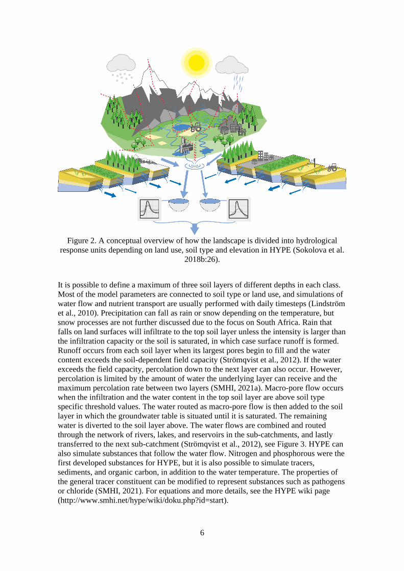
Figure 2. A conceptual overview of how the landscape is divided into hydrological

response units depending on land use, soil type and elevation in HYPE (Sokolova et al.

2018b:26).

It is possible to define a maximum of three soil layers of different depths in each class.

Most of the model parameters are connected to soil type or land use, and simulations of

water flow and nutrient transport are usually performed with daily timesteps (Lindström

et al., 2010). Precipitation can fall as rain or snow depending on the temperature, but

snow processes are not further discussed due to the focus on South Africa. Rain that

falls on land surfaces will infiltrate to the top soil layer unless the intensity is larger than

the infiltration capacity or the soil is saturated, in which case surface runoff is formed.

Runoff occurs from each soil layer when its largest pores begin to fill and the water

content exceeds the soil-dependent field capacity (Strömqvist et al., 2012). If the water

exceeds the field capacity, percolation down to the next layer can also occur. However,

percolation is limited by the amount of water the underlying layer can receive and the

maximum percolation rate between two layers (SMHI, 2021a). Macro-pore flow occurs

when the infiltration and the water content in the top soil layer are above soil type

specific threshold values. The water routed as macro-pore flow is then added to the soil

layer in which the groundwater table is situated until it is saturated. The remaining

water is diverted to the soil layer above. The water flows are combined and routed

through the network of rivers, lakes, and reservoirs in the sub-catchments, and lastly

transferred to the next sub-catchment (Strömqvist et al., 2012), see Figure 3. HYPE can

also simulate substances that follow the water flow. Nitrogen and phosphorous were the

first developed substances for HYPE, but it is also possible to simulate tracers,

sediments, and organic carbon, in addition to the water temperature. The properties of

the general tracer constituent can be modified to represent substances such as pathogens

or chloride (SMHI, 2021). For equations and more details, see the HYPE wiki page

(http://www.smhi.net/hype/wiki/doku.php?id=start).

7

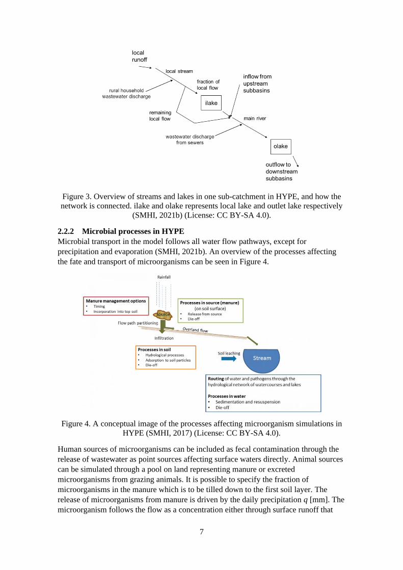
Figure 3. Overview of streams and lakes in one sub-catchment in HYPE, and how the

network is connected. ilake and olake represents local lake and outlet lake respectively

(SMHI, 2021b) (License: CC BY-SA 4.0).

2.2.2 Microbial processes in HYPE

Microbial transport in the model follows all water flow pathways, except for

precipitation and evaporation (SMHI, 2021b). An overview of the processes affecting

the fate and transport of microorganisms can be seen in Figure 4.

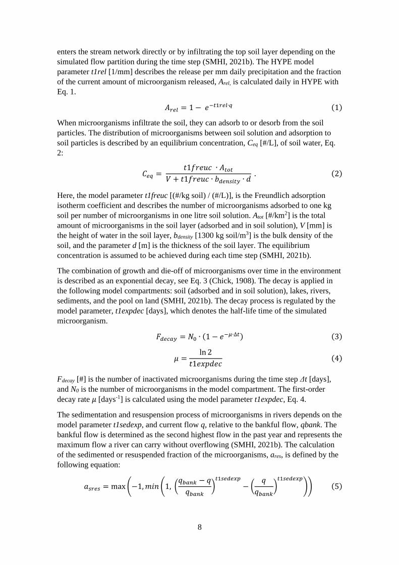
Figure 4. A conceptual image of the processes affecting microorganism simulations in

HYPE (SMHI, 2017) (License: CC BY-SA 4.0).

Human sources of microorganisms can be included as fecal contamination through the

release of wastewater as point sources affecting surface waters directly. Animal sources

can be simulated through a pool on land representing manure or excreted

microorganisms from grazing animals. It is possible to specify the fraction of

microorganisms in the manure which is to be tilled down to the first soil layer. The

release of microorganisms from manure is driven by the daily precipitation q [mm]. The

microorganism follows the flow as a concentration either through surface runoff that

8

enters the stream network directly or by infiltrating the top soil layer depending on the

simulated flow partition during the time step (SMHI, 2021b). The HYPE model

parameter t1rel [1/mm] describes the release per mm daily precipitation and the fraction

of the current amount of microorganism released, Arel, is calculated daily in HYPE with

Eq. 1.

𝐴𝑟𝑒𝑙 = 1 − 𝑒−𝑡1𝑟𝑒𝑙∙𝑞 (1)

When microorganisms infiltrate the soil, they can adsorb to or desorb from the soil

particles. The distribution of microorganisms between soil solution and adsorption to

soil particles is described by an equilibrium concentration, Ceq [#/L], of soil water, Eq.

2:

𝐶𝑒𝑞 = 𝑡1𝑓𝑟𝑒𝑢𝑐 ∙ 𝐴𝑡𝑜𝑡

𝑉 + 𝑡1𝑓𝑟𝑒𝑢𝑐 ∙ 𝑏𝑑𝑒𝑛𝑠𝑖𝑡𝑦 ∙ 𝑑 . (2)

Here, the model parameter t1freuc [(#/kg soil) / (#/L)], is the Freundlich adsorption

isotherm coefficient and describes the number of microorganisms adsorbed to one kg

soil per number of microorganisms in one litre soil solution. Atot [#/km2] is the total

amount of microorganisms in the soil layer (adsorbed and in soil solution), V [mm] is

the height of water in the soil layer, bdensity [1300 kg soil/m3] is the bulk density of the

soil, and the parameter d [m] is the thickness of the soil layer. The equilibrium

concentration is assumed to be achieved during each time step (SMHI, 2021b).

The combination of growth and die-off of microorganisms over time in the environment

is described as an exponential decay, see Eq. 3 (Chick, 1908). The decay is applied in

the following model compartments: soil (adsorbed and in soil solution), lakes, rivers,

sediments, and the pool on land (SMHI, 2021b). The decay process is regulated by the

model parameter, t1expdec [days], which denotes the half-life time of the simulated

microorganism.

𝐹𝑑𝑒𝑐𝑎𝑦 = 𝑁0 ∙ (1 − 𝑒−𝜇∙∆𝑡) (3)

𝜇 =ln 2

𝑡1𝑒𝑥𝑝𝑑𝑒𝑐 (4)

Fdecay [#] is the number of inactivated microorganisms during the time step Δt [days],

and N0 is the number of microorganisms in the model compartment. The first-order

decay rate 𝜇 [days-1] is calculated using the model parameter t1expdec, Eq. 4.

The sedimentation and resuspension process of microorganisms in rivers depends on the

model parameter t1sedexp, and current flow q, relative to the bankful flow, qbank. The

bankful flow is determined as the second highest flow in the past year and represents the

maximum flow a river can carry without overflowing (SMHI, 2021b). The calculation

of the sedimented or resuspended fraction of the microorganisms, ares, is defined by the

following equation:

𝑎𝑠𝑟𝑒𝑠 = max (−1, 𝑚𝑖𝑛 (1, (𝑞𝑏𝑎𝑛𝑘 − 𝑞

𝑞𝑏𝑎𝑛𝑘)

𝑡1𝑠𝑒𝑑𝑒𝑥𝑝

− (𝑞

𝑞𝑏𝑎𝑛𝑘)

𝑡1𝑠𝑒𝑑𝑒𝑥𝑝

)) (5)

9

Sedimentation occurs during low flow which yields a positive asres, while during high

flow, asres is negative and resuspension from the sediments occur:

𝐹𝑠𝑒𝑑 = 𝑎𝑠𝑟𝑒𝑠 ∙ 𝐶𝑟𝑖𝑣𝑒𝑟 ∙ 𝑉𝑟𝑖𝑣𝑒𝑟 , 𝑎𝑠𝑟𝑒𝑠 > 0 (6)

𝐹𝑟𝑒𝑠𝑢𝑠𝑝 = −𝑎𝑠𝑟𝑒𝑠 ∙ 𝐴𝑠𝑒𝑑 , 𝑎𝑠𝑟𝑒𝑠 < 0 . (7)

Here, Fsed and Fresusp are the amounts of microorganism per day for the two processes,

the parameter Criver [#/m3] is the river concentration of the microorganism, Vriver [m3] is

the volume of the river, and Ased [#] is the number of microorganisms in the sediment.

In lakes, no resuspension is simulated and the sedimentation, sedlake [#/d], is defined by:

𝑠𝑒𝑑𝑙𝑎𝑘𝑒 = 𝑡1𝑠𝑒𝑑𝑣𝑒𝑙 ∙ 𝐶𝑙𝑎𝑘𝑒 ∙ 𝐴𝑙𝑎𝑘𝑒 ∙ 10−3 (8)

The model parameter, t1sedvel [m/day], denotes the sedimentation velocity, Clake [#/m3],

is the concentration of microorganisms in the lake, and Alake [m2] is the area of the lake.

2.2.3 The World-Wide HYPE (WWH) model application in South Africa

WWH is a development of parameters for HYPE that covers almost the entire globe.

The current version of WWH consists of approximately 130,000 catchments with an

average size of about 1,000 km2.

The South Africa sub-model consists of 1657 sub-catchments and a total of 169 HRUs.

There are four prevalent soil types, water & floodplains, urban, rock, and average soil,

which are combined with 40 landcover types at various elevations to create the HRUs.

Topographical data, meteorological data, and observed river flow for South Africa were

provided and included in WWH version 1.3.7 by SMHI previous to this project (see

Arheimer et al. (2020) for details). Topographical data is needed for the delineation and

routing of catchment areas, whereas time series of meteorological data (temperature and

precipitation) are necessary forcing data when calculating water flow at a daily time

step in WWH. Hydrological data is included to calibrate and evaluate the simulated

flow.

Physiographical data

None of the existing databases cover the entire land surface of Earth, but GWD-LR

(Global Width Database for Large Rivers) covers the surface between 60° S to 80° N,

which includes South Africa. The raster GWD-LR dataset contains flow direction, river

width, flow accumulation, and elevation (Yamazaki et al., 2014). Additional

information about specific environments that are present in South Africa, such as karst,

deserts, and floodplains, was gathered since delineation of catchments can be

particularly complex in these areas (Arheimer et al., 2020). For the catchment

characteristics, such as land use and soil type, the ESA CCI Landcover version 1.6.1

epoch 2010 (300m) data source was used as a guideline to define the HRUs.

Meteorological data

Daily records of precipitation and temperature from various data sources were

combined through the Hydrological Global forcing Data (HydroGFD), a product

developed by SMHI (Berg et al. 2018). The data set time period begins in 1961 and

extends to near-real time (Arheimer et al., 2020).

10

Hydrological data

Daily and monthly time series of observed river flow at gauging stations were obtained

through open data sources such as Global Runoff Data Center (GRDC). Hydrological

datasets were used for parameter estimation and model evaluation. Specifically for

South Africa, hydrological information such as upstream area, elevation, and river name

was collected from the Department of Water & Sanitation (Arheimer et al., 2020).

3 METHOD

3.1 CHOICE OF MICROORGANISM FOR THIS STUDY

The initial step in this project was to perform a literature study and decide which

pathogen to simulate in WWH. To facilitate the decision, four criteria were established:

1. The pathogen must be waterborne,

2. The pathogen is prevalent and causes human health problems,

3. The pathogen’s most important host is humans,

4. There are observed surface water concentrations in South Africa and the process

parameters can be quantified based on the literature.

The aim is to study pathogen transport in surface water, and it is therefore crucial that

the pathogen is waterborne. Due to difficulties in assessing the contribution of

pathogens from animals, it would be preferred to simulate a pathogen where humans are

the major source as a first step. To realistically simulate pathogens in HYPE, their

survival and behavior in the environment must be quantified. Lastly, observed surface

water concentrations of the microorganism are required to evaluate the conformity of

the simulations in WWH. The literature study was performed with the criteria as a

foundation for the six pathogens described in section 2.1.1. The literature study

concluded that none of the above-mentioned pathogens satisfied all the criteria, see

Table 1.

Table 1. An overview of fulfilled criteria for each studied pathogen. X means the

criteria are fulfilled, and – means the criteria are not fulfilled.

E. coli Salmonella Shigella Vibrio Enteroviruses Rotaviruses

Criteria 1 X X X X X X

Criteria 2 X X X X X X

Criteria 3 - - X - - -

Criteria 4 X - - - - -

Shigella is the only pathogenic microorganism for which humans are the main host but

there is not enough available data regarding observed concentrations in surface water in

South Africa, which is necessary when evaluating the model simulations. E. coli was

the only microorganism with sufficient available data, but the contribution from warm-

blooded animals must be included as a contamination source in the model since E. coli

is prevalent in both humans and animals. Data availability is considered as the most

crucial criteria, which is why E. coli was selected as the microorganism to simulate in

WWH.

11

3.2 OBSERVED SURFACE WATER CONCENTRATIONS OF E. COLI IN

SOUTH AFRICA

This section describes the data set with E. coli concentrations in surface water in South

Africa regarding the number of sampling stations and measurements at sampling

stations, as well as how this information was linked to the sub-catchments in the WWH

model.

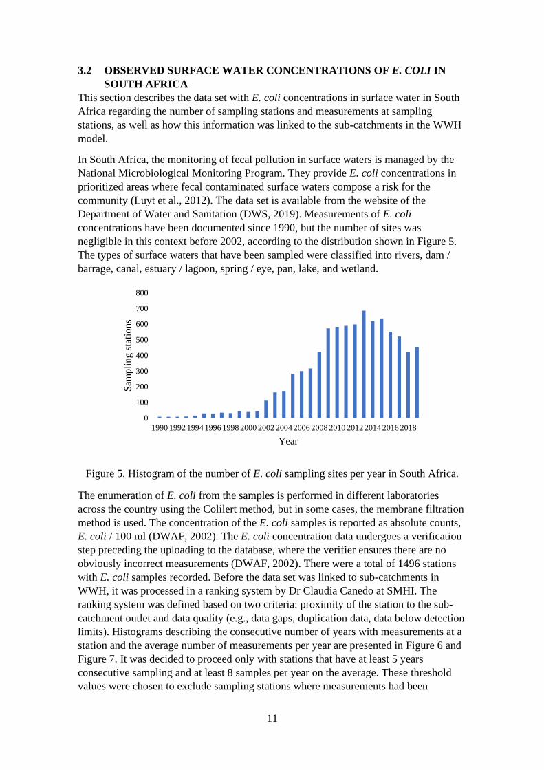
In South Africa, the monitoring of fecal pollution in surface waters is managed by the

National Microbiological Monitoring Program. They provide E. coli concentrations in

prioritized areas where fecal contaminated surface waters compose a risk for the

community (Luyt et al., 2012). The data set is available from the website of the

Department of Water and Sanitation (DWS, 2019). Measurements of E. coli

concentrations have been documented since 1990, but the number of sites was

negligible in this context before 2002, according to the distribution shown in Figure 5.

The types of surface waters that have been sampled were classified into rivers, dam /

barrage, canal, estuary / lagoon, spring / eye, pan, lake, and wetland.

Figure 5. Histogram of the number of E. coli sampling sites per year in South Africa.

The enumeration of E. coli from the samples is performed in different laboratories

across the country using the Colilert method, but in some cases, the membrane filtration

method is used. The concentration of the E. coli samples is reported as absolute counts,

E. coli / 100 ml (DWAF, 2002). The E. coli concentration data undergoes a verification

step preceding the uploading to the database, where the verifier ensures there are no

obviously incorrect measurements (DWAF, 2002). There were a total of 1496 stations

with E. coli samples recorded. Before the data set was linked to sub-catchments in

WWH, it was processed in a ranking system by Dr Claudia Canedo at SMHI. The

ranking system was defined based on two criteria: proximity of the station to the sub-

catchment outlet and data quality (e.g., data gaps, duplication data, data below detection

limits). Histograms describing the consecutive number of years with measurements at a

station and the average number of measurements per year are presented in Figure 6 and

Figure 7. It was decided to proceed only with stations that have at least 5 years

consecutive sampling and at least 8 samples per year on the average. These threshold

values were chosen to exclude sampling stations where measurements had been

0

100

200

300

400

500

600

700

800

1990 1992 1994 1996 1998 2000 2002 2004 2006 2008 2010 2012 2014 2016 2018

Sam

pli

ng s

tati

ons

Year

12

inconsistent. After the ranking system, 80 sites remained that fulfilled all the criteria.

The observed E. coli concentrations at these sites were hence used to evaluate the

simulations of E. coli in surface water.

Figure 6. Sampling stations and the corresponding number of consecutive years of E.

coli measurements.

Figure 7. The distribution of the average number E. coli observations in relation to the

number of sampling stations.

3.3 WWH MODEL SETUP

In this project, HYPE version 5.10.3 and the WWH version 1.3.7 were used.

Simulations were evaluated for the 80 sub-catchments with observed E. coli

concentrations in South Africa during the simulation period 2002 – 2016, with a warm-

up period 1987 - 2002. The output of the simulations is daily recorded and simulated

discharge and E. coli concentration at the outlet of the 80 sub-catchments. Furthermore,

the load of E. coli per day was calculated by multiplying E. coli concentration with

discharge.

The following section covers the required input data to create the HYPE model

application and explains how the E. coli contamination sources were introduced to the

0

100

200

300

400

500

600

700

800

1 2 3 4 5 6 7 8 9 10 11 12 13 14 15 16 17 18 19 20 21 22 23

Sam

pli

ng s

tati

on

s

Number of consecutive years

0

100

200

300

400

500

600

Sam

pli

ng s

tati

on

s

The average observations per year

13

model through wastewater discharge and contaminated manure. The required

calculations and assumptions to simulate E. coli concentrations and quantified values of

process parameters affecting the fate of E. coli in the model are also presented.

3.3.1 Quantification of human sources of E. coli

The contribution of E. coli from humans is modelled in HYPE as fecal contamination

through the release of wastewater. Therefore, to provide input to the model, information

about daily human excretion of feces, E. coli concentration in feces, and wastewater

discharge per person was gathered to calculate the concentration of E. coli in

wastewater and the corresponding volume of water released in each catchment.

The median human excretion of fecal wet mass, 128 g/person and day, was reported in a

study by Rose et al. (2015). The median is chosen from a set of recorded mean values of

feces per person and day for healthy individuals, which varied between persons in the

range 51 – 796 g/person and day. The concentration of E. coli in feces of healthy

humans can vary in the range of 6 – 7 Log10 CFU/g feces according to Forsythe (2008)

and between 7.5 – 7.7 Log10 CFU/g feces wet weight according to Cabral (2010). In

semi-arid areas, wastewater production is estimated to 35 – 75 L/person and day

(Helmer et al., 1997). The information from this paragraph is summarized in Table 2.

The chosen values that were used as an estimate in the model scenario Base case are

presented in section 3.4.

Table 2. Range and median values of the information needed to calculate the human

contribution of E. coli in the water environment. The median values are presented in the

parenthesis.

Type of information Unit Range References

Excretion of feces [g/person & day] 51 – 796 (128) (Rose et al., 2015)

E. coli concentration in

feces

[CFU/g] Log10 6 – 7 (6.5)

Log10 7.5 – 7.7 (7.6)

(Forsythe, 2008) &

(Cabral, 2010)

Wastewater discharge [L/person & day] 35 – 75 (55) (Helmer et al., 1997)

Additional information regarding individual human waste management was also

necessary, since the E. coli bacteria will contribute to surface water differently

depending on the human waste management that is implemented. It is therefore of high

importance to account for an estimate of the degree of human waste management. A

global data set with information about the level of individual human waste management

has recently been developed by Drs Conrad Brendel and Alena Bartosova at SMHI. The

data set contains the estimated number of people with access to different sanitation

levels in each WWH sub-catchment. In Figure 8, the total distribution of the sanitation

levels in South Africa is displayed. The sanitation levels are divided into six groups:

Managed sewer, Managed other improved, Unmanaged sewer, Unmanaged other

improved, and Not Applicable (NA). Managed sewer represents a sewer connection

where the wastewater is treated at a wastewater treatment plant, before being released to

surface water. Unmanaged sewer represents a sewer connection that releases untreated

wastewater directly to surface water. If an individual has access to septic tanks and

improved latrines, where the excreta is treated off-site or in-situ, the level of sanitation

is Managed other improved. However, if the waste is not treated off-site or in-situ, the

14

level of sanitation is Unmanaged other improved. The sanitation level Unmanaged

unimproved represents open defecation and no access to improved sanitation. The level

of waste management could not be estimated for a smaller fraction of the population,

which is represented by the NA category. In this thesis, the contributions from the

population with a sewer connection are considered as urban sources while remaining

sanitation levels are considered as rural sources, see Table 3.

Table 3. Classification of sanitation levels.

Urban sources Rural sources

Managed sewer Managed other improved

Unmanaged sewer Unmanaged other improved

Unmanaged unimproved

NA

Figure 8. The distribution of population according to the level of sanitation in South

Africa provided in the dataset developed by Drs Conrad Brendel and Alena Bartosova at

SMHI.

Urban sources

In the simulations, wastewater treatment was applied to the fraction of the population

with Managed sewer. According to Kumari (2021) and Hansen (2015), a common

treatment method at wastewater treatment plants in South Africa is conventional

activated sludge with chlorine disinfection, which typically has a log reduction for

bacteria in the range of 3 – 6 (WHO, 2006). The log-reduction is converted to a removal

efficiency of the wastewater treatment method, Effremoval, as described in section 2.1.

The removal efficiency was set to zero for the fraction of the population with

Unmanaged sewer since the wastewater of this sanitation level is released to surface

water directly. The calculated value of total daily E. coli contribution from Managed

sewer and Unmanaged sewer is incorporated into the model in WWH as a point source

to the main river in each relevant subbasin. The concentration of this source, variable

ps_t1 [CFU/L] was calculated as:

0

5

10

15

20

25

30

35

Managed

sewer

Managed

other

improved

Unmanaged

sewer

Unmanaged

other

improved

Unmanaged

unimproved

NA

Per

centa

ge

of

popula

tion [

%]

Sanitation level

15

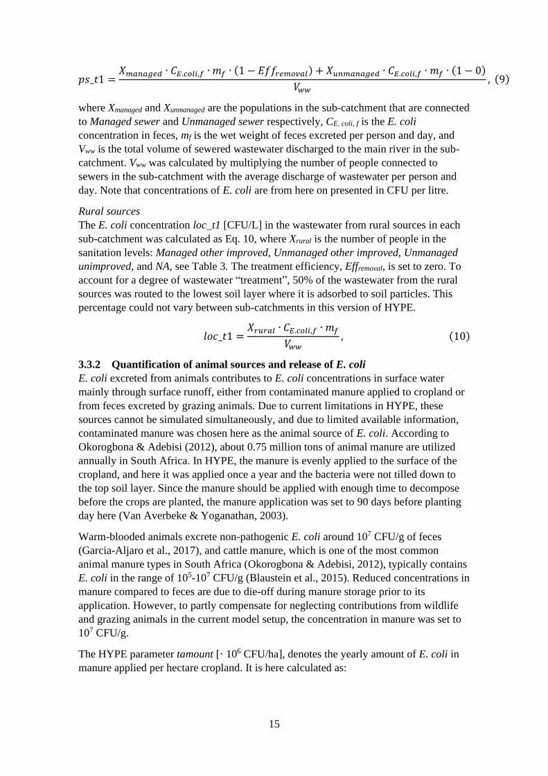
𝑝𝑠_𝑡1 =𝑋𝑚𝑎𝑛𝑎𝑔𝑒𝑑 ∙ 𝐶𝐸.𝑐𝑜𝑙𝑖,𝑓 ∙ 𝑚𝑓 ∙ (1 − 𝐸𝑓𝑓𝑟𝑒𝑚𝑜𝑣𝑎𝑙) + 𝑋𝑢𝑛𝑚𝑎𝑛𝑎𝑔𝑒𝑑 ∙ 𝐶𝐸.𝑐𝑜𝑙𝑖,𝑓 ∙ 𝑚𝑓 ∙ (1 − 0)

𝑉𝑤𝑤, (9)

where Xmanaged and Xunmanaged are the populations in the sub-catchment that are connected

to Managed sewer and Unmanaged sewer respectively, CE. coli, f is the E. coli

concentration in feces, mf is the wet weight of feces excreted per person and day, and

Vww is the total volume of sewered wastewater discharged to the main river in the sub-

catchment. Vww was calculated by multiplying the number of people connected to

sewers in the sub-catchment with the average discharge of wastewater per person and

day. Note that concentrations of E. coli are from here on presented in CFU per litre.

Rural sources

The E. coli concentration loc_t1 [CFU/L] in the wastewater from rural sources in each

sub-catchment was calculated as Eq. 10, where Xrural is the number of people in the

sanitation levels: Managed other improved, Unmanaged other improved, Unmanaged

unimproved, and NA, see Table 3. The treatment efficiency, Effremoval, is set to zero. To

account for a degree of wastewater “treatment”, 50% of the wastewater from the rural

sources was routed to the lowest soil layer where it is adsorbed to soil particles. This

percentage could not vary between sub-catchments in this version of HYPE.

𝑙𝑜𝑐_𝑡1 =𝑋𝑟𝑢𝑟𝑎𝑙 ∙ 𝐶𝐸.𝑐𝑜𝑙𝑖,𝑓 ∙ 𝑚𝑓

𝑉𝑤𝑤, (10)

3.3.2 Quantification of animal sources and release of E. coli

E. coli excreted from animals contributes to E. coli concentrations in surface water

mainly through surface runoff, either from contaminated manure applied to cropland or

from feces excreted by grazing animals. Due to current limitations in HYPE, these

sources cannot be simulated simultaneously, and due to limited available information,

contaminated manure was chosen here as the animal source of E. coli. According to

Okorogbona & Adebisi (2012), about 0.75 million tons of animal manure are utilized

annually in South Africa. In HYPE, the manure is evenly applied to the surface of the

cropland, and here it was applied once a year and the bacteria were not tilled down to

the top soil layer. Since the manure should be applied with enough time to decompose

before the crops are planted, the manure application was set to 90 days before planting

day here (Van Averbeke & Yoganathan, 2003).

Warm-blooded animals excrete non-pathogenic E. coli around 107 CFU/g of feces

(Garcia-Aljaro et al., 2017), and cattle manure, which is one of the most common

animal manure types in South Africa (Okorogbona & Adebisi, 2012), typically contains

E. coli in the range of 105-107 CFU/g (Blaustein et al., 2015). Reduced concentrations in

manure compared to feces are due to die-off during manure storage prior to its

application. However, to partly compensate for neglecting contributions from wildlife

and grazing animals in the current model setup, the concentration in manure was set to

107 CFU/g.

The HYPE parameter tamount [· 106 CFU/ha], denotes the yearly amount of E. coli in

manure applied per hectare cropland. It is here calculated as:

16

tamount = 𝐹𝑚𝑎𝑛𝑢𝑟𝑒 ∙ 𝐶𝐸.𝑐𝑜𝑙𝑖,𝑚𝑎𝑛𝑢𝑟𝑒

𝐴𝑐𝑟𝑜𝑝𝑙𝑎𝑛𝑑 , (11)

where, Fmanure [g/year], is the total amount of manure applied to cropland in South

Africa, CE. coli, manure [CFU/g] is the concentration of E. coli in animal manure, and

Acropland [ha] is the total cropland area in WWH, South Africa. The total yearly amount

of manure applied in each sub-catchment is tamount multiplied by the sub-catchment

cropland area.

Shelton et al. (2003) performed a study on the release of pathogens from surface applied

manure and obtained a release rate constant of 0.0054 ± 0.0015 min-1 for fecal coliform

with a simulated rainfall of 7.1 cm / h, which was used in this thesis (and in prior

pathogen modelling with HYPE (Sokolova et al. 2018b)) to estimate t1rel:

𝑡1𝑟𝑒𝑙 =0.0054 [𝑚𝑖𝑛−1]

7.1 [𝑐𝑚ℎ

] ∙1

60 [ℎ

𝑚𝑖𝑛] ∙ 10 [𝑚𝑚𝑐𝑚 ]

≈ 0.005 𝑚𝑚−1

3.3.3 Quantification of microbial transport processes

The degree of adsorption is dependent on soil type and has a large variation between

2000 – 60 000 CFU/kg soil / CFU/L where the lower value was determined for sandy

soils and the higher for clayey soils (Cho et al., 2016).

The half-life for E. coli in surface water varies between 1.5 – 3 days (Dufour & WHO,

2003), and between 1 – 7 days in soil and manure (Crane & Moore, 1985). However,

t1expdec can only be assigned one value in this model version for all model

compartments. The survival of E. coli in surface water is prioritized in this thesis and

therefore 1.5 – 3 days is the considered half-life time.

Due to difficulties in finding quantified scientific data, sedimentation and resuspension

in rivers and lakes were excluded in the simulations of this project.

3.4 BASE CASE SCENARIO AND MODEL SENSITIVITY

The E. coli fate, transport and its sensitivity to the discussed uncertainties in both

sources and processes are investigated in three steps. First, the dynamic behavior is

investigated by comparing the conformity between simulated and observed E.

coli concentrations. The conformity between simulated and observed E. coli load is also

compared. To measure the conformity, Nash-Sutcliffe efficiency (NSE) and bias were

calculated, more information can be found in section 3.4.1. The apportionment of E.

coli sources is studied to increase the understanding of contribution from different

sources and lastly, the model sensitivity is investigated through a sensitivity analysis.

Based on the parameter ranges described in the previous sections, a base-case E. coli

model application in WWH for South Africa was established. Each parameter value was

determined as the one that maximizes the conformity between the simulated and

observed E. coli concentration and load. The iterative study resulted in using the median

for most of the variables, see Table 4 and Table 5. The concentration of E. coli in feces

and t1freuc were the only factors where the median value was not used.

17

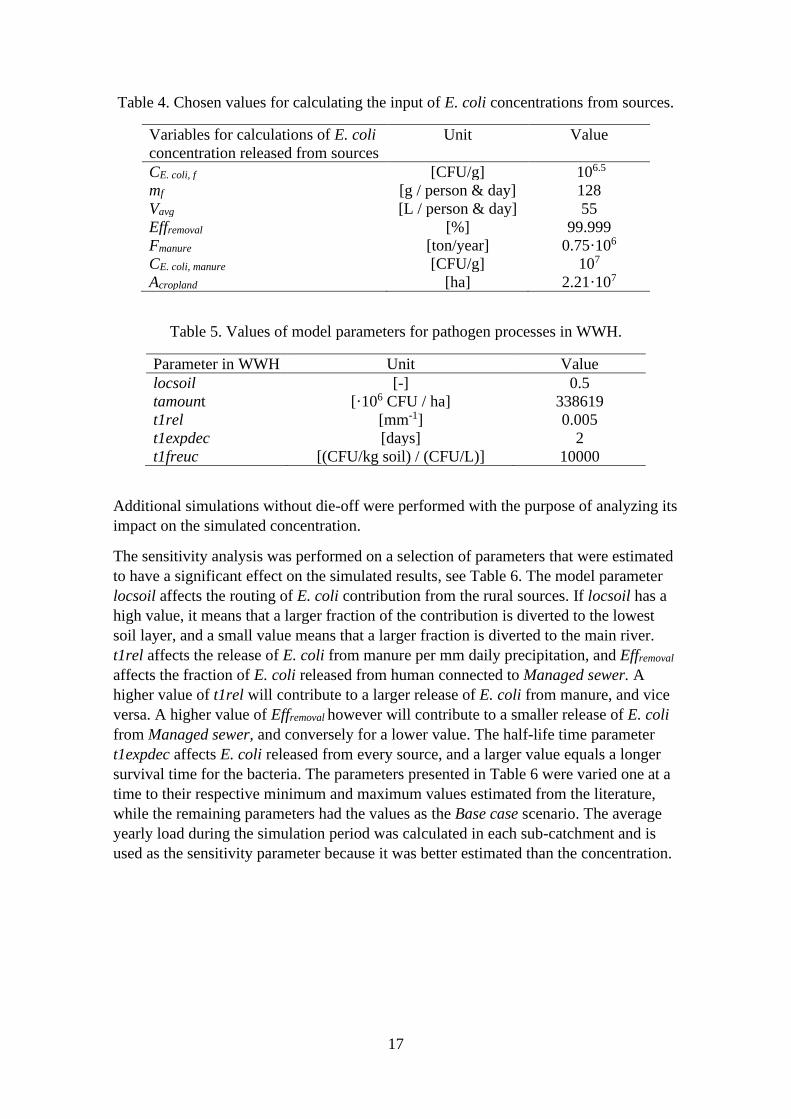
Table 4. Chosen values for calculating the input of E. coli concentrations from sources.

Variables for calculations of E. coli

concentration released from sources

Unit Value

CE. coli, f [CFU/g] 106.5

mf [g / person & day] 128

Vavg [L / person & day] 55

Effremoval [%] 99.999

Fmanure [ton/year] 0.75·106

CE. coli, manure [CFU/g] 107

Acropland [ha] 2.21·107

Table 5. Values of model parameters for pathogen processes in WWH.

Parameter in WWH Unit Value

locsoil [-] 0.5

tamount [·106 CFU / ha] 338619

t1rel [mm-1] 0.005

t1expdec [days] 2

t1freuc [(CFU/kg soil) / (CFU/L)] 10000

Additional simulations without die-off were performed with the purpose of analyzing its

impact on the simulated concentration.

The sensitivity analysis was performed on a selection of parameters that were estimated

to have a significant effect on the simulated results, see Table 6. The model parameter

locsoil affects the routing of E. coli contribution from the rural sources. If locsoil has a

high value, it means that a larger fraction of the contribution is diverted to the lowest

soil layer, and a small value means that a larger fraction is diverted to the main river.

t1rel affects the release of E. coli from manure per mm daily precipitation, and Effremoval

affects the fraction of E. coli released from human connected to Managed sewer. A

higher value of t1rel will contribute to a larger release of E. coli from manure, and vice

versa. A higher value of Effremoval however will contribute to a smaller release of E. coli

from Managed sewer, and conversely for a lower value. The half-life time parameter

t1expdec affects E. coli released from every source, and a larger value equals a longer

survival time for the bacteria. The parameters presented in Table 6 were varied one at a

time to their respective minimum and maximum values estimated from the literature,

while the remaining parameters had the values as the Base case scenario. The average

yearly load during the simulation period was calculated in each sub-catchment and is

used as the sensitivity parameter because it was better estimated than the concentration.

18

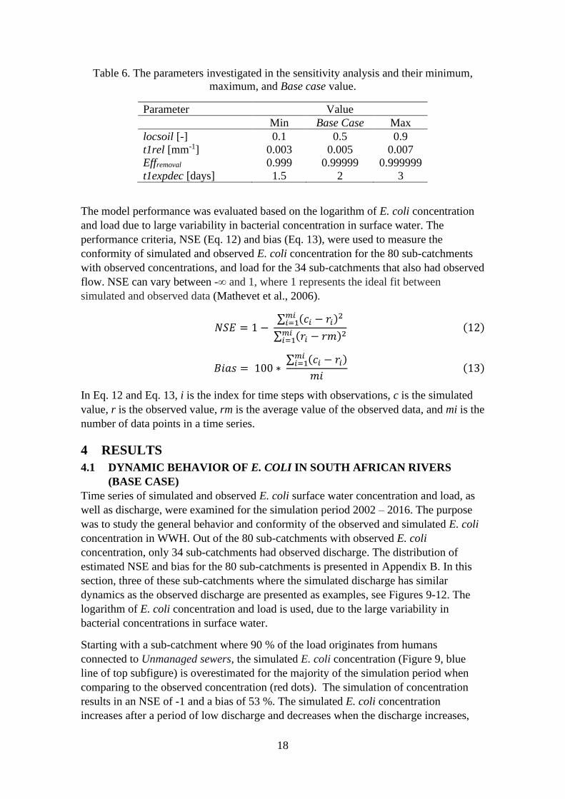
Table 6. The parameters investigated in the sensitivity analysis and their minimum,

maximum, and Base case value.

Parameter Value

Min Base Case Max

locsoil [-] 0.1 0.5 0.9

t1rel [mm-1] 0.003 0.005 0.007

Effremoval 0.999 0.99999 0.999999

t1expdec [days] 1.5 2 3

The model performance was evaluated based on the logarithm of E. coli concentration

and load due to large variability in bacterial concentration in surface water. The

performance criteria, NSE (Eq. 12) and bias (Eq. 13), were used to measure the

conformity of simulated and observed E. coli concentration for the 80 sub-catchments

with observed concentrations, and load for the 34 sub-catchments that also had observed

flow. NSE can vary between -∞ and 1, where 1 represents the ideal fit between

simulated and observed data (Mathevet et al., 2006).

𝑁𝑆𝐸 = 1 − ∑ (𝑐𝑖 − 𝑟𝑖)

2𝑚𝑖𝑖=1

∑ (𝑟𝑖 − 𝑟𝑚)2𝑚𝑖𝑖=1

(12)

𝐵𝑖𝑎𝑠 = 100 ∗ ∑ (𝑐𝑖 − 𝑟𝑖)

𝑚𝑖𝑖=1

𝑚𝑖 (13)

In Eq. 12 and Eq. 13, i is the index for time steps with observations, c is the simulated

value, r is the observed value, rm is the average value of the observed data, and mi is the

number of data points in a time series.

4 RESULTS

4.1 DYNAMIC BEHAVIOR OF E. COLI IN SOUTH AFRICAN RIVERS

(BASE CASE)

Time series of simulated and observed E. coli surface water concentration and load, as

well as discharge, were examined for the simulation period 2002 – 2016. The purpose

was to study the general behavior and conformity of the observed and simulated E. coli

concentration in WWH. Out of the 80 sub-catchments with observed E. coli

concentration, only 34 sub-catchments had observed discharge. The distribution of

estimated NSE and bias for the 80 sub-catchments is presented in Appendix B. In this

section, three of these sub-catchments where the simulated discharge has similar

dynamics as the observed discharge are presented as examples, see Figures 9-12. The

logarithm of E. coli concentration and load is used, due to the large variability in

bacterial concentrations in surface water.

Starting with a sub-catchment where 90 % of the load originates from humans

connected to Unmanaged sewers, the simulated E. coli concentration (Figure 9, blue

line of top subfigure) is overestimated for the majority of the simulation period when

comparing to the observed concentration (red dots). The simulation of concentration

results in an NSE of -1 and a bias of 53 %. The simulated E. coli concentration

increases after a period of low discharge and decreases when the discharge increases,

19

which is not a trend shown by the observations. The simulated discharge has similar

timing of high- and low-flow events as the observed discharge, but the magnitude is

indeed underestimated for the larger part of the simulation period. The simulated E. coli

load matches observations quite well both in terms of dynamics and magnitude.

However, the simulated load is underestimated during periods of high discharge. The

estimated NSE and bias was 0.69 and 7.7 % respectively for the simulated load.

Figure 9. Time series of E. coli concentration, discharge, and E. coli load in surface

water in one sub-catchment with 90 % of the load from Unmanaged sewer.

Figure 10 displays a sub-catchment where the E. coli load originates mostly from

humans connected to Unmanaged sewers and human rural sources, about 60 % and 40

% respectively. In contrast to Figure 9, the simulated E. coli concentration is mostly

underestimated compared to the observed E. coli concentration, as can be seen in Figure

10. The simulation of concentration resulted in an NSE of -0.30 and a bias of -68 %.

The simulated discharge is also mostly underestimated compared to the observed

discharge. Again, the overall dynamics of the load is well described by the simulations

where the estimated NSE was 0.67. However, the simulated E. coli load is

underestimated by several orders of magnitude during periods of very high discharge

with a bias of -67 %.

20

Figure 10. Time series of E. coli concentration, discharge, and E. coli load in surface

water in a sub-catchment with 60 % of the load from Unmanaged sewer and 40 % from

human rural sources.

In Figure 11, results are shown for a sub-catchment with no incoming flow from

upstream areas. The E. coli load originates with 100 % from human rural sources. The

simulated E. coli concentration is overestimated for the majority of the simulation

period. The simulated discharge is again underestimated but shares the general timing of

events with the observed discharge. The decrease of simulated E. coli load after a period

of low discharge is generally greater than one order of magnitude. The observed and

simulated E. coli load shares similar dynamics with peaks and low points. As seen in

Figure 9 – 11, the largest observed E. coli load generally correspond to observed high

discharge, not captured by the simulation. The estimated NSE and bias for the simulated

concentration was -0.91 and 58 %, respectively. The simulated load resulted in an NSE

of 0.65 and a bias of 0.07 %.

21

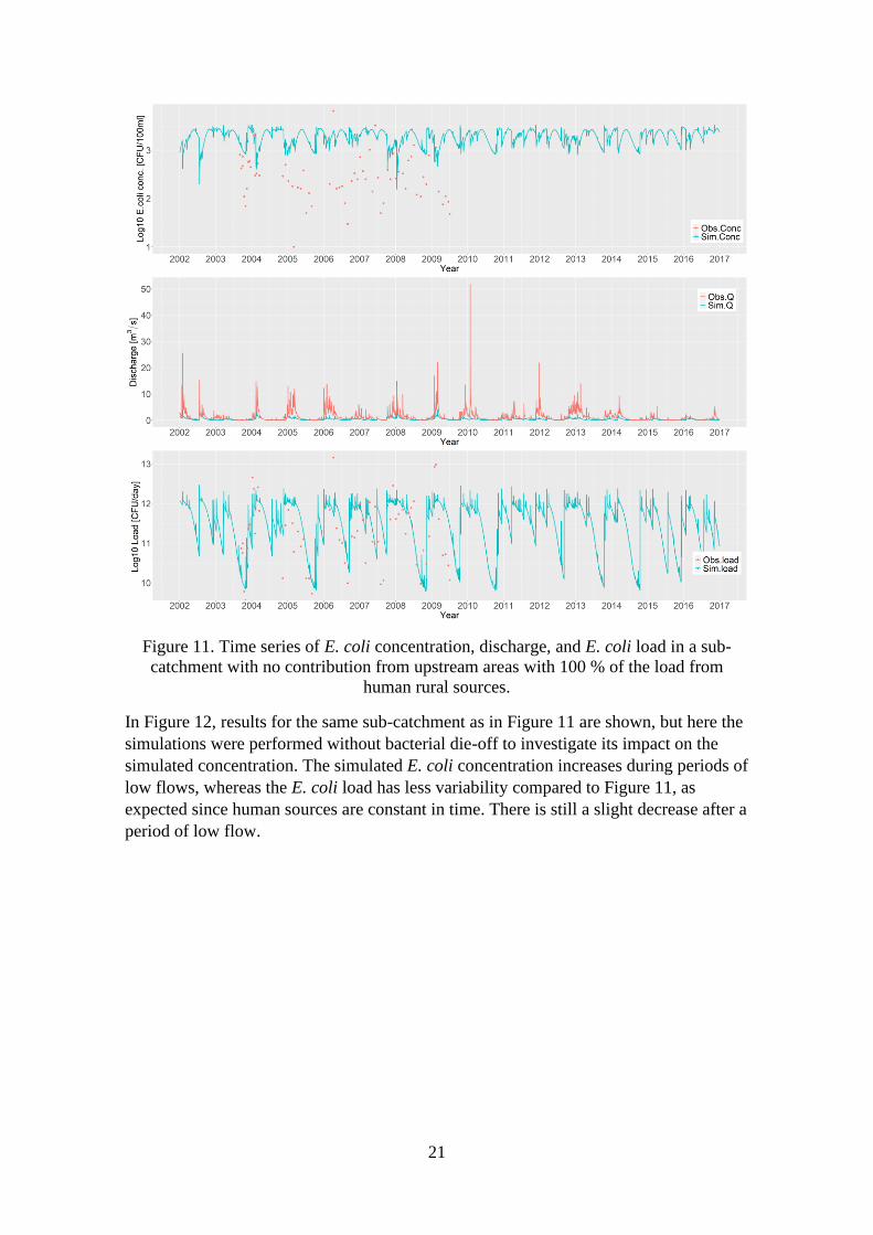
Figure 11. Time series of E. coli concentration, discharge, and E. coli load in a sub-

catchment with no contribution from upstream areas with 100 % of the load from

human rural sources.

In Figure 12, results for the same sub-catchment as in Figure 11 are shown, but here the

simulations were performed without bacterial die-off to investigate its impact on the

simulated concentration. The simulated E. coli concentration increases during periods of

low flows, whereas the E. coli load has less variability compared to Figure 11, as

expected since human sources are constant in time. There is still a slight decrease after a

period of low flow.

22

Figure 12. Time series of E. coli concentration, discharge, and E. coli load in a sub-

catchment with no contribution from upstream areas and E. coli die-off was excluded

from the simulation with 100 % of the load from human rural sources.

4.2 E. COLI SOURCE APPORTIONMENT

The total yearly load of E. coli released from the different sources prior to any treatment

or die-off is presented in Table 7.

Table 7. The total estimated E. coli load released from the different sources in this

model application.

Source of E. coli Total estimated load [· 1018 CFU / year]

Managed sewer 2.1

Unmanaged sewer 2.6

Rural sources 4.4

Animals 7.5

An important factor in the mitigation of pathogen exposure is to understand the

influence of different sources. This was investigated here for the microorganism E. coli

based on four simulations, introducing a new type of source between each simulation,

and finally reaching the base-case scenario. The corresponding increase in the load of E.

coli in surface water between simulations was registered, as shown in the maps of

Figure 13. The daily load was here defined by multiplying the surface water

23

concentration with the discharge rate, and the figure presents the average yearly loads in

relation to those of the base case which has all sources included. The largest

contributions of E. coli to surface water are easily distinguished as human sources in

urban areas connected to Unmanaged sewers, seen in Figure 13b, and human rural

sources, seen in Figure 13c. It is also noticeable that the contribution through urban

sources connected to Managed sewers, Figure 13a, is less than 0.0001 % for a major

part of South Africa and more than 0.01 % only in a few sub-catchments. Additionally,

humans connected to Managed sewer contribute to the same areas where humans

connected to Unmanaged sewer represent the primary contamination source. The

animal source as simulated here contributes less than 0.1 % of E. coli for a major part of

South Africa, and more than 1 % only in a small number of sub-catchments, see Figure

13d. Since the animal source is the only type of source that contributes once a year, it

was of interest to see the behavior of the simulated E. coli concentration and load in

surface water over time, which is presented in Figure 22 in Appendix C.

a) Urban source: Managed sewer b) Urban source: Unmanaged sewer

c) Rural sources: Managed other improved,

Unmanaged other improved, Unmanaged

unimproved, and NA

d) Animal source

24

Figure 13. Maps of a) Urban source: Managed sewer, b) Urban source: Unmanaged

sewer, c) Rural sources, and d) Animal source and their separate contribution to average

E. coli load per year expressed in percentage. Note the different scales. The white area

in the maps is where the simulated flow is zero, hence the E. coli load is zero. The black

dots in the maps illustrate large cities and the blue lines represent large rivers.

4.3 SENSITIVITY OF E. COLI LOAD

Table 8 presents an overview of the results from the sensitivity analysis. A perturbation

is introduced to each parameter, presented as Min and Max in the table, framing an

interval centered around the corresponding Base case value. The impact of this

deviation is studied in terms of changes in the load, which was determined for each

catchment and presented as an average between sub-catchments. The largest deviation is

observed for the parameters locsoil and t1expdec, corresponding to the fraction of E.

coli released from the human rural sources that are routed to the lowest soil layer and

the half-life time of E. coli. The largest increase in load was observed for the maximum

value of t1expdec, where the average deviation for the sub-catchments was 100 %. The

largest overall decrease in load was 60 %, observed for the maximum locsoil value. The

parameters t1rel and Effremoval, corresponding to release rate from manure and removal

efficiency of E. coli concentration in wastewater connected to Managed sewer, had

negligible deviations.

Table 8. The parameters investigated in the sensitivity analysis and their minimum,

maximum, and Base case value, and their average deviation in the sub-catchments

compared to the average E. coli load simulated in the Base case. The average E. coli

load between the sub-catchments was calculated to 1.1·1015 CFU / year for the Base

case scenario. An increase in average E. coli load per year is represented by +, and a

decrease is represented with -, before the percentage.

Parameter Value The average deviation between

sub-catchments [%]

Min Base Case Max Min Max

locsoil [-] 0.1 0.5 0.9 +60% -60%

t1rel [mm-1] 0.003 0.005 0.007 -0.04% +0.04

Effremoval [-] 0.999 0.99999 0.999999 +0.02% -0.0002%

t1expdec [days] 1.5 2 3 -40% +100%

In Figures 14 – 17, maps of the deviations in average E. coli load per year and sub-

catchment are illustrated. The deviation when altering the parameter locsoil is presented

in Figure 14, where the largest deviations correspond to the sub-catchments with human

rural sources as the largest contributor of E. coli load per year, cf. Figure 13c. When

locsoil is set to 0.1, the increase varies between 0 and 150 %. When setting locsoil to

0.9, the decrease varies between 0 and 100 %.

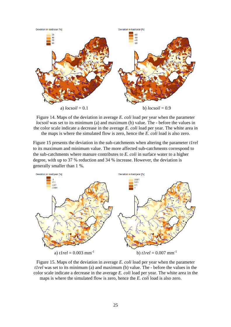
25

a) locsoil = 0.1 b) locsoil = 0.9

Figure 14. Maps of the deviation in average E. coli load per year when the parameter

locsoil was set to its minimum (a) and maximum (b) value. The - before the values in

the color scale indicate a decrease in the average E. coli load per year. The white area in

the maps is where the simulated flow is zero, hence the E. coli load is also zero.

Figure 15 presents the deviation in the sub-catchments when altering the parameter t1rel

to its maximum and minimum value. The more affected sub-catchments correspond to

the sub-catchments where manure contributes to E. coli in surface water to a higher

degree, with up to 37 % reduction and 34 % increase. However, the deviation is

generally smaller than 1 %.

a) t1rel = 0.003 mm-1 b) t1rel = 0.007 mm-1

Figure 15. Maps of the deviation in average E. coli load per year when the parameter

t1rel was set to its minimum (a) and maximum (b) value. The - before the values in the

color scale indicate a decrease in the average E. coli load per year. The white area in the

maps is where the simulated flow is zero, hence the E. coli load is also zero.

26

The deviation of average E. coli load per year when altering Effremoval is presented in

Figure 16. The affected sub-catchments are the ones with people connected to Managed

sewers, however the deviation is always smaller than 1 %.

a) Effremoval = 0.999 b) Effremoval = 0.999999

Figure 16. Maps of the deviation in average E. coli load per year compared to Base case

when the parameter Effremoval was set to its minimum (a) and maximum (b) value. The -

before the values in the color scale indicate a decrease in the average E. coli load per

year. The white area in the maps is where the simulated flow is zero, hence the E. coli

load is also zero.

The deviation of average E. coli load per year when altering t1expdec is presented in

Figure 17. When t1expdec was set to its minimum value, the range of the deviation was

between 12 – 100 %, and for the maximum value, it ranges between 13 – 750 %. This

parameter affects all sub-catchments (with flow) since die-off occurs everywhere.

a) t1expdec = 1.5 days b) t1expdec = 3 days

Figure 17. Maps of the deviation in average E. coli load per year when the parameter

t1expdec was set to its minimum (a) and maximum (b) value. The – before the values in

27

the color scale indicate a decrease in the average E. coli load per year. The white area in

the maps is where the simulated flow is zero, hence the E. coli load is also zero.

5 DISCUSSION

The time series of simulated and observed E. coli concentration, Figures 9-11, illustrate

that the observed E. coli concentration has a fluctuation of more than one order of

magnitude in one year. Generally, the highest observed concentration occurs around the

turn of the year which is also around the time when high discharge is observed. Overall,

the simulated and observed discharge magnitude in South Africa conformed with low

accuracy, which has a significant impact on the accuracy of simulated E. coli

concentration. When studying sub-catchments where the simulated discharge has a

similar timing of events as the observed discharge, the observed and simulated E. coli

load has better compliance which was confirmed by the increased NSE and decreased

bias. Load was simulated here because it describes the distribution and the relative

impact from different sources. However, load is not directly associated with risk, as

concentration is, which is why it is important to simulate pathogen concentration with

better accuracy. The simulation of load indicates that the model is also capable of

simulating E. coli concentrations in surface water but in order to achieve better model

results for concentration, it is necessary to improve the accuracy of simulated discharge.

There are still differences between observed and simulated load and the deviation in

magnitude can depend on numerous factors, such as large variations in E. coli

concentration in feces and excretion rates from humans, and underestimation of sources

which contributes to E. coli in surface water at high discharge.

By comparing Figure 11 and Figure 12, it is seen that the die-off rate has a large impact

on the decline of the E. coli concentration during periods of low discharge. This could

be a result of a greater residence time in lakes within the sub-catchment (there is no

upstream catchment here and no outlet lake) when the discharge is low, which increases

the bacteria’s travel time to the outlet, giving higher inactivation. This could have a

greater impact on the E. coli released from rural sources because the release is simulated

to occur before the local lakes, compared to E. coli release from urban sources which

are simulated to occur to the main river after the local lakes (cf. Figure 3). Additionally,

when comparing the time series of E. coli load in comparison to E. coli concentration,

the load always reaches a low point after a period of low discharge independent of if the

simulated concentration increases or decreases, see Figure 9 – 12. This is because the

concentration may increase due to reduced dilution, but the load responds to the

increased inactivation at low flows.

The total yearly E. coli load released, prior to treatment and die-off, from the different

sources in this model application are in the same order of magnitude. However, the

maps illustrating E. coli contribution from different sources for the Base case model

scenario, Figure 13a-13d, show that the human rural sources and the urban source,

Unmanaged sewer, generally have much higher contribution to surface water than urban

sources using Managed sewer or the animal source. This is because of treatment of

Managed sewer and die-off from the animal source before it reaches the surface water,

as discussed in further detail below.

28

The urban sources, Managed sewer and Unmanaged sewer, are here simulated as point

sources of E. coli release directly to surface water. The Managed sewer fraction has a

removal efficiency which was here assumed to be equal in every sub-catchment. In

reality, the removal efficiency is not constant or equal in the whole country. Information

about the wastewater treatment plants in South Africa and their respective treatment

method and performance was not discovered during this work but is an important aspect

to consider when modeling pathogens in surface water. However, from the sensitivity

analysis, it is evident that the removal efficiency, Effremoval, does not have a large impact

on the total load (under the assumption that the treatment plant is functioning). It is also

worth mentioning that Managed sewer and Unmanaged sewer contribute with the

highest percentage in corresponding areas, see Figure 13. This implies that a larger

reduction of E. coli in surface water would be attained if more people were connected to

existing wastewater treatment plants than if the wastewater treatment plants had a

higher removal efficiency of bacteria. In other areas with current release directly to

rivers, or in areas where the capacity of existing plants is reached, the results indicate

that new treatment plants would be vital in order to reduce surface water concentrations.

The human rural sources, Managed other improved, Unmanaged other improved, NA

and Unmanaged unimproved, are the most important sources in areas with deficient

sanitation and are here classified as one source type with equal E. coli reduction. E. coli

can in reality be released directly to the surface of the ground or to the first soil layer.

The bacteria on the surface and in the first soil layer are mainly affected by precipitation

and routed to surface water through surface runoff. This version of HYPE is unable to

simulate human contamination of that type and E. coli from human rural sources are

routed to the lowest soil layer or directly to surface water. For example, Unmanaged

unimproved should represent defecation in the open which ideally would be represented

by contamination on land surface. This type of contamination may contribute to the

high observed E. coli concentrations during periods of high discharge, which were not

captured by the simulations. Suggested improvements in HYPE are therefore the

possibility to rout human fecal contamination to different soil layers and to the land

surface. Another limitation with the HYPE version used here was the inability to alter

locsoil in different sub-catchments. Since locsoil affects the removal efficiency of E.

coli released from the rural sources, it would be interesting to alter this variable

depending on the most prevalent sanitation level in the sub-catchments where

contributions from rural sources dominate.

This HYPE version was unable to simultaneously simulate contributions from manure

and grazing animals which means that the continuous contribution from grazing and

wild animals is not estimated in this project. The animal source is therefore likely

underestimated because it is solely simulated as manure which is applied once a year in

the model setup. However, to partly compensate for this, the concentration in manure

was set to the highest value found in the literature and it was assumed that the manure is

not tilled down, as is otherwise possible. This type of contamination could also be the

reason for the high observed E. coli concentrations during periods of high discharge.

Since the aim of the model setup was to resemble reality, the possibility to include

multiple animal sources would increase the reliability of the results.

29

The uncertainty analysis was performed by altering the parameters within a reasonable

interval estimated from the literature. The uncertainty analysis shows that locsoil, which

affects E. coli contamination from human rural sources, has a great impact on the

simulated average E. coli load per year in surface water. The die-off parameter,

t1expdec, is estimated based on literature values of E. coli survival in water and affects

E. coli concentration in water, soil, and manure (SMHI, 2021b). Hence, it affects all

contamination sources of E. coli and model compartments which is why the deviation is

generally larger in the whole country, seen in Figure 17. The minimum and maximum

value of parameters t1rel and Effremoval resulted in small deviations (Table 7) relative to

the Base case, which is most likely due to the sources they affect. t1rel only affects the

E. coli contribution originating from the animal source, and as seen in Figure 13d,

where the percentage of the total load per year is generally below 0.1 %. The animal

source continuously has a minor contribution because there is enough time for bacterial

die-off before reaching surface water. The parameter Effremoval which is only

implemented on the fraction connected to managed sewers (Figure 13a), showed

negligible deviations partly because only 23 % of the population are connected to

treatment plants, but also because even the lowest reasonable treatment efficiency

removes a lot of bacteria, and the remaining part is small compared to the other sources.

To test if the adsorption had a significant impact, the parameter t1freuc was altered to a

value close to zero. The total E. coli load in surface water did not change after the

alteration, and it is likely because the transport time of the bacteria from soil to surface

water is enough for the bacteria to become inactivated. The fraction of E. coli that enters

the soil could have a larger impact on the result if a longer half-life time were used.

Possible development for HYPE could be to implement half-life time parameters that

vary between model compartments, such as soil, manure, and surface water since the

survival of E. coli and other microorganisms is largely dependent on environmental

factors (Aw, 2018). Additionally, E. coli is an indicator organism, and it is important to

be careful when drawing conclusions about individual pathogens since the die-off rate is

organism specific.

Several assumptions were made in this project with the intention to realistically model

waterborne E. coli transport in South Africa. In the modelled Base case scenario,

reasonable values from the literature were used. The data regarding wastewater

discharge may be underestimated because the water sanitation has improved the last 25

years, which leads to more water being used and thus, more wastewater being

discharged. Hence, this might lead to an overestimation of E. coli concentration in this

model setup. Furthermore, according to the literature, the concentration of E. coli in

human feces varies by nearly two orders of magnitude (Forsythe, 2008, Cabral, 2010)

and the amount of feces excreted per day varies with one order of magnitude (Rose et

al. 2015). This has a great effect on the simulated E. coli concentration released from

human sources and is likely contributing to varying observed E. coli concentration in

surface water. To account for the variation, implementing a statistical distribution on

factors affecting the E. coli input sources is a possible future development of the work

presented here. However, this WWH version uses single points as daily input of E. coli

contamination through wastewater in each sub-catchment.

30

In this work, rather than performing an actual calibration, the features of concentration

and load were analysed in areas of varying sources, and the relation to flow was

established. In the attempt to maximize the conformity of the simulation against the

trends in the observation, the model parameters were altered with the goal to achieve

higher E. coli load and concentration where the discharge is high. However, the

parameter variation did not notably change the trend in the simulation. The Base case

setup was shown to have good overall description of the orders of magnitude and

dynamics for the load, and therefore code improvements to account for the remaining

deviations in load and a better description of concentration were suggested. Before

performing an actual calibration of the simulated E. coli concentration against observed

data, the conformity of the discharge needs to improve.

6 CONCLUSIONS The simulations and analyses show that HYPE is a promising tool for simulating

pathogen concentration and load in surface water. The time series of observed and

simulated E. coli load shows overall good conformity, but the simulated discharge

needs to be improved to achieve better conformity of the E. coli concentration in surface

water. The main challenge was to simulate accurate E. coli concentration and load at

periods of higher discharge, which was not achieved in this project. This is most likely

due to limitations in the model when implementing and routing the E. coli sources.

More research, with better accuracy of the simulated discharge, is encouraged to

conclude WWH’s ability to simulate pathogen concentration in surface water.

Main findings of this thesis:

• the largest contribution of E. coli to surface water are through direct release of

wastewater from humans with Unmanaged sewer and the category human rural

sources,

• the process parameter half-life time has the most significant effect on the

simulated concentration,

• improvement of the simulated discharge is necessary to simulate E. coli

concentration in surface water with better accuracy,

• it is of great importance to estimate the contamination sources accurately.

• a larger reduction of E. coli in surface water is likely attained if more people are

connected to wastewater treatment plants than if the wastewater treatment plants

have higher removal efficiencies.

Suggestions for further HYPE and WWH developments:

• the possibility to rout human fecal contamination to the land surface and

different soil layers,

• the possibility to alter locsoil between sub-catchments,

• implement separate half-life time parameters for different model compartments

(e.g., soil, manure, surface water)

• the possibility to simultaneously simulate contribution from manure and grazing

animals.

31

This thesis contributes to the work towards developing a water quality model with the

ability to simulate waterborne pathogens all over the world since WWH is a global

model application, and the findings increase the understanding of the simulation tool

and its necessary improvements. A model of that calibre could have a large impact for

the analysis and effective management of pathogen risk globally.

32

REFERENCES

Arheimer, B., Pimentel, R., Isberg, K., Crochemore, L., Andersson, J.C.M., Hasan, A.

& Pineda, L. (2020). Global catchment modelling using World-Wide HYPE

(WWH), open data, and stepwise parameter estimation. Hydrology and Earth

System Sciences, 24 (2), 535–559. https://doi.org/10.5194/hess-24-535-2020

Aw, T. (2018). Environmental Aspects and Features of Critical Pathogen Groups.

Global Water Pathogen Project, Michigan State University, E. Lansing, MI,

UNESCO. https://www.waterpathogens.org/book/environmental-aspects-and-

features-of-critical-pathogen-groups [2021-02-18]

Bartram, J., Ballance, R., United Nations & World Health Organization (eds.) (1996).

Water quality monitoring: a practical guide to the design and implementation of

freshwater quality studies and monitoring programmes. 1st ed. London ; New

York: E & FN Spon.

https://www.who.int/water_sanitation_health/resourcesquality/wqmchap10.pdf

Basson, M.S. (2011). Water development in South Africa. UN Water.

https://www.un.org/waterforlifedecade/green_economy_2011/pdf/session_1_eco

nomic_instruments_south_africa.pdf [2021-02-24]

Berg, P., Donnelly, C. & Gustafsson, D. (2018). Near-real-time adjusted reanalysis

forcing data for hydrology. Hydrology and Earth System Sciences, 22 (2), 989–

1000. https://doi.org/10.5194/hess-22-989-2018

Blaustein, R.A., Pachepsky, Y.A., Shelton, D.R. & Hill, R.L. (2015). Release and

Removal of Microorganisms from Land-Deposited Animal Waste and Animal

Manures: A Review of Data and Models. Journal of Environmental Quality, 44

(5), 1338–1354. https://doi.org/10.2134/jeq2015.02.0077

Bridle, H. (ed.) (2014). Waterborne pathogens: detection methods and applications.

Amsterdam: Elsevier/Academic Press.

https://www.sciencedirect.com/science/article/pii/B9780444643193000022

Cabral, J.P.S. (2010). Water Microbiology. Bacterial Pathogens and Water.

International Journal of Environmental Research and Public Health, 7 (10),

3657–3703. https://doi.org/10.3390/ijerph7103657

Chick, H. (1908). An Investigation of the Laws of Disinfection. Journal of Hygiene, 8

(1), 92–158. https://doi.org/10.1017/S0022172400006987

Cho, K.H., Pachepsky, Y.A., Oliver, D.M., Muirhead, R.W., Park, Y., Quilliam, R.S. &

Shelton, D.R. (2016). Modeling fate and transport of fecally-derived

microorganisms at the watershed scale: State of the science and future

opportunities. Water Research, 100, 38–56.

https://doi.org/10.1016/j.watres.2016.04.064

Coffey, R., Benham, B., Krometis, L.-A., Wolfe, M.L. & Cummins, E. (2014).

Assessing the Effects of Climate Change on Waterborne Microorganisms:

Implications for EU and U.S. Water Policy. Human and Ecological Risk

Assessment: An International Journal, 20 (3), 724–742.

https://doi.org/10.1080/10807039.2013.802583

Crane, S.R. & Moore, J.A. (1985). Modeling enteric bacterial die-off: a review. Water,

Air, and Soil Pollution, 27, 411–439

Dufour, A. & WHO (eds.) (2003). Assessing microbial safety of drinking water:

improving approaches and methods. London: IWA Publ. [u.a.]. (WHO drinking

water quality series)

DWAF (2002). National Microbial Monitoring Programme for Surface Water.

Implementation Manual. Department of Water Affairs and Forestry.

33

https://www.dws.gov.za/iwqs/microbio/Document/NMMP_implementation_Sur

faces.pdf [2021-04-17]

DWS (2019-06-05). National Microbiological Monitoring Programme for South Africa.

[2021-04-16]

Eckner, K.F. (1998). Comparison of Membrane Filtration and Multiple-Tube

Fermentation by the Colilert and Enterolert Methods for Detection of

Waterborne Coliform Bacteria, Escherichia coli, and Enterococci Used in

Drinking and Bathing Water Quality Monitoring in Southern Sweden. Applied

and Environmental Microbiology, 64 (8), 3079–3083.

https://doi.org/10.1128/AEM.64.8.3079-3083.1998

Feachem, R.G. (ed.) (1983). Sanitation and disease: health aspects of excreta and

wastewater management. Chichester [West Sussex] ; New York: Published for

the World Bank by Wiley. (World Bank studies in water supply and sanitation;

3)

Forsythe, S.J. (2008). The Microbiology of Safe Food. https://nbn-

resolving.org/urn:nbn:de:101:1-2014121912153 [2021-04-27]

Garcia-Aljaro, C., Momba, M. & Muniesa, M. (2017). Pathogenic members of

Escherichia coli & Shigella spp. Shigellosis. Global Water Pathogen Project.

http://www.waterpathogens.org/book/ecoli [2021-02-08]

Hansen, K. (2015). Overview of Wastewater Treatment in South Africa. Association for

Water and Rural Development (AWARD). [2021-03-25]

Harwood, V., Shanks, O., Koraijkic, A., Verbyla, M., Ahmed, W. & Iriate, M. (2017).

General and host-associated bacterial indicators of faecal pollution. Global

Water Pathogen Project. http://www.waterpathogens.org/book/bacterial-

indicators [2021-02-05]

Hasan, R., Nordin, A.C., Shakoor, S., Keenum, I. & Vinneras, B. (2019). Salmonella,

Enteric Fevers, and Salmonellosis. Global Water Pathogen Project.

https://www.waterpathogens.org/book/salmonella-enteric-fevers-salmonellosis

[2021-02-11]

Helmer, R., Hespanhol, I., United Nations Environment Programme, Water Supply and

Sanitation Collaborative Council & World Health Organization (eds.) (1997).

Water pollution control: a guide to the use of water quality management

principles. 1st. ed. London ; New York: E & FN Spon.

https://www.who.int/water_sanitation_health/resourcesquality/watpolcontrol.pdf

Lindström, G., Pers, C., Rosberg, J., Strömqvist, J. & Arheimer, B. (2010).

Development and testing of the HYPE (Hydrological Predictions for the

Environment) water quality model for different spatial scales. Hydrology

Research, 41 (3–4), 295–319. https://doi.org/10.2166/nh.2010.007

Luyt, C.D., Tandlich, R., Muller, W.J. & Wilhelmi, B.S. (2012). Microbial Monitoring

of Surface Water in South Africa: An Overview. International Journal of

Environmental Research and Public Health, 9 (8), 2669–2693.

https://doi.org/10.3390/ijerph9082669

Mathevet, T., Michel, C., Andreassian, V. & Perrin, C. (2006). A bounded version of

the Nash-Sutcliffe criterion for better model assessment on large sets of basins.

Large Sample Basin Experiments for Hydrological Model Parameterization:

Results of the Model Parameter Experiment–MOPEX, (307).

https://iahs.info/uploads/dms/13614.21--211-219-41-MATHEVET.pdf [2021-

06-30]

34

Momba, M. & El-Liethy, A. (2018). Vibrio cholerae and Cholera biotypes. Global

Water Pathogen Project. https://www.waterpathogens.org/book/Vibrio [2021-

02-18]

Murphy, H. (2017). Persistence of Pathogens in Sewage and Other Water Types. Global

Water Pathogen Project. https://www.waterpathogens.org/book/persistence-in-

sewage [2021-02-18]

Nataro, J.P. & Kaper, J.B. (1998). Diarrheagenic Escherichia coli. Clinical

Microbiology Reviews, 11 (1), 142–201

Okorogbona, A.O.M. & Adebisi, L.O. (2012). Animal Manure for Smallholder

Agriculture in South Africa. In: Lichtfouse, E. (ed.) Farming for Food and

Water Security. Dordrecht: Springer Netherlands, 201–242.

https://doi.org/10.1007/978-94-007-4500-1_9

Oliver, D.M., Porter, K.D.H., Pachepsky, Y.A., Muirhead, R.W., Reaney, S.M., Coffey,

R., Kay, D., Milledge, D.G., Hong, E., Anthony, S.G., Page, T., Bloodworth,

J.W., Mellander, P.-E., Carbonneau, P.E., McGrane, S.J. & Quilliam, R.S.

(2016). Predicting microbial water quality with models: Over-arching questions

for managing risk in agricultural catchments. Science of The Total Environment,

544, 39–47. https://doi.org/10.1016/j.scitotenv.2015.11.086

Perciva, S.L. (2013). Microbiology of Waterborne Diseases. Elsevier Science.

http://www.totalboox.com/book/id-2872172695791280907 [2021-02-09]

Shelton, D.R., Pachepsky, Y.A., Sadeghi, A.M., Stout, W.L., Karns, J.S. & Gburek,

W.J. (2003). Release Rates of Manure-Borne Coliform Bacteria from Data on

Leaching through Stony Soil. Vadose Zone Journal, 2 (1), 34–39.

https://doi.org/10.2136/vzj2003.3400

SIS (2014a). SS-EN ISO 9308-1:2014 Water quality – Enumeration of Escherichia coli

and coliform bacteria - Part 1: Membrane filtration method for waters with low

bacterial background flora (ISO9308-1:2014). Swedish Standards Institute.

[2021-05-27]

SIS (2014b). SS-EN ISO 9308-2:2014 Water quality – Enumeration of Escherichia coli

and coliformbacteria – Part 2: Most probable number method (ISO 9308-

2:20). Swedish Standards Institute. [2021-05-27]

SMHI (2021-02-26). HYPE Model Documentation: Land routines.

http://www.smhi.net/hype/wiki/doku.php?id=start:hype_model_description:hype

_land [2021-03-08]

SMHI (2021-04-15). HYPE Model Documentation: Rivers and lakes.

http://www.smhi.net/hype/wiki/doku.php?id=start:hype_model_description:hype

_routing [2021-06-03]

SMHI (2021-01-29). HYPE Model Documentation: Tracers.

http://www.smhi.net/hype/wiki/doku.php?id=start:hype_model_description:hype

_tracer [2021-02-22]

Sokolova, E., Lindström, G., Pers, C., Strömqvist, J., Lewerin, S.S., Wahlström, H. &

Sörén, K. (2018a). Water quality modelling: microbial risks associated with

manure on pasture and arable land. Journal of Water and Health, 16 (4), 549–

561. https://doi.org/10.2166/wh.2018.278

Sokolova, E., Lindström, G., Pers, C., Strömqvist, J., Nordström, A., Sörén, K.,

Wahlström, H. & Sternberg Lewerin, S. (2018b). Modellering av

smittämnestransport för ökad förståelse för spridning av zoonotiska smittämnen

från lantbrukets djur och människor via ytvatten. Statens Veterinärmedicinska

Anstalt, Chalmers, SMHI, SLU. [2021-04-12]

35

Strömqvist, J., Arheimer, B., Dahné, J., Donnelly, C. & Lindström, G. (2012). Water

and nutrient predictions in ungauged basins: set-up and evaluation of a model at

the national scale. Hydrological Sciences Journal, 57 (2), 229–247.

https://doi.org/10.1080/02626667.2011.637497

UNESCO & WWAP (eds.) (2006). Water: a shared responsibility. Paris, France : New

York: United Nations Educational, Scientific and Cultural Organization

(UNESCO) ; Berghahn Books.

https://portals.iucn.org/library/sites/library/files/documents/Bios-Eco-Aqua-017-

2.pdf

Van Averbeke, W. & Yoganathan, S. (2003). Using Kraal Manure as a Fertiliser.

Agricultural and Rural Development Research Institute, Fort Hare, 2nd.

https://www.nda.agric.za/docs/Infopaks/KraalManure.pdf

Verlicchi, P. & Grillini, V. (2020). Surface Water and Groundwater Quality in South

Africa and Mozambique—Analysis of the Most Critical Pollutants for Drinking

Purposes and Challenges in Water Treatment Selection. Water, 12 (1), 305.

https://doi.org/10.3390/w12010305

Wagner, E.G. & Lanoix, J.N. (1958). Excreta disposal for rural areas and small

communities. WHO.

https://apps.who.int/iris/bitstream/handle/10665/41687/WHO_MONO_39_%28

part1%29.pdf?sequence=1&isAllowed=y [2021-02-18]

WHO (ed.) (2006). Excreta and greywater use in agriculture. 3. ed. Geneva: World

Health Organization. (Guidelines for the safe use of wastewater, excreta and

greywater; World Health Organization ; Vol. 4)

WHO (2017). Diarrhoeal disease. https://www.who.int/news-room/fact-

sheets/detail/diarrhoeal-disease [2021-02-24]

WHO (2017b). Guidelines for drinking-water quality. 4th ed. Geneva: World Health

Organization.

WHO (2018). Guidelines on sanitation and health. World Health Organization. [2021-

02-08]

WHO & UNICEF (2019). Progress on household drinking water, sanitation and

hygiene 2000-2017: Special focus on inequalities. New York. [2021-06-23]

Yamazaki, D., O’Loughlin, F., Trigg, M.A., Miller, Z.F., Pavelsky, T.M. & Bates, P.D.

(2014). Development of the Global Width Database for Large Rivers. Water

Resources Research, 50 (4), 3467–3480.

https://doi.org/10.1002/2013WR014664

Personal communication

Kumari, Sheena, at Durban University of Technology

Amoah, Dennis Isaac, Doctor at Durban University of Technology

36

APPENDIX

APPENDIX A: LIST OF VARIABLES USED

Acropland total cropland area in South Africa in WWH [ha]

CE. coli, f E. coli concentration in feces [CFU/g]

CE. coli, manure E. coli concentration in animal manure [CFU/g]

Fmanure total amount of manure [g/year]

Effremoval removal efficiency of wastewater treatment [-]

locsoil fraction of microorganisms from rural wastewater that is

released directly to the lowest soil layer, the rest is released

to surface water [-]

mf wet weight mass of feces [g/person & day]

tamount yearly amount of E. coli in manure [CFU/ha]

t1rel release per mm daily precipitation [mm-1]

t1freuc Freundlich adsorption isotherm coefficient [(#/kg soil) /

(#/L)]

t1expdec half-life time [days]

Vavg wastewater discharge [L/person & day]

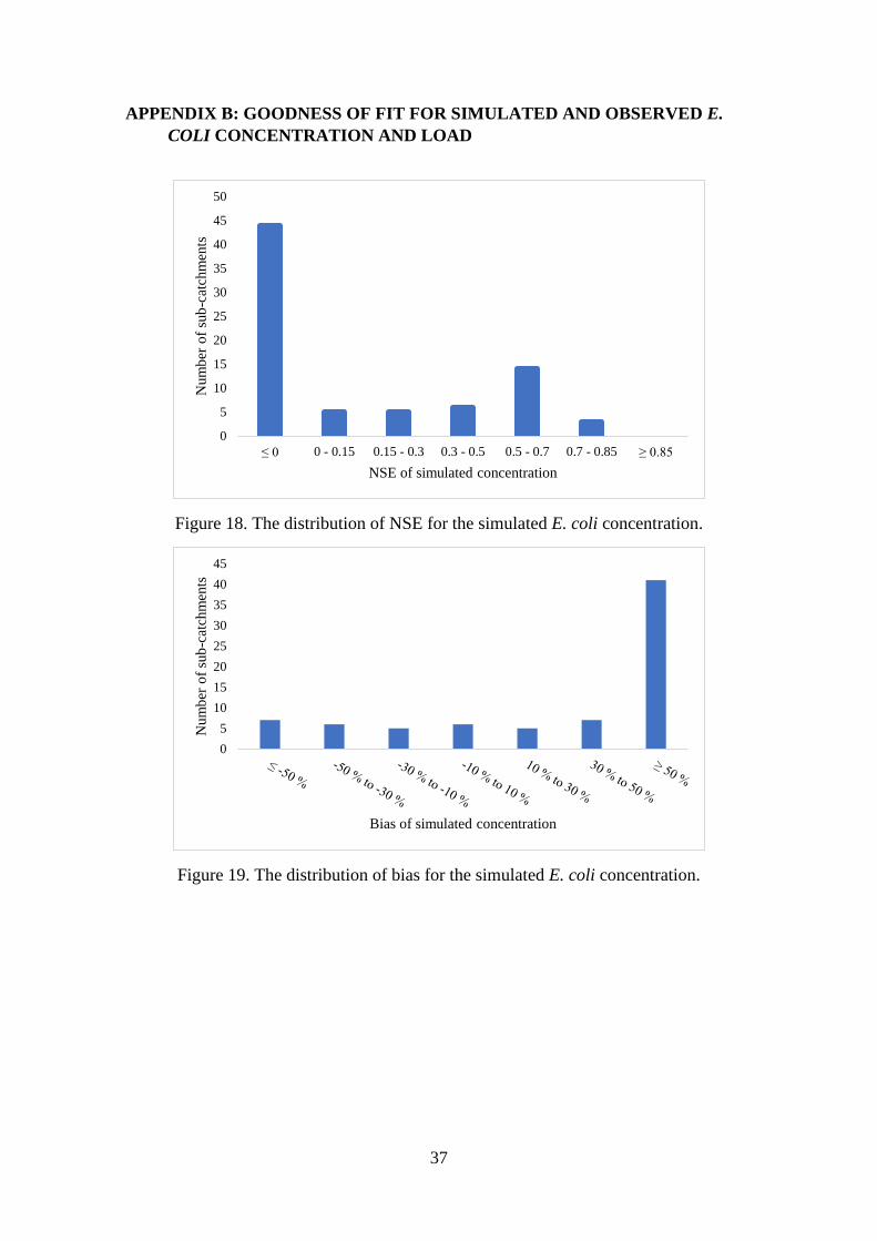
37

APPENDIX B: GOODNESS OF FIT FOR SIMULATED AND OBSERVED E.

COLI CONCENTRATION AND LOAD

Figure 18. The distribution of NSE for the simulated E. coli concentration.

Figure 19. The distribution of bias for the simulated E. coli concentration.

0

5

10

15

20

25

30

35

40

45

50

≤ 0 0 - 0.15 0.15 - 0.3 0.3 - 0.5 0.5 - 0.7 0.7 - 0.85 ≥ 0.85

Num

ber

of

sub

-cat

chm

ents

NSE of simulated concentration

0

5

10

15

20

25

30

35

40

45

Num

ber

of

sub

-cat

chm

ents

Bias of simulated concentration

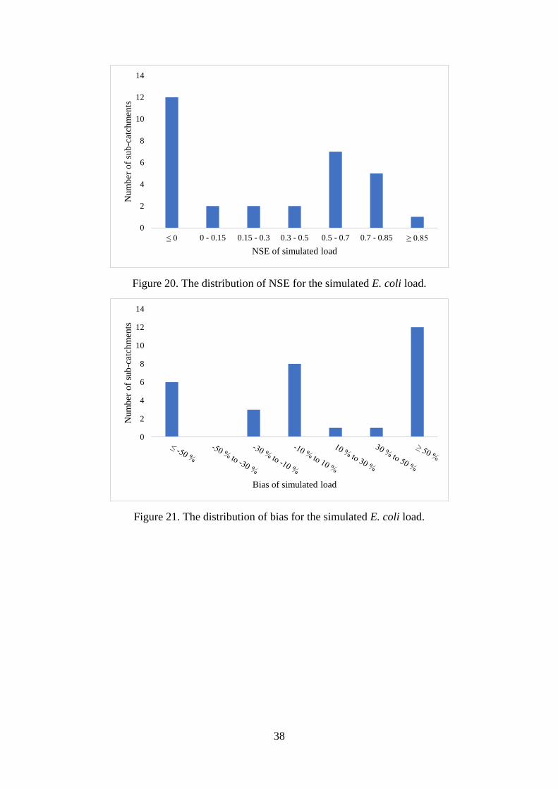
38

Figure 20. The distribution of NSE for the simulated E. coli load.

Figure 21. The distribution of bias for the simulated E. coli load.

0

2

4

6

8

10

12

14

≤ 0 0 - 0.15 0.15 - 0.3 0.3 - 0.5 0.5 - 0.7 0.7 - 0.85 ≥ 0.85

Num

ber

of

sub

-cat

chm

ents

NSE of simulated load

0

2

4

6

8

10

12

14

Num

ber

of

sub

-cat

chm

ents

Bias of simulated load

39

APPENDIX C: TIME SERIES OF CONCENTRATION, DISCHARGE AND

LOAD IN SURFACE WATER FOR THE ANIMAL SOURCE

Figure 22 displays simulation results of the same sub-catchment as in Figure 10, but

here the only contribution of E. coli originates from the animal source which is applied

once a year. Therefore, a single peak of E. coli concentration and load occurs during the

time period of one year. The magnitude of the concentration and load is significantly

smaller than when every type of E. coli source is included (cf. Figure 10).

Figure 22. Time series of E. coli concentration, discharge, and E. coli load in surface

water with only the animal source as the E. coli contamination source.