modeling the effects of the immune system on bone

MODELING THE EFFECTS OF THE IMMUNE SYSTEM ON BONE

FRACTURE HEALING

by

IMELDA TREJO LORENZO

Presented to the Faculty of the Graduate School of

The University of Texas at Arlington in Partial Fulfillment

of the Requirements

for the Degree of

DOCTOR OF PHILOSOPHY

THE UNIVERSITY OF TEXAS AT ARLINGTON

May 2019

Copyright c© by Imelda Trejo Lorenzo 2019

All Rights Reserved

ACKNOWLEDGEMENTS

First, I would like to thank the Concejo Nacional de Ciencia y Tecnologıa

(CONACyT) and The University of Texas at Arlington (UTA) for financially sup-

porting my PhD graduate program. This program finishes with the elaboration

and submission of the present dissertation manuscripts. I want also to thank the

Consejo de Ciencia, Tecnologıa e Innovacıon de Hidalgo, the Universidad Autonoma

del Estado de Hidalgo (Mathematics and Health and Medicine Deparments) and the

Collegio de Bachilleres Plantel Tasquillo who provide the documentations needed for

the CONACyT application and for paying my flight tickets to join the UTA graduate

program.

Second, I would like to express my gratitude to my advisor Dr. Hristo Ko-

jouharov for guiding me through the PhD program and helping me to prepare for

life after the doctorate. His advice and encouragement helped me to excel in my

academics and research work. I wish to thank Dr. Benito Chen, Dr. Marco Brotto,

Dr. Guojun Liao and Dr. Gaik Ambartsoumian for their interest in my research and

for taking time to serve in my comprehensive committee and dissertation committee.

I also would like to thank Dr. Benito Chen and Dr. Christopher Kribs for their help

and support in all my four year graduate program. I want to extend my appreciation

to all my mentors: Dr. Francisco Javier Solıs, Dr. Raul Felipe, Dr. Ruben Martınez

Avedano, Dr. Margarita Tetlalmatzi Montiel, Dr. Jaime Cruz Sampedro, and Dr.

iii

Alicia Prieto how have shaped my abilities to do mathematics and have encouraged

me during all my academic studies.

Next, I would like to thank Lona, Michel, Velvet, Laura, and Shanna for their

time and assistance throughout the graduate program. Furthermore, I want to express

my great gratitude to all my UTA friends, they made my PhD graduate program

the most exciting, enjoyable, and value ever: Mehtap Lafci, Mayowa Olawoyin,

Sita Charkrit, May Trieu, Talon Johnson, Ariel Bowman, Mary Gockenbach, Kiran

Mainali, Julio Enciso, Susana Aguirre-Medel, Paola Sotelo, Enrique Barragan, Miguel

Arellano, Maria Garcıa, Emel Bolat, Felicia Puerto, and all my other friends.

Finally, I am extremely grateful to my parents, sister, brother, and all my

family for their sacrifice, encouragement, and patience. Without their love and help,

I would not have gone this far.

April 26, 2019

iv

ABSTRACT


FRACTURE HEALING

Imelda Trejo Lorenzo, Ph.D.

The University of Texas at Arlington, 2019

Supervising Professor: Hristo V. Kojouharov

Bone fracture healing is a complex biological process that results in a full

reconstruction of the bone [36]. However, it is not always an easy and successful

process. Indeed, in some unfavorable conditions, the bone fracture healing fails

with approximately 10% of fractures resulting in nonunion [49]. Furthermore, the

risk of nonunion healing increases with age, severe trauma, and immune deficiency

[29, 55]. In addition, clinical consequences of fractures include surgical management,

prolonged hospitalization, and rehabilitation resulting in high socioeconomic costs

[31]. A better understanding of bone healing would enable to find optimal conditions

for successful outcomes and to develop strategies for fracture treatments under normal

or pathological scenarios.

Immune cells and their released molecular factors play a key role for successful

bone healing [29, 47]. During bone fracture healing, the immune system cells clear up

debris and regulate tissue cellular functions: proliferation, differentiation, and tissue

production [47]. However, the exact mechanisms and functions of the immune cells

present at the fracture site are still not completely understood [49]. Prolonged and

v

chronic participation of the immune cells during the inflammation phase results in

delayed union or nonunion healing, while depletion of them results in delayed bone

formation [29, 47, 49]. Therefore, for successful bone healing, the participation of

immune cells in the healing process must be brief and well regulated [47, 49].

In this work, several new mathematical models are presented that describe

the process of bone fracture healing. The models incorporate complex interactions

between immune cells and bone cells at the fracture site. The resulting systems of

nonlinear ordinary differential equations are studied analytically and numerically.

Mathematical conditions for successful bone fracture repairs are formulated. The

models are used to numerically monitor the evolution of broken bones for different

types of fractures and to explore possible treatments that can accelerate the bone

fracture healing process.

vi

TABLE OF CONTENTS

ACKNOWLEDGEMENTS . . . . . . . . . . . . . . . . . . . . . . . . . . . . iii

ABSTRACT . . . . . . . . . . . . . . . . . . . . . . . . . . . . . . . . . . . . v

Chapter Page

1. INTRODUCTION . . . . . . . . . . . . . . . . . . . . . . . . . . . . . . . 1

1.1 Bone Fracture Healing Phases . . . . . . . . . . . . . . . . . . . . . . 1

1.1.1 Sequence of healing events . . . . . . . . . . . . . . . . . . . . 3

1.2 Immune System Responses after a Bone Fracture . . . . . . . . . . . 4

1.2.1 Immune system cells . . . . . . . . . . . . . . . . . . . . . . . 4

1.2.2 Regulatory molecules . . . . . . . . . . . . . . . . . . . . . . . 5

1.3 Bone and Tissue Forming Cells . . . . . . . . . . . . . . . . . . . . . 7

1.3.1 Tissue forming cells . . . . . . . . . . . . . . . . . . . . . . . . 7

1.3.2 Bone tissue types . . . . . . . . . . . . . . . . . . . . . . . . . 8

1.3.3 Bone tissue formation . . . . . . . . . . . . . . . . . . . . . . 8

1.3.4 Bone structure . . . . . . . . . . . . . . . . . . . . . . . . . . 8

2. MODELING THE FUNDAMENTAL FUNCTIONS OF THE IMMUNE

SYSTEM IN BONE FRACTURE HEALING . . . . . . . . . . . . . . . . 10

2.1 Modeling Assumptions . . . . . . . . . . . . . . . . . . . . . . . . . . 10

2.2 Model Formulation . . . . . . . . . . . . . . . . . . . . . . . . . . . . 12

2.3 Qualitative Analysis . . . . . . . . . . . . . . . . . . . . . . . . . . . 14

2.4 Numerical Results . . . . . . . . . . . . . . . . . . . . . . . . . . . . . 20

2.4.1 Different outcomes of the bone fracture healing process . . . . 21

vii

2.4.2 Importance of macrophages during the bone fracture healing

process . . . . . . . . . . . . . . . . . . . . . . . . . . . . . . . 24

2.4.3 Evolution of the healing process for different types of fractures 26

2.5 Summary of the Results . . . . . . . . . . . . . . . . . . . . . . . . . 30

3. MODELING THE MACROPHAGE-MEDIATED INFLAMMATION IN-

VOLVED IN THE BONE FRACTURE HEALING PROCESS . . . . . . . 33





3.4.1 Comparison of Model (2.1)-(2.7) and Model (3.1)-(3.10) . . . . 42


process . . . . . . . . . . . . . . . . . . . . . . . . . . . . . . . 43

3.4.3 Immune-modulation therapeutic treatments of bone fractures . 44


4. MODELING THE EFFECTS OF THE IMMUNE SYSTEM ON BONE

FRACTURE HEALING . . . . . . . . . . . . . . . . . . . . . . . . . . . . 53





4.4.1 Comparison of Model (4.1)-(4.12) with existing models . . . . 62


process . . . . . . . . . . . . . . . . . . . . . . . . . . . . . . . 64

4.4.3 Administration of anti-inflammatory cytokines and growth fac-

tors during the healing of a broken bone . . . . . . . . . . . . 66

viii

4.5 Mechanism of the Osteogenic Cell Differentiation . . . . . . . . . . . 69

4.5.1 Qualitative Analysis . . . . . . . . . . . . . . . . . . . . . . . 69

4.5.2 Numerical simulations . . . . . . . . . . . . . . . . . . . . . . 76


5. CONCLUSION AND FUTURE WORK . . . . . . . . . . . . . . . . . . . 85

APPENDIX . . . . . . . . . . . . . . . . . . . . . . . . . . . . . . . . . . . . . 88

REFERENCES . . . . . . . . . . . . . . . . . . . . . . . . . . . . . . . . . . . 91

BIOGRAPHICAL STATEMENT . . . . . . . . . . . . . . . . . . . . . . . . . 99

ix

CHAPTER 1

INTRODUCTION

Bone fracture healing is a complex biological process that results in a full

reconstruction of the bone [36]. This process is given through a sequence of events

that involves the participation of different cell types and is strongly regulated by

several molecular factors and mechanical stimuli [5, 8, 41, 43, 47, 48]. This chapter,

the biological background of long bone fracture repair is described with an emphasis

on the immune system regulations during the healing process.

1.1 Bone Fracture Healing Phases

The bone fracture healing process can be described in three characteristic phases:

inflammatory, repair, and remodelling. Figure 1.1 describes the time-line of events

occurring in each phase. During inflammation, necroses of cells results in the delivery

of pro-inflammatory cytokines which activate and attract inflammatory immune cells,

such as neutrophils and monocytes, to the injury site [38, 49, 12]. In response to

their phagocytic activities these cells magnify pro-inflammatory production, leading

to an acute inflammation [9, 38, 19]. Subsequently, monocytes differentiate into

macrophages to down-regulate the inflammation and resolve it. Once this differentia-

tion begins, the influx of inflammatory cells ceases and they die out [50]. During the

resolution of inflammation, macrophages increase their population by migration and

activate to their classical and alternative phenotypes accordingly to the cytokines

stimuli [48, 40]. Classically activated macrophages release a high concentration of

pro-inflammatory cytokines, including the tumor necrotic factor-α (TNF-α), and low

1

levels of anti-inflammatory cytokines in response to their engulfing functions [25].

Alternatively activated macrophages secrete high levels of the interleukin-10 (IL-10),

transforming growth factor-β (TGF-β), and low levels of TNF-α, as they continue

with the clearance of debris and the modulation of inflammation [25]. The TNF-α,

Il-10, and TGF-β stimulate the migration of mesenchymal stem cells (MSCs) to the

injury site and promote the differentiation and proliferation of the tissue forming

cells: MSCs, fibroblasts, chondrocytes, and osteoblasts [11]. The correct modulation

among the TNF-α, Il-10, and the TGF-β is essential to stimulate and secure the

healing of a broken bone.

During the repair phase, migrating MSCs contribute to the delivery of IL-10, and

proliferate or differentiate into fibroblasts, chondrocytes, and osteoblasts, according to

different molecular and mechanical stimuli [37, 11, 6, 24]. Particularly, specific growth

factors, such as the bone morphogenetic proteins (BMPs) and the TGF-β, activate

and direct the differentiation of MSCs into osteoblasts and chondrocytes [6, 2, 56].

Fibroblasts and chondrocytes proliferate and release the fibrinous/cartilagenous

extracellular matrix, which fills up the fracture gap and provides stability on the

fracture [2, 13, 43], while osteoblasts proliferate and deposit the new bone, also

called woven bone [2]. Bone deposit results from the mineralized collagen and other

proteins delivered by the osteoblasts [43]. After bone mineralization, osteoblasts

remain on the bone surface or differentiate into osteocytes which become part of the

bone extracellular matrix [12, 18].

During the last phase of the bone fracture healing process, the fibrocartilage

and the woven bone are constantly removed and replaced by a functional bone

[14]. This process is referred to as bone remodeling and consists of a systematic

tissue degradation and production by osteoclasts and osteoblasts, respectively. Bone

2

remodeling is a slow process that can take months to years until the bone tissue

recovers completely its functionality [35].

Figure 1.1. Inflammatory, repair, and remodeling phases of the bone fracture healingprocess. During the inflammatory phase, debris (D) activate the healing process byattracting macrophages M0 to the injury site, which subsequently activate into theirM1 or M2 phenotypes. Activated macrophages remove debris and secrete pro- andanti-inflammatory cytokines, such as the TNF-α (c1) and the IL-10 (c2), which regulatethe inflammation and the cellular functions. During the repair phase, migratingmesenchymal stem cells (MSCs) up-regulate the IL-10 production, proliferate, anddifferentiate into osteoblasts (Cb) and chondrocytes (Cc). The MSCs differentiationis regulated by growth factors, such as the transforming growth factor-β (c3). c3is synthesized by the M2, Cb, and Cc. Chondrocyte and osteoblast cells synthesizethe fibro/cartilage and woven bone, which closes the fracture gap. During the boneremodeling phase, osteoblasts and osteoclasts constantly remove and deposit newbone until the fracture is fully repaired.

1.1.1 Sequence of healing events

In a moderate fracture, acute inflammation is observed 24 hrs after the injury,

which is also when TNF-α peaks, returning to its baseline levels within 72 hrs [35, 38].

3

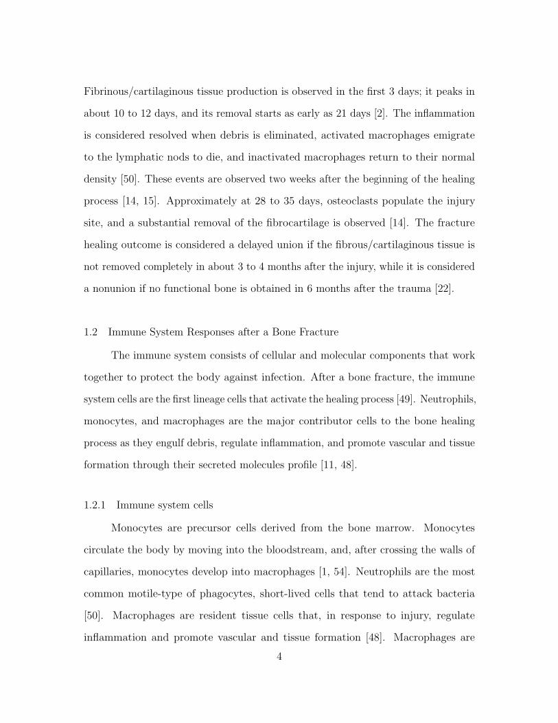
Fibrinous/cartilaginous tissue production is observed in the first 3 days; it peaks in

about 10 to 12 days, and its removal starts as early as 21 days [2]. The inflammation

is considered resolved when debris is eliminated, activated macrophages emigrate

to the lymphatic nods to die, and inactivated macrophages return to their normal

density [50]. These events are observed two weeks after the beginning of the healing

process [14, 15]. Approximately at 28 to 35 days, osteoclasts populate the injury

site, and a substantial removal of the fibrocartilage is observed [14]. The fracture

healing outcome is considered a delayed union if the fibrous/cartilaginous tissue is

not removed completely in about 3 to 4 months after the injury, while it is considered

a nonunion if no functional bone is obtained in 6 months after the trauma [22].

1.2 Immune System Responses after a Bone Fracture

The immune system consists of cellular and molecular components that work

together to protect the body against infection. After a bone fracture, the immune

system cells are the first lineage cells that activate the healing process [49]. Neutrophils,

monocytes, and macrophages are the major contributor cells to the bone healing

process as they engulf debris, regulate inflammation, and promote vascular and tissue

formation through their secreted molecules profile [11, 48].

1.2.1 Immune system cells

Monocytes are precursor cells derived from the bone marrow. Monocytes

circulate the body by moving into the bloodstream, and, after crossing the walls of

capillaries, monocytes develop into macrophages [1, 54]. Neutrophils are the most

common motile-type of phagocytes, short-lived cells that tend to attack bacteria

[50]. Macrophages are resident tissue cells that, in response to injury, regulate

inflammation and promote vascular and tissue formation [48]. Macrophages are

4

the most important immune cells present throughout all of the healing phases [47].

Macrophages are classified into classically and alternatively activated macrophages

[48, 10, 43]. Classically activated macrophages release high levels of pro-inflammatory

cytokines, including the TNF-α and the interleukin-1 (IL-1), which exhibit inhibitory

and destructive properties in high concentrations [9, 48]. In contrast, alternatively

activated macrophages are characterized with the secretion of the anti-inflammatory

cytokines, such as the IL-10 and the TGF-β, which increase their phagocytic activities,

mitigate the inflammatory responses, promote growth, and accelerate the fracture

healing [48, 10, 31, 29]. Within the bone, macrophages are founded in the periousteum

and endousteum [61]. Macrophages are also promising candidates for targets in

immune-modulatory interventions [31, 48].

1.2.2 Regulatory molecules

The bone fracture healing process is strongly regulated by released molecular

factors. These molecules can be categorized into two groups: cytokines and growth

factors [11]. Cytokines work as chemotactic agents and mainly regulate the immune

system responses, while growth factors promote proliferation and differentiation of

the tissue forming cells [17].

1.2.2.1 Cytokines

Cytokines are proteins that mainly regulate the immune system cells [17]. They

either have positive or negative effects on the cellular functions depending on the

influence of other cytokines, concentration, and exposed time [5, 8, 41, 43]. Cytokines

are functionally classified into pro-inflammatory and anti-inflammatory families.

Pro-inflammatory cytokines, such as the TNF-α, are mainly released by the

inflammatory cells and activate the immune system defense to kill bacteria and fight

5

infections. Anti-inflammatory cytokines block the pro-inflammatory synthesis and

activate the mesenchymal lineage cellular functions [29]. The IL-10 is one of the most

potent anti-inflammatory molecules that inhibit the pro-inflammatory production

[1, 29] and is mainly delivery by macrophages and MSCs [29].

The correct balance between the pro- and anti-inflammatory cytokines during

fracture healing is necessary for successful fracture repair. High levels of TNF-α

induce chronic inflammations, inhibits proliferation and differentiation of the tissue

cells, and induces a gradual destruction of the cartilage and bone tissue [41]. However

the absence of TNF-α results in nonunion or delayed nonunion [9, 38]. Furthermore,

the TNF-α exhibits a dual effect on the MSCs, below to 15-20 ng/mL, it enhances

MSCs’ proliferation while, above of this concentration, inhibits MSCs’ proliferation

[4].

1.2.2.2 Growth factors

Growth factors are proteins that activate and promote cellular proliferation

and differentiation [11]. The bone morphogenetic proteins (BMPs) and the TGF-β

are the two major families that promote bone formation [6, 2, 56].

BMPs regulate growth of different cell types and potentially induce MSCs differ-

entiation into chondrocytes and osteoblasts [11]. The main source of BMPs are MSCs,

osteoblasts, and chondrocytes. TGF-β enhances proliferation of MSCs, chondrocytes,

and osteoblasts. TGF-β also directs the MSCs differentiation into osteoblasts and

chondrocytes [2]. Furthermore, TGF-β suppresses the pro-inflammatory cytokine

productions [1] and is a potent chemotactic stimulator for MSCs and macrophages

[11]. TGF-beta is released by the immune-system cells at the time of fracture and is

synthesized by both osteoblasts and chondrocytes at specific times during the fracture

healing process [2, 26].

6

1.3 Bone and Tissue Forming Cells

Bone fracture healing is given by a systematic tissue formation and degradation.

Bellow, the functions of the most important bone cells involved in tissue formation

are described.

1.3.1 Tissue forming cells

Mesenchymal stem cells (MSCs) are adult, nonhematopoietic, stem cells that

have the ability to proliferate and differentiate into osteoblasts, chondrocytes, fibrob-

lasts, and adipocytes, among other connective tissue, such as bone, cartilage, tendon,

skeletal muscle, and adipose tissue, which makes them an attractive cell source for

cell-based regenerative therapies [6, 58]. MSCs reside in specific environments located

within the vicinity of vessel walls [58]. Within the bone tissue they are located in the

perousteum, endosteum, and bone marrow [58, 61, 46].

Osteoblasts are derived from MSCs and are responsible for bone formation

[12]. Osteoblasts have the ability to proliferate and differentiate into osteocytes [2].

They are located on the bone surface (osteon), where release collagen and other

proteins which in a process of mineralization result in bone tissue [43]. After bone

mineralization, osteoblasts remain on the bone surface or differentiate [12, 18].

Chondrocytes are derived from MSCs and synthesize cartilage. They have

the ability to proliferate with a terminal stage. Fibroblasts secrete collagen fibers.

Both fibroblasts and chondrocytes are residents of connective-cartilage tissue. During

the bone fracture healing, chondrocytes and fibroblasts proliferate and secrete the

fibro/cartilagenous tissue that supports bone formation [35, 13].

Osteoclasts remove bone by demineralizing it with acid and dissolving collagen

with enzymes [12]. These cells originate from the bone marrow cells (from hematopoi-

7

etic precursor cells) similar to monocytes and machrophages. They are located on

the bone surface.

1.3.2 Bone tissue types

Woven and lamellar bone are two types of bone tissue that differ in composition,

organization, growth, and mechanical properties. Woven bone is quickly formed

and poorly organized with a more or less random arrangement of collagen fibers

and mineral crystals. Lamellar bone is slowly formed, organized in parallel layers or

lamellae that make it stronger than woven bone [12]. During bone fracture healing,

woven bone is firstly created and, then, through the bone remodeling process, is

totally replaced by the lamellar bone [12, 14].

1.3.3 Bone tissue formation

There are two ways of bone tissue formation: intramembranous and endo-

chondral ossification [12]. In intramembranous ossification, MSCs differentiate to

osteoblasts which directly deposit bone [11]. In endochondral ossification, MSCs

differentiate into chondrocytes which synthesize cartilage. This cartilage is mineral-

ized through chondrocyte apoptosis, and subsequently osteoblasts penetrate the dead

structure and generate bone [18].

1.3.4 Bone structure

Long bones are structured in different layers, from the outside to the inside:

periosteum, cortical bone, endosteum, trabecullar, and bone marrow [12]. The

periosteum is the boundary layer attached to the soft tissue. It provides a good

blood supply to the bone and contains progenitor cells. The cortical bone consists

of cylindrical structures of lamellar bone (also called osteon) [12]. The trabecullar

8

or cancellous bone consists of interconnected cuboid bones filled with bone marrow.

The endosteum is a thin vascular membrane of connective tissue that lines the inner

surface of the bone tissue and the medullary cavity where lies the bone marrow. Bone

marrow is a tissue composed of blood vessels, nerves, and various types of cells, whose

main function is to produce the basic blood cells.

9

CHAPTER 2

MODELING THE FUNDAMENTAL FUNCTIONS OF THE IMMUNE SYSTEM

IN BONE FRACTURE HEALING

The most important effects of the immune system on bone fracture healing are

observed during the inflammatory and repair phases of the healing process [27, 48, 47].

During the inflammatory phase, immune system cells modulate and resolve the

inflammation by engulfing debris. During the repair phase immune system cells

provide an optimal environment for the cellular proliferation, differentiation, and

tissue production through their released molecules factors [36]. In this chapter the

phagocytic and the pro-inflammatory regulatory effects of the immune system in

the bone fracture healing are modeled. In order to mathematically represent and

study the complex processes involved in bone fracture healing different modeling

assumptions will be established.

2.1 Modeling Assumptions

The primary variables during the inflammatory and repair phases of the bone

fracture healing process are debris (D), macrophages (M), MSCs (Cm), osteoblasts

(Cb), TNF-α (c1), fibrocartilage (mc), and woven bone (mb). The biological system

interactions are depicted in Figure 2.1. In the flow diagram, the cells and cellular

dynamics are represented by the circular shapes and solid arrows. The molecular

concentrations and their production/decay are represented by the octagonal shapes

and dashed arrows. The pro-inflammatory cytokines activation/inhibition effects on

the cellular functions are represented by the dotted arrows. Removal of debris and

10

the negative effect among the variables are represented by the dot-ending dotted

arrows.

𝐷

𝑐1

𝑘0𝑘1

𝑀

𝑅𝑀

𝑑𝑀𝑑𝑐1

𝐶𝑏

𝐶𝑚

𝐹1

𝑚𝑏

𝑚𝑐

𝐴𝑚

𝐴𝑏

𝑝𝑐𝑠

𝑝𝑏𝑠

𝑞𝑐𝑑2

𝑑𝑏

𝑅𝑚𝑘𝑑

Inflammation Repair

Figure 2.1. Flow diagram of the cellular and molecular dynamics during the inflam-matory and repair phases of the bone fracture healing process .

It is assumed that the tissue cellular functions are regulated by c1. It is also

assumed that c1 is delivered through cell necrosis and by the macrophages. It is

further assumed that the repair process is governed by the production of mc and

mb [2, 7], whose final levels are used to classify the outcome of the bone healing

process. Additionally, it is assumed that debris D are proportional to the number

of necrotic cells [27]. It is also assumed that macrophages M release c1 and engulf

debris. Additionally, the population of macrophages increases proportionally in size

to the density of debris up to a maximal value of Mmax [40]. The accumulation of

11

macrophages at the injury site is modeled by its recruitment due to inflammation,

which is assumed to be proportional to the debris density.

Furthermore, it is assumed that the differentiation rates of MSCs into osteoblasts

and osteoblasts into osteocytes are constant. MSCs synthesize the fibrocartilage, while

osteoblasts synthesize the woven bone. It is also assumed that only the fibrocartilage

is constantly removed by the osteoclasts, with the density of the osteoclasts being

assumed proportional to the density of the osteoblasts [2]. In addition, it is assumed

that the populations of the two tissue cells, Cm and Cb, experience logistic growth,

where the growth rates decrease linearly as the populations’ sizes approach a maximum

value, Klm and Klb, imposed by the limited resources of the environment [2, 42]. It is

also assumed that MSCs increase their population by migration proportionally to the

debris density. However, it is assumed that there is no recruitment of osteoblasts.

2.2 Model Formulation

The inflammatory and repair phases of the bone fracture healing process are

modeled with a mass-action system of nonlinear ordinary differential equations. All

variables represent homogeneous quantities in a given volume. Following the outlined

biological assumptions and the flow diagram given in Figure 2.1 yields the resulting

system of equations:

dD

dt= −RDM (2.1)

dM

dt= RM − dMM (2.2)

dc1dt

= k0D + k1M − dc1c1 (2.3)

dCm

dt= (Rm + AmCm)

(1− Cm

Klm

)− F1Cm (2.4)

12

dCb

dt= AbCb

(1− Cb

Klb

)+ F1Cm − dbCb (2.5)

dmc

dt= (pcs − qcd1mc)Cm − qcd2mcCb (2.6)

dmb

dt= (pbs − qbdmb)Cb (2.7)

Equation (2.1) describes the rate of change with respect to time of the debris

density, which decreases proportionally to M . The engulfing rate RD is modeled by a

Hill Type II function to represent the saturation of the phagocyte rate of macrophages

[34, 39]:

RD = kd ×D

aed +D.

Equation (2.2) describes the rate of change with respect to time of the macrophages

density. It increases because of migration and decreases by a constant emigration

rate, dM . It is assumed that M migrate to the injury site proportionally to D up to

a maximal constant rate, kmax, [1, 25]:

RM = kmax

(1− M

Mmax

)D.

Equations (2.3) describes the rate of change with respect to time of c1. Here, k0 and

k1 are the constant rates of the cytokine production and dc1 is the cytokine constant

decay rates. Equation (2.4) describes the rate of change with respect to time of

Cm, which increases by cellular migration and division up to a constant-maximal

carrying capacity, Klm, and decreases by differentiation [2]. The migration rate of

MSCs is modeled proportional to the debris density, Rm = kmD, and the total MSCs

proliferation rate is modeled by [51]:

Am = kpm ×a2pm + apm1c1

a2pm + c21,

where in the absence of inflammation, c1 = 0, MSCs proliferate at a constant rate

kpm. However, when there is inflammation, c1 > 0, the proliferation rate of MSCs

13

increases or decreases according to the concentration of c1, i.e., high concentration

levels of c1 inhibit Cm proliferation, while low concentration levels of c1 accelerate

Cm proliferation. The differentiation rate of Cm is inhibited by c1, which is modeled

by the following function [27]:

F1 = dm ×amb1

amb1 + c1.

Equation (2.5) describes the rate of change with respect to time of Cb. It increases

when MSCs differentiate into osteoblasts or when osteoblasts proliferate [2]. It

decreases at a constant rate db when osteoblasts differentiate into osteocytes. The

osteoblasts proliferation rate is inhibited by c1, which is modeled by the following

function [27]:

Ab = kpb ×apb

apb + c1.

Equations (2.6) and (2.7) describe the rate of change with respect to time of the

fibrocartilage and woven bone, where pcs and pbs are the tissue constant synthesis

rates, and qcd1, qcd2, and qbd are the tissue degradation rates, respectively [2].

2.3 Qualitative Analysis

The analysis of Model (2.1)-(2.7) is done by finding the equilibria and their

corresponding stability properties. An equilibrium is a state of the system where the

variables do not change over time and can be found by setting the right-hand sides of

the equations equal to zero [42]. Once the equilibria are identified, it is important to

determine the behavior of the model near equilibria by analyzing their local stability

properties. An equilibrium is locally stable if the system moves toward it when it is

near the equilibrium, otherwise it is unstable [42]. Therefore, the equilibria provide

the possible outcomes of the bone fracture healing process and their corresponding

14

stability properties define the conditions under which a particular healing result

occurs.

An equilibrium point of the model is denoted by the vector form E(D,M, c1,

Cm, Cb,mc,mb). The model has three biologically meaningful equilibria: E0(0, 0, 0, 0,

0,m∗c0 ,m∗b0

), E1(0, 0, 0, 0, Klb(1− db/kpb), 0, pbs/qbd), E2(0, 0, 0, C∗m, C

∗b ,m

∗c , pbs/qbd).

Their definitions, existence, and corresponding stability conditions are described in

the following theorems. The existence of each equilibrium point arises from the fact

that all biologically meaningful variables are nonnegative, and their stability analysis

is conducted using the Jacobian of the system at each equilibrium point and finding

its corresponding eigenvalues [42, 60].

Theorem 2.3.1. Suppose that m∗c0 ≥ 0 and m∗b0 ≥ 0. Then E0(0, 0, 0, 0, 0,m∗c0,m∗b0)

exists for all the parameter values and E0 belongs to the set B = (0, 0, 0, 0, 0,mc,mb) :

0 ≤ mc ≤ pcs/qcd1 , 0 ≤ mb ≤ pbs/qbd, which is a local attractor set of the solution set

given by System (2.1)-(2.7) if and only if kpm ≤ dm and kpb ≤ db.

Proof of Theorem 2.3.1. E0(0, 0, 0, 0, 0,m∗c0,m∗b0) exists for all the parameter values,

since its elements are nonnegative and do not depend on the parameters. Next, it will

be proved that any solution of the System (2.1)-(2.7) with positive initial conditions

is positive. The right-hand side functions of System (2.1)-(2.7) are continuous and

bounded, since all model variables and parameters are positive. Hence, for each initial

condition of the system, there is a unique solution [53]. Since zero is a solution of the

System (2.1)-(2.7) and by uniqueness of solution then all the solutions of the system

with positive initial condition are positive [53].

Next, it will be proved that the hyperplane A = (0, 0, 0, 0, 0,mc,mb) : mc ≥

0,mb ≥ 0 is an attractor set of the solutions of the system (2.1)-(2.7). There

15

are two cases to consider based on the relation between the cells proliferation and

differentiation rates.

First, let us examine the case when kpm < dm and kpb < db. The Jacobian

matrix J(E0) is given by the following lower triangular block matrix

J(E0) =

J1(E0) 0 0

J∗1 J2(E0) 0

0 J∗2 J3(E0)

,

where

J1(E0) =

0 0 0

kmax −dM 0

k0 0 −dc1

, J2(E0) =

−dm + kpm 0

dm −db + kpb

,

J3(E0) =

0 0

0 0

,

and J∗1 , J∗2 are non zero submatrices. Therefore the corresponding characteristic

polynomial associated with J(E0) is given by the product of the characteristic

polynomials associated with each submatrix [52]:

p(λ) = λ3 (λ+ dM) (λ+ dc1) (λ+ dm − kpm) (λ+ db − kpb)

Therefore, the eigenvalues of J(E0) are negative for the variables M , c1, Cm, and

Cb and are equal to zero for D, mc, and mb. Since D′(t) ≤ 0 for all the variables in

the system (2.1)-(2.7) and (D∗, 0, 0, 0, 0,mc,mb) with D∗ 6= 0 is not an equilibrium

point, then the solutions of the system (2.1)-(2.5) are attracted to the set A =

(0, 0, 0, 0, 0,mc,mb) : mc ≥ 0,mb ≥ 0. Equations (2.6) and (2.7) imply that m′c ≤ 0

and m′b ≤ 0 for all mc > pcs/qcd1 and mb > pbs/qbd. Therefore, set B is a local

attractor set of A [53].

16

Next, let us consider the case when kpm = dm and db = kpb. Here, the eigenvalues

of J(E0) are the same as above except those associated with Cm and Cb, which are

equal to zero. Therefore, in this case, considering the second order approximations

of the right hand sides of Equations (2.4) and (2.5), instead of just the first order

approximations, and using similar arguments as above, proves that the set B is a

local attractor set of A.

It is important to note that the System (2.4)-(2.5) is well-posedness, since for

any non-negative initial condition, the solution of the system exists, is unique, and

remains within the state space, i.e., D ≥ 0, M ≥ 0, c1 ≥ 0, Cm ≥ 0, Cb ≥ 0, mc ≥ 0

and mb ≥ 0, see the proof of Theorem 2.3.1.

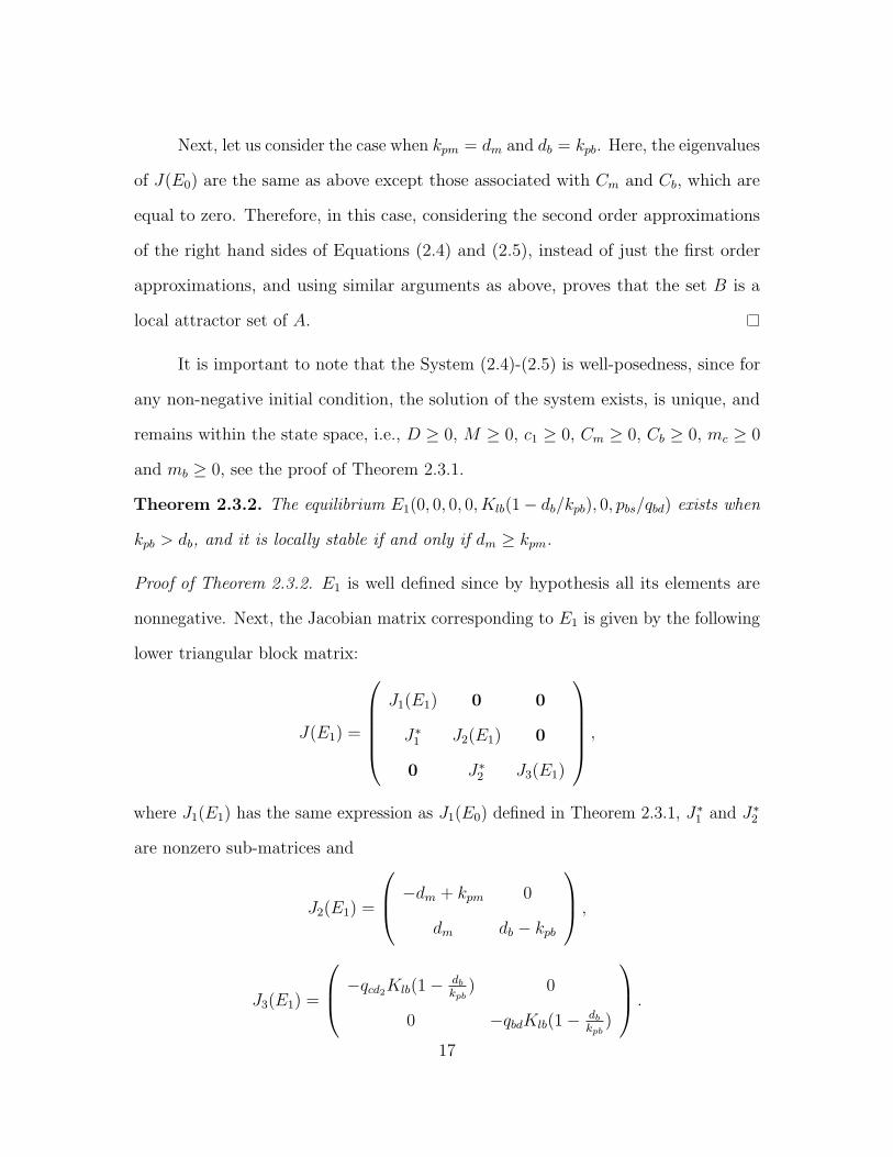
Theorem 2.3.2. The equilibrium E1(0, 0, 0, 0, Klb(1− db/kpb), 0, pbs/qbd) exists when

kpb > db, and it is locally stable if and only if dm ≥ kpm.

Proof of Theorem 2.3.2. E1 is well defined since by hypothesis all its elements are

nonnegative. Next, the Jacobian matrix corresponding to E1 is given by the following

lower triangular block matrix:

J(E1) =

J1(E1) 0 0

J∗1 J2(E1) 0

0 J∗2 J3(E1)

,

where J1(E1) has the same expression as J1(E0) defined in Theorem 2.3.1, J∗1 and J∗2

are nonzero sub-matrices and

J2(E1) =

−dm + kpm 0

dm db − kpb

,

J3(E1) =

−qcd2Klb(1− dbkpb

) 0

0 −qbdKlb(1− dbkpb

)

.

17

Since dm − kpm ≥ 0 and kpb > db and all the eigenvalues of J1(E0) are non-positive

values, then all the eigenvalues of J(E1) are all negative except the eigenvalues

associated with D and Cm when kpm = dm, which are equal to zero. Therefore,

by applying similar arguments provided in the proof of Theorem 2.3.1 when the

eigenvalues are zero, it implies that E1 is a locally stable node.

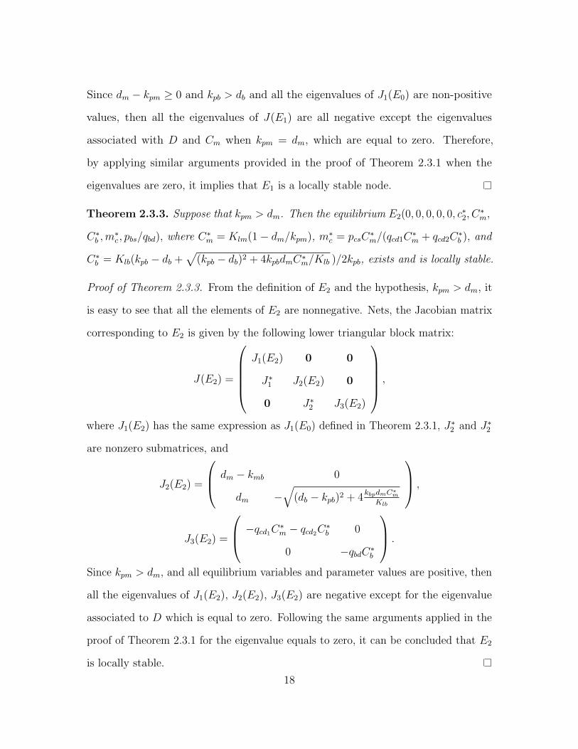
Theorem 2.3.3. Suppose that kpm > dm. Then the equilibrium E2(0, 0, 0, 0, 0, c∗2, C

∗m,

C∗b ,m∗c , pbs/qbd), where C∗m = Klm(1− dm/kpm), m∗c = pcsC

∗m/(qcd1C

∗m + qcd2C

∗b ), and

C∗b = Klb(kpb − db +√

(kpb − db)2 + 4kpbdmC∗m/Klb )/2kpb, exists and is locally stable.

Proof of Theorem 2.3.3. From the definition of E2 and the hypothesis, kpm > dm, it

is easy to see that all the elements of E2 are nonnegative. Nets, the Jacobian matrix

corresponding to E2 is given by the following lower triangular block matrix:

J(E2) =

J1(E2) 0 0

J∗1 J2(E2) 0

0 J∗2 J3(E2)

,

where J1(E2) has the same expression as J1(E0) defined in Theorem 2.3.1, J∗2 and J∗2

are nonzero submatrices, and

J2(E2) =

dm − kmb 0

dm −√

(db − kpb)2 + 4kbpdmC∗

m

Klb

,

J3(E2) =

−qcd1C∗m − qcd2C∗b 0

0 −qbdC∗b

.

Since kpm > dm, and all equilibrium variables and parameter values are positive, then

all the eigenvalues of J1(E2), J2(E2), J3(E2) are negative except for the eigenvalue

associated to D which is equal to zero. Following the same arguments applied in the

proof of Theorem 2.3.1 for the eigenvalue equals to zero, it can be concluded that E2

is locally stable.

18

The existence conditions for the three equilibria are summarized in Table 2.1,

and their stability conditions and the all possible resulting set of equilibria are

summarized in Table 2.2. From Theorems 2.3.1-2.3.1, the existence condition for

E0 requires that the steady state tissue densities to be either zero or any positive

number. For E1, the existence condition arises from the requirement that the steady

state density of Cb must be greater than zero, which implies that the proliferation

rate of osteoblasts must be greater than their differentiation rate, i.e., kpb > db.

Similarly for E2, the existence condition arises from the requirement that

the steady state density for Cm must be greater than zero, which implies that

the proliferation rate of MSCs must be greater than their differentiation rate, i.e.,

kpm > dm.

Table 2.1. Existence conditions for the equilibrium points and their biological meaning.

Equilibria Conditions Meaning

E0

(0, 0, 0, 0, 0,m∗c0 ,m

∗b0

)m∗c0 ,m

∗b0≥ 0 nonunion

E1

(0, 0, 0, 0,Klb(1− db

kpb), 0, pbsqbd

)kpb > db successful healing

E2

(0, 0, 0, C∗m, C∗b ,m

∗c ,

pbsqbd

)kpm > dm nonunion or delayed union

E0 is stable when kpm ≤ dm and kpb ≤ db (see Theorem 2.3.1), which implies

that the differentiation rates of the MSCs and osteoblasts are greater than or equal

to their proliferation rates, respectively. The steady-state E0 represents a nonunion.

In this case, the inflammation is resolved since the first five entries of E0 are zero;

however, the repair process has failed since the osteoblasts and osteoclasts have died

out before the beginning of the remodeling process. Hence, the tissue densities, m∗c0

and m∗b0 , can be any two positive values smaller than their maximal densities, pcs/qcd1

and pbs/qbd, respectively (see Theorem 2.3.1).

19

E1 is stable when kpm ≤ dm and kpb > db (see Theorem 2.3.2). The steady-state

E1 represents a successful repair of the bone fracture; where the inflammation is

resolved, the fibrocartilage is completely removed from the repair site, and the woven

bone has achieved its maximal density. In this case, osteoblasts proliferate faster

than they differentiate while MSCs have the opposite behavior.

E2 is stable when kpm > dm (see Theorem 2.3.3). The steady-state E2 represents

a nonunion or delayed union, where the inflammation is resolved but the osteoclasts

have failed to degrade the cartilage in a timely fashion.

Table 2.2. Stability conditions for the equilibrium points.

Equilibria Stability Conditions Stability

E0 kpm ≤ dm, kpb ≤ db E0 belongs to an attracting local setE0, E1 kpm ≤ dm, kpb > db E0 unstable; E1 locally stableE0, E2 kpm > dm, kpb ≤ db E0 unstable; E2 locally stable

E0, E1, E2 kpm > dm, kpb > db E0 and E1 unstable; E2 locally stable

2.4 Numerical Results

The proposed new model (2.1) - (2.7) is used to study the importance of

macrophages during the inflammatory and repair phases of the bone fracture healing

process, which occur within the first 21 days after trauma [27, 64]. It is also used to

investigate the evolution of a broken bone under normal and pathological conditions.

Table 5.1 summarizes the baseline parameter values and units for the numerical

simulations. These values are estimated in a qualitative manner from data in other

studies [39, 40, 63, 2, 24, 27]. Some of those from [27, 55] were also rescaled to account

for the different mathematical expressions of the proliferation and differentiation

rates of the tissue cells. All parameter values are based on murine experiments with

healthy mice having a moderate fracture (a broken long bone with a gap size less

20

than 3mm) [2, 24]. However, the bone fracture healing process for humans involves

the same cells, cytokines, and qualitative dynamics, differing only in the number of

cells, concentrations, and the length of time it takes for a full recovery [20].

First, a set of numerical simulations is presented to support the theoretical

results (successful and nonunion equilibria) and to numerically monitor the healing

progression of a moderate fracture in normal conditions. Next, the mathematical

model is used to investigate the effects of macrophages during the bone fracture

repair. Then, another set of numerical simulations is performed to analyze the

inflammatory effects in bone healing for different types of fractures. Finally, a set

of numerical simulations is presented to explore various cellular treatments under

numerous pathological conditions.

2.4.1 Different outcomes of the bone fracture healing process

A set of numerical simulations is presented to support the theoretical results.

According to the qualitative analysis of the model, there are three equilibria: E0, E1

and E2, where their stability conditions are determined by the tissue cells’ proliferation

and differentiation rates, kpm, kpb, dm and db, respectively. The following parameter

values are used: kpm = 0.5, dm = 1, kpb = 0.2202, and db = 0.3, to demonstrate the

stability of E0, since then kpm < dm and kpb < db. The stability of E1 is demonstrated

using the following parameter values: dm = 1, kpm = 0.5, kpb = 0.2202, and db = 0.15,

since then kpm ≤ dm and kpb > db. Finally, the following parameter values are used:

kpm = 0.5 and dm = 0.1, to demonstrate the stability of E2, since then kpm > dm.

Different time-periods are used in Figures 2.2-2.4 to better demonstrate the qualitative

behavior of the system under different stability conditions.

21

Figure 2.2 shows the qualitative behavior of E1 for the macrophages, debris,

and TNF-α densities, with the inflammation being resolved in about 40 days. Since

at this time, macrophages density is near zero.

0 20 40 60 80 1000

1

2

3

4

5x 10

7

Debris (

cells

/mL)

Days

E1

0 20 40 60 80 1000

2

4

6

x 105

Macro

phages (

cells

/mL)

Days

E1

0 20 40 60 80 1000

5

10

15

20

25

30

TN

F −

α (

ng/m

L)

Days

E1

Figure 2.2. Cellular and molecular evolution of the resolution of the inflammation innormal conditions.

Figure 2.3 shows the qualitative behaviors of E1 for the MSCs, osteoblasts,

cartilage, and bone densities. Here, the MSCs density decays to zero over time, while

the osteoblasts maintain a constant density below their carrying capacity Klb = 1×106.

In addition, the bottom plots of Figure 2.3 show that the cartilage is eventually

degraded by the osteoclasts, and the bone achieves its maximum density of 1 ng/mL.

Therefore, E1 exhibits the temporal progression of a successful bone fracture healing.

Figure 2.4 shows the qualitative evolution for the MSCs, osteoblasts, cartilage,

and bone densities for E0 (solid lines) and E2 (dotted lines). Since the temporal

evolution of macrophages, debris, and cytokines densities in E0 and E2 are similar to

those for E1 showed in Figure 2.2, then they are omitted here. It can be observed

22

0 100 200 300 4000

2

4

6

8

x 105

MS

Cs (

cells

/mL)

Days

E1

0 100 200 300 4000

2

4

6

8

10

x 105

Oste

obla

sts

(cells

/mL)

Days

E1

0 100 200 300 4000

0.2

0.4

0.6

Cart

ilage (

g/m

L)

Days

E1

0 100 200 300 4000

0.2

0.4

0.6

0.8

Bone (

g/m

L)

Days

E1

Figure 2.3. Cellular and molecular evolution of the repair process in a successfulfracture healing.

0 100 200 300 4000

2

4

6

8

x 105

MS

Cs (

cells

/mL)

Days

E0

E2

0 100 200 300 4000

2

4

6

x 105

Oste

obla

sts

(cells

/mL)

Days

E0

E2

0 100 200 300 4000

0.2

0.4

0.6

0.8

Cart

ilage (

g/m

L)

Days

E0

E2

0 100 200 300 4000

0.2

0.4

0.6

0.8

Bone (

g/m

L)

Days

E0

E2

Figure 2.4. Cellular and molecular evolution of the repair process in a nonunionfracture healing.

in Figure 2.4 that the two cellular densities in E0, MSCs and osteoblasts, decay to

zero over time, with the osteoclasts failing to degrade the cartilage, which results

in nonunion. Mathematically, this case occurs when osteoblasts proliferate at a

23

rate lower than their differentiation rate, i.e., kpb < db. In practice, this scenario

is commonly observed in advanced-age patients whose MSCs and osteoblast cells

decrease their capability to proliferate and differentiate [31]. On the other hand, the

two cells and the two tissues in E2 remain at positive constant values (Figure 2.4), but

the final fracture healing outcome is still a nonunion. Here, the osteoclasts again fail

to degrade the cartilage [31], even though the bone has achieved its maximum density

of 1 ng/mL. Therefore, in this case, migration of osteoclasts must be enhanced

through surgical interventions in order to achieve a successful bone repair [2].

2.4.2 Importance of macrophages during the bone fracture healing process

Next, the mathematical model is used to investigate the effects of macrophages

during the inflammatory and repair phases of the bone fracture healing process. The

major contribution of macrophages to fracture healing is through their phagocytic

function and their regulation of the tissue cellular functions, which is modeled with

the c1. Therefore, the values of the parameter kd, representing the phagocytic rate of

macrophages, and k1, representing the secretion rates of c1 by M are varied in the

numerical simulations as compared to their base values from Table 5.1.

Figure 2.5 shows that macrophages have drastic effects on the short-term tissue

dynamics during the healing process. Because of the faster phagocytic rate (dashed-

doted lines) of macrophages, the fibrocartilage formation is less, and its degradation

started earlier, while woven bone doubles in about 1 week. In contrast, with a slower

phagocytic rate (dashed lines) of macrophages, the fibrocartilage experiences an

increase during the second week and beyond, while the woven bone hardly formed.

Figure 2.6 shows that macrophages promote the production of the fibrocartilage

after the second week and beyond, while macrophages lightly inhibit the woven bone

production during the second week.

24

0 2 4 6 8 10 12 14 16 18 200

0.2

0.4

0.6

0.8

1

Cartilage(g/mL)

kd=13kd=48kd=3

0 2 4 6 8 10 12 14 16 18 200

0.1

0.2

0.3

0.4

Bone(g/mL)

Days

kd=13kd=48kd=3

Figure 2.5. Tissues evolution for different phagocytic rates: baseline phagocytic rate(solid line), kd = 13; faster phagocytic rate (dashed-doted line), kd = 48; slowerphagocytic rate (dashed line), kd = 3.

0 2 4 6 8 10 12 14 16 18 200

0.2

0.4

0.6

Cart

ilage

(g/m

L)

k1=8.3× 10

−6

k1=0

0 2 4 6 8 10 12 14 16 18 200

0.1

0.2

0.3

0.4

Bone (

g/m

L)

Days

k1=8.3× 10

−6

k1=0

Figure 2.6. Tissues evolution when the regulatory effect of macrophages through c1is modeled in the healing process (solid line), k1 = 8.3× 10−6, and when they do notcontribute to the healing process (dashed line), k1 = 0.

25

0 2 4 6 8 10 12 14 16 18 200

0.2

0.4

0.6

0.8

1

Cartilage(g/mL)

k1=8.3× 10

−6

k1=2× 8.3× 10

−6

k1=6× 8.3× 10

−6

0 2 4 6 8 10 12 14 16 18 200

0.1

0.2

0.3

0.4

Bone(g/mL)

Days

k1=8.3× 10

−6

k1=2× 8.3× 10

−6

k1=6× 8.3× 10

−6

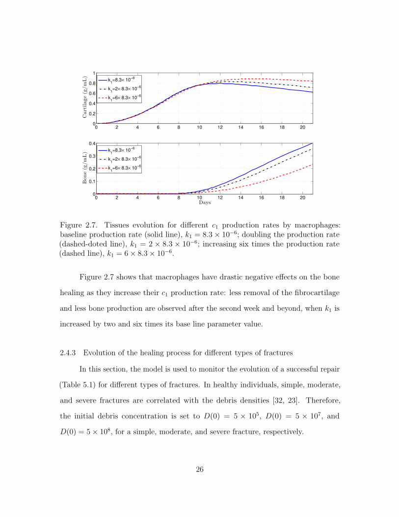
Figure 2.7. Tissues evolution for different c1 production rates by macrophages:baseline production rate (solid line), k1 = 8.3× 10−6; doubling the production rate(dashed-doted line), k1 = 2 × 8.3 × 10−6; increasing six times the production rate(dashed line), k1 = 6× 8.3× 10−6.

Figure 2.7 shows that macrophages have drastic negative effects on the bone

healing as they increase their c1 production rate: less removal of the fibrocartilage

and less bone production are observed after the second week and beyond, when k1 is

increased by two and six times its base line parameter value.

2.4.3 Evolution of the healing process for different types of fractures

In this section, the model is used to monitor the evolution of a successful repair

(Table 5.1) for different types of fractures. In healthy individuals, simple, moderate,

and severe fractures are correlated with the debris densities [32, 23]. Therefore,

the initial debris concentration is set to D(0) = 5 × 105, D(0) = 5 × 107, and

D(0) = 5× 108, for a simple, moderate, and severe fracture, respectively.

26

0 2 4 6 8 10 12 14 16 18 200

0.2

0.4

0.6

0.8

1

Cartilage

(g/m

L) Simple fracture

Moderte fractureSevere fracture

0 2 4 6 8 10 12 14 16 18 200

0.1

0.2

0.3

0.4

Bon

e(g/m

L)

Days

Simple fractureModerte fractureSevere fracture

Figure 2.8. Tissues evolution of a successful repair for different types of fractures.

0 2 4 6 8 10 12 14 16 18 200

0.2

0.4

Small fracture

0 2 4 6 8 10 12 14 16 18 200

20

40

Pro-inflam

matorycytokines

concentration

(ng/mL)

Moderate fracture

0 2 4 6 8 10 12 14 16 18 200

200

400

Days

Severe fracture

Figure 2.9. Concentration of inflammatory cytokines present in small, moderate, andsevere fractures.

27

Figure 2.8 shows that the tissue production is a slow process for a simple

fracture, since both the cartilage and bone densities are less than the corresponding

tissue densities for moderate and severe fractures. A slow healing process is commonly

observed in micro-crack healing [32]. Furthermore, there is less cartilage formation

over time in simple fractures [23]. For a moderate fracture, the maximal production

of the cartilage is observed around 10 days followed by a significant degradation, while

the bone tissue production occurs after the first week. For a severe fracture, Figure

2.8 shows that there is a delay in the two tissues production compared with those

given by moderate fractures, with the peak of the cartilage and bone productions

observed at around day 16.

From Figure 2.9, it can be observed that the peak of inflammatory cytokines

concentration increases as debris densities increases. Furthermore, high concentration

of inflammatory cytokines leads to delayed healing, as it is observed in severe fractures.

Therefore the healing time of a broken bone is determined by the inflammatory

cytokines concentrations.

2.4.3.1 Cellular therapeutic interventions under immune-compromised conditions

Additions of MSCs to the injury site through injection and/or transplantation

have been used in practice to stimulate and augment bone fracture healing [29].

Another cellular intervention is the scaffold implants, where macrophages and MSCs

are co-cultured together [31]. In this section, the Model (2.1)-(2.7) is used to explore

these possible therapeutic treatments to accelerate the healing of a broken bone

under normal and pathological conditions such as severe fractures, advanced age, and

senile osteoporosis [31]. The parameter values used in the numerical simulations that

explore these possible therapeutic treatments are the same as in Subsection 2.4.3.

28

0 2 4 6 8 10 12 14 16 18 200

0.2

0.4

0.6

0.8

Cartilage(g/mL)

0 2 4 6 8 10 12 14 16 18 200

0.1

0.2

0.3

0.4

Bone(g/mL)

Days

Moderate fracture

Cm

injection

M and Cm

transplantation

Moderate fracture

Cm

injection

M and Cm

transplantation

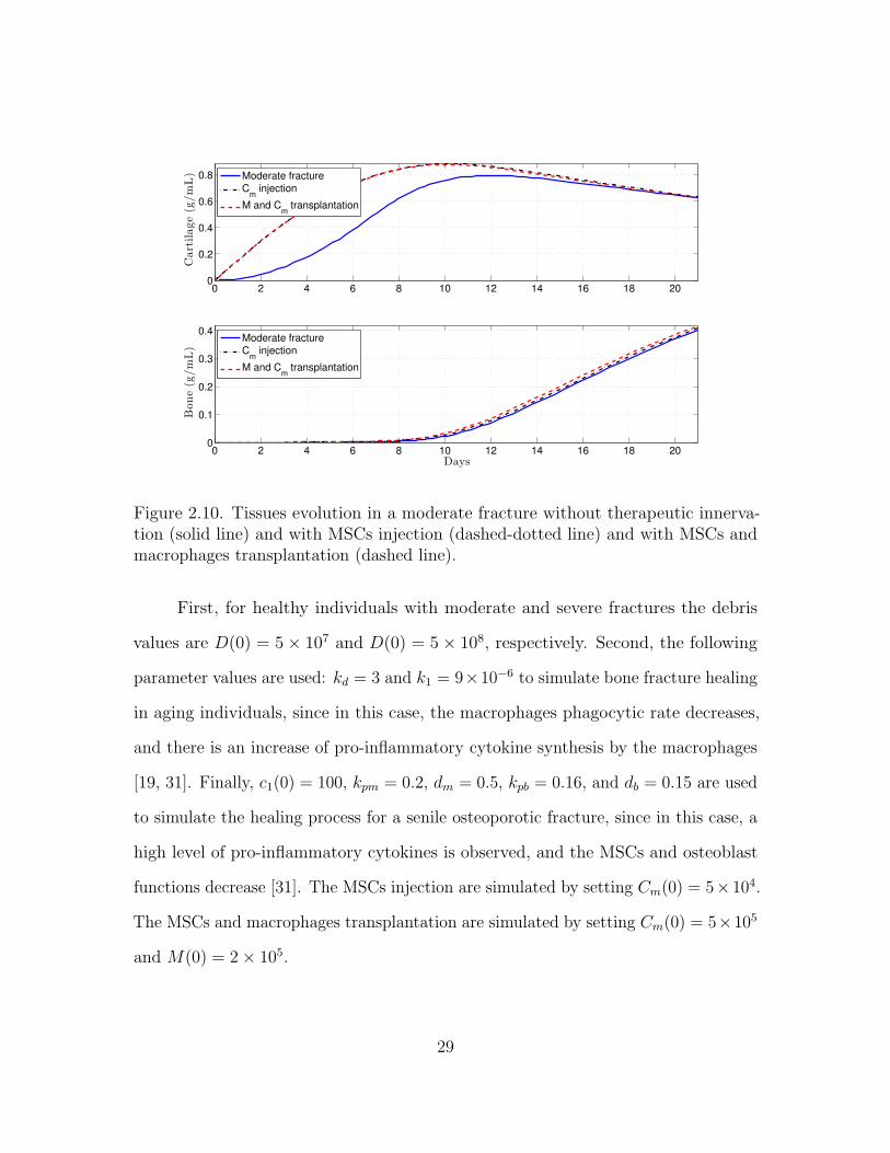
Figure 2.10. Tissues evolution in a moderate fracture without therapeutic innerva-tion (solid line) and with MSCs injection (dashed-dotted line) and with MSCs andmacrophages transplantation (dashed line).

First, for healthy individuals with moderate and severe fractures the debris

values are D(0) = 5× 107 and D(0) = 5× 108, respectively. Second, the following

parameter values are used: kd = 3 and k1 = 9×10−6 to simulate bone fracture healing

in aging individuals, since in this case, the macrophages phagocytic rate decreases,

and there is an increase of pro-inflammatory cytokine synthesis by the macrophages

[19, 31]. Finally, c1(0) = 100, kpm = 0.2, dm = 0.5, kpb = 0.16, and db = 0.15 are used

to simulate the healing process for a senile osteoporotic fracture, since in this case, a

high level of pro-inflammatory cytokines is observed, and the MSCs and osteoblast

functions decrease [31]. The MSCs injection are simulated by setting Cm(0) = 5×104.

The MSCs and macrophages transplantation are simulated by setting Cm(0) = 5×105

and M(0) = 2× 105.

29

0 2 4 6 8 10 12 14 16 18 200

0.2

0.4

0.6

0.8Cartilage

(g/m

L)

0 2 4 6 8 10 12 14 16 18 200

0.5

1

1.5

x 10−3

Bon

e(g/m

L)

Days

Severe fracture

Cm

injection

M and Cm

transplantation

Severe fracture

Cm

injection

M and Cm

transplantation

Figure 2.11. Tissues evolution in a severe fracture without therapeutic innerva-tion (solid line) and with MSCs injection (dashed-dotted line) and with MSCs andmacrophages transplantation (dashed line).

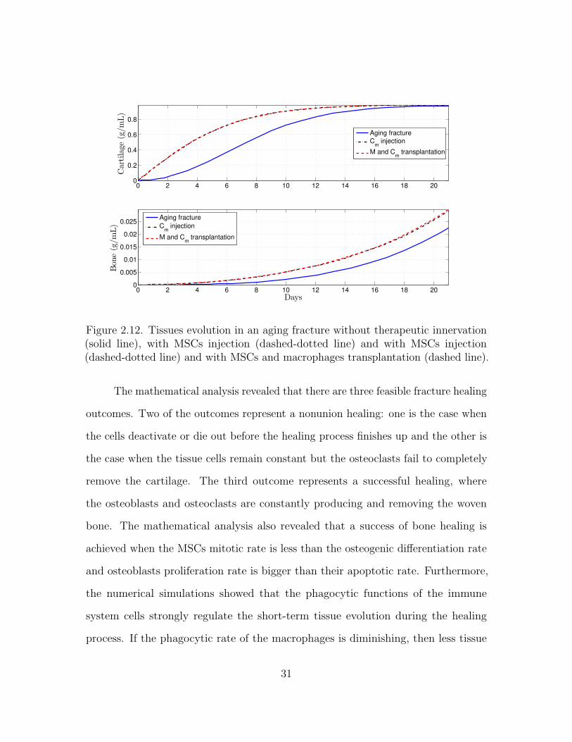
Figures 2.10, 2.11, 2.12, and 2.13 show that the two cellular interventions

increase both tissue productions. Furthermore, those interventions result in larger

improvements in aging fractures, see Figure 2.12. However, there is no bigger difference

between the two therapeutic interventions, the MSCs injection and the MSCs and

macrophages transplantation.

2.5 Summary of the Results

In this Chapter 2, a new mathematical model was formulated to gain a better

understanding of the most fundamental functions of the immune system during the

bone fracture healing process: phagocytosis and the delivery of pro-inflammatory

cytokines.

30

0 2 4 6 8 10 12 14 16 18 200

0.2

0.4

0.6

0.8Cartilage

(g/m

L)

0 2 4 6 8 10 12 14 16 18 200

0.005

0.01

0.015

0.02

0.025

Bon

e(g/m

L)

Days

Aging fracture

Cm

injection

M and Cm

transplantation

Aging fracture

Cm

injection

M and Cm

transplantation

Figure 2.12. Tissues evolution in an aging fracture without therapeutic innervation(solid line), with MSCs injection (dashed-dotted line) and with MSCs injection(dashed-dotted line) and with MSCs and macrophages transplantation (dashed line).

The mathematical analysis revealed that there are three feasible fracture healing

outcomes. Two of the outcomes represent a nonunion healing: one is the case when

the cells deactivate or die out before the healing process finishes up and the other is

the case when the tissue cells remain constant but the osteoclasts fail to completely

remove the cartilage. The third outcome represents a successful healing, where

the osteoblasts and osteoclasts are constantly producing and removing the woven

bone. The mathematical analysis also revealed that a success of bone healing is

achieved when the MSCs mitotic rate is less than the osteogenic differentiation rate

and osteoblasts proliferation rate is bigger than their apoptotic rate. Furthermore,

the numerical simulations showed that the phagocytic functions of the immune

system cells strongly regulate the short-term tissue evolution during the healing

process. If the phagocytic rate of the macrophages is diminishing, then less tissue

31

0 2 4 6 8 10 12 14 16 18 200

0.2

0.4

0.6

0.8Cartilage

(g/m

L)

Senile fracture

Cm

injection

M and Cm

transplantation

0 2 4 6 8 10 12 14 16 18 200

0.05

0.1

0.15

0.2

0.25

Bon

e(g/m

L)

Days

Senile fracture

Cm

injection

M and Cm

transplantation

Figure 2.13. Tissues evolution in a senile fracture without therapeutic innervation(solid line) and and with MSCs injection (dashed-dotted line) and with MSCs andmacrophages transplantation (dashed line).

productions is observed over time. Furthermore, that high concentration levels of

pro-inflammatory cytokines negatively affect the healing time of a fracture. It was

also found that the administration of growth factors improve the healing process in

a dose-dependant manner in moderate fractures and always improve the healing in

severe fractures. Furthermore, that the administration of growth factors exhibited

the most improvement treatments during the healing of a broken bone compare

to the anti-inflammatory cytokines administration. In addition, the injection and

transplantation of MSCs and macrophages to the injury site at the beginning of the

healing process accelerate the healing time.

32

CHAPTER 3

MODELING THE MACROPHAGE-MEDIATED INFLAMMATION INVOLVED

IN THE BONE FRACTURE HEALING PROCESS

In this chapter, the mathematical model (2.1)-(2.7) is extended to separately

incorporate the two different phenotypes of macrophages: classically and alterna-

tively activated macrophages, as they have distinct functions during the healing

process [10, 43, 48]. Classically activated macrophages release high levels of pro-

inflammatory cytokines, including the TNF-α and IL-1, which exhibit inhibitory

and destructive properties in high concentrations [9, 48]. In contrast, alternatively

activated macrophages are characterized with the secretion of the anti-inflammatory

cytokines, such as the IL-10 and TGF-β, which increase their phagocytic activities,

mitigate the inflammatory responses, promote growth, and accelerate the fracture

healing [10, 29, 31, 48]. This extension leads to a more realistic model by incorpo-

rating the different phagocytic rates and the separate production of the pro- and

anti-inflammatory cytokines by the two types of macrophages [10, 33].

The model can be used to investigate the anti-inflammatory regulatory effects

of the immune system during bone fracture healing. The model can also be used to

investigate potential therapeutic treatments based on the use of anti-inflammatory

cytokines, stem cells, and macrophages, suggesting possible ways to guide clinical

experiments and bone tissue engineering strategies [10, 48].

33


The modeling assumptions follow the assumptions provided in Chapter 2 with

the incorporation of further details on the macrophages and the pro- and anti-

inflammatory, described below. The macrophages density is modeled separately

as undifferentiated macrophages (M0), classical macrophages (M1), and alternative

macrophages (M2). It is also included a generic anti-inflammatory cytokines (c2),

which is delivered by the M2, Cm, and Cb. The biological system interactions are

depicted in Figure 3.1. In the flow diagram, the cells and cellular dynamics are

represented by the circular shapes and solid arrows. The molecular concentrations

and their production/decay are represented by the octagonal shapes and dashed

arrows. The pro- and anti-inflammatory cytokines activation/inhibition effects on the

cellular functions are represented by the dotted arrows. Removal of debris and the

negative effect among the variables are represented by the dot-ending dotted arrows.

It is assumed that the cellular functions are regulated by c1, such as the TNF-α,

and c2, such as a combination of the IL-10 and the TGF-β. It is also assumed that c1

is delivered through cell necrosis and by the classically activated macrophages, while

c2 is delivered by the alternatively activated macrophages, MSCs, and osteoblasts.

It is also assumed that unactivated macrophages M0 do not release cytokines and

do not engulf debris. Additionally, the population of M0 increases proportionally in

size to the density of debris up to a maximal value of Mmax [40]. The only source

of activated macrophages, M1 and M2, is M0. Even though both phenotypes of

activated macrophages have the ability to release both pro- and anti-inflammatory

cytokines, it is assumed that only M1 deliver c1 and M2 deliver c2, as those are the

major cytokines for each phenotype [39]. M0 activate to M1 under the c1 stimulus,

while they activate to M2 under the c2 stimulus. M1 and M2 macrophages do not

34

𝐷

𝑐1

𝑀2

𝑀1

𝑐2

𝑀0

𝑘21 𝑘12

𝐺1

𝑅𝑀

𝐺2

𝑘0

𝑘1

𝑘2

𝑘3

𝑑2

𝑑1𝑑0

𝑑𝑐1

𝑑𝑐2

𝑘𝑒2 𝑘𝑒1

𝐶𝑏

𝐶𝑚

𝐹1

𝑚𝑏

𝑚𝑐

𝐴𝑚

𝐴𝑏

𝑝𝑐𝑠

𝑝𝑏𝑠

𝑞𝑐𝑑2

𝑑𝑏

𝑘4

𝑅𝑚

Inflammation Repair

Figure 3.1. Flow diagram of the cellular and molecular dynamics during the inflam-matory and repair phases of the bone fracture healing process.

de-differentiate back to the M0 macrophages [63]; and are able to switch phenotypes

at a constant rate [59].


The inflammatory and repair phases of the bone fracture healing process are

modeled with a mass-action system of nonlinear ordinary differential equations. All

variables represent homogeneous quantities in a given volume. Following the outlined

biological assumptions and the flow diagram given in Figure 3.1 yields the resulting

system of equations:

dD

dt= −RD(ke1M1 + ke2M2) (3.1)

dM0

dt= RM −G1M0 −G2M0 − d0M0 (3.2)

35

dM1

dt= G1M0 + k21M2 − k12M1 − d1M1 (3.3)

dM2

dt= G2M0 + k12M1 − k21M2 − d2M2 (3.4)

dc1dt

= H1(k0D + k1M1)− dc1c1 (3.5)

dc2dt

= H2(k2M2 + k3Cm + k4Cb)− dc2c2 (3.6)

dCm

dt= (Rm + AmCm)

(1− Cm

Klm

)− F1Cm (3.7)

dCb

dt= AbCb

(1− Cb

Klb

)+ F1Cm − dbCb (3.8)

dmc

dt= (pcs − qcd1mc)Cm − qcd2mcCb (3.9)

dmb

dt= (pbs − qbdmb)Cb. (3.10)

Equation (3.1) describes the rate of change with respect to time of the debris density,

which decreases proportionally to M1 and M2. Equation (3.2) describes the rate of

change with respect to time of the undifferentiated macrophages density. It increases

because of migration and decreases by differentiating into M1 and M2 or by a constant

emigration rate. It is assumed that M0 migrate to the injury site proportionally to D

up to a maximal constant rate, kmax, [1, 25]:

RM = kmax

(1− M

Mmax

)D,

where M = M0 + M1 + M2. The differentiation rates of M0 into M1 and M2 are

stimulated by the cytokines accordingly to a Hill Type II equations, respectively [59]:

G1 = k01 ×c1

a01 + c1, G2 = k02 ×

c2a02 + c2

.

Equation (3.3) describes the rate of change with respect to time of M1, which increases

when M0 activate to M1 and M2 shift phenotype; and decreases by emigration and

when M1 shift phenotype. Similarly, Equation (3.4) describes the rate of change with

respect to time of M2. Equations (3.5) and (3.6) describes the rate of change with

36

respect to time of c1 and c2. Here, k0, k1, k2, k3, and k4 are the constant rates of

the cytokine productions and dc1 and dc2 are the cytokine constant decay rates. The

inhibitory effects of the anti-inflammatory cytokines to the c1 and c2 production rates

are modeled by the following functions [59]:

H1 =a12

a12 + c2, H2 =

a22a22 + c2

.

The equations (3.7)-(3.10) were introduced and described in Section 2.2.


The analysis of model is done by finding the equilibria and their corresponding

stability properties. An equilibrium point of the model is denoted by the vector form

E (D,M0,M1,M2, c1, c2, Cm, Cb,mc,mb) and it is found by setting the right-hand sides

of the equations (3.1)-(3.10) equal to zero [42]. The model has three biologically mean-

ingful equilibria: E0(0, 0, 0, 0, 0, 0, 0, 0,m∗c0,m∗b0), E1(0, 0, 0, 0, 0, c

∗2, 0, C

∗b , 0, pbs/qbd),

E2(0, 0, 0, 0, 0, c∗2, C

∗m, C

∗b ,m

∗c , pbs/qbd). Their definitions, existence, and corresponding

stability conditions are stated and proved below. The analysis is conducted using

the Jacobian of the system at each equilibrium point, and finding its corresponding

eigenvalues [42, 53].

Theorem 3.3.1. The E0(0, 0, 0, 0, 0, 0, 0, 0,m∗c0,m∗b0) belongs to the set B = (0, 0, 0,

0, 0, 0, 0, 0,mc,mb) : 0 ≤ mc ≤ pcs/qcd1 , 0 ≤ mb ≤ pbs/qbd, which is a local attractor

set of the solution set given by System (3.1)-(3.10) if and only if kpm ≤ dm and

kpb ≤ db.

Proof of Theorem 3.3.1. The right-hand side functions of System (3.1)-(3.10) are

continuous and bounded, since all model variables and parameters are positive.

Hence, for each initial condition of the system, there is a unique solution [53]. Then,

37

as zero is a solution of the System (3.1)-(3.10) and by uniqueness of solution, all the

solutions of the system with positive initial condition are positive [53].

Next, it will be proved that the hyperplane A = (0, 0, 0, 0, 0, 0, 0, 0,mc,mb) :

mc ≥ 0,mb ≥ 0 is an attractor set of the solutions of the system (3.1)-(3.10). There

are two cases to consider based on the relation between the cells proliferation and

differentiation rates.

First, let us examine the case when kpm < dm and kpm < db. The Jacobian

matrix J(E0) is given by the following lower triangular block matrix

J(E0) =

J1(E0) 0 0

∗ J2(E0) 0

0 ∗ J3(E0)

,

where

J1(E0) =

0 0 0 0

kmax −d0 0 0

0 0 J11 0

k0 0 ∗ −dc1

, J11 =

−d1 − k12 k21

k12 −d2 − k21

J2(E0) =

−dc2 k3 k4

0 −dm + kpm 0

0 dm −db + kpb

, J3(E0) =

0 0

0 0

.

Therefore the corresponding characteristic polynomial associated with J(E0) is given

by the product of the characteristic polynomials associated with each submatrix [52]:

p(λ) = λ3 (λ+ d0) (λ+ dc1) (λ+ dc2) (λ+ dm − kpm) (λ+ db − kpm) (λ2 + aλ+ b),

where a = d1 + d2 + k12 + k21 and b = k12d2 + k21d1 + d1d2. The polynomial factor

of order two of p(λ) has the following two roots: (−a ±√a2 − 4b )/2, which are

38

negative since a2 − 4b = (d1 − d2 + k12 − k21)2 + 4k12k21 > 0 and b > 0. Therefore,

the eigenvalues of J(E0) are negative for the variables M0, M1, M2, c1, c2, Cm, and

Cb, and are equal to zero for D, mc, and mb. Since D′(t) ≤ 0 for all the variables

in the system (3.1)-(3.10) and (D∗, 0, 0, 0, 0, 0, 0, 0,mc,mb) with D∗ 6= 0 is not an

equilibrium point, then the solutions of the system (3.1)-(3.8) are attracted to the set

A = (0, 0, 0, 0, 0, 0, 0, 0,mc,mb) : mc ≥ 0,mb ≥ 0. Equations (3.9) and (3.10) imply

that m′c ≤ 0 and m′b ≤ 0 for all mc > pcs/qcd1 and mb > pbs/qbd. Therefore, the set B

is a local attractor set of A [53].

Next, let us consider the case when kpm = dm and db = kpb. Here, the eigenvalues

of J(E0) are the same as above except those associated with Cm and Cb, which are

equal to zero. Therefore, in this case, by considering the second order approximations

of the right hand sides of Equations (3.7) and (3.8), instead of just the first order

approximations, and using similar arguments as above, proves that the set B is a

local attractor set of A.

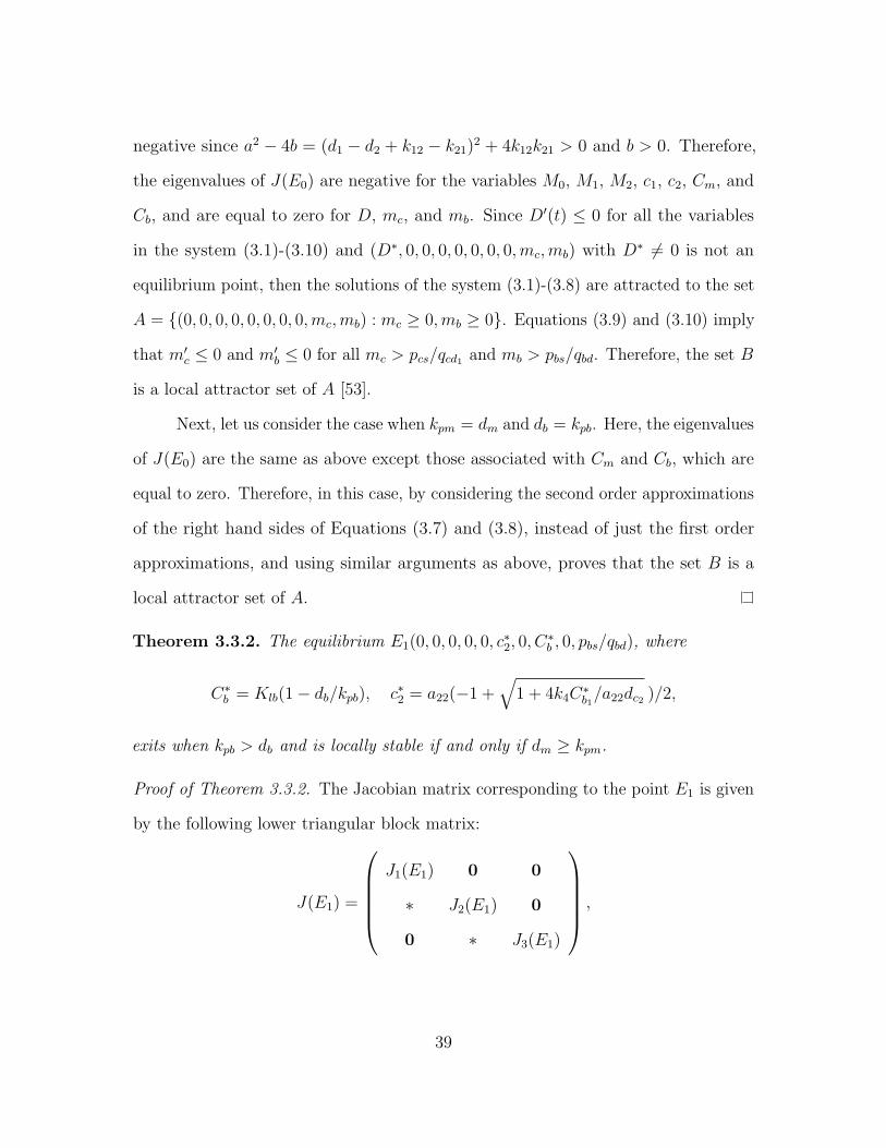
Theorem 3.3.2. The equilibrium E1(0, 0, 0, 0, 0, c∗2, 0, C

∗b , 0, pbs/qbd), where

C∗b = Klb(1− db/kpb), c∗2 = a22(−1 +√

1 + 4k4C∗b1/a22dc2 )/2,

exits when kpb > db and is locally stable if and only if dm ≥ kpm.

Proof of Theorem 3.3.2. The Jacobian matrix corresponding to the point E1 is given

by the following lower triangular block matrix:

J(E1) =

J1(E1) 0 0

∗ J2(E1) 0

0 ∗ J3(E1)

,

39

where

J1(E1) =

0 0 0 0

kmax −d0 −G∗2 0 0

0 ∗ J11 0

k0H∗1 0 ∗ −dc1

,

J2(E2) =

−dc2

(1 +

c∗21a22+c∗21

)k3H

∗2 k4H

∗2

0 −dm + kpm 0

0 dm db − kpb

,

J3(E1) =

−qcd2Klb(1− dbkpb

) 0

0 −qbdKlb(1− dbkpb

)

,

G∗2 =k02c∗2a02+c∗2

, H∗1 = a12a12+c∗2

, H∗2 = a22a22+c∗2

and J11 is defined as in Theorem 3.3.1. Since

all the eigenvalues of J11 are negative (Theorem 3.3.1) and dm−kpm ≥ 0 and kpb > db,

then the eigenvalues of J(E1) are negative except the eigenvalues associated with D

and Cm when kpm = dm, which are equal to zero. Therefore, E1 is a locally stable

node, since D′ ≤ 0 for all the variables of the system (3.1)-(3.10) and C ′m ≤ 0 when

kpm = dm.

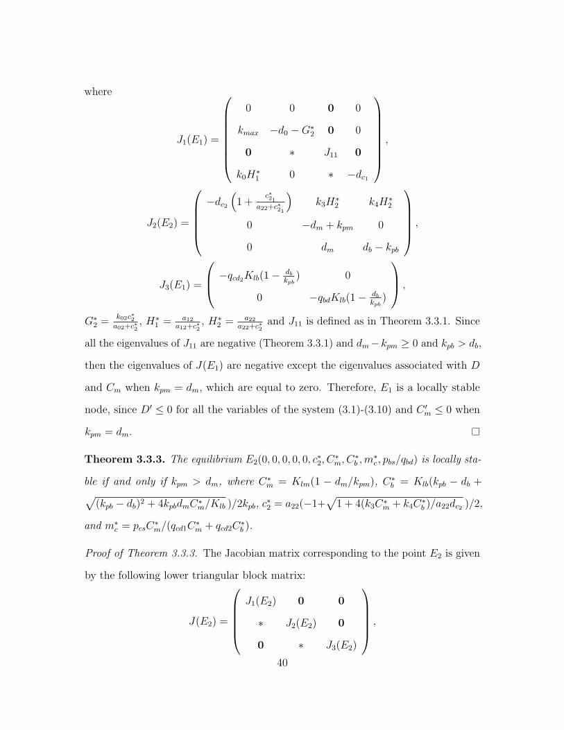
Theorem 3.3.3. The equilibrium E2(0, 0, 0, 0, 0, c∗2, C

∗m, C

∗b ,m

∗c , pbs/qbd) is locally sta-

ble if and only if kpm > dm, where C∗m = Klm(1 − dm/kpm), C∗b = Klb(kpb − db +√(kpb − db)2 + 4kpbdmC∗m/Klb )/2kpb, c

∗2 = a22(−1+

√1 + 4(k3C∗m + k4C∗b )/a22dc2 )/2,

and m∗c = pcsC∗m/(qcd1C

∗m + qcd2C

∗b ).

Proof of Theorem 3.3.3. The Jacobian matrix corresponding to the point E2 is given

by the following lower triangular block matrix:

J(E2) =

J1(E2) 0 0

∗ J2(E2) 0

0 ∗ J3(E2)

,

40

where J1(E2) has the same expression as J1(E1) defined in Theorem 3.3.2, but with

the steady state variables defined by Theorem 3.3.3 and

J2(E2) =

−dc2

(1 +

c∗2a22+c∗2

)k3H

∗2 k4H

∗2

0 dm − kmb 0

0 dm −√

(db − kpb)2 + 4kbpdmC∗

m

Klb

,

J3(E2) =

−qcd1C∗m − qcd2C∗b 0

0 −qbdC∗b

,

G∗2 =k02c∗2a02+c∗2

, H∗1 = a12a12+c∗2

, H∗2 = a22a22+c∗2

and J11 is defined in Theorem 3.3.1. Since all

the eigenvalues of J11 are negative (Theorem 2.3.1) and kpm > dm, and all equilibrium

variables and parameter values are positive, then all the eigenvalues of J1(E2), J2(E2),

J3(E2) are negative except for the eigenvalue associated to D which is equal to zero.

Therefore, since D′ ≤ 0 for all the variable system, then E2 is locally stable.

In summary, the mathematical analysis of Model (3.1)-(3.10) revels that the

number of equilibria and their corresponding existence and stability conditions are

the same as Model (2.1)-(2.7), with the appropriate set of variables.


The proposed new model (3.1)-(3.10) is used to study the importance of


process. First, a set of numerical simulation results is presented to compare the

models (2.1)-(2.7) and (3.1)-(3.1). Second, a set of numerical simulations is performed

to analyze the effects of different concentrations of anti-inflammatory cytokines on

the fracture healing under numerous pathological conditions.

41

3.4.1 Comparison of Model (2.1)-(2.7) and Model (3.1)-(3.10)

The model (2.1)-(2.7) takes into account the regulatory effects of the immune

system given by its phagocytes, M , and their released pro-inflammatory cytokines,

c1. The present mathematical model (3.1)-(3.10) extend the model (2.1)-(2.7) by

incorporating the ability of the immune system to regulate the inflammation by its

anti-inflammatory cytokines, c2, production. Therefore, the two different phenotypes

of macrophages M1 and M2 were separately incorporated in the model as c1 is mainly

delivery by M1 and c2 is mainly delivered by the M2. The models (2.1)-(2.7) and

(3.1)-(3.10) are compared to demonstrate the importance of the immune system as

inflammatory-mediators involved in the bone fracture healing process. The same

parameter values are used in both models (Table 5.1), with ke1 = 1, ke2 = 2, k01 = 0.55,

k01 = 0.55, k01 = 0.55×10−6, k3 = 8×10−6, qbd = 5×10−8, and dM = 0.121. Figure

0 2 4 6 8 10 12 14 16 18 200

0.2

0.4

0.6

Cartilage

(g/mL) Model (2.1)-(2.7)

Model (3.1)-(3.10)

0 2 4 6 8 10 12 14 16 18 200

0.1

0.2

0.3

0.4

0.5

Bon

e(g/mL)

Days

Model (2.1)-(2.7)Model (3.1)-(3.10)

Figure 3.2. Comparison of tissues evolution in Model (2.1) - (2.7) and Model (3.1) -(3.10).

42

3.2 shows the numerical evolutions of the tissues’ production when D(0) = 5× 107.

In all simulations, we refer to fibrocartilage and woven bone as cartilage and bone,

respectively. More cartilage production mc and less bone production mb is observed

when the c2 is not incorporated, model (2.1)-(2.7). Moreover, the model (3.1)-(3.10)

is much more realistic as the mb production is observed in the first week according to

the experimental data.


In this section, the mathematical model is used to investigate the regulatory

effects of macrophages through their two phenotypes, M1 and M2, which deliver

separately the pro- and anti-inflammatory cytokines. Therefore, the values of the

parameters ki, representing the secretion rates of ci by Mi, i = 1, 2, are varied in the

numerical simulations as compared to their base values from Table 5.1.

0 2 4 6 8 10 12 14 16 18 200

0.2

0.4

0.6

0.8

Cartilage

(g/m

L)

0 2 4 6 8 10 12 14 16 18 200

0.2

0.4

Bon

e(g/m

L)

Days

k1 = 8.3 × 10−4, k2 = 3.72 × 10−4

k1 = 0, k2 = 0

k1 = 8.3 × 10−4, k2 = 3.72 × 10−4

k1 = 0, k2 = 0

Figure 3.3. Tissues evolution when macrophages contribute to the healing process(solid line), k1, k2 6= 0, and when they do not contribute to the healing process (dashedline), k1 = k2 = 0 .

43

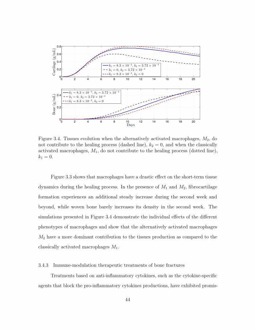
0 2 4 6 8 10 12 14 16 18 200

0.2

0.4

0.6

0.8

Cartilage

(g/m

L)

k1 = 8.3 × 10−4, k2 = 3.72 × 10−4

k1 = 0, k2 = 3.72 × 10−4

k1 = 8.3 × 10−4, k2 = 0

0 2 4 6 8 10 12 14 16 18 200

0.2

0.4

Bon

e(g/m

L)

Days

k1 = 8.3 × 10−4, k2 = 3.72 × 10−4

k1 = 0, k2 = 3.72 × 10−4

k1 = 8.3 × 10−4, k2 = 0

Figure 3.4. Tissues evolution when the alternatively activated macrophages, M2, donot contribute to the healing process (dashed line), k2 = 0, and when the classicallyactivated macrophages, M1, do not contribute to the healing process (dotted line),k1 = 0.

Figure 3.3 shows that macrophages have a drastic effect on the short-term tissue

dynamics during the healing process. In the presence of M1 and M2, fibrocartilage

formation experiences an additional steady increase during the second week and

beyond, while woven bone barely increases its density in the second week. The

simulations presented in Figure 3.4 demonstrate the individual effects of the different

phenotypes of macrophages and show that the alternatively activated macrophages

M2 have a more dominant contribution to the tissues production as compared to the

classically activated macrophages M1.

3.4.3 Immune-modulation therapeutic treatments of bone fractures

Treatments based on anti-inflammatory cytokines, such as the cytokine-specific

agents that block the pro-inflammatory cytokines productions, have exhibited promis-

44

ing clinical results and have led to intense orthopedic research activities [9, 16, 18,

29, 38, 44, 49, 62]. In this section, a set of numerical simulations is presented to

investigate the effect of the administrations of anti-inflammatory cytokines during the

bone fracture healing process in healthy individuals and also in immune-compromised

patients.

In healthy individuals, the administration of anti-inflammatory drugs is imple-

mented for simple, two moderate, and severe fractures: D(0) = 5×106, D(0) = 2×107,

D(0) = 5× 107, and D(0) = 5× 108, respectively. First, the administration of anti-

inflammatory cytokines is done by increasing the initial concentration of c2: c2(0) = 0,

10 and 100 ng/mL. Second, anti-inflammatory cytokines is continuously administrate.

It is modeled by increasing the anti-inflammatory cytokines production rate of the

M2, i.e., k2 = 3.72× 10−4, 2× 3.72× 10−4, 6× 3.72× 10−4 ng/mL.

0 2 4 6 8 10 12 14 16 18 200

0.1

0.2

0.3

0.4

Cartilage

(g/m

L)

0 2 4 6 8 10 12 14 16 18 200

0.1

0.2

0.3

0.4

Bon

e(g/m

L)

Days

0 ng/mL10 ng/mL100 ng/mL


Figure 3.5. Tissues evolution in a simple fracture under different initial anti-inflammatory cytokines concentrations, D(0) = 5× 106.

45

0 2 4 6 8 10 12 14 16 18 200

0.2

0.4

0.6Cartilage

(g/m

L)

0 2 4 6 8 10 12 14 16 18 200

0.1

0.2

0.3

0.4

0.5

Bon

e(g/m

L)

Days

0 ng/mL

10 ng/mL

100 ng/mL


Figure 3.6. Tissues evolution in a moderate fracture under different initial anti-inflammatory cytokines concentrations, D(0) = 5× 107.

0 2 4 6 8 10 12 14 16 18 200

0.2

0.4

0.6

0.8

Cartilage

(g/m

L)

0 ng/mL

10 ng/mL

100 ng/mL

0 2 4 6 8 10 12 14 16 18 200

0.05

0.1

0.15

Bon

e(g/m

L)

Days


Figure 3.7. Tissues evolution in a severe fracture under different initial anti-inflammatory cytokines concentrations D(0) = 5× 108.

Figure 3.5 shows that in the simple fracture the administration of anti- in-

flammatory drugs at the beginning of the healing process inhibits the two tissue’s

46

production. Figures 3.6 shows that the administration of c2 at the beginning of the

healing process in a moderate fractures, D(0) = 5× 107, does not lead to any drastic

change in the two tissue’s production. Figures 3.7 shows that the administration of

c2 at the beginning of the healing process in the severe fractures, D(0) = 5 × 108,

enhances the production of bone, while the cartilage production does not experience

any change.

0 2 4 6 8 10 12 14 16 18 200

0.1

0.2

0.3

0.4

Cartilage

(g/m

L)

0 2 4 6 8 10 12 14 16 18 200

0.1

0.2

0.3

Bon

e(g/m

L)

Days

k2 = 3.72 × 10−4

k2 = 2 × 3.72 × 10−4

k2 = 6 × 3.72 × 10−4

k2 = 3.72 × 10−4

k2 = 2 × 3.72 × 10−4

k2 = 6 × 3.72 × 10−4

Figure 3.8. Tissues evolution in a simple fracture under a continuous administrationof anti-inflammatory cytokines: k2 = 3.72× 10−4 (solid line), k2 = 2× 3.72× 10−4

(dotted-dashed line), k2 = 6× 3.72× 10−4 (dashed line).

Figure 3.8 shows that in the simple fracture the continuous administration of

anti-inflammatory drugs drastically inhibit the two tissue’s production. Figures 3.9

shows that the excessive administration of c2 in a moderate fractures D(0) = 2× 107

inhibit the two tissue’s production. Figures 3.10 shows that the administration of c2

in the moderate fractures with D(0) = 5× 107 improves the bone tissue evolution

while enhance a fast removal of the cartilage tissue. Figures 3.11 shows that the

47

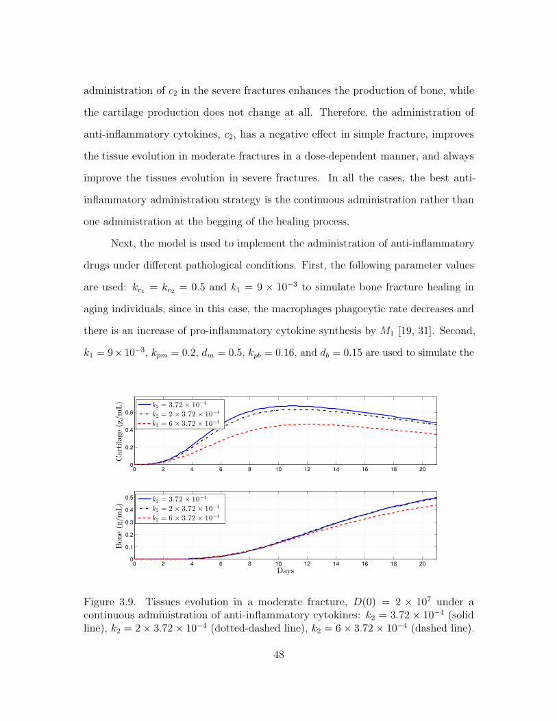
administration of c2 in the severe fractures enhances the production of bone, while

the cartilage production does not change at all. Therefore, the administration of

anti-inflammatory cytokines, c2, has a negative effect in simple fracture, improves

the tissue evolution in moderate fractures in a dose-dependent manner, and always

improve the tissues evolution in severe fractures. In all the cases, the best anti-

inflammatory administration strategy is the continuous administration rather than

one administration at the begging of the healing process.

Next, the model is used to implement the administration of anti-inflammatory

drugs under different pathological conditions. First, the following parameter values

are used: ke1 = ke2 = 0.5 and k1 = 9 × 10−3 to simulate bone fracture healing in

aging individuals, since in this case, the macrophages phagocytic rate decreases and

there is an increase of pro-inflammatory cytokine synthesis by M1 [19, 31]. Second,

k1 = 9×10−3, kpm = 0.2, dm = 0.5, kpb = 0.16, and db = 0.15 are used to simulate the

0 2 4 6 8 10 12 14 16 18 200

0.2

0.4

0.6

Cartilage

(g/m

L)

0 2 4 6 8 10 12 14 16 18 200

0.1

0.2

0.3

0.4

0.5

Bon

e(g/m

L)

Days

k2 = 3.72 × 10−4

k2 = 2 × 3.72 × 10−4

k2 = 6 × 3.72 × 10−4

k2 = 3.72 × 10−4

k2 = 2 × 3.72 × 10−4

k2 = 6 × 3.72 × 10−4

Figure 3.9. Tissues evolution in a moderate fracture, D(0) = 2 × 107 under acontinuous administration of anti-inflammatory cytokines: k2 = 3.72× 10−4 (solidline), k2 = 2× 3.72× 10−4 (dotted-dashed line), k2 = 6× 3.72× 10−4 (dashed line).

48

0 2 4 6 8 10 12 14 16 18 200

0.2

0.4

0.6Cartilage

(g/m

L)

0 2 4 6 8 10 12 14 16 18 200

0.1

0.2

0.3

0.4

0.5

Bon

e(g/m

L)

Days

k2 = 3.72 × 10−4

k2 = 2 × 3.72 × 10−4

k2 = 6 × 3.72 × 10−4

k2 = 3.72 × 10−4

k2 = 2 × 3.72 × 10−4

k2 = 6 × 3.72 × 10−4

Figure 3.10. Tissues evolution in a moderate fracture, D(0) = 5 × 107, under acontinuous administration of anti-inflammatory cytokines: k2 = 3.72× 10−4 (solidline), k2 = 2× 3.72× 10−4 (dotted-dashed line), k2 = 6× 3.72× 10−4 (dashed line).

0 2 4 6 8 10 12 14 16 18 200

0.2

0.4

0.6

0.8

Cartilage

(g/m

L)

0 2 4 6 8 10 12 14 16 18 200

0.05

0.1

0.15

0.2

0.25

Bon

e(g/m

L)

Days

k2 = 3.72 × 10−4

k2 = 2 × 3.72 × 10−4

k2 = 6 × 3.72 × 10−4

k2 = 3.72 × 10−4

k2 = 2 × 3.72 × 10−4

k2 = 6 × 3.72 × 10−4

Figure 3.11. Tissues evolution in a severe fracture under a continuous administrationof anti-inflammatory cytokines: k2 = 3.72× 10−4 (solid line), k2 = 2× 3.72× 10−4

(dotted-dashed line), k2 = 6× 3.72× 10−4 (dashed line).

49

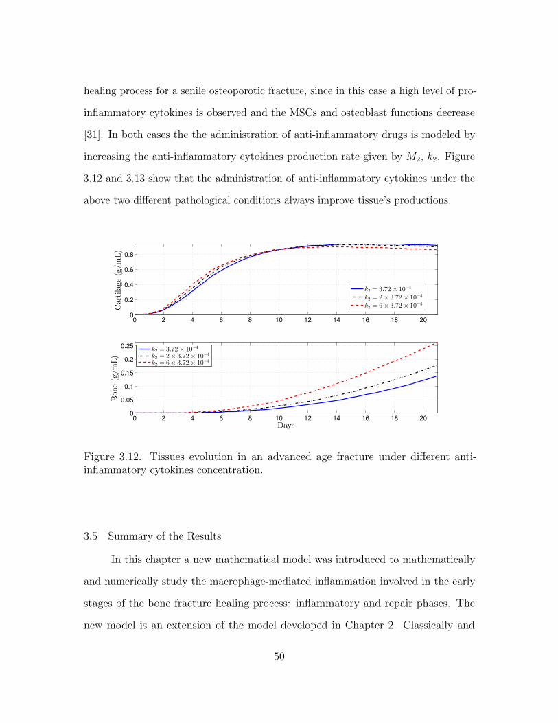
healing process for a senile osteoporotic fracture, since in this case a high level of pro-

inflammatory cytokines is observed and the MSCs and osteoblast functions decrease

[31]. In both cases the the administration of anti-inflammatory drugs is modeled by

increasing the anti-inflammatory cytokines production rate given by M2, k2. Figure

3.12 and 3.13 show that the administration of anti-inflammatory cytokines under the

above two different pathological conditions always improve tissue’s productions.

0 2 4 6 8 10 12 14 16 18 200

0.2

0.4

0.6

0.8

Cartilage

(g/m

L)

0 2 4 6 8 10 12 14 16 18 200

0.05

0.1

0.15

0.2

0.25

Bon

e(g/m

L)

Days

k2 = 3.72 × 10−4

k2 = 2 × 3.72 × 10−4

k2 = 6 × 3.72 × 10−4

k2 = 3.72 × 10−4

k2 = 2 × 3.72 × 10−4

k2 = 6 × 3.72 × 10−4

Figure 3.12. Tissues evolution in an advanced age fracture under different anti-inflammatory cytokines concentration.


In this chapter a new mathematical model was introduced to mathematically

and numerically study the macrophage-mediated inflammation involved in the early

stages of the bone fracture healing process: inflammatory and repair phases. The

new model is an extension of the model developed in Chapter 2. Classically and

50

0 2 4 6 8 10 12 14 16 18 200

0.2

0.4

0.6

0.8Cartilage

(g/m

L)

0 2 4 6 8 10 12 14 16 18 200

0.05

0.1

0.15

Bon

e(g/m

L)

Days

k2 = 3.72× 10−4

k2 = 2× 3.72× 10−4

k2 = 6× 3.72× 10−4

k2 = 3.72× 10−4

k2 = 2× 3.72× 10−4

k2 = 6× 3.72× 10−4

Figure 3.13. Tissues evolution in a senile osteoporotic fracture under different anti-inflammatory cytokines concentrations.

alternatively activated macrophages were incorporated in the model to study their

capabilities to modulate and resolve the inflammation through their delivered pro-

and anti-inflammatory cytokines. The resolution of the inflammation was assumed to

be initiated with the activation of the macrophages into their classical phenotype.

The classically activated macrophages deliver the pro-inflammatory cytokines, such

as TNF-α, as they engulf debris. Then the alternatively activated macrophages,

MSCs, and osteoblasts modulate the inflammation by releasing the anti-inflammatory

cytokines, such as IL-10 and TGF-β. Finally, the alternatively activated macrophages

remove the remaining debris. The new model also incorporated the different engulfing

rates of activated macrophages, allowing a better understanding of the interplay

between macrophages and tissue cells during the bone fracture healing process.

51

The mathematical analysis of Model (3.1)-(3.10) revels that the number of

equilibria and their corresponding existence and stability conditions are the same as

Model (2.1)-(2.7), with the appropriate set of variables.

The new model was used to study numerically the importance of macrophages

during the early stages of tissue productions. It revealed that macrophages significantly

improve the tissue productions with alternatively activated macrophages having the

main affect on the process. Then, the model was also used to monitor the progression

of the healing of a broken bone and to predict its final outcome under different

types of treatments. In particular, the administration of anti-inflammatory drugs to

improve the bone fracture healing process was numerically simulated. It was found

that the administration of anti-inflammatory cytokines fails to accelerate the healing

process in simple fractures, while it accelerates the healing process in moderate

fractures depending on the cytokine concentrations, and always improves the healing

process in severe fractures. Such results have been also clinically observed when

corticosteroids and nonsteroidal anti-inflammatory drugs (NSAIDs) are administered

in bone fractures [38].

Therefore, based on the model findings, the concentration of debris must be

carefully considered when administering anti-inflammatory drugs to enhance the

fracture healing process [23].

52

CHAPTER 4


FRACTURE HEALING

In this chapter the model (3.1)-(3.10) is extended by incorporating the chon-

drocytes and the growth factors. This extension leads to a more realistic model

by incorporating the two distinct functions of MSCs and chondrocytes during the

healing process: chondrocytes synthesize the cartilage [12] and the TGF-β, and MSCs

release the IL-10 but not the TGF-β [11, 26]. Moreover, the MSCs differentiation into

chondrocytes or osteoblasts is stimulated by growth factors [6, 26, 56]. Furthermore,

this extension allows improvements in modeling the immune system functions during

the bone fracture healing process. Both the immune system and the MSCs modulate

the inflammation [29, 27] by the anti-inflammatory cytokine production [28, 49]. Both

the immune cells, and the osteoblasts and chondrocytes release the growth factors

[11]. Growth factors also suppress the pro-inflammatory cytokine production [1], and

regulate the MSCs differentiation [3, 26].


The modeling assumptions follow the assumptions provided in Chapters 2 and

3 with the incorporation of the chondrocytes (Cc) and a generic growth factor (c3),

such as the TGF-β. The biological system interactions are depicted in Figure 4.1.

In the flow diagram, the cells and cellular dynamics are represented by the circular

shapes and solid arrows. The molecular concentrations and their production/decay

are represented by the octagonal shapes and dashed arrows. Growth factors, pro- and

53

anti-inflammatory cytokines activation/inhibition effects on the cellular functions are

represented by the dotted arrows. Removal of debris and the negative effect among

the variables are represented by the dot-ending dotted arrows. It is assumed that

the chondrocytes are derived from MSCs, proliferate, deposit the fibrocartilage, and

die [12]. Cc experience a logistic growth, and hypertrophic chodrocytes (necrotic

chondrocytes) are replaced by osteoblasts [2, 12]. It is assumed that the chondrocyte

replacement is regulated by the growth factor c3 [2]. It is also assume that the c3

activate and regulate the Cm differentiation into Cb and Cc [26, 11]. It is assume that

the c3 is delivered by alternative activated macrophages, osteoblasts, and chondrocytes

[11]. It is also assume that the anti-inflammatory cytokines c2 is delivered by the M2

and the Cm, and both c2 and c3 inhibit the c1 production [1, 29].

𝐷

𝑐1

𝑀2

𝑀1

𝑐2

𝑀0

𝑘21 𝑘12

𝐺1

𝑅𝑀

𝐺2

𝑘0

𝑘1

𝑘2

𝑘3

𝑘5

𝑑2

𝑑1𝑑0

𝑘𝑒2 𝑘𝑒1

𝐶𝑏

𝐶𝑐

𝐹3

𝑚𝑏

𝑚𝑐

𝐴𝑐

𝐴𝑏

𝑝𝑐𝑠

𝑝𝑏𝑠

𝑞𝑐𝑑2

𝑑𝑏

𝑐3

𝑘4

𝑅𝑚

𝐹2𝐶𝑚

𝑘6𝐹1

𝐴𝑚

Inflammation Repair

Figure 4.1. Flow diagram of the cellular and molecular dynamics during the inflam-matory and repair phases of the bone fracture healing process.

54


Following the outlined biological assumptions and the flow diagram given in

Figure 4.1 by using a mass-action system yields the resulting system of equations:

dD

dt= −RD(ke1M1 + ke2M2) (4.1)

dM0

dt= RM −G1M0 −G2M0 − d0M0 (4.2)

dM1

dt= G1M0 + k21M2 − k12M1 − d1M1 (4.3)

dM2

dt= G2M0 + k12M1 − k21M2 − d2M2 (4.4)

dc1dt

= H1(k0D + k1M1)− dc1c1 (4.5)

dc2dt

= H2(k2M2 + k3Cm)− dc2c2 (4.6)

dc3dt

= H3(k4Cb + k5M2 + k6Cc)− dc3c3 (4.7)

dCm

dt= (Rm + AmCm)

(1− Cm

Klm

)− F1Cm − F2Cm (4.8)

dCc

dt= AcCc

(1− Cc

Klc

)+ F2Cm − F3Cc (4.9)

dCb

dt= AbCb

(1− Cb

Klb

)+ F1Cm + F3Cc − dbCb (4.10)

dmc

dt= (pcs − qcd1mc)Cc − qcd2mcCb (4.11)

dmb

dt= (pbs − qbdmb)Cb. (4.12)

Equation (4.7) describes the rate of change with respect to time of c3. It increases by

the M2, Cc, and Cb production and it decreases by degradation. The production of

c3 is modeled with the following equation [2]:

H3 =c3

c3 + a33.

55

Equation (4.9) describes the rate of change with respect to time of Cc. It increases

when MSCs differentiate into chondrocytes or when chondrocytes proliferate, and it

decreases by apoptosis. Necrosis of Cc is regulated by the c1 and c3 as follow [2]:

F3 = dc ×acb1

acb1 + c1× c3acb + c3

.

Chondrocyte replacement is modeled with the F3Cc term, which is incorporated in

the Equation (4.10). The differentiation rates of Cm into Cb and Cc is activated by

the c3 and regulated by c1 accordingly to the following functions [2, 27]:

F1 = dm ×amb1

amb1 + c1× c3amb + c3

, F2 = dmc ×amc1

amc1 + c1× c3amc + c3

.

The differentiation term of Cm into Cc, i.e., F2Cm, is also incorporated in the Equation

(4.8). The remaining equations and terms of Model (4.1)-(4.12) are explaining in

Chapters 2 and 3.


The analysis of model is done by finding the equilibria and their corresponding

stability properties. An equilibrium point of the model is denoted by the vector

form E (D,M0,M1,M2, c1, c2, c3, Cm, Cc, Cb,mc,mb) and it is found by setting the

right-hand sides of the equations (4.8) - (4.12) equal to zero [42]. The model has

eleven equilibria: E0(0, 0, 0, 0, 0, 0, 0, 0, , 0, 0,m∗c0,m∗b0), E1(0, 0, 0, 0, 0, 0, 0, 0, 0, Klb(1−

db/kpb), 0, pbs/qbd), E2(0, 0, 0, 0, 0, 0, 0, 0, Klc, 0, pcs/qcd1 ,m∗b0

), E3(0, 0, 0, 0, 0, 0, 0, 0, Klc,

Klb(1−db/kpb),m∗c , pbs/qbd), E4(0, 0, 0, 0, 0, c∗2, 0, Klm, 0, 0,m

∗c0,m∗b0), E5(0, 0, 0, 0, 0, c

∗2,

0, Klm, 0, Klb(1− db/kpb), 0, pbs/qbd), E6(0, 0, 0, 0, 0, c∗2, 0, Klm, Klc, 0, pcs/qcd1,m

∗b0

), E7

(0, 0, 0, 0, 0, c∗2, 0, Klm, Klc, Klb(1−db/kpb),m∗c , pbs/qbd), E8(0, 0, 0, 0, 0, 0, c∗3, 0, 0, Klb(1−

db/kpb), 0, pbs/qbd), E9(0, 0, 0, 0, 0, 0, c∗3, 0, C

∗c , C

∗b ,m

∗c , pbs/qbd), E10(0, 0, 0, 0, 0, c

∗2, c∗3, C

∗m,

C∗c , C∗b ,m

∗c , pbs/qbd).

56

Their definitions, existence, and corresponding stability conditions are stated

and proved below. The analysis is conducted using the Jacobian of the system at

each equilibrium point, and finding its corresponding eigenvalues [42, 53].

Theorem 4.3.1. Suppose that m∗c0 ≥ 0, m∗c0 ≥ 0, c∗2 = a22(−1+√

1 + 4k3Klm/a22dc2 )

/2, and m∗c = pcsKlc/(qcd1Klc +qcd2Klb(1−db/kpb)). Then the E0(0, 0, 0, 0, 0, 0, 0, 0, 0,

m∗c0 ,m∗b0

), E2(0, 0, 0, 0, 0, 0, 0, 0, Klc, 0, pcs/qcd1 ,m∗b0

), and E4(0, 0, 0, 0, 0, c∗2, 0, Klm, 0, 0,

m∗c0 ,m∗b0

) exist for all the parameter values, and the E1(0, 0, 0, 0, 0, 0, 0, 0, 0, Klb(1−

db/kpb), 0, pbs/qbd), E3(0, 0, 0, 0, 0, 0, 0, 0, Klc, Klb(1−db/kpb),m∗c , pbs/qbd), and E5(0, 0,

0, 0, 0, c∗2, 0, Klm, 0, Klb(1− db/kpb), 0, pbs/qbd) exist when kpb > db. Furthermore, the

Ei, i = 0, 1, 2, 3, 4, 5, are unstable.

Proof of Theorem 4.3.1. From the hypotheses all the steady state variables of each

Ei, i = 0, 1, 2, 3, 4, 5, are non-negative. Hence all of them exist. The Jacobian matrix

of J(Ei), i = 0, 1, 2, 3, 4, 5, is given by the following lower triangular block matrix:

J(Ei) =

J1(Ei) 0 0

∗ J2(Ei) 0

0 ∗ J3(Ei)

,

where J1(Ei) is equal to J1(E0) defined in Theorem 3.3.1, J3(Ei) is a two by two

triangular matrix, similar to those defined in Chapter 3, and

J2(Ei) =

∗ 0 ∗ 0 0

0 ∗ 0 0 0

0 ∗ kpm 0 0

0 ∗ 0 ∗ 0

0 ∗ 0 0 ∗

or J2(Ej) =

∗ 0 ∗ 0 0

0 ∗ 0 0 0

0 ∗ ∗ 0 0

0 ∗ 0 kpc 0

0 ∗ 0 0 ∗

for i = 0, 1, 2, 3 and j = 4, 5. Hence, J2(Ei), i = 0, 1, 2, 3, 4, 5 has at least one positive

eigenvalue. Therefore, Ei is unstable, for all i = 0, 1, 2, 3, 4, 5 [42].

57

Theorem 4.3.2. The E6(0, 0, 0, 0, 0, c∗2, 0, Klm, Klc, 0, pcs/qcd1,m

∗b0

) , where c∗2 =

a22(−1 +√

1 + 4k3Klm/a22dc2 )/2 exists for all the parameter values and it belongs to

the set B = (0, 0, 0, 0, 0, 0, 0, 0, 0, 0, pcs/qcd1 ,mb) : 0 ≤ mb ≤ pbs/qbd, which is a local

attractor set of the solution set given by System (4.1)-(4.12) if and only if kpb ≤ db

and k6Klc/dc3 < a33.

Proof of Theorem 4.3.2. The proof is similar to the presented proof provided in

Theorem 3.3.1 by using the follow matrices and the corresponding value of c∗2:

J(E2) =

J1(E2) 0 0

∗ J2(E2) 0

0 ∗ J3(E2)

,

where J1(E2) is equal to J1(E0) defined in Theorem 3.3.1, and

J2(E2) =

−dc2(

1 +c∗22

c∗22+a22

)0 k3H2∗ 0 0

0 −dc3 + k6Klc/a33 0 0 0

0 ∗ −kpm 0 0

0 ∗ 0 −kcp 0

0 ∗ 0 0 −db + kpb

,

J3(E2) =

−qcd1Klc 0

0 0

.

Theorem 4.3.3. The E7(0, 0, 0, 0, 0, c∗2, 0, Klm, Klc, C

∗b ,m

∗c , pbs/qbd), where C∗b = Klb(1−

db/kpb), and c∗2 = a22(−1 +√

1 + 4k3Klm/a22dc2 )/2 exists when kpb > db and it is

stable when (k4C∗b + k6Klc)/dc3 > a33.

58

Proof of Theorem 4.3.3. The proof is similar to the proof presented in Theorem 3.3.2

by using the bellow matrix:

J2(E7) =

−dc2(

1 +c∗2

c∗2+a22

)0 k3H

∗2 0 0

0 −dc3 +k4C∗

b+k6Klc

a330 0 0

0 ∗ −kpm 0 0

0 ∗ 0 −kpc 0

0 ∗ 0 0 −db + kpb

.

Theorem 4.3.4. The E8(0, 0, 0, 0, 0, 0, c∗3, 0, 0, C

∗b , 0, pbs/qbd), where C∗b = Klb(1 −

db/kpb), c∗3 = k4C∗b /dc3 − a33 exists when kpb > db and k4C

∗b /dc3 > a33. Further-

more, E8 is stable if and only if dm > kpb, dc > kpc, and c∗3 > maxambkpm/(dm −

kpm), acbkpc/(dc − kpc).

Proof of Theorem 4.3.4. The proof is similar to the proof given in Theorem 3.3.2 by

using the bellow matrix:

J2(E8) =

−dc2 0 k3 0 0

0 −dc3(

a33c∗3+a33

)0 0 ∗

0 0 kpm − F ∗1 0 0

0 0 F ∗2 kpc − F ∗3 0

0 0 F ∗1 F ∗3 −db + kpb

,

where F ∗i are values of the function Fi at c∗3, i = 1, 2, 3.

We were not be able to determine the stability conditions for the equilibria E9

and E10 due to the complexity on the Jacobian Matrices given by c3 6= 0. However

in Section 4.5 the model (4.1)-(4.12) is simplified by only consider the interaction

among the c3, Cm, Cb. These model simplification leads a better understanding on the

59

regulatory effects of c3 during bone fracture repair, and allows to study the stability

conditions for the equilibria when c3 6= 0 and at least two forming cells, i.e. Cm, Cc or

Cb, are not zero, that are similar to the states of E9 and E10. Table 4.3 summarizes

the existence and stability conditions for the equilibrium Ei, i = 0, . . . , 8, of Model

(4.1)-(4.12).

Equilibria Existence StabilityE0, · · · , E5 m∗c0 ,m

∗b0≥ 0 unstable

E6 always kpb < db, k6Klc/dc3 < a33E7 kpb > db k4C

∗b + k6Klc/dc3 > a33

E8 kpb > db, c∗3 > maxambkpm/(dm − kpm),k4C

∗b /dc3 > a33 acbkpc/(dc − kpc)

The steady-states E0 and E4 exist when the two tissue densities are non-negative

values, i.e., m∗c0 ,m∗b0≥ 0. These equilibria represent a nonunion healing. Since in

both cases, the inflammation is resolved since the first five entries of E0 and E4 are

zero; however, the repair process has failed since the chondrocytes, osteoblasts, and

osteoclasts have died out before the beginning of the remodeling process. Hence,

the tissue densities, m∗c0 and m∗b0 , can be any two positive values smaller than their

maximal densities, pcs/qcd1 and pbs/qbd, respectively (see Theorem 4.3.1).

The steady-states E1, E5, and E8 exist when the proliferation rate of the

osteoblasts is bigger than their differentiation rate, i.e., kpb > db (see Theorems 4.3.1

and 4.3.4). Furthermore, it is also required that the growth factor production rate

over the growth factor degradation rate is bigger than the half saturation of the

growth factor, i.e., k4C∗b /dc3 > a33, for the existence of E8, and m∗c0 ,m

∗b0≥ 0 for the

existence of E1 and E5. The three equilibria, E1, E5, and E8, represent potential

successful outcomes of the bone fracture healing process. Since in these cases, the

inflammation is resolved, the fibrocartilage is completely removed from the repair

60

site, and the woven bone has achieved its maximal density. However in the equilibria

E1 and E5 the growth factor concentration are degraded completely, while in E8 it

remains in a positive concentration. Since in healthy individuals, the concentration of

growth factors within the bone is positive [2], the steady-state E1 and E5 represent

an unsuccessful repair, while the E8 represents a successful outcome. According to

the stability condition of E8, a broken bone with positive osteoblast and growth

factor densities, will eventually evolve to a successful healing outcome, i.e., E8, when

the differentiation rate of the MSCs into the osteoblasts is bigger than the MSCs

proliferation rate, i.e., dm > kpm, and the apoptotic rate of the chondrocytes is bigger

than chondrocyte proliferation rate, i.e., dc > kpc, and the growth factor concentration

is above to the concentration quantity: maxambkpm/(dm − kpm), acbkpc/(dc − kpc).

The steady-states E2 exists when m∗b0 > 0, and E6 exists for all parameter

values (see Theorems 4.3.1 and 4.3.2). These two equilibria represent a nonunion

healing. Since in both cases, the inflammation is resolved; however, the repair process

has failed since the osteoblasts, and osteoclasts have died out before the beginning of

the remodeling process, and the chondrocyte has achieved its maximal density. Hence,

the woven bone density, m∗b0 , can be any positive values smaller than their maximal

densities, pbs/qbd, and the fibrocartilage achieves its maximal density, pcs/qcd1.

The equilibria E3, E7, E9, and E10 represent delayed union or no-union outcomes.

Since in this case the inflammation is resolved; however the osteoblasts and hence the

osteoclasts have fail to remove the cartilage density. Furthermore, these equilibria

describe the endochondral ossification, where both the fibrocartilage and woven bone

are constantly produced by the chondrocytes and osteoblasts, respectively.

61


The proposed new model (4.1)-(4.12) is used to study the importance of


process, which occur within the first 21 days after trauma [27, 64]. It is also used to

investigate the evolution of a broken bone under normal and pathological conditions

and to investigate the effects of different concentrations of growth factors on the

fracture healing under numerous pathological conditions.

4.4.1 Comparison of Model (4.1)-(4.12) with existing models

Several mathematical models have been developed to have a better understand-

ing of the bone fracture healing process. However, none of them have incorporated

the debris density and the immune system functions during the the bone fracture

healing process [13, 32]. In this section the model (4.1)-(4.12) is used to demonstrate

the importance of the immune system during the inflammatory and repair phases of

bone fracture healing process.

First, to demonstrate the importance of the immune system during the bone

fracture healing process the initial conditions of the model (4.1)-(4.12) for the debris

density is set to D(0) = 0 and D(0) = 5×107. When D(0) = 0, the model (4.1)-(4.12)

does not incorporate the immune system variables: macrophages and their synthesized

molecular factors. Hence the model (4.1)-(4.12) is reduced to the proposed model

developed in [2].

Figure 4.2 shows the numerical evolutions of the tissues’ production for the

Model (4.1)-(4.12) when D(0) = 0 (dashed lines) and when D(0) = 5 × 107 (solid

lines), with both Cm(0) = 1000, c3(0) = 20, and the other initial conditions are

set to be equal to zero. The production of cartilage mc and bone mb given by the

present model with D(0) = 5× 107 is much more realistic than the production given

62

by the same model with D(0) = 0, since, according to the experimental data, the

cartilage production peaks to its maximal density about 10-12 days after trauma and

a significant bone tissue production is observed after the second week [45].

0 2 4 6 8 10 12 14 16 18 200

0.1

0.2

0.3

0.4

Cartilage(g/m

L)

0 2 4 6 8 10 12 14 16 18 200

0.2

0.4

Bon

e(g/m

L)

Days

Model [2]

Model (4.1)-(4.12)

Model [2]

Model (4.1)-(4.12)

Figure 4.2. Comparison of tissues evolution for Model (4.1)-(4.12) when the immunesystem and debris are modeled (solid lines) and when the immune system and debrisare not modeled (dashed lines).

Second, the models (3.1)-(3.10) and (4.1)-(4.12) are compared, both models

incorporate the immune system functions during the bone fracture healing process.

However, the model (4.1)-(4.12) carefully incorporate the c3 and the Cc, where c3

activate and direct the differentiation of Cm into Cb, and Cc. Furthermore, Cc

synthesize the mc. In addition, the incorporation of c3 allows to carefully model the

immune system molecular productions during the bone repair process: the pro- and

anti-inflammatory cytokines, and growth factors. The same parameter values are

used in both models (Table 5.1).

63

0 2 4 6 8 10 12 14 16 18 200

0.2

0.4

0.6

0.8

Cartilage(g/m

L)

Model (3.1)-(3.10)

Model (4.1)-(4.12)

0 2 4 6 8 10 12 14 16 18 200

0.2

0.4

0.6

Bon

e(g/m

L)

Days

Model (3.1)-(3.10)

Model (4.1)-(4.12)

Figure 4.3. Comparison of tissues evolution in Model (3.1)-(3.10) and Model (4.1)-(4.12).

Figure 4.3 shows the numerical evolution of the tissues’ production of the

two compared models. There is less and slower fibrocartilage formation in model

(4.1)-(4.12) than in Model (3.1)-(3.10). In model (4.1)-(4.12), there is more bone

tissue production after the first week, than in Model (3.1)-(3.10). Therefore, the

model (4.1)-(4.12) reveals that the chondrocytes formation is also a slow process.


In this section, the mathematical model is used to investigate the effects of


process. The major contribution of macrophages to fracture healing is through their

phagocytic capabilities and from their delivered molecular factors: pro and anti-

inflammatory cytokines and the TFG-β at the repair site. Therefore, the values of

64

the parameters ki, representing the secretion rates of ci by Mi, i = 1, 2, 5, are varied

in the numerical simulations as compared to their base values from Table 5.1.

0 2 4 6 8 10 12 14 16 18 200

0.2

0.4

0.6

0.8

1

Cartilage

(g/mL)

Model (4.1)−(4.12) with no immune cells

Model (4.1)−(4.12) with immune cells

0 2 4 6 8 10 12 14 16 18 200

0.2

0.4

0.6

Bon

e(g/m

L)

Days

Model (4.1)−(4.12) with no immune cells

Model (4.1)−(4.12) with immune cells

Figure 4.4. Tissues evolution when macrophages contribute to the healing process(solid line), kmax = 0.015, and when they do not contribute to the healing process(dashed line), kmax = 0.

Figure 4.4 shows that macrophages determine the successful fracture healing

outcome. In the absence of macrophages there is no woven bone formation, while

only fibrocartilage formation is observed. Furthermore, the fibrocartilage experiences

an additional steady, doubling its density after the second week and beyond. Figure

4.5 shows that macrophages have a drastic effect on the short-term tissue dynamics

during the healing process. In the presence of M1 and M2, fibrocartilage formation is

less than doubles in about 1 week, while woven bone experiences an additional steady

increase during the same period and beyond. The simulations presented in Figure 4.6

demonstrate the individual effects of the different phenotypes of macrophages and show

65

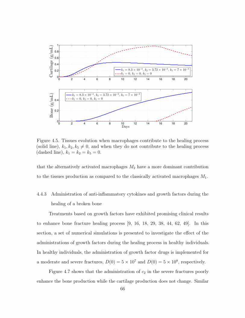
0 2 4 6 8 10 12 14 16 18 200

0.2

0.4

0.6

0.8

1

Cartilage

(g/m

L)

0 2 4 6 8 10 12 14 16 18 200

0.2

0.4

Bon

e(g/m

L)

Days

k1 = 8.3× 10−4, k2 = 3.72× 10−3, k5 = 7× 10−3

k1 = 0, k2 = 0, k5 = 0

k1 = 8.3× 10−4, k2 = 3.72× 10−3, k5 = 7× 10−3

k1 = 0, k2 = 0, k5 = 0

Figure 4.5. Tissues evolution when macrophages contribute to the healing process(solid line), k1, k2, k5 6= 0, and when they do not contribute to the healing process(dashed line), k1 = k2 = k5 = 0.

that the alternatively activated macrophages M2 have a more dominant contribution

to the tissues production as compared to the classically activated macrophages M1.

4.4.3 Administration of anti-inflammatory cytokines and growth factors during the

healing of a broken bone

Treatments based on growth factors have exhibited promising clinical results

to enhance bone fracture healing process [9, 16, 18, 29, 38, 44, 62, 49]. In this

section, a set of numerical simulations is presented to investigate the effect of the

administrations of growth factors during the healing process in healthy individuals.

In healthy individuals, the administration of growth factor drugs is implemented for

a moderate and severe fractures, D(0) = 5× 107 and D(0) = 5× 108, respectively.

Figure 4.7 shows that the administration of c2 in the severe fractures poorly

enhance the bone production while the cartilage production does not change. Similar

66

0 2 4 6 8 10 12 14 16 18 200

0.5

1

Cartilage

(g/m

L)

0 2 4 6 8 10 12 14 16 18 200

0.2

0.4

0.6

Bone(g/m

L)

Days

k1 = 8.3× 10−4, k2 = 3.72× 10−3, k5 = 7× 10−3

k1 = 0, k2 = 3.72× 10−3, k5 = 7× 10−3

k1 = 8.3× 10−4, k2 = 0, k5 = 0

k1 = 8.3× 10−4, k2 = 3.72× 10−3, k5 = 7× 10−3

k1 = 0, k2 = 3.72× 10−3, k5 = 7× 10−3

k1 = 8.3× 10−4, k2 = 0, k5 = 0

Figure 4.6. Tissues evolution when the alternatively activated macrophages, M2, donot contribute to the healing process (dashed line), k2 = 0, and when the classicallyactivated macrophages, M1, do not contribute to the healing process (dotted line),k1 = 0.

0 2 4 6 8 10 12 14 16 18 200

0.2

0.4

0.6

0.8

1

Cartilage

(g/m

L)

0 2 4 6 8 10 12 14 16 18 200

0.05

0.1

0.15

0.2

Bon

e(g/m

L)

Days

k2=3.72× 10

−3

k2=2*3.72× 10

−3

k2=8*3.72× 10

−3

k2=3.72× 10

−3

k2=2*3.72× 10

−3

k2=8*3.72× 10

−3

Figure 4.7. Tissues evolution in a severe fracture under different anti-inflammatorycytokines administration, D(0) = 5× 108.

67

0 2 4 6 8 10 12 14 16 18 200

0.2

0.4

0.6

0.8

Cartilage

(g/m

L)

0 2 4 6 8 10 12 14 16 18 200

0.2

0.4

Bon

e(g/m

L)

Days

k5=7× 10

−3

k5=2*7× 10

−3

k5=8*7× 10

−3

k5=7× 10

−3

k5=2×7× 10

−3

k5=8×7×10

−3

Figure 4.8. Tissues evolution in a moderate fracture under different growth factorconcentration, D(0) = 5× 107.

0 2 4 6 8 10 12 14 16 18 200

0.2

0.4

0.6

0.8

1

Cartilage

(g/m

L)

0 2 4 6 8 10 12 14 16 18 200

0.1

0.2

0.3

0.4

0.5

Bon

e(g/m

L)

Days

k5=7× 10

−3

k5=2*7× 10

−3

k5=8*7× 10

−3

k5=7× 10

−3

k5=2*7× 10

−3

k5=8*7× 10

−3

Figure 4.9. Tissues evolution in a severe fracture under different growth factorconcentration, D(0) = 5× 108.

68

results were obtained for a small and moderate fractures under the administration of

c2. Figure 4.8 shows that the administration of c3 in a moderate fracture slows down

the cartilage productions and improves the bone evolution but in a dose-dependent

manner. Figure 4.9 shows that the administration of c3 in a severe fracture improves

the bone tissue production and barely stimulate the removal of the cartilage.

4.5 Mechanism of the Osteogenic Cell Differentiation

In this section the Model (4.1)-(4.12) is reduced by considering only the dynamics

among the mesenchymal stem cells (Cm), osteoblasts (Cb), and the transforming

growth factor-β (c3). This model simplification leads to have a better understanding

of the regulatory effects of the c3 directing the differentiation of the Cm into Cb. The

modeling reduction is as follow:

dCm

dt= kpmCm

(1− Cm

Klm

)− dmc3Cm (4.13)

dCb

dt= kpbCb

(1− Cb

Klb

)+ dmc3Cm − dbCb (4.14)

dc3dt

= k4Cb − dc3c3, (4.15)

where the differentiation rate of the Cm into Cb is modeled with a linear function with

respect to c3, i.e., F1 = dmc3, and the c3 production rate is modeled with a constant

rate, i.e., H3 = k4.

4.5.1 Qualitative Analysis

The analysis of model (4.13)-(4.15) is done by finding the equilibria and their

corresponding stability properties. An equilibrium point of the model is denoted

by the vector form E(C∗m, C∗b , c∗3) and it is found by setting the right-hand sides

of the equations (4.13)-(4.15) equal to zero [42]. The model has four biologically

69

meaningful equilibria: E0(0, 0, 0), E1(Klm, 0, 0), E2(0, C∗b , c∗3), and E3(C

∗m3, C∗b3 , c

∗33).

Their definitions, existence, and corresponding stability conditions are described in

the following theorems. The existence of each equilibrium point arises from the fact

that all biologically meaningful variables are nonnegative, and their stability analysis

is conducted using the Jacobian of the system at each equilibrium point and finding

its corresponding eigenvalues [42, 60]. Table 4.1 summarizes the equilibria and their

corresponding stability conditions.

Table 4.1. Existence and stability conditions for the equilibrium points.

Equilibrium Points Existence Conditions Local Stability

E0(0, 0, 0) always unstable

E1(Klm, 0, 0) always db > kpb + Klmdmk4dc3

E2(0, C∗b2, c∗32) db < kpb db < kpb

(1− kpmdc3

dmk4Klb

)E3(C

∗m3

, C∗b3 , c∗33) kpb

(1− kpmdc3

dmk4Klb

)< db < kpb + Klm

dmk4dc3

b1b2 − b3 > 0

Theorem 4.5.1. The equilibria E0(0, 0, 0) exists for all the parameters and it is

unstable.

Proof of Theorem 4.5.1. The elements of E0 are non-negative for all the model pa-

rameters, hence E0 always exists. The Jacobian matrix J(E0) is given by the following

sub-triangular matrix:

J(E0) =

kpm 0 0

0 kpb − db 0

0 k4 −dc3

.

Since the eigenvalue λCm = kpm > 0, then E0 is unstable [42].

Theorem 4.5.2. The E1(Klm, 0, 0) exists for all the parameters and is locally stable

if db > kpb + dmk4Klm/dc3 .

70

Proof of Theorem 4.5.2. The E1 exists for all the parameters of the model since their

elements are non-negative. The Jacobian matrix J(E1) is as follows:

J(E1) =

−kpm 0 −dmKlm

0 kpb − db dmKlm

0 k4 −dc3

.

Hence the characteristic polynomial of J(E1) is given by p(λ) = (λ+kpm)(λ2+a1λ+a0),

where a1 = dc3 + (db − kpb) and a0 = dc3(db − kpb) − dmk4Klm. By hypothesis

db − kpb > dmk4Klm/dc3 > 0 therefore a0 > 0 and a1 > 0. By the Routh-Hurwitz

criteria, n = 2, the roots of λ2 + a1λ + a0 are negative or have negative real part.

These imply that E1 is locally stable [42].

Theorem 4.5.3. The E2(0, C∗b , c∗3) exists if kpb > db and it is stable if and only if

kpb > db + dc3kpbkpm/dmk4Klb, where

C∗b = Klb(1− db/kpb), and c∗3 = k4C∗b /dc3 .

Proof of Theorem 4.5.3. By hypothesis kpb > db, hence C∗b and c∗3 are positive and

then E2 is well defined. The Jacobian matrix J(E2) is given by the following triangular

matrix:

J(E2) =

kpm − dmc∗3 0 0

dmc∗3 −kpb + db 0

0 k4 −dc3

.

Since kpm − dmc∗3 = (dc3kpbkpm − dmk4Klb(kpb − db)) /dc3kpb, then, by hypothesis, it

implies that kpm − dmc∗3 < 0. Hence all the eigenvalues of J(E2) are negative values.

Therefore, E2 is locally stable [42].

Theorem 4.5.4. The E3(C∗m3, C∗b3 , c

∗33) exists if kpb (1− kpmdc3/dmk4Klb) < db <

kpb +Klmdmk4/dc3, and is defined as follow

C∗m3=kpm∆

(kpbKlb

+dmk4(db − kpb)

kpmdc3

), C∗b3 =

kpm∆

(dmk4dc3

+kpb − dbKlm

),

71

c∗33 =k4kpmdc3 ∆

(dmk4dc3

+kpb − dbKlm

), ∆ =

(dmk4dc3

)2

+kpmkpbKlmKlb

.

Furthermore, E3 is locally stable if b1b2 − b3 > 0, is unstable if b1b2 − b3 < 0, and is

locally a center if b1b2 − b3 = 0, where b1, b2, b3 are defined as follow:

b1 =kpmC

∗m3

Klm

+kpbC

∗b3

Klb

+dmk4C

∗m3

dc3+ dc3 , b3 = dc3∆C

∗m3C∗b3 ,

b2 =kpmC

∗m3

Klm

(kpbC

∗b3

Klb

+dmk4C

∗m3

dc3+ dc3

)+ dc3

kpbC∗b3

Klb

.

Proof of Theorem 4.5.4. For the first statement of the theorem, notice that the

C∗m3and C∗b3 are monotonic functions with respect to the parameter db. Therefore,

C∗m3> C∗m3

(kpb(1− kpmdc3/dmk4Klb)) = 0, and C∗b3 > C∗b3 (kpb +Klmdmk4/dc3) = 0

for all db in the interval I = (kpb (1− kpmdc3/dmk4Klb) , kpb+Klmdmk4/dc3). Therefore,

C∗m3> 0 and C∗b3 > 0 in I. This also implies that c∗3 > 0 in I. Hence E3 is well

defined and E3 6= Ei, i = 0, 1, 2. Next, for the second statement of the theorem, the

Jacobian matrix J(E3) is given by the following matrix:

J(E3) =

−kpmC∗m3

/Klm 0 −dmC∗m3

dmk4C∗b3dc3 −(kpbC

∗b3/Klb + dmk4C

∗m3/dc3) dmC

∗m3

0 k4 −dc3

.

Hence the polynomial characteristic of J(E3) is given by p(λ) = λ3 + b1λ2 + b2λ+ b3,

where b1, b2, and b3 are defined in the theorem. From the fact that C∗m3> 0 and

C∗b3 > 0, it can be concluded that each bi > 0, i = 0, 1, 2. Therefore, when b1b2−b3 > 0

by Routh-Hurwitz criteria, n = 3, the roots of p(λ) are negative or have negative real

part. Hence E3 is locally stable.

Next, suppose that b1b2 − b3 < 0, it will be proved that E3 is unstable. By the

Descartes’ rule of sign, the polynomial p(λ) does not has positive roots, since bi > 0,

i = 0, 1, 2. Therefore, all the roots of p(λ) are negative or complex. If all of them are

72

negative, then E3 is stable, and then by Routh-Hurwitz criteria, b1b2 − b3 > 0, that

contradicts the hypothesis. Therefore, p(λ) has a negative root, −b, and two complex

conjugate roots, µ± iw, since p(λ) is of degree three. Notice that b > 0 and µ > 0.

Since, if µ < 0 then E3 is stable, and then by Routh-Hurwitz criteria b1b2 − b3 > 0.

This also contradicts the hypothesis. Therefore, µ > 0, and hence E3 is unstable.

Finally, if b1b2 − b3 = 0, the J(E3) has one negative root and two purely

imaginary roots given by: −b1 and ±i√b2. Therefore, E3 is locally a center.

The following corollary provides a sufficient condition to guaranty the stability

of E3.

Corollary 4.5.5. The E3(Cm, Cb, c3) defined in Theorem 4.5.4 is locally stable when

dmk4dc3

≤√

2kpmkpbKlmKlb

.

Proof of Corollary 4.5.5. From the Theorem 4.5.4, it is enough to prove that b1b2 −

b3 > 0. From the definition of each bi, i = 1, 2, 3, it follows that

b1b2 − b3 = −CbCmd2mk24dc3

+2CbCmdc3kpbkpm

KlbKlm+

C3md2mk24kpmd2c3Klm

+2CbC

2mdmk4kpbkpm

dc3KlbKlm

+CbCmdmk4kpb

Klb+

C3mdmk4k2pmdc3K

2lm

+ 2C2mdmk4kpmKlm

+C2

bCmk2pbkpm

K2lbKlm

(4.16)

+C2

b dc3k2pb

K2lb

+CbC

2mkpbk

2pm

KlbK2lm

+Cbd

2c3

kpb

Klb+

C2mdc3k

2pm

K2lm

+Cmd2c3kpm

Klm.

Since Cm > 0 and Cb > 0 then

b1b2 − b3 > −CbCmd

2mk

24

dc3+

2CbCmdc3kpbkpmKlbKlm

= dc3CbCm

(2kpbkpmKlbKlm

− d2mk24

d2c3

),

which from the hypothesis follows that b1b2 − b3 > 0.

The following lemma establishes the number of equilibria of the model (4.13)-

(4.15), and their corresponding stability properties. The proof of the lemma follows

from the Theorems 4.5.1-4.5.4.

73

Lemma 4.5.6. The number of equilibria of the model (4.13)-(4.15) and their stability

properties are stated as follow:

1. there are two equilibria given by E0 and E1 when db > kpb +Klmdmk4/dc3. In

this case, the E0 is unstable, and E1 is locally stable.

2. there are three equilibria given by E0, E1, and E3 when kpb < db < kpb +

Klmdmk4/dc3. In this case, the E0 and E1 are unstable, and E3 is locally stable

if b1b2 − b3 > 0.

3. there are four equilibria given by E0, E1, E2, and E3 when kpb (1− kpmdc3/dmk4Klb) <

db < kpb. In this case, the E0, E1, and E2, are unstable, and E3 is locally stable

if b1b2 − b3 > 0.

4. there are three equilibria given by E0, E1, E2 when db < kpb (1− kpmdc3/dmk4Klb).

In this case, the E0 and E1 are unstable, and E2 is locally stable.

Notice that from Lemma 4.5.6, the number of equilibria and their corresponding

stability changes as the parameter db changes. When the stability of an equilibrium

point E∗ changes in a neighborhood of a parameter µ, the parameter µ is called

bifurcation, and it is said that the system undergoes to a bifurcation at (E∗, µ) [60].

Therefore, the stability of the system (4.13)-(4.15) can be explained by looking at

the bifurcation of each equilibria with respect to the parameter db. Two cases can be

distinguished: (I) the case when b1b2 − b3 > 0 and (II) the case when b1b2 − b3 < 0.

For the case I, from the Lemma 4.5.6, there are two values of db where the

system (4.13)-(4.15) undergoes to a bifurcation: (E1, d1) and (E2, d2), where d1 =

kpb + Klmdmk4/dc3 and d2 = kpb (1− kpmdc3/dmk4Klb). Notice that d2 exists only

when kpmdc3 < dmk4Klb. Figure 4.10 shows the bifurcation diagrams for the steady

state of the variables C∗m and C∗b of the equilibria E1 (red lines), E2 (blue lines) and

E3 (dark lines). The variables for the E0 are omitted since E0 is unstable for all db

values. System (4.13)-(4.15) undergoes to a bifurcation at (E1, d1), since J(E1) has

74

an eigenvalue equal to zero at db = d1, and E1 is stable when db > d1 (red solid line

from the Figure 4.10), and it is unstable when db < d1 (red dashed line from the

Figure 4.10). Results that follow from Lemma 4.5.6 and from the proof of Theorem

4.5.2. System (4.13)-(4.15) undergoes to a bifurcation at (E2, d2), since J(E2) has an

eigenvalue equal to zero, when db = d2, and E2 is stable when db < d2 (blue solid line

at the Figure 4.10), and it is unstable when db > d2 (blue dashed line at the Figure

4.10). Results that follow from Lemma 4.5.6 and from the proof of Theorem 4.5.2.

0 5 10 15

0

2000

4000

6000

8000

10000

C∗ m

db

E1:C

*

m1

E2:C

*

m2

E3:C

*

m3

0 5 10 15

0

2000

4000

6000

8000

10000

C∗ b

db

E1:C

*

b1

E2:C

*

b2

E3:C

*

b3

Figure 4.10. Bifurcation diagram when kpmdc3 < dmk4Klb and b1b2 − b3 > 0: they-axes exhibits the steady state for the MSCs and osteoblasts densities, C∗m and C∗b .The x-axis correspond to the values of the parameter db. Solid lines (stable), dashedlines (unstable). E1 exists for all db, E2 exists when db < kpb, and E3 exists whend1 < db < d2. E1 changes stability at d1 and E2 changes stability at d2.

For the case II, when b1b2−b3 < 0, the stability of E3 changes with respect to db,

where db is defined in the interval I = (kpb (1− kpmdc3/dmk4Klb) , kpb +Klmdmk4/dc3).

Let us introduce the concept of Hopf-bifurcation to show that the stability of E3

changes with respect to db. The system (4.13)-(4.15) undergoes to a Hopf-bifurcation

at (E3, db), if J(E3) has a purely imaginary eigenvalue at db, and the stability of E3

changes in a neighborhood of db (the imaginary part of the complex eigenvalue of

J(E3) smoothly crosses the imaginary axes in a neighborhood of db) [60]. Due to the

75

complexity of the of the expressions of E3 and J(E3) with respect to db for any value of

db in I, we do not provide a theoretical proof of the existence of the Hopf-bifurcation

at (E3, d3), where d3 is a positive root of b1b2−b3, i.e., b1b2−b3(d3) = 0. However from

the explicit expression of b1b2 − b3 given in Equation (4.16) and from the Theorem

4.5.4, it is easy to show that at d3, J(E3) has purely imaginary eigenvalues and the

stability of E3 changes in a neighborhood of d3, as is described below. From the

definition of E3, the equation b1b2 − b3 defines a polynomial of degree three with

respect to db when all the parameters are fixed and db varies in I. Therefore, from

the definition of C∗m3and C∗b3 , it follows that C∗m3

(kpb + Klmdmk4/dc3) = Klm and

C∗b3(kpb + Klmdmk4/dc3) = 0. Hence, in a neighborhood of kpb + Klmdmk4/dc3 the

polynomial b1b2− b3 is positive. Therefore, b1b2− b3 < 0 and b1b2− b3 > 0 in I, which

implies that there exists a value d3 of db such that (b1b2 − b3)(d3) = 0. Hence from

Theorem 4.5.4, J(E3) has purely conjugate imaginary eigenvalue at d3. Furthermore,

it is also expected that E3 changes stability near to d3 since E3 is unstable at db such

that b1b2 − b3 < 0 and E3 is stable at db such that b1b2 − b3 > 0, ensuring that db

belongs in I, see Theorem 4.5.4. Figure 4.11 shows the bifurcation diagram for the

equilibria E3, the plots were obtained from the xpp-auto software, see Appendix for

the codes and parameter values. For these particular set of parameter values, the

system undergoes to a Hopf-bifurcation at two different values of db, (db = 0.4078

and db = 0.4641). Hence E3 changes stability in I, when b1b2 − b3 < 0.

4.5.2 Numerical simulations

In this subsection a set of numerical simulations is presented to support the

theoretical results. Accordingly to the qualitative analysis of the Model (4.13)-

(4.15), there are four equilibria: E0, E1, E2, and E3 where their stability con-

ditions are determined by the bifurcation parameters: d1 = kpb + Klmdmk4/dc3 ,

76

0.05

0.06

0.07

0.08

0.09

0.1

0.11

0.12

CM

0.3 0.35 0.4 0.45 0.5 0.55 0.6

db

0.1

0.11

0.12

0.13

0.14

0.15

0.16

0.17

0.18

0.19

CB

0.3 0.35 0.4 0.45 0.5 0.55 0.6

db

Figure 4.11. Bifurcation diagram when kpmdc3 < dmk4Klb and b1b2 − b3 < 0 obtainedfrom xxpp-auto: the y-axes exhibits the steady state for the MSCs and osteoblastsdensities, C∗m and C∗b . The x-axis correspond to the values of the parameter db.Red-solid line (stable), dark-solid line (unstable).

d2 = kpb (1− kpmdc3/dmk4Klb), and d3 such that d2 < d3 < d1 and d3 is a root of the

polynomial function b1b2 − d3 with respect to db.

To demonstrate the stability of E1, db = 51 and the other parameters are set to

be as the given values from Table 5.1. Since in this case db = 51 > d1 = 50.2202. The

initial conditions are Cm(0) = 1000, Cb(0) = 1000, and c3(0) = 200. Figure 4.12

shows the qualitative behaviors for the MSCs, osteoblasts, and the TGF-β densities

of E1. Here, the MSCs maintain a maximum constant density given by its carrying

capacity Klm = 1× 106 while the osteoblasts and growth factor densities decays to

zero over the time.

The stability of E2 is demonstrated using the following parameter values:

db = 0.1, since then db = 0.1 < kpb

(1− kpmdc3

dmk4Klb

)= 0.218. Figure 4.13 shows the

qualitative behaviors of E2 for the MSCs, osteoblasts, and growth factor. Here, the

MSCs density decays to zero over the time, while the osteoblasts and growth factor

maintain a constant density.

The following parameter values are used to show the existence of a Hopf-

bifurcation for the model (4.13)-(4.15): Klm =10000, kpm = 0.5, dm = 0.1, kpb =

77

10−4

10−3

10−2

10−1

100

101

102

103

104

0

2

4

6

8

10

12x 10

5

MSCs(cells/mL)

10−4

10−3

10−2

10−1

100

101

102

103

104

−500

0

500

1000

1500

2000

2500

Osteo

blasts(cells/mL)

10−4

10−3

10−2

10−1

100

101

102

103

104

−50

0

50

100

150

200

TGF-β(n

g/mL)

Days

Figure 4.12. Cellular and molecular evolution for E1.

0.2202, Klb = 10000, dc3=100, k4=0.05. For this case E3 has a Hopf-biufurcation

at d3 = 5.091, approximately. Figure 4.14 shows how the stability of E3 changes as

the parameter db changes around d3: (a) when db = 5, the trajectory solution of the

system does not converge to E3, it evolves to a limit cycle (boundary of the figure);

(b) when db = 6, the trajectory solution of the system converges to E3.

Figure 4.15 shows the numerical solution for E3, when E3 is stable: db = 6,

that implies b1b2 − b3 < 0. Here, the MSCs, osteoblasts, and growth factors densities

remain constantly over time.

78

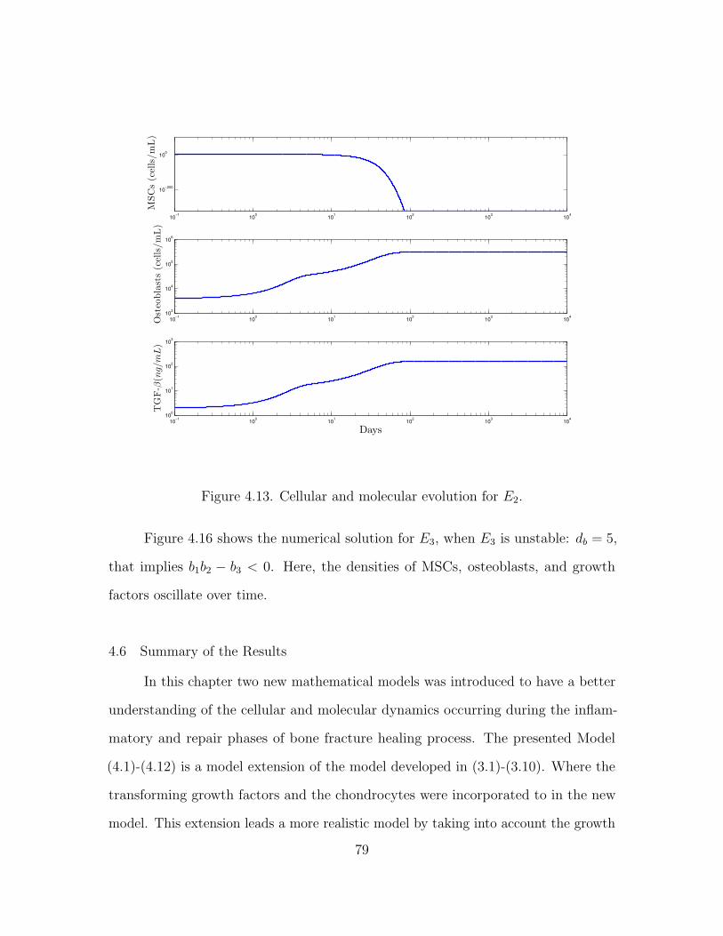
10−1

100

101

102

103

104

10−200

100

MSCs(cells/mL)

10−1

100

101

102

103

104

103

104

105

106

Osteo

blasts(cells/mL)

10−1

100

101

102

103

104

100

101

102

103

TGF-β(n

g/mL)

Days

Figure 4.13. Cellular and molecular evolution for E2.

Figure 4.16 shows the numerical solution for E3, when E3 is unstable: db = 5,

that implies b1b2 − b3 < 0. Here, the densities of MSCs, osteoblasts, and growth

factors oscillate over time.


In this chapter two new mathematical models was introduced to have a better

understanding of the cellular and molecular dynamics occurring during the inflam-

matory and repair phases of bone fracture healing process. The presented Model

(4.1)-(4.12) is a model extension of the model developed in (3.1)-(3.10). Where the

transforming growth factors and the chondrocytes were incorporated to in the new

model. This extension leads a more realistic model by taking into account the growth

79

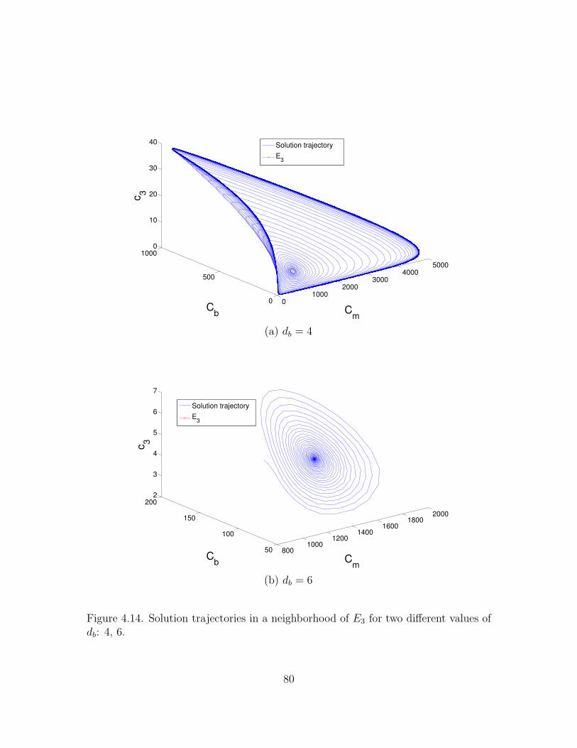
01000

20003000

40005000

0

500

10000

10

20

30

40

Cm

Cb

c3

Solution trajectory

E3

(a) db = 4

8001000

12001400

16001800

2000

50

100

150

2002

3

4

5

6

7

Cm

Cb

c3

Solution trajectory

E3

(b) db = 6

Figure 4.14. Solution trajectories in a neighborhood of E3 for two different values ofdb: 4, 6.

80

100

101

102

103

104

104

105

MSCs(cells/mL)

100

101

102

103

104

100

Osteo

blasts(cells/mL)

100

101

102

103

104

100

TGF-β(n

g/mL)

Days

Figure 4.15. Cellular and molecular evolution for E3, when E3 is stable: b1b2− b3 > 0,db = 6, from 0 to 10000 days.

factor stimuli in the MSCs differentiation, and also to separately model the molecular

production by the different types of cells. Particularly, the three main molecular

production given by the immune cells: the pro- and anti-inflammatory cytokines,

and growth factors was carefully modeled. Hence, allowing to gain a greater degree

of understanding of the immune system functions during the bone fracture healing

process.

The quality analysis of the model showed that the incorporation of c3 and Cc is a

more realistic model, as several new equilibria of the bone fracture healing were found.

The set of equilibria of the new model, Model (4.1)-(4.1), includes the equilibria

obtained in the two previous models, Models (2.1)-(2.1) and (3.1)-(3.1), and other

81

103.95

103.951

103.952

103.953

103.954

103

MSCs(cells/mL)

103.95

103.951

103.952

103.953

103.954

102

Osteo

blasts(cells/mL)

103.95

103.951

103.952

103.953

103.954

101

TGF-β(n

g/mL)

Days

Figure 4.16. Cellular and molecular evolution for E3, when E3 is unstable: db = 4,b1b2 − b3 < 0, from 8900 to 9000 days.

steady-states that captures the endochondral and osteogenic ossification outcomes:

E2, E3, E7, E9, E10. These new equilibria represent nonunion or delayed union,

since in all these cases, the osteoclasts fail to completely remove the fibrocartilage.

Furthermore, base on the qualitative analyzes of the new model, to observe a successful

healing outcome, that is given by the equilibrium E8, it requires not only the stability

conditions founded in the previous model, but also it requires a minimal concentration

of growth factor to secure the successful repair. Therefore, to observe a successful

healing outcome, E8, three conditions must be satisfied: (1) the differentiation rate

of the MSCs into the osteoblasts is bigger than the osteoblast proliferation rate, i.e.,

dm > kpb, (2) the apoptotic rate of the chondrocytes is bigger than the chondrocyte

82

proliferation rate, i.e., dc > kpc, (3) the growth factor production rate over the growth

factor degradation rate is bigger than the half saturation of the growth factor, i.e.,

k4C∗b /dc3 > a33, and (4) the growth factor concentration is above to the concentration

quantity: maxambkpm/(dm − kpm), acbkpc/(dc − kpc). These mathematical condition

finding confirm the numerical results provided in [2], where the authors hypothesized

that there is a minimal concentration of growth factors to secure the healing of a

broken bone.

Furthermore, a new model was introduced, Model (4.13)-(4.15) to have a

better understanding of the regulatory effect of the growth factors during the MSCs

differentiation. Model (4.13)-(4.15) is a model reduction of Model (4.13)-(4.15) and

the model introduced in [2], where only the interaction among the MSCs, osteoblasts,

and growth factors are taking into account. The mathematical analysis of Model

(4.13)-(4.15) exhibited that the stability of the equilibria, nonunion or delayed union

healing outcomes, may change as the parameter values change. These results may

justify the different pathological outcomes of bone fracture healing process, where

unsuccessful and chronic bone healing are observed. Therefore, the stability conditions

of each outcome of the new model can be used to biologically explain why the fracture

healing fails, and to design therapeutic interventions to stimulate or accelerate the

healing process.

Similar numerical results were also obtained when the administration of growth

factors and cytokines are implemented to promote the repair of a broken bone. The

administration of anti-inflammatory cytokines and growth factors fails to accelerate

the healing process in simple fractures, while it accelerates the healing process in

moderate fractures depending on the molecular concentrations, and always improves

the healing process in severe fractures. Furthermore, the numerical results suggested

83

that the administration of growth factors is the most promising therapeutic treatments

to enhance bone formation.

84

CHAPTER 5

CONCLUSION AND FUTURE WORK

Several mathematical and computational models have been recently developed

for modeling the bone fracture healing process. However, none of them have considered

the immune system functions during the healing process [13, 32]. In this work, new

mathematical models were introduced that carefully incorporate the immune system

role in bone fracture healing. The models were used to study the regulatory effects of

the immune system in order to gain a greater degree of understanding of the bone

fracture healing process.

First, the incorporation of the immune system in the models leads to more

realistic numerical results, where the evolution of the fibrocartilage and woven bone

correlates with the experimental data, see Chapter 4. Second, if the immune cells do

not participate in the bone fracture healing process, the healing process evolves into

nonunion or delayed union, Chapter 4; such findings have also been supported by

several experimental results [29, 47, 49]. In addition, in Chapter 1, it was found that

deregulation on the immune system functions leads to nonunion or delayed unions.

Furthermore, more fibrocartilage is produced and less bone tissue is synthesized

when the immune cells lose their capabilities to engulf debris or when the immune

cells deliver high concentration of pro-inflammatory cytokines. In Chapters 2 and

3, it was found that the immune system strongly regulates the evolution of the

bone fracture healing through delivered molecular factors, such as the pro- and

anti-inflammatory cytokines, and growth factors. The numerical simulations revealed

that in small fractures, the immune system does not need additional molecular stimuli

85

to accelerate the healing process. Indeed, if anti-inflammatory or growth factor drugs

are administrated in small fractures, then the drugs negatively affect the progression

of the bone healing. However, the administration of anti-inflammatory or growth

factor drugs in moderate fractures accelerate the healing process in a dose-dependent

manner, and the drugs always improve the healing process in severe fractures or in

immune-compromised people. Such results have been also clinically observed when

corticosteroids and nonsteroidal anti-inflammatory drugs (NSAIDs), or growth factors

drugs are administered in bone fractures [38].

Furthermore, the stability analysis of the model revealed the biological condi-

tions to observe successful healing outcomes. Moreover, the mathematical conditions

obtained through the stability analysis of the models confirmed that a minimal

concentration of growth factors is needed to secure the healing of a broken bone,

Chapter 4. Such result was hypothesized in [2] based on the presented numerical

results. In addition, the presented stability analysis revealed conditions on the model

parameter values that lead to a successful healing outcome evolving into a nonunion.

Therefore, based on the model findings, the immune system is a main factor

that determines the successful outcomes of bone fracture repair. Furthermore, the

concentration of debris must be carefully considered when administration of anti-

inflammatory and growth factor drugs are implemented to enhance the fracture healing

process. In addition, the immune system potentially promotes bone fracture healing in

severe and immune-compromised individuals through the delivered anti-inflammatory

and growth factors.

The presented mathematical models can also be easily adapted to represent

other therapeutic approaches, such as the administration of different tyeps of drugs,

suggesting a variety of possible ways to guide clinical experiments and bone tissue

engineering strategies.

86

Future research directions include modifications of the models by incorporating

additional molecular and cellular interactions, and processes during the inflammatory

and repair phases of fracture healing, such as macrophages and MSCs migration

due to cytokine stimuli, and the incorporation of the osteoclasts. Another research

direction is the incorporation of the bone remodeling phase of the healing process,

which begins at the end of the repair phase and continues long after fracture union.

There are different factors that affect the bone remodeling, including other bone

cells, such as osteoclasts, osteocytes, progenitor cells, and other sources of cytokines

[2, 24, 12]. Therefore, capturing the long-term dynamics of bone fracture healing

requires combining the current model for the inflammatory and repair phases of the

process with other mathematical models that are specifically developed for the bone

remodeling phase of the healing process. This presents a challenging new research

direction in the pursuit to better understand the bone fracture healing process and

the development of new treatment strategies.

87

APPENDIX

In this appendix the parameter values used in the presented models are defined

and described. Table 5.1, summarizes the baseline parameter values and units for

the numerical simulations. These values are estimated in a qualitative manner from

data in other studies [39, 40, 63, 2, 24, 27, 55]. Some of those from [27, 55] were also

rescaled to account for the different mathematical expressions of the proliferation

and differentiation rates of the tissue cells. All parameter values are based on murine

experiments with healthy mice having a moderate fracture (a broken bone with a gap

size less than 3mm) [2, 24]. However, the bone fracture healing process for humans

involves the same cells, cytokines, and qualitative dynamics, differing only in the

number of cells, concentrations, and the length of time it takes for a full recovery [20].

All simulations are obtained by using the adaptive Matlab solver ode23s

and are initiated with densities of debris, macrophages, MSCs, chondrocytes, and

osteoblasts set to D(0) = 5 × 107, M0(0) = 0, M1(0) = 0, M2(0) = 0, Cm(0) = 0,

Cc(0) = 0, Cb(0) = 0, respectively, and the molecular initial concentrations are set

to c1(0) = 0, c2(0) = 0, c3(0) = 20, which represent the densities profiles observed

some minutes after a fracture occurs [2]. Some of the Parameter values given in

[55, 27, 2, 39, 59] were also re-scaled to account for the different mathematical

expressions of the model’s variables.

The following parameter values are used for Model (2.1)-(2.7): Ω1 = k0 =

8.5×10−6; k1 = 8.3×10−6, dc1 = 12.79; kd = 13; aed = 4.71×106; kmax = 0.015;Mmax =

1 × 106; dM = 0.121; km = 0.0015;Klm = 1 × 106; kpm = 0.5; apm =√

10; apm1 =

88

13; dm = 1; amb1 = 0.1; kpb = 0.2202; apb = 10; db = 0.15;Klb = 1 × 106; pcs =

3× 10−7; qcd1 = 3× 10−7; qcd2 = 0.8× 10−7; pbs = 5× 10−8; qbd = 5× 10−8

Table 5.1. Parameter descriptions and units.

Parameter Description Range of values Reference

kd Macrophages phagocytic rate 3− 48/day [39, 34]aed Half-saturation of debris 4.71× 106 cells/mL [39]kmax Maximal migration rate 0.015− 0.1 /day [63, 57]Mmax Maximal macrophages density 6× 105 − 1× 106cells/mL [34, 40]k01 Activation rate of M1 0.55− 0.611 /day [63, 59]k02 Activation rate of M0 to M2 0.0843− 0.3 /day [59]k12 Transition rate from M1 to M2 0.083− 0.075 /day [63, 59]k21 Transition rate from M2 to M1 0.005− 0.05/ day [59]d0 Emigration rate of M0 0.156− 0.02 /day [63, 59]d1 Emigration rate of M1 0.121− 0.2 /day [59, 63, 39]d2 Emigration rate of M2 0.163− 0.2 /day [59, 39, 63]k0 Secretion rate of c1 by debris 5× 10−7 − 8.5× 10−6 ng/cells/day [39]k1 Secretion rate of c1 by M1 macrophages 8.3× 10−6 ng/cells/day [39]k2 Secretion rate of c2 by M2 macrophages 3.72× 10−6 ng/cells/day [39]k3 Secretion rate of c2 by MSCs 7× 10−7 − 8× 10−6 ng/cells/day [27]dc1 Decay rate of c1 12.79− 55 /day [59, 39]dc2 Decay rate of c2 2.5− 4.632 /day [59, 39]a12 Effectiveness of c2 inhibition of c1 synthesis 0.025 ng/mL [59]a22 Effectiveness of c2 inhibition of c2 synthesis 0.1 ng/mL [59]apm Effectiveness of c1 inhibition of Cm proliferation 3.162 ng/mL [27, 3]amb1 Effectiveness of c1 inhibition of Cm differentiation 0.1 ng/mL [27, 21]a01 Half-saturation of c1 to activate M1 0.01 ng/mL [59]a02 Half-saturation of c2 to activate M2 0.005 ng/mL [59]apb Effectiveness of c1 inhibition of Cb proliferation 10 ng/mL [27, 30]apm1 Constant enhancement of c1 to Cm proliferation 13 ng/mL [27, 3]kpm Proliferation rate of Cm 0.5 /day [27]dm Maximal differentiation rate of Cm to Cb 1 /day [2, 27]amb1 Effectiveness of c1 inhibition of Cm differentiation into Cb 10 ng/mL [27, 30]amc1 Effectiveness of c1 inhibition of Cm differentiation into Cc 10 ng/mL [2]amb Half saturation of c3 enhancing Cm differentiation into Cb 10 ng/mL [2]amc Half saturation of c3 enhancing Cm differentiation into Cc 10 ng/mL [2]acb Half saturation of c3 enhancing necroses of Cc 10 ng/mL [2]kpb Proliferation rate of Cb 0.2202 /day [2, 27]db Differentiation rate of Cb 0.15 /day [2, 27]pcs Fibrocartilage synthesis rate 3× 10−6 g/cells/day [2, 27]qcd1 Fibrocartilage degradation rate 3× 10−6 mL/cells/day [2, 27]qcd2 Fibrocartilage degradation rate by osteoclasts 0.2× 10−6 mL/cells/day [2, 27]pbs Bone tissue synthesis rate 5× 10−8 g/cells/day [2, 27]qbd Bone tissue degradation rate 5× 10−8 mL/cells/day [2]Klb Carrying capacity of Cb 1× 106 cells/mL [2, 27]Klm Carrying capacity of Cm 1× 106 cells/mL [2, 27]D(0) Density of necrotic cells 1× 106 − 2× 108 cells/mL [34, 39, 40]

The following parameter values are used for Model (3.1)-(3.10): Ω2 = kd =

13; aed = 4.71 × 106; kmax = 0.015;Mmax = 1 × 106; ke1 = 1; ke2 = 2; k0 = 8.5 ×

10−6; k1 = 8.3 × 10−4; dc1 = 12.79;Klm = 1.0 × 106; kpm = 0.5; apm =√

10; km =

89

0.0015; dm = 1; amb1 = 0.1; pcs = 3 × 10−7; qcd1 = 3 × 10−7; qcd2 = 0.8 × 10−7; pbs =

5×10−8; qbd = 5×10−8; kpb = 0.2202; apb = 10; db = 0.15;Klb = ×106; apm1 = 13; k01 =

0.55; k02 = 0.0843; k12 = 0.083; k21 = 0.005; d0 = 0.156; d1 = 0.121; d2 = 0.163; a12 =

0.025; a22 = 0.1; a01 = 0.01; a02 = 0.005; k2 = 3.72 × 10−4; k3 = 3 × 10−5; k4 =

0.7× 10−4; dc2 = 4.632

For Model (4.1)-(4.12) the parameter values defined in Ω2 and the following

parameter values are used: dmc = 10; dcb = .81; kpc = .8; apc = 3.162; acb1 =

.05; acb = 10; amc = 10; amc1 = .05; amb = 10;Klc = 1e6; dc3 = 10; k5 = 7e−3; k4 =

4e− 3; k6 = 2e− 3; a33 = 10; k2 = 3.72e− 4; k3 = 3e− 5; dc2 = 4.632.

The following parameter values are used for Model (4.13)-(4.15): Ω3 = k5 =

0.05; kpm = 0.5; dmb = dm/amb = 0.1; kpb = 0.2202; db = 0.15; dc3 = 100;Klm = Klb =

×106.

Code for the numerical simulations in the xpp-auto software:

init Cm=0.1 init Cb=0.1 init c3=0.2

par kpm=0.5 dm=1 kpb=0.2202 db=1 dc3=1 kb=3 dCm/dt=kpm*Cm*(1-

Cm)-dm*Cm*c3

dCb/dt=kpb*Cb*(1-Cb)+dm*Cm*c3-db*Cb

dc3/dt=kb*Cb-dc3*c3

@ total=5000,dt=.5, xlo=0, xhi=2, ylo=0.0, yhi=10, zlo=0.0, zhi=10,

bound=8000, maxstor=100000, yp=p, dsmin=1e-5, dsmax=0.002, ds=-.0001,

parmin=.000, parmax=.004, autoxmin=0,

autoymin=0, autoymax=60, nmax=50000, npr=1000, ntst=30,

dsmin=1e-5, dsmax=0.002, ds=-.0001, parmin=0.0, parmax=5, autoxmin=0.0

@autoxmax=5, autoymin=0, autoymax=5,

nmax=50000, npr=1000 @ EPSU=.0000001, EPSS=.0000001,

EPSL=.0000001

90

REFERENCES

[1] Guillermo Arango Duque and Albert Descoteaux. Macrophage cytokines: in-

volvement in immunity and infectious diseases. Frontiers in immunology, 5:491,

2014.

[2] Alicia Bailon-Plaza and Marjolein CH Van Der Meulen. A mathematical frame-

work to study the effects of growth factor influences on fracture healing. Journal

of Theoretical Biology, 212(2):191–209, 2001.

[3] Angela P Bastidas-Coral, Astrid D Bakker, Behrouz Zandieh-Doulabi, Cornelis J

Kleverlaan, Nathalie Bravenboer, Tim Forouzanfar, and Jenneke Klein-Nulend.

Cytokines tnf-α, il-6, il-17f, and il-4 differentially affect osteogenic differentiation

of human adipose stem cells. Stem Cells International, 2016, 2016.

[4] Lena Batoon, Susan Marie Millard, Liza Jane Raggatt, and Allison Robyn Pettit.

Osteomacs and bone regeneration. Current Osteoporosis Reports, 15(4):385–395,

2017.

[5] Wayne A Border and Nancy A Noble. Transforming growth factor β in tissue

fibrosis. New England Journal of Medicine, 331(19):1286–1292, 1994.

[6] Scott P Bruder, David J Fink, and Arnold I Caplan. Mesenchymal stem cells in

bone development, bone repair, and skeletal regenaration therapy. Journal of

cellular biochemistry, 56(3):283–294, 1994.

[7] Aurelie Carlier, Liesbet Geris, Nick van Gastel, Geert Carmeliet, and Hans

Van Oosterwyck. Oxygen as a critical determinant of bone fracture healing—a

multiscale model. Journal of theoretical biology, 365:247–264, 2015.

91

[8] Jean-Marc Cavaillon. Pro-versus anti-inflammatory cytokines: myth or reality.

Cellular and molecular biology (Noisy-le-Grand, France), 47(4):695–702, 2001.

[9] James K Chan, Graeme E Glass, Adel Ersek, Andrew Freidin, Garry A Williams,

Kate Gowers, Ana I Espirito Santo, Rosemary Jeffery, William R Otto, Richard

Poulsom, et al. Low-dose tnf augments fracture healing in normal and osteo-

porotic bone by up-regulating the innate immune response. EMBO molecular

medicine, page e201404487, 2015.

[10] Eunkyung Chung and Youngsook Son. Crosstalk between mesenchymal stem

cells and macrophages in tissue repair. Tissue Engineering and Regenerative

Medicine, 11(6):431–438, 2014.

[11] Rozalia Dimitriou, Eleftherios Tsiridis, and Peter V Giannoudis. Current con-

cepts of molecular aspects of bone healing. Injury, 36(12):1392–1404, 2005.

[12] M Doblare, JM Garcıa, and MJ Gomez. Modelling bone tissue fracture and

healing: a review. Engineering Fracture Mechanics, 71(13):1809–1840, 2004.

[13] LF Echeverri, MA Herrero, JM Lopez, and G Oleaga. Early stages of bone

fracture healing: formation of a fibrin–collagen scaffold in the fracture hematoma.

Bulletin of mathematical biology, 77(1):156–183, 2015.

[14] Thomas A Einhorn. The science of fracture healing. Journal of orthopaedic

trauma, 19(10):S4–S6, 2005.

[15] Thomas A Einhorn and Louis C Gerstenfeld. Fracture healing: mechanisms and

interventions. Nature Reviews Rheumatology, 11(1):45, 2015.

[16] MS Gaston and AHRW Simpson. Inhibition of fracture healing. Bone & Joint

Journal, 89(12):1553–1560, 2007.

[17] Louis C Gerstenfeld, Cory M Edgar, Sanjeev Kakar, Kimberly A Jacobsen, and

Thomas A Einhorn. Osteogenic growth factors and cytokines and their role in

bone repair. pages 17–45, 2007.

92

[18] Mohammad S Ghiasi, Jason Chen, Ashkan Vaziri, Edward K Rodriguez, and

Ara Nazarian. Bone fracture healing in mechanobiological modeling: A review

of principles and methods. Bone Reports, 2017.

[19] E Gibon, F Loi, Luis A Cordova, J Pajarinen, T Lin, L Lu, A Nabeshima, Z Yao,

and Stuart B Goodman. Aging affects bone marrow macrophage polarization:

relevance to bone healing. Regenerative engineering and translational medicine,

2(2):98–104, 2016.

[20] Emmanuel Gibon, Laura Y Lu, Karthik Nathan, and Stuart B Goodman. In-

flammation, ageing, and bone regeneration. Journal of orthopaedic translation,

10:28–35, 2017.

[21] Linda Gilbert, Xiaofei He, Paul Farmer, Scott Boden, Mirek Kozlowski, Janet

Rubin, and Mark S Nanes. Inhibition of osteoblast differentiation by tumor

necrosis factor-α 1. Endocrinology, 141(11):3956–3964, 2000.

[22] Enrique Gomez-Barrena, Philippe Rosset, Daniel Lozano, Julien Stanovici,

Christian Ermthaller, and Florian Gerbhard. Bone fracture healing: cell therapy

in delayed unions and nonunions. Bone, 70:93–101, 2015.

[23] Florian Hoegel, Ahmed Abdulazim, Peter Augat, and Volker Buehren. Quantifi-

cation of reaming debris at the fracture gap of diaphyseal a2 and a3 fractures

after reamed intramedullary nailing of the sheep tibia. European Journal of

Trauma and Emergency Surgery, 34(6):587–591, 2008.

[24] Hanna Isaksson. Recent advances in mechanobiological modeling of bone regen-

eration. Mechanics Research Communications, 42:22–31, 2012.

[25] Paola Italiani and Diana Boraschi. From monocytes to m1/m2 macrophages:

phenotypical vs. functional differentiation. Frontiers in immunology, 5, 2014.

[26] Michael E Joyce, Anita B Roberts, Michael B Sporn, and Mark E Bolander.

Transforming growth factor-beta and the initiation of chondrogenesis and os-

93

teogenesis in the rat femur. The Journal of cell biology, 110(6):2195–2207,

1990.

[27] H V Kojouharov, I Trejo, and B M Chen-Charpentier. Modeling the ef-

fects of inflammation in bone fracture healing. AIP Conference Proceedings,

1895(1):020005, 2017.

[28] Svetlana V Komarova, Robert J Smith, S Jeffrey Dixon, Stephen M Sims,

and Lindi M Wahl. Mathematical model predicts a critical role for osteoclast

autocrine regulation in the control of bone remodeling. Bone, 33(2):206–215,

2003.

[29] Tracy K Kovach, Abhijit S Dighe, Peter I Lobo, and Quanjun Cui. Interactions

between mscs and immune cells: implications for bone healing. Journal of

immunology research, 2015, 2015.

[30] DC Lacey, PJ Simmons, SE Graves, and JA Hamilton. Proinflammatory cy-

tokines inhibit osteogenic differentiation from stem cells: implications for bone

repair during inflammation. Osteoarthritis and Cartilage, 17(6):735–742, 2009.

[31] Florence Loi, Luis A Cordova, Jukka Pajarinen, Tzu-hua Lin, Zhenyu Yao, and

Stuart B Goodman. Inflammation, fracture and bone repair. Bone, 86:119–130,

2016.

[32] Yanfei Lu and Tomasz Lekszycki. Modeling of an initial stage of bone fracture

healing. Continuum Mechanics and Thermodynamics, 27(4-5):851, 2015.

[33] Alberto Mantovani, Silvano Sozzani, Massimo Locati, Paola Allavena, and

Antonio Sica. Macrophage polarization: tumor-associated macrophages as a

paradigm for polarized m2 mononuclear phagocytes. Trends in immunology,

23(11):549–555, 2002.

94

[34] Athanasius FM Maree, Mitsuhiro Komba, Cheryl Dyck, Marek Labkecki, Diane T

Finegood, and Leah Edelstein-Keshet. Quantifying macrophage defects in type

1 diabetes. Journal of theoretical biology, 233(4):533–551, 2005.

[35] Richard Marsell and Thomas A Einhorn. The biology of fracture healing. Injury,

42(6):551–555, 2011.

[36] Brian McKibbin. The biology of fracture healing in long bones. In J Bone Joint

Surg [Br. Citeseer, 1978.

[37] Pedro Moreo, Jose Manuel Garcıa-Aznar, and Manuel Doblare. Bone ingrowth

on the surface of endosseous implants. part 2: Theoretical and numerical analysis.

Journal of theoretical biology, 260(1):13–26, 2009.

[38] Paschalia M Mountziaris and Antonios G Mikos. Modulation of the inflammatory

response for enhanced bone tissue regeneration. Tissue Engineering Part B:

Reviews, 14(2):179–186, 2008.

[39] Sridevi Nagaraja, Anders Wallqvist, Jaques Reifman, and Alexander Y Mitro-

phanov. Computational approach to characterize causative factors and molec-

ular indicators of chronic wound inflammation. The Journal of Immunology,

192(4):1824–1834, 2014.

[40] SIMON L Newman, JANET E Henson, and PETER M Henson. Phagocytosis

of senescent neutrophils by human monocyte-derived macrophages and rabbit

inflammatory macrophages. Journal of Experimental Medicine, 156(2):430–442,

1982.

[41] Bilal Osta, Giulia Benedetti, and Pierre Miossec. Classical and paradoxical

effects of tnf-α on bone homeostasis. Frontiers in immunology, 5:48, 2014.

[42] Sarah P Otto and Troy Day. A biologist’s guide to mathematical modeling in

ecology and evolution. Princeton University Press, 2011.

95

[43] Jukka Pajarinen, Tzuhua Lin, Emmanuel Gibon, Yusuke Kohno, Masahiro

Maruyama, Karthik Nathan, Laura Lu, Zhenyu Yao, and Stuart B Goodman.

Mesenchymal stem cell-macrophage crosstalk and bone healing. Biomaterials,

2018.

[44] Timothy T Roberts and Andrew J Rosenbaum. Bone grafts, bone substitutes

and orthobiologics: the bridge between basic science and clinical advancements

in fracture healing. Organogenesis, 8(4):114–124, 2012.

[45] H Schell, GN Duda, A Peters, S Tsitsilonis, KA Johnson, and K Schmidt-

Bleek. The haematoma and its role in bone healing. Journal of experimental

orthopaedics, 4(1):5, 2017.

[46] Aaron Schindeler, Michelle M McDonald, Paul Bokko, and David G Little. Bone

remodeling during fracture repair: The cellular picture. In Seminars in cell &

developmental biology, volume 19, pages 459–466. Elsevier, 2008.

[47] Claudia Schlundt, Thaqif El Khassawna, Alessandro Serra, Anke Dienelt, Se-

bastian Wendler, Hanna Schell, Nico van Rooijen, Andreas Radbruch, Richard

Lucius, Susanne Hartmann, et al. Macrophages in bone fracture healing: their

essential role in endochondral ossification. Bone, 106:78–89, 2018.

[48] Claudia Schlundt, Hanna Schell, Stuart B Goodman, Gordana Vunjak-Novakovic,

Georg N Duda, and Katharina Schmidt-Bleek. Immune modulation as a ther-

apeutic strategy in bone regeneration. Journal of experimental orthopaedics,

2(1):1, 2015.

[49] Katharina Schmidt-Bleek, Brian J Kwee, David J Mooney, and Georg N Duda.

Boon and bane of inflammation in bone tissue regeneration and its link with

angiogenesis. Tissue Engineering Part B: Reviews, 21(4):354–364, 2015.

[50] Charles N Serhan and John Savill. Resolution of inflammation: the beginning

programs the end. Nature immunology, 6(12):1191–1197, 2005.

96

[51] Jonathan A Sherratt and JD Murray. Models of epidermal wound healing. Proc.

R. Soc. Lond. B, 241(1300):29–36, 1990.

[52] Gilbert Strang, Gilbert Strang, Gilbert Strang, and Gilbert Strang. Introduction

to linear algebra, volume 3. Wellesley-Cambridge Press Wellesley, MA, 1993.

[53] Andrew Stuart and Anthony R Humphries. Dynamical systems and numerical

analysis, volume 2. Cambridge University Press, 1998.

[54] Filip K Swirski, Ingo Hilgendorf, and Clinton S Robbins. From proliferation to

proliferation: monocyte lineage comes full circle. In Seminars in immunopathol-

ogy, volume 36, pages 137–148. Springer, 2014.

[55] Imelda Trejo, Hristo Kojouharov, and Benito Chen-Charpentier. Modeling the

macrophage-mediated inflammation involved in the bone fracture healing process.

Mathematical and Computational Applications, 24(1):12, 2019.

[56] Maria Valenti, Luca Dalle Carbonare, and Monica Mottes. Osteogenic differenti-

ation in healthy and pathological conditions. International journal of molecular

sciences, 18(1):41, 2017.

[57] Ralph Van Furth, Martina MC Diesselhoff-den Dulk, and Herman Mattie. Quan-

titative study on the production and kinetics of mononuclear phagocytes during

an acute inflammatory reaction. Journal of experimental medicine, 138(6):1314–

1330, 1973.

[58] Alessio Giai Via, Antonio Frizziero, and Francesco Oliva. Biological properties of

mesenchymal stem cells from different sources. Muscles, Ligaments and Tendons

Journal, 2(3):154, 2012.

[59] Yunji Wang, Tianyi Yang, Yonggang Ma, Ganesh V Halade, Jianqiu Zhang,

Merry L Lindsey, and Yu-Fang Jin. Mathematical modeling and stability analysis

of macrophage activation in left ventricular remodeling post-myocardial infarction.

BMC genomics, 13(6):S21, 2012.

97

[60] Stephen Wiggins. Introduction to applied nonlinear dynamical systems and chaos,

volume 2. Springer Science & Business Media, 2003.

[61] Andy C Wu, Liza J Raggatt, Kylie A Alexander, and Allison R Pettit. Unraveling

macrophage contributions to bone repair. BoneKEy reports, 2, 2013.

[62] Mengrui Wu, Guiqian Chen, and Yi-Ping Li. Tgf-β and bmp signaling in

osteoblast, skeletal development, and bone formation, homeostasis and disease.

Bone research, 4:16009, 2016.

[63] Tony Yu. Design and validation of a mathematical model to describe macrophage

dynamics in wound healing. PhD thesis, Drexel University, 2014.

[64] Ran Zhang, Yi Liang, and Shuxiang Wei. M2 macrophages are closely associ-

ated with accelerated clavicle fracture healing in patients with traumatic brain

injury: a retrospective cohort study. Journal of orthopaedic surgery and research,

13(1):213, 2018.

98

BIOGRAPHICAL STATEMENT

Imelda Trejo was born in Tasquillo, Hidalgo, Mexico in 1984. She earned her

B.S. and M.S. degrees in Applied Mathematics at the Universidad Autonoma del

Estado de Hidalgo and at the Centro de Investigacion en Matematicas, Guanajuato,

Mexico, in 2008 and 2011, respectively. Her research interests focus on computational

and mathematical modeling of biological systems that include cellular and molecular

dynamics, tissue regeneration, immune system dynamics, uncertainty quantification,

and parametric estimation.

99

modeling the effects of the immune system on bone

Documents

Transcript of modeling the effects of the immune system on bone