Modeling reactive transport in sediments subject to bioturbation and compaction
17
doi:10.1016/j.gca.2005.01.004 Modeling reactive transport in sediments subject to bioturbation and compaction FILIP J. R. MEYSMAN, 1, *BERNARD P. BOUDREAU, 2 and JACK J. MIDDELBURG 1 1 Netherlands Institute of Ecology (NIOO-KNAW), Centre for Estuarine and Marine Ecology, Korringaweg 7, 4401 NT Yerseke, The Netherlands 2 Department of Oceanography, Dalhousie University, Halifax NS B3H 4J1, Canada (Received July 20, 2004; accepted in revised form January 10, 2005) Abstract—Current bioturbation models are marked by confusion in their treatment of porosity. Different equations appear to be needed for different biodiffusion mechanisms, i.e., interphase mixing, where biological activity causes bulk mixing of sediment affecting both tracer and porosity profiles, versus intraphase mixing, where the solid components are intermixed, but the porosity is left unchanged. Another issue is whether the model depends upon the particle type with which tracers are associated, e.g., 137 Cs on small clay particles versus 210 Pb on larger grains. This uncertainty has lead to conflicting conservation equations for radiotracers, and in particular, to the question whether the porosity should be placed inside or outside of the differential term that governs the biodiffusive flux. We have reexamined this situation in the context of multiphase, multicomponent continuum theory. Most importantly, we prove that under the assumption of steady-state porosity, there exists only one correct form of the steady-state conservation equation for a radiotracer, regardless of biodiffusion mechanism and particle type, i.e., x s D B C s x F sed s s C s x s C s 0 where x is depth, C s is the concentration/activity of the tracer, F sed s is the constant flux of solid sediment to the sediment, s is the density of the solid phase, s is the solid volume fraction, D B is the biodiffusion coefficient, and is the decay constant. This pertinent finding results from a substantial revision and extension of diagenetic theory. By considering the conservation of momentum, as well as mass, we have identified the correct reference velocities to define biodiffusional fluxes. From that, we have formulated a consistent set of model equations that govern (1) transient porosity and transient tracer concentrations, (2) steady-state porosity and transient tracer concentrations, and (3) steady-state porosity and steady-state tracer concentrations, in sediments that are subject to both compaction and bioturbation. Copyright © 2005 Elsevier Ltd 1. INTRODUCTION Biodiffusion refers to a mathematical model that treats bio- turbation, the biological mixing of solid sediment particles, as a diffusive process. Biodiffusion has a relatively long lineage in the geochemical literature, reaching back some 40 years to the seminal work of Goldberg and Koide (1962) and its popular- ization by Guinasso and Schink (1975). Since that time the biodiffusion model has been adopted as the standard descrip- tion for solid radiotracer studies in both marine (e.g., Nozaki et al., 1977; Benninger et al., 1979; Cochran, 1985; Henderson et al., 1999) and lacustrine environments (e.g., Robbins et al., 1977; Hancock and Hunter, 1999; Dellapena et al., 2003). Typically, these studies are simple applications of Fick’s Laws to tracer profiles, assuming a mixed layer of constant porosity. However, the surface layer of aquatic sediments exhibits ap- preciable gradients in porosity due to compaction. Bioturbation thus occurs in a deformable porous medium, and accordingly, Berner (1980), Christensen (1982) and Officer (1982) argued that tracer models should account for both bioturbation and compaction effects. Unfortunately, two contradictory forms of such tracer mod- els have been advanced, which account differently for porosity effects. The central point of discussion is whether the volume fraction should be placed inside or outside the partial derivative of the biodiffusion term. Berner (1980) and Christensen (1982) suggested that bioturbation acts to eliminate not only the tracer gradient by mixing, but also the porosity gradient. Accordingly, the flux due to biodiffusion should be stated as J D B s C x (1a) where J is the flux of a solid component being mixed, x is depth, C is the concentration of that component (expressed per unit volume of solid phase), s 1 f is the volume fraction of solids where f is porosity, and D B is the biodiffusion coefficient, which characterizes the intensity of mixing. Berner (1980) and Christensen (1982, 1983) further state that the steady-state conservation equation for a solid radiotracer sub- ject to Eqn. 1a should be of the form x D B s C x s C x s C 0 (1b) where is the decay constant and is termed the “burial rate” (Berner, 1980) or the “sedimentation rate” (Christensen, 1982). Note the non unique terminology that is used to designate the velocity . This imprecision in velocity terminology continues in present day communications (e.g., “sedimentation rate” and “sediment accumulation rate” are frequently used as syn- * Author to whom correspondence should be addressed (f.meysman@ nioo.knaw.nl). Geochimica et Cosmochimica Acta, Vol. 69, No. 14, pp. 3601–3617, 2005 Copyright © 2005 Elsevier Ltd Printed in the USA. All rights reserved 0016-7037/05 $30.00 .00 3601
Transcript of Modeling reactive transport in sediments subject to bioturbation and compaction

Geochimica et Cosmochimica Acta, Vol. 69, No. 14, pp. 3601–3617, 2005Copyright © 2005 Elsevier Ltd
Printed in the USA. All rights reserved
doi:10.1016/j.gca.2005.01.004
Modeling reactive transport in sediments subject to bioturbation and compaction
FILIP J. R. MEYSMAN,1,* BERNARD P. BOUDREAU,2 and JACK J. MIDDELBURG1
1Netherlands Institute of Ecology (NIOO-KNAW), Centre for Estuarine and Marine Ecology, Korringaweg 7, 4401 NT Yerseke, The Netherlands2Department of Oceanography, Dalhousie University, Halifax NS B3H 4J1, Canada
(Received July 20, 2004; accepted in revised form January 10, 2005)
Abstract—Current bioturbation models are marked by confusion in their treatment of porosity. Differentequations appear to be needed for different biodiffusion mechanisms, i.e., interphase mixing, where biologicalactivity causes bulk mixing of sediment affecting both tracer and porosity profiles, versus intraphase mixing,where the solid components are intermixed, but the porosity is left unchanged. Another issue is whether themodel depends upon the particle type with which tracers are associated, e.g., 137Cs on small clay particlesversus 210Pb on larger grains. This uncertainty has lead to conflicting conservation equations for radiotracers,and in particular, to the question whether the porosity should be placed inside or outside of the differentialterm that governs the biodiffusive flux. We have reexamined this situation in the context of multiphase,multicomponent continuum theory. Most importantly, we prove that under the assumption of steady-stateporosity, there exists only one correct form of the steady-state conservation equation for a radiotracer,regardless of biodiffusion mechanism and particle type, i.e.,
�
�x��sDB
�Cs
�x ��Fsed
s
�s
�Cs
�x� �s�Cs � 0
where x is depth, Cs is the concentration/activity of the tracer, Fseds is the constant flux of solid sediment to
the sediment, �s is the density of the solid phase, �s is the solid volume fraction, DB is the biodiffusioncoefficient, and � is the decay constant. This pertinent finding results from a substantial revision and extensionof diagenetic theory. By considering the conservation of momentum, as well as mass, we have identified thecorrect reference velocities to define biodiffusional fluxes. From that, we have formulated a consistent set ofmodel equations that govern (1) transient porosity and transient tracer concentrations, (2) steady-state porosityand transient tracer concentrations, and (3) steady-state porosity and steady-state tracer concentrations, in
0016-7037/05 $30.00 � .00
sediments that are subject to both compaction and bioturbation. Copyright © 2005 Elsevier Ltd
1. INTRODUCTION
Biodiffusion refers to a mathematical model that treats bio-turbation, the biological mixing of solid sediment particles, asa diffusive process. Biodiffusion has a relatively long lineage inthe geochemical literature, reaching back some 40 years to theseminal work of Goldberg and Koide (1962) and its popular-ization by Guinasso and Schink (1975). Since that time thebiodiffusion model has been adopted as the standard descrip-tion for solid radiotracer studies in both marine (e.g., Nozaki etal., 1977; Benninger et al., 1979; Cochran, 1985; Henderson etal., 1999) and lacustrine environments (e.g., Robbins et al.,1977; Hancock and Hunter, 1999; Dellapena et al., 2003).Typically, these studies are simple applications of Fick’s Lawsto tracer profiles, assuming a mixed layer of constant porosity.However, the surface layer of aquatic sediments exhibits ap-preciable gradients in porosity due to compaction. Bioturbationthus occurs in a deformable porous medium, and accordingly,Berner (1980), Christensen (1982) and Officer (1982) arguedthat tracer models should account for both bioturbation andcompaction effects.
Unfortunately, two contradictory forms of such tracer mod-els have been advanced, which account differently for porosityeffects. The central point of discussion is whether the volume
* Author to whom correspondence should be addressed ([email protected]).
3601
fraction should be placed inside or outside the partial derivativeof the biodiffusion term. Berner (1980) and Christensen (1982)suggested that bioturbation acts to eliminate not only the tracergradient by mixing, but also the porosity gradient. Accordingly,the flux due to biodiffusion should be stated as
J � �DB
��sC
�x(1a)
where J is the flux of a solid component being mixed, x isdepth, C is the concentration of that component (expressed perunit volume of solid phase), �s � 1 � �f is the volume fractionof solids where �f is porosity, and DB is the biodiffusioncoefficient, which characterizes the intensity of mixing. Berner(1980) and Christensen (1982, 1983) further state that thesteady-state conservation equation for a solid radiotracer sub-ject to Eqn. 1a should be of the form
�
�x�DB
��sC
�x �����sC
�x� �s�C � 0 (1b)
where � is the decay constant and � is termed the “burial rate”(Berner, 1980) or the “sedimentation rate” (Christensen, 1982).Note the non unique terminology that is used to designate thevelocity �. This imprecision in velocity terminology continuesin present day communications (e.g., “sedimentation rate” and
“sediment accumulation rate” are frequently used as syn-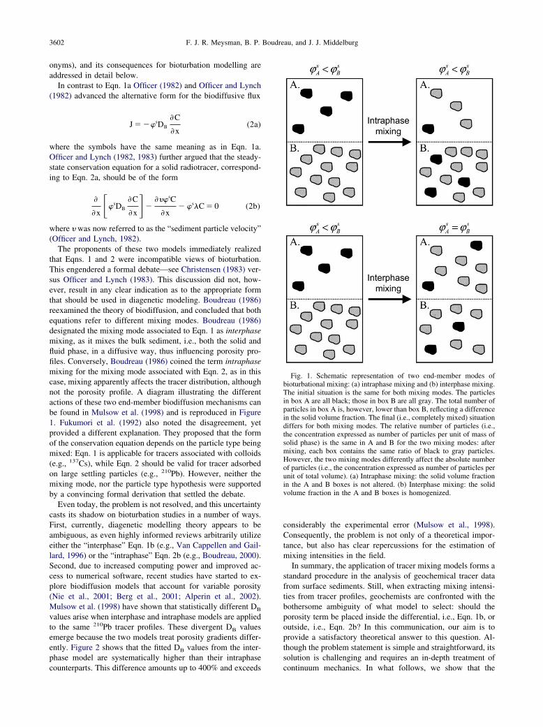
3602 F. J. R. Meysman, B. P. Boudreau, and J. J. Middelburg
onyms), and its consequences for bioturbation modelling areaddressed in detail below.
In contrast to Eqn. 1a Officer (1982) and Officer and Lynch(1982) advanced the alternative form for the biodiffusive flux
J � ��sDB
�C
�x(2a)
where the symbols have the same meaning as in Eqn. 1a.Officer and Lynch (1982, 1983) further argued that the steady-state conservation equation for a solid radiotracer, correspond-ing to Eqn. 2a, should be of the form
�
�x ��sDB
�C
�x����sC
�x� �s�C � 0 (2b)
where was now referred to as the “sediment particle velocity”(Officer and Lynch, 1982).
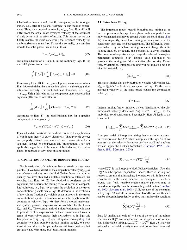
The proponents of these two models immediately realizedthat Eqns. 1 and 2 were incompatible views of bioturbation.This engendered a formal debate—see Christensen (1983) ver-sus Officer and Lynch (1983). This discussion did not, how-ever, result in any clear indication as to the appropriate formthat should be used in diagenetic modeling. Boudreau (1986)reexamined the theory of biodiffusion, and concluded that bothequations refer to different mixing modes. Boudreau (1986)designated the mixing mode associated to Eqn. 1 as interphasemixing, as it mixes the bulk sediment, i.e., both the solid andfluid phase, in a diffusive way, thus influencing porosity pro-files. Conversely, Boudreau (1986) coined the term intraphasemixing for the mixing mode associated with Eqn. 2, as in thiscase, mixing apparently affects the tracer distribution, althoughnot the porosity profile. A diagram illustrating the differentactions of these two end-member biodiffusion mechanisms canbe found in Mulsow et al. (1998) and is reproduced in Figure1. Fukumori et al. (1992) also noted the disagreement, yetprovided a different explanation. They proposed that the formof the conservation equation depends on the particle type beingmixed: Eqn. 1 is applicable for tracers associated with colloids(e.g., 137Cs), while Eqn. 2 should be valid for tracer adsorbedon large settling particles (e.g., 210Pb). However, neither themixing mode, nor the particle type hypothesis were supportedby a convincing formal derivation that settled the debate.
Even today, the problem is not resolved, and this uncertaintycasts its shadow on bioturbation studies in a number of ways.First, currently, diagenetic modelling theory appears to beambiguous, as even highly informed reviews arbitrarily utilizeeither the “interphase” Eqn. 1b (e.g., Van Cappellen and Gail-lard, 1996) or the “intraphase” Eqn. 2b (e.g., Boudreau, 2000).Second, due to increased computing power and improved ac-cess to numerical software, recent studies have started to ex-plore biodiffusion models that account for variable porosity(Nie et al., 2001; Berg et al., 2001; Alperin et al., 2002).Mulsow et al. (1998) have shown that statistically different DB
values arise when interphase and intraphase models are appliedto the same 210Pb tracer profiles. These divergent DB valuesemerge because the two models treat porosity gradients differ-ently. Figure 2 shows that the fitted DB values from the inter-phase model are systematically higher than their intraphase
counterparts. This difference amounts up to 400% and exceedsconsiderably the experimental error (Mulsow et al., 1998).Consequently, the problem is not only of a theoretical impor-tance, but also has clear repercussions for the estimation ofmixing intensities in the field.
In summary, the application of tracer mixing models forms astandard procedure in the analysis of geochemical tracer datafrom surface sediments. Still, when extracting mixing intensi-ties from tracer profiles, geochemists are confronted with thebothersome ambiguity of what model to select: should theporosity term be placed inside the differential, i.e., Eqn. 1b, oroutside, i.e., Eqn. 2b? In this communication, our aim is toprovide a satisfactory theoretical answer to this question. Al-though the problem statement is simple and straightforward, itssolution is challenging and requires an in-depth treatment of
Fig. 1. Schematic representation of two end-member modes ofbioturbational mixing: (a) intraphase mixing and (b) interphase mixing.The initial situation is the same for both mixing modes. The particlesin box A are all black; those in box B are all gray. The total number ofparticles in box A is, however, lower than box B, reflecting a differencein the solid volume fraction. The final (i.e., completely mixed) situationdiffers for both mixing modes. The relative number of particles (i.e.,the concentration expressed as number of particles per unit of mass ofsolid phase) is the same in A and B for the two mixing modes: aftermixing, each box contains the same ratio of black to gray particles.However, the two mixing modes differently affect the absolute numberof particles (i.e., the concentration expressed as number of particles perunit of total volume). (a) Intraphase mixing: the solid volume fractionin the A and B boxes is not altered. (b) Interphase mixing: the solidvolume fraction in the A and B boxes is homogenized.
continuum mechanics. In what follows, we show that the

3603Modeling bioturbation and compaction
present application of continuum theory in early diagenesis ispartly inconsistent and partly incomplete. The inconsistencyrelates to an improper definition of reference velocities forbiodiffusive fluxes. The incompleteness refers to the need for awider perspective in early diagenetic modeling theory. In itspresent form (Berner, 1980; Boudreau, 1997), the theory isexclusively focused on mass conservation. Nevertheless, po-rosity gradients are created by sediment compaction, which isinherently a momentum transfer phenomenon. Thus, the reso-lution of the problem requires the combined application ofmass and momentum conservation to a sediment subject tocompaction, mixing and reactions. As the proper application ofcontinuum theory is central to our discussion, this paper beginswith a detailed exposure of its implementation in early diagen-esis. Subsequently, we revisit the biodiffusion controversy andderive a consistent set of equations to model radiotracers insurface sediments, under both dynamic and steady-state poro-sity conditions.
2. MODEL FORMULATION
2.1. Conservation Equations
Early diagenetic modeling (Berner, 1980; Boudreau, 1997) ispart of the broader theory of continuum physics, which pro-vides a general description for the conservation of mass, mo-mentum, energy, and entropy in natural systems (Truesdell andToupin, 1960; Bear, 1972; Bowen, 1976; Bear and Bachmat,1991; Gray and Hassanizadeh, 1998). However, in its presentform, the reactive transport formalism of diagenetic theory onlyconsiders mass conservation explicitly (Berner, 1980; Bou-dreau, 1997). Accordingly, diagenetic models include one typeof partial differential equation, i.e., the so-called general diage-netic equation as originally advanced by Berner (1980). Thisequation constitutes a particular form of the component massconservation equation from multi-component, multi-phase con-tinuum theory, which is typically written as (Bear and Bach-
Fig. 2. Biodiffusion coefficients DB derived from fitting the inter-phase and intraphase model to the same excess 210Pbxs and solidvolume fraction data profiles from Canadian JGOFS sites. Data ex-tracted from tables 4 and 5 in Mulsow et al. (1998).
mat, 1991)
�
�t��Ci
� ��
�x�Ji
� � Ri � �i
(3)
where � denotes the volume fraction of the -th phase, Ci
represents the concentration of the i-th chemical component inthe -phase, and Ji
denotes the mass flux of this component.For reference, Table 1 provides a list of symbols used in thistext. For simplicity, though without a loss of generality, werestrict this treatment to one dimension; the coordinate x rep-resents depth, which is measured downwards from the sedi-ment-water interface. In the case of aquatic sediments, the-phase can be pore water, solid sediment, or possibly gas.Hereafter, we do not consider a gas phase, and simply representthe sediment as a two-phase system consisting of pore water,denoted the fluid phase “f” which consists of nf chemicalspecies, and the solid sediment matrix, denoted the solid phase“s” which consists of ns chemical species. The volume fractionsof the two phases are related through the constraint of volumeconservation
�f � �s � 1 (4)
The term Ri represents the total production rate of i-th chem-
ical species in the -phase due to both homogeneous andheterogeneous reactions. In its most general form, this term canbe written as a function of volume fractions, concentrations,temperature, time, space, etc., i.e.,
Ri � Ri
�� , Cj , etc.� j � 1, · · · , n � f,s (5)
Here, it is sufficient to assume that proper constitutive equa-tions of the form (5) are available (see Lasaga, 1998 for detailson particular kinetic expressions). The term �i
represents a netsource-sink term due to nonlocal biological transport (Bou-dreau and Imboden, 1987; Meysman et al., 2003). As localdiffusive mixing processes are the main focus of this commu-nication, we will assume that nonlocal transport is absent, i.e.,�i
� 0. This implies no loss of generality.Applying the general conservation principle to the mass of
the -phase as a whole, one obtains the phase mass conserva-tion equation (Bear and Bachmat, 1991)
�
�t���� �
�
�x�J� � R (6)
where � denotes the mass density, J the total mass flux, andR denotes a mass source/sink due to heterogeneous reactionsat solid/fluid interfaces. Note that due to stoichiometric massconservation, homogeneous reactions do not contribute to R.Equally, the stoichiometry of heterogeneous reactions requiresthat the mass reaction terms in the fluid and solid phase must beequal in magnitude and opposite in sign, i.e., Rf � �Rs.
Eqn. 6 is typically referred to as the continuity equation forthe phase. Alternatively, it is also obtained through a mass-weighted summation of individual component mass balances.To this end, we can multiply Eqn. 3 by the molecular mass Mi,and subsequently, sum over all constituents within a phase.Comparing the corresponding terms in both equations, we findthat the mass density �, the mass flux J, and the reaction term
R, are respectively defined as
Intergr
3604 F. J. R. Meysman, B. P. Boudreau, and J. J. Middelburg
� � �i�t
n
MiCi (7)
J � �i�1
n
MiJi (8)
R � �i�1
n
MiRi (9)
The component mass flux Ji is defined in continuum physics as
(Bear and Bachmat, 1991)
Ji � �vi
Ci (10)
where vi denotes the component velocity, that is the average
velocity of all the particles/molecules/ions of the given chem-ical species within a given representative elementary (averag-ing) volume (see also Kirkwood and Crawford, 1952; Curtiss
Table 1. List of symbols used (M � Mass, N
—�, �f, �s —�o
s —��
s —Mi M N�1
Ci N L�3
� � � MiCi M L�3
�̂ � �� M L�3
Ri N L�3 T�1
R �� MiRi M L�3 T�1
�i N L�3 T�1
�i T�1
vi L T�1
Ji � �vi
Ci N L�2 T�1
vref L T�1
�vi � vi
� vref L T�1
Ji,ref � �vref
Ci N L�2 T�1
Ji,dif � Ji
� Ji,dif N L�2 T�1
J � � MiJi M L�2 T�1
Jref � � MiJi,ref
M L�2 T�1
Ji,dif � � MiJi,ref
M L�2 T�1
u � (v)M L T�1
(v)N L T�1
(v)M L T�1
us L T�1
ucomps L T�1
ubios L T�1
� L T�1
L T�1
U � �fuf � �sus L T�1
Fseds M L�2 T�1
�sed � Fseds /(�s�o
s) L T�1
�acc � Fseds /(�s��
s ) L T�1
Jis N L�2 T�1
Ji,comps � �sucomp
s Cis N L�2 T�1
Ji,bios � Ji
s � Ji,comps N L�2 T�1
Js � �MiJis M L�2 T�1
Jcomps � � MiJi,comp
s M L�2 T�1
Jbios � � MiJi,bio
s M L�2 T�1
Di,Bintra L�2 T�1
DBinter L�2 T�1
Di,B � Di,Bintra � DB
inter L�2 T�1
Is M L�2
� M L�1 T�1
k, kbio L2
g L T�2
�=, �=bio M L�1 T�2
and Bird, 1999). Based on Eqn. 10, we can now introduce the
mass-averaged or barycentric velocity of a phase as (Bear andBachmat, 1991; Bird et al., 2002, p. 533),
�v�M �J
���
�i�1
n
MiJi
�i�1
n
Mi�Ci
�1
� �i�1
n
MiviCi
(11)
where (v)M designates the mass-weighted averaging proce-dure. To obtain the equality on the right-hand side of Eqn. 11,we have used Eqns. 7 and 10. To reduce the notational burden,and to emphasize the difference between component and phasevelocities, we will use the shorthand notation u � (v)M
hereafter. In analogy to Eqn. 10, the phase mass flux can nowbe written as
mber of particles, L � Length, T � Time).
indicator (f � fluid; s � solid)e fraction phase , porosity, solid volume fractionfree solid volume fractiontotic solid volume fraction
ular massntration of species i in phase y of phase ntration of phase on rate of species i in phase eaction rate in phase al transport rate of species i in phase constantnent velocity
f species i in phase nce velocity (species independent)ty deviation in a given reference frametive flux of species i in phase in a given reference frameive flux of species i in phase in a given reference frame
ass flux in phase dvective flux in phase for a given reference frameiffusive flux in phase for a given reference frameveraged velocityaveraged velocitye-averaged velocityveraged velocityction velocity
bation velocitytive velocity in “interphase” equation of Christensen (1982)tive velocity in “intraphase” equation of Officer and Lynch (1982)e-averaged velocity of the bulk sedimententation rateentation velocityent accumulation velocityux of solid species i
tive flux of solid species i with respect to the compaction velocityfusive flux of solid species i with respect to the compaction velocity
ass flux in the solid phasetive flux in the solid phase with respect to the compaction velocityfusive flux in the solid phase with respect to the compaction velocityase biodiffusion coefficient (species dependent)ase biodiffusion coefficient (species independent)iodiffusion coefficient (species dependent)
ory of solidsity of the pore waterabilitiesational accelerationanular stress
� Nu
PhaseVolumStress-AsympMolecConceDensitConceReactiTotal rNonlocDecayCompoFlux oRefereVelociAdvecDiffusTotal mTotal aTotal dMass-aMolar-VolumMass-aCompaBioturAdvecAdvecVolumSedimSedimSedimTotal flAdvecBiodifTotal mAdvecBiodifIntraphInterphTotal bInventViscosPermeGravit
J � �u� (12)

3605Modeling bioturbation and compaction
Substitution of Eqn. 12 into the phase mass balance Eqn. 6results in
�
�t���� �
�
�x��u�� � R (13)
For a typical early diagenetic setting, Eqn. 13 can be simplified.First, the bulk mass transfer due to heterogeneous reactions isgenerally small, although major exceptions can occur withextensive and rapid dissolution of minerals. Neglecting thisheterogeneous mass transfer, Eqn. 13 now reads
�
�t���� �
�
�x��u�� � 0 (14)
Second, in most early diagenetic situations the density of boththe pore water and the solid phases are relatively constant(Berner, 1980). Only in some special situations, such as saltdissolution and brine-freshwater mixing, does the phase densitychange significantly. The assumption of constant phase densityis an important simplification, which implies that each phase isincompressible. Note that even when each phase is consideredincompressible, the sediment mixture itself remains compress-ible as long as the phases can move relative to each other, i.e.,squeezing the pore water from between the solid grains. Withthe incompressibility constraint, the mass balance equationEqn. 14 for each phase reduces to a conservation statement forthe corresponding volume fraction
��
�t�
�
�x��u� � 0 (15)
Eqn. 15 can be used to calculate phase volume fractions,provided an expression for the mass-averaged velocity u isavailable (Berner, 1980; Boudreau, 1997). If Eqn. 15 issummed for both sediment phases, the term
�
�t��f � �s�
vanishes because of volume conservation, i.e. Eqn. 4. Thus, weobtain
�
�x��fuf � �sus� �
�U
�x� 0 (16)
The quantity U � �fuf � �sus represents the volume averagevelocity of the bulk sediment mixture and, as such, has units ofvelocity. The quantity U plays an important role in the theorygiven below. Interestingly, it may also be interpreted as thevolume flux of bulk sediment and Eqn. 16 informs us that U isindependent of depth.
2.2. Constitutive Theory: The Diffusive Formulation
Mass conservation statements, such as Eqn. 3, lead to amathematically underdetermined problem because each equa-tion contains two unknown variables, i.e., the concentration Ci
and the component velocity vi. In principle there are two
distinct approaches to resolve this indeterminacy: either in-crease the number of conservation equations, or introduce
additional constitutive expressions that relate the variables. Asan example of the first approach, we could introduce a momen-tum balance equation for each component, thereby defining thevelocities vi
. The resulting set of equations is known as aStefan-Maxwell problem (Taylor and Krishna, 1993), and someauthors have explored this approach in a geochemical context(e.g., Kirwan and Kump, 1987; Hassanizadeh, 1996). However,the far more common approach is to add constitutive equations,specifically by introducing diffusive fluxes. This is the conven-tional approach adopted in early diagenesis (Berner, 1980;Boudreau, 1997), as well as in other reactive transport disci-plines, such as groundwater geochemistry, contaminant hydrol-ogy, mineral-rock interactions, and petroleum engineering(Huyakorn and Pinder, 1983; Lichtner, 1985; Steefel and Mac-Quarrie, 1996). These additional “diffusive” constitutive ex-pressions reduce the number of variables in the model, againresolving the indeterminacy.
The term “diffusion” should be adopted with care, as differ-ent interpretations are employed by different disciplines. Incontinuum mechanics, the diffusive flux Ji,dif
is formally de-fined as the deviation of the actual component flux Ji
fromsome reference flux Ji,ref
. This reference flux is defined as Ji,ref
� �vref Ci
, where vref is a reference velocity that is the same
for all constituents within a given phase. Accordingly, thediffusive flux can be written as
Ji,dif � Ji
� Ji,ref � Ji
� �vref Ci
� �Ci�vi
� vref � � �Ci
�vi
(17)
where the velocity deviation �vi is introduced as the deviation
of the component velocity from the reference velocity, i.e. �vi
� (vi � vref
). The choice of vref defines the diffusion reference
frame, and it should not be confused with the geometric refer-ence frame, i.e. the coordinate system x that is employed in themodel. Substitution of Eqn. 17 into the component conserva-tion Eqn. 3 removes the unknown component velocities
�
�t��Ci
� ��
�x�Ji,dif
� �vref Ci
� � Ri (18)
Note that, using the molecular mass as a weighing factor, theweighted summation of Eqn. 18 yields
�
�t���� �
�
�x�Jdif
� �vref �� � R (19)
where the diffusive phase mass flux Jdif is defined as
Jdif � �
i�1
n
MiJi,dif (20)
Comparing Eqns. 14 and 19, or alternatively, by weightedsummation of Eqn. 17, one finds that J � Jdif
� �vref �.
The number of model variables can be reduced properly ifthe diffusion terms can be expressed solely in terms of theremaining concentration variables � , Cj
, or their derivatives,i.e.,
Ji,dif � f�� , Cj
, � � , � Cj , · · ·� j � 1, · · · , n � f,s
(21)
The mathematical form of the function f (Ê) in Eqn. 21
depends on the specific “diffusive” phenomenon in question.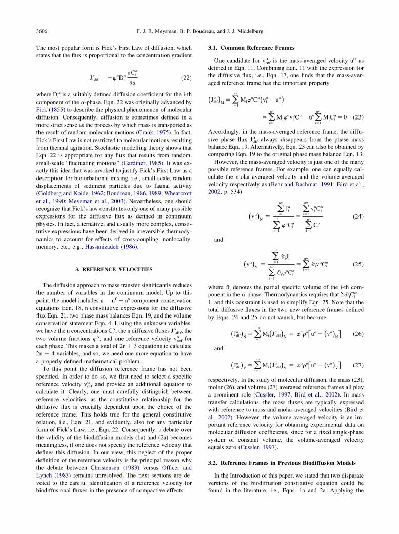
3606 F. J. R. Meysman, B. P. Boudreau, and J. J. Middelburg
The most popular form is Fick’s First Law of diffusion, whichstates that the flux is proportional to the concentration gradient
Ji,dif � ��Di
�Ci
�x(22)
where Di is a suitably defined diffusion coefficient for the i-th
component of the -phase. Eqn. 22 was originally advanced byFick (1855) to describe the physical phenomenon of moleculardiffusion. Consequently, diffusion is sometimes defined in amore strict sense as the process by which mass is transported asthe result of random molecular motions (Crank, 1975). In fact,Fick’s First Law is not restricted to molecular motions resultingfrom thermal agitation. Stochastic modelling theory shows thatEqn. 22 is appropriate for any flux that results from random,small-scale “fluctuating motions” (Gardiner, 1985). It was ex-actly this idea that was invoked to justify Fick’s First Law as adescription for bioturbational mixing, i.e., small-scale, randomdisplacements of sediment particles due to faunal activity(Goldberg and Koide, 1962; Boudreau, 1986, 1989; Wheatcroftet al., 1990; Meysman et al., 2003). Nevertheless, one shouldrecognize that Fick’s law constitutes only one of many possibleexpressions for the diffusive flux as defined in continuumphysics. In fact, alternative, and usually more complex, consti-tutive expressions have been derived in irreversible thermody-namics to account for effects of cross-coupling, nonlocality,memory, etc., e.g., Hassanizadeh (1986).
3. REFERENCE VELOCITIES
The diffusion approach to mass transfer significantly reducesthe number of variables in the continuum model. Up to thispoint, the model includes n � nf � ns component conservationequations Eqn. 18, n constitutive expressions for the diffusiveflux Eqn. 21, two phase mass balances Eqn. 19, and the volumeconservation statement Eqn. 4. Listing the unknown variables,we have the n concentrations Ci
, the n diffusive fluxes Ji,dif , the
two volume fractions �, and one reference velocity vref for
each phase. This makes a total of 2n � 3 equations to calculate2n � 4 variables, and so, we need one more equation to havea properly defined mathematical problem.
To this point the diffusion reference frame has not beenspecified. In order to do so, we first need to select a specificreference velocity vref
and provide an additional equation tocalculate it. Clearly, one must carefully distinguish betweenreference velocities, as the constitutive relationship for thediffusive flux is crucially dependent upon the choice of thereference frame. This holds true for the general constitutiverelation, i.e., Eqn. 21, and evidently, also for any particularform of Fick’s Law, i.e., Eqn. 22. Consequently, a debate overthe validity of the biodiffusion models (1a) and (2a) becomesmeaningless, if one does not specify the reference velocity thatdefines this diffusion. In our view, this neglect of the properdefinition of the reference velocity is the principal reason whythe debate between Christensen (1983) versus Officer andLynch (1983) remains unresolved. The next sections are de-voted to the careful identification of a reference velocity for
biodiffusional fluxes in the presence of compactive effects.3.1. Common Reference Frames
One candidate for vref is the mass-averaged velocity u as
defined in Eqn. 11. Combining Eqn. 11 with the expression forthe diffusive flux, i.e., Eqn. 17, one finds that the mass-aver-aged reference frame has the important property
�Jdif �M � �
i�1
n
Mi�Ci
�vi � u�
� �i�1
n
Mi�vi
Ci � u�
i�1
n
MiCi � 0 (23)
Accordingly, in the mass-averaged reference frame, the diffu-sive phase flux Jdif
always disappears from the phase massbalance Eqn. 19. Alternatively, Eqn. 23 can also be obtained bycomparing Eqn. 19 to the original phase mass balance Eqn. 13.
However, the mass-averaged velocity is just one of the manypossible reference frames. For example, one can equally cal-culate the molar-averaged velocity and the volume-averagedvelocity respectively as (Bear and Bachmat, 1991; Bird et al.,2002, p. 534)
�v�N ��i�1
n
Ji
�i�1
n
�Ci
��i�1
n
viCi
�i�1
n
Ci
(24)
and
�v�V ��i�1
n
�iJi
�i�1
n
�i�Ci
� �i�1
n
�iviCi
(25)
where �i denotes the partial specific volume of the i-th com-ponent in the -phase. Thermodynamics requires that ��iCi
�1, and this constraint is used to simplify Eqn. 25. Note that thetotal diffusive fluxes in the two new reference frames definedby Eqns. 24 and 25 do not vanish, but become
�Jdif �N � �
i�1
n
Mi�Ji,dif �N � ���u � �v�N� (26)
and
�Jdif �V � �
i�1
n
Mi�Ji,dif �V � ���u � �v�V� (27)
respectively. In the study of molecular diffusion, the mass (23),molar (26), and volume (27) averaged reference frames all playa prominent role (Cussler, 1997; Bird et al., 2002). In masstransfer calculations, the mass fluxes are typically expressedwith reference to mass and molar-averaged velocities (Bird etal., 2002). However, the volume-averaged velocity is an im-portant reference velocity for obtaining experimental data onmolecular diffusion coefficients, since for a fixed single-phasesystem of constant volume, the volume-averaged velocityequals zero (Cussler, 1997).
3.2. Reference Frames in Previous Biodiffusion Models
In the Introduction of this paper, we stated that two disparateversions of the biodiffusion constitutive equation could be
found in the literature, i.e., Eqns. 1a and 2a. Applying the
3607Modeling bioturbation and compaction
theory from the previous sections, it is insightful at this point,to identify the reference velocity that is implicitly employed inthese formulations. Starting with Eqn. 2, the presentations inOfficer (1982) and Officer and Lynch (1983) contain a “sedi-ment particle velocity” . This velocity can be equated to themass-averaged velocity us as defined above. To verify thisstatement, we note that Officer and Lynch (1983) define thetotal flux of a component as
Jis � �sCi
s � �sDB
�Cis
�x(28)
using our notation. If we now sum Eqn. 28 over all solidcomponents, we find that
Js � �i�1
ns
MiJis � �s�s � �sDB
��s
�x� �s�s (29)
because of the assumed incompressibility of the solid phase. Bycomparing Eqns. 12 and 29, we obtain that
�Js
�s�s� us (30)
which readily demonstrates that Officer’s velocity in Eqn. 28can be interpreted as the mass-averaged velocity of thesolids us.
Conversely, the total flux in the Berner (1980) and Chris-tensen (1982) treatments has the form
Jis � �s�Ci
s � DB
��sCis
�x(31)
The reference velocity � was termed the “sedimentation rate”by Christensen (1982), while Berner (1980) called it the “burialvelocity.” Carrying out a similar summation as for Eqn. 28, oneobtains
Js � �i�1
ns
MiJis � �s��s � �sDB
��s
�x(32)
Eqn. 32 is not the same as Eqn. 29, and this is the basis for thedisagreement between Christensen (1983) and Officer andLynch (1983). Comparison of Eqns. 12 and 32 leads to therelation
� � us �DB
�s
��s
�x(33)
Therefore, when porosity gradients are present, the velocity �is not equivalent to the mass-averaged velocity us. As a con-sequence, the biodiffusional flux as defined by Eqn. 1a cannotbe regarded as a diffusive flux in the mass-averaged referenceframe; consequently, the problem remains to properly interpretthe velocity �.
4. GENERAL NON-STEADY-STATE MODEL FORVOLUME FRACTIONS AND TRACER CONCENTRATIONS
The above model comparison illustrates the need for theidentification of a logically consistent reference velocity tocharacterize the mixing of sediments. From Eqns. 28 to 33 it is
also clear that the mass-averaged velocity plays a pivotal role.This should be not so surprising, as the mass-averaged refer-ence frame claims a special status in continuum mechanics.This is because the mass-averaged velocity also features in theother conservation equations of momentum, energy, and en-tropy (Bear and Bachmat, 1991; Bird et al., 2002). Compactiontheory, which is a subdiscipline of continuum mechanics, de-scribes the self-weight consolidation of soil and sedimentsspecifically based on the mass-averaged reference frame(Fowler and Noon, 1999; Bustos et al., 1999). In the nextsections, our aim is to derive a general, non-steady-state modelthat governs the volume fractions and tracer concentrations ina sediment that is subject to both compaction and bioturbation.Accordingly, we will need to relate the mass-averaged velocityused in compaction theory to the reference velocities 30 and 33that are used in biodiffusion models. To this end, we willproceed in a sequential fashion. As a reference case, we willfirst calculate the mass-averaged velocity in a compactingsediment that is not subject to bioturbation. Subsequently, wewill examine how bioturbational mixing modifies this mass-averaged velocity.
4.1. Phase Momentum Balance without Bioturbation
Sediment compaction involves stresses and flows, and hence,in addition to mass conservation, the problem must be analyzedin terms of momentum conservation. This combined mass-momentum approach is employed in the geotechnical literature,i.e., in the study of settling and consolidation of cohesivesediments (e.g., Toorman, 1996; Bustos et al., 1999) and thecompaction of sedimentary basins (Biot, 1941; Fowler andNoon, 1999). Its full derivation, starting from the momentumconservation equations for both solids and fluids, includingdetails of all simplifying assumptions, can be found in reviewson compaction theory (e.g., Bustos et al., 1999; Fowler andNoon, 1999). Here, we only provide a cursory overview, fo-cusing on the aspects that are relevant to the present problem.See also Meysman (2001) for a detailed development of themomentum equations for both the pore water and the solidsediment in the context of early diagenesis.
When inertial effects can be ignored, the momentum conser-vation equation for the bulk sediment reduces to a balance ofstatic forces, known as the saturated soil stress balance (Ter-zaghi, 1942; Gibson, 1958; Toorman, 1996; Boudreau andBennett, 1999). This equation describes how the effective stresson each layer of particles results from the downward force dueto the buoyant weight of the particles, decreased by an upwarddrag force due to flow of the fluid relative to the solids. In adifferential form, the saturated soil stress balance is given by(Toorman, 1996)
���′
��s·��s
�x� �sg��s � �f� �
�
k�f�uf � us� (34)
where �= represents the inter-granular stress, g the gravitationalconstant, � the dynamic viscosity of the pore water, and k thepermeability of the sediment. Eqn. 34 illustrates the central roleof the mass-averaged reference frame in continuum mechanics;the saturated soil stress balance is formulated as a function ofthe mass-averaged velocity, though not the molar or volume-
averaged velocity. Using the definition of the total volume flux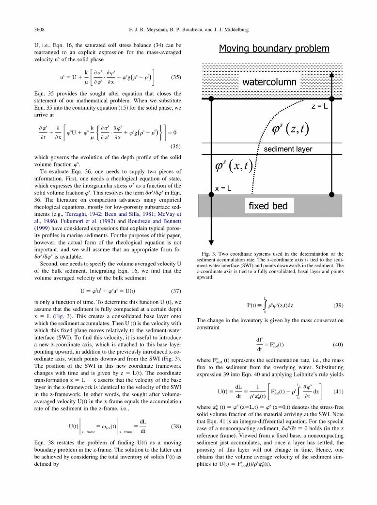
3608 F. J. R. Meysman, B. P. Boudreau, and J. J. Middelburg
U, i.e., Eqn. 16, the saturated soil stress balance (34) can berearranged to an explicit expression for the mass-averagedvelocity us of the solid phase
us � U �k
����′
��s·��s
�x� �sg��s � �f�� (35)
Eqn. 35 provides the sought after equation that closes thestatement of our mathematical problem. When we substituteEqn. 35 into the continuity equation (15) for the solid phase, wearrive at
��s
�t�
�
�x ��sU � �sk
���′
��s·��s
�x� �sg��s � �f��� 0
(36)
which governs the evolution of the depth profile of the solidvolume fraction �s.
To evaluate Eqn. 36, one needs to supply two pieces ofinformation. First, one needs a rheological equation of state,which expresses the intergranular stress �= as a function of thesolid volume fraction �s. This resolves the term ��=/��s in Eqn.36. The literature on compaction advances many empiricalrheological equations, mostly for low-porosity subsurface sed-iments (e.g., Terzaghi, 1942; Been and Sills, 1981; McVay etal., 1986). Fukumori et al. (1992) and Boudreau and Bennett(1999) have considered expressions that explain typical poros-ity profiles in marine sediments. For the purposes of this paper,however, the actual form of the rheological equation is notimportant, and we will assume that an appropriate form for��=/��s is available.
Second, one needs to specify the volume averaged velocity Uof the bulk sediment. Integrating Eqn. 16, we find that thevolume averaged velocity of the bulk sediment
U � �fuf � �sus � U�t� (37)
is only a function of time. To determine this function U (t), weassume that the sediment is fully compacted at a certain depthx � L (Fig. 3). This creates a consolidated base layer ontowhich the sediment accumulates. Then U (t) is the velocity withwhich this fixed plane moves relatively to the sediment-waterinterface (SWI). To find this velocity, it is useful to introducea new z-coordinate axis, which is attached to this base layerpointing upward, in addition to the previously introduced x-co-ordinate axis, which points downward from the SWI (Fig. 3).The position of the SWI in this new coordinate frameworkchanges with time and is given by z � L(t). The coordinatetransformation z � L � x asserts that the velocity of the baselayer in the x-framework is identical to the velocity of the SWIin the z-framework. In other words, the sought after volume-averaged velocity U(t) in the x-frame equals the accumulationrate of the sediment in the z-frame, i.e.,
U�t��x�frame
� �acc(t)�z�frame
�dL
dt(38)
Eqn. 38 restates the problem of finding U(t) as a movingboundary problem in the z-frame. The solution to the latter canbe achieved by considering the total inventory of solids Is(t) as
defined byIs�t� � �0
L
�s�s(z,t)dz (39)
The change in the inventory is given by the mass conservationconstraint
dIs
dt� Fsed
s (t) (40)
where Fseds (t) represents the sedimentation rate, i.e., the mass
flux to the sediment from the overlying water. Substitutingexpression 39 into Eqn. 40 and applying Leibnitz’s rule yields
U�t� �dL
dt�
1
�s�0s(t) �Fsed
s (t) � �s�0
L ��s
�tdz� (41)
where �0s (t) � �s (z�L,t) � �s (x�0,t) denotes the stress-free
solid volume fraction of the material arriving at the SWI. Notethat Eqn. 41 is an integro-differential equation. For the specialcase of a noncompacting sediment, ��s/�t � 0 holds (in the zreference frame). Viewed from a fixed base, a noncompactingsediment just accumulates, and once a layer has settled, theporosity of this layer will not change in time. Hence, oneobtains that the volume average velocity of the sediment sim-
Fig. 3. Two coordinate systems used in the determination of thesediment accumulation rate. The x-coordinate axis is tied to the sedi-ment-water interface (SWI) and points downwards in the sediment. Thez-coordinate axis is tied to a fully consolidated, basal layer and pointsupward.
plifies to U(t) � Fseds (t)/�s�0
s(t).
3609Modeling bioturbation and compaction
Eqns. 36 and 41, in combination with a particular choice ofthe rheological equation of state, ��=/��s, form a completemathematical statement of the compaction problem (Fowlerand Noon, 1999). Starting from some initial condition �s(x, 0),these equations specify how the depth profile of the solidvolume fraction �s (x, t) evolves as a function of time. See, forexample Bustos et al. (1999) for the solution under conditionsof batch sedimentation, i.e., Fsed
s (t) � 0, or for a constant rainof solid material, i.e., Fsed
s (t) � F0.
4.2. A Reference Velocity with Compaction andBioturbation
In the previous section, we considered a sediment that issolely subject to compaction, and not influenced by bioturba-tion, referred to hereafter as the “C only” situation. CombiningEqns. 12 and 35, we find that the total flux of solids through acertain horizon at depth x from the SWI, is given by
Js � Jcomps � �s�sucomp
s
� �s�sU �k
����′
��s·��s
�x� �sg��s � �f��(42)
The subscript “comp” has been used to emphasize that the solidphase flux is only due to compaction and sedimentation.Equally, the mass-averaged velocity is only due to compactionand sedimentation, i.e.,
us �Js
�s�s� ucomp
s (43)
We now need to consider the question of the change in the solidphase flux Js that results from the presence of bioturbatingorganisms, hereafter referred to as the “C � B” situation.
To answer this question, consider the following thoughtexperiment, which involves two identical sediment setups Aand B that are subject to compaction and bioturbation. If onetakes a snapshot of the solid volume fraction profile at a giventime t, one would obtain the same �obs
s (x, t) profile in bothsetups, since we have assumed that the history of both setups iscompletely identical. At that same time t, we annihilate thebioturbation activity in the B setup by a fast-working and fastspreading poison, while the A setup is left as it is. Using �obs
s
(x, t) as the initial condition, Eqn. 35 then calculates the“compaction velocity,” i.e., the velocity that is induced uponthe solid phase resulting from compaction. This calculation ispossible for both setups. In other words, Eqn. 35 will yielducomp
s (x, t) in the B setup (“C only”) and in the A setup (“C� B”). The difference between both setups lies in the relationbetween the calculated compaction velocity and the mass-averaged velocity. In the B setup (“C only”), compaction is theonly process that causes mass transfer of solids, and hence, themass-averaged velocity equals the compaction velocity, i.e., us
� ucomps . In other words, Eqn. 35 can be substituted into the
continuity equation (15) for the solid phase, so one arrives atEqn. 36, which then governs the evolution of the solid volumefraction in B setup for times t= t. Conversely, in the A setup(“C � B”), there may be an additional flux of solid material dueto bioturbation, and so the mass-averaged velocity cannot not
equal the compaction velocity, i.e., us ucomps . Based on �obss
(x, t), Eqn. 35 can still be used to calculate that fraction of themass-averaged velocity that is due to compaction. However,because there may be an additional flux of solid material due tobioturbation, Eqn. 35, cannot be substituted into the continuityequation (15) for the solid phase as such, but must be firstcorrected for bioturbation. As a consequence, Eqn. 36 is nolonger valid in the “C � B” case.
Our thought experiment reveals that in the “C � B” situa-tion, the total solid flux results from a superposition of the twoseparate effects, i.e., compaction and bioturbation. In otherwords, the total solid flux can be split into two separate com-ponents
Js � Jcomps � Jbio
s (44)
where Jcomps is that part of the total solid flux generated by
compaction, and Jbios is an additional solid mass flux resulting
from bioturbation. For both component fluxes in Eqn. 44, wecan introduce the corresponding “compaction velocity” ucomp
s
� Jcomps /�s�s and the “bioturbation velocity” ubio
s � Jbios /�s�s.
Accordingly, the mass-averaged velocity in the “C � B” situ-ation now becomes
us � ucomps � ubio
s (45)
Just like the fluxes in Eqn. 44, the mass-averaged velocity ofthe solid phase consists of a contribution due to compaction andone due to bioturbation. Eqn. 45 shows that in the “C � B”situation, the compaction velocity ucomp
s does not necessarilyequal the mass-averaged velocity us. This occurs specificallyfor bioturbation mechanisms that produce a nonvanishing ubio
s
contribution (e.g., interphase mixing; see below). So in order tocalculate us in the “C � B” situation, we need to find properconstitutive expressions for the compaction velocity ucomp
s andthe bioturbation velocity ubio
s in Eqn. 45. Our thought experi-ment reveals that the procedure to arrive at the compactionvelocity in bioturbated sediments is the same as in nonbiotur-bated sediments. In other words, the procedure to calculate thevelocity ucomp
s is identical to the one outlined in the previoussection, i.e., via Eqns. 35–41.
However, this does not exclude that a sediment with macro-fauna can and often does compact differently than withoutmacrofauna. Macrofauna can alter the physicochemical state ofthe sediment, e.g., by producing faecal pellets or via digestiveprocesses of deposit feeders, which can influence the perme-ability and rheological properties of the sediment (Jones andJago, 1993; Murray et al., 2002; Reise, 2002). To account forthese effects, we advance following modified version of Eqn.35:
ucomps � U �
kbio
����bio
′
��s·��s
�x� �sg��s � �f�� (46)
The difference between Eqn. 46 and its abiotic counterpart Eqn.35, is that the sediment permeability kbio and the parameters inthe rheological equation �bio
′ (�s) now reflect the influence ofmacrofauna. At present, it is unclear how strong macrofaunawill affect these parameters. If this is only a second-ordereffect, Eqn. 46 reduces to Eqn. 35, apart from the importantdistinction that Eqn. 46 calculates us rather than us.
compEqn. 46 calculates the mass-averaged velocity that a fauna-
3610 F. J. R. Meysman, B. P. Boudreau, and J. J. Middelburg
inhabited sediment would have if it compacts, but is no longermixed, e.g., after the poison treatment in our thought experi-ment. Thus, the compaction velocity ucomp
s from Eqn. 46 willdiffer from the actual mass-averaged velocity of the sedimentus only because of the effect of mixing. This means that we canfinally resolve the issue concerning the reference velocity forthe bioturbational mass flux. To see this formally, one can firstrewrite the solid phase flux in Eqn. 44 as
Js � �s�sucomps � Jbio
s (47)
and upon substitution of Eqn. 47 in the continuity Eqn. 15 forthe solid phase, we arrive at
�
�t��s�s� �
�
�x��s�sucomp
s � Jbios � � 0 (48)
Comparing Eqn. 48 to the general phase mass conservationEqn. 19, we find that the compaction velocity is the sought afterreference velocity for bioturbational transport, i.e., vref
s
� ucomps . Using this relation, the component mass conservation
equation (18) can be rewritten as
�
�t��sCi
s� ��
�x��sucomp
s Cis � Ji,bio
s � � Ris (49)
According to Eqn. 17, the biodiffusional flux for a specificcomponent is then given by
Ji,bios � �sCi
s�vis � �sCi
s�vis � ucomp
s � (50)
Eqns. 48 and 49 constitute the cardinal results of the applicationof continuum theory to early diagenesis. They provide correctand properly defined statements of mass conservation for asediment subject to compaction and bioturbation. They areapplicable regardless of the mode of bioturbation, i.e., inter-phase, intraphase or any other mixing model.
5. APPLICATION TO SPECIFIC BIODIFFUSION MODELS
Our investigation of continuum theory reveals two germanepoints. (1) We have identified the compaction velocity ucomp
s asthe reference velocity to scale biodiffusive fluxes, and conse-quently, we have obtained a suitable equation to calculate thisvelocity, i.e., Eqn. 46. (2) We obtained a consistent set ofequations that describe the mixing of solid tracers in compact-ing sediments, i.e., Eqn. 49 governs the evolution of the tracerconcentration Ci
s itself, while Eqn. 48 determines the evolutionof the volume fraction �s, which is as an unknown in the tracerconcentration Eqn. 49. In combination with the equation for thecompaction velocity (Eqn. 46), they form a closed mathemat-ical system, provided expressions are available for the fluxesJi,bio
s and Jbios . The essential task of a bioturbation model is then
to provide explicit expressions for these bioturbation fluxes interms of observables and/or their derivatives, as in Eqn. 21.Interphase mixing (Fig. 1a) and intraphase mixing (Fig. 1b)comprise two such possible particle mixing models. We nowillustrate and discuss the particular constitutive equations that
are associated with these two biodiffusion models.5.1. Intraphase Mixing
The intraphase model regards bioturbational mixing as aninternal process with respect to a phase: sediment particles areonly exchanged and moved around within the solid phase (Fig.1a). Consequently, intraphase mixing operates solely at theconstituent level and not between phases. The differential trans-port induced by intraphase mixing does not change the solidvolume fraction, or equally the porosity, at a given location.The presence of organisms may change the value of rheologicalparameters compared to an “abiotic” case, but that is notgermane; the mixing itself does not affect the porosity. There-fore, by definition, intraphase mixing will not induce a net fluxof solid material, i.e.,
�Jbios �intra � 0 (51)
This also implies that the bioturbation velocity will vanish, i.e.,ubio
s � Jbios /�s�s � 0. As a consequence of Eqn. 45, the mass-
averaged velocity of the solid phase equals the compactionvelocity, i.e.,
us � ucomps (52)
Internal mixing further imposes a clear restriction on the bio-turbational velocity deviations �vi
s � (vis � ucomp
s ) of theindividual solid constituents. Specifically, Eqn. 51 leads to theconstraint
�Jbios �intra � �
i�1
ns
Mi�Ji,bios �intra � �
i�1
ns
Mi�sCi
s�vis � 0 (53)
A proper model of intraphase mixing then constitutes a consti-tutive expression for �vi
s, which complies with Eqn. 53. If weassume that the velocity deviations �vi
s are small and random,we can apply the Fickian formalism (Gardiner, 1985; Bou-dreau, 1986; Meysman, 2001)
�Ji,bios �intra � ��sDi,B
intra�Ci
s
�x(54)
where Di,Bintra is the intraphase biodiffusion coefficient. Note that
Di,Bintra can be species dependent. Indeed, there is no a priori
reason to assume that intraphase bioturbation will influence allconstituents in the same manner. For example, it has beenargued that fresh, reactive organic matter particles may bemixed more rapidly than the surrounding solid matrix (Smith etal., 1993; Soetaert et al., 1998). Still, because of the constraintset by Eqn. 53 not all the intraphase biodiffusion coefficientscan be chosen independently, as they must satisfy the condition
�i�1
ns
MiDi,Bintra
�Cis
�x� 0 (55)
Eqn. 55 implies that only ns � 1 out of the total ns intraphasecoefficients Di,B
intra are independent. In the special case of spe-cies-independent mixing, i.e., Di,B
intra � DBintra, Eqn. 55 is always
satisfied if the solid density is constant, as we have assumed,
i.e.,
3611Modeling bioturbation and compaction
�i�1
ns
MiDi,Bintra
�Cis
�x� DB
intra
� �i�1
ns
MiCis�
�x� DB
intra��s
�x� 0
(56)
Upon substitution of the constitutive relations of the intraphasemixing model, i.e., Eqns. 51 and 54, into the general conser-vation equations Eqn. 48 and Eqn. 49, we obtain for a solidconstituent
�
�t��sCi
s� ��
�x ��sucomps Ci
s � �sDi,Bintra
�Cis
�x �� Ris (57)
and for the total solid phase
��s
�t�
�
�x��s�sucomp
s � � 0 (58)
Together with Eqn. 46, which is used to calculate the referencevelocity ucomp
s , the conservation equations 57 and 58 form thecomplete non-steady-state model for a solid tracer experiencingburial, compaction, and intraphase mixing. Again, we repeatthat in the case of intraphase mixing ucomp
s equals the actualmass-averaged velocity us of the solids.
5.2. Interphase Mixing
Interphase mixing describes bioturbation as the exchange ofsmall volume packages of bulk sediment between adjacentdepths. A simple image of the process could be that of anorganism that removes one package of bulk sediment at somedepth and replaces it with an identical sized volume packagefrom somewhere nearby (Fig. 1b). Since the exchanged volumepackages can contain different volume fractions, the exchangeprocess results in a net transfer of pore water and solids, whena porosity gradient is present. The latter also means that allconstituents within a given volume package are subject to thesame type of displacement. Interphase mixing thus operates atthe phase level as well as the constituent level.
For a two-phase system like sediments, we can rewrite thetotal solid phase mass balance, Eqn. 48 as
��̂s
�t�
�
�x��Js�inter � �̂sucomp
s � � 0 (59)
where �̂s � �s�s denotes the solid mass concentration and(Js)inter is the phase mass flux due to interphase bioturbation. Ifwe assume that the velocity deviations of the transported vol-ume packages occur on small scales and are random in direc-tion, we can again apply the Fickian formulation, although thistime for the exchange of bulk volume packages of sediment
�Js�inter � �DBinter
��̂s
�x(60)
where DBinter is the interphase biodiffusion coefficient. Because
whole volume packages are transported, all constituents withina given phase are subject to the same degree of mixing. Hence,by definition, the interphase biodiffusion coefficient DB
inter doesnot depend on the constituent. From Eqn. 60 we can derive the
bioturbation velocity asubios �
1
�̂s�Jbio
s �inter � �DB
inter
�̂s
��̂s
�x� �
DBinter
�s
��s
�x(61)
Eqn. 61 implies that ubios vanishes only in the absence of
porosity gradients. Accordingly, due to Eqn. 45, the mass-averaged velocity generally differs from the compaction veloc-ity
us�ucomps �
DBinter
�s
��s
�x(62)
Eqn. 60 specifies the total solid flux due to interphase mixing.To arrive at the fluxes of the individual solid constituents, wecan substitute �s � �s�s � �s�i�1
nsMiCi
s into Eqn. 60, to obtain
�Jbios �inter � �
i�1
ns
Mi �DBinter
��sCis
�x �� �i�1
ns
Mi�Ji,bios �inter (63)
from which we can derive the solid component flux due tointerphase bioturbation
�Ji,bios �inter � �DB
inter��sCi
s
�x(64)
Upon substitution of the constitutive relations of the intraphasemixing model, i.e., Eqns. 60 and 64, into the conservationequations 48 and 49, we obtain, respectively,
��sCis
�t�
�
�x ��sucomps Ci
s � DBinter
��sCis
�x �� Ris (65)
��s
�t�
�
�x ��sucomps � DB
inter��s
�x �� 0 (66)
Together with Eqn. 46, which provides the reference velocityucomp
s , the conservation equations 65 and 66 comprise thecomplete non-steady-state model for a solid tracer subject toburial, compaction, and interphase mixing.
5.3. Combined Intraphase and Interphase Mixing
The intraphase and interphase models represent differentmechanisms of mixing, and there is no reason why they cannotbe present at the same time. In fact, one can prove that anarbitrary velocity deviation �vi
s induced by bioturbation can bedecomposed into a factor due to interphase bioturbation and aresidual factor due to intraphase bioturbation (Meysman,2001). If the intraphase and interphase model are combined, theflux Ji,bio
s can be written as
Ji,bios � �Ji,bio
s �intra � �Ji,bios �inter � ��sDi,B
intra�Ci
s
�x� DB
inter��sCi
s
�x
(67)
As discussed above, this flux must be expressed with referenceto the compaction velocity, and consequently, the total flux of
a solid constituent becomes
3612 F. J. R. Meysman, B. P. Boudreau, and J. J. Middelburg
Jis � Ji,comp
s � Ji,bios � ��sucomp
s Cis � �sDi,B
intra�Ci
s
�x� DB
inter��sCi
s
�x
(68)
where the compaction velocity ucomps is calculable via Eqn. 46.
Alternatively, with the aid of Eqn. 62, this same flux can bewritten with respect to the mass-averaged velocity us of thesolid phase as
Jis � �susCi
s � �sDi,B
�Cis
�x(69)
where the net biodiffusion coefficient Di,B for the tracer isintroduced as
Di,B � Di,Bintra � DB
inter (70)
Note that the mass-averaged velocity us in Eqn. 69 cannot beaccessed directly, but must be calculated implicitly as part ofthe solution to the problem, i.e., by first calculating ucomp
s viaEqn. 46 and then determining us via Eqn. 62.
Eqns. 67 and 69 illustrate the importance of distinguishingreference frames in biodiffusion models. The biodiffusionalflux of a solid tracer Ji,bio
s is expressed differently in the com-paction reference frame (vref
s � ucomps ) as in the mass-averaged
reference frame (vrefs � us), i.e.,
Ji,bios �
vrefs �ucomp
s���sDi,B
intra�Ci
s
�x� DB
inter��sCi
s
�x(71)
versus
Ji,bios �
vrefs �us
���s�Di,Bintra � DB
inter��Ci
s
�x(72)
respectively. Eqns. 71 and 72 also constitute the resolution tothe dispute between Christensen (1983) and Officer and Lynch(1983). When Di,B
intra � 0, Eqn. 71 is the constitutive Eqn. 1aproposed by Berner (1980) and Christensen (1982), and so,these papers clearly employ the compaction velocity referenceframe. Consequently, the velocity � featured in the solid fluxEqn. 31 and the conservation Eqn. 1 is the compaction velocityas defined in Eqn. 46 and is neither the sedimentation rate asargued by Christensen (1982), nor the burial rate as advocatedby Berner (1980). In a similar fashion, we can identify Eqn. 72as the constitutive Eqn. 2a proposed by Officer and Lynch(1982). Consequently, the term “sediment particle velocity”from Officer and Lynch (1982), denoting the velocity v in thesolid flux Eqn. 28 and the conservation Eqn. 2b, thus actuallyrefers to the mass-averaged velocity us.
In summary, the relation between the “interphase” and “in-traphase” tracer equations can be summarized as follows:
● Eqns. 1b and 2b are both consistent equations, provided thecorrect reference velocities are introduced;
● Eqn. 1b is only valid for intraphase mixing, and the advec-tive velocity in this equation must be interpreted as thecompaction velocity;
● Eqn. 2b is valid for both interphase and intraphase mixing,and the advective velocity in this equation must be inter-
preted as the mass-averaged phase velocity;● For the case of interphase mixing, Eqn. 1b is equivalent toEqn. 2b, and these equations can be transformed into oneanother by relating us to ucomp
s , i.e., via Eqn. 62.
With regard to the last conclusion, there is however an impor-tant caveat. The fact that both tracer models Eqns. 1b and 2bare equivalent from a theoretical point of view, does not implythat they are equivalent in practical applications of tracer dataanalysis. This equivalence will be apparent only if either us orucomp
s is experimentally accessible. A number of case studieswill clarify this point in the next section.
6. MODEL SIMPLIFICATIONS AND SPECIAL CASES
The previous sections have elucidated the proper equationset when modeling biodiffusion in a non-steady-state porosityregime. However, when modelling radiotracer profiles, theassumption of steady state with respect to porosity and/ortracers is commonly employed, either implicitly or explicitly.Hence, the consequences of this assumption deserve closerinspection.
6.1. Steady-State Porosity and Transient TracerConcentration Modeling
A common assumption in early diagenetic studies is that thevolume fraction profile does not change with time. This as-sumption is classically referred to as “steady-state compaction”(Berner, 1980). Strictly, this terminology implies that porositygradients are solely created by compaction, thus excluding thepotential influence of bioturbation on porosity profiles. Accord-ingly, we will refer to it as the “steady-state porosity” assump-tion. For the solid fraction, this implies that
��s
�x� 0 (73)
The steady-state situation given by Eqn. 73 also requires thatthe flux of solid material arriving at the SWI, i.e., the sedimen-tation rate Fsed
s as introduced above, remains constant in time.A time-variable sedimentation rate would in general not lead toa steady state.
The adoption of steady-state porosity significantly simplifiesthe diagenetic model for a solid tracer. Upon substitution ofEqn. 73 in the conservation equation for the volume fraction48, one obtains
�
�x��s�sucomp
s � Jbios � � 0 (74)
In theory one could calculate the porosity profile �calcs (x) as the
solution of Eqn. 74 provided a suitable compaction and bio-diffusion model is adopted. However, this is not the way it isdone in practice. Instead of being modeled as a dependentvariable, the volume fraction is usually treated as a knownfunction of depth, i.e., porosity profiles are measured, and theresulting data is used as input to the model. To this end, anempirical formula �emp
f (x) is employed to describe the poros-ity, or equivalently the solid fraction �emp
s (x), as a function ofdepth. The adoption of such a predetermined expression for the
porosity profile makes Eqn. 74 redundant.
3613Modeling bioturbation and compaction
Whether Eqn. 74 is solved to obtain �calcs (x) or porosity data
is fitted to obtain �emps (x) makes no difference for what
follows. In each case, we arrive at a “fixed” steady-state solidvolume fraction profile �fix
s (x), from which the mass-averagedvelocity can be derived. To this end, the phase mass conserva-tion Eqn. 14 states that the flux of solid material Fs � �sus�s
must be constant with depth, and hence, this flux should equalto the sedimentation rate, i.e., Fs � Fsed
s . Accordingly, in thecase of steady-state porosity, one can calculate the mass-aver-aged velocity directly as a function of depth, i.e.,
us(x) �1
�s�fixs (x)
Fseds (75)
Eqn. 75 provides a good starting point to sort out the differencebetween “sedimentation rate,” the “burial rate” and “sedimentaccumulation rate.” First, Eqn. 75 represents the mass-averagedvelocity of the solid phase relative to the sediment-water inter-face, and therefore, it may be equally termed the “burial rate,”or better “burial velocity,” as it expresses the advective velocitywith which solids are buried at a given depth. Note that in thisinterpretation, the burial velocity is dependent on depth. Sec-ond, the “sediment accumulation rate” was already formallydefined in Eqn. 38, and represents the velocity of the SWIrelative to a fully consolidated base layer, or equally, thevelocity of this base layer relative to the SWI. In the case ofsteady-state porosity, this base layer is actually characterizedby the asymptotic solid volume fraction.
��s � lim
x→���fix
s (x)�
Accordingly, the sediment accumulation rate matches the burialvelocity at infinite depth, i.e.,
�acc � limx→�
�us(x)� �1
�s��s
Fseds (76)
Therefore, in the case of steady-state porosity, �acc can bedirectly calculated from Eqn. 76, while conversely, for the caseof non-steady-state porosity, the sediment accumulation rate�acc must be obtained from the solution of a complex movingboundary problem, given by Eqn. 41. Third, and as notedpreviously, the sedimentation rate comprises the flux of solidmaterial arriving at the SWI. Hence, it constitutes a mass fluxand not a velocity. However, the sedimentation rate is tightlylinked to the associated sedimentation velocity �sed, which canbe defined as
�sed � limx→0
�us(x)� �1
�s�0s
Fseds (77)
where �0s � �fix
s (0) is the stress-free solid volume fraction (atthe SWI). The sedimentation velocity would match both thesediment accumulation velocity and the (depth independent)burial velocity if compaction were absent. In the latter case,there are no porosity gradients, i.e., �0
s � ��s � �s, and
comparison of Eqns. 75–77 directly yields that �sed � �acc
� us.If we substitute Eqn. 75 into the general conservation equa-
tion for combined interphase and intraphase mixing, i.e., Eqn.
69, the transient mass balance for a solid component becomes�fixs
�Cis
�t�
�
�x �Fseds
�sCi
s � �fixs Di,B
�Cis
�x �� Ris (78)
where the concentration Cis is still treated as an unknown, but
the solid volume fraction �fixs is a prescribed function of depth.
Eqn. 78 provides the complete non-steady-state model for asolid tracer under the assumption of steady-state porosity. Thismodel is also valid when the porosity profile changes slowlycompared to the tracer profile. In general, Eqn. 78 constitutes atwo-parameter model, where both parameters Di,B and Fsed
s ,need to be calculated by inverse modelling of tracer profiles(e.g., 239,240Pu in Nie et al., 2001, and Alperin et al., 2002).
A remarkable conclusion from Eqn. 78 is that, under theassumption of steady-state porosity, both intraphase and inter-phase mixing result in the same conservation equation for asolid tracer. Accordingly, when fitting radiotracer profiles, ex-actly the same sedimentation rate Fsed
s and the same bioturba-tion coefficient Di,B will be found irrespective of the mixingmode. If the difference between interphase and intraphasemixing does not show in the diagenetic equation, where thenlies the distinction between these models? The answer can befound by comparing the solution of Eqn. 74 when implement-ing the same compaction model but different bioturbation mod-els. A sediment that is subject to intraphase mixing will pro-duce a different final porosity profile than the same sedimentsubject to interphase mixing. Intraphase mixing has - by defi-nition - no influence on porosity, and hence, the resulting�calc,intra
s is only determined by compaction. In the case ofinterphase mixing, the shape of �calc,inter
s will be determined bya balance between compaction and bioturbation, and �calc,intra
s
�calc,inters . This finding has also important repercussions
when using field porosity data �emps (x). First, it implies that
one should be able to differentiate the two mixing modes by theshape of the porosity curves. In other words, by inspection ofthe porosity profile, it should be possible to decide whether agiven type of biological activity tends to interphase or inter-phase mixing. Second, if one imposes a porosity profile �emp
s
(X), i.e., uses it as an input parameter in the model, theinfluence of the mixing mechanism is already imbedded withinthe profile. This finding is particularly relevant for the case ofinterphase mixing: if one would modify Eqn. 78 and put thevolume fraction under the differential (e.g., as is done in Eqn.1a), one would effectively account twice for the same phenom-enon, which is inconsistent.
So, given a profile �fixs , both mixing models adopt the same
tracer conservation equation (78). The reason for this is thatEqn. 78 is expressed in the mass-averaged reference frame, andthis reference frame generates the same form of tracer equationfor both interphase and intraphase mixing. But previously, wehave shown that the mass-averaged and the compaction refer-ence frame are theoretically equivalent, if one uses the appro-priate flux formulation for a given reference velocity, i.e., Eqn.71 versus Eqn. 72. So, why can’t one adopt a similar inversemodelling procedure, and use the tracer equation in the com-paction reference frame to estimate mixing coefficients? Forintraphase mixing, this is not relevant, as there is no differencebetween the mass-averaged and the compaction velocity (seeEqn. no. 52). However, for interphase mixing, these velocitiesare different, and the tracer equation in the compaction refer-
ence frame becomes
3614 F. J. R. Meysman, B. P. Boudreau, and J. J. Middelburg
�fixs
�Cis
�t�
�
�x ��fixs ucompCi
s � �fixs
��DBinterCi
s��x �� Ri
s (79)
We could treat Eqn. 79 equally as a two-parameter model, wherethe parameters ucomp and DB
inter are now calculated by inversemodeling of tracer profiles. However, such a procedure is incon-sistent, because the compaction velocity ucomp in Eqn. 79 is nolonger constant with depth, in contrast to the sedimentation rateFsed
s in Eqn. 78. Despite being theoretically equivalent, this ex-plains why the mass reference frame is preferred over the com-paction reference frame, when estimating mixing intensities underthe assumption of steady-state porosity. It also illustrates thefundamental difference in the solution procedure when comparedwith the non-steady porosity situation. In the case of steady-stateporosity, the mass-averaged velocity us constitutes the experimen-tally accessible velocity. Given a value for the (constant) sedimen-tation rate Fsed
s , one can calculate the mass-averaged velocity us
via Eqn. 75, and so, the biodiffusion flux in the conservation Eqn.78 must be stated in the mass-averaged reference frame. In con-trast, in the case of non-steady-state porosity, the compactionvelocity constitutes the experimentally accessible velocity. Basedon data for the rheological equation �bio
′ (�s) and permeability kbio,the compaction velocity ucomp
s can be calculated via Eqn. 46, andthe biodiffusion flux in Eqn. 49 must be stated in the compactionreference frame.
6.2. Steady-State Porosity and Steady-State TracerConcentration Modeling
For some radiotracer profiles, e.g., 210Pbxs, it is typicallyassumed that the tracer concentration profile itself is also insteady state, i.e.,
�Cis
�t� 0 (80)
Incorporating Eqn. 80 into Eqn. 78, and specifying the reactionrate expression for a radioactive tracer as Ri
s � ��s�iCis, where
�i is the decay constant, yields the simplified tracer conserva-tion equation
�
�x ��fixs Di,B
�Cis
�x ��Fsed
s
�s
�Cis
�x� �fix
s �iCis � 0 (81)
Similar to Eqn. 78, Eqn. 81 constitutes a two-parameter modelthat can be solved by inverse modeling, e.g., 210Pbxs in Nie etal. (2001), Berg et al. (2001), and Alperin et al. (2002). Bothintraphase mixing and interphase mixing result in the sameconservation equation for a solid tracer, for the same reasons asdiscussed above. Using inverse modeling, exactly the samesedimentation rate Fsed
s and the same bioturbation coefficientDi,B will be found, irrespective of the mixing mode. ComparingEqn. 81 to the form proposed by Berner (1982) and Christensen(1982), i.e., Eqn. 1b, and the form employed by Officer andLynch (1982), i.e., Eqn. 2b, one must conclude that both aretheoretically equivalent, but only the latter is the proper form toestimate biodiffusional coefficients via an inverse modellingprocedure. Therefore, treatments that use the “interphase” form(1b), and at the same time assume a prescribed porosity profile,
generate inconsistent values for the mixing coefficient.7. CONCLUSIONS
1. As argued by Boudreau (1986), one needs to differentiatebetween the two basic end-member mechanisms of biodiffu-sion. Intraphase mixing only mixes particles within the solidphase and does not affect porosity profiles. Interphase mixingexchanges bulk sediment volumes, which counteracts porositygradients. Both mixing mechanisms can exist at the same timeand provide a separate contribution to the overall biodiffusioncoefficient.
2. The central issue in the debate between Christensen (1983)and Officer and Lynch (1983) is not so much the form of thediffusive flux expression, i.e., Eqn. 1a versus Eqn. 2a, but thecorrect reference velocity to define these fluxes. In essence, thisdebate has remained unresolved, because neither party was ableto properly characterize the advective velocity in their presen-tations. This imprecision in velocity terminology is not limitedto the quoted debate, but prevails extensively in the geochemi-cal literature. Terms like “sedimentation,” “accumulation,” and“burial” on the one hand, and “rate” and “velocity” on the otherhand, are used interchangeably, and most often, without formaldefinition. To avoid further confusion and ambiguity, a stan-dardisation of velocity terminology is necessary (see Eqns.75–77).
3. The present theory of early diagenesis, based on massbalance considerations alone, does not allow a consistent def-inition of biodiffusive fluxes. Based on continuum theory, i.e.,combining both mass and momentum conservation, we haveidentified the compaction velocity as the fundamental referencevelocity for biodiffusive fluxes in tracer models. We also pro-vide explicit expressions to calculate the compaction velocity,i.e., Eqn. 46, and to relate it to the mass-averaged velocity, i.e.,Eqn. 45.
4. The tracer conservation equation in the compaction andmass-averaged reference frames are theoretically equivalent, aslong as one uses the correct form of the biodiffusive flux, i.e.,the one that corresponds to the given reference velocity. In thegeneral case of combined interphase and intraphase mixing, theresulting tracer conservation in the compaction reference framebecomes
��sCis
�t�
�
�x ��sucomps Ci
s � DBinter
��sCis
�x� �sDi,B
intra�Ci
s
�x �� Ris
(82)
The equivalent tracer conservation in the mass-averaged refer-ence frame reads
��sCis
�t�
�
�x ��susCis � �s�DB
inter � Di,Bintra�
�Cis
�x �� Ris
(83)
The equivalence between Eqns. 82 and 83 is established by therelation between the two reference velocities (Eqn. 62 repeated)
us � ucomps � ubio
s � ucomps � DB
inter1
�s
��s
�x(84)
Eqn. 84 shows that, in the general, the total advective velocityof the solids is composed of a physical part, determined by
accumulation and compaction, and a superimposed biological
3615Modeling bioturbation and compaction
part, due to (interphase) biodiffusion. In the case of intraphasemixing alone, the advective velocity is-by definition-not influ-enced by mixing. Formally, by inserting DB
inter � 0 in Eqns.82–84, one finds that the advective velocity is completelydetermined by accretion and compaction, i.e., ubio
s � 0 and us
� ucomps , and the tracer conservation equation has the same
form in the compaction and mass-averaged reference frame.Conversely, by inserting Di,B
intra � 0 in the case of intraphasemixing, one obtains that the tracer conservation equation has adifferent form in the compaction and mass-averaged referenceframe, because ubio
s 0 and hence us ucomps . The mass-
averaged velocity is now truly governed by the interplay be-tween bioturbation and compaction. This profound insight wasrecognized by Fukumori et al. (1992), who stated that “densityprofiles are determined by a balance between mixing andgravity settling.” Here, we are able to translate this idea quan-titatively into Eqn. 84.
5. The discussion between Christensen (1983) and Officerand Lynch (1983) essentially concerns the case of interphasemixing, i.e., when both bioturbation and compaction influenceporosity profiles. The main reason for the inconclusiveness ofthis debate is that neither party was able to properly identify thereference velocities in the disputed tracer equations. The dis-cussion can be settled by comparing the allegedly “conflicting”Eqns. 1b and 2b to our Eqns. 82 and 83. The “interphase form”(1b) corresponds to the tracer conservation for interphase mix-ing in the compaction reference frame. The “intraphase form”(2b) corresponds to the tracer conservation for interphase mix-ing in the mass-averaged reference frame. In contrast to Bou-dreau (1986), there is no one-to-one linkage between separatetracer mixing models and the contested tracer conservationequations. Effectively, the disputed tracer conservation Eqns.1b and 2b both apply to interphase mixing. Most importantly,since Eqn. 82 and 83 are theoretically equivalent, the “inter-phase form” (1b) and the “intraphase form” (2b) can be re-garded two equivalent representations of the same conservationequation.
6. The “compactive” form (82) [or (1b)] and the “mass-averaged” form (83) [or (2b)] are equivalent tracer conserva-tion equations, which can be transformed into one another viaEqn. 84. However, this theoretical equivalence by no meansimplies that these equations are equivalent when used in prac-tical applications of tracer mixing. The reason for this is that aparticular tracer conservation equation in itself constitutes anincomplete tracer mixing model: it still contains the volumefraction �s as an unknown variable. One can close the problemin either of two ways. In the general case, i.e. when consideringnon-steady-state porosity, one includes an additional conserva-tion equation that governs the dynamic behavior of the volumefraction. In this scenario, the compaction reference frame is theframe of choice, as one explicitly calculates the compactionvelocity ucomp
s and the bioturbation velocity ubios . In contrast, in
the special case of steady-state porosity, one imposes a fixedporosity profile. This way one actually specifies the mass-averaged velocity as a function of depth via Eqn. 75. In thislatter scenario, the mass-averaged reference is the appropriatereference frame.
7. In the current procedure for the estimation of mixingcoefficients, one imposes a fixed porosity profile �f (x) � 1
emp� �emps (x) on the tracer model, i.e., one uses this profile as a
data-derived input parameter. We prove that under this condi-tion of steady-state porosity, there exists only one correct formof the steady-state conservation equation for a radiotracer,regardless of the mode of biodiffusion. When imposing aprofile �emp
s (x), the influence of the mixing mechanism isalready imbedded within that profile. The correct equation thusbecomes
�
�x ��emps DB
�Cs
�x ��Fsed
s
�s
�Cs
�x� �emp
s �Cs � 0 (85)
where x is depth, Cs is the concentration/activity of the tracer,Fsed
s is the constant flux of solid sediment to the sediment-waterinterface, �s is the density of the solid phase, �s is the solidvolume fraction, DB is the biodiffusion coefficient, and � is thedecay constant. Accordingly, for both the case of intraphaseand interphase mixing, the volume fraction term should beplaced outside the differential in Fick’s First Law.
8. The interphase form (1b) has the volume fraction inside,and hence, becomes an inappropriate tracer model under thecondition of steady-state porosity. The combination of an in-terphase description (Eqn. 1a, b), with steady-state porosity hasbeen employed in past tracer mixing studies (e.g., Christensenand Bhunia, 1986; Fukumori et al., 1992). As the basic premiseof these studies is incorrect, it might be appropriate to reexam-ine the effect of this finding on their conclusions. Also, theapplication of the “interphase” form (1b) by Mulsow et al.(1998) is invalid, and hence, the resulting “interphase” Dbvalues in Figure 2 must be qualified as inconsistent. In otherwords, one cannot elucidate the relative importance of intra-phase and interphase mixing by application of to tracer profiles.However, one should be able to differentiate between the twomodes of mixing by the shape of the imposed porosity curves�emp
s (x). This might reveal whether the mechanism of inter-phase mixing is important in shaping porosity profiles, or forthat matter, whether or not interphase mixing comprises a goodmodel for the influence of biology on porosity.
9. Fukumori et al. (1992) have made a previous claim to theresolution of the equation problem, and argued that it is prin-cipally a matter of particle size: Eqn. 1b should be used fortracers associated to colloids (e.g., 137Cs), while Eqn. 2b isvalid for tracers adsorbed on large settling particles (e.g.,210Pbxs). This claim is however untenable, and the associatedconclusion concerning particle size is unjustified. Effectively,Fukumori et al. (1992) anticipated the approach presented here,as they stated that an appropriate theory should solve “themomentum equation coupled with the mass conservation equa-tion. However, the resulting system of equations is cumber-some and the mixing effect is not readily included. Instead, thetheory of elasticity for soil mechanics is chosen as a prelimi-nary approach.” This “cumbersome” route is exactly the onetaken here: it is shown how mass and momentum equationsshould be coupled and how biodiffusive mixing enters thisequation set. By comparing their “preliminary approach” toours, it can be readily seen that Fukumori et al. (1992) failed toidentify crucial aspects of the problem. The treatment in, Fu-kumori et al. (1992) made no differentiation between the twoend-member biodiffusion mechanisms, did not recognize theproblem of reference velocities, and, most importantly, did not
identify the critical role of the steady-state porosity assumption.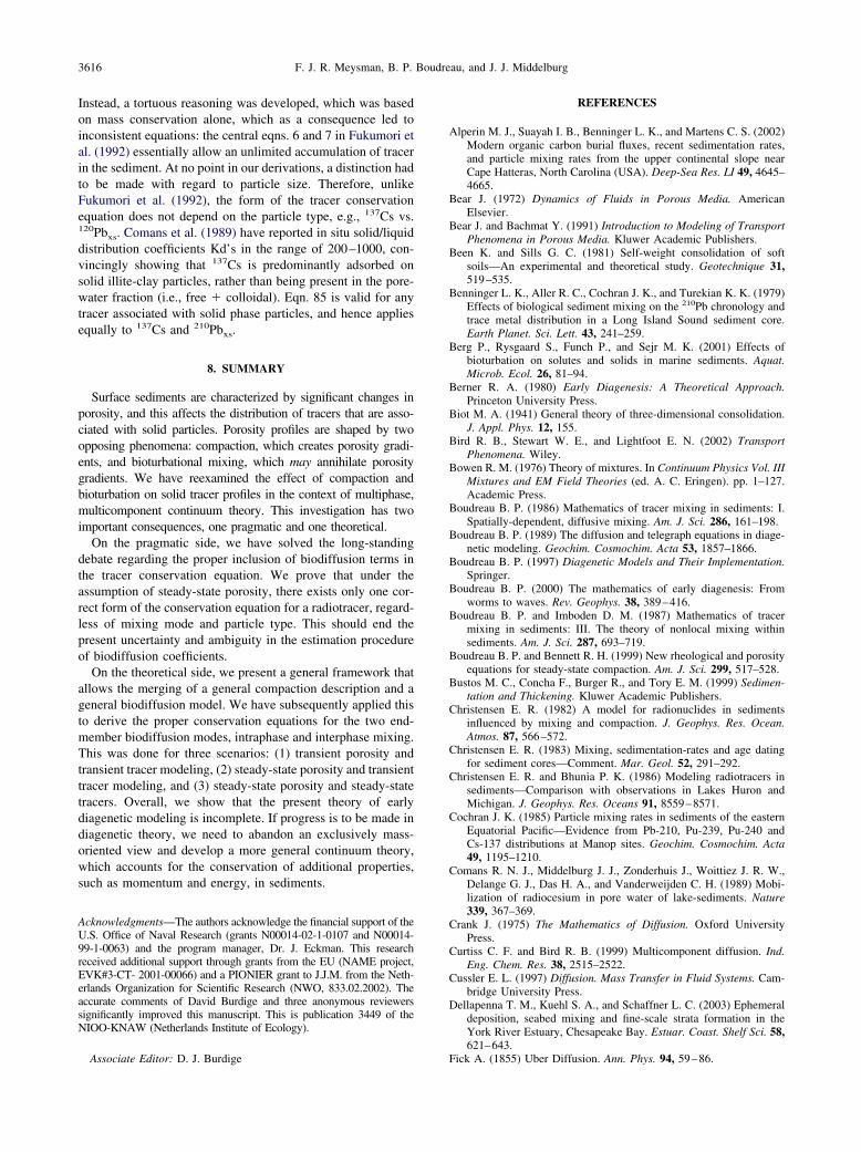
3616 F. J. R. Meysman, B. P. Boudreau, and J. J. Middelburg
Instead, a tortuous reasoning was developed, which was basedon mass conservation alone, which as a consequence led toinconsistent equations: the central eqns. 6 and 7 in Fukumori etal. (1992) essentially allow an unlimited accumulation of tracerin the sediment. At no point in our derivations, a distinction hadto be made with regard to particle size. Therefore, unlikeFukumori et al. (1992), the form of the tracer conservationequation does not depend on the particle type, e.g., 137Cs vs.120Pbxs. Comans et al. (1989) have reported in situ solid/liquiddistribution coefficients Kd’s in the range of 200–1000, con-vincingly showing that 137Cs is predominantly adsorbed onsolid illite-clay particles, rather than being present in the pore-water fraction (i.e., free � colloidal). Eqn. 85 is valid for anytracer associated with solid phase particles, and hence appliesequally to 137Cs and 210Pbxs.
8. SUMMARY
Surface sediments are characterized by significant changes inporosity, and this affects the distribution of tracers that are asso-ciated with solid particles. Porosity profiles are shaped by twoopposing phenomena: compaction, which creates porosity gradi-ents, and bioturbational mixing, which may annihilate porositygradients. We have reexamined the effect of compaction andbioturbation on solid tracer profiles in the context of multiphase,multicomponent continuum theory. This investigation has twoimportant consequences, one pragmatic and one theoretical.
On the pragmatic side, we have solved the long-standingdebate regarding the proper inclusion of biodiffusion terms inthe tracer conservation equation. We prove that under theassumption of steady-state porosity, there exists only one cor-rect form of the conservation equation for a radiotracer, regard-less of mixing mode and particle type. This should end thepresent uncertainty and ambiguity in the estimation procedureof biodiffusion coefficients.
On the theoretical side, we present a general framework thatallows the merging of a general compaction description and ageneral biodiffusion model. We have subsequently applied thisto derive the proper conservation equations for the two end-member biodiffusion modes, intraphase and interphase mixing.This was done for three scenarios: (1) transient porosity andtransient tracer modeling, (2) steady-state porosity and transienttracer modeling, and (3) steady-state porosity and steady-statetracers. Overall, we show that the present theory of earlydiagenetic modeling is incomplete. If progress is to be made indiagenetic theory, we need to abandon an exclusively mass-oriented view and develop a more general continuum theory,which accounts for the conservation of additional properties,such as momentum and energy, in sediments.
Acknowledgments—The authors acknowledge the financial support of theU.S. Office of Naval Research (grants N00014-02-1-0107 and N00014-99-1-0063) and the program manager, Dr. J. Eckman. This researchreceived additional support through grants from the EU (NAME project,EVK#3-CT- 2001-00066) and a PIONIER grant to J.J.M. from the Neth-erlands Organization for Scientific Research (NWO, 833.02.2002). Theaccurate comments of David Burdige and three anonymous reviewerssignificantly improved this manuscript. This is publication 3449 of theNIOO-KNAW (Netherlands Institute of Ecology).
Associate Editor: D. J. Burdige
REFERENCES
Alperin M. J., Suayah I. B., Benninger L. K., and Martens C. S. (2002)Modern organic carbon burial fluxes, recent sedimentation rates,and particle mixing rates from the upper continental slope nearCape Hatteras, North Carolina (USA). Deep-Sea Res. LI 49, 4645–4665.
Bear J. (1972) Dynamics of Fluids in Porous Media. AmericanElsevier.
Bear J. and Bachmat Y. (1991) Introduction to Modeling of TransportPhenomena in Porous Media. Kluwer Academic Publishers.
Been K. and Sills G. C. (1981) Self-weight consolidation of softsoils—An experimental and theoretical study. Geotechnique 31,519–535.
Benninger L. K., Aller R. C., Cochran J. K., and Turekian K. K. (1979)Effects of biological sediment mixing on the 210Pb chronology andtrace metal distribution in a Long Island Sound sediment core.Earth Planet. Sci. Lett. 43, 241–259.
Berg P., Rysgaard S., Funch P., and Sejr M. K. (2001) Effects ofbioturbation on solutes and solids in marine sediments. Aquat.Microb. Ecol. 26, 81–94.
Berner R. A. (1980) Early Diagenesis: A Theoretical Approach.Princeton University Press.
Biot M. A. (1941) General theory of three-dimensional consolidation.J. Appl. Phys. 12, 155.
Bird R. B., Stewart W. E., and Lightfoot E. N. (2002) TransportPhenomena. Wiley.
Bowen R. M. (1976) Theory of mixtures. In Continuum Physics Vol. IIIMixtures and EM Field Theories (ed. A. C. Eringen). pp. 1–127.Academic Press.
Boudreau B. P. (1986) Mathematics of tracer mixing in sediments: I.Spatially-dependent, diffusive mixing. Am. J. Sci. 286, 161–198.
Boudreau B. P. (1989) The diffusion and telegraph equations in diage-netic modeling. Geochim. Cosmochim. Acta 53, 1857–1866.
Boudreau B. P. (1997) Diagenetic Models and Their Implementation.Springer.
Boudreau B. P. (2000) The mathematics of early diagenesis: Fromworms to waves. Rev. Geophys. 38, 389–416.
Boudreau B. P. and Imboden D. M. (1987) Mathematics of tracermixing in sediments: III. The theory of nonlocal mixing withinsediments. Am. J. Sci. 287, 693–719.
Boudreau B. P. and Bennett R. H. (1999) New rheological and porosityequations for steady-state compaction. Am. J. Sci. 299, 517–528.
Bustos M. C., Concha F., Burger R., and Tory E. M. (1999) Sedimen-tation and Thickening. Kluwer Academic Publishers.
Christensen E. R. (1982) A model for radionuclides in sedimentsinfluenced by mixing and compaction. J. Geophys. Res. Ocean.Atmos. 87, 566–572.
Christensen E. R. (1983) Mixing, sedimentation-rates and age datingfor sediment cores—Comment. Mar. Geol. 52, 291–292.
Christensen E. R. and Bhunia P. K. (1986) Modeling radiotracers insediments—Comparison with observations in Lakes Huron andMichigan. J. Geophys. Res. Oceans 91, 8559–8571.
Cochran J. K. (1985) Particle mixing rates in sediments of the easternEquatorial Pacific—Evidence from Pb-210, Pu-239, Pu-240 andCs-137 distributions at Manop sites. Geochim. Cosmochim. Acta49, 1195–1210.
Comans R. N. J., Middelburg J. J., Zonderhuis J., Woittiez J. R. W.,Delange G. J., Das H. A., and Vanderweijden C. H. (1989) Mobi-lization of radiocesium in pore water of lake-sediments. Nature339, 367–369.
Crank J. (1975) The Mathematics of Diffusion. Oxford UniversityPress.
Curtiss C. F. and Bird R. B. (1999) Multicomponent diffusion. Ind.Eng. Chem. Res. 38, 2515–2522.
Cussler E. L. (1997) Diffusion. Mass Transfer in Fluid Systems. Cam-bridge University Press.
Dellapenna T. M., Kuehl S. A., and Schaffner L. C. (2003) Ephemeraldeposition, seabed mixing and fine-scale strata formation in theYork River Estuary, Chesapeake Bay. Estuar. Coast. Shelf Sci. 58,621–643.
Fick A. (1855) Uber Diffusion. Ann. Phys. 94, 59–86.

3617Modeling bioturbation and compaction
Fowler A. C. and Noon C. G. (1999) Mathematical models of com-paction, consolidation and regional groundwater flow. Geophys.J. Int. 136, 251–260.
Fukumori E., Christensen E. R., and Klein R. J. (1992) A model forCs-137 and other tracers in lake-sediments considering particle-sizeand the inverse solution. Earth Planet. Sci. Lett. 114, 85–99.
Gardiner C. W. (1985) Handbook of Stochastic Methods for Physics,Chemistry and the Natural Sciences. Springer. Verlag.
Gibson. R. E. (1958) The progress of consolidation in a clay layerincreasing in thickness with time. Geotechnique 8, 171–182.
Goldberg E. D. and Koide M. (1962) Geochronological studies ofdeep-sea sediments by the lo/Th method. Geochim. Cosmochim.Acta 26, 417–450.
Gray W. G. and Hassanizadeh S. M. (1998) Macroscale continuummechanics for multiphase porous-media flow including phases,interfaces, common lines and common points. Adv. Water Resour.21, 261–281.
Guinasso N. L. and Schink D. R. (1975) Quantitative estimates ofbiological mixing rates in abyssal sediments. J. Geophys. Res.Ocean. Atmos. 80, 3032–3043.
Hancock G. J. and Hunter J. R. (1999) Use of excess Pb-210 andTh-228 to estimate rates of sediment accumulation and bioturbationin Port Phillip Bay, Australia. Mar. Freshw. Res. 50, 533–545.
Hassanizadeh S. M. (1986) Derivations of basic equations of masstransport in porous media, Part 2. Generalized Darcy’s and Fick’sLaws. Adv. Water Resour. 9, 207–222.
Hassanizadeh S. M. (1996) On the transient non-Fickian dispersiontheory. Transp. Porous Media 23, 107–124.
Henderson G. M., Lindsay F. N., and Slowey N. C. (1999) Variation inbioturbation with water depth on marine slopes: A study on theLittle Bahamas Bank. Mar. Geol. 160, 105–118.
Huyakorn P. S. and Pinder G. F. (1983) Computational Methods inSubsurface Flow. Academic Press.
Jones S. E. and Jago C. F. (1993) In situ assessment of modification ofsediment properties by burrowing invertebrates. Mar. Biol. 115,133–142.
Kirkwood J. G. and Crawford B. J. (1952) The macroscopic equationsof transport. J. Phys. Chem. 56, 1048–1051.
Kirwan A. D. and Kump L. R. (1987) Models of geochemical systemsfor mixture theory—Diffusion. Geochim. Cosmochim. Acta 51,1219–1226.
Lasaga A. C. (1998) Kinetic Theory in the Earth Sciences. PrincetonUniversity Press.
Lichtner P. C. (1985) Continuum model for simultaneous chemicalreactions and mass transport in hydrothermal systems. Geochim.Cosmochim. Acta 49, 779–800.
McVay M., Townsend F., and Bloomquist D. (1986) Quiescent con-solidation of phosphatic waste clays. J. Geotech. Eng. ASCE 112,1033–1049.
Meysman F. J. R. (2001) Modelling the influence of ecological inter-actions on reactive transport processes in sediments. Ph.D. disse.
Ghent University.Meysman F. J. R., Boudreau B. P., and Middleburg J. J. (2003)Relations between local, nonlocal, discrete and continuous modelsof bioturbation. J. Mar. Res. 61, 391–410.
Mulsow S., Boudreau B. P., and Smith J. N. (1998) Bioturbation andporosity gradients. Limnol. Oceanage. 43, 1–9.
Murray J. M. H., Meadows A., and Meadows P. S. (2002) Biogeomor-phological Implications of microscale interactions between sedi-ment geotechnics and marine benthos: A review. Geomorphology47, 15–30.
Nie Y. H., Suayah I. B., Benninger L. K., and Alperin M. J. (2001)Modeling detailed sedimentary Pb-210 and fallout Pu-239, Pu-240profiles to allow episodic events: An application in ChesapeakeBay. Limnol. Oceanogr. 46, 1425–1437.
Nozaki Y., Cochran J. K., Turekian K. K., and Keller G. (1977)Radiocarbon and Pb-210 distribution in submersible-taken deep-seacores from Project Famous. Earth Planet. Sci. Lett. 34, 167–173.
Officer C. B. (1982) Mixing. sedimentation-rates and age dating forsediment cores. Mar. Geol. 46, 261–278.
Officer C. B. and Lynch D. R. (1982) Interpretation procedures for thedetermination of sediment parameters from time-dependent fluxinputs. Earth Planet. Sci. Lett. 61, 55–62.
Officer C. B. and Lynch D. R. (1983) Mixing, sedimentation-rates andage dating for sediment cores—Reply—Mar. Geol. 52, 292–296.
Reise K. (2002) Sediment mediated species interactions in coastalwaters. J. Sea Res. 48, 127–141.
Robbins J. A., Krezoski J. R., and Mozley S. C. (1977) Radioactivityin sediments of Great Lakes—Post-depositional redistribution bydeposit-feeding organisms. Earth Planet. Sci. Lett. 36, 325–333.
Smith C. R., Pope R. H., Demaster D. J., and Magaard L. (1993)Age-dependent mixing of deep-sea sediments. Geochim. Cosmo-chim. Acta 57, 1473–1488.
Soetaert K., Herman P. M. J., Middelburg J. J., and Heip C. (1998)Assessing organic matter mineralization, degradability and mixingrate in an ocean margin sediment (Northeast Atlantic) by diageneticmodeling. J. Mar. Res. 56, 519–534.
Steefel C. I. and MacQuarrie K. T. B. (1996) Approaches to modelingof reactive transport in porous media. In Reactive Transport inPorous Media (eds. P. C. Lichtner, C. C. Steefel, and E. H.Oelkers), pp. 83–129. Mineralogical Society of America.
Taylor R. and Krishna R. (1993) Multicomponent Mass Transfer.Wiley Interscience.
Terzaghi K. (1942) Theoretical Soil Mechanics. Wiley.Toorman E. A. (1996) Sedimentation and self-weight consolidation:
General unifying theory. Geotechnique 46, 103–113.Truesdell C. and Toupin R. (1960) The classical field theories. In
Handbuch der Physik (ed. S. Flugge). pp. 226–793. Springer.Van Cappellen P. and Gaillard J. F. (1996) Biogeochemical dynamics
in aquatic sediments. In Reactive Transport in Porous Media (eds.P. C. Lichtner, C. C. Steefel, and E. H. Oelkers), pp. 335–376.Mineralogical Society of America.
Wheatcroft R. A., Jumars P. A., Smith C. R., and Nowell A. R. M.(1990) A mechanistic view of the particulate biodiffusion coeffi-cient—Step lengths, rest periods and transport directions. J. Mar.
Res. 48, 177–207.