Accepted Manuscript

Modeling of shear stress and pressure acting on small-amplitude wavy surfacein channels with turbulent flow

S. Knotek, M. Jicha

PII: S0307-904X(13)00806-8DOI: http://dx.doi.org/10.1016/j.apm.2013.11.065Reference: APM 9836

To appear in: Appl. Math. Modelling

Please cite this article as: S. Knotek, M. Jicha, Modeling of shear stress and pressure acting on small-amplitudewavy surface in channels with turbulent flow, Appl. Math. Modelling (2014), doi: http://dx.doi.org/10.1016/j.apm.2013.11.065

This is a PDF file of an unedited manuscript that has been accepted for publication. As a service to our customerswe are providing this early version of the manuscript. The manuscript will undergo copyediting, typesetting, andreview of the resulting proof before it is published in its final form. Please note that during the production processerrors may be discovered which could affect the content, and all legal disclaimers that apply to the journal pertain.

Modeling of shear stress and pressure acting on

small-amplitude wavy surface in channels with

turbulent flow

S. Knotek∗, M. Jicha

Energy Institute, Faculty of Mechanical Engineering, Brno University of Technology,

Brno, Czech Republic

Abstract

Simulation results and algebraic models of wall shear stress and pressureforces acting on the wavy surface in channels with turbulent flow are pre-sented in dependence on channel height H, ratio of the wavelength λ to thewave amplitude a and bulk velocity Ub. The models have been designed usingresults of the set of steady numerical simulations computed by k-ε V2F tur-bulence model for various configurations defined by selection of ratio H/λ inrange from 0.6 to 1.4, steepness ratio λ/a in range from 20 to 200 and bulk ve-locity Ub in range of Reynolds number Re=HUb/ν from 3830 to 89366. Theapplicability of the k-ε V2F model is verified by DNS results and derivedalgebraic models are validated using experimental data and other models.Very good agreement with measurements is observed within a defined rangeof conditions.

Keywords: CFD modeling, turbulent flow, wavy surface, wall shear stress

1. Introduction

The study of turbulent flow over the wavy surface is motivated by var-ious industrial and environmental applications. It constitutes the basis for

∗Corresponding author at: Energy Institute, Faculty of Mechanical Engineer-ing, Brno University of Technology, Technicka 2896/2, 616 69 Brno, Czech Republic.Tel.:+420 54114 3242.

Email addresses: knotek@fme.vutbr.cz (S. Knotek), jicha@fme.vutbr.cz (M.Jicha)

Preprint submitted to Applied Mathematical Modelling January 8, 2014

research of wind wave phenomenon either on the air-sea interface [1], or onthin liquid film [2]. The simulations of the turbulent flow over wavy wallsare used in coastal studies for the prediction of transport of sediments overthe continental shelf [3], [4] or in cooling applications for the determinationof heat transfer coefficient or pressure and temperature distribution in heatexchangers [5], [6].

Even though the air-water interface is often succesfully modeled as movinge.g. by VOF approach [7] or others [8], the so-called quasi-static approxima-tion [9] has still its importance [10]. It is based on the assumption that, forlarge ratios of fluid densities and fluid viscosities, the surface can be consid-ered as static and solid. In the first step, the force effect of the gas flow actingon the solid surface defined by amplitude and wavelength are evaluated. Inthe second step, these forces, specifically wall pressure and wall shear stressas have been identified in [2], are included in the calculations of the stabil-ity problem as its own. To determine these quantities, some mathematicalmodels have been developed based on the solution of the Orr-Sommerfeldequation [11] or two-equation turbulence models, such as that employed by[12] to the computation of the shearing flow over realistic waves designedin [13].

The aim of our study was first to compare the simulations of the describedphenomenon using a commercial software with classical solutions and experi-ments, and second to design simple algebraic models, which could be useddirectly in technical applications. For these reasons and regarding the wavesinstability problem mentioned above, we have designed algebraic models ofshear stress and pressure forces using the set of numerical simulations com-puted for configurations defined in the range of conditions for which liquidfilm instability occurs according to Hanratty in [2].

2. Problem description

For the reasons discussed in more details below, the desired values ofshear stress and pressure in our study have been obtained using the set ofnumerical simulations of the steady turbulent flow in a 2D channel withthe sinusoidal lower wall and the flat upper wall. Due to the fact that thedevelopment of boundary layers along the channel affects the values of shearstress and pressure, the flow has been investigated using periodic boundaryconditions in the streamwise direction in the segment whose length equals totwo prescribed wavelengths. The computational domain is shown in Figure 1.

2

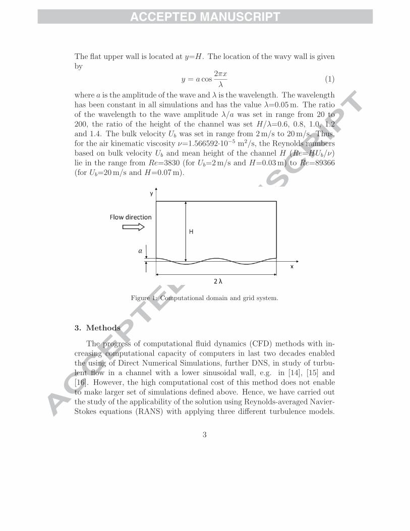
The flat upper wall is located at y=H. The location of the wavy wall is givenby

y = a cos2πx

λ(1)

where a is the amplitude of the wave and λ is the wavelength. The wavelengthhas been constant in all simulations and has the value λ=0.05 m. The ratioof the wavelength to the wave amplitude λ/a was set in range from 20 to200, the ratio of the height of the channel was set H/λ=0.6, 0.8, 1.0, 1.2and 1.4. The bulk velocity Ub was set in range from 2 m/s to 20 m/s. Thus,for the air kinematic viscosity ν=1.566592·10−5 m2/s, the Reynolds numbersbased on bulk velocity Ub and mean height of the channel H (Re=HUb/ν)lie in the range from Re=3830 (for Ub=2 m/s and H=0.03 m) to Re=89366(for Ub=20 m/s and H=0.07 m).

Figure 1: Computational domain and grid system.

3. Methods

The progress of computational fluid dynamics (CFD) methods with in-creasing computational capacity of computers in last two decades enabledthe using of Direct Numerical Simulations, further DNS, in study of turbu-lent flow in a channel with a lower sinusoidal wall, e.g. in [14], [15] and[16]. However, the high computational cost of this method does not enableto make larger set of simulations defined above. Hence, we have carried outthe study of the applicability of the solution using Reynolds-averaged Navier-Stokes equations (RANS) with applying three different turbulence models.

3

We used the standard Wilcox’s k-ε [17], k-ω SST of Menter [18] and finallyk-ε V2F [19] RANS equations model. The results of these models have beencompared with DNS results [16] and [14]. Note that the latter have beenfrequently referred as a benchmark case that can be downloaded from [20]and are compared with measurements of Hudson published in [21].

Because the flow is assumed to be homogeneous in the spanwise direction,periodic boundary conditions have been used in DNS simulations. However,in our case we have used only two-dimensional geometry. From the compari-son with results for three- dimensional geometry, see Figure 2, it follows thatthis simplification is acceptable at least for values of wall shear stress andpressure forces. Thus, the periodic boundary conditions are assigned and theconstant mass flow rate is adjusted in the streamwise direction.

0 0.2 0.4 0.6 0.8 1 1.2 1.4 1.6 1.8 20

0.05

0.1

0.15

0.2

Pw /

ρ U

b

2

x/λ

k−ε V2F 3D geometry

k−ε V2F 2D geometry

0 0.2 0.4 0.6 0.8 1 1.2 1.4 1.6 1.8 2.0−5

0

5

10

15x 10

−3

τ w /

ρ U

b

2

x/λ

k−ε V2F 3D geometry

k−ε V2F 2D geometry

Figure 2: Comparison of pressure and wall shear stress distribution at wavy wall for 2Dand 3D geometry by using k-ε V2F turbulence model.

3.1. Turbulent model selection and verification

As was mentioned above, we used three turbulent models known as k-ε ofWilcox, k-ω SST and k-ε V2F. To study the applicability of these models forprecise calculation of shear stress and pressure, simulations were performedwith the same configuration as the DNS calculation of Maass & Schumann

4

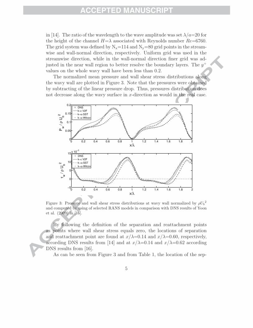
in [14]. The ratio of the wavelength to the wave amplitude was set λ/a=20 forthe height of the channel H=λ associated with Reynolds number Re=6760.The grid system was defined by Nx=114 and Ny=80 grid points in the stream-wise and wall-normal direction, respectively. Uniform grid was used in thestreamwise direction, while in the wall-normal direction finer grid was ad-justed in the near wall region to better resolve the boundary layers. The y+

values on the whole wavy wall have been less than 0.2.The normalized mean pressure and wall shear stress distributions along

the wavy wall are plotted in Figure 3. Note that the pressures were obtainedby subtracting of the linear pressure drop. Thus, pressures distribution doesnot decrease along the wavy surface in x-direction as would in the real case.

0 0.2 0.4 0.6 0.8 1 1.2 1.4 1.6 1.8 20

0.05

0.1

0.15

0.2

Pw /

ρ U

b

2

x/λ

DNS

k−ε V2F

k−ω SST

k−ω Wilcox

0 0.2 0.4 0.6 0.8 1 1.2 1.4 1.6 1.8 2−5

0

5

10

15x 10

−3

τ w /

ρ U

b

2

x/λ

DNS

k−ε V2F

k−ω SST

k−ω Wilcox

Figure 3: Pressure and wall shear stress distributions at wavy wall normalized by ρUb2

and computed by using of selected RANS models in comparison with DNS results of Yoonet al. (2009) in [16].

By following the definition of the separation and reattachment pointsas points where wall shear stress equals zero, the locations of separationand reattachment point are found at x/λ=0.14 and x/λ=0.60, respectively,according DNS results from [14] and at x/λ=0.14 and x/λ=0.62 accordingDNS results from [16].

As can be seen from Figure 3 and from Table 1, the location of the sep-

5

aration point is predicted quite well by all of RANS models used in oursimulations. However, the reattachment point is overpredicted by all ofRANS models. The best result in reattachment point prediction is givenby k-ε V2F model. In addition, the prediction of extreme values of pressureand wall shear stress by this model gives relatively good and very good re-sults, respectively. This is in good agreement with the fact, that this modelis designed to capture the near-wall turbulence effects more accurately, whichis crucial for prediction of skin friction and flow separation. The both k-ωmodels predictions of pressure and wall shear stress distribution are quitesimilar. They differ most in prediction of the maximum values.

Separation ReattachmentCases xS/λ xR/λExperiments of Hudson (1996) 0.22 0.58DNS of Maass & Schumann (1996) 0.14 0.60DNS of Yoon et al. (2009) 0.14 0.62k-ε V2F 0.14 0.66k-ω SST 0.13 0.71k-ω Wilcox 0.13 0.71

Table 1: The x/λ location of separation and reattachment points predicted by selectedmodels in comparison with experimental data of Hudson (1996) in [22], DNS results ofMaass & Schumann (1996) in [14] and Yoon et al. (2009) in [16].

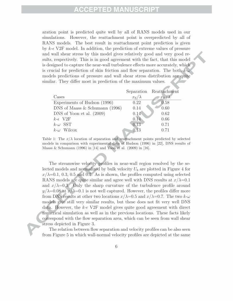
The streamwise velocity profiles in near-wall region resolved by the se-lected models and normalized by bulk velocity Ub are plotted in Figure 4 forx/λ=0.1, 0.3, 0.5 and 0.7. As is shown, the profiles computed using selectedRANS models are quite similar and agree well with DNS results at x/λ=0.1and x/λ=0.3. Only the sharp curvature of the turbulence profile aroundy/λ=0.08 at x/λ=0.1 is not well captured. However, the profiles differ morefrom DNS results at other two locations x/λ=0.5 and x/λ=0.7. The two k-ωmodels give still very similar results, but these does not fit very well DNSdata. However, the k-ε V2F model gives quite good agreement with directnumerical simulation as well as in the previous locations. These facts likelycorrespond with the flow separation area, which can be seen from wall shearstress depicted in Figure 3.

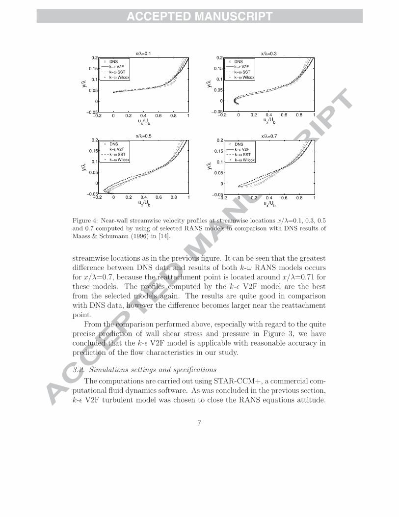
The relation between flow separation and velocity profiles can be also seenfrom Figure 5 in which wall-normal velocity profiles are depicted at the same

6

−0.2 0 0.2 0.4 0.6 0.8 1−0.05

0

0.05

0.1

0.15

0.2

y/λ

ux/U

b

x/λ=0.1

−0.2 0 0.2 0.4 0.6 0.8 1−0.05

0

0.05

0.1

0.15

0.2

y/λ

ux/U

b

x/λ=0.3

−0.2 0 0.2 0.4 0.6 0.8 1−0.05

0

0.05

0.1

0.15

0.2

y/λ

ux/U

b

x/λ=0.5

−0.2 0 0.2 0.4 0.6 0.8 1−0.05

0

0.05

0.1

0.15

0.2

y/λ

ux/U

b

x/λ=0.7

DNS

k−ε V2F

k−ω SST

k−ω Wilcox

DNS

k−ε V2F

k−ω SST

k−ω Wilcox

DNS

k−ε V2F

k−ω SST

k−ω Wilcox

DNS

k−ε V2F

k−ω SST

k−ω Wilcox

Figure 4: Near-wall streamwise velocity profiles at streamwise locations x/λ=0.1, 0.3, 0.5and 0.7 computed by using of selected RANS models in comparison with DNS results ofMaass & Schumann (1996) in [14].

streamwise locations as in the previous figure. It can be seen that the greatestdifference between DNS data and results of both k-ω RANS models occursfor x/λ=0.7, because the reattachment point is located around x/λ=0.71 forthese models. The profiles computed by the k-ε V2F model are the bestfrom the selected models again. The results are quite good in comparisonwith DNS data, however the difference becomes larger near the reattachmentpoint.

From the comparison performed above, especially with regard to the quiteprecise prediction of wall shear stress and pressure in Figure 3, we haveconcluded that the k-ε V2F model is applicable with reasonable accuracy inprediction of the flow characteristics in our study.

3.2. Simulations settings and specifications

The computations are carried out using STAR-CCM+, a commercial com-putational fluid dynamics software. As was concluded in the previous section,k-ε V2F turbulent model was chosen to close the RANS equations attitude.

7

−0.04 −0.03 −0.02 −0.01 0 0.01−0.1

0

0.1

0.2

0.3

0.4

0.5

y/λ

uy/U

b

x/λ=0.1

−0.04 −0.02 0 0.02 0.04−0.1

0

0.1

0.2

0.3

0.4

0.5

y/λ

uy/U

b

x/λ=0.3

−0.06 −0.04 −0.02 0 0.02−0.1

0

0.1

0.2

0.3

0.4

0.5

y/λ

uy/U

b

x/λ=0.5

−0.02 0 0.02 0.04 0.06−0.1

0

0.1

0.2

0.3

0.4

0.5

y/λ

uy/U

b

x/λ=0.7

DNS

k−ε V2F

k−ω SST

k−ω Wilcox

DNS

k−ε V2F

k−ω SST

k−ω Wilcox

DNS

k−ε V2F

k−ω SST

k−ω Wilcox

DNS

k−ε V2F

k−ω SST

k−ω Wilcox

Figure 5: Wall-normal velocity profiles at streamwise locations x/λ=0.1, 0.3, 0.5 and0.7 computed by using of selected RANS models in comparison with DNS results ofYoon et al. (2009) in [16].

A k-ε turbulence model is a two-equation model in which transport equa-tions are solved for the turbulent kinetic energy k and its dissipation rateε. The V2F k-ε model ([19], [23], [24]) is known to capture the near-wallturbulence effects more accurately, which is crucial for the accurate predic-tion of heat transfer, skin friction and flow separation. This model solvestwo additional turbulence quantities, namely the normal stress function andthe elliptic function, in addition to k and ε. The transition equations weresolved by the finite volume method with the use of the second order upwindscheme. The underrelaxation factors are presented in Table 2. The modelemployed all y+ treatment. For detailed specifications, the reader is advisedto consult the manual [25]. A typical run of a simulation took about 30–40minutes using Intel Pentium IV personal computer.

3.3. Grid-independency study

As was mentioned above, the computational domain was two-dimensionaland the flow was solved as steady. In order to study the effect of grid refine-

8

Variable Relaxation Factorvelocity 0.7pressure 0.3elliptic k-ε turbulence 0.8turbulence viscosity 1

Table 2: Relaxation factors used in k-ε V2F model.

ment, many different grids have been solved. From the results was concludedthat the wall shear stress and pressure values are dependent mostly on y+

values on the wall, further y+wall.

Grid Size max y+wall max Pw/ρUb

2 max τw/ρUb2

1 120× 80 1.4 2.0600 (99.30 %) 0.0895 (96.86 %)2 120× 88 0.8 2.0693 (99.74 %) 0.0918 (99.35 %)3 120× 92 0.6 2.0746 (100 %) 0.0924 (100 %)

Table 3: Characteristics of the grids using for study of grid resolution effect. The compu-tational domain is defined by H=λ, λ/a=80 and Re=31916 (H=0.05 m, Ub=10 m/s).

For more detailed study of y+wall effect on the wall shear stress and pres-

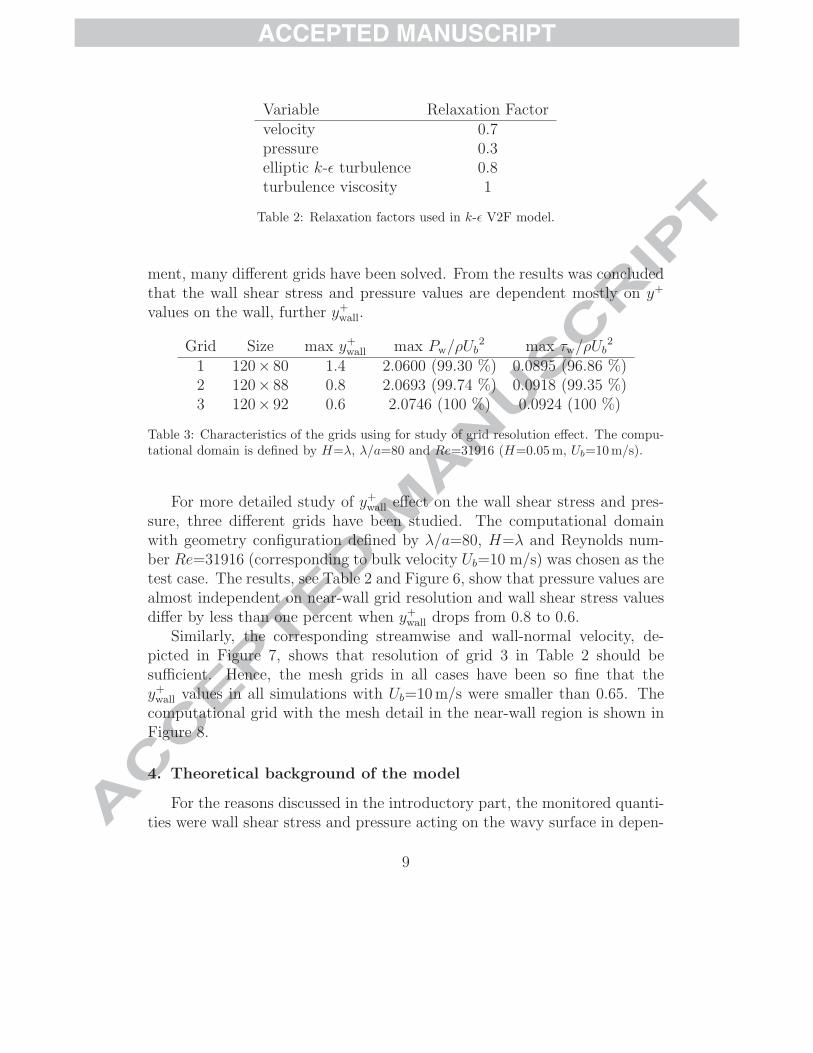
sure, three different grids have been studied. The computational domainwith geometry configuration defined by λ/a=80, H=λ and Reynolds num-ber Re=31916 (corresponding to bulk velocity Ub=10 m/s) was chosen as thetest case. The results, see Table 2 and Figure 6, show that pressure values arealmost independent on near-wall grid resolution and wall shear stress valuesdiffer by less than one percent when y+

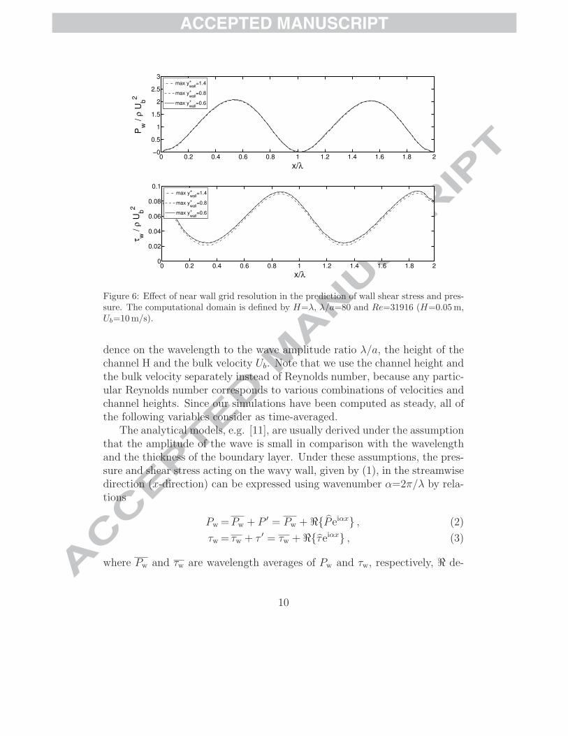
wall drops from 0.8 to 0.6.Similarly, the corresponding streamwise and wall-normal velocity, de-

picted in Figure 7, shows that resolution of grid 3 in Table 2 should besufficient. Hence, the mesh grids in all cases have been so fine that they+

wall values in all simulations with Ub=10 m/s were smaller than 0.65. Thecomputational grid with the mesh detail in the near-wall region is shown inFigure 8.

4. Theoretical background of the model

For the reasons discussed in the introductory part, the monitored quanti-ties were wall shear stress and pressure acting on the wavy surface in depen-

9

0 0.2 0.4 0.6 0.8 1 1.2 1.4 1.6 1.8 2−0

0.5

1

1.5

2

2.5

3

Pw /

ρ U

b

2

x/λ

max ywall

+=1.4

max ywall

+=0.8

max ywall

+=0.6

0 0.2 0.4 0.6 0.8 1 1.2 1.4 1.6 1.8 20

0.02

0.04

0.06

0.08

0.1

τ w /

ρ U

b

2

x/λ

max ywall

+=1.4

max ywall

+=0.8

max ywall

+=0.6

Figure 6: Effect of near wall grid resolution in the prediction of wall shear stress and pres-sure. The computational domain is defined by H=λ, λ/a=80 and Re=31916 (H=0.05 m,Ub=10 m/s).

dence on the wavelength to the wave amplitude ratio λ/a, the height of thechannel H and the bulk velocity Ub. Note that we use the channel height andthe bulk velocity separately instead of Reynolds number, because any partic-ular Reynolds number corresponds to various combinations of velocities andchannel heights. Since our simulations have been computed as steady, all ofthe following variables consider as time-averaged.

The analytical models, e.g. [11], are usually derived under the assumptionthat the amplitude of the wave is small in comparison with the wavelengthand the thickness of the boundary layer. Under these assumptions, the pres-sure and shear stress acting on the wavy wall, given by (1), in the streamwisedirection (x-direction) can be expressed using wavenumber α=2π/λ by rela-tions

Pw = Pw + P ′ = Pw + �{P̂ eiαx} , (2)

τw = τw + τ ′ = τw + �{τ̂eiαx} , (3)

where Pw and τw are wavelength averages of Pw and τw, respectively, � de-

10

0 0.1 0.2 0.3 0.4 0.5 0.6 0.7 0.8 0.9 110

0.2

0.4

0.6

0.8

1

1.2

Ux /

Ub

y/H

max ywall

+=1.4

max ywall

+=0.8

max ywall

+=0.6

0 0.1 0.2 0.3 0.4 0.5 0.6 0.7 0.8 0.9 1

−4

−2

0

2

x 10−3

Uy /

Ub

y/H

max ywall

+=1.4

max ywall

+=0.8

max ywall

+=0.6

x/λ=1 (crest)

x/λ=0.5 (trough)

x/λ=0.5 (trough)

x/λ=1 (crest)

Figure 7: Effect of near wall grid resolution on the prediction of streamwise and wall-normal velocity profiles at x/λ=0.5 (trough) and x/λ=1 (crest). The computational do-main is defined by H=λ, λ/a=80 and Re=31916 (H=0.05 m, Ub=10 m/s).

Figure 8: Computational grid for domain defined by H/λ=0.6 and λ/a=60.

notes the real part and P̂ and τ̂ are complex numbers

P̂ = PSR + iPSI , (4)

τ̂ = τSR + iτSI . (5)

11

The pressure and wall shear stress variations over the surface are thereforemodeled by harmonic functions and described by formulas

P ′ = PSR cos αx − PSI sin αx = |P̂ | cos (αx + θP) , (6)

τ ′ = τSR cos αx − τSI sin αx = |τ̂ | cos (αx + θτ ) . (7)

Because it is assumed that the pressure and wall shear stress wavelengthaverage values, Pw and τw, can be easily obtained from the problem of flowin a smooth channel, the problem of pressure and wall shear stress analysisis reduced to modeling of their wave variations P ′ and τ ′, i.e. componentsPSR, PSI, τSR and τSI in dependence on bulk velocity Ub, steepness ratio λ/aand height of the channel H.

5. Results

5.1. Pressure

The pressure variation components PSR, PSI have been computed fromamplitude of pressure variation |P̂ | and phase shift against the wave surfaceθP according formula (6) by relations (8) and (9).

PSR = |P̂ | cos θP (8)

PSI = |P̂ | sin θP (9)

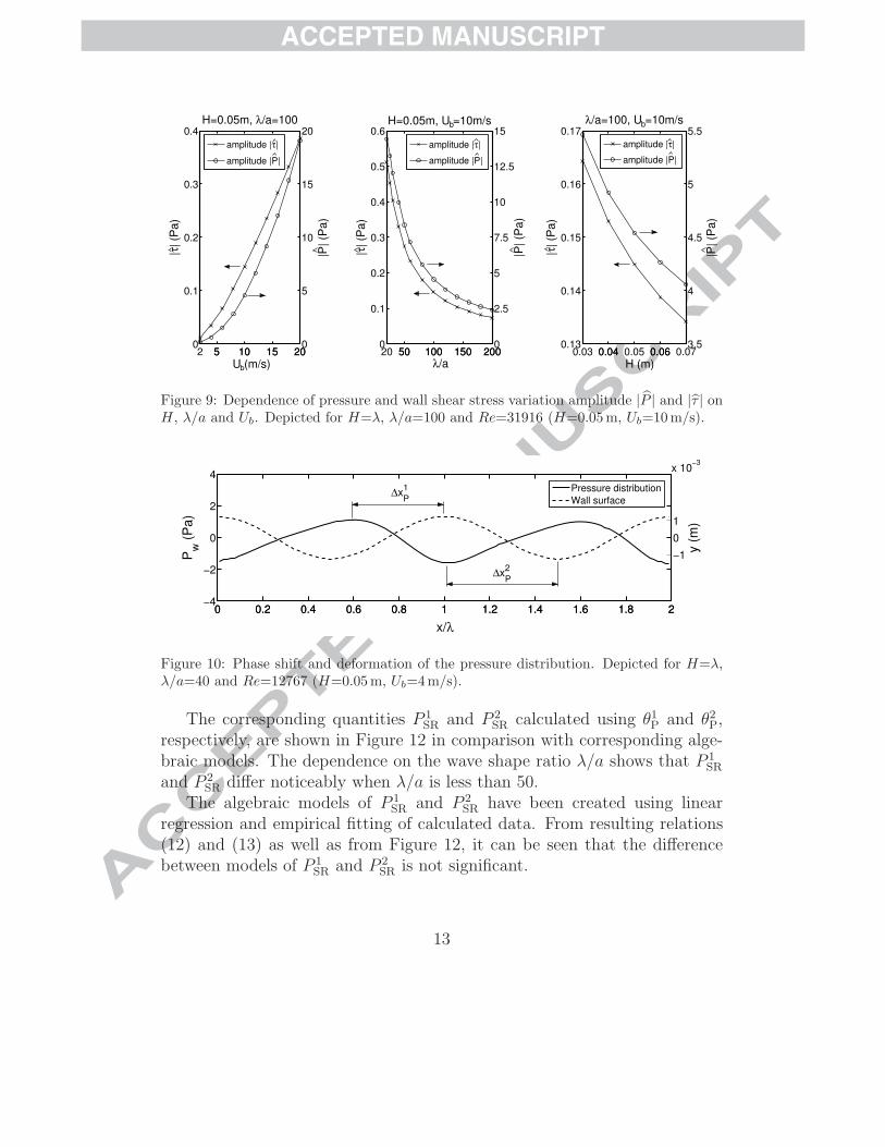
The pressure variation amplitude |P̂ | has been determined easily as the halfof the difference between maximum and minimum values. The dependenceof this variable on H, λ/a and Ub is depicted in Figure 9 in comparisonwith the wall shear stress variation amplitude |τ̂ |. It can be seen that thedependencies of both variables are similar. The amplitudes increase withincreasing bulk velocity Ub, decreasing ratio λ/a and channel height H.

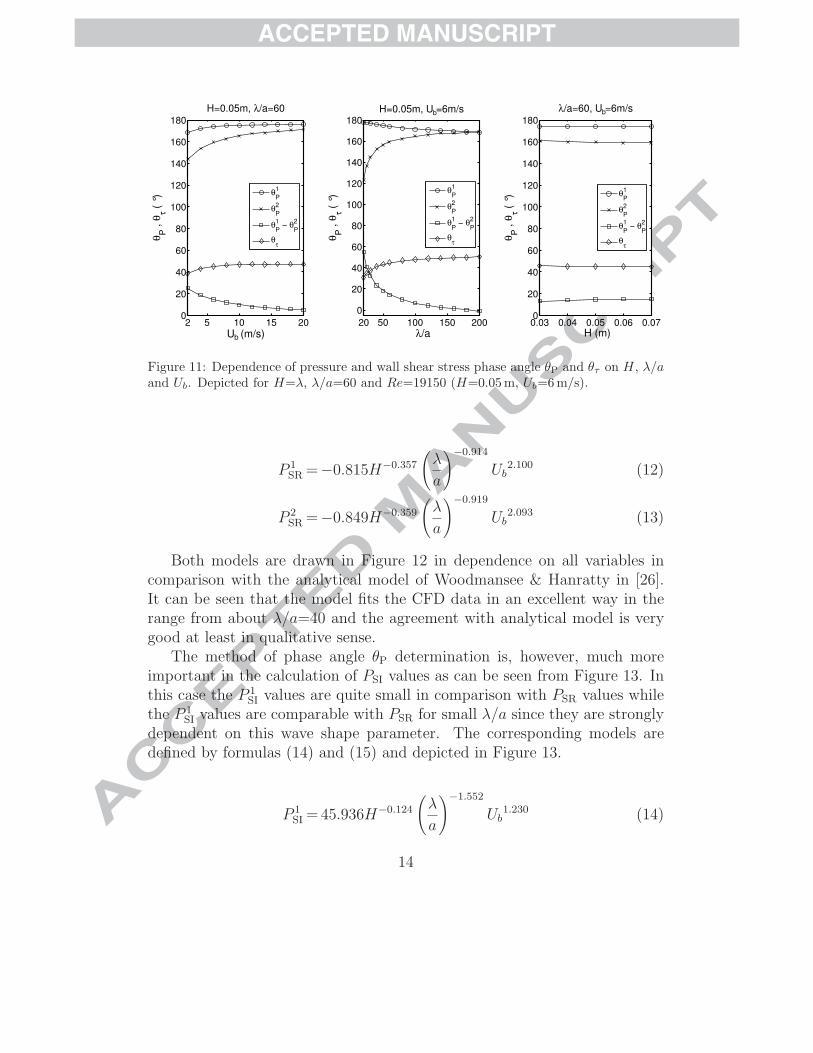
Determination of phase angle θP has been not so unambiguous because ofthe pressure distribution deformation especially for small bulk velocity Ub andsmall values of ratio λ/a as can be seen from Figure 10 and 11. Therefore, thephase shift has been determined using the pressure maximum shift againstthe wave crest, ∆x1

P, and using the pressure minimum shift against the wavethrough, ∆x2

P, as is illustrated in Figure 10. The corresponding phase anglesθ1P and θ2

P have been calculated using formula (10) and (11).

θ1P =

∆x1P

λ· 360◦ (10)

θ2P =

∆x2P

λ· 360◦ (11)

12

5 10 15 202

0

0.1

0.2

0.3

0.4H=0.05m, λ/a=100

|τ| (P

a)

U (m/s)5 10 15 20

0

5

10

15

20

|P| (P

a)

amplitude |τ|

amplitude |P|

50 100 150 200200

0.1

0.2

0.3

0.4

0.5

0.6H=0.05m, U =10m/s

|τ| (P

a)

λ/a50 100 150 200

0

2.5

5

7.5

10

12.5

15

|P| (P

a)

amplitude |τ|

amplitude |P|

0.03 0.04 0.05 0.06 0.070.13

0.14

0.15

0.16

0.17λ/a=100, U =10m/s

|τ| (P

a)

H (m)0.04 0.06

3.5

4

4.5

5

5.5

|P| (P

a)

amplitude |τ|

amplitude |P|

b

bb

Figure 9: Dependence of pressure and wall shear stress variation amplitude |P̂ | and |τ̂ | onH, λ/a and Ub. Depicted for H=λ, λ/a=100 and Re=31916 (H=0.05 m, Ub=10 m/s).

0 0.2 0.4 0.6 0.8 1 1.2 1.4 1.6 1.8 2−4

−2

0

2

4

Pw

(P

a)

x/λ

0 0.2 0.4 0.6 0.8 1 1.2 1.4 1.6 1.8 2

−1

0

1

x 10−3

y (

m)

Pressure distribution

Wall surface∆x

P

1

∆xP

2

Figure 10: Phase shift and deformation of the pressure distribution. Depicted for H=λ,λ/a=40 and Re=12767 (H=0.05 m, Ub=4 m/s).

The corresponding quantities P 1SR and P 2

SR calculated using θ1P and θ2

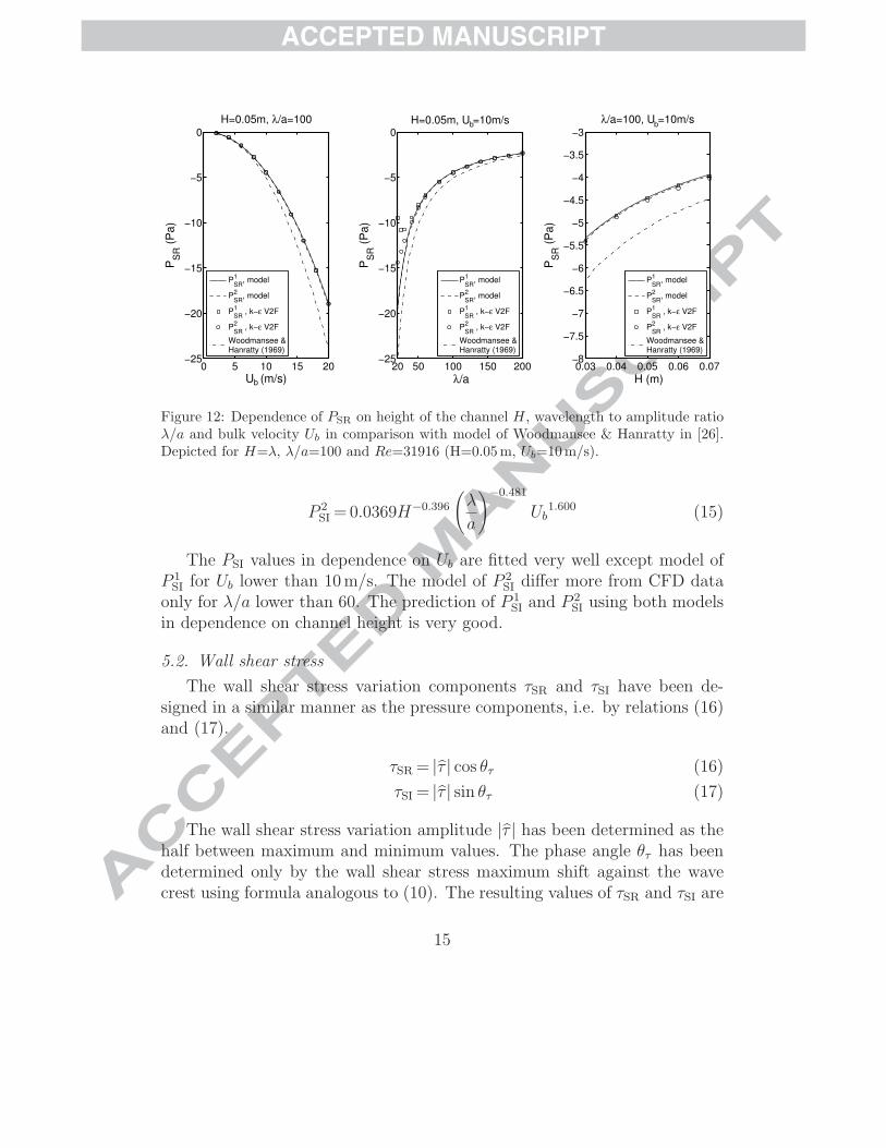
P,respectively, are shown in Figure 12 in comparison with corresponding alge-braic models. The dependence on the wave shape ratio λ/a shows that P 1

SR

and P 2SR differ noticeably when λ/a is less than 50.

The algebraic models of P 1SR and P 2

SR have been created using linearregression and empirical fitting of calculated data. From resulting relations(12) and (13) as well as from Figure 12, it can be seen that the differencebetween models of P 1

SR and P 2SR is not significant.

13

5 10 15 202

0

20

40

60

80

100

120

140

160

180

H=0.05m, λ/a=60

θP ,

θτ (

°)

U (m/s)

θ1

P

θ2

P

θ1

P − θ2

P

θτ

50 100 150 20020

0

20

40

60

80

100

120

140

160

180H=0.05m, U =6m/s

θP ,

θτ (

°)

λ/a

θ1

P

θ2

P

θ1

P − θ2

P

θτ

0.03 0.04 0.05 0.06 0.070

20

40

60

80

100

120

140

160

180

λ/a=60, U =6m/s

θP ,

θτ (

°)

H (m)

θ1

P

θ2

P

θ1

P − θ2

P

θτ

b

b

b

Figure 11: Dependence of pressure and wall shear stress phase angle θP and θτ on H, λ/aand Ub. Depicted for H=λ, λ/a=60 and Re=19150 (H=0.05 m, Ub=6 m/s).

P 1SR =−0.815H−0.357

(λ

a

)−0.914

Ub2.100 (12)

P 2SR =−0.849H−0.359

(λ

a

)−0.919

Ub2.093 (13)

Both models are drawn in Figure 12 in dependence on all variables incomparison with the analytical model of Woodmansee & Hanratty in [26].It can be seen that the model fits the CFD data in an excellent way in therange from about λ/a=40 and the agreement with analytical model is verygood at least in qualitative sense.

The method of phase angle θP determination is, however, much moreimportant in the calculation of PSI values as can be seen from Figure 13. Inthis case the P 1

SI values are quite small in comparison with PSR values whilethe P 1

SI values are comparable with PSR for small λ/a since they are stronglydependent on this wave shape parameter. The corresponding models aredefined by formulas (14) and (15) and depicted in Figure 13.

P 1SI = 45.936H−0.124

(λ

a

)−1.552

Ub1.230 (14)

14

0 5 10 15 20−25

−20

−15

−10

−5

0

H=0.05m, λ/a=100

PS

R (

Pa

)

U (m/s)

PSR

1, model

PSR

2, model

PSR

1 , k−ε V2F

PSR

2 , k−ε V2F

Woodmansee &Hanratty (1969)

50 100 150 20020−25

−20

−15

−10

−5

0H=0.05m, U =10m/s

PS

R (

Pa

)

λ/a

PSR

1, model

PSR

2, model

PSR

1 , k−ε V2F

PSR

2 , k−ε V2F

Woodmansee &Hanratty (1969)

0.03 0.04 0.05 0.06 0.07−8

−7.5

−7

−6.5

−6

−5.5

−5

−4.5

−4

−3.5

−3

λ/a=100, U =10m/s

PS

R (

Pa

)

H (m)

PSR

1, model

PSR

2, model

PSR

1 , k−ε V2F

PSR

2 , k−ε V2F

Woodmansee &Hanratty (1969)

b

b

b

Figure 12: Dependence of PSR on height of the channel H, wavelength to amplitude ratioλ/a and bulk velocity Ub in comparison with model of Woodmansee & Hanratty in [26].Depicted for H=λ, λ/a=100 and Re=31916 (H=0.05 m, Ub=10 m/s).

P 2SI = 0.0369H−0.396

(λ

a

)−0.481

Ub1.600 (15)

The PSI values in dependence on Ub are fitted very well except model ofP 1

SI for Ub lower than 10 m/s. The model of P 2SI differ more from CFD data

only for λ/a lower than 60. The prediction of P 1SI and P 2

SI using both modelsin dependence on channel height is very good.

5.2. Wall shear stress

The wall shear stress variation components τSR and τSI have been de-signed in a similar manner as the pressure components, i.e. by relations (16)and (17).

τSR = |τ̂ | cos θτ (16)

τSI = |τ̂ | sin θτ (17)

The wall shear stress variation amplitude |τ̂ | has been determined as thehalf between maximum and minimum values. The phase angle θτ has beendetermined only by the wall shear stress maximum shift against the wavecrest using formula analogous to (10). The resulting values of τSR and τSI are

15

0 5 10 15 2020

0

0.5

1

1.5

2

2.5

H=0.05m, λ/a=100

PS

I (P

a)

U (m/s)

PSI

1 , model

PSI

2 , model

PSI

1 , k−ε V2F

PSI

2 , k−ε V2F

50 100 150 200200

2

4

6

8

10

12H=0.05m, U =10m/s

PS

I (P

a)

λ/a

PSI

1 , model

PSI

2 , model

PSI

1 , k−ε V2F

PSI

2 , k−ε V2F

0.03 0.04 0.05 0.06 0.070.4

0.5

0.6

0.7

0.8

0.9

1

1.1

1.2

1.3

1.4

λ/a=100, U =10m/s

PS

I (P

a)

H (m)

PSI

1 , model

PSI

2 , model

PSI

1 , k−ε V2F

PSI

2 , k−ε V2F

b

b b

Figure 13: Dependence of PSI on height of the channel H, wavelength to amplitude ra-tio λ/a and bulk velocity Ub. Depicted for H=λ, λ/a=100 and Re=31916 (H=0.05 m,Ub=10 m/s).

shown in Figure 14 with corresponding algebraic models given by relations(18) and (19).

τSR = 0.303H−0.219

(λ

a

)−1.080

Ub1.356 (18)

τSI = 0.126H−0.263

(λ

a

)−0.920

Ub1.450 (19)

The models limitations in comparison with CFD results are similar as inthe previous case of pressure variation components. The absolute differencesseem to be significant only for low values of λ/a especially in prediction ofτSI values.

The corresponding model of wall shear stress wavelength average valueshas the form

τw = 2.857 · 10−3H−0.224 U1.746b . (20)

6. Discussion

The main properties of pressure and wall shear stress variation are clearlyoutlined in Figure 9 and 11 using dependencies on channel height H, ratio

16

0 5 10 15 20

0

0.05

0.1

0.15

0.2

0.25

0.3

0.35

H=0.05m, λ/a=100

τ SR

, τ

SI (

Pa

)

U (m/s)

τSR

, model

τSI

, model

τSR

, k−ε V2F

τSI

, k−ε V2F

50 100 150 200200

0.05

0.1

0.15

0.2

0.25

0.3

0.35

0.4

0.45

0.5H=0.05m, U =10m/s

τ SR

, τ

SI (

Pa

)

λ/a

τSR

, model

τSI

, model

τSR

, k−ε V2F

τSI

, k−ε V2F

0.03 0.04 0.05 0.06 0.070.08

0.09

0.1

0.11

0.12

0.13

0.14

λ/a=100, U =10m/s

τ SR

, τ

SI (

Pa

)

H (m)

τSR

, model

τSI

, model

τSR

, k−ε V2F

τSI

, k−ε V2F

b b

b

Figure 14: Dependence of τSR and τSI on height of the channel H, wavelength to amplituderatio λ/a and bulk velocity Ub. Depicted for H=λ, λ/a=100 and Re=31916 (H=0.05 m,Ub=10 m/s).

λ/a and bulk velocity Ub depicted for selected configuration. Investigation ofother configurations confirms that both amplitudes increase strongly with in-creasing bulk velocity Ub and with decreasing ratio λ/a and decrease slightlywith increasing channel height H.

Depending on the bulk velocity, the wall shear stress amplitude |τ̂ | isabout 10 (for Ub=2 m/s) to 50 (for Ub=20 m/s) times smaller than the pres-sure amplitude |P̂ | and this ratio remains almost the same when λ/a and Hare changing. The pressure maximum shift against the wave crest increaseswith increasing bulk velocity and decreases with decreasing λ/a. The effectof channel height is not significant. The corresponding phase shift anglecomputed by formula (10) in case of channel height H=λ varies from 159◦

(for Ub=2 m/s and λ/a=200) to 178◦ (for Ub=20 m/s and λ/a=20). Thepressure minimum shift against the wave through decreases with increasingbulk velocity and with λ/a and very slightly with increasing channel height.The phase shift angle changes from 103◦ (for Ub=2 m/s and λ/a=20) to 175◦

(for Ub=20 m/s and λ/a=200). The wall shear stress maximum shift againstthe wave crest increases with increasing bulk velocity and λ/a. The effect ofchannel height is not significant likewise as in the case of pressure maximumshift. The phase shift angle varies from 29◦ (for Ub=2 m/s and λ/a=20) to

17

57◦ (for Ub=20 m/s and λ/a=200).Although amplitudes |P̂ |, |τ̂ | and phase angles θP, θτ are transparent

variables, the components PSR, PSI, τSR and τSI are much more suitable foruse in mathematical models such as the wave formation. From relations (6)and (7) it follows that PSR and τSR are in phase with wave crest and PSI andτSI are in phase with wave slope. Only the component PSR is negative whilethe others are positive. A positive value of PSI causes the minimum pressureto be upstream of the wave crest. Positive values of τSR and τSI indicate thatthe maxima of the wall shear stress are upstream of the wave crest.

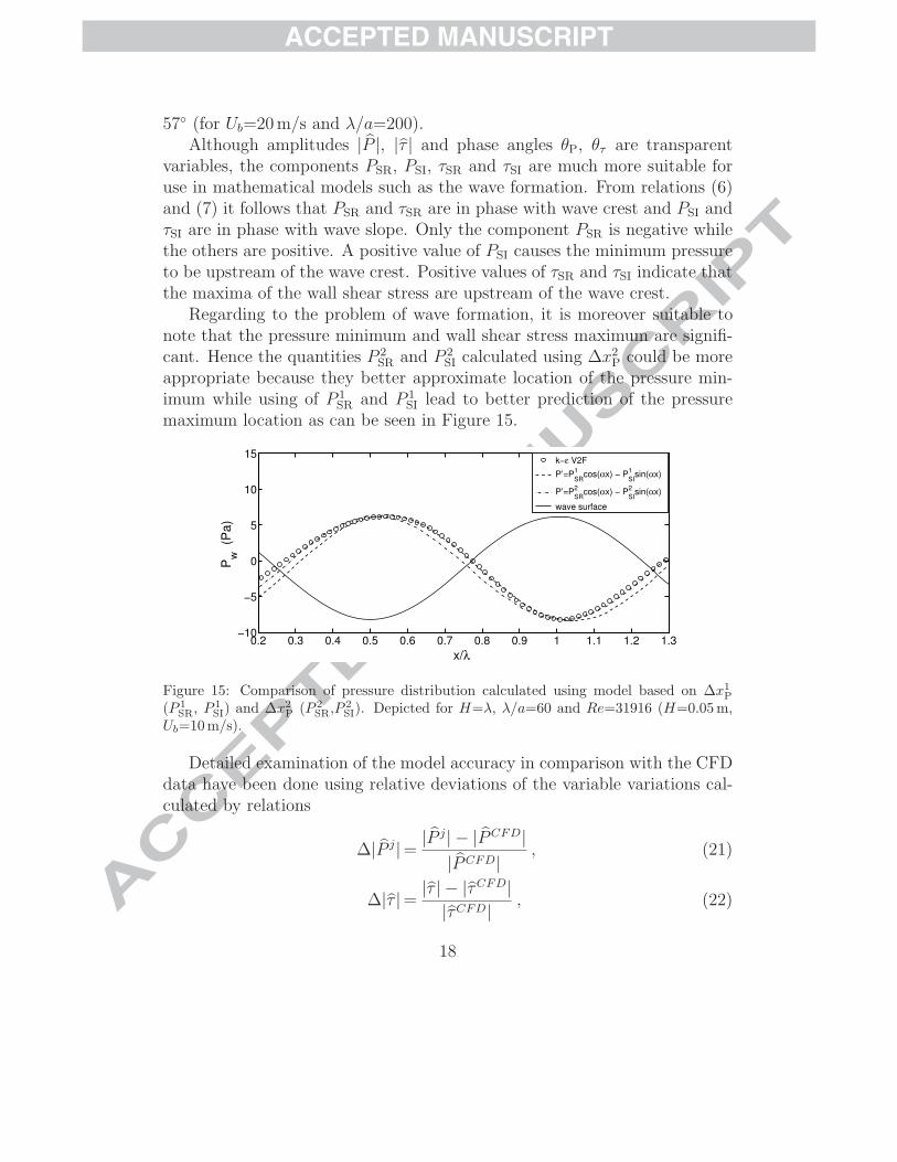
Regarding to the problem of wave formation, it is moreover suitable tonote that the pressure minimum and wall shear stress maximum are signifi-cant. Hence the quantities P 2

SR and P 2SI calculated using ∆x2

P could be moreappropriate because they better approximate location of the pressure min-imum while using of P 1

SR and P 1SI lead to better prediction of the pressure

maximum location as can be seen in Figure 15.

0.2 0.3 0.4 0.5 0.6 0.7 0.8 0.9 1 1.1 1.2 1.3−10

−5

0

5

10

15

Pw

(P

a)

x/λ

k−ε V2F

P’=P1

SRcos(αx) − P

1

SIsin(αx)

P’=P2

SRcos(αx) − P

2

SIsin(αx)

wave surface

Figure 15: Comparison of pressure distribution calculated using model based on ∆x1P

(P 1SR, P 1

SI) and ∆x2P (P 2

SR,P 2SI). Depicted for H=λ, λ/a=60 and Re=31916 (H=0.05 m,

Ub=10 m/s).

Detailed examination of the model accuracy in comparison with the CFDdata have been done using relative deviations of the variable variations cal-culated by relations

∆|P̂ j|=|P̂ j| − |P̂CFD|

|P̂CFD|, (21)

∆|τ̂ |=|τ̂ | − |τ̂CFD|

|τ̂CFD|, (22)

18

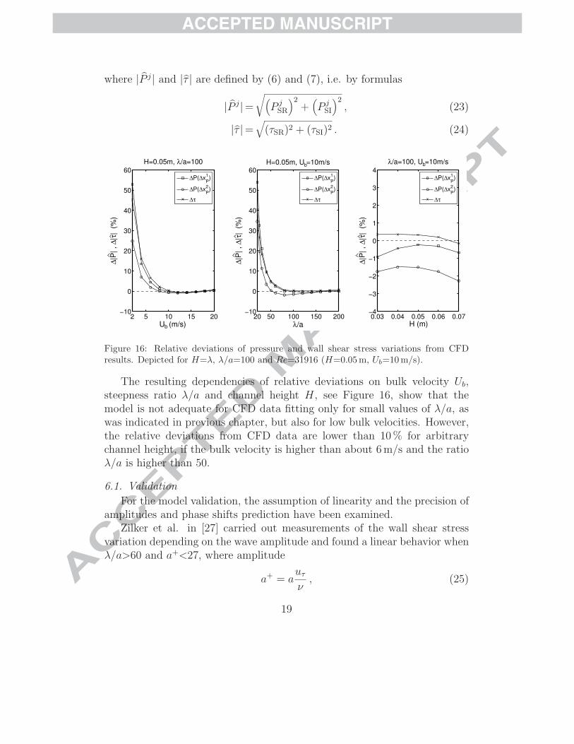
where |P̂ j| and |τ̂ | are defined by (6) and (7), i.e. by formulas

|P̂ j|=

√(P j

SR

)2+

(P j

SI

)2, (23)

|τ̂ |=√

(τSR)2 + (τSI)2 . (24)

5 10 15 202−10

0

10

20

30

40

50

60

H=0.05m, λ/a=100

∆|P

| ,

∆|τ

| (

%)

U (m/s)

∆P(∆xP

1)

∆P(∆xP

2)

∆τ

50 100 150 20020−10

0

10

20

30

40

50

60H=0.05m, U =10m/s

∆|P

| ,

∆|τ

| (

%)

λ/a

∆P(∆xP

1)

∆P(∆xP

2)

∆τ

0.03 0.04 0.05 0.06 0.07−4

−3

−2

−1

0

1

2

3

4

λ/a=100, U =10m/s

∆|P

| ,

∆|τ

| (

%)

H (m)

∆P(∆xP

1)

∆P(∆xP

2)

∆τ

b b

b

Figure 16: Relative deviations of pressure and wall shear stress variations from CFDresults. Depicted for H=λ, λ/a=100 and Re=31916 (H=0.05 m, Ub=10 m/s).

The resulting dependencies of relative deviations on bulk velocity Ub,steepness ratio λ/a and channel height H, see Figure 16, show that themodel is not adequate for CFD data fitting only for small values of λ/a, aswas indicated in previous chapter, but also for low bulk velocities. However,the relative deviations from CFD data are lower than 10 % for arbitrarychannel height, if the bulk velocity is higher than about 6 m/s and the ratioλ/a is higher than 50.

6.1. Validation

For the model validation, the assumption of linearity and the precision ofamplitudes and phase shifts prediction have been examined.

Zilker et al. in [27] carried out measurements of the wall shear stressvariation depending on the wave amplitude and found a linear behavior whenλ/a>60 and a+<27, where amplitude

a+ = auτ

ν, (25)

19

is made dimensionless using the kinematic viscosity ν and the friction velocity

uτ =√

τw/ρ , (26)

where τw would be obtained for a flat wall.Abrams in [11] states that the analysis carried out by Thorsness in [28]

indicates that for thick boundary layers the phase angle θτ characterizing theshear stress variation is a unique function of a dimensionless wave number

α+ =2π

λ

ν

uτ

, (27)

the amplitude of the shear stress variation |τ̂ | is found vary linearly with a+

and the ratio of the dimensionless amplitude a+ to a is also a unique functionof α+. Therefore, the results are further validated in dependence on thedimensionless variables just mentioned.

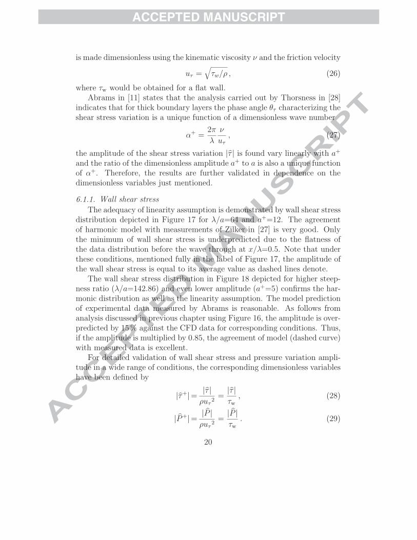
6.1.1. Wall shear stress

The adequacy of linearity assumption is demonstrated by wall shear stressdistribution depicted in Figure 17 for λ/a=64 and a+=12. The agreementof harmonic model with measurements of Zilker in [27] is very good. Onlythe minimum of wall shear stress is underpredicted due to the flatness ofthe data distribution before the wave through at x/λ=0.5. Note that underthese conditions, mentioned fully in the label of Figure 17, the amplitude ofthe wall shear stress is equal to its average value as dashed lines denote.

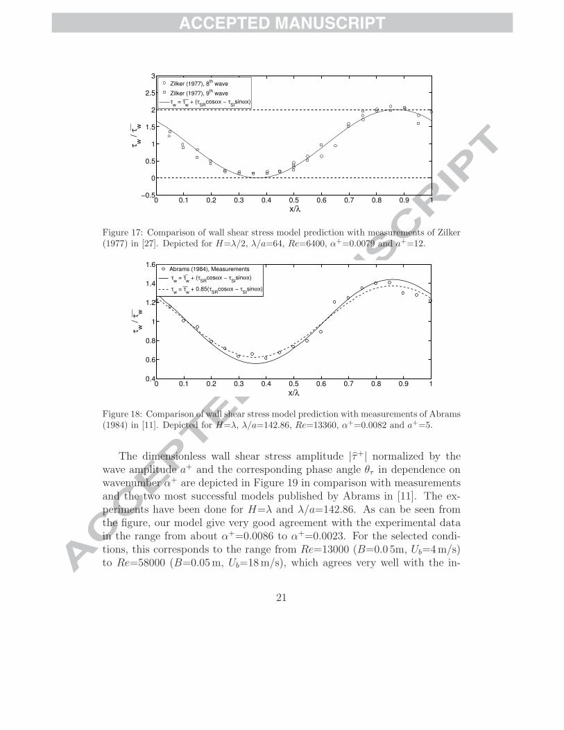
The wall shear stress distribution in Figure 18 depicted for higher steep-ness ratio (λ/a=142.86) and even lower amplitude (a+=5) confirms the har-monic distribution as well as the linearity assumption. The model predictionof experimental data measured by Abrams is reasonable. As follows fromanalysis discussed in previous chapter using Figure 16, the amplitude is over-predicted by 15 % against the CFD data for corresponding conditions. Thus,if the amplitude is multiplied by 0.85, the agreement of model (dashed curve)with measured data is excellent.

For detailed validation of wall shear stress and pressure variation ampli-tude in a wide range of conditions, the corresponding dimensionless variableshave been defined by

|τ̂+|=|τ̂ |

ρuτ2

=|τ̂ |

τw

, (28)

|P̂+|=|P̂ |

ρuτ2

=|P̂ |

τw

. (29)

20

0 0.1 0.2 0.3 0.4 0.5 0.6 0.7 0.8 0.9 1

−0.5

0

0.5

1

1.5

2

2.5

3

τ w /

τw

x/λ

Zilker (1977), 8th

wave

Zilker (1977), 9th

wave

τw

= τw

+ (τSR

cosαx − τSI

sinαx)

Figure 17: Comparison of wall shear stress model prediction with measurements of Zilker(1977) in [27]. Depicted for H=λ/2, λ/a=64, Re=6400, α+=0.0079 and a+=12.

0 0.1 0.2 0.3 0.4 0.5 0.6 0.7 0.8 0.9 10.4

0.6

0.8

1

1.2

1.4

1.6

τ w /

τw

x/λ

Abrams (1984), Measurements

τw

= τw

+ (τSR

cosαx − τSI

sinαx)

τw

= τw

+ 0.85(τSR

cosαx − τSI

sinαx)

Figure 18: Comparison of wall shear stress model prediction with measurements of Abrams(1984) in [11]. Depicted for H=λ, λ/a=142.86, Re=13360, α+=0.0082 and a+=5.

The dimensionless wall shear stress amplitude |τ̂+| normalized by thewave amplitude a+ and the corresponding phase angle θτ in dependence onwavenumber α+ are depicted in Figure 19 in comparison with measurementsand the two most successful models published by Abrams in [11]. The ex-periments have been done for H=λ and λ/a=142.86. As can be seen fromthe figure, our model give very good agreement with the experimental datain the range from about α+=0.0086 to α+=0.0023. For the selected condi-tions, this corresponds to the range from Re=13000 (B=0.0 5m, Ub=4 m/s)to Re=58000 (B=0.05 m, Ub=18 m/s), which agrees very well with the in-

21

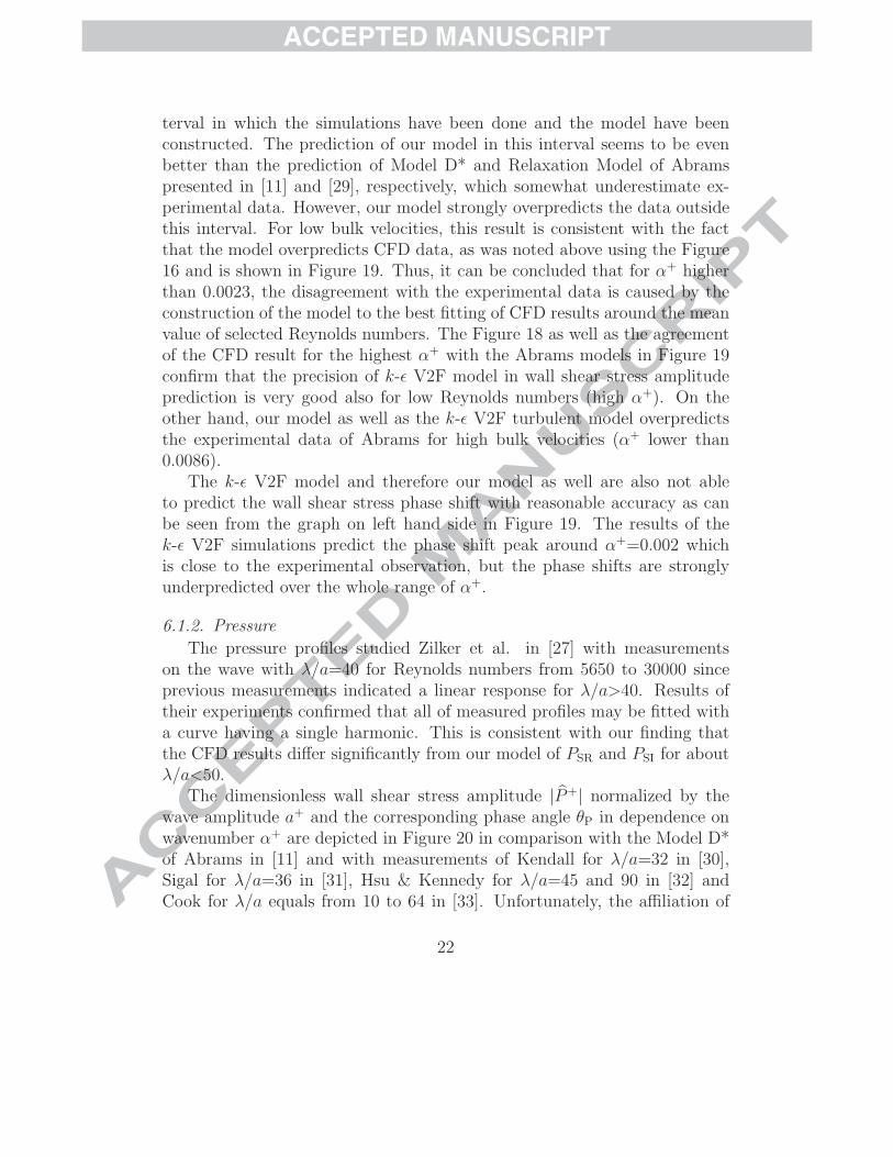
terval in which the simulations have been done and the model have beenconstructed. The prediction of our model in this interval seems to be evenbetter than the prediction of Model D* and Relaxation Model of Abramspresented in [11] and [29], respectively, which somewhat underestimate ex-perimental data. However, our model strongly overpredicts the data outsidethis interval. For low bulk velocities, this result is consistent with the factthat the model overpredicts CFD data, as was noted above using the Figure16 and is shown in Figure 19. Thus, it can be concluded that for α+ higherthan 0.0023, the disagreement with the experimental data is caused by theconstruction of the model to the best fitting of CFD results around the meanvalue of selected Reynolds numbers. The Figure 18 as well as the agreementof the CFD result for the highest α+ with the Abrams models in Figure 19confirm that the precision of k-ε V2F model in wall shear stress amplitudeprediction is very good also for low Reynolds numbers (high α+). On theother hand, our model as well as the k-ε V2F turbulent model overpredictsthe experimental data of Abrams for high bulk velocities (α+ lower than0.0086).

The k-ε V2F model and therefore our model as well are also not ableto predict the wall shear stress phase shift with reasonable accuracy as canbe seen from the graph on left hand side in Figure 19. The results of thek-ε V2F simulations predict the phase shift peak around α+=0.002 whichis close to the experimental observation, but the phase shifts are stronglyunderpredicted over the whole range of α+.

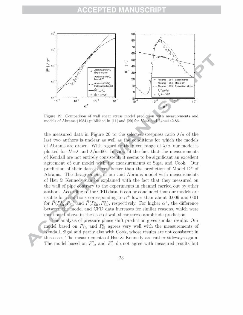
6.1.2. Pressure

The pressure profiles studied Zilker et al. in [27] with measurementson the wave with λ/a=40 for Reynolds numbers from 5650 to 30000 sinceprevious measurements indicated a linear response for λ/a>40. Results oftheir experiments confirmed that all of measured profiles may be fitted witha curve having a single harmonic. This is consistent with our finding thatthe CFD results differ significantly from our model of PSR and PSI for aboutλ/a<50.

The dimensionless wall shear stress amplitude |P̂+| normalized by thewave amplitude a+ and the corresponding phase angle θP in dependence onwavenumber α+ are depicted in Figure 20 in comparison with the Model D*of Abrams in [11] and with measurements of Kendall for λ/a=32 in [30],Sigal for λ/a=36 in [31], Hsu & Kennedy for λ/a=45 and 90 in [32] andCook for λ/a equals from 10 to 64 in [33]. Unfortunately, the affiliation of

22

10−4

10−3

10−2

10−1

10−4

10−3

10−2

10−1

100

|τ

| /

a

α+

Abrams (1984),Experiments

Abrams (1984),Model D*

Abrams (1984),Relaxation Model

|τ|(τSR

,τSI

)

|τ|, k−ε V2F

10−4

10−3

10−2

10−1

−10

0

10

20

30

40

50

60

70

80

90

α+

θτ (°)

Abrams (1984), Experiments

Abrams (1984), Model D*

Abrams (1985), Relaxation Model

θτ (τ

SR,τ

SI)

θτ, k−ε V2F

+

+

Figure 19: Comparison of wall shear stress model prediction with measurements andmodels of Abrams (1984) published in [11] and [29] for H=λ and λ/a=142.86.

the measured data in Figure 20 to the selected steepness ratio λ/a of thelast two authors is unclear as well as the conditions for which the modelsof Abrams are drawn. With regard to the given range of λ/a, our model isplotted for H=λ and λ/a=60. In view of the fact that the measurementsof Kendall are not entirely consistent, it seems to be significant an excellentagreement of our model with the measurements of Sigal and Cook. Ourprediction of their data is even better than the prediction of Model D* ofAbrams. The disagreement of our and Abrams model with measurementsof Hsu & Kennedy can be explained with the fact that they measured onthe wall of pipe contrary to the experiments in channel carried out by otherauthors. According to the CFD data, it can be concluded that our models areusable for conditions corresponding to α+ lower than about 0.006 and 0.01for P̂ (P 1

SR, P 1SI) and P̂ (P 2

SR, P 2SI), respectively. For higher α+, the difference

between the model and CFD data increases for similar reasons, which werementioned above in the case of wall shear stress amplitude prediction.

The analysis of pressure phase shift prediction gives similar results. Ourmodel based on P 1

SR and P 1SI agrees very well with the measurements of

Kendall, Sigal and partly also with Cook, whose results are not consistent inthis case. The measurements of Hsu & Kennedy are rather sideways again.The model based on P 2

SR and P 2SI do not agree with measured results but

23

10−4

10−3

10−2

10−1

10−1

100

101

|P

| /

a

α+

Cook (1970)

Sigal (1970)

Kendall (1970)

Hsu & Kennedy (1971)

Abrams (1984), model D*

|P| (P1

SR,P

1

SI)

|P| (P2

SR,P

2

SI)

|P|, k−ε V2F

10−4

10−3

10−2

10−1

120

130

140

150

160

170

180

θP (°

)

α+

Cook (1970)

Sigal (1970)

Kendall (1970)

Hsu & Kennedy (1971)

Abrams (1984), model D*

Abrams (1984), model D*with Curvature Correction

θ1

P (P

1

SR,P

1

SI)

θ2

P (P

2

SR,P

2

SI)

θ1

P, k−ε V2F

θ2

P, k−ε V2F

+

+

Figure 20: Comparison of model prediction of the pressure variation with models ofAbrams in [11] and measurements of Kendall in [30], Sigal in [31], Hsu & Kennedy in[32] and Cook in [33].

this is not decisive because of the specific selection of the phase shift whichwas surely not used by authors of referred experiments. Regarding to thefact that the model D* overpredicts measurements, except results of Sigal,Abrams made curvature correction specified more detailed in [11]. However,the new model seems to be able to predict the measurements rather forhigher α+ as is indicated by disagreement with results of Sigal and by oursimulations results plotted in Figure 20. While the θ2

P model agrees verywell with CFD data in the whole range of α+, the θ1

P model is usable for α+

lower than about 0.006 which is consistent with the range of applicability ofamplitude model as was noted above.

7. Conclusions

This paper presents algebraic models of wall shear stress and pressureforces acting on the wavy surface in channels with turbulent flow in depen-dence on channel height, ratio of the wavelength to the wave amplitude andbulk velocity.

The models have been constructed using results of the set of steady nu-merical simulations computed for various configurations defined by selection

24

of channel height H in range of H/λ from 0.6 to 1.4, wave steepness ratioλ/a in range from 20 to 200 and bulk velocity Ub in range of Re=HUb/νfrom 3830 to 89366. From the comparison of the pressure and wall shearstress distributions as well as velocity profiles computed for selected turbu-lence models with DNS results, the applicability of the k-ε V2F has beenproved and hence this model has been used for numerical simulations. Thecorresponding computational grids has been made with regards to the findingthat the results differ very little if maximal value of y+

wall is less than 0.8.The Reynolds decomposition of the pressure and wall shear stress given

by (2)–(5) introduces variables PSR, PSI, τSR and τSI defined by relations(6) and (7). Our models of wall shear stress and pressure variations arebased on linear regression and empirical fitting of PSR, PSI, τSR and τSI givenby numerical results. From the comparison of our models with original CFDdata, it follows that the multiplicative models using by us are very well usable.The relative deviations from CFD data are lower than 10 % for arbitrarychannel height in range mentioned above, if the bulk velocity is higher thanabout 6 m/s and the ratio λ/a is higher than 50. The disagreement of themodel prediction with the experimental data for low velocities is caused bythe construction of the model to the best fitting of CFD results around themean value of selected Reynolds numbers.

Because of the pressure distribution deformation observed for low Reynoldsnumbers and low value of λ/a, we have defined the phase angle θ1

P by phaseshift of the pressure maximum against the wave crest and the phase an-gle θ2

P by phase shift of the pressure minimum against the wave through.The difference θ1

P − θ2P decreases with increasing bulk velocity and increasing

steepness ratio λ/a. The pressure and wall shear stress variation amplitudeincrease with increasing bulk velocity and decrease strongly with increasingratio λ/a and slightly with increasing channel height. Depending on the bulkvelocity, the wall shear stress amplitude |τ̂ | is about 10 (for Ub=2 m/s) to 50(for Ub=20 m/s) times smaller than the pressure amplitude |P̂ | and this ratioremains almost the same when λ/a and H are changing.

The model has been validated by the examination of the linearity (har-monic) assumption and the precision of amplitude and phase shift prediction.The linearity confirmed Zilker in [27] for λ/a>60 and a+<27 in the case ofwall shear stress distribution and for λ/a>40 in the case of pressure distri-bution. The agreement of the wall shear stress distribution given by mea-surements with the harmonic function generated by our model for low valueof a+ is very good. The model of wall shear stress amplitude gives excellent

25

agreement with the experimental data in the range from about α+=0.0086to α+=0.0023. Our prediction in this interval seems to be better than theprediction of Model D* and Relaxation Model of Abrams presented in [11]and [29], respectively. On the other hand, the k-ε V2F model and thereforeour model as well are not able to predict the wall shear stress phase shiftwith reasonable accuracy. The phase shifts are strongly underpredicted overthe whole range of α+. The prediction of pressure variation amplitude andphase angle seems to be usable for conditions corresponding to α+ lower thanabout 0.006. In this range, our model gives better agreement with experi-mental data than models of Abrams, although the considerable scatter aswell as the lack of experimental data makes the comparison difficult.

From the validation part, it can be therefore summarized that the k-ε V2Fturbulence model gives very good results in pressure prediction in a widerange of conditions, but the wall shear stress phase shift is predicted onlyin qualitative sense and the prediction of its variation amplitude is limitedby the dimensionless wavenumber α+. However, with regards to the ratiobetween variation amplitude of pressure and wall shear stress, the forcesprediction in given range of conditions gives very good results in comparisonwith rather complex models of Abrams and thus the models could be usedwith the advantages of its simplicity in simulations of several industrial orenvironmental applications where force action on wavy surface is desired.

8. Acknowledgement

The authors would like to greatly acknowledge the financial support re-ceived from the Czech Science Foundation (project No. GA P105/11/1339).

References

[1] G. Csanady, Air-sea interaction, Laws and mechanisms., CambridgeUniversity Presss, 2004.

[2] T. J. Hanratty, Interfacial instabilities caused by air flow over a thin liq-uid layers, in: R. E. Meyer (Ed.), Waves on Fluid Interfaces, AcademicPress, New York, NY, 1983, pp. 221–259.

[3] Y. S. Chang, A. Scotti, Modeling unsteady turbulent flows overripples: Reynolds-averaged Navier-stokes equations (RANS) ver-sus large-eddy simulation (LES), J. Geophys. Res. 109 (2004).doi:10.1029/2003JC002208.

26

[4] S. G. Sajjadi, J. N. Aldridge, Prediction of turbulent flow over roughasymmetrical bed forms, Appl. Math. Modelling 19 (1995).

[5] S. W. Chang, A. W. Lees, T. C. Chou, Heat transfer and pressure dropin furrowed channels with transverse and skewed sinusoidal wavy walls,International Journal of Heat and Mass Transfer 52 (2009) 4592–4603.

[6] M. A. Mehrabian, R. Poulter, Hydrodynamics and thermal character-istics of corrugated channels: computational approach, Applied Mathe-matical Modelling 24 (2000) 343–364.

[7] A. Balabel, Numerical modeling of turbulence-induced interfacial insta-bility in two-phase flow with moving interface, Applied MathematicalModelling 36 (2012) 3593–3611.

[8] Z. Xie, Two-phase flow modelling of spilling and plunging breakingwaves, Applied Mathematical Modelling (2012). Article in press.

[9] R. Miesen, B. J. Boersma, Hydrodynamics stability of sheared liquidfilm, J. Fluid Mech. 301 (1995) 175–202.

[10] L. O Naraigh, P. D. M. Spelt, O. K. Matar, T. A. Zaki, Interfacialinstability in turbulent flow over a liquid film in a channel, InternationalJournal of Multiphase Flow 37 (2011) 812–830.

[11] J. Abrams, Turbulent flow over small amplitude solid waves, Ph.D. the-sis, University of Illinois at Urbana-Champaign, 1984.

[12] N. C. G. Markatos, Heat, mass and momentum transfer across a wavzboundary, Computer Methods in Applied Nechanics and Engineering14 (1978) 323–376.

[13] N. C. G. Markatos, Stochastic modelling of dynamic properties of non-linear water waves, Appl. Math. Modelling 2 (1978) 227–238.

[14] C. Maass, U. Schumann, Direct numerical simulation of separated tur-bulent flow over wavy boundary, in: E. H. Hirschel (Ed.), Flow Sim-ulation with High-Performance Computers (Notes on Numerical FluidMechanics), Friedrich Vieweg & Sohn Verlag, 1996, pp. 227–241.

27

[15] P. Cherukat, Y. Na, T. J. Hanratty, J. McLaughlin, Direct numericalsimulation of a fully developed turbulent flow over a wavy wall, Theoret.Comput. Fluid Dynamics 11 (1998) 109–134.

[16] H. S. Yoon, O. A. El-Samni, A. T. Huynh, H. H. Chun, H. J. Kim, A. H.Pham, I. Park, Effect of wave amplitude on turbulent flow in a wavychannel by direct numerical simulation, Ocean Engineering 36 (2009)697–707.

[17] D. C. Wilcox, Turbulence Modeling for CFD, DCW Industries, Inc., 2ndedition, 1998.

[18] F. Menter, Two-equation eddy-viscosity turbulence modeling for engi-neering applications, AIAA Journal 32 (1994) 1598–1605.

[19] L. Davidson, P. V. Nielsen, A. Sveningsson, Modifications of the V2model for computing the flow in a 3D wall jet, Turbulence, Heat andMass Transfer 4 (2003) 577–584.

[20] European research community on flow, Turbulence and CombustionDatabase, Classic collection, http://cfd.mace.manchester.ac.uk/

ercoftac/index.html, January 2012.

[21] J. D. Hudson, The effect of a wavy boundary on turbulent flow, Ph.D.thesis, University of Illinois, Urbana, IL, 1993.

[22] J. D. Hudson, L. Dykhno, T. J. Hanratty, Turbulence production inflow over a wavy wall, Exper. Fluids 20 (1996) 257.

[23] L. S. Lien, G. Kalitzin, P. A. Durbin, Rans modeling for compressibleand transitional flows, in: Center for Turbulence Research - Proceedingsof the Summer Program 1998.

[24] P. A. Durbin, On the k-e stagnation point anomaly, Int. J. Heat andFluid Flow 17 (1996) 89–90.

[25] User Guide, STAR-CCM+, Version 6.04.016, CD-adapco, 2011.

[26] D. E. Woodmansee, T. J. Hanratty, Mechanism for the removal ofdroplets from a liquid surface by a parallel air flow, Chemical Engineer-ing Science 24 (1969) 299–307.

28

[27] D. P. Zilker, G. W. Cook, T. Hanratty, Influence of the amplitude ofa solid wavy wall on a turbulent flow. part 1. non-separated flows, J.Fluid Mech. 82 (1977) 29–51.

[28] C. B. Thorsness, Transport phenomena associated with flow over a solidwavy surface, Ph.D. thesis, Department of Chemical Engineering, Uni-versity of Illinois, Urbana, 1975.

[29] J. Abrams, T. J. Hanratty, Relaxation effects observed for turbulentflow over a wavy surface, J. Fluid Mech. 151 (1985) 443–455.

[30] J. M. Kendall, The turbulent boundary layer over a wall with progressivesurface waves, J. Fluid Mech. 41 (1970).

[31] A. Sigal, An Experimental Investigation of the Turbulent BoundaryLayer over a Wavy Wall, Ph.D. thesis, Department of Aeronautical En-gineering, California Institute of Technology, 1970.

[32] S. Hsu, J. F. Kennedy, Turbulent flow in wavy pipes, J. Fluid Mech. 47(1971).

[33] G. W. Cook, Turbulent Flow Over Solid Wavy Surfaces, Ph.D. thesis,Department of Chemical Engineering, University of Illinois, Urbana,1970.

29