�����������������

Citation: Das, S.; Kumar, U.

Modeling of Bi-Polar Leader

Inception and Propagation from

Flying Aircraft Prior to a Lightning

Strike. Atmosphere 2022, 13, 943.

https://doi.org/10.3390/

atmos13060943

Academic Editor: Eduardo

García-Ortega

Received: 3 May 2022

Accepted: 6 June 2022

Published: 9 June 2022

Publisher’s Note: MDPI stays neutral

with regard to jurisdictional claims in

published maps and institutional affil-

iations.

Copyright: © 2022 by the authors.

Licensee MDPI, Basel, Switzerland.

This article is an open access article

distributed under the terms and

conditions of the Creative Commons

Attribution (CC BY) license (https://

creativecommons.org/licenses/by/

4.0/).

atmosphere

Article

Modeling of Bi-Polar Leader Inception and Propagation fromFlying Aircraft Prior to a Lightning StrikeSayantan Das * and Udaya Kumar

Electrical Engineering Department, Indian Institute of Science, Bangalore 560012, India; udayk@iisc.ac.in* Correspondence: sayantand3@gmail.com

Abstract: Lightning is one of the major environmental threats to aircraft. The lightning strikes duringflying are mostly attributed to aircraft-triggered lightning. The first step toward designing suitableprotective measures against lightning is identifying the attachment locations. For this purpose,oversimplified approaches are currently employed, which do not represent the associated dischargephenomena. Therefore, in this work, a suitable model is developed for simulating the inception andpropagation of bi-polar leader discharge from the aircraft. Modeling of leader discharges requiresfield computation around the aircraft, which is carried out employing the Surface Charge SimulationMethod (SCSM) combined with sub-modeling, which ensures the best accuracy of field computationsnear nosecone, wingtips, etc. A DC10 aircraft model is considered for the simulation. Simulationsare performed for different pairs of leader inception points on aircraft using the developed model.Subsequently, corresponding ambient fields required for stable bi-polar discharge from aircraft aredetermined. These values are in the range of measured ambient fields reported in the literature. Insummary, the present work has come up with a suitable model for simulating the bi-polar leaderinception and propagation from the flying aircraft. Using the same, a detailed quantitative descriptionof the discharge phenomena from the aircraft is provided.

Keywords: lightning; lightning strike to aircraft; surface charge simulation method; bi-polar leaderdischarge; positive leader discharge; negative leader discharge

1. Introduction

Since the early age of aviation, lightning strikes have been proven to be hazardousto aircraft. It is estimated that on average, a commercial aircraft gets struck by lightningonce in every 1000 flight hours, which is approximately equivalent to once in a year [1].The effect of a lightning strike on aircraft spans from minor damages (i.e., burn markson the skin, creation of holes, local deformation of parts, etc.) to complete destruction ofaircraft (due to damage to fuel tanks, an explosion of the air–fuel mixture, destruction ofinternal circuitry, etc.). Hence, the threat caused by lightning needs serious consideration.Adding on to it, in modern aircraft, fiber-glass, carbon fiber, etc., materials are being in-creasingly employed due to their higher strength to mass ratio. However, due to their poorconductivity, the stroke current can lead to structural damage and higher field diffusionin the interior regions. In addition, extensive use of sensitive electronic equipment hasfurther escalated the risk due to lightning strikes. According to National Oceanic andAtmospheric Administration, lightning strikes cost approximately two billion dollars forairline operators, excluding repair expenses [2]. Therefore, lightning protective measureshave become an inextricable part of modern aircraft design.

A lightning strike on aircraft can occur in two possible ways. Bi-directional leaderscan get initiated from aircraft in a high ambient field created by cloud and stepped leader.This type of aircraft-initiated lightning is responsible for almost 90% of the recorded cases sofar [3]. The other rare event is the aircraft intercepts a descending lightning leader from

Atmosphere 2022, 13, 943. https://doi.org/10.3390/atmos13060943 https://www.mdpi.com/journal/atmosphere

Atmosphere 2022, 13, 943 2 of 18

the cloud. Hence, considering the higher probability of the former type of attachment, thiswork will only be confined to aircraft-initiated lightning strikes.

Several in-flight measurement programs have provided insight into the phenomenaassociated with a lightning strike on aircraft. NASA’s Storm Hazard Program (F-106Baircraft, 1978–1986) [4–6], USAF/FAA Lighting Characterization program (CV-580 aircraft,1984–1987) [7,8], ONERA/CEV Transall Program (C-160 aircraft, 1984, 1988) [9,10], andmost recently the EXAEDRE project (Falcon 20 aircraft, 2016–2019, France) [11] are the majorprograms which were conducted to gather data on lightning strike. In all these programs,instrumented aircraft have been flown intentionally in and around the thundercloud torecord the electric field and currents at selected locations preceding to and during thelighting strikes. Some recorded videos [10] have provided more clarity on the mechanismsinvolved in lightning attachment to aircraft.

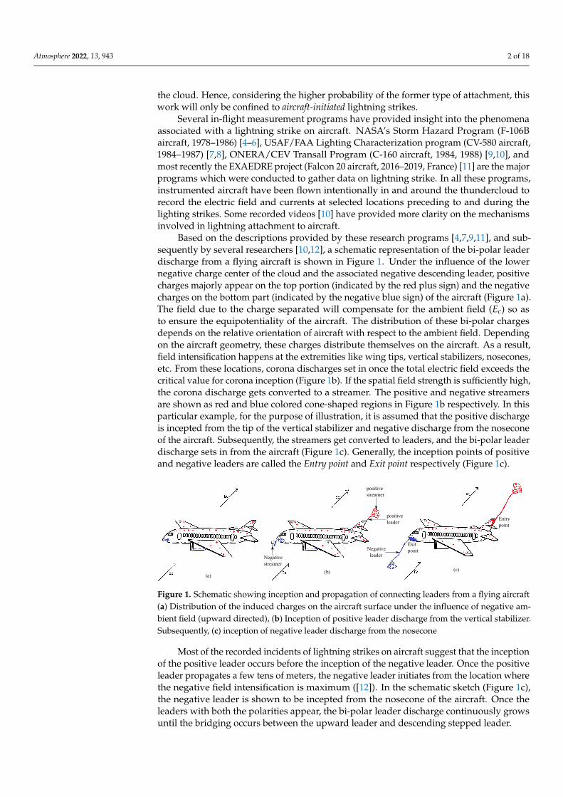
Based on the descriptions provided by these research programs [4,7,9,11], and sub-sequently by several researchers [10,12], a schematic representation of the bi-polar leaderdischarge from a flying aircraft is shown in Figure 1. Under the influence of the lowernegative charge center of the cloud and the associated negative descending leader, positivecharges majorly appear on the top portion (indicated by the red plus sign) and the negativecharges on the bottom part (indicated by the negative blue sign) of the aircraft (Figure 1a).The field due to the charge separated will compensate for the ambient field (Ec) so asto ensure the equipotentiality of the aircraft. The distribution of these bi-polar chargesdepends on the relative orientation of aircraft with respect to the ambient field. Dependingon the aircraft geometry, these charges distribute themselves on the aircraft. As a result,field intensification happens at the extremities like wing tips, vertical stabilizers, nosecones,etc. From these locations, corona discharges set in once the total electric field exceeds thecritical value for corona inception (Figure 1b). If the spatial field strength is sufficiently high,the corona discharge gets converted to a streamer. The positive and negative streamersare shown as red and blue colored cone-shaped regions in Figure 1b respectively. In thisparticular example, for the purpose of illustration, it is assumed that the positive dischargeis incepted from the tip of the vertical stabilizer and negative discharge from the noseconeof the aircraft. Subsequently, the streamers get converted to leaders, and the bi-polar leaderdischarge sets in from the aircraft (Figure 1c). Generally, the inception points of positiveand negative leaders are called the Entry point and Exit point respectively (Figure 1c).

(c)

positive

leader

Exit

point

(b)

Negative

leaderNegative

streamer

(a)

Entry

point

positive

streamer

Figure 1. Schematic showing inception and propagation of connecting leaders from a flying aircraft(a) Distribution of the induced charges on the aircraft surface under the influence of negative am-bient field (upward directed), (b) Inception of positive leader discharge from the vertical stabilizer.Subsequently, (c) inception of negative leader discharge from the nosecone

Most of the recorded incidents of lightning strikes on aircraft suggest that the inceptionof the positive leader occurs before the inception of the negative leader. Once the positiveleader propagates a few tens of meters, the negative leader initiates from the location wherethe negative field intensification is maximum ([12]). In the schematic sketch (Figure 1c),the negative leader is shown to be incepted from the nosecone of the aircraft. Once theleaders with both the polarities appear, the bi-polar leader discharge continuously growsuntil the bridging occurs between the upward leader and descending stepped leader.

Atmosphere 2022, 13, 943 3 of 18

Depending on the lightning attachment points and resulting current distribution,the aircraft surface can be classified into different zones. This part of designing is called“Zoning” where the outer surface of aircraft is divided into well-defined regions (1A, 1B,1C, 2A, 2B, 3 as suggested in [13]) depending on how they experience different phases oflightning stroke. This study in this paper only deals with identifying the initial attachmentspoints on aircraft, which fall under Zone 1A and 1B.

Several methods for the zoning of aircraft have been developed in the last few decades.In 1989, British Aerospace (BAe) proposed a method of zoning of aircraft [14] based onthe Rolling Sphere Method (RSM) [15] which is an empirical method based on the Electro-geometrical method (EGM) [16]. EGM, which was developed for lightning protection oftransmission lines, was later modified to RSM for lightning protection of grounded objects.RSM is a well-recognized and widely used method for lightning protection of groundedobjects. In RSM, a sphere with a radius of striking distance (calculated from prospectivereturn stroke current) is rolled over the objects to determine the probable locations forlighting strike [15]. In 1999, the Society of Automotive Engineers (SAE) published aregulatory document, “ARP5414A” [13] regarding the zoning of an aircraft. In this standard,the approach involved in RSM for grounded objects has been extended for the zoning ofaircraft. In the literature [13], apart from RSM, the similarity principle has been suggestedwhere zoning was conducted based on zone data available from previously certified aircraft.This method is entirely qualitative and only applicable for aircraft with similar geometries.Field-based approaches for zoning and zoning based on laboratory testing on a scaled modelof aircraft or isolated parts of aircraft have been mentioned in this literature [13] as well.In 2012, Lalande et al. proposed a probabilistic method of zoning of aircraft [17] basedon previous methodologies (RSM, similarity principle, laboratory testing). These existingmethods for zoning are highly simplified and do not include different aspects of long air gapbreakdown. For a more accurate assessment, the inception and propagation of bi-directionalleaders from aircraft need to be taken into account. None of these aforementioned methodshave considered the discharge mechanisms involved in lightning attachment in detail.In view of the above, this work aims to develop a model for bi-polar discharge from aircraft,which will lead to the identification of lightning attachments points.

Experimental works have been reported in the literature on bi-polar discharge fromfloating objects in laboratory gaps. In 1995, Rizk came up with an analytical model [18]for the breakdown of long laboratory gaps (5, 8 m), including a floating conductor un-der applied switching impulse. Subsequently, in 1998, Castellani et al. also presentedexperimental data on discharge from a floating object placed in a 10.5 m long plane–planegap [19,20]. Most recently, Jiachen Gao et al. [21] reported breakdown voltages of a gap of2 m in the presence of floating rods and spheres.

The sequence of events associated with lightning initiation from aircraft is well estab-lished and widely accepted. However, due to the complexity involved in the dischargemechanism, literature on modeling of discharge from aircraft is rather difficult to find.Therefore, this work focuses on the development of a suitable macroscopic model forbi-polar discharge from aircraft prior to aircraft-triggered lightning strikes. Dischargefrom a flying aircraft involves both positive and negative leader discharges. Invariably,models for lightning attachment are developed based on laboratory findings. Therefore,detailed literature surveys on positive and negative leader discharges in long air gaps arecarried out.

2. Modeling of Bi-Polar Discharge from Aircraft2.1. Modeling of Positive Leader Discharge

Positive discharge in long air gaps starts with the initiation of a positive coronafollowed by positive streamer bursts with a common stem. If the existing ambient fieldis increasing or sufficiently high, the streamer grows, and the corresponding charge flowcauses heating of the stem to more than 1500 K. Due to this thermalization of the stem, itgets converted to a leader [22]. Several such intermittent leaders emerge and vanish before

Atmosphere 2022, 13, 943 4 of 18

a stable leader propagation gets established. This stable leader propagates continuouslywith a positive streamer zone ahead of it.

Over the years, several models for positive leader discharge have been proposed.Hutzler’s model for leader propagation [23], the Critical radius criterion [24,25], Criticalstreamer length criterion [26,27], empirical model [28,29], and thermo-hydrodynamical model [22]are the few mentions. In 2006, using the findings of Gallimberti et al. [22,30], Becerraand Cooray proposed a physical model [31] called the self consistent leader inception model(SLIM). This model was validated for leader discharges in laboratory gaps [31], connectingleader inception from grounded objects [31] and for rocket triggered lightning [32] as well.The SLIM needs significant computational resources. To reduce that, a simplified model isalso suggested in [31]. This simplified method was successfully implemented on groundedstructures [33,34]. For inception and propagation of positive connecting leader from aircraft,this simplified model [31] is considered.

In Figure 2, a schematic of positive leader discharge from an electrode is shown (at thetop) along with a corresponding distance–voltage diagram (at the bottom). The distance–voltage diagram includes the potential distributions along the discharge axis at differentinstants of discharge growth. The blue color curve (Pback) in distance–voltage diagram(Figure 2) represents the background potential distribution. Once, the streamer appears, it isrepresented with a straight line (P(0)) with a slope set to the positive streamer gradient [31].Each green and red color curve (P(i) for ith leader increment) represents the potentialdistribution for leader length at one instant, where the red part corresponds to the positivestreamer. The leader itself is represented by a straight line (green color with the slope set tothe leader gradient.

lL(1) lL

(2) lL(4)

lL(3)

lst(5)lst(2)lst(1)lst(3) lst(4)

Positive

streamer

Positive

leader

Distance along the discharge axis

Po

ten

tial

Electrode

Pback

P(0)P(1)

P(3)P(2) P(4)

Figure 2. Schematic of positive leader growth and the corresponding axial potential distributions asdescribed in [31].

The steps involve in this model ([31]) are explained with the reference of Figure 2.

• Adding up ambient potential and reaction potential due to induced charges on aircraft,total potential distribution (Pback in Figure 2) is obtained.

• A straight line with a slope of 450 kV/m is considered as streamer section (such asP(0) in Figure 2). Streamer charge is computed from the area between backgroundpotential distribution and modified potential distribution (Equation (1)) [30,31].

Qstr = KQ∫ l(1)st

0(Pback − P(0)) dx (1)

where x is the distance along the discharge axis. KQ is the geometrical factor whosevalue is taken as 4× 10−11 C/V·m.

Atmosphere 2022, 13, 943 5 of 18

• If Qstr ≥ 1µC, positive discharge starts with an initial length of 5 cm. The correspond-ing potential drop along the leader length is calculated using Rizk’s equation [31],

V(i)ldrop = l(i)L E∞ + x0E∞ ln [

Estr

E∞− Estr − E∞

E∞e−

l(i)Lx0 ] (2)

where l(i)L is the leader length at ith step, Estr is gradient of positive streamer,E∞ = 30 kV/m is the final quasi-stationary leader gradient, and x0 = 0.75 m is thetime constant.

• In subsequent steps, the incremental streamer charge (4Q(i)str) is again calculated

from the area between two consecutive potential distributions. Subsequently, theincremental leader length is evaluated.

4Q(i)str = KQ

∫ l(i−1)st

l(i−2)L

(P(i−1) − P(i−2)) dx (3)

4l(i)L =4Q(i)

strqL

(4)

where P(i) is the potential distribution at tth instant in presence of leader and streamerboth (Figure 2). qL = 65 µC/m, is the charge per unit length of positive leader [31].

• The modified leader length at ith instant is calculated as l(i)L = l(i)L +4l(i)L .

A more elaborated explanation of different aspects of this positive leader model isavailable in [31].

2.2. Modeling of Negative Leader Discharge

Unlike positive leader discharges, negative leader discharges are more complicatedphysical phenomena. The first phase of negative discharge is the formation of a negativecorona if the field value at the electrode exceeds a critical level. Once the corona attains itscritical volume, i.e., contains a critical amount of negative charges, a space stem appears atthe tip of the discharge [19,35]. This space stem initiates bi-directional streamers called apilot system involving a positive streamer towards the electrode and a negative streamerahead of the discharge, as shown in Figure 3(II). Injection of these streamer charges heatsup the space stem and converts it into bi-directional space leaders. When the positivespace leader reaches the primary negative leader tip, all the streamer charges flow to theelectrode through the discharge channel resulting in a sudden elongation of the mainnegative leader [35]. This phase is observed as a highly illuminated channel in recordingsof laboratory discharge [35]. Again, a negative streamer is formed ahead of the newlyformed extension of the negative leader (Figure 3(IV)), followed by the formation of a spacestem. These inter-step processes keep on repeating, which results in step-wise elongationof negative discharge.

-Vapplied-Vapplied-Vapplied-Vapplied

Electrode

I. II. III. IV.

Positive

tream

Positive

space

leaderNegative

space

leader

Primary

negative

leader

Space

stemNegative

space

streamer

Positive

space

streamerNegative

streamer

Figure 3. Schematic representation of stages of negative leader discharge.

Atmosphere 2022, 13, 943 6 of 18

Despite having substantial experimental data (Les Renadieres [35], Castellaniet al. [19,20]),research on the physical model of negative leader discharge is limited. In 1994, Bechh-iega et al. [36] developed a theoretical model for negative leader discharge. Subsequently,Mazur et al. [37], L. Arevalo, and Cooray [38] came up with physical models for negativedischarges. The RLC linear circuit model for negative discharge was presented by Rako-tonandrasana et al. [39] and most recently, in 2019 Zixin Guo, Rakov et al. [40] proposeda simplified model for negative leader propagation. Because of ease of implementationand requirement of less computational resources, this model [40] is considered for negativeleader inception and propagation from aircraft. This model is validated in [40] for differentlaboratory gap discharges.

For the negative leader discharge, a different distance–voltage diagram can be drawnas shown in Figure 4. The background potential distribution prior to negative discharge isshown as V(0)

back (black curve). Once, the primary negative streamer appears, it is shown witha straight line (blue line, P(0)) with a slope set to the negative streamer gradient. The inter-section between V(0)

back and P(0) provides the axial extension of the negative streamer andit is also the position at which the space stem (shown with a black dot) appears. The po-tential distributions for different space leaders lengths are labeled as P(0), P(1), P(2), P(3).Positive (red line) and negative space streamers (blue line) are represented with straightlines with slope set to their respective streamer gradient. The space leaders are shown withhorizontal lines (dashed), while the primary negative leader is shown with a black (dashed)line in the distance–voltage diagram (Figure 4).

Vback(0)

Vback(1)Vback

(2)

P(0) P(1)P(2)

P(3)

Primary negative leader

Negative space leader (nsl)Positive space leader (psl)

Positive streamer Negative streamer (nstr)

Distance along discharge axis

Poten

tial

Vapplied

Space stem (ss)

x

lnsl(2)lnsl

(3) lnstr(1) lnstr

(2)lnstr

(3)lpsl

(2) lpsl(3)lL

(2) lL(3) lss

Figure 4. Illustration of graphical method for negative discharge development on distance–voltagediagram as described in [40].

The steps involved in this model [40] can be briefly stated with the reference ofdistance–voltage diagram shown in Figure 4 as follows,

• Like a positive streamer [31], negative streamer charge is also calculated from thearea between background potential (Vback) and potential distribution modified bynegative streamer (P(0), Figure 3) which is represented as a straight line with a slopeof 750 kV/m in Figure 4.

Qstr = KQ ·∫ lss

0(V(0)

back − P(0)) dx (5)

• If Qstr ≥ 0.8 µC [19], the pilot system starts from the boundary of the negative streamerfollowed by inception of space leaders.

• Space leaders are represented with horizontal lines (zero leader gradient [40]) in

Figure 4. Corresponding space streamer charges (∆Q(i)strp and ∆Q(i)

strn) are computedfrom the area between the potential distributions as shown in Equation (6). Subse-

Atmosphere 2022, 13, 943 7 of 18

quently, the incremental space leader lengths (∆l(i)PSL and ∆l(i)NSL) are calculated fromthe incremental space streamer charges (Equation (6)).

∆Q(i)strp = KQ ·

∫ l(i−1)psl

l(i−1)L

(P(i−2) − P(i−1)) dx

∆Q(i)strn = KQ ·

∫ l(i−1)nstr

l(i−1)nsl

(P(i−2) − P(i−1)) dx

∆l(i)PSL =∆Q(i)

strp

qPSL; ∆l(i)NSL =

∆Q(i)strn

qNSL

(6)

where P(i) is the potentil distribution along discharge axis at ith instant. qPSL = 53.1 µC/m,qNSL = 166.7 µC/m [40] are the charge per unit length for positive and negative spaceleaders respectively.

• The space leader length are update by adding the incremental leader lengths.

l(i)PSL = l(i−1)PSL + ∆l(i)PSL; l(i)NSL = l(i−1)

NSL + ∆l(i)NSL; (7)

• When the positive space leader tip reaches the primary negative leader i.e., l(i)L +

length(i)psl ≥ lss (Figure 4) the length of the negative leader jumps suddenly, and a step-ping process is completed. The corresponding negative leader length is calculated as,

l(i+1)L = l(i)L + l(i)PSL + l(i)NSL (8)

• Again, these steps are followed for new extension of main negative leader.

2.3. Electric Field Computation

As explained in previous Sections (2.1 and 2.2), modeling leader inception and propa-gation requires computation of the field around the aircraft. Because of the involvementof complex geometries, an analytical solution is not feasible. Therefore, an appropriatenumerical computational methodology must be chosen for field computation.

The electric field distribution during the attachment can be considered as quasi-staticbecause of the negligible contribution from the time-varying magnetic field. Hence, Pois-son’s equation (∇2φ = −ρ/ε) needs to be solved in space where the charge density atthe RHS arises due to corona and streamer charges. As this problem is an open geometryproblem, boundary-based methods appear to be more appropriate over domain-based meth-ods. Hence, considering applicability and accuracy, the surface charge simulation method(SCSM) [41,42] is employed for computation of field and potential.

In the SCSM, the surface of the geometry is divided into surface elements. The pointcollocation scheme of the SCSM is employed where the residues (Ri), i.e., the differencebetween computed potential (φ̃) and known potential (φknown) is forced to zero at the centerof each surface element.

Ri = (φ̃i − φiknown) = 0 ; f or, i = 1 to np, (9)

where np is the number of surface elements. The condition of Equation (9) provides a set oflinear equations by solving which the unknown charge densities on surface elements canbe obtained. Steps involved in field computation using the SCSM are described in [41,43].

2.3.1. Salient Features of Bi-Polar Leader Discharge from Aircraft

Aircraft skin is considered to be conducting. For both metallic and aircraft in compositeelements, it is worth recalling that the composite parts are covered with aluminum/coppermesh to provide conducting path for the lightning current. Therefore, a cruising aircraft

Atmosphere 2022, 13, 943 8 of 18

acts as a floating conductor whose potential is not known beforehand. Hence, anothercondition of zero net charges on aircraft is brought into the potential co-efficient matrix,and then it is solved for both the unknown aircraft potential and surface charges. Details ofthis method are available in [41,42].

Unlike grounded objects or excited laboratory electrodes, the potential of the air-craft changes with increments in connecting leader lengths and also with the change inthe ambient field. Hence, after each stage of leader propagation, the modified potentialdistribution needs to be re-calculated, which requires modeling of connecting leaders.Connecting leaders (of either polarity) are modeled using several segments with cylindricalcharge distribution whose density is considered to be varying linearly within each seg-ment. Boundary conditions are imposed on each leader segment based on correspondingleader gradients as suggested in the adopted models for the positive [31] and negativeleader [40]. For every new leader segment, one row and one column are appended to themain potential coefficient matrix. This augmented matrix forms the new SCSM potentialco-efficient matrix by solving which modified charge distribution due to connecting leaders,and corresponding aircraft potential is obtained.

For this work, a commercial aircraft model McDonnell Douglas DC-10 (dimensions:length—55.55 m, wingspan—47.35 m, height—17.86 m) was downloaded from [44]. Itshould be noted that the radome of the actual aircraft is built with non-metallic materialsto provide transparency to the antenna communication. For protection of the radome,several segmented metallic diverter strips are installed on it. Due to the unavailabilityof the number and dimensions of the diverter strips for this particular aircraft model,the radome portion is also considered as a conducting structure like the rest of the aircraft.The outer surface of this aircraft model is discretized into 11,000 triangular surface elementsusing MeshLab software. This results in the formation of an 11 k × 11 k co-efficient matrixin the SCSM.

The potential distribution around the DC10 aircraft, cruising at the altitude of 500 mfrom the ground under a uniform ambient field of 50 kV/m (in a vertically upwarddirection) is illustrated in Figure 5.

Figure 5. Equipotentials around DC-10 aircraft under uniform ambient field.

2.3.2. Accurate Evaluation of Local Field Using Sub-Modeling

The total electric field gets significantly enhanced at sharp edges and corners of aircraftlike nose cones, vertical stabilizers, wing tips, etc., which can initiate connecting leaders.The radius of curvature at edges and corners is typically in the order of a few centimeters,and in some places, it is even less. Therefore, local field intensification caused by theseregions gets weakened within a meter. For precise modeling of these highly localizedperturbations, Sub-modeling [43] is employed. In this method, a critical region of originalgeometry is remodeled, and an artificial boundary is constructed around it. The potential ofthis boundary is evaluated from the solution of the original problem. All the field compu-

Atmosphere 2022, 13, 943 9 of 18

tations inside the sub-model are performed using the charge simulation method (CSM) [45]by considering the imposed boundary conditions. The sub-model is employed at thevery initial stage of discharge, where the critical regions majorly govern the field distri-bution. Once the discharge propagates by significant length (i.e., one meter of leaderlength), the sub-modeling is removed, and subsequent calculations are performed usingthe original discretization.

A sub-model with a shape of truncated ellipsoid (major axis—3–4 m and minor axes—1–2 m) is employed around the critical regions (Figure 6). The maximum error in computedpotential on the sub-model is kept below 0.1% which ensures sufficiently accurate localmodeling of edges and corners.

sub-domain

Sub-modeling

at nosecone

Sub-modeling

at the tip of

vertical

stabilizer

Figure 6. Schematic showing sub-modeling at two extremities of the aircraft. In the enlarged view ofsub-models, the green colored regions are the surrounding ellipsoidal domains and the blue coloredregions are parts of the aircraft.

A 3.5 m long axis is considered in normal direction from the tip of vertical stabilizerwhere sub-modeling is also employed. Potential distributions along the axis evaluatedusing both the original discretization and sub-model are presented in Figure 7.

0 0.5 1 1.5 2 2.5 3 3.5

Distance along discharge axis (m)

-70

-60

-50

-40

-30

-20

-10

0

Pote

nti

al (

MV

)

Using sub-model Using original charges

0 0.02 0.04 0.06 0.08 0.1

-20

-15

-10

-5

Figure 7. Comparison of computed potentials along axis

From Figure 7, it can be seen that the sub-model provides a more detailed distributionof potential as compared to the original geometry.

2.4. Steps Involved in Simulation

According to the existing literature [25,26,29,31], for grounded objects, 2–5 m lengthof positive connecting leader ensures a stable propagation. However, for aircraft, it is seenfrom the in-flight measurements [4,7,9] that at least 10 m of positive leader length is requiredfor the inception of negative leader from other extremities. Therefore, the simulation needsto be performed until both the connecting leaders attain significant lengths. Sequences ofsteps involved in the simulation of bi-directional leader discharge are,

1. The simulation begins with the identification of the locations on the aircraft wherethe condition for positive [31] or negative [40] corona inception is reached. Once the

Atmosphere 2022, 13, 943 10 of 18

locations of corona onset are identified, criteria for the inception of the initial leadersection are checked.

2. From the locations of leader inception, discharge paths are determined by tracingthe direction of the electric field. Initial leader extensions are considered along thecorresponding discharge axis.

3. Modified potential distribution is computed, including the newly formed connectingleader segments (Section 2.3).

4. Subsequently, at the locations of leader inception, corresponding incremental positiveand negative leader lengths are obtained.

5. If, at any location, the incremental leader length decreases in a few consecutive stepsand becomes less than 5 mm, it is considered an unsuccessful leader inception. Furthercomputation at that location is terminated.

6. For the other locations where significant leader increment is obtained, steps 3, 4, and 5are performed until a stable bi-polar discharge from the aircraft gets established.

Details of the simulation steps are shown in a flowchart in Figure 8.For both the field computation using the SCSM and subsequent leader inception and

propagation, codes are written in MATLAB-R2017b. The simulation time is typically 24–30 hon a computer with Intel Core i5− 8400CPU @ 2.80 GHz and 64 GB RAM with Ubuntuoperating system.

Identify the locations with

positive corona inception

('np' no. of points)

Calculate positive

streamer charge

(Qstrp)

Find discharge paths by

tracing field direction

If,

Qstrp > 1uC

i = i + 1;

flag = flag + 1;

If,

flag > 0

Run positive leader model

for all eligible points.

Evaluate - Lp, lp

If,

lp(i) > 1 cm Re-compute modified charge

distribution and aircraft potential

Identify the locations with

negative corona inception

('nn' no. of points)

Calculate negative

streamer charge

(Qstrn)

j = j + 1;

flag = flag + 1;

If,

Qstrn > 0.8 uC If,

flag > 0

Run negative leader model

for all eligible points.

Evaluate - Ln, ln, lpsl, lnsl

Insufficient

ambient field

Find discharge paths by

tracing field direction

If,

�lpsl(j)> 0

�lnsl(j)> 0

choking

of

discharge

NO

NO

Discard

jth gridDiscard

ith grid

NO

YES

YES NO

NO

YES

NO

YES

NO

YES

If,

polarity > 0

polarity = +1polarity = -1

ith pointjth point

NOYES

Sort the locations in

descending order of

average field over 1 m.

set i = 1, flag = 0;

Sort the locatons in

descending order of

average field over 1 m.

set j = 1, flag = 0;

If,

Ln(j)> 5 m

YES

STABLE

DISCHSRGE

If,

i = np

NO NO

YES

If,

j = nn

YES

START

Figure 8. Detailed flowchart for the proposed model.

3. Simulation Results for DC-10 Aircraft

The locations of connecting leader inception points depend on the aircraft’s orientationrelative to the ambient field. There are specific ranges of permissible pitch, yaw, and rollangles. At the same time, the ambient field due to the lightning leader could be in manydirections. For understanding the different steps involved in the inception and propagationof the bi-polar leaders, certain variables need to be fixed. With the intention of clearlyidentifying the steps, the aircraft is considered to be in a cruising position. However,

Atmosphere 2022, 13, 943 11 of 18

the direction of the ambient field is not constrained. Kindly note that the model developedis not limited to any particular aircraft orientation.

Bi-polar leader inception happens due to distortion of the ambient field around theaircraft. The ambient field might be caused by cloud charges, approaching leaders, or acombination of these. As a first step towards modeling the inception and propagation ofthe bi-polar leaders from the aircraft, instead of any specific source, static and uniformambient field (~E0) distribution is considered. This would help in segregating the influenceof different participating factors. Inception points for positive and negative leaders dependon the relative orientation of the ambient field with respect to the aircraft. Depending onthe local field intensification for different directions of the ambient field, some probableleader inception locations are marked on the aircraft (Figure 9). In the same, the aircraftextremities are named with some letters which will be used in the following discussionto denote the corresponding location. Subsequently, simulation is carried out as per thedetails provided in Section 2.4.

Figure 9. Aircraft orientation used in simulation and obtained inception points of connecting leadersfrom aircraft

In this study, four different events (Cases-A, B, C, and D in Table 1 of bi-polar leaderinception from a aircraft cruising (roll, pitch, and yaw angles are 0, as shown Figure 9) at analtitude of 500 m are considered. The ambient field directions (refer to Table 1) are chosen insuch a way that distinct pair of inception points (marked in Figure 9) is obtained. For Case-A,equipotentials on a bisecting xz plane around the inception locations, at different instantsare shown in Figure 10. This clearly indicates how the background field gets distortedduring the propagation of connecting leaders from aircraft.

Figure 10. Equipotential plots at four different instances of bi-polar leader propagation from aircraftin Case-A of Figure 11. (a) Prior to discharge initiation, (b) −ve leader just incepted from noseconewith a step-length of 2.5 m and +ve leader length— 5 m, (c) +ve leader length—9.5 m and −ve leaderlength—4.6 m, (d) +ve leader length—15.7 m and −ve leader length—7.8 m.

Atmosphere 2022, 13, 943 12 of 18

Propagation of connecting leaders and the corresponding change in aircraft potentialfor all the cases (Cases-A, B, C, and D) are shown in Figure 11. Results for four differentpairs of inception locations are provided in this figure. The figures in the top row i.e.,Figure 11a–d display the orientation of the aircraft relative to the ambient field consideredand corresponding propagation paths of the bi-polar leader of the aircraft in different cases.The figures in the bottom row i.e., Figure 11e–h show the variation in connecting leaderlengths (blue and red curves) and corresponding variation in aircraft potential (black curve).In these figures, the left y-axis corresponds to the length of connecting leaders while the y-axis at the right represents the percentage change of aircraft potential (%∆Vaircra f t). It shouldbe noted that the time axis shown in Figure 11, is a pseudo time scale that is determined insuch a way that the velocity of the positive connecting leader throughout the simulationperiod remains within the range of 2× 104 to 106 m/s. The percentage changes in aircraftpotential (%∆Vaircra f t) in Figure 11 are calculated with respect to the magnitude of aircraft

potential just prior to leader initiation (Vinitial) i.e., % ∆Vaircra f t =Vaircra f t−Vinitial|Vinitial |

× 100.Where Vaircra f t is the potential of aircraft at any instant after leader initiation.

It is worth mentioning that aircraft potential is always negative as the ambient fieldis considered to be negative (directed upward). Hence, in the subsequent explanations,an increase in aircraft potential refers to a more negative potential of aircraft and vice versa.

Analysis of Propagation of Connecting Leaders

Case-A in Figure 11 is considered as a reference event for describing the phenomenainvolved in bi-directional leader propagation. In this case, the positive leader incepts fromthe tip of the vertical stabilizer prior to the negative leader from the nosecone (Figure 11a).

As the positive leader elongates, it deposits negative charges on the aircraft causingaircraft potential to increase, which is indicated as P to Q in Figure 11e. This slows downthe growth of the positive leader (encircled in Figure 11e) and, on the other hand, facilitatesthe inception of the negative leader from the nosecone. Once the negative leader appears,aircraft potential decreases (Q to R in Figure 11e) due to the deposition of positive charge,which causes a rapid increase in positive leader length. As the positive leader propagates,the aircraft potential again increases (R to S in Figure 11e) and thereby slowing down itsgrowth until stepping occurs at the negative leader discharge at the nosecone. This cyclekeeps on repeating in subsequent propagations.

It is worth mentioning that if during the retarding phase (P-Q or R-S in Figure 11e)of positive leader progression, the negative leader does not incept, the positive dischargewould have been choked, resulting in unsuccessful leader inception from aircraft. Hence,stable uni-polar discharge from a cruising aircraft is non-viable as it always needs supportfrom the discharge of opposite polarity.

The critical field required for positive leader inception and propagation is less com-pared to the negative leader [22]. Therefore, in most of the recorded events of lightningstrikes to aircraft [46], positive leader inceptions were reported to occur prior to the neg-ative leader. This is also observed in Cases-A, B, and D (Figure 11). However, the localfield intensification around the inception location strongly influences the inception and theinitial phase of leader propagation from aircraft. Therefore, for some specific directionsof the ambient field, the negative leader might get incepted earlier. This phenomenon isobserved in Case-C (Figure 11g) where the first significant increment occurs in negativeleader length. A smaller radius of curvature at the wing tip than the nosecone provides anearlier elongation of the negative leader. Once the leader grows, the effect of the local radiusof curvature gets weaker, and the positive leader propagates faster than the negative leader.

If sufficient field intensifications occur at multiple locations of aircraft, multiple posi-tive or negative leader inceptions can happen. Such phenomenon is observed in Case-Dwhere multiple negative leaders (nosecone and wing tip) incept at different instants ofdischarge (Figure 11d). First, the positive leader starts propagating from vertical stabilizer(VSF, Figure 9). Then a negative leader incepts from the nosecone, followed by the inceptionof another negative leader from the wing tip (Figure 11h). The direction of the ambient

Atmosphere 2022, 13, 943 13 of 18

field (Table 1) is more aligned to the negative leader from the wing tip than the noseconeresulting in stable propagation from the wing tip. On the other hand, the negative leaderfrom the nosecone gets choked off after 3.5 m of propagation due to the lack of spatialfield strength.

Figure 11. Four cases with different relative orientations of ambient field with respect to aircraft areconsidered. In all the cases, position and orientation of the aircraft have been kept same as mentionedin Section 3. Inception points and discharge paths of the connecting leaders for Case-A, B, C, D areshown in (a–d) respectively. Corresponding bi-polar leader progression from aircraft and variation ofaircraft potential are shown in (e–h).

Table 1. Minimum ambient field (~E0) required for stable bi-polar discharge from DC-10 aircraft fordifferent positive and negative leader inception locations (Figure 11). Corresponding difference inambient potential (∆Vpn) between the leader inception locations are also tabulated.

CasesLocations of

Leader InceptionsComponents of

~E0 (kV/m)~E0

(kV/m)∆Vpn(MV)

+ve −ve Ex Ey EzA. VSR NC 22.6 0 82.5 85.6 2.37B. NC EM −52 0 94.4 108 2.34C. NC LW −37 37 110 122 2.33D. VSF LW/NC * 0 18 133 134 2.3E. RW LW 0 55 101 115 2.38

NC * represents inception of an unstable negative connecting leader from the nosecone. It gets choked after 3.5 mof propagation.

4. Ambient Electric Field Required for Stable Bi-Polar Discharge from Aircraft

After the inception of bi-polar leaders from the aircraft, their growths depend on thenet field at the tips of the leaders. Generally, the ambient field required for the inception ishigher than the ambient field required for propagation. Further, the ambient field createdby the cloud and descending leader is maintained for large spatial extensions and therebyensuring continuous growth. Based on the simulation results on DC-10 aircraft, it is seenthat typically 10–20 m of positive and negative leader propagation is required to ensurea stable bi-polar discharge from aircraft. Simulations are carried out following the stepsdescribed in Section 2.4. Minimum ambient fields (~E0) obtained for stable bi-polar leaderdischarge from DC10 aircraft are given in Table 1. It includes several pairs of leaderinception locations as shown in Figure 11. Corresponding ambient potential differences(∆Vpn) between the pair of leader inception locations are also mentioned in Table 1. It canbe seen that the magnitude of ~E0 varies significantly for different pairs of leader inceptionpoints. These higher ambient field values mentioned in Table 1 might not be established by

Atmosphere 2022, 13, 943 14 of 18

the cloud charges alone. However, in the presence of an approaching descending leader,the ambient field can reach that range.

The ambient field values reported in Table 1 are for cruising aircraft. However, dur-ing takeoff and landing, due to changes in aircraft orientation, the ambient field requiredfor stable bi-polar leader inception will differ from the case of cruising aircraft. For instance,ambient fields evaluated for three different pitch angles (i.e., the angle between the axisalong the fuselage and horizontal axis) corresponding to landing and takeoff are shownin Table 2. The directions of the ambient field are considered the same as Case-A (forlanding) and Case-B (for takeoff). It can be seen that for a fixed direction of the ambientfield, aircraft with a higher pitch angle require less ambient field for the inception of stablebi-polar leader discharge. However, the component of the ambient field along the positiveand negative leader inception points increases with pitch angle. As a result, the ambientpotential difference (∆Vpn) between the leader inception points increases.

Table 2. Dependency of the minimum ambient field required for the bi-polar discharge inception onthe aircraft orientation for different pitch angles.

Pitch Angle(Degree)

Locations of Leader Inceptionsand Direction of Ambient Field

~E0(kV/m)

∆Vpn(MV)

Landing2 Same as

Case-A

79 2.555 70 2.578 67.5 2.61

Take-off5 Same as

Case-B

83.6 2.5910 70 2.8315 62.3 3.05

In Table 3, ambient field values measured before the lightning strike on aircraft indifferent research campaigns [7,9,11] and the dimensions of aircraft used in these campaignsare provided.

Table 3. Ambient electric fields measured before lightning initiation (Eamb) from different instru-mented aircraft. Corresponding ESTP values are the corrected ambient fields at STP which are directlyquoted from the respective literature.

References Aircraft Length(m)

Wingspan(m)

No. ofEvents

Altitude(km)

Eamb(kV/m)

ESTP(kV/m)

[7,8,10,12] CV580 22.76 28 33 ≤6 25–87 32–172[9,10,12] C160 32.4 40 16 4.2–4.6 44–75 77–131

[11] Falcon 20 17 16.2 1 8.4 80 194

The DC-10 aircraft model, considered for this study, is larger than these aircraft.The geometry of aircraft strongly influences the bi-polar discharge from aircraft [12,47].Moreover, during the measurement, the orientation of the aircraft, and leader inceptionlocations are also not explicitly mentioned in the literature. Even though more details arerequired for a precise comparison, it is worth noting that the ambient field at the stablebi-polar leader inception, as predicted by the model, is in the close range of the measuredambient fields corrected to STP (ESTP).

5. Discussion

This work develops the model for bi-polar leader inception and propagation fromaircraft based on available positive and negative leader models. Different discharge param-eters used in the simulation exercises reported in Sections 3 and 4, correspond to STP (20 ◦Ctemperature, 1 atm pressure). However, the atmospheric conditions change with altitude.Further, the movement of the aircraft causes a very localized change in ambient conditionslike air density and pressure around the aircraft. All these influence the inception and

Atmosphere 2022, 13, 943 15 of 18

propagation of connecting leaders from aircraft. Therefore, this section aims to provide apertinent review of these factors.

5.1. Atmospheric Conditions

Atmospheric conditions such as relative air density and humidity have a strongimpact on the leader discharges [22]. Commercial aircraft are usually not flown inside athundercloud. Hence, they get struck by cloud-to-ground lightning, typically at an altitudeof ≤6 km. Within this range of altitude, the atmospheric conditions vary significantly. Allthe data presented in Tables 1 and 2 are based on streamer and leader parameters suggestedat STP. To obtain the results corresponding to flying conditions, atmospheric factors mustbe brought in. Streamer gradients (determine the streamer charges) and charge per unitlength of leader (ql , related to the rate of energy input at the head of a leader, decides leaderspeed) are the two most impactful parameters for leader discharge. Streamer gradients havea strong correlation with air density and humidity, which is readily available in [48,49].On the other hand, the charge per unit length of a leader (ql) varies significantly withwater content in the air [22], but its relationship to air density is not clearly reported inthe literature. Further, the local humidity at flying altitude is difficult to anticipate as itstrongly depends on the vicinity of a thundercloud. Hence, the same ql values ([31,40]),suggested for discharges at standard conditions are used in subsequent computations. So,only including air density correction for streamer gradients, minimum ambient field (~E0)for stable bi-polar discharge for Case-A (Figure 11) are recomputed for six different altitudes(Table 4). Relative air densities at different altitudes are obtained from the InternationalStandard Atmosphere (ISA, [50]), and corresponding streamer gradients are calculatedas suggested by the authors of [49] keeping the absolute humidity constant at 5 gm/m3.The first row of Table 4 corresponds to streamer gradients at STP. As compared to thecritical field provided in Table 1, a significant reduction (4–40%) can be observed in Table 4for altitude of ≤6 km.

Table 4. Minimum ambient field required for stable bi-polar leader inception (inception locationsand direction of ambient field are same as Case-A of Table 1) from a cruising aircraft with air-density correction for streamer gradients (E+ve

str , E−vestr ) corresponding to different altitude. Absolute

humidity—5 gm/m3 for all the altitudes.

Cruising Altitude (m) Relative Air Density E+vestr

(kV/m)E−ve

str(kV/m)

~E0(kV/m)

0 1 450 750 85.6500 0.95 419 698 83.31000 0.9 397 661 77.42000 0.82 355 592 69.84000 0.67 281 469 616000 0.54 220 367 51

5.2. Aircraft Speed

For most commercial aircraft, takeoff and landing speeds remain in the range of66–80 m/s while the cruising speed could be as high as 246–250 m/s. Here, two aspectsneed consideration. At one of the attachment points, the discharge has to elongate so it hasto be connected with the aircraft. At the other end, the connecting leader sweeping on thesurface would tend to modify the local field disturbance caused by the aircraft. As reportedin [12], the measured velocity of the upward positive leader from rocket-triggered lightningis between 2× 104 to 106 m/s. Considering this velocity range, it will take approximately500 µs to simulate a few tens of meters of connecting leaders. Based on the aforementionedaircraft velocity and simulation time, the shifting distance (250 m/s × 500 µs =12.5 cm) canbe found to be less than a few tens of centimeters, whose effect can be considered negligible.

Due to the movement of the aircraft and relative airflow, variation of local air pressureand formation of vortices (usually trail from wing tips) occur around the extremities of a

Atmosphere 2022, 13, 943 16 of 18

flying aircraft. Typically, the local pressure tends to increase around the leading extremitieslike the nosecone while it decreases at the trailing extremities like the wing tip, empennage,etc. These localized variations of pressure, and air density in the vicinity of probableleader inception locations might influence the inception of connecting leaders from aircraft.However, no efforts could be made in this work in that direction.

6. Summary

Noting that more than 90% of the strike to the aircraft is due to the aircraft-initiatedlightning, the present work, based on the works on impulse breakdown of long air gaps,has constructed a model for simulating the inception and propagation of the bi-polarleaders from the aircraft. It involves a detailed calculation of the associated electric field byemploying the surface charge simulation method (SCSM) and sub-modeling. The inception andgrowth of the leaders are based on computationally efficient models. For the numericalsimulation, the model of a DC-10 aircraft, which is readily available in an online source,is considered.

The simulation results indicate that under the action of a negative leader and thenegative charge center in the cloud, a positive upward leader usually appears first (in mostof the cases), which is followed by a negative downward leader.

It is shown that stable unipolar leader propagation is not possible without the supportof an opposite polarity leader from the other side of the aircraft.

The minimum ambient field required for stable inception of bi-polar leaders fromaircraft is strongly dependent on the orientation of the aircraft relative to the direction ofthe ambient field. Variation of air density and humidity with the flying altitude stronglyimpacts the bi-polar leader discharge from the aircraft. The higher flying altitude favorsthe initiation and propagation of bi-polar discharge from aircraft.

This work finds its application in two places. Firstly, it supports modeling the leaderphase of the cloud-to-ground lightning involving an aircraft and quantifies the associ-ated phenomena.

Secondly, it finds a serious application in the zoning of the aircraft for lightningprotection. Identifying the initial attachment points (i.e., Zone-1A) of the aircraft is the firststep for aircraft zoning. As most of the lightning strikes are dominated by the connectingleaders from the aircraft, the bi-polar discharge model proposed here is employed toidentify Zone-1A. Unlike the usually employed and very conservative approaches for theidentification of Zone-1A, a better quantification approach is presented.

In this work, some initial attachment points are identified on the aircraft which showsthat Zone-1A is more limited than what is predicted by the rolling sphere method (which is awidely followed method for zoning) and hence provides a means for optimized design ofthe lightning protective measures.

Author Contributions: The problem has been conceptualized by U.K. (Udaya Kumar) and S.D.(Sayantan Das); Methodology, S.D.; The SCSM program for field computation was developed by U.K.and the programs for bi-polar leader discharges from aircraft were developed by S.D.; Validation,S.D.; Formal analysis, S.D.; Investigation, S.D. and U.K.; Resources, U.K.; Data curation, SD.; Writing—original draft preparation, S.D. and U.K.; Writing—review and editing, S.D. and U.K.; Visualization,S.D.; Supervision, U.K. All authors have read and agreed to the published version of the manuscript.

Funding: This research received no external funding.

Institutional Review Board Statement: Not applicable.

Informed Consent Statement: Not applicable.

Data Availability Statement: Not applicable.

Conflicts of Interest: The authors declare no conflict of interest.

Atmosphere 2022, 13, 943 17 of 18

References1. Fisher, F.A.; Plumer, J.A. Lightning Protection for Aircraft; National Aeronautics and Space Administration, Scientific and Technical

Information Office: Huntsville, AL, USA, 1980.2. Golding, W.L. Lightning strikes on commercial aircraft: How the airlines are coping. J. Aviat. Educ. Res. 2005, 15, 7. [CrossRef]3. Lalande, P.; Bondiou-Clergerie, A.; Laroche, P. Analysis of Available In-Flight Measurements of Lightning Strikes to Aircraft; Technical

Report; SAE Technical Paper; International Conference on Lightning and Static Electric: Onera, France, 1999.4. Fisher, B.; Plumer, J. Lightning attachment patterns and flight conditions experienced by the NASA F-106B airplane from 1980 to

1983. In Proceedings of the 22nd Aerospace Sciences Meeting, Reno, NV, USA, 9–12 January 1984; p. 466.5. Thomas, M. Direct strike lightning measurement system. In Proceedings of the 1st Flight Test Conference, Tokyo, Japan, 12–14

January 1981; p. 2513.6. Pitts, F.L. Electromagnetic measurement of lightning strikes to aircraft. J. Aircr. 1982, 19, 246–250. [CrossRef]7. Burket, H.D.; Walko, L.C.; Reazer, J.S.; Serrano, A.V. In-Flight Lightning Characterization Program on a CV-580 Aircraft; Technical

Report, Report No. AFWAL-TR-88-3024; Air Force Wright Aeronautical Labs Wright-Patterson Afb Oh Flight Dynamics Lab:Wright-Patterson, OH, USA, 1988.

8. Rustan, P., Jr. The lightning threat to aerospace vehicles. J. Aircr. 1986, 23, 62–67. [CrossRef]9. Laroche, P.; Dill, M.; Gayet, J.; Friedlander, M. In-flight thunderstorm environmental measurements during the Landes 84

campaign. Onera TP 1985, 1985, 9.10. Moreau, J.P.; Alliot, J.C.; Mazur, V. Aircraft lightning initiation and interception from in situ electric measurements and fast video

observations. J. Geophys. Res. Atmos. 1992, 97, 15903–15912. [CrossRef]11. Buguet, M.; Lalande, P.; Laroche, P.; Blanchet, P.; Bouchard, A.; Chazottes, A. Thundercloud electrostatic field measurements

during the inflight EXAEDRE campaign and during lightning strike to the aircraft. Atmosphere 2021, 12, 1645. [CrossRef]12. Mazur, V. A physical model of lightning initiation on aircraft in thunderstorms. J. Geophys. Res. Atmos. 1989, 94, 3326–3340.

[CrossRef]13. Group, S.I. Aircraft Lightning Zoning, ARP 5414. In Aerospace Recommended Practice; Revision A; SAE: Warrendale, PA, USA, 1999.14. Jones, C. The Rolling Sphere As a Maximum Stress Predictor for Lightning Attachment and Current Transfer; International Aerospace

and Ground Conference on lightning and Statis Electricity: Bath, UK, 1989.15. Lee, R.H. Protection zone for buildings against lighning strokes using transmission line protection practice. IEEE Trans. Ind. Appl.

1978, 6, 465–469. [CrossRef]16. Armstrong, H.; Whitehead, E.R. Field and analytical studies of transmission line shielding. IEEE Trans. Power Appar. Syst. 1968, 1

270–281. [CrossRef]17. Lalande, P.; Delannoy, A. Numerical Methods for Zoning Computation; AerospaceLab: Mont-Saint-Guibert, Belgium, 2012; pp. 1–10.18. Rizk, F.A. Effect of floating conducting objects on critical switching impulse breakdown of air insulation. IEEE Trans. Power Deliv.

1995, 10, 1360–1370. [CrossRef]19. Castellani, A.; Bondiou-Clergerie, A.; Lalande, P.; Bonamy, A.; Gallimberti, I. Laboratory study of the bi-leader process from an

electrically floating conductor. I. General results. IEE Proc.-Sci. Meas. Technol. 1998, 145, 185–192. [CrossRef]20. Castellani, A.; Bondiou-Clergerie, A.; Lalande, P.; Bonamy, A.; Gallimberti, I. Laboratory study of the bi-leader process from an

electrically floating conductor. Part 2: Bi-leader properties. IEE Proc.-Sci. Meas. Technol. 1998, 145, 193–199. [CrossRef]21. Gao, J.; Wang, L.; Wu, S.; Xie, C.; Tan, Q.; Ma, G.; Tueraili, H.; Song, B. Effect of a floating conductor on discharge characteristics

of a long air gap under switching impulse. J. Electrost. 2021, 114, 103629. [CrossRef]22. Gallimberti, I. The mechanism of the long spark formation. J. Phys. Colloq. 1979, 40, C7-193–C7-250. [CrossRef]23. Hutzler, B.; Hutzler-Barre, D. Leader propagation model for predetermination of switching surge flashover voltage of large air

gaps. IEEE Trans. Power Appar. Syst. 1978, 4, 1087–1096. [CrossRef]24. Carrara, G.; Thione, L. Switching surge strength of large air gaps: A physical approach. IEEE Trans. Power Appar. Syst. 1976,

95, 512–524. [CrossRef]25. Dellera, L.; Garbagnati, E. Lightning stroke simulation by means of the leader progression model. I. Description of the model and

evaluation of exposure of free-standing structures. IEEE Trans. Power Deliv. 1990, 5, 2009–2022. [CrossRef]26. Petrov, N.; Waters, R. Determination of the striking distance of lightning to earthed structures. Proc. R. Soc. London. Ser. Math.

Phys. Sci. 1995, 450, 589–601.27. Kumar, U.; Bokka, P.K.; Padhi, J. A macroscopic inception criterion for the upward leaders of natural lightning. IEEE Trans. Power

Deliv. 2005, 20, 904–911. [CrossRef]28. Rizk, F.A. Modeling of lightning incidence to tall structures. I. Theory. IEEE Trans. Power Deliv. 1994, 9, 162–171. [CrossRef]29. Rizk, F.A. Modeling of lightning incidence to tall structures. II. Application. IEEE Trans. Power Deliv. 1994, 9, 172–193. [CrossRef]30. Goelian, N.; Lalande, P.; Bondiou-Clergerie, A.; Bacchiega, G.; Gazzani, A.; Gallimberti, I. A simplified model for the simulation

of positive-spark development in long air gaps. J. Phys. Appl. Phys. 1997, 30, 2441. [CrossRef]31. Becerra, M.; Cooray, V. A simplified physical model to determine the lightning upward connecting leader inception. IEEE Trans.

Power Deliv. 2006, 21, 897–908. [CrossRef]32. Becerra, M.; Cooray, V. Time dependent evaluation of the lightning upward connecting leader inception. J. Phys. Appl. Phys. 2006,

39, 4695. [CrossRef]

Atmosphere 2022, 13, 943 18 of 18

33. Becerra, M.; Cooray, V.; Hartono, Z. Identification of lightning vulnerability points on complex grounded structures. J. Electrost.2007, 65, 562–570. [CrossRef]

34. Becerra, M.; Cooray, V.; Roman, F. Lightning striking distance of complex structures. IET Gener. Transm. Distrib. 2008, 2, 131–138.[CrossRef]

35. LR Group. Negative discharges in long air gaps at Les Renardières. 1978 results. Electra 1981, 40, 67–216.36. Gallimberti, I.; Bacchiega, G.; Bondiou-Clergerie, A.; Lalande, P. Fundamental processes in long air gap discharges. Comptes

Rendus Phys. 2002, 3, 1335–1359. [CrossRef]37. Mazur, V.; Ruhnke, L.; Bondiou-Clergerie, A.; Lalande, P. Computer simulation of a downward negative stepped leader and its

interaction with a ground structure. J. Geophys. Res. Atmos. 2000, 105, 22361–22369. [CrossRef]38. Arevalo, L.; Cooray, V. Preliminary study on the modelling of negative leader discharges. J. Phys. Appl. Phys. 2011, 44, 315204.

[CrossRef]39. Beroual, A.; Rakotonandrasana, J.; Fofana, I. Modelling of the negative lightning discharge with an equivalent electrical network.

In IXth SIPDA; HAL Open Science: Foz de Iguacu, Brazil, 2007; pp. 1–7.40. Guo, Z.; Li, Q.; Bretas, A.; Rakov, V.A. A simplified physical model of negative leader in long sparks. Electr. Power Syst. Res. 2019,

176, 105955. [CrossRef]41. Harrington, R.F. Field Computation by Moment Methods; Wiley-IEEE Press: Hoboken, NJ, USA, 1993.42. Misaki, T.; Tsuboi, H.; Itaka, K.; Hara, T. Computation of three-dimensional electric field problems by a surface charge method

and its application to optimum insulator design. IEEE Trans. Power Appar. Syst. 1982, 3, 627–634. [CrossRef]43. Chatterjee, S. Dimensioning Of Corona Control Rings For EHV/UHV Line Hardware And Substations. Ph.D. Thesis, IISc,

Bangalore, India, 2015.44. Grabcad Free 3D Models. Available online: http://https://grabcad.com/library/mcdonnell-douglas-dc10-martinair-1

(accessed on 30 August 2021).45. Singer, H.; Steinbigler, H.; Weiss, P. A charge simulation method for the calculation of high voltage fields. IEEE Trans. Power

Appar. Syst. 1974, 5, 1660–1668. [CrossRef]46. Lalande, P.; Bondiou-Clergerie, A.; Laroche, P. Analysis of Available In-Flight Strikes to Aircraft; Technical Report; SAE Technical

Paper; SAE: Onera, France, 1999.47. Bazelyan, E.; Aleksandrov, N.; Raizer, Y.P.; Konchakov, A. The effect of air density on atmospheric electric fields required for

lightning initiation from a long airborne object. Atmos. Res. 2007, 86, 126–138. [CrossRef]48. Allen, N.; Ghaffar, A. The variation with temperature of positive streamer properties in air. J. Phys. Appl. Phys. 1995, 28, 338.

[CrossRef]49. Hui, J.; Guan, Z.; Wang, L.; Li, Q. Variation of the dynamics of positive streamer with pressure and humidity in air. IEEE Trans.

Dielectr. Electr. Insul. 2008, 15, 382–389.50. Cavcar, M. The International Standard Atmosphere (ISA); Anadolu University: Eskisehir, Turkey, 2000; Volume 30, pp. 1–6.