Biometrical Journal 55 (2013) 5, 647–660 DOI: 10.1002/bimj.201200233 647

Modeling heterogeneity for count data: A study of maternalmortality in health facilities in Mozambique

Osvaldo Loquiha1,2, Niel Hens2,3, Leonardo Chavane4, Marleen Temmerman5,and Marc Aerts∗,2

1 Department of Mathematics and Informatics, Universidade Eduardo Mondlane, Av. Julius Nyerere,Campus, 3453, P.O. Box 257, Maputo, Mozambique

2 Interuniversity Institute for Biostatistics and Statistical Bioinformatics (I-BioStat), HasseltUniversity, Agoralaan 1, B-3590 Diepenbeek, Belgium

3 Centre for Health Economics Research and Modeling Infectious Diseases and Centre for theEvaluation of Vaccination, Vaccine & Infectious Disease Institute, University of Antwerp,Universiteitsplein 1, B2610 Wilrijk, Belgium

4 Jhpiego, MCHIP Maternal and Child Health Integrated Program, Maputo, Mozambique5 International Centre for Reproductive Health, Ghent University, De Pintelaan 185 P3, 9000 Ghent,

Belgium

Received 8 November 2012; revised 15 March 2013; accepted 17 April 2013

Count data are very common in health services research, and very commonly the basic Poisson regres-sion model has to be extended in several ways to accommodate several sources of heterogeneity: (i)an excess number of zeros relative to a Poisson distribution, (ii) hierarchical structures, and correlateddata, (iii) remaining “unexplained” sources of overdispersion. In this paper, we propose hierarchicalzero-inflated and overdispersed models with independent, correlated, and shared random effects forboth components of the mixture model. We show that all different extensions of the Poisson model canbe based on the concept of mixture models, and that they can be combined to account for all differentsources of heterogeneity. Expressions for the first two moments are derived and discussed. The modelsare applied to data on maternal deaths and related risk factors within health facilities in Mozambique.The final model shows that the maternal mortality rate mainly depends on the geographical locationof the health facility, the percentage of women admitted with HIV and the percentage of referrals fromthe health facility.

Keywords: Hierarchical model; Maternal mortality; Negative binomial; Overdispersion;Zero-inflated model.

� Additional supporting information may be found in the online version of this articleat the publisher’s web-site

1 Introduction

In this paper, we investigate factors related to the maternal mortality within health facilities (HF) inMozambique. Lack of infrastructures and human resources (Cutts et al., 1996) are known to be themain determinants of maternal mortality in Mozambique, which in many situations requires referralsof patients to better HFs. As most of the maternal deaths occur within HFs, the referrals from onefacility to another may imply that no deaths are reported during a period of time, hence triggering a

∗Corresponding author: e-mail: marc.aerts@uhasselt.be, Phone: +32-11-268247, Fax: +32-11-268299

C© 2013 WILEY-VCH Verlag GmbH & Co. KGaA, Weinheim

648 O. Loquiha et al.: Hierarchical zero-inflated models

phenomenon that appears quite often in count data collected in health services: the excessive numberof zero counts, more than expected relatively to a Poisson distribution. Consider for instance the firstthree columns of Table 2. The second column shows the observed frequencies of counts of maternaldeaths from our data from the Needs for Maternal and Neonatal Health (NMNH) survey, introducedin the next section. The third column lists the corresponding predicted counts based on a Poissonregression model (details in Section 4). Although this model incorporates many effects (of location,percentage malaria cases, etc.), it clearly fails in predicting the high number of observed zero deaths.

Various models have been developed to analyze count data with excess of zero counts in differentsettings. Zero-inflated Poisson (ZIP) or zero-inflated negative binomial (ZINB) and the closely relatedHurdle model have been proposed to model data with extra zeros. Zero-inflated models assume thatfor each observation there are two possible data generating processes with different probabilities:one generates a zero (not-at-risk subpopulation) and the other a Poisson or negative binomial count(at-risk subpopulation). So, there are structural zeros (subjects not at risk) and sampling zeros (fromsubjects at risk). Ridout et al. (1998) presented a detailed survey on models for excessive zero countsand Bohning et al. (1997) discussed zero-inflated count models with applications in public health andsocial sciences while Bohning (1998) offered a variety of examples from different disciplines.

Unlike a zero-inflated model, a Hurdle model assumes that all study subjects are at-risk (of reportingmaternal death, in our case) and once a “hurdle” is surpassed a truncated discrete distribution is usedto explain the nonzero counts, hence only sampling zeros are to be expected in this process (see e.g.Baughman, 2007). Thus, the decision on the two alternative modeling frameworks, zero-inflation orhurdle-surpassing, needs to be based on the study objectives and on the underlying processes generatingthe zero counts. In the NMNH survey, some health facilities have no maternity ward or an operationblock. It is known that in such HFs all complications are directly transferred to better-equipped HFsand it is known that such HFs structurally report zero maternal deaths. They are also located moreoften outside the district capital. Because the structural zeros exist and interest is in modeling theprobability on them, zero-inflated models were preferred over Hurdle models.

As will be discussed in Section 3, zero-inflated mixture models induce the variance of the countto become larger than its mean, whereas they are equal in a Poisson model. This phenomenon isknown, in general terms, as overdispersion. Other sources of overdispersion appear when the countsare correlated or when there are hierarchical structures present in the data (geographic, administrative,household, . . . ) that even could occur simultaneously with zero-inflation (Lee et al., 2006; Xiang et al.,2006). Models for correlated overdispersed count data have been studied well in the last decade (Dobbieand Welsh, 2001; Yau and Lee, 2001; Molenberghs et al., 2007). On the one hand, marginal modelsaccommodate correlated overdispersed count data by either ignoring the data dependency duringestimation and correcting afterwards through robust sandwich estimates or by means of generalizedestimating equations using so-called working correlation matrices into the model fitting algorithm(Li et al., 1999; Hall and Zhang, 2004; Lee et al., 2006; Rose et al., 2006). On the other hand, itis intuitively also appealing to extend the zero-inflated models with cluster/subject-specific randomeffects to account simultaneously for excess zeros and intracluster-correlation among measurements.Hall (2000) described a ZIP and zero-inflated binomial model with random effects (only on thePoisson part of the model) while Lee et al. (2006) extended the ZIP model by incorporating distinctbut independent random effects for the Poisson and binary mixture indicator of the model.

The aim of this paper is to study which characteristics of the HFs play a role on the maternalmortality as observed in HFs in Mozambique, based on data from the 2006–2007 NMNH survey. Somebackground information on this survey and the resulting data is presented in Section 2. In Section 3,we systematically cover the different sources of heterogeneity for count data, and present appropriatestatistical models to deal with each source separately as well as any combination. We extend existingmodels with random effects models for zero-inflation with correlated and shared random effects.Section 4 presents the results of an extensive analysis of the NMNH mortality data. The paper endswith a final discussion and concluding remarks in Section 5 and with some mathematical details andsoftware code in the Appendix.

C© 2013 WILEY-VCH Verlag GmbH & Co. KGaA, Weinheim www.biometrical-journal.com

Biometrical Journal 55 (2013) 5 649

2 Maternal mortality: the NMNH survey

Since the launch of the Safe Motherhood Initiative in 1987 and the addition of decreasing mater-nal mortality in the Millennium Development Goals (MDG 5), maternal mortality has increasinglyreceived special attention by various governments worldwide. The NMNH survey is a nationwidesurvey at the level of HFs, conducted from November 1, 2006 to October 31, 2007 by the MozambicanMinistry of Health, in order to provide the health authorities with an assessment of the progress incontrolling and decreasing maternal and neonatal mortality within the HFs as well as an assessmentof the availability of infrastructures and other resources for the management of maternal obstetric andnewborn complications (MISAU, 2009).

In the NMNH survey, information was gathered from a random sample of 450 HFs from 126randomly selected districts in 11 provinces. There were 278,173 obstetric admissions registered inthe sampled HFs, which resulted in 1857 recorded maternal deaths (ratio of 668 maternal deathsper 100,000 obstetric admissions) with mean of 5.48 deaths and variance of 630.94 (clearly mean <

variance). About 68% were due to direct obstetric complications, the most common cause of maternaldeath (Romagosa et al., 2007) in the country.

In this study, the following covariates were included: region (north, center, and south), location ofHF (inside or outside district capital), type of HF (central hospital, general hospital, health centers I,II, III, and health posts), existence of emergency obstetric care (yes or no), waiting house (or room,yes or no), proportion of HIV and malaria cases (over obstetric admissions), ratio of medical doctors(over total number of medical staff), and proportion of referrals from and to the HF.

We focus here on the 337 complete cases, with a maximum of 10 HFs in a given district and nearly63% of HFs reported 0 maternal deaths. The average number of maternal deaths equals 5.51, withvariance 634.52 (minimum 0 and maximum 244). The proportion of HIV cases in the HFs is on average0.0120, the proportion of malaria cases 0.0125. The average ratio of medical doctors is equal to 0.473,the proportion of referrals from the HF 0.032 and the proportion referrals to 1.373. The majorityof HFs are Type II/III/health post (64.1%), next to central hospitals (0.6%), provincial and generalhospitals (2.7%), Type I HFs (27%), and rural hospitals (5.6%). Obstetric emergency care is full-timeavailable in 53.6 % of the HFs, and a waiting house is available in only 27.6%. The geographicaldistribution of the HFs is: 34.7% in the north, 32.6% in the center and 32.6% in the south; and 35% ofthe HFs are located inside the district capitals.

In the next section, we describe the different statistical models that will be applied to the NMNHmaternal deaths data.

3 Modeling heterogeneity for count data

Let yi j be the number of maternal deaths from the jth HF in the ith district (i = 1, . . . , n; j =1, . . . , ni), and let xi j denote a corresponding explanatory variable or risk factor (possibly vectorvalued). The starting model is a Poisson regression model, for which yi j | xi j is assumed to follow aPoisson distribution with mean and variance E (yi j | xi j ) = Var(yi j | xi j ) = μi j with

log(μi j ) = β0 + β1xi j . (1)

Overdispersion (E (yi j | xi j ) < Var(yi j | xi j )) can have many causes and different modeling conceptscan accommodate different types of additional heterogeneity. But they share the common idea ofmixing the Poisson distribution with one or more additional random variables, albeit in quite differentways. Different approaches can be combined into one model in order to assign different sourcesof heterogeneity to different causes. We first consider each mixture approach separately, and nextcombinations of them.

C© 2013 WILEY-VCH Verlag GmbH & Co. KGaA, Weinheim www.biometrical-journal.com

650 O. Loquiha et al.: Hierarchical zero-inflated models

A first option is to consider a continuous mixture of Poisson distributions (discarding any subscripts)

f (y) =∫ ∞

0

μy

y!e−μ f (μ)dμ, (2)

with different means μ varying according to a continuous mixture or heterogeneity distribution f (μ),typically the gamma distribution. This leads to the (hierarchical) gamma-Poisson mixture distribution,also known as the negative binomial distribution, and it satisfies the overdispersion identity, withμi j = E (yi j | xi j ),

Var(yi j | xi j ) = μi j (1 + μi jφ), (3)

with φ the dispersion parameter (see e.g. Hinde and Demetrio, 1998; Agresti, 2002). In this approachoverdispersion is not related to any observed specific cause or structure; it is rather left unexplained,and consequently the dispersion parameter φ is typically considered as a nuisance parameter. For agiven φ, the negative binomial is in the natural exponential family, and for φ tending to 0, the negativebinomial distribution converges to the Poisson distribution. The mean parameter μi j is modeled asin (1).

For hierarchical/clustered data, additional randomness or heterogeneity can also be introducedafter the covariates have been added to the Poisson model, with a random intercept bi (or possiblywith additional random slopes)

log(E (yi j | xi j, bi)) = (β0 + bi) + β1xi j . (4)

Such random effects models can be used in two ways: as a cluster specific or as a marginal model(after integrating over the random effect). Most often the random effects are assumed to be normallydistributed and the variance component(s) associated with the random effect(s) measures (indirectly)the overdispersion or intracluster correlation (see e.g. Agresti, 2002; Molenberghs and Verbeke, 2005).In case of a single random effect bi ∼ N(0; σ 2

b ) as in (4) the marginal mean and variance expressionsof the hierarchical Poisson (HP) model can be written as

μi j = E (yi j | xi j ) = exp

{σ 2

b

2

}exp{β0 + β1xi j}, (5)

Var(yi j | xi j ) = μi j

(1 + μi j

(eσ 2

b − 1))

. (6)

Note that the variance expression (6) is identical to that of the negative binomial model (3) withφ = eσ 2

b − 1. But σ 2b also appears in the expression for the mean (5), and it affects the mean structure

in a multiplicative way. The larger the variance component σ 2b , the larger the overdispersion and the

larger the multiplicative factor in the mean function. When σ 2b tends to zero, the model reduces again

to the classical Poisson model.A very specific cause for overdispersed count data is the presence of an excess number of zero counts

relative to a Poisson distribution. This can be modeled by a mixture (2) where now the heterogeneitydistribution f (μ) is a two mass distribution given mass π to count ν and mass (1 − π) to 0 (see e.g.Bohning, 1998; Ridout et al., 1998). More precisely,

yi j ∼{

Poisson(νi j) with probability πi j0 with probability 1 − πi j

.

The mean E (yi j | xi j ) now depends on both parameters πi j and νi j

μi j = E (yi j | xi j ) = πi jνi j, (7)

C© 2013 WILEY-VCH Verlag GmbH & Co. KGaA, Weinheim www.biometrical-journal.com

Biometrical Journal 55 (2013) 5 651

and the variance equals

Var(yi j |xi j ) = πi jνi j{1 + νi j (1 − πi j )} = μi j

{1 + μi j

(1 − πi j

πi j

)}. (8)

The expression for the variance has again the same structure, with also a multiplicative effect on themean structure. When the mixture probability πi j tends to 1, this distribution reduces also to thePoisson distribution. For this ZIP model, the mean parameter νi j can be modelled as a function ofcovariates as in (4), as well as the mixture probability πi j as

logit(πi j ) = α0 + α1zi j . (9)

Here the covariates z can be vector-valued, and possibly different from x; the logit link functioncould be replaced by alternative link functions (probit, cloglog, etc.). Note that the mean count μi jas in (7) now depends on covariates xi j, zi j through both factors with model (1) for νi j and (9) forπi j . For simplicity, we keep the conditional notation however limited to E (yi j |xi j ) (without includingthe covariates zi j when actually needed; the xi j need to be interpreted in a generic way, including allcovariates).

In case of hierarchical data with an excess count of zeros and with a remaining concern of “unex-plained” heterogeneity, two or three of these mixture-based modeling strategies can be combined. Forinstance, a ZINB model has probability function

f (yi j ) =⎧⎨⎩

(1 − πi j ) + πi j

(κ

ν+κ

)κ, for yi j = 0

πi j

{(yi j+κ)

(κ)(yi j+1)

(κ

ν+κ

)κ (1 − κ

ν+κ

)yi j

}, for yi j = 1, 2, 3, . . .

, (10)

where κ = φ−1. In this case yi j has mean

μi j = E (yi j |xi j ) = πi jνi j, (11)

and variance

Var(yi j |xi j ) = πi jνi j{1 + νi j (1 − πi j + φ)} = μi j

{1 + μi j

(1 − πi j + φ

πi j

)}. (12)

Note that the ZINB model contains two parameters related to overdispersion: πi j and φ andVar(yi j |xi j ) ≥ μi j for 0 ≤ πi j ≤ 1 and φ ≥ 0, with equality only if φ = 0 and π = 1 (the Poissoncase). Expression (12) is also a remarkably simple combination of formulas (3) and (8).

As discussed in Molenberghs et al. (2007, 2010), random effects (4) can be applied to models foroverdispersed count data, and, for example a random intercept can be introduced in the model for themean μi j of the negative binomial model, leading to a hierarchical negative binomial model (HNB).Doing so, expression (5) remains unchanged and (6) can be extended to

Var(yi j |xi j ) = μi j + μ2i j

(eσ 2

b − 1 + φeσ 2b). (13)

Again two parameters are related to overdispersion: σ 2b and φ in this case and Var(yi j |xi j ) ≥ μi j for

σ 2b ≥ 0 and φ ≥ 0, with equality only if σ 2

b = 0 and φ = 0 (the Poisson case). For more details, seeMolenberghs et al. (2007, 2010).

The ZIP model with only a random effect term bi ∼ N(0; σ 2b ) in the model for the Poisson mean νi j

has been introduced and studied by Hall (2000). For this model, the logarithm of the marginal meancan be expressed as

log(μi j ) =(

β0 + σ 2b

2

)+ β1xi j − log(1 + exp(−α0 − α1zi j )), (14)

C© 2013 WILEY-VCH Verlag GmbH & Co. KGaA, Weinheim www.biometrical-journal.com

652 O. Loquiha et al.: Hierarchical zero-inflated models

and the marginal variance as

Var(yi j |xi j ) = μi j

{1 + μi j

(eσ 2

b − πi j

πi j

)}. (15)

Note that formula (15) combines (6) and (8) into one formula and reduces to the Poisson variance ifσ 2

b = 0 and πi j = 1. Lee et al. (2006) extended the model of Hall further with additional (independent)random effects for the mixture probability πi j . See also Min and Agresti (2005). Unlike in the Poissoncase, closed forms for neither the mean nor the variance follow when normal random effects are presentfor the mixture probability πi j .

To combine all three approaches, the ZINB can be extended to account for hierarchical/correlateddata with the inclusion of subject-specific random effects in one or both model components (4) and(9)

log(E (yi j | xi j, ui j = 1, bi)) = (β0 + bi) + β1xi j, logit(P(ui j = 1 | zi j, ai)) = (α0 + ai) + α1zi j, (16)

with random intercepts ai and bi (typically normally distributed). Here ui j is the binary mixtureindicator, with previously denoted mean πi j . The cluster-specific mean count E (yi j |xi j, ai, bi) can thenbe written (on the log scale) as

log{E (yi j | xi j, ai, bi)} = (β0 + bi) + β1xi j − log(1 + exp(−α0 − ai − α1zi j )). (17)

The ZINB model with only a random effect term bi ∼ N(0; σ 2b ) in the log model for the Poisson mean

νi j and no random effect ai has the same marginal mean (14) as the corresponding ZIP model, but themarginal variance can be proven to be

Var(yi j | xi j ) = μi j

{1 + μi j

(eσ 2

b (1 + φ) − πi j

πi j

)}, (18)

combining variance expressions (3), (6), and (8). Three parameters in (18) represent additional het-erogeneity on top of the Poisson variance: πi j , φ, and σ 2

b and Var(yi j | xi j ) ≥ μi j when 0 ≤ πi j ≤ 1,φ ≥ 0 and σ 2

b ≥ 0 with equality only if πi j = 1, φ = 0, and σ 2b = 0. A proof of identities (14) and (18)

is provided in Appendix A. For the ZINB with a random effect ai ∼ N(0; σ 2a ) in the logit model for

the mixture probability πi j , closed forms for the marginal mean and variance are no longer available.Whereas Lee et al. (2006) and Yau et al. (2003) used independent random effects in the ZIP model

and the ZINB model, respectively, we extend the ZINB model to correlated random effects

(aibi

)∼ N2 (0, ) , =

(σ 2

a ρσaσb

ρσaσb σ 2b

),

with σ 2a and σ 2

b the variance components and ρ their correlation parameter; and to shared randomeffects

bi = cai, ai ∼ N(0, σ 2

a

),

for some proportionality constant, implying that σ 2b = c2σ 2

a . This model will be indicated as theHierarchical ZINB (HZINB) model with versions (i) HZINB (ind) for independent random effects,(ii) HZINB (cor) for correlated, and (iii) HZINB (shared) for shared random effects. Note that theHZINB (cor) model with zero correlation reduces to the HZINB (ind) model, and the HZINB (cor)model with correlation one reduces to the HZINB (shared) model. In a similar way, we will denotedifferent versions of the HZIP model.

Because only complete cases were analyzed, we assumed the data to be missing completely at random(MCAR). Methodologies to deal with nonignorable missingness in zero-inflated models are provided

C© 2013 WILEY-VCH Verlag GmbH & Co. KGaA, Weinheim www.biometrical-journal.com

Biometrical Journal 55 (2013) 5 653

in Hasan et al. (2009) and Maruotti (2011). For the NMNH data, there is no clear indication whysome observations for some HFs are missing, but it is rather expected to be the result of a randommechanism. Therefore it was considered reasonable to assume MCAR.

All models were fitted within the maximum likelihood framework using the SAS procedureNLMIXED (SAS Institute, 2008); see also Liu and Cela (2008). Illustrative code is included inAppendix B. Model selection was based on Akaike’s Information Criterion (AIC; Akaike, 1973) aswell as on the Bayesian Information Criterion (BIC; Schwarz, 1978).

4 Application to the NMNH survey

The intrahospital maternal mortality rate is defined here as the number of maternal deaths at a HFrelative to the number of obstetric admissions. The actual number of women at risk at a HF withinthe period of study is not known, but the number of obstetric admissions to the HF is considered asa good proxy for the number of women at risk. Therefore the starting model is a Poisson regressionmodel with mean μi j and

log(μi j ) = η0i j + xTi jβ, (19)

where η0i j is the offset log(Ei j ), with Ei j representing the number of obstetric admissions to the HF.This offset is also part of any extension of the Poisson model.

All models presented in the previous methodological section were applied to investigate the maineffects and all two-way interaction effects of geographical location, type of HF, existence of emergencyobstetric care and waiting house, proportion of HIV and malaria cases (over obstetric admissions), ratioof medical doctors (over total number of medical staff), and the proportion of obstetric admissionsreferred to and from other HFs. Parsimonious models were found through a backward regressionprocedure with significance level for removal set at 0.20.

The data analysis started with a simple Poisson regression model, followed by its extensions ac-commodating one or more sources of heterogeneity. The hierarchical models include a district-specificrandom intercept. So, the associated variance component represents the heterogeneity across the dis-tricts, or interdistrict variability. We did not investigate the nested effects of districts in provinces. Asan alternative we examined the effect of all districts across provinces. Of course in this way we cannotdisentangle the heterogeneity originating from the provinces and that from the districts within theprovinces. The reason for our approach is twofold: there is little interest in the particular effect of theprovinces (purely administrative structure); the SAS PROC NLMIXED does not allow nested randomeffects in a ZINB mixture model.

The model estimation for the HZIP and HZIBN was done using the SAS NLMIXED procedurewith Adaptive Gaussian Quadrature. The number of quadrature points varied from 5 to 10, accordingto model complexity and computational time. For simpler models like those with independence corre-lation assumption for random effects, we used 10 quadrature points. Initial values were obtained fromthe corresponding ZIP and ZINB models.

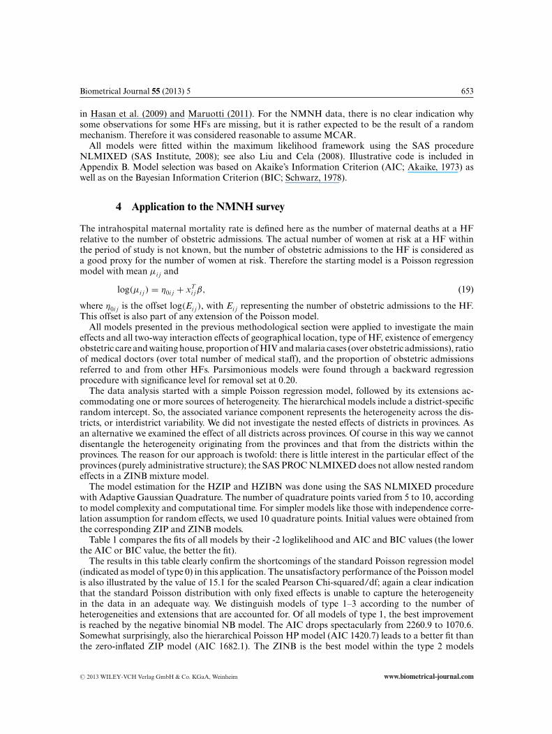
Table 1 compares the fits of all models by their -2 loglikelihood and AIC and BIC values (the lowerthe AIC or BIC value, the better the fit).

The results in this table clearly confirm the shortcomings of the standard Poisson regression model(indicated as model of type 0) in this application. The unsatisfactory performance of the Poisson modelis also illustrated by the value of 15.1 for the scaled Pearson Chi-squared/df; again a clear indicationthat the standard Poisson distribution with only fixed effects is unable to capture the heterogeneityin the data in an adequate way. We distinguish models of type 1–3 according to the number ofheterogeneities and extensions that are accounted for. Of all models of type 1, the best improvementis reached by the negative binomial NB model. The AIC drops spectacularly from 2260.9 to 1070.6.Somewhat surprisingly, also the hierarchical Poisson HP model (AIC 1420.7) leads to a better fit thanthe zero-inflated ZIP model (AIC 1682.1). The ZINB is the best model within the type 2 models

C© 2013 WILEY-VCH Verlag GmbH & Co. KGaA, Weinheim www.biometrical-journal.com

654 O. Loquiha et al.: Hierarchical zero-inflated models

Table 1 Comparison of model fit for the Poisson model and its extensions as discussed in Section 3.The column “Type” refers to the number of extensions as compared to the Poisson model; the column“-2ll” shows the values of -2×log-likelihood; “# Par” the number of parameters in the model; “AIC”and “BIC” the AIC and BIC values, respectively, and the columns “Rank” refers to the ranking of themodels according to the AIC and the BIC criterions.

Distribution Model Type -2ll # Par AIC Rank BIC Rank

P 0 2222.9 19 2260.9 12 2333.5 12HP 1 1380.7 20 1420.7 10 1477.5 10ZIP 1 1634.1 24 1682.1 11 1773.8 11

Poisson HZIP (ind) 2 1001.2 26 1053.2 7 1126.9 6HZIP (cor) 2 995.4 27 1049.4 6 1125.9 5HZIP (shared) 2 995.5 26 1047.5 5 1121.2 4

NB 1 1030.6 20 1070.6 9 1147.0 9HNB 2 1025.8 21 1067.8 8 1127.4 7

Negative ZINB 2 982.0 25 1032.0 3 1127.5 8binomial HZINB (ind) 3 977.9 27 1031.9 2 1108.5 2

HZINB (cor) 3 976.1 28 1032.1 4 1111.5 3HZINB (shared) 3 977.5 27 1031.5 1 1108.1 1

(AIC 1032.0), followed by the HZIP models (AIC from 1047.5 to 1053.2) and the HNB model (AIC1067.8). All models of type 3 (all HZINB models) have very similar AIC values, and very close to thevalue of 1032 of the ZINB model. Based on AIC, the best model is the HZINB (shared) model, butthe difference with the ZINB is negligible. The ranking according to BIC is not exactly the same, butthe same models HZINB (shared) and HZINB (ind) are ranked on position one and two, but they arenow more clearly separated from the models with ranks 3 and 4.

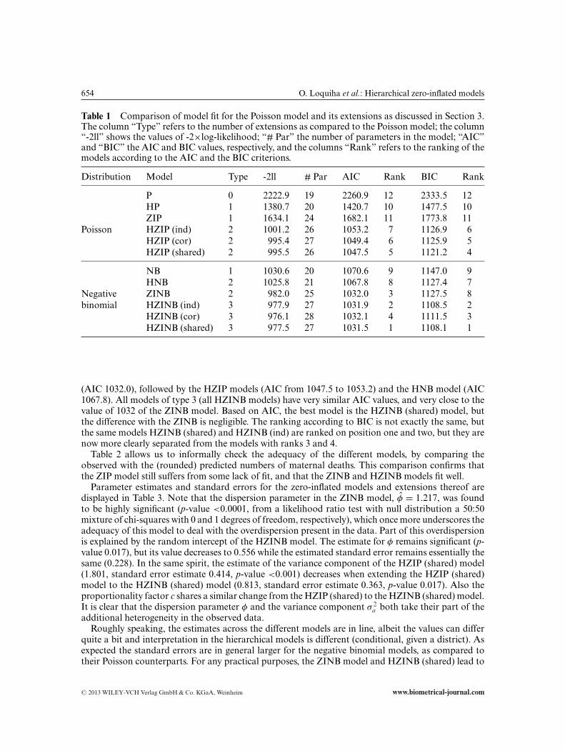
Table 2 allows us to informally check the adequacy of the different models, by comparing theobserved with the (rounded) predicted numbers of maternal deaths. This comparison confirms thatthe ZIP model still suffers from some lack of fit, and that the ZINB and HZINB models fit well.

Parameter estimates and standard errors for the zero-inflated models and extensions thereof aredisplayed in Table 3. Note that the dispersion parameter in the ZINB model, φ = 1.217, was foundto be highly significant (p-value <0.0001, from a likelihood ratio test with null distribution a 50:50mixture of chi-squares with 0 and 1 degrees of freedom, respectively), which once more underscores theadequacy of this model to deal with the overdispersion present in the data. Part of this overdispersionis explained by the random intercept of the HZINB model. The estimate for φ remains significant (p-value 0.017), but its value decreases to 0.556 while the estimated standard error remains essentially thesame (0.228). In the same spirit, the estimate of the variance component of the HZIP (shared) model(1.801, standard error estimate 0.414, p-value <0.001) decreases when extending the HZIP (shared)model to the HZINB (shared) model (0.813, standard error estimate 0.363, p-value 0.017). Also theproportionality factor c shares a similar change from the HZIP (shared) to the HZINB (shared) model.It is clear that the dispersion parameter φ and the variance component σ 2

a both take their part of theadditional heterogeneity in the observed data.

Roughly speaking, the estimates across the different models are in line, albeit the values can differquite a bit and interpretation in the hierarchical models is different (conditional, given a district). Asexpected the standard errors are in general larger for the negative binomial models, as compared totheir Poisson counterparts. For any practical purposes, the ZINB model and HZINB (shared) lead to

C© 2013 WILEY-VCH Verlag GmbH & Co. KGaA, Weinheim www.biometrical-journal.com

Biometrical Journal 55 (2013) 5 655

Table 2 Observed and predicted number of maternal deaths from the Poisson model and zero-inflatedextensions.

Predicted frequency

Maternal Observed HZIP HZINBdeaths frequency Poisson ZIP (shared) ZINB (shared)

0 215 172 203 206 214 2131 33 64 50 44 37 392 18 19 21 22 22 243 18 15 16 16 13 124 6 11 8 2 7 75 6 5 1 6 5 36 2 2 2 5 5 77 3 5 4 2 3 38 4 4 2 6 3 39 2 2 2 2 2 210 4 2 2 2 3 111–50 21 26 18 17 18 1851–100 2 6 5 3 3 3101–150 1 3 1 1 0 0>151 4 3 2 3 4 4

similar conclusions and interpretations. Remember that for the HZINB model the maternal mortalityrate is modelled as (combining (11) and (19))

μi j

Ei j= πi jνi j . (20)

Hence the total effect of a covariate plays through both parameters, the mixing parameter πi j and theparameter νi j , in a multiplicative way.

Focusing first on the model for the mixture probability πi j , only region, location of HF and per-centage of women admitted with malaria play a role. HFs in the central region (as compared tothose in the south), and HFs located outside the district capital show a higher propensity to de-clare more zero deaths and hence have a lower probability πi j . This latter observation might beexplained by a tendency of HFs located outside the district capital to transfer most of its compli-cated cases to other HFs in the district capital. The effect of the percentage of women with malariaimplies that a higher percentage leads to a lower probability πi j , but this effect was no longersignificant when switching from the Poisson to the better fitting negative binomial version of themodel.

Switching to the model for νi j , the effect of region and location is a bit more complicated, as theyalso interact in their effect. In the north, HFs located outside the district capital have a lower estimatedvalue for νi j ; the same holds for HFs in the center but less pronounced, and for HFs in the south thereis no difference between HFs in the district capital or outside.

Although the health facility type appeared to be (highly) significant in the ZIP and HZIP (shared)model, it is no longer the case for the ZINB model. For the HZINB (shared) model, type II, III,Health Post has a significant lower mortality rate as compared to central hospitals. The propor-tion referrals to and from the HFs seem to have a negative effect, implying a decrease in mor-tality rate as the proportion referrals increases. A possible explanation is that the maternal death

C© 2013 WILEY-VCH Verlag GmbH & Co. KGaA, Weinheim www.biometrical-journal.com

656 O. Loquiha et al.: Hierarchical zero-inflated models

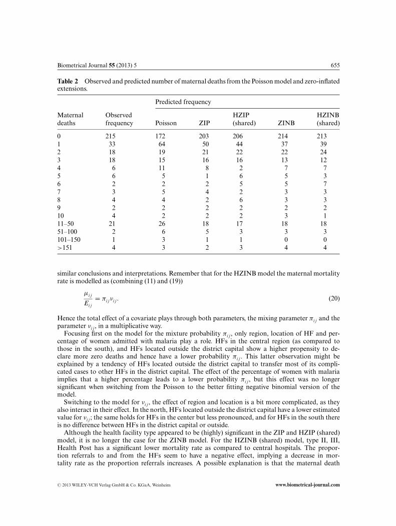
Table 3 Parameter estimates and standard errors for zero-inflated Poisson (ZIP) model, zero-inflatednegative binomial (ZINB) model, zero-inflated Poisson with shared random effects (HZIP) model, andzero-inflated negative binomial with shared random effects (HZINB) model. Estimation was done bymaximum likelihood using numerical integration over the random effects.

Model for logit(πi j )

ZIP ZINB HZIP (shared) HZINB (shared)

Effect (reference) Estimate (s.e.) Estimate (s.e.) Estimate (s.e.) Estimate (s.e.)

Intercept 1.015(0.408) 1.577(0.566) 2.136(0.662) 1.761(0.593)Region (south)North 2.297(0.988) 7.300(17.038) 1.330(0.806) 7.643(23.541)Center −0.741(0.393) −0.974(0.477) −1.415(0.581) −1.099(0.509)Location (district capital)Outside district capital −2.112(0.404) −2.268(0.522) −2.648(0.532) −2.475(0.539)Malaria cases (%) 19.198(8.520) 18.399(10.872) 23.945(12.868) 17.393(10.370)

Model for log(νi j )

Intercept −3.603(0.156) −4.046(0.856) −2.898(0.443) −3.464(0.791)Region (south)North −1.248(0.108) −0.802(0.389) −0.745(0.427) −0.700(0.403)Center −0.512(0.102) 0.742(0.425) 0.297(0.492) 0.451(0.483)HF type (central hospital)General hospital 0.210(0.075) 0.699(0.895) −0.168(0.097) 0.197(0.742)Type I −1.139(0.100) −0.335(0.842) −1.693(0.154) −1.283(0.719)Type II, III, H. Post −1.035(0.198) −0.664(0.925) −2.622(0.358) −1.893(0.850)Rural hospital −0.829(0.122) −0.312(0.910) −1.072(0.343) −0.979(0.767)Location (district capital)Outside district capital 1.228(0.116) 0.673(0.508) 0.539(0.356) 0.849(0.533)Obstetric emergency care (not available/partial time)Full time −0.186(0.135) −0.279(0.322) −0.605(0.271) −0.316(0.341)Malaria cases (%) −6.008(1.311) 1.721(3.473) −5.088(2.977) 0.822(3.669)HIV cases (%) 8.595(0.974) 9.496(2.833) 11.857(2.547) 8.373(3.118)Waiting house (not available)Available 0.460(0.079) 0.060(0.295) −0.020(0.281) 0.011(0.303)Ratio of medical doctors 0.180(0.284) 0.778(0.647) 1.511(0.540) 1.155(0.729)Proportion of referrals to −3.422(0.228) −3.335(2.307) −3.690(0.377) −3.621(1.514)Proportion of referrals from −12.682(1.437) −13.981(3.463) −17.146(3.073) −13.046(3.790)Region × LocationNorth|Outside district capital −2.625(0.325) −2.786(0.550) −1.974(0.504) −2.940(0.556)Center|Outside district capital −0.826(0.209) −1.543(0.676) 0.053(0.413) −0.762(0.732)Region× HIV cases (%)North|HIV cases (%) 238.891(29.761) 7.950(70.322) 114.670(80.999) 13.386(77.236)Center|HIV cases (%) −29.011(4.074) −53.792(12.999) −33.558(15.279) −41.699(14.926)Dispersion (φ) − 1.217(0.221) − 0.556(0.228)

Variance b1i (σ 2a ) − − 1.801(0.414) 0.813(0.363)

Proportionality factor (c) − − 0.511(0.260) 0.370(0.466)

C© 2013 WILEY-VCH Verlag GmbH & Co. KGaA, Weinheim www.biometrical-journal.com

Biometrical Journal 55 (2013) 5 657

occurrence will be registered in a different HF, rather than in the actual HF where the patient checkedin.

In the ZINB and HZINB (shared) models, there was no significant effect of the existenceof a waiting house, of the availability of emergency obstetric care and of the ratio of medicaldoctors.

5 Concluding remarks

This paper investigates which factors are related to institutional maternal mortality in Mozambiqueusing data from the NMNH survey and using different models for count data. We extended thePoisson regression model to a HZINB with independent, correlated, and shared random effects. TheHZINB model explicitly models (i) the excess of zero counts (mixing parameter πi j), (ii) the hierarchicalstructure in the data (variance component σ 2

a and/or σ 2b ), and (iii) incorporates implicitly other sources

of heterogeneity/overdispersion (overdispersion parameter φ). Mathematical expressions for the meanand variance structures were derived, illustrating nicely the contribution to the total heterogeneityrepresented by each of the parameters πi j, σ

2b , and φ.

The HZINB and all intermediate and simpler models dealing with one or two additional struc-tures were applied to counts on maternal deaths as obtained in the NMNH survey. The final modelwas selected using AIC. This led to the HZINB (shared) model as best model, but the differ-ence in AIC with the simpler ZINB model was so minor, that the latter model suffices for mostpractical purposes. We used the traditional “marginal” definition of AIC, as provided with PROCNLMIXED in SAS. We do recognize that the use of the conditional AIC has been advocated whenthe research focus is on clusters. The conditional AIC has first been introduced in mixed models(see e.g. Vaida and Blanchard, 2005), and has recently been extended to generalized linear-mixedmodels (see Liang et al., 2008; Donohue et al., 2011; Lian, 2012; Yu and Yau, 2012). We basedmodel selection on the marginal AIC for the reason that the conditional AIC has not been studiedor implemented yet for the HZINB type of models. This is an interesting topic for further research.Another interesting point for further research is the development of a formal test for overdispersionwith zero-inflated count data, such as an extension of Baksh et al. (2011) with the inclusion of covariateinformation.

We found that the maternal mortality rate mainly depends on the geographical location of the HF, thepercentage of women admitted with HIV and the percentage of referrals from the HF. Some of thesecovariates had an effect on both model components (mixture probability πi j and mean parameterνi j) and some of them interacted in their effect. The ZINB model also showed that an increase inthe proportion of admitted women with HIV tends to increase the maternal mortality rate, whichis in line with findings from Menendez et al. (2008). This fact, in addition to a nonsignificant effectof emergence obstetric care, might point out that there is still room for additional public healthprogrammes by the Mozambican health authorities, with special attention to the quality of care forpregnant women within HFs. Although the increasing role of malaria on maternal mortality has beenmentioned in literature (Romagosa et al., 2007), and although this effect appeared to be relevant inthe Poisson models, their negative binomial counterparts did not indicate any significant effect of thepercentage of women with malaria.

However, we would like to mention some limitations of the data and consequently of our analy-ses: only aggregated data on the level of HFs was available, and only complete cases were included.Inference from aggregated data may suffer from the well-known ecological fallacy. This fallacy liesin the assumption that an association observed at one level of aggregation (e.g. HFs) also holdson the nonaggregated level (individual patients). Complete case analysis assumes that the missingdata mechanism is missing completely at random. Although these limitations imply some cautious-ness in formulating conclusions, we are convinced that such data need more attention and need to

C© 2013 WILEY-VCH Verlag GmbH & Co. KGaA, Weinheim www.biometrical-journal.com

658 O. Loquiha et al.: Hierarchical zero-inflated models

be analyzed with appropriate models. But of course, limitations and constraints should be clearlymentioned.

Acknowledgments The authors would like to thank the Associate Editor and three reviewers for their valuablecomments that have led to an improved version of the manuscript. This study was only possible thanks to thefinancial support of the Flemish Interuniversity Council (VLIR-UOS) in collaboration with Eduardo MondlaneUniversity (UEM) through the DESAFIO Program. The authors would also like to acknowledge the supportgiven by the Mozambican Ministry of Health provided the data and research questions.

Conflict of interestThe authors have declared no conflict of interest.

Appendix

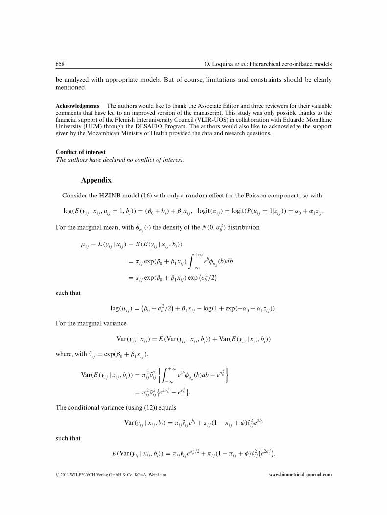
Consider the HZINB model (16) with only a random effect for the Poisson component; so with

log(E (yi j | xi j, ui j = 1, bi)) = (β0 + bi) + β1xi j, logit(πi j ) = logit(P(ui j = 1|zi j )) = α0 + α1zi j .

For the marginal mean, with φσb(·) the density of the N(0, σ 2

b ) distribution

μi j = E (yi j | xi j ) = E (E (yi j | xi j, bi))

= πi j exp(β0 + β1xi j )

∫ +∞

−∞ebφσb

(b)db

= πi j exp(β0 + β1xi j ) exp(σ 2

b /2)

such that

log(μi j ) = (β0 + σ 2

b /2) + β1xi j − log(1 + exp(−α0 − α1zi j )).

For the marginal variance

Var(yi j | xi j ) = E (Var(yi j | xi j, bi)) + Var(E (yi j | xi j, bi))

where, with νi j = exp(β0 + β1xi j ),

Var(E (yi j | xi j, bi)) = π2i j ν

2i j

{∫ +∞

−∞e2bφσb

(b)db − eσ 2b

}

= π2i j ν

2i j

{e2σ 2

b − eσ 2b}.

The conditional variance (using (12)) equals

Var(yi j | xi j, bi) = πi j vi jebi + πi j (1 − πi j + φ)ν2

i je2bi

such that

E (Var(yi j | xi j, bi)) = πi j νi jeσ 2

b /2 + πi j (1 − πi j + φ)ν2i j

(e2σ 2

b).

C© 2013 WILEY-VCH Verlag GmbH & Co. KGaA, Weinheim www.biometrical-journal.com

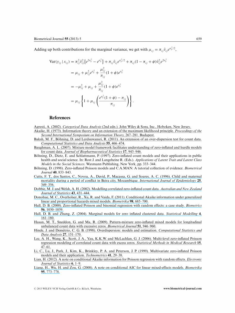
Biometrical Journal 55 (2013) 5 659

Adding up both contributions for the marginal variance, we get with μi j = πi j νi jeσ 2

b /2,

Var(yi j | xi j ) = π2i j ν

2i j

{e2σ 2

b − eσ 2b} + πi j νi je

σ 2b /2 + πi j (1 − πi j + φ)ν2

i je2σ 2

b

= μi j + μ2i je

σ 2b + μ2

i j

πi j(1 + φ)eσ 2

b

= −μ2i j + μi j + μ2

i j

πi j(1 + φ)eσ 2

b

= μi j

{1 + μi j

(eσ 2

b (1 + φ) − πi j

πi j

)}.

References

Agresti, A. (2002). Categorical Data Analysis (2nd edn.). John Wiley & Sons, Inc., Hoboken, New Jersey.Akaike, H. (1973). Information theory and an extension of the maximum likelihood principle. Proceedings of the

Second International Symposium on Information Theory, 267–281. Budapest.Baksh, M. F., Bohning, D. and Lerdsuwansri, R. (2011). An extension of an over-dispersion test for count data.

Computational Statistics and Data Analysis 55, 466–474.Baughman, A. L. (2007). Mixture model framework facilitates understanding of zero-inflated and hurdle models

for count data. Journal of Biopharmaceutical Statistics 17, 943–946.Bohning, D., Dietz, E. and Schlattmann, P. (1997). Zero-inflated count models and their applications in public

health and social science. In: Rost J. and Langeheine R. (Eds.). Applications of Latent Trait and Latent ClassModels in the Social Sciences. Waxmann Publishing, New York, pp. 333–344.

Bohning, D. (1998). Zero-inflated Poisson models and C.A.MAN: A tutorial collection of evidence. BiometricalJournal 40, 833–843.

Cutts, F. T., dos Santos, C., Novoa, A., David, P., Macassa, G. and Soares, A. C. (1996). Child and maternalmortality during a period of conflict in Beira city, Mozambique. International Journal of Epidemiology 25,349–356.

Dobbie, M. J. and Welsh, A. H. (2002). Modelling correlated zero-inflated count data. Australian and New ZealandJournal of Statistics 43, 431–444.

Donohue, M. C., Overholser, R., Xu, R. and Vaida, F. (2011). Conditional Akaike information under generalizedlinear and proportional hazards mixed models. Biometrika 98, 685–700.

Hall, D. B. (2000). Zero-inflated Poisson and binomial regression with random effects: a case study. Biometrics56, 1030–1039.

Hall, D. B. and Zhang, Z. (2004). Marginal models for zero inflated clustered data. Statistical Modelling 4,161–180.

Hasan, M. T., Sneddon, G. and Ma, R. (2009). Pattern-mixture zero-inflated mixed models for longitudinalunbalanced count data with excessive zeros. Biometrical Journal 51, 946–960.

Hinde, J. and Demetrio, C. G. B. (1998). Overdispersion: models and estimation. Computational Statistics andData Analysis 27, 151–170.

Lee, A. H., Wang, K., Scott, J. A., Yau, K.K.W. and McLachlan, G. J. (2006). Multi-level zero-inflated Poissonregression modeling of correlated count data with excess zeros. Statistical Methods in Medical Research 15,47–61.

Li, C., Lu, J., Park, J., Kim, K., Brinkley, P. A. and Peterson, J. P. (1999). Multivariate zero-inflated Poissonmodels and their application. Technometrics 41, 29–38.

Lian, H. (2012). A note on conditional Akaike information for Poisson regression with random effects. ElectronicJournal of Statistics 6, 1–9.

Liang, H., Wu, H. and Zou, G. (2008). A note on conditional AIC for linear mixed-effects models. Biometrika95, 773–778.

C© 2013 WILEY-VCH Verlag GmbH & Co. KGaA, Weinheim www.biometrical-journal.com

660 O. Loquiha et al.: Hierarchical zero-inflated models

Liu, W. and Cela, J. (2008). Count data models in SAS. Proceedings of the SAS R© Global Forum 2008 Conference,paper 371. Cary, NC: SAS Institute Inc.

Maruotti, A. (2011). A two-part mixed-effects pattern-mixture model to handle zero-inflation and incompletenessin a longitudinal setting. Biometrical Journal 53, 716–734.

Menendez, C., Romagosa, C., Ismail , M. R., Carrilho, C., Saute, F., Osman, N., Machungo, F., Bardaji, A.,Quint, L., Mayor, A., Naniche, D., Dobao, C., Alonso, P. L. and Ordi, J. (2008). An autopsy study ofmaternal mortality in Mozambique: the contribution of infectious diseases. PLoS Medicine 5, 44.

Min, Y. and Agresti, A. (2005). Random effect models for repeated measures of zero-inflated count data. StatisticalModelling 5, 1–19.

MISAU (2009). Avaliacao de Necessidades em Saude Materna e Neonatal em Mocambique, Relatorio preliminar-Parte II. Unpublished.

Molenberghs, G., Verbeke, G. and Demetrio, C. G. B. (2007). An extended random-effects approach to modelingrepeated, overdispersed count data. Lifetime Data Analysis 13, 513–531.

Molenberghs, G., Verbeke, G., Demetrio, C. G. B. and Vieira, A. M. C. (2010). A family of generalized linearmodels for repeated measures with normal and conjugate random effects. Statistical Science 25, 325–347.

Ridout, M., Demetrio, C. G. B. and Hinde, J. (1998). Models for count data with many zeros. Proceedings of theXIXth International Biometric Conference, 179–192, Invited Papers. Cape Town, South Africa: InternationalBiometric Society.

Romagosa, C., Ordi, J., Saute, F., Quinto, L., Machungo, F., Ismail, M. R., Carrilho, C., Osman, N., Alonso, P.L. and Menendez, C. (2007). Seasonal variations in maternal mortality in Maputo, Mozambique: The roleof malaria. Tropical Medicine and International Health 12, 62–67.

Rose, C. E., Martin, S. W., Wannemuehler, K. A. and Plikaytis, B. D. (2006). On the use of zero-inflated andhurdle models for modelling vaccine adverse event count data. Journal of Biopharmaceutical Statistics 16,463–481.

Schwarz, G. E. (1978). Estimating the dimension of a model. Annals of Statistics 6, 461–464.Vaida, F. and Blanchard, S. (2005). Conditional Akaike information for mixed-effects models. Biometrika 92,

351–370.Yau, K. K. W. and Lee, A. H. (2001). Zero-inflated Poisson regression with random effects to evaluate an

occupational injury prevention programme. Statistics in Medicine 20, 2907–2920.Yau, K. K. W., Wang, K. and Lee, A. H. (2003). Zero-inflated negative binomial mixed regression modeling of

over-dispersed count data with extra zeros. Biometrical Journal 45, 437–452.Yu, D. and Yau, K. K. W. (2012). Conditional Akaike information criterion for generalized linear mixed models.

Computational Statistics and Data Analysis 56, 629–644.

C© 2013 WILEY-VCH Verlag GmbH & Co. KGaA, Weinheim www.biometrical-journal.com