arX

iv:1

012.

1281

v1 [

q-bi

o.PE

] 6

Dec

201

0

Modeling Dengue Outbreaks

Marcelo J Otero, Daniel H Barmak, Claudio O Dorso, Hernan G Solari

Departamento de Fısica, FCEyN-UBA and IFIBA-CONICET

Mario A Natiello

Centre for Mathematical Sciences, Lund University, Sweden

Abstract

We introduce a dengue model (SEIR) where the human individuals are treatedon an individual basis (IBM) while the mosquito population, produced by anindependent model, is treated by compartments (SEI). We study the spread ofepidemics by the sole action of the mosquito. Exponential, deterministic andexperimental distributions for the (human) exposed period are considered intwo weather scenarios, one corresponding to temperate climate and the other totropical climate. Virus circulation, final epidemic size and duration of outbreaksare considered showing that the results present little sensitivity to the statisticsfollowed by the exposed period provided the median of the distributions arein coincidence. Only the time between an introduced (imported) case and theappearance of the first symptomatic secondary case is sensitive to this distribu-tion. We finally show that the IBM model introduced is precisely a realizationof a compartmental model, and that at least in this case, the choice betweencompartmental models or IBM is only a matter of convenience.

Keywords: epidemiology, dengue, Individual Based Model, CompartmentalModel, stochastic

1. Introduction

Dengue fever is a vector-born disease produced by a flavivirus of the fam-ily flaviviridae [1]. The main vectors of dengue are Aedes aegypti and Aedesalbopictus.

The research aimed at producing dengue models for public policy use be-gan with Newton and Reiter [2] who introduced the minimal model for denguein the form of a set of Ordinary Differential Equations (ODE) for the humanpopulation disaggregated in Susceptible, Exposed, Infected and Recovered com-partments. The mosquito population was not modeled in this early work. Adifferent starting point was taken by Focks et al. [3, 4] that began by describingmosquito populations in a computer framework named Dynamic Table Modelwhere later the human population (as well as the disease) was introduced [5].

Preprint submitted to Elsevier December 7, 2010

Newton and Reiter’s model (NR) favours economy of resources and mathe-matical accessibility, in contrast, Focks’ model emphasize realism. These modelsrepresent in Dengue two contrasting compromises in the standard trade-off inmodeling. A third starting point has been recently added. Otero, Solari andSchweigmann (OSS) developed a dengue model [6] which includes the evolutionof the mosquito population [7, 8] and is spatially explicit. This last model issomewhat in between Focks’ and NR as it is formulated as a state-dependentPoisson model with exponentially distributed times.

Each approach has been further developed [9, 10, 11, 12, 13, 14, 15]. ODEmodels have received most of the attention. Some of the works explore: variabil-ity of vector population [9], human population [10], the effects of hypotheticalvertical transmission of Dengue in vectors [11], seasonality [12], age structure[13] as well as incomplete gamma distributions for the incubation and infectioustimes [16]. Contrasting modeling outcomes with those of real epidemics hasshown the need to consider spatial heterogeneity as well [17].

The development of computing technology has made possible to produce In-dividual Based Models (IBM) for epidemics [18, 19]. IBM have been advocatedas the most realistic models [19] since their great flexibility allows the modeler todescribe disease evolution and human mobility at the individual level. When theresults are only to be analysed numerically, IBM are probably the best choice.However, they are frequently presented in a most unfriendly way for mathemati-cians as they usually lack a formulation (expression in closed formulae) and are–at best– presented as algorithms if not just in words [18]. In contrast, workingon the ODE side, it has been possible, for example, to achieve an understandingof the influence of distribution of the infectious period in epidemic modeling[20, 21, 22]. IBM have been used to study the time interval between primaryand secondary cases [23] which is influenced, in the case of dengue, mainly bythe extrinsic (mosquito) and intrinsic (human) incubation period.

In this work an IBM model for human population in a dengue epidemic ispresented. The model is driven by mosquito populations modeled with spatialheterogeneity with the method introduced in [8] (see Section II). The IBMmodel is then used to examine the actual influence of the distribution of theincubation period comparing the most relevant information produced by denguemodels: dependence of the probability of dengue circulation with respect tothe mosquito population and the total epidemic size. Exponential, delta (fixedtimes, deterministic) and experimental [24] distributions are contrasted (SectionIII). The infectious period and the extrinsic incubation period is modeled usingexperimental data and measured transmission rates (human to mosquito) [24].

The IBM model produced is critically discussed. We show that it can bemapped exactly into a stochastic compartmental model of a novel form (seeSection IV) thus crossing for the first time the valley separating IBM from com-partmental models. This result opens new perspectives which we also discussin Section IV. Finally, Section V presents the conclusions of this work.

2

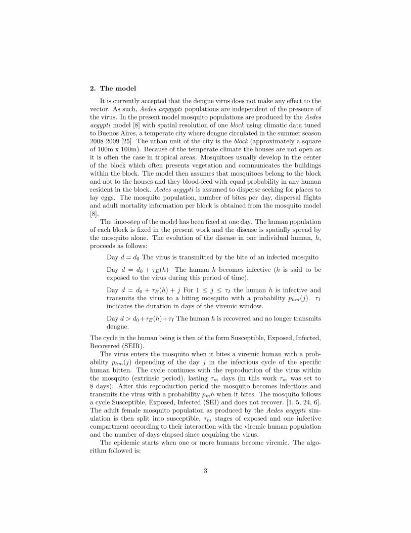
2. The model

It is currently accepted that the dengue virus does not make any effect to thevector. As such, Aedes aepgypti populations are independent of the presence ofthe virus. In the present model mosquito populations are produced by the Aedesaegypti model [8] with spatial resolution of one block using climatic data tunedto Buenos Aires, a temperate city where dengue circulated in the summer season2008-2009 [25]. The urban unit of the city is the block (approximately a squareof 100m x 100m). Because of the temperate climate the houses are not open asit is often the case in tropical areas. Mosquitoes usually develop in the centerof the block which often presents vegetation and communicates the buildingswithin the block. The model then assumes that mosquitoes belong to the blockand not to the houses and they blood-feed with equal probability in any humanresident in the block. Aedes aegypti is assumed to disperse seeking for places tolay eggs. The mosquito population, number of bites per day, dispersal flightsand adult mortality information per block is obtained from the mosquito model[8].

The time-step of the model has been fixed at one day. The human populationof each block is fixed in the present work and the disease is spatially spread bythe mosquito alone. The evolution of the disease in one individual human, h,proceeds as follows:

Day d = d0 The virus is transmitted by the bite of an infected mosquito

Day d = d0 + τE(h) The human h becomes infective (h is said to beexposed to the virus during this period of time).

Day d = d0 + τE(h) + j For 1 ≤ j ≤ τI the human h is infective andtransmits the virus to a biting mosquito with a probability phm(j). τIindicates the duration in days of the viremic window.

Day d > d0+τE(h)+τI The human h is recovered and no longer transmitsdengue.

The cycle in the human being is then of the form Susceptible, Exposed, Infected,Recovered (SEIR).

The virus enters the mosquito when it bites a viremic human with a prob-ability phm(j) depending of the day j in the infectious cycle of the specifichuman bitten. The cycle continues with the reproduction of the virus withinthe mosquito (extrinsic period), lasting τm days (in this work τm was set to8 days). After this reproduction period the mosquito becomes infectious andtransmits the virus with a probability pmh when it bites. The mosquito followsa cycle Susceptible, Exposed, Infected (SEI) and does not recover. [1, 5, 24, 6].The adult female mosquito population as produced by the Aedes aegypti sim-ulation is then split into susceptible, τm stages of exposed and one infectivecompartment according to their interaction with the viremic human populationand the number of days elapsed since acquiring the virus.

The epidemic starts when one or more humans become viremic. The algo-rithm followed is:

3

1. Give individual attributes, τE(h) according to prescribed distribution.

2. Read geometry, size of viremic window, probabilities pmh(j), j = 1...τI ,human population in each block, day of the year when the epidemic starts.

3. Initialise the blocks with the human population.

4. Read total adult female mosquito population of the day (M), bites, flightsto neighbouring blocks and mosquito death probability. Initialise all mosquitoesas susceptible (MS). Set infective bites to zero.

5. Day-loop begins:

(a) Calculate the amount of surviving infected mosquitoes. Computesurviving mosquito population with d exposed days, age them byone day. Exposed mosquitoes evolve to infected ones after d = τmdays (Use binomial random number generator).

(b) Compute probability for a mosquito bite to transmit dengue as pminf =pmhMI/M (compound probability of being infective and being effec-tive in the transmission). Each bite is an independent event accordingto the underlying mosquito model.

(c) Compute the probability for a bite to be made by a susceptiblemosquito out of all the non-infective bites potras = MS/(M(1 −pminf )). The non-infective bites have probability (1 − pminf ), andcome from infected mosquitoes failing to transmit the virus, ex-posed and susceptible mosquitoes, M(1 − pminf ) = M − pmhMI =MS +ME + (1− pmh)MI .

(d) Calculate the number of infected and susceptible mosquito bites usingbinomials with the previous probabilities and the number of totalbites.

(e) Compute number of humans bitten in each day of the infected state,HI(j).

(f) Compute the number of new exposed mosquitoes, taking into accountthat the probability of human-mosquito contagion is dependent onthe stage-day of the human infection. The amount of new infectedinsects is chosen using binomials. For this purpose, we add the re-sults of the calculation of the number of susceptible mosquitoes thatbite humans and get infected, MNE =

∑τIj=1

Bin(phm(j), HI(j)).Where MNE are the new exposed mosquitoes, Bin(HI(j), phm(j))is a binomial realization with the day-dependent probability phm(j)and HI(j) the quantity of infected humans bitten by susceptiblemosquitoes on infection day j.

(g) Perform a random equi-distributed selection of humans bitten byinfectious mosquitoes. Build a table of bitten individuals.

(h) Update the state of all the humans. If the human belongs to theSusceptible state and has been bitten according to the table builtin (5g) then change the state of selected human to Exposed, recordd0 for each exposed human. Susceptible individuals not bitten byan infective mosquito will remain as such and consequently theirintrinsic time d remains in 0. Increase the intrinsic time of Exposed

4

and Infected humans by one. Those Exposed individuals for whichtheir intrinsic time has surpassed the value d = d0+τE(h) are movedto the Infected state, while those Infected individuals whose intrinsictime is larger than d = d0 + τE(h) + τI , are moved to the Removedstate

i. Compute the number of individuals in each state for every cell.ii. Read the total adult female mosquito population of the day (M),

bites, flights to neighboring blocks.

6. Repeat all over again from (5a). Each iteration is a new day of the simu-lation.

3. Epidemic dependence on the distribution of the exposed period

We implemented four different distributions for the duration of the exposedperiod assigned to human individuals: Nishiura’s experimental distribution([24]), a delta and exponential distributions with the same mean that the ex-perimental one and an exponential distribution with the same median than theexperimental one. We call them N,D,E1 and E2 respectively.

The study was performed in two different climatic scenarios, one with con-stant temperature of 23 degrees Celsius, that represents tropical regions and onewith the mean and amplitude characteristic of Buenos Aires, a city with tem-perate climate. The number of effective breeding sites [7] was varied between50 and 1000.

The main questions were: considering the total number of recovered indi-viduals, how is the distribution of epidemic sizes influenced by the choice ofdistribution? How does the probability for having no secondary cases change?How is the predicted duration of the epidemic influenced by our choices? Andfinally, how is the distribution of time between epidemiologically related casesaffected?

Before showing our results, it is worth to realise that the probability ofhaving no secondary cases will not be sensitive to the choice of distributionfor the exposed period, as this probability depends only on the probabilityof the introduced case being bitten by the mosquitoes, the probability of themosquitoes of acquiring the virus, surviving the extrinsic period and finallytransmitting the virus to a human in a bite. Nothing in this process dependson the choice of distribution. In contrast, we expect the distribution of timesbetween epidemiologically related cases to depend strongly on the choice ofdistribution, since it reflects the sum of the two incubation periods (intrinsicand extrinsic).

The simulations were performed using identical mosquito populations in allcases (same data file), for an homogeneous urban area of 20 by 20 blocks, host-ing 100 people per block, making a total of 40000 human beings. Hence, alldifferences correspond to the disease dynamics that was previously identifiedas the main source of stochastic variations. The simulations with temperateclimate were started on January 1st, i.e., ten days after the summer solstice

5

(December 21st in the southern hemisphere). The reported statistics is com-puted by averaging the outcomes of 1000 simulations with different seeds forthe pseudo-random routines.

Confirming the reasoning above, there is no sensitivity for the probability ofhaving local circulation of the virus (defined as having at least one secondarycase following the introduced case) with the statistical distribution of the ex-posed period, see Figure 1.

The size of the epidemic at constant temperatures makes a transition fromvery small outbreaks to a large outbreak reaching almost all the people in thesimulation. The transition happens in the region 50-100 breading sites per blockfor the four distributions studied, see Figure 2. We detected no epidemiologi-cally important differences produced by the use of one or another distributionfunction.

The size of epidemics with seasonal dependence is presented in Figure 3.The size of the epidemic outbreak begins to increase with the number of breed-ing sites in the 100-150 region for all the distributions, suggesting that R0 (thebasic reproductive number) is not affected by the statistic of exposed times(conceptually, R0 is the average number of secondary cases produced by a sin-gle case when the epidemic starts). The results for the D-distributions andN-distribution do not present differences. The E1-distribution (equal mean)overestimates the final size while the E2-distribution substantially agrees withthe N (experimental) one. Both exponential distributions present a larger vari-ance than the N-distribution. This difference may matter when worst-possiblescenarios are considered.

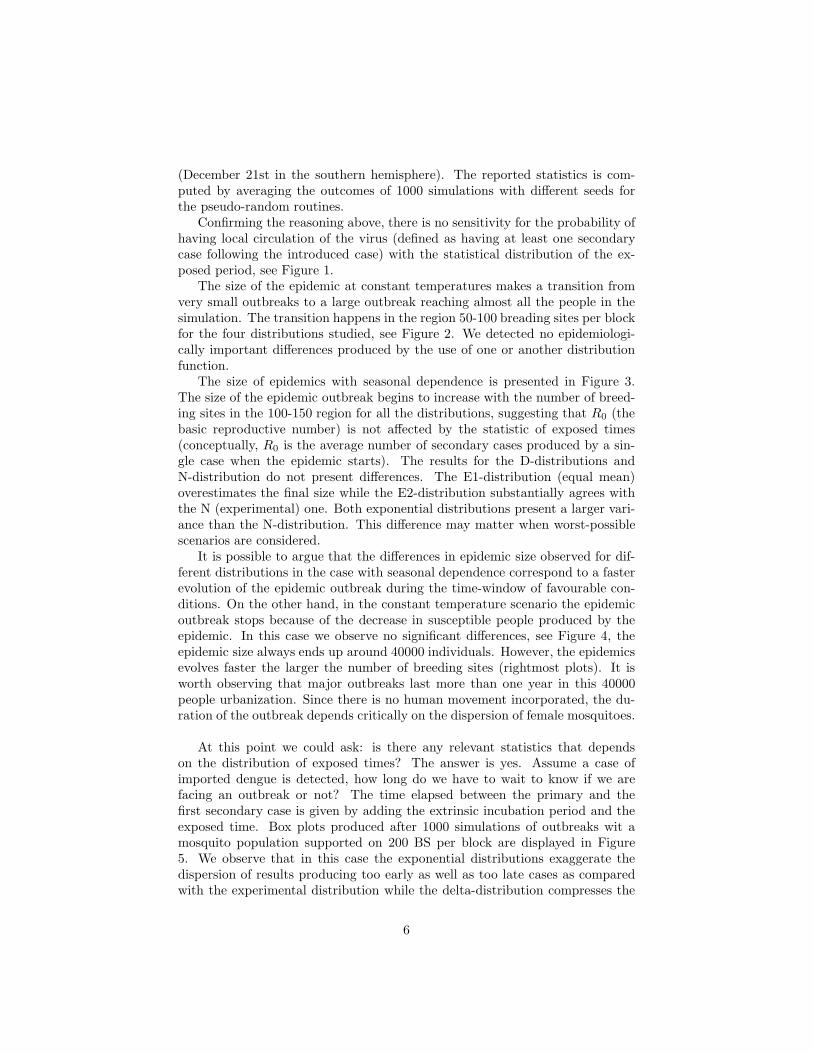
It is possible to argue that the differences in epidemic size observed for dif-ferent distributions in the case with seasonal dependence correspond to a fasterevolution of the epidemic outbreak during the time-window of favourable con-ditions. On the other hand, in the constant temperature scenario the epidemicoutbreak stops because of the decrease in susceptible people produced by theepidemic. In this case we observe no significant differences, see Figure 4, theepidemic size always ends up around 40000 individuals. However, the epidemicsevolves faster the larger the number of breeding sites (rightmost plots). It isworth observing that major outbreaks last more than one year in this 40000people urbanization. Since there is no human movement incorporated, the du-ration of the outbreak depends critically on the dispersion of female mosquitoes.

At this point we could ask: is there any relevant statistics that dependson the distribution of exposed times? The answer is yes. Assume a case ofimported dengue is detected, how long do we have to wait to know if we arefacing an outbreak or not? The time elapsed between the primary and thefirst secondary case is given by adding the extrinsic incubation period and theexposed time. Box plots produced after 1000 simulations of outbreaks wit amosquito population supported on 200 BS per block are displayed in Figure5. We observe that in this case the exponential distributions exaggerate thedispersion of results producing too early as well as too late cases as comparedwith the experimental distribution while the delta-distribution compresses the

6

“alert window” too much with respect to the experimental distribution.

4. Is the IBM model an implementation of a compartmental model?

The use of IBM in epidemiology is usually advocated on an ontological per-spective [26, 19], we quote the argument in [19]

. . . the epidemiology literature has always described an infection his-tory as a sequence of distinct periods, each of which begins and endswith a discrete event. The critical periods include the latent, theinfectious, and the incubation periods. The critical events includethe receipt of infection, the emission of infectious material, and theappearance of symptoms.. . . Several implications can be drawn fromthese epidemiological principles and serve as a conceptual modelfor an individual infection process. First, it is most appropriate torepresent the individual infection as a series of discrete events andperiods. Second, the discrete events have no duration in their ownright and only trigger the change between infection periods. Third,the discrete periods indicate the infection status of an individual andare part of the individual’s characteristics.

The evolution of dengue at the individual level is described in detail in theliterature, including experimental results [24] which are seldom available forother illnesses. Thus, dengue is a good case to put the thesis at test.

The description in terms of events immediately calls for stochastic populationmodels, while the different human to mosquito transmission probabilities canbe handled easily introducing age structure in the infective human population,The description of the proper probability distribution for the exposed (latent)period is the major obstacle towards a compartmental stochastic model.

Each human individual spends k days, k ∈ {1 . . . τE}, in the exposed statebefore becoming infective. The probability of any individual to spend k daysis P (k). Hence, in the group of N individuals that become infected at d = d0,a portion N(k) will spend k days before they become infective, where N(k) isa random deviate taken from Multinomial(N,P (1), . . . , P (τE)), a multinomialdistribution. This is the only information available to the simulation. IBMgenerate additional structure, since each individual is assigned to one of theclasses N(1), · · · , N(τE) in an entirely random way. This apparent additionalinformation is in fact arbitrary because of the randomness and it is averagedout when presenting the results. Although the algorithm of the IBM modelassigns the time spent in the exposed class to the individual, the final causeof having a distribution of exposed times is not known (neither to us nor tothe algorithm). Different exposed times may arise either because of differences(in virus resistance) in the exposed individuals or because of differences in theincoming virus due e.g., to biological processes concerning the development andtransmission of the virus by the mosquito.

7

Let us define

P (k) =

τE∑

j=k

P (j) (1)

Q(k) =P (k)

P (k)= P (j = k/j ≥ k) (2)

Nk = N −k∑

j=1

N(j) (3)

Clearly Q(k) ≤ 1 and Q(τE) = 1. Consider the numbers E(1) = N , E(k) =Binomial(E(k − 1), 1−Q(k)) and N(k) = E(k − 1)− E(k) for 2 ≤ k ≤ τE .

We will now recall a few elementary results regarding multinomial distribu-tions. We write Multi for the multinomial distribution

Lemma 1. (Multinomial splitting)

Multi(N, p(1), . . . , p(k − 1), p(k), . . . , p(τE)) = (4)

= Multi(N, p(1), . . . , p(k − 1), P (k))Multi(N(k), Q(k), . . . , Q(τE))

Proof. The proof is simple algebra simplifying the expression for the proba-bilities in the right side of the equation.

Corollary 1. (Binomial decomposition) The multinomial distribution can befully decomposed in terms of binomial distributions in the form

Multi(N, p(1), . . . , p(τE)) =

τE∏

k=1

Binomial(E(k), Q(k)) (5)

Proof. Repeated application of the previous lemma is all what is needed.

We now state the application of these results to our modeling problem.

Theorem 1. (Compartmental presentation) Consider τE compartments asso-ciated to the days k = 1, . . . , τE after receiving the virus from the mosquito forthose humans that are not yet infective. Let the population number in the kcompartment be E(k), and the number of humans that become infective on dayk be N(k) which is a random deviate distributed with Binomial(E(k), Q(k)),with the definitions given above. Then the exposed period that corresponds tothe individuals is distributed with P (k).

Proof. It follows immediately from the corollary.

8

5. Summary, discussion and conclusions

We have developed an IBM model for the evolution of dengue outbreaks thattakes information from mosquito populations simulated with an Aedes aegyptimodel and builds thereafter the epidemic part of the evolution. The split be-tween mosquito evolution and epidemic evolution is not perfect since the eventsbite and flight are treated as independent events while they are in fact correlated[27, 28, 29, 30], both being related to oviposition.

For mosquito populations sufficiently large to support the epidemic spreadof dengue, most of the stochastic variability is provided by the epidemic processrather than by stochastic fluctuations in the mosquito population. Thus, thesplitting of the models improves substantially the performance of the codes.

The model we developed is shown to be an IBM implementation of a com-partmental model, of a form not usually considered. At the level of the descrip-tion in this work, IBM does not play a fundamental role, contrary to what ithas been previously argued [26, 19]. Rather, its use is a matter of algorithmicconvenience. This result indicates that “IBM versus compartmental models” isnot a fundamental dichotomy but it may be a matter of choice (depending ofthe skills and goals of the user): IBM facilitate coding, compartmental modelslend themselves to richer forms of analysis.

The model was used to explore the actual influence of the distribution of ex-posed time for humans in those characteristics of epidemic outbreaks that matterthe most: determining the level of mosquito abundance that makes unlikely theoccurrence of a dengue outbreak and determining the size and time-lapse of theoutbreak. The distributions used are (a) an experimentally obtained distribu-tion (Nishiura [24]) (labeled N), (b) and (c) exponential distributions adjustedto have the same mean or the same median as N, labeled E1 and E2, and (d)a fixed time equal to the experimental mean (labeled the D-distribution). Theprobability of producing one or more secondary cases after the arrival of an in-fective human does not depend on the choice of distribution. The characteristicsize of the epidemics under a temperate climate are exaggerated by the E1-distribution but presents no substantial difference for the other distributions.The dispersion of values is exaggerated by both exponential distributions. Weobserved no important differences in the duration of epidemics developed undera constant temperature since the outbreaks reach almost all the population andthe velocity is regulated by the dispersion of the mosquitoes in the absence ofmovement by humans.

The only statistic able to discriminate easily between the four distributionsof exposed time was found to be the time of appearance of the first secondarycase. A result that was expected as well.

In conclusion, only very specific matters seem to depend on the character-istics of the distribution of exposed times for human beings. Looking towardsthe past, conclusions reached using exponential and delta distributions cannotbe objected on such basis. Looking towards the future, simple compartmentalmodels can be constructed as well using realistic distributions and there is noreason to limit the models to the choice: exponential, gamma or delta.

9

References

[1] D. J. Gubler, Dengue and dengue hemorrhagic fever, Clinical MicrobiologyReview 11 (1998) 480–496.

[2] E. A. C. Newton, P. Reiter, A model of the transmission of dengue feverwith an evaluation of the impact of ultra-low volume (ulv) insecticide ap-plications on dengue epidemics, Am. J. Trop. Med. Hyg. 47 (1992) 709–720.

[3] D. A. Focks, D. C. Haile, E. Daniels, G. A. Moun, Dynamics life tablemodel for aedes aegypti: Analysis of the literature and model development,Journal of Medical Entomology 30 (1993) 1003–1018.

[4] D. A. Focks, D. C. Haile, E. Daniels, G. A. Mount, Dynamic life table modelfor aedes aegypti: Simulations results, Journal of Medical Entomology 30(1993) 1019–1029.

[5] D. A. Focks, D. C. Haile, E. Daniels, D. Keesling, A simulation model ofthe epidemiology of urban dengue fever: literature analysis, model devel-opment, preliminary validation and samples of simulation results, Am. J.Trop. Med. Hyg. 53 (1995) 489–505.

[6] M. Otero, H. G. Solari, Mathematical model of dengue disease transmissionby aedes aegypti mosquito, Mathematical Biosciences 223 (2010) 32–46.

[7] M. Otero, H. G. Solari, N. Schweigmann, A stochastic population dynamicmodel for aedes aegypti: Formulation and application to a city with tem-perate climate, Bull. Math. Biol. 68 (2006) 1945–1974.

[8] M. Otero, N. Schweigmann, H. G. Solari, A stochastic spatial dynamicalmodel for aedes aegypti, Bulletin of Mathematical Biology 70 (2008) 1297–1325.

[9] L. Esteva, C. Vargas, Analysis of a dengue disease transmission model,Mathematical Biosciences 150 (1998) 131–151.

[10] L. Esteva, C. Vargas, A model for dengue disease with variable humanpopulation, Journal of Mathematical Biology 38 (1999) 220–240.

[11] L. Esteva, C. Vargas, Influence of vertical and mechanical transmissionon the dynamics of dengue disease, Mathematical Biosciences 167 (2000)51–64.

[12] L. M. Bartley, C. A. Donnelly, G. P. Garnett, The seasonal pattern ofdengue in endemic areas: Mathematical models of mechanisms, Transac-tions of the royal society of tropical medicine and hygiene 96 (2002) 387–397.

[13] P. Pongsumpun, I. M. Tang, Transmission of dengue hemorrhagic fever inan age structured population, Mathematical and Computer Modelling 37(2003) 949–961.

10

[14] K. Magori, M. Legros, M. E. Puente, D. A. Focks, T. W. Scott, A. L. Lloyd,F. Gould, Skeeter buster: A stochastic, spatially explicit modeling tool forstudying Aedes aegypti population replacement and population suppressionstrategies, PLoS Negl Trop Dis 3 (9) (2009) e508.

[15] M. L. Fernandez, M. Otero, H. G. Solari, N. Schweigmann, Eco-epidemiological modelling of aedes aegypti ransmitted diseases. case study:yellow fever in buenos aires 1870-1871, under review process. Preprint avail-able from the authors (2010).

[16] G. Chowella, P. Diaz-Duenas, J. Miller, A. Alcazar-Velazco, J. Hyman,P. Fenimore, C. Castillo-Chavez, Estimation of the reproduction numberof dengue fever from spatial epidemic, Mathematical Biosciences 208 (2007)571–589.

[17] C. Favier, D. Schmit, C. D. M. Muller-Graf, B. Cazelles, N. Degallier,B. Mondet, M. A. Dubois, Influence of spatial heterogeneity on an emerginginfectious disease: The case of dengue epidemics, Proceedings of the RoyalSociety (London): Biological Sciences 272 (1568) (2005) 1171–1177.

[18] V. Grimm, Ten years of individual-based modelling in ecology: what havewe learned and what could we learn in the future?, Ecological Modelling115 (2-3) (1999) 129 – 148.

[19] L. Bian, A conceptual framework for an individual-based spatially explicitepidemiological model, Environment and Planning B: Planning and Design31 (3) (2004) 381–385.

[20] A. Lloyd, Destabilization of epidemic models with the inclusion of realisticdistributions of infectious periods, Proceedings Royal Society London B268 (2001) 985–993.

[21] A. L. Lloyd, Realistic distributions of infectious periods in epidemic models:Changing patterns of persistence and dynamics, Theoretical PopulationBiology 60 (1) (2001) 59 – 71.

[22] Z. Feng, D. Xu, H. Zhao, Epidemiological models with non-exponentiallydistributed disease stages and applications to disease control, Bulletin ofMathematical Biology 69 (2007) 1511–1536.

[23] P. Fine, The interval between successive cases of an infectious disease,American Journal of Epidemiology 158 (11) (2003) 1039–1047.

[24] H. Nishiura, S. B. Halstead, Natural history of dengue virus (denv)-1 anddenv-4 infections: Reanalysis pf classic studies, Journal of Infectious Dis-eases 195 (2007) 1007–1013.

[25] A. Seijo, Y. Romer, M. Espinosa, J. Monroig, S. Giamperetti, D. Ameri,L. Antonelli, Brote de dengue autoctono en el area metropolitana buenosaires. experiencia del hospital de enfermedades infecciosas f. j. muniz,Medicina 69 (2009) 593–600, iSSN 0025-7680.

11

[26] J. S. Koopman, J. W. Lynch, Individual causal models and populationsystem models in epidemiology, American Journalof Public Health 89 (8)(1999) 1170–1174.

[27] M. Wolfinsohn, R. Galun, A method for determining the flight range ofaedes aegypti (linn.), Bull. Res. Council of Israel 2 (1953) 433–436.

[28] P. Reiter, M. A. Amador, R. A. Anderson, G. G. Clark, Short report: dis-persal of aedes aegypti in an urban area after blood feeding as demonstratedby rubidium-marked eggs., Am. J. Trop. Med. Hyg 52 (1995) 177–179.

[29] L. E. Muir, B. H. Kay, Aedes aegypti survival and dispersal estimated bymark-release-recapture in northern australia., Am. J. Trop. Med. Hyg. 58(1998) 277–282.

[30] J. D. Edman, T. W. Scott, A. Costero, A. C. Morrison, L. C. Harring-ton, G. G. Clark, Aedes aegypti (diptera culicidae) movement influenced byavailability of oviposition sites., J. Med. Entomol. 35 (4) (1998) 578–583.

12

List of Figures

1 Probability of local circulation of virus (probability of havingat least one secondary case). Top: with a tropical temperaturescenario. Bottom: with a temperated climate. . . . . . . . . . . . 14

2 Box plot graphs for the epidemic size (total number of infectedhumans) at constant temperature. Top-left: N-distribution, top-right: E1-distribution, bottom-left D-distribution and bottom-right: E2-distribution. . . . . . . . . . . . . . . . . . . . . . . . . 15

3 Box plot graphs for the epidemic size with seasonal dependence.Top-left, N-distribution, top-right, E1-distribution, bottom-leftD-distribution and bottom-right, E2-distribution. In x-axis num-ber of breading sites, BS, per block. . . . . . . . . . . . . . . . . 16

4 Statistics for the duration (in days) of the epidemic outbreak atconstant temperature for different number of breeding sites, leftto right 50, 100, 150 and 200 BS per block. Top line, N-statistics,second line E1-statistics, third line E2-statistics and bottom lineD-statistics. . . . . . . . . . . . . . . . . . . . . . . . . . . . . . . 17

5 Distribution of times between the arrival of an infectious personand the time for the first secondary case. The scenario corre-sponds to 200BS/block at constant temperature of 23oC and 100people per block. Results correspond to the delta-distribution(D), the experimental distribution (N), the exponential E2 andE1 distributions. . . . . . . . . . . . . . . . . . . . . . . . . . . . 18

6 Scheme for the progression of dengue. Circles for human sub-populations (Susceptible, Exposed by day, Infective by day andRecovered) and squares for mosquito subpopulations. Solid di-rected arrows indicate daily progression, doted directed arrowsindicate several days of progression, bi-directed arrows with acircle indicate interactions resulting in transitions for membersof one population. Probabilities are indicated next to arrows.The mosquito dynamics (birth, death, . . . ) is not represented. . . 18

13

0 200 400 600 800 1000

0.0

0.2

0.4

0.6

0.8

1.0

BS

P

NE1E2D

0 200 400 600 800 1000

0.0

0.2

0.4

0.6

0.8

1.0

BS

P

NE1E2D

Figure 1: Probability of local circulation of virus (probability of having at least one secondarycase). Top: with a tropical temperature scenario. Bottom: with a temperated climate.

14

10 50 100

150

200

250

0

10000

20000

30000

40000

N

Epi

dem

ics

Siz

e

10 50 100

150

200

250

0

10000

20000

30000

40000

E1

Epi

dem

ics

Siz

e

10 50 100

150

200

250

0

10000

20000

30000

40000

D

Epi

dem

ics

Siz

e

10 50 100

150

200

250

0

10000

20000

30000

40000

E2

Epi

dem

ics

Siz

e

Figure 2: Box plot graphs for the epidemic size (total number of infected humans) at constanttemperature. Top-left: N-distribution, top-right: E1-distribution, bottom-left D-distributionand bottom-right: E2-distribution.

15

BS010 BS200 BS400 BS600 BS800 BS1000

0

5000

10000

15000

20000

25000

30000

N

Epi

dem

ics

size

BS010 BS200 BS400 BS600 BS800 BS1000

0

5000

10000

15000

20000

25000

30000

E1

Epi

dem

ics

size

BS010 BS200 BS400 BS600 BS800 BS1000

0

5000

10000

15000

20000

25000

30000

D

Epi

dem

ics

size

BS010 BS200 BS400 BS600 BS800 BS1000

0

5000

10000

15000

20000

25000

30000

E2

Epi

dem

ics

size

Figure 3: Box plot graphs for the epidemic size with seasonal dependence. Top-left, N-distribution, top-right, E1-distribution, bottom-left D-distribution and bottom-right, E2-distribution. In x-axis number of breading sites, BS, per block.

16

0 500 1500 2500 3500 0 200 400 600 800 0 200 400 600 800 0 200 400 600 800

0 500 1500 2500 3500 0 200 400 600 800 0 200 400 600 800 0 200 400 600 800

0 500 1500 2500 3500 0 200 400 600 800 0 200 400 600 800 0 200 400 600 800

0 500 1500 2500 3500 0 200 400 600 800 0 200 400 600 800 0 200 400 600 800

Figure 4: Statistics for the duration (in days) of the epidemic outbreak at constant tempera-ture for different number of breeding sites, left to right 50, 100, 150 and 200 BS per block. Topline, N-statistics, second line E1-statistics, third line E2-statistics and bottom line D-statistics.

17

010

2030

4050

60

N

time

/ day

s

010

2030

4050

60

E1

010

2030

4050

60

E2

010

2030

4050

60

D

Figure 5: Distribution of times between the arrival of an infectious person and the time forthe first secondary case. The scenario corresponds to 200BS/block at constant temperatureof 23oC and 100 people per block. Results correspond to the delta-distribution (D), theexperimental distribution (N), the exponential E2 and E1 distributions.

S E(1) E(2) E(Te)

I(1) I(2) I(Ti) R

SMIM EM(1)EM(Tm)

Q(1) Q(2) Q(Te)=1

1−Q(1)

1 1

Pmh

1

Phm(Ti)

Phm(1)

Figure 6: Scheme for the progression of dengue. Circles for human subpopulations (Sus-ceptible, Exposed by day, Infective by day and Recovered) and squares for mosquito sub-populations. Solid directed arrows indicate daily progression, doted directed arrows indicateseveral days of progression, bi-directed arrows with a circle indicate interactions resulting intransitions for members of one population. Probabilities are indicated next to arrows. Themosquito dynamics (birth, death, . . . ) is not represented.

18