Model-independent comparison of simulation output

The peer-reviewed version of this paper is published in Simulation Modelling Practice and Theory (http://dx.doi.org/10.1016/j.simpat.2016.12.013). This version is typeset by the authors and differs only in pagination and typographical detail.

Model-independent comparison of simulation output

Nuno Fachada1, Vitor V. Lopes2, Rui C. Martins3, and Agostinho C. Rosa1

1Institute for Systems and Robotics, LARSyS, Instituto Superior Técnico, Universidade de Lisboa, Lisboa,Portugal

2UTEC - Universidad de Ingeniería & Tecnología, Lima, Jr. Medrano Silva 165, Barranco, Lima, Perú3INESC TEC, Campus da FEUP, Rua Dr. Roberto Frias, 4200-465 Porto, Portugal

Abstract

Computational models of complex systems are usually elaborate and sensitive to implementa-tion details, characteristics which often affect their verification and validation. Model replicationis a possible solution to this issue. It avoids biases associated with the language or toolkit used todevelop the original model, not only promoting its verification and validation, but also fosteringthe credibility of the underlying conceptual model. However, different model implementationsmust be compared to assess their equivalence. The problem is, given two or more implemen-tations of a stochastic model, how to prove that they display similar behavior? In this paper,we present a model comparison technique, which uses principal component analysis to convertsimulation output into a set of linearly uncorrelated statistical measures, analyzable in a consis-tent, model-independent fashion. It is appropriate for ascertaining distributional equivalence of amodel replication with its original implementation. Besides model-independence, this techniquehas three other desirable properties: a) it automatically selects output features that best explainimplementation differences; b) it does not depend on the distributional properties of simulationoutput; and, c) it simplifies the modelers’ work, as it can be used directly on simulation outputs.The proposed technique is shown to produce similar results to the manual or empirical selectionof output features when applied to a well-studied reference model.

Keywords— Model alignment; Docking; PCA; Model replication; Simulation output analysis

1 IntroductionComplex systems are usually described as consisting of mutually interacting objects, often exhibit-ing complex global behavior resulting from the interactions between these objects. This behavior istypically characterized as “emergent” or “self-organizing” as the system’s constituting parts do notusually obey a central controller [1]. Analytic treatment generally does not yield the complete theoryof a complex system. Therefore, modeling and simulation techniques play a major role in our under-standing of how these systems work [2]. Methodologies such as agent-based modeling (ABM), systemdynamics, discrete event simulation, among others, are frequently employed for this purpose [3]. Ofthese, ABM provides an instinctive approach for describing many complex systems, as agents are reg-ularly a suitable match to the individual and heterogeneous objects composing these systems. Thelocal interactions of these objects, as well as their individual and adaptive behavior, are often criticalfor understanding global system response [4, 5]. ABMs are commonly implemented as a stochasticprocess, and thus require multiple runs (observations) with distinct pseudo-random number generator(PRNG) seeds in order to have appropriate sample sizes for testing hypotheses and differentiatingmultiple scenarios under distinct parameterizations [6].

Computational models of complex systems in general, and ABMs in particular, are usually verysensitive to implementation details, and the influence that seemingly negligible aspects such as datastructures, discrete time representation and sequences of events can have on simulation results is

1

arX

iv:1

509.

0917

4v4

[cs

.OH

] 6

Jan

201

7

http://dx.doi.org/10.1016/j.simpat.2016.12.013


notable [7]. Furthermore, most model implementations are considerably elaborate, making them proneto programming errors [8]. This can seriously affect model validation1 when data from the system beingmodeled cannot be obtained easily, cheaply or at all. Model verification2 can also be compromised, tothe point that wrong conclusions may be drawn from simulation results.

A possible answer to this problem is the independent replication of such models [8]. Replicationconsists in the reimplementation of an existing model and the replication of its results [11]. Replicatinga model in a new context will sidestep the biases associated with the language or toolkit used to developthe original model, bringing to light dissimilarities between the conceptual and implemented models, aswell as inconsistencies in the conceptual model specification [12, 9]. Additionally, replication promotesmodel verification, model validation [9], and model credibility [11]. More specifically, model verificationis promoted because if two or more distinct implementations of a conceptual model yield statisticallyequivalent results, it is more likely that the implemented models correctly describe the conceptualmodel [9]. Thus, it is reasonable to assume that a computational model is untrustworthy until it hasbeen successfully replicated [12, 13].

Model parallelization is a an illustrative example of the importance of replication. Parallelizationis often required for simulating large models in practical time frames, as in the case of ABMs reflectingsystems with large number of individual entities [14]. By definition, model parallelization implies anumber of changes, or even full reimplementation, of the original model. Extra care should be taken inorder to make sure a parallelized model faithfully reproduces the behavior of the original serial model.There are inclusively reports of failure in converting a serial model into a parallel one [15].

Although replication is considered the scientific gold standard against which scientific claims areevaluated [16], most conceptual models have only been implemented by the original developer, and thus,have never been replicated [17, 9, 8, 11]. Several reasons for this problem have been identified, namely:a) lack of incentive [8, 11]; b) below par communication of original models [16, 18]; c) insufficientknowledge and uncertainty of how to validate results of a reimplemented model [9]; and, d) the inherentdifficulty in reimplementing a model [12, 9, 8]. This work targets c), with positive influence on d).Replication is evaluated by comparing the output of the reimplementation against the output of theoriginal model [11], and this process, as will be discussed, is empirically driven and model-dependent(or even parameter-dependent). Furthermore, it is sometimes unclear as to what output features bestdescribe model behavior. A robust and ready to use output comparison method would thus reduce oreliminate uncertainty of how to validate reimplementation results (reason c), eliminating this obstaclein the overall process of model replication (reason d).

We present a model comparison technique, which uses principal component analysis (PCA) [19]to convert simulation output into a set of linearly uncorrelated statistical measures, analyzable ina consistent, model-independent fashion. It is appropriate for ascertaining statistical equivalence ofa model replication with its original implementation. Besides model-independence, this techniquehas three additional desirable features: a) it automatically selects output features that best explainimplementation differences; b) it does not depend on the distributional properties of simulation output;and, c) it simplifies the modelers’ work, as it can be used directly on model output, avoiding manualselection of specific points or summary statistics. The proposed method is presented within the broadercontext of comparing and estimating the statistical equivalence of two or more model replicationsusing hypothesis tests. The technique is evaluated against the empirical selection of output summarystatistics, using the PPHPC ABM [20] as a test case. This model is thoroughly studied in terms ofsimulation output for a number of parameter configurations, providing a solid base for this discussion.

The paper is organized as follows. First, in Section 2, we review commonly used methods forcomparing the output of simulation models, as well as previous work on model replication using thesemethods. An overview of hypothesis testing within the scope of model output comparison is conductedin Section 3. The main steps in designing and performing a model comparison experiment usinghypothesis tests are presented in Section 4. The proposed model-independent comparison methodology

1Determining if the model implementation adequately represents the system being modeled [9] for its intended purpose[10].

2Determining if the model implementation corresponds to a specific conceptual model [9].

2

is described in Section 5. Section 6 introduces PPHPC, the simulation model used as a test case forthe proposed model comparison approach. Section 7 delineates the experimental setup for assessingthis methodology against the manual selection of output summary measures. In Section 8, resultsof the empirical and model-independent comparison approaches are presented. A discussion and anevaluation of these results is performed in Section 9. Recommendations on using the proposed methodare given in Section 10. Section 11 summarizes what was accomplished in this paper.

2 BackgroundAxtell et al. [17] defined three replication standards (RSs) for the level of similarity between modeloutputs (Carley [21] calls the RS the emphasis of demonstration): numerical identity, distributionalequivalence and relational alignment. The first, numerical identity, implies exact numerical output, butit is difficult to demonstrate for stochastic models and not critical for showing that two such modelshave the same dynamic behavior. To achieve this goal, distributional equivalence is a more appropriatechoice, as it aims to reveal the statistical similarity between two outputs. Finally, relational alignmentbetween two outputs exists if they show qualitatively similar dependencies with input data, which isfrequently the only way to compare a model with another which is inaccessible (e.g., implementationhas not been made available by the original author), or with a non-controllable “real” system (such as amodel of the human immune system [22]). For the remainder of this text we assume the distributionalequivalence RS when discussing model replication.

For the distributional equivalence RS, a set of statistical summaries representative of each outputare selected. It is these statistical summaries, and not the complete outputs, that will be compared inorder to assert the similarity between the original model and the replication. As models may producelarge amounts of data, the summary measures should be chosen as to be relevant to the actual modelingobjective. The summaries of all model outputs constitute the set of focal measures (FMs) of a model[9], or more specifically, of a model parameterization (since different FMs may be selected for distinctparameterizations). There are three major statistical approaches used to compare FMs: 1) statisticalhypothesis tests; 2) confidence intervals; and, 3) graphical methods [23].

Statistical hypothesis tests are often used for comparing two or more model implementations [17,9, 12, 24, 25, 14]. More specifically, hypothesis tests check if the statistical summaries obtainedfrom the outputs of two (or more) model implementations are drawn from the same distribution.However, statistical testing may not be the best option for comparing the output of a model with theoutput of the system being modeled. Since the former is only an approximation of the latter, the nullhypothesis that FMs from both are drawn from the same distribution will almost always be rejected.Although statistical procedures for comparing model and system outputs using hypothesis tests havebeen proposed [26], confidence intervals are usually preferred for such comparisons, as they provide anindication of the magnitude by which the statistic of interest differs from model to system. Confidenceintervals are also commonly used when evaluating different models that might represent competingsystem designs or alternative operating policies [23, 27]. Graphical methods, such as Q–Q plots, canalso be employed for comparing output data, though their interpretation is more subjective than theprevious methods.

A number of simulation models have been replicated and/or aligned by using statistical methodsto compare FMs. In reference [17], Axtell et al. compared two initially different models, with oneiteratively modified in order to be aligned with the other. The authors evaluated how can distinctequivalence standards be statistically assessed using non-parametric statistical tests (namely the Kol-mogorov–Smirnov [28] and Mann–Whitney U [29] tests), and how minor variations in model designaffect simulation outcomes. They concluded that comparing models developed by different researchersand with different tools (i.e., programming languages and/or modeling environments), can lead toexposing bugs, misinterpretations in model specification, and implicit assumptions in toolkit imple-mentations. The concepts and methods of “computational model alignment” (or “docking”) were firstdiscussed in this work.

3

Edmonds and Hales [12] performed two independent replications of a previously published modelinvolving co-operation between self-interested agents. Several shortcomings were found in the originalmodel, leading the authors to conclude that unreplicated simulation models and their results cannot betrusted. This work is one of the main references in model replication, describing in detail the processof running two model implementations with different parameters, selecting comparison measures andperforming adequate statistical tests.

In reference [9], the authors presented an ABM replication case study, describing the difficultiesthat emerged from performing the replication and determining if the replication was successful. Astandard t-test was used for comparing model outputs. The authors concluded that model replicationinfluences model verification and validation and promotes shared comprehension concerning modelingdecisions.

Miodownik et al. [24] replicated an ABM of social interaction [30], originally implemented inMATLAB, using the PS-I environment for ABM simulations [31]. A statistical comparison of the meanlevels of “civicness” at the end of the simulation (over 10 runs) was performed using the Mann–WhitneyU test. Results showed that, while distributional equivalence was obtained in some cases, the twomodels were mostly only relationally aligned. The authors attribute this mainly to the fact that someaspects of the original model were not implementable with PS-I.

A method for replicating insufficiently described ABMs was discussed in reference [25], consistingin modeling ambiguous assumptions as binary parameters and systematically applying statistical teststo all combinations for their equivalence to the original model. The approach was used to replicate Ep-stein’s demographic prisoner’s dilemma model [32], with only partial success, suggesting the existenceof some undefined assumptions concerning the original model. The authors also conducted a numberof statistical tests regarding the influence of specific design choices, highlighting the importance thatthese be explicitly documented.

Alberts et al. [33] implemented a CUDA [34] version of Toy Infection Model [35], and comparedit with the original version implemented in NetLogo [36], as well as to an in-house optimized serialversion. Statistical validation was performed visually using Q–Q plots.

Multiple serial and parallel variants of the PPHPC model were compared in reference [14]. Simulta-neous comparison of the several variants was accomplished by applying the multi-group non-parametricKruskal–Wallis test [37] to predetermined FMs of the several model outputs. Results showed that allmodel variants could not be considered misaligned for a number of different parameters.

3 Statistical hypothesis tests for comparing FMsAs described in the previous section, hypothesis tests are commonly used for comparing FMs collectedfrom two or more model implementations. Since statistical tests are a central subject matter in thisdiscussion, the current section aims to clarify their use in the context of model comparison. Morespecifically, this section illustrates: a) how to generically interpret statistical tests; b) what tests touse and how their choice strongly depends on the statistical properties of FMs; c) what techniques areavailable to assess these properties; and, d) how to deal with the case of multiple FMs and/or testresults.

In statistical hypothesis testing, a null hypothesis (H0) is tested against an alternative hypothesis(H1). The test can have two results: 1) fail to reject H0; or, 2) reject H0 in favor of H1. In the mostsimple terms, the result of a statistical test is derived from the p-value it generates. The p-value is theprobability of obtaining a result equal or more unexpected than what was observed in the data if H0

is true. If the p-value is below a predefined significance level α, the test result is deemed statisticallysignificant and the null hypothesis, H0, is rejected. However, the test result may not be clear, especiallywhen the p-value is close to the typically used significance levels, α = 0.01 or α = 0.05. Thus, it maybe preferable to show the p-value instead of presenting the test result as a binary decision.

The rejection of a true H0 is designated as a false positive or a type I error. Consequently, it stemsfrom the p-value definition that the significance level, α, also represents the type I error rate. A type II

4

error, or false negative, occurs when the test fails to reject a false H0. The type II error rate, denotedas β, has an inverse relation with α, such that there is a trade-off between the two. The statisticalpower of a test, defined as 1 − β, is the probability that it correctly rejects a false H0. Reducing thetype I error rate, α, increases β, and consequently reduces the power of a test. Increasing the samplesize is a general way to increase the power of a test without modifying α [38].

In the context of model comparison, the tests of interest are two-sample (or multi-sample) statisticaltests which test for the null hypothesis that the observations in each sample are drawn from the samedistribution, against the alternative that they are not. Here, samples or groups correspond to themodel implementations being compared. Typically, when more than one FM is to be compared,univariate tests are used to compare individual FMs. Nonetheless, FMs may also be combined intoone multidimensional random variable, and then simultaneously compared using a multivariate test.In either case, the choice of test also depends on characteristics of the FM and on the assumptions thatcan be made concerning its underlying distribution. Tests which make such assumptions are labeledas parametric tests. Such tests are generally more powerful than their non-parametric counterparts,which do not expect any particular underlying distribution. Table 1 lists tests which, according tothese aspects, are commonly used to check if samples are drawn from the same distribution.

Parametric Non-parametricUnivariate(s = 2 groups)

t-test [38] Mann–Whitney [29]Kolmogorov–Smirnov[28]

Univariate(s > 2 groups)

ANOVA [38] Kruskal–Wallis [37]

Multivariate MANOVA [39, 40] Various [41, 42, 43, 44, 45]

Table 1 – Hypothesis tests commonly used to check if samples are drawn from the same distribution.Tests are organized by parametric assumptions, sample dimensionality and number of groups (samples)which can be compared.

The tests listed in Table 1 expect that samples are mutually independent. This can be guaran-teed if samples are properly collected, as discussed later in Section 4.2. The parametric tests makemore stringent assumptions, though, also requiring that [46, 47, 39]: a) each sample is drawn from anormally distributed population (multivariate normality for MANOVA); and, b) samples are drawnfrom populations with equal variances (for MANOVA, the variance–covariance matrix should be thesame for each population). These assumptions can be checked using additional statistical tests. Morespecifically, group sample normality can be assessed using the Shapiro–Wilk test [48] (Royston test [49]for multivariate samples), while equality of variances among groups can be verified with the Bartletttest [50] (Box’s M test [51] for homogeneity of variance–covariance matrices in the multivariate case).However, Box’s M test is very sensitive and can lead to false negatives (type II errors). Fortunately,MANOVA is considerably robust to violations in the homogeneity of variance–covariance matriceswhen groups have equal sample sizes [40].

If these assumptions are not met, non-parametric tests may be used instead. Non-parametric testsmay be also preferable if: a) a specific FM is better represented by the median (the listed parametrictests check for differences in means); b) the sample size is small; c) the data is not continuous; or, d)the data contains outliers.

If the choice falls on multivariate tests there are a few caveats. For example, in MANOVA eachFM is a dependent variable (DV). However, MANOVA is not appropriate when: a) DVs are highlycorrelated, which may be the case for FMs derived from outputs of the same simulation run; and, b)when the number of DVs or dimensions is higher than the number of observations (i.e., when thereare more FMs than runs per model implementation). Additionally, the non-parametric multivariatealternatives (e.g., [41, 42, 43, 44, 45]) are not as widespread and well established as MANOVA, and

5

are commonly oriented towards specific research topics.When more than one FM is to be compared and the choice of test falls on univariate tests, several p-

values will be generated, as one test will be applied per FM. This is known as a multiple comparisonsproblem. Since the p-value is the probability of obtaining a result equal or more unexpected thanwhat was observed if H0 is true, the generation of multiple p-values increases the likelihood of falsepositives, i.e., of rejecting a true H0 in some of the performed tests. For example, with α = 0.05, itis expected that approximately 5% of the tests incorrectly reject H0. This problem can be addressedwith a multiple testing correction procedure, such as the Bonferroni or Holm methods [52]. However,multiple comparison correction methods often assume independency of test statistics, which might notbe possible to assure when testing different outputs of the same simulation model, which are mostlikely correlated. Additionally, such approaches may increase the likelihood of type II errors. As such,it is often preferable to simply present the p-values and discuss possible interpretations, such that thereader can draw his own conclusions [53].

In the case of models with multiple outputs and multiple statistical summaries per output, theremay exist an intermediate logical grouping of FMs. More specifically, FMs can be logically groupedby output. In such cases, does the researcher ignore this logical grouping of FMs, and bundles themtogether in a multivariate or multiple univariate comparison problem? Or does the researcher treatFMs from different outputs separately? This a model-dependent issue, and generally, the simplestcourse of action is to perform a univariate test per FM, present all the (uncorrected) p-values, anddiscuss the results considering the increased likelihood of type I errors.

4 Designing and performing a model comparison experimentIn order to setup a model comparison experiment it is necessary to first define a research question,which can be stated as follows:

Determine if two or more implementations of a conceptual simulation model display sta-tistically indistinguishable behavior.

If two or more implementations produce the same dynamic behavior it is reasonable to expect thatany output collected over a number of independent runs also comes from the same distribution [12].Thus, the research question can be reformulated in the following manner:

Determine if two or more implementations of a conceptual simulation model generate sta-tistically indistinguishable outputs, given the same inputs.

As described in Section 2, output similarity is assessed using statistical summaries representativeof each output, i.e., by verifying if the selected FMs are distributionally equivalent. Furthermore, toanswer the original question with a higher degree of confidence, output similarity should be observedfor distinct input parameter sets [12]. Consequently, the research question can be further refined:

Determine if two or more implementations of a conceptual simulation model generate sta-tistically indistinguishable FMs for several parameterizations.

Procedure 1 summarizes the process of performing a model comparison experiment using hypothesistests to answer this research question. In the following subsections each step of the procedure isanalyzed in detail.

4.1 Choose the parameter sets with which to generate FMsIn order to demonstrate that two or more model implementations are misaligned, it is sufficient toshow that at least one FMs is statistically different for one parameterization. On the other hand,demonstrating that FMs are drawn from the same distribution for any number of parameter sets does

6

Procedure 1 Steps for performing a model comparison experiment.

1. Choose the parameter sets with which to generate FMs.

2. For each parameter set:

2.1 Perform n replications for each model implementation and collect the respective outputs.

2.2 Select FMs to compare.

2.3 Extract FMs from collected outputs.

2.4 Analyze statistical properties of FMs.

2.5 Compare FMs using hypothesis tests.

2.6 Decide on the alignment or otherwise of the compared model implementations for the currentparameter set.

3. Decide on the global alignment or otherwise of the compared model implementations.

not definitively prove that the compared implementations are aligned. Nonetheless, demonstratingalignment for more parameter sets increases the confidence that the implementations are in fact globallyaligned [12].

As a starting point, a minimum of two parameterizations should be used to verify if implementa-tions are aligned. The chosen parameter sets should induce noticeably distinct simulation behaviors,thus triggering different model mechanisms and increasing the probability of finding implementationdifferences.

4.2 Perform a number of replications for each model implementation andcollect the respective outputs

Statistical best practices should be followed when setting up the replications or runs for each modelimplementation. More specifically: a) there should be enough replicates in order to guarantee adequatestatistical power; and, b) the replicates should be independently generated.

Considering the first issue, an appropriate minimum sample size (i.e., number of replicates or runsper model implementation) is required so that the test adequately rejects false null hypotheses. Longrun times in more complex models may limit the number of observations which can be collected inpractice. While small sample sizes reduce the likelihood that statistically significant results indicate atrue difference, large samples can lead to the detection of small and/or irrelevant differences [38]. Thedetermination of sample size for a desired power level depends on the distributional properties of eachFM, which in practice could mean that different FMs warrant distinct samples sizes. Additionally, ina two-sample or s > 2 sample testing scenario, it is preferable to have equal numbers of observationsfrom the populations being compared, since this may facilitate interpretation of results and makeparametric tests more robust to variance homogeneity assumptions [40, 38]. As such, sample sizeshould be chosen by balancing the desired statistical power, the available computational resources, aswell as the simplicity and/or convenience of the analysis to be performed. A thorough discussion ondetermining the minimum sample size for a desired power level in the context of simulation models ispresented in reference [6].

The second issue concerns the independence of replicates. This can be achieved by performingeach run with a distinct pseudo-random number stream. Typically, the same PRNG algorithm withdifferent seeds is used for this purpose. However, some care is required in order to avoid correlatedor overlapped streams. For example, using the run number as the seed should be avoided. A simplesolution consists of using a random spacing approach to split the PRNG stream, for example by

7

applying a cryptographic hash (distinct from the PRNG algorithm used in the simulations) to the runnumber, and use the resulting value as the PRNG seed [20, 14]. Allying this technique with a long-period PRNG such as the Mersenne Twister [54] minimizes the likelihood of correlated or overlappedstreams being used in different runs.

4.3 Select FMs to compareOutput summary measures, or more generally, FMs, are commonly selected in an empirical fashion,and normally consist of long-term or steady-state means. Nonetheless, being limited to analyze aver-age system behavior can lead to incorrect conclusions [27, 6]. Consequently, other measures such asproportions or extreme values can also be used to assess model behavior.

For steady-state FMs, care must be taken with initialization bias, which may cause substantialoverestimation or underestimation of the long-term performance [55]. Such problems can be avoidedby discarding data obtained during the initial transient period, before the system reaches steady-stateconditions. The simplest way of achieving this is to use a fixed truncation point, l, for all runs withthe same initial conditions, selected such that: a) it systematically occurs after the transient state;and, b) it is associated with a round and clear value, which is easier to communicate [55]. A movingaverage procedure for selecting l is discussed in references [20, 27].

4.4 Extract FMs from collected outputsLet Xj =

[Xj0 Xj1 Xj2 . . . Xjm

]be an output collected from the jth simulation run of one

model implementation. The Xji’s (rows under ‘Iterations’ in Table 2) are random variables that will,in general, be neither independent nor identically distributed [27], and as such, are not adequate tobe used directly in a classical statistical analysis. On the other hand, let X1i, X2i, . . . , Xni be theobservations of an output at iteration i for n runs (columns under ‘Iterations’ in Table 2), where eachrun begins with the same initial conditions, but uses a different stream of random numbers as a sourceof stochasticity. The Xji’s will now be independent and identically distributed (IID) random variables,to which classical statistical analysis can be applied. However, because individual values of the outputat some iteration i are unlikely to be representative of the output as a whole, summary measures, asshown in Table 2, under ‘Statistical summaries’, should be used instead.

Rep. Iterations Statistical summaries

1 X10 X11 . . . X1,m−1 X1,m f1(X1) f2(X1) . . . fq−1(X1) fq(X1)2 X20 X21 . . . X2,m−1 X2,m f1(X2) f2(X2) . . . fq−1(X2) fq(X2)...

......

. . ....

......

.... . .

......

n Xn0 Xn1 . . . Xn,m−1 Xn,m f1(Xn) f2(Xn) . . . fq−1(Xn) fq(Xn)

Table 2 – Values of a generic simulation output from one model implementation (under ‘Iterations’) forn replications of m iterations each (plus iteration 0, i.e., the initial state), and the respective summarymeasures (under ‘Statistical summaries’). Values along columns are IID.

The statistical summaries, or more generally, FMs, can be empirically defined as discussed inSection 4.3 or automatically extracted using the method proposed in Section 5. FMs can be consideredas functions, f1(.) to fq(.), which when applied to individual output observations, return scalar values.Taken column-wise, these values are IID (because they are obtained from IID replications), constitutinga sample prone to statistical analysis, or more specifically, to hypothesis testing. There will be asmany samples (or groups of observations) per FM as there are model implementations. For example,considering some conceptual model with a single output X, FM samples for the hth implementationwould be constituted as follows:

8

fh1 =[f1(X

h1 ) f1(X

h2 ) . . . f1(X

hn)]

fh2 =[f2(X

h1 ) f2(X

h2 ) . . . f2(X

hn)]

...

fhq =[fq(X

h1 ) fq(X

h2 ) . . . fq(X

hn)]

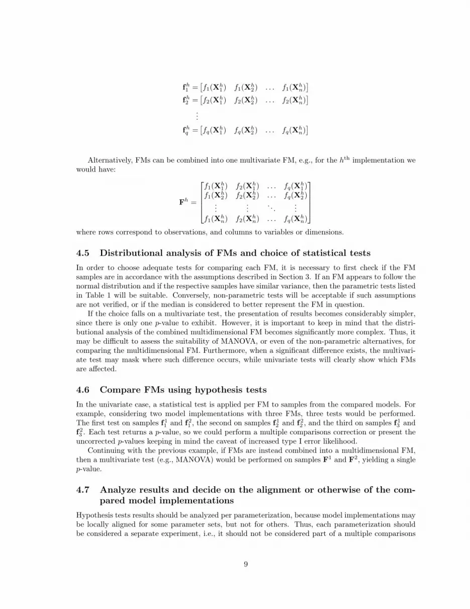
Alternatively, FMs can be combined into one multivariate FM, e.g., for the hth implementation wewould have:

Fh =

f1(Xh1 ) f2(X

h1 ) . . . fq(X

h1 )

f1(Xh2 ) f2(X

h2 ) . . . fq(X

h2 )

......

. . ....

f1(Xhn) f2(X

hn) . . . fq(X

hn)

where rows correspond to observations, and columns to variables or dimensions.

4.5 Distributional analysis of FMs and choice of statistical testsIn order to choose adequate tests for comparing each FM, it is necessary to first check if the FMsamples are in accordance with the assumptions described in Section 3. If an FM appears to follow thenormal distribution and if the respective samples have similar variance, then the parametric tests listedin Table 1 will be suitable. Conversely, non-parametric tests will be acceptable if such assumptionsare not verified, or if the median is considered to better represent the FM in question.

If the choice falls on a multivariate test, the presentation of results becomes considerably simpler,since there is only one p-value to exhibit. However, it is important to keep in mind that the distri-butional analysis of the combined multidimensional FM becomes significantly more complex. Thus, itmay be difficult to assess the suitability of MANOVA, or even of the non-parametric alternatives, forcomparing the multidimensional FM. Furthermore, when a significant difference exists, the multivari-ate test may mask where such difference occurs, while univariate tests will clearly show which FMsare affected.

4.6 Compare FMs using hypothesis testsIn the univariate case, a statistical test is applied per FM to samples from the compared models. Forexample, considering two model implementations with three FMs, three tests would be performed.The first test on samples f11 and f21 , the second on samples f12 and f22 , and the third on samples f13 andf23 . Each test returns a p-value, so we could perform a multiple comparisons correction or present theuncorrected p-values keeping in mind the caveat of increased type I error likelihood.

Continuing with the previous example, if FMs are instead combined into a multidimensional FM,then a multivariate test (e.g., MANOVA) would be performed on samples F1 and F2, yielding a singlep-value.

4.7 Analyze results and decide on the alignment or otherwise of the com-pared model implementations

Hypothesis tests results should be analyzed per parameterization, because model implementations maybe locally aligned for some parameter sets, but not for others. Thus, each parameterization shouldbe considered a separate experiment, i.e., it should not be considered part of a multiple comparisons

9

scenario. If at least one FM is shown to be statistically different for a given parameterization, thenthe compared implementations can be considered globally misaligned.

If the p-value(s) for a specific parameterization are above the chosen significance level α, theimplementations can be considered locally aligned for that parameter set. When one or more p-valuesare significant in a multiple comparison scenario (for the same parameterization), they should be inthe proportion predicted by α. No p-values should remain significant after Bonferroni-type correctionsare performed. In the multivariate approach, where all the FMs are merged into one multidimensionalFM, the single p-value should not be significant.

It is important to understand that statistical tests may not provide a definitive answer. Only inthe case of clear misalignments, with very significant p-values, can one reject H0 with confidence. Inmany situations some p-values may appear to be borderline significant, and is up to the modeler tojudge if the detected misalignment has practical significance.

5 Model-independent selection of FMsThe empirical selection of FMs, as described in Section 4.3, has a number of disadvantages. First, itrelies on summary measures which are model-dependent and, probably, user-dependent. Furthermore,for different model parameters, the originally selected FMs may be of no use, as simulation outputmay change substantially. For example, the warm-up period for the steady-state statistical summariescan be quite different. Certain models and/or parameterizations might not even display a steady-statebehavior. Finally, it might not be clear which FMs best capture the behavior of a model.

A model-independent approach to FM selection should work directly from simulation output, au-tomatically selecting the features that best explain potential differences between the implementationsbeing compared, thus avoiding the disadvantages of an empirical selection. Additionally, such a methodshould not depend on the distributional properties of simulation output, and should be directly appli-cable by modelers.

Our proposal consists of automatically extracting the most relevant information from simulationoutput using PCA. PCA is a widely used technique [56] which extracts the largest variance componentsfrom data by applying singular value decomposition to a mean-centered data matrix. In other words,PCA is able to convert simulation output into a set of linearly uncorrelated measures which can beanalyzed in a consistent, model-independent fashion. This technique is especially relevant for stochasticsimulation models, as it considers not only equilibrium but also dynamics over time [9]. Procedure 2summarizes this approach, replacing steps 2.2 and 2.3 of Procedure 1.

Procedure 2 accepts, on a per output basis, the collected data (Procedure 1, step 2.1) in the form ofmatrix X, yielding matrix T, which contains the representation of Xc (i.e., the column mean-centeredversion of X) in the principal components (PCs) space, as well as vector λ, containing the eigenvaluesof the covariance matrix of Xc. The columns of T correspond to PCs, and are orderer by decreasingvariance, i.e., the first column corresponds to the first PC, and so on. Rows of T correspond to obser-vations. The kth column of T contains sn model-independent observations for the kth PC, n for eachimplementation. Thus, each PC corresponds to an FM. As in the case of empirically selected FMs,univariate or multivariate statistical tests can be used to check if samples from different implemen-tations are drawn from the same distribution. However, both testing approaches will not prioritizedimensions, even though the first PCs are more important for characterizing model differences, as theyexplain more variance. This can be handled in the univariate case by prioritizing PCs according totheir explained variance using the weighted Bonferroni procedure on the resulting p-values [57]. Formultivariate tests, dimensions/variables can be limited to the number of PCs that explain a prespecifiedamount of variance, although there is no prioritization within the selected dimensions.

The eigenvalues vector λ is also important for this process, for two reasons: 1) to select a numberof PCs (i.e., FMs) to be considered for hypothesis testing, such that these explain a prespecifiedpercentage of variance; 2) the alignment or otherwise of s model implementations can be empiricallyassessed by analyzing how the explained variance is distributed along PCs. The percentage of variance

10

Procedure 2 Obtaining model-independent summary measures from one generic simulation outputfrom s model implementations.

1. Group the Xhji’s from all replications row-wise in matrix X for each implementation, as follows:

X =

X110 X1

11 . . . X11,m−1 X1

1,m

X120 X1

21 . . . X12,m−1 X1

2,m...

.... . .

......

X1n0 X1

n1 . . . X1n,m−1 X1

n,m...

.... . .

......

Xs10 Xs

11 . . . Xs1,m−1 Xs

1,m

Xs20 Xs

21 . . . Xs2,m−1 Xs

2,m...

.... . .

......

Xsn0 Xs

n1 . . . Xsn,m−1 Xs

n,m

2. Determine matrix Xc, which is the column mean-centered version of X.

3. Apply PCA to matrix Xc, considering that rows (replications) correspond to observations andcolumns (iterations or time steps) to variables. This yields:

• Matrix T, containing the representation of the original data in the principal components(PCs) space.

T =

T 111 T 1

12 . . . T 11,u−1 T 1

1,u

T 121 T 1

22 . . . T 12,u−1 T 1

2,u...

.... . .

......

T 1n1 T 1

n2 . . . T 1n,u−1 T 1

n,u...

.... . .

......

T s11 T s

12 . . . T s1,u−1 T s

1,u

T s21 T s

22 . . . T s2,u−1 T s

2,u...

.... . .

......

T sn1 T s

n2 . . . T sn,u−1 T s

n,u

• Vector λ, containing the eigenvalues of the covariance matrix of Xc in descending order,each eigenvalue corresponding to the variance of the columns of T.

λ =[λ1 λ2 . . . λu−1 λu

]

11

explained by each PC can be obtained as shown in Eq. 1.

S2k(%) =

λk∑λ

(1)

where k identifies the kth PC, λk is the eigenvalue associated with the kth PC, and∑

λ is the sum of alleigenvalues. If the variance is well distributed along many PCs, it is an indication that the comparedimplementations are aligned, at least for the output being analyzed. On the other hand, if most of thevariance is explained by the first PCs, it can be an indication that at least one model implementationis misaligned. The rationale being that if all implementations show the same dynamical behavior, thenthe projection of their outputs in the PC space will be close together and have similar statistics, i.e.,means, medians and variance. As such, PCA will be unable to find components which explain largequantities of variance, and the variance will be well distributed along the PCs. If at least one modelimplementation is misaligned, the projection of its outputs in the PC space will be farther apart thanthe projections of the remaining implementations. As such, PCA will yield at least one componentwhich explains large part of the overall variance.

The alignment of two or more implementations can be assessed by analyzing the following infor-mation: 1) the p-values produced by the univariate and multivariate statistical tests, which should beabove the typical 1% or 5% significance levels in case of implementation alignment; in the univariatecase, it may be useful to adjust the p-values using the weighted Bonferroni procedure to account formultiple comparisons; 2) in case of misalignment, the total number of PCs required to explain a pre-specified amount of variance should be lower than in case of alignment; also, more variance should beexplained by the first PCs of the former than by the same PCs of the latter; and, 3) the scatter plot ofthe first two PC dimensions, which can offer visual, although subjective feedback on model alignment;e.g., in case of misalignment, points associated with runs from different implementations should formdistinct groups.

5.1 Extension to multiple outputsDetermining the alignment of models with multiple outputs may be less straightforward. If model im-plementations are clearly aligned or misaligned, conclusions can be drawn by analyzing the informationprovided by the proposed method applied to each one of the model outputs.

In order to compare all model outputs simultaneously, a Bonferroni or similar p-value correctioncould be used. This strategy can be directly applicable in the multivariate case, since there is one p-value per model output. However, a direct application to the univariate case would be more complex,since there will be multiple p-values per model output (one p-value per PC), and these may have beenpreviously corrected with the weighted Bonferroni procedure according to their explained variance.

We propose an alternative approach based on the concatenation of all model outputs, centered andscaled. This reduces a model with g outputs to a model with one output, which can be processedwith Procedure 2. In order to perform output concatenation, outputs are centered and scaled suchthat their domains are in the same order of magnitude, replication-wise. This can be performed usingrange scaling on each output, for example, as shown below for a given simulation output;

Xji =Xji −Xj

maxXj −minXj, i = 0, 1, . . . ,m; j = 1, . . . , sn (2)

Xj =[Xj0 Xj1 . . . Xjm

](3)

where i represents iterations or time steps, j is the replication number, Xji is the output value at iter-ation i and replication j, Xj is a row vector with the complete output generated in the jth replication,and Xj is its range scaled version. Other centering and scaling methods, such as auto-scaling or levelscaling [58], can be used as an alternative to range scaling in Eq. 2. For a model with g outputs, theresulting concatenated output for the jth replication is given by

12

Aj = 1Xj ⊕ 2Xj ⊕ . . .⊕ gXj (4)

where ⊕ is the concatenation operator, and Aj is the concatenation of all model outputs for replicationj. Model implementations can thus be compared with the proposed method using the “single” modeloutput.

6 Simulation modelThe Predator–Prey for High-Performance Computing (PPHPC) model is a reference model for studyingand evaluating spatial ABM (SABM) implementation strategies, capturing important characteristicsof SABMs, such as agent movement and local agent interactions. It is used in this work as a test casefor the proposed model comparison method. The model is thoroughly described in reference [20] usingthe ODD protocol [4]. Here we present a summarized description of the model.

6.1 DescriptionPPHPC is a predator–prey model composed of three entity classes: agents, grid cells and environment.Agents can be of type prey or predator. While prey consume passive cell-bound food, predatorsconsume prey. Agents have an energy state variable, E, which increases when feeding and decreaseswhen moving and reproducing. When energy reaches zero, the agent is removed from the simulation.Instances of the grid cell entity class are where agents act, namely where they try to feed and reproduce.Grid cells have a fixed grid position and contain only one resource, cell-bound food (grass), which canbe consumed by prey, and is represented by the countdown state variable C. The C state variablespecifies the number of iterations left for the cell-bound food to become available. Food becomesavailable when C = 0, and when a prey consumes it, C is set to cr (an initial simulation parameter).The set of all grid cells forms the environment entity, a toroidal square grid where the simulation takesplace. The environment is defined by its size and by the restart parameter, cr. The temporal scale isrepresented by a positive integer m, which represents the number of iterations.

Simulations start with an initialization process, where a predetermined number of agents are ran-domly placed in the simulation environment. Cell-bound food is also initialized at this stage. Afterinitialization, and to get the simulation state at iteration zero, outputs are collected. The schedulerthen enters the main simulation loop, where each iteration is sub-divided into four steps: 1) agentmovement; 2) food growth in grid cells; 3) agent actions; and, 4) gathering of simulation outputs.Note that the following processes are explicitly random: a) initialization of specific state variables(e.g., initial agent energy); b) agent movement; c) the order in which agents act; and, d) agent repro-duction. For process c), this implies that the agent list should be explicitly shuffled before agents canact.

Six outputs are collected at each iteration i: P si , Pw

i , P ci , E

s

i , Ew

i , and Ci. P si and Pw

i refer to thetotal prey (sheep) and predator (wolf ) population counts, respectively, while P c

i holds the quantityof available cell-bound food. E

s

i and Ew

i contain the mean energy of prey and predator populations.Finally, Ci refers to the mean value of the C state variable in all grid cells.

6.2 ParameterizationsReference parameters for the PPHPC model are specified in reference [20]. Parameters are qualita-tively separated into size-related and dynamics-related groups. Although size-related parameters alsoinfluence model dynamics, this separation is useful for parameterizing simulations.

Concerning size-related parameters, a base grid size of 100 × 100 is associated with 400 prey and200 predators. Different grid sizes should have proportionally assigned agent population sizes, suchthat the initial agent density and the initial ratio between prey and predators remains constant. We

13

define model size as the association between grid size and initial agent population. For example, modelsize 200 corresponds to a grid size of 200× 200 with 1600 prey and 800 predators at iteration 0.

For the dynamics-related parameters, two parameter sets, 1 and 2, are proposed. The two param-eterizations generate distinct dynamics, with the second set typically yielding more than twice thenumber of agents than the first during the course of a simulation. We will refer to a combinationof model size and parameter set as “size@set”, e.g., 400@1 for model size 400, parameter set 1. Thereference number of iterations, m, is 4000, not counting with the initial simulation state at iteration 0.

6.3 Empirical selection of FMsUnder the parameterizations discussed in the previous subsection, all outputs have an initial transientstage, entering steady-state after a number of iterations. The point at which simulations enter thisstate of equilibrium varies considerably from parameter set 1 to parameter set 2, occurring considerablysooner in the former. Model size does not seem to affect the steady-state truncation point, mainlyinfluencing the magnitude of the collected outputs. As such, steady-state is empirically established fori > 1000 and i > 2000 for parameter sets 1 and 2, respectively [20].

Considering this information, as well as the recommendations discussed in Section 4.3, the followingstatistical summaries are selected for individual outputs: 1) maximum value (max); 2) iteration wheremaximum value occurs (argmax); 3) minimum value (min); 4) iteration where minimum value occurs(argmin); 5) steady-state mean (X

ss); and, 6) steady-state sample standard deviation (Sss). Thus,

we specify a total of 36 FMs (six statistical summaries from six outputs). Naturally, the steady-statemeasures are collected after the truncation point defined for each parameter set.

As discussed in reference [20], all measures, except argmax and argmin, are amenable to be com-pared using parametric methods, as they follow (or approximately follow) normal distributions.

6.4 ImplementationsTwo implementations of the PPHPC model are used for evaluating the proposed model comparisontechnique. The first is developed in NetLogo [20], while the second is a Java implementation withseveral parallel variants [14]. For the results discussed in this paper, simulations performed withthe Java implementation were executed with the EX parallelization strategy using eight threads. Inthis strategy, each thread processes an equal part of the simulation environment, and reproduciblesimulations are guaranteed. Individual threads use their own sub-sequence of a global random sequence,obtained with a random spacing approach using the SHA-256 cryptographic hash function. TheMersenne Twister pseudo-random number generator (PRNG) [54] is used by both implementations fordriving the model’s random processes. Complete details of both implementations are available in theprovided references, and their source code is available at https://github.com/fakenmc/pphpc/.

7 Experimental setupIn order to test the model comparison methods, we define a base PPHPC configuration using theNetLogo implementation and compare it with three configurations using the Java implementation.All configurations are tested for model sizes 100, 200, 400 and 800, and parameter sets 1 and 2, asdescribed in Section 6.2. The four configurations follow the conceptual model, except when statedotherwise:

1. NetLogo implementation.

2. Java implementation.

3. Java implementation: agents are ordered by energy prior to agent actions, and agent list shufflingis not performed.

14

https://github.com/fakenmc/pphpc/

4. Java implementation: the restart parameter, cr, is set to one unit less than specified in the testedparameterizations (9 instead of 10 for parameter set 1, 14 instead of 15 for parameter set 2).

The goal is to assess how the two FM selection strategies (empirical and model-independent) exposethe increasing differences of comparing configuration 1 with configurations 2–4. More specifically, weare interested in checking if the proposed model-independent comparison method is able to exposethese differences in the same way as the manual or empirical approach. As such, we define threecomparison cases:

Case I Compare configuration 1 with configuration 2. These configurations should yield distribution-ally equivalent results.

Case II Compare configuration 1 with configuration 3. A small misalignment is to be expected.

Case III Compare configuration 1 with configuration 4. There should be a mismatch in the outputs.

For each “size@set” combination, independent samples of the six model outputs are obtained fromn = 30 replications for each configuration, in a total of 4n = 120 runs. Each replication r = 1, . . . , 4nis performed with a PRNG seed obtained by taking the MD5 checksum of r and converting theresulting hexadecimal string to an integer (limited to 32-bits for NetLogo and 128-bits for the Javaimplementation), guaranteeing independence between seeds, and consequently, between replications.The same samples are used for the evaluation of both empirical and model-independent FM selection.

In order to evaluate how the tested methodologies respond to larger sample sizes, an additionaln = 100 replications were performed per configuration for the 400@1 combination, in a total of 4n = 400runs. The PRNG seeds for individual replications were obtained in the same fashion. Similarly, thetested methodologies were also compared with n = 10 for the 400@1 combination, but in this caseusing the first 10 replications from the n = 30 setup for each configuration. All samples sizes werechosen for convenience with the purpose of simplifying analysis of results, namely of how the two FMselection approaches, empirical and model-independent, fare under the same conditions.

For the model-dependent comparisons, results were obtained with the SimOutUtilsMATLAB tool-box [59]. The micompr R package [60] provides an implementation of the proposed model-independentcomparison approach, and was used to produce the corresponding results.

The data generated by this computational experiment, as well as the scripts used to set up theexperiment, are made available to other researchers at https://zenodo.org/record/46848.

8 ResultsIn this section we mainly focus on the results for the 400@1 combination. Results for the remainingsize/set combinations are provided as Supplementary material, and are referred to when appropriate.

8.1 Empirical selection of FMsTable 3 shows the results for the empirical approach to cases I, II and III. The corresponding p-valueswere obtained with the t-test for max, min, X

ssand Sss statistics, and with the Mann–Whitney U

test for the argmax and argmin statistics. For the latter, when all points in both samples have thesame value, we simply present 1.00 as the p-value, since the test is not performed.

Results for case I show that the two configurations are reasonably well aligned. In a total of 36FMs, five are below the 5% significance level, and of these, only one is below 1%. Since the p-valuesare not corrected for multiple comparisons, it is expected that some of them present “significant”differences. For case II, the effect of not shuffling the agents before they act in the Java implementation(configuration 3) is evident, as half of the p-values are below 0.05. Of these, all but one are also below0.01. Finally, in case III, most p-values show very significant differences, such that we can reject, with

15

https://zenodo.org/record/46848

Comp. Stat. Outputs

P s Pw P c Es

Ew

C

I

max 0.213 0.288 0.011 0.231 0.774 0.086argmax 0.733 0.802 0.056 0.858 0.284 0.279min 0.002 0.088 0.094 0.275 0.076 0.011argmin 0.048 0.350 0.279 1.000 0.091 1.000X

ss0.457 0.905 0.546 0.833 0.049 0.551

Sss 0.242 0.282 0.285 0.474 0.109 0.285

II

max 7e−6 1e−7 2e−4 2e−7 0.322 0.004argmax 1e−4 0.540 0.230 0.703 0.052 1e−4min 1e−5 4e−4 0.009 0.508 0.017 0.001argmin 0.712 0.906 0.001 1.000 0.009 1.000X

ss0.206 < 1e−8 6e−8 < 1e−8 0.938 6e−8

Sss 0.735 0.324 0.712 0.218 0.688 0.713

III

max < 1e−8 < 1e−8 < 1e−8 < 1e−8 < 1e−8 < 1e−8argmax 2e−5 0.115 < 1e−8 0.134 0.332 1e−5min 7e−8 < 1e−8 < 1e−8 0.582 0.003 < 1e−8argmin 2e−5 0.070 2e−5 1.000 0.004 < 1e−8

Xss

< 1e−8 < 1e−8 < 1e−8 < 1e−8 < 1e−8 < 1e−8Sss 3e−7 7e−8 5e−5 4e−8 0.013 0.013

Table 3 – P -values for the empirical selection of FMs for model size 400, parameter set 1, and n = 30 runsper configuration. P -values were obtained with the t-test formax, min, Xss and Sss statistics, and with theMann-Whitney U test for argmax and argmin statistics. Case I weights two similar configurations, caseII compares configurations with a small implementation difference, and case III compares configurationswith a different parameter. Values lower than 0.05 are underlined, while values lower than 0.01 aredouble-underlined.

16

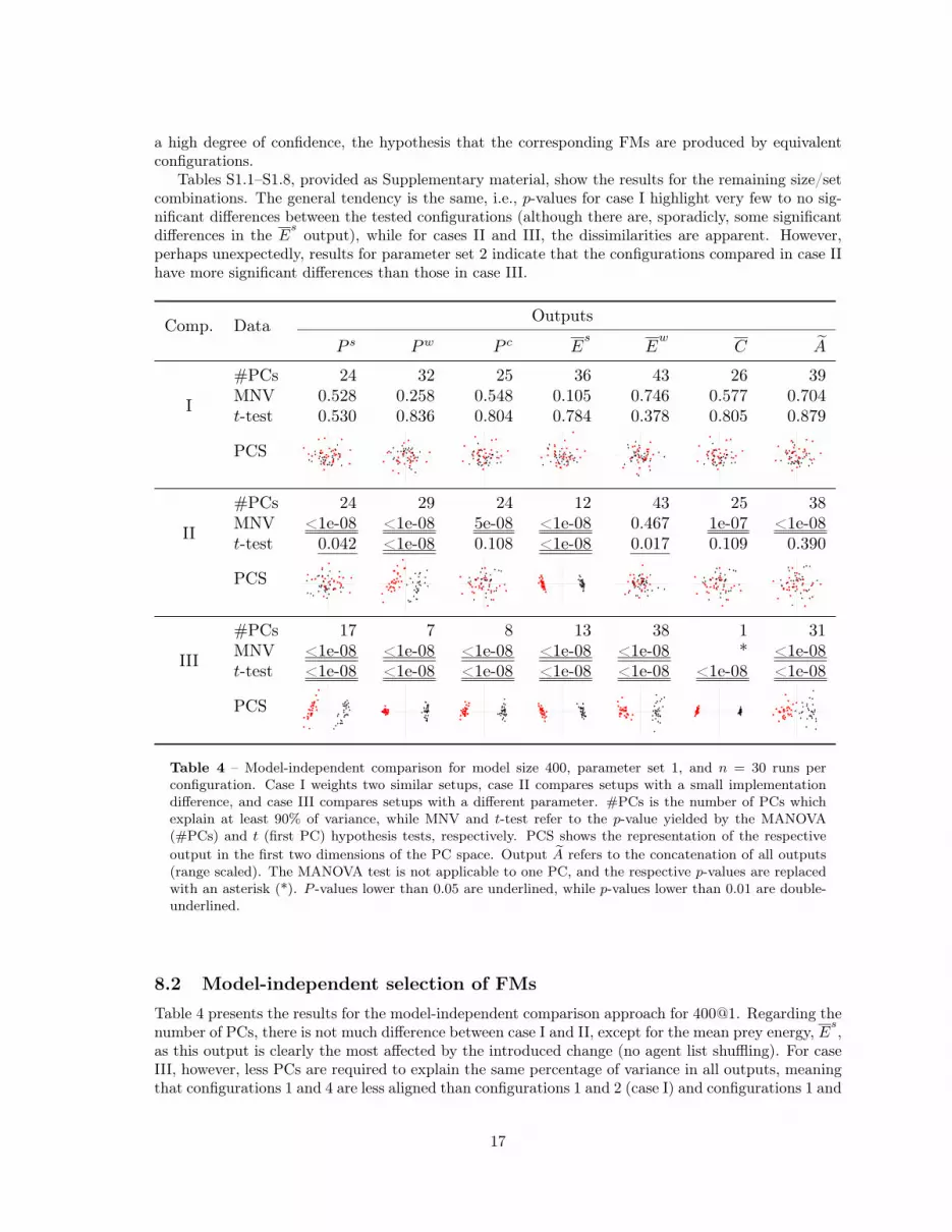
a high degree of confidence, the hypothesis that the corresponding FMs are produced by equivalentconfigurations.

Tables S1.1–S1.8, provided as Supplementary material, show the results for the remaining size/setcombinations. The general tendency is the same, i.e., p-values for case I highlight very few to no sig-nificant differences between the tested configurations (although there are, sporadicly, some significantdifferences in the E

soutput), while for cases II and III, the dissimilarities are apparent. However,

perhaps unexpectedly, results for parameter set 2 indicate that the configurations compared in case IIhave more significant differences than those in case III.

Comp. Data Outputs

P s Pw P c Es

Ew

C A

I

#PCs 24 32 25 36 43 26 39MNV 0.528 0.258 0.548 0.105 0.746 0.577 0.704t-test 0.530 0.836 0.804 0.784 0.378 0.805 0.879

PCS

II

#PCs 24 29 24 12 43 25 38MNV <1e-08 <1e-08 5e-08 <1e-08 0.467 1e-07 <1e-08t-test 0.042 <1e-08 0.108 <1e-08 0.017 0.109 0.390

PCS

III

#PCs 17 7 8 13 38 1 31MNV <1e-08 <1e-08 <1e-08 <1e-08 <1e-08 * <1e-08t-test <1e-08 <1e-08 <1e-08 <1e-08 <1e-08 <1e-08 <1e-08

PCS

Table 4 – Model-independent comparison for model size 400, parameter set 1, and n = 30 runs perconfiguration. Case I weights two similar setups, case II compares setups with a small implementationdifference, and case III compares setups with a different parameter. #PCs is the number of PCs whichexplain at least 90% of variance, while MNV and t-test refer to the p-value yielded by the MANOVA(#PCs) and t (first PC) hypothesis tests, respectively. PCS shows the representation of the respectiveoutput in the first two dimensions of the PC space. Output A refers to the concatenation of all outputs(range scaled). The MANOVA test is not applicable to one PC, and the respective p-values are replacedwith an asterisk (*). P -values lower than 0.05 are underlined, while p-values lower than 0.01 are double-underlined.

8.2 Model-independent selection of FMsTable 4 presents the results for the model-independent comparison approach for 400@1. Regarding thenumber of PCs, there is not much difference between case I and II, except for the mean prey energy, E

s,

as this output is clearly the most affected by the introduced change (no agent list shuffling). For caseIII, however, less PCs are required to explain the same percentage of variance in all outputs, meaningthat configurations 1 and 4 are less aligned than configurations 1 and 2 (case I) and configurations 1 and

17

3 (case II). Nonetheless, the p-values offer more objective answers, displaying increasingly significantdifferences from case I to case III, i.e., in line with the results from the empirical approach. P -valueswere obtained with the t-test for the first PC, and with MANOVA for the number of PCs whichexplain at least 90% of the variance. The assumptions for these parametric tests seem to be verified,and are discussed with additional detail in Section 8.2.3. MANOVA appears to be more sensitive toimplementation differences than the t-test, generally presenting more significant p-values. As would beexpected, significant p-values from both MANOVA and t-tests are associated with clearer distinctionsbetween samples in the PC scatter plots.

The concatenated output, A, has less discriminatory power than individual outputs. This is espe-cially clear for case II, where both the t-test and scatter plot do not suggest significant discrepancies.However, the MANOVA test is able to pick up the implementation difference, yielding a significantp-value. While in this case MANOVA on A answers to the question of whether the implementationsare statistically equivalent, only a comprehensive analysis of individual outputs allows to diagnose howthe model is affected by the implementation differences. For example, the number of PCs and thescatter plot indicate that the E

soutput is by far the most affected in case II, something which is not

possible to deduce by just analyzing A. This consideration would also be difficult to infer from theempirical comparison data in Table 3, as the p-values are not much different from those associatedwith other outputs. As described in Section 5.1, outputs were range scaled prior to concatenation. Wehave experimented with other types of centering and scaling [58], and did not find major differenceson how the proposed model-independent comparison method evaluates the concatenated output.

Results for the remaining size/set combinations, provided in Supplementary Tables S2.1–S2.8,are in accordance with the discussion thus far. The number of PCs required to explain 90% of thevariance for cases II and III are generally smaller than for case I. Furthermore, the number of PCsfor parameter set 2 is consistently lower in case II than in case III, attesting to what was observedin the model-dependent analysis: configurations compared in case II are more dissimilar than thosein case III. This is also corroborated by the p-values, and even more clearly, by the PC scatter plots.For the majority of individual comparisons in cases II and III, MANOVA seems more sensitive toimplementation differences than the t-test. However, there are some instances where the latter is ableto perform better distinctions, as for example in case II of the 100@1 size/set combination. Concerningthe concatenated output, it was generally adequate for detecting implementation differences, withMANOVA and/or the t-test yielding significant p-values. Nonetheless, this approach failed for caseIII of 100@2. Analyzing the overall results for all size/set combinations, it is also possible to concludethat, as model size increases, implementation differences become more pronounced for both parametersets.

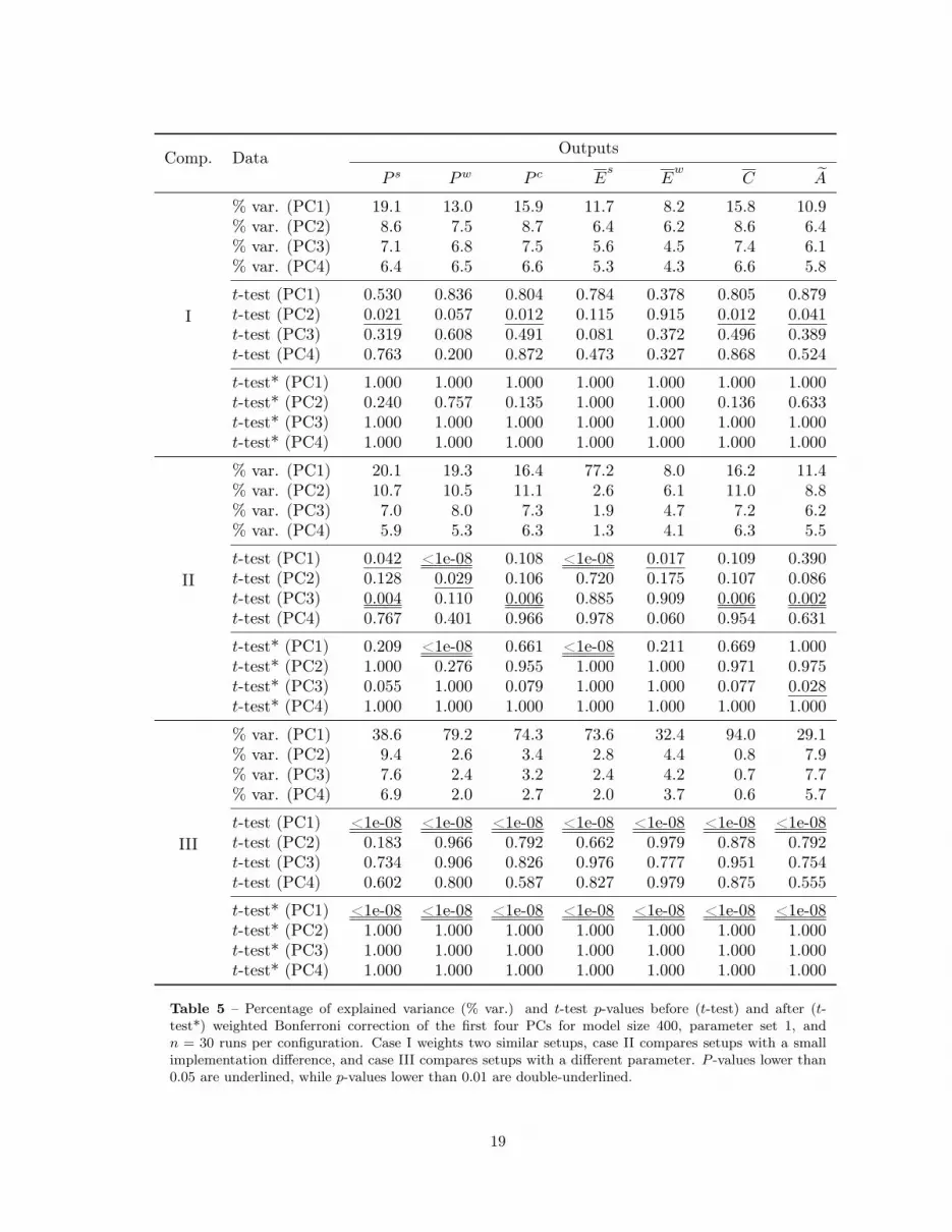
8.2.1 Assessing the t-test applied to individual PCs and the distribution of explainedvariance

Table 5 shows, for the first four PCs of the 400@1 combination, the percentage of variance explained byindividual PCs, as well as the respective t-test p-values, before and after weighted Bonferroni correction.For case I, p-values for the first PC are never significant, but a few for the second PC are significantat the α = 0.05 level. However, no p-values remain so after adjustment with the weighted Bonferronicorrection. For case II, p-values for the first PC are usually the most significant, although this doesnot always hold, e.g., output A. In this instance, only the 3rd, 6th and 15th PC p-values are significant(the 3rd and 6th remain so at α = 0.05 after correction), which is the reason for MANOVA catchingthe implementation difference (as shown in Table 4). For case III, the first PC p-value is always highlysignificant (before and after weighted Bonferroni correction), with the PC2–PC4 p-values showingno significance at all. The implementation differences in the first PC, captured by the t-test, seemsufficient for MANOVA, which considers all PCs simultaneously, to also spot the dissimilarities. Thedistribution of explained variance along PCs also reflects what was discussed in Section 5. Morespecifically, it is possible to observe that the first PC or PCs explain more variance in misaligned casesII and III than in case I (aligned).

18

Comp. Data Outputs

P s Pw P c Es

Ew

C A

I

% var. (PC1) 19.1 13.0 15.9 11.7 8.2 15.8 10.9% var. (PC2) 8.6 7.5 8.7 6.4 6.2 8.6 6.4% var. (PC3) 7.1 6.8 7.5 5.6 4.5 7.4 6.1% var. (PC4) 6.4 6.5 6.6 5.3 4.3 6.6 5.8

t-test (PC1) 0.530 0.836 0.804 0.784 0.378 0.805 0.879t-test (PC2) 0.021 0.057 0.012 0.115 0.915 0.012 0.041t-test (PC3) 0.319 0.608 0.491 0.081 0.372 0.496 0.389t-test (PC4) 0.763 0.200 0.872 0.473 0.327 0.868 0.524

t-test* (PC1) 1.000 1.000 1.000 1.000 1.000 1.000 1.000t-test* (PC2) 0.240 0.757 0.135 1.000 1.000 0.136 0.633t-test* (PC3) 1.000 1.000 1.000 1.000 1.000 1.000 1.000t-test* (PC4) 1.000 1.000 1.000 1.000 1.000 1.000 1.000

II


t-test (PC1) 0.042 <1e-08 0.108 <1e-08 0.017 0.109 0.390t-test (PC2) 0.128 0.029 0.106 0.720 0.175 0.107 0.086t-test (PC3) 0.004 0.110 0.006 0.885 0.909 0.006 0.002t-test (PC4) 0.767 0.401 0.966 0.978 0.060 0.954 0.631

t-test* (PC1) 0.209 <1e-08 0.661 <1e-08 0.211 0.669 1.000t-test* (PC2) 1.000 0.276 0.955 1.000 1.000 0.971 0.975t-test* (PC3) 0.055 1.000 0.079 1.000 1.000 0.077 0.028t-test* (PC4) 1.000 1.000 1.000 1.000 1.000 1.000 1.000

III


t-test (PC1) <1e-08 <1e-08 <1e-08 <1e-08 <1e-08 <1e-08 <1e-08t-test (PC2) 0.183 0.966 0.792 0.662 0.979 0.878 0.792t-test (PC3) 0.734 0.906 0.826 0.976 0.777 0.951 0.754t-test (PC4) 0.602 0.800 0.587 0.827 0.979 0.875 0.555

t-test* (PC1) <1e-08 <1e-08 <1e-08 <1e-08 <1e-08 <1e-08 <1e-08t-test* (PC2) 1.000 1.000 1.000 1.000 1.000 1.000 1.000t-test* (PC3) 1.000 1.000 1.000 1.000 1.000 1.000 1.000t-test* (PC4) 1.000 1.000 1.000 1.000 1.000 1.000 1.000

Table 5 – Percentage of explained variance (% var.) and t-test p-values before (t-test) and after (t-test*) weighted Bonferroni correction of the first four PCs for model size 400, parameter set 1, andn = 30 runs per configuration. Case I weights two similar setups, case II compares setups with a smallimplementation difference, and case III compares setups with a different parameter. P -values lower than0.05 are underlined, while p-values lower than 0.01 are double-underlined.

19

These observations generally remain valid when considering all tested size/set combinations (TablesS3.1–S3.8, provided as Supplementary material). For case I, in which the compared configurations areassumed to be aligned, a few significant PC1 p-values (at the α = 0.05 level) stand-out for [email protected], after the weighted Bonferroni correction, all t-test p-values from PC1–PC4 are non-significant for all size/set combinations. For case II, a global size/set analysis confirms that p-valuesfor the first PC are usually the most significant for all outputs. The most notable exception occurs forthe 200@1 combination, in which only the E

soutput presents a significant p-value (at α = 0.01, before

and after weighted Bonferroni correction). However, this p-value is enough for the respective MANOVA(Table S2.3) to catch the difference directly in E

s, and indirectly in the concatenated output. With

very few exceptions, the PC2–PC4 p-values are not significant, especially after the weighted Bonferronicorrection. Results for case III broadly confirm what was observed for 400@1, i.e., that the first PC p-value is always highly significant (before and after weighted Bonferroni correction), with the PC2–PC4p-values showing little to no significance. The exception is 100@2, for which only the PC1 p-value for P s

is significant at α = 0.05, but losing significance after the weighted Bonferroni correction. Nonetheless,dissimilarities between configurations 1 and 4 are detected by the MANOVA test (Table S2.2) in themajority of outputs due to misalignments in PCs other than the first (e.g., for output C these arevisible for PC2 and PC3). Considering these results, it is possible to conclude that the p-value of thefirst PC is undoubtedly the most important for evaluating model alignment. Nonetheless, there arealso instances, namely for smaller model sizes, where it is necessary to look at the MANOVA p-valuein order to draw solid conclusions. The distribution of explained variance along PCs generally reflectsthe alignment of configurations, with less aligned ones having more variance explained by the first PCor PCs. Again the exception is 100@2, where the difference in explained variance does not changemuch from case to case.

8.2.2 Changing the variance for the selection of the number of PCs for MANOVA

The MANOVA p-values shown in Table 4 were obtained by requiring that the respective number ofPCs explain at least 90% of the variance in the data. As this percentage must be predefined by themodel developer, it is important to understand how the MANOVA results are affected when this valueis changed. Table 6 shows, for the 400@1 instance, the number of PCs, as well as the associatedMANOVA p-values, required to explain 30%, 50%, 70% and 90% of the variance. Three aspects canbe highlighted from this table: 1) conclusions concerning configuration alignment do not change withdifferent percentages of variance; 2) more variance seems to make the MANOVA test more sensitive incase II, although this trend is not very well-defined; 3) lower prespecified percentages of variance implyless PCs to explain it; in the limit, this makes the MANOVA test inapplicable if just one PC is required,as observed for several instances of cases II and III. This latter aspect is not crucial, because the t-testis the equivalent of a “univariate MANOVA” for two groups. Nonetheless, if the MANOVA p-valuesare deemed important for a specific comparison, it seems preferable to specify a higher percentage ofvariance to explain.

Results for the remaining size/set combinations, provided in Supplementary Tables S4.1–S4.8,generally follow the tendencies verified for 400@1, perhaps further blurring the slight trend observedin the relation between percentage of variance and MANOVA sensitivity.

8.2.3 Assumptions for the t and MANOVA parametric tests

As described in Section 5, the t and MANOVA tests make several assumptions about the underlyingdata. To confirm that the presented results are statistically valid, it is important to perform an overallsurvey of these assumptions, namely: 1) whether the data is normally distributed within groups; and,2) if samples are drawn from populations with equal variances. The former assumption can be verifiedwith the Shapiro–Wilk test for univariate normality or the Royston test for multivariate normality.The latter can be evaluated with the Bartlett test or Box’s M test for the univariate and multivariatecases, respectively. Table 7 presents aggregated results for these tests for all size/set combinations.

20

Comp. Data Outputs

P s Pw P c Es

Ew

C A

I

#PCs (30% var.) 3 4 3 5 6 3 5#PCs (50% var.) 6 8 6 10 13 7 9#PCs (70% var.) 11 15 12 19 25 12 19#PCs (90% var.) 24 32 25 36 43 26 39

MNV (30% var.) 0.080 0.235 0.078 0.185 0.696 0.078 0.297MNV (50% var.) 0.267 0.514 0.278 0.020 0.530 0.311 0.614MNV (70% var.) 0.241 0.611 0.344 0.044 0.682 0.344 0.527MNV (90% var.) 0.528 0.258 0.548 0.105 0.746 0.577 0.704

II


MNV (30% var.) 0.038 <1e-08 0.004 * 0.035 0.004 0.007MNV (50% var.) 2e-06 <1e-08 3e-04 * 0.034 3e-04 3e-04MNV (70% var.) 4e-05 <1e-08 0.002 * 0.049 0.001 2e-06MNV (90% var.) <1e-08 <1e-08 5e-08 <1e-08 0.467 1e-07 <1e-08

III


MNV (30% var.) * * * * * * <1e-08MNV (50% var.) <1e-08 * * * <1e-08 * <1e-08MNV (70% var.) <1e-08 * * * <1e-08 * <1e-08MNV (90% var.) <1e-08 <1e-08 <1e-08 <1e-08 <1e-08 * <1e-08

Table 6 – Number of principal components (#PCs) and MANOVA test p-values (MNV) for severalpercentages of explained variance for model size 400, parameter set 1, and n = 30 runs per configuration.Case I weights two similar setups, case II compares setups with a small implementation difference, andcase III compares setups with a different parameter. Output A refers to the concatenation of all outputs(range scaled). The MANOVA test is not applicable to one PC, and the respective p-values are replacedwith an asterisk (*). P -values lower than 0.05 are underlined, while p-values lower than 0.01 are double-underlined.

21

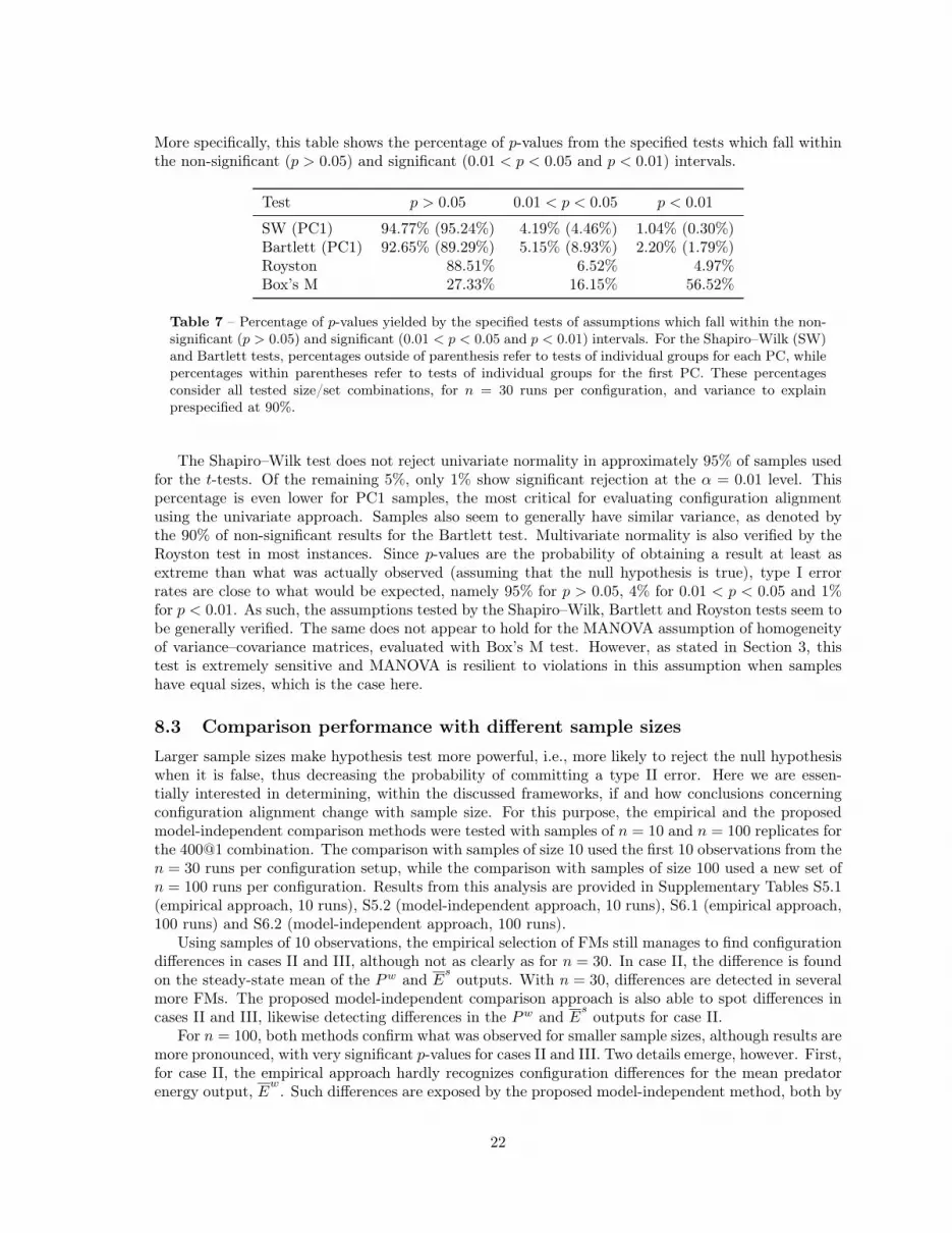
More specifically, this table shows the percentage of p-values from the specified tests which fall withinthe non-significant (p > 0.05) and significant (0.01 < p < 0.05 and p < 0.01) intervals.

Test p > 0.05 0.01 < p < 0.05 p < 0.01

SW (PC1) 94.77% (95.24%) 4.19% (4.46%) 1.04% (0.30%)Bartlett (PC1) 92.65% (89.29%) 5.15% (8.93%) 2.20% (1.79%)Royston 88.51% 6.52% 4.97%Box’s M 27.33% 16.15% 56.52%

Table 7 – Percentage of p-values yielded by the specified tests of assumptions which fall within the non-significant (p > 0.05) and significant (0.01 < p < 0.05 and p < 0.01) intervals. For the Shapiro–Wilk (SW)and Bartlett tests, percentages outside of parenthesis refer to tests of individual groups for each PC, whilepercentages within parentheses refer to tests of individual groups for the first PC. These percentagesconsider all tested size/set combinations, for n = 30 runs per configuration, and variance to explainprespecified at 90%.

The Shapiro–Wilk test does not reject univariate normality in approximately 95% of samples usedfor the t-tests. Of the remaining 5%, only 1% show significant rejection at the α = 0.01 level. Thispercentage is even lower for PC1 samples, the most critical for evaluating configuration alignmentusing the univariate approach. Samples also seem to generally have similar variance, as denoted bythe 90% of non-significant results for the Bartlett test. Multivariate normality is also verified by theRoyston test in most instances. Since p-values are the probability of obtaining a result at least asextreme than what was actually observed (assuming that the null hypothesis is true), type I errorrates are close to what would be expected, namely 95% for p > 0.05, 4% for 0.01 < p < 0.05 and 1%for p < 0.01. As such, the assumptions tested by the Shapiro–Wilk, Bartlett and Royston tests seem tobe generally verified. The same does not appear to hold for the MANOVA assumption of homogeneityof variance–covariance matrices, evaluated with Box’s M test. However, as stated in Section 3, thistest is extremely sensitive and MANOVA is resilient to violations in this assumption when sampleshave equal sizes, which is the case here.

8.3 Comparison performance with different sample sizesLarger sample sizes make hypothesis test more powerful, i.e., more likely to reject the null hypothesiswhen it is false, thus decreasing the probability of committing a type II error. Here we are essen-tially interested in determining, within the discussed frameworks, if and how conclusions concerningconfiguration alignment change with sample size. For this purpose, the empirical and the proposedmodel-independent comparison methods were tested with samples of n = 10 and n = 100 replicates forthe 400@1 combination. The comparison with samples of size 10 used the first 10 observations from then = 30 runs per configuration setup, while the comparison with samples of size 100 used a new set ofn = 100 runs per configuration. Results from this analysis are provided in Supplementary Tables S5.1(empirical approach, 10 runs), S5.2 (model-independent approach, 10 runs), S6.1 (empirical approach,100 runs) and S6.2 (model-independent approach, 100 runs).

Using samples of 10 observations, the empirical selection of FMs still manages to find configurationdifferences in cases II and III, although not as clearly as for n = 30. In case II, the difference is foundon the steady-state mean of the Pw and E

soutputs. With n = 30, differences are detected in several

more FMs. The proposed model-independent comparison approach is also able to spot differences incases II and III, likewise detecting differences in the Pw and E

soutputs for case II.

For n = 100, both methods confirm what was observed for smaller sample sizes, although results aremore pronounced, with very significant p-values for cases II and III. Two details emerge, however. First,for case II, the empirical approach hardly recognizes configuration differences for the mean predatorenergy output, E

w. Such differences are exposed by the proposed model-independent method, both by

22

the t-test and MANOVA. Second, the model-independent method perceives a difference where thereshould not be any, namely in output E

sof case I, via the MANOVA test. The PC1 t-test p-value is

not significant, as is the case for the vast majority of remaining PCs. For the 72 PCs (dimensions)considered by MANOVA, the t-test p-value is significant at α = 0.01 in three cases: PC11, PC22and PC48. After weighted Bonferroni correction, only the PC11 p-value, associated with 2.4% of thevariance, remains significant, with a value of 0.006. Since these PCs, and PC11 in particular, accountfor a small amount of output variability, conclusions concerning output similarity (and consequently,model alignment), do not necessarily change. In practice this result is not totally unexpected, sincethe increase in power (due to a larger sample size) together with a MANOVA test on many PCs ordimensions, leads to a higher probability of detecting smaller or irrelevant differences. Overall, whatseems clear for a sample of n = 100 replicates, is that a t-test on the first PC of each individual output(or even the concatenated output) is enough to pick up implementation differences.

9 DiscussionThe empirical approach and the proposed model-independent method were able to identify the changesintroduced in configurations 3 and 4, even though these were of different nature. The change introducedin configuration 3, case II, confirms the sensitivity of this type of models: a trivial implementationdiscrepancy led to statistically different behavior. In turn, the change in configuration 4, case III,was expected to be noticed, since it implied the alteration of a model parameter. Nonetheless, inspecific conditions, namely for parameter set 2, configuration 3 presented more dissimilar behaviorthan configuration 4, when compared to configuration 1. Since parameter set 2 generates more agentsduring simulations (as described in Section 6.2), the effect of not shuffling the agent list in configuration3, case II, may be more pronounced. Additionally, the cr parameter is larger in parameter set 2 thanin parameter set 1. As such, the smaller relative difference of decreasing cr by one unit in configuration4 may lead to less significant discrepancies in case III.

In the context of a smaller sample size, namely for n = 10 runs per configuration, both methods werecapable of discerning differences in cases II and III. Differentiation was better with increasing numberof replicates, i.e., when going from n = 10, then n = 30, and finally n = 100. In practice, however,more replicates did not yield different conclusions regarding output and configuration alignment.

Globally, results for the proposed model-independent method were in accordance with the empiricalapproach on an per output basis. The method was also able to expose a few implementation differencesnot detected when empirically selecting FMs, and, in other instances, it identified these differences moreconclusively. As such, the proposed method was shown to be a more direct, and often more effectivealternative to the empirical and model-dependent selection of FMs.

The p-values yielded by the t and MANOVA tests offer an objective assessment concerning thealignment of individual outputs. While in most instances the two tests generated the same decision,there were situations in which results differed. In case of alignment, the t-test on the first PC neverproduced p-values significant at α = 0.01, even prior to weighted Bonferroni correction. MANOVA,however, signaled a few false positives for the E

soutput, especially in the n = 100 observations

per sample case, which also affected the A output. A careful analysis revealed the cause to be amisalignment in one or more PCs, which in themselves did not account for much output variance, butwere sufficient to provoke a type I error in the MANOVA test. In case of configuration misalignment,MANOVA was generally more sensitive than the PC1 t-test, and with the exception of 100@1, flaggeda few misalignments unnoticed by the t-test.

The concatenated output provides a single answer on whether two or more model implementationsare aligned or not. In terms of false positives on A, i.e., reporting a misalignment where none isexpected, this was observed once by a MANOVA test for the n = 100 runs per configuration instance.The t-test, however, did not flag any configuration difference. False negatives, i.e., failure to detectoutput mismatch when it is known to exist, occurred a few times for both MANOVA and the t-test,and were essentially associated with smaller model sizes. Additionally, neither test was able to detect

23

differences on A in case II for the n = 10 runs per configuration instance.

10 Recommendations on using the model-independent methodGiven the results presented and discussed in the previous sections, a number of recommendations onusing the proposed model-independent method can be made.

The t and MANOVA tests should both be performed, and in case of disagreement, it is important tofind the cause. More specifically, 1) if the PC1 t-test p-value is significant (and the MANOVA p-valueis not), it should be adjusted with the weighted Bonferroni correction, and considered instead; 2) if theMANOVA p-value is significant (and the PC1 t-test p-value is not), the t-test should be performed onother PCs to find which ones are likely to be influencing the MANOVA result. A decision on alignmentshould consider how much variance the culprit PCs explain. As an alternative to performing the t-teston PC1 and MANOVA on the number of PCs which explain a minimum percentage of variance, it isalso possible to perform the t-test on all PCs individually, and consider the resulting p-values afterweighted Bonferroni correction. This also has the advantage of automatically privileging the mostimportant PCs, i.e., the ones that explain more variance. Furthermore, if samples do not appear tobe drawn from a normal distribution, a non-parametric test can be used instead of the t-test (e.g.,Mann–Whitney or Kolmogorov–Smirnov).

The prespecified variance determines the number of PCs used in the MANOVA test. While con-clusions concerning configuration alignment do not appear to change dramatically with different per-centages of variance, it seems preferable to specify more variance than less, otherwise one may not beable to use MANOVA. A minimum variance of 90% seems appropriate for this purpose, but this mayvary with models, outputs characteristics and parameterizations. Another possibility is to use a fixednumber of PCs for MANOVA instead of specifying a percentage of variance to explain. A potentialproblem with this approach is that MANOVA could eventually consider very different percentages ofvariance from output to output and/or case to case.

The eigenvalue structure, reflected in the number of PCs required to explain a prespecified per-centage of variance, as well as in the variance explained by the first PC or PCs, is also an interestingcomparison metric to consider. For aligned outputs, in contrast with misaligned ones, more PCs arerequired to explain the same amount of variance, and less variance is explained by the first PC or PCs.However, the information provided by this metric in general, and by the number of PCs in particular,is only useful when assessing multiple cases, for which it can be relatively compared.

The scatter plot of the first two PC dimensions is also useful for quickly assessing possible outputmisalignments. If the outputs have a clear mismatch, points associated with runs from differentimplementations form visibly distinct groups. Although this technique is basically a type of facevalidation, it provides a useful intuition on the alignment of two or more implementations for anygiven output.

Finally, output concatenation also provides a practical and rapid way of assessing model alignment,but should not be fully relied upon to make a final decision. Additionally, the analysis of individualoutputs allows to diagnose which model aspects are most affected by possible mismatches, somethingwhich the concatenated output does not permit.

Altogether, no single metric of the proposed method provides a definitive answer, and decisionsconcerning model alignment should be taken based on the different types of information it produces.

11 ConclusionsA technique for comparing simulation models in a model-independent fashion was presented in this pa-per. The method dispenses the need for selecting model-specific FMs, and is appropriate for comparingmultiple implementations of a conceptual model or replications of an existing model. The techniquewas validated against the commonly used approach of empirically selecting output statistical sum-maries using the PPHPC ABM on a number of model sizes and parameter sets. Results showed that

24

the proposed method offered similar conclusions concerning output and model alignment, providingstronger misalignment detection power in some situations.

Although the proposed framework is presented in the context of simulation output comparison, itis a generic statistical comparison methodology. As such, it can be employed in circumstances whereobservations yield a large number of correlated variables [60].

AcknowledgmentsThis work was supported by the Fundação para a Ciência e a Tecnologia (FCT) projects UID/EEA/50009/2013 and UID/MAT/04561/2013, and partially funded with grant SFRH/BD/48310/2008, alsofrom FCT.

References[1] N. Boccara, Modeling Complex Systems, Graduate Texts in Contemporary Physics series,

Springer-Verlag New York, 2004. doi:10.1007/b97378.

[2] Y. Bar-Yam, Dynamics of complex systems, Vol. 213, Addison-Wesley Reading, MA, 1997.

[3] A. Bagdasaryan, Discrete dynamic simulation models and technique for complex control systems,Simulation Modelling Practice and Theory 19 (4) (2011) 1061–1087. doi:10.1016/j.simpat.2010.12.010.

[4] V. Grimm, U. Berger, D. DeAngelis, J. Polhill, J. Giske, S. Railsback, The ODD protocol: A reviewand first update, Ecological Modelling 221 (23) (2010) 2760–2768. doi:10.1016/j.ecolmodel.2010.08.019.

[5] A. S. Shirazi, T. Davison, S. von Mammen, J. Denzinger, C. Jacob, Adaptive agent abstractionsto speed up spatial agent-based simulations, Simulation Modelling Practice and Theory 40 (2014)144–160. doi:10.1016/j.simpat.2013.09.001.

[6] J.-S. Lee, T. Filatova, A. Ligmann-Zielinska, B. Hassani-Mahmooei, F. Stonedahl, I. Lorscheid,A. Voinov, J. G. Polhill, Z. Sun, D. C. Parker, The complexities of agent-based modeling outputanalysis, Journal of Artificial Societies and Social Simulation 18 (4) (2015) 4. doi:10.18564/jasss.2897.URL http://jasss.soc.surrey.ac.uk/18/4/4.html

[7] U. Merlone, M. Sonnessa, P. Terna, Horizontal and vertical multiple implementations in a modelof industrial districts, Journal of Artificial Societies and Social Simulation 11 (2) (2008) 5.URL http://jasss.soc.surrey.ac.uk/11/2/5.html

[8] O. Will, R. Hegselmann, A replication that failed – on the computational model in ‘Michael W.Macy and Yoshimichi Sato: Trust, cooperation and market formation in the U.S. and Japan.Proceedings of the National Academy of Sciences, May 2002’, Journal of Artificial Societies andSocial Simulation 11 (3) (2008) 3.URL http://jasss.soc.surrey.ac.uk/11/3/3.html

[9] U. Wilensky, W. Rand, Making models match: replicating an agent-based model, Journal ofArtificial Societies and Social Simulation 10 (4) (2007) 2.URL http://jasss.soc.surrey.ac.uk/10/4/2.html

[10] S. Robinson, R. E. Nance, R. J. Paul, M. Pidd, S. J. Taylor, Simulation model reuse: definitions,benefits and obstacles, Simulation Modelling Practice and Theory 12 (7–8) (2004) 479–494. doi:10.1016/j.simpat.2003.11.006.

25

http://dx.doi.org/10.1007/b97378



http://dx.doi.org/10.1016/j.ecolmodel.2010.08.019

http://dx.doi.org/10.1016/j.ecolmodel.2010.08.019


http://jasss.soc.surrey.ac.uk/18/4/4.html


http://dx.doi.org/10.18564/jasss.2897

http://dx.doi.org/10.18564/jasss.2897













[11] J. C. Thiele, V. Grimm, Replicating and breaking models: good for you and good for ecology,Oikos 124 (6) (2015) 691–696. doi:10.1111/oik.02170.

[12] B. Edmonds, D. Hales, Replication, replication and replication: Some hard lessons from modelalignment, Journal of Artificial Societies and Social Simulation 6 (4) (2003) 11.URL http://jasss.soc.surrey.ac.uk/6/4/11.html

[13] N. David, Validating simulations, in: Simulating Social Complexity, Understanding ComplexSystems, Springer Berlin Heidelberg, 2013, pp. 135–171. doi:10.1007/978-3-540-93813-2\_8.

[14] N. Fachada, V. V. Lopes, R. C. Martins, A. C. Rosa, Parallelization strategies for spatialagent-based models, International Journal of Parallel Programming (2016) 1–33doi:10.1007/s10766-015-0399-9.

[15] H. R. Parry, M. Bithell, Large scale agent-based modelling: A review and guidelines for model scal-ing, in: A. J. Heppenstall, A. T. Crooks, L. M. See, M. Batty (Eds.), Agent-Based Models of Geo-graphical Systems, Springer Netherlands, 2012, pp. 271–308. doi:10.1007/978-90-481-8927-4\_14.

[16] R. D. Peng, Reproducible research in computational science, Science 334 (6060) (2011) 1226–1227.doi:10.1126/science.1213847.

[17] R. Axtell, R. Axelrod, J. M. Epstein, M. D. Cohen, Aligning simulation models: a case studyand results, Computational and Mathematical Organization Theory 1 (2) (1996) 123–141. doi:10.1007/BF01299065.

[18] B. Müller, S. Balbi, C. M. Buchmann, L. de Sousa, G. Dressler, J. Groeneveld, C. J. Klassert, Q. B.Le, J. D. Millington, H. Nolzen, D. C. Parker, J. G. Polhill, M. Schlüter, J. Schulze, N. Schwarz,Z. Sun, P. Taillandier, H. Weise, Standardised and transparent model descriptions for agent-basedmodels: Current status and prospects, Environmental Modelling & Software 55 (2014) 156–163.doi:10.1016/j.envsoft.2014.01.029.

[19] I. Jolliffe, Principal component analysis, 2nd Edition, Springer Series in Statistics, Springer, 2002.doi:10.1007/b98835.

[20] N. Fachada, V. V. Lopes, R. C. Martins, A. C. Rosa, Towards a standard model for researchin agent-based modeling and simulation, PeerJ Computer Science 1 (2015) e36. doi:10.7717/peerj-cs.36.

[21] K. M. Carley, Computational organizational science and organizational engineering, SimulationModelling Practice and Theory 10 (5) (2002) 253—-269. doi:10.1016/S1569-190X(02)00119-3.

[22] N. Fachada, V. V. Lopes, A. Rosa, Simulating antigenic drift and shift in influenza A, in: Proc.of the 2009 ACM symposium on Applied Computing, SAC ’09, ACM, New York, NY, USA, 2009,pp. 2093–2100. doi:10.1145/1529282.1529744.URL http://doi.acm.org/10.1145/1529282.1529744

[23] O. Balci, R. G. Sargent, Validation of simulation models via simultaneous confidence intervals,American Journal of Mathematical and Management Sciences 4 (3–4) (1984) 375–406. doi:10.1080/01966324.1984.10737151.

[24] D. Miodownik, B. Cartrite, R. Bhavnani, Between replication and docking: “Adaptive agents,political institutions, and civic traditions” revisited, Journal of Artificial Societies and SocialSimulation 13 (3) (2010) 1.URL http://jasss.soc.surrey.ac.uk/13/3/1.html

26

http://dx.doi.org/10.1111/oik.02170




http://dx.doi.org/10.1007/978-3-540-93813-2_8

http://dx.doi.org/10.1007/s10766-015-0399-9

http://dx.doi.org/10.1007/s10766-015-0399-9

http://dx.doi.org/10.1007/978-90-481-8927-4_14

http://dx.doi.org/10.1007/978-90-481-8927-4_14

http://dx.doi.org/10.1126/science.1213847

http://dx.doi.org/10.1007/BF01299065

http://dx.doi.org/10.1007/BF01299065

http://dx.doi.org/10.1016/j.envsoft.2014.01.029

http://dx.doi.org/10.1007/b98835

http://dx.doi.org/10.7717/peerj-cs.36

http://dx.doi.org/10.7717/peerj-cs.36

http://dx.doi.org/10.1016/S1569-190X(02)00119-3

http://doi.acm.org/10.1145/1529282.1529744

http://dx.doi.org/10.1145/1529282.1529744

http://doi.acm.org/10.1145/1529282.1529744

http://dx.doi.org/10.1080/01966324.1984.10737151

http://dx.doi.org/10.1080/01966324.1984.10737151




[25] W. Radax, B. Rengs, Prospects and pitfalls of statistical testing: Insights from replicating thedemographic prisoner’s dilemma, Journal of Artificial Societies and Social Simulation 13 (4) (2010)1.URL http://jasss.soc.surrey.ac.uk/13/4/1.html

[26] R. G. Sargent, A new statistical procedure for validation of simulation and stochastic models,Tech. Rep. SYR-EECS-2010-06, Department of Electrical Engineering and Computer Science,Syracuse University (Nov. 2010).

[27] A. M. Law, Simulation Modeling and Analysis, 5th Edition, McGraw-Hill, Columbus, OH, USA,2015.

[28] F. J. Massey Jr., The Kolmogorov-Smirnov test for goodness of fit, Journal of the AmericanStatistical Association 46 (253) (1951) 68–78. doi:10.1080/01621459.1951.10500769.

[29] J. D. Gibbons, S. Chakraborti, Nonparametric statistical inference, 5th Edition, Statistics: Text-books & Monographs, Chapman and Hall/CRC, Boca Raton, FL, USA, 2010.

[30] R. Bhavnani, Adaptive agents, political institutions and civic traditions in modern Italy, Journalof Artificial Societies and Social Simulation 6 (4) (2003) 1.URL http://jasss.soc.surrey.ac.uk/6/4/1.html

[31] V. Dergachev, M. Garces, Ps-i, SourceForge (2013).URL http://ps-i.sourceforge.net/

[32] J. M. Epstein, Zones of cooperation in demographic prisoner’s dilemma, Complexity 4 (2) (1998)36–48. doi:10.1002/(SICI)1099-0526(199811/12)4:2<36::AID-CPLX9>3.0.CO;2-Z.

[33] S. Alberts, M. K. Keenan, R. M. D’Souza, G. An, Data-parallel techniques for simulating a mega-scale agent-based model of systemic inflammatory response syndrome on graphics processing units,Simulation 88 (8) (2011) 895–907. doi:10.1177/0037549711425180.

[34] Nvidia, CUDA Toolkit Documentation v7.0, Nvidia Corporation (Mar. 2015).

[35] G. An, Toy infection model, NetLogo User Community Models (Jul. 2007).URL http://ccl.northwestern.edu/netlogo/models/community/Toy_Infection_Model

[36] U. Wilensky, NetLogo (1999).URL http://ccl.northwestern.edu/netlogo/

[37] W. H. Kruskal, W. A. Wallis, Use of ranks in one-criterion variance analysis, Journal of the Amer-ican Statistical Association 47 (260) (1952) 583–621. doi:10.1080/01621459.1952.10483441.

[38] D. C. Montgomery, G. C. Runger, Applied statistics and probability for engineers, sixth Edition,John Wiley & Sons, 2014.

[39] W. J. Krzanowski, Principles of Multivariate Analysis: A User’s Perspective, Oxford UniversityPress, New York, USA, 1988.

[40] B. G. Tabachnick, L. S. Fidell, Using multivariate statistics, sixth Edition, Pearson, 2013.

[41] M. J. Anderson, A new method for non-parametric multivariate analysis of variance, AustralEcology 26 (1) (2001) 32–46. doi:10.1111/j.1442-9993.2001.01070.pp.x.

[42] K. R. Clarke, Non-parametric multivariate analyses of changes in community structure, AustralianJournal of Ecology 18 (1) (1993) 117–143. doi:10.1111/j.1442-9993.1993.tb00438.x.URL http://dx.doi.org/10.1111/j.1442-9993.1993.tb00438.x

27




http://dx.doi.org/10.1080/01621459.1951.10500769



http://ps-i.sourceforge.net/

http://ps-i.sourceforge.net/

http://dx.doi.org/10.1002/(SICI)1099-0526(199811/12)4:2<36::AID-CPLX9>3.0.CO;2-Z

http://dx.doi.org/10.1177/0037549711425180

http://ccl.northwestern.edu/netlogo/models/community/Toy_Infection_Model

http://ccl.northwestern.edu/netlogo/models/community/Toy_Infection_Model

http://ccl.northwestern.edu/netlogo/

http://ccl.northwestern.edu/netlogo/

http://dx.doi.org/10.1080/01621459.1952.10483441

http://dx.doi.org/10.1111/j.1442-9993.2001.01070.pp.x

http://dx.doi.org/10.1111/j.1442-9993.1993.tb00438.x



[43] P. W. Mielke Jr, K. J. Berry, E. S. Johnson, Multi-response permutation procedures for a prioriclassifications, Communications in Statistics - Theory and Methods 5 (14) (1976) 1409–1424.doi:10.1080/03610927608827451.

[44] P. R. Rosenbaum, An exact distribution-free test comparing two multivariate distributions basedon adjacency, Journal of the Royal Statistical Society: Series B (Statistical Methodology) 67 (4)(2005) 515–530. doi:10.1111/j.1467-9868.2005.00513.x.

[45] L. Baringhaus, C. Franz, On a new multivariate two-sample test, Journal of Multivariate Analysis88 (1) (2004) 190–206. doi:10.1016/s0047-259x(03)00079-4.

[46] C. A. Boneau, The effects of violations of assumptions underlying the t test, Psychological Bulletin57 (1) (1960) 49–64. doi:10.1037/h0041412.

[47] O. Balci, R. G. Sargent, Validation of multivariate response models using Hotelling’s two-sampleT 2 test, Simulation 39 (6) (1982) 185–192. doi:10.1177/003754978203900602.

[48] S. S. Shapiro, M. B. Wilk, An analysis of variance test for normality (complete samples),Biometrika 52 (3/4) (1965) 591–611. doi:10.2307/2333709.

[49] J. Royston, An extension of Shapiro and Wilk’s W test for normality to large samples, Journal ofthe Royal Statistical Society. Series C, Applied Statistics 31 (2) (1982) 115–124. doi:10.2307/2347973.

[50] M. S. Bartlett, Properties of sufficiency and statistical tests, Proceedings of the Royal Society ofLondon. Series A, Mathematical and Physical Sciences 160 (901) (1937) 268–282. doi:10.1098/rspa.1937.0109.

[51] G. E. P. Box, A general distribution theory for a class of likelihood criteria, Biometrika 36 (3/4)(1949) 317–346. doi:10.2307/2332671.

[52] J. P. Shaffer, Multiple hypothesis testing, Annual Review of Psychology 46 (1995) 561–584. doi:10.1146/annurev.ps.46.020195.003021.

[53] T. V. Perneger, What’s wrong with bonferroni adjustments, BMJ 316 (7139) (1998) 1236–1238.doi:10.1136/bmj.316.7139.1236.

[54] M. Matsumoto, T. Nishimura, Mersenne twister: a 623-dimensionally equidistributed uniformpseudo-random number generator, ACM Transactions on Modeling and Computer Simulation8 (1) (1998) 3–30. doi:10.1145/272991.272995.

[55] S. M. Sanchez, ABC’s of output analysis, in: Simulation Conference Proceedings, 1999 Winter,Vol. 1, IEEE, Phoenix, AZ, USA, 1999, pp. 24–32. doi:10.1109/WSC.1999.823048.

[56] N. Fachada, M. A. T. Figueiredo, V. V. Lopes, R. C. Martins, A. C. Rosa, Spectrometric differen-tiation of yeast strains using minimum volume increase and minimum direction change clusteringcriteria, Pattern Recognition Letters 45 (2014) 55–61. doi:10.1016/j.patrec.2014.03.008.

[57] R. Rosenthal, D. B. Rubin, Ensemble-adjusted p values, Psychological Bulletin 94 (3) (1983)540–541. doi:10.1037/0033-2909.94.3.540.

[58] R. A. Berg, H. C. Hoefsloot, J. A. Westerhuis, A. K. Smilde, M. J. Werf, Centering, scaling,and transformations: improving the biological information content of metabolomics data, BMCGenomics 7 (1) (2006) 142. doi:10.1186/1471-2164-7-142.

[59] N. Fachada, V. V. Lopes, R. C. Martins, A. C. Rosa, SimOutUtils - utilities for analyzing timeseries simulation output, Journal of Open Research Software 4 (1) (2016) e38. doi:10.5334/jors.110.

28

http://dx.doi.org/10.1080/03610927608827451

http://dx.doi.org/10.1111/j.1467-9868.2005.00513.x

http://dx.doi.org/10.1016/s0047-259x(03)00079-4

http://dx.doi.org/10.1037/h0041412

http://dx.doi.org/10.1177/003754978203900602

http://dx.doi.org/10.2307/2333709

http://dx.doi.org/10.2307/2347973

http://dx.doi.org/10.2307/2347973

http://dx.doi.org/10.1098/rspa.1937.0109

http://dx.doi.org/10.1098/rspa.1937.0109

http://dx.doi.org/10.2307/2332671

http://dx.doi.org/10.1146/annurev.ps.46.020195.003021

http://dx.doi.org/10.1146/annurev.ps.46.020195.003021

http://dx.doi.org/10.1136/bmj.316.7139.1236

http://dx.doi.org/10.1145/272991.272995

http://dx.doi.org/10.1109/WSC.1999.823048

http://dx.doi.org/10.1016/j.patrec.2014.03.008

http://dx.doi.org/10.1037/0033-2909.94.3.540

http://dx.doi.org/10.1186/1471-2164-7-142

http://dx.doi.org/10.5334/jors.110

http://dx.doi.org/10.5334/jors.110

[60] N. Fachada, J. Rodrigues, V. V. Lopes, R. C. Martins, A. C. Rosa, micompr: An R package formultivariate independent comparison of observations, The R Journal[IN PRESS].

29

Supplementary tables

Comp. Stat. Outputs

P s Pw P c Es

Ew

C

I

max 0.151 0.620 0.016 0.028 0.343 0.138argmax 0.424 0.853 0.033 0.106 0.264 0.005min 0.007 0.054 0.082 3e−5 0.152 0.014argmin 0.623 0.842 0.014 1.000 0.168 0.140X

ss0.446 0.292 0.212 0.838 0.945 0.211

Sss 0.143 0.226 0.131 0.109 0.237 0.130

II

max 0.924 0.017 4e−5 4e−6 0.250 0.974argmax 2e−4 0.355 0.223 0.002 0.147 4e−5min 8e−5 0.009 0.830 2e−5 0.025 6e−5argmin 0.043 0.544 0.001 1.000 0.795 0.591X

ss0.005 < 1e−8 0.325 < 1e−8 0.337 0.323

Sss 0.004 0.007 0.005 0.005 0.204 0.005

III

max < 1e−8 < 1e−8 2e−5 0.029 0.303 < 1e−8argmax 0.015 0.652 < 1e−8 0.876 0.399 2e−4min 0.013 6e−5 0.463 0.001 0.094 < 1e−8argmin 0.042 0.636 0.001 1.000 0.378 < 1e−8

Xss

< 1e−8 < 1e−8 < 1e−8 < 1e−8 < 1e−8 < 1e−8Sss 9e−8 < 1e−8 5e−6 < 1e−8 0.002 0.003

Table S1.1 P -values for the empirical selection of FMs for model size 100, pa-rameter set 1, and n = 30 runs per configuration. P -values were obtained withthe t-test for max, min, Xss and Sss statistics, and with the Mann-Whitney Utest for argmax and argmin statistics. Case I weights two similar configurations,case II compares configurations with a small implementation difference, and caseIII compares configurations with a different parameter. Values lower than 0.05are underlined, while values lower than 0.01 are double-underlined.

i

Comp. Stat. Outputs

P s Pw P c Es

Ew

C

I


ss0.675 0.926 0.960 0.970 0.594 0.973

Sss 0.615 0.776 0.781 0.898 0.789 0.782

II

max < 1e−8 2e−6 0.001 0.087 1e−6 9e−5argmax 0.014 0.047 0.554 0.024 0.350 0.542min 0.009 0.630 8e−8 < 1e−8 0.898 0.001argmin 0.112 0.542 0.096 9e−5 0.392 0.492X

ss< 1e−8 < 1e−8 < 1e−8 < 1e−8 < 1e−8 < 1e−8

Sss 0.090 0.058 0.699 0.870 0.028 0.706

III

max < 1e−8 0.009 0.040 0.175 0.155 < 1e−8argmax 0.893 0.745 0.824 0.701 0.059 0.402min 0.147 0.058 0.616 0.975 0.503 0.009argmin 0.069 0.917 0.152 0.274 0.459 0.982X

ss5e−5 < 1e−8 < 1e−8 0.762 < 1e−8 < 1e−8

Sss 0.010 0.011 0.026 0.010 0.037 0.277


ii

Comp. Stat. Outputs

P s Pw P c Es

Ew

C

I


ss0.383 0.924 0.339 0.252 0.075 0.336

Sss 0.173 0.408 0.162 0.879 0.540 0.162

II

max 0.003 2e−7 0.349 6e−7 0.236 0.013argmax 0.003 0.446 0.764 0.005 0.464 0.073min 0.274 0.870 0.007 3e−4 0.907 0.258argmin 0.197 0.906 0.060 1.000 0.853 0.654X

ss0.617 < 1e−8 0.001 < 1e−8 0.788 0.001

Sss 0.090 0.078 0.124 0.029 0.646 0.123

III

max < 1e−8 < 1e−8 < 1e−8 < 1e−8 5e−4 < 1e−8argmax 0.095 0.912 < 1e−8 0.640 0.982 0.005min 0.155 0.004 3e−6 0.021 0.908 < 1e−8argmin 0.034 0.111 0.005 1.000 0.864 < 1e−8

Xss

< 1e−8 < 1e−8 < 1e−8 < 1e−8 < 1e−8 < 1e−8Sss 1e−8 < 1e−8 9e−7 6e−8 1e−5 0.001


iii

Comp. Stat. Outputs

P s Pw P c Es

Ew

C

I

max 0.499 0.992 0.578 3e−4 0.819 0.815argmax 0.068 0.354 0.911 0.387 0.738 0.472min 0.132 0.602 0.796 0.387 0.314 0.575argmin 0.157 0.777 0.869 0.643 0.461 0.749X

ss0.448 0.318 0.475 0.041 0.139 0.472

Sss 0.543 0.754 0.672 0.481 0.987 0.670

II

max < 1e−8 < 1e−8 9e−6 0.001 < 1e−8 < 1e−8argmax 2e−8 0.784 1e−4 0.267 0.598 0.256min 0.036 0.855 < 1e−8 < 1e−8 0.886 1e−5argmin 0.061 0.497 0.887 < 1e−8 0.068 8e−5

Xss

< 1e−8 < 1e−8 < 1e−8 < 1e−8 < 1e−8 < 1e−8Sss 0.093 0.135 0.797 0.219 0.099 0.804

III

max < 1e−8 1e−8 3e−5 3e−6 4e−5 < 1e−8argmax 0.246 0.667 0.079 0.164 0.431 1e−6min 0.041 0.132 0.001 0.652 0.980 2e−6argmin 0.118 0.011 0.398 0.001 0.366 0.109X

ss< 1e−8 < 1e−8 < 1e−8 0.001 < 1e−8 < 1e−8

Sss 0.271 0.417 0.723 0.804 0.421 0.605


iv

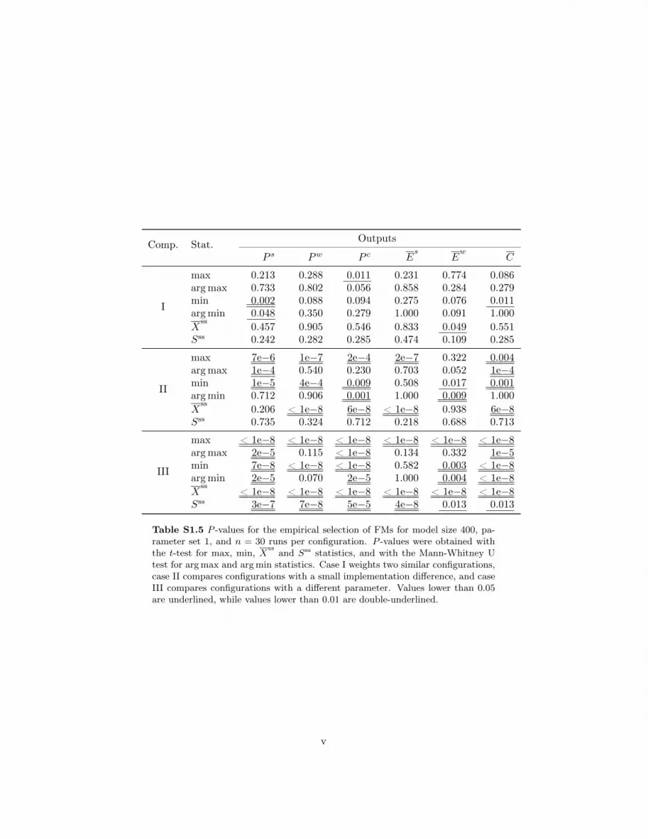
Comp. Stat. Outputs

P s Pw P c Es

Ew

C

I


ss0.457 0.905 0.546 0.833 0.049 0.551

Sss 0.242 0.282 0.285 0.474 0.109 0.285

II

max 7e−6 1e−7 2e−4 2e−7 0.322 0.004argmax 1e−4 0.540 0.230 0.703 0.052 1e−4min 1e−5 4e−4 0.009 0.508 0.017 0.001argmin 0.712 0.906 0.001 1.000 0.009 1.000X

ss0.206 < 1e−8 6e−8 < 1e−8 0.938 6e−8

Sss 0.735 0.324 0.712 0.218 0.688 0.713

III

max < 1e−8 < 1e−8 < 1e−8 < 1e−8 < 1e−8 < 1e−8argmax 2e−5 0.115 < 1e−8 0.134 0.332 1e−5min 7e−8 < 1e−8 < 1e−8 0.582 0.003 < 1e−8argmin 2e−5 0.070 2e−5 1.000 0.004 < 1e−8

Xss

< 1e−8 < 1e−8 < 1e−8 < 1e−8 < 1e−8 < 1e−8Sss 3e−7 7e−8 5e−5 4e−8 0.013 0.013


v

Comp. Stat. Outputs

P s Pw P c Es

Ew

C

I


ss0.528 0.469 0.379 0.326 0.786 0.362

Sss 0.631 0.634 0.685 0.669 0.657 0.684

II

max < 1e−8 < 1e−8 < 1e−8 0.169 < 1e−8 < 1e−8argmax < 1e−8 0.423 < 1e−8 0.649 0.161 0.207min 0.019 0.173 < 1e−8 < 1e−8 0.056 < 1e−8argmin 0.006 0.091 0.988 < 1e−8 0.055 < 1e−8

Xss

< 1e−8 < 1e−8 < 1e−8 < 1e−8 < 1e−8 < 1e−8Sss 0.135 0.289 0.871 0.245 0.258 0.870

III

max < 1e−8 < 1e−8 < 1e−8 < 1e−8 < 1e−8 < 1e−8argmax 0.035 0.315 2e−6 0.100 0.001 1e−7min 0.038 0.236 < 1e−8 0.997 0.488 < 1e−8argmin 0.022 0.442 0.020 0.001 0.190 1e−6

Xss

< 1e−8 < 1e−8 < 1e−8 2e−6 < 1e−8 < 1e−8Sss 0.164 0.110 0.043 0.027 0.135 0.006


vi

Comp. Stat. Outputs

P s Pw P c Es

Ew

C

I


ss0.782 0.075 0.820 0.041 0.080 0.818

Sss 0.111 0.116 0.161 0.131 0.434 0.159

II

max < 1e−8 < 1e−8 < 1e−8 < 1e−8 0.168 3e−8argmax < 1e−8 0.947 1.000 0.464 0.143 9e−5min 4e−6 6e−8 3e−8 0.045 0.348 < 1e−8argmin 0.094 0.001 2e−6 1.000 0.916 1.000X

ss0.005 < 1e−8 < 1e−8 < 1e−8 0.018 < 1e−8

Sss 0.580 0.398 0.553 0.431 0.593 0.552

III

max < 1e−8 < 1e−8 < 1e−8 < 1e−8 < 1e−8 < 1e−8argmax 1e−8 < 1e−8 < 1e−8 0.647 0.145 < 1e−8min < 1e−8 < 1e−8 < 1e−8 0.063 0.001 < 1e−8argmin 1e−4 6e−7 < 1e−8 1.000 0.456 < 1e−8

Xss

< 1e−8 < 1e−8 < 1e−8 < 1e−8 < 1e−8 < 1e−8Sss 1e−5 2e−6 0.001 4e−6 0.049 0.188


vii

Comp. Stat. Outputs

P s Pw P c Es

Ew

C

I

max 0.913 0.018 0.178 0.444 0.347 0.194argmax 1.000 0.203 0.774 1.000 0.068 0.510min 1.000 0.024 0.728 8e−6 0.053 0.182argmin 1.000 0.047 0.876 0.974 0.954 0.397X

ss0.638 0.515 0.028 0.136 0.261 0.029

Sss 0.718 0.609 0.639 0.696 0.646 0.642

II

max < 1e−8 < 1e−8 < 1e−8 0.379 < 1e−8 < 1e−8argmax < 1e−8 0.006 < 1e−8 0.002 0.065 0.249min 0.108 1e−5 < 1e−8 < 1e−8 0.001 < 1e−8argmin 0.042 0.007 0.006 < 1e−8 0.081 < 1e−8

Xss

< 1e−8 < 1e−8 < 1e−8 < 1e−8 < 1e−8 < 1e−8Sss 0.619 0.773 0.469 0.022 0.977 0.476

III

max < 1e−8 < 1e−8 < 1e−8 < 1e−8 < 1e−8 < 1e−8argmax 2e−5 0.012 < 1e−8 0.001 1.000 < 1e−8min 1.000 0.911 < 1e−8 0.178 0.104 < 1e−8argmin 1.000 0.239 0.605 2e−4 0.132 < 1e−8

Xss

< 1e−8 < 1e−8 < 1e−8 < 1e−8 < 1e−8 < 1e−8Sss 0.775 0.783 0.337 0.317 0.924 0.084


viii

Comp. Data Outputs

P s Pw P c Es

Ew

C A

I

#PCs 26 32 26 37 43 27 38MNV 0.852 0.509 0.851 0.966 0.285 0.879 0.486t-test 0.036 0.057 0.049 0.023 0.503 0.049 0.077

PCS

II

#PCs 25 32 25 34 43 26 38MNV 0.023 4e-05 0.276 <1e-08 0.448 0.256 0.496t-test 0.001 0.001 0.003 <1e-08 0.956 0.003 0.003

PCS

III

#PCs 22 26 21 32 42 15 35MNV <1e-08 <1e-08 <1e-08 <1e-08 0.001 <1e-08 6e-06t-test 6e-08 <1e-08 <1e-08 <1e-08 0.003 <1e-08 <1e-08

PCS

Table S2.1 Model-independent comparison for model size 100, parameter set 1,and n = 30 runs per configuration. Case I weights two similar setups, case IIcompares setups with a small implementation difference, and case III comparessetups with a different parameter. #PCs is the number of PCs which explain atleast 90% of variance, while MNV and t-test refer to the p-value yielded by theMANOVA (#PCs) and t (first PC) hypothesis tests, respectively. PCS showsthe representation of the respective output in the first two dimensions of thePC space. Output A refers to the concatenation of all outputs (range scaled).The MANOVA test is not applicable to one PC, and the respective p-values arereplaced with an asterisk (*). P -values lower than 0.05 are underlined, whilep-values lower than 0.01 are double-underlined.

ix

Comp. Data Outputs

P s Pw P c Es

Ew

C A

I

#PCs 20 19 15 29 31 15 22MNV 0.116 0.141 0.175 0.085 0.121 0.175 0.125t-test 0.108 0.128 0.106 0.111 0.067 0.106 0.099

PCS

II

#PCs 20 19 15 27 29 15 22MNV <1e-08 <1e-08 <1e-08 <1e-08 <1e-08 <1e-08 5e-06t-test <1e-08 1e-06 3e-08 <1e-08 <1e-08 3e-08 2e-07

PCS

III

#PCs 21 18 15 29 30 15 22MNV 0.006 0.001 0.110 0.139 2e-04 <1e-08 0.147t-test 0.037 0.472 0.322 0.324 0.054 0.116 0.346

PCS


x

Comp. Data Outputs

P s Pw P c Es

Ew

C A

I

#PCs 25 32 25 36 43 26 38MNV 0.287 0.214 0.157 0.123 0.699 0.187 0.356t-test 0.783 0.810 0.895 0.973 0.830 0.895 0.979

PCS

II

#PCs 24 31 25 27 43 25 38MNV 0.022 <1e-08 0.276 <1e-08 0.778 0.270 0.038t-test 0.616 0.056 0.481 <1e-08 0.773 0.480 0.534

PCS

III

#PCs 21 19 17 27 41 6 35MNV <1e-08 <1e-08 <1e-08 <1e-08 <1e-08 <1e-08 3e-08t-test <1e-08 <1e-08 <1e-08 <1e-08 <1e-08 <1e-08 <1e-08

PCS


xi

Comp. Data Outputs

P s Pw P c Es

Ew

C A

I

#PCs 21 19 15 29 31 15 21MNV 0.138 0.264 0.322 0.342 0.652 0.322 0.244t-test 0.192 0.294 0.280 0.985 0.378 0.280 0.240

PCS

II

#PCs 18 17 14 20 26 14 19MNV <1e-08 <1e-08 <1e-08 <1e-08 <1e-08 <1e-08 <1e-08t-test <1e-08 <1e-08 <1e-08 <1e-08 <1e-08 <1e-08 <1e-08

PCS

III

#PCs 19 18 15 28 30 14 20MNV <1e-08 <1e-08 <1e-08 0.001 <1e-08 <1e-08 0.001t-test <1e-08 3e-05 1e-07 8e-08 <1e-08 <1e-08 4e-06

PCS


xii

Comp. Data Outputs

P s Pw P c Es

Ew

C A

I

#PCs 24 32 25 36 43 26 39MNV 0.528 0.258 0.548 0.105 0.746 0.577 0.704t-test 0.530 0.836 0.804 0.784 0.378 0.805 0.879

PCS

II

#PCs 24 29 24 12 43 25 38MNV <1e-08 <1e-08 5e-08 <1e-08 0.467 1e-07 <1e-08t-test 0.042 <1e-08 0.108 <1e-08 0.017 0.109 0.390

PCS

III


PCS


xiii

Comp. Data Outputs

P s Pw P c Es

Ew

C A

I

#PCs 21 18 15 28 32 15 21MNV 0.740 0.936 0.849 0.776 0.854 0.850 0.990t-test 0.919 0.925 0.942 0.856 0.778 0.941 0.992

PCS

II


PCS

III


PCS


xiv

Comp. Data Outputs

P s Pw P c Es

Ew

C A

I

#PCs 25 32 25 36 43 26 39MNV 0.521 0.817 0.617 0.004 0.338 0.630 0.276t-test 0.316 0.341 0.307 0.502 0.577 0.307 0.262

PCS

II

#PCs 23 24 24 1 43 25 37MNV <1e-08 <1e-08 <1e-08 * 0.013 <1e-08 <1e-08t-test <1e-08 <1e-08 <1e-08 <1e-08 1e-05 <1e-08 <1e-08

PCS

III

#PCs 9 1 1 1 26 1 21MNV <1e-08 * * * <1e-08 * <1e-08t-test <1e-08 <1e-08 <1e-08 <1e-08 <1e-08 <1e-08 <1e-08

PCS


xv

Comp. Data Outputs

P s Pw P c Es

Ew

C A

I

#PCs 20 17 14 28 31 15 20MNV 0.242 0.274 0.252 0.005 0.379 0.285 0.322t-test 0.597 0.979 0.819 0.813 0.788 0.819 0.927

PCS

II

#PCs 3 4 3 1 3 3 4MNV <1e-08 <1e-08 <1e-08 * <1e-08 <1e-08 <1e-08t-test <1e-08 <1e-08 <1e-08 <1e-08 <1e-08 <1e-08 <1e-08

PCS

III


PCS


xvi

Comp. Data Outputs

P s Pw P c Es

Ew

C A

I




II


t-test (PC1) 0.001 0.001 0.003 <1e-08 0.956 0.003 0.003t-test (PC2) 0.766 0.886 0.884 0.829 0.096 0.885 0.942t-test (PC3) 0.441 0.874 0.355 0.728 0.967 0.357 0.536t-test (PC4) 0.515 0.250 0.287 0.887 0.160 0.285 0.220

t-test* (PC1) 0.007 0.005 0.018 <1e-08 1.000 0.019 0.033t-test* (PC2) 1.000 1.000 1.000 1.000 1.000 1.000 1.000t-test* (PC3) 1.000 1.000 1.000 1.000 1.000 1.000 1.000t-test* (PC4) 1.000 1.000 1.000 1.000 1.000 1.000 1.000

III


t-test (PC1) 6e-08 <1e-08 <1e-08 <1e-08 0.003 <1e-08 <1e-08t-test (PC2) 0.604 0.915 0.944 0.888 0.257 0.951 0.944t-test (PC3) 0.951 0.851 0.921 0.820 1e-06 0.972 0.983t-test (PC4) 0.510 0.842 0.802 0.893 0.312 0.892 0.704

t-test* (PC1) 4e-07 <1e-08 <1e-08 <1e-08 0.041 <1e-08 <1e-08t-test* (PC2) 1.000 1.000 1.000 1.000 1.000 1.000 1.000t-test* (PC3) 1.000 1.000 1.000 1.000 2e-05 1.000 1.000t-test* (PC4) 1.000 1.000 1.000 1.000 1.000 1.000 1.000

Table S3.1 Percentage of explained variance (% var.) and t-test p-values before(t-test) and after (t-test*) weighted Bonferroni correction of the first four PCs formodel size 100, parameter set 1, and n = 30 runs per configuration. Case I weightstwo similar setups, case II compares setups with a small implementation differ-ence, and case III compares setups with a different parameter. P -values lowerthan 0.05 are underlined, while p-values lower than 0.01 are double-underlined.

xvii

Comp. Data Outputs

P s Pw P c Es

Ew

C A

I




II


t-test (PC1) <1e-08 1e-06 3e-08 <1e-08 <1e-08 3e-08 2e-07t-test (PC2) 0.010 0.786 0.087 0.588 0.245 0.087 0.181t-test (PC3) 0.597 0.004 0.190 0.095 0.669 0.190 0.402t-test (PC4) 0.299 0.089 0.060 0.667 0.034 0.061 0.045

t-test* (PC1) 2e-08 5e-06 2e-07 <1e-08 <1e-08 2e-07 9e-07t-test* (PC2) 0.096 1.000 0.723 1.000 1.000 0.730 1.000t-test* (PC3) 1.000 0.034 1.000 1.000 1.000 1.000 1.000t-test* (PC4) 1.000 0.990 0.656 1.000 0.500 0.661 0.538

III





xviii

Comp. Data Outputs

P s Pw P c Es

Ew

C A

I




II


t-test (PC1) 0.616 0.056 0.481 <1e-08 0.773 0.480 0.534t-test (PC2) 0.440 0.077 0.489 0.463 0.915 0.490 0.433t-test (PC3) 0.476 0.075 0.448 0.994 0.617 0.448 0.488t-test (PC4) 0.036 2e-05 0.050 0.889 0.831 0.050 0.030

t-test* (PC1) 1.000 0.473 1.000 <1e-08 1.000 1.000 1.000t-test* (PC2) 1.000 0.820 1.000 1.000 1.000 1.000 1.000t-test* (PC3) 1.000 1.000 1.000 1.000 1.000 1.000 1.000t-test* (PC4) 0.576 4e-04 0.742 1.000 1.000 0.748 0.534

III


t-test (PC1) <1e-08 <1e-08 <1e-08 <1e-08 <1e-08 <1e-08 <1e-08t-test (PC2) 0.345 0.965 0.939 0.820 0.018 0.954 0.785t-test (PC3) 4e-05 0.800 0.574 0.559 0.008 0.819 0.245t-test (PC4) 0.291 0.544 0.317 0.545 0.418 0.731 0.764

t-test* (PC1) <1e-08 <1e-08 <1e-08 <1e-08 <1e-08 <1e-08 <1e-08t-test* (PC2) 1.000 1.000 1.000 1.000 0.309 1.000 1.000t-test* (PC3) 5e-04 1.000 1.000 1.000 0.154 1.000 1.000t-test* (PC4) 1.000 1.000 1.000 1.000 1.000 1.000 1.000


xix

Comp. Data Outputs

P s Pw P c Es

Ew

C A

I




II




III


t-test (PC1) <1e-08 3e-05 1e-07 8e-08 <1e-08 <1e-08 4e-06t-test (PC2) 0.171 0.003 0.060 0.039 0.416 0.502 0.044t-test (PC3) 0.609 0.092 0.111 0.950 0.066 0.027 0.141t-test (PC4) 0.611 0.229 0.742 0.087 0.448 0.381 0.651

t-test* (PC1) <1e-08 2e-04 6e-07 5e-07 <1e-08 <1e-08 2e-05t-test* (PC2) 1.000 0.019 0.323 0.304 1.000 1.000 0.261t-test* (PC3) 1.000 0.929 1.000 1.000 0.919 0.286 1.000t-test* (PC4) 1.000 1.000 1.000 1.000 1.000 1.000 1.000


xx

Comp. Data Outputs

P s Pw P c Es

Ew

C A

I




II


t-test (PC1) 0.042 <1e-08 0.108 <1e-08 0.017 0.109 0.390t-test (PC2) 0.128 0.029 0.106 0.720 0.175 0.107 0.086t-test (PC3) 0.004 0.110 0.006 0.885 0.909 0.006 0.002t-test (PC4) 0.767 0.401 0.966 0.978 0.060 0.954 0.631

t-test* (PC1) 0.209 <1e-08 0.661 <1e-08 0.211 0.669 1.000t-test* (PC2) 1.000 0.276 0.955 1.000 1.000 0.971 0.975t-test* (PC3) 0.055 1.000 0.079 1.000 1.000 0.077 0.028t-test* (PC4) 1.000 1.000 1.000 1.000 1.000 1.000 1.000

III





xxi

Comp. Data Outputs

P s Pw P c Es

Ew

C A

I




II




III





xxii

Comp. Data Outputs

P s Pw P c Es

Ew

C A

I




II


t-test (PC1) <1e-08 <1e-08 <1e-08 <1e-08 1e-05 <1e-08 <1e-08t-test (PC2) 0.005 0.609 0.015 0.906 0.066 0.015 0.060t-test (PC3) 0.819 0.792 0.956 0.948 0.395 0.952 0.759t-test (PC4) 0.775 0.913 0.826 0.959 0.485 0.827 0.875

t-test* (PC1) <1e-08 <1e-08 <1e-08 <1e-08 1e-04 <1e-08 <1e-08t-test* (PC2) 0.055 1.000 0.162 1.000 1.000 0.163 0.767t-test* (PC3) 1.000 1.000 1.000 1.000 1.000 1.000 1.000t-test* (PC4) 1.000 1.000 1.000 1.000 1.000 1.000 1.000

III





xxiii

Comp. Data Outputs

P s Pw P c Es

Ew

C A

I




II




III





xxiv

Comp. Data Outputs

P s Pw P c Es

Ew

C A

I



II


MNV (30% var.) 0.011 0.010 0.019 <1e-08 0.273 0.019 0.032MNV (50% var.) 0.041 0.060 0.044 <1e-08 0.176 0.044 0.169MNV (70% var.) 0.070 0.013 0.152 <1e-08 0.405 0.150 0.262MNV (90% var.) 0.023 4e-05 0.276 <1e-08 0.448 0.256 0.496

III


MNV (30% var.) 2e-06 <1e-08 <1e-08 <1e-08 2e-08 * 3e-08MNV (50% var.) 9e-06 <1e-08 <1e-08 <1e-08 <1e-08 * 1e-06MNV (70% var.) <1e-08 <1e-08 <1e-08 <1e-08 1e-08 <1e-08 5e-05MNV (90% var.) <1e-08 <1e-08 <1e-08 <1e-08 0.001 <1e-08 6e-06

Table S4.1 Number of principal components (#PCs) and MANOVA test p-values(MNV) for several percentages of explained variance for model size 100, parameterset 1, and n = 30 runs per configuration. Case I weights two similar setups, caseII compares setups with a small implementation difference, and case III comparessetups with a different parameter. Output A refers to the concatenation of alloutputs (range scaled). The MANOVA test is not applicable to one PC, and therespective p-values are replace with an asterisk (*). P -values lower than 0.05 areunderlined, while p-values lower than 0.01 are double-underlined.

xxv

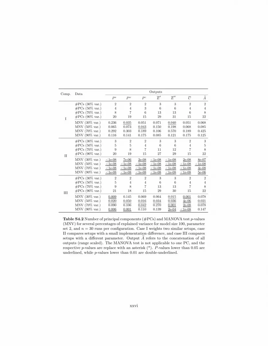
Comp. Data Outputs

P s Pw P c Es

Ew

C A

I



II


MNV (30% var.) <1e-08 7e-06 2e-08 <1e-08 <1e-08 2e-08 8e-07MNV (50% var.) <1e-08 <1e-08 <1e-08 <1e-08 <1e-08 <1e-08 <1e-08MNV (70% var.) <1e-08 <1e-08 <1e-08 <1e-08 <1e-08 <1e-08 4e-08MNV (90% var.) <1e-08 <1e-08 <1e-08 <1e-08 <1e-08 <1e-08 5e-06

III


MNV (30% var.) 0.009 0.145 0.069 0.064 0.015 0.001 0.078MNV (50% var.) 0.020 0.050 0.016 0.034 0.036 4e-06 0.021MNV (70% var.) 0.090 0.106 0.042 0.270 0.001 2e-08 0.078MNV (90% var.) 0.006 0.001 0.110 0.139 2e-04 <1e-08 0.147


xxvi

Comp. Data Outputs

P s Pw P c Es

Ew

C A

I



II


MNV (30% var.) 0.719 2e-06 0.674 * 0.847 0.674 0.186MNV (50% var.) 0.400 <1e-08 0.471 <1e-08 0.780 0.471 0.547MNV (70% var.) 0.618 <1e-08 0.800 <1e-08 0.305 0.799 0.457MNV (90% var.) 0.022 <1e-08 0.276 <1e-08 0.778 0.270 0.038

III


MNV (30% var.) <1e-08 * * * <1e-08 * <1e-08MNV (50% var.) <1e-08 <1e-08 <1e-08 <1e-08 <1e-08 * 6e-08MNV (70% var.) <1e-08 <1e-08 <1e-08 <1e-08 <1e-08 * <1e-08MNV (90% var.) <1e-08 <1e-08 <1e-08 <1e-08 <1e-08 <1e-08 3e-08


xxvii

Comp. Data Outputs

P s Pw P c Es

Ew

C A

I



II


MNV (30% var.) * * * * * * <1e-08MNV (50% var.) <1e-08 <1e-08 <1e-08 <1e-08 <1e-08 <1e-08 <1e-08MNV (70% var.) <1e-08 <1e-08 <1e-08 <1e-08 <1e-08 <1e-08 <1e-08MNV (90% var.) <1e-08 <1e-08 <1e-08 <1e-08 <1e-08 <1e-08 <1e-08

III


MNV (30% var.) <1e-08 6e-07 6e-08 1e-07 <1e-08 <1e-08 1e-06MNV (50% var.) 5e-08 4e-07 3e-08 1e-07 <1e-08 <1e-08 4e-06MNV (70% var.) 1e-06 <1e-08 5e-07 3e-05 <1e-08 <1e-08 9e-07MNV (90% var.) <1e-08 <1e-08 <1e-08 0.001 <1e-08 <1e-08 0.001


xxviii

Comp. Data Outputs

P s Pw P c Es

Ew

C A

I



II


MNV (30% var.) 0.038 <1e-08 0.004 * 0.035 0.004 0.007MNV (50% var.) 2e-06 <1e-08 3e-04 * 0.034 3e-04 3e-04MNV (70% var.) 4e-05 <1e-08 0.002 * 0.049 0.001 2e-06MNV (90% var.) <1e-08 <1e-08 5e-08 <1e-08 0.467 1e-07 <1e-08

III


MNV (30% var.) * * * * * * <1e-08MNV (50% var.) <1e-08 * * * <1e-08 * <1e-08MNV (70% var.) <1e-08 * * * <1e-08 * <1e-08MNV (90% var.) <1e-08 <1e-08 <1e-08 <1e-08 <1e-08 * <1e-08


xxix

Comp. Data Outputs

P s Pw P c Es

Ew

C A

I



II


MNV (30% var.) * * * * * * *MNV (50% var.) * * * * * * *MNV (70% var.) <1e-08 <1e-08 <1e-08 * <1e-08 <1e-08 <1e-08MNV (90% var.) <1e-08 <1e-08 <1e-08 <1e-08 <1e-08 <1e-08 <1e-08

III


MNV (30% var.) * * * * * * *MNV (50% var.) <1e-08 <1e-08 * <1e-08 <1e-08 * <1e-08MNV (70% var.) <1e-08 <1e-08 <1e-08 <1e-08 <1e-08 <1e-08 <1e-08MNV (90% var.) <1e-08 <1e-08 <1e-08 <1e-08 <1e-08 <1e-08 <1e-08


xxx

Comp. Data Outputs

P s Pw P c Es

Ew

C A

I



II


MNV (30% var.) <1e-08 * <1e-08 * 1e-06 <1e-08 <1e-08MNV (50% var.) <1e-08 <1e-08 <1e-08 * 2e-04 <1e-08 <1e-08MNV (70% var.) <1e-08 <1e-08 <1e-08 * 0.001 <1e-08 <1e-08MNV (90% var.) <1e-08 <1e-08 <1e-08 * 0.013 <1e-08 <1e-08

III


MNV (30% var.) * * * * * * *MNV (50% var.) * * * * * * *MNV (70% var.) * * * * <1e-08 * <1e-08MNV (90% var.) <1e-08 * * * <1e-08 * <1e-08


xxxi

Comp. Data Outputs

P s Pw P c Es

Ew

C A

I



II


MNV (30% var.) * * * * * * *MNV (50% var.) * * * * * * *MNV (70% var.) * * * * * * *MNV (90% var.) <1e-08 <1e-08 <1e-08 * <1e-08 <1e-08 <1e-08

III


MNV (30% var.) * * * * * * *MNV (50% var.) * * * * * * *MNV (70% var.) * * * <1e-08 * * *MNV (90% var.) <1e-08 <1e-08 <1e-08 <1e-08 <1e-08 <1e-08 <1e-08


xxxii

Comp. Stat. Outputs

P s Pw P c Es

Ew

C

I


ss0.995 0.415 0.967 0.679 0.017 0.962

Sss 0.402 0.326 0.415 0.593 0.343 0.415

II

max 0.014 3e−4 0.024 0.023 0.494 0.171argmax 0.019 0.307 0.077 0.206 0.140 0.025min 0.063 0.173 0.209 0.237 0.017 0.037argmin 0.720 0.184 0.017 1.000 0.294 1.000X

ss0.244 < 1e−8 0.012 < 1e−8 0.456 0.013

Sss 0.751 0.685 0.826 0.196 0.404 0.826

III

max < 1e−8 < 1e−8 < 1e−8 1e−7 4e−4 < 1e−8argmax 0.066 0.345 0.001 0.009 0.044 0.015min 0.004 8e−5 5e−5 0.949 0.010 < 1e−8argmin 0.047 0.402 0.015 1.000 0.044 2e−5

Xss

8e−8 < 1e−8 < 1e−8 < 1e−8 < 1e−8 < 1e−8Sss 0.010 0.014 0.074 0.001 0.388 0.457

Table S5.1 P -values for the empirical selection of FMs for model size 400, pa-rameter set 1, n = 10 runs per configuration. P -values were obtained with thet-test for max, min, Xss and Sss statistics, and with the Mann-Whitney U testfor the argmax and argmin statistics. Case I weights two similar configurations,case II compares configurations with a small implementation difference, and caseIII compares configurations with a different parameter. Values lower than 0.05are underlined, while values lower than 0.01 are double-underlined.

xxxiii

Comp. Data Outputs

P s Pw P c Es

Ew

C A

I

#PCs 12 14 13 15 16 13 15MNV 0.591 0.120 0.503 0.858 0.927 0.505 0.790t-test 0.662 0.575 0.539 0.492 0.364 0.539 0.504

PCS

II

#PCs 12 13 12 7 16 12 14MNV 0.046 2e-05 0.118 <1e-08 0.410 0.118 0.056t-test 0.365 8e-07 0.723 <1e-08 0.039 0.725 0.902

PCS

III

#PCs 10 5 6 7 14 1 13MNV <1e-08 <1e-08 <1e-08 <1e-08 0.001 * 5e-04t-test <1e-08 <1e-08 <1e-08 <1e-08 <1e-08 <1e-08 1e-08

PCS

Table S5.2 Results for the model-independent comparison for model size 400,parameter set 1, and n = 10 runs per configuration. Case I weights two similarsetups, case II compares setups with a small implementation difference, and caseIII compares setups with a different parameter. #PCs is the number of PCswhich explain at least 90% of variance, while MNV and t-test refer to the p-valueyielded by the MANOVA (#PCs) and t (first PC) statistical tests, respectively.PCS shows the representation of the respective output in the first two dimensionsof the PC space. Output A refers to the concatenation of all outputs (rangescaled). Values lower than 0.05 are underlined, while values lower than 0.01 aredouble-underlined. The MANOVA test is not applicable to one PC, and therespective p-values are replace with an asterisk (*).

xxxiv

Comp. Stat. Outputs

P s Pw P c Es

Ew

C

I


ss0.547 0.052 0.491 0.080 0.209 0.481

Sss 0.259 0.100 0.228 0.973 0.467 0.228

II

max < 1e−8 < 1e−8 < 1e−8 < 1e−8 0.042 3e−7argmax < 1e−8 0.143 0.078 3e−4 0.155 < 1e−8min < 1e−8 < 1e−8 9e−7 0.225 0.056 < 1e−8argmin 0.324 0.225 < 1e−8 1.000 0.136 0.158X

ss3e−5 < 1e−8 < 1e−8 < 1e−8 0.034 < 1e−8

Sss 0.082 0.097 0.136 2e−4 0.862 0.138

III

max < 1e−8 < 1e−8 < 1e−8 < 1e−8 < 1e−8 < 1e−8argmax < 1e−8 5e−5 < 1e−8 0.015 0.024 < 1e−8min < 1e−8 < 1e−8 < 1e−8 0.248 0.001 < 1e−8argmin < 1e−8 4e−7 < 1e−8 1.000 8e−5 < 1e−8

Xss

< 1e−8 < 1e−8 < 1e−8 < 1e−8 < 1e−8 < 1e−8Sss < 1e−8 < 1e−8 < 1e−8 < 1e−8 < 1e−8 2e−5

Table S6.1 P -values for the empirical selection of FMs for model size 400, pa-rameter set 1, and n = 100 runs per configuration. P -values were obtained withthe t-test for max, min, Xss and Sss statistics, and with the Mann-Whitney U testfor the argmax and argmin statistics. Case I weights two similar configurations,case II compares configurations with a small implementation difference, and caseIII compares configurations with a different parameter. Values lower than 0.05are underlined, while values lower than 0.01 are double-underlined.

xxxv

Comp. Data Outputs

P s Pw P c Es

Ew

C A

I

#PCs 35 56 36 72 108 38 93MNV 0.750 0.164 0.756 1e-05 0.521 0.657 3e-05t-test 0.522 0.528 0.479 0.164 0.909 0.479 0.352

PCS

II

#PCs 35 49 36 19 107 37 91MNV <1e-08 <1e-08 <1e-08 <1e-08 3e-06 <1e-08 <1e-08t-test <1e-08 <1e-08 <1e-08 <1e-08 1e-06 <1e-08 2e-08

PCS

III


PCS

Table S6.2 Results for the model-independent comparison for model size 400,parameter set 1, and n = 100 runs per configuration. Case I weights two similarsetups, case II compares setups with a small implementation difference, and caseIII compares setups with a different parameter. #PCs is the number of PCswhich explain at least 90% of variance, while MNV and t-test refer to the p-valueyielded by the MANOVA (#PCs) and t (first PC) statistical tests, respectively.PCS shows the representation of the respective output in the first two dimensionsof the PC space. Output A refers to the concatenation of all outputs (rangescaled). The MANOVA test is not applicable to one PC, and the respective p-values are replace with an asterisk (*). P -values lower than 0.05 are underlined,while p-values lower than 0.01 are double-underlined.

xxxvi

Model-independent comparison of simulation output

Documents

Transcript of Model-independent comparison of simulation output