Model-based reasoning about learner behaviour

Artificial Intelligence 117 (2000) 173–229

Model-based reasoning about learner behaviour

Kees de Koning, Bert Bredeweg∗, Joost Breuker, Bob WielingaDepartment of Social Science Informatics (SWI), University of Amsterdam,

Roetersstraat 15, 1018 WB Amsterdam, Netherlands

Received 23 August 1999

Abstract

Automated handling of tutoring and training functions in educational systems requires theavailability of articulate domain models. In this article we further develop the application ofqualitative models for this purpose. A framework is presented that defines a key role for qualitativemodels as interactive simulations of the subject matter. Within this framework our research focuseson automating the diagnosis of learner behaviour. We show how a qualitative simulation model ofthe subject matter can be reformulated to fit the requirements of general diagnostic engines such asGDE. It turns out that, due to the specific characteristics of such models, additional structuring isrequired to produce useful diagnostic results. A set of procedures is presented that automaticallymaps detailed simulation models into a hierarchy of aggregated models by hiding non-essentialdetails and chunking chains of causal dependencies. The result is a highly structured subject mattermodel that enables the diagnosis of learner behaviour by means of an adapted version of the GDEalgorithm. An experiment has been conducted that shows the viability of the approach taken, i.e.,given the output of a qualitative simulator the procedures we have developed automatically generatea structured subject matter model and subsequently use this model to successfully diagnoses learnerbehaviour. 2000 Elsevier Science B.V. All rights reserved.

Keywords:Qualitative reasoning; Model aggregation; Model-based diagnosis; Student modelling; Interactivelearning environments

1. Introduction

Both in professional and every-day life people have to interact with and reason abouta large number of systems. Computer simulations can be used to construct interactiveenvironments by means of which people can develop knowledge about the behaviour ofthese systems. The steady increase in computing power has in fact given simulation a

∗ Corresponding author. Email: [email protected].

0004-3702/00/$ – see front matter 2000 Elsevier Science B.V. All rights reserved.PII: S0004-3702(99)00106-X

174 K. de Koning et al. / Artificial Intelligence 117 (2000) 173–229

solid position within the area of educational systems [26]. However, several studies haveshown that simulations are only effective when proper guidance is provided [36,51,67,69]. Automating certain tutoring and training functions in order to provide such guidancerequires the simulation model to bearticulate[12,39,41]. Two further requirements followfrom this. Firstly, a specific simulation model should manifest all the behavioural featuresof the ‘real’ system as far as those are relevant to the educational goals. Secondly,a simulation model should contain the appropriatehandles, by means of which thesefeatures are indexed, to enable a knowledgeable communication with the learner about themodel contents. Qualitative simulators, such asQPE [39] andGARP [8], provide a basisfor generating articulate simulation models. Given such models, a remaining challengeconcerns the automated handling of guidance by the educational system.

Providing guidance means that the learning environment should be able to adapt theinteraction to the situation at hand, both with respect to the specific subject matter thatis considered and to the individual learner it is interacting with. Guidance may take onmany forms, such as providing explanations, presenting counter examples, suggestingassignments, and the like. Whatever the specific form, individual guidance requiresknowledge about the learner and hence involves assessment of his or her knowledge.More specifically, the educational system has to diagnose the learner’sproblem solvingbehaviour. 1 The subject matter we are dealing with in this article concerns ‘behaviouranalysis’, i.e., learners should acquire problem solving skills such as predicting or‘postdicting’ (explaining) the behaviour of systems using qualitative terms. Hence, thelearner’s problem solving behaviour consists of a set of inferences about the behaviourof these systems. The way the student interacts with the learning environment reflectsthis problem solving behaviour. The educational system therefore has to monitor thisinteraction (performance assessment) and diagnose deviations, with respect to some norm,in terms of problem solving errors made by the learner (behaviour diagnosis).

In research on artificial intelligence in education, diagnosis of problem solvingbehaviour is generally considered extremely difficult, or even infeasible [75]. Oneimportant reason is that behaviour diagnosis is usually based on hand-crafted cataloguesof misconceptions, or bugs, which makes diagnostic systems very expensive to develop.Moreover, a catalogue of bugs is only applicable to one specific domain. When thesubject matter changes, a new catalogue has to be developed and implemented. Alternativeapproaches that try to overcome these difficulties, e.g., by generating bugs dynamically[18], have also proven to be difficult. Although no hand-crafted catalogues are needed,domain specific filters have to be used to avoid generation of implausible bugs. In addition,the construction of generative theories has turned out to be problematic, mainly as a resultof lacking operational theories on how people acquire knowledge.

In this article we propose a different,model-based, approach [47] to diagnose learnerbehaviour. Following [62], this choice is based on the fact that model-based diagnosis is anextensively studied and well-understood field of research, and hence we can reuse existingtechniques and representations. Model-based diagnosis claims to be generic and domain

1 Throughout this article, the term ‘learner behaviour’ refers to the ‘problem solving behaviour of a learner’.‘Learner behaviour’ should not be confused with ‘system behaviour’ which refers to the subject matter that thestudent has to master.

K. de Koning et al. / Artificial Intelligence 117 (2000) 173–229 175

Fig. 1. Model-based diagnosis of device versus learner behaviour.

independent. It does not require explicit fault models or bug catalogues for its operation,but instead reasons from a representation of the correct behaviour of the system to bediagnosed. More specific, in model-based diagnosis the behaviour of a device is comparedto the behaviour predicted by a model of that device. In the case of diagnosing learnerbehaviour we propose to automatically generate this model using a qualitative simulator.On the basis of the output of the simulator a subject matter model can be constructed thatacts as a normative model of the learner behaviour and as such can be used for modelbased diagnosis. Deviations in the problem solving behaviour of the learner, i.e., incorrectpredictions or postdictions concerning the behaviour of the system that is the subject of theteaching activity, are then diagnosed as inferences made by the qualitative simulator thatthe learner cannot have applied correctly given the observations. Fig. 1 illustrates the high-level mapping between model-based diagnosis of device behaviour and learner behaviour.

The same diagnostic component (e.g., GDE [30]) can be applied to different (subjectmatter) models, as long as they comply with the modelling principles required by thediagnostic algorithms. One of the main requirements is that the system under diagnosiscan be modelled as a set ofconnected components, for which the behaviour can bedefined individually. These components should model the smallest entities that can beindividually repaired; diagnosis is only useful down to the level of possible repairs. In thecontext of learning, this means that these components should represent the smallest unitsof problem solving knowledge that are still relevant in an educational setting (e.g., thatcan be individually explained). The constraints that the component-connection paradigmputs on the subject matter models are not only a requirement for diagnosis, but are alsouseful for other educational functions: a clear separation of the knowledge in terms ofindexed elements that make sense in education is a prerequisite for automated structured


explanation, generation of questions, or subject matter sequencing. Only with such amodular structure, different components can be freely combined, selected, and sequenced.

Following the above argumentation, we propose a framework for the constructionof interactive learning environments based on qualitative models. These models areused as simulations of the subject matter and provide the basis for the construction ofadvanced educational functions to support the interaction with the learner. The proceduresimplementing this approach should be domain independent, i.e., they should not depend onthe specific system that is being simulated by the qualitative simulator, and they should dotheir work fully automatic. In the research presented we focus on the function ‘diagnosisof learner behaviour’ because it is central to any form of individualised interaction.

The following topics must be addressed. First, it should be shown that the qualitativesimulator represents knowledge that fits the way teachers and learners communicate aboutsystem behaviour. The qualitative simulator should produce a description of the systembehaviour that is useful in an educational setting, i.e., it should bedidactically plausible. Itshould produce a description that learners can comprehend and in principle learn. Althoughimportant, the construction of such articulate models is not the main focus of the researchpresented here. Section 2.3 reports on previously published research [33] that supports thehypothesis that the simulator we use produces such models.

The second topic concerns the mapping of the simulation model onto the component-connection paradigm (Section 3). Recall that the simulation model reflects all the necessaryinference steps that must be made in order to produce a correct behaviour analysis.Thus, the simulation model provides the ingredients for the norm model of the model-based diagnostic engine and hence all the inferences must be represented as ‘inferencecomponents’ in this norm model. Typically, each inference should be represented as anindividual, context independent inference component that derives output from input usinga behaviour rule. In addition, behaviour rules should be defined for deriving input fromoutput. Being able to construct a component-connectionmodel out of the simulation modelmeans that we can represent the skill ‘qualitative behaviour analysis’ as the norm modelto be used by the diagnostic engine. Hence, we are able to diagnose learner behaviour interms of how it deviates from this model.

The third topic concerns the tractability of the general diagnostic engine (Section 4). Itturns out that due to the specific characteristics of qualitative simulation models, additionalstructuring is required in order to deliver useful diagnostic results. One reason is that thecomponent’s behaviour rules make use of qualitative calculi, which are relatively weakcompared to the behaviour rules used in typical applications of model-based diagnosis suchas electronic circuits. In artifacts, solving the tractability problem can be done by using thehierarchical structure that is often evident from the physical or functional structure of thedevice. Such a natural decomposition is not available for the kind of norm models that weuse. The inference components that are part of this model do not necessarily map ontocomponents in the ‘real’ system. Alternative structuring principles have to be developedfor these models. As mentioned before, an additional requirement is that the structuringmust be performed automatically on the basis of the component-connection model that hasbeen generated using the output of the simulator.

A fourth and related topic concerns the fact that the diagnostic engine has to operate inthe context of an educational system. Measurement selection, and candidate discrimination


in general, are bound to the ongoing discourse between the education system and thelearner. Putting the diagnostic engine to work in the context of an educational system issubject of Section 5. In the next section (Section 2) we will first discuss the theoreticalbackground of our approach.

2. Theoretical background

Important to the research presented in this article is the idea of using a qualitativesimulation model as the kernel of an educational system. Section 2.1 describes the maincharacteristics of the simulator that we use for this purpose. How the qualitative simulatorcan be embedded in an interactive learning environment is subject of Section 2.2, whichpresents an architecture for simulation-based educational systems. Putting the qualitativesimulation in the heart of the educational system puts specific requirements on thesimulator. Section 2.3 discusses research that supports the hypothesis that the simulatorwe use produces didactically plausible models. Finally, Section 2.4 discusses the role ofdiagnosis in educational systems. We emphasise the importance of ‘behaviour diagnosis’,in contrast to ‘learner modelling’, and the usefulness of model-based techniques forperforming the former diagnostic task.

2.1. Generating articulate simulation models

Qualitative simulation models typically represent knowledge about the structure andthe qualitative distinct behavioural features of a system. To produce such models we useGARP [8], an interactive simulator that predicts behaviour starting from a user selectedscenario. The scenario captures the initial structural description of a system, possiblyaugmented with some initial behavioural facts.GARP can be controlled to produce afull simulation at once, or to work on specific states of behaviour in interaction with theuser. Model fragment libraries [37] are used to feed the simulator with domain specificknowledge. The simulator itself implements a domain independent qualitative reasoningshell.2

The primitives that can be used within the model fragments for representing thebehaviour of a system include: quantities, values, behavioural constraints, and causaldependencies. Quantities represent the changing properties of the system. Values arerepresented in quantity spaces (Qsp), i.e., ordered sets of alternating points and intervals.Values are assigned to quantities using a dedicated predicate. Values from different quantityspaces are considered unrelated except when these quantity spaces include the value‘zero’, which is universal to all quantity spaces. In such cases, simple transitive inequalityreasoning is in principle possible, e.g.,value(Q1,V1), value(Q2,V2), Qsp1 : V1 < 0,Qsp2 : V2 > 0→ Q1 < Q2. Behavioural constraints are implemented by inequalitystatements and serve a number of purposes. They can be used to specify a range ofvalues that a quantity may have (e.g.,temperature1> freezingpoint1), they can be usedfor specifying dependencies between quantities (e.g.,temperature1> temperature2), and

2 GARP is freeware and implemented inSWI-Prolog [77].


they can be use to relate the values of different quantity spaces (e.g.,freezingpoint1>freezingpoint2).

In a specific state a quantity has a value, or its value is unknown. In addition,behavioural constraints may hold. If a quantity does not have a value and is not involvedin any constraints it obviously has no effect on the simulation and can be consideredsuperfluous in that state of behaviour. When the value refers to an interval, notice thesubtle difference between ‘having the same value’ and ‘being equal’. Quantities mayhave the same qualitative interval value and at the same time be unequal. For example,two similar containers filled with different amounts of liquid, may be represented asvalue(Level1, plus) andvalue(Level2, plus) andLevel1> Level2.

Knowledge about causality is represented using an adapted version ofQPT [38].Changes are ‘caused by’ influences as defined byprocessesand agents. The formerrepresent flows that occur because entities differ on some quantity, for example, a flow ofenergy between two objects because they differ in temperature. Agents represent externalfactors, e.g., someone controlling a device. Changes are propagated to other quantities byproportionalities. Correspondences can be used to relate certain quantity values. However,the notion of correspondence inGARP is different from the one used inQPT. First,correspondences are defined to be directed or undirected, referring to a causal dependencyor to a non-causal one. Second, correspondences are defined for either specific values oftwo quantities (value correspondence), or for all the values that two quantities can have(quantity space correspondence). In the case of the latter, such quantities have the sametype of quantity space.

Qualitatively distinct states of behaviour are characterised by differences in the set ofquantity values and/or inequality statements that hold in each state.Termination rulesimplement knowledge about state changes. Two sets of termination rules exist. One setdeals with individual quantities. These rules specify the value that a quantity will have inthe next state, given the value it has in the current state and the sign of its derivative (i.e.,its direction of change). The limit rule [28] is an example of such a rule. The second set ofrules deals with inequalities between quantities. They specify how inequality statements inthe current state will change, given the signs of the derivatives of the involved quantities.For example, two quantities may become unequal because one of them increases whereasthe other remains constant. Not all potential changes will lead to actual state changes. Somewill have to be ignored because other changes precede them. In addition, changes may bemerged because they are related. Knowledge on these issues is implemented byprecedencerules. The simulator uses these rules to merge related changes first. It then removes thosesets of changes that are preceded by other sets. The remaining sets of changes are (bydefinition) fully independent. State changes are therefore generated for each individualset and for all possible combinations of these sets. Some quantities have derivatives withsign ‘zero’ and may therefore not be involved in any change.Continuity rulesare used toexplicitly specify non-changing quantities between states.

2.2. Architecture for learning environments

Fig. 2 illustrates how a qualitative simulator can be embedded in an interactive learningenvironment. The figure presents an abstract view on the interaction between the learner


Fig. 2. Conceptual architecture for an educational system.

and the simulation, showing the most important tutoring and training functions (functionalunits). Exactly how a learning environment presents itself to a learner depends onthe realisation of these functional units (see [13] and [80] for general discussions onarchitectures for educational systems). Below we discuss the specific implementation ofthe architecture as used for the construction ofSTARlight; the prototype educational systemthat we have developed for evaluation purposes (Section 6).

In Fig. 2 the ‘generic qualitative knowledge’ refers to the library of model fragments, thedifferent sets of rules for determining state changes, and the scenario’s that can be used togenerate new prediction exercises. The output of the qualitative simulator forms the basisfor the subject matter model. By manipulating the interface objects the learner can controlthe simulator, give answers to questions or ask for help. Two main control flow loops exist:as long as the learner’s behaviour is consistent with the subject matter model, the mainloop is learner interface → performance assessment → subject matter sequencing →question/assignment generation. When all the topics related to a specific predictionexercise have been dealt with sufficiently, thesubject matter sequencing can switch toa new prediction exercise (after which the previous loop continues). When a discrepancyis detected between the learner’s behaviour and the subject matter model, the diagnoseris activated, and the main loop becomeslearner interface→ performance assessment→behaviour diagnosis→ question/assignment generation. This loop continues until thediagnosis is satisfactory (e.g., a single deviating inference step is found); if this is thecase, the diagnostic process ends, and an explanation is generated on the basis of the


diagnosis. The learner model may provide additional means for keeping track of learnerspecific information to further refine the activities performed by the functional units.

As shown in Fig. 2, a central role is assigned to the output that is generated by thesimulator. This subject matter model is input to all the functional units in the educationalsystem, as shown by the grey arrows. An important requirement for our research approachis to ensure that the different training and tutoring functions in the educational systemoperate domain independently; they must work independent of the specific system that isbeing simulated by the qualitative simulator. This means that the output of the simulator,i.e., the subject matter model, must consist of two intertwined but still well distinguishableparts. The first part consists of all the facts that together represent the behaviour ofthe system that is being simulated, i.e., the simulation model itself (e.g.,volume > 0& increasing, etc.). The second part implements a kind of meta-level view [70] on thecontents of this model. It consists of the qualitative vocabulary, as discussed in Section 2.1,by means of which the domain specific facts are indexed (e.g., ‘volume’ is a quantity, ‘>’is an in-equality statement, ‘0’ is a value fromQsp1, etc., see [7,8] for details). In thisway, the functional units can assess the subject matter model using domain independentterms. In fact, each functional unit should only assess the subject matter model using thesedomain independent terms. In addition, all the reasoning within these units should eitherbe in terms of this vocabulary or fully independent from the simulation model all together(e.g., knowledge on discourse management [80]). Following this approach, we accomplishthat the learning environment as a whole is domain independent to the extent that thesimulator is domain independent. This is an important advancement.

2.3. Articulate models

When using simulation models in an educational system, these models should bedidactically plausible. Two requirements follow from this. The model should manifest allthe behavioural features of the real system as far as those are relevant to the educationalgoals and the model should be suitable for communication. The latter means that themodel should providehandles(indexes) for interaction, which are needed to extract theright knowledge from the model [12,39–41]. Although qualitative reasoning has historicallinks to educational systems, it is not self-evident that qualitative simulation models indeedcontain the right knowledge, in the right format, to support an educational interaction [10].We therefore investigated whether the knowledge, terminology and reasoning, used ina real educational interaction could be covered by models generated by qualitativesimulators, such asGARP andQPE. To this end, we conducted aWizard of Ozexperiment,in which a learner and a teacher communicate about a problem solving task via computerterminals [33]. Eight learners participated in the experiment, and three teachers. Thelearners were first year psychology students who had passed their final in physics at highschool. The problem solving task was predicting the behaviour of abalance system, asis shown in Fig. 3. This physical system is also used as a running example throughoutthe article. On each side of the balance sits a container partially filled with water. Thecontainers are equal in weight when empty, and have an equally sized outlet in the bottom.Through this outlet, the water flows out of the container, thereby decreasing the weighton that side of the balance. The flow rate of the two contained liquids can be different,


Fig. 3. The balance system.

corresponding to the pressure at the bottom. As a consequence, the balance moves to newpositions, but the final state is always an equilibrium. In the experiment, a teacher and alearner discuss the behaviour of the balance system once the outlets are opened.

The analysis of the dialogue protocols showed that the terminology as it is used in theinteraction is sufficiently covered by the simulation models: all concepts that appear inthe protocols can be mapped to counterparts in a simulation model. This is similar to theresults reported in [11]. However, the reasoning patterns employed by human reasonersdiffer substantially from the simulator’s. One reason is that qualitative simulators usuallygenerate all derivations in a breadth-first way; people, on the other hand, use heuristic,focused search based on “best-first” strategies [32]. A second difference is in thegrainsizeof the reasoning steps taken: the inferences made by the simulators do not alwaysmap directly to the reasoning steps made by learners. For instance, a reasoning step like“the pressure is higher on the left, so the outflow is higher there as well” (inequalityproportionality) is at a higher level of aggregation than those produced by the simulators.Nevertheless, the analysis of the dialogue protocols showed that this level of inference isconsidered primitive (i.e., the lowest useful level of detail) both by learners and teachers.

The analysis of the dialogue protocols has resulted in a vocabulary and a set of basicinferences (see also Table 1, Section 3) that can be used to model the way teachersand learners perform behaviour prediction. The vocabulary consists of a set of semi-formalexpressionsabout entities, quantities, values, etc., that map onto the representationalprimitives of the qualitative simulatorGARP. The basic inferences do not have directcounterparts in the simulator’s output, mainly because they are at a different grain sizelevel. The expressions and basic inferences form the basis for the definition (and thegeneration) of our subject matter models, which is further discussed in Section 3. For adetailed discussion of the protocol analysis and the experimental results, see [31,33].

2.4. Diagnosis and learner behaviour

Assessment of learner behaviour is often referred to as cognitive diagnosis and viewedas similar to student modelling [58]. In this section we review the most typical approachesin this area (Section 2.4.1), and argue that there is an important difference between thediagnosis of learner behaviour and the maintenance of a learner model (Section 2.4.2). Wethen discuss model-based techniques for diagnosing device behaviour (Section 2.4.3), and


present the hypothesis that the realisation of behaviour diagnosis in educational systemsmay benefit from using these techniques (Section 2.4.4).

2.4.1. Cognitive diagnosis and learner modellingExtensive research exists on learner modelling and cognitive diagnosis in Intelligent

Tutoring Systems (ITS) [24,35,45,63,75]. Two dominant approaches emerge from thisliterature:overlayandperturbation. Overlay models keep track of the knowledge that alearner has acquired by recording for each entity in the subject matter model whether it isknown by the learner or not. The underlying idea is that the subject matter model representsthe expert behaviour, and that all differences between the learner’s behaviour and that ofthe expert model can be explained in terms of the learner lacking certain knowledge. Anoverlay model was used in many early educational systems [3,21–23]. The overlay modelworks well in situations where the knowledge represented in the subject matter modelcan be transferred directly to the learner. This is true for teaching factual knowledge suchas geography or English vocabulary, and for a limited set of procedural domains (e.g.,training fixed safety-critical procedures in nuclear power plants). The usability of overlaymodels significantly decreases when the subject matter requires the acquisition of complexproblem solving skills and the learner is allowed an increasing freedom in how to approachthe teaching material.

The second approach views the learner’s knowledge not as a subset of an expert’sknowledge, but as intersecting with it: part of the learner’s knowledge will be ‘correct’(i.e., identical to the subject matter model), and part of it will be different. This ‘different’knowledge is usually referred to asmisconceptionsor bugs. Hence, the learner modelconsists of an overlay of the subject matter model, possibly extended with a numberof buggy facts or procedures. One of the key ideas behind the perturbation approachis that these extensionsexplain the learner’s erroneous problem solving behaviour. Twoapproaches exist. One approach uses explicit representations of the bugs stored in abug catalogue[16,17,19,25,44,50]. The advantage of a bug catalogue is that, once it isavailable and complete, the diagnostic process is reduced to ‘comparing’ erroneous factsand procedures (mal-rules, [65]) with the learner’s problem solving behaviour. However,the usability of bug catalogues is hampered by the fact that their construction is extremelylaborious. Furthermore, bug catalogues are domain-specific and hence not reusable. Alsoit is impossible to ensure that a bug catalogue is complete. The alternative approach tries toovercome these difficulties byreconstructingor generatingbugs dynamically. To this end,generative theories of bugs were developed [6,18,72]. Generative systems are based oncognitive theories on how bugs come into being. For instance,REPAIR Theory [18] centresaround the idea of repair of impasses inimpasse-driven problem solving; an impasseoccurs when no further relevant knowledge is available or when conflicting knowledgeis applied, resulting in the learner being unable to proceed. Learners will now search forrepairs to fill this knowledge gap. Applying the repair to an impasse may lead to a bug.Although no hand-crafted bug catalogues are needed, a disadvantage of generative theoriesis that domain-specific filters have to be used to avoid the generation of implausible bugs.Moreover, the construction of generative theories has proven to be difficult, mainly as aresult of lacking operational theories on how people acquire knowledge.


Fig. 4. A functional decomposition of performance-based learner modelling.

2.4.2. Behaviour, bugs and misconceptionsIn contrast to most existing approaches we explicitly distinguish between behaviour

diagnosis and learner model construction. The different roles are illustrated in Fig. 4 bymeans of afunctional decompositionof the learner modelling task [9,13]. The global partof learner modelling refers to the actual construction of the learner model. This modeltypically contains data of very different types such as the name of the learner or the numberof errors made in the last exercise, and may persist over several educational sessions. Inaddition, this model may include information about what the learner is believed (not) toknow, including certain misconceptions. However, as mentioned before, a full realisationof the latter requires an operational theory about human learning. The research presentedin this article is concerned with the local part of learner modelling. This part, which inprinciple is independent from the global part, can be divided into three major functions:monitoring, diagnosis, and repair [14,80]. As indicated in the figure, these functionscorrespond to three educational functions in terms of our architecture (Fig. 2): performanceassessment, behaviour diagnosis and explanation generation. The function of diagnosisis limited to finding a consistentexplanationof some behavioural deviation and is notconcerned with identifying the deviation itself. The latter is part of the monitoring function,i.e., performance assessment [15]. The repair function comprises the activities that can beundertaken to remediate the deviation in the learner’s problem solving behaviour. Notice,that the learner model may be used as an additional input for each of these functions (seealso Fig. 2), but this is not a prerequisite. In the case of diagnosis such extra input could beused as afocus[27].

In existing approaches, thepurposeof diagnosis is often said toexplainor indicate thecauseof errors made by the learner. Such causes are referred to by various terms, suchasbugsor misconceptions. However, there is an important distinction between the two,as observed in [35]. The difference can be clarified by placing bugs on thebehaviourallevel, and misconceptions on theconceptual level. Hence, misconceptions are higher-level deviating or erroneous conceptions about the domain, such as “heat and temperatureare the same thing”. Bugs are behavioural errors, and can as such be manifestationsof misconceptions. For instance, the derivation “the heat is constant, and therefore thetemperature as well” can be a bug. To complete the terminology,errors are deviationsin the output of the learner. The answer “the temperature is constant” is an example ofa possible error. Summarising, errors are manifestations of bugs, which in turn may becaused by misconceptions.


We focus on detecting bugs rather than misconceptions. This means that we restrictourselves to diagnosing the problem solving of the learner at the behavioural level, ratherthan trying to find explanations of the learner’s (mis)conceptions about the domain. Eachproblem solving process can be viewed as the application of a set of individual inferenceor reasoning steps (cf. [78]). Hence, we define a diagnosis as follows:

A diagnosis is a (minimal) set of reasoning steps that cannot have been performedcorrectly by the learner given the observations

A diagnosis explains the behaviour of the learner in terms ofhow this behaviour deviatesfrom the norm behaviour, rather thanwhy this happened. A major advantage of thisapproach is that it can be based solely on a model of the reasoning steps that arerequired for the problem solving process; no knowledge is required about the specificmisconceptions that learners may have about the domain. Note that by concentrating onindividual reasoning steps, we do not prescribe the order in which reasoning steps areapplied (i.e., the problem solving strategy). For instance, it does not matter whether alearner derives the boiling of a liquid by first recognizing that the temperature of a liquidis below it’s boiling point, and then that it is increasing, or the other way around.

2.4.3. Model-based diagnosisIn model-based diagnosis [47], the basic idea is that faults appear as a discrepancy

between the behaviour of a device, and the prediction of that behaviour made by usinga model of the device. An important consequence is that all erroneous behaviour is definedin terms of its deviation from the correct behaviour (i.e., the behaviour as representedin the model). Therefore, model-based diagnosis does not necessarily incorporate faultmodels, and thus does not depend on the completeness of these fault models. Thenotion of consistencyis mostly used to define diagnoses. Initially, all components areassumed to be operating correctly. In the case of a discrepancy these assumptions arereconsidered. The diagnosis, defined as a set of model components for which the behaviouris unspecified, is the set of components for which the correctly operating assumption hasto be retracted in order for the system behaviour as a whole to be consistent with theobservations.

One of the most influential diagnostic frameworks that has been developed is theGeneralDiagnostic Engine[30]. This approach is meant to provide a general framework for model-based diagnosis, being capable of handling single as well as multiple faults. The diagnosticprocess is completely separated from the mechanism for the prediction of behaviour. Thedevice model used inGDE consists of the device components, their connections, and thebehavioural constraints for each component. Furthermore, with each component an initialassumption is associated stating that the component is functioning correctly. The diagnosticprocedure consist of three main steps: conflict recognition, candidate generation, andcandidate discrimination. Aconflict is a set of component assumptions that conflicts withthe observations. That is, if each component in a conflict is assumed to behave correctly, thepredicted behaviour of the device is inconsistent with the observations. Conflict generationis guided by observations: after each measurement, the new observation is employed to findnew conflicts. Only subset-minimal conflicts have to be located, because each superset ofa conflict is automatically a conflict as well. The search for minimal conflicts is done by


selecting so-calledenvironments, sets of assumptions which are all assumed to be true.Each environment is tested for consistency with the observations. If an inconsistency isencountered, then the current environment is a conflict. Acandidatein theGDE paradigmis a hypothesis about the difference between the actual artifact and the correct model.A candidate defines a set of components that are all considered to be malfunctioning. Likein the case of the conflicts, only minimal candidates are generated. Each candidate has toaccount for all the known conflicts, and therefore should have at least one componentin common with each conflict. The ultimate goal of diagnosis is to find one minimalcandidate that accounts for all conflicts. The set of candidates is pruned by selecting themost discriminating probe based on ‘minimal entropy’, a concept known from the field ofdecision and information theory.

A major problem of model-based diagnosis is its computational complexity: thediagnostic problem as it is defined inGDE and other model-based diagnostic systemsis NP-hard [20]. In model-based reasoning, this problem is alleviated by improvingthe algorithms of the diagnostic engine (e.g., [27]) or by introducing more advancedknowledge representations, such ashierarchies(e.g., [43,46,57]). In the case of the latter,the top level of the model provides only an abstract view on the system modelled. Whena component of the top-level model is identified as relevant to be explored in more detail,that component is decomposed into a set of lower-level components.

2.4.4. Model-based diagnosis of learner behaviourFollowing ideas presented in [62], we propose a model-based approach to diagnosis of

learner behaviour. In ITS research, model-based diagnosis has not been applied often. Thework of Huang et al. [49] that uses Reiter’sHS-Tree algorithm [60] comes very close, andalso the logic-programming, deductive approach presented in [4,48] is a form of model-based diagnosis, but references to existing research on the subject in the field of artificialintelligence are hardly made within these publications.

Recall that in model-based diagnosis, a diagnosis is defined in terms of defective modelcomponents. In our approach, each component represents an instantiated reasoning step inthe problem solving process. These components are used to define the diagnostic modelas areasoning traceincorporating all individual reasoning steps that must be masteredby the learner to derive the correct solution. In accordance with this model definition, adiagnosis is a set of reasoning steps that the learner cannot have applied correctly given theobservations.

In this respect it is interesting to note that in the Wizard-of-Oz experiment (seeSection 2.3 and [33]) teachers never came forward with remarks concerning why thelearner made an error. Instead they were mainly concerned with what the learner had donewrong in relation to how the problem should have been solved, i.e., the norm model.This supports the hypothesis that automating this assessment activity for simulation-based learning environments is an important breakthrough in realising a knowledgeablecommunication between such environments and learners.

Although the advantages of using model-based diagnosis in education are considerablein terms of generality, reusability, and transferability, a major bottleneck is the fact that thebehaviour models of the ‘correct problem solving behaviour’ are not readily available [62].As such, the costs of building domain-specific bug catalogues, or developing a generative


theory of bugs, may seem to be replaced by the cost of building domain-specific diagnosticmodels. To solve this problem we propose to generate the diagnostic domain modelsautomatically from the output of a qualitative simulator, in which case the advantage isevident. This requires that the output of the simulator can be transformed to meet the ratherstrong requirements for model-based diagnosis (Section 3). In addition, the computationalcomplexity of model-based diagnosis needs to be addressed (Section 4).

3. The base model

The first problem that should be tackled in order to apply model-based techniques toreasoning knowledge is the mapping of this knowledge onto the model-based paradigm.This section discusses the definition of problem solving knowledge in terms of component-connection models. The resulting models are referred to as thebase models.

3.1. Representation of the base model

For a specific prediction of behaviour, the base model represents the set of all reasoningsteps orinferencesthat are required for this prediction. An inference can be defined byan input, an output, and some (generic) support knowledge to derive the output from theinput (e.g., [68,79]). For instance, aninfluencefrom quantityA to B serves as supportknowledge for deriving the derivative ofB from the value ofA. In the base model, eachindividual reasoning step is represented as acomponent. More precisely, eachapplicationof an inference is represented as a component in the model. A base model component hasa non-empty set of input ports, a possibly empty set of generic support knowledge ports,and one output port.3 Each component port is connected to exactly one measure point, butone measure point can be connected to more than one component port. If a measure pointis only connected to input (or only output) ports, the point is a model input (or output). Thedata flowthrough these connections is formed by instantiatedexpressions(inequalities,causal dependencies, or quantity spaces).

A base model fragment is shown in Fig. 5, where the behaviour of a single emptyingcontainer is considered. The model represents the derivation of two terminations: ‘volumeis going to zero’ (V > 0→ V = 0) and ‘level is going to zero’ (L > 0→ L = 0). Forthe leftmost component in Fig. 5, calledquantity correspondence, the support knowledgeexpression isdir_corr(V ,L), 4 the input expression isV > 0, and the output expressionis L > 0. The behaviour of a component is defined by a procedure orbehaviour rulethatcalculates the output from the dynamic and static (support) inputs:

IF V > 0 & dir_corr(V ,L) THENL> 0.

Reasoning from the value of the volumeV , we can subsequently derive the value ofthe levelL, the pressureP and the flow rateFl. The derivative of the volumeδV is

3 Note that the support knowledge is not the same as the behaviour rule of the component: given an influencerelationpos_infl(A,B) as support knowledge, a behaviour rule can be defined thatusesthis relation in calculatingδB from δA.

4 dir_corr refers to ‘directed quantity space correspondence’ (Section 2.1).


Fig. 5. The base model representation.

derived fromFl by a quantity influence component. The negative value forδV , togetherwith the given model inputV > 0 and the quantity space[0,+], allows for the derivationof V = 0 in the next state by aquantity termination component. Similarly, the terminationL> 0→ L= 0 can be derived by calculating the derivative of the level (δL) from δV , andapplying an equivalentquantity termination.

Based on previous research (see Section 2.3), ten main component types have beendefined for the construction of base models. These components deal with correspondences,proportionalities, influences, terminations, and determinations. The latter inferences are

Table 1Basic inference component types

Component Example input(s) Example Example

support knowledge output

Quant. correspondence A> 0 dir_corr(A,B) B > 0

Quant. proportionality δA> 0 pos_prop(A,B) δB > 0

Quant. influence A> 0 pos_infl(A,B) δB > 0

Quant. termination A> 0, δA < 0 [0,+] A= 0

Ineq. correspondence A1 >A2 dir_corr(A,B) B1>B2

Ineq. proportionality δA1> δA2 pos_prop(A,B) δB1> δB2

Ineq. influence A1 >A2 pos_infl(A,B) δB1> δB2

Ineq. termination A>B,δA< δB — A= BA>B,δA< 0, δB > 0 — A= B

Value determination A=B C =A−B C = 0

A> 0,B > 0 C =A+B C > 0

Deriv. determination A>B δC =A−B δC > 0

A> 0,B = 0 δC =A−B δC > 0


used to define a value or derivative in terms of the sum of or difference between othervalues or derivatives; e.g., the position of a balance in Fig. 3 can be determined from thedifference between the weight at the left and right side. Different component versions existfor manipulating individual quantity values and derivatives, and for (in)equalities (Table 1).

To convey the basic idea behind the component definitions, we discuss one componenttype in more detail: thequantity influence. For the remaining component definitions, thereader is referred to Appendix A.

Influencesbetween quantities induce change: given a value forA, and an influence ofA on B, derive a derivative forB. To this end, a quantity influence component has onequantity value as input, one influence as support knowledge input, and a quantity derivativeas its output. For these ports, the behaviour rules that define the “forward” behaviour of theinference component is shown below. The syntax of the behaviour rules is as follows: ‘In’denotes the input(s) of the component, ‘Sup’ denotes the support knowledge, and ‘Out’denotes the output expression of the component. Expressions are printed in square brackets.When different possibilities for one expression are given, such as in [δA= −/0/+], thepositional equivalent expression should be chosen in other parts of the rule.

Forward behaviour rules: In & Sup→ Out

IF In= [A>/=/<0]& Sup= [pos_infl(A,B)] THEN Out= [δB =+/0/−]IF In= [A>/=/<0]& Sup= [neg_infl(A,B)] THEN Out= [δB =−/0/+]

Backward behaviour rules:

Out & Sup→ In

In 6= 0 & Out 6= 0→ Sup

Backward behaviour rules can be defined analogously5 except for one case: when thederivatives in the input and output expression are zero (therefore:In 6= 0 & Out 6= 0), thenthe influence relation at the support knowledge input (Sup) cannot be uniquely determined.For example, from an inputA= 0 and an outputδB = 0, we cannot determine whether thesupport knowledge ispos_infl(A,B) or neg_infl(A,B).

3.2. Modelling competing inferences

In qualitative prediction, causal dependencies and state changes are not alwaysindependent, and can interfere with each other. For instance, two quantities may haveopposite influences on the derivative of another quantity, or a change in a quantityvalue may not occur (yet) because another change takes place first. We refer to suchinferences ascompeting. The representation of competing inferences in the base modelis problematic, because the model-based reasoning representation employed in the basemodel requires the components to obey theno-function-in-structureprinciple [28]. Thismeans that the behaviour of each component should be defined independent of its context,i.e., independent of the behaviour of other components. Below, we discuss how respectivelycompeting dependencies and competing terminations are represented in the base model.

5 Substitute theOut, Sup andIn as specified in the forward rule to reconstruct the backward rules.


3.2.1. Competing dependenciesConsider the container system shown in Fig. 6, where water flows in from the tap, and

at the same time water flows out from the outlet at the bottom. Given a ratio of the inflowF lin and the outflowFlout, sayFlin < Flout, the derivativeδV < 0 can be derived for thevolumeV . When no explicit constraint is modelled between such competing influencesthe situation is ambiguous. Qualitative simulators typically generated all possible statesof behaviour in such situations (here, one state for each possible value ofδV ) but theyusually do not specify the different ratios between the competing influences that aretrue for each of the behaviours (here:Flin < Flout→ δV < 0, Flin = Flout→ δV = 0andFlin > Flout→ δV > 0). Hence, competitive causal effects are always governed byconstraints on the ratio of the inputs of the components modelling the causal effects,although these constraints are not always explicitly available in the simulator’s output.

To obey the no-function-in-structure principle, the behaviour of each component mustbe determined solely by its inputs, without making reference to (the behaviour of) othercomponents. For competitive dependencies, one solution would be to define separatecombinationcomponents. In the case of the above example, this ‘combination’ componentwould haveFlin > 0 and Flout > 0 as inputs, the influencespos_infl(Flin, V ) andneg_infl(Flout, V ) as well as the constraintFlin < Flout as support knowledge, and deliverδV < 0 as an output. This approach has several drawbacks however. Firstly, the above ‘add’definition only works fortwo competing dependencies. If three or more depedencies arecompeting, the number of inputs and supports will increase. Hence, the structural definitionof the ‘combination’ component is variable with respect to the number of competingdepedencies. Secondly, the complexity of the component is also disadvantageous froma computational point of view. The rules that govern the component’s behaviour arevery complex, and backward propagation of values is impossible for most cases. Finally,a problem related to the previous one is that the semantics of the ‘combination’component would become rather complex. Even for the simplest case with two competingdependencies, the number of ports is relatively large, and advanced techniques would beneeded to explain or ask questions about the component in an educational context.

Other solutions, for instance using explicit ‘add’ components for adding dependenciestwo at a time, yield similar problems: both the computational properties and the semanticsare problematic [31]. Given the educational purpose of the representation, we propose asimpler solution. We define extra types ofquantity proportionality andquantity influencecomponents, calledsubmissive. As can be seen in Fig. 7, this allows for explicit

Fig. 6. Representing competitive dependencies.


Fig. 7. Submissive components.

representation of ‘competing’ influences. These submissive influence components have anextra input, representing the constraint that was needed to resolve the conflict. The sameextra input is also input to the corresponding non-submissive influence or proportionalitycomponent (the lower component in Fig. 7). When no explicit constraint is available in thesimulator’s output, it is generated automatically.6

By modelling submissive causal relations this way, the educational system has availableall information needed for explaining the competitive effects. Although no backwardreasoning is possible through submissive components, because of its ambiguity, a majoradvantage over other solutions is the clarity of this solution.

3.2.2. Competing terminationsSimilar to what happens when proportionalities and/or influences cannot be applied

unambiguously, not all state terminations that are possible will occur. As an example,consider the balance system in Fig. 8(a). In this situation, the correct transition to thenext state contains, among others, the termination fromPos= 0 to Pos< 0: the balanceposition changes from equilibrium to ‘left hand side down’ (Fig. 8(b), upper one). Thetermination ofVl > 0 toVl = 0 (the left container becomes empty) isnotapplied, althoughthe conditions are met (Fig. 8(b), lower one). The order in which terminations happen isgoverned byprecedence rules(Section 2.1), in this case theε-ordering rule[28]: the resultof the former termination is immediate, whereas the latter is not. More precisely, a changefrom a point(Pos= 0) to an interval(Pos< 0) is instantaneous, whereas a change froman interval(V > 0) to a point(V = 0) is not. Therefore the former termination will haveprecedence over the latter one. Hence,Vl remainspositive in the next state: the terminationcomponent issubmissivehere.

This idea of usingsubmissive termination components to ‘transport’ non-changingvalues to the next state shows similarity with the use ofcontinuity rulesin GARP (seeSection 2.1). The main difference is that continuity rules do not distinguish betweenterminations that do not occur because they are ‘overruled’, and quantities that have anexplicit reason not to change, namely a zero derivative. We use submissive terminationsonly for terminations that are ‘overruled’, and definecontinuity components to account fortransporting quantities with a zero derivative to the next state. Acontinuity componentis

6 Because the base model is generated on the basis of an existing behaviour simulation, we can always generatethis constraint from the available knowledge in the simulator’s output (see Section 3.3).


(a) (b)

Fig. 8. Submissive terminations.

defined analogously to a termination component, except that derivative inputs are requiredto be zero.

3.3. Base model generation

The base models are generated automatically fromGARP’s output. This simulationmodel contains all correctfacts that we want the learner to know or derive, and as suchdefines the base for the subject matter model. A post-processor was developed that takesthese facts, generated by the simulator, and creates a base model measure point for eachof them. The facts define the expressions at the created measure points. Subsequently, allpossible validreasoning stepsare added to the base model. This is done by matching thebehaviour rules of each component type (see Table 1) to the expressions, and adding eachcomponent that represents a valid inference step in the model. This way, the output ofGARP is used to build an explicit model of the reasoning knowledge, while the adequategrain size of the reasoning steps is guarded by the component definition (cf. Section 2.3).An example base model is discussed in Section 4.4.

4. Model aggregation

The base model represents the reasoning knowledge we want to interact about withthe learner, modelled at the most detailed level still relevant for education. However,a complete prediction for the balance system (Fig. 3), consisting of six behaviouralstates, yields a base model of 665 components and 612 points. This size makes themodel hardly suitable for model-based diagnosis in a run-time learning environment.Although in theory such a number is not prohibitive for real-time diagnosis [27], the basemodel has a number of specific characteristics that are disadvantageous with respect tomodel-based diagnosis. Firstly, the connectivity between components is relatively low,as compared to digital circuits. Secondly, the number of observations, and particularlyobserved outputs, is low. Finally, because the calculi underlying qualitative reasoning arerelatively weak, the definition of behaviour rules for backward propagation is not possiblefor all component types. The combination of these characteristics together with the largenumber of components provides a ‘worst case scenario’ for model-based diagnosis. That is,


the situation is highly underconstraint leading to large numbers of diagnosis being found.Although none of the above-mentioned characteristics of the model violates an explicitrequirement for model-based diagnosis, no ‘typical’ models (read: electronic circuits) havethese characteristics.

To make things tractable, we apply hierarchical modelling techniques. Hierarchicalstructuring requires two issues to be addressed. Firstly, the hierarchical structure mustbe generated automatically from the the contents of the base models. In artifacts, thehierarchical structure is often evident from the physical and/or functional structure of thedevice. Devices are usuallydesignedhierarchically for reasons of component reuse andmaintainability, and hence the hierarchical diagnostic models can be derived from the blueprints [43]. Such a natural decomposition is not available for the kind of norm modelsused in our approach. The inference components that are part of the base model do notnecessarily map onto components in the ‘real’ system: they do not have any serviceablephysical counterpart, and no blue prints are available. Despite this problem we have to findmethods for automatic aggregation.

Secondly, hierachical modelling has not only computational advantages, but from aneducational point of view it is also a necessity. A set of 665 reasoning steps, as requiredfor predicting the behaviour of the balance system, is large and therefore difficult tocommunicate without any further means of distinguishing the crucial reasoning stepsfrom the less essential ones. Given this additional purpose of the hierarchical models, thehierarchical structure should preserve the cognitive nature of the base model as much aspossible. The measure points that will be available on each of the aggregation levels playa major role. For adequate diagnoses, there are preferably few measure points on higherlevels, which should also be easily measurable. In an artifact, the costs of a measurementare determined by factors like physical reachability and the cost of the measuring deviceneeded. Measurements in the models that we use have different characteristics, and hencedifferent ‘costs’: in an educational context, probes are taken by asking questions. The costsare determined by the discourse context (a question should fit in with the current topic),but also by the knowledge level of the learner (the learner should be able to understand andanswer the question).

The two aspects discussed above are operationalised in the following main principlesfor hierarchical model generation. The first principle, referred to ashiding non-essentialdetails, results in some components and points of the model to be discarded at a higherlevel, because they do not belong to the main derivation traces in the prediction at hand. Thesecond principle, referred to aschunking, amounts to replacing a sequence of componentsby one abstract inference component, thus combining a chain of reasoning steps intoone.7 In addition to these principles, we exploit the existing partition in the simulator’soutput into behavioural states and transitions between these states. That is, at the mostabstract level, wegroup the different inference components according to the behaviouralstate or transition to which they belong. Below, we present the aggregation principles. Thealgorithms that implement the aggregation can be found in Appendix B.

7 The names of these principles suggest relations to learning and teaching theories, and although such relationsexist, there are important differences (see also Section 7).


Fig. 9. Hiding of non-essential details: fully-corresponding quantities.

4.1. Hiding non-essential details

The first notion of non-essentialness is concerned with quantities that play similar rolesin the problem solving process. Such quantities are calledfully-corresponding. Pairs offully-correspondingquantities are abstracted into one new quantity, and hence all inferencecomponents that manipulate them are integrated. For example, the quantitiesmass andweight can be considered equivalent when notions such as gravitational force are abstractedfrom. An example of fully-corresponding quantities is presented in Fig. 9, where for anemptying container the quantitiesmass andvolume of the liquid are combined. Note thatthe fact that two quantities are fully corresponding depends on the modelling assumptionsmade: in the above example, the full correspondence between the volume and mass of aliquid depends on the assumption that this liquid is a homogeneous mass.

Fully-Corresponding Quantities. For two quantitiesA and B with dependenciescorr(A,B), pos_prop(A,B), andpos_prop(B,A), a combined valuevalue([A,B]) andderivativederivative([A,B]) are defined.8

All data inputs and outputs concerning eitherA or B are replaced by[A,B], and allduplicate derivations are removed.

The conditions for quantities to be considered fully corresponding incorporate twoproportionalities and an undirected correspondence between those quantities. We applyhiding as a mechanism for abstracting from what one could callqualitative synonyms: thosequantities that are behavingidenticallyin the context of this specific simulation. Weakeningthe notion of full correspondence, by for example only requiring one proportionality,may yield problems with directions of causality: fully-corresponding quantities can thenno longer be guaranteed to behave identically. In simulation practice, qualitative modelsusually do not contain opposite proportionality relations. We define the notion of fullcorrespondence for educational reasons, such that information about the relation between

8 In the figures, fully-corresponding quantities should not be confused with quantity spaces, which are alsorepresented in square brackets.


Fig. 10. Hiding of non-essential details: removing submissive components.

fully-corresponding quantities can be used explicitly in the interaction with a learner.Accordingly, full correspondence between different quantities is not something that is‘discovered’ by the aggregation algorithm in arbitrary models, but it should be modelledexplicitly as such by the constructor (i.e., in terms of the model fragments thatGARP usesfor generating a simulation model).

The second form of hiding consists of leaving out submissive causal relation compo-nents, submissive termination components, and continuity components. Submissive com-ponents represent inferences that are usually not reported by learners or tested by teachersunless there is a local misunderstanding [33]. Therefore, we can hide submissive compo-nents. An example for the emptying container is provided in Fig. 10: the quantity width,that does not play an active role in the prediction, is abstracted from.

The third and last form of hiding consists of the removal of inactive paths in the model.Because of earlier hiding steps, some inference paths may have become “dead ends”, andhence their derivation is no longer essential to the prediction. Removal of inactive paths inthe aggregation is also done in the context of chunking (see below), and its definition iscontext dependent.

4.2. Chunking

The next step in model abstraction is chunking: when a number of steps in the reasoningprocess are directly related, and the data derived by the intermediate steps are not relevantto other parts of the reasoning process, then these steps can be taken together. We employtwo chunking principles, differing in the types of components involved:transitive chunkingandkey component chunking.

Transitive chunking amounts to chunking components of the same type: both corre-spondence and proportionality relations are transitive, and hence subsequent componentsof such types can be chunked. The notation below uses the termsinput(C) andoutput(C) torefer to the input and the outputpointsa componentC is connected to.

Transitive Chunking. Two componentsC1 andC2 of equal typequantity correspon-dence, inequality correspondence, quantity proportionality, or inequality proportionality,with output(C1) = input(C2) are combined into a new transitive componentCn with in-put(Cn)= input(C1) andoutput(Cn)= output(C2).


output(C1) should not be connected to any other specification component thanC2 (thenon-branching condition).

In general, intermediate data can only be omitted when it is not input to some otherinference component, i.e., when the sequence of inferences is non-branching. In ourmodel, however, this non-branching condition is weakened to allow one specific type ofbranching, namely to termination components. In fact, we want intermediate quantities tostay intermediate when they are part of a group of quantities that all change values at acertain state change. To explain this, consider Fig. 11, where for the emptying containerthe derivative of the flow rate is derived to be negative (i.e., the flow is decreasing). In thisderivation, there are branches to termination components from each of the intermediatepoints (which will deriveV = 0, L = 0, P = 0, andFl = 0 respectively). Followingthe definition presented above, chunking is not possible here. When replacing, say, thetwo upper-leftquantity correspondence components by introducing a component derivingP > 0 from V > 0, one input of a termination is lost:L > 0 is no longer explicitlyderived. However, the other input of that termination component (δL < 0) can also beremoved by chunking the two lower-leftquantity proportionality components. In this case,we can remove the termination component from the abstract model, under the additionalrequirement that (in the next state) the output of the termination can also be derivedby other means. In the above example, the model contains aquantity correspondencecomponent that derivesL= 0 fromV = 0 in the next state. Fig. 12 shows an example ofhow chunking is implemented by means of both transitive correspondences and transitiveproportionalities. The model depicted is the ‘chunked’ version of Fig. 11. The quantitieslevel andpressure are abstracted from in the higher-level model, enabling inferences like“there is [a positive volume of] water in the container, so it will flow out”.

The next step in chunking iskey component chunking, which is based on the idea thatsome component types are more central to the behaviour of a system than others. Weconsider influences and value/derivative determinations to be thekey componentsin thebase model. The rationale behind this definition is as follows. Influences represent theexistence of aprocess, which is considered an important concept in system behaviour [38].Value and derivative determinations represent the definition of a new quantity in terms

Fig. 11. Sample derivation before chunking.


Fig. 12. Sample derivation after transitive chunking.

of others. In general, quantities that represent a difference or sum are considered to play amore important role in the prediction than quantities whose value and derivative are derivedby propagation through correspondences and proportionalities. Note that both types ofkey components are often (but not always) related: a typical example of a quantity that isdefined by avalue determination is a flow rate (i.e.,Fl = Ts − Tg), which in turn is input toaquantity influence (i.e.,pos_infl(Fl,Hg)).

Key components are chunked in two phases: first their input is chunked with thepreceding component(s) (predecessor chunking), next the result is combined with thesucceeding component(s) (successor chunking). The definition for chunking a quantityinfluence with its predecessor is given below; for an exact definition of other possiblechunks, see Appendix B.

Combined Quantity Influence. A componentCinfl of type quantity influence canbe combined with a componentCcorr of type (transitive) quantity correspondence ifoutput(Ccorr) = input(Cinfl), andoutput(Ccorr) is not connected to any other specificationcomponent thanCinfl.

A new componentCn of typecombined quantity influence 1 is defined withinput(Cn)=input(Ccorr) andoutput(Cn)= output(Cinfl).

An example is given in Fig. 13, where the model from Fig. 12 is further abstracted bychunking thetransitive correspondence component with thequantity influence component.The transitive proportionality component in Fig. 12 can be removed because its only

Fig. 13. Sample derivation after predecessor chunking.


purpose is to derive an input for the termination component. This termination componentis removed by the chunking algorithm: the outputFl > 0 of the termination component inthe next state is also abstracted from by the chunking algorithm.

4.3. Grouping

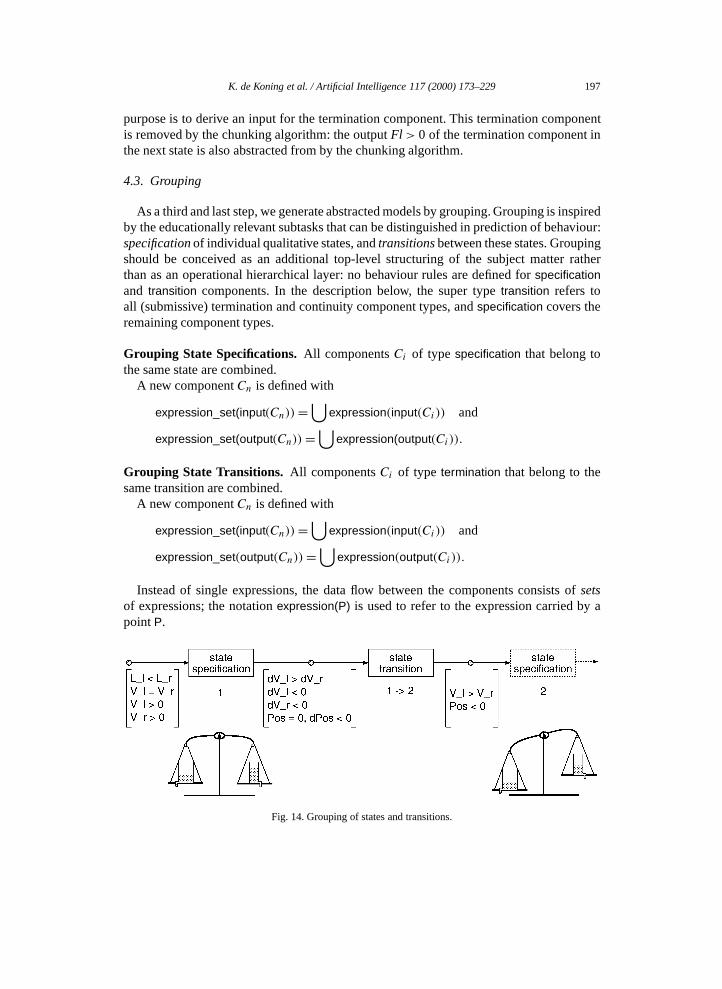
As a third and last step, we generate abstracted models by grouping. Grouping is inspiredby the educationally relevant subtasks that can be distinguished in prediction of behaviour:specificationof individual qualitative states, andtransitionsbetween these states. Groupingshould be conceived as an additional top-level structuring of the subject matter ratherthan as an operational hierarchical layer: no behaviour rules are defined forspecificationand transition components. In the description below, the super typetransition refers toall (submissive) termination and continuity component types, andspecification covers theremaining component types.

Grouping State Specifications.All componentsCi of type specification that belong tothe same state are combined.

A new componentCn is defined with

expression_set(input(Cn))=⋃

expression(input(Ci)) and

expression_set(output(Cn))=⋃

expression(output(Ci)).

Grouping State Transitions. All componentsCi of type termination that belong to thesame transition are combined.

A new componentCn is defined with

expression_set(input(Cn))=⋃

expression(input(Ci)) and

expression_set(output(Cn))=⋃

expression(output(Ci)).

Instead of single expressions, the data flow between the components consists ofsetsof expressions; the notationexpression(P) is used to refer to the expression carried by apointP.

Fig. 14. Grouping of states and transitions.


Fig. 15. The piston system.

Because grouping is applied as the last aggregation step, the expressions flowingbetween the different specification and transition components are likely to be small innumber; many expressions in the base model are already abstracted from in the otheraggregation steps. To exemplify this, consider the high-level model for the balance domaindepicted in Fig. 14. Because we abstracted from various intermediate quantities at lowerlevels, such as pressure and flow rate, the state description that forms the output of the firststate specification is relatively small. If we apply grouping directly to the base model, thenthis state specification output contains 13 instead of 5 elements.

4.4. An example model

As an example of the modelling and structuring principles discussed above, consider thepiston system in Fig. 15. The piston system consists of a movable piston in a container.

Fig. 16. Part of the base model for the piston.


Fig. 17. Same model part after hiding of non-essential knowledge.

Between the heater and the gas in the container, a heat path exists. In the initial state ofthe system, the temperature of the gas and that of the outside world are given to be equaland the heater has been turned on, expressed by the fact that its temperature is higher thanthat of the gas. Furthermore, the temperature of the outside world is given not to change,and the piston is in its starting position. The model generation algorithm as described inSection 3.3 generates a base model for the behaviour of the piston system consisting of 824components and 802 points. For the initial state and the transition to the second state, themost important part of the base model is shown in Fig. 16. At the left hand side, the boldface expressions likePos= s (the position of the piston is in thestarting position) representthe inputs of the model, i.e., the information that is given to the learner, and hence can beassumed to be known. The movement of the piston is modelled as influenced by a ‘moveforce’ Fm, which is the difference between the outward forceFo and the inward forceFi .Because no friction is modelled, these two forces are equal to the pressure of the gas andthe pressure of the surrounding world, respectively. What happens in the model part shownis that the temperature difference between the heat source and the gas (Ts > Tg), causes anincrease in the pressure of the gas (δPg > 0) and in the outward force (δFo > 0). Becausethe temperature of the outside world is given to be steady (δT = 0), we can derive that thepressure of the gas becomes higher than the pressure in the outside world (Pg > Pw), andhence also the outward force becomes bigger than the inward force (Fo > Fi ).

The first aggregation principle applied to the base model is that of hiding non-essentialdetails (fully-corresponding quantities, submissive components, and inactive paths). Themodel that is generated on top of the base model is shown in Fig. 17. For hiding, the effectis particularly strong in the piston example because there are a number of quantities whosevalues never change.9 For instance, both the temperature and the heat of the heat source(Ts andHs ), as well as those of the surrounding world (Tw andHw), have the valueplus inevery behavioural state. Recall that in the base model, this kind of ‘staying the same’ fromstate to state is modelled bycontinuity components, which are abstracted from by the hidingalgorithm. The hiding algorithm is also concerned with simplifying the model by merging

9 In the base model, these values are indeed derived, but they are left out of Fig. 16 for clarity of presentation.


Fig. 18. Same model part after chunking.

quantities that are fully-corresponding. For example, the outward force and the pressure ofthe gas are modelled as fully corresponding, resulting in the combined quantity[Pg,Fo],and also the volume of the gas and of the container ([Vg,Vc]). The latter combination ishowever removed because it does not matter for the reasoning in this state: the volume doesnot change, hence it has no effect on the pressure (cf. thesubmissive quantity proportionalitycomponent in Fig. 17). ComponentSIT is removed because it is a submissive termination.

Fig. 18 shows the next generated abstract model after chunking. Although in factchunking is done in three phases, we only show the resulting model. The chain of reasoningsteps from the model inputTs > Tg to δ[Pg,Fo]> 0 is chunked into onecombined quantityinfluence component. As a result of this chunk, theinequality termination componentderivingTg > Tw loses one input (δTg > 0). This component is removed becauseTg > Twis not used in any successor state; although it is a valid termination, it does not have anyimpact on the behaviour in the subsequent states, and hence is considered a “dead end”.

Finally, grouping selects the different states and transitions, and creates one componentfor each (Fig. 19). As a result, the format of the data flow between the components changesfrom single expressions to sets of expressions representing state descriptions.

5. Diagnosing learner behaviour

Although the base models are defined in terms of components and connections for thesake of model-based diagnosis, some additional processing is needed to apply diagnostic

Fig. 19. Same model part after grouping.


techniques to these models. Firstly, some additional ‘fine tuning’ of the hierarchical modelsis required to befit the diagnostic task (Section 5.1). Secondly, we need aprediction enginethat, given a set of observations, predicts the behaviour of the system to diagnose, in ourcase the learner’s reasoning process (Section 5.2). Finally, thediagnostic engineof GDEneeds a dedicated selection mechanism for obtaining additional observations (Section 5.3).

5.1. The role of inputs

In device diagnosis, ‘inputs’ are defined as the values that the diagnostician puts on a setof points in the device, in order to observe the values at another set of points, the ‘outputs’.For models that we use, two different kinds of inputs exists. Firstly,exercise inputsare theexpressions that are presented to the learner as part of the problem statement. For instance,when the learner is presented with the balance problem in Fig. 3, the exercise inputs are

Wl >Wr, Ll < Lr, Vl = Vr, Vl > 0, Vr > 0.

Secondly,support knowledge inputsare all other inputs of the model, consisting of domainknowledge expressions that are used to perform inferences, such as causal dependenciesand quantity spaces. For instance, the relationdir_corr(L,P ) between the level and thepressure is a support knowledge input of the model.

The difference between the two types of inputs is problematic for diagnosis. Theassumption made in (device) diagnosis that all model inputs are correct only holds forexercise inputs: the expressions explicitly presented to the learner can be assumed tobe applied correctly. In contrast, support knowledge inputscannot be assumed to becorrect. For instance, learners may think that in the balance system the volume insteadof the level determines the pressure. The problem is that a diagnosis that is defined interms of defective components cannot discriminate between a support knowledge inputthat is not correctly known, and a reasoning step that cannot be executed: both will betraced to the component modelling the reasoning step. The solution to this problem isshown in Fig. 20. The correspondence between the level and the pressure in a containedliquid (dir_corr(L,P )) is connected to the actual inference component by means of anintermediateretrieval component. We can now diagnose the fact that a learner does notknow a support knowledge input as afaulty retrieval component. The retrieval inferencecan be interpreted as representing the action of retrieving a piece of knowledge frommemory.

Fig. 20. Fallible domain knowledge inputs: retrieval components.


5.2. The prediction engine

The prediction engine used is similar to a constraint propagator, but instead of constraintsit uses directedrules to propagate expressions through the model (cf. Section 3). Fora component with three ports, three behaviour rules are needed to match the predictivepower of a constraint. The complete set of component types as defined in Appendix Ahas 78 ports in total, and 40 behaviour rules are specified. Since the behaviour of thecomponents is underspecified, the conflict set calculated by the prediction engine willnot always be minimal. When the conflict set is non-minimal, this means that the setof resulting candidate diagnoses will also be non-minimal. However, the candidate set isstill guaranteed to be complete: no valid candidates will ever be missed [30]. Because thehierarchical diagnostic models are small (typically less than 10 components), calculatinglarger candidate sets does not pose computational problems, although sometimes a largernumber of probes will be needed to arrive at a satisfactory diagnosis.

5.3. The diagnostic engine

TheGDE engine as introduced in Section 2.4.3 is used without significant modificationsto calculate possible candidate diagnoses. The one important remaining bottleneck is whichadditional measurements should be taken to discriminate between candidate diagnoses.The specific nature of reasoning models requires a dedicated technique for selectingmeasure points. In this section, we discuss some properties of these models that can beexploited in developing criteria for measurement selection. Subsequently, we propose amethod for determining measure points.

An important difference between models that we use and digital circuits lies in thenature of the components. In a digital circuit, two components of the same type maybehave according to the same rules, but are still physically distinct instances. In reasoningmodels, this is not necessarily the case: one reasoning step applied correctly in one partof the model is very likely to behave correctly as well in another part: by their nature,different components of the same type are likely to fail collectively. A learner that doesnot know how to apply a quantity termination is likely to exhibit the same error (faultyquantity termination inference) at several places in the model. The only exception is formedby components of theretrieval type: here, different instantiations are indeed independentoperations, because they refer to the retrieval of different knowledge facts. The error of notcorrectly ‘retrieving’ the relation between, for instance, level and pressure is usually notrelated to an incorrect retrieval of the negative influence of the, for instance, flow rate on thevolume. This different nature of reasoning models is exploited by the diagnostic algorithm:the failure probability of a set of instances of the same component type is defined tobe equal to that of a single component. Hence, a candidate consisting of four failinginequality correspondence components has the same probability as a single componentcandidate.

For retrieval components, it is possible to employ an additional heuristic in candidatediscrimination: because most errors made in the experiment appeared to be caused bymissing or confused domain knowledge [33], retrieval components can be assumed tohave a highera priori failure rate than inference components. In addition,decomposable


components have a highera priori failure rate than individual base model components,because they incorporate a number of reasoning steps in the base model.

Important to note is that the use ofa priori failure rate only depends on the type ofcomponent, and is independent of the specific contents of the simulation model. More ingeneral, the diagnostic engine exploits only the structure of the model and the types of thecomponents, and does not make any reference to the specific behaviour prediction that ismodelled (see also Section 2.2).

The heuristic method used to find the split point in the set of candidate diagnoses isbased on the same ideas as thehalf split criteria employed in for exampleSOPHIE-III [29]andFAULTY [5]. The half split approach aims at finding the point that optimally splits theset of components that contributes to a symptom: given the set of componentsCpSthatcontributes to a symptom, thesplitting factor for a possible measure pointp is definedas |CpSbp− CpSap|, whereCpSbp is the subset ofCpScontributing to the value ofp(“before p”) and CpSap the subsetCpSnot contributing to the value ofp (“after p”).In our case, simply taking the difference in numbers of components does not work:because we do not make the single fault assumption, and also use differenta priori faultprobabilities, a candidate is no longer synonym with one component. Hence, we introducethe weighted cardinality of a candidate, facilitating the comparison of candidates. Theweighted cardinality of a candidate expresses its probability in terms of the number andtype of components it consists of.

The algorithm for candidate discrimination as shown below first checks whether thecandidate set found so far is satisfactoryfor the current hierarchical model, according tothe criterion of the educational system. If so, and further decomposition is possible, thedecomposition algorithm proposes a new diagnostic model; if no further decompositionis possible, the diagnostic session ends (see below). Otherwise, the algorithm proceedsto determine the possible measure points. In step 2(b), the weighted cardinality of eachcandidate is calculated. The definition of a candidate’s weighted cardinality embodies thedifferent aspects discussed before: retrieval and decomposable components have a higherapriori failure rate and are counted individually. Components of the same type are countedonly once. By its definition, the lower the weighted cardinality of a candidate, the higherits probability. Subsequently, we can map these weighted cardinalities on the individualcomponents, yielding theunnormalised probability of a component. This probabilityexpresses the different candidates that a component is part of: when a component belongsto more than one candidate, knowing its status will provide more information. Hence,the higher a component’s unnormalised probability, the more important it is to focus thediagnostic process on this component (step 2(c)). The unnormalised probabilities of thecomponents are used in calculating the splitting factor for each measure point (step 2(e)).

Algorithm: Candidate Discrimination(1) If the candidate setCaSmeets the criteria as set by the educational system, then go

to thedecompositionalgorithm (Appendix B).(2) Else, determine a measure point.

(a) Collect the set of all possible measure pointsMPSby tracing backwards fromthe set ofsymptoms(i.e., observations that do not match the predicted value)through the model.


(b) For each candidateCai ∈CaS, calculate itsweighted cardinality WCCai .LetR be the number of retrieval components inCai .LetH be the number of decomposable components inCai .Let T be the number of other componenttypesin Cai .The weighted cardinality of a candidate is defined asWCCai = 0.7∗ R + 0.5∗H + T .

(c) LetCpSbe the set of components that contribute to the set of symptoms. Definethe unnormalised probability of a componentCp∈ CpSto be

∑1/WCCai for

all candidatesCai containingCp.(d) For each pointp in MPS, let CpSbp ⊂ CpS be the set of components that

contribute to the value ofp and letCpSap=CpS\CpSbp.(e) For each pointp in MPS, calculate its splitting factorSFp . Let UPbp be the sum

of the unnormalised probabilities of the components inCpSbp, andUPap thesum of the unnormalised probabilities of the components inCpSap.The splitting factorSFp of measure pointp is defined as|UPbp−UPap|.

(f) Order the probe points inMPSaccording to their splitting factorSFp: the bestprobe point is the one with the smallest value forSF.

(3) Execute a probe by outputting the ordered list of probe points, and wait for the setOBSof returned expressions.

(4) Call theGDE conflict recognition algorithm (Appendix B) with the setOBS.

The definition of the weighted cardinality of a candidate includes some numericalinterpretations of qualitative observations that may prove to be non-optimal. For example,the fact that a retrieval component is counted as 0.7 is a somewhat arbitrary quantificationof the observation that more errors are made in the domain knowledge than in the reasoningknowledge. Because of the small number of components that is diagnosed at once in thehierarchical model, the impact of such choices will be relatively small.

A major advantage of the discrimination algorithm is that the computational costs arelow because no behaviour propagation is involved. However, the final diagnosis may notalways be found in the minimum number of probes possible: the algorithm does not useestimations about the total number of probes needed to pin down the final diagnosis, as isfor instance done in [28]. Apart from the fact that in general estimations of the total numberof probes needed are not necessarily cost-effective [29], a more specific reason exists fornot using such estimations: because the hierarchical models ensure that the diagnosticmodels are small, the number of possible probe points is generally low. Hence, the impactof a suboptimal probe point selection is limited.

As defined in step (3), the candidate discrimination algorithm does not deliver one probepoint, but a list of possible probe points ordered to their discriminating power (i.e., theirsplitting factor). Although the diagnostic machinery can reason about the expectedresultsof a certain probe point, it cannot determine thecostsof a specific probe within the currenteducational context. As a result, the most effective probe suggested may be very expensive,in the sense that it does not fit in with the current dialogue. In this case, the educationalsystem may select another probe point from the list.

The diagnostic method presented above works within a model at one level of abstraction.Throughdecomposition, a diagnosis found on one level of abstraction can be refined


Fig. 21. Top-level diagnostic model.

by considering the related components at a lower level. Especially if multiple faultsare possible, it is difficult to ensure soundness and completeness of the diagnosticprocess when hierarchical decomposition is applied [57]. In our models we cannot expectsoundness or completeness: apart from the possibility of multiple faults, there are alsodifferent kinds of aggregations with different properties. We take a practical stance: withina specific model, we diagnose until the external criteria for what constitutes a satisfyingdiagnosis are met. If not already at the lowest hierarchical level, the component withthe maximum unnormalised probability is decomposed, and diagnosis is resumed in theresulting lower-level model. If the diagnostic algorithm returns an empty set of candidates(i.e., the decomposed model does not reveal a conflict), the decomposition is undone andthe next most probable component is selected for decomposition. This last step is onlyneeded to account for the (undesirable) situation in which the external criterion for asatisfactory diagnosis is too weak. Hence, the candidate discrimination algorithm may callfor decomposition with a too large candidate set: the component first selected may notbelong to the correct minimal diagnosis.

5.4. An example diagnosis

This section exemplifies the use of the diagnostic algorithms in an educational setting.We continue the piston example as used in Section 4.4. The top-level model from Fig. 19for the first state and transition is repeated in Fig. 21.10 The learner is presented with adescription and a picture of the initial behavioural state of the piston system. The questionsasked are multiple choice. Suppose the strategy for subject matter sequencing that is usedby the educational system is to follow the top-level model and ask for each change (i.e.,each output of atransition component).11 As a result of this strategy, the first questionasked is about the output of thetransition componentST. The only expression availableis the inequality between the combinedpressure/force quantities of the world and the gas.For convenience, in the remainder of this section we will only refer to pressure, both inthe questions and in the figures. However, the educational system has the possibility to

10 Recall from Section 4.3 that the input of a state transition also contains the input expressions of the precedingstate specification. These are left out for reasons of presentation.11 Additional control is needed when alternative transitions and/or cycles exist, but this is not essential to the

diagnostic approach.


talk about force instead of pressure if that would fit in better with the current educationalcontext.

Probe 1.Teacher: The pressure of the gas is initially equal to the pressure of the outside

world (Pg = Pw).What do you think about this pressure ratio in the next behavioural state?a. Pg < Pw ;b. Pg = Pw ;c. Pg > Pw .

Learner: b. Pg = Pw .

The answer is wrong, so one or more components in Fig. 21 must be erroneous. Becauseno observations are known about the point betweenSS and ST, the top-level focusingalgorithm asks for additional observations. At this point, two expressions can be measured:δPg > 0 or δPw = 0. Suppose the educational system chooses to ask only the first one.

Probe 2.Teacher: Is the pressure of the gas initially:

a. increasing;b. steady;c. decreasing.

Learner: a. increasing.

According to the top-level focussing heuristic, the diagnostic system assumes that an errorhas been made in thetransition component: an expression in the input is measured tobe correct, and one in the output is measured to be incorrect. Therefore, thetransitioncomponent is decomposed, resulting in the situation in Fig. 22. This decomposition doesnot yield a larger number of components, but only splits the compound expression intothree new ones. Because we do not have an observation for the lowest input port ofIT-2 (δPw), no conflict is found: the prediction engine will derive the incorrect expressionδPw > 0 for this port, but there is no observation to conflict with this expression. As a

Fig. 22. Decomposition of the state transition component.


result, the diagnoser returns with an empty conflict set, and the educational system is askedfor new observations at the top level. The only resulting expression to ask for isδPw = 0.

Probe 3.Teacher: Is the pressure of the world initially:


Learner: b. steady.

Because the answer is correct, the same decomposition ofST is executed. This time,the new observation results in the single-fault diagnosis[IT-2]: all inputs are either given(Pg = Pw) or observed to be correct(δPg > 0, δPw = 0), and the output is observed to befaulty (Pg = Pw).

As a second example, consider the case in which the learner gives another answer inProbe 2.

Probe 2b.Teacher: Is the pressure of the gas initially:


Learner: b. steady.

The top-level focussing algorithm now restarts the search for the initial focus fromthe point betweenSS and ST, and finds that the error must be inSS: all inputs areknown to be correct, because they are given, and the output contains an incorrectobservation. Hence, the statespecification component is decomposed as shown in Fig. 23.

Fig. 23. Decomposition of the state specification component.


Fig. 24. Decomposition of the transitive quantity proportionality component.

In this case, the decomposition yields an immediate single-fault diagnosis[CQI-2] atlevel 4. BecauseCQI-2 is an aggregated component, the decomposition algorithm (seeAppendix B) is called. This results in the level 3 model shown in the lower part ofFig. 23. The diagnostic algorithm is now called on this five component model. Oneconflict is found, namely〈R1, R2, VD, QI, TQP〉, resulting in the single-fault candidates[R1], [R2], [VD], [QI], and [TQP]. There are four possible measure points that provideinformation for discriminating between these components, labeledFl = Ts − Tg , Fl > 0,pos_infl(Fl, Hg), andδHg > 0. Because each of the five components in the submodel isa single-fault candidate, the unnormalised probability is 1/0.7= 1.43 for the two retrievalcomponentsR1 andR2, 1/0.5= 2 for the decomposable componentTQP, and 1 for thebase model componentsVD andQI. Calculation of the splitting factor of these measurepoints yields the smallest value for the pointFl > 0: |(1.43+ 1)− (1.43+ 1+ 2)| = 2.Hence, the best point to probe is to ask for the value of the flow rateFl.

Probe 3b.Teacher: What is the direction of the heat flow between source and gas?

a. from source to gas;b. from gas to source;c. there is no heat flow between source and gas.

Learner: a. from source to gas.

The new candidate set consists of[R2], [QI], and[TQP]. Calculating the splitting factor forthe two remaining measure pointspos_infl(Fl, Hg) andδHg > 0 now yields|1.43− (1+2)| = 1.57 and|(1.43+ 1)− 2| = 0.43, respectively. NowδHg > 0 is measured.

Probe 4b.Teacher: Is the heat of the gas initially:



The single-fault diagnosis found now,[TQP], results in a new decomposition, as depicted inFig. 24. The diagnoser returns a candidate set consisting of[R3], [QP1], [R4], and[QP2].


The measure pointδTg > 0 exactly splits the set of candidates in two, as is reflected by itssplitting factor|(1.43+ 1)− (1.43+ 1)| = 0. Hence, the next probe concernsδTg .

Probe 5b.Teacher: Is the temperature of the gas initially:



Because the answer is correct, two candidates[R2] and[QP2] remain, and one possibleprobe pointpos_prop(Tg, Hg).

Probe 6b.Teacher: What is the relation between the temperature and the pressure of the gas

in the current state?a. if the temperature increases, then the pressure increases;b. if the temperature increases, then the pressure decreases;c. if the temperature increases, then this does not affect the pressure.

Learner: a. if the temperature increases, then the pressure increases.

The final diagnosis found is[QP2]: the learner does know the relation between temperatureand pressure, but did not apply it here.

The interaction traces reflect diagnostic sessions in which a maximally detaileddiagnosis is determined using a minimal amount of information. In a full-fledgededucational system, other functional components are available to provide a richerinteraction, such as a discourse planner [80]. In addition, a number of observations may bealready available from the learner model, which can be used both to improve the dialogueand to reduce the number of probes. The educational system does not need to proceed untilone single fault is located in the base model, but may decide to start explaining a largerpart of the process after some probes.

6. TheSTARlight prototype system

To assess the feasibility of the diagnostic process and the usefulness of the aggregatedsubject matter models, theSTARlight prototype system12 was developed and try-outsessions with learners were conducted. The design of theSTARlight system concentratedon the main research topics, namely subject matter model generation and diagnosis. Bothcomponents were fully implemented according to the techniques and algorithms describedin this article. For the other components of the architecture, which was shown in Fig. 2, weimplemented ‘light’ versions.

12 The acronymSTAR stands forSystem forTeachingAboutReasoning. Because the prototype only implementsthe subject matter model and the diagnostic function of theSTAR system in detail, it is christenedSTARlight.


The explanation generator in the prototype is based on explaining individual compo-nents. For each component type, a generic explanation frame can be constructed that com-plies with the current situation, and this frame is filled in with the terms in the modelusing a set of domain-specific verbalisations. The question generator works similarly, andgenerates multiple choice questions about specific points in the model.

Although in the implementation hardly any effort was made to optimise the performanceof the system, it is nevertheless adequate for real-life applications. On a 200 MHz Pentium-Pro platform under Linux, the diagnostic component returns a candidate set mostly withinone second. The longest calculation time needed in the try-out sessions was four seconds.The domain-specific verbalisations and graphics are as yet only implemented for thebalance domain. Hence, the try-out sessions of the system were conducted using thissystem. For larger predictions, the performance is expected to be similar: as a result of theaggregations used, the size and complexity of the diagnostic models does not increase withlarger simulations. The only increase is in the simulation and model generation process,but these can be processed in the background.

An example of the interface screen is shown in Fig. 25. In the upper half of the screen,the behavioural states of the balance system are shown. The pictures are generated fromthe subject matter model; a set of quantitative measures is added to define the actual size ofthe levels and the widths of the water columns on the screen. The lower half of the screendisplays the questions and explanations provided by the system. At the bottom, buttonsare provided for selection of an answer, as well as a ‘give me a hint’ button that providesa help text in a separate window. This help text is also constructed by the explanationgenerator.

Fig. 25. A screen dump of the interface.


6.1. Try-out sessions

We conducted a small number of try-out sessions to determine whether theSTARlight

system is useable in an educational setting. Because theSTARlight system has beendeveloped to demonstrate the diagnostic framework developed, we did not try to evaluateit as a full-fledged educational system.

In the try-out sessions, the subjects were asked to do a series of four balance predictionexercises. The think-aloud method [71] was employed to provide information about thesubject’s reasoning behaviour. There were two separate sessions. In the first session,four subjects participated, all being third or fourth year university students who hadsome background in knowledge-based educational systems and the subject matter (i.e.,qualitative behaviour analysis). These subjects will be referred to as ‘advanced subjects’.In the second session, there were five subjects from different backgrounds, who had noexperience with either educational systems or the subject matter. We refer to these subjectsas ‘novice subjects’. The experiment took about 30 minutes for each subject. Afterwards,the subjects were asked a number of questions about their experiences. These questionswere aimed at the explanations of the final diagnoses and at the probe questions. Thesubjects were asked whether they thought that the system correctly determined the mistakethey made, and whether the questions asked by the diagnoser were appropriate, in a logicalorder, and not too large in number.

Each of the nine subjects performed the same four prediction exercises about the balancesystem. In total, 31 diagnostic sessions were run and 707 questions were answered. Novicesappeared to make about twice as many errors as advanced subjects. For most cases thenumber of probes that was needed, to arrive at a satisfactory diagnosis, varied from oneto three. In eight diagnostic sessions, more probes were needed. The longest sequenceof probes was eight, which occurred twice. The number of probes per diagnoses wason average the same for novices and advanced subjects. Also, the variation in the typesof the components found as the final diagnoses (e.g.,retrieval components versus othercomponent types) was not significantly different in both groups.

6.2. An example diagnosis

A worked-out example is provided of a diagnosis session that occurred in the try-outsessions. The example is taken from the first session with advanced subjects. A part ofthe interaction, combined with the think-aloud remarks made by the subject, is shownbelow.13 The dialogue starts when the subject is asked to predict the next behaviour state,starting from the balance situation shown in Fig. 3. This situation is equal to the leftmoststate shown in Fig. 25.

1. What will be the difference between volume left and volume right in the next state?2. Hey, look, the volumes are equal. I didn’t take notice of that.3. Yes, I think they stay equal?

13 Lines with plain text are generated by theSTARlight system. Lines in italic starting witha:, b: or c: are answersgiven by the learner. Think-aloud remarks are in italic with indent.


4. b: volume left will be equal to volume right5. That’s not correct.6. Before we go on with the prediction, I would like to know what you think about the

present situation.7. Please answer the following question:8. What do you know about the difference between the decrease in volume left and the

decrease in volume right?9. Volume left decreasing slower than volume right?

10. No, at the same speed I would say.11. b: volume left is decreasing at the same speed as volume right12. That’s not true.13. Please answer the following question:14. What do you know about the difference between outflow left and outflow right?15. Well I would say that the outflow is equal, but that is now

when the pressure [incomprehensible]16. Ah! Is that it? The outflow left is smaller17. c: outflow left is smaller than outflow right18. That’s right.19. Please answer the following question:20. which quantity causes a change in volume?21. The outflow, or the pressure, yes the outflow22. c: outflow23. That’s right.24. I think you don’t fully understand the following:25. the difference between outflow left and outflow right has a direct influence on the

difference between the decrease in volume left and the decrease in volume right.26. This means that because outflow left is smaller than outflow right, volume left is

decreasing slower than volume right.27. Let’s continue with the exercise where we left off.28. All right, interesting. . .

To explain the diagnostic process underlying this interaction, consider Fig. 26. Theanswer given in line 4 supplies the observationVl = Vr in the output of thestate transitioncomponentST. ST models the transition from the first to the second state at the highesthierarchical level. In the prototype system, the subject matter sequencing is simplifiedto only asking the output of each subsequenttransition component. Hence, a conflict atthe highest level results in a decomposition oftwo components: the precedingtransitioncomponent plus the previousspecification component (for more details, see [31]). Hence,SS andST are decomposed into the seven-component model depicted. The first call tothe diagnoser delivers one conflict:〈CII, IT〉, and hence two diagnoses[CII] and [IT].Thecombined inequality influence CII is a decomposable component that summarises thecalculation of a derivative inequality (in this case, the ratio of the decreases in volumeδVl > δVr ) from an (in)equality (the ratio of the water levelsLl < Lr ). The inequalitytermination IT determines the new inequality between the values in the next state. Theonly probe point that yields information about the candidates[CII] and [IT] is in between


Fig. 26. First diagnostic cycle.

these components. Hence, a question is asked about the inequality between the derivativesof the volumes(δVl > δVr , line 8). The answer given in line 11 is incorrect, yielding asingle-fault diagnosis[CII]. Because this is a higher-level component, it is decomposed intoa lower-level model as shown in Fig. 27. The next diagnostic cycle yields one conflict〈TIC, R3, II〉 and three candidates[TIC], [R3], and [II]. For the two existing measurepoints, the splitting factors are determined by the discrimination algorithm. For the pointneg_infl(Fl,V ), the splitting factor is calculated on the basis of thea priori failure ratesof retrieval componentR3 (0.7), decomposable componentTIC (0.5), and ‘normal’ basemodel componentII (1): |1/0.7− (1/0.5+ 1/1)| = 1.57. ForFl < Fr , the splitting factoris |1/0.5− (1/0.7+ 1/1)| = 0.43. Fl < Fr has the lowest value, and thus the highestdiscriminating power. Hence, this one is questioned (line 14) and answered correctly(line 17). This results in the new conflict〈R3, II〉 and two candidates[R3] and [II]. Thelast probe onneg_infl(Fl,V ) in line 20 delivers the inequality influence componentII as afinal single-fault diagnosis. In lines 24–26, an explanation is generated for this component.

Fig. 27. Second diagnostic cycle.


6.3. Evaluation

According to the interviews held with the subjects after the experiment, especiallyadvanced subjects were satisfied about the prototype’s interaction. The amount of questionswas considered reasonable, the subject of the questions to the point, and the order in whichthe questions were asked occurred natural to them. In general, they had the idea that thediagnoses were correct and the explanations useful, although sometimes “outdated”: theprobe questions sometimes triggered self-repair by the subjects, and hence the ultimatediagnosis pointed out an already fixed problem (see also Section 8).

Novices reported problems with the sometimes rather cryptic questions and the specific,one-component based explanations. Clearly, a more advanced question and explanationgenerator is required to communicate with novices. Furthermore, the balance systemmay not be very suitable for novices, because it involves rather complicated inequalityreasoning. As will be discussed in the next section, starting with simpler systems (e.g., oneemptying container) may yield better results for novices.

7. Related work

As indicated in Section 2.4, we propose a novel, generic approach to diagnosis oflearner behaviour based on existing techniques from the field of model-based reasoning.Whereas we discussed qualitative reasoning and model-based diagnosis, as well as earlierapproaches to educational diagnosis, we did not yet discuss how the aggregation techniquesrelate to existing work on abstraction in both model-based reasoning and theories oneducation

An alternative for the aggregation procedures presented in this article would be to derivethe abstract models by generating more abstract simulations of the intended behaviourin the first place [37]. The base model generation algorithm can then be applied to eachof these models to generate the related hierarchical layer in the subject matter model. Inthis alternative approach the actual abstraction process has moved to the scenarios and thelibrary of model fragments. In fact, within the field of qualitative reasoning, substantialresearch has been done on how thegenerationof qualitative simulation models can beadapted, e.g. [54,61,66,73,74]. The motivation for these adaptations varies from removingirrelevant details, or spurious behaviours, to tailoring for a specific task. An importantadvantage of abstraction before simulation is that often the number of states that isgenerated by the simulator can be decreased; this is precisely the aim when trying to avoidspurious behaviours. However, in our research we have the additional goal of exploitingthe abstractions in an educational context. We therefore need to have the relations betweenthe different abstraction models explicitly available. If we generate the models separately,from different scenarios, we do not have explicit knowledge about the connections betweenthe components in the different models.

Some research has been done on summarising the results of qualitative simulations, i.e.reformulating the output after it has been generated. In [42], an approach is described thatuses a set of heuristics to collapse chains in a causal order graph of quantity relations forthe purpose of simplifying explanations. The major difference with our approach lies in


the application of the technique: while they focus on explanations, we focus on teachinga reasoning process. As such, we do not aggregate the relations in the causal order graphitself, but a model that represents the reasoning steps that can be made with these relations.This way, we can locate those reasoning steps that a student did not yet master, and not onlythe causal relations they do not know. Most other approaches that are aimed at simplifyingsimulation outputs operate again at the level of states. An example is [55], where complexbehaviour graphs are abstracted by reducing the number of states to be considered. Thisapproach is complementary to ours. We take the number of states and state transitions asa given, and try to abstract from less relevant details in the reasoning that is done ‘within’these states and transitions.

The aggregation procedures presented in this article hide details when mapping thecurrent level to the next higher level. The idea of exploiting models of differing complexityin teaching has been investigated in [76].14 Model Progression Theoryproposes a set ofmodels to be used in educational systems. They define three dimensions on which thesemodels may vary:perspective, order, and degree of elaboration. The key idea is thatlearning can be optimally supported when different models are presented in succession,starting from the simplest one. The aims of model progression are clearly different fromours, and therefore the techniques are complimentary. Model progression is primarilyconcerned with subject matter sequencing and supporting the learning process at a moreglobal level. Hence, where model progression is about selecting the right model in aprogressive sequence, we take a specific simulation model to start with as a given. In fact,the evaluative remarks in Section 6.3 already indicated that for novice learners a ‘modelprogression-like’ approach can be very beneficial. Note however that the construction of aset of models according to the dimensions specified by causal model progression is as yetnot an automated process (see [34] for ideas on how to automate model progression).

Whereas model progression concentrates mainly on acquiring new knowledge, thereare also a number of theories that model learning in terms of combining and improvingexisting knowledge. InSOAR [52], a general architecture for modelling intelligentbehaviour, an important learning operator ischunking: if a procedure (consisting of aset of inferences) is processed once, then often one abstract inference can be compiledto replace future processing of the procedure [53].SOAR’s learning-by-chunking mainlyincreases efficiency.Knowledge Compilation[2] is similar to chunking, in that it modelsthe process of constructing domain-specific shortcuts for general (inefficient) reasoningpaths during learning. In theACT* andACT-R theory, knowledge compilation is viewed asan important learning mechanism in skill acquisition [1]. An important difference betweenthese techniques and the aggregation principles described in this article is that we do notaim at modelling efficient learning over cases, but at supporting diagnosis in one specificcase. The goal of both chunking and knowledge compilation is to facilitate easier and moreefficient reasoning in future occurrences of the same problem. We do not generalise overcases (i.e., predictions), but only compact inference sequences within one case. A seconddifference is the fact that our aggregation approach coversall possiblecorrect reasoningpaths of a specific case. In compilation and also explanation based generalisation [56]chunking is only overonespecific reasoning trace per case.

14 In [64], multiple models are employed in a related way, although with a different theoretical footing.


8. Conclusions

In this article we showed that model-based techniques can be applied successfullyto solve outstanding problems in research on the use of AI technology for educationalpurposes. In particular, we employed qualitative simulation and model-based diagnosis torepresent and analyse the reasoning behaviour of a learner when predicting the behaviourof a device. The main advantage of this approach is that it provides ageneric methodfor the task of cognitive diagnosis, which as of yet has mostly been based on predefined,domain-specific bug catalogues. Qualitative simulators provide a means for automaticallygenerating the behaviour of a device, and this output was shown to be convertible into abase modelthat can be used as the backbone of an educational system: the base modelrepresents all the correct facts and reasoning steps that are required for a correct predictionof behaviour. Being based on earlier experimental research about human problem solvingbehaviour, the knowledge represented in the base model can be considered didacticallyrelevant: both the type and the grain size of the reasoning steps in the model correspond tohow teachers and learners communicate about device behaviour.

The base model adheres to the representational constraints of model-based reasoning:each reasoning step is defined as an inference component in the model. Hence, diagnostictechniques such asGDE can be applied. Accordingly, the diagnostic task is defined asdetermining those reasoning steps that the learner cannot have applied correctly given theobservations. The important consequence of this definition is that we do not try to grasp thelearner’s mental model, nor that we force the learner into a predefined reasoning trajectory:we do not assume that the reasoning model is a cognitive model of what goes on in the mindof the student. We do assume however that the model is didactically plausible: it representsknowledge that the student should acquire in the learning process. The role of diagnosis isnot to detect “mind bugs”, but to detect and locatebehaviouraldeviations. The results ofthe diagnosis are used to focus the dialogue with the student on those topics that correspondto erroneous behaviour.

The application ofGDE to the base models required two issues to be addressed.Firstly, a new technique for measurement selection had to be developed that accountsfor the selection of educationally relevant probing points (i.e., subjects for questions).Secondly, the base models were too large and too loosely structured to apply model-baseddiagnostic techniques directly in an efficient and effective manner. We therefore developeda structuring mechanism that automatically transforms the base model into a hierarchyof aggregated models by removing irrelevant detail and by chunking chains of causalinference steps. The resulting structured subject matter model does sufficiently enable thediagnostic process to produce useful diagnostic results in a real-time environment.

An experiment was conducted with learners that showed the utility of the approachpresented in this article. We believe theSTAR framework to be particularly usefulfor the development of educational environments that stimulate the learner’sself-repaircapabilities. The experiment showed that by focusing on behaviour errors in a systematicway, the learner’s ability to self-repair is stimulated. Such a focus on learning from errorsrequires a view on education that is not commonly practiced by human teachers: theyappear to rely mainly on pattern recognition on the basis of known misconceptions, ratherthan on detailed diagnosis [13,51]. On the one hand, this is influenced by traditional


educational views on errors: “School teaches that errors are bad; the last thing one wants todo is to pore over them, dwell on them, or think about them” [59]. But more importantly,detailed structured diagnosis is often computationally infeasible for human teachers.

The prototype system presented is only a partial implementation of the completeframework we envision. In the near future, other components of the architecture willbe researched in more detail, hopefully resulting in a complete set of truly model-basedtechniques that can support education in an articulate and yet generic way.

Acknowledgement

The authors would like to thank David Rühl for his contributions to the implementationof the STARlight prototype system. Richard Benjamins, Frank van Harmelen, RemcoStraatman and Radboud Winkels provided valuable comments on earlier drafts of thisarticle.

Appendix A. Model component definitions

For the 10 base model component types, the definitions are provided below. Notethat two versions exist for inequality terminations, value determinations and derivativedeterminations, depending on the number and type of inputs used for the inference (seealso [31]). When different possibilities for one expression are given, such as in[δA =−/0/+], the positional equivalent expression should be chosen in other parts of the rule.The notationssucc(Val) andpred(Val) stand for the successor and predecessor ofVal in itsquantity space, respectively.

Quantity Correspondence

ports: In= quantity value,Sup= value correspondence,Out= quantity valueexample: “The level is positive, therefore the pressure is positive as well”

(L > 0 & dir_corr(L,P )→ P > 0)forward behaviour rules: In & Sup→Out

IF In= [A= Val]& Sup= [corr(A,B)] THEN Out= [B = Val]IF In= [A= Val]& Sup= [corr(B,A)] THEN Out= [B = Val]IF In= [A= Val]& Sup= [dir_corr(A,B)] THEN Out= [B = Val]IF In= [A= ValA]& Sup= [v_corr(A,ValA,B,ValB)] THEN Out= [B = ValB]IF In= [A= ValA]& Sup= [v_corr(B,ValB,A,ValA)] THEN Out= [B = ValB]IF In= [A= ValA]& Sup= [dir_v_corr(A,ValA,B,ValB)]

THEN Out= [B = ValB ]backward behaviour rules: Out& Sup→ In

Quantity Proportionality

ports: In=quantity derivative,Sup= proportionality,Out= quantity derivativeexample: “The level decreases, therefore the pressure is decreasing as well”

(δL < 0 & pos_prop(Ll,Pl)→ δPl < 0)


forward behaviour rules: In & Sup→OutIF In= [δA=−/0/+]& Sup= [pos_prop(A,B)] THEN Out= [δB =−/0/+]IF In= [δA=−/0/+]& Sup= [neg_prop(A,B)] THEN Out= [δB =+/0/−]

backward behaviour rules: Out & Sup→ InIn 6= 0 & Out 6= 0→ Sup

Quantity Influence

ports: In= quantity value,Sup= influence,Out= quantity derivativeexample: “There is a [positive] flow, so the volume decreases”

(Fl > 0 & neg_infl(Fl,V )→ δV < 0)

forward behaviour rules: In & Sup→OutIF In= [A>/=/<0]& Sup= [pos_infl(A,B)] THEN Out= [δB =+/0/−]IF In= [A>/=/<0]& Sup= [neg_infl(A,B)] THEN Out= [δB =−/0/+]

backward behaviour rules: Out & Sup→ InIn 6= 0 & Out 6= 0→ Sup

Quantity Termination

ports: In= quantity value, derivative,Sup= quantity space,Out= quantity value

example: “The volume goes down to zero, so it will become empty”(V > 0, δV < 0 & [0,+]→ V = 0)

forward behaviour rules: In & Sup→OutIF In1= [A= Val]& In2= [δA=+/−]& Sup=QS(A)

THEN Out= [A= succ(Val)/pred(Val)]backward behaviour rules: Out & Sup& In1→ In2

Out & Sup& In2→ In1

Inequality Correspondence

ports: In= value inequality,Sup= value correspondence,Out= value inequalityexample: “The level is higher [at the right], [therefore] the pressure as well”

(Ll < Lr & dir_corr(L,P )→ Pl < Pr)

forward behaviour rules: In & Sup→OutIF In= [A1</=/>A2]& Sup= [corr(A,B)] THEN Out= [B1</=/>B2]IF In= [A1</=/>A2]& Sup= [corr(B,A)] THEN Out= [B1</=/>B2]IF In= [A1</=/>A2]& Sup= [dir_corr(A,B)] THEN Out= [B1</=/>B2]

backward behaviour rules: Out & Sup→ In

Inequality Proportionality

parts: In= derivative inequality,Sup= proportionality,Out= derivative inequality

example: “The level decreases faster at the left, so does the pressure”(δLl < δLr & pos_prop(L,P )→ δPl < δPr)


forward behaviour rules: In & Sup→OutIF In= [δA1</=/>δA2]& Sup= [pos_prop(A,B)]

THEN Out= [δB1</=/>δB2]IF In= [δA1</=/>δA2]& Sup= [neg_prop(A,B)]

THEN Out= [δB1>/=/<δB2]backward behaviour rules: Out & Sup→ In

Inequality Influence

parts: In= value inequality,Sup= influence,Out= derivativeexample: “The right flows faster, so [the volume] decreases faster”

(Fll < Flr & neg_infl(F,V )→ δVl > δVr)

forward behaviour rules: In & Sup→OutIF In= [A1</=/>A2]& Sup= [pos_infl(A,B)]

THEN Out= [δB1</=/>δB2]IF In= [A1</=/>A2]& Sup= [neg_infl(A,B)]

THEN Out= [δB1>/=/<δB2]backward behaviour rules: Out& Sup→ In

Inequality Termination (type 1)

ports: In= value inequality, derivative inequalitySup= ∅, Out= value inequalityexample: “The level is higher [at the right], but also goes down faster, that means they

become equal”(Ll < Lr, δLl > δLr & —→Ll = Lr)

forward behaviour rules: In & Sup→OutIF In1= [A1=/>A2]& In2= [δA1< δA2] THEN Out= [A1</=A2]IF In1= [A1</=A2]& In2= [δA1> δA2] THEN Out= [A1=/>A2]

backward behaviour rules: Out& In1→ In2Out & In2→ In1

Inequality Termination (type 2)

ports: In= value inequality, 2 value derivatives,Sup= ∅, Out= value inequalityexample: “There’s more water on the right hand side,. . . it goes down there and up at the

left, so it becomes leveled”(Vl < Vr, δVl > 0, δVr < 0 & —→ Vl = Vr)

forward behaviour rules: In & Sup→OutIF In1= [A1=/>A2]& In2= [δA1< 0]& In3= [δA2> 0]

THEN Out= [A1</=A2]IF In1= [A1=/>A2]& In2= [δA1= 0]& In3= [δA2> 0]

THEN Out= [A1</=A2]IF In1= [A1=/>A2]& In2= [δA1< 0]& In3= [δA2= 0]

THEN Out= [A1</=A2]IF In1= [A1</=A2]& In2= [δA1> 0]& In3= [δA2< 0]

THEN Out= [A1=/>A2]


IF In1= [A1</=A2]& In2= [δA1= 0]& In3= [δA2< 0]THEN Out= [A1=/>A2]

IF In1= [A1</=A2]& In2= [δA1> 0]& In3= [δA2= 0]THEN Out= [A1=/>A2]

backward behaviour rules: Out& In2& In3→ In1

Value Determination (type 1)

ports: In= value inequality,Sup= value definition,Out= quantity valueexample: “The volumes are equal, therefore the balance will be leveled”

(Vl = Vr & Pos= Vl − Vr→ Pos= 0)

forward behaviour rules: In & Sup→OutIF In= [A</=/>B]& Sup= [C =A−B] THEN Out= [C</=/>0]

backward behaviour rules: Out& Sup→ InIn & Out→ Sup

Value Determination (type 2)

ports: In= quantity values,Sup= value definition,Out= quantity valueexample: “The mass of the container plus the mass of the liquid makes up a positive total

mass”(Mc > 0, Ml > 0 &Mt =Mc +Ml→Mt > 0)

forward behaviour rules: In & Sup→OutIF In1= [A< 0]& In2= [B>/=0]& Sup= [C =A−B] THEN Out= [C < 0]IF In1= [A</=0]& In2= [B > 0]& Sup= [C =A−B] THEN Out= [C < 0]IF In1= [A= 0]& In2= [B = 0]& Sup= [C =A−B] THEN Out= [C = 0]IF In1= [A< 0]& In2= [B</=0]& Sup= [C =A+B] THEN Out= [C < 0]IF In1= [A</=0]& In2= [B < 0]& Sup= [C =A+B] THEN Out= [C < 0]IF In1= [A= 0]& In2= [B = 0]& Sup= [C =A+B] THEN Out= [C = 0]IF In1= [A> 0]& In2= [B>/=0]& Sup= [C =A+B] THEN Out= [C > 0]IF In1= [A>/=0]& In2= [B > 0]& Sup= [C =A+B] THEN Out= [C > 0]

backward behaviour rules: Out & In1& Sup→ In2 (partially)Out & In2& Sup→ In1 (partially)Out & In1& In2→ Sup (partially)

Derivative Determination (type 1)

ports: In= value inequality,Sup= derivative definition,Out= quantity derivativeexample: “The flow rate is larger at the right, therefore the balance will move up there”

(Fl < Flr & δPos= Fll − Flr→ δPos< 0)

forward behaviour rules: In & Sup→OutIF In= [A</=/>B]& Sup= [δC =A−B] THEN Out= [δC </=/>0]

backward behaviour rules: Out& Sup→ InIn & Out→ Sup


Derivative Determination (type 2)

parts: In= quantity values,Sup= derivative definition,Out= quantity derivative

example: “Only the left flows, so the balance goes up [there]”(Fll > 0, Flr = 0 & δPos= Fll − Flr→ δPos> 0)

forward behaviour rules: In & Sup→Outanalogous to type 2 value determinations

backward behaviour rules: Out & In1& Sup→ In2 (partially)Out & In2& Sup→ In1 (partially)Out & In1& In2→ Sup (partially)

analogous to type 2 value determinations

Appendix B. Algorithms: Hierarchical aggregation and diagnosis

Algorithm B.1 first collects all sets of fully-corresponding quantities (step (1)). Allreferences to a quantity that belongs to such a set are replaced by a reference to anew quantity representing the whole set (step (2)). Now, all sets of points with identicalexpressions are merged to one point (step (3)), thereby ‘flattening’ network parts such asthe one shown in Fig. 9. In steps (4) and (5), identical components between points, as wellas components that have the same point as input and output, are removed.15 The lattercategory of circular components consists of correspondences and proportionalities: aftercombining two quantitiesA andB, a correspondence component fromA > 0 to B > 0becomes one from[A,B]> 0 to [A,B]> 0.

Algorithm B.1 (Hiding fully-corresponding quantities).(1) Find in the model all maximal sets of quantitiesS = {Q1, . . . ,Qn} for which the

following condition holds:

∀Qi ∈ S ∃Qj ∈ S: (corr(Qi,Qj )∨ corr(Qj ,Qi))

∧pos_prop(Qi,Qj )∧ pos_prop(Qj ,Qi).

(2) For each setS = {Q1, . . . ,Qn} found, do the following:(a) find the set of all expressions that refer to a memberQi of S;(b) in each of these expressions, replace each member ofS with a new quantity[Q1, . . . ,Qn].

(3) Within each state, merge all points that have equal expressions associated to them byremoving all but one and reconnect all incoming and outgoing connections to this oneremaining point.

(4) For each non-unique componentC, let C1, . . . ,Cn be the set of components suchthat ∀Ci,1 6 i 6 n: (type(C) = type(Ci), inputs(C) = inputs(Ci), generic(C) =

15 Removal of components refers to removal at the newly created level: all aggregation algorithms operate byfirst copying the complete model from the previous level, and then transforming the copy into the new model.


generic(Ci), and output(C) = output(Ci)) ∨ (inputs(Ci) = output(Ci) = in/output(C)). Add a decomposition16 C→ C,C1, . . . ,Cn.

(5) Remove each set of componentsC1, . . . ,Cn from the model.

Algorithm B.2 collects all submissive and continuity components from the copied basemodel (step (1)), and then removes them (step (2)). The input expression of the removedsubmissive component may not be used for anything else, in which case it can be removedas well, to avoid redundancy in the model. Therefore, the second step recursively checksfor redundant components and points (recall thatinput(C) is a point). Step (3) adds thedecomposition relation for transitions.

Algorithm B.2 (Hiding submissive components).(1) Find the setS of all submissive and continuity components.(2) Until S is empty, do the following for a componentC ∈ S:

(a) if input(C) is not input to any other component, then for allC′,C′ 6= C:output(C′)= input(C), addC′ to S;

(b) remove componentC from the model;(c) removeC from S.

(3) For each setT ⊂ S of submissive termination andcontinuity components removed in aparticular transitiont , add a decompositionS′ → S′ ∪ T , whereS′ = S\T is the set ofremaining termination components int .

(4) For each set of removed componentsC1, . . . ,Ck with ∀Ci∃Cj ,1 6 i < j 6 k:output(Ci)= input(Cj ), do the following:(a) if C1 ∈ S: add a decompositionCn, . . . ,Cm → Cn, . . . ,Cm,C1, . . . ,Ck , where

Cn, . . . ,Cm is the set of components with the same input asC1 (‘head’decomposition);

(b) if Ck ∈ S: add a decompositionCn, . . . ,Cm → Cn, . . . ,Cm,C1, . . . ,Ck , whereCn, . . . ,Cm is the set of components with the same output asCk (‘tail’decomposition).

Algorithm B.3 first locates chains of connected components of the right type (step(1)). An extra condition is that no branching is allowed in a chain, except for branchesto termination components (step 1(c)), i.e., chains should be straight sequences, andmaximally separated from the rest of the model. Steps (2) to (4) make sure that if sucha termination cannot be removed because not all of its inputs are ‘removable’, the chainwill split at that point.

Algorithm B.3 (Chunking transitive components).(1) Find in the model all maximal lists of componentsL= [C1, . . . ,Cn], n> 2, for which

the following conditions hold:(a) eachCi has the same typet ∈ {quantity correspondence, quantity proportionality,

inequality correspondence, inequality proportionality};16 The term ‘decomposition’ is used instead of ‘aggregation’ because the aggregated models are used for

decomposition.


Table B.1Possible predecessor chunking combinations

ComponentC1 Key componentC2

(transitive) quantity correspondence + quantity influence

(transitive) inequality correspondence + inequality influence

(transitive) inequality correspondence + value determination (type 1)

(transitive) inequality correspondence + derivative determination (type 1)

(transitive) inequality proportionality + value determination (type 1)

(transitive) inequality proportionality + derivative determination (type 1)

(b) L is a chain:∀Ci, Ci+1 ∈ L: output(Ci)= input(Ci+1);

(c) L obeys the non-branching condition:@ point P : ((P = output(Ci), 16 i < n)∧ (∃C: P = input(C), C /∈L∧ type(C) 6= termination)).

(2) Mark the input port of each transition component connected to a point in betweenC1andCn for someL as ‘removable’.

(3) Remove all transition components of which each input port is marked as ‘removable’.(4) For eachL= [C1, . . . ,Cn], split the list in sub-listsLs = [Ci, . . . ,Cj ],16 i < j 6 n,

such that@ pointP : ((P = output(Ck), i 6 k < j)∧ (P = input(C), C /∈Ls)).(5) For each remaining sub-listLs = [Ci, . . . ,Cj ] with j > i, do the following:

(a) create a new componentC of type transitive 〈t 〉, where〈t 〉 is the type of themembers ofLs ;

(b) generate behaviour rules relatinginput(Ci) to output(Cj );(c) defineinput(C)= input(Ci), output(C)= output(Cj );(d) add a decompositionC→Ci, . . . ,Cj ;(e) remove all components inLs , plus all points in between, from the model.

Algorithm B.4 combines pairs as mentioned in Table B.1 (step (1)). Important to note isthat step 1(c) forbids branching toothertypes of components, but not to the ones mentionedin the right column of Table B.1. This way, it is possible to chunk two pairsC1,C2 andC1,C3 into two differentcombined types.

Algorithm B.4 (Predecessor chunking).(1) Find in the model all pairs of componentsC1,C2 for which the following conditions

hold:(a) output(C1)= input(C2);(b) type(C1) andtype(C2) appear as a row in Table B.1;(c) output(C1) is not input to any component of a type other than mentioned in the

right column of Table B.1, or a termination type.(2) For each pairC1,C2, do the following:

(a) create a new componentC of typecombined 〈t 〉 1, where〈t 〉 is the type ofC2;(b) generate behaviour rules relatinginput(C1) to output(C2);(c) defineinput(C)= input(C1), output(C)= output(C2);


(d) add a decompositionC→C1,C2;(e) remove all terminationsT that haveoutput(C1) as an input, and for which

output(T ) is not input to any component.(3) Remove all component pairsC1,C2 from the model.(4) Remove all inactive paths from the model.

Algorithm B.5 is analogous to Algorithm B.4.

Algorithm B.5 (Successor chunking).(1) Find in the model all maximal lists of componentsL= [C1, . . . ,Cn], n> 2, for which

the following conditions hold:(a) C1 is a key component or combined key component, i.e., it is of type(combined)

influence, (combined) value determination, or (combined) derivative determination;(b) L is a chain:∀Ci,Ci+1 ∈ L: output(Ci)= input(Ci+1);

(c) L obeys the non-branching condition:@ pointP : ((P = output(Ci), 16 i < n)∧(∃C: P = input(C),C /∈ L∧ type(C) 6=transition)).

(2) For each listL, remove all terminationsT that haveoutput(Ci), 16 i < n, as an input,and for whichoutput(T ) is not input to any component.

(3) For each listL do the following:(a) create a new componentC of typecombined 〈t 〉 2, where〈t 〉 is the type ofC1;(b) generate behaviour rules relatinginput(C1) to output(Cn);(c) defineinput(C)= input(C1), output(C)= output(Cn);(d) add a decompositionC→C1, . . . ,Cn;(e) RemoveL from the model.

(4) Remove all inactive paths from the model.

Algorithm B.6 not only refers toinputs andoutputs of components, but also ofsets. Fora setS, input(S) andoutput(S) are defined as follows:

P ∈ input(S) iff ∃Ci ∈ S: P = input(Ci)∧ @Co ∈ S: P = output(Co),

P ∈ output(S) iff @Ci ∈ S: P = input(Ci)∧ ∃Co ∈ S: P = output(Co).

The algorithm first splits the set of all specification components according to the state theybelong to (step (1)), and creates a new component for each state specification (step (2)).Then the termination components between a subsequent pair of states are combined intoa new state transition component (steps (4), (5)). New points and connections are addedby combining all connections that existed between the different sets (steps (7), (8)). Thepoints that are to be generated in steps (7) and (8) may already exist in the case that a statehas more than one successor or predecessor state.

Algorithm B.6 (Grouping).(1) Find all setsSi of specification components that belong to the same statei.(2) For eachSi , create a new componentCi of typestate specification.


(3) Add a decompositionCi→ Si .(4) For each two setsSi, Sj for which state(j) = succ(state(i)), find the setTij of all

termination componentsC for which input(C) ∈ input(Si) andoutput(C) ∈ output(Sj ).(5) For each set of termination componentsTij , create a new componentCij of typestate

transition.(6) Add a decompositionCij → Tij .(7) For each pair of componentsCi,Cij , if no point Pi already exists for which

output(Ci)= Pi , then create it, and defineoutput(Ci)= Pi = input(Cij ).(8) For each pair of componentsCij ,Cj , if no point Pj already exists for which

output(Cj )= Pj , then create it, and defineoutput(Cij )= Pj = input(Cj ).(9) For each pointPi (Pj ) created in steps (6), (7), create expressionsEi (Ej ) where

Ei =⋃

expression(Pk): Pk ∈ (output(Si) ∪ input(Tij )) and

Ej =⋃

expression(Pk): Pk ∈ (output(Tij )∪ input(Sj )).

(10) Remove all components of type other thanstate specification or state transition fromthe model.

Algorithm B.7 implements the basicGDE engine for computing candidates.

Algorithm B.7 (Computing candidates).

Conflict RecognitionLet COMPbe the set of components in the model.Let OBSbe the set of new observations.(1) Retrieve the labelCfS1 of the nogood node in the ATMS, constituting the current

conflict set.(2) Add each observation inOBSas a premise to the ATMS.(3) For each possible subset ofCOMP that is not a superset of a nogood, call the

prediction engine to derive new facts. Each new derivation is passed as a justificationto the ATMS.

(4) Retrieve the new labelCfS2 of the nogood node in the ATMS.(5) Determine the set of new conflictsCfSn =CfS2\CfS1. If CfSn is empty, then stop.

Candidate GenerationUpdate the candidate set for each new conflict byincremental set covering:

(1) For each candidate that does not cover any of the new conflicts, replace it with a setof new candidates, each of which contains the old candidate plus one element fromthe new conflict;

(2) Minimalise the resulting set by removing each candidate that is subsumed orduplicated by another candidate.

If not already at the lowest level (step (1)), Algorithm B.8 select the component with themaximum unnormalised probability as defined in the candidate discrimination algorithm(steps (2) and (3)), and decompose this component into its lower level representative. This


is done by finding the decomposition relation that contains the selected component in theantecedent (step (4)).

Algorithm B.8 (Decomposition).Let the input be a candidate setCaSat levell.

(1) If l = 0, then stop.(2) If l > 0, calculate the unnormalised probability of each componentCp ∈ Cai for

candidatesCai ∈CaS.(3) Select the componentCmax with the maximum unnormalised probability. If more than

one component has the maximum value, pick one randomly.(4) Find the decomposition relationMl→Ml−1 with Cmax∈Ml .(5) Transfer all known observations to the new modelMl−1.(6) Call the main diagnostic Algorithm B.7 onMl−1.(7) If the diagnostic algorithm returns an empty set of candidates, return to step (3) and

select another component.

References

[1] J.R. Anderson, Rules of the Mind, Lawrence Erlbaum Associates, Hillsdale, NJ, 1993.[2] J.R. Anderson, C.F. Boyle, A.T. Corbett, M. Lewis, Cognitive modeling and intelligent tutoring, Artificial

Intelligence 42 (1990) 7–49.[3] A. Barr, M. Beard, R.C. Atkinson, The computer as a tutorial laboratory: The Stanford BIP project, Internat.

J. Man-Machine Studies 8 (1976) 567–596.[4] S. Beller, H.U. Hoppe, Deductive error reconstruction and classification in a logic programming framework,

in: P. Brna, S. Ohlsson, H. Pain (Eds.), Proc. World Conference on Artificial Intelligence in Education,Charlottesville, VA, AACE, 1993, pp. 433–440.

[5] V.R. Benjamins, Problem solving methods for diagnosis, Ph.D. Thesis, University of Amsterdam, 1993.[6] J.G. Bonar, E. Soloway, Preprogramming knowledge: A major source of misconceptions in novice

programmers, Human Computer Interaction 1 (2) (1985) 133–161.[7] B. Bredeweg, Introducing meta-levels to qualitative reasoning, Appl. Artificial Intelligence 3 (2) (1989)

85–100.[8] B. Bredeweg, Expertise in qualitative prediction of behaviour, Ph.D. Thesis, University of Amsterdam, 1992.[9] B. Bredeweg, J.A. Breuker, ‘Device Models’ for model-based diagnosis of student behaviour, in: P. Brna,

S. Ohlsson, H. Pain (Eds.), Proc. World Conference on Artificial Intelligence in Education, Charlottesville,VA, AACE, 1993, pp. 441–448.

[10] B. Bredeweg, K. de Koning, C. Schut, Modelling the influence of non-changing quantities, in: J. Wainer,A. Carvalho (Eds.), Advances in Artificial Intelligence, Springer, Berlin, 1995, pp. 131–140.

[11] B. Bredeweg, C. Schut, Cognitive plausibility of a conceptual framework for modeling problem solvingexpertise, in: Proc. Cognitive Science Society Conference, Lawrence Erlbaum Associates, Hillsdale, NJ,1991, pp. 473–479.

[12] B. Bredeweg, R.G.F. Winkels, Qualitative models in interactive learning environments: An introduction,Interactive Learning Environments 5 (1) (1998) 1–18.

[13] J.A. Breuker (Ed.), EUROHELP: Developing Intelligent Help Systems, EC, Amsterdam, 1990.[14] J.A. Breuker, Components of problem solving, in: L. Steels, A.Th. Schreiber, W. van de Velde (Eds.),

A Future for Knowledge Acquisition: Proceedings of the European Knowledge Acquisition Workshop-94,Springer, Berlin, 1994, pp. 118–136.

[15] J.A. Breuker, B.J. Wielinga, Model-driven knowledge acquisition, in: P. Guida, G. Tasso (Eds.), Topics inthe Design of Expert Systems, North-Holland, Amsterdam, 1989, pp. 265–296.

[16] J.S. Brown, Uses of AI and advanced computer technology in education, in: R.J. Seidel, M. Rubin (Eds.),Computers and Communications: Implications for Education, Academic Press, New York, 1977.


[17] J.S. Brown, R.R. Burton, Diagnostic models for procedural bugs in basic mathematical skills, CognitiveSci. 2 (1978) 155–192.

[18] J.S. Brown, K. van Lehn, Repair theory: A generative theory of bugs in procedural skills, Cognitive Sci. 4(1980) 379–426.

[19] R.R. Burton, Diagnosing bugs in a simple procedural skill, in: D.H. Sleeman, J.S. Brown (Eds.), IntelligentTutoring Systems, Academic Press, London, 1982.

[20] T. Bylander, D. Allemang, M.C. Tanner, J.R. Josephson, The computational complexity of abduction,Artificial Intelligence 49 (1991) 25–60.

[21] J.R. Carbonell, AI in CAI: An artificial intelligence approach to computer-assisted instruction, IEEE Trans.Man-Machine Systems 11 (4) (1970) 190–202.

[22] B. Carr, I.P. Goldstein, Overlays: A theory of modeling for computer aided instruction, AI Memo 406, AILaboratory, Massachusetts Institute of Technology, Cambridge, MA, 1977.

[23] W.J. Clancey, The epistemology of a rule based system—A framework for explanation, ArtificialIntelligence 20 (1983) 215–251.

[24] W.J. Clancey, Qualitative student models, in: J.F. Traub (Ed.), Annual Review of Computer Science, Vol. 1,Annual Review Inc., Palo Alto, CA, 1986, pp. 381–450.

[25] A. Collins, A.L. Stevens, Goals and strategies for inquiry teachers, in: R. Glaser (Ed.), Advances inInstructional Psychology, Vol. II, Lawrence Erlbaum Associates, Hillsdale, NJ, 1982.

[26] T. de Jong, L. Sarti (Eds.), Design and Production of Multimedia and Simulation-Based Learning Material,Kluwer, Dordrecht, the Netherlands, 1994.

[27] J. de Kleer, Focusing on probable diagnoses, in: Proc. AAAI-91, Anaheim, CA, 1991, pp. 842–848.[28] J. de Kleer, J.S. Brown, A qualitative physics based on confluences, Artificial Intelligence 24 (1984) 7–83.[29] J. de Kleer, J.S. Brown, Model-based diagnosis in SOPHIE III, in: W.C. Hamscher, L. Console, J. de Kleer

(Eds.), Readings in Model-Based Diagnosis, Morgan Kaufmann, San Mateo, CA, 1992, pp. 179–205.[30] J. de Kleer, B.C. Williams, Diagnosing multiple faults, Artificial Intelligence 32 (1987) 97–130.[31] K. de Koning, Model-Based Reasoning about Learner Behaviour, IOS Press, Amsterdam, 1997.[32] K. de Koning, B. Bredeweg, A framework for teaching qualitative models, in: A. Cohn (Ed.), Proc. 11th

European Conference on Artificial Intelligence, Wiley, New York, 1994, pp. 197–202.[33] K. de Koning, B. Bredeweg, Qualitative reasoning in tutoring interactions, J. Interactive Learning

Environments 5 (1998) 65–80.[34] K. de Koning, B. Bredeweg, C. Schut, J.A. Breuker, Dynamic model progression, in: Proc. East–West

Conference on Computer Technologies in Education, Moscow, International Center for Scientific andTechnical Information, 1994, pp. 136–141.

[35] P. Dillenbourg, J.A. Self, A framework for learner modelling, Interactive Learning Environments 2 (1992)111–137.

[36] M. Elsom-Cook (Ed.), Guided Discovery Tutoring: A Framework for ICAI Research, Paul Chapman,London, 1990.

[37] B.C. Falkenhainer, K.D. Forbus, Compositional modeling: Finding the right model for the job, ArtificialIntelligence 51 (1991) 95–143.

[38] K.D. Forbus, Qualitative process theory, Artificial Intelligence 24 (1984) 85–168.[39] K.D. Forbus, The qualitative process engine, in: D.S. Weld, J. de Kleer (Eds.), Readings in Qualitative

Reasoning about Physical Systems, Morgan Kaufmann, San Mateo, CA, 1990, pp. 220–235.[40] K.D. Forbus, Towards tutor compilers: Self-explanatory simulations as an enabling technology, in:

L. Birnbaum (Ed.), Proc. 3rd Internat. Conference on the Learning Sciences, Evanston, IL, 1991.[41] K.D. Forbus, Using qualitative physics to create articulate educational software, IEEE Expert 12 (3) (1997)

32–41.[42] P.O. Gautier, T.R. Gruber, Generating explanations of device behavior using compositional modeling causal

ordering, in: Proc. AAAI-96, Portland, OR, MIT Press, Cambridge, MA, 1996, pp. 264–270.[43] M.R. Genesereth, The use of design descriptions in automated diagnosis, Artificial Intelligence 24 (1984)

411–436.[44] D.R. Gentner, Toward an intelligent computer tutor, in: H. O’Neil (Ed.), Procedures for Instructional

Systems Development, Academic Press, New York, 1979.[45] J.E. Greer, G.I. McCalla (Eds.), Student Modelling: The Key to Individualized Knowledge-Based

Instruction, Series F: Computer and System Sciences, Vol. 125, Springer, Berlin, 1994.


[46] W.C. Hamscher, L. Console, J. de Kleer, Introduction to Chapter 7: Hierarchies, in: Readings in Model-Based Diagnosis, Morgan Kaufmann, San Mateo, CA, 1992.

[47] W.C. Hamscher, L. Console, J. de Kleer (Eds.), Readings in Model-Based Diagnosis, Morgan Kaufmann,San Mateo, CA, 1992.

[48] H.U. Hoppe, Deductive error diagnosis and inductive error generalization for intelligent tutoring systems,J. Artificial Intelligence in Education 5 (1) (1994) 27–49.

[49] X. Huang, G.I. McCalla, E. Neufeld, Using attention in belief revision, in: Proc. AAAI-91, Anaheim, CA,1991, pp. 275–280.

[50] W.L. Johnson, E. Soloway, PROUST: An automatic debugger for pascal programs, in: G. Kearsley (Ed.),Artificial Intelligence and Instruction: Applications and Methods, Addison-Wesley, Reading, MA, 1987,pp. 49–67.

[51] P. Kamsteeg, Teaching problem solving by computer, Ph.D. Thesis, University of Amsterdam, 1994.[52] J.E. Laird, A. Newell, P.S. Rosenbloom, SOAR: An architecture for general intelligence, Artificial

Intelligence 33 (1987) 1–64.[53] J.E. Laird, P.S. Rosenbloom, A. Newell, Chunking in SOAR: The anatomy of a general learning mechanism,

Machine Learning 1 (1986) 11–46.[54] A.Y. Levy, Y. Iwasaki, H. Motoda, Relevance reasoning to guide compositional modelling, in: Proc. 6th

International Workshop on Qualitative Reasoning about Physical Systems, Edinburgh, Scotland, Heriot-WattUniversity, 1992, pp. 7–21.

[55] R.S. Mallory, B.W. Porter, B.J. Kuipers, Comprehending complex behavior graphs through abstraction, in:Y. Iwasaki, A. Farquhar (Eds.), Proc. 10th International Workshop on Qualitative Reasoning, AAAI Press,Menlo Park, CA, 1996, pp. 137–146. AAAI Technical Report WS-96-01.

[56] T.M. Mitchell, Generalization as search, Artificial Intelligence 18 (1982) 203–226.[57] I. Mozetic, Hierarchical model-based diagnosis, Internat. J. Man-Machine Studies 35 (3) (1991) 329–362.[58] S. Ohlsson, Some principles of intelligent tutoring, Instructional Science 14 (1986) 293–326.[59] S. Papert, Mindstorms: Children, Computers, and Powerful Ideas, Basic Books, New York, 1980.[60] R. Reiter, A theory of diagnosis from first principles, Artificial Intelligence 32 (1987) 57–96.[61] C. Schut, B. Bredeweg, Automatic enhancement of model parsimony, in: D.S. Weld (Ed.), Proc. 7th

International Workshop on Qualitative Reasoning about Physical Systems, Seattle, WA, University ofWashington, 1993, pp. 194–203.

[62] J.A. Self, Model-based cognitive diagnosis, User Modeling and User-Adapted Interaction 3 (1993) 86–106.[63] J.A. Self, Formal approaches to student modelling, in: G.I. McCalla, J. Greer (Eds.), Student Modelling:

The Key to Individualized Knowledge-Based Instruction, Springer, Berlin, 1994, pp. 295–352.[64] J.A. Sime, R.R. Leitch, A learning environment based on multiple qualitative models, in: G. Frasson,

G. Gauthier, G.I. McCalla (Eds.), Proc. 2nd International ITS Conference, Edinburgh, Scotland, UK, LectureNotes in Computer Science, Vol. 608, Springer, Berlin, 1992, pp. 116–123.

[65] D.H. Sleeman, Inferring student models for intelligent computer-aided instruction, in: R.S. Michalski, J.G.Carbonell, T.M. Mitchell (Eds.), Machine Learning: An Artificial Intelligence Approach, Vol. 1, MorganKaufmann, Palo Alto, CA, 1983, pp. 483–510.

[66] D. Subramanian, M.R. Genesereth, The relevance of irrelevance, in: Proc. IJCAI-87, Milan, Italy, 1987,pp. 416–422.

[67] M.B. Twidale, Coping with the variety of student actions in simulations, in: Proc. EARLI Conference, Aixen Provence, 1993.

[68] W. van de Velde, An overview of CommonKADS, in: J.A. Breuker, W. van de Velde (Eds.), TheCommonKADS Library for Expertise Modelling, Chapter 2, IOS Press, Amsterdam, 1994, pp. 9–30.

[69] A. van der Hulst, Cognitive tools, Ph.D. Thesis, University of Amsterdam, 1996.[70] F. van Harmelen, Meta-level Inference Systems, Research Notes in AI, Pitmann/Morgan Kaufmann,

London/San Mateo, CA, 1991.[71] M. van Someren, Y.F. Barnard, J.A.C. Sandberg, The Think Aloud Method: A Practical Guide to Modelling

Cognitive Processes, Academic Press, London, 1994.[72] K. van Lehn, Learning one subprocedure per lesson, Artificial Intelligence 31 (1) (1987) 1–40.[73] D.S. Weld, Approximation reformulations, in: Proc. AAAI-90, Boston, MA, AAAI Press/MIT Press, Menlo

Park, CA, 1990, pp. 407–412.


[74] D.S. Weld, S. Addanki, Task-driven model abstraction, in: B. Faltings, P. Struss (Eds.), Recent Advances inQualitative Physics, MIT Press, Cambridge, MA, 1992.

[75] E. Wenger, Artificial Intelligence and Tutoring Systems, Morgan Kaufmann, Los Altos, CA, 1987.[76] B.Y. White, J.R. Frederiksen, Causal model progressions as a foundation for intelligent learning environ-

ments, Artificial Intelligence 42 (1990) 99–157.[77] J. Wielemaker, SWI-Prolog 2.8: Reference Manual, Social Science Informatics (SWI), University of

Amsterdam, 1997. http://www.swi.psy.uva.nl/usr/jan/SWI-Prolog/Manual/Title.html.[78] B.J. Wielinga, J.A. Breuker, Models of expertise, in: Proc. ECAI-86, Brighton, UK, 1986, pp. 306–318.[79] B.J. Wielinga, A.Th. Schreiber, J.A. Breuker, KADS: A modelling approach to knowledge engineering,

Knowledge Acquisition J. 4 (1) (1992) 5–53.[80] R.G.F. Winkels, Explorations in Intelligent Tutoring and Help, IOS Press, Amsterdam, 1992.

Model-based reasoning about learner behaviour

Documents

Transcript of Model-based reasoning about learner behaviour