Moatsos, Ioannis (2005) Ultimate strength of ship structures ...
421
Glasgow Theses Service http://theses.gla.ac.uk/ [email protected] Moatsos, Ioannis (2005) Ultimate strength of ship structures including thermal and corrosion effects: a time variant reliability based approach. PhD thesis. http://theses.gla.ac.uk/5326/ Copyright and moral rights for this thesis are retained by the author A copy can be downloaded for personal non-commercial research or study, without prior permission or charge This thesis cannot be reproduced or quoted extensively from without first obtaining permission in writing from the Author The content must not be changed in any way or sold commercially in any format or medium without the formal permission of the Author When referring to this work, full bibliographic details including the author, title, awarding institution and date of the thesis must be given.
-
Upload
khangminh22 -
Category
Documents
-
view
2 -
download
0
Transcript of Moatsos, Ioannis (2005) Ultimate strength of ship structures ...

Glasgow Theses Service http://theses.gla.ac.uk/
Moatsos, Ioannis (2005) Ultimate strength of ship structures including thermal and corrosion effects: a time variant reliability based approach. PhD thesis. http://theses.gla.ac.uk/5326/ Copyright and moral rights for this thesis are retained by the author A copy can be downloaded for personal non-commercial research or study, without prior permission or charge This thesis cannot be reproduced or quoted extensively from without first obtaining permission in writing from the Author The content must not be changed in any way or sold commercially in any format or medium without the formal permission of the Author When referring to this work, full bibliographic details including the author, title, awarding institution and date of the thesis must be given.

ULTIMATE STRENGTH OF SHIP STRUCTURES
INCLUDING THERMAL AND CORROSION EFFECTS:
, A TIME VARIANT RELIABILITY BASED APPROACH
By
Ioannis Moatsos MEng (Hans)
Thesis submitted for the Degree of Doctor of Philosophy
UNIVERSITYof
GLASGOW
Department of Naval Architecture and Marine Engineering
Universities of Glasgow and Strathclyde
The 1st of December 2005
© Ioannis Moatsos 2005

For my cousin Nicolaos Metaxas
& all the family members I lost during the years of my studies .
I wish I could share with them what I have achieved today .
The places I've travelled, the joys I have lived,
my plans for the future, my dreams being fulfilled ...
May the Lord allow them to watch over our family,
Whenever we may sail, compete or travel by sea ...
Eternal Father, strong to save
Whose arm hath bound the restless wave.
Who bidd'st the mighty ocean deep
Its own appointed limits keep
Oh hear us when we cry to thee
For those in peril on the sea
Rev. William Whiting. 1860

ABSTRACT
The aim of this Thesis is to investigate the effects of temperature variation, slamming and
corrosion on ultimate strength in a structural reliability context. Ship structural design has
traditionally been driven by rule-based deterministic procedures. Assumptions are made that
all factors influencing the load applied to that structure are known and that the strength-load
effects are a known function of these parameters, ignoring uncertainties that might occur
such as fluctuations of loads, variability of material properties or uncertainty in analysis
models, all of which could contribute to the possibility that the structure will not perform as
it was originally designed. High implied margins of safety or load factors generate
structures that are on average appreciably stronger than their nominal as-designed ultimate
capacity. Structural reliability analysis offers an alternative stochastic structural design
process based on probability theory where a structure can be designed with adequate and
consistent level of safety.
InDecember 17th 2002 the World Meteorological Organization issued a statement according
to which the global mean surface temperature has risen and consequently 2002 was the
warmest year in the 1961-2002 period. Positive sea surface temperature anomalies across
much of the land and sea surface of the globe in general contributed to the near record
temperature ranking for the year along with climate anomalies in many regions across the
globe. Climate change as a result of global warming is a worldwide occurring phenomenon
which the experts have only recently started to understand and which affects and
significantly will affect us in the near future. The effects of climate change have been
somehow neglected by the ship and offshore related academic and research communities.
In the case of thermal effects on ships structures, unless the problem solved is temperature
dependent, this type of stress has often been neglected and not been taken into account in
most types of analysis. The most likely reason behind this would seem to be that the stresses
produced from temperature changes would be too small to be taken into account compared
with still water loads or wave bending stresses. This is not the case though. Records exist of
ships having broken in half while moored in still water and major hull fractures occurred in
still water while the temperature was changing as it can be seen from the relevant published
literature. Very little work on thermal stress on ship structures has been published since the

1950s and 1960s and no work has been done that considers temperature effects on ultimate
strength.
Research undertaken aims to incorporate temperature effects on existing ultimate strength
formulation by using a thermal stress approach, compare and use recently proposed
corrosion models to model corrosion effects on ultimate strength and provide a foundation
on which reliability analysis could then be performed for TankerIFPSO structures operating
in the North Sea. After comparing a number of possible approaches that would enable the
loading components to be combined in a stochastic fashion, the loading part of the
reliability analysis is handled using extreme wave statistics and the Ferry Borges-Castanheta
load combination method. Annual reliability indices and probabilities of failure are
calculated for hogging and sagging conditions using both time-variant and time-invariant
approaches and a variety of reliability analysis approaches showing the effects of
temperature along with Partial Safety Factors for all variables taken into account.

DECLARATION
Except where reference is made to the work of others,
This Thesis is believed to be original.

ACKNOWLEDGMENTS
The author would like to express his sincerest gratitude to his supervisor, Prof. Pumendu K.
Das Professor of Marine Structures in the Dept. of Naval Architecture and Marine Eng. of
the Universities of Glasgow and Strathclyde for all his guidance, valuable assistance,
support, encouragement and technical excellence that made possible the successful
completion of the present work.
The author would also like to express his sincerest gratitude to the Alexander S. Onassis
Public Benefit Foundation, in Greece for awarding the author with a Doctoral Scholarship
allowing him to pursue postgraduate studies. Also to the Dept. of Naval Architecture and
Marine Eng., the University of Glasgow, the University of Strathclyde, the UK Health and
Safety Executive (HSE) and the UK Engineering and Physical Sciences Research Council
(EPSRC), The Royal Society of Edinburgh and The Royal Academy of Engineering for
their financial support in the form of Doctoral Scholarships/Studentships that made possible
the funding of this research but also enabled the author's attendance to conferences
worldwide.
The author would furthermore like to express his sincerest gratitude to Mrs Thelma Will,
Secretary in the Department of Naval Architecture and Marine Engineering of the
Universities of Glasgow and Strathclyde for all her help, support and encouraging words
throughout the 9 years that I have been studying in Glasgow. She has a very special place in
my heart.
The author is also deeply and truly grateful to his family for their love, support and
guidance by all means. My mother Irini and my father Rev. Georgios-Nikolaos have always
taught me to follow my dreams and my heart and have always encouraged me to do the
things that I believed and knew that would make me happy. For teaching me above all to
love, to forgive and to always believe in people I will forever be grateful to them.
Through the duration of this degree I achieved goals, personal and academic, and
experienced places, physically and mentally, that if somebody had asked me 10 years ago
whether I thought I would ever achieve, I would have called them crazy. lowe my life, my
work, my success and my experiences to all the people mentioned above equally and for this
I will forever be grateful to them. Thank you ever so much for helping me be the person that
I am today.

CONTENTS
ABSTRACT .•.•••••••••••.....••••.••..••••••••.•...•••.....••...••.••.•.•••••.••..••.•.•...•....•.•••.....•••••••....•••.•••..••••....•••..•.•...•....••••...• 3DECLARATION .•..•••..•...•....••.•.•••.•••••.••...••.••.•.....••••...•.••••••••...•..•.•••••..•..•..•••••.•.••.•.••••...••..•.••.••.•.•..•••••....•.•.••. 5ACKNOWLEDGMENTS .••..•.•...•••••••..•••..•.••••..•....••.•••••..•.•••..•...•••...•••••..•..••..••.....••...••.....•..............•............. 6CONTENTS •.....••••••••.....••••.•••..••••••.•...•...•••..••...•...............•••....••.....•....•.....................•....•..•..•••••.......••......••...• 7THESIS LAYOUT .•••••••.••.•.•.••••.•••..•••.••••..••••••••.•.••••..••••.••••••.••...•.•....•.••..••.•..•.•..••.••.•••...•.•••...•..•.•.•..•.•.••..•..• 11SUMMARY ••••.••.•.....••••••••.••..•...•.••...•.••••.••.••...••••.... :•••••.••...•.•••....•••.••.•••..•.••••...••.•..•...••...••••••••••.••..••.........•• 12LIST OF FIGURES BY CHAPTER •...••....•..••••.•...••.•......•••.•....•......••...•••••.••.••.•..•••...•••..••••...•••••••....•••••..••...• 15LIST OF TABLES BY CHAPTER ..•••....•....•••...•••.•••••••.........................•...•......•..•...•....•...•.........•........•....•.... 20LIST OF TABLES BY CHAPTER .•.•..••........•••..........••••........•...........•...............••.•.•..•.....••••.•••.••••.••••••..•..•..• 20NOTATION-NOMENCLATURE AND ABBREVIATIONS .•••..•••....•.....••..•.•..•.•.•••.•.••.•.....••..•..•..•.•..•••••.•• 22
CHAPTER!
INTR 0 DUCTI 0 N 37
1.1 INTRODUCTION .••••........•..•.•••....•..•..•••••..••.•..•••••.•.•..•.••...•••.•.••.....••••••••••••.•...•••••••••.......•••••....••••••.•..• 371.2 RATIONALLy-BASED STRUCTURAL DESIGN ......•...........•••••..•......••....•...••....••.....•....•.......•••......••••.•. 371.3 RELIABILITY BASED CODE FORMATS .••..••..••..•..•.••••...••••.••.••••••.••••••..••...•.•••••••.•••••.••••••••....••••.•.•.•.•• 391.3.1 CSA OFFSHORE STRUCTURES CODE ......•.••..••••.......•••....•.•...•••••••••........••••.••••...••....••••..••••..••.•.•.•••..• 411.3.2 NORSOKSTANDARDS ••.••..•••••••.•••...••••..•••.•••..•.••••.•.••.•...•.•..••..••.•••.•••....••...•••...••.•.••.••••••••.••.•••...•••. 431.3.3 JCSS PROBABILISTIC MODEL CODE ...••....•.•.•........................••..•.......••........•......••..•............•..••.•.•.. .451.3.4 BV RULES FOR THE CLASSIFICATION OF SHIPS ..•••.••.•....•••...•••••........•••.•.••....•..••.•...•.•..••.....••.•.•.•••.• .461.4 DISCUSSION-REMARKS •..••••.••••.•.••••...•...••.•........•.••...•...•••..•.••••..•.••.•••••....••.....•••.•.•........•.••.••..••..••.•. 48CHAPTER 1,REFERENCES: .••.•.•...••...•••..••••..••••..••••.••..• :.••........•....•.•.••....•....••••....•.....•••.•..•.•••••.•••..•...•••••.•....•.. 50ApPENDIX 1,FIGURES ••••••.•••••..••...••.•.•.•.•.••.••.•••...••....••••••••••••••••....••..••...•.••.••.•.•..••....•••....•...•.••••.•.•....••••..•...• 52ApPENDIX 1,TABLES .•.......•.......•...••.••.•••.•......•......•....•....•.•••....•..•..••.•.•..•..•••.•.•..•.••.•.•••..••••........••••......•••.••.•. 54
CHAPTER2
GLOBAL WARMING AND THE CLIMATE CHANGE PROBLEM ••••••••••••••••••••••••••••••••••••••••••••••••••••••57
2.1 INTRODUCTION •..••..•••..••••..••..•••..•..••...••..•...•••••.••.•.•.•..•.••..••......•••••..••.....••••.••...••.••...•........•.••.••..•••.• 572.2 GLOBAL WARMING & STATEMENTS ON FuTURE CLIMATE .••••••.••••••.•..••.••••.....•••••..•••••••••..•••.•••....•. 572.3 CLIMATE CHANGE RESEARCH IN OTHER ENGINEERING FIELDS....••.•.•...••••..•••..•••..•..•..•••.••.....•.••••..... 592.4 CLIMATE CHANGE CURRENT PROJECTIONS AND IMPLICATIONS, ••..•....•....••••.•.•.••..•.•.....•.••..••....•••••.•. 602.5 THE CORROSION PROBLEM ...••...••...•.••••..•••...•.••••.....••...•••..••..••.•.•.••.••••••••..•...••.•.••.•••••••.•.•••••...•..••.•. 612.6 THERMAL STRESSES RELATED FAILURES IN SHIPS ......••.•••....•••••..•.••••••••••••..••••••••.••.••••.•••••.••••.•••..•.•. 632.7 ApPROACH TO BE FOLLOWED .•••.....•..•.•..••••••••••..•••••...••••...••.••••.•••••..•....••••..••••.••..•....•..••••....•.•••.••.... 65CHAPTER 2, REFERENCES: ...•••.••••.••••.•••..•.••..••....••••...•.•••.•••....•••..••...•••.•••..•.•...••........•.••••.••••••••..•.•.•..••...••••..•• 68ApPENDIX 2, FIGURES •...••.•.••..•.••..•••.•.••...••••...•••••••.....••...••••..••.•.•.•....•.•••..•...•....••..•.•••.......••••••••.....•••.•...••••.•. 70
CHAPTER3
CRITICAL REVIEW OF PUBLISHED WORK •••••••••••••••••••••••••••••••••••••••••••••••••••••••••.••••••••••••••••••••••••••••••••73
3.1 INTRODUCTION .••.•.••••..•••...•••.••.•••••..••••.•••.••••••••••••••..•••.••..•.•••..•••••••...•..••....•.•••••..•••••••••...•••..•.....•••..•.••...•. 733.2 THERMAL STRESS ON SHIP STRUCTURES PUBLISHED RESEARCH 733.2.1 INTRODUCTION ••••••.••••••.•••••..••••.•••••..•••..•••..••.•..•••....•••••.••••..•..•••••.•••••••.•...••••••...••.••..••••••••.••...•.••••..• 733.2.2 DEFLECTION .•••••.•••....••.•••.•••..•••.•.••••.••••...••••.........•••.•••...•••.•••..••••...•••••••...••••••....••••.••.•.•••..•..•...•••..•• 753.2.3 CHANGES IN PROPERTIES OF MATERIAL •.••••••••.•.•••••..•.••.•••...•••••..•••.•...••••..••••....••••••..••••••....•••.•.•••..• 753.2.4 TEMPERATURE STRESSES .••...••••••••..•.•.•..•••..•••••.••.....•.•..•••.•......•.•..•..•....•.•..•••...••..••.••••..••••..•.•...•....•. 763.2.5 CALCULATION OF TEMPERATURE GRADIENTS AND THERMAL STRESSES - THEORETICAL ANDEXPERIMENTAL .••....•..•••••••..••••••.•.••..••....•.•••••••••••••••••••••...••.••••.••••.•••.•.•..•••••..••••..•...•••.••••••.•..•...•••.•••.••....••••.•. 763.3 ULTIMATE STRENGTH OF SHIP STRUCTURES PUBLISHED RESEARCH 783.3.1 INTRODUCTION •..•••••.••••...••••.••••••.•.••.••••.•.••.•.•••.••••..•.••...•..•..•.•.••...•.•.•....••...••....••.•.••.•..•.•••••.•.•••••••••• 783.3.2 STIFFENED AND UNSTIFFENED PLATE ULTIMATE STRENGTH 793.3.3 HULL GIRDER ULTIMATESTRENGTH ••..••.•••••••....•.••••.•..•...............•.........•.....•....••.......•••••.••••...•..•.••• 813.4 CORROSION EFFECTS ON SHIP STRUCTURES PUBLISHED RESEARCH .••••.••••••.••••••..•••.•••.··•·••••••••••••••••.843.4.1 INTRODUCTION •••••••...••.••••.••••••.•••••••••••••••••....••••••••.•••••••..••.•.•...•.•••..••..•••.•.•••...•••••••..•..•...•.•.•.••••••.••. 843.4.2 CORROSION MODELLING .•••..••.•••••.•••....•••••••••••.••••.••••.•••••.•.••••.•••..•.••••.•..•.•..•.•••••.•.•..•.•...•••...........••. 853.5 STILL WATER LoADS CRITICAL REVIEW OF WORK ...•.••••••••.••...••.••........•....••....•.•.•..••..•..................•. 863.6 WAVE-INDUCED LOADS •••..•••.••••..••.••••..•••..•.•...•.•...•....••...•.••..••.•..••..•....•........•...••......•.•••....•.........•. 86

3.7 LoADCOMBINATION ..•...••..•..•••......•..•.•..•....•.........•.••....•..............••...•....•........•...................•.....••..... 883.8 RELIABILITY BASED STRUCTURAL ANALYSIS •.•••.•..•...••...•................•..•...•...•..•.•...••.•.••.•••...••...•.••••. 893.8.1 INTRODUCTION ••.•••••.••••...•••••.•••.•••..••••••.....•••..•..••••..•....••••.•.•••••.•.•••.••••.••..•••••••.•••..••••...•.••.•.•..•••.••••• 893.8.2 RELIABILITY ANALYSIS ••••..••••••..••••.••...••••..•.......•.••...•..•••••.....••••.••...••.•..•...•••..•.•.•.••.•.••.•...•••....••...•. 893.9 COMBINATORIAL PUBLISHED WORK .....•...••.....••••......•••...........••.•.....•.•....•.•••••••••••••.••.••••...••••...••.••• 913.10 DISCUSSION-REMARKS .........................................•..•..........••...•...............................••..............••.•.••. 93CHAPTER 3, REFERENCES: 95ApPENDIX 3, FIGURES •••.•..••.••......•...•.•..•••.•.•.•.••...•••.•••.•....•••....•.••••••....••..•••.•...•..•.......•....•...••.•...•.....••.•..•.••. 105ApPENDIX 2, TABLES •••••••••••.•.•••••.••.••••.••••.....•••...•••.••••••...••.••....•••.•••••••.••••.••..•....•....•.......••...••..••.•••••.•••••.•.• 108
CHAPTER4
VESSELS & AREA DESCRIPTION & CONSIDERATIONS ..•.••..•••..••.••••.•••••...•.•••....••....••...••••.•.••.•..••.•115
4.1 INTRODUCTION 1154.2 THE FPSO DESIGN CONCEPT HISTORY .•........••••••.•.•.••••••••..•••.••.•.••••.••••.•.••••.•.••••••...••.....••••..•.••....• 1164.3 FPSO IMPLEMENTATION OF DESIGN AND CLASSIFICATION REGULATIONS •...••.....••••...•.•....•.•.••...• 1174.4 FPSO ARRANGEMENTS .•.••••.••...••••••••.••.••.•...•••••.•.•••••••..•••••••••..••..•••••••••....•..•.•.••••.•••••.•••....•••...•••..• 1204.5 FPSO STORAGE AND OFFLOADING .•.•••.•..•••...•.••••••.••....•..•...•...•..••.........•.••••.•...............•...•.•....•.•..• 1204.6 THENoRTHSEA 1214.6.1 GEOGRAPHICAL TERRITORY OF THE WEST OF SHETLAND 1214.6.2 ENVIRONMENTAL ApPREHENSION 1224.6.3 MET-OCEAN CONDITIONS 1234.7 TYPICAL FIELD HISTORY - SCHIEHALLION FIELD 1234.8 DESCRIPTION OF VESSELS ANALYSED 1244.9 DISCUSSION-REMARKS 127CHAPTER 4, REFERENCES: 129ApPENDIX 4, FIGURES 130ApPENDIX 4, TABLES 138
CHAPTERS
THERMAL STRESS ON SHIP STRUCTURES 141
5.1 INTRODUCTION 1415.2 TERMINOLOGY 1415.3 TEMPERATURE CONDITIONS IN SHIP STRUCTURES AND THEIR EFFECTS •...•....•..•••.••..••....•.•••••..•••...• 1425.4 TEMPERATURES PREVAILING AT TIMES OFCASUALTIES 1425.4.1 DEFLECTION 1425.4.2 CHANGE IN THE PROPERTIES OFTHEMATERIAL .•.••••...••••......•..•.....•.•..•••...••••••••..••••...••.....•.••••.•...• 1435.5 TEMPERATURE STRESSES .••...•.••..••.....••••••...•.•...•.•••.••...••...•...••.••...••••.•.••.....•.•...•••••.•...••.....•••..•••..•• 1435.6 FLUCTUATIONS INMARINE STRUCTURAL TEMPERATURES 1475.7 TEMPERATURE DIFFERENTIALS 1495.8 CALCULATION OF TEMPERATURE GRADIENTS •.•.••••••..•••.•••....•.•••....•.•..••••.••••••••..•..••....••....•••..••.•••. 1525.9 CALCULATION OF TEMPERATURE STRESSES ..•••••.••.•••••••••••..•.•....•...•••..•.••...••..••.....••.•.••....•••...•.•.•.. 1535.9.1 ELEMENTARY THERMAL STRESS RELATIONSHIPS 1535.9.2 THERMAL STRESSES ON ABox GIRDER 1555.10 EXPERIMENTAL DATA ON TEMPERATURE STRESSES & Puu, SCALE MEASUREMENTS .•...•.....••..•.. 1625.11 METOCEAN CONDITIONS & TEMPERATURE STATISTICS NORTH SEA .•..••••••••.•••••••.••••..•..••...••...••••• 1655.12 TIME-DEPENDENCY INTEMPERATURE EFFECTS 1665.13 DISCUSSION-RESULTS 1675.13.1 RESULTS OBTAINED 1675.13.2 PROPOSAL ON EXPERIMENTAL PROCEDURES 1695.13.3 METHODS OF ALLEVIATING TEMPERATURE EFFECTS ON SHIPS 172CHAPTER 5, REFERENCES: 175ApPENDIX 5, FIGURES 177ApPENDIX 5, TABLES 193ApPENDIX 5, ADDITIONAL THEORY 197

CHAPTER6
ULTIl\fA TE STRENGTH OF SHIP STRUCTURES 199
6. 1 INTRODUCTION•••..•••••••••.•••••......•...••••••••....•..•••.•..•..••..•••.••••••••••••.••.•.••••••••.••••.•••••••••••••••.••••..•.•.•••••1996.2 UNCERTAINTIESIN THECALCULATIONOFUS .•••.•••.••.•..•..•••.•••.••.•.•••..•.•.••••..•••••••••••.••...••..•..••.•.•..••2026.3 BEHAVIOUROFUNSTIFFENEDPLATES•••••••••••••.•.•.•••..••••..•••..•••••••••...••.•.•••••••..••••••••••••..•••.••.••..••••••2046.3.1 PARAMETERSINFLUENCINGSTRENGTH.••••••.•••.••••••••....••.•••.•.••••••••••..••••.••••.••••..••••.•••••••.•••••...•••••••.2046.4 BEHAVIOUROFSTIFFENEDPLATES••••••.•..••••••••••••••.••••••••••••••••.••.•.•••.••••.••.•..••••.••.••••••.•.••••••.•.•••••••.2056.4.1 PARAMETERSINFLUENCINGSTRENGTH.••.••••••••••..•.•••.•.•..•..•.•••••..•.......•.•..•..•.•.••••.•.•••.••.••..••.••..••.•••2056.5 ULTIMATE STRENGTHOFUNSTIFFENEDANDSTIFFENEDPANELSEXISTINGLITERATURE..•...•..•.•••2076.6 ULTIMATE STRENGTHOFHULL GIRDERSEXISTINGLITERATURE.•.••••.•.••••••••••••••••...•••••••••..•.••.••••.2076.7 MODELLINGTHEULTIMATE STRENGTHOFHULL GIRDERS...•••.•.••.•••.•••..••.•••....•.•••.••••.•.••...•..•••..•.2086.7.1 GUEDESSOARES(1988) UNSTIFFENEDPANELSANALYTICALMETHOD .•.•...•.•.•...•...•••.••..•...••.•••..•2086.7.2 FAULKNER(1975) STIFFENEDPANELSANALYTICALMETHOD ..•...••......•.••....•••.••..•.•••...••.••.•••...••••2116.7.3 PAIK ANDTHAYAMBALLI (1997) EMPIRICALFORMULATION 2136.7.4 HULL GIRDERULTIMATE STRENGTHMODELS••.•••.••...•..•.•••.•.••..•••...•.•••..••..••...•••••..•••••••..••..•.•••••••2156.7.5 PAIK ANDMANSOUR(2001) ANALYTICAL ApPROACH••.•.....•••••••••...••••..•••••.••••••.••..••....•..•••..•...••••2156.7.6. MODIFIEDSMITHANALYTICAL ApPROACH..•••••.•••....••......•..••....•••....•••...•....•••....••..•••••••.••.•..••••••.•220CHAPTER6, REFERENCE:••••.••••.••••••••••....•..•.••••••.•...••..•.•.•.••..•...••••..•••..•.•...•••......•••••.••.••••......•.•••.••••••••.•.•••••231ApPENDIX6, FIGURES•.....•••.•••••••••••••.••...••...•.••••....•••..•••••.••.••....•.•..•....••••••••••....•..•••.•...•••••••••••••••••••••••..•••.••235ApPENDIX6, TABLES ••.•.•..••••••••••...••••...•..•.•.•..•••••.•••.••...••.••.••••..•••.••.•.•..•.....••.•.•....•...••...••••••.....••..••••.••..•••••247
CHAPTER7
CORROSION EFFECTS ON SHIP STRUCTURES •••••..••.••.••.•..•••••••••.••••••.•••••..•.•••••...••••...••••••••••••••..•••••249
7.1 INTRODUCTION••.•••.••..••...•..••••.•.•••••••.••.•..••••.••••..•••••.••••••••••••.•••.•.••••..•••.•••..••••••••••••.•••....•••••.•••......2497.2 CORROSIONMECHANISM.•••••••..••••.••..••••....•.•..••••.•••••.•.••••.•.•..••••••••••••.••••••.....•••••••••.••••.••••••••.••••••••2507.3 GENERALFORMSOFCORROSION.•••...••••..•.•.••.•••.•.•.••••.••.•••••.•.••.•••.••...••.••••...••.••••••••••••..••.••••.••••••..2527.4 CORROSIONIN THEMARINE ENVIRONMENT••..••...•••••••••.•••••..•.•.•••.••.••.••••••.•.•••..••..•.•••..•••.••••.••••••..2557.5 MECHANICSOFCORROSIONINTANKERlFPSO STRUCTURES.....•.......•.••••••••.•••.•..••.•••..•••.•••..•.......2557.6 CORROSIONMODELS•...•....•.......................•...••.•.•.............•••.•....•....•........••....•..••......•....•••.•.•..•...••. 2607.6.1 LINEAR CORROSIONMODEL [PAIK, LEE, HWANGANDPARK (2003)] ••••.••.••.•..••.••....••....••..•.•.••••.•2627.6.2 NON-LINEAR CORROSIONMODEL [GUEDES-SOARES& GARBATOV(1999)] ...•••••....•••..••••......•••.•2647.6.3 COMBININGCORROSIONMODEL [QIN ANDCUI (2001)] .•...•..••••••••••.•.•.••..•.•••.•.••••••••.....•..••..••.••••.•2667.7 OTHERTYPESOFCORROSION.•••.••••....•...••...••.•.........••..........••.•..•••...•.••••.•.....••.•......•••..•.•..••••.•......2687.8 DISCUSSION-CONCLUSIONS•••.•••..•••••..••..••••..••....••••...•.••.••••..••......•••...•...•••...••..••.•.•.••••...•..•••.••...••.2707.8.1 RESULTS.•••••.••.•••.•...•••..••...•.••..••..•••••..••.•••••..•••••••......••...•••.•......••...••....••..•••.....••..•....••.......••..•••.••.2707.8.2 PROPOSALONALTERNATIVECORROSIONFORMULAnON 272CHAPTER7, REFERENCE:...••••••.••••••••..••..••••••••••••..••••••••••••••••••••••.•...•.••.....•••••••••......••••.••.•.•••...•....••••••..••.•••.274ApPENDIX7, FIGURES 276ApPENDIX7, TABLES •.••••••.••••••.••••.•••••.•••••••.•.•.••••....•.•...••••••.••...••••••••••••••.••....•••••.•.••••••....•.••.•....••.••..••••...•.•284
CHAPTERS
LOADS, STOCHASTIC PROCESSES AND THEIR COMBINA TION .••..••••••••.•.••••..........•..•..••.••.•.••••.•286
8.1 INTRODUCTION.•..•••....•.•..•.•.•••••••.•••••.••....•.•...•.•••••••...•.•...•.•.•••••••••..•••••.•....••....••••••••..•••.•••••.••.••.••..2868.2 MET-OCEAN CONDITIONSNORTHSEA ......•.•.•••..••.....•••.••..•.............••.•.......••....••••....•••.•.•.•.••.••..••.•2898.3 ASSUMPTIONSMADE.•..••..•••••••••••••.•...••..•.•••.....•...••.•.••.•..•.••...•••..••....•••......••••....••.•...••..•..••••..•••••..•2908.4 MODELLINGSTILLWATER BENDINGMOMENT (SWBM) .••.•.••...••...•••.•••.•.•......••....••..•.•.••.•••••.•••••2918.5 MODELLINGVERTICALWAVE BENDINGMOMENT (VWBM) ••.•••....•.•.•..••.••....•••...•.•••.•.••..••...••••..2958.6 METHODSOFLOAD COMBINATION.....•••.•.•..••••••••••...•....••••••...•••.••••..•.••••••.••••..•.••••.••••..••.••..••..•.••..2988.6.1 GENERALFORMULATION•.••••..•••.••......•••.••...•.•..••..••.•.••..••••••.....••...•....•••.......•....••••..•••..••••••••••••••.•.2998.6.2 POINTCROSSINGMETHOD.•...•••••.•••........••...•••..•••.••..••.....•.••......•••••.•..••••••••..••..•••••..•••..••..•..•.••...•..3028.6.3 LOAD COINCIDENCEMETHOD••••..••.••..•••.•••..•.•.••••.•...••••.••••••..•.••..•••....•••••••••••.•.••••.•.•••..•••.•..•.•.••.•••3038.6.4 FERRYBORGESAPPROACH.••.••••..•••••..•••.••••.•••..•.•.••..•••.••••.••..•.•••...•••...•.•••••...•..•..••••..•••.••.•••••••••••••3038.6.5 PEAKCOINCIDENCEAPPROACH..••..•..••••...••.••••••.•••...•..•..•.••.•••••.•••...•••••.•.••••••••...•.••••.•...•••.•.••••••.•••3048.6.6 TURKSTRA'SRULEApPROACH 3048.6.7 SRSS RULEApPROACH 3058.7 MODELLINGSLAMMING 3068.8 lACS LOADING 3138.9 APPROACH 314

8.9.1 INTRODUCTION .••••...•••...••••••....••••.••••...••••..•••••••....••..•••••••.••.••...•••..••...•••••..•..•....•.••.•..••...•.••...••...••• 3148.9.2 FERRY BORGES-CAST ANHETA METHOD .•••••••...•......•..•........•..••...•..•...•...••••..•.••....••..•......••...••......• 3178.10 DISCUSSION-CONCLUSIONS •.••...••...•••••••••.•••••••....•••.•••..••.•.•.•....•...•....•.•....•...•....•...•..••...••.••..•..•.•.•. 3198.10.1 COMPARING THE LOAD COMBINATION METHODS .....•......••••.•...•...•••.••.....•.•....•....•....•...•...••...•• 3198.10.2 CALCULATED LoADING •••••..••..•••..•••••••••..••..••.••..•.•••••••••••.•...•.••.•...••..••••••.•••..•••••.••.••••.••.••••..•.•• 320CHAPTER 8, REFERENCES: .•..•••..•••...••••••.•.••...•.•••••••••.••.••..•••••...•.•••.•..••••••..••••••...••....•.•••••..•••...•••..•••..•..•••.•.•• 326ApPENDIX 8, FIGURES •••••••••••.•.•.••••..•.•.•••.••.••.•••••••••••••••.•••...•••..••••••••...•••...•••.•••....•..•.•••••....•••.•.••...•.•..•••.....• 329ApPENDIX 8, TABLES ••..•.•••.•..••••..••.••••••.•••..•••..•.•.•••.•...•.•••.....•....•..•••••..•.•...••••.•••....••.•••.••.•.....••••.••..•..•••..•••. 340
CHAPTER9
RELIABILITY 343
9.1 INTRODUCTION .•••..•••••••••..•••••...••.•.••••.••.•••••..••••••.••..••..••....•••••....••.••••.•••••.•....•••••.•••••.•.....•••.•..•.•.•• :3439.5 FORM & SORM RELIABILITY METHODS •••••......•••.•••.•••••.••..•.....••...••••..•••••.......•..•...••..••..•.•••••..••• 3519.5.1 INTRODUCTION •..•...••...••••..••.••••..•.•.••..••...•..•.••.•..•••••.•••..•••.•...•.••...•••..•••.••.•••.••.•...••••.••••.•.•..••.•.•••... 3519.5.2 FORM ..•••••.•••.•.••..•••••...•••..••.•.•••...•••.••••.•.••••..••••.....•...•....•••.....•••.••.••••.••.•..••..••••.•••.••...•.•.••••.•....•••. 3549.5.3 SORM •••••••.••.•..••..•••..................•............•••••....•••••...•..•.......••..•...•••..........•...••....•..••.........•.••.••...•.•• 3569.8 MONTE CARLO SIMULATION •••••••••....•••••.••.•.•••.••..•••.•••••..•..•••..•..••...•.•....•.•..••.••.•••.•..•.••...•••.••.••••..• 3679.8.1 INTRODUCTION ••....•••••.••••....••.••.••.•••...••••.••••..•••..••.•••..•.•.••..•.••••..•.•...•.••.•..•••.••.•.••••••...•.....•••••.•..•.•• 3679.8.2 RANDOM VARIATE GENERATION •••.•••.••...•.••.•.•••••••••••.•.••.••••..•.••...•.•....••.•..•••.•....••.•••••••.••••••••••....•. 3699.8.3 DIRECT SAMPLING - CRUDE MONTE CARLO .•••.•.••••...•..•......•....•.•......•.........••....•••••....•••......••....•..• 3709.8.4 NUMBER OF SAMPLES REQUIRED .•••.••.•.••••••..•••.•....••.•••••••••••.••••..•••....•••..•.••.•.•••..••.••..•.••...••••••...•••• 3719.9 THE LIMIT STATE EQUATION & STOCHASTIC MODEL •....••.•..••••.•••••.••••••••.••..•••.....•..•.••.•.••....••..•.•. 3729.10 TIME INVARIANT RELIABILITY RESULTS •••••.••..•••••..••..••.•••.••.•..•.....••.•..•••.••••••...••..•..•.•..•••.•.••....•..• 3779.11 TIME VARIANT RELIABILITY RESULTS •••...••.•••.•..•••...•.....•..........••...••....•••.......•.••..•.•..••...•...••...••... 3789.11 DISCUSSION-CONCLUSIONS •...••.....•......••.•.......•.•.•.•.............•.•••................•..••....•••••..••••••.•....•...•.••. 379CHAPTER 10,REFERENCE: ..•.•.•..•••.•..•...••....••••....•..•••..••••••••.•••.•••.•••••....••.•••••••.••••..••....•••..•••••.•.•••..•....••..••••• 384ApPENDIX 9, FIGURES ., .•..••.••.••••...•••••.•..•••..•••••..••..••••.••••.••••..•..•.•..••••...••.•.••••..•••.•...•••••••....••••..•••..••..•••..••... 388ApPENDIX 9, TABLES •.••••.••...•.•••.•...•••••..•••..•..••.••••.•••••••••••••••..•••••.•••••••.••••••••...•.•...•••••••••..••••••••••••••••••••...••..397
CHAPTERIO
DISCUSSION & CONCLUSION •••••••••••••••••••••.••••••••••••••••••••••••••••••••••••••••••••••••••••••••••.••••••••••••••••••••••••••••••••400
10.1 INTRODUCTION 40010.2 THERMAL STRESSES ON MARINE STRUCTURES .40010.3 ULTIMATE STRENGTH 40410.4 CORROSION MODELING 40910.5 LOAD EFFECTS MODELLING 41010.6 TIME INVARIANT AND TIME VARIANT RELIABILITY ANALYSIS .41410.7 FuTuRE RESEARCH 41610.8 CLOSURE 420
THESIS LAYOUT
This thesis adheres to the Guidelines for Presentation of Theses as set by the Glasgow
University Library and the British Standard BS4821: 1990, British Standard
recommendations for the Presentation of theses and dissertations.
The thesis is arranged into 10 chapters each of which has its own tables, figures and
references placed at the end of each chapter. The references are organised alphabetically and
can also be found at the end of the thesis. The numbering system for equations, tables and
figures and references starts with the chapter number in front followed by the number of the
equation. References to figures or equations are placed within parentheses whereas citations
and bibliographical references follow the Harvard system with references by the author's
name and date in the text and the list at the end of each chapter in alphabetical order.
The word processing application used to prepare all chapters of this thesis has been MS
Word 2003 for Windows throughout the entire length of the text. However several other
software packages have been used for the analysis of data, calculations and in the
preparation of this thesis, namely: MS Visual Studio for Fortran compiling, MS Excel 2003
for Windows and Visual Basic, Mathsoft MathCAD 13.0, Lloyd's Register LRPASS, DNV
PROBAN, DNV WASIM, RCP Consulting COMREL and various other graphing and
reporting tools.

SUMMARY
In the beginning of this thesis, in Chapter 1, an introduction is given on the concepts of
rationally based structural design and how this has developed to extend today to reliability
based code formats, some of which are explained in detail with particular emphasis on the
definition of limit states, modelling of environmental characteristics and how the different
load components are combined. The trend to limit state based code formats is recognized
and the need to develop a framework that takes into account as much detail of
environmental loading as possible is identified.
In Chapter 2 the problem of global warming & climate change is discussed and it is made
evident from the relevant literature that very limited analysis and data exist on this particular
problem. Thermal effects on marine structures are ignored in most of the cases studied or
appear to have been somehow neglected. Emphasis is placed on casualties resulting from
such phenomena and under what conditions such failure might occur. Particular emphasis is
also placed in the extreme nature of loadings that affect marine structures, especially with
modem climate changes that appear more evident in the last 10 years.
Chapter 3 reviews in a critical manner all literature that was available during this study.
Each individual element of this study is examined providing information on the significant
research over the last 50 years, with particular emphasis on the thermal effects on marine
structures, various types of loading imposed on the structure and the ultimate bending
moment modelling of marine structures that would enable reliability analysis to be
performed for a particular type of structure. The issues of corrosion and slamming effects on
marine structures are also critically reviewed as they are identified of particular importance
to marine structure and the environments under which they operate. Suggestions on the
possible approaches that this research might follow are made in the concluding sections of
this chapter.
In Chapter 4 the type of vessel to be analysed is described in detail along with the history of
its development and operational procedures that formulate its unique characteristics. The
vessels to be analysed are described in detail and a thorough description of the area they
operate and its unique geographical and climatological conditions is made. This provides a
thorough understanding of the nature of the problem to be investigated and will enable a

detailed study to be carried out based on the actual conditions that prevail in the particular
area.
Chapter 5 contains detailed evaluation of some of the procedures that already have been
adopted for thermal analysis of ship structures in an attempt to define their limitations and
scope their applicability. A detailed procedure for analysing the structures and the effects of
diurnal temperature changes is described based on thermal stress theory and analysis of
statistical data obtained from the actual area of operations of the vessels analysed,
demonstrating the significant effect that it may have on the safety of the structure under
extreme conditions. All theoretical background behind the approaches is described in detail
and commented upon. Analysis is carried out for the vessels in question using the proposed
procedure and some of the results obtained are discussed briefly.
Chapter 6 describes an investigation of the best possible way of modelling the ultimate
strength of the hull girder for the vessel analysed. A variety of different approaches, each
described in detail throughout the chapter, are developed into a code entitled MUSACT that
uses a variety of formulation and approaches, both empirical and semi-analytical to
investigate the effect of the formulation on the results. The ultimate strength of stiffened and
unstiffened plates is formulated in the code and combined using closed form and
progressive collapse analysis formulation. All theoretical background behind the approaches
is described in detail and commented upon. From the results obtained it is evident that the
overall hull girder strength can significantly vary depending on the combination of
approaches used. The results obtained also investigate the effect of various corrosion
formulations on the ultimate strength as described in Chapter 7. Results obtained for the as
built condition of the vessels are validated against commercial codes used by a major
Classification Society and experimental data available in the published literature.
Chapter 7 describes the nature of the corrosion phenomenon in marine structures and the
various forms it can take, both physically and chemically. Various approaches proposed for
modelling the corrosion wastage on various parts of marine structures are discussed, both
linear and non-linear and are incorporated into the MUSACT code for the determination of
the overall hull girder ultimate bending moment. The combined ultimate bending moment
and corrosion results are presented forming the basis for the resistance part of the limit state

equation to be used for reliability analysis. All theoretical background behind the
approaches is described in detail and commented upon.
In Chapter 8 the load imposed on the structures analysed and their nature is discussed and
particular emphasis is placed in the vertical bending moments acting on the structures. Still
water loads and vertical wave bending loads and their extreme responses are discussed and
the stochastic natures of the phenomena are described in detail. Both short term and long
term formulation for the description of the loads experienced is used to formulate the
loading components required for reliability analysis. All theoretical background behind the
approaches is described in detail and commented upon. The effect of impulsive loads like
slamming and green water on deck on the wave-induced bending moment is estimated by a
semi-analytical approach. The impulse loads leading to transient vibrations are described on
terms of magnitude, phase lag relative to the wave-induced peak and decay rate. The
stochastic nature of all loading components is also investigated and the best possible way
for combining the extreme responses is investigated.
Chapter 9 describes the structural reliability analysis performed and the results obtained
both from time-invariant and time-variant analyses using second moment and simulation
methods. Uncertainties in the analysis and their nature are described and the best way for
combining all the elements investigated throughout the study is investigated. A stochastic
model and limit state function for time-variant and time-invariant analysis is proposed
forming failure criterion used by the reliability methods used. All theoretical background
behind the approaches is described in detail and commented upon. The effect of thermal
stresses and corrosion in the probability of failure and the reliability indices obtained is
demonstrated.
Although results are presented in each individual chapter, Chapter 10 provides a wider,
overall discussion on the results obtained, their significance and comments upon the theory
used throughout this thesis. Proposals are made on future research and experimentation that
will complement the study carried out but also methods to reduce phenomena such as
excessive thermal stresses and corrosion.

LIST OF FIGURES BY CHAPTER
CHAPTER 1FIGURE 1.1 (LEFT) HIGHEST AND LOWEST AIR TEMPERATURE WITH AN ANNUAL
PROBABILITY OF EXCEEDANCE OF 10-2 • (MIDDLE) HIGHEST SURFACE TEMPERATURE INTHE SEA WITH AN ANNUAL PROBABILITY OF EXCEEDANCE OF 10.2• (RIGHT) LOWESTSURFACE TEMPERATURE IN THE SEA WITH AN ANNUAL PROBABILITY OF EXCEEDANCEOF 10.2• THE TEMPERATURES ARE GIVEN IN DEGREES CELSIUS. (NORSOK N003, 1999) 52
FIGURE 1.2.CURVE BENDING MOMENT CAPACITY M VERSUS CURVATURE X (BV, 2004) 52FIGUREl. 3. FLOW CHART OF THE PROCEDURE FOR THE EVALUATION OF THE CURVE M-X
(BV, 2004) 53
CHAPTER2FIGURE 2.1 COMBINED ANNUAL LAND, AIR AND SEA SURFACE TEMPERATURES (1860-2002)
RELATIVE TO 1961-1990. (WMO 2(02) 70FIGURE 2.2 GLOBAL SIGNIFICANT CLIMATE ANOMALIES IN 2002 (WMO 2(02) 70FIGURE 2.3 PRECIS OUTPUT (HADLEY CENTRE 2005) 71FIGURE 2.4 PRELIMINARY MAP OF BASE WIND SPEEDS FOR THE UK (THE STRUCTURAL
ENGINEER 2(03) 71FIGURE 2.5 TREND IN DECENNIAL EXTREME WINDS 1970-1999 FOR THE UK (THE
STRUCTURAL ENGINEER 2(03) 72FIGURE 2.6 CORROSION IN BALLAST TANKS (HUGHES 2(05) 72FIGURE 2.7 AIR TEMPERATURE AND TEMPERATURE GRADIENT AT TIME OF FRACTURE.
(HECHTMAN 1956) 72
CHAPTER3FIGURE 3.1 MEAN AND DYNAMIC HULL STRESSES ON A CONTAINER SHIP (SHI ET AL, 1996) .
................................................................................................................................................................ 105FIGURE 3.2 TEMPERATURE GRADIENT BETWEEN THE INNER AND OUTER WALLS ON A
CONTAINER SHIP (SHI ET AL, 1996) 105FIGURE 3.3 TEMPERATURE READINGS OVER SEVERAL DAYS AT THE LONGITUDINAL
BULKHEAD AND SIDE SHELL (SHI ET AL., 1996) 105FIGURE 3.4 PORT TEMPERATURES AND MEAN HULL STRESSES (SHI ET AL., 1996) 106FIGURE 3.5 MEAN HULL STRESSES DURING ONE DAY TEMPERATURE CYCLE (SHI ET AL,
1996) 106FIGURE 3.6 HULL THERMAL STRESSES UNDER SYMMETRICAL (LEFT) AND ASYMMETRICAL
(RIGHT) TEMPERATURE GRADIENTS (SHI ET AL., 1996) 106FIGURE 3.7 DISTRIBUTION OF SWBM OF CONTAINER SHIPS (MANO, 1977) 107
CHAPTER4FIGURE 4.1 THE 'GLAS DOWR' FPSO. (MARIN, 2(05) 130FIGURE 4.2 THE 'TRITON' FPSO (HESS, 2(05) 130FIGURE 4.3 THE 'SCHIEHALLION' FPSO (SHELL, 2(05) 130FIGURE 4.4 'ANASURIA' FPSO (MITSUBISHI HEAVY INDUSTRIES LTD, 2005) 131FIGURE4.5 GROWTH IN THE WORLD'S FPSO FLEET 1985-2001, (BLUEWATER 2(05) 131FIGURE 4.6 DISTRIBUTION OF THE WORLD'S FPSO FLEET, (BLUEWATER 2005) 132FIGURE 4.7 FPSO OWNERSHIP, (BLUEWATER 2(05) 132FIGURE 4.8 TERRA NOVA FPSO DECK AND OPERATIONAL ARRANGEMENTS, (TERRA NOVA
PROJECT, 2005) 133FIGURE 4.9 TERRA NOV A FPSO OFFLOADING OPERATIONAL ARRANGEMENTS, (TERRA NOV A
PROJECT, 2(05) 133FIGURE 4.10 THE WEST OF SHETLAND AREA OF SCOTLAND 134FIGURE 4.11 ENVIRONMENTAL CHARACTERISTICS COMPARISON OF THE WEST OF SHETLAND
AND THE NORTH SEA 135FIGURE 4.12 THE FOINA VEN, SCHIEHALLION AND LOYAL FIELDS 135FIGURE 4.13 ANASURIA FPSO STRUCTURAL DETAILS & CONFIGURATION 136FIGURE4.14 SCHIEHALLION FPSO STRUCTURAL DETAILS & CONFIGURATION 136FIGURE 4.15 TRITON FPSO STRUCTURAL DETAILS & CONFIGURATION 137FIGURE 4.16 FUTURE FPSO INSTALLATIONS, (DOUGLAS-WESTWOOD, 2003) 137

CHAPTER5FIGURE 5.1 COMPUTED THERMAL STRESS IN SHELL & DECK PLATING OF T2 TANKER FOR
DIFFERENT DRAFTS WITH LBHD AT 0°, (HECHTMAN, 1956) 177FIGURE 5.2 COMPUTED THERMAL STRESS IN SHELL & DECK PLATING OF T2 TANKER FOR
DIFFERENT DRAFTS WITH LBHD AT lo°, (HECHTMAN, 1956) 177FIGURE 5.3 COMPUTED THERMAL STRESSES IN T2 TANKER WITH SUN AT PORT SIDE,
(HECHTMAN, 1956) 178FIGURE 5.4 TEMPERATURES AND RADIATION CONTROL PLOT, (HECHTMAN, 1956) 178FIGURE 5.5 TEMPERATURE CHANGES ON TRANSVERSE AND LONGITUDINAL TEST SECTION
(CORLET, 1950) 179FIGURE 5.6 TEMPERATURE CHANGE IN TRANSVERSE SECTION FOR 10°F DIFFERENCE
BETWEEN AIR &WATER TEMPERATURE (HECHTMAN, 1956) 180FIGURE 5.7 EFFECT OF COLOUR UPON TEMPERATURE OF HORIZONTAL SURFACES
SUBJECTED TO INSOLATION. (HECHTMAN, 1956) 180FIGURE 5.8 TEMPERATURE GRADIENT RESULTING FROM DIFFERENCE IN COLOUR SURFACE
(MERIAM ET AL., 1958) 181FIGURE 5.9 SCHEMATIC DIAGRAM OF THREE-DIMENSIONAL TEMPERATURE VARIA TION IN
STRUCTURAL CORNER 181FIGURE 5.10 ELEMENTARY THERMAL STRESS MATERIAL DEFINITIONS 182FIGURE 5.11 TEMPERATURE GRADIENTS IN BEAM WITH RECTANGULAR CROSS SECTION 182FIGURE 5.12 IDEALIZED GIRDER OF UNIFORM CROSS SECTION THROUGHOUT ITS LENGTH
WITH CONNECTIONS BETWEEN THE SIDES OF THE BOX ASSUMED HINGED 183FIGURE 5.13 NON APPLICABILITY OF THERMAL STRESS DISTRIBUTION THEORETICAL
SOLUTION NEAR THE ENDS OF BEAM 183FIGURE 5.14 ASSUMED SYMMETRICAL TEMPERATURE DISTRIBUTION, (JASPER, 1956) 184FIGURE 5.15 ASSUMED ASYMMETRICAL TEMPERATURE DISTRIBUTIONS" (JASPER, 1956) 184FIGURE 5.16 TEMPERATURES AND CORRESPONDING THERMAL STRESSES ON TRANSVERSE
AND LONGITUDINAL TEST SECTIONS (MERIAM ET AL., 1958) 185FIGURE 5.17 TEMPERATURES AND CORRESPONDING THERMAL STRESSES ON TRANSVERSE
AND LONGITUDINAL TEST SECTIONS, MERIAM ET AL. (1958) 185FIGURE 5.18 FAIR ISLE WEATHER STATION LOCATION 186FIGURE 5.19 MONTHLY AVERAGE DIURNAL CHANGE IN T (FAIR ISLE) 1978-1998 186FIGURE 5.20 MONTHLY HIGH, LOW AND AVERAGE AIR TEMPERATURE (FAIR ISLE) 1989 187FIGURE 5.21 MONTHLY AVERAGE CLOUD COVER (FAIR ISLE) FOR YEARS OF AVERAGE
EXTREME T CHANGES 187FIGURE 5.22 AVERAGE SEASONAL DIURNAL THERMAL STRESSES ON TRITON FPSO
STRUCTURAL ELEMENTS 188FIGURE 5.23 EXTREME SUMMER DIURNAL THERMAL STRESSES ON TRITON FPSO
STRUCTURAL ELEMENTS 188FIGURE 5.24 EXTREME WINTER DIURNAL THERMAL STRESSES ON TRITON FPSO
STRUCTURAL ELEMENTS : 189FIGURE 5.25 EXTREME FALL DIURNAL THERMAL STRESSES ON TRITON FPSO STRUCTURAL
ELEMENTS : 189FIGURE 5.26 EXTREME SPRING DIURNAL THERMAL STRESSES ON TRITON FPSO STRUCTURAL
ELEMENTS 190FIGURE 5.27 US VARIATION ON THE OUTER SHELL OF THE STRUCTURE RESULTING FROM
DIURNAL THERMAL STRESSES FOR ALL SCENARIOS (TRITON FPSO) 190FIGURE 5.28 US VARIATION ON THE INNER SHELL OF THE STRUCTURE RESULTING FROM
DIURNAL THERMAL STRESSES FOR ALL SCENARIOS (TRITON FPSO) 191FIGURE 5.29 US VARIATION ON THE CENTERLINE OF THE STRUCTURE RESULTING FROM
DIURNAL THERMAL STRESSES FOR ALL SCENARIOS (TRITON FPSO) 191FIGURE 5.63 STRAIN GAGE BEAM DEFINITION 192FIGURE 5.31 COMBINED STRESS DISTRIBUTION ON BEAM AS A RESULT OF AXIAL FORCE 192FIGURE 5.32 STRAIN GAGE LOCATION ACCORDING TO POLYNOMIAL DISTRIBUTION 192
CHAPTER6FIGURE 6.1 STIFFENED PLATE DEFINITIONS (FAULKNER 1972) 235FIGURE 6.2 EQUIVALENT SECTION CONFIGURATION OF A SHIP'S HULL. 235FIGURE 6.3 LINEAR DISTRIBUTION OF LONGITUDINAL AXIAL STRESSES IN A HULL SECTION
................................................................................................................................................................ 235

FIGURE 6.4 PRESUMED LONGITUDINAL STRESS DISTRIBUTION OVER HULL CROSS SECTIONAT OVERALL COLLAPSE STATE 236
FIGURE 6.5 COMBINED BENDING OF THE HULL GIRDER 236FIGURE 6.6 MUSACT VB CODE FOR MS EXCEL 2003 236FIGURE 6.7 MUSACT VB CODE FOR MS EXCEL 2003 SOURCE CODE 237FIGURE 6.8 EFFECT OF VARIOUS US FORMULATION ON OB STIFFENED PANEL AVERAGE US
(ANASSURIA FPSO) : 237FIGURE 6.9 EFFECT OF VARIOUS US FORMULATION ON SS STIFFENED PANEL AVERAGE US
(ANASSURIA FPSO) 238FIGURE 6.10 EFFECT OF VARIOUS US FORMULATION ON DECK STIFFENED PANEL AVERAGE
US (ANASSURIA FPSO) 238FIGURE 6.11 EFFECTS OF VARIOUS CORROSION AND US FORMULATION ON HOGGING HULL
GIRDER US (ANASSURIA FPSO) 239FIGURE 6.12 EFFECfS OF VARIOUS CORROSION AND US FORMULATION ON HOGGING HULL
GIRDER US (ANASSURIA FPSO) 239FIGURE 6.13 SAMPLE STRESS-STRAIN CURVE OUTPUT FROM LRPASS FOR TRITON FPSO 240FIGURE 6.14 TRITON FPSO SAGGING US USING LRPASS 240FIGURE 6.15 TRITON FPSO HOGGING US USING LRPASS 241FIGURE 6.16 SCHIEHALLION FPSO SAGGING US USING LRPASS 241FIGURE 6.17 SCHIEHALLION FPSO HOGGING US USING LRPASS 242FIGURE 6.18 ANASSURIA FPSO SAGGING US USING LRPASS 242FIGURE 6.19 ANASSURIA FPSO HOGGING US USING LRPASS 243FIGURE 6.20 LRPASS-MUSACT VALIDATION OF US VERTICAL MOMENT RESUL TS 243FIGURE 6.21 LRPASS-MUSACT VALIDATION OF US VERTICAL MOMENT RESULTS, (TRITON
FPSO) 244FIGURE 6.22 LRPASS-MUSACT VALIDATION OF US VERTICAL MOMENT RESULTS,
(SCHIEHALLION FPSO) 244FIGURE 6.23 COMPARATIVE MUSACf RESULTS FOR ALL FPSOS ANALYSED 245FIGURE 6.24A-C MIDHSIP SECTIONS OF DOWLING'S BOX GIRDER MODELS TESTED IN THE
HOGGING CONDITION (MM) 245FIGURE 6.25A, B MIDSHIP SECTIONS OF NISHIHARA'S BOX GIRDER MODELS TESTED IN THE
SAGGING CONDITION (MM) 246FIGURE 6.26 MIDSHIP SECfION OF MANSOUR'S BOX GIRDER MODEL II TESTED IN THE
HOGGING CONDITION (MM) 246FIGURE 6.27 MIDSHIP SECTION OF ONE-THIRD-SCALE FRIGATE HULL MODEL TESTED IN THE
SAGGING CONDITION (MM) 246
CHAPTER 7FIGURE 7.1 FLOW BETWEEN ANODIC AND CATHODIC AREAS (GORDON ENGLAND, 2005) ..... 276FIGURE 7.2 ANODIC AND CATHODIC AREAS RESULTING FROM SURFACE VARIATIONS
(GORDON ENGLAND, 2005) 276FIGURE 7.3 CORROSION PROCESS IN AN AQUEOUS ELECTROLYTE (GORDON ENGLAND, 2005) .
................................................................................................................................................................ 276FIGURE 7.4 CORROSION OF IRON (FE) IN AN AQUEOUS ELECTROLYTE (GEORGIA STATE
UNIVERSITY, 2005) 277FIGURE 7.5 TYPES OF CORROSION WASTAGE: A)GENERAL, (B) LOCALIZED, (C) FATIGUE
CRACKS FROM LOCALISED CORROSION (PAIK, LEE, HWANG & PARK, 2003) 277FIGURE 7.6 VARIOUS ANODE SHAPES (CRAFT, 1981) 277FIGURE 7.7 PAIK, LEE, HWANG AND PARK PROPOSED CORROSION MODEL (PAIK, LEE,
HWANG & PARK, 2003) 278FIGURE 7.8 GUEDES SOARES AND GARBATOV PROPOSED CORROSION MODEL (GUEDES
SOARES & GARBATOV, 1991) 278FIGURE 7.9QIN & CUI SUGGESTED CORROSION MODEL (QIN & CUI, 2001) 278FIGURE 7.10 SELECTOR FOR ORGANIC COATINGS (FONTANA & GREEN, 1967) 279FIGURE 7.11 STRESS CORROSION CRACKING (JASTRZEBSKI, 1976) 279FIGURE 7.12 S-N DIAGRAM FOR CORROSION FATIGUE (CRAFT, 1981) 279FIGURE 7.13 MUSACT VB CODE FOR MS EXCEL 2003 DISPLAYING CORROSION AND RESULTS
WINDOWS 280FIGURE 7.14 INFLUENCE OF CORROSION MODELS ON DECK PLATING WASTAGE 280FIGURE 7.15 INFLUENCE OF CORROSION MODELS ON BOTTOM PLATING WASTAGE 281

FIGURE 7.16 INFLUENCE OF TRANSITION TIME ON THE NON-LINEAR GUEDES SOARES &GARBATOV (1999) MODEL 281
FIGURE 7.17 INFLUENCE OF LONG TERM CORROSION DEPTH IN THE GUEDES SOARES &GARBATOV (1999) NON-LINEAR MODEL. 282
FIGURE 7.18 EFFECTS OF VARIOUS CORROSION AND US FORMULATION ON HOGGING HULLGIRDER US (ANASSURIA FPSO) 282
FIGURE 7.19 EFFECTS OF VARIOUS CORROSION AND US FORMULATION ON HOGGING HULLGIRDER US (ANASSURIA FPSO) 283
CHAPTER 8FIGURE 8.1 TYPICAL EXTREME (lOOYR) WAVE HEIGHTS, (IMAREST, 2004) 329FIGURE 8.2 CENTRAL NORTH SEA WIND SPEEDS (MIS), (IMAREST, 2(04) 329FIGURE 8.3 FPSO WIND TUNNEL TESTING, (THE NAVAL ARCHITECT, 2004) 329FIGURE 8.4 MODELLING OF SWBM BY A POISSON RECTANGULAR PULSE PROCESS 330FIGURE 8.5 SAGGING SWBM DISTRIBUTION IN PRODUCTION SHIP, (MOAND & HAO, 1988) 330FIGURE 8.6 LONG-TERM DISTRIBUTION OF DECK STRESSES RESULTING FROM VWBM,
(FRIEZE ET AL., 1991) 330FIGURE 8.7 REALIZATION OF PROCESS X(T) SHOWING CLUMPING EFFECT AND BARRIER
CROSSING 331FIGURE 8.8 LOAD COINCIDENCE FOR RECTANGULAR PULSE PROCESSES, (WEN 1990) 331FIGURE 8.9 FERRY BORGES PROCESSES 331FIGURE 8.10 PIECE-WISE PRISMATIC BEAM 332FIGURE 8.11 ASSUMED VARIATION OF BENDING MOMENT WITH BLOCK COEFFICIENT
(JENSEN & MANSOUR, 2(02) 332FIGURE 8.12 FPSO TRITON WEIGHT DISTRUBUTION FOR VARIOUS LOADING CONDITIONS 332FIGURE 8.13 TRITON FPSO CROSS-SECTIONAL OFFSETS 333FIGURE 8.14 TRITON FPSO HULL GEOMETRY MODEL IN AUTOHYDRO 333FIGURE 8.15 ASSUMED OPERATIONAL PROFILE FITTED AS A PULSE PROCESS 334FIGURE 8.16 THE EXTREME SWBM PROBABILITY DENSITY FUNCTIONS FOR 3 LOADING
CONDITIONS (TRITON FPSO) 334FIGURE 8.17 THE EXTREME SWBM PROBABILITY DISTRIBUTION FUNCTION FOR 3 LOADING
CONDITIONS (TRITON FPSO) 335FIGURE 8.18 TRANSFER FUNCTIONS FOR TRITON FPSO FOR FULL LOAD CONDITION 335FIGURE 8.19 ALGORITHM FOR THE CALCULATION OF THE LONG-TERM PROBABILITY
DISTRIBUTION OF WAVE INDUCED LOAD EFFECTS 336FIGURE 8.20 LONG-TERM WEIBULL FIT DISTRIBUTION OF THE VERTICAL BENDING MOMENTS
FOR SCHIEHALLION FPSO 337FIGURE 8.21 ANASSURIA FPSO NON-LINEAR LONG-TERM PROBABILITY OF EXCEEDANCE 337FIGURE 8.22 SCHIEHALLION FPSO NON-LINEAR LONG-TERM PROBABILITY OF EXCEEDANCE .
................................................................................................................................................................ 338FIGURE 8.23 TRITON FPSO NON-LINEAR LONG-TERM PROBABILITY OF EXCEEDANCE 338FIGURE 8.24 LOAD DISTRIBUTION FUNCTIONS FOR TRITON FPSO IN FULL LOAD CONDITION .
................................................................................................................................................................ 339FIGURE 8.25 LOAD DISTRIBUTION FUNCTIONS FOR TRITON FPSO IN PARTIAL LOAD
CONDITION 339FIGURE 8.26 LOAD DISTRIBUTION FUNCTIONS FOR TRITON FPSO IN BALLAST LOAD
CONDITION 339
CHAPTER9FIGURE 9.1 TWO RANDOM VARIABLE JOINT DENSITY FUNCTION FRs{ R,S), MARGINAL
DENSITY FUNCTIONS FR AND Fs AND FAILURE DOMAIN D 388FIGURE 9.2 BASIC R-S PROBLEM: FRf)Fs{) REPRESENTATION 388FIGURE 9.3 BASIC R-S PROBLEM: FRf)Fs{) REPRESENTATION 388FIGURE 9.4 HASOFER-LIND RELIABILITY INDEX: LINEAR PERFORMANCE FUNCTION 389FIGURE 9.5 HASOFER-LIND RELIABILITY INDEX: NONLINEAR PERFORMANCE FUNCTION 389FIGURE9.6 RACKWITZ ALGORITHM FOR FINDING PHL' 389FIGURE 9.7 THE ORDERING PROBLEM IN THE HASOFER-LIND RELIABILITY INDEX 390FIGURE 9.8 POLYHEDRAL APPROXIMATION TO THE LIMIT STATE 390FIGURE 9.9 FITTING OF PARABOLOID IN ROTATED STANDARD SPACE (DER KIUREGHIAN ET
AL, 1987) 391

FIGURE 9.10 SCHEMATIC TIME-DEPENDENT RELIABILITY PROBLEM 391FIGURE 9.11 TYPICAL REALIZATION OF RANDOM PROCESS LOAD EFFECT.: 391FIGURE 9.12 REALIZATION OF SAFETY MARGIN PROCESS Z(T) AND TIME TO FAILURE 392FIGURE 9.13 OUT-CROSSING OF VECTOR PROCESS X(T) 392FIGURE 9.14 INVERSE TRANSFORM METHOD FOR GENERATION OF RANDOM VARIATES 392FIGURE 9.15 USE OF FITTED CUMULATIVE DISTRIBUTION FUNCTION TO ESTIMATE PF •••••••• 393FIGURE 9.16 TEMPERATURE AND CORROSION EFFECT ON PFIN SAGGING CONDITION 393FIGURE 9.17 TEMPERATURE AND CORROSION EFFECT ON PIN SAGGING 393FIGURE 9.18 TEMPERATURE AND CORROSION EFFECT ON PFIN HOGGING 394FIGURE 9.19 TEMPERATURE AND CORROSION EFFECT ON PIN HOGGING 394FIGURE 9.20 TEMPERATURE EFFECT ON THE PARTIAL SAFETY FACTORS IN SAGGING 394FIGURE 9.21 TEMPERATURE EFFECT ON THE PARTIAL SAFETY FACTORS IN HOGGING 395FIGURE 9.22 INSTANTANEOUS AND TIME VARIANT PROBABILITY OF FAILURE 395FIGURE 9.23 INSTANTANEOUS AND TIME VARIANT RELIABILITY INDEX 396

LIST OF TABLES BY CHAPTER
CHAPTER 1TABLE 1.1 DESIGN LIMIT STATES CONSIDERED BY STATUTORY AND REGULATORY BODIES
WORLDWIDE. 54TABLE 1.2 SAFETY CLASSES AND RELIABILITY LEVELS (FREDERKING ET AL., 2004). 55TABLE 1.3 LOAD FACTORS AND LOAD COMBINATIONS (FREDERKING ET AL., 2004). 55TABLE 1.4 CHARACTERISTIC ACTIONS AND COMBINATIONS (NORSOK N003, 1999). 55TABLE 1.5 LOAD ACTION COMBINATIONS (NORSOKNOO4, 1998). 56TABLE 1.6 TENTATIVE TARGET RELIABILITY iNDICES P(AND ASSOCIATED TARGET FAILURE
RATES) RELATED TO ONE YEAR REFERENCE PERIOD AND ULTIMATE LIMIT STATES.(JCSS, 1999). 56
TABLE 1.7 TARGET RELIABILITY INDICES (AND ASSOCIATED PROBABILITIES) RELATED TOONE YEAR REFERENCE PERIOD AND IRREVERSIBLE SLS (JCSS, 1999). 56
TABLE 1.8 PARTIAL SAFETY FACTORS (BV, 2004). 56
CHAPTER2No Tables
CHAPTER3TABLE 3.1 REVIEW OF THERMAL STRESS RESEARCH SINCE THE 1900S IN CHRONOLOGICAL
ORDER. 108TABLE 3.2 REVIEW OF UNSTIFFENED PANELS ULTIMATE STRENGTH RESEARCH SINCE THE
1970S IN CHRONOLOGICAL ORDER. 109TABLE 3.3 REVIEW OF STIFFENED PANELS ULTIMATE STRENGTH RESEARCH SINCE THE 1970S
IN CHRONOLOGICAL ORDER. 1 IOTABLE 3.4 REVIEW OF HULL GIRDER ULTIMATE STRENGTH RESEARCH SINCE THE 1960S IN
CHRONOLOGICAL ORDER. 111TABLE 3.5 SIGNIFICANT CORROSION WORK SINCE THE 1980S IN CHRONOLOGICAL ORDER. 112TABLE 3.6 SIGNIFICANT RELIABILITY ANALYSIS WORK PUBLISHED SINCE THE 1950S IN
CHRONOLOGICAL ORDER. 113TABLE 3.7 SIGNIFICANT COMBINATORIAL PUBLISHED WORK IN ALPHABETICAL ORDER. 114
CHAPTER4TABLE 4.1 TABLE OF OIL COMPANY OWNED FPSOS OPERA TINGIPLANNED TO OPERATE IN
THE NORTH SEA, (BLUEWATER, 1999). 138TABLE 4.2 TABLE OF CONTRACTOR OWNED FPSOS OPERA TINGIPLANNED TO OPERATE IN
THE NORTH SEA, (BLUEWATER, 1999). 138TABLE 4.3 CLASSIFICATION ABANDONED EXAMPLES, (STILL, 2004). 139TABLE 4.4 CLASSIFICATION RETAINED EXAMPLES, (STILL 2(04). 139TABLE 4.5 FPSO PRINCIPAL & OPERATIONAL PARTICULARS. 139TABLE 4.6 FPSO MIDHSIP SECTION PROPERTIES-AS BUILT CONDITION. 140
CHAPTER5TABLE 5.1 PROBABLE MAXIMUM AND MINIMUM AIR TEMPERATURES IN THE NORTH SEA 193TABLE 5.2 VARIATIONS IN SEA SURFACE TEMPERATURE 193TABLE 5.3 DECK COLOUR TEMPERATURE DIFFERENCES 193TABLE 5.4 US CALCULATION SAGGING & HOGGING, NO THERMAL EFFECTS. 194TABLE 5.5 US CALCULATION SAGGING & HOGGING, AVERAGE SEASONAL SCENARIO. 194TABLE 5.6 US CALCULATION SAGGING & HOGGING, EXTREME SUMMER SCENARIO. 195TABLE 5.7 US CALCULATION SAGGING & HOGGING, EXTREME WINTER SCENARIO. 195TABLE 5.8 US CALCULATION SAGGING & HOGGING, EXTREME FALL SCENARIO. 196TABLE 5.9 US CALCULATION SAGGING & HOGGING, EXTREME SPRING SCENARIO. 196
CHAPTER6TABLE 6.1 PERCENTILE DIFFERENCES IN US THEORETICAL MODELS USED FOR ANNASSURIA
FPSO. 247

TABLE 6.2 PERCENTILE DIFFERENCES IN US THEORETICAL MODELS USED FORSCHIEHALLION FPSO. 247
TABLE 6.3 PERCENTILE DIFFERENCES IN US THEORETICAL MODELS USED FOR TRITON FPSO.247
TABLE 6.4 FPSO ULTIMATE STRENGTH RESULTS. 247TABLE 6.5 PROPERTIES OF EQUIVALENT CROSS SECTIONS AND COMPARISON OF ULTIMATE
STRENGTH FORMULATIONS WITH TEST MODELS AND NUMERICAL RESULTS. 248
CHAPTER 7TABLE7.l THE GALVANIC SERIES (CRAFT, 1981). 284TABLE 7.2 PERCENTILE DIFFERENCES IN US THEORETICAL MODELS USED FOR ANNASSURIA
FPSO. 284TABLE 7.3 PERCENTILE DIFFERENCES IN US THEORETICAL MODELS USED FOR
SCHIEHALLION FPSO. 285TABLE 7.4 PERCENTILE DIFFERENCES IN US THEORETICAL MODELS USED FOR TRITON FPSO.
285
CHAPTER 8TABLE 8.1 LOAD COMBINATION FACTORS FOR STILL WATER ANDWAVE-INDUCED BENDING
MOMENTS. 340TABLE 8.2 BLOCK COEFFICIENT FACTOR FcB(CB) 340TABLE 8.3 SAGGING LOAD COMBINATION FACTOR COMPARISON USING DIFFERENT MODELS.
340TABLE 8.4 lACS REQUIREMENTS FOR WAVE AND STILL WATER BENDING MOMENTS. 341TABLE 8.5 CHARACTERISTIC AND EXTREME VALUES OF THE SWBM FOR 3 FPSOS ANALYSED.
341TABLE 8.6 ANASSURIA FPSO COMPARATIVE RESULTS FOR BENDING MOMENT INCLUDING
THE EFFECT OF SLAMMING. 341TABLE 8.7 SCHIEHALLION FPSO COMPARATIVE RESULTS FOR BENDING MOMENT INCLUDING
THE EFFECT OF SLAMMING. 341TABLE 8.8 TRITON FPSO COMPARATIVE RESULTS FOR BENDING MOMENT INCLUDING THE
EFFECI' OF SLAMMING. 342TABLE 8.9 VBM VALUES WITH 0.5 LEVEL OF EXCEEDANCE AND EQUIVALENT LOAD
COMBINATION FACTORS FOR FPSOS ANALYSED. 342
CHAPTER 9TABLE 9.1 RELIABILITY LEVELS AND METHODOLOGY. 397TABLE 9.2 RANDOM VARIABLES RELATED TO INHERENT UNCERTAINTIES IN STRENGTH. 397TABLE 9.3 RANDOM VARIABLES RELATED TO MODEL UNCERTAINTIES. 397TABLE 9.4 STOCHASTIC MODEL USED FOR TIME VARIANT AND TIME-INVARIANT
RELIABLITY ANALYSIS. 398TABLE 9.5 FPSO RELIABILITY LEVELS PUBLISHED SINCE 1990. 398TABLE 9.6 TANKER RELIABILITY LEVELS PUBLISHED SINCE 1990 399

GFUS
American Bureau of Shipping
Advanced First Order Second Moment Method
American Petroleum Institute
1 Barrel = 159 litres = 0.159 m3
Barrels per Day = 50 tonnes per year
Bureau Veritas
Centre of Gravity
Central North Sea
Coefficient of Variation
Corrosion Protection System
Design and Construction Regulations
Det Norske Veritas
Extreme value type-I distribution
Extreme value type-Il distribution
Extend Well Test
Joint Probability Density Function
Finite Element Method
First Order Reliability Method
First Order Second Moment Method
Iron Element
Floating Production System
Floating Production and Storage Offloading Vessels
Floating Production Semi-Submersibles
Gas Oil Ratio
Ultimate strength using Guedes Soares (1999)
Corrosion model and the Paik & Thayamballi (1997)
stiffened plate US formulation
Ultimate strength using Guedes Soares (1999)
Corrosion model and the Faulkner (1975) stiffened
plate US formulation
NOTATION-NOMENCLATURE AND ABBREVIATIONS
Abbreviations
ABS
AFOSM
API
Bbl
Bpd
BV
CG
CNS
COY
CPS
DCR
DNV
EV-I
EV-II
EWT
JPDF
FEM
FORM
FOSM
Fe
FPS
FPSO
FPSS
GOR
GPUS

PSR
PSF
PULS
PFEER
Hydrogen Element
Hasofer-Lind method
Health and Safety Executive
International Association of Classification Societies
Inner Bottom
International Maritime Organisation
Intergovernmental Panel on Climate change
International Ship and Structures Congress
Idealised Structural Unit Method
Joint Probability Density Function
Lloyd's Register of Shipping
Load and resistance factor design
Management and Administration Regulations
Maritime and Coastguard Agency
Marine Corrosion Forum
Microsoft
Monte Carlo Simulation
North Atlantic Oscillation
The Net Load of the section
Northern North Sea
Norwegian Petroleum Directorate
Oxygen Element
Outer Bottom
Probability Density Function
Ultimate strength using Paik et al. (2003) Corrosion
model and the Paik & Thayamballi (1997) stiffened
plate US formulation
Ultimate strength using Paik et al. (2003) Corrosion
model and the Faulkner (1975) stiffened plate US
formulation.
Pipeline Safety Regulations
Partial Safety Factor
Panel Ultimate Limit State
Prevention of Fire Explosion Escape and Response
H
H-L
HSE
lACS
ill
IMO
IPCC
ISSC
ISUM
JPDF
LR
LRFD
MAR
MCA
MCF
MS
MSC
NAO
NL
NNS
NPD
oOB
PPUS
PFUS

pH Potential of Hydrogen
RS Response Surface
RSM Response Surface Method
SLS Serviceability Limit State
SNS Southern North Sea
SORM Second Order Reliability Method
SOSM Second Order Second Moment Method
SRA Structural Reliability Analysis
SS Side Shell
SSC Ship Structure Committee
SWBM Still Water Bending Moment
IT Tvedt's Three Term Formula
TLP Tension Leg Platform
ULS Ultimate Limit State
UN United Nations
US Ultimate Strength
VB Visual Basic
VBM Vertical Bending Moment
VOC Volatile Organic Compound
VWBM Vertical Wave Bending Moment
WMO World Meteorological Organisation

Nomenclature
a
Definition)
a,ll1
The length of the plate or stiffener (Structural
B
The coefficient of thermal expansion (Thermal Stress)
The boundary conditions coefficients
The plate slenderness ratio (Structural Analysis)
The reliability (safety) index (Reliability Analysis)
The ship heading (Loads & Slamming)
The effective plate slenderness ratio
The Hasofer-Lind reliability index
The Euler's constant
The material factor
The permanent and variable action factor
The partial safety factor associated with the SWBM
The partial safety factor associated with the VWBM
The environmental action factor
The initial plate deflection
The initial stiffener deflection
The reduction of strength due to the weld induced
residual stress
The shift of neutral axis
The observed strain (Thermal Stress)
The spectrum broadness parameter (Loading Theory)
The strain of element i
The strain in any direction
The thermal strain
The yield strain
The yield tension block coefficient
The angle between vector curvature and x-axis
(Reliability Analysis)
The scale parameter (Loads)
PPPPePHLY
YM
Ys
~
Yw
Yw
&&s.J~
.JG
e
ee,

The ship heading angle (Loads)
The angle between an angular wave component and
the dominant wave direction (Loads)
The Smith correction factor
The stiffener slenderness (Structural)
The wave length rvv ave Loading)
The mean pulse arrival rate of the process Y;(t)
The uncertainty in ultimate strength bending moment
calculation
The uncertainty in the wave load bending moment
prediction
The mean duration of the pulses of Y;( t)
The mean of the SWBM.
The ship speed
The mean arrival rate of one load condition
The Poissson's Ratio
The mean arrival rate of one wave cycle
Stress (Thermal)
Stresses found by the uni-axial strain gages (Thermal)
8
8
K
J1swV
Vt
Vw
0;.
The elastic strength of the stiffened plate
The yield stress
The average stress of element i
The maximum stress
The material stresses of deck and outer bottom
The material yield stresses of inner bottom, upper side
shell and lower side shell
The proportional limit stress
The residual stress
The compressive plate welding stresses
The axial welding stresses in the stiffener
The ultimate strength of the stiffened plate

OJ
The standard deviation of the SWBM
The yield strength of the stiffened plate
The tensile yield strength of the vessel material
The cumulative density function of the standard
normal variate (Reliability Theory)
The partial safety factor associated with the resistance
of the structure
The strength of an unwelded plate
The load combination factor
The cumulative distributions function of the standard
normal variate
The average stress of element i at a strain of e;
normalized by yield stress
The frequency response function for the vertical wave-
induced bending moment for a homogeneously loaded
box shape vessel
Applied curvature (Code Formats)
The uncertainty as a result of non-linear load effects.
The uncertainty as a result of non-linear load effects.
Planes of reference
The uncertainty in ultimate strength
The uncertainty in wave load prediction
The load combination factor
The wave bending moment load combination factor
The still water bending moment load combination
factor
The wave frequency
OJO"y
Xnl
Xnw

Cl-C5
C
CJ, c.C
Cb,CB
Cw
Cx
Cy
The Gumbel parameter of the extreme SWBM
Accidental load parameter (Code Formats)
The (n-l )x(n-l) second derivative matrix (Reliability
Theory)
The cross-sectional area of one longitudinal stiffener
including associated full plating (Structural)
Total hull sectional area at deck, outer bottom and
inner bottom
The area of the flange
The sectional area of element iThe cross sectional area of the stiffener
The cross sectional area of the stiffener alone
Half of the total hull sectional area for side shell
including all longitudinal bulkheads
The total cross-sectional area
The area of the web
The sectional area of horizontal members at Y=Yi
The sectional area of vertical members at Z =Zj
The breadth of the stiffened panel
The stiffener spacing
The Weibull shape parameter (Statistical Theory)
The effective breadth (width) of the stiffened panel
The tangest effective width of the plate
The breadth of the stiffener flange
The vessel breadth
Structural test constants
The loading condition
The corrosion coefficients
Curvature
The block coefficient
The wave coefficient
Curvature over x-axis
Curvature over y-axis
asw
A
A
A
AI
Ai
As
Ast
As
At
AwAyi
A_zy
b
b
b
be'blB, e,

Fi
Corrosion wastage thickness
The design draught
The scantling draught
Thickness of the corrosion wastage at time t
Long-term thickness of the corrosion wastage
Corrosion rate
The density distribution function of still-water bending
moment in one year
The point-in-time distribution for load process [x}
The point-in-time distribution function for load
process [x]
Vector of differentiable processes (Gaussian and non-
Gaussian)
The depth of the vessel (Structural Analysis)
The failure domain (Reliability Definitions)
The nxn second derivative matrix of the limit state
surface in the standard normal space evaluated at the
design point (Reliability Theory)
The Young's Modulus of Elasticity (Structural
Analysis)
Environmental load parameter (Code Formats)
Specified frequent load parameter
Specified rare load parameter
The tangent modulus of element i
The tangent Young' modulus
The buckling flexural rigidity of the stiffener
The nonnormal cumulative density function of Xi
The nonnormal time variant cumulative density
function of XiThe probability density function of the extreme
SWBM
The nonnormal cumulative distribution function of Xi
d
ddesign
dscantd(t)
doo
d(t)fsw
!xir;
D
D
D
D
E
E
Ef
Ert:Et
Ele'
fi
fi(t)

Fsw The cumulative probability distribution of the extreme
SWBM
1
L
L
L
The inverse cumulative probability density distribution
of the extreme SWBM
The Froude number
The neutral axis
Permanent load parameter (Code Formats)
The shear modulus (Structural Analysis)
The performance function (Reliability Definitions)
Dead load parameter
Deformation load parameter
The instantaneous abscissa of the centroid
The instantaneous ordinate of the centroid
The height of the stiffener web
The shape parameter
The significant wave height
The moment of inertia of one longitudinal stiffener
including associated full plating (Structural Analysis)
The identity matrix (Reliability Theory)
Vector of rectangular wave renewal processes
Thermal Stress Coefficients
The skewness of the distribution (Slamming)
The wave number
The Weibull scale parameter (Statistical Theory)
The ith main curvature of the limit state at the
minimum distance point
The load combination factor related to the dynamic
bending moment arising from either slamming or
springing
The frame spacing
Subscript indicating lower part
The length of the ship
The load (Reliability Definitions)
The length between perpendiculars
Fn
g
G
G
G
I
I
J
k;

The scantling length.
The sectional added mass
Magnitude of the bending moment
The dynamic bending moment arising from either
slamming or springing
The characteristic bending moment resistance of the
hull girder calculated as an elastic beam
The magnitude of the bending moment in harbour
conditions in sagging and hogging
The maximum vertical wave bending moment in the
design life.
The component of moment about x-axis
The full plastic bending moment
The permissible still water bending moment in harbour
conditions
The characteristic design still water bending moment
based on actual cargo and ballast conditions
The most probable extreme still water bending
Lscant
M
MG
Mw.o
moment
Mw
The specified maximum still water bending moment
The long term most probable value of the SWBM as a
function of time
The still water moment
The total bending moment
The ultimate bending moment
The ultimate strength as a function of the time
dependent corrosion
The extreme vertical wave bending moment
The characteristic wave bending moment with annual
probability of exceedance of 10-2
The long term most probable value of the VWBM as a
function of time
The component of moment about y-axis
Ms.o
Mit)
MswMt
MuMit)
Mwe

rr
The first yield hull girder moments at deck and outer
bottom
The number of occurrences of each load condition
The number of peaks counted in the period reAxial forces in the x-, y-, z-direction
Co-ordinate system of reference
The probability of the most probable failure region
The peak factor
The probability of failure
The time variant probability of failure
The nominal probability of failure
The probability of the i'h failure regions
The joint probability of the th and r failure regions
Time dependent failure probability function
The degree of effectiveness of the CPS
Vector of stationary or ergodic sequences (Reliability
Formulation)
The applied loading (Reliability Definition)
Operational load parameter (Code Formats)
Short term load parameter
Long term load parameter
The characteristic shear resistance of the hull girder
calculated as an elastic beam
The characteristic design still water shear force based
on actual cargo and ballast conditions
The characteristic wave shear force with annual
probability of exceedance of 10-2
The radius of gyration of one longitudinal stiffener
including associated full plating
The effective tangent radius of gyration
The annualized corrosion rate (mm/year)
Vector of random variables (Reliability Formulation)
The resistance of the structure (Reliability Definition)
The rotation matrix (Reliability Theory)
PI
P
PIpit)
PfN
Pi
Pij
Pit)
q
Q
Qs
Qw
r
R
R
R

T
T
To
Tc
Telstarts
t;
The time variant resistance of the structure (Reliability
Definition)
The standard deviation of the relative vertical velocity
at the bow
Vector of not necessarily stationary random process
variables whose parameters depend on Q and/or R
(Reliability Formulation)
The load effect (Reliability Definition)
The seaway spectrum
The bending spectrum
The time variant load effect (Reliability Definition)
Time (years)
Thickness
Duration of a sequence of independently and
identically distributed random variables
The thickness of the stiffener flange
The lifetime of the structure
The thickness of the plating
The depth of corrosion wastage
The vessel draught (Principal Dimensions)
The random time of exit into the failure domain
(stochastic Processes
The age of the vessel (years) (Corrosion)
The temperature change (OC)(Thermal Stress)
The return period of the design life
The life of the coating (years)
The life of the CPS at which the general corrosion
R(t)
SVr
S
S
S;SBSet)
t
t
T
T
The time of exposure under the corrosion environment
in years
A uniform temperature experienced by an element
The average period
The instant at which the pitting corrosion starts

Xi
The duration of transition in years
The wave period
The corrosion accelerating life
The life of the structure or the time at which repair and
maintenance action takes place
The temperature of the water
The temperature of the air
The mode of the asymptotic extreme-value distribution
The Gumbel parameter of the extreme SWBM
Subscript indicating upper part
A standard normal process (Slamming)
The vessel's speed.
Coating life (years)
Transition time (years)
The distance of the centroid of element i to the
Uw
Usw
uuV
centerline
z
The horizontal distance of centroid of element i to the
instantaneous centre of gravity
The basic variables
A stochastic process
Coordinate indicating the position of horizontal
members above the base line
The distance of the centroid of element i to the
baseline
The vertical distance of the centroid of element I to the
instantaneous centre of gravity
The arbitrary-point-in-time value of lj
A sequence of independently and identically
distributed random variables
The neutral axis height
Coordinate indicating the position of vertical members
from a reference outer shell
The section modulus of a vessel
Xgi
Xi
X(t)
Y
Yi
Zo
Zj

Section modulus (the lesser of ZD and ZB)
Section moduli at deck and at outer bottom

Blank Page

CHAPTER!
INTRODUCTION
1.1 Introduction
One of the most familiar and fundamental concepts in engineering is that of a system, which
may be anything from a simple device to a vast multilevel complex of subsystems. A ship is
an obvious example of a relatively large and complex engineering system, and in most cases
the vessel itself is a part of an even larger system which influences with its behaviour, shape
and the economics involved in all the processes involved in building and maintaining such a
complex system. The ship consists of several subsystems, each essential to the whole
system such as the propulsion subsystem, and the cargo handling subsystem. The structure
of the ship can be regarded as a subsystem providing physical means whereby other
subsystems are integrated into the whole and given adequate protection and suitable
foundation for their operation. In general terms the design of an engineering system may be
defined as:
"The formulation of an accurate model of the system in order to analyze its
response-internal and external-to its environment, and the use of an
optimization method to determine the system characteristics that will best
achieve a specified objective, while also fulfilling certain prescribed
constraints on the system characteristics and the system response."
1.2 Rationally-Based Structural Design
The ever increasing demand for more efficient marine transport has lead engineers in that
field to consider a number of significant changes in ship sizes, types and production
methods over the last 40 years. Different types of vessels have appeared attempting to meet
the demands of the shipping industry. The growing number of factors which give rise to this
process of change The need for protection against pollution, new trade patterns that emerge,
new types of cargos and the need to safely transport any type that might be considered
dangerous, increasing numbers in production lines of standard ship designs and their
consequent development to achieve a higher degree of efficiency and the development of
structures in vehicles for the extraction of ocean resources, require scientific, powerful and
versatile methods for structural design. One can say that we are at present in the midst of a
Moatsos, I. 2005

Chapter l.Introduction 38 II
Based on individual ship designer and shipyard experience and ship performance, in the
past ship structural design had been mostly empirical based on the structural designers'
accumulated experience This approach lead eventually to the publication of structural
design codes, or "rules" as they are referred to in the industry, published by various ship
classification societies. These "manuals" of ship structural design provided a simplified and
care-free method for the determination of a ship's structural dimensions. This procedure
provided a time and cost effective method for design offices and simplified classification
and approval process at the same time. The method unfortunately has several disadvantages
including the inability to handle the large number of complex modes of structural failure,
the possibility of unsuitable results in regard to the specific goals of the ship owner or the
particular purpose or economic environment that the ship is required to operate in and the
inability to distinguish between structural adequacy and over adequacy leading to increased
cost and steel weight in a structure. Most important though is the large number of
simplifying assumptions included which bound such design process within certain limits.
progressive and gradual but profound change m the philosophy and practice of ship
structural design.
For these reasons there is a trend within the shipbuilding and ship design industry and the
academic institutions involved in research related to these fields toward "rationally-based"
structural design, which may be defined according to Hughes (1983) as:
"Design which is directly and entirely based on structural theory and computer-
based methods of structural analysis and optimization, and which achieves and
optimum structure on the basis of a designer-selected measure ofmerit"
Thus rationally-based design involves a thorough and accurate analysis of all the factors
affecting the safety and performance of the structure throughout its life, and a synthesis of
this information, together with the goal or objective which the structure is intended to
achieve, to produce that design which best achieves the objective and which provides
adequate safety. This process involves far more calculation, but that can be more than offset
by using computers. For this reason rationally-based structural design is necessarily a
computer-based, semi-automated design process.
One of the most significant trends in the design of marine structures is the ongoing shift
from deterministic to probabilistic bases for design. In deterministic design, the engineer
Moatsos, I. 2005

Chapter l.Introduction 39
selects a load which he considers to be on the high side of the loading spectrum, and a
design strength approach which he feels will be conservative, thus underestimating actual
strength, and then just to be safe may add a factor of safety on either or both sides to cover
any shortcomings in his analysis. Coupled with thousands of ship-years of experience and
extensive investigations after casualties, this approach usually leads to a successful design.
Yet with every success, the designer never knows how close he came to failure, and with
each failure, he never knows how close he came to success. And with a failure, particularly
the ones that lead to loss of the ship, it is nearly impossible to trace the failure to a design
flaw, material imperfections, weak inspection, poor maintenance, imprudent seamanship,
improper loading, freak environmental conditions, or a number of other factors individually
or combined. The probabilistic approach provides another dimension to the safety analysis
by associating with each event a joint probability of success, or conversely, of failure. This
presumably permits the designer, the builder, the Class, owner and all concerned regulatory
bodies to determine how close a successful design will come to failure, but it does not
guarantee success.
1.3 ReliabilityBased Code Formats
Over the past several years, there has been an increasing trend toward the implementation of
structural reliability theory in the development of design codes for marine and other types of
structures. The trend to reliability based approaches to design takes into account some
important considerations resulting from research and experience such as:
1. The advantages of specifying and designing for, a certain level of safety or
reliability over an entire structure.
2. The importance of limit-state-failure approach to design, as distinct from a purely
working-stress approach.
3. The statistical nature and especially the randomness of the design variables
associated with both loading and resistance ..
A reliability approach to design, based on the above consideration, provides the opportunity
to better quantify the "safety" of a particular marine structure, and also to establish a more
direct relationship between design, redundancy and inspection. The reliability approaches
which have been investigated and have been widely published to date have generally been
Moatsos, I.2005

Chapter l.Introduction 40
based on Level-II first-order second moment methods mostly. A major aspect of these
methods is the concept of a reliability or safety index fl, which is related to the notional
probability of failure and thus is a measure of the safety of a particular design. Once a target
reliability index is established for a structure, and the design variables associated with
loading and strength are represented in a realistic statistical manner, appropriate "partial
safety factors" are derived from use in a limit-state safety-check equation which relates
extreme loading to strength of the specific limit state. In this manner, design is directly
related to a specified level of reliability or safety, and some of the inherent and subjective
uncertainties in load predictions and as-built structural conditions are better defined and
properly taken into consideration. Thus, the reliability concept can be used to improve
structural performance for a marine structure, thereby enhancing the structure's ability to
fulfil its design purpose. Since a limit-state approach to design is inherent in reliability
methods, the subject of redundancy can be more directly addressed and quantified than in
traditional working stress approaches. Also it may be possible to establish quantitative
trade-offs between the safety level and redundancy. For example, the target reliability p, andcorresponding partial safety factors, could be directly related to the degree of redundancy
available. Thus, a highly redundant structural component could be assigned a lower (more
liberal) target fl than its no redundant counterpart, all other aspects being equal. The
potential also exists for using structural reliability theory in the design stage to determine
the required level of redundancy for an overall structural system, although this is an area
requiring further development.
In the same manner that options are available for relating design to redundancy in a
reliability-based approach, this interrelation could also include consideration involving
inspection and repair capabilities. That is, the quantitative trade-offs possible between target
reliability and level of redundancy could be expanded to include consideration of such
factors as accessibility of structural components for in-service inspections, dependability of
proposed inspection techniques, difficulty and cost repair, etc.
Similar to the structural resistance, a more realistic representation can also be extended to
the load effects in the reliability approach. The environmental loadings of a marine
structure, particularly of a floating offshore structure, such as wind, wave current and tide
are random in nature. Therefore, it is essential to have a proper statistical description of
Moatsos, I. 2005

Chapter l.1ntroduction 41
these random events in predicting load effects.· Often, it requires knowledge of the
multivariate joint probability distribution for the simultaneous occurrence of all correlated
and uncorrelated environmental parameters. For each event, loading and structural response
are computed, and then these responses are weighted according to the probability of
occurrence of each environmental event. Applying order statistics, for instance, the most
probable value or extreme value of loading and load effects can be predicted in conjunction
with probability level of exceedance. Based on the distribution of these extreme values, a
set of corresponding partial safety factors with respect to various load components can be
derived.
In various recent guidelines and regulations by various statutory and regulatory bodies, the
semi-probabilistic method has been chosen as the common basis for steel and concrete
structural design. However, the crux of the matter does not mainly depend on the method as
such, but on the proper definitions of the relevant limit states and the associated partial load
and material safety factors. The four limit states generally applied in such guidelines can be
found in the appendix (Table 1.1). A more detailed view of some of the approaches is
required to discuss the most current developments in some of the International Standards
published for Marine Structures and the extent to which some of the current ship and
offshore regulations have assimilated Structural reliability Analysis (SRA) techniques and
the Ultimate Limit State as equivalent measures of structural safety compared to traditional
methodology. In certain cases the way that loads are combined is described but also how
uncertainties in associated variables are considered. The principal international standard for
offshore structures is ISO 13819-1 (ISO 2005): General requirements, which also will be
published as a European standard EN-ISO 13819-1(ISO 2005). Information about actions
and action effects can be found in the related standards, ISO 13819-2 (ISO 2005).
1.3.1 CSAOffshore Structures Code
The CSA Offshore Structures Code was developed during the late 1980s, and was
subsequently adopted in the early 1990s. These Standards have been used in Canada and
elsewhere, particularly because of their treatment of extreme environments; i.e. sea ice,
icebergs, and combinations of them with other environmental factors such as waves and
earthquakes. The CSA Offshore Structures Code (2004), as described by Frederking et al.
(2004), uses limit states design procedures to accommodate the uncertainties in the
Moatsos, I. 2005

Chapter l.1ntroduction 42
environment and associated loads, as well as uncertainties in structure resistance. The
fundamentals of the approach are set out in the S471 Standard (CSA, 1992). The design
approach of the Standard defines two limit states:
• Ultimate limit states: limit states concerned with safety of life and environmental
protection.
• Serviceability limit states: those that restrict the normal use or occupancy of the
structure or affect its durability.
There is a further definition of two safety classes of the ultimate limit state for verifying the
safety of the structure or any of its structural elements:
• Safety Class I: for loading conditions where failure would result in great risk to life
or a high potential for environmental damage.
• Safety Class 2: for loading conditions where failure would result in small risk to life
and a low potential for environmental damage.
To meet the design objectives for safety, target reliability levels have been established that
were subsequently used for calibrating the design limit states. The target reliability levels
selected are outlined in the appendix (Table 1.2). Other standards set similar reliability
levels, e.g. NORSOK (1999) and the Joint Committee on Structural Safety (2001). The CSA
Standard and the noted standards use an annual probability of failure rather than a return
period.
Reliability considers the uncertainty of loads, environmental and other, as well as the
resistance or strength of the structure. Design to the prescribed reliability levels requires
partial factors for both loads and the resistance. The values of the partial factors were
calibrated for various loads and load combinations in a series of studies that are mentioned
in Frederking et al. (2004). In addition to general requirements for design, the Standard
provides guidance on describing environment conditions and the use of environmental
parameters in determining environmental loads and load combinations. The load
combinations and load factors are presented in abbreviated form in the appendix (Table
1.3). The 2004 edition of S471 contains extensive guidance notes on the use of the table
Moatsos, I. 200S

Chapter l Jntroduction 43
(Table 1.3) and the guidelines should not be used without reference to the whole Standard.
Load parameters include Permanent G, Dead GD, Deformation GR, Operational Q, Short-term Qj, Long-term Q2, Environmental E, Specified frequent Ej. Specified rare Er, and
Accidental A.
1.3.2 NORSOK Standards
The NORSOK standards are developed by the Norwegian petroleum industry as a part of
the NORSOK initiative and are jointly issued by OLF (The Norwegian Oil Industry
Association) and TBL (Federation of Norwegian Engineering Industries). NORSOK
standards are administered by NTS (Norwegian Technology Standards Institution). Their
purpose is to replace the individual oil company specifications for use in existing and future
petroleum industry developments, subject to the individual company's review and
application. The standards make extensive references to international standards and specify
general principles and guidelines for determination of actions and action effects for the
structural design and the design verification of structures. The standard is applicable to all
types of offshore structures used in the petroleum activities, including bottom-founded
structures as well as floating structures and is also applicable to the design of complete
structures including substructures, topside structures, vessel hulls, foundations, mooring
systems, risers and subsea installations and to the different stages of construction (namely
fabrication, transportation and installation), to the use of the structure during its intended
life, and to its abandonment. Combinations of environmental actions can be found in
Section 6.7 of N003 (NORSOK 1999), and combination of accidental actions can be found
in Section 8.7 of NOO3(NORSOK 1999). In the appendix (Table 1.4) demonstrates a
summary of characteristic actions and combinations as described by the standard.
A part of it the standard also makes provision for taking into account temperature effects on
the structure designed as a result of the variability of air and sea temperature levels in the
North Sea. According to the standard structures shall be designed for the most extreme
temperature differences they may be exposed to. This for instance applies to:
• Storage tanks.
Moatsos, l.2005

Chapter l.Introduction 44
• Structural parts that are exposed to radiation from the top of a flare boom. One hour
mean wind with a return period of 1 year may be used to calculate the spatial flame
extent and the air cooling in the assessment of heat radiation from the flare boom.
• Structural parts that are in contact with pipelines, risers or process equipment.
The ambient sea or air temperature is calculated as an extreme value with an annual
probability of 10.2, unless more accurate measurements or calculations are carried out, air
and sea temperatures may be taken from according to the appendix (Fig. I. I). Sea
temperature also varies with depth. The local air temperature may be higher as a result of
sun radiation. During fabrication of the structure, all dimensions should be related to a
reference temperature. Eriksred and Adlandsvik (1997) give data for sea temperatures at the
sea floor that can be used in an early design phase.
According to NOO4 the hull girder strength shall be evaluated for relevant combinations of
still water bending moment and shear force, and wave induced bending moment and shear
force. The wave-induced bending moments and shear forces shall be calculated by means of
an analysis carried out utilising the appropriate statistical site specific environmental data.
Relevant non-linear action effects shall be accounted for. The following design format shall
be applied:
(1.1)
(1.2)
where MG is the characteristic bending moment resistance of the hull girder calculated as an
elastic beam; Ms is the characteristic design still water bending moment based on actual
cargo and ballast conditions; Mw is the characteristic wave bending moment with annual
probability of exceedance of 10.2; QG is the characteristic shear resistance of the hull girder
calculated as an elastic beam; Qs is the characteristic design still water shear force based on
actual cargo and ballast conditions; Qw is the characteristic wave shear force with annual
probability of exceedance of 10.2; YM is the material factor; Ys is the permanent and variable
action factor and rw is the environmental action factor. The action factors shall be in
accordance with the Norwegian Petroleum Directorate (NPD), (Table 1.5).
Moatsos, I. 2005

Chapter Llntroduction 45
For combination of actions an action coefficient of 1.0 shall be applied for permanent
actions where this gives the most unfavourable response. The action coefficient for
environmental actions may be reduced to 1.15 in action combination b, when the maximum
still-water bending moment represents between 20 and 50 % of the total bending moment.
This reduction is applicable for the entire hull, both for shear forces and bending moments.
1.3.3 JCSS Probabilistic Model Code
The JCSS Probabilistic model code was written with fixed structures in mind and not
necessarily marine structures but the safety levels and techniques described within are
commonly applied to marine structures. Target reliability values are provided within the
Code and they are based on optimization procedures and on the assumption that for almost
all engineering facilities the only reasonable reconstruction policy is systematic rebuilding
or repair. Target reliability values for ultimate limit states are proposed in the appendix
(Table 1.6). and are obtained based on cost benefit analysis for the public at characteristic
and representative but simple existing structures and are compatible with calibration studies
and statistical observations.
The shadowed value (Table 1.6) should be considered as the most common design situation.
In order to make the right choice in this table a classification into consequence classes based
on the ratio p is used. The ratio is defined as the ratio between total costs (Le construction
cost plus direct failure costs) and construction costs.
• Class 1Minor Consequences: p is less than approx. 2
Risk to life, given a failure is small to negligible and economic consequences are
small or negligible (e.g. agricultural structures, silos, masts)
• Class 2 Moderate Consequences: p is between 2 and 5
Risk to life, given a failure, is medium or economic consequences are considerable
(e.g. office buildings. industrial buildings. apartment buildings)
• Class 3 Large Consequences: p is between 5 and 10
Moatsos, I. 2005

Chapter l.lntroduction 46
Risk to life, given a failure, is high, or economic consequences are significant (main
bridges, theatres, hospitals, high rise buildings)
If P is larger than 10 and the absolute value of H is also large, the consequences should be
regarded as extreme and a full cost benefit analysis is recommended. The conclusion might
be that the structure should not be built at all.
According to the code in terms of the Serviceability Limit State (SLS), when setting targets
for SLS it is important to distinguish between irreversible and reversible SLS. Target values
for SLS can be derived based on decision analysis methods. For irreversible SLS tentative
target values are given in the appendix (Table 1.7). A variation from the target serviceability
indexes of the order of 0.3 can be considered for reversible SLS no general values are given.
1.3.4 BV Rules for the Classification of Ships
In 2001 Bureau Veritas (BV) was the first Classification Society to incorporate in its
Regulations for the Classification of Steel Vessels Ultimate Limit State checks for the
design of marine structures through a detailed algorithm described in details in the
published standards. Its requirements applying to ships equal to or greater than 170 m in
length also include partial safety factors developed through reliability analysis and code
calibration. The partial safety factors to be considered for checking the ultimate strength of
the hull girder are specified in the appendix (Table 1.8).
The bending moment in navigation M and harbour conditions MH, in sagging and hogging
conditions, considered in the ultimate strength check of the hull girder, is obtained, in kNm,
from the following formulae:
M = YSIM sw + YWIM wv
MH =YsIMp.H +O.lYwIMwv
(1.3)
(1.4)
where Mp.H is the permissible still water bending moment in harbour conditions, at any hull
transverse section in harbour conditions, in hogging or sagging conditions and is obtained,
in kN.m, from the following formula:
Moatsos, I. 2005
Chapter l.Introduction 47
(1.5)
where ZA,M is the lesser of ZAB and ZAD as defined by the rules in a procedure similar to such
suggested by IACS and followed by all major Classifications societies worldwide.
The bending moment in sagging and hogging conditions, to be considered in the ultimate
strength check of the hull girder, is obtained, in kNm, from the following formula:
(1.6)
The ultimate bending moment capacities of a hull girder transverse section, in hogging and
sagging conditions, are defined as the maximum values of the curve of bending moment
capacity M versus the curvature X of the transverse section considered (Figure 1.2). The
curvature X is positive for hogging condition and negative for sagging condition and the
curve M-X is to be obtained through an incremental-iterative procedure.
The hull girder transverse sections are constituted by the elements contributing to the hull
girder longitudinal strength, considered with their net scantlings. As it can be seen in the
appendix (Figure 1.3) each step of the incremental procedure is represented by the
calculation of the bending moment M, which acts on the hull transverse section as the effect
of an imposed curvature Xi.
It is to be checked that the hull girder ultimate bending capacity at any hull transverse
section is in compliance with the following formula:
(1.7)
Mu is the ultimate bending moment capacity of the hull transverse section considered, in
kNm where in hogging conditions Mu =MUR and in sagging conditions Mu =Mus; MUR the
ultimate bending moment capacity in hogging conditions; M us the ultimate bending moment
capacity in sagging conditions and M the bending moment, in kNm.
Moatsos, I. 2005

Chapter l.Introduction 48
1.4 Discussion-Remarks
Although the general approaches that has been proposed so far, and that will be described in
detail in the subsequent chapters of this thesis, for the calculation of the ultimate strength
(bending moment) of the hull girder appear to be valid, there are various complicating
factors which introduce element of uncertainty into the process. These include:
• The possible effects of corrosion
• The presence of lateral pressure on some hull elements
• Imperfections in the as-built structure, including both geometrical and residual stress
defects
• The influence of finite element modelling
Despite such uncertainties and by maintaining consistent assumptions (Thayamballi, Chen
& Chen, 1987) ultimate strength analysis can lead to useful conclusions for the purposes of
design assessment, and for indicating usage factors and safety margins implicit in design
codes. It can thus be concluded that hull strength analysis, though not yet a regular part of
ship structural design is becoming accepted as a potentially valuable part of that process.
The essential requirement, therefore, in evaluating ultimate hull bending strength is an
ability to predict moment-curvature relationships and any investigation of the strength of the
hull girder for design purposes should incorporate such relationships.
Recent trends in the regulatory development of regulatory frameworks for marine structures
(Moatsos and Das 2004, Moatsos and Das 2005) signify that the volume of research in the
development of approaches and methodology for reliability analysis will increase in the
near future reliability based code formats will become even more popular for marine
applications.
There is an increasing tendency to adopt a "goal-based" approach to regulation in general
and there are good technical and commercial reasons for believing this approach is
preferable to more prescriptive regulatory approaches. This trend is very apparent in recent
developments at the International Maritime Organisation (IMO) whose purpose is to
develop and control worldwide maritime safety legislation. The key elements of the safety
Moatsos, I. 2005

Chapter l.Introduction 49
philosophy behind "goal-based regulation" at IMO (ARGOS et al. 2005) include a rational
set of safety goals and consistent definitions of functional requirements to be compiled with
by ship design and construction rules and best-practice codes developed by Classification
Societies, among others. However a mechanism to verify such compliance is still missing
from the modem regulatory regime.
The need exists for the development of more detailed approaches that will not only
accurately model the variety of extreme conditions encountered by current and future
developed marine structures, but will also not prohibit innovative solutions and provide the
basis upon which modem regulatory approaches can develop without following a strict
prescriptive approach. This study aims to propose such an approach for FPSOffanker type
of marine structures by using a variety of existing formulations and combining them in a
unique way, so as to examine the best possible way to perform such an analysis and study
the effects of a variety of extreme conditions encountered by vessels already in operation.
Moatsos, I. 2005

Chapter l.Introduction 50
Chapter 1, References:
TheAmerican Bureau of Shipping Website [Online. Internet.] Available:http://www.eagle.org! , Accessed: 1 Jun, 2005.
ARGOS, RINA, MCA, SSRC & PRS 2005, "GOALREG: Development of Goal BasedRegulations for Ship Design, Construction and Operation", EU 6th FrameworkProgramme Project Proposal.
ASRANet Networkfor Integrating Structural Analysis, Risk and Reliability Website [Online.Internet.] Available: http://www.asranet.com!. Accessed: 1 Jun, 2005.
BV Rules for the Classification of Steel Ships 2004, Part B Chapters 5 and 6, BureauVeritas, France, January 2004.
CSA 2004, "S471-04 General requirements, design criteria, the environment and loads"Published as a National Standard of Canada, Canadian Standards Association, Ontario,Canada.
CSA 1992, "CAN!CSA-S47i-92 General requirements, design criteria, the environment andloads", Published as a National Standard of Canada, Canadian Standards Association,Ontario, Canada.
Det Norske Veritas Website [Online. Internet.] Available: http://www.dnv.com!. Accessed:1 Jun, 2005.
Eriksred, G., Adlandsvik, B. 1997, "Bottom Temperatures along the Mid-NorwegianShelf', Havforskningsinstituttet, Bergen.
Frederking R., Brown T., Grant R. 2004, "Updating the Canadian Standards AssociationOffshore Structures Code", Proceedings of the Fourteenth International Offshore andPolar Engineering Conference ISOPE 2004, Toulon, France, May 23-28.
Hughes, O.F. 1983, Ship Structural Design, A Rationally Based, Computer Aided,Optimization Approach, John Wiley and Sons, New York.
International Association of Classification Societies Website [Online. Internet.] Available:http://www.iacs.org.ukl , Accessed: 1 Jun, 2005.
International Organization for Standardization Website [Online. Internet.] Available:http://www.iso.org! ,Accessed: 1 Jun, 2005.
International Maritime Organisation Website [Online. Internet.]http://www.imo.org! , Accessed: 1 Jun,2005.
JCSS Probabilistic Model Code 1999, The Joint Committee on Structural Safety, 12th Draft
Available:
Lloyd's Register Website [Online. Internet.] Available: http://www.1r.org/ , Accessed: 13Jun,2005.
Moatsos, I., Das, P.K. 2004, "Structural Reliability Framework for FPSOsIFSUs: Phase I",UK Health and Safety Executive (HSE) Report 261 Project D4007, HSE Books, ISBN0717628906, London, UK.
Moatsos, I., Das, P.K. 2005, ''''Structural Reliability Framework for FPSOsIFSUs: PhaseII", UK Health and Safety Executive (HSE) Report Project R34.011, HSE Books,London, UK.
NORSOK Standards 1999. "Actions and Action Effects N-003", Norwegian TechnologyStandards Institution.
Moatsos, I. 2005

Chapter l.Introduction 51
NORSOK Standards 1998, "Design of Steel Structures N-004'', Norwegian TechnologyStandards Institution.
Ship Structure Committee Website [Online. Internet.] Available:http://www.shipstructure.org/. Accessed: 10 Jun, 2005.
Thayamballi, A.K., Chen, Y.K., Chen, H.H. 1987, "Deterministic and Reliability BasedRetrospective Strength Assessment of Oceangoing Vessels", Transactions of the Societyof Naval Architects and Marine Engineers (SNAME).
The Joint Committee on Structural Safety Website [Online. Internet.] Available:http://www.jcss.ethz.ch/. Accessed: 20 May, 2005.
Moatsos, I.2005

Chapter l.Introduction 52
Appendix 1, Figures
Figure 1.1 (Left) Highest and lowest air temperature with an annual probability of exceedance of 10-2 •
(Middle) Highest surface temperature in the sea with an annual probability of exceedance of 10-2•(Right) Lowest surface temperature in the sea with an annual probability of exceedance of 10-2• The
temperatures are given in degrees Celsius. (NORSOK N003, 1999).
M
--~--------~~--------~-+XXF
Sagging condition
Figure 1.2.Curve bending moment capacity M versus curvature X(DV, 2004).
Moatsos, L 2005

Chapterl.Introduction 53
Cs.lculatioo a lne srain [. induced an eachslrudural elemertt by the rul\fature Xi
ionhe net!'!ral ax is position Nhl
Foream sru::tural element.; calatf.atiiooat the oS!r;:;ss{Jrele.lant to 1h;:; slrain E. (.----11>1
Calcul81ion d !he nel\' pDStioo cd thenerJi:ral axis ~ .impo~ the equifbium
00 the Slress resultant F
'-----NO
YES
YES
C\a!oofatiioo at the bentt."Ig moments M.refelsm tothe curvature Xi ISIUlmming the
COCltrlbutioo of ead'l ttroo· ral ~ement stress
L-------------------NOYES
~
Figurel. 3. Flow chart of the procedure for the evaluation of the curve M-x. (RV, 2004).
Moatsos, 1. 2005

Chapter l.Introduction 54
Appendix 1, Tables
Limit States of Design Main Characteristics
Ultimate Limit State (ULS) Ultimate load carrying capacity
Rupture or yielding of sections
Collapse or instability of single members of
structure
Transformation into mechanisms
Loss of Equilibrium, etc.
Fatigue Limit State (FLS) Accumulated effects caused by cyclic or
repeated stresses during service life
Disintegration caused by accumulated
fatigue damage
Insufficient residual strength
Progressive Collapse Limit State (PLS) Accidental loss or overloading of single
members may render the structure or major
parts thereof into a condition where
progressive failure may take place
Serviceability Limit State (SLS) Specifications as regards serviceability or
durability
Excessive deformations (vibrations) without
loss of equilibrium
Damage caused by corrosion
Aspects of durability in the general sense,
including unforeseen amount of maintenance
and repair
Table 1.1 Design Limit States considered by statutory and regulatory bodies worldwide.
Moatsos, 1. 2005

Chapter Llntroduction 55
Safety Class Consequence of Failure Target AnnualReliability Level(reliability = 1 - PO
Safety Class 1 Great risk to life or a 0.99999 = (1- 10.5)high potential forenvironmental damage
Safety Class 2 Small risk to life and a 0.999 = (1- 10.3)low potential forenvironmental damage
Serviceabil ity Impaired function 0.9 = (1- 10.1)
Table 1.2 Safety Classes and Reliability Levels (Frederking et al., 2004).
Load Load factorscombination
ultimate limit states - Safety Class 11 125 Go.+ Ott+ 1.45 QriJ-12 <l2+ 0.7 Er2 125 Go.+ Ott + 1.15 Qt+ 1.7 <l2+0.7 Er3 1.05 Go.+ Ott + 1.15 Ql+ 1.35 Er4 1.05 Gn +Ott + 1.15 Ql+ s,5 1.05 Gn + G. + L15 O!+ A
6damaged (1.05 or 0.9) 0;.;+-~ +Q1+Erultimate limit states - Safety Class :2
7 1.05 Go +Gx. + 1.1Q1+ 0.7502 + 0.85 Er8 1.05 Gn + Ott + 0.9 Ql+ 1J .~ + 0.85 Er9 1.05 CiD + Ga + 0.9 Ql+.Er
10damawi (LOS or 0.9) Go + Ott+ Ql+ O.7 ~Ultimate limit states - Fati2Ue
11 Go.+Gx.+~+ErServiceabilitv limit states
12 Gn+~+o,+0.7&
Table 1.3 Load factors and load combinations (Frederking et al., 2004).
TEMPORAlty (O}'1>mONS NORMAL OPERATIONS
Sc\-n~ Fmp t;'bl~. IA=demll=it m~ S.",iculW.ity F.n,...Dmit LlIiwa. Dmit kcmDbllimit mtelimit UIbI hmit_ hmit_ AbDOnllO! D~ Iimit_ ute 0U1a AOa!mml ~
.&ot <ODditiom .f!'.oct conditic>Olp~actiom EXPECTED VALL"!!V..,.ble_tico>.al SPECIFlED VAllJEaeti<u;
A=uolCr."_ DopeadaI- bpoded Dopeudat ... Expeded A=uol A=uol pmb.ability of
....ut ope2umW - Volue d..poDdmJI .......... .,,_ tIk ... opor.IbOI1>l JC'licol probability of ..... bability of _eedimee
IdIODS ~ hUtoay teqWnIDI!I>IS m.uxy .~ ~ -ur'_104 -1c;4
lHfDnu.tIaDactiom EXPECTED EXTREME VALL"E
A=uol
kc:ia.-! Not oppIiable ~ Not oppIiable pn>bability of Not oppljcableIdIODS GIl ~.-- .IO~
w-
Table 1.4 Characteristic Actions and Combinations (NORSOK N003, 1999).
Moatsos, L 2005

Chapter l.Introduction 56
Action 1s 1wcombinations
a 1.3 0.7b 1.0 1.3
Table 1.5 Load Action Combinations (NORSOK N004, 1998).
1 2 3 4Relative cost of Minor Moderate Large consequencessafety measure consequences of consequences of of failure
failure failureLarge (A) 6=3.1 (Pr-10·3) 6=3.3 (pr-lOA) 6=3.7 (pr-10·4)Normal (B) 6=3.7 (pr-1O.3) ~=4.2 (PF10-5) 13=4.4(Pr- 10.5)Small (C) 6=4.2 (pr-10·3) 6=4.4 (pr-10·6) 6=4.7 (Pr-1O·6)
Relative Cost of Safety Measure Target Indexes (irreversibleSLS)
High 6=1.3 (Pr-lO·I)Normal 6=1.7 (Pr-S 10.2)Low 6=2.3 (pr-lO·2)
Table 1.6 Tentative target reliability indices p (and associated target failure rates) related to one yearreference period and ultimate limit states. (JCSS, 1999).
Table 1.7 Target reliability indices (and associated probabilities) related to one year reference periodand irreversible SLS (JCSS, 1999).
Partial safety factor covering Symbol Valueuncertainties on:
Still water hull girder loads YSI 1,00
Wave induced hull girder loads YWI 1,10
Material YM 1,02
Resistance YR 1,03
Table 1.8 Partial safety factors (BV, 2004).
Moatsos, 1. 2005

CHAPTER2
GLOBAL WARMING AND THE CLIMATE CHANGEPROBLEM
2.1 Introduction
The 2003 heatwave in Europe that killed at least 20,000 people and triggered losses of an
estimated £7bn could represent the future behaviour of our climate, according to research
reported in the Guardian (2004). Climate scientists from Zurich have reported in Nature
online (2004) that the summer heat-wave that broke all records in France, Germany and
central Europe had been extremely unusual, even given the steady rise in average global
temperatures over the past 150 years. Swiss researchers used computer-driven weather
models to determine whether climate variability, the already large difference between
weather extremes, was likely to increase with average temperature and growing
concentrations of greenhouse gases. In one simulation they found that, towards the end of
the century, every second summer could be as hot and as dryas 2003.
2.2 Global Warming & Statements on Future Climate
In December 2002 and March 2003 the World Meteorological Organisation (WMO) issued
a number of statements in the form of press releases concerning the status of global climate
(WMO 2002) in 2002 and concerns over the future of our climate (WMO 2003). According
to the WMO statements and the relevant published research the global mean surface
temperature for 2002 is expected to be approximately 0.50 °C above the 1961-90 annual
mean value, according to records maintained by Members of the World Meteorological
Organization (WMO). Consequently, 2002 will supplant 2001 as the second warmest in the
instrumental record. The warmest year in the 1860 to present record for land and sea surface
areas remains 1998. The ten warmest years have all occurred since 1987, nine since 1990.
While the trend toward warmer globally averaged surface temperatures has been uneven
over the course of the last century, the trend for the period since 1976 is roughly three times
that for the past 100 years as a whole (Fig. 2.1). The rise in global average surface
temperatures since 1900 now exceeds more than 0.60 C (Fig. 2.1) where the solid curves
have sub-decadal time-scale variations smoothed with a binomial filter. Sea surface
temperature anomalies across much of the land and sea surface of the globe in general
Moatsos, I. 2005

Chapter 2.Glohal Climate Change 58
contributed to the near record temperature ranking for the year. Recent occurrences extreme
weather- and climate-related events could well be glimpses of what a change in climate
could bring upon us. According to the WMO statements and research reports, the future cost
of inaction to protect climate is expected to exceed by far the cost of timely action.
Climate change will force temperatures up and precipitation down across the Scottish
islands over the next 100 years, according to research published by the Hadley Centre
(British-Irish Council 2003). While the summers wi1l be drier, the winters wi1l be wetter
says the report prepared for the British-Irish Council using computers at the Hadley Centre
for Climate Prediction and Research, part of the UK Meteorological office. By the year
2100, annual average temperatures will increase across the Western Isles, the Orkney
Islands and the Shetland Isles according to the report, which is based on four contrasting
scenarios of future greenhouse gas emissions derived from the work of the
Intergovernmental Panel on Climate Change (lPCC). The authors attach a "relatively high
degree of confidence" to the main trends described in the study. But they admit to scientific
uncertainties associated with the climate change scenarios, as a result of the level of
uncertainty of how levels of greenhouse gas emissions will change in the future. For the
medium-high scenario of future emissions, annual temperatures could rise by 1.8 degrees
Celsius (3.24 degrees Fahrenheit) for the Western Isles, 2 degrees C (3.6 degrees F) for the
Orkney Islands, and 2.2 degrees C (3.96 degrees F) for the Shetland Isles. Perhaps most
alarmingly, the report admits that we do not understand much about the Gulf Stream and the
related ocean currents that bring warm water to the west coast of Scotland, but it is
predicted to lose 20 percent of its strength over the next 100 years. The frequency and
severity of storms will increase, the report predicts, threatening coastal communities and
wildlife habitats with flooding. More unpredictable weather could add nearly half a meter,
or about 20 inches, to high tide levels in the worst storms.
Weather anomalies are a global phenomenon these days (Fig. 2.2) which can occur during
any season and take a large number of different shapes ranging from tropical storms in the
middle of winter to hurricanes and gale force winds in the middle of summer. The
meteorological community has developed a number of tools for modelling weather
phenomena (Fig. 2.3) such as the ones used by the Hadley Centre and the Met Office in the
UK. As it can be seen from the figure an average diurnal change in temperature can easily
be in the region of 10°C, especially during the summer months.
Moatsos, I. 2005

Chapter 2.Global Climate Change 59
The way that climate change will affect us in the next 20 years may go as far as to become a
matter of national security according to The Observer (2004). In articles published recently
according to reports commissioned by the US Department of Defence and the Pentagon,
Climate change over the next 20 years could result in a global catastrophe costing millions
of lives in wars and natural disasters as the document predicts that abrupt climate change
could bring the planet to the edge of anarchy as countries develop a nuclear threat to defend
and secure dwindling food, water and energy supplies. The threat to global stability vastly
eclipses that of terrorism according to the report and is clearly stated that it was already
possibly too late to prevent a disaster happening as it is unknown exactly where we are in
the process. It could start tomorrow and we would perhaps not know for another five years.
More specifically:
• Between 2010 and 2020 Europe will be hardest hit by climatic change with an
average annual temperature drop of 6degrees Fahrenheit. Climate in Britain might
become colder and drier as weather patterns begin to resemble Siberia.
• By 2010 the US and Europe might experience a third more days with peak
temperatures above 90 degrees Fahrenheit. Climate could possibly become an
'economic nuisance' as storms, droughts and hot spells create havoc for farmers.
It may all sound like a script coming from a science fiction film but unfortunately, and most
worryingly, these are issues that are in discussion not only within Scientific groups as a
matter of academic interest but is also an issue of debate within the United Nations. We
reach the conclusion that Global Warming is a more than well established phenomenon
occurring on our planet as result of which is an ever increasing number of weather
anomalies.
2.3 Climate Change research in other engineering fields
The issue of extreme climate change and weather phenomena has recently appeared in
publications by institutions from other engineering fields and in particular in publications of
the Institute of Structural Engineers. Cook (2003) of Anemos Associates Ltd describes how
while researching extreme wind speeds in the UK (Fig.2.4) the average trend (Fig. 2.5),
increasing at 0.12% per year, is exceeded by its standard deviation of 1.27%, Le. by 10: 1.
Moatsos, I. 2005

Chapter 2.Global Climate Change 60
The standard deviation of weather stations from which data was gathered was 7.2%, or 70
times the trend, so this average trend is not likely to be significant. This does not mean
however that the observed climate changes over the last few decades have no effect on
extreme wind speeds, just that the tiny observed effect is swamped by the natural variation.
In similar research but this time in the area of climate change, Nethercot (2003) describes
how climate change will manifest itself in a greater number of extreme events and a greater
severity of the most of these. Variations will differ throughout the world, with, in some
cases, opposite effects being experienced within different parts of the UK. He also identifies
a gap in our quantitative understanding of the likely effects of climate change on the
response of structures and as a result of obvious uncertainties of the subject the tone is
deliberately one of raising issues.
2.4 Climate change current projections and implications,
The WMO and the United Nations Environment Programme jointly established the
Intergovernmental Panel on Climate change (IPCC) in 1988 to assess the scientific and
technical literature on climate change and the potential impacts of changes in climate
according to Breslin and Wang (2004). The IPCC today is looked upon as one of the pre-
eminent sources for valid assessments of the impacts of climate change. Consistent with
earlier findings, the IPCC, concluded in 2001 that the emissions of C02 resulting from the
use of fossil fuels are virtually certain to be the dominant influence on the trends in
atmospheric C02 concentration in this century. Relative to 1990, models project that
average surface temperatures will increase by 1.4°C to 5.8°C by the year 2100. In addition,
according to IPCC(2001) relative to 1990 it is projected that the global mean sea level will
rise by 0.09m to 0.88m by 2100. The IPCC also examined the implications to human
populations of temperature and sea level rise. The IPCe concluded that the human systems
that are the most sensitive to climate change include, water resources, food, forestry, coastal
zones and fisheries, human settlements, energy, industry, insurance, and human health.
Model-based projections of the mean annual number of people who may be flooded by
coastal storm surges could increase several fold, by 75 to 200 million people according to
IPCC (2001). A study commissioned in 2001 by the current Bush administration generally
agreed with the basic findings of the IPCC. The US National Research Council (2001)
concluded that:
Moatsos, I.2005

Chapter 2.Global Climate Change 61
"Global warming could well have serious adverse societal and ecological
impacts by the end of this century, especially if globally-averaged
temperature increases approach the upper end of the [pee projections".
In November 2001, representatives from 160 Nations meeting in Morocco concluded
negotiations and agreed to the 1997 Kyoto Protocol. Although in attendance, the United
States was not part of the agreement, for various reasons that fall well beyond the scope of
this thesis. The treaty calls for 40 industrialized nations to reduce emissions of C02 and
other global warming gases by about 5% below 1990 levels by 2012. Fifty five nations must
ratify the treaty before it takes effect according to United Nations (2001) and the Washing
Post (2001). It appears likely that the treaty will be ratified and according to Breslin and
Wang (2004) and IPCC projections, it appears likely that the treaty as currently written is
grossly insufficient for the purpose of combating climate change in a meaningful way. If
treaties concerning ozone depleting substances, oil pollution, or the discharge of solid waste
at sea can be used as any sort of indicator, it would also appear likely that future
modifications to the Kyoto Protocol will call for ever-increasing restrictions on the
emissions and perhaps even the production of certain global warming gases.
With so much interest in global warming and its effects in the recent years, it surprising that
the marine research, design and construction communities have not started taking into
account the effects of global climate change more explicitly in their design approaches.
2.5 The Corrosion Problem
Year upon year the cost of marine corrosion has increased until it is estimated today at 4 %
of the Gross National Product for the UK according to the Marine Corrosion Forum (MCF
2005). The annual corrosion-related costs of the U.S. marine shipping industry are estimated
at $2.7 billion. This cost is divided into costs associated with new construction ($1.12
billion), with maintenance and repairs ($810 million), and with corrosion-related downtime
($785 million). Most ships that serve U.S. ports do not sail under U.S. flag, but under that of
nations with less restrictive laws and taxation; therefore, it is difficult to estimate the
national cost of corrosion for this sector. Furthermore, the shipping industry is much
diversified in terms of size, cost, and cargo. An enlightened approach to materials selection,
protection and corrosion control is needed to reduce the burden of wasted materials, wasted
Moatsos, I. 2005
Chapter 2.Global Climate Change 62
energy and wasted money. The corrosive effect that sea water and cargo has on unprotected
steelwork reduces the thickness of structural members and consequently the strength of the
entire hull structure (Fig 2.6). Many different types of destructive attack can occur to
structures, ships and other equipment used in sea water service. The term 'aqueous
corrosion' describes the majority of the most troublesome problems encountered in contact
with sea water, but atmospheric corrosion of metals exposed on or near coastlines, and hot
salt corrosion in engines operating at sea or taking in salt-laden air are equally problematical
and like aqueous corrosion require a systematic approach to eliminate or manage them.
In the past corrosion allowances were "built-in" to the scantlings and the regulations for
their design in the form of a safety factors based on the class society's experience.
Structural designers in the past not receiving the correct guidance from the regulations
would also increase thicknesses to compensate for the problem leading to ships that were
significantly heavier and more expensive in their maintenance and construction designs. It
is only comparatively recently that classification societies have taken this problem into
account and rules now include a provisions for surfaces to be protected by approved coating
systems that have to be maintained in a satisfactory condition in order for the ship to remain
in class. Prior to this sacrificial anodes were often used to protect against tank corrosion but
this labour intensive method has largely been replaced (Hughes 2005).
Sea water, if not destructive enough on its own, has several powerful allies assisting the
breakdown of metals and non metals alike. Living allies in sea water also enhance its
destructive power. Microbiological organisms, cIusterings of weed, limpets as well as
deposits of sand, silt or slime not only exclude oxygen but often create locally corrosive
conditions under these deposits which aggravate attack. Coatings and composite structures
can experience rapid degradation. Sulphate reducing bacteria, left undisturbed in marine silt
or mud deposits, will produce concentrations of hydrogen sulphide which are particularly
aggressive to steel and copper based alloys.
Key factors in the prevention of marine corrosion are design, selection of materials,
construction, use and maintenance. Failings in anyone of these may lead to a total failure
to prevent attack, which once started may cost far more to correct or eliminate than any
notional savings on materials achieved at the outset. In a recent survey corrosion was found
to be responsible for 30% of failures on ships and other marine equipment according to the
Moatsos, I.2005

Chapter 2.Global Climate Change 63
MeF (MeF 2005). These are expensive errors arising from the selection and use of
unsuitable materials and are compounded by ever increasing penalties on vessels, civil and
military for breakdown and unnecessarily short intervals between outages for major repairs.
On offshore platforms the cost penalty for replacement of failed equipment is several times
that required for a similar onshore facility, and this does not take into account any losses of
oil or gas production.
Corrosion remains a problem, however, as the maintenance of a protective coating can
prove to be difficult especial1y for Floating Production Storage and Offloading (FPSO)
vessels that remain in operation in a particular area for years and most servicing and repairs
have to be carried out while in operation.
2.6 Thermal stresses related failures in Ships
In the case of thermal effects on ships structures, unless the problem solved is temperature
dependent, this type of stress has often been neglected and not been taken into account in
most types of analysis. The most likely reason behind this would seem to be that the stresses
produced from temperature changes would be too small to be taken into account compared
with stil1water loads or wave bending stresses. This is not the case though. Records exist of
ships having broken in half while moored in still water and ABS in the 50s observed that
many major hull fractures occurred in still water while the temperature was changing with
the possibility that some of them might have occurred from brittle fracture at low
temperatures (Benham and Hoyle 1964). According to sse Reports (1973) records of
midship stress obtained on five bulk carriers indicated surprisingly high thermal effects.
These showed consistent diurnal variations, with magnitudes 14-24MPa (2000-3500 Psi/in)
is some cases. Very few quantitative data are available (Jasper 1956) to indicate the actual
stress and temperature variations that might be expected in a ship's voyage or even for the
duration of the vessel's life.
According to Hechtman (1956) a number of reviews on brittle fracture in ships have been
published providing the main sources of information for thermal stress investigation. Using
also a number of casualty reports describing particular failures, (Hechtman 1956)
investigated 250 casualties in which less than half provided information that permitted a
form of appraisal as to the causes of the failure in each case. In approximately 60 cases
Moatsos, I. 2005

Chapter 2.Global Climate Change 64
where thermal stresses would appear significant, circumstances prevailed which would
produce thermal stresses of sufficient magnitude to be an important factor in the failure. The
larger part of the ship casualties have occurred under heavy weather. However, the term
"Heavy weather" is used to describe quite a range of intensities of wind and sea (Hechtman
1956). Some of the failures were undoubtedly the result of heavy weather alone, but most,
of the so-called heavy weather failures, would appear to entail other factors, one of which
was thermal stresses.
In a study of thermal stresses as related to ship failures, the researcher is faced with the fact
that reduced air temperature is likely to increase the temperature difference between water
and air but it also increases the tendency towards brittleness in the steel. The analysis (Fig
2.7) according to Hechtman (1956) studied these two trends covering vessels constructed
prior to 1945. No similar study has been carried out since and hence no data is available for
modem commercial vessels in any of the published literature. The upper plot, as it can be
seen in the appendix, (Fig 2.7) gives the frequency of fracture at any air temperature for
casualties of different severity. The shapes of the curves for the Group I (less severe) and
combined Group II and III casualties are similar, but the curve for the former is displaced
about 10°F lower on the temperature scale than that for the latter. When it is considered the
fairly wide range of operating temperatures in which steels in the 1950s of shell plating
thickness could exhibit brittleness, this 10°F difference does not appear to be of great
significance. It would seem that air temperature was not the only important factor in
determining the severity of the fracture. The lower plot (Fig 2.7) relates the temperature
gradient to which the ships were subjected with the frequency of casualties of different
severity. The Group II and III casualties were most frequent when the temperature gradient
was close to zero. The Group I casualties were most frequent when the air temperature was
lower than that of the water around 8 degrees Fahrenheit. This difference may seem small
until it is realised that temperature gradients of 20 degrees Fahrenheit or more are rather
infrequent in ships at sea.
The amount of unpredictable factors when in comes to ship design seems to be ever
increasing with the two of the more significant being the actual medium in which marine
vehicles are designed to operate and the weather. But questions arise as to whether we have
really managed to corne to grips with the unpredictability of the variables influencing ship
design. For thermal effects to be included in design calculations (Lewis et al. 1973), an
Moatsos, I. 2005

Chapter 2.Global Climate Change 65
estimation of the magnitude of the effect under different conditions of sun exposure and an
estimation of the frequency of occurrence of these different conditions in service is required.
2.7 Approach to be followed
As already mentioned in Chapter 1 (1.3.5) during the description of the background behind
this study, the need exists for the development of more detailed approaches for the analysis
of structures that will not only accurately model the variety of extreme conditions
encountered by current and future developed marine structures, but will also not prohibit
innovative solutions and provide the basis upon which modem regulator approaches can
develop without following a strict prescriptive approach. This study aims to propose such an
approach for FPSOffanker type of marine structures by using a variety of existing
formulation and combining it in a unique way, so as to examine the best possible way to
perform such an analysis and study the effects of a variety of extreme conditions
encountered by vessels already in operation. In the next chapters of this thesis the
development of each approach and details on the formulation and analysis techniques will
be described in detail. Three vessels will be analysed, both new built vessels and
conversions, examining different structural configurations examining the effects of these
different configurations on the results to be obtained in each case.
As it is evident from the literature review, the best way of modelling thermal effects on the
structures to be analysed, needs to be examined in detail so as to enable the research to
study the effects of global warming and the corresponding extreme diurnal changes in
temperature on marine structures. This will be carried out using a modified Jasper (1956)
approach not only for the accuracy of the results that will be obtained but also due to the
fact that it has been the recommended practice by the SSC. Statistical data for a period of 20
years based on actual measurements from the North Sea will then be examined to determine
the range of temperatures to be used for analysis.
After examining published research on the accuracy of various leading ultimate strength
approaches, some of the most accurate and appropriate for the modelling of the problem,
methods will be compared to determine the best approach that will enable the resistance
component for reliability analysis to be modelled. This will be done in both component
levels (stiffened and un stiffened plate) also for the entire hull girder. All results will be
Moatsos, I. 2005

Chapter 2.Global Climate Change 66
benchmarked and compared against LRPASS and industry standard software used by
Lloyds Register of Shipping and each method selected will need to have been already
benchmarked against experimental data to ensure its accuracy. Codes using Fortran and
Visual Basic will be developed building a strength model that takes into account diurnal
temperature changes and corrosion providing comparison between corrosion and ultimate
strength formulation used. The effect of corrosion models on ultimate strength results will
be examined and will also be incorporated in the codes developed. After comparing these
and selecting the best possible solution, corrosion will be applied to the strength model for a
period of 25 years without taking into account repairs and inspections, hence generating the
final resistance component to be used in reliability analysis
The loading component to be used in reliability analysis will be calculated using both
industry standard regulatory approaches and long-term statistical formulation. To examine
the effects of slamming on the hull girder and the vertical bending moment the Jensen &
Mansour (2002) approach will be used as being sophisticated enough to provide high
accuracy results without using a time and resources consuming strip theory approach but
also flexible enough to be used quickly and efficiently even at an early design stage. The
best way for combining all load components will be investigated and after comparing all
possible solutions the most appropriate formulation will be used to provide long-term
loading data, distributions and load combination factors to be used in reliability analysis.
Reliability limit state formulation will be proposed by the author after studying similar
published approaches and using a time-variant and invariant approach in combination with a
variety of reliability analysis techniques the probabilities of failure, the reliability indices
and partial safety factors (where applicable) for the vessels to be analysed shall be
calculated. Both results obtained by time-variant and invariant analyses will be compared to
examine the extent to which each approach influences the results obtained.
The combination of all aforementioned elements and the entire approach on this study is
unique, and no similar study had been found published after extensive literature review
carried out by the author and research reviews that were examined by the author that were
carried out by leading research committees and groups such as the ISSC/SSC, lACS, JCSS,
ASRANet Ship Group, The Royal Society and the Royal Academy of Engineering.
Moatsos, I. 2005

Chapter 2.Global Climate Change 67
Whenever applicable the results obtained will be compared with similar data or results
available in published literature.
Concluding this study, comments will be made on the results and the approaches used but
also on the nature of the phenomena examined and what directions future research can take
in some of the fields examined. Also thoughts and issues on the results and points raised
during this investigation that require critical comments will be recorded for use by future
readers of this thesis that will enable them to use this study as the foundation for further
investigations on the examined subjects.
A detailed literature review of all components involved in this study is required as a next
step in this study and will be the subject of the next chapter, providing the foundation upon
decisions on the suitability of approaches chosen for analysis will be made.
Moatsos, I. 2005

Chapter 2.Global Climate Change 68
Chapter 2, References:
ASRANet Networkfor Integrating Structural Analysis, Risk and Reliability Website [Online.Internet.] Available: http://www.asranet.com/. Accessed: 1 Jun, 2005.
Benham, P.P., Hoyle, R., (eds) 1964, Thermal Stress, London, Sir Isaac Pitman & Sons Ltd.
Breslin, D.A, Wang, Y-L.2004, "Climate Change, National Security, and Naval ShipDesign", Naval Engineer's Journal, Vol. 116, No.1, pp 27-40.
British-Irish Council Website, [Online. Internet.] Available:
http://www.british-irishcouncil.org/c1imatechan ge, Accessed 24 Jul 2003.
Cook, N. 2003, "Extreme Wind Speeds in the UK", The Structural Engineer, InternationalJournal ofthe Institute of Structural Engineers, Vol.81, No.8, pp 18-19.
Hadley Centre for Climate Prediction and Research, [Online. Internet.] Available:http://www.metoffice.comlresearchlhadleycentre/. Accessed 1 Jun, 2005.
Hechtman, R.A. 1956, "Thermal Stresses in Ships", Ship Structure Committee Report,Serial No. SSC-95, National Academy of Sciences-National Research Council,Washington DC, USA.
Hughes, C. 2005, "From Pig Iron to Mitten Crabs", Marine Engineer's Review, IMarEST,Dec-Jan, pp 30-31.
International Weekly Journal of Science, [Online. Internet.] Available:http://www.nature.comlnature/index.html. Accessed 22 Feb, 2004.
Jasper N.H. 1956, "Temperature-Induced Stresses in Beams and Ships", ASNE Journal,USA, Vol. 68, pp 485-497.
Intergovernmental Panel on Climate Change, 200 1a, "Summary for Policy Makers ClimateChange 2001", Working Group I Report, IPCC, USA.
Intergovernmental Panel on Climate Change, 2001b "Summary for Policy Makers ClimateChange 2001: Impacts Adaptation and Vulnerability", Working Group II Report, IPCC,USA.
International Association of Classification Societies Website [Online. Internet.] Available:http://www.iacs.org.uk/ , Accessed: 1 Jun, 2005.
Lewis, E.V., Zubaly, R.B., Hoffman, D., Maclean, W.M., Van Hoof, R. 1973, "LoadCriteria for Ship Structural Design", Ship Structure Committee Report, Serial No. SSC-240, US Coast Guard, Washington DC, USA.
Marine Corrosion Forum Website, [Online. Internet.], Available:http://www.marinecorrosionforum.org, Accessed June 6th 2005.
Nethercot, D.A. 2003, "Climate Change: the Structural Engineers' Response", TheStructural Engineer, International Journal of the Institute of Structural Engineers,Vol.81, No.1, pp 24-28.
Radford, T. 2004, "Freak Summers Will Happen Regularly", The Guardian Online [Online.Internet.] Available: http://observer.guardian.co.ukl, Guardian Newspapers Ltd,Accessed February 22nd 2004.
Ship Structure Committee Website [Online. Internet.]
Available: http://www.shipstructure.org/. Accessed: 10 Jun, 2005.
Moatsos, I. 2005

Chapter 2.Global Climate Change 69
The Environment News Service Website, [Online. Internet]. Available: http://www.ens-news.com, Accessed 24 Jul, 2003.
The Joint Committee on Structural Safety Website [Online. Internet.]
Available: http://www.jcss.ethz.ch/. Accessed: 1 Jun, 2005.
Townsend, M., Harris, P. 2004, "Now the Pentagon tells Bush: Climate Change WillDestroy Us", The Observer Online, [Online. Internet.] Available:http://observer.guardian.co.ukJ, Guardian Newspapers Ltd, Accessed 22 Feb 2004.
United Nations, 2001, "Governments Ready to Ratify the Kyoto Protocol", United NationsFramework Convention on Climate change (UNFCC), Secretariat, United Nations,November 10.
US National Research Council, 2001, "Climate Change Science: An Analysis of Some KeyQuestions", National Academy Press, USA.
Washington Post, 2001, "160 Nations Agree to Warming Pact: U.S. Was on Sidelines inMorocco Talks", Washington Post, Section A, November 2001.
World Meteorological Organisation, 2002, "WMO Statement on Status of the GlobalClimate in 2002", Press Release 684, Geneva, Switzerland, 17thDecember.
World Meteorological Organisation, 2003, "Statement of Status of the Global Climate in2002", Press Release 684, Geneva, Switzerland, 17thDecember.
Moatsos, I. 2005

Chapter 2.Global Climate Change 70
Appendix 2, Figures
0.8U 0.60.._..0 0.4enenr-I 0.2r-
<.Denr- 0E0'- -0.2-(l)uc -0.4(l)I-(l)It::CS -0.6
-0.81860
Globe
_ Temperature anomalySmoothed witha binomial filter
1880 1900 1920 1940 1960 1980 2000Figure 2.1 Combined annual land, air and sea surface temperatures (1860-2002) relative to 1961-1990.
(WM02002).
.rI*...ellll ___.1Ii"_lbIIh_~1ID!cI_ ....r.._'I!1~ 1OoIIIIoItC'
1lo::;H-
II iii: '1JII,..nSST, n~~f- tIliMtt~iJIYjf
C 10-~_.,.,..r!ctfW~ _~I"""""':------,
SignificantClimate Anomaliesand Events in 20021Io·.q gtttIlIIrlBIIlI1llt1.~ CIIt6XIIlIRAil gI:OIIllIIl=- shlt 110)_ [&'C
Figure 2.2 Global Significant Climate Anomalies in 2002 (WMO 2002).
Moatsos, 1. 2005

Chapter 2.Global Climate Change 71
Figure 2.3 PRECIS Output (Hadley Centre 2005).
1200
1100
1000
900
BOO
500
400
300
200
100
o
100 200 300 400 500 600 700
Figure 2.4 Preliminary map of base wind speeds for the UK (The Structural Engineer 2003).
Moatsos, 1. 2005

Chapter 2.Global Climate Change 72
11l9O
Slartyet!f
Figure 2.5 Trend in decennial extreme winds 1970-1999 for the UK (The Structural Engineer 2003).
Figure 2.6 Corrosion in Ballast Tanks (Hughes 2005).
0
I rGROUP I_
II ,Kt·I\~,J-GROUP II II litI
0I
I , \ \II '-,I
V.~ ~---\J,..............._----:- --"'w
5 0~ -20
"'.."oJ<t..o..u..o
'"'"<t...~ 2o0:
'"...
20 40 60 '0 100
AIR TEMPERATURE 1j..-F
0r,
r~I \III
0
\ L-GROUP t,
GROUP n a m"",<,,--.' ,: \~
0: I
I .' / \\. 1\
I rl \ -\I,- ~,~
... , r--~ ----0 --20 20 '0 60
-60
Figure 2.7 Air Temperature and Temperature Gradient at Time of Fracture. (Hechtman 1956).
Moatsos, I. 2005

CHAPTER3
CRITICAL REVIEW OF PUBLISHED WORK
3.1 Introduction
The complexity, academic level and level of details required for this particular study
requires the author to examine all relevant published work in corresponding fields, in order
for him to build upon his knowledge of the subject and acquire and develop the particular
tools that will enable him to provide answers to the questions that are being investigated.
During this exercise the author must determine the trustworthiness, relevance and quality of
the publications and work in each particular field of this study as a source. These will not
necessarily be published just in the marine engineering field and careful examination of
research carried out in other engineering, mathematical and science fields. This will also
enable the author of this thesis to comment upon the work of others working in similar
fields and the applicability of their findings and methodology to the subject of the particular
study. Then all the knowledge examined and critically commented can be used by the
author as a foundation upon to build this study and follow references from work on similar
fields upon which the best and most complete knowledge possible in each area can be
acquired.
3.2 Thermal Stress on ship structures published research
3.2.1 Introduction
According to Hechtman (1956) the designers of large bridges were apparently the first to
study the effect of temperature change as early as 1893 observing temperatures of 54°C in
parts of a steel arch bridge exposed to the sun and 40°C in the shaded portions when the air
temperature in the shade was 32.2°C with indications that stresses can arise from such
differential. The first published paper mentioning thermal stresses in ships dates as early as
1913 and is written by Smith (1913).
The fact that ship structures do encounter temperature conditions that induce thermal
stresses and deformation of practical importance has been recognized for some time and in
the late 50s and 60s the subject of temperature stressing in ships received particular
attention with the design and construction of vessels able to carry liquefied gases at
Moatsos, 1. 2005

Chapter 3. Critical Review of Published Work 74
temperatures down to -190°C and the carriage of liquid sulphur at temperatures in the region.of 260°C. Hechtman lists a paper by Suychiro and Inokuty (published in the 1916 volume of
the Japanese Society of Naval Architects Journal) as one of the first to be devoted
specifically to this topic. Following that papers by Hurst (1943); Corlett (1950); Jasper
(1955); Hechtman (1956) and Meriam, Lyman, Steidel and Brown (1958) have been
published and all relevant research has been well documented by the Ship Structures
Committee (SSC) which summarizes to a certain extent the pertinent investigations devoted
specifically to the effect of environmental temperatures on ship structures.
By way of comparison some 200 papers had appeared in the literature between the late
1940s and the 1960s that were written with the specific intent of contributing to the better
understanding of temperature problems associated with aircraft structures. This number
does not include some 400 additional investigations devoted to the creep behaviour of
aircraft structures and materials and a textbook on thermal stresses with applications to
aircraft and missiles written by Gatewood (1957). The 'boom' of the space race in the 1950s
and the interest of the defence industries worldwide from the 50s until today has more that
quadrupled the numbers of relevant published research since then, according to Gatewood
(1957). One might say that the environmental temperature conditions that aircraft and
missile structures vary significantly in magnitude and nature from those that ship structures
encounter. That is true. The temperature conditions encountered by supersonic aircraft and
missiles are much more severe than those encountered by ships, and for this reason it is
reasonable to expect that the aircraft structures' thermal problems would receive
considerably more attention. On the other hand, one cannot rightly say that the thermal
problems in ship structures are of so much less importance as to justify the comparatively
little attention they have received and are still receiving since the 1960s. Obviously, any
single service condition that induces stresses in the 8,000 to 12,000 psi (55-83MN/m2) range
cannot be considered negligible. That such thermal stresses can arise in ship structures from
perfectly commonplace temperature conditions has been well documented, as it can be seen
in Jasper (1955).
The problem of the stresses set up by the temperature gradients under normal operating
conditions is common to all ships the magnitude of which will be dependant on the range of
temperature changes that the structure will be submitted to. Nevertheless, the effects of
temperature for all mare structures are threefold (Gatewood 1957):
Moatsos, I. 2005

Chapter 3. Critical Review of Published Work 75
1. Temperature changes will cause a deflection of the hull
2. Temperature change can result in the properties of the material of the hull girder to
change
3. Temperature resultant stresses will be generated
3.2.2 Deflection
The early work on temperature effects in ships was concerned with the effect on the draft's
deflection of the hull. According to Bennet (1929) it can cause changes of up to 6" in draft
on a 600' Great Lake Ore Carrier. For other ships it is suggested by the same author that the
deflection due to temperature variations normally encountered in service is small and of
secondary importance to the stresses.
3.2.3 Changes in Properties ofMaterial
Hechtman (1957) studied a number of failures resulting from brittle fractures brought about
by low temperatures and the increased tensile stresses consequent upon sudden changes in
temperature. There is little information on the changes in the other properties of steel in the
range of temperatures above OnCwhich are likely to be encountered. A survey of available
literature is given by Meikle and Binning (1961) according to Miller (1961) which includes
some data of tests conducted. Mounce, Crossett and Armstrong (1959) reported on the
properties of steel suitable for the containment of liquid gases down to -270°C. The
particular paper also discusses the brittle fracture problem under such conditions. It is made
clear in the discussion part of this paper that carbon steels now exist that have satisfactory
brittle fracture properties down to -40°C, which cover the extremes of cold temperatures
experienced by ordinary vessels.
As a result of the aeronautics industry interest, data on the behaviour of aluminium alloys
under high temperature conditions are more commonly available and have been recorded by
Hoyt (1952) for a variety of metals and a number of stressing problems involving
aluminium at elevated temperatures have been discussed by Gatewood (1960). In low
temperatures considerable research has been carried out on the use of aluminium alloys for
the storage of liquefied gases as reported by Mounce, Crossett and Armstrong (1959) and
comparisons show that for liquefied gas container vessels, both steel and aluminium alloys
Moatsos, I. 2005

Chapter 3. Critical Review of Published Work 76
are today commonly available, which have satisfactory properties that include resistance to
brittle fracture.
3.2.4 Temperature Stresses
The most extensive study of temperature induced stresses so far has been undoubtedly
carried out by Hechtman (1956) in which the conditions that existed at the time of failure of
a large number of ships has been examined, reaching the conclusion that temperature
stresses would have been present to a considerable degree in about 50% of the cases
examined. Zubaly, as it can be seen in Lewis et al. (1973), suggested that a programme of
research should be instituted to determine the maximum variations in temperature likely to
occur on anyone sea route but the numbers of factors affecting any particular ship are so
large that to obtain reliable results a very large number of ships would have to be
instrumented. Hence research concentrates in the determination of extreme gradients that
may occur and estimating the stresses which will arise in particular cases.
3.2.5 Calculation of Temperature Gradients and Thermal Stresses>
Theoretical and Experimental
There is considerable literature on heat transfer with McAdams (1960) providing a good
bibliography on the subject, but with ship structures, loading and operating conditions being
so complicated, not much of this work is directly applicable. Full scale tests as reported by
Meriam et al. (1958) and Ossowski (1960) have provided relatively accurate results for
temperature gradients which will arise away from structural details only for liquefied cargo
ships.
The calculation of the longitudinal stresses in the hull girder resulting from two dimensional
temperature gradients has been the subject of several papers written by Hurst (1943), Corlett
(1950) and Jasper (1955). All the methods and procedure suggested produce relatively
similar results and it is considered that Jasper's statement of the problem, based on
Timoshenko's Theory, is the clearest and easiest to apply showing good agreement with
experimental values on both the model and full scale tests as reported by Meriam et
a1.(1958), Ossowski (1960) and Corlett (1950).
Moatsos, I. 2005

Chapter 3. Critical Review of Published Work 77
Hechtman (1956) also gives a short list of temperature-stress problems that have been
solved and the bibliography in Gatewood (1957) gives a very extensive list of references.
Unfortunately nearly all of the references are connected with aircraft problems and very few
of the solutions can be applied directly to ships but they do supply much valuable
information on theoretical and experimental techniques which can be applied to ships
related problems.
The earliest data on temperature stresses were produced as a by-product of full scale test on
ships to determine the behaviour of the hull girder under various loading conditions. A
review of the data obtained from the early tests is given by Hechtman (1956) and Corlett
(1950) carried out tests on a box shaped model made of steel with an aluminium
superstructure under controlled temperature conditions with good confirmation of the two
dimensional theory. In the 1960s a very extensive investigation has been carried out on
behalf of the S.10 Panel of SNAME as reported by Meriam et al. (1958). As also reported
by the SSC (Kaplan, Benatar, Bentson & Achtarides 1984) records exist of full scale
measurements on 2 vessels (S.S. Wolverine State & ESSO Malaysia) giving information on
the statistical nature of the thermal stresses experienced by these vessel during their voyages
and pointing out the significance in the magnitude of the thermal stresses encountered.
Of significance, since very little thermal stress research has been published since the late
1960s, is the published work of Shi, Thompson & Le Hire (1996) analysing temperature and
hull stress signals recorded from a container ship (double skinned) and a bulk carrier (single
skinned) (Fig. l-Fig. 5) examining stress variations in response to representative changes in
these vessels using both beam bending and finite element approaches (Fig. 6). In addition to
this using similar approaches to the pioneering work on thermal stresses published in the
1950s, work on thermal stresses has been recently published by Du (1991) reviewing and
comparing existing methodology and by Heder, Josefson & Ulvfarson (1991) calculating
the thermal deformations and stresses in OBO vessels carrying heated cargo. Some of the
most significant publications and work on thermal stress can be found in a summarised form
in the Appendix (Table 3.1).
Moatsos, I.2005

Chapter 3. Critical Review of Published Work 78
3.3 Ultimate strength of ship structures published research
3.3.1 Introduction
The longitudinal strength of a vessel, as is otherwise known the ability of a ship to
withstand longitudinal bending under operational and extreme loads without suffering
failure, is one of the most fundamental aspects of the strength of a ship and of primary
importance for Naval Architects. Assessment of the ability of the ship hull girder to carry
such loads involves the evaluation of the capacity of the hull girder under longitudinal
bending and also the estimation of the maximum bending moment which may act on it.
From the initial work of pioneers in the area of ship structural design such as the likes of
Thomas Young and Sir Isambard K. BruneI and Timoshenko the fundamental idea to assess
longitudinal strength of a ship's hull was first presented by John (1874). By calculating the
bending moment assuming the wave whose length is equal to the ship length he proposed an
approximate formula to evaluate the bending moment at a midship section. He also
calculated the deck maximum stress and by comparing that to the material breaking strength
he managed to determine the panel optimum thickness. Although John's theory remains in
use until today, subsequent methods of stress analysis and wave loading have improved
substantially with criteria that help to determine optimal thickness changing from breaking
strength to yield strength. One of the most recent developments in that area is that of taking
into account, when assessing the hull girder strength, the ultimate strength of the hull girder.
Stiffened plates are the most common and versatile structural units used today worldwide in
a variety of structural applications ranging from buildings and bridges to ships, offshore and
sub-sea structures and aeroplanes. Although research on the behaviour and strength of
stiffened plates dates back to the last century, a large number of notable theoretical studies
have been carried out since the 1970s. Post-buckling behaviour of plates loaded in
compression has been studied in great detail by various sources and many design methods
employing empirical solutions are widely available in the published literature. An excellent
review on pre-1975 available unstiffened plating formulation can be found in Faulkner
(1975) and for stiffened plating in Guedes Soares & Soreide (1983).
Moatsos, I. 2005

Chapter 3. Critical Review of Published Work 79
3.3.2 Stiffened and Unstiffened Plate Ultimate Strength
Since the 1970s, when the pioneering work by Smith (1975) was perhaps the most
significant work in the ultimate strength structural design area, several new methods have
been published for plates examining their post-buckling behaviour when loaded in
compression with Vilnay & Rockley (1981) proposing a generalised effective width formula
which was based on the numerical results by Frieze et al. (1976), Smith, Davidson,
Chapman & Dowling (1987) investigated the strength and stiffness of stiffened plating
under in-plane compression and tension for imperfect rectangular plates through a
combination of nonlinear PEA and regression analysis of test results, Chen et al. (1983)
investigated buckling and post-buckling strength of individual structural components using
an PEA approach and Rhodes (1981) proposing a simple method to generate the load-
shortening curve of plates loaded in compression which although shows good agreement
with some numerical methods for perfect plate, the results for imperfect plates, especially in
the cases of initial deflection over 30% of plate thickness not being very satisfactory. Using
a similar approach Bonello, Chryssanthopoulos & Dowling (1991) presented strength
formulation for unstiffened plates in which two characteristic points in load-shortening
curves were defined. Unfortunately since two parameters in the procedure are still obtained
from two groups of curves derived from numerical load-shortening curves, the method
seems to be not very suitable for design purposes. Both the Bonello et al. (1991) and the
Rhodes (1981) approaches have as their main philosophy to establish post buckling curves
which again makes them unsuitable for design purposes. On the other hand Guedes Soares
(1988a) developed formulation in which the initial deflection and residual stress could be
explicitly considered based on existing experimental and numerical data which shows very
good agreement when compared with other analytical and experimental results and
Davidson, Chapman, Smith, & Dowling (1991) also derived empirical formulation for
plating.
For stiffened plating work has been published by Carlsen (1980), based on the Perry-
Robertson formula, adopting the criteria for initial yielding in the outer fibres. Also based
on the Perry-Robertson formulae Bonello, Chryssanthopoulos & Dowling (1992) proposed
a formulation in which both compression and lateral pressure are considered. According to
Guedes Soares (1983) when comparing available formulation in the 1980s the approach
Moatsos, I. 2005

Chapter 3. Critical Review of Published Work 80
suggested by Faulkner (1975) provided better behaviour prediction and this approach was
extended by Pu & Das (1994) to incorporate more recent research results in plate panels.
Since then work has been published by Paik & Pedersen (1995, 1996) on simplified
methods for predicting the ultimate strength of stiffened panels with initial deflections based
on large deflection theory, rigid-plastic analysis based on the collapse mechanism taking
into account large deformation effects. Approximate methods have also been suggested by
Gordo & Guedes Soares (1996) which have been compared with all the available and
published tests on stiffened plates and FE code results showing good correlation.
A significant volume of work has been published by Paik, with various other co-authors, on
analytical methods for calculating the ultimate compressive strength of stiffened panels,
first appearing in Paik & Kim (1997) and also published in Paik, Thayamballi & Kim
(1999), which has been improved and extended to include combined axial loads, edge shear
and lateral pressure in Paik, Thayamballi & Kim (2000) and Paik, Thayamballi, Kim,
Wang, Shin & Liu (2000), incorporated in the ALPSIULSAP Computer Program (Paik,
Lee, Kim, Lee, Hughes & Riga, 2000) and can be found in their latest form in Paik,
Thayamballi & Kim (200 1)
More recently Mansour & Masaoka (2004) have proposed new simple design equations
modelling the ultimate compressive strength of imperfect unstiffened plates; Assakkaf &
Ayyub (2004) compared various bias and uncertainty approaches for load and resistance
factor design (LRFD) rues for stiffened gross panels of ship structures; Egorov &
Kozlyakov (2004) analysed ultimate loads on ship grillages accounting for the simultaneous
action of ultimate bending moments at total longitudinal bending and pressures on the
grillages, taking into account plastic bending, shear & torsion; Steen, Byklum, Vliming &
0stvold (2004) have applied geometrical non-linear plate theory forming part of the Det
Norske Veritas (DNV) Panel Ultimate Limit State (PULS) code which forms part of the
new DNV rules and standards for ships and offshore structures, validating their code against
non-lnear FE analyses, existing Class Society codes and laboratory experiments and
. Keding, Olaru & Fujikubo (2004) developed ISUM plate elements considering lateral
pressure effects and compared them with FE analysis demonstrating the applicability of the
approach to stiffened plates. Some of the most significant publications and work on
Moatsos, I. 2005

Chapter 3. Critical Review ofPuhlished Work 81
stiffened and unstiffened ultimate strength research can be found in a summarised form in
the Appendix (Table 3.2), (Table 3.3).
3.3.3 Hull Girder Ultimate Strength
With two methods being more dominant over others that are used to evaluate the ultimate
hull girder strength of a vessel under longitudinal bending a number of different opinions
exist on which leads to more accurate results. One calculates the ultimate hull girder
strength directly and the other performs a progressive collapse analysis on a hull girder.
Work by Caldwell (1965) originally attempted theoretically to evaluate the ultimate hull
girder strength of a vessel. He introduced "Plastic Design", as it is known today, by
considering the influence of buckling and yielding of structural members composing a
ship's hull. By introducing a stress reduction factor at the compression side of bending he
managed to calculate the bending moment produced by the reduced stress which he
considered as the ultimate hull girder strength. By not taking into account the reduction in
the capacity of structural members beyond their ultimate strength his method overestimates
the hull girder's ultimate strength in general and since exact values of reduction factors for
structural members were not known, the "real" value could not be calculated, only an
approximation. Since then it has been improved by work carried out by Maestro and Marino
(1989) and Nishihara (1983) who extended the formulation to include bi-axial bending,
modified it to such extent as to be able to estimate the influence of damage due to grounding
and to improve the accuracy of the strength reduction factor. By proposing their own
formulae Edo et al. (1988) and Mansour et a1. (1990) performed simple calculations that
lead to the development of further methods like the one proposed by Paik and Mansour
(1995). By applying this Paik et a1. (1997) performed reliability analysis considering
corrosion damage. Although these methods do not explicitly take into account of the
strength reduction in the members, the evaluated ultimate strength showed good correlation
with measured/calculated results from other cases. Paik and Mansour (1995) compared the
predicted results with those by experiments and Idealized Structural Unit Method (ISUM)
analysis and the differences between the two were found to be between -1.9% and +9.1 %.
By taking into account the strength reduction (load shedding) of structural members when
the collapse behaviour of a ship's hull is simulated, a number of methods were developed
which can be grouped under the overall term "Progressive Collapse Analysis" whose
Moatsos, I. 2005

Chapter 3. Critical Review of Published Work 82
fundamental part could be the application of the Finite Element Method (FEM) considering
both geometrical and material nonlinearities. Unfortunately the large amount of computer
resources required to perform such type of analysis and to reassure the reliability of the
subsequent results has lead to the development of simplified methods such as the one
proposed by Smith (1977). This is done by taking into account the strength reduction of
structural members after their ultimate strength as well as the time lag in collapse of
individual members and Smith was also the first to demonstrate that the cross-section
cannot sustain fully plastic bending moment. The accuracy of the derived results depends
largely on the accuracy of the average stress strain relationships of the elements. Problems
in the use of the method occur from modelling of initial imperfections (deflection and
welding residual stresses) and the boundary conditions (multi-span model, interaction
between adjacent elements). To improve this recent research is focusing on the development
of more reliable stress-strain curves and it can be seen in work by Gordo & Guedes Soares
(1993) and Paik (1999). Smith also performed a series of elasto-plastic large deflection
analysis by FEM to derive the average stress-strain relationships of elements and analytical
methods have been proposed such as the one by Ostapenko (1981) which includes
combined applied in-plane bending and shear as well as combined thrust and hydraulic
pressure. Rutherford and Caldwell (1990) proposed an analytical method combining the
ultimate strength formulae and solution of the rigid-plastic mechanism analysis. In both
methods, the strength reduction after the ultimate strength is considered. Yao (1993) also
proposed an analytical method to derive average stress-strain relationship for the element
composed of a stiffener and attached plating which derives average stress-strain
relationships for the panel by combining the elastic large deflection analysis and the rigid-
plastic mechanism analysis in analytical forms from work performed by Yao and Nikolov
(1991) & (1992). Then by taking into account the equilibrium condition of forces and
bending moments acting on the element the relationships are derived. When the stiffener
part is elastic, a sinusoidal deflection mode is assumed, whereas after the yielding has
started, a plastic deflection component is introduced which gives constant curvature at the
yielded mid-span region. A number of practical applications of the methods mentioned here
have been published with one of the most significant being the investigation of the causes of
the loss of the Energy Conservation VLCC by Rutherford and Caldwell (1990) by
performing progressive collapse analysis.
Moatsos, I. 2005

Chapter 3. Critical Review of Published Work 83
With simplified methods for progressive collapse analysis, the applications of ordinary
FEM are very few due to the influences of both material and geometrical nonlinearities
which have to be considered when applying such an incremental procedure. With a ship's
hull girder being, perhaps, too large for such kind of analysis to get rational results easily, a
number of some significant works has, nevertheless, been published. Chen et al. (1983) and
Kutt et al. (1985) performed static and dynamic FEM analyses modelling a part of a ship
hull with plate and beam-column elements and orthotropic plate elements representing
stiffened plate and discussed the sensitivities of the ultimate hull girder strength with
respect to yield stress, plate thickness and initial imperfection based on the calculated
results. Valsgaard et al. (1991) analysed the progressive collapse behaviour of the girder
models tested by Mansour et al. (1990) and Energy concentration but unfortunately there
are not many results of FEM analysis evaluation of ultimate hull girder strength are not so
many at the moment because the number of elements and nodal points become very huge if
rational results are required.
Apart from Smith's method, the Idealized Structural Unit Method (ISUM) is another simple
procedure that takes into account a larger structural unit considered as one element thus
reducing the computational time required to achieve results. The essential point of this
method is to develop effective and simple element (dynamical model) considering the
influences of both buckling and yielding. Ueda et al. (1984) developed plate and stiffened
plate elements that accurately simulate buckling/plastic collapse behaviour under combined
bi-axial compression/tension and shear loads. Paik improved this work and performed
different progressive collapse analyses as published in Paik et al. (1990) and (1992). Ueda
and Rashed (1991) improved their results with Paik (1994) following with an attempt to
introduce the influence of tensile behaviour of elements in ISUM. Finally Bai et al. (1993)
developed beam element, plate element and shear element based on the Plastic Node
Method, as originally published by Ueda and Yao (1982) and managed to achieve
progressive collapse analysis. While in Smith's method accurate results are obtained when
only the bending moment is acting, the ISUM can be applicable for the case with any
combination of compression/tension, bending, shear and torsion loadings but sophisticated
elements are required to get accurate results and to improve this ISUM elements are still
under development.
Moatsos, I. 2005

Chapter 3. Critical Review of Published Work 84
Using modified Smith (1975) approaches, Gordo, Guedes Soares & Faulkner (1996) and
Rahman & Chowdhury (1996) have looked into simplified approaches for the determination
of the ultimate longitudinal strength of the hull girder of ships. Paik (2004b) has suggested
principles and criteria for ultimate limit state design and strength assessment of ship hulls
based on work that he has previously published and Yao et al. (2004) have investigated the
influence of warping due to vertical shear force on the ultimate hull girder strength. Some of
the most significant publications and work on ultimate hull girder strength research can be
found in a summarised form in the Appendix (Table 3.4).
3.4 Corrosion effects on ship structures published research
3.4.1 Introduction
According to Paik (2004c), corrosion appears as non-protective, friable rust, largely on
internal surfaces that are unprotected. Over time, the rust scale continually breaks off,
exposing fresh metal to corrosive attack. Thickness loss cannot sometimes be judged
visually until excessive loss has occurred. Failure to remove mill scale during construction
of the ship can accelerate the corrosion experienced in service and severe corrosion, usually
characterized by heavy scale accumulation, can lead to significant steel renewals. It is
important to realize that the corrosion process of seawater ballast tank structures can be
different from that of "at-sea" stationary immersion corrosion. Water temperature inside
ballast tanks is normally warmer than that at sea condition. In loading and unloading
cargoes at harbour, ballasting and de-ballasting will also occur in order to adjust freeboard
or trim. Such ballast cycles may accelerate the corrosion process as a result of the steel
surface becoming repeatedly dry or wet by seawater. Where coatings are present, the
progress of corrosion will normally very much depend on the degradation of such anti-
corrosion coatings. Structural flexing due to wave loading could also increase corrosion
rates due to the continuing loss of scale and exposure of new surface to corrosion. While
most classification societies usually recommend carrying out of maintenance for the
corrosion protection system in time, this may not always be the case in reality unless safety
is likely to be compromised. Extensive studies related to corrosion of ship structures have
previously been undertaken in the literature, addressing the fundamental of the corrosion
mechanism and the related factors affecting the progress of corrosion, and useful
mathematical models have been developed to predict the time-variant corrosion wastage of
ship structures.
Moatsos, I. 2005

Chapter 3. Critical Review of Published Work 85
3.4.2 Corrosion Modelling
The conventional models of corrosion assume a constant corrosion rate, leading to a linear
relationship between the material lost and time. Southwell et al. (1979) proposed both a
linear and bi-linear corrosion model for design purposes, Melchers and Ahammed (1998)
have suggested both a steady-state model and a power approximation and Yamamoto&
Ikegami (1998) presented results of analysis of corrosion wastage in different location of
many ships, exhibiting the non-linear time dependence of time and a tendency of levelling-
off. Guedes Soares (Guedes Soares (1988b), Guedes Soares and Garbatov (1996), Guedes
Soares and Garbatov (1998) have studied the time-dependant reliability of ships hulls in
which plates are subjected to corrosion and repair actions and the reliability of plate
elements under compressive forces using initially constant corrosion rates independent of
time and in Guedes Soares and Garbatov (1999) using a non-linear general corrosion
wastage model.
An attempt to establish realistic corrosion rates for ship plates as a function of different
environmental conditions has been considered by a number of authors for different areas of
the ship hull as proposed by Akita (1983), for different types of ships as suggested by the
Tanker Structure Cooperative Forum (1992), depending on the ocean area and steel type as
suggested by Boy and Fink (1979) and Maximadj et al. (1982) and as an input for optimal
inspection strategies as suggested by Ma et al.(1997) and Huang et a1.(1997).The problem
of change in compressive strength due to corrosion has also attracted the interest of several
researchers, most notably of Hart et al. (1986) White and Ayyub (1992) and Shi (1993).
More recently Paik et al. (2003) have proposed a time-dependent corrosion wastage model
for single and double hulled tankers that can also be used for FSOs and FPSOs and Qin &
Cui (2003) have also proposed an alternative corrosion model which takes into account the
corrosion protection system's life (CPS) and the interaction between the CPS and the
environment and the accelerating and decelerating phases of corrosion once the CPS breaks
down. Melchers (2003a, 2003b) has proposed a probabilistic model for "at sea" immersion
corrosion of mild and low alloy steels based on fundamental physiochemical corrosion
mechanics and in MeIchers (2003b) has examined the process of pitting corrosion of mild
steel in a marine immersion environment. Some of the most significant publications and
Moatsos, I. 2005

Chapter 3. Critical Review of Published Work 86
work on corrosion of marine structures can be found in a summarised form in the Appendix
(Table 3.5).
3.5 Still Water Loads critical review of work.
The issue of statistical analysis of still water bending moment (SWBM) has been addressed
since the 1970' s and quite a significant volume of published work exists on the subject. The
idea that any ship has probability distributions of SWBM was first supported by Lewis et al.
(1973) based on limited data of several cargo ships and one bulk carrier. Ivanov and
Madjarov (1975) fitted the normalized maximum SWBM by a normal distribution
according to full or partial cargo load conditions from eight cargo ships for periods of two
to seven years. Mano et al. (1977) studied the nature of still water conditions by surveying
log-books of 10 container ships and 13 tankers, and concluded that their distribution is
approximately normal, as shown in (Fig.3.7). Dalzell et al. (1979) examined the service and
full scale stress data of a large, fast containership, a VLCC, and a bulk carrier. They
concluded that the still water bending stress variations appear to be random and subject to
. the control of their extremes by the operators.
In the early 1980's some still water bending stresses of different ships were reported by
Akita (1982) as a result of work carried out in Japan. This information was presented
separately for a group of 10 containerships as well as for a group of 8 tankers. Based on
this, Kaplan et al. (1984) found that the coefficient of variation (COV) of SWBM for
containerships is 0.29 and for tankers it is 0.99 for ballast condition and 0.52 for full load
condition. More recently, Soares and Moan (1988) analyzed SWBM resulting from about
2000 voyages for 100 ships belonging to 39 ship-owners in 14 countries. Still water load
effects were assumed to vary from voyage to voyage for a particular ship, from one ship to
another in a particular class of hips and also from one class of ships to another. The analysis
was centred on the mean values and standard deviations of the loads in the critical midship
region. The still water loads were treated as ordinary random variables and in the results the
authors reported a very large variability for tankers.
3.6 Wave-Induced Loads
The most important load parameter in the structural design of ships is undoubtedly the
wave-induced vertical bending moment. Vast numbers of published research work on
Moatsos, I. 2005

Chapter 3. Critical Review of Published Work 87
calculating wave induced loads using a variety of approaches ranging from simplified
formulas to Computational Fluid Dynamics (CFD) approaches exist. The most common
way to establish design loads by direct calculations is by the means of a long-term
description of the response. This requires that a wide range of sea states and operational
conditions must be analyzed and that the final distribution is obtained as a weighted sum of
these stationary conditions. In addition, information about routes and operational profiles
must be obtained. If linear response analyses are conducted, the response in a given
stationary condition is defined by the transfer function, while time domain simulations are
in general required to obtain the nonlinear response. This can lead to a very time and
resources consuming analysis. Simplified methods are necessary to improve the efficiency
of the direct calculation of the nonlinear long-term extreme values. Any attempt to
investigate all possible approaches would fall well beyond the scope of this study. Focusing
our attention to simplified procedures and closed form approaches, that have been compared
with other available methods and validated against experimental and full scale measurement
data; these can easily be used to provide a good estimate of mean values for use in
reliability based structural analysis.
Pioneering work by Ochi (1981) and Mansour (1981) on the principles of extreme value
statistics, their combination for reliability-based designs and their application to ships, set
the way for simplified methods such as the work of Guedes Soares (1984), Farnes (1990),
Farnes & Moan (1994), Videiro (1998) and Videiro & Moan (1999) in the application of a
direct long-term approach to non-Gaussian response. This may be executed in a variety of
ways, such as using design waves and design sea states.
Discussion of the present state of the art in wave induced load calculation methodology can
be found in ISSC 2000 Committee VI.I (2000) reports. Several ingenious procedures have
been developed in order to reduce the computational effort either by proper selection of the
most important sea states, such as the ones suggested by Adegeest et al. (1998) and Sagli
Baarholm & Moan (2001), or to simplify the non-linear analysis to second or higher order
Volterra equations, such as the ones suggested by Jensen, Petersen and Pedersen (1990) and
Pastor (2001). Generally such direct calculation procedures are not very useful at the
conceptual design phase because of the lack of detailed data for the ship analysed and
because it requires significant expertise and time to perform the calculations.
Moatsos, I. 2005

Chapter 3. Critical Review of Published Work 88
Notable work has been published by Ferro & Mansour (1985) on the probabilistic analysis
of combined slamming and wave-induced responses but also by Friis Hansen (1994) on the
combination of slamming and wave induced responses for ships. Significant work on the
magnitude of the bow flare slamming loads of wedge-shaped sections has been published by
Zhao & FIatinsen (1993) and for green water loads by Buchner (1995) and Wang et al.
(1998). The phase lag relative to the wave-induced peak and the decay rate are mainly
derived from experimental results such as the work of Sikora (1998). Mansour & Wasson
(1995) published a methodology for developing charts for preliminary estimates of the
nonlinearities associated with wave bending moments acting on ships moving on stationary
seas. More recently Sagli Barholm & Jensen (2004) have investigated the influence of
whipping on long-term extreme vertical bending moment by considering only a few short-
term sea states that have a certain probability of occurrence, known as the contour line
approach.
3.7 Load combination
It is not an easy task to combine all the relevant extreme loads at the same time and hence
we have to focus our interest in the most important combination problem, the combination
of SWBM and VWBM in the long term, i.e., in a ship's design lifetime. For this to be
achieved it would be interesting to also examine, as it has been discussed previously in all
relevant elements of this thesis, the volume of published work on the subject. In the existing
ship rules, such as DNV (2005) and lACS Requirements S 11 (2003) and S7 (1989) these
two loads are simply added together following the peak coincidence method which assumes
that the maximum values of the two loads occur at the same instant during a ship's design
lifetime. In addition lACS also specifies that the maximum SWBM and VWBM should not
exceed their respective allowable values, even if one of the moments is negligible, based on
Nitta (1994).
Soding (1979) combined SWBM and VWBM by modelling them as random variables.
Although this approach is more rational than the peak coincidence method, it is simplistic to
model SWBM and VWBM as random variables rather than physically correct random
processes. Besides, Soding's solution was conditioned upon the assumption that the SWBM
is a normal variable and the VWBM is an exponential variable. Moan and Jiao (1988)
considered both SWBM and VWBM as stochastic processes, and, based on a particular
Moatsos, I. 2005

Chapter 3. Critical Review of Published Work 89
solution by Larrabee (1978) they introduced a load combination factor to reduce the
conservatism inherent in the peak coincidence method as adopted by the existing ship rules.
While this approach has been the most rational, the accuracy in applying Larrabee's
solution remains to be verified against other acceptable load combination methods.
Furthermore Moan and Jiao (1988) considered the sagging condition only. Extension is then
needed with regard to the hogging condition.
Mansour & Jensen (1995) have published work on simplified approaches for the
preliminary estimate of characteristic extreme values of combined slightly non-linear loads
on ships and Guedes Soares (1995) has published work on modelling the directionality of
waves in the calculation of long-term wave-induced load effects on ships.
3.8 Reliability Based Structural Analysis.
3.8.1 IntroductionHaving examined all research work individually contributing to the aims of this study, it is
of paramount importance to also examine and comment on the work that combines all these
elements in similar approaches to the one used by the author, in an attempt to compare the
advantages and disadvantages of each method. Although all attempts to combine all the
individual methodology into a unified approach can be very dissimilar to each other, one
does not fail to recognise similar elements in the effort to mathematically model the
physical phenomena and their random nature.
3.8.2 Reliability Analysis
Reliability theory of engineering structural systems has three significant parts:
• Identification of all possible dominant failure modes.
• Calculation of the failure probability and sensitivity with respect to the obtained
dominant limit states.
• Determination of the upper and lower bounds of the overall structural system
according to the correlation between the dominant failure modes and their failure
probability.
Moatsos, I. 2005

Chapter 3. Critical Review of Published Work 90
The identification of the dominant failure mode is performed by either traditional mechanics
or a mathematical programming approach. Although all proposed methods in this field show
a significant amount of effectiveness, the computational effort is still quite demanding for
complex structural systems. No close form of the limit states can be obtained since
numerical methods calculate the response. As an alternative, work has also focused on the
analysis of structural components or the local behaviour of a structural system.
The determination of the failure probability is the most researched part of all parts
comprising the theory of reliability. Work by Cornell (1969), Hasofer and Lind (1974) and
Shinozhuka et al. (1983) has produced the First Order and Second Order Moment theories
(FOSM and SOSM) which are well established and have found an ever-increasing use in a
significant amount of engineering fields. In this type of theory the integration of the joint
probability density function of the design variables is circumvented by transformation of the
actual problem into a least distance problem in standard normal space. Orthogonal
transform is used to uncouple the correlated design variables which essential shows that the
problem is in its core an optimization procedure.
A number of insurmountable problems in numerical integration of highly dimensional Joint
Probability Density Functions (JPDFs) in normal space lead research into the conclusion
that the failure probability of the structural system has not be given in a "weak form".
Instead of calculating the failure probability itself, an interval is given to bond the exact
value. Two methods have been proposed to help achieve this, the Wide Bound Method as
proposed by Cornell (1967) and the Narrow Bound Method as proposed by Ditlevsen
(1979). They are first order and second order approximations respectively. However with
the increase of failure modes and their correlation, the bounds will become too loose. In this
case, formulation of higher order approximations can be developed or different point
evaluation techniques can be used such as the ones proposed by Ang et al. (1981) and Song
(1992). A modified bound method can also be found in Cornell's (1967) original work.
Monte Carlo Simulation (MSC) also plays a very important role in different levels of
reliability analysis. The high accuracy that the method produces is only dependent on the
sampling number and is not affected by the distribution type and the number of basic
variables. The method can be used in even those cases where the limit state function is not
known implicitly and it is the only approach to highly non-linear problems. A number of
Moatsos, I. 2005

Chapter 3. Critical Review of Published Work 91
variation reduction techniques have been proposed such as the Importance Sampling
Method but as always the computation cost in large complex structural systems is still
significantly high.
The Response Surface Method (RSM) is one of the latest developments in the field of
structural reliability analysis. It is very suitable in cases where the limit state function is
known only point-wisely by such numerical methods as the FEM rather than in closed form.
In essence, RSM is a system identification procedure, in which a transfer function relates
the input parameters (loading and system conditions) to the output (response in terms of
displacements or stresses). The observations required for the identification of the most
suitable way to relate those two are usually taken from systematic numerical experiments
with the full mechanical model and the transfer function obtained approximately defined as
the response surface (RS). The basis of the RSM can be tracked back to the 50s in the
experimental field, but only recently, it has been introduced into the field of reliability
analysis. It combines deterministic structural analysis software and the basic reliability ideas
aforementioned. In addition to this, even for those problems that other approximate methods
seem to be susceptible to, the RSM is shown to be superior in both accuracy and efficiency
with its only drawbacks being the experiment design and the identification of unknown
parameters in the RS which influence the whole algorithm. Work by Bucher (1990) and
Rajashekhar (1993) lead the ways for future research. Advanced algorithms based on that
work can be found in work published by Kim et al. (1997), Zheng & Das (2000) and Yu,
Das & Zheng (2001).
More recently Lua & Hess (2003) have proposed a hybrid reliability methodology for
predicting the safety of single and advanced double-hull ship structures. Some of the most
significant publications and work on structural reliability analysis research can be found in a
summarised form in the Appendix (Table 3.6).
3.9 Combinatorial Published WorkThe idea of implementing reliability methods to marine structures goes back to the early
1980s (Mansour. Jan. Zigelman, Chen & Harding. 1984) when for the first time frameworks
of procedures that can be applied to ship structures were published. As part of a project
entitled "Probability Based Ship Design Procedures-a Demonstration" undertaken by the
Ship Structure Committee (SSC) in the thrust area of reliability-based ship design. for the
Moatsos, I. 2005

Chapter 3. Critical Review of Published Work 92
first time, in full, a framework was demonstrated of how probability based safety analysis
can be implemented in detail in ship structural analysis (Mansour, Lin, Hovem &
Thayamballi, 1993, Mansour & Hovem 1994). Since then a significant amount of work that
combines reliability based procedures with ultimate strength of ship structures and corrosion
has been published by various authors but most notably, Wang, Jiao & Moan (1996) on
structural reliability of stiffened panels on FPSOs considering load combination and
ultimate strength using a FEA approach, Paik , Kim, Yang & Thayamballi (1997) on the
ultimate strength reliability of corroded tanker hulls using closed form formulation for the
determination of the ultimate strength and a corrosion model based on actual measurements
from tankers. Wirsching, Ferensic & Thayamballi (1997) looked at the reliability of
corroding ship hulls and the effect on the ultimate strength as a function of the section
modulus using a linear corrosion wastage model and Guedes Soares & Garbatov (1999)
investigated the reliability of maintained ship hull subjected to corrosion and fatigue under
combined loading, using mathematical corrosion models suggested by the same authors.
Paik et al. (1998) using ultimate strength and corrosion formulation that he has suggested in
previous work has also investigated the same issues. Also notable is the work of Guedes
Soares & Texeira (2000) on the structural reliability of bulk carriers using long term loading
formulation and analytical formulation for the determination of the ultimate strength and
which also has a sensitivity study on the effects of the variables in the different loading
conditions and the time variant probability of failure. Looking at time dependent reliability
assessment of corroding ship hull structures notable work has been published by Sun & Bai
(2000) and Akpan, Koko, Ayyub & Dunbar (2002, 2003), modelled corrosion as a time
dependent random function and used SORM to calculate the instantaneous reliability of the
primary hull structure. Using a similar approach but investigating the effects of fatigue
cracks on the tensile and compressive residual ultimate strength of stiffened panels and
unstiffened plates using FEA Hu & Cui (2004) applied their recommended procedure to a
tanker structure taking into account the effects of inspection and repair. Furthermore Sun &
Bai (2003) also examined the time variant reliability of specifically FPSO structures, with
emphasis on crack propagation and corrosion, using an analytical approach for the
determination of the ultimate strength and the Ferry-Borges method for the combination of
stochastic loading. A very informative review of the latest developments regarding safety
management of floating structures can be found in Moan (2004).
Moatsos, I. 200S

Chapter 3. Critical Review of Published Work 93
Paik (2004a) published a practical guide for ultimate longitudinal strength assessment of
ships comparing progressive collapse analysis & closed form design formulas which will
form the core of the ISO code 18072-2: ships and Marine Technology-Ship Structures-Part
2: Requirements of their Ultimate Strength Assessment. Significant work in the field has
also been published by Guedes Soares et al. (1996) providing calibration of partial safety
factors (PSF) for ship structural design through improved models of linear and non-linear
load effects using long term formulation. Through reliability assessment of several tankers
and containerships as part of the SHIPREL project the basis was set for the definition of a
target safety level which was used to assess the partial safety factors suitable for use in a
new design rule format to be adopted in modern ship structural design. Some of the most
significant publications and work on combining all the aforementioned research for use in
structural reliability analysis and design of marine structures can be found in a summarised
form in the Appendix (Table 3.7).
3.10 Discussion-RemarksWhile a number of useful methodologies for analysing the safety and reliability of ship
structures have been developed over the past decades, as discussed in all the previous
sections of this Chapter, further developments are needed. Some further considerations in
probability-based design of ship structures are as follows:
• Geometric parameters may be treated as deterministic, although this may need to be
confirmed in the case of deck and bottom plating thickness.
• Elastic modulus may be taken as deterministic, but yield stress needs to be treated as
a random variable with a mean value based on a fuller assessment of strain-rate
effects on yield in large scale representative ship-type structures. In the first
instance, yield stress values could be based on tensile coupon test results when
wave-induced bending moments dominate, and similarly derived static values of
yield stress for dominant still water load conditions.
• Hull girder and stiffened panel ultimate strength models require benchmarking
against realistic mechanical collapse data so that the distribution parameters for their
associated modelling errors may be evaluated.
• When time-variant structural degradation, such as resulting from corrosion and
fatigue, is considered, the probabilistic characteristics of such damage at any
Moatsos, 1. 2005

Chapter 3. Critical Review of Published Work 94
particular time should be quantified. While some work still continues in this area,
there exist probabilistic corrosion rates estimation models for tanker structures,
(Tanker Structure Co-Operative Forum, 1997), (Loseth et al., 1994), (Paik & Park,
1998).
• Consensus is required about the preferred methodology for determining an
appropriate return period of response for ship design and how this might be achieved
given the current status of environmental parameters and data records.
• The load factor methodology promoted in the literature is extremely promising as its
form is compatible with limit state (LRFD) design formats. Consensus is required
concerning its generality and any further development. Classification Society and
Naval experiences should be helpful in identifying load combinations to be
addressed. However, in identifying a safety format, account should be taken of
relevant ISO codes (e.g. ISO 2394) in this area.
• Target safety reliability initially requires a calibration approach to determine
appropriate values, followed by adjustments based on judgements concerning
successful design and target reliabilities in other industries, whilst recognizing that
floating structures probably need one order of magnitude (in probability of failure
terms) more reliability that comparable bottom-founded structures, and an
expectation that component and system reliabilities should differ by about one order
in probability of failure terms. In the context of longitudinally stiffened ships, plate
buckling should be treated sometimes as a serviceability limit state and sometimes
as an ultimate limit state.
• Partial factor determination will require some form of simplified modelling of
strength, loading or the reliability process in order that such determination can
proceed efficiently. Curve-or surface-fitting can be applied in all cases.
Moatsos, I. 2005

Chapter 3. Critical Review of Published Work 95
Chapter 3, References:
Adeegest, L., Braathen, A., Vada, T. 1998, "Evaluation of Methods for Estimation ofExtreme Nonlinear Shif Responses based on Numerical Simulations and Model Tests",Proceedings of the 22n Symposium on Naval Hydrodynamics, Washington DC, Vol. 1,pp 70-84.
Akita, Y. 1982, "Lessons Learned from Failure and Damage of Ships", Joint Sessions 1, 8th
International Ship Structures Congress, Gdansk, Poland.
Akita, Y. 1983, "Statistical Trend of Ship Hull Failure", Proceedings of the InternationalSymposium on Practical Design and Shipbuilding (PRADS'83), Vol. 1, pp 619-624.
Akpan, U.O., Koko, T.S., Ayyub, B, Dunbar, T.E. 2002, "Risk Assessment of Aging ShipHull Structures in the Presence of Corrosion and Fatigue", Marine Structures, ElsevierPublishing, Vol. 15, pp 211-231.
Akpan, U.O., Koko, T.S., Ayyub, B, Dunbar, T.E. 2003, "Reliability Assessment ofCorroding Ship Hull Structure", Naval Engineers Journal, American Society of NavalEngineers, Vol. 115, No.4, pp 37-48.
Ang, H.S., Ma, H.F. 1981, "On the Reliability of Structural Systems", Proceedings of theInternational Conference on Structural Safety and Reliability, Trondheim.
Assakkaf, I.A., Ayyub, B.M. 2004, "Comparative and Uncertainty Assessment of DesignCriteria for Stiffened Panels", Journal of Ship Research, Vol. 48, No.3, pp 231-247.
Bennet, W. 1929, "Great Lakes Bulk Freighters", Transactions of the Society of NavalArchitects and Marine Engineers (SNAME), Vol. 37, pp 12-23.
Bonello, M.A., Chryssanthopoulos, M.K., Dowling, P.J. 1991, "Probabilistic StrengthModelling of Unstiffened Plates Under Axial Compression", Proceedings of the Jd
h
International Conference on Offshore Mechanics and Arctic Engineering (OMAE91),Stavanger, Norway.
Bonello, M.A., Chryssanthopoulos, M.K., Dowling, PJ. 1992, "Ultimate Strength Design ofStiffened Plates Under Axial Compression and Bending", Charles Smith MemorialConference, Recent Developments in Structural Research, DERA, Dunfermline,Scotland.
Boyd, W.K., Fink, F.W. 1979, "Corrosion of Metals in Marine Environments-AnOverview" Seawater Corrosion Handbook, Noyes Data Corporation, New Jersey, pp 1-
104.Bucher, e.G., Bourgound, U. 1990 "A Fast and Efficient Response Surface Approach for
Structural Reliability Problems", Structural Safety, Elsevier Science Publishing Ltd.,Vol. 7, pp 57-66.
Buchner, B. 1995, "On the Impact if Green Water Loading on Ship and Offshore UnitDesign", The 6th International Symposium on practical Design of Ships and Mobile Units(PRADS97), Seoul, Korea, pp 430-443.
Caldwell, J.B. 1965, "Ultimate Longitudinal Strength", Transactions of the Royal Institutionof Naval Architects (RINA), 1965, Vol. 107. pp 411-430.
Carlsen, e.A. 1980 "A Parametric Study of Collapse of Stiffened Plates in Compression",The Structural Engineer, Vol. 58B, No.2.
Moatsos, l. 2005

Chapter 3. Critical Review of Published Work 96
Chen, Y-K, Kutt, L.M., Piaszczyk, M., Bieniek, M.P. 1983, "Ultimate Strength of ShpStructures", Transactions of the Society of Naval Architects and Marine Engineers(SNAME), Vol. 91, pp 149-168.
Corlett, E.C.B. 1950, "Thermal Expansion Effects in Composite Ships", Transactions of theInstitute of Naval Architects (RINA), London, UK Vol. 92, pp 376-398.
Cornell, C.A. 1967, "Bounds on the Reliability of Structural Systems", Journal of theStructural Division of the American Society of Civil Engineers, (ASCE, STl), Vol. 93,pp 171-200.
Cornell, C.A. 1969, "A Probability Based Structural Code", Journal of the AmericanConcrete Institute, Vol. 66, No. 12, pp 974-985.
Dalzell, J.F., Maniar, N.M., Hsu, M.W. 1979, "Examination of Service and Stress Data ofThree Ships for Development of Hull Girder Load Criteria", Report No. SSC-287, ShipStructures Committee, Washington DC, USA.
Davidson, P.C., Chapman, J.c., Smith, C.S., Dowling, PJ. 1991, "The Design of PlatePanels Subject to Bi-axial Compression and Lateral Pressure", The Royal Institution ofNaval Architects (RINA), W3, London, United Kingdom.
Das, P.K., Zheng, Y. 2000, "Cumulative Formation of Response Surface and its use inReliability Analysis", Probabilistic Engineering Mechanics, Elsevier Science PublishingLtd., Vol. 15, pp 309-315.
Det Norske Veritas 2005, Hull Structural Design of Ships with Length 100m and Above,Rulesfor Classification of Ships. Part 3.Chapter 1, Det Norske Veritas, Norway.
Ditlevsen, O. 1979, "Narrow Reliability Bounds for Structural Systems", Journal ofStructural Mechanics, Vol. 7(4), pp 453-472.
Du, Z.G. 1991, "Calculation Method and Comparative Evaluation of the Thermal Stress inLongitudinal Hull Structural Components", Shipbuilding of China, April, 1991.
Egorov, G., V., Kozlyakov, V., V. 2004, "Ship Grillages Ultimate Strength Assessment",Shiffbautechnische GessellschaJt, 9th Symposium on Practical Design of Ships and OtherFloating Structures (PRADS05), Luebeck-Travemuende, Germany, pp 141-147.
Faulkner, D. 1975, "Compression Strength of Welded Grillages", Chapter 21 in ShipStructural Design Concepts, Evans, J.M. (ed), Cornell Maritime Press.
Ferro, G., Mansour, A.E. 1985, "Probabilistic Analysis of Combined Slamming and Wave-Induced responses", Journal of Ship Research, Vol. 29, No.3, pp 170-188.
Frieze, P.A., Dowling, PJ., Hobbs, R.E. 1976, "Ultimate Load Behaviour of Plates inCompression" Conference on Steel Plated Structures, Dowling, PJ. et al. (eds), CrosbyLockwood Staples, London.
Friis-Hansen, P. 1994, "On Combination of Slamming and Wave Induced Responses",Journal of Ship Research, Vol. 38, No.2, pp 104-114.
Fujikubo, M., Yao, T. Varghese, B. 1997, "Buckling and Ultimate Strength of PlatesSubjected to Combined Loads", Proceedings of the rh International Offshore and PolarEngineering Conference (ISOPE97), Vol. N, pp 380-387.
Gatewood, B.E. 1957, Thermal Stresses- With Applications to Airplanes, Missiles, Turbinesand Nuclear Reactors, McGraw-Hill Book Co., New York, USA.
Gatewood, B.E. 1960, Thermal Stresses, McGraw Hill Publications.
Moatsos, I. 2005

Chapter 3. Critical Review of Published Work 97
Gordo, I.M., Guedes Soares, C. 1993, "Approximate Load Shortening Curves for StiffenedPlates under Uni-axial Compression", Integrity of Offshore Structures, EMAS, pp 189-211.
Gordo, I.M., Guedes Soares, C. 1996, "Approximate Method to Evaluate the Hull GirderCollapse Strength", Marine Structures, Elsevier Science Ltd., Vol. 9, pp 449-470.
Gordo, I.M., Guedes Soares, C. 1996, "Approximate Assessment of the UltimateLongitudinal Strength of the Hull Girder", Journal of Ship Research, Vol. 40, No.1, pp60-69.
Guedes Soares, C., Soreide, T.H. 1983, "Behaviour and Design of Stiffened Plates underPredominantly Compressive Loads", International Shipbuilding Progress, Vol. 30, pp13-27.
Guedes Soares, C. 1988a, "Design Equation for the Compressive Strength of UnstiffenedPlate Elements with Initial Imperfections", Journal of Constructional Steel Research,Vol. 9, No.4, pp 287-310.
Guedes Soares, C. 1988b, "Uncertainty Modelling in Plate Buckling", Structural Safety,Vol. 5, ppI7-34.
Guedes Soares, C. Moan, T. 1988, "Statistical Analysis of Stillwater Load Effects in ShipStructures, Transactions of the Society of Naval Architects and Marine Engineers(SNAME), Vol. 96, pp 129-156.
Guedes Soares, C. 1995 ,"Effect of Wave Directionality on Long-Term Wave-Induced LoadEffects on Ships", Journal of Ship Research, Vol. 39, No.2, pp 150-159.
Guedes Soares, c., Garbatov, Y. 1996, "Reliability of Maintained Ship Hulls Subjected toCorrosion", Journal of Ship Research, Vol. 40, No.3, pp 235-243.
Guedes Soares, c., Dogliani, M., Ostergaard, C., Parmentier, G., Pedersen, P.T. 1996,"Reliability Based Ship Structural Design" Transactions of the Society of NavalArchitects and Marine Engineers (SNAME), Vol. 104, pp 357-389.
Guedes Soares, C., Garbatov, Y. 1998, "Reliability of Plate Elements Subjected toCompressive Loads and Accounting for Corrosion and Repair", Structural Safety andReliability, Vol. 3, Rotterdam: Balkema, pp 2013-20120.
Guedes Soares, c., Garbatov, Y. 1999a, "Reliability of Maintained, Corrosion ProtectedPlates Subjected to Non-linear Corrosion and Compressive Loads", Marine Structures,Elsevier Publishing, Vol. 12, pp 425-455.
Guedes Soares, C., Garbatov, Y. 1999b, "Reliability of Maintained Ship Hulls Subjected toCorrosion and fatigue under combined Loading", Journal of Constructional SteelResearch, Elsevier Publishing, Vol. 52, pp 93-115.
Guedes Soares, C., Teixeira, A.P. 2000, "Structural Reliability of Two Bulk CarrierDesigns", Marine Structures, Elsevier Publishing, Vol. 13, pp 107-128.
Hart, D.K., Rutherford, S.E., Wichham, A.H.S. 1986, "Structural Reliability Analysis ofStiffened Panels", Transactions of the Royal Institution of Naval Architects (RINA),London UK, Vol. 128, pp 293-310.
Hasofer, A.M., Lind, N.C. 1974, "Exact and Invariant Second Moment Code Format"Journal of the Engineering Mechanics Division of the American Society of CivilEngineering, Vol. 100(EM1), pp 111-121.
Moatsos, I. 2005

Chapter 3. Critical Review of Published Work 98
Hechtman, R.A. 1956, "Thermal Stresses in Ships", Ship Structure Committee Report SerialNo. SSC-95, National Academy of Sciences-National Research Council, WashingtonDC, USA.
Heder, M., Josefson, B.L., Ulfvarson, A. 1991, "Thermal Deformations and Stresses in anOBO Vessel Carrying a Heated Cargo", Marine Structures, Vol. 4, 1991.
Hoyt, S.L. 1952, Metal Data, Reinhold Publishing Corporation, New York, USA.
Hu, Y., Cui, W. 2004, "Time-variant Ultimate Strength of Shif Hull Girder ConsideringCorrosion and Fatigue" ShiJjbautechnische Gessellschaft, 9' Symposium on PracticalDesign of Ships and Other Floating Structures (PRADS05), Luebeck-Travemuende,Germany, pp 243-251.
Huang, R.T, McFarland, B.L., Hodgman, R.Z. "Microbial Influenced Corrosion in CargoOil Tanks of Crude Oil Tankers", Proceedings ofCorrosion'97, Vol. 535.
Hurst, o. 1943, "Deflections of Girders and Ship Structures: A Note on TemperatureEffects", Transactions of the Institute of Naval Architects (RINA), Vol. 85, London, UK,pp74.
IACS 1989, lACS Requirement S7, Minimum Longitudinal Strength Standards, Revision 3,International Association of Classification Societies, London, United Kingdom.
IACS 2003, lACS Requirement Sll, Longitudinal Strength Standard, Revision 3",International Association of Classification Societies, London, United Kingdom.
ISSC 2000, "Extreme Hull Girder Loading", Committee Vll Report, Proceedings of theInternational Ship Structures Congress 2000, Vol. 2, Nagasaki, Japan, Elsevier, pp 263-320.
ISSC 2000, "Ultimate Strength", Committee IIll Report, Proceedings of the InternationalShip Structures Congress 2000, Vol. I, Nagasaki, Japan, Elsevier, pp 257-308.
ISSC 2000, "Ultimate Hull Girder Strength", Committee VI.2 Report, Proceedings of theInternational Ship Structures Congress 2000, Vol. 2, Nagasaki, Japan, Elsevier, pp 321-390.
Ivanov, L., Madjarov, H. 1975, "The Statistical Estimation of SWBM for Cargo Ships",Shipping World & Shipbuilder, Vol. 168, pp 759-762.
Jasper N.H. 1955, "Temperature-Induced Stresses in Beams and Ships", DTMB Report 937,David Taylor Model Basin, Washington DC, USA.
Jensen, J.J. et al. 1994, "Report of Committee ULl, Ductile Collapse", Proceedings of the12th International Ship and Offshore Structures Congress, Vol. 1, pp 229-387.
Jensen, J.1., Petersen, J.B., Pedersen, P.T. 1990, "Prediction of Non-Linear Wave-InducedLoads on Ships", Proceedings of IUTAM Symposium on Dynamics of Marine Vehiclesand Structures in Waves, Brunel University, London
John, W.G. 1874, "On the Strength of the Iron Ship", Transactions of the Institute of NavalArchitects (RINA), Vol. 15, pp 74-93.
Kaplan, P., Benatar, M., Bentson, J., Achtarides, T.A. 1984, "Analysis and Assessment ofMajor Uncertainties Associated with Ship Hull Ultimate Failure" Report No. SSC-322,Ship Structure Committee, Washington DC, USA.
Kaeding P., Olaru, D.V., Fujikubo, M. 2004, "Development of ISUM Plate Element withConsideration of Lateral Pressure Effects and its Application to Stiffened Plates of
Moatsos, I. 2005

Chapter 3. Critical Review of Published Work 99
Ships", Shiffbautechnische Gessellschaft, 9th Symposium on Practical Design of Shipsand Other Floating Structures (PRADS05), Luebeck-Travemuende, Germany, pp 148-155.
Kim, S.H., Na, S.W. 1997, "Response Surface Method using Vector Projected SamplingPoints", Structural Safety, Elsevier Science Publishing Ltd., Vol. 19,No.1, pp 3-19.
Larrabee, R.D. 1978, "Stochastic Analysis of Multiple Load: Load Combination and BridgeLoads", Ph.D. thesis, Department of Civil engineering, MIT, Cambridge MA, USA.
Lewis, E.V., Gerard, G. (eds) (1959) "A Long Range Research Programme in ShipStructural Design", American Ship Structures Committee Report, SSC-124.
Lewis, E.V., Hoffman, D., Maclean, W.M., van Hoof, R, Zubaly, RB. (1973), "LoadCriteria for Ship Structural Design", Report No. SSC-224, Ship Structure Committee,Washington DC, USA.
Loseth, R., Sekkesseter, G. & Valsgaard, S. 1994, "Economies of High Tensile Steel in ShipHulls", Marine Structures, Vol. 7(1), pp 31-50.
Ma, K., Orsamoglou, I.R, Bea, R, Huang, R 1997, "Towards Optimal InspectionStrategies for Fatigue and Corrosion Damage", Transactions of the Society of NavalArchitects and Marine Engineers (SNAME), Vol. 3, pp 1-21.
Maestro, M., Marino, A. 1998, "An Assessment of the Structural Capacity of DamagedShips: The Plastic Approach in Longitudinal Symmetrical Bending and the Influence ofBuckling", International Shipbuilding Progress, Vol. 36:408, pp 255-265.
Masaoka, K., Mansour, A. 2004, "Ultimate Compressive Strength of Imperfect UnstiffenedPlates: Simple Design Equations", Journal of Ship Research, Vol. 48, No.3, pp 191-201.
Mano, H., Kawabe, H., Iwakawa, K., Mitsumune, N. 1977, "Statistical Character of theDemand on Longitudinal Strength (2nd Report)-Long Term Distribution of Still WaterBending Moment", Journal of the Society of Naval Architects of Japan, Vol. 142, inJapanese.
Mansour, A.E. 1981, "Combining Extreme Environmental Loads for Reliability-BasedDesigns", Proceedings of the Extreme Loads Response Symposium, Arlington VA, USA,pp 63-74.
Mansour, A.E., Jan, H.Y., Zigelman, C.I., Chen, Y.N., Harding, SJ. 1984, "Implementationof Reliability Methods to Marine Structures" Transactions of the Society of NavalArchitects and Marine Engineers (SNAME), Vol. 92, pp 353-382.
Mansour, A.E., Yang, J.M., Thayamballi, A. 1990, "An Experimental Investigation on ShipHull Ultimate Strength", Transactions of the Society of Naval Architects and MarineEngineers (SNAME), Vol. 98, pp 411-440.
Mansour" A.E., Lin, M., Hovem, L., Thayamballi, A. 1993, "Probability-Based ShipDesign (Phase 1) A Demonstration" Report No. SSC-368, Ship Structure Committee,Washington DC, USA.
Mansour, A.E., Hovem, L. 1994, "Probability-Based Ship Structural Analysis" Journal ofShip Research, Vol. 38, No.4, pp 329-339.
Mansour, A.E., Jensen, J.1. 1995, "Slightly Nonlinear Extreme Loads and LoadCombinations", Journal of Ship Research, Vol. 39, No.2, pp 139-149.
Moatsos, I. 2005

Chapter 3. Critical Review of Published Work 100
Mansour, A.E., Wasson, J-P. 1995, "Charts for Estimating Nonlinear Hogging and SaggingBending Moments", Journal of Ship Research, Vol. 39, No.3, pp 240-249.
Maximadj, A.I., Belenkij, L.M., Briker, A.S., Neugodov, A.U. 1982, "TechnicalAssessment of Ship Hull Girder", Petersburg: Sudostroenie (in Russian).
McAdams, W.H. 1960, Heat Transmission (Third Edition). McGraw Hill Book Company.
Meikle, G., Binning, M.S. 1961, "The Effect of Heating Steels to Moderately ElevatedTemperatures", RAE Technical Note METI99.
Me1chers, RE. 1998, "Probabilistic Modelling of Immersion Marine Corrosion", StructuralSafety and Reliability, Balkema, pp 1143-1149.
Me1chers, RE., 2003a, "Pitting Corrosion of Mild Steel in Marine Immersion EnvironmentPart 1: Maximum Pit Depth", Research Report No. 238.07.2003, Dept. of Civil,Surveying and Environmental Engineering, the University of Newcastle, Australia.
Me1chers, RE., 2003b, "Probabilistic Model for Marine Corrosion of Steel for StructuralReliability Assessment", Journal of Structural Engineering, ASCE, Vol. 129, No.lt, pp1484-1493.
Meriam, J.L., Lyman, P.T., Steidel, RF., and Brown, G.W. 1958, "Thermal Stresses in theS.S. Boulder Victory" Journal of Ship Research, Vol. 2, pp 123-138.
Miller, N.S. 1961, "Temperature Stresses in Ships", Proceedings of the I" InternationalShip Structures Congress, Glasgow, Scotland, UK, pp 7-12.
Moan, T. 2004, "Safety of Floating Offshore Structures", Shifjbautechnische Gessellschaft,9th Symposium on Practical Design of Ships and Other Floating Structures (PRADS05),Luebeck-Travemuende, Germany, pp 10-37.
Moan, T., Jiao, G. 1988, "Characteristic Still-Water Load Effects for Production Ships",Report MKIR 104/88, The Norwegian Institute of Technology, Trondheim, Norway.
Mounce, W.S., Crossett, J.W., Armstrong, T.N. 1959, "Steels for the Containment ofLiquefied Gas Cargoes", Transactions of the Society of Naval Architects and MarineEngineers (SNAME), Vol. 67, pp 423-446.
Newman, IN. Marine Hydrodynamics, MIT Press, 1977.
Nikolaidis, E., Kaplan, P. 1991, "Uncertainties in Stress Analysis of Marine Structures",Ship Structure Committee Report, SSC-363, No.1.
Nishihara, S. 1983, "Analysis of Ultimate Strength of Stiffened Rectangular Plate (4th
Report)-On the Ultimate Bending Moment of the Ship Hull Girder", Journal of theSociety of Naval Architects of Japan, Vol 154 (367-375) in Japanese, 1983.
Nitta, A. 1994, On C. Guedes Soares discussion of paper by A. Nitta et al. "Basis of IACSUnified Longitudinal Strength Standard", Vol. 5, (1992) 1-21, Marine Structures, Vol.7, pp 567-572.
Ochi, M.K. 1981, "Principles of Extreme Value Statistics and their Application",Proceedings of the Extreme Loads Response Symposium, Arlington VA, USA, ppI5-30.
Ossowski, W. 1960, "Investigation of Thermal Stresses in a Tanker due to Hot Cargo Oil,BSRA Report No. 333.
Ostapenko, A. 1981 "Strength of Ship Hull Girder Under Moment, Shear and Torque",Proceedings of the Extreme Loads Response Symposium, Arlington VA, USA.
Moatsos, I. 2005

Chapter 3. Critical Review of Published Work 101
Paik, 1.K, Mansour, A.E. 1995, "A Simple Formulation for Predicting the UltimateStrength of Ships", Journal of Marine Science and Technology, Vol. 1, pp 52-62.
Paik, 1.K, Pedersen, P.T. 1995, "Ultimate and Crushing Strength of Plated Structures",Journal of Ship Research, Vol. 39, No.3, pp 250-261.
Paik, 1.K, Pedersen, P.T. 1996, "A Simplified Method for Predicting Ultimate CompressiveStrength of Ship Panels", International Shipbuilding Progress, Vol. 43, No. 434, pp 139-157.
Paik, 1.K., Kim, D.H. 1997, "An Analytical Method for Predicting Ultimate CompressiveStrength of Stiffened Panels", Journal of the Research Institute of Industrial Technology,Vol. 52, No.6, pp 215-230.
Paik, J.K, Kim, S.K, Yang, S. H., Thayamballi, A.K 1997, "Ultimate Strength Reliabilityof Corroded Ship Hulls", Transactions of the Royal Institution of Naval Architects(RINA), London, UK, 1997.
Paik, 1.K., Park, Y.E. 1998, "A Probabilistic Corrosion Rate Estimation Model forLongitudinal Strength Members of Tanker Structures", Journal of the Society of NavalArchitects of Korea, Vol. 35(2), pp 83-93.
Paik, 1.K, Thayamballi, A.K., Kim, S.K., Yang, S.H. 1998, "Ship Hull Ultimate StrengthReliability Considering Corrosion", Journal of Ship Research, Vol. 42, No.2, pp 154-165.
Paik, 1.K. 1999, "SPINE, A Computer Program for Analysis of Elastic-Plastic LargeDeflection Behaviour of Stiffened Panels. User's Manual", Pusan National Univ., Korea.
Paik, 1.K., Lee, M.S., Kim, n.r., Lee, S.K., Hughes, O.F., Rigo, P. 2000, "ALPSIULSAPSoftware for Advanced Ultimate Strength Design of Ship Stiffened Plate Structures",KSSC Transactions, Vol. 14, No.2, pp 67-81.
Paik, 1.K., Thayamballi, A.K, Kim, BJ. 2000, "Ultimate Strength and Effective WidthFormulations for Ship Plating Subject to Combined Axial Load, Edge Shear and LateralPressure", Journal of Ship Research, Vol. 44, No.4, pp 247-258.
Paik, 1.K, Thayamballi, A.K, Kim, D.H. 2000, "An Analytical Method for the UltimateCompressive Strength and Effective Plating. of Stiffened Panels", Journal ofConstructional Steel Research, Vol. 49, pp 43-68.
Paik, J.K., Thayamballi, A.K, Kim, B.J. 2001, "Advanced Ultimate Strength Formulationsfor Ship Plating Under Combined Biaxial CompressionfTension, Edge Shear and LateralPressure Loads", Marine Technology, Vol. 38, No.1, pp 9-25.
Paik, J.K., Thayamballi, A.K, Kim, n.r., Wang, G., Shin, Y.S., Liu, D. 2001, "UltimateLimit State Design of Ship Stiffened Panels and Grillages", SNAME Annual MeetingPaper, Orlando, Florida.
Paik, 1.K., Lee, 1.M., Hwang, 1.S., Park, Y.!. 2003, "A Time-Dependent Corrosion WastageModel for the Structures of Single and Double Hull Tankers and FSOs and FPSOs",Marine Technology, Vol. 40, No.3, pp 201-217.
Paik, 1.K. 2004a, "A Guide for the Ultimate Longitudinal Strength Assessment of Ships",Marine Technology, Vol. 41, No.3, pp 122-139.
Paik, 1.K. 2004b, "Principles and Criteria for Ultimate Limit State Design and StrengthAssessment of Ship Hulls", International Journal of Maritime Engineering. The
Moatsos, I. 2005

Chapter 3. Critical Review of Published Work 102
Transactions of the Royal Institution of Naval Architects (RINA), Vol. 146, Part A3, pp1-11.
Paik, lK. 2004c, "Corrosion Analysis of Seawater Ballast Tank Structures", InternationalJournal of Maritime Engineering, The Transactions of the Royal Institution of NavalArchitects (RINA), Vol. 146, Part AI, pp 1-12.
Pastoor, W. 2001, "Nonlinear Reliability Based Sea-keeping Performance on NavalVessels", Proceedings of FAST 2001, Southampton UK, pp 213-223.
Pu, Y., Das, P.K. 1994, "Ultimate Strength and Reliability Analysis of Stiffened Plate",Dept. of Naval Architecture and Ocean Engineering Report, NAOE 94-37, University ofGlasgow, Scotland, UK.
Qin, S., Cui, W. 2001, "A New Corrosion Model for the Deterioration of Steel Structures inMarine Environments", 1st International ASRANet Colloquium, Glasgow Scotland, pp 1-9.
Rajashekhar, M.R, Ellingwood, B.R. 1993, "A New Look at the Response Surface approachfor Reliability Analysis", Structural Safety, Elsevier Science Publishing Ltd., Vol. 12, pp205-220.
Rahman, M.K., Chowdhury, M. 1996, "Estimation of Ultimate Longitudinal BendingMoment of Ships and Box Girders", Journal of Ship Research, Vol. 4, No.3, pp 244-257.
Rhodes, J. 1981, "On the Approximate Prediction of Elasto-Plastic Plate Behaviour",Proceedings of the Institution of Civil Engineers, Vol. 71, pp 165-183.
Rutherford, S.E., Caldwell, J.B. 1990, "Ultimate Longitudinal Strength of Ships, A CaseStudy", Transactions of the Society of Naval Architects and Marine Engineers(SNAME), Vol. 98, pp 441-471.
Sagli Baarholm, G., Jensen, J.1. 2004, "Influence of Whipping on Long-term VerticalBending Moment", Journal of Ship Research, Vol. 28, No.4, pp 261-272.
Sagli Baarholm, G., Moan, T. 2001, "Application of Contour Line Method to EstimateExtreme Ship Hull Loads Considering Operational Restrictions", Journal of ShipResearch, Vol. 45, No.3, pp 228-240.
Shi, W.B. 1993, "In-Service Assessment of Ship Structures: Effects of General Corrosionon Ultimate Strength", Transactions of the Royal Institution of Naval Architects (RINA),London UK..Vol. 135, pp 77-91.
Shi, W.B., Thompson, P.A., Le Hire, J.-C. 1996, "Thermal Stress and Hull StressMonitoring", Transactions of the Society of Naval Architects and Marine Engineers(SNAME), Vol. 104, pp 61-79.
Shinozuka, M. 1983, "Basic Analysis of Structural Safety", Journal of the StructuralDivision of the American Society of Civil Engineers (ASCE), Vol. 109, No.3, pp 721-740.
Sikora, J.P. 1998, "Cumulative Lifetime Loadings for Naval Ships", Symposium onHydroelasticity and Unsteady Fluid Loading on Naval Structures, Anaheim CA, USA.
Smith, S.F. 1913, "Change in Shape of Recent Colliers", Transactions of the Society ofNaval Architects and Marine Engineers (SNAME), Vol. 21, pp 143-152.
Moatsos, I. 2005

Chapter 3. Critical Review of Published Work 103
Smith, C.S., D 1975, "Compressive Strength of Welded Steel Ship Grillages", Transactionsof the Royal Institution of Naval Architects (RINA), pp 325-359.
Smith, C.S. 1977, "Influence of Local Compressive Failure on Ultimate LongitudinalStrength of a Ship's Hull", Proceedings of the International Symposium on PracticalDesign in Shipbuilding, Tokyo, Japan, pp 73-79.
Smith, C.S., Davidson, P.c., Chapman, J.C., Dowling, PJ. 1987, "Strength and Stiffness ofShips' Plating Under In-Plane Compression and Tension", Transactions of the RoyalInstitution of Naval Architects (RINA), pp 277-296.
Soding, H. 1979, "The Prediction of Still-Water Wave-Bending Moments inContainerships", Schiffstechnik, Vol. 26, pp 24-41.
Song, B.F. 1992, "A Numerical Method in Affine Space and a Method with High Accuracyfor Computing Structural System Reliability", Computers and Structures, Vol. 42, No.2.
Southwell, C.R., Bultman, J.D., Hummer Jr, C.W. 1979, "Estimating of Service Life ofSteel and Seawater", Seawater Corrosion Handbook, Noyes Data Corporation, NewJersey USA, pp 374-387.
Steen, E., Byklum, E., Vilming, K.G., 0stvold, T.K. 2004, "Computerized Buckling Modelsfor Ultimate Strength Assessment of Stiffened Ship Hull Panels", ShiffbautechnischeGessellschaft, 9th Symposium on Practical Design of Ships and Other Floating Structures(PRADS05), Luebeck-Travemuende, Germany, pp 235-242.
Sun, H-H., Bai, Y. 2000, "Reliability Assessment of a FPSO Hull Giredr Subjected toDegradations of Corrosion and Fatigue", Proceedings of the Jdh InternationalConference of Offshore and Polar Engineering (2000), Seattle, USA.
Sun, H-H., Bai, Y. 2003, "Time-Variant Reliability Assessment of FPSO Hull Girders"Marine Structures, Elsevier Publishing, Vol. 16, pp 219-253.
Tanker Structure Cooperative Forum 1992, Condition Evaluation and Maintenance ofTanker Structures, Witherby & Co. Ltd, London UK.
Tanker Structure Cooperative Forum 1997, Guidance Manual for Tanker Structures,Witherby & Co. Ltd, London UK.
Vilnay, 0., Rockley, K.C. 1981, "A Generalised Effective Width Method for Plates Loadedin Compression", Journal of Constructional Steel Research, Vol. 1, No.3, pp 3-12.
Wang, X., Jiao, G., Moan, T. 1996, "Analysis of Oil Production Ships considering LoadCombination, Ultimate Strength and Structural Reliability", Transactions of the Societyof Naval Architects and Marine Engineers (SNAME), Vol. 104, pp 3-30.
Wang, Z, Jensen, J.J., Xia, J. 1998, "On the Effect of Green Water on Deck on the WaveBending Moment", Proceedings of the 1h International Symposium on practical Designof Ships and Mobile Units (PRADS98), the Netherlands, pp 239-245.
White, G.J, Ayyub, B.M. 1992, "Determining the Effects of Corrosion on Steel Structures:A Probabilistic Approach", Proceedings of the 11th International Conference on OffshoreMechanics and Arctic Engineering (OMAE'92), Vol. II, New York, USA, ASME, pp45-52.
Wirshing, P.H., Ferensic, J., Thayamballi, A. 1997, "Reliability with Respect to UltimateStrength of a Corroding Ship Hull", Marine Structures, Elsevier Science Ltd., Vol. 10,pp 501-518.
Moatsos, I. 2005

Chapter 3. Critical Review ofPuhlished Work 104
Yamamoto, N. 1998, "Reliability Based Criteria for Measures to Corrosion", Proceedingsof the I1h International Conference on Offshore Mechanics and Arctic Engineering(OMAE'98), Safety and Reliability Symposium, New York USA, ASME.
Yamamoto, N., Ikegami, K. 1998, "A study on the Degradation of Coating and Corrosion ofShip's Hull Based on the Probabilistic Approach", Journal of Offshore Mechanics andArctic Engineering, ASME, Vol. 120, pp 120-128.
Yao, T., Nikolov, P. I., 1991, "Progressive Collapse Analysis of a Ship'S Hull underLongitudinal Bending", Journal of the Society of Naval Architects of Japan, Vol. 170, pp449-461.
Yao, T., Nikolov, P. I., 1992, "Progressive Collapse Analysis of a Ship's Hull underLongitudinal Bending (2nd Report)", Journal of the Society of Naval Architects of Japan,Vol. 172, pp 437-446.
Yao, T. 1993, "Analysis of Ultimate Longitudinal Strength of a Ship's Hull. Text Book ofMini-Symposium on BucklingIPlastic Collapse and Fatigue Strength; State of the Artand Future Problems", The West-Japan Soc. Naval Arch., pp 154-177, in Japanese.
Yao, T., Fujikubo, M., Kondo, K. Nagahama, S. 1994, "Progressive Collapse Behaviour ofDouble Hull Tanker under Longitudinal Bending", Proceedings of the 4th InternationalOffshore and Polar Engineering Conference (ISOPE94), Vol. VI, pp 570-577, Osaka.
Yao, T., Fujikubo, M., Varghese, B., Yamamura, K., Niho, O. 1997, "Buckling/PlasticCollapse Strength of Rectangular Plate under Combined Pressure and Thrust", Journal ofthe Society of Naval Arch. of Japan, Vol. 18, pp 561-570.
Yao, T., Niho, 0., Fujikubo, M., Varghese, B., Mizutani, K. 1997, "BucklinglUltimateStrength of Ship Bottom Plating", Proceedings of the International Conference onAdvances in Marine Structures III, Paper 28, Dunfermline UK.
Yao, T., Imayasu, E., Maeno, Y., Fujii, Y. 2004, "Influence of Warping due to VerticalShear Force on Ultimate Hull Girder Strength" Shiffbautechnische Gessellschaft, 9
th
Symposium on Practical Design of Ships and Other Floating Structures (PRADS05),Luebeck-Travemuende, Germany, pp 322-328.
Yu, L., Das, P.K., Zheng, Y. 2001, "Stepwise Response Surface Method and its Applicationin Reliability Analysis of Ship Hull Structure", zo" International Conference onOffshore Mechanics and Arctic Engineering (OMAEOl), A.S.M.E., Rio de Janeiro,Brazil.
Zhao, R., Faltinsen, O. 1993, "Water Entry of Two-Dimensional Bodies", Journal of FluidMechanics, Vol. 246, pp 593-612.
Zheng, Y., Das, P.K. 2000, "Improved Response Surface Method and its application toStiffened Plate Reliability Analysis", Engineering Structures, Elsevier SciencePublishing Ltd., Vol. 22, pp 544-551.
Moatsos, I. 2005

Chapter 3. Critical Review of Published Work 105
Appendix 3, Figures60
50
.... 40ee )0•el lO
! 10
II) 0'3:r: -10
-20
-30
- Port Dynamic-- Starboard Dynamic
,••------1'---·I •, .. .. _ ... ...e- ...... -- _.- -- -_ .....,-._------ _-----
• I• I , •,-----.------------~-----~--.--------~-~.------..---~----~------------------~---..-----• • I t~ : I I
12 Sept Oh 13 Sept Oh 14 Sept Oh IS Sept Oh 16 Sept Oh
Figure 3.1 Mean and dynamic hull stresses on a container ship (Shi et ai, 1996).
35
-Pt,
i D Pt10___....__PI, • ---~ICIIIl.--.----;--.- .. ----- ..--~-- ---~--... -Pt 3l........
... 11)( Pt~1
..._Pt7
-+-Pt3630
IS
IC
10 +-----------------------------------------~------~~~~4 • 12 16 10 0
Time Ihour)
Figure 3.2 Temperature Gradient between the Inner and Outer Walls on a container ship (Shi et ai,1996).
~ r-------------------------------------------------------------------------------------~3S ...-, .....__ . ",.", .
i!
-Outel' Wall--Innet' Wall
Q )0
I:10
12 16 20 0 4 • U 16 20 0 .. I 12 16 :w 0 .. • 12 16 20 0 5 9 13 11 21 1 S fJ .
Time (hour)Figure 3.3 Temperature readings over several days at the longitudinal bulkhead and side shell (Shi et
al.,1996).
Moatsos, l. 2005

Chapter 3. Critical Review of Published Work 106
I•• , I... -- ...... --..--------t---- _.----------- -:------------------i--···---, ~ ¥ I
• • t....-----.~----.. ----------r-----------------4------- ---- ----· , ,L---~~----~----_\.r_--~~:n~~j~ I I
504S
403S
30 ~e
2S !20 8-
EIS ~10
S
0
IS
10
e 5e• 0ee! -5:=~ -10:; -IS:x:
-20
·25Day One Day Two
-Port Mean Stress - Port Temperature
Day Three Day Four Day Five
Figure 3.4 Port Temperatures and Mean Hull Stresses (Shi et al., 1996).
s
0
·s
•to
-IS
-20 : ..
·25
SO4S
40
" U30 t...
e,. 2$ !, t 20 S."'~-i
e~ -~, t j,
IS t:.I i
-}'wtManS,_ 10
-}'wt Temperature S0
Time Interval (hour)
Figure 3.5 Mean Hull Stresses During One Day Temperature Cycle (Shi et al., 1996).
Figure 3.6 Hull thermal stresses under symmetrical (left) and asymmetrical (right) temperaturegradients (Shi et al., 1996).
Moatsos, I. 2005

Chapter 3. Critical Review of Published Work 107
O.9S~~
2020
::020
O~~~~~~~~1.0 c;6<O.85
00
Figure 3.7 Distribution of SWBM of Container Ships (Mano, 1977).
Moatsos, L 2005

Chapter 3. Critical Review of Published Work 108
Appendix 2, Tables
Author Date of Approach Comments Advantages!
Publication Limitations
Smith 1913 ExperimentaV First record of work published Work based only on
Measurements investigating thermal stresses in observations and
ships measurements with notheoretical basis
Suychiro & 1916 ExperimentaV First record of work published Work based only on
Inokuty Measurements specifically investigating thermal observations and
stresses in ships measurements with notheoretical basis
Hurst 1943 Theoretical/ First record of theoretical approach Homogeneous 2D restricted
Experimental backed by experimental beam with stresses arising
Beam investigation devoted to ship from non-linear temperature
structures. Includes deflections. distribution on unrestricteddirection
Corlett 1950 Theoretical/ Strength of materials type of Non-homogeneous beam with
Experimental analysis. Does not Include stresses occurring from any
Beam deflections change in temperature
Jasper 1955 Exact Increased accuracy theory of 2D temperature distribution.
ThermoelasticlExp elasticity approach. Includes Not valid for square holes
erimental deflections. SSC recommended with sharp comersapproach
Hechtman 1956 Exact Increased accuracy theory of 2D temperature distribution
ThermoelasticlExp elasticity approach. Includes which includes thermal
erimental deflections. Similar to Jasper stresses on boundary of
approach. openings. Not valid for squareholes with sharp corners
Meriam, Lyman, 1958 ExperimentaVFull Full scale measurements on Navy Same as above
Steidel & Brown Scale vessels analysed using the Jasper &measurements Hechtman approaches
Gatewood 1969 Review Review of state of the art in Review
thermal stress research inaeronautical engineering
Du 1991 Review Review of state of the art in Reviewthermal stress research inaeronautical/civil/marine
engineering
Heder, Josefson 1991 FEAlFull scale Thermal deformations and stresses Beam theory comparison with
& Ulvfarson measurements in OBO vessels carrying heated full scale mea~urements.
cargo Results applicable only forvessels analysed
Shi, Thompson & 1996 Full scale Investigation on double skinned FEA modelling including
Le Hire measurements! container ship & single skin bulk thermal stresses. Results
Beam bending carrier applicable only for vessels
FEA analysed
Table 3.1 Review of Thermal Stress Research since the 1900s in chronological order.
Moatsos, I. 2005

Chapter 3. Critical Review of Published Work 109
Author Date of Approach Comments Advantages!
Publication LimitationsUnstifTened Plating
Faulkner 1975 Review Review of pre 1975 available Review
formulation on strength ofunstiffened panels.
Vilnay & Rockley 1981 Semi-Empirical Based on work by Frieze et al. Post buckling behaviour of
(1976) unstiffened plates whenloaded in compression. Based
on generalised effectivewidth.
Rhodes 1981 Simplified Load shortening curves of plates Good agreement with some
analytical loaded in compression. Method not numerical methods for perfect
very suitable for design purposes. plate, results for imperfectplate with initial deflectionover 30% of plate thickness
not verv satisfactory.
Chenet al. 1983 FEA Buckling and post buckling FEA modelling
strength of individual components. characteristics alwaysdebatable.
Guedes Soares 1988 Simplified Based on existing experimental and Initial deflection and residual
analytical numerical data. stress are explicitlyconsidered. Very good
agreement when comparedwith other analytical andexperimental results.
Disadvantages in calculationof maximum strength whileignoring the strain at whichmaximum values occur.
Bonnello, 1991 Semi-empirical Two characteristic points in load - With two parameters in the
Chryssanthopoulos Regression based shortening corves defined. procedure obtained from two
&Dowlinggroups of curves derived fromnumerical load-shorteningcurves, the method not verysuitable for design purposes
Davidson, 1991 FEA- Regression Unstiffened plating under in plane Limited to extent of coverage
Chapman, Smith & based compression & tension for by the data available.
Dowlingimperfect rectangular plates.
Mansour& 2004 Simplified- Design equations modelling the
Masaoka analytical ultimate compressi ve strength ofimperfect unstiffened plates.
Table 3.2 Review of Unstiffened Panels Ultimate Strength Research since the 1970s in chronologicalorder.
Moatsos, I. 2005

Chapter 3. Critical Review of Published Work 110
Author Date of Approach Comments Advantages!
Publication LimitationsStiffened Plating
Faulkner 1975 Simplified semi- Based on Johnnson-Ostenfeld No consideration of lateral
analytical formulae. pressure.
Carlsen 1980 Semi-empirical Based on the Perry-Robertson No compression or lateral
formulae adopting criteria for pressure considered.
initial yielding in the outer fibres.
Bonnello, 1992 Semi -empirical Based on the Perry-Robertson Compression and lateral
Chryssanthopoulos Regression based formulae adopting criteria for pressure are considered.
&Dowling initial yielding in the outer fibres.
Smith, Davidson, 1987 FEA-Regression Stiffened plating under in plane Limited to extent of coverage
Chapman& based formulae compression & tension for by the data available.
Dowling imperfect rectangular plates.
Pu &Das 1994 Simplified semi- Extension of Faulkner's work. Limited to extent of coverage
analytical by the data available althoughit incorporates recent research
results in plate panels.
Paik & Pedersen 1994,1995 Simplified semi- Based on large deflection theory, Detailed approach on which
analytical rigid plastic analysis based on the the ALPSIULSAP wascollapse mechanism taking into originally based.
account large deformation effects.
Guedes Soares 1996 Simplified semi- Stiffened plating under in plane Good correlation with FE
analytical compression & tension for results and published tests onimperfect rectangular plates. sti ffened plates.
Paiketa/. 1997-2001 Semi-analytical Ultimate compressive strength of Good correlation with various
stiffened panels including published test data. Basis for
combined loads, edge shear and the ALPSIULSAP program.lateral pressure.
Assakkaf & Ayyub 2004 Review& Comparison of various bias and Review
Comparison uncertainty approaches for LRFDrules for stiffened panels
Egorov & 2004 Semi- Ultimate loads on ship grillages. Ultimate bending moments
Kozlyakov analyticalfFEA and pressures on grillages bytaking into account plasticbending, shear & torsion.
Steen et al. 2004 Analytical Geometrical non-linear plate Basis for the DNY PULS
theory. code which has beenvalidated against non-linearFEA, existing Class society
codes and laboratoryexperiments
Keding, Olaru & 2004 AnalyticaUISUM Developed ISUM elements FEA type of approach that
Fujikuboconsidering lateral pressure effects. reduces computational time
and requirements. Goodcorrelation with full FEA
approaches.
Table 3.3 Review of Stiffened Panels Ultimate Strength Research since the 1970s in chronological order.
Moatsos, I. 2005

Chapter 3. Critical Review of Published Work 111
Author Date of Approach Comments Advantages! LimitationsPublicati
onHull Girder
Caldwell 1965 DirectJ First attempt to theoretically Reduction in the capacity of structural membersAnalytical evaluate the ultimate hull girder beyond their US not taken into account and thus
strength of a vessel overestimating the overall USJohn 1974 Approximate First record of work published Bending moment calculation assuming wave
formula investigating ultimate strength in length equal to ship's length.ships
Smith 1977 Semi- Progressive Collapse Analysis Consideration of both geometrical and materialAnalyticallF non-linearities.
EA Problems from modelling initial imperfectionsand boundary conditions. Accurate results when
onlv the bending moment is actingOstapenko 1981 Semi- Different approach and formulation Combined applied in-plane bending and shear as
analytical from the original Caldwell work. well as combined thrust and hydraulic pressure.Strength reduction after US considered.
Nishihara 1983 Simplified Extension of Caldwell's work. Includes bi-axial bending and improved accuracySemi- Modifications that enable of the strength reduction factor.
Analytical estimation of the influence ofdamage due to grounding.
Chet et al. 1983 FEA Modelling of part of ship structure Static and dynamic FEA. Discussion onusing beam-column elements and sensitivities of US with respect to yield stress,
orthotropic plate elements. plate thickness and initial imperfection.Uedaetal. 1984 ISUM First paper published on the ISUM Development of plate and stiffened plate
method. elements simulating buckling/plastic collapsebehaviour under combined bi-axial
compression/tension and shear loads. Goodresults with any combination of
compression/tension, bending, shear and torsionloadings.
Kult et al. 1%5 FEA Modelling of part of ship structure Static and dynamic FEA. Discussion onusing beam-column elements and sensitivities of US with respect to yield stress,
orthotropic plate elements. plate thickness and initial imperfection.Maestro& 1989 Direct! Extension of Caldwell's work. Includes bi-axial bending and improved accuracyMarino Analytical Modifications that enable of the strength reduction factor.
estimation of the influence ofdamage due to grounding.
Edoetal .. 1988 Simplified Different approach and formulation Reduced level of accuracy resulting fromSemi- from the original Caldwell work. assumptions.
AnalvticalMansouret 1990 DirectJ Different approach and formulation Reduced level of accuracy resulting from
al. Analytical from the original Caldwell work assumptions.Rutherford 1990 Simplified Progressive Collapse Analysis Combination of the ultimate strength formulae&Caldwell Semi- and solution of the rigid-plastic mechanism
Analytical analvsis. Strength reduction after US considered.Paik 1990 lSUM Improvement of ISUM models. Various progressive collapse analyses and
studies.Valsgaard 1991 FEA Analysis of progressive collapse Comparative study.
et al. behaviour of models tested byMansour et al. (1990)
Gordo& 1993 Semi- Progressive Collapse Analysis Improved stress strain curves for elements.Guedes AnalyticallFSoares EAYao 1993 Semi- Progressive Collapse Analysis, Combination of elastic large deflection analysis
AnalyticallF based on work by Yao & Nikolov and the rigid plastic-mechanism analysis inEA (1991) & (]992) analvtical forms.
Bai et al. 1993 ISUM Improvement of lSUM models Development of beam element, plate element andbased on work by Ueda & Yao shear element based on the plastic node method.
(1982)Paik 1994 ISUM Improvement of ISUM models. Introduction of influence of tensile behaviour of
ISUM elements.Faulkner 1996 Modified Simplified approach for the Improvement on the Smith (1975) approach.
Smith determination of the US of a ship'shull ~irder.
Paik 1999 Semi- Progressive Collapse Analysis Improved stress strain curves for elements.AnalyticallF
EAYaoet at. 2004 Analytical Investigation on the influence of Improvement of previously proposed theoretical
warping from vert. shear force. models.
Table 3.4 Review of Hull Girder Ultimate Strength Research since the 1960s in chronological order.
Moatsos, I. 2005

Chapter 3. Critical Review of Published Work 112
Author Date of Approach Comments Advantages! Limitations
PublicationCorrosion
Southwell 1979 Regression Linear-bilinear model for design Constant corrosion rate, leading to a linear
et al. Based purposes. relationship between material loss and time.
Melchers & 1998 Theoretical/ Extensi ve theoretical and Steady state model and power approximation.
Ahammed Regression experimental investigation.Based
Yamamoto 1998 Experimental Analysis of corrosion wastage in Non-linear time dependence of time and tendency
& Ikegami Study different location for a variety of of corrosion levelling off.types of ships.
Guedes 1998 Theoretical Study on the time dependent Repair actions taken into account using constant
Soares & Approach reliability of ship hulls. corrosion rates independent of ti me.
GarbatovGuedes 1999 Theoretical Study on the time dependent Repair actions taken into account using non-
Soares & Approach reliability of ship hulls. linear general corrosion wastage model.
GarbatovPaiketal.. 2003 Regression Time-dependent corrosion The mathematical model is essentially linear and
Based/Full wastage model for the two parameters affecting the equation are
Scale FPSOsITankers based on a database of corrosion wastage
measurement measurements.
Qin&Cui 2003 Theoretical Mathematical model that can Takes into account the CPS life and thesimulate the behaviour of the interaction between the CPS and the environmentModels proposed by Melchers accelerating and decelerating phases of corrosion
(1998), Guedes Soares & once the CPS breaks down.Garbatov (1998) and Paik et al.
(2003)Melchers 2003 Theoretical/ Mathematical model for "at sea" Probabilistic model based on fundamental
Experimental immersion corrosion of mild and physiochemical corrosion. Also taking intolow alloy steels. account the process of pitting corrosion of mild
steel in a marine immersion environment.
Table 3.5 Significant Corrosion Work since the 1980s in chronological order.
Moatsos, I. 2005

Chapter 3. Critical Review of Published Work 113
Author Date of Approach Comments Advantages! Limitations
PublicationReliability Analysis
Kahn 1956 MCS Significant work published on Approximate numerical solution of the
the concept of Monte Carlo probability integral.
Simulation.
Cornell 1967 Theoretical/ Wide bound method for the Exact solution to the problem of probability of
Wide Bound determination and integration of failure but very mathematically demanding. First
Method the JPDF order approximation.
Cornell 1969 Theoretical/ Pioneering work on Reliability Probability based structural code for concrete.
CodelFORM Analysis-SORM
Stroud 1971 MCS Significant work published on Approximate numerical solution of the
the concept of Monte Carlo probability integral.
Simulation.
Hasofer & 1974 Theoretical/ Significant work on use of Exact and invariant Second Moment Code
Lind FORM- Second moment methods. Format.
SORM
Ditlevsen 1979 Theoretical/ Narrow bound method for the Exact solution to the problem of probability of
Narrow determination and integration of failure but very mathematically demanding.
Bound the JPDF Second order approximation.
Method
Angetal. 1981 TheoreticaV Attempt to determine and Higher order approximation solving the problem
Exact integrate the JPDF of increased failure modes and their correlationthat lead to loose bounds.
Shinozuka 1983 TheoreticaV Pioneering work on FORM Development of basic framework for reliability
FORM- SORM analysis analysis using FORM-SORM.
SORM
Bucher et 1990 RSM Significant contribution to the Very suitable in cases were limit state function is
al. development of RSM for known point -wisely such as in the case of FEA.
structural reliability.
Song 1992 TheoreticaV Attempt to determine and Different point evaluation as an alternative to
Exact intestate the JPDF higher order approximations.
Rajashekhar 1993 RSM Significant contribution to the Different approach to the one proposed by
& development of RSM for Bucher et al. (I990).Superior accuracy for RSM
Ellngwood structural reliability. in general but drawbacks in the experimentdesign and the identification of unknownparameters in the response function which
influence the entire algorithm.
Kim et al. 1997 RSM Use of vector projected sampling Advanced RSM algorithm.
points.
Zheng& 2000 RSM Application in stiffened plate Improved RSM algorithms.
Das reliability.
Yu, Das& 2001 RSM Application in structural Stepwise response surface method
Zheng reliability analysis of ship hullstructure.
Table 3.6 Significant Reliability Analysis Work Published since the 1950s in chronological order.
Moatsos, I. 2005

Chapter 3. Critical Review of Published Work 114
Author Date of Approach Comments Advantages! LimitationsPublication
Combinatorial Work
Manrouret 1984 Theoretical/ First significant attempt of First development of a framework for reliability
al. Analytical implementing reliability analysis of marine structures.methods to marine structures.
Masnouret 1994 Review& SSC sponsored work on Full review an demonstration of approaches
al. Demo reliability based ship-design. available and development of solid framework ofreliabilitv analvsis
Wang, Jiao 1996 PEA/Load Detailed application of Reliability of stiffened panels with consideration
&Moan Combination reliability analysis on FPSO of ultimate strength and load combination.structural units.
Paik eta/. 1997 Semi- Application on corroded tanker Closed form formulation for the determination ofempirical/ hulls. US with corrosion model based on actualFull scale measurements.
measurementWirsching, 1997 Semi- Application on corroding ship Effect of US as a function of the section modulus
Ferensic & Empirical hulls. using linear corrosion wastage model.
ThavambaliGuedes 1999 Theoretical/ Reliability of maintained ship Maintenance, fatigue and combined loading taken
Soares & Analytical hulls. into account using corrosion models as suggested
Garbatov by the authors.
Guedes 2000 Theoretical I Structural Reliability of Bulk Use of long term loading formulation and
Soares & Analytical Carriers analytical US with sensitivity study and time
Texeira variant probability of failure.
Sun&Bai 2000 Theoretical/ Time-variant reliability of ship Corrosion modelled as a time dependent randomAnalytical structures. function and SORM used to calculate the
instantaneous reliability of the primary structure.
Sun&Bai 2003 Theoretical/ Time-variant reliability of FPSO Emphasis on crack propagation and corrosion.Analytical structures. Use of Ferry-Borges for combination of
stochastic loading.
Hu&Cui 2004 PEA Investigation of effects of Taking into account effects of inspections andfatigue cracks on the tensile and repairs on stiffened panels only.compressive residual ultimate
strength.
Table 3.7 Significant Combinatorial Pubhshed Work in alphabetical order.
Moatsos, I. 2005

CHAPTER4
VESSELS & AREA DESCRIPTION & CONSIDERATIONS
4.1 Introduction
The North Sea offshore industry, established in the early 1970s, provides a significant
portion of the energy requirements of the neighbouring countries according to reports
published by the IMarEST Technical Affairs Committee (2004). Many of the major
developments are entering the twilight of their production, which has lead to divestment by
some of the major operators, and entry by independents seeking to work over existing
fields. Generally, fixed platforms are utilised in the Central and Southern North Sea. In
areas further north other developments make use of floater technology such as Tension Leg
Platforms (TLPs) and Floating Production Storage and Offloading (FPSO) solutions.
As a design solution Floating Production and Storage Offloading Vessels (FPSOs), such as
the Glas Dowr (Fig. 4.1), Triton (Fig. 4.2) Schiehallion (Fig. 4.3) and Anasuria (Fig. 4.4)
were initially used in the development of fields which are either marginal in terms of
reserves or remotely located. A "low cost" second hand tanker would be converted into a
FPSO vessel, permanently moored offshore, processing and storing crude oil produced
through sub-sea wellheads. Oil would periodically be offloaded onto shuttle tankers for
export to market. This concept eliminated the use of expensive fixed platforms and seabed
pipelines to shore based facilities in water depths up to 200m.
Advancements in design of mooring systems and sub-sea technology made FPSOs good
design options in extreme water depths and hostile weather environments. FPSOs would
provide a solution for the discovery of hydrocarbons in deep waters and also a deepwater
cost effective solution when compared with other options in terms of crude oil storage and
processing capabilities. In the last 20 years the ever-increasing numbers of operating FPSOs
worldwide (Fig. 4.5) show that not only does it provide an attractive cost-efficient design
option, but also one that is increasingly preferred over other design options such as jack-ups
(which are rarely used for oil production) and fixed platforms.
Moatsos, I. 2005

Chapter 4. Vessels & Area Description & Considerations 116
The West of Shetland area in Scotland is known as the most technically demanding in
oilfield development in the UK. FPSOs have already undertaken the challenge not only of
surviving in such a harsh region but also to provide a platform for the extraction and process
of hydrocarbon products of a lower capital cost and hopefully more profitable when
compared to other options.
4.2 The FPSO Design Concept History
Early FPSOs (Floating Production Storage and Off-loading Vessel) were simple, flat-
bottomed barges, developed for work in swampy conditions and shallow seas. As
development activity started up in less benign environments, such as the Far East and
Africa, moored ship-shaped vessels were introduced. By the early seventies, semi-
submersibles were being used for drilling in aggressive offshore conditions, and in 1974 the
first semi-submersible was converted for production duty in the North Sea in the Argyll
field. There then followed a whole series of production 'semis', both converted and new
built, for work in the North Sea, Brazil, the Gulf of Mexico, Australia and the Far East. As
FPSO technology developed, swivel and rotating turret mooring capabilities revolutionised
deployment opportunities. The first turrets were external to the hull-a few of which are still
in operation today. The development of the internal turret used the full strength of the ship's
hull to withstand heavy mooring loads and more aggressive environments. FPSOs are now
considered to be the base-case development in many situations. They are cheaper than
conventional platforms and therefore ideal for the exploitation of deep-water marginal fields
as well as small fields with short production lives. It has been suggested that while FPSO
development and deployment in the North Sea had been held up partly due to engineering
and management prejudice (with many people believing that FPSOs could not survive or
work effectively in such hazardous conditions), it had also been necessary to develop and
gain confidence in associated technology such as sub-sea trees, control systems, flexible
risers, shuttle tankers, etc. The breakthrough in the North Sea came with Amerada Hess'
Angus field. Angus was too small for a conventional platform development and too far
away from existing infrastructure for sub-sea tiebacks. The only solution was to hire a
production vessel, and the Petrojarl was converted, commissioned, and deployed in the
field for nineteen months. This fast turnaround maximised the profitability of Angus.
Twelve FPSOs are currently operating in the North Sea company (Table 4.1) and contractor
owned (Table 4.2). The change in attitude towards FPSOs in the North Sea is not just about
Moatsos, I. 2005

Chapter 4. Vessels & Area Description & Considerations 117
the advances in hardware. Commercial arrangements have also changed dramatically and
field operators/owners no longer demand sole ownership of the equipment. Amerada Hess
has been involved in FPSOs for five fields -Angus, Fife, Hudson, DurwardlDauntless and
Schiehallion -and only one was owned by the field partners. A general belief exists amongst
offshore-related companies that for practical reasons the FPSO will win the medium-term
popularity contest and become the production workhorse in many areas of the world.
With FPSOs having become a well-established development concept in offshore oil and gas
production, they have been chosen for an increasing number of field developments in recent
years (Figs. 4.5, 4.6 & 4.7). High payload capacity, short development schedule and in-built
cargo storage capacity are some important advantages that make "Ship Shaped" FPSOs very
attractive for field developers. The operation and maintenance profiles of an FPSO differ
from those of a traditional merchant ship, and those differences will significantly influence
the structural reliability of the vessel.
Both new-build FPSOs and tanker conversions have a role to play, with selection being
based on the particular field requirements. A site-specific assessment of the global structural
response must be carried out. FPSOs are designed to endure long-term deployment, often in
very harsh environment; minimum production downtime may dictate that the vessels
operate without dry-docking and survey on station. The vertical bending moment and shear
forces for a production vessel have been estimated to be approximately 30 % higher than for
a tanker with the same main particulars
4.3 FPSO Implementation of Design and Classification Regulations
Classification determines the minimum design and construction standards of a vessel. The
owner determines the required classification and under certain circumstances the owner may
request that a particular system is designed to a higher standard without altering the
classification of the vessel. Hypothetically, an owner may decide to build a vessel without
involving a Classification Society provided that the vessel will comply with both the
International Maritime Organisation (IMO) and Maritime and Coastguard Agency (MCA)
requirements. However, to meet IMO requirements regarding the flag, the vessel must be
built to Class Society Standards and failure to meet the standards set by the IMO and the
MCA will result in the vessel being impounded until the shortcomings are rectified.
Moatsos, I. 2005

Chapter 4. Vessels & Area Description & Considerations 118
Nonetheless, if the vessel is to be used as an FPSO in the UK sector, Design and
Construction Regulations (DCR) will apply according to Still (2004).
In the UK offshore sector, several operators of FPSO vessels today have the choice to
abandon classification society rules in the favour of the Offshore Installation (Design and
Construction) Regulations 1996 (DCR SI 1996/913). However, the operator, known as the
duty holder, must employ an independent body to verify his choice of the safety critical
elements that should be inspected by a third party in regular intervals. Records associated
with selection of the safety critical elements and the results of inspections carried out are
reviewed by the UK Health and Safety Executive (HSE) to ensure that the duty holder is not
in breach of the regulations. The main benefit of applying these design and construction
regulations requirements instead of classification requirements is that it allows the duty
holder to select the safety-critical elements and decide the frequency of inspections.
A series of new statutory instruments were introduced after the Piper Alpha disaster as a
consequence of the Lord Cullen Enquiry (1990) who recommended the introduction of a
safety regime offshore, which was introduced in 1992. This safety regime, referred to as the
Offshore Installations (Safety Case) Regulations (SI 1992/2885) (1992) is supported by the
following regulations according to Still (2004):
• MAR: Offshore Installations and Pipeline Works (Management and Administration
Regulations) 1995 (SI 19951738)• DCR: Offshore Installations (Design and Construction) Regulations 1996 (SI
1996/913)
• PFEER: Offshore Installations (Prevention of Fire Explosion Escape and Response)
Regulations 1995 (SI 19951743)
• PSR: Pipeline Safety Regulations 1996 (SIl996/825)
The MAR and PFEER regulations demonstrate that the management systems in place
comply with the relevant statutory health and safety provisions. The DCR scheme was
introduced to address the areas of integrity of offshore installations, well safety, and safety
of the workplace offshore and verification of safety critical items within the offshore
Moatsos, I. 2005

Chapter 4. Vessels & Area Description & Considerations 119
installation. Both fixed platforms and FPSO vessels are classed as installations since no
wellhead equipment is located on an FPSO and this party of the DCR is not applicable.
Offshore Installations and Wells (Design and Construction etc) Regulations 1996 (SI
1996/913) were introduced in 1996 and replaced the Offshore installations 1974
(Construction and Survey) Regulations (SI 1974/289) which were introduced in 1974.
FPSO vessels can either be constructed as new purpose built units, converted from an
existing tanker, or as an "interception" where a vessel slot within the shipyard programme is
purchased from a shipping company prior to or during the building of a trading tanker.
Although their hulls are constructed in accordance with classification rules, FPSO operators
may insist on inspecting critical and fatigue sensitive areas during construction, over and
above classification requirements, by their own site inspection team. Also depending on the
service conditions, the FPSO operator may request the shipyard to change both materials
and welding consumables for the outer hull to a grade that would provide better crack-arrest
properties for fatigue sensitive areas. Classification societies have developed rules for
building vessels such as trading tankers and have also introduced rules for vessels, designed
for FPSO service. In the UK, potential FPSO operators use the classification rules, in
conjunction with SI 1996/913, for the construction of new hull structures.
FPSOs operating in UK waters fall into two categories according to Still (2004): Vessel
Classification abandoned, some examples of which can be seen in the appendix (Table 4.3),
and vessel classification retained, some examples of which can also be seen in the appendix
(Table 4.4). In order for the vessel to satisfy the DCR requirements, the examination and
verification scheme is developed by the Independent Competent Body (ICB) appointed by
the duty holder. The examination and verification scheme is approved and executed by the
duty holder. It is the responsibility of the duty holder to ensure the examination and
verification is completed to the satisfaction of the ICB. Should this not be the case, an
anomaly report or verification reservation is issued. Provided the duty holder can
demonstrate to the Health and Safety Executive (HSE) that the anomaly or reservation can
be justified through an engineering route, the item will be accepted. The DCR requirements
place responsibility upon the duty holder to ensure that the vessel and topsides are
maintained in a safe condition.
Moatsos, l. 2005

Chapter 4. Vessels & Area Description & Considerations 120
4.4 FPSO Arrangements
A typical FPSO, such as the Terra Nova FPSO (Fig. 4.10), has four main topsides modules-
the M02 water injection module, the M03 separation and high-pressure compression
module, the M04 produced water/glycol module, and the M05 separation and low pressure/
medium pressure compression module. In addition to containing modules that process and
separate the oil, gas and water produced from the wells, the topsides structures also include
the turret assembly, the flare tower, the power generation module, the offloading reel, and
the platform cranes. Once reservoir fluids enter the FPSO, it moves up through the turret
and into the topsides modules. In the separation and compression modules, the fluids are
separated into oil, water and gas streams. The processed oil is then routed to the vessel's
storage tanks (Fig. 4.11), from where it will eventually be loaded onto tankers and shipped
to market. The separated water and gas streams will undergo further treatment. The
produced water will be cleaned and routed to the ocean. The gas may go back through the
turret to be re-injected into the well or reservoir to aid in oil recovery. Additionally, some of
the gas will be used to run machinery on the FPSO, such as the boilers and power
generation modules. In the event of a process upset or shutdown when the gas compressors
are not running, a small portion of the gas could be burned off through a flare tower located
at the rear of the vessel. Modules M02, M04, the flare tower and miscellaneous deck
assemblies were built at the Bull Arm Fabrication Site, where the power generation module
was also assembled. The M03 and M05 modules were constructed in Scotland. The
modules, which weigh up to 2 200 tonnes each, were lifted onto the FPSO at Bull Arm
using the heavy lift crane Asian Hercules II. Terra Nova's flare tower is among the largest
ever built, rising 100 metres from the rear deck of the vessel. In fact, a counterbalance was
required to keep the flare structure upright when it was being lifted onto the FPSO.
4.5 FPSO Storage and Offloading
Once oil moves from the reservoir into the FPSO and has been processed, the oil will be
stored within the vessel's 14 storage tanks. These tanks have a capacity ranging from over
50,000 barrels to nearly 78,000 barrels. The biggest tanks are 27m x 17m x 26m high. The
Terra Nova FPSO is double hulled - providing double containment and the oil cargo tanks
are located within the inside hull, and are surrounded by a series of ballast tanks, which
contain seawater. The FPSO's storage tanks can store up to 960,000 barrels and have a
heating system to help prevent any build up of wax in the tanks. To move oil to market from
Moatsos. I. 2005

Chapter 4. Vessels & Area Description & Considerations 121
the Terra Nova field, oil is transported by a shuttle-tanker capable of storing 850,000 barrels
of oil. However, oil must first be moved from the FPSO into the shuttle tanker via the
vessel's offloading system - designed for wave 'significant' heights of up to about five
metres (16.5 feet). When it is time to transfer oil, the shuttle tanker positions itself about 70
metres behind the FPSO. The FPSO then sends a messenger line toward the tanker.
Attached to this line is a mooring line known as the Mooring Hawser and an Offloading
Hose _ a hose 20 inches in diameter that transports the oil from the FPSO to the tanker.
Once the offloading hose is securely connected to the tanker, and the vessels meet a series
of safety checks and balances, the transfer of oil can begin. Fuel is pumped from the FPSO's
storage tanks into two export pipes, through the export line to the Offloading Hose. Crude
flows through the Offloading Hose at a rate of up to 50,000 barrels per hour. During the
transfer, the oil passes through what is known as the Export Oil Fiscal Metering Package.
This allows the Terra Nova owners to calculate the amount of crude offloaded and available
for sale in the market. It will take about 24 hours to transfer a full load of crude from the
FPSO to the tanker.
4.6 The North Sea
The North Sea may be considered a semi-closed basin with the European landmass and
United Kingdom providing east and west boundaries, and the English Channel a restricted
entrance at its southern extremity. Broadly speaking the North Sea may be split into three
regions with regard to Met-Ocean conditions; The Northern North Sea (NNS), Central
North Sea (CNS) and Southern North Sea (SNS). Such a set of regions is also consistent
with the three major groupings of oil and gas developments and the bathymetric properties.
For the latter the SNS can be considered to have depths less than 50m, the CNS depths of
50-100m and the NNS depths greater than 100m. A deep trench, The Rinne, is also present
in the NNS along the coast of Norway.
4.6.1 Geographical Territory of the West of Shetland
The area referred to in this thesis as "West of Shetland" stretches between the Shetland and
Orkney Islands, North if the Scottish mainland, to the Faroe Islands, some 450 km to the
North West. The area is split between UK and Faroese designated waters (to the South-East
and North-West respectively) with a zone in the middle, known as the 'White Zone' (Fig
4.10) which is still in contention between the two Governments and therefore effectively
Moatsos, 1. 2005

Chapter 4. Vessels & Area Description & Considerations 122
unavailable to the industry for exploration. The vast majority of the offshore related
activities such as exploration, drilling and all oil discoveries to date have been made in UK
waters. In the last 3 years, BP and Shell activities have been focused on the Southern end of
the Basin.
Characteristic of the Faroe Shetland area is the relatively deep water with water depths to
200 meters extending some 100-150 km to the North-West of the Shetland Orkney Islands.
Thereafter the sea bed deepens quite steeply reaching a maximum of about 1200 metres in
the centre of the Faroe-Shetland Trough before rising again towards the Faroe Islands.
These are considerably greater than in the North Sea where the deepest water development
in the Norwegian sector is Troll at some 320 metres and UK sector is Magus at less than
200 metres.
4.6.2 Environmental Apprehension
Bird colonies are of international importance on the Shetlands and Orkney. Islands with
many designated areas of scientific interest and naturally beauty which will be at risk in the
case of produce water discharge, disposal of cuttings and hydrocarbon emissions. All these
factors have also led to the key concern of oil spills. With wind and currents presence oil
spills could beach on either Shetland or Orkney. In the case of the North Sea, on the other
hand, any oil spill would tend to move away from the land to North-East open waters.
Specifically in the case of the Shetland Island, susceptibility to oil spills has magnified as a
result of the Braer incident in January 1993 on the southern coast of Shetland, where 85000
tonnes of light crude oil were spilled in a severe storm. The macrocosm of the oil fields
West of Shetland is of high wax content, therefore in the case of an oil spill if it is not
treated rapidly with dispersant, a form of emulsion will be formed which would prove lethal
to the underwater flora and fauna of the area.
Primarily oil production activity planning and operations include processes that minimize
the risk of any oil spill through design and operations procedures and through arrangements
that would efficiently handle any oil spills that might occur.
Moatsos, I. 2005

Chapter 4. Vessels & Area Description & Considerations 123
4.6.3 Met-Ocean Conditions
The metocean conditions in this particular area are recognised as one of the most severe
globally in which the industry is operating. Long swells, rapidly changing weather
conditions and complex current regimes characterise the area. From BP's design criteria for
Foinaven of 100 year return conditions, wind speed of 40 m/s and significant wave height
Hs of 18 meters the extreme nature of the sea conditions that are typically present in the
area can be seen, however these conditions are not significantly greater that the ones present
in the North Sea.
Analysis of current measurements by BP revealed large variations in design current speed
with location. Severity of the metocean conditions in water depths in excess of 500 meters
made BP suspend an exploration well in 830 meters of water, due to combined forces being
exerted on the rig by the wind, waves and currents that made station keeping extremely
difficult.
Although improvements exist in our cognition, a multitude of uncertainties still exists on
metocean parameters and efforts are continuing from various sources in the industry to meet
the challenges in this distinctive area.
4.7 Typical Field history - Schiehallion field
Schiehallion was discovered in late 1993 by BP and the field lies some 15km to the east of
Foinaven in somewhat shallower water (350-400m). The field rides on the boundary
between block 204/20 (BP and Shell) and Block 204/25b (held by Amerada, Aran, Murphy
and OMV). There are minor extensions into three adjacent Blocks (all held by BP and
Shell). The first exploration well drilled suing 3D seismic techniques was acquired after the
discovery of Foinaven. In the spring of 1994, the extension of Schiehallion to the South into
the Amerada operated Block 204125a was proved by well 204/25a-2. A Northern satellite
known as Loyal was drilled and proved at the end of 1994 lying wholly within the BP/Shell
Block 204/20 but plans exist for that to be in development in parallel with the main
Schiehallion field.
In 1994 and 1995, six appraisal wells were drilled together with a horizontal well which was
subject to an EWT and proved to be the most productive well drilled to date in the West
Moatsos, I. 2005

Chapter 4. Vessels & Area Description & Considerations124
Shetland province. From a 60 day test, flow rates in excess of 20,000 barrels per day (bpd)
were recorded and 714,000 Barrels (bbl) of oil were recovered. This verified the value of
dynamic data in appraising a field for development by EWT on Schiehallion.
Geologically, Schiehallion's reservoir is of superior quality than Foinaven albeit complex in
structure. Faulting is less severe and reservoir communication is excellent throughout. The
oil is similar in nature to Foinaven with API gravity of 26°C, Gas Oil Ratio (GOR) of 340
scflbbl., wax content 7-11%, viscosity 3.4 cps. As a result of the better reservoir quality and
the absence of a gas cap, a higher recovery factor is anticipated. On the other hand Loyal is
a younger, but deeper, reservoir similar to both Foinaven and Schiehallion, but noticeably
smaller. Consequently the collective reserves of Schiehallion and Loyal are in the range of
250-500 mmbbls.
Utilization plans for Schiehallion, concerning 29 subsea wells comprised of 22 wells on
Schiehallion, 6 wells on Loyal plus a gas injector including 16 producers and 12 water
injector from four main drilling centres, 3 for Schiehallion and 1 for Loyal, production
through an FPSO and export by shuttle tanker, which was the same conceptually as
Foinaven but to some extent bigger. Horizontal producers and multi-lateral wells were
planned and produced gas is re-injected to reduce emissions as part of BP's initiative.
Volatile Organic Compound (VaC) emission is also reduced through the use of a displaced
gas recycling system when transferring production to the offloading shuttle tanker. The
FPSO is designed for a production rate of 142,000 bpd. The Schiehallion FPSO with a
storage capacity of 892,800 bbls is one of the biggest FPSO's in the world.
4.8 Description of VesselsAnalysed
For the purposes of this research 3 FPSO vessels were selected to be analysed of different
structural configurations but also ranging from new built vessels to tanker conversions. The
three individual design approaches would represent the variety of FPSO configurations
operating worldwide but specifically in the North Sea.
TritonThe first vessel, of which structural and operational details were available for analysis, was
the Amerada Hess/Shell jointly owned and operated Triton FPSO. The vessel was originally
Moatsos, I. 2005

Chapter 4. Vessels & Area Description & Considerations 125
built as a tanker and was later converted to an FPSO and as a result of that has a structural
arrangement that is closer to that of a conventional tanker with double bottom, side and
hopper tanks. The entire structure is built from Grade AH high tensile steel with the
exception of the inner bottom and areas close to the neutral axis. Very limited data on its
design characteristics and operational profiles was available and it was assumed that they
follow similar patterns as the other two FPSOs for which a large wealth of information was
available. The Bittern field has been developed as part of the Triton Development Project in
conjunction with Shell and the owners of the Guillemot West and North West fields. Bittern
is located 118 miles east of Aberdeen in Blocks 29/1a & b and was discovered in 1996.
The fields are produced via an array of subsea infrastructure and the Triton FPSO. Oil
export is via shuttle tankers and gas export via the Fulmar pipeline to St Fergus. The FPSO
Triton was installed on location in March 2000 and first oil achieved just four weeks later
on 15th April. Plateau production from Bittern is expected to be approx. 60,000 barrels/day.
AnasuriaThe second vessel, of which structural and operational details were available for analysis,
was the Shell UK owned and operated Anasuria FPSO. The vessel is a purpose built FPSO
and as a result of that has a structural arrangement with single bottom and side tanks. The
entire structure is built from Grade DH high tensile steel with the exception of areas close to
the neutral axis and the majority of the longitudinal stiffening. A large wealth of
information was made available to the author through the generous cooperation of Shell UK
and the Health and Safety Executive (HSE) describing its design and operational
characteristics.
Anasuria is the first purpose-built floating production storage and offloading (FPSO) vessel
to be constructed for Shell UK Exploration and Production (Shell ExPro) in the UK North
Sea. The vessel was designed and constructed by Mitsubishi Heavy Industries (MHI) in
Nagasaki, for the combined development of the Teal, Teal South and Guillemot A fields.
The well stream enters the vessel through a swivel and is offloaded to shuttle tankers using a
stern mooring system. The structure consists of seven cargo tanks, which can store 850,000
barrels, and two slop tanks surrounded by ballast tanks. The tanks are formed by
longitudinal and transverse bulkheads, including a longitudinal centreline wash bulkhead.
Moatsos, 1. 2005

Chapter 4. Vessels & Area Description & Considerations 126
The hull has a single bottom for protection of the cargo tanks - particularly against collision
damage from moored shuttle tankers. Strong points were welded on to the structural
interface between topsides and vessel deck. allowing topsides pillar supports to be included.
The topsides facilities were designed as separate modules. Amec used the largest single
pedestal crane in Europe. a PC9600 from Grayston, White and Sparrow. to lift two modules
a day, including the 555t lower section of the turret and the 340t switch-gear module. The
twelve mooring lines are anchored to the seabed by piles in six pairs.
Pumping is carried out by hydraulically-driven, 1400m3 per hour cargo pumps, powered by
high-voltage motors. When offloading, four pumps are used simultaneously (5,600m3 per
hour). Inert gas supply and tank purging closed systems obviate the release of tank gas on
the maindeck area. The topside process design consists of a conventional three-stage crude
oil stabilisation train. Wellhead fluids are received separately by two identical first-stage
separators, each designed to cater for 55,OOObpd.The associated gas is dehydrated and
compressed prior to export. Produced water is treated to an oil-in-water specification of
20ppm by means of hydrocyclones. The separators are aligned parallel with the vessel's
longitudinal axis and located amidships, where pitch and heave accelerations are lowest.
The stabilised crude is routed to the wet crude reception tank for final dehydration prior to
storage. Water injection facilities are provided to inject treated seawater for reservoir
pressure maintenance. The turret and swivel anchor the facility to the seabed, acting as the
entry point for the well fluids and the exit points for gas exports and water injection.
Schiehallion
The third vessel, of which structural and operational details were available for analysis, was
the BP owned and operated Schiehallion FPSO. The vessel is a purpose built FPSO and as a
result of that has a structural arrangement with single bottom and side tanks. The entire
structure is built from Grade DH high tensile steel with the exception of areas close to the
neutral axis and the majority of the longitudinal stiffening. A large wealth of information
was made available to the author through departmental involvement in various
investigations examining design characteristics of the particular FPSO describing its design
and operation. The Schiehallion is the world's largest new build vessel of its type and is
capable of processing around 150,000 barrels of oil a day and storing 900,000 barrels of oil.
The smaller Petrojarl Foinaven can process up to 120,000 barrels of oil a day and store
around 280,000 barrels of oil. Both the Petrojarl Foinaven and the Schiehallion FPSOs have
Moatsos, I.2005

Chapter 4. Vessels & Area Description & Considerations 127
been specially designed to withstand the harsh climates of areas like the Atlantic Margin.
Extreme conditions have been encountered over the past few years of operating experience -
with a fifty year wave of 27 metres in February 1997 and the tail-end of hurricane Mitch in
November 1998 - which have contributed to improving our knowledge and procedures for
operating safely.
Structural arrangements and configurations for all three vessels can be found in the
Appendix (Fig 4.14, Fig 4.15 & Fig 4.16) along with principal particulars and operational
details (Table 4.5). The sectional properties of all three vessels were calculated for their as-
built condition to be used in later stages of the research using a FORTRAN90 based, author
developed code and validated using the CSSP software developed by Prof. P.K. Das of the
Dept. of Naval Architecture and Marine Engineering of the Universities of Glasgow and
Strathclyde. Results of the analysis can be found for all three vessels in the Appendix (Table
4.6). The results reflect the difference in structural arrangements, scantlings and size of the
vessels.
4.9 Discussion-Remarks
The recently published third edition of the World Floating Production Report, by Douglas-
Westwood Ltd, the UK based energy industry analyst, forecasts strong growth in the
demand for floating production systems over the next five years. There are proposals for
FPSOs which incorporate drilling facilities (FPDSOs), which are intended for deployment
in remote and/or harsh environments. Although the FPDSO concept has certain attractions,
there are no indications that it will be adopted in the near future. Recently, the FPS sector
has been affected by a number of factors, both intrinsic and extrinsic, which have had
repercussions on the market at both regional and global levels. These include:
• Structural changes in the UK sector of the North Sea, where increases in the
industry's tax burden have been coupled with indications that some oil majors are
re-assessing their positions in the light of potentially more lucrative opportunities
elsewhere.• Political change in Brazil in the wake of the election of a left-leaning president, has
led to a tightening of local content requirements which have contributed to the slow
progress of some significant projects.
Moatsos, I.2005

Chapter 4. Vessels & Area Description & Considerations 128
• A number of very experienced offshore contractors have fared badly on large-scale
deepwater turnkey EPIC projects. The suitability of lump-sum contracts in such
high-cost and technically challenging contexts is increasingly being called into
question.
Projects valued at more than US$4biIIion (£2.5 billion) are likely during the period 2003-
2007. FPSOs represent an ever-larger share of the market (Fig. 4.17) The four main drivers
behind the continued demand growth within the FPS sector today are:
• Continuing expansion in the use of subsea production technologies.
• The industry's move into deep water areas.
• Exploitation of marginal fields
• Growing emphasis on fast-track and/or phased developments.
In terms of market value, the world's three major deepwater regions, Africa, North
America, and Latin America, account for three-quarters of the forecast global expenditure.
The relatively benign environments and shallow waters in which most FPS prospects in
Asia are located will enable the adoption of cheaper FPS solutions.
Moatsos, I.2005

Chapter 4. Vessels & Area Description & Considerations 129
Chapter 4, References:
Bluewater Energy Services Website [Online. Internet] Available: http://www.bluewater-offshore.com, Accessed: July 2005.
BP Website [Online. Internet] Available: http://www.BP.com ,Accessed: July 2005.
Chua, Chung-San 1997, "Optimum FPSO Design for West of Shetland", Final Year Project,University of Glasgow, Department of Naval Architecture and Ocean Engineering,NAOE-97-03
Douglas-Westwood Ltd. 2003, "The World Floating Production Report III (2003-2007)",Douglas- Westwood Ltd, Kent, UK.
HESS Website [Online. Internet] Available: http://Hess.com ,Accessed: July 2005.
IMarEST Technical Affairs Committee 2004, "Met-Ocean features in the North Sea", TheJournal of Offshore Technology, Vol. 12, No.2, March/April, pp 32-35.
Lloyd's Ship Manager, (June 1994-July 1996) Periodical.
Maritime Research Institute of Netherlands Wageningen Website [Online. Internet]Available: http://www.marin.nl/. Accessed: July 2005.
Offshore Engineer, (May 1995-Sept. 1996) Periodical.
Offshore Technology Website [Online. Internet] Available: http://www.offshore-technology.com , Accessed: July 2005.
SHELL Website [Online. Internet] Available: http://www.shell.com, Accessed: July 2005.
Ship Technology Website [Online. Internet] Available: http://wwwship-technology.com ,Accessed: July 2005.
STATOILMagazine, (1994-1996), Issues No. 1-4, Periodical.
STATOIL Website [Online. Internet] Available: http://www.Statoi1.com , Accessed: July2005.
Still, J. 2004, "FPSO Hull Structures - All Change to New UK Regulations?" The NavalArchitect, The Royal Institution of Naval Architects (RINA), pp 41-44.
The Offshore Installations (Safety Case) Regulations 1992, SI 1992/2885, HMSO, ISBN011025869 X.
The Society of Petroleum Engineers Website [Online. Internet] Available: http://www.spe-uk.org/index.htm, Accessed: July 2005.
Terra Nova Project Website [Online. Internet] Available: http://www.terranovaproject.com.Accessed: July 2005.
UK Department of Energy 1990, "The Public Enquiry into the Piper Alpha Disaster (CullenReport)", Cm 1310, HMSO, ISBN 010113102 X, 2 Volumes.
Whitehead, H. 1993, An A-Z of Offshore Oil and Gas, Gulf Publishing Company, Houston,USA.
Moatsos, I.2005

Chapter 4. Vessels & Area Description & Considerations 130
Appendix 4, Figures
Figure 4.1 The 'Glas Dowr' FPSO. (Marin, 2005).
Figure 4.2 The 'Triton' FPSO (Hess, 2005)
Figure 4.3 The 'Schiehallion' FPSO (Shell, 2005)
Moatsos, I. 200S

Chapter 4. Vessels & Area Description & Considerations l31
Figure 4.4 'Anasuria' FPSO (Mitsubishi Heavy Industries Ltd, 2005)
10
to
II
~
......-: ( I
III !
I /J
~ t---V 1-er--- I
I I~ ___ moI~boKinds I
70
60
so
30
10
o1915 1917 1989 1991 1993 t~ t991 1999 _t
NoI&: Fleet totIIs for 1991-1001 Include FPSOs comnoIUedtor construction as of IUy 1998 i..e. DO pfOjection tor fuIuno,owtII willi rapcct 10 otdcts pI.Ked in 1999-1001.
Prcp¥l:d "y • __ tM.c~ 14, 1000
Figure 4.5 Growth in the World's FPSO Fleet 1985-2001, (Bluewater 2005)
Moatsos, I. 2005

Chapter 4. Vessels & Area Description & Considerations 132
bluewaterPropnd ~ ~ IIIrCh 14, 1000
Figure 4.6 Distribution of the World's FPSO Fleet, (Bluewater 2005)
(ontractorOwn2d
. Contractor Own«!
Rest of Wot1d
Prepared by BloewatCH'March 24, 2000
Figure 4.7 FPSO Ownership, (Bluewater 2005)
Moatsos, I. 2005

Chapter 4. Vessels & Area Description & Considerations 133
It is widely used n the Iltemational oil and gas Industry. Now. noafing produClion technology i.beCO<Tlltlgpart of openationson the Grand Bank. of NlI'Nfoundiand. Terra Nova's purpo.e-bui~Floating. Production. Stor.ogeand OfIIoading V"Me' (FPSO) is due to begin cperauons next year.In tius tSSUit. we conlinue a senes of articles on how Tetrl Nova's, FPSO works. featUring someof the vessel's ey systems and cofT1)Onents.
flanTOI
w....l't~..
Turret Ate. Atcornmodat,on1'0& Helideck
The FPSO has lout main IOpsidesmodules. andseveral other components. Here the various pansof the vessel ate hoghtighted from stem to stem.
Figure 4.8 Terra Nova FPSO Deck and operational arrangements, (Terra Nova Project, 2005)
It is Widely used In the International 011and gas industry Now, "oating pmducrion technoklgy isbecomongpan of operations on the Grand Banks of ew1oundland. Torra Nova's purpcse-bul~Floating, Production, Storage and OfIIoading veMei (FPSO) is due 10 begin operations next year.In th.. issue, we continue a seties of anides on how Terra Nova's FPSO wotlls, featuring someof the veuel's ay systems and components.
Offloading Ho••
\..
~~~ ..~---.To Shuttle
Tanker
Below: An illustration of how a shuUle tanker ... 11receive oi from lIle FPSO, Left. An internal viewof Ih. FPSO's storage tanks
Figure 4.9 Terra Nova FPSO Omoading operational arrangements, (Terra Nova Project, 2005)
The Terra Nova FPSO uses a tandem stem oiftoadingsystem Oil WIllbe transferred 10an 011tanker VIaa speciallydes gned oftloading hose at lIIe rear of the FPSO.
Moatsos, I. 2005

Chapter 4. Vessels & Area Description & Considerations 134
.~.....3'" l'
.. .. 4' ~
"
.\",..~~
.
.':
.'
' ....~.~ .
. .._ ..•... ; ,"'. "111., ,~.....
1 .FAROEISLANDS'.
,."
.... v , ~ ." ..... - -.; ~ ..... , .. - .. ~
.: ', ~ ~ .',' .~, :~~ ,<":':""",-."
·:_.-\;··-··~.irt..:: ....
..... I
, ,.
:.'
:
...".' '.. ' ...."
.:...",
.'
.' .... , ,
.r ».. ,.' . ,
..... ' ~...'.' • ... 1
.;.- ...f
,,, ...~... '.\ .. -,", ,'. -,
' ...-..-.... -.<",-'.:
-'
..',/.:;~:.:::j '; ..
... ,. ,, " .... ',.... '....... / " -, .,~----" ...
'.. ..'l_~;.,-J :~:::.",- "-, ORKNEYISLES
.. ,. .','
:','
IS·tE OF,1.EWIS
"'_ I"
..~.:], ........ - .. - .....-::...
.' "r .,.Figure 4.10 The West of Shetland area of Scotland.
Moatsos, 1. 2005

Chapter 4. Vessels & Area Description & Considerations 135
Environmental Characteristic
West of Shetland
S)40.0mIsNorth Sea
Figure 4.11 Environmental characteristics comparison of the West of Shetland and the North Sea.
Foinaven, Schiehallion & Loyal
o
2WIH·
205/16
204/20-4.
Schiehallion
•Z04I251-3
Figure 4.12 The Foinaven, Schiehallion and Loyal fields.
Moatsos, 1. 2005

Chapter 4. Vessels & Area Description & Considerations 136
.$..t!.N.tai.~_ .....lt;;.~_.!'!r.,!tl!_.. ... '.n""ft! t~ ..--.--~-
.&UL..).~_~!,!.,!,~·'''·!'r'T··'HJ!!,.l..l.Ul--"J.~,_- ....- ...--
l!!!..... 'W ......... , •. ~J.-
.<, 1!'" "lL"'
I .... Or •• .,,,
! ••• o ••• ,rw
J '_''''IM!C'<>_~.,....:..u..
• j"~ ., ...... "
~.!Lw./.~~v
! ••• , !11
,....L..rtIDl6...t....:~• t ... ' .... i ..." .. '·(· .. 9· ...
".L....-.u'..:...!..IJbLI'.l
n '."'.'11'.. '.'( ......... !!
"'rr ·"M'm• ...... , ,,!! w'·'· glIf '!W1r ,llli~"~I~• _,f ...... ,.,
_~ • .I!J._
M ....... ,.; .... ",
--...u-W~w.u.... _ {,..
Figure 4.13 Anasuria FPSO Structural Details & Configuration.
"'~"".'."!"W;".J,:~~'~~".TI'/~:;r~=fk!;'~
>'! • ..!ll:E '_J:!
J\~::::~~il-\< !~._ •• ~." •• "l~~'1:" .------
.:£=~-",../' ~~.!:'::.
Figure 4.14 Schiehallion FPSO Structural Details & Configuration.
Moatsos, 1. 2005

Chapter 4. Vessels & Area Description & Considerations 137
ORDINARY SE9T10N ::.<
Figure 4.15 Triton FPSO Structural Details & Configuration.
Figure 4.16 Future FPSO Installations, (Douglas-Westwood, 2003).
Moatsos, I.2005

Chapter 4. Vessels & Area Description & Considerations 138
Appendix 4, Tables
North Sea, oil company owned (total of 9)
Vessel Name Entered 0'Ml8r Origin Current Lee. Status Prod. cap., Dead..i1 Siorage cap., bbI
service bopd
Gryphon A 1993 Kerr McGee newbuild Gryphon, UK 112 Kerr McGee 1993 working 120,000 87,000 527,100
Anasuria 1996 Shell newbuild TeaV 90 Shell 1996 working 85,000 129,550 850,500Guillemot. UK
Captain FPSO 1996 Texaco newbuild Captain, UK 104 Texaco 1996 working 60,000 114,000 540,000
Nome 1997 Staloil newbuild Nome, NorMIY 380 Staloil 1997 working 170,000 97,000 724,000
SchiehBJlion 1998 B.P newbuild Schiehallion, UK 400 BP 1997 working 142,000 154,000 892,800
AsgarcJAFPSO 1998 Statoil newbuild Asgard, NorNay 300 Staloil 1998 working 175,000 175,000 950,000
JotunFPSO 1999 Esso Norge newbuild Jotun, NOrMIY 126 Esso Norge 1999 working 92,800 585,000
8a/d8rFPU 1999 Esso Norge newbuild Balder, NOrMIY 126 Esso Norge 1997 working 98,700 86,700 380,000
Triton 1999 Amerada newbuild Bittem, UK 188 Am. 1999 conSlructiHess/Shell Hess/Shell on
Table 4.1 Table of Oil Company owned FPSOs operating/planned to operate in the North Sea,(Bluewater, 1999).
North Sea, contractor owned [total of 10)
--- 0.0- OrIgIn a.- w_ Opor-. -.- ~ ........ ........f'eboiorll 1_ PGS -_,UK 14 Ivoo 1095 WOIIdng 60,000 31,413 191,000
UisgeGonn 1995 Bluewater conversfm Fde. Fergus & 70 AmeIada Hess &95 wodc.ing 50,000 100.000 616,000Flora UK
_s- 1981 - ...- MacruIocI1, 150 Ccnoco 1091 ~ 60,000 98,224 550,000,,_ UK
GlasDowr 1991 BlU6'W8ter ...-av_
95 Amerada Hess 3/97 available 50.000 105.000 640,000
PotrojatIFoina_ 1981 PGS COftV'8I'Iion Forev..,lJ( 461 BP 2091 WOIIdng 140,000 302,000
_eun- 1981 - ...- ~,lJI( 78 - 4091 _..., 55,000 100,000 560,000
81eoHo/m 1991 Btuewater
ne_Aoss~ 100 TalIsnaMlG 3091Ross wOO<mg 100,000 105,000 660,000
UK 2001 Blake
HcsweneSnm 1997 ~ nAwbuild ?terce,Ut< 85 Enterpnse 1997 working 70.000 103.000 650,000
BanlrFPSO 1_ P.G.S. - _,U.K. 100 Canoco 1_ wod<ing 60,000 20,000 120.000
PotrojatIV-v 1_ P.G.S. -V_~ ~ WOIIdng 60,000 450,000
Table 4.2 Table of Contractor owned FPSOs operating/planned to operate in the North Sea, (Bluewater,1999).
Moatsos, I. 2005

Chapter 4. Vessels & Area Description & Considerations 139
OPERATOR VESSEL REMARKS
Shell Expro Anasuria UKForeign Office advised the owner to classthe vessel. This action was to provideprotection for the vessel if attached during
transit.On arrival at Tyneside for fittingout process facilities, the classwas dropped.No propulsion installed
BP Exploration Schiehallion No propulsion installed
Amerada Hess Triton 1 Engines removed
ChevronTexaco North Sea Captain FPSO No propulsion installed
Table 4.3 Classification Abandoned Examples, (Still, 2004).
Owner - Vessel Operator Oilfield Vessel
PGS - Conoeo Phillips Banff Ram/arm Banff '" A
Bluewater - Shell Expro Pierce Haewene Brim .. A
Bluewater - Amerada Hess Fife, Fergus, Flora & Angus Uisge Gorm '" A
Bluewater - Talisman Energy Ross, Parry & Blake Bleo Holm" A
A P MOller· Canadian Natural Resources Curlew & Kyle Maersk Curlew" A
NSPC • ConocoPhillips MacCuUoeh North SeaProducer" A
PGS - BP Expro Foinaven Pertrojarl Foinoven .. A
Kerr McGee Gryphon Gryphon A A
Kerr McGee leaden Global Producer 111 A
.. \""",-",dsowl'k.'(.ltty non-o!>sct ~)WI'k!'r:>an! jccsed lO the .L~,;;d opeeuor ,t:.r pt'otJuclion purpo:st:s and :.U\: retained in classilication as IIcouduioo
ofthe mOf1S.;SI!. Mortg3~e I.:ondilion -, are dh.:talni h) J 00n\. ullowmg it to :K°UIhl.· vessel in the event ,h.;Jt the owner ':1K:~lItnh:~r .. tim1lK.:lai
difficulties.
" These vessels have retained their propul5ion machinery
Table 4.4 Classification Retained Examples, (Still 2004).
Main Paritculars TRITON ANASURIA SCHIEHALLION
i: 233 m 225.8 m 228.4 m
Lscant 230.375 m 219.026 m 227.756 m
B 42 m 44.8 m 45 m
D 21.3 m 23.8 m 27.25 m
ddesil!n 13.6 m 16.65 m 20 m
dscant 14.7 m 16.8 m 20 m
Cb 0.91 m 0.9617 m 0.911 m
Tonnage 105000 OWT 129550 OWT 154000 OWT
Capacity 630000 bbls 850500 bbls 1000000 bbls
Production per 105000 Bopd 85000 Bopd 142000 Bopd
dayProduction 6 days 10 days 7 days
cycleOjJ1oading 5 days 9 days 6 days
everyTsw.full 73 days/year 73 days/year 73 days/year
Tswfull 24 hours 24 hours 24 hours
nswfuJl 73 hours 73 hours 73 hours
Table 4.5 FPSO Principal & Operational Particulars.
Moatsos, I. 2005

Chapter 4. Vessels & Area Description & Considerations 140
TRITON ANASURIA SCHIEHALLION
Structural 5.8089*106 mm2 6.2955*106 mm" 7.8274*106 mm"
AreaElastic C. 9.4349 m 11.617 m 12.622 m
Zco-ord.2ndMom zz 1.2099*10'J mm" 1.5474*109 mm" 1.9328*10'J mm4
2ndMom yy 4.0166*1O~ mm" 5.6532*1O~ mm" 8.7603*lcf mm4
Shear C. Z -3.5236 m 12.020 m 9.6640 m
co-ord.zz Shear 1.3427*1OD mm" 1.8523*10° mm" 2.0122*10° mmT
Areayy Shear 1.1315*1OD mm" 1.6246*10° mm" 1.7160* 1()o mm2
AreaTorsional 2.7297*108 7.8950*108 9.8046*10l!
ConstantTable 4.6 FPSO Midhsip Section Properties-As Built Condition.
Moatsos, I. 2005

CHAPTER5
THERMAL STRESS ON SHIP STRUCTURES
5. 1 Introduction
Having examined the history and approaches of thermal effects in ship structures in
(Chapter 3), and the nature of the problem of Global Warming in (Chapter 2) now it seems
suitable to examine the ways in which we can model our problem in more detail and
investigate the effects of diurnal temperature changes and the best way of mathematically
modelling such phenomena. The Naval Architect is interested principally in five aspects of
temperature effects in ships:
1. Temperature gradients in the hull- their shape and magnitude.
2. Deflections of the hull girder caused by thermal expansion.
3. Thermal Stresses in the hull structure.
4. Buckling of the hull plating resulting from thermal expansion
5. Contribution of thermal stresses to brittle fracture
With the issue of diurnal temperature anomalies and global climate change already
discussed in (Chapter 1) and (Chapter 2) of this thesis, the question arises of how we can
accurately model mathematically such phenomena and their effects on marine structures.
5.2 Terminology
It would be useful in this point to describe thermal stress terminology which will be
extensively used throughout this chapter. The phrase "temperature distribution" is used in
this thesis to describe the temperatures at a given time at selected points of the structure and
the term "thermal stress" refers to the changes in stress which are computed from an actual
or an assumed temperature distribution. The algebraic signs given the thermal stress indicate
the direction of the change and do not describe the nature of the stress, tension or
compression, unless the initial temperature condition was accompanied by a zero stress.
"Insolation" is the rate of solar radiation striking an exposed surface.
Moatsos, I. 2005

Chapter 5. Thermal Stress 142
5.3 Temperature conditions in ship structures and their effects
As mentioned in (Chapter 3), containing the critical review of this thesis, the problem of the
stresses set up by the temperature gradients under normal operating conditions is common
to all ships. The effects of temperature are threefold according to Miller (1961):
4. Temperature changes cause a deflection of the hull
5. Temperature change can result in the properties of the material of the hull girder to
change
6. Temperature resultant stresses are generated
When it comes to taking into account temperature effects on ship structures the main
problem confronting designers is that of determining the maximum service temperature
changes and related temperature distributions that could occur during a ship's lifetime.
These difficulties arise from the fact that the ship's structure temperature at any given point
is sensitive to the ship's environmental conditions that can change between hours, days and
seasons. This leads to the simple conclusion that the structural temperature of a ship must
also continuously change in somewhat the same manner. Unfortunately ship designers have
little or no control over factors such as changes in weather, climate and service conditions
that can influence ship design.
In thermal analysis of structures, temperature difference is the most important factor. In the
case of a ship's structure, as a result of the structure's size and complexity a large number of
such temperature differences can occur that can also vary between different parts of the
ship. A set of temperature conditions that can give rise to a significant temperature
difference in one segment of the ship's structure may not necessarily be the same set of
temperature conditions that will create the most adverse temperature difference for another
segment of the vessel.
5.4 Temperatures prevailing at times of casualties
5.4.1 Deflection
If the temperature change over the whole hull is uniform or if it consists of a linear gradient,
then the hull will change in volume or will bend or both with stresses not being present.
Moatsos, I. 2005

Chapter 5. Thermal Stress 143
Such conditions are unlikely to arise in ships and generally the temperature gradients will be
such that stresses will always coexist with the deflection.
5.4.2 Change in the Properties of the Material
According to an extensive literature review by Meikle & Binning (1961) as described in
Miller (1961) test data indicates that for a wide range in steels the change in Young's
Modulus E is nearly linear with change in temperature in the range of OnCto SO°C, the rate
of decline with increase of temperature being of the order of 0.760MNI (m2S0tonlin2) per
10°C. No data is available on the effect of Shear Modulus G but it is believed that Poisson's
ratio increases with increasing temperature, so that it is to be expected that the effect on G
will be greater than the effect on E. Of greater importance in our case is the increase in
ultimate strength as the temperature rises so that at 200°C the ultimate strength has
increased by 2S%. The change in 0.1 % proof stress is much less but also shows slight
increase up to 200°C. This effect is due to the strain hardening which is imparted by the
applied stress coupled with the "thermal hardening" effect of the elevated temperature. The
coefficient of thermal expansion of mild steel increases with increase in temperature from a
value of approximately 11.92xl0-6 per -c at OnCto approximately 7.7xl0-6 at 260°C. These
changes are not affected by the time of heating and unfortunately no information on fatigue
strength in the range of SO-SOO°Ccould be found.
Mounce, Crossett & Armstrong (19S9) reported on the properties of steel suitable for the
containment of liquid gases down to -270°C but in the case of this study such data was not
of use. Similarly in the case of aluminium alloys under high temperatures, the effects are
considered to be much more complicated but since aluminium is not likely to be used in the
solution of marine high temperature problems such issues have not been investigated in this
thesis and are not being discussed.
5.5 Temperature Stresses
According to Hechtman (19S6), if we examine the conditions which existed at the time of
failure of a large number of ships we can safely say that temperature stresses would have
been present to a considerable degree in about SO% of the cases examined. After careful
examination of that study we can deduce that factors causing temperature stresses are:
Moatsos, I. 2005

Chapter 5. Thermal Stress 144
1. Localised artificially induced temperature change.
a. Heating of fuel oil in the double bottom of transversely framed ships
(Maximum temperature 55°C).
b. Heating of liquid cargo in tankers. If we examine cargo handling practices
since the 60s (Miller. 1961). the temperature of oil cargo during loading may
be higher than at sea and may reach 71°C. Before pumping the oil cargo
temperature may be raised to as high as 57°C.
c. Cleaning with boiling water of liquid cargo spaces in tankers (maximum
temperatures used can reach 99°C although the recommended is 74°C).
d. Refrigeration of cargo spaces in dry cargo ships (Temperatures of -20°C).
e. Loading or discharging liquid cargo or ballast (Maximum temperature of oil
would appear to be about 71°C).
2. Rapid Change in water temperature. An example described by Miller (1961) lists
that in waters bounding Gulf Stream off the American coast this would amount to a
16.5°C temperature change in about six hours sailing.
3. Rapid change in air temperature. Again from (Miller. 1961) recorded temperature
drops at time of casualties would range from 8°C to 20°C.
4. Temperature of air well below that of water. No specific data is given by Miller
(1961) or Hechtman (1956) for specific casualties but a figure of +/- 35°C maximum
variation of air from water temperature would appear reasonable.
5. Sunshine on the side of the vessel only in northern latitudes on winter mornings.
Due to insolation in combination with albedo effects (reflection from sea surface).
the steel temperature. if it is painted black. may be 35°-45°C higher than the air
temperature. This is the maximum that could occur in still air and this figure is
affected by the atmospheric conditions. losses by convection. conduction and
radiation to surrounding media. the heat capacity of the structures and the colour of
the paint used. No data is available on the actual extremes of temperature on ships
due to insolation. Light reflecting paints could do much to reduce this effect as in
similar circumstances to those giving a rise of 35°C in a black surface the
corresponding rise on white and aluminium surfaces was only 5.5° to 8.5°C.
6. Combinations of any of the above five circumstances. Unfortunately very little data
on extremes of temperature are available.
7. Heavy weather coupled with any of the above conditions.
Moatsos, I. 2005

Chapter 5. Thermal Stress 145
In any case the last statement, of the aforementioned, appears to be the most important as
there is evidence that ships structures can withstand the stresses set up by temperature
gradients far in excess of anything quoted above. In the case of bitumen (tar-like substance
which is a direct product of oil refinement) it is usual to load the bitumen at temperatures as
high as 180°C and to heat it for pumping to temperatures in the region of 150°C.
Interestingly none of the casualties, as reported by Hechtman (1956), was associated with
this type of ship. Based on this evidence, items (2) and (3) from the aforementioned list
involved temperature gradients much too small to cause failure themselves although many
ships undoubtedly failed in regions where such conditions are prevalent. It has been
suggested (Miller, 1956) that "thermal shock" might be in part responsible for these
instances but the time scale involved appears too large for this to be the case. Taking all
these effects together it would seem that the worst combination would be very hot internal
liquid coupled with either low sea temperature or low air temperature or both, or the ship
refrigerated internally and subject to bright sunshine. At worst this could lead to a gradient
of the order of 110°C.
As already mentioned if the temperature gradient involves very low temperatures then
brittle fracture may result if the temperature is below the transition temperature for the steel
but the temperature stresses associated with such fractures may be comparatively low,
especially if high tensile stresses exist due to static loading or some other cause. This
emphasises the importance of judicious still water loading. It is possible that when low
temperature conditions are expected, the still water loading can be arranged to place the
parts of the hull girder having tensile stresses into compression. Indeed the possibility of
neutralising the tensile stresses set up by temperature stresses by suitable loading conditions
might be studied for both hot and cold conditions especially in tankers carrying oil at high
temperatures. The thermal stress pattern which may arise in the hull of a tanker can be seen
in the appendix (Fig. 5.1-Fig. 5.3). The stresses are shown with the longitudinal bulkheads
first at the water temperature and then at the temperature of the deck. A number of
interesting points can be made raised from the graphs:
1. The thermal stresses in the main deck and bottom plating for the 10°F
differential are relatively small.2. The maximum tension stresses occur just above the waterline, and the maximum
compression stresses just below the waterline.
Moatsos, I. 2005

Chapter 5. Thermal Stress 146
3. The maximum tension stresses range from 50 to 75 per cent of those
corresponding to full restraint against thermal strain.
4. In the figures, the maximum tension stresses are developed at the smallest draft,
while stresses in the deck and bottom are not greatly affected by the draft.
5. The effect of having the longitudinal bulkheads of the T-2 tanker at different
temperatures has a small change in the values of the thermal stresses.
According to Hechtman (1956) and all the available published literature on the subject,
ships have suffered severe fractures when the early morning rays of the sun were directed at
the side of the vessel but did not strike the main deck. Thermal stresses for a T-2 tanker
under such conditions of insolation can be seen in the appendix (Fig. 5.3). The maximum
tension stresses occur in the vicinity of the bilge and in the main deck, in each case on the
side of the hull toward the sun. At these two locations they are approximately 25 and 20 per
cent, respectively, of the stresses for full restraint of thermal strain. The appreciable amount
of energy stored in the relatively warmer side shell can be seen.
The important factor in any case is really the probability of the occurrence of adverse
temperature conditions in conjunction with other adverse loadings but when examining the
route that a vessel would take such information would only apply to that particular single
route and it is doubtful if it will ever be wise to design a ship structurally for the
temperature variation on one particular route since the changes in the pattern of world trade
over a ship's lifetime may force many changes in its use.
Concentrating on the determination of the extreme gradients that may occur and estimating
the stresses which will result in particular cases data is required on the extremes of
temperature due to:
1. Changes in sea water temperature
2. Changes in air temperature
3. Maximum differential between positions (a) and (b) at any position
4. Maximum solar radiation
5. Changes in internal temperature of the ship
Moatsos, I. 2005

Chapter 5. Thermal Stress 147
Meteorological data supplied over a number of years from weather ships or weather stations
can provide sufficient information on items 0), (2) and (3) of the aforementioned list. Solar
radiation is rarely recorded at sea but sufficient data is available for its effects from land
observations for a reasonable inference of its maximum effect in the light of other
meteorological observations. Item (5) can readily be determined for any particular vessel
but a margin of human error should be allowed as is shown by the number of cases where
the temperature of the water for tank cleaning was much above the recommended
temperature.
5.6 Fluctuations in Marine Structural Temperatures
A strong dependency exists between the temperature fluctuation that a ship's structural
components experience during its lifetime and the temperature of the surrounding air and
water and on the hold temperature. The changes in the temperature that occur in the air and
water surrounding the external surfaces of the ship are, to a certain extent, influenced by
such obvious factors as the ship's geographical locality, the season, the particular time of
the day, and the prevailing weather conditions. Alteration in hold temperature conditions, on
the other hand, reflects particular service conditions of the vessel. To bring an example to
this statement, let us consider the cases of a refrigerated ship and a vessel carrying liquid
cargo, such as fuel oil, in the winter. In the case of the refrigerated ship, the temperature of
the structural components can vary from the temperature of the hold to temperatures
approaching those of the outside environment, whereas in the case of the liquid cargo
carrying vessel, the structure's temperature must reflect the cargo temperature and the lower
temperature of the external environment.
When investigating the thermal stress problem, we are mainly concerned with the
temperature of the ship's structure and we are only interested in the temperature of the
surrounding medium only insofar as it helps us to establish the temperatures of the adjacent
structure. It is convenient then to think of the ship's structural components as those with
surfaces exposed to either the cargo or inside air or to an outside environment of water and
air. The structural surfaces that are in contact with the hold medium or the water we assume,
that the temperature at the structure's contact surface is the same as that of the surrounding
medium. We cannot use the same assumptions for surfaces exposed to the external air
environment such as the portion of the vessel that lies above the waterline as these surfaces
Moatsos, I. 2005

Chapter 5. Thermal Stress 148
are subjected to solar radiation and, as such, develop temperatures higher than that of the
ambient air. Factors influencing temperature differences that can exist at anyone time
between the exposed surfaces and the ambient air are many and include:
1. Insolation: The rate of solar radiation striking and exposed surface.
2. Weather Conditions: Humidity, cloudiness, wind and precipitation.
3. Heat Transfer: The heat transfer characteristics of the exposed surfaces.
Hechtman (1956) provides a good description for the way in which these factors affect the
surface temperature of a ship.
Temperature problems in marine structures have cyclic characteristics which can be easily
made evident when one considers the effects of solar radiation. Let us consider a case where
a vessel is moored in a particular location for a one year period, during which the
temperature of the water is always constant and the atmospheric conditions are such that
they never influence the rate of radiation striking a surface. Assuming that the vessel can be
oriented to such a fashion as to always permit the vessel's surfaces to have the same
orientation with respect to the sun during any given daylight hour, permits us to eliminate
the influence of diurnal variation of insolation and under such assumed conditions, the
surface temperature of each part of the vessel's structure exposed to the sun will change
during each 24 hour period. The extent to which the structure's surface temperatures would
change each day could be somewhat similar to the figure shown in the appendix (Fig. 5.4).
In this hypothetical case, if the vessel was subjected to the described conditions for a period
of 20 years, it would experience 7300 temperature cycles and an equivalent number of
thermal stress and strain cycles. In a sense then, the vessel's structural material will be
subjected to cyclic phenomena similar to those encountered in a thermal fatigue test. In an
actual ship though the daily temperature cycles resulting from the solar condition would not
be the same as in our hypothesis as service conditions and climatic and seasonal changes
would influence the day-to-day temperature fluctuations. Under such conditions, the
vessel's structural material would be subjected to temperature conditions that could be
described as a random, thermal-cycle fatigue phenomenon.
Whether or not the cyclic character of temperature fluctuation is of importance in
determining the structural integrity of a ship is not clearly known and this is quite evident
Moatsos, I. zoos

Chapter 5. Thermal Stress 149
from all the relevant published literature. It seems reasonable to assume that the cyclic
nature of the temperature variations and the resulting thermal stress conditions should alter
the materials, and thus the ship structural characteristics. After careful examination of the
published literature at the present time there is not sufficient available materials data to
judge the significance of the cyclic temperature condition encountered during a ship's
normal lifetime. In addition to this the method of analysis for the steady-state temperature
conditions is yet to be mastered to such extent as to feel comfortable to proceed with the
exceedingly more complex cyclic temperature problems. As a consequence, the approach
used by the author and all analysis carried out has ignored the cyclic character of the
temperature problem as there is no alternative but to wait for further developments in the
state of the art.
5.7 Temperature Differentials
As mentioned in the previous section, our main concern with the surface temperatures of a
ship's structure is not with the temperature per se but more with the temperature differences
that can arise between different parts of the structure. If we assume a situation where the
temperature of every single structural component of a ship increases uniformly during a
specified time interval and by assuming that a temperature gradient did not exist at any time
in any portion of the ship's structure, it would be necessary to merely observe an increase in
the ship's dimension in all directions and to compute these changes in dimension by using
the familiar coefficient of thermal expansion for the material. Unfortunately uniform
temperature distribution does not occur in marine structures.
As a matter of convenience throughout this research the author has considered only those
temperature differences that exist at a specific time and under certain environmental and
services conditions treating each temperature problem as if it was occurring for the first
time and ignoring past or future temperature conditions. The only manner in which the
element of time-dependency will enter into the discussion will be on a later stage when the
thermal stress calculation will be combined with ultimate strength formulation to be used in
time-dependent reliability analysis.
Moatsos,l. 2005

Chapter 5. Thermal Stress 150
A number of cases exist which give rise to significant temperature differentials and which
contribute appreciably to the deformational characteristics and structural integrity of the
ship:
a) Waterline: Significant temperature differences exist on the exterior of
surfaces of the hull's side plating. This vertical temperature gradient is a
consequence of the plating above the water being subjected to ambient air
temperature and solar radiation while the plating below the waterline reflects
the relatively constant temperature of the surrounding water. Under certain
circumstances, two different situations can arise where, in one case, the
temperatures of the exposed plating above the waterline can be above that of
the plating below (Fig 5.5), while in the other, the exact reverse can occur
(Fig 5.6). In the first case the temperatures shown are the hull plate
temperature changes (the increase in temperature achieved at each
instrumented point above the waterline during the interval between an early
morning reference hour and a later daylight hour) as measured on the surface
of the plating during one day. In the second case the temperature distribution
merely represents the difference in temperature between the ambient air and
the water. It can be surmised that this represents the condition at some point
during the night, thereby excluding the effects of insolation and permitting
the use of the ambient air temperature to denote the structure's surface
temperature. We can then conclude that if the temperature difference of -
10°F (5.55°C)represents the maximum temperature change during a specific
time interval, the reference hour must be taken as that hour of the day when
the temperature of the structure's surfaces exposed to air was the same as the
water temperature.
b) Differences in surface finish: Abrupt temperature gradients can also occur in
the portion of the hull above the waterline as a result of different types of
surface finish. Such conditions are directly attributed to the surfaces' solar
radiation-absorption characteristics. Examples of the effect of surface finish
and colouring can be found in the appendix (Fig 5.7). The importance of the
colouring as it influences the temperature of certain portions of a ship's
surface when subjected to a particular intensity of solar radiation can also be
found in the appendix. (Fig 5.8) where it can be noticed that, at the dividing
line between those portions of the ship's surface painted black and those
Moatsos, l. 2005

Chapter 5. Thermal Stress 151
painted white, a surface temperature change of 15°F (8.33°C) occurs over a
distance of only 3ft (O.9144m).
c) Non-uniform exposure to solar radiation: Temperature differences also arise
when the exposed surfaces of the ship do not receive the same amount of
insolation which is partially dependent on the orientation of the surface with
respect to the sun (Hechtman, 1956). Under such conditions one would
expect a considerable difference in surface temperature to exist between the
hull plating on the port and starboard side above the waterline during early
times of the day when the sun is rising, say, on the port side as well as a
temperature difference between the portion of the decking on the port side
and that on the starboard. The condition of thermal symmetry shown in (Fig
5.6) is only possible when the sun is immediately overhead.
d) Difference between hold and external temperatures: Although we have
limited our discussion of temperature differences to those occurring as a
result of external phenomena, it is quite apparent that for ships that carry
liquid or refrigerated cargo, the temperature of the internal environment can
have a very pronounced effect on the temperature throughout the transverse
section of the ship. It is most convenient to describe temperature gradients
that result from differences in external and internal environment
temperatures by a means of a sketch (Fig 5.9) Looking at a comer where the
plate ABC is the deck, the plate ADE, the side of the hull, and the plate FGHI
the bulkhead, we assume that the temperature gradient is uniform in the X-
direction and through any plate thickness. The deck and hull plate
temperatures shown represent the increase in temperature during a particular
interval of time above the inside temperature of the ship. It is noticeable that
the temperature gradient in plate FGHI can then vary in both the Y- and Z-
directions thereby creating a two-dimensional thermal stress problem. Kayan
& Gates (1958) propose an interesting analytical approach for describing
such temperature conditions by using a "simple fin" treatment in which the
temperature gradients for any type of extended surface projections (fins)
exposed to different temperatures can be found by direct analysis, a
numerical method or by an electrical analogy. This procedure although it is
applied to the steel frame of a building, would be equally applicable to the
framing members of a ship.
Moatsos, I. 2005

Chapter 5. Thermal Stress 152
e) Across plate thickness: Temperature can vary from point to point within and
on the boundaries of structural component. In the case of a flat plate where
one surface is exposed to an environment at one temperature and the other at
a different temperature, then obviously a temperature difference must exist
through the thickness of the plate. It is debatable whether the temperature
gradient through the thickness of a plate is of practical significance and
dependant on many factors such as the temperature difference between the
two surfaces, the plate thickness, the thermal conductivity of the plate
material and the surface heat transfer coefficients on both sides of the plate,
assuming that the plate and the surroundings have attained a condition of
steady-state thermal equilibrium. In reality, however, the plate temperature is
dependent on time which becomes quite self evident when it is recognised
that a plate can store heat and can emit and absorb heat (by radiation, by
conduction to internal structural components and by conduction or
convection to the internal air or cargo). For the purposes of this study we are
mostly interested in the maximum temperature difference that can exist at
any given time across the plate'S thickness since this would be the condition
that would give rise to the most severe thermal deformations. In any case, it
is always necessary to know of a significant temperature difference actually
does exist across the plate thickness. If it does exist, it then becomes
necessary to describe the thermal gradient across the plate's thickness.
5.8 Calculation of Temperature Gradients
Having determined the range of temperature possible it will then be necessary to estimate
the temperature gradients which are likely to occur in a particular ship. With structure,
loading and operating conditions of ships being so variable significant work carried out in
the area of heat transfer is not directly applicable. In particular, design details such as
bracket connections on longitudinals, hatch comers, etc vary so greatly that an immense
effort would be required to study particular cases theoretically. For this type of problem
model tests under controlled temperature conditions are likely to yield much quicker and
more accurate results. The temperature gradients which will arise away from structural
details can be estimated with sufficient accuracy as a result of full scale tests as reported by
Meriam et al. (1958) and Ossowski (1960). None of the test data available were obtained on
Moatsos, 1.2005

Chapter 5. Thermal Stress 153
loaded dry cargo ships and possible variations are so large that it would be very expensive
to investigate the effects fully. The cargo will in nearly all cases provide an increased
thermal capacity and will reduce the effects of sudden changes in temperature so that an
empty ship probably constitutes the worst case.
5.9 Calculation of Temperature Stresses
As described in the literature review for this subject in Chapter 3 of this thesis, a number of
authors have suggested methodology for the calculation of the longitudinal stresses in the
hull girder resulting from two dimensional temperature gradients and all the methods
produce similar results with Jasper's (1956) statement of the problem, based on Timoshenko
(1934), as recommended by SSC Reports No. 95 by Hechtman (1961) and No. 240 by
Lewis et al. (1973), is the clearest and most applicable. Before the magnitudes of the
thermal stresses are formulated in detail, one should consider how thermal strains are
related to thermal stresses.
5.9.1 Elementary Thermal Stress Relationships
Let us consider a small element of material (Fig 5.10) that experiences an increase in
temperature. If it can be assumed that the entire element attains a uniform temperature of Tf
during a given time interval and that the element is free to expand, then the thermal strain
developed in any direction is:
e, =a,T (5.1)
where et is the thermal strain, Q1 the coefficient of thermal expansion which is a weak
function of the temperature and the direction chosen for measuring e, and T the temperature
change.
Let us now assume that the element is also subjected to hydrostatic pressure of such
intensity as to partially cancel out the thermal expansion:
(5.2)
Moatsos, I. 2005

Chapter 5. Thermal Stress 154
Since our study is limited to linear-elastic isotropic materials then for Young's Modulus:
(5.3)
and the strain Co in any direction resulting from the stresses 0"0 is:
(5.4)
where Vt is the Poisson's ratio. The net strain resulting from thermal expansion and
compression owing to the hydrostatic pressure is thus the algebraic sum of the individual
strains:
e=et =£0 = 0"0 (1-2vt)+atTE,
(5.5)
If the hydrostatic pressure, which may now be thought of as a restraint on the thermal
expansion, is sufficient to cancel fully the free-expansion thermal strain (possible only with
an infinitely rigid restraint with zero clearances), then:
e= 0= 0"0 (1- 2v )+a TEt',(5.6)
or
-a,TE,0"0 =
1-2v t
(5.7)
If the concept of using equal stresses in three dimensions as a means of restraint is
abandoned, and if it is assumed that the degree of restraint that occurs in the X-, Y-, or Z-
directions differs, then following the same procedure as was used to derive Eq. (5.5), it is
possible to derive the following equations for total strain for an isotropic material:
Moatsos, I. 2005

Chapter 5. Thermal Stress 155
Cx= C~ + C, = _1_[(0" IX- V, (0" ty + O",J)]+ a,T
E,
cy =C~+C, = ~ [(O"ty-VI(O"IX+O"/Z))]+a,TI (5.S)
rxv.YZ.Urxy,)7.,U = IisI
On the other hand, it is possible to express the thermal stresses in terms of strain:
O"IX=k1e+k2cX-k3a; =k,e+k2cy -k3O"/Z=k1e+k2cz -k3
(5.9)
where:
k = vrEr1 (1+vIXl-2v,)
k -_5_2-1+v I
k _ 2aE,T3- 1-2v,
e=e, +cy +cz
(5.10)
For an unstressed bar, a detailed description can be found in the appendix of this chapter.
5.9.2 Thermal Stresses on a BoxGirder
Before the application of thermal stress theory described in previous sections can be applied
to an idealized girder of uniform cross section throughout its length with connections
between the sides of the box assumed hinged, as it can be seen in the appendix (Fig 5.12), ,
the number of assumptions that were made have to be clearly stated:
Moatsos, I. 2005

Chapter 5. Thermal Stress 156
• The plating in ships is sufficiently thin so that usually no significant temperature
difference can exist across the plate thickness and most theoretical solutions for
thermal stresses in plates assume uniform temperature across the thickness
• The position, when it comes to details of the girder, is not so good and little is
known about the effect of temperature gradients in a way of positions likely to give
rise to stress concentrations.• The usual elementary theory of bending of beams is assumed to be applicable. Thus
in the initial development it is assumed that there are no restraints which would
prevent deformation in the transverse planes and that O'y=OZ=O. Later it will be
shown that if such restraints were fully effective in a thin-walled box beam, for
example, by providing closely spaced rigid diaphragms, all the stresses throughout
the beam will be modified in the same ratio. The actual stress variations in a box
beam should lie somewhere between these two extreme assumptions of full and zero
transverse restraint.• The change in temperature distribution is identical in every transverse cross section
of the beam.• There are no external moments or forces acting on the beam.
• St. Venant's principle applies.
To determine the stress distribution in a transverse section of an idealized ship girder, one
can reach the conclusion from the assumptions that the stress distribution is the same at
every transverse section sufficiently distant from the ends of the beam. As required by
equilibrium the net moment, the total longitudinal force and the total transverse shear force
in any direction at any transverse section must be zero. With the assumption that the girder
acts as if it were made up of separate longitudinal fibres fitted together in the form of the
ship girder these are initially allowed to expand freely due to temperature changes. Stress
fields are then imposed so as to satisfy the requirements of continuity, geometry,
equilibrium and the boundary conditions imposed. By choosing the origin of the coordinates
so that the Oy and Oz axes coincide with the principal centroidal axes of inertia, for beams
constructed of more than one material initially a set of stresses 0'1 is defined preventing all
longitudinal fibres of the beam from thermal expansion.
(5.11)
Moatsos, l. 2005

Chapter 5. Thermal Stress 157
Both E and a can vary over the cross section, where a is the coefficient of thermal
expansion. Then a constant stress 0"2 is added which will make the total longitudinal force
on the section zero. Now Oi must vary in proportion to E in order to equalize strain in all
fibres:
E2 JEAdA- JaAEATAdA=O=>O"n =E2EL
JaAEATAdA=> O"n = EL JEAdA
(5.12)
A set of stresses 0"3 and 0"4, corresponding to pure bending in the Xy and Xz planes
respectively (the x axis being longitudinal), is added to the stresses (YJ and 0"2 so that the net
bending moment at the section equals zero. One can achieve this by choosing the Oy and o,
axes to coincide with the principal centroidal axes of inertia but if E is allowed to vary then
with the principal area of El. So initially for a homogeneous beam by taking moments about
the o, axis:
(5.13)
This expression is obtained by taking moments about the oz axis, therefore:
(5.14)
from,
(5.15)
And similarly,
Moatsos, I. 2005

Chapter 5. Thermal Stress 158
(5.16)
from,
(5.17)
Since the Oy and Oz axes are chosen to coincide with the principal centroidal axes of inertia,
(5.18)
(5.19)
(5.20)
Now for a composite beam in pure bending,
(5.21)
Also we locate the axes so that bending in the Yx and Zx axes is uncoupled so that the strain is
proportional to y or z respectively,
JEydA = JEzdA = JEyzdA = 0 (5.22)
This determines the principal centroidal axis of an area comprised of area elements EdA,
which have the coordinates y, z of dA. So,
(5.23)
Moatsos, I. 2005

Chapter 5. Thermal Stress 159
(5.24)
Where kJ and k2 are constants.
Ey ICF3 = I aETydAEidA
(5.25)
Ez ICF4 = I 2 aETzdA
Ez dA(5.26)
The resultant stress distribution (which is the sum of the four CFcomponents) is the desired
solution inasmuch as it satisfies the requirements of equilibrium, continuity, beam theory
and the boundary conditions, except near the ends of the beam (Fig 5.13). By St. Venant's
principle the solution will be valid at sections distant from the ends of the beam, even
though the boundary conditions are not completely satisfied at the ends of the beam.
(5.27)
IaETdA Ey E:(J' = -aET +E J + J JaETydA + J JaETzdAEdA EidA Ez2dA
(5.28)
This can be also written as:
kI kvI kZICF = -aET +- aETdA + -(I ') aETydA +r;T aETzdAA£ 0. e ,lo\, J ... £
(5.29)
where,
Moatsos, I. 2005

Chapter 5. Thermal Stress 160
..
(5.30)
With E, an arbitrary constant which in our case is the Young's Modulus of mild steel. Eq.
(5.19) provides the stress distribution for any given change T in temperature distribution in a
non homogeneous beam but up to this point we have assumed that no transverse restraint
has been applied on the beam. With the existence of transverse bulkheads in a ship structure
providing such a transverse restraint, which to some extent will prevent the free transverse
expansion of the sections during a temperature change, those effects should also be taken
into account. To achieve this some additional assumptions have to be made:
• The walls of the box beam are thin so that there are no stresses normal to the
thickness of the wall.
• The cross-sectional shape and dimensions are preserved by closely spaced,
imaginary diaphragms, which are rigid in the plane of the diaphragm and free to
warp out of their plane.
• The diaphragms are insulated from the box beam and the temperature of the
diaphragms remains constant while the walls of the beam are subjected to
temperature changes.
To determine again the stresses i.e. eX=O, the stress strain temperature relationships are,
(5.31)
(5.32)
(5.33)
Moatsos, I. 2005

Chapter 5. Thermal Stress 161
For horizontal surfaces (parallel to the xz p1ane, such as the top deck) 0.=0 as it occurs from
the second assumption, therefore from Eq. (5.31) to Eq. (5.33) by equating Ex to 0. it is
found that,
._
(5.34)
Using this and the first assumption made (that ay=O) Eq. (5.31) gives,
aET(I-V)
And with similarly the desired normal stresses a] in the axial direction and the peripheral
normal stresses a8 parallel to the yz plane are given by the expression derived above:
aET(I-V)
(5.35)
By substituting the value of a], which includes full effective lateral restraint, in p1ace of the
value previously used we obtain the final relationship for s since none of the remainder of
the theory used is affected by the addition of the restraint.
aET k J ky J k: Ja= (_ )+- aETdA+-( -)- aETydA+~ aETzdA1 V A£ 10: £ \IOY )e
(5.36)
It is noticed that the stress changes induced by temperature changes are greater when a
transverse restraint is acting than would otherwise be the case. If, for example Poisson's
ratio v=l/3 is used then the stress variations will be increased by 50 percent. The actual
stress in a box beam would be expected to lie somewhere between those obtained for the
assumption of zero restraint and full transverse restraint.
As suggested by Lewis et al. (1973), apart from the average diurnal change in air
temperature a number of other parameters, as already discussed, had to be taken into
account. Deck p1ating would be subjected to this temperature change plus the change due to
inso1ation (the absorption of radiant heat). The temperature change due to insolation
Moatsos, I. 2005

Chapter 5. Thermal Stress 162
depends on cloud cover and the colour of the deck. As an approximation according to
Taggart (1980) the appendix (Table 5.3) shows maximum differences between air and deck
(sun overhead. unshaded) for different colour of the deck.
It was assumed in our case that the deck colour in all FPSOs was dark grey. The prediction
of average thermal stresses and expected maxima requires also that the frequency of
occurrence of different conditions of sun exposure be determined. The assumption of the
vessel operating constantly in the North Sea simplified this and monthly cloud cover data
was used averaging from 1978 to 1998 and specifically on the dates of extreme temperature
changes. Initially a simplified distribution of L1T is assumed with the temperature remaining
constant over the deck and the sides down to the water line and L1t=O elsewhere (below WL)
(Fig 5.14) and then for an asymmetrical distribution of L1T with the temperature varying
accordingly (Fig 5.15). Longitudinals are assumed to have the same L1T as the plating.
which they support. Longitudinal bulkheads and associated longitudinals are assumed to
have L1t decreasing linearly from the deck L1t at top to L1t=O at the assumed level of oil inside
the tanks. The vessel is also assumed to be initially at a state of zero stress and while on the
stocks. when the final welds in the cross-section were made. the temperature of the upper
deck exposed structure would be lower than the more sheltered lower parts of the hull.
5.10 Experimental Data on Temperature Stresses & Full Scale Measurements
As already mentioned in Chapter 3, the earliest data on temperature stresses were produced
as a by-product of full scale tests on ships to determine the behaviour of the hull girder
under various loading conditions. In a review of the data obtained from the early tests. as
given by Hechtman (1956) is shown that stresses of the order of 76N/mm2 (5tonlin
2)were
associated with a temp of 22.78°C (73°F). Generally speaking the instrumentation on these
tests was not elaborate enough to enable rigorous comparison of theory and experiment as
far as temperature effects were concerned. Corlett (1950) carried out tests on a box shaped
model made of steel with an aluminium superstructure under controlled temperature
conditions with good confirmation of the two dimensional theory obtained. In the 1960s a
very extensive investigation was carried out on behalf of the SNAME S.l 0 panel as reported
by Meriam et al. (1958). In this case the whole instrumentation was designed especially for
temperature stress measurement on a laid up cargo ship subject to large diurnal temperature
variations. The maximum deck temperature during the test was 29.5°C and the maximum
Moatsos, l. 2005

Chapter 5. Thermal Stress 163
stress recorded was of the order of 60.81N/mm2 (4tonlin2). The ship was empty at the time
of the test and the temperature gradient through the plating was negligible under these
conditions. The extremely good agreement between the measured stresses and those
calculated using Jasper's (1956) method indicate that reliable results can be expected from
purely theoretical investigations into the effects of heating or cooling the internal structure
of the hull. This has also been confirmed by tests performed in the 1960s by the British Ship
Research Association (BSRA) on a tanker loaded with oil at 95°C when the sea and air
temperatures were of the order of 5°C. In this case since only the centre tanks and a few
wing tanks contained the hot oil there was a considerable three dimensional gradient
imposed on the hull but the two dimensional theory neglecting transverse restraint gave very
good agreement with the measured stresses. The highest value measured was 147,44N/mm2
(9.7tonlin2) towards the base of the longitudinal bulkhead but it was believed that slightly
higher stresses occurred in the bottom centre girder. The maximum stress in the outer shell
was 59.72N/mm2 (3.9tonlin2). In this case the longitudinal bulkhead was transversely
framed so that the plating buckled between the frames and thus helped to relieve the loads
imposed on the remainder of the hull. More severe loading would be expected with a
longitudinally framed bulkhead in which case higher stresses in the hull would be expected.
Unfortunately there are few experimental results that can be used as an aid to engineering
judgement to determine whether or not the thermal gradients that can exist across a ship's
plating thickness are of any practical importance. Tests in Meriam, Lyman, Steidel &
Brown (1958) reveal that the maximum temperature difference measured across any plate
thickness was only 0.74°C (1-113 OF).This program, however, only involved measurements
of temperature at various points on both sides of the plating in an empty Victory-Class ship
where the environmental temperature data available showed that the maximum air
temperature differential was 8.33°C (l5°F) between the air in the upper 'tween deck and the
air in the lower hold. This is a rather mild temperature condition which does not at all
approach the more adverse temperature states already discussed.
The ultimate objective of an experimental investigation of thermal effects on a ship's
structure is to acquire strain data so that it may be possible to ascertain the validity of the
thermo-elastic theories used to compute thermal stresses and deformations. To accomplish
this objective, experimental programs must at the same time acquire data describing the
temperature distribution as well as the temperature changes that occur in the ship's structure
Moatsos, I. 2005

Chapter 5. Thermal Stress 164
during a given period of time. Furthermore, if such temperature data are to be meaningful, it
must completely define a reference time and temperature and all the possible conditions that
could influence the ship structure's temperature state. Other experimental programs may be
undertaken wherein only the temperature data are acquired and no strain measurements are
taken. Knowing the temperature state of a ship structure at any given time, however, merely
provides data that can be used to compute a change in the stress and deformation state.
The majority of the ship temperature investigations reported in the literature give
temperature data measured for a very restricted set of environmental conditions. This type
of experimental information has been thoroughly discussed in the published literature. In the
past, investigations involving thermal stresses in ship structures have, for the most part,
been limited to taking an assumed or experimentally acquired temperature condition and
then using this temperature information to compute the thermal stress. Other experimental
studies that have been reported (Meriam et al., 1958), on the other hand, represent a well
organised investigation that makes a concerted effort to acquire experimentally a
quantitative measure of the thermal strain induced in a ship. When comparing theoretical
results with experimental data available it is worthwhile to discuss a few of the interesting
points that arise from such an exercise.
As it can be seen in Appendix 5, (Fig. 5.16 & Fig. 5.17) we can observe the temperature
changes, the measured, longitudinal thermal stress changes, and the computed, thermal-
stress change for two test times (1335 PDT and 1810 PDT) according to data available in
Meriam et al. (1958). The computed thermal stresses were acquired by using the approach
& equations described in this chapter of the thesis, with a and E assumed constant. It is
evident from these figures (Fig. 5.16 & Fig 5.17) that an excellent correlation exists
between the stresses defined by the measured strains and those computed using the
approach selected by the author. We can then safely conclude, as it can also be found in
Meriam et al. (1958), that an approach, based on a beam equation neglecting the transverse
strains and based on the assumption that the temperature distribution in the longitudinal
direction is uniform, is adequate for the particular test section used in the investigation. We
must pay particular attention though to the fact that the test section used was located in a
portion of the ship where the transverse stiffness resulting from bulkheads was minimum
and the temperature and strain gradients in the longitudinal direction were small.
Moatsos, I. 2005

Chapter 5. Thermal Stress 165
As described again in the investigation by Meriam et al. (1958), evidence of both local plate
bending and buckling was found. By taking strain measurements on both the inside and the
outside surface of the plate above the waterline, a location was found where the plates'
bending stress reached a magnitude of 82.737 N/mm2 (12 Kpsi), occurring on an early
morning on the starboard side with the sun rising on the same side. Evidence of local plate
buckling was also found during the same test period.
5.11 Metocean Conditions & Temperature Statistics North Sea
The North Sea experiences a relatively wide range of air temperatures that vary within
season, as it can be seen from the appendix (Table 4.1) according to the IMarEST Technical
Affairs Committee (2004). Visibility is generally reduced by occurrences of fog resulting
from high humidity caused by warm air over cooler seas. Fog is more common during
winter than summer, and is more likely to occur close to the shore. The variation in sea
surface temperature is greatest in the summer, as it can be seen again in the appendix (Table
4.2), due to greater heat transfer in the southern latitudes of the North Sea. Stratification of
the water column occurs in the Central and Northern North Sea, but in the Southern North
Sea due to tidal mixing.
In the absence of available recorded air temperature data from FPSOs in the North Sea, data
had to be obtained from a different source (Fair Isle Weather Station, 2005). Fair Isle is the
most southerly island of the Shetland group (the northernmost islands of the British Isles). It
lays approximately 25 kilometres South South West of the Shetland mainland (Fig 5.18),
and approximately the same distance northeast of North Ronaldsay (the most northerly of
the Orkney Islands). To most people in the UK Fair Isle is a name known from the BBC R4
Shipping Forecasts. Since it is in the North Sea its climate accurately represents the
conditions that exist in the area throughout the year. Air temperatures and cloud cover data
for the period 1978 to 1998 was used and since the diurnal variation of temperature was
required the daily average maximum and minimum temperatures recorded were used. From
all the years a seasonal average and seasonal extreme values were selected to provide an
extreme and average model of the climatological conditions experienced in that area and
that would be very close to the conditions experienced by installations in the North Sea. The
assumption was made that there is no significant difference between air temperatures
recorded on Fair Isle and air temperatures recorded on the actual installations. This can be
Moatsos, I. 2005

Chapter 5. Thermal Stress 166
said to be very close to the truth since Fair Isle is geographically situated to the North of the
FPSO locations and measurements taken in that area (even though they are taken over land),
would represent the worst possible conditions that an FPSO could experience. The same
procedure was followed for the cloud cover data requiring again obtaining average and
extreme values. In the appendix in (Fig.5.19) the average temperature for each of the
months of the year for the 1978 to 1998 period used in the analysis can be found in
graphical format. Also in the appendix (Fig 5.20) the figure shows an example of the air
temperature in Fair Isle for the year 1989 (one of the years that an extreme seasonal change
in temperature was recorded) from which it can be seen that the months during which
extreme temperature are usually recorded are May until late August-September (the spring
and fall months exhibiting the largest diurnal differences) and that differences during these
months can be as high as 18.37°C (the largest temperature difference recorded for the time
period analysed). Hence five temperatures were selected representing five distinct cases that
can be encountered:
I. I I.7°C: The average seasonal diurnal change in temperature
2. 16.01°C: The extreme summer diurnal change in temperature based on monthly
averages for the time period analysed.3. 16.26°C: The extreme winter diurnal change 10 temperature based on monthly
averages for the time period analysed.
4. 17.2IoC: The extreme fall diurnal change in temperature based on monthly averages
for the time period analysed.5. 18.37°C: The extreme spring diurnal change in temperature based on monthly
averages for the time period analysed.
For each of the years of extreme temperature changes the cloud cover can also be seen in
the appendix, (Fig. 5.21). Cloud cover data enables the procedure to be fully implemented
without any assumption needing to be made for the area and thus obtain accurate results for
the specific area that the FPSO vessels are operating.
5.12 Time-Dependency in Temperature Effects
The thermal problems dealt in this study, for the most part, are limited to time-independent
temperature conditions involving those temperature conditions that exist at a specific instant
Moatsos, I. 2005

Chapter 5. Thermal Stress 167
of time, and the rate at which the temperature changed before and after that instant of time
was not incorporated in the analysis procedure. Stating the same condition in another way,
the discussion has not dealt with the transience of the temperature conditions, but has
assumed that the temperature distribution at the instant of interest represents a steady-state,
thermal equilibrium condition. Thus, the temperature terms are not stated as functions of
time, and the equations derived for thermal strain, stresses and deflections are also
independent of time.
This is really not the case for any real structure, and it is certainly not true for a ship's
structure as in ships, the ever-changing environmental conditions themselves deny the
existence of a truly time-independent temperature state. In addition to this any structural
component will store, radiate and conduct heat to other components, convect or conduct
heat to or receive heat from the external and internal media. There are, however, two
reasons which serve to justify the adoption of these restrictions. One is that for the design
and analysis of marine structures, we usually seek the maximum values of strain, stress and
deflection, resulting from isolated thermal conditions. The second reason lies in the fact for
ship structures there is little or no information to which we can base our study when
investigating whether or not transient temperature conditions are of practical importance to
a ship's structure. It is not likely that the rate of change of stress resulting from temperature
transients will be enough to alter the static properties of the structure.
5.13 Discussion-Results
5.13.1 Results Obtained
By following the theory and the procedure already described in Section (5.9) and Section
(5.10) of this chapter and the recommendation of the sse suggested procedure as stated in
Lewis et al. (1973), the temperature change was calculated for all 3 TankerlFPSO structural
design generating thermal stresses occurring from extreme and average diurnal changes in
temperature for the North Sea. The stresses were then combined with the ultimate strength
data obtained to produce the ultimate strength of each stiffened panel but also an overall
ultimate strength of the hull girder for the two FPSOffanker structures analysed. The full
details of the theory behind the calculation of the US will are described in (Chapter 6) and
the overall results and their significance are discussed again in (Chapter 10) in the
concluding part of this thesis.
Moatsos, I. 2005

Chapter 5. Thermal Stress 168
Jasper's theory has a number of assumptions that require attention and are worthy of some
discussion. Although the theory neglects the effects of transverse restraint on the
longitudinal stresses, good agreement has been shown between theoretical calculations and
experimental results on both model and full scale. Away from transverse bulkheads it
appears the transverse restraint is small and the theory is satisfactory for the longitudinal
strength problem.
An interesting point arises in all theoretical approaches suggested that solutions for the
thermal stress problems for holes in plates under various boundary conditions all indicate
stress concentrations of the same order as under tensile loading conditions so that the two
effects may well be superimposed in cases where there is a temperature gradient over the
stress raiser as well as tensile stresses in operation. This would explain the cracks that have
been observed around piping holes and other stress raisers in refrigerated ships and
emphasises the importance of detail design when the detail itself is subject to a temperature
gradient.
The results of the analysis for 1 FPSO as a sample can be found, for each of the cases
examined in Graphs the Appendix. Starting with (Fig. 5.22) showing the average seasonal
diurnal thermal stresses for each part of the FPSO structure, plotted against the height of the
structure, (Fig. 5.23) for the extreme winter, (Fig. 5.24) for the extreme fall, (Fig. 5.25) for
the extreme spring and (Fig. 5.26) for the extreme spring, all demonstrating the same trend
as illustrated in (Fig. 5.15) for an assumed asymmetrical temperature distribution.
The overall effect on the US of the stiffened plate elements for each part of the FPSO
structure plotted against the height of the structure can be found also in the appendix
starting with (Fig. 5.27) showing the US variation on the outer shell of the structure due to
diurnal thermal stresses for all scenarios examined, (Fig. 5.28) for the inner shell and (Fig.
5.29) for the centerline. Again the effect of diurnal temperature changes can be seen
reducing the US in all of the structural elements.
The overall effect of the diurnal temperature change on the US according to all the scenarios
examined can be found in tabular form in the appendix starting with (Table 5.4) showing
Moatsos, I. 2005

Chapter 5. Thermal Stress 169
the calculation for US for the entire hull girder with no corrosion effects and with no effect
of thermal stresses, (Table 5.5) the calculation of US for the entire hull girder with no
corrosion effects for the average seasonal diurnal thermal stresses, (Table 5.6) for the
extreme winter scenario, (Table 5.7) for the extreme fall scenario and (Table 5.8) for the
extreme spring scenario again with no corrosion effects.
The preliminary analysis of the FPSO structure indicated a significant effect. Hogging
ultimate strength change results compared to results that did not include temperature effects
produced a change ranging from 2.6% to 5.1% for the temperature changes examined with
the corresponding change for the average diurnal overall change in temperature found to be
2.6%. In the case of sagging ultimate strength change the results obtained were of the
magnitude expected showing a 41% reduction in ultimate strength during sagging in the
"worst case scenario" analysed. The sagging analysis produced a change ranging from
24.3% to 40.8% for the temperature changes examined with the corresponding change for
the average diurnal overall change in temperature found to be 24.3%. Another reason
between the differences would be the fact that the deck is more prone to buckling than the
bottom. Any assumptions used for the residual stresses in the structure can be found in
Chapter 6 where the formulation used for analysing the Ultimate strength of the structure is
described in detail.
The next step in our study would be to incorporate these results in a Reliability Analysis
performed on the structures in order to get an initial structural reliability estimate for the
design but in order for us to do so we also have to explore the best ways of modelling all the
other physical phenomena that will enable us to formulate all the related variables in our
limit state equation. The next chapters will be devoted to doing so in detail starting with the
next chapter, (Chapter 6) examining the Ultimate Strength of the structures and thus
providing the resistance part of the limit state along with (Chapter 7) describing Corrosion
modelling and this chapter, (Chapter 5) for the thermal stresses.
5.13.2 Proposal on Experimental Procedures
Any concerted effort to include the effect of temperature in the design of ship structures
must begin with the acquisition of temperature data from adequately instrumented ships
over a variety of conditions. The overall research program must include the development of
Moatsos, I. 2005

Chapter 5. Thermal Stress 170
methods of analysis for thermal stress and thermal buckling that will be particularly suitable
for ship structures. Before such a development can take place, however, it is necessary to
acquire experimentally a sufficient quantity of ship structure temperature data to clearly
identify typical temperature histories. These temperature histories must not only define the
maximum changes in temperature that can occur for a given set of environmental and cargo
conditions but must also adequately describe the cyclic character of the temperature and the
rate at which the temperature changes.
For a structure as large and complex as a ship, this represents an ambitious undertaking
even if the ultimate goal is to acquire only exemplary temperature data. It becomes feasible
and utilitarian if the overall experimental program is well planned so that the end product
can be achieved with a minimum expenditure or time and money and yet guarantee that the
temperature data so acquired do indeed encompass all the conditions that can yield the most
adverse temperature states. The selection of the ship to be instrumented is simultaneously
the first and most important decision that will confront the planner of such a study as a ship
selected from an old fleet will have the advantage of being readily available for continuous,
unhindered experimentation but at the same time has the disadvantage of being
representative of materials, structural configurations and service conditions of a past era.
Such disadvantages would not exist in the case of a newly commissioned ship where
problems would result from conflicts between service and experimental requirements. The
second most important decision that will confront the planner of such a study is the
selection of the location of the temperature measuring devices. The number of points to be
instrumented on the ship's structure must be such as to provide a conclusive picture of the
transverse temperature gradients existing in the hull and the top and 'tween decks at several
typical transverse sections (at bulkheads and between bulkheads), as well as the longitudinal
temperature gradients. In addition, thermocouples should be located on internal structures so
that two-dimensional and three-dimensional temperature gradients could be defined.
The temperature data so acquired would serve as a guide, not only for establishing the
research programs to develop a method for analysis for thermal stresses and thermal
buckling in ship structures, but also for developing temperature equations to describe
transient thermal conditions. With the development of the various methods of analysis,
there arises the necessity of proving the correctness of the theories. Thus, in selecting the
ship and temperature instrumentation, the planners must also take into account the fact that
Moatsos, I. 2005

Chapter S. Thermal Stress 171
the ship must eventually be instrumented with strain gauges. On one hand, the
measurements of strain must distinguish the thermal strains from the strains resulting from
other load conditions so as to permit a check on the validity of theories developed for
thermal analysis. On the other hand, such strain measurements must also reflect the
composite strain picture, for the stresses and deformations resulting from temperature effect
are of consequence in ship structures only when they are superimposed on stresses and
deformations resulting from other load conditions.
Since it is quite evident that additional research programs might be undertaken in the future
to measure thermal strains in ship structures, it would be of practical use to future readers of
this thesis to discuss the experimental problem of measuring the strains and stresses in a
structure subjected simultaneously to external loads and thermally induced loads and
suggest the best methodology for approaching such a complex issue. All approaches
attempting to formulate the thermal stresses on marine structures treat the thermal stresses
and deformations as separate and independent of all the other sources of stresses and strains.
The approaches assume that what has happened to the structure at any time in its past and
the temperature-independent loads existing on the structure do not influence the thermal
stress and strain state. However, it is widely accepted that any point on a ship structure
where a thermal strain might be measured, will quite likely be in a state of strain as a result
of external loads and as a result of fabrication. Therefore, the strain data acquired from a
ship instrumented with strain gages reflect the change in strain resulting from the change in
the structure's temperature, but also from the changes on other load conditions. No specific
published research has been devoted to this problem specifically for ship structures and the
most suitable approach has been reported by Levy (1954) in which a perfectly general
technique for judiciously and correctly locating the strain gages.
Let us consider a structure with a temperature gradient subjected to an externally applied
load of unknown magnitude. If the structure is instrumented beforehand with temperature
compensated strain gages, the measured strains will convey the deformation resulting from
the thermal as well as from the external loads. To separate the thermal effect we can use
Gauss formulas for numerical integration to strategically locate the strain gages so as to
permit a separate computation of the external loads. Consider a beam (Fig. 5.30) with a
temperature gradient in the Y-direction only. If the beam is subjected to the axial force Nx,
then the combined stress distribution will be as shown in (Fig. 5.31). If the total stress
Moatsos, I. 2005

Chapter 5. Thermal Stress 172
distribution can be approximated by a polynomial of third degree, the value of N, can be
determined by:
(5.36)
where (TA and (TB are the stresses found by the uni-axial strain gages mounted as shown in
(Fig. 5.32). If a polynomial of fifth degree is required to approximate the total stress
distribution, then:
(5.37)
where point C, D and E are as shown in (Fig. 5.32). A similar procedure can be followed for
a beam subjected to bending load for beams with variable thickness cross-sections subjected
to axial loads, or for beams with constant cross-sections subjected to shear loads.
Such a study would provide a means of comparison of the available theoretical approaches,
but also the effect of temperature in the latest shipbuilding materials, as such type of
analysis has never been carried out in detail and no reference for modem high tensile steels
is available in the published literature that was investigated. Such study would form an
excellent PhD study focusing more on experimental investigation and the development of
techniques for accurately measuring thermal stresses and their effects on marine structures.
5.13.3 Methods of Alleviating Temperature effects on Ships
Since it is impossible to avoid many of the temperature effects discussed in previous
chapters of this thesis, thought must be given to avoiding serious failure of the structure due
to this cause. Possible methods which can be used and are suggested by the author include:
1. Greater use of insulating materials
2. The elimination of temperature stresses in regions of high stress due to loading or
wave effects
3. The use of material having a lower coefficient of expansion
Moatsos, I. 2005

Chapter 5. Thermal Stress 173
4. The avoidance of unfavourable painting schemes
5. The use of sprays to maintain even temperature
Let us consider each one of these at a time.
Insulating MaterialsMuch research is at present being applied to the production of materials having good
insulation properties at low cost and it is possible that this may offer a solution to some of
the temperature problems arising from the carriage of hot liquids in ordinary ships as well as
in those vessels designed for extremes of temperature. Corlett (196) and Abrahamsen (1960)
in the 1960s discussed the properties of some of the materials available at the time from a
thermal effect and thermal stresses point of view and the application of such materials to
marine structures. The majority of these apply to all ships where insulation is used to restrict
thermal effects. The most important is the possibility of failure of the insulation (and of the
container) where the surrounding structure must be expected to withstand the full
temperature gradient. Various measures to provide secondary "defences" against this
occurrence have been suggested for liquefied gas carriers but only experience will show if
they are adequate. In normal vessels the steel must be of a quality able to withstand such an
accident or crack arresters inserted which will limit the spread of failure. Great care must be
experienced in the design stage to avoid the possibility of "bridge connections" between the
body at extreme temperature and the hull. There are indications that the positions where
piping and ventilating trunking penetrate decks, etc are often trouble spots in refrigerated
ships due to inadequate precautions. No attempt appears to have been made to insulate "hot
oil" carriers. In bitumen carriers a layer of solid bitumen rapidly forms on the inside of the
tanks and provides the insulating layer which may account for the small amount of trouble
which has been experienced in these ships where one might expect very high stresses. With
improved insulating materials, it is possible that similar protection may be possible in
tankers.
Elimination a/Temperature Stresses due to Loading and Wave Loading
Heating oil fuel tanks has often led to structural damage. Possible methods for reducing
thermal stress levels include insulation and the use of corrugated bulkheads to allow
expansion effects to be take up more easily. When the tank is bounded by the side shell on
one or more sides, notch tough steel should be used in those positions when tensile stresses
Moatsos, I. 2005

Chapter 5. Thermal Stress 174
will occur on the tank boundaries. This is already common practice in tankers where notch
tough steel is required at the connections of bulkheads and centre girders to the shell. When
the tanks to be heated are towards the ends of the ship, the dangers of fracture are reduced
and no special precautions are required unless exceptionally high temperatures are used.
Materials with Lower Coefficients of Thermal Expansion
Although steels with much lower coefficients of expansion than mild steel are available,
their cost is so high that this could not seem an economic method of overcoming the
problem in the immediate future. Aluminium and its alloys is considerably worse than steel
in this respect.
Painting SchemesThe importance of paint colour in heat absorption and temperature stressing appears not to
be widely accepted amongst ship owners and the publication of data for a wide range of
paints would be useful to designers.
Use of SpraysBefore loading liquefied gas into tanks it is common practice with some operators to cool
the tank by fine sprays of the liquefied material in order to avoid conditions of thermal
shock. The same principle might be used to cool heated plating and to prevent excessive
thermal stresses in the deck and side above the waterline.
Moatsos, I.2005

Chapter 5. Thermal Stress 175
Chapter 5, References:
Abrahamsen, E. 1960, "Special Ships for the Transport of Liquefied Gas from theClassification Viewpoint", European Shipbuilding, Vol. 9.
Benham, P.P., Hoyle, R., Editors, 1964, Thermal Stress, Sir Isaac Pitman & Sons Ltd.,London United Kingdom.
Bennet, W. 1929, "Great Lakes Bulk Freighters", Transactions of the Society of NavalArchitects and Marine Engineers (SNAME), Vol. 37, pp 12-23.
Corlett E.C.B, Lethard, J.F. 1960, "Methane Transportation by Sea", Transactions of theRoyal Institute of Naval Architects (RINA), Vol. 102, London, UK, pp 471-484.
Corlett, E.C.B. 1950, "Thermal Expansion Effects in Composite Ships", Transactions ofthe Institute of Naval Architects (RINA), London, UK Vol. 92, pp 376-398.
Du, Z.G. 1991, "Calculation Method and Comparative Evaluation of the Thermal Stressin Longitudinal Hull Structural Components", Shipbuilding of China, April, 1991.
Evans, J.H. (Ed), 1975, Ship Structural Design Concepts, Cornell Maritime Press.
Fair Isle Weather Station Web-Site, [Online, Internet], Available:
http://www.zetnet.co.uk/sigs/weather/, Accessed June 6th 2005.
Gatewood, RE. 1957, Thermal Stresses-With Applications to Airplanes, Missiles,Turbines and Nuclear Reactors, McGraw-Hill Book Co., New York, USA.
Gatewood, RE. 1960, Thermal Stresses, McGraw Hill Publications.
Goodier, J.N. 1937, "Thermal Stress", ASME Journal of Applied Mechanics, Vol. 4, No.1, March.
Goodier, J.N. 1957, "Thermal Stress and Deformation" ASME Journal of AppliedMechanics, Vol. 24, No.3, September.
Hechtman, R.A. 1956, "Thermal Stresses in Ships", Ship Structure Committee ReportSerial No. SSC-95, National Academy of Sciences-National Research Council, WashingtonDC, USA.
Heder, M., Josefson, B.L., Ulfvarson, A. 1991, "Thermal Deformations and Stresses inan OBO Vessel Carrying a Heated Cargo", Marine Structures, Vol. 4, 1991.
Hoyt, S.L. 1952, Metal Data, Reinhold Publishing Corporation, New York, USA.
Hughes, O.F. 1983, Ship Structural Design, A Rationally-Based, Computer Aided,Optimization Approach, New York, John Wiley & Sons.
Hurst, O. 1943, "Deflections of Girders and ship Structures: A Note on TemperatureEffects", Transactions of the Institution of Naval Architects (RINA), Vol. 85, pp.74-82.
IMarEST Technical Affairs Committee 2004, "Metocean features in the North Sea", TheJournal of Offshore Technology, Vol. 12, No.2, March/April.
Jasper N.H. 1956, "Temperature-Induced Stresses in Beams and Ships", ASNE Journal,USA, Vol. 68, pp 485-497.
Kaplan, P., Benatar, M., Bentson, J., Achtarides, T.A. 1984, "Analysis and Assessmentof Major Uncertainties Associated with Ship Hull Ultimate Failure" Report No. SSC-322,Ship Structure Committee, Washington DC, USA.
Moatsos, I. 2005

Chapter 5. Thermal Stress 176
Kaya, C.F., Gates, R. G. 1958, "Temperature Distribution in Fins and Other Projections,Including those of Other Building Structures, by Several Procedures", ASME Transactions,Vol. 80.
Levy, S., 1958, "Determination of Loads in the Presence of Thermal Stresses", Journalof Aeronautical Sciences, October.
Lewis, E.V., Zubaly, R.B., Hoffman, D., Maclean, W.M., Van Hoof, R. 1973, "LoadCriteria for Ship Structural Design", Ship Structure Committee Report Serial No. SSC-240,US Coast Guard, Washington DC, USA.
Lewis, E.V., Editor, 1988, Principles of Naval Architecture, Volume 1, Stability andStrength, The Society of Naval Architects and Marine Engineers (SNAME), USA.
Maulbetsch, J.L. 1935, "Thermal Stress in Plates", ASME Journal of Applied Mechanics,Vol. 2, No.4, December.
McAdams, W.H. 1960, Heat Transmission (Third Edition). McGraw Hill BookCompany.
Meikle, G., Binning, M.S. 1961, "The Effect of Heating Steels to Moderately ElevatedTemperatures", RAE Technical Note METI99.
Meriam J.L., Lyman, P.T., Steidel, R.F., Brown, G.W., 1958, "Thermal Stresses in S.S.Boulder Victory", Journal of Ship Research, Vol. 2, No.2.
Miller, N.S. 1961, "Temperature Stresses in Ships", Proceedings of the I" InternationalShip Structures Congress, Glasgow, Scotland, UK, pp 7-12.
Mounce, W.S., Crossett, J.W., Armstrong, T.N. 1959, "Steels for the Containment ofLiquefied Gas Cargoes", Transactions of the Society of Naval Architects and MarineEngineers (SNAME), Vol. 67, pp 423-446.
Ossowski, W. 1960, "Investigation of Thermal Stresses in a Tanker due to Hot CargoOil", BSRA Report No. 333.
Shi, W.B., Thompson, P.A., Le Hire, J.-C. 1996, "Thermal Stress and Hull StressMonitoring", Transactions of the Society of Naval Architects and Marine Engineers(SNAME), Vol. 104, pp 61-79.
Taggart, R. Editor, 1980, Ship Design and Construction, The Society of Naval Architectsand Marine Engineers (SNAME), USA.
Timoshenko, S. 1934, Theory of Elasticity, New York, McGraw-Hill Book Company.
Vasta, J. 1958, "Lessons Learned from Full Scale Structural Tests", Transactions of theSociety of Naval Architects and Marine Engineers (SNAME), Vol. 66, pp 165-243.
Vilner, A.C. 1986, "Development of Ship Strength Formulations", Proceedings of theInternational Conference on Advances in Marine Structures, Elsevier, London, UK, pp 152-173.
Vouthounis, P.A, 1993, Technical Mechanics-Strength of Materials, (In Greek), Athens,Greece.
Moatsos.L 2005

Chapter 5. Thermal Stress 177
> -10'?
CROSS SrCT.O"1--TI.AT FRAME 58
-.O~
- I -
"I
+1000
_TEMPERATUAE DISTRIBUTION THERMAL STRESSON CROSS SECTION-PSI
Figure 5.1 Computed Thermal Stress in Shell & Deck Plating of T2 Tanker for different drafts withLBHD at 0°, (Hechtman, 1956).
$V" .aT "
CIIOSS SECTIONAT 'IIAM£ :18-'0'/
--10 ,
-1000
~TE"'PERATURE DISTRI8UTlON THERMAL STRESSON CROSS SECTION -PSI
Figure 5.2 Computed Thermal Stress in Shell & Deck Plating of T2 Tanker for different drafts withLBHD at 10°, (Hechtman, 1956).
1...1000
Moatsos, l. 2005

Chapter 5. Thermal Stress 178
~"
PORT-720~ ___ ._
~.-.- ..
f: 0>.....,.,+ 0,
IIII
-1540 I -IOFV I
• I-. I1
'-..... Ir I.(II~j i\
s,I
l I~470: - . -~,- - -- - _,
-100
-170
TEMPERATURE fUSE a COMPRESSIVE
STRESS PLOTTED OUTWARDS
TEMPERATURE -- --- - ---- - - -- ---
STRESS
Figure 5.3 Computed Thermal Stresses in T2 Tanker with sun at Port Side, (Hechtman, 1956).
SOOB 1i:c:"" ":c:'"CE+§A &I::s::i .::1: N... a:- ...a:-
... --.+ ,t;t, .., ".. e
t, .. :t
C,
" a:~
:s ~ ...a: , ",;~,
u --- Deck Temp, B .."" I \~ao
§ .~ I ,(00--- STaD Temp, A .... , \,---Port. Temp, C
1-00 ,
1~I ,/\-.
0 I , \ "\
a, , '
0 I , \ \... I / ' 1.. I \ \.. • , ,.. u I,... c: / \
.: I , I,
III j.,.-,! I , \to I... II
I.. -0 ;'1 r'\, •
u .... , ,\... a:~ \ I F>; I ,..
00 1'1 I , \•-a to c I ~ / \ I,, \WI • ::I I \... ~a: I / \ "• "
,II
l I / \ • .. \:0: "I, -, I _--- ,..100 "
,•... J ' "'."",,.----~ / /'--
I ' ,0 /',' _,.- ---- -.."-__ _ L-.........,.---·
- _______ -::---.- .,..-.1- ...._---_#'.,
120
110 ;::t-Ilk::I
100 .....toE..(00
O~ ~ ~ ~ ~ ~ _.~
0000 0400 0800 1200 1600Time of D&y. (P. D. T.)
lOOO 2400
Figure 5.4 Temperatures and Radiation Control Plot, (Hechtman, 1956).
Moatsos, I. 2005

Chapter 5. Thermal Stress 179
&a40000·CZ)..o~NO f 0r-: .- r - -.
t--l!~r~t
I 6' ITranmm ~ 11'---~+l -'/ Transverse
Test se~ction fl T• .) _j'~===! f Te.t Sectron
.. ------- ----o----1!~ r L~_-. I. ~- . .. lO:..----O----!.---'O---
For~ Ll~['lJ~Port !Starboard -i~·I"~-=6=':+=6=.~+-·t--~6~'---+·;~6:--'~F~ard
Starboard Side ShelllDngitudinal Section
II .,Q,I,;- --,,•~•,I
~•- --,_~
I•~,
I .,'
Port Side ShellLongitudinal Section
:~ ~//o--o---o-.- -,'O40 I
lOt ii' ii' t+--+_·-"_·_·'" 0 0 °r...._+-·- ..-·-·t~p -, ,- +9la. I I " \ I I la.o ~ • " \ .. I 0..0 6! " \ lc~ ~
• I ~ r: Itt 1 -; I I •~ • : ~ l+f'1 · " ..L+ I I v6.. j t. .J
T ~.t ~.2...._+ )$:: --0-- T Hull Plate Tem.perature .,
~...J31L-~i_~. kL.._L~:::iOF j=C)
Starboard
Test IIIDate: Aug. 9. 1957Time; 1335 PDTSky: Clear
Ship's heading: 326 deg trueSun'S azimuth: 186 degSun's altitude: 66 deg
Figure 5.5 Temperature Changes on Transverse and Longitudinal Test Section (Corlet, 1950).
Moatsos, I. 2005

Chapter 5. Thermal Stress 180
r--sYM ABT er..
I ". I-- -10 Fi ~ /
I.~
•
I O·F~•
II
I ",--t ""IF'"
I (:,
•• ;n-../
Figure 5.6 Temperature Change in Transverse Section for 10°F Difference between Air & WaterTemperature (Hechtman, 1956).
6
-u... 14......"..::s.. ,,... ,.r- Red"Q, rE" rHtoo
"uIt... 10..::JII)
Time
Figure 5.7 Effect of Colour upon Temperature of Horizontal Surfaces Subjected to Insolation.(Hechtman, 1956).
Moatsos, I. 2005

Chapter 5. Thermal Stress 181
o 10 ZO'C o S lOFT
DI"[lSIOJ$ COUITIONS
l.~ •• .- HI naU." 61.15nOt'nM ('TO u,.,.u otu) 3".75 nlrn SlC"tO~ ""10SM.n
CL... oliOT II1( MGOIf
WATtII Tlf'lpt"".,.1 66.0aFAA.'UT S.U£ TUlrtUTUII( 12.50FEII•• ~M lULl Sij)l HH"UUIUI( 84.S0fWftIH ItJ'-. UII U"pl,ufultt 16.00f
TemperaturefOT Plate ABC
/z..-rrTT1'1':'-""""r-rr"T""~~1 TZ
r--_~T
Figure 5.8 Temperature Gradient resulting from Difference in Colour Surface (Meriam et aI., 1958).
----x
Ternpe::rature
Figure 5.9 Schematic Diagram of three-dimensional Temperature Variation in Structural Corner
Moatsos, L 2005

Chapter 5. Thermal Stress 182
Figure 5.10 Elementary Thermal Stress Material Definitions
IY"I ~
1 ~- --II
Tx = Tv:: Constant at any planeparallel to XZ plane
__ x
T z = T Y '" Constant at any pla.neparallel to XZ plane
Figure 5.11 Temperature Gradients in Beam with Rectangular Cross Section
Moatsos, I. 2005

Chapter 5. Thermal Stress 183
y
Jill'"Bow
Figure 5.12 Idealized girder of Uniform Cross Section throughout its Length with Connections betweenthe Sides of the Box assumed Hinged
+y
--lD-Solution not
appncablehere
-z '-.x aas
Figure 5.13 Non Applicability of Thermal Stress Distribution Theoretical Solution Near the Ends ofBeam
Moatsos, I. 2005

Chapter 5. Thermal Stress 184
1930 PliCompression
----- Temperotu .. ChonQe, de9 F
1,100 deQF.I Ref_ T....perotu ... • - . 40 deQ tllrouQflout Ship
__ --Stnts .~ (HIIIIPlatinQ)
r-~~0~i1
/
@"f 6710 PII \r: Tension ~ ---__'@
NflUlrol
Z
Aais ® '\ ",(comPuted) ,
3710psiCompression
• Tilt S,ctlon ~ ... t of t"rtil (,a - 1.314 )( lOa in4, lid I.,. - 2.706)( 10' in4
30,tDraft
1---- LonQitudlnot Bulkheads -----I
The SICUOIIAre, Of Stael A -.3393 in2
Figure 5.14 Assumed Symmetrical Temperature Distribution, (Jasper, 1956).
'/_____ Stress ClIonoe (HIIII Plo1ino)
~4000 PSi-+j -\_Iii ,...---
----- Temperolure Chono., deo F
,.100 deo F ., Reference Temperoture40 deo throuGhout Ship
5450 psiCompreSSion
3450 psi ITension I
I~--+J
////
Oil Level Inside Tank$(Some os WL Level)
y
I\ @l_,,,~ I\.,---------+®,\'\\\c--'\\\
5710 psiTension
30 ftDraft@
Lon(jitlldinol Bulkheads
2130 psiC_ion
The Sedion Yo ... nt of Inertia' o. - 1.314 )( 10' in4, and' "1- 2. 706)( 10' in4
The Section Arel of Steei A - 3393 ift2 Location of N. Axis 20' - 8.2"above B.L.
Figure 5.15 Assumed Asymmetrical Temperature Distributions, , (Jasper, 1956).
Moatsos, I. 2005

Chapter 5. Thermal Stress 185
"0.1 'IoJM §oo€U.iA'*"'_' •• ~HC:'I"_
."."'.0 ,... ~u.~.... 'lMI~ .. l ~U'.l ..
!hip',i.udiJl,l )U"'.IN<*~ ..'.w ....u.: UftdclS~.' •• ldmd.t! 20 4q
Figure 5.16 Temperatures and corresponding thermal stresses on transverse and longitudinal testsections (Meriam et al., 1958).
Figure 5.17 Temperatures and corresponding thermal stresses on transverse and longitudinal testsections, Meriam et at. (1958).
Moatsos, I. 2005

Chapter 5. Thermal Stress 186
...' e
.nree2. Stornoway3. Lerwick4. Fire Ness5. Bridllngton6. Sandett:le LV Auto7. Oreenwtch LV Auto8. Jerseyt. Channel LV Auto10. Scilly Auto11. Valentia12. Ronaldsway13. Malin Head
0_
Figure 5.18 Fair Isle Weather Station Location
Average Change In Temperature 78-98
12.0~1~1 Jw.".,
~?r10.0 "'" ~ ~ ~
~-I ¥.1. '\~
eT
8.0 I_;. ...,..
Degrees (oC) 6.0 VI
.L4.0 VI
J..20VI r-r-e-
l h..:&0.0 J..oJ..:..!
JAN FEB C,"" """MAR APR
~
MAY JUN JUL AUGMonth SEP OCT
ID A",rage 78.981
Figure 5.19 Monthly Average Diurnal Change in T (Fair Isle) 1978-1998.
Moatsos, 1. 2005

Chapter 5. Thermal Stress 187
Air Temperature Fair Isle 1989
DegreesrC)
18.0
16.0
14.0
12.0
DECMonth
!C AWrag& 89 • Air Higwst Max. 0 Air Lowest Min.]
Figure 5.20 Monthly High, Low and Average Air Temperature (Fair Isle) 1989.
Cloud Cover Fair Isle during years of Extreme Temperature changes
1",989.,978 []1998 o 19921
Figure 5.21 Monthly Average Cloud Cover (Fair Isle) for Years of Average Extreme T Changes.
Moatsos, 1. 2005

Chapter 5. Thermal Stress 188
Therrral Stresses TAlON FPSO(11.7"C Average Seasonal Durnal Terrp. OlangeScenario)
100 1 0
Figure 5.22 Average Seasonal Diurnal Thermal Stresses on Triton FPSO Structural Elements.
~zgQ)o
~is -2
-150
1 0
Figure 5.23 Extreme Summer Diurnal Thermal Stresses on Triton FPSO Structural Elements.
Therrral Stress.(l\VrTTlf)
Centerline
Moatsos, I. 2005
_ Qrtter Shell --Inner Shell _ rwvr Girders - Stringers
Therrml Stresses TATQ\J FPSO(16.01°C Extrerre SUmrer Durnal Terrp. O1angeScen r."
-150
lherrral Stress (I\VrTTlf)
_ Qrtter Shell --Inner Shell _ rwvr Girtders - Stringers Centerline

Chapter 5. Thermal Stress 189
Therrral Stresses lATON FPSO(16.26 QC8<trerre Winter Durnal Terrp. OlangeScenario)
-150
Thermal Stress (NI ..... ·)
_ Outter Shell -Inner Shell _ twT Girders - Stringers Centerline
1 0
Figure 5.24 Extreme Winter Diurnal Thermal Stresses on Triton FPSO Structural Elements.
Therrral Stresses TRITONFPSO(17.21QC8<trerre Fall Durnal Terrp. OlangeScenario)
1 0
Figure 5.25 Extreme Fall Diurnal Thermal Stresses on Triton FPSO Structural Elements.
Therrml Stress (N'rTl'li)
_ QJter Shell -Inner Shell ~ NNf Girders _._ Stringers Centerline
Moatsos, I. 2005

Chapter 5. Thermal Stress 190
lherrral Stresses TRITONFPSO(18.37"C Extrerre Spring Durnal Terrp. O1angeScenario)
150
lherrral Stress (N'rTfri?)
_ CAJterShell - Tank Top _.... NVVTGirders .....,_ Stringers Centerline
Figure 5.26 Extreme Spring Diurnal Thermal Stresses on Triton FPSO Structural Elements.
Utirrate Strength Variation due to lherrral Stress (Oetter Shell)TRITONFPSO24roOT-------~--------------------------------------------------,
19roo
E§.a:i 14roOQ)
£E0~Q)o 9roOc::
*i54roO
sU AJst 16.01
Figure 5.27 US Variation on the Outer Shell of the structure resulting from Diurnal Thermal Stressesfor all scenarios (TRITON FPSO).
_sUA'elherrral-sUAJst 11.7
_sUAJst 16.26 _sUAJst 17.21 --sUAJst 18.37
Moatsos, I. 2005

Chapter 5. Thermal Stress 191
Utirmte Strength Variation due to 1herrml Stress (Inner Shell)'l"RTONFFSO
20000
'f~criQ) 15000
£EgQ) 100000c:(Ij
Uil5
5000
o so 100 1SO 200 2SO 300 350
Utirmte Strength (r-Yrrrrf)
_sU Pre Therrml--sU Fbst 11.7 sU Fbst 16.01
_ su Fbst 16.26 _ sU Fbst 17.21 -- sU Fbst 18.37
Figure 5.28 US Variation on the Inner Shell of the structure resulting from Diurnal Thermal Stressesfor all scenarios (TRITON FPSO).
Utirmte Strength Variation due to Therrml Stress (Centerline)'l"RTON FPSO
~z£gQ)oc:sCIlis
o so t:lO-soTherrml Stress (r-Yrrrrf)
-sU PreTherrml--sU FOst 11.7 sU Fbst 16.01
-sU Fbst 16.26 _sU Fbst 17.21 -sU Fbst 18.37
Figure 5.29 US Variation on the Centerline of the structure resulting from Diurnal Thermal Stresses forall scenarios (TRITON FPSO).
Moatsos, I. 2005

Chapter 5. Thermal Stress 192
Nx
-H-'-tFigure 5.30 Strain Gauge beam definition.
h
LStress Dueto ExternalLoad
Self-Equilibrating T~tal StressThermalStreu
Figure 5.31 Combined Stress Distribution on Beam as a result of Axial Force.
Tt _j__ $-rIA-
o. ~l1h c--f h/l
!D-
1B--_j_
E_ _LO.211h 1 o. ll3hT T
Figure 5.32 Strain Gauge Location According to Polynomial Distribution.
Moatsos, I. 2005

Chapter 5. Thermal Stress 193
Appendix 5, Tables
LOCATION AIR TEMPERATURE °C
PROBABLE MAX PROBABLE MIN
NNS 22° _5°
CNS 23° _6°
SNS 240 _7°
Table 5.1 Probable Maximum and Minimum Air Temperatures in the North Sea
LOCATION TYPICAL SEA TEMPERATURE °C
SUMMER WINTER
NNS 14.0° 7.0°
CNS 14.5° 6.0°
SNS 16.0° 5.0°
Table 5.2 Variations in Sea Surface Temperature
Temperature difference °cDeck
Colour
Black 10.00
Red 4.44
Aluminium -12.22
White -12.22
Table 5.3 Deck Colour Temperature Differences
Moatsos, I. 2005

Chapter 5. Thermal Stress 194
Ultimate Strength Calculation - No Thermal Effects
Total Areas Oy Ou
m2 Nlmm2 Nlmm2
Outer Bottom 0.62586 311.56 235.01Inner Bottom 0.41549 315.00 220.23
Side 1.11719 289.00 197.73Deck 0.47935 347.93 199.12
DepthDB Height
21.200 m
2.200 m1437.5153742179.6260781197.099671-303.5111959
505.229682
0.40858
Depth of collapsed sides under compression10.860 m
the location of the N.A. above the B.L.
HoggingH
Depth of collapsed sides under compression1.176 m
the location of the N.A. above the B.L. 3352.39636650.6246588213.8181182
1894.8603
Table 5.4 US Calculation Sagging & Hogging, No Thermal Effects.
Ultimate Strength Calculation -11.7 -c Senario (Average Seasonal Diurnal Change In Temperature)
Total Areas ay au18.37m2 Nlmm2 Nlmm2 Depth 21.200 m
Outer Bottom 6.2586E-01 311.56 230.02 DB Height 2.200 m
Inner Bottom 4.1549E-01 315.00 205.22 863.47528
Side 1.1172E+00 289.00 151.83 2339.5534
Deck 4.7935E-01 347.93 104.56 7.7470E+02-95.009587183.503766
SaggingC1 0.15084913
Depth of collapsed sides under compression
15.140 m
the location of the N.A. above the S.L.
HoggingH
Depth of collapsed sides under compression
3.909 m
3310.65053653.495547494.7790221493.83064
the location of the N.A. above the S.L.
Table 5.5 US Calculation Sagging & Hogging, Average Seasonal Scenario.
Moatsos, I. 2005

Chapter 5. Thermal Stress 195
Ultimate Strength Calculation -16.01 QCSenario (Extreme Spring Diurnal Change In Temperature)
Total Areas aym2 Nlmm2
Outer Bottom 6.2586E-01 311.56Inner Bottom 4.1549E-01 315.00
Side 1.1172E+00 289.00Deck 4.7935E-01 347.93
SaggingC1 0.045970732
au18.37Nlmm2
227.97199.41135.6470.52
DepthDB Height
21.200 m2.200 m
608.9605552303.707916.2113E+02-36.606511113.676863
Depth of collapsed sides under compression
16.519 m
the location of the N.A. above the B.L.
Reduction
HoggingH
Depth of collapsed sides under compression
5.031 m
~.1%
3290.0483662.479926552.3920241356.59266
the location of the N.A. above the B.L.
Table 5.6 US Calculation Sagging & Hogging, Extreme Summer Scenario.
Ultimate Strength Calculation -16.26 QCSenario (Extreme Spring Diurnal Change In Temperature)
Total Areas ay au16.26m' Nlmm' Nlmm2 Depth 21.200 m
Outer Bottom 6.2586E-01 311.56 227.77 DB Height 2.200 m
Inner Bottom 4.1549E-01 315.00 198.95 598.565119
Side 1.1172E+00 289.00 134.76 2298.80086
Deck 4.7935E-01 347.93 69.17 6.1397E+02-34.323826110.869522
SaggingC1 0.040568965C2 8.1819E-01H 4.616978225
Depth of collapsed sides under compression
16.583 m
the location of the N.A. above the B.l.
HoggingH
Depth of collapsed sides under compression
5.100 m
the location of the NA above the B.L. 3.2881E+03662.931561555.5688481348.22982
Table 5.7 US Calculation Sagging & Hogging, Extreme Winter Scenario.
Moatsos, I. 2005

Chapter 5. Thermal Stress 196
Ultimate Strength Calculation -17.21 DCSenario (Extreme Spring Diurnal Change In Temperature)
Total Areas ay au17.21m2 Nlmm2 Nlmm2 Depth 21.200 m
Outer Bottom 6.2586E-01 311.56 227.34 DB Height 2.200 m
Inner Bottom 4.1549E-01 315.00 197.71 537.744642
Side 1.1172E+00 289.00 131.17 2280.98453
Deck 4.7935E-01 347.93 61.58 5.8187E+02-24.73924498.8659641
SaggingC1 0.01605766
C2 8.1819E-01H 4.338492852
2.984
Depth of collapsed sides under compression
16.862 m
the location of the N.A. above the B.l.
37.3 '"
HoggingH
Depth of collapsed sides under compression
5.360 m
the location of the N.A. above the B.l. 3.2834E+03665.778646565.01099
1317.89736
Table 5.8 US Calculation Sagging & Hogging, Extreme Fall Scenario.
Ultimate Strength Calculation -18.37 DCSenario (Extreme Spring Diurnal Change In Temperature)
Total Areas ay au18.37m' Nlmm' Nlmm2 Depth 21.200 m
Outer Bottom 6.2S86E-01 311.56 227.17 DB Height 2.200 m
Inner Bottom 4.1549E-01 315.00 196.66 447.829988
Side 1.1172E+00 289.00 125.97 2248.71043
Deck 4.7935E-01 347.93 50.65 5.3738E+02-13.46614483.501999
SaggingC1 -0.02009836
C2 8.1819E-01H 3.957207663
Depth of collapsed sides under compression
17.243 m
the location of the N.A. above the B.l.
40.8%
HoggingH
Depth of collapsed sides under compression
5.718 m
the location of the N.A. above the B.l. 3279.46075671.45225
573.7894021278.20227
Table 5.9 US Calculation Sagging & Hogging, Extreme Spring Scenario.
Moatsos, 1. 2005

Chapter 5. Thermal Stress 197
Appendix 5, Additional Theory
Thermal Strains and Stresses in an unstressed bar.
For an unstressed bar fitted between two rigid supports, as the temperature of the bar
increases, no longitudinal strain occurs because the bar is restrained. The thermal stress
developed corresponds to the strain which would have taken place if the bar had been free to
expand.
Assuming that the same bar for the given temperature rise would elongate an amount .1 if
free to expand and that the distance between the rigid supports is longer than the bar by the
amount 0.4.1. As the bar expanded under increasing temperature to close this gap, a thermal
elongation of 0.4.1 would be observed; but no thermal stress would be developed on the bar.
However, as the bar continued to expand beyond this point to its final temperature, no
additional thermal strain would be observed; but a thermal stress proportional to the
elongation, (.1-0.4.<:1)or 0.6.1, which the bar was restrained from developing, would occur. A
somewhat similar situation would exist if instead of a gap the bar was attached to adjacent
deformable members. The thermal stress in the bar would be proportional to the portion of
the free temperature expansion which was prevented by the attached members from
occurring.
A distinction should be made between the strains arising from a change in temperature and
the strains resulting from external loads. In the latter case, the stresses are proportional to
the strains. By contrast, thermal stresses arise when the thermal strains are inhibited. It is
important to recognize that the thermal strains observed in ships represent the free
expansion part of this process and cause no stress but rather are manifested in elongation
and bending of the hull. When considered together with the temperature distribution, the
measured thermal strains can be used to determine the amount of thermal strain which has
been prevented from occurring by the rigidity of the surrounding structure. This amount
determines the actual thermal stress.
Now suppose that the bar was a flat rectangular plate restrained on all four edges by rigid
supports so that the expansion in its plane would be impossible. A uniform temperature rise
would tend to cause expansion in the longitudinal and transverse directions and therefore
Moatsos, I. 2005
Chapter 5. Thermal Stress 198
biaxial compressive thermal stress. Moreover, because of Poisson effect, each longitudinalI
component of stress would produce an additional compressive stress in the transverse
direction and vice versa. Thus, either of the components of biaxial stress in this last case
would be greater than the longitudinal stress developed by the same temperature increase in
the original bar. Since the panel of plating in a ship ordinarily has restraints on all four
edges, a condition approaching the one just described occurs. For complete restraint in the
axial direction only, the thermal stress a for uniform temperature change T in a bar where
no bending occur is:
a=-EaT (A.5.1)
where a is the coefficient of thermal expansion. For partial restraint in the axial direction Eq
(A.S.!) becomes:
a =Ee-EaT (A.S.2)
Where e is the observed thermal strain.
For a rectangular flat plate partially restrained on the four edges and subjected to uniform
temperature changes, the biaxial thermal stresses are:
E ( ) EaT(j =-- e +ve ---
x l-v2 x Y I-v
E ( ) EaT(j =-- e +Ve ---
Y l-v2 Y x I-v
(A.S.3)
Moatsos, I. 2005

CHAPTER6
ULTIMATE STRENGTH OF SHIP STRUCTURES
6. 1 Introduction
Recent years have seen the growth of interest in the ultimate strength of ships' hulls and in
related problems of nonlinear behaviour and Elasto-plastic collapse of ships' structural
elements. Research in this area has contributed to the development of limit state design
methods and quantitative reliability analysis which require explicit consideration of ultimate
limit state (collapse) conditions. Research into the mechanics of structural failure has been
stimulated since the early 1980s, according to Smith (1983), by the growth in power of
computers, which has allowed effective numerical treatment of previously intractable
nonlinear problems. Systematic numerical studies, based usually on finite element or similar
techniques and supported in some cases by experimental data, have led to a much improved
understanding of the collapse behaviour of stiffened and unstiffened plates and shells. The
importance of structural imperfections, including particularly initial deformations and
residual stresses caused by welding and cold forming, has become generally recognized, as
has the need for a statistical definition of such imperfections and their effect on strength. It
has also been recognized that the performance of a redundant structure such as a ship's hull
or an offshore platform may be generally affected by pre-collapse load carrying capacity of
structural components. Evidence of the importance of imperfections has led to investigation
of damage conditions, as may be caused in a ship by collisions, grounding, hydrodynamic
overload or weapon effects, and to recognition of a need for damage-tolerant structural
designs.
Previous studies on the development of a formulation for ultimate hull strength prediction
may be classified into three groups, as described in (Chapter 3) during the critical review of
this study:
1. The first is a linear approach where the behaviour of the hull up to failure of the
compression flange is assumed to be linear elastic, Le. ignoring buckling, and the
ultimate moment capacity of the hull is basically expressed as the ultimate strength
of the compression flange multiplied by the elastic section modulus, with a simple
Moatsos, I. 2005

Chapter 6. Ultimate Strength 200
correction for buckling and yielding, as it can be seen in (Valsgraard & Steen,
1991), (Vasta, 1958) and (Viner, 1986).
2. The second is an empirical approach, where an expression is derived on the basis of
experimental or numerical data from scaled or real hull model tests, as it can be
seen in (Faulkner & Sadden, 1979), (Frieze & Lin, 1991) and (Mansour et al.,
1995).
3. The third is an analytical approach, based on a presumed stress distribution over the
hull section (plane sections remain plane) from which the moment of resistance of
the hull is theoretically calculated, taking into account buckling in the compression
flange, as it can be seen in (Caldwell, 1965), (Paik & Mansour, 1995) and (Paik et
al. 2001).
The first approach is quite simple, but its accuracy is usually wanting as after buckling of
the compression flange, the behaviour of the hull is not longer linear, and the neutral axis
changes position. The second approach of empirical formulations may provide reasonable
results for conventional hulls, but one has to be careful when using such an approach for
new and general-type hulls, since they are usually derived on the basis of limited data, or for
a particular hull form. On the other hand the third approach of analytical formulations can
be applied to new or general hulls as they include section effects more precisely. The ship
hull ultimate strength formula is eventually expressed as a function of design parameters
related to geometric and material properties including plate thickness, yield strength and
Young's modulus. When time-variant structural degradation, as such as corrosion or
fatigue, is considered, the value of member thickness at any particular time is a function of
such damage. In probability-based design methods, all the design parameters are treated as
the random variables and the hull ultimate strength formula is normally different from that
fro sagging.
The strength of stiffened plating forming the shell and deck structure of a ship's hull
depends critically, particularly under compressive load, on the behaviour of individual
rectangular plate elements contained between stiffeners. Such plate elements are normally
bounded at their sides by closely spaced stringers aligned in the direction of the dominant
load and at their ends by relatively widely spaced transverse frames. The strength of a
stiffened shell is influenced not only by the collapse strength (maximum load carrying
Moatsos, I. 2005

Chapter 6. Ultimate Strength 201
capacity) of plate elements but also by the pre-collapse loss of stiffness resulting from
elastic buckling and/or yielding.
In the task that a ship structural designer faces when deciding what primary ship structural
characteristics are acceptable three important aspects need to be considered according to
Faulkner (1972):
i. Fracture: brittle, by fatigue or by low-energy propagation.
11. Ultimate load: the inability to carry further load in the cross section due to general
tensile or compression failure.
111. Excessive stiffness or limberness: vibration (comfort or equipment malfunction),
alignment, vibratory bending perhaps augmenting quasi-static ship bending, and
fatigue.
In this study emphasis is placed on the second point as in the case of failure, ship loss is a
possibility. Tensile yielding in metals can be easily evaluated and stated in statistical terms
but the role of compression and its importance in the cross-section elements produces two
major uncertainties:
a. The true compression strength of stiffened plates in the presence of lateral pressure
and some in-plane transverse compression and in-plane shear and bending is a
subject that is yet to be properly understood. Compression strength is subject to a
large amount of statistical variance and residual strength degradations.
b. The failure of compression elements to sustain a high enough portion of their
maximum load after this has been reached, so that elasto-plastic buckling actions
may be considered through entire cross sections, creates a number of difficulties
which arise from the observed rapid fall in load capacity beyond the collapse strain.
We consider the capacity of the structural member being reached moment as having been
reached when the first sizable and important element of the ship's cross section reaches its
maximum compression load. Hence n the design of the hull bottom, of a ship structure, and
of the strength deck, in particular, compression strength is the key parameter and inelastic
buckling considerations determine the behaviour. The fact that indications from calculations
Moatsos, I.2005

Chapter 6. Ultimate Strength 202
show that extreme loads sagging wave bending moments may be appreciably higher that
hogging ones places even more emphasis on the importance of compression.
Although research on stiffened plate behaviour started as back as the last century, a large
number of theoretical and numerical studies on both stiffened and unstiffened plate
behaviour have been carried out since 1970. As it can be seen in the Appendix (Fig. 6.1)
shows a typical stiffened plate consisting of plate and longitudinal stiffeners as well as
transverse stiffeners (girders). The failure modes of a stiffened plate are:
1. Plate Failure
2. Stiffener-Plate Column Failure which can be divided into two modes:
a. Plate Induced Failure
b. Stiffener Induced Failure
3. Torsional Failure of the Stiffener
4. Overall Grillage Buckling
Plate failure may occur before or after the failure of column-like failure, which affect the
stiffness and the effective width of the plating associated with the stiffener. Failure modes 3
and 4 should be avoided as they result in quick loss of strength in the post-buckling region.
For preventing Torsional buckling, the ratio of the web height to thickness is generally kept
to less than 10. Overall grillage buckling is usually avoided by provision of stiff transverse
frames and support from minor bulkheads and pillars.
6.2 Uncertainties in the calculation of US
Any methodology used for the determination of the US of either stiffened-un stiffened plates
or of the overall hull girder is subject to a number of uncertainties both with respect to
construction and to the analytical procedures used. Uncertainties associated with the
construction include variability of material properties, construction tolerances and the
effects of in-service damage. The effect on the results that these might have will be briefly
discussed in the next paragraphs and their effects are incorporated in the analysis performed
either through the formulations and approaches used or via the stochastic modelling of the
variables used in the limit state equation for reliability analysis.
Moatsos, I. 2005

Chapter 6. Ultimate Strength 203
Although all material properties will affect the yield strength of a hull is some way or
another, the influence of yield strength is probably the most significant. A study by
Wickham & Hart (1984) on the variability of this parameter indicates that the mean and
standard deviation found within batches vary between mills and are dependent on thickness.
In the latter case, the additional working of material required for the production of thinner
plating has been found to enhance the strength but at an expense of greater variability.
During the fabrication process, imperfections are induced in the structure in the form of
local distortions and residual stress. Both are functions of the welding process and have an
influence on local strength. High tensile stresses which develop in the vicinity of a weld due
to shrinkage are balanced, according to Rutherford & Caldwell (1990), by non-uniform
compressive stresses across the plate. These compressive stresses affect the yielding process
and hence reduce the pre-collapse stiffness of the structure. Depending on the slenderness of
the plate involved, the collapse strength may also be affected. The level of residual stress in
a new ship may well be modified in service by the loading and subsequent unloading which
occurs with bending of the hull. Under the application of a tensile stress, the edge zones
which are already at yield will strain at constant stress while the remainder of the plate
carries the entire applied load. When the plate is unloaded, a modified self-equilibrating
stress pattern will have formed where both the tensile and compressive residual stresses are
reduced. The influence of residual stresses during our analysis is assumed as described by
the theories and approaches described in the subsequent sections of this chapter and will be
described in details in each case for stiffened and unstiffened plates. In certain cases forms
part of the formulations or in the case of regression equations based on tests in somehow
assumed as "built-in" the coefficients that form the equations.
The one-sided welding process used in fabrication generally causes a dishing of plate panels
between longitudinals together with a bowing of the stiffened panels between frames. The
main effect of such distortions is to produce out-of-plane deflections from the onset of
loading which influence the stiffness of the structure and hence the collapse strength. The
prediction of imperfections is uncertain both with respect to magnitude and direction since
the final shape of the structure depends not only on the welding process but also on the
shape of individual components prior to welding. The initial bow of a stiffening member
will tend to force the plating to develop a similar bow which may oppose or add th the
imperfection caused by weld shrinkage.
Moatsos, I. 2005

Chapter 6. Ultimate Strength 204
6.3 Behaviour of Unstiffened plates
As part of a stiffened panel, plate elements are commonly used as structural components in
ships and marine structures. Since the global failure of a stiffened panel is usually avoided
by design, the inter-frame failures of the plate elements between stiffeners are the main
failure modes and hence the prediction of the plate strength is a prerequisite for assessing
the strength of a stiffened plate.
6.3.1 Parameters influencing strength
The most important parameters influencing the strength of unstiffened plates are:
• Plate slenderness as it results from the non-dimensional variable that results from the
Bryan expression for the critical buckling load (J'c of an infinitely long thin, elastic
plate with simply supported edges and which is the most important factor:
(6.1)
• Residual stresses that arise from the fact that plates are welded components of
structures
• Initial distortion which gives rise to a decrease in the rigidity and ultimate strength
of plates.
• The boundary conditions which are classified into two extreme conditions: simple
and clamped supports. For unloaded edges, the conditions are grouped into three
subgroups: constrained, restrained and unrestrained. In the first two cases the edges
are forced to remain straight, something that does not happen in the unrestrained
case. For restrained conditions no displacements are allowed in the transverse
direction, whereas they are allowed for the other two cases.
• The aspect ratio of the plate, the ratio of the plate length over the plate breadth.
• The combination of the loads imposed on the plate with the ones generally
considered being: longitudinal compression, transverse in-plane compression, shear,
bending moment and lateral loading. Although the effect of combined loading can
be reasonably predicted by numerical methods, these can be improved much further.
Moatsos, I.2005

Chapter 6. Ultimate Strength 205
6.4 Behaviour of stiffened plates
Due to the interaction of the different failure modes, the situation is rather complicated. As
already discussed in the introduction of this chapter, Failure modes 3 and 4 are excluded by
properly selecting the dimensions of the stiffened plates and the behaviour of the stiffened
plates can be represented by an assemblage of the stiffener and its associated plate with
effective width. The behaviour of the assemblage can be exactly (in a purely mathematical
sense) analysed by a numerical method, such as the finite difference or finite element
methods. It has been suggested by Smith et al. (1991) and Chalmers and Smith (1992) that
numerical methods could be directly used in design in such a way that the entire load
shortening curves generated and stored in a computer facilitate in the calculation of the
ultimate strength of a stiffened plate by interpolation of the stored data. Numerical methods
have also been used to establish safety margins equations is reliability analysis as
demonstrated by Bonello and Chryssanthopoulos (1993).
Although is likely that numerical analysis in the form of FE techniques could be directly
used in design in the near future, as a result of the reduction of. costs and increase of
processing power of modem computer systems, nevertheless relatively simple analytical
formulations are still the preferred design practice at the moment
6.4.1 Parameters influencing strength
The parameters might be classified as geometrical and imperfection parameters, according
to Das (2004). The main geometrical parameters which influence the strength are as
follows:
Geometrical Parameters
• Stiffener slenderness A
• Plate slenderness p• Ratio of stiffener to cross-sectional Area A/At
• Ratio of top flange to web area AIAw
• Cross-Sectional slenderness of the stiffener.
Moatsos, I. 2005

Chapter 6. Ultimate Strength 206
Uncertainty Parameters
• Initial stiffener deflection 4Js• Relative stiffener deflection 4Js/4Js2• Initial plate deflection 4J• Compressive plate welding stresses arp
• Axial welding stresses in the stiffener ars
• Yield stress ao
When formulating the ultimate strength of stiffened panels, two important issues involved in
the selection of different parameters in the design formula should be considered.
a) Determination a/the Effective Width/or the Stiffened Plate
Although there are some good formulae to determine the effective width in maximum
compression of the plate, there are few formulae to calculate the effective width when
the compression is below the maximum compression. Unfortunately, for plates with
moderate residual stress, the maximum strength a reached for in plane compression
when tiC{F 1.5-2.0, while, except for very stocky stiffeners, the stiffener itself will
collapse by compressive yielding in top of the stiffener before the plate has reached its
maximum load. Therefore from the theoretical point of view, the effective width should
be determined by iterative equilibrium analysis or incremental analysis.
b) The Interaction between Adjacent Stiffener Spans
The primary interaction effect between adjacent stiffener spans is due to the plate flange
buckling causing larger reduction in out-of plane stiffness for the stiffener element
deflections away from the plate flange than that for the adjacent elements deflecting in
the opposite direction. The former element will thereby cause deteriorating end
moments on the stiffener-induced elements and itself somewhat restrained by the end
moments
The increased out-of-plane deflection magnification due to plate buckling may be
considered as the result of:
i. Reduced effective Euler stress giving larger magnification factor
Moatsos, I. 2005

Chapter 6. Ultimate Strength 207
11. Eccentricity of end loads due to larger buckling induced shift of neutral axis at the
midspan rather than at the ends
lll. Restraining end moment due to smaller lateral deflection in the stiffener induced
span.
The eccentricity effect could be treated as a modified initial stiffener deflection.
6.S Ultimate Strength of Unstiffened and Stiffened Panels existing literature.
A number of methods have been proposed for the evaluation of the ultimate strength of
unstiffened and stiffened panels. For unstiffened panels a number of methods employing
empirical solutions have been available for a number of years. Work by ViInay (1981)
proposed a generalised effective width formula and Rhodes (1981) employed a simple
method to generate the load shortening curve of a plate loaded in compression showing
good agreement with results from numerical methods but not so good for imperfect plates
with large deflections. If we focus our attention to design oriented methods, most notable
work includes work by Faulkner (1975), Carlsen (1977), Bonello (1991) and Guedes Soares
(1988). In a comparison between the methods according to Das (2004), Guedes Soares
(1988) approach produces the best result when the methods were calibrated against existing
experimental and numerical data. For stiffened panels, most notable work includes formulae
proposed by Faulkner (1975), Carlsen(1980), Imperial College (1991) and Das and Pu
(1994). In a comparison between the methods according to Das (2004), as it can be seen in
the appendix (Table 6.1), Faulkner (1975) method produces the best result with the mean
value of 1.041 and coefficient of variation of 11.7 % when the methods were calibrated
against existing experimental and numerical data.
6.6 Ultimate Strength of Hull Girders existing literature.
Previous studies on the development of a formula for the ultimate strength can be classified
into three groups:
1. The Linear Approach: The behaviour of the hull up to collapse of the compression
flange is assumed to be linear elastic without buckling, and the ultimate moment
capacity of the hull is basically expressed as the ultimate strength of the compression
flange multiplied by the elastic section modulus with a simple correction for
Moatsos, I. 2005

Chapter 6. Ultimate Strength 208
buckling and yielding. Work using the particular approach has been published by
Vasta (1958), Mansour and Faulkner (1973), Viner (1986) and Valsgaard and Steen
(1991). The approach is quite simple but accuracy might not be good as a result of
the non linear behaviour of the hull and the change in position of the neutral axis
after buckling of the compression flange.
2. The Empirical Approach: An expression is derived on the basis of experimental and
numerical data from scaled hull models. Work using the particular approach has
been published by Faulkner and Sadden (1979), Frieze and Lin (1991) and Mansour
et al. (1995). Empirical formulations may provide reasonable solutions for
conventional hulls but one has to be careful in using empirical formulations for new
and general type hulls since usually they are derived on the basis of limited data.
3. The Analytical Approach: The approach is based on a presumed strain distribution
over the hull section (plane cross section remains plane), from which the moment of
resistance of the hull is theoretically calculated taking into account buckling in the
compression flange and yielding in the tension flange. Work using the particular
approach has been published by Caldwell (1965), Paik and Mansour (1995).
Analytical formulations can be applied to new or general hulls since they include
section effects more precisely
6.7 Modelling the Ultimate Strength of Hull Girders
Before the method proposed by the author is described, a comparative study of various
existing methods was performed to determine which of the most accurate methods can be
effectively combined to form the suggested procedure. The Faulkner (1975) stiffened panel
ultimate strength formulation and Guedes-Soares (1988) unstiffened plate formulation was
combined with Paik's(l997) work on Stiffened Plates and the Paik, Hughes and Mansour
(2001) closed form formulation for the determination of the ultimate strength of the entire
hull girder and compared with a modified Smith (1977) approach. Each approach will be
described in detail in the following sections.
6.7.1 Guedes Soares (1988) UnstifTened Panels Analytical Method
For the determination of the ultimate strength of a plate from the comparison of the existing
methodology, according to Das (2004b), the Guedes Soares (1988) approach was selected
Moatsos, I. 2005

Chapter 6. Ultimate Strength 209
as being the most accurate. As described in Guedes Soares (1988) the method presented has
two forms and accounts explicitly for p, 1], and &:
~ = (1.08~,(1.07 - 0.99 <l.:,11- (0.626 -0.12IP)~' 10.76 + 0.0111+ 0.24 ~' +O.lp) for P > 1.0
9= (1.08¢,{(1- 1~:~}1 +0.007817)II-(0.626-0.12IP)~' 10.665+0.00611+0.3<' +0.14P)(6.2), (6.3)
The terms in the first brackets predict the strength of perfect plates, the first and the second
predict the strength of plates with residual stress, the first and third indicate the strength of
plates with initial deflections and the four terms are used for plates that have both initial
deflections and residual stress. The terms ~. the strength of an unwelded plate and L1~, the
reduction of strength due to the weld induced residual stress, are calculated as follows:
(6.4)
where E is the Young's Modulus of Elasticity and p the plate slenderness ratio is calculated
from:
(6.5)
and the boundary condition constants ai, az are:
al = 2.0 and a2 = 1.0 For simple supports
al = 2.5 and a2 = 1.56 For clamped supports
(6.6a)
(6.6b)
The residual stress, O"r can be obtained from:
O"r 21]-=---=--
ay m-211 (6.7)
Moatsos, I. 2005

Chapter 60 Ultimate Strength 210
Where 1] is the yield tension block coefficient which varies for as built and after shakedown,
the progressive reduction is residual stresses arising from applied stresses in service:
405< 1] < 600 , for as built
300< 1] < 405 ,for after 'shakedown'
(608a)
(608b)
Also the Tangent Young' modulus Et is given from:
(609a)
(609b)
in which the proportional limit stress op:
ap -arP =r a
y
(6010)
According to Faulkner (1975), Pr is generally adopted as 0.5.
The boundary constants a3 and a4 are again for simply supported and clamped supported
plates:
a3 = 3.62 and a4 = 13.1 For simple supports
a3 = 6.31 and a4 = 39.8 For clamped supports
(6.lla)
(6.11 b)
As it can be seen from the theoretical description of the work in Guedes Soares (1988),
these equations should only be applicable to simply supported plates but whenever the
correct boundary conditions are used according to the particular coefficients in (Eq. 6.6), to
quantify l/Jb these can also be applied to clamped plates.
Moatsos, I. 2005

Chapter 6. Ultimate Strength 211
One can also not fail to notice that the most striking disadvantage of the method is the fact
that the maximum strength is estimated while ignoring the strain at which the maximum
values occur, which is very important for the case of sharp load shortening curves.
6.7.2 Faulkner (1975) Stiffened Panels Analytical Method
The Faulkner (1975) work is based on the Johnson-Ostenfeld formulae and the ultimate
strength of a stiffened panel is expressed as:
(6.12)
where:
O"e =1_'!_O"Y
=. 40"E
O"e 0"E-=-
0"E ~ 0.50" y(6.13)
In the aforementioned formulae we define O"u as the ultimate strength of the stiffened plate,
OJ the yield strength of the stiffened plate, As the area of the stiffener, t the thickness of the
plate and O"E the elastic strength of the stiffened plate. be is the effective breadth of the
stiffened panel, a definition of which is given in (Eq. 6.17) . O"E is defined as:
(6.14)
where a is the length of the plate and ree is the effective tangent radius of gyration defined
as:
(6.15)
Moatsos, I. 2005

Chapter 6. Ultimate Strength 212
and El,' is the buckling flexural rigidity of the stiffener. The tangest effective width of the
plate be' is given by:
b; =_1 Rb Pe r
b; =Rb r
(6.16)
where Pe is the effective plate slenderness ratio.
The effective width of the plate be is related to the plate slenderness ratio as follows:
(6.17)
Pe < 1
where:
(6.18)
R =1-[ 277 ]( p2 J~
r b _ 277 2P -1 Et
P ~ 1
R =1-[ 277 ]~r b E
--277t
(6.19)
P < 1
and:
Moatsos, I. 2005

Chapter 6. Ultimate Strength 213
Et ( 3.62p2 )2E= 13.1+0.25p4
Et =1E
(6.20)
P>2.7
6.7.3 Paik and Thayamballi (1997) Empirical Formulation
Paik and Thayamballi (1997) derived a simple empirical formulation based on test data by
Home et al. (1976) and (1977), Faulkner (1977), Niho (1978) and Yao (1980) and tests on
an additional series of 12 longitudinally stiffened plates with three different slenderness
value to improve an approach originaUy proposed by Lin (1985). The formulation suggested
by Lin (1985) is expressed in terms of the plate slenderness ration and the column (stiffener)
slenderness ratio and takes the following form:
(6.21)
where CrC5 are the test constants, p the slenderness ratio of plating between longitudinal
stiffeners given from (Eq. 6.5), 1 the column slenderness ratio of stiffener with full plating
given from:
(6.22)
in which a is the length of the longitudinal stiffener between transverse support frames and r
is the radius of gyration of one longitudinal stiffener including associated full plating given
from:
r=~ (6.23)
Moatsos, I.2005

Chapter 6. Ultimate Strength 214
in which I is the moment of inertia of one longitudinal stiffener including associated full
plating and A is the cross-sectional area of one longitudinal stiffener including associated
full plating. The moment of inertia I is given from:
(6.24)
in which Zo is the neutral axis height given from:
(6.25)
with b the stiffener spacing, tp the thickness of the plating, li; the height of the stiffener web,
bf the breadth of the stiffener flange, tf the thickness of the stiffener flange. The areas A and
Ast of the stiffener alone are calculated from:
A =btp +As,
As, = hwtw+bftf(6.26), (6.27)
With the analysis of the existing and new supplementary collapse test data, Paik &
Thayamballi (1997) determined the following improved set of constants by using the least
squares method:
Cl =0.995,c2 =0.936,c3 =0.176,c4 =0.188,c5 =-0.067 (6.28)
and substitution of (Eq. 6.28) into (Eq. 6.21) yields a new uni-axially stiffened plate
ultimate strength formula given by:
(Tu 1--=-r============================~O.995+0.936A? +O.170p2 +O.188A?P2 -0.067A_4
(6.29)
Moatsos, I. 2005

Chapter 6. Ultimate Strength 215
6.7.4 Hull Girder Ultimate Strength Models
Ship hull structures in the intact condition will sustain applied loads smaller than their
design loads, and in normal sea loading conditions .structural damages such as buckling and
collapse will not occur except for possible localized yielding according to Paik, Hughes and
Mansour (2001). Due to rough seas though or unusualloadinglunloading of cargo a certain
degree of uncertainty exists. Applied loads then could exceed design loads and the ship hull
structure could collapse globally. In addition to this, in the case of ships already in service
having suffered structural damage due to corrosion and fatigue the structural resistance may
have weakened as a result of such phenomena and the hull may collapse under applied loads
even smaller than the design loads. Most classification society criteria and procedure for
ship structural design are based on first yield of hull structures together with buckling
checks for structural components and not for the whole structure. This type of analysis has
proven to be effective for intact vessels in normal seas and loading conditions. Also ultimate
strength collapse could generally occur during storms where the difference in air and sea
temperatures is less than the one that occurs during sunny days and therefore showing that
the temperature effect is smaller. It is important to determine the true ultimate strength of a
ship hull girder if one is to obtain consistent measures of safety, which can form a fairer
basis for comparisons of vessels of different sizes and types. Ability to better assess the true
margin of safety should also lead to improvements in regulations and design requirements.
6.7.5 Paik and Mansour (2001) Analytical Approach
The approach is based on the analytical closed form expressions originally developed by
Caldwell (1965). The improvements lies in the fact that the original Caldwell formulation
assumes that the material of the entire ship hull in compression has reached its ultimate
buckling strength and full yielding occurs for the material in tension. The Paik and Mansour
(2001) approach has been derived based on the assumption that in the vicinity of the final
neutral axis the side shells will often remain in the elastic state until the overall collapse of
the hull girder takes place, while the flange and part of the side shell undergo compression
collapse and the other flange and part of the side shell yield.
Moatsos, I. 2005

Chapter 6. Ultimate Strength 216
To analytically describe the approach for hull girder bending design, it is of interest to
calculate linear first yield and full plastic bending moments of ship hulls under vertical
bending, which does not accommodate buckling collapse. An idealised hull section is
shown in (Fig. 6.2) with equivalent sectional areas at deck, outer bottom, inner bottom and
side shell. All longitudinal stiffeners are smeared into the related plating. Vertical or
horizontal sectional areas replace inclined member sections. All inner side plating and
longitudinal bulkheads are regarded as side. The section moduli of the equivalent hull can in
this case be given as follows:
Z - Zz Z _ ZzD - 'B-D-g g
(6.30), (6.31)
Where,
(6.32)
(6.33)
ZD and ZB, are section moduli at deck and outer bottom respectively. AD, AB and AB! are total
hull sectional area at deck, outer bottom and inner bottom respectively, while As is half of
the total hull sectional area for side shell including all longitudinal bulkheads. Until the
outermost fibre of the hull section in the ship depth direction yields, distribution of
longitudinal axial stresses in a hull section is linear elastic as shown in (Fig. 6.3). Linear
first yield moments (immediately after deck or outer bottom yields) can be calculated by:
(6.34), (6.35)
Where MyD and MyB are first yield hull girder moments at deck and outer bottom,
respectively, O"oD and o;JB are material stresses of deck and outer bottom respectively.
Moatsos, I.2005

Chapter 6. Ultimate Strength 217
After the equivalent hull section reaches the fully plastic state without buckling collapse as
shown in (Fig. 6.4), the full plastic bending moments (denoted by Mp) can approximately be
given by,
Where
(6.37)
a,.JB[, O"osu and (J'oSL are material yield stresses of inner bottom, upper side shell and lower
side shell, respectively.
The collapse of the compression flange governs the overall collapse of a ship hull under
vertical bending moment as shown by reassessment of actual failures according to Faulkner
et al.(1984) and according to numerical studies of full scale ships by Kutt et al. (1985),
Rutherford and Caldwell (1990), Valsgaard and Steen (1991) and Beghin et al. (1995)
amongst others, there is still some reserve strength beyond collapse of the compression
flange as a result of hull cross section neutral axis movement toward the tension flange,
after the collapse of the compression flange, and a further increase of the applied bending
moment is sustained until the tension flange yields. At later stages of the process, side shells
around the compression and the tension flanges will also fail. However in the immediate
vicinity of the final neutral axis, the side shells will often remain in the elastic state until the
overall collapse of the hull girder takes place. Depending on the geometric and material
properties of the hull section, these parts may also fail.
Paik and Mansour (1995) derived an analytical closed form expression for predicting the
ultimate vertical moment capacity of ships with general-type hull sections by using an
longitudinal stress distribution approach in the hull cross section at the moment of overall
collapse. In the compressed parts of the section, the hull girder flange and a part of the side
shell are at their ultimate compressive limit. In the flange parts of the section subjected to
tension, full tensile yield develops, but the sides remain in the elastic state. The stress
Moatsos, I. 2005

Chapter 6. Ultimate Strength 218
distribution in the vicinity of the neutral axis is linear. From the absence of net axial force
acting on the hull girder and the stress distribution in the vicinity of the neutral axis being
linear elastic, the neutral axis of the hull section at collapse is calculated. The ultimate
moment capacity is then obtained by integrating the first moment of the longitudinal
stresses with regard to the neutral axis. This approach was later extended to a general hull
section with multi-decks and multi-longitudinal bulkheads/side shell as shown in (Fig. 6.4).
The figure also shows the presumed longitudinal axial stress distribution over the hull
section at the ultimate limit state. The number of horizontal and vertical members is (m+ l)
and (n=l) respectively. The coordinate Y indicates the position of horizontal members (such
as bottoms and decks) above the base line and Zj shows the position of vertical members
(such as side shells and longitudinal bulkheads) from a reference (left/port) outer shell. The
sectional area of horizontal members at Y=Yi is denoted by Ay;, while the sectional area of
vertical members at Z =z; is denoted A;;j. In the sagging condition the longitudinal stress
distribution over the hull cross-section can be expressed as:
ax =aoB at y= Yo =0 (outer bottom)
1=-[(uusu +uosJy-HuosJ at 0::;; y::;; HH
= -uusu at H::;; Y ::;;D1
= --[(Uusu +aosJYi - HuoSL] at Y = Yi i = 1,2,... ,(m -1)H
= -uuD at Y = YJdeck)
(6.38)
Where subscripts Land U indicate the lower and upper parts of side shell plating,
respectively. No net axial force acts on the hull i.e.:
(6.39)
and the stress distribution in the vicinity of the neutral axis is elastic linear. The neutral axis
g above the base line may be calculated from
HUoSLg =---"=-ausu+aoSL
H = CID +~C12D2 + 2C2D
(6.40), (6.41)
Moatsos, I. 2005

Chapter 6. Ultimate Strength 219
Where
(6.42), (6.43)
The ultimate moment capacity of the hull for sagging is then given by
M Vus = -A)""O"UD(D- sl+ ~ (O"uSu+O"osLfL:~l A).;(gYi - yn]+
+O"osLfL:~l AYi(Yi - g )]- 2~ t~=oAlj XD- HXD+H - 2g )o-usu - AyoO"oBg- :v t~=oAlj )(6.44)
x [(2H -3gpuSu -(H -3gPosJ
Where g and H are calculated from (Eq. 6.40) and (Eq. 6.41) respectively.
Similarly in the Hogging condition, the stress distribution can be expressed as:
a, = O"oD at Y = Ym = 0 (Deck)1
= --[(O"USL + O"osu)Y - HO"osu] at 0 ~ Y ~ HH
= -O"uSl at H ~ Y ~ D
= _!_ [(O"USL+ O"Usu )Yi - H O"osu] at y = Yi' i = 2,3, ... , (m -1)H
= -O"uIB at Y = Yi (Inner Bottom)
= -O"uB at Y = Yo (Outer Bottom)
(6.45)
It is noted that, for simplicity, the positive direction of the y-axis in hogging condition is
taken opposite to that of sagging condition. The ultimate moment capacity of the hull under
Hogging is then obtained as:
Moatsos, I. 2005

Chapter 6. Ultimate Strength 220
g = HCfosu • H =C1D+~CI2D2 +2CzD,CfuSL +Cfosu
The approach suggested has a number of weaknesses and the quality of the results is
compromised as a result of the following factors:
1. The strength of each hull girder section (deck, bottom, etc) depends on the average
or weighted average of the ultimate strength of each element not taking into account
the position of each element or the behaviour of the surrounding elements.
2. Highly complex structures with internal bulkheads and multiple decks such as ro-ro
and passenger ferry vessels cannot be analysed since the complexity of the structure
and the interaction between multiple decks and bulkhead cannot be effectively
modelled with the set of assumptions taken by the method.
3. The method looks at the imposed stresses without taking into account the behaviourof the entire structure and the changes that occur in its longitudinal shape.
6.7.6. Modified Smith Analytical Approach
The alternative approach examined is that suggested by Gordo, Gudes Soares and Faulkner
(1996) which follows the general approach presented by BiIIingsley (1980) and by
Rutherford & Cadl well (1990) based on the original suggestions by Smith(1977). The
approach suggests that the moment curvature relationships is determined by imposing a set
of curvatures on the hull's girder. For each curvature the state of the average strain of each
beam column element is determined. Entering with these values in the load-shortening
Moatsos, 1. 2005

Chapter 6. Ultimate Strength 221
curves, the load sustained by each element may be calculated. The bending moment
sustained by the cross section is obtained from the summation of the moments of the forces
in the individual elements and the derived set of values defines the desired moment-
curvature relation.
The method makes a number of basic assumptions:
1. The elements into which the cross section is subdivided are considered to act and
behave independently.
2. Plane sections are assumed to remain plane when curvature is increasing; this
condition is necessary to estimate the strain level of elements, but its validity is
doubtful when shear is present in plane elements.
3. Overall grillage collapse is avoided by sufficiently strong transverse frames.
Initially the position of the neutral axis is required and is estimated though an elastic
analysis because, when the curvature is small, the section behaves elastically. The elastic
neutral axis passes through a point given by:
Gx = 0, due to symmetry
(6.47)
where Ai is the sectional area of element i, and Yi the distance of the centroid of element i to
the baseline and the origin is centred in the intersection of the baseline and centerline as it
can be seen in (Fig 6.5).
The most general case corresponds to that in which the ship is subjected to curvature in the
x- and y-directions, respectively denoted as C, and C; The Global curvature C is related to
these two components by:
(6.48)
or by:
Moatsos, I. 2005

Chapter 6. Ultimate Strength 222
C, = CcosBC, = CsinB
(6.49)
adopting the right hand rule, where B is the angle between the neutral axis and the x -axis.
The strain at the centroid of any element ti is consequently:
(6.50)
or from (Eq. 6.49):
e, = C(y gi cos B - X gi sin e) (6.51)
where (Xgi, Ygi) is the vector from the centroid of the section to the centroid of the element i
(stiffener and associated effective plate). The relation between these local coordinates and
the global coordinates is:
Xgi = Xi -Gx
Ygi = s, -o,(6.52)
(Eq. 6.50) and (Eq. 6.51) are still valid if one used any point belonging to the neutral axis
instead of the point on the intersection of the axes resulting from horizontal and vertical
equilibrium of the longitudinal forces due to the bending moment.
Once the strain state of each element is achieved, the corresponding average stresses are
then calculated and consequently the components of the bending moment at a curvature C
are:
M x = LY gi<l>~)o-oAi
My = LXgi<l>~)o-oAi(6.53)
where Xgi and Ygi are the distances from the element i to a local axis of a reference datum
located in the precise position of the instantaneous centre of gravity (CG) and e, is the
nondimensional strain of the element i at the instantaneous curvature.
Moatsos, I. 2005

Chapter 6. Ultimate Strength . 223
The modulus of the total amount is:
(6.54)
which is the bending moment on the cross section if the instantaneous CG is placed in the
correct location. Along the step-by-step process, however, this location shifts and so it is
necessary to calculate the shift between the two imposed curvatures. Rutherford and
Caldwell (1990) suggested that the shift could be taken equal to:
(6.55)
The expression seems to underestimate the shift and may cause problems in convergence.
As an alternative Gordo, Guedes Soares and Faulkner (1996) have proposed a trial and error
approach, having as stopping criteria, one of two conditions, the total net load in the section
NL or the error in the shift estimation LtGshould be less than or equal to sufficiently low
values:
NL= L(a;A;}$;;aoL(A;}
NL
(6.56)
AG = kE " $; 0.0001CE~A;(6.57)
(Eq. 6.56) and CEq.6.57) demonstrate the two conditions analytically, where; was taken
equal to 10,6. The factor kE is a function of the curvature and yield strain introduced to
permit a better convergence of the method, and it is a result of the variation in global
tangent modulus of the section with curvature.
However, the approach creates two distinct problems in its implementation:
1. The sequence and spacing of the imposed curvatures strongly influences the
convergence of the method due to the shift of the neutral axis.
Moatsos, I.2005

Chapter 6. Ultimate Strength 224
2. Modelling the ship's section and determining the position of the neutral axis itself
are important issues.
6.8 Comparative ResultsBased on the theories described in the previous sections, a comparative study was carried
out to determine the best approach for modelling the ultimate strength of stiffened panels
and the overall hull girder. A computer code in Visual Basic running in MS Excel 2003
called MUSACT (Moatsos Ultimate Strength Analysis with Corrosion and Thermal effects)
was written based on all the theories described in this chapter so far and the theories and
approaches in (Chapter 5), (Chapter 7) and (Chapter 8) of this thesis. MUSACT was made
to analyse and to compare the results obtained by the formulation and with all of the 3
FPSO vessels analysed.
The formulation and theoretical approaches explained in detail in previous sections of this
chapter are combined in the MUSACT to provide a comparative analysis of the different
approaches available for determining the overall ultimate strength of the hull girder but also
as a means of comparing the overall suggested approach that the MUSACT code uses but
also to form the basis upon the Thermal Stress analysis and the comparison of different
corrosion approaches will be compared and utilized by the code. Stress-strain data from
using the LR.PASS Program No. 20202 which calculates the strength strain relationship of
various types of different stiffened panels is also incorporated in the analysis providing the
basis for combining the modified Smith Analytical approach with the unstiffened and
stiffened plate analysis approaches by Guedes Soares (1988) and Faulkner (1975)
respectively. The code iteratively utilizes all stress strain relationships from a large database
of stiffened panels of various geometrical and material type configurations modeled for all
the FPSOs analyzed in this study and the theory extensively described in previous sections
of this chapter accordingly to converge to the correct solution as the curvature progressively
increases.
A sample window of the code is MS Excel 2003 can be seen in (Fig. 6.6) with (starting
clockwise from top right) the Panel Data Input window, the Corrosion Model Data window
and the Results & Reports window visible. In (Fig. 6.7) the VB Editor with part of the
MUSACT macro source code can be seen. As an example of the analysis carried out (Fig.
6.8), (Fig. 6.9) and (Fig. 6.10) illustrate the effect of the variety of formulation on the
Moatsos, I. 2005

Chapter 6. Ultimate Strength 225
average US of stiffened panels on the outer bottom, deck and side of the structure
respectively.
The effect of corrosion models will be discussed in detail in Chapter 7 but as it can be seen
from (Fig. 6.11) for sagging hull girder US and (Fig. 6.12) for hogging hull girder US
clearly when combined with the different US formulation, the results can vary and as it can
be seen from (Table 6.1) for Anasuria the difference is in the range of 3.4% for the OB,
7.5% for SS, 3.1% for the Deck, 2% for Sagging US and 1.5% for Hogging US for no
corrosion between the Paik simplified formulation plate US approach and the author
developed analytical approach with the Paik approach providing more conservative results.
In a similar fashion the results for Schiehallion can be seen in (Table 6.2) and for Triton in
(Table 6.3).
6.9 Validation against Commercial Code LRPASSThe suite of computer programs entitled LRPASS (Lloyd's Register, 1997) developed in
Lloyd's Register of Shipping (LR) was used to validate the results obtained by the
MUSACT code developed. In LRPASS local strength characteristics generated at specified
locations around the hull are used to evaluate the moment-curvature response. The
procedure used by LRPASS Program 20203 is based on the approach by Smith (1977) for
the overall hull girder. As a first step in the analysis, the selected cross-section of the hull is
subdivided into elements which are assumed to act independently. Two further assumptions
are made:
• Any stresses acting in the transverse direction have a negligible effect on the
elements' behaviour under longitudinal stress. This can be justified on the basis that
the panels between transverse frames are longitudinally stiffened only, thus
generating a stress field which is predominantly longitudinal.
• Any incompatibility of out-of-plane displacements between adjacent elements is
negligible. Again the typical design of stiffened panel between transverse frames
and deep girders in the main strength zones of deck and bottom involves panels
whose element sections and properties are uniform across the panel width, so that
relative displacements between adjacent elements will be small or zero.
Moatsos, I. 2005

Chapter 6. Ultimate Strength 226
For the ultimate strength of the stiffened panels a beam-column approach is used in which
the panel behaviour is typified by that of a single stiffener together with an effective width
of plating. The overall axial strength is obtained from a strut formulation in which the
individual plate and stiffener strengths provide the limiting extreme fibre stresses. The
original theory, developed by Chaterjee & Dowling (1977) for application to box-girder
bridges, has been modified according to Rutherford & Caldwell (1990), to allow for
moderate applications of lateral pressure in conjunction with axial stress and to take into
account stiffener buckling, according to Rogers (1975). Full details of this revised theory
which forms the LR.PASS Program No.20202 are given in (Rutherford, 1982) but also in
the appendix of the paper written by Rutherford & Caldwell (1990). Transverse stress in the
bottom structure resulting from pressure on the side shell have been estimated to be
approximately 4% of the yield stress for tanker type structures according to Rutherford &
Caldwell (1990). This level of stress will have a negligible influence on the axial-carrying
capacity of the structure and has therefore been ignored. Overall bending of the bottom
structure between bulkheads and girders has been similarly ignored on the basis that the
resulting longitudinal plating tension in the vicinity of these members will be counteracted
by compression in the remaining structure. Lateral pressure effects on a local level
considered in the analysis are therefore restricted to:
• Local bending of plate panels between stiffeners
• Overall bending of the stiffened panels between frames.
Both of these are accounted for automatically in the theory used to generate element stress-
strain data. Two predictions of ultimate strength of stiffened plate elements are given by the
program:
• One relating to plate induced failure
• One relating to stiffener induced failure.
The lowest of these defines the ultimate condition and identifies the mode to be used in
selecting a load shedding response beyond the ultimate stress. In this respect, four separate
theories are includes in the program, two for plate failure and two for stiffener failure; in
both cases, one theory allows for buckling while the other assumes pure plastic action. The
Moatsos, I.2005

Chapter 6. Ultimate Strength 227
buckling theories follow the work of Murray (1973) and are described together with the
plastic theories in Rutherford (1982). The stiffener buckling theory relates strictly to flat bar
stiffeners and consequently the plastic theory is used for angle and tee sections. The theory
can be found summarised in Rutherford & Caldwell (1990). The results using LRPASS for
the overall hull girder ultimate strength of the 2 FPSOs analysed when curvature is applied
on the structure can be seen in (Fig. 6.13) for sample output of the LR.PASS Program
No.20202 stress-strain relationships generated code for one of the stiffened panels from the
Triton FPSO analysed, (Fig. 6.14) and (Fig. 6.15) for the Triton FPSO in sagging and
hogging respectively, (Fig. 6.16) and (Fig. 6.17) for the Schiehallion FPSO for sagging and
hogging respectively and (Fig. 6.18) and (6.19) for the Anassuria FPSO for sagging and
hogging respectively. The ultimate bending moment results can be seen in summarised form
in (Table 6.4). A comparative graph showing results from both LRPASS and MUSACT can
be seen in (Fig. 6.20) for Anassuria FPSO, (Fig. 6.21) for Triton and (Fig. 6.22) for
Schiehallion FPSO analysed with the results obtained using the MUSACT code proving to
be of a similar magnitude to the results obtained from LRPASS until the ultimate bending
moment is reached but varying significantly in the post ultimate region. A comparative
graph of the results obtained from all 3 FPSOs comparing the ultimate bending moment in
sagging and hogging conditions can be seen in (Fig. 6.23)
6.10 Validation against Experimental DataIn the available published literature six large scale box girder test models were found which
were tested under pure vertical bending. Results of the test and the model sections have
been published in Dowling, Moolani and Frieze (1976), Nishhara (1983) Mansour, Yang
and Thayamballi (1990) and Dow (1991) can be seen in Figures 5-8. Dowling's models
were originally tested in the sagging condition, but since the compression flanges were
heavier than the tension flanges, the actual situation corresponds to a hogging condition if
the model is turned over. Dowling, Moolani and Frieze (1976) provided experimental data
of the ultimate strength of the compression flanges as well as of the overall hull. In
Mansour's Test model II under the hogging condition, the bending moment was generated
using air pressure cells (positive or negative pressure) located below the model, idealizing
bottom pressure and load distribution on actual ship hulls. The other models were all loaded
by a four-point bending mechanism. Experimental data for a larger model that can reduce
scaling effects is always preferable when attempting to check the validity of simplified
methods. Taking this into account the best model in the published literature is the one
Moatsos, I.2005

Chapter 6. Ultimate Strength 228
reported by Dow (1991) who tested a one-third-scale frigate hull model in the sagging
condition.
As our theoretical model was decided after comparison of some of the available options,
although each one of the methods has been compared against some form of full scale data,
test measurements or FEA analysis, it would be interesting to investigate how well our
developed code and approach compared against some of the published test data available in
the relevant literature in order for us to ensure that the approach is providing accurate results
for use in reliability analysis. In the available literature, 6 large-scale box girder test models
under pure vertical bending as shown in (Fig. 6.24a-c) from Dowling, Moolani & Frieze
(1976), (Fig. 6.25a-b) from Nishihara (1983), (Fig. 6.26) from Mansour, Yand and
Thayamba1li (1991) and (Fig. 6.27) from Dow (1991). A Comparative study between the
scale model tests and results using the MUSACT code was carried out to ensure the validity
of the calculated figures that will be used for reliability analysis.
In (Table 6.5) the comparison between the experimental values available in the published
literature, the MUSACT code using the modified Smith (1977) approach and the combined
Paik & Mansour (200 1) and Paik & Thaymaballi (1997) approach but also ALPSIISUM
results available in Paik & Mansour (1995). For calculation of the hull girder ultimate
strength using the Paik & Mansour (200 1) approach, the designer needs to know in advance
the ultimate strength of the compression flange as well as the sides in the vicinity of the
compression flange and that is the reason behind using the Paik & Thayamballi (1997)
approach. The ultimate strengths of the compression flange for all test model sections are
shown in the first part of (Table 6.5) and by comparison with the results of Dowling's
models it was found that the Paik & Thayamballi (1997) approach provides a reasonable
solution with an error of 15% in the worst case.
There are significant differences in the results as the last columns in the table show the
percentage error of the formulation when compared with the experimental results. As seen
in the second section of (Table 6.5) the proposed approach gives a closer agreement with
the experimental and numerical results. It could be said that the differences between the
combined approach and the MUSACT could be a results from the difference in stress
distribution in the sides. In the combined formulation, the stresses are assumed to remain in
the elastic range for the areas of the sides under compression in the immediate vicinity of
Moatsos, 1. 2005

Chapter 6. Ultimate Strength 229
the final neutral axis as well as for the areas under tension. The MUSACT codes does not
make this assumption but instead utilises the moment curvature relationships as described in
the relevant section of this chapter.
6.11 Discussion-ConclusionsFor the closed form formulation used credible distributions of longitudinal stresses over the
hull section at the overall collapse state were assumed and it was postulated that part of the
compressed side shell as well as the compression flange will reach their ultimate limit state
in compression. The tension flange will reach the yield strength of the material while
compressed side shells in the immediate vicinity of the final neutral axis as well as all side
shells under tension are assumed to remain elastic and the stress distribution there is
assumed to be linear. The neutral axis location as well as the depth at which the stress
distribution starts to become linear can be determined from two conditions:
1. No axial force exists on the hull girder.
2. The stress distribution is linear near the neutral axis.
The approach calculates the ultimate strength moment of the hull by integrating the assumed
stress distribution with respect to the neutral axis. This resulted in explicit ultimate moment
expressions for the sagging and hogging conditions. The simplified formulation assumed
uniform compressive stress distribution (average values), but the actual stress distribution
will be non-uniform as a result of buckling and post buckling effective width. If the uniform
value is a good indication of the actual value, then the calculated moment should not be
very different from that due to the actual stress distribution, because the distance to the
neutral axis is the same in both cases. As the emphasis of the approach is to use simple
formulation, uniform (average) compressive stress is assumed.
As far as the developed code that formed the core part of the MUSACT code is concerned
and the theory behind this approach the bending moment sustained by the cross section is
obtained from the summation of the moments of the forces in the individual elements and
the derived set of values defines the desired moment-curvature relation. The method makes
a number of basic assumptions than need to be stated:
Moatsos, I. 2005

Chapter 6. Ultimate Strength 230
1. The elements into which the cross section is subdivided are considered to act and
behave independently.2. Plane sections are assumed to remain plane when curvature is increasing; this
condition is necessary to estimate the strain level of elements, but its validity is
doubtful when shear is present in plane elements.3. Overall grillage collapse is avoided by sufficiently strong transverse frames.
Moatsos, I. 2005

Chapter 6. Ultimate Strength 231
Chapter 6, Reference:
Beghin, D., Jastrzebski, T., Taczala, M. 1995, "Result- A Computer Code for Evaluation ofthe Ultimate Strength of the Hull Girder", Proceedings of the International Symposiumof Practical Design of Ships PRADS95, Seoul, Korea, September, pp 832-843.
Billingsley, D.W. 1980, "Hull Girder Response to Extreme Bending Moments",Proceedings of the 5th STAR Symposium, The Society of Naval Architects and MarineEngineers (SNAME), pp 51-63.
Bonello, M.A., Chryssanthopoulos, M.K., Dowling, P.J. 1991, "Probabilistic StrengthModelling of Unstiffened Plates under Axial Compression", Proceedings of the Jd
h
International Conference on Offshore Mechanics and Arctic Engineering (OMAE91),Stavanger, Norway, June 1991.
Bonello, M.A., Chryssanthopoulos, M.K. 1993, "Buckling Analysis of Plated StructuresUsing System Reliability Concepts", Proceedings of the tr" Offshore Mechanics andArctic Engineering Conference (OMAE93), Glasgow Scotland, UK, Vol. 2, pp 313-321.
Caldwell, J.B. 1965, "Ultimate Longitudinal Strength", Transactions of the Royal Institutionof Naval Architect (RJNA), Vol. 107, pp 411-430.
Carlsen, C.A., 1977, "Simplified Collapse Analysis of Stiffened Plates", NorwegianMaritime Research, No.4.
Carlsen, C.A. 1980, "A Parametric Study of Collapse of Stiffened Plates in Compression",The Structural Engineer, Vol. 58b, No.2, June 1980.
Chalmers, D.W., Smith, C.S. 1992, "The Ultimate Longitudinal Strength of a Ship's Hull",Proceedings of the 5th International Symposium on the Practical Design of Ships andMobile Units (PRADS '92), University of Newcastle Upon Tyne, UK.
Chaterjee, S., Dowling, P.J. 1977. "The Design of Box Girder Compression Flanges", SteelPlated Structures, Dowling, PJ. (Ed), Crosby Lockwood Staples, London.
Das, P.K. 2004, "Analysis and Design of Stiffened and Unstiffened Plates" Notes fromASRANet Course Design by Advanced Structural Analysis, ASRANet, Glasgow,Scotland, UK, May 2004. .
Det Norske Veritas, 2004, DNV Rules for Ships, Rules for Classification, 1, Pt. , Ch. 1,Sec.5, pp 39-60.
Dow, R.S. 1991, "Testing and Analysis of a 1/3-Scale Welded Steel Frigate Model",Proceedings of the International Congress on Advances in Marine Structures, Elsevier,London-New York, pp 749-773.
Dowling, P.J., Molani, P.M., Frieze, P.A. 1976, "The Effect of Shear Lag on the UltimateStrength of Box Girders", International Congress on Steel Plated Structures, ImperialCollege, London, July, pp 108-147.
Evans, J.H. (Ed), 1975, Ship Structural Design Concepts, Cornell Maritime Press.Faulkner, D. 1975, "Compression Strength of Welded Grillages", Chapter 21 in Ship
Structural Design Concepts, Edited by Evans, J.H., Cornell Maritime Press, pp 633-712.
Faulkner, D. 1975, "A Review of Effective Steel Plating for Use in the Analysis ofStiffened Plating", Journal of Ship Research, Vol. 10. pp 1-17.
Moatsos, I. 2005

Chapter 6. Ultimate Strength 232
Faulkner, D. 1977, "Compression Tests on Welded Eccentrically Stiffened Plates used inGirders", Steel Plates Structures, PJ. Dowling et al, (Eds), Crosby Lockwood Staples,London, pp 581-617.
Faulkner, D., Sadden, J.A. 1979, "Toward a Unified Approach to Ship Structural Safety",Transactions of the Royal Institution of Naval Architects (RINA), Vol. 121, pp 1-28.
Faulkner, J.A., Clarke, J.D, Smith, C.S., Faulkner, D. 1984, "The Loss of HMS Cobra-aReassessment", Transactions of the Royal Institution of Naval Architects (RINA), Vol.126, pp 125-151.
Frieze, P.A. et al. 1991, "Report of Committee V.1. Applied Design", Proceedings of the1J'h International Ship and Offshore Structure Congress, Hsu, P.H. & Wu Y.S. (Eds),Elsevier Applied Science, London.
Frieze, P.A., Lin, Y.T. 1991, "Ship Longitudinal Strength Modelling for ReliabilityAnalysis", Proceedings of the Marine Structural Inspection, Maintenance andMonitoring Symposium, SSC/SNAME, Arlington, Virginia, March, 111.B.l-111.B.19.
Goodman, L.E., Rosenblueth, E., "Newmark, N.M., 1954, "Aseismic Design of FirmlyFounded Elastic Structures", ASCE Transactions, Proceedings Paper 2726.
Gordo, J.M., Guedes Soares, C. 1993, "Approximate Load Shortening Curves for StiffenedPlates Under Uni-axial Compression", Integrity of Offshore Structures-S, D. Faulkner etal. (Eds), EMAS, pp 189-211.
Gordo, J.M., Guedes Soares, C., Faulkner, D. 1996, "Approximate Assessment of theLongitudinal Strength of the Hull Girder", Journal of Ship Research, Vol. 40, No.1, pp60-69.
Guedes Soares, C. 1988, "Design Equation for the Compressive Strength of UnstiffenedPlate Elements with Initial Imperfections", Journal of Constructional Steel Research,Vol. 9, No.4, pp 287-310.
Home, M.R, Narayan, R. 1976, "Ultimate capacity of stiffened plates used in girders",Proceedings of the Institute of Civil Engineers, Vol. 61, Part 2, pp 253-280.
Home, M.R, Monatgues, P., Narayan, R 1977, "Influence on Strength of CompressionPanels of Stiffener Section, Spacing, and Welded Connection", Proceedings of theInstitute of Civil Engineers, Vol. 63, Part 2, pp 1-20.
lACS 1989, lACS Requirement S7, Minimum Longitudinal Strength Standards, Revision 3,International Association of Classification Societies, London, United Kingdom.
lACS 2003, lACS Requirement Sl l, Longitudinal Strength Standard, Revision 3",International Association of Classification Societies, London, United Kingdom.
ISSC 2000, "Ultimate Strength", Committee 111.1Report, Proceedings of the InternationalShip Structures Congress 2000, Vol. 1, Nagasaki, Japan, Elsevier, pp 257-308.
ISSC 2000, "Ultimate Hull Girder Strength", Committee VI.2 Report, Proceedings of theInternational Ship Structures Congress 2000, Vol. 2, Nagasaki, Japan, Elsevier, pp 321-390.
ISSC 2003, "Ultimate Strength", Committee 111.1Report, Proceedings of the InternationalShip Structures Congress 2000, Vol. 1, San Diego, USA, Elsevier.
Moatsos, I. 2005

Chapter 6. Ultimate Strength 233
Kutt, L.M., Piaszczyk, C.M., Chen, Y.K., Lin, D. 1985, "Evaluation of the LongitudinalUltimate Strength of Various Ship Hull Configurations", Transactions of the Society ofNaval Architects and Marine Engineers (SNAME), Vol. 93, pp 33-53.
Lin, Y.T. 1985, "Ship Longitudinal Strength Modelling", PhD Thesis, Department of NavalArchitecture and Ocean Engineering, University of Glasgow, Glasgow, Scotland.
Lloyd's Register of Shipping. 1997, LR.PASS Personal Computer Programs, User'sManual, Vol. 2 Direct Calculations, London, England, UK.
Lloyd's Register of Shipping. 1997, LR.PASS Personal Computer Programs, User'sManual, Vol. 3 Ship Initial Design, London, England, UK.
Mansour, A.E., Faulkner, D. 1973, "On Applying the Statistical Approach to Extreme SeaLoads and Ship Hull Strength", Transactions of the Royal Institution of Naval Architects(RINA), Vol. 115, pp 277-313.
Mansour, A.E., Yang, J.M., Thayamballi, A. 1990, "An Experimental Investigation on ShipHull Ultimate Strength", Transactions of the Society of Naval Architects and MarineEngineers (SNAME), Vol. 98, pp 411-440.
Mansour, A.E., Lin, Y.H., Paik, J.K. 1995, "Ultimate Strength of Ships under CombinedVertical and Horizontal Moments" Proceedings of the International Symposium onPractical Design of Ships and Mobile Units (PRADS95), Seoul, Korea, Vol. 2, pp 985-990.
Mansour, A.E., Wirsching, P.H., Lucket, M.D., Plumpton, A.M., Lin, Y.H. 1997,"Structural Safety of Ships", Transactions of the Society of Naval Architects and MarineEngineers (SNAME), Vol. 105, pp 61-98.
Murray, N.W. 1973, "Buckling of Stiffened Panels Loaded Axially and in Bending", TheStructural Engineer, Journal of the Institute of Structural Engineers, London, UK.
Niho, o. 1978, "Ultimate Strength of Plated Structures", PhD Thesis, Department of NavalArchitecture and Ocean Engineering, University of Tokyo, Tokyo, Japan (In Japanese).
Nishihara, S. 1983, "Analysis of Ultimate Strength of Stiffened Rectangular Plate", (inJapanese), Journal of the Society of Naval Architects of Japan, Vol. 154, pp 367-375.
Paik, J.K., Mansour, A.E. 1995, "A Simple Formulation for Predicting the UltimateStrength of Ships", Journal of Marine Science and Technology, Vol. 1, December, pp52-62.
Paik, J.K., Thayamballi, A.K. 1997, "An Empirical Formulation for Predicting the UltimateCompressive Strength of Stiffened Panels", Proceedings of the 1h International Offshoreand Polar Engineering Conference (ISOPE97), Honolulu, Hawaii, USA, 25-30 May.
Paik, J.K., Hughes, O.F., Mansour, A.E 2001, "Advanced Closed Form Ultimate StrengthFormulation for Ships", Journal of Ship Research, Vol. 45, No.2, June, pp 111-132.
Pu, Y., Das, P.K. 1994, "Ultimate Strength and Reliability Analysis of Stiffened Plate",Dept. of Naval Architecture and Ocean Engineering Report NAOE-94-37, University ofGlasgow, Scotland, UK.
Rhodes, J. 1981, "On the Approximate Prediction of Elasto-Plastic Plate Behaviour",Proceedings of the Institute of Civil Engineers, London, UK, Vol. 71, pp 3-12.
Rogers, N.A. 1975, "Outstand Failure in Stiffened Steel Compression Panels", CambridgeUniversity Report, CUED/C-StructffR.54.
Moatsos, I. 2005

Chapter 6. Ultimate Strength 234
Rutherford, S.E. 1982, "Stiffened Compression Panels: the Analytical Approach", Lloyd'sRegister Internal Report, No.82/261R2.
Rutherford, S.E., Caldwell, J.B. 1990, "Ultimate Longitudinal Strength of Ships, A CaseStudy", Transactions of the Society of Naval Architects and Marine Engineers(SNAME), Vol. 98, pp 441-471.
Shi, W.B. 1992, "In Service Assessment of Ship Structures: Effects of General Corrosion onUltimate Strength", Presented at the Spring Meeting of the Royal Institution of NavalArchitects (RINA), No.4.
Smith, C. 1977, "Influence of Local Compressive Failure on Ultimate Longitudinal Strengthof a Ship'S Hull", Proceedings of the International Symposium on Practical Design inShipbuilding (PRADS77), Tokyo, Japan, pp 73-79.
Smith, C.S. 1983, "Structural Redundancy and Damage Tolerance in Rleation to UltimateShip-Hull Strength", Proceedings of an International Symposium on The Role of Design,Inspection and Redundancy in Marine Structural Reliability, US National ResearchCouncil, National Academy Press, Washington DC, pp 91-117.
Smith, C.S., Anderson, N., Chapman, J.c., Davidson, P.C., Dowling, P.J. 1991, "Strength ofStiffened Plating under Combined Compression and Lateral Pressure", RINA SpringMeeting Paper No.4, London, UK.
Valsgaard, S., Steen, E. 1991, "Ultimate Hull Girder Strength Margins in Present ClassRequirements", Proceedings of the Marine Structural Inspection, Maintenance andMonitoring Symposium, SSC/SNAME, Arlington, Virginia, March, 111.B.l-111.B.19.
Vasta, J. 1958, "Lessons Learned from Full Scale Structural Tests", Transactions of theSociety of Naval Architects and Marine Engineers (SNAME), Vol. 66, pp 165-243.
Vilnay, 0., Rockley, K.C. 1981, "A Generalised Effective Width Method for Plates Loadedin Compression", Journal of Constructional Steel Research, Vol. 1, No.3, pp 3-12.
Viner, A.C. 1986, "Development of Ship Strength Formulations", Proceedings of theInternational Conference on Advances in Marine Structures, Elsevier, London, pp 152-173.
Wickham, A.H.S., Hart, D.K. 1983, "A Review of Structural Uncertainties", Lloyd'sRegister of Shipping, Internal Report No.84/22.
Yao, T. 1980, "Ultimate Compressive Strength of Ship Platings", PhD Thesis, Departmentof Naval Architecture and Ocean Engineering, University of Tokyo, Tokyo, Japan (InJapanese).
Moatsos, I.2005

Chapter 6. Ultimate Strength 235
Appendix 6, Figures
p
7
/,~--------- A ~,--------~~
t PLATE THICKNESSp LONGITUOINALS
q TRANSVERSES
Figure 6.1 Stiffened plate definitions (Faulkner 1972)
AD
As-
t
Figure 6.2 Equivalent section configuration of a ship's hull
Figure 6.3 Linear Distribution of longitudinal axial stresses in a hull section
Moatsos, I. 2005

Chapter 6. Ultimate Strength 236
v:.711VinVlVo
Zo Z1 Zf Zj Zn·f Zn·1 Zn
The HullSeetion
Figure 6.4 Presumed longitudinal stress distribution over hull cross section at overall collapse state
Figure 6.5 Combined bending of the hull girder
~~- ,_,_ .~..... ~~ ..... ~.- --- - - - - ~~A..~ .......- u ~~.~. ....... -..~~ -. . .~. 1oQf'I..'......" - "'ft,t-~ ·_M - .- - .- wt•. '~ •.. _n _.- - ~ "'" .._. _ . .~....."-~ _. ..-_. _, t,.Ul.~_. - _.-.. ._, -..~ UA - _A -_u~ " .- -....:~7'~'.~...-
~__ ... u ..
• ..... , -.u'~", ,,..,
.. ~~~E~': L~• .1'IA »1,.,. •. _,._
...... rwrN .._H. __• .w. uoa.fM"'_ ~_'!: ::: :::::::::
" •• H,(Oob.J;j '}.RosuItS,(1nt I
'~~"_I"_fy,_' lK","_ rt._,,..al Hol:ttt tt.tl'M I''''
~§§'~~:§.!.: '!.': ::: :.:
1< ) I
Ct.. •
. . ."'_.I' rrso""'TlIInTNI"I ...... '_con .....s
-~uwu...,.. un
'.NI... .... NI_.f "NI
'.NI
..~.~..~..u
"..D'U
,~..~.--...~.n.•It.'tu ..NI ~._
!::: ::;~: :~!!..-~- J..'-.' •. "JIJ~1&..;jt. '"It,
"._. IU_. tU 1M.. tU J.'"'.t .... I... ,...,... ,... tfrM... ... ... ... I.. ..,....
r'IJ:i¥, 'dl.·~:ti ~O.'_:f.:»-J't .:....1"
.U
.H_.,_._s.
.- un. ~ .- .~..~ ..,_ .- un 'M' u•:::: ..- .-._'"" ..- .- ..~ ... '.N • UN ..- •.U, .~k_ .MM ~ ..- ..- .- .M un ..- u. U1' ..- ....., ."
IROI:w)
U''H .- .- ,M ,.1" •.]n ... '.M' .~UlO(f) ..- ..-~)
,~. u~._ ,~
._~ I.'" .~,,_ ..~ .~_. u. ...un .~,,.*.... .... ~ ..- ..- ..- 'GO u~ .~.- UN
IA.IOIIOI) .- '.'Il ,~ ..~ L~ L~
:-!" ._U~ ..- '.nl .... ,~ .- .~...~ ._. ,•. UM UII .n. ~ ..- .~-~ ~ ... .., ..."."""" U~ .~. ..- .., LM' !."' ... .~
""'" ..- .... ..- •.- ..- ..- ". 'M' .- .m .. N._
""..., ._= ..- ..,n '.-
v,,-_.
"~~A~erB L~"Z~iS:; i~1R~:Z;~?O.. . .
Figure 6.6 MUSACT VB Code for MS Excel 2003.
Moatsos, I. 200S

Chapter 6. Ultimate Strength 237
tl Microsoft V;. ... ,lIasic . AnassurUS.xls - [Modulel ((ode)),4 E" ~.. _ lr-' _ Qebuo &.., 1oo1s add-lns ~ t!oI?
H~j·'d 1 I>" "~I~_j":; I ..dI,Geneul1
+ luncre:s (FI.KRES.XUI ...+ .. Intemet_Auiltant (t
-~_je<t(""""'1- es Micr050ft Excel Ob;ec
@) Sheet, (Word.@)_'O(_,@JSheet2 (0<.<"")@) Shoot3 (lmri)@) Shoot. (Sklc)@) Shoot5(Oed<)@J_._)il"lSh8ItllRed:sl ..,
< 1 >
F'"Table Fa6sekn.--- 0- __R_
(SPPA(y) I 5hee'to("VPandLoad:!l") .ce i re t s , 3)) , (Shee't:!l("VPandLoeull5") .CelU(6, J) - lRHog('L ..(9PP1(y) 11 ARHog(y, 1) I (3 1 Sheet.!I("VPl!lnd.Loa~").Cel1s(6, 3)11· «2 1r AlUlog(y, 1) - 3
Sheets("Result.s") .ce i is (6 + y, 3) - 2 • lRHoq(y. 3) I 10 ,.. 9
''''.1r.Soaro!!~ Garbatov ccc roe rcn-Peax St. Panel
I saO'~1nQ1.RSsq(y, 6) _ (DGPA(y) 11 DGPUS(y) + 2 • 3GPl.(y) 11 5GPUS(y) - OBGP1.(y) 11' OBSY - IBGPl(y) " SST)
ARSaq(y, 7) ,. IBGP1(y) 11 Sheets ("VPandLoad!5'If) .ce i iets, 6) / SGP1(y)ARSl1q(y, 8) _ (ARSaq(y, 6) It 5heet.s('"VPanciLoad:!!llt) .Cells(6, 3) + Sqr( (ARSaq(y, 6) .. 2) .. (3hc:et......J.l.P.S~(y, 9) .. (.lP.Sao-(Y, 6) .. Shl!ets("VPandLoad.!l") .Cells(6, 3) + 3qr( (~ag(v, 6) .. 2) .. (SheetJ.RSao(y, 10) .. -DGPJ,(y) .. (Shee:t:!l("'VPandLoad:!!l").Ce:ll:!!l16, 3) - lR5aq(v. 51) .. DGPUS(?) - (SGPll
(IBGPJ.(y) / llSag(y, 8))" (lRSag(y, 9) _SheeU(WVPandLoads").Cell:!l16, 6»" (Sht!ees("VP@(SGP1(v) .. J.RSag(v, 8) I (3 .. Sheets("VPandLoad!l").Ce11:!!1(6, 3») .. (2" AR5aq(y, 8) - 3 '
Sheet:l("Rt!:!u.les") .Ct!1l:5(6 + y, S) .. Z .. USag(?, 10) / 10 ... 9
, Hoq~l.ngAIUkH~'(Y, 4) .. 9he:ets('"VPandLoads") .Cells(6, 3) .. (OBGPJ.(y) .. OBGPUS(y) ... IBGPA(V) .. IBG-PUS(y)UUIoq(y, 5) .. Sheets ('"VPandLoads") .ce i re t s, 3) .. (OBGP.l(V) .. OBGPtJS(y) .. SST + IBGPJ,(y) .. IBGI.t.RHog(y, 6) .. DGPAly) .. J.RBoq(y, S) .. DSY + OBGPA(y) .. (Sheee:!l('"VPMdLO&~") .Cell:!l(6, 3) - ARl
lElGPA.(y) .. (Sheets("VPand.Load.~") .Cells(6, 3) - J.RHog(y, SI - Shet!ts("VPandLoads") .Ce11:5(6,(SGPJ.(y) I Sheets ("VPandLoa&") .Ce11s(6, 3)1 .. (Shee:t:!l("'VPanclLoads") .Ce11:1(6, 3) - lRHog(\(SGPJ.(y) .. AlUIoq(y, 4) I (3" SheetSC"VPandLoad!l").Ce11::5(6, 3))) .. «(2 .. lRHog(y, 4) - 3 '
Shll!et::5C"Re:sules") .Ce:1h(6 ... y, 9) ,. 2 .. l..RHog(y, 6) I 10 A 9
' ....... Palk Coccosion-raulkner Se.Panel, 3agr;11n'J
UtSag(?, 11) • (DPP.1.(y) ... DPFUS(y) + 2 ... SPP.1.(y) ... SPFUS(y) - OBPP.1(y) ... OBSY - lBPPA(?) .. SS,
ARSag(y, 12) - lBPPA.(?) .. Sheec.:!!('"VPandLoads") .Cell:!l(6, 6) I SPPA(y)J.P,Saq(?, 13) _ (J.RSaq(y, 11) • Sheees('"VPandLoo.ds") .Celh(6, 3) + Sqr«lRSa~{?# 11) A 2) .. (St_;
10 20 25
Figure 6.7 MUSACT VB Code for MS Excel2003 Source Code
Effect of Corrosion and Strength Models in Outer Bottom PanelA\erage US--------------------------------------~~~_GPUS
J. PFUS
-x-GFUS
284282
€ 280~-- 278(/)::la; 276c~ 274 ----272
2700 5 3015
Time (Years)
Figure 6.8 Effect of various US formulation on OB stiffened panel average US (Anassuria FPSO).
Moatsos, I. 2005

Chapter 6. Ultimate Strength 238
205200
........ 195'EE~ 190UJ~ 185Qjc:~ 180
175170
0
Effect of Corrosion and Strength Models in Side Shell PanelA\erage US
-+-PR..E___ GFUS
PFUS
~GFLS
15Time (Years)
Figure 6.9 Effect of various US formulation on SS stiffened panel average US (Anassuria FPSO).
25 30
Effect of Corrosion and Strength Models in Deck Panel AwrageUS
268266264
~ 262E 260~t/) 258~Qj 256c:~ 254
252250248
0
5 10 20
-+-PR..E___ GFUS
- PFUS~GFUS
5 10 15Time (Years)
20 25 30
Figure 6.10 Effect of various US formulation on deck stiffened panel average US (Anassuria FPSO).
Moatsos, I.2005

Chapter 6. Ultimate Strength 239
-14000
-14500
-15000 /~
E/ ..
Z/ .....
:IE -15500 r_.. _/'en:::>
_.- -+- Paik Cor.lPaik St.Rate/
.>
-16000 ____ Paik Cor.lFaulkner SI.Rate
-16500Soares-Garbatov Cor.lPaiSI.Rate
~ Soares-Garbatov
-17000Cor.lFaulkner SI.Rate
0 5 10 15 20 25 30Time (Years)
Effect of Corrosion & Plate Strength Models in Sagging US
Figure 6.11 Effects of various corrosion and US formulation on hogging hull girder US (AnassuriaFPSO).
16000
15500
15000
14500 -
Effect of Corrosion & Plate Strength Models in Hogging US
____ Paik Cor.lFaulkner SI.Rate
Soares-Garbatov Cor .IPaikSI.Rate
~ Soares-GarbatovCor.lFaulkner SI.Rate
14000+---~----~----~----~--~~--~o 5 10 15 20 25 30
Time (Years)
Figure 6.12 Effects of various corrosion and US formulation on hogging hull girder US (AnassuriaFPSO).
Moatsos, 1. 2005

Chapter 6. Ultimate Strength 240
TruTON FPSO OT OCSCP 6 ; 450Xl1.5X15OXlI.l 1 AHJ2 19.5 OHJ2STRESS-STRAINCURVE Yield Stress = 315.00 Njmm2
Yield Strcin = 1529'E-{)J
STRAtI RATIO
Figure 6.13 Sample Stress-Strain Curve output from LRPASS for Triton FPSO.
o
TRITON FPSO OTOC HOGVERTICAl Wl.£NT -{;URVATURE GRAPH : SAGGING
xr-9
MAX = 7.1630E+12
200 250
VERTICAl. CURV-.TURE (mrn-1)
Figure 6.14 Triton FPSO Sagging US using LRPASS.
Moatsos, I.2005

Chapter 6. Ultimate Strength 241
--------------------------------------------------------------------TRITON FPSO otoc HOGVERTICAL MJl.£NT -CURVATURE GRAPH : HOGGING MAX = 9.7546E+12
1:$0IE-II
. VERTICAL CURV ....TURE (mm-1)
Figure 6.15 Triton FPSO Hogging US using LRPASS.
1)0
Sctiehollion FPSO or OC Ultim. StrengthVERTICAl ~NT -CURVATURE GRAP~ : SAGGING MAX = 1.4625E+13
Figure 6.16 Schiehallion FPSO Sagging US using LRPASS.VERTICJ\I.. CURV ....TURE mm-l
Moatsos, I. 2005

Chapter 6. Ultimate Strength 242
'.Sctiehallion FPSO OT OC Ultim. StrengthVERTICAL W£NT -CURVATURE GRAPI-f : HOGGING MAX = 1.6767E+13
VERTICAl. CURV....TURE(~_]
Figure 6.17 Schiehallion FPSO Hogging US using LRPASS.
---------------------------------------------------------------_.ANASSURIA FPSO OCOT SAGVERTICAl W£NT -CURVATURE GRAPH: SAGGING MAX = 1.0088E+13
xE12 VERTICAl.. Io4OIoEHT ("mm)
200"llO
VERTICAl CURVATURE mm-l
Figure 6.18 Anassuria FPSO Sagging US using LRPASS.
Moatsos, I. 2005

Chapter 6. Ultimate Strength 243
ANASSURIA FPSO OCOT HOGVERTICAL ~NT -CURVATURE GRAPH HOGGING WJ( = 1.1472E+13
3.0E-071.56+13
1.06+13
5.06+-12
O.OEtOO
-5.06+12
-1.06+13
-1.56+13
IE12 VERTICAl t.tOt.£NT (Nmm)12
50 100 150 200IE-9
VERTICAL CURVATURE (nvn-1'
Figure 6.19 Anassuria FPSO Hogging US using LRPASS.
LRPASS-MUSACT Ultimate Bending Moment Comparison ANASSURIA
-3.0E-07 O.OEtOO 2.0E-07-1.0E-07 1.0E-07-2.0E-07
EEz
Vertical Curvature (x1Q"9mm")
1_ M..JSAGr SAG - LAPASS SAG • LFPASS I-OG - M..JSACT I-OG 1Figure 6.20 LRPASS-MUSACT Validation of US Vertical Moment Results
Moatsos, I. 2005

Chapter 6. Ultimate Strength 244
LRPASS-MUSACT Ultimate Bending Moment Comparison TRITON
-3.0&07 -2.0&07 -1.0&07 0.06+00 1.0E-07 2.0E-07 3.0E-07
1.2&13
1.0&13
8.0&12
6.0&12
4.0&12
2.0&12
0.06+00
-2.0&12
-4.0&12
-6.0&12
-8.0&12
-1.0&13
Figure 6.21 LRPASS-MUSACT Validation of US Vertical Moment Results, (Triton FPSO).
-2.0&07 -1.5&07 -1.0&07 -5.0&08 0.06+00 5.0&08 1.0&07 1.5E-07 2.0E-07 2.5E-07
2.0E+13
Vertical Curvature (x1<t8mm-')
1- M..SACT SAG - LRPASS SAG ..... LAPASS I-()G _ M..SACT I-()G 1
LRPASS-MUSACT Ultimate Bending Moment ComparisonSCHIEHALLION
1.5E+13
1.0&13
5.0E+12
0.06+00
-5.0E+12
-1.0E+13
-1.5E+13
-2.0&13
Figure 6.22 LRPASS-MUSACT Validation of US Vertical Moment Results, (Schiehallion FPSO).
Vertical Curvature (x104 mm-')
1-M.BACT SAG - LFPASS SAG . LFPASS I-()G - M.BACT I-()G I
Moatsos, I. 2005

Chapter 6. Ultimate Strength 245
MUSACT Ultimate Bending Moment Comparison 3FPSOs Analysed
-3.013-07 -2.013-07 -1.013-07 0.06+00 1.013-07 2.013-07 3.013-07
2.0&13
1.5&13
1.0&13
5.0&12
0.06+00
-5.0&12
-1.0&13
-1.5&13
-2.0&13
Figure 6.24a-c Midhsip Sections of Dowling's box girder models tested in the hogging condition (mm)
Moatsos, 1. 2005
Vertical Curvature (x10" mm"]
- TRTON SAG - TRTON I-(JG AN<\SSLfllA SAG
-- AN<\SSLflIA I-(JG _ SOi8-V\LLION SAG - SQ-lI8-V\LLION I-OG
Figure 6.23 Comparative MUSACT results for all FPSOs analysed.
I - 157.4.8 ! = 157'.48
f---1219.2~ f---1219. 2___!._____..j
(b) Model"
, = 523.94
T-914.4
112.70 6.1468
69.85x79375Plat
1-----1219.2----..,
(c) "odel ]0

Chapter 6. Ultimate Strength 246
(..) Model KST-S (I» "'odel KST-~
Figure 6.25a, b Midship sections of Nishihara's box girder models tested in the sagging condition (mm)
L=609.6
t-r304.8-1T t (1) Zd2 ~(1) .508 9.525- - _L
17 : 2.7688(1) 50.8x9.525 Flat~ 63.5)(6.35Flate 31. 75x3.175 Flat
.!E ~ ~ 0l a> °1-------- 2438.4---------1
Figure 6.26 Midship section of Mansour's box girder model n tested in the hogging condition (mm)
1------ 2051) ---...;
base line
(unit. : mm)(f) 101.7)(3~ 203.2x3Q 203.2x2@ 38.1xl.78 ~W)
14,73)(3,3 F)~ 228.6';.3 Vi)
152.4X5 (F)® 162.0)(2 (W)
51.0"2 (F)e 117.5x2 (W)51.0x2 (F)
Q;b " 1.0x2 (W)5f.OX2 (Fj
~ 292.0'><6~ 120.0><6e 60.0)(.8~ 114.0><5 (W)
44.5)(9.5 (F)
Frame Spacing=457.2
Figure 6.27 Midship section of one-third-scale frigate hull model tested in the sagging condition (mm)
Moatsos, 1. 2005

Chapter 6. Ultimate Strength 247
Appendix 6, Tables
AnnasuriaOverall us Results
Outer Bottom Side Shell Deck Inner Bottom Guedes Soares Paik
Diff "10 Diff "10 Diff% Diff% Diff"lo Diff "10
Years Paik Guedes Paik Guedes Paik Guedes Paik Guedes Sa!1 Hog Sag Hog
0 3.419 3.419 7.472 7.472 3.120 3.120 No Inner Bottom 1.994 1.502 1.994 1.502
2.5 3.419 3.419 7.472 7.472 3.120 3.120 1.994 1.502 1.994 1.502
5 3.419 3.419 7.472 7.472 3.120 3.120 1.994 1.502 1.994 1.502
7.5 3.323 3.030 7.496 7.557 2.956 2.444 1.933 1.008 1.981 1.490
10 3.226 2.779 7.518 7.596 2.786 1.992 1.884 0.853 1.965 1.478
12.5 3.126 2.622 7.539 7.615 2.612 1.705 1.852 0.813 1.949 1.464
15 3.023 2.523 7.558 7.624 2.430 1.524 1.830 0.817 1.931 1.450
17.5 2.921 2.462 7.576 7.629 2.245 1.413 1.816 0.848 1.912 1.436
20 2.814 2.425 7.591 7.632 2.055 1.344 1.807 0.901 1.891 1.420
22.5 2.705 2.402 7.606 7.634 1.859 1.303 1.802 0.978 1.869 1.404
25 2.596 2.391 7.618 7.635 1.658 1.277 1.799 1.079 1.846 1.387
Table 6.1 Percentile differences in US theoretical models used for Annassuria FPSO.
SchiehallionOverall us Results
Outer Bottom Side Shell Deck Inner Bottom Guedes Soares Paik
Diff% Diff% Diff 0"- Diff% Diff% Diff "10
Years Paik Guedes Paik Guedes Paik Guedes Paik Guedes Sag Hog Sa!1 Hog
0 6.078 6.078 4.430 4.430 4.510 4.510 No Inner Bottom 1.980 2.168 1.980 2.168
2.5 6.078 6.078 4.430 4.430 4.510 4.510 1.980 2.168 1.980 2.168
5 6.078 6.078 4.430 4.430 4.510 4.510 1.980 2.168 1.980 2.168
7.5 5.967 5.640 4.379 4.229 4.411 4.117 1.915 1.774 1.964 2.149
10 5.856 5.369 4.327 4.117 4.312 3.873 1.875 1.657 1.947 2.130
12.5 5.745 5.203 4.276 4.057 4.212 3.723 1.851 1.629 1.931 2.111
15 5.633 5.101 4.226 4.023 4.111 3.633 1.838 1.631 1.914 2.091
17.5 5.519 5.038 4.178 4.004 4.009 3.578 1.830 1.650 1.897 2.071
20 5.406 5.001 4.131 3.993 3.906 3.544 1.825 1.682 1.880 2.051
22.5 5.291 4.978 4.088 3.987 3.803 3.523 1.822 1.730 1.864 2.031
25 5.176 4.964 4.047 3.984 3.700 3.511 1.820 1.795 1.848 2.011
Table 6.2 Percentile differences in US theoretical models used for Schiehallion FPSO.
TritonOverall us Results
Outer Bottom Side Shell Deck Inner Bottom Guedes Soares Paik
Diff% Diff "10 Diff% Diff% Diff "10 Diff"lo
Years Paik Guedes Paik Guedes Paik Guedes Paik Guedes Saa Hog Sag Hog
0 1.437 1.437 10.571 10.571 3.732 3.732 -0.412 -0.412 5.801 -0.041 5.801 -0.041
2.5 1.437 1.437 10.571 10.571 3.732 3.732 -0.412 -0.412 5.801 -0.041 5.801 -0.041
5 1.437 1.437 10.571 10.571 . 3.732 3.732 -0.412 -0.412 5.801 -0.041 5.801 -0.041
7.5 1.223 0.844 10.726 11.209 3.543 2.970 -0.560 -0.971 5.884 -0.602 5.822 -0.172
10 1.097 0.520 10.886 11.637 3.353 2.476 -0.708 -1.298 5.929 -0.672 5.845 -0.190
12.5 0.967 0.318 11.051 11.912 3.157 2.162 -0.855 -1.492 5.953 -0.671 5.866 -0.209
15 0.836 0.193 11.221 12.085 2.957 1.969 -0.978 -1.604 5.966 -0.663 5.886 -0.253
17.5 0.701 0.115 11.396 12.193 2.755 1.848 -1.118 -1.674 5.972 -0.657 5.906 .().272
20 0.565 0.068 11.577 12.259 2.545 1.774 -1.255 -1.715 5.976 -0.643 5.924 "().291
22.5 0.427 0.040 11.764 12.300 2.330 1.730 -1.390 -1.740 5.978 -0.613 5.941 ..().310
25 0.285 0.023 11.957 12.324 2.111 1.702 -1.520 -1.755 5.980 ..().559 5.956 .().329
Table 6.3 Percentile differences in US theoretical models used for Triton FPSO.
Paik LRPASS
FPS03
Sagging 12.754*10IlNmmHogging 11.559*1012NmmSagging 17.96*1012NmmHogging 16.28*1012NmmSagging lO.56*lOI2NmmHogging 6.45*1012Nmm
13.13661012Nmm11.9438 lO'2Nmm
19.33 lO'2Nmm14.372 lOl2Nmm9.7546* lOl2Nmm7.1630*1012Nmm
FPSOI
FPS02
Table 6.4 FPSO Ultimate Strength Results.
Moatsos, I. 2005

Chapter 6. Ultimate Strength 248
PropertlM .. ing P8ik a Lee (1897) MuIII
SlMSY lip ElIperiIMnI ALPS/ISUII CeIcuI8tecl EmIr~_1EJp EmIr,_lILPSIIIIIIlI
Model ~ a: ss _I Palk IIUSACT Palk IIUSACT PaIk IIUSACT
DowIIng2 H 1 0.6.s9 -, 0.450 233.500 0.684 0.723 0.722 0.721 5.263 5.132 -0.139 -0.277
0.789Dowhg" H { Q:a56' 0.856 256.800 0.844 0.856 0.858 0.867 1.632 2.653 0.233 1.269
0.984DowlIng 10 H ;'0 .•7-63. 0.610 641.720 0.736 0.755 0.810 0.805 9.136 8.571 6.790 6.211
0.745Nishihata MST3 S 0.672 0.672 83.960 0.715 0.619 0.759 0.733 5.797 2.456 18.445 15.553
NishIhsra lIST" S 0.785 0.785 109.960 0.805 0.747 0.818 0.816 1.589 1.348 8.680 8.456
"'_II H 0.445 0.756 219.900 0.632 0.618 0.621 0.620 -1.771 -1.935 0.483 0.323
DowFdaBM S 0.537 0.537 1502.000 0.644 0.652 0.632 0.647 -1.899 0.464 ·3.165 -0.773
H: Hogging, S:Sagging. CF: Compression Flange, SS: Side Shell
l6XP.etmel')taJ· .Table 6.5 Properties of equivalent cross sections and comparison of ultimate strength formulations with
test models and numerical results.
Moatsos, 1. 2005

CHAPTER7CORROSION EFFECTS ON SHIP STRUCTURES
7.1 Introduction
In the past decade, several casualties of merchant ships have occurred while they were
under operation and one of the possible causes for such casualties is thought to be the
structural failure of aging ships in rough seas and weather. Clearly, in such cases the
structures that started out being adequate somehow become marginal later in life. Corrosion
and fatigue-related potential problems are considered to be the two most important factors
potentially leading to such age-related structural degradation of ships and, of course, many
other types of steel structures. Graff (1981) defines corrosion, for both metals and non-
metals, as:
"The deterioration of a solid body through interaction with its environment. That is,
destruction through unintentional chemical or electro-chemical reaction beginning at itssurface. "
Even though the term corrosion is used to describe the destruction of metals, paint and
rubber deterioration by sunlight or chemicals is also a form of corrosion and the
deterioration of the ceramic lining in a furnace or the hardening and cracking of plastics in
heat or sunlight may also be considered as forms of corrosion. In distinguishing the types of
corrosion that occur on metallic and non-metallic materials, the terms wet and dry corrosion
are sometimes used.
The term wet corrosion is used from the fact that in electrochemical corrosion the
electrolyte involved is moist. Almost all metals suffer corrosion to some extent due to the
action of the water and the atmosphere and they often corrode from electrochemical action
because of their crystallographic nature (electrons are free to move through their lattice
structures). Electrochemical corrosion involves the presence of an electrolyte in contact with
the metal. An electrolyte can be any conducting substance, but it usually is an aqueous
solution of a salt, acid, or alkali.
Moatsos, I. 2005

Chapter 7.Corrosion Effects on Marine Structures 250
The term dry corrosion results from the fact that chemical corrosion In non metallic
materials occurs in the absence of a liquid phase or above the dew point of the environment.
In the case of non-metallic materials, these are usually resistant to the attack of mildly
corrosive media, such as water and the atmosphere but they are also attacked by certain
chemical agents under certain specific conditions. Such type of corrosion is usually caused
by various chemicals in gaseous or vapour form, often in high temperature.
7.2 Corrosion Mechanism
Metals usually exist in nature in combined forms such as oxides, hydroxides, carbonates,
sulphides, sulphates and silicates. For the metal to be refined to its pure form and to be
extracted a considerable amount of energy is spent thus making a refined metal to be of a
much higher energy state when compared to its unrefined ore. If we look at the problem of
corrosion from a metallurgical point of view, the definition of corrosion of a metal is
extractive metallurgy in reverse, according to Fontana and Greene (1967), i.e. the natural
tendency of the material to seek the lower energy level contained in its combined state. We
define as rust the dark-reddish brown coating which forms on iron or steel in a moist or wet
environment and consists of a hydrated form of ferric oxide (Fe203). It is common to
reserve the term "rust" for steel and iron corrosion whereas for other metals when they form
oxides on their surfaces, they are said to simply corrode.
The corrosion of electrochemical corrosion of metals in aqueous electrolytes is associated
with the flow of electric current between anodic and cathodic areas within the system as it
can be seen in (Fig. 7.1) in the Appendix. Two distinct regions exist within the system:
• The Anodic Region, where the metal atoms are transformed into positive ions and
free electrons.
• The Cathodic Region, where the free electrons unite with ions of the electrolyte to
produce either hydrogen or oxygen.
Corrosion occurs in the anodic region, i.e. where the dissolution of the metal causes metal
ions to go into solution. The surface of one component may become the anode and the
surface of another component in contact with it the cathode. Usually, corrosion cells will be
much smaller and more numerous, occurring at different points on the surface of the same
Moatsos, I. 2005

Chapter 7.Corrosion Effects on Marine Structures 251
component. Anodes and cathodes may arise from differences in the constituent phases of
the metal itself, from variations in surface deposits or coatings on the metal or from
variations in the electrolyte as it can be seen in (Fig. 7.2). As already mentioned, the metal
may be immersed in an electrolyte, as in (Fig. 7.3) or the electrolyte may be present only as
a thin condensed or adsorbed film on the metal surface. The rate of corrosion is influenced
considerably by the electrical conductivity of the electrolyte. Pure water has poor electrical
conductivity and the corrosion rate will be much lower than sayan acid solution of high
conductivity.
Corrosion of iron (Fe) in an aqueous electrolyte can be described, according to Jastrzebski
(1976) as:
1. In the absence of oxygen, Hydrogen Evolution
(7.1)
Solid Liquid Solid Gas
The corroding metal simply supplies ions to replace the hydrogen ions in the electrolyte.
This type of reaction usually occurs in acid environments. The anodes are usually large
areas while the cathodes small areas. The electrons freed by the dissolution of the corroding
metal flow through the metal to the small cathodic areas where the hydrogen is released.
2. In the presence of oxygen, Oxygen Absorption
(7.2)
In neutral (PH=7) aqueous electrolyte, or one that is slightly alkaline, iron corrodes in the
presence of oxygen. In this case the electrons are freed by the dissolution of the metal are
intercepted by the oxygen according to
(7.3)
Moatsos, I. 2005

Chapter 7.Corrosion Effects on Marine Structures 252
The free electrons are converted to hydroxyl ions. In this case the anodic areas on the
surface of the metal are due to cracks in the oxide film coating the metal. Consequently, the
anodic areas are very small, whereas almost the entire surrounding surface of the metal
constitutes the cathode. The corrosion current is concentrated within a very small area and
causes a very strong, localized attack.
With the presence of sodium and chlorine ions in solution in seawater, one of the best
electrolytes existing in nature, the cathodic product of this form of corrosion is sodium
hydroxide and the anodic product is ferrous chloride. Both product are readily soluble and
will diffuse away from their respective electrodes. As they meet in solution, ferrous
hydroxide is precipitated. With the presence of sufficient oxygen, ferrous hydroxide
oxidizes to ferric hydroxide, which precipitates even more quickly. As a result of the
tendency of both products on the electrodes to diffuse away, the corrosion will continue in
the presence of enough oxygen. In cases where agitation of the solution occurs, as with
waves and currents offshore, the rate of corrosion increases as the aeration of the solution
increases.
7.3 General Forms of Corrosion
Depending on the surrounding environment, the process of corrosion can occur in various
forms:
1. Concentration Cell Corrosion
Occurring as a result of differential aeration, where part of the metal body is exposed to
a different air concentration than another part. A difference is created in between the
differently aerated areas and the surface area exposed to the electrolyte of low-oxygen
concentration is anodic whereas the surface area exposed to high-oxygen concentration
is cathodic with the flow of electrons between the two areas termed as a differential
aeration current. This particular form of corrosion occurs just below the waterline for
metals that are partially immersed in seawater. Dissolution of the metal just below the
waterline releases electrons that flow through the metal body to the highly aerated
region, just above the waterline. The electrons are said to flow through the metal circuit,
or the external circuit. In the cathodic area oxygen combines with the free electrons to
form hydroxyl ions. The internal circuit of the corrosion cell consist of the migrant of
Moatsos, I. 2005

Chapter 7.Corrosion Effects on Marine Structures 253
the metal ions through the electrolyte. The amount of oxygen available controls the
magnitude of the corrosion current.
A drop of water on a steel or iron surface constitutes a simple example of concentration
cell corrosion, which can be seen in (Fig. 7.4). The central portion of the surface
covered by the drop is farthest from the oxygen of the air and becomes anodic, while the
outer periphery of the surface covered by the drop has ready access to oxygen and
becomes cathodic. The spot of rust forms at the centre of the drop of water. In a moist
environment this form of corrosion occurs where some object rests on a metal surface
and screen that portion of the surface from oxygen access. For example, steel plate will
rust under a block of wood that is left lying for some time. Steel or iron equipment
exposed to the weather for a long time will rust because of the stagnant films of water
left in recesses on the metal surface. Corrosion from differential aeration leads to pitting
on the surface.
2. Galvanic Corrosion
Galvanic Corrosion is electrochemical corrosion that occurs when two dissimilar metals
are n contact with one another in an electrolyte. A potential difference naturally occurs
between the two dissimilar metals when they are immersed in an electrolyte. If the two
metals are physically touching, or if they are otherwise electrically connected, the
potential difference causes an electron flow between them. The less corrosion resistant
metal becomes anodic and corrodes, and the more corrosion resistant metal becomes
cathodic. The cathodic metal corrodes very little or not at all in this situation. The
chemical reaction at the cathode may be either hydrogen evolution or oxygen absorption
depending on the nature of the corrosive environment. The free electrons, resulting from
the anodic metal transforming into ions and going into solution, flow through the
electrical junction between the two metals and are intercepted by positive ions from the
solution at the cathode.
Chemists have developed values of standard electrode potentials for metals completely
free of oxide films on their surfaces. In reality most metals are covered with oxide films
which tend to make their electrical potentials more positive, making their surfaces more
protected from attack in corrosive environments and as a fact galvanic corrosion occurs
between two corroding metals. With most engineering metals being alloys and not pure
Moatsos, I. 2005

Chapter 7.Corrosion Effects on Marine Structures 254
metals, only rarely are these alloys in equilibrium with their ions in solution. To account
for environmental conditions met in practical applications the galvanic series exists of
the most often used industrial metals and alloys in ascending order from the most easily
corroded to the ones least likely to corrode. The series can be found in (Table 7.1) in the
Appendix with Noble denoting the materials least likely to corrode (gold and platinum).
The position of a material in the galvanic series agrees with the position of its
constituent element in the series of standard electrode potentials. When two of these
materials, which are adjacent or closely separated in the series, are coupled, there is little
danger of galvanic corrosion as a result of the small relative electric potential generated
between the two materials, whereas more rapid corrosion will occur from two materials
whose listing are farther apart in the galvanic series. While the series provides a better
representation of actual galvanic corrosion characteristics than the series of standard
electrode potentials, the corrosion processes tend to change with time. The product of
corrosion may accumulate at either the anode or the cathode, or both, and lead to a
reduction of the process.
3. Atmospheric Corrosion
The atmospheric form of corrosion primarily occurs as a result of the moisture and
oxygen in the air. A classification exists in the types of atmosphere that exist and a
particular type may be classified as Industrial, Marine and Rural. Industrial and Marine
atmospheres frequently contain such gaseous products as sulphur dioxide, hydrogen
sulphide and sodium chloride. These products tend to increase corrosion rates,
especially in the presence of moisture.
The oxidizing action of the air on the exposed metal surface brings about film
formation, and electrochemical action causes the breakdown of the film, a process
which occurs when there is moisture in the air according to Hanson and Hurst (1969).
With most oxide films absorbing moisture, the presence of an electrolyte is certain and
although the film created may prevent corrosion taking place, should it crack or be
destroyed through mechanical impact or abrasion, new metal will be exposed and
concentration cells will be developed. Rain could also wash away part of the oxide film, in
addition to providing moisture, unless the particular oxide that has formed is exceptionally
adhesive. In addition to this rain also removes accumulated corrosion products that help
Moatsos, I. 2005

Chapter 7.Corrosion Effects on Marine Structures 255
slow down the rate of corrosion and lead to an increase of the atmospheric corrosion rate
following rain.
Gaseous sulphur compounds of the atmosphere in the presence of moisture produce acids
which increase the conductivity if the liquid layer on the metal surface. Sodium chloride in
marine atmospheres also increases conductivity of the liquid on the metal surface. In the
case of atmospheric corrosion the corrosion rate is controlled by the supply of moisture to
the metal surface compared to corrosion of metals immersed in a solution where the
corrosion rate is controlled by the volume of oxygen available.
The primary product of iron and steel corrosion is ferrous hydroxide, which oxidizes to
hydrated ferric oxide (red rust) and forms a non adherent film which falls away easily from
the surface. The addition of copper, nickel and chromium in small amounts (tenths of 1%)
improves the resistance of steel to atmospheric corrosion since such alloys cause steel to
form tighter, more protective rust films. Nickel and copper form insoluble sulphates during
atmospheric corrosion that do not easily separate from the metal surface. Stainless steels
have the best corrosion resistance characteristics and the galvanizing of steel is also
common for atmospheric corrosion protection.
7.4 Corrosion in the Marine Environment
Ship structures operate in a complex environment. Water properties such as salinity,
temperature, oxygen content, pH level and chemical composition can vary according to
location and water depth. Also the inside face of plates will be exposed to aggressive
environments existing in cargo tanks. The structures are often protected, either with paints
or with cathodic systems that deliver a current intensity to the protected metal surface
inhibiting the corrosion process.
7.5 Mechanics of Corrosion in TankerlFPSO Structures
In a paper proposing a time-dependent corrosion wastage model for single and double
hulled TankerlFSOIFPSO structures Paik et al. (2003) provides an excellent description of
the mechanics of corrosion in tanker-type structures. According to that description corrosion
appears as non-protective, friable rust, largely on internal surfaces that are unprotected.
Over time, the rust scale continually breaks off, exposing fresh metal to corrosive attack.
Moatsos, I. 2005

Chapter 7.Corrosion Effects on Marine Structures 256
Thickness loss cannot sometimes be judged visually until excessive loss has occurred.
Failure to remove mill scale during construction of the vessel can accelerate the corrosion
experienced in service. Severe corrosion, usually characterised by heavy scale
accumulation, can lead to significant steel renewals. In addition to general (uniform)
corrosion, which reduces the plate thickness uniformly, there are other types of more
localised corrosion patterns identifiable in ships, which can be seen in (Fig. 7.5) The most
important of these are:
• Pitting: Pitting is a localised form of corrosion that typically occurs on bottom
plating, other horizontal surfaces, and at structural details that trap water,
particularly at the aft bays of tanks. In coated surfaces pitting produces deep and
relatively small diameter pits that can lead to patches (e.g. 800 mm diameter),
resembling a condition of general corrosion. Severe pitting can lead to significant
steel renewals.
• Grooving: Grooving corrosion is localized, linear corrosion that occurs at structural
intersections where water collects or flows. This corrosion is sometimes referred to
as "in-line pitting attack" and can also occur on vertical members and flush sides of
bulkheads in areas of flexing.
• Weld Metal Corrosion: Weld metal corrosion is defined as preferential corrosion of
the weld deposit. The most likely reason for this type is galvanic action with the
base metal, which may initially lead to pitting. This often occurs in hand welds as
opposed to machine welds.
In fact pitting can lead to leakage but in general, because it is much localised, it does not
affect the in-plane stress distribution in a plate. In any case, pitting is accounted in this study
along with the other types of corrosion and general corrosion since the corrosion wastage
measurements used have been collected for all types of corrosion and are mathematically
modelled as a monotonic decrease in plate thickness.
In most existing TankerlFPSO vessels, one can distinguish five types of cargo and ballast
tanks spaces:
• Segregated Ballast Spaces
Moatsos, I. 2005

Chapter 7.Corrosion Effects on Marine Structures 257
• Cargo/Clean Ballast Spaces
• CargolDirty Ballast Spaces
• Cargo/Storm Ballast Spaces
• Cargo-Only Spaces
The areas of the ship most exposed to corrosion are wing ballast tanks, due to exposure of
seawater, humidity, a salty atmosphere when empty, and increases in temperature when
deck and sides are exposed to sunlight. Combined ballast and cargo tanks are somewhat less
exposed to corrosion. They are however exposed to water washing, which can destroy the
protective oil film, thus exposing fresh steel for corrosion. In cargo-only tanks, the bottom
area may suffer from acidic water setting out from the oil. At the sides and the top of these
tanks, the oil normally provides a form of protection. The time in ballast is typically 50% of
the first two types of spaces and much less, around 5%, for the third. Cargo-only tanks are
exposed to cargo about 50% of the time and are typically empty for the rest of the time.
The frequency of filling heavy ballast holds is decided by characteristics of the trade route
and weather conditions. In loading and unloading cargoes at harbour, empty cargo holds
may be partly filled with ballast water to adjust trim, which increases the possibility of wet
and dry cycles, affecting corrosion rates therein. The type of cargo carried also affects
corrosion rates. Typically in tankers, certain types of oil can lead to higher corrosion. For
example, sour crude is worse than a sweet one, and cargoes that are higher in oxygen
content, such as gasoline, lead to higher corrosion rates.
In any type of vessel, corrosion rates in a compartment depend on the structural component
location and orientation and the type of corrosion protection employed. In ballast tanks,
which are normally coated, corrosion will start in with coating breakdown and in high stress
zones, such as ends of structural elements and free edges of cut-outs. Significant corrosion
of elements in ballast tanks adjacent heated cargo tanks or tanks with consumables is also
possible. An increased degree of local structural flexibility has been claimed to increase
corrosion rates as time progresses. This is apparently because of serial increases in scale
loss and structural flexibility. Locations of necking and grooving are disproportionately
affected.
Moatsos, I. 2005

Chapter 7.Corrosion Effects on Marine Structures 258
It is important to realize that the corrosion process of ship structures can be different from
that of "at-sea" stationary immersion corrosion. Temperature inside ballast or cargo tanks
can be warmer that that of at sea. In loading and unloading cargoes at harbour, ballasting
and debaIIasting will also occur in order to adjust freeboard or trim. Such ballast cycles may
accelerate the corrosion process because the steel surface becomes repeatedly dry or wet by
seawater.
Where coatings are present the process of corrosion will normally very much depend on the
degradation characteristics of such anticorrosion coatings. Structural flexing resulting from
wave loading could also increase corrosion rates due to the continuing loss of scale and
exposure of new surface to corrosion. Although most classification societies usually
recommend carrying out of maintenance for the corrosion protection system in time, this
may not universally be the case in reality unless safety is likely to be compromised.
The life (or durability) of a coating can in a specific case correspond to the time when a
predefined and measurable extent of corrosion starts after either:
1. The time when a ship enters service
2. The application of coating in a previously bare case
3. Repair of a failed coating area in an existing structure to a good intact standard.
The life of coating typically depends on the type of coating systems used, details of its
application (e.g. surface preparation, stripe coats, film thickness, humidity and salt control
during application, etc.), and relevant maintenance and other factors. The coating life to a
predefined state of breakdown is often assumed to follow the log-normal distribution
according to Yamamoto and Ikegami (1998). After the effectiveness of the coating is lost,
some transition time, that is, duration between the time of coating effectiveness loss and the
time of corrosion initiation, may be considered to exist before the corrosion "initiates" over
a large enough and measurable area. The transition time is often considered to be an
exponentially distributed random variable according to Yamamoto & Ikegami (1998).
Apart from the coating of steel with various types of corrosion protective paints, the most
commonly applied form of corrosion protection in the marine environment is that of
utilising cathodic protection. Such process of electrochemical metal corrosion prevention or
Moatsos, I. 2005

Chapter 7.Corrosion Effects on Marine Structures 259
reduction makes the protected metal the cathode of the corrosion process. Electronic current
supplied to the metal comes from sacrificial galvanic anodes or impressed current through
insoluble electrodes or expandable auxiliary anodes. Cathodic protection offers one of the
most effective means of corrosion control and is extensively used by the offshore and
shipping industries
In the case of Sacrificial Galvanic Anodes these are bars of metal welded or bolted to the
metal structure to be protected and are made of magnesium, zinc, aluminium or alloys of
these metals which have a negative potential below that of the metal to be protected.
Current flows continuously from the sacrificial metal through the welded or bolted joint into
the metal to be protected making it the cathode of the corrosion cell. Good quality sacrificial
anodes develop insignificant anodic polarization during their service lives and have a low
rate of dissolution according to Sansonetti (1969). The electrical current produced by one
sacrificial anode amounts to only a few hundred milliamperes and hence a number of
anodes are required for protection of structures depending on their size. (Fig. 7.6) shows
some of the various sizes and shapes of sacrificial anodes as different sizes and shapes are
available for every requirement in length-ta-weight and surface area-ta-weight ratios.
For Impressed Current Cathodic Protection the system can be best explained through the
use of an example as described in Graff (1981). If the steel structure to be protected and an
expandable auxiliary electrode are immersed in an electrolyte and the two are wired or
connected electrically through a battery or de rectifier so that the negative side of the battery
is connected to the steel structure, and the positive side is connected to the auxiliary
electrode, electrons will flow from the auxiliary electrode through the battery to the steel
structure, making it cathodic or negative. Positive ions released into the electrolyte at the
auxiliary electrode travel through the electrolyte to the protected structure and complete the
electric circuit. Electron protective flow, before application of an external source of
electrical power is limited to the difference in local electrode potentials divided by the sum
of the electrical resistances in both the cathodic body and the auxiliary anode. To prevent
corrosion, external electrical power is supplied through the battery or de rectifier to boost
the flow of electrons to the protected structure, although the phrase "flow of electrons" is a
paradox considering that by convention, positive electricity flows from positive to negative.
Auxiliary electrodes for the impressed current system in the form of expendable anodes are
made from the same materials as sacrificial anodes for galvanic corrosion protection. The
Moatsos, I. 2005

Chapter 7.Corrosion Effects on Marine Structures 260
some of the most common materials used for inert impressed current electrodes in offshore
applications include graphite and high-silicon iron, steel and lead-silver-antimony alloy but
also the more expensive platinized titanium and platinum clad titanium due to their long
lifetime of 5-7 and 20 years in seawater respectively.
Guedes Soares (1998) studied the effect of general corrosion in decreasing the thickness of
the plating and considered that repair actions were performed whenever the plate thickness
would decrease below a defined limit value. It was shown that in the steady-state situation
with frequent inspections the expected value of plate thickness depends on the repair criteria
and is independent of the corrosion rate. The steady-state situation only occurs whenever
there are several plate replacements during the ship's life and thus at a random point in time,
the plates in the area considered have a thickness that is governed by the replacement
criteria rather than by the corrosion rate. Although this situation may occur in some special
areas of some ship types, the most common situation is for plating to be replaced only once
during the ship's life if at all. Therefore, they will never reach the so-called steady-state
situation and a model is required to describe the transient situation of wastage increase until
plate replacement. In many situations the expected value of reliability at a random point in
time is not enough and informant about the time variation of the reliability is desired.
Guedes Soares and Garbatov (1996) proposed a model to describe the time-dependent
reliability of a ship hull in which the plates are subjected to corrosion and repair actions.
However the effect of corrosion was represented by an uncertain but constant corrosion rate,
which resulted in a linear decrease of plate thickness with time.
7.6 CorrosionModels
Until now, the fleet of FPSOs has been relatively small in number when compared to the
number of bulk carriers or tankers operating today worldwide. The structural flexibility
characteristics of ocean-going single- or doubles-skin tankers may be different from those
of FPSOs, which load and unload a lot more frequently, sometimes every week. Such
frequent loading/unloading patterns for FPSOs may accelerate the corrosion process. On the
other hand, FPSOs typically operate at a standstill at a specific sea site, and this aspect may
likely mitigate the dynamic flexing, keeping the corrosive scale static, compared with that
of ocean-going vessels. The two counter aspects may then offset the positive and negative
effects of corrosion. While further study is pending, it is considered that the corrosion
Moatsos, I.2005

Chapter 7.Corrosion Effects on Marine Structures 261
models often defined for ocean-going single-or double-skin tanker structures can be applied
to corrosion prediction of structures of FPSOs as long as the corrosion environment is
similar.
The conventional models of corrosion assume a constant corrosion rate, leading to a linear
relationship between the material lost and time. Experimental evidence of corrosion
reported by various authors show that a non-linear model is more appropriate. Southwell et
al. (1979) observed that the wastage thickness increases non-linearly in a period of 2-5
years of exposure, but afterwards it becomes relatively constant. This means that after a
period of initial non-linear corrosion, the oxidised material that is produced remains on the
surface of the plate and does not allow the continued contact of the plate surface with the
corrosive environment, stopping corrosion. Southwell et al. (1979), proposed a linear, (Eq.
7.4), and bilinear, (Eq. 7.5), model which were considered appropriate for design purposes
in mm and where 1 is measured in years.
d = 0.076 + 0.038t
d = 0.090t, 0.00 s t s 1.46d = 0.076 + 0.038t, 1.46 s t s 16.00
(7.4)
(7.5)
Both models are conservative in the early stages in that they overestimate the corrosion
depth, which might occur at the initial phases of the corrosion process.
Melchers & Ahammed (1998) suggested a steady-state model for corrosion wastage
thickness, which is given by:
d = 0.170t 0 s t s 1d = 0.152+0.01861 1s t s 8d = -0.364 + 0.0831 8 ~ t ~ 16
(7.6)
and they also proposed a power approximation for the corrosion depth given as:
d = 0.1207t06257 (7.7)
Moatsos, I.2005

Chapter 7.Corrosion Effects on Marine Structures 262
Yamamoto (1998) has presented results of the analysis of corrosion wastage in different
location of many ships, exhibiting the non-linear dependence of time and a tendency of
levelling off. All reference to these early works shows that the non-linear time dependence
of corrosion rates has been already identified experimentally.
7.6.1 Linear Corrosion Model [Paik, Lee, Hwang and Park (2003)]
Paik et al. (2003) have proposed a time dependent corrosion wastage model .specifically
based on measurements from Single- Double-Hull and FSOs and FPSOs. (Fig. 7.7) is a
graphical representation of the proposed model for a coated area in a marine steel structure.
The corrosion behaviour in this model is categorised into three phases, on account of:
1. The durability of the coating
2. The transition to visibly obvious corrosion
3. The progress of such corrosion
The curve showing corrosion progression, as indicated by the sold line in (Fig. 7.7), is
convex, but it may in some cases be concave (dotted line). The convex curve indicates that
the corrosion rate (i.e. the curve gradient) is increasing in the beginning but is decreasing as
the corrosion progress proceeds. This is due to the fact that corroded material stays on the
steel surface, protecting it from contact with the corrosive environment and the corrosion
process stops. This type of corrosion progression may be typical for statically loaded
structures so that relatively static corrosion scale at the steel surface can disturb the
corrosion progression. On the other hand the concave curve (dotted line) in (Fig. 7.7)
represents a case where the corrosion rate is accelerating as the corrosion progression
proceeds. This type of corrosion progression may be likely to occur in dynamically loaded
structures, such as ship structures, where structural flexing due to wave loading continually
exposes additional fresh surface to the corrosive attack.
The corrosion behaviour can be expressed as a function of the time (year) as:
(7.8)
(7.9)
Moatsos, I. 2005

Chapter 7.Corrosion Effects on Marine Structures 263
where t, is the depth of corrosion wastage in mm, rr the annualized corrosion rate in mm per
year, T,the time of exposure under the corrosion environment in years, which may be taken
as:
(7.10)
with T the age of the vessel in years, T; the life of the coating in years, T, the duration of
transition in years and Cl. C2 the corrosion coefficients. T,can be taken as 0 indicating that
corrosion starts immediately after the breakdown of coating. Although the coating life Te, to
a predefined state of breakdown must be a random variable, it is treated as a constant
parameter in this case.
The coefficient C2 in (Eq. 7.8) and (Eq, 7.9) determines the trend of corrosion progress,
while the coefficient Cl, is in part indicative of the annualized corrosion rate, r.; which can
be by differentiating (Eq. 7.8) with respect to time. These two coefficients closely interact,
and in principle they can be simultaneously determined based on carefully collected
statistical corrosion data for existing ship structures. However, this approach is in most
cases not straightforward to apply, mainly because of the differences in data collection sites
typically visited over the life of the vessel, and possibly also differing time between visits.
That is, it is normally difficult to track corrosion at a particular site based on the typically
available thickness gauging data for ships, which are mostly obtained at periodic inspections
(surveys) of different "representative" regions of the structure. This is part of the reason for
the relatively large scatter of corrosion data in many studies.
An easier alternative is thus to determine the coefficient Cl at a constant value of the
coefficient C2. This is mathematically a simpler model, but it does not negate any of the
limitations arising due to usual methods of data collection in surveys. It does, however,
make possible the postulation of different modes of corrosion behaviour over time
depending on the value adopted for C2 alone in an easy-to-understand way.
For corrosion of marine structures, some past studies indicate, according to Paik et al.
(2003), that the coefficient C2 may be typically in the range of 0.3-1.5. Clearly the
coefficient C2 affects the implied trend of the corrosion progress. For the purpose of
Moatsos, I. 2005

Chapter 7.Corrosion Effects on Marine Structures 264
practical design C2=1 can be used, with the corrosion behaviour perhaps linearised over
convenient and small enough extents of time. Then (Eq. 7.8) and (Eq. 7.9) can be simplified
to:
(7.11)
(7.12)
The only coefficient to be left undetermined is Cl for now while re is treated as a constant
parameter.
The sources of uncertainty involved in corrosion data are various, as already mentioned in
previous sections, and the coating life is also a factor in such uncertainties. In corrosion loss
measurements, information on the coating life is normally unclear. In fact, a 5-year coating
life is considered to represent an undesirable situation, whereas 10 years or longer is a
relatively more desirable state of affairs.
7.6.2 Non-Linear Corrosion Model [Guedes-Soares & Garbatov (1999)]
The corrosion wastage mathematical model, of which a graphical representation can be seen
in (Fig. 7.8), proposed by Guedes Soares and Garbatov (1999) and adopted in this study,
uses a non-linear function of timethat describes the growth of corrosion on three different
phases:
1. In the first phase, it is assumed that there is no corrosion because the corrosion
protection system is effective. Failure of the protection system will occur at a
random point of time and the corrosion wastage will start a non-linear growing
process with time. The first stage depends on many factors and statistics, according
to Emi et al. (1994), show that in ships it varies in the range of 1.5-5.5 years. In (Fig.
7.8) t belongs to [0' ,0].
2. The second phase is initiated when the corrosion protections is damaged and
corresponds really to the existence of corrosion, which decreases the thickness of the
plate. In (Fig. 7.8) t belongs to [O,B]. This process was observed to last a period
around 4-5 years in typical ship plating according to Maximadj et al. (1982).
Moatsos, I.2005

Chapter 7.Corrosion Effects on Marine Structures 265
3. The third phase corresponds to a stop in the corrosion process and the corrosion rate
becomes zero. In (Fig. 7.8) t>B. Corroded material stays on the plate surface,
protecting it from the contact with the corrosive environment and the corrosion
process stops. Cleaning the surface or any involuntary action that removes that
surface material originates the new start of the non-linear corrosion growth process.
The formulation uses the asymptotic value of corrosion wastage as input for creating an
exponential function of time that describes the effect of corrosion and thus can be applied
for the reliability assessment of different plate elements. The model can be described by the
solution of a differential equation of the corrosion wastage:
dood(t)+ d(t) = d; (7.13)
where d; is the long-term thickness of the corrosion wastage, d(t) is the thickness of the
corrosion wastage at time t and d (t ) is the corrosion rate.
The solution of (Eq. 7.13) can have the general form:
(7.14)
and the particular solution leads to:
(((-Te)]
d(t)=doo l-e T, ,
(7.15)
where tC is the coating life, which is equal to the time interval between the painting of the
surface and the time when its effectiveness is lost and t; is the transition time, which may be
calculated as:
Moatsos, I. 200S

Chapter 7.Corrosion Effects on Marine Structures 266
doc"(=--I tga
(7.16)
where ais the angle defined by OA and OB in (Fig. 7.8)
The model adopted in addition to being a more flexible alternative to all other suggested,
once the long-term corrosion wastage and the duration of the corrosion process is known,
also generalises the concept by including an early phase with the corrosion protected surface
and free parameters that can be adjusted to the data in specific situations.
7.6.3 Combining Corrosion l\1odel [Qin and Cui (2001)]
In the Melchers (1999) model, the corrosion protection system (CPS) was not considered
while in Guedes Soares & Garbatov (1999) model and Paik et al. (2003) model the CPS was
considered. However, in these models, the corrosion was assumed to start immediately after
CPS effectiveness is completely lost or more accurately they define the instant as CPS life
when the general corrosion starts. No interaction between the CPS and the environment was
considered. In reality, the CPS such as coating will deteriorate gradually and the pitting
corrosion may start before the CPS loses its complete effectiveness as described in
Yamamoto and Ikegami (1998). According to Qin and Cui (2001), if one defines a
parameter q as the degree of effectiveness of the CPS, when the CPS is new and fully in
function, (q=I); when the CPS completely loses its effectiveness (q=O). This time should be
defined as the life of the CPS. Therefore for each CPS, two parameters Tst and Tel may be
used to describe its corrosion protection function. 1'..vt is the instant at which the pitting
corrosion starts which can be measured. Tel is the life of the CPS at which the general
corrosion starts. If we assume that the degree of effectiveness of the CPS is a measurable
quantity, then Tel can also be measured if we apply the CPS to a non-corrosive material such
as Titanium.
Due to the fact that many factors such as location, environmental conditions and stress
levels will affect the life of the CPS, both Tst and Tel may be best modelled as random
variables. By distinguishing the corrosion initiation life as Tst and the life of the CPS as Tel,
one can reach the conclusion that in the state of pitting corrosion progress both the CPS and
the environmental parameters (macro and micro) will affect the corrosion rate. The
Moatsos, I. 2005

Chapter 7.Corrosion Effects on Marine Structures 267
corrosion rate can then be defined by equating the volume of pitting corrosion to uniform
corrosion. Regarding this as the transition period, the corrosion rate increases and the
particular period can also be termed as the acceleration period. With the complete loss of
effectiveness of the CPS, general corrosion starts and the corrosion rate decreases as a result
of the increasing thickness of the corrosion product and the microbial biomass. As a result
of all of the above and according to Qin and Cui (2001) we can subdivide the corrosion
process, in a similar way as already described in Guedes Soares' approach in the previous
section, into three stages as it can be seen in Fig (7.9):
1. A no corrosion stage during which the CPS is fully effective and t belongs to [O,Ts,]
2. A stage where corrosion accelerates when the pitting corrosion generates and
progresses and t belongs to [Tsh TA]
3. A stage where corrosion decelerates and t belongs to [TA, Td where TL is the life of
the structure or the time at which repair and maintenance action takes place.
In practice the corrosion accelerating life TA may be different from the CPS life Tel and at Tel
a change in the corrosion rate may occur. However we assume in this case that TA=Tel.
A Wei bull function is used to describe the corrosion rate and hence in this corrosion model
the corrosion rate is modelled as:
r{t)= 0
r(t}=d_~(t-:. r_1-('-;'nO~t~Tst
(7.17)
where doo,P,T],Tst are four model parameters to be determined. The maximum corrosion
rate occurs when:
1
TA =T: =T. +1/(P;lyTA = Tst
P>l (7.18)
P~1
and the value is:
Moatsos, I. 2005

Chapter 7.Corrosion Effects on Marine Structures 268
P=1 (7.19)
rmax =~ 00 P<1
The instants at which the corrosion rate reaches the maximum under different conditions
can be seen in (Fig. 7.9). Using this corrosion model, the wear thickness due to corrosion
can be calculated from:
d{t}= 0
d(ll=d_{-exp[ _(,-;" rJ} (7.20)
The proposed model is flexible and can be fitted to most of the situations, once the four
parameters d"",P,7],Tst are known.
7.7 Other Types of Corrosion
A number of other types of corrosion exist and, although they are not examined in detail in
this thesis, can contribute to general wastage corrosion once coating breakdown occurs or
the CPS ceases to operate efficiently and therefore should be described in some detail. Such
types are Biological Corrosion, Stress Corrosion and Corrosion Fatigue.
a) Biological Corrosion, although not strictly a type of corrosion occurs from the
deterioration of metal by various corrosion processes as a result of metabolic activity
of living micro-organisms. These micro-organisms are found in fluidized mediums
with pH values from 6 to 11 (seawater pH is 8), in temperatures from -1.1 °c to 82°C
and under pressures up to 98 MPa.
The normal metabolic activities of micro-organisms affect corrosion in seawater by:
i. Altering anodic and cathodic reactions
11. Changing surface films
Moatsos, l. 2005

Chapter 7.Corrosion Effects on Marine Structures 269
iii. Creating corrosion conditions (differential aeration)
The two classes of micro-organisms that exist are: aerobic, which require oxygen for their
metabolic processes; and anaerobic, which live and grow in environments containing little
or no oxygen according to Cleary (1969). In our case, from these two categories, three types
of micro-organisms are of most concern in sea water corrosion:
I. Sulphate-Reducing Anaerobic bacteria produce the most problems and have
an accelerating influence on the corrosion behaviour of buried pipelines,
piles below the mud-line and deeply submerged steel components. In a low
oxygen environment the bacteria can utilize the hydrogen cathodically
formed at the steel surface to reduce sulphate from the electrolyte and
increase the local corrosivity of the environment. The corrosion result is the
formation of pits on the steel surface filled with black iron sulphide and
ferrous hydroxide products.
II. Thiosulfate-Oxidizing Aerobic bacteria thrive in near neutral pH fluids
containing dissolved oxygen and increase the corrosive conditions by
increasing the local sulphuric acid concentration.
Ill. Iron Aerobic bacteria assimilate ferrous iron from the electrolyte and
precipitate ferrous hydroxide as tubercles or nodules on the steel surface.
This accumulation tends to produce crevice corrosion.
IV. Furthermore fouling organisms, such as barnacles, may enhance localised
corrosion during which differential aeration cells are created and sometimes
the excrement of the organism itself may cause increased corrosion.
As a preventative measure to biological corrosion a number of different organic coatings are
used in marine applications, as it can be seen in (Fig. 7.10), depending on the area to be
coated.
b) Stress Corrosion is defined as the cracking of a metal under the combined effect of
tensile stresses and a corrosive environment. Stress cracking is a very distinct type
and differs from ordinary cracking caused by hydrogen embrittlement as the second
type occurs when atomic hydrogen evolving at the metal surface in a hydrogen
sulphide rich solution diffuses into the metal collecting in vacancies and dislocations
Moatsos, I. 2005

Chapter 7.Corrosion Effects on Marine Structures 270
and lowering metal strength and ductility. As it can be seen from (Fig. 7.10) stress
corrosion cracking progresses in a direction perpendicular to the existing tensile
stress, whose type can be either applied, residual from forming or welding or
thermal. Almost no physical evidence of the formation of stress corrosion cracking
is visible since the cracks are very fine until the latter stages of corrosion. The
corrosion pit or gouge which forms on the metal surface acts as a stress raiser and
corrosion and the tip of the notch causes the stress corrosion crack to start there.
This type of corrosion is highly localised and failure that might occur from this type
resembles brittle fracture. The most common way of preventing stress corrosion is
cathodic protection
c) Corrosion Fatigue is defined as the reduction of the metal fatigue resistance caused
by the presence of a corrosive medium. Cracks resulting from fatigue propagate
faster in the presence of cyclic stresses that expand the lattice of the metallic
structure with the frequency of stress cycle application having a pronounced effect
on corrosion fatigue, especially at low frequencies where the metal lattice in
expanded or strained condition has a significantly longer contact time with the
corrosive environment. Again as in stress corrosion, corrosion fatigue is most likely
to occur in solutions or electrolytes that cause pitting attack with the corrosion pit
serving as a stress raiser and crack initiator. Ferrous alloys submerged in seawater
tend to lose the fatigue limit characteristic of their behaviour for stress-cycling in air.
The term fatigue limit indicates the particular cyclic stress level applied to the metal
below which the metal will cycle an infinite number of times without fracture. In
seawater steels appear to show continually decreasing ability to withstand cyclic
stresses as the number of cycles of stress application increases. (Fig. 7.12) in the
Appendix demonstrates the relationship of metal corrosion fatigue behaviour when
compared with in-air fatigue behaviour.
7.8 Discussion-Conclusions
7.8.1 Results
After an investigation of the corrosion occurrmg on manne structures a number of
interesting remarks can be made as far as this area of the analysis is concerned. Corrosion of
the hull results in a reduction in modulus and hence an increase in applied stress for a given
bending moment. In conjunction with this, a reduction in local strength occurs and the two
Moatsos, 1.2005

Chapter 7.Corrosion Effects on Marine Structures 271
effects combine to give a lower factor of safety against collapse. The amount and
distribution of corrosion which takes place depend on a number of factors which include the
quality and maintenance of surface coatings, environmental conditions such as temperature
and humidity, the frequency of tank washing, the type of cargo carried and mechanical
action such as stress reversal which can remove protective scales and hence speed the
corrosion process. Two forms of wastage are typically found in ships:
1. General overall reduction in thickness.
2. Localised pitting of the surface.
The latter, which is unlikely to affect the buckling resistance significantly, is typically found
in bottom plating and on horizontal surfaces where corrosive substances can accumulate.
The former is more usual in decks and in the uppermost shell and bulkhead structures where
maintenance is more difficult to carry out and where conditions of high humidity exist.
Using the theories described in the previous sections of this chapter, a study was carried out
investigating the effects of various corrosion models on US formulation for stiffened plates
and the overall hull girder US that would help to determine the best strength model for use
in reliability analysis and to help shape the proposed models and approach. As briefly
mentioned in Chapter 6, the aforementioned approaches and corresponding formulation was
incorporated into computer code in Visual Basic running in MS Excel 2003 called
MUSACT (Moatsos Ultimate Strength Analysis with Corrosion and Thermal effects) to
analyse and to compare the results obtained by the formulation and with all of the 3 FPSO
vessels analysed. A sample window of the code is MS Excel 2003 can be seen in (Fig. 7.13)
with the Corrosion Model Data window and the Results & Reports window visible. The
corrosion models for the 2 approaches in the MUSACT code can be seen in (Fig. 7.14) and
(Fig. 7.15) for deck and bottom plating respectively. In all cases no repairs are assumed.
It is assumed that for the first 5 years of the vessel's life there is no break-down in the CPS
after which corrosion follows each of the models for a total of 30 years assuming that no
repairs are carried out on the structure. This can be very close to reality as FPSO structures
hardly ever leave their assigned locations and are rarely repaired or serviced while on
service. Stopping production to dry-dock the vessel would incur huge loss of profit to the
owner and operator and such practices have very rarely occurred. Looking at the two
Moatsos, I.2005

Chapter 7.Corrosion Effects on Marine Structures 272
corrosion modelling approaches it is interesting to note that both produce very similar
results after 30 years of corrosion, a fact that occurs from the maximum wastage used in
each of the approaches being similar, but throughout the life of the vessel the amount of
corrosion wastage that each of the approaches calculates, varies with the linear model
underestimating the values by as much as 2 times compared with the non-linear approach.
Hence it was decided to proceed to reliability analysis by using the non-linear approach and
avoid the conservative linear method that would oversimplify the mathematical modelling
of the phenomenon and add more assumptions and simplifications to this analysis.
As the Guedes Soares-Garbatov approach was selected as more suitable for use in our
reliability analysis, the code also investigated the influence of the transition time on the on-
linear model and the results of the analysis can be seen in (Fig. 7.16) for deck plating with 5
years duration of coating, but also the influence of long-term corrosion depth on the non-
linear model used, the results of which can be seen in (Fig. 7.17) for 5 years transition time
and 5 years coating duration.
As it can be seen from (Fig. 7.18) for sagging hull girder US and (Fig. 7.19) for hogging
hull girder US clearly when combined with the different US formulation, the results can
vary with the US results following the "trends" and shape curves of the corrosion models
used demonstrating that the corrosion model to be chosen will influence greatly both the.
strength and reliability results to be obtained. As it can be seen from (Table 7.2) for
Anassuria the difference is in the range of 3.4% for the OB, 7.5% for SS, 3.1% for the
Deck, 2% for Sagging US and 1.5% for Hogging US for no corrosion between the Paik
simplified formulation plate US approach and the author developed analytical approach
with the Paik approach providing more conservative results. In a similar fashion the results
for Schiehallion can be seen in (Table 7.3) and for Triton in (Table 7.4).
7.8.2 Proposal on alternative corrosion formulation
It was not possible to apply to the analysis all the corrosion models that were described in
(Chapter 7) as a results of the time constraints set for this study. The two basic corrosion
models as proposed by Paik et al. (2003) and Guedes Soares & Garbatov (1999) were
implemented in the MUSACT code and compared demonstrating the differences that can
arise when using a linear and non-linear corrosion model respectively. This leaves room for
further comparison and improvement of the MUSACT code through the utilisation of the
Moatsos, I. 2005

Chapter 7.Corrosion Effects on Marine Structures 273
Qin & Cui (2001) approach that combines both mathematical models and can utilise
essentially both approaches by modelling effectively different phases of the corrosion
process and using the same format. The approach was described in detail in previous
sections of this chapter along with a detailed comparison of the three models can be found
in Qin & Cui (2001). When b=l , (Eq. 7.20) can be rewritten as:
(7.21)
• which is essentially the corrosion model proposed by Guedes Soares & Garbatov (1999).
When 17=1. if one applies the Taylor series expansion in (Eq. 7.20) and only keeps the
linear term one can obtain:
(7.22)
• which is essentially the corrosion model as proposed by Paik et al. (2003). Then when:
doc = 0.1207 TSI = 0 17= 1 f3 = 0.6257 (7.23)
• then essentially the model becomes:
d{t) = 0.1207to.6257 (7.24)
• which is essentially the corrosion model proposed by Melchers (1999). This demonstrates
the flexibility of the approach and would definitely improve the MUSACT code if it is
incorporated in the analysis in the future.
Moatsos, I. 2005

Chapter 7.Corrosion Effects on Marine Structures 274
Chapter 7, Reference:
Cleary, H.J. 1969, "On the Mechanism of Corrosion of Steel Immersed in Saline Water",OTe Preprints, Vol. 1, Paper No. 1038.
Emi, H., Arima, T., Umino, M.A. 1994, "A Study on Developing a Rational CorrosionProtection System of Hull Structures", NKK Technical Bulletin, pp 65-79.
Fontana, M.B., Greene, N.D. 1967, Corrosion Engineering, The McGraw -Hill BookCompany.
Georgia State University Department of Physics and Astronomy HyperPhysics Website[Online. Internet], Available: http://hyperphysics.phy-astr.gsu.edu/hbaselhframe.html,Accessed: 26/01/05.
Gordon England Consultants Website [Online. Internet.]
Available: www.gordonengland.co.uk, Accessed: 26/01/05.
Graft, W.J 1981, Introduction to Offshore Structures, Design-Fabrication-Installation,Chapter 12Corrosion, The Gulf Publishing Company, Houston Texas USA, pp 239-258.
Guedes Soares, C., Garbatov, Y. 1996, "Reliability of Maintained Ship Hulls Subjected toCorrosion", Journal of Ship Research, Vol. 40, No.3, pp 235-243.
Guedes Soares, C., Garbatov, Y. 1998, "Reliability of Plate Elements Subjected toCompressive Loads and Accounting for Corrosion and Repair", Structural Safety andReliability, Vol. 3, Rotterdam: Balkema, pp 2013-20120.
Guedes Soares, C., Garbatov, Y. 1999, "Reliability of Maintained, Corrosion ProtectedPlates Subjected to Non-Linear Corrosion and Compressive Loads", Marine Structures,Elsevier Publishing, Vol. 12, pp 425-455.
Hanson, H.R., Hurst, D.C. 1969, "Corrosion Control: Offshore Platforms" OTC Reprints,Vol. 1, Paper No. 1042.
Jastrzebski, Z.D. 1976, The Nature and Properties of Engineering Materials, 2nd Edition,Chapter 15, John Wiley and Sons Publishing.
Maximadj, A.I., Belenkij, L.M., Briker, A.S., Neugodov, A.U. 1982, "TechnicalAssessment of Ship Hull Girder", Petersburg: Sudostroenie (in Russian).
Melchers, R.E. 1998, "Probabilistic Modelling of Immersion Marine Corrosion", StructuralSafety and Reliability, Balkema, pp 1143-1149.
Melchers, R.E. 1999, "Corrosion Uncertainty modelling for Steel Structures", Journal ofConstructional Steel Research, Vol. 52, pp3-19.
Paik, J.K., Lee, J.M., Hwang, J.S., Park, Y.l2003, "A Time-Dependent Corrosion WastageModel for the Structures of Single- and Double-Hull Tankers and FSOs and FPSOs",Marine Technology, Vol. 40, No.3, pp 201-217.
Paik, J.K., Thayamballi, A.K., Kim, S.K., Yang. S.H. 1998, "Ship Hull Ultimate StrengthReliability Considering Corrosion", Journal of Ship Research, Vol. 42(2), pp 154-165.
Peterson, M.L. 1975, "Corrosion Fatigue of Offshore Welded Steel Structures", OceanEngineering, November 1975.
Moatsos,l. 2005

Chapter 7.Corrosion Effects on Marine Structures 275
Qin, S., Cui, W. 2001, "A New Corrosion Model for the Deterioration of Steel Structures inMarine Environments", Proceedings of the I" International ASRANet Colloquium,Glasgow Scotland, UK.
Sansonetti, S.J. (1969) "To Prevent Corrosion at Sea: Think Aluminium Anodes", OTCPreprints, Vol. 1, Paper No. 1040.
Shi, W.B. 1992, "In Service Assessment of Ship Structures: Effects of General Corrosion onUltimate Strength", Presented at the Spring Meeting of the Royal Institution of NavalArchitects (RINA), No.4.
Southwell, CR., Bultman, J.D., Hummer Jr, C.W. 1979, "Estimating of Service Life ofSteel in Seawater", Seawater Corrosion Handbook, Noyes Data Corporation, New JerseyUSA, pp 374-387.
Sun, H.H., Bai, Y., 2000, "Reliability Assessment of a FPSO Hull Girder SUbjected toDegradations of Corrosion and Fatigue", Proceedings of the International Society ofOffshore and Polar Engineers (lSOPE), Vol. VI, pp 355-363.
Wirsching, P.H., Ferensic, J., Thayamballi, A.K. 1997, "Reliability with respect to UltimateStrength of a Corroded Ship Hull",Marine Structures, Vol. 10(7), pp 501-518.
Yamamoto, N. Ikegami, K. 1998, "A Study on the Degradation of Coating and Corrosion ofShip's Hull Based on the Probabilistic Approach", Journal of Offshore Mechanics andArctic Engineering, No. 120, pp 121-128.
Yamamoto, N. 1998, "Reliability Based Criteria for Measures to Corrosion", Proceedingsof the I1h International Conference on Offshore Mechanics and Arctic Engineering(OMAE'98), Safety and Reliability Symposium, New York, USA, ASME.
Moatsos, 1. 2005

Chapter 7.Corrosion Effects on Marine Structures 276
Appendix 7, Figures
Electron flow \,....._." ",~I '_-"" I
Electrolyte
~--~~r--- ~~ __- +veions-+
+- -ve ions
Cathode
Figure 7.1 Flow between anodic and cathodic areas (Gordon England, 2005).
Figure 7.2 Anodic and cathodic areas resulting from surface variations (Gordon England, 2005).
Atmosphere
Figure 7.3 Corrosion process in an aqueous electrolyte (Gordon England, 2005).
Moatsos, I. 2005

Chapter 7.Corrosion Effects on Marine Structures 277
T~ hydroYicEIQUP::kl~'oxld,:esto brm f\Jst
waterdroPletIron hydrQAlde
lormc andpre~ipial~s
FIp.t1rnchp.mirJ'l10311action drivenby the energy ofoddanon continu5!$the eorroslonprocess,
;"''..-2, . OH 0
Fe' 2I '. /
:;athOde acton·tlUJOt;;~ I,;xy~1I'rom Q r, f,:>rr'l'ling,ydro1ddQ ions.
Figure 7.4 Corrosion of iron (Fe) in an aqueous electrolyte (Georgia State University, 2005).
(a) (b) (c)
Figure 7.5 Types of corrosion wastage: a)general, (b) localized, (c) fatigue cracks from localisedcorrosion (Paik, Lee, Hwang & Park, 2003).
BOLT-ON TYPES
WELD-ON AND CLAMP-ON
~~~
6 II • II 1)
• I. J 11
~161nCLAMPS
OR
HANGING TYPES
~2.1' 2.7 ...
~~141'O
~
~B.ACKETS
Figure 7.6 Various anode shapes (Craft, 1981).
Moatsos, 1. 2005

Chapter 7.Corrosion Effects on Marine Structures 278
Transition
Durability • .1 .i . Progress of corrosionof coating I
IIIIIII
Tc Tc+1jStructure age T (years)
Figure 7.7 Paik, Lee, Hwang and Park proposed corrosion model (Paik, Lee, Hwang & Park, 2003).
0'
o
T. T,
L- A! '1i i! /IIl !;
d,
o B
Figure 7.S Guedes Soares and Garbatov proposed corrosion model (Guedes Soares & Garbatov, 1991).
0.5
~=O.s
- 0.4...a:JCD~
0.3E.s--- 0.2...
0.'
0.0
o Tst 5 10 15 20 25
t (years)
Figure 7.9Qin & Cui suggested corrosion model (Qin &Cui, 2001).
Moatsos, I. 2005

Chapter 7.Corrosion Effects on Marine Structures 279
Figure 7.10 Selector for organic coatings (Fontana & Green, 1967).
Direction of crackpropagation
1
Figure 7.11 Stress corrosion cracking (Jastrzebski, 1976).
_..TENSILESTRENGTH OFMATERIAL
AIR FATIGUE
AIR FATIGUE LIMITCORROSION FATIGUE
LOG, (LIFE OR CYCLES TO FAILURE)
Figure 7.12 S-N Diagram for corrosion fatigue (Craft,1981).
Moatsos, I. 2005

Chapter 7.Corrosion Effects on Marine Structures 280
r,t:. 1: • ~ n I !II
... '~.. ,
: u
1 to '~].. .-
00
r:~="""=4;::.;;:••".'---111 !Cwb~," ('"') I
L~-"'''''''''!L"_·'''''__ '''...JII .'/20031
I
,-- _s_ ..·........_ _ ...,_ ..._-- :::' -- ..... :::' ..... :::' OiH~- - - - '" ..._IUU.•~ "ut.' ·" .. ;Ul ..~ U .•~ .0... ·,Ull ..~. ,... ,-
-" .. LJf, tu...... . .•~ .uu ,... ,-·tUtUf .~u
._ -., .,,," tKIU ,.•.-.... - ·"1)11 tlu•.' ....:-tlH'
_.-.... u
G••
.- MU' .• -wn4 MlM.1 .....~H. ..-~-.. n.'
._ -.• ~~.Ut?._, -.. ._.~N' .. -W))t -,_, ....".~... n.1 -.tItI.U - U.• .~"-.• .,."", ....•.\ UtI
._" . .. .~.I~U U'"'
" . u . n. .. H N
U.. .~ .... un ,_ .... ,_ ,.... ,_ - un 'M,U
._ ,_"" un Uf1 1.1'1:1 ,.... •m ...
,u .~..~ .- ..,,'._ ._ ~. ... un... ...u• UR •.- 'H' lot"
,_ .., .-H un ~, .~OJ..• J
.. 141 , •... _, 1"'-1)1 H.nn ))._1
....." ' .....Uf It.nn JJ._I
... "'" 1"'-$11 tt.nu ))."6).,1,. ,..." U.flll n."'"..,~ n~.'"U..... M._
..."", n..._ 14._ :M.,MI.M,UN '~.'14 U.*H 1".UtM.UQ In.n U.ltH H.T"'"
~ .. uu ,. ..... 1"'1'1.1 l'U1fll
" • • ~L~L DebuQ ~ Results,(Jnt /
l.tMH HU1t !LN." u..u'.MAI ItUM "'.~" U.*41T.MNI ItU" ".et"' n,.utUIUt ....,., M."" !4.ln'l.'lU. IN.)UlJ....." n.-l.' __ OU lJ.)" D.,",
u.~ !It.''' o."l1 U ....1._ 'M.Ul U_ U.....,.
,.,... 'lI.1Il1._. n.JM1
~D[...... I~·" "DO:JRoody
Figure 7.13 MUSACT VB Code for MS Excel2003 displaying corrosion and results windows.
Corrosion Models Deck Plating
2.5
2.0EE 1.5.......Q)
f 1.0c0.~ 0.5...8
0.00 10 20 30 40
Time (Years)
- Guedes-Soares &Garbatov (1999)
- Paik, Lee, l-lwang, Park(2003)
Figure 7.14 Influence of corrosion models on deck plating wastage.
Moatsos, I. 2005

Chapter 7.Corrosion Effects on Marine Structures 281
1.400
1.200
1.000ES 0.800Cl)Cl
! 0.600e0 0.400.~......8 0.200
0.000
Corrosion Models Bottom Plating
•__...-- /
.: ~
I ;1'/
/ ,"/
~
f •,/I /"
l,r'
_ Guedes-Soares &Garbatov (1999)
- Paik, Lee, Hwang, Park(2003)
o 10 20Time (Years)
30 40
Figure 7.15 Influence of corrosion models on bottom plating wastage.
Influence of Transition Time on The Non-Unear Guedes Soares & Garbatov (1999)Model (Deck Plating-5 Years Duration of Coating)
Transition Time(Years)
Corrosion Time (Years)
Corrosion Wastage(mm)
• 2.000-2.500
o 1.500-2.000
o 1.000-1.500
• 0.500-1.000
00.000-0.500
Figure 7.16 Influence of transition time on the non-linear Guedes Soares & Garbatov (1999) model.
Moatsos, I. 2005

Chapter 7.Corrosion Effects on Marine Structures 282
Influence of long-term corrosion depth on the Non Linear Guedes Soares &Garbatov (1999) Model (5 years transition time, 5 Years coating duration) ~----~
I D 1.8O(}2.000• 1.600-1.80001.400-1.600• 1.200-1.400o 1.000-1.200• 0.80(} 1.000o 0.600-0.800o 0.400-0.600.0.200-0.400o 0.000-0.200
Long Term Corrosion(Years)
2.000
1.800
1.600
oCorrosion Time (Years)
Corrosion Wastage(mm)
Figure 7.17 Influence of long term corrosion depth in the Guedes Soares & Garbatov (1999) non-linearmodel.
Effect of Corrosion & Plate Strength Models in Sagging US
-14000
-14500
-15000Ez~ -15500(J):::J
-16000
-16500
-170000
~ Paik Q)r.lPaik St.Rate
___ Paik Q)r.lFaulkner St.Rate
.. Soares-Garbatov Q)r.lPai
St.Rate~ Soares-Garbatov
Cor JFaulkner st. Rate
5 10 15 20 25 30Time (Years)
Figure 7.18 Effects of various corrosion and US formulation on hogging hull girder US (AnassuriaFPSO).
Moatsos, I. 2005

Chapter 7.Corrosion Effects on Marine Structures 283
16000
15500
15000
14500
14000
Effect of Corrosion & Plate Strength Models in Hogging US
I~.
____ Paik Cor.lFaulkner St.Rate
Soares-Garbatov Cor.lPaikSt.Rate
~ Soares-GarbatovCor./Faulkner SI.Rate
o 5 10 15 20 25 30Time (Years)
Figure 7.19 Effects of various corrosion and US formulation on hogging hull girder US (AnassuriaFPSO).
Moatsos, I. 2005

Chapter 7.Corrosion Effects on Marine Structures 284
Appendix 7, Tables
Anodic, least noble, most readily corroded
Magnesium and magnesium alloysZincCommercially pure aluminumCadmiumAluminum alloy (4.5% Cu, 1.5% Mg, 0.6% Mn)Steel or ironCast ironChromium stainless steel, 13% Cr (active)High nickel cast iron18% Cr, 8% Ni steel (active)18% Cr, 8% Ni, 3% Mo steel (active)Hastelloy C (active) (62% Ni, 18% Cr, 15% Mo)lead-tin soldersleadTinNickel (active)Inconel (active) (BOOIo Ni, 13% Cr, 7% Fe)Hastelloy A (60% Ni, 20% Mo, 20% Fe)Hastelloy B (65% Ni, 30% Mo, 5% Fe)Chorimet 2 (66% Ni, 32% Mo, 1% Fe)Brasses (Cu-Sn)CopperBronzes (Cu-Sn)Copper-nickel alloysMonel (70% Ni, 30% Cu)Silver solderNickel (passive)Inconel (passive) (80% Ni, 13% Cr, 7% Fe)Chromium stainless steel, 13% Cr (passive)18% Cr, 8% Ni steel (passive)18% Cr, 8% Ni, 3% Mo steel (passive)Hastelloy C (passive) (62% Ni, 18% Cr, 15% Mo)Chlorimet 3 (62% Ni, 18% Cr, 18% Mo)SilverTitaniumGraphiteGold and Platinum
Cathodic, most noble, least likely to corrode-------
Table 7.1 The Galvanic Series (Craft, 1981).
AnnasuriaOverall us Results
Outer Bottom Side Shell Deck Inner Bottom Guedes Soares Paik
Diff% Diff% Diff% Diff% Diff% Diff%
Years Paik Guedes Paik Guedes Paik Guedes Paik Guedes Sag Hog Sag Hog
0 3.419 3.419 7.472 7.472 3.120 3.120 No Inner Bottom 1.994 1.502 1.994 1.502
2.5 3.419 3.419 7.472 7.472 3.120 3.120 1.994 1.502 1.994 1.502
5 3.419 3.419 7.472 7.472 3.120 3.120 1.994 1.502 1.994 1.502
7.5 3.323 3.030 7.496 7.557 2.956 2.444 1.933 1.008 1.981 1.490
10 3.226 2.779 7.518 7.596 2.786 1.992 1.884 0.853 1.965 1.478
12.5 3.126 2.622 7.539 7.615 2.612 1.705 1.852 0.813 1.949 1.464
15 3.023 2.523 7.558 7.624 2.430 1.524 1.830 0.817 1.931 1.450
17.5 2.921 2.462 7.576 7.629 2.245 1.413 1.816 0.848 1.912 1.436
20 2.814 2.425 7.591 7.632 2.055 1.344 1.807 0.901 1.891 1.420
22.5 2.705 2.402 7.606 7.634 1.859 1.303 1.802 0.978 1.869 1.404
25 2.596 2.391 7.618 7.635 1.658 1.277 1.799 1.079 1.846 1.387
Table 7.2 Percentile differences in US theoretical models used for Annassuria FPSO.
Moatsos, I.2005

Chapter 7.Corrosion Effects on Marine Structures 285
SchiehallionOverall us Results
Outer Bottom Side Shell Deck Inner Bottom Guedes Soares PaikDiff% Diff% Djff% Djff% Djff% Djff 0..-
Years Paik Guedes Paik Guedes Paik Guedes Paik Guedes Sag Hog Sag Hog
0 6.078 6.078 4.430 4.430 4.510 4.510 No Inner Bottom 1.980 2.168 1.980 2.1682.5 6.078 6.078 4.430 4.430 4.510 4.510 1.980 2.168 1.980 2.1685 6.078 6.078 4.430 4.430 4.510 4.510 1.980 2.168 1.980 2.168
7.5 5.967 5.640 4.379 4.229 4.411 4.117 1.915 1.774 1.964 2.14910 5.856 5.369 4.327 4.117 4.312 3.873 1.875 1.657 1.947 2.130
12.5 5.745 5.203 4.276 4.057 4.212 3.723 1.851 1.629 1.931 2.11115 5.633 5.101 4.226 4.023 4.111 3.633 1.838 1.631 1.914 2.091
17.5 5.519 5.038 4.178 4.004 4.009 3.578 1.830 1.650 1.897 2.07120 5.406 5.001 4.131 3.993 3.906 3.544 1.825 1.682 1.880 2.051
22.5 5.291 4.978 4.088 3.987 3.803 3.523 1.822 1.730 1.864 2.03125 5.176 4.964 4.047 3.984 3.700 3.511 1.820 1.795 1.848 2.011
Table 7.3 Percentile differences in US theoretical models used for Schiehallion FPSO.
Triton
Outer Bottom Side Shell Deck Inner Bottom Guedes Soares PaikDiff% Diff% Diff% Diff% Diff% Diff%
Years Paik Guedes Paik Guedes Paik Guedes Paik Guedes Sag Ho!! Sa!! Hog
0 1.437 1.437 10.571 10.571 3.732 3.732 -0.412 -0.412 5.801 -0.041 5.801 -0.0412.5 1.437 1.437 10.571 10.571 3.732 3.732 -0.412 -0.412 5.801 -0.041 5.801 -0.0415 1.437 1.437 10.571 10.571 3.732 3.732 -0.412 -0.412 5.801 -0.041 5.801 -0.041
7.5 1.223 0.844 10.726 11.209 3.543 2.970 -0.560 -0.971 5.884 -0.602 5.822 -0.17210 1.097 0.520 10.886 11.637 3.353 2.476 -0.708 -1.298 5.929 -0.672 5.845 -0.190
12.5 0.967 0.318 11.051 11.912 3.157 2.162 -0.855 -1.492 5.953 -0.671 5.866 -0.20915 0.836 0.193 11.221 12.085 2.957 1.969 -0.978 -1.604 5.966 -0.663 5.886 -0.253
17.5 0.701 0.115 11.396 12.193 2.755 1.848 -1.118 -1.674 5.972 -0.657 5.906 -0.27220 0.565 0.068 11.577 12.259 2.545 1.774 -1.255 -1.715 5.976 -0.643 5.924 -0.291
22.5 0.427 0.040 11.764 12.300 2.330 1.730 -1.390 -1.740 5.978 -0.613 5.941 -0.31025 0.285 0.023 11.957 12.324 2.111 1.702 -1.520 -1.755 5.980 -0.559 5.956 -0.329
Overall US Results
Table 7.4 Percentile differences in US theoretical models used for Triton FPSO.
Moatsos, I. 2005

CHAPTERS
LOADS, STOCHASTIC PROCESSES AND THEIR
COMBINATION
8.1 Introduction
The accurate prediction of loads and load effects is a fundamental task in the design of ship
structures which in general consists of three major aspects:
• The prediction of still water resultant loads and load effects
• The prediction of wave resultant loads and load effects
• The prediction of combined loads and load effects
The occurrence of still water loads exists from forces that result from the action of the ship
self-weight. the cargo or deadweight and the buoyancy. They include bending moment.
shear force and lateral pressure and remain constant under specific loading conditions.
However. still water loads may vary from one load condition to another as a result of a
variation of the aforementioned parameters and need to be considered as stochastic
processes in the long term. Typically. the most important still water load component is the
still water bending moment (SWBM).
Wave loads are forces resulting from wave action and include vertical, horizontal bending
and Torsional moments. shear forces. hydrodynamic pressure and transient loads such as
springing and slamming. Due to the random nature of the ocean, wave loads are stochastic
processes both in the short-term and in the long term. The most typical and important
component of wave loading is the vertical wave bending moment (VWBM).
Since still water loads and wave loads are of quite different random natures. their respective
extreme value has been thought that would not occur at the same time in most cases. For the
appropriate determination of rational values of the extreme combined loads. a load
combination theory needs to be employed that considers each random load as a stochastic
process in the time domain and combines two or more loads as scalar or vector processes.
Moatsos, I.2005

Chapter 8.Loads, Stochastic Processes and their Combination 287
Mansour and Thayamballi (1993) have addressed the issue of different load combination
problems for ships and the primary types are:
• Hull girder loads, i.e., vertical bending, horizontal bending and Torsional loads
• Hull girder loads and local pressure loads
• Hull girder loads and transient loads, i.e., springing, slamming or whipping
moments.
The major hull girder loads of design interest are the vertical and horizontal bending
moments and shear forces and sometimes the Torsional moments depending on the ship
type such as in the case of multi-hulls or containerships which have low Torsional rigidity
and therefore Torsional loads are of primary importance. In most, merchant vessels that do
not have wide hatches, such as tankers with closed sections, Torsional stresses are
nevertheless small. Horizontal bending moment and shear force excited by low frequency
waves are of less concern, due to the fact that they do not result in significant stresses in
ocean-going ship structures. For production marine structures designed for being always
headed on to waves in operation, although the actual heading may be subjected to
uncertainty when wind, current and waves are not collinear, the horizontal bending and
shear effects are negligible. In cases when shear forces need to be accounted for, the focus
may be on the stem quarter body which is likely to have more critical shear forces than the
forward one.
When examining hull girder loads the following are the typical extreme loads and load
combinations of interest.
• Extreme vertical bending loads, with coexisting values of vertical and horizontal
bending and Torsional loads. Vertical bending moments are important in the
midship region.
• Extreme Torsional loads, with coexisting values of vertical and horizontal bending
loads. This needs to be addressed in the forward quarter body of ship structures with
low Torsional rigidity.
Moatsos, I. 2005

Chapter 8.Loads, Stochastic Processes and their Combination 288
Traditionally, the total bending moment M, is defined as the extreme algebraic sum of still
water moment Msw and wave-induced moment Mw, as follows:
(8.1)
where Msw is taken as the maximum value of the still water bending moment resulting from
the worst load condition on the ship in both hogging and sagging. A detailed distribution of
the still water moment along the ship's length can be calculated by a double integration of
the difference between the weight force and the buoyancy force, using simple beam theory.
For merchant ships, the mean value of Msw may be taken as the maximum allowable still
water bending moment provided by a Classification Society. Mw is taken as the mean value
of the extreme wave-induced bending moment which the ship is likely to encounter during
its lifetime. For the safety and reliability assessment of damaged ship structures, short-term
analysis using linear strip theory may be used to determine Mw when the ship encounters a
storm of specific duration, and with a certain small encounter probability. On the other
hand, a long term analysis will be employed to determine Mw for newly built ships. In
calculating Mw, a second-order strip theory may be used to distinguish between sagging and
hogging wave-induced bending moments. To approximately take into account the
correlation between still water and wave induced bending moments, the following equation
can be used for calculating the total bending moment:
(8.2)
where ksw and kw are load combination factors for still water and wave-induced bending
moments, respectively. We can reduce (Eq. 8.2) to (Eq. 8.1) when ksw=kw=1.0. In the post-
accident condition, which is not examined during this study but nevertheless should be
mentioned, the ship should not operate at high speed and should also avoid rough seas,
resulting in it experiencing a reduced (moderate) wave height. Therefore, the related wave-
induced moment may normally be smaller than that for the normal extreme design
condition. When both Msw and Mw are calculated for the intact design case and taken as the
maximum allowable values of still water and wave induced moments provided by a
Classification Society, the ABS SafeHull guide (ABS, 1995) suggest the load combination
coefficients depending on the damage condition as indicated in (Table 8.1). However it
Moatsos, I. 2005

Chapter 8.Loads, Stochastic Processes and their Combination 289
should be noted that when Msw and Mw are calculated by the direct method with specific
loading conditions, operational conditions and sea states the load combination should be
made by (Eq. 8.2) with more relevant factors. To consider dynamic load effects, the total
bending moment can be evaluated from:
(8.3)
, where kd is the load combination factor related to the dynamic bending moment Md arising
from either slamming or springing. Md is taken as the mean value of the extreme dynamic
bending moment in the same wave condition as the wave-induced bending moment, while
the effect of ship hull flexibility is accounted for in the computation of Md. For springing in
very high sea states, Md is normally ignored. For slamming it is approximated by
Md=O.1l5Mw, for tankers in sagging and Md=O in hogging (Mansour, Wirsching et al.,
1994) & (Mansour et al., 1994). Nevertheless there is an immediate effect in sagging but
dynamic response will give a possible large hogging as well.
8.2 Met-Ocean conditions North Sea
While strong winds can occur throughout the North Sea, wave heights vary greatly due to
fetch limitations and depth effects. In areas of shorter fetch, for example the Southern North
Sea, storm waves are shorter, steeper and less high than in the open areas of the Northern
North Sea. The latter is more likely to see greater occurrences of swell, with periods up to
20 sec and which may be the result of remote meteorological systems rather than local
winds. The effects of fetch and depth are shown in (Fig. 8.1) illustrating typical extreme
(lOD-year) wave heights.
Although this thesis does not take into account the effects of wind loads and currents,
explicitly on the structures analysed, it is worthwhile to briefly discuss the subjects.
Currents in the North Sea are considered as a stochastic element, driven by tides, and a
residual component generally dominated by storm driven currents. Currents are an
important consideration in the North Sea as current forces directly impact offshore
infrastructure, and a good description of the current regime is required to ensure the safety
of personnel and the environment. Although the current regime is relatively simple in open
Moatsos, I. 2005

Chapter 8.Loads, Stochastic Processes and their Combination 290
waters, the presence of shallow banks, channels and headlands can lead to a more complex
flow. In these areas the tidal streams are generally high.
The wind regime in the North Sea varies seasonally and is characterised by the passage of
anti-cyclonic systems that often give rise to strong storms. Although these storms can occur
n the summer, it used to be though that they tend to be considerably weaker as the low
pressure associated with them is less intense. Nevertheless global warming has changed this
and often violent storms can occur even during the summer. The most intense winds and
waves occur within the frontal systems associated with the anti-cyclonic depressions.
Generally, the strongest winds occur between the southwest and northwest sectors.
However, in the Central North Sea, as it can be seen from (Fig. 8.2), strong winds and
waves can occur in the east sector due to passage of frontal systems westward from the
Skaggerak. Wind loads have to be considered when helicopter operations and smoke
dispersion is taken into account in an analysis and often wind tunnel testing is the best
method to visualise the effect of the wind on the structure, as it can be seen from (Fig. 8.3)
In terms of the long-term variability, decadal and greater, the intensity of storms has been
related to climatic indices such as the North Atlantic Oscillation (NAO). For example, it has
been reported that the 1990s experienced stronger storm conditions, likely to be a result of
the positive NAO during the early part of the decade. When the NAO Index is positive, the
westerly flow across the North Atlantic and Western Europe is enhanced, leading to higher
winds and waves.
8.3 Assumptionsmade
Hydrostatic pressure acting on the side shell will induce transverse stresses in the bottom
plating as well as local bending stresses in the side shell. As the hull strength programs that
were used to validate the MUS ACT code developed for the determination of the US of the
hull girder were restricted to the application of bending loads alone, these additional
components were not taken into account.
As also stated on Chapter 6 of this thesis, transverse stress in the bottom structure resulting
from pressure on the side shell have been estimated to be approximately 4% of the yield
stress for tanker type structures according to Rutherford & Caldwell (1990). This level of
Moatsos, I.2005

Chapter 8.Loads, Stochastic Processes and their Combination 291
stress will have a negligible influence on the axial-carrying capacity of the structure and has
therefore been ignored. Overall bending of the bottom structure between bulkheads and
girders has been similarly ignored on the basis that the resulting longitudinal plating tension
in the vicinity of these members will be counteracted by compression in the remaining
structure. Lateral pressure effects on a local level considered in the analysis are therefore
restricted to:
• Local bending of plate panels between stiffeners
• Overall bending of the stiffened panels between frames.
Both of these are accounted for automatically in the theory used to generate element stress-
strain data. Slamming effects are treated separately and combined with the overall loading
as described in (Section 8.7) of this Chapter.
8.4 Modelling Still Water Bending Moment (SWBM)
It has been widely accepted and described in Moan and Wang. (1996) that the SWBM can
be efficiently modelled as a Poisson rectangular pulse process in the time domain as
illustrated in (Fig. 8.4). The reason behind such a conclusion lies in the fact that the SWBM
at a given section of the ship is constant under a specific load condition but can easily vary
from one load condition to another. The duration of each load condition can also be a
random variable.
The space variation of still waters mostly depends on the amount of cargo a vessel is
carrying and the cargo's distribution along the length of the ship. A number of measures are
often taken to ensure that the maximum specified still water loads are not exceeded during
ship operation. Captains are often encouraged by Classification Societies, Local
Government Maritime Regulations and the IMO to load their ships in a way not
dramatically different from those reference conditions given in the ship's loading manual, in
the hope that maximum values are not exceeded. Reality far differs from such suggestions
as advances in technology have allowed for the application of computerized load
distribution procedures, giving captains the freedom to load their vessel in any way they
seem fit as long as the maximum loads are within the specified allowable limits. As a result
of that the loading manual is less likely to be followed and a large variation of load
Moatsos, I. 2005

Chapter 8.Loads, Stochastic Processes and their Combination 292
conditions results from human decisions involved and unfortunately such freedom of choice
could also lead to a larger probability of load exceedance due to human errors in the choice
of load conditions for which very limited control exists worldwide with decisions laying
solely in the hands of the captain and the operator. Moan & Jiao (1988) describe such
examples observed during the operation of an offshore production ship.
The available statistical results have shown that a normal distribution may be considered as
appropriate for the SWBM in conventional ships: cargo ships, containerships and tankers.
FPSOs could be considered as 'modified tankers' as their construction often results from
tanker conversions and even in newly built vessels their hull shape is rather similar to that
of tankers. One could then easily suggest that the SWBM statistics for tankers would be
applicable for FPSOs. As a result of the special characteristics of FPSOs, in particular due
to their frequently changing load distribution, which results from loading and offloading the
vessel, the SWBM in FPSOs differs from the one in tankers and other conventional ships.
Loading conditions specified in the loading manual of FPSOs include docking, normal
operating and severe storm conditions, but the maximum SWBM is controlled by an on-
board computer rather than the load manual, before a new load condition during operation is
to be approved, according an article published in the Naval Architect (2004). Hence, the
captain (also called the Foreman of the FPSO) is able to determine which tanks are to be
loaded and unloaded or what the cargo distribution along the ship is to be depending upon
his personal judgement or operational convenience. As a result of that, the actual SWBM is,
in fact, randomly determined and should thus be described with a probabilistic model.
Following such an arbitrary operational procedure it may also be reasonable to assume that
individual load conditions are mutually independent.
Based on 453 actual still water load condition recorded during the first two operational
years of an FPSO, with typical duration of each load condition varying from several hours
to one day, Moan & Jiao (1988) found that the cumulative distribution function of the
individual sagging SWBM as shown in (Fig. 8.5) is well fitted by a Rayleigh distribution:
(8.4)
Moatsos, I. 2005

Chapter 8.Loads, Stochastic Processes and their Combination 293
in which M, is the SWBM of an individual load condition, and the scale parameter B is so
determined that the specified maximum SWBM, Ms.o , corresponds to a return period of the
design life To,
(8.5)
in which Vs is the mean arrival rate (i.e. the frequency) of one load condition e.g. vs=1.0 day"
1. Substituting 8 solved from Eq. (8.2) into Eq. (8.1) we obtain
(8.6)
While the sagging SWBM follows a Raleigh distribution, the data reported in Moan and
Jiao (1988) indicate that the hogging SWBM follows an exponential distribution:
(8.7)
According to DNV (2005), the specified maximum SWBM for conventional ships in a
design lifetime of 20 years, Ms.o is given by
M 5.0 = -O.06SCw L2 B(CB + 0.7 Xsagging )
= CwL2 B(0.122S - O.OISC B )(hogging)(8.8) (8.9)
In which L, B and CB are the length, breadth and block coefficient of the ship, respectively,
and Cw is the wave coefficient given by
Moatsos, I. 2005

Chapter 8.Loads. Stochastic Processes and their Combination 294
Cw =10.75_[300-L]% for 1oo<L$;300100
= 10.75 for 300 < L $; 350 (8.10), (8.11), (8.12) 1
III
3
=1O.75_[L-350]2 for L~350150
It should be noted that the rule moments given by (Eq. 8.8) and (Eq. 8.9) are not intended
for FPSOs specifically. The maximum SWBM for FPSOs should be determined on a case to
case basis. As a result of lack of vessel design data that would enable a full analysis of each
case to be considered, an alternative solution based on published research had to be found
that would enable rule moments.
According to the data reported by Moan and Jiao (1988), the maximum midship sagging
and hogging moments specified in the load manual are 72.6% and 79.2% of the
corresponding Rule moment respectively. Within the two first years of operation, however,
the experienced maximum sagging and hogging moments are 75% and 83% of the
corresponding Rule moment, respectively. Although these values are all below the Rule
moments, the experienced maximum moments in two years have already exceeded the
specified maximum moments in the load manual. This situation is allowable since the FPSO
of concern was designed to comply with DNV (2005), although smaller moments may be
achieved if the load manual is strictly followed. Nevertheless, the Rule moments are used as
a convenient reference in this study.
It is also noted that the 20-year maximum sagging and hogging moments are 87% and 112%
of the corresponding Rule moment, respectively, by extrapolating the experienced
maximum moments observed in two years, without accounting for load control. Since load
control is required, however, any moments larger than the Rule moments have to be
rejected. This implies that a truncation of the distribution functions given by (Eq. 8.6) and
(Eq. 8.7) at Ms.o may be considered. Being conservative, no truncation is considered in
further analysis.
In the extreme model assumed for this study, the SWBM was originally assumed to follow a
normal distribution in both hogging and sagging. This slightly conservative approximation
Moatsos.L 2005

U =F-t(l __ l)sw swnsw
(8.13)
Chapter 8.Loads, Stochastic Processes and their Combination 295
was applied in order to simplify the extreme model. When the values J1sw and ~w of the
normal distribution are known, the extreme values may be approximated as a Gumbel law.
The Gumbel parameters can be estimated from:
«: =(l-Fsw)t;
(8.14)
where nsw is the number of occurrences of a particular load condition in the reference
period, r.;' is the inverse cumulative probability density distribution, Fsw is the cumulative
probability distribution and!sw is the probability density function. The mean and standard
deviation of the Gumbel distribution could then be calculated as:
u; =«;+ .L:asw
(8.15)
(8.16)
Fse and!se are then gi ven from:
(8.17)
Fse (x) = exp[- exp{- asw(M se - Usw)}] (8.18)
8.5 Modelling Vertical Wave Bending Moment (VWBM)
As a result of the random nature of the ocean, the VWBM is a stochastic process. It may be
described by either short-term or long-term statistics or probabilistic estimates. The short-
term VWBM corresponds to a steady (random) sea state which is considered as stationary
with duration of several hours. Within one sea state, the VWBM follows a Gaussian
Moatsos, I. 2005

Chapter 8.Loads, Stochastic Processes and their Combination 296
process. The maxima of the VWBM thus follow a Rice distribution. For a narrow-banded
Gaussian process, the Rice distribution reduces to the simple Rayleigh distribution.
The long-term statistics are based on weighted short-term statistics over the reference period
of concern. Typically, design wave loads in classification society rules are specifically
based on long-term statistics, according to Meyerhoff (1991). The long-term prediction of
wave loads is usually based on linear analysis, which is then corrected to account for non-
linear effect, based on experiments and/or full-scale measurements.
The long-term formulation of the response amplitudes of bending moment may be
expressed in many ways, but it is basically a joint probability of x and mo expressed as
(8.19)
where p(xlmo), the probability of x for a given mn; is the conditional density function of x
with respect to ma, which is assumed to be Raleigh distributed. Thus,
. 2
p(x1mo)=(:,} :.. (8.20)
and p(mo) is the probability density of the response variance in the considered sea states. It
depends on several variables such as the wave climate represented by H, and Tz, the ship
heading (J, speed v and loading condition c,
(8.21)
The cumulative long-term distribution is defined by,
Q(x > x;) = J Jp(x Imo )fR (r}drXi 0
(8.22)
And since the cumulative Raleigh distribution is
Moatsos, I.2005

Chapter 8.Loads, Stochastic Processes and their Combination 297
00 X2
Jp(x Imo) = e 2"'0 (8.23)Xi
The probability of exceeding amplitude x for a given mo is given by
00 x2
Q(x> Xi) = Je- 2Il10 IR(r )dro
(8.24)
IR(r) may be a complicated function, or group of functions, that defines the probabilities of
different combinations of the variables H; Tz, B, v and c.
The most important of these variables to consider is the ship heading relative to the
dominant wave direction. Ship speed, which has relatively small effect on wave bending
moment, can be eliminated as a variable by assuming either the design speed or the highest
practicable speed for the particular sea condition and the ship heading under consideration.
The effect of amounts and distribution of cargo and weights, which in turn affects draft and
trim, transverse stability, longitudinal radius of gyration, etc, can be a complicated problem.
Usually, however, it can be simplified by assuming two or more representative conditions
offloading, such as normal full load, partial load and ballast condition. Then completely
independent short and long term calculations can be carried out for all load conditions.
With the above simplifications, we are left with the following variables, to be considered in
the probability calculation: H; T, and 8. The variables are considered to be mutually
independent. The probabilities of different combinations of H, and T, are given in a wave
scatter diagram. The probabilities of each ship heading Bhave to be established for different
cases but in general one can say that they are random.
It is generally accepted that the long-term VWBM may be modelled as a Poisson process.
The peak of each individual VWBM, Mw, can be well approximated by a two parameter
Weibull distribution, as shown in (Fig. 8.6), according to Frieze et al. (1991). Denoting Mw.o
as the maximum VWBM in the reference design period To, the cumulative distribution
function of each individual Mw is then expressed as
Moatsos, I.2005

Chapter 8.Loads, Stochastic Processes and their Combination 298
(8.25)
in which b; is the shape parameter and Vw is the mean arrival rate of one wave cycle. It
would be important to note that the above formulation does not account for the dependence
between individual peaks, while in reality there are correlated within a single sea-state.
Alternatively Mw in (Eq. 8.25) may be considered to refer to the individual maximum
moment of each sea state, in which Vw then becomes the mean arrival rate of one sea-state,
so that mutual dependence of individual moments can be neglected.
8.6 Methods of Load Combination
Although the SWBM and VWBM are related to some common parameters, such as the
mass distribution, a correlation between these two loads seems to be negligible for the
estimation of the extreme bending moment. This is because the extreme VWBM is
dominated by the random environment while the extreme SWBM is associated with the
operational procedure, as described in previous sections of this chapter. In subsequent
analysis, no correlation between the SWBM and VWBM is considered. There may be
correlations in trading ships as ballast may be changed before a storm. FPSOs may be prone
to seeing storms in an unloaded condition as shuttle tankers may arrive early to ensure
production will continue during a storm and will no result in a loss of profit for the oil
company.
To combine the SWBM and VWBM, the following two types of methods may be applied
• Stochastic methods which combine the stochastic processes directly
• Deterministic methods which combine the characteristic values of the stochastic
processes.
Commonly applied stochastic methods include general formulation, the point crossing
method, the load coincidence method and the Ferry Borges method. Commonly applied
deterministic methods include the peak coincidence method, Turkstra's rule and the square
root of the sum of squares (SRSS) rule.
Moatsos, I. 200S

Chapter 8.Loads. Stochastic Processes and their Combination 299
8.6.1 General formulation
All the reasons behind using a stochastic approach for the determination of loads and
subsequently the reliability of the structures will be made more evident in (Chapter 9),
which explains in detail reliability theory and discretized approaches for calculating the
probability of failure of time dependent phenomena and processes. To create a link between
loads and their combination and the use of loads in reliability and to appreciate the
effectiveness of stochastic approaches, it is necessary to describe some of the basic elements
of stochastic process theory before describing and comparing in detail the approaches and
methods available.
As described in detail by Melchers (200 1), if we look at a time dependent random process
by splitting it into smaller and smaller time intervals, we have, in the limit, what might be
called the "instantaneous" approach for dealing with time dependent problems as the time
intervals become so small that they effectively do not differ from time-invariant problems.
If we carefully look at (Fig. 8.7) we can define a stochastic process X(t) as a random
function of time t such that for any point in time, the value of X is a random variable. The
outcome x(t) of X(t) is governed by the probability density function fx(x,t). Of course, the
variable t maly be replaced by any kind of finite or countable infinite set of values, such as
the number of load applications. However, time is convenient.
For each value of t, the observed outcome of X(t) may be plotted; the complete set of such
values over a given time interval is called a "realization" or "sample function", as it can be
seen in (Fig. 8.7). Since X is a random variable, the precise form of the realization cannot be
predicted. However, statements can be made about its statistical properties and the mean of
all possible realizations at any point in time is given from:
(8.26)
where fJx,t) is the probability density function at time t. The correlation between the
realizations at two points in time tt and tz is termed the "autocorrelation function" since it
relates to one realization, as it can be seen in (Fig. 8.7):
Moatsos, I. 2005

Chapter 8.Loads, Stochastic Processes and their Combination 300
(8.27)
where f xx ( ) = d 2Fxx I dX1dX2 is the joint probability density function.
function as :
(8.28)
It can be easily shown that if tz=ti=t. the (auto)covariance function becomes the variance
function a/et):
a; (t) = Cxx (t,t) = Rxx (t,t)- p;(t) (8.29)
The correlation function (matrix) may be defined as:
(8.30)
When the random nature of a stochastic process does not change with time, it is said to be a
"(strictly) stationary" process. This means that all its moments are also independent of time.
When only the mean pit) and the autocorrelation RXX(t],t2), are independent of absolute
time, the process is said to be "weakly stationary" or "covariance stationary". Since the
normal distribution is uniquely described by its first two moments, a weakly stationary
normal process is also strictly stationary. As a direct consequence of a process being
stationary, for Cxx( ) and Rxx( ) only the relative difference, e.g. (t]-t2), is of importance and
(Eq. 8.27) becomes:
Rxx(r)= E[X(t)X(t+r)] (8.31)
Moatsos, I. 2005

Chapter 8.Loads, Stochastic Processes and their Combination 301
and in particular, if T=O,Rxx(O)=E(X2), which represents the "mean square" value of X(t).
The mean (Eq. 8.26) and the correlation (Eq. 8.27) have been defined for a stationary
process as averages over realizations. If they can be defined equally well by the time
average over a single realization of a stationary process, the process is "weakly ergodic". If
the equality holds for all moments of a strictly stationary process, the process is "strictly
ergodic". Ergodicity in the mean can be defined as:
(8.32)
and ergodicity in correlation as:
(8.33)
This property clearly can hold only for stationary processes. It is of considerable practical
value in estimating statistical parameters from one or a few sufficiently long records of the
process. The accuracy obtained will depend on the duration T of available records. Often
stationarity and ergodicity are assumed to hold in the analysis of stochastic process records
unless (and until) there is evidence of the contrary.
If Ydt) and Y2(t) are mutually independent continuous load processes, the probability
distribution in a time interval [O,t] for the sum Y=Y/+ Y2 can be obtained using the
assumption that the upcrossings follow a Poisson distribution
(8.34)
in which v(y,t) is the upcrossing rate of the threshold level Y=y at time t. if Yiit) and Ylt)
are stationary, the upcrossing rate v(y,t)=v(y) is time dependent.
Moatsos, I. 2005

Chapter 8.Loads, Stochastic Processes and their Combination 302
In principle the expected upcrossing rate may be determined by using Rice's Formula
(1954)
00
v(y) = J(z - y)f yy (y, z}liy
(8.35)
The joint probability density function fyy() can be calculated by means of the convolution
integral
(8.36)
By changing the integration variables and order, the resulting upcrossing rate is of the
following triple integral, according to Melchers (2001) and Wen (1990):
V(y) = J J J(YI + Y2 )!Y1Y1 (z, YI )!t;Y21 (y - Z,)12 )dY2dYldZ-00-00)'=- j'l
(8.37)
8.6.2 Point Crossing method
The general formulation given by (Eq. 8.37) involves triple integration and is usually hard
to evaluate numerically. The point-crossing formula replaces (Eq 8.37) by a simple upper
bound:
00 00
(8.38)
Where v[u} is the upcrossing rate for the process Y[t). For an important class of process
combinations, such as that one of the two processes Yj or Y2 has a discrete distribution, the
point-crossing formula represents an exact solution. More generally, it is exact if:
ply; (t) > 0 n Yj (t) < OJ= 0 (8.39)
Moatsos, I. 2005

Chapter 8.Loads, Stochastic Processes and their Combination 303
For all processes i,j and all time t. This condition ensures that one process does not cancel
out the act of upcrossing of the other process by decreasing the value.
8.6.3 Load coincidencemethod
For the sum of two non-negative impulse type processes with the pulses returning to zero,
as shown in (Fig. 8.8) The load coincidence method, as it can be found in Wen (1977),
consists if calculating the upcrossing rate by considering upcrossings of each process acting
alone as well as upcrossing when the pulses of both processes overlap. The approximation is
given by:
(8.40)
, in which A.; is the mean pulse arrival rate of the process flt), J1j is the mean duration of the
pulses of flt), F/(y)=l-Fly) is the exceedance probability of threshold y, and F*12(Y)is the
exceedance probability of the coincidence process. The accuracy of the load coincidence
method, accoriding to Wen (1977) and (1990), is good regardless of the sparsity of the
processes, and is always on the conservative side. The method is applicable for linear
combinations of Poisson processes, intermittent processes, and pulse and intermittent
processes and can also be extended to the consideration of multiple load combinations, and
load dependencies including clustering within loads and also correlations within loads.
8.6.4 Ferry Borges Approach
The Ferry Borges approach, as it can be found in Ferry Borges & Castanheta (1971) and is
graphically illustrated in (Fig. 8.9), is a discrete process generated by a sequence fk of
independently and identically distributed random variables, each acting over a duration ti,
Due to independence, the distribution of the extreme value of the sequence in an interval
[O,T] is given by:
(8.41)
Moatsos, I.2005

Chapter 8.Loads, Stochastic Processes and their Combination 304
If we consider two Borges processes YI and f2, as it is demonstrated in (Fig. 8.9), with
durations '/ and 12 respectively, where Tj/'2 is an integer, which is satisfied for more
practical applications when ti» '!2. Within the duration of ti, the maximum value of linear
combination of Y/ and Y2 can be expressed as:
(8.42)
which has the following cumulative distribution function:
T)
r;.....r(y) = r..fy) (v)[FY2 (y - v)r dv (8.43)
8.6.5 Peak Coincidence Approach
The peak coincidence method simply assumes that the maximum values of individual
processes will occur at' the same instant in time. Hence, the maximum value of
f(t) =L Y; (t) in a reference time period of T is given by:
(8.44)
which in most cases provides a conservative result.
8.6.6 Turkstra's Rule Approach
According to Turkstra (1970) and his approach, the maximum value of the sum of two
independent random processes occurs when one of the processes has its maximum value,
that is:
(8.45)
in which Y/ is the arbitrary-point-in-time value of lj. Typically, lj. is taken as the mean
value of lj. Although a simple and convenient rule for code calibration and some other
Moatsos, I. 2005

Chapter 8.Loads, Stochastic Processes and their Combination 305
situations, Turkstra's rule may be a lower bound solution to load combination, and may thus
somewhat underestimate the maximum value.
8.6.7 SRSS Rule Approach
The square root of the sum of squares (SRSS) rule was originally proposed by Rosenblueth
et al. (1954), and has been used traditionally to combine the peaks of collinear modal
responses. In the case of a linear combination of the structure's independent modal
responses (i.e., modal frequencies are well separated):
(8.46)
where c, are constants, the root-mean-square (rms) value of yet) is a time period T
approximately follows:
~E[Y(TY] ::: (8.47)
Goodman et al. (1954), contend that the ratio between the maximum response and rms value
at time T is approximately the same for all the modal responses and for the combined
response, independent of their periods and frequency contents, i.e.:
E[Ymax]::: p~ E[Y(TY]
E[Xj,max]= P~E[Xi(T)2] i=I, ... ,n
(8.48)
(8.49)
in which the constant p is known as the peak factor. Hence, the expected maxima of the
combined response and of the modal responses are related by the SRSS rule as follows:
(8.50)
If the peak factors are not identical, the SRSS rule may then be easily extended to:
Moatsos, I.2005

Chapter 8.Loads. Stochastic Processes and their Combination 306
(8.51)
It has been thought that the peak factor of the combined response may be considerably
larger than those of the modal responses, i.e., Pr » Px.» because the combined responseI
tends to have a larger bandwidth, according to Toro (1984). This implies that the SRSS rule
based on assuming an equal peak factor may considerably underestimate the combined
extreme response.
8.7 l\fodelling Slamming
According to Jensen & Mansour (2002), in the conceptual design phase an accurate estimate
of this parameter is needed to derive the necessary section modulus of the hull and usually
its value is taken from classification society rules where explicit formulas are given for the
hogging and sagging wave-induced bending moments. These depend only on the main
dimensions of the ship (length, breadth, block coefficient and sometimes bow flare and
forward speed) and the operational profile does not enter these expressions, with the vessel
modelled as a piece-wise prismatic beam (Fig. 8.10). The formulas are empirical in nature
relying strongly on past experience on hull failure together with a good engineering
judgement on the pertinent parameters. However, since the formulas do not depend on the
operational profile, the naval architect cannot asses the influence of e.g. a weather routing
system or speed reduction in heavy sea.
Direct ca1culation of the maximum wave-induced bending moment a ship may encounter
during its operational lifetime can be performed taking into account the hull form, mass
distribution and operational profile, according to Jensen & Mansour (2002). A linear
analysis is straightforward using either two or three dimensional hydrodynamic procedures
based on potential theory. However, the maximum values of the measured wave-induced
bending moment show significant non-linearities with respect to wave height, especially for
ships with fine forms and large bow flare. Thus the best way to approach such a problem
would be through the use of a non-linear procedure that will be able to capture such effects
Moatsos, I.2005

Chapter 8.Loads. Stochastic Processes and their Combination 307
and that will take into account the stochastic nature of the sea necessitating a large number
of time domain simulations and a proper estimation of the extreme values.
Jensen & Mansour (2002) have suggested a rational procedure which is able to predict the
design wave-induced bending moment by taking into account parameters such as length,
breadth, draught, block coefficient, bow flare coefficient, forward speed and operational
profile. Non-linearities in the wave-induced response and whipping contributions are
included and the formulas derived are semi-analytical to provide ease of calculation thus
enabling the naval architect to estimate the wave-induced bending moment at the conceptual
design phase and to perform a sensitivity study of its value with respect to the pertinent
design parameters and the operational profile. Therefore the procedure can be useful in
reliability assessments of the hull girder where uncertainties in the strength and the
degradation due to wear and corrosion can be accounted for.
The effect of impulsive loads like slamming and green water on deck on the wave-induced
bending moment is estimated by a semi-analytical approach. The impulse loads leading to
transient vibrations are described on terms of magnitude, phase lag relative to the wave-
induced peak and decay rate. These loads can be due to bow flare slamming, bottom
slamming or green water loads as they all can be characterised by a short duration relative to
the wave cycle.
The frequency response function l/JM for the vertical wave-induced bending moment for a
homogeneously loaded box shape vessel can be derived analytically using the linear strip
theory proposed by Gerritsma and Beukelman (1964). Neglecting the small contribution
from hydrodynamic damping the result becomes according to Jensen (2001):
(8.52)
Here k is the wave number, lOthe wave frequency (oJ=kg) and L the length of the box. The
Smith correction factor Kis approximated by:
K === e:" (8.53)
Moatsos, I. 2005

Chapter 8.Loads, Stochastic Processes and their Combination 308
, where T is the draught. The sectional added mass m; is assumed independent of OJ and
taken as equal to the displaced water:
(8.54)
such that lPM becomes:
(8.55)
with:
kL ..,n2q=-=/~~2
(8.56)
where:
(8.57)
Here A is the wave length and:
Tr=-L
(8.58)
It is evident that (Eq. 8.55) also holds for forward speeds greater than zero in case of a box-
shaped homogeneous loaded vessel. However for block coefficients Ci«l corrections factor
for speed V (or Froude Number Fn = ;;,) and block coefficient Cb need to be introduced.vgL _
A speed correction factor has been proposed by Sikora (1998) based mainly on naval ships:
Moatsos, I.2005

Chapter 8.Loads, Stochastic Processes and their Combination 309
(8.59)
where Cv is given for different type of vessels and with V in knots. In this study the speed
dependence factor was taken as:
Fv (Fn) = 1+ 3Fn2 (8.60)
as it is found to be a better approximation of results from strip theory analyses performed
for a range of ship types. It also reflects that the low speed usually does not change
considerably the magnitude of the bending moment response. For ships with small block
coefficient Cs, the submerged volume of the fore part is especially reduced. This must result
in a lower bending moment as the wave-induced force in the fore part becomes smaller. In
order to get an estimate of this effect, a box shaped beam with two breadths Band B1 but the
same draught T along the whole length is considered. As it can clearly be seen in the
appendix (Fig 8.10) B JIB, a and Cb are related according to:
(8.61)
If the wave-induced loading on the vessel is assumed proportional to the breadth but
otherwise the same along the whole length, then the bending moment M amidships becomes
proportional to:
(8.62)
Assuming BJIB-O.6 as a representative value yields a reduction factor FCb(Cb) as shown in
(Table 8.1). As FcdCi) is a factor on the frequency response function it is, however, easy to
replace it with another one, reflecting better a specific type of ship. With this factor the peak
of the new frequency response function (Eq. 8.55) reduces to about O.018pgBL2 for Cb=O.6
and V=O. This is in agreement with most measurements and calculations for fine form ships
as represented in Sikora's empirical expression for the frequency response function,
according to Sikora (1998), but also reflects that the bending moment increase with Cb, as
Moatsos, I.2005

Chapter 8.Loads. Stochastic Processes and their Combination 310
also stipulated in the formulas issued by the classification societies. However, the variations
of the block coefficient factors differ in as shown in (Fig. 8.11).
The standard deviation of the wave induced bending moment is given from:
s. = pgBL'H,F, (Fn)F",(C. )/.(T' ~ Llc!sP\ Jl{ 4Jr
2T~g }3(~)cOS~~
(8.63)
The skewness of the response is the most important statistical moment for the
sagginglhogging ratio for the wave induced bending moment and also, albeit together with
the kurtosis, for non-linear behaviour in general. For the sagging bending moment the
kurtosis is less important as its effect on increasing the moment is much less than that of the
skewness (Vinje & Haver, 1994). For the hogging bending moment the situation is different
as the skewness and kurtosis here counteract each other for the wave induced bending
moments. The result is typically that the non-linear hogging moment peaks become slightly
lower than the linear prediction (Jensen & Pedersen, 1979). An examination of the results
for the skewness k3 reveals that it changes with heading p and Froude number Fn according
to:
[ (-1OFn]J (T -5 )k3 =O.26H se f 1- exp IcosPI min ~ ,1 (8.64)
For the kurtosis there is not a useful analytical expression that can be used (Jensen &
Mansour, 2(02) and as the kurtosis only has a relative small influence on the sagging
response the non-linear response is based on the skewness only and no non-linearities are
included in the hogging response, but according to (Jensen & Pedersen, 1979) these non-
linearities tend to reduce the hogging response to a lesser extend of 10-15%. The wave
induced bending moment then becomes accordingly:
(8.65)
Moatsos, l.2005

Chapter 8.Loads. Stochastic Processes and their Combination 311
where U is a standard normal process and:
(8.66)
which holds is sag as k3>O but for hogging responses the expression cannot be used as k3<O
yields a non-monotonic transformation.
Whipping is then modelled as a stochastic process resulting from the water impact on the
bow and its magnitude of contribution to the bending moment amidships expected to be of
the order:
M wh QC L2pBs~, (8.67)
where L2 accounts for the lever and longitudinal extend of the force and SVr is the standard
deviation of the relative vertical velocity at the bow. This term is typically given in non
dimensional form as:
(8.68)
where TJ depends on the operational profile and to some extent also on ship geometry. If this
variation is ignored then:
M wh QC pgBLH; (8.69)
The quadratic variation with HS is in agreement with observation made by (Ochi & Bolton,
1973) & (Sikora, 1998) that the whipping response is exponentially distributed. Then from
(Eq. 8.69) the standard deviation may be written as:
(8.70)
Moatsos, I.2005

Chapter 8.Loads, Stochastic Processes and their Combination 312
which is expected to increase with bow flare as the load is related to the impulse generated
when a section re-enters water. It should be noted in this point that the more slowly varying
momentum force related to the change of added mass during immersion is taken into
account in the skewness. Both the whipping and the skewness are assumed hence to be
proportional to the bow flare but with time variations of these load components being very
different. The whipping load is also assumed to be inversely proportional to the block
coefficient to reflect that full-form ships structures, like FPSOs, experience less whipping,
which leads to:
(8.71)
For the estimation of the Jl value the ratio between the standard deviations of the whipping
and wave-induced bending moment can be used:
2 c,JlpgBLHs - C
_S,,_'h = Cb :::;:300Hs _I J10.0033pgBLH; L c, (8.72)
where the number 0.0033 corresponds to the maximum standard deviation using the Sikora
(1998) frequency response function, without speed effect and in head seas. If this ratio is
known from simulations or model tests in a specific sea state, J1 can then be estimated.
Typical values are expected to be in the range of 0.02-0.05 but it should also be noted that
the ratio between the extreme values of the two responses is larger than the ratio:
Swh InN swh fi N 10-=r===>- or ~SM .J21nN SM
(8.73)
The hull girder stiffness does not influence (Eq. 8.71) as its main influence is on the
vibration frequency and decay rate. A detailed description of the procedure can be found in
Jensen and Mansour (2002) and has been extended in Jensen and Mansour (2003) to cover
more in detail the whipping contribution
Moatsos, I.2005

Chapter 8.Loads, Stochastic Processes and their Combination 313
8.8 lACS Loading
If reliable measure of ship safety is to be established, the accuracy in load determination
must match that of capability. In recent years much experience has been gained on the
subject of wave-induced loads, as it can be seen from the previous sections of this chapter
and the review of some of the available literature in (Chapter 3), and the magnitudes now
thought to be appropriate for design are higher than those used in the past. The International
Association of Classification Societies (lACS) has agreed on a unified longitudinal strength
standard (lACS, 1989), (lACS, 2003) where the midship wave-induced bending moments
are defined as follows:
In Hogging: (8.74)
In Sagging: (8.75)
where B is the greatest moulded breadth in meters, L is the length of the ship in meters, Cs
the block coefficient and the coefficient C is given from:
C=1O.75-[(3~~L)r for 90'; L'; 300
C = 10.75 for 300 < L < 350
C = 1O.75__ [(L-350)]1.5 for 50:C:;L:C:; 500150
(8.75)
lACS also gives the following recommendations for the minimum design midship still-
water bending moments M.rw:
In Hogging: (8.76)
In Sagging: (8.77)
The rules also state that larger values based on load conditions are to be applied when
relevant.
Moatsos, I.2005

Chapter 8.Loads, Stochastic Processes and their Combination 314
8.9 Approach
8.9.1 Introduction
For the wave-induced short term loading, St. Denis & Pierson (1974) accomplished the
extension of regular wave results to predicting ship responses to short-crested irregular seas,
on the assumption that both the irregular waves and the short-term responses are stationary
stochastic processes. The response of a ship in irregular waves can be taken as the
summation of the individual response to the regular waves, which form the confused sea.
By short-term is meant periods of typically a few hours during which sea conditions remain
essentially constant. Hence under these assumptions, the bending moment response can be
predicted for any ship for which transfer functions are available. The square of the transfer
functions are called response amplitude operators (RAO) and they can be multiplied by the
directional wave spectra to produce the directional response spectra:
SB (OJ, Ii) = S; (OJ, Ii ) ·1<1> (OJ, u~2 (8.78)
where SB is the bending spectrum given by the product of the non-linear transfer function t:/J
for a specified relative heading and significant wave height (RAO), and the seaway
spectrum S;. When these components are integrated over the wave direction a single
response spectrum is obtained, whose area and shape define the bending moment response:
(8.79)
Short terms statistics can be derived from the response spectrum by taking the various
moments SB( OJ),
(8.80)
For the modelling of the response the variance is of special interest and is given by:
Moatsos, I.2005

Chapter 8.Loads, Stochastic Processes and their Combination 315
(8.81)
The fundamental assumption in this approach is that the wave induced stresses are a linear
function of suitably defined wave elevations and that the response spectrum may be
estimated using a computer code or model tests. A consequence of this assumption is that
the wave-induced stresses must be a zero mean random Gaussian process. A further
consequence is that the process must be statistically symmetrical. That is, the short term
statistics for the wave induced bending moment maxima in hogging are assume the same as
for sagging.
For a broad-banded response spectrum, the Rayleigh distribution in not immediately
applicable and a more generalised distribution, involving the spectrum broadness parameter
C, is required. The statistics of a broad-banded response are different in many respects from
those of a narrow banded spectrum having the same ma and rn2. Nevertheless Ochi (1973)
showed that the most probable extreme value and the mean extreme value are still
theoretically predicted by the narrow band formulae. Dalzell et al. (1979) proved that for a
slow, ocean going ship with with C» (such as 0.84), a Rayleigh distribution is an adequate
statistical description of the short-term response amplitudes of bending moment.
A number of long-term prediction procedures have been proposed (Lewis, 1957).
(Norden strom. 1971) & (Guedes Soares, 1984) for the bending moment response estimation
for any ship, with several assumptions, for which transfer functions are available. The
method used to define suitable sea spectra was the ISSC version of the Pierson-Moskowitz
spectrum given by Wamsick (1964),
(8.82)
where Tm is the average period and H, is the significant wave height. Having the Response
Amplitude Operators (RAOs), the bending moment response spectra can be calculated by
superposition for all of the selected wave spectra. The directional spectrum represents the
distribution of wave energy both in frequency of the wave components and in direction. B.
Moatsos, I.2005

Chapter 8.Loads. Stochastic Processes and their Combination 316
The analysis of directional buoy records has shown that the spreading function is function
of both direction and frequency. Pierson and St. Denis used a directional spreading function
that became somewhat generalised because of its simplicity. It is a frequency independent
formulation given by:
G(8)=O
(8.83)2G(8)=-cos28n
(8.84)
where 8 is the angle between an angular wave component and the dominant wave direction.
The short-term responses were combined with long-term wave statistics to determine the
long-term probability of exceedance of different wave induced vertical bending moments. A
Weibull distribution was fitted to the resulting distribution. The rationally based design of
ships requires the consideration of the largest value (extreme value) of the wave loading,
especially the wave-induced bending moment, which is expected to occur within the ship's
lifetime. The prediction of the characteristic value, which is associated with a certain
probability of non-exceedance in the time, is of particular interest. The characteristic value
is that magnitude of extreme value, which has an appropriate probability of exceedance.
There are usually good theoretical grounds for expecting the variable to have a distribution
function, which is very close to one of the asymptotic extreme-value distributions. It has
been shown that the extreme Vertical Wave Bending Moment (VWBM) can be described
by a Type I extreme-value distribution, generally called Gumbel distribution:
FGumb (M ~)= exp[-exp(-a(M ~ -u))] (8.85)
Guedes Soares (1984) showed that the Gumbel parameters can be estimated from the initial
Weibull fit using the following equations:
(8.86) (8.87)
where nw is the number of peaks counted in the period T; given by:
Moatsos, I.2005

Chapter 8.Loads, Stochastic Processes and their Combination 317
Tn =_cw ~
(8.88)
which is the average mean zero crossing periods of waves. The parameters Uw and aware
respectively measures of location and dispersion and Uw is the mode of the asymptotic
extreme-value distribution, k and b are the Weibull scale and shape parameters. The mean
and standard deviation of the Gumbel distribution is related to the Uw and aw parameters as
follows:
(8.89) (8.90)
where 'Y is Euler's constant equal to 0.5772.
Considering only the still water induced and wave induced components of the hull girder
loads independently and by using the Ferry Borges-Castanheta load combination method
(Ferry Borges, & Castanheta, 1971), the load combination factor, 'I'w, for the deep condition
can be obtained. As the still water and wave bending moments are stochastic process, the
maximum SWBM and VWBM do not necessarily occur simultaneously in a ship's service
lifetime. Moan and Jiao (1988) considered both SWBM and VWBM as stochastic process,
and, based on a particular solution by Larrabee & Cornell (1981) they introduced a load
combination factor, derived by the combination of two stochastic processes:
M le =M"", + fjIswM se= fjI wM we +M see (8.91)
where 'P'swand 'P'ware load combination factors, while Mse and Mwe are the extremes of the
still-water and wave induced bending moments.
8.9.2 Ferry Borges-Castanheta :Method
The method simplifies the loading process in such a way that the mathematical problems
connected with estimating the distribution function of the maximum value of a sum of
loading process are avoided by assuming that the loading changes intensity after a
Moatsos, I.2005

Chapter 8.Loads, Stochastic Processes and their Combination 318
prescribed deterministic, equal time interval, during which they remam constant. The
intensity of the loads in the different elementary time intervals is an outcome of identically
distributed and mutually independent variables. A time interval for still-water loads would
typically be one voyage for a conventional ship. For a production ship, the period between
different loading conditions must be defined from the operational profile.
In the method, the point-in-time distribution for load process {x} is defined as !xi (densityfunction) and the corresponding distribution function is Fxi. The cumulative distribution
function of the maximum value in the reference period T is then given by (Fxiti, i.e.:
(8.92)
From load combination theory, we have that the density functions are determined by the
convolution integral:
00
fZi+Zj (x)= JIZi (z}/zj (x- z}lz (8.93)
and from basic statistics we have
00
FZji (x)= flzi (z).dz (8.94)
By combining (Eq. 8.92), (Eq. 8.93) & CEq.8.94) we end up with the following expression:
00
FImX.z,+Zj(x)={ flzj (z}.[FZ;(x- zWj d; }nj (8.95)
Taking Xi and Xj as Msw and M; respectively, (Eq, 8.95) may be applied directly to the
combination of still water and wave induced bending moments. The total vertical bending
moment, Mt. may then be estimated by:
Moatsos, I. 2005

Chapter 8.Loads, Stochastic Processes and their Combination 319
(8.96)
The density distribution functionji; is the still-water bending moment in one year, which is
a normal distribution. The number of occurrences of each load condition, nsw, is defined by
the operation profile. [Fw]nw is the Gumbel distribution of the extreme wave induced
bending moment in one load condition derived from the Weibull distribution assuming nw
wave loads in each load condition.
Jn =~... J ...
(8.97)
Introducing a load combination factor, the total load might be defined as:
(8.98)
where the extreme distributions are considered at 0.5 exceedance level. The load
combination factor can then be determined by the following relationship:
F,-t (0.5)- F;:; (0.5)'1'... = F;I(O.5) (8.90)
8.10 Discussion-Conclusions
8.10.1 Comparing the Load Combination Methods
As a starting point for the loading analysis of this study, as it is quite evident from the
theory that has been examined so far, the best way for combining SWBM and VWBM using
different stochastic and deterministic methods needed to be examined. All the different
approaches theoretically examined so far, were mathematically modelled in Mathcad
Version 12.0 developed by Mathsoft. The sagging condition for one of the FPSOs was
examined and using the design SBWM and VWBM according to the IACS (IACS, 2003)
recommendations the long term distribution of the VWBM and SWBM was determined
according to (Section 8.4) using a design life period of 20 years corresponding to a total
Moatsos, I. 2005

Chapter 8.Loads, Stochastic Processes and their Combination 320
number of 108 wave cycles. The mean period of a still water load condition was taken as
l/vs=lday. This corresponds to the average duration of the still-water load condition for
such type of vessel. As it can be seen in (Moan & Jiao, 1988) & (Wang & Moan, 1995) the
load combination factors are not sensitive to a variation of l/v, in the range from several
hours to a few days. Load combination factors using all the approaches were calculated and
the results can be seen in (Table 8.3). Assuming that the exact solution is provided by the
point-crossing method, the differences between the methods were calculated. From the
methods compared the other stochastic models, namely, the load coincidence method, the
Ferry Borges method and the solution by Moan & Jiao (Wang & Moan, 1995) & (Moan &
Jiao, 1988), all resulted in very close and similar results, indicating that although such type
of analysis and approach might have originally been developed for use in other types of
problems combining various types of loading, not necessarily in marine structures, can be
very accurate and suitable for application in the combination of SBWM & VWBM in FPSO
structures. In addition to this, as expected, the peak coincidence method is very conservative
with an over-prediction of the maximum total moment by 24%. The other deterministic
models are all nonconservative, with the solution by Soding (1979) giving the smallest
deviation of 2.3%. The approach by Turkstra ·(1970) giving a deviation of 8.3% and the
SRSS rule (Goodman et al., 1954) is the most divergent with a difference of 9.4%. All of
the results calculated were based on the assumption that the peak wave moments of each
cycle are mutually uncorrelated.
8.10.2 Calculated Loading
Applying the lACS formulation described in (Section 8.8) of this chapter to the 3 FPSO
structures provided the minimum design midship sti1l-water bending moment values and the
minimum design midship wave-induced bending moments as summarised in (Table 8.4).
All these values were used throughout the analysis to either specify mean values or starting
values for the methods used, as discussed in all the previous sections of this chapter. They
formed a basis for comparison to the results obtained when slamming effects were taken
into account and as "ballpark figures" to ensure that the calculations were of the correct
magnitude.
The prediction of the still-water load effects raises no difficulties once the loading
procedures of the vessel are specified. In this case the primary hull structure is modelled as
Moatsos, I.2005

Chapter 8.Loads, Stochastic Processes and their Combination 321
a beam and the load effects are determined by integration over the length of the ship. This
can readily be done in a number of computer packages. In determining the design value of
the still-water load-effects, several representative load conditions must be considered. The
reference value adopted for deterministic design is the maximum that occurs in these
conditions or the minimum design requirement for Classification Societies' Rules,
whichever is greater. In a reliability-based analysis, the SWBM for each condition is taken
as the mean or characteristic value, and an uncertainty is assigned. The SWBM for each
loading condition were calculated using Autohydro computer code which is part of the
Autoship suite of programs developed by the Autoship Systems Corp. and that is used by
the Dept. of Naval Architecture and Marine Engineering of the Universities of Glasgow and
Strathclyde. The main input to the program for one of the FPSOs analysed can be seen in
(Fig. 8.12) for the weight distribution, (Fig. 8.13) for the offsets and (Fig. 8.14) for the hull
geometry model. The longitudinal loads in the hull girder were calculated and the
characteristic values of the SWBM were taken as the highest value in each loading
condition (Table 8.5).
The operational profile for the vessels was provided for two of the FPSOs from Shell UK,
Exploration & Production but in some cases no operational profile was available at all. A
simplified operational profile was used in these cases based on the production and storage
capacities and a rectangular pulse process was fitted. The operational procedures and
profiles used were described in (Chapter 4) and can be seen in (Table 4.5). The assumed
operational profile can also be seen in (Fig. 8.15). Then the extreme model (Section 8.4)
was applied for each of the load conditions to obtain all the short-term and long-term
required for reliability analysis. As an example of the results obtained for the TRITON
FPSO, (Fig. 8.16) illustrates the Gumbel probability density function of the extreme SWBM
for the loading conditions and (Fig. 8.17) the distribution function for the extreme SWBM
again for all the loading conditions analysed. The extreme SWBM caluclatn were carried
out as part of the load combination factor calculation and (Table 8.5) gives a summery of
the extreme values of the SWBM obtained for the FPSOs analysed. The differences
between the sagging and hogging extreme values are quite significant, keeping in mind the
sign convention, positive values for hogging and negative values for sagging. In hogging the
wave load and SWBM will have the same sign, both will give hogging moments, whereas in
sagging there will be a hogging SWBM and a sagging VWBM. This is a very significant
factor when considering the reliability of the vessel in (Chapter 9).
Moatsos, I. 2005

Chapter 8.Loads, Stochastic Processes and their Combination 322
For the calculations of the transfer functions of the FPSOs analysed the WASIM code
developed by DNV (DNV, 2003) which forms part of the SESAM suite of programs.
WASIM is a program for computing global responses and local loading of vessels moving
at forward or no speed, as long as the vessel is not planning. A detailed description of the
theory used by the code can be found in (DNV, 2003) and is not described in detail in this
thesis as it falls beyond the scope of this study. Nevertheless the approach used is briefly
commented upon in (Chapter 10). The wave load analysis was performed for all operating
conditions and the ship was assumed moored and free to weathervane within +/- 3rJ' fromthe predominant wave direction. The wave induced response serves as input to the post
processing code that calculates the long-term distribution of the VWBM. The transfer
functions for one of the FPSOs analysed can be seen in (Fig. 8.18)
A FORTRAN 90 code was developed to calculate the probability distribution of the wave
induced load effects that occur during-long term operation of the ship and a flow chart of
the procedure can be seen in (Fig. 8.19). The code reads the RAOs for the vessel analysed
and the data from the scatter diagram from data files. The RAOs are given in a non-
dimensionalised form, so all the values obtained have to be multiplied by pgaBL2 in order to
get consistency in the calculations. Then the code calculates the average rna for 7 different
ship headings, and then calculates the probability for exceeding a value of the VWBM, for
this particular combination of wave height, wave period, ship speed and load condition. A
summation of rna over 11 T; and 15 H, is then performed in order to obtain the total
probability of exceeding amplitude x. As described in (Section 8.5) ship and speed load
conditions are taken into account by assuming constant speed and performing calculations
for different conditions. The calculations for Q(x> VWBM) is done for 12 values of VWBM,
from 500MNm up to 6000 MNm and the results are written in an output file.
The long-term prediction of wave induced bending moments has taken into account the
actual environment that the FPSOs have been operating. From its nature the FPSO is a
stationary vessel and a site-specific analysis is required. In our case for all the FPSOs
analysed, Area 11 of the Global Wave Statistics (Hogben et al., 1987) were used.
Measurements of the directional spectrum at the site over many years would have been the
preferred basis for the wave statistical analysis but unfortunately very few sites where
Moatsos, I.2005

Chapter 8.Loads, Stochastic Processes and their Combination 323
spectra are available for a minimum of 2-5 years exist in the published literature and hence
the Global Wave Statistics are widely used for design purposes. The long-term distribution
for the Full Load of the Schiehallion FPSO can be seen in (Fig. 8.20) according to the
theory described in (Section 8.5) & (Section 8.9). As this is a non-linear analysis, no
distinction is made in this stage between hogging and sagging moments. The effect of non-
linearity is incorporated by introducing a correction factor Xnl in reliability analysis (Chapter
9).
For the slamming calculations, a modified version of the "Probabilistic Design Loads"
(PRODEL) code developed for MS Excel by Dr. J.J. Jensen was used, after obtaining his
permission. The code calculates the standard deviation, the peak value distribution and, if
requested, the combined wave-induced and whipping bending moment response according
to the theory described in (Section 8.6) of this chapter. The long-term response is also
calculated applying the user-defined operational profile of the vessel and a Weibull fitting
of the response is performed. The coefficients in the Wei bull distribution are obtained
through a Visual Basic code utilising the SOLVER option that MS Excel has as standard.
The results of the analysis using a scatter diagram for the actual area of FPSO operations
can be found in (Fig. 8.21) showing the non-linear long-term probability of exceedance and
(Table 8.6) showing the comparative results obtained for the Anassuria FPSO, (Fig. 8.22)
and (Table 8.7) for the Schiehallion FPSO and (Fig. 8.23) and (Table 8.8) for Triton FPSO.
The load combination factors were calculated for the three loading conditions, based on the
operational profile and extreme loads and for all conditions in all events considered
(different locations, different load models etc). These calculations form part of the basis of
the reliability analysis. As an example, the cumulative distribution functions for the
individual loads and the combine effect can be seen in (Fig. 8.24), (Fig. 8.25) and (Fig.
8.26) for the Full Load, Partial Load and Ballast Load conditions respectively. The values of
particular interest to our analysis for the load combination are the VBMs that have exactly
50% probability of being exceeded. These can be found in Tabulated form for all of the
FPSOs in (Table 8.9).
Hydrostatic pressure acting on the side shell Will induce transverse stresses in the bottom
plating as well as local bending stresses in the side shell. As the hull strength programs that
Moatsos, I.2005

Chapter 8.Loads, Stochastic Processes and their Combination 324
were used to validate the MUSACT code developed for the determination of the US of the
hull girder were restricted to the application of bending loads alone, these additional
components were not taken into account. These additional components need to be
incorporated where necessary by adjusting the uni-axial stress data. Furthermore, as stated
in previous sections of this chpater, transverse stress in the bottom structure resulting from
pressure on the side shell have been estimated to be approximately 4% of the yield stress for
tanker type structures according to Rutherford & Caldwell (1990). This level of stress will
have a negligible influence on the axial-carrying capacity of the structure and has therefore
been ignored. Overall bending of the bottom structure between bulkheads and girders has
been similarly ignored on the basis that the resulting longitudinal plating tension in the
vicinity of these members will be counteracted by compression in the remaining structure.
Lateral pressure effects on a local level considered in the analysis are therefore restricted to:
• Local bending of plate panels between stiffeners
• Overall bending of the stiffened panels between frames.
Both of these are accounted for automatically in the theory used to generate element stress-
strain data. Slamming effects are treated separately and combined with the overall loading
as described in (Chapter 8) of this thesis.
The transfer functions calculated usmg the WASIM Code were obtained through
simulations in the time domain but results are also transformed in to the frequency domain
by using Fourier transforms. The code used solved the fully 3-dimensional
radiation/diffraction problem by a Rankine panel method. For these methods panels are
required both on the hull and on the free surface. The current version of the code only
supports transfer of normal pressures for the linear option and in this case the pressures are
transferred in frequency domain. Also a number of non-linear effects were included during
the non-linear analysis:
• Integration of Froude-Krylov and hydrostatic pressure over exact wetted surface.
• Quadratic terms in the Bernoulli equation are included.
• Exact treatment of rotation angles in inertia and gravity terms.
• Quadratic roll damping.
Moatsos, I.200S

Chapter 8.Loads, Stochastic Processes and their Combination 325
With the non-linear option, the radiation/diffraction problem is also solved on the mean free
surface and mean wetted surface.
Moatsos, I. 2005

Chapter 8.Loads, Stochastic Processes and their Combination 326
Chapter 8, References:
American Bureau of Shipping, 1995, Guide for Dynamic Based Design and Evaluation ofBulk Carrier Structures, SafeHull Project Report, ABS, USA.
Det Norske Veritas 2003, SESAM User Manual, WASIM Wave Loads in Vessels withForward Speed, Version 2.1, Det Norkse Veritas, Norway.
Det Norske Veritas 2005, Hull Structural Design of Ships with Length 100 metres andabove, Rulesfor Classification of Ships. Part 3.Chapter 1,Det Norske Veritas, Norway.
Ferry-Borges, J., Castanheta, M., 1971, Structural Safety, Laboratoria Nacional deEngenhera Civil, Lisbon.
Frieze, P.A., Dogliani, M., Huss, M., Jensen, 1.J., Kunow, R., Mansour, A.E, Murotsu, Y.,Valsgard, S. 1991, "Applied Design. Report of Committee V.l", Proceedings of the 11th
International Ship & Offshore Structures Congress, Wuxi, China.
Gerritsman, J. and Beukelman, W., 1964, "The Distribution of Hydrodynamic Forces onHeaving and Pitching Ship Model in Still Water", Proceedings of the Fifth Symposiumon Naval Hydrodynamics, Bergen, Norway.
Goodman, L.E., Rosenblueth, E., Newmark, N.M., 1954, "Aseismic Design of FirmlyFounded Elastic Structures", ASCE Transactions, Proceedings Paper 2726.
Guedes Soares, C., 1984 "Probabilistic Models for Load Effects in Ship Structures",Norwegian Institute of Technology, Report UR-84-83, Div. Marine Structures.
Hogben, N. Da Cuna, L.F., Ollivier, H.N. 1986, Global Wave Statistics, British MaritimeTechnology, London, UK
lACS 1989, lACS Requirement S7, Minimum Longitudinal Strength Standards, Revision 3,International Association of Classification Societies, London, United Kingdom.
lACS 2003, lACS Requirement Sll, Longitudinal Strength Standard, Revision 3",International Association of Classification Societies, London, United Kingdom.
IMarEST Technical Affairs Committee. 2004, "Metocean features in the North Sea", TheJournal of Offshore Technology, Vol. 12, No.2, March/April, pp 32-35.
Jensen, J.1., 2001, Load and Global Response of Ships, Elsevier Ocean Engineering BookSeries, Vol. 4.
Jensen, J.J., Mansour, A.E. 2002 "Estimation of Ship Long-Term Wave-Induced BendingMoment Using Closed-Form Expressions", Transactions of the Royal Institution ofNaval Architects (RINA), London, UK, W291(2002), pp 1-12.
Jensen, J.1., Mansour, A.E., 2003, "Estimation of the Effect of Green Water and Bow FlareSlamming", Proceedings of the 3rd International Conference on Hydroelasticity inMarine Technology, The University of Oxford, Oxford, UK, pp 155-161.
Jensen, 1.1., Pedersen, P.T. 1979, "Wave Induced Bending Moments in Ships-A QuadraticTheory", Transactions of the Royal Institution of Naval Architects (RINA), London, UK,Vol. 121, pp 151-165.
Larrabee, R.D., Cornell, CA., 1981 "Combination of Various Load Processes", Journal ofthe Structural Division of the American Society of Civil Engineers, Vol. 107, pp 223-238.
Lewis, E.V., 1957"A Study of Midships Bending Moments in Irregular Head Seas", Journalof Ship Research, Vol.I.
Moatsos, I. 2005

Chapter 8.Loads, Stochastic Processes and their Combination 327
Maerli, A., Das, P.K. 1998, "Structural Reliability Analysis of FPSOs, Towards a RationalDesign Procedure", Dept. of Naval Architecture and Ocean Engineering, Unversity ofGlasgow, Report No. NAOE-98-30, Glasgow, Scotland, UK.
Mansour, A.E., Ayyub, B., Wirsching, P.H., White, G.1. 1994, "Probability-Based ShipDesign Implementation of Design Guidelines for Ships: A demonstration", Report SR-1345, Ship Structure Committee, Washington DC, USA.
Mansour, A.E., ThayambaIIi, A. 1993, "Probability-Based Ship Design Procedures", ShipStructure Committee, Draft Report SR-1337, Washington DC, USA.
Mansour, A.E., Wirsching, P.H., Lucket, M.D., Plumpton, A.M., Lin, Y.H., Preston, D.B.,White, G.1., ThayambaIli, A.K., Chang, S.M. 1994, "Assessment of Reliability of ShipStructures Phase II", Ship Structure Committee, Report SR-1344, Washington DC, USA.
Melchers. R.E., 2001, Structural Reliability Analysis and Prediction", Ellis HorwoodLimited, West Sussex, UK.
Meyerhoff, W.K., Arai, M., Chen, H.H., Day, Y.-S., Isaacson, M., Jankowski, J., Jefferys,E.R., Lee, S.-C., Mathisen, J., Richer, J.-Ph, Riska, K., Romeling, J.U. 1991, "Loads,Report of Committee 1.2", Proceedings of the 1th International Ship & OffshoreStructures Congress, Wuxi, China.
Moan, T., Wang, X. 1996, "Stochastic and Deterministic Combinations of StilI Water andWave Bending Moments in Ships", Marine Structures, Elsevier Science Ltd, VoI.9, pp787-810.
Moan, T., Jiao, G. 1988, "Characteristic still-water load effects for production ships",Report MKIR 104/88, The Norwegian Institute of Technology, Trondheim, Norway.
Nordenstrom, N., 1971 "Methods for predicting long term distributions of wave loads andprobability of failure of ships", Det Norske Yeritas, Research and Development Report71-2-S.
Ochi, M.K., Bolton, W.E. 1973, "Statistics for Prediction of Ship Performance in aSeaway", International Shipbuilding Progress, No. 222, No. 224 and No. 229.
Rackwitz, R. 1993, "On the Combination of Non-Stationary Rectangular Wave RenewalProcesses", Structural Safety, Vol. 13 (1+2), pp 21-28.
Rice, S.O., 1954 "Mathematical analysis of random noise", Selected Papers on Noise andStochastic Processes, N. Wax (Ed), Dover NY, pp.133-294.
Rutherford, S.E., Caldwell, J .B. 1990, "Ultimate Longitudinal Strength of Ships, A CaseStudy", Transactions of the Society of Naval Architects and Marine Engineers(SNAME), Vol. 98, pp 441-471.
Sikora, J.P. 1998, "Cumulative Lifetime Loadings for Naval Ships", Symposium onHydroelasticity and Unsteady Fluid Loading on Naval Structures, Anaheim CA, USA.
St. Denis, M. & Pierson, W.J. 1974, "Prediction of Extreme Ship Responses in Rough Seasof the North Atlantic", Proceedings of the Symposium 011 the Dynamics of MarineVehicles and Structures in Waves.
Toro, G.R., 1984, "Probabilistic Analysis of Combined Dynamic Responses", PhD Thesis,Dept. of Civil Engineering Stanford University, Stanford USA.
Turkstra, C.J., 1970, Theory of Structural Design Decisions, Study No.2, Solid MechanicsDivision, University of Waterloo, Waterloo-Ontario, USA.
Moatsos, I.2005

Chapter 8.Loads, Stochastic Processes and their Combination 328
The Naval Architect 2004, "Low Speed Manoeuvering Project at Force Technology forOffshore Tankers", The Royal Institution of Naval Architects (RINA), April 2004, pp 32-33.
Vinje, T., Haver, S. 1994, "On the Non-Gaussian Structure of Ocean Waves", Proceedingsof the BOSS'94 Conference, Vol. II, Boston, USA, Pergamon Press, pp 453-479.
Wen, Y.K., 1977, "Statistical combination of Extreme Loads", Journal of the StructuralDivision of ASCE, Vol. 103, pp 1079-1093.
Wen, Y.K., 1990, Structural Load Modelling and Combination for Performance and SafetyEvaluation, Elsevier, The Netherlands.
Moatsos, I. 2005

Chapter 8.Loads, Stochastic Processes and their Combination 329
Appendix 8, Figures
eNS
I
Il
I • Maximum WayeHeight
.Peak Period
t 1 .Significant Wav.
I Height
NNS
SNS
~ H ~Wave Height [m] I Peak Period lseesl
Figure 8.1 Typical Extreme (100yr) Wave Heights, (IMarEST, 2004).
N
w
s
Figure 8.2 Central North Sea wind speeds (mls), (IMarEST, 2004).
Figure 8.3 FPSO Wind Tunnel testing, (The Naval Architect, 2004)
Moatsos, 1. 2005

Chapter 8.Loads, Stochastic Processes and their Combination 330
SWBM
T
Figure 8.4 Modelling of SWBM by a Poisson rectangular pulse process.
Il.. '.00U
0 ••
0••
0••
0 ••
0.0a au
__ eet1IIIIl CDF
___fitt" byl •• ", COF
10 ea ea .aoBEND ING MOMENT
Figure 8.5 Sagging SWBM distribution in production ship, (Moand & Jiao, 1988)
140- w..buI approx. ~ seas_--- w..buI approa. short-c:resttld seas• 0ir8d summalicII\ ~ ...o Onct summatiOn short-ct8SUld __:t20
!.• tOO1:: 80rc 60••! 40o
20
O+---~--r-~~~~~---T-'-T~-r~~~ ~ ~ ~ 4 4 4 ~ ~ 0
logOFigure 8.6 Long-term distribution of deck stresses resulting from VWBM, (Frieze et al., 1991)
Moatsos, I. 2005

Chapter 8.Loads, Stochastic Processes and their Combination 331
clumping
~Realization of X({)
"~ \
I I
" ':
Figure 8.7 Realization of process X(t) showing clumping effect and barrier crossing.
T
.......Strct)
Figure 8.8 Load coincidence for rectangular pulse processes, (Wen 1990).
tl
Figure 8.9 Ferry Borges Processes
!
.J
Moatsos, I. 2005

Chapter 8.Loads, Stochastic Processes and their Combination 332
iJJJ-d~
I t-~ I. l
~
.ru..
~
2I Tt I·
~
:]8, le :Figure 8.10 Piece-wise prismatic beam
1f-FCb(Cb): 81/8=0.6'I-IAC$-sag
0.9 ::_--~-".~-,-
0.8
0.7
0.60.6 0.7 0.8 0.9 1
Figure 8.11 Assumed variation of bending moment with block coefficient (Jensen & Mansour, 2002).
5000, -e-Fuli Load
4500 __ ParlialLoad
4000 -6-Ballasl Load
3500
iii 3000~:.eCl 2500..s
2000
15001I1000 i•I
500'
...... '1>'1;>.. ~ ... '). .. 'b~~'1> ,\'00,.'" t§>'?'" ~tf> -voJ> ......<;>" ,,}' ..... 0/ n,'O~ ~~ '\ -,~ ~ ~ -c~~
Longitudinal location of point weights (m)
Figure 8.12 FPSO Triton weight distrubution for various loading conditions.
Moatsos, I.2005

Chapter 8.Loads, Stochastic Processes and their Combination 333
gs:i 10.0c
15.0
5.0
0.021.0 18.0 15.0 12.0 9.0 6.0 3.0 0.0 3.0 6.0 9.0 12.0 15.0 18.0 21.0
Breadth (m)
Figure 8.13 Triton FPSO cross-sectional offsets.
Figure 8.14 Triton FPSO hull geometry model in Autohydro.
Moatsos, I. 2005

Chapter 8.Loads, Stochastic Processes and their Combination 334
Full Load
Partial Load
Sdays ...24 h.< ,,( 72h. 24h.
)( )
-,,,,-,,,,
-,,,,,,,,,J.,',,,
I,,,..__ I
I II ~
po~-~
,.1" I'
"
,,,,, ",,,
/1'11•• " ... Load L..j I I
I
,,
IL------. Assumed Load Process- Simplified Load Process
Figure 8.15 Assumed operational profile fitted as a pulse process.
0.0071
0.006
0.005
-; 0.004::I!
J0.003
0.002
0.001
00
I -FuUload
__ Ballast load
-- Partial load
r--··~·--'1
500 1000 1500 2000 2500 3000 3500 4000 4500
Figure 8.16 The extreme SWBM probability density functions for 3loading conditions (Triton FPSO).
M_(MNm)
Moatsos, I.2005

Chapter 8.Loads, Stochastic Processes and their Combination 335
1.00 r------:ii"'------~-.------.....-....,0.90
0.80
0.70 ,__._J__-Full load,-- Ballast load1--Partial load
I
0.60 1i. 0.50.110. 0.40
~:: 11
0.10
0.00 .......--~o 500 1000 1500 2000 2500 3000 3500 4000
M.(MNm)
Figure S.17 The extreme SWBM probability distribution function Cor 310ading conditions (TritonFPSO).
0.02
:..11:1Cl..0..
I0.0151
I0.01 1
!
-6-0·
-6-30·
-e-eo·--90'
-+-120·
-H-150·
0.2 0.• 0.11 1.2 1.•
Ie.e.. 1
o l···o 0.11
Frequency (redl.)
Figure S.18 Transfer functions Cor Triton FPSO Cor Cull load condition.
Moatsos, I. 2005

Chapter 8.Loads, Stochastic Processes and their Combination 336
I Start J~.
Read Data from filesRAO.res, frequency.dat
and scatter.dat
1.. Calculate Q(x) for 12 different
Vertical Bending Moments
!Summation ofQ(x) over the Scatter Diagram
(llx15 entries)
+Calculate average moover 7 Ship Headings
+.. Calculate the Pierson-Moskowitz
Wave Spectrum for 19 frequencies
~
Calculate the Directional Response Spectrum
~Calculate mo. by integrating theDirectional Response Spectrum
+Calculate Q(x)
~Write Q(x) and VBMto the file Output.res
~Stop
JFigure 8.19 Algorithm for the calculation of the long-term probability distribution of wave induced load
effects.
Moatsos, I. 2005

Chapter 8.Loads, Stochastic Processes and their Combination 337
EZ YBMn
6+++ 200~ YBMn
>-
350
300
250
[00
50
oL-___L ~ __~ _L L_ __ ~ ~ L_ __ _L __ ~~
['10-10 ['10-9 1'10-8 1.10-7 1'10-6 ['10-5 1'10-4 ['[0-3 O.O[ 0.1Qx.,, Weibulln
Q(x)
Figure 8.20 Long-term WeibuUfit distribution of the vertical bending moments for Schiehallion FPSO.
Non-linear long tenn probability of exceedance for individual sag peakvalues (new AAO and Sikoras)
-- Numerical integration
--Weibull: Scale (MNm): 89.1 Exponent: 0.7176
- - - .num. integration using Sikora's RAO1 .E+OO -r---===~====:::::;=====::::;:::=====::;::=====;:======;======:;::===:_'1.E-01
1.E-06
1.E-07 -
1.E-08
1.E-09 -
1.E-101.E-11 .L, .....J
1.E-02
1.E-03
1.E-04 -
1.E-OS
1000 3000 4000 5000 6000 7000MNm
8 02000
Figure 8.21 Anassuria FPSO non-linear long-term probability of exceedance.
Moatsos, I. 2005

Chapter 8.Loads. Stochastic Processes and their Combination 338
Non-linear long term probability of exceedance for individual sag peakvalues (new RAO and Sikoras)
- Numerical integration
--Weibull: Scale (MNm): 41.0 Exponent: 0.6346
- ••. num. integration using Sikora's RAO
1.E+OO -.-----===:::;=====:;:::====:;:::====:::;:::====::;::====~====~==:::-_,1.E-01
1.E-02
1.E-Q3
1.E-04
1.E-OS
1.E-06
1.E-07
1.E-08
1.E-Q9
1.E-10
1.E-111.E-12 .L ~_~
1000 2000 3000 5000 6000 7000MNm
8
1.E+OO -.-----===::;:=====::;:::=====;::====:::;::=====:::;:====:::::::;======;::::==~1.E-01
1.E-02
1.E-03
1.E-04
1.E-OS
4000..
Figure 8.22 Schiehallion FPSO non-linear long-term probability of exceedance.
Non-linear long term probability of exceedance for individual sag peakvalues (new RAO and Sikoras)
-- Numerical. integration
--Weibull: Scale (MNm): 130.3 Exponent: 0.7549
- • - . num. integration using Sikora's RAO
8 0
1.E-06
1.E-07
1.E-08
1.E-09
1.E-101.E-11 ..1- __1
3000 5000 6000 7000MNm
Moatsos, I. 2005
40001000 2000
.. .. .. .. .. .. .. .. .... ...... .... .. "... ".
Figure 8.23 Triton FPSO non-linear long-term probability of exceedance.

Chapter 8.Loads, Stochastic Processes and their Combination 339
1.0010.90
0.801
0.70
0.60 .
0.50 t-! ---I------_,I---l
;=10.10 ~
0.00 L-- ..o 1000 2000 3000
I =:::~i -Fte,FL
VBM (MNm)
4000
Figure 8.24 Load distribution functions CorTriton FPSO in Full Load Condition.
1.00
0.90
0.80
0.70
- 0.60:::!:CO 0.50~K 040U.
0.30
0.20 ~
0.10
0.000 1000 2000 3000 4000
I-':"'_Fwe. PL__ Fse.PL
! -Fte.PL
sooo 6000
VBM (MNm)
Figure 8.2S Load distribution functions CorTriton FPSO in Partial Load Condition.
1.00 10.90
0.8010.70 I
i" 0.60
aI 0.50~..0.40U-
0.30 j
''10.10
0.00 .'-'-0 1000 2000 3000 4000
r
--::;.. Fwe,BL -.
__ Fse.BL
-FIe,BL
5000 6000
VBM(MNm)
Figure 8.26 Load distribution functions CorTriton FPSO in Ballast Load Condition.
Moatsos, I.2005

Chapter 8.Loads, Stochastic Processes and their Combination 340
Appendix 8, Tables
Coefficient/Condition Intact Grounding Collision
Hogging ksw 1.0 1.1 1.0kw 1.0 0.5 0.7
Sagging ksw 1.0 0.9 1.0kw 1.0 0.5 0.7
Table 8.1 Load combination factors for still water and wave-induced bending moments.
A0.99 ...0.750.500.25
0.60.70.80.9
0.6000.6250.7000.825
Table 8.2 Block Coefficient Factor Fcb(Cb)
Sag ging Load Com binatio n Factors by 0 iffere nt M ode Is T0=20 Years
Model lI'w
Peak 1.0coincide nee
Turkstra's 0.59
SRSS Rule 0.57
Soding 0.66
Ferry Borges 0.69Method
Moan &Jiao 0.69
Point Crossing 0.69Method
Load 0.69coincide nceMethod
Table 8.3 Sagging load combination factor comparison using different models.
Moatsos, I.2005

Chapter 8.Loads, Stochastic Processes and their Combination 341
FPSO TotalsHogging Sagging Hogging Saggingu.; Mw u.; MwMNm MNm MNm MNm MNm MNm
TRITON 2577 3447 2238 3787 6025 6025ANASSURIA 2496 4220 2494 4221 6716 6716SCHIEHALLION 2592 4122 2494 4220 6714 6714
Table 8.4 lACS Requirements for wave and still water bending moments.
Characteristic ValuesTriton Anassuria Schiehallion
Full 57517 564 55740 547 56381 553Partial 147971 1452 143399 1407 145050 1423Ballast 234425 2300 227181 2229 229797 2255
tonne-m MNm tonne-m MNm tonne-m MNm
Extreme ValuesTriton Anassuria Schiehallion
IJow a.w IJoo a.. IJow a.w 110. a.. IJow a.w I10e a..Hogging
Full 564 84.6 770 42.4 547 82 746 41 553 83 755 42Partial 1452 218 1982 109.3 1407 211 1921 106 1423 214 1943 107Ballast 2300 345 3139 173.1 2229 334 3042 168 2255 338 3077 170
Sagging .Full 564 85 358 42.4 547 82 347 41 553 83 351 42
Partial 1452 218 922 109.3 1407 211 894 106 1423 214 904 107Ballast 2300 345 1461 173.1 2229 334 1416 168 2255 338 1432 170
MNm MNm MNm MNm MNm MNm MNm MNm MNm MNm MNm MNm. .Table 8.5 Characteristic and extreme values of the SWBM for 3 FPSOs analysed •
Main results for most probable largest bendil'!9_moment (MNm) amidshipsCt: 0.25 Bow flare ext: 0.005 Green w. ext.: 0 Non-lin new
Rule Rule (ON\,) Linear New Linear Sikora Non-lin. New short-crestedSag 4221 5066 3596 3584 5059 4553
HOQ 4220 4220 3596 3584 3596 3237SaQ/hoQ 1.00 1.20 1.41Sag/Rule 0.85 0.85 1.20 1.08Sag/ONV 0.71 0.71 1.00 0.90
Hog/Rule 0.85 0.85 0.85 0.77. . .Table 8.6 Anassurra FPSO comparative results for bending moment including the effect of slanumng .
Main results for most probable largest bendin_g_moment (MNm) amidshi~sCf: 0.25 Bow flare ext: 0.005 Green w. ext.: 0 Non-lin new
Rule Rule (ONV) Linear New Linear Sikora Non-lin. New short-crestedSag 4220 5064 2713 3699 3945 3550
Hog 4122 4122 2713 3699 2713 2442Sag/hog 1.02 1.23 1.45Sag/Rule 0.64 0.88 0.93 0.84Sag/ONV 0.54 0.73 0.78 0.70
Hog/Rule 0.66 0.90 0.66 0.59Table 8.7 Schiehallion FPSO comparative results for bending moment including the effect ofslanumng.
Moatsos, I. 2005

Chapter 8.Loads, Stochastic Processes and their Combination 342
Main results for most probable largest bending moment (MNm) amidshipset: 0.25 Bow flare ext: 0.005 Green w. ext.: 0 Non-lin new
Rule Rule (DNV) Linear New Linear Sikora Non-lin. New short-crestedSag 4247 5097 4505 3593 6062 5456
HO(! 4243 4243 4505 3593 4505 4054SaQ/hoQ 1.00 1.20 1.35Sag/Rule 1.06 0.85 1.43 1.28SaglDNV 0.88 0.70 1.19 1.07
Hog/Rule 1.06 0.85 1.06 0.96
Table 8.8 Triton FPSO comparative results for bending moment including the effect of siammmg.
Load Combination FactorsTriton Anassuria Schiehallion
M... (O.5) M.. (O.5) Mt(O.5) 'I'w M.w(O.5) Mw(O.5) Mt(O.5) 'I'w M.w(O.5) Mw(O.S) Mt(O.S) 'I'w
HoggingFull 763 2319 2882 0.91 739 2247 2793 0.88 748 2273 2825 0.92
Partial 1964 2500 4065 0.84 1903 2423 3939 0.81 1925 2451 3985 0.85
Ballast 3111 2251 4859 0.84 3015 2181 4709 0.81 3050 2207 4763 0.85
SaggingFull -365 2319 1754 0.91 -354 2247 1700 0.88 -358 2273 1719 0.92
Partial -940 2500 1162 0.84 -911 2423 1126 0.81 -921 2451 1139 0.85
Ballast -1490 2251 259 0.78 -1444 2181 251 0.76 -1461 2207 254 0.79
MNm MNm MNm MNm MNm MNm MNm MNm MNm MNm MNm MNm
Table 8.9 VBM values with 0.5 level of exceedance and equivalent load combination factors for FPSOsanalysed.
Moatsos, 1. 2005

CHAPTER9
RELIABILITY
9.1 Introduction
The need to incorporate uncertainties in an engineering design has long been recognized
(Haldar & Mahadevan, 2000b). The absolute safety of a structure cannot be guaranteed as a
result of the unpredictability of future loading conditions; the inability to obtain and express
the in-place material properties accurately; the use of simplified assumptions in predicting
the behaviour of the structure due to the loading under consideration; the limitations in the
numerical methods used; and human factors (e.g. errors and omissions). However, the
probability of structural failure can be limited to a reasonable level. The sti8matn of
structural failure probability is an important task for an engineer. The area of structural
reliability has grown at a tremendous rate in the last decade as it was described in Chapter 3
in the literature review of this thesis and many methods have been proposed, considering the
type of the problem, the parameters involved, and the uncertainty associated with these
parameters Structural reliability can be classified into two types: element reliability and
system reliability. The term element reliability (component reliability) refers to the
probability of survival of an individual element of a structure corresponding to a
performance criterion. The term system reliability refers to the probability of survival of the
structural system as a whole.
The manner, by which engineering structures respond to the loading imposed on them,
depends on the type and magnitude of the applied load and the structural strength and
stiffness of the particular structure. As very accurately stated by Me1chers (2001), whether
the response is considered satisfactory depends on the requirements which must be satisfied.
These include safety of the structure against collapse, limitations on damage, or on
deflections or some other form of criteria. Each of these requirements may be termed a limit
state and the 'violation' or 'failure' of a limit state can then be defined as the attainment of
an undesirable condition for the structure. There are various types of limit states, as
described in Chapter 1 of this thesis (Table 1.1) and each of the codes, depending on the
type of the code, uses a different type of approach in defining this limit state. From
observation it is known that very few structures col1apse, or require major repairs, so that
Moatsos, I.2005

Chapter 9.Reliability 344
the violation of the most serious limits states is a relatively rare occurrence. When such a
violation of a limit state does occur, the consequences may be extreme.
The study of structural reliability is concerned, as again defined by Melchers (2001), with
the calculation and prediction of the probability of limit state violation for an engineered
structural system at any stage during its life. In particular, the study of structural safety is
concerned with the violation of the ultimate or safety limit states for the structure. The
probability of occurrence of an event such as a limit state violation is a numerical measure
of the chance of its occurrence. This measure either may be obtained from measurements of
the long-term frequency of occurrence of the event for generally similar structures, or may
be simply a subjective estimate of the numerical value. In practice, it is seldom possible to
observe for a sufficiently long period of time, and a combination of subjective estimates and
frequency observations for structural components and properties may be used to predict the
probability of limit state violation for the structure.
In probabilistic assessments any uncertainty concerning a variable is taken into account
explicitly. This is not the case in traditional ways of measuring safety, such as the 'factor of
safety' or 'load factor' approaches. These are 'deterministic' measures since the variables
describing the structure, its strength and the applied loads are assumed to take on known (if
conservative) values about which the assumption is made to be no uncertainty.
As mentioned in Chapter 1, during the introduction of this thesis, there are various 'levels'
at which safety (or more generally) limit state violation can be defined and summarised in
(Table 9.1):
l. Levell: At the lowest, and simplest, level we have Level 1 procedures
providing a workable design method in which appropriate safety margins are
provided usually on a structural element basis by specifying a number of partial
safety factors related to some defined characteristic values of the basic variables. In
the strength model these values will usually correspond with the 'nominal' values
specified in design codes. No explicit reliability calculations are undertaken and the
levels of risk in different structures are essentially unknown. Design methods
involving a number of PSFs are likely to be of much greater practical value than
Level 2 and Level 3 methods.
Moatsos, I. 2005

Chapter 9.Reliability 345
2. Level2: Level 2 methods use means and second moment properties of load
and strength distributions for components and structural assemblies in terms of a
'reliability' or 'safety index' ,8which corresponds to a notional probability of failure
or level or reliability for each failure mode or limit state during the life of the
structure. Appropriate partial safety factors may then be derived for particular design
situations. These safety checks made only at selected points on the failure boundary
(as defined by the appropriate limit state) rather than as a continuous process, as at
Level 3. These methods may be used for analysis or design. Unfortunately, the
essential features are conceptually less straightforward than Level 3 methods which
need make no attempt to find the region of basic variable or state-space which has
the highest probability of failure density. This is central to Level 2 methods and
provides the basis for calculating PFSs at Levell.
3. Level3: Level 3 methods are 'exact' probabilistic analysis methods for whole
structural systems involving the convolution integral. They are conceptually
straightforward but in practice difficult to formulate and solve. They cannot be
directly used in design, for example, for a specified reliability level. Level 3
methods are the only methods which can satisfactorily incorporate all modes of
failure when estimating the total reliability. Very clearly such approaches are not
suitable for normal design purposes but there is much scope for the use of Level 3
techniques for checking the validity and accuracy of the simplified Level 2 and
Level 1 methods by analysis of specific structures.
4. Characteristic values are usually given as functions or mean values, coefficients of
variation and distribution types. As indicated from Level 2 the PSFs may be
deducted from Level 2. Level 1 methods can be made identical to Level 2 methods if
the PSFs are continuous functions of the means and variances of the basic variables
and of the safety indices. Existing Level 1 methods replace this continuous function
by discrete values of the factors. In general PSFs, can be associated with each basic
variable but this is inconvenient and in practice are subsumed in cognate groups
such as 'load' and 'strength' related, 'consequences', 'modelling', 'systems' (or
redundancy) etc.
Moatsos, I. 2005

Chapter 9.Reliability 346
9.2 Basics of Structural Reliability Analysis
The basic structural reliability problem considers only one load effect S resisted by one
resistance R. Each is described by a known probability density function fs() and fR()
respectively. As noted, S may be obtained from the applied loading Q through a structural
analysis (either deterministic or without random components). It is important that Rand S
are expressed in the same units. For convenience, but without loss of generality, only the
safety of a structural element will be considered here and as usual, that structural element
will be considered to have failed if its resistance R is less than the stress resultant S acting
on it. The probability PI of failure of the structural element can be stated in any of the
following ways:
PI=P(R~S)
PI = P(R-S s 0)
PI =p(~ ~1)PI = P(lnR-lnS ~O)
PI =[G(R,S)~O]
(9.1a)
(9.1b)
(9.1c)
(9.1d)
(9.1e)
with GO defined as the 'limit state function' and the probability of failure is identical with
the probability of limit state violation. All of the (Eq. 9.1) set of equations can also be
written in terms of Rand Q for the structure as a whole.
Quite general (marginal) density functions js andfs for Rand S respectively can be seen in
(Fig. 9.1) along with the joint (bivariate) density function fRS(r,s). For any infinitesimal
element (Lir..::is) the latter represent the probability that R takes on a value between rand
r+Lir and S a value between sand s+L1s. as Lir and zls each approach zero. In (Fig. 9.1) any
of the (Eq, 9.1) set of equations are represented by the hatched failure domain D, so that the
failure probability becomes:
PI =P(R-S~O)= JJfRS(r,s)drdsD
(9.2)
When Rand S are independent:
Moatsos, I.2005

Chapter 9.Reliability 347
fRS (r, s) = fR (r )fs (s) (9.3)
which combined with (Eq, 9.2) give:
00 s~r
PI = P(R -S ~ 0)= J JfR{r)fs(s)drds (9.4)
We have to note here that for any random variable X, the cumulative distributions function
is given by:
..Fx{x)=P(X)~x= Jfx{y)dy (9.5)
provided that x>y, it follows that for the common, but special case when Rand S are
independent then (Eq. 9.4) can be written in the single integral form:
..PI =P(R-S ~O)= JFR(x)fs(x)dx (9.6)
This is known as a 'convolution integral'. As it can be seen in (Fig. 9.2) the integral
ca1culates the probability of R being less than or equal to x or the probability that the actual
resistance R of the member is less than some value x. We define this as a representation of
failure. The termfs(x) represent the probability that the load effect S acting on the member
has a value between x and x+Ax in the limit as Ax approaches zero. By considering all
possible values of x, i.e. by taking the integral over all x, the total failure probability is
obtained. This is also seen in (Fig. 9.3) where the (marginal) density functions js andfs have
been drawn along the same axis. Through integration of fRO in (Eq. 9.4), the order of
integration was reduced by one. This is convenient and useful but not always possible and
hence this cannot be generalised but in this case it was possible as R was assumed
independent of S. In general, dependence between variables should be considered. An
alternative to (Eq. 9.6) is:
Moatsos, I. 2005

Chapter 9.Reliability 348
DO
Pt = ~l-Fs(x)lrR(x}dx (9.7)
which is simply the total of the failure probabilities over all the cases of resistance for which
the load exceeds the resistance. The lower limit of integration shown in (Eq. 9.4) to (Eq.
9.7) may not be totally satisfactory, since the 'negative' resistance usually is not possible.
The lower integration limit therefore should be strictly zero, although this may be
inconvenient and slightly inaccurate if R & S are both modelled by distributions unlimited
in the lower tail, such as in the case of normal or Gaussian distributions. The inaccuracy
arises strictly from the modelling of Rand/or S and not from the theory involved with (Eq.
9.4) to (Eq. 9.7). This important point is sometimes overlooked in discussions about
appropriate distributions to represent random variables.
The fundamental variables which defined and characterize the behaviour and safety of a
structure may be termed as the basic variables. These are variables used in traditional
structural analysis and design such as dimensions, densities or unit weights, materials, loads
or material strengths. It is convenient to choose the basic variables such that they are
independent from one another but this may not always be the case. Dependence between
basic variables usually adds some complexity to reliability analysis and it is important that
the dependence structure between the variables be known and expressible in some form.
Usually this will be through a correlation matrix but this can at best provide only limited
information. The probability distributions to be assigned to the basic variables depend on
the knowledge that is available. If it can be assumed that past observations and experience
for similar structures can be used for the structure under consideration the probability
distributions might be inferred directly from such observed data. More generally, subjective
information may be employed or some combination of techniques is required as there are
seldom sufficient data available to identify only one distribution as appropriate. In a lot of
cases physical reasoning may be used to suggest an appropriate probability distribution and
where a basic variable consists of the sum of many other variables which are not explicitly
considered, the central limit theorem can be invoked to predict that normal distributions can
be used. It is not always possible to describe each basic variable by an appropriate
probability distribution as the required information may not be available and in this case a
'point estimate' of the value of the variables can be used as an estimate of its mean and its
Moatsos, I. 2005

Chapter 9.Reliability 349
variance. This is known as a 'second moment' representation and can be interpreted is that
in the absence of more precise data, the variable might be assumed to have a normal
distribution which is completely described by the mean and the variance, the first two
moments.
9.3 Uncertainties
Identification of uncertainties for complex systems can be a very difficult and time
consuming task and usually it is advantageous to use a systematic scheme to help to
enumerate all operational and environmental loading states and for each consider possible
combinations of error and malfunction. There are various ways in which the types of
uncertainties might be classified. One is to distinguish between 'aleatory' (or intrinsic)
uncertainty referring to underlying, inherent uncertainties and 'epistemic' uncertainty
referring to uncertainties which might be reduced with additional data or information, better
modelling and better parameter estimation. We can also classify uncertainties (DNV, 1992)
more in detail as:
1. Phenomenological uncertainties, resulting from an apparently 'unimaginable'
phenomenon occurring to cause structural failure and being of particular importance
for novel projects. Evidently, only subjective estimates of the effect of this type of
uncertainty can be given.
2. Decision uncertainties, arising In connection with the decision as to whether a
particular phenomenon has occurred. In terms of limit states it is concerned purely
with the decision as to whether a limit state violation has occurred.
3. Modelling uncertainties, associated with the use of one (or more) simplified
relationship between the basic variables to represent the 'real' relationship or
phenomenon of interest. In its simplest form it concerns the uncertainty In
representation of physical behaviour, such as through limit state equations.
Modelling uncertainty is often simply due to the lack of knowledge and it can easily
be reduced with research or increased availability of data.
4. Prediction uncertainties, associated with the refinement on knowledge available on
the variables and the system analysed, particularly during the construction phase as
actual data on the strength and loading replaces original estimates which was based
on past performance and experiences with similar systems.
Moatsos, I. 2005

Chapter 9.Reliability 350
5. Physical uncertainties, which is identified with the inherent random nature of a basic
variable. It usually cannot be eliminated but it can be reduced with greater
availability of data or in some cases with greater effort in quality control. Generally,
the physical uncertainty for any basic variable is not known a priori and must be
estimated from observations of the variable or be assessed subjectively.
6. Statistical uncertainties, caused by the observations of the variables not representing
it perfectly and resulting in bias in the data as recorded but also from different
statistical estimators produced from different sample data sets. Statistical uncertainty
can be incorporated in a reliability analysis by letting the parameters such as the
mean and the variance themselves be random variables. Alternative the reliability
analysis might be repeated using different values of the parameters to indicate
sensitivity.
7. Human factor uncertainties, resulting from human involvement in the design,
construction and use of systems. They can be considered as due to the effects of
human errors and human intervention and in practice there is interaction between the
two.
9.4 Time-Invariant Component Reliability
Reliability analysis methods were developed corresponding to limit state functions of
different type and complexity, as it can be seen in Ang & Tang (1975) & (1984), Madsen et
al. (1986), Melchers (2001) and Thoft-Christensen & Baker (1982) the first step toward
evaluating the reliability of a structure is to decide on the relevant load and resistance
parameters, called the basic variables Xi, and the functional relationship among them. This
can be described in mathematical terms as:
(9.8)
The failure surface or performance function of the limit stet of interest can then be defined
as Z=O. Using (Eq. 9.8), failure occurs when Z<O and therefore the probability of failure PI
is given by the integral:
(9.9)
Moatsos, I.2005

Chapter 9.Reliability 351
in which !x(Xj,X2, ••• ,Xn) is the joint probability density function for Xj,X2, ... ,Xn and the
integration is performed over the region in which gr. )<0. If the random variables are
statistically independent, then the joint probability density function may be replaced by the
product of the individual density functions in the integral. The computation of Pt by (Eq.
9.9) is called the full distributional approach and can be considered to the fundamental
equation of structural reliability analysis, In general the joint probability density function of
random variables is practically impossible to obtain. Even if this function is available, the
evaluation of the multiple integral is extremely complicated. Therefore, one possible
approach is to use analytical approximations of this integral that are simpler to compute. For
clarity of presentation, all these methods can be grouped into two types, namely, first- and
second-order reliability methods (FORM and SORM). The limit state functions of interest
can be linear or nonlinear functions of the basic variables. FORM can be used to evaluate
(Eq. 9.9) when the limit state function is a linear function of the uncorrelated normal
variables or when the nonlinear limit state function is represented by the first-order (linear)
approximation, that is, by a tangent at the design point. The SORM estimates the probability
of failure by approximating the nonlinear linear state function, including a linear limit state
function with correlated non-normal variables, by a second-order representation.
9.5 FORM & SORM Reliability Methods
9.5.1 Introduction
The development of FORM & SORM can be traced historically to second-moment
methods, which used the information on first and second moments of the random variables.
These are the first-order second-moment (FOSM) by Cornell (1969) and advanced first-
order second moment (AFOSM) methods (Ravindra et al., 1974) which dealt with the
problem of the variables not being statistically independent normal or lognormal distributed,
nor the performance function being a simple additive or multiplicative function of these
variables, as required by FOSM.
According to Cornell (1969), a limit state function is defined as:
Z=R-S (9.10)
Moatsos, I.2005

Chapter 9.Reliability 352
Assuming that Rand S are statistically independent normally distributed random variables,
the variable Z is also normally distributed and its mean and variance can be determined
from:
(9.11)
The event of failure is R<S, or Z<O and the probability of failure is given from:
(9.12)
where l/J is the cumulative distribution function for a standard normal variable. Thus the
probability of failure depends on the ratio of the mean value of Z to its standard deviation,
which Cornell (1969) named as safety index (reliability index) and denoted it as /3:
(9.13)
and hence (Eq. 9.12) can be re-written as:
P f = <1>(- /3) (9.14)
Nevertheless, FOSM also has serious drawbacks in its approach as it does not use the
distribution information about the variables even if they are available. More importantly
Cornell's safety index fails to be constant under different but 'mechanically equivalent'
formulations of the same performance function. More particularly they can be linked to the
Hasofer-Lind (1974) approach, which was developed to deal with the lack of invariance
noticed in all proposed approaches so far, and his definition of the reliability index as the
minimum distance of the limit state surface from the origin which can be extended to
estimate the probability of failure.
The Hasofer-Lind (1974) (H-L) method first defines the reduced variables as:
Moatsos, I. 2005

Chapter 9.Reliability 353
. X. -X. ( )X; = I I , i = 1,2,... ,n0';
(9.15)
where Xi' is a random variable with zero mean and unit standard deviation. Equation (Eq.
9.15) is used to transform the original limit state g(X)=O, to the reduced limit state, g(X';=O.
We define the X coordinate system as the original coordinate system, X· as the transformed
or reduced coordinate system and Y as the reduced, uncorrelated, standard normal
coordinate system. A safety index PHL is then defined as the minimum distance from the
origin of the axes in the reduced coordinate system, to the limit state surface (failure
surface):
(9.16)
The minimum distance point on the limit state surface is called the design point or checking
point, It is denoted by x· in the original space or x'· in the reduced variable space. In the
space of the reduced variables, the limit state equation can be represented as shown in (Fig.
9.4) with the safe and failure regions clearly marked. If we examine (Fig. 9.4) it is evident
that if the failure line (limit state line) is closer to the origin, the failure region is larger and
if it is farther away from the origin, the failure region is smaller. Thus the position of the
limit state surface relative to the origin is a measure of the reliability of the system. The
distance of the limit state line from the origin is:
(9.17)
which is essentially the reliability index defined by Cornell (1969) for normal variables R
and S. In general for many random variables represented by the vector X=(X/,X2, ... ,Xn), the
limit state g(X)=O is a nonlinear function as shown for two variables in (Fig. 9.5) and the
computation of the minimum distance becomes an optimisation problem:
Minimize D = .JX TX· subject to the constraint g(X) = 0 (9.18)
Moatsos, l. 2005

Chapter 9.Reliability 354
for which an algorithm was formulated by Rackwitz (1976) to compute PilL and x,t. Thisalgorithm is shown geometrically in (Fig. 9.6). The algorithm constructs a linear
approximation to the limit state at every search point and finds the distance from the origin
to the linear limit state. This is a first order approach similar to the FOSM method with the
important difference that the limit state becomes linear at the most probable failure point
rather than the mean values of the random variables. Ditlevsen (1979) showed that for a
nonlinear limit state surface, PlfL lacks comparability and that the ordering of /3JIL values
may not be consistent with the ordering of actual reliabilities. An example of this can be
seen in (Fig. 9.7) with two limit states surfaces: one flat and the other curved. The shaded
region to the right of each limit state represents the corresponding failure region. The
structure with the flat limit state has higher reliability than the one with the curved limit
state surface but the PilL values are identical for both surfaces and suggest equal reliability.
As already mentioned the Hasofer-Lind definition of the reliability index as the minimum
distance of the limit state surface from the origin may be extended to estimate the
probability of failure. The information on the distributions of the random variables may also
be included in this computation. The probability of failure has been estimated using two
types of approximations to the limit state at the design point" first order (leading to the
name FORM) and second order (leading to the name SORM).
9.5.2 FORM
The Hasofer-Lind reliability index can be exactly related to the failure probability by using
(Eq. 9.14) if all the variables are normally distributed and the limit state surface is linear.
For the nonlinear limit state surface, the FORM uses a linear approximation to the limit
state at the design point, and estimates the probability of failure as PF l/J( -PilL), as illustrated
in (Fig. 9.7). If all the variables are not normally distributed, as is common in structural
problems, then it is difficult to relate PHL to the exact probability of failure. Rackwitz &
Fiessler (1976) suggested that this problem could be solved by transforming the nonnormal
variable in to equivalent normal variables and the FORM method was born.
Conceptually ths transformation can be made in several ways since a normal variable can be
described uniquely by two parameters (the mean and standard deviation) and any two
appropriate conditions can be used for this purpose. In the method the parameters of the
Moatsos, I.2005

Chapter 9.Reliability 355
normal distribution are estimated by imposing two conditions. The cumulative distributions
functions and the probability density functions of the actual variables and equivalent normal
variables should be equal at the checking point (x/,x/, ... ,xn"') on the failure surface. The
mean value and standard deviation of the equivalent normal variables are
(9.19)
(9.20)
in which F; and f are the non normal cumulative distribution and density functions of X, and
l/J and ¢are the cumulative distribution and density function of the standard normal variate.
Having determined (Eq. 9.19) and (Eq.(9.20) and proceeding similarly to the case in which
all random variables are normal, using the method of Langrage multipliers according to
Sinozuka (1983), the minimum distance to the design point is obtained as:
~n .*( ag ).L.,;i=t
Xj ax;PHL = - 2"
1::,(::;)(9.21)
where the derivatives are evaluated at (X/··,X2·"', ••• ,xn·"'). The asterisk after the derivative
indicates that is evaluated at the same interval. The design point is given by:
(9.23)
where:
(9.24)
Moatsos, I.2005

Chapter 9.Reliability 356
Are the cosines along the coordinate axes Xi'. In the space of the original variables, the
design point is given from:
(9.25)
Fot he calculation of (Eq, 9.25) & (Eq. 9.24) the same algorithm by Rackwitz (1976) as
described in (Section 9.5.1) can be used. The above system of equations (Eq. 9.21) to (Eq.
9.25) can be solved to obtain the value of ~HLand (Eq. 9.14) can be used to calculate the
probability of failure. The entire approach is often referred to as the Rackwitz-Fiessler
algorithm and has been extensively used in all relevant literature. Chen and Lind (1982)
proposed an extension of the Rackwitz-Fiessler algorithm by using a three parameter
approximation. The third parameter A is established, in addition to the mean and standard
deviation by imposing the condition that at the design point the slopes of the probability
density function be equal for both the original and the transformed, normal distributions. As
the additional parameter was introduced to control the transformation between the original
and equivalent normal distributions, it was anticipated that the Chen-Lind method would
produce more accurate estimates of the probability of failure but research has shown (Wu,
1984) that the two methods generally have the same estimates of the probability of failure
and in very limited cases the Chen-Lind method performs better that the Rackwitz-Fiessler
method. Both methods are sometimes referred to as advanced first-order second-moment
methods (AFOSM).
9.5.3 SO~1
The limit state could be nonlinear as a result of the nonlinear relationship between the
random variables and the limit state function, or as a result of some variables being
nonnormal. Even a linear limit state in the original space becomes nonlinear when
transformed to the standard normal space (which is where the search for the minimum
distance space is conducted) if any of the variables is nonnormal but also the transformation
from correlated to uncorrelated variables might induce nonlinearity. If the joint probability
density function of the random variables decays rapidly, as we move away from the
minimum distance point, then the above first-order estimate of the probability of failure is
quite accurate. If on the other hand the decay is slow and the limit state highly nonlinear,
then one must use a higher order approximation for the computation of the PI- Ditlevsen
Moatsos, I. 200S

Chapter 9.Reliability 357
(1979a) suggested the use of a polyhedral envelope for the nonlinear limit state, as seen in
(Fig. 9.8) consisting of tangent hyperplanes at selected minimum distance points on the
limit state. The PI is then obtained through the union of the failure regions defined by the
individual hyperplanes providing a better estimate than a single approximation at the global
minimum distance point. The approach, sometimes referred to as a multiple-point FORM,
results in bounds on the failure probability resulting from the difficulty in computing the
joint probability of multiple failure regions. The following second-order bounds have been
derived by Ditlevsen (1979b):
(9.26)
where pt is the probability of the most probable failure region, Pi is the probability of the irh
failure regions and Pij is the joint probability of the irh andr failure regions.
An alternative to polyhedral surface is the construction of a second-order approximation ath
the minimum distance point. This type of computation is essentially referred to as second-
order reliability method (SORM), taking into account the curvature of the limit state around
the minimum distance point. Fiessler et al. (1979) explored the use of various quadratic
approximations and a closed-form solution for PI of a region bounded by a quadratic limit
was given by Breitung (1984), using asymptotic approximations as:
n-I 1
Pf == <1>(- P)TI (1+ {lk; t2;=1
(9.27)
where k, denotes the ;rh main curvature of the limit state at the minimum distance point.
According to this approach this second-order probability estimate asymptotically
approaches the first-order estimate as P approaches infinity, if {lki remains constant. Tvedt
(1983) & (1990) proposed three formulas to include curvatures in the probability estimate
which become clear when we consider a rotated standard normal space r' in which the y'n
axis coincides with the perpendicular from the origin to the tangent hyperplane at the
minimum distance point y. (Der Kiureghian et al., 1987). This is achieved by an orthogonal
transformation:
Moatsos, I.zoos

Chapter 9.Reliability 358
y'=RY (9.28)
where the nth row of R is selected to be y*/(y*Ty*)l!2. A standard Gram-Schmidt algorithm
may be used to determine R. Consider a second-order surface in this rotated standard space
as:
(9.29)
where A is the (n-l)x(n-l) second derivative matrix. The elements of A are obtained from:
(RDRTt ( )aij = IVG(l ~' i, j = 1,2,... ,n-1 (9.30)
where D is the nxn second derivative matrix of the limit state surface in the standard normal
space evaluated at the design point, R is the rotation matrix and VG(Y·) is the gradient
vector in the standard space. It is also interesting to not that the main curvatures ki, used in
Breitung's formula previously mentioned are eigenvalues of the matrix A. With these
definitions, Tvedt's three term (TT) formula is:
where I is the identity matrix, ¢ is the standard normal density function, and i=(-l )112. The
first term is equivalent to the result of Breitung's formula, but is expressed in determinant
form. Tvedt's single-integral formula is:
Moatsos, I.2005
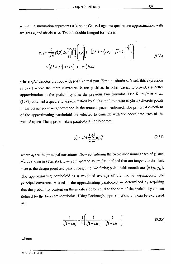
Chapter 9.Reliability 359
where the summation represents a k-point Gauss-Laguerre quadrature approximation with
weights Wj and abscissas Sj. Tvedt's double-integral formula is:
(9.33)
1
X (;32 +2S)2 exp(- s - u 2}tsdu
where rp(.) denotes the root with positive real part. For a quadratic safe set, this expression
is exact where the main curvatures ki are positive. In other cases, it provides a better
approximation to the probability than the previous two formulas. Der Kiureghian et al.
(1987) obtained a quadratic approximation by fitting the limit state at (2n-n) discrete points
in the design point neighbourhood in the rotated space mentioned. The principal directions
of the approximating paraboloid are selected to coincide with the coordinate axes of the
rotated space. The approximating paraboloid then becomes:
1 n-l, ,,'2YII =P+ 2~aiYi (9.34)
where a, are the principal curvatures. Now considering the two-dimensional space of Yi' and
y'n. as shown in (Fig. 9.9). Two semi-parabolas are first defined that are tangent to the limit
state at the design point and pass through the two fitting points with coordinates(±kp,77±i)'
The approximating paraboloid is a weighted average of the two semi-parabolas. The
principal curvatures a, used in the approximating paraboloid are determined by requiring
that the probability content on the unsafe side be equal to the sum of the probability content
defined by the two semi-parabolas. Using Breitung's approximation, this can be expressed
as:
(9.35)
where:
Moatsos, I. 2005

Chapter 9.Reliability 360
(9.36)
are the curvatures of the two semi-parabolas. As the principal directions of this point-fitted
paraboloid are assumed to coincide with the coordinate aces in the rotated space, the effect
of second-order cross-derivative forms is ignored and hence less computational effort is
required. For a problem with n variables, at most four deterministic runs per fitting point are
required with a total of 8(n-l) computations to define the paraboloid completely. On the
other hand, the formulas of Breitung and Tvedt imply curvature-fitted paraboloids, and
require and complete second-order deri vati ve matrix, requiring a total of 2(n-l/
computations using a central difference scheme, and n(n+l)l2 computations using a
forwards difference scheme. This difference in the amount of computation becomes
significant for problems with large numbers of random variables and should not really be an
issue during this study but nevertheless it should be noted for use but future readers of this
study.
It should also be emphasised that all methods mentioned so far, the original variables
(which can in some cases be correlated and nonnormal) are transformed to an equivalent
uncorrelated standard normal space to search for the minimum distance point on the limit
state surface. It is not necessary to make such a transformation as Breitung (1989)
developed a procedure that maximizes the 'loglikelihood' function of the probability
distribution in the original space. Second-order approximations to the limit state surface are
then constructed at these maximum likelihood points.
9.6 Time Dependent Reliability
In general, the loads which are applied to a structure fluctuate with time and are of uncertain
value at any point in time. This is carried over directly to the load effects (or internal
actions) S. In a similar fashion the structural resistance R will be a function of time (but not
fluctuating) as a result of deterioration and similar actions. Loads have a tendency to
increase, and resistances to decrease, with time and in most cases uncertainty in both
quantities increases with times. Hence the probability density functions is( ) and iR( )
become wider and flatter with time and the mean values of Sand R also change with time.
Moatsos, I. 2005

Chapter 9.Reliability 361
The general reliability problem can be seen illustrated in (Fig. 9.10). The safety limit state
will be violated whenever, at any time t:
R{t}- S{t}< 0 or ~~:~< I (9.37)
The probability of this occurring for anyone load application (or load cycle) is the
probability of limit state violation, or simply the probability of failure PI' Roughly it may be
represented by the amount of overlap of the probability density functions fR and fs in (Fig.
9.10). Since this overlap may vary with time, PI also may be a function of time but in many
situations it is convenient to assume that neither Q nor S is a function of time as in the case
of the load Q being applied once only to the structure and the probability of limit state
violation is sought for that load application only. However, if the load is applied for a large
number of times and R is taken as constant, then it is the maximum value of that load within
a given time interval [0, TJ which is of interest. It can then be assumed that the structure can
fail under the once only application of this maximum load. In this case the load is more
properly presented by an extreme value distribution (Me1chers, 2001) such as the Gumbel
(EV-I) or the Frechet (EV-II). If this is done, the effect of time may now be ignored in the
reliability calculations but this approach is not satisfactory when more than one load is
involved or when the resistance changes with time.
The elementary reliability problem as stated in (Eq. 9.1) in 'stochastic' or 'time-variant'
terms with a resistance R(t) and a load effect Set), at time t becomes:
P f (t) = P[R{t) ~ S{t)] (9.38)
If the instantaneous probability density functions jijr) and fit) of R(t) and Set) respectively
are known, the instantaneous failure probability pjt) can be obtained from the convolution
integral (Eq. 9.6). Schematically, the changes in fRet), fit) and pjt) with time can be
depicted in (Fig. 9.10).
Now (Eq. 9.38) only has meaning if the load effect Set) increases in value at time t
(otherwise failure could have occurred earlier) or if the random load effect is re-applied
Moatsos, I.2005

Chapter 9.Reliability 362
precisely at this time. Failure could not occur precisely at the very instant of time t
(assuming of course that at time less than t the member was safe). We can conclude hence
that a change in load or load effect is required if:
1. There are discrete load changes
2. For continuous time-varying loads, an arbitrary small increment (i, in time, is
considered instead of an instantaneous time t.
As a result of this we can hence formulate:
p/t)= ffx(,) [X (t)]dx (t)G[X(I)~O
(9.39)
which in two-dimensional space may be represented according to (Fig. 9.1) for any given
time t. As mentioned already X(t) is a vector of the basic variables. In principle though, the
instantaneous failure probability, as formulated in (Eq. 9.38) and (Eq. 9.39) can be
integrated over an interval of time [O,tJ to obtain the failure probability over that period. In
practice however, the instantaneous value of pit) usually is correlated to the value
p f (t + (i), (i ~ 0, since typically the processes X(t) themselves are correlated in time. This
can be easily identified in a typical 'sample' function or 'realization' of a random process
load effect, as illustrated in (Fig. 9.11).
The classical approach according to MeIchers (2001) is to consider the integration
transformed to the load or load effect process, which is often assumed to be represented,
over the total time period, by an extreme value distribution. The resistance is assumed
essentially time invariant. This approach is (often referred to as 'classical' reliability) forms
the basis of this study. A refinement is to consider shorter periods of time, such as in the
duration of a storm or a year, and to apply extreme value theory within that period. Simple
ideas similar to the concept of the return period then can be used to determine the failure
probability over the lifetime of the structure. Such type of analysis is often preferred for
practical reliability analysis of structures such as offshore platforms subject to definable and
discrete loading events.
Moatsos, I.2005

Chapter 9.Reliability 363
A somewhat different approach to the problem is to consider the safety margin associated
with (Eq. 9.38) as:
z{t) = R{t)- S{t) (9.40)
and to establish the probability that Z(t) becomes zero or less in the lifetime tt. of the
structure. This constitutes a so-called 'crossing' problem. The time at which Z(t) becomes
less than zero for the first time is called the 'time to failure' (Fig. 9.12) and is a random
variable. The probability that Z{t):::;;0 occurs during tt. is called the 'first-passage'
probability. The corresponding situation in two-variable space is illustrated in (Fig. 9.13).
The probability that the vector process X(t) will leave the safe region G(x»D (the
probability that an 'out-crossing' will occur) during the structural lifetime tt. is again in the
so called 'first-passage' probability. This is equal to the probability of failure of the
structure since failure is defined by G{X):::;; O. The first passage concept is more general that
the classical approaches as there is no restriction on the form of G(X). However, the
determination of the first passage probability and a proper understanding of the concept of
stochastic processes as described in (Chapter 8). For the basic reliability problem to be
applicable in the cases of more than one load or load effect it is necessary to combine two or
more load effects into an equivalent load effect as it is extensively described in (Chapter 8).
9.7 Time-Variant Component Reliability
Time-variant reliability is more difficult to compute that time-invariant component
reliability. In this case one is not interested in the time dependent failure probability
function Pjt) where t is treated as a parameter but in quantities like the probability of first
passage into the failure domain, the total duration of individual exceedances and other
related criteria. The quantity
N(t) = fix (x,t)d.xg(X.l )so
(9.41)
is rather denoted by non-availability so that,
A(t)= 1-N(t) (9.42)
Moatsos, I. 2005
Chapter 9.Reliability 364
is the availability. Both quantities can be easily determined.
For the determination of Time-Variant Component Reliability of the TankerIFPSO
structures analysed in this Thesis, STRUREL(RCP, 1999) software was used, developed by
RCP Reliability Consulting, Munich Germany and specifically its COMREL- TV Version
7.0 component. COMREL-TI can only handle criteria of the first mentioned type. In
principle the basic formulation then is
(9.43)
where T is the random time of exit into the failure domain and [0, tl is the considered time
interval. If the component does not fail at time t=0 failure occurs at a random time and the
distribution function of T must be known. Unfortunately this is rarely the case. Exceptions
are the failure times of non-structural components (electrical or other) where often rich
statistical material is available. Then it is also possible to use a time-invariant approach
because the limit state will simply be:
g{x}= T -1< 0 (9.44)
In all other cases T, must be inferred from the characteristics of the random process
affecting the performance of the component. T must be considered as a first passage time,
i.e. is the time where the component enters the failure domain for the first time given that
the component was in the safe state at time 1=0. Exact first passage time distributions are
known for only very few types of processes which generally are of little practical interest.
In COMREL-TV the so called out crossing approach is implemented for the determination
of the probability of first passage failure. As in time-invariant component reliability there
exists a state function depending on random vectors and on random process variables. More
specifically, COMREL-TV distinguishes between three types of variables:
• R is a vector of random variables as in time-invariant reliability. Its distribution
parameters can be deterministic functions of time. This vector is used to model
Moatsos, I.2005

Chapter 9.Reliability 365
resistance variables. The most important characteristics of this type of variable is
that they are non-ergodic.
• Q is a vector of stationary or ergodic sequences. Usually, it is used to model long-
term variations in time (traffic, sea states, wind velocity regimes, etc.). Quite in
general these variables determine the fluctuating parameters of the random process
variables described next.
• S is a vector of (sufficient mixing) not necessarily stationary random process
variables whose parameters can depend on Q and/or R. The vector S is further
subdivided into:
o A vector J of rectangular wave renewal processes
o A vector D of differentiable processes (Gaussian and non-Gaussian)
The safe state, limit state and failure state of the component is defined for:
g(r,q,s(t ),t) > 0g(r,q,s(t ),t) = 0g(r,q,s(t ),t) ~ 0
(9.45)
and the state function can contain time as a parameter too.
A rate of out-crossings into the failure domain conditional on q and r can be defined:
v+ (F, 1'1 r.q )lim4~o.!_ p({g(S(1'), 1'1 r,q) > O}(l{g(S(1' +~),1'+ ~ I r,q) s o})~
. (9.46)
F denotes the failure domain {g(s(t),tI r,q)~O}. In order to exist it is necessary that the
limiting operation can be performed. This excludes certain processes which fluctuate too
rapidly in time. Further in small time interval there is at most one crossing. The probability
of more than one crossing is negligible small. Then the process of crossings is cal1ed a
regular point process.
The mean number of crossings in the time interval [tj, t21 conditional on q and r can be
determined from,
Moatsos, I. 2005

Chapter 9.Reliability 366
'2E[N+(tpt2)1 q,r]= JV+(F,rl q,r)dr (9.47)
Thus, the time-dependent out-crossing rates are additive for a regular process. Then, it has
been shown by Bolotin (1981) that an upper bound to the conditional probability is:
(9.48)
If further the process is strongly mixing it is asymptotically for Pt (t1 ,t21 q, r) ~ 0 according
to Cramer and Leadbetter (1967):
(9.49)
The conditions can be removed by integration. Whereas the expectation operation with
respect to the condition on q can be performed inside the exponent by making use of the
ergodic property of Q, it cannot be done with respect to the R-variables.
(9.50)
Schall et al. (1991) showed that for the upper bound solution
(9.51)
A lower bound is also available but is not particularly of interest in this study and the
detailed formulation can be found in (RCP, 1999).
COMREL-TV offers for the general case upper bound solution together with a, not always
close, lower bound solution. In most cases PI.!l) is negligible small. It will always be
calculated if the upper bound solution is chosen. For two special cases the expectation with
respect to R in the asymptotic approximation can also be performed by simple importance
sampling Monte Carlo integration. For the upper bound solution R-variables are treated like
Q-variables and for all computations a probability distribution transformation into standard
Moatsos, I.2005

Chapter 9.Reliability 367
space, as in time-invariant reliability is performed. Unfortunately as it can be seen from
Engelund et al. (1995) the out-crossing approach cannot be improved easily.
For all computations a probability distribution transformation into standard space as in time-
invariant reliability is performed. It is also assumed that random processes start with
random initial conditions throughout. Since it has been found that asymptotic solutions also
with respect to the time integration (RCP, 1999) are too inaccurate under non-asymptotic
conditions and pure first-order solutions are rarely satisfying, a compromise between
asymptotic solutions and somewhat more exact time integration schemes in implemented in
COMREL-TV. In all cases it is assured that the solutions implemented converge to
asymptotic solutions under appropriate conditions and the stationary or non-stationary
solution for linear failure surfaces (int the standard space) is always recovered. FORM
options, although generally available, are not recommended and the computational effort is
significantly larger than for time-invariant reliability problems, especially when general
intermittent processes are to be considered. The methods described above are of limited use
for dynamic systems. Then, it is not only difficult to assess the auto- and cross-correlation
structure of the interesting output quantities. Also, the combination of rectangular waves as
well as intermittencies as described above make little sense if passed through a dynamic
structure. The transient phases of the system generally lead to an oscillatory behaviour of
system states. Therefore, the time integration schemes with respect to time require a certain
amount of modifications.
9.8 Monte Carlo Simulation
9.8.1 Introduction
There are essentially three ways in which multidimensional integration can be performed
for structural reliability purposes:
1. Direct Integration (possible only in a very limited number of special cases).
2. Numerical Integration (Monet Carlo techniques).
3. Obviating the integration through transforming the integrand to a multi-normal joint
probability density function for which some special results are immediately
available (techniques which fall beyond the purposes of this study).
Moatsos, I. 2005

Chapter 9.Reliability 368
In practice, limit state functions usually are of more general form than linear functions and
random variables associated with these limit state functions are unlikely all to be normally
distributed random variables. Methods have developed to deal with these issues and
integration methods would be suitable, in principle. However, because of the rapidly
increasing computational demands as the number of dimensions increases (the so-caIled
"curse of dimensionality"), numerical integration of the classic variety has not found great
favour in reliability computations. Instead, researchers in the field have opted for methods
developed for other large integrations problems (Kahn, 1956) and described in standards
texts (Stroud, 1971) dealing with numerical integration. These methods are the simulation
or Monte Carlo Methods and they form a class of approximate numerical solutions to the
probability integral:
PI = p[G(X)~O]= J... JfJx}dxG(Xf-;O
(9.52)
applicable to problems for which the limit state function G(x)=O may have any form, and
for which the probabilistic description of the random variables Xi is unrestricted.
As the name implies, Monte Carlo Simulation techniques involve sampling at random to
simulate artificially a large number of experiments and to observe the result. In the case of
analysis for structural reliability, this means, in the simplest approach, sampling each
random variable Xi, randomly to give a sampling value Xi. The limit state function
G(x) = 0 is then checked. If the limit state is violated, the structure or structural element has
failed. The experiment is repeated many times, each time with a randomly chosen vector of
values. If N trials are conducted, the probability of failure is given approximately by:
(9.53)
where n(G(x;) ~ 0) denotes the number of trials n for which (G(x;) ~ 0). Obviously the
number N of trials required is related to the desired accuracy of Pt·
Moatsos, I. 2005

Chapter 9.Reliability 369
It is clear that in the Monte Carlo method a game of chance is constructed from known
probabilistic properties in order to solve the problem many times over, and from that to
deduce the required result, which in our case is the failure probability. In principle, Monte
Carlo Methods are only worth exploiting when the number of trials or simulations is less
than the number of integration points required in numerical integration. This is achieved for
higher dimensions by replacing the systematic selection of points by random selection,
under the assumption that the points so selected will be some way unbiased in their
representation of the function being integrated.
To apply Monte Carlo techniques to structural reliability problems it is necessary:
1. To develop systematic methods for numerical sampling of the basic variables X.
2. To select an appropriate economical and reliable simulation technique or sampling
strategy.
3. To consider the effect of the complexity of calculating G(x;) and the number of
basic variables on the simulation technique used.
4. For a given simulation technique to be able to determine the amount of sampling
required to obtain a reasonable estimate of PI'
Itmay be necessary also to deal with dependence between all or some of the basic variables.
9.8.2 Random Variate Generation
Basic variables only seldom have a uniform distribution. A sample value for a basic variable
with a given (non-uniform) distribution is called a random variate and can be obtained by a
number of mathematical techniques. The most general of these is the inverse transform
method. If we consider the basic variable Xi for which the cumulative distribution function-
Fx;(xj) must, by definition, lie in the range (0,1) as it can be seen in (Fig. 9.14).
The inverse transform technique is to generate a uniformly distributed random number
Ii(O ~ Ii ~ 1) and equate this to as Fx;(xj):
(9.54)
Moatsos, I. 2005

Chapter 9.Reliability 370
This uniquely fixes the sample value Xi = Xi' provided that an analytic expression for the
inverse F:r~1 (r;) exists (as it does for the Weibull, Exponential, Gumbell and rectangularI
distributions among others). In these cases the inverse transform method is likely to be the
most efficient technique. The technique can also be applied to basic variables whose
cumulative distribution function has been obtained from direct observation.
9.8.3 Direct Sampling - Crude Monte Carlo
The technique as described in Section (9.6.1) is the simplest Monte Carlo approach for
reliability problem but certainly not the most efficient. The basis for its application is lies in
the traditional probability of limit state violation and may be expressed as:
(9.55)
where If J is an indicator function which equals 1 if f J is true and 0 if f J is false. Thus the
indicator function identifies the integration domain. If X j represents the jth vector of
random observations fromfx( ), it follows directly from sample statistics that
(9.56)
is an unbiased estimator of 1. Thus the expression in (Eq, 9.56) can provide a direct estimate
of Pt. In exploiting this procedure, three maters are of interest:
1. How to extract most information from the simulation points.
2. How many simulation points are needed for a given accuracy.
3. How to improve the sampling technique to obtain greater accuracy.
Let us consider all of these so as to have a complete view of how we can utilise this
technique most efficiently. It would be important to note that one way that the results of the
mentioned sampling technique may be represented is as a cumulative distribution function
Fa(g) as it can be see in (Fig. 9.15):
Moatsos, 1. 2005

Chapter 9.Reliability 371
Obviously, much of the range of Fc(g) is of little interest, since the structure or member is
(usually) amply safe. To estimate the failure probability the region for which G( ):::;;0,
which represents failure is clearly of most interest.
The estimation of Pf using (Eq. 9.56) can be improved by fitting an appropriate distribution
function through the points which G( ):::;;0, i.e. the left hand tail in (Fig. 9.15). However,
the choice of an appropriate distribution function may be difficult. Distributions which
could be of use for this purpose are the Johnson and Pearson distribution systems (Elderton
& Johnson, 1969). However it is possible that the parameters of the distribution function are
rather sensitive to extreme results in the region G( ):::;;O. In that case the choice of
distribution function parameters may not stabilize until N is quite large (Moses & Kinser,
1967). Rather than fitting a single distribution to the sample points, it is possible to fit a
sequence of distributions and to optimize their parameters to give a best-fit to the sample
points (Grigoriu, 1983).
9.8.4 Number of Samples Required
An estimate of the number of simulations required for a given confidence level may be
made as follows. Since G(X) is a random variable in X, the indicator function I[G(X):::;; 0] is
also a random variable, albeit with only two possible outcomes. It follows from the central
limit theorem that the distribution of 1] given by the sum of independent sample function
(Eq. 9.56) approaches a normal distribution as N ~ 00. The mean of this distribution is:
N
E(1I)= LE[/(G:::;;O)]=E[/(G:::;;O)];=1
(9.57)
which is equal to J, while the variance is given by:
N 1 a2
a;i =L -2 var[/( G s0)]= /(GSO)
;=1 N N(9.58)
which shows that the standard deviation of 1] and hence of the Monte Carlo estimate varies
directly with the standard deviation of I( ) and inversely with NI12• These observations are
Moatsos, 1. 2005

Chapter 9.Reliability 372
important in determining the number of simulations required for a particular level of
confidence. To actually calculate confidence levels, an estimate of ~ ( ) is required. The
variance is given:
(9.59)
so that the sample variance is given by:
(9.60)
where the last { } term is simply the mean (Eq. 9.60) or, by (Eq. 9.59) the estimate J: of PI'
On the basis that the central limit theorem applies, the following confidence statement can
be given for the number (h) of trails in which failure occurs:
p(- ka < 11 - J.l < +keY) = C (9.61)
where J.l is the expected value of 11 given by (Eq. 9.60) and eris given by (Eq. 9.58).
9.9 The Limit State Equation & Stochastic Model
As described in Section (9.2) of this chapter, according to the basic concept of the structural
theory of reliability analysis, the first step toward evaluating the reliability of a structure is
to decide on the relevant load and resistance parameters, cal1ed the basic variables Xi, and
the functional relationship among them. This can be described in mathematical terms as:
(9.62)
The failure surface or performance function of the limit stet of interest can then be defined
as Z=O. This is the boundary between the safe and unsafe regions in the design parameter
space, and it also represents a state beyond which a structure can no longer fulfil the
function for which it was designed. The limit state equation (performance function) plays an
important role in the development of structural reliability analysis methods. A limit state
Moatsos, I. 2005

Chapter 9.Reliability 373
function can be an implicit or explicit function of basic random variables and it can be in a
simple or complicated form.
In limit state analysis the classic treatment of the problem considers the hull to be a box
beam experiencing pure bending. The problem is then just a simple beam in bending and
can be written as:
(9.63)
where Mu is the ultimate bending moment, Z is the sections modulus of the vessel at the
section of interest, and O'y is the tensile yield stress of the vessel material. The limit state for
hull girder bending can be expressed as already mentioned by:
G=R-L (9.64)
where G is the performance function, R is the resistance and L is the load. When G:::;;0 the
structure fails; when G>O the structure survives. When expressed in terms of (Eq. 9.63) a
nonlinear performance function is the result. This form separates the load into wave and
still-water bending moments, Mw and Msw, respectively; and G is expressed in units of the
bending moments:
(9.65)
Here the product O'yZ represents the resistance strength of the system. The still-water
bending moment Msw could be considered as one load effect and the wave-induced bending
moment Mw as another load effect. Each will have its own distributions type, mean vale and
coefficient of variation. Each will represent the distribution of the loading in the lifetime of
the vessel. Although this is not a very sophisticated manner of combining load effects, it is
useful to show the flexibility of simulation methods.
As described in (Section 9.3) of this Chapter when describing the nature of uncertainties, in
reliability analyses, all design variables are in principle regarded as random variables with
certain level of uncertainties. The probabilistic characteristics of the random variables can
Moatsos, I. 2005

Chapter 9.Reliability 374
be quantified by regression analysis based on statistical observations. In addition to mean
and standard deviation of the variables, the type of the probability distribution has a crucial
impact in reliability analysis, since the predicted reliability significantly depends on its tail
shape. When detailed information for the particular random variable is not available, a
relevant type of the probability distribution may be presumed. Normal or log-normal
distribution is typically adopted for analysis of ship structural reliability (Paik & Frieze,
200 1), the former being relevant for strength variables, while the latter is required for load
variables or the variables which always take positive values.
As stated in Chapter 8, traditionally, the total bending moment M, is defined as the extreme
algebraic sum of still water moment Msw and wave-induced moment Mw, as follows:
(9.66)
When we adopt this approach for calculation of the total bending moment, the failure
condition associated with hull girder collapse can be written as:
(9.67)
where Mu is the random variable representing the hull girder ultimate strength, Msw and Mw
are random variables representing the still water or wave induced bending moments, Xu the
random variable representing the model uncertainties associated with hull girder ultimate
strength determination. and Xsw, Xw the random variables representing the model
uncertainties associated with still water or wave-induced bending moment predictions. The
failure conditions (Eq, 9.67) portrays the limit state function for hull girder collapse as
function of six variables. However Mu involves parameters related to geometric and material
properties (plate thickness, yield strength, Young's modulus) of the various structural
members in a functional form. The value of member thickness at any particular time will be
a function of time-variant structural degradation due to corrosion or fatigue when the safety
and reliability of aging structures is considered. Also the wave-induced bending moment
involves random parameters related to sea states, such as the wave height, and operational
condition, such as the ship speed and heading. Therefore, the number of random variables
considered in the limit state function is normally significantly more than in (Eq. 9.67).
Moatsos, I. 2005

Chapter 9.Reliability 375
The mean still water bending moment Msw is normally calculated by substituting the mean
values of ship principal particulars into the design formula provided by a Classification
Society. The Msw so obtained is actually an extreme design value, and its use as a mean
value is usually pessimistic. The long-term variability in still water will depend on the ship
type, loading condition, voyage routes, changes in cargo loading patterns from voyage to
voyage, etc. The coefficient of variation (COV) associated with still water bending moment
us normally large and can be as high as 40% (Mansour & Hovem, 1994) and is usually
assumed to follow the normal distribution. To the extent that the mean of this distribution is
taken to coincide with the design still water bending moment value adopting a 40% COY
would be quite pessimistic. In a short-term analysis of the wave-induced bending moment
the inherent COY of the extreme can be shown to be approximately 10% (Paik & Frieze,
2(01). The mean value of the ultimate strength of the hull is calculated assuming that the
average value of the yield strength of the material is the Classification Society rule
minimum value, which can be pessimistic by perhaps 15%. For mean values of the plate
(initial) thickness and modulus of elasticity of the material, conventional nominal values can
be used. Other details of the statistical characterization of the inherent uncertainties
associated with plate thickness, yield strength and Young's modulus can be taken as
indicated in (Table 9.2) as indicated in (Mansour & Hovem, 1994). The time variant
strength can be considered to be normally distributed with a COY of 10%. Within the
context of the reliability analysis procedures used, such a simplified approach to the COY of
the ultimate strength is actually not necessary because the probability of failure could have
been calculated by direct input of the applicable means, and COY s associated with
geometric and material properties. It is often assumed that the probability density function
of any random variable representing a model uncertainty follows the normal distribution.
Typical means and COVs for model uncertainties used for such calculation can be founding
(Table 9.3) according to Mansour & Hovem (1994). It would be worth noting in this case
that the uncertainties listed in (Table 9.3) are actually estimated guesses and whenever
better information is available (Frieze & Plane, 1987) it is possible to refine such values.
Mansour & Hovem (1994) evaluated the reliability of ship hull girder strength with the
variation in the correlation coefficient between the still water and the wave-induced
components and they concluded that the interaction of these two load components might be
Moatsos, I.2005

Chapter 9.Reliability 376
usually ignored. The two loading components were considered independent and Ferry
Borges-Castanheta load combination method was applied to obtain a load combination
factor. The failure surface for the ultimate longitudinal strength of the hull girder was
defined as;
g(X) = Xu Mu - Mse - V'W Xnl Xw Mwe = 0 (9.66)
Mu, represents the ultimate bending moment capacity of the hull girders and a factor Xu,
(uncertainty on ultimate strength) is introduced in the failure surface equation in order to
account for the uncertainties in the ultimate strength model and in the material properties.
Teixeira (1997) estimated a realistic COV for the total uncertainty on ultimate strength to be
10%, which is in good agreement with Faulkner (1992) who proposed a COV of 10-15% for
the modelling uncertainty for flat panel collapse. Thus, Xu was assumed normally
distributed, with a mean value of 1.0 and a standard deviation of 0.10. The most probable
extreme still water bending moment, Mse, is calculated based on a mean still water moment
Msw. The still water bending moment is always hogging for this vessel. A COY of 15 %
was applied to this mean value. The load combination factor, 'lW, is introduced to account
for the low probability that the extreme still water and wave bending moments will occur at
the same instant. A factor of 0.78 for the structure analysed was obtained respectively, using
Ferry Borges-Castanheta load combination method as described in Chapter 8.
In addition to the non-linear effects, there are other uncertainties associated with the linear
strip theory programs. Different programs will use different procedures for calculating the
hydrodynamic coefficients. Dogliani et al. (1998) showed that the linear strip theory
programs generally over-predicted the wave induced bending moments at the 10-8
probability level. Shellin et al. (1996) identified large variations in long-term distributions
of midship induced loads based on transfer functions obtained by different methods. Values
of 10% for Xw (Uncertainty in wave load prediction) and 1.2 in Sagging and 0.8 in Hogging
for Xnl (Non-linear effects) were based on the previous research works carried out at
Glasgow University (Das, 1998) & (Maerli et al. 2000). Extreme vertical wave bending
moment, Mwe, was obtained by combining the short-term responses with the wave statistics
for the Fair Isle area as described in the procedure in Chapter 8. The long-term probability
Moatsos, L 2005

Chapter 9.Reliability 377
of exceedance of different wave-induced vertical bending moments was obtained, and a
Weibull distribution was fitted to the resulting distribution.
9.10 Time Invariant Reliability Results
Reliability analysis using a First Order Reliability Method (FORM) and a Second Order
Reliability Method (SORM) was performed on the structure by assuming that the ultimate
strength of the hull girder follows a Lognormal distribution with a coefficient of variation
(COV) of 10%, the wave bending moment following a Gumbel distribution with a COV of
15% and the still water bending moment a Gumbel distribution with a COV of 15%.
Although wave bending moment variations could often be in the range of 25% the 15%
figure was chosen as an initial starting point for the procedure. Reliability indices fl for the
structure in the range of temperatures examined and probabilities of failure Pt were obtained
for sagging and hogging conditions. As it can be seen in the Appendix of this Chapter (Fig.
9.16) depicts the temperature and corrosion effects in Pt in sagging condition for one of the
FPSOs analysed, and (Fig. 9.17) the similar effects on the reliability index fl.For hogging in
a similar fashion (Fig. 9.18) shows the effects in PI and (Fig. 9.19) in fl and the results
showed an obvious decrease in fl and an increase in the probability of failure as diurnal
change in temperature increased. The stochastic model used is in accordance to the
approaches used and described in Section (9.7) and can be found summarised in a tabular
form in (Table 9.4) and the limit state equation takes the form:
M" ~ Ultimate Bending Moment Capacity
A" ~ Uncertainty on Ultim.Strength
M S~ ~ Still Water Bending Moment
rp(J) ~ Load Combinat. Factor
A{J) ~ Uncertainty in Wave Load prediction
AnD} ~ Non -linear effectsM we ~ Extreme Vertical Wave Bending Moment
(9.67)
Results also show that fl values reduce following a 3rd order Polynomial trend whereas PI
values reduce following and exponential trend. In both cases the effect of temperature and
Moatsos, I. 2005

Chapter 9.Reliability 378
corrosion on the values is quite significant. Partial safety factors for the variables used in
reliability analysis could be obtained which would provide a code format for design
purposes and allow the design to be even further optimized. If a simple code format such as
¢R> YsMs +YwMw (9.68)
was assumed where (jJ, 'r.> and Yw are the partial safety factors for the strength R, the still
water bending moment Ms and Mw the wave bending moment respectively then the design
could be easily optimized. Partial safety factors shown in (Fig. 9.20) for sagging and (Fig.
9.21) for hogging, for all the variables influencing the probability of failure in the limit
state equation and for the determination of safety criteria for the structure, are obtained and
showed not to be affected by temperature changes in both sagging and hogging conditions
whereas in sagging the wave bending moment partial safety factor decreased as diurnal
temperature change increased as a result of the sign convention used that made only the
wave bending moment to have a negative effect on the limit state function.
9.11 Time Variant Reliability Results
The limit state function used and the stochastic model and the limit state function used for
the calculation of the instantaneous and time dependent through life reliability of the vessel
can be seen in (Eq. 9.69) and (Table 9.4).
(9.69)
, where MuCt) the ultimate strength as a function of the time dependent corrosion, MsCt) and
M....(t) the long term most probable values of the SWBM and VWBM, 'lfw the load
combination factor for SWBM and VWBM, Aw an uncertainty for non-linearity in the
prediction of the VWBM and Xu, xs, Xw the model uncertainties for predicting the hull girder
strength, SWBM and VWBM. Typical values for the random variables of model
uncertainties were used according to published research.
The instantaneous long term reliability of the vessel was obtained using the limit state
equation described in (Eq, 9.69) using a Second Order Reliability Method (SORM)
Moatsos, I.2005

Chapter 9.Reliability 379
approach but without taking into account of time and computing the probabilities of failure
and reliability indices by using the values that result as most probable extremes for the loads
and for each corrosion year for the ultimate strength and that are distributed according to the
stochastic model.
For the time-variant reliability results, the variance of the variables with time was taken into
account and Monte Carlo Simulation (MC) using 50.000 samples was used to compensate
for the non-linearity of the problem and provide a more accurate result. As it can be seen
from the results for one of the FPSOs analysed in (Fig. 9.22) and (Fig. 9.23) vary quite
significantly and show not to follow the mathematical trend of the corrosion model as the
probability of failure curve obtained could be fitted to a 6th order polynomial for the time
variant results and a 5th order for the instantaneous and a 4th and 3rd order respectively for
the reliability index.
9.11 Discussion-Conclusions
It is interesting to compare the results obtained with available reliability indices published in
the available literature, as summarised in (Table 9.5) for FPSO structures and (Table 9.6)
for Tanker structures. It should be noted that in the majority of the literature reviewed no
thermal effects are taken into account and in the majority of the results published, no
corrosion effects are taken into account. The reliability indices are in certain cases annual
and in other cases for a 20 year period, a fact that needs to be taken into account when
comparing the results obtained during this study with the available published literature. The
large variability in the results both from this study and the available literature suggest that
still a large amount of work is required before commonly acceptable levels of safety can be
set for the design of marine structures using reliability based approach.
The reliability concept encompasses a wide range of probabilistic thinking and analysis. It is
able to incorporate knowledge of the probabilistic aspects of design and loading, including a
factor expressing the designer's confidence in the quality of the probabilistic information. It
can accommodate empirically determined values where probabilities are not clearly known,
and it can even take into account aspects of a shipping operation that have no bearing on
strength such as the decision made by an owner to select a probability of success from all
causes, factoring in probabilities such as disastrous events as fires and collisions. In the pure
Moatsos, I. 2005

Chapter 9.Reliability 380
sense, however, structural reliability starts with a goal of reaching a sufficiently small
probability of structural failure, all other types of failure aside. Of course the quality of a
structural design depends entirely on the information going into the reliability analysis, and
the approach can produce in the most sophisticated way a "perfectly terrible" design. The
old saying about computers is equally valid for a reliability analysis: "garbage in, garbage
out".
The use of probabilistic methods in design can provide several benefits and some unique
features. As bullet points among those benefits which have already been discussed in
previous chapters of this thesis include:
• The explicit consideration and evaluation of uncertainties associated with the design
variables.
• The inclusion of all available relevant information in the design process.
• The provision of a framework of sensitivity measures.
• The provision of a means of decomposition of global safety of a structure into partial
safety factor associated with individual design variables.
• The provision of a means for achieving uniformity of safety within a given class of
structures (or specified non-uniformity).
• Minimum ambiguity when updating design criteria.
• The provision of a means to weigh variables in terms of their significance.
• The provision of a rationale for data gathering.
• The provision of guidance in novel design.
• The provision of the potential for reducing weight without loss of reliability, or the
improvement of reliability with an increase in weight. Structural reliability methods
can identify and correct overly and unduly conservative designs.
In addition to the aforementioned benefits, reliability technology lends itself for certain use
for which it is much more suitable than traditional design methods. Its use includes:
• The possibility of comparison of alternative designs, particularly in the early design
stages when several competing design concepts are considered.
• The ability to perform failure analysis of a component or system.
Moatsos, I.2005

Chapter 9.Reliability 381
• The development of a strategy for design and maintenance of structures which age
as a result of corrosion and fatigue and to determine inspection intervals.
• The ability to execute 'economic value analysis' or 'risk based economics' to
provide a design with minimum life cycle costs.
• The ability to develop a strategy for design, warranties, spare-part requirements
• In general, as a design tool to manage uncertainty in engineering problems.
The use and implementation of probabilistic methods are not without problems. Some of the
drawbacks include:
• The use of reliability analysis in safety and design processes requires more
information on the environment, loads and the properties and characteristics of the
structure than typical deterministic analyses. Often some information might no~ be
readily available or may require considerable time and effort to collect. Time and
schedule restrictions on design are usually limiting factors on the use of such
methods.
• The application of probabilistic and reliability methods usually requires some
familiarity of basic concepts in probability, reliability and statistics. Practitioners
and designers are gaining such familiarity through seminars, symposia, and special
courses. Educational institutions are also requiring more probability and statistics
courses to be taken by students at the graduate and undergraduate levels. This
however is a slow process that will take some time to produce the necessary
'infrastructure' for a routine use of reliability and probabilistic methods in design.
• On a more technical aspect, reliability analysis does not deliver what it initially
promised, that is a true measure of the reliability of a structure by a 'true and actual'
probability of failure. Instead what it delivered is 'notional probabilities' failure and
safety indices which are good only as comparative measure. Only notional values
are delivered because of the many assumptions and approximations made in the
analysis producing such probabilities and indices. These approximations,
deficiencies and assumptions, however are made, can be found not only in
probability-based design, but also in traditional design. Approximations are made in
Moatsos, I. 2005

Chapter 9.Reliability 382
the determination of loads using hydrodynamics theory and in the structural analysis
and response to the applied loads. When all such assumptions and deficiencies are
removed from the design analysis, the resulting probabilities of failure will approach
the 'true' probabilities.
In using such an approach the designer also begins to enter into areas of moral and political
implications. The question arises of who will decide what the probability of failure should
be, of whether the public will understand that it never can be reduced to zero and that there
is an ever-increasing cost associated with each little reduction of risk? Casualty statistics
will give an indication of what society has traditionally accepted in structural failure rates
for vessels, but once a number is assigned to the probability of failure, there will be
tremendous pressure to make it lower from various interested and affected parties. To add
the previous questions, even more questions arise such as what protection can be afforded
and who is responsible for such decision when a ship bears out the statistical nature of the
analysis by going down, whether different types of vessels should have different structural
reliability and more importantly who is the person who decides what is the value of a
human life.
Phenomenological, modeling, prediction and physical, statistical and human factor
uncertainties will all be affected as a result of global climate changes. In case of
phenomenological uncertainties resulting from highly uncertain changes in temperature or
loading, the consequences will clearly be difficult to formulate and measure. For modeling
uncertainties the lack of availability of data in measuring the effect of extreme temperature
changes resulting from global climate change also makes it difficult to quantify the effects.
However the overall prediction uncertainties are more associated with how and when such
extreme meteorological changes might occur and not as much as with the effect they will
have on the engineering system but nevertheless their association with the entire process
should be noted. Physical and statistical uncertainties again are affected by the lack of
measurement of such type of phenomena on marine structures but the effect of climate
change could perhaps be more easily demonstrated by looking at the climate change trends.
These could perhaps be incorporated into reliability analysis by, as already discussed,
having the mean and variance of the strength, thermal stress or loading variables (depending
on how the limit state equation is formulated) themselves being random variables based on
statistical analysis of the trends encountered so far. Finally in terms of human factor
Moatsos.L 2005

Chapter 9.Reliability 383
uncertainties the fact that nature and the environment affect human behavior is
unquestionable. Human behavior and emotions can vary significantly depending on the
surrounding climatologically conditions thus having a direct effect on the quality of
construction and design of any engineering structure but again to demonstrate the effect of
climate change into such type of uncertainty would require additional research data and
study which falls beyond the scope of this research.
The effect of global warming on reliability analysis is hence made evident from the above.
In the absence of measured data such as variability of occurrence of extreme temperature
effects on marine structures or the measurement of temperature and thermal stresses on
ships or offshore structures the exact effect of global warming in the analysis carried out in
this thesis becomes an extremely tedious and complicated task that falls well beyond the
scope of this study but nevertheless should be pointed out as a means of perhaps linking
future research with the results, ideas and suggestions that have been documented during
this study.
Fortunately, the difficult and gloomy thoughts expressed above are just the bottom line of a
reliability analysis and issues that will eventually have to be addressed especially by
regulatory bodies and governments. At the same time, there are other benefits of reliability
analysis that can and are achieved right now such as the fact that reliability concepts can
deal with the probability of failure of structural components as wen as the overall structure.
Such an approach enables designers to make direct comparisons on the basis of overall
strength between different structural components or arrangements under different loading
conditions to evaluate their relative strengths from the perspective of a lifetime of operation.
Trade offs between strength, redundancy, and serviceability can be made to optimize
structures from the standpoint of strength, weight, cost, or any other parameter. By means of
reliability analysis, a more thorough understanding of loads, structural analysis, and
material behaviour can provide more efficient ship structures, resulting in lighter scantlings
with no reduction n the overall level of structural safety.
Moatsos,l. 2005

Chapter 9.Reliability 384
Chapter 9, Reference:Ang, A.H.-S., Tang, W.H. 1975, Probability Concepts in Engineering Planning and Design
Vol. I:Basic Principles, J. Wiley & Sons Ltd., New York.Ang, A.H.-S., Tang, W.H. 1984, Probability Concepts in Engineering Planning and Design
Vol. 2:Design, Risk & Relibaility, J. Wiley & Sons Ltd., New York.
Bolotin, V.V. 1981, "Wahrscheinlichkeitsmethoden zur Berechnung von Konstruktionen",VEB Verlagfur Bauwesen, Berlin (in German).
Breitung, K. 1984, "Assymptotic Approximations for Multinormal Integrals", Journal ofEngineering Mechanics Division of American Society of Civil Engineers, No. 110(3), pp357-366.
Breitung, K. 1989, "Probability Approximations by Loglikelihood Maximization", Seminarfur Angewandte Stochastik, Institute fur Statistic and Wissenschaftstheoric, Seric StoNr.6, University of Munich, Munich ,Germany.
Cassela, G., Dogliani, M., Guedes Soares, C. 1996, "Reliability Based design of the PrimaryStructure of Oil Tankers", Proceedings of the International Offshore Mechanics andArctic Engineering Symposium (OMAE 96), Vol. 2, pp 217-224.
Cassela, G., Dogliani, M., Guedes Soares, C. 1997, "Reliability Based design of the PrimaryStructure of Oil Tankers", Journal of Offshore Mechanics and Arctic Engineering, Vol.119, pp 263-269.
Casela, G., Rizzuto, E. 1998, "Second-level Reliability Analysis of a Double Hull OilTanker", Marine Structures, Vol. 11(9), pp 373-399.
Chen, H.H., Hsein, Y.J., Conlon, J.P., Liu, D. 1993, "New Approach for the Design andEvaluation of Double Hull Tanker Structures", Transactions of the Society of NavalArchitects and Marine Engineers (SNAME), Vol. 1010, pp 215-245.
Chen, X., Lind, N.C. 1982, "A New Method for Fast Proability Integration", University ofWaterloo, Paper No. 171, Waterloo, Canada.
Cornell, C.A. 1969, "A Probability-Based Structural Code", Journal of the AmericanConcrete Institute, No. 66(12), pp 974-985.
Cramer, H., Leadbetter, M.R. 1967, Stationary and Related Processes, Chapman & Hall,London UK.
Das, P.K., 1988, "The Application of Reliability Analysis Techniques towards a RationalDesign of Ship Hull Girders", DERA, Report, Dunfermline, Scotland, UK.
Der Kiureghian, A., Lin, H.Z., Hwang, S.P. 1987, "Second-Order ReliabilityApproximations", Journal of Engineering Mechanics Division of American Society ofCivil Engineers, No. 113(8), pp 1208-1225.
Ditlevsen, O. 1979a, "Generalised Second Moment Reliability Index", Journal of StructuralMechanics, No. 7(4), pp 435-451.
Ditlevsen, O. 1979b, "Narrow Reliability Bounds for Structural Systems", Journal ofStructural Mechanics, No. 7(4), pp 453-472.
Det Norske Veritas, 1992, Structural Reliability Analysis of Marine Structures, DNVClassification Notes 30:6.
Moatsos, I. 2005

Chapter 9.Reliability 385
Dogliani, M., Casells, G., Guedes Soares, C., 1998, "SHIPREL-Reliability Methods forShip Structural Design", BRITElEURAM Project 9559, Lisbon.
Elderton, W.P., Johnson, M.L. 1969, Systems of Frequency Curves, Cambridge UniversityPress.
Engelund, S., Rackwitz, R., Lange, C. 1995, "Approximations of First Passage Times forDifferentiable Processes Based on Higher Order Threshold Crossings", ProbabilisticEngineering Mechanics, Vol. 10, No.1, pp-53-60.
Faulkner, D., 1992, "Introduction to Probability Methods in Advanced Design for Ships andOffshore Floating Systems", Dept. of Naval Architecture and Ocean Engineering,Report, University of Glasgow, Glasgow, Scotland, UK.
Fiessler, B., Neumann, H.J., Rackwitz, R. 1979, "Quadratic Limit States in StructuralReliability", Journal of Engineering Mechanics Division of American Society of CivilEngineers, No. 105(4), pp 661-676.
Frieze, P.A., Plane, C.A. 1987, "Partial Safety Factor Evaluation for some Aspects ofBuckling of Offshore Structures-A Pilot Study", HMSO, BS 5400 Part 3, London UK.
Frieze, P.A. et al. 1991, "Report of Committee V.1. Applied Design", Proceedings of theJ t" International Ship and Offshore Structure Congress, Hsu, P.H. & Wu Y.S. (Eds),Elsevier Applied Science, London.
Grigoriu, M. 1983, "Approximate Analysis of Complex Reliability Problems", StructuralSafety, Vol. 1 (4), pp 277-288.
Guedes Soares, C., Texeira, A.P. 2000, "Structural Reliability of Two Bulk CarrierDesigns", Marine Structures, Vol. 13(2), pp 107-128.
Haldar, A., Mahadevan S. 2000a, Reliability Assessment Using Stochastic Finite ElementAnalysis, J. Wiley & Sons Ltd, New York.
Haldar, A., Mahadevan S. 2000b, Probability, Reliability and Statistical Methods inEngineering Design, J. Wiley & Sons Ltd, New York.
Hasofer, A.M., Lind, N.C. 1974, "Exact & Invariant Second Moment Code Format",Journal of the Engineering Mechanics Division of the American Society of CivilEngineers, loo(EM1), pp 111-121.
Kahn, H .• 1956 "Use of Different Monte Carlo Techniques", Proceedings of the Symposiumon Monte Carlo Methods, H.A. Meyer (Ed), John Wiley and Sons, New York. pp 149-190.
Leheta, H.W., Mansour, A.E. 1997, "Reliability Based Method for Optimal StructuralDesign of Stiffened Panels", Marine Structures, Vol. 10(5), pp 323-352.
Madsen, H.O., Krenk, S., Lind, N.C. 1986, Methods of Structural Safety, Englewood Cliffs,Prentice Hall, New Jersey.
Maerli, A., Das, P.K. 1998, "Structural Reliability Analysis of FPSOs, Towards a RationalDesign Procedure", Dept. of Naval Architecture and Ocean Engineering, Unversity ofGlasgow, Report No. NAOE-98-30, Glasgow, Scotland, UK.
Maerli, A., Das, P.K., Smith, S.N., 2000, "A rationalisation of Failure Surface Equation forthe Reliability Analysis of FPSO Structures", International Shipbuilding Progress, No.450, pp 215-225.
Moatsos, I. 2005

Chapter 9.Reliability 386
Mansour, A. E. & Hovem, L. 1994, "Probability-Based Ship Structural Safety Analysis",Journal of Ship Research, Vol. 38, no.4, pp 329-339.
Mansour, A.E., Lin, M., Hovem, L. and ThayambaIli, A. 1993, "Probability-Based ShipDesign Procedures: A Demonstration", Ship Structure Committee, Report No. SSC-368.
Mansour, A.E., Wirsching, P.H. 1995, "Sensitivity Factors and their Application to MarineStructures", Marine Structures, Vol. 8(3), pp 229-255.
Mansour, A.E., Wirsching, P.H., Lucket, M.D., Plumpton, A.M., Lin, Y.H. 1997,"Structural Safety of Ships", Transactions of the Society of Naval Architects and MarineEngineers (SNAME), Vol. 105, pp 61-98.
Melchers, R.E. 200 I, Structural Reliability Analysis and Prediction, 2nd Edition, John Wiley& Sons Ltd, New York.
Moses, F., Kinser, D.E. 1967, "Analysis of Structural Reliability", Journal of the StructuralDivision of ASCE, Vol. 93 (ST5), pp 146-164.
Paik, J.K., Thayamballi, A.K., Kim, S.K., Yang, S.H. 1998, "Ship Hull Ultimate StrengthReliability Considering Corrosion", Journal of Ship Research, Vol. 42(2), pp 154-165.
Paik, I.K., Frieze, P.A. 2001, "Ship Structural Safety & Reliability", Progress in StructuralEngineering and Materials, John Wiley & Sons Ltd., No.3, ppI98-21O.
Rackwitz, R. 1976, Practical Probabilistic Approach to Design, Bulletin No. 112 ComiteEuropean du Beton, Paris, France.
Rackwitz, R., Fiessler, B. 1976, "Note on Discrete Safey Checking when Using Non-Normal Stochastic Models for Basic Variables", Massachusetts Institute of Technology,Load Project Working Session, Cambridge, Massachusetts, USA.
Rackwitz, R. 1993, "On the Combination of Non-Stationary Rectangular Wave RenewalProcesses", Structural Safety, Vol. 13 (1+2), pp 21-28.
Ravindra, M.K., Lind, N.C., Siu, W.W. 1974, "Illustrations of Reliability-Based Design",Journal of Structural Division of American Society of Civil Engineers, 100(ST9), pp1789-1811.
RCP Consulting 1999, STRUREL A Structural Reliability Analysis Program System,COMREL and SYSREL Version 7.0 User Manual, RCP GmbH Consulting.
Schall, G., Faber, M., Rackwitz, R. 1991, "The Ergodicity Assumption for Sea States in theReliability Assessment of Offshore Structures", Journal of Offshore Mechanics andArctic Engineering, ASME, Vol. 113, No.3, pp 241-246.
Shellin, T., Ostergaard, C., Guedes Soares, C., 1996, "Uncertainty Assessment of LowFrequency Wave Induced Load Effects for Container Ships", Marine Structures, Vo1.9,No.3-4, pp 313-332.
Shi, W.B. 1992, "In Service Assessment of Ship Structures: Effects of General Corrosion onUltimate Strength", Presented at the Spring Meeting of the Royal Institution of NavalArchitects (RINA), No.4.
Shi, W.B., Frieze, P.A. 1993, "Time Variant Reliability Analysis of a Mobile OffshoreUnit", Proceedings of the Ship Structure Symposium, The Ship StructureCommittee(SSC)-The Society of Naval Architects and Marine Engineers (SNAME),Arlington, Virginia, USA.
Moatsos, I. 2005

Chapter 9.Reliability 387
Shinozuka, M. 1983, "Basic Analysis of Structural Safety", Journal of the StructuralDivision of the American Society of Civil Engineers, No. 109(3), pp 721-740.
Stroud, A.H. 1971, Appropriate Calculation of Multiple Integrals, Prentice Hall,Englewood Cliffs.
Sun, H.H., Bai, Y., 2000, "Reliability Assessment of a FPSO Hull Girder Subjected toDegradations of Corrosion and Fatigue", Proceedings of the International Society ofOffshore and Polar Engineers (ISOPE), Vol. VI, pp 355-363.
Teixeira, A, 1997, "Reliability of Marine Structures in the Context of Risk Based Design",MSc Thesis, Dept. of Naval Architecture and Ocean Engineering, University ofGlasgow, Glasgow, Scotland UK.
Thoft-Christensen, P., Baker, M.J. 1982, Structural Reliability Theory and its Applications,Springer Verlag, New York.
Turkstra, C.J., 1970, Theory of Structural Design Decisions, Study No.2, Solid MechanicsDivision, University of Waterloo, Waterloo-Ontario, USA.
Tvedt, L. 1983, "Two Second-Order Approximations to the Failure Probability", DetNorske Veritas (DNV), Report No. RDNI20-004-83, Hevik, Norway.
Tvedt, L. 1990, "Distribution of Quadratic Forms in Normal Space-Application toStructural Reliability", Journal of Engineering Mechanics Division of American Societyof Civil Engineers, No. 116(6), pp 1183-1197.
Wirsching, P.H., Ferensic, J., ThayambaIli, A.K. 1997, "Reliability with respect to UltimateStrength of a Corroded Ship Hull", Marine Structures, Vol. 10(7), pp 501-518.
Moatsos, I. 2005

Chapter 9.Reliability 388
Appendix 9, Figures
f:;(s)
fsilsr) .
o
G < 0 : Failuredomain D
Figure 9.1 Two random variable joint density function/Rs(r,s), marginal density functions/R and/s andfailure domain D.
Figure 9.2 Basic R-S problem: FRC)/sO representation.
Load effect- Se.g. bending moment
Resistance'- Re.g. flexural capacity
Failuredensity
FJI,xJ!ix)
Figure 9.3 Basic R-S problem: fHO/SO representation.
Moatsos, I. 2005

Chapter 9.Reliability 389
s·
Failure State
B
Safe StateFigure 9.4 Hasofer-Lind reliability index: Linear performance function.
X·2
g(X} < 0
x'· (Design point)
g(X) = 0
X·1Figure 9.S Hasofer-Lind reliability index: Nonlinear performance function.
xiFigure9.6 Rackwitz Algorithm for finding ~HL'
Moatsos, I. 2005

Chapter 9.Reliability 390
G2(X') = 0
s
Xl
Figure 9.7 The ordering problem in the Hasofer-Lind reliability index.
G(Y) <0
G(Y»O
Figure 9.8 Polyhedral approximation to the limit state.
Moatsos, I. 2005

Chapter 9.Reliability 391
Figure 9.9 Fitting of paraboloid in rotated standard space (Der Kiureghian et al., 1987).
R•.'i
-__ .::=:--/s(s 1, .. ,.)
Tra«S(r}Typical Load Effect
Figure 9.10 Schematic time-dependent reliability problem.
Load effectS(t)
oFigure 9.11 Typical realization of random process load effect.
Moatsos, I. 2005

Chapter 9.Reliability 392
Z(t) = R(t)-S(I)
Realizationof Z(t)
Figure 9.12 Realization of safety margin process Z(t) and time to failure.
Failure region. G(X)<O
b ~Figure 9.13 Out-crossing of vector process X(t).
Uniformlydistributedrandom numbers
~. 10r- ~~,
" Cumulative distributionfunction of randomvariable.
" R Ii .XI ..... ea zauon orartificial sample
o x
Figure 9.14 Inverse Transform Method for Generation of Random variates.
Moatsos, I. 2005
_-,-------

Chapter 9.Reliability 393
Fe (g)
\.0+-------------------
Failure~fe
G(x) 0 I Fitted cumulativedistribution function
o
Figure 9.15 Use of fitted cumulative distribution function to estimate PI'
Reliability Index p in Sagging
5.0~--------------------------___,
'.5
4.0
2.110
2.5
2.0
2.5 12.5 22.5 27.517.57.5
CorroaJon In V.....
I • 0 De•. C. 11.7 DOll.C. 1•. 3 Dog. C. Poly. (O!leg. C.) Poly. (".7!leg. C.) Poly. (1•. 3!leg. c.d
Figure 9.17 Temperature and Corrosion Effect on P in Sagging.
Moatsos, I. 2005

Chapter 9.Reliability 394
Prob of Fallur. P, In Hoggingeom.ion in V .. ,..
10 20 3025'5
1.00E~1
5.35E~1
3.521:-0\
1.41E~
Figure 9.18 Temperature and Corrosion Effect on Plio Hogging.I • 0 • 11.7 18.3 Expon. (18.3) Export. (1'.7) Expon. (0) I
Reliability Index ~ In Hogging
I • 0 e.g. C. • 11.7 o.g C. 1•.30..,. C. Poly. (00..,. C.) Poly. (11.7 Ceg. C.) Po~. (1•. 30..,. c.) ICorTo-'on In y..,..
Figure 9.19 Temperature and Corrosion Effect on pin Hogging.
2.0
5 1.5
~ TU.
~ 1.0 •-Jl •iii •'f 0.5caCl.
0.0
0
TerJ1)I!I'8tU'e Effect on PSF in Sagging
.- .--.-------------------T-----------T
---------------------.'-----------.• - i.. ..
-.- Extr. Still Water BM-.- Extr. Wwe BM.... Ultimate Str. Uncertainty-T-Uncert. in Wave Load Prediction• Ultimate Strength
5 10 2015
TerJ1)eI'8lure Olange·C
Figure 9.20 Temperature effect on the Partial Safety Factors in Sagging.
Moatsos, L 2005

Chapter 9.Reliability 395
Temperature Effect on PSF in Hogging
1.05
Figure 9.21 Temperature effect on the Partial Safety Factors in Hogging.
0.01
0.001
y = -1 E-09x· + 1E-07xs - 6E-06x4 + 0.0001 x3 - 0.0012x2 + 0.0061 x - .005R' =0.9983
.. .. ..• ••.-------------------- -----------'.1.00
-.- Extr. Still Water BM• Extr. Wave BMAt. Ultimate Str. Uncertainty" Uncert. in Wave Load Prediction• Ultimate Strength
30
y = 8E-10xs + 1E-09x' - 6E-07x3 + 1E-05x2 - 7E-05x + 0.0008 __ RJIy. (lirre VariantR' = 0.9944 FFSClJ)
RlIy. ( hstantaneousFFSClJ)0.0001 L_ L- ~ ~
... 0.95
~LL 0.90
fIII 0.85
iii .. ..1: 0.80iiiCl.
0.75
•0.70 ••
0 5 10 15 20
Temperature Change QC
Propability of Failure Against Corrosion Time
o 5 10 15 20 25
Figure 9.22 Instantaneous and Time Variant Probability of Failure.
/~
r-~
.-=--- ~ ---Tirre Variant FFSClJ
~ / --- nstantaneous FFSClJ
Moatsos, I. 2005
Time (Years)

Chapter 9.Reliability 396
3.1
2.9
2.7
I2.5
.~j 2.3;!
2.1
1.9
1.7
1.50
Reliability Index against Corrosion TIme
3.3
y = 2E-05x'· O.OOlx2+O.OO19x + 3.1408/ A'=O.9927
~'-----~
-lirre Variant FFSa>
- nstantaneous FFSa>
RlIy. (nstantaneous FPSCb)
- RlIy. (TIITBVariant FFSa»
y = 1E-05X<. 0.0008x3 + 0.0171 x2 • 0.194x + 3.2053A' =0.9988
5 10 15
Time (Years)
25 3020
Figure 9.23 Instantaneous and Time Variant Reliability Index.
Moatsos, 1. 2005

Chapter 9.Reliability 397
Appendix 9, Tables
Level Calculation Probability Limit State Uncertainty Result
Methods Distributions Functions Data
I :Code Level (Calibration to Not used Linear Arbitrary factors Partial factors
Methods existing code functions
rules using (usually)
Level2 or 3)
2:'Second Second Normal Linear, or May be included 'Nominal' failure
Moment' Moment distributions approximated as second probability PJN
Methods Algebra only as linear moment data
3:'Exact' Transformation Related to Linear, or May be included Failure probability PI
Methods equivalent approximated as random
Normal as linear variables
distributions
Numerical Fully used Any form
Integration and
Simulation
4:Decision Any of the above, plus economic data Minimum cost, or
Methods maximum benefit
Table 9.1 Reliability levels and methodology.
Random Variables Distribution COYPlate thickness Normal 0.05Yield strength Normal 0.10
Young's modulus Log-normal 0.03Table 9.2 Random variables related to inherent uncertainties in strength.
Random Variables Distribution Mean COVXu Normal 1.0 0.10
Xsw Normal 1.0 0.05
X... Normal 0.9 0.15Table 9.3 Random variables related to model uncertainties.
Moatsos, I. 2()()5

Chapter 9.Reliability 398
Variable Distribution COV Mean
Au Ultimate Strength Uncertainty Normal 0.10 1
Mu Ultimate Strength LogNormal 0.10 Calc.
Mse Most Probable Extreme Still Water Gumbel Extreme 0.15 Calc.Bending Moment,. Load Combination Factor Constant N/A 0.78
A.. Uncertainty in Wave Load Prediction Constant N/A 0.1
Xnat Non-Linear Effects Constant N/A 1.2 S0.8 H
M_ Extreme Vertical Wave Bending Gumbel Extreme 0.15 Calc.Moment
Table 9.4 Stochastic Model Used for Time Variant and Time-Invariant Reliablity Analysis.
Reference Year Ship Type Component/Hull Analysis Reference ReliabilityGirder Method Time Index p
Frieze et al. 1991 FPS Deck Buckling FORM 6.5Method 2
1 3.520 2.8100 2.5
Hull Girder, Method FORM 1 cycle 5.9/6.9/6.61/2/3
1 3.8/4.1/3.520 3.3/3.6/2.8100 3.0/3.3/2.4
DNV 1992 FPS Deck Buckling 1 3.7Shi & 1993 FPS Hull Girder FORM 20 3.2
FriezeHull Girder w/cc FORM+ 1.5Hull Girder w/o cc FORM+ 0.3
Sun & Bai 2000 FPS Hull Girder MC 1 2.720 2.5
MC+ 1 2.120 1.922++
I Linear 2 Empirical 3 Analytical w/cc: with corrosion w/occ: + Time variant ++Fatigue
Approach Approach Approach control without structure crackingcorrosion accounting for occurring in thecontrol corrosion 21" ~ear
Table 9.5 FPSO Reliability Levels Published since 1990.
Moatsos, I.2005
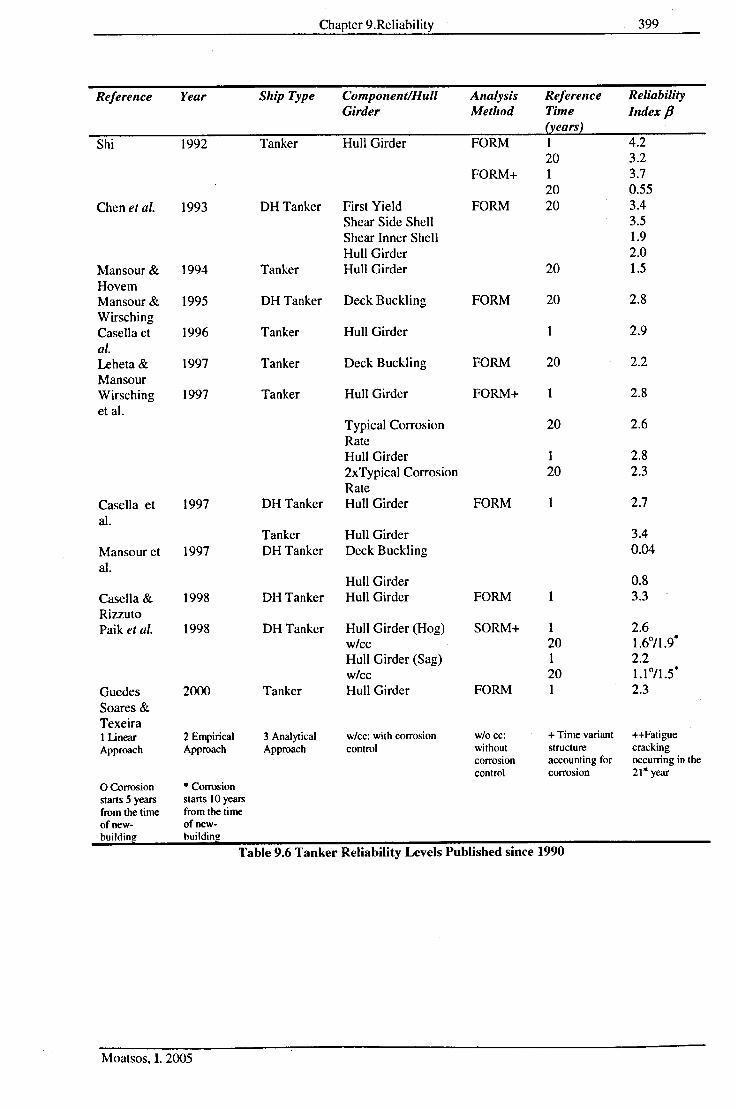
Chapter 9.Reliability 399
Reference Year Ship Type Component/Hull Analysis Reference ReliabilityGirder Method Time Index p
Shi 1992 Tanker Hull Girder FORM 1 4.220 3.2
FORM+ 1 3.720 0.55
Chen et al. 1993 DH Tanker First Yield FORM 20 3.4Shear Side Shell 3.5Shear Inner Shell 1.9Hull Girder 2.0
Mansour & 1994 Tanker Hull Girder 20 1.5HovemMansour & 1995 DH Tanker Deck Buckling FORM 20 2.8WirschingCasella et 1996 Tanker Hull Girder 1 2.9al.Leheta & 1997 Tanker Deck Buckling FORM 20 2.2MansourWirsching 1997 Tanker Hull Girder FORM+ 1 2.8et al.
Typical Corrosion 20 2.6RateHull Girder 1 2.82xTypicai Corrosion 20 2.3Rate
Casella et 1997 DH Tanker Hull Girder FORM 1 2.7al.
Tanker Hull Girder 3.4Mansour et 1997 DH Tanker Deck Buckling 0.04al.
Hull Girder 0.8Casella & 1998 DH Tanker Hull Girder FORM 1 3.3RizzutoPaik et al. 1998 DH Tanker Hull Girder (Hog) SORM+ 1 2.6
w/cc 20 1.6°1l.9·Hull Girder (Sag) 1 2.2w/cc 20 1.1°11.5·
Guedes 2000 Tanker Hull Girder FORM 1 2.3Soares &TexeiraILinear 2 Empirical 3 Analytical w/cc: with corrosion wlo cc: + Time variant ++FatigueApproach Approach Approach control without structure cracking
corrosion accounting for occurring in thecontrol corrosion 21" year
OCorrosion • Corrosionstarts 5 years starts 10 yearsfrom the time from the timeof new- of new-huildin buildin
Table 9.6 Tanker Reliability Levels Published since 1990
Moatsos, I. 2005

CHAPTERIO
DISCUSSION & CONCLUSION
10.1 Introduction
A number of changes in ship design have been implemented over the years with the result
that in modem design longitudinal strength requirements can now be met using less material
than in older ships. One example of this relates to the introduction of segregated ballast
requirements in tankers where changes in structural arrangement have produced a new
generation of ships with length to depth ratio less than traditionally used. In providing less
material to generate the required modulus, local strength requirements become more
difficult to satisfy and the distribution of material between the plate and stiffener
components becomes critical. In this respect ultimate strength techniques such as the ones
compared and developed in this study can assist in the determinant of structurally efficient
hull cross sections. In developing the design of such sections, it should be clearly be a
primary requirement that the margins of safety against hull failure in hogging and sagging
should be similar.
This chapter discusses & concludes more in detail all the parts of this study that the author
believed were of importance. Theoretical models used throughout this study were discussed
at the end of each chapter along with assumptions made and possible implications of both
the assumption and the results. Proposals are also made on future research and experimental
procedures that would complement this study and further advance the knowledge gained in
the particular fields by future readers of this thesis and researchers studying in similar fields.
Each element of this study discussed in each of the chapters of this thesis is treated
separately but in some cases where there is a certain amount of overlap in the effects of
certain approaches taken or in the implications that certain results might have, these are
discussed together.
10.2 Thermal Stresses on Marine Structures
Thermal stress analysis and the study on the effects of diurnal temperate stresses on marine
structures formed one of the most important elements of this study. It was identified during
the critical review of published work in (Chapter 3) of this thesis that although the problem
Moatsos, I. 2005

Chapter 10.Discussion and Conclusions 401
of thermal stresses affecting marine structures troubled researchers in the mid 1950s and
1960s, and although the significant effect and even the possibility of being responsible for
structural failure was documented, very little research on the particular subjected has been
published since then.
Looking at the problem from the global warming point of view, as discussed in (Chapter 2),
the increase in average temperatures globally and the extreme nature of the weather that
countries worldwide are currently experiencing, various engineering fields such as the
automotive and the civil engineering have started looking at these effects more in detail.
With so much interest in global warming and its effects in the recent years, it surprising that
the marine technology research, design and construction communities have not started
taking into account the effects of global climate change more explicitly in their design
approaches. It could be that the nature of the industry is so conservative that unfortunately
such effects might take years yet to become normal practice and could require a catastrophic
failure or accident that would be solely attributed to such conditions, before such effects are
effectively implemented into standard engineering practices and ship structural design.
In thermal analysis of structures, temperature difference is the most important factor. In the
case of a ship's structure, as a result of the structure's size and complexity a large number of
such temperature differences can occur that can also vary between different parts of the
ship. A set of temperature conditions that can give rise to a significant temperature
difference in one segment of the ship's structure may not necessarily be the same set of
temperature conditions that will create the most adverse temperature difference for another
segment of the vessel.
Jasper's theory has a number of assumptions that require attention and are worthy of some
discussion. Although the theory neglects the effects of transverse restraint on the
longitudinal stresses, good agreement has been shown between theoretical calculations and
experimental results on both model and full scale. Away from transverse bulkheads it
appears the transverse restraint is small and the theory is satisfactory for the longitudinal
strength problem.
An interesting point arises in all theoretical approaches suggested that solutions for the
thermal stress problems for holes in plates under various boundary conditions all indicate
Moatsos, I. 2005

Chapter lu.Discussion and Conclusions 402
stress concentrations of the same order as under tensile loading conditions so that the two
effects may well be superimposed in cases where there is a temperature gradient over the
stress raiser as well as tensile stresses in operation. This would explain the cracks that have
been observed around piping holes and other stress raisers in refrigerated ships and
emphasises the importance of detail design when the detail itself is subject to a temperature
gradient.
The preliminary analysis of the FPSO structure as described in (Chapter 5) of the thesis
indicated a significant effect. Hogging ultimate strength change results compared to results
that did not include temperature effects produced a change ranging from 2.6% to 5.1% for
the temperature changes examined with the corresponding change for the average diurnal
overall change in temperature found to be 2.6%. In the case of sagging ultimate strength
change the results obtained were of the magnitude expected showing a 41% reduction in
ultimate strength during sagging in the "worst case scenario" analysed. The sagging analysis
produced a change ranging from 24.3% to 40.8% for the temperature changes examined
with the corresponding change for the average diurnal overall change in temperature found
to be 24.3%. This shows the significant effect that temperature change induced stresses
could have on the ultimate strength of ship structures. Looking at the reasons behind such
data and for an interpretation of the results obtained, some interesting conclusions can be
reached. The rapid reduction of the deck strength, which is the primary load bearing part of
the ships' structure in hogging and sagging conditions, translates to a significant reduction
in hull girder US, as it is of primary importance in all mathematical formulation used. From
a physical point of view the reduction would be more obvious when the structural
components were not in tension (as they would be in a hogging condition) when the load
bearing properties of the stiffened panel would be influenced more by properties of the
material, but rather in compression (as they would be in a sagging condition) where the
dimensions of the stiffened panel and the structural configuration of the area along with the
type of stresses imposed on the structure would be of more significance. Its is difficult to
say what effect the structural configuration of each of the vessel can have on the US as more
detailed analysis would have to be carried out (FEA for each of the vessels) in conjunction
with detailed data on the temperatures of cargo their· variation and distribution.
Unfortunately such type of data was not easy to obtain for this study as it is often that no
records are kept for analysis by FPSO owners and operators. Should such type of data, to
the level of detail and accuracy required, have been available, it would have enabled such a
Moatsos, I. 2005

Chapter 10.Discussion and Conclusions 403
study of thermal loading induced by the cargo to be made, its patterns to be investigated and
would have complemented the current work by improving the quality of the results enabling
further investigations on such effects to be carried out.
The effect of temperature change and corrosion in the reliability based structural design of
TankerlFPSO structures was investigated and a procedure was proposed which took into
account diurnal changes of temperature in the North Sea and a statistically derived corrosion
wastage mathematical model. The significant reduction of the hull girder ultimate strength
when thermal stresses and corrosion were taken into account could be attributed to the way
in which thermal stress occurrence was modelled and the extreme nature of the values used
which in our case had a 20-year period. Extreme diurnal temperature variations occurred in
summer months during which extreme wave bending phenomena would have a lower
probability of occurrence, which explains the magnitude of the results. Unfortunately no
new evidences from experiments and design practices exist to justify the importance of
thermal effects on ship structures, but it is the observed and well documented abnormal
changes in surface temperature and global weather and the fact that marine structures
experience abnormal weather phenomena more often than they did in the past that justify
the need for more research in the field. One could also argue that temperature change at a
specified site is a random variable, which could be fitted by a certain probabilistic
distribution based on the loading and offloading manual of the FPSO under typical loading
conditions, hence overestimating the effect of temperature change. This would be true but it
would only enable modelling of temperature change for the cargo areas of the structure and
not the diurnal temperature change which is more significant. More research in developing
accurate temperature models is certainly required.
The size of stresses measured indicates the importance of this problem in the design of the
hull girder. It reinforces the argument for maintaining low still water loading stresses where
the temperature stress can vary between tensile and compressive values during the course of
voyage or time subjected to loading which will be the case in all ships which do not have a
large amount of internal heating or cooling. In the latter cases it is possible that no matter
what the air and sea temperature variations are the temperature stresses will be either tensile
or compressive at certain parts of the hull girder and might be offset by the way the ship is
loaded. This requires further investigation of particular cases.
Moatsos, I. 2005

Chapter 10.Discussion and Conclusions 404
10.3 Ultimate strength
A framework for predicting the ultimate strength of ships for various configurations under
vertical bending moment was proposed and incorporated in a Visual Basic code for MS
Excel 2003. The code incorporates various proposed formulations which were selected for
their simplicity and ease of use when compared with high-end numerical solutions and can
be used for comparison and analysis for ship structures but is also flexible enough to accept
further approaches to be used and compared but also any corrosion wastage data as input.
The approach calculates the ultimate strength moment of the hull by integrating the assumed
stress distribution with respect to the neutral axis. This resulted in explicit ultimate moment
expressions for the sagging and hogging conditions. The simplified formulation assumed
uniform compressive stress distribution (average values), but the actual stress distribution
will be non-uniform as a result of buckling and post buckling effective width. If the uniform
value is a good indication of the actual value, then the calculated moment should not be
very different from that due to the actual stress distribution, because the distance to the
neutral axis is the same in both cases. As the emphasis of the approach is to use simple
formulation, uniform (average) compressive stress is assumed.
As far as the developed code that formed the core part of the MUSACT code is concerned
and the theory behind this approach the bending moment sustained by the cross section is
obtained from the summation of the moments of the forces in the individual elements and
the derived set of values defines the desired moment-curvature relation. Initially the position
of the neutral axis is required and is estimated through an elastic analysis because, when the
curvature is small, the section behaves elastically. However, the approach creates two
distinct problems in its implementation:
3. The sequence and spacing of the imposed curvatures strongly influences the
convergence of the method due to the shift of the neutral axis.
4. Modelling the ship's section and determining the position of the neutral axis itself
are important issues.
5. Although Faulkner's method used for the determinant of the ultimate strength of the
stiffened panels in comparison with all other available methods produces the best
Moatsos, l. 2005

Chapter 10.Discussion and Conclusions 405
results, it gives poor prediction when the initial imperfection (including residual
stress in plate, initial deflection in stiffener and load eccentricity) is large.
The procedure used in this work to predict the behaviour of the hull girder under
predominant longitudinal bending seems to be quite accurate when the results are compared
with those obtained with different approaches, but also when applied to already built FPSO
structures, both new-built and conversions. On the other hand, if the preparation time of the
model and the computational running time are considered and compared with methods
using finite-elements or ISUM elements, then the developed procedure and code is far better
and more useful for design practice. The code takes about 3-5 minutes to run (depending on
the complexity of the structure) using a Pentium 4 2.8GHz Personal Computer, simulating
corrosion and thermal effects and calculating the US of both panels and overall hull girder
in sagging and hogging conditions using a variety of formulations, while finite-element
methods normally need a parallel computing environment and may take from several hours
to several days (always depending on the complexity of the problem) to provide a result that
needs to be interpreted according to the boundary and modelling conditions used. In relation
to the preparation time of the model, finite-element approaches may take several weeks to
implement the model (for a relatively experienced user of the FE code used) not to mention
the time required to familiarise the person performing the analysis with the software and the
code in order for accurate and realistic results to be acquired. On the other hand the code
developed only requires a couple of days for familiarisation, implementation and
interpretation of the results obtained. It has to be noted though that the code runs in an MS
Excel environment and is not a stand-alone program and hence the user has to be in
possession of a version of MS Excel in order to run the code and obtain results.
Furthermore the approach predicts a load-shedding pattern in the behaviour of the stiffened
plate after buckling. This prediction is based mainly on the assumed variation of the
effective width of the associated plate and thus it requires confirmation by other methods,
experiments and finite-element approaches. This confirmation is especially important for
the prediction of the ultimate strength of the ship hull girder by taking into account the cross
section due to the different state of strain of each stiffened element where some of them are
already in the pos-buckling region. As far as residual stresses are concerned and their
impact in plate elements used in this analysis, a particular case of stress distribution was
assumed as specified and formulated in the theories and approaches used. However a
Moatsos, I. 2005

Chapter 10.Discussion and Conclusions 406
smooth transition between the tension and compression zones may easily be implemented
by the modification of the equations used, quantifying the changes of the material
behaviour.
As stated in the introduction of this chapter, ultimate strength techniques such as the ones
compared and developed in this study can assist in the determination of structurally efficient
hull cross sections. In developing the design of such sections, it should be clearly be a
primary requirement that the margins of safety against hull failure in hogging and sagging
should be similar. This requires that the buckling and post-buckling properties of the upper
and lower parts of the structure should be properly matched to the applied bending moments
in sagging and hogging respectively. Load shedding characteristics of panels beyond initial
buckling can evidently be of critical importance, and the relative merits in this respect of,
for example, flat bar, tee-bar or bulb plate longitudinal stiffeners must be considered.
At the level of detailed design of compression panels, it is tempting to argue that the most
efficient design will be one in which the various modes of instability, whether by stiffener
tripping, web buckling, plate buckling or overall panel column instability, should occur at
similar levels of stress. This approach to design optimisation, sometimes referred to as the
"one-hess shay" concept, has often been used in the past in other structural contexts. The
analysis suggested by various approaches in the published literature confirms the possible
danger of this approach. If the simultaneous occurrence of various modes of failure leads to
a sudden, rapid deterioration in compression stiffness (a high rate of load-shedding) then
any reserve of strength beyond the limit bending moment may be reduced to zero. Not only
would there be no warning of imminent failure, but such failure could be total and
catastrophic. It is not possible on the basis of this study and from all the published literature
examined to draw any general conclusions regarding the optimum distribution of material in
hull cross-sections. It can be said though that there is clearly a need for structural designers
to use the tools now available for calculating ultimate compressive properties of stiffened
panels to investigate systematically the relative merits of alternative design configurations.
The predicted moment-curvature relationship for the hull beyond its ultimate strength
conditions must be viewed as approximate, particularly at the higher levels of curvature
where a number of assumptions made could be violated such as:
Moatsos, I. 2005

Chapter 10.Discussion and Conclusions 407
• The stabilising effect of displacement continuity between elements ignored in the
analysis may become significant at high levels of strain.
• At high strains, the assumption that plane sections remain plane is likely to be
violated as will the assumption of circular bending.
The sudden change of slope of the moment curvature diagram in sagging, and the steep
negative slope resulting from rapid load shedding both in the results obtained by the
MUSACT code and LRPASS, suggest that failure of such a hull in sagging would be
sudden, rapid and potentially catastrophic. Although behaviour beyond the ultimate is of
theoretical interest, the ability to predict maximum strength is crucial in the assessment of
ship safety. Such predictions are quite sensitive to assumptions regarding corrosion, so a
logical and consistent approach is needed to specify the margins to be used in strength
calculations. The results presented are also inconclusive regarding the possible influence of
imperfections due to fabrication, as it was not intended to investigate the effect in the first
place but nevertheless they influence the accuracy and behaviour and failure patterns of
stiffened panels and should be investigated more in detail in future research.
Using results from large-scale box girder models, a 113 scale frigate hull model, a
commercial widely used code and numerical results available in the published literature, a
comparison was made of the approaches used and the code developed. The results of the
comparisons with experiments and numerical evaluations show that any simplifications and
assumptions made were acceptable and did not compromise the accuracy of the final results.
With the Triton being the only conversion-built FPSO and the only structure with a double
bottom and Schiehallion and Anasuria only having a single bottom and being purpose-built
FPSOs, the comparative results allow us to make a number of interesting conclusions:
• The overall structural strength of the FPSOs is greatly benefited from a double
bottom, as the double bottom FPSO has a significantly larger ultimate bending
moment in both sagging and hogging conditions.
• The two purpose built FPSOs although of relatively similar size and structural
configuration, exhibit different overall ultimate bending moment behaviour,
resulting from the structural details and the materials used throughout the structure.
Moatsos, I.2005

Chapter IO.Discussion and Conclusions 408
• Although the double bottomed FPSO demonstrates significantly higher ultimate
bending moments when compared with the single bottomed FPSOs, in the sagging
condition, the loss of strength is far more rapid with progressively increased applied
curvature. This is obviously subject to the post ultimate strength being modelled
accurately and there is still a significant amount of research & progress yet to be
made on this subject.
Overall some final conclusions and additional suggestions can also be made:
• The ultimate collapse strength of a ship's hull under a vertical bending moment
correlates with the failure of the side shells as well as of the compression/tension
flanges and is a significant measure of the ship's hull strength and should be used in
design and in the assessment of ship strength and/or reliability.
• Predictions of Mu appears feasible within acceptable confidence limits, using the
various approaches discussed but there are significant differences in the ultimate
moment results obtained from the different formulas and approaches used in the
companson.
• In design, the rules of classification societies specifying the requirements for the
ship section modulus should be based on ultimate strength rather than initial yield,
as in some cases initial yield does not reflect the true strength of the hull girder.
• All proposed approaches and the entire framework provide quite reasonable results
in comparison with experimental data and numerical results. As the approach takes
into account the geometric and material properties of the hull section more precisely,
it may be applied to any general-type hull cross section. The framework and code
developed may be useful in preliminary design estimates of the ultimate strength of
ships under a vertical bending moment.
• Inclusion of tripping formulation in the behaviour of stiffened panels is seen to be
very important. The deck stiffeners, made of bars, don't have much flexural-
torsional rigidity and the calculated tripping stress is lower than the flexural
buckling stress of the stiffener with associated plate. This fact leads to a very high
reduction of the ultimate bending moment in sagging compared with the moment in
hogging, where the deck is in tension. Future work is required on the subject and, as
it can be seen from the relevant literature nowadays it is possible and relatively easy
Moatsos, I. 2005

Chapter 10.Discussion and Conclusions 409
to compare the prediction of the tripping stress using approximate methods and
results of finite-element methods for stiffened panels.
10.4 Corrosion Modeling
Reliability assessment by considering corrosion and fatigue is very important for the
optimal scheme of maintenance and repair. Different corrosion models would have
significant influence on the assessed reliability and by studying some of the currently
available corrosion models it is argued that not all of these models may fully reflect the
reality. The models adopted in addition to being a more flexible alternative to all other
suggested also generalise the concept by including an early phase with the corrosion
protected surface and free parameters that can be adjusted to the data in specific situations.
Residual stresses and corrosion have a degrading effect on the ultimate moment. However,
these effects occur at separate times in the ship's life; the residual stresses are present in the
early stage of the ship's life and the effect tends to reduce with the normal operating
conditions, while the corrosion level tends to increase with time. So both effects should not
be considered together for design purposes, i.e., if an allowance for corrosion is included in
the design, then a reduced allowance for the residual stresses should be considered.
The corrosion model used does not explicitly take into account the effect of pitting and
rather an overall wastage of the members approach is used which can limit the modelling of
the actual corrosion process encountered. Nevertheless when compared with a linear
approach the non-linearity of the physical problem is modelled significantly better as it can
be seen from the detailed description of the process. For the calculation of the ultimate
strength of the entire hull girder the approach is very much dependent on the accuracy of the
corrosion model and the maximum wastage used. For the time dependent nature of the
corrosion process to be model accurately, one has to take into account the time dependent
nature of the variables into account and calculate the probabilities of failure using an
approach that will be able to interpret accurately the non-linearity of the problem.
In the corrosion models for the 2 approaches in the MUSACT code, in all cases, no repairs
are assumed and it is assumed that for the first 5 years of the vessel's life there is no break-
down in the CPS after which corrosion follows each of the models for a total of 30 years
Moatsos, I. 2005

Chapter lO.Discussion and Conclusions 410
assuming that no repairs are carried out on the structure. The nature of operations for FPSO
structures restrict frequent repairs in the cargo and ballast holds. Significant repairs can only
be effectively carried out when the FPSO ceases operations, to an obvious financial loss,
and severs and abandons the field that is currently assigned to. This certainly does not
negate the fact that repairs would often be carried out on the structure as a results of period
surveys where defective plating and structural members would be replaced. As a result of
such conditions, the assumption made appears to be a relatively good representation of the
actual condition the structure might be throughout its operational life. Looking at the two
corrosion modelling approaches it is interesting to note that both produce very similar
results after 30 years of corrosion, a fact that occurs from the maximum wastage used in
each of the approaches being similar, but throughout the life of the vessel the amount of
corrosion wastage that each of the approaches calculates, varies with the linear model
underestimating the values by as much as 2 times compared with the non-linear approach.
Hence it was decided to proceed to reliability analysis by using the non-linear approach and
avoid the conservative linear method that would oversimplify the mathematical modelling
of the phenomenon and add more assumptions and simplifications to this analysis.
When combined with the different US formulation, the results can vary with the US results
following the "trends" and shape curves of the corrosion models used demonstrating that the
corrosion model to be chosen will influence greatly both the strength and reliability results
to be obtained. As it can be seen from for Anasuria the difference is in the range of 3.4% for
the OB, 7.5% for SS, 3.1% for the Deck, 2% for Sagging US and 1.5% for Hogging US for
no corrosion between the Paik simplified formulation plate US approach and the author
developed analytical approach with the Paik approach providing more conservative results.
10.5 Load Effects Modelling
Applying the lACS formulation described in (Section 8.8) of this chapter to the 3 FPSO
structures provided the minimum design midship still-water bending moment values and the
minimum design midship wave-induced bending moments as summarised in (Table 10.5).
After comparing the strength results obtained with the lACS loading levels specified (lACS,
1989), (lACS 2003) it can be seen that the safety factors obtained when combined with the
still water loads calculated are rather low. Such low values of safety factors and especially
the pronounced influence of the wave component on their values, underlines the need to
Moatsos, I. 2005

Chapter lO.Discussion and Conclusions 411
make the predictions of the loads on, and the strengths of, hull structures as accurate as
possible. It is doubtful if, even in the light of improved knowledge and understanding of the
phenomena involved, factors as low as these calculated should be accepted. The adverse
effect of corrosion, and the need to control or monitor it has been evident in throughout this
entire thesis and is particular evident from this comparison.
Using commonly applicable deterministic load combination methods, it was determined that
the peak coincidence as applied in the existing ship rules is very conservative. On the other
hand, other deterministic methods including Turkstra's rule and the SRSS rule, all
underestimate the combined bending moment, with the SRSS rule being the least
satisfactory. Using stochastic methods, including the exact point-crossing method,
approximate load coincidence method and the Ferry Borges method, all lead to identical
predictions. For code application, load combination factors are introduced to reduce the
conservatism inherent in the existing ship rules. A considerable reduction of the total design
bending moment, as required in the existing ship rules, is found to be acceptable. It should
also be noted that the load combination factors are dependent on the type of distributions for
both SWBM and VWBM, the specified design SBWM and VWBM, as well as the reference
time period. The load combination factors presented in this paper are valid for the particular
FPSOs analysed and no attempt whatsoever should be made to consider these in amore
general fashion for other types of vessels.
The extreme models used for the calculation of loading are only dependent on the number
of occurrences and not on the total time spent in that condition. One interpretation of this
could be that the uncertainty is associated with changes in the loading, and not with the
duration of the condition. This is a suitable assumption for merchant ships, where the same
loading conditions are maintained over the whole duration of the voyage. The assumption
might not hold for an FPSO, which experiences continually changing loading every day,
where higher uncertainties would be expected. On the other hand, FPSOs are generally
fitted with better loading monitoring instruments than traditional tankers, resulting in better
load control and thus reducing the uncertainties in the effective calculation of the SWBM.
All these points were considered when assigning uncertainties to the SWBM in the extreme
and stochastic model for reliability analysis. Furthermore from the operational profile of
the vessels is such that they will be experiencing, almost always hogging still water bending
moment and the extreme SWBM values for the ballast load condition will tend to be
Moatsos, I. 2005

Chapter l O.Discussion and Conclusions 412
conservative as a result of the distributions used during the analysis being the same for
hogging and sagging conditions and not taking into account the effect of heavy weather
countermeasures during this study.
Short term responses in irregular waves were calculated usmg the principle of linear
superposition and wave statistics. The short term responses were combined with long term-
wave statistics for the specific area of operations of the FPSOs in order for the long-term
distribution of the VWBM to be determined. When the long-term distribution is known, the
most probable extreme value in any reference period may be found. The reference period
can be 1 or 20 years for the reliability analysis. During the long-term response analysis
carried out, it was stated in (Chapter 8) that the particular area wave statistics were believed
to give a good representation of the actual operational location of the FPSOs analysed.
Different fields may have different wave statistics, which may lead to variations in the wave
induced loads acting on the vessel. The recent trend in offshore development is to develop
marginal oil fields, with shorter field life and lower field value. Under such circumstances,
it may be desirable to design the FPSO with a longer service life and then operate the vessel
at new locations after a field is depleted. If this is the case, thorough consideration during
the design procedure should be given to where the vessel may be operated in its lifetime.
Getting the design right the first time may save costly improvement at a later stage.
It was evident during the analysis that the largest VBM response was generated when the
wave direction is predominately head-on or from the stem. It is obvious that this difference
in response to waves from different angles will affect the overall probabilities of
exceedance, depending on the vessel's heading. It is assumed that traditional tankers have
equal probability of encountering waves at all headings during a voyage, as opposed to
FPSOs, where the waves will have higher probabilities of approaching the vessel from
certain angles. It is important to keep in mind that by wave direction, we define the
predominant direction of the waves in the sea-state, relative to the ship heading. Although
the wave direction could be O', waves will approach from other directions at the same time.
This "short-crestedness" was achieved in the theory behind our analysis and used during
this study by introducing the spreading function, as described in (Chapter 8). The largest
amplitudes of responses were found at 180° and 0° which represent following seas and head
seas respectively. The lowest response was found at 90°, when the vessel encounters the
waves sideways. These results are quite reasonable and in good agreement with results
Moatsos, I. zoos

Chapter l O.Discussion and Conclusions 413
obtained from various other similar analyses found in the published literature. The
magnitude of the maximum response is approximately 500MNm.
During the slamming analysis of this study, for the still water loads, DNV Rules and lACS
suggested formulation were used to determine the maximum values to be used for the
combination of loads and the Jensen and Mansour approach using code developed for the
calculation of the long term hogging and sagging wave bending moments. The results were
compared with the values given from the lACS Rules and the DNV modified Rules with a
Sagging to Hogging ratio of 1.41, 1.45 and 1.35 respectively, Sagging to lACS Rule ratio of
1.20, 0.93 and 1.43 respectively. According to the results the difference between the rules
and approach used is quite significant with differences of 22% between the DNV Rules and
the simplified approach and 35% between the lACS Rules in the case of one of the FPSOs
analysed and the simplified approach as a result of the draft-to-length ratio with the values
of the method being lower than the Rules computed values. As the methodology is
dependent on the area of operations of the vessels this signifies that the prescribed rule
requirements can often be inadequate in determining the maximum bending moments and
some form of adjustments would be required to compensate for the location of operations
instead of one overall approach for all locations.
Combining the vertical bending moments in an appropriate way is not a straightforward
task, given the different random nature of the loads. Still water loads are very slow varying,
wave induced loads have load frequency, whereas slamming induced high frequency loads.
All three have been considered during the analysis. These loading components have been
considered independent and the Ferry Borges-Castanheta load combination methods was
applied, after comparing all the available options, to obtain a load combination factor. As no
reliable information on the loading procedures for some the FPSOs was made available, a
simplified operation profile based on the production capacities was used, and a rectangular
pulse process was fitted to describe the nature of the loading conditions experienced. The
load combination factor was found to vary significantly with the ratio of Stillwater load to
the total load. It is also interesting to note that the load combination factors remain the same
for hogging and sagging with each loading condition. Historically several deterministic
methods have been applied to derive load combination factors for SWBM and VWBM for
both sagging and hogging conditions. The correlation between these loads is negligible for
the estimation of the extreme combined bending moment. In the existing ship rules, such as
Moatsos, I. 2005

Chapter IO.Discussion and Conclusions 414
the lACS Requirements, SWBM and VWBM are simply added together, assuming that the
maximum values of the two loads occur at the same instant during a ship's design life.
lACS also specifies that the maximum SBWM and VWBM should not exceed their
respective allowable values, even if one of the moments is negligible. As the SWBM and
VWBM are stochastic processes, the maximum SBMW and VWBM do not necessarily
occur simultaneously in a ship's service lifetime. The load combination factors were
calculated for the three loading conditions, based on the operational profile and extreme
loads and for all conditions in all events considered (different locations, different load
models etc). These calculations form part of the basis of the reliability analysis.
10.6 Time Invariant and Time Variant Reliability Analysis
The instantaneous long term reliability of the vessel was obtained using the limit state
equation described in (Chapter 9) using a FORM approach and improving the results by
using a SORM approach but without taking into account of time and computing the
probabilities of failure and reliability indices by using the values that result as most
probable extremes for the loads and for each corrosion year for the ultimate strength and
that are distributed according to the stochastic model.
During the time-invariant analysis for Anasuria FPSO, the annual reliability index in
sagging was found to be varying from 3.819 to 4.714. in the un-corroded state. As
temperature differences increased and the amount of corrosion in the structure increased as
well, a reduction in reliability indices was noticed as expected For Triton FPSO, the annual
reliability index was found to be varying between 2.359 to 2.75 in the un-corroded state.
This is rather low value corresponds to approximately one failure in 110 years or one failure
per year in 110 structures. From the reliability analysis, it is also found that the safety of the
FPSOs is very sensitive to variables associated with the wave bending moment.
For the time-variant reliability results, the variability of the variables with time was taken
into account and Monte Carlo Simulation (MC) was used to compensate for the non-
linearity of the problem and provide a more accurate result for Schiehallion FPSO. The
results vary quite significantly and show not to follow the mathematical trend of the
corrosion model as the probability of failure curve obtained could be fitted to a 6th order
Moatsos, I. 2005

Chapter 10.Discussion and Conclusions 415
polynomial for the time variant results and a 5th order for the instantaneous and a 4th and
3rd order respectively for the reliability index.
A number of assumptions have been taken into account in each of the approaches used
which also restrict the accuracy of the problem and can be found in each of the relevant
publications in detail. Since closed form solutions were used extensively throughout this
analysis, the accuracy of the results cannot be compared with those that one could obtained
by running a detailed FE model or a non-linear approach for the determination of the loads.
Nevertheless when compared in terms of time required for the calculation the closed form
approaches can quickly produce sufficiently accurate results for a designer to assess the
safety of the structure since all the methods used have been extensively compared with
model tests or they are the result of such model tests. The corrosion model used does not
explicitly take into account the effect of pitting and rather an overall wastage of the
members approach is used which can limit the modelling of the actual corrosion process
encountered. Nevertheless when compared with a linear approach the non-linearity of the
physical problem is modelled significantly better as it can be seen from the detailed
description of the process. For the calculation of the ultimate strength of the entire hull
girder the approach is very much dependent on the accuracy of the corrosion model and the
maximum wastage used. For the time dependent nature of the corrosion process to be model
accurately, one has to take into account the time dependent nature of the variables into
account and calculate the probabilities of failure using an approach that will be able to
interpret accurately the non-linearity of the problem.
It is interesting to compare the results obtained with available reliability indices published in
the available literature. It should be noted that in the majority of the literature reviewed no
thermal effects are taken into account and in the majority of the results published, no
corrosion effects are taken into account. The reliability indices are in certain cases annual
and in other cases for a 20 year period, a fact that needs to be taken into account when
comparing the results obtained during this study with the available published literature. The
large variability in the results both from this study and the available literature suggest that
still a large amount of work is required before commonly acceptable levels of safety can be
set for the design of marine structures using reliability based approach.
Moatsos, I. 2005

Chapter 10.Discussion and Conclusions 416
10.7 Future Research
From the evidence produced in this thesis and the results and comparisons with full scale
tests it is clear that thermal stresses of the same order as the still water loading will be
encountered by nearly all ships. There is a considerable demand for the carriage of cargoes
at more extreme temperatures than operators and designers are experienced at present and
the thermal stress problem is likely to increase in importance. The stress resulting from
thermal gradients can be calculated with sufficient accuracy by existing methods. such as
the on proposed in this thesis by the author, where there is no problem of stress
concentration involved. However information on the frequency and magnitude of the
thermal gradients experienced by ships in operation is insufficient for design calculations
and more research is required on:
1. Model tests for details which may give rise to stress concentrations
2. The stresses resulting from the gradients. Away from points of stress concentration
and transverse restraint these may be calculated by existing methods but theoretical
and experimental work will be required for local stresses around details which are of
most importance.
3. The fatigue properties of ship steels under steady load, fluctuating loading and the
extreme temperature gradients.
4. Methods of alleviating thermal effects due to loading, local design, use of special
material and crack arrestors, insulation, etc.
There are many other areas of ship structure temperature research worthy of consideration
even at this time. For example, the thermal buckling of curved and flat plates under
conditions of thermal input peculiar to ship structures and in conjunction with non-thermal
buckling loads is one problem that requires investigations of an analytical and experimental
nature. Thermal stresses in flat plates resulting from two-dimensional temperature gradients
and one-, two-, or three-dimensional conditions of restraint are another type of investigation
that could be undertaken. Researchers undertaking such an investigation must carefully
consider the fact that the approaches used in analytically solving these problems must
reflect rather sensitively the range of temperatures and the temperature distribution peculiar
structure and its environment. In other words, there is a chance that without knowing in
advance the temperature conditions, one can normally expect a considerable amount of
Moatsos, I. 2005

Chapter 10.Discussion and Conclusions 417
effort will be devoted to solving a completely unrealistic problem, or even a problem which
is non-existent in ship structures. One can argue that such investigations can be used to
define the limits of temperature gradients that must exist in order to influence the behaviour
of the structure. This may be necessary in the event that instrumentation of an actual ship is
not feasible. Ultimately, however, it becomes necessary to provide experimental proof using
a full-size ship. In effect, then, by conducting research involving ship structure temperature
effects without first defining the important parameters, one merely postpones the
unavoidable task of full-scale experimentation.
It is widely accepted and the author agrees that there is a lack of experimental data from
large-scale steel models, and there is a need for further verification of all published and
future developed formulation using such data. In particular, tests are needed using models of
double hulled structures as such types have never been tested and all available published
results are based on numerical studies.
Although it was not investigated in this thesis but nevertheless is an interesting feature that
the author of this thesis came across in a variety of publications that the ultimate bending
moment in the upright position is greater than the moment at small angles of heel, no matter
if the vessel is hogging or sagging. It is necessary to evaluate if this reduction should be
included in the rules for classification societies. In practice, if an Elasto-plastic analysis of
the hull girder is performed and the calculation of the minimum ultimate moment is
required. then one should look for the minimum at an angle of heel of about 10° or more.
Alternatively, a reduction to the upright moment should be considered but this would be
worse to the 10°C angle of heel proposal as the degree of the reduction depends on the
compressive strength of the deck and the side panels.
Future development of approximate methods to predict the hull girder strength could
perhaps include implementation of an explicit method that can account for transverse
strength of the hull and overall buckling of large panels. In order for this to be achieved it
would be important to test extensively over the practical range of plate and column
slenderness of the derived load-end shortening curves of unstiffened and stiffened plates,
investigating carefully the agreement in the post-buckling range. Also load-shedding
characteristics of stiffened panels after initial buckling can strongly influence the moment-
Moatsos, I.200S

Chapter IO.Discussion and Conclusions 418
curvature characteristics of a ship's hull and certainly more work is needed on this aspect of
structural behaviour.
An interesting feature in the analysis that was not examined in detail was the statistical data
used for representing the sea conditions in each area. It is certain that by using almost
similar data and such assumptions in all FPSO analyses the level of accuracy is certainly
compromised. Such decision and assumptions had to be made as a result of lack of data but
nevertheless the author believes that the data used gives a reasonable representation of what
conditions are in each of the area of operations of the FPSOs. It would be interesting to
perform a study investigating the effect of the variability of wave induced loads acting on
the vessels by using data obtained from other sites and how these compare with the
prescribed levels of safety used today. There is always a strong possibility that the particular
vessels may be required to operate even in a different continent under completely different
conditions that could affect the overall structural safety of the vessel.
The theory for time-dependent reliability assessment has developed rapidly, although in
certain aspects it is not as fully developed, researched and publicised as time independent
reliability. We can safely reach the conclusion that the simulation-based approaches become
natural extensions of time-independent analysis once the out-crossing rate can be estimated
efficiently, however, the FORMISORM methods applied to time-dependent problems to
determine probabilities of failure tend to be considerably more difficult and laborious than
for time independent problems and researchers often have to make use of numerical
techniques to solve the resulting formulations with importance sampling suggested as the
approach producing the most satisfying results). Unlike time independent reliability
techniques. for which there has been extensive discussion and comparison. there has been
rather little comparison of the various approaches for the time-dependent solution
techniques. This can be attributed to the excessive computational times required for basic
(e.g. crude Monte Carlo) comparisons when stochastic processes are involved.
For many problems of practical significance. a fully time-dependent approach is only
required when the resistance basic variables are time-dependent or when more than one
loading case must be considered. It is evident that the methods of solution which are
necessary usually are too complex for application in practical design and for use in
Moatsos, I. 2005

Chapter to.Discussion and Conclusions 419
structural design codes. For these, simplified rules are required. How such rules might be
derived is a matter of particular importance for relating design code formulations to
structural reliability and an area that still deserves and requires a large amount of research.
Overall having touched upon the way that global warming will affect the individual
variables forming the limit state equation one can see that the results will vary depending on
how extreme the loads or the corrosion might be as a result of significant temperature or
weather changes. An attempt was made in this thesis to quantify some of these effects. The
exact effect of Global Warming and global climate change forms itself an issue of larger
debate not only to the engineering research community but is tackled more widely by
medical, social and political sciences. It has nevertheless been brought often to the attention
of the media and the public extremely often as extreme climate phenomena is not just only
easily observable and affect our everyday lives but also often result in catastrophic and
tragic events that affect the lives of millions of people worldwide. One has to just look at
the recent global effect that and isolated incidents such as Tsunami's or extreme climate
changes in Africa affect and what global social, economical and political effect they not
only had but still have.
The optimistic trend of the engineering research communities examining more in detail the
effects of Global climate change proves that such phenomena do not only exist and that
their effects should be investigated more in detail but also have a direct impact on the safety
of engineering systems. Hence the effects of such phenomena on marine structures should
not be taken lightly but instead always incorporated into any design and analysis approach
used. The conservative nature of the marine industries has always been the deterrent of
promoting pro-active engineering research in such fields and in the case of the effects of
global climate change research the engineering research community should not await for a
new catastrophe to occur as a result of such conditions before researching ways of
describing the particular effects on engineering structures in a better mathematical format or
the means of designing safer structures.
Moatsos, I.2005

Chapter 10.Discussion and Conclusions 420
10.8 Closure
The study presented in this thesis constitutes the first stage in the development of a
rationalised framework for the study of the effects of thermal stresses in marine structures
from a reliability and probabilistic point of view which formed part of the research interests
of the Structures and Reliability Group in the Dept. of Naval Architecture and Marine
Engineering of the Universities of Glasgow and Strathclyde. It is hoped that the work
presented in this thesis will be useful, at least to the Structures and Reliability Group in the
Department, in pursuing further research in the analysis of marine structures.
Moatsos, I.2005