Mixing Synthetic and Video Images of an Outdoor UrbanEnvironment

M.-O. Berger B. Wrobel-Dautcourt S. Petitjean G. Simon

First submission: 11 July 1997 - Revised: April 1998

Abstract

Mixing video and computer-generated images is a new and promising area of research for enhancing reality.It can be used in all the situations when a complete simulation would not be easy to implement. Past work on thesubject has relied for a large part on human intervention at key moments of the composition.

In this paper, we show that if enough geometric information about the environment are available, then efficienttools developed in the computer vision literature can be used to build a highly automated augmented reality loop.We focus on outdoor urban environments and present an application for the visual assessment of a new lightingproject of the bridges of Paris.

We present a fully augmented 300-image sequence of a specific bridge, the Pont Neuf. Emphasis is put on therobust calculation of the camera position. We also detail the techniques used for matching 2D and 3D primitivesand for tracking features over the sequence. Our system overcomes two major difficulties. First, it is capable ofhandling poor quality images, resulting from the fact that images were shot at night since the goal was to simulatea new lighting system. Second, it can deal with important changes in viewpoint position and in appearancealong the sequence. Throughout the paper, many results are shown to illustrate the different steps and difficultiesencountered.

1 Introduction

Augmented reality is the technique by which real images can be enhanced by addition of computer-generated orreal information. At least, this is the definition of augmented reality we shall adopt in this paper, since the termis currently used in different ways by different people, without what could reasonably be considered a consistentdefinition. Augmented reality shows great promises in fields where a simulationin situwould be either impossible,not realistic enough or too expensive. Of particular interest are applications in medical imaging [1, 25], urban design- for instance for visually assessing the incidence of a future building in an already existing urban environment [7]- and manufacturing [5]. Also, this type of integration is gaining importance in the film industry.

However, this area has up-to-now been largely under-explored and the few applications that have been developedrely heavily on the intervention of the user at the different steps of the mixing process. There are two reasons forthis. First, the superposition of the real and virtual objects has to be very accurate for a satisfactory visual effect.Jittering effects are highly unpleasing in a video sequence. Second, the camera may make abrupt position changes,in which case it is very difficult to predict beforehand what features can be detected in images and what featureswill be used to compute the viewpoint and do the tracking in a sequence.

1.1 A Look at the Literature

We focus here on those works in augmented reality where the authors have attempted to use vision tools for thesuper-imposition of synthetic objects on video images. It should be noted that past research has essentially dealtwith very good quality images of indoor scenes.

Perhaps the first work to consider the overlay of computer-generated images onto a background photograph isthat of [28]. [18] give manual solutions for evaluating the visual impact of a building on the landscape. A first tryat automating the composition process is presented in [19]. The authors explore some of the key issues involved inaugmented reality: computation of the shadows cast by real light sources on virtual objects, simulation of weatherphenomena, improvement of the quality of the montage using a novel anti-aliasing technique. Their approachsuffers however from two drawbacks. The parameters of the camera are determined by matching 2D points withthe corresponding 3D points of the model, but these points are determined manually. In addition, the influence ofvirtual light sources and specular inter-reflections is not taken into account.

1

In [14], a composition technique is described that works for a full image sequence and a method for mapping anaerial photograph onto a three-dimensional terrain model is presented. This environmental assessment applicationis however largely simplified by the fact that aerial photo data are considered as textures. Also, viewpoint deter-mination is only briefly addressed. [9] present a general system for combining virtual buildings and real imagesof the environment, which is capable of realizing computer animations. Viewpoint determination is achieved byassuming that there are points in the image whose world coordinates are known (passpoints). These passpoints arethen tracked in a sequence of images to estimate the new position of the camera from the one previously computed.Also, the detection of occluding objects of the real scene is done manually.

A framework is proposed in [13] for automating as much as possible the mixing process. Applications presentedconcern indoor environments (e.g., a virtual ball moving in front of a set of plates). The acquisition system canbe controlled with excellent precision, so its position is supposed to be known. The optical characteristics of thecamera are computed using a reference background object of the real scene.

The system of [27] uses computer vision techniques for overlaying real images onto very good quality videoimages. Pose calculation uses Newton’s method but is only briefly discussed. Tracking is correlation-based andobject registration is reliably achieved by tracking many features of the object. To check whether features havebeen correctly tracked, two cross-ratios of four areas of the triangles formed by five points are computed. They areprojective invariants and should remain the same over images. A low latency vision hardware allows overlay ofimage to be done in real-time.

Finally, a registration system allowing to track objects in real time is presented in [21, 22]. A user-specifiedset of model-image correspondences, known camera parameters and a pre-compiled aspect table that associatesdiscrete viewpoints with object features visible from those views are used to initialise the system. An initial poseis computed using the given 2D-3D correspondences. The system then goes on by repeating a three-step loop:

view indexing - pose information is used to extract visible features from the aspect table;

tracking - visible features are used as location hypotheses of feature templates in the next image;

pose computation - the templates are matched in the image and a new pose is computed.

Some of the system characteristics used by these authors match fairly closely our choices: use of robust meth-ods for pose estimation - iterative re-weighting least squares form of M-estimation [17] -, and correlation-basedtracking, combined with steerable filters. Combinations of rotations and translations do not seem to be accuratelycompensated by their tracker however. Also, the aspect table is constructed manually off-line.

1.2 Motivations and General Framework

To be able to efficiently mix video and virtual images, it is necessary to have a robust method for computing theposition of the camera in order to insert the virtual objects at their right place in the images. Among existing systemsfor the composition of images, one can distinguish between two classes: those which make use of markers ade-quately placed in the scene to facilitate viewpoint determination and those which base the calculation of the cameraposition on the natural structures of the scene. Since we aim at using our system in outdoor urban environments,we can not hope to get help from markers. We are thus uniquely concerned with works on image compositionwhere registration is achieved using the sole geometric features of the scene. We also intend to bring the numberof manual operations to a minimum.

Most of the current research works on image composition deal with manufactured environments - see for in-stance [27, 22] - filmed in good light conditions and from a close range. By contrast, our work is concerned withcomplex outdoor environments filmed in poor lighting conditions, since the ultimate goal is to simulate the effectof a new lighting system on the surrounding architectural elements. And even if the different steps leading to thepose estimation remain the same,i.e., feature detection and extraction, tracking, viewpoint calculation, our systemstands out from previous work on the following grounds:

Difficult primitive extraction . The scene is filmed from far range and the images are noisy. Contourextraction is then a difficult operation and the contour chains obtained are not stable from one image to theother. Contrary to other approaches, we have only few prominent points to extract and in addition they maybe poorly localized. Besides, it is out of the question to be able to properly extract junctions.

Inaccurate modelling. Since it was built from architectural maps, the modelling of the architectural sceneconsidered deviates significantly from the truth at certain places. This, along with unreliable contour data,explains why we have improved our calculations by the use of the robust technique of M-estimators.

2

Figure 1: The160th image of the sequence.

Figure 2: The complete wireframe model of the bridge. The poor quality of this modelling is quite apparent atcertain places. Small circles show the location of feature points used for 2D-3D primitive matching (those thatseemingly hover over the bridge correspond to street lamps).

No structuring of primitives . In outdoor environments, the primitives extracted are often points, sometimeslines and curves. However, only few more complex features such as corners or junctions are present. More-over, the features extracted are not topologically structured, making it impossible to use a structural approachto minimise the problems of the initial matching between image and model primitives.

Large vision field. We do not impose anya priori either on the distance of observation or on the position ofthe viewpoint. The “aspect graph” types of approach which propose model points likely to appear in the nextimage are thus excluded because these points change drastically as a function of the distance of observation.

1.3 Application: The Bridges of Paris

A simulation of the illumination of a large architectural set may be quite difficult to implementin situ, not to mentionthat it would be very expensive. Thus, recent years have seen computer simulations become more and more popular.Reliable global illumination softwares are now available, so trial-and-error lighting experiments can now be donealmost routinely (at the cost of large computation times though). Our motivation came from the insertion of a modelilluminated synthetically in its real environment. Decision-makers of the Paris city administration were willing tohave a new lighting system for a number of bridges of the Seine around the “Ile de la Cite”. They wanted to testseveral candidate illumination projects and be able to choose on computer simulations alone what project was thebest. Most importantly, they also wanted to evaluate the influence of this illumination on the surrounding elements.

A 300-image sequence of the Pont Neuf, one image of which is shown in Fig. 1, was shot at dusk time fromanother bridge. The fact that the images are dark has a strong influence on the quality of the segmentation andconsequently on the strategies used for the tracking. It also restricts the number of reliable features that we are ableto use. The reader should keep this in mind when visually evaluating the final composition.

It should also be noted that the modelling of the bridge was done mostly manually using information fromarchitectural maps. Fig. 2 shows that it is very unreliable at places, as the staircase effect on some of the archesreveals. Much better results could certainly be obtained with a laser modelling.

3

Detection, image iTracking

Viewpointcalculation, image 1

Detection, image 1Matching

illumination3D scene Global Image

renderingOccluding object

determinationmodelling compositionImage

calculation, image iViewpoint

3D model

i=i+1 i<p

i=2

i=pimage sequence

Video acquisitionp images

Computer vision

Image synthesis Image composition

Figure 3: An augmented reality loop.

1.4 Paper Outline

In this paper, we present a framework for enriching a large image sequence of an outdoor urban environment andwe apply these solutions to the sequence of the Pont Neuf. We assume noa priori knowledge on the extrinsicparameters of the camera system and the detection of features in images is autonomous, except for the first imageand at certain key images where it is guided.

Our augmented reality loop works as follows. A set of non-coplanar features is detected in the first image ofthe sequence and matched semi-automatically to their corresponding features in the 3D model of the virtual objectto inlay. These features are used to compute an estimate of the position of the camera with the scaled orthographyapproach of [8]. This initial guess is then refined by a robust minimisation of the projection errors. Once theviewpoint has been computed, a virtual object, rendered previously by a radiosity algorithm, can be embedded inthe image. The features detected in the first image are then tracked over the sequence and matched to 3D features.This way, viewpoint position is determined for each image by applying the above procedure to the features tracked.

We now proceed as follows. In Section 2, the complete augmented reality loop is outlined in more details. Thealgorithms used for estimating pose are presented in Section 3 and the method for matching 2D image points with3D geometric primitives in the first image is explained in Section 4. Section 5 presents the techniques we havedeveloped for tracking features over the sequence of images. Results of the composition for the bridge sequenceare then presented in Section 6. Finally, areas of current and future research are discussed in Section 7, beforeconcluding. Note that a preliminary version of this work appeared in [3].

2 Augmented Reality Loop

Let us first outline the different building blocks of our augmented reality system. As can be seen on Fig. 3, thissystem really consists of three distinct parts. The first relies on computer vision tools and is the subject of thispaper. The second part originates in image synthesis and in the third computer-generated and real information arecombined to enhance the reality and produce a visually satisfying result. For sake of completeness we give a veryshort presentation of these last two parts here, but the interested reader should refer to [7] for more details on howto properly handle the interactions between real and virtual objects and light sources.

2.1 Image synthesis

The computer graphics part of our system aims at modelling the objects to inlay in the sequence of images and atglobally illuminating these objects. Modelling the 3D scene really is a three-fold process: it involves

modelling the geometry - here, a set of polygonal faces obtained from various architectural plans;

modelling the properties of the materials assigned to the surfaces of the scene - this is based onin situmeasures [6];

modelling the positions and intensities of the virtual light sources,i.e., imitating real source characteristics.

Objects in an urban environment are made of diffuse and specular materials. A radiosity algorithm is used tocompute the diffuse inter-reflections between the surfaces [10]. A major feature of radiosity methods is that theircomputations are viewpoint-independent, so that illumination will not have to be computed for each image of thesequence.

4

2.2 Image composition

Once the viewpoint is determined for each image, the computer-generated images are rendered using a ray-castingalgorithm. The main bottleneck of this step lies in the determination of the real occluding objects that stand betweenthe camera and the virtual objects. The different virtual objects are then superimposed using composition operators(overlay, addition, multiplication) and the coherence of the composition is ensured.

In the image sequence of the Pont Neuf, a boat is stationed in front of the rightmost bridge pile in the last 40images of the sequence and thus occludes the synthetic bridge. Currently, these occlusions are determined manuallyroughly every ten images and by interpolation in-between. But since occlusions may be more severe in general, weare currently investigating ways of automating their determination - see Section 7 and [4] for more.

3 Viewpoint Determination

To accurately place virtual objects in a video image, a necessary task is to compute the position of the camerathat shot the image. When the computation is done using images ofn scene points and their 3D counterparts, theproblem is known as theperspectiven-point problem.

Past work on the subject has seen two different kinds of solutions: closed-form and iterative methods. Closed-form solutions usually deal with very special configurations of scene primitives (four coplanar points, three orthog-onal segments, a circle, . . . ). Iterative solutions use a number of features usually larger than closed-form methodsbut may be more robust both because measurement errors and image noise usually average out between featuresand because of the redundancy of information brought by the larger number of features.

We have implemented two methods for estimating pose in our system: the first is closed-form and based onthe perspective inversion of four coplanar feature points [11] and the second is iterative and takes as input a set ofnon-coplanar points [8]. Though looking for coplanar features seemed a natural way to go in an urban environment,computations with such features have however turned out to be unstable and thus difficult to use in our application.We will thus mainly focus on the second method in this section but report a few interesting conclusions we drewafter using the first.

3.1 Camera Setup and Calibration

The camera model used is the classical pinhole model. The intrinsic parameters of the camera are obtained bycalibration on a reference object close to the observer - in the 3 meters range - while the scene under considerationis far from the camera - in the 300 meters range -, which induces a lot of noise on these parameters. The reasonwhy the computation of the intrinsic parameters has been clearly separated from viewpoint determination is that thenumber of features that we will be able to detect and track over the sequence is usually small (typically, between10 and 20), and in any case insufficient to perform a complete calibration.

We assume that our camera is centered at pointO and that the image plane is located atz = f , with f thefocal length. A scene with feature pointsM0; ;Mn is in the camera field of view, with the coordinate frame(M0u;M0v;M0w) attached to it. The coordinates of the pointMi in the object frame are assumed to be known, aswell as the image coordinates(xi; yi) of the projectionmi ofMi. CallW the matrix transforming world coordinatesinto viewing coordinates,

W = RT ;

whereR is the3 3 rotation matrix andT is the3 1 translation matrix. The perspective projection matrixM isthen obtained fromW as follows:

M =

0@ f 0 0

0 f 00 0 1

1A W :

Determining viewpoint then consists in computing the six parametersa1; ; a6 of matrixW , i.e., the three pa-rameters of the rotation matrixR (for instance the Euler angles) and the three parameters of the translation matrixT .

3.2 The Method of Ferri et al.

The first method we have implemented for estimating pose is the exact perspective inversion of four coplanar points,which follows from the invariance of the cross ratio of four collinear points [11]. We thoroughly tested this methodof determining viewpoint, but it turned out to be highly unreliable in our experiments:

5

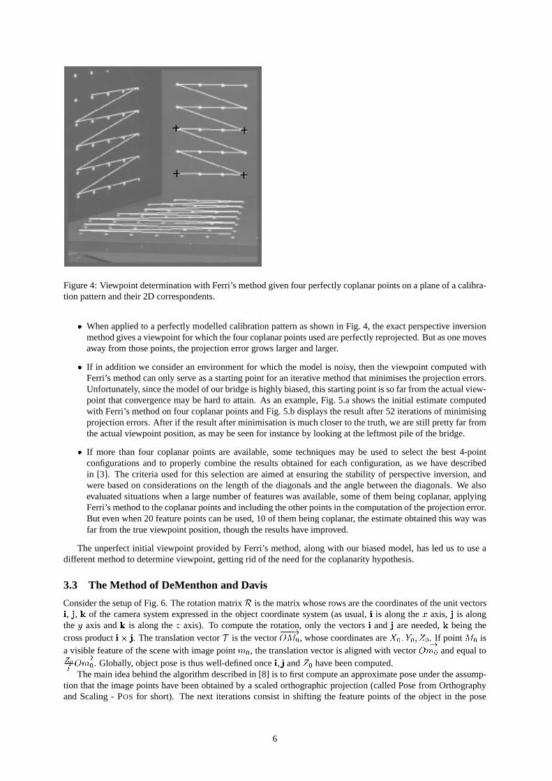
Figure 4: Viewpoint determination with Ferri’s method given four perfectly coplanar points on a plane of a calibra-tion pattern and their 2D correspondents.

When applied to a perfectly modelled calibration pattern as shown in Fig. 4, the exact perspective inversionmethod gives a viewpoint for which the four coplanar points used are perfectly reprojected. But as one movesaway from those points, the projection error grows larger and larger.

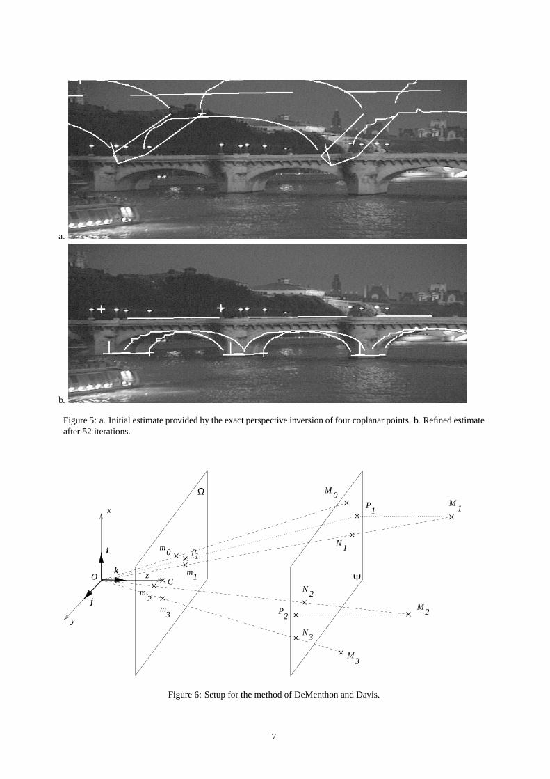
If in addition we consider an environment for which the model is noisy, then the viewpoint computed withFerri’s method can only serve as a starting point for an iterative method that minimises the projection errors.Unfortunately, since the model of our bridge is highly biased, this starting point is so far from the actual view-point that convergence may be hard to attain. As an example, Fig. 5.a shows the initial estimate computedwith Ferri’s method on four coplanar points and Fig. 5.b displays the result after 52 iterations of minimisingprojection errors. After if the result after minimisation is much closer to the truth, we are still pretty far fromthe actual viewpoint position, as may be seen for instance by looking at the leftmost pile of the bridge.

If more than four coplanar points are available, some techniques may be used to select the best 4-pointconfigurations and to properly combine the results obtained for each configuration, as we have describedin [3]. The criteria used for this selection are aimed at ensuring the stability of perspective inversion, andwere based on considerations on the length of the diagonals and the angle between the diagonals. We alsoevaluated situations when a large number of features was available, some of them being coplanar, applyingFerri’s method to the coplanar points and including the other points in the computation of the projection error.But even when 20 feature points can be used, 10 of them being coplanar, the estimate obtained this way wasfar from the true viewpoint position, though the results have improved.

The unperfect initial viewpoint provided by Ferri’s method, along with our biased model, has led us to use adifferent method to determine viewpoint, getting rid of the need for the coplanarity hypothesis.

3.3 The Method of DeMenthon and Davis

Consider the setup of Fig. 6. The rotation matrixR is the matrix whose rows are the coordinates of the unit vectorsi, j, k of the camera system expressed in the object coordinate system (as usual,i is along thex axis, j is alongthe y axis andk is along thez axis). To compute the rotation, only the vectorsi and j are needed,k being thecross producti j. The translation vectorT is the vector

!OM0, whose coordinates areX0; Y0; Z0. If point M0 is

a visible feature of the scene with image pointm0, the translation vector is aligned with vector!Om0 and equal to

Z0

f

!Om0. Globally, object pose is thus well-defined oncei; j andZ0 have been computed.The main idea behind the algorithm described in [8] is to first compute an approximate pose under the assump-

tion that the image points have been obtained by a scaled orthographic projection (called Pose from Orthographyand Scaling - POS for short). The next iterations consist in shifting the feature points of the object in the pose

6

a.

b.

Figure 5: a. Initial estimate provided by the exact perspective inversion of four coplanar points. b. Refined estimateafter 52 iterations.

M1

M3

N1

M0P

1

N2M

2P2

N3

m1

m0 p1

m2

m3

Ψ

Ω

j

y

x

i

kO z

C

Figure 6: Setup for the method of DeMenthon and Davis.

7

obtained to the lines of sight, obtain a scaled orthographic projection of these shifted points, and compute an ap-proximate pose using this projection (algorithm called POSIT - POS with iterations). Only a few iterations areneeded to converge to an accurate pose.

3.3.1 Perspective Projection

Call the plane throughM0 and parallel to the image plane. The viewline throughMi intersects in Ni andMi

projects orthogonally onto in Pi. Thus

!M0Mi =

!M0Ni +

!NiPi +

!PiMi:

It is clear that!M0Ni =

Z0

f!m0mi:

If C is the intersection of thez axis with the image plane, then the two vectors!NiPi and

!Cmi are proportional:

!NiPi =

!M0Mi:k

f

!Cmi:

Now we want to take the dot product of!M0Mi with i. The product

!PiMi:i is zero. The product!m0mi:i is xi x0

and!Cmi:i is xi. We thus end up with the first fundamental equation of perspective projection:

!M0Mi:

f

Z0i = xi(1 + "i) x0;

where

"i =1

Z0

!M0Mi:k:

Similarly,!M0Mi:

f

Z0j = yi(1 + "i) y0:

Writing I = fZ0

i andJ = fZ0

j, the system of equations is then:

(!M0Mi:I = xi(1 + "i) x0;!M0Mi:J = yi(1 + "i) y0:

(1)

3.3.2 Scaled Orthographic Projection

Scaled orthography is an approximation to perspective projection, where assumption is made that the depthsZi ofthe different points of the scene do not vary much and can be set to the depth of a reference pointM0. The imageof a pointMi is thus a point of the image plane with coordinates

x0i = fXi

Z0; y0i = f

Yi

Z0:

Now we may work out a construction somewhat similar to the above. We have:

!M0Mi =

!M0Pi +

!PiMi:

The vector!M0Pi is Z0

f!m0pi, wherepi is the image ofPi. The dot product of!m0pi with i is x0i x0 and the dot

product!PiMi:i is zero. We thus have that:

x0i = xi(1 + "i);

and similarlyy0i = yi(1 + "i):

8

3.3.3 Pose Estimation

The basic idea behind the POS algorithm is that if values are given to"i, then System (1) is a linear system ofequations the unknowns of which are the coordinates ofI andJ. Once we haveI andJ, i andj are obtained bynormalisingI andJ, andZ0 is obtained from the norm of one of the vectors:Z0 = f

kIk . See the next section forthe scheme used for solving System (1).

As we have seen, solving for pose by assuming that"i is given amounts to finding the pose for which the pointsMi have as scaled orthographic projections the image points with coordinates[xi(1 + "i); yi(1 + "i)].

Initially, one can set"i = 0. The POS algorithm then solves System (1) fori; j andZ0. From these values,vectork is computed and a new value of"i is obtained:

"i =1

Z0

!M0Mi:k:

With this new value, System (1) is solved again. The repetition of the above process is the core of the POSIT

algorithm. Several iterations are sufficient to converge to an accurate pose estimation.

3.3.4 Solving the Linear System

Suppose then that the values of"i have been computed at the previous step. Writing System (1) for then pointsMi

of the scene, we have two matrix equations:

AI = a; AJ = b;

wherea (resp. b) is the vector withi-th coordinatexi(1 + "i) (resp. yi(1 + "i)) andA is the matrix of thecoordinates of the pointsMi in the object frame.

If we have at least three visible points other thanM0, such that these points are not coplanar, then matrixA hasfull rank and one can compute its pseudo-inverseB using a Singular Value Decomposition ofA. This justifies whatwe do in Section 4.

3.4 Refining the First Estimate

Once the method of DeMenthon and Davis has given us a perspective projection matrix that is more or less closeto the correct one, the idea now is to use this matrix as a starting point to iteratively converge to the best possiblematrix.

The robustness of the above estimation must be improved because errors or outliers in the tracking stage willseverely affect the accuracy of the viewpoint location. Such a process is needed for at least two reasons: mismatchesmay occur during the tracking process (for instance, two neighbouring features may overlap) and will be propagatedalong the sequence. Besides, the 2D features are not detected accurately due to the bad quality of our images.Hence a robust technique for the viewpoint computation is needed [17] because it is well-known that least-squareestimations are very sensitive to noise. The most popular estimators are the M-estimators and the least median ofsquares. The advantage of the M-estimator is that it can be reduced to a weighted least square problem. It is robustto bad localisation errors but it is not really robust to false matches (outliers). On the other hand, the least medianof squares is robust to outliers but it cannot be reduced to a formula. In our application, we mainly have to dealwith bad localisations, so we focus on the use of the M-estimator.

3.4.1 Improving Robustness

Suppose thata1; ; a6 are the six parameters of displacement,i.e., the parameters of matrixW . The optimisationis done only on these six parameters. Then, if(u0i; v

0i) are the pixel coordinates of the projection of a pointMi

(obtained byM) and (ui; vi) its pixel coordinates as given by the feature detector, we want to minimise thefunction:

g(a1; ; a6) =nXi=1

(ri);

wheren is the number of points considered,ri = ri(a1; ; a6) = d((ui; vi); (u0i; v

0i)) is the residual andd denotes

the Euclidean distance. Note that each point could be weighted for instance by a measure of confidencei givenby the feature detector, in which case we would minimise the function

Pni=1

1i

(ri).

9

The function is chosen according to statistical considerations [23]. If is the derivative of, then the aboveamounts to solving the following system:

nXi=1

(ri)@ri

@ak= 0; k = 1; ; 6:

This shows that may be seen as a weighting or influence function. Different probability distributions can be used(normal, doubly exponential), but an appropriate choice is the Cauchy-Lorentz distribution, with:

(z) = log

1 +

z2

2

; (z) =

z

1 + z2

2

:

That is, the more the points deviate from the model, the less importance they have in the calculation. The Cauchy-Lorentz distribution thus allows in practice to eliminate the more distant points.

3.4.2 Minimising the Functiong

a.

b.

Figure 7: a. Initial estimate with the method of DeMenthon and Davis applied to four non-coplanar points. b.Refined estimate after 23 iterations using Powell’s method.

Numerous works have been devoted to the minimisation of a multivariate function starting from an initialpositionA0 - see in particular [20] and [26]. This complex problem is generally decomposed into several simplerones: a set of 1-dimensional minimisations done successively in several directions. The main difference betweenthe different methods lies in the choice of these directions. For instance:

Powell proposed a very simple algorithm, said ofquadratic convergence, which converges to a local mini-mum: the direction used at stepi isAi Aip, wherep is some positive integer.

The conjugate gradient method minimises at stepi in the directionrg(Ai).

10

Projection error M estimator (Lorentz)

Frames

initial guess (mean)

0

2

4

6

8

10

12

14

0 50 100 150 200 250

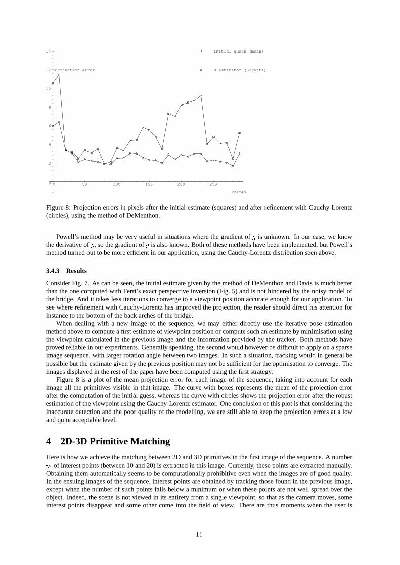
Figure 8: Projection errors in pixels after the initial estimate (squares) and after refinement with Cauchy-Lorentz(circles), using the method of DeMenthon.

Powell’s method may be very useful in situations where the gradient ofg is unknown. In our case, we knowthe derivative of, so the gradient ofg is also known. Both of these methods have been implemented, but Powell’smethod turned out to be more efficient in our application, using the Cauchy-Lorentz distribution seen above.

3.4.3 Results

Consider Fig. 7. As can be seen, the initial estimate given by the method of DeMenthon and Davis is much betterthan the one computed with Ferri’s exact perspective inversion (Fig. 5) and is not hindered by the noisy model ofthe bridge. And it takes less iterations to converge to a viewpoint position accurate enough for our application. Tosee where refinement with Cauchy-Lorentz has improved the projection, the reader should direct his attention forinstance to the bottom of the back arches of the bridge.

When dealing with a new image of the sequence, we may either directly use the iterative pose estimationmethod above to compute a first estimate of viewpoint position or compute such an estimate by minimisation usingthe viewpoint calculated in the previous image and the information provided by the tracker. Both methods haveproved reliable in our experiments. Generally speaking, the second would however be difficult to apply on a sparseimage sequence, with larger rotation angle between two images. In such a situation, tracking would in general bepossible but the estimate given by the previous position may not be sufficient for the optimisation to converge. Theimages displayed in the rest of the paper have been computed using the first strategy.

Figure 8 is a plot of the mean projection error for each image of the sequence, taking into account for eachimage all the primitives visible in that image. The curve with boxes represents the mean of the projection errorafter the computation of the initial guess, whereas the curve with circles shows the projection error after the robustestimation of the viewpoint using the Cauchy-Lorentz estimator. One conclusion of this plot is that considering theinaccurate detection and the poor quality of the modelling, we are still able to keep the projection errors at a lowand quite acceptable level.

4 2D-3D Primitive Matching

Here is how we achieve the matching between 2D and 3D primitives in the first image of the sequence. A numberm of interest points (between 10 and 20) is extracted in this image. Currently, these points are extracted manually.Obtaining them automatically seems to be computationally prohibitive even when the images are of good quality.In the ensuing images of the sequence, interest points are obtained by tracking those found in the previous image,except when the number of such points falls below a minimum or when these points are not well spread over theobject. Indeed, the scene is not viewed in its entirety from a single viewpoint, so that as the camera moves, someinterest points disappear and some other come into the field of view. There are thus moments when the user is

11

Figure 9: Contour chains.

requested to point some new feature points in the image. These new 2D points have to be automatically matchedwith the 3D points of the model.

4.1 Pruning the Hypotheses

To solve the problem of matching 2D and 3D primitives in the first image of the sequence, we have the followingat our disposal:

a wireframe model of the scene (see Fig. 2) or to be more precise a complete wireframe model of an objectthat may not be fully visible in any image of the sequence.

We have manually extracted from this modeln distinguished feature points (roughly 70): corners, top pointof each arch, centres of the lamps... They are shown on Fig. 2.

m 2D points extracted manually from the first image corresponding to feature points of the model.

Also we suppose that at any moment there are at least four 3D model points that we know are present in the currentimage.

Now, four non-coplanar 3D feature points and their 2D matches are sufficient to compute the pose of the scene.From these, we can generatem!

(m4)! potential pose estimates. To prune these estimates and find the best one, weapply successively two heuristics that have proved reliable for the application of the bridges of Paris:

Heuristic 1 is classical: keep only those pose estimates for which the sum of the projection errors for the four3D points is smaller than some threshold. We usually keep between 100 and 400 estimates at this stage.

Heuristic 2 is similar to the first except that the calculation of the projection error is achieved on all featurepoints of the model. When computing this error, we penalise those model points for which we have not beenable to locate a 2D correspondent in a given window. We keep the best estimate after this step.

4.2 A Few Words on the Use of Contour Chains

Initially, we planned to use the contour image of the scene to evaluate the adequation of the projection of the modelof the bridge with the real bridge. Unfortunately, since the sequence has been shot at night, the images are notsufficiently contrasted and it is very difficult to obtain a significative gradient image. The contour chains built fromthese gradients are “unstable”: they are very dependent on viewpoint position and very sensitive to the thresholdused - compare Figs. 9 and 11.a. They also lead to poor evaluations when superimposing the image of chains ofstrong gradient and the projection of the model.

A high threshold produces few chains which do not generally correspond to parts of the model, since the bridgeis not sufficiently “contrasted” with respect to the surrounding environment. A low threshold produces many chainsfor which any viewpoint estimate is equally correct: it is easy to find a chain in the neighbourhood of a contour ofthe reprojected model. Our images are not good enough to obtain correct contour chains and to allow the evaluationof each viewpoint estimate by comparing the entire edge contours of the object with the image edges as in [12].To be efficient in our context, this method would need to be coupled with somea priori knowledge on the scene,something we wanted to avoid.

12

a.

b.

Figure 10: Matching 2D and 3D primitives. a. The first image of the sequence, including 20 points extractedmanually from the contour map. b. Result of computing viewpoint by automatic 2D-3D primitive matching.

4.3 Result Images

The first image of the scene contains 20 of then distinguished feature points of the bridge model and is shown inFig. 10.a. The result of computing the viewpoint by automatic matching of 2D-3D primitives on the first image ofthe sequence is given on Fig. 10.b.

5 Feature Tracking

We describe in this section the tracking techniques that we implemented in our system. Two kinds of features willbe tracked: points, used to determine the viewpoint, and curve segments (the arches). The arches are not useddirectly as curved segments for viewpoint determination in the present version of the system, as could be done withthe method of [16], but only because they provide interesting feature points (the top of each arch for instance - seepoint 4 of Fig. 11.c). In fact, we will see that even points are tracked using a curve-based tracking tool.

Features to be tracked are selected before execution in the first image and the corresponding 3D points in themodel are retained. Then, they are tracked along the sequence in the autonomous way described below. Because ofthe length of the sequence, new features to be tracked appear as the sequence evolves. The tracking process is thusstopped momentarily to select these new features.

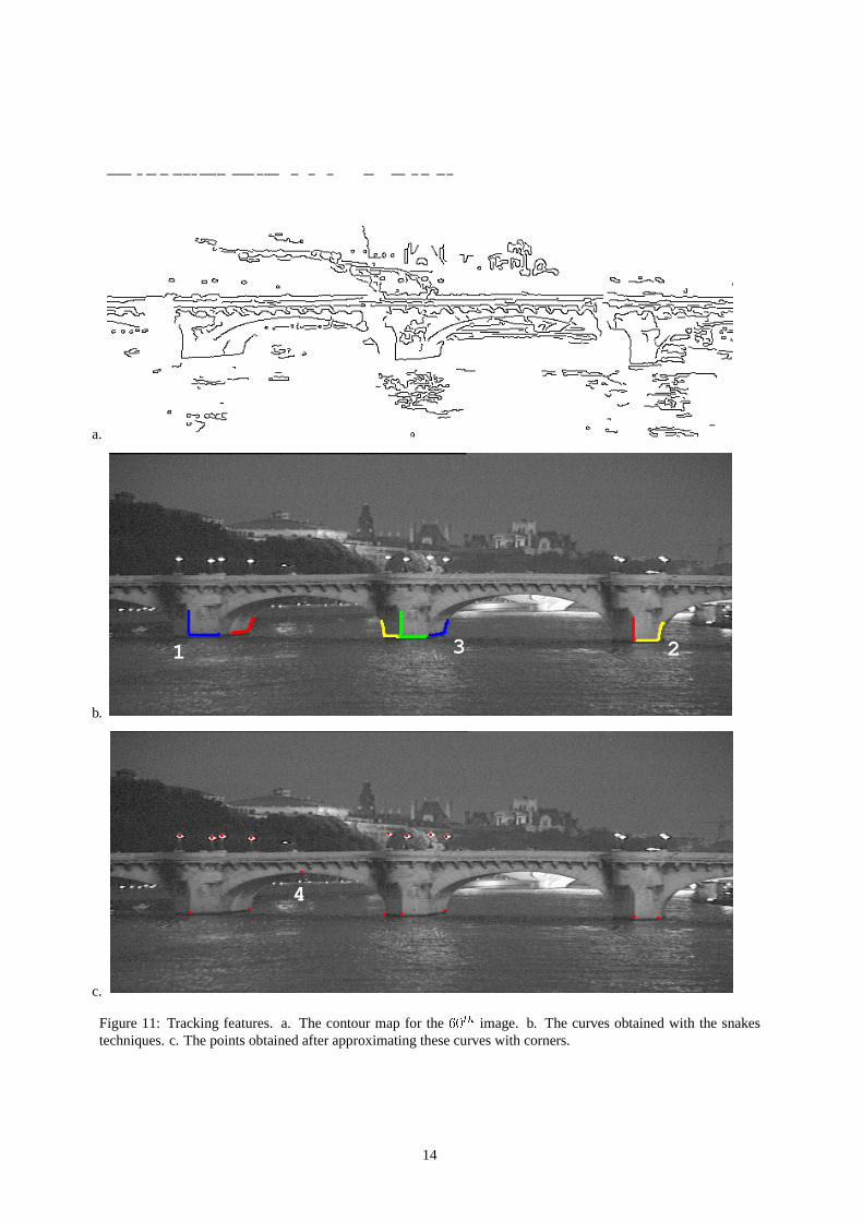
The sequence we consider here was shot in nighttime. Consequences are that the segmentation is very poor andthat feature points cannot be tracked using the contour map. Hence, we use a curve-based tracking tool capableof tracking interest curves containing the feature points used for the pose computation. For instance, as shown inFig. 11, instead of tracking the point at the basis of the bridge pier, we track the curve drawn in red and we inferthe point position by computing the corner best fitting the curve. As shown in the examples, sufficiently accuratefeatures can then be obtained.

Other points than the bases of the piers can be of great interest for the pose computation: the street lamps on the

13

a.

b.

1 3 2

c.

4

Figure 11: Tracking features. a. The contour map for the60th image. b. The curves obtained with the snakestechniques. c. The points obtained after approximating these curves with corners.

14

bridge whose 3D position is known. The light emitted by these lamps always appears as white blobs in the imageswhatever the viewpoint and can be tracked using correlation methods as described below.

We now describe in details the two tracking techniques used: correlation-based tracking and curve-based track-ing.

5.1 Correlation-Based Tracking

As soon as a new street lamp appears, the centre of the light bulb is detected in the following way: the user drawsa small polygon enclosing the light bulb; because the light appears as a white blob on the image, the bulb can beoutlined using a simple threshold. The centroid of this blob is then considered as the image of the 3D centroid ofthe bulb.

The lamp is then tracked along the sequence using correlation. Given a small square enclosing the lamp inthe current image, the correlation process computes the translation best fitting this window in the next image. Thecentroid of the white blob in this new window gives the position of the feature in the next image.

5.2 Curve-Based Tracking

Other points than the lamps are tracked using a curve tracker. The tracker we designed is described in earlierworks [2]. It is made up of the following two steps:

a predictionstep: an approximation of the 2D motion field is computed iteratively from the normal opticalflow on the whole curve;

a convergencestep: from the predicted curve, an active contour [15] converges towards the nearest contourwhich is generally the homologous one. It must be noted than some strategies have been developed to bestensure this convergence.

This tool is used to track curved features like the arches of the bridge. In order to detect feature points, wetake advantage of the fact that most of them are the corner points of contour lines. Once an interest point has beenchosen, a sufficiently contrasted curve containing this point is outlined using for instance a snake technique. Thiscurve is then tracked along the sequence using the tool described above. Then, we search for the angular point ofeach of these curves: for each pointMi belonging to such a curve, the two lines best fittingMjfj<ig andMjfjigare computed. The point giving rise to the best fitting score is retained and the intersection of these two lines isconsidered as the searched feature point (point 1 on Fig. 11.b). Note that this method is used to track angularpoints between lines or between curves. In fact, if the curve containing the feature point is sufficiently small, theapproximation of the curve with a line is quite satisfactory (points 2 and 3 on Fig. 11.b). Such a method turns outto be very robust to noise since most feature points are not easily detectable in the images.

Nevertheless, some of these angular points do not correspond to 3D points of the model because they are theintersections of a vertex of the bridge with the river surface (points 1, 2, 3 in Fig. 11.b). The elevation of thesepoints can however be roughly estimated because the dimensions of the bridge are known. The elevation of the riversurface is then refined in the following way: from the upper estimationh0, we compute for each elevationh in the[h0 50 cm; h0+50 cm] range (regularly sampled) the viewpoint corresponding to the tracked set of points, whenthe elevation of the points on the river surface is set toh. The correct elevation is the one for which the projectionerror is the smallest.

6 Results and Discussion

In the previous sections, we have examined the different components of our system separately and discussed thealgorithmic choices we made. We now turn our attention to the augmented reality loop as a whole, present resultsof applying it to the Pont Neuf sequence and discuss its performance.

A quantitative analysis of the performance of the feature tracking and pose estimation algorithms on syntheticdata and for various types of features is given elsewhere [24].

6.1 The Augmented Pont Neuf Sequence

The entire 300-image sequence has been augmented with the procedure described in this paper. Fig. 12 describes thecomposition of the 60th image: Fig. 12.a shows the original image on which we have superimposed the projectionof the model using the viewpoint computed and Fig. 12.b shows the final result of the composition. Figure 13 showssimilar results for the 100th image.

15

a.

b.

Figure 12: Composition for the 60th image. a. The red curves correspond to the model projected onto the imageusing the viewpoint computed. The 2D features used for viewpoint determination appear in green and the projectionof the corresponding 3D points are in blue. b. Result of the composition.

16

a.

b.

Figure 13: Composition for the 100th image of the sequence.

17

Several MPEGmovies are available on our WWW server at the address:

http://www.loria.fr/isa/Bridges/

(tracking

projectionaugmented

).mpg ;

where tracking stands for the sequence showing the features used for the tracking,projection for theoriginal sequence with the model superimposed andaugmented for the fully augmented sequence, with thebridge illuminated synthetically (each is roughly 2.4 MB in size).

6.2 Discussion

Some comments are in order. The above results prove that our system can handle poor quality images and aninaccurate modelling of the object to inlay. In addition, it can account for a large vision field and a rotating motion:in the Pont Neuf application, the motion is purely panoramic and the total camera rotation is roughly 20 degrees(the bridge is 90 meters long and the viewpoint is located 300 meters away from the bridge). Our experiments showthat the tracker is able to deal with an apparent motion of the primitives of up to 20 pixels between two consecutiveimages.

Considering the conditions that we have already mentioned (bad segmentation due to darkness, poor modelling),the overall visual impression is quite satisfactory. The reader who gets a chance to see the entire augmentedsequence will however witness a slight jittering effect, that may best be explained with the help of Fig. 14. Theworld coordinates are such that thez-axis represents the depth of field and they coordinate is the elevation. InFig. 14, we drew the evolutions of thex; y andz coordinates of a pointP standing on the optical axis of the cameraat a distance of one meter of the optical centreC. It appears that the evolutions of thex andz coordinates are veryregular, but that ofy is highly singular, thus yielding this jittering. Incidentally, our analysis of the modelling of thebridge showed that it is quite correct in thex andz directions, but inconsistent in they direction. For instance, wewere never able to correlate both the lamps on the parapets and the arches at the same time, due to this incoherentmodelling in they direction. Also, it should be noted that the lens of the camera used had a distortion that we werenot able to fully correct.

6.3 System Performance

Although latency and execution speed are not central to the present application, they usually are key issues inaugmented reality research. We shall thus say a few words here about the computational requirements of oursystem.

Without any kind of optimisation, the only algorithmic part that does not currently achieve real time is the2D-3D primitive matching for the first image. On a Sun Ultra 1 Model 10 (the following computation times haveall been measured on this machine with Rational Software’s Quantify), this matching takes 34.4 seconds for a setof 17 2D points and 70 3D points. The determination of viewpoint with the method of DeMenthon and Davisapplied to 20 input points takes less than one millisecond, while optimisation to converge to an accurate viewpointposition takes 92 milliseconds. And tracking a primitive of 30 points takes 97 milliseconds for the prediction stepand 70 milliseconds for the convergence step. In other words, apart from the initialisation on the first image of thesequence, the tools presented in this paper are amenable to real-time performance. Of course, global illuminationalgorithms are known to have large computation times. And indeed, notably because of the high number of lightsources involved, more than 50, the rendering of the bridge we inlayed in our image sequence took more than 7hours to compute.

7 Conclusion and Future Research Directions

We have presented in this paper a complete augmented reality forward loop. An application to the simulation of alighting project of a bridge in Paris has been explained and results are shown that prove the validity of our approach.Emphasis has been put on the computer vision tools used to determine viewpoint and to track a set of features ina sequence of images of an outdoor urban environment. The method overcomes several weaknesses of previousapproaches, especially as far as automatic and robust viewpoint determination is concerned.

We are currently working on several features that would robustify and enhance our augmented reality system:

Perspective inversion of curved segments.If curved arcs are present in the scene, they may be used tofurther converge to the position of the viewpoint. Except in the case of circles [11], an exact perspectiveinversion for ellipses is not possible. We may thus use an iterative algorithm developed by [16], takingas initial estimate the perspective projection matrix obtained for a number of (coplanar or non-coplanar)

18

250 300 b.

10.57

10.572

10.574

10.576

10.578

10.58

0 50 100 150 200 250 300

c.

317.1

317.2

317.3

317.4

317.5

317.6

317.7

0 50 100 150 200 250 300

Figure 14: Evolutions of thex; y andz coordinates of a point standing on the optical axis of the camera. Abscissarepresents frame number and ordinate is measured in meters.

19

points. We did not use this feature in the application described because the modelling of the arches was tooinconsistent.

Smoothing the sequence.We do not currently ensure any kind of global coherence of the sequence, meaningthat it is not smoothed to avoid jittering for instance (tracking provides a local coherence). This could verywell be accounted for by a technique based on Kalman filtering for instance. Also, the regularity of thecamera motion could be used to improve the prediction of a feature position in the next image.

Occlusions. One of the limitations of the present system is that the mask of the occluding objects must bedetermined by hand. Hence we are currently investigating an algorithm allowing the static occluding objectsto be detected without 3D reconstruction. The underlying idea is to compare for each image point the opticalflow of this feature with the theoretical flow generated by the 3D point of the virtual object that projects ontothe feature point [4].

References

[1] Bajura, M., Fuchs, H., and Ohbuchi, R. (1992). Merging virtual objects with the real world: seeing ultra-sound imagery within the patient.Computer Graphics Proceedings, Annual Conference Series, 26:203–210.Proceedings of SIGGRAPH’92.

[2] Berger, M.-O. (1994). How to track efficiently piecewise curved contours with a view to reconstructing 3Dobjects. InProceedings of 12thICPR (International Conference on Pattern Recognition), Jerusalem, Israel,volume 1, pages 32–36.

[3] Berger, M.-O., Simon, G., Petitjean, S., and Wrobel-Dautcourt, B. (1996). Mixing synthesis and video imagesof outdoor environments: application to the bridges of Paris. InProceedings of 13thICPR (InternationalConference on Pattern Recognition), Vienna, Austria, volume 1, pages 90–94.

[4] Berger, M.-O. (1997). Resolving occlusions in augmented reality: a contour-based approach without 3Dreconstruction. InProceedings ofCVPR (IEEE Conference on Computer Vision and Pattern Recognition),Puerto Rico.

[5] Caudel, T. and Mizell, D. (1992). Augmented reality: an application of heads-up display technology to manualmanufacturing processes. InProceedings of Hawaii International Conference on System Sciences.

[6] Cazier, D., Chamont, D., Deville, P., and Paul, J.-C. (1994). Modeling characteristics of light: a method basedon measured data. InProceedings of the Second Pacific Conference on Computer Graphics and Applications,pages 113–128.

[7] Chevrier, C., Belblidia, S., and Paul, J.-C. (1995). Compositing computer-generated images and video films:an application for visual assessment in urban environments. In Earnshaw, R. and Vince, J., editors,Proceed-ings ofCGI’95 (Computer Graphics International), pages 115–125. Academic Press.

[8] DeMenthon, D. and Davis, L. (1995). Model-based object pose in 25 lines of code.International Journal ofComputer Vision, 15:123–141.

[9] Ertl, G., Mueller-Seelich, H., and Tabatabai, B. (1991). Move-x: a system for combining video films andcomputer animation. In Purgathofer, W., editor,Proceedings of Eurographics’91, pages 305–314.

[10] Fasse, I., Paulo, S. S., Perrin, J.-P., and Paul, J.-C. (1994). Accurate synthesis images for architectural design.In Proceedings of the Conference on Multimedia for Architecture and Urban Design, pages 229–243.

[11] Ferri, M., Mangili, F., and Viano, G. (1993). Projective pose estimation of linear and quadratic primitives inmonocular computer vision. CVGIP: Image Understanding, 58(1):66–84.

[12] Huttenlocher, D. and Ullman, S. (1990). Recognizing solid objects by alignment with an image.InternationalJournal of Computer Vision, 5(2):195–212.

[13] Jancene, P., Neyret, F., Provot, X., Tarel, J.-P., Vezien, J.-M., Meilhac, C., and Verroust, A. (1995). RES:computing the Interactions between Real and Virtual Objects in Video Sequences. InProceedings of theIEEE

Workshop on Networked Realities, Boston, MA, pages 27–40.

20

[14] Kaneda, K., Kato, F., Nakamae, E., Nishita, T., Tanaka, H., and Noguchi, T. (1989). Three-dimensional terrainmodelling and display for environmental assessment.Computer Graphics Proceedings, Annual ConferenceSeries, 23:207–214. Proceedings of SIGGRAPH’89.

[15] Kass, M., Witkin, A., and Terzopoulos, D. (1988). Snakes: active contour models.International Journal ofComputer Vision, 1:321–331.

[16] Kriegman, D. and Ponce, J. (1990). On recognizing and positioning curved 3D objects from image contours.IEEE Transactions on Pattern Analysis and Machine Intelligence, 12(12):1127–1137.

[17] Kumar, R. and Hanson, A. (1994). Robust methods for estimating pose and a sensitivity analysis. CVGIP:Image Understanding, 60(3):313–342.

[18] Maver, T., Purdie, C., and Stearn, D. (1985). Visual impact analysis - modelling and viewing the natural andbuilt environment.Computer and Graphics, 9(2):117–124.

[19] Nakamae, E., Harada, K., Ishizaki, T., and Nishita, T. (1986). A montage method: the overlaying of the com-puter generated images onto a background photograph.Computer Graphics Proceedings, Annual ConferenceSeries, 20:207–214. Proceedings of SIGGRAPH’86.

[20] Press, W., Flannery, B., Tenkolsky, S., and Vetterling, W. (1988).Numerical Recipes in C, The Art of ScientificComputing. Cambridge University Press.

[21] Ravela, S., Draper, B., Lim, J., and Weiss, R. (1995). Adaptive tracking and model registration across distinctaspects. InProceedings ofIROS’95 (IEEE/RSJ Conference on Intelligent Robots and Systems), pages 174–180, Pittsburgh.

[22] Ravela, S., Draper, B., Lim, J., and Weiss, R. (1996). Tracking object motion across aspect changes foraugmented reality. InProceedings ofIUW (DARPA Image Understanding Workshop).

[23] Rousseeuw, P. and Leroy, A. (1987).Robust Regression and Outlier Detection. Series in Probability andMathematical Statistics. Wiley.

[24] Simon, G. and Berger, M.-O. (1998). A two-stage robust statistical method for temporal registration fromfeatures of various type.International Journal of Computer Vision, submitted.

[25] State, A., Livingstone, M., Garett, W., Hirota, G., Whitton, M., and Pisan, E. (1996). Technologies for Aug-mented Reality Systems: Realizing Ultrasound Guided Needle Biopsies.Computer Graphics Proceedings,Annual Conference Series, 30:439–446. Proceedings of SIGGRAPH’96.

[26] Stoer, J. and Bulirsch, R. (1980).Introduction to Numerical Analysis. Springer-Verlag, New York.

[27] Uenohara, M. and Kanade, T. (1996). Real-time vision-based object registration for image overlay.Journalof Computers in Biology and Medicine. In press.

[28] Uno, S. and Matsuka, H. (1979). A general purpose graphic system for computer-aided design.ComputerGraphics Proceedings, Annual Conference Series, 13(2):25–32. Proceedings of SIGGRAPH’79.

21