MinervaLab - ADDI
255
MinervaLab Release 0.1 Jun 18, 2020
-
Upload
khangminh22 -
Category
Documents
-
view
2 -
download
0
Transcript of MinervaLab - ADDI

MinervaLabRelease 0.1
Jun 18, 2020


Contents
1 Applications 11.1 Mathematical analysis of the van der Waals isotherms . . . . . . . . . . . . . . . . . . . . . . . . . 1
1.1.1 Interface . . . . . . . . . . . . . . . . . . . . . . . . . . . . . . . . . . . . . . . . . . . . . 11.1.2 CSS . . . . . . . . . . . . . . . . . . . . . . . . . . . . . . . . . . . . . . . . . . . . . . . 21.1.3 Packages . . . . . . . . . . . . . . . . . . . . . . . . . . . . . . . . . . . . . . . . . . . . 31.1.4 Physical functions . . . . . . . . . . . . . . . . . . . . . . . . . . . . . . . . . . . . . . . . 31.1.5 Functions related to the interaction . . . . . . . . . . . . . . . . . . . . . . . . . . . . . . . 51.1.6 Main interface . . . . . . . . . . . . . . . . . . . . . . . . . . . . . . . . . . . . . . . . . . 8
1.2 Mathematical analysis of the effect of a and b parameters . . . . . . . . . . . . . . . . . . . . . . . . 171.2.1 Interface . . . . . . . . . . . . . . . . . . . . . . . . . . . . . . . . . . . . . . . . . . . . . 171.2.2 CSS . . . . . . . . . . . . . . . . . . . . . . . . . . . . . . . . . . . . . . . . . . . . . . . 181.2.3 Packages . . . . . . . . . . . . . . . . . . . . . . . . . . . . . . . . . . . . . . . . . . . . 181.2.4 Physical functions . . . . . . . . . . . . . . . . . . . . . . . . . . . . . . . . . . . . . . . . 181.2.5 Functions related to interaction . . . . . . . . . . . . . . . . . . . . . . . . . . . . . . . . . 201.2.6 Main interface . . . . . . . . . . . . . . . . . . . . . . . . . . . . . . . . . . . . . . . . . . 23
1.3 Effect of a and b in van der Waals isotherms . . . . . . . . . . . . . . . . . . . . . . . . . . . . . . 281.3.1 Interface . . . . . . . . . . . . . . . . . . . . . . . . . . . . . . . . . . . . . . . . . . . . . 281.3.2 CSS . . . . . . . . . . . . . . . . . . . . . . . . . . . . . . . . . . . . . . . . . . . . . . . 291.3.3 Packages . . . . . . . . . . . . . . . . . . . . . . . . . . . . . . . . . . . . . . . . . . . . 291.3.4 Physical functions . . . . . . . . . . . . . . . . . . . . . . . . . . . . . . . . . . . . . . . . 291.3.5 Functions related to interaction . . . . . . . . . . . . . . . . . . . . . . . . . . . . . . . . . 311.3.6 Main interface . . . . . . . . . . . . . . . . . . . . . . . . . . . . . . . . . . . . . . . . . . 35
1.4 Effect of a and b in van der Waals isotherms (reduced variables) . . . . . . . . . . . . . . . . . . . . 431.4.1 Interface . . . . . . . . . . . . . . . . . . . . . . . . . . . . . . . . . . . . . . . . . . . . . 431.4.2 CSS . . . . . . . . . . . . . . . . . . . . . . . . . . . . . . . . . . . . . . . . . . . . . . . 431.4.3 Packages . . . . . . . . . . . . . . . . . . . . . . . . . . . . . . . . . . . . . . . . . . . . 441.4.4 Physical functions . . . . . . . . . . . . . . . . . . . . . . . . . . . . . . . . . . . . . . . . 441.4.5 Functions related to interaction . . . . . . . . . . . . . . . . . . . . . . . . . . . . . . . . . 451.4.6 Main interface . . . . . . . . . . . . . . . . . . . . . . . . . . . . . . . . . . . . . . . . . . 48
1.5 Critical points for various fluids . . . . . . . . . . . . . . . . . . . . . . . . . . . . . . . . . . . . . 561.5.1 Interface . . . . . . . . . . . . . . . . . . . . . . . . . . . . . . . . . . . . . . . . . . . . . 561.5.2 CSS . . . . . . . . . . . . . . . . . . . . . . . . . . . . . . . . . . . . . . . . . . . . . . . 571.5.3 Packages . . . . . . . . . . . . . . . . . . . . . . . . . . . . . . . . . . . . . . . . . . . . 581.5.4 Physical functions . . . . . . . . . . . . . . . . . . . . . . . . . . . . . . . . . . . . . . . . 581.5.5 Functions related to the interaction . . . . . . . . . . . . . . . . . . . . . . . . . . . . . . . 611.5.6 Main interface . . . . . . . . . . . . . . . . . . . . . . . . . . . . . . . . . . . . . . . . . . 66
i

1.6 Compare elements’ isotherms . . . . . . . . . . . . . . . . . . . . . . . . . . . . . . . . . . . . . . 781.6.1 Interface . . . . . . . . . . . . . . . . . . . . . . . . . . . . . . . . . . . . . . . . . . . . . 791.6.2 CSS . . . . . . . . . . . . . . . . . . . . . . . . . . . . . . . . . . . . . . . . . . . . . . . 791.6.3 Packages . . . . . . . . . . . . . . . . . . . . . . . . . . . . . . . . . . . . . . . . . . . . 791.6.4 Physical functions . . . . . . . . . . . . . . . . . . . . . . . . . . . . . . . . . . . . . . . . 801.6.5 Functions related to interaction . . . . . . . . . . . . . . . . . . . . . . . . . . . . . . . . . 821.6.6 Main interface . . . . . . . . . . . . . . . . . . . . . . . . . . . . . . . . . . . . . . . . . . 85
1.7 Maxwell’s construction on van der Waals isotherms . . . . . . . . . . . . . . . . . . . . . . . . . . 911.7.1 Interface . . . . . . . . . . . . . . . . . . . . . . . . . . . . . . . . . . . . . . . . . . . . . 911.7.2 CSS . . . . . . . . . . . . . . . . . . . . . . . . . . . . . . . . . . . . . . . . . . . . . . . 921.7.3 Packages . . . . . . . . . . . . . . . . . . . . . . . . . . . . . . . . . . . . . . . . . . . . 921.7.4 Physical functions . . . . . . . . . . . . . . . . . . . . . . . . . . . . . . . . . . . . . . . . 931.7.5 Functions related to the interaction . . . . . . . . . . . . . . . . . . . . . . . . . . . . . . . 991.7.6 Functions related to visualization . . . . . . . . . . . . . . . . . . . . . . . . . . . . . . . . 1151.7.7 Main interface . . . . . . . . . . . . . . . . . . . . . . . . . . . . . . . . . . . . . . . . . . 117
1.8 p-T plane and Gibbs free energy . . . . . . . . . . . . . . . . . . . . . . . . . . . . . . . . . . . . . 1291.8.1 Interface . . . . . . . . . . . . . . . . . . . . . . . . . . . . . . . . . . . . . . . . . . . . . 1291.8.2 CSS . . . . . . . . . . . . . . . . . . . . . . . . . . . . . . . . . . . . . . . . . . . . . . . 1291.8.3 Packages . . . . . . . . . . . . . . . . . . . . . . . . . . . . . . . . . . . . . . . . . . . . 1301.8.4 Physical functions . . . . . . . . . . . . . . . . . . . . . . . . . . . . . . . . . . . . . . . . 1301.8.5 Functions related to interaction . . . . . . . . . . . . . . . . . . . . . . . . . . . . . . . . . 1361.8.6 Main interface . . . . . . . . . . . . . . . . . . . . . . . . . . . . . . . . . . . . . . . . . . 139
1.9 Chemical potential of a van der Waals real gas . . . . . . . . . . . . . . . . . . . . . . . . . . . . . 1431.9.1 Interface . . . . . . . . . . . . . . . . . . . . . . . . . . . . . . . . . . . . . . . . . . . . . 1431.9.2 CSS . . . . . . . . . . . . . . . . . . . . . . . . . . . . . . . . . . . . . . . . . . . . . . . 1451.9.3 Packages . . . . . . . . . . . . . . . . . . . . . . . . . . . . . . . . . . . . . . . . . . . . 1461.9.4 Physical functions . . . . . . . . . . . . . . . . . . . . . . . . . . . . . . . . . . . . . . . . 1461.9.5 Functions related with the interaction . . . . . . . . . . . . . . . . . . . . . . . . . . . . . 1521.9.6 Functions related to visualization . . . . . . . . . . . . . . . . . . . . . . . . . . . . . . . . 1591.9.7 Main interface . . . . . . . . . . . . . . . . . . . . . . . . . . . . . . . . . . . . . . . . . . 161
1.10 Stability condition on van der Waals isotherms . . . . . . . . . . . . . . . . . . . . . . . . . . . . . 1781.10.1 Interface . . . . . . . . . . . . . . . . . . . . . . . . . . . . . . . . . . . . . . . . . . . . . 1781.10.2 CSS . . . . . . . . . . . . . . . . . . . . . . . . . . . . . . . . . . . . . . . . . . . . . . . 1791.10.3 Packages . . . . . . . . . . . . . . . . . . . . . . . . . . . . . . . . . . . . . . . . . . . . 1801.10.4 Physical functions . . . . . . . . . . . . . . . . . . . . . . . . . . . . . . . . . . . . . . . . 1801.10.5 Functions related to interaction . . . . . . . . . . . . . . . . . . . . . . . . . . . . . . . . . 1811.10.6 Main interface . . . . . . . . . . . . . . . . . . . . . . . . . . . . . . . . . . . . . . . . . . 185
1.11 Visualization of molar volume during a liquid-gas phase transition . . . . . . . . . . . . . . . . . . . 1911.11.1 Interface . . . . . . . . . . . . . . . . . . . . . . . . . . . . . . . . . . . . . . . . . . . . . 1911.11.2 CSS . . . . . . . . . . . . . . . . . . . . . . . . . . . . . . . . . . . . . . . . . . . . . . . 1921.11.3 Packages . . . . . . . . . . . . . . . . . . . . . . . . . . . . . . . . . . . . . . . . . . . . 1921.11.4 Physical functions . . . . . . . . . . . . . . . . . . . . . . . . . . . . . . . . . . . . . . . . 1931.11.5 Functions related to the interaction . . . . . . . . . . . . . . . . . . . . . . . . . . . . . . . 1981.11.6 Functions related to visualization . . . . . . . . . . . . . . . . . . . . . . . . . . . . . . . . 2001.11.7 Main interface . . . . . . . . . . . . . . . . . . . . . . . . . . . . . . . . . . . . . . . . . . 203
1.12 Change in molar entropy during a first-order phase transition . . . . . . . . . . . . . . . . . . . . . . 2101.12.1 Interface . . . . . . . . . . . . . . . . . . . . . . . . . . . . . . . . . . . . . . . . . . . . . 2101.12.2 CSS . . . . . . . . . . . . . . . . . . . . . . . . . . . . . . . . . . . . . . . . . . . . . . . 2111.12.3 Packages . . . . . . . . . . . . . . . . . . . . . . . . . . . . . . . . . . . . . . . . . . . . 2111.12.4 Physical functions . . . . . . . . . . . . . . . . . . . . . . . . . . . . . . . . . . . . . . . . 2121.12.5 Functions related to the interaction . . . . . . . . . . . . . . . . . . . . . . . . . . . . . . . 2181.12.6 Functions related to visualization . . . . . . . . . . . . . . . . . . . . . . . . . . . . . . . . 2211.12.7 Main interface . . . . . . . . . . . . . . . . . . . . . . . . . . . . . . . . . . . . . . . . . . 223
1.13 Van der Waals isotherms in 3D . . . . . . . . . . . . . . . . . . . . . . . . . . . . . . . . . . . . . . 229
ii

1.13.1 Interface . . . . . . . . . . . . . . . . . . . . . . . . . . . . . . . . . . . . . . . . . . . . . 2291.13.2 Packages . . . . . . . . . . . . . . . . . . . . . . . . . . . . . . . . . . . . . . . . . . . . 2301.13.3 Physical functions . . . . . . . . . . . . . . . . . . . . . . . . . . . . . . . . . . . . . . . . 2301.13.4 Functions related to interaction . . . . . . . . . . . . . . . . . . . . . . . . . . . . . . . . . 2311.13.5 Main interface . . . . . . . . . . . . . . . . . . . . . . . . . . . . . . . . . . . . . . . . . . 231
2 Azalpen teorikoak 2352.1 Fase-trantsizioak . . . . . . . . . . . . . . . . . . . . . . . . . . . . . . . . . . . . . . . . . . . . . 235
2.1.1 Bibliografia . . . . . . . . . . . . . . . . . . . . . . . . . . . . . . . . . . . . . . . . . . . 2382.2 van der Waals-en egoera-ekuazioa . . . . . . . . . . . . . . . . . . . . . . . . . . . . . . . . . . . . 239
2.2.1 Puntu kritikoa . . . . . . . . . . . . . . . . . . . . . . . . . . . . . . . . . . . . . . . . . . 2402.2.2 Potentzial kimikoaren azterketa . . . . . . . . . . . . . . . . . . . . . . . . . . . . . . . . . 2412.2.3 Lerro isotermo errealak . . . . . . . . . . . . . . . . . . . . . . . . . . . . . . . . . . . . . 2422.2.4 Bolumen molarraren aldaketa . . . . . . . . . . . . . . . . . . . . . . . . . . . . . . . . . . 2452.2.5 Entropia molarraren aldaketa . . . . . . . . . . . . . . . . . . . . . . . . . . . . . . . . . . 2462.2.6 Bibliografia . . . . . . . . . . . . . . . . . . . . . . . . . . . . . . . . . . . . . . . . . . . 247
3 Indices and tables 249
iii

iv

CHAPTER 1
Applications
1.1 Mathematical analysis of the van der Waals isotherms
Code: #118-000
File: apps/van_der_waals/mathematical_analysis.ipynb
Run it online:
The aim of this notebook is to show the mathematical function of van der Waals isotherms.
1.1.1 Interface
The main interface (main_block_118_000) is divided in two HBox: top_block_118_000 andbottom_block_118_000. top_block_118_000 contains of a bqplot Figure (fig_118_001) andbottom_block_118_000 contains 4 bqplot Figures: fig_118_003, fig_118_004, fig_118_005 andfig_118_006. The slider zoom_slider controls the zoom of fig_118_001.
[1]: from IPython.display import ImageImage(filename='../../static/images/apps/118-000_1.png')
1

MinervaLab, Release 0.1
[1]:
[2]: Image(filename='../../static/images/apps/118-000_2.png')
[2]:
1.1.2 CSS
A custom css file is used to improve the interface of this application. It can be found here.
[1]: from IPython.display import HTMLdisplay(HTML("<head><link rel='stylesheet' type='text/css' href='./../../static/→˓custom.css'></head>"))display(HTML("<style>.container { width:100% !important; }</style>"))
<IPython.core.display.HTML object>
2 Chapter 1. Applications

MinervaLab, Release 0.1
<IPython.core.display.HTML object>
1.1.3 Packages
[2]: from bqplot import *import bqplot as bqimport bqplot.marks as bqmimport bqplot.scales as bqsimport bqplot.axes as bqa
import ipywidgets as widgets
import urllib.parseimport webbrowser
import sys
1.1.4 Physical functions
This are the functions that have a physical meaning:
• calculate_critic
• get_absolute_isotherms
• bar_to_atm
[3]: def calculate_critic(a, b):
"""This function calculates the critic point(p_c, v_c, T_c) from given a and b parameters ofthe Van der Waals equation of state for real gases.
:math:`(P + a \\frac{n^2}{V^2})(V - nb) = nRT`
:math:`p_c = \\frac{a}{27 b^2}`:math:`v_c = 3b`:math:`T_c = \\frac{8a}{27 b R}`
Args:a: Term related with the attraction between particles inL^2 bar/mol^2.\nb: Term related with the volume that is occupied by onemole of the molecules in L/mol.\n
Returns:p_c: Critical pressure in bar.\nv_c: Critical volume in L/mol.\nT_c: Critical tenperature in K.\n
"""
if b == 0.0:return None
(continues on next page)
1.1. Mathematical analysis of the van der Waals isotherms 3

MinervaLab, Release 0.1
(continued from previous page)
k_B = 1.3806488e-23 #m^2 kg s^-2 K^-1N_A = 6.02214129e23R = 0.082 * 1.01325 #bar L mol^-1 K^-1
p_c = a/27.0/(b**2)v_c = 3.0*bT_c = 8.0*a/27.0/b/R
return p_c, v_c, T_c
[4]: def get_absolute_isotherms(a, b, v_values, T_values):"""This function calculates the theoretical p(v, T) plane
(in absolute coordinates) according to van der Waalsequation of state from a given range of volumesand tenperatures.
Args:a: Term related with the attraction between particles in
L^2 bar/mol^2.\nb: Term related with the volume that is occupied by onemole of the molecules in L/mol.\nv_values: An array containing the values of vfor which the isotherms must be calculated.\nT_values: An array containing the values of T for whichthe isotherms must be calculated.\n
Returns:isotherms: A list consisted of numpy arrays containing thepressures of each isotherm.
"""isotherms = []
R = 0.082 * 1.01325 #bar L mol^-1 K^-1
for T in T_values:
isot = []
for v in v_values:
p = R*T/(v - b) - (a/v**2)isot = np.append(isot, p)
isotherms.append(isot)
return isotherms
[5]: def bar_to_atm(p_values):"""This function changes the pressures of an arrayform bars to atm.
Args:p_values: List consisted of pressures in bars.\n
(continues on next page)
4 Chapter 1. Applications

MinervaLab, Release 0.1
(continued from previous page)
Returns:p_values: List consisted of pressures in atm.\n
"""
p_values = np.array(p_values) * 0.9869
return p_values
1.1.5 Functions related to the interaction
[6]: def update_scales(change):"""This function updates the scales of fig_118_001 (and its marks)when the value of zoom_slider is changed.\n"""index = change.owner.value
new_scale_x = bqs.LinearScale(min = x_min[index], max = x_max[index])new_scale_y = bqs.LinearScale(min = y_min[index], max = y_max[index])
# if the scales are not updated in this order the transition# is a bit laggy
for mark in fig_118_001.marks:
mark.scales = {'x' : new_scale_x,'y' : new_scale_y
}
axis_x_118_001.scale = new_scale_xaxis_y_118_001.scale = new_scale_y
[7]: def change_view(change):"""This function changes the visualization of all thecomponents of the application so they are suitable fora projection.\n"""
obj = change.owner
if obj.value:
obj.description = 'Presentation mode (ON)'
display(HTML("<style>" \".widget-readout { font-size: 30px ; }" \".widget-label-basic {font-size: 30px;}" \"option {font-size: 25px;}" \".p-Widget.jupyter-widgets.widget-slider.widget-vslider.widget-inline-
→˓vbox {width: auto}" \".p-Widget .jupyter-widgets .widgets-label {width: auto; height: auto;
→˓font-size: 30px;}" \
(continues on next page)
1.1. Mathematical analysis of the van der Waals isotherms 5

MinervaLab, Release 0.1
(continued from previous page)
".widget-label {font-size: 30px ; height: auto !important;}" \".p-Widget .bqplot .figure .jupyter-widgets {height: auto !important;}" \".widget-text input[type='number'] {font-size: 30px;height: auto;}" \".option { font-size: 30px ;}" \".p-Widget .jupyter-widgets .jupyter-button.widget-button {font-size:
→˓30px ; width: auto; height: auto;}" \".p-Widget.jupyter-widgets.jupyter-button.widget-toggle-button{font-size:
→˓30px ; width: auto; height: auto;}" \".p-Widget.p-Panel.jupyter-widgets.widget-container.widget-box.widget-
→˓vbox {padding-bottom: 30px}" \".bqplot > svg .axis text.axislabel, .bqplot > svg .axis tspan.axislabel
→˓{font-size: 30px;}" \".q-grid .slick-cell {font-size: 30px;}" \".slick-column-name {font-size: 30px;}""</style>")
)
for figure in figures:
figure.legend_text = {'font-size': '30px'}figure.title_style = {'font-size': '30px'}
for axis in figure.axes:axis.tick_style = {'font-size': '30px'}axis.label_style = {'font-size': '30px'}
else:
obj.description = 'Presentation mode (OFF)'
display(HTML("<style>" \".widget-readout { font-size: 14px ;}" \".widget-label-basic {font-size: 14px;}" \"option {font-size: 12px;}" \".p-Widget .jupyter-widgets .widgets-label {font-size: 14px;}" \".widget-label {font-size: 14px ;}" \".widget-text input[type='number'] {font-size: 14px;}" \".option { font-size: 14px ;}" \".p-Widget .jupyter-widgets .jupyter-button.widget-button {font-size:
→˓14px;}" \".p-Widget.jupyter-widgets.jupyter-button.widget-toggle-button {font-size:
→˓ 14px;}" \".bqplot > svg .axis text.axislabel, .bqplot > svg .axis tspan.axislabel
→˓{font-size: 14px;}" \".q-grid .slick-cell {font-size: 14px;}" \".slick-column-name {font-size: 14px;}""</style>")
)
for figure in figures:
figure.legend_text = {'font-size': '14px'}figure.title_style = {'font-size': '20px'}
(continues on next page)
6 Chapter 1. Applications

MinervaLab, Release 0.1
(continued from previous page)
for axis in figure.axes:axis.tick_style = {'font-size': '14px'}axis.label_style = {'font-size': '14px'}
[8]: def prepare_export(button):"""This function sends the selected plot to the 'export_plot'function."""
if button is prepare_export_fig_118_001_button:
export_plot(fig_118_001)
elif button is prepare_export_fig_118_003_button:
export_plot(fig_118_003)
elif button is prepare_export_fig_118_004_button:
export_plot(fig_118_004)
elif button is prepare_export_fig_118_005_button:
export_plot(fig_118_005)
elif button is prepare_export_fig_118_006_button:
export_plot(fig_118_006)
[9]: def export_plot(plot):"""This function sends the selected plot to the export module."""
global data
text_lines = []
np.set_printoptions(threshold=sys.maxsize)
for mark in plot.marks:mark.tooltip = None
data = repr((plot, text_lines))
%store data
rel_url = "../../../apps/modules/export_module.ipynb"abs_url = urllib.parse.urljoin(notebook_url, rel_url)
if not webbrowser.open(abs_url):go_to_export_button.value = "<form action=" + abs_url + " target='_blank'>
→˓<button type=''submit''>Open in export module</button></form>"
[ ]: %%javascript
(continues on next page)
1.1. Mathematical analysis of the van der Waals isotherms 7

MinervaLab, Release 0.1
(continued from previous page)
//Get the URL of the current notebook
var kernel = Jupyter.notebook.kernel;var command = ["notebook_url = ",
"'", window.location.href, "'" ].join('')
kernel.execute(command)
1.1.6 Main interface
[ ]: #In this program we are going to use water's parametersa = 5.536 #L^2 bar mol^-2b = 0.03049 #L mol^-1
colors = ['#0079c4','#f09205','#21c400', '#850082']
p_c, v_c, T_c = calculate_critic(a, b)
p_c = p_c * 0.9869 #unit change from bar to atm
v_values = np.linspace(-5.0, 5.0, 3000) #L/molT_values = [0.9*T_c, 1.0*T_c, 1.1*T_c]
p_values = get_absolute_isotherms(a, b, v_values, T_values)p_values = bar_to_atm(p_values)
v_values_hd = np.linspace(-20, 20, 10000)p_values_hd = get_absolute_isotherms(a, b, v_values_hd, T_values)
###########################TOP BLOCK###########################
top_block_118_000 = widgets.VBox([],layout=widgets.Layout(align_items='center')
)
scale_x_118_001 = bqs.LinearScale(min = min(v_values), max = max(v_values))scale_y_118_001 = bqs.LinearScale(min =-500.0, max = 500.0)
axis_x_118_001 = bqa.Axis(scale=scale_x_118_001,tick_format='.1f',tick_style={'font-size': '15px'},num_ticks=5,grid_lines = 'none',grid_color = '#8e8e8e',label='v (L/mol)',label_location='middle',label_style={'stroke': 'black', 'default-size': 35},label_offset='50px'
)
axis_y_118_001 = bqa.Axis((continues on next page)
8 Chapter 1. Applications

MinervaLab, Release 0.1
(continued from previous page)
scale=scale_y_118_001,tick_format='.0f',tick_style={'font-size': '15px'},num_ticks=5,grid_lines = 'none',grid_color = '#8e8e8e',orientation='vertical',label='p (atm)',label_location='middle',label_style={'stroke': 'red', 'default_size': 35},label_offset='50px'
)
fig_118_001 = Figure(title='',marks=[],axes=[axis_x_118_001, axis_y_118_001],animation_duration=500,legend_location='top-right',background_style= {'fill': 'white', 'stroke': 'black'},min_aspect_ratio=1.0,fig_margin=dict(top=70, bottom=60, left=80, right=30),toolbar = True,layout = widgets.Layout(),
)
marks = [bqm.Lines(
x = [v_values for elem in p_values],y = p_values,scales = {'x': scale_x_118_001, 'y': scale_y_118_001},opacities = [1.0],visible = True,colors = colors,
)]
fig_118_001.marks = marks
prepare_export_fig_118_001_button = widgets.Button(description='Export',disabled=False,button_style='',tooltip='',layout=widgets.Layout(
width='initial',align_self='center'
))
prepare_export_fig_118_001_button.on_click(prepare_export)
zoom_slider = widgets.IntSlider(value=0,min=0,max=30,
(continues on next page)
1.1. Mathematical analysis of the van der Waals isotherms 9

MinervaLab, Release 0.1
(continued from previous page)
step=1,description='Zoom:',disabled=False,continuous_update=True,orientation='vertical',readout=False,readout_format='d',layout = widgets.Layout(margin='35px 0 0 0', height='80%')
)
zoom_slider.observe(update_scales, 'value')
# Calculate the values of the scalesx_min = np.linspace(scale_x_118_001.min, 0.0, zoom_slider.max+1)x_max = np.linspace(scale_x_118_001.max, 5.0*v_c, zoom_slider.max+1)
y_min = np.linspace(scale_y_118_001.min, 0.0, zoom_slider.max+1)y_max = np.linspace(scale_y_118_001.max, 456.0, zoom_slider.max+1)
change_view_button = widgets.ToggleButton(value=False,description='Presentation mode (OFF)',disabled=False,button_style='',tooltip='',icon='desktop',layout=widgets.Layout(
width='initial',align_self='center'
))
change_view_button.observe(change_view, 'value')
top_block_118_000.children = [change_view_button,widgets.HBox([
widgets.VBox([fig_118_001,prepare_export_fig_118_001_button,
]),zoom_slider
])]
#########################BOTTOM BLOCK##########################
bottom_block_118_000 = widgets.HBox([],layout=widgets.Layout(
height='300px',width='100%'
(continues on next page)
10 Chapter 1. Applications

MinervaLab, Release 0.1
(continued from previous page)
))
scale_x_118_003 = bqs.LinearScale(min = scale_x_118_001.min,max = scale_x_118_001.max
)
scale_y_118_003 = bqs.LinearScale(min = scale_y_118_001.min,max = scale_y_118_001.max
)
axis_x_118_003 = bqa.Axis(scale=scale_x_118_003,tick_format='.0f',tick_style={'font-size': '15px'},num_ticks=5,grid_lines = 'none',grid_color = '#8e8e8e',label='v (L/mol)',label_location='middle',label_style={'stroke': 'black', 'default-size': 35},label_offset='50px'
)
axis_y_118_003 = bqa.Axis(scale=scale_y_118_003,tick_format='.0f',tick_style={'font-size': '15px'},num_ticks=5,grid_lines = 'none',grid_color = '#8e8e8e',orientation='vertical',label='p (atm)',label_location='middle',label_style={'stroke': 'red', 'default_size': 35},label_offset='50px'
)
marks = [bqm.Lines(
x = [v_values for elem in p_values],y = p_values,scales = {'x': scale_x_118_003, 'y': scale_y_118_003},opacities = [1.0],visible = True,colors = colors
)]
fig_118_003 = Figure(title='',marks=marks,axes=[axis_x_118_003, axis_y_118_003],animation_duration=0,legend_location='top-right',
(continues on next page)
1.1. Mathematical analysis of the van der Waals isotherms 11

MinervaLab, Release 0.1
(continued from previous page)
background_style= {'fill': 'white', 'stroke': 'black'},min_aspect_ratio=1.0,fig_margin=dict(top=50, bottom=60, left=80, right=30),toolbar = False,layout = widgets.Layout(height='90%', width='95%')
)
scale_x_118_004 = bqs.LinearScale(min = -2.0, max = 2.0)scale_y_118_004 = bqs.LinearScale(min = -2.2*p_c, max = 2.2*p_c)
axis_x_118_004 = bqa.Axis(scale=scale_x_118_004,tick_format='.0f',tick_style={'font-size': '15px'},num_ticks=5,grid_lines = 'none',grid_color = '#8e8e8e',label='v (L/mol)',label_location='middle',label_style={'stroke': 'black', 'default-size': 35},label_offset='50px'
)
axis_y_118_004 = bqa.Axis(scale=scale_y_118_004,tick_format='.0f',tick_style={'font-size': '15px'},tick_values = [-500, -250, 0, 250, 500],grid_lines = 'none',grid_color = '#8e8e8e',orientation='vertical',label='p (atm)',label_location='middle',label_style={'stroke': 'red', 'default_size': 35},label_offset='50px'
)
marks = [bqm.Lines(
x = [v_values_hd for elem in p_values_hd],y = p_values_hd,scales = {'x': scale_x_118_004, 'y': scale_y_118_004},opacities = [1.0],visible = True,colors = colors,
)]
fig_118_004 = Figure(title='',marks=marks,axes=[axis_x_118_004, axis_y_118_004],animation_duration=0,legend_location='top-right',background_style= {'fill': 'white', 'stroke': 'black'},min_aspect_ratio=1.0,fig_margin=dict(top=50, bottom=60, left=80, right=30),
(continues on next page)
12 Chapter 1. Applications

MinervaLab, Release 0.1
(continued from previous page)
toolbar = True,layout = widgets.Layout(height='90%', width='95%')
)
scale_x_118_005 = bqs.LinearScale(min = 0.0, max = 2.0)scale_y_118_005 = bqs.LinearScale(min = 0.0, max = 2.2*p_c)
axis_x_118_005 = bqa.Axis(scale=scale_x_118_005,tick_format='.1f',tick_style={'font-size': '15px'},num_ticks=5,grid_lines = 'none',grid_color = '#8e8e8e',label='v (L/mol)',label_location='middle',label_style={'stroke': 'black', 'default-size': 35},label_offset='50px'
)
axis_y_118_005 = bqa.Axis(scale=scale_y_118_005,tick_format='.0f',tick_style={'font-size': '15px'},tick_values = [0, 150, 300, 450],grid_lines = 'none',grid_color = '#8e8e8e',orientation='vertical',label='p (atm)',label_location='middle',label_style={'stroke': 'red', 'default_size': 35},label_offset='50px'
)
marks = [bqm.Lines(
x = [v_values_hd for elem in p_values_hd],y = p_values_hd,scales = {'x': scale_x_118_005, 'y': scale_y_118_005},opacities = [1.0],visible = True,colors = colors,
)]
fig_118_005 = Figure(title='',marks=marks,axes=[axis_x_118_005, axis_y_118_005],animation_duration=0,legend_location='top-right',background_style= {'fill': 'white', 'stroke': 'black'},min_aspect_ratio=1.0,fig_margin=dict(top=50, bottom=60, left=80, right=30),toolbar = True,
(continues on next page)
1.1. Mathematical analysis of the van der Waals isotherms 13

MinervaLab, Release 0.1
(continued from previous page)
layout = widgets.Layout(height='90%', width='95%'))
scale_x_118_006 = bqs.LinearScale(min = 0.5*v_c, max = 5.0*v_c)scale_y_118_006 = bqs.LinearScale(min = 0.0, max = 2.0*p_c)
axis_x_118_006 = bqa.Axis(scale=scale_x_118_006,tick_format='.2f',tick_style={'font-size': '15px'},num_ticks=5,grid_lines = 'none',grid_color = '#8e8e8e',label='v (L/mol)',label_location='middle',label_style={'stroke': 'black', 'default-size': 35},label_offset='50px'
)
axis_y_118_006 = bqa.Axis(scale=scale_y_118_006,tick_format='.0f',tick_style={'font-size': '15px'},tick_values = [0, 100, 200, 300, 400],grid_lines = 'none',grid_color = '#8e8e8e',orientation='vertical',label='p (atm)',label_location='middle',label_style={'stroke': 'red', 'default_size': 35},label_offset='50px'
)
marks = [bqm.Lines(
x = [v_values_hd for elem in p_values_hd],y = p_values_hd,scales = {'x': scale_x_118_006, 'y': scale_y_118_006},opacities = [1.0],visible = True,colors = colors,
)]
fig_118_006 = Figure(title='',marks=marks,axes=[axis_x_118_006, axis_y_118_006],animation_duration=0,legend_location='top-right',background_style= {'fill': 'white', 'stroke': 'black'},min_aspect_ratio=1.0,fig_margin=dict(top=50, bottom=60, left=80, right=30),toolbar = True,layout = widgets.Layout(height='90%', width='95%')
)
(continues on next page)
14 Chapter 1. Applications

MinervaLab, Release 0.1
(continued from previous page)
prepare_export_fig_118_003_button = widgets.Button(description='Export',disabled=False,button_style='',tooltip='',layout=widgets.Layout(
width='initial',align_self='center'
))
prepare_export_fig_118_003_button.on_click(prepare_export)
prepare_export_fig_118_004_button = widgets.Button(description='Export',disabled=False,button_style='',tooltip='',layout=widgets.Layout(
width='initial',align_self='center'
))
prepare_export_fig_118_004_button.on_click(prepare_export)
prepare_export_fig_118_005_button = widgets.Button(description='Export',disabled=False,button_style='',tooltip='',layout=widgets.Layout(
width='initial',align_self='center'
))
prepare_export_fig_118_005_button.on_click(prepare_export)
prepare_export_fig_118_006_button = widgets.Button(description='Export',disabled=False,button_style='',tooltip='',layout=widgets.Layout(
width='initial',align_self='center'
))
prepare_export_fig_118_006_button.on_click(prepare_export)
bottom_block_118_000.children = [widgets.VBox([
fig_118_003,prepare_export_fig_118_003_button,],
(continues on next page)
1.1. Mathematical analysis of the van der Waals isotherms 15

MinervaLab, Release 0.1
(continued from previous page)
layout=widgets.Layout(width='25%',
)),widgets.VBox([
fig_118_004,prepare_export_fig_118_004_button,
],layout=widgets.Layout(
width='25%',)
),widgets.VBox([
fig_118_005,prepare_export_fig_118_005_button,
],layout=widgets.Layout(
width='25%',)
),widgets.VBox([
fig_118_006,prepare_export_fig_118_006_button,
],layout=widgets.Layout(
width='25%',)
),]
#########################MAIN BLOCK##########################
main_block_118_000 = widgets.VBox([],layout=widgets.Layout(align_items='center')
)
main_block_118_000.children = [top_block_118_000,bottom_block_118_000
]
figures = [fig_118_001,fig_118_003,fig_118_004,fig_118_005,fig_118_006,
]
main_block_118_000
16 Chapter 1. Applications

MinervaLab, Release 0.1
1.2 Mathematical analysis of the effect of a and b parameters
Code: #119-000
File: apps/van_der_waals/parameters_analysis.ipynb
Run it online:
The aim of this notebook is to visualize the effect of a and b parameters on van der Waals’ isotherms.
1.2.1 Interface
The main interface (main_block_119_000) is divided in two HBox: top_block_119_000 andbottom_block_119_000. top_block_119_000 contains of 2 bqplot Figures: fig_119_001 andfig_119_002.
[1]: from IPython.display import ImageImage(filename='../../static/images/apps/119-000_1.png')
[1]:
The sliders a_slider and b_slider update the values of 𝑎 and 𝑏 which updates the isotherms of fig_119_001and fig_119_002.
[2]: Image(filename='../../static/images/apps/119-000_2.png')
[2]:
1.2. Mathematical analysis of the effect of a and b parameters 17

MinervaLab, Release 0.1
1.2.2 CSS
A custom css file is used to improve the interface of this application. It can be found here.
[1]: from IPython.display import HTMLdisplay(HTML("<head><link rel='stylesheet' type='text/css' href='./../../static/→˓custom.css'></head>"))display(HTML("<style>.container { width:100% !important; }</style>"))
<IPython.core.display.HTML object>
<IPython.core.display.HTML object>
1.2.3 Packages
[2]: from bqplot import *import bqplot as bqimport bqplot.marks as bqmimport bqplot.scales as bqsimport bqplot.axes as bqa
import ipywidgets as widgets
import urllib.parseimport webbrowser
import sys
1.2.4 Physical functions
This are the functions that have a physical meaning:
• get_absolute_isotherms
• calculate_critic
• bar_to_atm
[3]: def get_absolute_isotherms(a, b, v_values, T_values):"""This function calculates the theoretical p(v, T) plane
(in absolute coordinates) according to van der Waalsequation of state from a given range of volumesand tenperatures.
Args:a: Term related with the attraction between particles in
L^2 bar/mol^2.\nb: Term related with the volume that is occupied by onemole of the molecules in L/mol.\nv_values: An array containing the values of vfor which the isotherms must be calculated.\nT_values: An array containing the values of T for whichthe isotherms must be calculated.\n
Returns:
(continues on next page)
18 Chapter 1. Applications

MinervaLab, Release 0.1
(continued from previous page)
isotherms: A list consisted of numpy arrays containing thepressures of each isotherm.
"""isotherms = []
R = 0.082 * 1.01325 #bar L mol^-1 K^-1
for T in T_values:
isot = []
for v in v_values:
p = R*T/(v - b) - (a/v**2)isot = np.append(isot, p)
isotherms.append(isot)
return isotherms
[4]: def calculate_critic(a, b):
"""This function calculates the critic point(p_c, v_c, T_c) from given a and b parameters ofthe Van der Waals equation of state for real gases.
:math:`(P + a \\frac{n^2}{V^2})(V - nb) = nRT`
:math:`p_c = \\frac{a}{27 b^2}`:math:`v_c = 3b`:math:`T_c = \\frac{8a}{27 b R}`
Args:a: Term related with the attraction between particles inL^2 bar/mol^2.\nb: Term related with the volume that is occupied by onemole of the molecules in L/mol.\n
Returns:p_c: Critical pressure in bar.\nv_c: Critical volume in L/mol.\nT_c: Critical tenperature in K.\n
"""
if b == 0.0:return None
k_B = 1.3806488e-23 #m^2 kg s^-2 K^-1N_A = 6.02214129e23R = 0.082 * 1.01325 #bar L mol^-1 K^-1
p_c = a/27.0/(b**2)v_c = 3.0*bT_c = 8.0*a/27.0/b/R
(continues on next page)
1.2. Mathematical analysis of the effect of a and b parameters 19

MinervaLab, Release 0.1
(continued from previous page)
return p_c, v_c, T_c
[5]: def bar_to_atm(p_values):"""This function changes the pressures of an arrayform bars to atm.
Args:p_values: List consisted of pressures in bars.\n
Returns:p_values: List consisted of pressures in atm.\n
"""
p_values = np.array(p_values) * 0.9869
return p_values
1.2.5 Functions related to interaction
[6]: def get_zoom_arrays(initial_x_range, final_x_range, initial_y_range, final_y_range,→˓size):
"""This function calculates the arrays of the max/min values ofx/y for some given limits.
Args:initial_x_range: List consisted of initial values of x.\nfinal_x_range: List consisted of final values of x.\ninitial_y_range: List consisted of initial values of y.\nfinal_y_range: List consisted of final values of y.\n
Returns:x_min: Array consisted of minimun values of x.\nx_max: Array consisted of maximun values of x.\ny_min: Array consisted of minimun values of y.\ny_max: Array consisted of maximun values of y.\n
"""
x_min = np.linspace(min(initial_x_range), min(final_x_range), size)x_max = np.linspace(max(initial_x_range), max(final_x_range), size)
y_min = np.linspace(min(initial_y_range), min(final_y_range), size)y_max = np.linspace(max(initial_y_range), max(final_y_range), size)
return x_min, x_max, y_min, y_max
[7]: def update_isotherms(change):"""This function updates the isotherms of bqplot Figure'fig_119_002' when 'a_slider' of 'b_slider' are updated."""
p_values = get_absolute_isotherms(a_slider.value,b_slider.value,
(continues on next page)
20 Chapter 1. Applications

MinervaLab, Release 0.1
(continued from previous page)
v_values,T_values
)
p_values = bar_to_atm(p_values)
marks = [bqm.Lines(
x = [v_values for elem in p_values],y = p_values,scales = {'x': scale_x_119_001, 'y': scale_y_119_001},opacities = [1.0],visible = True,colors = colors,
)]
fig_119_002.marks = marks
[8]: def change_view(change):"""This function changes the visualization of all thecomponents of the application so they are suitable fora projection.\n"""
obj = change.owner
if obj.value:
obj.description = 'Presentation mode (ON)'
display(HTML("<style>" \".widget-readout { font-size: 30px ; }" \".widget-label-basic {font-size: 30px;}" \"option {font-size: 25px;}" \".p-Widget.jupyter-widgets.widget-slider.widget-vslider.widget-inline-
→˓vbox {width: auto}" \".p-Widget .jupyter-widgets .widgets-label {width: auto; height: auto;
→˓font-size: 30px;}" \".widget-label {font-size: 30px ; height: auto !important;}" \".p-Widget .bqplot .figure .jupyter-widgets {height: auto !important;}" \".widget-text input[type='number'] {font-size: 30px;height: auto;}" \".option { font-size: 30px ;}" \".p-Widget .jupyter-widgets .jupyter-button.widget-button {font-size:
→˓30px ; width: auto; height: auto;}" \".p-Widget.jupyter-widgets.jupyter-button.widget-toggle-button{font-size:
→˓30px ; width: auto; height: auto;}" \".p-Widget.p-Panel.jupyter-widgets.widget-container.widget-box.widget-
→˓vbox {padding-bottom: 30px}" \".bqplot > svg .axis text.axislabel, .bqplot > svg .axis tspan.axislabel
→˓{font-size: 30px;}" \".q-grid .slick-cell {font-size: 30px;}" \".slick-column-name {font-size: 30px;}" \".widget-html-content {font-size: 30px;}""</style>"
(continues on next page)
1.2. Mathematical analysis of the effect of a and b parameters 21

MinervaLab, Release 0.1
(continued from previous page)
))
for figure in figures:
figure.legend_text = {'font-size': '30px'}figure.title_style = {'font-size': '30px'}
for axis in figure.axes:axis.tick_style = {'font-size': '30px'}axis.label_style = {'font-size': '30px'}
else:
obj.description = 'Presentation mode (OFF)'
display(HTML("<style>" \".widget-readout { font-size: 14px ;}" \".widget-label-basic {font-size: 14px;}" \"option {font-size: 12px;}" \".p-Widget .jupyter-widgets .widgets-label {font-size: 14px;}" \".widget-label {font-size: 14px ;}" \".widget-text input[type='number'] {font-size: 14px;}" \".option { font-size: 14px ;}" \".p-Widget .jupyter-widgets .jupyter-button.widget-button {font-size:
→˓14px;}" \".p-Widget.jupyter-widgets.jupyter-button.widget-toggle-button {font-size:
→˓ 14px;}" \".bqplot > svg .axis text.axislabel, .bqplot > svg .axis tspan.axislabel
→˓{font-size: 14px;}" \".q-grid .slick-cell {font-size: 14px;}" \".slick-column-name {font-size: 14px;}" \".widget-html-content {font-size: 14px;}""</style>")
)
for figure in figures:
figure.legend_text = {'font-size': '14px'}figure.title_style = {'font-size': '20px'}
for axis in figure.axes:axis.tick_style = {'font-size': '14px'}axis.label_style = {'font-size': '14px'}
[9]: def prepare_export(button):"""This function sends the selected plot to the 'export_plot'function."""
if button is prepare_export_fig_119_001_button:
export_plot(fig_119_001)
(continues on next page)
22 Chapter 1. Applications

MinervaLab, Release 0.1
(continued from previous page)
elif button is prepare_export_fig_119_002_button:
export_plot(fig_119_002)
[10]: def export_plot(plot):"""This function sends the selected plot to the export module."""
global data
text_lines = []
np.set_printoptions(threshold=sys.maxsize)
tooltips = []
for mark in plot.marks:tooltips.append(mark.tooltip)mark.tooltip = None
data = repr((plot, text_lines))
%store data
rel_url = "../../../apps/modules/export_module.ipynb"abs_url = urllib.parse.urljoin(notebook_url, rel_url)
if not webbrowser.open(abs_url):go_to_export_button.value = "<form action=" + abs_url + " target='_blank'>
→˓<button type=''submit''>Open in export module</button></form>"
for i in range(len(plot.marks)):mark = plot.marks[i]mark.tooltip = tooltips[i]
[ ]: %%javascript
//Get the URL of the current notebook
var kernel = Jupyter.notebook.kernel;var command = ["notebook_url = ",
"'", window.location.href, "'" ].join('')
kernel.execute(command)
1.2.6 Main interface
[ ]: #In this program we are going to use water's parametersa = 5.536 #L^2 bar mol^-2b = 0.03049 #L mol^-1
colors = ['#0079c4','#f09205','#21c400', '#850082']
p_c, v_c, T_c = calculate_critic(a, b)
(continues on next page)
1.2. Mathematical analysis of the effect of a and b parameters 23

MinervaLab, Release 0.1
(continued from previous page)
p_c = p_c * 0.9869 #unit change from bar to atm
v_values = np.linspace(-5, 5, 3000) #L/molT_values = [0.9*T_c, 1.0*T_c, 1.1*T_c]
p_values = get_absolute_isotherms(a, b, v_values, T_values)p_values = bar_to_atm(p_values)
###########################TOP BLOCK###########################
top_block_119_000 = widgets.VBox([],layout=widgets.Layout(
align_items='center',)
)
scale_x_119_001 = bqs.LinearScale(min = -0.5, max = 0.5)scale_y_119_001 = bqs.LinearScale(min = -300, max = 300)
axis_x_119_001 = bqa.Axis(scale=scale_x_119_001,tick_format='.1f',tick_style={'font-size': '15px'},num_ticks=5,grid_lines = 'none',grid_color = '#8e8e8e',label='v (L/mol)',label_location='middle',label_style={'stroke': 'black', 'default-size': 35},label_offset='50px'
)
axis_y_119_001 = bqa.Axis(scale=scale_y_119_001,tick_format='.0f',tick_style={'font-size': '15px'},num_ticks=4,grid_lines = 'none',grid_color = '#8e8e8e',orientation='vertical',label='p (atm)',label_location='middle',label_style={'stroke': 'red', 'default_size': 35},label_offset='50px'
)
fig_119_001 = Figure(title='',marks=[],axes=[axis_x_119_001, axis_y_119_001],animation_duration=0,legend_location='top-right',background_style= {'fill': 'white', 'stroke': 'black'},
(continues on next page)
24 Chapter 1. Applications

MinervaLab, Release 0.1
(continued from previous page)
min_aspect_ratio=1.0,fig_margin=dict(top=10, bottom=60, left=80, right=30),toolbar = True,layout=widgets.Layout(
height='350px',)
)
marks = [bqm.Lines(
x = [v_values for elem in p_values],y = p_values,scales = {'x': scale_x_119_001, 'y': scale_y_119_001},opacities = [1.0],visible = True,colors = colors,
)]
fig_119_001.marks = marks
tb_119_001 = Toolbar(figure=fig_119_001, layout=widgets.Layout(align_self='center'))
fig_119_002 = Figure(title='',marks=[],axes=[axis_x_119_001, axis_y_119_001],animation_duration=0,legend_location='top-right',background_style= {'fill': 'white', 'stroke': 'black'},min_aspect_ratio=1.0,fig_margin=dict(top=10, bottom=60, left=80, right=30),toolbar = True,layout=widgets.Layout(
height='350px',)
)
fig_119_002.marks = marks
change_view_button = widgets.ToggleButton(value=False,description='Presentation mode (OFF)',disabled=False,button_style='',tooltip='',icon='desktop',layout=widgets.Layout(
width='initial',align_self='center'
))
change_view_button.observe(change_view, 'value')
prepare_export_fig_119_001_button = widgets.Button((continues on next page)
1.2. Mathematical analysis of the effect of a and b parameters 25

MinervaLab, Release 0.1
(continued from previous page)
description='Export',disabled=False,button_style='',tooltip='',layout=widgets.Layout(
align_self='center')
)
prepare_export_fig_119_001_button.on_click(prepare_export)
prepare_export_fig_119_002_button = widgets.Button(description='Export',disabled=False,button_style='',tooltip='',layout=widgets.Layout(
align_self='center')
)
prepare_export_fig_119_002_button.on_click(prepare_export)
top_block_119_000.children = [change_view_button,tb_119_001,widgets.HBox([
widgets.VBox([prepare_export_fig_119_001_button,fig_119_001
]),widgets.VBox([
prepare_export_fig_119_002_button,fig_119_002
])])
]
###########################BOTTOM BLOCK########################
bottom_block_119_000 = widgets.VBox([],layout=widgets.Layout(
align_items='center',width='100%',margin='30px 0 0 0'
))
a_slider = widgets.FloatSlider(min=0,max=34.0,step=0.001,value=a,description='a',
(continues on next page)
26 Chapter 1. Applications

MinervaLab, Release 0.1
(continued from previous page)
disabled=False,continuous_update=False,orientation='horizontal',readout=True,layout=widgets.Layout(width='90%'),
)
a_slider.observe(update_isotherms, 'value')
b_slider = widgets.FloatSlider(min=0,max=0.1735,step=0.0001,value=b,description='b',disabled=False,continuous_update=False,orientation='horizontal',readout=True,layout=widgets.Layout(width='90%'),
)
b_slider.observe(update_isotherms, 'value')
bottom_block_119_000.children = [widgets.HBox([
a_slider,widgets.HTMLMath(
value=r"\( \frac{L^2 bar}{mol^2} \)",layout=widgets.Layout(height='60px')
)],layout=widgets.Layout(
width='50%',height='100%'
)),widgets.HBox([
b_slider,widgets.HTMLMath(
value=r"\( \frac{L}{mol} \)",layout=widgets.Layout(height='60px')
)],layout=widgets.Layout(
width='50%',height='100%'
))
]
#########################MAIN BLOCK##########################
main_block_119_000 = widgets.VBox([],layout=widgets.Layout(align_items='center')
)(continues on next page)
1.2. Mathematical analysis of the effect of a and b parameters 27

MinervaLab, Release 0.1
(continued from previous page)
main_block_119_000.children = [top_block_119_000,bottom_block_119_000
]
figures = [fig_119_001,fig_119_002
]
main_block_119_000
1.3 Effect of a and b in van der Waals isotherms
Code: #114-000
File: apps/van_der_waals/effect_of_a_and_b.ipynb
Run it online:
The aim of this notebook is to visualize the effect of a and b parameters on van der Waals’ isotherms.
1.3.1 Interface
The main interface (main_block_114_000) is divided in two HBox: top_block_114_000 andbottom_block_114_000. top_block_114_000 contains of 5 bqplot Figures: fig_114_001,fig_114_002, fig_114_003, fig_114_004 and fig_114_005.
[1]: from IPython.display import ImageImage(filename='../../static/images/apps/114-000_1.png')
[1]:
28 Chapter 1. Applications

MinervaLab, Release 0.1
The sliders a_slider_114_003 and b_slider_114_004 update the values of 𝑎 and 𝑏 which updates theisotherms of fig_114_003, fig_114_004 and fig_114_005. The button reset_button resets the val-ues of 𝑎 and 𝑏.
[2]: Image(filename='../../static/images/114-000_2.png')
[2]:
1.3.2 CSS
A custom css file is used to improve the interface of this application. It can be found here.
[3]: from IPython.display import HTMLdisplay(HTML("<head><link rel='stylesheet' type='text/css' href='./../../static/→˓custom.css'></head>"))display(HTML("<style>.container { width:100% !important; }</style>"))display(HTML("<style>.widget-label { display: contents !important; }</style>"))display(HTML("<style>.slider-container { margin: 12px !important; }</style>"))
<IPython.core.display.HTML object>
<IPython.core.display.HTML object>
<IPython.core.display.HTML object>
<IPython.core.display.HTML object>
1.3.3 Packages
[4]: from bqplot import *import bqplot as bqimport bqplot.marks as bqmimport bqplot.scales as bqsimport bqplot.axes as bqa
import ipywidgets as widgets
import urllib.parseimport webbrowser
import sys
1.3.4 Physical functions
This are the functions that have a physical meaning:
1.3. Effect of a and b in van der Waals isotherms 29

MinervaLab, Release 0.1
• get_absolute_isotherms
• calculate_critic
• bar_to_atm
[5]: def get_absolute_isotherms(a, b, v_values, T_values):"""This function calculates the theoretical p(v, T) plane
(in absolute coordinates) according to van der Waalsequation of state from a given range of volumesand tenperatures.
Args:a: Term related with the attraction between particles in
L^2 bar/mol^2.\nb: Term related with the volume that is occupied by onemole of the molecules in L/mol.\nv_values: An array containing the values of vfor which the isotherms must be calculated.\nT_values: An array containing the values of T for whichthe isotherms must be calculated.\n
Returns:isotherms: A list consisted of numpy arrays containing thepressures of each isotherm.
"""isotherms = []
R = 0.082 * 1.01325 #bar L mol^-1 K^-1
for T in T_values:
isot = []
for v in v_values:
p = R*T/(v - b) - (a/v**2)isot = np.append(isot, p)
isotherms.append(isot)
return isotherms
[6]: def calculate_critic(a, b):
"""This function calculates the critic point(p_c, v_c, T_c) from given a and b parameters ofthe Van der Waals equation of state for real gases.
:math:`(P + a \\frac{n^2}{V^2})(V - nb) = nRT`
:math:`p_c = \\frac{a}{27 b^2}`:math:`v_c = 3b`:math:`T_c = \\frac{8a}{27 b R}`
Args:
(continues on next page)
30 Chapter 1. Applications

MinervaLab, Release 0.1
(continued from previous page)
a: Term related with the attraction between particles inL^2 bar/mol^2.\nb: Term related with the volume that is occupied by onemole of the molecules in L/mol.\n
Returns:p_c: Critical pressure in bar.\nv_c: Critical volume in L/mol.\nT_c: Critical tenperature in K.\n
"""
if b == 0.0:return None
k_B = 1.3806488e-23 #m^2 kg s^-2 K^-1N_A = 6.02214129e23R = 0.082 * 1.01325 #bar L mol^-1 K^-1
p_c = a/27.0/(b**2)v_c = 3.0*bT_c = 8.0*a/27.0/b/R
return p_c, v_c, T_c
[7]: def bar_to_atm(p_values):"""This function changes the pressures of an arrayform bars to atm.
Args:p_values: List consisted of pressures in bars.\n
Returns:p_values: List consisted of pressures in atm.\n
"""
p_values = np.array(p_values) * 0.9869
return p_values
1.3.5 Functions related to interaction
[8]: def update_isotherms(change):"""This function update the lines a_line, b_line andunique_isotherm when a_slider_114_003 or b_slider_114_004 areupdated."""
obj = change.ownerT_values = [0.95*T_c]
if obj is a_slider_114_003:
v_values = np.linspace(1.2*b_initial, 10*v_c, 500)
(continues on next page)
1.3. Effect of a and b in van der Waals isotherms 31

MinervaLab, Release 0.1
(continued from previous page)
isotherms = get_absolute_isotherms(a_slider_114_003.value,b_initial,v_values,T_values
)
a_line.y = bar_to_atm(isotherms)[0]
elif obj is b_slider_114_004:
v_values = np.linspace(1.2*b_slider_114_004.value, 10*v_c, 500)
if b_slider_114_004.value == 0.0:
v_values = np.linspace(0.0001, 10*v_c, 500)
isotherms = get_absolute_isotherms(a_initial,b_slider_114_004.value,v_values,T_values
)
b_line.x = v_valuesb_line.y = bar_to_atm(isotherms)[0]
if b_slider_114_004.value == 0.0:
v_values = np.linspace(0.0001, 10*v_c, 500)
isotherms = get_absolute_isotherms(a_slider_114_003.value,b_slider_114_004.value,v_values,T_values
)
unique_isotherm.x = v_valuesunique_isotherm.y = bar_to_atm(isotherms)[0]
[9]: def restart(a):"""This function sets the values of a_slider_114_003and b_slider_114_004 to their initial ones."""
a_slider_114_003.value, b_slider_114_004.value = a_initial, b_initial
[10]: def change_view(change):"""This function changes the visualization of all thecomponents of the application so they are suitable fora projection.\n"""
obj = change.owner
(continues on next page)
32 Chapter 1. Applications

MinervaLab, Release 0.1
(continued from previous page)
if obj.value:
obj.description = 'Presentation mode (ON)'
display(HTML("<style>" \".widget-readout { font-size: 30px ; }" \".widget-label-basic {font-size: 30px;}" \"option {font-size: 25px;}" \".p-Widget.jupyter-widgets.widget-slider.widget-vslider.widget-inline-
→˓vbox {width: auto}" \".p-Widget .jupyter-widgets .widgets-label {width: auto; height: auto;
→˓font-size: 30px;}" \".widget-label {font-size: 30px ; height: auto !important;}" \".p-Widget .bqplot .figure .jupyter-widgets {height: auto !important;}" \".widget-text input[type='number'] {font-size: 30px;height: auto;}" \".option { font-size: 30px ;}" \".p-Widget .jupyter-widgets .jupyter-button.widget-button {font-size:
→˓30px ; width: auto; height: auto;}" \".p-Widget.jupyter-widgets.jupyter-button.widget-toggle-button{font-size:
→˓30px ; width: auto; height: auto;}" \".p-Widget.p-Panel.jupyter-widgets.widget-container.widget-box.widget-
→˓vbox {padding-bottom: 30px}" \".bqplot > svg .axis text.axislabel, .bqplot > svg .axis tspan.axislabel
→˓{font-size: 30px;}" \".q-grid .slick-cell {font-size: 30px;}" \".slick-column-name {font-size: 30px;}" \".widget-html-content {font-size: 30px;}""</style>")
)
for figure in figures:
figure.legend_text = {'font-size': '30px'}figure.title_style = {'font-size': '30px'}
for axis in figure.axes:axis.tick_style = {'font-size': '30px'}axis.label_style = {'font-size': '30px'}
else:
obj.description = 'Presentation mode (OFF)'
display(HTML("<style>" \".widget-readout { font-size: 14px ;}" \".widget-label-basic {font-size: 14px;}" \"option {font-size: 12px;}" \".p-Widget .jupyter-widgets .widgets-label {font-size: 14px;}" \".widget-label {font-size: 14px ;}" \".widget-text input[type='number'] {font-size: 14px;}" \".option { font-size: 14px ;}" \".p-Widget .jupyter-widgets .jupyter-button.widget-button {font-size:
→˓14px;}" \(continues on next page)
1.3. Effect of a and b in van der Waals isotherms 33
MinervaLab, Release 0.1
(continued from previous page)
".p-Widget.jupyter-widgets.jupyter-button.widget-toggle-button {font-size:→˓ 14px;}" \
".bqplot > svg .axis text.axislabel, .bqplot > svg .axis tspan.axislabel→˓{font-size: 14px;}" \
".q-grid .slick-cell {font-size: 14px;}" \".slick-column-name {font-size: 14px;}" \".widget-html-content {font-size: 14px;}""</style>")
)
for figure in figures:
figure.legend_text = {'font-size': '14px'}figure.title_style = {'font-size': '20px'}
for axis in figure.axes:axis.tick_style = {'font-size': '14px'}axis.label_style = {'font-size': '14px'}
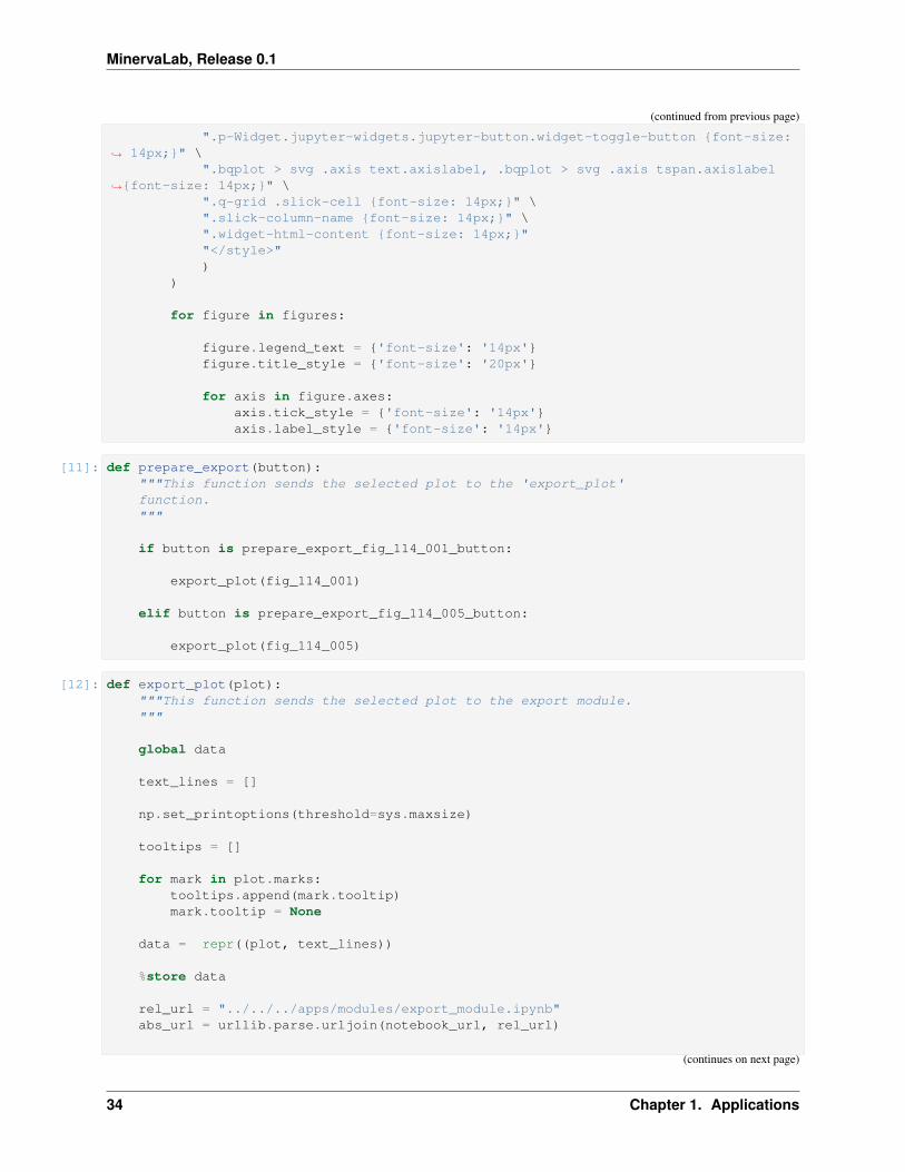
[11]: def prepare_export(button):"""This function sends the selected plot to the 'export_plot'function."""
if button is prepare_export_fig_114_001_button:
export_plot(fig_114_001)
elif button is prepare_export_fig_114_005_button:
export_plot(fig_114_005)
[12]: def export_plot(plot):"""This function sends the selected plot to the export module."""
global data
text_lines = []
np.set_printoptions(threshold=sys.maxsize)
tooltips = []
for mark in plot.marks:tooltips.append(mark.tooltip)mark.tooltip = None
data = repr((plot, text_lines))
%store data
rel_url = "../../../apps/modules/export_module.ipynb"abs_url = urllib.parse.urljoin(notebook_url, rel_url)
(continues on next page)
34 Chapter 1. Applications

MinervaLab, Release 0.1
(continued from previous page)
if not webbrowser.open(abs_url):go_to_export_button.value = "<form action=" + abs_url + " target='_blank'>
→˓<button type=''submit''>Open in export module</button></form>"
for i in range(len(plot.marks)):mark = plot.marks[i]mark.tooltip = tooltips[i]
[ ]: %%javascript
//Get the URL of the current notebook
var kernel = Jupyter.notebook.kernel;var command = ["notebook_url = ",
"'", window.location.href, "'" ].join('')
kernel.execute(command)
1.3.6 Main interface
[ ]: a_initial = 5.536 #L^2 bar/mol^2b_initial = 0.03049 #L/mol
a, b = a_initial, b_initial
p_c, v_c, T_c = calculate_critic(a, b)
T_values = [0.95*T_c, T_c, 1.2*T_c]v_values = np.linspace(1.2*b, 10*v_c, 500)colors = ['#0079c4','#f09205','#21c400']
p_values = get_absolute_isotherms(a, b, v_values, T_values)p_values = bar_to_atm(p_values)
######################################################FIGURES########################################################
fig_114_001 = bq.Figure(title='p vs v (Fixed T)',marks=[],axes=[],animation_duration=0,legend_location='top-right',background_style= {'fill': 'white', 'stroke': 'black'},fig_margin=dict(top=70, bottom=60, left=80, right=30),toolbar = True,layout = widgets.Layout(width='100%', height='500px')
)
fig_114_002 = bq.Figure(title='',marks=[],
(continues on next page)
1.3. Effect of a and b in van der Waals isotherms 35

MinervaLab, Release 0.1
(continued from previous page)
axes=[],animation_duration=0,legend_location='top-right',background_style= {'fill': 'white', 'stroke': 'black'},fig_margin=dict(top=30, bottom=60, left=25, right=10),toolbar = True,layout = widgets.Layout(width='90%', height='40%')
)
fig_114_003 = bq.Figure(title='',marks=[],axes=[],animation_duration=0,legend_location='top-right',background_style= {'fill': 'white', 'stroke': 'black'},fig_margin=dict(top=10, bottom=60, left=25, right=10),toolbar = True,layout = widgets.Layout(width='90%', height='40%')
)
fig_114_004 = bq.Figure(title='',marks=[],axes=[],animation_duration=0,legend_location='top-right',background_style= {'fill': 'white', 'stroke': 'black'},fig_margin=dict(top=10, bottom=60, left=25, right=10),toolbar = True,layout = widgets.Layout(width='90%', height='40%')
)
fig_114_005 = bq.Figure(title='p vs v (Fixed T)',marks=[],axes=[],animation_duration=0,legend_location='top-right',background_style= {'fill': 'white', 'stroke': 'black'},fig_margin=dict(top=70, bottom=60, left=80, right=30),toolbar = True,layout = widgets.Layout(width='100%', height='500px')
)
scale_x = bqs.LinearScale(min = 0.0, max = max(v_values))scale_y = bqs.LinearScale(min = 0, max = 2.0*p_c)
axis_x = bqa.Axis(scale=scale_x,tick_format='.2f',tick_style={'font-size': '15px'},tick_values = np.linspace(0, max(v_values), 5),grid_lines = 'none',grid_color = '#8e8e8e',label='v (L/mol)',label_location='middle',
(continues on next page)
36 Chapter 1. Applications

MinervaLab, Release 0.1
(continued from previous page)
label_style={'stroke': 'black', 'default-size': 35},label_offset='50px'
)
axis_y = bqa.Axis(scale=scale_y,tick_format='.1f',tick_style={'font-size': '15px'},tick_values = np.linspace(0, 2.0*p_c, 4),grid_lines = 'none',grid_color = '#8e8e8e',orientation='vertical',label='p (atm)',label_location='middle',label_style={'stroke': 'red', 'default_size': 35},label_offset='50px'
)
axis_x_no_ticks = bqa.Axis(scale=scale_x,tick_format='.2f',tick_style={'font-size': '15px'},num_ticks=0,grid_lines = 'none',grid_color = '#8e8e8e',label='v (L/mol)',label_location='middle',label_style={'stroke': 'black', 'default-size': 35},label_offset='15px'
)
axis_y_no_ticks = bqa.Axis(scale=scale_y,tick_format='.0f',tick_style={'font-size': '15px'},num_ticks=0,grid_lines = 'none',grid_color = '#8e8e8e',orientation='vertical',label='p (atm)',label_location='middle',label_style={'stroke': 'red', 'default_size': 35},label_offset='15px'
)
fig_114_001.axes = [axis_x, axis_y]fig_114_002.axes = [axis_x_no_ticks, axis_y_no_ticks]fig_114_003.axes = [axis_x_no_ticks, axis_y_no_ticks]fig_114_004.axes = [axis_x_no_ticks, axis_y_no_ticks]fig_114_005.axes = [axis_x, axis_y]
######################################################MARKS##########################################################
x_values = [ v_values for i in range(len(p_values))]y_values = []
(continues on next page)
1.3. Effect of a and b in van der Waals isotherms 37

MinervaLab, Release 0.1
(continued from previous page)
color_values = []label_values = []
for i in range(len(p_values)):
y_values.append(p_values[i])color_values.append(colors[i])label_values.append(str(T_values[i]))
new_state = bqm.Lines(x = x_values,y = y_values,scales = {'x': scale_x, 'y': scale_y},opacities = [1.0 for elem in p_values],visible = True,colors = color_values,labels = label_values,
)
old_state = bqm.Lines(x = x_values,y = y_values,scales = {'x': scale_x, 'y': scale_y},opacities = [1.0 for elem in p_values],visible = True,colors = color_values,labels = label_values,
)
current_state = bqm.Lines(x = x_values[0],y = y_values[0],scales = {'x': scale_x, 'y': scale_y},opacities = [1.0 for elem in p_values],visible = True,colors = color_values,labels = label_values,
)
a_line = bqm.Lines(x = x_values[0],y = y_values[0],scales = {'x': scale_x, 'y': scale_y},opacities = [1.0 for elem in p_values],visible = True,colors = color_values,labels = label_values,
)
b_line = bqm.Lines(x = x_values[0],y = y_values[0],scales = {'x': scale_x, 'y': scale_y},opacities = [1.0 for elem in p_values],visible = True,colors = color_values,labels = label_values,
(continues on next page)
38 Chapter 1. Applications

MinervaLab, Release 0.1
(continued from previous page)
)
ideal_isotherms = get_absolute_isotherms(0, 0, v_values, T_values)ideal_isotherms = bar_to_atm(ideal_isotherms)
ideal_line = bqm.Lines(x = x_values,y = ideal_isotherms,scales = {'x': scale_x, 'y': scale_y},opacities = [1.0 for elem in p_values],visible = True,colors = color_values,labels = label_values,
)
unique_isotherm = bqm.Lines(x = x_values[0],y = y_values[0],scales = {'x': scale_x, 'y': scale_y},opacities = [0.6],visible = True,colors = ['#c90000'],labels = [label_values[0]],stroke_width = 5
)
fig_114_001.marks = [old_state]fig_114_002.marks = [current_state]fig_114_003.marks = [a_line]fig_114_004.marks = [b_line]fig_114_005.marks = [ideal_line, unique_isotherm]
######################################WIDGETS#######################################
a_slider_114_003 = widgets.FloatSlider(min=0.0,max=2.0*a,step=0.1,value=a,description='a',disabled=False,continuous_update=True,orientation='horizontal',readout=True,layout=widgets.Layout(width='90%')
)
a_slider_114_003.observe(update_isotherms, 'value')
b_slider_114_004 = widgets.FloatSlider(min=0.0,max=4.0*b,step=0.001,value=b,description='b',
(continues on next page)
1.3. Effect of a and b in van der Waals isotherms 39

MinervaLab, Release 0.1
(continued from previous page)
disabled=False,continuous_update=True,orientation='horizontal',readout=True,layout=widgets.Layout(width='90%')
)
b_slider_114_004.observe(update_isotherms, 'value')
reset_button = widgets.Button(description='Reset',disabled=False,button_style='',tooltip='Return to the original state',
)
reset_button.on_click(restart)
change_view_button = widgets.ToggleButton(value=False,description='Presentation mode (OFF)',disabled=False,button_style='',tooltip='',icon='desktop',layout=widgets.Layout(
width='initial',align_self='center'
))
change_view_button.observe(change_view, 'value')
prepare_export_fig_114_001_button = widgets.Button(description='Export',disabled=False,button_style='',tooltip='',
)
prepare_export_fig_114_001_button.on_click(prepare_export)
prepare_export_fig_114_005_button = widgets.Button(description='Export',disabled=False,button_style='',tooltip='',
)
prepare_export_fig_114_005_button.on_click(prepare_export)
#####################################BLOCKS#########################################
top_block_114_000 = widgets.HBox([],
(continues on next page)
40 Chapter 1. Applications

MinervaLab, Release 0.1
(continued from previous page)
layout=widgets.Layout(width='100%',align_self='center'
))
top_block_114_000.children = [widgets.VBox([
fig_114_001,prepare_export_fig_114_001_button
],layout=widgets.Layout(
width='33%',align_items='center'
)),widgets.VBox([
fig_114_002,fig_114_003,a_slider_114_003
],layout=widgets.Layout(
width='16%',height='500px',align_items='center',margin='40px 0 0 0'
)),widgets.VBox([
fig_114_002,fig_114_004,b_slider_114_004
],layout=widgets.Layout(
width='16%',height='500px',align_items='center',margin='40px 0 0 0'
)),widgets.VBox([
fig_114_005,prepare_export_fig_114_005_button
],layout=widgets.Layout(
width='33%',align_items='center'
)),
]
bottom_block_114_000 = widgets.HBox([],layout=widgets.Layout(
width='100%',height='60px',align_self='center'
(continues on next page)
1.3. Effect of a and b in van der Waals isotherms 41

MinervaLab, Release 0.1
(continued from previous page)
))
bottom_block_114_000.children = [widgets.VBox([
widgets.HTMLMath(value=r"\( (p + \frac{a}{v^2})(v - b) = k_B T \)"
)],
layout=widgets.Layout(width='33%',align_items='center'
)),widgets.VBox(
[reset_button],layout=widgets.Layout(
width='33%',align_items='center'
)),widgets.VBox([
widgets.HTMLMath(value=r"\( p v = k_B T \)"
)],
layout=widgets.Layout(width='33%',align_items='center'
))
]
main_block_114_000 = widgets.VBox([],layout=widgets.Layout(
width='100%',align_items='center'
))
main_block_114_000.children = [change_view_button,top_block_114_000,bottom_block_114_000
]
figures = [fig_114_001,fig_114_002,fig_114_003,fig_114_004,fig_114_005,
]
main_block_114_000
42 Chapter 1. Applications
MinervaLab, Release 0.1
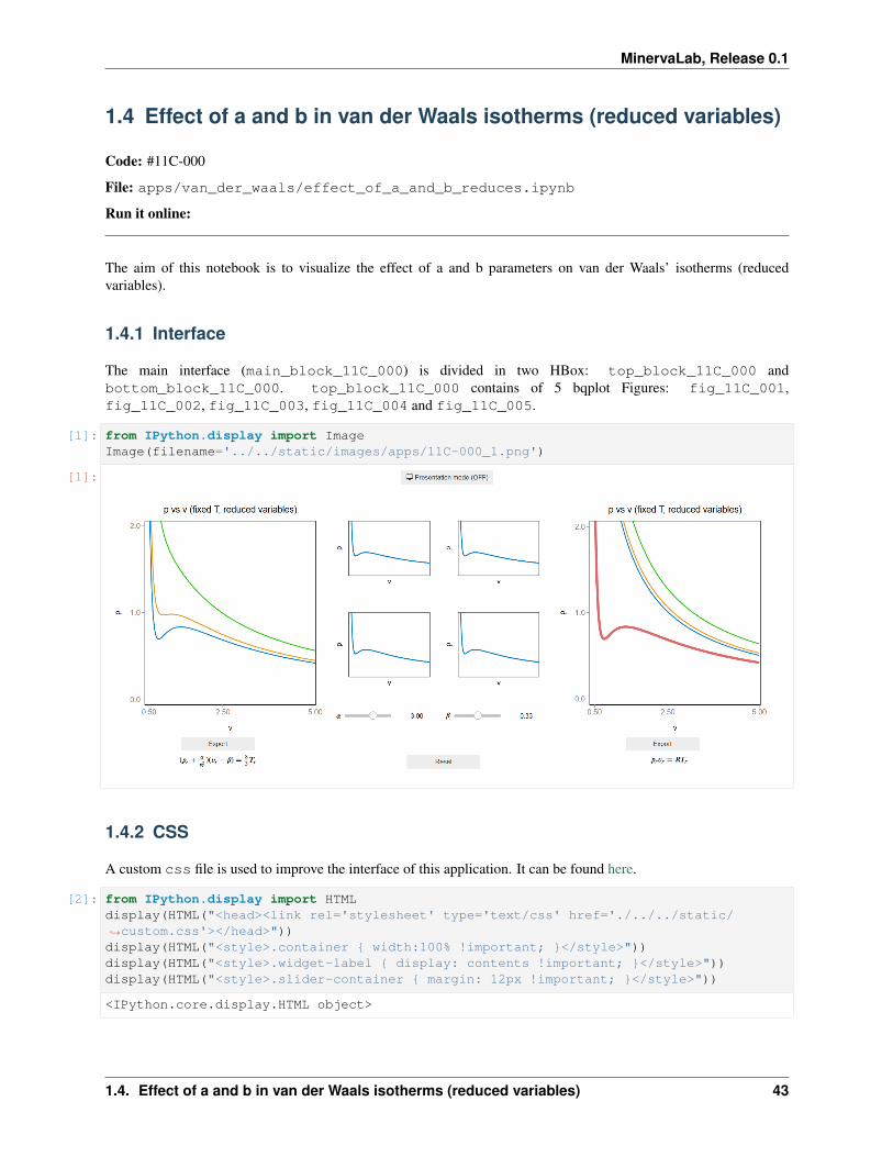
1.4 Effect of a and b in van der Waals isotherms (reduced variables)
Code: #11C-000
File: apps/van_der_waals/effect_of_a_and_b_reduces.ipynb
Run it online:
The aim of this notebook is to visualize the effect of a and b parameters on van der Waals’ isotherms (reducedvariables).
1.4.1 Interface
The main interface (main_block_11C_000) is divided in two HBox: top_block_11C_000 andbottom_block_11C_000. top_block_11C_000 contains of 5 bqplot Figures: fig_11C_001,fig_11C_002, fig_11C_003, fig_11C_004 and fig_11C_005.
[1]: from IPython.display import ImageImage(filename='../../static/images/apps/11C-000_1.png')
[1]:
1.4.2 CSS
A custom css file is used to improve the interface of this application. It can be found here.
[2]: from IPython.display import HTMLdisplay(HTML("<head><link rel='stylesheet' type='text/css' href='./../../static/→˓custom.css'></head>"))display(HTML("<style>.container { width:100% !important; }</style>"))display(HTML("<style>.widget-label { display: contents !important; }</style>"))display(HTML("<style>.slider-container { margin: 12px !important; }</style>"))
<IPython.core.display.HTML object>
1.4. Effect of a and b in van der Waals isotherms (reduced variables) 43

MinervaLab, Release 0.1
<IPython.core.display.HTML object>
<IPython.core.display.HTML object>
<IPython.core.display.HTML object>
1.4.3 Packages
[3]: from bqplot import *import bqplot as bqimport bqplot.marks as bqmimport bqplot.scales as bqsimport bqplot.axes as bqa
import ipywidgets as widgets
import urllib.parseimport webbrowser
import sys
1.4.4 Physical functions
This are the functions that have a physical meaning:
• get_relative_isotherms_params
[4]: def get_relative_isotherms_params(alpha, beta, v_range, T_range):"""This function calculates the theoretical p(v, T) plane
(in reduced coordinates) according to van der Waalsequation of state from a given range of volumesand tenperatures and taking into account the valuesof alpha and beta.
Args:alpha: The value of the a parameter.\nalpha: The value of the b parameter.\nv_range: An array containing the values of v(in reduced coordinates)for which the isotherms must becalculated.\nT_range: An array containing the values of T(in reduced coordinates)for which the isotherms must becalculated.\n
Returns:isotherms: A list consisted of numpy arrays containing thepressures of each isotherm.
"""
isotherms = []
for T in T_range:p_R = []for v in v_range:
(continues on next page)
44 Chapter 1. Applications

MinervaLab, Release 0.1
(continued from previous page)
val = (8.0/3.0*T/(v - beta) - alpha/v**2)p_R = np.append(p_R, val)
isotherms.append(p_R)
return isotherms
1.4.5 Functions related to interaction
[5]: def update_isotherms(change):"""This function update the lines 'alpha_line', 'beta_line' and'unique_isotherm' when 'alpha_slider_11C_003' or 'beta_slider_11C_004' areupdated."""
obj = change.ownerT_values = [0.95]
if obj is alpha_slider_11C_003:
v_values = np.linspace(0.4, 5.0, 500)isotherms = get_relative_isotherms_params(
alpha_slider_11C_003.value,beta_initial,v_values,T_values
)
alpha_line.y = isotherms[0]
elif obj is beta_slider_11C_004:
v_values = np.linspace(0.4, 5.0, 500)
if beta_slider_11C_004.value == 0.0:
v_values = np.linspace(0.4, 5.0, 500)
isotherms = get_relative_isotherms_params(alpha_initial,beta_slider_11C_004.value,v_values,T_values
)
beta_line.x = v_valuesbeta_line.y = isotherms[0]
if beta_slider_11C_004.value == 0.0:v_values = np.linspace(0.4, 5.0, 500)
isotherms = get_relative_isotherms_params(alpha_slider_11C_003.value,beta_slider_11C_004.value,v_values,
(continues on next page)
1.4. Effect of a and b in van der Waals isotherms (reduced variables) 45

MinervaLab, Release 0.1
(continued from previous page)
T_values)
unique_isotherm.x = v_valuesunique_isotherm.y = isotherms[0]
[6]: def restart(a):"""This function sets the values of 'alpha_slider_11C_003'and 'beta_slider_11C_004' to their initial ones."""
alpha_slider_11C_003.value, beta_slider_11C_004.value = alpha_initial, beta_→˓initial
[7]: def change_view(change):"""This function changes the visualization of all thecomponents of the application so they are suitable fora projection.\n"""
obj = change.owner
if obj.value:
obj.description = 'Presentation mode (ON)'
display(HTML("<style>" \".widget-readout { font-size: 30px ; }" \".widget-label-basic {font-size: 30px;}" \"option {font-size: 25px;}" \".p-Widget.jupyter-widgets.widget-slider.widget-vslider.widget-inline-
→˓vbox {width: auto}" \".p-Widget .jupyter-widgets .widgets-label {width: auto; height: auto;
→˓font-size: 30px;}" \".widget-label {font-size: 30px ; height: auto !important;}" \".p-Widget .bqplot .figure .jupyter-widgets {height: auto !important;}" \".widget-text input[type='number'] {font-size: 30px;height: auto;}" \".option { font-size: 30px ;}" \".p-Widget .jupyter-widgets .jupyter-button.widget-button {font-size:
→˓30px ; width: auto; height: auto;}" \".p-Widget.jupyter-widgets.jupyter-button.widget-toggle-button{font-size:
→˓30px ; width: auto; height: auto;}" \".p-Widget.p-Panel.jupyter-widgets.widget-container.widget-box.widget-
→˓vbox {padding-bottom: 30px}" \".bqplot > svg .axis text.axislabel, .bqplot > svg .axis tspan.axislabel
→˓{font-size: 30px;}" \".q-grid .slick-cell {font-size: 30px;}" \".slick-column-name {font-size: 30px;}" \".widget-html-content {font-size: 30px;}""</style>")
)
for figure in figures:
(continues on next page)
46 Chapter 1. Applications

MinervaLab, Release 0.1
(continued from previous page)
figure.legend_text = {'font-size': '30px'}figure.title_style = {'font-size': '30px'}
for axis in figure.axes:axis.tick_style = {'font-size': '30px'}axis.label_style = {'font-size': '30px'}
else:
obj.description = 'Presentation mode (OFF)'
display(HTML("<style>" \".widget-readout { font-size: 14px ;}" \".widget-label-basic {font-size: 14px;}" \"option {font-size: 12px;}" \".p-Widget .jupyter-widgets .widgets-label {font-size: 14px;}" \".widget-label {font-size: 14px ;}" \".widget-text input[type='number'] {font-size: 14px;}" \".option { font-size: 14px ;}" \".p-Widget .jupyter-widgets .jupyter-button.widget-button {font-size:
→˓14px;}" \".p-Widget.jupyter-widgets.jupyter-button.widget-toggle-button {font-size:
→˓ 14px;}" \".bqplot > svg .axis text.axislabel, .bqplot > svg .axis tspan.axislabel
→˓{font-size: 14px;}" \".q-grid .slick-cell {font-size: 14px;}" \".slick-column-name {font-size: 14px;}" \".widget-html-content {font-size: 14px;}""</style>")
)
for figure in figures:
figure.legend_text = {'font-size': '14px'}figure.title_style = {'font-size': '20px'}
for axis in figure.axes:axis.tick_style = {'font-size': '14px'}axis.label_style = {'font-size': '14px'}
[8]: def prepare_export(button):"""This function sends the selected plot to the 'export_plot'function."""
if button is prepare_export_fig_11C_001_button:
export_plot(fig_11C_001)
elif button is prepare_export_fig_11C_005_button:
export_plot(fig_11C_005)
1.4. Effect of a and b in van der Waals isotherms (reduced variables) 47
MinervaLab, Release 0.1
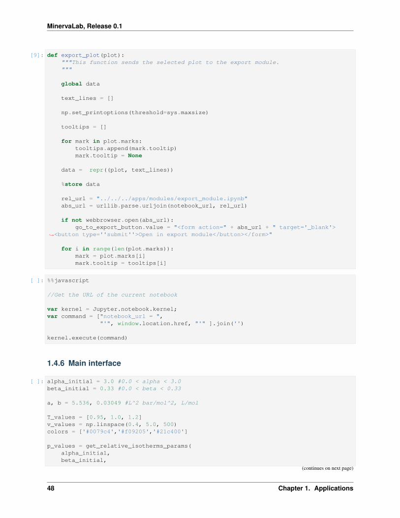
[9]: def export_plot(plot):"""This function sends the selected plot to the export module."""
global data
text_lines = []
np.set_printoptions(threshold=sys.maxsize)
tooltips = []
for mark in plot.marks:tooltips.append(mark.tooltip)mark.tooltip = None
data = repr((plot, text_lines))
%store data
rel_url = "../../../apps/modules/export_module.ipynb"abs_url = urllib.parse.urljoin(notebook_url, rel_url)
if not webbrowser.open(abs_url):go_to_export_button.value = "<form action=" + abs_url + " target='_blank'>
→˓<button type=''submit''>Open in export module</button></form>"
for i in range(len(plot.marks)):mark = plot.marks[i]mark.tooltip = tooltips[i]
[ ]: %%javascript
//Get the URL of the current notebook
var kernel = Jupyter.notebook.kernel;var command = ["notebook_url = ",
"'", window.location.href, "'" ].join('')
kernel.execute(command)
1.4.6 Main interface
[ ]: alpha_initial = 3.0 #0.0 < alpha < 3.0beta_initial = 0.33 #0.0 < beta < 0.33
a, b = 5.536, 0.03049 #L^2 bar/mol^2, L/mol
T_values = [0.95, 1.0, 1.2]v_values = np.linspace(0.4, 5.0, 500)colors = ['#0079c4','#f09205','#21c400']
p_values = get_relative_isotherms_params(alpha_initial,beta_initial,
(continues on next page)
48 Chapter 1. Applications

MinervaLab, Release 0.1
(continued from previous page)
v_values,T_values
)
##############################################CREATE THE FIGURES#####################################################
fig_11C_001 = bq.Figure(title='p vs v (fixed T, reduced variables)',marks=[],axes=[],animation_duration=0,legend_location='top-right',background_style= {'fill': 'white', 'stroke': 'black'},fig_margin=dict(top=70, bottom=60, left=80, right=30),toolbar = True,layout = widgets.Layout(
width='100%',height='500px'
))
fig_11C_002 = bq.Figure(title='',marks=[],axes=[],animation_duration=0,legend_location='top-right',background_style= {'fill': 'white', 'stroke': 'black'},fig_margin=dict(top=30, bottom=60, left=25, right=10),toolbar = True,layout = widgets.Layout(
width='90%',height='40%'
))
fig_11C_003 = bq.Figure(title='',marks=[],axes=[],animation_duration=0,legend_location='top-right',background_style= {'fill': 'white', 'stroke': 'black'},fig_margin=dict(top=10, bottom=60, left=25, right=10),toolbar = True,layout = widgets.Layout(
width='90%',height='40%'
))
fig_11C_004 = bq.Figure(title='',marks=[],
(continues on next page)
1.4. Effect of a and b in van der Waals isotherms (reduced variables) 49

MinervaLab, Release 0.1
(continued from previous page)
axes=[],animation_duration=0,legend_location='top-right',background_style= {'fill': 'white', 'stroke': 'black'},fig_margin=dict(top=10, bottom=60, left=25, right=10),toolbar = True,layout = widgets.Layout(
width='90%',height='40%'
))
fig_11C_005 = bq.Figure(title='p vs v (fixed T, reduced variables)',marks=[],axes=[],animation_duration=0,legend_location='top-right',background_style= {'fill': 'white', 'stroke': 'black'},fig_margin=dict(top=70, bottom=60, left=80, right=30),toolbar = True,layout = widgets.Layout(
width='100%',height='500px'
))
scale_x = bqs.LinearScale(min = 0.4, max = 5.0)scale_y = bqs.LinearScale(min = 0, max = 2.0)
axis_x = bqa.Axis(scale=scale_x,tick_format='.2f',tick_style={'font-size': '15px'},tick_values = [0.5, 2.5, 5.0],grid_lines = 'none',grid_color = '#8e8e8e',label='v',label_location='middle',label_style={'stroke': 'black', 'default-size': 35},label_offset='50px'
)
axis_y = bqa.Axis(scale=scale_y,tick_format='.1f',tick_style={'font-size': '15px'},tick_values = [0, 1, 2],grid_lines = 'none',grid_color = '#8e8e8e',orientation='vertical',label='p',label_location='middle',label_style={'stroke': 'red', 'default_size': 35},label_offset='50px'
)
(continues on next page)
50 Chapter 1. Applications

MinervaLab, Release 0.1
(continued from previous page)
axis_x_no_ticks = bqa.Axis(scale=scale_x,tick_format='.2f',tick_style={'font-size': '15px'},num_ticks=0,grid_lines = 'none',grid_color = '#8e8e8e',label='v',label_location='middle',label_style={'stroke': 'black', 'default-size': 35},label_offset='15px'
)
axis_y_no_ticks = bqa.Axis(scale=scale_y,tick_format='.0f',tick_style={'font-size': '15px'},num_ticks=0,grid_lines = 'none',grid_color = '#8e8e8e',orientation='vertical',label='p',label_location='middle',label_style={'stroke': 'red', 'default_size': 35},label_offset='15px'
)
fig_11C_001.axes = [axis_x, axis_y]fig_11C_002.axes = [axis_x_no_ticks, axis_y_no_ticks]fig_11C_003.axes = [axis_x_no_ticks, axis_y_no_ticks]fig_11C_004.axes = [axis_x_no_ticks, axis_y_no_ticks]fig_11C_005.axes = [axis_x, axis_y]
#####################################################MARKS###########################################################
x_values = [v_values for i in range(len(p_values))]y_values = []color_values = []label_values = []
for i in range(len(p_values)):
y_values.append(p_values[i])color_values.append(colors[i])label_values.append(str(T_values[i]))
new_state = bqm.Lines(x = x_values,y = y_values,scales = {'x': scale_x, 'y': scale_y},opacities = [1.0 for elem in p_values],visible = True,colors = color_values,labels = label_values,
(continues on next page)
1.4. Effect of a and b in van der Waals isotherms (reduced variables) 51

MinervaLab, Release 0.1
(continued from previous page)
)
old_state = bqm.Lines(x = x_values,y = y_values,scales = {'x': scale_x, 'y': scale_y},opacities = [1.0 for elem in p_values],visible = True,colors = color_values,labels = label_values,
)
current_state = bqm.Lines(x = x_values[0],y = y_values[0],scales = {'x': scale_x, 'y': scale_y},opacities = [1.0 for elem in p_values],visible = True,colors = color_values,labels = label_values,
)
alpha_line = bqm.Lines(x = x_values[0],y = y_values[0],scales = {'x': scale_x, 'y': scale_y},opacities = [1.0 for elem in p_values],visible = True,colors = color_values,labels = label_values,
)
beta_line = bqm.Lines(x = x_values[0],y = y_values[0],scales = {'x': scale_x, 'y': scale_y},opacities = [1.0 for elem in p_values],visible = True,colors = color_values,labels = label_values,
)
ideal_isotherms = get_relative_isotherms_params(0,0,v_values,T_values
)
ideal_line = bqm.Lines(x = x_values,y = ideal_isotherms,scales = {'x': scale_x, 'y': scale_y},opacities = [1.0 for elem in p_values],visible = True,colors = color_values,labels = label_values,
(continues on next page)
52 Chapter 1. Applications

MinervaLab, Release 0.1
(continued from previous page)
)
unique_isotherm = bqm.Lines(x = x_values[0],y = y_values[0],scales = {'x': scale_x, 'y': scale_y},opacities = [0.6],visible = True,colors = ['#c90000'],labels = [label_values[0]],stroke_width = 5
)
fig_11C_001.marks = [old_state]fig_11C_002.marks = [current_state]fig_11C_003.marks = [alpha_line]fig_11C_004.marks = [beta_line]fig_11C_005.marks = [ideal_line, unique_isotherm]
alpha_slider_11C_003 = widgets.FloatSlider(min=0.0,max=5.0,step=0.01,value=alpha_initial,description=r"\( \alpha \)",disabled=False,continuous_update=True,orientation='horizontal',readout=True,layout=widgets.Layout(width='90%')
)
alpha_slider_11C_003.observe(update_isotherms, 'value')
beta_slider_11C_004 = widgets.FloatSlider(min=0.0,max=0.66,step=0.001,value=beta_initial,description=r"\( \beta \)",disabled=False,continuous_update=True,orientation='horizontal',readout=True,layout=widgets.Layout(width='90%')
)
beta_slider_11C_004.observe(update_isotherms, 'value')
return_button = widgets.Button(description='Reset',disabled=False,button_style='',tooltip='Return to the original state',
)
return_button.on_click(restart)(continues on next page)
1.4. Effect of a and b in van der Waals isotherms (reduced variables) 53

MinervaLab, Release 0.1
(continued from previous page)
change_view_button = widgets.ToggleButton(value=False,description='Presentation mode (OFF)',disabled=False,button_style='',tooltip='',icon='desktop',layout=widgets.Layout(
width='initial',align_self='center'
))
change_view_button.observe(change_view, 'value')
prepare_export_fig_11C_001_button = widgets.Button(description='Export',disabled=False,button_style='',tooltip='',
)
prepare_export_fig_11C_001_button.on_click(prepare_export)
prepare_export_fig_11C_005_button = widgets.Button(description='Export',disabled=False,button_style='',tooltip='',
)
prepare_export_fig_11C_005_button.on_click(prepare_export)
top_block_11C_000 = widgets.HBox([],layout=widgets.Layout(
width='100%',align_self='center'
))
top_block_11C_000.children = [widgets.VBox([
fig_11C_001,prepare_export_fig_11C_001_button
],layout=widgets.Layout(
width='33%',align_items='center'
)),widgets.VBox([
fig_11C_002,fig_11C_003,alpha_slider_11C_003
],(continues on next page)
54 Chapter 1. Applications

MinervaLab, Release 0.1
(continued from previous page)
layout=widgets.Layout(width='16%',height='500px',align_items='center',margin='40px 0 0 0'
)),widgets.VBox([
fig_11C_002,fig_11C_004,beta_slider_11C_004
],layout=widgets.Layout(
width='16%',height='500px',align_items='center',margin='40px 0 0 0'
)),widgets.VBox([
fig_11C_005,prepare_export_fig_11C_005_button
],layout=widgets.Layout(
width='33%',align_items='center'
)),
]
bottom_block_11C_000 = widgets.HBox([],layout=widgets.Layout(
width='100%',height='60px',align_self='center'
))
bottom_block_11C_000.children = [widgets.VBox([
widgets.HTMLMath(value=r"\( (p_r + \frac{\alpha}{v_r^2})(v_r - \beta) = \frac{8}{3} T_r \)"
)],layout=widgets.Layout(
width='33%',align_items='center'
)),widgets.VBox(
[return_button],layout=widgets.Layout(
width='33%',align_items='center'
)),widgets.VBox([
(continues on next page)
1.4. Effect of a and b in van der Waals isotherms (reduced variables) 55

MinervaLab, Release 0.1
(continued from previous page)
widgets.HTMLMath(value=r"\( p_r v_r = R T_r \)"
)],layout=widgets.Layout(
width='33%',align_items='center'
))
]
main_block_11C_000 = widgets.VBox([],layout=widgets.Layout(
width='100%',align_items='center'
))
main_block_11C_000.children = [change_view_button,top_block_11C_000,bottom_block_11C_000
]
figures = [fig_11C_001,fig_11C_002,fig_11C_003,fig_11C_004,fig_11C_005,
]
main_block_11C_000
1.5 Critical points for various fluids
Code: #113-000
File: apps/van_der_waals/critical_points.ipynb
Run it online:
The aim of this notebook is to visualize the critical points of various fluids.
1.5.1 Interface
The main interface (main_block_113_000) is divided in three VBox: top_block_113_000,middle_block_113_000 and bottom_block_113_000. top_block_113_000 contains a bqplotFigure (fig_113_001) and a qgrid chart (qgrid_table). middle_block_113_000 contains of 3 bqplotFigures: fig_113_002, fig_113_003 and fig_113_005.
56 Chapter 1. Applications

MinervaLab, Release 0.1
[1]: from IPython.display import ImageImage(filename='../../static/images/apps/113-000_1.png')
[1]:
[2]: Image(filename='../../static/images/apps/113-000_2.png')
[2]:
1.5.2 CSS
A custom css file is used to improve the interface of this application. It can be found here.
[1]: from IPython.display import HTMLdisplay(HTML("<head><link rel='stylesheet' type='text/css' href='./../../static/→˓custom.css'></head>"))display(HTML("<style>.container { width:100% !important; }</style>"))
<IPython.core.display.HTML object>
<IPython.core.display.HTML object>
1.5. Critical points for various fluids 57
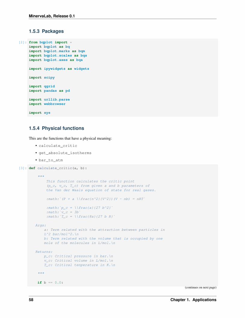
MinervaLab, Release 0.1
1.5.3 Packages
[2]: from bqplot import *import bqplot as bqimport bqplot.marks as bqmimport bqplot.scales as bqsimport bqplot.axes as bqa
import ipywidgets as widgets
import scipy
import qgridimport pandas as pd
import urllib.parseimport webbrowser
import sys
1.5.4 Physical functions
This are the functions that have a physical meaning:
• calculate_critic
• get_absolute_isotherms
• bar_to_atm
[3]: def calculate_critic(a, b):
"""This function calculates the critic point(p_c, v_c, T_c) from given a and b parameters ofthe Van der Waals equation of state for real gases.
:math:`(P + a \\frac{n^2}{V^2})(V - nb) = nRT`
:math:`p_c = \\frac{a}{27 b^2}`:math:`v_c = 3b`:math:`T_c = \\frac{8a}{27 b R}`
Args:a: Term related with the attraction between particles inL^2 bar/mol^2.\nb: Term related with the volume that is occupied by onemole of the molecules in L/mol.\n
Returns:p_c: Critical pressure in bar.\nv_c: Critical volume in L/mol.\nT_c: Critical tenperature in K.\n
"""
if b == 0.0:
(continues on next page)
58 Chapter 1. Applications
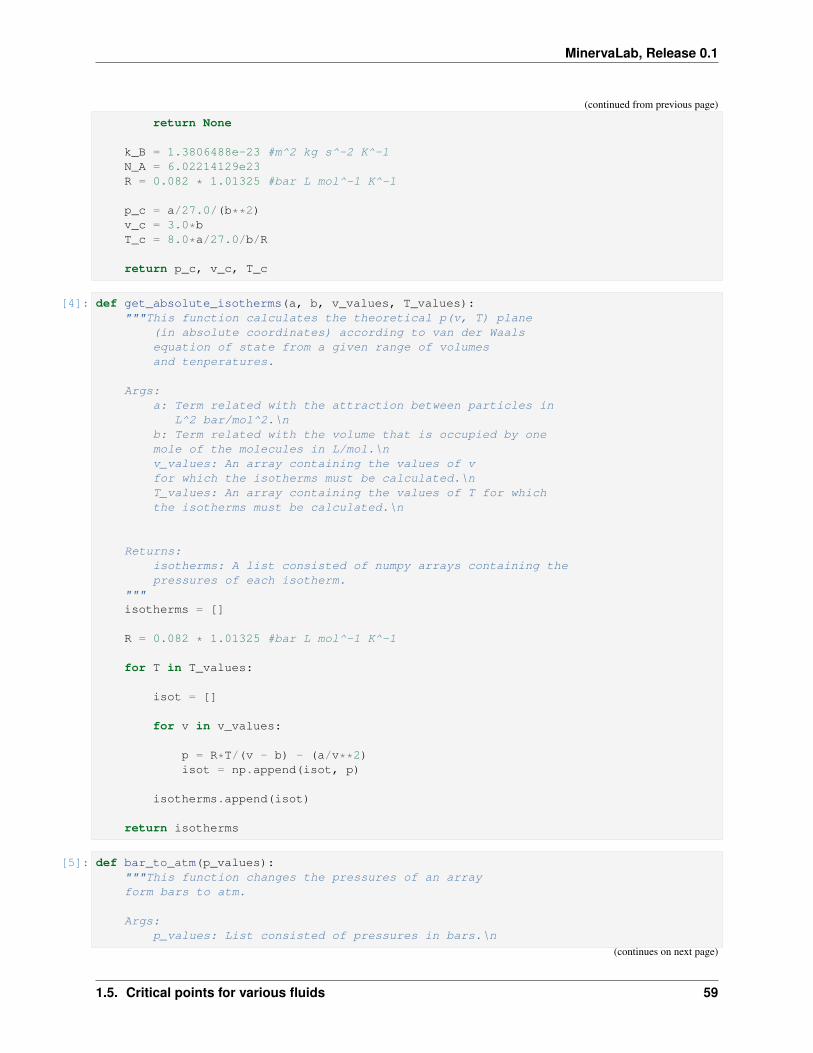
MinervaLab, Release 0.1
(continued from previous page)
return None
k_B = 1.3806488e-23 #m^2 kg s^-2 K^-1N_A = 6.02214129e23R = 0.082 * 1.01325 #bar L mol^-1 K^-1
p_c = a/27.0/(b**2)v_c = 3.0*bT_c = 8.0*a/27.0/b/R
return p_c, v_c, T_c
[4]: def get_absolute_isotherms(a, b, v_values, T_values):"""This function calculates the theoretical p(v, T) plane
(in absolute coordinates) according to van der Waalsequation of state from a given range of volumesand tenperatures.
Args:a: Term related with the attraction between particles in
L^2 bar/mol^2.\nb: Term related with the volume that is occupied by onemole of the molecules in L/mol.\nv_values: An array containing the values of vfor which the isotherms must be calculated.\nT_values: An array containing the values of T for whichthe isotherms must be calculated.\n
Returns:isotherms: A list consisted of numpy arrays containing thepressures of each isotherm.
"""isotherms = []
R = 0.082 * 1.01325 #bar L mol^-1 K^-1
for T in T_values:
isot = []
for v in v_values:
p = R*T/(v - b) - (a/v**2)isot = np.append(isot, p)
isotherms.append(isot)
return isotherms
[5]: def bar_to_atm(p_values):"""This function changes the pressures of an arrayform bars to atm.
Args:p_values: List consisted of pressures in bars.\n
(continues on next page)
1.5. Critical points for various fluids 59

MinervaLab, Release 0.1
(continued from previous page)
Returns:p_values: List consisted of pressures in atm.\n
"""
p_values = np.array(p_values) * 0.9869
return p_values
[6]: def generate_critical_points(df):"""This function takes a Pandas dataframe containing threecolumns (element, a, b) and returns four lists: pc, vc, Tc and names
Args:df: Pandas dataframe consisted of three columns: element, a, b.\n
Returns:pc: A numpy array consisted of the values of the critical pressures.\nvc: A numpy array consisted of the values of the critical volumes.\nTc: A numpy array consisted of the values of the critical tenperatures.\nnames: A list consisted of the names of the elements.\n
"""
pc = []vc = []Tc = []
names = []
name_values = df.iloc[:,0]a_values, b_values, names_sorted = get_a_b_names(df)
for i in range(len(a_values)):
names.append(names_sorted[i])
a = float(a_values[i])b = float(b_values[i])p, v, T = calculate_critic(a, b)
pc = np.append(pc, p)vc = np.append(vc, v)Tc = np.append(Tc, T)
return pc, vc, Tc, names
[7]: def get_a_b_names(df):"""This function takes a pandas dataframe containing thecolumns 'a (L2bar/mol2)', 'b (L/mol)' and 'Element' and return thelists of the colums sorted by the values of 'a (L2bar/mol2)'.
Args:df: Pandas dataframe consisted of three columns: 'a (L2bar/mol2)','b (L/mol)' and 'Element'.\n
Returns:
(continues on next page)
60 Chapter 1. Applications

MinervaLab, Release 0.1
(continued from previous page)
a_values_sorted: A list array consisted of the sorted values of 'a (L2bar/→˓mol2)'.\n
b_values_sorted: A list array consisted of the sorted values of 'b (L/mol)'.\nnames_sorted: A list consisted of the names of the sorted values of 'Element'.
→˓\n"""
a_values = list(df['a (L2bar/mol2)'])b_values = list(df['b (L/mol)'])names = list(df['Element'])
a_values_sorted = sorted(a_values)
#Sort values of b depending on the order of ab_values_sorted = [y for _,y in sorted(zip(a_values, b_values))]names_sorted = [y for _,y in sorted(zip(a_values, names))]
return a_values_sorted, b_values_sorted, names_sorted
1.5.5 Functions related to the interaction
[8]: def change_visible_points(event, QGridWidget):"""This function changes the visible points infig_113_002, fig_113_003 and fig_113_004 according tothe values filtered in qgrid_table."""
i = QGridWidget.get_changed_df().index
new_pc = pc[i]new_vc = vc[i]new_Tc = Tc[i]
new_names = np.asarray(names_sorted)[i].tolist()
new_a_values = np.asarray(a_values)[i].tolist()new_b_values = np.asarray(b_values)[i].tolist()
scale_x_v = bqs.LinearScale(min = min(new_vc), max = max(new_vc))scale_y_p = bqs.LinearScale(min = min(new_pc), max = max(new_pc))scale_y_T = bqs.LinearScale(min = min(new_Tc), max = max(new_Tc))
scale_x_004 = bqs.LinearScale(min = min(new_b_values), max = max(new_b_values))scale_y_004 = bqs.LinearScale(min = min(new_a_values), max = max(new_a_values))
axis_x_v.scale = scale_x_vaxis_y_p.scale = scale_y_paxis_y_T.scale = scale_y_T
axis_x_004.scale = scale_x_004axis_y_004.scale = scale_y_004
fig_113_002.axes = [axis_x_v, axis_y_p]fig_113_003.axes = [axis_x_v, axis_y_T]fig_113_004.axes = [axis_x_004, axis_y_004]
(continues on next page)
1.5. Critical points for various fluids 61

MinervaLab, Release 0.1
(continued from previous page)
for mark in fig_113_002.marks:
mark.scales = {'x': scale_x_v,'y': scale_y_p
}
for mark in fig_113_003.marks:
mark.scales = {'x': scale_x_v,'y': scale_y_T
}
fig_113_002.marks[0].x, fig_113_002.marks[0].y = new_vc, new_pcfig_113_002.marks[0].names = new_names
fig_113_003.marks[0].x, fig_113_003.marks[0].y = new_vc, new_Tcfig_113_003.marks[0].names = new_names
for mark in fig_113_004.marks:
mark.scales = {'x': scale_x_004,'y': scale_y_004
}
update_slider_options(new_a_values, new_b_values)
[9]: def change_selected_points(event, QGridWidget):"""This function changes the selected points infig_113_002 and fig_113_003 according tothe values selected in qgrid_table."""
i = QGridWidget.get_changed_df().index
new_pc = pc[i]new_vc = vc[i]new_Tc = Tc[i]
new_names = np.asarray(names_sorted)[i].tolist()
selected_113_002.x, selected_113_002.y = new_vc, new_pcselected_113_002.names = new_names
selected_113_003.x, selected_113_003.y = new_vc, new_Tcselected_113_003.names = new_names
[10]: def update_slider_options(a_values, b_values):"""This function changes the options ofa_slider and b_slider sliders.
Args:a_values: List consisted of a_slider's new options.\n
(continues on next page)
62 Chapter 1. Applications

MinervaLab, Release 0.1
(continued from previous page)
b_values: List consisted of b_slider's new options.\n"""
a_slider.options = a_valuesb_slider.options = b_values
a_slider.value = a_values[0]b_slider.value = b_values[0]
[11]: def update_sliders(change):"""This function updates the visible mark infig_113_005 and the tracers tracer_113_002 andtracer_113_003.\n"""
index = change.get('owner').indexname = change.get('owner').description
if name == 'a':
b_slider.value = b_slider.options[index]
elif name == 'b':
a_slider.value = a_slider.options[index]
tracer_113_002.x = np.array([scatter_113_002.x[index]])tracer_113_002.y = np.array([scatter_113_002.y[index]])
tracer_113_003.x = np.array([scatter_113_003.x[index]])tracer_113_003.y = np.array([scatter_113_003.y[index]])
i = a_values.index(a_slider.value)element_name = fig_113_005.marks[i].labels[0]
tracer_113_002.names = [element_name]tracer_113_003.names = [element_name]
for mark in fig_113_005.marks:
if mark.labels[0] == element_name:
mark.visible = True
else:
mark.visible = False
[12]: tt = widgets.Label("")
def hover_handler(self, content):tt.value = str(content.get('data').get('name'))
[13]: def change_view(change):"""This function changes the visualization of all the
(continues on next page)
1.5. Critical points for various fluids 63

MinervaLab, Release 0.1
(continued from previous page)
components of the application so they are suitable fora projection.\n"""
obj = change.owner
if obj.value:
obj.description = 'Presentation mode (ON)'
display(HTML("<style>" \".widget-readout { font-size: 30px ; }" \".widget-label-basic {font-size: 30px;}" \"option {font-size: 25px;}" \".p-Widget.jupyter-widgets.widget-slider.widget-vslider.widget-inline-
→˓vbox {width: auto}" \".p-Widget .jupyter-widgets .widgets-label {width: auto; height: auto;
→˓font-size: 30px;}" \".widget-label {font-size: 30px ; height: auto !important;}" \".p-Widget .bqplot .figure .jupyter-widgets {height: auto !important;}" \".widget-text input[type='number'] {font-size: 30px;height: auto;}" \".option { font-size: 30px ;}" \".p-Widget .jupyter-widgets .jupyter-button.widget-button {font-size:
→˓30px ; width: auto; height: auto;}" \".p-Widget.jupyter-widgets.jupyter-button.widget-toggle-button{font-size:
→˓30px ; width: auto; height: auto;}" \".p-Widget.p-Panel.jupyter-widgets.widget-container.widget-box.widget-
→˓vbox {padding-bottom: 30px}" \".bqplot > svg .axis text.axislabel, .bqplot > svg .axis tspan.axislabel
→˓{font-size: 30px;}" \".q-grid .slick-cell {font-size: 30px;}" \".slick-column-name {font-size: 30px;}""</style>")
)
for figure in figures:
figure.legend_text = {'font-size': '30px'}figure.title_style = {'font-size': '30px'}
for axis in figure.axes:axis.tick_style = {'font-size': '30px'}axis.label_style = {'font-size': '30px'}
else:
obj.description = 'Presentation mode (OFF)'
display(HTML("<style>" \".widget-readout { font-size: 14px ;}" \".widget-label-basic {font-size: 14px;}" \"option {font-size: 12px;}" \".p-Widget .jupyter-widgets .widgets-label {font-size: 14px;}" \".widget-label {font-size: 14px ;}" \
(continues on next page)
64 Chapter 1. Applications

MinervaLab, Release 0.1
(continued from previous page)
".widget-text input[type='number'] {font-size: 14px;}" \".option { font-size: 14px ;}" \".p-Widget .jupyter-widgets .jupyter-button.widget-button {font-size:
→˓14px;}" \".p-Widget.jupyter-widgets.jupyter-button.widget-toggle-button {font-size:
→˓ 14px;}" \".bqplot > svg .axis text.axislabel, .bqplot > svg .axis tspan.axislabel
→˓{font-size: 14px;}" \".q-grid .slick-cell {font-size: 14px;}" \".slick-column-name {font-size: 14px;}""</style>")
)
for figure in figures:
figure.legend_text = {'font-size': '14px'}figure.title_style = {'font-size': '20px'}
for axis in figure.axes:axis.tick_style = {'font-size': '14px'}axis.label_style = {'font-size': '14px'}
[14]: def prepare_export(button):"""This function sends the selected plot to the 'export_plot'function."""
if button is prepare_export_fig_113_002_button:
export_plot(fig_113_002)
elif button is prepare_export_fig_113_003_button:
export_plot(fig_113_003)
elif button is prepare_export_fig_113_004_button:
export_plot(fig_113_004)
elif button is prepare_export_fig_113_005_button:
export_plot(fig_113_005)
[15]: def export_plot(plot):"""This function sends the selected plot to the export module."""
global data
text_lines = []
np.set_printoptions(threshold=sys.maxsize)
tooltips = []
(continues on next page)
1.5. Critical points for various fluids 65

MinervaLab, Release 0.1
(continued from previous page)
for mark in plot.marks:tooltips.append(mark.tooltip)mark.tooltip = None
data = repr((plot, text_lines))
%store data
rel_url = "../../../apps/modules/export_module.ipynb"abs_url = urllib.parse.urljoin(notebook_url, rel_url)
if not webbrowser.open(abs_url):go_to_export_button.value = "<form action=" + abs_url + " target='_blank'>
→˓<button type=''submit''>Open in export module</button></form>"
for i in range(len(plot.marks)):mark = plot.marks[i]mark.tooltip = tooltips[i]
[ ]: %%javascript
//Get the URL of the current notebook
var kernel = Jupyter.notebook.kernel;var command = ["notebook_url = ",
"'", window.location.href, "'" ].join('')
kernel.execute(command)
1.5.6 Main interface
[17]: #data taken from https://en.wikipedia.org/wiki/Van_der_Waals_constants_(data_page)→˓using https://wikitable2csv.ggor.de/#format: Element, a (L2bar/mol2), b (L/mol)
raw_data = ["Acetic acid",17.71,0.1065,"Acetic anhydride",20.158,0.1263,"Acetone",16.02,0.1124,"Acetonitrile",17.81,0.1168,"Acetylene",4.516,0.0522,"Ammonia",4.225,0.0371,"Argon",1.355,0.03201,"Benzene",18.24,0.1154,"Bromobenzene",28.94,0.1539,"Butane",14.66,0.1226,"Carbon dioxide",3.640,0.04267,"Carbon disulfide",11.77,0.07685,"Carbon monoxide",1.505,0.03985,"Carbon tetrachloride",19.7483,0.1281,"Chlorine",6.579,0.05622,"Chlorobenzene",25.77,0.1453,"Chloroethane",11.05,0.08651,"Chloromethane",7.570,0.06483,
(continues on next page)
66 Chapter 1. Applications

MinervaLab, Release 0.1
(continued from previous page)
"Cyanogen",7.769,0.06901,"Cyclohexane",23.11,0.1424,"Diethyl ether",17.61,0.1344,"Diethyl sulfide",19.00,0.1214,"Dimethyl ether",8.180,0.07246,"Dimethyl sulfide",13.04,0.09213,"Ethane",5.562,0.0638,"Ethanethiol",11.39,0.08098,"Ethanol",12.18,0.08407,"Ethyl acetate",20.72,0.1412,"Ethylamine",10.74,0.08409,"Fluorobenzene",20.19,0.1286,"Fluoromethane",4.692,0.05264,"Freon",10.78,0.0998,"Germanium tetrachloride",22.90,0.1485,"Helium",0.0346,0.0238,"Hexane",24.71,0.1735,"Hydrogen",0.2476,0.02661,"Hydrogen bromide",4.510,0.04431,"Hydrogen chloride",3.716,0.04081,"Hydrogen selenide",5.338,0.04637,"Hydrogen sulfide",4.490,0.04287,"Iodobenzene",33.52,0.1656,"Krypton",2.349,0.03978,"Mercury",8.200,0.01696,"Methane",2.283,0.04278,"Methanol",9.649,0.06702,"Neon",0.2135,0.01709,"Nitric oxide",1.358,0.02789,"Nitrogen",1.370,0.0387,"Nitrogen dioxide",5.354,0.04424,"Nitrous oxide",3.832,0.04415,"Oxygen",1.382,0.03186,"Pentane",19.26,0.146,"Phosphine",4.692,0.05156,"Propane",8.779,0.08445,"Radon",6.601,0.06239,"Silane",4.377,0.05786,"Silicon tetrafluoride",4.251,0.05571,"Sulfur dioxide",6.803,0.05636,"Tin tetrachloride",27.27,0.1642,"Toluene",24.38,0.1463,"Water",5.536,0.03049,"Xenon",4.250,0.05105]
[ ]: """
.. module:: critical_points.ipynb:sypnopsis: This module creates an interface to interact with thecritical points of different fluids.\n
.. moduleauthor:: Jon Gabirondo López ([email protected])
"""
(continues on next page)
1.5. Critical points for various fluids 67

MinervaLab, Release 0.1
(continued from previous page)
# Prepare the database
data_array = np.array(raw_data)data_reshaped = np.reshape(data_array, (-1,3)); #reshape in three columns
database = pd.DataFrame(data=data_reshaped,columns=["Element", "a (L2bar/mol2)", "b (L/mol)"]
)
# numpy converts all elements to 'object' and# pandas interprets them as string, but I want a and b values to be floatdatabase["a (L2bar/mol2)"] = np.round(
pd.to_numeric(database["a (L2bar/mol2)"]),4
)
database["b (L/mol)"] = np.round(pd.to_numeric(database["b (L/mol)"]),5
)
a_values, b_values, names_sorted = get_a_b_names(database)
database["Element"] = names_sorteddatabase["a (L2bar/mol2)"] = a_valuesdatabase["b (L/mol)"] = b_values
# Show the database in QGrid chart.
grid_options = {# SlickGrid options'fullWidthRows': True,'syncColumnCellResize': True,'forceFitColumns': True,'defaultColumnWidth': 150,'rowHeight': 28,'enableColumnReorder': False,'enableTextSelectionOnCells': True,'editable': False, #lehen True'autoEdit': False,'explicitInitialization': True,
# Qgrid options'maxVisibleRows': 7, #we have changed it to 5 (default = 15)'minVisibleRows': 7, #we have changed it to 5 (default = 8)'sortable': True,'filterable': True,'highlightSelectedCell': False,'highlightSelectedRow': True
}
qgrid_table = qgrid.show_grid(database, grid_options=grid_options)
qgrid_table.on(['filter_changed'], change_visible_points)qgrid_table.on(['selection_changed'], change_selected_points)
(continues on next page)
68 Chapter 1. Applications

MinervaLab, Release 0.1
(continued from previous page)
# QGrid triggering actions#[# 'cell_edited',# 'selection_changed',# 'viewport_changed',# 'row_added',# 'row_removed',# 'filter_dropdown_shown',# 'filter_changed',# 'sort_changed',# 'text_filter_viewport_changed',# 'json_updated'#]
###################################################TOP BLOCK############################################################
top_block_113_000 = widgets.VBox([],layout=widgets.Layout(
width='100%',align_self='center',
))
fig_113_004 = bq.Figure(title='a vs b',marks=[],axes=[],animation_duration=0,legend_location='top-right',background_style= {'fill': 'white', 'stroke': 'black'},fig_margin=dict(top=80, bottom=80, left=80, right=30),toolbar = True,layout = widgets.Layout(height='400px')
)
scale_x_004 = bqs.LinearScale(min = min(b_values), max = max(b_values))scale_y_004 = bqs.LinearScale(min = min(a_values), max = max(a_values))
axis_x_004 = bqa.Axis(scale=scale_x_004,tick_format='.2f',tick_style={'font-size': '15px'},num_ticks=5,grid_lines = 'none',grid_color = '#8e8e8e',label='b (L/mol)',label_location='middle',label_style={'stroke': 'black', 'default-size': 35},label_offset='50px'
)
axis_y_004 = bqa.Axis(scale=scale_y_004,tick_format='.0f',
(continues on next page)
1.5. Critical points for various fluids 69

MinervaLab, Release 0.1
(continued from previous page)
tick_style={'font-size': '15px'},num_ticks=4,grid_lines = 'none',grid_color = '#8e8e8e',orientation='vertical',label='a (L^2 bar/mol)',label_location='middle',label_style={'stroke': 'red', 'default_size': 35},label_offset='50px'
)
fig_113_004.axes = [axis_x_004, axis_y_004]
scatter_113_004 = bqm.Scatter(name = '',x = b_values,y = a_values,scales = {'x': scale_x_004, 'y': scale_y_004},default_opacities = [0.2],visible = True,colors = ['#6a03a1'],names = names_sorted,display_names = False,labels=[],tooltip = tt
)
scatter_113_004.on_hover(hover_handler)
fig_113_004.marks = [scatter_113_004]
message1 = widgets.HTML(value='<p>You can choose the points directly in the table</p>→˓')
change_view_button = widgets.ToggleButton(value=False,description='Presentation mode (OFF)',disabled=False,button_style='',tooltip='',icon='desktop',layout=widgets.Layout(
width='initial',align_self='center'
))
change_view_button.observe(change_view, 'value')
prepare_export_fig_113_004_button = widgets.Button(description='Export',disabled=False,button_style='',tooltip='',
)
prepare_export_fig_113_004_button.on_click(prepare_export)(continues on next page)
70 Chapter 1. Applications

MinervaLab, Release 0.1
(continued from previous page)
top_block_113_000.children = [change_view_button,widgets.HBox([
widgets.VBox([qgrid_table,message1
],layout=widgets.Layout(
width='50%',margin='80px 0 0 0'
)),widgets.VBox([
fig_113_004,prepare_export_fig_113_004_button
],layout=widgets.Layout(
width='50%',align_items='center',
))
])]
###################################################MIDDLE BLOCK#########################################################
middle_block_113_000 = widgets.HBox([],layout=widgets.Layout(
width='100%',align_self='center',align_content='center'
))
fig_113_002 = bq.Figure(title='pc vs vc',marks=[],axes=[],animation_duration=0,legend_location='top-right',background_style= {'fill': 'white', 'stroke': 'black'},fig_margin=dict(top=80, bottom=80, left=80, right=30),toolbar = True,layout = widgets.Layout(width='90%')
)
fig_113_003 = bq.Figure(title='Tc vs vc',marks=[],axes=[],animation_duration=0,legend_location='top-right',
(continues on next page)
1.5. Critical points for various fluids 71

MinervaLab, Release 0.1
(continued from previous page)
background_style= {'fill': 'white', 'stroke': 'black'},fig_margin=dict(top=80, bottom=80, left=80, right=30),toolbar = True,layout = widgets.Layout(width='90%')
)
pc, vc, Tc, names = generate_critical_points(database)
scale_x_v = bqs.LinearScale(min = min(vc), max = max(vc))scale_y_p = bqs.LinearScale(min = min(pc), max = max(pc))scale_y_T = bqs.LinearScale(min = min(Tc), max = max(Tc))
axis_x_v = bqa.Axis(scale=scale_x_v,tick_format='.2f',tick_style={'font-size': '15px'},num_ticks=5,grid_lines = 'none',grid_color = '#8e8e8e',label='v (L/mol)',label_location='middle',label_style={'stroke': 'black', 'default-size': 35},label_offset='50px'
)
axis_y_p = bqa.Axis(scale=scale_y_p,tick_format='.0f',#'0.2f',tick_style={'font-size': '15px'},num_ticks=4,grid_lines = 'none',grid_color = '#8e8e8e',orientation='vertical',label='p (atm)',label_location='middle',label_style={'stroke': 'red', 'default_size': 35},label_offset='50px'
)
axis_y_T = bqa.Axis(scale=scale_y_T,tick_format='.0f',#'0.2f',tick_style={'font-size': '15px'},num_ticks=4,grid_lines = 'none',grid_color = '#8e8e8e',orientation='vertical',label='T (K)',label_location='middle',label_style={'stroke': 'red', 'default_size': 35},label_offset='50px'
)
(continues on next page)
72 Chapter 1. Applications

MinervaLab, Release 0.1
(continued from previous page)
fig_113_002.axes = [axis_x_v, axis_y_p]fig_113_003.axes = [axis_x_v, axis_y_T]
scatter_113_002 = bqm.Scatter(name = '',x = vc,y = pc,scales = {'x': scale_x_v, 'y': scale_y_p},default_opacities = [0.2],visible = True,colors = ['#2807a3'],names = names,display_names = False,labels=[],tooltip = tt
)
scatter_113_002.on_hover(hover_handler)
scatter_113_003 = bqm.Scatter(name = '',x = vc,y = Tc,scales = {'x': scale_x_v, 'y': scale_y_T},default_opacities = [0.2 for v in vc],visible = True,colors = ['#f5426c'],names = names,display_names = False,labels=[],tooltip = tt
)
scatter_113_003.on_hover(hover_handler)
tracer_113_002 = bqm.Scatter(name = 'tracer_113_002',x = [1.0],y = [1.0],scales = {'x': scale_x_v, 'y': scale_y_p},default_opacities = [1.0],visible = True,colors=['black'],
)
tracer_113_003 = bqm.Scatter(name = 'tracer_113_003',x = [1.0],y = [1.0],scales = {'x': scale_x_v, 'y': scale_y_T},default_opacities = [1.0],visible = True,colors=['black'],
)
selected_113_002 = bqm.Scatter((continues on next page)
1.5. Critical points for various fluids 73

MinervaLab, Release 0.1
(continued from previous page)
name = 'selected_113_002',x = [],y = [],scales = {'x': scale_x_v, 'y': scale_y_p},default_opacities = [1.0],visible = True,display_names = False,colors = scatter_113_002.colors,tooltip = tt
)
selected_113_002.on_hover(hover_handler)
selected_113_003 = bqm.Scatter(name = 'selected_113_003',x = [],y = [],scales = {'x': scale_x_v, 'y': scale_y_T},default_opacities = [1.0],visible = True,display_names = False,colors = scatter_113_003.colors,tooltip = tt
)
selected_113_002.on_hover(hover_handler)
fig_113_002.marks = [scatter_113_002,selected_113_002,tracer_113_002
]
fig_113_003.marks = [scatter_113_003,selected_113_003,tracer_113_003
]
colors = ['#0079c4','#f09205','#21c400']
fig_113_005 = bq.Figure(title='p vs v',marks=[],axes=[],animation_duration=500,legend_location='top-right',background_style= {'fill': 'white', 'stroke': 'black'},fig_margin=dict(top=80, bottom=80, left=80, right=20),toolbar = True,layout = widgets.Layout(width='90%')
)
p_values = []v_values = []
for i in range(len(a_values)):(continues on next page)
74 Chapter 1. Applications

MinervaLab, Release 0.1
(continued from previous page)
a = a_values[i]b = b_values[i]
p_c, v_c, T_c = calculate_critic(a, b)
v = np.linspace(0.45*v_c, 5.0*v_c, 300)T_values = [0.95*T_c, T_c, 1.2*T_c]
p = get_absolute_isotherms(a, b, v, T_values)
p_values.append(bar_to_atm(p))v_values.append(v)
v_mean = np.mean(v_values)v_min = np.min(v_values)
p_mean = np.mean(p_values)p_min = np.min(p_values)
scale_x_005 = bqs.LinearScale(min = 0.0, max = 1.2*v_mean)scale_y_005 = bqs.LinearScale(min = 0.0, max = 1.2*p_mean)
axis_x_005 = bqa.Axis(scale=scale_x_005,tick_format='.2f',tick_style={'font-size': '15px'},num_ticks=5,grid_lines = 'none',grid_color = '#8e8e8e',label='v (L/mol)',label_location='middle',label_style={'stroke': 'black', 'default-size': 35},label_offset='50px'
)
axis_y_005 = bqa.Axis(scale=scale_y_005,tick_format='.0f',tick_style={'font-size': '15px'},num_ticks=4,grid_lines = 'none',grid_color = '#8e8e8e',orientation='vertical',label='p (atm)',label_location='middle',label_style={'stroke': 'red', 'default_size': 35},label_offset='50px'
)
fig_113_005.axes = [axis_x_005, axis_y_005]
marks = []
for i in range(len(a_values)):(continues on next page)
1.5. Critical points for various fluids 75

MinervaLab, Release 0.1
(continued from previous page)
marks.append(bqm.Lines(x = v_values[i],y = p_values[i],scales = {'x': scale_x_005, 'y': scale_y_005},opacities = [1.0 for elem in p_values],visible = a == a_values[i],colors = colors,labels = [names_sorted[i]])
)
fig_113_005.marks = marks
prepare_export_fig_113_002_button = widgets.Button(description='Export',disabled=False,button_style='',tooltip='',
)
prepare_export_fig_113_002_button.on_click(prepare_export)
prepare_export_fig_113_003_button = widgets.Button(description='Export',disabled=False,button_style='',tooltip='',
)
prepare_export_fig_113_003_button.on_click(prepare_export)
prepare_export_fig_113_005_button = widgets.Button(description='Export',disabled=False,button_style='',tooltip='',
)
prepare_export_fig_113_005_button.on_click(prepare_export)
middle_block_113_000.children = [widgets.VBox([
fig_113_002,prepare_export_fig_113_002_button
],layout=widgets.Layout(
width='33%',align_items='center',
)),widgets.VBox([
fig_113_003,prepare_export_fig_113_003_button
],layout=widgets.Layout(
width='33%',(continues on next page)
76 Chapter 1. Applications

MinervaLab, Release 0.1
(continued from previous page)
align_items='center',)
),widgets.VBox([
fig_113_005,prepare_export_fig_113_005_button
],layout=widgets.Layout(
width='33%',align_items='center',
))
]
###################################################BOTTOM BLOCK#########################################################bottom_block_113_000 = widgets.VBox(
[],layout=widgets.Layout(
align_items='center',width='100%',margin='30px 0 0 0'
))
a_slider = widgets.SelectionSlider(options=a_values,value=a_values[0],description='a',disabled=False,continuous_update=True,orientation='horizontal',readout=True,layout=widgets.Layout(width='90%'),
)
a_slider.observe(update_sliders, 'value')
b_slider = widgets.SelectionSlider(options=b_values,value=b_values[0],description='b',disabled=False,continuous_update=True,orientation='horizontal',readout=True,layout=widgets.Layout(width='90%'),
)
b_slider.observe(update_sliders, 'value')
bottom_block_113_000.children = [widgets.HBox([
a_slider,widgets.HTMLMath(
value=r"\( \frac{L^2 bar}{mol^2} \)",(continues on next page)
1.5. Critical points for various fluids 77

MinervaLab, Release 0.1
(continued from previous page)
layout=widgets.Layout(height='60px'))],layout=widgets.Layout(
width='50%',height='100%'
)),widgets.HBox([
b_slider,widgets.HTMLMath(
value=r"\( \frac{L}{mol} \)",layout=widgets.Layout(height='60px')
)],layout=widgets.Layout(width='50%', height='100%')
)]
###################################################MAIN BLOCK###########################################################
main_block_113_000 = widgets.VBox([],layout=widgets.Layout(align_content='center')
)
main_block_113_000.children = [top_block_113_000,middle_block_113_000,bottom_block_113_000
]
figures = [fig_113_002,fig_113_003,fig_113_004,fig_113_005
]
main_block_113_000
1.6 Compare elements’ isotherms
Code: #115-000
File: apps/van_der_waals/compare_elements.ipynb
Run it online:
The aim of this Notebook is to compare the isotherms of different elements.
78 Chapter 1. Applications

MinervaLab, Release 0.1
1.6.1 Interface
The main interface (main_block_115_000) is divided in two VBox: left_block and right_block.left_block consists of four bqplot Figures and right_block contains fig_115_001.
[1]: from IPython.display import ImageImage(filename='../../static/images/apps/115-000_1.png')
[1]:
1.6.2 CSS
A custom css file is used to improve the interface of this application. It can be found here.
[2]: from IPython.display import HTMLdisplay(HTML("<head><link rel='stylesheet' type='text/css' href='./../../static/→˓custom.css'></head>"))display(HTML("<style>.container { width:100% !important; }</style>"))
<IPython.core.display.HTML object>
<IPython.core.display.HTML object>
1.6.3 Packages
[3]: from bqplot import *import bqplot as bqimport bqplot.marks as bqmimport bqplot.scales as bqsimport bqplot.axes as bqa
import ipywidgets as widgets
import urllib.parseimport webbrowser
(continues on next page)
1.6. Compare elements’ isotherms 79

MinervaLab, Release 0.1
(continued from previous page)
import sys
1.6.4 Physical functions
This are the functions that have a physical meaning:
• calculate_critic
• get_absolute_isotherms
• get_relative_isotherms
• bar_to_atm
[4]: def calculate_critic(a, b):
"""This function calculates the critic point(p_c, v_c, T_c) from given a and b parameters ofthe Van der Waals equation of state for real gases.
:math:`(P + a \\frac{n^2}{V^2})(V - nb) = nRT`
:math:`p_c = \\frac{a}{27 b^2}`:math:`v_c = 3b`:math:`T_c = \\frac{8a}{27 b R}`
Args:a: Term related with the attraction between particles inL^2 bar/mol^2.\nb: Term related with the volume that is occupied by onemole of the molecules in L/mol.\n
Returns:p_c: Critical pressure in bar.\nv_c: Critical volume in L/mol.\nT_c: Critical tenperature in K.\n
"""
if b == 0.0:return None
k_B = 1.3806488e-23 #m^2 kg s^-2 K^-1N_A = 6.02214129e23R = 0.082 * 1.01325 #bar L mol^-1 K^-1
p_c = a/27.0/(b**2)v_c = 3.0*bT_c = 8.0*a/27.0/b/R
return p_c, v_c, T_c
[5]: def get_absolute_isotherms(a, b, v_values, T_values):"""This function calculates the theoretical p(v, T) plane
(continues on next page)
80 Chapter 1. Applications

MinervaLab, Release 0.1
(continued from previous page)
(in absolute coordinates) according to van der Waalsequation of state from a given range of volumesand tenperatures.
Args:a: Term related with the attraction between particles in
L^2 bar/mol^2.\nb: Term related with the volume that is occupied by onemole of the molecules in L/mol.\nv_values: An array containing the values of vfor which the isotherms must be calculated.\nT_values: An array containing the values of T for whichthe isotherms must be calculated.\n
Returns:isotherms: A list consisted of numpy arrays containing thepressures of each isotherm.
"""isotherms = []
R = 0.082 * 1.01325 #bar L mol^-1 K^-1
for T in T_values:
isot = []
for v in v_values:
p = R*T/(v - b) - (a/v**2)isot = np.append(isot, p)
isotherms.append(isot)
return isotherms
[6]: def get_relative_isotherms(v_range, T_range):"""This function calculates the theoretical p(v, T) plane
(in reduced coordinates) according to van der Waalsequation of state from a given range of volumesand tenperatures.
Args:v_range: An array containing the values of v(in reduced coordinates)for which the isotherms must becalculated.\nT_range: An array containing the values of T(in reduced coordinates)for which the isotherms must becalculated.\n
Returns:isotherms: A list consisted of numpy arrays containing thepressures of each isotherm.
"""
(continues on next page)
1.6. Compare elements’ isotherms 81

MinervaLab, Release 0.1
(continued from previous page)
isotherms = []
for T in T_range:p_R = []for v in v_range:
val = (8.0/3.0*T/(v - 1.0/3.0) - 3.0/v**2)p_R = np.append(p_R, val)
isotherms.append(p_R)
return isotherms
[7]: def bar_to_atm(p_values):"""This function changes the pressures of an arrayform bars to atm.
Args:p_values: List consisted of pressures in bars.\n
Returns:p_values: List consisted of pressures in atm.\n
"""
p_values = np.array(p_values) * 0.9869
return p_values
1.6.5 Functions related to interaction
[8]: def change_view(change):"""This function changes the visualization of all thecomponents of the application so they are suitable fora projection.\n"""
obj = change.owner
if obj.value:
obj.description = 'Presentation mode (ON)'
display(HTML("<style>" \".widget-readout { font-size: 30px ; }" \".widget-label-basic {font-size: 30px;}" \"option {font-size: 25px;}" \".p-Widget.jupyter-widgets.widget-slider.widget-vslider.widget-inline-
→˓vbox {width: auto}" \".p-Widget .jupyter-widgets .widgets-label {width: auto; height: auto;
→˓font-size: 30px;}" \".widget-label {font-size: 30px ; height: auto !important;}" \".p-Widget .bqplot .figure .jupyter-widgets {height: auto !important;}" \".widget-text input[type='number'] {font-size: 30px;height: auto;}" \".option { font-size: 30px ;}" \
(continues on next page)
82 Chapter 1. Applications

MinervaLab, Release 0.1
(continued from previous page)
".p-Widget .jupyter-widgets .jupyter-button.widget-button {font-size:→˓30px ; width: auto; height: auto;}" \
".p-Widget.jupyter-widgets.jupyter-button.widget-toggle-button{font-size:→˓30px ; width: auto; height: auto;}" \
".p-Widget.p-Panel.jupyter-widgets.widget-container.widget-box.widget-→˓vbox {padding-bottom: 30px}" \
".bqplot > svg .axis text.axislabel, .bqplot > svg .axis tspan.axislabel→˓{font-size: 30px;}" \
".q-grid .slick-cell {font-size: 30px;}" \".slick-column-name {font-size: 30px;}" \".widget-html-content {font-size: 30px;}""</style>")
)
for figure in figures:
figure.legend_text = {'font-size': '30px'}figure.title_style = {'font-size': '30px'}
for axis in figure.axes:axis.tick_style = {'font-size': '30px'}axis.label_style = {'font-size': '30px'}
else:
obj.description = 'Presentation mode (OFF)'
display(HTML("<style>" \".widget-readout { font-size: 14px ;}" \".widget-label-basic {font-size: 14px;}" \"option {font-size: 12px;}" \".p-Widget .jupyter-widgets .widgets-label {font-size: 14px;}" \".widget-label {font-size: 14px ;}" \".widget-text input[type='number'] {font-size: 14px;}" \".option { font-size: 14px ;}" \".p-Widget .jupyter-widgets .jupyter-button.widget-button {font-size:
→˓14px;}" \".p-Widget.jupyter-widgets.jupyter-button.widget-toggle-button {font-size:
→˓ 14px;}" \".bqplot > svg .axis text.axislabel, .bqplot > svg .axis tspan.axislabel
→˓{font-size: 14px;}" \".q-grid .slick-cell {font-size: 14px;}" \".slick-column-name {font-size: 14px;}" \".widget-html-content {font-size: 14px;}""</style>")
)
for figure in figures:
figure.legend_text = {'font-size': '14px'}figure.title_style = {'font-size': '20px'}
for axis in figure.axes:axis.tick_style = {'font-size': '14px'}
(continues on next page)
1.6. Compare elements’ isotherms 83

MinervaLab, Release 0.1
(continued from previous page)
axis.label_style = {'font-size': '14px'}
[9]: def prepare_export(button):"""This function sends the selected plot to the 'export_plot'function."""
if button is prepare_export_fig_0_button:
export_plot(figures[0])
elif button is prepare_export_fig_1_button:
export_plot(figures[1])
elif button is prepare_export_fig_2_button:
export_plot(figures[2])
elif button is prepare_export_fig_3_button:
export_plot(figures[3])
elif button is prepare_export_fig_115_001_button:
export_plot(fig_115_001)
[10]: def export_plot(plot):"""This function sends the selected plot to the export module."""
global data
text_lines = []
np.set_printoptions(threshold=sys.maxsize)
tooltips = []
for mark in plot.marks:tooltips.append(mark.tooltip)mark.tooltip = None
data = repr((plot, text_lines))
%store data
rel_url = "../../../apps/modules/export_module.ipynb"abs_url = urllib.parse.urljoin(notebook_url, rel_url)
if not webbrowser.open(abs_url):go_to_export_button.value = "<form action=" + abs_url + " target='_blank'>
→˓<button type=''submit''>Open in export module</button></form>"
for i in range(len(plot.marks)):mark = plot.marks[i]
(continues on next page)
84 Chapter 1. Applications

MinervaLab, Release 0.1
(continued from previous page)
mark.tooltip = tooltips[i]
[ ]: %%javascript
//Get the URL of the current notebook
var kernel = Jupyter.notebook.kernel;var command = ["notebook_url = ",
"'", window.location.href, "'" ].join('')
kernel.execute(command)
1.6.6 Main interface
[ ]: #(a, b, element's name)parameters = [(5.536, 0.03049, 'Water'),
(4.225, 0.0371, 'Ammonia'),(1.358, 0.02789, 'Nitric oxide'),(4.25, 0.05105, 'Xenon')]
colors = ['#0079c4','#f09205','#21c400', '#850082']
#I want to show the same range in v so you can compare the isotherms of all the→˓elements#so, let's calculate the critic point of the first one and use as a reference for the→˓rest
p_c1, v_c1, T_c1 = calculate_critic(parameters[0][0], parameters[0][1])v_values = np.linspace(0.8*parameters[0][1], 10*v_c1, 500)
scale_x = bqs.LinearScale(min = min(v_values), max = max(v_values))scale_y = bqs.LinearScale(min = 0.0, max = 2.0*p_c1)
axis_x = bqa.Axis(scale=scale_x,tick_format='.2f',tick_style={'font-size': '15px'},tick_values=[0, 0.45, 0.9],grid_lines = 'none',grid_color = '#8e8e8e',label='v (L/mol)',label_location='middle',label_style={'stroke': 'black', 'default-size': 35},label_offset='50px'
)
axis_y = bqa.Axis(scale=scale_y,tick_format='.0f',tick_style={'font-size': '15px'},tick_values=[0, 200, 400],grid_lines = 'none',grid_color = '#8e8e8e',orientation='vertical',
(continues on next page)
1.6. Compare elements’ isotherms 85

MinervaLab, Release 0.1
(continued from previous page)
label='p (atm)',label_location='middle',label_style={'stroke': 'red', 'default_size': 35},label_offset='50px'
)
main_block_115_000 = widgets.VBox([],layout=widgets.Layout(width='100%')
)
left_block = widgets.VBox([],layout=widgets.Layout(width='60%')
)
right_block = widgets.VBox([],layout=widgets.Layout(width='40%')
)
h_block_1 = widgets.HBox([])left_block.children = [h_block_1]
if len(parameters) > 3:
h_block_2 = widgets.HBox([])left_block.children = [
h_block_1,h_block_2
]
figures = []
for i in range(len(parameters)):
elem = parameters[i]
a = elem[0]b = elem[1]name = elem[2]
p_c, v_c, T_c = calculate_critic(a, b)
T_values = [0.8*T_c, 0.95*T_c, T_c, 1.2*T_c]T_values_str = [str(t) for t in T_values]v_values = np.linspace(b+0.01, 0.9, 500)
isotherms = get_absolute_isotherms(a, b, v_values, T_values)isotherms = bar_to_atm(isotherms)
block = widgets.VBox([],layout=widgets.Layout(width='100%')
)
marks = [](continues on next page)
86 Chapter 1. Applications

MinervaLab, Release 0.1
(continued from previous page)
lines = bqm.Lines(x = [v_values for elem in isotherms],y = isotherms,scales = {'x': scale_x, 'y': scale_y},opacities = [1.0],visible = True, #True, #t == '1.00',colors = colors,labels = T_values_str,
)
critical_point = bqm.Scatter(name = '',x = [v_c],y = [p_c],scales = {'x': scale_x, 'y': scale_y},default_opacities = [1.0],visible = True,colors = ['#2807a3'],
)
marks = [lines,critical_point
]
fig = Figure(title=name,marks=marks,axes=[axis_x, axis_y],animation_duration=0,legend_location='top-right',background_style= {'fill': 'white', 'stroke': 'black'},min_aspect_ratio=1.0,fig_margin=dict(top=80, bottom=60, left=80, right=30),toolbar = True,layout = widgets.Layout(width='90%', height='250px')
)
figures.append(fig)
block.children = [fig,widgets.HBox([
widgets.HTML(value='a: '+str(a)),widgets.HTML(value='b: '+str(b)),
],layout=widgets.Layout(
align_self='center',justify_content='space-around',width='100%'
))
]
if i > 1:(continues on next page)
1.6. Compare elements’ isotherms 87

MinervaLab, Release 0.1
(continued from previous page)
h_block_2.children = h_block_2.children + (block,)
else:h_block_1.children = h_block_1.children + (block,)
v_values = np.linspace(0.45, 5.0, 500)T_values = [0.8, 0.95, 1.0, 1.2]T_values_str = [str(t) for t in T_values]relative_isotherms = get_relative_isotherms(v_values, T_values)
scale_x = bqs.LinearScale(min = 0.45, max = 5.0)scale_y = bqs.LinearScale(min = 0.0, max = 2.0)
axis_x = bqa.Axis(scale=scale_x,tick_format='0.2f',tick_style={'font-size': '15px'},tick_values=[1,2,3,4,5],grid_lines = 'none',grid_color = '#8e8e8e',label='v (L/mol)',label_location='middle',label_style={'stroke': 'black', 'default-size': 35},label_offset='50px'
)
axis_y = bqa.Axis(scale=scale_y,tick_format='0.2f',tick_style={'font-size': '15px'},tick_values=[0,1,2],grid_lines = 'none',grid_color = '#8e8e8e',orientation='vertical',label='p (atm)',label_location='middle',label_style={'stroke': 'red', 'default_size': 35},label_offset='50px'
)
fig_115_001 = Figure(title='van der Waals isotherms (reduced variables)',marks=[],axes=[axis_x, axis_y],animation_duration=0,legend_location='top-right',background_style= {'fill': 'white', 'stroke': 'black'},min_aspect_ratio=1.0,fig_margin=dict(top=80, bottom=60, left=80, right=30),toolbar = True,layout = widgets.Layout(width='90%')
)
lines = bqm.Lines(x = [v_values for elem in relative_isotherms],y = relative_isotherms,scales = {'x': scale_x, 'y': scale_y},
(continues on next page)
88 Chapter 1. Applications

MinervaLab, Release 0.1
(continued from previous page)
opacities = [1.0],visible = True,colors = colors,labels = T_values_str,
)
critical_point = bqm.Scatter(name = '',x = [1.0],y = [1.0],scales = {'x': scale_x, 'y': scale_y},default_opacities = [1.0],visible = True,colors = ['#2807a3'],
)
fig_115_001.marks = [lines,critical_point
]
right_block.children = [fig_115_001]
change_view_button = widgets.ToggleButton(value=False,description='Presentation mode (OFF)',disabled=False,button_style='',tooltip='',icon='desktop',layout=widgets.Layout(
width='initial',align_self='center'
))
change_view_button.observe(change_view, 'value')
prepare_export_fig_0_button = widgets.Button(description='Export '+parameters[0][2],disabled=False,button_style='',tooltip='',
)
prepare_export_fig_0_button.on_click(prepare_export)
prepare_export_fig_1_button = widgets.Button(description='Export '+parameters[1][2],disabled=False,button_style='',tooltip='',
)
prepare_export_fig_1_button.on_click(prepare_export)
prepare_export_fig_2_button = widgets.Button((continues on next page)
1.6. Compare elements’ isotherms 89

MinervaLab, Release 0.1
(continued from previous page)
description='Export '+parameters[2][2],disabled=False,button_style='',tooltip='',
)
prepare_export_fig_2_button.on_click(prepare_export)
prepare_export_fig_3_button = widgets.Button(description='Export '+parameters[3][2],disabled=False,button_style='',tooltip='',
)
prepare_export_fig_3_button.on_click(prepare_export)
prepare_export_fig_115_001_button = widgets.Button(description='Export',disabled=False,button_style='',tooltip='',layout=widgets.Layout(
align_self = 'center',)
)
prepare_export_fig_115_001_button.on_click(prepare_export)
tenperatures_text = widgets.HTML(value="<div style='width:30px;text-align:left;display:inline-block;margin-left:
→˓30px;" \+ "border: 5px solid #0079c4;opacity: 0.5'> </div>" \+ " T = 0.8 Tc" \+ "<div style='width:30px;text-align:left;display:inline-block;margin-left:
→˓30px;" \+ "border: 5px solid #f09205;opacity: 0.5'> </div>" \+ " T = 0.95 Tc" \+ "<div style='width:30px;text-align:left;display:inline-block;margin-left:
→˓30px;" \+ "border: 5px solid #21c400;opacity: 0.5'> </div>" \+ " T = Tc" \+ "<div style='width:30px;text-align:left;display:inline-block;margin-left:
→˓30px;" \+ "border: 5px solid #850082;opacity: 0.5'> </div>" \+ " T = 1.2 Tc" \
)
left_block.children = left_block.children + (widgets.HBox([
prepare_export_fig_0_button,prepare_export_fig_1_button,prepare_export_fig_2_button,prepare_export_fig_3_button
],layout=widgets.Layout(
align_self = 'center',(continues on next page)
90 Chapter 1. Applications

MinervaLab, Release 0.1
(continued from previous page)
)),
)
right_block.children = right_block.children + (prepare_export_fig_115_001_button,tenperatures_text
)
main_block_115_000.children = [change_view_button,widgets.HTMLMath(
'$a: L^2 bar / mol \quad b: L/mol$',layout=widgets.Layout(
align_self = 'center',)
),widgets.HBox([
left_block,right_block,
])]
figures.append(fig_115_001)
main_block_115_000
1.7 Maxwell’s construction on van der Waals isotherms
Code: #111-000
File: apps/van_der_waals/p_v_2D.ipynb
Run it online:
1.7.1 Interface
The main interface (main_block_111_000) is divided in two Box: top_block_111_000 andmiddle_block_111_000.
top_block_111_000 contains the widgets to control the tenperatute range shown and the toggles of the differentareas and isother types.
middle_block_111_000 contains the main figure (fig_111_000) and the different controlers to implementMaxwell’s construction: T_slider changes the selected isotherm and p_slider controls the isobaric line.
Some buttons are only available if maxwell_construction_checkbox is activated.
v_slider controls the position of the mark tracer and it is only available if show_tracer_checkbox isactivated.
[1]: from IPython.display import ImageImage(filename='../../static/images/apps/111-000_1.png')
1.7. Maxwell’s construction on van der Waals isotherms 91

MinervaLab, Release 0.1
[1]:
1.7.2 CSS
A custom css file is used to improve the interface of this application. It can be found here.
[2]: from IPython.display import HTMLdisplay(HTML("<head><link rel='stylesheet' type='text/css' href='./../../static/→˓custom.css'></head>"))display(HTML("<style>.container { width:100% !important; } .jupyter-button {white-→˓space: normal !important;}</style>"))
<IPython.core.display.HTML object>
<IPython.core.display.HTML object>
1.7.3 Packages
[3]: from bqplot import *import bqplot as bqimport bqplot.marks as bqmimport bqplot.scales as bqsimport bqplot.axes as bqa
import ipywidgets as widgets
from scipy import interpolatefrom scipy.signal import argrelextrema
import urllib.parseimport webbrowser
(continues on next page)
92 Chapter 1. Applications

MinervaLab, Release 0.1
(continued from previous page)
import sys
1.7.4 Physical functions
This are the functions that have a physical meaning:
• get_relative_isotherms
• experimetal_isotherms
• get_roots
• p_indefinite_integral
• p_definite_integral
• find_real_fixed_p
• find_real_fixed_T
[4]: def get_relative_isotherms(v_range, T_range):"""This function calculates the theoretical p(v, T) plane
(in reduced coordinates) according to van der Waalsequation of state from a given range of volumesand tenperatures.
Args:v_range: An array containing the values of v(in reduced coordinates)for which the isotherms must becalculated.\nT_range: An array containing the values of T(in reduced coordinates)for which the isotherms must becalculated.\n
Returns:isotherms: A list consisted of numpy arrays containing thepressures of each isotherm.
"""
isotherms = []
for T in T_range:p_R = []for v in v_range:
val = (8.0/3.0*T/(v - 1.0/3.0) - 3.0/v**2)p_R = np.append(p_R, val)
isotherms.append(p_R)
return isotherms
[5]: def experimental_isotherms(p_range, v_range, T_range, fixed_p, fixed_T):"""This function calculates the experimental p(v, T) plane
(in reduced coordinates) according to van der Waalsequation of state for a given range of volumes
(continues on next page)
1.7. Maxwell’s construction on van der Waals isotherms 93

MinervaLab, Release 0.1
(continued from previous page)
and tenperatures or for a given range of volumesand pressures.
Args:p_range: An array containing the values of p(in reduced coordinates)for which the isotherms must becalculated. Only used if fixed_p == True.\nv_range: An array containing the values of v(in reduced coordinates)for which the isotherms must becalculated.\nT_range: An array containing the values of v(in reduced coordinates)for which the isotherms must becalculated. Only used if fixed_T == True.\nfixed_p: Boolean variable which represents if the isothermsmust be calculated for a given pressures.\nfixed_T: Boolean variable which represents if the isothermsmust be calculated for a given pressures.\n
Returns:expe_data: A list consisted of numpy arrays containing thepressures of each theoretical isotherm.\ntheo_data: A list consisted of numpy arrays containing thepressures of each theoretical isotherm.\nv_limits: A list consisted of arrays of the volume limits ofthe phase-transition of each subcritical isotherm.\np_limits: A list consisted of arrays of the pressure limits ofthe phase-transition of each subcritical isotherm.\ntenperatures: A list consisted of the tenperatures of theisotherms.\n
"""
if fixed_T:
theo_data = get_relative_isotherms(v_range, T_range)expe_data = []
v_limits = []p_limits = []
p_range = np.linspace(0.001, 1.0, num=10000)pressures, v_isobaric_limits = find_real_fixed_T(p_range, T_range)
for i in range(len(theo_data)):
p_expe = []
if i < len(v_isobaric_limits):
v_lim = v_isobaric_limits[i]
if len(v_lim) > 1: #check if there is only one pointfor j in range(len(v_range)):
if v_range[j] > v_lim[0] and v_range[j] < v_lim[1]:p_expe.append(pressures[i])
(continues on next page)
94 Chapter 1. Applications

MinervaLab, Release 0.1
(continued from previous page)
else:p_expe.append(theo_data[i][j])
v_limits = np.append(v_limits, [v_lim[0], v_lim[1]])p_limits = np.append(p_limits, [pressures[i], pressures[i]])
else:p_expe = theo_data[i]v_limits = np.append(v_limits, [1.0])p_limits = np.append(p_limits, [1.0])
else:
p_expe = theo_data[i]
expe_data.append(p_expe)
tenperatures = T_range
return expe_data, theo_data, p_limits, v_limits, tenperatures
elif fixed_p:
tenperatures, v_isobaric_limits = find_real_fixed_p(p_range, T_range)
theo_data = get_relative_isotherms(v_range, tenperatures)expe_data = []
v_limits = []p_limits = []
for i in range(len(theo_data)):
p_expe = []
if i < len(v_isobaric_limits):
v_lim = v_isobaric_limits[i]
if len(v_lim) > 1: #check if there is only one point
for j in range(len(v_range)):
if v_range[j] > v_lim[0] and v_range[j] < v_lim[1]:p_expe.append(p_range[i])
else:p_expe.append(theo_data[i][j])
v_limits = np.append(v_limits,[v_lim[0],v_lim[1]]
)p_limits = np.append(
p_limits,[p_range[i],
(continues on next page)
1.7. Maxwell’s construction on van der Waals isotherms 95

MinervaLab, Release 0.1
(continued from previous page)
p_range[i]])
else:p_expe = theo_data[i]v_limits = np.append(v_limits, [1.0])p_limits = np.append(p_limits, [1.0])
else:
p_expe = theo_data[i]
expe_data.append(p_expe)
return expe_data, theo_data, p_limits, v_limits, tenperatures
[6]: def get_roots(p, T):"""This function calculates the roots of a van der Waalsisotherm of a given T and set of pressures.
Args:p: Numpy array consisted of the pressures of the isotherm.\nT: Value of the tenperature.\n
Returns:roots_in_range: A list consisted of the real roots.\n
"""
roots = np.roots([1.0, - 1.0/3.0*(1.0 + 8.0*T/p), 3.0/p, -1.0/p])roots_in_range = []
for root in roots:if np.isreal(root):
root = np.real(root)if root > 0:
roots_in_range.append(root)roots_in_range.sort()
return roots_in_range
[7]: def p_indefinite_integral(p_0, v_0, T):"""This function calculates the indefinite integral betweena van der Waals isotherm and a isobaric line.
Args:p0: Isobaric line's pressure.\nv0: Value of the volume.\nT: Value of the tenperature.\n
Returns:integral: Value of the indefinite integral between avan der Waals isotherm at T and a isobaric line of p0 at avolume v0.\n
"""
(continues on next page)
96 Chapter 1. Applications

MinervaLab, Release 0.1
(continued from previous page)
integral = 8.0/3.0 * T *np.log(v_0 - 1.0/3.0) + 3.0/v_0 - p_0*v_0
return integral
[8]: def definite_integral(p_0, v_range, T):"""This function 'p_indefinite_integral' function to calculatethe definite integral between a van der Waals isotherm and aisobaric line.
Args:p0: Isobaric line's pressure.\nv_range: Tuple or list consisted of volume limits.\nT: Value of the tenperature.\n
Returns:integral: Value of the definite integral between avan der Waals isotherm at T and a isobaric line of p0 in avolume range v_range.\n
"""
v_0, v_1 = v_range[0], v_range[1]
integral = p_indefinite_integral(p_0, v_1, T) - p_indefinite_integral(p_0, v_0, T)
return integral
[9]: def find_real_fixed_T(p_values, T_values):"""This function uses Maxwell's construction to find the
pressures in which phase transition happens given somefixed tenperatures.\n
Args:p_values: List of pressures in which the real isotherm issearched.\nT_values: List of tenperatures of the isotherms.\n
Returns:pressures: List of pressures in which phase transitionhappens.\nv_range: Volume limits of phase transition zones.
"""
eps = 1e-3
pressures = []v_ranges = []
for T in T_values:
if T < 1.0:
for p in p_values:
roots = get_roots(p, T)
(continues on next page)
1.7. Maxwell’s construction on van der Waals isotherms 97

MinervaLab, Release 0.1
(continued from previous page)
if len(roots) == 3:
v_range = [roots[0], roots[2]]area = definite_integral(p, v_range, T)
if abs(area) < eps:
pressures.append(p)v_ranges.append(v_range)
break
elif T == 1.0:
pressures.append(1.0)v_ranges.append([1.0])
return pressures, v_ranges
[10]: def find_real_fixed_p(p_values, T_values):"""This function uses Maxwell's construction to find the
tenperatures in which phase transition happens given somefixed pressures.\n
Args:p_values: List of pressures of the isotherms.\nT_values: List of tenperatures in which the real isotherm issearched.\n
Returns:tenperatures: List of tenperatures in which phase transitionhappens.\nv_range: Volume limits of phase transition zones.
"""
eps = 1e-3
tenperatures = []v_ranges = []
for p in p_values:
if p < 1.0:
for T in T_values:
roots = get_roots(p, T)
if len(roots) == 3:
v_range = [roots[0], roots[2]]area = definite_integral(p, v_range, T)
if abs(area) < eps:
(continues on next page)
98 Chapter 1. Applications

MinervaLab, Release 0.1
(continued from previous page)
tenperatures.append(T)v_ranges.append(v_range)
break
elif p == 1.0:
tenperatures.append(1.0)v_ranges.append([1.0])
return tenperatures, v_ranges
1.7.5 Functions related to the interaction
[11]: def get_t_range(t_min_input, t_max_input, num_input):"""This function calculates the set of N values between thevalues of the t_min_input and t_max_input widgets.
Args:t_min_input: IPython widget which values represents thelower limit of the range.\nt_max_input: IPython widget which values represents theupper limit of the range.\nnum_input: IPython widget which values represents thenumber of values calculated.\n
Returns:t_range: Numpy array containing the calculated valuesrounded to 3 decimals.
"""
t_min = t_min_input.valuet_max = t_max_input.valuenum = num_input.value
t_range = []
if t_min > t_max:t_range = np.linspace(start=t_max, stop=t_min, num=num)
elif t_min == t_max:t_range = [t_min]
else:t_range = np.linspace(start=t_min, stop=t_max, num=num)
if 1.0 not in t_range:t_range = np.append(t_range, 1.0)t_range = np.sort(t_range)
t_range = np.round(t_range, 3)
return t_range
1.7. Maxwell’s construction on van der Waals isotherms 99

MinervaLab, Release 0.1
[12]: def find_nearest_index(array, value):"""This function find index of the element in an array whichvalue is the nearest to the given one.
Args:array: A list or numpy array containing the elements.\nvalue: Float number.\n
Returns:idx: Index of the element in array which value is the nearestto value.
"""
array = np.asarray(array)idx = (np.abs(array - value)).argmin()return idx
[13]: def show_tracer(change):"""This function controls if the bqplot mark 'tracer' ofthe bqplot figure 'fig_111_000' is visible or not.\n"""
if show_tracer_checkbox.value:tracer.visible = Truev_slider.disabled = Falseupdate_tracer(change)
label_input.disabled = Falseadd_label_button.disabled = Falseundo_label_button.disabled = False
else:tracer.visible = Falsev_slider.disabled = True
label_input.disabled = Trueadd_label_button.disabled = Trueundo_label_button.disabled = True
[14]: def update_tracer(change):"""This function updates the position of the bqplot mark 'tracer'of the bqplot figure 'fig_111_000' and the representation of the positionof the tracer.\n"""
v = v_slider.valueT = T_slider.value
for mark in fig_111_000.marks:
if str(T) in mark.labels:
i = mark.labels.index(str(T))x_values = mark.xy_values = mark.y[i]
break(continues on next page)
100 Chapter 1. Applications

MinervaLab, Release 0.1
(continued from previous page)
i_v = find_nearest_index(x_values, v)tracer.x = np.array([x_values[i_v]])tracer.y = np.array([y_values[i_v]])
tracer_p.value = " " + str(np.round(tracer.y, 3)[0])tracer_v.value = " " + str(np.round(tracer.x, 3)[0])tracer_T.value = " " + str(T_slider.value)
[15]: def add_label(x, y, label):"""This function adds a point and a name to the bqplot mark'labels_points' of the bqplot figure 'fig_111_000'.\n"""
x_labels = [elem for elem in labels_points.x]y_labels = [elem for elem in labels_points.y]
x_labels.append(tracer.x[0])y_labels.append(tracer.y[0])
labels_points.x, labels_points.y = x_labels, y_labelslabels_points.names = np.append(labels_points.names, label)
[16]: def get_new_label(labels):"""This function returns an alphabetical label differentfrom the ones given in the 'labels' list.
Args:labels: A list consisted of the current labels.\n
Returns:elem: A string with a new label which is not in 'labels'.\n
"""
alpha = 'ABCDEFGHIJKLMNOPQRSTUVWXYZ'alpha2 = 'ABCDEFGHIJKLMNOPQRSTUVWXYZ'count = 0i = 0while i < len(alpha):
elem = alpha[i]
if not np.isin(elem,labels):break
if i == (len(alpha) - 1):alpha = [alpha2[count] + elem for elem in alpha2]i = 0count = count + 1
i = i + 1
return elem
1.7. Maxwell’s construction on van der Waals isotherms 101

MinervaLab, Release 0.1
[17]: def add_label_button_clicked(a):"""This function is called when 'add_label_button' is clickedand calls 'add_label' function.\n"""
label = label_input.value
if label == '':label = get_new_label(labels_points.names)
add_label(tracer.x[0], tracer.y[0], label)label_input.value = ''
[18]: def undo_label_button_clicked(a):"""This function removes the last label added to the bqplotmark 'labels_points' of the bqplot figure 'fig_111_000'.\n"""
if len(labels_points.x) > 0:
labels_points.x, labels_points.y = labels_points.x[:-1], labels_points.y[:-1]labels_points.names = labels_points.names[:-1]
[19]: def update_isobaric(change):"""This function updates the bqplot mark 'isobaric' of the bqplot figure'fig_111_000' when the slider 'p_slider' is moved. Also updates the valueof the integrals.\n"""
p = p_slider.valueT = T_slider.value
for mark in fig_111_000.marks:
if str(T) in mark.labels:
i = mark.labels.index(str(T))
x_values = mark.xy_values = mark.y[i]break
roots = get_roots(p, T)
if len(roots) == 3:
isobaric.fill = 'between'shade_areas(change)
#find where the isobaric curve intersects the isothermi_min = find_nearest_index(x_values, roots[0])i_max = find_nearest_index(x_values, roots[2])x_real = x_values.tolist()[i_min:i_max]
#we have two lines: one for the isobaric and the other for the isothermx = [x_real, x_real]y = [[p for elem in x_real], y_values[i_min:i_max]]
(continues on next page)
102 Chapter 1. Applications

MinervaLab, Release 0.1
(continued from previous page)
v_range_1 = (roots[0], roots[1])v_range_2 = (roots[1], roots[2])
left_integral = definite_integral(p, v_range_1, T)right_integral = definite_integral(p, v_range_2, T)
integral_value_left_text.value = '%.2f' % left_integralintegral_value_right_text.value = '%.2f' % right_integral
integral_value_text.value = '%.2f' % (left_integral + right_integral)
else:isobaric.fill = 'none'x = [x_values, x_values]y = [[p for elem in x_values], y_values]
integral_value_left_text.value = '-'integral_value_right_text.value = '-'integral_value_text.value = '-'
isobaric.x, isobaric.y = x, y
[20]: def shade_areas(change):"""This function shades the area between the bqplot mark'isobaric' and the isotherm mark of the bqplot figure'fig_111_000'.\n"""
if shade_areas_checkbox.value:
isobaric.fill_opacities = [0.35]
else:
isobaric.fill_opacities = [0.0]
[21]: def find_real_isotherm(a):"""This function moves p_slider to find the real isothermwhere both areas value is equal.\n"""
if T_slider.value < 1.0:
p_min = p_slider.minp_max = 1.0step = p_slider.step
p_range = np.arange(p_max, p_min, -step)
for p in p_range:p_slider.value = pif integral_value_text.value == '0.00':
break
1.7. Maxwell’s construction on van der Waals isotherms 103

MinervaLab, Release 0.1
[22]: def generate_isotherm_marks(p_range, v_range, T_range, fixed_T, fixed_p, scale_x,→˓scale_y):
"""This function generates the marks of the experimental andtheoretical isotherms (in reduced variables) and of the limitsof the phase transition and the non-existence zones for a givenrange of volumes and tenperatures or for a given range ofvolumes and pressures.
Args:p_range: An array containing the values of p(in reduced coordinates)for which the isotherms must becalculated. Only used if fixed_p == True.\nv_range: An array containing the values of v(in reduced coordinates)for which the isotherms must becalculated.\nT_range: An array containing the values of v(in reduced coordinates)for which the isotherms must becalculated. Only used if fixed_T == True.\nfixed_p: Boolean variable which represents if the isothermsmust be calculated for a given pressures.\nfixed_T: Boolean variable which represents if the isothermsmust be calculated for a given pressures.\n
Returns:marks: The marks of the experimental andtheoretical isotherms (in reduced variables) and of the limitsof the phase transition and the non-existence zones.\nT_limits: A list consisted of the tenperatures of theisotherms.\n
"""
data = experimental_isotherms(p_range=p_range,v_range=v_range,T_range=T_range,fixed_T = fixed_T,fixed_p = fixed_p
)
expe_p_values = data[0]theo_p_values = data[1]
p_limits = data[2]v_limits = data[3]T_limits = data[4]
marks = []
#generate a gradient from red to yellowcolors = generate_gradient('#FF0000', '#FFfa00', len(T_limits))opacities = [opacity_theo_slider.value for t in T_limits]opacities[int(len(T_limits)/2)] = 1.0
#theoretical isothermsmarks.append(bqm.Lines(
x = v_range,
(continues on next page)
104 Chapter 1. Applications

MinervaLab, Release 0.1
(continued from previous page)
y = np.array([theo_p_values]),scales = {'x': scale_x, 'y': scale_y},opacities = opacities,visible = True,colors = colors,labels = [str(t) for t in T_limits],name = 'theo'))
p_values_real = []v_values_real = []
#experimental isothermsmarks.append(bqm.Lines(
x = v_range,y = np.array([expe_p_values]),scales = {'x': scale_x, 'y': scale_y},opacities = opacities,visible = experimental_toggle.value,colors = colors,labels = [str(t) for t in T_limits],line_style = 'solid'))
scatter_colors = []
for color in colors:
scatter_colors.append(color)scatter_colors.append(color)
#maxwell limitsmarks.append(
bqm.Scatter(x = v_limits,y = p_limits,scales = {'x': scale_x, 'y': scale_y},opacities = [opacity_theo_slider.value],visible = show_transition_limits_checkbox.value,colors = ['blue'],names = [],labels = ['maxwell_limits'],default_size = 15,tooltip = tt
))
try:
# If there is only one point the interpolation# can't be done.
f_maxwell = interpolate.interp1d(v_limits,p_limits,kind = 'cubic',fill_value = 'extrapolate'
(continues on next page)
1.7. Maxwell’s construction on van der Waals isotherms 105

MinervaLab, Release 0.1
(continued from previous page)
)
maxwell_v = np.linspace(0.45, v_limits[1], 1000)maxwell_interp = f_maxwell(maxwell_v)
except:
maxwell_v = []maxwell_interp = []
marks.append(bqm.Lines(x = maxwell_v,y = maxwell_interp,scales = {'x': scale_x, 'y': scale_y},opacities = [0.4],visible = show_transition_line_checkbox.value,colors = ['blue'],labels = ['maxwell_limits_interpolated'],line_style = 'solid',stroke_width = 3,fill = 'bottom',fill_opacities = [0.1])
)
#non-existence limitsnon_e_min, non_e_max = find_local_extrema(theo_p_values)
non_e_v_limits = []non_e_p_limits = []
for i in range(len(non_e_min)):
idx = non_e_min[i]non_e_p_limits = np.append(non_e_p_limits, np.take(theo_p_values[i],idx))non_e_v_limits = np.append(non_e_v_limits, np.take(v_range, idx))
for i in range(len(non_e_max)):
idx = non_e_max[i]non_e_p_limits = np.append(non_e_p_limits, np.take(theo_p_values[i],idx))non_e_v_limits = np.append(non_e_v_limits, np.take(v_range,idx))
non_e_p_limits = np.append(non_e_p_limits, 1.0)non_e_v_limits = np.append(non_e_v_limits, 1.0)
marks.append(bqm.Scatter(
x = non_e_v_limits,y = non_e_p_limits,scales = {'x': scale_x, 'y': scale_y},opacities = [opacity_expe_slider.value],visible = show_existence_limits_checkbox.value,colors = ['green'],names = [],labels = ['non-existence limits'],
(continues on next page)
106 Chapter 1. Applications

MinervaLab, Release 0.1
(continued from previous page)
default_size = 15,tooltip = tt
))
try:
# If there is only one point the interpolation# can't be done.
f_non_e = interpolate.interp1d(non_e_v_limits,non_e_p_limits,kind='cubic'
)
non_e_v = np.linspace(min(non_e_v_limits), max(non_e_v_limits), 1000)non_e_interp = f_non_e(non_e_v)
except:
non_e_v = []non_e_interp = []
marks.append(bqm.Lines(x = non_e_v,y = non_e_interp,scales = {'x': scale_x, 'y': scale_y},opacities = [0.4],visible = show_existence_line_checkbox.value,colors = ['green'],labels = ['non_existence_limits_interpolated'],line_style = 'solid',stroke_width = 3,fill = 'bottom',fill_opacities = [0.1])
)
return marks, T_limits
[23]: def change_isotherms(a):"""This function replaces the marks from the figure withthe new calculated ones."""
v_range = np.linspace(start=0.45, stop=5.2, num=500)t_range = get_t_range(t_min_input, t_max_input, num_input)
marks, T_limits = generate_isotherm_marks(p_range=[],v_range=v_range,
(continues on next page)
1.7. Maxwell’s construction on van der Waals isotherms 107

MinervaLab, Release 0.1
(continued from previous page)
T_range=t_range,fixed_T=True,fixed_p=False,scale_x=scale_x,scale_y=scale_y
)
marks.append(tracer)marks.append(labels_points)marks.append(isobaric)
fig_111_000.marks = marks
T_slider.options = t_range
str_t_range = [str(t) for t in reversed(t_range)]
select_visible.options = str_t_rangeselect_visible.value = str_t_range
T_slider.value = t_range[0]T_slider.value = t_range[int(t_range.size/2)]
[24]: def select_isotherm(change):"""This function selects a isotherm from the figure usingT_slider."""
# an error is generated in that caseif len(T_slider.options) == len(select_visible.options):
indexes = []
for index in select_visible.index:
indexes.append(len(select_visible.options)-1 - index)
theo_opacities = [0.0 for t in T_slider.options]expe_opacities = [0.0 for t in T_slider.options]
for i in indexes:
theo_opacities[i] = opacity_theo_slider.valueexpe_opacities[i] = opacity_expe_slider.value
if T_slider.index in indexes:
if theoretical_toggle.value:
theo_opacities[T_slider.index] = 1.0
elif experimental_toggle.value:
expe_opacities[T_slider.index] = 1.0
for i in range(len(fig_111_000.marks)):
(continues on next page)
108 Chapter 1. Applications

MinervaLab, Release 0.1
(continued from previous page)
mark = fig_111_000.marks[i]label = mark.labels[0]
if str(T_slider.value) in mark.labels:
if i%3 == 0 and label in select_visible.value:
mark.opacities = theo_opacities
elif i%3 == 1 and label in select_visible.value:
mark.opacities = expe_opacities
if maxwell_construction_checkbox.value:
update_isobaric(change)
if show_tracer_checkbox.value:
update_tracer(change)
[25]: def show_isotherm(change):"""This function changes the visibility of the isothermsaccording to the ones which are selected in 'select_visible'."""
# an error is generated in that caseif len(T_slider.options) == len(select_visible.options):
indexes = []
for index in select_visible.index:
indexes.append(len(select_visible.options)-1 - index)
theo_opacities = [0.0 for t in T_slider.options]expe_opacities = [0.0 for t in T_slider.options]
for i in indexes:
theo_opacities[i] = opacity_theo_slider.valueexpe_opacities[i] = opacity_expe_slider.value
if T_slider.index in indexes:
if theoretical_toggle.value:
theo_opacities[T_slider.index] = 1.0
elif experimental_toggle.value:
expe_opacities[T_slider.index] = 1.0
for i in range(len(fig_111_000.marks)):
(continues on next page)
1.7. Maxwell’s construction on van der Waals isotherms 109

MinervaLab, Release 0.1
(continued from previous page)
mark = fig_111_000.marks[i]label = mark.labels[0]
if str(T_slider.value) in mark.labels:
if i%3 == 0:
mark.opacities = theo_opacities
elif i%3 == 1:
mark.opacities = expe_opacities
elif label not in ('isobaric', 'labels', 'tracer'):
if i%3 == 0 and label in select_visible.value:
mark.visible = theoretical_toggle.value
elif i%3 == 1 and label in select_visible.value:
mark.visible = experimental_toggle.value
elif i%3 == 2 and label in select_visible.value:
mark.visible = show_limits_checkbox.value
[26]: def show_all(a):"""This function makes all isotherms visible."""
select_visible.value = [str(t) for t in T_slider.options]
[27]: def show_maxwell(change):"""This function enables the buttons related toMaxwell's construction."""
if maxwell_construction_checkbox.value:
p_slider.disabled = Falseshade_areas_checkbox.disabled = Falsefixed_T_button.disabled = Falsefixed_p_button.disabled = False
isobaric.visible = Trueupdate_isobaric(change)
else:
p_slider.disabled = Trueshade_areas_checkbox.disabled = Trueisobaric.visible = Falsefixed_T_button.disabled = Truefixed_p_button.disabled = True
110 Chapter 1. Applications

MinervaLab, Release 0.1
[28]: def show_limits(change):"""This function controls the visibility of the limitsof the phase transition and non-existence zones."""
fig_111_000.marks[2].visible = show_transition_limits_checkbox.valuefig_111_000.marks[3].visible = show_transition_line_checkbox.valuefig_111_000.marks[4].visible = show_existence_limits_checkbox.valuefig_111_000.marks[5].visible = show_existence_line_checkbox.value
[29]: def change_isotherm_type(change):"""This function controls the visibility of the theoreticaland experimental isotherms."""
t_options = [str(t) for t in T_slider.options]
for i in range(len(fig_111_000.marks)):
mark = fig_111_000.marks[i]
if i == 0:
mark.visible = theoretical_toggle.value
elif i == 1:
mark.visible = experimental_toggle.value
[30]: def find_local_extrema(array):"""This function fidn the local maxima and minima of a givenarray.
Args:array: Numpy array containing the values.\n
Returns:local_min_ind: List consisted of the indexes of the localminima.\nlocal_max_ind: List consisted of the indexes of the localmaxima.\n
"""
local_min_ind = []local_max_ind = []
for a in array:
local_min_ind.append(argrelextrema(a, np.less))local_max_ind.append(argrelextrema(a, np.greater))
return local_min_ind, local_max_ind
[31]: def add_isotherm_mark_fixed_p(a):
(continues on next page)
1.7. Maxwell’s construction on van der Waals isotherms 111

MinervaLab, Release 0.1
(continued from previous page)
"""This function adds a isotherm which real isotherm has a phasetransition at pressure p to the figure.\n"""
if p_slider.value < 1.0:
v_values = np.linspace(start=0.45, stop=5.2, num=500)p_values = [p_slider.value]T_values = np.linspace(0.01, 1.0, 10000)
new_marks, new_T_values = generate_isotherm_marks(p_range = p_values,v_range = v_values,T_range = T_values,fixed_T = False,fixed_p = True,scale_x = scale_x,scale_y = scale_y
)
#only take first three decimalsnew_T_values = [float(str(T)[:5]) for T in new_T_values]
#calculate new tenperature range including new isothermst_range = np.append(T_slider.options, new_T_values)new_t_range = np.sort(t_range)
#get where the new marks should be insertedindexes, = np.where(new_t_range == new_T_values)
#add data from the new isotherm to the old onesold_marks = fig_111_000.marks
for i in range(2):
try:old_marks[i].y = np.insert(
old_marks[i].y,indexes,new_marks[i].y,axis=0
)
except:old_marks[i].y = np.insert(
old_marks[i].y,indexes,[new_marks[i].y],axis=0
)
for label in new_marks[i].labels:new_labels = np.insert(
old_marks[i].labels,indexes,label
)(continues on next page)
112 Chapter 1. Applications

MinervaLab, Release 0.1
(continued from previous page)
old_marks[i].labels = new_labels.tolist()
for i in range(2, 4):
old_marks[i].x = np.append(old_marks[i].x,new_marks[i].x,axis=0
)
old_marks[i].y = np.append(old_marks[i].y,new_marks[i].y,axis=0
)
#update colorscolors = generate_gradient(
'#FF0000','#FFfa00',len(new_t_range)
)
old_marks[0].colors = colorsold_marks[1].colors = colors
fig_111_000.marks = old_marks
#update tenperature slider and visible selectorT_slider.options = new_t_rangeT_slider.value = new_t_range[0]
T_slider.value = T_slider.options[indexes[0]]
select_visible.options = [str(t) for t in T_slider.options[::-1]
]select_visible.value = [
str(t) for t in T_slider.options[::-1]]
[32]: def prepare_export(button):"""This function sends the selected plot to the 'export_plot'function."""
if button is prepare_export_fig_111_000_button:
export_plot(fig_111_000)
[33]: def change_view(change):"""This function changes the visualization of all thecomponents of the application so they are suitable fora projection.\n"""
(continues on next page)
1.7. Maxwell’s construction on van der Waals isotherms 113

MinervaLab, Release 0.1
(continued from previous page)
obj = change.owner
if obj.value:
obj.description = 'Presentation mode (ON)'
display(HTML("<style>" \".widget-readout { font-size: 30px ; }" \".widget-label-basic {font-size: 30px;}" \"option {font-size: 25px;}" \".p-Widget.jupyter-widgets.widget-slider.widget-vslider.widget-inline-
→˓vbox {width: auto}" \".p-Widget .jupyter-widgets .widgets-label {width: auto; height: auto;
→˓font-size: 30px;}" \".widget-label {font-size: 30px ; height: auto !important;}" \".p-Widget .bqplot .figure .jupyter-widgets {height: auto !important;}" \".widget-text input[type='number'] {font-size: 30px;height: auto;}" \".option { font-size: 30px ;}" \".p-Widget .jupyter-widgets .jupyter-button.widget-button {font-size:
→˓30px ; width: auto; height: auto;}" \".p-Widget.jupyter-widgets.jupyter-button.widget-toggle-button{font-size:
→˓30px ; width: auto; height: auto;}" \".p-Widget.p-Panel.jupyter-widgets.widget-container.widget-box.widget-
→˓vbox {padding-bottom: 30px}" \".bqplot > svg .axis text.axislabel, .bqplot > svg .axis tspan.axislabel
→˓{font-size: 30px;}""</style>")
)
for figure in figures:
figure.legend_text = {'font-size': '30px'}figure.title_style = {'font-size': '30px'}
for axis in figure.axes:axis.tick_style = {'font-size': '30px'}axis.label_style = {'font-size': '30px'}
else:
obj.description = 'Presentation mode (OFF)'
display(HTML("<style>" \".widget-readout { font-size: 14px ;}" \".widget-label-basic {font-size: 14px;}" \"option {font-size: 12px;}" \".p-Widget .jupyter-widgets .widgets-label {font-size: 14px;}" \".widget-label {font-size: 14px ;}" \".widget-text input[type='number'] {font-size: 14px;}" \".option { font-size: 14px ;}" \".p-Widget .jupyter-widgets .jupyter-button.widget-button {font-size:
→˓14px;}" \".p-Widget.jupyter-widgets.jupyter-button.widget-toggle-button {font-size:
→˓ 14px;}" \ (continues on next page)
114 Chapter 1. Applications

MinervaLab, Release 0.1
(continued from previous page)
".bqplot > svg .axis text.axislabel, .bqplot > svg .axis tspan.axislabel→˓{font-size: 14px;}"
"</style>")
)
for figure in figures:
figure.legend_text = {'font-size': '14px'}figure.title_style = {'font-size': '20px'}
for axis in figure.axes:axis.tick_style = {'font-size': '14px'}axis.label_style = {'font-size': '14px'}
[34]: def export_plot(plot):"""This function sends the selected plot to the export module."""
global data
text_lines = []
np.set_printoptions(threshold=sys.maxsize)data = repr((plot, text_lines))
%store data
rel_url = "../../../apps/modules/export_module.ipynb"abs_url = urllib.parse.urljoin(notebook_url, rel_url)
if not webbrowser.open(abs_url):go_to_export_button.value = "<form action=" + abs_url + " target='_blank'>
→˓<button type=''submit''>Open in export module</button></form>"
[ ]: %%javascript
//Get the URL of the current notebook
var kernel = Jupyter.notebook.kernel;var command = ["notebook_url = ",
"'", window.location.href, "'" ].join('')
kernel.execute(command)
1.7.6 Functions related to visualization
[36]: def hex_to_rgb(number_hex):"""This function converts a hexadecimal color to its rgbequivalent.
Args:number_hex: String containing the hexadecimal representationof the color.\n
(continues on next page)
1.7. Maxwell’s construction on van der Waals isotherms 115

MinervaLab, Release 0.1
(continued from previous page)
Returns:number_rgb: Tuple consisted of the 3 numbers of the rgbrepresentation of the color.\n
"""
if '#' in number_hex:number_hex = number_hex[1:]
number_rgb = (int(number_hex[0:2], 16), \int(number_hex[2:4], 16), \int(number_hex[4:], 16))
return number_rgb
[37]: def rgb_to_hex(number_rgb):"""This function converts a rgb color to its hexadecimalequivalent.
Args:number_rgb: Tuple consisted of the 3 numbers of the rgbrepresentation of the color.\n
Returns:number_hex: String containing the hexadecimal representationof the color.\n
"""
number_rgb = '#' \+ format(number_rgb[0], '02x') \+ format(number_rgb[1], '02x') \+ format(number_rgb[2], '02x')
return number_rgb
[38]: def generate_gradient(initial, final, length):"""This function generates a color gradient consisted of Ncolors from the initial to the final.
Args:initial: String of the hexadecimal representation of theinitial color.\nfinal: String of the hexadecimal representation of thefinal color.\nlength: Number of colors.\n
Returns:colors: List consisted of strings of the hexadecimalcolors.\n
"""
i_r, i_g, i_b = hex_to_rgb(initial)f_r, f_g, f_b = hex_to_rgb(final)
r_step = (f_r - i_r)/lengthg_step = (f_g - i_g)/length
(continues on next page)
116 Chapter 1. Applications

MinervaLab, Release 0.1
(continued from previous page)
b_step = (f_b - i_b)/length
r, g, b = i_r, i_g, i_bcolors = []
for i in range(length):
h = rgb_to_hex((int(round(r)),int(round(g)),int(round(b))))
colors.append(h)
r = r + r_stepg = g + g_stepb = b + b_step
return colors
1.7.7 Main interface
[ ]: """
.. module:: p_v_2D.ipynb:sypnopsis: This module creates an interface to interact with thevan der Waals isotherms in the p(v, T) plane.\n
.. moduleauthor:: Jon Gabirondo López ([email protected])
"""
saved = []
###################################TOP BLOCK###########################################
top_block_111_000 = widgets.VBox([],layout=widgets.Layout(align_items='center')
)
change_view_button = widgets.ToggleButton(value=False,description='Presentation mode (OFF)',disabled=False,button_style='',tooltip='',icon='desktop',layout=widgets.Layout(
width='auto')
)
change_view_button.observe(change_view, 'value')
t_min_input = widgets.BoundedFloatText((continues on next page)
1.7. Maxwell’s construction on van der Waals isotherms 117

MinervaLab, Release 0.1
(continued from previous page)
value=0.85,min=0.5,max=3.0,step=0.005,description=r'\( T_{min}: \)',disabled=False
)
t_max_input = widgets.BoundedFloatText(value=1.05,min=0.5,max=3.0,step=0.005,description=r'\( T_{max}: \)',disabled=False
)
num_input = widgets.IntSlider(value=6,min=1,max=20,description=r'\( \# \)',disabled=False,continuous_update=True,orientation='horizontal',readout=True,
)
generate_button = widgets.Button(description='Generate',disabled=False,button_style='',tooltip='Generate isotherms in the selected T range.',
)
generate_button.on_click(change_isotherms)
##############################isotherm_type_block#############################
theoretical_toggle = widgets.ToggleButton(value=True,description='Theoretical',disabled=False,button_style='',tooltip='Show theoretical isotherms',style = {'description_width': 'initial'},layout = widgets.Layout(
align_self='center',width='100%'
))
experimental_toggle = widgets.ToggleButton(value=False,description='Experimental',
(continues on next page)
118 Chapter 1. Applications

MinervaLab, Release 0.1
(continued from previous page)
disabled=False,button_style='',tooltip='Show experimental isotherms',style = {'description_width': 'initial'},layout = widgets.Layout(
align_self='center',width='100%'
),)
theoretical_toggle.observe(change_isotherm_type, 'value')experimental_toggle.observe(change_isotherm_type, 'value')
show_transition_limits_checkbox = widgets.Checkbox(value=False,description='Show transition limits',disabled=False,layout = widgets.Layout(width='148px !important')
)
show_transition_line_checkbox = widgets.Checkbox(value=False,description='Show transition line',disabled=False,layout = widgets.Layout(width='148px !important')
)
show_existence_limits_checkbox = widgets.Checkbox(value=False,description='Show existence limits',disabled=False,layout = widgets.Layout(width='148px !important')
)
show_existence_line_checkbox = widgets.Checkbox(value=False,description='Show existence line',disabled=False,layout = widgets.Layout(width='148px !important')
)
show_transition_limits_checkbox.observe(show_limits, 'value')show_transition_line_checkbox.observe(show_limits, 'value')show_existence_limits_checkbox.observe(show_limits, 'value')show_existence_line_checkbox.observe(show_limits, 'value')
isotherm_type_block = widgets.HBox([],layout = widgets.Layout(
align_self='center',margin='10px 0 0 0'
))
top_block_111_000.children = [change_view_button,widgets.HTML('</br>'),
(continues on next page)
1.7. Maxwell’s construction on van der Waals isotherms 119

MinervaLab, Release 0.1
(continued from previous page)
widgets.HBox([t_min_input,t_max_input,num_input,generate_button
]),widgets.HBox([
theoretical_toggle,experimental_toggle,
],layout = widgets.Layout(
margin='20px 0 20px 0',width='33%')
),widgets.HBox([
show_transition_limits_checkbox,show_transition_line_checkbox,show_existence_limits_checkbox,show_existence_line_checkbox
],layout = widgets.Layout(
margin='20px 0 20px 0',width='100%')
)]
#########################################MIDDLE BLOCK##################################
middle_block_111_000 = widgets.HBox([],layout=widgets.Layout(width='100%')
)
T_values = get_t_range(t_min_input, t_max_input, num_input)
#############################FIGURE############################
scale_x = bqs.LinearScale(min = 0.45, max = 5.0)scale_y = bqs.LinearScale(min = 0.0, max = 2.0)
fig_111_000 = bq.Figure(title='Van der Waals isotherms',marks=[],axes=[],animation_duration=0,layout = widgets.Layout(
align_self='center',width='75%'
),legend_location='top-right',background_style= {'fill': 'white','stroke': 'black'},fig_margin=dict(top=80,bottom=80,left=60,right=30),toolbar = True
(continues on next page)
120 Chapter 1. Applications

MinervaLab, Release 0.1
(continued from previous page)
)
axis_x = bqa.Axis(scale=scale_x,tick_format='0.2f',tick_style={'font-size': '15px'},tick_values=[1.0, 2.0, 3.0, 4.0, 5.0],grid_lines = 'none',grid_color = '#8e8e8e',label='v',label_location='middle',label_style={'stroke': 'black', 'default-size': 35},label_offset='50px'
)
axis_y = bqa.Axis(scale=scale_y,tick_format='0.2f',tick_style={'font-size': '15px'},tick_values=[0.0, 1.0, 2.0],grid_lines = 'none',grid_color = '#8e8e8e',orientation='vertical',label='p',label_location='middle',label_style={'stroke': 'red', 'default_size': 35},label_offset='50px'
)
fig_111_000.axes = [axis_x, axis_y]
tt = bq.Tooltip(fields = ['y', 'x'],formats = ['.3f', '.3f'],labels = ['p', 'v']
)
marks = []
tracer = bqm.Scatter(name = 'tracer',x = [1.0],y = [1.0],scales = {'x': scale_x, 'y': scale_y},visible = False,colors = ['black'],names = [],labels=['tracer'],tooltip = tt
)
marks.append(tracer)
labels_points = bqm.Scatter(name = 'labels',x = [],
(continues on next page)
1.7. Maxwell’s construction on van der Waals isotherms 121

MinervaLab, Release 0.1
(continued from previous page)
y = [],scales = {'x': scale_x, 'y': scale_y},#opacities = [1.0],visible = True,colors = ['black'],names = [],labels=['labels'],tooltip = tt,
)
marks.append(labels_points)
isobaric = bqm.Lines(x = [],y = [],scales = {'x': scale_x, 'y': scale_y},opacities = [1.0, 0.0],visible = False,colors = ['green'],fill_opacities = [0.35],fill = 'none',labels = ['isobaric'],
)
marks.append(isobaric)
#################################LEFT BLOCK################################
left_block_111_000 = widgets.VBox([],layout = widgets.Layout(
width='15%',margin = '70px 0 0 0'
))
maxwell_construction_checkbox = widgets.Checkbox(value=False,description='Maxwell Construction',disabled=False
)
maxwell_construction_checkbox.observe(show_maxwell, 'value')
p_slider = widgets.FloatSlider(value=1.0,min=0.001,max=scale_y.max,step=0.001,description=r'\( p_r \)',disabled=True,continuous_update=True,orientation='vertical',readout=True,
(continues on next page)
122 Chapter 1. Applications

MinervaLab, Release 0.1
(continued from previous page)
readout_format='.3f',layout = widgets.Layout(
height = '80%',margin = '45px 0 0 0'
))
p_slider.observe(update_isobaric, 'value')
shade_areas_checkbox = widgets.Checkbox(value=False,description='shade areas',disabled=True
)
shade_areas_checkbox.observe(shade_areas, 'value')
integral_value_text = widgets.HTML(value="",
)
integral_value_left_text = widgets.HTML(value="",
)
integral_value_right_text = widgets.HTML(value="",
)
fixed_T_button = widgets.Button(description='Calculate real isotherm (fixed T)',disabled=True,button_style='',tooltip="Use Maxwell's construction to" \
"calculate real isotherm (fixed T)",layout = {
'width' : 'auto','height' : 'auto',
})
fixed_T_button.on_click(find_real_isotherm)
fixed_p_button = widgets.Button(description='Calculate real isotherm (fixed p)',disabled=True,button_style='',tooltip="Use Maxwell's construction to" \
"calculate real isotherm (fixed p)",layout = {
'width' : 'auto','height' : 'auto',
})
fixed_p_button.on_click(add_isotherm_mark_fixed_p)
(continues on next page)
1.7. Maxwell’s construction on van der Waals isotherms 123

MinervaLab, Release 0.1
(continued from previous page)
left_block_111_000.children = [maxwell_construction_checkbox,shade_areas_checkbox,widgets.HTML(value="</br>"),widgets.HBox([
widgets.Label(value="$Left:$"),integral_value_left_text,
]),widgets.HBox([
widgets.Label(value="$Right:$"),integral_value_right_text,
]),widgets.HBox([
widgets.Label(value="$Sum:$"),integral_value_text,
]),widgets.HTML(value="</br>"),fixed_T_button,fixed_p_button
]
#################################RIGHT BLOCK################################
right_block_111_000 = widgets.VBox([],layout = widgets.Layout(
width='15%',margin = '70px 0 0 0'
))
T_slider = widgets.SelectionSlider(options=T_values,value=T_values[int(T_values.size/2)],description=r'\( T_r \)',disabled=False,continuous_update=True,orientation='vertical',readout=True,layout = widgets.Layout(
height = '80%',margin = '45px 0 0 0'
))
T_slider.observe(select_isotherm, 'value')
select_visible = widgets.SelectMultiple(options=[str(t) for t in T_values],value=[str(t) for t in T_values],rows=10,description='',disabled=False,layout = widgets.Layout(width = '90%')
)(continues on next page)
124 Chapter 1. Applications

MinervaLab, Release 0.1
(continued from previous page)
select_visible.observe(show_isotherm, 'value')
show_all_button = widgets.Button(description='Show all',disabled=False,button_style='',tooltip='Show all isotherms',
)
show_all_button.on_click(show_all)
opacity_theo_slider = widgets.FloatSlider(value=0.2,min=0.0,max=1.0,step=0.05,description="",disabled=False,continuous_update=True,orientation='horizontal',readout=True,layout = widgets.Layout(width = '90%')
)
opacity_theo_slider.observe(select_isotherm, 'value')
opacity_expe_slider = widgets.FloatSlider(value=0.2,min=0.0,max=1.0,step=0.05,description="",disabled=False,continuous_update=True,orientation='horizontal',readout=True,layout = widgets.Layout(width = '90%')
)
opacity_expe_slider.observe(select_isotherm, 'value')
tracer_p = widgets.Label(value=" - ")tracer_p_base = widgets.Label(value="$p =$")
tracer_v = widgets.Label(value=" - ")tracer_v_base = widgets.Label(value="$v =$")
tracer_T = widgets.Label(value=" - ")tracer_T_base = widgets.Label(value="$T =$")
right_block_111_000.children = [widgets.Label(value="Select visible isotherms:"),select_visible,show_all_button,widgets.Label(
value="Theoretical opacity:",(continues on next page)
1.7. Maxwell’s construction on van der Waals isotherms 125

MinervaLab, Release 0.1
(continued from previous page)
layout=widgets.Layout(margin='20px 0 0 0'
)),opacity_theo_slider,widgets.Label(
value="Experimental opacity:",layout=widgets.Layout(
margin='20px 0 0 0')
),opacity_expe_slider,widgets.HBox([
tracer_p_base,tracer_p,
]),widgets.HBox([
tracer_v_base,tracer_v,
]),widgets.HBox([
tracer_T_base,tracer_T,
]),]
#################################tracer_block################################
tracer_block_111_000 = widgets.VBox([],layout=widgets.Layout(
align_items="center",width="100%"
))
show_tracer_checkbox = widgets.Checkbox(value=False,description='Show tracer',disabled=False,layout=widgets.Layout(width='40%')
)
show_tracer_checkbox.observe(show_tracer, 'value')
v_slider = widgets.FloatSlider(value=1.0,min=0.5,max=5.0,step=0.001,description=r'\( v \)',disabled=True,continuous_update=True,orientation='horizontal',
(continues on next page)
126 Chapter 1. Applications

MinervaLab, Release 0.1
(continued from previous page)
readout=True,readout_format='.2f',layout = widgets.Layout(width = '90%')
)
v_slider.observe(update_tracer, 'value')
label_input = widgets.Text(value='',placeholder="Label:",disabled = True,
)
add_label_button = widgets.Button(description='Add label',disabled=True,button_style='',tooltip="Add label in tracer's position",
)
add_label_button.on_click(add_label_button_clicked)
undo_label_button = widgets.Button(description='Undo',disabled=True,button_style='',tooltip="Remove last added label",
)
undo_label_button.on_click(undo_label_button_clicked)
tracer_block_111_000.children = [widgets.HBox([
show_tracer_checkbox,],
layout=widgets.Layout(align_items="center",width="70%")
),v_slider,widgets.HBox([
label_input,add_label_button,undo_label_button
],layout=widgets.Layout(
align_items="center")
)]
##############################FIGURE BLOCK#############################change_isotherms(None)
figure_block_111_000 = widgets.VBox((continues on next page)
1.7. Maxwell’s construction on van der Waals isotherms 127

MinervaLab, Release 0.1
(continued from previous page)
[],layout = widgets.Layout(width='70%')
)
prepare_export_fig_111_000_button = widgets.Button(description='Export',disabled=False,button_style='',tooltip='',
)
prepare_export_fig_111_000_button.on_click(prepare_export)
go_to_export_button = widgets.HTML()
figure_block_111_000.children = [widgets.HBox([
p_slider,fig_111_000,T_slider
]),widgets.VBox([
prepare_export_fig_111_000_button,go_to_export_button],layout=widgets.Layout(
align_items="center",width="100%"
)),tracer_block_111_000
]
middle_block_111_000.children = [left_block_111_000,figure_block_111_000,right_block_111_000
]
####################################MAIN BLOCK######################################
main_block_111_000 = widgets.VBox([],layout=widgets.Layout(
width='100%',align_items='center'
))
main_block_111_000.children = [top_block_111_000,middle_block_111_000,
]
(continues on next page)
128 Chapter 1. Applications

MinervaLab, Release 0.1
(continued from previous page)
figures = [fig_111_000
]
main_block_111_000
1.8 p-T plane and Gibbs free energy
Code: #11B-000
File: apps/van_der_waals/p_T_2D.ipynb
Run it online:
The aim of this Notebook is to visualize the Gibbs energy in different points of the p-T plane.
1.8.1 Interface
The main interface (main_block_11B_000) is divided in two VBox containing two bqplot Figures andfig_11B_001 and fig_11B_001.
[1]: from IPython.display import ImageImage(filename='../../static/images/apps/11B-000_1.png')
[1]:
1.8.2 CSS
A custom css file is used to improve the interface of this application. It can be found here.
[2]: from IPython.display import HTMLdisplay(HTML("<head><link rel='stylesheet' type='text/css' href='./../../static/→˓custom.css'></head>"))display(HTML("<style>.container { width:100% !important; }</style>"))
1.8. p-T plane and Gibbs free energy 129

MinervaLab, Release 0.1
<IPython.core.display.HTML object>
<IPython.core.display.HTML object>
1.8.3 Packages
[3]: from bqplot import *import bqplot as bqimport bqplot.marks as bqmimport bqplot.scales as bqsimport bqplot.axes as bqa
import ipywidgets as widgets
import urllib.parseimport webbrowser
import sys
1.8.4 Physical functions
This are the functions that have a physical meaning:
• get_relative_isotherms
• experimental_isotherms
• find_real_fixed_T
• get_roots
• p_indefinite_integral
• definite_integral
• get_gibbs_energy
[4]: def get_relative_isotherms(v_range, T_range):"""This function calculates the theoretical p(v, T) plane
(in reduced coordinates) according to van der Waalsequation of state from a given range of volumesand tenperatures.
Args:v_range: An array containing the values of v(in reduced coordinates)for which the isotherms must becalculated.\nT_range: An array containing the values of T(in reduced coordinates)for which the isotherms must becalculated.\n
Returns:isotherms: A list consisted of numpy arrays containing thepressures of each isotherm.
"""
(continues on next page)
130 Chapter 1. Applications

MinervaLab, Release 0.1
(continued from previous page)
isotherms = []
for T in T_range:p_R = []for v in v_range:
val = (8.0/3.0*T/(v - 1.0/3.0) - 3.0/v**2)p_R = np.append(p_R, val)
isotherms.append(p_R)
return isotherms
[5]: def experimental_isotherms(p_range, v_range, T_range, fixed_p, fixed_T):"""This function calculates the experimental p(v, T) plane
(in reduced coordinates) according to van der Waalsequation of state for a given range of volumesand tenperatures or for a given range of volumesand pressures.
Args:p_range: An array containing the values of p(in reduced coordinates)for which the isotherms must becalculated. Only used if fixed_p == True.\nv_range: An array containing the values of v(in reduced coordinates)for which the isotherms must becalculated.\nT_range: An array containing the values of v(in reduced coordinates)for which the isotherms must becalculated. Only used if fixed_T == True.\nfixed_p: Boolean variable which represents if the isothermsmust be calculated for a given pressures.\nfixed_T: Boolean variable which represents if the isothermsmust be calculated for a given pressures.\n
Returns:expe_data: A list consisted of numpy arrays containing thepressures of each theoretical isotherm.\ntheo_data: A list consisted of numpy arrays containing thepressures of each theoretical isotherm.\nv_limits: A list consisted of arrays of the volume limits ofthe phase-transition of each subcritical isotherm.\np_limits: A list consisted of arrays of the pressure limits ofthe phase-transition of each subcritical isotherm.\ntenperatures: A list consisted of the tenperatures of theisotherms.\n
"""
if fixed_T:
theo_data = get_relative_isotherms(v_range, T_range)expe_data = []
v_limits = []p_limits = []
(continues on next page)
1.8. p-T plane and Gibbs free energy 131

MinervaLab, Release 0.1
(continued from previous page)
p_range = np.linspace(0.001, 1.0, num=10000)pressures, v_isobaric_limits = find_real_fixed_T(p_range, T_range)
for i in range(len(theo_data)):
p_expe = []
if i < len(v_isobaric_limits):
v_lim = v_isobaric_limits[i]
if len(v_lim) > 1: #check if there is only one pointfor j in range(len(v_range)):
if v_range[j] > v_lim[0] and v_range[j] < v_lim[1]:p_expe.append(pressures[i])
else:p_expe.append(theo_data[i][j])
v_limits = np.append(v_limits, [v_lim[0], v_lim[1]])p_limits = np.append(p_limits, [pressures[i], pressures[i]])
else:p_expe = theo_data[i]v_limits = np.append(v_limits, [1.0])p_limits = np.append(p_limits, [1.0])
else:
p_expe = theo_data[i]
expe_data.append(p_expe)
tenperatures = T_range
return expe_data, theo_data, p_limits, v_limits, tenperatures
elif fixed_p:
tenperatures, v_isobaric_limits = find_real_fixed_p(p_range, T_range)
theo_data = get_relative_isotherms(v_range, tenperatures)expe_data = []
v_limits = []p_limits = []
for i in range(len(theo_data)):
p_expe = []
if i < len(v_isobaric_limits):
v_lim = v_isobaric_limits[i]
if len(v_lim) > 1: #check if there is only one point(continues on next page)
132 Chapter 1. Applications

MinervaLab, Release 0.1
(continued from previous page)
for j in range(len(v_range)):
if v_range[j] > v_lim[0] and v_range[j] < v_lim[1]:p_expe.append(p_range[i])
else:p_expe.append(theo_data[i][j])
v_limits = np.append(v_limits, [v_lim[0], v_lim[1]])p_limits = np.append(p_limits, [p_range[i], p_range[i]])
else:p_expe = theo_data[i]v_limits = np.append(v_limits, [1.0])p_limits = np.append(p_limits, [1.0])
else:
p_expe = theo_data[i]
expe_data.append(p_expe)
return expe_data, theo_data, p_limits, v_limits, tenperatures
[6]: def get_roots(p, T):"""This function finds the intersection between an isobaric curve
and Van der Waals equation of state for a given T.\nValues of v with no physical meaning are dismissed(v < 0 or complex).
Args:p: Pressure of the isobaric curve.\nT: Tenperature of the isotherm.\n
Returns:roots_in_range: A sorted list of the volumes in which theisobaric curve intersects the isotherm.\n
"""
roots = np.roots([1.0, - 1.0/3.0*(1.0 + 8.0*T/p), 3.0/p, -1.0/p])roots_in_range = []
for root in roots:
# A third degree polynomial has 3 complex roots,# but we are only interested in the ones which are# purely real.
if np.isreal(root):
root = np.real(root)
if root > 0:
(continues on next page)
1.8. p-T plane and Gibbs free energy 133

MinervaLab, Release 0.1
(continued from previous page)
roots_in_range.append(root)
roots_in_range.sort()
return roots_in_range
[7]: def p_indefinite_integral(p_0, v_0, T):"""This function calculates the indefinite integral betweena van der Waals isotherm and a isobaric line.
Args:p0: Isobaric line's pressure.\nv0: Value of the volume.\nT: Value of the tenperature.\n
Returns:integral: Value of the indefinite integral between avan der Waals isotherm at T and a isobaric line of p0 at avolume v0.\n
"""
integral = 8.0/3.0 * T *np.log(v_0 - 1.0/3.0) + 3.0/v_0 - p_0*v_0
return integral
[8]: def definite_integral(p_0, v_range, T):"""This function 'p_indefinite_integral' function to calculatethe definite integral between a van der Waals isotherm and aisobaric line.
Args:p0: Isobaric line's pressure.\nv_range: Tuple or list consisted of volume limits.\nT: Value of the tenperature.\n
Returns:integral: Value of the definite integral between avan der Waals isotherm at T and a isobaric line of p0 in avolume range v_range.\n
"""
v_0, v_1 = v_range[0], v_range[1]
integral = p_indefinite_integral(p_0, v_1, T) - p_indefinite_integral(p_0, v_0, T)
return integral
[9]: def find_real_fixed_T(p_values, T_values):"""This function uses Maxwell's construction to find the
pressures in which phase transition happens given somefixed tenperatures.\n
Args:p_values: List of pressures in which the real isotherm issearched.\n
(continues on next page)
134 Chapter 1. Applications

MinervaLab, Release 0.1
(continued from previous page)
T_values: List of tenperatures of the isotherms.\n
Returns:pressures: List of pressures in which phase transitionhappens.\nv_range: Volume limits of phase transition zones.
"""
eps = 1e-3
pressures = []v_ranges = []
for T in T_values:
if T < 1.0:
for p in p_values:
roots = get_roots(p, T)
if len(roots) == 3:
v_range = [roots[0], roots[2]]area = definite_integral(p, v_range, T)
if abs(area) < eps:
pressures.append(p)v_ranges.append(v_range)
break
elif T == 1.0:
pressures.append(1.0)v_ranges.append([1.0])
return pressures, v_ranges
[10]: def get_gibbs_energy(G_1, G_2, G_3, G_4, phi):"""This function calculates the representation of Gibbs energyfor a given constants.\n
G = G_1*phi + G_2*phi**2 + G_3*phi**3 + G_4*phi**4
Args:G_1, G_2, G_3, G_4: Values of the parameters.phi: Array consisted of the values where Gibbs energymust be calculated.
Returns:gibbs: Array containing the values of Gibbs energy.
"""
(continues on next page)
1.8. p-T plane and Gibbs free energy 135

MinervaLab, Release 0.1
(continued from previous page)
gibbs = []
for f in phi:gibbs = np.append(gibbs, G_1*f + G_2*f**2 + G_3*f**3 + G_4*f**4)
return gibbs
1.8.5 Functions related to interaction
[11]: def hover_handler(self, content):"""This function update the line 'gibbs_lines' from'fig_11B_002' when the cursor goes over 'scatter_points'."""
g = {0:[-40, -40, 1.0, 20],1:[0, -40, 0, 40],2:[40, -40, -1.0, 20],3:[0, 40, 0, 20]}
params = g.get(content.get('data').get('index'))
gibbs = get_gibbs_energy(G_1=params[0],G_2=params[1],G_3=params[2],G_4=params[3],phi = phi
)
scale_y_11B_002.min = min(gibbs) - 100scale_y_11B_002.max = 200
gibbs_lines.y = gibbs#tt_box.children = [fig_11B_002,]
[12]: def change_view(change):"""This function changes the visualization of all thecomponents of the application so they are suitable fora projection.\n"""
obj = change.owner
if obj.value:
obj.description = 'Presentation mode (ON)'
display(HTML("<style>" \".widget-readout { font-size: 30px ; }" \".widget-label-basic {font-size: 30px;}" \"option {font-size: 25px;}" \".p-Widget.jupyter-widgets.widget-slider.widget-vslider.widget-inline-
→˓vbox {width: auto}" \
(continues on next page)
136 Chapter 1. Applications

MinervaLab, Release 0.1
(continued from previous page)
".p-Widget .jupyter-widgets .widgets-label {width: auto; height: auto;→˓font-size: 30px;}" \
".widget-label {font-size: 30px ; height: auto !important;}" \".p-Widget .bqplot .figure .jupyter-widgets {height: auto !important;}" \".widget-text input[type='number'] {font-size: 30px;height: auto;}" \".option { font-size: 30px ;}" \".p-Widget .jupyter-widgets .jupyter-button.widget-button {font-size:
→˓30px ; width: auto; height: auto;}" \".p-Widget.jupyter-widgets.jupyter-button.widget-toggle-button{font-size:
→˓30px ; width: auto; height: auto;}" \".p-Widget.p-Panel.jupyter-widgets.widget-container.widget-box.widget-
→˓vbox {padding-bottom: 30px}" \".bqplot > svg .axis text.axislabel, .bqplot > svg .axis tspan.axislabel
→˓{font-size: 30px;}" \".q-grid .slick-cell {font-size: 30px;}" \".slick-column-name {font-size: 30px;}" \".widget-html-content {font-size: 30px;}""</style>")
)
for figure in figures:
figure.legend_text = {'font-size': '30px'}figure.title_style = {'font-size': '30px'}
for axis in figure.axes:axis.tick_style = {'font-size': '30px'}axis.label_style = {'font-size': '30px'}
else:
obj.description = 'Presentation mode (OFF)'
display(HTML("<style>" \".widget-readout { font-size: 14px ;}" \".widget-label-basic {font-size: 14px;}" \"option {font-size: 12px;}" \".p-Widget .jupyter-widgets .widgets-label {font-size: 14px;}" \".widget-label {font-size: 14px ;}" \".widget-text input[type='number'] {font-size: 14px;}" \".option { font-size: 14px ;}" \".p-Widget .jupyter-widgets .jupyter-button.widget-button {font-size:
→˓14px;}" \".p-Widget.jupyter-widgets.jupyter-button.widget-toggle-button {font-size:
→˓ 14px;}" \".bqplot > svg .axis text.axislabel, .bqplot > svg .axis tspan.axislabel
→˓{font-size: 14px;}" \".q-grid .slick-cell {font-size: 14px;}" \".slick-column-name {font-size: 14px;}" \".widget-html-content {font-size: 14px;}""</style>")
)
for figure in figures:(continues on next page)
1.8. p-T plane and Gibbs free energy 137

MinervaLab, Release 0.1
(continued from previous page)
figure.legend_text = {'font-size': '14px'}figure.title_style = {'font-size': '20px'}
for axis in figure.axes:axis.tick_style = {'font-size': '14px'}axis.label_style = {'font-size': '14px'}
[13]: def prepare_export(button):"""This function sends the selected plot to the 'export_plot'function."""
if button is prepare_export_fig_11B_001_button:
export_plot(fig_11B_001)
elif button is prepare_export_fig_11B_002_button:
export_plot(fig_11B_002)
[14]: def export_plot(plot):"""This function sends the selected plot to the export module."""
global data
text_lines = []
np.set_printoptions(threshold=sys.maxsize)
tooltips = []
for mark in plot.marks:tooltips.append(mark.tooltip)mark.tooltip = None
data = repr((plot, text_lines))
%store data
rel_url = "../../../apps/modules/export_module.ipynb"abs_url = urllib.parse.urljoin(notebook_url, rel_url)
if not webbrowser.open(abs_url):go_to_export_button.value = "<form action=" + abs_url + " target='_blank'>
→˓<button type=''submit''>Open in export module</button></form>"
for i in range(len(plot.marks)):mark = plot.marks[i]mark.tooltip = tooltips[i]
[ ]: %%javascript
//Get the URL of the current notebook
(continues on next page)
138 Chapter 1. Applications

MinervaLab, Release 0.1
(continued from previous page)
var kernel = Jupyter.notebook.kernel;var command = ["notebook_url = ",
"'", window.location.href, "'" ].join('')
kernel.execute(command)
1.8.6 Main interface
[ ]: v_values = np.linspace(start=0.4, stop=5, num=1000)T_values = np.linspace(start=0.85, stop=1.0, num=8)
expe_data, theo_data, trans_pressures, v_limits, trans_tenperatures = experimental_→˓isotherms(
p_range = [],v_range = v_values,T_range = T_values,fixed_p = False,fixed_T = True
)
trans_pressures = np.unique(trans_pressures)
j = 5
scatter_pres = [trans_pressures[j]-0.05,trans_pressures[j],trans_pressures[j]+0.05,1.0
]
scatter_tenp = [T_values[j], T_values[j], T_values[j], 1.0]
phi = np.linspace(-12, 5, 500)
scale_x_11B_001 = bqs.LinearScale(min = min(T_values), max = 1.05)scale_y_11B_001 = bqs.LinearScale(min = min(trans_pressures), max = 1.2)
fig_11B_001 = bq.Figure(title='p vs T (fixed v, reduced variables)',marks=[],axes=[],animation_duration=0,layout = widgets.Layout(width='100%'),legend_location='top-right',background_style= {'fill': 'white', 'stroke': 'black'},fig_margin=dict(top=80, bottom=80, left=60, right=30),toolbar = True,
)
axis_x_11B_001 = bqa.Axis(scale=scale_x_11B_001,tick_format='0.2f',tick_style={'font-size': '15px'},
(continues on next page)
1.8. p-T plane and Gibbs free energy 139

MinervaLab, Release 0.1
(continued from previous page)
tick_values=[0.85, 0.9, 0.95, 1, 1.05],grid_lines = 'none',grid_color = '#8e8e8e',label='T',label_location='middle',label_style={'stroke': 'black', 'default-size': 35},label_offset='50px'
)
axis_y_11B_001 = bqa.Axis(scale=scale_y_11B_001,tick_format='0.2f',tick_style={'font-size': '15px'},tick_values=[0.5, 0.85, 1.2],grid_lines = 'none',grid_color = '#8e8e8e',orientation='vertical',label='p',label_location='middle',label_style={'stroke': 'red', 'default_size': 35},label_offset='50px'
)
fig_11B_001.axes = [axis_x_11B_001,axis_y_11B_001
]
pressures_lines = bqm.Lines(name = '',x = T_values,y = trans_pressures,scales = {'x': scale_x_11B_001, 'y': scale_y_11B_001},visible = True,colors = ['black'],names = [],labels=['labels']
)
critic_point = bqm.Scatter(name = '',x = [1.0],y = [1.0],scales = {'x': scale_x_11B_001, 'y': scale_y_11B_001},visible = True,colors = ['red'],names = [],labels=[]
)
tt_box = widgets.HBox([])
scatter_points = bqm.Scatter(name = '',x = scatter_tenp,y = scatter_pres,scales = {'x': scale_x_11B_001, 'y': scale_y_11B_001},
(continues on next page)
140 Chapter 1. Applications

MinervaLab, Release 0.1
(continued from previous page)
visible = True,colors = ['red'],names = [],labels=[],
)
scatter_points.on_hover(hover_handler)
fig_11B_001.marks = [pressures_lines,scatter_points
]
scale_x_11B_002 = bqs.LinearScale(min = -4, max = 4)scale_y_11B_002 = bqs.LinearScale()
fig_11B_002 = bq.Figure(title='G (T, phi)',marks=[],axes=[],animation_duration=0,layout = widgets.Layout(width='100%'),legend_location='top-right',background_style= {'fill': 'white', 'stroke': 'black'},fig_margin=dict(top=80, bottom=80, left=60, right=30),toolbar = True
)
axis_x_11B_002 = bqa.Axis(scale=scale_x_11B_002,tick_format='0.2f',tick_style={'font-size': '15px'},num_ticks=0,grid_lines = 'none',grid_color = '#8e8e8e',label='phi',label_location='middle',label_style={'stroke': 'black', 'default-size': 35},label_offset='50px'
)
axis_y_11B_002 = bqa.Axis(scale=scale_y_11B_002,tick_format='0.2f',tick_style={'font-size': '15px'},num_ticks=0,grid_lines = 'none',grid_color = '#8e8e8e',orientation='vertical',label='G',label_location='middle',label_style={'stroke': 'red', 'default_size': 35},label_offset='30px'
)
fig_11B_002.axes = [axis_x_11B_002,
(continues on next page)
1.8. p-T plane and Gibbs free energy 141

MinervaLab, Release 0.1
(continued from previous page)
axis_y_11B_002]
gibbs_lines = bqm.Lines(name = '',x = phi,y = [],scales = {'x': scale_x_11B_002, 'y': scale_y_11B_002},visible = True,colors = ['blue'],names = [],labels=['']
)
fig_11B_002.marks = [gibbs_lines]
change_view_button = widgets.ToggleButton(value=False,description='Presentation mode (OFF)',disabled=False,button_style='',tooltip='',icon='desktop',layout=widgets.Layout(
width='initial',align_self='center'
))
change_view_button.observe(change_view, 'value')
prepare_export_fig_11B_001_button = widgets.Button(description='Export',disabled=False,button_style='',tooltip='',
)
prepare_export_fig_11B_001_button.on_click(prepare_export)
prepare_export_fig_11B_002_button = widgets.Button(description='Export',disabled=False,button_style='',tooltip='',
)
prepare_export_fig_11B_002_button.on_click(prepare_export)
main_block_11B_000 = widgets.VBox([],layout = widgets.Layout(
align_items='center',width='100%'
))
(continues on next page)
142 Chapter 1. Applications

MinervaLab, Release 0.1
(continued from previous page)
main_block_11B_000.children = [change_view_button,widgets.HBox([
widgets.VBox([fig_11B_001,prepare_export_fig_11B_001_button
],layout = widgets.Layout(
align_items='center',width='100%'
)),widgets.VBox([
fig_11B_002,prepare_export_fig_11B_002_button
],layout = widgets.Layout(
align_items='center',width='100%'
)),
],layout = widgets.Layout(
align_items='center',width='100%'
))
]
figures = [fig_11B_001,fig_11B_002
]
main_block_11B_000
1.9 Chemical potential of a van der Waals real gas
Code: #117-000
File: apps/van_der_waals/chemical_potential.ipynb
Run it online:
The aim of this notebook is to show the contruction of the chemical potential based in van der Waals’ isotherms.
1.9.1 Interface
The main interface (main_block_117_000) is divided in five VBox: block_1, block_2, block_3,block_4 and block_5. block_1 contains two bqplot Figures: fig_117_001 and fig_117_002. block_2contains the T_slider widget which controls the isotherms and chemical potentials shown in fig_117_001,fig_117_002, fig_117_003 and fig_117_004. block_3 contains two bqplot Figures: fig_117_003
1.9. Chemical potential of a van der Waals real gas 143

MinervaLab, Release 0.1
and fig_117_004. block_4 contains two bqplot Figures: fig_117_005 and fig_117_006. block_5contains two bqplot Figures: fig_117_007 and fig_117_008.
[1]: from IPython.display import ImageImage(filename='../../static/images/apps/117-000_1.png')
[1]:
[2]: Image(filename='../../static/images/apps/117-000_2.png')
[2]:
[3]: Image(filename='../../static/images/apps/117-000_3.png')
144 Chapter 1. Applications

MinervaLab, Release 0.1
[3]:
[4]: Image(filename='../../static/images/apps/117-000_4.png')
[4]:
1.9.2 CSS
A custom css file is used to improve the interface of this application. It can be found here.
[5]: from IPython.display import HTMLdisplay(HTML("<head><link rel='stylesheet' type='text/css' href='./../../static/→˓custom.css'></head>"))display(HTML("<style>.container { width:100% !important; }</style>"))display(HTML("<style>.widget-label { display: contents !important; }</style>"))display(HTML("<style>.slider-container { margin: 12px !important; }</style>"))display(HTML("<style>.jupyter-widgets { overflow: auto !important; }</style>"))
<IPython.core.display.HTML object>
1.9. Chemical potential of a van der Waals real gas 145
MinervaLab, Release 0.1
<IPython.core.display.HTML object>
<IPython.core.display.HTML object>
<IPython.core.display.HTML object>
<IPython.core.display.HTML object>
1.9.3 Packages
[6]: from bqplot import *import bqplot as bqimport bqplot.marks as bqmimport bqplot.scales as bqsimport bqplot.axes as bqa
import ipywidgets as widgets
import urllib.parseimport webbrowser
import sys
1.9.4 Physical functions
This are the functions that have a physical meaning:
• get_relative_isotherms
• experimetal_isotherms
• get_roots
• p_indefinite_integral
• p_definite_integral
• find_real_fixed_p
• find_real_fixed_T
• get_chemical_potential
[7]: def get_relative_isotherms(v_range, T_range):"""This function calculates the theoretical p(v, T) plane
(in reduced coordinates) according to van der Waalsequation of state from a given range of volumesand tenperatures.
Args:v_range: An array containing the values of v(in reduced coordinates)for which the isotherms must becalculated.\nT_range: An array containing the values of v(in reduced coordinates)for which the isotherms must becalculated.\n
(continues on next page)
146 Chapter 1. Applications

MinervaLab, Release 0.1
(continued from previous page)
Returns:isotherms: A list consisted of numpy arrays containing thepressures of each isotherm.
"""
isotherms = []
for T in T_range:p_R = []for v in v_range:
val = (8.0/3.0*T/(v - 1.0/3.0) - 3.0/v**2)p_R = np.append(p_R, val)
isotherms.append(p_R)
return isotherms
return isotherms
[8]: def experimental_isotherms(p_range, v_range, T_range, fixed_p, fixed_T):"""This function calculates the experimental p(v, T) plane
(in reduced coordinates) according to van der Waalsequation of state for a given range of volumesand tenperatures or for a given range of volumesand pressures.
Args:p_range: An array containing the values of p(in reduced coordinates)for which the isotherms must becalculated. Only used if fixed_p == True.\nv_range: An array containing the values of v(in reduced coordinates)for which the isotherms must becalculated.\nT_range: An array containing the values of v(in reduced coordinates)for which the isotherms must becalculated. Only used if fixed_T == True.\nfixed_p: Boolean variable which represents if the isothermsmust be calculated for a given pressures.\nfixed_T: Boolean variable which represents if the isothermsmust be calculated for a given pressures.\n
Returns:expe_data: A list consisted of numpy arrays containing thepressures of each theoretical isotherm.\ntheo_data: A list consisted of numpy arrays containing thepressures of each theoretical isotherm.\nv_limits: A list consisted of arrays of the volume limits ofthe phase-transition of each subcritical isotherm.\np_limits: A list consisted of arrays of the pressure limits ofthe phase-transition of each subcritical isotherm.\ntenperatures: A list consisted of the tenperatures of theisotherms.\n
"""
if fixed_T:
(continues on next page)
1.9. Chemical potential of a van der Waals real gas 147

MinervaLab, Release 0.1
(continued from previous page)
theo_data = get_relative_isotherms(v_range, T_range)expe_data = []
v_limits = []p_limits = []
p_range = np.linspace(0.001, 1.0, num=10000)pressures, v_isobaric_limits = find_real_fixed_T(p_range, T_range)
for i in range(len(theo_data)):
p_expe = []
if i < len(v_isobaric_limits):
v_lim = v_isobaric_limits[i]
if len(v_lim) > 1: #check if there is only one pointfor j in range(len(v_range)):
if v_range[j] > v_lim[0] and v_range[j] < v_lim[1]:p_expe.append(pressures[i])
else:p_expe.append(theo_data[i][j])
v_limits = np.append(v_limits, [v_lim[0], v_lim[1]])p_limits = np.append(p_limits, [pressures[i], pressures[i]])
else:p_expe = theo_data[i]v_limits = np.append(v_limits, [1.0])p_limits = np.append(p_limits, [1.0])
else:
p_expe = theo_data[i]
expe_data.append(p_expe)
tenperatures = T_range
return expe_data, theo_data, p_limits, v_limits, tenperatures
elif fixed_p:
tenperatures, v_isobaric_limits = find_real_fixed_p(p_range, T_range)
theo_data = get_relative_isotherms(v_range, tenperatures)expe_data = []
v_limits = []p_limits = []
for i in range(len(theo_data)):
(continues on next page)
148 Chapter 1. Applications

MinervaLab, Release 0.1
(continued from previous page)
p_expe = []
if i < len(v_isobaric_limits):
v_lim = v_isobaric_limits[i]
if len(v_lim) > 1: #check if there is only one point
for j in range(len(v_range)):
if v_range[j] > v_lim[0] and v_range[j] < v_lim[1]:p_expe.append(p_range[i])
else:p_expe.append(theo_data[i][j])
v_limits = np.append(v_limits, [v_lim[0], v_lim[1]])p_limits = np.append(p_limits, [p_range[i], p_range[i]])
else:p_expe = theo_data[i]v_limits = np.append(v_limits, [1.0])p_limits = np.append(p_limits, [1.0])
else:
p_expe = theo_data[i]
expe_data.append(p_expe)
return expe_data, theo_data, p_limits, v_limits, tenperatures
[9]: def get_roots(p, T):"""This function finds the intersection between an isobaric curve
and Van der Waals equation of state for a given T.\nValues of v with no physical meaning are dismissed(v < 0 or complex).
Args:p: Pressure of the isobaric curve.\nT: Tenperature of the isotherm.\n
Returns:roots_in_range: A sorted list of the volumes in which theisobaric curve intersects the isotherm.\n
"""
roots = np.roots([1.0, - 1.0/3.0*(1.0 + 8.0*T/p), 3.0/p, -1.0/p])roots_in_range = []
for root in roots:
# A third degree polynomial has 3 complex roots,# but we are only interested in the ones which are# purely real.
(continues on next page)
1.9. Chemical potential of a van der Waals real gas 149

MinervaLab, Release 0.1
(continued from previous page)
if np.isreal(root):
root = np.real(root)
if root > 0:
roots_in_range.append(root)
roots_in_range.sort()
return roots_in_range
[10]: def p_indefinite_integral(p_0, v_0, T):"""This function calculates the indefinite integral betweena van der Waals isotherm and a isobaric line.
Args:p0: Isobaric line's pressure.\nv0: Value of the volume.\nT: Value of the tenperature.\n
Returns:integral: Value of the indefinite integral between avan der Waals isotherm at T and a isobaric line of p0 at avolume v0.\n
"""
integral = 8.0/3.0 * T *np.log(v_0 - 1.0/3.0) + 3.0/v_0 - p_0*v_0
return integral
[11]: def definite_integral(p_0, v_range, T):"""This function 'p_indefinite_integral' function to calculatethe definite integral between a van der Waals isotherm and aisobaric line.
Args:p0: Isobaric line's pressure.\nv_range: Tuple or list consisted of volume limits.\nT: Value of the tenperature.\n
Returns:integral: Value of the definite integral between avan der Waals isotherm at T and a isobaric line of p0 in avolume range v_range.\n
"""
v_0, v_1 = v_range[0], v_range[1]
integral = p_indefinite_integral(p_0, v_1, T) - p_indefinite_integral(p_0, v_0, T)
return integral
[12]: def find_real_fixed_T(p_values, T_values):
(continues on next page)
150 Chapter 1. Applications

MinervaLab, Release 0.1
(continued from previous page)
"""This function uses Maxwell's construction to find thepressures in which phase transition happens given somefixed tenperatures.\n
Args:p_values: List of pressures in which the real isotherm issearched.\nT_values: List of tenperatures of the isotherms.\n
Returns:pressures: List of pressures in which phase transitionhappens.\nv_range: Volume limits of phase transition zones.
"""
eps = 1e-3
pressures = []v_ranges = []
for T in T_values:
if T < 1.0:
for p in p_values:
roots = get_roots(p, T)
if len(roots) == 3:
v_range = [roots[0], roots[2]]area = definite_integral(p, v_range, T)
if abs(area) < eps:
pressures.append(p)v_ranges.append(v_range)
break
elif T == 1.0:
pressures.append(1.0)v_ranges.append([1.0])
return pressures, v_ranges
[13]: def get_chemical_potential(p_values, v_values):"""This function calculates chemical potential by integratingv(p) isotherms.\n
Args:p_values: List of numpy arrays containing the pressures ofthe isotherms.\nv_values: List of numpy arrays containing the volumes of
(continues on next page)
1.9. Chemical potential of a van der Waals real gas 151

MinervaLab, Release 0.1
(continued from previous page)
the isotherms.\n
Returns:mu: List of numpy arrays containing the chemical potentials ofthe isotherms.
"""
mu = []
for i in range(len(v_values)):
v = v_values[i]p = p_values[i]
pot = [10.0] #starting random value
l = np.size(p)
for j in range(1, l):pot.append(pot[j-1] + v[j]*(p[j] - p[j-1]))
mu.append(pot)
return mu
1.9.5 Functions related with the interaction
[14]: def find_nearest_index(array, value):"""This function find index of the element in an array whichvalue is the nearest to the given one.
Args:array: A list or numpy array containing the elements.\nvalue: Float number.\n
Returns:idx: Index of the element in array which value is the nearestto value.
"""
array = np.asarray(array)idx = (np.abs(array - value)).argmin()return idx
[15]: def update_tracer(change):"""This function updates the tracer marks tracer_117_003(fig_117_003) and tracer_117_004 (fig_117_004).\n"""
tracer_117_003.visible = Truetracer_117_004.visible = True
(continues on next page)
152 Chapter 1. Applications
MinervaLab, Release 0.1
(continued from previous page)
if p_slider.value == p_slider.options[-1]:p_slider.disabled = True
v = theo_v_values_inverted[T_slider.index][p_slider.index]p = theo_p_values_inverted[T_slider.index][p_slider.index]
tracer_117_003.x, tracer_117_003.y = [p], [v]
area_117_003.x = np.append(area_117_003.x, p)area_117_003.y = np.append(area_117_003.y, v)
lines_117_004.x = np.append(lines_117_004.x, p)lines_117_004.y = np.append(lines_117_004.y, mu[T_slider.index][p_slider.index])
tracer_117_004.x, tracer_117_004.y = [p], [mu[T_slider.index][p_slider.index]]
[16]: def restart_chemical_potential(a):"""This function clear fig_117_004 and restartsthe tracers tracer_117_003 and tracer_117_004 anddeletes the labels labels_117_003 and labels_117_004.\n"""
lines_117_004.x, lines_117_004.y = [], []area_117_003.x, area_117_003.y = [], []
p_slider.index = 0p_slider.disabled = False
axis_y_004.scale = bqs.LinearScale(min = min(mu[T_slider.index]),max = max(mu[T_slider.index])
)
lines_117_004.scales = {'x': scale_x_004, 'y': axis_y_004.scale}
fig_117_004.axis = [axis_x_004,axis_y_004
]
labels_117_003.x, labels_117_003.y = [], []labels_117_003.names = []
labels_117_004.x, labels_117_004.y = [], []labels_117_004.names = []
[17]: def change_tenperature(change):"""This function changes the visible isothermin fig_117_001, fig_117_002 and fig_117_003.\n"""
p_slider.options = theo_v_values_inverted[T_slider.index]
#restart chemical potential plot and tracerrestart_chemical_potential(None)update_tracer(None)
(continues on next page)
1.9. Chemical potential of a van der Waals real gas 153

MinervaLab, Release 0.1
(continued from previous page)
obj = change.owner
i = obj.index
opacities = [0.0 for t in obj.options]opacities[i] = 1.0
lines_117_001.opacities = opacitieslines_117_002.opacities = opacities
v = theo_v_values_inverted[T_slider.index][i]p = theo_p_values_inverted[T_slider.index][i]
tracer_117_003.x, tracer_117_003.y = [p], [v]
axis_y_004.scale = bqs.LinearScale(min = min(mu[T_slider.index]),max = max(mu[T_slider.index])
)
lines_117_004.scales = {'x': scale_x_004, 'y': axis_y_004.scale}tracer_117_004.scales = {'x': scale_x_004, 'y': axis_y_004.scale}labels_117_004.scales = {'x': scale_x_004, 'y': axis_y_004.scale}
fig_117_004.axis = [axis_x_004,axis_y_004
]
[18]: def show_all_potentials(change):"""This function show all mu(p,T) lines infig_117_004.\n"""
max_limit = 0.0min_limit = 100.0
for pot in mu:max_pot = max(pot)min_pot = min(pot)
if max_pot > max_limit:max_limit = max_pot
if min_pot < min_limit:min_limit = min_pot
axis_y_004.scale = bqs.LinearScale(min = min_limit, max = max_limit)
lines_117_004.scales = {'x': scale_x_004, 'y': axis_y_004.scale}axis_y_004.tick_values = np.linspace(0.0, max_limit, 4)
p_values = [p.tolist() for p in theo_p_values_inverted]mu_values = [m.tolist() for m in mu]
(continues on next page)
154 Chapter 1. Applications

MinervaLab, Release 0.1
(continued from previous page)
lines_117_004.x, lines_117_004.y = p_values, mu_values
tracer_117_004.visible = False
[19]: def update_text(change):"""This function show all mu(p,T) lines infig_117_004.\n"""
obj = change.owneri = obj.index
p_text.value = '<p> {:.3f} </p>'.format(theo_p_values_inverted[T_slider.index][i])
[20]: def add_label(mark, x, y, label):"""This function adds a point and a name to the bqplot mark.\n
Args:mark: A bqplot marks.\nx: x value of the new point.\ny: y value of the new point.\nlabel: String containing the new label.\n
"""
x_labels = [elem for elem in mark.x]y_labels = [elem for elem in mark.y]
x_labels.append(x)y_labels.append(y)
mark.x, mark.y = x_labels, y_labelsmark.names = np.append(mark.names, label)
[21]: def get_new_label(labels):"""This function returns an alphabetical label differentfrom the ones given in the 'labels' list.
Args:labels: A list consisted of the current labels.\n
Returns:elem: A string with a new label which is not in 'labels'.\n
"""
alpha = 'ABCDEFGHIJKLMNOPQRSTUVWXYZ'alpha2 = 'ABCDEFGHIJKLMNOPQRSTUVWXYZ'count = 0i = 0while i < len(alpha):
elem = alpha[i]
if not np.isin(elem,labels):
(continues on next page)
1.9. Chemical potential of a van der Waals real gas 155

MinervaLab, Release 0.1
(continued from previous page)
break
if i == (len(alpha) - 1):alpha = [alpha2[count] + elem for elem in alpha2]i = 0count = count + 1
i = i + 1
return elem
[22]: def add_label_button_clicked(a):"""This function is called when 'add_label_button_117_003' or'add_label_button_117_004' are clicked and calls 'add_label'function.\n"""
if a is add_label_button_117_003:
label = label_input_117_003.value
if label == '':
label = get_new_label(labels_117_003.names)
add_label(labels_117_003,tracer_117_003.x[0],tracer_117_003.y[0],label
)
label_input_117_003.value = ''
elif a is add_label_button_117_004:
label = label_input_117_004.value
if label == '':
label = get_new_label(labels_117_004.names)
add_label(labels_117_004,lines_117_004.x[-1],lines_117_004.y[-1],label
)
label_input_117_004.value = ''
[23]: def undo_label_button_clicked(a):"""This function is called when 'undo_label_button_117_003' or'undo_label_button_117_004' are clicked and removes the lastlabel added from the bqplot marks 'labels_117_003' or
(continues on next page)
156 Chapter 1. Applications

MinervaLab, Release 0.1
(continued from previous page)
'labels_117_004' of the bqplot figures 'fig_117_003'and 'fig_117_004'.\n"""
if a is undo_label_button_117_003 and len(labels_117_003.x) > 0:
labels_117_003.x, labels_117_003.y = labels_117_003.x[:-1], labels_117_003.y[:→˓-1]
labels_117_003.names = labels_117_003.names[:-1]
elif a is undo_label_button_117_004 and len(labels_117_004.x) > 0:
labels_117_004.x, labels_117_004.y = labels_117_004.x[:-1], labels_117_004.y[:→˓-1]
labels_117_004.names = labels_117_004.names[:-1]
[24]: def change_view(change):"""This function changes the visualization of all thecomponents of the application so they are suitable fora projection.\n"""
obj = change.owner
if obj.value:
obj.description = 'Presentation mode (ON)'
display(HTML("<style>" \".widget-readout { font-size: 30px ; }" \".widget-label-basic {font-size: 30px;}" \"option {font-size: 25px;}" \".p-Widget.jupyter-widgets.widget-slider.widget-vslider.widget-inline-
→˓vbox {width: auto}" \".p-Widget .jupyter-widgets .widgets-label {width: auto; height: auto;
→˓font-size: 30px;}" \".widget-label {font-size: 30px ; height: auto !important;}" \".p-Widget .bqplot .figure .jupyter-widgets {height: auto !important;}" \".widget-text input[type='number'] {font-size: 30px;height: auto;}" \".option { font-size: 30px ;}" \".p-Widget .jupyter-widgets .jupyter-button.widget-button {font-size:
→˓30px ; width: auto; height: auto;}" \".p-Widget.jupyter-widgets.jupyter-button.widget-toggle-button{font-size:
→˓30px ; width: auto; height: auto;}" \".p-Widget.p-Panel.jupyter-widgets.widget-container.widget-box.widget-
→˓vbox {padding-bottom: 30px}" \".bqplot > svg .axis text.axislabel, .bqplot > svg .axis tspan.axislabel
→˓{font-size: 30px;}""</style>")
)
for figure in figures:
figure.legend_text = {'font-size': '30px'}
(continues on next page)
1.9. Chemical potential of a van der Waals real gas 157

MinervaLab, Release 0.1
(continued from previous page)
figure.title_style = {'font-size': '30px'}
for axis in figure.axes:axis.tick_style = {'font-size': '30px'}axis.label_style = {'font-size': '30px'}
else:
obj.description = 'Presentation mode (OFF)'
display(HTML("<style>" \".widget-readout { font-size: 14px ;}" \".widget-label-basic {font-size: 14px;}" \"option {font-size: 12px;}" \".p-Widget .jupyter-widgets .widgets-label {font-size: 14px;}" \".widget-label {font-size: 14px ;}" \".widget-text input[type='number'] {font-size: 14px;}" \".option { font-size: 14px ;}" \".p-Widget .jupyter-widgets .jupyter-button.widget-button {font-size:
→˓14px;}" \".p-Widget.jupyter-widgets.jupyter-button.widget-toggle-button {font-size:
→˓ 14px;}" \".bqplot > svg .axis text.axislabel, .bqplot > svg .axis tspan.axislabel
→˓{font-size: 14px;}""</style>")
)
for figure in figures:
figure.legend_text = {'font-size': '15px'}figure.title_style = {'font-size': '20px'}
for axis in figure.axes:axis.tick_style = {'font-size': '15px'}axis.label_style = {'font-size': '15px'}
[25]: def prepare_export(button):"""This function sends the selected plot to the 'export_plot'function."""
if button is prepare_export_fig_117_001_button:
export_plot(fig_117_001)
elif button is prepare_export_fig_117_002_button:
export_plot(fig_117_002)
elif button is prepare_export_fig_117_003_button:
export_plot(fig_117_003)
elif button is prepare_export_fig_117_004_button:
(continues on next page)
158 Chapter 1. Applications

MinervaLab, Release 0.1
(continued from previous page)
export_plot(fig_117_004)
elif button is prepare_export_fig_117_005_button:
export_plot(fig_117_005)
elif button is prepare_export_fig_117_006_button:
export_plot(fig_117_006)
elif button is prepare_export_fig_117_007_button:
export_plot(fig_117_007)
elif button is prepare_export_fig_117_008_button:
export_plot(fig_117_008)
[26]: def export_plot(plot):"""This function sends the selected plot to the export module."""
global data
text_lines = []
np.set_printoptions(threshold=sys.maxsize)data = repr((plot, text_lines))
%store data
rel_url = "../../../apps/modules/export_module.ipynb"abs_url = urllib.parse.urljoin(notebook_url, rel_url)
if not webbrowser.open(abs_url):go_to_export_button.value = "<form action=" + abs_url + " target='_blank'>
→˓<button type=''submit''>Open in export module</button></form>"
[ ]: %%javascript
//Get the URL of the current notebook
var kernel = Jupyter.notebook.kernel;var command = ["notebook_url = ",
"'", window.location.href, "'" ].join('')
kernel.execute(command)
1.9.6 Functions related to visualization
[28]: def hex_to_rgb(number_hex):"""This function converts a hexadecimal color to its rgbequivalent.
(continues on next page)
1.9. Chemical potential of a van der Waals real gas 159

MinervaLab, Release 0.1
(continued from previous page)
Args:number_hex: String containing the hexadecimal representationof the color.\n
Returns:number_rgb: Tuple consisted of the 3 numbers of the rgbrepresentation of the color.\n
"""
if '#' in number_hex:number_hex = number_hex[1:]
number_rgb = (int(number_hex[0:2], 16), \int(number_hex[2:4], 16), \int(number_hex[4:], 16))
return number_rgb
[29]: def rgb_to_hex(number_rgb):"""This function converts a rgb color to its hexadecimalequivalent.
Args:number_rgb: Tuple consisted of the 3 numbers of the rgbrepresentation of the color.\n
Returns:number_hex: String containing the hexadecimal representationof the color.\n
"""
number_rgb = '#' \+ format(number_rgb[0], '02x') \+ format(number_rgb[1], '02x') \+ format(number_rgb[2], '02x')
return number_rgb
[30]: def generate_gradient(initial, final, length):"""This function generates a color gradient consisted of Ncolors from the initial to the final.
Args:initial: String of the hexadecimal representation of theinitial color.\nfinal: String of the hexadecimal representation of thefinal color.\nlength: Number of colors.\n
Returns:colors: List consisted of strings of the hexadecimalcolors.\n
"""
i_r, i_g, i_b = hex_to_rgb(initial)
(continues on next page)
160 Chapter 1. Applications

MinervaLab, Release 0.1
(continued from previous page)
f_r, f_g, f_b = hex_to_rgb(final)
r_step = (f_r - i_r)/lengthg_step = (f_g - i_g)/lengthb_step = (f_b - i_b)/length
r, g, b = i_r, i_g, i_bcolors = []
for i in range(length):
h = rgb_to_hex((int(round(r)),int(round(g)),int(round(b))))
colors.append(h)
r = r + r_stepg = g + g_stepb = b + b_step
return colors
1.9.7 Main interface
[31]: #v_values_1 = np.geomspace(0.48, 0.8, 1000)#v_values_2 = np.geomspace(0.8, 5.2, 500)##v_values = np.concatenate((v_values_1, v_values_2))v_values = np.geomspace(0.48, 5.0, 1000)T_values = np.round(np.linspace(0.85, 1.1, 15), 2)
if 1.0 not in T_values:T_values = np.sort(np.append(T_values, 1.0))
data = experimental_isotherms(p_range=[],v_range=v_values,T_range=T_values,fixed_T = True,fixed_p = False
)
expe_p_values = data[0]theo_p_values = data[1]
p_limits = data[2]v_limits = data[3]T_limits = data[4]
colors = generate_gradient('#FF0000', '#FFfa00', len(T_limits))opacities = [0.0 for t in T_values]opacities[0] = 1.0
# change view button
change_view_button = widgets.ToggleButton((continues on next page)
1.9. Chemical potential of a van der Waals real gas 161

MinervaLab, Release 0.1
(continued from previous page)
value=False,description='Presentation mode (OFF)',disabled=False,button_style='',tooltip='',icon='desktop',layout=widgets.Layout(
width='auto')
)
change_view_button.observe(change_view, 'value')
[32]: ######################################1ST BLOCK#################################################
# This block shows the p(v,T) (fig_117_001) and# v(p,T) (fig_117_002) figures.
block_1 = widgets.VBox([],layout=widgets.Layout(
align_items='center',align_self= 'center'
))
scale_x = bqs.LinearScale(min = 0.4, max = 5.0)scale_y = bqs.LinearScale(min = 0.0, max = 2.0)
axis_x_001 = bqa.Axis(scale=scale_x,tick_format='.2f',tick_style={'font-size': '15px'},tick_values = [1.0, 2.0, 3.0, 4.0, 5.0],grid_lines = 'none',grid_color = '#8e8e8e',label='v',label_location='middle',label_style={'stroke': 'black', 'default-size': 35},label_offset='50px'
)
axis_y_001 = bqa.Axis(scale=scale_y,tick_format='.1f',tick_style={'font-size': '15px'},tick_values = [0, 1.0, 2.0],grid_lines = 'none',grid_color = '#8e8e8e',orientation='vertical',label='p',label_location='middle',label_style={'stroke': 'red', 'default_size': 35},
(continues on next page)
162 Chapter 1. Applications

MinervaLab, Release 0.1
(continued from previous page)
label_offset='50px')
fig_117_001 = Figure(title='p vs v (fixed T, reduced variables)',marks=[],axes=[axis_x_001, axis_y_001],animation_duration=250,legend_location='top-right',background_style= {'fill': 'white', 'stroke': 'black'},min_aspect_ratio=1.0,max_aspect_ratio=1.0,fig_margin=dict(top=80, bottom=60, left=70, right=20),toolbar = True
)
lines_117_001 = bqm.Lines(x = v_values,y = np.array(theo_p_values),scales = {'x': scale_x, 'y': scale_y},opacities = opacities,visible = True,colors = colors,
)
fig_117_001.marks = [lines_117_001]
axis_x_002 = bqa.Axis(scale=scale_y,tick_format='.1f',tick_style={'font-size': '15px'},tick_values = [0, 1.0, 2.0],grid_lines = 'none',grid_color = '#8e8e8e',label='p',label_location='middle',label_style={'stroke': 'black', 'default-size': 35},label_offset='50px'
)
axis_y_002 = bqa.Axis(scale=scale_x,tick_format='.2f',tick_style={'font-size': '15px'},tick_values = [1.0, 2.0, 3.0, 4.0, 5.0],grid_lines = 'none',grid_color = '#8e8e8e',orientation='vertical',label='v',label_location='middle',label_style={'stroke': 'red', 'default_size': 35},label_offset='50px'
)
fig_117_002 = Figure(title='v vs p (fixed T, reduced variables)',marks=[],
(continues on next page)
1.9. Chemical potential of a van der Waals real gas 163

MinervaLab, Release 0.1
(continued from previous page)
axes=[axis_x_002, axis_y_002],animation_duration=250,legend_location='top-right',background_style= {'fill': 'white', 'stroke': 'black'},min_aspect_ratio=1.0,max_aspect_ratio=1.0,fig_margin=dict(top=80, bottom=60, left=70, right=20),toolbar = True,
)
lines_117_002 = bqm.Lines(x = np.array(theo_p_values),y = np.array([v_values for p in theo_p_values]),scales = {'x': scale_y, 'y': scale_x},opacities = opacities,visible = True,colors = colors
)
fig_117_002.marks = [lines_117_002]
# Export buttons
prepare_export_fig_117_001_button = widgets.Button(description='Export',disabled=False,button_style='',tooltip='',
)
prepare_export_fig_117_001_button.on_click(prepare_export)
prepare_export_fig_117_002_button = widgets.Button(description='Export',disabled=False,button_style='',tooltip='',
)
prepare_export_fig_117_002_button.on_click(prepare_export)
block_1.children = [widgets.HBox([
widgets.VBox([fig_117_001,prepare_export_fig_117_001_button
],layout=widgets.Layout(
align_items='center')),widgets.VBox([
fig_117_002,prepare_export_fig_117_002_button
],layout=widgets.Layout(
align_items='center'(continues on next page)
164 Chapter 1. Applications

MinervaLab, Release 0.1
(continued from previous page)
)),],
layout=widgets.Layout(width='100%',align_items='center'
))
]
[33]: ######################################2ND BLOCK#################################################
# This block shows the slider to control the tenperature# (T_slider).
block_2 = widgets.VBox([],layout=widgets.Layout(align_items='center')
)
T_slider = widgets.SelectionSlider(options= T_values,value=T_values[0],description=r'\( T \)',disabled=False,continuous_update=True,orientation='horizontal',readout=True,layout = widgets.Layout(
width = '300px',height = 'auto',margin='0 0 0 50px'
))
T_slider.observe(change_tenperature, 'value')
block_2.children = [T_slider]
[34]: ######################################3RD BLOCK#################################################
# This block shows the v(p,T) (fig_117_003) and# mu(p,T) (fig_117_004) figures.
fig_117_003 = Figure(title='v vs p (fixed T, reduced variables)',marks=[],axes=[axis_x_002, axis_y_002],animation_duration=0, #500,legend_location='top-right',background_style= {'fill': 'white', 'stroke': 'black'},min_aspect_ratio=1.0,max_aspect_ratio=1.0,
(continues on next page)
1.9. Chemical potential of a van der Waals real gas 165

MinervaLab, Release 0.1
(continued from previous page)
fig_margin=dict(top=80, bottom=60, left=70, right=20),toolbar = True,
)
area_117_003 = bqm.Lines(x = [],y = [],scales = {'x': scale_y, 'y': scale_x},opacities = [1.0],visible = True,colors = ['#39362d'],fill = 'bottom',fill_colors = ['#ffd429'],fill_opacities = [0.4]
)
tracer_117_003 = bqm.Scatter(name = '',x = [0.0],y = [0.0],scales = {'x': scale_y, 'y': scale_x},opacity = [1.0, 0.0],visible = False,colors = ['#2807a3'],
)
tt_003 = bq.Tooltip(fields = ['x', 'y'],formats = ['.3f', '.3f'],labels = ['v', 'p']
)
labels_117_003 = bqm.Scatter(name = 'labels',x = [],y = [],scales = {'x': scale_y, 'y': scale_x},#opacities = [1.0],visible = True,colors = ['black'],names = [],labels=['labels'],tooltip = tt_003,
)
fig_117_003.marks = [lines_117_002,area_117_003,tracer_117_003,labels_117_003
]
theo_p_values_inverted = []theo_v_values_inverted = []
for p_values in theo_p_values:
(continues on next page)
166 Chapter 1. Applications

MinervaLab, Release 0.1
(continued from previous page)
indexes = np.where(p_values < 2.2)
theo_p_values_inverted.append(np.flip(np.take(p_values, indexes[0]))
)
theo_v_values_inverted.append(np.flip(np.take(v_values, indexes[0]))
)
mu = get_chemical_potential(theo_p_values_inverted,theo_v_values_inverted
)
for i in range(len(mu)):mu[i] = np.array(mu[i]) - 10.0*T_slider.options[i]
p_text = widgets.HTML(value='<p> {:.3f} </p>'.format(theo_p_values_inverted[T_slider.index][i]),layout = widgets.Layout(height='auto', margin='10px 0 0 10px')
)
p_slider = widgets.SelectionSlider(options= theo_v_values_inverted[0],value=theo_v_values_inverted[0][0],description=r'\( p \)',disabled=False,continuous_update=True,orientation='horizontal',readout=False,layout = widgets.Layout(
width = '60%',height = 'auto',margin='0 0 0 50px'
))
p_slider.observe(update_tracer, 'value')p_slider.observe(update_text, 'value')
# Figure fig_117_004
scale_x_004 = bqs.LinearScale(min = 0.0, max = 2.0)scale_y_004 = bqs.LinearScale(
min = min(mu[T_slider.index]),max = max(mu[T_slider.index])
)
axis_x_004 = bqa.Axis(scale=scale_x_004,tick_format='.2f',tick_style={'font-size': '15px'},tick_values = [0.0, 1.0, 2.0],grid_lines = 'none',grid_color = '#8e8e8e',
(continues on next page)
1.9. Chemical potential of a van der Waals real gas 167

MinervaLab, Release 0.1
(continued from previous page)
label='p',label_location='middle',label_style={'stroke': 'black', 'default-size': 35},label_offset='50px'
)
axis_y_004 = bqa.Axis(scale=scale_y_004,tick_format='.2f',tick_style={'font-size': '15px'},num_ticks = 0,grid_lines = 'none',grid_color = '#8e8e8e',orientation='vertical',label='mu',label_location='middle',label_style={'stroke': 'red', 'default_size': 35},label_offset='50px'
)
fig_117_004 = Figure(title='mu vs p (fixed T)',marks=[],axes=[axis_x_004, axis_y_004],animation_duration=0,legend_location='top-right',background_style= {'fill': 'white', 'stroke': 'black'},min_aspect_ratio=1.0,max_aspect_ratio=1.0,fig_margin=dict(top=80, bottom=60, left=70, right=20),toolbar = True,
)
lines_117_004 = bqm.Lines(x = [],y = [],scales = {'x': scale_x_004, 'y': scale_y_004},opacities = [1.0],visible = True,colors = colors,
)
tracer_117_004 = bqm.Scatter(name = '',x = [0.0],y = [0.0],scales = {'x': scale_x_004, 'y': scale_y_004},opacity = [1.0, 0.0],visible = True,colors = ['#2807a3'],
)
labels_117_004 = bqm.Scatter(name = 'labels',x = [],y = [],scales = {'x': scale_x_004, 'y': scale_y_004},
(continues on next page)
168 Chapter 1. Applications

MinervaLab, Release 0.1
(continued from previous page)
#opacities = [1.0],visible = True,colors = ['black'],names = [],labels=['labels'],
)
fig_117_004.marks = [lines_117_004,tracer_117_004,labels_117_004,
]
restart_button = widgets.Button(description='Clean figure',disabled=False,button_style='',tooltip="",layout = widgets.Layout(height='auto')
)
restart_button.on_click(restart_chemical_potential)
show_all_button = widgets.Button(description='Show all potentials',disabled=False,button_style='',tooltip="",layout = widgets.Layout(height='auto')
)
show_all_button.on_click(show_all_potentials)
# Label buttons
label_input_117_003 = widgets.Text(value='',placeholder="Label:",disabled = False,
)
add_label_button_117_003 = widgets.Button(description='Add label',disabled=False,button_style='',tooltip="Add label in tracer's position",
)
add_label_button_117_003.on_click(add_label_button_clicked)
undo_label_button_117_003 = widgets.Button(description='Undo',disabled=False,button_style='',tooltip="Remove last added label",
(continues on next page)
1.9. Chemical potential of a van der Waals real gas 169

MinervaLab, Release 0.1
(continued from previous page)
)
undo_label_button_117_003.on_click(undo_label_button_clicked)
label_input_117_004 = widgets.Text(value='',placeholder="Label:",disabled = False,
)
add_label_button_117_004 = widgets.Button(description='Add label',disabled=False,button_style='',tooltip="Add label in tracer's position",
)
add_label_button_117_004.on_click(add_label_button_clicked)
undo_label_button_117_004 = widgets.Button(description='Undo',disabled=False,button_style='',tooltip="Remove last added label",
)
undo_label_button_117_004.on_click(undo_label_button_clicked)
# Export buttons
prepare_export_fig_117_003_button = widgets.Button(description='Export',disabled=False,button_style='',tooltip='',layout=widgets.Layout(align_self='center')
)
prepare_export_fig_117_003_button.on_click(prepare_export)
prepare_export_fig_117_004_button = widgets.Button(description='Export',disabled=False,button_style='',tooltip='',
)
prepare_export_fig_117_004_button.on_click(prepare_export)
block_3 = widgets.VBox([],layout=widgets.Layout(align_items='center')
)
block_3.children = [widgets.HBox([
(continues on next page)
170 Chapter 1. Applications

MinervaLab, Release 0.1
(continued from previous page)
widgets.VBox([fig_117_003,prepare_export_fig_117_003_button,widgets.HBox([p_slider, p_text])],layout=widgets.Layout(
height='auto',)),
widgets.VBox([fig_117_004,prepare_export_fig_117_004_button,widgets.HBox([restart_button, show_all_button]),
],layout=widgets.Layout(align_items='center')
)]),widgets.HBox([
label_input_117_003,add_label_button_117_003,undo_label_button_117_003,widgets.HTML('<div style="width:10px"></div>'),label_input_117_004,add_label_button_117_004,undo_label_button_117_004
]),]
[35]: ######################################4TH BLOCK#################################################
block_4 = widgets.HBox([],layout=widgets.Layout(
align_items='center')
)
tt_005 = bq.Tooltip(fields = ['y', 'x'],formats = ['.3f', '.3f'],labels = ['p', 'v']
)
lines_117_005 = bqm.Lines(x = v_values,y = theo_p_values,scales = {'x': scale_x, 'y': scale_y},opacities = [1.0],visible = True,colors = colors,
)
scatter_117_005 = bqm.Scatter(name = '',x = v_limits,y = p_limits,
(continues on next page)
1.9. Chemical potential of a van der Waals real gas 171

MinervaLab, Release 0.1
(continued from previous page)
scales = {'x': scale_x, 'y': scale_y},visible = True,colors = ['black'],default_size = 15,tooltip = tt_005
)
fig_117_005 = Figure(title='v vs p (fixed T, reduced variables)',marks=[lines_117_005, scatter_117_005],axes=[axis_x_001, axis_y_001],animation_duration=0, #500,legend_location='top-right',background_style= {'fill': 'white', 'stroke': 'black'},min_aspect_ratio=1.0,max_aspect_ratio=1.0,fig_margin=dict(top=80, bottom=60, left=70, right=20),toolbar = True,
)
# fig_117_006
# Calculate the limits of the plotmax_limit = 0.0min_limit = 100.0
for pot in mu:max_pot = max(pot)min_pot = min(pot)
if max_pot > max_limit:max_limit = max_pot
if min_pot < min_limit:min_limit = min_pot
# Calculate the phase transition points in the mu(p, T) planetrans_mu = []
trans_p = np.unique(p_limits)
for i in range(len(trans_p)):
p = trans_p[i]m = mu[i]
j = find_nearest_index(theo_p_values_inverted[i], p)
trans_mu.append(mu[i][j])
scale_x_006 = bqs.LinearScale(min = 0.0, max = 2.0)scale_y_006 = bqs.LinearScale(min = min_limit, max = max_limit)
axis_x_006 = bqa.Axis(scale=scale_x_006,tick_format='.2f',tick_style={'font-size': '15px'},
(continues on next page)
172 Chapter 1. Applications
MinervaLab, Release 0.1
(continued from previous page)
tick_values = [0.0, 1.0, 2.0],grid_lines = 'none',grid_color = '#8e8e8e',label='p',label_location='middle',label_style={'stroke': 'black', 'default-size': 35},label_offset='50px'
)
axis_y_006 = bqa.Axis(scale=scale_y_006,tick_format='.2f',tick_style={'font-size': '15px'},num_ticks = 5,grid_lines = 'none',grid_color = '#8e8e8e',orientation='vertical',label='mu',label_location='middle',label_style={'stroke': 'red', 'default_size': 35},label_offset='50px'
)
lines_117_006 = bqm.Lines(x = [p.tolist() for p in theo_p_values_inverted],y = [m.tolist() for m in mu],scales = {'x': scale_x_006, 'y': scale_y_006},opacities = [1.0],visible = True,colors = colors,
)
scatter_117_006 = bqm.Scatter(name = '',x = trans_p,y = trans_mu,scales = {'x': scale_x_006, 'y': scale_y_006},visible = True,colors = ['black'],default_size = 15,
)
fig_117_006 = Figure(title='mu vs p (fixed T)',marks=[lines_117_006, scatter_117_006],axes=[axis_x_006, axis_y_006],animation_duration=0,legend_location='top-right',background_style= {'fill': 'white', 'stroke': 'black'},min_aspect_ratio=1.0,max_aspect_ratio=1.0,fig_margin=dict(top=80, bottom=60, left=70, right=20),toolbar = True,
)
# Export buttons(continues on next page)
1.9. Chemical potential of a van der Waals real gas 173

MinervaLab, Release 0.1
(continued from previous page)
prepare_export_fig_117_005_button = widgets.Button(description='Export',disabled=False,button_style='',tooltip='',layout=widgets.Layout(align_self='center')
)
prepare_export_fig_117_005_button.on_click(prepare_export)
prepare_export_fig_117_006_button = widgets.Button(description='Export',disabled=False,button_style='',tooltip='',
)
prepare_export_fig_117_006_button.on_click(prepare_export)
block_4.children = [widgets.HBox([
widgets.VBox([fig_117_005,prepare_export_fig_117_005_button
],layout=widgets.Layout(
align_items='center')),widgets.VBox([
fig_117_006,prepare_export_fig_117_006_button
],layout=widgets.Layout(
align_items='center')),
],layout=widgets.Layout(
width='100%',align_items='center'
))
]
[36]: ######################################5TH BLOCK#################################################
# This block contains the p(T) and T(p) figures
block_5 = widgets.HBox([],layout=widgets.Layout(align_items='center')
)
(continues on next page)
174 Chapter 1. Applications

MinervaLab, Release 0.1
(continued from previous page)
scale_y_007 = bqs.LinearScale(min = min(T_values),max = max(T_values)
)
axis_y_007 = bqa.Axis(scale=scale_y_007,tick_format='.2f',tick_style={'font-size': '15px'},tick_values = [0.0, 1.0, 2.0],grid_lines = 'none',grid_color = '#8e8e8e',orientation='vertical',label='T',label_location='middle',label_style={'stroke': 'red', 'default_size': 35},label_offset='50px',
)
tt_007 = bq.Tooltip(fields = ['y', 'x'],formats = ['.3f', '.3f'],labels = ['T', 'p']
)
lines_117_007 = bqm.Lines(x = trans_p,y = T_values,scales = {'x': scale_x_006, 'y': scale_y_007},opacities = [1.0],visible = True,colors = ['red'],
)
scatter_117_007 = bqm.Scatter(name = '',x = trans_p,y = T_values,scales = {'x': scale_x_006, 'y': scale_y_007},visible = True,colors = ['black'],default_size = 15,tooltip = tt_007
)
fig_117_007 = Figure(title='T vs p (fixed v, reduced variables)',marks=[lines_117_007, scatter_117_007],axes=[axis_x_006, axis_y_007],animation_duration=0,legend_location='top-right',background_style= {'fill': 'white', 'stroke': 'black'},min_aspect_ratio=1.0,max_aspect_ratio=1.0,fig_margin=dict(top=80, bottom=60, left=70, right=20),toolbar = True,
)(continues on next page)
1.9. Chemical potential of a van der Waals real gas 175

MinervaLab, Release 0.1
(continued from previous page)
# fig_117_008
scale_y_008 = bqs.LinearScale(min = min(T_values),max = max(T_values),reverse = True
)
axis_x_008 = bqa.Axis(scale=scale_x_006,tick_format='.2f',tick_style={'font-size': '15px'},tick_values = [0.0, 1.0, 2.0],grid_lines = 'none',grid_color = '#8e8e8e',label='p',label_location='middle',label_style={'stroke': 'black', 'default-size': 35},label_offset='30px',side='top'
)
axis_y_008 = bqa.Axis(scale=scale_y_008,tick_format='.2f',tick_style={'font-size': '15px'},tick_values = [0.0, 1.0, 2.0],grid_lines = 'none',grid_color = '#8e8e8e',orientation='vertical',label='T',label_location='middle',label_style={'stroke': 'red', 'default_size': 35},label_offset='50px',
)
tt_008 = bq.Tooltip(fields = ['y', 'x'],formats = ['.3f', '.3f'],labels = ['T', 'p']
)
lines_117_008 = bqm.Lines(x = trans_p,y = T_values,scales = {'x': scale_x_006, 'y': scale_y_008},opacities = [1.0],visible = True,colors = ['red'],
)
scatter_117_008 = bqm.Scatter(name = '',x = trans_p,y = T_values,scales = {'x': scale_x_006, 'y': scale_y_008},
(continues on next page)
176 Chapter 1. Applications

MinervaLab, Release 0.1
(continued from previous page)
visible = True,colors = ['black'],default_size = 15,tooltip = tt_008
)
fig_117_008 = Figure(title='T vs p (fixed v, reduced variables)',marks=[lines_117_008, scatter_117_008],axes=[axis_x_008, axis_y_008],animation_duration=0,legend_location='top-right',background_style= {'fill': 'white', 'stroke': 'black'},min_aspect_ratio=1.0,max_aspect_ratio=1.0,fig_margin=dict(top=160, bottom=60, left=70, right=20),toolbar = True,
)
# Export buttons
prepare_export_fig_117_007_button = widgets.Button(description='Export',disabled=False,button_style='',tooltip='',layout=widgets.Layout(align_self='center')
)
prepare_export_fig_117_007_button.on_click(prepare_export)
prepare_export_fig_117_008_button = widgets.Button(description='Export',disabled=False,button_style='',tooltip='',
)
prepare_export_fig_117_008_button.on_click(prepare_export)
block_5.children = [widgets.HBox([
widgets.VBox([fig_117_007,prepare_export_fig_117_007_button
],layout=widgets.Layout(
align_items='center')),widgets.VBox([
fig_117_008,prepare_export_fig_117_008_button
],layout=widgets.Layout(
align_items='center')),
],(continues on next page)
1.9. Chemical potential of a van der Waals real gas 177

MinervaLab, Release 0.1
(continued from previous page)
layout=widgets.Layout(width='100%',align_items='center'
))
]
[ ]: ################################################MAIN BLOCK###############################################
main_block_117_000 = widgets.VBox([],layout=widgets.Layout(align_items='center')
)
main_block_117_000.children = [change_view_button,block_1,block_2,block_3,block_4,block_5
]
figures = [fig_117_001,fig_117_002,fig_117_003,fig_117_004,fig_117_005,fig_117_006,fig_117_007,fig_117_008,
]
main_block_117_000
1.10 Stability condition on van der Waals isotherms
Code: #11A-000
File: apps/van_der_waals/stability.ipynb
Run it online:
The aim of this notebook is to visualize the(
𝜕𝑝𝜕𝑣
)𝑇,𝑁
< 0 stability condition on van der Waals isotherms.
1.10.1 Interface
The main interface (main_block_11A_000) is divided in two HBox: top_block_11A_000 andbottom_block_11A_000. bottom_block_11A_000 contains of 2 bqplot Figures: fig_11A_001 and
178 Chapter 1. Applications

MinervaLab, Release 0.1
fig_11A_002.
[1]: from IPython.display import ImageImage(filename='../../static/images/apps/11A-000_1.png')
[1]:
The slider T_slider updates the values of 𝑇 which updates the lines of fig_11A_001 and fig_11A_002.
[2]: Image(filename='../../static/images/apps/11A-000_2.png')
[2]:
1.10.2 CSS
A custom css file is used to improve the interface of this application. It can be found here.
[3]: from IPython.display import HTMLdisplay(HTML("<head><link rel='stylesheet' type='text/css' href='./../../static/→˓custom.css'></head>"))display(HTML("<style>.container { width:100% !important; }</style>"))display(HTML("<style>.widget-label { display: contents !important; }</style>"))display(HTML("<style>.slider-container { margin: 12px !important; }</style>"))display(HTML("<style>.jupyter-widgets { overflow: auto !important; }</style>"))
<IPython.core.display.HTML object>
<IPython.core.display.HTML object>
<IPython.core.display.HTML object>
<IPython.core.display.HTML object>
<IPython.core.display.HTML object>
1.10. Stability condition on van der Waals isotherms 179

MinervaLab, Release 0.1
1.10.3 Packages
[4]: from bqplot import *import bqplot as bqimport bqplot.marks as bqmimport bqplot.scales as bqsimport bqplot.axes as bqa
import ipywidgets as widgets
import urllib.parseimport webbrowser
import sys
1.10.4 Physical functions
This are the functions that have a physical meaning:
• get_relative_isotherms
• get_derivative_y_by_x
[5]: def get_relative_isotherms(v_range, T_range):"""This function calculates the theoretical p(v, T) plane
(in reduced coordinates) according to van der Waalsequation of state from a given range of volumesand tenperatures.
Args:v_range: An array containing the values of v(in reduced coordinates)for which the isotherms must becalculated.\nT_range: An array containing the values of T(in reduced coordinates)for which the isotherms must becalculated.\n
Returns:isotherms: A list consisted of numpy arrays containing thepressures of each isotherm.
"""
isotherms = []
for T in T_range:p_R = []for v in v_range:
val = (8.0/3.0*T/(v - 1.0/3.0) - 3.0/v**2)p_R = np.append(p_R, val)
isotherms.append(p_R)
return isotherms
180 Chapter 1. Applications

MinervaLab, Release 0.1
[6]: def get_derivative_y_by_x(y_values, x_values):"""This function calculates the derivative an y arraywith respect to an x array calculated with the difference quotient.
Args:y_values: An array containing the values of y.\nx_values: An array containing the values of x.\n
Returns:der: An array containing the values of thederivative of y_values with respect to x_values.
"""
der = []
for i in range(len(x_values)):
x = x_values[i]y = y_values[i]
d = []
l = np.size(y)
for j in range(1, l):d.append((y[j] - y[j-1])/(x[j] - x[j-1]))
der.append(d)
return der
1.10.5 Functions related to interaction
[7]: def update_tracer(change):"""This function updates the marks 'tracer_11A_001' and'lines_11A_002' from figures 'fig_11A_001' and'fig_11A_002'."""
tracer_11A_001.visible = True
i = change.get('owner').valuev = dense_v_values_filtered[T_slider.index][i]p = dense_p_values_filtered[T_slider.index][i]
tracer_11A_001.x, tracer_11A_001.y = [v], [p]
x_values = np.append(lines_11A_002.x, v)y_values = np.append(lines_11A_002.y, der[T_slider.index][i])
lines_11A_002.x, lines_11A_002.y = x_values, y_values
1.10. Stability condition on van der Waals isotherms 181

MinervaLab, Release 0.1
[8]: def restart_derivative(a):"""This function clears the mark 'lines_11A_002'from figure 'fig_11A_002' when 'restart_button' is pressed."""
lines_11A_002.x, lines_11A_002.y = [], []
[9]: def change_tenperature(change):"""This function changes the tenperature of themarks 'lines_11A_002' and 'tracer_11A_001' from figures'fig_11A_002' and 'fig_11A_003'."""
v_slider.max = len(dense_v_values_rounded[T_slider.index])-2restart_derivative(None)
obj = change.owner
opacities = [0.0 for t in T_values]opacities[T_slider.index] = 1.0lines_11A_001.opacities = opacities
lines_11A_002.x, lines_11A_002.y = p_values[T_slider.index], v_values
tracer_11A_001.x, tracer_11A_001.y = [lines_11A_002.x[0]], [lines_11A_002.y[0]]
[10]: def show_all_derivatives(change):"""This function shows all the calculated derivatives in'lines_11A_002'."""
lines_11A_002.x, lines_11A_002.y = [v.tolist()[:-1] for v in dense_v_values_→˓filtered], der
[11]: def update_text(change):"""This function update the volume of the 'tracer_11A_001'shown in 'v_text' widget."""
obj = change.owneri = obj.value
v_text.value = '<p>' + str(dense_v_values_rounded[T_slider.index][i])+ '</p>'
[12]: def change_view(change):"""This function changes the visualization of all thecomponents of the application so they are suitable fora projection.\n"""
obj = change.owner
if obj.value:
obj.description = 'Presentation mode (ON)'
(continues on next page)
182 Chapter 1. Applications

MinervaLab, Release 0.1
(continued from previous page)
display(HTML("<style>" \".widget-readout { font-size: 30px ; }" \".widget-label-basic {font-size: 30px;}" \"option {font-size: 25px;}" \".p-Widget.jupyter-widgets.widget-slider.widget-vslider.widget-inline-
→˓vbox {width: auto}" \".p-Widget .jupyter-widgets .widgets-label {width: auto; height: auto;
→˓font-size: 30px;}" \".widget-label {font-size: 30px ; height: auto !important;}" \".p-Widget .bqplot .figure .jupyter-widgets {height: auto !important;}" \".widget-text input[type='number'] {font-size: 30px;height: auto;}" \".option { font-size: 30px ;}" \".p-Widget .jupyter-widgets .jupyter-button.widget-button {font-size:
→˓30px ; width: auto; height: auto;}" \".p-Widget.jupyter-widgets.jupyter-button.widget-toggle-button{font-size:
→˓30px ; width: auto; height: auto;}" \".p-Widget.p-Panel.jupyter-widgets.widget-container.widget-box.widget-
→˓vbox {padding-bottom: 30px}" \".bqplot > svg .axis text.axislabel, .bqplot > svg .axis tspan.axislabel
→˓{font-size: 30px;}" \".q-grid .slick-cell {font-size: 30px;}" \".slick-column-name {font-size: 30px;}" \".widget-html-content {font-size: 30px;}""</style>")
)
for figure in figures:
figure.legend_text = {'font-size': '30px'}figure.title_style = {'font-size': '30px'}
for axis in figure.axes:axis.tick_style = {'font-size': '30px'}axis.label_style = {'font-size': '30px'}
else:
obj.description = 'Presentation mode (OFF)'
display(HTML("<style>" \".widget-readout { font-size: 14px ;}" \".widget-label-basic {font-size: 14px;}" \"option {font-size: 12px;}" \".p-Widget .jupyter-widgets .widgets-label {font-size: 14px;}" \".widget-label {font-size: 14px ;}" \".widget-text input[type='number'] {font-size: 14px;}" \".option { font-size: 14px ;}" \".p-Widget .jupyter-widgets .jupyter-button.widget-button {font-size:
→˓14px;}" \".p-Widget.jupyter-widgets.jupyter-button.widget-toggle-button {font-size:
→˓ 14px;}" \".bqplot > svg .axis text.axislabel, .bqplot > svg .axis tspan.axislabel
→˓{font-size: 14px;}" \".q-grid .slick-cell {font-size: 14px;}" \
(continues on next page)
1.10. Stability condition on van der Waals isotherms 183

MinervaLab, Release 0.1
(continued from previous page)
".slick-column-name {font-size: 14px;}" \".widget-html-content {font-size: 14px;}""</style>")
)
for figure in figures:
figure.legend_text = {'font-size': '14px'}figure.title_style = {'font-size': '20px'}
for axis in figure.axes:axis.tick_style = {'font-size': '14px'}axis.label_style = {'font-size': '14px'}
[13]: def prepare_export(button):"""This function sends the selected plot to the 'export_plot'function."""
if button is prepare_export_fig_11A_001_button:
export_plot(fig_11A_001)
elif button is prepare_export_fig_11A_002_button:
export_plot(fig_11A_002)
[14]: def export_plot(plot):"""This function sends the selected plot to the export module."""
global data
text_lines = []
np.set_printoptions(threshold=sys.maxsize)
tooltips = []
for mark in plot.marks:tooltips.append(mark.tooltip)mark.tooltip = None
data = repr((plot, text_lines))
%store data
rel_url = "../../../apps/modules/export_module.ipynb"abs_url = urllib.parse.urljoin(notebook_url, rel_url)
if not webbrowser.open(abs_url):go_to_export_button.value = "<form action=" + abs_url + " target='_blank'>
→˓<button type=''submit''>Open in export module</button></form>"
for i in range(len(plot.marks)):
(continues on next page)
184 Chapter 1. Applications

MinervaLab, Release 0.1
(continued from previous page)
mark = plot.marks[i]mark.tooltip = tooltips[i]
[ ]: %%javascript
//Get the URL of the current notebook
var kernel = Jupyter.notebook.kernel;var command = ["notebook_url = ",
"'", window.location.href, "'" ].join('')
kernel.execute(command)
1.10.6 Main interface
[ ]: v_values = np.linspace(0.4, 5.0, 500)T_values = [0.85, 0.9, 0.95, 1.0, 1.05, 1.1, 1.15, 1.2]
p_values = get_relative_isotherms(v_values, T_values)
######################################TOP BLOCK#################################################
top_block = widgets.VBox([],layout=widgets.Layout(align_items='center')
)
T_slider = widgets.SelectionSlider(options= T_values,value=T_values[0],description=r'\( T \)',disabled=False,continuous_update=True,orientation='horizontal',readout=True,layout = widgets.Layout(
width = '300px',height = 'auto',margin='0 0 0 50px'
))
T_slider.observe(change_tenperature, 'value')
change_view_button = widgets.ToggleButton(value=False,description='Presentation mode (OFF)',disabled=False,button_style='',tooltip='',icon='desktop',layout=widgets.Layout(
(continues on next page)
1.10. Stability condition on van der Waals isotherms 185

MinervaLab, Release 0.1
(continued from previous page)
width='initial',align_self='center'
))
change_view_button.observe(change_view, 'value')
top_block.children = [change_view_button,T_slider
]
######################################BOTTOM BLOCK##############################################
bottom_block = widgets.HBox([],layout=widgets.Layout(
width='100%',align_items='center'
))
dense_v_values = np.linspace(min(v_values), max(v_values), 10000)dense_p_values = get_relative_isotherms(dense_v_values, T_values)
dense_v_values_filtered = []dense_p_values_filtered = []
dense_v_values_inverted = []dense_p_values_inverted = []
dense_v_values_rounded = []
for i in range(len(T_values)):
i_in_range, = np.where(dense_p_values[i] < 2.0)
dense_v_values_filtered.append(np.take(dense_v_values, i_in_range))dense_p_values_filtered.append(np.take(dense_p_values[i], i_in_range))dense_v_values_rounded.append(np.round(dense_v_values_filtered[i], 3))
v_text = widgets.HTML(value="<p>" + str(dense_v_values_rounded[T_slider.index][i]) + "</p>",layout = widgets.Layout(
height='auto',margin='8px 0 0 10px',width='initial'
))
der = get_derivative_y_by_x(dense_p_values_filtered, dense_v_values_filtered)
v_slider = widgets.IntSlider(min=0,max=len(der[T_slider.index])-1,
(continues on next page)
186 Chapter 1. Applications

MinervaLab, Release 0.1
(continued from previous page)
value=0,description=r'\( v \)',disabled=False,continuous_update=True,orientation='horizontal',readout=False,layout = widgets.Layout(width = '75%', height='auto', margin='0 0 0 100px')
)
v_slider.observe(update_tracer, 'value')v_slider.observe(update_text, 'value')
play = widgets.Play(interval=1,value=0,min=0,max=v_slider.max,step=1,description="Press play",disabled=False
)
widgets.jslink((play, 'value'), (v_slider, 'value'));
scale_x = bqs.LinearScale(min = min(v_values), max = max(v_values))scale_y = bqs.LinearScale(min = 0.0, max = 2.0)
color_scale = bqs.ColorScale(colors = ['#FF0000', '#FFfa00'],min=min(T_values),max=max(T_values)
)
axis_x_001 = bqa.Axis(scale=scale_x,tick_format='.2f',tick_style={'font-size': '15px'},tick_values = [0.5, 2.5, 5.0],grid_lines = 'none',grid_color = '#8e8e8e',label='v',label_location='middle',label_style={'stroke': 'black', 'default-size': 35},label_offset='50px'
)
axis_y_001 = bqa.Axis(scale=scale_y,tick_format='.1f',tick_style={'font-size': '15px'},tick_values = [0.0, 1, 2],grid_lines = 'none',grid_color = '#8e8e8e',orientation='vertical',label='p',label_location='middle',label_style={'stroke': 'red', 'default_size': 35},
(continues on next page)
1.10. Stability condition on van der Waals isotherms 187

MinervaLab, Release 0.1
(continued from previous page)
label_offset='50px')
axis_color = bqa.ColorAxis(label = 'T',scale=color_scale,tick_format='.2f',orientation='vertical',side='right'
)
fig_11A_001 = Figure(title='p vs v (fixed T, reduced variables)',marks=[],axes=[axis_x_001, axis_y_001, axis_color],animation_duration=0,legend_location='top-right',background_style= {'fill': 'white', 'stroke': 'black'},fig_margin=dict(top=70, bottom=75, left=80, right=100),toolbar = True,layout = widgets.Layout(width='85%')
)
lines_11A_001 = bqm.Lines(x = v_values,y = p_values,scales = {'x': scale_x, 'y': scale_y, 'color': color_scale},opacities = [1.0] + [0.0 for i in range(len(T_values)-1)],visible = True,color = T_values,
)
tracer_11A_001 = bqm.Scatter(name = '',x = [0.0],y = [0.0],scales = {'x': scale_x, 'y': scale_y},opacity = [1.0],visible = False,colors = ['#2807a3'],
)
fig_11A_001.marks = [lines_11A_001,tracer_11A_001
]
scale_x_002 = bqs.LinearScale(min = 0.0, max = 2.0)scale_y_002 = bqs.LinearScale(min = -2.0, max = 2.0)
axis_y_002 = bqa.Axis(scale=scale_y_002,tick_format='.2f',#'0.2f',tick_style={'font-size': '15px'},tick_values = [-2, -1, 0, 1, 2],grid_lines = 'none',grid_color = '#8e8e8e',
(continues on next page)
188 Chapter 1. Applications

MinervaLab, Release 0.1
(continued from previous page)
orientation='vertical',label='dp/dv',label_location='middle',label_style={'stroke': 'red', 'default_size': 35},label_offset='50px'
)
fig_11A_002 = Figure(title='dp/dv vs v (fixed T, reduced variables)',marks=[],axes=[axis_x_001, axis_y_002],animation_duration=0,legend_location='top-right',background_style= {'fill': 'white', 'stroke': 'black'},fig_margin=dict(top=70, bottom=75, left=80, right=100),toolbar = True,layout = widgets.Layout(width='85%')
)
lines_11A_002 = bqm.Lines(x = [0.4],y = [1.0],scales = {'x': scale_x, 'y': scale_y_002, 'color':color_scale},opacities = [1.0],visible = True,color = T_values,
)
zero_11A_002 = bqm.Lines(x = v_values,y = [0.0 for v in v_values],scales = {'x': scale_x, 'y': scale_y_002},opacities = [1.0],visible = True,colors = ['#FF0000'],line_style = 'dotted'
)
fig_11A_002.marks = [zero_11A_002,lines_11A_002
]
restart_button = widgets.Button(description='Clean figure',disabled=False,button_style='',tooltip="",layout = widgets.Layout(height='auto')
)
restart_button.on_click(restart_derivative)
show_all_button = widgets.Button(description='Show all derivatives',disabled=False,button_style='',
(continues on next page)
1.10. Stability condition on van der Waals isotherms 189

MinervaLab, Release 0.1
(continued from previous page)
tooltip="",layout = widgets.Layout(height='auto', width='initial')
)
show_all_button.on_click(show_all_derivatives)
prepare_export_fig_11A_001_button = widgets.Button(description='Export',disabled=False,button_style='',tooltip='',
)
prepare_export_fig_11A_001_button.on_click(prepare_export)
prepare_export_fig_11A_002_button = widgets.Button(description='Export',disabled=False,button_style='',tooltip='',
)
prepare_export_fig_11A_002_button.on_click(prepare_export)
slider_box = widgets.HBox([v_slider, v_text],layout=widgets.Layout(
height='auto',width='100%',align_items='center'
))
bottom_block.children = [widgets.VBox([
fig_11A_001,prepare_export_fig_11A_001_button,slider_box,play
],layout=widgets.Layout(
height='auto',width='50%',align_items='center'
)),widgets.VBox([
fig_11A_002,prepare_export_fig_11A_002_button,restart_button,show_all_button
],layout=widgets.Layout(
height='auto',width='50%',align_items='center'
(continues on next page)
190 Chapter 1. Applications

MinervaLab, Release 0.1
(continued from previous page)
))
]
main_block_11A_000 = widgets.VBox([],layout=widgets.Layout(align_items='center')
)
main_block_11A_000.children = [top_block,bottom_block
]
figures = [fig_11A_001,fig_11A_002
]
main_block_11A_000
1.11 Visualization of molar volume during a liquid-gas phase transi-tion
Code: #112-000
File: apps/van_der_waals/phase_transition_volume.ipynb
Run it online:
The aim of this notebook is to visualize the change in molar volume during a first-orden liquid-gas transition.
1.11.1 Interface
The main interface (main_block_112_000) is divided in two HBox: top_block_112_000 andbottom_block_112_000. bottom_block_112_000 contains of 3 bqplot Figures: fig_112_001,fig_112_002 and fig_112_003.
[1]: from IPython.display import ImageImage(filename='../../static/images/apps/112-000_1.png')
1.11. Visualization of molar volume during a liquid-gas phase transition 191

MinervaLab, Release 0.1
[1]:
The slider T_slider updates the values of 𝑇 which updates the bars and scatter points of fig_112_001,fig_112_002 and fig_112_003.
[2]: Image(filename='../../static/images/apps/112-000_2.png')
[2]:
1.11.2 CSS
A custom css file is used to improve the interface of this application. It can be found here.
[3]: from IPython.display import HTMLdisplay(HTML("<head><link rel='stylesheet' type='text/css' href='./../../static/→˓custom.css'></head>"))display(HTML("<style>.container { width:100% !important; }</style>"))
<IPython.core.display.HTML object>
<IPython.core.display.HTML object>
1.11.3 Packages
[4]: from bqplot import *import bqplot as bqimport bqplot.marks as bqmimport bqplot.scales as bqsimport bqplot.axes as bqa
import ipywidgets as widgets(continues on next page)
192 Chapter 1. Applications

MinervaLab, Release 0.1
(continued from previous page)
import numpy as np
import urllib.parseimport webbrowser
import sys
1.11.4 Physical functions
This are the functions that have a physical meaning:
• get_relative_isotherms
• experimetal_isotherms
• get_roots
• p_indefinite_integral
• p_definite_integral
• find_real_fixed_T
• get_volumes_propotions
[5]: def get_relative_isotherms(v_range, T_range):"""This function calculates the theoretical p(v, T) plane
(in reduced coordinates) according to Van der Waalsequation of state from a given range of volumesand tenperatures.
Args:v_range: An array containing the values of v(in reduced coordinates)for which the isotherms must becalculated.\nT_range: An array containing the values of v(in reduced coordinates)for which the isotherms must becalculated.\n
Returns:isotherms: A list consisted consisted of numpy arrays containing thepressures of each isotherm.
"""
isotherms = []
for T in T_range:p_R = []for v in v_range:
val = (8.0/3.0*T/(v - 1.0/3.0) - 3.0/v**2)p_R = np.append(p_R, val)
isotherms.append(p_R)
return isotherms
1.11. Visualization of molar volume during a liquid-gas phase transition 193

MinervaLab, Release 0.1
[6]: def experimental_isotherms(p_range, v_range, T_range, fixed_p, fixed_T):"""This function calculates the experimental p(v, T) plane
(in reduced coordinates) according to van der Waalsequation of state for a given range of volumesand tenperatures or for a given range of volumesand pressures.
Args:p_range: An array containing the values of p(in reduced coordinates)for which the isotherms must becalculated. Only used if fixed_p == True.\nv_range: An array containing the values of v(in reduced coordinates)for which the isotherms must becalculated.\nT_range: An array containing the values of v(in reduced coordinates)for which the isotherms must becalculated. Only used if fixed_T == True.\nfixed_p: Boolean variable which represents if the isothermsmust be calculated for a given pressures.\nfixed_T: Boolean variable which represents if the isothermsmust be calculated for a given pressures.\n
Returns:expe_data: A list consisted of numpy arrays containing thepressures of each theoretical isotherm.\ntheo_data: A list consisted of numpy arrays containing thepressures of each theoretical isotherm.\nv_limits: A list consisted of arrays of the volume limits ofthe phase-transition of each subcritical isotherm.\np_limits: A list consisted of arrays of the pressure limits ofthe phase-transition of each subcritical isotherm.\ntenperatures: A list consisted of the tenperatures of theisotherms.\n
"""
if fixed_T:
theo_data = get_relative_isotherms(v_range, T_range)expe_data = []
v_limits = []p_limits = []
p_range = np.linspace(0.001, 1.0, num=10000)pressures, v_isobaric_limits = find_real_fixed_T(p_range, T_range)
for i in range(len(theo_data)):
p_expe = []
if i < len(v_isobaric_limits):
v_lim = v_isobaric_limits[i]
if len(v_lim) > 1: #check if there is only one pointfor j in range(len(v_range)):
(continues on next page)
194 Chapter 1. Applications

MinervaLab, Release 0.1
(continued from previous page)
if v_range[j] > v_lim[0] and v_range[j] < v_lim[1]:p_expe.append(pressures[i])
else:p_expe.append(theo_data[i][j])
v_limits = np.append(v_limits, [v_lim[0], v_lim[1]])p_limits = np.append(p_limits, [pressures[i], pressures[i]])
else:p_expe = theo_data[i]v_limits = np.append(v_limits, [1.0])p_limits = np.append(p_limits, [1.0])
else:
p_expe = theo_data[i]
expe_data.append(p_expe)
tenperatures = T_range
return expe_data, theo_data, p_limits, v_limits, tenperatures
elif fixed_p:
tenperatures, v_isobaric_limits = find_real_fixed_p(p_range, T_range)
theo_data = get_relative_isotherms(v_range, tenperatures)expe_data = []
v_limits = []p_limits = []
for i in range(len(theo_data)):
p_expe = []
if i < len(v_isobaric_limits):
v_lim = v_isobaric_limits[i]
if len(v_lim) > 1: #check if there is only one point
for j in range(len(v_range)):
if v_range[j] > v_lim[0] and v_range[j] < v_lim[1]:p_expe.append(p_range[i])
else:p_expe.append(theo_data[i][j])
v_limits = np.append(v_limits, [v_lim[0], v_lim[1]])p_limits = np.append(p_limits, [p_range[i], p_range[i]])
else:(continues on next page)
1.11. Visualization of molar volume during a liquid-gas phase transition 195

MinervaLab, Release 0.1
(continued from previous page)
p_expe = theo_data[i]v_limits = np.append(v_limits, [1.0])p_limits = np.append(p_limits, [1.0])
else:
p_expe = theo_data[i]
expe_data.append(p_expe)
return expe_data, theo_data, p_limits, v_limits, tenperatures
[7]: def get_roots(p, T):"""This function finds the intersection between an isobaric curve
and Van der Waals equation of state for a given T.\nValues of v with no physical meaning are dismissed(v < 0 or complex).
Args:p: Pressure of the isobaric curve.\nT: Tenperature of the isotherm.\n
Returns:roots_in_range: A sorted list of the volumes in which theisobaric curve intersects the isotherm.\n
"""
roots = np.roots([1.0, - 1.0/3.0*(1.0 + 8.0*T/p), 3.0/p, -1.0/p])roots_in_range = []
for root in roots:
# A third degree polynomial has 3 complex roots,# but we are only interested in the ones which are# purely real.
if np.isreal(root):
root = np.real(root)
if root > 0:
roots_in_range.append(root)
roots_in_range.sort()
return roots_in_range
[8]: def p_indefinite_integral(p_0, v_0, T):"""This function calculates the indefinite integral betweena van der Waals isotherm and a isobaric line.
Args:p0: Isobaric line's pressure.\nv0: Value of the volume.\n
(continues on next page)
196 Chapter 1. Applications

MinervaLab, Release 0.1
(continued from previous page)
T: Value of the tenperature.\n
Returns:integral: Value of the indefinite integral between avan der Waals isotherm at T and a isobaric line of p0 at avolume v0.\n
"""
integral = 8.0/3.0 * T *np.log(v_0 - 1.0/3.0) + 3.0/v_0 - p_0*v_0
return integral
[9]: def definite_integral(p_0, v_range, T):"""This function 'p_indefinite_integral' function to calculatethe definite integral between a van der Waals isotherm and aisobaric line.
Args:p0: Isobaric line's pressure.\nv_range: Tuple or list consisted of volume limits.\nT: Value of the tenperature.\n
Returns:integral: Value of the definite integral between avan der Waals isotherm at T and a isobaric line of p0 in avolume range v_range.\n
"""
v_0, v_1 = v_range[0], v_range[1]
integral = p_indefinite_integral(p_0, v_1, T) - p_indefinite_integral(p_0, v_0, T)
return integral
[10]: def find_real_fixed_T(p_values, T_values):"""This function uses Maxwell's construction to find the
pressures in which phase transition happens given somefixed tenperatures.\n
Args:p_values: List of pressures in which the real isotherm issearched.\nT_values: List of tenperatures of the isotherms.\n
Returns:pressures: List of pressures in which phase transitionhappens.\nv_range: Volume limits of phase transition zones.
"""
eps = 1e-3
pressures = []v_ranges = []
(continues on next page)
1.11. Visualization of molar volume during a liquid-gas phase transition 197

MinervaLab, Release 0.1
(continued from previous page)
for T in T_values:
if T < 1.0:
for p in p_values:
roots = get_roots(p, T)
if len(roots) == 3:
v_range = [roots[0], roots[2]]area = definite_integral(p, v_range, T)
if abs(area) < eps:
pressures.append(p)v_ranges.append(v_range)
break
elif T == 1.0:
pressures.append(1.0)v_ranges.append([1.0])
return pressures, v_ranges
[11]: def get_volumes_propotions(v_limits, v):"""This function calculates the propotion of gas/liquid
during a phase transistion at a volume v.\n
Args:v_limits: Volume limits in which the phase transitionhappens.\nv: value of the volume.\n
Returns:x_g: propotion of the gas phase.\nx_l: propotion of the liquid phase.
"""
v_l = v_limits[0]v_g = v_limits[1]
x_l = (v_g - v)/(v_g - v_l)x_g = (v - v_l)/(v_g - v_l)
return x_g, x_l
1.11.5 Functions related to the interaction
[12]: def update_tracer(change):"""This function update the position of the tracer and the
(continues on next page)
198 Chapter 1. Applications

MinervaLab, Release 0.1
(continued from previous page)
values and colors of the bars.\n"""
tracer_112_001.visible = True
i = change.get('owner').indexv = v_values[i]p = expe_data[T_slider.index][i]
tracer_112_001.x, tracer_112_001.y = [v], [p]
lines_112_003.y = [v, v]
if T_slider.value < 1.0:
v_g = v_limits[2*T_slider.index + 1]v_l = v_limits[2*T_slider.index]
if v > v_g:
bar_112_002.colors = ['#b5e5ff', '#221ba1']bar_112_002.y = [[v],[0.0]]
bar_112_003.colors = ['#221ba1', '#b5e5ff']bar_112_003.y = [[0.0], [v]]
elif v > v_l and v < v_g:x_g, x_l = get_volumes_propotions((v_l, v_g), v)
bar_112_002.colors = ['#221ba1', '#b5e5ff']bar_112_002.y = [[v_l*x_l], [v_g*x_g]]
bar_112_003.colors = ['#221ba1', '#b5e5ff']bar_112_003.y = [[v_l*x_l], [v_g*x_g]]
elif v < v_l:
bar_112_002.colors = ['#b5e5ff', '#221ba1']bar_112_002.y = [[0.0], [v]]
bar_112_003.colors = ['#221ba1', '#b5e5ff']bar_112_003.y = [[v], [0.0]]
else:
bar_112_002.y = [[v],[0.0]]bar_112_002.colors = [gradient[i]]
bar_112_003.y = [[v]]bar_112_003.colors = [gradient[i]]
[13]: def change_tenperature(change):"""This function changes the visible isotherm in the figure.\n"""
lines_112_001.y = [theo_data[T_slider.index], expe_data[T_slider.index]]
(continues on next page)
1.11. Visualization of molar volume during a liquid-gas phase transition 199

MinervaLab, Release 0.1
(continued from previous page)
v_slider.value = v_slider.options[-1]
i = v_slider.index
v = v_values[i]p = expe_data[T_slider.index][i]
tracer_112_001.x, tracer_112_001.y = [v], [p]
1.11.6 Functions related to visualization
[14]: def hex_to_rgb(number_hex):"""This function converts a color expressed in
hexadecimal to rgb.\n
Args:number_hex: A string expressing a color in hexadecimal format.\n
Returns:A tuple containing the three integers of the rgb color.
"""
if number_hex.startswith('#'):number_hex = number_hex[1:]
return (int(number_hex[0:2], 16), int(number_hex[2:4], 16), int(number_hex[4:],→˓16))
[15]: def rgb_to_hex(number_rgb):"""This function converts a color expressed in
rgb to hexadecimal.\n
Args:number_rgb: A tuple containing the three integers of the rgb color.\n
Returns:A string expressing a color in hexadecimal format.
"""
return '#' + format(number_rgb[0], '02x') + format(number_rgb[1], '02x') +→˓format(number_rgb[2], '02x')
[16]: def generate_gradient(initial, final, length):"""This function generates a list of colors forming a gradient
from initial color to final color.\n
Args:initial: Initial color of the gradient in hexadecimalformat.\nfinal: Final color of the gradient in hexadecimalformat.\nlenght: An integer expressing the number of colors tocalculate.\n
(continues on next page)
200 Chapter 1. Applications

MinervaLab, Release 0.1
(continued from previous page)
Returns:colors: A list consisted of the strings of the colorscolors of the gradient in hexadecimal format.
"""
i_r, i_g, i_b = hex_to_rgb(initial)f_r, f_g, f_b = hex_to_rgb(final)
r_step = (f_r - i_r)/lengthg_step = (f_g - i_g)/lengthb_step = (f_b - i_b)/length
r, g, b = i_r, i_g, i_bcolors = []
for i in range(length):
h = rgb_to_hex((int(round(r)),int(round(g)),int(round(b))))
colors.append(h)
r = r + r_stepg = g + g_stepb = b + b_step
return colors
[17]: def change_view(change):"""This function changes the visualization of all thecomponents of the application so they are suitable fora projection.\n"""
obj = change.owner
if obj.value:
obj.description = 'Presentation mode (ON)'
display(HTML("<style>" \".widget-readout { font-size: 30px ; }" \".widget-label-basic {font-size: 30px;}" \"option {font-size: 25px;}" \".p-Widget.jupyter-widgets.widget-slider.widget-vslider.widget-inline-
→˓vbox {width: auto}" \".p-Widget .jupyter-widgets .widgets-label {width: auto; height: auto;
→˓font-size: 30px;}" \".widget-label {font-size: 30px ; height: auto !important;}" \".p-Widget .bqplot .figure .jupyter-widgets {height: auto !important;}" \".widget-text input[type='number'] {font-size: 30px;height: auto;}" \".option { font-size: 30px ;}" \".p-Widget .jupyter-widgets .jupyter-button.widget-button {font-size:
→˓30px ; width: auto; height: auto;}" \".p-Widget.jupyter-widgets.jupyter-button.widget-toggle-button{font-size:
→˓30px ; width: auto; height: auto;}" \
(continues on next page)
1.11. Visualization of molar volume during a liquid-gas phase transition 201

MinervaLab, Release 0.1
(continued from previous page)
".p-Widget.p-Panel.jupyter-widgets.widget-container.widget-box.widget-→˓vbox {padding-bottom: 30px}" \
".bqplot > svg .axis text.axislabel, .bqplot > svg .axis tspan.axislabel→˓{font-size: 30px;}"
"</style>")
)
for figure in figures:
figure.legend_text = {'font-size': '30px'}figure.title_style = {'font-size': '30px'}
for axis in figure.axes:axis.tick_style = {'font-size': '30px'}axis.label_style = {'font-size': '30px'}
else:
obj.description = 'Presentation mode (OFF)'
display(HTML("<style>" \".widget-readout { font-size: 14px ;}" \".widget-label-basic {font-size: 14px;}" \"option {font-size: 12px;}" \".p-Widget .jupyter-widgets .widgets-label {font-size: 14px;}" \".widget-label {font-size: 14px ;}" \".widget-text input[type='number'] {font-size: 14px;}" \".option { font-size: 14px ;}" \".p-Widget .jupyter-widgets .jupyter-button.widget-button {font-size:
→˓14px;}" \".p-Widget.jupyter-widgets.jupyter-button.widget-toggle-button {font-size:
→˓ 14px;}" \".bqplot > svg .axis text.axislabel, .bqplot > svg .axis tspan.axislabel
→˓{font-size: 14px;}""</style>")
)
for figure in figures:
figure.legend_text = {'font-size': '14px'}figure.title_style = {'font-size': '20px'}
for axis in figure.axes:axis.tick_style = {'font-size': '14px'}axis.label_style = {'font-size': '14px'}
[18]: def prepare_export(button):"""This function sends the selected plot to the 'export_plot'function."""
if button is prepare_export_fig_112_001_button:
(continues on next page)
202 Chapter 1. Applications

MinervaLab, Release 0.1
(continued from previous page)
export_plot(fig_112_001)
elif button is prepare_export_fig_112_002_button:
export_plot(fig_112_002)
elif button is prepare_export_fig_112_003_button:
export_plot(fig_112_003)
[19]: def export_plot(plot):"""This function sends the selected plot to the export module."""
global data
text_lines = []
np.set_printoptions(threshold=sys.maxsize)data = repr((plot, text_lines))%store data
rel_url = "../../../apps/modules/export_module.ipynb"abs_url = urllib.parse.urljoin(notebook_url, rel_url)
webbrowser.open(abs_url)
[ ]: %%javascript
//Get the URL of the current notebook
var kernel = Jupyter.notebook.kernel;var command = ["notebook_url = ",
"'", window.location.href, "'" ].join('')
kernel.execute(command)
1.11.7 Main interface
[ ]: """This module visualizes the change in molar volumen of both phasesduring a liquid-gas phase transition.
"""
v_values = np.linspace(0.4, 5.0, 500)T_values = np.round(np.linspace(0.85, 1.2, 10), 2)
colors = ['#221ba1','#b5e5ff'] #light blue, dark_bluegradient = generate_gradient(colors[0], colors[1], 500)
expe_data, theo_data, p_limits, v_limits, tenperatures = experimental_isotherms([],v_values,T_values,
(continues on next page)
1.11. Visualization of molar volume during a liquid-gas phase transition 203

MinervaLab, Release 0.1
(continued from previous page)
fixed_p = False,fixed_T = True,
)
##############################TOP BLOCK###########################
top_block = widgets.VBox([], layout=widgets.Layout(align_items='center', width='100%→˓'))
change_view_button = widgets.ToggleButton(value=False,description='Presentation mode (OFF)',disabled=False,button_style='',tooltip='',icon='desktop',layout=widgets.Layout(
width='auto')
)
change_view_button.observe(change_view, 'value')
T_slider = widgets.SelectionSlider(options= T_values,value=T_values[0],description=r'\( T \)',disabled=False,continuous_update=True,orientation='horizontal',readout=True,layout = widgets.Layout(
width = '33%',align_self='center',margin='20px 0 0 0'
))
T_slider.observe(change_tenperature, 'value')
top_block.children = [change_view_button,T_slider
]
##############################MIDDLE BLOCK###########################
middle_block = widgets.HBox([], layout=widgets.Layout(align_items='center', width='100→˓%'))
scale_x = bqs.LinearScale(min = 0.0, max = max(v_values))scale_y = bqs.LinearScale(min = 0, max = 2.0)
(continues on next page)
204 Chapter 1. Applications

MinervaLab, Release 0.1
(continued from previous page)
axis_x = bqa.Axis(scale=scale_x,tick_format='.2f',tick_style={'font-size': '15px'},tick_values = np.linspace(0, max(v_values), 5),grid_lines = 'none',grid_color = '#8e8e8e',label='v',label_location='middle',label_style={'stroke': 'black', 'default-size': 35},label_offset='50px'
)
axis_y = bqa.Axis(scale=scale_y,tick_format='.1f',tick_style={'font-size': '15px'},tick_values = np.linspace(0, 2.0, 4),grid_lines = 'none',grid_color = '#8e8e8e',orientation='vertical',label='p',label_location='middle',label_style={'stroke': 'red', 'default_size': 35},label_offset='50px'
)
fig_112_001 = bq.Figure(title='p vs v (fixed T, reduced variables)',marks=[],axes=[axis_x, axis_y],animation_duration=0, #500,legend_location='top-right',legend_text = {'font-size': '14px'},background_style= {'fill': 'white', 'stroke': 'black'},fig_margin=dict(top=80, bottom=60, left=80, right=30),toolbar = True,layout = widgets.Layout(width='100%', height='500px'),
)
lines_112_001 = bqm.Lines(x = v_values,y = [theo_data[T_slider.index], expe_data[T_slider.index]],scales = {'x': scale_x, 'y': scale_y},opacities = [0.2, 1.0],visible = True,colors = ['red'],labels = ['theoretical', 'experimental'],display_legend = True
)
tracer_112_001 = bqm.Scatter(name = '',x = [0.0],y = [0.0],scales = {'x': scale_x, 'y': scale_y},opacity = [1.0, 0.0],
(continues on next page)
1.11. Visualization of molar volume during a liquid-gas phase transition 205

MinervaLab, Release 0.1
(continued from previous page)
visible = False,colors = ['#2807a3'],
)
fig_112_001.marks = [lines_112_001, tracer_112_001]
v_values_rounded = np.round(v_values, 3)
v_slider = widgets.SelectionSlider(options=v_values_rounded,value=v_values_rounded[-1],description=r'\( v \)',disabled=False,continuous_update=True,orientation='horizontal',readout=True,layout = widgets.Layout(width = '100%', margin='0 50px 0 50px')
)
v_slider.observe(update_tracer, 'value')
new_x_scale = bqs.LinearScale(min=0.5, max=1.5)
bar_112_002 = bqm.Bars(x=[1.0],y=[max(v_values)],scales={'x': bqs.OrdinalScale(), 'y': scale_x},colors=['#b5e5ff', '#221ba1'],
)
original_112_002 = bqm.Bars(x=[1.0],y=[max(v_values)],scales={'x': bqs.OrdinalScale(), 'y': scale_x},colors=['#d9d9d9'],opacities = [0.2]
)
axis_x_002 = bqa.Axis(scale=new_x_scale,tick_format='.2f',tick_style={'font-size': '15px'},num_ticks=0,grid_lines = 'none',grid_color = '#8e8e8e',label='',label_location='middle',label_style={'stroke': 'black', 'default-size': 35},label_offset='50px'
)
axis_y_002 = bqa.Axis(scale=scale_x,tick_format='.1f',tick_style={'font-size': '15px'},tick_values = np.linspace(0, max(v_values), 4),
(continues on next page)
206 Chapter 1. Applications

MinervaLab, Release 0.1
(continued from previous page)
grid_lines = 'none',grid_color = '#8e8e8e',orientation='vertical',label='v',label_location='middle',label_style={'stroke': 'red', 'default_size': 35},label_offset='50px'
)
fig_112_002 = bq.Figure(title='',marks=[],axes=[axis_x_002, axis_y_002],animation_duration=0,legend_location='top-right',background_style= {'fill': 'white', 'stroke': 'black'},fig_margin=dict(top=65, bottom=75, left=80, right=30),toolbar = True,layout = widgets.Layout(width='100%', height='500px')
)
fig_112_002.marks = [original_112_002, bar_112_002, ]
bar_112_003 = bqm.Bars(x=[[1.0],[1.0]],y=[[0.0], [max(v_values)]],scales={'x': bqs.OrdinalScale(), 'y': scale_x},colors=['#221ba1', '#b5e5ff'],type='grouped'
)
lines_112_003 = bqm.Lines(x = [0.0, 5.0],y = [max(v_values), max(v_values)],scales = {
'x': bqs.LinearScale(min=0, max=1.0),'y': scale_x
},visible = True,colors = ['#eb9c00'],
)
axis_x_003 = bqa.Axis(scale=new_x_scale,tick_format='.2f',tick_style={'font-size': '15px'},num_ticks=0,grid_lines = 'none',grid_color = '#8e8e8e',label='',label_location='middle',label_style={'stroke': 'black', 'default-size': 35},label_offset='50px'
)
axis_y_003 = bqa.Axis(scale=scale_x,
(continues on next page)
1.11. Visualization of molar volume during a liquid-gas phase transition 207

MinervaLab, Release 0.1
(continued from previous page)
tick_format='.1f',tick_style={'font-size': '15px'},tick_values = np.linspace(0, max(v_values), 4),grid_lines = 'none',grid_color = '#8e8e8e',orientation='vertical',label='v',label_location='middle',label_style={'stroke': 'red', 'default_size': 35},label_offset='50px'
)
fig_112_003 = bq.Figure(title='',marks=[],axes=[axis_x_003, axis_y_003],animation_duration=0,legend_location='top-right',background_style= {'fill': 'white', 'stroke': 'black'},fig_margin=dict(top=65, bottom=75, left=80, right=30),toolbar = True,layout = widgets.Layout(width='100%', height='500px')
)
fig_112_003.marks = [bar_112_003, lines_112_003]
prepare_export_fig_112_001_button = widgets.Button(description='Export',disabled=False,button_style='',tooltip='',
)
prepare_export_fig_112_001_button.on_click(prepare_export)
prepare_export_fig_112_002_button = widgets.Button(description='Export',disabled=False,button_style='',tooltip='',
)
prepare_export_fig_112_002_button.on_click(prepare_export)
prepare_export_fig_112_003_button = widgets.Button(description='Export',disabled=False,button_style='',tooltip='',
)
prepare_export_fig_112_003_button.on_click(prepare_export)
export_button = widgets.HTML(value = ""
)
middle_block.children = [(continues on next page)
208 Chapter 1. Applications

MinervaLab, Release 0.1
(continued from previous page)
widgets.VBox([fig_112_001,prepare_export_fig_112_001_button,v_slider
],layout = widgets.Layout(
align_items='center',width='33%'
)),widgets.VBox([
fig_112_002,prepare_export_fig_112_002_button,
],layout = widgets.Layout(
align_items='center',width='33%'
)),widgets.VBox([
fig_112_003,prepare_export_fig_112_003_button
],layout = widgets.Layout(
align_items='center',width='33%'
)),
]
##############################BOTTOM BLOCK#############################
bottom_block_112_000 = widgets.VBox([widgets.HBox([
widgets.HTML('<svg width="20" height="20">' \'<rect width="20" height="20"' \'style="fill:#221ba1;stroke-width:3;' \'stroke:rgb(0,0,0)"/></svg>' \
),widgets.Label("Liquid phase",),widgets.HTML('<span style="display:inline-block; width: 100px;"></span>'),widgets.HTML(
'<svg width="20" height="20">' \'<rect width="20" height="20"' \'style="fill:#b5e5ff;stroke-width:3;' \'stroke:rgb(0,0,0)"/></svg>' \
),widgets.Label("Gaseous phase"),
])],layout=widgets.Layout(
align_items='center',width='100%'
))
(continues on next page)
1.11. Visualization of molar volume during a liquid-gas phase transition 209

MinervaLab, Release 0.1
(continued from previous page)
##############################MAIN BLOCK#############################
main_block_112_000 = widgets.VBox([],layout=widgets.Layout(
align_items='center',width='100%'
))
main_block_112_000.children = [top_block,middle_block,bottom_block_112_000
]
figures = [fig_112_001,fig_112_002,fig_112_003
]
main_block_112_000
1.12 Change in molar entropy during a first-order phase transition
Code: #11D-000
File: apps/van_der_waals/entropy.ipynb
Run it online:
The aim of this notebook is to visualize the change in molar entropy during a first-orden liquid-gas transition.
1.12.1 Interface
The main interface (main_block_11D_000) is divided in two HBox: top_block_11D_000 andbottom_block_11D_000. bottom_block_11D_000 contains of 2 bqplot Figures: fig_11D_001 andfig_11D_002.
[1]: from IPython.display import ImageImage(filename='../../static/images/apps/11D-000_1.png')
210 Chapter 1. Applications

MinervaLab, Release 0.1
[1]:
The slider T_slider updates the values of 𝑇 which updates the lines and scatter points of fig_11D_001 andfig_11D_002.
[2]: Image(filename='../../static/images/11D-000_2.png')
[2]:
1.12.2 CSS
A custom css file is used to improve the interface of this application. It can be found here.
[3]: from IPython.display import HTMLdisplay(HTML("<head><link rel='stylesheet' type='text/css' href='./../../static/→˓custom.css'></head>"))display(HTML("<style>.container { width:100% !important; } .jupyter-button {white-→˓space: normal !important;}</style>"))
<IPython.core.display.HTML object>
<IPython.core.display.HTML object>
1.12.3 Packages
[4]: from bqplot import *import bqplot as bqimport bqplot.marks as bqmimport bqplot.scales as bqsimport bqplot.axes as bqa
import ipywidgets as widgets
from scipy.signal import argrelextrema
(continues on next page)
1.12. Change in molar entropy during a first-order phase transition 211

MinervaLab, Release 0.1
(continued from previous page)
import urllib.parseimport webbrowser
import sys
1.12.4 Physical functions
This are the functions that have a physical meaning:
• get_relative_isotherms
• experimetal_isotherms
• get_roots
• p_indefinite_integral
• p_definite_integral
• find_real_fixed_p
• find_real_fixed_T
[5]: def get_relative_isotherms(v_range, T_range):"""This function calculates the theoretical p(v, T) plane
(in reduced coordinates) according to van der Waalsequation of state from a given range of volumesand tenperatures.
Args:v_range: An array containing the values of v(in reduced coordinates)for which the isotherms must becalculated.\nT_range: An array containing the values of T(in reduced coordinates)for which the isotherms must becalculated.\n
Returns:isotherms: A list consisted of numpy arrays containing thepressures of each isotherm.
"""
isotherms = []
for T in T_range:p_R = []for v in v_range:
val = (8.0/3.0*T/(v - 1.0/3.0) - 3.0/v**2)p_R = np.append(p_R, val)
isotherms.append(p_R)
return isotherms
212 Chapter 1. Applications

MinervaLab, Release 0.1
[6]: def experimental_isotherms(p_range, v_range, T_range, fixed_p, fixed_T):"""This function calculates the experimental p(v, T) plane
(in reduced coordinates) according to van der Waalsequation of state for a given range of volumesand tenperatures or for a given range of volumesand pressures.
Args:p_range: An array containing the values of p(in reduced coordinates)for which the isotherms must becalculated. Only used if fixed_p == True.\nv_range: An array containing the values of v(in reduced coordinates)for which the isotherms must becalculated.\nT_range: An array containing the values of v(in reduced coordinates)for which the isotherms must becalculated. Only used if fixed_T == True.\nfixed_p: Boolean variable which represents if the isothermsmust be calculated for a given pressures.\nfixed_T: Boolean variable which represents if the isothermsmust be calculated for a given pressures.\n
Returns:expe_data: A list consisted of numpy arrays containing thepressures of each theoretical isotherm.\ntheo_data: A list consisted of numpy arrays containing thepressures of each theoretical isotherm.\nv_limits: A list consisted of arrays of the volume limits ofthe phase-transition of each subcritical isotherm.\np_limits: A list consisted of arrays of the pressure limits ofthe phase-transition of each subcritical isotherm.\ntenperatures: A list consisted of the tenperatures of theisotherms.\n
"""
if fixed_T:
theo_data = get_relative_isotherms(v_range, T_range)expe_data = []
v_limits = []p_limits = []
p_range = np.linspace(0.001, 1.0, num=10000)pressures, v_isobaric_limits = find_real_fixed_T(p_range, T_range)
for i in range(len(theo_data)):
p_expe = []
if i < len(v_isobaric_limits):
v_lim = v_isobaric_limits[i]
if len(v_lim) > 1: #check if there is only one pointfor j in range(len(v_range)):
(continues on next page)
1.12. Change in molar entropy during a first-order phase transition 213

MinervaLab, Release 0.1
(continued from previous page)
if v_range[j] > v_lim[0] and v_range[j] < v_lim[1]:p_expe.append(pressures[i])
else:p_expe.append(theo_data[i][j])
v_limits = np.append(v_limits, [v_lim[0], v_lim[1]])p_limits = np.append(p_limits, [pressures[i], pressures[i]])
else:p_expe = theo_data[i]v_limits = np.append(v_limits, [1.0])p_limits = np.append(p_limits, [1.0])
else:
p_expe = theo_data[i]
expe_data.append(p_expe)
tenperatures = T_range
return expe_data, theo_data, p_limits, v_limits, tenperatures
elif fixed_p:
tenperatures, v_isobaric_limits = find_real_fixed_p(p_range, T_range)
theo_data = get_relative_isotherms(v_range, tenperatures)expe_data = []
v_limits = []p_limits = []
for i in range(len(theo_data)):
p_expe = []
if i < len(v_isobaric_limits):
v_lim = v_isobaric_limits[i]
if len(v_lim) > 1: #check if there is only one point
for j in range(len(v_range)):
if v_range[j] > v_lim[0] and v_range[j] < v_lim[1]:p_expe.append(p_range[i])
else:p_expe.append(theo_data[i][j])
v_limits = np.append(v_limits,[v_lim[0],v_lim[1]]
(continues on next page)
214 Chapter 1. Applications

MinervaLab, Release 0.1
(continued from previous page)
)p_limits = np.append(
p_limits,[p_range[i],p_range[i]]
)
else:p_expe = theo_data[i]v_limits = np.append(v_limits, [1.0])p_limits = np.append(p_limits, [1.0])
else:
p_expe = theo_data[i]
expe_data.append(p_expe)
return expe_data, theo_data, p_limits, v_limits, tenperatures
[7]: def get_roots(p, T):"""This function calculates the roots of a van der Waalsisotherm of a given T and set of pressures.
Args:p: Numpy array consisted of the pressures of the isotherm.\nT: Value of the tenperature.\n
Returns:roots_in_range: A list consisted of the real roots.\n
"""
roots = np.roots([1.0, - 1.0/3.0*(1.0 + 8.0*T/p), 3.0/p, -1.0/p])roots_in_range = []
for root in roots:if np.isreal(root):
root = np.real(root)if root > 0:
roots_in_range.append(root)roots_in_range.sort()
return roots_in_range
[8]: def p_indefinite_integral(p_0, v_0, T):"""This function calculates the indefinite integral betweena van der Waals isotherm and a isobaric line.
Args:p0: Isobaric line's pressure.\nv0: Value of the volume.\nT: Value of the tenperature.\n
Returns:integral: Value of the indefinite integral between a
(continues on next page)
1.12. Change in molar entropy during a first-order phase transition 215

MinervaLab, Release 0.1
(continued from previous page)
van der Waals isotherm at T and a isobaric line of p0 at avolume v0.\n
"""
integral = 8.0/3.0 * T *np.log(v_0 - 1.0/3.0) + 3.0/v_0 - p_0*v_0
return integral
[9]: def definite_integral(p_0, v_range, T):"""This function 'p_indefinite_integral' function to calculatethe definite integral between a van der Waals isotherm and aisobaric line.
Args:p0: Isobaric line's pressure.\nv_range: Tuple or list consisted of volume limits.\nT: Value of the tenperature.\n
Returns:integral: Value of the definite integral between avan der Waals isotherm at T and a isobaric line of p0 in avolume range v_range.\n
"""
v_0, v_1 = v_range[0], v_range[1]
integral = p_indefinite_integral(p_0, v_1, T) - p_indefinite_integral(p_0, v_0, T)
return integral
[10]: def find_real_fixed_T(p_values, T_values):"""This function uses Maxwell's construction to find the
pressures in which phase transition happens given somefixed tenperatures.\n
Args:p_values: List of pressures in which the real isotherm issearched.\nT_values: List of tenperatures of the isotherms.\n
Returns:pressures: List of pressures in which phase transitionhappens.\nv_range: Volume limits of phase transition zones.
"""
eps = 1e-3
pressures = []v_ranges = []
for T in T_values:
if T < 1.0:
(continues on next page)
216 Chapter 1. Applications

MinervaLab, Release 0.1
(continued from previous page)
for p in p_values:
roots = get_roots(p, T)
if len(roots) == 3:
v_range = [roots[0], roots[2]]area = definite_integral(p, v_range, T)
if abs(area) < eps:
pressures.append(p)v_ranges.append(v_range)
break
elif T == 1.0:
pressures.append(1.0)v_ranges.append([1.0])
return pressures, v_ranges
[11]: def find_real_fixed_p(p_values, T_values):"""This function uses Maxwell's construction to find the
tenperatures in which phase transition happens given somefixed pressures.\n
Args:p_values: List of pressures of the isotherms.\nT_values: List of tenperatures in which the real isotherm issearched.\n
Returns:tenperatures: List of tenperatures in which phase transitionhappens.\nv_range: Volume limits of phase transition zones.
"""
eps = 1e-3
tenperatures = []v_ranges = []
for p in p_values:
if p < 1.0:
for T in T_values:
roots = get_roots(p, T)
if len(roots) == 3:
v_range = [roots[0], roots[2]]
(continues on next page)
1.12. Change in molar entropy during a first-order phase transition 217

MinervaLab, Release 0.1
(continued from previous page)
area = definite_integral(p, v_range, T)
if abs(area) < eps:
tenperatures.append(T)v_ranges.append(v_range)
break
elif p == 1.0:
tenperatures.append(1.0)v_ranges.append([1.0])
return tenperatures, v_ranges
[12]: def get_entropy(v_values):"""This function calculates the entropy for a givenarray of molar volumes.
Args:v_values: Array consisted of the values of molar volume.
Returns:s: Array containing the values of the entropy.
"""v_values = np.asarray(v_values)s = 8.0/3.0*np.log(3.0*v_values - 1.0)
return s
1.12.5 Functions related to the interaction
[13]: def find_nearest_index(array, value):"""This function find index of the element in an array whichvalue is the nearest to the given one.
Args:array: A list or numpy array containing the elements.\nvalue: Float number.\n
Returns:idx: Index of the element in array which value is the nearestto value.
"""
array = np.asarray(array)idx = (np.abs(array - value)).argmin()return idx
[14]: def change_tenperature(change):
index = change.owner.index
(continues on next page)
218 Chapter 1. Applications

MinervaLab, Release 0.1
(continued from previous page)
opacities = [def_op for T in T_values]opacities[index] = 1.0
isotherms.opacities = opacities
if index == selected:
state.x, state.y = state_v[index], [p_0, p_0]state_s.x, state_s.y = [T_values[index], T_values[index]], s_values[index]
else:
state.x, state.y = [state_v[index]], [p_0]state_s.x, state_s.y = [T_values[index]],[s_values[index]]
[16]: def change_view(change):"""This function changes the visualization of all thecomponents of the application so they are suitable fora projection.\n"""
obj = change.owner
if obj.value:
obj.description = 'Presentation mode (ON)'
display(HTML("<style>" \".widget-readout { font-size: 30px ; }" \".widget-label-basic {font-size: 30px;}" \"option {font-size: 25px;}" \".p-Widget.jupyter-widgets.widget-slider.widget-vslider.widget-inline-
→˓vbox {width: auto}" \".p-Widget .jupyter-widgets .widgets-label {width: auto; height: auto;
→˓font-size: 30px;}" \".widget-label {font-size: 30px ; height: auto !important;}" \".p-Widget .bqplot .figure .jupyter-widgets {height: auto !important;}" \".widget-text input[type='number'] {font-size: 30px;height: auto;}" \".option { font-size: 30px ;}" \".p-Widget .jupyter-widgets .jupyter-button.widget-button {font-size:
→˓30px ; width: auto; height: auto;}" \".p-Widget.jupyter-widgets.jupyter-button.widget-toggle-button{font-size:
→˓30px ; width: auto; height: auto;}" \".p-Widget.p-Panel.jupyter-widgets.widget-container.widget-box.widget-
→˓vbox {padding-bottom: 30px}" \".bqplot > svg .axis text.axislabel, .bqplot > svg .axis tspan.axislabel
→˓{font-size: 30px;}" \".q-grid .slick-cell {font-size: 30px;}" \".slick-column-name {font-size: 30px;}" \".widget-html-content {font-size: 30px;}""</style>")
)
for figure in figures:
(continues on next page)
1.12. Change in molar entropy during a first-order phase transition 219
MinervaLab, Release 0.1
(continued from previous page)
figure.legend_text = {'font-size': '30px'}figure.title_style = {'font-size': '30px'}
for axis in figure.axes:axis.tick_style = {'font-size': '30px'}axis.label_style = {'font-size': '30px'}
else:
obj.description = 'Presentation mode (OFF)'
display(HTML("<style>" \".widget-readout { font-size: 14px ;}" \".widget-label-basic {font-size: 14px;}" \"option {font-size: 12px;}" \".p-Widget .jupyter-widgets .widgets-label {font-size: 14px;}" \".widget-label {font-size: 14px ;}" \".widget-text input[type='number'] {font-size: 14px;}" \".option { font-size: 14px ;}" \".p-Widget .jupyter-widgets .jupyter-button.widget-button {font-size:
→˓14px;}" \".p-Widget.jupyter-widgets.jupyter-button.widget-toggle-button {font-size:
→˓ 14px;}" \".bqplot > svg .axis text.axislabel, .bqplot > svg .axis tspan.axislabel
→˓{font-size: 14px;}" \".q-grid .slick-cell {font-size: 14px;}" \".slick-column-name {font-size: 14px;}" \".widget-html-content {font-size: 14px;}""</style>")
)
for figure in figures:
figure.legend_text = {'font-size': '14px'}figure.title_style = {'font-size': '20px'}
for axis in figure.axes:axis.tick_style = {'font-size': '14px'}axis.label_style = {'font-size': '14px'}
[17]: def prepare_export(button):"""This function sends the selected plot to the 'export_plot'function."""
if button is prepare_export_fig_11D_001_button:
export_plot(fig_11D_001)
elif button is prepare_export_fig_11D_002_button:
export_plot(fig_11D_002)
220 Chapter 1. Applications

MinervaLab, Release 0.1
[18]: def export_plot(plot):"""This function sends the selected plot to the export module."""
global data
text_lines = []
np.set_printoptions(threshold=sys.maxsize)data = repr((plot, text_lines))
%store data
rel_url = "../../../apps/modules/export_module.ipynb"abs_url = urllib.parse.urljoin(notebook_url, rel_url)
if not webbrowser.open(abs_url):go_to_export_button.value = "<form action=" + abs_url + " target='_blank'>
→˓<button type=''submit''>Open in export module</button></form>"
[19]: %%javascript
//Get the URL of the current notebook
var kernel = Jupyter.notebook.kernel;var command = ["notebook_url = ",
"'", window.location.href, "'" ].join('')
kernel.execute(command)
<IPython.core.display.Javascript object>
1.12.6 Functions related to visualization
[20]: def hex_to_rgb(number_hex):"""This function converts a hexadecimal color to its rgbequivalent.
Args:number_hex: String containing the hexadecimal representationof the color.\n
Returns:number_rgb: Tuple consisted of the 3 numbers of the rgbrepresentation of the color.\n
"""
if '#' in number_hex:number_hex = number_hex[1:]
number_rgb = (int(number_hex[0:2], 16), \int(number_hex[2:4], 16), \int(number_hex[4:], 16))
return number_rgb
1.12. Change in molar entropy during a first-order phase transition 221

MinervaLab, Release 0.1
[21]: def rgb_to_hex(number_rgb):"""This function converts a rgb color to its hexadecimalequivalent.
Args:number_rgb: Tuple consisted of the 3 numbers of the rgbrepresentation of the color.\n
Returns:number_hex: String containing the hexadecimal representationof the color.\n
"""
number_rgb = '#' \+ format(number_rgb[0], '02x') \+ format(number_rgb[1], '02x') \+ format(number_rgb[2], '02x')
return number_rgb
[22]: def generate_gradient(initial, final, length):"""This function generates a color gradient consisted of Ncolors from the initial to the final.
Args:initial: String of the hexadecimal representation of theinitial color.\nfinal: String of the hexadecimal representation of thefinal color.\nlength: Number of colors.\n
Returns:colors: List consisted of strings of the hexadecimalcolors.\n
"""
i_r, i_g, i_b = hex_to_rgb(initial)f_r, f_g, f_b = hex_to_rgb(final)
r_step = (f_r - i_r)/lengthg_step = (f_g - i_g)/lengthb_step = (f_b - i_b)/length
r, g, b = i_r, i_g, i_bcolors = []
for i in range(length):
h = rgb_to_hex((int(round(r)),int(round(g)),int(round(b))))
colors.append(h)
r = r + r_stepg = g + g_stepb = b + b_step
return colors
222 Chapter 1. Applications

MinervaLab, Release 0.1
1.12.7 Main interface
[ ]: T_values = np.round(np.linspace(0.95, 0.97, 7), 3)v_values = np.linspace(0.45, 5.2, 500)
colors = generate_gradient('#914040', '#feb901', len(T_values))
def_op = 0.2opacities = [def_op for T in T_values]opacities[0] = 1.0
data = experimental_isotherms(p_range=[],v_range=v_values,T_range=T_values,fixed_T = True,fixed_p = False
)
expe_p_values = data[0]theo_p_values = data[1]
p_limits = data[2]v_limits = data[3]T_limits = data[4]
# The index of the pressure of the selected isothermselected = 3
p_0 = np.unique(p_limits)[selected]
state_v = []T_values_repeated = []colors_repeated = []
for i in range(len(T_values)):
if i == selected:
state_v.append(np.array([v_limits[2*i],v_limits[2*i+1]])
)
T_values_repeated.append(T_values[i]
)
colors_repeated.append(colors[i])
else:
idx = find_nearest_index(expe_p_values[i], p_0)state_v.append(v_values[idx])
T_values_repeated.append(T_values[i]
)
(continues on next page)
1.12. Change in molar entropy during a first-order phase transition 223

MinervaLab, Release 0.1
(continued from previous page)
colors_repeated.append(colors[i])
s_values = []
for v in state_v:s_values.append(get_entropy(v))
s_values_plain = np.hstack(s_values)
##################################TOP BLOCK###################################
top_block_11D_000 = widgets.HBox([],layout=widgets.Layout(
align_items='center',width='100%'
))
# fig_11D_001
scale_x_11D_001 = bqs.LinearScale(min = 0.55, max = 2.0)scale_y_11D_001 = bqs.LinearScale(min = 0.75, max = 1.02)
axis_x_11D_001 = bqa.Axis(scale=scale_x_11D_001,tick_format='0.2f',tick_style={'font-size': '15px'},tick_values=[1.0, 2.0, 3.0, 4.0, 5.0],grid_lines = 'none',grid_color = '#8e8e8e',label='v',label_location='middle',label_style={'stroke': 'black', 'default-size': 35},label_offset='50px'
)
axis_y_11D_001 = bqa.Axis(scale=scale_y_11D_001,tick_format='0.2f',tick_style={'font-size': '15px'},tick_values=[0.0, 1.0],grid_lines = 'none',grid_color = '#8e8e8e',orientation='vertical',label='p',label_location='middle',label_style={'stroke': 'red', 'default_size': 35},label_offset='50px'
)
isotherms = bqm.Lines(x = np.array([v_values]),y = np.array([expe_p_values]),
(continues on next page)
224 Chapter 1. Applications

MinervaLab, Release 0.1
(continued from previous page)
scales = {'x': scale_x_11D_001, 'y': scale_y_11D_001},opacities = opacities,visible = True,colors = colors,labels = [str(t) for t in T_limits],
)
isobaric = bqm.Lines(x = [v_values[0], v_values[-1]],y = np.array([p_0, p_0]),scales = {'x': scale_x_11D_001, 'y': scale_y_11D_001},opacities = [0.5],visible = True,colors = ['#01b6cf'],stroke_width = 5,
)
state = bqm.Scatter(x = [state_v[0]],y = [p_0],scales = {'x': scale_x_11D_001, 'y': scale_y_11D_001},visible = True,colors = ['black'],names = [],#tooltip = tt
)
fig_11D_001 = bq.Figure(title='van der Waals reduced isotherms',marks=[],axes=[axis_x_11D_001, axis_y_11D_001],animation_duration=0,layout = widgets.Layout(
align_self='center',),legend_location='top-right',background_style= {'fill': 'white','stroke': 'black'},fig_margin=dict(top=80,bottom=80,left=60,right=30),toolbar = True
)
fig_11D_001.marks = [isotherms,isobaric,state
]
# fig_11D_002
scale_x_11D_002 = bqs.LinearScale(min=0.945, max=0.975)scale_y_11D_002 = bqs.LinearScale()
axis_x_11D_002 = bqa.Axis(scale=scale_x_11D_002,tick_format='0.2f',tick_style={'font-size': '15px'},tick_values=[0.95, 0.96, 0.97],
(continues on next page)
1.12. Change in molar entropy during a first-order phase transition 225

MinervaLab, Release 0.1
(continued from previous page)
grid_lines = 'none',grid_color = '#8e8e8e',label='T',label_location='middle',label_style={'stroke': 'black', 'default-size': 35},label_offset='50px'
)
axis_y_11D_002 = bqa.Axis(scale=scale_y_11D_002,tick_format='0.2f',tick_style={'font-size': '15px'},num_ticks=0,grid_lines = 'none',grid_color = '#8e8e8e',orientation='vertical',label='s',label_location='middle',label_style={'stroke': 'red', 'default_size': 35},label_offset='50px'
)
entropy_line = bqm.Lines(x = T_values_repeated,y = s_values_plain,scales = {'x': scale_x_11D_002, 'y': scale_y_11D_002},opacities = [0.5],visible = True,colors = ['#edba00'],labels = [str(t) for t in T_limits],stroke_width = 5,
)
entropy_scatter = bqm.Scatter(x = T_values_repeated,y = s_values_plain,scales = {'x': scale_x_11D_002, 'y': scale_y_11D_002},opacities = opacities,visible = True,colors = colors_repeated,labels = [str(t) for t in T_limits],
)
state_s = bqm.Scatter(x = [T_values[0]],y = [s_values_plain[0]],scales = {'x': scale_x_11D_002, 'y': scale_y_11D_002},visible = True,colors = ['black'],names = [],
)
fig_11D_002 = bq.Figure(title='Molar entropy vs tenperature',marks=[],axes=[axis_x_11D_002, axis_y_11D_002],animation_duration=0,
(continues on next page)
226 Chapter 1. Applications

MinervaLab, Release 0.1
(continued from previous page)
layout = widgets.Layout(align_self='center',
),legend_location='top-right',background_style= {'fill': 'white','stroke': 'black'},fig_margin=dict(top=80,bottom=80,left=60,right=30),toolbar = True
)
fig_11D_002.marks = [entropy_line,entropy_scatter,state_s
]
prepare_export_fig_11D_001_button = widgets.Button(description='Export',disabled=False,button_style='',tooltip='',layout = widgets.Layout(
align_self='center')
)
prepare_export_fig_11D_001_button.on_click(prepare_export)
prepare_export_fig_11D_002_button = widgets.Button(description='Export',disabled=False,button_style='',tooltip='',layout = widgets.Layout(
align_self='center')
)
prepare_export_fig_11D_002_button.on_click(prepare_export)
top_block_11D_000.children = [widgets.VBox([
fig_11D_001,prepare_export_fig_11D_001_button
]),widgets.VBox([
fig_11D_002,prepare_export_fig_11D_002_button
])]
bottom_block_11D_000 = widgets.VBox([],layout=widgets.Layout(
align_items='center',width='100%'
))
(continues on next page)
1.12. Change in molar entropy during a first-order phase transition 227

MinervaLab, Release 0.1
(continued from previous page)
isobaric_line = widgets.HTML(value="<div style='width:30px;text-align:left;display:inline-block;" \
+ "border: 5px solid #01b6cf;opacity: 0.5'> </div>" \+ " Phase transition pressure"
)
T_slider = widgets.SelectionSlider(options=T_values,value=T_values[0],description=r'\( T_r \)',disabled=False,continuous_update=True,orientation='horizontal',readout=True,layout = widgets.Layout(
width = '50%',margin = '45px 0 0 0'
))
T_slider.observe(change_tenperature, 'value')
bottom_block_11D_000.children = [isobaric_line,T_slider
]
change_view_button = widgets.ToggleButton(value=False,description='Presentation mode (OFF)',disabled=False,button_style='',tooltip='',icon='desktop',layout=widgets.Layout(
width='initial',align_self='center'
))
change_view_button.observe(change_view, 'value')
main_block_11D_000 = widgets.VBox([],layout=widgets.Layout(
align_items='center',width='100%'
))
main_block_11D_000.children = [change_view_button,top_block_11D_000,bottom_block_11D_000,
]
(continues on next page)
228 Chapter 1. Applications

MinervaLab, Release 0.1
(continued from previous page)
figures = [fig_11D_001,fig_11D_002
]
main_block_11D_000
1.13 Van der Waals isotherms in 3D
Code: #116-000
File: apps/van_der_waals/p_v_T_3D.ipynb
Run it online:
1.13.1 Interface
The main interface (main_block_116_000) contains the 3D ipyvolume figure fig3d and the play anddegrees_slider widgets. Those widgets update the angle of the camera of the figure.
[1]: from IPython.display import ImageImage(filename='../../static/images/apps/116-000_1.png')
1.13. Van der Waals isotherms in 3D 229

MinervaLab, Release 0.1
[1]:
1.13.2 Packages
[2]: import ipywidgets as widgetsimport ipyvolume as ipv
import numpy as np
1.13.3 Physical functions
This are the functions that have a physical meaning:
• get_relative_isotherms
230 Chapter 1. Applications

MinervaLab, Release 0.1
[3]: def get_relative_isotherms(v_range, T_range):"""This function calculates the theoretical p(v, T) plane
(in reduced coordinates) according to van der Waalsequation of state from a given range of volumesand tenperatures.
Args:v_range: An array containing the values of v(in reduced coordinates)for which the isotherms must becalculated.\nT_range: An array containing the values of T(in reduced coordinates)for which the isotherms must becalculated.\n
Returns:isotherms: A list consisted of numpy arrays containing thepressures of each isotherm.
"""
isotherms = []
for T in T_range:p_R = []for v in v_range:
val = (8.0/3.0*T/(v - 1.0/3.0) - 3.0/v**2)p_R = np.append(p_R, val)
isotherms.append(p_R)
return isotherms
1.13.4 Functions related to interaction
[4]: def update_camera_angle(change):"""This function updates the camera angle takingthe values from dregees_slider widget."""
ipv.pylab.view(azimuth=degrees_slider.value)
1.13.5 Main interface
[ ]: T_values = np.linspace(0.8, 1.0, 10)v_values = np.linspace(0.45, 5.0, 500)
p_values = get_relative_isotherms(v_values, T_values)
fig3d = ipv.pylab.figure(key=None,width=600,height=500,lighting=True,
(continues on next page)
1.13. Van der Waals isotherms in 3D 231

MinervaLab, Release 0.1
(continued from previous page)
controls=True,controls_vr=False,controls_light=False,debug=False
)
ipv.pylab.xlim(min(v_values), max(v_values))ipv.pylab.ylim(0.0, 2.0)ipv.pylab.zlim(min(T_values), max(T_values))
ipv.pylab.xlabel('v')ipv.pylab.ylabel('p')ipv.pylab.zlabel('T')
ipv.pylab.view(azimuth=180, elevation=None, distance=None)
for i in range(len(T_values)):
x_values = np.asarray(v_values)y_values = np.asarray(p_values[i])z_values = np.asarray(
[T_values[i] for elem in v_values])
ipv.pylab.plot(x_values,y_values,z_values
)
degrees_slider = widgets.IntSlider(value=180,min=0,max=360,step=1,description='',disabled=False,continuous_update=True,orientation='horizontal',readout=True,readout_format='d'
)
degrees_slider.observe(update_camera_angle, 'value')
play = widgets.Play(value=180,min=0,max=360,step=1,description="Press play",disabled=False
)
widgets.jslink((play, 'value'), (degrees_slider, 'value'));
main_block_116_000 = widgets.VBox([(continues on next page)
232 Chapter 1. Applications

MinervaLab, Release 0.1
(continued from previous page)
fig3d,widgets.HBox([
play,degrees_slider
])],layout=widgets.Layout(
align_items='center')
)
main_block_116_000
1.13. Van der Waals isotherms in 3D 233

MinervaLab, Release 0.1
234 Chapter 1. Applications

CHAPTER 2
Azalpen teorikoak
2.1 Fase-trantsizioak
Azalpen guztiak Josu M. Igartua irakasleak gainbegiratu ditu.
Fase-trantsizio bat sistema batek bere ezaugarrietan jasaten duen aldaketa da, sistemaren potentzial termodinamikoenderibaturen batek ez-jarraitasun bat azaltzen duenean gertatzen dena [1].
Potentzial termodinamikoak sistemaren egoera-funtzioak konbinatzean lortzen diren magnitude eskalarrak dira, ener-giaren dimentsioak dituztenak [2]. Egoera-funtzio horien balioak sistemak konfigurazio-espazioan duen kokapenarenmenpekoak baino ez dira. Ondorioz, konfigurazio-espazioko puntu batetik beste batera mugitzean, egoera-funtzioakjasandako aldaketa hasierako eta amaierako puntuen araberakoa da eta ez batetik bestera joateko jarraitutako bidearena.
Aipaturiko egoera-funtzioen artean 𝑈 sistemaren barne-energia dago. Barne-energia 𝑝, 𝑉 , 𝑇 eta 𝑆 egoera-funtzioekinkonbinatzean lortzen dira potentzial termodinamikoak. Konbinazio posible guztietatik hiru bereziki erabilgarriak diraeta izen bereziak jasotzen dituzte: 𝐻 = 𝑈+𝑝𝑉 (entalpia), 𝐹 = 𝑈−𝑇𝑆 (Helmholtz-en energia) eta 𝐺 = 𝑈+𝑝𝑉 −𝑇𝑆(Gibbs-en energia).
Sistema baten egonkortasun-baldintzak potentzial termodinamikoen menpe idatzi daitezke: sistema bat egonkorra izandadin potentzial horiek beraien aldagai intentsiboekiko ganbilak izan behar dira eta estentsiboekiko, aldiz, ahurrak(ikus 2.1, 2.2 eta 2.3. ekuazioak) [3]. (
𝜕2𝐹
𝜕𝑇 2
)𝑉,𝑁
≤ 0
(𝜕2𝐹
𝜕𝑉 2
)𝑇,𝑁
≥ 0 (2.1)
(𝜕2𝐻
𝜕𝑆2
)𝑃,𝑁
≥ 0
(𝜕2𝐹
𝜕𝑉 2
)𝑆,𝑁
≤ 0 (2.2)(𝜕2𝐺
𝜕𝑇 2
)𝑃,𝑁
≤ 0
(𝜕2𝐺
𝜕𝑃 2
)𝑇,𝑁
≤ 0 (2.3)
Orokortasunik galdu gabe Gibbs-en energiaren (edota potentzial kimikoaren) kasua bakarrik azter daiteke. Sarritanpotentzial hori erabiltzen da bere aldagai naturalak (𝑝 eta 𝑇 ) laborategian erraz manipulagarriak direlako. Jarraianegingo diren hausnarketa eta azalpenak beste potentzial bat oinarritzat hartuta emango liratekeenen analogoak dira.
235

MinervaLab, Release 0.1
Paul Ehrenfest-ek proposatutako sailkapenaren arabera [1], fase-trantsizio baten ordena ez-jarraitasuna agertzen duen𝐺-ren (edota 𝜇-ren) ordena txikieneko deribatuaren ordena da. Gaur egun, aldiz, lehen ordenako trantsizioak etatrantsizio ‘’jarraituak” (lehen ordenatik goragoko trantsizioak) ezberdintzen dira. Izan ere, lehen eta bigarren ordenakotrantsizioen arteko ezberdintasunak gainontzeko trantsizioen artekoak baino esanguratsuagoak dira.
Lehen ordenako fase-trantsizio bat lehen aipatutako egonkortasun-baldintzen hutsegitea bezala uler daiteke.Egonkortasun-baldintzak betetzen ez direnean, sistema bi fase ezberdin eta bereizgarrietan (edo gehiagotan) ba-natzen da. Bi fase horiek ezberdinak eta bereizgarriak izateak konfigurazio-espazioko bi puntu ezberdin eta urrunetankokatuta daudela esan nahi du eta bien arteko trantsizioa berehala gertatzen dela. Kasu honetan, ‘’bat-batekotasun”honek ez dauka prozesuak denboran iraun dezakeenarekin zerikusirik: ‘’berehala” gertatzeak sistema egonkorrak di-ren tarteko egoera guztietatik kuasiestatikoki pasatu beharrean hasierako egoeratik zuzenean amaierakora igarotzendela adierazi nahi du.
Gibbs-en energiaren ikuspuntutik, lehen ordenako trantsizioen bidez lotutako 𝑁 fasetan aurki daitekeen sistema batenGibbs-en energiak 𝑁 minimo izango ditu. Azpimarragarria da minimo bakoitzak fase bati dagokiola eta minimo ugariegoteak ezinbestean egonkortasun baldintzen haustura suposatzen duela, bi minimoen artean aurkako kurbadura dueneremua baitago derrigor. Sistema beti agertuko da minimorik sakonenean eta konfigurazio-espaziotik mugitzean min-imoen arteko sakonera erlatiboak aldatuz joango dira. Ondoz-ondoko bi minimoen arteko sakonera berdina denean,hau da, bi faseen Gibbs-en energiaren balioa berdina denean, sistema fase batetik bestera alda daiteke lehen ordenakotrantsizio baten bidez.
Ehrenfest-en sailkapenean oinarrituta, trantsizio horretan kontserbatuko ez diren aldagaiak identifika daitezke. Lehenordenako fase-trantsizio batean Gibbs-en energiaren lehenengo deribatua ez-jarraitua izango da. Partikula kopuruakonstante mantentzen dela onartuz, ondorengo garapenak egin daitezke:(
𝜕𝐺
𝜕𝑝
)𝑇,𝑁
=
(𝜕(𝜇𝑁)
𝜕𝑝
)𝑇,𝑁
= 𝑁
(𝜕𝜇
𝜕𝑝
)𝑇,𝑁
(2.4)
(𝜕𝐺
𝜕𝑇
)𝑝,𝑁
=
(𝜕(𝜇𝑁)
𝜕𝑇
)𝑝,𝑁
= 𝑁
(𝜕𝜇
𝜕𝑇
)𝑝,𝑁
(2.5)
Potenzial kimikoaren adierazpen diferentziala erabiliz:
𝑑𝜇 = 𝑣 𝑑𝑝− 𝑠 𝑑𝑇 (2.6)(𝜕𝜇
𝜕𝑝
)𝑇,𝑁
= 𝑣
(𝜕𝜇
𝜕𝑇
)𝑝,𝑁
= −𝑠 (2.7)
Bolumen eta entropia molarrak (eta potentzial kimikoaren ordena altuagoko deribatuak) izango dira, beraz, lehenordenako trantsizio batean bi faseen artean jarraituak izango ez diren ezaugarriak. Aipatu behar da hemengo garapenasistema hidrostatiko baten kasurako egin dela baina prozedura hau guztiz analogoa izango litzatekeela beste izaerabateko sistema baten kasuan (sistema magnetiko batean, esaterako [4]).
Sistema hidrostatikoaren egonkortasun-baldintzak sistemaren egoera-aldagaien menpe idatz daitezke, 2.3 eta 2.7.adierazpenak erabilita: (
𝜕2𝜇
𝜕𝑝2
)𝑇,𝑁
=
(𝜕𝑣
𝜕𝑝
)𝑇,𝑁
≤ 0 (2.8)
(𝜕2𝜇
𝜕𝑇 2
)𝑝,𝑁
=
(𝜕𝑠
𝜕𝑇
)𝑝,𝑁
≤ 0 (2.9)
Bigarren ordenako fase-trantsizioei dagokionez, ez dira egonkortasun-balditzak hausten eta, ondorioz, sistema fasebatetik bestera egonkorrak diren egoeretatik pasatzen da, kuasiestatikoki. Bigarren ordenako (eta ordena altuagoko)fase-trantsizio baten bidez lotutako bi egoera konfigurazio-espazioan bata bestearen alboan kokatuta daude, bien artekoezberdintasunak nahi bezain txikiak izanik.
Nahiz eta aurrerago kontzeptu horietan sakondu, aipagarria da kasu batzuetan posible dela sistema hasierako ego-era batetik amaierakora lehen zein bigarren ordenako fase-trantsizioen bidez eramatea. Lehenengo kasuan, sistemaezegonkortu egin beharko da eta, ondorioz, fase-trantsizioa gertatzen den bitartean hasierako eta amaierako faseak
236 Chapter 2. Azalpen teorikoak

MinervaLab, Release 0.1
aldi berean existituko dira. Bigarrenean aldiz, sistema guztia modu jarraituan aldatuz joango da, elkarren artean iabereiztezinak diren egoeretatik pasatuz amaierako egoerara iritsi arte.
1. irudia: Bigarren ordenako fase-trantsizioak azaltzeko sortutako irudia. Karratu bakoitzak koloreaz ezaugarritu-tako sistemaren egoera bati dagokio.
Bigarren ordenako fase-trantsizioen izaera argitzeko ??. irudiko adibidea prestatu da. Kutxa bakoitzak sistema berarenegoera ezberdin bat adierazten du, fase-aldagai bakarrez ezaugarritua: kolorea. Muturretako karratuek (A eta E)hasierako eta amaierako egoerak adierazten dituzte. A eta B-ren artean bigarren ordenako trantsizio bat gertatzen da,nahiz eta bi sistemak ia berdinak izan. Antzera gertatzen da B-C, C-D eta D-E trantsizioekin: konfigurazio-espazioanondoan egonik, ezaugarri gehienak komunean dituzte. Hala ere, A eta E-ren arteko ezberdintasunak nabarmenak dira,sistemaren egoera oso gutxi (nahi bezain gutxi) aldatzen duten bigarren ordenako fase-trantsizioak etengabe jasateansistema konfigurazio-espazioan aldenduta egon daitezkeen puntu batetik bestera mugi baitaiteke. Aipatzekoa da ereadibide honetan A-tik E-rako aldaketa zuzenean egiten duen fase-trantsizioa lehen ordenakoa izango litzatekeela,sistema elkarren artean bereizgarriak diren egoera batetik bestera joango bailitzake.
Lehen egindakoaren antzera, bigarren ordenako trantsizioetan ez-jarraitasunak agertuko dituzten aldagaiak identifikadaitezke: (
𝜕2𝜇
𝜕𝑝2
)𝑇,𝑁
=
(𝜕𝑣
𝜕𝑝
)𝑇,𝑁
= −𝑣 𝜅𝑇 (2.10)
(𝜕2𝜇
𝜕𝑇 2
)𝑝,𝑁
=
(𝜕𝑠
𝜕𝑇
)𝑝,𝑁
= 𝑐𝑝/𝑇 (2.11)
(𝜕2𝜇
𝜕𝑝𝜕𝑇
)𝑁
=
(𝜕𝑣
𝜕𝑇
)𝑝,𝑁
= 𝑣 𝛼 (2.12)
Bigarren ordenako fase-trantsizio bat denez, bolumen molarra jarraitua izango da eta 𝜅𝑇 (konprimagarritasun isoter-moa), 𝑐𝑝 (presio konstantepeko bero kapazitatea) eta 𝛼 (zabalkuntza termikoaren koefizientea) ez-jarraituak izangodira [1].
Zenbait kasutan, badago lehen eta bigarren ordenako trantsizioak erlazionatzen dituen konfigurazio-espazioko puntubat: puntu kritikoa. Bertan, Gibbs-en energia minimo ugari izatetik bakar bat izatera pasatzen da: lehen eta bigarrenordenako trantsizioen arteko muga adierazten du puntu horrek.
Une honetan interesgarria izan daiteke sistema baten fase-diagramari erreparatzea. Adibidez, 2. irudian ageri denasistema hidrostatiko bati dagokio. Bertan, fase bakoitza egonkorra den guneak lerro batzuen bidez bereizita azaltzendira. Lerro horiek koexistentzia kurba izenaz ezagutzen dira: bertan bi faseen potentzial kimikoak berdinak direnez,sistemaren bi faseak koexistitu egiten dira eta sistema kurba horiek zeharkatzean fase batetik bestera lehen ordenakotrantsizio baten bidez pasatzen da.
2.1. Fase-trantsizioak 237

MinervaLab, Release 0.1
2. irudia: Solido, likido eta gas-faseak erakusten dituen uraren fase-diagrama. Lerro horizontalak presio atmos-ferikoa adierazten du eta puntu txurien bidez uraren irakite eta izozte-puntuak adierazi dira. Iturria: “Conceptsin Thermal Physics” [1].
Diagraman bi puntu berezi azpimarratu behar dira: lehena, puntu hirukoitza, zeinetan koexistentzia kurba guztiakelkartzen diren eta, ondorioz, hiru faseak potentzial kimiko berdina agertzen duten. Bigarrena, aldiz, lehen aipatutakopuntu kritikoa da, likido-gas kurbaren amaiera markatzen duena. Sistema bat kurba horretan zehar puntu hirukoitzetikpuntu kritikora eramatean, fase bien entropia eta bolumen molarrak berdinduz joango dira. Puntu kritikora iristean,ezaugarri horiek guztiz identikoak izango dira bi faseetan eta, ondorioz, sistema osoa fase bakarrean agertuko da.
Antzeko zerbait gertatzen da Gibbs-en energiaren kasuan: puntu hirukoitzean sakonera berdineko hiru minimo ikustendiren bitartean, sistema likido-gas koexistentzia kurbatik gora mugitzen den heinean bi minimoen artean topa daite-keen maximoaren altuera txikituz joango da. Maximo hori guztiz desagertuko da sistema puntu kritikora iristean.Koexistentzia kurba puntu hortatik harago jarraituz gero, bertan gertatuko liratekeen fase-trantsizio guztiak bigarrenordenakoak izango lirateke.
Likido-gas koexistentzia kurbaren malda Clausius-Clapeyron-en ekuazioak ematen du (ikus 2.13. ekuazioa), kurbanzehar bi faseen potentzial kimikoak berdinak izatetik ondorioztatzen dena [1].
𝑑𝑝
𝑑𝑇=
𝑠2 − 𝑠1𝑣2 − 𝑣1
(2.13)
Amaitzeko, aipagarria da solido-likido koexistentzia kurbak ez duela puntu kritikorik azaltzen eta, ondorioz, bi fasehorien arteko trantsizioa lehen ordenakoa izango dela beti.
2.1.1 Bibliografia
[1] Stephen J. Blundell eta Katherine M. Blundell. Phase transition. In Concepts in Thermal Physics, 305-323 or.Oxford University Press, 2009.
[2] Stephen J. Blundell eta Katherine M. Blundell. Thermodynamic potentials. In Concepts in Thermal Physics,164-167 or. Oxford University Press, 2009.
[3] Herbert B. Callen. Stability of thermodynamic system. In Thermodynamics and an Introduction to Thermostatis-tics, 207-208 or. Wiley, 2. edizioa, 1985.
[4] Yevgen Melikhov, R. L. Hadimani, eta Arun Raghunathan. Phenomenological modelling of first order phasetransitions in magnetic systems. Journal of Applied Physics,115(18), 2014.
238 Chapter 2. Azalpen teorikoak

MinervaLab, Release 0.1
2.2 van der Waals-en egoera-ekuazioa
Azalpen guztiak Josu M. Igartua irakasleak gainbegiratu ditu.
Nahiz eta fase-trantsizioen atzean dagoen oinarri fisikoa potentzial kimikoaren topologia izan, sarritan sistema termod-inakoen azterketa lerro isotermoen forman oinarritzen da. Jariakin baten kasuan, oso interesgarria da van der Waals-enegoera-ekuazio mekanikoa (ikus 2.14. ekuazioa)betetzen duen jariakin errealaren kasua aztergaitzat hartzea.(
𝑝 +𝑎
𝑣2
)(𝑣 − 𝑏) = 𝑅𝑇 (2.14)
non 𝑎 eta 𝑏 van der Waals-en parametroak, 𝑣 jariakinaren bolumen molarra, 𝑝 presioa, 𝑇 tenperatura eta 𝑅 gas idealenkonstantea diren.
Gas idealen egoera-ekuazio mekanikoaren moldaketa bat bezala uler daiteke J.D. van der Waals herbeheretar fisikariakbere tesian proposatutako ekuazioa [1].
𝑝𝑣 = 𝑅𝑇 (2.15)
Gas idealen egoera-ekuazioa (ikus 2.15. ekuazioa) gas partikulak puntualak eta elkarren artean elkarrekintzarikgabekoak izatetik ondorioztatzen da. Van der Waals-en egoera ekuazioak, aldiz, bi faktore horiek kontuan hartzenditu gas idealaren ekuazioari bi atal gehituz: 𝑎 parametroarekiko proportzionala denak partikulen arteko elkarrekintzaintegratzen du eta 𝑏 parametroak, aldiz, partikulek espazioan betetzen duten bolumena adierazten du [3]. Konposatubakoitzerako bi parametro horien balioa esperimentalki lor daiteke.
Van der Waals-en arabera, jariakina osatzen duten partikulen bolumena zein haien arteko elkarrekintza berdina dasistemaren likido eta gas faseetan eta bi faseetako portaera bere egoera-ekuazioaren bidez deskriba daiteke, ondorioz.Are gehiago, ekuazioa bi faseetan baliagarria denez, bien arteko trantsizioak deskribatzeko ere baliagarria izango da.
Aipatu beharra dago egoera-ekuazio horrek ez duela jariakin errealen portaera modu kuantitatibo batean azaltzen,baina bai erabilgarria dela azalpen kualitatibo edota erdi-kuantitatiboak emateko.
Funtzioaren analisi-matematikoa lerro isotermoetan oinarritutako azterketaren abiapuntua izan daiteke, proposatutakofuntzioak ez baitauka esangura fisikorik bere izate-eremu guztian. Lerro isotermoen adierazpena 2.14. ekuaziotikondoriozta daiteke.
𝑝(𝑣;𝑇 ) =𝑅𝑇
𝑣 − 𝑏− 𝑎
𝑣2(2.16)
Begi-bistakoa denez, lerro isotermoen funtzioak polo bana du 𝑣 = 0 eta 𝑣 = 𝑏 puntuetan, 2.16. adierazpenak erakustenduen moduan. Edozein elementurentzat 𝑇 tenperaturako lerro isotermoa 𝑣 > 0 eremuan irudikatuz (ikus ??. irudia)aipagarria da 𝑣 ∈ (0, 𝑏) tartean (𝜕𝑝/𝜕𝑣)𝑇 > 0 dela. Sistema ezengonkorra da tarte horretan, egonkortasun-baldintzenarabera. Zonalde ezegonkor hori bi poloen artean mugatuta dagoenez, ez da posible sistema fisikoa eremu horretanegotea. Ondorioz, van der Waals-en egoera ekuazioak esangura fisikoa duen eremua 𝑣 ∈ (𝑏,∞) da eta hori izango dahemendik aurrera aztertuko dena.
2.2. van der Waals-en egoera-ekuazioa 239

MinervaLab, Release 0.1
1. irudia: van der Waals-en egoera-ekuaziotik lortutako lerro isotermoen itxura. Irudia 118-000 programarekinsortu da.
Eremu horren barruan lerro isotermo ezberdinak irudikatzean, nabarmena da bi zonalde ezberdintzen direla (ikus2. irudia). Tenperatuta baxuetan agertzen den zonaldean lehen aipatutako egonkortasun-baldintzak huts egiten dueneremuak identifika daitezke eta, beraz, tenperatura horietan sistemak lehen ordenako fase-trantsizio bat jasaten duelaondoriozta daiteke. Tenperatura altuetan aldiz, sistema egonkorra da eremu guztian.
2. irudia: van der Waals-en egoera-ekuaziotik lortutako lerro isotermoen itxura. Irudia 111-000 programarekinsortu da.
2.2.1 Puntu kritikoa
Van der Waals-en egoera-ekuazioak lehen ordenako fase-trantsizioak aurreikusten dituenez, onargarria da puntu kri-tikoaren existentzia ere aurreikusi dezakeela pentsatzea. Kasu honetan, nahikoa da hurrengo baldintzak aplikatzeapuntu kritikoa kalkulatzeko (baldintza orokorra potentzial kimikoaren ordena guztietako deribatuak nuluak izatea da):(
𝜕2𝜇
𝜕𝑝2
)𝑇
= 0 eta 𝑣 ≡(𝜕𝜇
𝜕𝑝
)𝑇
→(𝜕2𝜇
𝜕𝑝2
)𝑇
≡(𝜕𝑣
𝜕𝑝
)𝑇
= 0 (2.17)
(𝜕3𝜇
𝜕𝑝3
)𝑇
= 0 →(𝜕3𝜇
𝜕𝑝3
)𝑇
≡(𝜕2𝑣
𝜕𝑝2
)𝑇
= 0 (2.18)
Puntu kritikoaren adierazpena 2.17 eta 2.18 adierazpenetako baldintzak 2.16. ekuazioko lerro isotermoari aplikatzeanlortzen da:
𝑝𝐶 =𝑎
27𝑏2𝑣𝐶 = 3𝑏 𝑇𝐶 =
8𝑎
27𝑏(2.19)
Tenperatura kritikoko lerro isotermoa lerro isotermo kritikoa izango da eta horrek bananduko ditu 2. irudian ageridiren bi zonaldeak [3].
Van der Waals-en egoera-ekuazioko 𝑎 eta 𝑏 parametroak deskribatutako jariakinaren partikulen bolumenarekin etahaien arteko elkarrekintzarekin erlazionatuta daudenez, jariakin bakoitzarentzat bakarrak eta bereizgarriak dira. Puntukritikoaren kokapena bi parametro horien menpekoa baino ez denez, jariakin bakoitzaren puntu kritikoa konfigurazio-espazioko puntu ezberdin batean egongo da kokatuta. Hori bistaratzeko 113-000 programa garatu da: ohiko elementueta konposatuen parametroen balioak jasotzeaz gain haien puntu kritikoak grafika ezberdinetan erakusten ditu (ikus 3.irudiko grafikak).
240 Chapter 2. Azalpen teorikoak

MinervaLab, Release 0.1
3. irudia: Elementu eta konposatu batzuen puntu kritikoak. Parametroen balioak “CRC Handbook of Chemistryand Physics” liburutik atera dira [4]. Irudia 113-000 programarekin sortu da.
Puntu kritikoaren kokapena aztertutako jariakinaren menpekoa izateak, tenperatura berdinerako elementu bakoitzarenlerro isotermoek forma ezberdina azaltzea eragiten du (hori 113-000 programan ere behatu daiteke). Hala ere, behinpuntu kritikoaren adierazpena ezagututa, posible da egoera-ekuazioa puntu kritikoaren menpe adieraztea:(
𝑝𝑅 +3
𝑣2𝑅
)(3𝑣𝑅 − 1) = 8𝑇𝑅 non 𝑝𝑅 =
𝑝
𝑝𝐶𝑣𝑅 =
𝑣
𝑣𝐶𝑇𝑅 =
𝑇
𝑇𝐶(2.20)
Ekuazio horri egoera-ekuazio laburtua deritzo eta jariakin guztietarako komuna da, ez baitu 𝑎 eta 𝑏 parametroekikomenpekotasun espliziturik [2]. Forma laburtua oso erabilgarria da adierazpen-grafikoak eta garapenak egiterako or-duan, orokortasunik galdu gabe manipulatu beharreko parametroen kopurua murrizten baita eta, gainera, sistemaguztiak aldi berean azaltzen baitira. Horregatik, hemendik aurrera adierazpen horretatik lortutako lerro isotermoakaztertuko dira (ikus 2.21. ekuazioa).
𝑝𝑅 (𝑣𝑅, 𝑇𝑅) =8𝑇𝑅
(3𝑣𝑅 − 1)− 3
𝑣2𝑅(2.21)
2.2.2 Potentzial kimikoaren azterketa
Fase-trantsizioen inguruko teoria orokorrak van der Waals-en egoera-ekuazioan duen eragina aztertzeko, 𝜇 potentzialkimikoaren adierazpena lortu behar da. Horretarako, 2.22. adierazpeneko Gibbs-Duhem-en erlaziotik abiatuz lerroisotermoan zehar tenperatura konstantea dela aplika daiteke integrala ebazteko:
𝑑𝜇 = −𝑠 𝑑𝑇 + 𝑣 𝑑𝑝𝑇=kte−−−−→ (𝑑𝜇)𝑇 = 𝑣 (𝑑𝑝)𝑇 (2.22)
𝜇 =
∫𝑣 𝑑𝑝 + 𝜑(𝑇 ) (2.23)
non 2.23. adierazpeneko 𝜑(𝑇 ) gaia integrazio-konstantea den, tenperaturaren menpekoa. Gai horren ondorioz, metodohorren bidez lortutako 𝜇 = 𝜇(𝑝, 𝑇 ) planoa ez da kuantitatiboki baliagarria izango, beti faltako baitu konstante horrenekarpena [2].
Zenbait tenperaturatan kokatutako sistementzat integral horren balioa kalkulatuz gero (117-000 programan lantzenden moduan), honelako 𝜇-ren adierazpenak lortzen dira:
2.2. van der Waals-en egoera-ekuazioa 241

MinervaLab, Release 0.1
4. irudia: Tenperatura ezberdinetarako lortutako potentzial kimikoak. Irudiak 117-000 programarekin sortu dira.
Hiru adar bereiz daitezke 4. irudiko lehenengo grafikan: irudiko lehenengo grafikan: lehena, puntu baxuenetik hasitakurbadura negatiboarekin igotzen dena, gas egoerari dagokion potentzial kimikoa da. Bigarrena presio handietanbakarrik topa daitekeen kurba da, hau ere kurbadura negatiboduna eta likido egoeraren potentzial kimikoa adieraztenduena.
Bi kurba horiek eskuragarri dauden presioetan kontuan izan behar da sistema beti bi kurbetatik 𝜇 txikiena dueneanegongo dela, aurreko atalean azaldu denez. Ondorioz, 𝑝 txikietan sistema gas egoeran egongo da. Bi kurbak elkartzendiren puntuan bien potentzial kimikoak berdinak direnez, sistemak lehen ordenako fase-trantsizioa jasango du. Hortikaurrera sistema likido egoeran egongo da, horri dagokiona izango baita balio baxueneko potentzial kimikoak dituenkurba.
Bi adar horien artekoari dagokionez, azpimarragarria da bere kurbadurak besteek azaltzen dutenaren aurkako zeinuaduela. Aurreko atalean aipatutako egonkortasun-baldintzei erreparatuz (ikus 2.3. adierazpenak), argi gelditzen dagune horretan sistema ez dela egonkorra eta, ondorioz, sistemak ez duela inoiz hirugarren adar hori jarraituko. Ohartu,4. irudian potentzial kimikoa aldagai intentsibo baten menpe adierazten dela eta, beraz, sistema egonkorra izan dadinbere bigarren deribatua negatiboa izan behar dela.
Beste bi grafiketan ageri denez, 𝑇 ≥ 𝑇𝐶 kasuetan ez da hirugarren adar hori azaltzen. Ondorioz, sistema egonkorrada eremu guztian eta lehen ordenako fase-trantsizioak jasan beharrean, bigarren ordenakoak jasaten ditu.
2.2.3 Lerro isotermo errealak
Egonkortasun-baldintzak betetzen diren edozein puntutan topatu daiteke sistema; hau da: posiblea da sistema 5.irudiko C edo E puntuetan topatzea, nahiz eta potentzial kimikoa minimizatzen duten egoerak ez izan. Egoera metae-gonkorrak dira horiek: ertan kokatutako sistema batek perturbazio txiki bat jasanez gero, bi fase bereizgarrietan ba-natuko da.
Sistema C puntuan dagoenean likido gain berotua egoeran dagoela esaten da eta E puntuan aldiz gas azpi hoztuaegoeran [3].
Sistema ezin denez egoera ezegonkor batean egon, argi dago ez dela C puntutik E puntura 2.23. irudiko lerro isoter-moan zehar joaten eta behin fase-trantsizioa hasita sistema beste lerro isotermo bati jarraitzen diola.
Ideia horretan sakontzeko,117-000 programan 𝑣 = 𝑣(𝑝, 𝑇 ) grafikako puntuak 𝜇 = 𝜇(𝑝, 𝑇 ) grafikako puntuekinzuzenenan erlazionatu daitezke, 7. irudian erakusten denez. Ezkerreko grafikako lerro isotermoan zehar 6. ekuaziokointegrala kalkulatuz eskuineko irudiko potentzial kimikoa lor daiteke. Markatutako puntuek esangura berezia dute:lehen azaldutako C eta E puntuez gain, A eta G puntuek sistema fase bakarrean ageri deneko egoerak adieraztendituzte, B eta F puntuek lehen ordenado fase-trantsizioaren muga azaltzen dute eta D puntuak sistema ezegonkorraden egoera adierazten du.
242 Chapter 2. Azalpen teorikoak

MinervaLab, Release 0.1
5. irudia: Potentzial kimikoaren eraikuntza erakusteko sortutako irudiak. Aukeratutako lerro isotermoa 𝑇 =0.9 𝑇𝐶 tenperaturari dagokio. Irudiak 117-000 programarekin sortu dira.
Azaldutako puntu berezi horiek ohiko lerro isotermoaren gainean proiektatu daitezke fase-trantsizioa hasten deneanlerro isotermoan gertatzen dena aztertzeko.
6. irudia: Tenperatura azpikritikodun lerro isotermoa, 5. irudiko grafikak sortzeko erabilitakoa. Koloreztatutakoazalerak Maxwell-en eraikuntzari dagokio: sistema tenperatura batean finkatu ostean bi azalera horien balioakberdintzen presioan gertatuko da lehen ordenako fase trantsizioa. Irudia 111-000 programarekin sortu da.
Lehen aipatu denez, bi faseen potentzial kimikoak berdinak direnean gertatuko da lehen ordenako fase-trantsizioa.Ondorioz, B eta F puntuetan 𝜇1 = 𝜇2 baldintza bete behar da, 𝜇𝑖 fase bakoitzari dagokion potentzial kimikoa izanik.
𝜇1 = 𝜇2 →∫ 𝐵
𝐹
𝑣(𝑝)𝑑𝑝 = 0 (2.24)
Integral hori bi zatitan bana daiteke: ∫ 𝐷
𝐹
𝑣(𝑝)𝑑𝑝 +
∫ 𝐵
𝐷
𝑣(𝑝)𝑑𝑝 = 0 (2.25)
2.2. van der Waals-en egoera-ekuazioa 243

MinervaLab, Release 0.1
Hau da, 6. irudian koloreztatutako bi azalerak balioz berdinak izan behar dira. Arau horri Maxwell-en eraikuntzaderitzo: sistemaren isoterma erreala trunkatutako isoterma ideala izango da [2].
Sistemaren tenperatura tenperatura kritikoa baino baxuagoa den kasuetan (6. irudikoa, esaterako), sistema G puntutikB puntura van der Waals-ek proposatutako lerro isotermoari jarraituz garatuko da, F-B tartea lerro isobarikoan zeharegingo du eta B puntutik A punturako bidea berriro ere hasierako lerrotik egingo du, trantsizio guztian egonkortasun-baldintza hautsi gabe. Sistema tenperatura kritikoaren gainetik finkatzean, bigarren ordenako fase-trantsizioa van derWaals-en isotermei jarraituz gertatuko da.
Hori hobeto azaltzeko, 111-000 programaren bidez 7. irudia sortu da. Bertan, zenbait tenperatura ezberdinetankokatutako sistemek errealitatean izango luketen garapena azaltzen da, Maxwell-en eraikuntzaren bidez kalkulatu-takoa. Gainera, 𝑇 < 𝑇𝐶 kasuetan van der Waals-en lerro isotermo idealak ere adierazten dira, opakutasun txikiagokolerroen bitartez.
7. irudia: Zenbait tenperaturatan kokatutako sistema hidrostatiko baten lerro isotermo errealak. Koloreztatutakoazalerak Maxwell-en eraikuntzari dagokio: sistema tenperatura batean finkatu ostean bi azalera horien balioakberdintzen presioan gertatuko da lehen ordenako fase trantsizioa. Irudia 111-000 programarekin sortu da.
Azterketa hori sakontzeko, tenperatura gehiagotan ipin daiteke sistema, 8. irudian azaltzen den grafika lortuz. Lerrourdinak mugatutako guneari koexistentzia-gunea deritzo: bi fasetan banatuta agertu ohi da bertan kokatutako sistema[2]. Lerro berdeak, aldiz, egonkortasun-baldintzak betetzen ez diren gunea inguratzen du: ezinezkoa da, beraz, berdezkoloreztatutako gunean sistema fase bakarrean topatzea. Zonalde urdinean egonkortasun-baldintzak betetzen direnez,baldintza egokiak betez gero, sistema osoa egoera metaegonkor batean ager daiteke [5]. Bi muga horien eta irudikatu-tako lerro isotermoen arteko ebakidurak puntuek adierazten dituzte.
244 Chapter 2. Azalpen teorikoak

MinervaLab, Release 0.1
8. irudia: Zenbait tenperaturatan kokatutako sistema hidrostatiko baten lerro isotermo errealak. Koexistentzia-gunea urdinez koloreztatu da eta existentziarik gabeko gunea berdez. Koloretako puntuek bi muga horien etalerro isotermoen arteko ebakidurak adierazten dituzte. Irudia 111-000 programarekin sortu da.
2.2.4 Bolumen molarraren aldaketa
Aurreko atalean azaldutako koexistentzia-gunearen mugak sistemaren fase bakoitzeko bolumen molarrak jakitekoerabil daitezke. Lehen aipatu denez, sistema lerro isotermoko eremu isobarikoan zehar garatuko da lehen ordenakofase-trantsizioa jasatean. Trantsizio hori gertatzen den bitartean, fase banatan agertzen den bolumenaren proportzioapalankaren erregela-ren bitartez kalkula daiteke (ikus 2.27. adierazpena) [2]. Sistemaren bolumen molar osoa 𝑣 izaniketa 𝑣𝑔 eta 𝑣𝑙, hurrenez hurren, gas eta likido faseen bolumen molarrak badira, honakoa ondorizta daiteke:
𝑣 =𝑉
𝑁→ 𝑉 = 𝑣𝑁 = 𝑁(𝑥𝑙𝑣𝑙 + 𝑥𝑔𝑣𝑔) (2.26)
𝑥𝑙 =𝑣𝑔 − 𝑣
𝑣𝑔 − 𝑣𝑙𝑥𝑔 =
𝑣 − 𝑣𝑙𝑣𝑔 − 𝑣𝑙
(2.27)
Bi adierazpen horiek oso erabilgarriak izan daitezke likido/gas fase-trantsizioa irudikatzeko, 112-000 programan eginden moduan. Aipaturiko programaz baliatuz 9. irudiko bi diagramak sortu dira. Ezkerrekoan 𝑇 = 0.85 𝑇𝐶 tenperatu-rari dagokion sistemaren lerro isotermo esperimental eta teorikoa azaltzen dira (azken hau opakutasun gutxiagorekin).Bertako puntu urdinak sistemaren egoera adierazten du, jatorrizko programan lerro isotermo guztian zehar mugi daite-keena. Eskuinean, aldiz, laborategian behatuko litzatekeenaren diagrama sinplifikatu bat ageri da, puntu urdinakfinkatutako egoerari dagokiona hain zuzen ere. Diagramako blokeen koloreak faseen bolumen molarrarekin erlazion-atuta daude: urdin argiak gas-faseak betetzen duen bolumen molarra adierazten duen bitartean, ilunak likido-fasearenaadierazten du.
9. irudia: Laborategian sistema hidrostatiko baten fase-trantsizioa lantzean behatuko litzatekeena azaltzeko sortu-tako irudiak. Kasu honetan 𝑇 = 0.85 𝑇𝐶 tenperaturan kokatu da sistema. Irudiak 112-000 programarekin sortudira.
Bigarren grafika horrek jariakinaren portaera esperimentala aurreikusteko aukera ematen du. Presio txikietan sistemagas egoera egongo litzateke (urdin argia) eta presioa handitu ahala gasaren bolumen molarra txikituz joango litzatekefase-trantsizioa hasi arte. Une horretan likido tantak agertuko lirateke (urdin iluna) eta fase-trantsizioak iraun bitarteanbi egoeren bolumenen arteko proportzioa palankaren erregelak emandakoa izango litzateke. Sistema osoa fasez al-datzean argi gelditzen da likidoaren konprimagarritasun isotermoa askoz txikiagoa dela, presio aldaketa berdinerakobolumenean eragindako aldaketa lehen baino txikiagoa baita.
Programa beraz baliatuz, sistema 𝑇 > 𝑇𝐶 tenperatura batean finkatu eta bigarren ordenako fase-trantsizioen ezaugar-riak behatzea ere interesgarria izan daiteke. Kasu horretan, 10. irudian aurkeztutako diagramak lortzeko 𝑇 = 1.2 𝑇𝐶
2.2. van der Waals-en egoera-ekuazioa 245

MinervaLab, Release 0.1
tenperaturan finkatu da sistema. Baldintza horren pean sistemak bigarren ordenako fase-trantsizioa jasaten duenez,ez dira aldi berean bi fase bereizi inoiz behatzen: presio baxuko egoera batetik hasi eta presioa pixkanaka handituz,diagramako sistema urdin argiz margotuta egotetik urdin ilunez margotuta egotera pasa da.
Horrek fase-trantsizioen inguruko mezu garrantzitsu bat ematen du, fase-trantsizioen inguruko atalean aipatutakoa:sistema hidrostatikoaren kasuan, lehen ordenako trantsizio batean bolumen molarrak jauzi bat aurkezten du eta bigar-ren ordenekoetan, aldiz, aipaturiko ezaugarria modu jarraituan garatzen da.
10. irudia: Laborategian sistema hidrostatiko baten fase-trantsizioa lantzean behatuko litzatekeena azaltzeko sortu-tako irudiak. Kasu honetan 𝑇 = 1.20 𝑇𝐶 tenperaturan kokatu da sistema. Irudiak 112-000 programarekin sortudira.
2.2.5 Entropia molarraren aldaketa
Bolumen molarraz gain, entropia molarrak ere ez-jarraitasuna azaltzen du lehen ordenako fase-trantsizioetan. En-tropiaren adierazpena bere definizioa eta 2.21. ekuazioan aurkeztutako lerro isotermoen adierazpena erabiliz kalkuladaiteke.
𝑑𝑠 =
(𝜕𝑝
𝜕𝑇
)𝑣
𝑑𝑣 eta 𝑝𝑅 (𝑣𝑅, 𝑇𝑅) =8𝑇𝑅
(3𝑣𝑅 − 1)− 3
𝑣2𝑅→ 𝑑𝑠 =
8
3𝑣 − 1(2.28)
𝑠 =
∫8
3𝑣 − 1𝑑𝑣 =
8
3ln |3𝑣 − 1| + kte (2.29)
Lortutako adierazpen horrek ez du entropiaren balio absolutua kalkulatzeko balio, baina bere itxura irudikatzeko erabildaiteke (ikus 11. irudia). Oraingoan, sistema tenperatura jakin batean finkatu beharrean presio konstateko baldintzetanmantendu da. Horrela, tenperatura aldatzean, presio eta tenperatura horri dagozkion bolumena hartuko du sistemak.Lehen ordenako fase-trantsizioari dagozkion presio eta tenperaturara iristean, bi bolumen izango ditu eskuragarri, bifaseei dagozkienak, hain zuzen ere. Entropia molarraren bi balio bereizgarri ere izan ahalko ditu, ondorioz. Trantsizioagertatzen deneko tenperatura gaindituta, sistemak berriro ere entropia bakar bat izango du eskuragarri. Prozesu hauerakusteko 11D-000 programa sortu da, 11. irudiko grafikak egiteko aukera ematen duena.
246 Chapter 2. Azalpen teorikoak

MinervaLab, Release 0.1
11. irudia: Presio konstantean mantendutako sistema baten entropiak tenperaturarekiko duen menpekotasunaazaltzeko sortutako irudiak. Kasu honetan 𝑇 = 1.20 𝑇𝐶 tenperaturan kokatu da sistema. 11D-000 progra-marekin sortu dira.
Sistema presio konstantean mantentzen denez, urdinez markatutako lerro isobarikoaren eta bere tenperaturari dagokionlerro isotermoaren arteko ebakiduran egongo da. Ezkerreko grafikan ikusten denez, tenperatura eta presio jakinetansistemak lehen ordenako fase-trantsizioa jasaten badu, ebakidura horretako puntuen kopurua infinitoa izango da etasistema ezkerreko grafikan beltzez adierazitako bi egoeren nahasketa bezala agertuko da. Tenperatuta gehiago handituzgero, fase-trantsizioa amaituko da eta sistema osoa fase bakar batean agertuko da (kasu honetan gas egoeran).
Amaitzeko, aipagarria da orain arte azaldutako programa ezberdinak erabiliz fase-trantsizioan gertatutako bero sorrakalkula daitekeela (ikus 2.30. garapena) [2].
𝛿𝑄 =
(𝜕𝑠
𝜕𝑇
)𝑇=kte−−−−→ ∆𝑄 =
1
𝑇∆𝑠 =
8
3𝑇ln
3𝑣𝑙 − 1
3𝑣𝑔 − 1
(2.30)
2.2.6 Bibliografia
[1] J. D. van der Waals. On the Continuity of the Gaseous and Liquid States. Elsevier Science Publisher B.V., 2004.
[2] Herbert B. Callen. First-order phase transitions in single component systems. In Thermodynamics and an Intro-duction to Thermostatistics, 215-241 or. Wiley, 2. edizioa, 1985.
[3] Stephen J. Blundell eta Katherine M. Blundell. Real gases. In Concepts in Thermal Physics, 280–288 or. OxfordUniversity Press, 2009.
[4] David R. Lide. Fluid properties. In CRC Handbook of Chemistry and Physics, 43 or. CRC Press, 84. edizioa,2003.
[5] Pablo G. Debenedetti. Thermodynamics. In Metastable liquids: concepts and principles, Physical chemistry(Princeton, N.J.), 84–88 or. Princeton University Press,1996.
2.2. van der Waals-en egoera-ekuazioa 247

MinervaLab, Release 0.1
248 Chapter 2. Azalpen teorikoak

CHAPTER 3
Indices and tables
• genindex
• modindex
• search
249