Metodos Numericos y Analisis paraEcuaciones Parabolicas Degeneradas y

Sistemas de Reaccion-Difusion

Ricardo Ruiz Baier

Tesis para optar al grado de Doctor en Ciencias

Aplicadas con Mencion en Ingenierıa Matematica

Departamento de Ingenierıa Matematica

Facultad de Ciencias Fısicas y Matematicas

Universidad de Concepcion, Chile

2008

Universidad de Concepcion

Departamento de Ingenierıa Matematica

Casilla 160-C, Concepcion, Chile

Phone +45 45253351, Fax +45 45882673

rruiz@ing-mat.udec.cl

www.ing-mat.udec.cl

Copyright c 2008 by Ricardo Ruiz Baier

ISSN 0909-3192

All rights reserved

Metodos Numericos y Analisis para Ecuaciones ParabolicasDegeneradas y Sistemas de Reaccion-Difusion

Ricardo Ruiz Baier

Departamento de Ingenierıa MatematicaUniversidad de Concepcion

Comision evaluadora

Prof. Rosa Donat, Universitat de Valencia, Espana.Prof. Norbert Heuer, Universidad Catolica de Chile.Prof. Kai Schneider, Universite de Provence, Francia.Prof. Jose Miguel Urbano, Universidade de Coimbra, Portugal.

Comision examinadora

Firma:Prof. Raimund Burger, director de tesis y director del programa.

Firma:Prof. Mauricio Sepulveda, Universidad de Concepcion.

Firma:Prof. Freddy Paiva, Universidad de Concepcion.

Firma:Prof. Juan Davila, Universidad de Chile.

Firma:Prof. Norbert Heuer, Universidad Catolica de Chile.

Aprobado:

Concepcion, 22 de Diciembre de 2008

ii

Preface

This dissertation was prepared and it is submitted in partial fulfillment of the require-ments for acquiring the degree of Doctor en Ciencias Aplicadas con mencion en IngenierıaMatematica, at the Departamento de Ingenierıa Matematica, Universidad de Concepcion,Chile. Although this thesis has been written as a monograph, it is based on a collection ofsix original research papers written during the period 2006–2008 and elsewhere submittedfor publication:

[7] M. Bendahmane, R. Burger and R. Ruiz, A multiresolution space-time adaptivescheme for the bidomain model in electrocardiology, Numer. Meth. Partial Diff. Eqns.,submitted.

[8] M. Bendahmane, R. Burger and R. Ruiz, Convergence of a finite volume schemefor cardiac propagation, J. Comput. Appl. Math., submitted.

[10] M. Bendahmane, R. Burger, R. Ruiz and K. Schneider, Adaptive multiresolu-tion schemes with local time stepping for two dimensional degenerate reaction-diffusionsystems, Appl. Numer. Math., accepted for publication.

[12] M. Bendahmane, R. Burger, R. Ruiz and J.M. Urbano, On a doubly nonlineardiffusion model of chemotaxis with prevention of overcrowding, Math. Meth. Appl.Sci., accepted for publication.

[40] R. Burger, R. Ruiz, K. Schneider and M. Sepulveda, Fully adaptive multires-olution schemes for strongly degenerate parabolic equations in one space dimension,ESAIM: Math. Model. Numer. Anal., 42 (2008), pp. 535–563.

[41] R. Burger, R. Ruiz, K. Schneider and M. Sepulveda, Fully adaptive multires-olution schemes for strongly degenerate parabolic equations with discontinuous flux, J.Engrg. Math., 60 (2008), pp. 365–385,

iv

and other scientific publications including contributions to conference proceedings:

[9] M. Bendahmane, R. Burger and R. Ruiz, Un metodo adaptativo para el modelobidominio en electrocardiologıa, Mec. Comp., 6(1), ISSN 0718-171X (2008), pp. 77–88.

[11] M. Bendahmane, R. Burger, R. Ruiz and K. Schneider, Adaptive multireso-lution schemes for reaction-diffusion systems, submitted to PAMM Proc. Appl. Math.Mech.

[42] R. Burger, R. Ruiz, K. Schneider, and M. Sepulveda, Fully adaptive multires-olution schemes for an extended clarifier–thickener model, submitted to PAMM Proc.Appl. Math. Mech.

[141] R. Ruiz, Multiresolution Schemes and its Application to Sedimentation Models, Proc.III Intl. Conf. Math. Appl. Eng., Buenos Aires 2005.

Therefore there might be minor differences in notation between Sections of the same Chapter.Furthermore, the thesis also contains unpublished material. The work presented in this thesisis, to the best of my knowledge and belief, original except as acknowledged in the text. Ihereby declare that I have not submitted this material, either in full or in part, for a degreeat this or any other institution.

Concepcion, December 3, 2008

Ricardo Ruiz Baier

Abstract

This dissertation deals with different aspects of numerical and mathematical analysis ofsystems of possibly degenerate partial differential equations. Under particular conditions,solutions to these equations in the considered applications exhibit steep gradients, and inthe degenerate case, sharp fronts and discontinuities. This calls for a concentration of com-putational effort in zones of strong variation. To achieve this goal we introduce suitablefinite volume methods and fully adaptive multiresolution schemes for spatially one, two andthree-dimensional, possibly degenerate reaction-diffusion systems, focusing on sedimenta-tion processes in the mineral industry and traffic flow problems, two and three-dimensionalreaction-diffusion systems modelling population dynamics, combustion processes, cardiacpropagation and models of pattern formation and chemotaxis in mathematical biology. Anovel result is the existence and Holder regularity of weak solutions of a new nonlineardiffusion model of chemotaxis. Also, for the bidomain equations in electrocardiology, animplicit finite volume method on unstructured meshes is formulated and its convergence tothe corresponding weak solution is proved. In order to achieve sparse enough systems whilemaintaining the same rate of convergence as in the reference methods, the choice of an op-timal thresholding strategy for the multiresolution device is addressed. Several numericalexperiments confirm the efficiency, good performance and accuracy of the proposed schemesand give insight about the qualitative behavior of the proposed models.

vi

Resumen

Esta tesis trata diferentes aspectos en el analisis numerico y matematico de sistemas de ecua-ciones diferenciales parciales parabolicas degeneradas. Los enfoques principales correspondena extensiones de metodos de multiresolucion para resolver numericamente ecuaciones difer-enciales parciales parabolicas en una dimension espacial, que aparecen naturalmente en elmodelamiento de procesos de sedimentacion de partıculas en la industria minera y en proble-mas de trafico vehicular; sistemas de reaccion-difusion en dos y tres dimensiones espaciales,que modelan dinamicas de poblaciones, procesos de combustion, propagacion de actividadelectrica en problemas cardiacos, biologıa celular; convergencia de las soluciones aproxi-madas obtenidas mediante metodos de volumenes finitos; y analisis de existencia, unicidady regularidad de soluciones debiles de los problemas anteriormente mencionados.

viii

Acknowledgements

Firstly, I would wish to express my gratitude to God Almighty for his everlasting grace andloving forgiveness. ”I still love you Lord, in the same old fashioned way”. Secondly I thankmy family and close friends for their constant support and faith in my scientific career.

I am greatly indebted to my thesis advisors Prof. Raimund Burger, Prof. Mostafa Ben-dahmane and to my former advisor Prof. Mauricio Sepulveda for their helpful suggestionsand fruitful discussions. In addition, I wish to thank the valuable advices and encouragingcomments (going beyond mathematics most of the time) received from Prof. Gabriel Gaticaand Prof. Freddy Paiva. I am also extremely grateful to the rest of the PhD fellows at theCabina 6 for their friendship, kindness and for creating a comfortable atmosphere of hardwork and collaboration.

I also gratefully acknowledge the invitation and kind hospitality of Prof. Jose Miguel Urbanofrom the Center for Mathematics at the University of Coimbra, Portugal and Prof. KaiSchneider from the Laboratoire de Modelisation et Simulation Numerique en Mecaniquedu CNRS and Centre de Mathematiques et d’ Informatique at the Universite de Provence,Marseille, France. I truly enjoyed the months spent at these centers.

Next, thanks are also due to the different sources of financial support: Mecesup projectsUCO0406 and UCO9907, Direccion de Postgrado de la Universidad de Concepcion, CMUC-FCT, Agence Nationale de la Recherche project M2TFP and Conicyt Fellowship.

Last but not least, I would like to express my upmost gratitude to my loving wife Veronica,for her unconditional love. This work is dedicated to her.

x

Contents

Preface iii

Abstract v

Resumen (in Spanish) vii

Acknowledgements ix

Introduction xv

Introduccion (in Spanish) xxv

1 Mathematical models and analysis 1

1.1 Strongly degenerate parabolic equations . . . . . . . . . . . . . . . . . . . . 1

1.2 Degenerate parabolic equations with discontinuous flux . . . . . . . . . . . . 5

1.3 A class of reaction-diffusion systems . . . . . . . . . . . . . . . . . . . . . . . 9

1.4 The macroscopic bidomain and monodomain models . . . . . . . . . . . . . 14

xii CONTENTS

1.5 Doubly nonlinear chemotaxis model . . . . . . . . . . . . . . . . . . . . . . . 20

1.5.1 Existence of solutions to the chemotaxis model . . . . . . . . . . . . . 23

1.5.2 Holder continuity of weak solutions for the chemotaxis model . . . . . 29

2 Finite volume methods 51

2.1 A FVM for degenerate parabolic equations . . . . . . . . . . . . . . . . . . . 51

2.2 A FVM for reaction-diffusion systems . . . . . . . . . . . . . . . . . . . . . . 56

2.3 A FVM for the bidomain equations . . . . . . . . . . . . . . . . . . . . . . . 57

2.3.1 An explicit FV scheme for cardiac models on uniform meshes . . . . . 58

2.3.2 An implicit FV scheme for cardiac models on unstructured meshes . . 61

2.3.3 Well-definedness of the FV scheme for cardiac models . . . . . . . . . 65

2.3.4 A priori estimates and convergence of the scheme . . . . . . . . . . . 71

2.4 A FVM for a doubly nonlinear chemotaxis model . . . . . . . . . . . . . . . 79

3 Multiresolution and wavelets 81

3.1 Wavelet basis and detail coefficients . . . . . . . . . . . . . . . . . . . . . . . 82

3.1.1 The one-dimensional case . . . . . . . . . . . . . . . . . . . . . . . . 82

3.1.2 A two-dimensional extension . . . . . . . . . . . . . . . . . . . . . . . 85

3.2 Graded tree data structure . . . . . . . . . . . . . . . . . . . . . . . . . . . . 90

3.3 Choice of the threshold parameter . . . . . . . . . . . . . . . . . . . . . . . . 93

3.3.1 Error analysis for conservation laws and parabolic equations . . . . . 93

3.3.2 Reference tolerance for degenerate reaction-diffusion systems . . . . . 95

CONTENTS xiii

4 Numerical simulations 99

4.1 Strongly degenerate parabolic equations . . . . . . . . . . . . . . . . . . . . 99

4.1.1 Numerical results for batch sedimentation . . . . . . . . . . . . . . . 99

4.1.2 Traffic flow on a circular road . . . . . . . . . . . . . . . . . . . . . . 105

4.2 Degenerate parabolic equations with discontinuous flux . . . . . . . . . . . . 115

4.2.1 Diffusively corrected kinematic model with changing road surface con-ditions . . . . . . . . . . . . . . . . . . . . . . . . . . . . . . . . . . . 115

4.2.2 Clarifier-thickener treating an ideal suspension (A ≡ 0). . . . . . . . . 120

4.2.3 Clarifier-thickener treating a flocculated suspension (A ≡ 0) . . . . . 123

4.2.4 An extended clarifier-thickener model . . . . . . . . . . . . . . . . . . 127

4.3 A class of reaction-diffusion systems . . . . . . . . . . . . . . . . . . . . . . . 128

4.3.1 A single-species model . . . . . . . . . . . . . . . . . . . . . . . . . . 128

4.3.2 Interaction between two flame balls . . . . . . . . . . . . . . . . . . . 136

4.3.3 A Turing model of pattern formation . . . . . . . . . . . . . . . . . . 139

4.3.4 A chemotaxis-growth system . . . . . . . . . . . . . . . . . . . . . . . 142

4.4 The monodomain and bidomain models . . . . . . . . . . . . . . . . . . . . . 146

4.4.1 2D monodomain model . . . . . . . . . . . . . . . . . . . . . . . . . . 152

4.4.2 3D monodomain model . . . . . . . . . . . . . . . . . . . . . . . . . . 152

4.4.3 A 2D bidomain model . . . . . . . . . . . . . . . . . . . . . . . . . . 154

4.5 A doubly nonlinear diffusion model of chemotaxis . . . . . . . . . . . . . . . 163

5 Summary and concluding remarks 175

xiv CONTENTS

6 Discusion general (in Spanish) 181

A Time-step accelerating methods and algorithms 187

A.1 Local time stepping . . . . . . . . . . . . . . . . . . . . . . . . . . . . . . . . 187

A.2 A Runge-Kutta-Fehlberg method . . . . . . . . . . . . . . . . . . . . . . . . 190

A.3 A general multiresolution algorithm . . . . . . . . . . . . . . . . . . . . . . . 193

B Abstracts of papers included in the thesis 197

Introduction

Mathematical background and motivation

Degenerate parabolic equations arise in the mathematical description of a wide variety ofphenomena, not only in the natural sciences but also in engineering and economics. To men-tion a few examples, one could consider problems arising in different contexts: gas dynamics,melting processes, certain biological models, the pricing of assets in economics, compositemedia. Usually the interfaces corresponding to degeneracies in the constitutive functionseparate different media in the physical problem. The importance of these equations fromthe applications’ viewpoint is equally interesting from that of mathematical analysis, sinceit requires the design of novel techniques to attack the always valid questions of existence,uniqueness and regularity of solutions. This subject is therefore of substantial and growinginterest in science and engineering.

In general, even though the nature and origin of the degeneracies may be different, their verypresence would imply a weakening of the structure and for instance, that the well knownregularizing properties of parabolic equations may be lost [156]. Therefore, it is of interestto understand the extent to which this weakening of the structure in the equation in zoneswhere the degeneracies arise, compromises the features of parabolic problems, not only in theanalysis, but also in the construction, implementation and validation of numerical methods.

Let us start by devoting particular attention to several kind of applications all having thecommon ingredient of being modeled by degenerate nonlinear parabolic systems. As we willsee throughout this thesis, our study will be highly motivated by these applications, forwhich we provide a systematic exposition of the main ideas.

Sedimentation processes and traffic flow problems.- Sedimentation processes are of critical

xvi Introduction

importance, especially in the field of solid-liquid separations in the chemical, mining, pulpand paper, wastewater, food, pharmaceutical, ceramic and other industries. Mathematicalmodels for these processes are of obvious theoretical and practical importance. One of themost important breakthroughs in the modelling of mineral processing was Kynch’s kinematicsedimentation theory published in 1952. Mathematically, this theory gives rise to a nonlinearfirst-order scalar conservation law for the local solids concentration. Extensions of thistheory include continuous sedimentation, flocculent and polydisperse suspensions, vesselswith varying cross-section, centrifuges, several space dimensions [31]. Here we are specificallyinterested in a theory of sedimentation-consolidation processes of flocculated suspensionsoutlined in [19]. In these models, the behavior of the local solids concentration is governedby a strongly degenerate parabolic equation.

On the other hand, the well-known Lighthill-Whitham-Richards (LWR) kinematic traffic flowmodel [111, 135] for one-directional flow on a single-lane highway is based on the principleof conservation of cars, governed by a one-dimensional conservation law. Over the years,numerous extensions and improvements of the LWR model have been proposed, includingthe diffusively corrected kinematic wave model (DCKWM) [126] which extends the LWRmodel by introducing a strongly degenerating diffusion term. From the model viewpoint,this extension accounts for the drivers’ delay in their response to events, and an anticipatingdistance, which means that drivers adjust their velocity to the density seen the mentioneddistance ahead. This model can be further extended to include abruptly changing roadsurface conditions [32]. The result is a strongly degenerate convection-diffusion equation,where the diffusion term, accounting for the drivers’ behavior, is effective only where the localcar density exceeds a critical value, and the convective flux function depends discontinuouslyon the location.

In [32] the authors introduce an appropriate entropy solution concept defining generalizedsolutions, uniqueness of these solutions, and existence for a particular subcase (namely, thecase where the diffusion does not involve a discontinuous parameter) by a convergence prooffor a simple upwind difference scheme. We mention the relevant work of Carrillo [43] thatpermits applying Kruzkov’s “doubling of the variables” technique to strongly degenerateparabolic equations. Solutions of strongly degenerate parabolic equations, which includescalar conservation laws as a special case, are in general discontinuous, and need to bedefined as weak solutions along with an entropy condition to select the physically relevantweak solution. This property excludes the application of standard numerical schemes foruniformly parabolic equations having smooth solutions; rather, appropriate schemes arebased on finite volume schemes for hyperbolic conservation laws. In addition, the localnature of the processes involved calls for numerical methods considering both space andtime adaptivity.

A class of degenerate reaction-diffusion systems and some applications.- Reaction-diffusionsystems are mathematical models that describe how the concentration of one or more sub-

xvii

stances distributed in space changes under the influence of two processes: local chemicalreactions in which the substances are converted into each other, and diffusion which causesthe substances to spread out in space. As this description implies, reaction-diffusion systemsare naturally applied in chemistry. However, the equations can also describe dynamical pro-cesses of non-chemical nature. Examples are found in biology, geology, finance and physics.Mathematically, reaction-diffusion systems take the form of semi-linear parabolic partialdifferential equations [161]. First consider an initial-boundary value problem for a scalarreaction-diffusion equation with zero-flux boundary conditions, which may serve as a scalarprototype degenerate reaction-diffusion model. For the non-degenerate case, in a biologicalsetting, this system corresponds to the population dynamics of the spruce band-worm [124],and models the growth of the population by a logistic expression and the rate of mortalitydue to predation by other species.

Most standard spatial models of population dynamics simply assume constant diffusion,where the diffusion coefficient measures the dispersal efficiency of the species. Motivated byWitelski [160], who advanced degenerate diffusion in the context of population dynamics,we utilize herein a strongly degenerate diffusion coefficient. The introduction of stronglydegenerate diffusion gives rise to difficulties in the wellposedness analysis, specifically in thecorrect formulation of the zero flux boundary conditions. For the case of non-homogeneousDirichlet boundary conditions, however, Mascia, Porretta, and Terracina [113] demonstratedexistence and uniqueness of L∞ entropy solutions. As an extension of the applications of asimple thermo-diffusive model describing a combustion process, as those considered e.g. in[137, 138], we are interested in the simulation of the interaction between flame balls. A flameball denotes a slowly propagating spherical flame structure in a premixed gaseous mixture,and the phenomenon is modeled by a reaction-diffusion system characterized by single-stepArrhenius kinetics and radiative heat losses. In this kind of settings, only diffusion, radiation,and chemical reaction interact. Because buoyant convection can destroy such structures,usually these processes are experimentally studied in weak gravity fields.

On the other hand, similar governing equations also arises in mathematical biology as awell-known reaction-diffusion system modelling the interaction between two chemical species.Under certain conditions, it produces stationary solutions with Turing-type spatial patterns[124, 153] and a standard proof of existence and uniqueness can be found for instance in[25]. As in the previous case, here we introduce strongly degenerate diffusion coefficientsand it turns out that, even if the stability analysis does not apply to the degenerate case,we numerically observe the phenomenon of pattern formation. Again the problem fromthe wellposedness viewpoint in the degenerate case, is the presence of zero-flux boundaryconditions. A successful technique for proving uniqueness of (entropy weak) solutions todegenerate parabolic equations with Dirichlet boundary condition is based on Kruzkov’smethod [106].

These equations produce solutions that vary smoothly wherever the solution causes the PDE

xviii Introduction

to be parabolic, but produce sharp fronts, or even discontinuities, close to solution valuesat which the equation degenerates, so suitable methods coming from the community ofhyperbolic equations are a proper device to efficiently capture these fronts. In these casesan adaptive strategy is extremely useful, especially when the front is well localized in space,since fine grids are only needed in small subregions of the computational domain, for examplein the region of the thin flame front. On the other hand, chemical reactions are known toinvolve a large range of temporal scales, especially in long-time evolutions. Then an adaptivetime stepping strategy would be also recommendable.

The macroscopic bidomain model.- The obvious difficulty of performing direct measurementsin electrocardiology has motivated wide interest in the numerical simulation of cardiac mod-els. In 1952, Hodgkin and Huxley [92] introduced the first mathematical model of wavepropagation in squid nerve, which was modified later on to describe several phenomena inbiology. This led to the first physiological model of cardiac tissue [127] and many others.Among these models, the bidomain model, firstly introduced by Tung [152], is one of themost accurate and complete models for the theoretical and numerical study of the electricactivity in cardiac tissue. The bidomain equations result from the principle of conservation ofcurrent between the intra- and extracellular domains, followed by a homogenization process(see e.g. [13, 54, 103]) derived from a scaled version of a cellular model on a periodic struc-ture of cardiac tissue. Mathematically, the bidomain model is a coupled system consistingof a scalar, possibly degenerate parabolic PDE coupled with a scalar elliptic PDE for thetransmembrane potential and the extracellular potential, respectively. These equations aresupplemented by a time-dependent ODE for the so-called gating variable, which is defined atevery point of the spatial computational domain. Here, the term “bidomain” reflects that ingeneral, the intra- and extracellular tissues have different longitudinal and transversal (withrespect to the fiber) conductivities; if these are equal, then the model is termed monodomainmodel, and the elliptic PDE reduces to an algebraic equation. The degenerate structure ofthe mathematical formulation of the bidomain model is essentially due to the differencesbetween the intra- and extracellular anisotropy of the cardiac tissue [13, 57].

We also stress that standard theory for coupled parabolic–elliptic systems (see e.g. [47])does not apply naturally for the analysis of the bidomain equations, since the anisotropies ofthe intra and extracellular media differ and the resulting system is of degenerate parabolictype. Colli Franzone and Savare [57] present a weak formulation for the bidomain model andshow that it has a structure suitable to apply the theory of evolution variational inequalitiesin Hilbert spaces. Bendahmane and Karlsen [13] prove existence and uniqueness for thebidomain equations using, for the existence part, the Faedo-Galerkin method and compact-ness theory, and Bourgault, Coudiere, and Pierre [23] prove existence and uniqueness for thebidomain equations, first reformulating the problem into a single parabolic PDE and thenapplying a semigroup approach.

From a computational viewpoint, the bidomain model represents a challenge since the width

xix

of an excitation front is roughly two orders of magnitude smaller than the long axis of ahuman-size right ventricle. This local feature, along with strongly varying time scales in thereaction terms, produces solutions with sharp propagating wave fronts in the potential field,which almost precludes simulations with uniform grids. Clearly, cardiac simulations shouldbe based on space- (and also time-) adaptive methods. Substantial contributions have beenmade in space adaptivity for cardiac models, including adaptive mesh refinement (AMR)(e.g., [48, 150]), adaptive finite element methods using a posteriori error techniques (see, e.g.,[54]) or multigrid methods applied to finite elements. Also in [134] a domain-decompositionmethod using an alternating direction implicit (ADI) method is presented. With respect totime adaptivity, Skouibine, Trayanova, and Moore [146] present a predictor-corrector timestepping strategy to accelerate a given finite differences scheme for the bidomain equationsusing active membrane kinetics (Luo Rudy phase II). Cherry, Greenside, and Henriquez [48]use local time stepping, similar to the method introduced in the germinal work of Bergerand Oliger [17], to accelerate a reference scheme. We mention that there are also parallelizedversions of part of the methods mentioned above (see e.g. [55, 142]).

A generalized chemotaxis model.- We will focus on another degenerate parabolic systemgiven by a generalization of the well known Keller-Segel equations. This model describes theaggregation of slime molds caused by their chemotactical features. Migration of cells playsan important role in a wide variety of biological phenomena. Several organisms as bacteria,protozoa and more complex organisms move, as in the case of chemotaxis, in response andtoward to a chemical gradient, in order to find mates, food, etc. And, it is often noticedthat the organisms tend to aggregate. Our generalization basically consists in considering adouble nonlinearity and two-point degeneracy in the diffusive term. From the viewpoint ofthe model, this generalization accounts for including the possibility of the process to be heldin a non-Newtonian medium and it also accounts for considering a switch to repulsion athigh densities, known as volume-filling effect, prevention of overcrowding or density control.

We mention that the Keller-Segel equations represent a widely studied model, see e.g. Murray[124] for a general background and Horstmann [94] for a fairly complete survey on the Keller-Segel model and the variants that have been proposed. Nonlinear diffusion equations forbiological populations that degenerate at least in one side were proposed in the 1970s byGurney and Nisbet [85] and Gurtin and McCamy [86]; more recent works include thoseby Witelski [160], Dkhil [65], Burger et al. [26] and Bendahmane et al. [15]. Furthermore,well-posedness results for these kinds of models include, for example, the existence of radialsolutions exhibiting chemotactic collapse [91], the local-in-time existence, uniqueness andpositivity of classical solutions, and results on their blow-up behavior [162], and existenceand uniqueness using the abstract theory developed in [1], see [110]. Burger et al. [26] provethe global existence and uniqueness of the Cauchy problem in R

N for linear and nonlineardiffusion with prevention of overcrowding.

The model proposed herein exhibits an even higher degree of nonlinearity, and offers further

xx Introduction

possibilities to describe chemotactic movement; for example, one could imagine that the cellsor bacteria are actually placed in a medium with a non-Newtonian rheology. In fact, theevolution p-Laplacian equation ut = div (|∇u|p−2∇u), p > 1, is also called non-Newtonianfiltration equation, see [72] and [161, Chapter 2] for surveys. Coming back to the Keller-Segel model, we conclude the discussion of models by mentioning that another effort toendow this model with a more general diffusion mechanism had been made recently by Bilerand Wu [21], who consider fractional diffusion. Various results on the Holder regularity ofweak solutions to quasilinear parabolic systems are based on the work by DiBenedetto [66];In this thesis we also contribute to this direction. Specifically Bendahmane, Karlsen, andUrbano [15] proved the existence and Holder regularity of weak solutions for a chemotaxismodel similar to the one proposed in this thesis. For a detailed description of the intrinsicscaling method and some suggested applications we refer to the books [66, 156].

Numerical methods: Finite volumes and multiresolution

Finite volume methods are discretization methods well suited for the numerical study ofseveral types of partial differential equations [77]. These techniques lead in general to robustnumerical schemes. Being based on an integral formulation, they are somehow closer to thephysical setting than the partial differential equation itself. Enormous progress has beenmade in the design of high-resolution finite volume schemes for the approximation of discon-tinuous solutions to conservation laws. High resolution schemes are of at least second-orderaccuracy in regions where the solution is smooth, and on the other hand resolve discontinu-ities sharply and without spurious oscillations. However, the main advantage of resolutionis achieved by these methods at the price of increased computational cost, specially whenwe consider systems, multidimensional problems and long term physical models. Here themultiresolution approach enters into the scene. Adaptive multiresolution schemes were intro-duced in the 1990s for hyperbolic conservation laws with the aim to accelerate discretizationschemes while controlling the error [88]. This approach has been exploited in different di-rections. Fully adaptive multiresolution schemes for hyperbolic equations are developed in[53]. In addition to CPU time reduction thanks to the reduced number of costly flux eval-uations, these schemes also allow a significant reduction of memory requirements by usingdynamic data structures. An overview on multiresolution techniques for conservation laws isgiven by Muller [121], see also Chiavassa et al. [51]. Fully adaptive multiresolution schemesfor parabolic equations are presented in [139]. Some approaches to define adaptive spacediscretizations emerge from ad hoc criteria, while others are based on a posteriori errorestimators using control strategies by solving computationally expensive adjoint problems[2, 148]. Adaptive mesh refinement methods introduced by Berger et al. [17] are now widelyused for many applications using structured or unstructured grids, see e.g. [3, 16]. Firstapplications of multiresolution schemes to scalar degenerate parabolic equations were pre-

xxi

sented in [38, 140]. In [38], the multiresolution method combines the switch between centralinterpolation or exact computation of numerical flux with a thresholded wavelet transformapplied to cell averages of the solution to control the switch. The multiresolution methodused in [38] closely follows the work of Harten [88]. Within that version, the differentialoperator is always evaluated on the finest grid, but computational effort is saved by replac-ing, wherever the solution is sufficiently smooth, exact flux evaluations by approximate fluxvalues that have been obtained more cheaply by interpolation from coarser grids. Thoughthe version of the multiresolution method of [38] is effective for our first kind of problems,it does not provide memory savings. In contrast to [38], the method presented in [140] andherein does provide significant memory savings, since the multiresolution representation ofthe solution is stored in a graded tree [53, 121, 139], whose leaves are the finite volumes forwhich the numerical divergence is computed. This means that the numerical flux is actuallyevaluated on the borders of these finite volumes. Since the flux is computed only at thesepositions, but not on all positions of the fine grid (as in [38]), we refer to our method as fullyadaptive.

On the other hand, the properties of the underlying discretization allow to derive an optimalchoice of the threshold parameter for the adaptive multiresolution computations, as suggestedin [53]. This choice guarantees that the perturbation error of the adaptive multiresolutionscheme is of the same order than the discretization error of the finite volume scheme. We alsoextend the adaptive multiresolution scheme for parabolic PDEs [139] and strongly degenerateparabolic PDEs in one space dimension [40, 41] to the case of two-dimensional systems ofdegenerate parabolic PDEs. In each time step, the solution is encoded with respect to amultiresolution basis corresponding to a hierarchy of nested grids. The size of the detailsdetermines the level of refinement needed to obtain an accurate local representation of thesolution. Therefore, an adaptive mesh is evolved in time by refining and coarsening in asuitable way. The multiresolution approach is applied to an explicit finite volume method ineach time step. Since the computational effort required for integrating a system of equationsfor one time step is usually substantially higher for an implicit scheme when compared toexplicit schemes, implicit schemes may be less efficient that explicit ones, especially whenthe overall number of time steps is large [48].

Another purpose is to provide time adaptivity to the introduced schemes. Earlier effortsin this direction, which include [40, 52, 70, 78] and the references therein, were based onusing the same time step to advance the solution on all parts of the computational domain,and controlling the time step through an embedded pair of Runge-Kutta schemes (known asRunge-Kutta-Fehlberg schemes). In these procedures, one compares the numerical solutionafter each time step with an (approximate) reference solution, and adjusts the time step if thediscrepancy is unacceptable. We here also adapt the locally varying time stepping strategyrecently introduced for multiresolution schemes for conservation laws and multidimensionalsystems in [109, 122]. This strategy is not precisely (time-)adaptive for scalar equations,since the time step for each level remains the same for all times. However, in the case of

xxii Introduction

nonlinear systems, coupling of components entering the CFL condition makes it necessaryto compute the time step after each iteration, according the evolving CFL condition, andtherefore we have a scheme adaptive in time. Our results in terms of CPU time savingsare encouraging and the strategy is consistent with a CFL condition, in contrast to theapproach based one the Runge-Kutta-Fehlberg device. We mention that in [122] the authorsalso combine local time stepping and multiresolution for implicit schemes, and that moredetails are also given in the germinal papers of Berger and Oliger [17], Osher and Sanders[129] and the references therein. We point out that these strategies are of different nature,but do not exclude each other, i.e., it is possible to combine them to obtain a potentiallymore powerful method (as is discussed e.g. in [71]).

Outline of the thesis

Chapter 1 contains a description of the main mathematical models studied in this thesis. Wemention some of the difficulties from the mathematical viewpoint, and we discuss some recentapproaches to tackle these difficulties. Specifically, Section 1.1 provides some preliminaries inthe study of scalar strongly degenerate parabolic equations arising in models of sedimentationprocesses and traffic flow problems. Then, in Section 1.2 we present a variant of the previousSection in the case of discontinuous flux function, and in Section 1.3 a class of degeneratereaction-diffusion systems modelling several phenomena is examined. Next, in Section 1.4,the bidomain and monodomain models of cardiac tissue are outlined. The general bidomainmodel can be expressed as a coupled system of a parabolic PDE and an elliptic PDE plusan ODE for the evolution of the local gating variable, while the monodomain model, whicharises as a particular sub-case of the bidomain model, is defined by a reaction-diffusionequation, which is again supplemented with an ODE for the gating variable. FinalizingChapter 1, Section 1.5 addresses the existence and regularity of weak solutions for a fullyparabolic model of chemotaxis, with prevention of overcrowding, that degenerates in a two-sided fashion, including an extra nonlinearity represented by a p-Laplacian diffusion term.To prove the existence of weak solutions, a Schauder fixed-point argument is applied to aregularized problem and the compactness method is used to pass to the limit. The localHolder regularity of weak solutions is established using the method of intrinsic scaling. Theresults are a contribution to showing, qualitatively, to what extent the properties of theclassical Keller-Segel chemotaxis models are preserved in a more general setting. Moreconcisely, Section 1.5.1 deals with the general proof of the first main result (existence ofweak solutions). We give the detailed proof of existence of solutions to a non-degenerateproblem, then we state and prove a fixed-point-type lemma, and therefore we get to theconclusion of the proof of Theorem 1.6. In Section 1.5.2 we use the method of intrinsicscaling to prove Theorem 1.7, establishing the Holder continuity of weak solutions to theproblem.

xxiii

Chapter 2 is devoted to the construction of the finite volume schemes used to solve theproblems presented in Chapter 1. Specifically, in Section 2.1 a numerical scheme is de-veloped to solve a class of scalar strongly degenerate parabolic equations. This scheme isbased on a finite volume discretization using the approximation of Engquist-Osher [74] forthe flux and explicit time stepping. The first-order version of this scheme is a monotoneupwind scheme and we also utilize a spatially second-order MUSCL-type discretization. InSection 2.2 we present several finite volume schemes for two-dimensional reaction-diffusionsystems. The applications include phenomena in population dynamics, combustion models,Turing instabilities and chemotaxis-growth systems. All basic schemes presented are firstorder in space and time, and the discretization is carried out in Cartesian meshes. Section 2.3deals with the construction of an appropriate finite volume method for the solution of boththe parabolic-elliptic system and the reaction-diffusion equation arising from the bidomainand monodomain equations modeling the electrical activity of the myocardial tissue. Firstwe introduce an explicit finite volume method in Cartesian meshes, for which we providea stability condition, and then we develop an implicit formulation for arbitrary meshes inthe special case of axial symmetry. For the latter we establish existence and uniqueness ofsolutions to the finite volume scheme, and show that it converges to a weak solution of thebidomain model. The convergence proof is based on deriving series of a priori estimates andusing a general Lp compactness criterion.

Next, in Chapter 3, we develop the multiresolution analysis used to endow the referencefinite volume schemes with space adaptivity. More precisely, we present the main ingredientsof the multiresolution framework in one-space dimension and we extend the description tothe two-dimensional case. In Section 3.1, we introduce the wavelet basis underlying the mul-tiresolution representation with the pertinent projection operator, the prediction operatorand the detail coefficients. Small detail coefficients on fine levels of resolution may be dis-carded (this operation is called thresholding), which allows for substantial data compression.In Section 3.2, we recall the graded tree data structure used for storage of the numericalsolution, and which is introduced for ease of navigation. In Section 3.3 we first recall theresults of the rigorous error analyses of Cohen et al. [53] and Roussel et al. [139] referringto conservation laws and strictly parabolic equations, respectively, and then show how thisanalysis motivates the choice of a reference tolerance εR for degenerate reaction-diffusion sys-tems, in a fashion similar to the treatment of scalar degenerate parabolic equations [40, 41].The quantity εR determines the comparison values εl used for the thresholding operation ateach level l of resolution. Overall, the basic goal is to choose the threshold values in such away that the resulting multiresolution scheme has the same order of accuracy as the usualfinite volume scheme.

In Chapter 4 we provide numerical examples putting into evidence the efficiency of the un-derlying methods, namely in Sections 4.1 and 4.2 we deal with strongly degenerate parabolicequations in one space dimension including batch sedimentation processes, models for clarifier-thickener units and traffic flow problems. Then in Section 4.3 we show a wide variety of ex-

xxiv Introduction

amples in two space dimensions describing population dynamics, interaction between flameballs, Turing instabilities and chemotaxis-growth models. Results for the monodomain andbidomain models in electrocardiology are shown in Section 4.4, and in Section 4.5 we presentfurther examples showing, qualitatively, to what extent the properties of the classical Keller-Segel chemotaxis models are preserved in a more general setting, namely by introducing ap-Laplacian term in the species diffusion.

Finally some conclusions that can be drawn from this thesis about the relevance of our results,effectiveness of our methods, and statement of current and possible further extensions to ourresearch are given in Chapters 5 and 6.

Additionally, Appendix A is concerned with the detailed description of two strategies forthe adaptive evolution in time of the space-adaptive multiresolution scheme, namely thelocally varying time stepping (LTS, Section A.1) and a variant of the well-known Runge-Kutta-Fehlberg (RKF, Section A.2) method, which allows to adaptively control the timestep. Here we also present in Section A.3 a general algorithm to accurately describe themultiresolution procedures. The abstracts of the papers conforming this thesis, are presentedin Appendix B. To facilitate access to the reader, this thesis will be rendered as self-contained as possible.

Introduccion

De acuerdo con el decreto U. DE C. Nro. 2001-186, tıtulo IX, artıculo 42-B, de la Universidadde Concepcion, se presentara a continuacion la motivacion, estructura, objetivos principalesy hallazgos generales de esta tesis.

Motivacion

Las ecuaciones parabolicas degeneradas surgen en la descripcion matematica de una am-plia variedad de fenomenos no solo en las ciencias naturales, sino ademas en ingenierıa yeconomıa. Algunos ejemplos incluyen problemas de dinamica de gases, procesos de derre-timiento, modelos microbiologicos, los precios de acciones en economıa, analisis de medioscompuestos, etc. Generalmente las interfaces correspondientes a las degeneraciones en lafuncion constitutiva de la ecuacion que gobierna estos fenomenos, separa a medios diferentesen el problema fısico. La importancia de este tipo de ecuaciones desde el punto de vista delas aplicaciones es igualmente interesante que su estudio desde el punto de vista del analisismatematico, ya que se requiere el diseno de tecnicas novedosas para tratar las preguntas,siempre validas, sobre existencia, unicidad y regularidad de soluciones.

En general, aun cuando la naturaleza y origen de las degeneraciones provengan de difer-entes fuentes, su sola presencia implica un debilitamiento en la estructura y por ejemplo,que las conocidas propiedades regularizantes, de las que gozan las ecuaciones parabolicas,se pierdan [156]. De este modo, es de gran interes entender hasta que punto este debilita-miento de la estructura parabolica en la ecuacion, en las regiones donde estas degeneracionesaparecen, compromete las caracterısticas de los problemas parabolicos, no solo en el analisismatematico, sino ademas en la construccion, implementacion y validacion de los metodosnumericos correspondientes.

xxvi Introduccion (in Spanish)

Algunos procesos de sedimentacion y problemas de trafico vehicular.- Los procesos de sedi-mentacion son de crıtica importancia, especialmente en el campo de las separaciones entrelıquidos y solidos en las industrias quımica, minera, celulosa, tratamiento de aguas servidas,alimentacion, farmaceutica, ceramica y otras. Los modelos matematicos de estos procesosson de obvia relevancia tanto teorica como practica. Uno de los aportes mas significaticos enel modelamiento del procesamiento de minerales fue la teorıa de sedimentacion cinematicapublicada por Kynch en 1952. Matematicamente, esta teorıa da lugar a una ley de conser-vacion escalar de primer orden para la concentracion local de solidos. Algunas extensionesde esta teorıa incluyen sedimentaciones continuas, suspensiones floculadas y polidispersas,recipientes con seccion transversal variante, centrıfugas, varias dimensiones espaciales, etc.[31]. En este caso, el interes radica especıficamente en la teorıa de procesos de sedimentacion-consolidacion de suspensiones floculadas, que se resume en [19]. En tales modelos, el com-portamiento de la concentracion local de solidos es gobernado por una ecuacion parabolicafuertemente degenerada.

Por otro lado, el bien conocido modelo cinematico de trafico vehicular introducido porLighthill-Whitham-Richards (LWR) [111, 135], que se aplica al flujo unidireccional sobreuna carretera, se basa en el principio de conservacion de vehıculos, gobernado por una ley deconservacion unidimensional. En los ultimos anos, se han propuesto numerosas extensionesy mejoras para el modelo LWR, incluyendo el modelo de onda cinematica corregido difu-sivamente (DCKWM por sus siglas en ingles) [126], en el cual se extiende el modelo LWRmediante la introduccion de un termino difusivo fuertemente degenerado. Desde el punto devista del modelo, esta extension corresponde a tomar en cuenta el retardo del conductor en surespuesta a los eventos, y tomar en cuenta una distancia de anticipacion, ante la cual el con-ductor puede ajustar su velocidad de acuerdo a la densidad de vehıculos. Este modelo puedeser extendido para incluir ademas condiciones de superficie en la carretera que cambien demanera abrupta [32]. El modelo resultante consiste en una ecuacion de conveccion-difusionfuertemente degenerada, donde el termino difusivo que modela el comportamiento del con-ductor es efectivo solo en las regiones donde la densidad local de vehıculos excede un valorcrıtico, y la funcion de flujo convectivo depende de manera discontinua de la variable espacial.

En [32] los autores introducen un concepto apropiado de solucion entropica mediante ladefinicion de soluciones generalizadas. Ademas se obtiene unicidad de tales soluciones, y ex-istencia en un caso particular (a saber, cuando el termino difusivo no involucra un parametrodiscontinuo) mediante la demostracion de convergencia de un simple esquema de diferenciasfinitas de tipo upwind. Por otro lado, el trabajo relevante de Carrillo [43] permite aplicar laconocida tecnica de doblamiento de variables, introducida por Kruzkov, al caso de ecuacionesparabolicas fuertemente degeneradas. Las soluciones de este tipo de ecuaciones, que incluyena las leyes de conservacion hiperbolicas escalares como un caso particular, son en generaldiscontinuas y es necesario definirlas como soluciones debiles asociadas a una condicion de en-tropıa, para poder seleccionar la solucion debil que es fısicamente relevante. Esta propiedadexcluye la aplicacion de esquemas numericos estandar usados para ecuaciones uniformemente

xxvii

parabolicas con soluciones suaves; en lugar de ello, los esquemas apropiados estan basadosen esquemas de volumenes finitos usados naturalmente en leyes de conservacion hiperbolicas.Ademas, la naturaleza local de los procesos involucrados hace que los metodos numericosque consideran adaptatividad tanto espacial como temporal, sean de una enorme utilidad.

Sistemas de reaccion-difusion degenerados y algunas aplicaciones.- Los sistemas de reaccion-difusion son utilizados como modelos matematicos para describir como la concentracion deuna o mas sustancias distribuidas en el espacio, cambia bajo la influencia de dos procesos:reacciones quımicas locales en las que las sustancias se convierten en otras, y la difusion,que produce que las sustancias se esparsan en el espacio. Tal como lo implica esta de-scripcion, los sistemas de reaccion-difusion son aplicados de manera natural en procesosquımicos. Sin embargo, estas ecuaciones pueden tambien describir procesos dinamicos denaturaleza diferente. Algunos ejemplos pueden hallarse en biologıa, geologıa, finanzas yfısica. Matematicamente, los sistemas de reaccion-difusion toman la forma de ecuacionesdiferenciales parciales parabolicas semilineales [161]. Considerese en primer lugar un prob-lema de valores iniciales y de frontera para una ecuacion escalar de reaccion-difusion provistade condiciones de borde de flujo cero. Esta ecuacion puede servir como prototipo escalarde un modelo de reaccion-difusion degenerado. Para el caso no degenerado, en un marcobiologico, este sistema corresponde al modelo de la dinamica de poblacion de un tipo par-ticular de polilla (spruce band-worm) [124], donde se toma en cuenta el crecimiento dela poblacion mediante una expresion logıstica y ademas la tasa de mortalidad debido ala predacion por parte de otras especies. En la mayor parte de los modelos estandar dedinamicas de poblacion se asume simplemente una difusion constante, donde este coeficientede difusion mide la eficiencia en la dispersion de las especies. Siguiendo las ideas de Wi-telski [160], quien presento un modelo de difusion degenerada en el contexto de dinamicasde poblacion, se propone utilizar aquı un coeficiente de difusion fuertemente degenerado.La introduccion de difusion fuertemente degenerada da cabida a diferentes dificultades, porejemplo en el analisis de existencia y unicidad de solucion del problema, especıficamente almomento de formular de manera correcta las condiciones de borde de flujo cero. Para el casode condiciones de borde de tipo Dirichlet no homogeneas, Mascia, Porretta, and Terracina[113] lograron demostrar existencia y unicidad de soluciones de entropıa en L∞.

Como una extension de las aplicaciones de un modelo termodifusivo que describe un pro-ceso de combustion (ver por ejemplo los casos estudiados en [137, 138]), en este trabajo sepresentan simulaciones numericas de la interaccion entre bolas de fuego. Una bola de fuegoes una llama con estructura esferica que se propaga lentamente en una mezcla gaseosa, yel fenomeno es modelado mediante un sistema de reaccion-difusion caracterizado por unacinetica de Arrhenius de un paso, considerando la perdida de calor causada por la radiacion.En este tipo de configuracion, solo se toma en cuenta la interaccion entre los procesos dedifusion, radiacion y reacciones quımicas. Dado que la conveccion de flotamiento puededestruir este tipo de estructuras, es usual que estos procesos sean estudiados experimen-talmente en campos de gravedad debil. Por otro lado, ecuaciones modelo similares a estas

xxviii Introduccion (in Spanish)

aparecen en la biologıa matematica como el conocido sistema de reaccion-difusion que modelala interaccion entre dos especies quımicas. Bajo ciertas condiciones, se producen solucionesestacionarias que muestran patrones espaciales de tipo Turing [124, 153]. Una demostracionestandar de existencia y unicidad de soluciones globales puede ser encontrada por ejemploen [25]. Tal como en el caso anterior, en este modelo se introducen coeficientes de difusionfuertemente degenerados y resulta que aun cuando el analisis de estabilidad realizado no seaplica al caso degenerado, numericamente se observa el fenomeno de formacion de patrones.Al igual que lo mencionado anteriormente, desde el punto de vista del analisis de existenciay unicidad de solucion, el problema radica en la presencia de condiciones de borde de flujocero. Una tecnica exitosa para probar unicidad de soluciones debiles de entropıa en ecua-ciones parabolicas degeneradas con condiciones de borde de tipo Dirichlet, es aquella basadaen el metodo de Kruzkov [106].

El tipo de ecuaciones analizadas produce soluciones que varıan de manera suave en las re-giones donde la ecuacion diferencial es de tipo parabolica. Sin embargo produce perfilesafilados o incluso discontinuidades en regiones donde la ecuacion se degenera. De este modo,con el fin de capturar de manera eficiente tales frentes, es necesario utilizar metodos disenadospara ecuaciones hiperbolicas. Ademas, el uso de estrategias adaptativas es de una enormeutilidad, especialmente cuando los frentes se encuentran bien localizados en espacio, dadoque en tal situacion, un refinamiento de la malla utilizada es necesario solo en pequenassubregiones del dominio computacional, como por ejemplo, en la zona delgada correspondi-ente al frente de una llama. Por otro lado, es sabido que las reacciones quımicas estudiadasinvolucran un amplio rango de escalas temporales, especialmente cuando se simulan evolu-ciones a largo plazo. Es ası como las estrategias de adaptatividad temporal son igualmenterecomendables en estas situaciones.

El modelo bidominio macroscopico.- Existe una dificultad obvia en realizar mediciones di-rectas en estudios electrocardiologicos. Esto ha motivado un gran interes en la simulacionnumerica de modelos cardiacos. En 1952, Hodgkin y Huxley [92] introdujeron el primermodelo matematico de propagacion de ondas en el nervio de calamar, el cual fue modifi-cado posteriormente para describir varios fenomenos en biologıa. Este modelo dio pie alprimer modelo fisiologico de tejido cardiaco [127] y muchos otros. Entre estos, el modelobidominio introducido por Tung [152], es uno de los modelos mas completos y precisos parael estudio teorico y numerico de la actividad electrica en el tejido cardiaco. Las ecuacionesde tal modelo resultan a partir del principio de conservacion de corriente entre los dominiosintra y extracelular, seguido de un proceso de homogenizacion (ver por ejemplo [13, 54, 103])derivado de una version escalada de un modelo celular basado en una estructura periodicade tejido cardiaco.

Matematicamente, el modelo bidominio consiste de un sistema acoplado formado por unaecuacion diferencial parabolica degenerada acoplada a una ecuacion diferencial elıptica parael potencial transmembrana y el potencial extracelular respectivamente. Estas ecuaciones son

xxix

suplementadas con una ecuacion diferencial ordinaria para la variable de compuerta, la quese define en cada punto del dominio computacional. El termino ”bidominio” refleja que engeneral, los tejidos intra y extracelular poseen diferentes conductividades en las direccioneslongitudinal y transversal (con respecto a la orientacion de la fibra correspondiente); siestas conductividades son iguales, entonces el modelo recibe el nombre de monodominio, yla ecuacion elıptica se reduce a una ecuacion algebraica. La estructura degenerada de laformulacion matematica del modelo bidominio es heredada esencialmente de las diferenciasexistentes entre las anisotropıas intra y extracelulares del tejido [13, 57]. La teorıa estandarpara sistemas acoplados elıptico-parabolicos (ver por ejemplo [47]) no se aplica de maneranatural al analisis de las ecuaciones de bidominio, basicamente debido a la degeneracion delsistema. Colli Franzone y Savare [57] presentaron una formulacion debil para las ecuacionesde bidominio y probaron que esta posee una estructura adecuada para poder aplicar lateorıa de desigualdades variacionales evolutivas en espacios de Hilbert. En [13], Bendahmaney Karlsen prueban la existencia y unicidad de solucion para las ecuaciones de bidominioutilizando el metodo de Faedo-Galerkin y la teorıa de compacidad, y Bourgault, Coudiere, yPierre [23] prueban existencia y unicidad de solucion para el modelo bidominio mediante lareformulacion del problema en una ecuacion parabolica, y luego aplicando un metodo basadoen la teorıa de semigrupos.

Desde un punto de vista computacional, el modelo de bidominio representa un verdaderodesafıo, ya que por ejemplo, la amplitud de un frente de excitacion es en esencia mas pequeno,en dos ordenes de magnitud, que el eje mas largo del ventrıculo derecho en humanos. Estacaracterıstica de tipo local, junto con la presencia de escalas temporales con variacionesmarcadas en los terminos de reaccion, produce soluciones con frentes de onda afilados quese propagan en el campo de los potenciales electricos. En la practica, tales soluciones hacenimposible las simulaciones que utilizan mallas uniformes. Claramente, las simulaciones detipo cardiaco deberıan estar basadas en metodos adaptativos tanto en espacio como entiempo. Se han realizado contribuciones sustanciales en el campo de la adaptatividad espacialpara modelos cardiacos, incluyendo refinamiento de malla adaptativo (AMR por sus siglas eningles) (ver por ejemplo [48, 150]), metodos de elementos finitos adaptativos usando tecnicasde error a posteriori (ver por ejemplo [54]) o metodos de miltimallas aplicados a metodos basede elementos finitos. Tambien en [134] se presenta un metodo de descomposicion de dominioutilizando un metodo implıcito de direccion alternante (ADI). Con respecto a adaptatividaden la variable temporal, Skouibine, Trayanova, y Moore [146] presentan una estrategia depaso temporal de tipo predictor-corrector para acelerar un esquema dado de diferencias finitaspara las ecuaciones de bidominio utilizando cineticas de membrana activas (modelo LuoRudy de fase II). Cherry, Greenside, y Henriquez [48] usan un paso temporal local, similaral presentado en el metodo de Berger y Oliger [17], para acelerar un esquema de referencia.Ademas existen versiones paralelizadas de algunos de los metodos recien mencionados (verpor ejemplo [55, 142]).

Un modelo generalizado de quimiotaxis.- Otro objetivo de esta tesis, es estudiar un sistema

xxx Introduccion (in Spanish)

parabolico degenerado que consiste en una generalizacion de las conocidas ecuaciones deKeller-Segel. Este modelo describe la agregacion del moho mucilaginoso (slime mold) cau-sada por sus caracterısticas quimiotacticas. La migracion de celulas juega un rol de granimportancia en una amplia variedad de fenomenos biologicos. Muchos organismos comobacterias, protozoos y organismos con estructuras mas complejas se mueven, tal como en elcaso de la quimiotaxis, en respuesta y hacia un gradiente quımico, con el fin de encontrarpareja, alimento, etc. A menudo se nota que estos organismos tienden a agregarse. Lageneralizacion propuesta consiste basicamente en considerar una doble nolinealidad y unadegeneracion en dos puntos, en el termino difusivo. Desde el punto de vista del modelo, lageneralizacion corresponde a considerar la posibilidad de que el proceso se lleve a cabo en unmedio no Newtoniano, y ademas a considerar un interruptor en altas densidades, conocidocomo efecto de llenado de volumen, prevencion de abarrotamiento o control de densidad.

Las ecuaciones Keller-Segel corresponden a un modelo ampliamente estudiado, ver por ejem-plo el libro de Murray [124] para hallar una base general, y Horstmann [94] para encontraruna compilacion bastante completa sobre los modelos de Keller-Segel y las variantes quehan sido propuestas en los ultimos anos. Las ecuaciones de difusion no lineal, usadas enpoblaciones biolocicas, que degeneran en al menos un punto, fueron propuestas en los anos70 por Gurney y Nisbet [85] y Gurtin y McCamy [86]; trabajos mas recientes incluyen losde Witelski [160], Dkhil [65], Burger et al. [26] y Bendahmane et al. [15]. Mas aun, algunosresultados sobre existencia y unicidad de solucion para este tipo de modelos incluyen porejemplo, la existencia de soluciones radiales donde se ve colapso quimiotactico [91], la ex-istencia local en tiempo, unicidad y positividad de soluciones clasicas junto con resultadossobre el comportamiento de tipo blow-up [162], y existencia y unicidad utilizando la teorıaabstracta desarrollada en [1], ver [110]. Burger et al. [26] prueban la existencia global yunicidad de solucion del problema de Cauchy en R

N para sistemas con difusion lineal y nolineal considerando prevencion de saturacion o abarrotamiento.

El modelo que se propone en esta tesis exhibe un grado de nolinealidad aun mayor, yofrece posibilidades adicionales para la descripcion del movimiento quimiotactico; por ejem-plo, tal como se menciono, podrıa imaginarse que los organismos estan ubicados en unmedio con reologıa no Newtoniana. De hecho, la ecuacion del p-Laplaciano evolutivo ut =div (|∇u|p−2∇u), p > 1, es tambien conocida como la ecuacion de filtracion no Newtoniana,ver [72] y [161, Capıtulo 2]. Volviendo al modelo de Keller-Segel, se concluye la discusionde los modelos relacionados, mencionando que otros esfuerzos recientes para proveer a estemodelo con un mecanismo de difusion mas general, han sido propuestos por Biler y Wu[21], quienes consideran difusion fraccional. Varios resultados sobre la regularidad Holderde soluciones debiles para sistemas parabolicos cuasilineales estan basados en el trabajo deDiBenedetto [66].Especıficamente, Bendahmane, Karlsen, y Urbano [15] probaron la exis-tencia y regularidad Holder para un problema de quimiotaxis similar al tratado en esta tesis.Para una descripcion detallada del metodo utilizado de escalamiento intrınseco y algunasaplicaciones sugeridas, ver los libros [66, 156].

xxxi

Volumenes finitos y multiresolucion

Los metodos de volumenes finitos corresponden a una tecnica de discretizacion muy utilen el estudio de varios tipos de ecuaciones diferenciales parciales. Estos metodos llevan engeneral a la construccion de esquemas numericos robustos. Dado que estan basados en unaformulacion integral, estos son de algun modo, mas cercanos al problema fısico que la mismaecuacion diferencial parcial que lo gobierna. En los ultimos anos se ha alcanzado un progresoenorme en el diseno de esquemas de volumenes finitos de orden superior para aproximarsoluciones discontinuas de leyes de conservacion. Estos esquemas son de al menos segundoorden de precision en las regiones donde la solucion es suave, y por otro lado, resuelven demanera adecuada los perfiles afilados o discontinuidades, sin presentar oscilaciones espureas.Sin embargo, las mayores ventajas presentadas por estos metodos se alcanzan al precio deincremento en el costo computacional, especialmente al considerar sistemas de ecuaciones,problemas multidimensionales y modelos fısicos que requieren largos tiempos de simulacion.Aquı es donde los metodos adaptativos entran forzosamente en escena.

Los metodos adaptativos de tipo multiresolucion fueron introducidos en los anos 1990 pararesolver numericamente leyes de conservacion hiperbolicas, con el objetivo de acelerar losesquemas de discretizacion ya existentes, y a su vez controlar el error incurrido [88]. Desdeentonces, tal idea ha sido explotada en diferentes direcciones. Por ejemplo en [53] se desarrol-laron metodos de multiresolucion completamente adaptativos para ecuaciones hiperbolicasescalares. Ademas de la reduccion en el tiempo de maquina (CPU time) alcanzada graciasal reducido numero de costosas evaluaciones de flujos numericos, estos esquemas permitenuna reduccion significativa de requerimientos de memoria computacional mediante el uso deestructuras de datos dinamicas. Una excelente monografıa sobre las tecnicas de multires-olucion para leyes de conservacion puede encontrarse en [121, 51]. Por otro lado, esquemasde multiresolucion completamente adaptativos son presentados en [139]. Algunas ideas paradefinir discretizaciones espaciales adaptativas emergen a partir de criterios ad hoc, mientrasque otros estan basados sobre estimadores de error a posteriori que utilizan estrategias decontrol para resolver problemas adjuntos que son generalmente caros desde el punto de vistacomputacional [2, 148]. Ademas, los metodos de refinamiento de mallas adaptativas (Adap-tive mesh refinement), que fueron introducidos en [17] son ampliamente usados en estos dıaspara variadas aplicaciones usando mallas estructuradas y no estructuradas, ver por ejemplo[3, 16].

Las primeras aplicaciones de metodos de multiresolucion en ecuaciones parabolicas degener-adas, se encuentran en [38, 140]. En [38], la estrategia de multiresolucion utilizada combinaun switch entre interpolacion central y calculo exacto de los flujos numericos, junto con unatransformacion de wavelet truncada aplicada a medias en celda de la solucion correspondientepara controlar el switch. Este metodo sigue de cerca las ideas introducidas por Harten [88].En ese tipo de trabajos, el operador diferencial es siempre evaluado sobre la malla mas fina,

xxxii Introduccion (in Spanish)

y el ahorro en esfuerzo computacional es alcanzado al reemplazar las evaluaciones exactas delos flujos por valores aproximados obtenidos de manera mas barata mediante interpolacionusando valores en mallas mas gruesas. Esto doquiera que la solucion sea lo suficientementesuave. Aun cuando estos metodos son eficientes y efectivos para el primer tipo de problemasabordados en esta investigacion, ellos no proveen ahorro de memoria computacional. Encontraste, el metodo presentado en [140] y en este trabajo, provee un ahorro significativode memoria computacional, dado que la representacion de multiresolucion es almacenada enuna estructura de tipo arbol graduado dinamico [53, 121, 139], cuyas hojas corresponden alos volumenes de control donde la divergencia numerica es calculada en la practica. Estosignifica que el flujo numerico es evaluado en realidad en los bordes de tales volumenes decontrol, y no sobre todas las posiciones de la malla mas fina (como es el caso del metodo en[38]). Por este motivo se refiere al metodo presentado como completamente adaptativo.

Por otro lado, ciertas propiedades de la discretizacion utilizada permiten derivar una eleccionoptima para el parametro de la estrategia de corte para los calculos de multiresolucion, talcomo se sugiere en [53]. Tal eleccion garantiza que el error de perturbacion del esquemaadaptativo se mantenga del mismo orden que el error de discretizacion del esquema devolumenes finitos de referencia. Ademas se extiende el esquema de multiresolucion comple-tamente adaptativa para ecuaciones parabolicas [139] y ecuaciones parabolicas fuertementedegeneradas en una dimension espacial [40, 41, 42] al caso de sistemas bidimensionales deecuaciones parabolicas degeneradas [10]. En cada paso temporal, la solucion es codificada conrespecto a una base de multiresolucion que corresponde a una jerarquıa de mallas anidadas.El tamano de los coeficientes de wavelets determina el nivel de refinamiento requerido paraobtener una representacion local de la solucion lo suficientemente precisa. Por lo tanto, unamalla adaptativa es evolucionada en el tiempo mediante el refinamiento y engrosamiento deun modo adecuado. La estrategia de multiresolucion es aplicada a un metodo de volumenesfinitos explıcito en cada paso temporal. Dado que el esfuerzo computacional requerido paraintegrar un sistema de ecuaciones, en un paso temporal es en general sustancialmente mayorpara un esquema implıcito que para uno explıcito, los primeros podrıan ser menos eficientes,especialmente cuando el numero total de pasos de tiempo es elevado [48].

Como proposito adicional, se desea proveer con adaptatividad en la variable temporal a losesquemas previamente introducidos. En la literatura pueden encontrarse varios trabajos eneste mismo espıritu, incluyendo por ejemplo [40, 52, 70, 78] y las referencias citadas en talestrabajos, los cuales se basan en el uso de el mismo paso temporal para la evolucion del sis-tema sobre la totalidad del dominio computacional, y el control del paso temporal medianteun par de esquemas tipo Runge-Kutta (conocidos como metodos Runge-Kutta-Fehlberg).En estos metodos, se compara la solucion numerica obtenida luego de cada paso temporal,con una solucion de referencia, para ası ajustar el nuevo paso temporal si la discrepanciaobservada es inaceptable. Ademas en este trabajo se introduce una adaptacion del metodode variacion local del paso temporal introducido recientemente en [109, 122] para esquemasde multiresolucion en leyes de conservacion escalares y sistemas multidimensionales. Esta

xxxiii

estrategia no es precisamente adaptativa en el tiempo para ecuaciones escalares, debido aque el paso temporal usado en cada nivel de resolucion se mantiene constante durante todala evolucion temporal. Sin embargo, para el caso de sistemas no lineales, el acoplamientode los componentes de la condicion CFL necesaria para garantizar la estabilidad del metodoexplıcito, produce la necesidad de calcular el paso temporal despues de cada iteracion, deacuerdo a la condicion CFL que en este caso evoluciona en el tiempo, y por lo tanto estoproduce un esquema general que sı es adaptativo en el tiempo. Los resultados obtenidosson prometedores en terminos de ahorro de esfuerzo computacional, y ademas la estrate-gia propuesta es consistente con la condicion CFL, en contraste con el metodo basado enla aproximacion mediante esquemas de Runge-Kutta-Fehlberg. Con respecto a este tema,en [122] los autores tambien aplican el metodo de paso temporal local para esquemas demultiresolucion en el caso de metodos implıcitos. Detalles adicionales sobre este tipo deestrategias pueden encontrarse en los trabajos germinales de Berger y Oliger [17], Oshery Sanders [129] y las correspondientes referencias. Ademas es importante notar que lasdos estrategias introducidas son de naturalezas diferentes, sin embargo no son mutuamenteexcluyentes, es decir, es posible combinar ambos procedimientos para obtener un metodopotencialmente mas eficiente (ver discusion presentada en [71]).

Estructura y principales objetivos

El Capıtulo 1 contiene una descripcion de los principales modelos matematicos estudia-dos en esta tesis. Aquı se mencionan algunas de las dificultades desde el punto de vistamatematico, y se discuten algunas tecnicas recientes para abordar tales dificultades. Es-pecıficamente, en la Seccion 1.1 se presentan los conceptos preliminares en el estudio deecuaciones parabolicas degeneradas escalares, que surgen en la modelacion de algunos proce-sos de sedimentacion y trafico vehicular. Luego, en la Seccion 1.2 se muestra una extension dela Seccion anterior, para incluir en la teorıa el caso de problemas que contengan una funcionde flujo discontinua. En la Seccion 1.3 se examina una clase de sistemas de reaccion-difusionque modelan varios fenomenos. Por otro lado, en la Seccion 1.4 se discuten los modelosmonodominio y bidominio para la actividad electrica en el tejido del miocardio. El modelobidominio general puede expresarse como un sistema acoplado formado por una ecuacionparabolica, otra elıptica y una ecuacion diferencial ordinaria para modelar la evolucion tem-poral de la variable local de compuerta, mientras que el modelo monodominio, que bajo elsupuesto de isotropıa en el tejido corresponde a un caso particular del modelo bidominio,puede expresarse mediante una ecuacion de reaccion-difusion, que es tambien suplementadacon una ecuacion diferencial ordinaria para la variable de compuerta.

Finalizando el Capıtulo 1, en la Seccion 1.5 se discuten la existencia y regularidad de solu-ciones debiles para un sistema completamente parabolico que modela el proceso de quimio-

xxxiv Introduccion (in Spanish)

taxis con prevencion de saturacion. Este sistema se degenera en dos puntos, e incluye una no-linealidad extra, representada por un termino difusivo de tipo p−Laplaciano. Para probar laexistencia de soluciones debiles, se aplica un argumento de punto fijo de Schauder a un prob-lema regularizado y luego se utiliza un metodo de compacidad para pasar al lımite. Ademas,se establece la regularidad Holder local de las soluciones debiles mediante el metodo de es-calamiento intrınseco. Los resultados obtenidos representan una contribucion en determinarcualitativamente hasta que punto las propiedades de los modelos clasicos de quimiotaxisKeller-Segel son preservadas en un marco mas general. Concisamente, la Seccion 1.5.1 tratasobre la demostracion general de la existencia de soluciones debiles. Se presenta una pruebadetallada de existencia de soluciones para un problema no degenerado, luego se enuncia yprueba un lema de tipo punto fijo, y entonces se llega a la conclusion de la demostracion delTeorema 1.6. Finalmente en la Seccion 1.5.2 se utiliza el metodo de escalamiento intrınsecopara obtener la demostracion del Teorema 1.7, estableciendo de este modo, la continuidadHolder local de las soluciones debiles del problema original.

En el Capıtulo 2 se aborda la construccion de esquemas de volumenes finitos utilizadospara resolver numericamente los problemas presentados en el Capıtulo 1. Especıficamente,en la Seccion 2.1 se desarrolla un esquema numerico para resolver una clase de ecuacionesparabolicas escalares fuertemente degeneradas. Este esquema esta basado en una discretizacionde volumenes finitos usando la aproximacion de Engquist-Osher [74] para la funcion de flujo,y un paso temporal explıcito. La version de primer orden de este esquema es un esquemaupwind monotono y ademas se utiliza una discretizacion espacial de segundo orden de tipoMUSCL. En la Seccion 2.2 se presentan varios esquemas de volumenes finitos para sistemasde reaccion-difusion en dos dimensiones espaciales. Las aplicaciones estudiadas incluyenfenomenos en dinamica de poblaciones, modelos de combustion, inestabilidades de tipo Tur-ing y sistemas de quimiotaxis con crecimiento. Todos los esquemas basicos presentados sonde primer orden en espacio y tiempo, y la discretizacion espacial es llevada a cabo en mallasCartesianas. La Seccion 2.3 describe la construccion de un metodo apropiado de volumenesfinitos para resolver el sistema parabolico-elıptico y la ecuacion de reaccion-difusion queaparecen en el modelamiento de la actividad electrica en el miocardio. En primer lugar seintroduce un metodo de volumenes finitos explıcito en mallas Cartesianas, para el cual seprovee de una condicion de estabilidad, y luego se desarrolla una formulacion implıcita paramallas arbitrarias en el caso especial de simetrıa axial. Para este ultimo caso, se establecenexistencia y unicidad de solucion para el esquema de volumenes finitos correspondiente, y seprueba que este converge a la solucion del modelo bidominio. La demostracion de conver-gencia esta basada en la derivacion de varias cotas a priori y el uso de un criterio general decompacidad en espacios Lp.

Luego, en el Capıtulo 3, se desarrolla el analisis de multiresolucion utilizado para proveer deadaptividad espacial a los metodos base de volumenes finitos previamente introducidos. Masprecisamente, se presentan los ingredientes basicos del marco de la multiresolucion en una di-mension espacial, y luego se extiende la descripcion al caso bidimensional. En la Seccion 3.1,

xxxv

se introduce la base de wavelets con la cual se construye la representacion de multiresolucionjunto con los operadores de proyeccion y prediccion, y los coeficientes de wavelets o detalles.Basados en ciertos criterios, los detalles pequenos en valor absoluto sobre niveles finos de res-olucion pueden ser eliminados (a esta operacion nos referimos con el termino thresholding), loque permite una compresion de datos sustancial. En la Seccion 3.2, se describe la estructurade arbol graduado dinamico utilizada para el almacenamiento de la solucion numerica, yque es introducida esencialmente para facilitar el traspaso de informacion. En la Seccion 3.3se revisan los resultados de los rigurosos analisis de error introducidos en [53, 139] paraleyes de conservacion hiperbolicas y ecuaciones estrictamente parabolicas respectivamente,y luego se muestra como estos analisis motivan la eleccion correcta de una tolerancia dereferencia εR para sistemas degenerados de reaccion-difusion, de un modo similar a lo hechoen [40, 41] para ecuaciones parabolicas degeneradas. La cantidad εR determina los valoresde comparacion εl que seran utilizados para la operacion de thresholding en cada nivel lde resolucion. A grandes rasgos, la idea basica es elegir estos valores de tal modo que elesquema de multiresolucion posea el mismo orden de precision que el esquema de volumenesfinitos de referencia.

El Capıtulo 4 contiene ejemplos numericos con los que se pone en evidencia la eficiencia delos metodos introducidos. Mas precisamente, en las Secciones 4.1 y 4.2 se tratan ecuacionesparabolicas fuertemente degeneradas en una dimension espacial, incluyendo la simulacionde procesos de sedimentacion batch, unidades de clarificador-espesador, y una clase especialde problemas de trafico vehicular. Mas adelante, en la Seccion 4.3 se muestra una ampliavariedad de ejemplos en dos dimensiones espaciales describiendo procesos de dinamicas depoblacion, interaccion entre bolas de fuego, inestabilidades de Turing y modelos de quimio-taxis con crecimiento. Ademas, se muestran resultados concernientes a los modelos monodo-minio y bidominio en electrocardiologıa (ver Seccion 4.4), y en la Seccion 4.5 se presentanalgunos otros ejemplos mostrando, cualitativamente, hasta que punto las propiedades de losmodelos clasicos de Keller-Segel son preservadas en un marco mas general, en particular, alintroducir un termino de tipo p-Laplaciano en la difusion de las especies.

Finalmente, algunas conclusiones que pueden ser obtenidas a partir de esta tesis, tratando larelevancia de los resultados encontrados, efectividad y eficiencia de los metodos presentados,junto con algunas extensiones posibles de esta investigacion, estan dadas en los Capıtulos 5y 6.

Ademas, en el Apendice A se describen en forma detallada dos estrategias para realizarla evolucion temporal de manera adaptativa en el esquema de multiresolucion adaptativoen espacio. Especıficamente se analizan el paso temporal localmente variable (LTS, en laSeccion A.1) y una variante de los bien conocidos metodos de Runge-Kutta-Fehlberg (RKF,en la Seccion A.2), mediante la cual es posible controlar adaptativamente el paso temporal.Ademas se presenta en la Seccion A.3 un algoritmo general para describir de manera precisalas rutinas de multiresolucion. Los resumenes de los artıculos sometidos en los cuales se basa

xxxvi Introduccion (in Spanish)

esta tesis, estan presentados en el Apendice B. Para facilitar el acceso al lector, esta tesisesta redactada de manera autocontenida en lo posible.

Chapter 1

Mathematical models and analysis

This Chapter provides a description of the mathematical models driven by the applicationsstudied in this thesis, and is intended to motivate our research not only toward the analysisbut also to the construction of appropriate numerical methods. Even when it is not ourpurpose to develop in detail the deduction of the governing equations, we briefly commenttheir mathematical background and current challenges. By the end of this Chapter, wepropose a new model for chemotactical movement which consists in a degenerate parabolicsystem with a doubly nonlinear diffusion term, and we prove existence and Holder continuityof weak solutions.

1.1 Strongly degenerate parabolic equations

Consider degenerate parabolic PDEs of the type

ut + b(u)x = A(u)xx, (x, t) ∈ QT := I × T , I ⊂ R, T := (0, T ), (1.1)

where the function b(u) is assumed to be Lipschitz continuous and piecewise smooth withb(u) > 0 for u ∈ (0, umax) and b(u) = 0 otherwise, where umax is a given maximum solutionvalue, and A(u) =

u

0a(s) ds, where a(u) is a bounded, non negative integrable function.

(In the sequel, whenever we refer to (1.1), it is understood that b(u) and A(u) satisfy theseassumptions.) Wherever a(u) vanishes, (1.1) degenerates into a first-order hyperbolic con-servation law. Since degeneracy is allowed to occur not only at isolated solution values, buton u-intervals of positive length, (1.1) is called strongly degenerate parabolic.

2 Mathematical models and analysis

For the interval I := (xa, xb), the zero-flux initial-boundary value problem, Problem A, isdefined by (1.1) and the initial and boundary conditions

u(x, 0) = u0(x), x ∈ I, (1.2)b(u) − A(u)x

(x, t) = 0, t ∈ T , x ∈ xa, xb. (1.3)

Problem B arises from replacing the zero-flux boundary condition (1.3) by the periodicitycondition

u(xa, t) = u(xb, t), t ∈ T .

Problems A and B admit an existence and uniqueness analysis if the functions b(u) and A(u)satisfy the assumptions stated above. In addition, we assume that the initial function u0

satisfies a regularity condition [27], which we here state in terms of a spatial discretizationthat will also be used for the corresponding finite volume approximation.

For the purpose of illustration, we recall here the definition of an entropy solution of Prob-lem A [27, 29].

Definition 1.1 A function u ∈ L∞(QT ) ∩ BV (QT ) is an entropy solution of the initial-boundary value problem (1.1), (1.2), (1.3) (Problem A) if the following conditions are satis-fied:

1. The integrated diffusion coefficient has the regularity A(u)x ∈ L2(QT ).

2. The boundary condition (1.3) holds in the following sense:

γ(x, t)b(u) − A(u)x

= 0, t ∈ T , x ∈ xa, xb,

where γ is the trace operator.

3. The initial condition (1.2) holds in the following sense:

limt↓0

u(x, t) = u0(x) for almost all x ∈ I.

4. The following entropy inequality holds for all test functions ϕ ∈ C∞0 (QT ), ϕ ≥ 0, and

all k ∈ R:

QT

|u − k|ϕt + sgn(u − k)

b(u) − b(k) − A(u)x

ϕx

dt dx ≥ 0.

The proof of existence of an entropy solution by the method of vanishing viscosity is outlinedin [29]. That paper also presents a sketch of the uniqueness proof, which relies on results byCarrillo [43] that permit applying Kruzkov’s “doubling of the variables” technique to stronglydegenerate parabolic equations. These results allow us to state the following theorem; asimilar analysis can be conducted for Problem B.

1.1 Strongly degenerate parabolic equations 3

Theorem 1.2 The initial-boundary value problem (1.1), (1.2), (1.3) (Problem A) has aunique entropy solution.

Sedimentation-consolidation processes.- The analysis of strongly degenerate parabolic equa-tions has in part been motivated by a theory of sedimentation-consolidation processes offlocculated suspensions outlined in [19]. Roughly speaking, sedimentation is a process inwhich particles or aggregates are separated from a liquid only under the force of gravity.This is probably the most important industrial large-scale method used in chemistry andmineral processing [131]. In solutions relatively diluted, particles do not behave discretelybut they tend to aggregate each other during the sedimentation process.

We here limit ourselves here to one-dimensional batch settling of a suspension of initialconcentration u0 = u0(x) in a column of depth H, where u0(x) ∈ [0, umax] and umax is amaximum solids volume fraction. The relevant initial-boundary value problem is Problem A,(1.1)–(1.3), with xa = 0 and xb = H. The unknown is the solid concentration u as a functionof time t and depth x. The suspension is characterized by the hindered settling function b(u)and the integrated diffusion coefficient A(u), which models the sediment compressibility.The function b(u) is assumed to be continuous and piecewise smooth with b(u) > 0 foru ∈ (0, umax) and b(u) = 0 for u ≤ 0 and u ≥ umax. A typical example is

b(u) =

v∞u(umax − u)K for u ∈ (0, umax),

0 otherwise,v∞ > 0, K > 0, (1.4)

where v∞ > 0 is the settling velocity of a single particle in unbounded fluid. Moreover, in theframework of the sedimentation-consolidation model we have that a(u) := b(u)σ

e(u)/(∆gu),where ∆ > 0 is the solid-fluid density difference, g is the acceleration of gravity, and σ

e(u)is the derivative of the material specific effective solid stress function σe(u). We assumethat the solid particles touch each other at a critical concentration value (or gel point)0 ≤ uc ≤ umax, and that σe(u),σ

e(u) = 0 for u ≤ uc and σe(u),σe(u) > 0 for u > uc. This

implies that a(u) = 0 for u ≤ uc, such that this application motivates an equation of type(1.1) that is indeed strongly degenerate parabolic. A typical function is

σe(u) =

0 for u ≤ uc,

σ0[(u/uc)β − 1] for u > uc,

σ0 > 0, β > 1. (1.5)

Traffic flow with driver reaction.- The classical Lighthill-Whitham-Richards (LWR) kine-matic wave model [111, 135] for unidirectional traffic flow on a single-lane highway startsfrom the principle of “conservation of cars” ut + (uv)x = 0 for x ∈ R and t > 0, where u isthe density of cars as a function of distance x and time t and v = v(x, t) is the velocity ofthe car located at position x at time t. The basic assumption of the LWR model is that v

4 Mathematical models and analysis

is a function of u only, v = v(u), i.e, each driver instantaneously adjusts his velocity to thelocal car density. A common choice is v(u) = vmaxV (u), where vmax is a maximum velocity adriver assumes on a free highway, and V (u) is a hindrance function taking into account thepresence of other cars that urges each driver to adjust his speed. Thus, the flux is

b(u) := uv(u) = vmaxuV (u) for 0 ≤ u ≤ umax, b(u) = 0 otherwise,

where umax is the maximum “bumper-to-bumper” car density. The simplest choice is thelinear interpolation V (u) = V1(u) := 1 − u/umax; but we may also consider the alternativeDick-Greenberg model [69, 82]

V (u) = V2(u) := min1,Θ ln(umax/u), Θ > 0. (1.6)

The diffusively corrected kinematic wave model (DCKWM) [32, 126] extends the LWR modelby a strongly degenerating diffusion term. This model incorporates a reaction time τ , rep-resenting drivers’ delay in their response to events, and an anticipating distance La, whichmeans that drivers adjust their velocity to the density seen the distance La ahead. We usethe equation [126] La = max(v(u))2/(2a), Lmin, where (v(u))2/(2a) is the distance requiredto decelerate to full stop from speed v(u) at deceleration a, and Lmin is a minimal anticipa-tion distance, regardless of how small the velocity is. If one assumes that reaction time andanticipation distance are only effective when the local car density exceeds a critical valueuc, then the governing equation (replacing ut + b(u)x = 0) of the DCKWM is the stronglydegenerate parabolic equation

ut + b(u)x = A(u)xx, x ∈ R, t > 0, (1.7)

where for simplicity we suppress dependence on the parameters τ and La, and

A(u) :=

u

0

a(s) ds, a(u) :=

0 if u ≤ uc,

−uvmaxV(u)

La(u) + τvmaxuV (u)

if u > uc.

(1.8)

There are at least two motivations for a critical density uc. One of them is based on theDick-Greenberg model (1.6); obviously, V

2(u) = 0 for u ≤ uc := umax exp(−1/Θ), so that(1.8) is satisfied for V (u) = V2(u). A more general viewpoint is that uc is a threshold value inthe sense that the drivers’ reaction can be considered instantaneous in relatively free trafficflow, i.e. when u ≤ uc, and otherwise is modeled by the diffusion term. Both motivationsgive rise to the same behavior of the diffusion coefficient. Moreover, we assume that V (u)is chosen such that a(u) > 0 for uc < u < umax. Consequently, the right-hand side of(1.7) vanishes on the interval [0, uc], and possibly at the maximum density umax. Thus, thegoverning equation of the DCKWM model (1.7) is strongly degenerate parabolic.

1.2 Degenerate parabolic equations with discontinuous flux 5

1.2 Degenerate parabolic equations with discontinuous

flux

In this Section, we specifically consider equations of the type

ut + fγ(x), u

x

=γ1(x)A(u)x

x

for x ∈ ΠT := R × (0, T ], (1.9)

where we assume that for each x, the function f(γ(x), ·) : R → R is piecewise smooth andLipschitz continuous, and that γ(x) is a vector of scalar parameters that are discontinuousat most at a finite number of points. On the other hand, we assume that the integrateddiffusion function A(·) is Lipschitz continuous and piecewise smooth with A(v) A(u) forv > u. We admit intervals [α, β] with A(u) = const. for all u ∈ [α, β], such that (1.9)degenerates into the first-order equation

ut + fγ(x), u

x

= 0 (1.10)

wherever u ∈ [α, β].

Equation (1.9) combines two independent non-standard ingredients of conservation laws: thestrongly degenerate diffusion term A(u)xx, and the flux f(γ(x), u) that depends discontinu-ously on the spatial position x.

As already mentioned above, the basic difficulty associated with degenerate parabolic equa-tions like (1.9), which is clearly related to (1.1), is that their solutions need to be definedas weak, in general discontinuous solutions along with an entropy condition to select thephysically relevant weak solution. Moreover, if degeneracy occurs on u-intervals of positivelength (and not only at isolated points), (1.9) is called strongly degenerate. Clearly, solutionsof (1.9) are in general discontinuous, and need to be characterized as weak solutions alongwith an entropy condition.

We briefly review some recent results for equations that include either ingredient. In [29]the existence of BV entropy weak solutions to an initial-boundary value problem for (1.1) inthe sense of Kruzkov [106] and Vol’pert and Hudjaev [158, 159] is shown via the vanishingviscosity method, while their uniqueness is shown by a technique due to Carrillo [43]. Thewell-posedness of multi-dimensional Dirichlet initial-boundary value problems for stronglydegenerate parabolic equations is shown in [113]. Further recent contributions to the analysisof strongly degenerate parabolic equations include [45, 46, 99, 114].

In the context of the clarifier-thickener model, the analysis of (1.9) for the case A ≡ 0,that is, of the first-order conservation law with discontinuous flux (1.10), has been topic ofa recent series of papers including [35, 33, 34], in which a rigorous mathematical (existence

6 Mathematical models and analysis

and uniqueness) and numerical analysis is provided. The main ingredient in these clarifier-thickener models is equation (1.10), where the (with respect to u, nonconvex) flux f and thediscontinuous vector-valued coefficient γ = (γ1, γ2) are given functions. When γ is smooth,Kruzkov’s theory [106] ensures the existence of a unique and stable entropy weak solutionto (1.10). Kruzkov’s theory does not apply when γ is discontinuous. In [35], a variant ofKruzkov’s notion of entropy weak solution for (1.10) that accounts for the discontinuities in γ

is introduced and existence and uniqueness (stability) of such entropy solutions in a certainfunctional class are proved. The existence of such solutions follows from the convergenceof various numerical schemes such as front tracking [33], a relaxation scheme [34, 97], andupwind difference schemes [35].

Strongly degenerate parabolic equations with discontinuous fluxes are also studied in [102,100, 101]. In [102] equations like (1.9) are studied with a concave convective flux u →f(γ(x), u) and with (γ1(x)A(u)x)x replaced by A(u)xx. Existence of an entropy weak solutionis established by proving convergence of a difference scheme of the type discussed in thisSection. Uniqueness and stability issues for entropy weak solutions are studied in [100] for aparticular class of equations. These analyses are extended to the traffic and clarifier-thickenermodels studied herein in [32] and [36], respectively.

Traffic flow with driver reaction and discontinuous road surface conditions.- Following Mo-chon [118], Burger and Karlsen [32] extend the DCKWM traffic model to variable roadsurface conditions by replacing the coefficient vmax in the flux term vmaxuV (u) by a discon-tinuously varying function vmax = vmax(x). However, the degenerate diffusion term modelsdriver psychology and should therefore not depend on road surface conditions. Consequently,the new model equation for the traffic model is

ut + fγ(x), u

x

= A(u)xx, fγ(x), u

:= γ(x)uV (u), γ(x) := vmax(x). (1.11)

For simplicity, we assume that on the major part of the highway, the maximum velocityassumes a constant value v0

max, which is also used as the value of vmax entering the definitionof A(u) in (1.8), and that there is an interval [a, b] on which the maximum velocity assumesan exceptional value v∗

max = v0max:

vmax(x) = γ(x) =

v∗

max for x ∈ [a, b],

v0max otherwise.

(1.12)

The initial-value problem for equation (1.11) with Cauchy data u(x, 0) = u0(x) for x ∈ R iswell posed [32], but we here insist on using a finite domain that can completely be representedby our data structure. Therefore we consider a circular road of length L, the initial condition

u(x, 0) = u0(x), x ∈ [0, L], (1.13)

and the periodic boundary condition

u(0, t) = u(L, t), t ∈ (0, T ]. (1.14)

1.2 Degenerate parabolic equations with discontinuous flux 7

Consequently, the “traffic model” is defined by the periodic initial-boundary value problem(1.11), (1.13), (1.14) under the assumptions (1.8) and (1.12), where we assume 0 < a < b < L.

A clarifier-thickener model.- As stated in the previous subsection, the analysis of (1.1) hasin part been motivated by a theory of sedimentation-consolidation processes of flocculatedsuspensions [19, 36], in which the unknown is the solids concentration u as a function of time tand depth x. The particular suspension is characterized by the hindered settling function b(u)and the integrated diffusion coefficient A(u), which models the sediment compressibility.The function b(u) is assumed to be continuous and piecewise smooth with b(u) > 0 foru ∈ (0, umax) and b(u) = 0 for u 0 and u umax. A typical example is (1.4) where v∞ > 0is the settling velocity of a single particle in unbounded fluid. Moreover, we have that

A(u) :=

u

0

a(s) ds, a(u) :=f(u)σ

e(u)

∆gu. (1.15)

Here, ∆ > 0 is the solid-fluid density difference, g is the acceleration of gravity, and σ e(u) is

the derivative of the material specific effective solid stress function σe(u). We assume that thesolid particles touch each other at a critical concentration value (or gel point) 0 uc umax,and that

σe(u),σe(u)

= 0 for u uc,

> 0 for u > uc.

This implies that a(u) = 0 for u uc, such that also this application motivates a stronglydegenerate parabolic equation (1.10). A typical function is

σe(u) =

0 for u uc,

σ0[(u/uc)β − 1] for u > uc,

σ0 > 0, β > 1.

The extension of the one-dimensional sedimentation-consolidation equation (1.1) (if b(u)and A(u) have the interpretation given herein) to continuous sedimentation processes leadsto the so-called clarifier-thickener model [36], see Figure 1.1. We consider a cylindrical vesselof constant cross-sectional area S, which occupies the depth interval [xL, xR] with xL < 0and xR > 0. At depth x = 0, fresh suspension of a given feed concentration uF ∈ [0, umax]is pumped into the unit at a volume rate QF > 0. Within the unit, the feed flow is dividedinto an upwards directed and a downwards-directed bulk flow with the signed volume ratesQL 0 and QR 0, where conservation of suspension implies QF = QR −QL. Furthermore,we assume that the feed suspension is loaded with solids at the given feed concentration uF.Finally, at x = xL and x = xR, overflow and underflow pipes are provided through which thematerial leaves the clarifier-thickener unit. We assume that the solid and the fluid phasesmove at the same velocity through these pipes, so that the solid-fluid relative velocity is zero

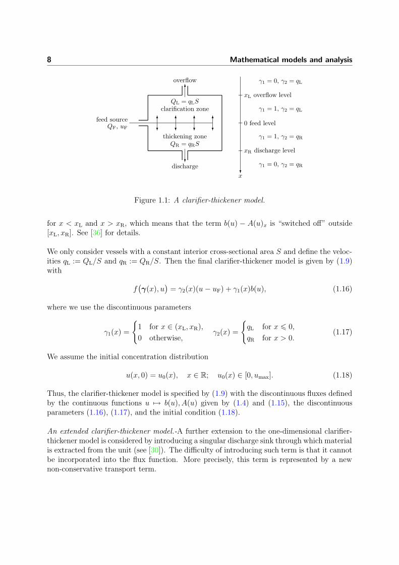
8 Mathematical models and analysis

QF, uF

feed source

overflow

QL = qLS

clarification zone

discharge

thickening zone

QR = qRS

0 feed level

xL overflow level

xR discharge level

γ1 = 0, γ2 = qL

γ1 = 1, γ2 = qL

γ1 = 1, γ2 = qR

γ1 = 0, γ2 = qR

x

Figure 1.1: A clarifier-thickener model.

for x < xL and x > xR, which means that the term b(u) − A(u)x is “switched off” outside[xL, xR]. See [36] for details.

We only consider vessels with a constant interior cross-sectional area S and define the veloc-ities qL := QL/S and qR := QR/S. Then the final clarifier-thickener model is given by (1.9)with

fγ(x), u

= γ2(x)(u − uF) + γ1(x)b(u), (1.16)

where we use the discontinuous parameters

γ1(x) =

1 for x ∈ (xL, xR),

0 otherwise,γ2(x) =

qL for x 0,

qR for x > 0.(1.17)

We assume the initial concentration distribution

u(x, 0) = u0(x), x ∈ R; u0(x) ∈ [0, umax]. (1.18)

Thus, the clarifier-thickener model is specified by (1.9) with the discontinuous fluxes definedby the continuous functions u → b(u), A(u) given by (1.4) and (1.15), the discontinuousparameters (1.16), (1.17), and the initial condition (1.18).

An extended clarifier-thickener model.-A further extension to the one-dimensional clarifier-thickener model is considered by introducing a singular discharge sink through which materialis extracted from the unit (see [30]). The difficulty of introducing such term is that it cannotbe incorporated into the flux function. More precisely, this term is represented by a newnon-conservative transport term.

1.3 A class of reaction-diffusion systems 9

Figure 1.2: Extended model for the clarifier-thickener model.

Let us consider the equation

ut + fγ(x), u

x

= γ3(x)ux for x ∈ ΠT := R × (0, T ], (1.19)

where f : Rn+1 → R is a piecewise smooth and Lipschitz continuous function, and γ(x) :=

(γ1(x), γ2(x)) is a vector of scalar parameters, which are discontinuous at most in a finitenumber of points. The unknown is the solids concentration u as function of time t anddepth x. A schematic representation of a clarifier-thickener unit is given in Figure 1.2.

The extended model for the clarifier–thickener is given by (1.19) along with the initial con-dition (1.18) and f as in (1.16) where the discontinuous parameters are

γ1(x) =

1 x ∈ [xL, xR],

0 otherwise,γ2(x) =

qR − qF x 0,

qR x > 0γ3(x) =

0 x < xD,

−qD x > xD.

Function b(u) is defined in (1.4) where v∞ > 0 is the settling velocity of a particle in anunbounded fluid, uF denotes the feed concentration, xL < xD < 0 < xR are the overflow,sink, and discharge levels respectively, qR < 0 and qF > 0 are given bulk flow velocitiesdescribing operating conditions, and qD is another velocity related to sink control. Thismodel is defined by a conservation law with a flux that is discontinuous at the source andtransition points, but not at the singular sink point.

The wellposedness analysis for a reduced model (discarding the discontinuities of the flux)is provided in [30].

1.3 A class of reaction-diffusion systems

A single-species reaction-diffusion model.- Consider the following initial-boundary value

10 Mathematical models and analysis

problem for a scalar reaction-diffusion equation, where x = (x, y) and (x, y, t) ∈ QT :=Ω × [0, T ], Ω ⊂ IR2:

ut = f(u,x) + ∆A(u), (1.20a)

u(x, 0) = u0(x) on Ω, (1.20b)

∇A(u) · n = 0 on ΣT := ∂Ω × [0, T ]. (1.20c)

This problem may serve as a scalar prototype degenerate reaction-diffusion model. Here, thezero-flux boundary condition (1.20c) implies that the reaction-diffusion domain is isolatedfrom the external environment. For f(u,x) = f(u), (1.20a) appears in [124] in an ecologicalsetting, where u denotes the population density of a species, and f(u) is its dynamics, whereit is assumed that f(0) = 0 and f (0) = 0. For example, f(u) = u(1 − u) − u2/(1 + u2)corresponds to the population dynamics of the spruce band-worm [124], and models thegrowth of the population by a logistic expression and the rate of mortality due to predationby other animals. We modify this expression by a radial spatial factor, and use

f(u,x) := 10

exp(−5r)u(1 − u) +

exp(−5r) − 1

u2

1 + u2

,

r :=

(x − 0.5)2 + (y − 0.5)2,

(1.21)

which means that the birth of individuals is concentrated near the center (0.5, 0.5), andmortality increases with increasing distance from the center. On the other hand, moststandard spatial models of population dynamics simply assume that A(u) = Du, where theconstant diffusion coefficient D > 0 measures the dispersal efficiency of the species underconsideration. Motivated by Witelski [160], who advanced degenerate diffusion in the contextof population dynamics, we utilize herein the strongly degenerate diffusion coefficient

A(u) =

0 for u uc,

D(u − uc) otherwise,(1.22)

where uc > 0 is an assumed critical (threshold) value of u beyond which diffusion will takeplace. (1.20) gives rise to a single-species example in Section 4.3.

The difficulty in the wellposedness analysis of the problem (1.20) lies in the boundary condi-tion (1.20c) when A is strongly degenerate. It is quite difficult to give a correct formulationof the zero flux boundary conditions. For the case of non-homogeneous Dirichlet bound-ary conditions, however, Mascia, Porretta, and Terracina [113] demonstrated existence anduniqueness of L∞ entropy solutions. In the special case where the function A is strictlyincreasing, the classical framework of variational solutions of parabolic equations is sufficientto satisfy this wish.

A two-species reaction-diffusion model.- Another model is given by the following initial-boundary value problem for a reaction-diffusion system on QT :

ut = γf(u, v) + ∆A(u) on QT , (1.23a)

1.3 A class of reaction-diffusion systems 11

Heat conduction

Reactant diffusion

Fuel and oxygen diffuse inward

Cold premixed gasRadiation

Reaction zone

Heat and products

diffuse outwardHot burnt gas

Figure 1.3: Sketch of the reduced dimensionless thermo-diffusive model.

vt = γg(u, v) + d∆B(v) on QT , (1.23b)

u(x, 0) = u0(x), v(x, 0) = v0(x) for x ∈ Ω, (1.23c)

∇A(u) · n = ∇B(u) · n = 0 on ΣT . (1.23d)

We study this system in the context of two applications, namely as a model of combustionand as a two-species model of mathematical biology.

For A(u) = B(u) = u, d = 1/Le and γ = 1, (1.23) represents a reduced dimensionlessthermo-diffusive model describing a combustion process, where Le is the Lewis number. Werestrict ourselves to a simple chemical reaction with only two reactants and one product, thefirst reactant and the product being highly diluted in the second reactant, and we neglectgravity (see Figure 1.3).

Since the chemical reaction takes place in a lean premixed gas, we focus on the limitingreactant, and denote by v its normalized partial mass, while u represents normalized tem-perature. The reaction rates are given by an Arrhenius law:

f(u, v) :=β2

2v exp

β(1 − u)

α(1 − u) − 1

, g(u, v) := −f(u, v), (1.24)

where α and β are the temperature rate and the dimensionless activation energy, calledZeldovich number, respectively. In Section 4.3.2, this model is employed to simulate theinteraction between two flame balls, as an extension of the applications of the same modelthat were considered in [137, 138]. Here, a flame ball denotes a slowly propagating sphericalflame structure in a premixed gaseous mixture.

If radiation effects are taken into account, (1.23a) is replaced by

ut = γf(u, v) + S(u) + ∆A(u) on QT , (1.25)

12 Mathematical models and analysis

where the dimensionless heat loss due to radiation S follows the Stefan-Boltzmann law

S(u) = ρ(u + α−1 − 1)4 − (α−1 − 1)4

, (1.26)

where α is the same parameter as in (1.24) and the dimensionless coefficient ρ controls theradiation level. Conditions (1.23d) imply that the process takes place inside a box withadiabatic walls. See [138] for details and a discussion of the case with one flame ball. Theinteraction of two flame balls including radiation is also simulated in Section 4.3.2.

On the other hand, (1.23) also arises in mathematical biology as a well-known reaction-diffusion system modelling the interaction between two chemical species with respectiveconcentrations u and v. Under certain conditions, it produces stationary solutions withTuring-type spatial patterns [124, 153]. To simulate the formation of such a pattern, we hereselect the kinetics between each species due to Schnakenberg [143]:

f(u, v) = a − u + u2v, g(u, v) = b − u2v. (1.27)

Alternative choices of f and g that lead to Turing-type patterns are discussed in [123, 124].For

A(u) = B(u) = u, (1.28)

this system has a uniform positive steady state (u0, v0) given by u0 = a+b and v0 = b/(a+b)2,where b > 0 and a + b > 0, and under certain conditions, (1.23) has a unique solution. Seefor instance [25] for the proof of existence and uniqueness.

We recall from [124, Sect. 2.3] some results on the conditions under which (1.23) produces adiffusion-driven instability giving rise to Turing-type pattern in the non-degenerate case. Anecessary condition is that the inequalities fu + gv < 0, fugv − fvgu > 0, dfu + gv > 0 and(dfu+gv)

2−4d(fugv−fvgu) > 0 are satisfied at (u, v) = (u0, v0). Evaluating these inequalitiesfor the system (1.23a), (1.23b) and the particular kinetics (1.27) yields the inequalities

0 < b − a < (a + b)3, (a + b)2 > 0, (1.29)

d(b − a) > (a + b)3,d(b − a) − (a + b)3

2> 4d(a + b)4.

To characterize the stationary pattern that arises from a choice of (a, b) that satisfies (1.29),we define

L±(a, b, d) :=d(b − a) − (a + b)3 ±

[d(b − a) − (a + b)3]2 − 4d(a + b)4

2d(a + b).

The analysis of general rectangular domains [124] implies that in the non degenerate case,the unstable patterned solution of the initial-boundary value problem (1.23) is given by

w(x, y, t) =

m,n

cnm expλ(k2)t

cos(nπx) cos(mπy),

1.3 A class of reaction-diffusion systems 13

where w = (u, v)T, the constants cnm depend on a Fourier series of the initial conditions forw, and the summation takes place over all numbers n and m that satisfy

γL−(a, b, d) =: k21 < k2 = π2(n2 + m2) < k2

2 := γL+(a, b, d),

and λ(k2) is the positive solution of the following equation, where fu, fv, gu and gv areevaluated at (u0, v0):

λ2 + λk2(1 + d) − γ(fu + gv)

+ dk4 − γ(dfu + gv)k

2 + γ2(fugv − fvgu) = 0.

In Section 4.3.3, we present a numerical solution of (1.23) with the kinetics (1.27) andthe diffusion coefficients (1.28), where parameters are chosen according to the precedingdiscussion such that indeed a Turing-type pattern is produced. On the other hand, also inSection 4.3.3, we present a simulation where (1.28) is replaced by the degenerate diffusionfunctions

A(u) =

0 for u uc,

u − uc otherwise, B(u) =

0 for u vc,

u − vc otherwise,uc, vc ≥ 0. (1.30)

It turns out that even if the stability analysis does not apply to the degenerate case, ournumerical experiments lead to the formation of a pattern.

We mention that the mathematical analysis of the system (1.23) is still an open problembecause of the presence of the boundary condition (1.23d). A successful technique for provinguniqueness of (entropy weak) solutions to degenerate parabolic equations with Dirichletboundary condition is based on Kruzkov’s method [106]. Related to this approach we mentionthat Holden, Karlsen, and Risebro [93] prove existence and uniqueness of entropy solutionsof weakly coupled systems of degenerate parabolic equations in an unbounded domain. Oursystem is an example of the degenerate reaction-diffusion system analyzed in [93], but isequipped here with the boundary condition (1.23d).

A chemotaxis-growth system.- We assume that Ω ⊂ IR2 is convex, bounded and open. Nowthe studied model is the following generalization of the Keller-Segel equations [95, 104] forchemotactical movement:

ut = ∇ ·σ∇u − u∇χ(v)

+ g(u) on QT ,

vt = h(u, v) + d∆v on QT ,

u(x, 0) = u0(x), v(x, 0) = v0(x) on Ω,

∇u · n = ∇v · n = 0 on ΣT .

(1.31)

The system (1.31) describes the aggregation of slime molds caused by their chemotacticalfeatures. Cell migration appears in numerous biological phenomena. In the case of chemo-taxis, cells (or an organism) move in response to a chemical gradient. Specifically, (1.31)

14 Mathematical models and analysis

corresponds to the model proposed by Mimura and Tsujikawa [115] for the spatio-temporalaggregation patterns shown by the bacteria Escherichia coli. This model incorporates foureffects: diffusion, chemotaxis, production of chemical substance, and population growth. Inthe absence of growth, u = u(x, t) usually represents the density of the cell population of theamoebae Dictyostelium discoideum, v = v(x, t) is the concentration of the chemo-attractant(cAMP: cyclic Adenosine Monophosphate), and χ denotes the chemotactical sensitivity func-tion, which may be given by

χ(v) = νv, ν > 0, (1.32)

where ν is a chemotactical parameter. The function g takes into account the growth rate ofthe population, and can be given by

g(u) = u2(1 − u). (1.33)

Moreover, σ > 0 and d > 0 are constant diffusion rates for both components. The function hdescribes the rates of production and degradation of the chemo-attractant; here, we choose

h(u, v) = αu − βv, α, β 0. (1.34)

Osaki et al. [128] showed that if 0 u0 ∈ L2(Ω), 0 v0 ∈ H1+r(Ω), and ∂Ω is smoothenough, (1.31) possesses a unique global solution, and Perthame [132] proved that if u0 andv0 are radial and u0L1 is sufficiently large, then u(t)L2 blows up in finite time. On theother hand, Efendiev, Klare, and Lasser [73] analyzed the fractal dimension of the exponentialattractor in dependence of ν. Our Examples of Section 4.3.4 are based on examples presentedin [73], and presents numerical solutions of (1.31) for various values of ν. We will return tothe discussion of chemotaxis models in Section 1.5.

1.4 The macroscopic bidomain and monodomain mod-

els

Since direct measurements represent an obvious difficulty in electro-cardiology, there existsa wide interest in the numerical simulations of cardiac models. In the 1950s, Hodgkin andHuxley [92] introduced the first mathematical model of wave propagation in squid nerve, andlater on, this model was modified to describe several phenomena in biology, which led to thefirst physiological model of cardiac tissue [127] and many others. Among these models, thebidomain model, firstly introduced by Tung [152], is one of the most accurate and completemodels for the theoretical and numerical study of the electric activity in cardiac tissue. Thebidomain equations result from the conservation of current between the intra- and extracel-lular domains, followed by a homogenization process (see e.g. [13, 54, 103]) derived from a

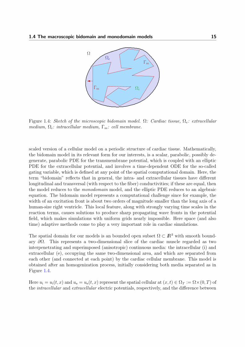
1.4 The macroscopic bidomain and monodomain models 15

Ωe

Γm

Ω

Ωi

Γm

Figure 1.4: Sketch of the microscopic bidomain model. Ω: Cardiac tissue, Ωe: extracellularmedium, Ωi: intracellular medium, Γm: cell membrane.

scaled version of a cellular model on a periodic structure of cardiac tissue. Mathematically,the bidomain model in its relevant form for our interests, is a scalar, parabolic, possibly de-generate, parabolic PDE for the transmembrane potential, which is coupled with an ellipticPDE for the extracellular potential, and involves a time-dependent ODE for the so-calledgating variable, which is defined at any point of the spatial computational domain. Here, theterm “bidomain” reflects that in general, the intra- and extracellular tissues have differentlongitudinal and transversal (with respect to the fiber) conductivities; if these are equal, thenthe model reduces to the monodomain model, and the elliptic PDE reduces to an algebraicequation. The bidomain model represents a computational challenge since for example, thewidth of an excitation front is about two orders of magnitude smaller than the long axis of ahuman-size right ventricle. This local feature, along with strongly varying time scales in thereaction terms, causes solutions to produce sharp propagating wave fronts in the potentialfield, which makes simulations with uniform grids nearly impossible. Here space (and alsotime) adaptive methods come to play a very important role in cardiac simulations.

The spatial domain for our models is an bounded open subset Ω ⊂ IR3 with smooth bound-ary ∂Ω. This represents a two-dimensional slice of the cardiac muscle regarded as twointerpenetrating and superimposed (anisotropic) continuous media: the intracellular (i) andextracellular (e), occupying the same two-dimensional area, and which are separated fromeach other (and connected at each point) by the cardiac cellular membrane. This model isobtained after an homogenization process, initially considering both media separated as inFigure 1.4.

Here ui = ui(t, x) and ue = ue(t, x) represent the spatial cellular at (x, t) ∈ ΩT := Ω×(0, T ) ofthe intracellular and extracellular electric potentials, respectively, and the difference between

16 Mathematical models and analysis

x

y

aTl (x)

al(x)

at(x)al(x)

z

x

y

an(x)

Figure 1.5: Orientation of the local and global coordinate systems of a single strand of fiber.

them

v = v(t, x) := ui − ue

is known as the transmembrane potential. The conductivity of the tissue is represented byscaled tensors Mi(x) and Me(x) given by

Mj(x) = σtjI + (σl

j − σtj)ral(x)raT

l (x),

where σlj = σl

j(x) ∈ C1(IR2) and σtj = σt

j(x) ∈ C1(IR2), j ∈ e, i, are the intra- and extra-cellular conductivity along and transverse respectively to the direction of the fiber (parallelto ral(x), see Figure 1.5).

For fibers aligned with the axis, which will be not necessarily our case, Mi(x) and Me(x)are diagonal matrices:

Mi(x) =

σl

i 00 σt

i

, Me(x) =

σl

e 00 σt

e

,

for the two-dimensional case and

Mi(x) =

σli 0 0

0 σti 0

0 0 σni

, Me(x) =

σle 0 0

0 σte 0

0 0 σne

.

for the three-dimensional case. When the so-called anisotropy ratios σ li/σ

ti and σl

e/σte are

equal, we are in the case of equal anisotropy, but generally the conductivities in the longi-tudinal direction l are higher than those across the fiber (direction t); such a case is called

1.4 The macroscopic bidomain and monodomain models 17

strong anisotropy of electrical conductivity and since the fibers usually rotate from bottomto top, this type of anisotropy is often refereed as rotational anisotropy.

The following coupled reaction-diffusion system forms the (in general, anisotropic) bidomainmodel [149, 163]:

βcm∂tv − divMi(x)∇ui

+ βIion(v, w) = 0,

βcm∂tv + divMe(x)∇ue

+ βIion(v, w) = −Iapp,

∂tw − H(v, w) = 0, (x, t) ∈ ΩT .

(1.35)

Here, cm > 0 is the so-called surface capacitance of the membrane, β is the surface-to-volume ratio, and w(t, x) is the so-called gating variable, which also takes into account theconcentration variables. The stimulation currents applied to the extracellular space arerepresented by the function Iapp = Iapp(t, x) satisfying

Ω

Iapp(t, x) dx = 0 for a.e. t ∈ (0, T ).

The functions H and Iion correspond to the Mitchell-Schaeffer membrane model [117] for themembrane and ionic currents, which is the one of the simplest among a wide variety of suchmodels:

H(v, w) =w∞(v/vp) − w

Rmcmη∞(v/vp), Iion(v, w) =

vp

Rm

v

vpη2

−v2(1 − v/vp)w

v2pη1

, (1.36)

where the dimensionless time constant η∞ and the state variable constant w∞ are given by

η∞(s) :=

η3 for s < η5,

η4 otherwise,w∞(s) =

1 for s < η5,

0 otherwise,

respectively. The quantity Rm is the surface resistivity of the membrane, and vp and η1, . . . , η5

are given parameters. A simpler choice for the membrane kinetics is the widely knownFitzHugh-Nagumo model [79, 125], often used by researchers to avoid computational diffi-culties such as the presence of a large number of coupling variables. This model is specifiedby

H(v, w) = av − bw, Iion(v, w) = −λw − v(1 − v)(v − θ)

, (1.37)

where a, b, λ and θ are nonnegative parameters. The system (1.35) can be written equiv-alently in terms of v and ue as the following strongly coupled parabolic–elliptic PDE-ODEsystem (see e.g. [149, 163]):

βcm∂tv + divMe(x)∇ue

+ βIion(v, w) = Iapp, (1.38a)

18 Mathematical models and analysis

−div(Mi(x) + Me(x))∇ue

= div

Mi(x)∇v

, (1.38b)

∂tw − H(v, w) = 0, (x, t) ∈ ΩT . (1.38c)

We supplement (1.38) with no-flux boundary conditions, representing an isolated cardiactissue:

Mj(x)∇uj) · n = 0 on ΣT := ∂Ω × (0, T ), j ∈ e, i, (1.39)

and with initial conditions for the transmembrane potential and gating variable (which aredegenerate for the potentials ui, ue):

v(0, x) = v0(x), w(0, x) = w0(x), x ∈ Ω. (1.40)

If we fixed both ue(x, 0) and ui(x, 0) as independent initial data, the problem could becomeunsolvable, since the time derivative involves only v = ui − ue (this is also referred to asdegeneracy in time). Moreover, ui and ue (as all electrical potentials defined on boundeddomains) are defined up to an additive constant, while v is uniquely determined. In ourcase, this constant is usually chosen so that the following condition holds (see e.g. [56])

Ω

ue(t, x) dx = 0 for a.e. t ∈ (0, T ). (1.41)

In the case that Mi ≡ µMe for some constant µ ∈ IR, the system (1.35) is equivalent toa scalar parabolic equation for the transmembrane potential v, coupled to an ODE for thegating variable w. This is known as the monodomain model :

βcm∂tv − div

Mi

1 + µ∇v

+ βIion(v, w) =

µ

1 + µIapp,

∂tw − H(v, w) = 0, (x, t) ∈ ΩT .

(1.42)

This model is, of course, much less involved and requires substantially less computationaleffort than the bidomain model, and even though the assumption of equal anisotropy ratiosis very strong and generally unrealistic, the monodomain model is adequate for a qualita-tive investigation of the repolarization sequences and the patterns of the action potentialdurations distribution [56].

We will assume that the functions Mj, j ∈ e, i and Iapp are sufficiently smooth so that thefollowing definition of weak solution makes sense. Namely, we assume that Iapp ∈ L2(ΩT )and

Mj ∈ L∞(Ω), Mjξ · ξ CM |ξ|2, (1.43)

for a.e. x ∈ Ω, for all ξ ∈ IR3, j ∈ e, i and constant CM > 0.

1.4 The macroscopic bidomain and monodomain models 19

Although numerical results shown in Section 4.4 indicate that the scheme converges for bothmembrane models (1.37) and (1.36), our well-definedness and convergence analysis is basedon assumptions that are met by the model (1.37) only. Specifically, for that model one candecompose Iion as Iion(v, w) =: I1,ion(v)+ I2,ion(w). Then, regarding the v−component of theionic current, I1,ion, it is straightforwardly seen that there exists a constant CI > 0 such that(see e.g. [57])

I1,ion(v1) − I1,ion(v2)

v1 − v2

≥ −CI , ∀v1 = v2.

Additionally, there is a constant C I > 0 such that

0 < lim inf|v|→∞

I1,ion(v)

v3

≤ lim sup|v|→∞

I1,ion(v)

v3

≤ C I . (1.44)

These inequalities will be needed in the proof of uniqueness of weak solution and convergenceof the numerical scheme.

For later reference, we now state the definitions of a weak solution for the bidomain and themonodomain model, respectively.

Definition 1.3 A triple u = (v, ue, w) of functions is a weak solution of the bidomain model(1.38)–(1.40) if v, ue ∈ L2(0, T ; H1(Ω)), w ∈ C([0, T ], L2(Ω)), (1.41) is satisfied and

βcm

Ω

v0(x)ϕ(0, x) dx + βcm

ΩT

v∂tϕ dx dt −

ΩT

Me(x)∇ue ·∇ϕ dx dt

+ β

ΩT

Iionϕ dx dt =

ΩT

Iappϕ dx dt,

ΩT

(Mi(x) + Me(x))∇ue ·∇ψ dx dt =

ΩT

Mi(x)∇v ·∇ψ dx dt,

−

Ω

w0(x)ξ(0, x) dx −

ΩT

w∂tξ dx dt =

ΩT

Hξ dx dt,

(1.45)

for all test functions ϕ,ψ, ξ ∈ D([0, T ) × Ω).

Definition 1.4 A pair u = (v, w) of functions is a weak solution of the monodomain model(1.42) if v ∈ L2(0, T ; H1(Ω)), w ∈ C([0, T ], L2(Ω)), and

βcm

Ω

v0(x)ϕ(0, x) dx

+

ΩT

βcmv∂tϕ + βIionϕ −

1

1 + µMi∇v ·∇ϕ

dx dt =

µ

1 + µ

ΩT

Iappϕ dx dt,

−

Ω

w0(x)ξ(0, x) dx −

ΩT

w∂tξ dx dt =

ΩT

Hξ dx dt,

for all test functions ϕ, ξ ∈ D([0, T ) × Ω).

20 Mathematical models and analysis

We mention that the wellposedness analysis for the bidomain model has already been stud-ied. See e.g. [57], where C. Franzone and Savare present a weak formulation for the bidomainmodel and show that it has a structure suitable to apply the theory of evolution variationalinequalities in Hilbert spaces. A different approach is presented in [13], where Bendahmaneand Karlsen prove existence and uniqueness for the bidomain equations using for the exis-tence, the Faedo-Galerkin method and compactness theory, Veneroni [157] derives existence,uniqueness and regularity results for a slightly different version of the degenerate bidomainequations, and in [23] Bourgault, Coudiere and Pierre prove existence and uniqueness for thebidomain equations, first reformulating the problem into a single parabolic PDE and thenapplying a semigroup approach.

1.5 A doubly nonlinear diffusion model of chemotaxis

In this section we study the existence and regularity of weak solutions of the followingparabolic system, which is a generalization of the well-known Keller-Segel model [94, 104, 124]of chemotaxis:

∂tu − div|∇A(u)|p−2∇A(u)

+ div

χuf(u)∇v

= 0 in QT := Ω × (0, T ), (1.46a)

∂tv − d∆v = g(u, v) in QT , (1.46b)

|∇A(u)|p−2a(u)∂u

∂η= 0,

∂v

∂η= 0 on ΣT := ∂Ω × (0, T ), (1.46c)

u(x, 0) = u0(x), v(x, 0) = v0(x) on Ω, (1.46d)

where T > 0 and Ω ⊂ RN is a bounded domain with sufficiently piecewise smooth boundary

∂Ω and outer unit normal η. Equation (1.46a) is doubly nonlinear, since we apply thep-Laplacian diffusion operator, where we assume 2 ≤ p < ∞, to the integrated diffusionfunction A(u) :=

u

0a(s) ds, where a(u) is a non-negative integrable function with support

on the interval [0, 1].

Migration of cells plays an important role in a wide variety of biological phenomena. Sev-eral organisms as bacteria, protozoa and more complex organisms move, as in the case ofchemotaxis, in response and toward to a chemical gradient, in order to find mates, food, etc.And, it is often noticed that the organisms tend to aggregate. In the biological phenomenondescribed by (1.46), the quantity u = u(x, t) is the density of organisms such as bacteriaor cells. The conservation PDE (1.46a) incorporates two competing mechanisms, namelythe density-dependent diffusive motion of the cells, described by the doubly nonlinear dif-fusion term, and a motion in response and toward to the gradient ∇v of the concentrationv = v(x, t) of a substance called chemoattractant. The movement in response to ∇v alsoinvolves the density-dependent probability f(u) for a cell located at (x, t) to find space in

1.5 Doubly nonlinear chemotaxis model 21

its neighboring location, and a constant χ describing chemotactic sensitivity. On the otherhand, the PDE (1.46b) describes the diffusion of the chemoattractant, where d > 0 is adiffusion constant and the function g(u, v) describes the rates of production and degradationof the chemoattractant; a common choice is

g(u, v) = αu − βv, α, β ≥ 0.

We assume that there exists a maximal population density of cells um such that f(um) = 0.This corresponds to a switch to repulsion at high densities, known as volume-filling effect,prevention of overcrowding or density control (see [15]). This means that cells stop toaccumulate at a given point of Ω after their density attains a certain threshold value, andthe chemotactic cross-diffusion term χuf(u) vanishes identically when u ≥ um. We alsoassume that the diffusion coefficient a(u) takes the form a(u) = u(1 − um), > 0, so that(1.46a) degenerates for u = 0 and u = um, while a(u) > 0 for 0 < u < um. Normalizingvariables by u = u/um, v = v, and f(u) = f(uum) we have um = 1, so in the sequel we willomit tildes in the notation.

The novelty of the present approach is that we address the question of the regularity ofweak solutions. This is delicate analytical issue as the structure of the equation combines adegeneracy of p-Laplacian type with a two-sided point degeneracy in the diffusive term. Weprove the local Holder continuity for the weak solutions of (1.46). Our approach is based onthe method of intrinsic scaling (see [66, 156]). The novelty lies in tackling the two types ofdegeneracy simultaneously and finding the right geometric setting for the concrete structureof the PDE. The resulting analysis combines the technique used by Urbano [155] to study thecase of a diffusion coefficient a(u) that decays like a power at both degeneracy points (withp = 2) with the technique by Porzio and Vespri [133] to study the p-Laplacian, with a(u)degenerating at only one side. We recover both results as particular cases of the one studiedhere. To our knowledge, the p-Laplacian is a new ingredient in chemotaxis models, so wealso include a few numerical examples that illustrate the behavior of solutions of (1.46) forp > 2, compared with solutions to the standard case p = 2, but including nonlinear diffusion.

Concerning uniqueness of solution, the presence of a nonlinear degenerate diffusion termand a nonlinear transport term represents a disadvantage because we cannot naturally proveuniqueness of weak solution. In contrast, in [26] the authors prove uniqueness of solutionsfor a degenerate parabolic-elliptic system set in an unbounded domain; and they used amethod which relies on a continuous dependence estimate from [99] that does not apply toour problem, because it is difficult to bound ∆v in L∞(QT ) due to the parabolic nature ofthe second equation in (1.46).

Before stating our main results, we provide the definition of a weak solution to (1.46), andrecall the notion of certain functional spaces. We denote by p the conjugate exponentof p (we will restrict ourselves to the degenerate case p ≥ 2): 1

p+ 1

p= 1. Moreover,

22 Mathematical models and analysis

Cw(0, T, Lp(Ω)) denotes the space of continuous functions with values in (a closed ball of)Lp(Ω) endowed with the weak topology, and ·, · is the duality pairing between W 1,p(Ω) andits dual (W 1,p(Ω)).

Definition 1.5 A weak solution of (1.46) is a pair (u, v) of functions satisfying the followingconditions:

0 ≤ u(x, t) ≤ 1 and v(x, t) ≥ 0 for a.e. (x, t) ∈ QT ,

u ∈ Cw

0, T, L2(Ω)

, ∂tu ∈ Lp

0, T ; (W 1,p(Ω))

, u(0) = u0,

A(u) =

u

0

a(s) ds ∈ Lp0, T ; W 1,p(Ω)

,

v ∈ L∞(QT ) ∩ Lr0, T ; W 1,r(Ω)

∩ C

0, T, Lr(Ω)

for all r > 1,

∂tv ∈ L20, T ; (H1(Ω))

, v(0) = v0,

and, for all ϕ ∈ Lp(0, T ; W 1,p(Ω)) and ψ ∈ L2(0, T ; H1(Ω)),

T

0

∂tu,ϕ dt +

QT

|∇A(u)|p−2∇A(u) − χuf(u)∇v

·∇ϕ dx dt = 0,

T

0

∂tv,ψ dt + d

QT

∇v ·∇ψ dx dt =

QT

g(u, v)ψ dx dt.

To ensure that all terms and coefficients are sufficiently smooth for this definition to makesense, we require that f ∈ C2[0, 1] and f(1) = 0, and assume that the diffusion coefficienta(·) has the following properties: a ∈ C1[0, 1], a(0) = a(1) = 0, and a(s) > 0 for 0 < s < 1.Moreover, we assume that there exist constants δ ∈ (0, 1/2) and γ2 ≥ γ1 > 1 such that

γ1φ(s) ≤ a(s) ≤ γ2φ(s) for s ∈ [0, δ],

γ1ψ(1 − s) ≤ a(s) ≤ γ2ψ(1 − s) for s ∈ [1 − δ, 1],(1.47)

where we define the functions φ(s) := sβ1/(p−1) and ψ(s) := sβ2/(p−1) for β2 > β1 > 0.

Our first main result is the following existence theorem for weak solutions.

Theorem 1.6 If u0, v0 ∈ L∞(Ω) with 0 ≤ u0 ≤ 1 and v0 ≥ 0 a.e. in Ω, then there exists aweak solution to the degenerate system (1.46) in the sense of Definition 1.5.

In Section 1.5.1, we first prove the existence of solutions to a regularized version of (1.46) byapplying the Schauder fixed-point theorem. The regularization basically consists in replacingthe degenerating diffusion coefficient a(u) by the regularized, strictly positive diffusion coef-ficient aε(u) := a(u) + ε, where ε > 0 is the regularization parameter. Once the regularized

1.5 Doubly nonlinear chemotaxis model 23

problem is solved, we send the regularization parameter ε to zero to produce a weak solu-tion of the original system (1.46) as the limit of a sequence of such approximate solutions.Convergence is achieved by means of a priori estimates and compactness arguments.

We denote by ∂tQT the parabolic boundary of QT , define M := u∞,QT, and recall the

definition of the intrinsic parabolic p-distance from a compact set K ⊂ QT to ∂tQT as

p-dist(K; ∂tQT ) := inf(x,t)∈K, (y,s)∈∂tQT

|x − y| + M (p−2)/p|t − s|1/p

.

Our second main result is the interior local Holder regularity of weak solutions.

Theorem 1.7 Let u be a bounded local weak solution of (1.46) in the sense of Definition 1.5,and M = u∞,QT

. Then u is locally Holder continuous in QT , i.e., there exist constantsγ > 1 and α ∈ (0, 1) depending only on the data such that for every compact K ⊂ QT ,∀(x1, t1), (x2, t2) ∈ K :

u(x1, t1) − u(x2, t2) ≤ γM

|x1 − x2| + M (p−2)/p|t2 − t1|

1/p

p-dist(K; ∂tQT )

α

.

In Section 1.5.2, we prove Theorem 1.7 by the technique of intrinsic scaling. This method isbased on regarding the underlying PDE in a geometry dictated by its degenerate structure,and this is achieved via an accommodation of the degeneracies by rescaling the standardparabolic cylinders by a factor that depends on the particular form of the degeneracies, andon the oscillation of the solution in these cylinders. This will allow us to obtain homogeneousenergy estimates over the rescaled cylinders, in the same fashion that it is done for theheat equation. The decisive part of the proof consists in the proper choice of the intrinsicgeometry. In the present case, the intrinsic geometry needs to take into account the p-Laplacian structure of the diffusion term, and that the diffusion coefficient a(u) vanishes atu = 0 and u = 1. At the core of the proof is the study of two alternative cases of similarnature, following a standard argument [66]. In either case the conclusion is that when goingfrom a rescaled cylinder into a smaller one, the oscillation of the solution decreases in a waythat can be quantified.

In the statement of Theorem 1.7 and its proof, we focus on the interior regularity of u; thatof v follows from classical theory of parabolic PDEs [108]. Moreover, standard adaptationsof the method are sufficient to extend results to the parabolic boundary, see [66, 68].

1.5.1 Existence of solutions to the chemotaxis model

We first prove of the existence of solutions to a non-degenerate, regularized version of prob-lem (1.46) using the Schauder fixed-point theorem, and our treatment closely follows that of

24 Mathematical models and analysis

[15]. We define the following closed subset of the Banach space Lp(QT ):

K :=u ∈ Lp(QT ) : 0 ≤ u(x, t) ≤ 1 for a.e. (x, t) ∈ QT

.

Weak solution to a non-degenerate problem.-We define the new diffusion term Aε(s) :=A(s) + εs, aε(s) = a(s) + ε, and consider, for each fixed ε > 0, the non-degenerate problem

∂tuε − div|∇Aε(uε)|

p−2∇Aε(uε)

+ divχf(uε)∇vε

= 0 in QT , (1.48a)

∂tvε − d∆vε = g(uε, vε) in QT , (1.48b)

|∇Aε(uε)|p−2aε(uε)

∂uε

∂η= 0,

∂vε

∂η= 0 on ΣT , (1.48c)

uε(x, 0) = u0(x), vε(x, 0) = v0(x) for x ∈ Ω. (1.48d)

With u ∈ K fixed, let v be the unique solution of the problem

∂tvε − d∆vε = g(u, vε) in QT , (1.49a)

∂vε

∂η= 0 on ΣT , vε(x, 0) = v0(x) for x ∈ Ω. (1.49b)

Given the function vε, let uε be the unique solution of the following quasilinear parabolicproblem, where v0 and u0 are functions satisfying the assumptions of Theorem 1.6:

∂tuε − div|∇Aε(uε)|

p−2∇Aε(uε)

+ divχuεf(uε)∇vε

= 0 in QT ,

|∇Aε(uε)|p−2aε(uε)

∂uε

∂η= 0 on ΣT , uε(x, 0) = u0(x) for x ∈ Ω.

(1.50)

Since for any fixed u ∈ K, (1.49a) is uniformly parabolic, standard theory for parabolicequations [108] immediately leads to the following lemma.

Lemma 1.8 If v0 ∈ L∞(Ω), then problem (1.49) has a unique weak solution vε, with vε ∈L∞(QT ) ∩ Lr(0, T ; W 2,r(Ω)) ∩ C(0, T ; Lr(Ω)), for all r > 1, satisfying in particular

vεL∞(QT ) + vεL∞(0,T ;L2(Ω)) ≤ C,

vεL2(0,T ;H1(Ω)) ≤ C,

∂tvεL2(QT ) ≤ C,

(1.51)

where C > 0 is a constant that depends only on v0L∞(Ω), α, β, and meas(QT ).

The following lemma (see [108]) holds for the quasilinear problem (1.50).

Lemma 1.9 If u0 ∈ L∞(Ω), then, for any ε > 0, there exists a unique weak solutionuε ∈ L∞(QT ) ∩ Lp(0, T ; W 1,p(Ω)) to problem (1.50).

1.5 Doubly nonlinear chemotaxis model 25

The fixed-point method.- We define a map Θ : K → K such that Θ(u) = u, where uε

solves (1.50), i.e., Θ is the solution operator of (1.50) associated with the coefficient u andthe solution v coming from (1.49). By using the Schauder fixed-point theorem, we now provethat Θ has a fixed point. First, we need to show that Θ is continuous. Let unn∈N be asequence in K and u ∈ K be such that un → u in Lp(QT ) as n → ∞. Define uεn := Θ(un),i.e., uεn is the solution of (1.50) associated with un and the solution vεn of (1.49). To showthat uεn → Θ(u) in Lp(QT ), we start with the following lemma.

Lemma 1.10 The solutions uεn to problem (1.50) satisfy

(i) 0 ≤ uεn(x, t) ≤ 1 for a.e. (x, t) ∈ QT .

(ii) The sequence uεnn∈N is bounded in Lp(0, T ; W 1,p(Ω)) ∩ L∞(0, T ; Lp(Ω)).

(iii) The sequence uεnn∈N is relatively compact in Lp(QT ).

Proof. The proof follows from that of Lemma 2.3 in [15] if we take into account that∂tuεnn∈N is uniformly bounded in Lp(0, T ; (W 1,p(Ω))).

The following lemma contains a classical result (see [108]).

Lemma 1.11 There exists a function vε ∈ L2(0, T ; H1(Ω)) such that the sequence vεnn∈N

converges strongly to v in L2(0, T ; H1(Ω)).

Lemmas 1.9–1.11 imply that there exist uε ∈ Lp(0, T ; W 1,p(Ω)) and vε ∈ L2(0, T ; H1(Ω))such that, up to extracting subsequences if necessary, uεn → uε strongly in Lp(QT ) andvεn → vε strongly in L2(0, T ; H1(Ω)) as n → ∞, so Θ is indeed continuous on K. Moreover,due to Lemma 1.10, Θ(K) is bounded in the set

W :=u ∈ Lp

0, T ; W 1,p(Ω)

: ∂tu ∈ Lp

0, T ; (W 1,p(Ω))

.

Similarly to the results of [145], it can be shown that W → Lp(QT ) is compact, and thus Θ

is compact. Now, by the Schauder fixed point theorem, the operator Θ has a fixed point uε

such that Θ(uε) = uε. This implies that there exists a solution (uε, vε) of

∀ϕ,ψ ∈ Lp(0, T ; W 1,p(Ω)) : T

0

∂tuε,ϕ dt

+

QT

|∇Aε(uε)|

p−2∇Aε(uε) − χuεf(uε)∇vε

·∇ϕ dx dt = 0,

(1.52)

T

0

∂tvε,ψ dt + d

QT

∇vε ·∇ψ dx dt =

QT

g(uε, vε)ψ dx dt.

26 Mathematical models and analysis

Existence of weak solutions.- We now pass to the limit ε → 0 in solutions (uε, vε) to obtainweak solutions of the original system (1.46). From the previous lemmas and considering(1.48b), we obtain the following result.

Lemma 1.12 For each fixed ε > 0, the weak solution (uε, vε) to (1.48) satisfies the maximumprinciple

0 ≤ uε(x, t) ≤ 1 and vε(x, t) ≥ 0 for a.e. (x, t) ∈ QT . (1.53)

Moreover, the first two estimates of (1.51) in Lemma 1.8 are independent of ε.

Lemma 1.12 implies that there exists a constant C > 0, which does not depend on ε, suchthat

vεL∞(QT ) + vεL∞(0,T ;L2(Ω)) ≤ C, vεL2(0,T ;H1(Ω)) ≤ C. (1.54)

Notice that, from (1.53) and (1.54), the term g(uε, vε) is bounded. Thus, in light of classicalresults on Lr regularity, there exists another constant C > 0 independently of ε such that

∂tvεLr(QT ) + vεLr(0,T ;W 1,r(Ω)) ≤ C.

Taking ϕ = Aε(uε) as a test function in (1.52) yields

T

0

∂tuε, A(uε) dt + ε

T

0

∂tuε, uε dt +

QT

|∇A(uε)|p dx dt

−

QT

χf(uε)∇vε ·∇Aε(uε) dx dt = 0;

then, using (1.54), the uniform L∞ bound on uε, an application of Young’s inequality to theterm ∇vε ·∇Aε(uε), and defining A(s) :=

s

0A(r) dr we obtain

sup0≤t≤T

Ω

A(uε)(x, t) dx + ε sup0≤t≤T

Ω

|uε(x, t)|2

2dx +

QT

|∇A(uε)|p dx dt ≤ C, (1.55)

for some constant C > 0, independent of ε.

Let ϕ ∈ Lp(0, T ; W 1,p(Ω)). Using the weak formulation (1.52), (1.54) and (1.55), we arriveat

T

0

∂tuε,ϕ dt

≤|∇Aε(uε)|

p−2∇Aε(uε)

Lp(QT )∇ϕLp(QT )

+ χuεf(uε)

L∞(QT )

∇vεLp(QT )∇ϕLp(QT )

≤ CϕLp(0,T ;W 1,p(Ω)),

1.5 Doubly nonlinear chemotaxis model 27

for some constant C > 0 independent of ε. From this we deduce the bound

∂tuεLp (0,T ;(W 1,p(Ω))) ≤ C. (1.56)

Therefore, by (1.54)–(1.56) and standard compactness results (see [145]) we can extractsubsequences, which we do not relabel, such that, as ε → 0,

uε → u and Aε(uε) → A(u) strongly in Lp(QT ) and a.e.,

vε → v strongly in L2(QT ),

∇vε → ∇v weakly in L2(QT ) and ∇Aε(uε) → ∇A(u) weakly in Lp(QT ),

|∇Aε(uε)|p−2∇Aε(uε) → Γ1 weakly in Lp(QT ),

vε → v weakly in L2(0, T ; H1(Ω)),

∂tuε → ∂tu weakly in Lp(0, T ; (W 1,p(Ω))) and

∂tvε → ∂tv weakly in L2(0, T ; (H1(Ω))).

(1.57)

The following Lemma is known as the Aubin lemma, see e.g. [145].

Lemma 1.13 Let X ⊂ B ⊂ Y be Banach spaces where the first embedding is compact. Ifthe set of functions F is bounded in L∞(0, T ; X) and the set ∂tF := ∂tF : f ∈ F isbounded in Lr(0, T ; Y ), r > 1; then F is relatively compact in C(0, T ; B).

From the compact embedding W 1,p(Ω) ⊂ L1(Ω) we have that the embedding L∞(Ω) ⊂(W 1,p(Ω)) is also compact, and according to Lemma 1.13 with X = W 1,p(Ω), B = (W 1,p(Ω))

and F = uεε>0, we can also conclude that uεnn∈N for any sequence εn → 0 is a Cauchysequence in C(0, T ; (W 1,p(Ω))). We also have the following lemma, se [15] for its proof.

Lemma 1.14 The functions vε converge strongly to v in L2(0, T ; H1(Ω)) as ε → 0.

Next, we identify Γ1 as |∇A(u)|p−2∇A(u) when passing to the limit ε → 0 in (1.52). Dueto this particular nonlinearity, we cannot employ the monotonicity argument used in [15];rather, we will utilize a Minty-type argument [116] and make repeated use of the following“weak chain rule” (see e.g. [22] for a proof).

Lemma 1.15 Let b : R → R be Lipschitz continuous and nondecreasing. Assume u ∈L∞(QT ) such that ∂tu ∈ Lp(0, T ; (W 1,p(Ω))), b(u) ∈ Lp(0, T ; W 1,p(Ω)), u(x, 0) = u0(x)a.e. on Ω, and u0 ∈ L∞(Ω). If we define B(u) =

u

0b(ξ)dξ, then there holds for all φ ∈

D([0, T ] × Ω) and for any s ∈ (0, T )

−

s

0

∂tu, b(u)φ dt =

s

0

Ω

B(u)∂tφ dx dt +

Ω

B(u0)φ(x, 0) dx

−

Ω

B(u(x, s))φ(x, s) dx.

28 Mathematical models and analysis

Lemma 1.16 There hold

Γ1 = |∇A(u)|p−2∇A(u), and ∇Aε(uε) → ∇A(u),

strongly in Lp(QT ).

Proof. We define QT := (t, s, x) : (x, s) ∈ Qt, t ∈ [0, T ]. The first step will be to showthat ∀σ ∈ Lp(0, T ; W 1,p(Ω)) :

QT

Γ1 − |∇A(u)|p−2∇A(u)

·∇A(u) −∇σ

dx ds dt ≥ 0. (1.58)

For all fixed ε > 0 we have the decomposition

QT

|∇Aε(uε)|

p−2∇Aε(uε) − |∇σ|p−2∇σ·∇A(u) −∇σ

dx ds dt

= I1 + I2 + I3,

I1 :=

QT

|∇Aε(uε)|p−2∇Aε(uε) ·

∇A(u) −∇Aε(uε)

dx ds dt,

I2 :=

QT

|∇Aε(uε)|

p−2∇Aε(uε) − |∇σ|p−2∇σ·∇Aε(uε) −∇σ

dx ds dt,

I3 :=

QT

|∇σ|p−2∇σ ·∇Aε(uε) −∇A(u)

dx ds dt.

Clearly, I2 ≥ 0 and from (1.57) we deduce that I3 → 0 as ε → 0. For I1, if we multiply (1.48a)by φ ∈ Lp(0, T ; W 1,p(Ω)) and integrate over QT := (t, s, x) : (x, s) ∈ Qt, t ∈ [0, T ], weobtain

T

0

t

0

∂tuε,φ ds dt −

QT

χuεf(uε)∇vε ·∇φ dx ds dt

+

QT

|∇Aε(uε)|p−2∇Aε(uε) ·∇φ dx ds dt = 0.

Now, if we take φ = A(u) − Aε(uε) ∈ Lp(0, T ; W 1,p(Ω)) and use Lemma 1.15, we obtain

I1 = −

T

0

t

0

∂tuε, A(u) ds dt +

T

0

t

0

∂tuε, Aε(uε) ds dt

+

QT

χuεf(uε)∇vε ·∇A(u) −∇Aε(uε)

dx ds dt

= −

T

0

t

0

∂tuε, A(u) ds dt +

QT

Aε(uε) dx dt − T

Ω

Aε(u0) dx

1.5 Doubly nonlinear chemotaxis model 29

+

QT

χuεf(uε)∇vε ·∇A(u) −∇Aε(uε)

dx ds dt.

Therefore, using (1.57) and Lemma 1.14, we conclude that

limε→0

I1 = −

T

0

t

0

∂tu,A(u) ds dt +

T

0

Ω

A(u(x, t)) dx dt − T

Ω

A(u0(x)) dx,

and from Lemma 1.15, this yields I1 → 0 as ε → 0. Consequently, we have shown that

QT

|∇Aε(uε)|

p−2∇Aε(uε) − |∇A(u)|p−2∇A(u)

·∇A(u) −∇Aε(uε)

dx ds dt ≤ 0,

which proves (1.58). Choosing σ = A(u) − λξ with λ ∈ R and ξ ∈ Lp(0, T ; W 1,p(Ω)) andcombining the two inequalities arising from λ > 0 and λ < 0, we obtain the first assertion ofthe lemma. The second assertion directly follows from (1.58).

With the above convergences we are now able to pass to the limit ε → 0, and we can identifythe limit (u, v) as a (weak) solution of (1.46). In fact, if ϕ ∈ Lp(0, T ; W 1,p(Ω)) is a testfunction for (1.52), then by (1.57) it is now clear that

T

0

∂tuε,ϕ dt →

T

0

∂tu,ϕ dt as ε → 0,

QT

|∇Aε(uε)|p−2∇Aε(uε) ·∇ϕ dx dt →

QT

|∇A(u)|p−2∇A(u) ·∇ϕ dx dt

as ε → 0.

Since h(uε) = uεf(uε) is bounded in L∞(QT ) and by Lemma 1.14, vε → v in L2(0, T ; H1(Ω)),it follows that

QT

χuεf(uε)∇vε ·∇ϕ dx dt →

QT

χuf(u)∇v ·∇ϕ dx dt as ε → 0.

We have thus identified u as the first component of a solution of (1.46). Using a similarargument, we can identify v as the second component of a solution.

1.5.2 Holder continuity of weak solutions for the chemotaxis model

Preliminaries.- We start by recasting Definition 1.5 in a form that involves the Steklovaverage defined for a function w ∈ L1(QT ) and 0 < h < T , by

wh :=

1

h

t+h

t

w(·, τ) dτ if t ∈ (0, T − h],

0 if t ∈ (T − h, T ].

30 Mathematical models and analysis

The proof of the following technical lemma can be obtained using general theory of Lp spaces(see e.g., [66]). This lemma will be used to allow the passage to the limit when using theSteklov average.

Lemma 1.17 If w ∈ Lq,r(QT ) then, as h → 0, the Steklov average wh converges to w inLq,r(QT−ε), for every ε ∈ (0, T ). If w ∈ C(0, T ; Lq(Ω)) then, as h → 0, the Steklov averagewh(·, t) converges to w(·, t) in Lq(Ω), for every t ∈ (0, T − ε) and every ε ∈ (0, T ).

Definition 1.18 A local weak solution u for (1.46) is a measurable function such that, forevery compact K ⊂ Ω and for all 0 < t < T − h, ∀ϕ ∈ W 1,p

0 (K) :

K×t

∂t(uh)ϕ +

|∇A(u)|p−2∇A(u)

h·∇ϕ −

χuf(u)∇v

h·∇ϕ

dx = 0. (1.59)

The following technical lemma on the geometric convergence of sequences (see e.g., [67,Lemma 4.2, Ch. I]) will be used later.

Lemma 1.19 Let Xn and Zn, n ∈ N0, be sequences of positive real numbers satisfying

Xn+1 ≤ CbnX1+α

n + Xαn Z1+κ

n

, Zn+1 ≤ Cbn

Xn + Z1+κ

n

,

where C > 1, b > 1, α > 0 and κ > 0 are given constants. Then Xn, Zn → 0 as n → ∞provided that

X0 + Z1+κ0 ≤ (2C)−(1+κ)/σb−(1+κ)/σ2

, with σ = minα,κ.

We will need as well, the following embedding theorem (see e.g., [66])

Theorem 1.20 Let p > 1. There exists a constant γ depending only on N and p such thatfor every v ∈ V p

0 (ΩT ),

vpp,ΩT

≤ γ||v| > 0|p

N+pvpV p(ΩT ).

The rescaled cylinders.- Let Bρ(x0) denote the ball of radius ρ centered at x0. Then, for apoint (x0, t0) ∈ R

n+1, we denote the cylinder of radius ρ and height τ by

(x0, t0) + Q(τ, ρ) := Bρ(x0) × (t0 − τ, t0).

Intrinsic scaling is based on measuring the oscillation of a solution in a family of nestedand shrinking cylinders whose dimensions are related to the degeneracy of the underlyingPDE. To formalize this, we fix (x0, t0) ∈ QT ; after a translation, we may assume that

1.5 Doubly nonlinear chemotaxis model 31

(x0, t0) = (0, 0). Then let ε > 0 and let R > 0 be small enough so that Q(Rp−ε, 2R) ⊂ QT ,and define

µ+ := ess supQ(Rp−ε,2R)

u, µ− := ess infQ(Rp−ε,2R)

u, ω := ess oscQ(Rp−ε,2R)

u ≡ µ+ − µ−.

Now construct the cylinder Q(a0Rp, R), where

a0 =ω

2

2−p 1

φ(ω/2m)p−1,

with m to be chosen later. To ensure that Q(a0Rp, R) ⊂ Q(Rp−ε, 2R), we assume that

1

a0

=ω

2

p−2

φ ω

2m

p−1

> Rε, (1.60)

and therefore the relationess osc

Q(a0Rp,R)u ≤ ω (1.61)

holds. Otherwise, the result is trivial as the oscillation is comparable to the radius. Wemention that for ω small and for m > 1, the cylinder Q(a0R

p, R) is long enough in thet−direction, so that we can accommodate the degeneracies of the problem. Without lossof generality, we will assume ω < δ < 1/2. We emphasize that we introduced the cylin-der Q(Rp−ε, 2R) and assumed (1.60) so that (1.61) is valid for the constructed cylinderQ(a0R

p, R).

Consider now, inside Q(a0Rp, R), smaller subcylinders of the form

Qt∗

R ≡ (0, t∗) + Q(dRp, R), d =ω

2

2−p 1

[ψ(ω/4)]p−1, t∗ < 0.

These are contained in Q(a0Rp, R) if a0R

p ≥ −t∗ + dRp, which holds whenever φ(ω/2m) ≤ψ(ω/4) and

t∗ ∈

(ω/2)2−pRp

ψ(ω/4)p−1−

(ω/2)p−2Rp

φ(ω/2m)p−1, 0

.

These particular definitions of a0 and of d turn out to be the natural extensions to the casep > 2 of their counterparts in [155]. Here, the scaling factor (ω/2)2−p takes into account thestructure of the p−Laplacian term, and the terms [ψ(ω/4)]p−1, [φ(ω/2m)]p−1 will take careof the two-sidedly degeneracy structure of a(u). Notice that for p = 2 and a(u) ≡ 1, werecover the standard parabolic cylinders.

The structure of the proof will be based on the analysis of the following alternative: eitherthere is a cylinder Qt∗

R where u is essentially away from its infimum, or such a cylinder cannot be found and thus u is essentially away from its supremum in all cylinders of that type.Both cases lead us to the conclusion that the essential oscillation of u when going to a smallercylinder decreases by a factor that can be quantified, and which does not depend on ω.

32 Mathematical models and analysis

Remark 1.5.1 (See [133, Remark 4.2]) Let us introduce quantities of the type BiRθω−bi,

where Bi and bi > 0 are constants that can be determined a priori from the data, indepen-dently of ω and R, and θ depending only on N and p. We assume without loss of generality,that

BiRθω−bi ≤ 1.

If this was not be valid, then we would have ω ≤ CRε for the choices C = maxi B1/bi and

ε = θ/ mini bi, and the result would be trivial.

The first alternative.-

Lemma 1.21 There exists ν0 ∈ (0, 1), independent of ω and R, such that if

(x, t) ∈ Qt∗

R : u(x, t) > 1 − ω/2 ≤ ν0

Qt∗

R

(1.62)

for some cylinder of the type Qt∗

R , then u(x, t) < 1 − ω/4 a.e. in Qt∗

R/2.

Proof. Let uω := minu, 1 − ω/4, take the cylinder for which (1.62) holds, define

Rn =R

2+

R

2n+1, n ∈ N0,

and construct the family

Qt∗

Rn:= (0, t∗) + Q(dRp

n, Rn) = BRn × (τn, t∗), τn := t∗ − dRp

n, n ∈ N0;

note that Qt∗

Rn→ Qt∗

R/2 as n → ∞. Let ξnn∈N be a sequence of piecewise smooth cutoff

functions satisfying

ξn = 1 in Qt∗

Rn+1, ξn = 0 on the parabolic boundary of Qt∗

Rn,

|∇ξn| ≤2n+1

R, 0 ≤ ∂tξn ≤

2p(n+1)

dRp, |∆ξn| ≤

2p(n+1)

Rp,

(1.63)

and definekn := 1 −

ω

4−

ω

2n+2, n ∈ N0.

Now take ϕ = [(uω)h − kn]+ξpn, K = BRn in (1.59) and integrate in time over (τn, t) for

t ∈ (τn, t∗). Applying integration by parts to the first term gives

F1 :=

t

τn

BRn

∂suh[(uω)h − kn]+ξpn dx ds

=1

2

t

τn

BRn

∂s

[(uω)h − kn]+

2ξpn dx ds

1.5 Doubly nonlinear chemotaxis model 33

+1 −

ω

4− kn

t

τn

BRn

∂s

u −

1 −

ω

4

+

h

ξpn dx ds

=1

2

BRn×t

[uω − kn]+h

2ξpn dx ds −

1

2

BRn×τn

[uω − kn]+h

2ξpn dx ds

−p

2

t

τn

BRn

[uω − kn]+h

2ξp−1n ∂sξn dx ds

+1 −

ω

4− kn

t

τn

BRn

∂s

u −

1 −

ω

4

+

h

ξpn dx ds.

In light of standard convergence properties of the Steklov average, we obtain

F1 → F ∗1 :=

1

2

BRn×t

[uω − kn]+

2ξpn dx ds

−p

2

t

τn

BRn

[uω − kn]+

2ξp−1n ∂sξn dx ds

+1 −

ω

4− kn

BRn×t

u −

1 −

ω

4

+

ξpn dx ds

− p

BRn×τn

u −

1 −

ω

4

+

ξp−1n ∂sξn dx ds

as h → 0.

Using (1.63) and the nonnegativity of the third term, we arrive at

F ∗1 ≥

1

2

BRn×t

[uω − kn]+

2ξpn dx

−p

2d

ω

4

2 2p(n+1)

Rp

t

τn

BRn

χuω≥kn dx ds

−p

d

ω

4

2 2p(n+1)

Rp

t

τn

BRn

χu≥1−ω/4 dx ds

≥1

2

BRn×t

[uω − kn]+

2ξpn dx

−3

2

p

d

ω

4

2 2p(n+1)

Rp

t

τn

BRn

χuω≥kn dx ds,

the last inequality coming from u ≥ 1 − ω/4 ⇒ uω ≥ kn. Since [uω − kn]+ ≤ ω/4, we knowthat

[uω − kn]+

2=[uω − kn]+

2−p[uω − kn]+

p

≥ω

4

2−p [uω − kn]+

p

34 Mathematical models and analysis

≥ω

2

2−p [uω − kn]+

p,

therefore, the definition of d implies that

F ∗1 ≥

1

2

ω

2

2−p

BRn×t

[uω − kn]+

pξpn dx

−3

2p2p−2

ω

4

p 2p(n+1)

Rpψ(ω/4)p−1

t

τn

BRn

χuω≥kn dx ds. (1.64)

We now deal with the diffusive term. The term

F2 :=

t

τn

BRn

a(u)p−1|∇u|p−2∇u

h·∇

[(uω)h − kn]+ξp

n

dx ds

converges for h → 0 to

F ∗2 :=

t

τn

BRn

a(u)p−1|∇u|p−2∇u

·∇[uω − kn]+ξp

n

dx ds

=

t

τn

BRn

a(u)p−1|∇u|p−2∇u

·∇(uω − kn)+ξp

n + p(uω − kn)+ξp−1n ∇ξn

dx ds

=

t

τn

BRn

a(u)p−1|ξn∇(uω − kn)+|p dx ds + F ∗2 ,

where we define

F ∗2 := p

t

τn

BRn

a(u)p−1|∇u|p−2∇u ·∇ξn(uω − kn)+ξp−1n dx ds.

Since ∇(uω − kn)+ is nonzero only within the set kn < u < 1 − ω/4 and a(u) ≥ γ1ψ(ω/4)on kn < u < 1 − ω/4, we may estimate the first term of F ∗

2 from below as follows: t

τn

BRn

a(u)p−1ξn∇(uω − kn)+

p dx ds ≥

[γ1ψ(ω/4)]p−1

t

τn

BRn

ξn∇(uω − kn)+p dx ds.

(1.65)

Let us now focus on F ∗2 . Using that ∇(uω − kn)+ is nonzero only within the set kn < u <

1 − ω/4, integrating by parts, and using (1.47) and (1.63), we obtain

F ∗2

≤p

t

τn

BRn

|a(u)|p−1|∇(uω − kn)+|p−1|∇ξn|(uω − kn)+ξp−1n dx ds

1.5 Doubly nonlinear chemotaxis model 35

+

p1 −

ω

4− kn

t

τn

BRn

ξp−1n ∇ξn

·∇

1

p − 1

u

1−ω/4

a(s) ds

p−1

+

dx ds

≤p [γ2ψ (ω/2)]p−1

t

τn

BRn

|∇ξn|(uω − kn)+ξn∇(uω − kn)+

p−1dx ds

+pω

4

− t

τn

BRn

u

1−ω/4

a(s) ds

p−1

+

×(p − 1)ξp−2

n |∇ξn|2 + ξp−1

n ∆ξn

dx ds

.

Next, we consider that

u

1−ω/4

a(s) ds

+

≤ω

4ψ (ω/4) ,

and apply Young’s inequality

ab ≤r2

rar +

br

rr2

if a, b ≥ 0,1

r+

1

r= 1,

for the choices

r = p, a = |∇ξn|(uω − kn)+, b =∇(uω − kn)+

p−1and

−p

1 =p

p

(γp−11 − 1)ψ(ω/4)p−1

γp−12 ψ(ω/2)p−1

> 0.

36 Mathematical models and analysis

This leads to

F ∗2

≤ 1

p1

[γ2ψ (ω/2)]p−1ω

4

p 2p(n+1)

Rp

t

τn

BRn

χuω≥kn dx ds

+ (p − 1)p

1 [γ2ψ(ω/2)]p−1

t

τn

BRn

ξn∇(uω − kn)+p dx ds

+ p2ω

4

p

ψ (ω/4)p−1 2p(n+1)

Rp

t

τn

BRn

χuω≥kn dx ds

≤

(p − 1)γp−1

2 ψ (ω/2)p−1

(γp−11 − 1)ψ (ω/4)p−1

p−1

[γ2ψ(ω/2)]p−1ω

4

p

×2p(n+1)

Rp

t

τn

BRn

χuω≥kn dx ds

+γ

p−11 − 1

ψ (ω/4)p−1

t

τn

BRn

ξn∇(uω − kn)+p dx ds

+ p2ω

4

p

ψ (ω/4)p−1 2p(n+1)

Rp

t

τn

BRn

χuω≥kn dx ds,

(1.66)

Hence, from (1.65) and (1.66) and taking into account that

ψ (ω/2)

ψ (ω/4)

p(p−1)

=

4

2

pβ2

= 2pβ2 ,

we obtain

F ∗2 ≥ψ (ω/4)p−1

t

τn

BRn

ξn∇(uω − kn)+p dx ds

−

p2 + 2pβ2

pγp

2

p(γp−11 − 1)

p−1ω

4

p

×2p(n+1)

Rpψ (ω/4)p−1

t

τn

BRn

χuω≥kn dx ds.

(1.67)

Finally, for the lower order term

F3 :=

t

τn

BRn

χuf(u)∇v

h·∇

[(uω)h − kn]+ξp

n

dx ds

we have

F3 → F ∗3 :=

t

τn

BRn

χuf(u)∇v ·∇(uω − kn)+ξp

n

1.5 Doubly nonlinear chemotaxis model 37

+ p(uω − kn)+ξp−1n ∇ξn

dx ds

=

t

τn

BRn

χuf(u)∇v ·∇(uω − kn)+ξpn dx ds

+ p

t

τn

BRn

χuf(u)∇v ·∇ξn(uω − kn)+ξp−1n dx ds as h → 0.

Applying Young’s inequality with

r = p, a = ∇(uω − kn)+ξn, b = χuf(u)ξp−1n ∇v and

p2 =

p

2ψ(ω/4)p−1 > 0,

using the fact that (uω − kn)+ ≤ ω/4 and defining M := χuf(u)L∞(QT ), we may estimateF ∗

3 by

F ∗3 ≤

p2

p

t

τn

BRn

∇(uω − kn)+ξn

p dx ds +Mp

pp

2

t

τn

BRn

|∇v|p

χuω≥kn dx ds

+ pM

t

τn

BRn

|∇v|ω

4

|∇ξn|χuω≥kn dx ds

≤1

2ψ (ω/4)p−1

t

τn

BRn

∇(uω − kn)+ξn

p dx ds

+(p/2)−p/p

pMp

ψ(ω/4)

t

τn

BRn

|∇v|p

χuω≥kn dx ds

+ p3

ω

4

p t

τn

BRn

|∇ξn|pχuω≥kn dx ds

+pMp

pp

3

t

τn

BRn

|∇v|p

χuω≥kn dx ds.

Applying Young’s inequality with

a = |∇ξn|ω/4, b = M |∇v|, p

3 = ψ (ω/4) > 0

to the last two terms in the last right-hand side and using (1.63), we obtain

F ∗3 ≤ F ∗∗

3 :=1

2ψ (ω/4)p−1

t

τn

BRn

∇(uω − kn)+ξn

p dx ds

+Mp

pψ(ω/4)

p

2

−p/p

+ p

t

τn

BRn

|∇v|p

χuω≥kn dx ds

+ω

4

p 2p(n+1)

Rpψ (ω/4)p−1

t

τn

BRn

χuω≥kn dx ds.

38 Mathematical models and analysis

Additionally, using the Holder inequality, we may write

t

τn

BRn

|∇v|p

χuω≥kn dx ds ≤ ∇vp

Lpp(QT )

t

τn

A+kn,Rn

(σ) dσ

1−1/p

,

where |A+kn,Rn

(σ)| is the N -dimensional measure of the set

A+kn,Rn

(σ) :=x ∈ BRn : u(x, σ) > kn

.

Thus we obtain

F ∗∗3 ≤

1

2ψ(ω/4)p−1

t

τn

BRn

ξn∇(uω − kn)+p dx ds

+ω

4

p 2p(n+1)

Rpψ (ω/4)p−1

t

τn

BRn

χuω≥kn dx ds

+Mp

pψ (ω/4)

p

2

−p/p

+ p

∇vp

Lpp(QT )

t

τn

A+kn,Rn

(σ) dσ

1−1/p

.

(1.68)

Combining the resulting estimates (1.64), (1.67), (1.68) and multiplying by 2(ω/2)p−2 yields

ess supτn≤t≤t∗

BRn×t

[uω − kn]+

pξpn dx ds +

2

d

t∗

τn

BRn

ξn∇(uω − kn)+p dx ds

≤

3

2p2p−2 + p2 + 2pβ2

pγp

2

p(γp−11 − 1)

p−1ω

4

p

×2p(n+1)

Rp

2

d

t∗

τn

BRn

χuω≥kn dx ds

+ 2(ω/2)p−2 Mp

pψ (ω/4)

p

2

−p/p

+ p

∇vp

Lpp(QT )

t∗

τn

|A+kn,Rn

(σ)| dσ

1−1/p

.

(1.69)

Next we perform a change in the time variable putting t := 1d(t − t∗), which transforms

Q(dRpn, Rn) into Qt∗

Rn. Furthermore, if we define uω(·, t) := uω(·, t) and ξn(·, t) = ξn(·, t),

then defining for each n,

An :=

0

−Rpn

BRn

χuω≥kn dx dt =1

d

t

τn

BRn

χuω≥kn dx ds

we may rewrite (1.69) more concisely as(uω − kn)+ξn

p

V p(Qt∗Rn

)≤

2

3

2p2p−2 + p2 + 2pβ2

pγp

2

p(γp−11 − 1)

p−1ω

4

p 2p(n+1)

RpAn

+ 2

p

2

−p/p

+ p

Mp

p

ω

2

(p−2)/p

ψ (ω/4)1−p−1/p ∇vp

Lpp(QT )A1−1/p

n ,

(1.70)

1.5 Doubly nonlinear chemotaxis model 39

where V p(ΩT ) = L∞(0, T ; Lp(Ω)) ∩ Lp(0, T ; W 1,p(Ω)) endowed with the norm

upV p(ΩT ) = ess sup

0≤t≤Tu(·, t)p

p,Ω + ∇upp,ΩT

.

Next, observe that by application of the embedding theorem 1.20, we get

1

2p(n+1)

ω

4

p

An+1 = |kn − kn+1|pAn+1

≤(uω − kn)+

p

p,Q(Rpn+1,Rn+1)

≤(uω − kn)+ξn

p

p,Q(Rpn,Rn)

≤ C(uω − kn)+ξn

p

V p(Qt∗Rn

)Ap/(N+p)

n .

Now, applying (1.70), we get

1

2p(n+1)

ω

4

p

An+1 ≤ 2C

3

2p2p−2 + p2 + 2pβ2

pγp

2

p(γp−11 − 1)

p−1

×ω

4

p 2p(n+1)

RpA1+p/(N+p)

n

+ 2C

p

2

−q/p

+ p

Mp

p

ω

2

(p−2)/p

× ψ(ω/4)1−p−1/p∇vp

Lpp(QT )A1−1/p+p/(N+p)

n .

(1.71)

Now let us define

Xn :=An

|Q(Rpn, Rn)|

, Zn :=A

1/pn

|BRn|, n ∈ N0.

Dividing (1.71) by 12p(n+1)

ω4

p|Q(Rp

n+1, Rn+1)| yields

Xn+1 ≤ 2pn

2C

3

2p2p−2 + p2 + 2pβ2

pγp

2

p(γp−11 − 1)

p−1X1+p/(N+p)

n

+ 23−2/p+pC

p

2

−p/p

+ p

Mp

p

ω

2

p−2

× ψ (ω/4)1−p−1/p RNκ∇vq

Lpp(QT )Xp/(N+p)

n Zp−1n

≤ γ2pnX1+α

n + Xαn Z1+κ

n

, n ∈ N0,

with α = p/(N + p) > 0, κ = p − 2 > 0 and

γ := 2C max

3

2p2p−2 + p2 + 2pβ2

pγp

2

p(γp−11 − 1)

p−1

,

40 Mathematical models and analysis

23−2/p+p

p

2

−p/p

+ p

Mp

p

ω

2

p−2

[ψ (ω/4)]1−p−1/p RNκ

> 0.

(In the choice of κ we need the assumption that p is strictly larger than 2.) In the spirit ofRemark 1.5.1, let us assume that

ω

2

p−2

[ψ (ω/4)]1−p−1/p RNκ ≤ 1.

Therefore, with this assumption we conclude that γ is independent of ω and R.

Reasoning analogously, we obtain

Zn+1 ≤ γ2pnXn + Z1+κ

n

.

Now, let σ = minα,κ and notice that, if we set ν0 := 2γ−(1+κ)/σ(2p)−(1+κ)/σ2, it follows

from (1.62) that

X0 + Z1+κ0 ≤ 2γ−(1+κ)/σ(2p)−(1+κ)/σ2

.

Then, using Lemma 1.19, we are able to conclude that Xn, Zn → 0 as n → ∞. Finally,notice that Rn → R/2 and kn → 1 − ω/4, and this implies that

(x, t) ∈ Q(R/2)p, R/2

: uω(x, t) ≥ 1 − ω/4

=(x, t) ∈ Qt∗

R/2 : u(x, t) > 1 − ω/4 = 0.

This completes the proof.

Now we show that the conclusion of Lemma 1.21 is valid in a full cylinder of the type Q(τ, ρ).To this end, we exploit that at the time level −t := t∗ − d(R/2)p, the function x → u(x, t)is strictly below 1 − ω/4 in the ball BR/2. We will use this time level as an initial conditionto make the conclusion of the lemma hold up to t = 0, eventually shrinking the ball. Thisrequires the use of logarithmic estimates.

Given constants a, b, c with 0 < c < a, we define the nonnegative function

±a,b,c(s) :=

ln

a

a + c − (s − b)|±

+

=

lna

a + c ± (b − s)if b ± c ≶ s ≶ b ± (a + c),

0 if s b ± c,(1.72)

whose first derivative is given by

±

a,b,c

(s) =

1

(b − s) ± (a + c)if b ± c ≶ s ≶ b ± (a + c)

0 if s ≶ b ± c 0,

1.5 Doubly nonlinear chemotaxis model 41

and its second derivative, away from s = b ± c, is

±

a,b,c

=

±a,b,c

2≥ 0.

Given u bounded in (x0, t0) + Q(τ, ρ) and a number k, define

H±u,k := ess sup

(x0,t0)+Q(τ,ρ)

(u − k)±,

and the function

Ψ±H±

u,k, (u − k)±, c

:= ±

H±u,k,k,c(u), 0 < c < H±

u,k.

Lemma 1.22 For every number ν1 ∈ (0, 1), there exists s1 ∈ N, independent of ω and R,such that

x ∈ BR/4 : u(x, t) ≥ 1 − ω/2s1 ≤ ν1|BR/2| for all t ∈ (−t, 0).

Proof. Let k = 1 − ω/4 and

c = ω/22+n, (1.73)

with n ∈ N to be chosen. Let 0 < ζ(x) ≤ 1 be a piecewise smooth cutoff function defined onBR/2 such that ζ = 1 in BR/4 and |∇ζ| ≤ C/R. Now consider the weak formulation (1.59)with ϕ = 2+(uh)(

+)(uh)ζp for K = BR/2, where + is the function defined in (1.72). After

an integration in time over (−t, t), with t ∈ (−t, 0), we obtain G1 + G2 − G3 = 0, where wedefine

G1 := 2

t

−t

BR/2

∂suh+(uh)(

+)(uh)ζp dx ds,

G2 := 2

t

−t

BR/2

|∇A(u)|p−2a(u)∇u

h·∇

+(uh)(

+)(uh)ζp

dx ds,

G3 := 2

t

−t

BR/2

χuf(u)∇v

h·∇

+(uh)(

+)(uh)ζp

dx ds.

Using the properties of ζ, we arrive at

G1 =

t

−t

BR/2

∂s

+(uh)

2ζp dx ds

=

BR/2×t

+(uh)

2ζp dx −

BR/2×−t

+(uh)

2ζp dx.

42 Mathematical models and analysis

Due to Lemma 1.21, at time −t the function x → u(x, t) is strictly below 1−ω/4 in the ballBR/2, and therefore +(u(x,−t)) = 0 for x ∈ BR/2. Consequently,

G1 →

BR/2×t

+(u)

2ζp dx −

BR/2×−t

+(u)

2ζp dx

=

BR/2×t

+(u)

2ζp dx as h → 0.

(1.74)

The definition of H±u,k implies that

u − k ≤ H+u,k = ess sup

Q(t,R/2)

u − 1 +

ω

4

+ ≤ ω

4. (1.75)

If H+u,k = 0, the result is trivial; so we assume H+

u,k > 0 and (1.73), n will be chosen largeenough so that

0 <ω

22+n< H+

u,k.

Therefore, since H+u,k + k − u + c > 0, the function +(u) is defined in the whole cylinder

Q(t, R/2) by

±

H+u,k,k,c

(u) =

lnH+

u,k

H+u,k + c + k − u

if u > k + c,

0 otherwise.

Relation (1.75) implies that

H+u,k

H+u,k + c + k − u

≤ω4

2c − ω4

= 2n, and therefore +(u) ≤ n ln 2; (1.76)

in the nontrivial case u > k+c, we also have an estimate for the derivative of the logarithmicfunction:

(+)(u)2−p

=

−1

H+u,k + c + k − u

2−p

≤

1

c

2−p

= ω

22+n

p−2

. (1.77)

With these estimates at hand, we have for the diffusive term:

G2 → G∗2 := 2

t

−t

BR/2

a(u)p−1|∇u|p−2∇u ·∇+(u)(+)(u)ζp

dx ds

=

t

−t

BR/2

a(u)p−1|∇u|p21 + +(u)

(+)(u)

2ζp

dx ds + G∗2

1.5 Doubly nonlinear chemotaxis model 43

as h → 0, where we define

G∗2 := 2p

t

−t

BR/2

a(u)p−1|∇u|p−2∇u ·∇ζ+(u)(+)(u)ζp−1

dx dt.

Applying Young’s inequality with the choices

r = p, a = |∇u|p−1ζp−1(+)(u)

2/p, b =

(+)(u)1−2/p

|∇ζ| and 4 = 1,

we obtain

G∗2

≤ 2p

t

−t

BR/2

a(u)p−1|∇u|p−1|∇ζ|+(u)(+)(u)

ζp−1 dx ds

= 2p

t

−t

BR/2

a(u)p−1+(u)|∇u|p−1ζp−1

×(+)(u)

2/p(+)(u)1−2/p

|∇ζ| dx ds

≤ 2p4

t

−t

BR/2

a(u)p−1+(u)|∇u|p(+)(u)

2ζp dx ds

+2p

pq4

t

−t

BR/2

a(u)p−1+(u)|∇ζ|p(+)(u)

2−pdx ds

= 2

t

−t

BR/2

a(u)p−1+(u)|∇u|p(+)(u)

2ζp dx ds

+ 2(p − 1)

t

−t

BR/2

a(u)p−1+(u)|∇ζ|p(+)(u)

2−pdx ds.

In light of this estimate, we obtain

G∗2 = 2

t

−t

BR/2

a(u)p−1|∇u|p(+)(u)

2ζp dx ds

− 2(p − 1)

t

−t

BR/2

a(u)p−1+(u)|∇ζ|p(+)(u)

2−pdx ds

≥ 2 [γ1ψ (ω/4)]p−1

t

−t

BR/2

|∇u|p(+)(u)

2ζp dx ds

− 2(p − 1)

t

−t

BR/2

a(u)p−1+(u)|∇ζ|p(+)(u)

2−pdx ds

≥ 2 [γ1ψ (ω/4)]p−1

t

−t

BR/2

|∇u|p(+)(u)

2ζp dx ds

− 2(p − 1)n ln 2

C

R

p ω

22+n

p−2 t

−t

BR/2

a(u)p−1χu>1−ω/4 dx ds

44 Mathematical models and analysis

and finally,

G∗2 ≥ 2 [γ1ψ (ω/4)]p−1

t

−t

BR/2

|∇u|p(+)(u)

2ζp dx ds

− 2(p − 1)n ln 2

C

R

p ω

22+n

p−2

t|BR/2| [γ2ψ (ω/4)]p−1 ,

(1.78)

where we have used the estimates (1.76), (1.77), the properties of ζ, and the fact that

γ1ψ (ω/4) ≤ a(u) ≤ γ2ψ (ω/4) on the set u > 1 − ω/4.

Moreover, from the definition of t and our choice for t∗ (recall that t∗ ≥ dRp − a0Rp), there

holds

t ≤ a0Rp =

ω

2

2−p Rp

φ (ω/2m)p−1 , (1.79)

and taking into account (1.79), we obtain from (1.78) that

G∗2 ≥ 2 [γ1ψ (ω/4)]p−1

t

−t

BR/2

|∇u|p(+)(u)

2ζp dx ds

− 2(p − 1)n ln 2Cp2(1+n)(2−p)|BR/2|

γ2

ψ (ω/4)

φ (ω/2m)

p−1

.

(1.80)

On the other hand, for the lower order term, by passing to the limit h → 0 we have

G3 → G∗3 := 2

t

−t

BR/2

χuf(u)∇v ·∇u

1 + +(u)

(+)(u)2

ζp

dx ds

+ 2p

t

−t

BR/2

χuf(u)∇v ·∇ζ+(u)(+)(u)ζp−1

dx ds

≤ 2M

t

−t

BR/2

1 + +(u)

(+)(u)

2ζp|∇u||∇v| dx ds

+ 2pM

t

−t

BR/2

+(u)(+)(u)

1−2/p

× |∇v||∇ζ|(+)(u)

2/pζp−1 dx ds.

Applying Young’s inequality to the first term of the last right-hand side with

r = p, a = |∇u|, b = |∇v| and =

pψ (ω/4)p−1

M(1 + n ln 2)

1/p

,

1.5 Doubly nonlinear chemotaxis model 45

and to the second term with

r = p, a =(+)(u)

1−2/p, b = |∇v|

(+)(u)2/p

ζp−1 and = 1,

we obtain

G∗3 ≤ 2ψ (ω/4)p−1

t

−t

BR/2

|∇u|p(+)(u)

2ζp dx ds

+ 2M

t

−t

BR/2

+(u)|∇ζ|(+)(u)

2−pdx ds

+ 2Mp − 1

p

pψ (ω/4)p−1

M(1 + n ln 2)

1/(1−p)

×

t

−t

BR/2

1 + +(u)

(+)(u)

2ζp|∇v|p

dx ds

+ 2M(p − 1)

t

−t

BR/2

+(u)|∇ζ||∇v|p(+)(u)

2ζp dx ds.

Using the estimates (1.76) and (1.77) and the properties of ζ, we then get

G∗3 ≤ 2ψ(ω/4)p−1

t

−t

BR/2

|∇u|p(+)(u)

2ζp dx ds

+ 2Mn ln 2C

R

ω

22+n

p−2

t|BR/2|

+ 2Mp − 1

p

pψ(ω/4)p−1

M(1 + n ln 2)

1/(1−p)

(1 + n ln 2) ω

22+n

−2

×

t

−t

BR/2

|∇v|p

χu>1−ω/4 dx ds

+ 2M(p − 1)n ln 2C

R

ω

22+n

−2 t

−t

BR/2

|∇v|p

χu>1−ω/4 dx ds.

Then, applying the Holder inequality and recalling the definition of t, we get

G∗3 ≤ 2ψ(ω/4)p−1

t

−t

BR/2

|∇u|p(+)(u)

2ζp dx ds

+ 2MCn ln 2 2(1+n)(2−p)φ(ω/2m)1−p|BR/2|Rp−1

+ 2M(p − 1)

pψ (ω/4)p−1

M(1 + n ln 2)

1/(1−p)1 + n ln 2

p+

C

Rn ln 2

ω

22+n

−2

× ∇vp

Lpp(QT )

a0R

p|BR/2|1−1/p

.

46 Mathematical models and analysis

In addition, thanks to Remark 1.5.1, we may obtain the estimates

ω

22+n

−2

p−pψ (ω/4)p−1

M(1 + n ln 2)

1/(1−p)

a1−1/p0 Rp−1 ≤ 1,

C ω

22+n

−2

a1−1/p0 Rp−2 ≤ 1, φ

ω

2m

1−p

Rp−1 ≤ 1,

and this finally gives

G∗3 ≤ 2ψ (ω/4)p−1

t

−t

BR/2

|∇u|p(+)(u)

2ζp dx ds

+ 2MCn ln 2 2(1+n)(2−p)|BR/2|

+ 2M(p − 1)Cn ln 2∇vp

Lpp(QT )|BR/2|

1−1/p.

(1.81)

Combining the estimates (1.74), (1.80) and (1.81) yields

BR/2×t

+(u)

2ζp dx ds

≤ 2M(p − 1)Cn ln 2∇vp

Lpp(QT )|BR/2|

1−1/p

+ (1 − γp−11 )2 [ψ (ω/4)]p−1

t

−t

BR/2

|∇u|p(+)(u)

2ζp dx ds

+ 2n ln 2 2(1+n)(2−p)|BR/2|

MC + (p − 1)Cpγ

p−12

ψ (ω/4)

φ (ω/2m)

p−1,

and since γ1 > 1 and n > 0, this implies

sup−t≤t≤0

BR/2×t

+(u)

2ζp dx

≤ 2M(p − 1)Cn ln 2∇vp

Lpp(QT )|BR/2|

1− 1p

+ 2n ln 2 22−p|BR/2|

MC + (p − 1)Cpγ

p−12

ψ (ω/4)

φ (ω/2m)

p−1.

(1.82)

Since the integrand in the left-hand side of (1.82) is nonnegative, the integral can be es-timated from below by integrating over the smaller set S = x ∈ BR/2 : u(x, t) ≥1 − ω/22+n ⊂ BR/2. Thus, noticing that

ζ = 1 and+(u)

2≥ln(2n−1)

2= (n − 1)2(ln 2)2 on S,

we obtain that (1.82) reads

x ∈ BR/2 : u(x, t) ≥ 1 − ω/22+n

1.5 Doubly nonlinear chemotaxis model 47

≤2Cn|BR/4|

(n − 1)2 ln 2

22−p

MC + (p − 1)Cpγ

p−12

ψ (ω/4)

φ (ω/2m)

p−1

+ M(p − 1)∇vp

Lpp(QT )

for all t ∈ (−t, 0). To prove the lemma we just need to choose s1 depending on ν1 such thats1 = 2 + n with

n > 1 +2C

ν1 ln 2

22−p

MC + (p − 1)Cpγ

p−12

ψ (ω/4)

φ (ω/2m)

p−1

+ M(p − 1)∇vp

Lpp(QT )

,

since if n ≥ 1 + 2/α then n/(n − 1)2 ≤ α, α > 0. Furthermore, s1 is independent of ω

because

ψ (ω/4)

φ (ω/2m)

p−1

=

(ω/4)β2/(p−1)

(ω/2m)β1/(p−1)

(p−1)

= ωβ2−β12mβ1−2β2 ≤ 2mβ1−2β2 .

The last inequality holds since β2 > β1. Now, the first alternative is established by thefollowing proposition.

Proposition 1.23 The numbers ν1 ∈ (0, 1) and s1 1 can be chosen a priori independentof ω, R such that if (1.62) holds, then

u(x, t) < µ+ −ω

2s1+1a.e. in Q(t, R/8).

We omit the proof of Proposition 1.23 because it is based on the argument of [66, Lemma 3.3]and [155], using for the extension the same technique applied in the proof of Lemma 1.21.

Corollary 1.24 There exist numbers ν0,σ0 ∈ (0, 1) independent of ω and R such that if(1.62) holds, then

ess oscQ(t,R/8)

u ≤ σ0ω.

Proof. In light of Proposition 1.23, we know that there exists a number s1 such that

ess supQ(t,R/8)

u ≤ µ+ −ω

2s1+1,

and this yields

ess oscQ(t,R/8)

u = ess supQ(t,R/8)

u − ess infQ(t,R/8)

u = µ+ −1

2s1+1− µ− ≤

1 −

1

2s1+1

ω.

48 Mathematical models and analysis

In this way, choosing σ0 = 1 − 1/2s1+1, which is independent of ω, we may complete theproof.

The second alternative.- Let us suppose now that (1.62) does not hold. Then the comple-mentary case is valid and for every cylinder Qt∗

R we have(x, t) ∈ Qt∗

R : u(x, t) < ω/2 ≤ (1 − ν0)

Qt∗

R

. (1.83)

Following an analogous analysis to the performed in the case in which the solution is near itsdegeneracy at one, a similar conclusion is obtained for the second alternative. Specifically,we first use logarithmic estimates to extend the result to a full cylinder and then we concludethat the solution is essentially away from 0 in a cylinder Q(τ, ρ). In this way we prove thefollowing corollary.

Corollary 1.25 Let t denote the second-alternative-counterpart of t. Then there exists σ1 ∈(0, 1), depending only on the data, such that

ess oscQ(t,R/8)

u ≤ σ1ω.

Since (1.62) or (1.83) must be valid, the conclusion of Corollary 1.24 or 1.25 must hold. Thus,choosing σ = maxσ0,σ1 and t = mint, t, we have proved the following proposition.

Proposition 1.26 There exists a constant σ ∈ (0, 1), depending only on the data, such that

ess oscQ(t,R/8)

u ≤ σω.

To finalize the proof (see, e.g., [66], [156], or the proof of [68, Th. 2]), let us define a sequenceof nested cylinders Qn, such that the essential oscillation of the solution u in these cylinderstends to zero as n → ∞, i.e., define the sequence ωn converging to zero such that

ess oscQn

u ≤ ωn.

We argue that this fact implies the local Holder continuity of u in QT . Indeed, it is possibleto determine a priori, in terms of the data only, γ > 1 and α ∈ (0, 1) such that for all thecylinders Q(a0ρ

p, ρ) with 0 < ρ ≤ R, it holds

ess oscQ(a0ρp,ρ)

u ≤ γ ρ

R

α

. (1.84)

Let M = u∞,QT. Fix (xi, ti) ∈ K, i = 1, 2 such that t2 > t1 and construct the cylinder

(x2, t2) + Q(M2−pRp, R). This cylinder is contained in QT if we choose

R ≤ infx∈K, y∈∂tQT

|x − y| and Mp−2

p R ≤ inft∈K

t1p ;

1.5 Doubly nonlinear chemotaxis model 49

therefore, in particular, we may take 2R = p − dist(K; ∂tQT ). To prove Holder continuity

in time, firstly assume that t2 − t1 < M2−pRp. Then, there exists ρ ∈ (0, R) such that

t2 − t1 = M2−pρp, i.e,

ρ = Mp−2

p |t2 − t1|1p .

Inequality (1.84) applied in the cylinder (x2, t2) + Q(a0ρp, ρ) implies

|u(x2, t2) − u(x1, t1)| ≤ γM

Mp−2

p |t2 − t1|1p

p − dist(K; ∂tQT )

α

,

and alternatively, if t2 − t1 ≥ M2−pRp then we have

|u(x2, t2) − u(x1, t1)| ≤ 4M

Mp−2

p |t2 − t1|1p

p − dist(K; ∂tQT )

.

The Holder continuity in space is proved in a similar fashion. Combining all previous results,we finally end up with the proof of the local Holder continuity of u in QT .

50 Mathematical models and analysis

Chapter 2

Finite volume methods

It is the purpose of this Chapter to discuss in detail the construction of numerical methodsfor solving the problems presented in Chapter 1. Specifically we will construct appropriatefinite volume methods, motivated by their most appealing feature which is that the resultingsolution satisfies the conservation of quantities such as mass, momentum, energy, and species.This approach can itself lead to valuable insight into the phenomena and also into the math-ematical structure of the problem. Furthermore, because the flux entering a given volumeis identical to that leaving the adjacent volume, these methods are naturally conservative.It is well known that this feature implies that finite volume methods automatically satisfy,for instance, jump conditions and hence give physically correct weak solutions even whencomputing discontinuous solutions, such as those arising in strongly degenerate parabolicequations.

2.1 A class of strongly degenerate parabolic equations

Let J ∈ N denote the number of space steps, ∆x := (xb − xa)/J , xj+1/2 := xa + (j + 1/2)∆xfor j = 0, . . . , J − 1, Ij := [xj−1/2, xj+1/2) and

u0j :=

1

∆x

Ij

u0(x) dx, j = 0, . . . , J. (2.1)

52 Finite volume methods

For Problem A, we assume that u0 ∈ BV (I), 0 ≤ u0(x) ≤ umax for all x ∈ I, and that thereexists a constant M > 0 such that

J−1

m=1

Au0

m+1

− 2A

u0

m

+ A

u0

m−1

≤ M∆x uniformly in ∆x; (2.2)

note that this requests, in particular, that M be independent of J . As detailed in [27], (2.2)is imposed to ensure uniform L1 Lipschitz continuity in time for the numerical solution whenthe discretization parameters tend to zero. The continuous version of (2.2) states that thetotal variation of (Aε(u0))x on the interval I must be uniformly bounded with respect to ε,where ε > 0 is a regularization parameter of a smooth regularization Aε(·) of A(·). In thecontinuous case, this condition was introduced in [29] to achieve a uniform estimate of thespatial variation of the time derivative of a viscous regularization of Problem A. Both (2.2)and the continuous n condition are satisfied, for example, if u0 is constant. Problem A isdiscretized in space with classical finite volumes. The computational domain I is decomposedinto cells Ij

2L

j=1. The initial-boundary value problem (IBVP) is then integrated over eachcell Ij, where the volume of each cell is denoted by |Ij|. Hence we get

duj

dt= Dj

U(t)

, j = 1, . . . , 2L,

where U(t) = (ui(t))i=1,...,2L contains the cell averages of the numerical solution at time t,such that

uj(t) ≈1

|Ij|

Ij

u(x, t) dx, j = 1, . . . , 2L,

and Dj(U(t)) is the numerical divergence of cell Ij at time t. In the one-dimensional case,Ij is an interval (the cell [xj−1/2, xj+1/2]) with step size ∆xj := xj+1/2 − xj−1/2, and we maysimply write

Dj(U(t)) ≈ −1

|Ij|

b(u) − A(u)x

xj+1/2

−b(u) − A(u)x

xj−1/2

, j = 1, . . . , 2L.

If Fj+1/2 and Fj−1/2 are the numerical fluxes associated with the left and right cell boundaries,respectively, then we may write

Dj = −1

∆xj

Fj+1/2 − Fj−1/2

, j = 1, . . . , 2L.

Available discretization methods differ by the definition of the numerical flux that approxi-mates Fj±1/2.

In addition to the notation introduced previously, we let N ∈ N be the number of timesteps, ∆t := T/N , and In := [tn, tn+1), where tn = n∆t for n = 0, . . . , N . We denote by un

j

2.1 A FVM for degenerate parabolic equations 53

the numerical solution at (xj, tn), assume that the values for n = 0 are given by (2.1), andapproximate the entropy solution of Problem A by a three-point finite difference scheme,which is defined by an “interior” formula for un

1 , . . . , unJ−1 and two “boundary” formulas for

un0 and un

J , respectively. Defining ν := ∆t/∆x2 and λ := ∆t/∆x, we employ the followingdiscretization, where hn

j+1/2 := h(unj , u

nj+1) and dn

j+1/2 := A(unj+1) − A(un

j ) for j = 0, . . . , J−1:

un+10 = un

0 − λhn1/2 + νdn

1/2, (2.3a)

un+1j = un

j − λhn

j+1/2 − hnj−1/2

+ ν

dn

j+1/2 − dnj−1/2

, j = 1, . . . , J − 1, (2.3b)

un+1J = un

J + λhnJ−1/2 − νdn

J−1/2, (2.3c)

We use the Engquist-Osher flux function [74]

h(u, v) := b(0) +

u

0

maxb(s), 0

ds +

v

0

minb(s), 0

ds. (2.4)

In [28] it is shown that the scheme (2.3), (2.4), which is the first-order version of the basicscheme used herein, converges to the entropy solution of Problem A, provided that thefollowing CFL condition is satisfied:

CFL := λb∞ + νa∞ ≤ 1/2 (2.5)

Convergence of a semi-implicit variant of (2.3), (2.4) is shown in [27] under the milder CFLcondition λb∞ ≤ 1/2. In both cases, the convergence proof relies on the monotonicity ofthe first-order scheme.

In order to upgrade the spatial discretization to second order, we use a MUSCL (variableextrapolation) scheme. We introduce a piecewise linear function un(x) defined by

un(x) := unj + sn

j (x − xj), x ∈ (xj−1/2, xj+1/2),

where snj denotes a suitable slope constructed from un. For smooth solutions, in regions where

snj is an O(∆x) approximation of ux(xj, tn), the reconstruction is linear and the truncation

error is O(∆x2). In regions where snj = 0, the reconstruction is piecewise constant and the

truncation error is O(∆x). For Cauchy problems, the slopes are limited to enforce the TotalVariation Diminishing (TVD) property of the scheme. In our case, we use the θ−limiter [83]

snj = M

θun

j − unj−1

∆x,

unj+1 − un

j−1

2∆x, θ

unj+1 − un

j

∆x

, θ ∈ [0, 2], (2.6)

where we choose θ = 0.5 as in [31], and M is the minmod function

M(a, b, c) :=

mina, b, c if a, b, c > 0,

maxa, b, c if a, b, c < 0,

0 otherwise.

54 Finite volume methods

Then we extrapolate the data to the boundaries of each cell and form the correspondingsecond order scheme. (An alternative “order upgrading” method would be to use a second-order essentially non-oscillatory (ENO) reconstruction [144], as done in [139].) For Problem A(with zero-flux boundary conditions), (2.6) is used for j = 2, . . . , J − 2, and we set

sn0 = sn

1 = snJ−1 = sn

J = 0. (2.7)

Experience in previous work [31] shows that the boundary formulas properly approximate thezero-flux boundary conditions (1.3) only if the first-order version (2.3a) and (2.3c) is utilized,that is, if condition (2.7) is imposed. Early numerical experiments showed that dropping thiscondition and calculating boundary slopes according to (2.6) produces oscillatory solutions.

For Problem B, the basic scheme is defined by formula (2.3b) for j = 0, . . . , J , provided thatthe space index is taken modulo J . In the same sense, (2.6) is used for all j.

The analysis of numerical schemes for (1.1) exhibits several difficulties; most notably, due tothe involved nonlinear structure of (1.1), it is usually difficult to construct an exact solution,the convergence rate is not known, and numerical experimentation is necessary to identifythe best suited parameters for a numerical scheme, for example the threshold parameters ina multiresolution scheme [38].

A case with discontinuous flux.- The numerical scheme for the solution of (1.9) is essentiallydescribed in [36]. As in the previous case, we begin the definition of the base algorithmdiscretizing R into cells Ij := [xj−1/2, xj+1/2), where xj+1/2 = (j + 1/2)∆x with j ∈ Z. Letλ = ∆t/∆x, µ = ∆t/(∆x)2 and U 0

j = u0(xj). For n > 0 we define the approximationsaccording to

Un+1j = Un

j − λ∆−h(γj+1/2, Unj+1, U

nj ) + µ∆−

γ1,j+1/2∆+A(Un

j ),

where

γj+1/2 := γx−

j+1/2

, γ1,j+1/2 := γ1

x−

j+1/2

. (2.8)

The symbols ∆± are spatial difference operators: ∆−Vj := Vj −Vj−1 and ∆+Vj := Vj+1 −Vj,and we use the Engquist-Osher flux [74] for the discontinuous case

h(γ, v, u) :=1

2

f(γ, u) + f(γ, v) −

v

u

|fu(γ, w)| dw

. (2.9)

Note that our pointwise discretization of γ, (2.8), follows the usage of [32, 36, 102, 100], butdiffers from that of [35], where γ is discretized by cell averages taken over the cells [xj, xj+1),where xj := j∆x, j ∈ Z. The important point is that in both cases, the discretizationof γ is staggered with respect to that of the conserved quantity u, and this property greatlyfacilitates the convergence analysis of the numerical schemes. If the discretizations were

2.1 A FVM for degenerate parabolic equations 55

aligned (i.e., not staggered), we would have to deal with more complicated 2 × 2 Riemannproblems at cell boundaries. Further discussion of this point is provided e.g. in [100]. Ourparticular choice of (2.8) (as opposed to forming cell averages) is basically its simplicity.

The space-time parameters are chosen in such way that we have the following CFL condition(see [36]):

λ maxu∈[0,1],x∈R

|fu(γ(x), u)| + µ maxu∈[0,1]

|A(u)| 1

2. (2.10)

which means that ∆t/(∆x)2 must be bounded. On the other hand, when the diffusion term isnot considered (as in the first Example of Section 4.2.2), the CFL condition is less restrictivethan (2.13), that is

λ maxu∈[0,1],x∈R

|fu(γ(x), u)| 1

2. (2.11)

which means that only ∆t/∆x must be bounded.

Let us mention that the scheme also admits a semi-implicit variant, in which the diffusionterms are evaluated at the time level tn+1. This variant has been used for numerical examplesin [36], and its convergence for a similar equation with a convective flux that does not dependon x, but which is supplemented by boundary conditions, has been proved in [27]. Theadvantage of a semi-implicit scheme is that it is stable under the CFL condition (2.11),which is milder than (2.10), so that much larger time step ∆t could be used. However, asemi-implicit version involves the solution of systems of nonlinear equations for each timestep, and these equations have to be solved iteratively by appropriate linearization.

We stress that equation (1.1) admits a rigorous convergence analysis for suitable numericalschemes. Evje and Karlsen [76] show that explicit monotone finite difference schemes [62]converge to BV entropy solutions for the Cauchy problem for (1.1). These results areextended to several space dimensions in [98]. The convergence of finite volume schemesfor initial-boundary value problems is proved in [114, 27]. The monotone scheme used fornumerical experiments in [35, 36] is the robust Engquist-Osher scheme [74].

A nonconservative case.- The numerical scheme for the solution of (1.19) is described indetail in [30]. The base finite volume method is defined by discretizing IR into cells Ij :=[xj−1/2, xj+1/2), where xj+1/2 = (j + 1/2)∆x with j ∈ Z. Let λ = ∆t/∆x and U 0

j = u0(xj).Therefore, for n > 0 the corresponding scheme is given by

Un+1j = Un

j − λ∆−h(γj+1/2, Unj+1, U

nj ) + λγ3

j ∆+Unj ., (2.12)

where γj+1/2 = γ(xj+1/2−), γ1,j+1/2 = γ1(xj+1/2−) and γ3j = γ3(xj−). The difference oper-

ators ∆± are ∆−Vj = Vj − Vj−1, ∆+Vj = Vj+1 − Vj, and h(γ, v, u) is the Engquist-Osher

56 Finite volume methods

numerical flux for the discontinuous case, obtained as in (2.9). The time-space parametersare chosen in such a way that the following CFL condition holds ([30]):

λ maxu∈[0,1],x∈IR

|fu(γ(x), u)| + λ maxx∈IR

λ3(x) 1

2. (2.13)

2.2 A class of degenerate reaction-diffusion systems

We employ a standard finite volume scheme to discretize a reaction-diffusion equation, whichis described here for a Cartesian mesh. The rectangular spatial domain Ω ⊂ R

2 is partitionedinto control volumes (Ωij)(i,j)∈Λ. Here Λ is the index set

Λ := (i, j) : i = 1, . . . , NLx, j = 1, . . . , NLy,

where NLxNLy is the number of cells of the grid, Ωij := [xi−1/2, xi+1/2] × [yj−1/2, yj+1/2],∆x := xi+1/2 − xi−1/2, ∆y := yj+1/2 − yj−1/2, for all (i, j) ∈ Λ, and ∆x := min∆x, ∆y.The cell average of a quantity q at time t is defined by

qij(t) =1

|Ωij|

Ωij

q(x, t) dx.

Discretization of the Turing model (1.23).- The finite volume scheme is described here for(1.20) and as it applies to the first equation of (1.23); for the second equation of (1.23), wereplace u by v, f(u, v) by g(u, v), and A(u) by dB(v). Integrating the respective equationand averaging over Ωij yields

1

|Ωij|

Ωij

ut(x, t) dx =1

|Ωij|

Ωij

Du(x, t),∇A

u(x, t)

dx +

1

|Ωij|

Ωij

f(u(x, t)) dx,

where D denotes the right-hand side of the PDE under consideration except for the reactionterm. For the two-dimensional case and on a Cartesian grid, D is discretized via

Dij := −1

∆x

Fi+1/2,j − Fi−1/2,j

−

1

∆y

Fi,j+1/2 − Fi,j−1/2

,

Fi+1/2,j := −1

∆x

A(ui+1,j) − A(uij)

, Fi,j+1/2 := −

1

∆y

A(ui,j+1) − A(uij)

.

The reaction term is approximated by fij ≈ f(uij, vij). If we incorporate a first-order Eulertime integration for both components, then the corresponding interior marching formula forModel 2 is

un+1ij = un

ij + ∆tγfij + ∆tDij

S(un

ij), ∆x, vn+1

ij = vnij + ∆tγgij + d∆tDij

S(vn

ij), ∆x,

(2.14)

2.3 A FVM for the bidomain equations 57

where S(·) denotes the stencil utilized for computing Dij. According to [49, 93], this schemeis stable under the CFL condition

λγfu∞ + fv∞ + gu∞ + gv∞

+ 4µ

A∞ + dB∞

1. (2.15)

Here λ := ∆t/∆x, µ := ∆t/∆x2.

Discretization of the chemotaxis model (1.31).- We define the difference operators δ±x Vij :=±(Vi±1,j −Vij) and δ±y Vij := ±(Vi,j±1−Vij). Then a suitable second order difference operatorfor a general term ∇ · (Q∇u) is

∇ · (Q∇u) ≈1

∆x2δ+x

Qi+1/2,jδ

−x uij

+

1

∆y2δ+y

Qi,j+1/2δ

−y uij

.

Integrating the corresponding equations, averaging over Ωij and discretizing yields the fol-lowing interior marching formula:

un+1ij =un

ij +σ∆t

∆x2δ+x δ−x un

ij +σ∆t

∆y2δ+y δ−y un

ij +∆t

∆x2

δ+x

Qn

i−1/2,jδ−x vn

ij

+∆t

∆y2

δ+y

Qn

i,j−1/2δ−y vn

ij

+ ∆tg

un

ij

,

vn+1ij =vn

ij + ∆thun

ij, vnij

+

d∆t

∆x2δ+x δ−x vn

ij +d∆t

∆y2δ+y δ−y vn

ij,

Qni,j+1/2 :=

1

2

χvn

ij

un

ij + χvn

i,j+1

un

i,j+1

, Qn

i+1/2,j :=1

2

χvn

ij

un

ij + χvn

i+1,j

un

i+1,j

.

(2.16)

Analogously to (2.15), the scheme (2.16) is stable under the corresponding CFL condition

λhu∞ + hv∞ + g∞

+ 4µd

σ + χ∞

1. (2.17)

The left-hand sides of (2.15) and (2.17) obviously evolve in time, so in practice, at each timestep we obtain ∆t from these conditions, and λ and µ are not constants; rather, they areadjusted in each time step.

2.3 The monodomain and bidomain equations

We first mention that Bendahmane and Karlsen [14] analyze a FV method for another versionof the bidomain equations, consisting in a system of two parabolic equations with Dirich-let boundary conditions. They prove existence, uniqueness and convergence of solutions tothe FV scheme. The present work complements that paper, since we here use similar tech-niques, but analyze a parabolic-elliptic system with Neumann boundary conditions, and also

58 Finite volume methods

include numerical experiments. Coudiere and Pierre [60] give stability conditions for twotime-stepping methods in different settings, and they prove convergence of an implicit FVapproximation to the monodomain equations. A discrete duality FV method (DDFV) tosolve the fully coupled heart and torso problem is presented by Coudiere et al. [61], who provewell-posedness of the problem and present various numerical tests using preconditioning.

We point out that the importance of our approach relies in the use of classical finite volumemethods in the study of the bidomain equations. From the applicative viewpoint, Harrildand Henriquez [90] give one of the first approaches of FV methods for cardiac problems,and Trew et al. [151] introduce a FV scheme for the bidomain equations but representingphysical discontinuities without the implicit removal of intracellular volume, which gives riseto linear instead of nonlinear systems.

2.3.1 An explicit FV scheme for cardiac models on uniform meshes

To approximate solutions to the bidomain equations (1.38), we employ a standard FVscheme, which is described here for a uniform grid. The square spatial domain Ω ⊂ R

2 ispartitioned into control volumes (Ωij)1≤i,j≤N , defining Ωij := [xi−1/2, xi+1/2] × [yj−1/2, yj+1/2],h = xi+1/2 − xi−1/2 = yj+1/2 − yj−1/2, for all 1 ≤ i, j ≤ N . We define cell averages of theunknowns H(v, w) and Iion(v, w):

Hn+1ij :=

1

h2∆t

tn+1

tn

Ωij

Hv(x, t), w(x, t)

dx dt,

In+1ion,(i,j) :=

1

h2∆t

tn+1

tn

Ωij

Iion

v(x, t), w(x, t)

dx dt,

and of the given function Iapp:

In+1app,(i,j) :=

1

h2∆t

tn+1

tn

Ωij

Iapp(x, t) dx dt.

Notice that if we denote by θ the angle of alignment of the fibers, then we may recast Mk(x)explicitly in the form (see e.g. [96])

Mk =

σt

k + (σlk − σt

k) sin2(θ) (σlk − σt

k) sin(θ) cos(θ)

(σlk − σt

k) sin(θ) cos(θ) σtk + (σl

k − σtk) cos2(θ)

for k ∈ e, i.

Therefore, defining the difference operators δsxVij := Vi+s,j −Vij and δs

yVij := Vi,j+s −Vij, thecorresponding diffusive term may be approximated by

∇ · (Mk∇u)i,j ≈ Dh(Mk, uij)

2.3 A FVM for the bidomain equations 59

:=1

h2

s∈−1,1

M11k δs

xuij + M12k ui+s,j+s + M21

k ui+s,j−s + M22k δs

yuij,

for all 1 ≤ i, j ≤ N and k ∈ e, i. We now describe the finite volume scheme employed toadvance the numerical solution from tn to tn+1, which is based on a simple explicit Eulertime discretization. The computation starts from the initial cell averages

v0ij =

1

h2

Ωij

v0(x) dx, w0ij =

1

h2

Ωij

w0(x) dx. (2.18)

Now, we first integrate the corresponding equations, average over Ωij and discretize. Then,assuming that at t = tn the quantities un

k,(i,j), k ∈ e, i, vnij = (un

i,(i,j) − une,(i,j)), and wn

ij

are known for all Ωij, we compute the values of these cell averages un+1k,(i,j), k ∈ e, i,

vn+1ij = (un+1

i,(i,j) − un+1e,(i,j)) and wn+1

ij at t = tn+1 from

βcmhvn+1

ij − vnij

∆t+ Dh

Me, u

ne,(i,j)

+ βh2In

ion,(i,j) = h2In+1app,(i,j), (2.19)

Dh

(Me + Mi), u

n+1e,(i,j)

+ Dh

Mi, v

n+1ij

= h2In+1

app,(i,j), (2.20)

h2wn+1

ij − wnij

∆t− h2Hn

ij = 0. (2.21)

The order in which these equations are used to advance the solution is explicitly stated inAlgorithm 2.3.1:

Algorithm 2.3.1 General method

1. Assume that uni , un

e , vn and wn are known (at time tn).

2. Solve the ODE

∂tw − H(v, w) = 0, x ∈ Ω,

approximately for tn < t ≤ tn+1 with initial condition wn and data vn, i.e., computewn+1 using (2.21).

3. Solve the parabolic PDE

βcm∂tv + divMe(x)∇ue

+ βIion(v, w) = Iapp, x ∈ Ω,

Me(x)∇ue) · n = 0 on ∂Ω

approximately for tn < t ≤ tn+1, with v(tn) = vn and w(tn) = wn, i.e., calculate vn+1

using (2.19).

60 Finite volume methods

4. Solve the elliptic problem

div(Mi(x) + Me(x))∇ue

+ div

Mi(x)∇v

= Iapp, x ∈ Ω

Mj(x)∇uj) · n = 0 on ∂Ω, j ∈ e, i

approximately for tn < t ≤ tn+1 with v(tn) = vn and ue(tn) = un

e , i.e., determine un+1e

by solving the linear system (2.20).

This algorithm structure is usually preferred for systems involving parabolic and ellipticequation, since it explicitly isolates the solution of the elliptic problem from the rest of thecomputations [130].

The boundary condition (1.39) is taken into account by imposing zero fluxes on the externaledges and the compatibility condition (1.41) is discretized via

N

i,j=1

h2une,ij = 0, n = 0, 1, 2, . . . .

Analogously, a FV method for the monodomain model (1.42) is given by determining vn+1ij

and wn+1ij for 1 ≤ i, j ≤ N and n = 0, 1, 2, . . . such that we start from the initial data and

use the following formulas to advance the solution over one time step:

βcmh2vn+1

ij − vnij

∆t+ Dh

1

1 + µMi, v

nij

+ βh2In

ion,(i,j) =µ

1 + µh2In+1

app,(i,j),

h2wn+1

ij − wnij

∆t− h2Hn

ij = 0.

As in [10], we may deduce that the previously detailed FV method (2.18)–(2.21), is stableunder the CFL condition

∆t h2 max

1≤i,j≤N

|In

ion,(i,j)| + |Inapp,(i,j)|

+ 4h−1 max

1≤i,j≤N

|Mi,(i,j)| + |Me,(i,j)|

−1

. (2.22)

Notice that the values of Inion,(i,j) and In

app,(i,j) depend on time. However, while Iapp is a givencontrol function for our model and therefore max1≤i,j≤N |In

app,(i,j)| can assumed to be bounded,the quantity In

ion,(i,j) is not bounded a priori for arbitrarily large times. Consequently, in our

computations, we evaluate the right-hand side of (2.22) after each iteration at t = tn, anduse (2.22) to define the time step size ∆t to advance the solution from tn to tn+1 = tn + ∆t.

2.3 A FVM for the bidomain equations 61

K

L

ηK L

Ω

xK xL

ηKL

σKL

Figure 2.1: Representation of a two-dimensional mesh and centers of the control volumes.

2.3.2 An implicit FV scheme for cardiac models on unstructuredmeshes

Now we give a definition of our FV scheme for approximate the solutions to the bidomainequations (1.38). This description follows the framework of [77]. An admissible mesh forΩ is formed by a family T of control volumes (open and convex polygons) of maximumdiameter h. For all K ∈ T , xK denotes the center of K, N(K) the set of neighbors of K,Eint(K) is the set of edges of K in the interior of T and Eext(K) the set of edges of K onthe boundary ∂Ω. For all L ∈ N(K) d(K,L) denotes the distance between xK and xL, σK,L

is the interface between K and L and ηK,L (ηK,σ respectively) is the unit normal vector toσK,L (σ ∈ Eext(K) respectively) oriented from K to L (from K to ∂Ω respectively). For allK ∈ T , |K| stands for the measure of the cell K. From the admissibility of T we have thatΩ = ∪K∈T K, K ∩L = ∅ if K,L ∈ T and K = L, and there exists a finite sequence (xK)K∈T

for which xKxL is orthogonal to σK,L (see Figure 2.1).

Now, consider K ∈ T and L ∈ N(K) with common vertices (a,K,L)1≤≤I with I ∈ N\0and let TK,L (respectively T ext

K,σ for σ ∈ Eext(K)) be the open and convex polygon withvertexes (xK , xL) (xK respectively) and (a,K,L)1≤≤I . Notice that Ω can be decomposed into

Ω = ∪K∈T ((∪L∈N(K)TK,L) ∪ (∪σ∈Eext(K)Text

K,σ)). For all K ∈ T , the approximation ∇huh of∇u is defined by

∇huh(x) =

|σK,L|

|TK,L|(uL − uK)ηK,L, if x ∈ TK,L,

0, if x ∈ T extK,σ.

To discretize (1.38)–(1.40), we choose an admissible discretization of QT , consisting of an

62 Finite volume methods

admissible mesh of Ω and a time step size ∆t > 0. We could choose N > 0 as the smallestinteger such that N∆t ≥ T , and set tn := n∆t for n ∈ 0, . . . , N.

On each cell K ∈ T , (positive definite) conductivity tensors are defined by

Mj,K =1

|K|

Ω

Mj(x) dx, j ∈ e, i.

Let Fj,K,L be an approximation of

σK,LMj(x)∇uj · ηK,Ldγ for j ∈ e, i, and for K ∈ T ,

L ∈ N(K) let

Mj,K,L =

1

|K|

K

Mj(x) dx ηK,L

:= |Mj,K ηK,L| , j ∈ e, i.

The diffusive fluxes Mj(x)∇uj · ηK,L on σK,L are approximated by

σK,L

(Mj(x)∇uj) · ηK,Ldγ

≈ |σK,L|∇uj(yσ) · (Mj,K ηK,L) = |σK,L|Mj,K,L∇uj(yσ) ·yσ − xK

d(K,σK,L)

≈ |σK,L|Mj,K,Luj,σ − uj,K

d(K,σK,L),

(2.23)

where yσ is the center of σK,L and uj,σ is an approximation of uj(yσ), j ∈ e, i. For theisotropic case, or more generally when Mi and Me have the axes of the mesh as eigenvectors,the resulting approximation of fluxes turns out to be consistent (see [77]). This is also truefor discretizations using uniform meshes. However, this flux computation is not consistent inthe general anisotropic case (see Remark 2.3.1 at the end of this Section, for further details).

In addition, the scheme should be conservative. This property enables us to determine theadditional unknowns uj,σ, and to compute the numerical fluxes on internal edges:

Fj,K,L = d∗j,K,L

|σK,L|

d(K,L)(uj,L − uj,K) if L ∈ N(K),

where we define

d∗j,K,L =

Mj,K,LMj,L,K

d(K,σK,L)Mj,K,L + d(L,σK,L)Mj,L,K

d(K,L),

while we discretize the zero-flux boundary condition by setting Fj,K,σ = 0. We define theunknowns Hn+1

K := H(vn+1K , wn+1

K ) and In+1ion,K := Iion(v

n+1K , wn+1

K ) and the cell averages of thegiven function Iapp:

In+1app,K :=

1

∆t|K|

tn+1

tn

K

Iapp(x, t) dx dt.

2.3 A FVM for the bidomain equations 63

The computation starts from the initial cell averages

v0K =

1

|K|

K

v0(x) dx, w0K =

1

|K|

K

w0(x) dx. (2.24)

To advance the numerical solution from tn to tn+1, we use the following implicit FV scheme:Determine (un

j,K)K∈T for j ∈ e, i and n ∈ 0, . . . , N, (vnK)K∈T = (un

i,K − une,K)K∈T for n ∈

0, . . . , N, and (wnK)K∈T for n ∈ 0, . . . , N, such that for all K ∈ T and n ∈ 0, . . . , N−1

βcm|K|vn+1

K − vnK

∆t+

L∈N(K)

d∗e,K,L

|σK,L|

d(K,L)(un+1

e,L − un+1e,K ) + β|K|In

ion,K = |K|Inapp,K , (2.25)

L∈N(K)

|σK,L|

d(K,L)

d∗

i,K,L + d∗e,K,L

un+1

e,L − un+1e,K

+ d∗

i,K,L

vn+1

L − vn+1K

= |K|In

app,K , (2.26)

|K|wn+1

K − wnK

∆t− |K|Hn

K = 0. (2.27)

The boundary condition (1.39) is taken into account by imposing zero–fluxes on externaledges:

d∗j,K,σ

|σK,L|

d(K,L)(un

j,L − unj,K) = 0 for σ ∈ Eext(K), j ∈ e, i, (2.28)

and the compatibility condition (1.41) is discretized via

K∈T |K|une,K = 0, for all n ∈

1, . . . , N − 1.

In order to prove existence and uniqueness of solution to (2.24)-(2.28) we will assume thatthe following mild time step condition is satisfied:

∆t <βcm

2βCI + β2λ2

b+ a2

b

, (2.29)

Finally, we introduce the “piecewise constant” functions

uj,h(t, x) = un+1j,K and wh(t, x) = wn+1

K , vh(t, x) = vn+1K , j ∈ i, e

for all (t, x) ∈ (n∆t, (n + 1)∆t]×K, with K ∈ T and n ∈ 0, . . . , N − 1, and for simplicityof notation, we define u := (v, ue, w) and uh := (vh, ue,h, wh).

Analogously, a FV method for the monodomain model (1.42) is given by determining vectors(vn

K)K∈T for n ∈ 0, . . . , N, and (wnK)K∈T for n ∈ 0, . . . , N, such that for all K ∈ T and

64 Finite volume methods

n ∈ 0, . . . , N − 1, we have (2.18) and

βcm|K|vn+1

K − vnK

∆t+

L∈N(K)

d∗e,K,Ld∗

i,K,L

d∗e,K,L + d∗

i,K,L

|σK,L|

d(K,L)(vn

L − vnK) + β|K|In

ion,K

=σl

i

σle + σl

i

|K|Inapp,K ,

|K|wn+1

K − wnK

∆t− |K|Hn+1

K = 0.

The convergence of the FV method given above is established by our main result, formulatedas follows.

Theorem 2.3.1 Suppose that v0 ∈ L2(Ω), w0 ∈ L2(Ω) and Iion ∈ L2(QT ), Iapp ∈ L2(QT ).Then the FV solution uh, generated by (2.24)-(2.28), converges along a subsequence to u ash → 0, where u is a weak solution of (1.38)-(1.40). The convergence is understood in thefollowing sense:

vh → v strongly in L2(QT ) and a.e. in QT ,

∇hue,h → ∇ue weakly in (L2(QT ))3, j ∈ i, e,

wh → w weakly in L2(QT ).

Remark 2.3.1 Note that our FV scheme is only consistent in the case where the diffusionmatrices are both isotropic, as for example in the monodomain model. Specifically, we stressthat the first equality in (2.23) is not true in general but only if Mj,KηK,L = |Mj,KηK,L|ηK,L,which is not the case except if ηK,L is an eigenvector of Mj,K. Furthermore, the underlyingscheme cannot be modified in a simple manner to be consistent in general for the bidomainequations. To overcome this difficulty, several variants of the proposed FV method have beenrecently proposed, such as the diamond scheme or the DDFV method (see e.g. [61]).

In light of this remark, the previous general description of the FV schemes could actuallybe presented in a simpler manner, for instance to fit the analysis to the particular case ofuniform meshes. Nevertheless, we keep a more general setting provided that the analysis isalso valid for general unstructured meshes in the case of equal anisotropy.

Remark 2.3.2 We also emphasize that since the proof of Theorem 2.3.1 is based on acompactness argument, we do not provide error estimates. Nevertheless, the numerical resultsgiven in Section 4.4 yield information about the experimental rate of convergence of themethod.

2.3 A FVM for the bidomain equations 65

2.3.3 Well-definedness of the FV scheme for cardiac models

This section is devoted to the proof of existence and uniqueness of solution to the FV method(2.25)-(2.27).

Let Hh(Ω) ⊂ L2(Ω) be the space of piecewise constant functions on each K ∈ T . For alluh ∈ Hh(Ω) and for all K ∈ T , uK denotes the constant value of uh in K. For (uh, vh) ∈(Hh(Ω))2, we define:

uh, vhHh=

1

2

K∈T

L∈N(K)

|σK,L|

d(K,L)(uL − uK)(vL − vK),

and uhHh(Ω) = (uh, uhHh)1/2. We also define Lh(Ω) ⊂ L2(Ω) as the space of piecewise

constant functions on each K ∈ T with the norm

(uh, vh)Lh(Ω) =

K∈T

|K|uKvK , uh2Lh(Ω) =

K∈T

|K| |uK |2 ,

for uh, vh ∈ Lh(Ω). In the sequel we will drop the time step superscript whenever is notneeded. For the existence part, we will make use of the following lemma provided in [112].

Lemma 2.3.2 Let (A, [·, ·], · ) be a finite dimensional Hilbert space, and let P be a con-tinuous mapping from A into itself such that

[P(ξ), ξ] > 0 for all ξ, ξ = r > 0.

Then there exists ξ ∈ A such thatP(ξ) = 0.

To prove existence of solution to the discrete problem, we will need the following discreteSobolev inequality (see e.g. [59]).

Lemma 2.3.3 Let u be a function such that 1|Ω|

Ω

u(x) dx = 0 and it is constant on each cell

of T , that is, u(x) = uK if x ∈ K, K ∈ T . Then there exists a constant Cp > 0, dependingon Ω, such that

u2L2(Ω) ≤ Cp u

2Hh(Ω) .

Proposition 2.1 Let D be an admissible discretization of ΩT . Then the FV scheme (2.25)-(2.27) admits a unique solution (vn

K , une,K , wn

K) for all K ∈ T and n ∈ 0, . . . , N.

Proof. Let Eh := Hh(Ω) × Hh(Ω) × Lh(Ω) be a Hilbert space endowed with the obviousnorm, let Φh = (ϕh,ψh, ξh) ∈ Eh and define the bilinear forms

Ah(unh, Φh) := (βcmvn

h ,−ψh)Lh(Ω) + (wnh , ξh)Lh(Ω),

66 Finite volume methods

Bh(un+1h , Φh) :=

K∈T

L∈N(K)

|σK,L|

d(K,L)

d∗

e,K,L(une,L − un

e,K)(ψL − ψK) + [(d∗i,K,L

+ d∗e,K,L)(un+1

e,L − un+1e,K ) + d∗

i,K,L(vn+1L − vn+1

K )][(ϕL + ψL) − (ϕK + ψK)]

,

and the operator Cn

(Cn+1, Φh)h :=

K∈T

|K|

−βIn+1

ion,KψK − In+1app,KψK − In+1

app,K(ϕK + ψK) − Hn+1K ξK

.

We proceed to multiply (2.25) by ϕK , (2.26) by ψK , (2.27) by ξK and summing the resultingsystem, we obtain

1

∆t

Ah(u

n+1h , Φh) − Ah(u

nh, Φh)

+ Bh(u

n+1h , Φh) + (Cn+1, Φh)h = 0.

Now, let us define the mapping P : Eh → Eh, by

[P(un+1h ), Φh] =

1

∆t

Ah(u

n+1h , Φh) − Ah(u

nh, Φh)

+ Bh(u

n+1h , Φh) + (Cn+1, Φh)h,

for all Φh ∈ Eh; and the strategy consists in applying Lemma 2.3.2 to obtain the existenceof un

K = (vnK , un

e,K , wnK) for all K ∈ T , n ∈ 0, . . . , N. Using the discrete Holder inequality,

we deduce the continuity of Ah, Bh. The continuity of the discrete form (Cn+1, ·)h is alsoeasy to verify. We then conclude that P is continuous and the task is now to show that

[P(un+1h ),un+1

h ] > 0, for un+1h Eh

= r > 0,

2.3 A FVM for the bidomain equations 67

for a sufficiently large r. To this end, firstly observe that

[P(un+1h ),un+1

h ] =

−βcm

∆t

K∈T

|K|(vn+1K − vn

K)un+1e,L +

1

∆t

K∈T

|K||wn+1K |2

+

K∈T

L∈N(K)

|σK,L|

d(K,L)

d∗

e,K,L(un+1e,L − un+1

e,K )2 + [(d∗i,K,L

+ d∗e,K,L)(un+1

e,L − un+1e,K ) + d∗

i,K,L(vn+1L − vn+1

K )][(vn+1L + un+1

e,L ) − (vn+1K + un+1

e,K )]

−1

∆t

K∈T

|K|wnKwn+1

K − β

K∈T

|K|In+1ion,Kun+1

e,K −

K∈T

|K|In+1app,Kun+1

e,K

−

K∈T

|K|In+1app,K(vn+1

K + un+1e,K ) −

K∈T

|K|Hn+1K

= −βcm

∆t

K∈T

|K|(vn+1K − vn

K)un+1e,L +

1

∆t

K∈T

|K||wn+1K |2

+

K∈T

L∈N(K)

|σK,L|

d(K,L)

d∗

e,K,L(un+1e,L − un+1

e,K )2 + d∗i,K,L[(vn+1

L + un+1e,L ) − (vn+1

K + un+1e,K )]2

+ d∗e,K,L(un+1

e,L − un+1e,K )[(vn+1

L + un+1e,L ) − (vn+1

K + un+1e,K )]

−1

∆t

K∈T

|K|wnKwn+1

K − β

K∈T

|K|In+1ion,Kun+1

e,K −

K∈T

|K|In+1app,Kun+1

e,K

−

K∈T

|K|In+1app,K(vn+1

K + un+1e,K ) −

K∈T

|K|Hn+1K .

(2.30)

Multiplying (2.25) by (vn+1K + un+1

e,K ) and summing over all K ∈ T we arrive at

βcm

∆t

K∈T

|K|(vn+1K − vn

K)(vn+1K + un+1

e,K ) + β

K∈T

|K|In+1ion,K(vn+1

K + un+1e,K )

+

K∈T

|K|In+1app,K(vn+1

K + un+1e,K )

=

K∈T

L∈N(K)

d∗e,K,L

|σK,L|

d(K,L)(un+1

e,L − un+1e,K )[(vn+1

L + un+1e,L ) − (vn+1

K + un+1e,K )].

(2.31)

Next, exploiting (2.31) we deduce from (2.30) that

[P(un+1h ),un+1

h ] =

68 Finite volume methods

βcm

∆t

K∈T

|K||vn+1K |2 +

1

∆t

K∈T

|K||wn+1K |2 −

βcm

∆t

K∈T

|K|vnKvn+1

K −1

∆t

K∈T

|K|wnKwn+1

K

+

K∈T

L∈N(K)

|σK,L|

d(K,L)

d∗

e,K,L(un+1e,L − un+1

e,K )2 + d∗i,K,L[(vn+1

L + un+1e,L ) − (vn+1

K + un+1e,K )]2

−

K∈T

|K|In+1app,Kun+1

e,L −

K∈T

|K|Hn+1K wn+1

K + β

K∈T

|K|In+1ion,Kvn+1

K .

Given (1.43) and Young’s inequality, it follows that

[P(un+1h ),un+1

h ] βcm

∆t

K∈T

|K||vn+1K |2 +

1

∆t

K∈T

|K||wn+1K |2 + CM(vn+1

h + un+1e,h 2

Hh(Ω) + un+1e,h 2

Hh(Ω))

− βCI

K∈T

|K|vn+1

K

2 − b

2

K∈T

|K|wn+1

K

2 − β2λ2

2b

K∈T

|K|vn+1

K

2 + b

K∈T

|K|wn+1

K

2

−a2

2b

K∈T

|K|vn+1

K

2 − b

2

K∈T

|K|wn+1

K

2 − CM

2C2p

K∈T

|K|un+1

e,h

2

− C(CM , Cp)

K∈T

|K|In+1

app,K

2 − βcm

2∆t

K∈T

|K|vn+1

K

2

− C(cm, β, ∆t)

K∈T

|K| |vnK |2 −

1

2∆t

K∈T

|K|wn+1

K

2 − C(∆t)

K∈T

|K| |wnK |2 ,

and therefore, from Lemma 2.3.3 we get

[P(un+1h ),un+1

h ]

βcm

2∆t− βCI −

β2λ2

2b−

a2

2b

K∈T

|K||vn+1K |2 +

1

2∆t

K∈T

|K||wn+1K |2

+CM

2(vn+1

h + un+1e,h 2

Hh(Ω) + un+1e,h 2

Hh(Ω))

− C(CM , Cp)

K∈T

|K|In+1

app,K

2 − C(cm, β, ∆t)

K∈T

|K| |vnK |2

− C(∆t)

K∈T

|K| |wnK |2 .

Finally, if we use (2.29), then, for a given unh we can choose un+1

h with norm large enough toconclude that Lemma 2.3.2 holds, and thus we have the existence of at least one solution tothe scheme (2.25)-(2.27).

It remains to prove the uniqueness. Let us first assume that there exists n ∈ 0, . . . , Nsuch that vn

K = vnK , un

e,K = une,K , and wn

K = wnK for all K ∈ T , but vn+1

K = vn+1K , un+1

e,K =

un+1e,K , and wn+1

K = wn+1K for some K ∈ T , all of these functions satisfying (2.25)-(2.27).

2.3 A FVM for the bidomain equations 69

Substracting the schemes for vnK , un

e,K , wnK and vn

K , une,K , wn

K, multiplying the resulting

scheme by (wn+1K − wn+1

K ), (vn+1K − vn+1

K ) and [(un+1e,L − un+1

e,L ) − (un+1e,K − un+1

e,K )] respectively,and summing over all K ∈ T , gives

βcm|K|vn+1

K − vn+1K

∆t+

L∈N(K)

d∗e,K,L

|σK,L|

d(K,L)

(un+1

e,L − un+1e,L ) − (un+1

e,K − un+1e,K )

+ β|K|(I1,ion(vn+1K ) − (I1,ion(v

n+1K )) − λβ|K|(wn+1

K − wn+1K ) = 0,

(2.32)

−

L∈N(K)

(d∗i,K,L + d∗

e,K,L)|σK,L|

d(K,L)

(un+1

e,L − un+1e,L ) − (un+1

e,K − un+1e,K )

=

L∈N(K)

d∗i,K,L

|σK,L|

d(K,L)

(vn+1

L − vn+1L ) − (vn+1

K − vn+1K )

(2.33)

|K|wn+1

K − wn+1K

∆t+ b |K|(wn+1

K − wn+1K ) − a |K|(vn+1 − vn+1

K ) = 0. (2.34)

Next, multiplying (2.32), (2.33), and (2.34) by −∆t(un+1e,K − un+1

e,K ), ∆t((vn+1K − vn+1

K ) +

(un+1e,K − un+1

e,K ) and ∆t(wn+1K − wn+1

K ) respectively and summing the resulting over K andn ∈ 0, . . . , N − 1 yields E1 + E2 + E3 = 0, where

E1 := −N−1

n=0

K∈T

βcm|K|(vn+1K − vn+1

K )(un+1e,K − un+1

e,K ) +N−1

n=0

K∈T

|K|wn+1

K − wn+1K

2 ,

E2 :=N−1

n=0

∆t

K∈T

L∈N(K)

|σK,L|

d(K,L)

d∗

e,K,L((un+1e,L − un+1

e,L ) − (un+1e,K − un+1

e,K ))2 + [(d∗i,K,L

+ d∗e,K,L)((un+1

e,L − un+1e,L ) − (un+1

e,K − un+1e,K )) + d∗

i,K,L((vn+1L − vn+1

L ) − (vn+1L − vn+1

K ))]

× [(vn+1L + un+1

e,L ) − (vn+1K + un+1

e,K )]

,

and

E3 := −N−1

n=0

∆t

K∈T

β|K|(I1,ion(vn+1K ) − (I1,ion(v

n+1K ))(un+1

e,K − un+1e,K )

+N−1

n=0

∆t

K∈T

λβ|K|(wn+1K − wn+1

K )(un+1e,K − un+1

e,K )

+N−1

n=0

∆t

K∈T

b |K|(wn+1K − wn+1

K )2 −N−1

n=0

∆t

K∈T

a |K|(vn+1K − vn+1

K )(wn+1K − wn+1

K ).

70 Finite volume methods

Multiplying (2.33) by ∆t((vn+1K − vn+1

K ) + (un+1e,K − un+1

e,K )) and summing over all K ∈ T andn ∈ 0, . . . , N − 1, we get

βcm

N−1

n=0

K∈T

|K|(vn+1K − vn+1

K )((vn+1K − vn+1

K ) + (un+1e,K − un+1

e,K ))

+N−1

n=0

∆t

K∈T

β|K|(I1,ion(vn+1K ) − (I1,ion(v

n+1K ))((vn+1

K − vn+1K ) + (un+1

e,K − un+1e,K ))

−N−1

n=0

∆t

K∈T

λβ|K|(wn+1K − wn+1

K )((vn+1K − vn+1

K ) + (un+1e,K − un+1

e,K ))

=N−1

n=0

∆t

K∈T

L∈N(K)

d∗e,K,L

|σK,L|

d(K,L)((un+1

e,L − un+1e,L ) − (un+1

e,K − un+1e,K ))

× [((vn+1L − vn+1

L ) + (un+1e,L − un+1

e,L )) − ((vn+1K − vn+1

K ) + (un+1e,K − un+1

e,K ))].

From this it follows that

E1 + E2 + E3 ≥N−1

n=0

K∈T

|K|

βcm(vn+1

K − vn+1K )2 +

wn+1K − wn+1

K

2

− ∆tλβ(wn+1K − wn+1

K )(vn+1K − vn+1

K )

+ ∆tβ[I1,ion(vn+1K ) − I1,ion(v

n+1K )](vn+1

K − vn+1K ) + ∆tb (wn+1

K − wn+1K )2

− ∆ta (vn+1 − vn+1K )(wn+1

K − wn+1K )

≥N−1

n=0

K∈T

|K|

βcm(vn+1

K − vn+1K )2

− βCI∆tvn+1

K − vn+1K

2 − b

2∆t

wn+1K − wn+1

K

2

−β2λ2

2b∆t

vn+1K − vn+1

K

2 +b

N

wn+1K − wn+1

K

2 − a2

2b∆t

vn+1K − vn+1

K

2

.

Consequently, putting all the previous inequalities together, we end up with

βcm

N−1

n=0

K∈T

|K|vn+1

K − vn+1K

2 ≤

βCI +β2λ2

2b+

a2

2b

N−1

n=0

∆t

K∈T

|K|vn+1

K − vn+1K

2 ,

(2.35)

and since

K∈T

|K|vn+1

K − vn+1K

= 0, from (2.35) we get

βcm2βCI + β2λ2

b+ a2

b

≤βcm

βCI + β2λ2

2b+ a2

2b

≤ ∆t,

2.3 A FVM for the bidomain equations 71

which contradicts (2.29).

2.3.4 A priori estimates and convergence of the scheme

First we need to establish several a priori estimates for the FV scheme, which eventually willimply the desired convergence results.

Lemma 2.3.4 Let (vnK , un

e,K , wnK)K∈T ,n∈0,...,N be a solution of the FV scheme (2.24)-(2.28).

Then there exist constants C1, C2, C3 > 0, depending on Ω, T , v0, w0, Iapp, and α, such that

maxn∈1,...,N

K∈T

|K|

|vn

K |2 + |wnK |2

≤ C1, (2.36)

N−1

n=0

∆t

K∈T

L∈N(K)

|σK,L|

d(K,L)

un+1

e,K − un+1e,L

2 +(vn+1

K + un+1e,K ) − (vn+1

L + un+1e,L )

2≤ C2,

(2.37)

and

N−1

n=0

∆t

K∈T

|K|

vn+1K

4 +I1,ion(v

n+1K )

r

≤ C3, (2.38)

for all 1 ≤ r ≤ 4/3.

Proof. We multiply (2.25), (2.26) and (2.27) by −∆tun+1e,K , ∆t(vn+1

K + un+1e,K ) and ∆twn+1

K ,respectively, and add together the outcomes. Summing the resulting equation over K,n andgathering by edges yields F1 + F2 + F3 = 0, where

F1 := −βcm

N−1

n=0

K∈T

|K|(vn+1K − vn

K)un+1e,K +

N−1

n=0

K∈T

|K|(wn+1K − wn

K)wn+1K ,

F2 :=N−1

n=0

∆t

K∈T

L∈N(K)

|σK,L|

d(K,L)

d∗

e,K,L(un+1e,L − un+1

e,K )2 + [(d∗i,K,L

+ d∗e,K,L)(un+1

e,L − un+1e,K ) + d∗

i,K,L(vn+1L − vn+1

K )][(vn+1L + un+1

e,L ) − (vn+1K + un+1

e,K )]

,

72 Finite volume methods

and

F3 := − β

N−1

n=0

∆t

K∈T

|K|In+1ion,Kun+1

e,K −N−1

n=0

∆t

K∈T

|K|In+1app,Kun+1

e,K

−N−1

n=0

∆t

K∈T

|K|In+1app,K(vn+1

K + un+1e,K ) −

N−1

n=0

∆t

K∈T

|K|Hn+1K wn+1

K .

Multiplying (2.25) by ∆t(vn+1K + un+1

e,K ), summing over K,n and gathering by edges leads to

βcm

N−1

n=0

∆t

K∈T

|K|(vn+1K − vn

K)(vn+1K + un+1

e,K ) + β

N−1

n=0

∆t

K∈T

|K|In+1ion,K(vn+1

K + un+1e,K )

+N−1

n=0

∆t

K∈T

|K|In+1app,K(vn+1

K + un+1e,K )

=N−1

n=0

∆t

K∈T

L∈N(K)

d∗e,K,L

|σK,L|

d(K,L)(un+1

e,L − un+1e,K )[(vn+1

L + un+1e,L ) − (vn+1

K + un+1e,K )].

From the inequality “a(a − b) ≥ 12(a2 − b2)”, we obtain

F1 = βcm

N−1

n=0

K∈T

|K|(vn+1K − vn

K)vn+1K +

N−1

n=0

K∈T

|K|(wn+1K − wn

K)wn+1K

≥βcm

2

N−1

n=0

K∈T

|K|vn+1

K

2 − |vnK |2

+

1

2

N−1

n=0

K∈T

|K|wn+1

K

2 − |wnK |2

=βcm

2

K∈T

|K|vN

K

2 −v0

K

2

+1

2

K∈T

|K|wN

K

2 −w0

K

2

.

Then we get

βcm

2

K∈T

|K|vN

K

2 −v0

K

2

+1

2

K∈T

|K|wN

K

2 −w0

K

2

+

K∈T

L∈N(K)

|σK,L|

d(K,L)

d∗

e,K,L(un+1e,L − un+1

e,K )2 + d∗i,K,L[(vn+1

L + un+1e,L ) − (vn+1

K + un+1e,K )]2

= −β

K∈T

|K|In+1ion,Kvn+1

K +

K∈T

|K|In+1app,Kun+1

e,L +

K∈T

|K|Hn+1K wn+1

K

≤ βCI

K∈T

|K|vn+1

K

2 +CM

2C2p

K∈T

|K|un+1

e,h

2 + C(CM , Cp)

K∈T

|K|In+1

app,K

2

+b

2

K∈T

|K|wn+1

K

2 +β2λ2

2b

K∈T

|K|vn+1

K

2 − b

K∈T

|K|wn+1

K

2

2.3 A FVM for the bidomain equations 73

+a2

2b

K∈T

|K|vn+1

K

2 +b

2

K∈T

|K|wn+1

K

2

≤ (βCI +β2λ2

2b+

a2

2b)

K∈T

|K|vn+1

K

2 +CM

2

K∈T

L∈N(K)

|σK,L|

d(K,L)d∗

e,K,L(un+1e,L − un+1

e,K )2

+ C(CM , Cp)

K∈T

|K|In+1

app,K

2 , (2.39)

which implies

βcm

2

K∈T

|K|vN

K

2 +1

2

K∈T

|K|wN

K

2

≤ C(CM , Cp)N−1

n=0

∆t

K∈T

|K|In+1

app,K

2 +

K∈T

|K|βcm

2

v0K

2 +1

2

w0K

2

+βCI +

β2λ2

2b+

a2

2b

N−1

n=0

∆t

K∈T

|K|vn+1

K

2 . (2.40)

Clearly,N−1

n=0

∆t

K∈T

|K|In+1

app,K

2 ≤ Iapp2L2(QT ) ,

and

K∈T

|K|βcm

2

v0K

2 +1

2

w0K

2≤

βcm

2v0

2L2(Ω) +

1

2w0

2L2(Ω) .

In view of (2.40), this implies the existence of constants C4, C5 > 0 such that

K∈T

|K|vN

K

2 ≤ C4 + C5

N−1

n=0

∆t

K∈T

|K|vn+1

K

2 . (2.41)

Note that (2.41) is also true if we replace N by n0 ∈ 1, . . . , N, so we have established

K∈T

|K| |vn0K |2 ≤ C4 + C5

n0−1

n=0

∆t

K∈T

|K|vn+1

K

2 . (2.42)

By a discrete Gronwall inequality, we obtain from (2.42)

K∈T

|K| |vn0K |2 ≤ C6, (2.43)

74 Finite volume methods

for any n0 ∈ 1, . . . , N and some constant C6 > 0. Then

maxn∈1,...,N

K∈T

|K| |vnK |2 ≤ C6.

Finally, from (2.40) and (2.43), there exist constants C7, C8 > 0 such that

maxn∈1,...,N

K∈T

|K| |wnK |2 ≤ C7,

N−1

n=0

∆t

K∈T

L∈N(K)

|σK,L|

d(K,L)

un+1e,K − un+1

e,L

2

+

L∈N(K)

|σK,L|

d(K,L)

(vn+1K + un+1

e,K ) − (vn+1L + un+1

e,σ )2≤ C8.

From the previous inequalities it easily follows that

0 ≤N−1

n=0

∆t

K∈T

|K|I1,ion(vn+1K )vn+1

K + CI

N−1

n=0

∆t

K∈T

|K|vn+1

K

2 ≤ C,

for some constant C > 0. Using this and (2.36), we get

N−1

n=0

∆t

K∈T

|K|I1,ion(v

n+1K )vn+1

K

≤ C , (2.44)

for some constant C > 0. Finally, from (1.44) and (2.44), there exists a constant C 9 > 0

such that

vhL4(QT ) + I1,ion(vh)Lr(QT ) ≤ C 9 for all 1 ≤ r ≤ 4/3.

Before passing to the limit, we derive space and time translation estimates implying thatthe sequence vh is relatively compact in L2(QT ).

Lemma 2.3.5 There exists positive a constant C > 0 depending on Ω, T , v0, Iapp and CI

such that

Ω×(0,T )

|vh(t, x + y) − vh(t, x)|2 dx dt ≤ C |y| (|y| + 2h),

for all y ∈ IR3 with Ω = x ∈ Ω, [x, x + y] ⊂ Ω, and

Ω×(0,T−τ)

|vh(t + τ, x) − vh(t, x)|2 dx dt ≤ Cτ.

for all τ ∈ (0, T ).

2.3 A FVM for the bidomain equations 75

The proof of Lemma (2.3.5) will be omitted since it is similar to that of Lemma 4.3 andLemma 4.6 in [77] (see also Lemma 6.1 in [14]). The next lemma is a consequence ofpreviously established a priori estimates.

Lemma 2.3.6 There exists a subsequence of uh, not relabeled, such that, as h → 0,

(i) uh → u weakly in L2(QT ),

(ii) vh → v strongly in L2(QT ) and a.e. in QT ,

(iii) ∇hue,h → ∇ue weakly in (L2(QT ))3.

(2.45)

Proof. Claims (i) and (ii) in (2.45) follow from Lemmas 2.3.4 and 2.3.5, for (ii) we alsouse Kolmogorov’s compactness criterion (see, e.g., [24, Theorem IV.25]). The proof of claim(iii) is omitted since it is similar to that of Lemma 4.4 in [44].

Our final goal is to prove that the limit functions v, ue, w constructed in Lemma 2.3.6 con-stitute a weak solution of (1.38)-(1.40). Let T ϕe,ψ ∈ D([0, T )× Ω) be such that ϕe belongto (0, T ) × x ∈ Ω : d(x, ∂Ω) > h for a sufficiently small h > 0. Observe that

ϕe(x) = 0 if x ∈ T extK,σ, (2.46)

for all σ ∈ Next(K) and K ∈ Ωh. We multiply (2.25) by ∆tϕe(tn, xK). Summing the result

over K and n yields cmT1 + T2 + T3 + T4 = T5, where

T1 :=N−1

n=0

K∈T

|K|(vn+1K − vn

K)ϕe(tn, xK),

T2 := −N−1

n=0

∆t

K∈T

L∈N(K)

d∗e,K,L

|σK,L|

d(K,L)(un+1

e,L − un+1e,K )ϕe(t

n, xK),

T3 :=N−1

n=0

∆t

K∈T

|K|I1,ion(vn+1K )ϕe(t

n, xK), T4 := δ

N−1

n=0

∆t

K∈T

|K|wn+1K ϕe(t

n, xK),

T5 :=N−1

n=0

∆t

K∈T

|K|In+1app,Kϕe(t

n, xK).

To obtain T2 we have used (2.46). Performing integration-by-parts and keeping in mind thatϕe(T, xK) = 0 for all K ∈ T , we obtain

T1 = −N−1

n=0

K∈T

|K|vn+1K (ϕe(t

n+1, xK) − ϕe(tn, xK)) −

K∈T

|K|v0Kϕe(0, xK)

= −N−1

n=0

K∈T

tn+1

tn

K

vn+1K ∂tϕe(t, xK) dx dt −

K∈T

K

v0(x)ϕe(0, xK) dx =: −T1,1 − T1,2.

76 Finite volume methods

Let us also introduce

T ∗1 = −

N−1

n=0

K∈T

tn+1

tn

K

vn+1K ∂tϕe(t, x) dx dt −

Ω

v0(x)ϕe(0, x) dx =: −T ∗1,1 − T ∗

1,2.

Then

T1,2 − T ∗1,2 =

K∈T

K

v0(x)(ϕe(0, xK) − ϕe(0, x)) dx.

By the regularity of ϕe, there exists a positive constant C such that |ϕe(0, xK) − ϕe(0, x)| ≤Ch. This implies

T1,2 − T ∗1,2

≤ Ch

K∈T

K

|v0(x)| dx. (2.47)

Sending h → 0 in (2.47) we arrive at limh→0

T1,2 − T ∗1,2

= 0. Next, note that

T1,1 − T ∗1,1 =

N−1

n=0

K∈T

vn+1K

tn+1

tn

K

∂tϕe(t, xK) − ∂tϕe(t, x)

dx dt,

and hence from the regularity of ∂tϕe and Holder’s inequality, we obtain

T1,1 − T ∗1,1

≤ C(h)

N−1

n=0

∆t

K∈T

|K|vn+1

K

21/2

,

where C(h) > 0 is a function satisfying C(h) → 0 as h → 0. In view of (2.3.4), we concludethat limh→0

T1,1 − T ∗1,1

= 0. Continuing, we define ID and T ∗2 by

ID :=

T

0

Ω

Me(x)∇ue ·∇ϕe dx dt, T ∗2 :=

T

0

Ω

ue,hdiv (Me(x)∇ϕe) dx dt.

Integration by parts yields

ID = −

T

0

Ω

uediv (Me∇ϕe) dx dt,

and then we see that T ∗2 → −ID as h → 0. Now, notice that

T ∗2 =

N−1

n=0

K∈T

L∈N(K)

un+1e,K

tn+1

tn

σK,L

Me(x)∇ϕe · ηK,Ldγ

= −1

2

N−1

n=0

K∈T

L∈N(K)

(un+1e,L − un+1

e,K )

tn+1

tn

σK,L

Me(x)∇ϕe · ηK,Ldγ,

2.3 A FVM for the bidomain equations 77

and

T2 = −N−1

n=0

∆t

K∈T

L∈N(K)

d∗e,K,L|σK,L|

un+1e,L − un+1

e,K

d(K,L)ϕe(t

n, xK)

=1

2

N−1

n=0

∆t

K∈T

L∈N(K)

d∗e,K,L

|σK,L|

d(K,L)(un+1

e,L − un+1e,K )(ϕe(t

n, xL) − ϕe(tn, xK)).

Therefore

T2 + T ∗2 =

1

2

N−1

n=0

K∈T

L∈N(K)

|σK,L|(un+1e,L − un+1

e,K )

×

tn+1

tn

d∗e,K,L

ϕe(tn, xL) − ϕe(t

n, xK)

d(K,L)−

1

|σK,L|

tn+1

tn

σK,L

Me(x)∇ϕe · ηK,Ldγ

.

Since the line [xK , xL] is orthogonal to σK,L, we have xK − xL = d(K,L)ηK,L. This impliesfrom the regularity of ϕe that

ϕe(tn, xL) − ϕe(t

n, xK)

d(K,L)≡ ∇ϕe(t

n, x) · ηK,L,

for some x ∈ [xK , xL], and then

tn+1

tn

d∗e,K,L

ϕe(tn, xL) − ϕe(t

n, xK)

d(K,L)−

1

|σK,L|

tn+1

tn

σK,L

Me(x)∇ϕe · ηK,Ldγ

≤ C∆t h,

(2.48)

for some constant C > 0. Using (2.48) and (2.37), we deduce

limh→0

T2 = −

T

0

Ω

uediv (Me(x)∇ϕe) dx dt =

T

0

Ω

Me(x)∇ue ·∇ϕe dx dt.

Next, we would like to show that

limh→0

T3 =

T

0

Ω

I1,ion(v)ϕe dx dt.

For this purpose, we introduce

T3,1 :=N−1

n=0

K∈T

I1,ion(vn+1K )

tn+1

tn

K

ϕe(t

n, xK) − ϕe(t, x)

dx dt,

78 Finite volume methods

and

T3,2 :=N−1

n=0

K∈T

tn+1

tn

K

I1,ion(v

n+1K ) − I1,ion(v)

ϕe(t, x) dx dt.

We have for all x ∈ K and t ∈ [tn, tn+1] that

|ϕe(tn, xK) − ϕe(t, x)| ≤ C(∆t + h), (2.49)

and thus, thanks to (2.38),

|T3,1| ≤ C(∆t + h)N−1

n=0

∆t

K∈T

|K|I1,ion(v

n+1K )

≤ C(∆t + h).

Hence, T3,1 → 0 as h → 0. We also have

|T3,2| ≤ C

T

0

Ω

|I1,ion(vh) − I1,ion(v)| dx dt.

By Lemma 2.3.4, I1,ion(vh) is bounded in L4/3(QT ), so

I1,ion(vh) → I1,ion(v) strongly in Lq(QT ) for q ∈ [1, 4/3),

and therefore |T3,2| tends to zero as h → 0.

Let

T4,1 := δ

N−1

n=0

K∈T

wn+1K

tn+1

tn

K

ϕe(t

n, xK) − ϕe(t, x)

dx dt,

and

T4,2 := δ

N−1

n=0

K∈T

tn+1

tn

K

wn+1

K − wϕe(t, x) dx dt.

From (2.36), we have

|T4,1| ≤ C(∆t + h)N−1

n=0

∆t

K∈T

|K|wn+1

K

≤ C(∆t + h),

and

|T4,2| := δ

T

0

Ω

wn+1

K − wϕe(t, x) dx dt.

Since wh → w weakly in L2(QT ) as h → 0,

limh→0

T4 =

T

0

Ω

wϕe dx dt.

2.4 A FVM for a doubly nonlinear chemotaxis model 79

It remains to prove that

limh→0

T5 =

T

0

Ω

Iappϕe dx dt.

To this end, we set

T5,1 =N−1

n=0

K∈T

In+1app,K

tn+1

tn

K

ϕe(t

n, xK) − ϕe(t, x)

dx dt,

and

T5,2 :=N−1

n=0

K∈T

tn+1

tn

K

In+1app,K − Iapp

ϕe(t, x) dx dt.

Since Iapp ∈ L2(QT ), we deduce from (2.49) and the L1 convergence of the piecewise constantIn+1app,K to Iapp that

limh→0

T5,1 = 0, limh→0

T5,2 = 0.

Reasoning along the same as above, we conclude that (1.45) holds and this proves thetheorem.

2.4 A doubly nonlinear chemotaxis model

Firstly we describe a finite volume method using Cartesian meshes. If we integrate thecorresponding equations, average over Ωij and discretize, we obtain the following interiormarching formula:

un+1ij = un

ij +∆t

∆x2i

δ+x (Pi−1/2,jδ

−x uij)

+

∆t

∆y2j

δ+y (Pi,j−1/2δ

−y uij)

+∆t

∆x2i

δ+x (Qi−1/2,jδ

−x vij)

+

∆t

∆y2j

δ+y Qi,j−1/2δ

−y vij)

,

vn+1ij = vn

ij + ∆th(unij, v

nij) +

d∆t

∆x2i

δ+x δ−x vij +

d∆t

∆y2j

δ+y δ−y vij,

where Pl,m and Ql,m are centered discretizations of P (u) := a(u)|∇u|p−2 and Q(u) :=χ(u)u f(u) respectively:

Pi,j+1/2 :=1

2

a(uij)R(uij, ui+1,j, ui,j+1) + a(ui,j+1)R(ui,j+1, ui+1,j+1, ui,j+2)

,

Pi+1/2,j :=1

2

a(uij)R(uij, ui+1,j, ui,j+1) + a(ui+1,j)R(ui+1,j, ui+2,j, ui+1,j+1)

,

80 Finite volume methods

Qi,j+1/2 :=1

2

χ(uij)uijf(uij) + χ(ui,j+1)ui,j+1f(ui,j+1)

,

Qi+1/2,j :=1

2

χ(uij)uijf(uij) + χ(ui+1,j)ui+1,jf(ui+1,j)

.

We discretize the norm of the gradient of the solution by forward differences, which keep thestability of the scheme (see [81]):

|∇u|p−2 ≈ R(uij, ui+1,j, ui,j+1) :=

(ui+1,j − uij)

2

∆x2i+1/2

+(ui,j+1 − uij)

2

∆y2j+1/2

(p−2)/2

.

Finally we give another formulation in the more general setting of arbitrary meshes (recallthe description in Section 2.3.2). We define for all σ ∈ E , the transmissibility coefficient as

τσ =

|σ|

d(xK , xL)for σ ∈ Eint(K), σ = K|L,

|σ|

d(xK ,σ)for σ ∈ Eext(K),

also define cell averages of the unknowns A(u), f(u) and g(u, v) over K ∈ T :

An+1K :=

1

∆t|K|

tn+1

tn

K

Au(x, t)

dx dt, gn+1

K :=1

∆t|K|

tn+1

tn

K

gu(x, t), v(x, t)

dx dt,

fn+1K :=

1

∆t|K|

tn+1

tn

K

fu(x, t)

dx dt,

and the initial conditions are discretized by

u0K =

1

|K|

K

u0(x) dx, v0K =

1

|K|

K

v0(x) dx.

We now give the finite volume scheme employed to advance the numerical solution from tn totn+1, which is based on a simple explicit Euler time discretization. Assuming that at t = tn,the pairs (un

K , vnK) are known for all K ∈ T , we compute (un+1

K , vn+1K ) from

|K|un+1

K − unK

∆t=

σ∈E(K)

τσ

∇hAnK,σ

p−2

h∇hA

nK,σ

+ χ

σ∈E(K)

τσ

∇hv

nK,σ

+un

KfnK −

∇hv

nK,σ

−un

LfnL

,

|K|vn+1

K − vnK

∆t=

σ∈E(K)

τσ∇hvnK,σ + |K|gn

K .

Here | · |h denotes the discrete Euclidean norm. Additionally, the Neumann boundary con-ditions are taken into account by imposing zero fluxes on the external edges.

Chapter 3

Multiresolution and wavelets

In this Chapter we summarize the relevant material on multiresolution techniques. They werefirst introduced by Harten [88] to improve the performance of schemes for one-dimensionalconservation laws. Later on, these original ideas were extended to several kinds of relatedproblems leading finally to the concept of fully adaptive multiresolution schemes [53, 63,121, 139]. The basic aim of this approach is to accelerate a given finite volume scheme on auniform grid at the cost of an at most controllable loss of accuracy, that is, the acceleratedscheme should be of the same order than the original one. The principle of the multiresolutionanalysis is to represent a set of data given on a fine grid as values on a coarser grid plus aseries of differences, called details, at different levels of nested dyadic grids. These differencescontain information on the local regularity of the solution. An appealing feature of this datarepresentation is that these details are small in regions where the solution is smooth. Bythresholding small details (cells whose coefficients are smaller than a prescribed toleranceare removed), a locally refined adaptive grid is defined. This threshold is chosen such thatthe discretization error of the reference scheme (i.e., the finite volume scheme on a fineuniform grid) is balanced with the accumulated thresholding error introduced in each timestep. Significant speed-up of the computation and data compression is achieved for long-time evolution problems, large systems, multidimensional domains, and solutions with sharpfronts.

82 Multiresolution and wavelets

k − 1

k

1 2 3 4 5 6 7 8

1 2 3 4

Figure 3.1: Sequence of nested grids.

3.1 Wavelet basis and detail coefficients

3.1.1 The one-dimensional case

The following description is based on a standard approach which for sake of completenesswe outline herein. For further details on the one-dimensional theory, we refer to the fairlycomplete description in [121].

Let us consider the simple domain Ω = [−H/2, H/2] in which we determine a mesh hierarchyby a dyadic partition of Ω: Vlk = [−H/2 + 2−lk,−H/2 + 2−l(k + 1)], k ∈ Il = 0, . . . , 2l − 1(a sketch is presented in Figure 3.1).

The refinement sets are Mlk = 2k, 2k + 1. The level box function is given by

ϕlk = 2lχ[0,1](2l ·−k),

and there is a two-levels relation of the form

ϕlk =1

2(ϕl+1,2k + ϕl+1,2k+1), ulk =

1

2(ul+1,2k + ul+1,2k+1). (3.1)

By introducing the wavelet function and the corresponding detail coefficients as

ψlk :=1

2(ϕl+1,2k − ϕl+1,2k+1), dlk := u, ψlk[0,1] =

1

2(ul+1,2k − ul+1,2k+1),

every box function on the level l + 1 may be written in function of ϕlk a nd ψlk using

ϕl+1,2k = ϕlk + ψlk, ϕl+1,2k+1 = ϕlk − ψlk, (3.2)

and in the same fashion, the relation holds for the cell averages:

ul+1,2k = ul,k + dlk, ul+1,2k+1 = ul,k − dlk.

3.1 Wavelet basis and detail coefficients 83

For sake of notation, we write Φl := (ϕlk)k∈Iland Ψl := (ψlk)k∈Il

. Then, for instance,

Φ0 = ϕ01, Φ1 =

ϕ11

ϕ12

, Φ2 =

ϕ21

ϕ22

ϕ23

ϕ24

, Φ3 =

ϕ31

ϕ32...

ϕ37

ϕ38

, etc.

In this notation, (3.1) reads

ΦTl = Φ

Tl+1Ml,0, Ψ

Tl = Φ

Tl+1Ml,1

where Ml,0 and Ml,1 are mask matrices formed by the coefficients in (3.1). For instance,

M1,0 =

12

012

00 1

2

0 12

, M1,1 =

12

0−1

20

0 12

0 −12

, M2,0 =

12

0 0 012

0 0 00 1

20 0

0 12

0 00 0 1

20

0 0 12

00 0 0 1

2

0 0 0 12

, etc.

Analogously, (3.2) reads

ΦTl+1 = Φ

Tl Gl,0 + Ψ

Tl Gl,1,

where Gl,i := 2MTl,i, i = 0, 1 are the mask matrices, and for instance

G1,0 =

1 1 0 00 0 1 1

, G1,1 =

1 −1 0 00 0 1 −1

, etc.

Notice that the matrices

Ml := [Ml,0 Ml,1], Gl := [GTl,0 GT

l,1]T (3.3)

are invertible. For example,

M1 =

12

0 12

012

0 −12

00 1

20 1

2

0 12

0 −12

, G1 = M−1

1 =

1 0 1 01 0 −1 00 1 0 10 1 0 −1

, etc.

Therefore we have

Ml,0Gl,0 + Ml,1Gl,1 = I, Gl,iMl,i = δi,iI, i, i ∈ 0, 1.

84 Multiresolution and wavelets

Let us define the dual system

ϕlk := 2−lϕlk, ψlk := 2−lψlk,

or more concisely Φl := 2−lΦl and Ψl := 2−lΨl. These elements correspond to the L∞-normalized counterpart of ϕlk and ψlk respectively; and therefore they also satisfy two-levelsrelations similar to (3.1)-(3.3). It can be shown that Φl ∪ Ψl and Φl ∪ Ψl are biorthogonal,i.e.,

Φl, Φl[0,1] = Ψl, Ψl[0,1] = I,

Φl, Ψl[0,1] = Ψl, Φl[0,1] = Θ.

Let

ul :=

k∈Il

u, ϕl,k[0,1]ϕl,k =: ΦTl ul,

be the projection of u over the constant functions at level l, or

ul = ΦTl−1ul−1 + Ψ

Tl−1dl−1.

This representation motivates the interpretation of detail coefficients as the updating whengoing from a coarse to a finer level.

The magnitude of the detail coefficients decrease where the solution is smooth. For constantu, we have

1, ψl,k[0,1] = 0.

In addition, ψl,kL1([0,1]) = 1 yields

|dl,k| infc∈IR

|u − c, ψl,k[0,1]| infc∈IR

u − cL∞(Vl,k) C2−luL∞(Vl,k).

From this relation we see that details decrease at a rate greater than 2−l (in the case that uis differentiable) and this fact motivates the discarding of information corresponding to suffi-ciently small details in order to compress data. In our particular case we have a biorthogonalsystem of higher order, which allows to write

p, ψl,k[0,1] = 0, p ∈ Pk.

Now we transform a vector with cell averages over the finest level, into something else inorder to obtain data compression. Therefore, using the mask matrices (3.3), we obtain

ul+1 = Gl

ul

dl

,

ul

dl

= Mlul+1.

By applying this relations iteratively, hatuL may be decomposed into a sequence of cellaverages over coarse levels and the corresponding detail coefficients.

3.1 Wavelet basis and detail coefficients 85

3.1.2 A two-dimensional extension

The extension of the standard one dimensional multiresolution analysis to the two dimen-sional case is carried out by using a tensorial product approach in Cartesian meshes. Considera rectangle which after a change of variables can be regarded as Ω = [0, 1]2. We determinea nested mesh hierarchy Λ0 ⊂ · · · ⊂ ΛL, using an uniform dyadic partition of Ω. Here eachgrid Λl := V(i,j),l(i,j), with (i, j) to be defined, is formed by the control volumes in eachlevel V(i,j),l := 2−l[i, i + 1] × [j, j + 1], i, j ∈ Il = 0, . . . , 2l − 1, l = 0, . . . , L. Here, l = 0corresponds to the coarsest and l = L to the finest level. The nestedness of the grid hier-archy is determined by the refinement sets M(i,j),l = 2(i, j) + e, e ∈ E := 0, 12 and#M(i,j),l = 4. For each level l = 0, . . . , L, the level box function is defined as

ϕ(i,j),l(x) :=1

|V(i,j),l|χV(i,j),l

(x) = 22lχ[0,1]2(2lx1 − i, 2lx2 − j),

and the averages of any function u(·, t) ∈ L1(Ω) for the cell (i, j) at level l can be expressedequivalently as in (2.18) as the inner product

u(i,j),l :=u, ϕ(i,j),l

L1(Ω)

After these preliminaries, we can define a two–levels relation for cell averages and box func-tions

ϕ(i,j),l =

r∈M(i,j),l

|Vr,l+1|

|V(i,j),l|ϕr,l+1

=1

4

ϕ2(i,j),l+1 + ϕ(2i,2j+1),l+1 + ϕ(2i+1,2j),l+1 + ϕ(2i+1,2j+1),l+1

,

u(i,j),l =

r∈M(i,j),l

|Vr,l+1|

|V(i,j),l|ur,l+1

=1

4(u2(i,j),l+1 + u(2i,2j+1),l+1 + u(2i+1,2j),l+1 + u(2i+1,2j+1),l+1). (3.4a)

This relation defines a projection operator, which allows us to move from finer to coarserlevels. For x ∈ V2(i,j)+ra,l+1 with ra ∈ E, we define the wavelet function depending on thebox functions on a finer level

ψ(i,j),e,l(x) := 22ϕ2(i,j)+ra,l+1(x).

Therefore

ψ(i,j),e,l =

ra∈E

2−2(−1)ra·eϕ2(i,j)+ra,l+1

86 Multiresolution and wavelets

=

r∈M(i,j),l

|Vr=2(i,j)+ra,l+1|

|V(i,j),l|(−1)ra·eϕr,l+1.

In contrast to the one-dimensional case, the number of related wavelets is #M(i,j),l − 1 = 3.Furthermore, since r · e ∈ 0, 1, 2 for r, e ∈ E, we have for instance that

ψ(i,j),(1,0),l =1

4

ϕ2(i,j),l+1 + ϕ2(i,j)+(0,1),l+1 − ϕ2(i,j)+(1,0),l+1 − ϕ2(i,j)+(1,1),l+1

.

Repeating the same relation for all e ∈ E∗ := E \ (0, 0), we end up with the system

14

−14

14

−14

14

14

−14

−14

14

−14

−14

14

14

14

14

14

ϕl+1,2(i,j)

ϕl+1,2(i,j)+(0,1)

ϕl+1,2(i,j)+(1,0)

ϕl+1,2(i,j)+(1,1)

=

ψl,(i,j),(0,1)

ψl,(i,j),(1,0)

ψl,(i,j),(1,1)

ϕl,(i,j)

,

where the solution

ϕl+1,2(i,j)

ϕl+1,2(i,j)+(0,1)

ϕl+1,2(i,j)+(1,0)

ϕl+1,2(i,j)+(1,1)

=

1 1 1 1−1 1 −1 1

1 −1 −1 1−1 −1 1 1

ψl,(i,j),(0,1)

ψl,(i,j),(1,0)

ψl,(i,j),(1,1)

ϕl,(i,j)

,

corresponds to the inverse two–levels relation deduced in [84]

ϕ2(i,j)+ra,l+1 =

e∈E

(−1)ra·eψ(i,j),e,l, ra ∈ E.

This equation is related to the concept of stable completions (see [121]). Roughly speak-ing, the L∞-counterparts of the wavelet functions ψ(i,j),li,j∈Il

form a completion of theL∞-counterpart of the basis system ϕ(i,j),li,j∈Il

, and this determines the existence of abiorthogonal system. For e ∈ E∗, we introduce the details, which will be crucial to detectzones with steep gradients:

d(i,j),e,l :=u, ψ(i,j),e,l

.

These detail coefficients also satisfy a two–levels relation, namely

d(i,j),e,l =1

4

2(i,j)+ra∈M(i,j),l

(−1)ra·eu2(i,j)+ra,l+1. (3.5)

An appealing feature is that we can determine a transformation between the cell averageson level L and the cell averages on level 0 plus a series of details. This can be achieved

3.1 Wavelet basis and detail coefficients 87

by applying recursively the two–levels relations (3.4a) and (3.5); but we also require thistransformation to be reversible:

u(i,j),l+1 =

r∈Sl(i,j)

gl(i,j),rur,l, (3.6)

where we denote bySl

(i,j) :=V([i/2]+r1,[j/2]+r2),l

r1,r2∈−s,...,0,...,s

the stencil of interpolation, gl(i,j),r are coefficients and the hat over u in the left-hand side of

(3.6) means that this corresponds to a predicted value.

Relation (3.6) defines the so called prediction operator, which allow us to move from coarserto finer resolution levels. In contrast with the projection, the prediction operator is notunique, but we will impose two constraints: To be consistent with the projection, in thesense that it is the right inverse of the projection, and to be local, in the sense that thepredicted value depends only on Sl

(i,j).

From the two–level relation (3.4a) we may easily deduce the value of the coefficients gl(i,j),r,

however, in order to determine the remaining coefficients, a prediction operator is needed.Notice that each term of the right-hand side of (3.4a) can be expressed in terms of ul,(i,j)

and the remaining terms. Thus we determine the prediction only for three of these terms:

ul+1,2(i,j)+e =

r∈Sl(i,j)

al(i,j),r,eul,r, e ∈ E∗.

The detail coefficients represent the error induced by the prediction operator, therefore wemay write

dl,(i,j),e = ul+1,2(i,j)+e − ul+1,2(i,j)+e. (3.7)

From (3.6)-(3.7), we have

ul+1,2(i,j)+e = ul+1,2(i,j)+e + dl,(i,j),e

=

r∈Sl(i,j)

al(i,j),r,eul,r + dl,(i,j),e, e ∈ E∗, (3.8)

and using (3.4a), (3.7), and (3.8) we arrive at

ul+1,2(i,j) = 4ul,(i,j) −

e∈E∗

ul+1,(i,j)+e

= 4ul,(i,j) −

e∈E∗

r∈Sl(i,j)

al(i,j),r,eul,r + dl,r,e

,

88 Multiresolution and wavelets

= 4ul,(i,j) −

r∈Sl(i,j)

al(i,j),r,e1

ul,r +

r∈Sl(i,j)

al(i,j),r,e2

ul,r

+

r∈Sl(i,j)

al(i,j),r,e3

ul,r

−

e∈E∗

r∈Sl(i,j)

dl,r,e,

= 4ul,(i,j) −

r∈Sl(i,j)

e∈E∗

al(i,j),r,eul,r −

e∈E∗

r∈Sl(i,j)

dl,r,e,

=

r∈Sl(i,j)

4δr,(i,j)ul,(i,j) −

r∈Sl(i,j)

e∈E∗

al(i,j),r,eul,r −

e∈E∗

r∈Sl(i,j)

dl,r,e,

=

r∈Sl(i,j)

4δr,(i,j) −

e∈E∗

al(i,j),r,e

ul,r −

r∈Sl(i,j)

e∈E∗

dl,r,e

, (3.9)

therefore, from (3.9) we get

ml(i,j),r = 4δr,(i,j) −

e∈E∗

al(i,j),r,e, and ml

(i,j),r = −1.

Analogously, we determine the remaining coefficients

ul+1,2(i,j)+e =

r∈Sl(i,j)

ml(i,j),r,eul,r +

i∈E∗

r∈Sl(i,j)

ml(i,j),r,e,idl,r,i

=

r∈Sl(i,j)

al(i,j),r,eul,r + dl,r,e

=

r∈Sl(i,j)

al(i,j),r,eul,r +

r∈Sl(i,j)

δr,(i,j)dl,r,e

=

r∈Sl(i,j)

al(i,j),r,eul,r +

i∈E∗

r∈Sl(i,j)

δr,(i,j)δe,idl,r,i,

and this implies

ml(i,j),r,e = al

(i,j),r,e, and ml(i,j),r,e,i = δr,(i,j)δe,i.

Now we want to determine gj(i,j),r. Using (3.7) and (3.4a) we have

dl,(i,j),e = ul+1,2(i,j)+e −

r∈Sl(i,j)

al(i,j),r,eul,r

= ul+1,2(i,j)+e −1

4

r∈Sl(i,j)

al(i,j),r,e

i∈E∗

ul+1,2r+i

3.1 Wavelet basis and detail coefficients 89

=

r∈Sl(i,j)

δr,(i,j)ul+1,2(i,j)+e −1

4

r∈Sl(i,j)

al(i,j),r,e

i∈E∗

ul+1,2r+i

=

i∈E∗

r∈Sl(i,j)

δr,(i,j)δe,i −

1

4al

(i,j),r,i

ul+1,2r+i.

And from this, we finally get

gl(i,j),r,e,i = δr,(i,j)δe,i −

1

4al

(i,j),r,i.

For sake of notation, in our case we may write (3.6) as

u(2i+e1,2j+e2),l+1 = u(i,j),l − (−1)e1Qx − (−1)e2Qy + (−1)e1e2Qxy,

where e1, e2 ∈ 0, 1 and

Qx :=s

n=1

γn

u(i+n,j),l − u(i−n,j),l

, Qy :=

s

p=1

γp

u(i,j+p),l − u(i,j−p),l

,

Qxy :=s

n=1

γn

s

p=1

γp

u(i+n,j+p),l − u(i+n,j−p),l − u(i−n,j+p),l + u(i−n,j−p),l

.

Here the corresponding coefficients are γ1 = − 22128

and γ2 = 3128

(see [20]).

In practice, the details are simply the differences between the exact and the predicted value

du(i,j),l := u(i,j),l − u(i,j),l.

The following lemma (see e.g. [53]) gives a notion of the relation between details and theregularity of a given function.

Theorem 3.1 If u is sufficiently smooth, then detail coefficients decrease when going fromcoarser to finer levels: du

(i,j),l

C2−2lru(r)L∞(V(i,j),l),

where r = 2s + 1 is the number of vanishing moments of the wavelets.

This means that the more regular u is over V(i,j),l, the smaller is the corresponding detailcoefficient. In view of this property, it is natural to think that we could discard the infor-mation corresponding to small details. This is called thresholding. Basically, we discard allthe elements corresponding to details below a level-dependent tolerance given by

εl = 22(l−L)εR, (3.10)

100 Numerical simulations

0

0.2

0.4

0.6

0.8

1

0

2000

4000

6000

8000

10000

120000

0.05

0.1

0.15

0.2

0.25

0.3

0.35

x[m]t[s]

u(x

,t)

0

0.2

0.4

0.6

0.8

1

0

2000

4000

6000

8000

10000

12000

0

0.05

0.1

0.15

0.2

0.25

0.3

0.35

x[m]t[s]

u(x

,t)

Figure 4.1: Batch sedimentation: time-space representation of the solution.

Before discussing in detail the performance of the scheme for this case, we display in Fig-ure 4.1 the complete numerical solution until t = 20000 s obtained by the fully adaptivemultiresolution scheme in order to illustrate the physics of the model. Figure 4.1 illustratesthat the suspension-clear liquid interface propagates as a sharp shock and the transitionbetween the region of initial concentration and the sediment rising from below is sharp. Wecan also note the formation of a stationary sediment. In Figure 4.1 the visual grid used torepresent the numerical solution is much coarser than the computational.

0 0.2 0.4 0.6 0.8 1−1

0

1

2

3

4

5

6

7x 10

−6

u

(u)

0 0.2 0.4 0.6 0.8 1

0

2

4

6

8

10

12

14x 10

−6

u

A(u

)

Figure 4.2: Batch sedimentation: model functions b(u) (left) and A(u) (right).

Computations on uniform fine meshes.-

To estimate the convergence rate of the FV scheme detailed in Section 2.1, we performednumerical experiments using a fixed time step (with the third-order, three-step RK scheme

4.1 Strongly degenerate parabolic equations 101

32 64 128 256 51210

−4

10−3

10−2

10−1

NL

Err

or

L1−norm

L2−norm

L∞−norm

Figure 4.3: Batch sedimentation: errors for different degrees of freedom.

defined by (A.2), (A.4) instead of an adaptive RKF time discretization) for all computations.We calculated a reference solution on a fine mesh with J = 2048 and performed computationsusing J = 128, 256, 512 and 1024. We compared errors at three different instants: beforethe front and back waves meet (t = 4000 s), near the point at which they meet (t = 9000 s),and after the solution has reached a steady state (t = 12000 s). In all cases, the errorsbetween the FV computations with 2l, l = 7, . . . , 10 control volumes are plotted in Figure 4.3versus the corresponding degrees of freedom in a double logarithmic graphic, where the slopecorresponding to the L1 norm of the error is α ≈ 0.6. We have also used different initialfunctions u0(x) (smooth functions and piecewise constants with several discontinuities). Ofcourse, the observed convergence rate depends on the number and strength of discontinuitiesof the initial datum; to obtain a conservative estimate, we choose the following fairly roughinitial condition, on which the results of Figure 4.3 are based:

u0(x) =

0 for x ∈ [0, 1

8] ∪ [2

8, 1

4] ∪ [5

8, 3

4] ∪ [7

8, 1],

0.1 otherwise,(4.1)

In Figure 4.4 we show the evolution of the time step depending on the initial CFL value,using the FV scheme on a uniform fine mesh with global adaptivity, and the RK3(2) methodintroduced in Section A.2. The parameters are NL = 128, δdesired = 0.0005 and S0 = 0.01.For all choices of the initial CFL number, the time step converges to the value 0.0621 s,and Table 4.1 indicates that the adaptation of the step size reduces the computational cost.Here, the gain is substantially larger for initial CFL values above the maximum CFL numberallowed by (2.5). We also note that the final error with respect to the reference solution isreduced for the time adaptive schemes compared to the FV scheme with fixed time step,even when these configurations violate (2.5).

Multiresolution examples.- For this example, we take an initial dynamic graded tree, allowingL = 11 multiresolution levels. We use a fixed time step determined by λ = 20 s/m, so that

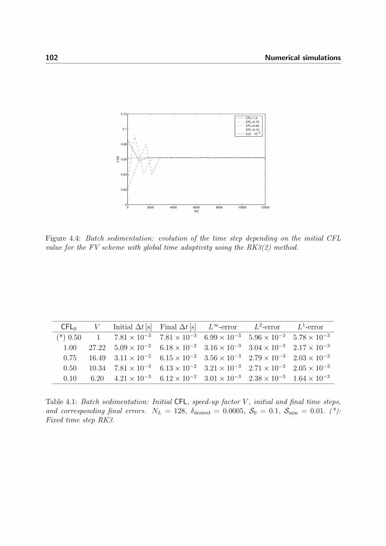
102 Numerical simulations

0 2000 4000 6000 8000 10000 120000

0.02

0.04

0.06

0.08

0.1

0.12

t[s]

∆ t[s

]CFL=1.0

CFL=0.75

CFL=0.50

CFL=0.10

6.21 10−2

Figure 4.4: Batch sedimentation: evolution of the time step depending on the initial CFLvalue for the FV scheme with global time adaptivity using the RK3(2) method.

CFL0 V Initial ∆t [s] Final ∆t [s] L∞-error L2-error L1-error

(*) 0.50 1 7.81 × 10−3 7.81 × 10−3 6.99 × 10−3 5.96 × 10−3 5.78 × 10−3

1.00 27.22 5.09 × 10−2 6.18 × 10−2 3.16 × 10−3 3.04 × 10−3 2.17 × 10−3

0.75 16.49 3.11 × 10−2 6.15 × 10−2 3.56 × 10−3 2.79 × 10−3 2.03 × 10−3

0.50 10.34 7.81 × 10−3 6.13 × 10−2 3.21 × 10−3 2.71 × 10−3 2.05 × 10−3

0.10 6.20 4.21 × 10−3 6.12 × 10−2 3.01 × 10−3 2.38 × 10−3 1.64 × 10−3

Table 4.1: Batch sedimentation: Initial CFL, speed-up factor V , initial and final time steps,and corresponding final errors. NL = 128, δdesired = 0.0005, S0 = 0.1, Smin = 0.01. (*):Fixed time step RK3.

4.1 Strongly degenerate parabolic equations 103

∆t = λhL. The prescribed tolerance εR is obtained from (3.17), where the constant C for thisexample corresponds to a factor C = 500 (see the Appendix for details) , so εR = 5.16×10−5

and the threshold strategy is εl = 2l−LεR. The constants in the corresponding form of (3.17)are b∞ = 9.0296 × 10−5 m/s and a∞ = 3.5981 × 10−5 m2/s.

We simulate the process until the phenomenon enters in a steady state (tfinal = 12000 s).Figures 4.5 (a), (c) and (e) show the solution before the front and back waves meet (t =2000 s), near the point when these waves meet (t = 9000 s), and after the solution hasreached a steady state (t = 12000 s), respectively. Figures 4.5 (b), (d) and (f) display thecorresponding positions of the leaves of the tree (where a “+” marks the center of each leaf).The plotted positions indicate that the adaptation of the mesh is adapted correctly, in thesense that the multiresolution method automatically detects steep gradient regions and addsfiner scales.

Method V µ L1-error L2-error L∞-error

t = 2000 s

FV 1 1 5.28×10−6 1.41×10−6 3.76×10−6

FV + RKF 14.32 1 1.79×10−5 8.91×10−6 1.66×10−5

MR 8.21 15.93 2.23×10−5 2.35×10−5 3.83×10−5

MR + RKF 27.42 15.92 1.28×10−4 4.57×10−5 6.36×10−5

t = 9000 s

FV 1 1 2.11×10−6 1.28×10−6 8.46×10−6

FV + RKF 14.38 1 3.45×10−5 8.95×10−6 3.29×10−5

MR 9.32 15.64 3.32×10−5 3.84×10−5 4.72×10−5

MR + RKF 31.20 15.65 2.49×10−4 4.08×10−5 7.65×10−5

t = 12000 s

FV 1 1 6.38×10−7 4.84×10−7 5.03×10−7

FV + RKF 14.49 1 5.61×10−6 1.27×10−6 4.31×10−6

MR 9.87 14.52 5.41×10−6 6.79×10−5 1.43×10−6

MR + RKF 33.05 14.52 8.74×10−5 1.82×10−5 4.29×10−5

Table 4.2: Batch sedimentation: corresponding simulated time t, speed-up factor V , datacompression rate µ, and normalized errors for different methods at different times. L = 11multiresolution levels.

From Table 4.2 we infer that the multiresolution computation is always cheaper in CPU timeand in memory requirements than the FV method on the finest grid. The CPU time usedwith adaptive time stepping is roughly a third of the CPU time required with a fixed timestep. The fixed time step for the MR calculation (with CFL = 1/2) is ∆tfixed = 8.24× 10−3 sand the adaptive time step for the MR (+RKF) calculation apparently converges to ∆t =

104 Numerical simulations

0 0.05 0.1 0.15 0.2 0.25 0.3 0.35

0

0.1

0.2

0.3

0.4

0.5

0.6

0.7

0.8

0.9

1

x[m

]

u(x)1 2 3 4 5 6 7 8 9 10 11

0

0.1

0.2

0.3

0.4

0.5

0.6

0.7

0.8

0.9

1

x[m

]

Multiresolution levels

0 0.05 0.1 0.15 0.2 0.25 0.3 0.35

0

0.1

0.2

0.3

0.4

0.5

0.6

0.7

0.8

0.9

1

x[m

]

u(x)1 2 3 4 5 6 7 8 9 10 11

0

0.1

0.2

0.3

0.4

0.5

0.6

0.7

0.8

0.9

1

x[m

]

Multiresolution levels

0 0.05 0.1 0.15 0.2 0.25 0.3 0.35

0

0.1

0.2

0.3

0.4

0.5

0.6

0.7

0.8

0.9

1

x[m

]

u(x)1 2 3 4 5 6 7 8 9 10 11

0

0.1

0.2

0.3

0.4

0.5

0.6

0.7

0.8

0.9

1

x[m

]

Multiresolution levels

Figure 4.5: Batch sedimentation: numerical solution (left) and positions of the leaves (right)at time instants t = 2000 s, t = 9000 s and t = 12000 s. The dashed vertical line is the initialdatum u0 = 0.08; the solid vertical line marks uc.

4.1 Strongly degenerate parabolic equations 105

2.34 × 10−2 s ≈ 3∆tfixed. It is worth pointing out that the time adaptivity is global in thesense that time stepping is dominated by the time step on the finest resolution level l = L.

7 8 9 10 11 12

1e−5

1e−4

1e−3

1e−2

L

|uM

R−u

FV|

L1−norm

L2−norm

L∞−norm

7 8 9 10 11 12

1e−5

1e−4

1e−3

1e−2

L|u

MR

/RK

F−u

FV|

L1−norm

L2−norm

L∞−norm

Figure 4.6: Batch sedimentation: errors uMR − uFV1, uMR − uFV2 and uMR − uFV∞(left) and errors uMR/RKF − uFV1, uMR/RKF − uFV2 and uMR/RKF − uFV∞ (right) fordifferent scales L. The simulated time is t = 2000 s.

The L1, L2, and L∞ norms of the error between the numerical solution obtained by multires-olution for different multiresolution levels L, and a finite volume approximation on a uniformfine grid, are depicted in Figure 4.6. In fact, we compute in practice the error between thenumerical solution obtained by multiresolution and the projection of the numerical solutionby FV approximation. Comparisons of speed-up factor and data compression for differentmaximal multiresolution levels L are displayed in Figure 4.7.

Table 4.3 summarizes the speed-up factor V , the compression rate µ and errors for the FVand multiresolution schemes using different maximal multiresolution levels. The simulatedtime is t = 2000 s. Figure 4.8 shows the corresponding L1-errors, compared with a referencesolution obtained by finite volume approximation on a uniform fine grid with 213 controlvolumes. Note that the slope for all methods is practically the same.

4.1.2 Traffic flow on a circular road

We consider the traffic model with driver’s reaction outlined in Section 1.1, and choose thevelocity function and model parameters according to [32, 126]. The velocity function is given

106 Numerical simulations

3 4 5 6 7 8 9 10 11 120

2

4

6

8

10

12

14

16

L

µ

MR

MR+RKF

3 4 5 6 7 8 9 10 11 12

10

20

30

40

50

60

70

80

90

L

V

MR

MR+RKF

Figure 4.7: Batch sedimentation: data compression rate µ (left) and speed-up factor V (right)for different scales L. Comparison between multiresolution with fixed and adaptive timestepping. The simulated time is t = 2000 s.

Method V µ L1-error L2-error L∞-error

L = 10

FV 1 1 1.35×10−5 8.70×10−4 9.35×10−4

MR 8.78 12.76 4.09×10−4 1.35×10−4 7.49×10−4

MR+RKF 32.15 12.76 6.35×10−4 2.74×10−4 8.88×10−4

L = 11

FV 1 1 4.37×10−6 5.68×10−7 1.47×10−5

MR 10.46 15.93 1.23×10−5 2.35×10−5 3.83×10−5

MR+RKF 39.19 15.95 5.34×10−5 4.39×10−5 6.01×10−5

L = 12

FV 1 1 1.29×10−9 6.37×10−9 8.65×10−10

MR 12.70 16.34 4.16×10−6 1.01×10−7 6.72×10−7

MR+RKF 43.21 16.35 5.47×10−6 6.44×10−7 1.38×10−6

Table 4.3: Batch sedimentation: Corresponding simulated time, speed-up factor V , datacompression rate µ, and errors for different methods at different maximal scales.

4.1 Strongly degenerate parabolic equations 107

6 7 8 9 10 111e−4

1e−3

5e−4

2e−4

L

L1−e

rror

Figure 4.8: Batch sedimentation: L1-errors for the MR method (dash-dotted), MR+RKFmethod (dotted) and FV method (dashed).

Figure 4.9: Traffic flow: time-space representation of the solution.

108 Numerical simulations

by (1.6) with umax = 220 cars/mi, C = e/7 = 0.38833 and vmax = 70 mph, so that

b(u) =

vmaxu for 0 ≤ u ≤ uc = 16.7512 cars/mi,

vmax(e/7)u ln(umax/u) for uc < u ≤ umax,

0 otherwise.

For the traffic flow example, we choose the parameters a = 0.1 g, where g is the accelerationof gravity in mi/h2, τ = 2 s = 0.0005 h and Lmin = 0.05 mi. This yields the followingintegrated diffusion coefficient A(u), measured in cars·mph, see [32] for details on its algebraicderivation:

A(u) =

0 for u ≤ uc,

1.27099 · (41.878u − 12.787u ln u + u(ln u)2)

−0.4105u − 286.54 for uc < u ≤ u∗,

117.9003 + 0.94864u for u > u∗,

where u∗ := 78.2198 cars/mi. The model functions b(u) and A(u) are depicted in Figure 4.10.

We assume a circular road of length H = 10 mi, so that the periodic boundary condition

u(H, t) = u(0, t), t ∈ (0, T ] (4.2)

applies. We assume the smooth initial density distribution u0(x) = 50(1 + sin(0.4πx))cars/mi. In addition, at x = 5 mi, a traffic light S is placed with

S(t) =

0 (red) for t ∈ [(k + 0.125) h, (k + 0.375) h], k = 0, 1, 2, . . . ,

1 (green) otherwise.(4.3)

Note that this example involves periodicity both in space (due to the periodic boundarycondition (4.2)), in time (due to the behavior of the traffic light), and is provided withperiodic initial condition.

Before discussing the performance of the fully adaptive multiresolution scheme, we presentin Figure 4.9 three-dimensional plots of the numerical solution obtained for by this scheme.It illustrates that a nearly periodic solution quickly evolves. Moreover, the depletion of thezone behind the traffic light and the queue of cars waiting in front of it periodically producestraveling type-change interfaces, i.e. jumps between the solution value zero and sub-criticalvalues. In Figure 4.9, the visual grid used to represent the numerical solution is again muchcoarser than the computational one.

Finest grid computations.- In Figure 4.11 we show the time evolution of the time step de-pending on the initial value of CFL, using the FV scheme on a uniform fine mesh with global

4.1 Strongly degenerate parabolic equations 109

0 20 40 60 80 100 120 140 160 180 200 220

200

400

600

800

1000

1200

1400

1600

1800

2000

2200

u[cars/mi]

f(u

)

0 20 40 60 80 100 120 140 160 180 200 220

0

50

100

150

200

250

300

350

u[cars/mi]

A(u

)

Figure 4.10: Traffic flow: model functions b(u) (left) and A(u) (right).

adaptivity and the RK3(2) method described in Section A.2. In all cases, the time step ap-parently converges to the value 1.217 × 10−4 s. Here, the adaptivity of the step size reducesthe computational cost, see Table 4.4.

0 0.05 0.1 0.15 0.2 0.25 0.3 0.35 0.4

0.6

0.8

1

1.2

1.4

1.6

x 10−4

t[s]

∆ t [s]

CFL=1.0

CFL=0.75

CFL=0.50

CFL=0.10

1.21710−4

0 0.01 0.02 0.03 0.04 0.05 0.06 0.070

1

2

x 10−4

t[s]

∆ t[s

]

CFL=1.0

CFL=0.10

CFL=0.50

CFL=0.75

1.217 10−4

Figure 4.11: Traffic flow: evolution of the time step depending on the initial value of CFL forthe FV scheme with global time adaptivity using the RK3(2) method (left), and zoom untilt = 0.07 h (right). NL = 256, δdesired = 0.001 and S0 = 0.01.

Multiresolution examples.- We take an initial dynamic graded tree, allowing L = 10 mul-tiresolution levels. First we use a multiresolution procedure with fixed time step, takingCFL = 1/2, and we simulate the process until tfinal = 1.6 h. Figure 4.12 shows the solutionbefore the traffic light is red and during the red phase. Figure 4.13 shows the solution rightafter the green phase and part of the second cycle of the traffic light. For this example, thefactor C in (3.17) is set to C = 1 × 106 (see details in the Appendix), yielding a reference

110 Numerical simulations

CFL0 V Initial ∆t [h] Final ∆t [h] L∞-error L2-error L1-error

(*) 0.50 1 4.10 × 10−5 4.10 × 10−5 5.62 × 10−4 1.47 × 10−4 8.32 × 10−4

1.00 16.32 8.22 × 10−5 1.29 × 10−4 8.53 × 10−3 5.41 × 10−3 5.06 × 10−3

0.75 11.34 6.16 × 10−5 1.17 × 10−4 1.38 × 10−3 2.77 × 10−3 3.46 × 10−3

0.10 8.75 8.62 × 10−5 1.22 × 10−4 7.51 × 10−4 2.01 × 10−3 8.86 × 10−4

Table 4.4: Traffic model: initial CFL, speed-up factor V , initial and final time steps, andcorresponding normalized errors. NL = 256, δdesired = 0.001, S0 = 0.1, Smin = 0.01. (*):Fixed time step RK3.

tolerance of εR = 1.33× 10−5 for L = 10. Here, the Lipschitz constants in the correspondingform of (3.17) are b∞ = 70 mi/h and a∞ = 7.9177 mi2/h. Errors in different norms andcompression rates V and µ for different methods are displayed in Table 4.5.

The errors in L1, L2, and L∞ norms between the numerical solution obtained by multires-olution for different multiresolution levels L, and the solution obtained by finite volumeapproximation in a uniform fine grid, are depicted in Figure 4.14. In fact, we compute inpractice the error between the numerical solution obtained by multiresolution and the projec-tion of the numerical solution by FV approximation. Furthermore, comparisons of speed-upfactor and data compression for different maximal multiresolution levels L, are depicted inFigure 4.15. All these calculations corresponds to the “red” phase, t = 0.2 h.

Table 4.6 summarizes the CPU time, compression rate and errors for the FV method and themultiresolution scheme, using different maximal multiresolution levels. The simulated timeis t = 0.4 h. Here we can see that the multiresolution computation is always cheaper in CPUtime and in memory requirements than the finite volume method on the finest grid, and wecan also notice that the gain in speed-up factor using an adaptive time stepping is aboutfour times the speed-up factor attained by fixed time stepping, this comes clear if we alsonote that the fixed time step for the MR calculation, with CFL = 1/2 is ∆t = 2.217× 10−5 hand the adaptive time step for the MR (+RKF) calculation tends to converge to the value∆t = 9.86 × 10−5 h, which is roughly four times the above value. Figure 4.16 shows thecorresponding L1-errors, compared with a reference solution obtained on a uniform fine gridwith 213 control volumes.

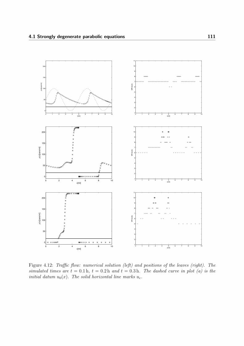
4.1 Strongly degenerate parabolic equations 111

0 1 2 3 4 5 6 7 8 9 10

0

50

100

150

200

x[mi]

ρ(x

)[ca

rs/m

i]

0 1 2 3 4 5 6 7 8 9 101

2

3

4

5

6

7

8

9

10

11

x[mi]

MR

le

ve

ls

0 2 4 6 8 10

0

50

100

150

200

x[mi]

ρ(x

)[cars

/mi]

0 1 2 3 4 5 6 7 8 9 101

2

3

4

5

6

7

8

9

10

11

x[mi]

MR

le

ve

ls

0 2 4 6 8 10

0

50

100

150

200

x[mi]

ρ(x

)[cars

/mi]

0 1 2 3 4 5 6 7 8 9 101

2

3

4

5

6

7

8

9

10

11

x[mi]

MR

le

ve

ls

Figure 4.12: Traffic flow: numerical solution (left) and positions of the leaves (right). Thesimulated times are t = 0.1 h, t = 0.2 h and t = 0.3 h. The dashed curve in plot (a) is theinitial datum u0(x). The solid horizontal line marks uc.

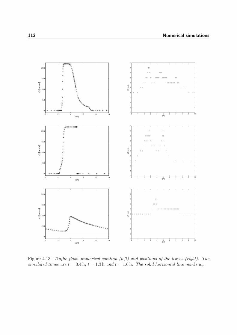
112 Numerical simulations

0 2 4 6 8 10

0

50

100

150

200

x[mi]

ρ(x

)[cars

/mi]

0 1 2 3 4 5 6 7 8 9 101

2

3

4

5

6

7

8

9

10

11

x[mi]

MR

levels

0 2 4 6 8 10

0

50

100

150

200

x[mi]

ρ(x

)[cars

/mi]

0 1 2 3 4 5 6 7 8 9 101

2

3

4

5

6

7

8

9

10

11

x[mi]

MR

levels

0 2 4 6 8 10

0

50

100

150

200

x[mi]

ρ(x

)[cars

/mi]

0 1 2 3 4 5 6 7 8 9 101

2

3

4

5

6

7

8

9

10

11

x[mi]

MR

levels

Figure 4.13: Traffic flow: numerical solution (left) and positions of the leaves (right). Thesimulated times are t = 0.4 h, t = 1.3 h and t = 1.6 h. The solid horizontal line marks uc.

4.1 Strongly degenerate parabolic equations 113

Method V µ L1-error L2-error L∞-error

t = 0.1h

MR 5.12 7.93 2.31×10−4 4.79×10−4 5.83×10−5

MR+RKF 12.47 7.93 6.18×10−4 1.07×10−3 6.66×10−5

t = 0.2 h

MR 5.21 5.99 1.76×10−4 7.68×10−5 8.39×10−6

MR+RKF 16.34 5.99 3.67×10−4 2.73×10−4 3.00×10−5

t = 0.3 h

MR 5.23 7.58 2.24×10−4 7.89×10−5 9.46×10−6

MR+RKF 17.34 7.58 7.47×10−4 9.21×10−5 3.67×10−5

t = 0.4 h

MR 7.42 5.54 1.83×10−4 3.32×10−5 4.36×10−6

MR+RKF 19.18 5.54 4.62×10−4 5.29×10−5 1.08×10−3

t = 1.3 h

MR 7.78 7.36 1.55×10−3 5.64×10−5 2.61×10−5

MR+RKF 21.62 7.37 2.31×10−3 8.06×10−5 3.17×10−5

t = 1.6 h

MR 7.59 9.75 6.17×10−3 1.01×10−4 2.94×10−4

MR+RKF 19.63 9.75 8.40×10−3 5.16×10−4 4.55×10−4

Table 4.5: Traffic flow: corresponding simulated time, speed-up factor V , data compressionrate µ, and errors for different methods. L = 10 multiresolution levels.

6 7 8 9 10 11

1e−4

1e−3

1e−2

1e−1

1e−4

1e−3

1e−2

L

|uM

R−u

FV|

L1−norm

L2−norm

L∞−norm

6 7 8 9 10 11

1e−4

1e−3

1e−2

1e−1

1e−4

1e−3

1e−2

L

|uM

R−u

FV|

L1−norm

L2−norm

L∞−norm

Figure 4.14: Traffic flow: errors uMR − uFV1, uMR − uFV2 and uMR − uFV∞ (left) anderrors uMR/RKF − uFV1, uMR/RKF − uFV2 and uMR/RKF − uFV∞ (right) for differentscales L. The simulated time is t = 0.2 h.

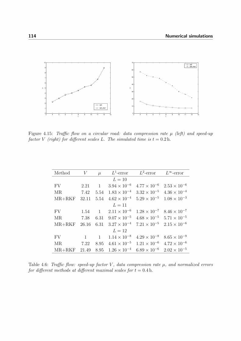
114 Numerical simulations

3 4 5 6 7 8 9 10 11 12 130

1

2

3

4

5

6

7

8

9

10

L

µ

MR

MR+RKF

3 4 5 6 7 8 9 10 11 12 130

10

20

30

40

50

60

70

L

V

MR

MR+RKF

Figure 4.15: Traffic flow on a circular road: data compression rate µ (left) and speed-upfactor V (right) for different scales L. The simulated time is t = 0.2 h.

Method V µ L1-error L2-error L∞-error

L = 10

FV 2.21 1 3.94 × 10−6 4.77 × 10−6 2.53 × 10−6

MR 7.42 5.54 1.83 × 10−4 3.32 × 10−5 4.36 × 10−4

MR+RKF 32.11 5.54 4.62 × 10−4 5.29 × 10−5 1.08 × 10−3

L = 11

FV 1.54 1 2.11 × 10−6 1.28 × 10−7 8.46 × 10−7

MR 7.38 6.31 9.07 × 10−5 4.68 × 10−5 5.71 × 10−5

MR+RKF 26.16 6.31 3.27 × 10−4 7.21 × 10−5 2.15 × 10−6

L = 12

FV 1 1 1.14 × 10−8 4.29 × 10−8 8.65 × 10−9

MR 7.22 8.95 4.61 × 10−5 1.21 × 10−6 4.72 × 10−6

MR+RKF 21.49 8.95 1.26 × 10−4 6.89 × 10−6 2.02 × 10−5

Table 4.6: Traffic flow: speed-up factor V , data compression rate µ, and normalized errorsfor different methods at different maximal scales for t = 0.4 h.

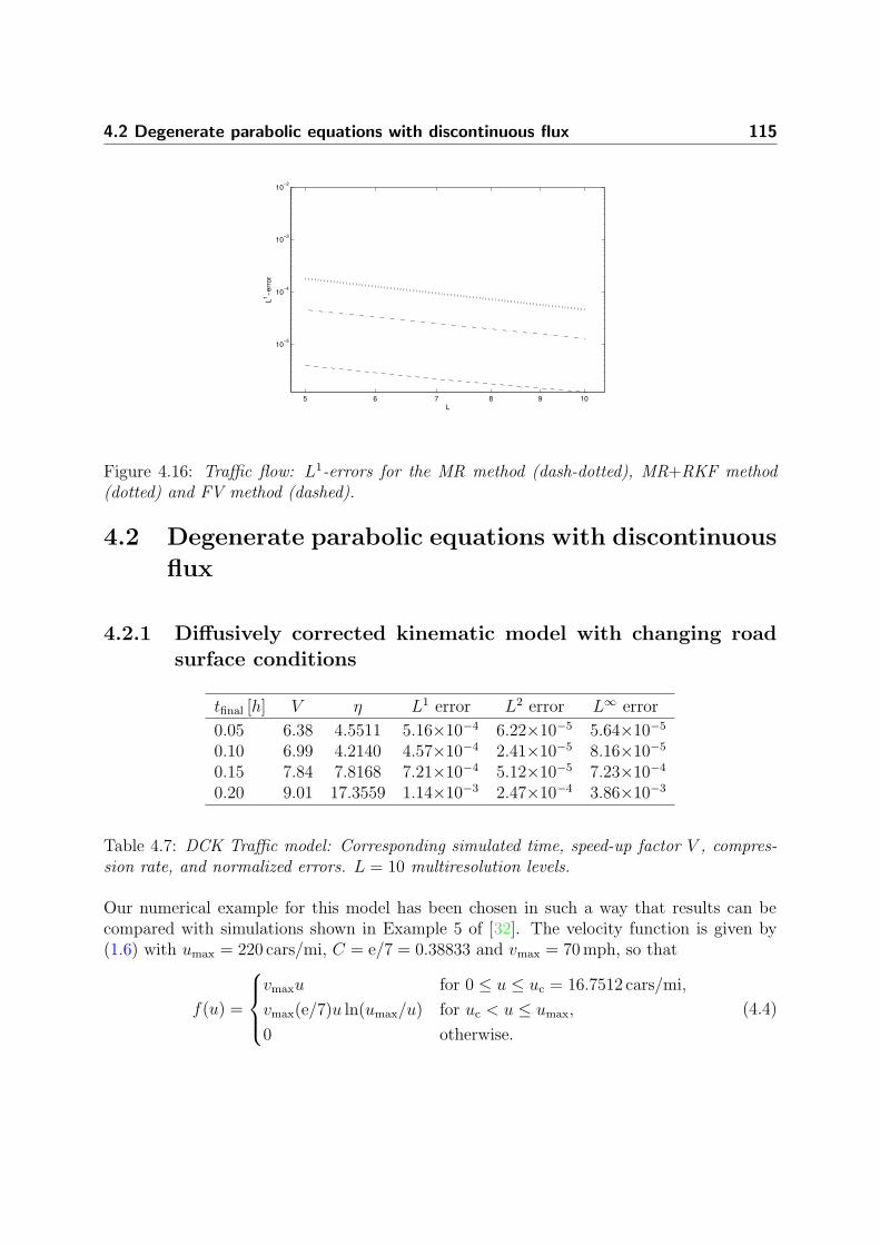
4.2 Degenerate parabolic equations with discontinuous flux 115

5 6 7 8 9 10

10−5

10−4

10−3

10−2

L

L1−e

rror

Figure 4.16: Traffic flow: L1-errors for the MR method (dash-dotted), MR+RKF method(dotted) and FV method (dashed).

4.2 Degenerate parabolic equations with discontinuous

flux

4.2.1 Diffusively corrected kinematic model with changing roadsurface conditions

tfinal [h] V η L1 error L2 error L∞ error

0.05 6.38 4.5511 5.16×10−4 6.22×10−5 5.64×10−5

0.10 6.99 4.2140 4.57×10−4 2.41×10−5 8.16×10−5

0.15 7.84 7.8168 7.21×10−4 5.12×10−5 7.23×10−4

0.20 9.01 17.3559 1.14×10−3 2.47×10−4 3.86×10−3

Table 4.7: DCK Traffic model: Corresponding simulated time, speed-up factor V , compres-sion rate, and normalized errors. L = 10 multiresolution levels.

Our numerical example for this model has been chosen in such a way that results can becompared with simulations shown in Example 5 of [32]. The velocity function is given by(1.6) with umax = 220 cars/mi, C = e/7 = 0.38833 and vmax = 70 mph, so that

f(u) =

vmaxu for 0 ≤ u ≤ uc = 16.7512 cars/mi,

vmax(e/7)u ln(umax/u) for uc < u ≤ umax,

0 otherwise.

(4.4)

116 Numerical simulations

−2

−1

0

1

2

3

0

0.05

0.1

0.15

0.2

0.25

0

50

100

150

Figure 4.17: DCK Traffic model: three-dimensional plot of the numerical solution.

4.2 Degenerate parabolic equations with discontinuous flux 117

−2 −1.5 −1 −0.5 0 0.5 1 1.5 2 2.5 3

0

20

40

60

80

100

120

140

160

180

x

ρ(x

,t)

−2 −1.5 −1 −0.5 0 0.5 1 1.5 2 2.5 31

2

3

4

5

6

7

8

9

10

11

x

Multiresolu

tion levels

−2 −1.5 −1 −0.5 0 0.5 1 1.5 2 2.5 3

0

20

40

60

80

100

120

140

160

180

x

ρ(x

,t)

−2 −1.5 −1 −0.5 0 0.5 1 1.5 2 2.5 31

2

3

4

5

6

7

8

9

10

11

x

Multiresolu

tion levels

Figure 4.18: DCK Traffic model: numerical solution (left) and positions of the leaves (right)at t = 0.05 h and t = 0.1 h.

118 Numerical simulations

−2 −1.5 −1 −0.5 0 0.5 1 1.5 2 2.5 3

0

20

40

60

80

100

120

140

160

180

x

ρ(x

,t)

−2 −1.5 −1 −0.5 0 0.5 1 1.5 2 2.5 31

2

3

4

5

6

7

8

9

10

11

x

Multiresolu

tion levels

−2 −1.5 −1 −0.5 0 0.5 1 1.5 2 2.5 3

0

20

40

60

80

100

120

140

160

180

x

ρ(x

,t)

−2 −1.5 −1 −0.5 0 0.5 1 1.5 2 2.5 31

2

3

4

5

6

7

8

9

10

11

x

Multiresolu

tion levels

Figure 4.19: DCK Traffic model: numerical solution (left) and positions of the leaves (right)at t = 0.15 h and t = 0.2 h.

4.2 Degenerate parabolic equations with discontinuous flux 119

101

102

103

104

10−10

10−5

100

105

NL

L1 −

err

ors

MR

FV

slope=1.00

Figure 4.20: DCK Traffic model: L1 errors.

We choose v0max = 70 mph and v∗

max = 25 mph. The initial density is chosen as

ρ0(x) =

100 cars/mi for −2 mi ≤ x ≤ −1 mi,

0 otherwise.

The integrated diffusion coefficient A(u) resulting from our choice of parameters satisfiesA(u) = 0 for 0 ≤ u ≤ uc = 16.7512 cars/mi, and has an explicit algebraic representation[32, 38].

In a first example, we consider an initial convoy of cars traveling on an empty road, andwish to see how the convoy passes through the reduced speed road segment. The numericalsolution obtained by our method is represented in a three-dimensional plot in Figure 4.17and shown at four different times in Figures 4.18 and 4.19. These figures also display the cor-responding position of the leaves. For these four times, Table 4.7 displays the correspondingvalues of the speed-up factor V , the compression rate η, and normalized approximate errors.These errors and the speed-up factor are measured with respect to a fine grid calculation(no multiresolution) with NL = 213 cells. (We further comment on the behavior of V and η

in the discussion of the third example.)

For this example, we take an initial dynamic graded tree, allowing L = 10 multiresolutionlevels. We use a fixed time step determined by λ = 0.0003 h/mi, thus ∆t = λhL. Theprescribed tolerance εR is obtained from (3.17), where the constant C for this examplecorresponds to a factor C = 105, so ε = 0.301 and the thresholding strategy is εk = 2k−Lε.

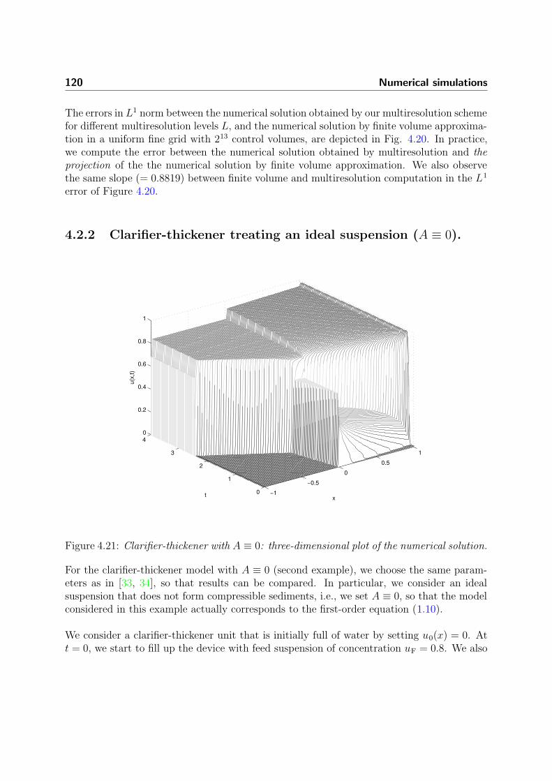
120 Numerical simulations

The errors in L1 norm between the numerical solution obtained by our multiresolution schemefor different multiresolution levels L, and the numerical solution by finite volume approxima-tion in a uniform fine grid with 213 control volumes, are depicted in Fig. 4.20. In practice,we compute the error between the numerical solution obtained by multiresolution and theprojection of the the numerical solution by finite volume approximation. We also observethe same slope (= 0.8819) between finite volume and multiresolution computation in the L1

error of Figure 4.20.

4.2.2 Clarifier-thickener treating an ideal suspension (A ≡ 0).

−1

−0.5

0

0.5

1

0

1

2

3

40

0.2

0.4

0.6

0.8

1

xt

u(x

,t)

Figure 4.21: Clarifier-thickener with A ≡ 0: three-dimensional plot of the numerical solution.

For the clarifier-thickener model with A ≡ 0 (second example), we choose the same param-eters as in [33, 34], so that results can be compared. In particular, we consider an idealsuspension that does not form compressible sediments, i.e., we set A ≡ 0, so that the modelconsidered in this example actually corresponds to the first-order equation (1.10).

We consider a clarifier-thickener unit that is initially full of water by setting u0(x) = 0. Att = 0, we start to fill up the device with feed suspension of concentration uF = 0.8. We also

124 Numerical simulations

−1

−0.5

0

0.5

1

0

1

2

3

4

5

x 104

0

0.05

0.1

0.15

0.2

0.25

0.3

0.35

0.4

x[m]t[s]

u(x

,t)

−1

−0.5

0

0.5

1

0

1

2

3

4

5

x 104

0

0.05

0.1

0.15

0.2

0.25

0.3

0.35

0.4

x[m]t[s]

u(x

,t)

Figure 4.25: Clarifier-thickener with flocculated suspension: two views of the time-spacerepresentation of the numerical solution.

tfinal [s] V η L1 error L2 error L∞ error

10000 7.88 4.1787 3.67×10−4 8.41×10−5 6.73×10−4

25000 9.01 4.4265 4.82×10−4 9.32×10−5 8.29×10−4

50000 10.74 4.4734 6.30×10−4 1.24×10−4 1.07×10−3

Table 4.9: Clarifier-thickener with flocculated suspension: Corresponding simulated time,speed-up factor V , compression rate, and normalized errors. L = 9 multiresolution levels.

4.2 Degenerate parabolic equations with discontinuous flux 125

−1 −0.8 −0.6 −0.4 −0.2 0 0.2 0.4 0.6 0.8 1

0

0.05

0.1

0.15

0.2

0.25

0.3

0.35

0.4

x[m]

u(x

)

−1 −0.8 −0.6 −0.4 −0.2 0 0.2 0.4 0.6 0.8 11

2

3

4

5

6

7

8

9

10

x

Multiresolu

tion levels

−1 −0.8 −0.6 −0.4 −0.2 0 0.2 0.4 0.6 0.8 1

0

0.05

0.1

0.15

0.2

0.25

0.3

0.35

0.4

x[m]

u(x

)

−1 −0.8 −0.6 −0.4 −0.2 0 0.2 0.4 0.6 0.8 11

2

3

4

5

6

7

8

9

10

x

Multiresolu

tion levels

Figure 4.26: Clarifier-thickener with flocculated suspension: numerical solution (stars) andinitial condition (dashed) (left) and positions of the leaves (right) at t = 10000 s, t = 25000 sfor the transition to a steady state from u0 = 0.09. The horizontal solid line in the leftdenotes the critical concentration uc = 0.1.

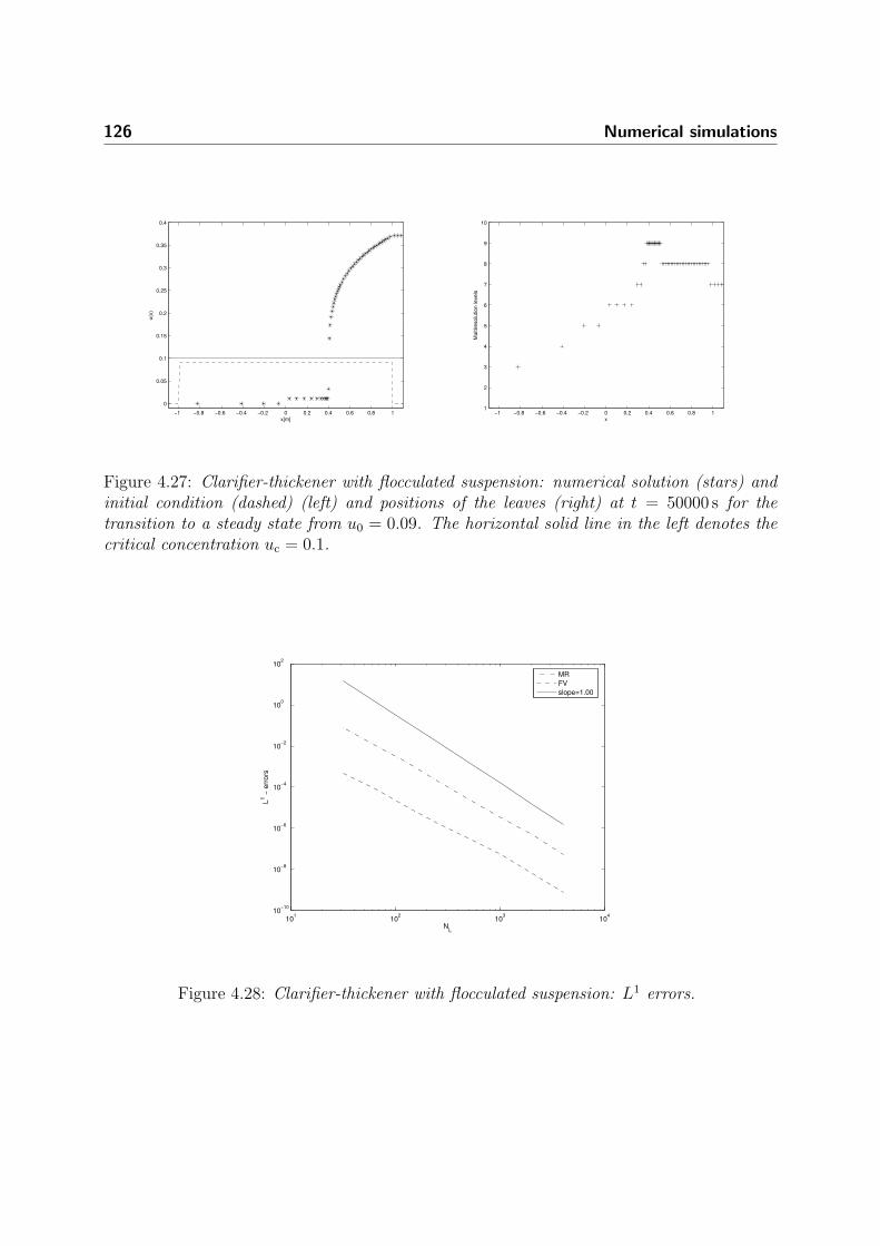
126 Numerical simulations

−1 −0.8 −0.6 −0.4 −0.2 0 0.2 0.4 0.6 0.8 1

0

0.05

0.1

0.15

0.2

0.25

0.3

0.35

0.4

x[m]

u(x

)

−1 −0.8 −0.6 −0.4 −0.2 0 0.2 0.4 0.6 0.8 11

2

3

4

5

6

7

8

9

10

x

Multiresolu

tion levels

Figure 4.27: Clarifier-thickener with flocculated suspension: numerical solution (stars) andinitial condition (dashed) (left) and positions of the leaves (right) at t = 50000 s for thetransition to a steady state from u0 = 0.09. The horizontal solid line in the left denotes thecritical concentration uc = 0.1.

101

102

103

104

10−10

10−8

10−6

10−4

10−2

100

102

NL

L1 −

err

ors

MR

FV

slope=1.00

Figure 4.28: Clarifier-thickener with flocculated suspension: L1 errors.

4.2 Degenerate parabolic equations with discontinuous flux 127

with λ = 40 s/m.

Our simulation corresponds to the choice qR = 2.5×10−6 m/s and qL = −1.0×10−5 m/s. Thefeed concentration corresponds to uF = 0.086. Figure 4.25 shows the numerical solution untilt = 50000 s. In this case we consider the device with an initial concentration distribution ofu0(x) = uc, x ∈ [xL, xR] and we can observe the initial stage of the fill-up process. For thisexample, we take an initial dynamic graded tree, allowing L = 8 multiresolution levels, andfor the reference tolerance we use C = 10−3, so εR = 2.24 × 10−4.

For the clarifier-thickener model with flocculated suspension we use as a reference solutiona fine grid computation with 213 control volumes. Table 4.9 again displays the behavior ofthe error and the gain in computational effort and data storage for different times. Also,analogously to the previous examples, we observe in Figure 4.28 the same slope between theL1 errors for the finite volume and multiresolution methods. This error is measured here att = 25000 s.

Note that in all numerical examples, the speed-up factor V increases as tfinal is increased, evenif the data compression rate η remains constant, which approximately is the case in Table 4.9,or even decreases, as we see, for example, by comparing the values of η for tfinal = 0.05 hand tfinal = 0.10 h in Table 4.7. The explanation of this discrepancy is that while η measuresthe quality of performance of the multiresolution seen at the instant t = tfinal, the speed-upfactor V is referred to the total time of simulation and also includes the “overhead” requiredby initializing the graded tree in step (2) of the multiresolution algorithm. The initializationrequires a fixed amount of CPU time, which is independent of the number of total timesteps (which is proportional to tfinal, since we consider ∆t to be fixed). On the other hand,a standard FV method on a fixed grid will always require CPU time proportional to thenumber of time steps. This explains why even if η does not change significantly, we observean improvement of the speed-up factor V as tfinal is increased.

4.2.4 An extended clarifier-thickener model

Let us consider a suspension characterized by b(u) as in (1.4) with v∞ = 1.0 × 10−4 m/s,C = 5 and umax = 1. Furthermore xL = −2 m and xR = 1 m, the device being initiallyempty (u0 ≡ 0). These parameters and the control variables qL = 0.0 m/s, qR = 0.6 m/s,qD = −1.0 m/s and uF = 0.7 are chosen as in Case 5 of [30] and [42]. The reference toleranceused for this example is ε = 4.6 × 10−4.

Figure 4.2.4 shows the numerical solution until t = 4. In this case the solid material enteringto the clarifying zone is fully absorbed by the singular sink term.

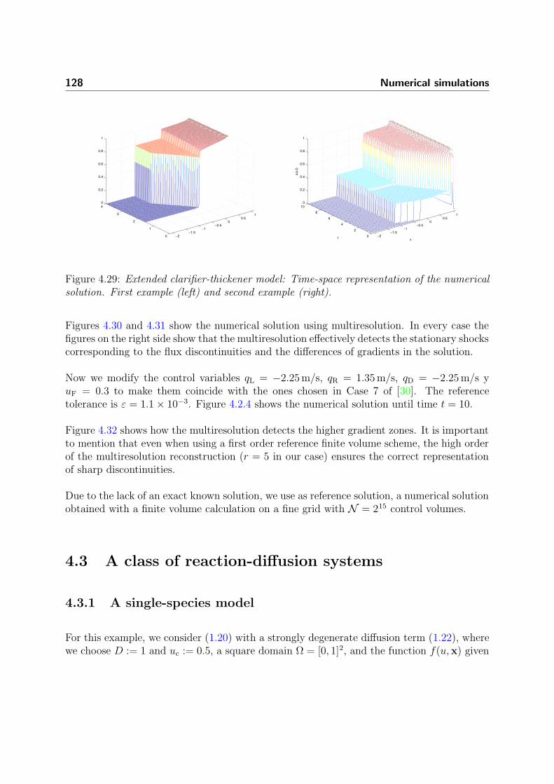
128 Numerical simulations

−2−1.5

−1−0.5

00.5

1

0

1

2

3

40

0.2

0.4

0.6

0.8

1

−2−1.5

−1−0.5

00.5

1

0

2

4

6

8

100

0.2

0.4

0.6

0.8

1

xt

u(x

,t)

Figure 4.29: Extended clarifier-thickener model: Time-space representation of the numericalsolution. First example (left) and second example (right).

Figures 4.30 and 4.31 show the numerical solution using multiresolution. In every case thefigures on the right side show that the multiresolution effectively detects the stationary shockscorresponding to the flux discontinuities and the differences of gradients in the solution.

Now we modify the control variables qL = −2.25 m/s, qR = 1.35 m/s, qD = −2.25 m/s yuF = 0.3 to make them coincide with the ones chosen in Case 7 of [30]. The referencetolerance is ε = 1.1 × 10−3. Figure 4.2.4 shows the numerical solution until time t = 10.

Figure 4.32 shows how the multiresolution detects the higher gradient zones. It is importantto mention that even when using a first order reference finite volume scheme, the high orderof the multiresolution reconstruction (r = 5 in our case) ensures the correct representationof sharp discontinuities.

Due to the lack of an exact known solution, we use as reference solution, a numerical solutionobtained with a finite volume calculation on a fine grid with N = 215 control volumes.

4.3 A class of reaction-diffusion systems

4.3.1 A single-species model

For this example, we consider (1.20) with a strongly degenerate diffusion term (1.22), wherewe choose D := 1 and uc := 0.5, a square domain Ω = [0, 1]2, and the function f(u,x) given

4.3 A class of reaction-diffusion systems 129

−2 −1.5 −1 −0.5 0 0.5 1

0

0.2

0.4

0.6

0.8

1

x

u(x

)

−2 −1.5 −1 −0.5 0 0.5 1

2

4

6

8

10

12

x

Multiresolu

tion levels

−2 −1.5 −1 −0.5 0 0.5 1

0

0.2

0.4

0.6

0.8

1

x

u(x

)

−2 −1.5 −1 −0.5 0 0.5 1

2

4

6

8

10

12

x

Multiresolu

tion levels

Figure 4.30: First Example for the extended clarifier-thickener model: Numerical solution(left) and position of the leaves (right) for the clarifier–thickener model, at t = 1 s and t = 2 s.

130 Numerical simulations

−2 −1.5 −1 −0.5 0 0.5 1

0

0.2

0.4

0.6

0.8

1

x

u(x

)

−2 −1.5 −1 −0.5 0 0.5 1

2

4

6

8

10

12

x

Multiresolu

tion levels

−2 −1.5 −1 −0.5 0 0.5 1

0

0.2

0.4

0.6

0.8

1

x

u(x

)

−2 −1.5 −1 −0.5 0 0.5 1

2

4

6

8

10

12

x

Multiresolu

tion levels

Figure 4.31: First Example for the extended clarifier-thickener model: Numerical solution(left) and position of the leaves (right) for the clarifier–thickener model, at t = 3 s and t = 4 s.

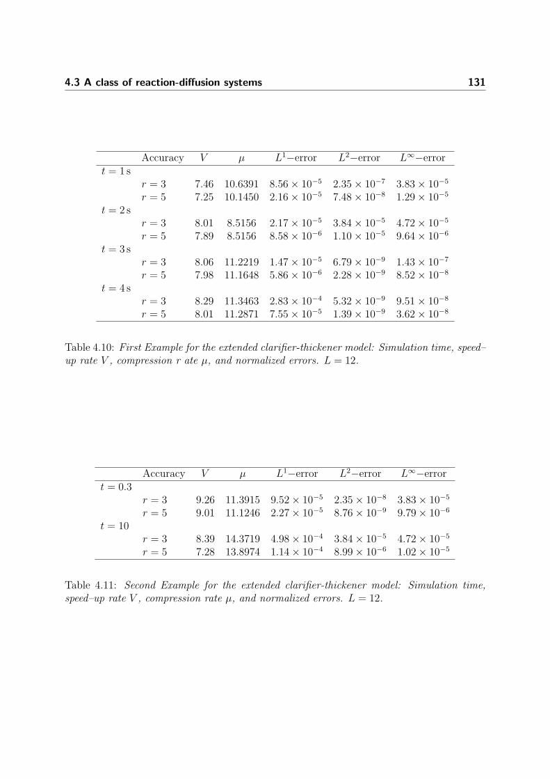
4.3 A class of reaction-diffusion systems 131

Accuracy V µ L1−error L2−error L∞−errort = 1 s

r = 3 7.46 10.6391 8.56 × 10−5 2.35 × 10−7 3.83 × 10−5

r = 5 7.25 10.1450 2.16 × 10−5 7.48 × 10−8 1.29 × 10−5

t = 2 sr = 3 8.01 8.5156 2.17 × 10−5 3.84 × 10−5 4.72 × 10−5

r = 5 7.89 8.5156 8.58 × 10−6 1.10 × 10−5 9.64 × 10−6

t = 3 sr = 3 8.06 11.2219 1.47 × 10−5 6.79 × 10−9 1.43 × 10−7

r = 5 7.98 11.1648 5.86 × 10−6 2.28 × 10−9 8.52 × 10−8

t = 4 sr = 3 8.29 11.3463 2.83 × 10−4 5.32 × 10−9 9.51 × 10−8

r = 5 8.01 11.2871 7.55 × 10−5 1.39 × 10−9 3.62 × 10−8

Table 4.10: First Example for the extended clarifier-thickener model: Simulation time, speed–up rate V , compression r ate µ, and normalized errors. L = 12.

Accuracy V µ L1−error L2−error L∞−errort = 0.3

r = 3 9.26 11.3915 9.52 × 10−5 2.35 × 10−8 3.83 × 10−5

r = 5 9.01 11.1246 2.27 × 10−5 8.76 × 10−9 9.79 × 10−6

t = 10r = 3 8.39 14.3719 4.98 × 10−4 3.84 × 10−5 4.72 × 10−5

r = 5 7.28 13.8974 1.14 × 10−4 8.99 × 10−6 1.02 × 10−5

Table 4.11: Second Example for the extended clarifier-thickener model: Simulation time,speed–up rate V , compression rate µ, and normalized errors. L = 12.

132 Numerical simulations

−2 −1.5 −1 −0.5 0 0.5 1

0

0.2

0.4

0.6

0.8

1

x

u(x

)

−2 −1.5 −1 −0.5 0 0.5 1

2

4

6

8

10

12

x

Multiresolu

tion levels

−2 −1.5 −1 −0.5 0 0.5 1

0

0.2

0.4

0.6

0.8

1

x

u(x

)

−2 −1.5 −1 −0.5 0 0.5 1

2

4

6

8

10

12

x

Multiresolu

tion levels

Figure 4.32: Second Example for the extended clarifier-thickener model: Numerical solution(left) and position of the leaves (right) for the clarifier–thickener model, at t = 0.3 s andt = 10 s.

4.3 A class of reaction-diffusion systems 133

0 0.2 0.4 0.6 0.8 10

0.1

0.2

0.3

0.4

0.5

0.6

0.7

0.8

0.9

1Position of the leaves

x

y

0 0.2 0.4 0.6 0.8 10

0.1

0.2

0.3

0.4

0.5

0.6

0.7

0.8

0.9

1Position of the leaves

x

y

0 0.2 0.4 0.6 0.8 10

0.1

0.2

0.3

0.4

0.5

0.6

0.7

0.8

0.9

1Position of the leaves

x

y

Figure 4.33: Single-species model: Numerical solution (left) and leaves (right) of the corre-sponding tree data structure at times t = 0 (top), t = 0.5 (middle) and t = 3 (bottom).

134 Numerical simulations

by (1.21). Figure 4.33 displays the numerical solution starting from the smoothly varyinginitial function

u0(x, y) = 0.51 + sin(1.1(x − cos(0.7y))

cos

0.5(y − sin(1.3x))

.

We choose a maximal resolution level of NL = 2562 = 65536 control volumes on the finestgrid. Figure 4.34 illustrates how the factor C in (3.19) is selected in our case as the optimalvalue from a finite selection of test values (each value giving a different value for the referencetolerance εR, see (3.19)).

4 6 8 10 120

2

4

6

8

10

12

L

η

C=1x107

C=1x108

C=1x109

C=1x1010

C=1x1011

4 6 8 10 12

10

20

30

40

50

60

70

80

L

V

C=1x107

C=1x108

C=1x109

C=1x1010

C=1x1011

6 7 8 9 10 11 12

10−6

10−5

L

L1−e

rror

C=1x107

C=1x108

C=1x109

C=1x1010

C=1x1011

FV

Figure 4.34: Single-species model: data compression rate η (left), speed-up factor V (middle)and L1-errors for different levels L and values of C (right). The simulated time is t = 0.

Figures 4.34 (a) and (b) indicate that for all displayed levels, the multiresolution procedure isin every case (for different values of C) cheaper (in terms of both CPU time acceleration andmemory savings) than the corresponding reference FV computation on the finest grid. Thegraph of Figure 4.34 (b) can be interpreted as follows: the better the resolution becomes, thebigger is the gain in CPU time. This happens independently of how far the grid is from beinguniform, since the behavior is similar for different values of C. Figure 4.34 (c) indicates thatthe computations obtained using C = 1.0×109 (and hence εR = 9.43×10−4) are sufficientlyaccurate, in the sense that with these choices, we keep the same slope for the L1-error as theFV calculations while increasing V and η. We remark that here, as in previous works thatuse similar methods (see e.g. [53]), there actually exists a range of threshold parameters thatpreserve the same slope for errors with respect to reference solution, for which C = 1.0×109

is an average value. Here, we compute errors using a reference FV solution on a fine gridwith NL = 20482 = 4194304 control volumes. (Here and in all other examples, we calculateerrors in the approximate sense with respect to a reference solution.)

4.3 A class of reaction-diffusion systems 135

0 0.2 0.4 0.6 0.8 10

0.1

0.2

0.3

0.4

0.5

0.6

0.7

0.8

0.9

1Position of the leaves

x

y

0 0.2 0.4 0.6 0.8 10

0.1

0.2

0.3

0.4

0.5

0.6

0.7

0.8

0.9

1Position of the leaves

x

y

0 0.2 0.4 0.6 0.8 10

0.1

0.2

0.3

0.4

0.5

0.6

0.7

0.8

0.9

1Position of the leaves

x

y

Figure 4.35: Interaction of two flame balls without radiation: Numerical solution for speciesu (left) and leaves of the corresponding tree data structure (right) at times t = 2 (top), t = 4(middle) and t = 10 (bottom).

136 Numerical simulations

4.3.2 Interaction between two flame balls

We study (1.23) as a dimensionless model for the interaction between two flame balls ofdifferent sizes. We consider a square domain Ω = [−30, 30]2 and that the walls are suffi-ciently far from the flame balls so that their influence is negligible. Physical parameterscharacterizing the gaseous mixture and the combustion process are chosen as in [137, 138].We use the parameters α = 0.64 and β = 10. The initial data is given by u(x, y, 0) =u0(r1, r2), v(x, y, 0) = v0(r1, r2) with r2

1 = (x − x1)2 + y2, r2

2 = (x − x2)2 + y2, where

u0(r1, r2) :=

1 if r1 < a or r2 < b,

maxexp(1 − r1/a), exp(1 − r2/b)

otherwise,

v0(r1, r2) := 1 − u0(r1, r2). (4.5)

In this example, we simulate the process without radiation, i.e., ρ = 0 and hence S(u) = 0.We set the Lewis number to Le = 1. Here x1 = −7.5, x2 = 7.5 and a = 1.8, b = 2.5 arethe respective x−position and initial radii of the two flame balls. This choice ensures thatthere is no interaction between the two flame balls at t = 0 and that there is no extinctionof the flame balls. We simulate the process until t = 10, and Figure 4.35 shows from leftto right the temperature and reaction rate configuration obtained using the fully adaptivemultiresolution scheme, and the position of the dynamic graded tree leaves, which form thecorresponding adaptive mesh. The different times correspond from the top to the bottomto: before (t = 2), during (t = 4) and after (t = 10) direct interaction between the twoflame balls, when the balls tend to create a new circular flame structure. We choose thefollowing multiresolution parameters: the maximal resolution level L = 9 correspondingto NL = 5122 = 262144 control volumes in the finest grid, and the reference toleranceεR = 4.94 × 10−3.

For comparison purposes, we introduce the global chemical reaction rate

R(t) :=

Ω

f(u, v) dx dy.

Errors in different norms, reaction rates, information on data compression and speed-uprate for different methods at three different times are depicted in Table 4.12. Due to theparticular shape of solutions, which is nearly constant away from the combustion front, byusing multiresolution, one can obtain very high rates of data compression, speed-up and lowerrors.

In another example, we simulate the case with radiation, i.e. we use (1.25) and (1.26), whereρ = 0.05 and Le = 0.3. Now x1 = −5, x2 = 5 and a = 0.5, b = 1 are the respectivex−position and initial radii of the two flame balls. We simulate the process until t = 10 andFigures 4.36 and 4.37 show the scenario for this case. First, the balls grow spherically, tend

4.3 A class of reaction-diffusion systems 137

0 0.2 0.4 0.6 0.8 10

0.1

0.2

0.3

0.4

0.5

0.6

0.7

0.8

0.9

1Position of the leaves

x

y

0 0.2 0.4 0.6 0.8 10

0.1

0.2

0.3

0.4

0.5

0.6

0.7

0.8

0.9

1Position of the leaves

x

y

Figure 4.36: Interaction of two flame balls with radiation: Numerical solution for species u(left) and and leaves of the corresponding tree (right) at times t = 0 and t = 5.

138 Numerical simulations

to create a new flame structure, and then their fronts tend to extinguish when they toucheach other, while the radiation effect causes the entire flame front to split. Here the maximalresolution level is set to L = 9 corresponding to NL = 5122 = 262144 control volumes in thefinest grid, and the reference tolerance is εR = 7.43 × 10−3.

0 0.2 0.4 0.6 0.8 10

0.1

0.2

0.3

0.4

0.5

0.6

0.7

0.8

0.9

1Position of the leaves

x

y

0 0.2 0.4 0.6 0.8 10

0.1

0.2

0.3

0.4

0.5

0.6

0.7

0.8

0.9

1Position of the leaves

x

y

Figure 4.37: Interaction of two flame balls with radiation: Numerical solution for species uand leaves of the corresponding tree (right) at times t = 12 and t = 20.

Notice that the multiresolution procedure automatically detects the higher gradient regionsand uses this information to adaptively represent the solution by the refinement and coars-ening of the mesh, i.e., by the adaptive addition and removal of control volumes on theseareas.

The L1, L2 and L∞ errors between the numerical solution obtained by our multiresolutionscheme for different multiresolution levels L and the reference solution (obtained by finite

4.3 A class of reaction-diffusion systems 139

volume approximation in a uniform fine grid with 228 control volumes) for the case withoutradiation, are depicted in Figure 4.38 (c) and (d). The slopes indicate a rate of convergenceslightly better than two.

For the case including radiation effects, we apply the locally varying time stepping (LTS)strategy detailed in Section A.1. We choose the maximum CFL number allowed by (2.15),which is CFL0 = 1 for the coarsest level. For the remaining levels we use CFLl = 2lCFL0,which means that we perform each macro time step with ∆t = ∆t0 = 2L∆tL as given by(A.1).

Time V η L1−error L2−error L∞−error Method R(t)

t = 2.0 12.47 138.2613 5.41 × 10−3 5.77 × 10−3 2.46 × 10−2 MR 56.7230FV 56.0078

t = 4.0 20.56 113.4331 6.39 × 10−3 8.42 × 10−4 3.02 × 10−2 MR 80.0374FV 79.5247

t = 10.0 34.42 83.9129 5.20 × 10−3 4.90 × 10−3 5.49 × 10−2 MR 98.9210FV 98.7942

Table 4.12: Interaction of two flame balls without radiation: Corresponding simulated time,speed-up rate V , compression rate η, errors for the u species, and total reaction rate R(t).

In Figure 4.39 we compare speed-up, data compression rate and total reaction rate forthe finite volume reference scheme, the multiresolution scheme with global time step, andthe multiresolution method with level-dependent time stepping. Notice that with LTS, thespeed-up rate is approximately doubled for all times, while the compression rate and thetotal reaction rate remain of the same order as the multiresolution computation with globaltime step.

4.3.3 A Turing model of pattern formation

We select the parameters a = −0.5, b = 1.9, d = 4.8 and γ = 210. According to thediscussion of Section 1.3, these parameters allow diffusion-driven instabilities to evolve. Theinitial concentration distribution is a normally distributed random perturbation around thestationary state (u0, v0) for the non-degenerate case, with a variance lower than the amplitudeof the final patterns, see Figure 4.40. For the case of non-degenerate diffusion (Example 4),we use A(u) and B(u) as given by (1.28). For these parameters, the steady state is (u0 =1.4, v0 = 0.96939).

For the first case, we choose a maximal resolution level of NL = 2562 = 65536 controlvolumes in the finest grid and a reference tolerance given by εR = 2.6× 10−3. The time step

140 Numerical simulations

(a) (b)

5 6 7 8 9 10 11 120

10

20

30

40

50

60

70

80

L

V

5 6 7 8 9 10 11 120

25

50

75

100

125

150

L

η

(c) (d)

6 7 8 9 10 11 12

10−5

10−4

10−3

10−2

10−1

L

||u

MR

−ure

f||

L1−norm

L2−norm

L∞−norm

6 7 8 9 10 11 12

10−6

10−4

10−2

L

||v

MR

−vre

f||

L1−norm

L2−norm

L∞−norm

Figure 4.38: Interaction of two flame balls without radiation: (a) speed-up rate V , (b) datacompression rate η, for different levels, at time t = 4.0; (c) errors uMR−uref1, uMR−uref2,uMR−uref∞ and (d) vMR−vref1, vMR−vref2 and vMR−vref∞ respectively for differentlevels L, at time t = 4. The thick solid line in plots (c) and (d) is the theoretical slope of aconvergence rate 2.

4.3 A class of reaction-diffusion systems 141

0 2 4 6 8 10 12 14 16 18 200

10

20

30

40

50

60

Time

V

MR

MR with LTS

0 2 4 6 8 10 12 14 16 18 2010

20

30

40

50

60

70

80

90

Time

η

MR

MR with LTS

0 5 10 15 200

10

20

30

40

50

60

70

80

90

100

Time

R(t

)

FV

MR

MR with LTS

0 5 10 15 20

10−4

10−3

10−2

Time

L1−e

rro

r

FV

MR

MR with LTS

Figure 4.39: Interaction of two flame balls with radiation: Time evolution of speed-up, datacompression, and total reaction rates; and L1-errors for different methods. L = 9 multireso-lution levels and reference tolerance εR = 7.43 × 10−3.

0 0.2 0.4 0.6 0.8 10

0.1

0.2

0.3

0.4

0.5

0.6

0.7

0.8

0.9

1u(x,y,t)

x

y

1.36

1.38

1.4

1.42

1.44

1.46

1.48

1.5

1.52

1.54

0 0.2 0.4 0.6 0.8 10

0.1

0.2

0.3

0.4

0.5

0.6

0.7

0.8

0.9

1v(x,y,t)

x

y

0.85

0.9

0.95

1

1.05

1.1

Figure 4.40: Turing pattern-formation: Initial data u0(x, y) (left) and v0(x, y) (right).

142 Numerical simulations

is the maximum allowed by the CFL condition (2.15). Table 4.13 summarizes the speed-up rate, compression rate and errors in different norms between the numerical solutionby multiresolution and the fine-mesh finite volume reference solution for different times.We depict errors between our multiresolution scheme and a reference FV solution withNL = 10242 = 1048576 control volumes in the finest grid, for different multiresolution levelsL in Figure 4.42 (c) and (d). In this case, the slopes equally indicate a rate of convergenceslightly larger than two. Concerning the computation of errors, when involving randominitial conditions, the system is evolved until the “random noise”, which is imposed as aninitial condition on the finest grid, has been smoothed sufficiently; then, this solution isprojected on coarser levels to obtain auxiliary initial conditions for all the needed levels.

Time V η Species L1−error L2−error L∞−error

t = 0.05 7.16 11.3783 u 6.81 × 10−4 4.76 × 10−5 3.46 × 10−3

v 4.09 × 10−4 3.92 × 10−4 5.38 × 10−4

t = 0.25 9.29 11.9756 u 8.37 × 10−4 6.94 × 10−5 9.93 × 10−3

v 4.22 × 10−4 5.43 × 10−4 8.48 × 10−4

t = 1.50 11.87 14.4739 u 9.26 × 10−4 2.71 × 10−4 2.44 × 10−2

v 4.30 × 10−4 9.77 × 10−5 8.39 × 10−3

Table 4.13: Turing model with non-degenerate diffusion: Corresponding simulated time, CPUratio V , compression rate η and componentwise errors.

For the second case, we use the degenerate diffusion coefficients (1.30) with uc = 1.2 and vc =0.7, and employ again the kinetics (1.27), but this time we choose the parameters a = −0.5,b = 1.9, d = 4.8 and γ = 395. We select a maximal resolution level of NL = 2562 = 65536control volumes in the finest grid, with a reference tolerance given by εR = 3.59×10−4. FromTable 4.14 we see that the multiresolution algorithm allows significant acceleration and datacompression rate are significantly increased by the multiresolution algorithm with very goodaccuracy. Figure 4.43 indicates that due to the degeneracy of the diffusion given by (1.30),and in contrast to the previous example, species u exhibits patterns with steeper gradients,and especially at t = 0.25 and t = 1.5, singularities appear.

4.3.4 A chemotaxis-growth system

For this example in (1.31) we consider a square domain Ω = [0, 16]2 and fix the parametersσ = 0.0625 and d = 1. The function h(u, v) is given by (1.34) with α = 1 and β = 32. Thegrowth function g(u) for the species u is given by (1.33), and the chemotactical sensitivityis given by (1.32). This configuration corresponds to the model of chemotaxis and growthpresented in [115], which is further analyzed in [73]. Similarly to [73], the initial datum is

4.3 A class of reaction-diffusion systems 143

0 0.2 0.4 0.6 0.8 10

0.1

0.2

0.3

0.4

0.5

0.6

0.7

0.8

0.9

1u(x,y,t)

x

y

1.385

1.39

1.395

1.4

1.405

1.41

1.415

1.42

0 0.2 0.4 0.6 0.8 10

0.1

0.2

0.3

0.4

0.5

0.6

0.7

0.8

0.9

1v(x,y,t)

x

y

0.96

0.965

0.97

0.975

0.98

0 0.2 0.4 0.6 0.8 10

0.1

0.2

0.3

0.4

0.5

0.6

0.7

0.8

0.9

1Position of the leaves

x

y

0 0.2 0.4 0.6 0.8 10

0.1

0.2

0.3

0.4

0.5

0.6

0.7

0.8

0.9

1u(x,y,t)

x

y

1.1

1.15

1.2

1.25

1.3

1.35

1.4

1.45

1.5

0 0.2 0.4 0.6 0.8 10

0.1

0.2

0.3

0.4

0.5

0.6

0.7

0.8

0.9

1v(x,y,t)

x

y

0.92

0.94

0.96

0.98

1

1.02

1.04

1.06

1.08

1.1

1.12

0 0.2 0.4 0.6 0.8 10

0.1

0.2

0.3

0.4

0.5

0.6

0.7

0.8

0.9

1Position of the leaves

x

y

0 0.2 0.4 0.6 0.8 10

0.1

0.2

0.3

0.4

0.5

0.6

0.7

0.8

0.9

1u(x,y,t)

x

y

0.4

0.6

0.8

1

1.2

1.4

1.6

1.8

0 0.2 0.4 0.6 0.8 10

0.1

0.2

0.3

0.4

0.5

0.6

0.7

0.8

0.9

1v(x,y,t)

x

y

0.8

0.9

1

1.1

1.2

1.3

1.4

1.5

0 0.2 0.4 0.6 0.8 10

0.1

0.2

0.3

0.4

0.5

0.6

0.7

0.8

0.9

1Position of the leaves

x

y

Figure 4.41: Turing model with non-degenerate diffusion: Numerical solution for species u(left) and v (right), and leaves of the corresponding tree data structure at times t = 0.05(top), t = 0.25 (middle) and t = 1.5 (bottom).

144 Numerical simulations

(a) (b)

5 6 7 8 9 10 11 120

10

20

30

40

50

60

70

L

V

5 6 7 8 9 10 11 120

25

50

75

L

η

(c) (d)

6 7 8 9 10 11 1210

−5

10−4

10−3

10−2

10−1

L

||u

MR

−ure

f||

L1−norm

L2−norm

L∞−norm

6 7 8 9 10 11 12

10−6

10−4

10−2

L

||v

MR

−vre

f||

L1−norm

L2−norm

L∞−norm

Figure 4.42: Turing model with non-degenerate diffusion: (a) CPU acceleration V , (b) datacompression rate η, for different levels, at time t = 0.75 s; (c) errors uMR − uref1, uMR −uref2, uMR − uref∞ and (d) vMR − vref1, vMR − vref2 and vMR − vref∞ respectively fordifferent levels L, at time t = 0.75. The thick solid line in plots (c) and (d) is the theoreticalslope of a convergence rate 2.

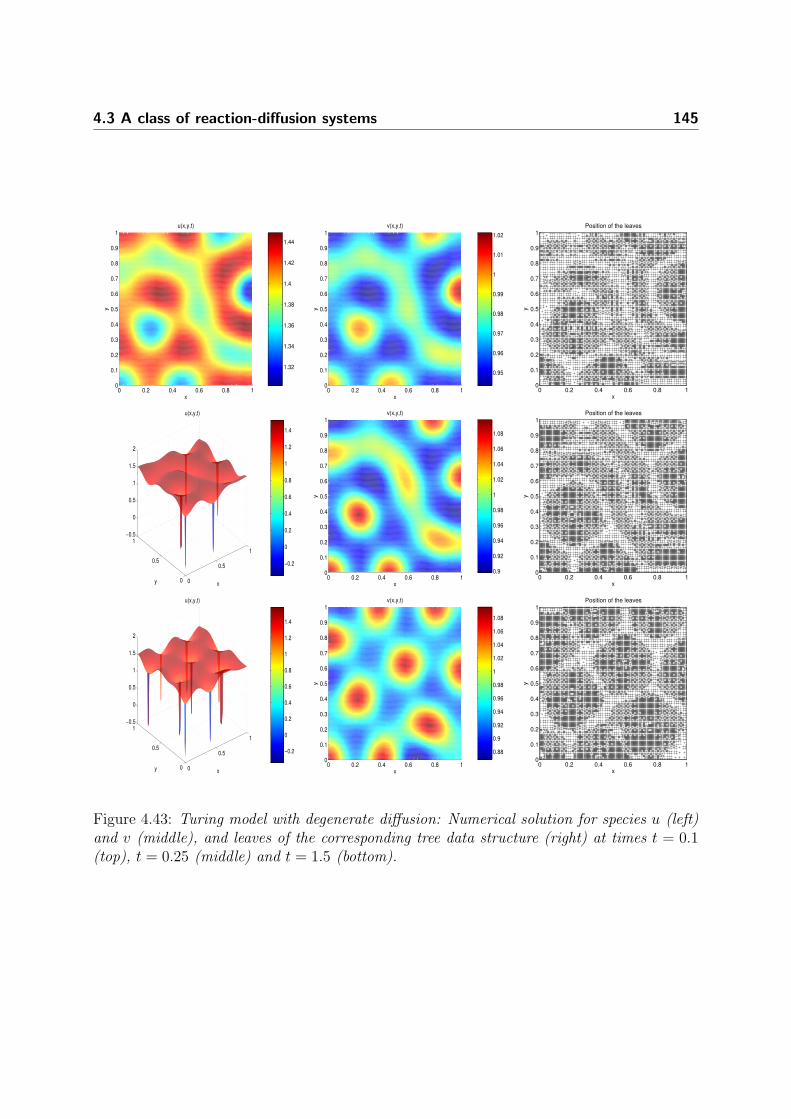
4.3 A class of reaction-diffusion systems 145

0 0.2 0.4 0.6 0.8 10

0.1

0.2

0.3

0.4

0.5

0.6

0.7

0.8

0.9

1u(x,y,t)

x

y

1.32

1.34

1.36

1.38

1.4

1.42

1.44

0 0.2 0.4 0.6 0.8 10

0.1

0.2

0.3

0.4

0.5

0.6

0.7

0.8

0.9

1v(x,y,t)

x

y

0.95

0.96

0.97

0.98

0.99

1

1.01

1.02

0 0.2 0.4 0.6 0.8 10

0.1

0.2

0.3

0.4

0.5

0.6

0.7

0.8

0.9

1Position of the leaves

x

y

0

0.5

1

0

0.5

1−0.5

0

0.5

1

1.5

2

x

u(x,y,t)

y

−0.2

0

0.2

0.4

0.6

0.8

1

1.2

1.4

0 0.2 0.4 0.6 0.8 10

0.1

0.2

0.3

0.4

0.5

0.6

0.7

0.8

0.9

1v(x,y,t)

x

y

0.9

0.92

0.94

0.96

0.98

1

1.02

1.04

1.06

1.08

0 0.2 0.4 0.6 0.8 10

0.1

0.2

0.3

0.4

0.5

0.6

0.7

0.8

0.9

1Position of the leaves

x

y

0

0.5

1

0

0.5

1−0.5

0

0.5

1

1.5

2

x

u(x,y,t)

y

−0.2

0

0.2

0.4

0.6

0.8

1

1.2

1.4

0 0.2 0.4 0.6 0.8 10

0.1

0.2

0.3

0.4

0.5

0.6

0.7

0.8

0.9

1v(x,y,t)

x

y

0.88

0.9

0.92

0.94

0.96

0.98

1

1.02

1.04

1.06

1.08

0 0.2 0.4 0.6 0.8 10

0.1

0.2

0.3

0.4

0.5

0.6

0.7

0.8

0.9

1Position of the leaves

x

y

Figure 4.43: Turing model with degenerate diffusion: Numerical solution for species u (left)and v (middle), and leaves of the corresponding tree data structure (right) at times t = 0.1(top), t = 0.25 (middle) and t = 1.5 (bottom).

146 Numerical simulations

Time V η Species L1−error L2−error L∞−error

t = 0.10 6.32 12.5438 u 6.31 × 10−4 5.82 × 10−4 2.72 × 10−3

v 4.98 × 10−4 5.37 × 10−4 9.46 × 10−4

t = 0.25 9.79 10.3457 u 6.12 × 10−4 2.46 × 10−5 3.03 × 10−3

v 3.91 × 10−4 9.22 × 10−4 9.92 × 10−4

t = 1.50 11.60 10.1984 u 3.42 × 10−4 7.34 × 10−4 3.40 × 10−3

v 2.63 × 10−4 4.98 × 10−4 2.81 × 10−3

Table 4.14: Turing model with degenerate diffusion: Corresponding simulated time, speed-uprate V , compression rate η and componentwise errors.

(u0, v0) = (1+ (x), 1/32), where (x) is a particular smooth perturbation which goes to zeronear (8, 8). We simulate the process until the solution reaches inhomogeneous stationarystates, and we present three cases corresponding to different values of ν, which is responsiblefor the complexity of the spatial patterns. For instance, for ν = 7 Figure 4.44 (middle)shows labyrinth-shaped patterns and for ν = 10 (bottom), single filaments and spots. Thecorresponding adaptive meshes were generated with NL = 5122 = 262144 control volumesin the finest grid, with εR = 8.43 × 10−4. For all these cases we implement locally varyingtime stepping, so we will choose the maximum CFL number allowed by (2.17), CFL0 = 1for the coarsest level and CFLl = 2lCFL0 for finer levels. From Figure 4.45 and Table 4.15we can observe that if we incorporate the local time stepping strategy, a substantial gain(a factor slightly lower than 2, which is consistent with the results by Lamby, Muller, andStiriba [109]) is obtained in speed-up rate when comparing with a multiresolution calculationusing global time stepping. The errors are computed from a reference solution in a grid withNL = 20482 = 4194304 control volumes. We conclude that the errors keep the same slopethat the errors obtained with a global time step. The compression rate η for both methodsis lower than in the previous examples, which could be explained by the complexity anddensity of the spatial patterns in this particular example.

4.4 The monodomain and bidomain models

We will present test cases showing the efficiency of the previously described methods incapturing the dynamical evolution of electro-physiological waves for both the monodomainand bidomain models. Since we are dealing with multi-component solutions, it is worthy tostate that we will consider a single mesh for representing the vector of relevant variables.In the bidomain model, the anisotropies, mesh structures as well as the size of the problemcause the sparse linear system corresponding to (1.38b) to be ill-conditioned. This systemneeds to be solved in each time step and to this end, we use the Cholesky method.

4.4 The monodomain and bidomain models 147

0 5 10 150

2

4

6

8

10

12

14

16Position of the leaves

x

y

0 5 10 150

2

4

6

8

10

12

14

16Position of the leaves

x

y

0 5 10 150

2

4

6

8

10

12

14

16Position of the leaves

x

y

Figure 4.44: Chemotaxis with growth: Numerical solution for species u (left) and v (middle),and leaves of the corresponding tree data structure (right) for ν = 6.04 (top), ν = 7 (middle)and ν = 10 (bottom).

148 Numerical simulations

0 2 4 6 8 10 12 14 16 18 200

5

10

15

20

25

30

35

40

45

50

Time

V

MR

MR with LTS

0 5 10 15 202

3

4

5

6

7

8

9

Time

η

LTS

MR

0 5 10 15 2010

−4

10−3

10−2

Time

L1−e

rro

r

FV

MR

MR with LTS

0 5 10 15 20

10−4

10−3

10−2

Time

L∞−e

rro

r

FV

MR

MR with LTS

Figure 4.45: Chemotaxis with growth, ν = 7: Time evolution for speed-up rate V , datacompression rate η and errors for different methods: Multiresolution scheme with global timestep, and multiresolution with locally varying time step.

4.4 The monodomain and bidomain models 149

Time Method V η L1-error L∞-error

t = 1 MR 16.79 5.37 8.41 × 10−4 3.54 × 10−3

MR with LTS 34.18 5.29 5.30 × 10−4 3.15 × 10−3

t = 5 MR 16.96 6.48 7.43 × 10−4 4.19 × 10−3

MR with LTS 33.51 6.23 6.14 × 10−4 3.71 × 10−3

t = 10 MR 15.44 7.87 6.20 × 10−4 2.86 × 10−3

MR with LTS 31.08 7.01 4.15 × 10−4 3.02 × 10−3

t = 20 MR 17.29 5.92 7.14 × 10−4 3.46 × 10−3

MR with LTS 33.87 5.50 4.99 × 10−4 3.40 × 10−3

Table 4.15: Chemotaxis with growth: Time evolution for data compression, speed-up rate,

and normalized errors for different methods: Multiresolution scheme with fixed global time

step, and multiresolution with locally varying time step. ν = 7.0, CFL0 = 1, εR = 5.0×10−4

and L = 10.

Time V η L1−error L2−error L∞−error

t = 0.0 ms 170.22 4.31 × 10−4 2.47 × 10−4 3.99 × 10−4

t = 1.5 ms 27.81 37.56 4.97 × 10−4 1.96 × 10−4 4.63 × 10−4

t = 3.5 ms 26.47 29.89 5.23 × 10−4 4.05 × 10−4 4.82 × 10−4

t = 4.5 ms 31.41 28.12 7.48 × 10−4 4.29 × 10−4 5.31 × 10−4

t = 5.5 ms 30.62 24.70 1.04 × 10−3 6.20 × 10−4 6.79 × 10−4

Table 4.16: 2D monodomain model: Corresponding simulated time, CPU ratio V, compres-sion rate η and normalized errors for v, using a MR method.

150 Numerical simulations

0 0.2 0.4 0.6 0.8 10

0.1

0.2

0.3

0.4

0.5

0.6

0.7

0.8

0.9

1Position of the leaves

x [cm]

y [cm

]

0 0.2 0.4 0.6 0.8 10

0.1

0.2

0.3

0.4

0.5

0.6

0.7

0.8

0.9

1Position of the leaves

x [cm]

y [cm

]

Figure 4.46: Monodomain model: Numerical solution for v, measured in [mV] (left) andleaves of the corresponding tree at times (from top to bottom) t = 1.5 ms, t = 3.5 ms.

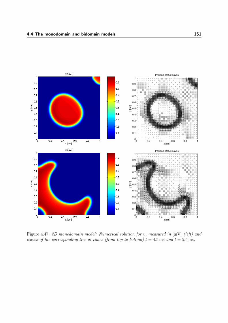
4.4 The monodomain and bidomain models 151

0 0.2 0.4 0.6 0.8 10

0.1

0.2

0.3

0.4

0.5

0.6

0.7

0.8

0.9

1Position of the leaves

x [cm]

y [cm

]

0 0.2 0.4 0.6 0.8 10

0.1

0.2

0.3

0.4

0.5

0.6

0.7

0.8

0.9

1Position of the leaves

x [cm]

y [cm

]

Figure 4.47: 2D monodomain model: Numerical solution for v, measured in [mV] (left) andleaves of the corresponding tree at times (from top to bottom) t = 4.5 ms and t = 5.5 ms.

152 Numerical simulations

4.4.1 2D monodomain model

For this example, we consider the simple monodomain model (1.42) with homogeneous Neu-mann boundary conditions. The ionic current and membrane model is determined by theFitzHugh-Nagumo membrane kinetics (1.37), with a = 0.16875, b = 1.0, λ = −100 andθ = 0.25. The computational domain is the square Ω = [0, 1 cm]2, and the remaining pa-rameters are cm = 1.0 mF/cm2 and β = 1.0 cm−1. The units for v, w are mV. We considerin (1.42) (1 + µ)−1Mi := diag(γ, γ) with γ = 0.01. The initial data are

v0(x, y) =

1 −

1

1 + exp(−50(x2 + y2)1/2 − 0.1)

mV, w0 = 0 mV.

After 4 ms, an instantaneous stimulus is applied in (x0, y0) = (0.5 cm, 0.5 cm) to the mem-brane potential v

µ

1 + µIapp :=

1 mV if (x − x0)

2 + (y − y0)2 < 0.04 cm2,

0 mV otherwise..

In this example, we use L = 10 resolution levels, N = 262144 elements in the finest level, atolerance of εR = 1×10−3 and we compute normalized errors by comparison with a referencesolution obtained with a fine mesh calculation with N = 10242 = 1048576 control volumes.The time evolution is made using a first order explicit Euler scheme. Plots of the numericalsolution with the corresponding adaptively refined meshes at different times are shown inFigures 4.46 and 4.47.

As can be seen from Table 4.16, the normalized errors are controlled to be of the same orderof the reference tolerance εR. We also see that the MR algorithm is efficient: we have highrates of memory compression and speed-up.

4.4.2 3D monodomain model

We perform a simulation for the simple monodomain model described in (1.42) with ho-mogeneous Neumann boundary conditions. The ionic current and membrane model is de-termined by the FitzHugh-Nagumo membrane kinetics (1.37), with a = 0.16875, b = 1.0,λ = −100 and θ = 0.25. The computational domain is the cube Ω = [0, 1 cm]3, the numberof control volumes is N = 262144 and the remaining parameters are cm = 1.0 mF/cm2 andβ = 1.0 cm−1. The units for v, w are mV. We consider in (1.42) (1 + µ)−1Mi := diag(γ, γ)with γ = 0.01.

4.4 The monodomain and bidomain models 153

t = 1.5 ms t = 3.5 ms t = 4.5 ms

0.25 0.5 0.75 1

Figure 4.48: 3D monodomain model: Numerical solution v, measured in [mV] for the mon-odomain model at different times.

The respective initial data for v and w are

v0(x, y) =

1 −

1

1 + exp(−50(x2 + y2)1/2 − 0.1)

mV, w0 = 0 mV.

After 4 ms, an instantaneous stimulus is applied in (x0, y0) = (0.5 cm, 0.5 cm) to the mem-brane potential v

µ

1 + µIapp :=

1 mV if (x − x0)

2 + (y − y0)2 < 0.04 cm2,

0 mV otherwise..

Snapshots of the corresponding numerical solution at different times are shown in Figure 4.48.Here, due to the lack of exact solutions for these examples, we compute errors in differentnorms using a numerical solution on a extremely fine mesh (of 134217728 and 1048576control volumes for the 3D and 2D models respectively) as reference. To measure errorsbetween such a reference solution ur and an approximate solution uh, we will use Lp-errors:ep = un − un

hp, p = 1, 2,∞, where

e∞ = maxK∈T

unr,K − un

hK

; ep =

1

|K|

K∈T

unr,K − un

hK

p1/p

, p = 1, 2.

Here unr,K stands for the projection of the reference solution onto the control volume K.

The corresponding convergence history for Example 1 is given in Table 4.17. From thisinformation we point out that the method provides a rate of convergence around 1.2. By

154 Numerical simulations

Time N h L1−error r1(v)

t = 1.5 4096 0.0625 5.68 × 10−2 −32768 0.0313 2.58 × 10−2 1.2412262144 0.0156 1.21 × 10−2 1.23562097152 0.0078 5.67 × 10−3 1.1936

t = 3.5 4096 0.0625 2.34 × 10−2 −32768 0.0313 1.07 × 10−2 1.2315262144 0.0156 4.91 × 10−3 1.22382097152 0.0078 2.28 × 10−3 1.2067

t = 4.5 4096 0.0625 9.12 × 10−3 −32768 0.0313 4.26 × 10−3 1.1982262144 0.0156 1.89 × 10−3 1.27252097152 0.0078 8.91 × 10−4 1.1849

Table 4.17: 3D monodomain model: Corresponding simulated time in [ms], number of con-trol volumes N , meshsize h, approximate L1−errors for the transmembrane potential v andconvergence rates r(v).

rate of convergence we mean

r(u) =log

e(u)e∗(u)

log(h/h∗),

where e(u) and e∗(u) denote the corresponding errors computed for two consecutive meshesof sizes h and h∗ respectively.

4.4.3 A 2D bidomain model

Now in the first example for the bidomain model, consider a two-dimensional domain Ω =[0, 1 cm]2, and the bidomain model (1.38) with rotational anisotropy and cm = 1.0 mF/cm2,σl

i = 3.0 × 10−3 Ω−1cm−1, σti = 3.1525 × 10−4 Ω−1cm−1 σl

e = 2.0 × 10−3 Ω−1cm−1, σte =

1.3514 × 10−3 Ω−1cm−1, β = 100 cm−1, Rm = 2.5 × 103 Ω cm2, vp = 100 mV, η1 = 0.0044,η2 = 0.12, η3 = 1, η4 = 13 and η5 = 0.15. The initial data is given by an initial stimulus of1 mV applied to the center of the extracellular medium and smooth initial distributions forthe transmembrane potential and gating variable.

We use a regular mesh of N = 65536 control volumes to obtain the series of plots of thenumerical solution for the extracellular potential that we depict in Figure 4.49. Due to thelack of exact solutions for these examples, we will compute errors in different norms using a

4.4 The monodomain and bidomain models 155

t = 0.01 ms t = 1.5 ms t = 3.0 ms

Figure 4.49: First example for the bidomain model: Transmembrane potential v, measuredin [mV] for the bidomain model at different times.

156 Numerical simulations

numerical solution on a extremely fine mesh (of 1048576 control volumes) as reference. Inaddition, from Table 4.18 we observe that the rate of convergence provided by the method isa bit higher than O(h), but still lower than the rates obtained for the monodomain case. Thisbehavior of the experimental rates of convergence can be also observed from Figure 4.50,where we show the meshsize and errors in different norms plotted in a log-log fashion againstthe number of control volumes.

Time N L1−error r1(v) L2−error r2(v) L∞−error r∞(v)

t = 0.01 1024 7.68 × 10−3 − 4.79 × 10−3 − 6.51 × 10−3 −4096 3.81 × 10−3 1.0135 2.28 × 10−3 1.0253 3.13 × 10−3 1.037816384 1.12 × 10−3 1.0904 9.85 × 10−4 1.0831 1.26 × 10−3 1.090365536 5.87 × 10−4 1.0812 4.69 × 10−4 1.0982 6.07 × 10−4 1.0894

t = 1.5 1024 3.15 × 10−3 − 3.01 × 10−4 − 7.14 × 10−3 −4096 1.28 × 10−3 1.0187 1.21 × 10−4 0.9804 3.54 × 10−3 1.095316384 5.89 × 10−4 1.0712 5.72 × 10−5 1.1034 1.63 × 10−4 1.093765536 2.61 × 10−4 1.1106 2.43 × 10−5 1.0267 7.58 × 10−5 1.0881

t = 3.0 1024 1.64 × 10−3 − 2.92 × 10−3 − 1.05 × 10−2 −4096 7.39 × 10−4 1.1053 1.40 × 10−3 0.9659 4.67 × 10−3 0.989616384 3.28 × 10−4 1.0972 6.82 × 10−4 1.0024 2.13 × 10−3 1.048065536 1.57 × 10−4 1.0835 2.97 × 10−4 1.1321 9.72 × 10−4 1.0875

Table 4.18: First example for the bidomain example: Corresponding simulated time in [ms],number of control volumes N , approximate errors in different norms for the transmembranepotential v and convergence rates r(v).

Now for a second example, the simulations use a computational domain Ω = [0, 5 cm]2 and theparameters in (1.38) and (1.36) (after [75, 146, 163, 164]) are given by the membrane capac-itance cm = 1.0 mF/cm2, the intracellular conductivity in the principal axis σ l

i = 6 Ω−1cm−1,the remaining intracellular conductivity σt

i = 0.6 Ω−1cm−1 (corresponding to an anisotropyratio of 10), the extracellular conductivities σ l

e = 24 Ω−1cm−1 and σte = 12 Ω−1cm−1 (corre-

sponding to an anisotropy ratio of 2), the surface-to-volume ratio β = 2000 cm−1, the surfaceresistivity Rm = 2 × 104 Ω cm2, vp = 100 mV, η1 = 0.005, η2 = 0.1, η3 = 1.5, η4 = 7.5, andη5 = 0.1. The fibers form an angle of π/4 with the x-axis and the initial datum is given by astimulus applied on the extracellular potential ue in the center of the domain, while both vand the gating variable w are initially set to zero (see Figure 4.51). The units for v, ue andw are mV.

The following MR setting is chosen. We utilize wavelets with r = 3 vanishing moments, amaximal resolution level L = 9, and therefore a finest mesh with N = 65536 elements. Thereference tolerance given by εR = 5.0 × 10−4.

4.4 The monodomain and bidomain models 157

103

104

105

106

10−6

10−5

10−4

10−3

10−2

N

err

or

h

L1−error

L2−error

L∞−error

Figure 4.50: First example for the bidomain model: Meshsize h and errors in different normsfor the transmembrane potential v versus the number of control volumes N . The simulatedtime is t = 1.5 ms.

0 1 2 3 4 50

0.5

1

1.5

2

2.5

3

3.5

4

4.5

5Position of the leaves

x [cm]

y [cm

]

Figure 4.51: Second example for the bidomain model: Initial condition for the extracellularpotential ue, and leaves of the corresponding tree data structure.

158 Numerical simulations

We show in Figures 4.52 and 4.53 a sequence of snapshots after an initial stimulus applied tothe center of the domain, corresponding to transmembrane potential v, extracellular potentialue and adaptive mesh.

Table 4.19 illustrates the efficiency and accuracy of the base MR method by tabulating CPUratio V, compression rate η and normalized errors. By using MR, we obtain an average datacompression rate of 17 and an increasing speed-up rate up to 26.09. Moreover, the errors inthree different norms remain of the order of εR. Here we have computed normalized errorsusing a reference FV solution on a grid with N = 10242 = 1048576 control volumes.

Time V η Pot. L1−error L2−error L∞−error

t = 0.1 13.74 19.39 v 3.68 × 10−4 8.79 × 10−5 6.51 × 10−4

ue 2.01 × 10−4 6.54 × 10−5 5.22 × 10−4

t = 0.5 21.40 17.63 v 4.06 × 10−4 9.26 × 10−5 6.83 × 10−4

ue 2.79 × 10−4 8.72 × 10−5 5.49 × 10−4

t = 2.0 25.23 17.74 v 4.37 × 10−4 1.25 × 10−4 6.88 × 10−4

ue 3.48 × 10−4 9.44 × 10−5 6.11 × 10−4

t = 5.0 26.09 16.35 v 5.29 × 10−4 1.94 × 10−4 7.20 × 10−4

ue 4.15 × 10−4 1.06 × 10−4 6.32 × 10−4

Table 4.19: Second example for the bidomain model: Corresponding simulated time, CPUratio V, compression rate η and normalized errors.

For the time integration using the LTS method, we choose the maximum CFL numberallowed by (2.22), CFLl=0 = 0.5 for the coarsest level and CFLl = 2lCFLl=0 for finer levels.For the RKF computations, we use δdesired = 1× 10−4, S0 = 0.1, Smin = 0.01, and the initialCFL condition CFLt=0 = 0.5.

We select this example for a detailed comparison of the performance of the FV and MRmethods with a global time step, the MR method with RKF adaptive global time stepping(MR-RKF), and the MR method with local time stepping (MR-LTS). The evolution ofthe speed-up factor V the and data compression rate η for the MR versions and of thenormalized L1 and L∞ errors for all these methods are displayed in Figure 4.55. From theseplots it is observed that with RKF and LTS, the data compression rate is of the same orderduring the time evolution, which means that the adaptive meshes are not too different frommethod to method. Also, a substantial additional gain is obtained in speed-up rate whencomparing with a MR calculation using global time stepping: The MR-LTS method givesus an additional speed-up factor of about 2, while with the RKF alternative we obtain anadditional speed-up of about 4. This effect could be explained in part from the fact thatthere is no need of a synchronization procedure for the RKF computations and the factthat the CFL condition (2.22) is not imposed during the time evolution with the MR-RKF

4.4 The monodomain and bidomain models 159

t = 0.1 ms t = 0.5 ms

0 1 2 3 4 50

0.5

1

1.5

2

2.5

3

3.5

4

4.5

5Position of the leaves

x [cm]

y [

cm

]

0 1 2 3 4 50

0.5

1

1.5

2

2.5

3

3.5

4

4.5

5Position of the leaves

x [cm]

y [

cm

]

Figure 4.52: Second example for the bidomain model: Numerical solution for transmembranepotential v and extracellular potential ue in [mV], and leaves of the corresponding tree datastructure at times t = 0.1 ms and t = 0.5 ms.

160 Numerical simulations

t = 2.0 ms t = 3.5 ms

0 1 2 3 4 50

0.5

1

1.5

2

2.5

3

3.5

4

4.5

5Position of the leaves

x [cm]

y [

cm

]

0 1 2 3 4 50

0.5

1

1.5

2

2.5

3

3.5

4

4.5

5Position of the leaves

x [cm]

y [

cm

]

Figure 4.53: Second example for the bidomain model: Numerical solution for transmembranepotential v and extracellular potential ue in [mV], and leaves of the corresponding tree datastructure at times t = 2.0 ms and t = 3.5 ms.

4.4 The monodomain and bidomain models 161

4 6 8 10 120

5

10

15

20

25

30

35

40

L

η

εR

=1 10−5

εR

=5 10−5

εR

=1 10−4

εR

=5 10−4

εR

=1 10−3

4 6 8 10 12

10

20

30

40

50

60

70

80

L

V

εR

=1 10−5

εR

=5 10−5

εR

=1 10−4

εR

=5 10−4

εR

=1 10−3

6 7 8 9 10 11 12

10−5

10−4

10−3

10−2

L

L1−e

rror

εR

=1 10−5

εR

=5 10−5

εR

=1 10−4

εR

=5 10−4

εR

=1 10−3

FV

Figure 4.54: Second example for the bidomain model: data compression rate η (top left),speed-up factor V (top right) and L1-errors for different scales L and values of εR (bottom).The simulated time is t = 2.0 ms.

162 Numerical simulations

method, allowing larger time steps. (Related to this fact, it should be noted that althoughcondition (2.22) guarantees numerical stability of the solutions, in practice this is observed tobe a too strict estimate). We can also conclude that the errors of the MR-LTS computationsare kept of the same order that the errors obtained with a global time stepping, while theincurred errors by using the MR-RKF method are larger during the whole time evolution.

0 0.5 1 1.5 2 2.5 3 3.510

15

20

25

t [ms]

η

MR

MR with LTS

MR with RKF

0 0.5 1 1.5 2 2.5 3 3.50

10

20

30

40

50

60

70

80

90

100

t [ms]

V

MR

MR with LTS

MR with RKF

0 0.5 1 1.5 2 2.5 3 3.510

−4

10−3

10−2

t [ms]

L1−e

rro

r

FV

MR

MR with LTS

MR with RKF

0 0.5 1 1.5 2 2.5 3 3.510

−4

10−3

10−2

t [ms]

L∞−e

rro

r

FV

MR

MR with LTS

MR with RKF

Figure 4.55: Second example for the bidomain model: Time evolution for data compressionrate η, speed-up rate V, and normalized errors for different methods: MR scheme with globaltime step, MR with locally varying time stepping and MR with RKF time stepping.

As a third example for the bidomain model, let us consider a slightly different setting. Firstwe apply an initial stimulus at the center of the domain, later in t = 0.2 ms we apply anotherstimulus to the northwest corner of the domain, and then in t = 1.0 ms we apply a thirdstimulus of the same magnitude to the northeast and southwest corners. The system is

4.5 A doubly nonlinear diffusion model of chemotaxis 163

evolved and we show snapshots of the numerical solution for v, ue and the adaptive mesh.We use the MR-RKF method with N = 65536, εR = 2.5 × 10−3, δdesired = 1 × 10−3 andthe remaining parameters are considered as in the previous subsection. From Figures 4.56and 4.57 we clearly notice the anisotropic orientation of the fibers.

4.5 A doubly nonlinear diffusion model of chemotaxis

In this section, we provide numerical examples to illustrate how the approximate solutionsof the simple chemotaxis model (1.46) vary when changing the parameter p from standardnonlinear diffusion (p = 2), to doubly nonlinear diffusion (p > 2). For the discretization ofthe examples, a standard first order finite volume method (see Section 2.4 for details on thenumerical scheme) on a regular mesh of 262144 control volumes is used. We choose a simplesquare domain Ω = [−1, 1]2 and use the functions a(u) = u(1 − u), f(u) = (1 − u)2 andg(u, v) = αu − βv along with parameters that are stated separately in each case.

For the first chemotaxis example, we choose = 0.01, α = 40, β = 160, χ = 0.2 and d = 0.05.The initial condition for the species density is given by

u0(x) =

1 for x ≤ 0.2

0 otherwise,,

and the concentration for the chemoattractant is assumed to have uniform distributionv0(x) = 4.5. In a first simulation, we consider the simple case of p = 2 and we comparethe result with an analogous experiment with p = 6. We evolve the system until t = 1.0,and show in Figure 4.58 a snapshot of the cell density at this instant for both cases. Notethat the special form of the functions a(u) and f(u) (they include the factor (1 − u)), inthe species diffusion and chemotactical cross diffusion, takes into account the volume fillingeffect: these terms vanish at u = 0 and u = um = 1.

As a second chemotaxis example we now choose the parameters = 0.5, α = 5, β = 0.5,χ = 1 and d = 0.25. The initial condition for the species density is given by

u0(x) =

1 for x − (−0.25, 0.25) ≤ 0.2 or x − (0.25,−0.25) ≤ 0.2

0 otherwise,

and for the chemoattractant

v0(x) =

4.5 for x − (0.25, 0.25) ≤ 0.2 or x + (0.25, 0.25) ≤ 0.2

0 otherwise.

164 Numerical simulations

t = 0.1 ms t = 0.5 ms

0 1 2 3 4 50

0.5

1

1.5

2

2.5

3

3.5

4

4.5

5Position of the leaves

x [cm]

y [

cm

]

0 1 2 3 4 50

0.5

1

1.5

2

2.5

3

3.5

4

4.5

5Position of the leaves

x [cm]

y [

cm

]

Figure 4.56: Third example for the bidomain model: Numerical solution for transmembranepotential v and extracellular potential ue in [mV], and leaves of the corresponding tree datastructure at times t = 0.1 ms and t = 0.5 ms.

4.5 A doubly nonlinear diffusion model of chemotaxis 165

t = 2.0 ms t = 5.0 ms

0 1 2 3 4 50

0.5

1

1.5

2

2.5

3

3.5

4

4.5

5Position of the leaves

x [cm]

y [

cm

]

0 1 2 3 4 50

0.5

1

1.5

2

2.5

3

3.5

4

4.5

5Position of the leaves

x [cm]

y [

cm

]

Figure 4.57: Third example for the bidomain model: Numerical solution for transmembranepotential v and extracellular potential ue in [mV], and leaves of the corresponding tree datastructure at times t = 2.0 ms and t = 5.0 ms.

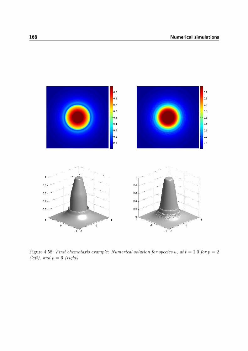
166 Numerical simulations

Figure 4.58: First chemotaxis example: Numerical solution for species u, at t = 1.0 for p = 2(left), and p = 6 (right).

4.5 A doubly nonlinear diffusion model of chemotaxis 167

Figure 4.59: Second chemotaxis example: Numerical solution for species u, at t = 0.1 forp = 2 (left), and p = 6 (right).

168 Numerical simulations

Figure 4.60: Second chemotaxis example: Numerical solution for species u, at t = 0.5 forp = 2 (left), and p = 6 (right).

4.5 A doubly nonlinear diffusion model of chemotaxis 169

Figure 4.61: Second chemotaxis example: Numerical solution for species u, at t = 2.5 forp = 2 (left), and p = 6 (right).

170 Numerical simulations

The behavior of the system for the cases p = 2 and p = 6 is presented in the left and rightplots, respectively, of Figures 4.59, 4.60 and 4.61.

For the third chemotaxis example, we use a model for chemotactic bacterial patterns in aliquid medium (see [154]) and to conciliate this model with the general framework of (1.46),we may rewrite (1.46) in the particular form:

∂tu = Dudiv (|∇u|p−2∇u) − div (χuf(v)∇v) in QT ,

∂tv = Dv∆v + g(u) in QT ,

|∇u|p−2 ∂u

∂η= 0,

∂v

∂η= 0 on ΣT , u(x, 0) = u0(x), v(x, 0) = v0(x).

Here Ω = [0, 10]2, g(u) = u2

1+u2 with Du = 0.33, Dv = 1, and χf(v) = α 1(1+v)2

with α = 80.The initial conditions consist in a random perturbation around u = 1 for the cell’s densityand v0 = 1. In a first simulation we consider the simple case of p = 2 and we compare theresult with an analogous experiment with p = 5. We evolve the system until t = 2.0, andshow in Figure 4.62 a snapshot of the cell density at this instant for both cases.

As a fourth chemotaxis example, we consider a similar model used by J. Adler in the 60’sfor simulating the behavior of bacterial chemotaxis (see [52]).

∂tu = Dudiv (|∇u|p−2∇u) + div (χ(1 − u)f(v)∇v) + g(u, v) in QT ,

∂tv = Dv∆v +1

V2

g(u, v) in QT ,

where Ω = [−1, 1]2, g(u, v) = − V1uvK1+v

with V1 = 0.35, K1 = 4 × 10−6, and χf(v) = K2

(K3+v)2,

with K2 = 0.02, K3 = 2 × 10−6. The remaining parameters are given by Du = 0.01,Dv = 0.05, V2 = 0.001 and the initial conditions are

u0(x) =

5 × 10−6 for x ≤ 9.5 × 10−2

0 otherwise,, v0(x) = 2.64 × 10−5,

which means that the bacteria are initially located at the center of the domain, and theconcentration for the chemoattractant (which in this case is galactose) is assumed to haveuniform distribution (see [52]). The term 1 − u in the cross diffusion takes into account thevolume filling effect. The cell densities for both p = 2 and p = 5 are displayed in Figure 4.63.We remark that in this example, the pattern shown by the model with p = 5 is qualitativelycloser to the numerical results tested against experimental data (compare with [52]).

More complex patterns can be driven by a slightly different model. Consider as a fifthchemotaxis example, a quadratic domain Ω = [0, 16]2 and rewrite the first two equations of(1.46) in the form

ut = ∇ ·σ|∇u|p−2∇u − uχ∇v

+ g(u) on QT ,

4.5 A doubly nonlinear diffusion model of chemotaxis 171

Figure 4.62: Third chemotaxis example: Numerical solution for species u, at t = 2.0 forp = 2 (left), and p = 5 (right).

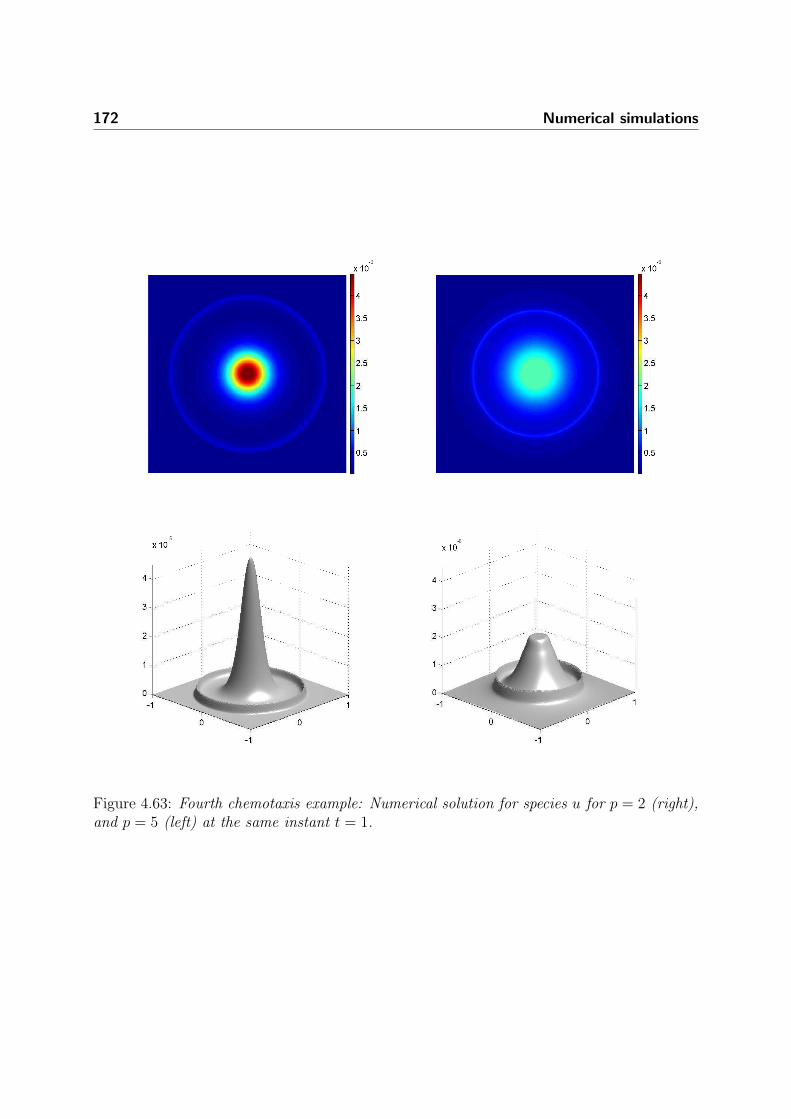
172 Numerical simulations

Figure 4.63: Fourth chemotaxis example: Numerical solution for species u for p = 2 (right),and p = 5 (left) at the same instant t = 1.

4.5 A doubly nonlinear diffusion model of chemotaxis 173

vt = h(u, v) + d∆v on QT .

This model describes in particular the spatio-temporal aggregation patterns shown by thebacteria Escherichia coli (see e.g., [10]). Here χ = 7, g(u) = u2(1 − u), h(u, v) = u − 32v,d = 1 and σ = 0.0625. The initial concentration for the bacteria is randomly distributed:(u0, v0) = (1+ (x), 1/32), where (x) is a particular smooth perturbation which goes to zeronear (8, 8). We simulate the process until the solution reaches inhomogeneous stationarystates, and again, from Figure 4.64 we see different patterns obtained by using both p = 2and p = 4.

Let us mention, roughly speaking, that these numerical examples show at least qualitativelythat the smaller the value of p, the steeper becomes the solution. This property is clearlyrelated to the proportional relation between p and the Holder exponent α, as we see theparticular form of α (which depends on σ, and σ depending on s1 and thus on n) andprovided that we can bound uniformly ∇vp

Lpp(QT ). Also notice that in examples 4 and 5,

growth functions g(u, v) and g(v) respectively, are considered for the equation modeling thedynamics of the cell’s density. We point out that the inclusion of these terms is not consideredin the previous performed analysis. Nevertheless, depending strongly on the growth structureof such terms (see e.g. [156]), natural changes may be applied to the proofs of existence andregularity of weak solutions, covering in this way the theory for these examples.

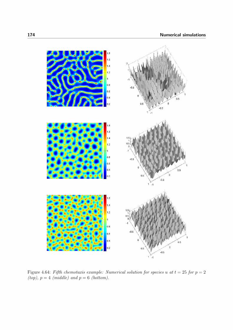
174 Numerical simulations

Figure 4.64: Fifth chemotaxis example: Numerical solution for species u at t = 25 for p = 2(top), p = 4 (middle) and p = 6 (bottom).

Chapter 5

Summary and concluding remarks

In the previous Chapters of this thesis we have described the primary goals of our research,namely the numerical and mathematical analysis of degenerate parabolic equations, theconstruction of finite volume schemes for these problems, and the application of techniquesarising from wavelet theory to improve the performance of the reference schemes. Two yearsago we structured the proposal of this doctoral thesis in four main steps:

Implementation of a numerical method. Aim: A feasibility study, preliminary results andextension to the results in [140].

Application to sedimentation and traffic flow models. Aim: To use the multiresolutionapproach to improve existing FV results in these applications.

Study of reaction-diffusion systems. Aim: A feasibility study and preliminary results, ex-tension of the previous steps to systems and 2-D.

Analysis of degenerate parabolic equations. Aim: Wellposedness theory for a class of solu-tions, regularity results for weak solutions, construction, implementation and conver-gence results for suitable FV schemes.

In addition to the successful development of these steps, we have also worked on the well-posedness and convergence analysis of a finite volume method for cardiac models. To finalizethis thesis, a summary of the main findings, highly motivated by the numerical and compu-tational challenges observed in the mathematical models considered, is discussed.

176 Summary and concluding remarks

Implementation of a numerical method

We have shown that the multiresolution approach is a suitable tool for the study of degener-ate parabolic equations. Concerning this subject we have presented numerical results usinga fully space–time adaptive finite volume-multiresolution scheme developed to be used forstrongly degenerate parabolic equations. The strong degeneracy of the diffusive term leads tosolutions that are discontinuous in general, and in particular exhibit sharp interfaces wherethe equation changes between parabolic and hyperbolic type. Multiresolution schemes arenatural candidates to capture these interfaces along with the classical shocks appearing inhyperbolic regions. The numerical results shown herein confirm that the proposed schemesare indeed well adapted to this kind of equations. We have also examined the advantage ofthe multiresolution approach compared with standard FV schemes. In our experiments, wehave obtained a considerable speed-up on the computations and also a substantial memorycompression, while keeping the same accuracy order as in the reference schemes. The ap-proximation order of the FV scheme is maintained due to a suitable choice of the threshold,which is a considerable improvement with respect to other multiresolution schemes where thetolerance is chosen in practice heuristically. Time step control is then introduced using anembedded RKF method which permits to adjust the time step automatically and to controlthe error. Different examples in one space dimension for sedimentation processes and trafficflow show the validity and efficiency of the new scheme. The interplay of the key ingredientsmentioned above could represent an asset specially in the case of large number of mesh ele-ments, systems, higher space dimensions and when the reference scheme is computationallyexpensive. Although we deal only with scalar and one space dimension applications, it isknown that the main features of our method (i.e., Runge–Kutta Fehlberg time stepping,general multiresolution and FV schemes) are applicable for the mentioned extensions.

The success of the improvements to the reference scheme depends on the proper tuning ofthe parameters, especially for the adaptivity of the time stepping. Also it is known thatthe efficiency of the multiresolution strategy is problem dependent. These are very delicateissues, and they are subject of future work. Possible extensions include the use of penalizationmethods for complex domains and schemes with local time adaptivity.

Application to sedimentation and traffic flow models

We have used the developed multiresolution approach to improve existing FV results. Beforediscussing our results, we comment that the standings of both applicative models are slightlydifferent. Numerous mathematical models have been proposed for one-directional flows ofvehicular traffic; reviews of this topic are given in the monographs by Helbing [89], Kerner[105] and Garavello and Piccoli [80], as well as in the articles by Bellomo et al. [4, 5, 6].

177

These and other works vividly illustrate that the number of balance equations (for the cardensity, velocity, and possibly other flow variables) that form a time-dependent model basedon partial differential equations, as well as the algebraic structure of these equations, is atopic of current research. Fortunately, all these models are spatially one-dimensional, anda circular road with periodic boundary conditions provides a setup that is both physicallymeaningful (since the flow is horizontal) and easy to implement for numerical simulation.This setup, on one hand, is widely used to compare different traffic models, and on theother hand allows to assess the local influence and long-term behavior of nonlinearities andinhomogeneities such as the ones introduced in Section 4.2.1.

While the traffic problem highlights the use of the scheme used herein to explore differentmodels, the clarifier-thickener model calls for an efficient tool to perform simulations, onone hand, related to clarifier-thickener design and control [36, 39], and on the other hand, toparameter identification calculations [58, 18]. In fact, depending on the parameters, clarifier-thickener operations such as fill-up may extend over weeks and months [39], and requirelarge simulation times, while the parameter identification procedures in [58, 18] proceed bysolution of an adjoint problem, which needs storage of the complete solution of the previouslysolved direct problem. Clearly, methods that imply savings in both computational time andmemory storage, such as the multiresolution scheme presented herein, are of significantpractical interest for the clarifier-thickener model.

Both mathematical models considered herein exhibit three types of fronts that typicallyoccur in solutions of (1.9), namely standard shocks (i.e., discontinuities between solutionvalues for both of which (1.9) is hyperbolic), hyperbolic-parabolic type-change interfaces(such as the sediment level), and stationary discontinuities located at the discontinuitiesof γ(x). The basic motivation for applying a finite volume multiresolution scheme is thatthis device is is sufficiently flexible to produce the refinement necessary to properly captureall these discontinuities, and leads to considerable gains in storage as can be seen from thesparsity of the graded trees in our numerical examples. Moreover, Figure 4.20 confirms thatwe may effectively control the perturbation error, in the sense that the errors of the resultingfinite volume multiresolution scheme remains of the same order as those observed for thesolution obtained by the finite volume scheme on a uniform grid. We recall from Section 3.3that the feasibility of this control depends on an estimate of the convergence rate of the basicdiscretization on a uniform grid, which is an open problem for strongly degenerate parabolicequations.

On the other hand, the basic finite volume scheme accurately resolves the discontinuities ofthe solution sitting at the jumps of γ(x) at any level of discretization; these discontinuitiesare not approximated by smeared transitions (as are discontinuities at positions where γ(x)is smooth), see [35]. This means that the refinement the multiresolution produces nearthese discontinuities, which is visible in Figures 4.22 and 4.23, and which is based on theadaptation of the refinement according to features of the solution (but not of γ(x)), is

178 Summary and concluding remarks

possibly unnecessary, and that a more efficient version of the present method may be feasible.

Our results concerning these applications are given in [40, 41, 42].

Study of degenerate reaction-diffusion systems

We presented a feasibility study and preliminary results, as an extension of the previous stepsto degenerate reaction-diffusion systems in two and three-space dimensions. We address theapplication of a MR method for FV schemes combined with LTS and RKF adaptive timestepping for solving several degenerate reaction-diffusion systems including the Keller-Segelequations, the Turing pattern-formation system, a model for flame balls instabilities, and thebidomain equations in electrocardiology. The numerical experiments illustrate that the usedmethods are efficient and accurate enough to simulate the phenomena mentioned above withaffordable effort. This is a real advantage in comparison with more involved methods thatrequire large scale computations on clusters. We here contribute to the recent work done byseveral groups in testing whether the combination of MR, LTS and RKF strategies is indeedeffective for a relevant class of problems. From a numerical point of view, the plateau-likestructures, associated with very steep gradients, of typical solutions motivate the use of alocally refined adaptive mesh, since we require high resolution near these steep gradientsonly. These areas of strong variation occupy a very reduced part of the entire domain only,especially in the case of sharp fronts. Consequently our gain will be less significant in thepresence of chaotic solutions or when multiple waves interact in the considered domain.Based on our numerical examples, we conclude that using a LTS strategy, we obtain asubstantial gain in CPU time speed-up of a factor of about 2 for larger scales. Also, theerrors obtained by using this strategy are nearly the same as those produced by a global timestepping strategy. On the other hand, using an MR-RKF strategy, we obtain an additionalspeed-up factor of about 4, but at the price of larger errors. However, in assessing ourfindings, it is important to recognize limitations. The high rates of compression obtainedwith our methods are problem-dependent and they may depend on the proper adjustment ofparameters. We have only considered here very simple geometries, because all computationsare concentrated on adaptivity and performance. Simulations on more complex and realisticgeometries are part of possible future work. The motivation to employ explicit schemesonly is the following. Even though implicit methods allow larger time steps, we need toiteratively solve a nonlinear system in each time step, using e.g. a Newton-Raphson method.The number of iterations is usually controlled by measuring the residual error, and cannotbe controlled a priori. Thus, it appears difficult to assess the true benefits of a time-steppingstrategy if the basic time discretization is an implicit one. On the other hand, of course, forthe Turing-type pattern formation problem, it is conceded that patterns appear when oneeigenvalue goes from negative to positive. At steady state (when the pattern is visible) allthe eigenvalues again have negative real part. Thus to converge to steady state once the

179

domain of attraction of the pattern is reached, implicit methods offer significant advantagessince they can use larger and larger time steps. We remark that for hyperbolic problems, theincorporation of an implicit time discretization to the MR-LTS strategy can possibly form asubstantial improvement in the speed-up rate, as presented in [122]. Our results concerningthese applications are given in [10, 11, 7].

Furthermore, we have focused our attention in the wellposedness and regularity analysisconcerning one of the discussed models, the Keller-Segel equations. In [12] we have addressedthe existence and regularity of weak solutions for a fully parabolic model of chemotaxis,with prevention of overcrowding, that degenerates in a two-sided fashion, including an extranonlinearity represented by a p-Laplacian diffusion term. To prove the existence of weaksolutions, a Schauder fixed-point argument is applied to a regularized problem and thecompactness method is used to pass to the limit. The local Holder regularity of weaksolutions is established using the method of intrinsic scaling and the results represent acontribution to showing, qualitatively, to what extent the properties of the classical Keller-Segel chemotaxis models are preserved in a more general setting. We have formulated andimplemented a suitable finite volume scheme and some numerical examples illustrate thebehavior of the model.

Finally, in [8] we combine the modern theory of nonlinear PDEs with constructive numericaltechniques to study rigorously the question of the convergence of a numerical scheme for solv-ing the bidomain equations in electrocardiology. We successfully developed, implemented,and tested both robust and efficient numerical methods for this kind of problems. We hereprove existence and uniqueness of the approximate solution obtained using finite volumemethods, and it is also shown that the numerical scheme converges to the correspondingweak solution for the monodomain model, and also for the bidomain equations in the specialcase of fibers aligned with the axis. The proof of existence of discrete solutions is obtainedusing a fixed point argument, then we obtain a priori estimates; and then after stating spaceand time translation estimates, we pass to the limit using Kolmogorov’s compactness crite-rion. Finally, from 2D and 3D examples we obtain experimental rates of convergence slightlyabove order h for both models.

180 Summary and concluding remarks

Chapter 6

Discusion general

En los Capıtulos anteriores de esta tesis se han descrito los principales objetivos y motiva-ciones de la investigacion, que son a saber, el analisis numerico y matematico de ecuacionesparabolicas degeneradas, la construccion de esquemas de volumenes finitos para tal tipo deproblemas, y la aplicacion de tecnicas provenientes de la teorıa de wavelets para mejorar elrendimiento en los esquemas de referencia. Hace dos anos se estructuro el proyecto de tesisen cuatro pasos principales:

Implementacion de un metodo numerico. Objetivos principales: Desarrollar un estudio defactibilidad, obtener algunos resultados preliminares que permitan decidir si la estrate-gia de multiresolucion es una herramienta consistente y efectiva para el tratamiento deecuaciones parabolicas degeneradas; y extender los resultados de [140].

Aplicacion al estudio de modelos de sedimentacion y trafico vehicular. Objetivo principal:Utilizar el analisis de multiresolucion para mejorar los resultados existentes en la liter-atura acerca de estas aplicaciones, obtenidos mediante metodos estandar de volumenesfinitos.

Estudio de algunos sistemas de reaccion-difusion. Objetivos principales: Realizar un estu-dio de factibilidad y extender los resultados obtenidos en los pasos anteriores al casobidimensional.

Analisis de ecuaciones parabolicas degeneradas. Objetivos principales: Desarrollar unateorıa de existencia y unicidad de solucion para una clase especial de problemas, obtener

182 Discusion general (in Spanish)

resultados de regularidad Holder para soluciones debiles, construir, implementar yprobar convergencia de esquemas clasicos de volumenes finitos para tales problemas.

Estos pasos fueron desarrollados de manera exitosa. Adicionalmente se ha trabajado en elanalisis de existencia y unicidad de solucion, y convergencia de un metodo de volumenesfinitos para modelos de propagacion cardiaca. Finalizando esta tesis, y en acuerdo al decretoU. DE C. Nro. 2001-186, tıtulo IX, artıculo 42-B, de la Universidad de Concepcion, se pre-senta a continuacion un resumen y discusion general de los principales hallazgos realizados,los cuales han sido claramente motivados por los desafıos observados desde el punto de vistanumerico y computacional en los modelos matematicos considerados.

Implementacion de un metodo numerico

Se ha comprobado que la estrategia de multiresolucion constituye una herramienta adecuadapara el estudio de las ecuaciones parabolicas degeneradas. Con respecto a este punto, se hanpresentado resultados numericos obtenidos mediante un esquema de volumenes finitos pro-visto de una estrategia de multiresolucion completamente adaptativa en espacio y tiempo.Este esquema es desarrollado para resolver de manera eficiente ecuaciones parabolicas fuerte-mente degeneradas en una dimension espacial. La degeneracion fuerte presente en el terminodifusivo conlleva a que las soluciones sean en general discontinuas y en particular que exhibaninterfaces agudas en las regiones en que la ecuacion cambia su naturaleza entre parabolicae hiperbolica. Los esquemas de multiresolucion son entonces candidatos naturales para cap-turar tales interfaces en conjunto con la presencia de choques clasicos en las regiones dondela ecuacion es hiperbolica. Los resultados numericos presentados en la tesis confirman quelos esquemas propuestos se adaptan adecuadamente a este tipo de problemas. Tambien seexamina la ventaja comparativa de la estrategia de de multiresolucion con respecto a losesquemas estandar de volumenes finitos. En los experimentos expuestos se obtuvo una acel-eracion considerable en los computos y una sustancial compresion de datos, mientras que semantuvo el mismo orden de precision que en los esquemas de referencia. Esta invarianza enel orden de la aproximacion de volumenes finitos es alcanzada gracias a una eleccion apropi-ada de la tolerancia de referencia, lo que representa una mejora considerable con respecto aotros metodos de multiresolucion en los que tal tolerancia es en la practica elegida de maneraheurıstica.

Se introduce el concepto de control del paso temporal mediante el uso de un metodo tipoRunge–Kutta Fehlberg anidado, el cual permite ajustar automaticamente el paso de tiempoy controlar el error al mismo tiempo. Mediante varios ejemplos numericos en una dimensionespacial, que incluyen procesos de sedimentacion de partıculas y problemas de trafico ve-hicular, se muestra la validez y eficiencia del esquema propuesto. La interaccion entre los

183

ingredientes clave ya mencionados, podrıa representar una gran ventaja especialmente altratar problemas con un gran numero de elementos en la malla computacional, sistemas deecuaciones, problemas multidimensionales, y ademas cuando el esquema de referencia seacomputacionalmente costoso. Aun cuando en este paso de la tesis se trata solo con aplica-ciones escalares y unidimensionales, es sabido que las caracterısticas principales del metodo(es decir, evolucion temporal de tipo Runge–Kutta Fehlberg, teorıa estandar de multires-olucion y esquemas de volumenes finitos) pueden ser aplicadas a las extensiones mencionadas.

El exito de las mejoras aplicadas a los esquemas de referencia depende de la eleccion apropi-ada de los parametros de multiresolucion y especialmente de los parametros relacionados ala evolucion temporal adaptativa. Ademas, es sabido que la eficiencia de los metodos demultiresolucion en general, depende del problema tratado. Estos aspectos son bastante deli-cados y son parte de investigacion futura. Entre las extensiones posibles de estas estrategias,se encuentran el uso de metodos de penalizacion para tratar con geometrıas mas complejasy el uso de adaptatividad local.

Aplicacion a modelos de sedimentacion y trafico vehicular

En este paso se ha utilizado la aproximacion de multiresolucion desarrollada para mejorar losresultados obtenidos con metodos de volumenes finitos. Antes de discutir tales resultados, esnecesario comentar que las caracterısticas de ambas aplicaciones consideradas son levementediferentes. Se han propuesto numerosos modelos matematicos para el problema del flujovehicular unidireccional; se pueden encontrar compilaciones y revisiones de este topico enlas monografıas de Helbing [89], Kerner [105] y Garavello, Piccoli [80], como tambien en losartıculos de Bellomo et al. [4, 5, 6]. Estos y otros trabajos ilustran vıvidamente que el numerode ecuaciones de balance (para la densidad de autos, velocidad, y posiblemente otras variablesde flujo) que forman un modelo evolutivo basado en ecuaciones diferenciales parciales, comotambien la estructura algebraica de estas ecuaciones, es un topico de investigacion actual.Afortunadamente todos estos modelos son espacialmente unidimensionales, y una rotondacon condiciones de borde periodicas provee un escenario con sentido fısico (pues el flujo eshorizontal) y a la vez sencillo de implementar para su simulacion numerica. Por un lado,tal escenario es ampliamente usado para comparar diferentes modelos de trafico vehicular, ypor otro lado permite identificar la influencia local y el comportamiento a largo plazo de lasnolinealidades y nohomogeneidades como aquellas introducidas en la Seccion 4.2.1.

Mientras el problema de trafico vehicular destaca el uso del esquema numerico en la ex-ploracion de diferentes modelos, en el problema del espesador-clarificador se necesida unaherramienta eficiente para realizar simulaciones, por un lado relacionadas al diseno de estosequipos y al control [36, 39], y por otro lado, a la identificacion de parametros [58, 18]. Dehecho, dependiendo de los parametros elegidos, las operaciones con unidades de espesador-

184 Discusion general (in Spanish)

clarificador como por ejemplo llenados, pueden extenderse por semanas e incluso meses [39]y requieren largos tiempos de simulacion, mientras que los procedimientos correspondientesa identificacion de parametros como en [58, 18] se llevan a cabo mediante la solucion de unproblema adjunto, el cual precisa el almacenamiento de la solucion completa del problemadirecto resuelto previamente. Claramente, aquellos metodos que impliquen ahorro tanto entiempo de calculo como en almacenamiento de datos (como el metodo de multiresolucionpropuesto), son de interes practico significativo.

Ambos modelos matematicos exhiben tres tipos de frentes que ocurren tıpicamente en solu-ciones de (1.9). Estos son choques estandar (es decir, discontinuidades entre valores dela solucion para los cuales (1.9) es hiperbolica), interfaces de cambio de tipo parabolica-hiperbolica (como por ejemplo el nivel de sedimento), y discontinuidades estacionarias lo-calizadas en las discontinuidades de la funcion de flujo. La motivacion basica para aplicarun esquema de multiresolucion-volumenes finitos es que este mecanismo es lo suficiente-mente flexible como para producir el refinamiento necesario para capturar adecuadamentetodas estas discontinuidades, y conlleva a una ganancia considerable en terminos de almace-namiento, como puede ser visto a partir de la naturaleza rala de los arboles graduados en losejemplos numericos. Aun mas, la Figura 4.20 confirma que es posible controlar el error deperturbacion, en el sentido de que los errores del esquema resultante permanecen del mismoorden que aquellos observados en la solucion obtenida mediante un esquema de volumenesfinitos sobre una malla uniforme. La factibilidad de tal control depende de una estimacionde la tasa de convergencia de la discretizacion basica sobre una malla uniforme, estimacionque aun representa un problema abierto para el caso de ecuaciones parabolicas fuertementedegeneradas.

Por otro lado, el esquema basico de volumenes finitos resuelve de modo preciso las discon-tinuidades de la solucion que estan en los saltos de γ(x) en cualquier nivel de discretizacion;estas discontinuidades no son aproximadas por transiciones redondeadas (ya que son discon-tinuidades en posiciones donde γ(x) es suave), ver [35]. Esto significa que el refinamientoque la multiresolucion produce cerca de tales discontinuidades, el que es claramente visibleen las Figuras 4.22 y 4.23, y que esta basado en la adaptacion del refinamiento de acuerdoa las caracterısticas de la solucion (y no de γ(x)), posiblemente sea innecesario.

Los resultados de la tesis concernientes a estas aplicaciones estan dados en los artıculos[40, 41, 42].

Estudio de sistemas de reaccion-difusion degenerados

En este paso de la tesis se presento un estudio de factibilidad y se obtuvieron resultados pre-liminares como una extension de los pasos anteriores al caso de sistemas de reaccion- difusion

185

degenerados en dos y tres dimensiones espaciales. Se trata la aplicacion de un metodo demultiresolucion para esquemas de volumenes finitos, combinado con evolucion temporal lo-cal (LTS) y evolucion temporal tipo Runge–Kutta Fehlberg (RKF) para resolver una ampliaclase de sistemas degenerados de reaccion-difusion, incluyendo las ecuaciones de Keller-Segel,sistemas de formacion de patrones de tipo Turing, modelos para inestabilidades en proce-sos de combustion y las ecuaciones de bidominio en electrocardiologıa. Los experimentosnumericos ilustran la eficiencia y precision de los metodos propuestos en la simulacion deestos fenomenos desplegando un esfuerzo reducido. Esto comprende una gran ventaja encomparacion con otros metodos mas complejos que en general requieren calculos a grandesescalas en clusters. Ademas se ha hecho una contribucion al trabajo reciente de varios gru-pos de investigacion, al probar si la combinacion de las estrategias de multiresolucion, LTS yRKF son efectivas para una clase relevante de problemas. Desde un punto de vista numerico,las estructuras de tipo meseta asociadas con altos gradientes que son apreciadas en solucionestıpicas de esta clase de fenomenos, motiva de forma natural el uso de una malla adaptativarefinada localmente, dado que se requiere una alta resolucion solo en las zonas cercanas a losgradientes pronunciados. Estas areas de fuerte variacion generalmente ocupan una porcionbastante reducida del dominio, especialmente en el caso de frentes. En consecuencia, laganancia obtenida sera menos significativa en la presencia de soluciones caoticas, o en elcaso que haya una interaccion entre ondas multiples en el dominio considerado. Basandoseen los ejemplos numericos, es posible concluir que usando la estrategia de LTS se obtiene unaganancia sustancial en la aceleracion de tiempo de maquina, a saber, de un factor de dos,para escalas mayores. Ademas, los errores obtenidos mediante esta estrategia son del mismoorden que aquellos producidos mediante una evolucion temporal global. Por otro lado, alutilizar una evolucion del tipo RKF, se obtiene una aceleracion adicional de un factor decuatro, pero al precio de errores de mayor magnitud.

Estas altas tasas de compresion son sin embargo, dependientes del problema y por lotanto podrıan depender del ajuste apropiado de los parametros. Tambien se han consid-erado geometrıas muy simples, debido a que el enfoque se encuentra en la adaptatividady rendimiento. La realizacion de simulaciones en geometrıas mas complejas y realistases parte de posible trabajo futuro. Finalmente se menciona que la motivacion para usarmetodos explıcitos obedece a que aun cuando los metodos implıcitos permiten pasos tempo-rales de mayor magnitud, es necesario resolver un sistema no lineal en cada paso, por ejemplomediante un metodo de tipo Newton-Raphson. El numero de iteraciones es generalmentecontrolado al medir el error residual, y este no puede ser controlado a priori. Por lo tanto esdifıcil evaluar los beneficios de una estrategia de evolucion temporal cuando la discretizaciontemporal base es de naturaleza implıcita. Por otro lado, es sabido que para los problemas deformacion de patrones de tipo Turing, los patrones aparecen cuando un valor propio pasa denegativo a positivo. En el estado estacionario (que es cuando los patrones se hacen visibles)todos los valores propios vuelven a tener parte real negativa. Es ası como para convergeral estado estacionario una vez que el dominio de atraccion de los patrones es alcanzado, laincorporacion de una discretizacion temporal implıcita a la estrategia LTS podrıa representar

186 Discusion general (in Spanish)

una mejora sustancial, como es sugerido en [122]. Los resultados de la tesis concernientes aestas aplicaciones se encuentran en los artıculos [10, 11, 7].

Adicionalmente, la tesis se enfoca en el analisis de existencia, unicidad y regularidad desoluciones para uno de los modelos discutidos, las ecuaciones de Keller Segel. En [12] seha tratado la existencia y regularidad de soluciones debiles para un modelo de quimiotaxiscompletamente parabolico con prevencion de saturacion, que degenera en dos partes de lasolucion y que ademas incluye una nolinealidad extra representada por un termino difusivodel tipo p−Laplaciano. Para demostrar existencia de soluciones debiles, se aplica un argu-mento de punto fijo de Schauder a un problema previamente regularizado y luego medianteel metodo de compacidad, se pasa al lımite. La regularidad local de tipo Holder de lassoluciones debiles se establece mediante el metodo de escalamiento intrınseco y estos resul-tados representan una contribucion en mostrar de manera cualitativa hasta que punto laspropiedades de los modelos de quimiotaxis clasicos basados en las ecuaciones de Keller-Segelson preservadas en un marco mas general. Ademas se ha formulado e implementado un es-quema de volumenes finitos apropiado, y mediante la inclusion de varios ejemplos numericos,se ilustra el comportamiento del modelo propuesto.

Finalmente, en [8] se combina la teorıa moderna de ecuaciones diferenciales no lineales contecnicas numericas constructivas para estudiar de manera rigurosa la convergencia de unesquema numerico que resuelve las ecuaciones de monodominio y bidominio en electrocardi-ologıa. En la tesis se han desarrollado, implementado y testeado de manera exitosa metodosrobustos y eficientes para este tipo de problemas. Se ha probado existencia y unicidad desolucion aproximada obtenida mediante el metodo de volumenes finitos clasico, y ademas seprueba que el esquema numerico correspondiente converge a la solucion debil del modelo demonodominio, y tambien para el modelo de bidominio en el caso especial en que las fibrasdel tejido cardiaco estan alineadas con los ejes coordenados. La demostracion de existenciade soluciones discretas se obtiene mediante un argumento de punto fijo, luego se obtienenestimaciones a priori; y luego de probar estimaciones de traslaciones en espacio y tiempose pasa al lımite usando el conocido criterio de compacidad de Kolmogorov. Finalmente,mediante la presentacion de ejemplos numericos en dos y tres dimensiones espaciales, seobtienen tasas experimentales de convergencia levemente por sobre el orden h en ambosmodelos estudiados.

Appendix A

Time-step accelerating methods andalgorithms

This appendix is devoted to the study of two strategies for advancing the time evolution ofthe space adaptive MR scheme presented in the previous section. One of these strategies isbased on using the same time step to advance the solution on all parts of the computationaldomain, and controlling the time step through an embedded pair of Runge-Kutta schemes(known as Runge-Kutta-Fehlberg schemes). In these procedures, one compares the numericalsolution after each time step with an (approximate) reference solution, and adjusts the timestep if the discrepancy is unacceptable. The other strategy consist in an adaptation of thelocally varying time stepping strategy recently introduced for multiresolution schemes forconservation laws and multidimensional systems in [109, 122]. This strategy is not precisely(time-)adaptive for scalar equations, since the time step for each level remains the same forall times, but the idea is to enforce a local CFL condition by using the same CFL numberfor all resolution levels, and then evolving all leaves using a local time step. We also presenta general algorithm to accurately describe the multiresolution procedures.

A.1 Local time stepping

We utilize a version of the locally varying time stepping strategy advanced by Muller andStiriba [122], and summarize here its principles. The basic idea is to enforce a local CFLcondition by using the same CFL number for all scales, and the strategy consists in evolving

188 Time-step accelerating methods and algorithms

all leaves on level l using the local time step

∆tl = 2L−l∆t, l = L − 1, . . . , 0, (A.1)

where ∆t = ∆tL corresponds to the time step on the finest level L. It is assumed that thefine grid is only used locally, so this strategy allows us to increase the time step for the majorpart of the adaptive mesh without violating the CFL stability condition.

Clearly, portions of the solution lying on different resolution levels need to be synchronizedto obtain a conservative scheme. This will be achieved after 2l time steps using ∆tl: all leavesforming the adaptive mesh are synchronized in time, so one time step with ∆t0 is equivalentto 2L intermediate time steps with ∆tL. In order to additionally save computational effort,we update the tree structure (refinement and coarsening) only each odd intermediate timestep 1, 3, . . . , 2L − 1 (as suggested in [17]), and furthermore, the projection and predictionoperators are performed only on the scales occupied by the leaves of the current tree, i.e.,we do not update the tree structure by prediction from the root cell, but from the coarsestleaves (we refer to this as partial grid adaptation). For the rest of the intermediate timesteps, we use the current tree structure. For the sake of synchronization and conservativityof the flux computation, for coarse levels (scales without leaves), we employ the same fluxes(Dij,l and fij,l) computed in the previous intermediate time step, because the cell averageson these scales are the same as in the previous intermediate time step. Only for finer levels(scales containing leaves), we compute fluxes, and do so in the following way: if there is a leafat the corresponding cell edge and at the same resolution level l, we simply perform a fluxcomputation using the brother leaves, and the virtual leaves at the same level if necessary;and if there is a leaf at the corresponding cell edge but on a finer resolution level l + 1 (inthis case we refer to this edge as an interface edge), the flux will be determined as in (3.11),that is, we compute the fluxes at a level l + 1 on the same edge, and we set the ingoing fluxon the corresponding edge at level l equal to the sum of the outgoing fluxes of the son cellsof level l + 1 (for the same edge). Notice that the graded tree structure ensures that theelements of the adaptive mesh do not differ for more than one resolution level. In order toalways have at hand the computed fluxes as in (3.11), we need to perform the locally varyingtime stepping recursively from fine to coarse levels. If at any instance of the procedure thereis a missing value, we can project the value from the sons nodes or we can predict this valuefrom the parent nodes. For illustrative purposes, we give an example of an interior first-orderflux calculation for Model 2, to complete a full macro time step, by the following algorithm:

Algorithm A.1.1 (Locally varying intermediate time stepping)

1. Grid adaptation (provided the former sets of leaves and virtual leaves).

2. do k = 1, . . . , 2L (and therefore the local time steps are n + 2−L, n + 2 · 2−L, n + 3 ·2−L, . . . , n + 1)

A.1 Local time stepping 189

(a) Synchronization:

do l = L, . . . , 1

do i = 1, . . . , |Λ|x(l), j = 1, . . . , |Λ|y(l)

if 1 l lk−1 then

if (i, j, l) is a virtual leaf then

F n+k2−L

(i,j,l)→(i+1,j,l) ← Fn+(k−1)2−L

(i,j,l)→(i+1,j,l)

fn+k2−L

ij,l ← fn+(k−1)2−L

ij,l , gn+k2−L

ij,l ← gn+(k−1)2−L

ij,l

endif

else

if (i, j, l) is a leaf then

fn+k2−L

ij,l ← fun+k2−L

ij,l , vn+k2−L

ij,l

, gn+k2−L

ij,l ← gun+k2−L

ij,l , vn+k2−L

ij,l

if (i + 1, j, l) is a leaf then compute fluxes by

F(i,j,l)→(i+1,j,l) ← −1

h(l)

A(ui+1,j,l) − A(ui,j,l)

F(i,j,l)→(i,j+1,l) ← −1

h(l)

A(ui,j+1,l) − A(ui,j,l)

endif

if (2i + 2, 2j, l + 1), (2i + 2, 2j + 1, l + 1) are leaves (interface edges)then compute fluxes by

F(i,j,l)→(i+1,j,l) ← F(2i+2,2j,l+1)→(2i+1,2j,l+1)

+ F(2i+2,2j+1,l+1)→(2i+1,2j+1,l+1)

F(i,j,l)→(i,j+1,l) ← F(2i,2j+2,l+1)→(2i,2j+1,l+1)

+ F(2i+1,2j+2,l+1)→(2i+1,2j+1,l+1)

endif

endif

endif

enddo

enddo

(b) Time evolution:

do l = 1, . . . , L, i = 1, . . . , |Λ|x(l), j = 1, . . . , |Λ|y(l)

190 Time-step accelerating methods and algorithms

if 1 l lk−1 then there is no evolution:

un+(k+1)2−L

ij,l ← un+k2−L

ij,l , vn+(k+1)2−L

ij,l ← vn+k2−L

ij,l

else

Interior marching formula only for the leaves (i, j, l):

un+(k+1)2−L

ij,l ← un+k2−L

ij,l + γ∆tlfn+k2−L

ij,l + ∆tlDij,l

Sun+k2−L

ij,l

, h(l)

vn+(k+1)2−L

ij,l ← vn+k2−L

ij,l + γ∆tlgn+k2−L

ij,l + d∆tlDij,l

Svn+k2−L

ij,l

, h(l)

endif

enddo

(c) Partial grid adaptation each odd intermediate time step:

do l = L, . . . , lk + 1

Projection from the leaves.

enddo

do l = lk, . . . , L

Thresholding, prediction, and addition of the safety zone.

enddo

enddo

Here, lk denotes the coarsest level containing leaves in the intermediate step k (as introducedin [122]), h(l) is the mesh size on level l, and |Λ|z(l) is the size of the set formed by leaves andvirtual leaves per resolution level l in the direction z. The interior marching formula is themodified marching formula (2.14) for Model 2, for the intermediate time steps k = 1, . . . , 2L,for the leaf in the position (i, j) at level l.

Our scheme is formulated for a first-order, explicit Euler time discretization. Generalizationsfor higher order schemes are given in [122] for Crank-Nicolson schemes and in [71] for Runge-Kutta schemes, respectively.

A.2 A Runge-Kutta-Fehlberg method

Most of the basic FV schemes described in Chapter 2 are only first order in time, and shouldbe upgraded to at least second order so that the second-order spatial accuracy is effective.This can be achieved if the time integration is done, for example, by a standard secondor higher order Runge-Kutta (RK) scheme. However, we herein utilize a particular class

A.2 A Runge-Kutta-Fehlberg method 191

of so-called embedded RK schemes [64, 78, 87], which, apart from providing the necessaryaccuracy, also allow for an adaptive control of the time step. Specifically, we utilize a simpleversion of a so-called Runge-Kutta-Fehlberg (RKF) method. RKF schemes are based on theobservation that by varying the vector b of weights for the stages calculated in the course of aRunge-Kutta step, pairs of schemes with different orders of accuracy can be generated. Thisallows to estimate the approximation error in time, and the time step can be automaticallyadjusted to control the error in time. The additional computational effort is moderate, sinceboth schemes utilize the same nodes and interior weights of the quadrature formula.

Same functions

∆tnew = ∆told|δdesired

δold|1/p

|∆tnew−∆told∆told

| < S

R-K (p − 1)with δold

Truncation errorδold = w − w

R-K (p)with δold

Figure A.1: Runge-Kutta-Fehlberg (RKF) time stepping schematic chart, after [136].

In the case of multi-species variables (with N species), we will consider naturally a vectorvalued RKF time stepping, i.e., u = (ui)

Ni=1, and for ease of discussion assume that the

problem is written as ut = A(t,u).

We use two Runge-Kutta methods, of orders p = 3 and p − 1 = 2

um+1 = um + b1κ1 + b2κ2 + b3κ3, um+1 = um + b1κ1 + b2κ2 + b3κ3, (A.2)

where

κ1 = ∆tA(tm, um), κ2 = ∆tA(tm + c2∆t, um + a21κ1),

κ3 = ∆tA(tm + c3∆t, um + a31κ1 + a32κ2),(A.3)

192 Time-step accelerating methods and algorithms

and the corresponding coefficients for the RK3(2) method are given in the following Butchertableau:

c1 = 0c2 = 1 a21 = 1c3 = 1/2 a31 = 1/4 a32 = 1/4

b1 = 1/6 b2 = 1/6 b3 = 2/3

b1 = 1/2 b2 = 1/2 b3 = 0

. (A.4)

These specific coefficients define an optimal pair of embedded TVD-RK methods of orderstwo and three [144].

The truncation error between the two approximations for um+1 is estimated by

δold := um+1 − um+1 =

p

i=1

(bi − bi)κi ∼ (∆t)p, δold := δold∞ (A.5)

Then we can adjust the step size in order to achieve prescribed accuracy δdesired in time. Wehave

∆tnew = ∆told|δdesired/δold|1/p,

with p = 3. We could adjust ∆t to maintain prescribed accuracy δdesired in time by using

∆tnew = ∆told|δdesired/δold|1/p

with p = 3, but to avoid excessively large time steps, a limiter function S is defined as

S(t) = (S0 − Smin) exp(−t/∆t) + Smin,

where S0 = 0.1 y Smin = 0.01. This implies that we initially allow 10% of variation in thetime step, and after a few iterations, we allow only 1%.

The new time step ∆tnew is then defined as

∆tnew =

∆told|δdesired/δold|1/p if |(∆tnew − ∆told)/∆told| ≤

1

2S(t,∆told),

1

2S(t,∆told)∆told + ∆told otherwise,

(A.6)

In Figure A.1 we present a schematic flowchart of the RKF method. Notice that ∆tnew isthe time step for computing um+2. The nomenclature of “RKF method” for the embeddedRunge-Kutta scheme used herein is widespread in the literature (see e.g. [147]). However,this scheme does not utilize what has become known as the “Fehlberg trick” [64] (i.e., κp

equals κ1 of the next time step).

A.3 A general multiresolution algorithm 193

Both the second- and third-order TVD-RK schemes presented herein are optimal in the sensethat if the first-order explicit Euler time discretization um+1 = um + ∆tL(tm, um) is stablein a certain norm, i.e., um+1 ≤ um under a condition ∆t ≤ ∆t1, then both schemes arestable under the same condition ∆t ≤ ∆t1, see [144] for details. This means that even thoughthese TVD-RK schemes are of second-order or third-order accuracy, the CFL condition forthe resulting FV scheme is still the CFL condition imposed on the first-order version of thescheme, which limits ∆t/∆x2.

A.3 A general multiresolution algorithm

Now we give a brief description of the general MR procedure.

Algorithm A.3.1 (Multiresolution procedure)

1. Initialization of parameters.

2. Creation of the initial tree:

(a) Create the root and compute its cell average value.

(b) Split the cell, compute the cell average values in the sons and compute details.

(c) Apply thresholding for the splitting of the new sons: If di,j,l > l then split the son.

(d) Repeat this until all sons have details below the required tolerance εl.

3. do n = 1, . . . , total time steps

(a) Determination of the leaves and virtual leaves sets.

(b) Time evolution with global time step: Compute the discretized space operator Afor all the leaves.

(c) Updating the tree structure:

• Recalculate the values on the nodes and the virtual nodes by projection fromthe leaves. Compute the details for all positions (·, ·, l) for l lk.if |di,j,l| < εl (here we use dl = max(du

l , dvl )) in a node and in its brothers

then

mark the cell and its brothers as deletable

endif

• if some node and all its sons are deletable and the sons are leaves withoutvirtual sons then

194 Time-step accelerating methods and algorithms

delete sons (coarsening)

if this node has no sons and it is not deletable and it is not at level l = L,then create sons (refinement).

endif

endif

• Update the values in the new sons by prediction from the former leaves.

enddo

4. Output: Save meshes, leaves and cell averages.

Here total time steps stands for the total number of time steps needed to reach Tfinal using∆t as the maximum time step allowed by the CFL condition using the finest space step.

When using a RKF strategy for the time evolution, replace step (3b) by the new step

(3) • Compute the discretized space operator A for all the leaves as in (A.3).

• Compute the difference between the two solutions obtained as in (A.5).

• Apply the limiter for the time step variation and compute the new time step by(A.6).

When using a LTS strategy, replace step (3b) by the new step

(3) do n = 1, . . . , total time steps

(a) Determination of the leaves and virtual leaves sets.

(b) Time evolution with local time stepping: Compute the discretized space operatorA for all the leaves and virtual leaves

(c) do k = 1, . . . , 2L (k counts intermediate time steps)

• Compute the intermediate time steps depending on the position of the leaf asexplained in Section A.1.

• if k is odd then update the tree structure:

– Recalculate the values on the nodes and the virtual nodes by projectionfrom the leaves. Compute the details in the whole tree. If the detail in anode is smaller than the prescribed tolerance, then the cell and its brothersare deletable.

A.3 A general multiresolution algorithm 195

– If some node and all its sons are deletable, and the sons are leaves withoutvirtual sons, then delete sons. If this node has no sons and it is notdeletable and it is not at level l = L, then create sons.

– Update the values in the new sons by prediction from the former leaves.

endif

enddo

(Now, after 2L intermediate steps, all the control volumes are synchronized.)

enddo

Here total time steps stands for the total number of time steps needed to reach Tfinal, with∆t0 as the maximum time step allowed by the CFL condition using the coarsest space step.

196 Time-step accelerating methods and algorithms

Appendix B

Abstracts of papers included in the thesis

A multiresolution space-time adaptive scheme for the bidomainmodel in electrocardiology

See [7]. Submitted to Numer. Meth. Partial Diff. Eqns.

The bidomain model of electrical activity of myocardial tissue consists of a possibly degener-ate parabolic PDE coupled with an elliptic PDE for the transmembrane and extracellular po-tentials, respectively. This system of two scalar PDEs is supplemented by a time-dependentODE modeling the evolution of the gating variable. In the simpler sub-case of the mon-odomain model, the elliptic PDE reduces to an algebraic equation. The membrane and ioniccurrents are described by the Mitchell-Schaeffer model or the simpler FitzHugh-Nagumomodel. Since typical solutions of the bidomain and monodomain models exhibit wavefrontswith steep gradients, we propose a finite volume scheme enriched by a fully adaptive mul-tiresolution method, whose basic purpose is to concentrate computational effort on zonesof strong variation of the solution. Time adaptivity is achieved by two alternative devices,namely locally varying time stepping and a Runge-Kutta-Fehlberg-type adaptive time inte-gration. A series of numerical examples demonstrates that these methods are efficient andsufficiently accurate to simulate the electrical activity in myocardial tissue with affordableeffort. In addition, the optimal choice of the threshold for discarding non-significant infor-mation in the multiresolution representation of the solution is addressed, and the numericalefficiency and accuracy of the method is measured in terms of CPU time speed-up, memorycompression, and errors in different norms.

198 Abstracts of papers included in the thesis

Convergence of a finite volume scheme for cardiac propagation

See [8]. Submitted to J. Comput. Appl. Math.

A finite volume method for solving the monodomain and bidomain models for the electricalactivity of myocardial tissue is presented. These models consist of a parabolic PDE anda system of a degenerate parabolic and an elliptic PDE, respectively, for certain electricpotentials, coupled to an ODE for the gating variable. Existence and uniqueness of the ap-proximate solution is proved. It is also shown that the scheme converges to the correspondingweak solution for the monodomain model, and also for the bidomain equations in the specialcase of fibers aligned with the axis. Numerical examples in two and three space dimensionsindicate experimental rates of convergence slightly above first order for both models.

Adaptive multiresolution schemes with local time stepping for two-dimensional degenerate reaction-diffusion systems

See [10]. Appl. Numer. Math., accepted for publication.

We present a fully adaptive multiresolution scheme for spatially two-dimensional, possiblydegenerate reaction-diffusion systems, focusing on combustion models and models of patternformation and chemotaxis in mathematical biology. Solutions of these equations in theseapplications exhibit steep gradients, and in the degenerate case, sharp fronts and disconti-nuities. This calls for a concentration of computational effort in zones of strong variation.

The multiresolution scheme is based on finite volume discretizations with explicit timestepping. The multiresolution representation of the solution is stored in a graded tree(“quadtree”), whose leaves are the non-uniform finite volumes on the borders of which thenumerical divergence is evaluated. By a thresholding procedure, namely the eliminationof leaves that are smaller than a threshold value, substantial data compression and CPUtime reduction is attained. The threshold value is chosen optimally, in the sense that thetotal error of the adaptive scheme is of the same slope as that of the reference finite volumescheme.

Since chemical reactions involve a large range of temporal scales, but are spatially well local-ized (especially in the combustion model), a locally varying adaptive time stepping strategyis applied. For scalar equations, this strategy has the advantage that consistence with a CFLcondition is always enforced. Numerical experiments with five different scenarios, in partwith local time stepping, illustrate the effectiveness of the adaptive multiresolution method.It turns out that local time stepping accelerates the adaptive multiresolution method by a

199

factor of two, while the error remains controlled.

On a chemotaxis model with doubly nonlinear diffusion and volume-filling effect

See [12]. Math. Meth. Appl. Sci., accepted for publication.

This paper addresses the existence and regularity of weak solutions for a fully parabolic modelfor chemotaxis with volume-filling effect that degenerates in a two-sided fashion, includingan extra nonlinearity represented by a p-Laplacian diffusion term. To prove existence ofweak solutions, a Schauder fixed-point argument is applied to a regularized problem and theAubin-Lions compactness method is employed. Local Holder regularity of weak solutionsis established by a degeneracy rescaling technique that is known as the intrinsic scalingmethod. Moreover, this work represents a contribution in showing qualitatively how much ofthe properties of the classical Keller-Segel chemotaxis models are preserved in a more generalclass of systems. Some numerical examples illustrate the model.

Fully adaptive multiresolution schemes for strongly degenerateparabolic equations with discontinuous flux

See [41]. J. Engrg. Math. 60:365–385 (2008).

A fully adaptive finite volume multiresolution scheme for one-dimensional strongly degener-ate parabolic equations with discontinuous flux is presented. The numerical scheme is basedon a finite volume discretization using the approximation of Engquist-Osher for the flux andexplicit time stepping. An adaptive multiresolution scheme with cell averages is then usedto speed up CPU time and memory requirements. A particular feature of our scheme is thestorage of the multiresolution representation of the solution in a dynamic graded tree, forsake of data compression and to facilitate navigation. Applications to traffic flow with driverreaction and a clarifier-thickener model illustrate the efficiency of this method.

Fully adaptive multiresolution schemes for strongly degenerateparabolic equations in one space dimension

See [40]. ESAIM: Math. Model. Numer. Anal., 42:535–563 (2008).

200 Abstracts of papers included in the thesis

We present a fully adaptive multiresolution scheme for spatially one-dimensional quasilinearstrongly degenerate parabolic equations with zero-flux and periodic boundary conditions.The numerical scheme is based on a finite volume discretization using the Engquist-Oshernumerical flux and explicit time stepping. An adaptive multiresolution scheme based oncell averages is then used to speed up the CPU time and the memory requirements ofthe underlying finite volume scheme, whose first-order version is known to converge to anentropy solution of the problem. A particular feature of the method is the storage of themultiresolution representation of the solution in a graded tree, whose leaves are the non-uniform finite volumes on which the numerical divergence is eventually evaluated. Moreoverusing the L1 contraction of the discrete time evolution operator we derive the optimal choiceof the threshold in the adaptive multiresolution method. Numerical examples illustrate thecomputational efficiency together with the convergence properties.

Bibliography

[1] H. Amann, Nonhomogeneous linear and quasilinear elliptic and parabolic boundaryvalue problems, Function spaces, differential operators and nonlinear analysis, pp. 9–126, Teubner-Texte Math. 133 Teubner Stuttgart 1993.

[2] R. Becker and R. Rannacher, An optimal control approach to a posteriori errorestimation in finite element methods, Acta Numer. 10 (2001), pp. 1–102.

[3] J. Bell, M.J. Berger, J. Saltzman and M. Welcome, Three-dimensional adap-tive mesh refinement for hyperbolic conservation laws, SIAM J. Sci. Comput. 15 (1994)pp. 127–138.

[4] N. Bellomo and V. Coscia, First order models and closure of the mass conservationequation in the mathematical theory of vehicular traffic flow, C. R. Mecanique 333(2005), pp. 843–851.

[5] N. Bellomo, M. Delitalia and V. Coscia, On the mathematical theory of ve-hicular traffic flow I. Fluid dynamic and kinetic modelling, Math. Models Meth. Appl.Sci. 12 (2002), pp. 1801–1843.

[6] N. Bellomo, A. Marasco and A. Romano, From the modelling of driver’s be-havior to hydrodynamic models and problems of traffic flow, Nonlin. Anal. Real WorldAppl. 3 (2002), pp. 339–363.

[7] M. Bendahmane, R. Burger and R. Ruiz Baier, Numerical solution ofthe bidomain model in electrocardiology by a multiresolution space-time adaptivescheme, preprint 2008-10, Depto. Ing. Mat., U. de Concepcion, available fromhttp://www.ing-mat.udec.cl/; submitted.

202 BIBLIOGRAPHY

[8] M. Bendahmane, R. Burger and R. Ruiz Baier, Convergence of a finite volumescheme for cardiac propagation, preprint 2008-21, Depto. Ing. Mat., U. de Concepcion,available from http://www.ing-mat.udec.cl/; submitted.

[9] M. Bendahmane, R. Burger and R. Ruiz Baier, Un metodo adaptativo parael modelo bidominio en electrocardiologıa, Mec. Comp. 6(1), ISSN 0718-171X (2008),pp. 77–88.

[10] M. Bendahmane, R. Burger, R. Ruiz Baier and K. Schneider, Adaptive mul-tiresolution schemes with local time stepping for two- dimensional degenerate reaction-diffusion systems, Appl. Numer. Math. accepted for publication.

[11] M. Bendahmane, R. Burger, R. Ruiz Baier and K. Schneider, Adaptive mul-tiresolution schemes for reaction-diffusion systems, submitted to PAMM Proc. Appl.Math. Mech.

[12] M. Bendahmane, R. Burger, R. Ruiz Baier and J.M. Urbano, On a dou-bly nonlinear diffusion model of chemotaxis with prevention of overcrowding, Math.Methods Appl. Sci. accepted for publication.

[13] M. Bendahmane and K.H. Karlsen, Analysis of a class of degenerate reaction-diffusion systems and the bidomain model of cardiac tissue, Netw. Heterog. Media 1(2006), pp. 185–218.

[14] M. Bendahmane and K.H. Karlsen, Convergence of a finite volume scheme forthe bidomain model of cardiac tissue, Appl. Numer. Math. accepted for publication.

[15] M. Bendahmane, K. H. Karlsen and J. M. Urbano, On a two–sidedly degen-erate chemotaxis model with volume–filling effect, Math. Models and Meth. Appl. Sci.17(5) (2007), pp. 783–804.

[16] M.J. Berger and R.J. LeVeque, Adaptive mesh refinement using wave-propagationalgorithms for hyperbolic systems, SIAM J. Numer. Anal. 35 (1998), pp. 2298–2316.

[17] M.J. Berger and J. Oliger, Adaptive mesh refinement for hyperbolic partial dif-ferential equations, J. Comput. Phys. 53 (1984), pp. 482–512.

[18] S. Berres, R. Burger, A. Coronel and M. Sepulveda, Numerical identifi-cation of parameters for a strongly degenerate convection-diffusion problem modellingcentrifugation of flocculated suspensions, Appl. Numer. Math. 52 (2005), pp. 311–337.

[19] S. Berres, R. Burger, K.H. Karlsen and E.M. Tory, Strongly degenerateparabolic-hyperbolic systems modeling polydisperse sedimentation with compression,SIAM J. Appl. Math. 64 (2003), pp. 41–80.

BIBLIOGRAPHY 203

[20] B.L. Bihari and A. Harten, Multiresolution schemes for the numerical solution of2-D conservation laws I, SIAM J. Sci. Comput. 18 (1997), pp. 315–354.

[21] P. Biler and G. Wu, Two-dimensional chemotaxis model with fractional diffusion,Math. Meth. Appl. Sci. 32(1) (2009), pp. 112–126.

[22] L. Boccardo, F. Murat and J. P. Puel, Existence of bounded solutions fornonlinear elliptic unilateral problems, Ann. Math. Pura Appl. 4(152) (1988), pp. 183–196.

[23] Y. Bourgault, Y. Coudiere, and C. Pierre, Existence and uniqueness of thesolution for the bidomain model used in cardiac electro-physiology, Nonlin. Anal. RealWorld Appl. 10(1) (2009), pp. 458–482.

[24] H. Brezis, Analyse Fonctionnelle, Theorie et Applications, Masson, Paris (1983).

[25] N.F. Britton, Reaction-Diffusion Equations and Their Application to Biology, Aca-demic Press, New York (1986).

[26] M. Burger, M. Di Francesco and Y. Dolak-Struss, The Keller-Segel modelfor chemotaxis with prevention of overcrowding: linear vs. nonlinear diffusion, SIAMJ. Math. Anal. 38 (2007), pp. 1288–1315.

[27] R. Burger, A. Coronel and M. Sepulveda, A semi-implicit monotone differencescheme for an initial-boundary value problem of a strongly degenerate parabolic equationmodelling sedimentation-consolidation processes, Math. Comp. 75 (2006), pp. 91–112.

[28] R. Burger, A. Coronel and M. Sepulveda, On an upwind difference schemefor strongly degenerate parabolic equations modelling the settling of suspensions in cen-trifuges and non-cylindrical vessels, Appl. Numer. Math. 56 (2006), pp. 1397–1417.

[29] R. Burger, S. Evje and K.H. Karlsen, On strongly degenerate convection-diffusion problems modeling sedimentation-consolidation processes, J. Math. Anal.Appl. 247 (2000), pp. 517–556.

[30] R. Burger, A. Garcıa, K.H. Karlsen KH and J.D. Towers, On an extendedclarifier-thickener model with singular source and sink terms, Eur. J. Appl. Math. 17(2006), pp. 257–292.

[31] R. Burger and K.H. Karlsen, On some upwind schemes for the phenomenologicalsedimentation-consolidation model, J. Engrg. Math. 41 (2001), pp. 145–166.

[32] R. Burger and K.H. Karlsen, On a diffusively corrected kinematic-wave trafficmodel with changing road surface conditions, Math. Models Meth. Appl. Sci. 13 (2003),pp. 1767–1799.

204 BIBLIOGRAPHY

[33] R. Burger, K.H. Karlsen, C. Klingenberg and N.H. Risebro, A front track-ing approach to a model of continuous sedimentation in ideal clarifier-thickener units,Nonlin. Anal. Real World Appl. 4 (2003), pp. 457–481.

[34] R. Burger, K.H. Karlsen and N.H. Risebro, A relaxation scheme for continu-ous sedimentation in ideal clarifier-thickener units, Comput. Math. Appl. 50 (2005),pp. 993–1009.

[35] R. Burger, K.H. Karlsen, N.H. Risebro and J.D. Towers, Well-posednessin BVt and convergence of a difference scheme for continuous sedimentation in idealclarifier-thickener units, Numer. Math. 97 (2004), pp. 25–65.

[36] R. Burger, K.H. Karlsen and J.D. Towers, A model of continuous sedimen-tation of flocculated suspensions in clarifier-thickener units, SIAM J. Appl. Math. 65(2005), pp. 882–940.

[37] R. Burger and A. Kozakevicius, Adaptive multiresolution WENO schemes formulti-species kinematic flow models, J. Comput. Phys. 224 (2007), pp. 1190–1222.

[38] R. Burger, A. Kozakevicius and M. Sepulveda, Multiresolution schemes forstrongly degenerate parabolic equations in one space dimension, Numer. Meth. PartialDiff. Eqns. 23 (2007), pp. 706–730.

[39] R. Burger and A. Narvaez Steady-state, control, and capacity calculations for floc-culated suspensions in clarifier-thickeners, Int. J. Mineral Process. 84 (2007), pp. 274–298.

[40] R. Burger, R. Ruiz, K. Schneider and M. Sepulveda, Fully adaptive multires-olution schemes for strongly degenerate parabolic equations in one space dimension,ESAIM: Math. Model. Numer. Anal. 42 (2008), pp. 535–563.

[41] R. Burger, R. Ruiz, K. Schneider, and M. Sepulveda, Fully adaptive multires-olution schemes for strongly degenerate parabolic equations with discontinuous flux, J.Engrg. Math. 60 (2008), pp. 365–385.

[42] R. Burger, R. Ruiz, K. Schneider, and M. Sepulveda, Fully adaptive mul-tiresolution schemes for an extended clarifier–thickener model, submitted to PAMMProc. Appl. Math. Mech.

[43] J. Carrillo, Entropy solutions for nonlinear degenerate problems, Arch. Rat. Mech.Anal. 147 (1999), pp. 269–361.

[44] C. Chainais-Hillairet, J-G. Liu and Y-J Peng, Finite volume scheme for multi-dimensional drift-diffusion equations and convergence analysis, M2AN Math. Model.Numer. Anal. 37(2) (2003), pp. 319–338.

BIBLIOGRAPHY 205

[45] G.Q. Chen and E. DiBenedetto, Stability of entropy solutions to the Cauchyproblem for a class of nonlinear hyperbolic-parabolic equations, SIAM J. Math. Anal.33 (2001), pp. 751–762.

[46] G.Q. Chen and B. Perthame, Well-posedness for non-isotropic degenerateparabolic-hyperbolic equations, Ann. Inst. H. Poincare Anal. Non Lineaire 20 (2003),pp. 645–668.

[47] H. Chen and X.-H. Zhong, Global existence and blow-up for the solutions to non-linear parabolic elliptic system modelling chemotaxis, IMA J. Appl. Math. 70 (2005),pp. 221–240.

[48] E. Cherry, H. Greenside, and C.S. Henriquez, Efficient simulation of three–dimensional anisotropic cardiac tissue using an adaptive mesh refinement method,Chaos 13 (2003), pp. 853–865.

[49] A. Chertok and A. Kurganov, A positivity preserving central-upwind scheme forchemotaxis and haptotaxis models, Numer. Math. 111 (2008), pp. 169–205.

[50] G. Chiavassa and R. Donat, Point value multiresolution for 2D compressible flows,SIAM J. Sci. Comput. 23 (2001), pp. 805–823.

[51] G. Chiavassa, R. Donat and S. Muller, Multiresolution-based adaptive schemesfor hyperbolic conservation laws, in: T. Plewa, T. Linde and V.G. Weiss (Eds.), Adap-tive Mesh Refinement—Theory and Applications, Lecture Notes in ComputationalScience and Engineering, Springer-Verlag, Berlin 41 (2003), pp. 137–159.

[52] C. Chiu and J.L. Yu, An optimal adaptive time-stepping scheme for solving reaction-diffusion-chemotaxis systems, Math. Bio. and Eng. 4 (2007), pp. 187–203.

[53] A. Cohen, S. Kaber, S. Muller and M. Postel, Fully adaptive multiresolutionfinite volume schemes for conservation laws, Math. Comp. 72 (2002), pp. 183–225.

[54] P. Colli Franzone, P. Deuflhard, B. Erdmann, J. Lang, and

L.F. Pavarino, Adaptivity in space and time for reaction–diffusion systems in electro-cardiology, SIAM J. Sci. Comput. 28 (2006), pp. 942–962.

[55] P. Colli Franzone and L.F. Pavarino, A parallel solver for reaction-diffusionsystems in computational electro-cardiology, Math. Models Meth. Appl. Sci. 14 (2004),pp. 883–911.

[56] P. Colli Franzone, L.F. Pavarino, and B. Taccardi, Simulating patterns ofexcitation, repolarization and action potential duration with cardiac Bidomain andMonodomain models, Math. Biosci. 197 (2005), pp. 35–66.

206 BIBLIOGRAPHY

[57] P. Colli Franzone and G. Savare, Degenerate evolution systems modeling thecardiac electric field at micro- and macroscopic level, Evolution equations, semigroupsand functional analysis (Milano, 2000), pp. 49–78, Progr. Nonlinear Differential Equa-tions Appl., 50, Birkhauser, Basel (2002).

[58] A. Coronel, F. James and M. Sepulveda, Numerical identification of parametersfor a model of sedimentation processes, Inverse Problems 19 (2003), pp. 951–972.

[59] Y. Coudiere, Th. Gallouet and R. Herbin, Discrete Sobolev inequalities and Lp

error estimates for finite volume solutions of convection diffusion equations, ESAIM:M2AN Math. Model. Numer. Anal. 35 (2001), pp. 767–778.

[60] Y. Coudiere and C. Pierre, Stability and convergence of a finite volume methodfor two systems of reaction–diffusion in electro–cardiology, Nonl. Anal.: Real WorldAppl. 7 (2006), pp. 916–935.

[61] Y. Coudiere, C. Pierre, and R. Turpault, Solving the fullycoupled heart and torso problems of electro-cardiology with a 3D dis-crete duality finite volume method, HAL preprint (2006), available fromhttp://hal.archives-ouvertes.fr/ccsd-00016825.

[62] M.G. Crandall and A. Majda, Monotone difference approximations for scalarconservation laws, Math. Comp. 34 (1980), pp. 1–21.

[63] W. Dahmen, B. Gottschlich-Muller, and S. Muller, Multiresolution schemesfor conservation laws, Numer. Math. 88 (2001), pp. 399–443.

[64] P. Deuflhard and F. Bornemann, Scientific Computing with Ordinary Differen-tial Equations, Springer-Verlag, New York (2002).

[65] F. Dkhil, Singular limit of a degenerate chemotaxis-Fisher equation, Hiroshima Math.J. 34 (2004), pp. 101–115.

[66] E. DiBenedetto, Degenerate Parabolic Equations, Springer-Verlag New York (1993).

[67] E. DiBenedetto, On the local behaviour of solutions of degenerate parabolic equationswith measurable coefficient, Ann. Scuola Norm. Sup. Pisa Cl. Sci. 4(13) (1986), pp. 487–535.

[68] E. DiBenedetto, J.M. Urbano and V. Vespri, Current issues on singularand degenerate evolution equations, Handbook of Differential Equations, Evolution-ary Equations, vol.1 pp. 169–286 Elsevier/North-Holland Amsterdam (2004).

[69] A.C. Dick, Speed/flow relationships within an urban area, Traffic Eng. Control 8(1966), pp. 393–396.

BIBLIOGRAPHY 207

[70] M. Domingues, O. Roussel and K. Schneider, An adaptive multiresolutionmethod for parabolic PDEs with time step control, ESAIM: Proc. 16 (2007), pp. 181–194.

[71] M. Domingues, S. Gomes, O. Roussel and K. Schneider, An adaptive mul-tiresolution scheme with local time-stepping for evolutionary PDEs, J. Comput. Phys.(2008) doi:10.1016/j.jcp.2007.11.046.

[72] P. Drabek, The p-Laplacian—mascot of nonlinear analysis, Acta Math. Univ.Comen., 77 (2007), pp. 85–98.

[73] M. Efendiev, M. Klare, and R. Lasser, Dimension estimate of the exponentialattractor for the chemotaxis-growth system, Math. Meth. Appl. Sci. 30 (2007), pp. 579–594.

[74] B. Engquist and S. Osher, One-sided difference approximations for nonlinear con-servation laws, Math. Comp. 36 (1981), pp. 321–351.

[75] E. Entcheva, J. Eason, F. Claydon, and R. Malkin, Spatial effects from bipo-lar current injection in 3D myocardium: implications for conductivity measurements,Computers in Cardiology 7 (1997), pp. 717–720.

[76] S. Evje and K.H. Karlsen, Monotone difference approximations of BV solutions todegenerate convection-diffusion equations, SIAM J. Numer. Anal. 37 (2000), pp. 1838–1860.

[77] R. Eymard, T. Gallouet, and R. Herbin, Finite volume methods. In: Handbookof Numerical Analysis, vol. VII, North-Holland, Amsterdam (2000).

[78] E. Fehlberg, Low order classical Runge-Kutta formulas with step size control andtheir application to some heat transfer problems, Computing 6 (1970), pp. 61–71.

[79] R. FitzHugh, Impulses and physiological states in theoretical models of nerve mem-brane, Biophys. J. 1 (1961), pp. 445–465.

[80] M. Garavello and B. Piccoli, Traffic Flow on Networks, American Institute ofMathematical Sciences, Springfield, MO, USA (2006).

[81] H. Garcke, B. Nestler, and B. Stoth, A Multiphase Field Concept: NumericalSimulations of Moving Phase Boundaries and Multiple Junctions, SIAM J. Appl. Math.60 (2000), pp. 295–315.

[82] H. Greenberg, An analysis of traffic flow, Oper. Res. 7 (1959), pp. 79–85.

[83] E. Godlewski and P.A. Raviart, Numerical Approximation of Hyperbolic Systemsof Conservation Laws, Springer-Verlag, New York (1996).

208 BIBLIOGRAPHY

[84] B. Gottschlich-Muller, Multiscale Schemes for Conservation Laws, PhD. Thesis,RWTH Aachen (1998).

[85] W.S.C. Gurney and R.M. Nisbet, The regulation of inhomogeneous populationsJ. Theor. Bio. 52 (1975), pp. 441–457.

[86] M.E. Gurtin and R.C. McCamy, On the diffusion of biological populations, Math.Biosc. 33 (1977), pp. 35–49.

[87] E. Hairer, S.P. Nørsett and G. Wanner, Solving Ordinary Differential Equa-tions I. Nonstiff Problems, Second Edition, Springer-Verlag, Berlin (1993).

[88] A. Harten, Multiresolution algorithms for the numerical solution of hyperbolic con-servation laws, Comm. Pure Appl. Math. 48 (1995), pp. 1305–1342.

[89] D. Helbing, Verkehrsdynamik, Springer-Verlag, Berlin (1997).

[90] D. Harrild and C.S. Henriquez, A Finite Volume Model of Cardiac Propagation,Ann. Biomed. Eng. 25 (1997), pp. 315–334.

[91] M.A. Herrero and J.J.L. Velazquez, Chemotactic collapse for the Keller-Segelmodel, J. Math. Biol. 35 (1996), pp. 177–194.

[92] A.L. Hodgkin and A.F. Huxley, A quantitative description of membrane cur-rent and its application to conduction and excitation in nerve, J. Physiol. 117 (1952),pp. 500–544.

[93] H. Holden, K.H. Karlsen, and N.H. Risebro, On uniqueness and existence ofentropy solutions of weakly coupled systems of nonlinear degenerate parabolic equations,Electron. J. Differential Equations 46 (2003), pp. 1–31.

[94] D. Horstmann, From 1970 until present: the Keller-Segel model in chemotaxis andits consequences, I, Jahresber. Deutsch. Math.-Verein. 105(3) (2003), pp. 103–165.

[95] D. Horstmann, From 1970 until present: the Keller-Segel model in chemotaxis andits consequences, II, Jahresber. Deutsch. Math.-Verein. 106 (2004), pp. 51–69.

[96] P.R. Johnston, The effect of simplifying assumptions in the bidomain model of car-diac tissue: Application to ST segment shifts during partial ischaemia, Math. Biosci.198 (2005), pp. 97–118.

[97] K.H. Karlsen, C. Klingenberg and N.H. Risebro, A relaxation scheme forconservation laws with a discontinuous coefficient, Math. Comp. 73 (2003), pp. 1235–1259.

BIBLIOGRAPHY 209

[98] K.H. Karlsen and N.H. Risebro, Convergence of finite difference schemes forviscous and inviscid conservation laws with rough coefficients, M2AN Math. Model.Numer. Anal. 35 (2001), pp. 239–269.

[99] K.H. Karlsen and N.H. Risebro, On the uniqueness and stability of entropy so-lutions of nonlinear degenerate parabolic equations with rough coefficients, DiscreteContin. Dyn. Syst. 9 (2003), pp. 1081–1104.

[100] K.H. Karlsen, N.H. Risebro and J.D. Towers, L1 stability for entropy solutionsof nonlinear degenerate parabolic convection-diffusion equations with discontinuous co-efficients, Skr. K. Nor. Vid. Selsk. (2003), pp. 1–49.

[101] K.H. Karlsen, N.H. Risebro and J.D. Towers, On a nonlinear degenerateparabolic transport-diffusion equation with a discontinuous coefficient, Electron. J. Diff.Eqns. 93 (2002), pp. 1–23.

[102] K.H. Karlsen, N.H. Risebro and J.D. Towers, On an upwind difference schemefor degenerate parabolic convection-diffusion equations with a discontinuous coefficient,IMA J. Numer. Anal. 22 (2002), pp. 623–664.

[103] J. Keener and J. Sneyd, Mathematical Physiology, Corr. Second Printing, Springer-Verlag, New York (2001).

[104] E.F. Keller and L.A. Segel, Model for chemotaxis, J. Theor. Biol. 30 (1971),pp. 225–234.

[105] B.S. Kerner, The Physics of Traffic, Springer-Verlag, Berlin (2004).

[106] S.N. Kruzkov, First order quasi-linear equations in several independent variables,Math. USSR Sbornik, 10 (1970), pp. 217–243.

[107] N.N. Kuznetsov, Accuracy of some approximate methods for computing the weaksolutions of a first order quasilinear equation, USSR Comp. Math. and Math. Phys.16 (1976), pp. 105–119.

[108] O.A. Ladyzhenskaya, V. Solonnikov and N. Ural’ceva, Linear and quasi-linear equations of parabolic type, Transl. AMS 23, Providence (1968).

[109] P. Lamby, S. Muller, and Y. Stiriba, Solution of shallow water equations usingfully adaptive multiscale schemes, Int. J. Numer. Meth. Fluids 49 (2005), pp. 417–437.

[110] P. Laurencot and D. Wrzosek, A chemotaxis model with threshold density anddegenerate diffusion, Nonlinear Elliptic and Parabolic Problems: Progr. Nonlinear Dif-ferential Equations Appl. 64:273–290, Birkhauser, Boston (2005).

210 BIBLIOGRAPHY

[111] M.J. Lighthill and G.B. Whitham, On kinematic waves. II. A theory of trafficflow on long crowded roads, Proc. Roy. Soc. London Ser. A 229 (1955), pp. 317–345.

[112] J.-L. Lions, Quelques methodes de resolution des problemes aux limites non lineaires,Dunod, Paris (1969).

[113] C. Mascia, A. Porretta, and A. Terracina, Nonhomogeneous Dirichlet prob-lems for degenerate parabolic-hyperbolic equations, Arch. Ration. Mech. Anal. 163(2002), pp. 87–124.

[114] A. Michel and J. Vovelle, Entropy formulation for parabolic degenerate equationswith general Dirichlet boundary conditions and application to the convergence of FVmethods, SIAM J. Numer. Anal. 41 (2003), pp. 2262–2293.

[115] M. Mimura and T. Tsujikawa, Aggregating pattern dynamics in a chemotaxismodel including growth, Physica A 230 (1996), pp. 499–543.

[116] G. Minty, Monotone operators in Hilbert spaces, Duke Math. J. 29 (1962), pp. 341–346.

[117] C. Mitchell and D. Schaeffer, A two-current model for the dynamic of cardiacmembrane, Bull. Math. Bio. 65 (2001), pp. 767–793.

[118] S. Mochon, An analysis of the traffic on highways with changing surface conditions,Math. Modelling 9 (1987), pp. 1–11.

[119] P.K. Moore, An adaptive finite element method for parabolic differential systems:some algorithmic considerations in solving in three space dimensions, SIAM J. Sci.Comput. 21 (2000), pp. 1567–1586.

[120] P.K. Moore, Solving regularly and singularly perturbed reaction–diffusion equationsin three space dimensions, J. Comput. Phys. 224 (2007), pp. 601–615.

[121] S. Muller, Adaptive Multiscale Schemes for Conservation Laws, Springer-Verlag,Berlin (2003).

[122] S. Muller and Y. Stiriba, Fully adaptive multiscale schemes for conservation lawsemploying locally varying time stepping, J. Sci. Comput. 30 (2007), pp. 493–531.

[123] J.D. Murray, Parameter space for Turing instability in reaction diffusion mecha-nisms: a comparison of models, J. Theor. Biol. 98 (1982), pp. 143–163.

[124] J.D. Murray, Mathematical Biology II: Spatial Models and Biomedical Applications,Third Edition, Springer-Verlag, New York (2003).

[125] J.S. Nagumo, S. Arimoto, and S. Yoshizawa, An active pulse transmission linesimulating nerve axon, Proc. Inst. Radio Eng. 50 (1962), pp. 2061–2071.

BIBLIOGRAPHY 211

[126] P. Nelson, Traveling-wave solutions of the diffusively corrected kinematic-wave model,Math. Comp. Modelling 35 (2002), pp. 561–579.

[127] D. Noble, A modification of the Hodgkin-Huxley equations applicable to Purkinje fibreaction and pacemaker potentials, J. Physiol. 160 (1962), pp. 317–352.

[128] K. Osaki, T. Tsujikawa, A. Yagi and M. Mimura, Exponential attractor for achemotaxis-growth system of equations, Nonlin. Anal. 51 (2002), pp. 119–144.

[129] S. Osher and R. Sanders, Numerical approximations to nonlinear conservationlaws with locally varying time and space grids, Math. Comp. 41 (1983), pp. 321–336.

[130] M. Pennacchio and V. Simoncini, Efficient algebraic solution of reaction-diffusionsystems for the cardiac excitation process, J. Comput. App. Math. 145 (2002), pp. 49–70.

[131] M. Perez, R. Font and C. Pastor, A mathematical model to simulate batchsedimentation with compression behavior, Comp. Chem. Eng. 22 (1998), pp. 1531–1541.

[132] B. Perthame, PDE models for chemotactic movements: parabolic, hyperbolic andkinetic, Appl. of Math. 6 (2004), pp. 539–564.

[133] M. Porzio and V. Vespri, Holder estimates for local solutions of some doublynonlinear degenerate parabolic equations, J. Diff. Eq. 103 (1993), pp. 146–178.

[134] W. Quan, S. Evans, and H. Hastings, Efficient integration of a realistic two-dimensional cardiac tissue model by domain decomposition, IEEE Trans. Biomed. Eng.45 (1998), pp. 372–385.

[135] P.I. Richards, Shock waves on the highway, Oper. Res. 4 (1956), pp. 42–51.

[136] O. Roussel, Development of a three–dimensional adaptive multiresolution algorithmfor parabolic PDEs. Application to thermodiffusive flame instabilities, PhD thesis, Uni-versite Aix-Marseille II (2003).

[137] O. Roussel and K. Schneider, An adaptive multiresolution method for combustionproblems: application to flame ball-vortex interaction, Comp. & Fluids 34 (2005),pp. 817–831.

[138] O. Roussel and K. Schneider, Numerical study of thermodiffusive flame structuresinteracting with adiabatic walls using an adaptive multiresolution scheme, Combust.Theory Modelling 10 (2006), pp. 273–288.

[139] O. Roussel, K. Schneider, A. Tsigulin and H. Bockhorn, A conservativefully adaptive multiresolution algorithm for parabolic conservation laws, J. Comput.Phys. 188 (2003), pp. 493–523.

212 BIBLIOGRAPHY

[140] R. Ruiz, Metodos de Multiresolucion y su Aplicacion a un Problema de Ingenierıa,Tesis para optar al tıtulo de Ingeniero Matematico, Universidad de Concepcion (2005).

[141] R. Ruiz, Multiresolution Schemes and its Application to Sedimentation Models, Proc.III Intl. Conf. Math. Appl. Eng., Buenos Aires 2005.

[142] H. Saleheen and K. Ng, A new three–dimensional finite-difference bidomain for-mulation for inhomogeneous anisotropic cardiac tissues, IEEE Trans. Biomed. Eng. 45(1998), pp. 15–25.

[143] J. Schnakenberg, Simple chemical reaction systems with limit cycle behaviour, J.Theor. Biol. 81 (1979), pp. 389–400.

[144] C.-W. Shu, Essentially non-oscillatory and weighted essentially non-oscillatoryschemes for hyperbolic conservation laws. In: B. Cockburn, C. Johnson, C.-W. Shuand E. Tadmor, Advanced Numerical Approximation of Nonlinear Hyperbolic Equa-tions (A. Quarteroni, Ed.), Springer-Verlag, Berlin (1998), pp. 325–432.

[145] J. Simon, Compact sets in the space Lp(0, T ; B), Ann. Mat. Pura Appl. (4) 146 (1987),pp. 65–96.

[146] K. Skouibine, N. Trayanova, and P. Moore, A numerically efficient model forsimulation of defibrillation in an active bidomain sheet of myocardium, Math. Biosci.166 (2000), pp. 85–100.

[147] J. Stoer and R. Bulirsch, Numerische Mathematik 2, Third Edition, Springer-Verlag, Berlin (1990).

[148] E. Suli and D.F. Mayers, An introduction to numerical analysis, Cambridge Uni-versity Press, Cambridge (2003).

[149] J. Sundnes, G.T. Lines, X. Cai, B.F. Nielsen, K.-A. Mardal, and

A. Tveito, Computing the electrical activity in the heart, Springer-Verlag, Berlin(2006).

[150] J. Trangenstein and C. Kim, Operator splitting and adaptive mesh refinement forthe Luo-Rudy I model, J. Comput. Phys. 196 (2004), pp. 645–679.

[151] M. Trew, I. Grice, B. Smaill and A. Pullan, A finite volume method formodeling discontinuous electrical activation in cardiac tissue, Ann. Biomed. Eng. 33(2005), pp. 590–602.

[152] L. Tung, A bi-domain model for describing ischemic myocordial D-C currents, PhDthesis, MIT, Cambridge, MA (1978).

BIBLIOGRAPHY 213

[153] A.M. Turing, The chemical basis of morphogenesis, Phil. Trans. Royal Soc. LondonSer. B 237 (1952), pp. 37–72.

[154] R. Tyson, S.R. Lubkin and J.D. Murray, Model and analysis of chemotacticbacterial patterns in a liquid medium, J. Math. Biol. 38 (1999), pp. 359–375.

[155] J.M. Urbano, Holder continuity of local weak solutions for parabolic equations ex-hibiting two degeneracies, Adv. Diff. Eqs. 6 (2001), pp. 327–358.

[156] J.M. Urbano, The Method of Intrinsic Scaling: A Systematic Approach to Regularityfor Degenerate and Singular PDEs, Lecture Notes in Mathematics, Vol. 1930, Springer-Verlag, New York (2008).

[157] M. Veneroni, Reaction-diffusion systems for the macroscopic Bidomain model of thecardiac electric field, Nonl. Anal.: Real World Appl. 10(2) (2009), pp. 849–868.

[158] A.I. Vol’pert, The spaces BV and quasilinear equations, Math. USSR Sb 2 (1967),pp. 225–267.

[159] A.I. Vol’pert and S.I. Hudjaev, Cauchy’s problem for degenerate second orderquasilinear parabolic equations, Math USSR. Sb 7 (1969), pp. 365–387.

[160] T.P. Witelski, Segregation and mixing in degenerate diffusion in population dynam-ics, J. Math. Biol. 35 (1997), pp. 695–712.

[161] Z. Wu, J. Zhao, J. Yin and H. Li, Nonlinear Diffusion Equations, World Scientific:Singapore (2001).

[162] A. Yagi, Norm behavior of solutions to a parabolic system of chemotaxis, Math. Japon.45 (1997), pp. 241–265.

[163] W.-J. Ying, A multilevel adaptive approach for computational cardiology, PhD Thesis,Department of Mathematics, Duke University (2005).

[164] W.-J. Ying, D.J. Rose, and C.S. Henriquez, Efficient fully implicit time in-tegration methods for modeling cardiac dynamics, Technical Report, Duke University(2007).