Air Force Institute of Technology Air Force Institute of Technology

AFIT Scholar AFIT Scholar

Theses and Dissertations Student Graduate Works

3-2006

Metamorphism as a Software Protection for Non-Malicious Code Metamorphism as a Software Protection for Non-Malicious Code

Thomas E. Dube

Follow this and additional works at: https://scholar.afit.edu/etd

Part of the Software Engineering Commons

Recommended Citation Recommended Citation Dube, Thomas E., "Metamorphism as a Software Protection for Non-Malicious Code" (2006). Theses and Dissertations. 3469. https://scholar.afit.edu/etd/3469

This Thesis is brought to you for free and open access by the Student Graduate Works at AFIT Scholar. It has been accepted for inclusion in Theses and Dissertations by an authorized administrator of AFIT Scholar. For more information, please contact richard.mansfield@afit.edu.

METAMORPHISM AS A SOFTWARE PROTECTION FOR NON-MALICIOUS CODE

THESIS

Thomas E. Dube, Captain, USAF

AFIT/GIA/ENG/06-04

DEPARTMENT OF THE AIR FORCE AIR UNIVERSITY

AIR FORCE INSTITUTE OF TECHNOLOGY

Wright-Patterson Air Force Base, Ohio

APPROVED FOR PUBLIC RELEASE; DISTRIBUTION UNLIMITED

The views expressed in this thesis are those of the author and do not reflect the official

policy or position of the United States Air Force, Department of Defense, or the U.S.

Government.

AFIT/GIA/ENG/06-04

METAMORPHISM AS A SOFTWARE PROTECTION FOR NON-MALICIOUS CODE

THESIS

Presented to the Faculty

Department of Electrical and Computer Engineering

Graduate School of Engineering and Management

Air Force Institute of Technology

Air University

Air Education and Training Command

In Partial Fulfillment of the Requirements for the

Degree of Master of Science

Thomas E. Dube, BCE

Captain, USAF

March 2006

APPROVED FOR PUBLIC RELEASE; DISTRIBUTION UNLIMITED

AFIT/GIA/ENG/06-04

METAMORPHISM AS A SOFTWARE PROTECTION FOR NON-MALICIOUS CODE

Thomas E. Dube, BCE

Captain, USAF

Approved: //SIGNED// ____________________________________ ________ Dr. Richard A. Raines, (Chairman) Date //SIGNED// ____________________________________ ________ Dr. Rusty O. Baldwin, (Member) Date //SIGNED// ____________________________________ ________ Dr. Barry E. Mullins, (Member) Date //SIGNED// ____________________________________ ________ Dr. Christopher E. Reuter, (Member) Date

AFIT/GIA/ENG/06-04

Abstract

The software protection community is always seeking new methods for defending

their products from unwanted reverse engineering, tampering, and piracy. Most current

protections are static. Once integrated, the program never modifies them. Being static

makes them stationary instead of moving targets. This observation begs a question,

“Why not incorporate self-modification as a defensive measure?”

Metamorphism is a defensive mechanism used in modern, advanced malware

programs. Although the main impetus for this protection in malware is to avoid detection

from anti-virus signature scanners by changing the program’s form, certain

metamorphism techniques also serve as anti-disassembler and anti-debugger protections.

For example, opcode shifting is a metamorphic technique to confuse the program

disassembly, but malware modifies these shifts dynamically unlike current static

approaches. This research assessed the performance overhead of a simple opcode-

shifting metamorphic engine and evaluated the instruction reach of this particular

metamorphic transform. In addition, dynamic subroutine reordering was examined.

Simple opcode shifts take only a few nanoseconds to execute on modern

processors and a few shift bytes can mangle several instructions in a program’s

disassembly. A program can reorder subroutines in a short span of time (microseconds).

The combined effects of these metamorphic transforms thwarted advanced debuggers,

which are key tools in the attacker’s arsenal.

v

Acknowledgments

Pride goeth before destruction, and an haughty spirit before a fall.

(Proverbs 16:18)

For when they shall say, Peace and safety; then sudden destruction

cometh upon them … and they shall not escape. (1 Thessalonians 5:3)

First and foremost, I would like to acknowledge God’s infinite grace in blessing me with

abilities beyond my training and education. Where I am today is a direct result of His

blessings upon my life. He alone is worthy of any praise or honor that my work might

earn.

I would also like to express my sincere appreciation to my faculty advisor, Dr. Richard

Raines, for his guidance and support throughout the course of this thesis effort. I

certainly appreciated the insight and experience he provided as well as the inputs of

several other faculty members. In addition, I would like to thank the sponsor, the Anti-

Tamper Software Protection Initiative Office from the Air Force Research Laboratory for

the latitude provided to me in this endeavor.

Finally, I would like to express my great appreciation for my wife and family for their

incredible support, encouragement, prayers, and sacrifices.

Thomas E. Dube

iv

Table of Contents

Page

Abstract ................................................................................................................................v

Acknowledgments.............................................................................................................. iv

Table of Contents.................................................................................................................v

List of Figures .................................................................................................................. viii

List of Tables ..................................................................................................................... xi

I. Introduction ......................................................................................................................1

1.1. Background............................................................................................................1

1.2. Research Goal and Objectives ...............................................................................2

1.3. Assumptions/Limitations.......................................................................................2

1.4. Implications ...........................................................................................................3

1.5. Preview ..................................................................................................................3

II. Literature Review............................................................................................................4

2.1. Chapter Overview..................................................................................................4

2.2. Introduction............................................................................................................4

2.3. Relevant Research .................................................................................................5

2.4. Protection Categories.............................................................................................7

2.4.1. Anti-disassembly ........................................................................................ 8

2.4.1.1. Encryption ...................................................................................... 11

2.4.1.2. Compression and Packing .............................................................. 13

2.4.1.3. Obfuscation .................................................................................... 14

2.4.1.4. Self-Mutation ................................................................................. 19

2.4.2. Anti-debugging......................................................................................... 25

2.4.2.1. Debugger Interrupt (INT) Manipulation........................................ 27

2.4.2.2. Guarding Against Debugger Breakpoints ...................................... 27

2.4.2.3. Observing and Using Debugger Resources.................................... 28

2.4.2.4. Debugger Detection........................................................................ 29

2.4.2.5. Debugger Obfuscation.................................................................... 30

v

2.4.3. Anti-Emulation ......................................................................................... 30

2.4.4. Anti-Heuristic ........................................................................................... 31

2.4.5. Anti-Goat (Anti-Bait) ............................................................................... 31

2.5. Summary..............................................................................................................32

III. Methodology ................................................................................................................34

3.1. Chapter Overview................................................................................................34

3.2. Problem Definition ..............................................................................................34

3.2.1. Goals......................................................................................................... 34

3.2.2. Approach .................................................................................................. 34

3.3. System Boundaries ..............................................................................................36

3.4. System Services ...................................................................................................37

3.5. Workload .............................................................................................................38

3.6. Performance Metrics............................................................................................38

3.7. Parameters............................................................................................................39

3.8. Factors..................................................................................................................40

3.9. Evaluation Technique ..........................................................................................41

3.10. Experimental Design .........................................................................................41

3.11. Summary............................................................................................................42

IV. Model Design, Development, and Validation .............................................................43

4.1. Chapter Overview................................................................................................43

4.2. Component Design ..............................................................................................43

4.2.1. Benchmark Program Modifications ......................................................... 43

4.2.2. MME and Morph Point Development...................................................... 46

4.2.2.1. Basic MME .................................................................................... 53

4.2.2.2. Advanced MME ............................................................................. 54

4.2.3. Regression Model Input Generator .......................................................... 58

4.3. Component Data Flow.........................................................................................59

4.4. Validation ............................................................................................................60

4.4.1. Benchmark Program Validation ............................................................... 60

4.4.2. MME and Morph Point Validation........................................................... 61

vi

4.5. Summary..............................................................................................................61

V. Analysis and Results .....................................................................................................63

5.1. Chapter Overview................................................................................................63

5.2. Experimental Results ...........................................................................................63

5.2.1. Morph Point Performance Experiment..................................................... 63

5.2.1.1. GCC Morph Point Performance Results ........................................ 64

5.2.1.2. VSNET Morph Point Performance Results ................................... 75

5.2.2. Instruction Reach Experiment .................................................................. 78

5.2.2.1. OllyDbg Results ............................................................................. 78

5.2.2.2. IDA Pro Results (GCC and Visual Studio .NET) .......................... 84

5.2.3. Function Reordering Experiment ............................................................. 88

5.3. Other Observations from Development and Experimentation ............................89

5.4. Investigative Questions Answered ......................................................................94

5.5. Summary..............................................................................................................95

VI. Conclusions and Recommendations ............................................................................97

6.1. Chapter Overview................................................................................................97

6.2. Conclusions of Research......................................................................................97

6.3. Research Contributions........................................................................................98

6.4. Recommendations for Future Research...............................................................99

6.5. Summary............................................................................................................100

Appendix: Regression Models........................................................................................101

Bibliography ....................................................................................................................112

Vita...................................................................................................................................116

vii

List of Figures

Figure Page

2.1. Inline assembly and C code snippet that prints “Hello, World!!!” ............................. 9

2.2. Disassembly of linear sweep and recursive traversal disassemblers ........................ 10

2.3. Example source code for simple function caller....................................................... 24

3.1. System Under Test (SUT) definition ........................................................................ 37

4.1. Simple morph point implementation ........................................................................ 48

4.2. Opaque branch jump target with morph data bytes in OllyDbg ............................... 49

4.3. Result of opaque branch with morph data bytes in OllyDbg.................................... 50

4.4. Simplest jump address calculation fooling OllyDbg ................................................ 51

4.5. IDA Pro disassembly of morph point with function call implementation ................ 52

4.6. Simplified Intel instruction code for ADD instruction............................................... 54

4.7. Sample function manager implementation ............................................................... 56

4.8. Macros replace function calls and handle parameter passing................................... 57

4.9. Program data flow diagram....................................................................................... 60

5.1. Resulting scatter plot for GCC test program data points .......................................... 67

5.2. Resulting Minitab quad chart from simple generator ............................................... 68

5.3. Minitab regression model for GCC benchmark........................................................ 69

5.4. Regression model generated by GCC FFT benchmark program.............................. 70

5.5. Resulting Minitab quad chart of using FFT target program as a generator .............. 70

5.6. Morph point means of differences by number of calls for GCC FFT ...................... 72

5.7. Regression model generated by GCC MC benchmark program .............................. 74

viii

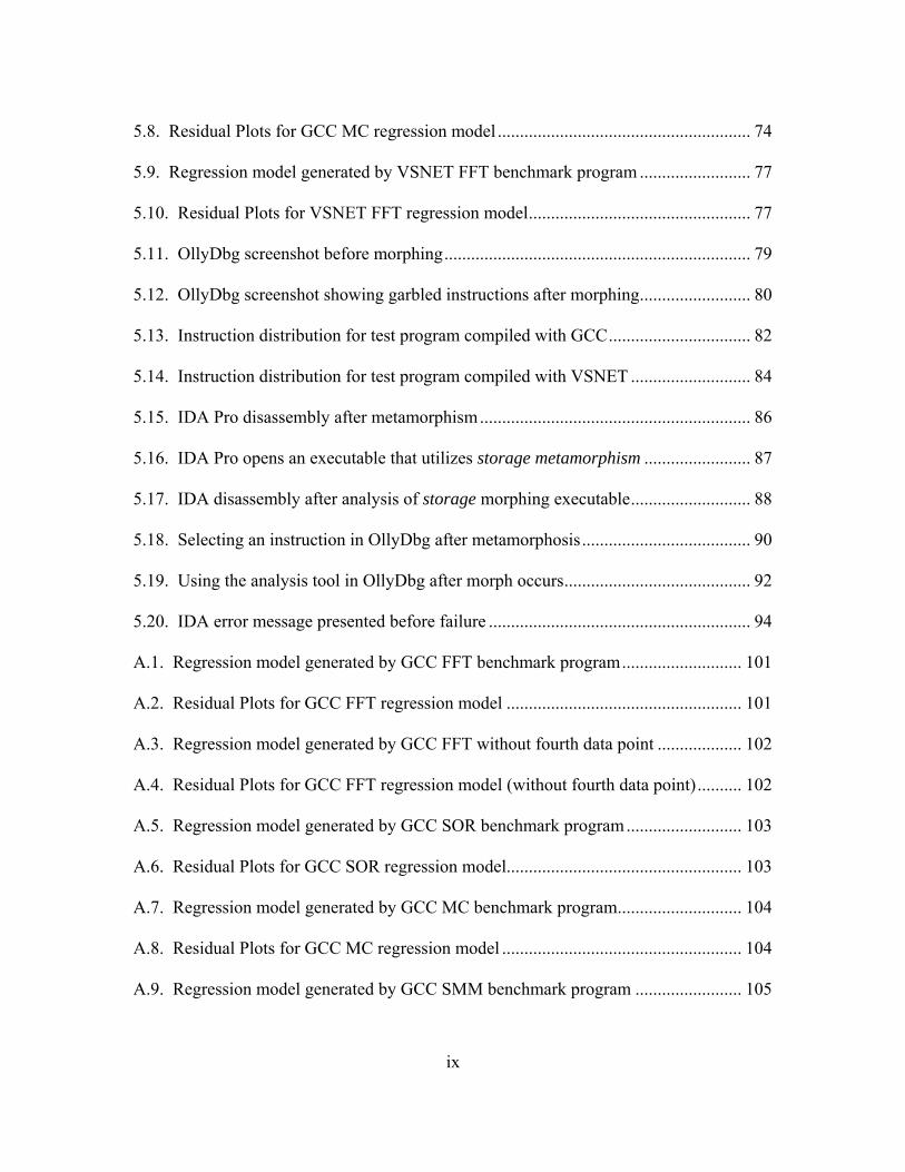
5.8. Residual Plots for GCC MC regression model ......................................................... 74

5.9. Regression model generated by VSNET FFT benchmark program ......................... 77

5.10. Residual Plots for VSNET FFT regression model.................................................. 77

5.11. OllyDbg screenshot before morphing..................................................................... 79

5.12. OllyDbg screenshot showing garbled instructions after morphing......................... 80

5.13. Instruction distribution for test program compiled with GCC................................ 82

5.14. Instruction distribution for test program compiled with VSNET ........................... 84

5.15. IDA Pro disassembly after metamorphism............................................................. 86

5.16. IDA Pro opens an executable that utilizes storage metamorphism ........................ 87

5.17. IDA disassembly after analysis of storage morphing executable........................... 88

5.18. Selecting an instruction in OllyDbg after metamorphosis...................................... 90

5.19. Using the analysis tool in OllyDbg after morph occurs.......................................... 92

5.20. IDA error message presented before failure ........................................................... 94

A.1. Regression model generated by GCC FFT benchmark program........................... 101

A.2. Residual Plots for GCC FFT regression model ..................................................... 101

A.3. Regression model generated by GCC FFT without fourth data point ................... 102

A.4. Residual Plots for GCC FFT regression model (without fourth data point).......... 102

A.5. Regression model generated by GCC SOR benchmark program.......................... 103

A.6. Residual Plots for GCC SOR regression model..................................................... 103

A.7. Regression model generated by GCC MC benchmark program............................ 104

A.8. Residual Plots for GCC MC regression model ...................................................... 104

A.9. Regression model generated by GCC SMM benchmark program ........................ 105

ix

A.10. Residual Plots for GCC SMM regression model ................................................. 105

A.11. Regression model generated by GCC LU benchmark program .......................... 106

A.12. Residual Plots for GCC LU regression model ..................................................... 106

A.13. Regression model generated by VSNET FFT benchmark program .................... 107

A.14. Residual Plots for VSNET FFT regression model............................................... 107

A.15. Regression model generated by VSNET SOR benchmark program ................... 108

A.16. Residual Plots for VSNET SOR regression model.............................................. 108

A.17. Regression model generated by VSNET MC benchmark program..................... 109

A.18. Residual Plots for VSNET MC regression model ............................................... 109

A.19. Regression model generated by VSNET SMM benchmark program.................. 110

A.20. Residual Plots for VSNET SMM regression model ............................................ 110

A.21. Regression model generated by VSNET LU benchmark program...................... 111

A.22. Residual Plots for VSNET LU regression model ................................................ 111

x

List of Tables

Table Page

4.1. Average morph point execution time for 1 billion iterations.................................... 53

5.1. MME performance summary.................................................................................... 64

5.2. GCC baseline performance summary ....................................................................... 65

5.3. GCC morph point performance summary................................................................. 65

5.4. GCC morph point calls and execution time per morph point ................................... 66

5.5. GCC baseline performance summary ....................................................................... 71

5.6. VSNET baseline performance summary .................................................................. 75

5.7. VSNET morph point performance summary............................................................ 76

5.8. VSNET morph point calls and execution time per morph point .............................. 76

5.9. Instruction reach experiment results for GCC compiler ........................................... 80

5.10. OllyDbg instruction reach results for VSNET compiler......................................... 83

5.11. Subroutine reordering function performance summary.......................................... 89

xi

METAMORPHISM AS A SOFTWARE PROTECTION FOR NON-MALICIOUS CODE

1. I. Introduction

1.1. Background

Before the early 1900s, many sicknesses and infections—even from minor

injuries—resulted in death. The absence of antibiotics contributed to a high mortality

rate allowing infections to kill literally millions of people. Fortunately, Ernest Duchesne

and later Alexander Fleming discovered that penicillin kills the bacteria that inevitably

caused death [Lew95]. Although this “medical miracle” has saved countless lives, its

discovery comes from an unlikely source, mold.

Although not generally considered a legitimate source of software protection

ideas, state-of-the-art malware programs take extraordinary efforts to protect themselves.

In fact, many of the tactics adopted by computer viruses are in general use in the non-

malicious software community. The impetus for this research stems from the belief that

many protections found in malware have applications for non-malicious programs. This

approach is certainly out-of-the-box thinking.

For instance, the software protection community has not yet considered

metamorphism as a software security mechanism. Meanwhile, computer viruses are

increasingly using metamorphism as a protective measure against signature detection

[Szo05]. However, metamorphism has other applications, such as anti-reversing, anti-

tamper, and even anti-piracy.

1

Many current standard software defenses, such as encryption and obfuscation, are

static. These static defenses do not change during the lifecycle of the software

application. Furthermore, users normally apply these protections in tandem, because they

often complement one another. While this research does not suggest discarding these

static protections by any means, it does advocate that adding dynamic protections, such

as metamorphism, will increase the overall defensive strength of the software protections.

1.2. Research Goal and Objectives

The use of metamorphism as a defense in non-malicious software appears to be a

new approach. A single reference was found that used a form of self-modification for

generating registration keys to protect against piracy [YiZ04].

Since metamorphism is in its infancy (in the non-malicious software world), this

research answers some basic questions. The research goal is to determine if metamorphic

transformations have predictable execution times. More specifically, this research

develops regression models to evaluate execution time overhead of basic metamorphism

transforms. Additionally, this study investigats the capabilities of metamorphic

transforms of subroutine reordering and opcode shifting as anti-disassembly and anti-

debugging protections. A by-product of this is a set of general implementation

procedures based on the experimental findings.

1.3. Assumptions/Limitations

The execution times from these experiments are platform-dependent because of

several factors affecting the experimental outcomes. For example, increasing processor

speed undoubtedly reduces the execution time, as do compiler optimizations.

2

1.4. Implications

The implications of this research are significant. The demonstration of

metamorphic capabilities alone may lead to a new focus area for software protection in

government and civilian communities. The experimental findings indicate that

metamorphism can be incorporated into sensitive applications while maintaining a degree

of confidence that performance requirements will still be met.

Further metamorphism studies may show that strategic self-modification

significantly bolsters the overall software protection level. If a metamorphic program

requires an attacker to possess increased skill to reverse engineer, it may further reduce

the pool of capable attackers. Prolonging the time required for an attacker to defeat

software security mechanism translates into dollar savings in the civilian community and

prolonged technology superiority for the military.

1.5. Preview

Chapter II introduces a classification of protective measures found in malicious

software. It also includes a description of the basic functionality of common reversing

tools, such as disassemblers and debuggers. Chapter III presents the design of the

experiment and explains how the study achieves statistically significant results. Next,

Chapter IV describes the design and development of the metamorphic engine used in the

experiments. The chapter presents lessons learned and rationale for the chosen

implementation. Chapter V shows the experimental results and their significance.

Finally, Chapter VI concludes the thesis, recaps the pertinent highlights, and provides

guidance on future research.

3

2. II. Literature Review

2.1. Chapter Overview

This chapter reviews research literature and summarizes standard protections

found in malware. Protections described include anti-disassembly, anti-debugging, anti-

emulation, anti-heuristic, and anti-goat strategies [Szo05]. Some protections are not

easily classified into a single protection category. Nonetheless, this classification

establishes a common basis for consideration. Metamorphism, for example, can serve as

an anti-disassembly as well as an anti-debugging protection. This defense technique is

the primary target of this research.

2.2. Introduction

Researching malware protective measures can provide new methods and ideas for

protecting sensitive software systems. Although there are many distinctions between

virus writers and the software protection community, there are also numerous similarities

between the two. For instance, preventing reverse engineering and tampering is a

common goal for both.

Common defensive strategies for software protection use many of the same

armoring techniques found in malware. The non-malware community commonly uses

encryption, obfuscation, and anti-debugging techniques for software protection.

Protection schemes often do not employ a single protection method but rather a

compliment of defenses. Each fortification has certain inherent vulnerabilities that an

attacker can target, but other complimentary protections minimize these weaknesses. For

instance, obfuscation helps to protect an encrypted program once it is decrypted.

4

In many cases, the only significant difference between the software protection

community and malware developers is the individuals’ motivation. The non-malicious

software protection community has a wide array of interests from preserving intellectual

property to safeguarding military weapon systems. In the malware world, the authors

seek to gain personal glory by maximizing their viruses’ propagation time, to expose

software vulnerabilities publicly, and to satisfy personal curiosities.

Since both malware and protection authors have similar goals, a reasonable step

for the software protection community is to consider some of the unique defensive

measures used in malware. For instance, some malware applications use a technique

referred to as metamorphism to evade signature-based anti-virus scanners. Although

virus authors use metamorphism primarily for avoiding detection, this defense has other

applications for the software protection community. Metamorphism—like the other

traditional protections—is not sufficient alone. For illustration, encryption only protects

a program until decryption. On the other hand, metamorphism only protects when the

target program is subject to change. If attackers take a snapshot of a metamorphic

program (and no longer allow it to change), they overcome all the protection

metamorphism itself offers. However, metamorphism is another complimentary

protection mechanism.

2.3. Relevant Research

In order to understand other applications for malware defenses, one must first

research its origin. This section highlights many sources referenced by this research to

understand malware defenses and the difficulties observed in overcoming them.

5

Peter Szor’s The Art of Computer Virus Research and Defense describes many

defensive strategies used in malware [Szo05]. He classifies many malware defensive

strategies and discusses many challenges that the anti-virus community faces when

reverse engineering malware applications.

Eldad Eilam presents similar information, but from a general reverse engineering

perspective. He describes basic and advanced software reverse engineering concepts in

his book, Reversing: Secrets of Reverse Engineering [Eil05]. He also discusses anti-

disassembly and anti-debugging protections as well as malware reversing and the

difficulties faced by malware defensive strategies.

Collberg, Thomborson, and Low propose a detailed classification of obfuscation

techniques in A Taxonomy of Obfuscating Transformations [CoT97]. The authors outline

an in-depth taxonomy for uniquely identifying particular obfuscation techniques.

Metamorphism has a strong parallel to many of these obfuscation transforms with one

key difference. Metamorphism acts as a dynamic obfuscator, which extends the static

obfuscation techniques.

Christodorescu and Jha describe the difficulties that anti-virus scanners have

detecting obfuscated viruses. They also portray the battle between virus authors and anti-

virus developers as “an obfuscation-deobfuscation game” [ChJ03]. The authors also

implement their detection method in a tool, the static analyzer for executables (SAFE),

and show that it is significantly more effective than at least three current anti-virus

products at detecting morphed code.

6

Sung et al. propose another seemingly more efficient detection method for

morphed malware in their static analyzer of vicious executables (SAVE) basing

signatures on API call sequences [SuX04]. Their simplistic approach is to ignore many

common malware obfuscations, which makes detection even more efficient. Xu et al.

also claim that SAVE is significantly more efficient than SAFE in their comparison

experiment [XuS04]. Finally, Gergely Erdélyi discusses stealth techniques in malware

and suggests motives of virus writers [Erd04].

2.4. Protection Categories

Virus armoring against reverse engineering includes a wide array of techniques to

hinder anti-virus developers [Szo05]. In the simplest sense, anti-disassembly tactics

confuse disassemblers and reverse engineers as well as hiding or masking (e.g.,

encrypting) instructions. Successfully confusing disassembly tools ultimately requires

human intervention to overcome. Anti-debugging techniques include using common

debugger resources (e.g., debug registers and the stack), active detection of a debugger,

and executing in memory space difficult for debuggers to follow. These techniques

normally result in either the debugger losing program state or improper program

execution. Similarly, anti-emulation tactics target emulators by consuming resources or

relying on obscure API calls the emulators do not model. Finally, malware uses anti-goat

techniques to avoid infecting bait files. A bait file is a simple executable file with known

file content such as a series of no-operation (NOP) assembly instructions that do nothing.

When a virus infects a bait file, it is simpler for anti-virus researchers to observe exactly

what portions of the executable the virus alters during infection.

7

Retroviruses, an additional category of malicious defenses, actively wreak havoc

on defensive programs such as anti-virus scanners and firewalls [Szo05]. They also fight

back when they detect tools that an attacker uses to analyze (or tamper) with them.

2.4.1. Anti-disassembly

Anti-disassembly techniques defend software against static analysis by an

attacker. The defender can apply a variety of methods to accomplish this. Some

techniques employed are unique, such as encryption and obfuscation. Encryption makes

a program completely unreadable until after it is decrypted. Obfuscation takes another

approach by making an unencrypted program virtually unreadable by dramatically

increasing its complexity.

Disassemblers operate in various ways to provide a correct program disassembly.

A simple linear sweep disassembler sequentially disassembles instruction code [Eil05].

NuMega’s SoftICE [Sof06] and Microsoft’s WinDbg [Win05] are popular linear sweep

disassemblers.

Recursive traversal disassemblers actually disassemble and analyze the

instructions themselves to determine the control flow and where disassembly should

resume (i.e., where next instruction boundary begins). Oleh Yuschuk’s OllyDbg [Oll05]

and DataRescue’s IDA Pro [IDA06] are popular recursive traversal disassemblers.

To demonstrate the differences between the two types of disassemblers, consider

the following obfuscated program consisting of inline assembly and a print statement

shown in Figure 2.1. This program performs an opcode shift. Opcode shifts introduce

data bytes into the code flow and include program logic to ensure the processor never

8

executes the data bytes. The inserted data bytes serve as false opcode prefixes. The

disassembler mistakenly assumes these data bytes are a legitimate prefix for another

instruction. Any remaining bytes needed for the false instruction are shifted from the

subsequent (real) instructions. This confuses disassemblers, which causes them to

potentially display a series of mangled instructions. The inline assembly (_asm

command) block shows both the logic and one data byte. In the program shown, the

inline assembly code instructs the processor to jump over a data byte (the 0x00 byte

generated by the _emit command in this case) to the label named L1. Since nothing

follows the label, the control flow returns to the C code and executes the printf

instruction.

{ _asm { jmp L1 ; logic to “skip” data byte _emit 0x00 ; inserted data byte L1: } printf("Hello, World!!!\n"); return 0; }

Figure 2.1. Inline assembly and C code snippet that prints “Hello, World!!!”

The two types of disassemblers produce dramatically different disassemblies of

the above code as shown in Figure 2.2. Notice how the minor obfuscation of the single

data byte (0x00) completely baffles WinDbg, a linear sweep disassembler, but does not

fool OllyDbg, a recursive traversal disassembler. OllyDbg is more robust, because it not

9

only translates the JMP instruction, but also considers the instruction’s function when

determining where to resume disassembling. This example also shows how WinDbg

misses the correct disassembly of the next four instructions and only resynchronized on

the return instruction (RET and RETN). The instruction reach of the opcode shift is the

number of instructions missing from the original (or correct) disassembly. For this

example, the instruction reach for the opcode shift in WinDbg is four, because WinDbg is

missing four instructions from the correct disassembly shown in the OllyDbg output.

Figure 2.2. Disassembly of linear sweep and recursive traversal disassemblers

WinDbg (linear sweep) output: 00401000 EB 01 jmp 00401003 00401002 00 68 D8 add byte ptr [eax-28h],ch 00401005 70 40 jo 00401047 00401007 00 E8 add al,ch 00401009 06 push es 0040100A 00 00 add byte ptr [eax],al 0040100C 0083 C40433C0 add byte ptr [ebx-3FCCFB3Ch], al 00401012 C3 ret

OllyDbg (recursive traversal) output: 00401000 EB 01 jmp short 00401003 ; logic 00401002 00 db 00 ; data byte 00401003 68 D8704000 push 004070D8 ; (printf 00401008 E8 06000000 call 00401013 ; instr.) 0040100D 83C4 04 add esp,4 00401010 33C0 xor eax,eax 00401012 C3 retn

Various opcode prefixes shift the code by different shift amounts. The shift

amount is the number of bytes that the disassembler takes from the instruction after the

data byte (false opcode prefix). In this example, the shift amount is two, because the

10

disassembler absorbs the next two bytes (the 0x68 and 0xD8). Opcode shifts do not

always result in a sequence of mangled instructions. Stealthy opcode shifts cleanly

absorb subsequent instructions by aligning on a correct instruction boundary. In the

above example, an opcode shift with a shift amount of five bytes (a five-byte shift) would

completely absorb the PUSH instruction and leave the CALL instruction untouched.

Opcode shifts that do not align on a correct instruction boundary are non-stealthy.

The recursive traversal disassembler is harder to fool than the linear sweep

version. However, the fact that recursive traversal disassemblers rely on the instruction

itself to determine the address to resume disassembly is a vulnerability. If presented with

two equally viable options or an abnormal program execution flow, even a recursive

traversal disassembler has difficulty.

One primary focus of anti-reverse engineering is the prevention of static analysis

of the protected code in a disassembler. Malware employs a wide range of strategies to

accomplish this goal. Obvious disassembly techniques include encryption and

compression (or packing) of the binary executable. Obfuscating the final executable

complicates analysis and reverse engineering. In some cases, applying obfuscation

transformations to the binary executable, such as opcode shifts, confuses disassemblers

and requires human intervention.

2.4.1.1. Encryption

The general structure of malware programs that use encryption (or packing)

includes an executable decryptor section, which is unencrypted, as well as an encrypted

(or packed) section [Szo05, Eil05]. The program uses the decryptor to decrypt the

11

remaining portion of the malware application immediately prior to its execution to protect

the program contents for as long as possible.

Software authors can use strong encryption to delay the disassembly of their

applications. Without the proper decryption key or algorithm, the encryption defeats both

static and dynamic analyses. An attacker must either defeat the encryption algorithm

itself or find another way to obtain the decryption key. After obtaining the key, the

attacker can decrypt the encrypted binary revealing the binary executable. This situation

is optimal for reverse-engineering, because the reverser can perform static and dynamic

analysis on the deciphered application. In many cases, the reverser can dynamically

analyze the program, because many programs decrypt themselves during execution.

The decryption method can use an internally or externally stored key. A

developer can store the decryption key in the program—possibly in an encoded form or

calculate it at runtime. On the other hand, the developer could store the key external to

the program either on a local hardware device or on a remote key server. In the latter

scenario, the program requests the key from the key server at runtime and the server

would only provide the encryption key after authenticating the client.

A malware application’s weakness is that it must eventually use the appropriate

decryption key or employ the decryption algorithm [Eil05]. Virus writers do not use the

key server approach for fear of prosecution (and obvious lawsuits). Nevertheless,

without the decryption key, their malicious software does not execute properly.

Therefore, typical malware applications do not use strong encryption because of the

performance and storage overhead. The malware writer wants the code to execute, so

12

they must supply the decryption key or algorithm anyway. For these reasons, malware

ciphers normally are simple, such as a short XOR, shift, or offset cipher. The

W95/Fix2001 worm [Fix99] uses weak encryption to conceal a destination e-mail address

to which it sends stolen account information [Szo05].

The main reason malware programs use encryption is to evade detection and to

obfuscate itself to prevent disassembly. Typically, malware applications encrypt the

main program body with a new encryption key for future generations to avoid detection.

These techniques force anti-virus researchers to develop signatures targeting the

relatively small (albeit static) decryptor sections of malware programs. There are other

methods of avoiding detection such as stealth, but the general purpose is the same, to

make the task of anti-virus researchers more difficult [Erd04].

Encryption has several weaknesses. In most cases, a reverser can use an

unpacking program to decrypt an executable automatically [Eil05]. However, if the

program generates or builds the key at runtime, the attacker cannot unpack the program

automatically. Another tactic is to wait until the program decrypts itself in memory and

simply capture the clear code from memory. Some malware authors mitigate these

weaknesses by decrypting short segments of their code into memory immediately prior to

execution. By doing this, the reverse engineer has a more difficult and potentially tedious

job.

2.4.1.2. Compression and Packing

Compressed (or packed) and encrypted malware share the same architecture.

Compressed malware has a small, uncompressed section that decompresses the remaining

13

portion of the program before execution. The compression of the malware application

offers a distinct advantage over encryption. The program is likely much smaller than an

encrypted form of itself.

Compression and packing causes problems for disassembly. In most cases, static

analysis is not possible until the program decompresses or unpacks itself. Dynamic

analysis is possible when the packing mechanism is present and the malware correctly

unpacks itself. If the malware fails to unpack itself correctly, erratic behavior results.

Malware authors have over 500 different packer programs to choose from, but not all of

these are effective [Szo05].

Compression tactics save precious malware space, and they hinder the reverse

engineering process. Once a user discovers malware in the wild, researchers quickly

develop anti-virus signatures and removal programs to eradicate them. Slowing down the

anti-virus companies’ analysis of the malware code effectively delays the development of

anti-virus signatures and removal programs allowing them to propagate further and cause

more damage. The infamous W32/Blaster worm [Bla05], an example of packed

malware, uses the UPX packer for both compression and obfuscation [Szo05].

2.4.1.3. Obfuscation

Obfuscation is a common technique in software protection to reduce an

application’s understandability. Defending software from reversing runs counter to the

tenets of software engineering. To promote maintainability, software practitioners advise

developers to write more understandable code and to use comments to promote

understanding by others. Obfuscation is the opposite of this, because the goal is to make

14

the practitioner’s code even more confusing than it was originally. The intention is to

delay an attacker—not necessarily to prevent the attacker from successfully reverse

engineering the code. If this delay becomes significant enough, the presence of heavily

obfuscated code might be a deterrent to an attacker. The quality of obfuscation tactics is

a function of four measures: potency, resilience, stealth and cost [CoT97].

Potency measures indicate the relative difficulty in understanding software as

originally designed versus obfuscated code. Practitioners can use software complexity

metrics, such as complexity profiling, to measure the potency of a particular obfuscation.

Resilience measures how effective an obfuscating transformation is against an automated

deobfuscator. The amount of development time to build an effective deobfuscator and

the execution time and space needed by such a tool are both acceptable measures for

resilience. Stealth measures reflect on how easy the process is to identify obfuscated

parts versus non-obfuscated parts of the application. Finally, cost measures specify how

much impact the obfuscation has on the execution time and space of the original

program.

Collberg et al. [CoT97] propose four obfuscation transformation categories:

layout, data, control, and preventive. Each category of transformation has its own unique

measures of potency, resilience, stealth, and cost. The main goal is to achieve the desired

level of obfuscation (and hopefully reverse engineering difficulty) while staying within

the cost budget in execution time and space.

Layout Transformations. Layout transformations target source code and include

such tactics as changing variable identifiers to another form—possibly gibberish—that

15

lends no understanding to the program based on their name and their use in the program.

Changing formats and inserting or deleting comments is also used in this transformation.

These types of modifications target source code—not the binary executable with the

possible exception of the symbol table. These types of transformations have a variable

potency, low resiliency, and very low stealth. However, layout transformations are very

favorable with respect to cost, because the transforms do not significantly affect the final

application’s execution time and space [CoT97].

This tactic is most useful in situations where security experts may inadvertently

(or intentionally if an insider threat) expose source code to attackers. In certain

situations, this disclosure is inevitable, but it is also a common practice for organizations

to refrain from inadvertently divulging the source code to adversary reverse engineers. In

some of these cases, the software protection community can adopt other security

precautions (e.g., physical security, non-disclosure agreements, etc.) to prevent such

disclosure.

Data Transformations. Data transformations increase the complexity of data

structures. An example of these transformations is changing the representation of a

Boolean to encoded values of the ordered pair of two separate integers. Although the

original Boolean can only have one of two values, the ordered pair of two integers can

assume a large number of different values when represented by two typical 32-bit

integers. Building strings at runtime instead of hard coding a constant string can

complicate the attacker’s task of locating a specific part of a program. This can be used

as a license or decryption key protective measure. Data aggregation transformations,

16

such as decomposing arrays and classes or merging primitive variables, increase potency

and resilience. An obfuscation transform can scramble array indices to randomize the

order that the program stores data. Specific data transformations have various levels of

potency, resiliency, stealth, and cost [CoT97].

An interesting example of data transformation in viruses is the absence of

standard API names in the program. Instead of using common strings that anti-virus

applications can search for, malware uses checksum values of API function names to find

them during execution. The absence of common search strings confounds anti-virus

scanners and therefore obfuscates the malware code. The W32/Dengue virus [Den00]

does not use any function name strings to access the Win32 API [Szo05].

The SAVE scanner claims to be highly efficient by basing malware signatures

primarily on API call sequences [XuS04]. However, SAVE disassembles the executable

and searches for key opcodes (namely CALL instructions). As a program executes, it

may overwrite seemingly benign instructions with CALL instructions that SAVE misses.

These camouflaging techniques can prove problematic for purely static analyses. Besides

using the API name checksums, a CALL instruction can be hidden by pushing appropriate

data onto the stack (e.g., the return address) and performing a JMP instruction with the

address of the desired API function [IA105]. When the called function returned, it would

pop the correct return address off the stack.

Control Transformations. Control transformations obscure the program flow of

the application and make it very difficult to follow [CoT97]. An obfuscator can create

opaque predicates or calculations that always result in a true or false, to provide stealth to

17

other obfuscations. These opaque predicates create false branches that waste reversers’

time. The attacker or their deobfuscator must thoroughly analyze these constructs, which

can include non-obvious, multiple-variable expressions, to determine if a particular

branch is possible. Opaque constructs camouflage dead code spurs inserted as alternative

branches, which further complicates reverse-engineering efforts.

Other forms of control transformations include meaningless code injects as well

as the removal of real procedural abstractions (inlining) and the insertion of false

procedural abstractions (outlining). Concurrent programming constructs (multithreading)

are one of the most effective methods of obfuscating static analysis although it can be

costly in terms of performance. The application can spawn decoy threads as well as split

actual program logic into multiple threads while using synchronization points to control

program flow. The obfuscator can disrupt the locality of program code by changing the

order of statements to increase the distance between logically related statements.

Reversers tend to rely on locality to understand a program because locality implies a

logical order [Eil05]. Other control transformations include loop unrolling, code

flattening, and recursion.

Preventive Transformations. In contrast to the previous three conversions,

preventive transformations focus almost entirely on hindering automated deobfuscation

tools. This approach includes both inherent and targeted preventive transformations.

Inherent preventive transformations exploit known automatic deobfuscation techniques.

For instance, a deobfuscation tool may analyze an obfuscated FOR loop that executes

backward and realize that it could convert the loop to forward execution. However, by

18

placing a bogus data dependency variable in the loop, its obfuscation may be too

ambiguous for the deobfuscation tool. Targeted preventive transformations exploit

known weakness of specific automated deobfuscation tools. This tactic may only work

against specific versions of the tool or under certain conditions [CoT97].

2.4.1.4. Self-Mutation

Many malware applications routinely change their appearance to avoid detection.

Self-mutation can take the form of polymorphism and metamorphism. Self-mutation can

change the code to be completely different from previous generations or change certain

parts to confuse detection programs. Insertion or deletion of garbage code (similar to

obfuscation techniques described earlier) is also a form of self-mutation. Malware

benefits from its obfuscation, which confuses reverse engineers, but the ability to avoid

detection is the primary advantage. All of these strategies have the goal of avoiding anti-

virus detection programs and complicating the development of an exhaustive set of

malware signatures.

Oligomorphism. Oligomorphic viruses alter their decrypters for subsequent

generations [Szo05]. Anti-virus software has little choice but to develop signature

patterns based solely on these smaller decryptor sections of malware code, because

viruses normally change their encryption keys during propagation. Using multiple

decryptors during propagation complicates the detection process. The malware

community develops numerous decryptors rather easily. Oligomorphic tactics in

malware are effective against signature scanning, because future generations (infections)

19

often do not resemble their ancestors at all, since the historically static portion of the

program is now dynamic.

To complicate the discovery, some malware employ a completely different

decryptor during replication. The new decryptor could simply be a different

implementation of the same algorithm or a new algorithm altogether. Nevertheless, this

approach complicates the construction of suitable anti-virus signatures, because scanners

need multiple signatures to ensure success against a single virus.

Some viruses use a probability scheme to complicate matters further. For

example, a particular decryptor may only be used occasionally. Therefore, not only do

anti-virus researchers need to develop multiple signatures, but to accurately recognize a

particular virus, they must develop an exhaustive set of signatures for the virus in

question. The Whale virus [Wha06] uses oligomorphic tactics and carries dozens of

different decryptors as it replicates [Szo05].

Polymorphism. When related to malware, the term polymorphism has a different

meaning than its standard meaning in software engineering. The term polymorph literally

means many forms. In software engineering, this refers to a function or method having

many forms depending on the invoking class. In malware, the term polymorphism refers

to the ability of the decryptor to assume many different forms in future generations.

Polymorphic viruses do not keep a small set of decryptors, but rather mutate their

decryptors possibly generating millions of different forms. Although the current

decryptor can mutate by simply inserting garbage instructions, there are more advanced

polymorphism implementations. In 1991, the Bulgarian virus writer Dark Avenger

20

released a modular, polymorphic mutation engine called MtE [Szo05]. This tool accepts

virus code as input and transforms it into a polymorphic virus. By passing certain

parameters to the mutation function, the MtE outputs a polymorphic decryptor and an

encrypted virus body. The ability to develop an exhaustive set of signatures to detect

polymorphic viruses is a function of the number of unique decryptors that a polymorphic

engine can develop. However, once researchers thoroughly analyze a polymorphic

engine, they can target similarities that all viruses made with the same engine share.

Metamorphism. Metamorphic viruses do not need decryptors, because they

manipulate themselves altering their appearance beyond recognition. One can think of

metamorphism as low-scale obfuscation that occurs during propagation. Various viruses

implement a variety of metamorphic techniques including manipulating and recompiling

source code, reordering binary subroutines and independent instructions, replacing

instructions with equivalent instructions, reversing conditions, and inserting garbage

instructions. Each alteration generates a number of new forms the virus can assume,

which makes the task of developing an effective virus scanner difficult. As an extra

protection, when metamorphic viruses replicate, they do not assume a form akin to their

parents.

The W32/Apparition virus [App05] carries its source code with it and recompiles

itself whenever it finds a compiler installed. Before recompiling, W32/Apparition

performs obfuscating layout transformations that mutate its source by inserting and

removing junk code. By mutating the source code instead of the binary, the compiled

binary looks quite different in future generations [Szo05]. Although carting source code

21

around is somewhat foolish from a software protection viewpoint, other methods of

metamorphism still have potential applications.

Some viruses, like W32/Ghost, change the order of subroutines to generate a large

potential set of mutations for progeny [Szo05]. Although not the only metamorphic

change possible, changing the order of subroutines is a good example to show how many

variants are feasible. W32/Ghost has 10 subroutines and it can generate up to

possible permutations based on subroutine reordering alone. Anti-virus

software can still detect these different combinations based on search strings, but this

type of scanning is not as effective since the target string could modify itself and

effectively hide from the scanner.

10! 3,628,800=

For many assembly instructions, alternative instructions (or a series of other

instructions) can have equivalent functionality. For instance, the assembly instruction

XOR EAX, EAX is the equivalent of SUB EAX, EAX as both set the EAX register to

the value of zero. The only difference between the two functions is the state of the AF

flag [IA205]. There are other equivalent, single-instruction methods of setting a

particular register value to zero as well.

Inserting garbage statements is also an effective method of foiling anti-virus

signature matching. In fact, in their experiments with four viruses, Christodorescu and

Jha found that commercial anti-virus products failed to detect the viruses after simple

obfuscation [ChJ03]. Perhaps the most surprising finding was the fact that the only

obfuscations required to evade the scanners were NOP insertions and code transpositions.

22

These methods, especially when used together, make the detection of such malware

applications very difficult—even for commercial scanners.

The W32/Evol virus [Evo00] uses even more metamorphic techniques. This virus

exchanges assembly instructions for others with equivalent functionality, changes the

order of subroutines, inserts garbage statements, and even changes the values of magic

numbers [Szo05]. (Magic numbers are direct, hard-coded references to numbers instead

of traditional constants in code [Wik06].) By modifying all of these components, the

W32/Evol virus becomes even more difficult to detect. Anti-virus scanners normally

detect viruses by searching for a signature within the virus, but as the signature becomes

smaller, more missed detections and false alarms result.

Furthermore, these mutations are probabilistic. In practice, a virus may only use a

particular morphing transform occasionally. This chance occurrence complicates the

anti-virus reverse-engineering process more, because a morphing might not ever occur

during examination. Rare mutations complicate the task of developing a reliable scanner

to detect the particular morphed version.

Malware metamorphoses primarily during the propagation stage. However,

metamorphosis can occur at other milestones (e.g., prior to or after execution) changing

the form of the executable often. An advanced metamorphic engine can metamorphose

the program even during execution.

Metamorphism adds another level of difficulty to reversing a control

transformation obfuscation such as a function caller. Consider a simple function caller

that takes an enumerated argument to determine which function to call. Figure 2.3 shows

23

the C code for a simple function caller procedure. (The flowchart-like symbols to the left

of the source code are a control structure diagram courtesy of jGRASP [jGR04].) The

function caller manages which function to execute. In this case, the developer relays

calls to specific functions through the function caller. The function caller architecture

serves as a control obfuscation, because a reverser would have difficulty determining the

target function to which the function caller actually relays the call. Metamorphism can

add complexity to this issue by randomly reordering the target functions (i.e., f1 and f2

in this example). Since only the function caller needs to know the function locations, this

Figure 2.3. Example source code for simple function caller

24

simplifies function reordering. After reordering, direct calls to the target functions will

likely cause the program to fail, because the function boundaries have changed.

Some other potential metamorphic transforms, whose existence in malware is

uncertain, can provide more obfuscation as well. For example, transforming a random

sequence of instructions into a subroutine (outlining) [Eil05] has minimal impact on

function, but certainly changes the structure (or form) of the program. Any registers

manipulated in the subroutine become desirable side effects for the defender. Using

recursion for short loops adds complexity to the executable at the expense of some stack

overhead. Finally, multithreading transforms can fracture a program into multiple

threads of execution further complicating reverse engineering efforts.

2.4.2. Anti-debugging

The ultimate goal of anti-debugging is to prevent reverse engineering of software

through dynamic analysis. Programs have many ways to detect if a debugger is present.

Anti-debugging is a basic defense against dynamic analysis and there are diverse methods

to thwart an attacker’s efforts.

Debuggers execute code within the debugger’s controlled environment. Two

basic features that a debugger offers are the ability to set a breakpoint, where the program

execution is interrupted and the debugger regains control, and the ability to step through

the program one instruction at a time.

There are two types of breakpoints: software and hardware. When setting a

software breakpoint, the debugger usually replaces the first byte of an instruction in

memory with a breakpoint interrupt (INT 3)—0xCC on an Intel processor. When the

25

processor sees the 0xCC byte, it generates an interrupt that the debugger catches. Once

received, the debugger replaces the 0xCC byte with the original first byte of the

instruction and pauses program execution for the user.

The processor itself manages hardware breakpoints via its debug registers

[IA305]. Since the processor manages the hardware breakpoint, the debugger has no

need to set breakpoint interrupts in the process memory space. However, the processor

can only manage a limited number of hardware breakpoints due to resource limitations

(i.e., a limited number of debug registers are available for storing breakpoint addresses).

The debugger provides the functionality to step through the program by enabling

the processor’s trap flag [Eil05]. Enabling this flag causes the processor to generate a

single-step interrupt (INT 1) after executing each instruction. The debugger can catch

these instructions and regain control allowing the user to analyze the state of the

debugged program.

Many anti-debugging protections try to cause the debugger to lose state. As a

debugger executes a program, it must keep track of the program’s state (i.e., variables,

register values, stack contents, etc.). However, the debugger uses these resources as well,

because the operating system shares these resources among several tasks (multitasking).

Since the debugger cannot query the system state while the target process (of the

debugger) executes, it must rely on the state information that it has gathered. Anti-

debugging techniques include any methods that cause the debugger to lose or change any

of its state information.

26

2.4.2.1. Debugger Interrupt (INT) Manipulation

Malware applications commonly hook interrupts causing debuggers to lose the

executing code’s context [Szo05]. Viruses hook interrupts by loading themselves into

memory and modifying the interrupt vector table (IVT) to point to themselves instead of

the normal interrupt handler. This places the virus at the beginning of the interrupt call

chain for that particular interrupt. Viruses commonly hook the single-step (INT 1) and

breakpoint (INT 3) interrupts. As previously mentioned, debuggers commonly use

these interrupts for stepping through and pausing programs for analysis. Some viruses

use these interrupts in their decryption routines. Other viruses overwrite the interrupt

handlers that debuggers normally use with interrupt return (IRET) instructions ultimately

causing debuggers to lose state.

Another defense is to disable the keyboard. This tactic prevents reverse engineers

from easily stepping through the program code, because they cannot use their

keyboards—often a required resource for debugging. Disabling debugger hotkeys stops

users from breaking into a program after it has started execution. The Cryptor virus

actually uses the keyboard buffer to store its decryption key [Szo05]. When a debugger

runs the program, it also uses the buffer and thereby destroys the decryption key.

2.4.2.2. Guarding Against Debugger Breakpoints

Other malware applications use checksums to verify that the code executing in

memory remains unchanged. The program calculates a checksum of the malware code

and stores it. Running the code in a debugger changes the code by inserting software

breakpoints (INT 3 – 0xCC) in place of the first byte of assembly opcodes. The

27

debugger must keep track of the replaced byte to continue execution correctly. Even

though it replaced a byte of an instruction opcode, the debugger displays the correct byte

to the user for readability purposes. This additional byte changes the checksum of the

actual program in memory when the malware application attempts to verify its integrity.

Some viruses also decrypt themselves backwards overwriting software

breakpoints in the process. The W95/Marburg virus [Mar98] uses this technique. The

software protection community could adopt methods like these as well—at little cost in

program performance and size.

Viruses can use the hardware debug registers (e.g., registers DR0-DR7 on Intel

architectures) to cause problems for some debuggers. Debug registers are privileged

resources used by debuggers to monitor breakpoints [IA305]. Viruses could disable all

breakpoints by toggling them off via the debug control register, DR7.

Incidentally, some viruses are self-annealing, which means they can detect and

correct small errors. Self-annealing viruses correct or disable breakpoints and thereby

exhibit anti-debugging characteristics. The Yankee Doodle virus employs such tactics

[Szo05].

2.4.2.3. Observing and Using Debugger Resources

Another trick malware authors use to detect debuggers is simply to observe the

top of the stack. Debuggers often push trace information onto the stack during execution,

which a malware application can easily detect. If a virus detects debugger information on

the stack, it may conceal itself by letting the infected program function normally.

28

In addition to observing the stack, some viruses use the stack to build a decryption

key or to decrypt their programs. If the debugger manipulates the stack as well, the virus

cannot successfully decrypt itself and therefore does not execute (or expose itself to

debugging).

2.4.2.4. Debugger Detection

A direct approach is to invoke an operating system (OS) application programming

interface (API) function such as the IsDebuggerPresent() function in Windows

[MSD05, Szo05]. This particular call returns a Boolean value indicating whether the

current program is executing in a debugger. Although simple to implement, this strategy

is easy to detect by searching for the key string. However, by using checksums of API

functions instead of the function name itself (c.f. Section 2.4.1.3), the malware program

can be obfuscated and avoid key string searches.

Malware can also scan through the registry for debugger keys. If the program

finds a debugger key, the malware may behave in a different manner—perhaps not

executing at all. Such activity can increase the difficulty of the reverse-engineering

process because a reverse engineer must normally locate and disable the anti-debugging

features first.

If a debugger requires loading a particular driver, the virus program could check

for that driver in memory. In addition, the malicious program can scan memory

(including video memory) for other indicators of a debugger’s presence.

29

2.4.2.5. Debugger Obfuscation

Other anti-debugging techniques do not use hooking, detection, or resource

consumption. Many debuggers cannot follow a program during exception handler

execution, which is another situation where the debugger can lose state information and

ultimately fail. Obfuscating the file format or the entry point can confuse debuggers that

work only with standard formats and entry points [Szo05]. In short, any technique that

causes the debugger to trace the wrong execution (or not follow the correct) path should

result in the debugger ultimately losing state and failing.

2.4.3. Anti-Emulation

Emulation mimics a program’s execution. All modeling is necessarily

incomplete, but an emulation is a low-fidelity representation that focuses primarily on

modeling program behavior—not functionality. Simulations, although still imperfect, are

higher-fidelity representations of program execution on another platform. Since it is an

incomplete model of program functionality, many opportunities exist to fool emulators.

Anti-emulation tactics commonly use obscure functions. Many emulators do not

model such functions and some even omit them entirely during execution. Examples of

such functions include coprocessor, MMX (multimedia extension), and undocumented

CPU instructions [Szo05]. Simply using these obscure functions can cause an emulator

to fail by losing state.

Another broad category of anti-emulation techniques uses various denial-of-

service attacks against emulators. A wily defender can exploit an emulator’s limited

resources in similar fashion as the classic denial-of-service network attacks. For

30

example, some viruses decrypt themselves by intentionally brute forcing their own

encryption, which might require millions of emulation iterations to finish decrypting.

The slower emulation process prolongs the time needed to decrypt the virus body for

analysis. Other similar denial-of-service tactics use long, complex loop constructs to

calculate a decryption key. This can fool an emulator into consuming significant

amounts of its available resources (i.e., memory).

2.4.4. Anti-Heuristic

Anti-virus researchers develop heuristic scanners to detect new viruses without

new virus signatures. As with intrusion detection systems, the developer (or user in some

cases) chooses a sensitivity level low enough to detect new viruses, but high enough to

minimize false positives. Commercial anti-virus products commonly use heuristics such

as the file infection area, because many viruses tend to infect either the beginning or end

of files. However, a scanner cannot use the same heuristic to detect viruses that follow

other infection strategies, such as cavity or overwriting infections.

Heuristic pattern matching potentially offers a better solution than traditional

signature-based scanning, because signatures are not needed for each individual virus.

However, detection of an unknown virus is only half the battle; developing a tool that

effectively removes the malicious code and repairs the infected file is the other half.

2.4.5. Anti-Goat (Anti-Bait)

Anti-virus researchers sometimes use special goat (or bait) files to reveal malware

infection techniques [Szo05]. Some of these infection methods are trivial, such as adding

the virus code to the end of the file and replacing the file’s first instruction with a jump to

31

the virus code. Other more advanced infections make the viruses more difficult to detect.

However, tricking a virus into infecting a goat file, which typically consists of a series of

NOP instructions, can easily show a virus’s infection method.

Viruses infect host files in a variety of ways. Prepending and appending viruses

use two of the simplest infection methods by inserting the virus code at the beginning and

end of the host file respectively. A cavity infection targets available areas in the file large

enough to hold the entire virus. On the other hand, a fragmented cavity infection breaks

up the malware code to fit any available cavity in the target host file.

To complicate the anti-virus researcher’s task, virus writers implement anti-goat

protections to prevent casually infecting goat files. Normally, the anti-goat viruses

heuristically determine if infection is appropriate. Some heuristics include not infecting

small files or files containing numerous NOP instructions. However, in the end, virus

writers must strike a balance between their making their programs too reckless or too

cautious in their infection habits. A reckless virus infects most goats, because its

heuristics are too optimistic. On the other hand, a cautious virus is not infectious enough,

because its heuristics are too pessimistic.

2.5. Summary

This chapter introduces the premise that the software protection community

should consider potential applications of unique defensive mechanisms found in

malware. A discussion of common anti-reverse engineering strategies used by malware

authors highlight a category of measures. Anti-disassembly, anti-debugging, anti-

emulation, anti-heuristic, and anti-goat categories loosely capture the broad range of

32

malware defensive techniques. This chapter highlights the similarities between the

software protection strategies of both non-malicious and malicious software authors even

though they have a stark contrast in motivation.

This chapter also introduces the defensive strategy of metamorphism and

describes it as dynamic obfuscation. Several metamorphic transforms can provide useful

protection to non-malicious software.

33

3. III. Methodology

3.1. Chapter Overview

This chapter describes the research experiments. It begins with a presentation of

the research goals and the approach taken to achieve those goals. Following sections

define the system under test, the component under test, and the system services. Next, a

discussion follows of the applied workload and the definition of the performance metrics.

Subsequent sections present the experimental factors and parameters as well as the

evaluation techniques used. Finally, the last section presents the experimental design.

3.2. Problem Definition

3.2.1. Goals

This research assesses the performance overhead of a representative sample of

metamorphic transforms, specifically opcode shifting and subroutine reordering. These

experiments utilize regression models for precisely evaluating performance overhead of

opcode shifting transforms. A final goal of this research is to determine the capabilities

of metamorphic opcode shifting and subroutine reordering. A proposal for

implementation procedures based on experimental findings is presented.

3.2.2. Approach

This research develops a metamorphic engine (MME) that reorders subroutines

and modifies assembly instructions in memory during execution. This engine integrates

with target applications for testing. As mentioned in Chapter 2, there are a large number

of metamorphic transforms. A representative list of metamorphic transforms includes

[Szo05, Eil05]:

34

1. Instruction substitution (replacing instructions with functional equivalents)

2. Instruction reordering (shuffling the order of instructions where possible)

3. Subroutine reordering (shuffling the order of subroutines)

4. Register substitution (shuffling register usage)

5. Recursion insertion (using recursive solutions versus iterative ones)

6. Program fragmentation (arbitrarily breaking up a program into subroutines)

7. Morphing of instructions in pipeline (changing instructions already fetched)

8. Garbage instruction insertion (inserting meaningless instructions)

9. Execution flow altering (changing execution flow (e.g., executing in heap))

10. Opcode shifting (calling/jumping into middle of instruction)

This research develops a MME that implements representative samples of these

transforms. The following sections describe the process for choosing the sample

transforms along with the detailed discussion of the transforms themselves. In this

experiment, the main program contains a call to the MME to modify other parts of the

program. The main program also collects performance metrics for subsequent analysis.

Morph points provide a mechanism for identifying points in a program that can be

modified by the MME during runtime. Each morph point is associated with an address, a

probability for changing, and a set of replacement values. Within a program, an instance

of an opcode shift construct is a type of morph point. Logical replacement values for an

opcode shift morph point include a set of instruction prefixes that cause disassemblers to

display incorrect instructions.

This research defines two sets of experiments to meet the research goals due to

the metrics evaluated. For instance, determining the instruction reach of a morph point

opcode shift requires executing the program inside a debugger. On the other hand,

35

running the performance-based tests inside a debugger generates near meaningless

metrics, because the debugger overhead itself is included.

Two performance experiments evaluate the execution overhead of opcode shifts

(via the morph point constructs described earlier) and subroutine reordering. The time

required to perform each transform (i.e., change the program) is measured in addition to

the execution overhead of the modified functions. These experiments directly measure

the execution time of baseline and metamorphic versions of the same test program. With

these results, the performance overhead of the metamorphic transforms is calculated by

subtracting the execution time for the baseline from the execution time for the

metamorphic version.

Another experiment assesses the instruction reach of an opcode shift construct.

This instruction reach experiment executes within the context of a debugger and the

opcode shift instruction reach is reported while stepping through the code.

3.3. System Boundaries

The system under test (SUT), as shown in Figure 3.1, consists of the CPU, main

memory, the benchmark program, and the debugger. Although applicable to numerous

platforms, many facets of these research implementations are hardware dependent when

the implementation utilizes non-portable, low level constructs like assembly language

instructions.

The components under test (CUT) are the morph points (instances of opcode shift

constructs) and the metamorphic engine. Multiple morph points are inserted into the

36

code where they execute millions of times. The metamorphic engine modifies these

morph points during runtime.

CPU Memory

SUT

BenchmarkProgram

Debugger

Figure 3.1. System Under Test (SUT) definition

3.4. System Services

The MME transforms an executable block of code into a different form with the

same functionality. Two outcomes are possible from this transformation. The following

constitutes a successful metamorphic transform:

1. the program executes and produces the expected output, and

2. any changed block of code executes with the same functional result (code size and execution performance are irrelevant).

37

The MME must always produce successful metamorphic transforms. Intuitively,

the following definition applies for a failed metamorphic transform:

1. the program fails to execute or it produces unexpected output, or

2. any changed block of code does not execute with the same functional result (not considering code size or execution performance).

3.5. Workload

The workload is the NIST SciMark2.0 benchmark suite [PoM04]. This test

program is selected because the C source code is readily available and a prototype MME

(already written in C) integrated easily with it. The suite’s five separate benchmark

programs execute and provide a million floating-point operations (MFLOP) metric. The

benchmark consists of Fast Fourier Transform (FFT), Jacobi Successive Over-relaxation

(SOR), Monte Carlo integration (MC), Spare Matrix Multiple (SMM), and Dense Unit

Lower Matrix Factorization (LU) programs. Each decomposes into a kernel function that

executes the test and a set of utility functions.

3.6. Performance Metrics

The execution performance of the benchmark program is the primary metric. In

particular, any performance loss due to the metamorphic protections of the benchmark

program is quantified. The performance of the MME itself is another key metric.

The instruction reach of the sample metamorphic transforms is assessed using the

number of instructions in the baseline program that a successful morph point can mangle

in the metamorphic program. A mangled instruction is an instruction in the original

38

metamorphic program that does not exist at the same address in the disassembly observed

during runtime. The instruction addresses in the baseline program will not match the

metamorphic program instruction addresses, because the morph point code shifts the

addresses.

Size metrics, such as executable size or memory usage, are not used although they

seem like obvious choices. Metamorphism introduces ambiguities to these terms, and

these ambiguities devalue the potential metrics. For instance, some transforms could

copy code into another segment of memory and execute in the new memory segment

rather than in the text or code segments. The standard definition of executable size would

likely not include these modified instructions.

3.7. Parameters

The system parameters are the system hardware (i.e., CPU, cache, memory, etc.),

the operating system, the compiler, and the metamorphic transforms themselves. Process

execution time is largely dependent on the performance capabilities of the system

hardware. Precautions are taken to minimize effects of the parameters not selected as

factors.

The operating system, Microsoft Windows XP Professional Edition (SP2), is an

important parameter, because it controls the scheduling of tasks on the system—including

the component under test, the benchmark program. Unfortunately, the experiment has

only minor control over the OS scheduler. In order to mitigate the effects of this

parameter, the experiments are conducted on a dual processor computer. Having an

available processor for the OS tends to reduce the influence of the scheduler-driven

39

context switches. The experiment system hardware is a dual processor (Intel Xeon 2.80

GHz) machine.

The compiler is also important, because different compilers produce code of

varying efficiencies. Compiler optimizations change the appearance of the generated

executables significantly. The crux of this experiment, however, is to evaluate the

performance of the morph points—not the effects of the optimizations. The goal, then, is

to generate a metamorphic version of a baseline program that differs only by the presence

of these morph points. For this reason, compiler optimizations are disabled.

The metamorphic transforms chosen include subroutine reordering and instruction

opcode shifting. These particular transforms show promise of dramatically changing the

program appearance with simple modifications to the assembly code.

The single most important parameter for these experiments is the MME and

morph point implementations. An inefficient implementation can result in performance

metrics that hide the effectiveness of metamorphism as a protection. On the other hand, a

reasonable implementation may yield results that imply potential utility. An

overwhelming number of possible implementations exist and the term “reasonable” is

relative. The implementation used is the result of a brief spiral development effort testing

each solution for what is considered to be reasonable efficiency. Using implementation

itself as an experimental factor is beyond the scope of this research.

3.8. Factors

The factors for both the morph point performance and function reordering

experiments are the compiler and the benchmark program. The two levels for the

40

compiler factor are the GCC C compiler (version 3.4.4) [GCC05] packaged in Cygwin

[Cyg05] and the Microsoft Visual C++ .NET (VSNET) compiler from Microsoft

Development Environment (version 7.1.3088) [Vis05]. These popular compilers are

representative of compilers in widespread use. The benchmark program factor has five

levels, the five programs comprising the benchmark suite.

The instruction reach experiment considers three factors: the debugger, the

compiler, and the opcode shift amount. The debugger levels are Oleh Yuschuk’s

OllyDbg (version 1.10) and DataRescue’s IDA Pro (version 4.6.0.809 SP1 32-bit). The

levels of the compiler factor are GCC compiler and the VSNET C compiler. The levels

for opcode shift amount are 1, 2, 3, 4, 5, 6, and 8 bytes, because the instructions’

displacement and immediate fields (1, 2, or 4 bytes each) allow easy achievement of

these values.

3.9. Evaluation Technique

This research uses direct measurement of the system. The number of CPU cycles

can be used as another performance metric, but some situations may require extra cycles

such as memory fetches (especially those missed in cache). Direct measurement of

execution time appears to be the most effective and available metric for this situation.

3.10. Experimental Design

The experimental design is full factorial for all tests. For the performance

experiments, the first factor, the compiler, has two levels and the second factor, the

program, has five levels. Therefore, the performance experiments require replicating 20

unique tests (10 for the baseline program and 10 for the metamorphic program). After

41

conducting a small sample of observations, it was determined that 200 samples would

achieve an error level of ±0.5% of the mean for the performance tests.

The instruction reach experiment has three factors: debugger (two levels), opcode

shift amount (seven levels), and compiler (two levels). This experiment requires 28

unique tests or observations. Because the instruction reach experiment is not stochastic,

it does not require replication.

3.11. Summary

This chapter defines the experiments conducted during this investigation.

Beginning with a presentation of the problem definition, this chapter also identifies the

boundaries of the system under test and the component under test. After describing the

system services, this chapter defines the applied workload. The performance metrics are

presented. This chapter also lists the experiment parameters and factors and concluded

with a description of the evaluation techniques and the experimental design.

42

4. IV. Model Design, Development, and Validation

4.1. Chapter Overview

Three distinct experiments comprise the majority of this research. This chapter

describes the design and development of the experiment components and rationale for the

design decisions. In particular, the MME went through several spiral development

iterations, where the effectiveness of the prototype was evaluated and the information

was used for the next spiral.

4.2. Component Design

This software experiment consists of only two significant components, the

benchmark program itself and the MME. This section describes the modifications made

to the benchmark program as well as the development process for the MME.

4.2.1. Benchmark Program Modifications

The NIST SciMark2.0 benchmark suite needs modifications for use as a test

program for these experiments. Among the changes, the kernels that control the

execution of the five test programs are modified to allow a fixed number of iterations.

The benchmark also uses dynamic memory and a custom random number generator

(RNG) during timing tests, which can cause non-deterministic results. Data recording

capabilities as well as validation features are required for this research. To eliminate the

time required to shift code in memory, morph points are added to the code as well.

Finally, the benchmark uses extensive compiler optimizations, which yield dissimilar

code for the baseline and metamorphic benchmark versions. This research addresses all

of these factors before running the final experiments.

43

The NIST SciMark2.0 benchmark kernels that control the execution of the five

test programs initially used a stopwatch construct to determine how long it should

execute. This stopwatch reliance makes the total execution time of the program

nondeterministic for sequential runs, because the tests complete when a time check

occurrs and the minimum execution time has elapsed. In order to remove this

nondeterministic behavior, each kernel function is modified to run for a fixed number of

iterations instead of checking against a minimum execution time. The number of

iterations is set to force the program to execute for at least three seconds per test.

Initial tests with the baseline benchmark suite were non-deterministic for the

Monte Carlo program. Since this study requires a higher degree of determinism, the

causes for the erratic execution times are investigated further. Two sources for this

erratic behavior, dynamic memory allocation and a custom RNG, are discovered. In an

effort to make the experiment more deterministic, the program is modified to use static

memory constructs within the benchmark program itself. After discovering that the

benchmark still exhibits non-deterministic behavior, the custom RNG is also disabled by

setting it to return a fixed value. The fact that this modification changes the benchmark

program is irrelevant considering the ultimate goal. The goal of the performance

experiments is to assess the predictability of the CUT, not to analyze the results of the

benchmark program. After accomplishing these changes, the program is ready for

testing.

44

Functions to monitor and record the execution times for each test kernel are also

added. The benchmark generates tab-delimited, ASCII-text, output files for later

analysis.

Validation code is added to the benchmark by using preprocessor definitions

during project compilation. This code displays nearly one hundred intermediate

calculations from each of the test programs. The new benchmark versions are validated

by comparing the validation outputs with the original SciMark2.0 baseline (with added

validation code only) outputs.

Adding metamorphic capabilities to the benchmark suite requires added hooks

(function calls) to the MME functions. Morph points are strategically placed throughout

each of the test programs’ kernel and utility functions to avoid code insertion overhead at

runtime. Although the morph point placement is irrelevant for the performance-based

experiments, the placement is important for analyzing the results of the instruction reach

experiment. Two key strategies are used to determine where to place morph points,

spacing and construct coverage. By placing the morph points at least 30 bytes apart, the

experiment avoids morph points garbling the next morph point’s instructions. The

second strategy is construct coverage. A variety of program constructs are preceded with

morph points to generate experiment results that model the general case. Placing morph

points before conditional statements, various assignment statements, and function calls

provided assurance against results biased towards specific cases.

Metamorphic applications modify the code (or text) segment. The access tags in

the portable executable headers are modified to allow writes as well.

45

Assembly programs differing only with the presence of morph points and the

presence of the MME are needed for the experiments. All compiler optimizations are

disabled and the resulting assemblies are compared. The programs are identical except

for the presence of the morph points and the MME.

4.2.2. MME and Morph Point Development

The MME modifies the program while it executes. The simplest MME does this

by modifying morph points. Modifying morph points confuses a reverser by randomly

changing strategically located data bytes. Although a single morph point may not

challenge a reverser much as Eilam alludes [Eil05], the same is not necessarily true of

hundreds—or millions—of morph points. This section describes different

implementations for MMEs and morph points and identifies advantages and

disadvantages for each.

There are conceptually two different kinds of MMEs, soldiers and scouts.

Soldiers take direct orders and the program must inform them of the exact location (via

relative or absolute addressing) of the modification targets. Scouts, on the other hand,

find morph points by using a search algorithm. Both of these implementations are useful,

and they each have unique advantages over the other. Soldiers are capable of precise

modifications, such as reversing the conditions of a single branch statement while leaving

others alone. A scout implementation requires less work to integrate because the

developer does not have to inform the MME of new morph point locations, if the

compiler relocates them after each recompilation. When using a scout implementation,

46

the developer must be certain that the scout does not destroy unintended code due to

inadvertent binary search string matches.

There are several types of morph points for opcode shifting and this research

introduces two, distinct classifications. The first assesses the stealth of the morph point

for opcode shifts. A stealthy morph point for opcode shifts precisely absorbs one or more

subsequent instructions without causing ripple effects in the disassembly. An example of

a stealthy morph point would be a one-byte opcode shift that consumes a one-byte PUSH

instruction. A semi-stealthy morph point does not precisely absorb instructions. That is,

the opcode shift does not align perfectly on the instruction boundary of one of the

original instructions.

The second classification scheme for opcode shifting morph points addresses

consistency. In a homogenous group, all of the morph points have the same

implementation. A developer likely does not want to have identical morph points

protecting a program, because an attacker can develop a simple tool that automatically

finds and destroys them. To avoid this consistency, the developer can choose a

heterogeneous group of morph points. The MME can also randomly alter the morph

point implementations during runtime. In these experiments, morph point always means

a homogenous morph point implementation.

Two relatively simple MMEs are produced. Both are capable of modifying data

bytes preceding a target instruction. To shift opcodes, the program must meet two

criteria. The morph point construct must never allow the false opcode prefix to execute,

47

which would inevitably crash the program, and the morph must be believable to the

disassembler.

Several rather obvious control flow implementations address the first criteria.

However, many reduce the believability of the morph. Consider the assembly code in

Figure 4.1. This example shows a trivial morph point implementation that will only fool

linear sweep disassemblers because recursive traversal disassemblers consider the jump

instruction when determining where to resume disassembly. The result of this

implementation is an ineffective morph point.

jmp Donedb 80h ; prefix for andb 00h ; ADD instructionDone:

; target instruction

Figure 4.1. Simple morph point implementation

Through experimentation, this research’s morph point implementations evolved to

a level difficult for recursive traversal disassemblers to follow. Although many of these

implementations are straightforward, the following paragraphs briefly describe them.

This research considers several implementations including the following:

1. Adding a conditional with an opaque predicate

2. Calculating a jump address

3. Modifying the return address during subroutine calls

48

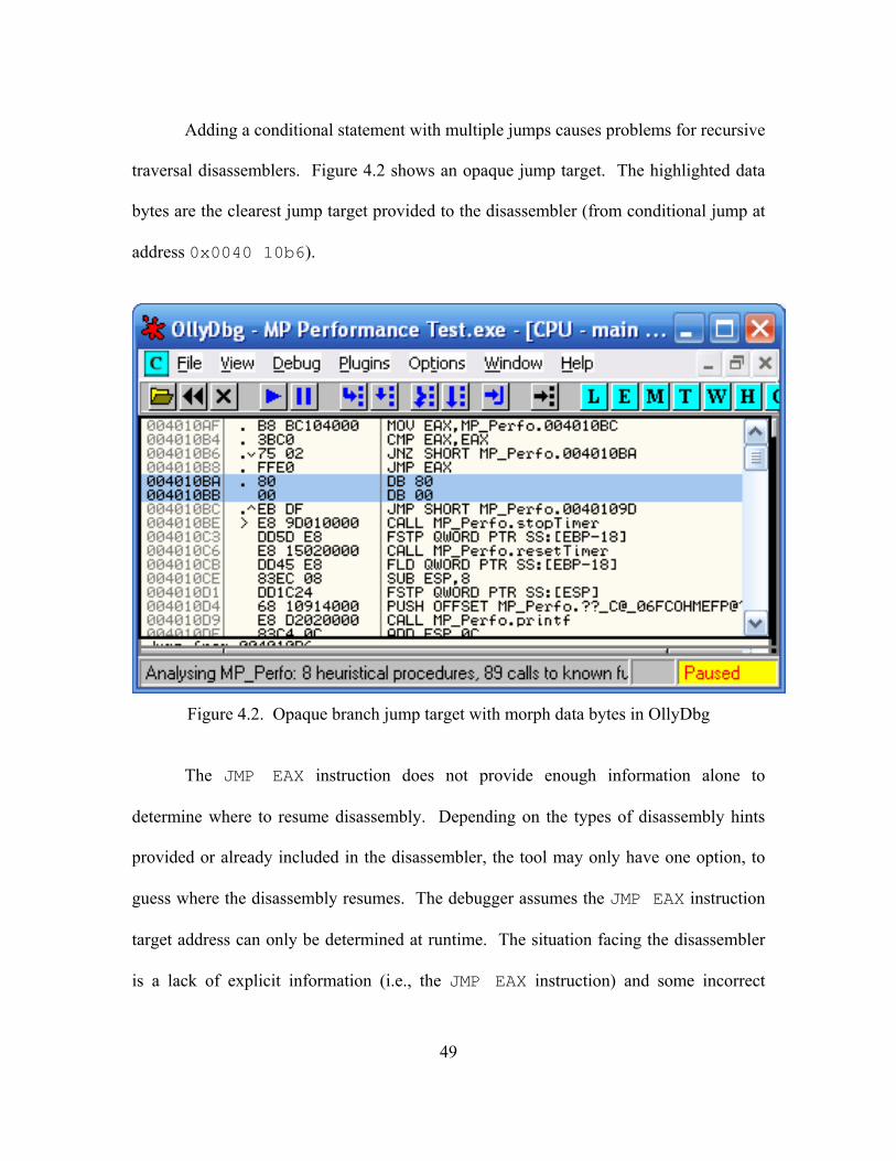
Adding a conditional statement with multiple jumps causes problems for recursive

traversal disassemblers. Figure 4.2 shows an opaque jump target. The highlighted data

bytes are the clearest jump target provided to the disassembler (from conditional jump at

address 0x0040 10b6).

Figure 4.2. Opaque branch jump target with morph data bytes in OllyDbg

The JMP EAX instruction does not provide enough information alone to

determine where to resume disassembly. Depending on the types of disassembly hints

provided or already included in the disassembler, the tool may only have one option, to

guess where the disassembly resumes. The debugger assumes the JMP EAX instruction

target address can only be determined at runtime. The situation facing the disassembler

is a lack of explicit information (i.e., the JMP EAX instruction) and some incorrect

49

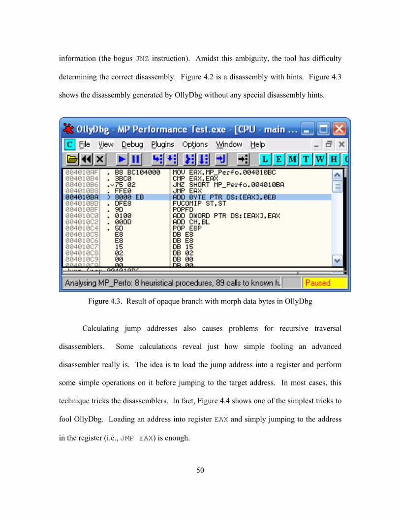
information (the bogus JNZ instruction). Amidst this ambiguity, the tool has difficulty

determining the correct disassembly. Figure 4.2 is a disassembly with hints. Figure 4.3

shows the disassembly generated by OllyDbg without any special disassembly hints.

Figure 4.3. Result of opaque branch with morph data bytes in OllyDbg

Calculating jump addresses also causes problems for recursive traversal

disassemblers. Some calculations reveal just how simple fooling an advanced

disassembler really is. The idea is to load the jump address into a register and perform

some simple operations on it before jumping to the target address. In most cases, this

technique tricks the disassemblers. In fact, Figure 4.4 shows one of the simplest tricks to

fool OllyDbg. Loading an address into register EAX and simply jumping to the address

in the register (i.e., JMP EAX) is enough.

50

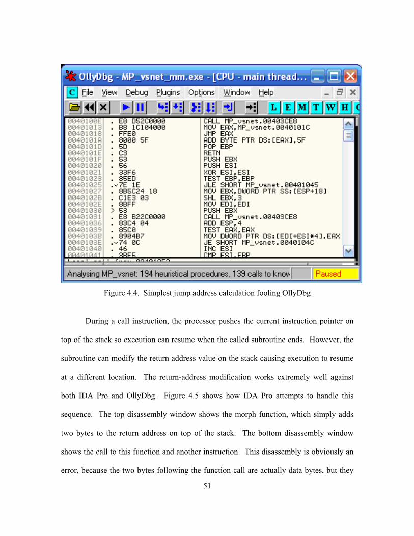
Figure 4.4. Simplest jump address calculation fooling OllyDbg

During a call instruction, the processor pushes the current instruction pointer on

top of the stack so execution can resume when the called subroutine ends. However, the

subroutine can modify the return address value on the stack causing execution to resume

at a different location. The return-address modification works extremely well against

both IDA Pro and OllyDbg. Figure 4.5 shows how IDA Pro attempts to handle this

sequence. The top disassembly window shows the morph function, which simply adds

two bytes to the return address on top of the stack. The bottom disassembly window

shows the call to this function and another instruction. This disassembly is obviously an

error, because the two bytes following the function call are actually data bytes, but they

51

deceptively match the prefix for an ADD instruction. In this case, the disassembler

confuses the data bytes for an ADD instruction.

Figure 4.5. IDA Pro disassembly of morph point with function call implementation

For these experiments, the function call implementation for morph points is

selected because of its simple design and effectiveness. This particular morph point

implementation is useful for capturing certain metrics of interest, such as the total number

of calls to morph points, and it never fails to fool any disassemblers during the

development and testing of these experiments. Unfortunately, the function call is also

one of the slowest implementations, likely attributable to the overhead of the CALL

instruction. Table 4.1 shows a performance summary of the various morph point

implementations just presented. Despite its slower performance, this implementation is

chosen for simplicity and its ability to capture metrics. Furthermore, during all the

development and testing, this implementation never failed to trick a disassembler.

This study uses two different engines, a basic MME that only modifies morph

points and an advanced MME capable of modifying morph points and reordering

52

functions. The following subsections describe each implementation and highlight the

differences between them.

Table 4.1. Average morph point execution time for 1 billion iterations

Morph Point Implementation

Avg Execution Time (s)

JUMP to Label 7.003 ns

Opaque Branch 20.533 ns

Jump Address Calculation 23.053 ns

Function Call 20.547 ns

4.2.2.1. Basic MME

The first version of the MME is a scout implementation that searches for morph

points (as sentinel values) in the code. Relying on a search engine can create problems

when using an optimizing compiler. Morph points that use a JMP instruction are

sometimes optimized out of the final executable. Debugging revealed that the JMP

instruction in some morph points jumped to another JMP instruction. Whereupon the

compiler optimizes this and points the morph point’s JMP instruction to the target address

of second JMP (instead of having a JMP to another JMP). Whenever this situation

occurs, the morph point is lost, because the resulting byte string for a far JMP is

significantly different from a near JMP. Due to this observation, a soldier

implementation is adopted for the MME.

The soldier implementation of the MME for the morph point experiment uses an

absolute morph point address. This is the second significant MME generated by this

53

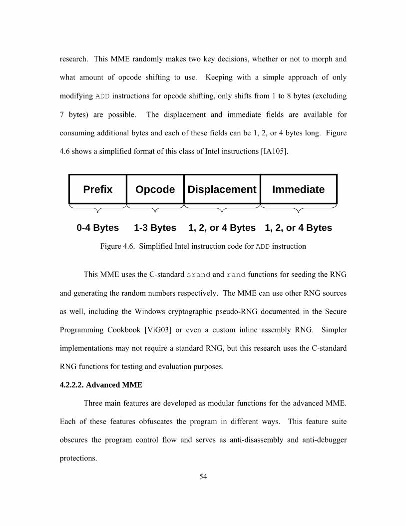
research. This MME randomly makes two key decisions, whether or not to morph and

what amount of opcode shifting to use. Keeping with a simple approach of only

modifying ADD instructions for opcode shifting, only shifts from 1 to 8 bytes (excluding

7 bytes) are possible. The displacement and immediate fields are available for

consuming additional bytes and each of these fields can be 1, 2, or 4 bytes long. Figure

4.6 shows a simplified format of this class of Intel instructions [IA105].

Prefix Opcode Displacement Immediate

0-4 Bytes 1-3 Bytes 1, 2, or 4 Bytes 1, 2, or 4 Bytes

Figure 4.6. Simplified Intel instruction code for ADD instruction

This MME uses the C-standard srand and rand functions for seeding the RNG

and generating the random numbers respectively. The MME can use other RNG sources

as well, including the Windows cryptographic pseudo-RNG documented in the Secure

Programming Cookbook [ViG03] or even a custom inline assembly RNG. Simpler

implementations may not require a standard RNG, but this research uses the C-standard

RNG functions for testing and evaluation purposes.

4.2.2.2. Advanced MME

Three main features are developed as modular functions for the advanced MME.

Each of these features obfuscates the program in different ways. This feature suite

obscures the program control flow and serves as anti-disassembly and anti-debugger

protections.

54

A function manager (FM) obscures the control flow of the program. Whenever

the main program calls a protected function, it sends a request for the protected function

to the function manager. The function manager relays all calls to the protected functions.

The main purpose for this type of protection is to delay the reversing process when

examining the main program to determine its general function. Instead of observing

several different identifying function calls, the program presents the reverser with another

layer of complexity. Figure 4.7 shows a function manager implementation for two

simple functions.

Parameter passing is problematic with such a simple implementation, because the

void function pointer (*f) has no parameters. To relay a call to another function with

parameters requires an explicit function pointer with an identical parameter list. It is

infeasible to declare a set of function pointers that use every possible permutation of

parameters. To simplify this component, the approach shown above (a void function

pointer with no parameters) is adopted. However, the void function pointers with no

parameters are still a problem. This is because many functions in the test program also

have return values, which the above implementation also does not support. Instead, the

program declares global parameter and return variables for passing parameters and

return values. To implement this, the basic approach defines macros that assign the

parameter values to the appropriate global variable before calling the function. Before

returning, the function assigns the return value to the global return value variable.

Replacing the original function calls with macro versions completes this approach.

Figure 4.8 shows a macro definition that calls one of the functions in the test program.

55

The return type becomes type void and the parameter list is now empty. Both values

pass through the declared global integer variables.

Figure 4.7. Sample function manager implementation

56

#define CALL_int_log2(n) \ _argumentN_int_log2__ = n; \ functionManager(INT_LOG2); int _argumentN_int_log2__, _returnInt_int_log2__; extern void int_log2(); // Originally the following // extern int int_log2(int n);

Figure 4.8. Macros replace function calls and handle parameter passing

Because the function manager calls the protected functions, only the function

manager needs to know where the functions truly reside in memory. Normally a C

compiler assigns a unique address for each function. Whenever the program wants to call

a function, the compiler inserts a CALL instruction with the appropriate function address.

During execution, if the functions change locations, their original addresses are no longer

valid. If the program does not use a function manager implementation, the program itself

must correct (regardless of location) every call to the relocated function to reflect the

function’s new address. This can require a substantial amount of overhead (e.g.,

searching the entire program’s memory space) depending on the implementation.

Moreover, if the program reorders functions often, this overhead increases substantially.

The function reordering experiment requires a more advanced MME capable of

shuffling functions in memory. This advanced MME needs to resolve several relative

addressing issues. For instance, many of the benchmark utility functions call other

functions. Herein, all calls pass through a function manager that relays the calls to other

functions, but invoking the function manager itself still requires a function call.

57

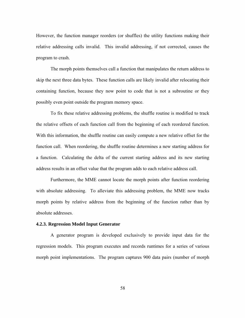
However, the function manager reorders (or shuffles) the utility functions making their

relative addressing calls invalid. This invalid addressing, if not corrected, causes the

program to crash.

The morph points themselves call a function that manipulates the return address to

skip the next three data bytes. These function calls are likely invalid after relocating their

containing function, because they now point to code that is not a subroutine or they

possibly even point outside the program memory space.

To fix these relative addressing problems, the shuffle routine is modified to track

the relative offsets of each function call from the beginning of each reordered function.

With this information, the shuffle routine can easily compute a new relative offset for the

function call. When reordering, the shuffle routine determines a new starting address for

a function. Calculating the delta of the current starting address and its new starting

address results in an offset value that the program adds to each relative address call.

Furthermore, the MME cannot locate the morph points after function reordering

with absolute addressing. To alleviate this addressing problem, the MME now tracks

morph points by relative address from the beginning of the function rather than by

absolute addresses.

4.2.3. Regression Model Input Generator

A generator program is developed exclusively to provide input data for the

regression models. This program executes and records runtimes for a series of various

morph point implementations. The program captures 900 data pairs (number of morph

58

point calls and total morph point execution time) as inputs for the regression models. The

data pairs include 30 samples for each of 30 predictor values chosen.

4.3. Component Data Flow

The data flow from the main program to the MME is simple. During

initialization, the main function of the benchmark program initializes the MME by

passing the following parameters: function addresses, call offsets (from function base

address), morph point offsets (from function base address), and the type of RNG to use.

The MME calculates the absolute address for function calls (within morphed functions)

and morph points by adding the offsets to the containing function’s base address. The

main program only provides this information to the MME at initialization. Afterwards,

the MME needs no more data, because it may manipulate the program structure to the

point that the main program no longer knows where functions reside. To invoke the

metamorphic transformation, the main program simply calls the appropriate MME

routine to metamorphose. Since the main program no longer understands its own

structure once morphed, it relies heavily on the MME.

On the other hand, the MME provides little data back to the main program. In

these research implementations, the MME only provides the number of times it modified

a particular set of morph points during a call to the MME. However, the MME tracks

other data, such as the number of times it modifies each specific morph point and the

number of morph point calls that program makes. Figure 4.9 shows the program

component data flow between the main function and the MME.

59

BenchmarkProgram

function1function2function3function4

main

MME MME

function addresses (initial)call offsetsmorph point addressesRNG source

# morphed

Figure 4.9. Program data flow diagram

4.4. Validation

This research employs many validation methods [Lil00]. Comparing the

modified versions of the benchmark with the original benchmark is one of the main

validation steps. This comparison is only partial, because the validation code does not

capture all intermediate values.

4.4.1. Benchmark Program Validation

First, the validation outputs (described earlier) from the developed models are

compared with the original program validation outputs. This approach constitutes

comparisons with the real system (the original benchmark) for partial, but exact, matches.

60

All models generate the same output results validating that the program function is

unchanged.

Second, the normal benchmark output and the added performance measuring

outputs are analyzed. The original benchmark suite provides an estimate of the millions

of floating-point operations per second (MFLOPs). The number of floating point

operations remains constant throughout the validation steps. After adding the timing

components, a thorough analysis of both the MFLOP and execution time metrics is

performed. The execution time and MFLOP metrics are inversely proportional and the

two can be compared because the number of FLOPs remains constant. Although not

exact matches because the MFLOP calculation uses a different timer, the resulting

percent increases in execution time are similar to the percent decreases in MFLOPs for

each of the test programs.

4.4.2. MME and Morph Point Validation

Engineering judgment is used when testing the MME and morph point

implementations for logical results. With the help of debuggers, the execution of the

MME itself and the morph points are analyzed to ensure proper functionality (i.e., the

data bytes inserted in the opcode shift are never executed). Furthermore, no experimental

tests failed to execute.

4.5. Summary

This chapter describes the rationale for the design of the experimental

components. It also highlights the more interesting products and observations of each

61

development spiral. Finally, the chapter concludes with a discussion of the component

data flow and component validation.

62

5. V. Analysis and Results

5.1. Chapter Overview

This chapter presents findings from the experiments. Beginning with a statistical

analysis of the experiments, the chapter proceeds to a detailed accounting of other

experimental observations and concludes with a proposed set of procedures for

implementing morph points.

5.2. Experimental Results

This section presents results and statistical analysis. Each subsection gives

specific details for each of the three experiments.

5.2.1. Morph Point Performance Experiment

The morph point performance experiment evaluates the performance overhead of

integrating simple data byte opcode shifts into various executables. The measured

overhead consists of the runtime performance of the MME and the execution time of the

added morph point instructions. In addition, the predictability of executables compiled

with the GCC and VSNET C compilers is assessed. Table 5.1 shows the performance

results for the MME for both compilers. These results indicate how long it takes the

MME to randomly modify 40 morph points contained in the test program. For each

morph point, the MME decides if it should modify it and determines what to change it to

if necessary. Even though the MME uses a RNG to make these decisions, the time

required is in the microsecond range, which is undetectable in an interactive application.

63

Table 5.1. MME performance summary

Compiler Average (μs) Standard Deviation (μs)

95% Confidence Interval (μs)

GCC 5.335 2.317 [ 5.014 , 5.656 ]

VSNET 6.030 1.962 [ 5.758 , 6.302 ]

To build a regression model, a data point generator produces data point pairs for

each compiler. This test program generates 30 data points for each predictor value and

uses 30 linearly increasing predictor values. For each data point, the program measures

the execution time of the morph points indirectly by calculating the performance

difference between the baseline and metamorphic versions of the test program. Finally,

these data points are used for building the regression models with the statistical program

Minitab [Min06]. In all of these models, the predictor variable is the number of function

calls (in millions of calls) and the response variable is the total morph point execution

time (in milliseconds). To ensure that Minitab generates regression coefficients that are

large enough in magnitude to read, the units for the number of calls is adjusted to

millions of calls and the execution time is changed from seconds to milliseconds. The

following subsections detail the regression models for each compiler and their results.

5.2.1.1. GCC Morph Point Performance Results

Tables 5.2 and 5.3 show summaries of the GCC performance tests. Collectively,

the benchmark programs contained 40 morph points strategically placed through the

protected functions to precede a variety of instructions (e.g., various assignments,

conditionals, function calls, etc.).

64

Table 5.2. GCC baseline performance summary

Benchmark Application Average (s) Standard

Deviation (s) 95% Confidence

Interval (s)

FFT 6.46 0.00585 [ 6.46 , 6.46 ]

SOR 4.63 0.00610 [ 4.63 , 4.63 ]

MC 3.68 0.00843 [ 3.68 , 3.68 ]

SMM 6.08 0.00402 [ 6.08 , 6.08 ]

LU 3.59 0.00403 [ 3.59 , 3.59 ]

Table 5.3. GCC morph point performance summary

Benchmark Application Average (s) Standard

Deviation (s) 95% Confidence

Interval (s)

FFT 9.18 0.00625 [ 9.17 , 9.18 ]

SOR 12.2 0.0102 [ 12.2 , 12.2 ]

MC 7.90 0.00402 [ 7.90 , 7.90 ]

SMM 15.2 0.00792 [ 15.2 , 15.2 ]

LU 7.97 0.00680 [ 7.97 , 7.97 ]

At first glance, the execution time increases are substantial with more than 150%

increases in two cases (SMM and LU). However, another factor contributing to the

execution time increase is the number of times the morph points execute, which leads to

the primary research metric for this experiment, execution time per morph point. Table

5.4 shows the number of morph point calls and the average execution times per morph

point for the benchmark programs. Unfortunately, significant variance exists in the

morph point execution times across the different programs.

65

Table 5.4. GCC morph point calls and execution time per morph point

Benchmark Application

Execution Time Increase (s)

Number of Morph Point Calls

Execution Time per Morph Point (ns)

FFT 2.72 250,856,512 10.8

SOR 7.58 314,694,286 24.1

MC 4.22 268,435,567 15.7

SMM 9.13 655,486,073 13.9

LU 4.38 330,979,498 13.2

Several discrepancies exist in these results. The execution times are expected to

be somewhat consistent. Instead, the average execution times are erratic and difficult to

explain. Process scheduling and other OS factors do not appear to cause this erratic

behavior, because repeated tests meet with similar results. Another explanation for the

performance decrease is that the morph points potentially cause instruction cache misses,

where the data requested does not reside in cache and the control unit must instead fetch

the data from memory [PaH05].

The scatter plot of the number of morph point calls and the resulting morph point

execution time shown in Figure 5.1 indicates that a strong linear relationship exists

between the predictor and response variables. This data is produced by the regression

model input generator program described previously. One of the first assumptions that

simple linear regression modeling requires is for the data to exhibit a linear relationship.

If the data set does not exhibit a linear relationship, simple linear regression modeling is

not a valid prediction method.

66

MP Calls (Millions)

Tota

l MP

Exec

Tim

e (m

s)

300250200150100500

4000

3000

2000

1000

0

Scatterplot of Total MP Exec Time (ms) vs MP Calls (Millions)

Figure 5.1. Resulting scatter plot for GCC test program data points

Although the data point pairs produce by the generator appear to have a strong

linear relationship, they unfortunately do not satisfy other assumptions necessary for

regression modeling. Figure 5.2 is a Minitab quad chart based on the same data. Since

the residual values (the error from the data point to the regression line) are not normally

distributed, the simple generator is not an adequate source for the regression model. In

addition, the variance, which should be constant, also appears to increase causing the

gradual fanning in the two charts on the right. The rate of change of the variance is

actually in the billionth range, which is reasonably constant.

67

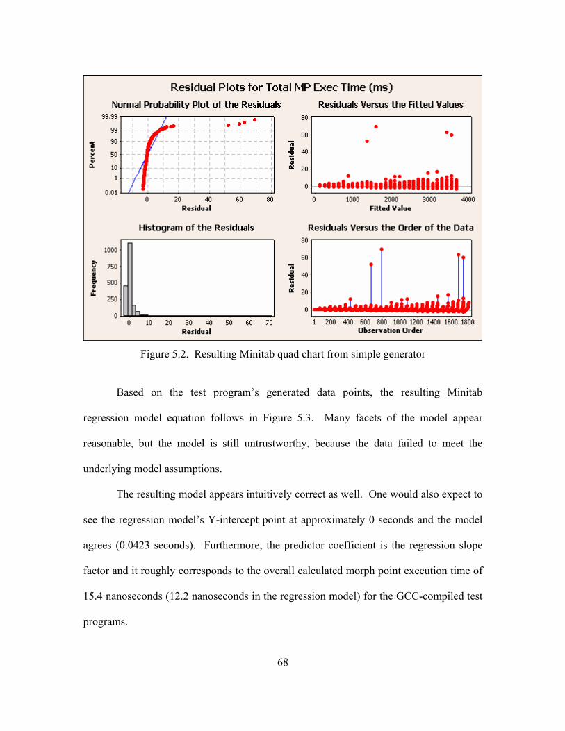
Figure 5.2. Resulting Minitab quad chart from simple generator

Based on the test program’s generated data points, the resulting Minitab

regression model equation follows in Figure 5.3. Many facets of the model appear

reasonable, but the model is still untrustworthy, because the data failed to meet the

underlying model assumptions.

The resulting model appears intuitively correct as well. One would also expect to

see the regression model’s Y-intercept point at approximately 0 seconds and the model

agrees (0.0423 seconds). Furthermore, the predictor coefficient is the regression slope

factor and it roughly corresponds to the overall calculated morph point execution time of

15.4 nanoseconds (12.2 nanoseconds in the regression model) for the GCC-compiled test

programs.

68

The regression equation is Total MP Exec Time (ms) = 0.042 + 12.2 MP Calls (Millions) Predictor Coef SE Coef T P Constant 0.0423 0.1997 0.21 0.832 MP Calls (Millions) 12.2155 0.0011 10859.05 0.000 S = 2.92099 R-Sq = 100.0% R-Sq(adj) = 100.0% PRESS = 7703.67 R-Sq(pred) = 100.00% Analysis of Variance Source DF SS MS F P Regression 1 1006108156 1006108156 1.17919E+08 0.000 Residual Error 898 7662 9 Lack of Fit 28 157 6 0.65 0.918 Pure Error 870 7505 9 Total 899 1006115818

Figure 5.3. Minitab regression model for GCC benchmark

Because the test generator is not an acceptable source of data for the regression

model, another approach is necessary. Instead of using a program with different

characteristics (i.e., instruction mix) as the target program, the target program itself is

used as a data point generator for the model. This approach meets with mixed success.

Figures 5.4 and 5.5 show the regression model and the resulting quad chart from using

the GCC FFT program as a generator that produces 25 replications of 5 predictor values.

The FFT program is changed to execute longer by changing the number of execution

cycles. The residuals still do not follow a normal distribution like the previous model.

However, after analyzing the stair-step pattern in the chart of Residuals Versus the Order

of the Data, it appears a factor external to the program is contributing to its performance

unpredictability. All outlier data points are removed, but the resulting models still exhibit

similar behavior. The five predictor values appear inconsistent with one another.

69

The regression equation is MP Execution Time = 64.2 + 10.4 MP Function Calls Predictor Coef SE Coef T P Constant 64.22 11.53 5.57 0.000 MP Function Calls 10.4476 0.0223 469.47 0.000 S = 85.1276 R-Sq = 99.9% R-Sq(adj) = 99.9% Analysis of Variance Source DF SS MS F P Regression 1 1597211240 1597211240 220405.25 0.000 Residual Error 123 891344 7247 Lack of Fit 3 882393 294131 3943.24 0.000 Pure Error 120 8951 75 Total 124 1598102585

Figure 5.4. Regression model generated by GCC FFT benchmark program

Residual

Per

cent

2001000-100-200

99.9

99

90

50

10

1

0.1

Fitted Value

Res

idua

l

100007500500025000

200

100

0

-100

Residual

Freq

uenc

y

16012080400-40-80

48

36

24

12

0

Observation Order

Res

idua

l

120

110

1009080706050403020101

200

100

0

-100

Normal Probability Plot of the Residuals Residuals Versus the Fitted Values

Histogram of the Residuals Residuals Versus the Order of the Data

Residual Plots for MP Execution Time (GCC - FFT)

Figure 5.5. Resulting Minitab quad chart of using FFT target program as a generator

70

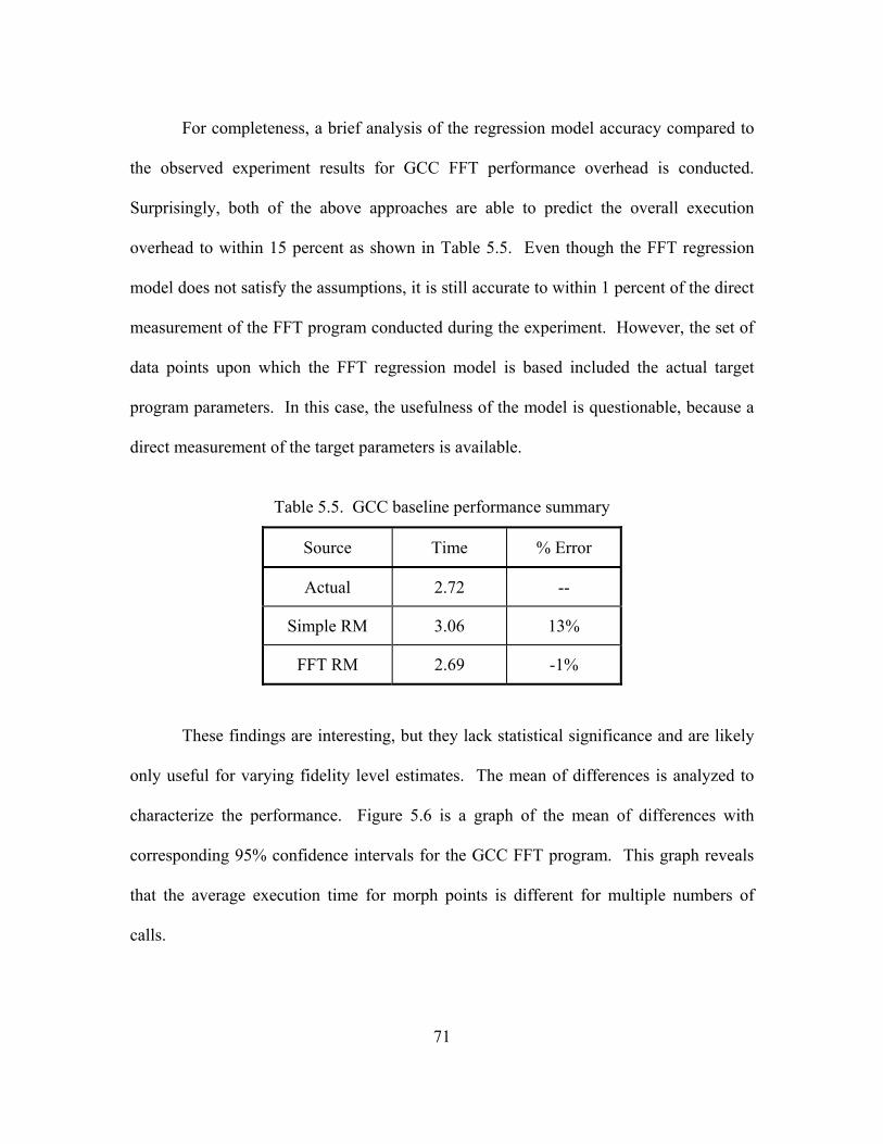
For completeness, a brief analysis of the regression model accuracy compared to

the observed experiment results for GCC FFT performance overhead is conducted.

Surprisingly, both of the above approaches are able to predict the overall execution

overhead to within 15 percent as shown in Table 5.5. Even though the FFT regression

model does not satisfy the assumptions, it is still accurate to within 1 percent of the direct

measurement of the FFT program conducted during the experiment. However, the set of

data points upon which the FFT regression model is based included the actual target

program parameters. In this case, the usefulness of the model is questionable, because a

direct measurement of the target parameters is available.

Table 5.5. GCC baseline performance summary

Source Time % Error

Actual 2.72 --

Simple RM 3.06 13%

FFT RM 2.69 -1%

These findings are interesting, but they lack statistical significance and are likely

only useful for varying fidelity level estimates. The mean of differences is analyzed to

characterize the performance. Figure 5.6 is a graph of the mean of differences with

corresponding 95% confidence intervals for the GCC FFT program. This graph reveals

that the average execution time for morph points is different for multiple numbers of

calls.

71

GCC FFT Morph Point Mean of Differences with 95% CI

10.924

10.793

10.533

10.905

10.44510.400

10.700

11.000

62,702,654 125,420,607 250,856,512 501,728,321 1,003,471,938

MP Calls

MP

Avg

Exe

cutio

n Ti

me

(ns)

MP Avg Time (ns)

Figure 5.6. Morph point means of differences by number of calls for GCC FFT

The only confidence interval overlap is for the 63-million and 502-million call

points, but only one mean falls within the confidence interval of the other. Therefore, a

simple t-test shows any statistically significant difference between the two test points.

The t-test calculations follow below. Since the confidence interval for the mean of

differences does not include zero, these two points have a statistically significant

difference with 95% confidence.

( )

( ) ( ) ( ) ( )( )

( ) [ ]

21 2 1 ; 1

1 2

1 2

,

0.139 ns, 0.479 ns 2.064

25 samples

, 0.422 ns,0.536 ns

dn

sc c d tn

c c

c c

α− −= ±

= ±

=

(5.1)

72

where

2 0.975;241 ; 1

before measurementafter measurement

mean value of 0.479 ns

2.064standard deviation of 0.139 nssample size25 samples

i

i

i i i

i

n

d i

bad a b

d d

t t

s d

n

α− −

==

= −

===

=====

These findings illustrate the difficulties of measuring program performance at a

detailed level. There was no control or visibility into the lower levels of the memory

hierarchy or the processor itself and it is likely that these components are contributing to

the unpredictability of the morph point execution times. The presence of morph points in

particular locations can cause instruction cache misses and force the processor to wait for

the instruction to load from a lower (and slower) level in the memory hierarchy. Others

note the impact of cache misses on performance and they specifically include it as a

parameter in their exection time estimation models [ShT05, Axe06].

Moreover, any similar investigation should consider the differences in program

control flow when executing with dissimilar or special parameter values. Data values are

often useful for directing program execution flow—especially in scientific and

engineering applications, which comprise the benchmark suite. In fact, the results for the

Monte Carlo (MC) test program supports this theory. The MC program is the most

73

sequential of the test programs as it consists of only one loop and one conditional.

Figures 5.7 and 5.8 show the resulting Monte Carlo regression model and quad chart.

The regression equation is MP Execution Time = 1.81 + 15.7 MP Function Calls Predictor Coef SE Coef T P Constant 1.814 1.402 1.29 0.198 MP Function Calls 15.7121 0.0025 6212.55 0.000 S = 10.3518 R-Sq = 100.0% R-Sq(adj) = 100.0% Analysis of Variance Source DF SS MS F P Regression 1 4135898919 4135898919 38595731.42 0.000 Residual Error 123 13181 107 Lack of Fit 3 595 198 1.89 0.135 Pure Error 120 12586 105 Total 124 4135912100

Figure 5.7. Regression model generated by GCC MC benchmark program

Residual

Per

cent

50250-25-50

99.9

99

90

50

10

1

0.1

Fitted Value

Res

idua

l

1600012000800040000

50

25

0

-25

-50

Residual

Freq

uenc

y

30150-15-30

30

20

10

0

Observation Order

Res

idua

l

1201101009080706050403020101

50

25

0

-25

-50

Normal Probability Plot of the Residuals Residuals Versus the Fitted Values

Histogram of the Residuals Residuals Versus the Order of the Data

Residual Plots for MP Execution Time (GCC - MC)

Figure 5.8. Residual Plots for GCC MC regression model

74

These results portray the fact that the data points satisfy the model assumptions, residual

normality and constant variance. Unfortunately, all of the other regression models fail to

satisfy these assumptions.

5.2.1.2. VSNET Morph Point Performance Results

Similar results are observed for the VSNET-compiled test programs, and these

findings are included for completeness. Tables 5.6 and 5.7 show summaries of the

VSNET performance tests. As before, the benchmark programs contains 40 morph

points strategically placed through the protected functions to precede a variety of

instructions (e.g., various assignments, conditionals, function calls, etc.).

Table 5.6. VSNET baseline performance summary

Benchmark Application Average (s) Standard

Deviation (s) 95% Confidence

Interval (s)

FFT 10.87 0.00561 [ 10.9 , 10.9 ]

SOR 4.86 0.00373 [ 4.86 , 4.86 ]

MC 3.05 0.00618 [ 3.05 , 3.05 ]

SMM 7.88 0.00392 [ 7.88 , 7.88 ]

LU 3.66 0.00469 [ 3.65 , 3.66 ]

As in the GCC experiments, another factor contributing to the execution time

increase is the number of times the morph points execute. Table 5.8 shows the number of

morph point calls and the average execution times per morph point for the VSNET-

compiled benchmark programs. The only key difference between the VSNET and GCC

results is the increased variance for the execution times per morph point between VSNET

test programs.

75

Table 5.7. VSNET morph point performance summary

Benchmark Application Average (s) Standard

Deviation (s) 95% Confidence

Interval (s)

FFT 13.6 0.00630 [ 13.6 , 13.6 ]

SOR 13.1 0.0108 [ 13.1 , 13.1 ]

MC 8.01 0.00852 [ 8.01 , 8.01 ]

SMM 12.7 0.00620 [ 12.7 , 12.8 ]

LU 11.2 0.0142 [ 11.2 , 11.2 ]

Table 5.8. VSNET morph point calls and execution time per morph point

Benchmark Application

Execution Time Increase (s)

Number of Morph Point Calls

Execution Time per Morph Point (ns)

FFT 2.77 250,856,512 11.0

SOR 8.23 314,694,286 26.1

MC 4.96 268,435,567 18.5

SMM 4.87 655,486,073 7.4

LU 7.57 330,979,498 22.9

Based on the test program’s generated data points, the resulting Minitab

regression model equation for the FFT program follows in Figure 5.9. Figure 5.10 shows

the resulting quad chart. This model also fails to satisfy assumptions. The residuals do

not follow a normal distribution about the regression line and they demonstrate the same

stair-step pattern as seen before.

76

The regression equation is MP Execution Time = - 40.5 + 11.0 MP Function Calls Predictor Coef SE Coef T P Constant -40.49 10.98 -3.69 0.000 MP Function Calls 10.9517 0.0212 516.61 0.000 S = 81.0927 R-Sq = 100.0% R-Sq(adj) = 100.0% Analysis of Variance Source DF SS MS F P Regression 1 1755049988 1755049988 266886.31 0.000 Residual Error 123 808851 6576 Lack of Fit 3 782762 260921 1200.15 0.000 Pure Error 120 26089 217 Total 124 1755858839

Figure 5.9. Regression model generated by VSNET FFT benchmark program

Residual

Per

cent

2001000-100-200

99.9

99

90

50

10

1

0.1

Fitted Value

Res

idua

l

100007500500025000

100

0

-100

-200

Residual

Freq

uenc

y

80400-40-80-120-160

40

30

20

10

0

Observation Order

Res

idua

l

120

110

1009080706050403020101

100

0

-100

-200

Normal Probability Plot of the Residuals Residuals Versus the Fitted Values

Histogram of the Residuals Residuals Versus the Order of the Data

Residual Plots for MP Execution Time (VSNET - FFT)

Figure 5.10. Residual Plots for VSNET FFT regression model

77

Since the VSNET results are so similar to the GCC results, this thesis makes no

further elaboration on the VSNET experiment itself. The appendix includes the

regression models for the remaining VSNET experiments.

5.2.2. Instruction Reach Experiment

The instruction reach experiment assesses the impact (in terms of number of

instructions) of an opcode shift. This experiment specifically examines the instruction

reach achieved by various runtime shift amounts and compares the differences between

the GCC and VSNET C compilers. Ideally, the impact of a single morph point would

reach dozens of instructions with cascading effects on other morph points.

This experiment has unexpected results and it highlights significant differences

between the two debuggers. The default behavior of the two debuggers is different for

runtime modifications to instruction code. OllyDbg immediately attempts to parse the

new disassembly without user input, whereas IDA assumes that the original instruction

addresses are correct and retains most of the original disassembly.

5.2.2.1. OllyDbg Results

OllyDbg generates a new disassembly as soon as a runtime instruction morph

occurs. This debugger indicates its uncertainty of the disassembly by marking suspicious

areas with question mark symbols. Figure 5.11 shows OllyDbg’s resulting disassembly

before metamorphosis. The disassembly includes two morph point constructs at

addresses 0x0040 1E29 and 0x0040 1E5C. The three PUSH EAX instructions

indicate placeholders for opcode shifts (the data bytes). Figure 5.12 shows OllyDbg’s

resulting disassembly with the uncertainty symbols after metamorphosis. When the shift

78

amount aligns to an instruction boundary, such as the shift at address 0x0040 1E2E in

the same figure, the debugger is certain (i.e., no question marks) of the generated

disassembly. However, in this case it misses one instruction (a MOV instruction),

because the morphed instruction absorbs it completely.

Figure 5.11. OllyDbg screenshot before morphing

Table 5.9 shows the results for the OllyDbg instruction reach experiment for the

GCC compiler. The overall trend implies that larger shift amounts mangle more

instructions. This observation seems obvious, because consuming additional bytes likely

will consume at least part of the following instruction thereby increasing the instruction

reach. The deviations from the observed trend require further explanation.

79

Figure 5.12. OllyDbg screenshot showing garbled instructions after morphing

Table 5.9. Instruction reach experiment results for GCC compiler

Compiler Shift Amount (Bytes)

Avg. Instruction Reach (# Instr.)

Avg. Byte Reach (Bytes)

GCC 1 2.58 10.2

GCC 2 2.40 9.53

GCC 3 1.68 7.13

GCC 4 3.83 14.4

GCC 5 3.80 14.4

GCC 6 3.13 11.6

GCC 8 4.60 16.8

80

For the GCC compiled test application, an opcode shift amount of three bytes

resulted in the lowest instruction reach of only 1.68 instructions on average. The six-byte

shift amount (3.13 instructions average) also deviates from the general trend as well.

These two shifts comprise the majority of the deviations from the observed trend. When

evaluating the morph point’s effectiveness in terms of instruction reach, it is helpful to

consider the instruction distribution of the protected region of the test program as well.

Figure 5.13 shows the instruction distribution for the region of the baseline GCC

compiled test program that the MME protects. The three-byte instructions are by far the

most common in the graph. Because of the predominance of three-byte (42%)

instructions, it makes sense that the three-byte shift amount results in the smallest reach,

because it is more likely to precede a three-byte instruction and resynchronize quickly.

The six-byte shift also resynchronizes quickly, because of the overwhelming prevalence

(70%) of the three-byte and smaller shifts.

Furthermore, the size of any particular instruction in the program is a dependent

random variable. That is, the beginning of a for-loop construct in source code translates

to a standard series of assembly instructions in GCC. In the test program, such instances

include the following instructions: a three-byte MOV, a three-byte CMP, and a six-byte

conditional jump. Introducing a six-byte shift before this sequence completely absorbs

the first two instructions. Since the shift realigns perfectly on the instruction boundary

before the conditional jump, the morph point does not affect any other instructions.

These types of instruction sequencing dependencies could explain other minor anomalies

in the data set.

81

Workload Instruction Distribution (GCC)

1B14%

2B17%

3B40%

4B3%

5B9%

7B6%

6B11%

8B0%

Figure 5.13. Instruction distribution for test program compiled with GCC

Table 5.10 summarizes the instruction reach results for the VSNET compiled test

program analyzed with OllyDbg. The trend holds. In general, shift amounts are directly

proportional to instruction reaches. Figure 5.14 shows the instruction size distribution for

the VSNET compiled test program. In fact, shift amounts of four bytes and less follow

more of a uniform distribution than with the GCC compiler. When comparing general

results for VSNET and GCC, the GCC compiler results in larger instruction reaches for

two- and four-byte shifts. The increased prevalence of these instruction sizes in the

VSNET-compiled program likely causes this disparity. The instruction sequential

82

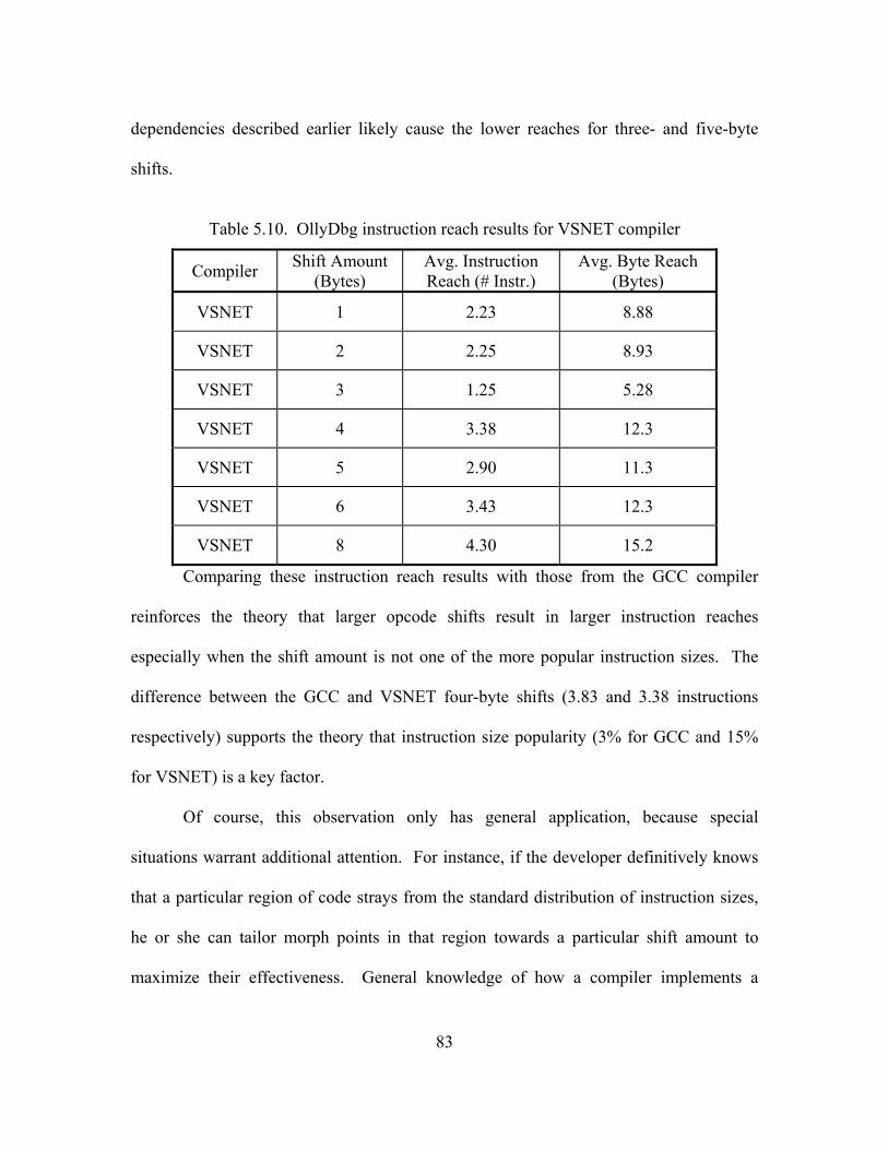
dependencies described earlier likely cause the lower reaches for three- and five-byte

shifts.

Table 5.10. OllyDbg instruction reach results for VSNET compiler

Compiler Shift Amount (Bytes)

Avg. Instruction Reach (# Instr.)

Avg. Byte Reach (Bytes)

VSNET 1 2.23 8.88

VSNET 2 2.25 8.93

VSNET 3 1.25 5.28

VSNET 4 3.38 12.3

VSNET 5 2.90 11.3

VSNET 6 3.43 12.3

VSNET 8 4.30 15.2

Comparing these instruction reach results with those from the GCC compiler

reinforces the theory that larger opcode shifts result in larger instruction reaches

especially when the shift amount is not one of the more popular instruction sizes. The

difference between the GCC and VSNET four-byte shifts (3.83 and 3.38 instructions

respectively) supports the theory that instruction size popularity (3% for GCC and 15%

for VSNET) is a key factor.

Of course, this observation only has general application, because special

situations warrant additional attention. For instance, if the developer definitively knows

that a particular region of code strays from the standard distribution of instruction sizes,

he or she can tailor morph points in that region towards a particular shift amount to

maximize their effectiveness. General knowledge of how a compiler implements a

83

particular construct and the resulting instruction sequence can assist the developer in

maximizing the instruction mangling.

Workload Instruction Distribution (VSNET)

1B28%

2B26%

3B18%

4B15%

5B8%

6B4%

7B1%

8B0%

Figure 5.14. Instruction distribution for test program compiled with VSNET

5.2.2.2. IDA Pro Results (GCC and Visual Studio .NET)

Whereas OllyDbg immediately pursues the new disassembly, IDA ignores the

modification’s potential impact on subsequent instructions and shows the morphed

instruction followed by the original instructions with their original addresses. The

resulting disassembly is inconsistent, because the morphed instruction appears to be only

84

a single byte long (the size of the original instruction at that address). If IDA believes the

morphed instruction is accurate, one would suspect that IDA would adjust the remaining

disassembly to reflect this fact. Since IDA still shows the original disassembly after the

morph, this particular metamorphic approach does not seem overly robust—even though

the resulting disassembly is inconsistent. Figure 5.15 shows an inconsistent IDA

disassembly, which occurrs after a six-byte opcode shift. Three bogus instructions follow

the morph point call in two cases shown (addresses 0x0040 22D7 and 0x0040

2315), but the original disassembly also remains visible.

For the first morph point call, the hexadecimal prefix for the six-byte shift is the

three-byte string 0x66 8180 starting at address 0x0040 22DC. The instruction

shown at this address is a nine-byte ADD instruction with a four-byte displacement (the

0x01C4 458B added to EAX) and a two-byte immediate value (the 0x8BF0 at the end

of the instruction). The address of the second byte in the prefix is 0x0040 22DD. At

this address, the instruction shown is actually a ten-byte ADD instruction with four-byte

displacement and immediate fields. However, IDA knows that the instruction address for

the second instruction should not be one byte more than the first instruction, because the

first instruction is nine-bytes long. The correct starting address for the second instruction

should be 0x0040 22E5—not 0x0040 22DD. Originally, all three bytes following the

morph point call were set to 0x50, which translates to three PUSH EAX instructions.

Because of the predefined definition of a mangled instruction and IDA Pro’s

default handling of runtime instruction changes, all of the IDA Pro instruction reach

85

experiments results in an instruction reach of zero. However, IDA’s propensity for not

reconsidering disassembly is also exploitable through different approaches.

Figure 5.15. IDA Pro disassembly after metamorphism

As a metamorphic exploit example, the software developer can apply

metamorphism not only to the execution of the program, but to the storage of it as well.

The program can randomly set the same morph points and save them to disk as parts of a

86

new executable. When opening the new executable, the debugger must decide what is

the true instruction code and what is not. Oftentimes, this ambiguity results in IDA

mistaking large blocks of instructions for data and other times displaying the false

mangled instructions. When reversing with IDA, you must address these issues in order

to comprehend the underlying program. Figure 5.16 shows how IDA Pro handles this

case when opening one of the test programs modified to default six-byte opcode shifts.

In this case, the morph point prefix fools IDA with the ADD instruction at address

0x0040 22AF. However, this screenshot is actually of the same memory region as

before. In fact, the data block shown at address 0x0040 22B8 absorbs both of the

morph points from the previous example (along with two others).

Figure 5.16. IDA Pro opens an executable that utilizes storage metamorphism

87

To produce the disassembly for this region of code, the user must manually select

the region and use IDA’s analysis tool to convert it to code. When IDA analyzes this

code though, the user must now contend with the previously avoided morph points,

because the analysis tool enables them and mangles the real instructions. Figure 5.17

shows the resulting disassembly for the region following the morph point at address

0x0040 22D7. Comparing these results with the results in Figure 5.15 shows that the

disassembler does not resynchronize with the correct instruction boundary until address

0x0040 22F2.

Figure 5.17. IDA disassembly after analysis of storage morphing executable

5.2.3. Function Reordering Experiment

The function reordering experiment examines the execution time necessary for

subroutine reordering. Table 5.11 shows the performance overhead statistics for the

subroutine reordering function based on 200 samples. The subroutine reordering function

performs several tasks during the measured execution time. It dynamically allocates

memory for function storage, randomly determines the new function order, copies the

88

functions, repairs any relative addressing problems, and clears the previous memory

space before copying the functions to their new locations. These results indicate the time

required to accomplish all of these tasks for one shuffle. Once again, these execution

times are nominal—at least for interactive applications. Furthermore, there is no other

performance overhead associated with this metamorphic transform (i.e., additional

instructions such as opcode shift logic).

Table 5.11. Subroutine reordering function performance summary

Compiler Average (μs) Standard Deviation (μs)

95% Confidence Interval (μs)

# Bytes

GCC 13.3 5.74 [ 12.5 , 14. 1 ] 1,596

VSNET 12.1 5.15 [ 11.4 , 12.9 ] 1,512

While the statistical results of the function reordering experiments are relatively

nondescript, the effects of function reordering are interesting. For instance, after

randomly changing the morph points and reordering subroutines, the process of re-

identifying the functions became more difficult, because both transforms garble the

disassembly. The next section describes the intangible benefits of metamorphism.

5.3. Other Observations from Development and Experimentation

Observations from development and experimentation offer more insight into the

effects of metamorphism. These observations run from graphical user interface problems

to completely crashing the debugger. This section highlights several interesting

observations.

89

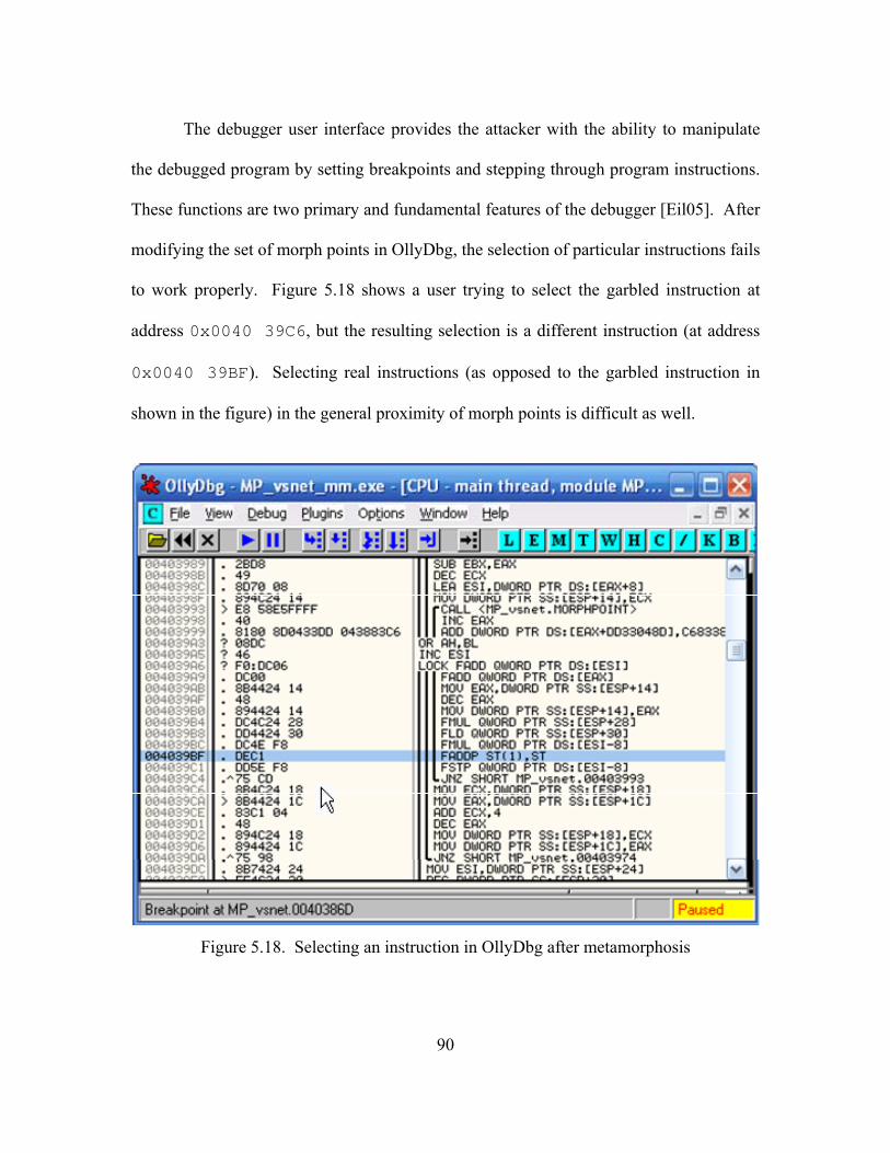
The debugger user interface provides the attacker with the ability to manipulate

the debugged program by setting breakpoints and stepping through program instructions.

These functions are two primary and fundamental features of the debugger [Eil05]. After

modifying the set of morph points in OllyDbg, the selection of particular instructions fails

to work properly. Figure 5.18 shows a user trying to select the garbled instruction at

address 0x0040 39C6, but the resulting selection is a different instruction (at address

0x0040 39BF). Selecting real instructions (as opposed to the garbled instruction in

shown in the figure) in the general proximity of morph points is difficult as well.

Figure 5.18. Selecting an instruction in OllyDbg after metamorphosis

90

The previous example also shows how OllyDbg expresses its uncertainty

concerning the disassembly. OllyDbg places the previously described question mark

symbol before the hexadecimal representation of the assembly instruction. The morph

also interrupts the loop and subroutine reference lines immediately preceding the

assembly instruction. When reversing with OllyDbg, it is common to use its built-in

analysis tool to generate or fix the disassembly. However, when using the analysis tool

in OllyDbg, the question mark symbols disappear. Figure 5.19 shows what happens after

using the built-in analysis tool in OllyDbg. Unfortunately, the uncertain disassembly

symbols (the question marks) are gone and the function and loop symbols disappear as

well. Even though OllyDbg restores proper selection functionality after analysis, the tool

no longer shows the useful symbols (i.e., the question marks, subroutine bounds, and loop

bounds). At this point, very few indicators point to a recent instruction metamorphosis.

In this particular morph, OllyDbg disassembles a data byte (DB F0) at address 0x0040

39A6. The only other indicator remaining is the absence of the period (.) symbol that

appears to indicate an instruction.

In addition, the instruction opcode shifting metamorphosis has another interesting

anti-debugging effect. If a user places a software breakpoint in a morph point, the

metamorphic engine randomly overwrote it. Although dependent upon the MME

implementation, this reinforces the effectiveness of metamorphism as an anti-debugging

protection. If the user attempts to remove the breakpoint, OllyDbg identifies and

describes the corruption of the breakpoint. However, OllyDbg gives no indication of the

corrupt breakpoint until this user interaction.

91

Figure 5.19. Using the analysis tool in OllyDbg after morph occurs

OllyDbg behaves strangely when the user steps to the first garbled instruction. In

the simpler opcode shifting transforms, OllyDbg correctly decodes the current hidden

instruction. As soon as the user steps to the next instruction or manipulates the window

(i.e., scrolls, resizes, etc.), OllyDbg hides the real instruction. With later advances of the

metamorphic engine, OllyDbg never shows the correct decoding of the current

instruction. This causes a mismatch between the instruction pointer and the address of

the current highlighted instruction (assuming the highlight indicated the current

instruction).

92

The morph points in this study causes another minor problem for both OllyDbg

and IDA Pro; neither debugger could step over a morph point without the program

continuing execution and not pausing. Apparently, both debuggers silently place

breakpoints on the instruction following the morph function call. The two debuggers

then assume that the execution will resume at the new breakpoint after the debugger steps

over the function call. If the execution actually resumed immediately after the function

call, the program would stop. However, with the morph points in this study, the program

does not stop and continues execution, because the called function modifies the true

return point, which sets up the opcode shift.

Both debuggers also have difficulties with moved breakpoints. When the user

places a breakpoint on a particular instruction, the debugger replaces the first byte of the

instruction with the breakpoint interrupt byte (0xCC). In these experiments, the

advanced MME randomly reorders protected subroutines. When the user places a

breakpoint in a protected subroutine, it is possible that the MME will move the

subroutine (including the breakpoint interrupt byte) to a new location. Every time the

MME moves the subroutine, neither debugger can resolve the original prefix to the

instruction, because the instruction no longer resides at its expected address. In these

cases, the program crashes inside the debugger and the user has to restart it.

IDA also exhibits more strange behavior when faced with the test program.

During morphing and shuffling, IDA mistakes a majority of code sections as data. While

trying to repair the disassembly by manually converting the regions of data back to code,

IDA often fails causing the debugger to crash. IDA normally offers the user an

93

opportunity to save the state of the debugged process. However, during this failure the

program makes no such offer. Whether or not the program truly saves the debugging

state successfully is questionable. Figure 5.20 shows the resulting error message that

IDA presents immediately prior to exiting.

Figure 5.20. IDA error message presented before failure

5.4. Investigative Questions Answered

This research does answer investigative questions regarding the predictability of

morph point overhead. Unfortunately, the findings imply that the morph point inclusion

is not highly conducive to accurate prediction.

This research also describes observed capabilities of the sample metamorphic

transforms. Reporting these observations provides the protection community with a

better understanding of how metamorphism protects as well as citing specific capabilities.

These findings do imply a general set of procedures for including morph points.

These procedures are quite simple.

1. Identify specific target areas for opcode shifting. This identification step is

important, because the developer likely would want to place stealthy opcode shifts in key strategic areas. For instance, a near-subroutine call is five bytes long. A stealthy five-byte opcode shift could precisely consume a sensitive, near-subroutine call leaving little evidence of opcode shifting. Of course, the developer needs to consider the performance impact of placing morph point

94

instructions at a particular location, because a single morph point could be executed several million times during normal program execution.

2. Determine level of change desired for morph point areas. Different protection goals drive key protection tactics. For example, if the primary function of the morph point is to distract an adversary, perhaps a changing morph point is best. However, unless a changing morph point could remain stealthy, a developer likely would not want to place it before sensitive instructions. The developer must also decide how the MME should make morph decisions, such as with a custom RNG. (Using a common RNG from a imported library creates a search vulnerability for the MME.)

3. Define morph point implementations. The developer must choose several morph point implementations. In addition, the developer should decide on a mix between homogenous and heterogeneous morph point implementations. A homogenous morph point does not change itself, only the opcode prefix for confusing the disassembly. The morph points used in these experiments were homogenous and are identifiable as constant instruction sequences. On the other hand, a heterogeneous morph point manipulates itself as well making it much harder to detect automatically—similar to the manner that malware uses metamorphism. For instance, a heterogeneous morph point might change itself from a function call to a calculated address implementation during runtime. This possibility is extremely plausible, because the MME already manipulates part of the morph point during runtime.

4. Implement the MME. Developing a custom MME is surprisingly simple. During this research, several MME variants are developed. From that experience, two broad categories of MMEs, scouts and soldiers, are identified. Scouts employ a search algorithm to find morph points, whereas the developer has to tell the soldiers where morph points are. An obvious advantage of scouts is that the programmer does not have to re-inform them when morph points move during recompilation. On the other hand, soldiers can easily perform precision morphs, such as inverting conditions for a particular branch while not touching other similar conditionals.

5. Obfuscate the MME. The need to protect the MME from reversing is noted as well. Obfuscating the MME enhances the security that the metamorphism offers.

5.5. Summary

This chapter describes the analysis and findings of this research. Findings include

statistical results as well as observations made during development and testing. A

95

presentation of investigative questions answered and a simple set of proposed procedures

conclude the chapter. Along with the procedures, the chapter also discusses lessons

learned.

96

6. VI. Conclusions and Recommendations

6.1. Chapter Overview

This chapter presents several highlights from this research. It also discusses the

significance of this research and recommends areas for future research in the field of

metamorphism.

6.2. Conclusions of Research

One goal of this research is to investigate the time necessary to implement

specific metamorphic transforms. The experiments yield the average time required to

modify a series of 40 morph points as well as the average time needed to reorder six

subroutines randomly during runtime. These times, 6 and 13 μs respectively, are nominal

relative to what a user would notice in an interactive application. This means it is

feasible that a developer can use these types of transforms to protect their software while

remaining within performance requirements. Furthermore, the time required for

subroutine reordering is the only overhead of that specific transform, since it does not

require additional program instructions like the opcode shift logic.

This research also determines the performance overhead predictability of using

morph points in a target program. The performance effects of morph point insertion are

predictable although it is heavily program dependent to the point of becoming execution

path dependent. Basing the regression model from data collected from the modified

target program produces a more accurate model than from simple regression point

generators. The average execution times for this research’s simple morph points show

reasonable performance overhead of tens of nanoseconds on a modern processor. With

97

the high likelihood that these measurements are accurate, this finding implies that their

widespread use is feasible—even if their execution time is not extremely predictable.

Performance tests conducted after a trial implementation canconfirm that the test program

remains within performance requirements.

This research also demonstrates opcode instruction shifting and function

reordering. A summary of opcode shift results shows potential instruction and byte reach

of these simple morph points. This thesis also presents other observations of difficulties

two common debuggers faced when executing metamorphism-protected programs.

Although not statistically significant, these observations show the reduced debugger

effectiveness against self-modifying code.

In addition, this research proposes a process for effectively implementing simple

morph points. Even though an attacker can easily detect homogenous morph points,

heterogeneous morph points would not be as simple to defeat. This research provides a

basis for expanding this concept.

6.3. Research Contributions

Metamorphism has applications in at least three focus areas of software

protection: anti-reverse engineering, anti-tamper, and anti-piracy. Increasing the time

required to reverse engineer protected software directly translates to dollar savings and

prolonged military dominance. Metamorphism can enhance traditional encryption and

obfuscation as well as stand alongside them as another significant contributor to software

protection. Different metamorphism implementation strategies can provide tamper

resistance. Developers can design programs to fail or heal themselves during execution if

98

they detect tampering. Yip and Zhou [YiZ04] use metamorphism in their registration

system for protecting software from piracy.

In addition, this research has contributed two technical papers, which the

International Conference on Information Warfare and Security has already accepted for

publication [DuE06, EdD06]. These papers describe various categories of software

protection found in malware and provide an in-depth analysis of metamorphism and its

potential application to non-malicious software.

6.4. Recommendations for Future Research

The field of software metamorphism is a new research area. Although there are

many research vectors to pursue in this area, several recommendations for future research

follow.

• Expanding this type of regression investigation to include other metamorphic

transforms. Capturing both protective benefits and procedures for integration could help streamline the maturation process.

• Refining the list of metamorphic transforms. Other promising transforms include storage metamorphism, instruction reordering, and dynamic control flow obfuscating transforms.

o Dynamic control flow obfuscation. Reverse branch conditions and encrypt dynamically. Dynamic encryption could re-encrypt with different keys and randomly encrypt different regions of code with either stored or calculated keys. This concept combined with a one-time pad cipher could prove highly stealthy. Unlike traditionally encrypted code, which tends to be obvious, the dynamic one-time pad transform could appear as completely legitimate code. This approach could prove quite effective, because attackers would have difficulty knowing when they were reversing the cipher code (i.e., garbage) or the real assembly.

o Dynamic variable redefinition. Swap variable storage locations in memory or perform other data obfuscations during runtime.

• Developing stealthy heterogeneous morph points.

99

6.5. Summary

This study examines software protections commonly found in malware. The

investigation also provides an in-depth study into the performance overhead and effects

of metamorphism. It is feasible to estimate the performance overhead of incorporating

function-reordering features while strategically planting opcode shifts throughout a target

program.

This research is a pioneering expedition into metamorphism in non-malicious

code but much research remains. Other transforms still require investigation, such as

register substitution, instruction reordering, and function outlining. The software

community will decide if an unlikely source for protection ideas, malware, can provide a

scientific breakthrough, as was the case with the discovery of penicillin. Time will tell if

history repeats itself.

100

Appendix: Regression Models

The regression equation is MP Execution Time = 64.2 + 10.4 MP Function Calls Predictor Coef SE Coef T P Constant 64.22 11.53 5.57 0.000 MP Function Calls 10.4476 0.0223 469.47 0.000 S = 85.1276 R-Sq = 99.9% R-Sq(adj) = 99.9% Analysis of Variance Source DF SS MS F P Regression 1 1597211240 1597211240 220405.25 0.000 Residual Error 123 891344 7247 Lack of Fit 3 882393 294131 3943.24 0.000 Pure Error 120 8951 75 Total 124 1598102585

Figure A.1. Regression model generated by GCC FFT benchmark program

Residual

Per

cent

2001000-100-200

99.9

99

90

50

10

1

0.1

Fitted Value

Res

idua

l

100007500500025000

200

100

0

-100

Residual

Freq

uenc

y

16012080400-40-80

48

36

24

12

0

Observation Order

Res

idua

l

120

110

1009080706050403020101

200

100

0

-100

Normal Probability Plot of the Residuals Residuals Versus the Fitted Values

Histogram of the Residuals Residuals Versus the Order of the Data

Residual Plots for MP Execution Time (GCC - FFT)

Figure A.2. Residual Plots for GCC FFT regression model

101

The regression equation is MP Execution Time = 37.7 + 10.4 MP Function Calls Predictor Coef SE Coef T P Constant 37.663 1.470 25.62 0.000 MP Function Calls 10.4067 0.0028 3694.95 0.000 S = 10.6261 R-Sq = 100.0% R-Sq(adj) = 100.0% Analysis of Variance Source DF SS MS F P Regression 1 1541576413 1541576413 13652673.70 0.000 Residual Error 98 11066 113 Lack of Fit 2 4485 2242 32.71 0.000 Pure Error 96 6581 69 Total 99 1541587478

Figure A.3. Regression model generated by GCC FFT without fourth data point

Residual

Per

cent

50250-25-50

99.9

99

90

50

10

1

0.1

Fitted Value

Res

idua

l

100007500500025000

50

25

0

-25

-50

Residual

Freq

uenc

y

32160-16-32-48

30

20

10

0

Observation Order

Res

idua

l

1009080706050403020101

50

25

0

-25

-50

Normal Probability Plot of the Residuals Residuals Versus the Fitted Values

Histogram of the Residuals Residuals Versus the Order of the Data

Residual Plots for MP Execution Time (GCC - FFT w/o DP #4)

Figure A.4. Residual Plots for GCC FFT regression model (without fourth data point)

102

The regression equation is MP Execution Time = 267 + 15.1 MP Function Calls Predictor Coef SE Coef T P Constant 267.3 106.4 2.51 0.013 MP Function Calls 15.0867 0.1638 92.13 0.000 S = 785.812 R-Sq = 98.6% R-Sq(adj) = 98.6% Analysis of Variance Source DF SS MS F P Regression 1 5241013789 5241013789 8487.46 0.000 Residual Error 123 75952616 617501 Lack of Fit 3 75897489 25299163 55070.55 0.000 Pure Error 120 55127 459 Total 124 5316966406

Figure A.5. Regression model generated by GCC SOR benchmark program

Residual

Per

cent

200010000-1000-2000

99.9

99

90

50

10

1

0.1

Fitted Value

Res

idua

l

20000150001000050000

1500

1000

500

0

-500

Residual

Freq

uenc

y

160012008004000-400

40

30

20

10

0

Observation Order

Res

idua

l

120

110

1009080706050403020101

1500

1000

500

0

-500

Normal Probability Plot of the Residuals Residuals Versus the Fitted Values

Histogram of the Residuals Residuals Versus the Order of the Data

Residual Plots for MP Execution Time (GCC - SOR)

Figure A.6. Residual Plots for GCC SOR regression model

103

The regression equation is MP Execution Time = 1.81 + 15.7 MP Function Calls Predictor Coef SE Coef T P Constant 1.814 1.402 1.29 0.198 MP Function Calls 15.7121 0.0025 6212.55 0.000 S = 10.3518 R-Sq = 100.0% R-Sq(adj) = 100.0% Analysis of Variance Source DF SS MS F P Regression 1 4135898919 4135898919 38595731.42 0.000 Residual Error 123 13181 107 Lack of Fit 3 595 198 1.89 0.135 Pure Error 120 12586 105 Total 124 4135912100

Figure A.7. Regression model generated by GCC MC benchmark program

Residual

Per

cent

50250-25-50

99.9

99

90

50

10

1

0.1

Fitted Value

Res

idua

l

1600012000800040000

50

25

0

-25

-50

Residual

Freq

uenc

y

30150-15-30

30

20

10

0

Observation Order

Res

idua

l

1201101009080706050403020101

50

25

0

-25

-50

Normal Probability Plot of the Residuals Residuals Versus the Fitted Values

Histogram of the Residuals Residuals Versus the Order of the Data

Residual Plots for MP Execution Time (GCC - MC)

Figure A.8. Residual Plots for GCC MC regression model

104

The regression equation is MP Execution Time = - 105 + 14.5 MP Function Calls Predictor Coef SE Coef T P Constant -105.024 8.170 -12.86 0.000 MP Function Calls 14.5116 0.0060 2403.83 0.000 S = 60.3379 R-Sq = 100.0% R-Sq(adj) = 100.0% Analysis of Variance Source DF SS MS F P Regression 1 21037089287 21037089287 5778378.41 0.000 Residual Error 123 447801 3641 Lack of Fit 3 322980 107660 103.50 0.000 Pure Error 120 124821 1040 Total 124 21037537088

Figure A.9. Regression model generated by GCC SMM benchmark program

Residual

Per

cent

2001000-100-200

99.9

99

90

50

10

1

0.1

Fitted Value

Res

idua

l

400003000020000100000

200

100

0

-100

Residual

Freq

uenc

y

240180120600-60

30

20

10

0

Observation Order

Res

idua

l

120

110

1009080706050403020101

200

100

0

-100

Normal Probability Plot of the Residuals Residuals Versus the Fitted Values

Histogram of the Residuals Residuals Versus the Order of the Data

Residual Plots for MP Execution Time (GCC - SMM)

Figure A.10. Residual Plots for GCC SMM regression model

105

The regression equation is MP Execution Time = 19.0 + 13.6 MP Function Calls Predictor Coef SE Coef T P Constant 19.03 11.01 1.73 0.087 MP Function Calls 13.6095 0.0161 844.37 0.000 S = 81.3454 R-Sq = 100.0% R-Sq(adj) = 100.0% Analysis of Variance Source DF SS MS F P Regression 1 4717762990 4717762990 712967.70 0.000 Residual Error 123 813901 6617 Lack of Fit 3 802488 267496 2812.59 0.000 Pure Error 120 11413 95 Total 124 4718576891

Figure A.11. Regression model generated by GCC LU benchmark program

Residual

Per

cent

2001000-100-200

99.9

99

90

50

10

1

0.1

Fitted Value

Res

idua

l

20000150001000050000

100

0

-100

Residual

Freq

uenc

y

150100500-50-100

20

15

10

5

0

Observation Order

Res

idua

l

120

110

1009080706050403020101

100

0

-100

Normal Probability Plot of the Residuals Residuals Versus the Fitted Values

Histogram of the Residuals Residuals Versus the Order of the Data

Residual Plots for MP Execution Time (GCC - LU)

Figure A.12. Residual Plots for GCC LU regression model

106

The regression equation is MP Execution Time = - 40.5 + 11.0 MP Function Calls Predictor Coef SE Coef T P Constant -40.49 10.98 -3.69 0.000 MP Function Calls 10.9517 0.0212 516.61 0.000 S = 81.0927 R-Sq = 100.0% R-Sq(adj) = 100.0% Analysis of Variance Source DF SS MS F P Regression 1 1755049988 1755049988 266886.31 0.000 Residual Error 123 808851 6576 Lack of Fit 3 782762 260921 1200.15 0.000 Pure Error 120 26089 217 Total 124 1755858839

Figure A.13. Regression model generated by VSNET FFT benchmark program

Residual

Per

cent

2001000-100-200

99.9

99

90

50

10

1

0.1

Fitted Value

Res

idua

l

100007500500025000

100

0

-100

-200

Residual

Freq

uenc

y

80400-40-80-120-160

40

30

20

10

0

Observation Order

Res

idua

l

120

110

1009080706050403020101

100

0

-100

-200

Normal Probability Plot of the Residuals Residuals Versus the Fitted Values

Histogram of the Residuals Residuals Versus the Order of the Data

Residual Plots for MP Execution Time (VSNET - FFT)

Figure A.14. Residual Plots for VSNET FFT regression model

107

The regression equation is MP Execution Time = 132 + 26.0 MP Function Calls Predictor Coef SE Coef T P Constant 131.79 13.08 10.08 0.000 MP Function Calls 26.0161 0.0201 1292.19 0.000 S = 96.6116 R-Sq = 100.0% R-Sq(adj) = 100.0% Analysis of Variance Source DF SS MS F P Regression 1 15585206103 15585206103 1669760.95 0.000 Residual Error 123 1148057 9334 Lack of Fit 3 919634 306545 161.04 0.000 Pure Error 120 228423 1904 Total 124 15586354160

Figure A.15. Regression model generated by VSNET SOR benchmark program

Residual

Per

cent

4002000-200

99.9

99

90

50

10

1

0.1

Fitted Value

Res

idua

l

3000020000100000

300

200

100

0

-100

Residual

Freq

uenc

y

300225150750-75

30

20

10

0

Observation Order

Res

idua

l

120

110

1009080706050403020101

300

200

100

0

-100

Normal Probability Plot of the Residuals Residuals Versus the Fitted Values

Histogram of the Residuals Residuals Versus the Order of the Data

Residual Plots for MP Execution Time (VSNET - SOR)

Figure A.16. Residual Plots for VSNET SOR regression model

108

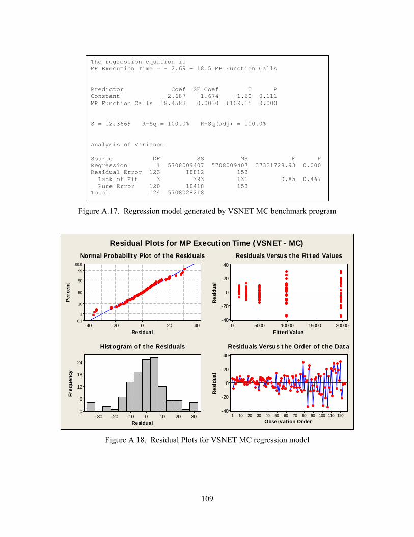
The regression equation is MP Execution Time = - 2.69 + 18.5 MP Function Calls Predictor Coef SE Coef T P Constant -2.687 1.674 -1.60 0.111 MP Function Calls 18.4583 0.0030 6109.15 0.000 S = 12.3669 R-Sq = 100.0% R-Sq(adj) = 100.0% Analysis of Variance Source DF SS MS F P Regression 1 5708009407 5708009407 37321728.93 0.000 Residual Error 123 18812 153 Lack of Fit 3 393 131 0.85 0.467 Pure Error 120 18418 153 Total 124 5708028218

Figure A.17. Regression model generated by VSNET MC benchmark program

Residual

Per

cent

40200-20-40

99.9

99

90

50

10

1

0.1

Fitted Value

Res

idua

l

20000150001000050000

40

20

0

-20

-40

Residual

Freq

uenc

y

3020100-10-20-30

24

18

12

6

0

Observation Order

Res

idua

l

1201101009080706050403020101

40

20

0

-20

-40

Normal Probability Plot of the Residuals Residuals Versus the Fitted Values

Histogram of the Residuals Residuals Versus the Order of the Data

Residual Plots for MP Execution Time (VSNET - MC)

Figure A.18. Residual Plots for VSNET MC regression model

109

The regression equation is MP Execution Time = - 58.9 + 7.87 MP Function Calls Predictor Coef SE Coef T P Constant -58.894 4.010 -14.69 0.000 MP Function Calls 7.87200 0.00296 2656.67 0.000 S = 29.6160 R-Sq = 100.0% R-Sq(adj) = 100.0% Analysis of Variance Source DF SS MS F P Regression 1 6190512863 6190512863 7057869.60 0.000 Residual Error 123 107884 877 Lack of Fit 3 93844 31281 267.35 0.000 Pure Error 120 14041 117 Total 124 6190620748

Figure A.19. Regression model generated by VSNET SMM benchmark program

Residual

Per

cent

100500-50-100

99.9

99

90

50

10

1

0.1

Fitted Value

Res

idua

l

20000150001000050000

80

40

0

-40

-80

Residual

Freq

uenc

y

806040200-20-40-60

24

18

12

6

0

Observation Order

Res

idua

l

1201101009080706050403020101

80

40

0

-40

-80

Normal Probability Plot of the Residuals Residuals Versus the Fitted Values

Histogram of the Residuals Residuals Versus the Order of the Data

Residual Plots for MP Execution Time (VSNET - SMM)

Figure A.20. Residual Plots for VSNET SMM regression model

110

The regression equation is MP Execution Time = - 36.6 + 23.3 MP Function Calls Predictor Coef SE Coef T P Constant -36.617 6.349 -5.77 0.000 MP Function Calls 23.2552 0.0093 2502.95 0.000 S = 46.8916 R-Sq = 100.0% R-Sq(adj) = 100.0% Analysis of Variance Source DF SS MS F P Regression 1 13775054047 13775054047 6264750.26 0.000 Residual Error 123 270455 2199 Lack of Fit 3 259236 86412 924.28 0.000 Pure Error 120 11219 93 Total 124 13775324502

Figure A.21. Regression model generated by VSNET LU benchmark program

Residual

Per

cent

1000-100

99.9

99

90

50

10

1

0.1

Fitted Value

Res

idua

l

3000020000100000

100

50

0

-50

-100

Residual

Freq

uenc

y

60300-30-60-90

40

30

20

10

0

Observation Order

Res

idua

l

120

110

1009080706050403020101

100

50

0

-50

-100

Normal Probability Plot of the Residuals Residuals Versus the Fitted Values

Histogram of the Residuals Residuals Versus the Order of the Data

Residual Plots for MP Execution Time (VSNET - LU)

Figure A.22. Residual Plots for VSNET LU regression model

111

Bibliography

[App05] “Win32.Apparition.” CNET Networks, Incorporated, 2005. <http://web.zdnet.de/itsupport/virencenter/dict/virus/virus3153-wc.html> Accessed 11 February 2006.

[Axe06] Axelsson, Jakob. “A Portable Model for Predicting the Size and Execution Time of Programs.” Department of Computer Science and Information Science, Linköping University. <http://www.ida.liu.se/~jakax/Publications/swtiming.pdf> Accessed 11 February 2006.

[Bla05] “W32.Blaster.Worm.” Symantec Corporation, 10 November 2005. <http://securityresponse.symantec.com/avcenter/venc/data/w32.blaster.worm.html> Accessed 11 February 2006.

[ChJ03] Christodorescu, Mihai, Somesh Jha. “Static Analysis of Executables to Detect Malicious Patterns.” Computer Science Department, University of Wisconsin, Madison, 2003.

[CoT97] Collberg, Christian, Clark Thomborson, Douglas Low. “A Taxonomy of Obfuscating Transformations.” Department of Computer Science, University of Auckland, 1997.

[Cyg05] “Cygwin™.” Red Hat, Incorporated, 2005. <http://www.redhat.com/software/cygwin/> Accessed 29 November 2005.

[Den00] “W32.Dengue.” Symantec Corporation, 24 April 2000. <http://securityresponse.symantec.com/avcenter/venc/data/w32.blaster.worm.html> Accessed 11 February 2006.

[DuE06] Dube, T. E., K. S. Edge, R. A. Raines, R. O. Baldwin, B. E. Mullins, and C. Reuter, “Metamorphism as a Software Protection,” accepted for presentation and publication in The International Conference on Information Warfare and Security, to be presented March 2006.

[EdD06] K. S. Edge, T. E. Dube, R. A. Raines, R. O. Baldwin, and C. Reuter, “A Taxonomy of Protections in Computer Viruses and Their Application to Software Protection,” accepted for presentation and publication in The International Conference on Information Warfare and Security, to be presented March 2006.

[Eil05] Eilam, Eldad. Reversing: Secrets of Reverse Engineering. Wiley Publishing, 2005.

112

[Erd04] Erdélyi, Gergely. “Hide ‘n’ Seek? Anatomy of Stealth Malware.” Virus Bulletin, 2004.

[Evo00] “W32.Evol.” Symantec Corporation, 27 July 2000. <http://www.symantec.com/avcenter/venc/data/w32.evol.html> Accessed 11 February 2006.

[Fix99] “W95.Fix2001.” Symantec Corporation, 16 September 1999. <http://www.symantec.com/avcenter/venc/data/w95.fix2001.html> Accessed 11 February 2006.

[GCC05] “Welcome to the GCC home page!” Free Software Foundation, Incorporated, 2005. <http://gcc.gnu.org/> Accessed 29 November 2005.

[IA105] “IA-32 Intel Architecture Software Developer’s Manual Volume 1: Basic Architecture.” Intel Corporation (June 2005).

[IA205] “IA-32 Intel Architecture Software Developer’s Manual Volume 2B: Instruction Set Reference, N-Z.” Intel Corporation (June 2005).

[IA305] “IA-32 Intel Architecture Software Developer’s Manual Volume 3: System Programming Guide.” Intel Corporation (June 2005).

[IDA06] “The IDA Pro Disassembler.” Data Rescue, (31 January 2006) <http://www.datarescue.com/> Accessed 13 February 2006.

[jGR04] “jGRASP.” Auburn University, 2004. <http://www.eng.auburn.edu/department/cse/research/grasp/> Accessed 29 November 2005.

[Lew95] Lewis, Ricki. “The Rise of Antibiotic-Resistant Infections.” FDA Consumer, Food and Drug Administration (September 1995).

[Lil00] Lilja, David. Measuring Computer Performance. Cambridge University Press, 2000.

[Mar98] “W95.Marburg.A / W95.Marburg.B.” Symantec Corporation, 23 July 1998. <http://securityresponse.symantec.com/avcenter/venc/data/w95.marburg.html> Accessed 11 February 2006.

[Min06] “Minitab.” Minitab, Inc. (2006) <http://www.minitab.com/> Accessed 13 February 2006.

113

[MSD05] “MSDN: IsDebuggerPresent.” Microsoft Corporation (July 2005) <http://msdn.microsoft.com/library/default.asp?url=/library/en-us/debug/base/isdebuggerpresent.asp> Accessed 15 August 2005.

[Oll05] “OllyDbg.” Oleh Yuschuk (Jan. 2005) <http://www.ollydbg.de/> Accessed 13 February 2006.

[PaH05] Patterson, David A., John L. Hennessy. Computer Organization and Design. Morgan Kaufmann Publishers, 2005.

[PoM04] Pozo, Roldan, Bruce Miller. “SciMark2.0.” National Institute of Science and Technology (March 2004) <http://math.nist.gov/scimark2> Accessed 13 February 2006.

[ShT05] Sharma, Vibhu Saujanya, Kishor S. Trivedi. “Architecture Based Analysis of Performance, Reliability, and Security of Software Systems.” Workshop on Software and Performance ’05, ACM, July 2005.

[Sof06] “SoftICE for DevPartner.” Compuware Corporation (2006) <http://www.compuware.com/products/devpartner/softice.htm> Accessed 13 February 2006.

[SuX04] Sung, A. H., P. Chavez, S. Mukkamala. “Static Analyzer of Vicious Executables (SAVE).” Department of Computer Science and Institute for Complex Additive Systems Analysis, New Mexico Institute of Mining and Technology, 2004.

[Szo05] Szor, Peter. The Art of Computer Virus Research and Defense. Addison-Wesley, February 2005.

[ViG03] Viega, John, Zachary Girouard, Matt Messier. Secure Programming Cookbook. O’Reilly Media, July 2003.

[Vis05] “Visual C++ .NET 2003.” Microsoft Corporation, 2005. <http://msdn.microsoft.com/visualc/previous/2003/default.asp> Accessed 29 November 2005.

[Wha06] “Whale (F-Secure Virus Descriptions).” F-Secure Corporation, 2006. <http://www.f-secure.com/v-descs/whale.shtml> Accessed 11 February 2006.

114

[Wik06] “Magic number (programming).” Wikipedia Foundation, Incorporated, 11 February 2006. <http://en.wikipedia.org/wiki/Magic_number_(programming)> Accessed 11 February 2006.

[Win05] “WinDbg Debugger.” Microsoft Corporation, December 2005. <http://msdn.microsoft.com/library/default.asp?url=/library/en-us/tools/tools/windbg_debugger.asp> Accessed 13 February 2006.

[XuS04] Xu, J-Y., A. H. Sung, P. Chavez, S. Mukkamala. “Polymorphic Malicious Executable Scanner by API Sequence Analysis.” Department of Computer Science, New Mexico Institute of Mining and Technology, 2004.

[YiZ04] Yip, Stephen, Qing Zhou. “Enhancing software protections with poly-metamorphism code.” New South Wales Society for Computers and Law Journal Issue 56 (2004) <http://www.nswsd.org.au/journal/56/YipZhou.html> Accessed 8 February 2006

115

Vita

Captain Thomas Dube is currently a graduate student pursuing a degree in

Information Assurance at the Air Force Institute of Technology. He has over fifteen

years experience in various fields of computing sciences including database

administration and development and software engineering. After earning an

undergraduate degree in Computer Engineering from Auburn University in 2000, he

worked for the Air Force Research Laboratory in the Air Vehicles Technology

Assessment and Simulation Branch of the Control Sciences Division. He has authored

several research publications ranging from air-to-air combat simulations to real-time

simulation executives.

His research interests include information security, software engineering,

information management, software management, and software protection strategies.

116

Form Approved REPORT DOCUMENTATION PAGE OMB No. 074-0188

The public reporting burden for this collection of information is estimated to average 1 hour per response, including the time for reviewing instructions, searching existing data sources, gathering and maintaining the data needed, and completing and reviewing the collection of information. Send comments regarding this burden estimate or any other aspect of the collection of information, including suggestions for reducing this burden to Department of Defense, Washington Headquarters Services, Directorate for Information Operations and Reports (0704-0188), 1215 Jefferson Davis Highway, Suite 1204, Arlington, VA 22202-4302. Respondents should be aware that notwithstanding any other provision of law, no person shall be subject to an penalty for failing to comply with a collection of information if it does not display a currently valid OMB control number. PLEASE DO NOT RETURN YOUR FORM TO THE ABOVE ADDRESS. 1. REPORT DATE (DD-MM-YYYY) 2. REPORT TYPE 3. DATES COVERED (From – To)

23-03-2006 Master’s Thesis Aug. 2005 – Mar. 2006 5a. CONTRACT NUMBER 4. TITLE AND SUBTITLE

5b. GRANT NUMBER

METAMORPHISM AS A SOFTWARE PROTECTION FOR NON-MALICIOUS CODE

5c. PROGRAM ELEMENT NUMBER

5d. PROJECT NUMBER 5e. TASK NUMBER

6. AUTHOR(S) Dube, Thomas E., Captain, USAF

5f. WORK UNIT NUMBER

8. PERFORMING ORGANIZATION 7. PERFORMING ORGANIZATION NAMES(S) AND ADDRESS(S) Air Force Institute of Technology Graduate School of Engineering and Management (AFIT/EN)

REPORT NUMBER AFIT/GIA/ENG/06-04

2950 Hobson Way, Building 640 WPAFB OH 45433-8865

10. SPONSOR/MONITOR’S ACRONYM(S)

9. SPONSORING/MONITORING AGENCY NAME(S) AND ADDRESS(ES) AT-SPI Technology Office AFRL/SNTA (POC: Dr. Christopher Reuter, Christopher.Reuter2@wpafb.af.mil) 11. SPONSOR/MONITOR’S REPORT

NUMBER(S) 2241 Avionics Circle WPAFB, OH 45433-7320 (937) 320-9068 12. DISTRIBUTION/AVAILABILITY STATEMENT APPROVED FOR PUBLIC RELEASE; DISTRIBUTION UNLIMITED.

13. SUPPLEMENTARY NOTES 14. ABSTRACT The software protection community is always seeking out new methods for defending their products from unwanted reverse engineering, tampering, and piracy. Most protections currently sought are static in nature. Once integrated, the program never modifies them. Being static makes them stationary instead of moving targets. This observation begs a question, “Why not incorporate self-modification as a defensive measure?” Metamorphism is a defensive mechanism used in modern, advanced malware programs. Although the main impetus for this protection in malware revolves around avoiding detection from anti-virus signature scanners by changing the program’s form, certain metamorphism techniques also serve as anti-disassembler and anti-debugger protections. For example, opcode shifting is a metamorphic technique used to confuse the program disassembly, but malware modifies these shifts dynamically unlike the software protection community’s current static approaches. This research assessed the performance overhead of a simple opcode-shifting metamorphic engine and evaluated the instruction reach of this particular metamorphic transform. In addition, the investigator examined the effects of dynamic subroutine reordering.

15. SUBJECT TERMS metamorphism, reverse engineering, software protection, malware, virus, malicious code

16. SECURITY CLASSIFICATION OF:

19a. NAME OF RESPONSIBLE PERSON Richard A. Raines, Civ, USAF

a. REPORT

18. NUMBER

17. LIMITATION OF

OF ABSTRACT 19b. TELEPHONE NUMBER (Include area code) b. ABSTRACT

U

c. THIS PAGE PAGES

(937) 255-6565, ext 4278 130 UU U U (rraines@afit.edu)

Standard Form 298 (Rev. 8-98) Prescribed by ANSI Std. Z39-18