MPRAMunich Personal RePEc Archive

Measuring de facto versus de iurepolitical institutions in the long-run: amultivariate statistical approach

Peter Foldvari

Utrecht University

10. June 2014

Online at http://mpra.ub.uni-muenchen.de/56576/MPRA Paper No. 56576, posted 10. June 2014 13:36 UTC

1

Measuring de facto versus de iure political institutions in the long-run: a multivariate statistical

approach

Peter Foldvari

Utrecht University

Drift 6, 3512 BS Utrecht, the Netherlands

e-mail: p.foldvari1@uu.nl

Abstract

In this paper we use the components of the PolityIV project’s polity2 and Vanhanen’s Index of

Democracy indicators to analyse the relationship between de iure and de facto political institutions

from 1820 until 2000 with a canonical correlation method, and a correction for the sample selection

bias, caused by the change in the number of available countries.

We find considerably fluctuation in the relationship between the two measures and that much of the

observed correlation is due to the sample selection bias. The relationship becomes strong and positive

only in the second half of the 20th century.

JEL-codes: N40, O17

keywords: democratization, de facto and de iure institutions, canonical correlation, Polity IV,

Vanhanen’s Index of Democracy

2

1. De iure versus de facto political institutions

The distinction between de iure and de facto institutions, or to be more precise, between de iure

institutional setting versus de facto situation is a crucial element in explaining observed divergence in

socio-economic outcomes (the distinction is introduced by Pande and Udry (2006)). North (1991)

defines institutions as a set of rules that constraint individual behaviour. The reason d’etre for

institutions is the reduction of transaction costs that increase as the potential market size and the degree

of the division of labour grows. Without institutions, more complex structure of interdependent

relations would be undermined by the potential gains from individual misbehaviour leading to distrust.

The government, as principal, hence plays a fundamental role in shaping the fundamental rules of

interactions, which takes the form of laws and practices. Yet, this crucial role of the state gives a

special importance to political rights inasmuch as those who make the laws, may also use them to their

own advantage. Acemoglu and Robinson (2012) introduce the concept of inclusive versus extractive

political institutions, the latter supporting the extractive economic institutions that are in place to

channel resources from the society toward the elite. But the concept of elite that shape the laws is not a

stationary one, as pointed out in their earlier work on the dynamics of regime changes (Acemoglu and

Robinson, 2006). Whenever another interest group is growing up in a society, the ruling elite will face

the choice of allowing them political rights leading to reforms or to resist them at the risk of revolution

or a coup d’état. The process is not automatic, though, as there is an underlying non-linearity in this

process: Acemoglu and Robinson find that regime changes are more likely to occur at intermediate

levels of income inequality. The important consequence of this finding is that some societies can stuck

in an extractive institutional setting in the long-run, which is a primary candidate to explain observed

cross-country income differences. But written rules may also arrive from outside, such as happened

historically in the case of colonization. Here we refer not as much to the celebrated reversal of fortune

thesis of Acemoglu et al (2002) as to legacy of colonial legislation of the European powers in Sub-

Saharan Africa, which does not seem to have lasted long or, if they did, they led to inefficient

outcomes. As Pande and Udry (2006) observes, the French and British rules regarding land ownership

in their African colonies were different, yet, the pre-colonial customary laws still play a prominent role

in many ex British and French colonies, independently of their colonial legal origin. Similarly, Blewet

(1995) finds that the British laws in Kenya, introducing private property of lands actually destroyed a

well-working land-management system leading to a relatively less efficient use of lands. Another

example on an obvious difference in de iure and de facto institutions, is the Soviet Constitution of

1936, which, even though clearly stated the Communist Party’s leading position, also granted the

3

freedom of consciousness and the equality under the law to all citizens, rights that remained pure

words in one of the world’s most dictatorial police state of the period.

One explanation for such deviation between the de iure and de facto political institutions is by Boettke

et al (2008) who distinguish among foreign-introduced exogenous, indigenously introduced exogenous

and indigenously introduced endogenous institutions. Exogenous institutions are constructed and

forced from above, either by an indigenous group or by a foreign power (colonizer or an international

organization). Endogenous institutions are the result of some spontaneous process. In the historical

process of the evolution of institutions, indigenously introduced endogenous institutions predated all

other type, being followed by endogenously introduced exogenous institutions, which were created by

the ruling elite. Boettke et al. claim that these different institution types exhibit different degree of

hysteresis or stickiness, a concept closely related to path dependence1. Endogenous institutions are the

stickiest of all, that will resist the effect of any new rules efficiently, and for a very long time. The least

sticky institutions are the foreign-induced ones, which do not necessarily serve the interest of the

population or the ruling elite. These may take the form of laws (such as Western type constitutions,

introduction of general suffrage or a system of education) but will be inefficient, and once the external

pressure ceases, they disappear. Hence, we can expect that the difference between de iure and de facto

political institutions has grown with the globalization as non-European countries were increasingly

subjected to the expectations of Western powers either directly (via colonization) or indirectly (by

conditioning aid on political or economic reforms). There are historical examples, however, when

foreign-induced institutions managed to replace indigenous institutions, such as democratization in

Japan and Germany after World War 2, since these externally designed and forced changes were

brought in conformity with certain indigenous traditions. Still the majority of the historical examples

reflect the lack of success such as the fall of many democratic African regimes in the 1960s attests.

Altogether, the distinction between de facto and de iure political institutions is of crucial importance

for understanding the obvious differences one can find among the degree of democratization of

countries when measured by different indicators, and it also offers an explanation why empirical

research, using traditional methods such as regression analysis, on the relationship between

democratization and aggregate socio-economic outcomes has limitations.

2. Measuring democracy: limitations and possibilities

1 See Mahoney(2000) on the different theoretical explanaton behind path dependence observed in social structures.

4

To our knowledge no current empirical measures of democratization are explicitly concerned about the

distinction between de iure and de facto institutions. They can all be placed into an underlying

theoretical framework as suggested in the critical review article by Coppedge et al. (2011), based on

different concepts of democracy. The most important theoretical point of departure is Dahl (1972) who

introduced the concept of polyarchy, with competition and participation (or contestation and

inclusiveness in his terminology) as two basic aspects of democracy. The identification of these two,

theoretically measurable, component of democracy is a common factor behind both the PolityIV

(polity) project (Marshall et al, 2012) and Vanhanen’s Index of Democracy (ID) (Vanhanen 2000,

2003), that are still the most popular datasets stretching over the last two centuries (the polity project is

constantly updated, currently having data on 167 countries for 1800-2012 while the ID includes 187

countries for 1820-2000) and which we also use in this paper.2 Coppedge et al. (2008) show that the

role of the factors competition and participation are predominant in all datasets and account for about

three-quarter of the total variation. In this paper we rely on the fundamental assumption that even if

both the ID and the polity attempt to capture the same dimensions of democracy, the latter is more

successful in measuring actual outcomes through directly using statistics on voter turnout and the

composition of parliaments, while polity is more measuring the formal rules and practices that shape

political processes, being a product of secondary literature research and expert opinion. In other words,

the ID reflects the de facto situation while the polity score (and its five components) is more about the

de iure institutional framework. This is observed by Munck and Verkuilen (2002) who notes that the

polity indicator is more concerned about the regulatory aspects of participation (if the elections are

competitive or not), but it does not reflect the actual magnitude of participation at all.

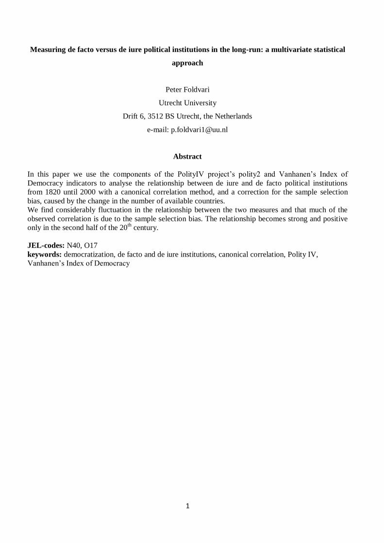
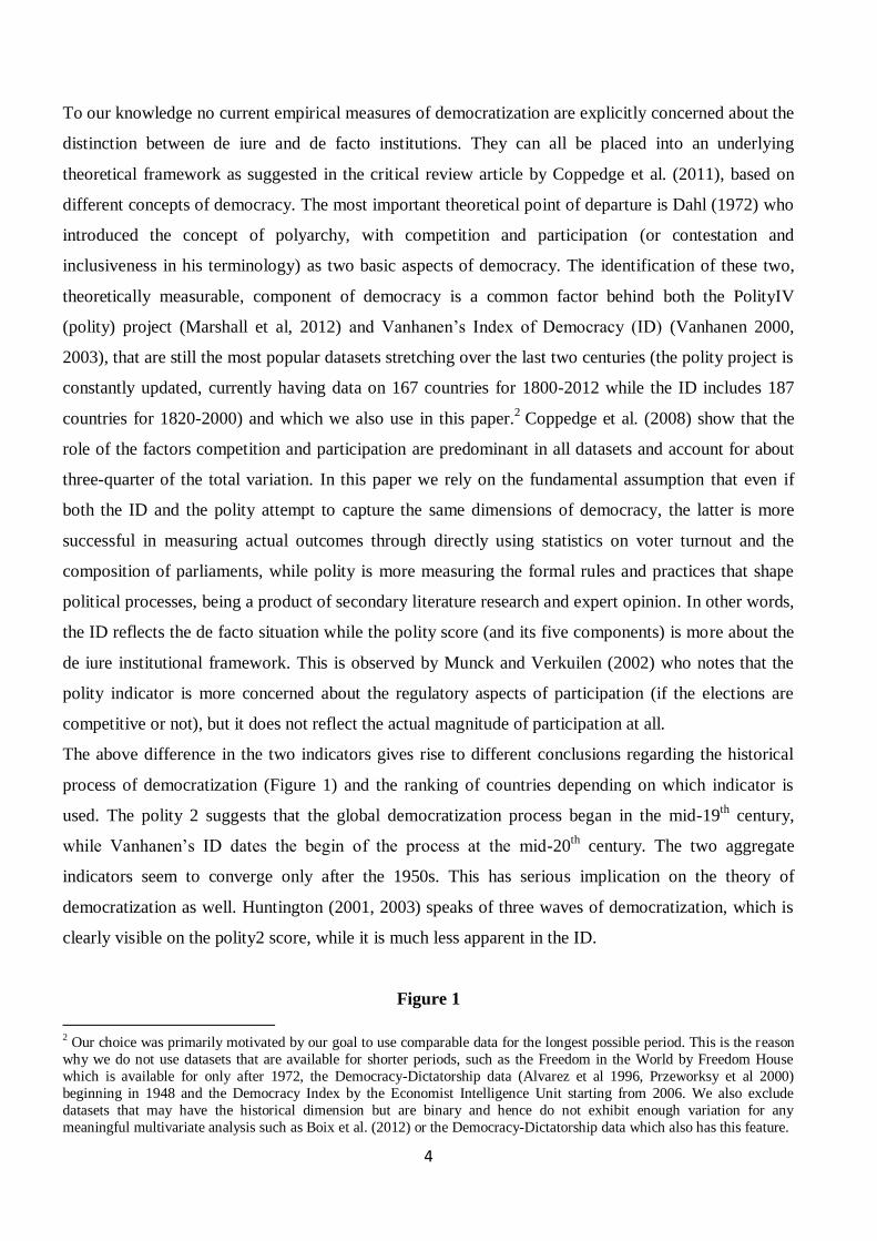
The above difference in the two indicators gives rise to different conclusions regarding the historical

process of democratization (Figure 1) and the ranking of countries depending on which indicator is

used. The polity 2 suggests that the global democratization process began in the mid-19th

century,

while Vanhanen’s ID dates the begin of the process at the mid-20th

century. The two aggregate

indicators seem to converge only after the 1950s. This has serious implication on the theory of

democratization as well. Huntington (2001, 2003) speaks of three waves of democratization, which is

clearly visible on the polity2 score, while it is much less apparent in the ID.

Figure 1

2 Our choice was primarily motivated by our goal to use comparable data for the longest possible period. This is the reason

why we do not use datasets that are available for shorter periods, such as the Freedom in the World by Freedom House

which is available for only after 1972, the Democracy-Dictatorship data (Alvarez et al 1996, Przeworksy et al 2000)

beginning in 1948 and the Democracy Index by the Economist Intelligence Unit starting from 2006. We also exclude

datasets that may have the historical dimension but are binary and hence do not exhibit enough variation for any

meaningful multivariate analysis such as Boix et al. (2012) or the Democracy-Dictatorship data which also has this feature.

5

World average scores in different measures of the degree of democracy of political institutions, 1820-

2010, Polity2 score of the Polity IV project (-10/+10) and the Index of Democracy (%)

Sources: the polity IV dataset by Marshall et al (2012) and the polyarchy data by Vanhanen (2000, 2003)

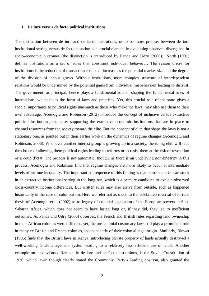
The most striking difference can be observed for the United States and the United Kingdom, though.

Figure 2 reflect a significant difference between the order of the United States and the United-

Kingdom in the democratization process. The polity IV project assigns very high score to the USA in

the first half of the 19th

century, even though a considerable percentage of the population was still

disfranchised. After the Civil War, the USA constantly has a maximum score of 10, which is only

achieved by the UK after World War 1. The Index of Democracy exhibits a fundamentally different

picture: both countries have a clear trend of increasing democracy, and the USA is overtaken by the

UK around 1920, with the significant extension of political rights that results in more participation and

competition. Similar differences between the two measures can be observed for most Western

European democracies after World War 2, for example in France, Switzerland and the Netherlands.

Figure 2

The polity2 and ID scores for the United States and the United Kingdom, 1810-2010, Polity2 score of

the Polity IV project (-10/+10) and the Index of Democracy (%)

0

2

4

6

8

10

12

14

16

-4

-3

-2

-1

0

1

2

3

4

1820 1840 1860 1880 1900 1920 1940 1960 1980 2000

Ind

ex

of

De

mo

cra

cy

po

lity2

polity2 index of democracy or polyarchy

6

Sources: the polity IV dataset by Marshall et al (2012) and the polyarchy data by Vanhanen (2000, 2003)

Table 1

Components of the polity2 index and coding rules

variable possible outcomes values weight in polity2 implied order

XRCOMP

Competitiveness

of Executive

Recruitment

Election 3 2 4

Transitional 2 1 3

Selection 1 -2 1

Unregulated 0 0 2

XROPEN

Openness of

Executive

Recruitment

Open (“Election”) 4 1 6

Dual: hereditary and

election

3 1 5

Dual: hereditary and

designation

2 -1 2

Closed 1 -1 1

Unregulated 0 0 4

Open(“No election” 4 0 3

XCONST

Constraint on

Chief Executive

Parity or subordination 7 4 7

Intermediate 1 6 3 6

Substantial limitation 5 2 5

Intermediate 2 4 1 4

Slight moderation 3 -1 3

Intermediate 3 2 -2 2

Unlimited Authority 1 -3 1

PARCOMP

Competitiveness

of Political

Participation

Competitive 5 3 6

Transitional 4 2 5

Factional 3 1 4

Restricted 2 -1 2

Suppressed 1 -2 1

Not applicable 0 0 3

PARREG Regulated 5 0 3

0

5

10

15

20

25

30

35

40

-4

-2

0

2

4

6

8

10

1810 1830 1850 1870 1890 1910 1930 1950 1970 1990 2010

Ind

ex

of

De

mo

cra

cy

po

lity2

USA(polity2) United Kingdom (polity2)

USA (ID) United Kingdom (ID)

7

Regulation of

participation

Multiple identity 2 0 3

Sectarian 3 -1 2

Restricted 4 -2 1

Unregulated 1 0 3

Source: Table 1 in Treier and Jackman (2008: 204), and Marshall et al (2013)

But conceptual limitations are not the only challenges a quantitative research has to cope with.

Munck and Verkuilen (2002) discuss some important technical issues that have potentially highly

significant consequences on the choice of statistical techniques and the results. The first important

issue is the level of measurement. Most institutional indicators are measured on nominal scale (like the

components of the polity2 score), which can usually be concerted to an ordinal scale based on some

theoretical expectations as done by Treier and Jackman (2008). On nominal scale one can measure if a

country’s political system fulfils certain qualitative condition, but no further arithmetic operation

makes sense. The only information conveyed by such variables is the difference among countries from

a certain aspect. On an ordinal scale at least an order is established, e.g., one can state that a country

where the chief executives are given authority by hereditary succession (XRCOMP=1 in the polity IV

dataset) has a lower rank compared to the situation when they are elected (XRCOMP=3) from the

perspective of democratization, but again, even the most fundamental operations like addition are

pointless: one could assign any arbitrary numbers to the different outcomes as long as they preserve

the order. In other words, assigning the number 0 to the XRCOMP=1 case, and 100 to the

XRCOMP=3 case would still convey the same information on the order of possible outcomes, but it

would change the mean from 1.5 to 99.5. Most statistical methods are designed for variables

measurable by at least interval scale, where the operations summation and subtraction makes sense,

and basic statistics, like the mean or the standard deviation can be defined.

The polity project addresses this problem by assigning arbitrary numbers (weights) to different

outcomes and sum them up to an aggregate measure labelled as polity2 in Polity IV (see Table 1).3

Numerous studies use this aggregate measure as an explanatory variable even though, unless the

arbitrary weighting accidently coincides with the theoretically correct one, this practice leads to an

omitted variable problem and biased coefficient estimates (see Appendix 1 for a proof).

Another issue is the inclusion of redundant variables as a result of arbitrary aggregation methods. The

polity2 score the sum of the weighted components, which completely neglects the effect and

importance of covariance among the components: components are correlated simply because, to a

different extent, they contain the same information (see Table 2 and 3). Hence, they are partly

redundant, since we could extract the same information from them. Adding these components up is

3 Marshall et al (2013) warns about the possible shortcomings of their aggregation method in their manual.

8

consequently a form of double counting, resulting in an aggregate component that has more variance,

than it should have if it were correctly representing the underlying latent democracy. The same applies

to the multiplicative aggregation adopted by Vanhanen who creates his aggregate Index of Democracy

by multiplying observed data on participation (voter turnout) and competition (one minus the share of

the winning party in the parliament). This method assures that only countries that have a balanced

performance in both aspects will have a high ID score, but there is no further reason to prefer it above

the additive aggregation.

Table 2

Spearman rank correlation coefficients between components of the polity2 score in 2000

XRCOMP XROPEN XCONST PARREG PARCOM

XRCOMP 1

XROPEN 0.884 1

XCONST 0.840 0.691 1

PARREG 0.801 0.629 0.808 1

PARCOM 0.790 0.691 0.839 0.784 1 N=151, note: we adopted the same ranking as Table 1 in Treier and Jackman (2008)

Table 3

Spearman rank correlation coefficients between components of the polity2 score in 1900

XRCOMP XROPEN XCONST PARREG PARCOM

XRCOMP 1

XROPEN 0.853 1

XCONST 0.533 0.498 1

PARREG 0.560 0.463 0.513 1

PARCOM 0.578 0.575 0.502 0.719 1 N=51, note: we adopted the same ranking as Table 1 in Treier and Jackman (2008)

But Tables 2 and 3 have an additional inconvenient message about usual weighting methods: the

degree of correlation changes over time, and hence the weights applied for aggregation cannot remain

constant either.

3. Methodology

It may be tempting at first sight to apply a simple dimension reducing method, such as Principal

Component Analysis (PCA) or an Exploratory Factor Analysis on the components of democracy to

arrive at some less arbitrary weighting scheme. Unfortunately, there is no guarantee that any of the

principal components (or factors) would be the latent democracy variable even if we use a rotation to

arrive at easier interpretable factors. In a PCA (which is usually the first step in a factor analysis) the

component loadings are identified so that the resulting principal components explain most of the

9

variance observed in the data, and the sum of squared loadings is one. But the observed correlation

among different components may include measurement errors or the effect of other external factors

that are not related to democratization and should be treated as noise rather than signal. It is hence

advisable either to rely on methods that introduce additional, theoretically formulated restrictions on

the estimated weights, such as Canonical Correlation (CC), Structural Equation Modelling (SEM), or

other latent variables methods such as Pemstein et al (2010). Yet one should be aware that the resulting

estimates for the latent democracy variable depend on a set of assumptions. Pemstein et al (2010), for

example, rely on the assumption that different democracy measures actually measure the same latent

variable and any observed difference are due to methodological differences and random measurement

errors. These effects are then filtered out to arrive at a unified measure. In this paper however, our

main assumption that we demonstrate in the next section, is that the Polity project and Vanhanen’s

dataset do not measure the same process, even though they are correlated.

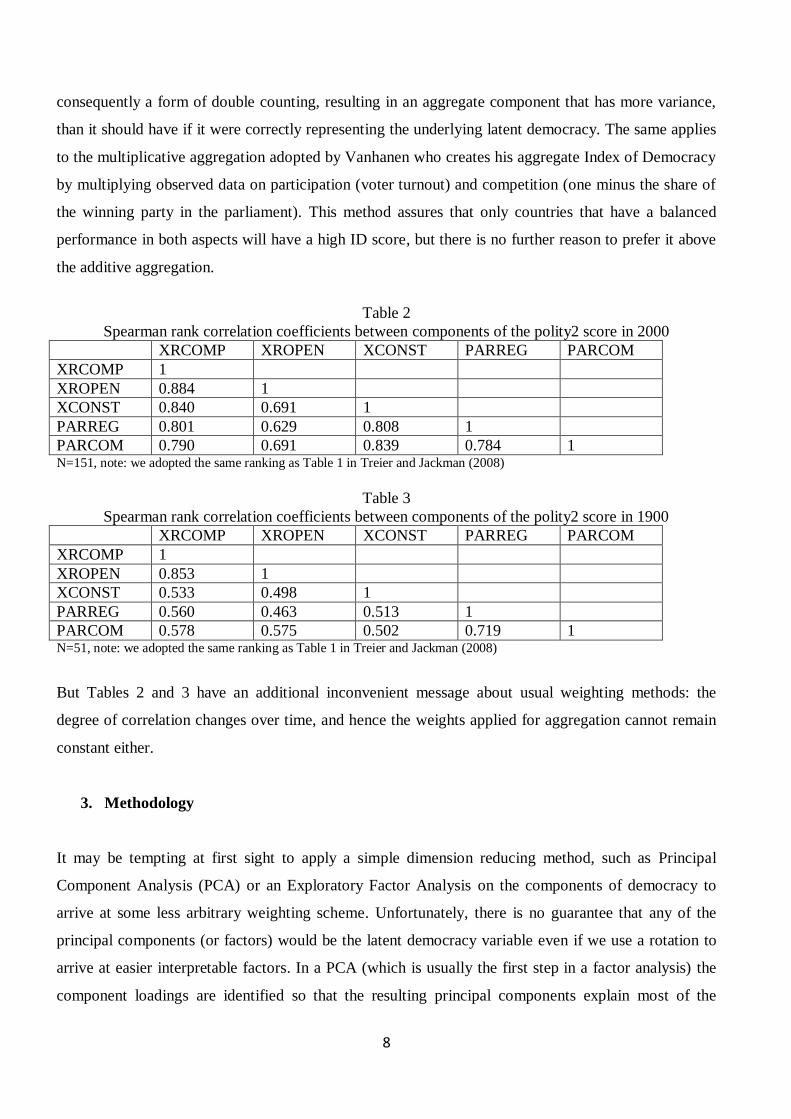
We therefore use a canonical correlation approach to find out how the relationship between de iure and

de facto political institutions changed over time. With canonical correlation we look for those weights

(or coefficients) that maximize the correlation between two component variables (or canonical

variates) that contain the components of polity2 and ID respectively. The underlying theory can be

summarized as a block diagram (Figure 3).

Figure 3

The theoretical outline of the canonical correlation model

The components of the polity2 score and the Index of Democracy are used to arrive at an estimate for

the two latent variables de iure and de facto political institutions. The crucial theoretical assumption

that identifies the coefficients of the observed variables is that two latent variables are correlated. If the

10

majority of political systems in the World exhibit a strong internal consistency between de iure and de

facto institutions, we should obtain a high canonical correlation coefficient. In the case the two are not

related, the canonical correlation should approach zero. Unfortunately, using canonical correlation has

a price too. Since the five components of the polity2 indicator are strongly correlated, we cannot use

them as dummy variables for the canonical correlation analysis, since they are usually perfectly

collinear. As an intermediary solution, we adopt the arbitrary weighting scheme by Marshal et all

(column 4 of Table 1), but we allow each component to have their own weight.4 While an imperfect

solution, this still allows a room for a reweighing of the components, and redundant variables will still

yield a close to zero coefficient. Also, exceptional events, denoted by codes -66, -77 and -88 in the

polity dataset are treated as missing values. We used modern countries, hence the data on historical

states that has no obvious equivalent today are omitted either.

Finally, since we use long-term historical data we also need to cope with the problem of sample

selection bias. Namely, the probability that a country is included in the data is not random and may be

correlated with the value of the components included in the analysis. Initially we have observations on

the developed Western nations such as the USA, the United Kingdom and France, while from the last

decades of the 19th century we will have data on the periphery to an increasing extent. Also the number

of countries increased steadily in the sample period. One should not underestimate the importance of

selection problems in cross-country analyses. Since countries with endogenously developed more

efficient institutions will have a higher chance of being observed (with probably less noise than

latecomers), the estimated correlation may easily be biased upward. The problem has been described

by Heckman (1979) who showed that this selection problem can be interpreted and treated as a form of

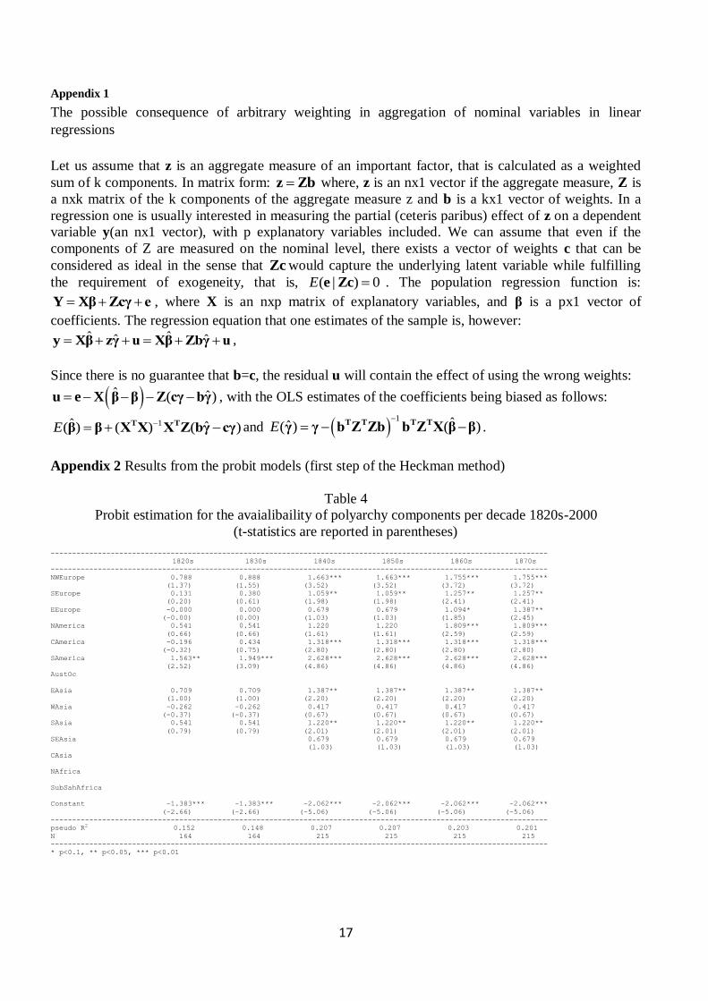
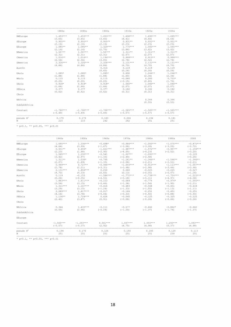
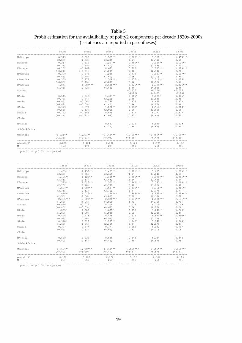
omitted variable bias. We follow his first, two-step procedure for the canonical correlation. In the first

step we estimate the probability if the components of the polity2 and the ID were observed for a

particular year conditioned on the subcontinent it is situated on with a probit model.5 The results of the

first step are reported as Table 4 and Table 5 in Appendix 2. In the second step we use the two Inverse

4 Unfortunately there is no canonical correlation method designed for ordinal variables. If one were to design such a

method, the choice of weights would matter only as much as they affect the order of the possible values of the components.

Yet, the established order should be primarily theory driven, hence it is questionable if a “canonical rank correlation”

would make practical sense. 5 The subcontinents loosely follows the Clio-Infra project’s adopted geographical categorization. The regions are: Western

and Northern Europe, Eastern Europe (including the USSR and later its successors west of the Ural), Southern Europe,

North America, Central America and the Caribbean, South America, Australia and Oceania, East-, West-, South-,

Southeast- and Central-Asia, North Africa, and Sub-Saharan Africa.

11

Mills ratios6 estimated form the first step, as additional variables in the canonical correlation analysis.

These should correct for the effect of selection bias in the coefficients, and once we use these corrected

coefficients to estimate the latent de facto and de iure political institution indices, we can estimate the

linear correlation coefficient between them as a canonical correlation coefficient corrected for

selection bias.

4. Results

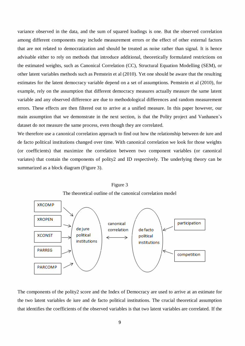
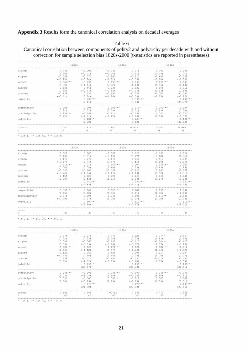
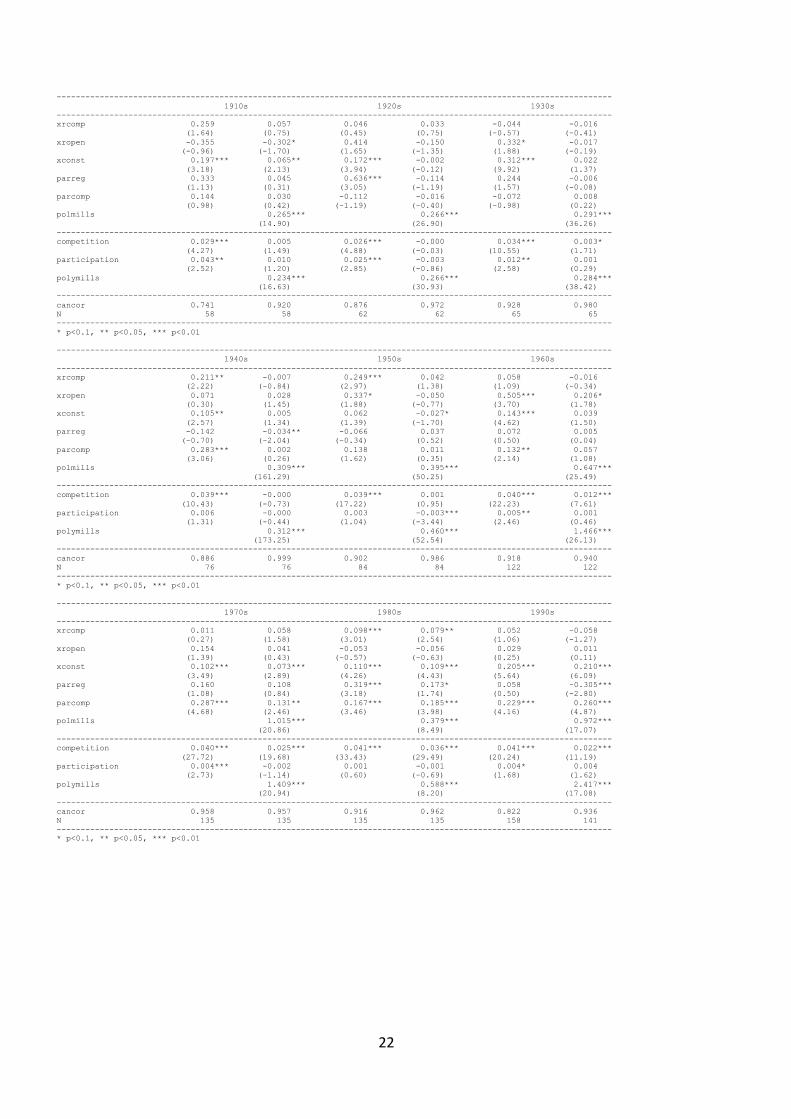
The results from the canonical correlation analysis on decadal averages are reported as Table 6 in

Appendix 3. The coefficients suggest that redundancy was indeed a significant issue, as usually only

one or two components are found to significant at at least 10%, and the rest is usually very close to

zero. We also carried out the estimation per year, but since the results are basically the same, for

convenience we report only the decadal estimates in Table 6. The figures are created from the annual

estimates for the canonical correlation, however, as these reflect a more precise picture. Figure 4 has

all estimated canonical correlations and the number of observations in a single graph.

Figure 4

Estimated canonical correlation coefficients per year 1820-2000

6 The Inverse Mills ratio is the ratio of a probability density function of a probability distribution to its cumulative

distribution function.

21ˆ

2

ˆ2 ( )

p

i

emills

p

, where p̂ is the estimated probability of observing observation i from the probit

model, and ˆ( )p denotes the value of the standard normal CDF at value p̂ .

0

20

40

60

80

100

120

140

160

-1

-0.5

0

0.5

1

1820 1840 1860 1880 1900 1920 1940 1960 1980 2000

Nu

mb

er o

f av

aila

ble

ob

s.

can

on

ical

co

rrel

atio

n

first canonical correlation with Inv. Mills ratio includedwith the effect of Inv. Mills ratio removed number of available observations

12

Figure 5 reveals a slow increase in the first canonical correlation coefficient7 ranging between 0.508 in

1873 and 0.947 in 1982. Even though these estimates are still biased by the selection problem, a trend

can already be established. Until about the 1860s the relationship between the two group of indicators

was relatively strong, which weakened until 1873 and slowly increased until World War I which

resulted in a temporary drop. In the 1930s we find a minor setback, followed by World War 2, which

had a seemingly smaller effect than World War 1, and the strong correlation gradually restores finally

by the 1960s.

Figure 5

The first canonical correlation coefficient (without correction for sample selection)

Figure 5 tells us a story which is in accordance with standard knowledge about the historical

democratization process. De iure political institutions and de facto practices become less connected in

periods of fundamental changes or crises such as World War I and II, the Great Depression.

Once we correct for sample selection biases, the magnitude of the correlation changes fundamentally

(Figure 6). As Table 6 attests, the effect of selection bias on the estimated canonical variates as the

coefficients are positive and significant. In other words, the omitted selection bias indeed resulted in an

overestimation of the relationship between de iure and de facto institutions, and also biased the

coefficients. In case of the components of the ID, we even obtain periods when none of the variables

yield a significant coefficients, indicating a complete detachment between de iure and de facto

institutions.

7 We use and report the first (highest) canonical correlation.

0.2

0.3

0.4

0.5

0.6

0.7

0.8

0.9

1

1820 1840 1860 1880 1900 1920 1940 1960 1980 2000

first canonical correlation lower conf. Interval (95%) upper conf. Interval (95%)

13

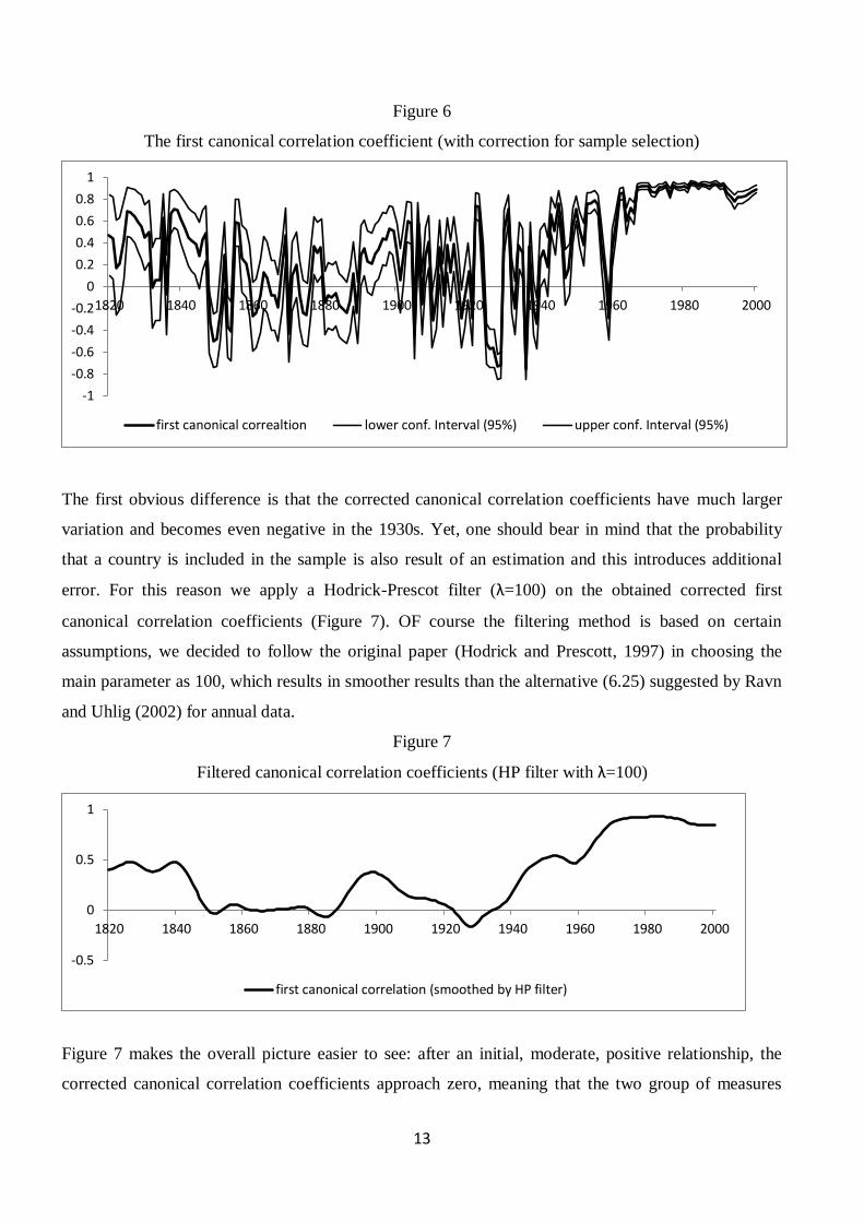
Figure 6

The first canonical correlation coefficient (with correction for sample selection)

The first obvious difference is that the corrected canonical correlation coefficients have much larger

variation and becomes even negative in the 1930s. Yet, one should bear in mind that the probability

that a country is included in the sample is also result of an estimation and this introduces additional

error. For this reason we apply a Hodrick-Prescot filter (λ=100) on the obtained corrected first

canonical correlation coefficients (Figure 7). OF course the filtering method is based on certain

assumptions, we decided to follow the original paper (Hodrick and Prescott, 1997) in choosing the

main parameter as 100, which results in smoother results than the alternative (6.25) suggested by Ravn

and Uhlig (2002) for annual data.

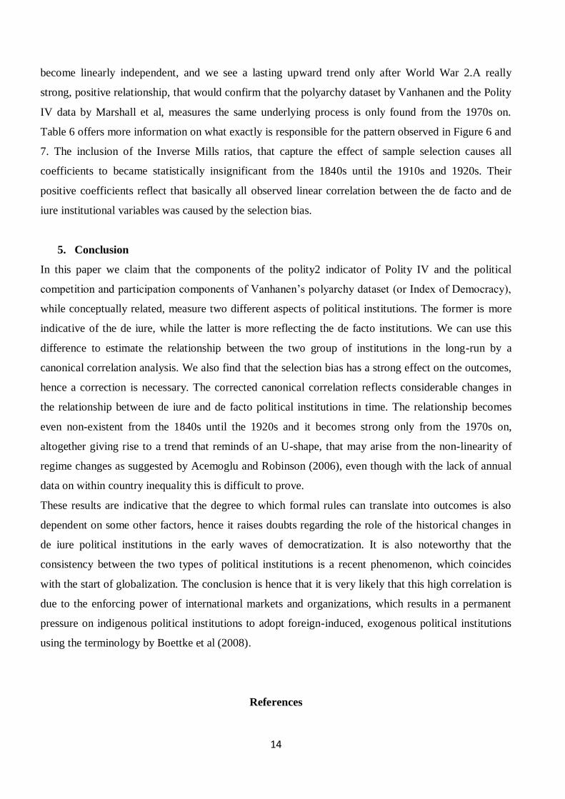
Figure 7

Filtered canonical correlation coefficients (HP filter with λ=100)

Figure 7 makes the overall picture easier to see: after an initial, moderate, positive relationship, the

corrected canonical correlation coefficients approach zero, meaning that the two group of measures

-1

-0.8

-0.6

-0.4

-0.2

0

0.2

0.4

0.6

0.8

1

1820 1840 1860 1880 1900 1920 1940 1960 1980 2000

first canonical correaltion lower conf. Interval (95%) upper conf. Interval (95%)

-0.5

0

0.5

1

1820 1840 1860 1880 1900 1920 1940 1960 1980 2000

first canonical correlation (smoothed by HP filter)

14

become linearly independent, and we see a lasting upward trend only after World War 2.A really

strong, positive relationship, that would confirm that the polyarchy dataset by Vanhanen and the Polity

IV data by Marshall et al, measures the same underlying process is only found from the 1970s on.

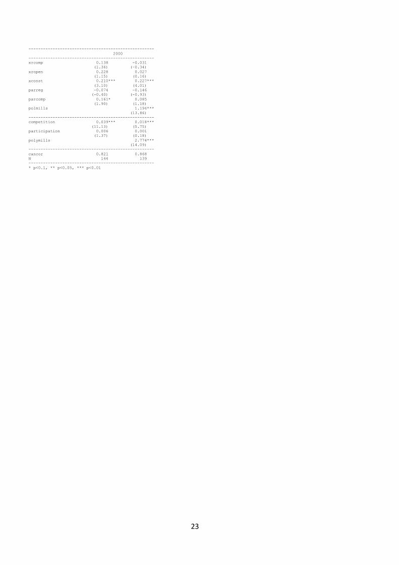
Table 6 offers more information on what exactly is responsible for the pattern observed in Figure 6 and

7. The inclusion of the Inverse Mills ratios, that capture the effect of sample selection causes all

coefficients to became statistically insignificant from the 1840s until the 1910s and 1920s. Their

positive coefficients reflect that basically all observed linear correlation between the de facto and de

iure institutional variables was caused by the selection bias.

5. Conclusion

In this paper we claim that the components of the polity2 indicator of Polity IV and the political

competition and participation components of Vanhanen’s polyarchy dataset (or Index of Democracy),

while conceptually related, measure two different aspects of political institutions. The former is more

indicative of the de iure, while the latter is more reflecting the de facto institutions. We can use this

difference to estimate the relationship between the two group of institutions in the long-run by a

canonical correlation analysis. We also find that the selection bias has a strong effect on the outcomes,

hence a correction is necessary. The corrected canonical correlation reflects considerable changes in

the relationship between de iure and de facto political institutions in time. The relationship becomes

even non-existent from the 1840s until the 1920s and it becomes strong only from the 1970s on,

altogether giving rise to a trend that reminds of an U-shape, that may arise from the non-linearity of

regime changes as suggested by Acemoglu and Robinson (2006), even though with the lack of annual

data on within country inequality this is difficult to prove.

These results are indicative that the degree to which formal rules can translate into outcomes is also

dependent on some other factors, hence it raises doubts regarding the role of the historical changes in

de iure political institutions in the early waves of democratization. It is also noteworthy that the

consistency between the two types of political institutions is a recent phenomenon, which coincides

with the start of globalization. The conclusion is hence that it is very likely that this high correlation is

due to the enforcing power of international markets and organizations, which results in a permanent

pressure on indigenous political institutions to adopt foreign-induced, exogenous political institutions

using the terminology by Boettke et al (2008).

References

15

Acemoglu, D. and Robinson, J. A. (2006), Economic Origins of Dictatorship and Democracy. New

York: Cambridge University Press

Acemoglu, D. and Robinson, J. A. (2012) Why nations fail? The origins of power, prosperity, and

poverty. Crown Business

Acemoglu, D., Johnson, S. and Robinson, J. A. (2002) Reversal of Fortune: Geography and

Institutions in the Making of the Modern World Income Distribution, The Quarterly Journal of

Economics, Vol. 117, No. 4, 1231-1294.

Alvarez, M., Cheibub, J. A., Limongi, F. & Przewroski, A. (1996). Classifying political

regimes". Studies in Comparative International Development. Vol. 31(2), 3–36.

Blewett, Robert A. (1995). “Property Rights as a Cause of the Tragedy of the Commons: Institutional

Change and the Pastoral Maasai of Kenya.”Eastern Economic Journal 21(4): 477–490.

Boettke, P. J., Coyne, C. J. Leeson, P. T. (2008) Institutional Stickiness and the New Development

Economics, American Journal of Economics and Sociology, Volume 67, Issue 2, 331–358

Boix, C., Miller, M., and Rosato, S. (2012), A Complete Data Set of Political Regimes, 1800-2007.

Comparative Political Studies, online version ahead of print, doi:10.1177/0010414012463905

Coppedge, M, Alvarez, A. and Maldonado, C. (2008) Two Persistent Dimensions of Democracy:

Contestation and Inclusiveness, The Journal of Politics Vol. 70(3), 632-647.

Coppedge, M., Gerring, J., Altman, D., Bernhard, M., Fish, S., Hicken, A., Kroenig, M., Lindberg, S.

I., Mcmann, K., Paxton, P., Semetko, H. A., Skaaning S., Staton, J., and Teorel, J. (2011)

Conceptualizing and Measuring Democracy: A New Approach (l), Perspectives On Politics Vol. 9(2),

247-267.

Dahl, R. A. (1972). Polyarchy: Participation and Opposition. Yale University Press, New Haven, CT.

Heckman, J. (1979). "Sample selection bias as a specification error". Econometrica 47 (1): 153–161.

Hodrick, R,, and Prescott, E. C. (1997) Postwar U.S. Business Cycles: An Empirical

Investigation, Journal of Money, Credit, and Banking, 29 (1), 1–16.

Huntington, S. P. (1991) Democracy’s third wave. Journal of Democracy, 2(2), 12-34.

16

Huntington, S. P. (1993) The third wave: democratization in the late twentieth century. University of

Oklahoma Press

Mahoney, J. (2000) Path Dependence in Historical Sociology, Theory and Society, Vol. 29(4), pp.

507-548.

Marshall, M. G., Gurr, T. R., and Jaggers, K. (2013) Polity™ IV Project. Political Regime

Characteristics and Transitions, 1800-2012 Dataset Users’ Manual. Center for Systematic Peace.

http://www.systemicpeace.org/inscr/p4manualv2012.pdf

Munck, G. L. and Verkuilen, J. (2002) Conceptualizing and measuring democracy. Evaluating

Alternative Indices. Comparative Political Studies, 35(1), 5-34.

North, D. C. (1991) Institutions, The Journal of Economic Perspectives, 5(1), pp. 97–112

Pande, R. and Udry, C. (2006) Institutions and Development: A View from Below, in Advances in

Economics and Econometrics 2006, Blundell, Newey and Persson, eds.

Pemstein, D., Meserve, S. A. and Melton, J. (2010) Democratic Compromise: A Latent Variable

Analysis of Ten Measures of Regime Type. Political Analysis (2010) 18:426–449

Przeworski, A., Alvarez, M. F., Cheibub, J. A., and Limongi, F. (2000). Democracy and Development.

Political Institutions and Well-being in the World, 1950-1990. Cambridge: Cambridge University

Press

Ravn. M. O. and Uhlig, H. (2002) On adjusting the Hodrick-Prescott filter for the frequency of

observations," The Review of Economics and Statistics vol. 84(2), 371-375.

Treier, S. and Jackman, S (2008) Democracy as a Latent Variable, American Journal of Political

Science, Vol. 52(1), 201–217.

Vanhanen, T. (2000) A new dataset for measuring democracy, 1810-1998. Journal of Peace Research

37 (2): 251-265.

Vanhanen, T. (2003) Democratization: A Comparative Analysis of 170 Countries. London: Routledge.

17

Appendix 1

The possible consequence of arbitrary weighting in aggregation of nominal variables in linear

regressions

Let us assume that z is an aggregate measure of an important factor, that is calculated as a weighted

sum of k components. In matrix form: z Zb where, z is an nx1 vector if the aggregate measure, Z is

a nxk matrix of the k components of the aggregate measure z and b is a kx1 vector of weights. In a

regression one is usually interested in measuring the partial (ceteris paribus) effect of z on a dependent

variable y(an nx1 vector), with p explanatory variables included. We can assume that even if the

components of Z are measured on the nominal level, there exists a vector of weights c that can be

considered as ideal in the sense that Zc would capture the underlying latent variable while fulfilling

the requirement of exogeneity, that is, ( | ) 0E e Zc . The population regression function is:

Y Xβ Zcγ e , where X is an nxp matrix of explanatory variables, and β is a px1 vector of

coefficients. The regression equation that one estimates of the sample is, however: ˆ ˆˆ ˆ y Xβ zγ u Xβ Zbγ u ,

Since there is no guarantee that b=c, the residual u will contain the effect of using the wrong weights:

ˆ ˆ( ) u e X β β Z cγ bγ , with the OLS estimates of the coefficients being biased as follows:

1ˆ ˆ( ) ( ) ( )E T Tβ β X X X Z bγ cγ and

1 ˆˆ( ) ( )E

T T T Tγ γ b Z Zb b Z X β β .

Appendix 2 Results from the probit models (first step of the Heckman method)

Table 4

Probit estimation for the avaialibaility of polyarchy components per decade 1820s-2000

(t-statistics are reported in parentheses)

--------------------------------------------------------------------------------------------------------------------

1820s 1830s 1840s 1850s 1860s 1870s

--------------------------------------------------------------------------------------------------------------------

NWEurope 0.788 0.888 1.663*** 1.663*** 1.755*** 1.755***

(1.37) (1.55) (3.52) (3.52) (3.72) (3.72)

SEurope 0.131 0.380 1.059** 1.059** 1.257** 1.257**

(0.20) (0.61) (1.98) (1.98) (2.41) (2.41)

EEurope -0.000 0.000 0.679 0.679 1.094* 1.387**

(-0.00) (0.00) (1.03) (1.03) (1.85) (2.45)

NAmerica 0.541 0.541 1.220 1.220 1.809*** 1.809***

(0.66) (0.66) (1.61) (1.61) (2.59) (2.59)

CAmerica -0.196 0.434 1.318*** 1.318*** 1.318*** 1.318***

(-0.32) (0.75) (2.80) (2.80) (2.80) (2.80)

SAmerica 1.563** 1.949*** 2.628*** 2.628*** 2.628*** 2.628***

(2.52) (3.09) (4.86) (4.86) (4.86) (4.86)

AustOc

EAsia 0.709 0.709 1.387** 1.387** 1.387** 1.387**

(1.00) (1.00) (2.20) (2.20) (2.20) (2.20)

WAsia -0.262 -0.262 0.417 0.417 0.417 0.417

(-0.37) (-0.37) (0.67) (0.67) (0.67) (0.67)

SAsia 0.541 0.541 1.220** 1.220** 1.220** 1.220**

(0.79) (0.79) (2.01) (2.01) (2.01) (2.01)

SEAsia 0.679 0.679 0.679 0.679

(1.03) (1.03) (1.03) (1.03)

CAsia

NAfrica

SubSahAfrica

Constant -1.383*** -1.383*** -2.062*** -2.062*** -2.062*** -2.062***

(-2.66) (-2.66) (-5.06) (-5.06) (-5.06) (-5.06)

--------------------------------------------------------------------------------------------------------------------

pseudo R2 0.152 0.148 0.207 0.207 0.203 0.201

N 164 164 215 215 215 215

--------------------------------------------------------------------------------------------------------------------

* p<0.1, ** p<0.05, *** p<0.01

18

--------------------------------------------------------------------------------------------------------------------

1880s 1890s 1900s 1910s 1920s 1930s

--------------------------------------------------------------------------------------------------------------------

NWEurope 1.453*** 1.453*** 1.453*** 1.608*** 1.695*** 1.695***

(3.65) (3.65) (3.65) (4.41) (4.64) (4.64)

SEurope 0.955** 0.955** 0.955** 0.931** 0.931** 0.931**

(2.10) (2.10) (2.10) (2.23) (2.23) (2.23)

EEurope 1.085** 1.085** 1.329*** 1.775*** 1.565*** 1.565***

(2.14) (2.14) (2.70) (3.86) (3.42) (3.42)

NAmerica 1.507** 1.507** 1.507** 1.311** 1.311** 1.311**

(2.31) (2.31) (2.31) (2.07) (2.07) (2.07)

CAmerica 1.016** 1.016** 1.194*** 0.999*** 0.913** 0.999***

(2.56) (2.56) (3.05) (2.78) (2.52) (2.78)

SAmerica 2.326*** 2.326*** 2.326*** 2.131*** 2.131*** 2.131***

(4.86) (4.86) (4.86) (4.70) (4.70) (4.70)

AustOc 0.314 0.119 0.119 0.119

(0.65) (0.26) (0.26) (0.26)

EAsia 1.085* 1.085* 1.085* 0.890 1.246** 1.246**

(1.88) (1.88) (1.88) (1.60) (2.34) (2.34)

WAsia 0.115 0.115 0.115 -0.080 0.283 0.723*

(0.20) (0.20) (0.20) (-0.15) (0.60) (1.70)

SAsia 0.918* 0.918* 0.918* 1.040** 1.040** 1.040**

(1.66) (1.66) (1.66) (2.07) (2.07) (2.07)

SEAsia 0.377 0.377 0.377 0.182 0.182 0.182

(0.62) (0.62) (0.62) (0.31) (0.31) (0.31)

CAsia

NAfrica 0.344 0.344

(0.55) (0.55)

SubSahAfrica

Constant -1.760*** -1.760*** -1.760*** -1.565*** -1.565*** -1.565***

(-5.49) (-5.49) (-5.49) (-5.57) (-5.57) (-5.57)

--------------------------------------------------------------------------------------------------------------------

pseudo R2 0.179 0.179 0.183 0.206 0.194 0.181

N 215 215 242 242 251 251

--------------------------------------------------------------------------------------------------------------------

* p<0.1, ** p<0.05, *** p<0.01

------------------------------------------------------------------------------------------------------------------------------------

1940s 1950s 1960s 1970s 1980s 1990s 2000

------------------------------------------------------------------------------------------------------------------------------------

NWEurope 1.695*** 1.336*** -0.498* -0.964*** -1.050*** -1.075*** -0.875***

(4.64) (3.99) (-1.67) (-3.06) (-3.28) (-3.20) (-2.72)

SEurope 0.931** 0.659* -1.021*** -1.487*** -1.572*** -0.957** -1.159***

(2.23) (1.68) (-2.90) (-4.05) (-4.23) (-2.52) (-3.20)

EEurope 1.565*** 1.293*** -0.541 -1.007** -1.093*** -0.125

(3.42) (2.97) (-1.33) (-2.40) (-2.58) (-0.26)

NAmerica 1.311** 1.039* -0.795 -1.261** -1.346** -1.546** -1.346**

(2.07) (1.69) (-1.33) (-2.08) (-2.21) (-2.51) (-2.21)

CAmerica 0.999*** 0.727** -0.946*** -1.043*** -0.913*** -1.113*** -1.057***

(2.78) (2.21) (-3.31) (-3.48) (-2.98) (-3.46) (-3.46)

SAmerica 2.131*** 1.859*** 0.250 0.060 -0.025 -0.225 -0.527

(4.70) (4.33) (0.60) (0.13) (-0.05) (-0.47) (-1.26)

AustOc 0.119 -0.153 -1.586*** -1.772*** -1.738*** -1.724*** -1.523***

(0.26) (-0.35) (-4.55) (-5.18) (-5.11) (-4.97) (-4.58)

EAsia 1.883*** 1.611*** -0.223 -0.689 -0.774 -0.974* -1.093**

(3.54) (3.15) (-0.46) (-1.38) (-1.54) (-1.90) (-2.21)

WAsia 1.311*** 1.167*** -0.416 -0.483 -0.568 -0.451 -0.418

(3.29) (3.15) (-1.24) (-1.33) (-1.55) (-1.13) (-1.11)

SAsia 2.089*** 1.817*** -0.017 -0.166 -0.251 -0.451 -0.251

(4.16) (3.78) (-0.04) (-0.33) (-0.50) (-0.88) (-0.50)

SEAsia 1.134** 1.724*** 0.426 -0.040 -0.125 -0.325 -0.125

(2.42) (3.87) (0.91) (-0.08) (-0.26) (-0.66) (-0.26)

CAsia

NAfrica 0.344 1.433*** -0.111 -0.577 -0.662 -0.862* -0.662

(0.55) (2.96) (-0.24) (-1.20) (-1.37) (-1.74) (-1.37)

SubSahAfrica

EEurope

Constant -1.565*** -1.293*** 0.541*** 1.007*** 1.093*** 1.293*** 1.093***

(-5.57) (-5.37) (2.92) (4.75) (4.98) (5.37) (4.98)

------------------------------------------------------------------------------------------------------------------------------------

pseudo R2 0.194 0.176 0.126 0.150 0.145 0.129 0.113

N 251 251 251 251 251 239 251

------------------------------------------------------------------------------------------------------------------------------------

* p<0.1, ** p<0.05, *** p<0.01

19

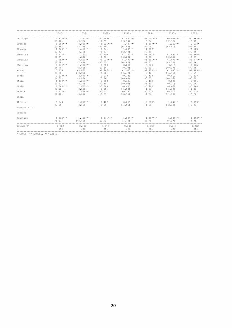
Table 5

Probit estimation for the avaialibaility of polity2 components per decade 1820s-2000s

(t-statistics are reported in parentheses)

--------------------------------------------------------------------------------------------------------------------

1820s 1830s 1840s 1850s 1860s 1870s

--------------------------------------------------------------------------------------------------------------------

NWEurope 0.519 0.625 1.567*** 1.265*** 1.361*** 1.453***

(0.85) (1.03) (3.30) (3.14) (3.40) (3.65)

SEurope 0.217 0.416 1.257** 0.955** 1.126** 1.126**

(0.33) (0.65) (2.41) (2.10) (2.53) (2.53)

EEurope -0.162 -0.162 0.679 0.792 1.085** 1.329***

(-0.21) (-0.21) (1.03) (1.48) (2.14) (2.70)

NAmerica 0.379 0.379 1.220 0.918 1.507** 1.507**

(0.45) (0.45) (1.61) (1.28) (2.31) (2.31)

CAmerica -0.359 0.272 1.318*** 1.016** 1.016** 1.016**

(-0.55) (0.45) (2.80) (2.56) (2.56) (2.56)

SAmerica 1.041 1.787*** 2.628*** 2.326*** 2.326*** 2.326***

(1.61) (2.72) (4.86) (4.86) (4.86) (4.86)

AustOc -0.026 -0.026 -0.026

(-0.05) (-0.05) (-0.05)

EAsia 0.546 0.546 1.387** 1.085* 1.085* 1.085*

(0.74) (0.74) (2.20) (1.88) (1.88) (1.88)

WAsia -0.061 -0.061 0.780 0.478 0.478 0.478

(-0.09) (-0.09) (1.40) (0.96) (0.96) (0.96)

SAsia 0.379 0.379 1.220** 0.918* 0.918* 0.918*

(0.53) (0.53) (2.01) (1.66) (1.66) (1.66)

SEAsia -0.162 -0.162 0.679 0.377 0.377 0.377

(-0.21) (-0.21) (1.03) (0.62) (0.62) (0.62)

CAsia

NAfrica 0.841 0.539 0.539 0.539

(1.22) (0.84) (0.84) (0.84)

SubSahAfrica

Constant -1.221** -1.221** -2.062*** -1.760*** -1.760*** -1.760***

(-2.21) (-2.21) (-5.06) (-5.49) (-5.49) (-5.49)

--------------------------------------------------------------------------------------------------------------------

pseudo R2 0.085 0.124 0.182 0.169 0.175 0.182

N 173 173 224 251 251 251

--------------------------------------------------------------------------------------------------------------------

* p<0.1, ** p<0.05, *** p<0.01

--------------------------------------------------------------------------------------------------------------------

1880s 1890s 1900s 1910s 1920s 1930s

--------------------------------------------------------------------------------------------------------------------

NWEurope 1.453*** 1.453*** 1.453*** 1.521*** 1.695*** 1.695***

(3.65) (3.65) (3.65) (4.17) (4.64) (4.64)

SEurope 1.126** 1.126** 1.126** 1.085*** 1.085*** 1.085***

(2.53) (2.53) (2.53) (2.64) (2.64) (2.64)

EEurope 1.329*** 1.329*** 1.329*** 1.565*** 1.775*** 1.565***

(2.70) (2.70) (2.70) (3.42) (3.86) (3.42)

NAmerica 1.507** 1.507** 1.507** 1.311** 1.311** 1.311**

(2.31) (2.31) (2.31) (2.07) (2.07) (2.07)

CAmerica 1.016** 1.016** 1.194*** 0.999*** 0.999*** 0.999***

(2.56) (2.56) (3.05) (2.78) (2.78) (2.78)

SAmerica 2.326*** 2.326*** 2.326*** 2.131*** 2.131*** 2.131***

(4.86) (4.86) (4.86) (4.70) (4.70) (4.70)

AustOc -0.026 -0.026 0.314 0.119 0.119 0.119

(-0.05) (-0.05) (0.65) (0.26) (0.26) (0.26)

EAsia 1.085* 1.085* 1.085* 0.890 1.246** 1.246**

(1.88) (1.88) (1.88) (1.60) (2.34) (2.34)

WAsia 0.478 0.478 0.478 0.528 0.890** 0.890**

(0.96) (0.96) (0.96) (1.19) (2.15) (2.15)

SAsia 0.918* 0.918* 1.235** 1.040** 1.040** 1.040**

(1.66) (1.66) (2.35) (2.07) (2.07) (2.07)

SEAsia 0.377 0.377 0.377 0.182 0.182 0.597

(0.62) (0.62) (0.62) (0.31) (0.31) (1.16)

CAsia

NAfrica 0.539 0.539 0.539 0.344 0.344 0.344

(0.84) (0.84) (0.84) (0.55) (0.55) (0.55)

SubSahAfrica

Constant -1.760*** -1.760*** -1.760*** -1.565*** -1.565*** -1.565***

(-5.49) (-5.49) (-5.49) (-5.57) (-5.57) (-5.57)

--------------------------------------------------------------------------------------------------------------------

pseudo R2 0.182 0.182 0.168 0.172 0.184 0.170

N 251 251 251 251 251 251

--------------------------------------------------------------------------------------------------------------------

* p<0.1, ** p<0.05, *** p<0.01

20

------------------------------------------------------------------------------------------------------------------------------------

1940s 1950s 1960s 1970s 1980s 1990s 2000s

------------------------------------------------------------------------------------------------------------------------------------

NWEurope 1.872*** 1.372*** -0.585** -1.051*** -1.051*** -0.969*** -0.963***

(5.10) (3.96) (-1.97) (-3.34) (-3.34) (-2.96) (-3.00)

SEurope 1.085*** 0.936** -1.021*** -1.487*** -1.487*** -1.253*** -0.613*

(2.64) (2.37) (-2.90) (-4.05) (-4.05) (-3.41) (-1.65)

EEurope 1.565*** 1.416*** -0.541 -1.007** -1.007** -0.125

(3.42) (3.19) (-1.33) (-2.40) (-2.40) (-0.26)

NAmerica 1.311** 1.162* -0.795 -1.261** -1.261** -1.440** -1.346**

(2.07) (1.87) (-1.33) (-2.08) (-2.08) (-2.36) (-2.21)

CAmerica 0.999*** 0.850** -1.025*** -1.491*** -1.491*** -1.671*** -1.576***

(2.78) (2.49) (-3.55) (-4.87) (-4.87) (-5.25) (-5.06)

SAmerica 2.131*** 1.982*** 0.250 0.060 0.060 -0.119 -0.025

(4.70) (4.52) (0.60) (0.13) (0.13) (-0.25) (-0.05)

AustOc 0.119 -0.030 -1.987*** -1.903*** -1.903*** -2.083*** -1.989***

(0.26) (-0.07) (-4.92) (-5.42) (-5.42) (-5.76) (-5.59)

EAsia 2.239*** 2.090*** 0.133 -0.333 -0.333 -0.512 -0.418

(4.02) (3.83) (0.26) (-0.63) (-0.63) (-0.96) (-0.79)

WAsia 1.439*** 1.290*** -0.288 -0.333 -0.483 0.095 -0.056

(3.62) (3.39) (-0.85) (-0.90) (-1.33) (0.21) (-0.14)

SAsia 1.565*** 1.669*** -0.288 -0.483 -0.483 -0.662 -0.568

(3.22) (3.50) (-0.65) (-1.03) (-1.03) (-1.39) (-1.21)

SEAsia 1.134** 1.846*** -0.111 -0.333 -0.577 -0.512 -0.125

(2.42) (4.07) (-0.27) (-0.75) (-1.34) (-1.13) (-0.26)

CAsia

NAfrica 0.344 1.276*** -0.402 -0.868* -0.868* -1.047** -0.953**

(0.55) (2.59) (-0.88) (-1.85) (-1.85) (-2.19) (-2.01)

SubSahAfrica

EEurope

Constant -1.565*** -1.416*** 0.541*** 1.007*** 1.007*** 1.187*** 1.093***

(-5.57) (-5.51) (2.92) (4.75) (4.75) (5.19) (4.98)

------------------------------------------------------------------------------------------------------------------------------------

pseudo R2 0.202 0.180 0.142 0.180 0.172 0.216 0.202

N 251 251 251 251 251 239 251

------------------------------------------------------------------------------------------------------------------------------------

* p<0.1, ** p<0.05, *** p<0.01

21

Appendix 3 Results form the canonical correlation analysis on decadal averages

Table 6

Canonical correlation between components of polity2 and polyarchy per decade with and without

correction for sample selection bias 1820s-2000 (t-statistics are reported in parentheses)

--------------------------------------------------------------------------------------------------------------------

1820s 1830s 1840s

--------------------------------------------------------------------------------------------------------------------

xrcomp 0.445 -0.003 -0.033 0.016 0.093 0.009

(1.24) (-0.02) (-0.20) (0.11) (0.38) (0.21)

xropen -0.069 -0.075 -0.247 -0.120 -0.408 -0.068

(-0.13) (-0.24) (-0.72) (-0.39) (-0.80) (-0.73)

xconst 0.352*** -0.097 0.493*** 0.068 0.444*** 0.003

(3.08) (-1.44) (7.52) (1.19) (4.53) (0.14)

parreg 0.346 -0.461 -0.038 -0.022 0.158 0.011

(0.44) (-0.97) (-0.12) (-0.07) (0.33) (0.13)

parcomp -0.178 0.135 -0.190 -0.079 -0.063 -0.040

(-0.61) (0.74) (-1.26) (-0.55) (-0.25) (-0.87)

polmills 0.239*** 0.399*** 0.108***

(7.11) (7.53) (24.97)

--------------------------------------------------------------------------------------------------------------------

competition 0.005 0.005 0.081*** 0.019* 0.060*** 0.004

(0.21) (0.37) (7.38) (2.01) (3.63) (1.50)

participation 1.336*** -0.369* -0.117 -0.064 0.080 -0.023

(3.72) (-1.81) (-1.27) (-0.80) (0.83) (-1.37)

polymills 0.181*** 0.287*** 0.106***

(9.38) (9.88) (32.82)

--------------------------------------------------------------------------------------------------------------------

cancor 0.780 0.913 0.840 0.875 0.700 0.985

N 24 24 34 34 38 38

--------------------------------------------------------------------------------------------------------------------

* p<0.1, ** p<0.05, *** p<0.01

--------------------------------------------------------------------------------------------------------------------

1850s 1860s 1870s

--------------------------------------------------------------------------------------------------------------------

xrcomp 0.027 0.000 -0.037 0.020 -0.160 0.024

(0.13) (0.01) (-0.19) (0.47) (-0.68) (0.56)

xropen -0.172 0.078 0.170 0.042 0.413 -0.004

(-0.37) (0.73) (0.47) (0.51) (0.90) (-0.05)

xconst 0.416*** 0.011 0.362*** 0.007 0.339*** 0.003

(5.00) (0.58) (4.68) (0.39) (3.63) (0.16)

parreg -0.330 -0.107 -0.532 -0.121 0.243 -0.078

(-0.76) (-1.06) (-1.17) (-1.19) (0.52) (-0.91)

parcomp 0.155 0.029 0.296 0.049 0.046 0.041

(0.68) (0.53) (1.31) (0.98) (0.17) (0.84)

polmills 0.240*** 0.253*** 0.260***

(20.63) (24.27) (25.06)

--------------------------------------------------------------------------------------------------------------------

competition 0.066*** 0.002 0.053*** 0.001 0.036*** -0.002

(5.66) (0.82) (5.36) (0.41) (2.72) (-0.90)

participation -0.014 0.004 0.045 0.001 0.118** 0.001

(-0.29) (0.37) (1.06) (0.07) (2.20) (0.08)

polymills 0.107*** 0.112*** 0.113***

(25.48) (27.67) (28.02)

--------------------------------------------------------------------------------------------------------------------

cancor

N 38 38 42 42 44 44

--------------------------------------------------------------------------------------------------------------------

* p<0.1, ** p<0.05, *** p<0.01

--------------------------------------------------------------------------------------------------------------------

1880s 1890s 1900s

--------------------------------------------------------------------------------------------------------------------

xrcomp 0.074 0.011 0.279 0.028 0.274* 0.057

(0.32) (0.23) (1.58) (0.53) (1.82) (1.13)

xropen 0.044 -0.063 -0.247 -0.113 -0.746** -0.125

(0.09) (-0.59) (-0.64) (-0.97) (-2.37) (-1.19)

xconst 0.306*** -0.029 0.272*** -0.026 0.302*** -0.010

(3.44) (-1.52) (4.47) (-1.38) (5.26) (-0.49)

parreg -0.122 0.063 0.458 0.006 0.317 0.007

(-0.23) (0.56) (1.14) (0.05) (1.08) (0.07)

parcomp 0.239 -0.077 -0.143 -0.050 -0.011 -0.037

(0.85) (-1.32) (-0.69) (-0.80) (-0.07) (-0.74)

polmills 0.197*** 0.195*** 0.197***

(20.47) (20.33) (22.41)

--------------------------------------------------------------------------------------------------------------------

competition 0.046*** -0.003 0.033*** -0.001 0.045*** -0.000

(3.03) (-1.05) (3.14) (-0.28) (5.90) (-0.11)

participation 0.058 -0.003 0.088** -0.012 0.007 0.002

(1.06) (-0.26) (2.29) (-1.05) (0.33) (0.31)

polymills 0.179*** 0.179*** 0.183***

(21.38) (20.99) (23.86)

--------------------------------------------------------------------------------------------------------------------

cancor 0.593 0.964 0.732 0.964 0.770 0.965

N 45 45 45 45 50 50

--------------------------------------------------------------------------------------------------------------------

* p<0.1, ** p<0.05, *** p<0.01

22

--------------------------------------------------------------------------------------------------------------------

1910s 1920s 1930s

--------------------------------------------------------------------------------------------------------------------

xrcomp 0.259 0.057 0.046 0.033 -0.044 -0.016

(1.64) (0.75) (0.45) (0.75) (-0.57) (-0.41)

xropen -0.355 -0.302* 0.414 -0.150 0.332* -0.017

(-0.96) (-1.70) (1.65) (-1.35) (1.88) (-0.19)

xconst 0.197*** 0.065** 0.172*** -0.002 0.312*** 0.022

(3.18) (2.13) (3.94) (-0.12) (9.92) (1.37)

parreg 0.333 0.045 0.636*** -0.114 0.244 -0.006

(1.13) (0.31) (3.05) (-1.19) (1.57) (-0.08)

parcomp 0.144 0.030 -0.112 -0.016 -0.072 0.008

(0.98) (0.42) (-1.19) (-0.40) (-0.98) (0.22)

polmills 0.265*** 0.266*** 0.291***

(14.90) (26.90) (36.26)

--------------------------------------------------------------------------------------------------------------------

competition 0.029*** 0.005 0.026*** -0.000 0.034*** 0.003*

(4.27) (1.49) (4.88) (-0.03) (10.55) (1.71)

participation 0.043** 0.010 0.025*** -0.003 0.012** 0.001

(2.52) (1.20) (2.85) (-0.86) (2.58) (0.29)

polymills 0.234*** 0.266*** 0.284***

(16.63) (30.93) (38.42)

--------------------------------------------------------------------------------------------------------------------

cancor 0.741 0.920 0.876 0.972 0.928 0.980

N 58 58 62 62 65 65

--------------------------------------------------------------------------------------------------------------------

* p<0.1, ** p<0.05, *** p<0.01

--------------------------------------------------------------------------------------------------------------------

1940s 1950s 1960s

--------------------------------------------------------------------------------------------------------------------

xrcomp 0.211** -0.007 0.249*** 0.042 0.058 -0.016

(2.22) (-0.84) (2.97) (1.38) (1.09) (-0.34)

xropen 0.071 0.028 0.337* -0.050 0.505*** 0.206*

(0.30) (1.45) (1.88) (-0.77) (3.70) (1.78)

xconst 0.105** 0.005 0.062 -0.027* 0.143*** 0.039

(2.57) (1.34) (1.39) (-1.70) (4.62) (1.50)

parreg -0.142 -0.034** -0.066 0.037 0.072 0.005

(-0.70) (-2.04) (-0.34) (0.52) (0.50) (0.04)

parcomp 0.283*** 0.002 0.138 0.011 0.132** 0.057

(3.06) (0.26) (1.62) (0.35) (2.14) (1.08)

polmills 0.309*** 0.395*** 0.647***

(161.29) (50.25) (25.49)

--------------------------------------------------------------------------------------------------------------------

competition 0.039*** -0.000 0.039*** 0.001 0.040*** 0.012***

(10.43) (-0.73) (17.22) (0.95) (22.23) (7.61)

participation 0.006 -0.000 0.003 -0.003*** 0.005** 0.001

(1.31) (-0.44) (1.04) (-3.44) (2.46) (0.46)

polymills 0.312*** 0.460*** 1.466***

(173.25) (52.54) (26.13)

--------------------------------------------------------------------------------------------------------------------

cancor 0.886 0.999 0.902 0.986 0.918 0.940

N 76 76 84 84 122 122

--------------------------------------------------------------------------------------------------------------------

* p<0.1, ** p<0.05, *** p<0.01

--------------------------------------------------------------------------------------------------------------------

1970s 1980s 1990s

--------------------------------------------------------------------------------------------------------------------

xrcomp 0.011 0.058 0.098*** 0.079** 0.052 -0.058

(0.27) (1.58) (3.01) (2.54) (1.06) (-1.27)

xropen 0.154 0.041 -0.053 -0.056 0.029 0.011

(1.39) (0.43) (-0.57) (-0.63) (0.25) (0.11)

xconst 0.102*** 0.073*** 0.110*** 0.109*** 0.205*** 0.210***

(3.49) (2.89) (4.26) (4.43) (5.64) (6.09)

parreg 0.160 0.108 0.319*** 0.173* 0.058 -0.305***

(1.08) (0.84) (3.18) (1.74) (0.50) (-2.80)

parcomp 0.287*** 0.131** 0.167*** 0.185*** 0.229*** 0.260***

(4.68) (2.46) (3.46) (3.98) (4.16) (4.87)

polmills 1.015*** 0.379*** 0.972***

(20.86) (8.49) (17.07)

--------------------------------------------------------------------------------------------------------------------

competition 0.040*** 0.025*** 0.041*** 0.036*** 0.041*** 0.022***

(27.72) (19.68) (33.43) (29.49) (20.24) (11.19)

participation 0.004*** -0.002 0.001 -0.001 0.004* 0.004

(2.73) (-1.14) (0.60) (-0.69) (1.68) (1.62)

polymills 1.409*** 0.588*** 2.417***

(20.94) (8.20) (17.08)

--------------------------------------------------------------------------------------------------------------------

cancor 0.958 0.957 0.916 0.962 0.822 0.936

N 135 135 135 135 158 141

--------------------------------------------------------------------------------------------------------------------

* p<0.1, ** p<0.05, *** p<0.01

23

----------------------------------------------------

2000

----------------------------------------------------

xrcomp 0.138 -0.031

(1.36) (-0.34)

xropen 0.228 0.027

(1.15) (0.16)

xconst 0.210*** 0.227***

(3.10) (4.01)

parreg -0.074 -0.146

(-0.40) (-0.93)

parcomp 0.161* 0.085

(1.90) (1.18)

polmills 1.194***

(13.86)

----------------------------------------------------

competition 0.039*** 0.018***

(11.13) (5.75)

participation 0.006 0.001

(1.37) (0.18)

polymills 2.774***

(14.09)

----------------------------------------------------

cancor 0.821 0.868

N 144 139

----------------------------------------------------

* p<0.1, ** p<0.05, *** p<0.01