Measurements of sulfur dioxide, ozone and ammonia concentrations in Asia, Africa, and South America...
16
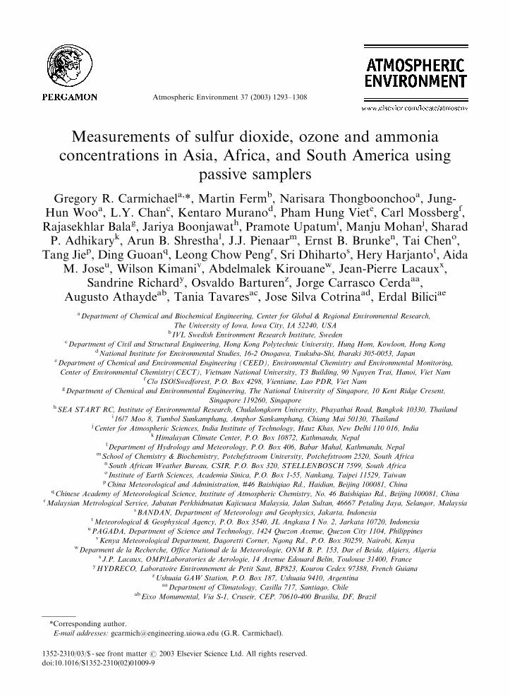
Atmospheric Environment 37 (2003) 1293–1308 Measurements of sulfur dioxide, ozone and ammonia concentrations in Asia, Africa, and South America using passive samplers Gregory R. Carmichael a, *, Martin Ferm b , Narisara Thongboonchoo a , Jung- Hun Woo a , L.Y. Chan c , Kentaro Murano d , Pham Hung Viet e , Carl Mossberg f , Rajasekhlar Bala g , Jariya Boonjawat h , Pramote Upatum i , Manju Mohan j , Sharad P. Adhikary k , Arun B. Shrestha l , J.J. Pienaar m , Ernst B. Brunke n , Tai Chen o , Tang Jie p , Ding Guoan q , Leong Chow Peng r , Sri Dhiharto s , Hery Harjanto t , Aida M. Jose u , Wilson Kimani v , Abdelmalek Kirouane w , Jean-Pierre Lacaux x , Sandrine Richard y , Osvaldo Barturen z , Jorge Carrasco Cerda aa , Augusto Athayde ab , Tania Tavares ac , Jose Silva Cotrina ad , Erdal Bilici ae a Department of Chemical and Biochemical Engineering, Center for Global & Regional Environmental Research, The University of Iowa, Iowa City, IA 52240, USA b IVL Swedish Environment Research Institute, Sweden c Department of Civil and Structural Engineering, Hong Kong Polytechnic University, Hung Hom, Kowloon, Hong Kong d National Institute for Environmental Studies, 16-2 Onogawa, Tsukuba-Shi, Ibaraki 305-0053, Japan e Department of Chemical and Environmental Engineering (CEED), Environmental Chemistry and Environmental Monitoring, Center of Environmental Chemistry(CECT), Vietnam National University, T3 Building, 90 Nguyen Trai, Hanoi, Viet Nam f C/o ISO/Swedforest, P.O. Box 4298, Vientiane, Lao PDR, Viet Nam g Department of Chemical and Environmental Engineering, The National University of Singapore, 10 Kent Ridge Cresent, Singapore 119260, Singapore h SEA START RC, Institute of Environmental Research, Chulalongkorn University, Phayathai Road, Bangkok 10330, Thailand i 16/7 Moo 8, Tumbol Sunkamphang, Amphor Sankamphang, Chiang Mai 50130, Thailand j Center for Atmospheric Sciences, India Institute of Technology, Hauz Khas, New Delhi 110 016, India k Himalayan Climate Center, P.O. Box 10872, Kathmandu, Nepal l Department of Hydrology and Meteorology, P.O. Box 406, Babar Mahal, Kathmandu, Nepal m School of Chemistry & Biochemistry, Potchefstroom University, Potchefstroom 2520, South Africa n South African Weather Bureau, CSIR, P.O. Box 320, STELLENBOSCH 7599, South Africa o Institute of Earth Sciences, Academia Sinica, P.O. Box 1-55, Nankang, Taipei 11529, Taiwan p China Meteorological and Administration, #46 Baishiqiao Rd., Haidian, Beijing 100081, China q Chinese Academy of Meteorological Science, Institute of Atmospheric Chemistry, No. 46 Baishiqiao Rd., Beijing 100081, China r Malaysian Metrological Service, Jabatan Perkhidmatan Kajicuaca Malaysia, Jalan Sultan, 46667 Petaling Jaya, Selangor, Malaysia s BANDAN, Department of Meteorology and Geophysics, Jakarta, Indonesia t Meteorological & Geophysical Agency, P.O. Box 3540, JL Angkasa I No. 2, Jarkata 10720, Indonesia u PAGADA, Department of Science and Technology, 1424 Quezon Avenue, Quezon City 1104, Philippines v Kenya Meteorological Department, Dagoretti Corner, Ngong Rd., P.O. Box 30259, Nairobi, Kenya w Deparment de la Recherche, Office National de la Meteorologie, ONM B. P. 153, Dar el Beida, Algiers, Algeria x J.P. Lacaux, OMP/Laboratories de Aerologie, 14 Avenue Edouard Belin, Toulouse 31400, France y HYDRECO, Laboratoire Environnement de Petit Saut, BP823, Kourou Cedex 97388, French Guiana z Ushuaia GAW Station, P.O. Box 187, Ushuaia 9410, Argentina aa Department of Climatology, Casilla 717, Santiago, Chile ab Eixo Monumental, Via S-1, Cruseir, CEP. 70610-400 Brasilia, DF, Brazil *Corresponding author. E-mail addresses: [email protected] (G.R. Carmichael). 1352-2310/03/$ - see front matter r 2003 Elsevier Science Ltd. All rights reserved. doi:10.1016/S1352-2310(02)01009-9
-
Upload
independent -
Category
Documents
-
view
0 -
download
0
Transcript of Measurements of sulfur dioxide, ozone and ammonia concentrations in Asia, Africa, and South America...
Atmospheric Environment 37 (2003) 1293–1308
Measurements of sulfur dioxide, ozone and ammoniaconcentrations in Asia, Africa, and South America using
passive samplers
Gregory R. Carmichaela,*, Martin Fermb, Narisara Thongboonchooa, Jung-Hun Wooa, L.Y. Chanc, Kentaro Muranod, Pham Hung Viete, Carl Mossbergf,Rajasekhlar Balag, Jariya Boonjawath, Pramote Upatumi, Manju Mohanj, Sharad
P. Adhikaryk, Arun B. Shresthal, J.J. Pienaarm, Ernst B. Brunken, Tai Cheno,Tang Jiep, Ding Guoanq, Leong Chow Pengr, Sri Dhihartos, Hery Harjantot, Aida
M. Joseu, Wilson Kimaniv, Abdelmalek Kirouanew, Jean-Pierre Lacauxx,Sandrine Richardy, Osvaldo Barturenz, Jorge Carrasco Cerdaaa,
Augusto Athaydeab, Tania Tavaresac, Jose Silva Cotrinaad, Erdal Biliciae
a Department of Chemical and Biochemical Engineering, Center for Global & Regional Environmental Research,
The University of Iowa, Iowa City, IA 52240, USAb IVL Swedish Environment Research Institute, Sweden
c Department of Civil and Structural Engineering, Hong Kong Polytechnic University, Hung Hom, Kowloon, Hong Kongd National Institute for Environmental Studies, 16-2 Onogawa, Tsukuba-Shi, Ibaraki 305-0053, Japan
e Department of Chemical and Environmental Engineering (CEED), Environmental Chemistry and Environmental Monitoring,
Center of Environmental Chemistry(CECT), Vietnam National University, T3 Building, 90 Nguyen Trai, Hanoi, Viet Namf C/o ISO/Swedforest, P.O. Box 4298, Vientiane, Lao PDR, Viet Nam
g Department of Chemical and Environmental Engineering, The National University of Singapore, 10 Kent Ridge Cresent,
Singapore 119260, Singaporeh SEA START RC, Institute of Environmental Research, Chulalongkorn University, Phayathai Road, Bangkok 10330, Thailand
i 16/7 Moo 8, Tumbol Sunkamphang, Amphor Sankamphang, Chiang Mai 50130, Thailandj Center for Atmospheric Sciences, India Institute of Technology, Hauz Khas, New Delhi 110 016, India
k Himalayan Climate Center, P.O. Box 10872, Kathmandu, Nepall Department of Hydrology and Meteorology, P.O. Box 406, Babar Mahal, Kathmandu, Nepal
m School of Chemistry & Biochemistry, Potchefstroom University, Potchefstroom 2520, South African South African Weather Bureau, CSIR, P.O. Box 320, STELLENBOSCH 7599, South Africao Institute of Earth Sciences, Academia Sinica, P.O. Box 1-55, Nankang, Taipei 11529, Taiwan
p China Meteorological and Administration, #46 Baishiqiao Rd., Haidian, Beijing 100081, Chinaq Chinese Academy of Meteorological Science, Institute of Atmospheric Chemistry, No. 46 Baishiqiao Rd., Beijing 100081, China
r Malaysian Metrological Service, Jabatan Perkhidmatan Kajicuaca Malaysia, Jalan Sultan, 46667 Petaling Jaya, Selangor, Malaysias BANDAN, Department of Meteorology and Geophysics, Jakarta, Indonesia
t Meteorological & Geophysical Agency, P.O. Box 3540, JL Angkasa I No. 2, Jarkata 10720, Indonesiau PAGADA, Department of Science and Technology, 1424 Quezon Avenue, Quezon City 1104, Philippines
v Kenya Meteorological Department, Dagoretti Corner, Ngong Rd., P.O. Box 30259, Nairobi, Kenyaw Deparment de la Recherche, Office National de la Meteorologie, ONM B. P. 153, Dar el Beida, Algiers, Algeria
x J.P. Lacaux, OMP/Laboratories de Aerologie, 14 Avenue Edouard Belin, Toulouse 31400, Francey HYDRECO, Laboratoire Environnement de Petit Saut, BP823, Kourou Cedex 97388, French Guiana
z Ushuaia GAW Station, P.O. Box 187, Ushuaia 9410, Argentinaaa Department of Climatology, Casilla 717, Santiago, Chile
ab Eixo Monumental, Via S-1, Cruseir, CEP. 70610-400 Brasilia, DF, Brazil
*Corresponding author.
E-mail addresses: [email protected] (G.R. Carmichael).
1352-2310/03/$ - see front matter r 2003 Elsevier Science Ltd. All rights reserved.
doi:10.1016/S1352-2310(02)01009-9

ac Chemistry Istitute Departmento de Quimica Analitica, Universidade Federal da Bahia Salvador, Bahia 40210-340, Brazilad De Investigacion y Desarrollo, Jr. Cahuida No. 785, Jesus Maria-Lima 11-peru, Peru
ae Turkish State Meteorological Service, Kalaba-Ankara 06120, Turkey
Received 20 July 2002; accepted 18 October 2002
Abstract
Measurements of gaseous SO2, NH3, and O3 using IVL passive sampler technology were obtained during a pilot
measurement program initiated as a key component of the newly established WMO/GAW Urban Research
Meteorology and Environment (GURME) project. Monthly measurements were obtained at 50 stations in Asia, Africa,
South America, and Europe. The median SO2 concentrations vary from a high of 13 ppb at Linan, China, to o0.03 ppb
at four stations. At 30 of 50 regional stations, the observed median concentrations are o1 ppb. Median ammonia
concentrations range from 20 ppb at Dhangadi, India, to o1 ppb at nine stations. At 27 of regional stations, the
ambient ammonia levels exceed 1 ppb. The median ozone concentrations vary from a maximum of 45 ppb at Waliguan
Mountain, China, to 8 ppb in Petit Saut, French Guiana. In general, the highest ozone values are found in the mid-
latitudes, with the Northern hemisphere mid-latitude values exceeding the Southern hemisphere mid-latitude levels, and
the lowest values are typically found in the tropical regions.
r 2003 Elsevier Science Ltd. All rights reserved.
Keywords: Diffusive samplers; Sulfur dioxide; Ammonia; Ozone; Asia; Africa
1. Introduction
Measurement programs play a critical role in air
pollution and atmospheric chemistry studies. Pressures
of costs and changing priorities often make it difficult to
maintain and expand long-term measurement programs.
In some cases, environmental planning activities are
severely hampered by the lack of information on the
ambient levels of pollutants. Such issues are presently
being faced by the World Meteorological Organization’s
Global Atmospheric Watch (GAW) program. GAW is a
coordinated network of observing stations and related
facilities whose purpose and long-term goals are to
provide data, scientific assessments, and other informa-
tion on changes of the chemical composition and related
physical characteristics of the background atmosphere
from all parts of the world. This information is needed
to improve our understanding of the behavior of the
atmosphere and its interactions with oceans and the
biosphere and to better anticipate the future states of
the earth–atmosphere system. One challenge facing the
GAW program is the need to expand its activities to
include measurements in each principal climatic zone
and each biome, and to continue to add important
species to the list of observed parameters.
Passive samplers present a means of addressing many
measurement issues in air pollution and atmospheric
chemistry, in that they provide a cost-effective way to
monitor specific species at urban, regional, and global
scales, and offer broad-capacity building opportunities.
There are a variety of uses for passive samplers in
atmospheric chemistry studies. They can be used: (a) to
increase the spatial resolution of measurements; (b) to
add species coverage to existing measurement sites; (c) to
add gas-phase measurement to precipitation measure-
ment sites; (d) in screening studies to evaluate monitor-
ing site locations; and (e) to aid measurement programs
by providing a means to increase data completion (e.g.,
to help keep time series complete during active instru-
ment downtimes).
To demonstrate the expanded use of passive samplers
in air quality studies, a pilot measurement program was
initiated as a key component of the newly established
WMO/GAW Urban Research Meteorology and Envir-
onment (GURME) project. This passive sampler project
was done in collaboration and as a component of the
IGAC-DEBITS program. This pilot activity combined
components of three separate studies:
(1) a pilot study funded by NOAA-US Weather
Service, to use passive samplers at selected WMO/
GAW stations;
(2) a continuation of the use of passive samplers as part
of the RAINS-Asia Phase-II funded by the Japan
Trust Fund at The World Bank; and
(3) a pilot study demonstrating the use of passive
sampler at both regional and urban scales, funded
by the Swedish Consultancy Fund at the World
Bank.
The pilot network consisted of stations from previous
studies in Asia and from existing GAW stations, along
with newly established sites; in total, 50 stations in 12
Asian countries (China, India, Indonesia, Japan, Korea,
Malaysia, Nepal, Philippines, Singapore, Thailand,
G.R. Carmichael et al. / Atmospheric Environment 37 (2003) 1293–13081294

Laos, and Vietnam), seven African countries (Algeria,
Cameroon, Ivory Coast, Niger, Morocco, Kenya, and
South Africa), five South American countries (Argenti-
na, Brazil, Chile, Peru, and French Guyana) and a
European country (Turkey). At these sites, sulfur dioxide
(SO2), ammonia (NH3), and ozone (O3) were monitored
monthly at the rural sites and with short sampling
periods at the urban sites. At the urban sites, weekly
samples of NO, NO2, HCOOH, CH3COOH, benzene,
ethyl benzene, toluene, and xylenes were also obtained.
The project aims were: (1) to repeat a previous
network for sulfur dioxide (SO2) in Asia; and (2) to
extend the capacity to monitor more pollutants in rural
as well as urban air. The network provides a valuable
data set that can be used for a variety of purposes
including model evaluation and inter-comparison
with other methods. In this paper, details and results
from the regional network are presented and discussed.
The urban results will be the subject of a separate
paper.
2. Passive samplers
The samplers used here are passive; but since there are
several types of passive samplers, the word diffusive
sampler is more specific for these samplers and is more
commonly used today. This project has, however, been
titled ‘‘The Passive Sampler Project’’. A diffusive
sampler has been defined by the European Committee
for Standardization as: ‘‘A device that is capable of
taking samples of gases or vapors from the atmosphere
at a rate controlled by a physical process such as gaseous
diffusion through a static air layer or a porous material
and/or permeation through a membrane, but which does
not involve active movement of air through the device’’.
The gas molecules are transported by molecular diffu-
sion, which is a function of air temperature and
pressure. A net flux into the sampler is accomplished
by placing an efficient sorbent for the target gas behind
the barrier. The driving force is the difference between
the ambient concentration and the concentration at the
sorbent, which should be negligible, compared to the
ambient concentration. The average net flux of pollutant
through the sampler is obtained from analysis of the
sorbent. The resistance of the barrier, as well as the time-
weighted average ambient concentration, can be calcu-
lated using Fick’s first law of diffusion. The solution to
this equation has been published in almost all articles
dealing with diffusive sampling. In order to solve it,
several prerequisites must be fulfilled. These have not
earlier been discussed in connection with the solution of
Fick’s first law. This is likely the main reason behind the
poor quality of some diffusive samplers.
The following prerequisites have to be fulfilled to
solve Fick’s equation. At steady state, the flux (which is
obtained from analysis of the sorbent) shall be constant
through the sampler implying that the gas is not
interacting with the wall or being transformed to
another pollutant on its way to the sorbent. This is
achieved by choosing an inert wall material and
minimizing the residence time by using a short transport
distance. The sorption must be quantitative and without
interferences. The formed product must be stable. The
sorption reaction must not be too slow. The sampler
gives a correct average concentration even when the
ambient concentration fluctuates and the flux and
concentration gradient inside the sampler are not
constant. This can be shown from Fick’s second law of
diffusion and has earlier been treated incorrectly in the
literature. Other transport mechanisms than molecular
diffusion or permeation must be negligible. Turbulent
diffusion, convection, and rotation of the sampler can
cause an active movement of air inside the sampler. This
can be avoided by using a membrane at the inlet,
shadowing the sampler and during personal monitoring,
facing the inlet downwards. Several articles have been
written on different parts of the theory behind diffusive
sampling, but some parts have been missing. A summary
of the published parts and an addition of some missing
parts for diffusive samplers using irreversible sorption
and a constant cross-sectional area (tube or badge type)
has recently been published (Ferm, 2001a).
A large number of different diffusive samplers for use
in outdoor air have been developed since Palmes and
Gunnison published a description of the first sampler
(Palmes and Gunnison, 1973). Several of them are today
commercially available. The quality of the results from
these samplers has varied widely and the technology has
therefore occasionally suffered from a bad reputation.
This study utilized diffusive samplers developed at the
IVL. At IVL, diffusive samplers for several gases have
been developed and described in the literature (Ferm
and Rodhe, 1997). They are fully based on these theories
implying that the ambient concentration is calculated
from the theoretical uptake rate and not from an
empirical one. This is to ensure that there are no biases
that we are not aware of.
The quality does, however, not only depend on the
sampler, but also on the analysis, the choice of sampling
points, design of network and the evaluation of results.
Stevenson et al. (2001) investigated in a laboratory
intercomparison the variation between different labora-
tories for analyses of doped Palmes tubes. They found
that the coefficient of variation (a statistical measure of
precision based on the difference between duplicate
samples) was for most laboratories within 725%, which
is acceptable for indicative monitoring.
In order to use diffusive measurements instead of
volumetric or instrumental analyses, an analytical
precision around 75% is needed. At IVL, the analytical
procedures for the diffusive samplers therefore have
G.R. Carmichael et al. / Atmospheric Environment 37 (2003) 1293–1308 1295

been accredited. This implies that certified standards are
used and statistical analyses of accuracy and precision of
duplicates and reference samples are maintained by the
use of control charts every time a batch of samples is
analyzed. An analysis of a diffusive sampler has to be
performed by personnel accredited for the analyses in
question. The laboratory at IVL has to participate in
intercomparisons to keep the accreditation. Further-
more, the IVL is participating in the standardization
work for testing diffusive samplers within the CEN
(European Committee for Standardization).
The IVL samplers are of badge type, 10 mm long and
20 mm internal diameter. A membrane is mounted at the
inlet to prevent them from wind-induced turbulent
diffusion. The membrane is protected from mechanical
damage by a stainless steel mesh. The SO2 and NO2
samplers have been compared to active sampling
within a routine network (Ferm and Svanberg, 1998).Fig. 1. Six diffusive samplers mounted under a metal disc.
Fig. 2. Location of the measurement sites used in this study (squares and triangles represent regional and urban sites, respectively).
G.R. Carmichael et al. / Atmospheric Environment 37 (2003) 1293–13081296

Table 1
Station information
Country Station Location Level
Latitude Longitude Elevation (m)
China Waliguan mountain 361170N 1001540E 3810 I
Linan 301180N 1191440E 132 I
Shang dian Zhi 401390N 1171070E 260 I
Cape D’Aequier 221120N 1141150E B1 I
Beijing B40120N B1161250E B137 II
Wenjiang 301420N 1031500E B488 II
Taiwan Taipei 2512.550N 120130.820E B0 II
Shui-Li 23149.10N 120150.860E 330 I
Japan Oki 361170N 1331110E 90 I
Malaysia Tanah Rata 041280N 1011220E 1471 I
Petaling Jaya 031060N 1011390E 45 II
Mersing 021270N 1031500E 44 II
Lawa Mandau 061020N 1161120E 830 I
Indonesia Bukit Kototabang 01120S 1001190E 865 I
Jakarta 61100S 1061480E B61 II
Kalimantan 21160S 1131560E B0 I
Vietnam Hanoi 211010N 1051510E B122 II
Thailand Bangkok 131450N 1001320E 1 II
Chiang Mai 20150N 991 230E B807 I
Nakhon Sri Thammarat B81150N B1001E B10 I
Laos Luang Prabang 191360N 1011540E 640 I
Vientiane 181N 1021360550 0E 200 II
Savannaketh 161300N 1061E 200 I
Philippines Mt. Sto. Tomas 161N 1201E 2200 I
Manila 141350N 1211E B15 II
Singapore Singapore 11160N 1031510E B0 II
Nepal Kathmandu 271420N 851220E B1524 II
Dhangadi 281410N 801360E B166 I
Nagarkot 271450N 851340E B948 I
Langtang 281430N 851370E B4676 I
India Delhi 281400N 771130E B213 II
Berhampur 201360N 841480E B316 I
Cochin 91350N 761440E B91 I
Agra 271110N 781010E B175 I
Bhubeneswar 201150N 851520E B24 I
Kenya Mt. Kenya 01S 371E 3780 I
South Africa Elandsfontein 261150S 291250E 1500 I
Cape point 341210S 181290E 230 I
Algeria Tamanrasset 221470N 51310E 1377 I
Niger Banizoumbou 131320N 21040E 220 I
G.R. Carmichael et al. / Atmospheric Environment 37 (2003) 1293–1308 1297

Additional information of the use of IVL-type samplers
and their comparison with active sampling results can be
found in Ayers et al. (1998, 2000, 2002) and Gillett et al.
(2000). The NH3 sampler was tested in an intercompar-
ison (Kirchner et al., 1999). The O3 sampler was
compared with UV-instrument (Sj .oberg et al., 2001).
The ozone sampler has also been validated for use in
workplace atmospheres (Ferm, 2001b). All the samplers
are also undergoing intercomparisons within CEN.
2.1. Sampling
The samplers were prepared at IVL and mailed
together with instructions to the contact persons in each
country. The samplers were mounted under a metal disc
ca 3 m above the ground in order to protect them for
rain and direct sunshine, see Fig. 1. After 1-month
exposure, the samplers were returned to IVL for
analysis. Some were not exposed and returned as field
blanks. Duplicates were always used.
The detection limit was estimated from a sampled
amount corresponding to three times the standard
deviation of the average field blanks using the actual
exposure time. For exactly 1-month sampling, this
corresponded to 0.03 (SO2), 1 (NH3) and 0.6 (O3) ppb.
For the SO2 measurements, 13% were below the
detection limit and for NH3 32% were below the
detection limit. The upper limit was exceeded for 5%
of the NH3 measurements (only in India and Nepal).
The upper limit, based on a sampled amount corre-
sponding to half the stoichiometric amount of sorbent
and exactly 1-month sampling, was 32 ppb. In several of
these samples, the ammonium amount found was equal
to the stoichiometric amount of sorbent. In these cases,
the upper limit was estimated from the sampled amount
and the actual exposure time.
The coefficients of variation (COV, a measure of the
precision, here it is defined as the median relative
standard deviation, assuming a normal distribution of
the deviation between parallel samples) for all duplicates
within the detection limits were: 12%, 20%, and 3.6%
for SO2, NH3, and O3, respectively. The detection limits
divided by the median concentrations were 13%, 23%,
and 3%, respectively. The COV (calculated in the same
way) for SO2 in an earlier test was 10% (Ferm and
Rodhe, 1997). The COV for NH3 was in the earlier test
25% when the membrane was not exchanged with a
solid lid after exposure. When the membrane was
exchanged, the COV was improved to 21%. In this
study, membranes were changed incorrectly on several
occasions. The measured NH3 concentrations can
therefore be somewhat over-estimated due to evapora-
tion of NH3 from deposited particulate matter. The
COV for O3 is similar to that earlier observed in Sweden.
The accuracy could not be estimated since we did not
receive data from parallel measurements using other
techniques.
Diffusive sampling is a very foolproof technique.
There are very few things that can affect the results if
the sampling protocol is not followed. The samplers are
color marked. Sometimes they were sent back in the
wrong storage container. This was noted during the
Table 1 (continued)
Country Station Location Level
Latitude Longitude Elevation (m)
Ivory Coast Lamto 61130N 51010W 136 I
Cameroon Zoetele 31150N 111530E 720 I
French Guiana Petit Saut 51030N 531030W 50 I
Argentina Isla Redonda 541510S 681 290W 3459 I
Ushuaia 541490S 681190W 10 I
Chile El Tololo 301100S 701480W B2172 I
Brazil Arembepe 121460S 381100W 0 I
Peru Marcapomacocha 11133.70S 76127.30W 4467 I
Turkey Camkoru 321290N 401280E 1350 I
Morocco Casablanca B331390N B71350W B137 II
Level I means ‘‘Regional Station’’ and Level II means ‘‘Urban/suburban Station’’.
G.R. Carmichael et al. / Atmospheric Environment 37 (2003) 1293–13081298
unpacking. At one station, blanks and samples were
mixed, which was easily discovered. The mounting of the
rain shield is simple and photos of the mounted
equipment have been received from most stations. We
therefore believe that the accuracy is similar to that
estimated within the accreditation. The average of the
duplicates was used here except from a very few cases (5
for SO2, 3 for NH3, and 2 for O3) when contamination
was suspected.
2.2. Site information
These passive samplers were sent to 50 stations
throughout Asia, South America, Africa, and Turkey.
At the 36 stations representing the regional sites, SO2,
NH3, and O3 were sampled on a monthly basis. Most
sites began measurement in September 1999 and
conducted measurements for 12 months. Measurement
at some sites started later and/or ran for longer periods.
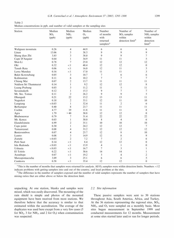
Table 2
Median concentrations in ppb, and number of valid samplers at the sampling sites
Station Median
SO2
(ppb)
Median
NH3
(ppb)
Median
O3
(ppb)
Number
of months
with
returned
samplersa
Number of
SO2 samples
within
detection limitb
Number of
NH3 samples
within
detection
limitb
Waliguan mountain 0.26 4 44.9 6 6 6
Linan 13.06 5 38.3 9 9 9
Shang dian Zhi 3.85 3 38.0 9 9 7
Cape D0Aequier 0.64 1 34.9 11 11 5
Shui-Li 0.78 7 25.0 12 12 12
Oki 0.32 o1 40.4 12 12 0
Tanah Rata 0.06 o1 16.0 12 11 3
Lawa Mandau 0.16 o1 17.0 11 11 3
Bukit Kototabang 0.05 3 10.7 7 6 6
Kalimantan 0.11 6 10.2 7 7 7
Chiang Mai 0.07 2 13.7 11 11 11
Nakhon Sri Thammarat 0.14 1 9.2 12 12 8
Luang Prabang 0.03 3 11.2 11 5 11
Savannaketh 0.12 1 15.3 9 7 7
Mt. Sto. Tomas 0.11 2 26.2 9 9 5
Dhangadi 0.21 22 15.2 13 13 11
Nagarkot 0.18 2 33.1 12 11 10
Langtang o0.03 1 32.4 11 2 6
Berhampur 0.40 8 23.7 11 11 11
Cochin 4.77 19 11.8 11 11 8
Agra 1.79 >40 30.8 12 12 0
Bhubeneswar 0.79 7 31.4 22 22 22
Mt. Kenya 0.03 1 30.0 8 4 6
Elandsfontein 6.99 2 35.1 10 10 10
Cape point 0.30 1 24.2 12 12 7
Tamanrasset 0.08 4 33.2 12 12 12
Banizoumbou 0.07 4 25.7 12 8 10
Lamto 0.08 3 14.9 12 8 9
Zoetele o0.03 2 7.2 7 2 6
Petit Saut 0.14 o1 8.4 12 12 0
Isla Redonda o0.03 o1 15.9 4 1 0
Ushuaia o0.03 o1 16.7 7 3 1
El Tololo 0.22 o1 30.6 14 14 1
Arembepe 0.07 o1 19.2 5 4 2
Marcapomacocha 3.09 3 25.1 6 6 5
Camkoru 0.58 o1 35.4 12 12 0
a This is the number of months that samplers were returned for analysis. All O3 samplers were within detection limits. Numbers o12
indicate problems with getting samplers into and out of the country, and local problem at the sites.b The difference in the number of samplers exposed and the number of valid samplers represents the number of samplers that have
mixing ratios that are either above or below the detection limit.
G.R. Carmichael et al. / Atmospheric Environment 37 (2003) 1293–1308 1299

The longest measurement period extended from
September 1999 to June 2001. Maps of these sampling
sites and station details are presented in Fig. 2 and Table
1, respectively. The regional sites were chosen to be
representative of rural conditions. Sites were chosen
when possible to be away from local sources, including
roads. Detailed site information including photographs
are available on the project web site (http://www.cgrer.-
uiowa.edu/people/nthongbo/Passive/passmain.html).
3. Result and discussion
A summary of the observed values is presented in
Table 2. The number of samples returned, along with the
number of samples within the detection limit, is
presented. The observed median concentrations of
SO2, NH3, and O3 obtained at the regional sites are
shown in Figs. 3, 4, and 6, respectively. The mean,
median, and maximum and minimum monthly values
Fig. 3. Measured SO2 concentrations. The bars indicate maximum, minimum and mean values, and the solid box designates the
median values.
Fig. 4. Measured NH3 concentrations. The bars indicate maximum, minimum and mean values, and the solid box designates the
median values.
G.R. Carmichael et al. / Atmospheric Environment 37 (2003) 1293–13081300

Dha
ngad
iB
aniz
oum
bou
Kal
iman
tan
Buk
it K
otot
aban
gT
aman
rass
etL
amto
Mt.
Ken
yaC
hian
g M
aiM
t.Sto
. Tom
asL
uang
Pra
bang
Ber
ham
pur
Wal
igua
n M
ount
ain
Nag
arko
tN
akho
n Sr
iTha
mm
arat
Sava
nnak
eth
Bhu
bene
swar
Shui
-Li
Cap
e po
int
Coc
hin
Cap
e D
'Aeq
uier
Shan
g D
ian
Zhi
Mar
capo
mac
ocha
Lin
An
Ela
ndsf
onte
i n
0
20
40
60
80
100
NH
3/S
O2 r
atio
0.01
0.1
1
10
100
0.01 0.1 1 10 100
SO2(ppb)
NH3(ppb )
Fig. 5. Ratios of median NH3 to SO2 concentrations. Insert shows the monthly NH3 and SO2 concentrations.
Fig. 6. Measured O3 concentrations. The bars indicate maximum, minimum and mean values, and the solid box designates the median
values.
G.R. Carmichael et al. / Atmospheric Environment 37 (2003) 1293–1308 1301

are shown. The range reflects the strength of the
seasonal cycle and will be discussed later. The observed
SO2 concentrations (Fig. 3) vary from a high of 13 ppb
at Linan, China, to o0.03 ppb at four stations. At 30 of
36 regional stations, the observed mean annual con-
centrations were o1.0 ppb. The high concentrations of
SO2 at Linan, China, Elandsfontein, S. Africa, Cochin,
India, Shang Dian Zhi China, Marcapomacocha, Peru,
and Agra, India, reflect major contributions from
anthropogenic SO2 emissions (i.e., power plant, indus-
trial boilers, heating, and cooking). Most stations show
a consistency between the median and mean concentra-
tions. The largest disagreements occurred at Cape D’
Aequier, Hong Kong, and Mt. Sto. Tomas, Philippines.
At the Hong Kong site, this was due to a rusted sampler
mesh. Mt. Sto. Tomas levels of SO2 were impacted by
the eruption of the Mayon volcano at the end of
February 2000 (see Fig. 10).
Median ammonia concentrations shown in Fig. 4
range from 20 ppb at Dhangadi, India, to o1 ppb at
nine stations. At 27 sites, the ambient ammonia levels
exceeded 1 ppb. The high median NH3 concentration in
the Indian sub-continent, Southeast and South Asia,
and Africa reflect high NH3 emissions from agricultural
activities (including fertilizer use), livestock, and the use
of biofuels (such as animal dung) as domestic fuel.
SO2 and ammonia play important roles in aerosol
processes, and in influencing the acidity of precipitation.
While SO2 has been relatively widely studied, little
information is available on ambient NH3 levels for large
regions of the World. The ratio of gaseous ammonia to
sulfur dioxide provides insight into the relative impor-
tance of these species. The ratios of observed ammonia
to sulfur dioxide are presented in Fig. 5. At 24 sites the
ammonia-mixing ratios exceed those of SO2, and at 15
sites the ratio exceeds 10.
The median ozone concentrations (Fig. 6) vary from a
maximum of 45 ppb at Waliguan Mountain, China, to
8 ppb in Petit Saut, French Guiana. The sorted plot of
ozone concentration with latitude (Fig. 7) shows that the
four stations with the highest ozone levels (Oki, Japan;
Waliguan Mountain, Shang Dian Zhi, and Linan,
China) are in the Northern Hemisphere mid-latitudes.
In general, the highest values are found in the mid-
latitudes of the Northern and Southern hemisphere, with
the Northern hemisphere mid-latitude values exceeding
the Southern hemisphere mid-latitude levels, and with
the lowest values typically found in the tropical regions.
The observed SO2, NH3, and O3 values in Asia are
plotted along with the emissions distributions in Fig. 8.
In general, the observations reflect the spatial distribu-
tions of the emissions. SO2 and ammonia are primary
pollutants, and both have high emissions around the
major urban and industrial centers. However, ammonia
emissions are more widespread, reflecting the large
contribution due to agricultural activity. Ozone is a
secondary pollutant formed by photochemical processes
involving NOx and reactive hydrocarbons. High ozone
levels are found in regions of high NOx and reactive
hydrocarbon emissions as seen at Linan and Cape
D’Aequier. But high levels are also found at Waliguan
Mountain, reflecting high background levels in the mid-
troposphere.
Time-series of monthly values at selected sites
are presented in Figs. 9 and 10. The seasonal variation
in ambient levels varies from station to station and
Fig. 7. Latitudinal variation in observed O3.
G.R. Carmichael et al. / Atmospheric Environment 37 (2003) 1293–13081302

Fig. 8. (a) Observed median SO2 and NH3 in Asia plotted along with the emissions distributions of SO2 (top) and NH3 (bottom). (b)
Observed median O3 values in Asia plotted along with the emissions distribution of NOx (top) and the ratio of non-methane volatile
organic carbon (NMVOC) to NOx ratios (bottom).
G.R. Carmichael et al. / Atmospheric Environment 37 (2003) 1293–1308 1303

Fig. 8 (continued).
G.R. Carmichael et al. / Atmospheric Environment 37 (2003) 1293–13081304

Linan, China
Sep-99 Jan-00May-00Sep-00 Jan-01May-01
0
5
10
15
20
25
SO2(p
pb)
Sep-99 Jan-00May-00Sep-00 Jan-01May-01
0
2
4
6
8
10
NH
3(ppb
)
Sep-99 Jan-00May-00Sep-00 Jan-01May-01
0
10
20
30
40
50
O3(p
pb)
Bhubeneswar, India
Sep-99 Jan-00May-00Sep-00 Jan-01May-01
0
1
2
3
4
SO2(p
pb)
Sep-99 Jan-00May-00Sep-00 Jan-01May-01
0
4
8
12
16
20
NH
3(ppb
)
Sep-99 Jan-00May-00Sep-00 Jan-01May-01
0
10
20
30
40
50
O3(p
pb)
Chiang Mai, Thailand
0
0.2
0.4
0.6
SO2(p
pb)
0
2
4
6
8
NH
3(ppb
)
Sep-99 Jan-00May-00Sep-00 Jan-01May-01 Sep-99 Jan-00May-00Sep-00 Jan-01May-01 Sep-99 Jan-00May-00Sep-00 Jan-01May-01
0
10
20
30
40
O3(p
pb)
Sep-99 Jan-00May-00Sep-00 Jan-01May-01 Sep-99 Jan-00May-00Sep-00 Jan-01May-01 Sep-99 Jan-00May-00Sep-00 Jan-01May-01
Sep-99 Jan-00May-00Sep-00 Jan-01May-01 Sep-99 Jan-00May-00Sep-00 Jan-01May-01 Sep-99 Jan-00May-00Sep-00 Jan-01May-01
Tamanrasset, Algeria
0
0.04
0.08
0.12
0.16
SO2(p
pb)
0
2
4
6
8
NH
3(ppb
)
0
10
20
30
40
50
O3(p
pb)
Lamto, Ivory Coast
0
0.04
0.08
0.12
0.16
0.2
SO2(p
pb)
0
4
8
12
16
NH
3(ppb
)
0
10
20
30
40
O3(p
pb)
Fig. 9. Seasonal variation in monthly values of SO2 (left), NH3 (middle) and O3 (right) at selected sites.
G.R. Carmichael et al. / Atmospheric Environment 37 (2003) 1293–1308 1305

region-to-region. For example, SO2 in East Asia peaks
during the winter season (as illustrated by the data at
Linan, China), reflecting an increase in emissions
associated with domestic heating in China and a
decrease in the rate of the gas-phase loss of SO2 via
chemical conversion to sulfate, and decrease in summer
in association with increased precipitation and a shift to
on-shore flows. The concentrations in Taiwan and Japan
show a similar trend, which may be in part a result of
long-range transport of SO2 from China. At Linan, the
minimum value in NH3 and O3 occurs in winter. In
South Asia, the peak SO2 values occur in winter and
spring, and decrease dramatically during the summer
monsoon season, reflecting the important role that wet
removal plays in influencing the seasonal cycle of
ambient SO2 levels. A similar cycle occurs for ozone.
However, ammonia does not show as distinct a decrease
during the monsoon. The measurements at Chiang Mai,
Thailand show a pronounced maximum in all the three
gases in spring. This reflects the importance of regional
scale biomass burning. Distinct seasonal cycles are
found at the sites in Africa and South America. These
also reflect the interplay between seasonal emissions
such as those due to biomass burning, and seasonal
meteorological conditions, including dry and wet
seasons and major shifts in wind direction.
At a few of the measurement sites in Asia, SO2 was
measured in 1994 using the same passive sampler
technique (Carmichael et al., 1995). This allows for a
comparison of SO2 levels in 1999/2000 with those in
1994. The results are presented in Fig. 11. As illustrated,
values in Hong Kong and Thailand show a marked
decrease, as do the values at Agra. At other Indian sites,
the values are either constant or increased (i.e., at
Cochin). These differences are consistent with changes in
regional SO2 emissions in Asia. In Hong Kong, China,
and parts of Thailand, sulfur emissions have been
declining due in part to a decrease in the sulfur content
of fuels. In Agra, local efforts to reduce the impact of
pollution on the Taj Mahal have led to closure of many
small industrial sources. Further details are discussed in
Street et al. (2001) and Carmichael et al. (2002).
4. Conclusions
Measurements of gaseous SO2, NH3, and O3 using
IVL passive sampler technology were obtained during a
pilot measurement program initiated by the WMO/
GAW Urban Research Meteorology and Environment
(GURME) project. Monthly measurements were ob-
tained for 1 yr at 36 stations in 12 Asian countries, five
African countries, six South American countries, and
Turkey. The observed SO2 concentrations varied from a
high of 13 ppb at Linan, China, to o0.03 ppb for four
stations. At 30 of 36 regional stations, the observed
Camkoru, Turkey
Sep-99 Jan-00May-00Sep-00 Jan-01May-01
0
0.4
0.8
1.2
1.6
2
Sep-99 Jan-00May-00Sep-00 Jan-01May-01
0
10
20
30
40
50
Petit Saut, French Guiana
Sep-99 Jan-00May-00Sep-00 Jan-01May-01
0
0.1
0.2
0.3
0.4
Sep-99 Jan-00May-00Sep-00 Jan-01May-01
0
4
8
12
16
O3(p
pb)
O3(p
pb)
O3(p
pb)
O3(p
pb)
O3(p
pb)
El Tololo, Chile
Sep-99 Jan-00May-00Sep-00 Jan-01May-01
0
0.2
0.4
0.6
0.8
0
10
20
30
40
50
Sep-99 Jan-00May-00Sep-00 Jan-01May-01
Sep-99 Jan-00May-00Sep-00 Jan-01May-01
Sep-99 Jan-00May-00Sep-00 Jan-01May-01 Sep-99 Jan-00May-00Sep-00 Jan-01May-01
Sep-99 Jan-00May-00Sep-00 Jan-01May-01
Cape Point, S. Africa
0
0.2
0.4
0.6
0.8
0
10
20
30
40
Mt. Sto. Tomas, Philippines
0.01
0.1
1
10
SO2(p
pb)
0
10
20
30
40
SO2(p
pb)
SO2(p
pb)
SO2(p
pb)
SO2(p
pb)
Fig. 10. Seasonal variation in monthly values of SO2 (left), and
O3 (right) at selected sites.
G.R. Carmichael et al. / Atmospheric Environment 37 (2003) 1293–13081306

mean annual concentrations were o1.0 ppb. Annual
median ammonia concentrations range from 20 ppb at
Dhangadi, India, to o1 ppb for nine stations. At 27 of
regional stations, the samples’ ambient ammonia levels
exceeded 1 ppb. The median ozone concentrations
varied from a maximum of 45 ppb at Waliguan
Mountain to 8 ppb at Petit Saut, French Guiana. In
general, the highest ozone values were found in the mid-
latitudes, with the Northern hemisphere mid-latitude
values exceeding the Southern hemisphere mid-latitude
levels, and the lowest values were found in the tropical
regions.
Results from this study help to demonstrate that
diffusive samplers are ideal for measurements at
remote sites, for checking transport models, screening
studies, mapping concentrations in cities, siting of
more advanced stations, personal monitoring, etc. The
main advantages are: the samplers are small, silent,
do not need electricity; the measurements are made in
situ (without inlet tubing); the measurement range is
very large; technical personnel are not needed at the
sampling site; field calibration is not needed; 100%
time coverage can be obtained, and they are simple to
deploy and mail. The drawbacks are that only gases can
be monitored, that the results are not obtained
immediately, and peak values of short duration are not
resolved.
Finally, these results demonstrate that a passive
sampler offers a low-cost means of obtaining high-
quality measurement, covering large regions, while
engaging many scientists around the world.
Acknowledgements
This study was supported in part with funds from
the NOAA/US Weather Service through WMO/
GAW GURME project, the Japan Trust Fund at the
World Bank as part of RAINS-Asia Part II and The
Swedish Consultancy Fund at the World Bank. We also
wish to thank all the individuals and institutes who
helped make this project a success.
References
Ayers, G.P., Keywood, M.D., Gillet, R.W., Manins, P.C.,
Malfroy, H., Bardsley, T., 1998. Validation of passive
diffusion samplers for SO2 and NO2. Atmospheric Envir-
onment 32, 3593–3609.
Ayers, G.P., Peng, L.C., Fook, L., Kong, C.W., Gillet, R.W.,
Manins, P.C., 2000. Atmospheric concentrations and
deposition of oxides sulfur and nitrogen species at Petaling
Jaya, Malaysia, 1993–1998. Tellus B 52, 60–73.
Ayers, G.P., Peng, L.C., Gillet, R.W., Fook, L., 2002.
Rainwater composition and acidity at five sites in Malaysia
in 1996. Water, Air and Soil Pollution 133, 15–30.
Carmichael, G.R., Ferm, M., Adikary, S., Ahmed, J.,
Mohan, M., Hong, M.-S., Chen, L., Fook, L., Liu, C.M.,
Soedomo, M., Tran, G., Suksomsank, K., Zhao, D., Arndt,
R., Chen, L.L., 1995. Observed regional distribution of
sulfur dioxide in Asia. Water, Air and Soil Pollution 85,
2289–2294.
Carmichael, G.R., Street, D.G., Calori, G., Amann, M.,
Jacobson, M.Z., Hansen, J., Ueda, H., 2002. Changing
StationCap
e D' A
equie
r
Tanah
Rat
ta
Lawa
Man
dau
Sur
atha
ni
Chiang
rai
Dhang
adi
Berha
mpu
r
Cochin Agr
a
SO
2 co
ncen
trat
ion(
ppb
)
0
1
2
3
4
5
6
'94'99-00
Cape
D' Aeq
uier
Tanah
Rat
ta
Lawa
Man
dau
Sur
atha
ni
Chiang
rai
Dhang
adi
Berha
mpu
r
Cochin Agr
a
SO
2 co
ncen
trat
ion(
ppb
)
0
1
2
3
4
5
6
'94'99-00
Fig. 11. Changes in annual median SO2 concentrations between 1994 and 1999/2000.
G.R. Carmichael et al. / Atmospheric Environment 37 (2003) 1293–1308 1307

trends in sulfur emissions in Asia: Implications for acid
deposition, air pollution and climate. Environmental
Science and Technology 36 (22), 4707–4713.
Ferm, M., 2001a. The theories behind diffusive sampling.
Proceedings from the International Conference on Measur-
ing Air Pollutants by Diffusive Sampling, Montpellier,
France, 26–28 September 2001, pp. 31–40.
Ferm, M., 2001b. Validation of a diffusive sampler for ozone in
workplace atmospheres according to EN838. Proceedings
from the International Conference on Measuring Air
Pollutants by Diffusive Sampling, Montpellier, France,
26–28 September 2001, pp. 298–303.
Ferm, M., Rodhe, H., 1997. Measurements of air con-
centrations of SO2, NO2 and NH3 at rural and remote sites
in Asia. Journal of Atmospheric Chemistry 27, 17–29.
Ferm, M., Svanberg, P.A., 1998. Cost-efficient techniques for
urban- and background measurements of SO2 and NO2.
Atmospheric Environment 32, 1377–1381.
Gillett, R.W., Ayers, G.P., Mhwe, T., Selleck, P.W., Harjanto,
H., 2000. Concentrations of nitrogen and sulfur species in
gas and rainwater from several sites in Indonesia. Water,
Air and Soil Pollution 120, 205–215.
Kirchner, M., Braeutigam, S., Ferm, M., Haas, M., Hang-
artner, M., Hofschreuder, P., Kasper-Giebl, A., R .ommelt,
H., Striedner, J., Terzer, W., Th .oni, L., Werner, H.,
Zimmerling, R., 1999. Field intercomparison of diffusive
samplers for measuring ammonia. Journal of Environmen-
tal Monitoring 1, 259–265.
Palmes, E.D., Gunnison, A.F., 1973. Personal monitoring
device for gaseous contaminants. American Industrial
Hygiene Association Journal 34, 78–81.
Sj .oberg, K., L .ovblad, G., Ferm, M., Ulrich, E., Cecchini, S.,
Dalstein, L., 2001. Ozone measurements at forest plots
using diffusive samplers. Proceedings from the International
Conference on Measuring Air Pollutants by Diffusive
Sampling, Montpellier, France, 26–28 September 2001,
pp. 116–123.
Stevenson, K., Bush, T., Mooney, D., 2001. Five years of
nitrogen dioxide measurement with diffusion tube samplers
at over 1000 sites in the UK. Atmospheric Environment 35,
281–287.
Street, D.G., Jiang, K., Hu, X., Sinton, J.E., Zhang, X.-Q.,
Xu, D., Jacobson, M.Z., Hansen, J.E., 2001. Recent
reductions in China’s greenhouse gas emissions. Science
294, 1835–1837.
G.R. Carmichael et al. / Atmospheric Environment 37 (2003) 1293–13081308