arX

iv:1

206.

5160

v3 [

hep-

ex]

30 S

ep 2

013

EUROPEAN ORGANIZATION FOR NUCLEAR RESEARCH (CERN)

CERN-PH-EP-2012-171LHCb-PAPER-2011-037

October 1, 2013

Measurement of prompt hadron

production ratios in pp collisions at√

s = 0.9 and 7 TeV

The LHCb collaboration1

Abstract

The charged-particle production ratios p/p, K−/K+, π−/π+, (p + p)/(π+ + π−),(K+ + K−)/(π+ + π−) and (p + p)/(K+ + K−) are measured with the LHCbdetector using 0.3 nb−1 of pp collisions delivered by the LHC at

√s = 0.9 TeV

and 1.8 nb−1 at√s = 7 TeV. The measurements are performed as a function of

transverse momentum pT and pseudorapidity η. The production ratios are comparedto the predictions of several Monte Carlo generator settings, none of which are ableto describe adequately all observables. The ratio p/p is also considered as a functionof rapidity loss, ∆y ≡ ybeam−y, and is used to constrain models of baryon transport.

Accepted by Eur. Phys. J. C

1Authors are listed on the following pages.

ii

LHCb collaboration

R. Aaij38, C. Abellan Beteta33,n, A. Adametz11, B. Adeva34, M. Adinolfi43, C. Adrover6,A. Affolder49, Z. Ajaltouni5, J. Albrecht35, F. Alessio35, M. Alexander48, S. Ali38,G. Alkhazov27, P. Alvarez Cartelle34, A.A. Alves Jr22, S. Amato2, Y. Amhis36, J. Anderson37,R.B. Appleby51, O. Aquines Gutierrez10, F. Archilli18,35, A. Artamonov 32, M. Artuso53,E. Aslanides6, G. Auriemma22,m, S. Bachmann11, J.J. Back45, V. Balagura28, W. Baldini16,R.J. Barlow51, C. Barschel35, S. Barsuk7, W. Barter44, A. Bates48, C. Bauer10, Th. Bauer38,A. Bay36, J. Beddow48, I. Bediaga1, S. Belogurov28, K. Belous32, I. Belyaev28, E. Ben-Haim8,M. Benayoun8, G. Bencivenni18, S. Benson47, J. Benton43, A. Berezhnoy29, R. Bernet37,M.-O. Bettler44, M. van Beuzekom38, A. Bien11, S. Bifani12, T. Bird51, A. Bizzeti17,h,P.M. Bjørnstad51, T. Blake35, F. Blanc36, C. Blanks50, J. Blouw11, S. Blusk53, A. Bobrov31,V. Bocci22, A. Bondar31, N. Bondar27, W. Bonivento15, S. Borghi48,51, A. Borgia53,T.J.V. Bowcock49, C. Bozzi16, T. Brambach9, J. van den Brand39, J. Bressieux36, D. Brett51,M. Britsch10, T. Britton53, N.H. Brook43, H. Brown49, A. Buchler-Germann37, I. Burducea26,A. Bursche37, J. Buytaert35, S. Cadeddu15, O. Callot7, M. Calvi20,j , M. Calvo Gomez33,n,A. Camboni33, P. Campana18,35, A. Carbone14,c, G. Carboni21,k, R. Cardinale19,i,35,A. Cardini15, L. Carson50, K. Carvalho Akiba2, G. Casse49, M. Cattaneo35, Ch. Cauet9,M. Charles52, Ph. Charpentier35, P. Chen3,36, N. Chiapolini37, M. Chrzaszcz 23, K. Ciba35,X. Cid Vidal34, G. Ciezarek50, P.E.L. Clarke47, M. Clemencic35, H.V. Cliff44, J. Closier35,C. Coca26, V. Coco38, J. Cogan6, E. Cogneras5, P. Collins35, A. Comerma-Montells33,A. Contu52, A. Cook43, M. Coombes43, G. Corti35, B. Couturier35, G.A. Cowan36, D. Craik45,R. Currie47, C. D’Ambrosio35, P. David8, P.N.Y. David38, I. De Bonis4, K. De Bruyn38,S. De Capua21,k, M. De Cian37, J.M. De Miranda1, L. De Paula2, P. De Simone18,D. Decamp4, M. Deckenhoff9, H. Degaudenzi36,35, L. Del Buono8, C. Deplano15,D. Derkach14,35, O. Deschamps5, F. Dettori39, J. Dickens44, H. Dijkstra35, P. Diniz Batista1,F. Domingo Bonal33,n, S. Donleavy49, F. Dordei11, A. Dosil Suarez34, D. Dossett45,A. Dovbnya40, F. Dupertuis36, R. Dzhelyadin32, A. Dziurda23, A. Dzyuba27, S. Easo46,U. Egede50, V. Egorychev28, S. Eidelman31, D. van Eijk38, F. Eisele11, S. Eisenhardt47,R. Ekelhof9, L. Eklund48, I. El Rifai5, Ch. Elsasser37, D. Elsby42, D. Esperante Pereira34,A. Falabella14,e, C. Farber11, G. Fardell47, C. Farinelli38, S. Farry12, V. Fave36,V. Fernandez Albor34, F. Ferreira Rodrigues1, M. Ferro-Luzzi35, S. Filippov30,C. Fitzpatrick47, M. Fontana10, F. Fontanelli19,i, R. Forty35, O. Francisco2, M. Frank35,C. Frei35, M. Frosini17,f , S. Furcas20, A. Gallas Torreira34, D. Galli14,c, M. Gandelman2,P. Gandini52, Y. Gao3, J-C. Garnier35, J. Garofoli53, J. Garra Tico44, L. Garrido33,D. Gascon33, C. Gaspar35, R. Gauld52, N. Gauvin36, E. Gersabeck11, M. Gersabeck35,T. Gershon45,35, Ph. Ghez4, V. Gibson44, V.V. Gligorov35, C. Gobel54, D. Golubkov28,A. Golutvin50,28,35, A. Gomes2, H. Gordon52, M. Grabalosa Gandara33, R. Graciani Diaz33,L.A. Granado Cardoso35, E. Grauges33, G. Graziani17, A. Grecu26, E. Greening52,S. Gregson44, O. Grunberg55, B. Gui53, E. Gushchin30, Yu. Guz32, T. Gys35,C. Hadjivasiliou53, G. Haefeli36, C. Haen35, S.C. Haines44, T. Hampson43,S. Hansmann-Menzemer11, N. Harnew52, S.T. Harnew43, J. Harrison51, P.F. Harrison45,T. Hartmann55, J. He7, V. Heijne38, K. Hennessy49, P. Henrard5, J.A. Hernando Morata34,E. van Herwijnen35, E. Hicks49, D. Hill52, M. Hoballah5, P. Hopchev4, W. Hulsbergen38,P. Hunt52, T. Huse49, N. Hussain52, R.S. Huston12, D. Hutchcroft49, D. Hynds48,V. Iakovenko41 , P. Ilten12, J. Imong43, R. Jacobsson35, A. Jaeger11, M. Jahjah Hussein5,

iii

E. Jans38, F. Jansen38, P. Jaton36, B. Jean-Marie7, F. Jing3, M. John52, D. Johnson52,C.R. Jones44, B. Jost35, M. Kaballo9, S. Kandybei40, M. Karacson35, T.M. Karbach9,J. Keaveney12, I.R. Kenyon42, U. Kerzel35, T. Ketel39, A. Keune36, B. Khanji20, Y.M. Kim47,M. Knecht36, O. Kochebina7, I. Komarov29, R.F. Koopman39, P. Koppenburg38, M. Korolev29,A. Kozlinskiy38, L. Kravchuk30, K. Kreplin11, M. Kreps45, G. Krocker11, P. Krokovny31,F. Kruse9, K. Kruzelecki35, M. Kucharczyk20,23,35,j , V. Kudryavtsev31, T. Kvaratskheliya28,35,V.N. La Thi36, D. Lacarrere35, G. Lafferty51, A. Lai15, D. Lambert47, R.W. Lambert39,E. Lanciotti35, G. Lanfranchi18,35, C. Langenbruch35, T. Latham45, C. Lazzeroni42,R. Le Gac6, J. van Leerdam38, J.-P. Lees4, R. Lefevre5, A. Leflat29,35, J. Lefrancois7,O. Leroy6, T. Lesiak23, L. Li3, Y. Li3, L. Li Gioi5, M. Lieng9, M. Liles49, R. Lindner35,C. Linn11, B. Liu3, G. Liu35, J. von Loeben20, J.H. Lopes2, E. Lopez Asamar33,N. Lopez-March36, H. Lu3, J. Luisier36, A. Mac Raighne48, F. Machefert7,I.V. Machikhiliyan4,28, F. Maciuc10, O. Maev27,35, J. Magnin1, S. Malde52,R.M.D. Mamunur35, G. Manca15,d, G. Mancinelli6, N. Mangiafave44 , U. Marconi14,R. Marki36, J. Marks11, G. Martellotti22 , A. Martens8, L. Martin52, A. Martın Sanchez7,M. Martinelli38, D. Martinez Santos35, A. Massafferri1, Z. Mathe12, C. Matteuzzi20,M. Matveev27, E. Maurice6, B. Maynard53, A. Mazurov16,30,35, J. McCarthy42, G. McGregor51,R. McNulty12, M. Meissner11, M. Merk38, J. Merkel9, D.A. Milanes13, M.-N. Minard4,J. Molina Rodriguez54, S. Monteil5, D. Moran51, P. Morawski23, R. Mountain53, I. Mous38,F. Muheim47, K. Muller37, R. Muresan26, B. Muryn24, B. Muster36, J. Mylroie-Smith49,P. Naik43, T. Nakada36, R. Nandakumar46, I. Nasteva1, M. Needham47, N. Neufeld35,A.D. Nguyen36, C. Nguyen-Mau36,o, M. Nicol7, V. Niess5, N. Nikitin29, T. Nikodem11,A. Nomerotski52,35, A. Novoselov32 , A. Oblakowska-Mucha24, V. Obraztsov32, S. Oggero38,S. Ogilvy48, O. Okhrimenko41, R. Oldeman15,d,35, M. Orlandea26, J.M. Otalora Goicochea2,P. Owen50, B.K. Pal53, J. Palacios37 , A. Palano13,b, M. Palutan18, J. Panman35,A. Papanestis46, M. Pappagallo48, C. Parkes51, C.J. Parkinson50, G. Passaleva17, G.D. Patel49,M. Patel50, G.N. Patrick46, C. Patrignani19,i, C. Pavel-Nicorescu26 , A. Pazos Alvarez34,A. Pellegrino38, G. Penso22,l, M. Pepe Altarelli35, S. Perazzini14,c, D.L. Perego20,j ,E. Perez Trigo34, A. Perez-Calero Yzquierdo33, P. Perret5, M. Perrin-Terrin6, G. Pessina20,A. Petrolini19,i, A. Phan53, E. Picatoste Olloqui33, B. Pie Valls33, B. Pietrzyk4, T. Pilar45,D. Pinci22, R. Plackett48 , S. Playfer47, M. Plo Casasus34, F. Polci8, G. Polok23,A. Poluektov45,31, E. Polycarpo2, D. Popov10, B. Popovici26, C. Potterat33, A. Powell52,J. Prisciandaro36, V. Pugatch41, A. Puig Navarro33, W. Qian53, J.H. Rademacker43,B. Rakotomiaramanana36 , M.S. Rangel2, I. Raniuk40, G. Raven39, S. Redford52, M.M. Reid45,A.C. dos Reis1, S. Ricciardi46, A. Richards50, K. Rinnert49, D.A. Roa Romero5, P. Robbe7,E. Rodrigues48,51, P. Rodriguez Perez34, G.J. Rogers44, S. Roiser35, V. Romanovsky32,M. Rosello33,n, J. Rouvinet36, T. Ruf35, H. Ruiz33, G. Sabatino21,k, J.J. Saborido Silva34,N. Sagidova27, P. Sail48, B. Saitta15,d, C. Salzmann37, B. Sanmartin Sedes34, M. Sannino19,i,R. Santacesaria22, C. Santamarina Rios34, R. Santinelli35, E. Santovetti21,k , M. Sapunov6,A. Sarti18,l, C. Satriano22,m, A. Satta21, M. Savrie16,e, D. Savrina28, P. Schaack50,M. Schiller39, H. Schindler35, S. Schleich9, M. Schlupp9, M. Schmelling10, B. Schmidt35,O. Schneider36, A. Schopper35, M.-H. Schune7, R. Schwemmer35, B. Sciascia18, A. Sciubba18,l,M. Seco34, A. Semennikov28, K. Senderowska24, I. Sepp50, N. Serra37, J. Serrano6, P. Seyfert11,M. Shapkin32, I. Shapoval40,35, P. Shatalov28, Y. Shcheglov27, T. Shears49, L. Shekhtman31,O. Shevchenko40, V. Shevchenko28, A. Shires50, R. Silva Coutinho45, T. Skwarnicki53,N.A. Smith49, E. Smith52,46, M. Smith51, K. Sobczak5, F.J.P. Soler48, A. Solomin43,

iv

F. Soomro18,35, D. Souza43, B. Souza De Paula2, B. Spaan9, A. Sparkes47, P. Spradlin48,F. Stagni35, S. Stahl11, O. Steinkamp37, S. Stoica26, S. Stone53, B. Storaci38, M. Straticiuc26,U. Straumann37, V.K. Subbiah35, S. Swientek9, M. Szczekowski25, P. Szczypka36,35,T. Szumlak24, S. T’Jampens4, M. Teklishyn7, E. Teodorescu26, F. Teubert35, C. Thomas52,E. Thomas35, J. van Tilburg11, V. Tisserand4, M. Tobin37, S. Tolk39, S. Topp-Joergensen52,N. Torr52, E. Tournefier4,50, S. Tourneur36, M.T. Tran36, A. Tsaregorodtsev6, N. Tuning38,M. Ubeda Garcia35, A. Ukleja25, U. Uwer11, V. Vagnoni14, G. Valenti14, R. Vazquez Gomez33,P. Vazquez Regueiro34, S. Vecchi16, J.J. Velthuis43, M. Veltri17,g , M. Vesterinen35, B. Viaud7,I. Videau7, D. Vieira2, X. Vilasis-Cardona33,n, J. Visniakov34, A. Vollhardt37, D. Volyanskyy10,D. Voong43, A. Vorobyev27, V. Vorobyev31, C. Voß55, H. Voss10, R. Waldi55, R. Wallace12,S. Wandernoth11, J. Wang53, D.R. Ward44, N.K. Watson42, A.D. Webber51, D. Websdale50,M. Whitehead45, J. Wicht35, D. Wiedner11, L. Wiggers38, G. Wilkinson52, M.P. Williams45,46,M. Williams50, F.F. Wilson46, J. Wishahi9, M. Witek23, W. Witzeling35, S.A. Wotton44,S. Wright44, S. Wu3, K. Wyllie35, Y. Xie47, F. Xing52, Z. Xing53, Z. Yang3, R. Young47,X. Yuan3, O. Yushchenko32, M. Zangoli14, M. Zavertyaev10,a, F. Zhang3, L. Zhang53,W.C. Zhang12, Y. Zhang3, A. Zhelezov11, L. Zhong3, A. Zvyagin35.

1Centro Brasileiro de Pesquisas Fısicas (CBPF), Rio de Janeiro, Brazil2Universidade Federal do Rio de Janeiro (UFRJ), Rio de Janeiro, Brazil3Center for High Energy Physics, Tsinghua University, Beijing, China4LAPP, Universite de Savoie, CNRS/IN2P3, Annecy-Le-Vieux, France5Clermont Universite, Universite Blaise Pascal, CNRS/IN2P3, LPC, Clermont-Ferrand, France6CPPM, Aix-Marseille Universite, CNRS/IN2P3, Marseille, France7LAL, Universite Paris-Sud, CNRS/IN2P3, Orsay, France8LPNHE, Universite Pierre et Marie Curie, Universite Paris Diderot, CNRS/IN2P3, Paris, France9Fakultat Physik, Technische Universitat Dortmund, Dortmund, Germany10Max-Planck-Institut fur Kernphysik (MPIK), Heidelberg, Germany11Physikalisches Institut, Ruprecht-Karls-Universitat Heidelberg, Heidelberg, Germany12School of Physics, University College Dublin, Dublin, Ireland13Sezione INFN di Bari, Bari, Italy14Sezione INFN di Bologna, Bologna, Italy15Sezione INFN di Cagliari, Cagliari, Italy16Sezione INFN di Ferrara, Ferrara, Italy17Sezione INFN di Firenze, Firenze, Italy18Laboratori Nazionali dell’INFN di Frascati, Frascati, Italy19Sezione INFN di Genova, Genova, Italy20Sezione INFN di Milano Bicocca, Milano, Italy21Sezione INFN di Roma Tor Vergata, Roma, Italy22Sezione INFN di Roma La Sapienza, Roma, Italy23Henryk Niewodniczanski Institute of Nuclear Physics Polish Academy of Sciences, Krakow, Poland24AGH University of Science and Technology, Krakow, Poland25Soltan Institute for Nuclear Studies, Warsaw, Poland26Horia Hulubei National Institute of Physics and Nuclear Engineering, Bucharest-Magurele, Romania27Petersburg Nuclear Physics Institute (PNPI), Gatchina, Russia28Institute of Theoretical and Experimental Physics (ITEP), Moscow, Russia29Institute of Nuclear Physics, Moscow State University (SINP MSU), Moscow, Russia30Institute for Nuclear Research of the Russian Academy of Sciences (INR RAN), Moscow, Russia31Budker Institute of Nuclear Physics (SB RAS) and Novosibirsk State University, Novosibirsk, Russia32Institute for High Energy Physics (IHEP), Protvino, Russia33Universitat de Barcelona, Barcelona, Spain

v

34Universidad de Santiago de Compostela, Santiago de Compostela, Spain35European Organization for Nuclear Research (CERN), Geneva, Switzerland36Ecole Polytechnique Federale de Lausanne (EPFL), Lausanne, Switzerland37Physik-Institut, Universitat Zurich, Zurich, Switzerland38Nikhef National Institute for Subatomic Physics, Amsterdam, The Netherlands39Nikhef National Institute for Subatomic Physics and VU University Amsterdam, Amsterdam, TheNetherlands40NSC Kharkiv Institute of Physics and Technology (NSC KIPT), Kharkiv, Ukraine41Institute for Nuclear Research of the National Academy of Sciences (KINR), Kyiv, Ukraine42University of Birmingham, Birmingham, United Kingdom43H.H. Wills Physics Laboratory, University of Bristol, Bristol, United Kingdom44Cavendish Laboratory, University of Cambridge, Cambridge, United Kingdom45Department of Physics, University of Warwick, Coventry, United Kingdom46STFC Rutherford Appleton Laboratory, Didcot, United Kingdom47School of Physics and Astronomy, University of Edinburgh, Edinburgh, United Kingdom48School of Physics and Astronomy, University of Glasgow, Glasgow, United Kingdom49Oliver Lodge Laboratory, University of Liverpool, Liverpool, United Kingdom50Imperial College London, London, United Kingdom51School of Physics and Astronomy, University of Manchester, Manchester, United Kingdom52Department of Physics, University of Oxford, Oxford, United Kingdom53Syracuse University, Syracuse, NY, United States54Pontifıcia Universidade Catolica do Rio de Janeiro (PUC-Rio), Rio de Janeiro, Brazil, associated to 2

55Institut fur Physik, Universitat Rostock, Rostock, Germany, associated to 11

aP.N. Lebedev Physical Institute, Russian Academy of Science (LPI RAS), Moscow, RussiabUniversita di Bari, Bari, ItalycUniversita di Bologna, Bologna, ItalydUniversita di Cagliari, Cagliari, ItalyeUniversita di Ferrara, Ferrara, ItalyfUniversita di Firenze, Firenze, ItalygUniversita di Urbino, Urbino, ItalyhUniversita di Modena e Reggio Emilia, Modena, ItalyiUniversita di Genova, Genova, ItalyjUniversita di Milano Bicocca, Milano, ItalykUniversita di Roma Tor Vergata, Roma, ItalylUniversita di Roma La Sapienza, Roma, ItalymUniversita della Basilicata, Potenza, ItalynLIFAELS, La Salle, Universitat Ramon Llull, Barcelona, SpainoHanoi University of Science, Hanoi, Viet Nam

vi

1 Introduction

All underlying interactions responsible for pp collisions at the Large Hadron Collider(LHC) and the subsequent hadronisation process can be understood within the contextof quantum chromodynamics (QCD). In the non-perturbative regime, however, precisecalculations are difficult to perform and so phenomenological models must be employed.Event generators based on these models must be optimised, or ‘tuned’, to reproduceexperimental observables. The observables exploited for this purpose include event vari-ables, such as particle multiplicities, the kinematical distributions of the inclusive particlesample in each event, and the corresponding distributions for individual particle species.The generators can then be used in simulation studies when analysing data to search forphysics beyond the Standard Model.

The relative proportions of each charged quasi-stable hadron, and the ratio of an-tiparticles to particles in a given kinematical region, are important inputs for generatortuning. Of these observables, the ratio of antiprotons to protons is of particular inter-est. Baryon number conservation requires that the disintegration of the beam particlesthat occurs in high-energy inelastic non-diffractive pp collisions must be balanced by thecreation of protons or other baryons elsewhere in the event. This topic is known as baryon-number transport. Several models exist to describe this transport, but it is not clear whichmechanisms are most important in driving the phenomenon [1–13]. Pomeron exchangeis expected to play a significant role, but contributions may exist from other sources,for example the Odderon, the existence of which has not yet been established [13–15].Experimentally, baryon-number transport can be studied by measuring p/p, the ratio ofthe number of produced antiprotons to protons, as a function of suitable kinematicalvariables.

In this paper results are presented from the LHCb experiment for the following pro-duction ratios: p/p, K−/K+, π−/π+, (p + p)/(π+ + π−), (K+ + K−)/(π+ + π−) and(p+ p)/(K+ +K−). The first three of these observables are termed the same-particle ra-tios and the last three the different-particle ratios. Only prompt particles are considered,where a prompt particle is defined to be one that originates from the primary interaction,either directly, or through the subsequent decay of a resonance. The ratios are measuredas a function of transverse momentum pT and pseudorapidity η = − ln(tan θ/2), where θis the polar angle with respect to the beam axis.

Measurements have been performed of the p/p ratio in pp collisions both at theLHC [16], and at other facilities [17–22]. Studies have also been made of the produc-tion characteristics of pions, kaons and protons at the LHC at

√s = 0.9 TeV at mid-

rapidity [23]. The analysis presented in this paper exploits the unique forward coverageof the LHCb spectrometer, and the powerful particle separation capabilities of the ring-imaging Cherenkov (RICH) system, to yield results for the production ratios in the range2.5 < η < 4.5 at both

√s = 0.9 TeV and

√s = 7 TeV. LHCb has previously published

studies of baryon transport and particle ratios with neutral strange hadrons [24], andresults for strange baryon observables at the LHC are also available in the midrapidityregion [25, 26]. New analyses have also been made public since the submission of this

1

paper [27].The paper is organised as follows. Section 2 introduces the LHCb detector and the

datasets used. Section 3 describes the selection of the analysis sample, while Sect. 4discusses the calibration of the particle identification performance. The analysis procedureis explained in Sect. 5. The assignment of the systematic uncertainties is described inSect. 6 and the results are presented and discussed in Sect. 7, before concluding in Sect. 8.Full tables of numerical results may be found in Appendix A. Throughout, unless specifiedotherwise, particle types are referred to by their name (e.g. proton) when both particlesand antiparticles are being considered together, and by symbol (e.g. p or p) when it isnecessary to distinguish between the two.

2 Data samples and the LHCb detector

The LHCb experiment is a forward spectrometer at the Large Hadron Collider with apseudorapidity acceptance of approximately 2 < η < 5. The tracking system beginswith a silicon strip Vertex Locator (VELO). The VELO consists of 23 sequential stationsof silicon strip detectors which retract from the beam during injection. A large areasilicon tracker (TT) follows upstream of a dipole magnet, downstream of which there arethree tracker stations, each built with a mixture of straw tube and silicon strip detectors.The dipole field direction is vertical, and charged tracks reconstructed through the fullspectrometer are deflected by an integrated B field of around 4 Tm. Hadron identificationis provided by the RICH system, which consists of two detectors, one upstream of themagnet and the other downstream, and is designed to provide particle identification overa momentum interval of 2–100 GeV/c. Also present, but not exploited in the currentanalysis, are a calorimeter and muon system. A full description of the LHCb detectormay be found in [28].

The data sample under consideration derives from the early period of the 2010 LHCrun. Inelastic interactions were triggered by requiring at least one track in either theVELO or the tracking stations downstream of the magnet. This trigger was more than99% efficient for all offline selected events that contain at least two tracks reconstructedthrough the whole system. Collisions were recorded both at

√s = 0.9 TeV and 7 TeV.

During 0.9 TeV running, where the beams were wider and the internal crossing-angle ofthe beams within LHCb was larger, detector and machine safety considerations requiredthat each VELO half was retracted by 10 mm from the nominal closed position. For7 TeV operation the VELO was fully closed.

The analysis exploits a data sample of around 0.3 nb−1 recorded at√s = 0.9 TeV

and 1.8 nb−1 at√s = 7 TeV. In order to minimise potential detector-related systematic

biases, the direction of the LHCb dipole field was inverted every 1–2 weeks of data taking.At 0.9 TeV the data divide approximately equally between the two polarities, while at7 TeV around two-thirds were collected in one configuration. The analysis is performedseparately for each polarity.

The beams collided with a crossing angle in the horizontal plane which was set to

2

compensate for the field of the LHCb dipole. This angle was 2.1 mrad in magnitude at√s = 0.9 TeV and 270 µrad at

√s = 7 TeV. Throughout this analysis momenta and any

derived quantities are computed in the centre-of-mass frame.Monte Carlo simulated events are used to calculate efficiencies and estimate system-

atic uncertainties. A total of around 140 million events are simulated at 0.9 TeV and 130million events at 7 TeV. The pp collisions are generated by Pythia6.4 [29] and the param-eters tuned as described in Ref. [30]. The decays of emerging particles are implementedwith the EvtGen package [31], with final state radiation described by Photos [32]. Theresulting particles are transported through LHCb by Geant4 [33,34], which models hitsin the sensitive regions of the detector as well as material interactions as described inRef. [35]. The decay of secondary particles produced in these interactions is controlled byGeant4. Additional Pythia6.4 samples with different generator tunes were producedin order to provide references with which to compare the results. These were Perugia 0,which was tuned on experimental results from SPS, LEP and the Tevatron, and Peru-gia NOCR, which includes an extreme model of baryon transport [36].

3 Selection of the analysis sample

The measurement is performed using the analysis sample, the selection of which is de-scribed here. Understanding of the particle identification (PID) performance provided bythe RICH sample is obtained from the calibration sample, which is discussed in Sect. 4.

Events are selected which contain at least one reconstructed primary vertex (PV)within 20 cm of the nominal interaction point. The primary vertex finding algorithmrequires at least three reconstructed tracks.2

Tracks are only considered that have hits both in the VELO detector and in the track-ing stations downstream of the magnet, and for which the track fit yields an acceptableχ2 per number of degrees of freedom (ndf). In order to suppress background from decaysof long-lived particles, or particles produced in secondary interactions, an upper boundis placed on the goodness of fit when using the track’s impact parameter (IP) to testthe hypothesis that the track is associated with the PV (χ2

IP < 49). To reduce system-atic uncertainties in the calculation of the ratio observables, a momentum cut is imposedof p > 5 GeV/c, as below this value the cross-section for strong interaction with thebeampipe and detector elements differs significantly between particle and anti-particle forkaons and protons. If a pair of tracks, i and j, are found to have very similar momenta(|pi−pj |/|pi+pj| < 0.001), then one of the two is rejected at random. This requirementis imposed to suppress ‘clones’, which occur when two tracks are reconstructed from thehit points left by a single particle, and eliminates O(1%) of candidates.

The analysis is performed in bins of pT and η. In pT three separate regions areconsidered: pT < 0.8 GeV/c, 0.8 ≤ pT < 1.2 GeV/c and pT ≥ 1.2 GeV/c. In η half-integer

2The PV requirement can be approximated in Monte Carlo simulation by imposing a filter at generatorlevel which demands at least three charged particles with lifetime cτ > 10−9 m, momentum p > 0.3 GeV/cand polar angle 15 < θ < 460 mrad.

3

bins are chosen over the intervals 3.0 < η < 4.5 for pT < 0.8 GeV/c, and 2.5 < η < 4.5for higher pT values. The η acceptance is not constant with pT because the limited sizeof the calibration samples does not allow for the PID performance to be determined withadequate precision below η = 3 in the lowest pT bin. The bin size is large compared tothe experimental resolution and hence bin-to-bin migration effects are negligible in theanalysis.

The RICH is used to select the analysis sample at both energy points from whichthe ratio observables are determined. A pattern recognition and particle identificationalgorithm uses information from the RICH and tracking detectors to construct a negativelog likelihood for each particle hypothesis (e, µ, π, K or p). This negative log likelihoodis minimised for the event as a whole. After minimisation, the change in log likelihood(DLL) is recorded for each track when the particle type is switched from that of thepreferred assignment to another hypothesis. Using this information the separation inlog likelihood DLL(x − y) can be calculated for any two particle hypotheses x and y,where a positive value indicates that x is the favoured option. In the analysis, cuts areplaced on DLL(p −K) versus DLL(p − π) to select protons and on DLL(K − p) versusDLL(K−π) to select kaons. Pions are selected with a simple cut on DLL(π−K). As theRICH performance varies with momentum and track density, different cuts are appliedin each (pT, η) bin. The selection cuts are chosen in order to optimise purity, togetherwith the requirement that the identification efficiency be at least 10%. Figure 1 shows thebackground-subtracted two-dimensional distribution of DLL(p−K) and DLL(p− π) forprotons, kaons and pions in the calibration sample for one example bin. The approximatenumber of positive and negative tracks selected in each PID category is given in Tables 1and 2. 3 A charge asymmetry can be observed in many bins, most noticeably for theprotons.

4 Calibration of particle identification

The calibration sample consists of the decays4 K0S → π+π−, Λ → pπ− and φ → K+K−,

all selected from the 7 TeV data. The signal yields in each category are 4.7 million, 1.4million and 5.5 million, respectively.

The K0S and Λ (collectively termed V 0) decays are reconstructed through a selection

algorithm devoid of RICH PID requirements, identical to that used in Ref. [24], providingsamples of pions and protons which are unbiased for PID studies. The purity of thesamples varies across the pT and η bins, but is found always to be in excess of 83% and87%, for K0

S and Λ, respectively. Isolating φ → K+K− decays with adequate purity isonly achievable by exploiting RICH information. A PID requirement of DLL(K−π) > 15is placed on one of the two kaon candidates, chosen at random, so as to leave the othercandidate unbiased for calibration studies. The purity of this selection ranges from 17%to 68%, over the kinematic range. Examples of the invariant mass distributions obtainedin a typical analysis bin for each of the three calibration modes are shown in Fig. 2.

3The journal version of this paper has incorrect entries in Table 2.4In this section the inclusion of the charge conjugate decay Λ → pπ+ is implicit.

4

0

10

20

30

40

50

60

70

80

K)−DLL(p -100 -50 0 50 100

)π −D

LL(p

-100

-80

-60

-40

-20

0

20

40

60

80

100

LHCb

(a)

0

5

10

15

20

25

K)−DLL(p -100 -50 0 50 100

)π −D

LL(p

-100

-80

-60

-40

-20

0

20

40

60

80

100

LHCb

(b)

0

10

20

30

40

50

K)−DLL(p -100 -50 0 50 100

)π −D

LL(p

-100

-80

-60

-40

-20

0

20

40

60

80

100

LHCb

(c)

Figure 1: Two-dimensional distribution of the change in log likelihood DLL(p−K) and DLL(p−π) for (a) protons, (b) kaons and (c) pions (here shown for negative tracks and one magnetpolarity) in the calibration sample with pT > 1.2 GeV/c and 3.5 < η ≤ 4.0. The regionindicated by the dotted lines in the top right corner of each plot is that which is selected in theanalysis to isolate the proton sample. The selection of the calibration sample is discussed inSect. 4.

5

Table 1: Number of particle candidates in the analysis sample at√s = 0.9 TeV, separated into

positive and negative charge (Q).

pT < 0.8 GeV/c 0.8 ≤ pT < 1.2 GeV/c pT ≥ 1.2 GeV/cQ p K π p K π p K π

2.5 < η < 3.0 + – – – 16k 39k 270k 19k 36k 130k− – – – 13k 35k 270k 13k 31k 120k

3.0 ≤ η < 3.5 + 21k 78k 1.1M 30k 63k 260k 34k 39k 120k− 17k 69k 1.1M 21k 55k 250k 20k 31k 100k

3.5 ≤ η < 4.0 + 55k 120k 1.9M 55k 60k 240k 31k 33k 97k− 38k 100k 1.9M 33k 49k 230k 14k 23k 85k

4.0 ≤ η < 4.5 + 26k 90k 1.2M 23k 30k 100k 14k 11k 39k− 21k 86k 1.2M 11k 22k 88k 4.2k 6.6k 30k

Table 2: Number of particle candidates in the analysis sample at√s = 7.0 TeV, separated into

positive and negative charge (Q).

pT < 0.8 GeV/c 0.8 ≤ pT < 1.2 GeV/c pT ≥ 1.2 GeV/cQ p K π p K π p K π

2.5 < η < 3.0 + – – – 180k 850k 6.8M 500k 1.3M 4.6M− – – – 170k 820k 6.8M 450k 1.2M 4.7M

3.0 ≤ η < 3.5 + 230k 1.5M 22M 380k 1.6M 6.7M 850k 1.4M 4.4M− 220k 1.4M 23M 350k 1.6M 6.7M 760k 1.4M 4.4M

3.5 ≤ η < 4.0 + 740k 2.5M 38M 930k 1.6M 6.4M 880k 1.2M 3.8M− 690k 2.4M 38M 840k 1.5M 6.3M 760k 1.2M 3.7M

4.0 ≤ η < 4.5 + 460k 3.4M 44M 490k 1.3M 4.6M 480k 650k 2.6M− 450k 3.2M 43M 420k 1.3M 4.4M 390k 580k 2.5M

6

)2 (MeV/cππm460 480 500 520 540

)2C

andi

date

s / (

0.9

5 M

eV/c

0

200

400

600

800

1000LHCb (a)

-π+π → S0K

)2 (MeV/cπpm1110 1120 1130

)2C

andi

date

s / (

0.3

MeV

/c

020406080

100120140160180200220

LHCb (b)-π p→ Λ

)2 (MeV/cKKm1000 1010 1020 1030 1040

)2C

andi

date

s / (

0.4

MeV

/c

0

100

200

300

400

500LHCb (c)

-K+ K→ φ

Figure 2: Invariant mass distributions reconstructed for one magnet polarity from the√s =

7TeV data in the analysis bin for which the positive final-state particle has pT ≥ 1.2 GeV and3.5 ≤ η < 4.0 for (a) K0

S → π+π−, (b) Λ → pπ− and (c) φ → K+K−. The results of unbinnedmaximum likelihood fits to the data are superimposed.

In order to study the PID performance on the unbiased K± tracks associated withgenuine φ decays the sPlot [37] technique is employed, using the invariant mass as theuncorrelated discriminating variable, to produce distributions of quantities such as theRICH DLL(K−π). Although the background contamination in the V 0 selections is smallin comparison, the same strategy is employed to extract the true DLL distributions fromall unbiased track samples in each analysis bin. The two V 0 signal peaks are parameterisedby a double Gaussian function, while the strongly decaying φ is described by a Breit-Wigner function convoluted with a Gaussian. The background is modelled by a first andthird order Chebyshev polynomial for the V 0 and φ distributions, respectively.

The resulting distributions cannot be applied directly to the analysis sample for tworeasons. The first is that the PID performance varies with momentum, and the finitesize of the (pT, η) bins means that the momentum spectrum within each bin is in generaldifferent between the calibration and analysis samples. The second is that the PID perfor-mance is also dependent on multiplicity, and here significant differences exist between thecalibration and analysis samples, most noticeably for the 0.9 TeV data. To obtain rates

7

applicable to the 0.9 TeV and 7 TeV analysis samples, it is therefore necessary to reweightthe calibration tracks such that their distributions in momentum and track multiplicitymatch those of a suitable reference sample. A single reference sample cannot be adoptedfor all particle types, as the unbiased momentum spectrum is in general different particle-to-particle. For this reason, the analysis samples are used, but with the final selectionreplaced by looser PID requirements. This modified selection minimises distortions to themomentum spectra, while providing sufficient purity for the differences in distributionsbetween particle species to be still evident. In each (pT, η) bin the reference and cali-bration samples are subdivided into six momentum and four track multiplicity cells, andthe relative proportion of tracks within each cell is used to calculate a weight. The PIDperformance as determined from the calibration samples after reweighting is then appliedin the analysis.

Calibrated MC PID efficiency0 0.5 1

MC

trut

h P

ID e

ffici

ency

0

0.2

0.4

0.6

0.8

1 LHCb simulation

(a) Protons

Calibrated MC PID efficiency0 0.5 1

MC

trut

h P

ID e

ffici

ency

0

0.2

0.4

0.6

0.8

1 LHCb simulation

(b) Kaons

Calibrated MC PID efficiency0.7 0.8 0.9 1 1.1

MC

trut

h P

ID e

ffici

ency

0.7

0.8

0.9

1

< 0.8 GeV/cT

p

< 1.2 GeV/cT

p≤ 0.8 1.2 GeV/c≥

T p

LHCb simulation

(c) Pions

0.9 TeV 7 TeV

Figure 3: Monte Carlo PID efficiency study for protons (a), kaons (b) and pions (c). Shown isa comparison of measured efficiencies from a Monte Carlo calibration sample, after backgroundsubtraction and reweighting, with the true values in the Monte Carlo analysis sample. Thediagonal line on each plot is drawn with unit gradient.

The reliability of the calibration can be assessed by comparing the results for the mea-sured PID efficiencies from a Monte Carlo simulated calibration sample, after backgroundsubtraction and reweighting, to the true values in the Monte Carlo analysis sample. The

8

results are shown in Fig. 3, where each entry comes from a separate (pT, η) bin. In generalgood agreement is observed over a wide range of working points, with some residual biasesseen at low pT. These biases can be attributed to minor deficiencies in the reweightingprocedure, which are expected to be most prevalent in this region.

5 Analysis procedure

The number of particles, NSi , selected in each of the three classes i = p, K or π, is related

to the true number of particles before particle identification, NTi , by the relationship

NSp

NSK

NSπ

=

ǫp→p ǫK→p ǫπ→p

ǫp→K ǫK→K ǫπ→K

ǫp→π ǫK→π ǫπ→π

NTp

NTK

NTπ

, (1)

where the matrix element ǫi→j is the probability of identifying particle type i as type j.This expression is valid for the purposes of the measurement since the fraction of otherparticle types, in particular electrons and muons, contaminating the selected sample isnegligible. As NS

i and ǫi→j are known, the expression can be inverted to determine NTi .

This is done for each (pT, η) bin, at each energy point and magnet polarity setting. Afterthis step (and including the low pT scaling factor correction discussed below) the puritiesof each sample can be calculated. Averaged over the analysis bins the purities at 0.9 TeV(7 TeV) are found to be 0.90 (0.84), 0.89 (0.87) and 0.98 (0.97) for the protons, kaonsand pions, respectively.

In order to relate NTi to the number of particles produced in the primary interac-

tion it is necessary to correct for the effects of non-prompt contamination, geometricalacceptance losses and track finding inefficiency. The non-prompt correction, accordingto simulation, is typically 1–2%, and is similar for positive and negative particles. Themost important correction when calculating the particle ratios is that related to the trackfinding inefficiency, as different interaction cross-sections and decays in flight mean thatthis effect does not in general cancel. All correction factors are taken from simulation, andare applied bin-by-bin, after which the particle ratios are determined. The correctionstypically lead to a change of less than a relative 10% on the ratios.

The analysis procedure is validated on simulated events in which the measured ratiosare compared with those expected from generator level. A χ2 is formed over all the η binsat low pT, summed over the different-particle ratios. Good agreement is found for thesame-particle ratios over all η and pT, and for the different-particle ratios at mid and highpT. Discrepancies are however observed at low pT for the different-particle ratios, whichare attributed to imperfections in the PID reweighting procedure for this region. Theχ2 in the low pT bin is then minimised by applying charge-independent scaling factors of1.33 (1.10) and 0.90 (0.86) for the proton and kaon efficiencies, respectively, at 0.9 TeV(7 TeV). An uncertainty of±0.11 is assigned to the scaling factors, uncorrelated bin-to-bin,in order to obtain χ2/ndf ≈ 1 at both energy points. This uncertainty is fully correlatedbetween positive and negative tracks. Although no bias is observed at mid and high pT, an

9

additional relative uncertainty of ±0.03 is assigned to the proton and kaon efficiencies forthese bins to yield an acceptable scatter (i.e. χ2/ndf ≈ 1). This uncertainty is also takento be uncorrelated bin-to-bin, but fully correlated between positive and negative tracks.The scaling factors and uncertainties from these studies are adopted for the analysis ofthe data.

6 Systematic uncertainties

The contribution to the systematic uncertainty of all effects considered is summarised inTables 3 and 4 for the same-particle ratios, and in Tables 5 and 6 for the different-particleratios.

The dominant uncertainty is associated with the understanding of the PID perfor-mance. Each element in the identification matrix (Eq. 1), is smeared by a Gaussianof width corresponding to the uncertainty in the identification (or misidentification) effi-ciency of that element, and the full set of particle ratios is recalculated. This uncertainty isthe sum in quadrature of the statistical error from the calibration sample after reweight-ing, as discussed in Sect. 4, and the additional uncertainty assigned after the analysisvalidation, described in Sect. 5. The procedure is repeated many times and the width ofthe resulting distributions is assigned as the systematic uncertainty. As can be seen inTables 3–6 there is a large range in the magnitude of this contribution. The uncertaintyis smallest at high pT and η, on account of the distribution of the events in the calibrationsample. For each observable the largest value is found in the lowest η bin at mid-pT. Ifthis bin and the lowest η bin at low pT are discounted, the variation in uncertainty of theremainder of the acceptance is much smaller, being typically a factor of two or three.

Knowledge of the interaction cross-sections and the amount of material encountered byparticles in traversing the spectrometer is necessary to determine the fraction of particlesthat cannot be reconstructed due to having undergone a strong interaction. The interac-tion cross-sections as implemented in the LHCb simulation agree with measurements [38]over the momentum range of interest to a precision of around 20% for protons and kaons,and 10% for pions. The material description up to and including the tracking detectors iscorrect within a tolerance of 10%. The effect of these uncertainties is propagated throughin the calculation of the track loss for each particle type from strong interaction effects.

The detection efficiency of positive and negative tracks need not be identical due to thefact that each category is swept by the dipole field, on average, to different regions of thespectrometer. Studies using J/ψ → µ+µ− decays in which one track is selected by muonchamber information alone constrain any charge asymmetry in the track reconstructionefficiency to be less than 1.0 (0.5)% for the 0.9 (7) TeV data. These values are used toassign systematic uncertainties on the particle ratios. The identification efficiencies in theRICH system are measured separately for each charge, and so this effect is accounted forin the inputs to the analysis. A cross-check that there are no significant reconstructionasymmetries left unaccounted for is provided by a comparison of the results obtainedwith the two polarity settings of the dipole magnet. Consistent results are found for all

10

observables.A possible source of bias arises from the contribution of ‘ghost’ tracks; these are tracks

which have no correspondence with the trajectory of any charged particle in the event,but are reconstructed from the incorrect association of hit points in the tracking detectors.Systematic uncertainties are therefore assigned in each (pT , η) bin for each category of ratioby subtracting the estimated contribution of ghost tracks for each particle assignment, anddetermining the resulting shifts in the calculated ratios. A sample enriched in ghost trackscan be obtained by selecting tracks where the number of hits associated with the track inthe TT detector is significantly less than that expected for a particle with that trajectory.Comparison of the fraction of tracks of this nature in data and simulation is used todetermine the ghost-track rate in data by scaling the known rate in simulation. Thisexercise is performed independently for identified tracks which are above and below theCherenkov threshold in the RICH system. The contamination from ghost tracks is lowerin the above-threshold category since the presence of photodetector hits is indicative of agenuine track. The total ghost-track fraction for pions and kaons is found to be typicallybelow 1%, rising to around 2% in certain bins. The ghost-track fraction for protons risesto 5% in some bins, on account of the larger fraction of this particle type lying belowthe RICH threshold. The charge asymmetry for this background is found to be smalland the assigned systematic uncertainty is in general around 0.1%. To provide furtherconfirmation that ghost tracks are not a significant source of bias the analysis is repeatedwith different cut values on the track-fit χ2/ndf and stable results are found.

Clones are suppressed by the requirement that only one track is retained from pairs oftracks that have very similar momentum. The analysis is repeated with the requirementremoved, and negligible changes are seen for all observables.

Contamination from non-prompt particles induces a small uncertainty in the mea-surement, as this source of background is at a low level and cancels to first order in theratios. The error is assigned by repeating the analysis and doubling the assumed chargeasymmetry of these tracks compared with the value found from the simulation. No sig-nificant variations are observed when the analysis is repeated with different cut values onthe prompt-track selection variable χ2

IP.The total systematic uncertainty for each observable is obtained by summing in

quadrature the individual contributions in each (pT, η) bin. In general, the system-atic uncertainty is significantly larger than the statistical uncertainty, with the largestcontribution coming from the knowledge of the PID performance, which is limited by thesize of the calibration sample.

7 Results

The measurements of the same-particle ratios are plotted in Figs. 4, 5 and 6, and thoseof the different-particle ratios in Figs. 7, 8 and 9. The numerical values can be found inAppendix A. Also shown are the predictions of several Pythia6.4 generator settings, or‘tunes’: LHCb MC [30], Perugia 0 and Perugia NOCR [36]. At 0.9 TeV the p/p ratio

11

Table 3: Range of systematic uncertainties, in percent, for same-particle ratios at√s = 0.9

TeV.p/p K−/K+ π−/π+

PID 7.5 − 46.7 4.9 − 42.4 0.8 − 6.0Cross-sections 0.2 − 1.6 0.1 − 1.5 <0.1 − 0.8Detector material 0.1 − 0.8 0.1 − 0.7 <0.1 − 0.8Ghosts <0.1 − 0.1 <0.1 − 0.1 <0.1 − 0.1Tracking asymmetry 1.0 1.0 1.0Non-prompt <0.1 − 0.2 <0.1 − 0.1 <0.1 − 0.1Total 7.7 − 46.7 5.0 − 42.4 1.3 − 6.0

Table 4: Range of systematic uncertainties, in percent, for same-particle ratios at√s = 7 TeV.

p/p K−/K+ π−/π+

PID 3.4 − 26.4 2.0 − 15.8 0.6 − 2.7Cross-sections 0.3 − 1.8 0.3 − 0.7 <0.1 − 0.2Detector material 0.2 − 0.9 0.1 − 0.4 <0.1 − 0.2Ghosts <0.1 − 0.4 <0.1 − 0.1 <0.1Tracking asymmetry 0.5 0.5 0.5Non-prompt <0.1 − 0.2 <0.1 − 0.1 <0.1 − 0.1Total 3.5 − 26.5 2.1 − 15.8 0.8 − 2.8

Table 5: Range of systematic uncertainties, in percent, for different-particle ratios at√s = 0.9

TeV.

(p+ p)/(π+ + π−) (K+ +K−)/(π+ + π−) (p+ p)/(K+ +K−)PID 10.2 − 63.7 8.1 − 46.8 5.9 − 42.6Cross-sections 0.1 − 1.6 0.4 − 1.3 0.2 − 2.4Detector material <0.1 − 0.8 0.2 − 0.7 0.1 − 1.2Ghosts <0.1 − 0.1 <0.1 − 0.1 <0.1 − 0.1Tracking asymmetry <0.1 <0.1 <0.1Non-prompt <0.1 − 0.2 0.1 <0.1 − 0.1Total 10.2 − 63.7 8.6 − 46.8 6.0 − 42.6

12

Table 6: Range of systematic uncertainties, in percent, for different-particle ratios at√s = 7

TeV.

(p+ p)/(π+ + π−) (K+ +K−)/(π+ + π−) (p+ p)/(K+ +K−)PID 5.9 − 31.1 4.6 − 26.6 3.7 − 16.1Cross-sections 0.3 − 2.2 1.2 − 1.5 0.2 − 2.1Detector material 0.2 − 1.1 0.6 − 0.8 0.1 − 1.0Ghosts <0.1 − 0.3 <0.1 − 0.3 <0.1 − 0.2Tracking asymmetry <0.1 <0.1 <0.1Non-prompt <0.1 − 0.3 0.1 − 0.2 <0.1 − 0.2Total 6.0 − 31.1 4.8 − 26.7 3.7 − 16.2

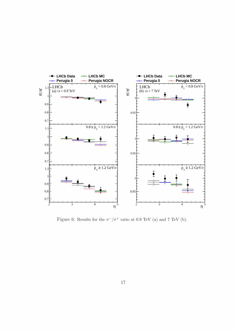
falls from around 0.8 at low η to around 0.4 in the highest pT and η bin. At this energypoint there is a significant spread between models for the Monte Carlo predictions, withthe data lying significantly below the LHCb MC and Perugia 0 expectations, but close tothose of Perugia NOCR. At higher energy the p/p ratio is higher and varies more slowly,in good agreement with LHCb MC and Perugia 0 and less so with Perugia NOCR. TheK−/K+ and π−/π+ ratios also differ from unity, most noticeably at high pT and high η.This behaviour is in general well modelled by all the generator tunes, which give similarpredictions for these observables. Small discrepancies are observed at 7 TeV for K−/K+

at low pT, and π−/π+ at high pT. When comparing the measurements and predictionsfor the different-particle ratios the most striking differences occur for (p + p)/(π+ + π−)and (K+ + K−)/(π+ + π−), where there is a tendency for the data to lie significantlyhigher than the Perugia 0 and NOCR expectations. The agreement with the LHCb MCfor these observables is generally good.

It is instructive to consider the p/p results as a function of rapidity loss, ∆y ≡ ybeam−y,where ybeam is the rapidity of the protons in the LHC beam which travels forward inthe spectrometer (ybeam = 6.87 at 0.9 TeV and 8.92 at 7 TeV). For the same-particleratios it is possible to determine the rapidity value to which the measurement in eachη bin corresponds. In each bin the mean and RMS spread of the rapidity of the tracksin the analysis sample is determined. Correlations are accounted for, but these are ingeneral negligible as the uncertainties are dominated by the PID errors, which for theseobservables are statistical in nature. A small correction is applied to this mean, obtainedfrom Monte Carlo, to account for the distortion to the unbiased spectrum that is inducedby the reconstruction and PID requirements. The values of the mean and RMS spreadof the rapidities for p/p can be found in Appendix A, together with those of K−/K+

and π−/π+. As no evidence is seen of any pT dependence in the distribution of the p/presults against ∆y the measurements in each η bin at each energy point are integratedover pT, with the uncertainties on the individual values of the ratios used to determine theweights of each input entering into the mean. The mean p/p ratios are given as a functionof ∆y in Table 7 and plotted in Fig. 10, with the results from other experiments [16–

13

Table 7: Results for p/p ratio integrated over pT in η bins as a function of the rapidity loss ∆y.√s η range ∆y Ratio

0.9TeV 4.0− 4.5 3.1± 0.2 0.48± 0.033.5− 4.0 3.5± 0.2 0.57± 0.023.0− 3.5 3.9± 0.2 0.65± 0.032.5− 3.0 4.3± 0.1 0.81± 0.09

7TeV 4.0− 4.5 5.1± 0.2 0.90± 0.033.5− 4.0 5.5± 0.2 0.92± 0.023.0− 3.5 5.9± 0.2 0.91± 0.022.5− 3.0 6.3± 0.1 0.89± 0.04

21] superimposed. The LHCb results cover a wider range of ∆y than any other singleexperiment and significantly improve the precision of the measurements in the region∆y < 6.5.

Within the Regge model, baryon production at high energy is driven byPomeron exchange and baryon transport by string-junction exchange [9]. Assum-ing this picture the ∆y dependence of the p/p ratio approximately follows the form1/ (1 + C exp[(αJ − αP )∆y]), where C determines the relative contributions of the twomechanisms, and αJ (αP ) is the intercept of the string junction (Pomeron) Regge tra-jectory. Figure 10 shows the results of fitting this expression to both the LHCb and, inorder to constrain the high ∆y region, the ALICE data. Both C and (αJ − αP ) are freeparameters of the fit and are determined to be 22.5 ± 6.0 and −0.98 ± 0.07 respectivelywith a χ2/ndf of 8.7/8. Taking αP = 1.2 [39] suggests a low value of αJ , significantlybelow the αJ ≈ 0.5 expected if the string-junction intercept is associated with that ofthe standard Reggeon (or meson). The value of αJ ≈ 0.9 which would be expected ifthe string junction is associated with the Odderon [13] is excluded using this fit model.The same conclusion applies if the LHCb and ALICE p/p ratio values are fitted with analternative parameterisation [11] C ′ · (s[GeV2])(αJ−αP )/2 · cosh[y(αJ − αP )], which yieldsthe results C ′ = 10.2± 1.8, (αJ − αP ) = −0.86± 0.05 with a χ2/ndf of 10.2/8.

8 Conclusions

Measurements have been presented of the charged-particle production ratios p/p,K−/K+,π−/π+, (p + p)/(K+ + K−), (K+ + K−)/(π+ + π−) and (p + p)/(π+ + π−) at both√s = 0.9 TeV and

√s = 7 TeV. The results at 7 TeV are the first studies of pion, kaon

and proton production to be performed at this energy. Comparisons have been madewith several generator tunes (LHCb MC, Perugia 0 and Perugia NOCR). No single tuneis able to describe well all observables. The most significant discrepancies occur for the(p+ p)/(π+ + π−) and (K+ +K−)/(π+ + π−) ratios, where the measurements are muchhigher than the Perugia 0 and Perugia NOCR predictions, but lie reasonably close to the

14

LHCb Data LHCb MCPerugia 0 Perugia NOCR

/p

p

0.5

1

LHCb = 0.9 TeVs(a)

< 0.8 GeV/cT

p

0.5

1

< 1.2 GeV/cT

p≤0.8

η2 3 4 5

0.5

1

1.2 GeV/c≥ T

p

LHCb Data LHCb MCPerugia 0 Perugia NOCR

/p

p

0.6

0.8

1

1.2

1.4 LHCb = 7 TeV s(b)

< 0.8 GeV/cT

p

0.6

0.8

1

1.2

1.4 < 1.2 GeV/cT

p≤0.8

η2 3 4 50.6

0.8

1

1.2

1.4 1.2 GeV/c≥ T

p

Figure 4: Results for the p/p ratio at 0.9 TeV (a) and 7 TeV (b).

15

LHCb Data LHCb MCPerugia 0 Perugia NOCR

+/K-

K

0.5

1

LHCb = 0.9 TeVs(a)

< 0.8 GeV/cT

p

0.5

1

< 1.2 GeV/cT

p≤0.8

η2 3 4 5

0.5

1

1.2 GeV/c≥ T

p

LHCb Data LHCb MCPerugia 0 Perugia NOCR

+/K-

K

0.6

0.8

1

1.2

1.4 LHCb = 7 TeV s(b)

< 0.8 GeV/cT

p

0.6

0.8

1

1.2

1.4 < 1.2 GeV/cT

p≤0.8

η2 3 4 5

0.6

0.8

1

1.2

1.4 1.2 GeV/c≥ T

p

Figure 5: Results for the K−/K+ ratio at 0.9 TeV (a) and 7 TeV (b).

16

LHCb Data LHCb MCPerugia 0 Perugia NOCR

+ π/- π

0.7

0.8

0.9

1

1.1 LHCb = 0.9 TeVs(a)

< 0.8 GeV/cT

p

0.7

0.8

0.9

1

1.1 < 1.2 GeV/cT

p≤0.8

η2 3 4 5

0.7

0.8

0.9

1

1.1 1.2 GeV/c≥ T

p

LHCb Data LHCb MCPerugia 0 Perugia NOCR

+ π/- π

0.95

1

LHCb = 7 TeV s(b)

< 0.8 GeV/cT

p

0.95

1

< 1.2 GeV/cT

p≤0.8

η2 3 4 5

0.95

1

1.2 GeV/c≥ T

p

Figure 6: Results for the π−/π+ ratio at 0.9 TeV (a) and 7 TeV (b).

17

LHCb Data LHCb MCPerugia 0 Perugia NOCR

)

- π++ π

)/(

p(p

+

0.1

0.2

0.3

0.4LHCb

= 0.9 TeVs(a) < 0.8 GeV/c

Tp

0.1

0.2

0.3

0.4

< 1.2 GeV/cT

p≤0.8

η2 3 4 5

0.1

0.2

0.3

0.4 1.2 GeV/c≥

Tp

LHCb Data LHCb MCPerugia 0 Perugia NOCR

)

- π++ π

)/(

p(p

+

0.1

0.2

0.3LHCb

= 7 TeV s(b) < 0.8 GeV/c

Tp

0.1

0.2

0.3 < 1.2 GeV/c

T p≤0.8

η2 3 4 5

0.1

0.2

0.3 1.2 GeV/c≥

Tp

Figure 7: Results for the (p + p)/(π+ + π−) ratio at 0.9 TeV (a) and 7 TeV (b).

18

LHCb Data LHCb MCPerugia 0 Perugia NOCR

)

- π++ π

)/(

-+

K+

(K

0.1

0.2

0.3

0.4 LHCb = 0.9 TeVs(a)

< 0.8 GeV/cT

p

0.1

0.2

0.3

0.4 < 1.2 GeV/c

T p≤0.8

η2 3 4 5

0.1

0.2

0.3

0.4 1.2 GeV/c≥ T

p

LHCb Data LHCb MCPerugia 0 Perugia NOCR

)

- π++ π

)/(

-+

K+

(K

0.1

0.2

0.3

0.4 LHCb = 7 TeV s(b)

< 0.8 GeV/cT

p

0.1

0.2

0.3

0.4 < 1.2 GeV/c

T p≤0.8

η2 3 4 5

0.1

0.2

0.3

0.4 1.2 GeV/c≥ T

p

Figure 8: Results for the (K+ +K−)/(π+ + π−) ratio at 0.9 TeV (a) and 7 TeV (b).

19

LHCb Data LHCb MCPerugia 0 Perugia NOCR

)

-+

K+

)/(K

p(p

+

1

2

LHCb = 0.9 TeVs(a)

< 0.8 GeV/cT

p

1

2

< 1.2 GeV/cT

p≤0.8

η2 3 4 5

1

2

1.2 GeV/c≥ T

p

LHCb Data LHCb MCPerugia 0 Perugia NOCR

)

-+

K+

)/(K

p(p

+

0.5

1

LHCb = 7 TeV s(b)

< 0.8 GeV/cT

p

0.5

1

< 1.2 GeV/cT

p≤0.8

η2 3 4 5

0.5

1

1.2 GeV/c≥ T

p

Figure 9: Results for the (p+ p)/(K+ +K−) ratio at 0.9 TeV (a) and 7 TeV (b).

20

y∆0 5 10

/pp

0

0.2

0.4

0.6

0.8

1

1.2

1.4 LHCb = 0.9 TeVs

= 7.0 TeVs

ALICEBRAHMSPHOBOSSTARISRPHENIX

Figure 10: Results for the p/p ratio against the rapidity loss ∆y from LHCb. Results fromother experiments are also shown [16–21]. Superimposed is a fit to the LHCb and ALICE [16]measurements that is described in the text.

21

LHCb MC expectation.The p/p ratio has been studied as a function of rapidity loss, ∆y. The results span the

∆y interval 3.1 to 6.3, and are more precise than previous measurements in this region.Fitting a simple Regge theory inspired model to the LHCb measurements, and those fromthe midrapidity region obtained by ALICE [16], yields a result with a string-junctioncontribution with low intercept value.

These results, together with those for related observables obtained by LHCb [24], willhelp in understanding the phenomenon of baryon-number transport, and the developmentof hadronisation models to improve the description of Standard Model processes in theforward region at the LHC.

Acknowledgements

We thank Yuli Shabelski for several useful discussions. We express our gratitude to ourcolleagues in the CERN accelerator departments for the excellent performance of the LHC.We thank the technical and administrative staff at CERN and at the LHCb institutes,and acknowledge support from the National Agencies: CAPES, CNPq, FAPERJ andFINEP (Brazil); CERN; NSFC (China); CNRS/IN2P3 (France); BMBF, DFG, HGFand MPG (Germany); SFI (Ireland); INFN (Italy); FOM and NWO (The Netherlands);SCSR (Poland); ANCS (Romania); MinES of Russia and Rosatom (Russia); MICINN,XuntaGal and GENCAT (Spain); SNSF and SER (Switzerland); NAS Ukraine (Ukraine);STFC (United Kingdom); NSF (USA). We also acknowledge the support received fromthe ERC under FP7 and the Region Auvergne.

Appendix

A Tables of results

The results for the same-particle ratios, including the rapidity to which the events ineach pseudorapidity bin correspond, are given in Tables 8, 9 and 10. The results for thedifferent-particle ratios can be found in Tables 11, 12 and 13.

22

Table 8: Results for the p/p ratio with statistical and systematic uncertainties, as a function of pT and η. Also shown is the meanrapidity, y, and RMS spread for the sample in each η bin.

pT < 0.8 GeV/c 0.8 ≤ pT < 1.2 GeV/c pT ≥ 1.2 GeV/cy (RMS) Ratio y (RMS) Ratio y (RMS) Ratio√

s = 0.9 TeV2.5 < η < 3.0 – – 2.42 (0.24) 1.107± 0.020± 0.349 2.63 (0.16) 0.794± 0.015± 0.0893.0 ≤ η < 3.5 2.58 (0.27) 0.751± 0.011± 0.163 2.96 (0.25) 0.684± 0.010± 0.049 3.08 (0.23) 0.614± 0.010± 0.0473.5 ≤ η < 4.0 2.96 (0.11) 0.729± 0.007± 0.040 3.40 (0.22) 0.576± 0.007± 0.032 3.56 (0.24) 0.456± 0.009± 0.0334.0 ≤ η < 4.5 3.34 (0.24) 0.660± 0.009± 0.046 3.87 (0.14) 0.451± 0.009± 0.038 4.02 (0.25) 0.328± 0.010± 0.049√s = 7 TeV

2.5 < η < 3.0 – – 2.41 (0.25) 1.181± 0.020± 0.195 2.63 (0.16) 0.880± 0.009± 0.0393.0 ≤ η < 3.5 2.55 (0.27) 0.734± 0.011± 0.124 2.98 (0.25) 0.942± 0.011± 0.036 3.12 (0.22) 0.905± 0.008± 0.0263.5 ≤ η < 4.0 2.96 (0.09) 1.015± 0.009± 0.037 3.40 (0.23) 0.916± 0.007± 0.022 3.59 (0.24) 0.903± 0.008± 0.0234.0 ≤ η < 4.5 3.34 (0.21) 0.957± 0.010± 0.051 3.86 (0.19) 0.906± 0.010± 0.039 4.06 (0.25) 0.831± 0.010± 0.050

23

Table 9: Results for the K−/K+ ratio with statistical and systematic uncertainties, as a function of pT and η. Also shown is themean rapidity, y, and RMS spread for the sample in each η bin.

pT < 0.8 GeV/c 0.8 ≤ pT < 1.2 GeV/c pT ≥ 1.2 GeV/cy (RMS) Ratio y (RMS) Ratio y (RMS) Ratio√

s = 0.9 TeV2.5 < η < 3.0 – – 2.65 (0.19) 0.870± 0.010± 0.267 2.69 (0.14) 0.936± 0.013± 0.0693.0 ≤ η < 3.5 2.99 (0.25) 0.834± 0.007± 0.069 3.12 (0.21) 0.847± 0.009± 0.040 3.18 (0.15) 0.783± 0.011± 0.0373.5 ≤ η < 4.0 3.32 (0.25) 1.001± 0.007± 0.064 3.62 (0.22) 0.792± 0.009± 0.028 3.70 (0.17) 0.723± 0.012± 0.0314.0 ≤ η < 4.5 3.67 (0.18) 1.002± 0.007± 0.093 4.11 (0.25) 0.680± 0.010± 0.041 4.20 (0.21) 0.506± 0.014± 0.050√s = 7 TeV

2.5 < η < 3.0 – – 2.65 (0.19) 0.995± 0.008± 0.101 2.70 (0.13) 0.991± 0.007± 0.0213.0 ≤ η < 3.5 3.02 (0.25) 0.992± 0.006± 0.063 3.12 (0.21) 0.966± 0.006± 0.019 3.20 (0.14) 0.999± 0.006± 0.0163.5 ≤ η < 4.0 3.34 (0.25) 1.062± 0.005± 0.040 3.62 (0.21) 0.948± 0.006± 0.014 3.70 (0.15) 0.930± 0.006± 0.0174.0 ≤ η < 4.5 3.72 (0.22) 1.161± 0.005± 0.055 4.11 (0.23) 0.898± 0.006± 0.025 4.21 (0.18) 0.958± 0.009± 0.049

24

Table 10: Results for the π−/π+ ratio with statistical and systematic uncertainties, as a function of pT and η. Also shown is themean rapidity, y, and RMS spread for the sample in each η bin.

pT < 0.8 GeV/c 0.8 ≤ pT < 1.2 GeV/c pT ≥ 1.2 GeV/cy (RMS) Ratio y (RMS) Ratio y (RMS) Ratio√

s = 0.9 TeV2.5 < η < 3.0 – – 2.74 (0.07) 0.987± 0.010± 0.013 2.75 (0.05) 0.970± 0.016± 0.0143.0 ≤ η < 3.5 3.23 (0.09) 0.979± 0.005± 0.010 3.23 (0.07) 0.971± 0.011± 0.010 3.24 (0.05) 0.926± 0.017± 0.0143.5 ≤ η < 4.0 3.71 (0.15) 0.968± 0.004± 0.011 3.75 (0.08) 0.951± 0.012± 0.010 3.75 (0.05) 0.871± 0.019± 0.0124.0 ≤ η < 4.5 4.15 (0.24) 0.929± 0.004± 0.017 4.30 (0.10) 0.971± 0.016± 0.019 4.30 (0.07) 0.816± 0.025± 0.029√s = 7 TeV

2.5 < η < 3.0 – – 2.74 (0.07) 1.002± 0.007± 0.006 2.74 (0.04) 1.015± 0.010± 0.0053.0 ≤ η < 3.5 3.23 (0.09) 1.011± 0.004± 0.006 3.24 (0.07) 0.998± 0.007± 0.004 3.24 (0.04) 0.998± 0.010± 0.0043.5 ≤ η < 4.0 3.70 (0.14) 1.002± 0.003± 0.006 3.74 (0.07) 1.003± 0.008± 0.004 3.75 (0.05) 1.000± 0.011± 0.0054.0 ≤ η < 4.5 4.14 (0.22) 0.976± 0.003± 0.006 4.26 (0.08) 0.998± 0.009± 0.008 4.26 (0.05) 0.974± 0.012± 0.017

25

Table 11: Results for the (p+ p)/(π+ + π−) ratio with statistical and systematic uncertainties,as a function of pT and η.

pT < 0.8 GeV/c 0.8 ≤ pT < 1.2 GeV/c pT ≥ 1.2 GeV/c√s = 0.9 TeV

2.5 < η < 3.0 – 0.328± 0.007± 0.104 0.300± 0.008± 0.0343.0 ≤ η < 3.5 0.086± 0.001± 0.021 0.208± 0.004± 0.016 0.272± 0.007± 0.0233.5 ≤ η < 4.0 0.062± 0.001± 0.008 0.175± 0.003± 0.011 0.252± 0.007± 0.0204.0 ≤ η < 4.5 0.076± 0.001± 0.010 0.233± 0.006± 0.022 0.301± 0.013± 0.047√s = 7 TeV

2.5 < η < 3.0 – 0.235± 0.004± 0.039 0.262± 0.004± 0.0143.0 ≤ η < 3.5 0.085± 0.001± 0.017 0.174± 0.002± 0.009 0.245± 0.003± 0.0113.5 ≤ η < 4.0 0.069± 0.001± 0.008 0.156± 0.002± 0.006 0.242± 0.003± 0.0104.0 ≤ η < 4.5 0.051± 0.001± 0.007 0.184± 0.003± 0.010 0.244± 0.004± 0.017

Table 12: Results for the (K+ + K−)/(π+ + π−) ratio with statistical and systematic uncer-tainties, as a function of pT and η.

pT < 0.8 GeV/c 0.8 ≤ pT < 1.2 GeV/c pT ≥ 1.2 GeV/c√s = 0.9 TeV

2.5 < η < 3.0 – 0.184± 0.003± 0.056 0.351± 0.008± 0.0283.0 ≤ η < 3.5 0.180± 0.002± 0.026 0.267± 0.004± 0.015 0.319± 0.008± 0.0183.5 ≤ η < 4.0 0.171± 0.001± 0.023 0.247± 0.004± 0.011 0.314± 0.009± 0.0174.0 ≤ η < 4.5 0.173± 0.001± 0.025 0.268± 0.006± 0.018 0.281± 0.012± 0.031√s = 7 TeV

2.5 < η < 3.0 – 0.224± 0.002± 0.024 0.371± 0.004± 0.0143.0 ≤ η < 3.5 0.181± 0.001± 0.024 0.263± 0.003± 0.010 0.357± 0.004± 0.0123.5 ≤ η < 4.0 0.173± 0.001± 0.021 0.262± 0.003± 0.009 0.367± 0.005± 0.0134.0 ≤ η < 4.5 0.131± 0.001± 0.016 0.275± 0.003± 0.011 0.328± 0.005± 0.020

26

Table 13: Results for the (p+ p)/(K++K−) ratio with statistical and systematic uncertainties,as a function of pT and η.

pT < 0.8 GeV/c 0.8 ≤ pT < 1.2 GeV/c pT ≥ 1.2 GeV/c√s = 0.9 TeV

2.5 < η < 3.0 – 1.831± 0.039± 0.822 0.855± 0.020± 0.1193.0 ≤ η < 3.5 0.481± 0.008± 0.139 0.779± 0.014± 0.073 0.851± 0.019± 0.0843.5 ≤ η < 4.0 0.363± 0.004± 0.066 0.709± 0.012± 0.055 0.799± 0.021± 0.0764.0 ≤ η < 4.5 0.433± 0.007± 0.086 0.865± 0.021± 0.097 1.067± 0.045± 0.200√s = 7 TeV

2.5 < η < 3.0 – 1.051± 0.020± 0.204 0.705± 0.009± 0.0463.0 ≤ η < 3.5 0.465± 0.008± 0.111 0.660± 0.009± 0.039 0.682± 0.007± 0.0383.5 ≤ η < 4.0 0.398± 0.004± 0.067 0.593± 0.006± 0.031 0.659± 0.007± 0.0374.0 ≤ η < 4.5 0.379± 0.004± 0.068 0.671± 0.009± 0.046 0.744± 0.011± 0.069

27

References

[1] G. C. Rossi and G. Veneziano, A possible description of baryon dynamics in dual andgauge theories, Nucl. Phys. B123 (1977) 507.

[2] A. B. Kaidalov and K. A. Ter-Martirosyan, Multihadron production at high energiesin the model of quark gluon strings, Sov. J. Nucl. Phys. 40 (1984) 135.

[3] X. Artru, String model with baryons: topology, classical motion,Nucl. Phys. B85 (1975) 442.

[4] M. Imachi, S. Otsuki, and F. Toyoda, Color constraint on urbaryon rearrangementdiagram, Prog. Theor. Phys. 52 (1974) 1061.

[5] M. Imachi, S. Otsuki, and F. Toyoda, Orientable hadron structure,Prog. Theor. Phys. 54 (1975) 280.

[6] B. Z. Kopeliovich, Mechanisms of pp interaction at low and high energies, Sov. J.Nucl. Phys. 45 (1987) 1078.

[7] B. Kopeliovich and B. Povh, Baryon asymmetry of the proton sea at low x,Z. Phys. C75 (1997) 693, arXiv:hep-ph/9607486.

[8] B. Kopeliovich and B. Povh, Baryon stopping at HERA: evidence for gluonic mech-anism, Phys. Lett. B446 (1999) 321, arXiv:hep-ph/9810530.

[9] D. Kharzeev, Can gluons trace baryon number?, Phys. Lett. B378 (1996) 238,arXiv:nucl-th/9602027.

[10] G. H. Arakelyan et al., Midrapidity production of secondaries in pp collisions at RHICand LHC energies in the quark-gluon string model, Eur. Phys. J. C54 (2008) 577,arXiv:0709.3174.

[11] C. Merino, M. M. Ryzhinskiy, and Y. M. Shabelski, Odderon effects in pp collisions:predictions for LHC energies, arXiv:0906.2659.

[12] S. E. Vance and M. Gyulassy, Anti-hyperon enhancement through baryon junctionloops, Phys. Rev. Lett. 83 (1999) 1735, arXiv:nucl-th/9901009.

[13] C. Merino, C. Pajares, M. M. Ryzhinskiy, and Y. M. Shabelski, Pomeron and odderoncontributions at LHC energies, arXiv:1007.3206.

[14] L. Lukaszuk and B. Nicolescu, A possible interpretation of pp rising total cross-sections, Lett. Nuovo Cim. 8 (1973) 405.

[15] R. Avila, P. Gauron, and B. Nicolescu, How can the Odderon be detected at RHICand LHC, Eur. Phys. J. C49 (2007) 581, arXiv:hep-ph/0607089.

28

[16] ALICE collaboration, K. Aamodt et al., Midrapidity antiproton-to-proton ratioin pp collisions at

√s = 0.9 and 7 TeV measured by the ALICE experiment,

Phys. Rev. Lett. 105 (2010) 072002, arXiv:1006.5432.

[17] A. M. Rossi et al., Experimental study of the energy dependence in proton protoninclusive reactions, Nucl. Phys. B84 (1975) 269.

[18] BRAHMS collaboration, I. G. Bearden et al., Forward and midrapidity like-particleratios from p + p collisions at

√s = 200 GeV, Phys. Lett. B607 (2005) 42,

arXiv:nucl-ex/0409002.

[19] PHENIX collaboration, S. S. Adler et al., Nuclear effects on hadron productionin d + Au collisions at

√sNN =200 GeV revealed by comparison with p+p data ,

Phys. Rev. C74 (2006) 024904, arXiv:nucl-ex/0603010.

[20] PHOBOS collaboration, B. B. Back et al., Charged antiparticle to particle ratios nearmidrapidity in p+ p collisions at

√sNN = 200 GeV, Phys. Rev. C71 (2005) 021901,

arXiv:nucl-ex/0409003.

[21] STAR collaboration, B. I. Abelev et al., Systematic measurements of identi-fied particle spectra in pp, d+Au and Au+Au collisions at the STAR detector,Phys. Rev. C79 (2009) 034909, arXiv:0808.2041.

[22] NA49 collaboration, T. Anticic et al., Inclusive production of protons, anti-protons and neutrons in p+p collisions at 158 GeV/c beam momentum,Eur. Phys. J. C65 (2010) 9, arXiv:0904.2708.

[23] ALICE collaboration, K. Aamodt et al., Production of pions, kaons and protons in ppcollisions at

√s =900 GeV with ALICE at the LHC, Eur. Phys. J. C71 (2011) 1655,

arXiv:1101.4110.

[24] LHCb collaboration, R. Aaij et al., Measurement of V 0 production ratios in pp col-lisions at

√s = 0.9 and 7TeV, JHEP 08 (2011) 034, arXiv:1107.0882.

[25] ATLAS collaboration, G. Aad et al., K0S and Λ production in pp interac-

tions at√s = 0.9 and 7 TeV measured with the ATLAS detector at the LHC,

Phys. Rev. D85 (2012) 012001, arXiv:1111.1297.

[26] ALICE collaboration, B. Abelev et al., Multi-strange baryon production in pp colli-sions at

√s =7 TeV with ALICE, arXiv:1204.0282.

[27] CMS collaboration, S. Chatrchyan et al., Study of the inclusive production ofcharged pions, kaons, and protons in pp collisions at

√s = 0.9, 2.76, and 7 TeV,

arXiv:1207.4724.

[28] LHCb collaboration, A. A. Alves Jr. et al., The LHCb detector at the LHC,JINST 3 (2008) S08005.

29

[29] T. Sjostrand, S. Mrenna, and P. Skands, PYTHIA 6.4 Physics and manual,JHEP 05 (2006) 026, arXiv:hep-ph/0603175.

[30] I. Belyaev et al., Handling of the generation of pri-mary events in Gauss, the LHCb simulation framework,Nuclear Science Symposium Conference Record (NSS/MIC) IEEE (2010) 1155.

[31] D. J. Lange, The EvtGen particle decay simulation package,Nucl. Instrum. Meth. A462 (2001) 152.

[32] P. Golonka and Z. Was, PHOTOS Monte Carlo: A precision tool for QED correctionsin Z and W decays, Eur. Phys. J. C45 (2006) 97, arXiv:hep-ph/0506026.

[33] GEANT4 collaboration, S. Agostinelli et al., GEANT4: A simulation toolkit,Nucl. Instrum. Meth. A506 (2003) 250.

[34] GEANT4 collaboration, J. Allison et al., GEANT4 developments and applications,IEEE Trans. Nucl. Sci. 53 (2006) 270.

[35] M. Clemencic et al., The LHCb simulation application, Gauss: design, evolution andexperience, J. of Phys: Conf. Ser. 331 (2011) 032023.

[36] P. Z. Skands, Tuning Monte Carlo generators: the Perugia tunes,Phys. Rev. D 82 (2010) 074018.

[37] M. Pivk and F. R. Le Diberder, sPlot: a statistical tool to unfold data distributions,Nucl. Instrum. Meth. A555 (2005) 356, arXiv:physics/0402083.

[38] IHEP Protvino, COMPAS database, http://wwwppds.ihep.su:8001/ppds.html.

[39] A. B. Kaidalov, L. A. Ponomarev, and K. A. Ter-Martirosyan, Total cross-sectionsand diffractive scattering in a theory of interacting pomerons with αP (0) > 1, Sov.J. Nucl. Phys. 44 (1986) 468.

30