Mobile call termination market review 2015-18

Annexes 7-13

Draft Statement

Date of notification to the EC: 6 February 2015

MCT review 2015-18

Contents

Annex Page 7 MCT cost model approach and design 1

8 Analysys Mason report 67

9 Calibration of the 2015 MCT model 68

10 Cost of capital 83

11 Other modelling issues 128

12 Model outputs and sensitivities 147

13 Brattle report 166

MCT review 2015-18

Annex 7

7 MCT cost model approach and design Introduction

A7.1 This annex outlines the approach we have taken to developing a new MCT cost model and explains its functionality. The final version of the model (the ‘2015 MCT model’) is published alongside this draft statement. The 2015 MCT model has been used to inform our conclusions in this draft statement. An earlier version of the model, the 2014 MCT model, was used to inform our proposals in the June 2014 Consultation.

A7.2 The 2015 MCT model uses a bottom-up approach to estimate the costs of an average efficient national MCP which is then calibrated against top-down data. It is capable of calculating both the LRIC and LRIC+ of MCT, but as explained in Section 6 and consistent with the 2009 EC Recommendation, we are using the LRIC as the cost standard to set the charge control on MTRs.

A7.3 In this annex we first provide some background to the modelling process. We then set out our June 2014 Consultation proposals, stakeholder responses to those proposals, our analysis of those responses and our conclusions in relation to the following:

• model aims;

• technology choice;

• treatment of inflation;

• model structure; and

• constituent modules of the model and calculations.

A7.4 Further details in relation to modelling are provided in the following annexes:

• Annex 8 is an Analysys Mason report explaining the details of the ‘Network’ and ‘Cost’ modules (including updates in light of stakeholder responses to the 2014 MCT model and new evidence);

• Annex 9 describes the model calibration process;

• Annex 10 contains the details of the WACC calculation;

• Annex 11 sets out our analysis in relation to other modelling issues including spectrum holdings, spectrum valuation and administrative costs;

• Annex 12 summarises the model outputs and sensitivity analysis; and

• Annex 13 is a report by Brattle estimating the equity and asset betas for UK MCP owners.

1

MCT review 2015-18

Overview of modelling process

A7.5 In October 2013, Ofcom commissioned Analysys Mason to assist with the development of a new MCT model for the 2015 MCT review. On 23 October 2013 we held a stakeholder workshop. At the workshop we outlined our initial views on some of the key issues that we were proposing to consider as part of the 2015 MCT review and we sought stakeholder views on these issues. The slides presented at this workshop are published on the Ofcom website alongside stakeholder responses to the workshop.1

A7.6 We have collected data from the four largest MCPs using our information gathering powers under section 135 of the Act. We sent information requests to the four largest MCPs on 8 November 2013 requesting detailed information in relation to:

• historical demand for network services;

• historical numbers of assets deployed and their unit costs;

• forecasts for traffic growth;

• information about planned changes to network architectures; and

• forecasts of asset price trends and operating cost trends.

A7.7 Based on our initial work and the information gathered up to that point we published a draft MCT model on 17 January 2014 (the ‘draft MCT model’).2 On 23 January 2014 we held a second stakeholder workshop to discuss the draft MCT model and issues related to our cost modelling. The slides presented at the workshop are published on Ofcom’s website alongside stakeholder responses to the workshop and the draft MCT model.3

A7.8 We sent further information requests under our statutory powers on 14 February 2014 and 18 March 2014 to each of the four largest MCPs that sought further information in relation to network design and network costs.

A7.9 Following the publication of the June 2014 Consultation, we sent an information request under our statutory powers on 19 September 2014 to each of the four largest MCPs. We requested updates of the information originally requested on 8 November 2013 and 14 February 2014 for the most recent periods. We sent further information requests on 3 October 2014 and 11 November 2014 to each of the four largest MCPs seeking further information in relation to network design and costs and voice over WiFI (VoWiFi) respectively.

A7.10 In November 2014, Ofcom commissioned Cartesian to provide an external review of the 2015 MCT model. Cartesian completed its work during December 2014, reporting that ‘overall we found that the 2015 MCT model is robust and captures Ofcom’s documented intent adequately’. Cartesian found ‘several minor issues’

1 See http://stakeholders.ofcom.org.uk/consultations/mobilecallterm/workshop2015-2018/. 2 See http://stakeholders.ofcom.org.uk/telecoms/policy/mobile-policy/mobile-call-termination-review-2015-2018/mct-review-2015-18-january2014/draft-MCT-model/. 3 See http://stakeholders.ofcom.org.uk/telecoms/policy/mobile-policy/mobile-call-termination-review-2015-2018/mct-review-2015-18-january2014/.

2

MCT review 2015-18

through its sensitivity analysis and ‘a few usability issues’. The issues raised by the external review were considered by Ofcom in finalising the 2015 MCT model.

Model aims

A7.11 The purpose of the 2015 MCT model is to forecast the cost of providing MCT for an average efficient MCP during the period 1 April 2015 to 31 March 2018. The forecast costs derived from our 2015 MCT model are then used to inform our conclusions for setting a charge control on MTRs.

A7.12 Therefore, the aim is not to model any specific MCP, but to estimate the costs of a representative average efficient MCP. In that regard the model is hypothetical, but by using inputs (e.g. equipment capacity, equipment replacement costs and spectrum holdings) sourced from the national MCPs and by using a careful calibration process to verify the model outputs against the national MCP networks (in terms of asset counts and accounting costs) the aim is to deliver a bottom-up model which is grounded in reality.

A7.13 Because the 2015 MCT model is based on a bottom-up network calibrated to the costs and asset counts of competing national networks, it is assumed to project an “efficient” level of costs. That is, the model projects the least cost means of delivering existing services using known technology, but recognising where an efficient national network would start from in terms of legacy network deployments.4 For this reason, there is not an explicit efficiency parameter built into the 2015 MCT model (or its predecessors), as would be the case in top-down accounting cost model.

Proposals in the June 2014 Consultation

A7.14 The charge control on MCT implemented in 2011 was set using the 2011 MCT model.5 In the June 2014 Consultation we explained that having considered the requirements for the 2014 MCT model, our view was that the 2011 MCT model had a sufficient level of functionality to serve as a reasonable starting point for the development of a new MCT model.

Responses to the June 2014 Consultation

A7.15 We did not receive any comments from stakeholders regarding our proposed approach to use the 2011 MCT model as a starting point for the development of a new MCT model.

A7.16 Stakeholders provided comments on the specific details of our 2014 MCT model and these are discussed in more detail in the relevant parts of this annex, Annex 8, Annex 9 and Annex 11.

4 See also paragraphs A7.45 and A7.46 which explain the idea of contestable markets which underpins our modelling. 5 The charge control was amended as part of the 2012 CAT Judgment. These amendments can be found in release 4 of the 2011 MCT model, see http://www.ofcom.org.uk/static/wmvct-model/model-2011.html.

3

MCT review 2015-18

Ofcom’s analysis of responses and conclusions

A7.17 We have concluded that the 2011 MCT model has a sufficient level of functionality to serve as a reasonable starting point for the development of the 2015 MCT model.

Technology choice

A7.18 In order to build a bottom-up network cost model, we need to decide which network technology or combination of technologies to model. As explained above, we wish to select a combination of technologies that reflect the decisions that would be taken by an average efficient MCP. This means that our interest in network technology choice is a means to an end, not an end in itself.

A7.19 With regards to historic periods up to the present day, we have sought to model the technologies that an average efficient MCP would have used. We base these modelled technologies on the networks that the national MCPs have deployed.

A7.20 In future periods, we consider that an average efficient MCP would only deploy new technologies if they are at least as efficient as the existing technologies, meaning that they are capable of delivering the same services at the same or lower cost. Our approach to modelling is to only include proven technologies (i.e. the technology of the day). This approach is sometimes referred to as ‘anchor pricing’, meaning that charges are ‘anchored’ to be no higher than the level that would prevail if there were no technological change. In this way customers (that is, wholesale purchasers of the regulated product) and ultimately consumers would be no worse off due to technological change. In practice this means that we model the current network based on the proven technology of the day with no further explicit technological changes in the future.

Proposals in the June 2014 Consultation

A7.21 In the June 2014 Consultation, when choosing between technologies, we considered the following factors:

• The technologies modelled in the 2011 MCT model, and technological and market developments since that time.

• Our economic objectives in setting cost-based charges, which are:

o allocative efficiency;

o productive efficiency;

o dynamic efficiency; and

o effective competition.

• The 2009 EC Recommendation.

• The technologies modelled by other NRAs for the purposes of setting MTRs.

• The views of respondents to the questions we posed at our modelling workshops in October 2013 and January 2014.

4

MCT review 2015-18

A7.22 Based on our analysis of these points we proposed to continue to model 2G and 3G networks and to also model a 4G network carrying data and 4G voice, i.e. voice over LTE (VoLTE). 6

Responses to the June 2014 Consultation

A7.23 BT’s consultation response made reference to its earlier comments provided in response to the January 2014 cost modelling workshop, where it argued that the MCT model should be based on a ‘modern multi-mode network’. BT considered this to be consistent with the approach taken to modelling fixed termination rates as part of the FNMR 2013. Although not reiterating these arguments in its response to the June 2014 Consultation, BT continued to consider that the 2015 MCT model should be based on 4G technology only.7

A7.24 BT also argued that we should include VoWiFi in the model. BT noted that EE and H3G have recently announced they will be introducing a VoWiFi service before the start of the charge control period and Telefonica is already offering such a service.8

A7.25 EE agreed with our proposal to model the costs of MCT on the basis that 2G and 3G technologies will continue being used in addition to 4G. It noted that an operator choosing to offer only 4G services would have a smaller customer base and a higher unit cost than operators supporting all technologies.9

A7.26 Telefonica agreed with our proposal. It considered that BT was incorrect to draw an analogy between the approach proposed by Ofcom for setting the costs of MCT and that used by Ofcom in the 2013 FNMR, since in the 2013 FNMR Ofcom adopted a position about core network architecture, with no implications for the end user.10

A7.27 Vodafone agreed with our proposal that the costs of MCT should be set on the basis of an average efficient operator using a 2G, 3G and 4G network. Vodafone considered that BT was mistaken in its claim that the average efficient operator should be based only on a 4G-only operator.

A7.28 In support of its view that the costs of MCT should be set on the basis of an average efficient operator that operates a 2G, 3G and 4G network (as opposed to a 4G only operator), Vodafone noted the following points.11

A7.29 First, Vodafone agreed with Telefonica that fixed and mobile regulation was very different, not only in terms of what components of the network that are being regulated by wholesale voice call termination, but also in terms of the nature of the customer access to the network in order to be able to make and receive calls. The portion of the network that is being regulated by fixed voice call termination is remote from the customer device, and assumptions made as to which generation of

6 In this document we use the terms ‘4G’ and ‘LTE’ interchangeably. 7 BT response to June 2014 Consultation, page 7 http://stakeholders.ofcom.org.uk/binaries/consultations/mobile-call-termination-14/responses/BT.pdf. 8 BT response to June 2014 Consultation, page 7. 9 EE response to Juen 2014 Consultation, page 49 http://stakeholders.ofcom.org.uk/binaries/consultations/mobile-call-termination-14/responses/Everything_Everywhere.pdf. 10 Telefonica response to June 2014 Consultation, page 8 http://stakeholders.ofcom.org.uk/binaries/consultations/mobile-call-termination-14/responses/Telefonica.pdf. 11 Vodafone response to June 2014 Consultation, page 40-45.

5

MCT review 2015-18

technology to model in the fixed network have no bearing on the ability of the call to be terminated. The specific fixed network customer device adopted to terminate a fixed voice call is thus irrelevant to the modelled network, provided it is capable of being plugged in at the customer’s premises.

A7.30 Vodafone argued that by contrast, it is the entire mobile network that is in the scope of MCT modelling, and in particular the mobile access network (i.e. from the radio spectrum to the cell site back to the core network). One implication is that the network considered to be in scope of the regulation must connect directly with the customer device. If the customer does not have a handset that can connect to the average efficient operator’s network, then the terminated call cannot happen. Therefore, voice termination services are required on all access network technologies demand by customers (i.e. 2G, 3G and 4G).

A7.31 Vodafone noted that Ofcom’s 2014 MCT model assumes a slow progression of VoLTE capability on 4G handsets during the charge control period, leading to an overall average 6% of voice traffic terminated using VoLTE during the charge control period. Vodafone argued that if the model assumed the average efficient operator was 4G only, it would only be able to terminate 6% (unless all 80 million devices in the UK were replaced).

A7.32 Second, Vodafone argued that setting charges based on a 4G-only operator would lead to a stranding of all the 2G and 3G investments. Vodafone noted that in relation to the 2013 FNMR, Ofcom considered the need to be able to recover outstanding historic investment if there were a change in the nature of the technology employed by the assumed average efficient operator. However, it was concluded in that context that there was not an issue largely because BT’s traditional TDM network was very heavily depreciated and the modelled cost recovery from the TDM network for future periods was lower than the suggested cost recovery levels under the NGN. Vodafone argued that the position would be very different in mobile, where investment in all technologies is on-going and book values are high.

A7.33 Third, Vodafone argued, from a practical point of view, that a 4G only network would not be able to maintain roaming arrangements with international operators to allow their customers to roam onto the average efficient operator’s network when travelling in the UK. Given that international roaming is a significant feature of the mobile service set, Vodafone considered that it would be a strange choice to assume that in the UK the average efficient operator was one that did not allow roaming on its network.

A7.34 Fourth, Vodafone argued that the extent of 4G coverage is somewhere behind 2G and 3G networks, and is likely to remain so for some time. According to the 2014 MCT model, at the commencement of the new charge control period Q1 2015/16, whilst the population coverage of 4G is modelled as having increased substantially, it is still only at 84.7%. This would mean that if a 4G only operator was assumed for the average efficient operator then more than 15% of the UK population would be out of the coverage area at the commencement of the new charge control.

A7.35 Vodafone considered, on balance, that 4G technology should be included in the modelled average efficient operator’s network (along with 2G and 3G technology). Vodafone noted that all four major operators have invested heavily in 4G spectrum and continue to invest in 4G network deployment. In addition, 4G capable handsets are being sold to customers and data traffic is increasingly significant as a result of

6

MCT review 2015-18

the adoption of 4G technology. An average operator that ignored this would not be representative.

Ofcom’s analysis of responses and conclusions

A7.36 In deciding between which network technology or combinations of technologies to model for the purposes of developing the 2015 MCT model, we have borne in mind the same factors as set out in the June 2014 Consultation and set out in paragraph A7.21 (with the addition of considering stakeholder responses to the June 2014 Consultation). This is set out in the following sub-sections.

The 2011 MCT model and market developments

A7.37 The 2011 MCT model was a bottom-up model that estimated the costs of an average efficient operator in the UK, and was based on the technologies and spectrum bands that were being used by national MCPs in the UK at that time, specifically 2G and 3G (including HSPA) services.

A7.38 Since the beginning of the last charge control period, we have seen spectrum being liberalised and allocated by auction, and 4G network deployment. The four largest MCPs now have live 4G data networks, and 4G data traffic is expected to increase considerably both before and during the next charge control period.

A7.39 Furthermore, although VoLTE is not currently being used in the UK, the evidence we have is consistent with VoLTE being included in the 2015 MCT model.

Economic objectives in setting cost-based charges

A7.40 In setting a charge control for MTRs, our main objectives are:12

7.40.1 Allocative efficiency, meaning that prices reflect forward looking marginal (or incremental) costs.

7.40.2 Productive efficiency, meaning that MCPs face incentives to minimise costs and there are efficient “build or buy” signals.

7.40.3 Dynamic efficiency, meaning that there is scope for increases in output possible from existing resources (as techniques of production are improved) and/or new services are developed. Delivering dynamic efficiency in regulated markets typically involves providing the opportunity (but not a guarantee) for firms to recover efficiently incurred costs.

7.40.4 Effective competition, meaning that our intervention promotes competition (i.e. those able to do things more efficiently can do so using their own resources and infrastructure) but does not unnecessarily restrict the ability of MCPs or other CPs already operating in regulated markets from competing.

A7.41 However we recognise that tension can exist between these objectives. For example:

12 These same objectives were used in the context of setting cost based charges for fixed termination and origination rates in the 2013 FNMR and the 2011 MCT Statement. See paragraph A5.38 et seq. of the 2013 FNMR Statement.

7

MCT review 2015-18

7.41.1 Pricing at forward looking marginal or incremental cost, while good for allocative efficiency, may not allow the recovery of sunk costs. Regulating in a way which does not provide an opportunity to recover sunk costs is undesirable from the point of view of dynamic efficiency because it undermines incentives to invest in new assets which, once acquired, are themselves sunk.

7.41.2 Setting prices on the basis of full replacement costs, typically determined by reference to the cost of a Modern Equivalent Asset (MEA), is likely to foster effective competition.13 This is because access seekers face appropriate “build or buy” signals. However, prices based on full replacement costs may not generate allocative efficiency because prices will depart from marginal/incremental costs if replacement costs involve making new sunk investments when there are already usable sunk assets in place. Moreover, if investment in competing infrastructure is not practicable or commercially viable, prices set on the basis of replacement cost may result in access seekers, and ultimately consumers, paying a higher price than the MCP needs for cost recovery.

2009 EC Recommendation

A7.42 The 2009 EC Recommendation provides guidance on the technologies to include in a bottom-up LRIC model for the purposes of setting MTRs. It states that:

“The cost model should be based on efficient technologies available in the timeframe considered by the model. Therefore the core part of both fixed and mobile networks could in principle be Next-Generation-Network (NGN)-based. The access part of mobile networks should also be based on a combination of 2G and 3G telephony”.14

A7.43 In making our technology choice for the 2015 MCT model we have taken utmost account of this recommendation, as we are required to do under Article 19(1) of the Framework Directive and section 4A of the Act. We explain this further below.

Technology choices made by other European NRAs

A7.44 We note that NRAs have recently taken a range of views to the choice of technology to include in the construction of MCT models, as shown in Table A7.1 below.

13 An MEA approach is an approach to setting charges based on the least cost proven technology that can offer the full range of regulated services. 14 2009 EC Recommendation, point 4.

8

MCT review 2015-18

Table A7.1: Technology choices made by other NRAs

NRA, Country

Year implemented

Technologies modelled

ACM, Netherlands 2013 2G, 3G

ARCEP, France 2012 2G, 3G (with 4G data implicit in HSPA

modelling, no VoLTE)

NPT, Norway 2013 2G, 3G (with some 4G economies of

scope implicitly accounted for in site costs)

PTS, Sweden

2013 2G, 3G, 4G (data only, no VoLTE)

DBA, Denmark 2012 2G, 3G

CMT, Spain 2013 2G, 3G, 4G (data only, no VoLTE)

BNetzA, Germany 2012 2G, 3G, 4G (data only, no VoLTE)

Source: Analysys Mason, Ofcom.

Relevant competitive constraint to be modelled

A7.45 Our longstanding approach to MCT modelling15 involves the use of economic depreciation, which reflects the on-going nature of investment and the recovery of these costs over a period of time significantly in excess of the duration of any individual charge control. The purpose of this approach is to mimic outcomes in a competitive or contestable market, which provides an appropriate benchmark for regulation.

A7.46 In modelling this competitive constraint we take account of both potential competition from new entrants and actual competition between incumbents. This involves assuming that entry is sustainable in the long run and there is sufficient competition between MCPs to remove super-normal profits, i.e. the modelled operator is assumed to recover the projected present value of lifetime network costs discounted at the weighted average cost of capital (WACC).

Continued inclusion of 2G and 3G technologies

A7.47 We consider that it is appropriate to include 2G and 3G technologies in the 2015 MCT model. We note that BT continues to consider that the costs of MCT should be set on the basis of a modelled average efficient operator adopting a 4G only network. However, we consider that the economic objectives explained in paragraph A7.40 above require the continued modelling of 2G and 3G technologies. While modelling only a 4G network might better reflect replacement costs based on

15 The origins of this approach stretch back to Oftel, Review of the charge control on calls to mobiles, A Statement issued by the Director General of Telecommunications on competition in mobile voice call termination and consultation on proposals for a charge control, 26 September 2001 and are explained in detail at http://www.ofcom.org.uk/static/archive/oftel/publications/mobile/depr0901.htm.

9

MCT review 2015-18

the MEA (and hence competitive/contestable market principles) it could threaten the opportunity to recover the efficiently incurred costs of the existing 2G and 3G networks and hence undermine dynamic efficiency. As noted in paragraph A7.41, signalling that past investments in 2G and 3G assets can be ignored (at least until there has been an opportunity to recover efficiently incurred expenditure) risks undermining regulatory predictability for MCPs and may compromise future incentives to invest.

A7.48 Additionally, we note that there are currently a large number of subscribers who do not have a 4G enabled device. Therefore, a 4G-only MCP would not be able to address the entire market and so would be at a competitive disadvantage. Indeed, given the nascency of VoLTE a 4G-only MCP could not achieve the assumed scale of an average efficient MCP until after the end of the charge control period.

A7.49 We note that EE, Telefonica and Vodafone supported our continued modelling of 2G and 3G technologies, and that this is consistent with the 2009 EC Recommendation.

A7.50 For the above reasons, we do not consider it appropriate to model a 4G only network, and have decided to include both 2G and 3G technologies in the 2015 MCT model. However, we recognise that in doing so care must be taken around the traffic volumes assumed to use the 2G and 3G networks, and the forecast voice and data migration from 2G and 3G to 4G.16 In relation to network modelling it is also necessary to reflect the use of single radio access network (S-RAN) technology and to appropriately capture its impact on 2G and 3G network costs. These issues are discussed further in the relevant sub-sections below.

Inclusion of 4G data technology

A7.51 We continue to consider it appropriate to include 4G data technology in the 2015 MCT model. 4G data is a proven technology in the UK and the four largest MCPs currently provide data services over 4G networks. The inclusion of 4G technology was explicitly supported by Vodafone and EE, and no respondents argued for the exclusion of 4G data technology from the model.

A7.52 We consider that the inclusion of 4G data services appropriately reflects the forward-looking costs of mobile service provision and hence promotes allocative efficiency without undermining incentives to invest. Given the increasing importance of data as a proportion of total mobile network traffic (a point we consider further in the traffic forecasts below), we consider it important to include 4G data from the point of view of appropriately capturing the effects of economies of scope in the provision of mobile services.

A7.53 While the 2009 EC Recommendation does not contain an explicit reference to the inclusion of 4G technology, we nevertheless consider that its inclusion is consistent with that recommendation. The 2009 EC Recommendation explains that the cost model “should be based on efficient technologies available in the timeframe considered by the model”. As we note in the previous paragraph, 4G data services

16 In response to the June 2014 Consultation, Vodafone commented on the consistency of our volume forecasts and spectrum allocations. This point is addressed in Annex 11, and we have checked to ensure that the volume forecasts, in combination with our other modelling assumptions, do not imply unrealistic network build outputs.

10

MCT review 2015-18

are currently offered by all four largest MCPs, suggesting that 4G technology is a sufficiently established technology to include in the 2015 MCT model.

A7.54 In support of this position, we note that data services using 4G technology have been modelled in a number of other European countries, as shown in Table A7.1 above.

Inclusion of 4G voice (VoLTE) technology

A7.55 VoLTE is a nascent technology in the UK, raising the question of whether it is appropriate to include it in the 2015 MCT model.17

A7.56 We have sought further information on VoLTE deployment since the June 2014 Consultation.18 We continue to consider it to be an efficient technology “available in the timeframe considered by the model”, as envisaged in the 2009 EC Recommendation. Since the June 2014 Consultation VoLTE services have been deployed commercially in more countries, and are now live in Hong Kong, Japan, South Korea, Romania, Singapore and the USA.19

A7.57 We specifically sought input on whether VoLTE should be included in the 2015 MCT model as part of the June 2014 Consultation, and note that no respondents have suggested to us that VoLTE should be excluded.

A7.58 For these reasons, we have decided that VoLTE should be included in the 2015 MCT model, and our base case includes VoLTE services. The effect of excluding VoLTE is shown in our sensitivity analysis in Annex 16.

Inclusion of VoWiFi technology

A7.59 As BT noted, VoWiFi services are already offered in the UK, and we anticipate that they will be used during the charge control period. However, the evidence we have collected shows that there is considerable uncertainty about the traffic volumes expected to use VoWiFi. We do not have any convincing evidence to suggest that VoWiFi will form a material proportion of total voice traffic during the period of the next charge control.20 In particular, it is unclear whether VoWiFi might be used for capacity purposes, or merely to provide coverage until 4G rollout is complete.

A7.60 We have also considered, with the aid of Analysys Mason, what work would be required to implement VoWiFi services in the 2015 MCT model. In addition to forecasts of VoWiFi traffic, this would require the definition of routing factors and the dimensioning of new core network assets. However, the extent of WiFi interworking that may be implemented by MCPs is still unclear adding further complexity to the model implementation.

A7.61 The uncertainty around VoWiFi traffic volumes and network architecture in combination with the changes that its implementation in the 2015 MCT model would require, leads us to conclude that it would not be proportionate for us to include VoWiFi services in the 2015 MCT model.

17 See paragraphs A11.53 to A11.57 of the June 2014 Consultation. 18 In response to our information requests dated 8 November 2013, two of the four MCPs advised us that they proposed to deploy VoLTE services during 2014/15. []. 19 See http://www.gsma.com/network2020/volte/ 20 []

11

MCT review 2015-18

Summary of technology choice in 2015 MCT model

A7.62 For the reasons set out in the preceding sub-sections, the 2015 MCT model is of an average efficient MCP, using a combination of 2G, 3G and 4G technologies, including VoLTE but excluding VoWiFi.

A7.63 We consider that this approach is consistent with our framework for technology choice, relevant technological developments since the last review, and the 2009 EC Recommendation.

Treatment of inflation

A7.64 As set out in Section 8, inflation is used as an input to the MCT charge control in two respects:

• First, to determine how the cap on charges is updated each year (e.g. in the form of a CPI+/-X charge control).

• Second, when setting a real terms charge control based on forecast costs, the cost inputs will need to be reported with respect to a particular measure of inflation.

A7.65 In Section 8 we decided that the CPI measure of inflation is preferable for the purposes of the charge control formula.

Proposals in the June 2014 Consultation

A7.66 In the June 2014 Consultation, we proposed that in order to ensure consistency with the charge control formula we would use CPI to deflate nominal costs, from which we then project the evolution of operating and capital cost price trends (including the WACC).

A7.67 In the 2014 MCT model, we derived a time series of CPI inflation from three sources:

7.67.1 CPI data are available from the ONS from 1997 onwards and were used for the years 1996/7 to 2012/13.21

7.67.2 For the period prior to 1996/7 we estimated CPI using the average difference between the ONS data explained above and the inflation time series in the 2011 MCT model (over the period 1996/97 to 2012/13).22

7.67.3 For 2013/14 onwards we used the Bank of England CPI inflation target of 2% as a forecast of long run CPI inflation.23

21 In the June 2014 Consultation we used figures from Table 6b (D7G7) of the ONS Consumer Price Inflation Tables: See ONS, Consumer Price Inflation – December 2013, published 14 January 2014. http://www.ons.gov.uk/ons/rel/cpi/consumer-price-indices/december-2013/consumer-price-inflation-reference-tables.xls. We use April to April changes over the prior 12 months to derive data in financial years. 22 The average difference is 0.6 percentage points. 23 See http://www.bankofengland.co.uk/monetarypolicy/Pages/framework/framework.aspx

12

MCT review 2015-18

A7.68 The use of an updated real WACC which is based on deflating the nominal WACC by CPI required us to adjust the value of the WACC from earlier MCT models to CPI-deflated terms to produce a consistent time series which is used as the real discount rate.24

Responses to the June 2014 Consultation

A7.69 H3G raised a concern about Ofcom’s reliance on using the Bank of England CPI inflation target as a forecast of long-run CPI inflation rather than independent estimates of future CPI inflation.25 BT commented that if CPI is used this should be ‘implemented in a transparent and appropriate way’.26 We did not receive any other comments on our proposal.

Ofcom’s analysis of responses and conclusions

A7.70 In order to ensure consistency with the charge control formula, we continue to consider that it is appropriate to use CPI to deflate nominal costs and we have therefore adopted this approach in the 2015 MCT model.

A7.71 In the 2015 MCT model we have updated the time series of CPI inflation figures as follows:

7.71.1 CPI data are available from the ONS from 1997 onwards and a figure for 2013/14 has been added to those for 1996/7 to 2012/13 used in the 2014 MCT model, as we explained we would in the June 2014 Consultation.27

Since the results of the model are produced in 2012/13 prices the 2013/14 figure is necessary only to improve the backwards forecast (see next sub-point) and for certain asset input prices.

7.71.2 For the period prior to 1996/7 we updated our estimate of CPI using data for the period 1996/97 to 2013/14 to calculate the difference between the geometric averages of the ONS data explained above and the inflation time series in the 2011 MCT model.28

7.71.3 For the period from 2013/14 onwards the calculation of unit costs in 2012/13 prices does not require an explicit inflation forecast since forecasts start from 2012/13 as the base year, where costs are expressed in 2012/13 price terms.

24 The real discount rate in the 2011 MCT model took a different value in each of the years 1990/91 to 2000/01, and then changed with the construction of successive MCT models in 2003/4, 2006/7 and 2009/10. We adjust the old values of the WACC in each of these years using expected inflation at those times, meaning that it remains constant through each of the prior charge control periods. This is calculated as: 𝐶𝐶𝐶𝐶𝐶𝐶 𝑟𝑟𝑟𝑟𝑟𝑟𝑟𝑟 𝑑𝑑𝑑𝑑𝑑𝑑𝑑𝑑𝑑𝑑𝑑𝑑𝑑𝑑𝑑𝑑 𝑟𝑟𝑟𝑟𝑑𝑑𝑟𝑟𝑡𝑡 = �(1 + 2011 𝑀𝑀𝐶𝐶𝑀𝑀 𝑟𝑟𝑟𝑟𝑟𝑟𝑟𝑟 𝑑𝑑𝑑𝑑𝑑𝑑𝑑𝑑𝑑𝑑𝑑𝑑𝑑𝑑𝑑𝑑 𝑟𝑟𝑟𝑟𝑑𝑑𝑟𝑟𝑡𝑡) × (1+2011 𝑀𝑀𝑀𝑀𝑀𝑀 𝑖𝑖𝑖𝑖𝑖𝑖𝑖𝑖𝑖𝑖𝑡𝑡𝑖𝑖𝑖𝑖𝑖𝑖𝑡𝑡)

(1+𝑀𝑀𝐶𝐶𝐶𝐶 𝑖𝑖𝑖𝑖𝑖𝑖𝑖𝑖𝑖𝑖𝑡𝑡𝑖𝑖𝑖𝑖𝑖𝑖𝑡𝑡)� − 1, where t

refers to each of the years in which prior MCT models were updated, as explained above. 25 H3G response to MCT Consultation, page 10 http://stakeholders.ofcom.org.uk/binaries/consultations/mobile-call-termination-14/responses/H3G.pdf 26 BT response, page 20. 27 Using Table 6b (D7G7) of the ONS Consumer Price Inflation Tables: See ONS, Consumer Price Inflation – November 2014, published 16 December 2014, http://ons.gov.uk/ons/rel/cpi/consumer-price-indices/november-2014/consumer-price-inflation-reference-tables.xls. 28 The difference is 0.6 percentage points.

13

MCT review 2015-18

A7.72 Consistent with the use of CPI inflation, we use a real WACC expressed relative to CPI. This real WACC is obtained by deflating the nominal WACC by CPI assuming a long run rate of 2%, as explained in Annex 10. In response to the point raised by H3G above, note that in Annex 10 we explain how we have cross-checked our use of a 2% CPI assumption against independent forecasts. Since the MCT model also requires a real discount rate in historical periods (not just for future periods), we need to adjust the WACC values from earlier MCT models to CPI real terms to produce a consistent time series for the discount rate.29

A7.73 For the purposes of calculating X in the CPI-X charge control formula we continue to use independent forecasts of CPI inflation compiled by HM Treasury, as explained in Section 8.

Model structure, calculation and outputs

Model structure

A7.74 Consistent with our proposals in the June 2014 Consultation, the 2015 MCT model comprises six modules, each of which is a separate Excel workbook (i.e. a separate Excel file), as shown in Figure A7.1 below.

Figure A7.1: Structure of the 2015 MCT model

Source: Ofcom.

A7.75 The functions of these modules and the linkages between them are as follows:

• The ‘Scenario Control’ module defines and allows the selection of the model scenarios and sensitivities. It also contains a summary of the key results.

• The ‘Traffic’ module contains the service demand forecasts and network coverage assumptions.

• The ‘Network’ module contains network dimensioning algorithms and forecasts the quantities of 2G, 3G and 4G network equipment required to provide network coverage and meet service demand ahead of time.

29 This follows the approach explained in footnote 24 above.

14

MCT review 2015-18

• The ‘Cost’ module uses the calculated equipment quantities (as derived in the network module) and unit equipment prices to calculate network costs (both capital and operating) over time.

• The ‘Economic’ module calculates service costs from the forecast network costs, based on economic depreciation. The outputs of this module form the model results.

• The ‘HCA CCA’ module calculates the accounting cost of the network based on historic cost accounting (HCA) and current cost accounting (CCA) approaches. HCA outputs from this module are used for the purposes of model calibration only, as explained in Annex 9.

A7.76 The ‘Scenario control’, ‘Traffic’, ‘Economic’ and ‘HCA CCA’ modules have been developed by Ofcom. Each of these modules is explained in detail under specific sub-sections below. Overviews are also provided for the ‘Network’ and ‘Cost’ modules, which have been developed by Analysys Mason. Full details of the network and cost modules are provided in the Analysys Mason report in Annex 8.

Summary of major changes to the model

Proposals in the June 2014 Consultation

A7.77 In the June 2014 Consultation we explained that taking the 2011 MCT model as the starting point the changes made in developing the 2014 MCT model fell into the following three categories:

• Those requiring updates purely to reflect the passage of time including:

o traffic forecasts;

o unit equipment capital and operating costs and cost trends; and

o WACC estimate.

• Those requiring modifications to existing model functionality including:

o additional (higher speed) HSPA developments;

o additional (higher speed) backhaul developments; and

o upgrades to the core network in terms of MSC-S/MGW deployment and core transmission.

• Those requiring the addition of new functionality including:

o 4G network modelling;

o VoLTE services;

o S-RAN technology; and

o Infrastructure sharing of active equipment.

15

MCT review 2015-18

A7.78 We also considered whether it was necessary to include femtocells in the MCT model but based on the analysis undertaken by Analysys Mason, we considered that its inclusion would not be proportionate.30

Ofcom’s analysis of responses and conclusions

A7.79 Where stakeholders have made specific points about the proposed changes to the model we discuss these in the relevant sub-sections below and outline how they have been addressed in the 2015 MCT model. We also consider that the broad changes we proposed in updating the 2011 MCT model for our consultation remain appropriate for developing the 2015 MCT model.

A7.80 Stakeholder comments relating to the network and cost module of the model are discussed in detail in Annex 12. We agree with Analysys Mason’s views on the stakeholder comments and the resulting changes that it has made (and has not made) in producing the 2015 MCT model.

Model calculation

A7.81 Consistent with the proposals in the June 2014 Consultation, the 2015 MCT model calculates the LRIC of MCT using a decremental approach. This calculation involves considering MCT as a ‘final increment’ with no common costs (such as the common costs of a ‘coverage network’) being allocated to MCT. Our approach to calculating LRIC is consistent with the 2009 EC Recommendation.

A7.82 The incremental costs associated with MCT traffic are derived in four stages:

i) Calculate the model outputs (service demand, asset volumes and cash flows for each network element) with MCT included.

ii) Calculate the model outputs (service demand, asset volumes and cash flows for each network element) with MCT traffic excluded.

iii) Use the incremental service demand, asset volumes and cash flows for each network element as inputs to the original economic depreciation (Original ED) algorithm.

iv) Take the outputs of the Original ED algorithm and combine them with the network element usage factors to determine the LRIC of a minute of MCT.

A7.83 The calculation flow used to determine LRIC is shown in Figure A7.2 below (with MCT referred to as ‘incoming voice’ in the flow chart).

30 See Section 2.8 of Analysys Mason, MCT review 2015-2018: Mobile network cost modelling proposals for model, 4 June 2014, http://stakeholders.ofcom.org.uk/binaries/consultations/mobile-call-termination-14/annexes/analysys-mason-Report_for_Ofcom.pdf.

16

MCT review 2015-18

Figure A7.2: How the LRIC of MCT is calculated

Source: Ofcom.

Model outputs

A7.84 The outputs of the 2015 MCT cost model are unit costs (either LRIC or LRIC+) in each year for MCT. The model works in real terms (relative to CPI inflation) indexed to 2012/13 prices, and all outputs are stated in 2012/13 prices.

Scenario control module

A7.85 The scenario control module contains the main parameters that affect the cost of MCT. These parameters then feed through to all other relevant modules.

A7.86 The Scenario worksheet in the module is constructed to allow the user to choose between different scenarios, with a macro enabling the calculation of either LRIC+ or LRIC results pertaining to these scenarios.

A7.87 The Outputs worksheet contains the most important results from the model.

A7.88 The functionality of the scenario control module in the 2015 MCT model remains unchanged from that proposed in the 2014 MCT model, with changes only to update the scenarios.

Traffic module

A7.89 The traffic module of the 2015 MCT model uses demand forecasts and network coverage assumptions to derive service traffic forecasts which are used in the Network module to dimension the 2G, 3G and 4G networks.

A7.90 In the June 2014 Consultation, we explained that there had been many changes in the mobile market since the 2011 MCT model was developed. The usage of services had differed from the forecasts in the 2011 MCT model, and 4G services have been introduced. Reflecting these developments, all of the demand forecasts were updated from those in the 2011 MCT model, and following the June 2014 Consultation all of the demand forecasts have been refreshed to reflect the latest evidence collected in response to the section 135 notice dated 19 September 2014.

17

MCT review 2015-18

A7.91 The 2015 MCT model has the functionality to forecast out to 2039/40; however we only included explicit traffic forecasts to Q4 2025/26 after which volumes are held constant. This mirrors the approach taken in the 2014 MCT model.

A7.92 We also note that our traffic forecasts must be consistent with our assumptions concerning network technology and spectrum. As explained in paragraph A7.19 above, the 2015 MCT model uses the technology of the day with no further developments in the future. This means that although in the short term the 2015 MCT model forecasts are based on data from MCPs, in the medium and longer term the forecasts are constrained by the technology and spectrum we are using.

A7.93 We forecast subscription numbers and demand per subscription for each modelled service to derive total demand for each service. The 2015 MCT model includes ‘High’, ‘Medium’ and ‘Low’ forecasts for each of the services listed in paragraph A7.95 below. These input forecasts were formulated with reference to:

• Historical data provided by the four largest MCPs (updated for the period Q2 2010/11 to Q2 2013/14);

• Forecast data provided by the four largest MCPs (up to Q4 2017 where possible); and

• Third party reports, forecasts and other Ofcom work (used as cross checks);

A7.94 We received a number of comments on the traffic forecasts included in the 2014 MCT model in response to the June 2014 Consultation. These inputs are addressed in full in the relevant sub-sections below.

A7.95 We created a range of forecasts for the total demand over the modelled network for each of the following services:

i) 2G incoming, outgoing and on-net voice calls;

ii) 2G SMS31 and MMS32;

iii) 2G packet data;

iv) 3G incoming, outgoing and on-net voice calls;

v) 3G SMS and MMS;

vi) 3G handset packet data;

vii) 3G data device33 packet data;

viii) 4G incoming, outgoing and on-net voice calls;

31 By ‘SMS’ we refer to individual text messages sent or received using the Short Message Service. 32 By ‘MMS’ we refer to individual messages with multimedia content sent or received using the Multimedia Messaging Service. 33 “Data devices” includes those devices built to primarily transmit and receive data, rather than voice, including: dongles, datacards, laptops, tablets and other integrated devices. These devices are typically used with a data-only subscription. In the June 2014 Consultation we referred to these devices simply as ‘datacards’.

18

MCT review 2015-18

ix) 4G SMS and MMS;

x) 4G handset packet data; and

xi) 4G data device packet data.

A7.96 An outline of the calculations contained in the traffic module is shown in Figure A7.3 below.

Figure A7.3: Summary of Traffic Module calculations

Source: Ofcom

Subscription numbers

Proposals in the June 2014 Consultation

A7.97 Our forecast for the total number of mobile subscriptions in the June 2014 Consultation was based on forecasts of the UK population and SIM penetration. We used historic data to inform penetration rates for handsets and data devices individually, which we then forecast forward subject to a saturation point

1 - Traffic Module

Scenario dependent input Non – Scenario dependent input Intermediate calculation Output

Market Share

Technological split

Traffic per subscriber

Rebalancing of traffic across technologies

Total Market Subscribers

Churn rate

Operator subscribers

Gross adds, net adds

Subscribers by technology

Subscriber traffic by technology

Network traffic by service and

technology

19

MCT review 2015-18

constraint.34 We then translated the total subscription base into a defined number of subscriptions for the modelled network using the assumed market share for the average efficient MCP.

Responses to the June 2014 Consultation

Handsets

A7.98 We did not receive any responses to the June 2014 Consultation in relation to our forecast of the total number of subscriptions and handset penetration. We did however receive a number of comments in relation to 4G and VoLTE handset penetration and handset churn.

Data devices

A7.99 BT noted that the forecasts in the 2014 MCT model were lower than those in the 2011 MCT model and argued that they underestimated data device penetration. 35 BT noted our point that subscribers who had previously used data devices can increasingly meet their data needs by tethering to a handset, and that the historical data show that data device penetration had fallen, but argued that this may be a short-lived trend because:

• Data device penetration observed between 2010/11 and 2013/14 needs to be considered in the context of the rapid increase in penetration rates observed in the years prior to this date.

• There is significant potential for expansion in the tablet computer market.

A7.100 BT put forward the following evidence and arguments to support its view in relation to tablets as data devices:

• A Mintel report “Rise of the 4G tablet” arguing that ‘US manufacturers will increasingly emphasise 4G tablets. Mobile operators in turn will also have an incentive to increase 4G tablet roll-out as they seek to expand their revenue streams and may thus contribute to a trend of increasing tablet penetration’.

• BT recognised that not all tablets contained embedded SIMs. However, it argued that even if this proportion doesn’t increase this would still lead to a rise in the overall data device penetration rate as the penetration of tablets in the population increases.

• BT also cited Ofcom’s 2013 Communications Market Report as stating that tablet computer ownership has doubled in the 12 months to Q1 2013, reaching 24% of UK households, and Enders Analysis as predicting that tablet penetration will increase to 63% by 2020.

A7.101 On the basis of this evidence BT concluded that tablet data devices alone would account for a data device penetration rate of 12.6% by 2020.

34 This was assumed to be 127% for handsets in the base case. 35 Deloitte, Volume forecasts in the Ofcom MCT model, A report for BT, 8 August 2014, Section 5. http://stakeholders.ofcom.org.uk/binaries/consultations/mobile-call-termination-14/responses/BT_Deloitte_volume_report.pdf (‘Deloitte Report’).

20

MCT review 2015-18

Ofcom’s analysis of responses and conclusions

Handsets

A7.102 We have updated the historical data on handset SIM penetration to reflect the latest data gathered in response to our September 2014 information request. We have then used this, in conjunction with data device penetration figures, to obtain handset penetration figures. Our updated data shows a slight decline to around 120% by Q1 2014/15.36 We have adjusted our forecasts to reflect this small decline over the last few quarters. The low and high scenarios now reach penetration levels of 117% and 125%, respectively, in 2025/26. Our medium forecast has a penetration level of 121% in 2025/26. The mobile handset penetration forecasts used in the 2015 MCT model are shown in Figure A7.4 below.

Figure A7.4: Mobile handset penetration (% of population)

Source: Ofcom 2015 MCT model.

Data devices

A7.103 In light of BT’s comments on tablet device penetration, we have reviewed our assumptions on data device penetration forecasts in the June 2014 Consultation. While we accept that tablet penetration is increasing and that this growth may continue, as BT recognised, not all tablets include or are capable of having mobile data connections. As a result, not all tablets are mobile data devices.

36 This is consistent with the trend that we found in our 2014 Communications Market Report, where we observed a fall in mobile subscriptions at the end of 2013 (see Ofcom, Communications Market Report 2014, 7 August 2014, page 336). http://stakeholders.ofcom.org.uk/binaries/research/cmr/cmr14/2014_UK_CMR.pdf

21

MCT review 2015-18

A7.104 Ofcom’s Technology Tracker (for Q2 2014) included the following evidence on tablet device penetration in the UK:37

• 46% of households have at least one tablet computer, and 81% of adults in these households said that they personally use a tablet computer, meaning that 37% of UK adults have access to and use a tablet computer.

• Of those who said they personally use a tablet computer, 44% said it was 3G or 4G enabled (this equates to 17% of all adults).

• Of those who reported using a 3G or 4G enabled tablet, 34% said it had a separate mobile subscription, allowing them to go online without the need for a Wi-Fi connection. This means that 6% of all adults have access to a tablet computer with a 3G or 4G subscription.

A7.105 These figures show that while nearly half of households have a tablet, only a subset of those are cellular enabled devices, and an even smaller subset are used with a cellular contract and are hence a data device for the purposes of MCT modelling.

A7.106 The latest evidence on data device penetration that we have gathered from MCPs shows that penetration still lies below the peak seen in Q4 2011/12 and has been relatively flat over the past year. We remain of the view that the introduction of 4G technology means that some data device users may choose to use a tethered 4G handset and to tether to this rather than use a separate data device, but recognise that growth in tablet penetration will work to offset this. It is unclear to us which of these effects will dominate the other, but on balance we consider that modest growth in data device penetration is more appropriate than modest decline (in contrast to the forecast in the June 2014 Consultation). The resulting mobile data device penetration forecasts used in the 2015 MCT model are shown in Figure A7.5 below.

37 See Ofcom, Ofcom Technology Tracker Wave 2 2014, published September 2014, http://stakeholders.ofcom.org.uk/binaries/research/statistics/2014sep/technology-tracker-wave-2-2014/main_set.pdf, Tables 34, 36, 39, and 40.

22

MCT review 2015-18

Figure A7.5: Mobile data device penetration (% of population)

Source: Ofcom 2015 MCT model.

Market share

Proposals in the June 2014 Consultation

A7.107 In the 2014 MCT model we assumed that our modelled MCP’s market share profile for handsets was identical to that used in the 2011 MCT model, with the exception that we adjusted the trend from the lowest point (in Q1 2010/11) to reach 25% by the end of 2025/26 rather than the end of 2020/21. This change was to reflect that the 25% market share is a long term assumption reached by the end of the modelling period.

A7.108 We proposed a different market share assumption for data devices than that used for handsets.38 This was to reflect the fact that H3G had a much greater share of the data device market than the other MCPs and therefore data traffic accounted for a larger proportion of total traffic for H3G than for the 2G/3G MCPs. The profile was adjusted to reach the long term assumption of a 25% market share by 2025/26 rather than 2020/21, mirroring the change made for the handset market share explained above.

38 This difference reflected a finding by the CC in its 2012 CC Determination, see http://www.catribunal.org.uk/files/1.1180-83_MCT_Determination_Excised_090212.pdf, paragraphs 4.138 to 4.144.

23

MCT review 2015-18

Responses to the June 2014 Consultation

A7.109 We received only one comment in response to the June 2014 Consultation on the subject of handset market share, with Vodafone explaining that it had ‘no present disagreement with the principle of 25% market share and [saw] no virtue in discussing alternative overall market share proportions for the average efficient operator’.

A7.110 We did not receive any comments on the data device market share in the June 2014 Consultation.39

Ofcom’s analysis of responses and conclusions

Handsets

A7.111 The handset market share in the 2015 MCT model remains unchanged from that explained in the June 2014 Consultation, which is in turn an update of the profile used in the 2011 MCT model.

A7.112 Prior to 2003/04, the market share is assumed to be 25% (corresponding to four national MCPs). Following the entry of a 3G only operator in 2003/04, the market share begins to trend downwards towards 20% in the long run (corresponding to five national MCPs). However, due to the merger (via a joint venture) between Orange and T-Mobile we considered it appropriate to move back towards a 25% long run market share. Accordingly, from Q1 2010/11 onwards the market share increases back towards 25% by the end of 2025/26. The handset market share used in the 2015 MCT model is shown in Figure A7.6 below.

39 Although we note that Vodafone did refer to the change made following the appeal of the MCT 2011 Statement, see page 54 of the Vodafone response.

24

MCT review 2015-18

Figure A7.6: Handset market share evolution

Source: Ofcom 2015 MCT model.

Data devices

A7.113 The data device market share in the 2015 MCT model remains unchanged from that used in the June 2014 Consultation, which is in turn an update of the profile used in the 2011 MCT model, following the appeal.

A7.114 The data device market share is set at the same level as the handset market share until Q3 2007/08. From this point onwards, the data device market share gradually decreases to 15% by Q3 2008/09, remaining constant at 15% until Q1 2010/11. Thereafter it increases gradually to reach 25% by 2025/26. This evolution is shown in Figure A7.7 below.

-%

5%

10%

15%

20%

25%

30%

Mar

ket S

hare

25

MCT review 2015-18

Figure A7.7: Data device market share evolution

Source: Ofcom 2015 MCT model.

4G launch and device migration

Proposals in the June 2014 Consultation

4G launch

A7.115 In the June 2014 Consultation we assumed that the modelled operator launched 4G (data) services in Q3 2013/14, with VoLTE services following in Q1 2015/16, noting that only a small proportion of 4G data enabled handsets were currently capable of supporting VoLTE.

Handsets

A7.116 In the 2014 MCT model, we forecast the migration of handset subscriptions using an assumption of the market (average) rate of subscriber churn. We forecast migration from 2G to 3G handsets, 3G to 4G handsets and 2G to 4G handsets.

A7.117 We do not hold data on handset churn rates so we use subscriber churn as a proxy. Subscriber churn does not include those subscribers who purchase a new handset without changing contract (e.g. upgrades), which other things being equal would lead to a higher churn rate. However there is also an opposing effect which is not taken into account, namely subscribers who take out new contracts but keep their existing handset. As a result of these opposing effects on handset churn, we consider subscriber churn provides a suitable proxy.

A7.118 In addition, we forecast the proportion of 4G devices which would support VoLTE by the end of 2017/18.

-%

5%

10%

15%

20%

25%

30%

Mar

ket S

hare

26

MCT review 2015-18

Data devices

A7.119 During the transition period between 3G and 4G we forecast the proportion of data devices which are either 3G or 4G enabled. We considered it would not be appropriate to model migration between the two technologies in the same way as we proposed with handsets because we had concerns over whether historical churn data was likely to be a reliable indicator of future churn rates. We consider that data device churn is likely to be low relative to that for handsets, with most users changing their data device in response to the availability of a new technology.

Responses to the June 2014 Consultation

A7.120 In relation to our handset and data device migration forecasts we received a number of responses to the June 2014 Consultation.

A7.121 BT argued that we had underestimated 4G handset subscription numbers, both in the short term and the longer term. BT referred to public statements from MCPs (in particular a quote from EE that “97% of our customer base will be on 4G devices by 2018”) and argued that the modelled operator should gain subscribers much more quickly.40 BT also argued that our 4G adoption profile is inconsistent with our assumed date for 1800 MHz spectrum refarming for 4G use. BT created two scenarios which increased the number of 4G subscribers and it found they led to a reduction in the blended MTR.

A7.122 In contrast, Vodafone stated that EE was in a unique position to launch 4G early, which was not available to any other operator. Therefore, EE’s 4G experience should not be used in the 2015 MCT model, at least during the charge control period.

A7.123 Vodafone claimed the 4G migration was both uncertain and of particular importance if we continue to use a LRIC cost standard due to the weighting of traffic in the blended MTR. It argued that given the LRIC of 4G is lower than the LRIC of 2G and 3G, if operators cannot transfer as much traffic from other technologies to 4G as forecast, they will face an MTR lower than their actual costs of termination. Therefore, a cost estimate produced on this blended MTR basis may lead to an MTR below that which the other operators (and, in Vodafone’s view, the average efficient operator) can possibly be expected to obtain.41

A7.124 EE argued that the assumed migration to 4G services was too high, and that we had not adjusted our forecasts in response to its previous comments or responded to them.42 It also reiterated its previous view that our forecasts might have been unduly influenced by EE’s own experience, and that ‘our current level of take-up will be higher than that achievable by an average UK mobile operator (which is the appropriate benchmark for Ofcom’s model)’.43

40 Deloitte Report, Section 3.3. 41 Vodafone response to June 2014 Consultation, page 30. 42 In their response to Ofcom’s draft cost model, EE compared Ofcom’s forecast rate of 4G take-up with take-up rates in other European countries. As discussed in paragraph 7.190.3 below, we consider data on UK MCPs to be more relevant than international comparisons. 43 EE response to June 2014 Consultation, Section 6.2.

27

MCT review 2015-18

A7.125 Telefonica considered that Ofcom’s estimate of handset churn was an overestimate for several reasons:44

• There is a distinction between post pay churn and pre-pay churn rates, with the former being far lower in Telefonica’s own experience (a monthly rate of 1% in its 2013 Annual Report, equating to an annualised rate of 12.7%). Telefonica noted this was particularly important as the majority of 4G subscriptions are post-pay.

• There is evidence that customers are on average keeping their handsets for longer (i.e. handset churn is falling).

• The use of a standard churn rate for the entire mobile base assumes that customers have a homogenous propensity to churn handsets. Telefonica considered this unrealistic as some customers are likely to churn their handset more frequently than others.

Ofcom’s analysis of responses and conclusions

A7.126 In response to these comments we have re-examined the 4G launch dates and device migration profiles used in the 2014 MCT model, as explained below.

4G launch date

A7.127 As noted by BT, EE launched 4G data services before the other UK MCPs. EE45 launched 4G services in October 2012 (Q3 2012/13), while Telefonica46 and Vodafone47 launched at the end of August 2013 (Q2 2013/14), and H3G48 began its launch in December 2013.

A7.128 The MCPs’ ability to launch 4G services was limited by a number of factors, including spectrum allocations and spectrum liberalisation. In this regard we note that:

7.128.1 The 1800 MHz licences held by EE were permitted for use with 4G technologies (as well as 2G and 3G) from 11 September 2012 (Q2 2012/13).49

7.128.2 All licences held in the 900 MHz, 1800 MHz and 2.1 GHz bands were varied to permit the deployment of LTE and WiMAX (4G) services under an Ofcom decision of 9 July 2013 (Q1 2013/14).50

7.128.3 All four national MCPs won additional spectrum in the 4G auction in February 2013. Licences for the new spectrum were issued on 1st March

44 Telefonica response to June 2014 Consultation, page 9. 45 http://ee.co.uk/our-company/newsroom/2012/10/30/ee-launches-superfast-4g-and-fibre-for-uk-consumers-and-business. 46 http://news.o2.co.uk/?press-release=o2s-4g-network-to-switch-on-from-29th-august. 47 http://www.vodafone.co.uk/cs/groups/configfiles/documents/contentdocuments/vftst043609.pdf 48 http://www.computing.co.uk/ctg/news/2317407/three-uk-begins-4g-rollout. 49 http://stakeholders.ofcom.org.uk/consultations/variation-1800mhz-lte-wimax/statement. 50 Ofcom, Statement on the Requests for Variation of 900 MHz, 1800 MHz and 2100 MHz Mobile Licences, statement, 9 July 2013. http://stakeholders.ofcom.org.uk/binaries/consultations/variation-900-1800-2100/statement/statement.pdf.

28

MCT review 2015-18

2013 and Ofcom stated that “consumer services [are] expected in spring or early summer 2013” (Q1 2013/14).51

A7.129 This means that the 4G launch date assumed in the June 2 014 Consultation (i.e. Q3 2013/14 for 4G data):

• followed the general availability of liberalised spectrum;

• was at least one month after two of the national MCPs launched; and

• was around the time that the other national MCP launched services on a large scale.

A7.130 We also consider that the modelled date for refarming 1800 MHz spectrum for 4G use in 2012/13 is consistent with the modelled launch of 4G services in Q3 2013/14. The difference in dates can be considered a planning period. The 2015 MCT model dimensions additional capacity such that the modelled operator deploys capacity ahead of demand, according to an assumed planning period of 12 months. Therefore this planning period between 1800 MHz refarming and 4G launch is consistent with how the modelled operator is assumed to deploy capacity.

A7.131 We continue to believe that our 4G launch date is a reasonable assumption base on the evidence of actual 4G launch dates of national MCPs. Consequently, we have retained the assumption that 4G data services are launched in the 2015 MCT model in Q3 2013/14.

4G adoption profile

A7.132 Using information gathered from MCPs we have examined levels of take up of 4G in the periods after each of the national MCPs launched services. This shows that, consistent with theories of diffusion of new technologies (where initial take-up is relatively slow, but once the technology becomes more established the rate of take-up increases) the national MCPs launching services later have experienced faster growth in subscriptions.

A7.133 We have investigated Vodafone’s and EE’s concerns that our 4G adoption profile was based too closely on the experience of EE and can confirm that this is not the case. Recent EE figures52 indicate stronger 4G subscriber growth than is assumed for our modelled operator, and we consider that our assumptions are a reasonable reflection of what our average efficient operator would achieve.

A7.134 With regard to BT’s comments, our average efficient operator is not modelled to replicate any particular MCP. Therefore our long term forecasts of 4G penetration should reflect all MCPs, rather than just EE. Furthermore, it is not entirely clear what is meant by EE’s prediction of “97% of our customer base will be on 4G devices in 2018”.53 Therefore we do not consider it appropriate to rely upon this 97% figure to reasonably reflect the 4G handset migration that our average efficient operator would achieve.

51 http://media.ofcom.org.uk/news/2013/winners-of-the-4g-mobile-auction/. 52 See http://ee.co.uk/our-company/newsroom/2015/01/09/ee-reaches-7-7-million-4g-customers-as-network-expansion-continues. 53 This lack of clarity is particularly evident in light of some related forecasted volumes provided to us by EE.

29

MCT review 2015-18

A7.135 We have not adjusted the proportion of gross additions taking 4G handsets. With regards to our estimated churn rate, we still consider that it reflects market data and results in appropriate estimates for handset migration. Telefonica’s comment does not elaborate on how heterogeneous customer propensity to churn handsets should be modelled.54 Although it is not explicitly modelled, the rate of handset migration55 does vary depending on whether the subscriber is switching from a 2G handset or a 3G handset.

A7.136 As a modelling simplification we assume a market (average) rate of subscriber churn to forecast the migration of handset subscriptions, see paragraphs A7.116 and A7.117 above. In reality, upgrades to 4G handsets without contract changes could outweigh 4G subscription migration without a change in handset. This could counterbalance the effect of 4G migrators primarily being post-pay consumers, who exhibit lower than average churn rates. We believe that this is the case given that our 4G subscriber forecasts reflect our market evidence.

A7.137 Telefonica’s rate of 1% is a monthly contract churn rate which is relevant for operators when considering customer retention. However, within the 2015 MCT model the churn rate is used to determine the net additions to 2G, 3G and 4G subscriptions, which are then used as a proxy for handset migration. Therefore, a total churn rate would be a more appropriate comparison, which Telefonica’s 2013 annual report56 highlighted to be around 2%. Furthermore, in the same report Telefonica has highlighted one of its achievements in the UK to be “holding a position as operator with the least churn in the marketplace”. It is therefore reasonable to expect an average efficient operator to have a higher total churn rate. A higher monthly churn rate would be consistent with an annual churn rate of around 40%57, as used within our model.

A7.138 As Telefonica has highlighted, there is evidence that churn rates fell in 2013 and this is reflected in our model where subscription churn falls from 41% in 2010/11 to 37% in 2012/13. In 2011, as a result of European telecoms law, there is a 24 month limit on contract lengths.58 This limits any further changes to churn rate and we have not forecast subscription churn rate to fall any further.

VoLTE launch date

A7.139 Following the June 2014 Consultation we sought updated information on VoLTE in our September 2014 information request. In response to this []. Vodafone conducted a successful test of VoLTE in August 2014 and stated at that time that

54 Telefonica’s response includes some discussion around different churn rates for post-pay and pre-pay but does not specify this divide with regards to heterogeneous propensities to churn handsets. 55 The 2015 MCT model uses net additions to 2G, 3G and 4G handset subscriptions as a proxy for handset migration. We recognise that some consumers may switch to a 3G or 4G subscription but continue to use a handset that is only 2G or 3G enabled, respectively. However, we consider this type of consumer to be a small proportion of total consumers. 56 Telefonica Annual Report 2013, Integrated Report – Be More Digital_ http://annualreport2013.Telefonica.com/sites/default/files/documentos/TELEF_Informe%20Integrado%20ENG%20%2803_07%29.pdf. 57 Source: Ofcom Market Intelligence. 58 Ofcom website, UK consumers benefit from European telecoms law changes, 25 May 2011 http://consumers.ofcom.org.uk/news/uk-consumers-benefit-from-european-telecoms-law-changes/

30

MCT review 2015-18

“Vodafone UK will now continue to test and develop the service as it works toward commercial launch in the future.”59

A7.140 We note that VoLTE services have yet to be launched in the UK, and while the evidence we have continues to indicate that launch is to be expected during the charge control period, it remains unclear precisely when this will be. In light of this we consider it appropriate to change the VoLTE launch date in the 2015 MCT model from that used in the 2014 MCT model. To this end, we have delayed the modelled operator’s VoLTE launch by half a year to Q3 2015/16.60

Conclusions: Total subscriptions of handset based services and data device services

A7.141 Using the input parameters discussed above, the 2015 MCT model calculates the number of subscriptions of the average efficient MCP. It also categorises these as a 2G subscription, a 3G subscription or a 4G subscription. The total subscriptions of the average efficient MCP under the medium demand scenarios are shown in Figure A7.8 below.

Figure A7.8: Modelled handset subscriptions by technology (millions)

Source: Ofcom 2015 MCT model.

A7.142 Using the input parameters relevant for data devices discussed above, the model calculates the number of data device subscriptions for the average efficient MCP.

59 http://www.vodafone.com/content/index/about/about-us/policy/news-releases/uk-lte-tests.html. 60 In addition we have modified our high and low forecasts of the proportion of 4G handsets which are VoLTE enabled in order to make them symmetric around the base case. We received limited updated evidence on this issue and have adjusted the high forecast to plateau at the same point in time as the base case and low forecasts. We have also increased the low forecast to plateau at 30%.

31

MCT review 2015-18

These are categorised as either a 3G or a 4G subscription.61 The data device subscription base under our medium data device penetration scenario is shown in Figure A7.9 below.

Figure A7.9: Modelled data device subscriptions by technology (thousands)

Source: Ofcom 2015 MCT model.

Outgoing voice usage per subscription

A7.143 Having established subscription numbers as described above, we next estimate outgoing voice, messaging and data service volumes on a per subscription basis. For voice and messaging services, our forecasts are the same across technologies. However, our forecasts of data volumes vary by technology, with higher data forecasts for 4G than 3G, and in turn for 3G than 2G.

A7.144 We note that all of our forecasts for voice, messaging and data usage are demand forecasts. In reality, due to handset capability, network technology coverage and any deliberate re-routing of traffic by MCPs, the actual traffic carried over the network may differ from the demand forecasts. We have captured this by ‘rebalancing’ the total demand taking into account these factors. This is discussed in more detail in paragraphs A7.203 to A7.205 below.

Proposals in the June 2014 Consultation

A7.145 In the 2014 MCT model, we updated actual data for the period 2010/11 to 2013/14 that showed that voice minutes per subscription have remained relatively flat at the

61 A 4G data device subscriber is able to use both the 4G and 3G network.

32

MCT review 2015-18

2010/11 levels, increasing only slightly from 134 to 140 minutes per month per subscription.

A7.146 We set out that we expected that a number of key factors would influence how voice usage would change in the future. In particular we identified the following:

• Increasing availability of larger inclusive call packages, including unlimited voice bundles. We would expect this to increase voice usage.

• Potential substitution from fixed call origination to mobile call origination.62

• Increasing use of OTT voice services and VoWiFi. We would be expect this to reduce the amount of identifiable voice traffic passing over the network.

• Increasing use of other forms of communication (e.g. social networks, text based messaging). We would expect this to reduce voice usage.

A7.147 In our medium scenario we forecast that voice usage would grow slowly. This was based on the assumption that the effect of larger voice bundles and potential substitution from fixed to mobile calls increases usage for the average subscription to such an extent as to dominate the effects of the other two factors. In the medium scenario we forecast voice minutes per subscription to grow modestly to reach 146 minutes per month by 2025/26.

Responses to the June 2014 Consultation

A7.148 BT noted that the voice usage per subscription in the 2014 MCT model was forecast to be lower than that in the 2011 MCT model.63 It did not present alternative forecasts, but argued that we should consider the delivery of voice services over WiFi.

Ofcom’s analysis of responses and conclusions

A7.149 In response to BT’s concern over VoWiFi, as explained in paragraphs A7.59 to A7.61 above, we have not explicitly modelled VoWiFI.

A7.150 We have updated the historic data on voice usage per subscription to reflect the more recent data available from our September 2014 information request. This update indicates that voice traffic per subscription per month has continued to grow. The resulting level of usage is slightly higher than our forecast in the 2014 MCT model. We continue to use the high, medium and low profiles used in the June 2014 Consultation, but do so from the new starting point which is 143 minutes per mobile handset subscription per month in Q1 2014/15, (up from 140 minutes per mobile handset subscription per month in Q2 2013/14).

A7.151 In our medium scenario therefore we continue to forecast modest growth in voice usage per subscription. This is based on the assumption that the effect of larger voice bundles and potential substitution from fixed to mobile calls will increase

62 As noted in paragraph 3.42 of the 2013 FNMR Statement, mobile calls now account for more than half of total originated call minutes showing increasing substitution to mobile. However we also found that the level of mobile-only households was fairly stable, and most consumers have access to both mobile and fixed methods of communication. 63 Deloitte report, Section 2.1.1.

33

MCT review 2015-18

usage for the average subscriber, and that this will dominate the effect of OTT voice services, VoWiFi and other forms of communication to reduce voice usage per subscription. The medium scenario now reaches 155 minutes per month by 2025/26, and the corresponding figures for the low and high scenarios are 135 and 171 minutes per month respectively. The resulting forecasts are shown in Figure A7.10 below.

Figure A7.10: Voice minutes per subscription per month

Source: Ofcom 2015 MCT model.

Cross-checks

A7.152 As was the case in the June 2014 Consultation we have cross-checked these forecasts against other sources, as explained below.

A7.153 We found that the number of active subscriptions in the 2015 MCT model is consistent with the figure in the Ofcom Telecommunications Market Data Tables. However, operators have also provided us with handset subscription figures (i.e. excludes datacards and other devices). We consider it appropriate to use these handset subscriptions when calculating a minutes per subscription figure in the 2015 MCT model. We also found that the total outgoing mobile volumes in the 2015 MCT model were slightly lower than those in the Ofcom Telecommunications Market Data Tables.

A7.154 We have confirmed with operators that the figures they provided to us via our statutory information requests are correct. We consider it appropriate to continue to use the data that we have specifically requested via the use of our legal powers for the 2015 MCT model.

34

MCT review 2015-18

A7.155 We have also compared our forecasts to a range of forecasts in other European countries. These comparisons show that our long term forecast for voice call usage sits comfortably within the range, and is of a similar trend to those forecasts across Europe, as shown in Figure A7.11 below.

Figure A7.11: Cross-country comparison of monthly outgoing voice minutes per subscription

Source: Western Europe telecoms market: interim forecast update 2013–2018, Analysys Mason.

Incoming and on-net voice usage

A7.156 The calculations explained in the preceding sub-sections produce forecasts of ‘outgoing’ traffic as the total of outgoing traffic to other networks (mobile and fixed) and on-net traffic. In order to derive forecasts of incoming traffic and to disaggregate outgoing (off-net) and on-net traffic, further calculations are necessary.

Proposals in the June 2014 Consultation

A7.157 In the June 2014 Consultation, we split the outgoing traffic forecasts between traffic to other networks and on-net traffic using an estimate of on-net traffic as a proportion of outgoing traffic. Our estimates of this parameter were updated using the evidence gathered from the four largest MCPs under our statutory powers.64

64 Forecasts have been calculated from Q4 2013/14, using the methodology from the 2011 MCT model. The proportion of on-net to outgoing traffic is calculated as on-net traffic divided by total outgoing traffic.

0

50

100

150

200

250

2010 2011 2012 2013 2014 2015 2016 2017 2018

Out

goin

g m

inut

es p

er su

bscr

iber

per

mon

th

Austria France GermanyItaly Netherlands NorwaySpain Sweden Ofcom 2014 cost model

35

MCT review 2015-18

A7.158 In order to calculate incoming voice traffic from our estimates of outgoing traffic, we used an estimate of incoming traffic from other networks as a proportion of outgoing traffic. Again, we updated our estimates of this parameter using the evidence gathered from the four largest MCPs under our statutory powers.65

A7.159 We also conducted a cross check with Ofcom’s 2013 FNMR model.66 As a result of these cross-checks we proposed an adjustment to the ratio of fixed to mobile calls parameter to make it vary over time. To ensure consistency with the 2013 FNMR model this parameter was proposed to decline over time resulting in fewer fixed to mobile call minutes over the period 2011/12 to 2025/26.

Ofcom’s analysis of responses and conclusions

A7.160 We did not receive any comments on our derivation of incoming and on-net voice traffic in response to the June 2014 Consultation. We have therefore continued to use the same method used to derive our incoming and on-net voice minutes forecasts.

A7.161 We also sought updated information from the four largest MCPs regarding their historical incoming and on-net minutes in our September 2014 information request. This additional evidence has been used to update the historical data in Q3 2013/14, Q4 2013/14 and Q1 2014/15.67

Voice traffic over different technologies

A7.162 Our input forecasts on a per subscription basis (as outlined above) are used to calculate total voice minutes carried by the average efficient MCP, categorised by technology. Figure A7.12 below shows the evolution of total call leg minutes over time under our medium demand scenario, and split by technology. 68 69

65 The proportion of incoming to outgoing traffic is shown by the following formula. 𝑖𝑖𝑖𝑖𝑖𝑖𝑖𝑖𝑖𝑖𝑖𝑖𝑖𝑖𝑖𝑖𝑖𝑖𝑜𝑜𝑡𝑡𝑖𝑖𝑖𝑖𝑖𝑖𝑖𝑖𝑖𝑖

=(𝑀𝑀𝑖𝑖𝑡𝑡𝑖𝑖𝑖𝑖 𝑖𝑖𝑖𝑖𝑓𝑓𝑓𝑓𝑓𝑓 𝑡𝑡𝑡𝑡𝑖𝑖𝑖𝑖𝑖𝑖𝑖𝑖𝑖𝑖 ∗𝑡𝑡𝑖𝑖𝑡𝑡𝑖𝑖𝑖𝑖 𝑖𝑖𝑖𝑖 𝑖𝑖𝑖𝑖𝑓𝑓𝑓𝑓𝑓𝑓 𝑡𝑡𝑖𝑖 𝑖𝑖𝑖𝑖𝑚𝑚𝑖𝑖𝑖𝑖𝑓𝑓 𝑖𝑖𝑖𝑖𝑖𝑖𝑖𝑖𝑐𝑐)+(𝑀𝑀𝑡𝑡𝑖𝑖𝑖𝑖𝑖𝑖𝑖𝑖𝑖𝑖 𝑖𝑖𝑡𝑡𝑖𝑖𝑖𝑖 𝑖𝑖𝑡𝑡ℎ𝑓𝑓𝑡𝑡 𝑖𝑖𝑖𝑖𝑚𝑚𝑖𝑖𝑖𝑖𝑓𝑓 𝑖𝑖𝑓𝑓𝑡𝑡𝑛𝑛𝑖𝑖𝑡𝑡𝑛𝑛∗𝑡𝑡𝑖𝑖𝑡𝑡𝑖𝑖𝑖𝑖 𝑖𝑖𝑖𝑖 𝑖𝑖𝑖𝑖𝑖𝑖𝑖𝑖𝑓𝑓𝑡𝑡 𝑖𝑖𝑖𝑖𝑚𝑚𝑖𝑖𝑖𝑖𝑓𝑓 𝑡𝑡𝑖𝑖 𝑖𝑖𝑖𝑖𝑚𝑚𝑖𝑖𝑖𝑖𝑓𝑓 𝑖𝑖𝑖𝑖𝑖𝑖𝑖𝑖𝑐𝑐)

𝑀𝑀𝑖𝑖𝑡𝑡𝑖𝑖𝑖𝑖 𝑖𝑖𝑜𝑜𝑡𝑡𝑖𝑖𝑖𝑖𝑖𝑖𝑖𝑖𝑖𝑖 𝑡𝑡𝑡𝑡𝑖𝑖𝑖𝑖𝑖𝑖𝑖𝑖𝑖𝑖

Incoming traffic is calculated as the traffic originating from the fixed network plus the traffic originating from other mobile networks. This is then divided by total outgoing traffic. 66 2013 FNMR Statement, 2013 NCC model, http://www.ofcom.org.uk/static/models/ncc-model-13.zip 67 In the latest figures, incoming traffic per subscriber amounts to just under half of outgoing traffic and on-net traffic per subscriber amounts to a little over a third of all outgoing traffic. These figures represent a continuation of the existing trends seen in the historical data. 68 Total call legs include incoming, outgoing off-net and two times on-net call minutes. This approach captures minutes generated by unique calls. 69 Voice minute usage per subscription is assumed not to vary across technologies. Therefore, the split shown is driven entirely by the change in 2G, 3G and 4G subscriptions.

36

MCT review 2015-18

Figure A7.12: Total call leg minutes per quarter by technology70

Source: Ofcom 2015 MCT model

Messaging services

Proposals in the June 2014 Consultation

A7.163 In the 2014 MCT model, we updated the actual figures of messaging services (SMS+MMS) using information gathered under our statutory powers. This showed a peak of almost 160 messages per subscription per month in Q1 2011/12. After this peak, actual figures indicated a decline to 143 messages per subscription per month by Q3 2013/14.

A7.164 Our forecasts in the June 2014 Consultation showed declines in the volume of messages per subscription under the medium and low scenarios, and volumes maintained at the current level under the high scenario. In the medium scenario we forecast a decline to 96 messages per subscription per month by 2025/26.

Ofcom’s analysis of responses and conclusions

A7.165 We did not receive any comments on our forecasts of message traffic in response to the June 2014 Consultation. We have updated the historic time series of message volumes using additional data collected from MCPs since the June 2014 Consultation. These data show a continued strong decline in messaging volumes, which is in line with what we saw in previous quarters. In light of the updated historic data, we have revised our forecasts downwards.

70 The values presented in Figure A7.12 are after rebalancing - see paragraphs A7.203 to A7.205 for an explanation of rebalancing in the 2014 MCT model.

37

MCT review 2015-18

A7.166 We now expect a greater decline in messages per subscription in all scenarios, falling to a level in 2025/26 of approximately 28, 51, and 74 messages per subscription per month in the low, medium, and high scenarios respectively. These forecasts are shown in Figure A7.13 below.

Figure A7.13: Outgoing messages per subscription per month

Source: Ofcom 2015 MCT model.

2G handset data usage

Proposals in the June 2014 Consultation

A7.167 In the June 2014 Consultation we explained that 2G handset data volumes had grown rapidly during the period since 2010/11, but remained at a low absolute level compared to 3G data usage. We also noted that it was unclear exactly how much of this 2G data was originated on 2G handsets, and how much was fall back from 3G/4G handsets outside of 3G/4G network coverage.

A7.168 As a result, we presented a total 2G handset data forecast rather than a forecast of 2G handset data per subscription. Under our medium scenario we forecast total 2G data would fall from a peak of almost 1,400TB (in Q2 2013/14) to less than 100TB by the end of 2025/26.

Ofcom’s analysis of responses and conclusions

A7.169 The forecasts of 2G data were not raised in any of the responses to the June 2014 Consultation. We have updated the historic data trend up to Q2 2014/15, which shows that growth in 2G handset data has slowed considerably. We continue to

38

MCT review 2015-18

believe this will be followed by a decline in total 2G handset data as a result of a reduction in:

• 2G only subscriptions;

• data usage per 2G only handset subscription; and

• fall back from 3G/4G subscriptions as coverage improves on those technologies.

A7.170 Our forecasts of total 2G handset data are therefore largely the same as those presented in the June 2014 Consultation, and are shown in Figure A7.14 below.

Figure A7.14: Monthly total 2G handset data (TB)

Source: Ofcom 2015 MCT model.

3G handset data usage

Proposals in the June 2014 Consultation

A7.171 In the June 2014 Consultation, we forecast that 3G handset data per subscription would continue to grow to the end of 2015/16 before beginning to decline. In our medium scenario, we forecast that 3G data per subscription per month peaked at around 1,050MB in Q4 2015/16, falling to a little over 800MB by Q4 2025/26. Under our high and low forecasts data usage peaked at 1,250MB and 850MB per subscription per month respectively, and then fell to a little over 1,000MB and 600MB per subscription per month respectively by 2025/26.

39

MCT review 2015-18

Ofcom’s analysis of responses and conclusions

A7.172 We did not receive any comments specifically in relation to our forecasts of 3G handset data usage per subscription. We did however receive stakeholder responses to our proposed 4G and total data forecasts, and these are described and addressed further below.

A7.173 We have updated the historic trend using updated information gathered from the four largest MCPs. These new data show strong growth in handset data per subscription and we have subsequently revised our forecasts upwards.

A7.174 Our latest forecasts are for 3G handset data per subscription per month to peak at approximately 950MB, 1,150MB, and 1,350MB in the low, medium, and high scenarios respectively. This peak is at a later point in time (Q1 2017/18) than in our consultation forecasts, but at a similar level. From that point onwards 3G handset data per subscription is forecast to decline at a steady rate through to 2025/26. These forecasts are shown in Figure A7.15 below.

Figure A7.15: Monthly 3G handset data usage per subscription (MB)

Source: Ofcom 2015 MCT model.

3G data device usage

Proposals in the June 2014 Consultation

A7.175 In the June 2014 Consultation, we forecast that 3G data device usage per subscription would fall over time due to users migrating to 4G based data devices. We forecast that usage per subscription per month would fall to around 800MB and 580MB in the medium and low demand scenarios respectively. We forecast that in

40

MCT review 2015-18

the high demand scenario the current usage will remain flat at about 1,350MB per subscription per month through to the end of 2025/26.

Ofcom’s analysis of responses and conclusions

A7.176 We did not receive any specific comments regarding 3G data device usage per subscription.

A7.177 We have updated the historic trend using information gathered from the four largest MCPs. This shows that 3G data device usage per subscription dropped significantly in Q3 2013/14, and increased again in the following two quarters up to Q1 2014/15 but to a lower level than the peak in Q4 2012/13. Overall we consider that the future trend is likely to be downwards, as subscribers migrate to 4G enabled data devices and 4G coverage increases.

A7.178 Our latest forecasts follow a similar trend to those presented in the June 2014 Consultation. Our low and medium scenarios now forecast usage per subscription per month to fall to approximately 600MB and 850MB respectively in 2025/26. Our high scenario forecasts usage per subscription per month to remain flat at the current level of approximately 1,255MB. These forecasts are shown in Figure A7.16 below.

Figure A7.16: Monthly 3G data device usage per subscription (MB)

Source: Ofcom 2015 MCT model.

4G data

A7.179 We received a number of responses to the June 2014 Consultation on the subject of 4G data, with a focus on 4G data in general rather than distinguishing between

41

MCT review 2015-18

handset 4G data and data device 4G usage. As a result we summarise our proposals below and then address comments on 4G handset data per subscription, 4G data device usage per subscription and total data usage together.

4G handset data proposals in the June 2014 Consultation

A7.180 In the June 2014 Consultation, we forecast 4G handset data to grow to levels of just under 3GB, 4GB and 6GB per subscription per month by 2025/26 under the low, medium and high demand scenarios respectively.

4G data device proposals in the June 2014 Consultation

A7.181 In the June 2014 Consultation we forecast that 4G data device usage would grow to levels of around 6.5GB, 8.5GB and 13GB per subscription per month under the low, medium and high demand scenarios respectively by 2025/26.

Total data levels in the June 2014 Consultation

A7.182 We also documented the implications of our data forecasts for handsets and data devices for total data traffic in the June 2014 Consultation, and compared the results with others produced for Ofcom and by other parties.

A7.183 We found that forecasts showed considerable variation and that comparisons between them were complicated by differences in the definitions of device types, but we were satisfied that our forecasts were broadly consistent in direction of change, and within a reasonable range of the magnitude of change predicted by external sources.71

Responses to the June 2014 Consultation

A7.184 BT made a number of points to support its view that our forecasts of total data traffic (and in particular 4G data) in the June 2014 Consultation were too low:

7.184.1 4G data usage per subscriber is forecast to be below 3G usage per subscriber between Q2 2013/14 and Q4 2013/14.72

7.184.2 EE reported usage per 4G subscriber was 1.4GB per month in Q4 2012/13, four times higher than the modelled operator’s traffic in Q3 2013/14 (the first quarter after launch). The forecast in the June 2014 Consultation remains below this level until Q1 2015/16.73

7.184.3 The GSMA has ‘suggested that Vodafone’s European 4G smartphone subscribers used twice as much data as their 3G counterparts in the first quarter of 2013’, and that ‘in Germany O2’s 4G smartphones [sic] users used on average three times as much data as those with non-4G smartphones’.74

71 See paragraph A11.167 of the June 2014 Consultation. 72 Deloitte report, page 17. 73 Deloitte report, page 18. 74 Deloitte report, page 19.

42

MCT review 2015-18

7.184.4 Comparison of the historical data in the 2014 MCT model with forecasts in the 2011 MCT model suggests that there may be systematic underestimation of data volumes.75

7.184.5 BT noted that the data traffic forecasts explained in the June 2014 Consultation were much higher than those in the 2011 MCT model, (reaching 120 PB per month by Q4 2017/18) but referred to Cisco forecasts which predict that mobile data traffic in the UK will reach 445PB per month by 2018.76

A7.185 Vodafone argued that the medium traffic scenario explained in the June 2014 Consultation was too high, and suggested that a more reasonable forecast would be between Ofcom’s current low and medium scenarios.77 It also argued that the ‘assumption of very greatly increasing traffic volume under 4G up to 2025/26’ was inconsistent with the assumptions on spectrum holdings in the June 2014 Consultation, and with Ofcom’s plans to release additional spectrum for 4G use by 2025/26. It claimed that this inconsistency manifested itself in a ‘sudden surge in required 4G sites from 2020 onwards’, and that ‘for the purposes of MTR modelling, a more central and more probable forecast of data traffic is required’.78

A7.186 Vodafone separately argued that the data forecasts set out in the June 2014 Consultation are very linear, and it would be more appropriate to model an S-shaped curve.79 In support of this view, Vodafone noted that whilst 4G smartphone penetration appears to flatten off somewhat from 2021/22, data usage per device keeps on growing from that point, and even accelerates slightly. It argued that a growth profile that starts to flatten off beyond 2020/21 would be more consistent with the model’s assumption of zero traffic change after 2025, and Vodafone suggested such a profile.

A7.187 Vodafone noted the comparison we made in the June 2014 Consultation between our data traffic forecasts with those used for the 700 MHz cost benefit analysis80, claiming that “Ofcom specifically states that that the forecast used in the MTR is at a similar level”. It argued that the different forecasts had been produced for different purposes, and that forecasts that involve “an assumption of very extensive release of additional spectrum both before 2025 and after that date” should not be used for MCT modelling.

A7.188 Vodafone also argued, as noted above that it would not be appropriate to base the average efficient operator’s 4G data traffic on the experience of EE.

Ofcom’s analysis of responses and conclusions

A7.189 Since the June 2014 Consultation we have updated our 4G data forecasts to take account of further historic data for Q3 2013/14 to Q1 2014/15. In light of the responses that we received to the June 2014 Consultation, we have placed more

75 Deloitte report, page 19. 76 Deloitte report, page 8. 77 Vodafone response to June 2014 Consultation, page 79. We note that Vodafone was not specific about whether it was referring to the 4G data forecasts, or total data forecasts. 78 Vodafone response to June 2014 Consultation, page 69. 79 Vodafone response to June 2014 Consultation, page 71. 80 The statement for which has since been published, see Ofcom, Decision to make the 700 MHz band available for mobile data, statement, 19 November 2014, http://stakeholders.ofcom.org.uk/binaries/consultations/700MHz/statement/700-mhz-statement.pdf

43

MCT review 2015-18

emphasis on the total volumes of 4G data traffic. We have revised both our forecasts and the last three quarters of our actuals to increase 4G data volumes.

A7.190 In response to the points raised by BT in paragraph A7.184 above that our 4G data usage is too low:

7.190.1 We consider that 4G data usage per subscription should be at least as high as 3G data usage per subscription between Q2 2013/14 and Q1 2014/15. Therefore we have adjusted our figure for 4G handset data usage per subscription to equal that of 3G, during this period. For data device usage per subscription, we adjusted the Q2 2013/14 figure for 4G to match the peak of 3G data device usage per subscription (which occurs in Q4 2012/13).

7.190.2 We note BT’s observations in relation to EE’s reported 4G traffic volumes. As explained in paragraph A7.11 above, we aim to model an average efficient operator. While we use evidence gathered on the four largest MCPs’ traffic volumes, we do not aim to model any particular MCP or any particular MCP’s traffic volumes. As a result, we do not consider BT’s observation in relation to EE to be a sufficient reason to further revise our traffic forecasts.

7.190.3 Comparisons to other 4G traffic volumes in other European countries provide interesting context, but we consider that the most relevant evidence of 4G data volumes in the UK is the evidence we have gathered on the four largest MCPs. As noted above, comparisons between operators are also complicated as a result of differences in 4G launch dates.

7.190.4 We accept that the data volumes forecast in the 2011 MCT model were lower than the data traffic volumes seen in the latest evidence on the four largest MCPs’ actual volumes. Forecasting necessarily involves uncertainty, and some of our projections were underestimates while others were overestimates.81

7.190.5 We respond to BT’s cross-check against Cisco forecasts in paragraph A7.202 below, and update it for our revised forecasts.

A7.191 Turning to Vodafone’s arguments that our forecasts are too high:

7.191.1 We address the arguments about consistency between traffic forecasts, spectrum allocations and the evolution of macrosite quantities in Annex 11, in which we explain that we do not agree with Vodafone’s argument for including additional spectrum in the model (and also reject EE’s similar argument).

7.191.2 On the ‘linear’ nature of our 4G data forecasts we note that the fact that our forecasts are constant from 2025/26 onwards is necessary in order to calculate a perpetuity-based terminal value,82 and not a reflection of our expectations of 4G traffic volumes at that point in time. It is also the case

81 We note, for example, that in the 2011 MCT model we forecast ‘datacard’ penetration in excess of the recent historical evidence. 82 See paragraph A6.31 of the 2011 MCT Statement.

44

MCT review 2015-18

that our forecasts explained in the June 2014 Consultation did exhibit a slightly lower growth rate towards the end of the explicit modelling period, and this remains the case in the revised forecasts explained below. We do not consider that further adjustment to our forecasts is necessary in order to address Vodafone’s point.

A7.192 Vodafone’s comments on the comparison of data traffic forecasts against those used in the 700 MHz cost benefit analysis are addressed in our discussion of cross-checks in paragraph A7.197 below.

A7.193 Our revised forecasts are that total 4G data usage will grow considerably over the period to 2025/26, reaching approximately 220PB, 320PB, and 420PB per month under our low, medium, and high scenarios respectively. This is shown in Figure A7.17 below.

Figure A7.17: Total monthly 4G data (PB)

Source: Ofcom 2015 MCT model.

A7.194 The above forecasts by technology are then used to calculate total data carried over the modelled network. Figure A7.18 below shows the evolution of total data over time under our medium demand scenario, split by technology.

45

MCT review 2015-18

Figure A7.18: Total monthly data traffic split by technology (PB)

Source: Ofcom 2015 MCT model

Cross-checks

A7.195 As in the June 2014 Consultation we have cross-checked our forecasts of data traffic against third party sources.83 We have also updated our comparison to the forecasts used in Ofcom’s recent 700 MHz Cost Benefit Analysis (CBA).84

A7.196 This comparison is presented in Figure A7.19 below, and shows that the revised medium MCT data traffic forecasts explained above lie below the forecasts used in our recently published 700 MHz CBA, during the charge control period and into the future.85

83 We have also checked our projected data volumes at the end of the forecast period against current fixed network data usage in order to ensure that they are not unreasonable. 84 Ofcom, Decision to make the 700 MHz band available for mobile data, statement, 19 November 2014, http://stakeholders.ofcom.org.uk/binaries/consultations/700MHz/statement/700-mhz-statement.pdf. 85 This comparison excludes 2G data which is not included in the 700 MHz CBA forecasts.

46

MCT review 2015-18

Figure A7.19: Total 2G and 3G data (PB per year)

Source: Ofcom 700 MHz CBA, 2015 MCT model

A7.197 We do not agree with Vodafone’s argument that the forecast used in the June 2014 Consultation is at a “similar level” to the 700 MHz forecasts, and we did not present this as being the case. Figure A7.19 shows that this is not the case even for our revised higher data forecasts. As part of Vodafone’s argument, it states that the Ofcom MCT forecasts are converted to a similar basis before comparing to the 700 MHz forecasts. It is unclear what conversion was done. We note that the 700 MHz forecasts used in both Vodafone’s response and in Figure A7.19 above are calculated after Wi-Fi (and femtocell) offload has been factored in.

A7.198 However, we agree with Vodafone that it would not be appropriate for us to use the 700 MHz CBA forecasts for the purposes of the 2015 MCT model. As we explain in paragraph A7.20, when modelling a mobile network for the purpose of setting an MTR charge control we use an anchor pricing approach. Anchor pricing involves charges being “anchored” to be no higher than the level that would prevail if there were no technological change. In this way customers (that is, wholesale purchasers of the regulated product) and ultimately consumers would be no worse off due to technological change. In practice this means that we model the current network based on the technology of the day with no further technological changes beyond evolutions of existing technologies within the control period (and partly related to this, no changes in spectrum either).

A7.199 In order to use this anchor pricing approach, any volume forecasts need to be able to be carried by a network using today’s technology. Although in the short term the 2015 MCT model forecasts are based on data from the MCPs and third party sources, in the medium and longer term the forecasts are constrained by the technology and spectrum we are using. If too much data traffic is passed over the

47

MCT review 2015-18

modelled network, the network could produce unrealistic network build outputs (e.g. numbers of cell sites that are unrealistic given planning constraints).

A7.200 The forecasts in the 700MHz CBA are produced on a different basis and for a different purpose. The Analysys Mason modelling is based on a view of how mobile networks will actually develop over the next 25 years. These developments include multiple future deployments of new versions of HSPA and LTE technologies (see Figure 3.8 and Figure 3.9 of the 2014 Analysys Mason report) and deployment of further spectrum (see Figure 3.10 and Figure 3.12), both during and after the MCT charge control period. Therefore the network that Analysys Mason has modelled is able to carry considerably more data traffic than the network modelled in the 2015 MCT review. The traffic forecasts in the 700MHz CBA modelling do not have the same technological and spectrum constraints placed on them as the forecasts in the 2015 MCT model.

A7.201 Given the differences in the purposes of each analysis, reflected in the differences in the underlying modelling approach taken in the 2015 MCT model and the 2014 Analysys Mason 700MHz CBA, we would not expect the data volume forecasts to be the same.

A7.202 For the same reasons we consider that BT’s comparison of our forecasts against the Cisco forecasts is of limited relevance. The basis of preparation for Cisco’s forecasts is not specified in the source, but we consider it unlikely that they have been produced on a comparable basis, given the explanation above about anchor pricing. While our updated forecasts for 2017/8 are higher than those in the June 2014 Consultation, at 146 PB per month they remain comfortably below the Cisco estimate of 445 PB.

Traffic ‘rebalancing’

A7.203 Traffic rebalancing refers to the reallocation of some of the forecast traffic demand between network technologies as a result of:

1. lack of network coverage; and

2. deliberate ‘network traffic management’.

Proposals in the June 2014 Consultation

A7.204 The traffic rebalancing calculations in the 2014 MCT model were performed in five steps:

• Step 1: we took account of a lack of 2G network coverage. 2G traffic in geotypes with incomplete 2G coverage was shifted to geotypes which have coverage, leaving the total volume of 2G traffic unchanged.

• Step 2: we then took account of lack of 3G network coverage. Any 3G traffic (voice, SMS and data) which could not be carried on the 3G network due to a lack of coverage was rebalanced onto the 2G network.

48

MCT review 2015-18

• Step 3: a proportion of 3G voice traffic was also deliberately carried onto the 2G network (i.e. was carried on the 2G network due to 3G network traffic management).86

• Step 4: where there was a lack of 4G coverage, voice traffic was, where possible, carried on the 3G network. If the 3G network was unable to carry the voice traffic it was further rebalanced onto the 2G network.

• Step 5: where there was a lack of 3G and 4G coverage, MMS and data traffic were rebalanced onto the 2G and 3G network respectively. However, not all of the traffic was assumed to be rebalanced.87

A7.205 There was no deliberate fall back of 4G traffic (i.e. 4G traffic was only carried on 3G, or ultimately 2G, due to coverage constraints, not for deliberate network management reasons).

Responses to the June 2014 Consultation

A7.206 Vodafone argued that the proposed proportion of 2G traffic for our average efficient operator is lower than that in the 2011 MCT model, in both the historical and forecast periods. [] Vodafone suggested increasing the deliberate 3G to 2G voice fall back assumption to correct the proportions of voice traffic on the 3G and 2G network.88

A7.207 Vodafone highlighted that H3G does not run a 2G network and queried whether Ofcom had excluded H3G’s traffic from our calculations of the historic mix of 2G and 3G of voice traffic. It argued that the average traffic mix is likely to be visibly different depending on whether H3G is included or not.

Ofcom’s analysis of responses and conclusions

A7.208 Following the June 2014 Consultation, we have sought further information from MCPs regarding both the proportion of 3G voice traffic which is deliberately routed onto the 2G network and also historical evidence and forecasts for the proportions of voice traffic on the 3G and 2G voice networks. As with all the assumptions made in the 2015 MCT model, we consider that operator information is used appropriately. In the case of historic and forecast mix of 2G and 3G voice traffic, we have only taken into account traffic information from relevant operators.89

A7.209 We have compared our deliberate 3G to 2G voice fall back assumption to the latest evidence and found that our assumption remains within the range provided by MCPs. We have therefore decided to maintain the proportion of 3G voice traffic

86 The proportion of 3G voice traffic deliberately rebalanced declines from 40% in Q4 2009/10 to 0% in Q4 2020/21, as in the 2011 MCT model. 87 For MMS traffic downgrading factors of 50% are applied, therefore 50% of MMS which cannot be carried on the first network is rebalanced and the remaining 50% is lost. For data traffic 75% downgrading factors are applied, therefore 75% of the traffic which cannot be carried on the first network is rebalanced and the remaining 25% of traffic is lost. 88 Vodafone’s response to June 2014 Consultation, page 76. http://stakeholders.ofcom.org.uk/binaries/consultations/mobile-call-termination-14/responses/Vodafone.pdf 89 In other words, we excluded H3G’s voice traffic when calculating our average efficient operator’s mix of 2G and 3G voice traffic.

49

MCT review 2015-18

deliberately routed onto 2G from the 2014 MCT model, as shown in Figure A7.20 below.

Figure A7.20: Proportion of 3G voice traffic deliberately routed onto 2G

Source: Ofcom 2014 MCT model and Ofcom 2015 MCT model.

A7.210 In response to Vodafone’s comment on the proportions of voice traffic on the 2G and 3G networks we have also re-examined the evidence provided by MCPs. This analysis showed that there are variations within the evidence the four largest MCPs provided, however, our average efficient operator’s proportions of 2G and 3G voice traffic are reasonable when considered in light of the evidence provided by MCPs.

Geotypes and network coverage

A7.211 ‘Geotypes’ are a means of mapping different geographical segments of the UK according to the likely density of traffic and building clutter that is experienced in those segments.90 These factors have a direct influence on the number of sites that are required to provide (a) network coverage; and (b) sufficient network capacity to carry all of the traffic in the busy hour.

A7.212 The geotype definitions used in the model capture these geographical factors, and are defined on the basis of population density (as a proxy for variations in traffic density and building clutter).

90 For example, city centres with high traffic density and high building clutter, which compares to rural areas with low traffic density and low building clutter.

50

MCT review 2015-18

Proposals in June 2014 Consultation

A7.213 The 2014 MCT model included a total of nine geotypes. The proportion of the UK within each geotype was estimated using geographical analysis of the postal sector areas in the UK. Demand was then distributed by geotype.

A7.214 We assumed that in the long term (by 2025/26) 2G coverage of 99.4% of population, 3G coverage of 99.0% of population and 4G coverage of 98.7% of population was appropriate for the average efficient operator in our model.91

Ofcom’s analysis and conclusions

A7.215 We did not receive any comments on the geotypes and network coverage assumptions used in the 2014 MCT model. The distribution of population, area and traffic by geotype assumed in the 2015 MCT model is provided in Table A7.2 below and is unchanged from the 2014 MCT model.

Table A7.2: Distribution of population, area and traffic by geotype

Geotype Minimum population density (per km2) % of population % of area % of traffic

Urban 7,959 6.0% 0.1% 12.8%

Suburban 1 3,119 30.0% 1.6% 59.0%

Suburban 2 782 32.8% 4.8% 14.0%

Rural 1 112 21.2% 19.4% 5.9%

Rural 2 47 7.0% 23.3% 1.7%

Rural 3 25 2.0% 13.7% 0.4%

Rural 4 0 1.0% 37.0% 0.2%

Highways n/a n/a n/a 3.0%

Railways n/a n/a n/a 3.0% Source: Analysys Mason.

A7.216 Nevertheless, we have reviewed the coverage assumptions in light of the most recent information from the four largest MCPs and have very slightly adjusted the coverage assumptions in the 2015 MCT model. As shown in Table A7.3 below, in the long term (by 2025/26) we now assume 2G coverage of 99.2% of population and corresponding 3G coverage of 98.9%.92 For 4G coverage our long term view remains unchanged but we have amended the coverage forecast in 2014/15 to reflect the latest evidence, as explained in Section A1.1 of Annex 8.

91 We note that there were small discrepancies between the figures quoted in paragraph A11.180 of the June 2014 Consultation and those in Table A7.3. The figures in Table A7.3 were the correct figures used in the 2014 MCT model. 92 We note the recent variation to the licence conditions for the 900MHz and 1800MHz spectrum bands, which require 90% geographic coverage in the UK by 31 December 2017 (available at http://licensing.ofcom.org.uk/binaries/spectrum/mobile-wireless-broadband/cellular/licences/VoiceCov-compliance-Final-20150130.pdf). We do not believe that these new licence conditions are materially different from the geographic coverage assumptions that we have in the 2015 MCT model.

51

MCT review 2015-18

Table A7.3: Population coverage assumptions by technology 2025/26

Geotype 2G 3G 4G

Urban 100.0% 100.0% 100.0%

Suburban 1 100.0% 100.0% 100.0%

Suburban 2 100.0% 100.0% 100.0%

Rural 1 99.5% 99.0% 100.0%

Rural 2 98.0% 93.0% 90.3%

Rural 3 80.0% 97.0% 80.0%

Rural 4 84.0% 76.3% 80.0%

Highways 100.0% 92.5% 100.0%

Railways 100.0% 92.5% 100.0%

Overall 99.2% 98.9% 98.7% Source: Analysys Mason, Ofcom.

Network module

A7.217 The network module takes the forecast levels of service demand and coverage per geotype derived in the Traffic module and uses them in calculating the quantities of each type of 2G, 3G and 4G network equipment necessary to meet these requirements. This process, which also involves the use of telecommunications engineering algorithms, is known as ‘dimensioning’, and has been completed by Analysys Mason.

A7.218 Full details of the Network module, stakeholder responses and changes that have been made since the 2014 MCT model can be found in the Analysys Mason report in Annex 8, and key points are noted below. We have reviewed and discussed the findings in detail with Analysys Mason and agree with its conclusions.

A7.219 The flow of the calculations in the network module is illustrated in Figure A7.21.

52

MCT review 2015-18

Figure A7.21: Summary of Network Module calculations

Source: Ofcom.

A7.220 The network module is where many of the modifications requiring new functionality or upgrades relative to the 2011 MCT model are found. The changes to the network module have been incorporated in a flexible manner, such that the impact of individual changes (e.g. the deployment of 4G and the use of S-RAN can easily be seen in the model).

Cost drivers

A7.221 In order to dimension the modelled 2G, 3G and 4G networks on the basis of cost causation relationships, the MCT model first converts the demand for each service under the selected input scenario into a number of specific cost drivers. These cost drives determine the deployment of certain network elements. Vodafone provided some comments regarding our 2G and 3G cost drivers; these are addressed in detail in the Analysys Mason report in Annex 8.

A7.222 A common measure of traffic output is required so that demand from multiple services can be aggregated appropriately. Traffic for each service is therefore converted into voice equivalent busy-hour Mbit/s. A matrix of routing factors is then applied to map the services onto a full set of network cost drivers.

Network dimensioning

A7.223 A number of technical parameters are required in order to establish quantifiable relationships between cost drivers and network deployment. These parameters and the calculations are explained in detail in the Analysys Mason report in Annex 8.

A7.224 To derive a realistic assessment of the cost structures for our average efficient MCP, we have used a bottom-up approach that calculates the quantities of each type of network element required. Assets are dimensioned in the model according to the cost drivers. Some assets are indirectly dimensioned by the cost drivers (i.e. assets that are dimensioned on the basis of other asset quantities).

A7.225 The general approach taken for dimensioning the modelled 2G, 3G and 4G networks is the same as we proposed in the June 2014 Consultation. Under this

2 - Network Module

Non – Scenario dependent input

Intermediate calculation

Output or input

Service-cost driver mapping

Network design algorithm per technology

Synergies between networks

Cost drivers for 2G, 3G and 4G

networks

Network deployment for 2G, 3G and 4G

Service demand per technology

Combined network

deployment

53

MCT review 2015-18

approach the radio network is dimensioned for coverage and capacity requirements in each geotype.

2G and 3G network design

A7.226 In the June 2014 Consultation we proposed to make revisions to the 2G/3G network design to reflect developments since the 2011 MCT Statement. We received a range of responses from stakeholders on the 2G and 3G network design, and Analysys Mason’s review of these issues and conclusions can be found in Annex 8. Issues that are covered in Annex 8 include:

• The network parameters used to dimension the 2G and 3G network that reflect the passage of time since the development of the 2011 MCT model, such as:

o the HSPA part of the 3G network to accommodate improvements in HSPA technology;

o the backhaul design and the addition of further high-speed backhaul options;

o the transmission within and to the core network (‘hub-to-core’); and

o cell breathing (which is now included in the model base case).

• The design of the 2G and 3G networks, such as:

o busy hour traffic;

o cell capacity and carrier overlays; and

o site requirements.

4G network design and other technological developments

A7.227 In the June 2014 Consultation we proposed to make additions to the network design to accommodate 4G infrastructure and other technological developments. Analysys Mason’s work in light of responses to the June 2014 Consultation and conclusions on these topics can also be found in Annex 8. These include:

• The design of the 4G radio network,93 including:

o radio coverage requirements;

o cell capacity and carrier overlays;94

93 As noted above, modelling of 4G mobile services is also included in the 700 MHz CBA model, and we have compared the network modelling outputs of the 700 MHz CBA model to those of the 2015 MCT model under similar input assumptions. Such a comparison is complicated by intrinsic differences in the approaches used to dimension the 4G networks in the two models (including the fact that the 700 MHz CBA model assumes a distribution of traffic within geotypes, whereas the 2015 MCT model dimensions using traffic averaged across sites in a geotype). Although direct comparisons between the two models are very difficult, analysis by Analysys Mason has not identified any inconsistencies with a material bearing on the LRIC results of the 2015 MCT model. 94 Carrier overlay refers to the deployment of additional spectrum (radio carriers) in the same cell to increase the total capacity of the cell.

54

MCT review 2015-18

o backhaul requirements; and

o site requirements.

• The design of the 4G core network.

• The design of the VoLTE network.

Spectrum holdings

A7.228 An important factor in determining radio equipment requirements are the assumptions made relating to the spectrum bandwidth and the spectrum holdings of the modelled MCP. The 2011 MCT model included modelling of spectrum in the following bands:

• 1800MHz spectrum, which was used for 2G technology; and

• 2.1GHz spectrum, which was used for 3G technology.

A7.229 For the 2014 MCT model and 2015 MCT model, we considered these bands as a starting point but we also considered what spectrum band(s) and holdings should be used to support the deployment of 4G.

A7.230 The spectrum holdings and associated assumptions included in the 2015 MCT model are summarised in Table A7.4 below.

Table A7.4: Conclusions on spectrum holdings for our modelled MCP

Band Holding (paired

MHz) Technology Modelled carrier size (paired MHz)

800MHz 10 4G 5

900MHz 0 n/a n/a

1800MHz 30 20 2G 0.2

10 4G95 5

2.1GHz 10, increasing to 15 in 2012/13

3G 5

2.6GHz 10 4G 5 Source: Ofcom, 2015 MCT model.

A7.231 A detailed explanation of our conclusions regarding spectrum holdings used in the 2015 MCT model, including our analysis of responses to our consultation proposals relating to spectrum holdings is provided in Annex 11.96

95 Following the assumed refarming of a portion of1800MHz spectrum from 2G to 4G in 2012/13. 96 We also note that the model includes options to exclude each of 800MHz, 1800MHz, and 2.6GHz spectrum from the 4G network. We have tested these scenarios and found that they have only a limited impact on the results.

55

MCT review 2015-18

Cost module

A7.232 Using the equipment quantities calculated in the network module as inputs, the cost module forecasts the total cash flows (investment and operating costs) that would be incurred in each year to purchase, renew, maintain and decommission the required number of each type of network element. This process allows us to calculate the costs that would be incurred by an average efficient MCP.

A7.233 The cost module of the model has been developed by Analysys Mason, and is explained fully in Annex 8. We have reviewed and discussed the findings in detail with Analysys Mason and agree with its conclusions. Both EE and H3G have provided comments which relate to our calculations of the cost of capital that is used in the 2015 MCT model. We set out and address their responses in Annex 10.97

A7.234 A summary of the workings of the module is shown in Figure A7.22 and explained below. The structure of the cost module is unchanged from that included in the 2014 MCT model.

97 It is worth noting that the WACC has increased relative to the value used in the 2011 MCT model. Changes in the WACC can give rise to transient anomalies in the outputs of the ED calculations and hence the model results. However, we have tested the model and are satisfied that this is not a concern in the model base case.

56

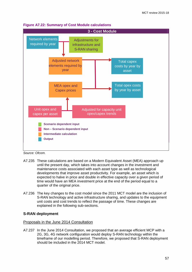
MCT review 2015-18

Figure A7.22: Summary of Cost Module calculations

Source: Ofcom.

A7.235 These calculations are based on a Modern Equivalent Asset (MEA) approach up until the present day, which takes into account changes in the investment and maintenance costs associated with each asset type as well as technological developments that improve asset productivity. For example, an asset which is expected to halve in price and double in effective capacity over a given period of time would have an MEA investment price at the end of the period equal to a quarter of the original price.

A7.236 The key changes to the cost model since the 2011 MCT model are the inclusion of S-RAN technology and active infrastructure sharing, and updates to the equipment unit costs and cost trends to reflect the passage of time. These changes are explained in the following sub-sections.

S-RAN deployment

Proposals in the June 2014 Consultation

A7.237 In the June 2014 Consultation, we proposed that an average efficient MCP with a 2G, 3G, 4G network configuration would deploy S-RAN technology within the timeframe of our modelling period. Therefore, we proposed that S-RAN deployment should be included in the 2014 MCT model.

3 - Cost Module

Scenario dependent input Non – Scenario dependent input Intermediate calculation Output

Unit opex and capex p er asset

Adjusted for capacity unit opex/capex trends

Adjusted network elements required by

year

MEA opex and Ca pex prices

Network elements required by year

Total capex costs by year by

asset

Adjustments for infrastructure and S - RAN sharing

Total opex costs by year by asset

57

MCT review 2015-18

A7.238 We captured the impact of S-RAN deployment by making adjustments to the cost trends of individual 2G, 3G and 4G base station assets and the costs allocated to these network elements. We assumed that S-RAN would become available for use in 2013/14 and that the existing radio equipment is completely replaced with S-RAN equipment over three years.

A7.239 In the base case of the 2014 MCT model, we assumed that all network technologies will be upgraded to use a combined 2G+3G+4G S-RAN i.e. other combinations of S-RAN (e.g. 3G+4G only) are not modelled.

Responses to the June 2014 Consultation

A7.240 BT agreed that the modelling approach should take account of the use of S-RAN technologies since this is how MCPs are now building their networks.98 However, it considered that the approach used to model S-RAN technologies in the 2014 MCT model, was an oversimplification which led costs to be overstated. BT argued that: 99

• The model distributes costs between 2G, 3G and 4G technologies with no attribution to traffic levels.

• The model assumes that when the network is dominated by 4G equipment carrying 4G traffic, a cost premium remains associated with the 2G equipment.

• Capex costs are being allocated to a technology where no traffic is being carried over it.

• Since the method of allocating costs is based on an assumption about the relative cost of different single technologies (i.e. 2G, 3G and 4G) this puts a price premium on 4G, even when the sites are 4G only, and long after 2G and 3G traffic has fallen away.

A7.241 BT considered that in this aspect, the model is generating unrealistic results and that, as stated in its response to Ofcom’s January 2014 stakeholder workshop, the appropriate way to take account of S-RAN equipment is to model its deployment explicitly in the Network module of the model.

A7.242 BT argued that if we chose to retain the approach taken in the 2014 MCT model the unit costs of equipment over their lifetimes would need to be revisited. For example, an S-RAN unit could be deployed as a 2G replacement with 4G capability and would command a cost premium compared to a 2G only or 4G only device (due to its capacity and associated licence fees). However, over time the S-RAN unit will be increasingly devoted to 4G traffic with processor load being diverted to 4G features and 2G eventually being withdrawn. At this point, the cost of the unit would be expected to be the same as a 4G only unit (i.e. it is not appropriate for a 4G cost premium to be applied in perpetuity).

98 BT response to June 2014 Consultation, page 9 http://stakeholders.ofcom.org.uk/binaries/consultations/mobile-call-termination-14/responses/BT.pdf 99 BT response to June 2014 Consultation, pages 24 – 25.

58

MCT review 2015-18

A7.243 H3G noted that the S-RAN unit cost profiling adjustment in the 2014 MCT model assumed a share of radio traffic for 3G which was based on 3G HSPA traffic only, rather than all 3G traffic. H3G identified this as an apparent coding error.100

A7.244 H3G also considered that the S-RAN unit cost profiling adjustment used in the 2014 MCT model appeared to result in some unintended and perverse consequences. To illustrate this point, H3G considered the impact of the profiling adjustment on the LRIC of 4G equipment. It noted that the profiling adjustment has the effect of making the assumed unit cost of 4G RAN equipment dependent upon 4G’s share of total radio traffic. However, 4G’s share of total radio traffic is lower in the “with incoming” scenario (i.e. when MCT traffic is included), than in the “no incoming” scenario (i.e. when MCT traffic is excluded). As a result, 4G RAN unit costs are lower in the “with incoming” scenario. The outcome is that total 4G RAN costs fall as the MCT increment gets added.101

A7.245 H3G noted that, although it could be argued that the change in assumed 4G unit costs should not be considered in the context of the 4G network alone, such an argument was not consistent with the fact that the ED calculations reflect the impact of the change on 4G voice termination alone.

A7.246 H3G considered that the fundamental cause of the problem is that:

7.246.1 One part of the model, that determines unit costs, assumes that RAN equipment is shared across technologies.

7.246.2 Another part of the model, which assumes the “with incoming” and “no incoming” scenarios in order to generate LRIC, assumes that each technology uses RAN equipment that is not shared across technologies.

A7.247 H3G explained that one solution would be to create new asset categories for S-RAN equipment, and treat it like other modelled assets that are shared across technologies (e.g. backhaul). It noted that we explained in the June 2014 Consultation that this was not adopted due to the significant effort involved. Therefore, pending a reconsideration of this, H3G suggested that another option would be to deactivate the assumed deployment of S-RAN altogether.

Ofcom’s analysis of responses and conclusions

A7.248 The detailed comments received from BT and H3G in relation to S-RAN modelling are addressed by Analysys Mason in Annex 8. We agree with Analysys Mason’s conclusions on these issues and with the changes it has implemented relative to the calculations in the 2014 MCT model.

Infrastructure sharing

Proposals in the June 2014 Consultation

A7.249 Sharing of passive infrastructure between operators was included in the 2011 MCT model, and in the June 2014 Consultation we proposed to also include active infrastructure sharing in the 2014 MCT model.

100 H3G response to June 2014 Consultation, Annex A page 2 http://stakeholders.ofcom.org.uk/binaries/consultations/mobile-call-termination-14/responses/H3G.pdf. 101 H3G response to June 2014 Consultation, Annex A pages 2 to 3.

59

MCT review 2015-18

A7.250 The calculations to implement infrastructure sharing were found in both the cost module and network module. At a high level, our approach increased the traffic on the modelled network to include that from a second operator sharing the infrastructure. However, we then identified only those costs that the modelled operator would pay for its own traffic, and then recovered those costs over the modelled operator’s own traffic using the existing routing factor table.

Responses to the June 2014 Consultation

A7.251 BT considered that the model should be amended to assume a greater level of network sharing to reflect reality.102 It noted that the 2014 MCT model restricted network sharing to areas outside the Urban and Suburban 1 geotypes and that in the baseline 2014 MCT model, in 2015/16, this assumption implied that 55% of macrocells were not eligible for network sharing. Given the recent announcements made by MCPs about the benefits of network sharing to their overall cost bases, BT considered that the level of exclusion of network sharing in the 2014 MCT model was not credible, and that the geotypes should be redefined or sharing allowed in the Urban and Suburban 1 geotypes to account for this.

A7.252 H3G observed that the cost trend profiles in the calculations in the 2014 MCT model with and without MCT are different, and suggested that the implication that unit costs are different in these two cases is not realistic.103

Ofcom’s analysis of responses and conclusions

A7.253 The responses we received in relation to infrastructure sharing are addressed in detail by Analysys Mason in Annex 8. We agree with Analysys Mason’s conclusions on these issues and with the changes it has implemented relative to the calculations in the 2014 MCT model.

A7.254 In relation to BT’s concerns we have reviewed the most recent evidence obtained from the four largest MCPs in response to information requests and we have concluded that some active infrastructure sharing should be assumed in the Suburban 1 geotype. The available evidence indicates that an assumption of 25% active infrastructure sharing in the Suburban 1 geotype is appropriate and has been implemented in the 2015 MCT model.

A7.255 Turning to H3G’s concern about unit costs profiles, Analysys Mason has implemented a fix in the 2015 MCT model so that this anomaly no longer arises.

Equipment unit costs and cost trends

Proposals in the June 2014 Consultation

A7.256 The 2014 MCT model contained equipment unit costs and equipment unit cost trends based on MCP data and benchmark models, with trends prior to 2010/11 left unchanged with the exception of changes to assumed equipment capacities.104

102 BT response to June 2014 Consultation, page 24. 103 H3G response to June 2014 Consultation, page 16. 104 See Analysys Mason, MCT review 2015-2018: Mobile network cost modelling proposals for model, 4 June 2014, Section 4.3. http://stakeholders.ofcom.org.uk/binaries/consultations/mobile-call-termination-14/annexes/analysys-mason-Report_for_Ofcom.pdf.

60

MCT review 2015-18

Responses to the June 2014 Consultation

A7.257 BT observed that a number of cost trends ‘are simply assumed to track inflation’, and argued that ‘it is inadequate to assume zero or near zero real terms price trends (or, in other words increases in nominal prices) in a world where a significant proportion of the cost base relates to electronic equipment which tends to become cheaper in real terms over time. We consider operating cost trends should also reflect potential efficiency gains’.105

A7.258 BT noted that the modelling in the 2013 FNMR assumed cost trends for electronic equipment that declined ‘between 3% and 5% per annum in real terms’, and argued that Ofcom should incorporate equivalent price declines ‘each year up until 2026/27 to ensure a consistent approach is adopted with the Fixed Termination Rate model’.

A7.259 H3G noted an apparent inconsistency in the referencing of capital costs that flow from the Cost module into the Economic module.106

Ofcom’s analysis of responses and conclusions

A7.260 As Analysys Mason explains in Annex 8, the capex trends in the 2014 MCT model were based on information gathered from the four largest MCPs under our statutory powers. However, little information was received in relation to opex trends, and Analysys Mason has extended the opex trends in the 2015 MCT model as explained in Annex 8. We agree that this modification is appropriate and consider that it addresses BT’s concerns. As noted in paragraph A7.13 we do not include an explicit efficiency parameter in our bottom-up models.

Economic module

A7.261 Once the yearly capex and opex of the average efficient MCP have been calculated in the cost module of the model, we must determine how these costs are recovered over time. This is done in the Economic module.

A7.262 The Economic module implements economic depreciation to calculate a cost per unit of output, in each year, for every asset in the model. An overview of the calculation flow in the economic module is shown in Figure A7.23 below. This is unchanged from the 2014 MCT model.

105 BT response to June 2014 Consultation, paragraphs 2.2.18-2.2.19. 106 H3G response to June 2014 Consultation, page 14.

61

MCT review 2015-18

Figure A7.23: Summary of Economic Module calculations

Source: Ofcom.

Use of economic depreciation

Proposals in the June 2014 Consultation

A7.263 In the June 2014 Consultation we proposed to use the form of economic depreciation known as Original Economic Depreciation (Original ED), consistent with our previous MCT models since 2005 (including the 2011 MCT model). 107

Ofcom’s conclusions on the use of economic depreciation

A7.264 We received no responses to the June 2014 Consultation specifically relating to the use of economic depreciation, and we have decided to adopt this approach instead of accounting approaches to depreciation, because we consider that it better reflects the forward looking economic value of an asset and hence better mimics the outcome of a competitive market. Furthermore, using economic depreciation is

107 Economic depreciation was also used by Oftel in 2001 in relation to its Review of the Charge Control on calls to mobile, See Oftel, Review of the charge control on calls to mobiles, A Statement issued by the Director General of Telecommunications on competition in mobile voice call termination and consultation on proposals for a charge control, 26 September 2001, http://www.ofcom.org.uk/static/archive/oftel/publications/mobile/ctm0901.pdf and Oftel, Economic depreciation in the Long Run Incremental Cost Model, 2001, http://www.ofcom.org.uk/static/archive/oftel/publications/mobile/depr0901.htm.

4 - Economic Module

Scenario dependent input Non – Scenario dependent input Intermediate calculation Output

Allocation of non network costs

(LRIC+)

Cost per network element

Allocation of costs due to location

updates (LRIC+)

Capex / Opex

Cost per service

Output by network element

Economic depreciation

al g orithm Routing factors for converting

network element unit costs to service units

costs

62

MCT review 2015-18

consistent with the 2009 EC Recommendation which states that “the recommended approach for asset depreciation is economic depreciation wherever feasible.”108

A7.265 We consider Original ED to be a better depreciation approach to other forms of economic depreciation because it better mimics the outcomes that would be seen in a competitive market. We note that the Original ED approach to economic depreciation has been supported by the CC each time it has been appealed, most recently in the 2012 CC Determination.

A7.266 Economic depreciation matches the cost of equipment to its actual and forecast use over the long-term. Consequently, there is relatively little depreciation in years when utilisation is low and relatively high depreciation in years of full, or almost full, equipment utilisation.

A7.267 An alternative way to characterise economic depreciation is as a cash flow analysis to answer the question: what time series of prices, consistent with trends in the underlying costs of production and given forecast traffic, yield an expected present value equal to the capital and operating cash flows from building and running the network?

A7.268 In order to answer this question, the economic module performs the following calculation in three stages:

• Stage 1: A constant unit cost is calculated as if the final year utilisation and input costs applied over the entire lifetime of the network.

• Stage 2: A second component is added to recover the additional costs caused by earlier under-utilisation of the network compared to the final year level.109 This step is also applied as a constant unit price for all years.

• Stage 3: A third component is added to recover the remaining unrecovered (or over-recovered) costs due to input costs in earlier years, including the WACC, being above (or below) the final year level. The shape of this component is determined by the arithmetic difference between the in-year and final-year input costs,110 and is therefore zero in the final year (or any year that shares the same level of input costs and WACC as the final year). More costs are recovered in years when asset prices and the WACC are higher than the final year.

Implementation of economic depreciation

Proposals in the June 2014 Consultation

A7.269 The Original ED algorithm used in the 2011 MCT model included a ‘fix’ that prevented unit costs for network elements from being negative. The ‘fix’ was applied through an iterative element to the final stage of the ED algorithm that shifted the cost profile weighting factor upwards until no unit costs for the output of that element were negative. We introduced this ‘fix’ because although negative unit

108 2009 EC Recommendation, point 7. 109 If utilisation is falling over time then this could be a negative value. 110 The ‘input costs’ for a particular year are the asset price (or operating cost) for that given year and the WACC. The arithmetic difference between in-year and final year input costs is given by: (Asset pricet x WACCt) – (Asset pricen x WACCn). Where (t) is the current year and (n) is the final year.

63

MCT review 2015-18

costs can be a legitimate output of the economic depreciation calculations given certain inputs, it was considered to be counter-intuitive.

A7.270 However, in the 2012 CC Determination111 the CC indicated that the ‘fix’ was unnecessary. Therefore we proposed in the June 2014 Consultation to disable the ‘fix’.

A7.271 The cost trends used in the Economic module of the 2014 MCT model excluded the impacts of the redistribution of S-RAN costs amongst the 2G, 3G and 4G assets. The reason for this was that the approach reflected a modelling simplification to capture the efficiencies associated with equipment sharing between MCPs rather than changes in the replacement costs of individual pieces of network equipment. We therefore believed the changes caused by the S-RAN implementation should not be used in determining the optimal path of cost recovery.

A7.272 As set out in Figure A7.23, the ED algorithm allows us to calculate the yearly unit cost for each network element. The network element unit cost was then multiplied by the routing factors which thereby converts the network element unit costs to the service unit costs i.e. the cost of MCT per minute.112

Responses to the June 2014 Consultation

A7.273 As noted above, H3G commented on the implementation of S-RAN and the implications of this for the inputs to the Economic module. These comments are addressed in Annex 12 and paragraph A7.248 above.

A7.274 Vodafone raised a concern with the outputs of the ED calculations in relation to negative cash flows in a given year. It urged greater scrutiny of these negative assets, which it noted were more numerous than in the 2011 MCT model, in order to ensure that they are all reasonable.113

A7.275 Vodafone also noted that the so-called ‘year 0 adjustment’ had not been implemented in the model. This adjustment had been suggested by Vodafone as part of the appeal of the 2011 MCT model, and would have the effect of avoiding situations in which ‘the LRIC version of the model builds equipment and then removes it in the year immediately following’.114

Ofcom’s analysis of responses and conclusions

A7.276 In relation to Vodafone’s observation about negative cashflows, we believe that negative cashflow can relate to two different issues. Negative cashflow can either refer to negative network element unit cost outputs (i.e. the unit cost recovery for each unit of output is negative rather than positive as we would expect), or negative

111 See paragraphs 3.502-3.503 of the 2012 CC Determination, http://www.catribunal.org.uk/files/1.1180-83_MCT_Determination_Excised_090212.pdf. 112 We have made two refinements to the Economic module in order to ensure consistent cost recovery when calculating LRIC. The first ensures that the costs of switch sites that are incremental to MCT are allocated solely to MCT (rather than allocated between voice and data traffic as they are under LRIC+). The second allocates costs using service volumes and routing factors rather than decremental element output (meaning the difference between element output with and without the termination increment). 113 Vodafone response to June 2014 Consultation, page 79. 114 Vodafone response to June 2014 Consultation, page 79 and footnote 71.

64

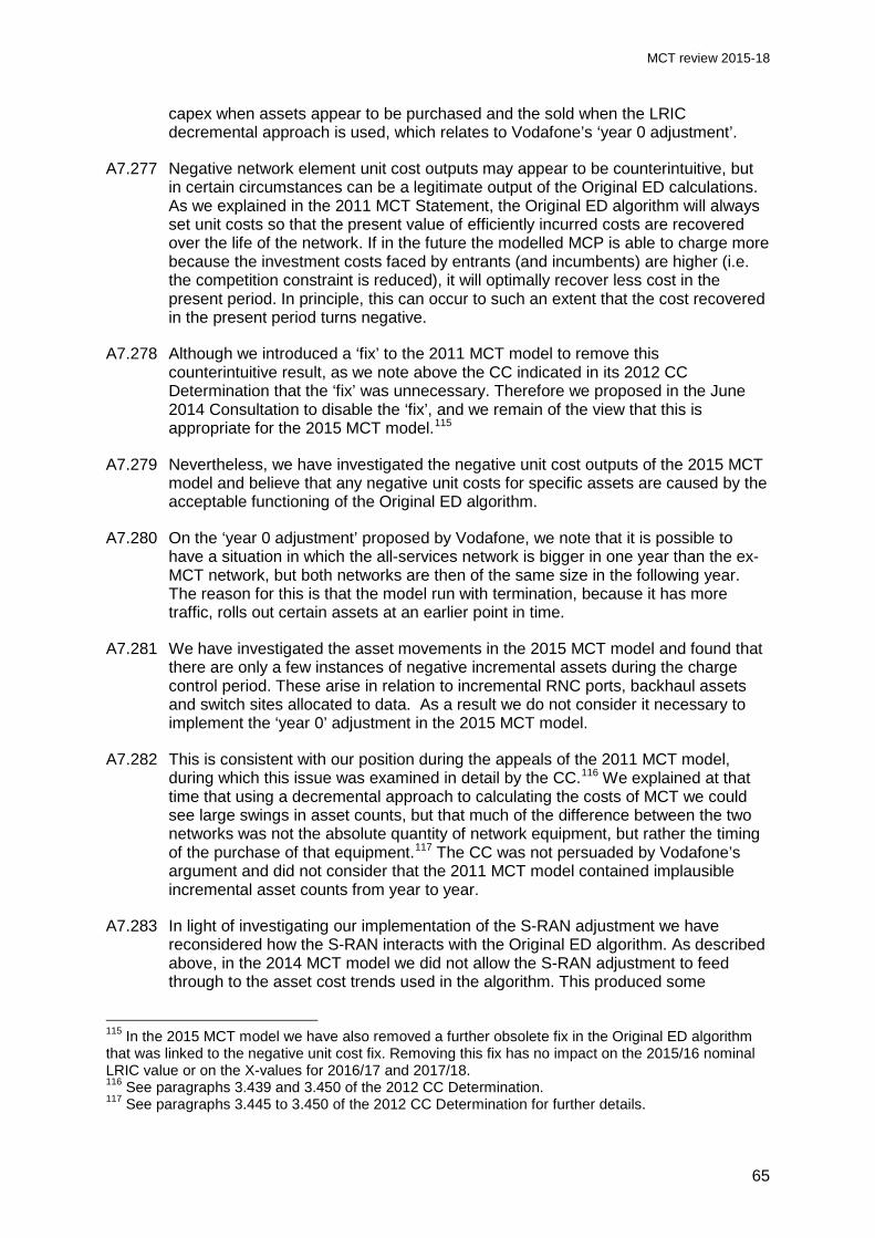
MCT review 2015-18

capex when assets appear to be purchased and the sold when the LRIC decremental approach is used, which relates to Vodafone’s ‘year 0 adjustment’.

A7.277 Negative network element unit cost outputs may appear to be counterintuitive, but in certain circumstances can be a legitimate output of the Original ED calculations. As we explained in the 2011 MCT Statement, the Original ED algorithm will always set unit costs so that the present value of efficiently incurred costs are recovered over the life of the network. If in the future the modelled MCP is able to charge more because the investment costs faced by entrants (and incumbents) are higher (i.e. the competition constraint is reduced), it will optimally recover less cost in the present period. In principle, this can occur to such an extent that the cost recovered in the present period turns negative.

A7.278 Although we introduced a ‘fix’ to the 2011 MCT model to remove this counterintuitive result, as we note above the CC indicated in its 2012 CC Determination that the ‘fix’ was unnecessary. Therefore we proposed in the June 2014 Consultation to disable the ‘fix’, and we remain of the view that this is appropriate for the 2015 MCT model.115

A7.279 Nevertheless, we have investigated the negative unit cost outputs of the 2015 MCT model and believe that any negative unit costs for specific assets are caused by the acceptable functioning of the Original ED algorithm.

A7.280 On the ‘year 0 adjustment’ proposed by Vodafone, we note that it is possible to have a situation in which the all-services network is bigger in one year than the ex-MCT network, but both networks are then of the same size in the following year. The reason for this is that the model run with termination, because it has more traffic, rolls out certain assets at an earlier point in time.

A7.281 We have investigated the asset movements in the 2015 MCT model and found that there are only a few instances of negative incremental assets during the charge control period. These arise in relation to incremental RNC ports, backhaul assets and switch sites allocated to data. As a result we do not consider it necessary to implement the ‘year 0’ adjustment in the 2015 MCT model.

A7.282 This is consistent with our position during the appeals of the 2011 MCT model, during which this issue was examined in detail by the CC.116 We explained at that time that using a decremental approach to calculating the costs of MCT we could see large swings in asset counts, but that much of the difference between the two networks was not the absolute quantity of network equipment, but rather the timing of the purchase of that equipment.117 The CC was not persuaded by Vodafone’s argument and did not consider that the 2011 MCT model contained implausible incremental asset counts from year to year.

A7.283 In light of investigating our implementation of the S-RAN adjustment we have reconsidered how the S-RAN interacts with the Original ED algorithm. As described above, in the 2014 MCT model we did not allow the S-RAN adjustment to feed through to the asset cost trends used in the algorithm. This produced some

115 In the 2015 MCT model we have also removed a further obsolete fix in the Original ED algorithm that was linked to the negative unit cost fix. Removing this fix has no impact on the 2015/16 nominal LRIC value or on the X-values for 2016/17 and 2017/18. 116 See paragraphs 3.439 and 3.450 of the 2012 CC Determination. 117 See paragraphs 3.445 to 3.450 of the 2012 CC Determination for further details.

65

MCT review 2015-18

inconsistencies between the way the algorithm recovered costs over time and the way costs were being incurred.

A7.284 In the 2014 MCT model, we did not believe it was appropriate to use the S-RAN adjusted cost trends in the Original ED algorithm because they did not reflect a true change in the asset cost trends. On reflection, we now believe it is appropriate to include the S-RAN adjusted asset costs in the Original ED algorithm. The Original ED algorithm is trying to mimic a competitive market. Once S-RAN is implemented, the competitive constraint on cost recovery comes from an MCP with a network using S-RAN. Therefore, the Original ED algorithm should adjust the cost recovery profile to account for the lower costs faced by a network using S-RAN (i.e. recover less cost once S-RAN is implemented). We have therefore adjusted the inputs to the Original ED algorithm to include the S-RAN adjustment.

66

MCT review 2015-18

Annex 8

8 Analysys Mason report This report is published separately

67

MCT review 2015-18

Annex 9

9 Calibration of the 2015 MCT model Introduction

A9.1 Cost models can be constructed in both ‘top-down’ and ‘bottom-up’ forms. In a bottom-up approach (as described in Annex 7), the network components are modelled at a disaggregated level based on forecast service traffic volumes. The costs of these network components are then allocated to services.

A9.2 In this market review, as in previous market reviews, we are using a hybrid modelling approach as described in the 2009 EC Recommendation.118 This method aims to capture the strengths of both top-down and bottom-up approaches. The 2015 MCT model has been developed as a bottom-up cost model with a view to establishing the unit cost benchmarks for MCT of an average efficient MCP, rather than MCP-specific unit cost benchmarks. It has then been calibrated by adjusting certain model parameters to ensure the model is reasonably in line with the asset quantities and actual costs of the 2G/3G/4G national MCPs (i.e. excluding H3G) in recent years.

A9.3 We consider that calibrating the 2015 MCT model using data from the 2G/3G/4G national MCPs is an important part of the modelling process. Although MCT is effectively a monopoly service, the four national MCPs do have incentives to be cost efficient in order to compete in the provision of access and origination services, which use many of the same assets as MCT. Because MCT assets are shared with services provided in competitive markets, we do not have reason to believe that the national MCPs would be operating inefficiently. This is in contrast to modelling a monopoly provider where much or most of its cost stack is not supporting services provided in competitive markets, and hence calibration may be of less use if we are seeking to model an efficient operator.

A9.4 This annex describes the method which has been used to calibrate the 2015 MCT model based on assets counts and accounting data, and summarises the results of the calibration (to the extent that this is possible while maintaining the confidentiality of the data provided by the four largest MCPs).

A9.5 This annex is structured as follows:

• Approach to calibration

• Asset count calibration results

• Cost calibration results

A9.6 All of the results for an average efficient 2G/3G/4G MCP presented in Section 7 and Annex 12 take into account the calibration of the model against operator data.

118 See point 3 and recital 9 of the 2009 EC Recommendation.

68

MCT review 2015-18

Approach to calibration

Proposals in June 2014 Consultation

A9.7 In the June 2014 Consultation we proposed to use evidence obtained in relation to asset counts, gross book value (GBV119) and network operating costs as the primary metrics for our calibration exercise, and to use net book value (NBV120) only as a cross-check.

A9.8 The calibration data collected from the MCPs are historical, and relate to a period before some of the latest technological developments included in the 2014 MCT model were actually implemented. In particular, S-RAN assets were introduced as recently as 2013 and hence the effects of their deployment were not fully reflected in the calibration data for the 2014 MCT model, which covered the period to Q3 2013. As a result we undertook our calibration exercise excluding S-RAN deployment.

A9.9 We explained in the June 2014 Consultation that we had encountered some difficulty with the calibration using accounting cost information because of material step changes between the GBV data provided for the 2011 MCT model and the data gathered in response to our information requests for the 2014 MCT model. We described the process we had followed in order to try to understand the reasons for the discrepancies but explained that [] were unable to provide a detailed and comprehensive explanation of the discrepancies. We found the same situation for operating costs for [].

A9.10 In order to overcome these problems it was necessary for us to adopt an alternative approach, and we explained that we had extrapolated the GBV from 2010 onwards and used this extrapolated GBV instead of the data provided in response to our information request from []. We similarly extrapolated operating costs for [].

A9.11 We considered this approach to be reasonable given the inconsistencies that we had found and in the absence of a compelling explanation for the lack of reconciliation to the data used in the 2011 MCT model. We also explained that we would be seeking further information on this issue prior to publication of the statement.

Responses to June 2014 Consultation

A9.12 Vodafone noted that as part of our model development we had sought information from the four national MCPs on customer numbers, traffic volumes and financial data. It recognised that it is necessary to be able to build a picture of the average efficient MCP in terms of traffic volumes and for financial calibration.121

A9.13 However, Vodafone considered that there are difficulties in how we take the MCP data and use it to develop a view of the past and future of the average efficient MCP. This is because the observed average of the four national MCPs may be different from the modelled average efficient MCP for sound reasons. It nevertheless argued that given much of the data that Ofcom receives is confidential

119 The GBV of an asset is the historical price paid for it, with no deductions for depreciation. 120 The NBV of an asset is the historical price paid for it, net of any accumulated depreciation. 121 Vodafone response to June 2014 Consultation, pages 53-54.

69

MCT review 2015-18

it is difficult from an individual stakeholder’s viewpoint to assess what Ofcom has done.

A9.14 Vodafone raised the following issues in relation to our assessment of the average efficient MCP:

• Given that H3G does not run a 2G network, Vodafone queried whether we had excluded its traffic from our calculations of the historic mix of 2G and 3G of voice traffic. It argued that the average traffic mix is likely to be visibly different depending on whether H3G is included or not.

• The formation of EE uniquely gave it sufficient spectrum in a suitable band to build and launch a 4G network in advance of all other MCPs. In light of this, Vodafone considered that EE’s 4G network deployment, 4G customer growth, 4G data growth, 4G VoLTE and movement from 3G data to 4G data should not be used in deriving the average efficient MCP’s experience, at least in the early years of 4G, up to 2017/18 (by which stage, the other MCPs might be assumed to have had sufficient opportunity to catch-up).

Ofcom’s analysis and conclusions

A9.15 The details of Vodafone’s points relating to the modelled average efficient MCP’s traffic and 4G network deployment are addressed in Annex 7, and we continue to consider that our approach to modelling an average efficient MCP is reasonable and uses the information we have received appropriately.

High level approach

A9.16 We did not receive any comments relating to our high level approach to calibration or our focus on GBV and operating costs in response to the June 2014 Consultation. Our overall approach to calibrating the 2015 MCT model is unchanged from that used in the 2014 MCT model. However, as anticipated in the June 2014 Consultation we have sought further information on the GBV and operating cost data submitted in response to our information requests, and have gained some further clarity on this.

A9.17 For financial calibration we consider that GBV is a more appropriate calibration benchmark than in-year capital expenditure or the NBV. Although we recognise that NBV could act as a cross-check for calibration purposes, we consider that the usefulness of NBV information is limited given that it is sensitive to the differences and changes to the depreciation approaches used by 2G/3G/4G MCPs (and is more sensitive than GBV to fluctuations in capex in each year). We have found that these concerns are borne out in the data submitted to us by the MCPs.

A9.18 We consider that network operating costs are likely to fluctuate less than capital costs on a year-to-year basis as these represent the costs of on-going network operation. Although we recognise that there are still likely to be year-on-year fluctuations in these cost benchmarks which are not explainable solely by the parameters and network dimensioning rules within the 2015 MCT model, we consider that network operating costs are useful for calibration purposes.

A9.19 We have therefore decided that it is appropriate to use the evidence obtained in relation to asset counts, GBV and network operating costs as the primary metrics for the calibration of the 2015 MCT model. This is consistent with our approach in the June 2014 Consultation.

70

MCT review 2015-18

A9.20 S-RAN is introduced in 2013/14 in the 2015 MCT model. As in the 2014 MCT model, the effects of S-RAN deployment will not be fully reflected in the calibration data which cover the period to Q2 2014.122 Therefore, and in accordance with our approach in the June 2014 Consultation, we have undertaken calibration of the MCT Model excluding S-RAN deployment.123

Data collection process

A9.21 Data to inform calibration of the model formed an important part of our information requests to the four largest MCPs using our powers under section 135 of the Communications Act 2003.

A9.22 Since our June 2014 Consultation we have requested additional equipment inventories from MCPs for the period Q4 2013 to Q2 2014. In relation to accounting cost data, to inform the 2014 MCT model we requested information from each of the four largest MCPs for network GBV, NBV and network operating costs for the period 2009/10 to 2013/14. 2013/14 remains the most recent full year of data available so we have not gathered or used further data.

A9.23 For network equipment counts it remains the case that none of the four largest MCPs was able to provide us with all of the information at the level of disaggregation requested. However, in relation to particularly significant asset types, such as site counts, all four of the national MCPs provided useful information. Where information requested has not been provided we have estimated asset counts where necessary, given the evidence available to us.

A9.24 As we found in the June 2014 Consultation, the process of calibration using accounting cost information is more challenging than for asset counts. This is partly because comparing accounting information to the intermediate outputs of the model is complicated by different classifications and definitions of types of costs, both between the individual MCPs and between the MCPs and the 2015 MCT model. We have also been unable to fully resolve the issues we found in the June 2014 Consultation in relation to consistency of the data provided by the MCPs with that used in the 2011 MCT model, despite having sought further clarifications from each of the largest MCPs. This is explained below.

A9.25 In relation to [] we continue to find a very significant downward step change between the GBV information provided in response to the 2011 MCT review and the 2015 MCT review. We sought explanation of this and [].

A9.26 For the purposes of calibrating the 2015 MCT model we do not consider that the data provided by [] appropriately reflects the underlying GBV. As a result we found it necessary to adopt an alternative approach. We use [] provided as part of the 2011 MCT review and extrapolate this based on the absolute change in the GBV figures provided for the period 2010 to 2013.124 We have then applied these changes to the corresponding GBV levels from the final year of calibration data from the 2011 MCT Model (i.e. from 2009) to provide an extrapolated set of GBV figures

122 S-RAN deployment is explained in Annex 8, Section 2.4.1. 123 This is scenario 45 in the 2015 MCT model. We note that the implementation of S-RAN in the 2015 MCT model (as explained in Annex 8) means that its deactivation in the calibration scenario only affects the financial and not the asset count calibration. 124 Since the new series begins in 2010 it was not possible to calculate the absolute change between 2009 and 2010, so we derive both the 2010 and 2011 values using the observed change between 2010 and 2011.

71

MCT review 2015-18

for the years 2010 to 2013. The extrapolated GBV series has then been used in the calibration of the 2015 MCT Model instead of the GBV data provided in response to our information request by [].

A9.27 Turning to [] we continue to find a significant reduction in GBV between 2010 and 2011.125 We sought explanation of this which revealed that this was due to [] We have considered extrapolating the GBV data from the 2011 MCT Model for [] as we did for the 2014 MCT Model. However, after further consideration of the issue, it is not clear to us that this would more appropriately reflect the GBV of the relevant assets and instead we have reflected our concerns by placing less weight on [] GBV data as part of our calibration of the 2015 MCT Model. This is explained further in paragraph A9.64 below.

A9.28 In relation to the information provided by [] we noted a significant reduction in its GBV between 2011 and 2012. We sought explanation for this and understand that []. Therefore, for our calibration exercise, we have [].126

A9.29 For operating costs [] was unable to provide operating cost data for 2010, requiring us to interpolate this figure using its 2009 and 2011 data.

A9.30 Finally, [] confirmed that it was not able to provide us with an opex figure for 2013. Since this is the last year used for the financial calibration, interpolation wasn’t possible, so we estimated this MCP’s 2013 opex using the average growth rate observed over the prior five years of actual opex.

Model inputs adjusted as part of the calibration

A9.31 To calibrate the 2015 MCT model we have adjusted certain bottom-up input parameters to achieve asset counts and costs (GBV and network operating costs) consistent with the top-down information obtained from the 2G/3G/4G MCPs, while constraining the bottom-up parameters to remain within the range of available bottom-up information from each of the four largest MCPs.

A9.32 Where the same input parameters are used in both the 2011 MCT model and the 2015 MCT model, our starting point for these inputs is the values in the 2011 MCT model. Some of these parameters have subsequently been adjusted to take account of bottom-up evidence provided by the four national MCPs.

A9.33 We have then adjusted the following model input parameters such that high-level asset counts and cost outputs (specifically GBV and network operating costs) for the modelled average efficient MCP are in line with the top-down evidence that we have collected:

i) Parameters adjusted for the asset count and financial calibration:

• unit capacities of network elements;

• minimum and maximum asset deployments;

• cell coverage radii;

125 We were satisfied that the operating cost data provided by [] did not show such a discrepancy. 126 []

72

MCT review 2015-18

• asset utilisation factors;

• the proportion of cell sites which are shared between 2G, 3G and 4G networks;

• NodeB processing parameters;

• the percentage of traffic in the busy hour; and

• GPRS data rate.

ii) Parameters adjusted for the financial calibration only (GBV and opex):

• MEA investment costs per unit of equipment over time; and

• MEA operating costs per unit of equipment over time.

Results of the 2015 MCT model calibration

A9.34 There have been considerable changes in the mobile industry over the calibration period. As a result, we recognise that some data provided by MCPs may not represent a network under normal conditions.

A9.35 For instance, reconciliation of network assets after two networks merge can cause top-down accounting costs to appear anomalous. Specifically, we observe that []. We would not wish to inadvertently capture this effect in our calibration.

A9.36 Similarly we recognise that the asset counts and network costs evident in the MCP data will depend, in part, on the MCPs’ market shares. We have taken this into account when considering the calibration of the 2015 MCT model.

A9.37 We consider the model well calibrated if the model results fall with the minimum and maximum values provided by the MCPs and follow a similar trend to the MCP data. We also consider how well the model outputs match the average of the MCP data.

Asset count calibration

A9.38 The general principle we applied in the 2015 MCT model was that the count of the most important assets (e.g. cell sites) should be reasonably close to the average count of the 2G/3G/4G MCPs,127 and always between the minimum and maximum values seen across all four largest MCPs.

A9.39 Table A9.1 shows the counts of key network equipment in the model compared to the average MCP benchmark after completing the calibration of the 2015 MCT model. This is shown on a randomised basis for the 2G/3G/4G MCPs. Each asset count average from the 2G/3G/4G MCPs has been randomised by +/- 10% in order to maintain the confidentiality of the section 135 responses.

127 Note that although we have used data from the 2G/3G/4G MCPs, the 2015 MCT model only includes 4G services from Q3 2013/14. As a result no 4G assets are included in the asset count calibration.

73

MCT review 2015-18

Table A9.1: Comparison of asset count of key network equipment between model output and 2G/3G/4G randomised MCP data in 2013/14

Asset type 2G/3G/4G MCP average

2G/3G/4G randomised

MCP average 2015 MCT

Model

% difference between

2015 MCT model (post calibration) and average

MCP data

2G macrocell equipment [] 10,676 9,742 []

2G micro and picocell equipment [] 2,796 2,351 []

3G macrocell equipment [] 10,962 11,851 []

3G micro and picocell equipment [] 1,729 1,135 []

Total macro sites [] 13,758 13,655 []

Total micro and pico sites [] 3,054 3,197 []

TRXs [] 94,147 108,258 []

BSCs [] 297 136 []

3G carriers [] 70,824 71,392 []

RNCs [] 125 117 []

2G/3G MSC server [] 27 21 []

2G/3G MGW [] 45 29 []

SMSC [] 8 3 []

HLR [] 14 9 []

SGSN [] 7 8 []

GGSN [] 7 8 [] Source: Ofcom analysis of section 135 responses and 2014 MCT model. A9.40 It is notable that the results in Table A9.1 show that the 2015 MCT model includes

less 2G macrocell, 2G micro and picocell, and 3G micro and picocell equipment than the average of the MCPs’ data. We have investigated this and found that it is driven by the fact that []. Comparison to the top-down data provided by the other MCPs shows that [] and we would not want to inadvertently capture this in our calibration. As a result, we consider the calibration of 2G and 3G cell equipment quantities to be reasonable.

A9.41 TRXs and 3G carrier numbers appear to be somewhat overstated in the 2015 MCT model, according to the data in Table A9.1. In these cases we note that the MCP

74

MCT review 2015-18

average reported in Table A9.1 2013/14 [].128 [] Bearing this in mind, we consider that the calibration of TRXs and 3G carriers in the 2015 MCT model is appropriate.

A9.42 For the reamining core network assets in Table A9.1, comparison of the average asset counts from MCPs and the outputs of the 2015 MCT model is less meaningful. The asset information provided by the MCPs shows wide variation in quantities, and the numbers from the 2015 MCT model are affected by the fact that the model uses assets with fixed capacities over time.. As a result, we have not placed as much emphasis on the calibration of core network assets as that on RAN assets and, in any case, these core network assets make a smaller contribution to network costs than the other assets shown in Table A9.1.

A9.43 In addition to Table A9.1 Table A9.the figures below compare the 2G/3G/4G MCP data and randomised averages for key assets against the outputs of the 2015 MCT model over the period 2011/12 to 2014/15. As above, where randomised results are shown these include a randomisation factor of +/-10% in order to maintain confidentially.

A9.44 Figure A9.1 shows a comparison of total 2G cell equipment in the 2015 MCT model against the 2G/3G/4G MCP data for Q1 in the years 2011/12 to 2014/15.

Figure A9.1: Comparison of total 2G cell equipment between the 2015 MCT model output and 2G/3G/4G MCP data [] Source: Ofcom analysis of section 135 responses and 2015 MCT model. A9.45 It is evident in Figure A9.1 that while the asset counts in the 2015 MCT model are at

all times during the calibration period within the range of the MCP data, they lie slightly above the figures provided by [] for most of the period, and comfortably below the data provided by []. As we explain in paragraph A9.35, we consider [] and we would not want to inadvertently capture this in our calibration. As a result we consider the calibration of 2G cell equipment in the 2015 MCT model to be reasonable.

A9.46 Figure A9.2 below shows a comparison of total 2G cell equipment in the 2015 MCT model against the randomised 2G/3G/4G MCP average for Q1 in the years 2011/12 to 2014/15.

128 []

75

MCT review 2015-18

Figure A9.2: Comparison of total 2G cell equipment between the 2015 MCT model output and the randomised 2G/3G/4G MCP average

Source: Ofcom analysis of section 135 responses and 2015 MCT model. A9.47 Figure A9.2 shows that the outputs of the 2015 MCT model lie below the

randomised average of the 2G/3G/4G MCP data. As explained in paragraph A9.45 this is [], and we consider the calibration of 2G cell equipment in the 2015 MCT model to be reasonable.

A9.48 Figure A9.3 below shows a comparison of total 3G cell equipment in the 2015 MCT model against the 2G/3G/4G MCP data for Q1 in the years 2011/12 to 2014/15.

Figure A9.3: Comparison of total 3G cell equipment between the 2015 MCT model and 2G/3G/4G MCP data [] Source: Ofcom analysis of section 135 responses and 2015 MCT model.

A9.49 In a similar manner to Figure A9.1, Figure A9.3 above shows that while the asset counts in the 2015 MCT model are at all times during the calibration period within the range of the MCP data, they lie above the figures provided by [] and comfortably below the data provided by []. As explained earlier in paragraph A9.35, we consider [] and we would not want to inadvertently capture this in our calibration. As a result we consider the calibration of 3G cell equipment in the 2015 MCT model to be reasonable.

A9.50 Figure A9.4 below shows a comparison of total 3G cell equipment in the 2015 MCT model against the 2G/3G/4G randomised MCP average for Q1 in the years 2011/12 to 2014/15.

76

MCT review 2015-18

Figure A9.4: Comparison of total 3G cell equipment between the 2015 MCT model output and randomised 2G/3G/4G MCP average

Source: Ofcom analysis of section 135 responses and 2015 MCT model. A9.51 Figure A9.4 above shows that the outputs of the 2015 MCT model lie below the

randomised average of the 2G/3G/4G MCP data. As explained in paragraph A9.45 earlier this is []. It is also notable that the 2015 MCT model output shows an increasing trend, whereas the 2G/3G/4G MCP average is stable over time. However, were it not for the fact that [] the average would climb gently over time (as can be inferred from Figure A9.3). In light of these observations we consider the calibration of 3G cell equipment in the 2015 MCT model to be reasonable.

A9.52 Figure A9.5 below shows a comparison of total macro sites in the 2015 MCT model against the 2G/3G/4G MCP data for Q1 in the years 2011/12 to 2014/15.

Figure A9.5: Comparison of total macrosites between the 2015 MCT model output and 2G/3G/4G MCP data

[] Source: Ofcom analysis of section 135 responses and 2015 MCT model. A9.53 Figure A9.5 above shows that while the total number of macrosites in the 2015

MCT model is at all times during the calibration period within the range of the MCP data, the modelled number of macrosites lies above the figures provided by [] for most of the calibration period, and comfortably below the data provided by []. As we explained earlier in paragraph A9.35, we consider [] and we would not want to inadvertently capture this in our calibration. As a result we consider the calibration of total macrosites in the 2015 MCT model to be reasonable.

77

MCT review 2015-18

A9.54 Figure A9.6 below shows a comparison of total macro sites in the 2015 MCT model against the 2G/3G/4G randomised MCP average for Q1 in the years 2011/12 to 2014/15.

Figure A9.6: Comparison of total macrosites between the 2015 MCT model output and the randomised 2G/3G/4G MCP average

Source: Ofcom analysis of section 135 responses and 2015 MCT model.

A9.55 Figure A9.6 above shows that the total macrosites calculated in the 2015 MCT model are well aligned to the randomised average of the MCP data, at the end of the calibration period. It is also notable that the 2015 MCT model output shows an increasing trend, whereas the 2G/3G/4G MCP average is stable over time. However, were it not for the fact that [] the average would climb gently over time (as can be inferred from Figure A9.5). In light of these observations we consider the calibration of total macrosites in the 2015 MCT model to be reasonable.

A9.56 Figure A9.7 below shows a comparison of total macro, micro and pico sites in the 2015 MCT model against the 2G/3G/4G MCP data and for Q1 in the years 2011/12 to 2014/15.

Figure A9.7: Comparison of total macro, micro and pico sites between the 2015 MCT model output and 2G/3G/4G MCP data [] Source: Ofcom analysis of section 135 responses and 2015 MCT model. A9.57 Figure A9.7 above shows that while the total number of macro, micro and pico sites

in the 2015 MCT model is at all times during the calibration period within the range of the MCP data, the aggregate site count lies above the figures provided by [],

78

MCT review 2015-18

and comfortably below the data provided by []. As explained earlier in paragraph A9.35, we consider [] and we would not want to inadvertently capture this in our calibration. As a result we consider the calibration total sites in the 2015 MCT model to be reasonable.

A9.58 Figure A9.8 below shows a comparison of total macro, micro and pico sites in the 2015 MCT model against the randomised 2G/3G/4G MCP average for Q1 in the years 2011/12 to 2014/15.

Figure A9.8: Comparison of total macro, micro and pico sites between the 2015 MCT model output and the randomised 2G/3G/4G MCP average

Source: Ofcom analysis of section 135 responses and 2015 MCT model. A9.59 Figure A9.8 above shows that the total site numbers in the 2015 MCT model lie

below the randomised average of the 2G/3G/4G MCP data. As explained in paragraph A9.45 this is largely due to the fact that []. It is also notable that the 2015 MCT model output shows an increasing trend, whereas the 2G/3G/4G MCP average declines modestly over time. However, were it not for the fact that [] the average would climb gently over time (as can be inferred from Figure A9.7). In light of these observations we consider the calibration of total site quantities in the 2015 MCT model to be reasonable.

Cost calibration

A9.60 The 2015 MCT model has been calibrated so that the GBV and operating cost outputs for 2010, 2011, 2012 and 2013 are reasonably close to the average of the 2G/3G/4G MCPs and at least always between the minimum and maximum values seen across all of the MCPs. We have also made use of the GBV and opex calibration data used for the 2011 MCT model, dating back to 2006, in order to check calibration over a longer time period.

79

MCT review 2015-18

A9.61 In addition to adjusting the network dimensioning parameters, we also performed a general adjustment to historic asset price trends in order to bring the GBV into calibration. Where we found a difference between the 2015 MCT model financial outputs and the MCP data, we first examined whether any of the bottom-up network build parameters should be adjusted. Once we were satisfied that the network build part of the model was well calibrated, we made a general adjustment to asset price trends in order to bring the 2015 MCT model into calibration.

A9.62 This adjustment is similar to the approach used in the 2012 CC determination, and uses the multipliers shown in Table A9.2 below in the base case.129

Table A9.2: Base case GBV multipliers

2008/09 2009/10 2010/11 2011/12

GBV multiplier 1.30 1.30 1.25 1.25 Source: 2015 MCT model.

A9.63 Figure A9.9 below compares the GBV from the 2015 MCT model with the actual (and non-randomised) average GBV from the 2G/3G/4G MCPs, adjusted where necessary in the manner explained in paragraphs A9.25 to A9.28.

Figure A9. A9.9: Nominal GBV comparison between the 2015 MCT model output and 2G/3G/4G MCP data (£m) [] Source: Ofcom adjusted section 135 responses and 2015 MCT model.

A9.64 Figure A9.9 above shows that the nominal GBV calculated in the 2015 MCT model is at all times within the range of the MCP data. It is also notable that the data provided by [] fall sharply in 2011. As we explained earlier in paragraph A9.27 it is not clear to us that these values appropriately reflect the underlying GBV, but we have chosen not to attempt to extrapolate the GBV. Instead, we consider it preferable to place less weight on the figures provided by [] when calibrating the GBV. As a result, we consider the calibration of the GBV produced by the 2015 MCT model to be reasonable.

A9.65 Figure A9.10 below compares the GBV output of the 2015 MCT model against the average of the 2G/3G/4G MCP data. It shows that the 2015 MCT model output lies somewhat above the MCP average in the last three years of the calibration period. However, the average of the 2G/3G/4G MCP data includes the relatively low figures provided by [] for those years, and as can be inferred from Figure A9.9, were this not the case then the output of the 2015 MCT model would align closely to the adjusted MCP data.

129 See 2012 CC Determination, Paragraph 7.271, http://www.catribunal.org.uk/files/1.1180-83_MCT_Determination_Excised_090212.pdf. A multiplier of 1 is applied in all other years (i.e. no adjustment is made).

80

MCT review 2015-18

Figure A9.10: Nominal GBV comparison between the 2015 MCT model output and average of 2G/3G/4G MCP data (£m)

Source: Ofcom adjusted section 135 responses and 2015 MCT model.

A9.66 In a similar manner to the GBV adjustment explained above, we have applied a general opex adjustment in the 2015 MCT model in order to achieve calibration against the MCP data. This adjustment uses the multipliers shown in Table A9.3 below.130

Table A9.3: Base case opex multiplier

2008/09 2009/10 2010/11 2011/12

Opex multiplier 0.98 0.98 0.98 0.98 Source: 2015 MCT model.

A9.67 Figure A9.11 below shows the nominal opex outputs from the 2015 MCT model and the projected (and non-randomised) average of opex values from the 2G/3G/4G MCPs. These figures include our estimates for [], as explained in paragraphs A9.29 and A9.30 above.

130 As in the case of the GBV multiplier above, in all other years a value of 1 is used, (i.e. no adjustment is made).

81

MCT review 2015-18

Figure A9.11: Nominal opex comparison between the 2015 MCT model output and 2G/3G/4G MCP data (£m) [] Source: Ofcom adjusted section 135 responses and 2015 MCT model. A9.68 Figure A9.11 above shows that the yearly nominal opex in the 2015 MCT model are

at all times during the calibration period within the range created by the MCP data.

A9.69 Figure A9.12 below compares the nominal opex output of the 2015 MCT model against the average of the 2G/3G/4G MCP data. While there is some variation in the values over time,131 we consider the calibration of opex in the 2015 MCT model to be reasonable.

Figure A9.12: Nominal opex comparison between the 2015 MCT model output and average of 2G/3G/4G MCP data (£m)

Source: Ofcom adjusted section 135 responses and 2015 MCT model. A9.70 In summary, having reviewed stakeholder responses and the latest MCP data, and

refined key input parameters in light of this evidence, we consider that the 2015 MCT model is well calibrated to an average efficient 2G/3G/4G MCP, both in terms of key asset quantities and financial outputs.

131 In particular we note that the 2015 MCT model shows a small increase in opex in 2012 compared to that in 2011. Investigation reveals that this is the result of migration from legacy to Ethernet backhaul (involving a short period of dual running), in combination with other effects including the shutdown of 2G MSC assets (replaced by combined 2G/3G MSCs) and the introduction of active infrastructure sharing in 2012.

82

MCT review 2015-18

Annex 10

10 Cost of capital Introduction

A10.1 In this annex we set out our estimate of the weighted average cost of capital (WACC) for an average efficient MCP. This WACC is used as the discount rate in the 2015 MCT model (which is a discounted cash flow model) used to set the MCT charge control.

A10.2 We have an established framework for estimating the WACC which has been used in previous charge controls (including the 2011 MCT review) and was also used in our June 2014 Consultation. We attach weight to the objective of promoting regulatory predictability by ensuring a consistent regulatory approach between and across market reviews, provided that we are satisfied that the circumstances of a specific case do not warrant us taking a different approach.

A10.3 We have decided to use a pre-tax real WACC for an average efficient UK MCP of 7.0%. This WACC estimate is in real terms with respect to CPI inflation, consistent with the use of CPI as the inflation index in the 2015 MCT model.

A10.4 Our estimates of the WACC for a UK MCP are shown in Table A10.1 alongside the WACC estimates used in the MCT 2011 Statement and the June 2014 Consultation.

83

MCT review 2015-18

Table A10.1: WACC estimate for an average efficient MCP

WACC component March 2011 (Statement)

June 2014 (Consultation)

January 2015 (Statement)

Real risk-free rate (RPI) 1.5% 1.3% 1.0%

RPI inflation 2.5% 3.3% 3.3%

Nominal risk-free rate 4.0% 4.6% 4.3%

Equity Risk Premium 5% 5% 5.3%

Debt beta 0.10 0.10 0.10

Asset beta 0.56 0.54 0.60

Gearing (forward looking) 30% 27% 40%

Equity Beta 0.76 0.70 0.93

Cost of equity (post-tax) 7.8% 8.2% 9.3%

Debt premium 1.5% 1.2% 1.1%

Corporate tax rate 24% 20% 20%

Cost of debt (pre-tax) 5.5% 5.8% 5.4%

WACC (pre-tax nominal) 8.9% 9.0% 9.1%

WACC (pre-tax real) (RPI deflation) 6.2% 5.5% 5.6%

WACC (pre-tax real) (CPI deflation) 6.9% 7.0%

Note: Real WACC with respect to RPI is calculated by deflating the nominal WACC by forecast RPI. Real WACC with respect to CPI is calculated by deflating the nominal WACC by forecast CPI.

A10.5 The remaining part of this annex is structured as follows:

• We explain how we calculate and use the cost of capital.

• We then explain how we have set each of the key parameters used in estimating the WACC, outline stakeholder responses to our June 2014 Consultation proposals; and then provide our analysis of these responses and our conclusions.

How we calculate and use the cost of capital

A10.6 Companies have two basic ways of obtaining funding, through debt or equity. By knowing the proportion of each type of funding, and estimating the cost of each, we can estimate the WACC.

A10.7 The model that we have consistently used for estimating the cost of equity is the Capital Asset Pricing Model (CAPM), which the CC has previously found to be the most robust way for a regulator to measure the returns required by shareholders.132 We consider that it remains the most appropriate method for estimating the cost of

132 Paragraph 13.19, page 13-14, Competition Commission, Northern Ireland Electricity Limited price determination, A reference under Article 15 of the Electricity (Northern Ireland) Order 1992, 26 March 2014 (‘the 2014 NIE Determination’). https://assets.digital.cabinet-office.gov.uk/media/535a5768ed915d0fdb000003/NIE_Final_determination.pdf

84

MCT review 2015-18

equity capital for regulatory purposes and we place weight on taking a consistent approach to estimating the cost of equity within the WACC over time.

The Capital Asset Pricing Model (CAPM)

A10.8 The pre-tax nominal WACC is defined as follows:

𝑊𝑊𝑊𝑊𝐶𝐶𝐶𝐶 =𝐾𝐾𝑟𝑟 ∗ (1 − 𝑔𝑔)

1 − 𝑑𝑑+ 𝐾𝐾𝑑𝑑 ∗ 𝑔𝑔

• Where Ke = the (post-tax) nominal cost of equity which is given by reference to the risk-free rate (Rf), the expected return on the equity market as a whole over the risk-free rate (i.e. the equity risk premium, or ERP) and the perceived riskiness of the asset in question (β) such that:

𝐾𝐾𝑟𝑟 = 𝑅𝑅𝑅𝑅 + 𝐸𝐸𝑅𝑅𝐶𝐶 ∗ 𝛽𝛽

• Kd = the (pre-tax) nominal cost of debt, which is given by reference to the risk-free rate and the debt premium of the firm, dp, such that:

𝐾𝐾𝑑𝑑 = 𝑅𝑅𝑅𝑅 + 𝑑𝑑𝑑𝑑

• t is the corporate tax rate; and

• g = gearing (debt funding as a proportion of total debt and equity funding).

A10.9 The pre-tax real WACC is obtained using the following formula:

𝐶𝐶𝑟𝑟𝑟𝑟 𝑑𝑑𝑟𝑟𝑡𝑡 𝑟𝑟𝑟𝑟𝑟𝑟𝑟𝑟 𝑊𝑊𝑊𝑊𝐶𝐶𝐶𝐶 =1 + 𝑑𝑑𝑟𝑟𝑟𝑟 𝑑𝑑𝑟𝑟𝑡𝑡 𝑑𝑑𝑑𝑑𝑛𝑛𝑑𝑑𝑑𝑑𝑟𝑟𝑟𝑟 𝑊𝑊𝑊𝑊𝐶𝐶𝐶𝐶1 + 𝑅𝑅𝑑𝑑𝑟𝑟𝑟𝑟𝑑𝑑𝑟𝑟𝑑𝑑𝑑𝑑 𝑑𝑑𝑑𝑑𝑅𝑅𝑟𝑟𝑟𝑟𝑑𝑑𝑑𝑑𝑑𝑑𝑑𝑑 𝑟𝑟𝑟𝑟𝑑𝑑𝑟𝑟

− 1

A10.10 Since we are calculating a pre-tax real WACC with respect to CPI, the forecast inflation used in this formula is CPI inflation.

Real risk-free rate Introduction

A10.11 The real risk-free rate (RFR) influences both the cost of equity and the cost of debt.

A10.12 Our WACC estimate (and the parameters that we use in arriving at this estimate), needs to be appropriate to use as the discount rate in a long-run discounted cash flow model.

Proposals in June 2014 Consultation

A10.13 Consistent with the 2014 FAMR Statement133 we proposed to use a real RFR of 1.3%134.

133 At the time of the June 2014 Consultation the 2014 FAMR Statement was in draft form and referred to as the “2014 FAMR Draft Statement”. Hereafter we refer to the 2014 FAMR Statement. The WACC parameter values in the final 2014 FAMR Statement were unchanged from the draft statement notified to the EC. 134 Paragraphs A14.26 to A14.51, 2014 FAMR Statement.

85

MCT review 2015-18

Responses to the June 2014 Consultation

A10.14 In its response to the June 2014 Consultation, EE said that it expected that, in its decision Ofcom would have regard to the latest data on yields, as well as the following:

• Long-dated index-linked yields have remained broadly below 1% for the last five years and current yields on ten-year Index Linked Gilts continue to remain close to zero.

• Forward curves suggest that long-term risk-free rates are expected to rise modestly over the period 2015-18.

• the CC adopted a range of 1-1.5% for the real RFR in the 2014 NIE Determination.

• In contrast to Ofcom’s view that a “degree of caution is required in interpreting the evidence available since a number of temporary distortions may be affecting the data”, Dimson, Marsh and Staunton (DMS) in the 2013 edition of the Credit Suisse Global Investment Returns Yearbook (2013 Yearbook) have stated that many alleged “distortions” are likely to be permanent and any of these factors are all likely to be well-understood and already built into market rates.135

A10.15 EE also said that if Ofcom were to update the estimate of the RFR, in light of any further market evidence, this should be taken into account when estimating the ERP EE added that Ofcom and the CC have previously pointed to evidence that equity market returns are relatively stable over time and therefore an inverse relationship may exist between the RFR and ERP.

Ofcom’s analysis of responses and conclusions

A10.16 We have updated our analysis of historical yields on index-linked gilts and forward rates on those gilts. We have also considered other recent regulatory decisions. We have decided to reduce our estimate of the real RFR from 1.3% to 1.0%.136

Yields on index-linked gilts

A10.17 We have updated our analysis of movements in historical averages of yields on index-linked gilts to October 2014. Table A10.2 compares the latest data to that presented in the 2014 FAMR Statement for both 5 and 10-year gilts. It also includes longer term 15-year and 20-year averages.

135 See page 7 of the 2013 Yearbook. 136 As explained in paragraphs A10.78 – A10.85 we have also increased the equity risk premium from 5.0% to 5.3%, maintaining the same real total market return of 6.3% proposed in the June 2014 Consultation.

86

MCT review 2015-18

Table A10.2: Yields on index-linked gilts

Averaging period

Five year gilts Ten year gilts

Data as at:

24 June 2013

(BCMR Statement)

17 Feb 2014

(FAMR Statement)

31 Oct 2014 (this Statement)

24 June 2013

(BCMR Statement)

17 Feb 2014

(FAMR Statement)

31 Oct 2014 (this Statement)

Spot rate -1.4 -0.9 -1.0 -0.6 -0.1 -0.6

1 Month -1.6 -0.9 -1.0 -0.8 -0.2 -0.6

3 Months -2.0 -1.0 -1.0 -1.1 -0.2 -0.5

1 Year -1.7 -1.5 -1.0 -0.8 -0.6 -0.3

2 Years -1.5 -1.5 -1.3 -0.6 -0.6 -0.5

5 Years -0.2 -0.7 -0.9 0.4 0.1 -0.1

10 Years 0.8 0.6 0.4 1.0 0.9 0.7

15 years 1.3 1.2 1.0 1.4 1.3 1.2

20 years 1.8 1.7 1.6 1.9 1.8 1.7

Source: Bank of England, Ofcom analysis

A10.18 Table A10.2 shows that, since our June 2014 Consultation (which relied on the inferences made in the 2014 FAMR Statement, using data up to February 2014), shorter-term averages of both five and ten year index-linked gilts remain negative and longer-term averages (calculated over five year periods or more) have decreased, with positive yields only apparent when averaging over more than a five-year period.

A10.19 Figure A10.1 illustrates that while spot rates showed signs of increasing at the time of the data considered in the 2014 FAMR Statement, they remain negative.

87

MCT review 2015-18

Figure A10.1: Spot rates on five, ten and twenty year index-linked gilts

Source: Bank of England, Ofcom analysis. Data as at 31 October 2014.

Forward rates on index-linked gilts

A10.20 Forward rates can indicate what investors currently expect to happen to real gilt rates in the future. Figure A10.2 illustrates that while forward rates on five and ten year gilts taken out in three years’ time were positive at the time of the 2014 FAMR Statement, they have since reduced and are currently negative, at around -0.4%.137

137 The forward rates represent the implied future yield on an investment in a five- or ten-year index-linked gilt made in three years’ time. They are calculated using the following formula:

, where for the five-year gilt calculation, rt denotes the yield in the first three years, so t=3 and rT denotes the yield in the first eight years, so T=8 in this example. In other words, for the forward five-year gilt calculation we are solving for the future yield required to equalise the difference between the yields on a gilt taken out today with three years to maturity (the proceeds of which can then be reinvested at a future yield for a further 5 years) and the yield on a gilt taken out today with eight years to maturity.

88

MCT review 2015-18

Figure A10.2 Forward rates on 5 and 10 year gilts taken out in three years’ time

Source: Bank of England, Ofcom analysis. Data as at 31 October 2014

Long run real returns on treasury bills and gilts

A10.21 Using 114 years of data from 1900 to 2013 the Credit Suisse Global Investment Sourcebook 2014 (2014 Sourcebook) calculates that the long run real return on treasury bills is 1.1% and on gilts it is 2.3%138. The CMA noted in its 2014 NIE Determination that treasury bills, being short term government instruments, may represent a better measure of the real RFR than longer term government gilts, though the CMA considered it doubtful that bills would be free of inflation risk.139

Recent regulatory decisions on the real RFR

A10.22 Table A10.3 summarises the real RFR used in other recent regulatory decisions. The table also reports the equity risk premium (ERP) and total market return (TMR, equal to the real RFR plus the ERP) since these are often considered together. This is because there may be an inverse relationship between the real RFR and ERP such that the TMR is more stable. The 2003 Smithers & Co report recommended that the cost of equity should be derived from estimates of the TMR, with any changes in the real RFR or ERP offsetting each other.140

A10.23 The CMA said in its 2014 NIE Determination that “historically, the market return has tended to be less volatile than the ERP (as measured, for example, by the ratio of standard deviation to mean) and there is some evidence of the ERP being negatively correlated with treasury bill rates over the short term”.141

138 Table 70, page 180, 2014 Sourcebook. This is the arithmetic average. 139 Paragraph 13.122, page 13-23, 2014 NIE Determination. Noting that investors in some countries have historically experienced negative real returns on bills (e.g. Germany), the 2014 Sourcebook says that “although we can generally regard short-dated government bills as risk-free, in cases of hyperinflation, this ceases to be the case, and bills become risker than equities” (page 12). 140 Pages 48 and 49, Smithers & Co, A study into certain aspects of the cost of capital for the regulated utilities in the UK, 13 February 2003 (’2003 Smithers & Co report’). http://www.ofcom.org.uk/static/archive/oftel/publications/pricing/2003/cofk0203.htm 141 Paragraph 13.148, page 13-30, 2014 NIE Determination.

89

MCT review 2015-18

Table A10.3: Recent regulatory decisions on the real RFR, ERP and TRP

Organisation Date Real RFR ERP Total market return

CMA Mar 14 1 – 1.5% 4 – 5% 5 – 6.5%

CAA Jun 14 0.75% 5.5% 6.25%

OFGEM Nov 14 1.6% 5.25% 6.85%

OFWAT Dec 14 1.25% 5.5% 6.75%

Source: CAA: page 10, NERL RP2142, Ofgem, ED1143, Ofwat, Page 41 Price control 2015-20 (A7 risk and reward)144. CMA Paragraph 13.161 2014 NIE Determination.

A10.24 In setting a range of 1-1.5% for the real RFR the CMA noted that “the effects of monetary policies and pension fund dynamics are increasingly well understood by the markets. Consequently we expect the market prices of [index-linked gilts] to incorporate effectively expectations of the effects of these factors and therefore to provide a reasonable guide to future returns.”145 The CMA also noted the view of DMS in the 2013 Yearbook referenced by EE (see paragraph A10.14 above).146

A10.25 The CMA recognised that long-dated index-linked yields have remained below 1 per cent for at least the last five years; which we note is a trend that has continued throughout 2014 (see Figure A10.1). The CMA concluded that “the prolonged period of low yields may suggest that long-run rather than temporary factors are at work. We therefore now see some grounds for assuming a lower RFR, more in line with actual long-dated index-linked yields. We think that there is some justification for an uplift to take account of the uncertain effects of quantitative easing”.147 The CMA concluded that a range for the real RFR of 1% to 1.5% was appropriate.

Conclusion on the real RFR

A10.26 We continue to believe that caution is required in interpreting the evidence available since there may be certain factors, as noted above, that affect the demand for gilts and therefore gilt yields. Given that we are attempting to estimate a real RFR appropriate for the end of the charge control period in 2018 it would be inappropriate to simply adopt the current low rates on index-linked gilts without considering the reasons why they could be depressed. Such factors include the

142 FAB, Performance Plan UK-Ireland FAB, Second reference period (2015-2019), June 2014. https://www.gov.uk/government/uploads/system/uploads/attachment_data/file/325428/uk-ireland-rp2-performance-plan.pdf 143 OFGEM, RIIO-ED1: Final determinations for the slow-track electricity distribution companies, 28 November 2014. https://www.ofgem.gov.uk/ofgem-publications/91564/riio-ed1finaldeterminationoverview.pdf 144 OFWAT, Setting price controls for 2015-2020, Final price control determination notice: policy chapter A7 – risk and reward, December 2014. http://www.ofwat.gov.uk/pricereview/pr14/det_pr20141212riskreward.pdf 145 Paragraph 13.124, page 13-24, 2014 NIE Determination. 146 The CMA also considered it plausible that yields on index linked gilts could be low due to imperfections associated with RPI as a measure of underlying inflation, including the forecast RPI-CPI wedge being higher than historically observed (Idem. paragraph 13.126). 147 Paragraph 13.127, page 13-24, 2014 NIE Determination.

90

MCT review 2015-18

wider macroeconomic environment in recent years and the significant bond market intervention by monetary authorities – such as via quantitative easing.148 We have put more weight on longer run yields for index-linked gilts because we consider it difficult to conclude that the real RFR in the economy is negative and taking a longer-run view is consistent with our established methodology.

A10.27 We recognise, however, that spot yields on index-linked gilts have been below our proposed real RFR of 1.3% for around five years. At the time we last estimated the real RFR (in the 2014 FAMR Statement) we considered that it would not be appropriate to reduce our estimate (from 1.3%) since spot and forward rates on index-linked gilts had shown some signs of increasing.149 However, as Figure A10.1 and Figure A10.2 show, spot rates and forward rates have fallen again since then.

A10.28 In setting the real RFR in previous decisions we have tried to strike a balance between longer term average yields on five and ten year gilts and current yields on those gilts. Figure A10.3 illustrates this by showing Ofcom’s decisions on the real RFR compared to yields on 10-year gilts over different averaging periods – spot rates, five year averages, 10 year averages and 15 year averages. As can be seen from Figure A10.3, our real RFR assumptions have more closely followed longer term averages of gilt yields. We have placed less weight on spot yields which may not be typical for the forward looking period for which the WACC is set and may not reflect the long-term features underlying the return required by investors in a risk-less asset.

Figure A10.3: Yields on 10-year gilts and Ofcom decisions on real RFR

Source: Ofcom analysis and Bank of England

A10.29 While we continue to place weight on longer-term averages, we recognise that the low yields on index-linked gilts as well as on implied forward rates suggests that our previous estimate of 1.3% for the real RFR is likely to be too high, However, we

148 We also note the remark from the CMA regarding the imperfections of RPI as a measure of inflation and the potential widening of the RPI-CPI wedge on a forward looking basis. While this may be a contributing factor to the currently low yield on RPI indexed gilts, it is difficult to know exactly what measure of inflation investors consider most important (for example, some may consider RPI a more relevant measure for their own circumstances) or how important this effect might be relative to other factors potentially explaining currently low index-linked gilt yields. Rather than seek to make a mechanistic adjustment to the real RFR, our revisions to the real RFR are taken in the round, considering information on longer-term average yields as well recognising the low observed yields in more recent years. 149 Paragraph A14.50, page 173, 2014 FAMR Statement.

91

MCT review 2015-18

remain of the view that it is not appropriate to infer that the true real return on assets free of systematic risk is close to zero or even negative. Moreover, considering the yields on gilts and bonds are typically positive over most averaging periods for the last century or more, we prefer a measured reduction in our estimate of the real RFR for this draft statement. Therefore, we have decided to reduce our real RFR estimate from 1.3% to 1.0%, which we note is at the lower end of the CMA’s range of 1% to 1.5%.

A10.30 Combined with our RPI inflation forecast for this draft statement of 3.3% (see paragraph A10.92), the nominal RFR is 4.3%.

Equity Risk Premium

Introduction

A10.31 Under the CAPM, the Equity Risk Premium (ERP) represents the extra return that investors require as a reward for investing in equities rather than a risk-free asset. It is market-specific, not company-specific.

A10.32 In previous estimates of the cost of capital, we have estimated the ERP by taking into account the following sources:

• historical data on the premium of UK equities over and above UK Government gilts;

• academic/user surveys (although we have tended to place little weight on these); and

• regulatory benchmarks which show recent ERP estimates, by the UK’s economic regulators.

A10.33 In more recent estimates of the cost of capital, we have also considered volatility in the UK stock market (using the FTSE All-share index as a proxy) to inform movements in our estimate of the ERP.

A10.34 We have also previously noted that the real RFR and the ERP are likely to move in opposite directions. In the 2014 FAMR Statement we considered whether our resulting Total Market Return (TMR), which is the sum of the real RFR and ERP) was reasonable.

A10.35 Proposals in June 2014 Consultation Consistent with the 2014 FAMR Statement, we proposed to use an ERP of 5%.150

Responses to the June 2014 Consultation

A10.36 EE thought than an ERP of 5.45% would better reflect the latest market evidence and also be consistent with a TMR of 6.75%, which it thought was more strongly supported by regulatory precedents than Ofcom’s implied TMR of 6.3%.151

150 Paragraph 14.11.2, page 76, June 2014 Consultation. 151 Page 54, EE response to June 2014 Consultation.

92

MCT review 2015-18

A10.37 EE considered that, as well as considering historical premiums, Ofcom should give proper consideration to forward looking estimates of ERP, including survey evidence and estimates using the dividend growth model (DGM).

A10.38 EE also said that Ofcom’s TMR appears low compared to the range used by the CMA in its 2014 NIE Determination and by other regulators.

Forward looking estimates of ERP

A10.39 EE noted that the surveys by Fernandez et al are widely referenced by UK regulators and the Fernandez 2013 survey152 provided a mean ERP of 5.5%.153

A10.40 EE also noted that the Bank of England’s Financial Stability Report of June 2014 reports “estimates of equity risk premia above historical averages for the S&P500, FTSE All-Share and Euro Stoxx”.154

A10.41 EE said that Ofcom should take into account implied forward looking ERP estimates from a DGM approach.

A10.42 EE said that the ‘country risk premium function’ provided by Bloomberg estimates that the average implied ERP was 8.9% over the three month period which followed the CMA’s 2014 NIE Determination (4 April to 4 July 2014).155 EE said that this compares to an average ERP of 8.3% in the first quarter of 2014 and an average ERP of 8.5% over the 12 months preceding the CMA’s 2014 NIE Determination.156 EE said that “while there may be differences between the levels calculated by different methodologies, we believe that the increase over recent months is generally informative that Ofcom’s earlier assumptions are outdated and consequently too low.”157

Total market returns

A10.43 EE said that the ERP can be derived through estimates of the TMR; an approach that the CMA has previously taken.

A10.44 EE noted that the CMA had a range for the TMR of 5-6.5% in its 2014 NIE Determination and the CMA said evidence for a TMR at the upper end of this range is stronger than at the lower end158. EE said that “within the historical data sample used to support the [CMA’s] TMR range, only six of the 40 estimates of the return

152 Fernandez, P., Aguirreamalloa, J. and Linares, P., Market Risk Premium and Risk Free Rate used for 51 countries in 2013: a survey with 6,237 Answers, 26 June 2013, http://papers.ssrn.com/sol3/papers.cfm?abstract_id=914160 (‘Fernandez 2013 Survey’). 153 Page 52, EE response to June 2014 Consultation. 154 Page 12, Bank of England Financial Stability Report, June 2014. http://www.bankofengland.co.uk/publications/Pages/fsr/2014/fsr35.aspx 155 Page 52, EE response to June 2014 Consultation. 156 Page 53, EE response to June 2014 Consultation. 157 Page 53, EE response to June 2014 Consultation. 158 The CMA said that “we consider that the lower bound of 5 per cent for the expected return on the market is less well supported than the upper end of the range of 6.5 per cent”. See paragraph 13.187, page 13-38, 2014 NIE Determination.

93

MCT review 2015-18

on equity have a value below Ofcom’s TMR of 6.3%, while 31 of the estimates cited by the CC take on a value of 6.5% or higher”.159

A10.45 EE also said that Ofcom’s TMR of 6.3% is below that used by other regulators. EE said that Ofwat and ORR had both used a TMR of 6.75%, equivalent to an ERP of 5.45% when applying Ofcom’s real RFR estimate of 1.3%. EE cited the publications shown in Table A10.4.

Table A10.4: TMRs used in regulatory decisions cited by EE

Regulator

Date of decision

ORR

Oct 13

Ofwat

Jan 14

Ofgem

Feb 14

CMA

Mar 14

TMR 6.5% - 6.75% 6.75% 6.5% 5% - 6.5%

Source: ORR: Table 13.1, page 491 “Final Determination of Network Rail’s outputs and funding for 2014-19. Ofwat: page 41 “setting price controls for 2015-20 – risk and reward guidance”. Ofgem: EE said this was derived from Ofgem’s cost of equity of 6%, equity beta of 0.9 and risk free rate of 1.25%; page 14 “Decision on our methodology for assessing the equity market return for the purpose of setting RIIO-ED1 price controls”. CMA Paragraph 13.161 2014 NIE Determination

Ofcom’s analysis of responses and conclusions

A10.46 We have previously estimated the ERP directly by placing most weight on the average historical premium of UK equities over government gilts. We have also considered academic/user surveys and regulatory benchmarks.

A10.47 As EE note, an alternative approach to estimating the ERP would be to first estimate the real TMR and to then deduct from this our estimate of the real RFR of 1.0%. The CMA says that this is its preferred approach: “there are two principal reasons for preferring to calculate the ERP in this manner: first ERP estimates can vary depending on the class of risk-free instrument used in the calculation; second the market return has tended to be less volatile than the ERP (as measured, for example, by the ratio of standard deviation to mean), and there is some evidence of the ERP being negatively correlated with Treasury bill rates over the short term.”160

A10.48 In recognition of the CMA’s approach, in the 2014 FAMR Statement we compared our implied TMR of 6.3% to the CMA’s range of 5% to 6.5% in the 2014 NIE Determination, noting that the CMA said that there was more support for estimates at the higher end of its range. Given that our implied TMR was within the CMA’s range, we considered that it was reasonable.

A10.49 Below we first consider evidence of the ERP of the type we have previously considered:

• historical premiums of UK equities over gilts;

• forward looking measures such as academic/user surveys;

• recent regulatory precedents; and

159 Page 53, EE response to June 2014 Consultation. EE is referencing Table 13.7 on page 13-27 of the 2014 NIE Determination. 160 Paragraph 13.82, page 13-16, 2014 NIE Determination.

94

MCT review 2015-18

• volatility of the FTSE All Share.

A10.50 We then consider evidence on the TMR considered by the CMA and what this suggests for the ERP. We conclude that it is appropriate to place more weight on the TMR approach than we have in previous reviews and have maintained the same TMR of 6.3% we proposed in the June 2014 Consultation. Combined with our real RFR estimate of 1.0%, this gives an ERP of 5.3%, which we find is consistent with other available data on the ERP.

Historical premiums of UK equities over gilts and treasury bills

A10.51 The 2014 Sourcebook is often quoted as a source of evidence on the historical premium of equities over government bonds. The 2014 Sourcebook reports that the average (arithmetic) premium for the UK between 1900 and 2013 was 5.2%.161 This represents a small increase over the 5.0% ERP from the 2013 and 2012 Sourcebooks. Relative to treasury bills the premium was 6.1% (arithmetic mean) for 1900 to 2013 (up from 6.0% for 1900 to 2012).

A10.52 Another source is the Barclays Equity Gilt Study 2014 (Barclays 2014 EGS). Like the 2014 Sourcebook this estimates returns over the period 1900 to 2013. The average (arithmetic mean) premium of equities over bonds for the UK between 1900 and 2013 in the Barclays 2014 EGS was 4.9%.162 Relative to treasury bills the premium was 5.9% (arithmetic mean) for 1900 to 2013.163

Forward looking measures such as academic/user surveys

Academic/user surveys

A10.53 EE argued that Ofcom should place more weight on forward looking measures such as academic/user surveys. EE noted that the Fernandez 2013 survey provided a mean ERP of 5.5%.

A10.54 We disagree that we should place more weight on survey evidence than we have in our previous statements. This is for much the same reasons as articulated by the CMA, which said “the results of such surveys tend to depend on the identity and outlook of the respondents and how they interpret the questions being asked. Some surveys do not clarify the time frame over which the parameters are to be estimated (the long-term equilibrium ERP or a shorter-term estimate); whether an arithmetic or geometric averaging approach should be used; or whether the ERP is over bonds or bills or some other instrument. In this report we have preferred to consider the underlying data on which survey respondents presumably base their views.”164

A10.55 Even if we were to place more weight on recent survey evidence we do not consider that the current evidence would support an ERP estimate quite as high as

161 Table 70, page 180, 2014 Sourcebook. 162 The arithmetic average real return on equities between 1900 and 2013 is was 6.9% using the table on page 140 of the Barclays 2014 EGS. The arithmetic average real return on UK gilts in the same period was 2% using the table on page 142 of the Barclays 2014 EGS. The difference is therefore 4.9%. 163 The arithmetic average real return on equities between 1900 and 2013 was 6.9% using the table on page 140 of the Barclays 2014 EGS. The arithmetic average real return on treasury bills in the same period was 1.0% using the table on pages 116 and 117 of the Barclays 2014 EGS. The difference is therefore 5.9%. 164 Paragraph 13.156, page 13-31, 2014 NIE Determination.

95

MCT review 2015-18

suggested by EE. The Fernandez 2013 survey estimated a median ERP for the UK of 5% alongside a mean of 5.5%. We consider that the median of 5% is likely to be a more satisfactory average statistic from this survey since it reduces the impact of outliers.165 Furthermore, the more recent 2014 survey by Fernandez et al166 estimated a mean ERP of 5.1% and median of 5%.

Dividend growth model

A10.56 With the dividend growth model (DGM) it is possible to calculate an implied ERP using current market values, forecasts for earnings/dividends and an assumption about the risk free rate. We have previously placed little weight on such methods because they require the use of very subjective input parameters such as analyst expectations and an assumption of future dividend growth rates.167 The CMA also raised reservations about the use of DGM approaches in its 2014 NIE Determination, saying “we think such approaches [DGM approaches], since they are based on current market data and short-run forecasts, are likely to be more suitable for estimating the short-run ERP and less so for estimating the long- run equilibrium ERP. Since we are concerned with the latter, we place less weight on results derived from this approach.”168

A10.57 In its 2014 NIE determination the CMA did, however, consider whether its ERP range of 4-5% was reasonable based on ERP estimates derived by the Bank of England using a DGM. Using outputs from the Bank of England’s DGM model the CMA said that “since 2007 the expected ERP has fluctuated around 5 per cent, towards the upper end of the historical inter-quartile range of between 4.25 and 5.34 per cent”.169 The CMA considered that the approximate 5% ERP suggested by data derived from a DGM to be at the upper end of expected returns.170

A10.58 Figure A10.4 below shows the Bank of England’s estimates of the ERP derived using a DGM. The historical inter-quartile range varies from 4.3% to 5.4% and is shown as a grey bar on the chart. The Bank of England’s ERP estimates appear to have been above historical averages during 2012 and 2013, but they have since fallen back towards these long term levels. In 2014 however, the ERP estimates appear to have increased again.

165 The Fernandez 2013 Survey reported ERP estimates between 2% and 11% (see Table 2 of the report). We note that the CMA took the same view in the 2014 NIE Determination, saying that “notwithstanding our reservations about survey estimates we consider that the median result from [the 2013 Fernandez survey] of 5 per cent is the more appropriate statistic as it reduces the influence of outliers. See Paragraph 13.158, page 13-32, 2014 NIE Determination. 166 Fernandez, P., Linares, P., Acin, I.F.,’Market Risk Premium Used in 88 Countries in 2014: A Survey with 8,228 Answers’, 20 June 2014. 167 See for example paragraphs A8.27 and A8.28 of Ofcom, A New Pricing Framework for Openreach, statement, 22 May 2009. http://stakeholders.ofcom.org.uk/binaries/consultations/openreachframework/statement/statement.pdf 168 Paragraph 13.151, pages 13-30, 2014 NIE Determination. 169 Paragraph 13.153, pages 13-30, 2014 NIE Determination. 170 Paragraph 13.155, pages 13-30, 2014 NIE Determination. This was largely because ERP estimates were based on the assumption that the future long-term growth in dividends per share is equal to an estimate of the potential growth of the economy; an assumption that is essentially arbitrary. Indeed, the CMA cites empirical support for expecting long-run growth in dividends per share to be less than potential economic growth.

96

MCT review 2015-18

Figure A10.4: Bank of England ERP estimates derived from a DGM, %

Source: Bank of England. Data to 31 October 2014. This is an updated version of Chart 1.6 shown in the Bank of England’s November 2013 Financial Stability Report. www.bankofengland.co.uk/publications/Documents/fsr/2013/fsrfull1311.pdf.

A10.59 We continue to place limited weight on estimates of the ERP derived from the DGM due to the use of subjective input parameters. Nevertheless, we note that the Bank of England’s recent ERP estimates would support quite a wide range for the ERP, with more recent data suggesting an ERP estimate above 5%.

A10.60 We also understand that the ‘country risk premium function’ cited by EE is estimated by Bloomberg using a DGM. Bloomberg’s approach results in higher estimates of the ERP than the Bank of England’s approach. This illustrates one of the reasons why we have previously placed little weight on DGM approaches; the results are dependent on subjective input parameters. Notwithstanding the significant difference between the estimates171 the evidence from these two DGM models would support a higher ERP than 5%.

Recent regulatory precedents

A10.61 Table A10.5 summarises the ERP used in decisions by some UK regulators during 2014.

Table A10.5: ERP estimates used in recent regulatory decisions

Regulator

Date of decision

CMA

Apr 14

CAA

Jun 14

Ofgem

Nov 14

Ofwat

Dec 14

ERP point estimate 5.0% 5.5% 5.25% 5.5%

Source: as per Table A10.3

A10.62 ERP estimates from recent regulatory decisions range from 5% to 5.5%, although these ERP estimates should be viewed in conjunction with Table A10.3 which reports the real RFR and TMR used in these decisions.

171 We have not investigated why the results differ so much, though we understand the Bank of England’s results are derived from the FTSE All Share index while Bloomberg’s results are based on the FTSE100 index. Because the FTSE All Share reflects a more diversified portfolio of equities, on this consideration we would favour the Bank of England results over those produced by Bloomberg.

97

MCT review 2015-18

Volatility of the FTSE All Share

A10.63 The FTSE publishes factsheets that show volatility for the FTSE All Share over the last year, three years and five years.172 Data from these factsheets is shown in Table A10.6 with more recent averages suggesting a decline in volatility.

Table A10.6: FTSE All Share volatility

1 year 3 year 5 year

Dec-14 10.8% 11.9% 12.3%

Dec-13 11.6% 15.9% 14.3%

Dec-12 13.5% 17.0% 17.6%

Dec-11 20.4% 19.5% 17.4%

Dec-10 16.9% 22.3% 16.9%

Dec-09 22.9% 22.3% 15.7% Source: FTSE All Share factsheets. A10.64 Changes in the volatility of equity returns could be suggestive of a change in the

ERP. However, in the 2013 Sourcebook DMS observed that “volatility is mean reverting, and that the mean reversion process has historically been quite rapid”.173 Therefore we would not expect medium to long term expectations of the ERP to be influenced significantly by changes in short term market volatility.

A10.65 As a result, we have placed little weight on this evidence in our judgment on the ERP. We have in fact adjusted the ERP, from 5% to 5.3%, the reasons for which are explained in paragraphs A10.78 to A10.82.

Total Market Return (TMR)

A10.66 In its 2014 NIE Determination the CMA placed most weight on historical ex post and historical ex ante approaches to estimating the TMR.174 Of these, the CMA said that the historical ex ante approach was preferable. We summarise below the evidence considered by the CMA.

Historical ex post approaches

A10.67 This approach assumes that the average realised TMR is a good proxy for the expected TMR.

A10.68 As with the ERP, the datasets from the 2014 Sourcebook and the 2014 Barclays EGS are the main source of evidence for historical returns.

A10.69 Table A10.7 shows arithmetic average returns over the period 1900 to 2013.

172 http://www.ftse.com/analytics/factsheets/Home/Search# 173 Page 36, 2013 Sourcebook. A discussion of whether the ERP changes over time is on pages 35 to 38. 174 Paragraph 13.137, pages 13-26, 2014 NIE Determination.

98

MCT review 2015-18

Table A10.7: Arithmetic average real return on equity, 1900-2013

Real return on equity

2014 Sourcebook 7.2%

2014 Barclays EGS 6.9%

Source: Table 70 of the 2014 Sourcebook, Ofcom calculations based on page 140 of the 2014 Barclays EGS.

A10.70 Table A10.7 shows the average for one-year returns. The CMA also considered average returns over holding periods of 2, 5, 10 and 20 years from the same datasets and concluded that the data suggests an average TMR of 6% to 7%175. It is this table from the CMA that EE refers to when it notes that Ofcom’s implied TMR of 6.3% in the June 2014 Consultation is lower than many of the historical TMR estimates calculated by the CMA from these datasets (see paragraph A10.44 above). While EE’s observation is correct, the CMA placed more weight on historical ex ante estimates of the TMR, rather than historical ex post estimates such as these. The CMA noted that “the CC said in recent regulatory inquiries that 7 per cent is an upper limit for the expected market return, based on the approximate historical average realized return for short holding periods. We think that it is now appropriate to move away from this upper limit based on historical ex post realized returns and place greater reliance on ex ante estimates derived from historical data which tend to support an upper limit of 6.5 per cent.”176

Historical ex ante approaches

A10.71 The CMA considered two historical ex ante approaches to estimating the TMR.

A10.72 First, it considered Fama and French’s approach of estimating the TMR from the sum of average dividend yield and the average rate of dividend growth.177 Data from the 2014 Barclays EGS suggests that the average dividend yield has been 4.5% over the period 1900 to 2013 while the real rate of dividend growth was about 1%. This suggests a long run TMR of around 5.5%, although the CMA notes that there is some evidence that expected returns may have been lower in recent years.178

A10.73 Second, the CMA considered work by DMS who tried to infer what returns investors may have been expecting in the past by separating the historical equity premium into elements that correspond to investor expectations and those that relate to non-repeatable good or bad luck. DMS takes into account dividend income, real dividend growth, expansion of valuation ratios and changes in the real exchange rate.179 DMS infer that investors currently expect an arithmetic average ERP over treasury bills of 4.5% to 5%.180 The CMA said that given the average return on

175 Table 13.7 and paragraph 13.141, pages 13-27, 2014 NIE Determination. 176 Paragraph 13.146, pages 13-29, 2014 NIE Determination. 177 Fama, E. F. and French, K. R., ‘The Equity Premium’, Journal of Finance Vol. LVII, No. 2, April 2002. 178 Paragraph 13.144, pages 13-28, 2014 NIE Determination. 179 See for example pages 29 to 34 of the 2014 Sourcebook. 180 Page 34 of the 2014 Sourcebook.

99

MCT review 2015-18

treasury bills was around 1% (see also paragraph A10.21) this implied an expected TMR of 5.5% to 6%.181

Recent regulatory precedent on the TMR

A10.74 In its 2014 NIE Determination the CMA placed most weight on ex ante estimates of the TMR derived from historical data which it said tended to support an upper limit for the TMR of 6.5%. The CMA said that the “weight of evidence tended to support numbers between 5.5 and 6.5 per cent for the expected market return”182.

A10.75 As set out in Table A10.3 other regulatory decisions in 2014 have used TMR estimates ranging from 6.25% (CAA) to 6.85% (Ofgem).

ERP estimates derived from the TMR

A10.76 Historical ex post approaches tend to support a TMR of between 6 and 7% while historical ex ante approaches tend to support a TMR of 5.5% to 6%. On balance, we consider that an appropriate range for the TMR would be between 5.5% and 6.5%.183 Recent regulatory decisions have tended to adopt a TMR towards the top end of this range (and sometimes above) although we have only once set a TMR above 6.5% (as shown in Figure A10.5 later in this annex).

A10.77 Deducting our real RFR estimate of 1.0% would give a range for the ERP of 4.5% to 5.5%.

Conclusion on the ERP

A10.78 Table A10.8 summarises the evidence we have considered above.

Table A10.8: Summary of evidence on the ERP

Basis ERP % Historical premiums of UK equities over gilts 4.9% - 5.2%

Academic/user surveys ~5%

Dividend growth model >5%

Recent regulatory precedent 5% - 5.5%

Derived from TMR 4.5% - 5.5% Source: Ofcom analysis

A10.79 The TMR approach is the preferred approach of the CMA and would represent an alternative way to estimate an ERP. We recognised this in our 2014 FAMR Statement when comparing our implied TMR of 6.3% with the CMA’s TMR range of 5% to 6.5%.

A10.80 In the previous section we concluded that it was appropriate to reduce the real RFR from 1.3% to 1.0%. The question is whether the ERP should increase to maintain an unchanged TMR or whether the ERP should remain unchanged and the TMR should be reduced. In the past we have recognised that there may be an inverse relationship between the real RFR and the ERP.

181 Paragraph 13.145, pages 13-29, 2014 NIE Determination. 182 Paragraph 13.187, pages 13-38, 2014 NIE Determination. 183 The CMA also considered that the evidence supported estimates of the TMR between 5.5% and 6.5%. See paragraph 13.187 of the 2014 NIE Determination.

100

MCT review 2015-18

A10.81 Estimating the ERP directly is difficult since it depends on what weight is placed on different sources of evidence, none of which will perfectly capture what is not a directly observable variable; the expected ERP. While the TMR is also not directly observable, the TMR has been historically less volatile than the ERP.184

A10.82 We do not consider it appropriate to change the TMR significantly between or across charge controls, particularly when charge control decisions are relatively close together as this one is to the 2014 FAMR Statement. We prefer to maintain a relatively stable TMR, as we have done in charge controls over the last few years.185 The TMR underpinning Ofcom decisions on the WACC in fixed and mobile market reviews is illustrated in Figure A10.5 below.

Figure A10.5: Ofcom’s previous decisions on the real RFR, ERP and TMR

Source: Ofcom analysis

A10.83 We therefore consider that it is appropriate to place weight on the TMR approach and to cross check the resulting ERP estimate against evidence we have previously considered relating to the ERP, such as the historical premiums of equities over gilts.

A10.84 As set out above, we consider that a TMR of between 5.5% and 6.5% would be appropriate. Our proposed TMR in the June 2014 Consultation of 6.3% sits within

184 From Table 70 of the 2014 Sourcebook the ratio of standard deviation to arithmetic mean for the real TMR is 2.8; lower than the equivalent ratio for the ERP calculated for equities against bonds (3.3) and equities against bills (3.2). 185 Our preference for a relatively stable estimate of the TMR over time is because we believe that a long-run perspective is appropriate for the overall cost of equity, in particular, the “common” or “non-firm specific” parameters in the WACC. This is because we are concerned with setting an overall return on capital required by investors to finance significant, and in some cases risky or long-lived, investments. Moreover, given the volatility inherent in equity returns and the prospect of mean-reversion (at least in the long-run), we consider that a relatively stable TMR from over time and across reviews is likely to enhance regulatory predictability. The importance of considering the long-run in understanding risk and return inherent in equities is articulated in the 2014 Sourcebook as follows, “To understand risk and return, we must examine long periods of history. This is because asset returns, and especially equity returns are very volatile. Even over periods as long as 20 years or more, we can still observe “unusual” returns.” (Ibid., p. 7).

101

MCT review 2015-18

this range, and is close to the top end of the range for which the CMA considered there was more evidence. We have therefore decided to maintain a TMR of 6.3%.

A10.85 After deducting our real RFR of 1.0%, a TMR of 6.3% implies an ERP of 5.3%. We consider that an ERP of 5.3% is supported by the evidence summarised in Table A10.8. The move to an ERP of 5.3% from 5.0% in the June 2014 Consultation reflects a rebalancing of the real RFR and ERP that are components of the TMR. We have therefore decided to use an ERP of 5.3%.

Inflation

A10.86 The 2015 MCT model is a discounted cash flow model, where costs are expressed in real terms model with respect to CPI. As explained in Annex 7, given the long-run horizon of this discounted cash flow model, we have decided to use a long-run forecast for the CPI inflation rate. We have therefore used the Bank of England’s target CPI inflation rate of 2% in our calculation of the real (CPI-deflated) WACC.

A10.87 However, we still need a long run estimate of RPI inflation as well as CPI inflation. The reason for this is that our estimate of the real RFR used to calculate the WACC is informed by RPI-linked gilts and the long-run real yield on government bonds and bills (expressed relative to RPI inflation).186 Combining the real RFR (defined relative to RPI) with a forecast for RPI inflation enables us to calculate a nominal risk-free rate on a consistent basis and, from this, a nominal WACC. This nominal WACC can then be translated into a real WACC with respect to CPI, by deflating it by forecast CPI.

Proposals in the June 2014 Consultation

A10.88 In the June 2014 Consultation we proposed to use a forecast RPI rate of inflation of 3.3% (based on long-run expectations) in our WACC calculation. This was derived by adding the Bank of England’s long-run estimated difference between RPI and CPI to the Bank of England’s CPI target of 2%. In its 2014 Inflation Report the Bank of England published a ‘long run’ estimate of the wedge between RPI and CPI of 1.3%.187 This implies an RPI forecast of around 3.3% based on long-run expectations. This is the RPI rate we proposed to use in our WACC calculation.

Responses to the June 2014 Consultation

A10.89 No stakeholders commented on our proposal to use a forecast RPI rate of 3.3% in our WACC calculation. However, as discussed in Annex 7, H3G raised a concern about Ofcom’s reliance on using the Bank of England CPI inflation target of 2% rather than independent estimates of future CPI inflation and was concerned about the relativity to RPI inflation forecasts and referred us to a report commissioned by Economic Insight on CPI and RPI inflation (albeit prepared for Ofcom’s review of annual licence fees (ALF)).188

186 The 2014 Sourcebook calculates real returns using the retail price index. The arithmetic mean inflation reported in the 2014 Sourcebook is 4.1%, see page 180 of the 2014 Sourcebook. 187 Page 34, Bank of England, Inflation Report, February 2014. http://www.bankofengland.co.uk/publications/Documents/inflationreport/2014/ir14feb.pdf 188 H3G response to MCT Consultation, page 10 http://stakeholders.ofcom.org.uk/binaries/consultations/mobile-call-termination-14/responses/H3G.pdf; see Annex B for the report by Economic Insight.

102

MCT review 2015-18

Ofcom’s analysis of responses and conclusions

A10.90 We continue to favour an approach to projecting RPI inflation based on adding a wedge to our long-run projection of CPI inflation. This reflects the long-run horizon used in the 2015 MCT model (which makes explicit cost forecasts to 2025/26 and uses perpetuity calculations thereafter). However, we recognise that inflation forecasting is uncertain and note the comments from H3G above regarding the basis for the CPI forecast and the RPI-CPI wedge assumed. We have therefore made some further cross-checks on our inflation assumptions, as explained below.

A10.91 As noted previously, 2% CPI inflation forms the basis of the Bank of England’s inflation target, so we place weight on this as the likely level of CPI inflation in the medium- to long-run. As a cross-check we note that the medium-term forecasts for CPI inflation compiled by HM Treasury are close to 2% and the Office for Budget Responsibility (OBR) forecasts CPI returning to 2% by the end of 2017. 189 190

A10.92 Adding a long-run estimate of the RPI-CPI wedge of 1.3% to this (as estimated by the Bank of England and used in our June 2014 Consultation), gives a long-run RPI forecast of 3.3%.

A10.93 Various cross-checks on this wedge are possible, although are not typically based on as long a horizon as that required for the MCT model. As a first cross-check we note that historically, the RPI-CPI wedge has been 0.7%,191 which is lower than the long-run forward looking wedge. While this average will be dominated by periods before the recent increase in the wedge due to the treatment of clothing costs in the indices from 2010, we note that taking the average from 2010 to date yields a very similar figure.192 A more forward looking cross-check is to refer to the average of forecasts compiled by HM Treasury where from the separate forecasts of CPI and RPI, it can be seen that the wedge averages 1.1% between 2015 and 2018 (and is 1.1% in 2018).193 While this is slightly lower than the 1.3% we have used from the Bank of England’s February 2014 Inflation Report, the forecasts compiled by HM Treasury only span the period to 2018 (i.e. less than the forecasting period in the 2015 MCT model). A slightly longer forecast is available from the recent OBR forecasts which go out to 2019. The OBR forecasts values for CPI and RPI which imply that the wedge is increasing each year between now and 2019: from 1.0% in 2015 to 1.6% in 2019.194

A10.94 Not surprisingly, an RPI assumption of 3.3% (from the combination of our CPI forecast at 2% and a long-run wedge of 1.3%) is also consistent with the RPI

189 Table M3 of HM Treasury Forecasts for the UK Economy, November 2014 https://www.gov.uk/government/uploads/system/uploads/attachment_data/file/376413/forecomp_201411.pdf. The final year of the charge control is 2017/18 and the average forecast of CPI for 2017 and 2018 from the above source is 2.1%. However, the MCT model requires a real WACC as the discount rate beyond the end of the charge control period. 190 OBR, Economic and fiscal outlook, December 2014, (‘OBR’) paragraph 3.62 and Table 3.6 and 4.1, http://cdn.budgetresponsibility.independent.gov.uk/December_2014_EFO-web513.pdf 191 Source: Ofcom calculations using ONS data tables (based on 12 month changes in the indices computed over the period February 1989 to December 2014). 192 The increase in the RPI-CPI wedge due to the treatment of clothing is explained by the ONS at para 32 of National Statistician’s consultation on options for improving the Retail Prices Index, where it is noted as adding around 0.5% points to the wedge (increasing from around 0.5% to around 1.0%). 193 Source: Ofcom calculations using Table M3 of HM Treasury Forecasts for the UK Economy, November 2014. 194 Table 3.6 OBR Economic and fiscal outlook, December 2014.

103

MCT review 2015-18

forecasts from the preceding sources. The medium-term forecasts for RPI compiled by HM Treasury are close to this long-run projection of 3.3% and the OBR forecasts RPI slightly higher for 2017/18 and beyond.195 196 Similarly, implied RPI inflation on forward gilts is around 3.3% for ten year horizons, and slightly higher when considering horizons longer than ten years.197 These cross-checks have not caused us to revise our long-run forecast RPI rate of 3.3%.

Equity beta

A10.95 A company’s equity beta measures the returns to shareholders relative to returns from the equity market as a whole.

Proposals in the June 2014 Consultation

A10.96 We proposed to derive an equity beta by estimating the following:

• First, the asset beta for an average efficient MCP. The asset beta is the beta of a firm assuming no gearing, i.e. zero debt funding. It can be used to assess the systematic risk of a company irrespective of its capital structure.

• Second, the forward-looking gearing for an average efficient MCP. This forward looking gearing rate is used to re-lever the asset beta in order to derive a forward looking equity beta, as used in the final calculation of the WACC.

A10.97 Following this approach, we:

• Proposed an asset beta of 0.54;

• Proposed a forward looking gearing rate of 27%; and

• Estimated an equity beta for an average efficient MCP (using our proposed debt beta estimate of 0.1) of 0.70.

Responses to the June 2014 Consultation

Asset beta

A10.98 EE argued that our beta analysis was inaccurate. First, EE considered that Ofcom should have placed more weight on beta estimates derived from the FTSE All Share rather than the FTSE All-World. This is because, in practice, investors have a home bias and tend to invest more heavily in local markets198. EE said that focusing on the FTSE All Share index would better reflect the situation of investors and also

195 The RPI projection for 2017 from the HM Treasury compiled averages is 3.3% and for 2018 is 3.2%. (Source: Table M3 HM Treasury Forecasts for the UK Economy, November 2014.) As noted earlier, however, the MCT model requires forecasts beyond the end of the control period. 196 For 2017 the OBR forecasts 3.4%, rising to 3.6% in 2018 and 2019. Source: OBR Table 3.6 and 4.1. 197 Taken from the Bank of England’s website using data to 23 January 2015. http://www.bankofengland.co.uk/statistics/pages/yieldcurve/default.aspx 198 EE referenced pages 96 and 97 of the 2003 Smithers & Co report. This said that when estimating betas it is more common to use the returns on an all equity portfolio and to use a domestic stock price index.

104

MCT review 2015-18

be consistent with Ofcom’s regulatory practice to date (Ofcom used the FTSE All Share index when estimating BT’s beta in the 2014 FAMR Statement and the 2011 MCT Statement). In relation to Vodafone’s beta, EE also disagreed with Brattle’s comment that “Vodafone’s 5% weighting in the FTSE All Share raises the possibility of enhanced correlation and some uplift to the beta”. EE noted that a similar point had not been made for BT, which also has a significant market capitalisation.

A10.99 Second, EE said that applying a ‘line of best fit’ to the US and UK evidence would lead to a higher estimate of the asset beta for an average efficient UK MCP. EE suggested that using the US data an estimate of 0.61 would be derived (applying Ofcom’s calculation from paragraph A14.45 of the June 2014 Consultation) while the UK MCP data would give an asset beta of 0.60 (using the FTSE All Share). EE said that a line of best fit for the asset betas calculated against local indices of all the telecoms operators considered by Ofcom would derive a mobile only asset beta of 0.65.

A10.100 EE considers that an asset beta of 0.65 would be more appropriate than the 0.54 proposed by Ofcom. EE said Ofcom’s estimate was only slightly higher than Ofcom’s asset beta of 0.50 for Openreach, “despite the fact that mobile operators face substantially higher systematic risks”.199 EE also notes that this would be close to the average asset beta for mobile operators of 0.66 which it derives from decisions from European regulators between 2012 and 2014 (the asset betas referenced by EE range from 0.43 to 0.90).200

A10.101 Third, EE said that Ofcom had “failed to account for estimation errors that are inherent when deriving beta estimates for MCPs”. EE suggests that Ofcom should consider a Vasicek adjustment to mitigate estimate error and increase the reliability of the beta estimates. EE notes that while the CMA did not apply such an adjustment in its 2014 NIE Determination, it did say the following:

“As regards a Bayesian or Vasicek adjustment, we accept that such an adjustment could be appropriate if we were estimating the beta for a quoted company (as such an adjustment would combine information on that specific company’s beta with information on other companies’ betas)”.201

Forward looking gearing

A10.102 No stakeholders commented on our forward looking gearing proposal of 27%.

Ofcom’s analysis of responses and conclusions

Asset beta

A10.103 We commissioned the Brattle Group (Brattle) to update the report they provided to us for the June 2014 Consultation. Brattle’s updated report can be found in Annex 13. Brattle calculated asset betas for the following groups of listed companies:

• European parent companies of UK MCPs;

199 Page 58, EE response to June 2014 Consultation. 200 Table 2, page 57, EE response to June 2014 Consultation. 201 Paragraph 13.177, 2014 NIE Determination.

105

MCT review 2015-18

• US mobile and fixed line operators;

• EU mobile and fixed line operators; and

• UK telecommunications companies.202

A10.104 Brattle estimated asset betas by first calculating the equity betas for these listed companies, based on regression analysis of the observed equity returns relative to a chosen equity index using data up to the end of 31 October 2014. Brattle calculated both one-year and two-year daily equity betas against a range of market indices, e.g. FTSE All Share and FTSE All World.

A10.105 Asset betas are then calculated using the following formula:

𝛽𝛽 𝑟𝑟𝑑𝑑𝑑𝑑𝑟𝑟𝑑𝑑 = 𝐺𝐺𝑟𝑟𝑟𝑟𝑟𝑟𝑑𝑑𝑑𝑑𝑔𝑔 ∗ 𝛽𝛽 𝑑𝑑𝑟𝑟𝑑𝑑𝑑𝑑 + (1 − 𝐺𝐺𝑟𝑟𝑟𝑟𝑟𝑟𝑑𝑑𝑑𝑑𝑔𝑔) ∗ 𝛽𝛽 𝑟𝑟𝑒𝑒𝑑𝑑𝑑𝑑𝑑𝑑𝑒𝑒

A10.106 Brattle calculated asset betas by de-levering the observed equity betas using an average gearing ratio consistent with the time period for estimating the equity beta. For example, a two-year equity beta was de-levered to an asset beta using the average two-year gearing in the same period. Brattle calculated the asset betas assuming a debt beta of zero and 0.1.203

A10.107 As in the June 2014 Consultation, our analysis is based on the two-year asset betas calculated by Brattle assuming a debt beta of 0.1. In previous WACC calculations we have generally placed most weight on the two-year beta because we consider that it provides the most appropriate balance between a short enough estimation period to remain relevant whilst having enough data points to be sufficiently statistically robust. We have considered asset betas calculated using a debt beta of 0.1 since this is consistent with our proposals in paragraphs A10.161 to A10.164.

A10.108 In the following paragraphs we present the updated asset betas calculated by Brattle using data up to 31 October 2014. We then provide our analysis and conclusions on the appropriate asset beta, setting out our decision to use an asset beta of 0.60 for an average efficient MCP.

European parent companies of UK MCPs

A10.109 The European parent companies of the UK MCPs considered by Brattle were: Vodafone, Telefonica (O2), Orange and Deutsche Telekom (who each own 50% of EE).204 In this annex we refer to these four parent companies as the UK MCPs. The UK MCPs share a number of common characteristics; they are all telecoms operators, they generate a significant proportion of their revenue, profitability and value in Europe, and they have a mix of fixed and mobile businesses.

202 We asked Brattle to include asset beta estimates for a selection of UK telecommunications companies in place of calculating asset betas for UK utility companies, since we consider the former to be more relevant for present purposes. 203 Brattle also ran a number of statistical tests to ensure that the equity beta estimates were sufficiently robust. These included tests for trading illiquidity and time distortions, and tests to ensure that the equity beta estimates satisfy the standard conditions underlying ordinary least squares regression. 204 We did not ask Brattle to consider Hutchison Whampoa, the owner of H3G, as it is a diversified conglomerate operating across a number of sectors including retail, ports and telecoms. Beta estimates for Hutchison Whampoa are therefore unlikely to convey useful information about an average efficient MCP.

106

MCT review 2015-18

A10.110 For each of the UK MCPs, Table A10.9 shows Brattle’s estimates of the asset beta alongside the proportion of total revenue that relates to mobile operations and the market capitalisation of the parent companies.

Table A10.9: Asset betas for the UK MCPs

All

Share All

World All

Europe Mobile

revenue % Market

Cap £bn Vodafone 0.76 0.67 0.53 80% 55 Telefonica 0.47 0.53 0.52 67% 43 Orange 0.46 0.52 0.52 52% 26 Deutsche Telekom 0.49 0.52 0.52 58% 43 Average 0.48 0.52 0.52 64%

Note: Table 3 of the Brattle report. Asset beta estimates based on two year equity betas with a debt beta of 0.1 using data to 31 October 2014. Market capitalisation is as at 31 October 2014. Mobile revenue data relates to the most recent annual results (2014 for Vodafone, 2013 for other UK MCPs) and was provided by Brattle. Averages are simple averages.

A10.111 Table A10.10 shows the change in asset betas since the June 2014

Consultation.205

Table A10.10: Change in asset betas for the UK MCPs

All

Share All

World All

Europe Vodafone 0.20 0.13 0.16 Telefonica (0.02) 0.02 (0.05) Orange 0.03 0.05 0.03 Deutsche Telekom 0.07 0.09 0.08 Average 0.00 0.03 0.05

Source: Ofcom analysis, Brattle.

A10.112 Figure A10.6 shows the rolling two-year asset betas for the UK MCPs against the FTSE All World, with a dotted line showing the data presented in the June 2014 Consultation (which considered data up to January 2014). The chart illustrates the small increases in the asset betas for Telefonica, Orange and Deutsche Telekom since the June 2014 Consultation and the significant increase in Vodafone’s asset beta. The latest two-year asset betas of Telefonica, Orange and Deutsche Telekom lie in a narrow range between 0.46 and 0.53 depending on the market index while Vodafone’s asset beta is higher than that of the others against all three indices considered (between 0.53 against the All Europe and 0.76 against the All Share).

205 We did not report the asset betas against the FTSE All Europe in the June 2014 Consultation but these were included in Table 2 on page 14 of Brattle’s report in Annex 17 of the June 2014 Consultation.

107

MCT review 2015-18

Figure A10.6: Two-year rolling asset betas against the FTSE All World for the UK MCPs

Source: Figure 15, Brattle report.

Why has Vodafone’s asset beta increased?

A10.113 As shown below, Vodafone’s equity beta has also increased in a similar way to its asset beta (derived from the equity beta whilst controlling for financial gearing). The rise in Vodafone’s two year equity beta is illustrated in Figure A10.7. The equity beta reflects Vodafone’s financing risk associated with its capital structure (mix of equity and debt) as well as the operating business risk.

Figure A10.7: Vodafone rolling two-year equity betas

Source: Figure 3, Brattle report

A10.114 In its report Brattle said that the sharp increase in Vodafone’s equity beta “corresponds with the announcement and completion of the Vodafone sale of its Verizon stake. We suspect that the sale of the Verizon stake may have represented a “structural break”, where a different relationship between Vodafone stock returns and the market emerges after the transaction, implying a different level of equity

108

MCT review 2015-18

beta. The sale effected a shift in Vodafone’s geographic focus, formed part of a new strategy to pursue more integrated operations in key markets, and as we describe below increased Vodafone’s financial leverage”.206

A10.115 Brattle found evidence of a structural break in Vodafone’s equity beta on the date of announcement of the Verizon transaction (2 September 2013) and on the closing date (24 February 2014).207 In both cases the equity beta was higher after the structural break than before it.

A10.116 Brattle said that “the apparent rise in Vodafone’s equity beta since the announcement and closing of the Verizon transaction can relate to two generic factors: an increase in financial leverage and/or a fundamental change in business risk. We examine the change in financial leverage in a subsequent section and conclude that it cannot fully explain the observed increase in Vodafone’s equity beta. At least some of the observed increase therefore appears to signal an increase in business risk”.208 Before the Verizon deal completed Vodafone’s gearing averaged around 27%, while after the transaction it averaged 35%.209 This increase in gearing explains some of the increase in the equity beta, but Brattle found that it cannot explain all of it – therefore the increase in Vodafone’s equity and asset beta appears to signal that the market perceives that Vodafone’s business risk has increased.

A10.117 Brattle considered what could have prompted an increase in Vodafone’s asset beta and business risk. Brattle said that “Vodafone changed overall strategy in 2012-3, consistent with the upward movement in the betas. Since then, Vodafone has sold its stake in Verizon for US$130 billion (£84 billion)210, spent over £15 billion on acquisitions including cable companies Kabel and Ono, spent a further £25 billion on network upgrades and expansion, and £7.9 billion on new spectrum. Vodafone intends to invest a further £19 billion in its networks between now and March 2016, and to pursue attractive acquisitions as and when they arise, such as those for Kabel and Ono211. Vodafone’s stated strategy is to invest and make acquisitions aimed at enabling an integrated service offering to consumers, covering mobile, fixed, data and TV”. 212

A10.118 Brattle adds that the impact of the new strategy on business risks is not obvious:

“The sale of the Verizon stake has increased relative exposure to emerging markets, which might be perceived as more risky. However, even after the Verizon sale, Vodafone’s overall exposure to emerging markets (35%) remains much lower than Telefonica’s (over 50%) and Telefonica’s asset beta is currently below Vodafone’s, so the emerging market explanation does not appear convincing.

206 Page 9, Brattle report. 207 Page 9 and Table 2, Brattle report. 208 Page 9, Brattle report. See also pages 20-21 of the Brattle report where it discusses the extent to which the increase in the equity beta can be explained by the increase in Vodafone’s gearing. 209 Table 4, page 20, Brattle report. 210 See 2 September 2013 Press Release, “Vodafone to realize US$130 billion for its 45% interest in Verizon Wireless”. 211 See Vodafone’s 2014 Annual Report, page 4 for the value of Kabel, page 7 for the value of ONO and page 13 for the planned investment in Project Spring. 212 Page 21, Brattle report.

109

MCT review 2015-18

We would have expected a shift towards more wireline activities to have potentially reduced business risks, given the typical view that wireline involves slightly less risks than wireless. However, the new strategy appears to involve Vodafone’s entry into various wireline and data markets, in which it previously has not been a major player.”213

A10.119 Brattle concludes that it is “too early to draw definitive conclusions about the new level of Vodafone’s equity and asset betas. We have only eight months of data since the completion of the Verizon sale, which our analysis suggests could represent a structural break. The rise in Vodafone’s equity and asset betas does not appear generally reflective of UK MNOs given the relative stability of the two year asset betas for the other UK MNOs”.214

A10.120 Brattle reports average asset betas for the UK MCPs both including and excluding Vodafone, as shown in Table A10.11.

Table A10.11: Average asset betas for UK MCPs

All Share All World All Europe Including Vodafone 0.55 0.56 0.52 Excluding Vodafone 0.48 0.52 0.52

Source: Table 5, Brattle report

US mobile and fixed line companies

A10.121 Brattle calculated asset betas for three pure play fixed line US telecommunications companies (Century Link, Frontier and Windstream) and six companies whose operations were principally in mobile (AT&T, Verizon, Sprint, Leap, T-Mobile and US Cellular) – each of these companies obtains more than half of its revenue from mobile operations.

A10.122 Table A10.12 summarises the asset beta estimates calculated by Brattle. As in the June 2014 Consultation, the asset betas for US mobile operators are currently all higher than those for US fixed line operators. Based on the All World index, the average asset beta for the US mobile operators considered by Brattle is 0.61 compared to an average of 0.42 for US fixed line operators. Against the domestic S&P 500 index, the average asset beta for the US mobile operators is similar at 0.58, compared to 0.37 for a US fixed line operator. Compared to the June 2014 Consultation, the average mobile and fixed line asset betas are slightly higher.

213 Pages 21-22, Brattle report. 214 Page 22, Brattle report.

110

MCT review 2015-18

Table A10.12: Asset betas for US telecommunications companies

Asset beta (S&P500)

Asset beta (All World)

Mobile revenue %

Market cap £bn

US mobile operators T-Mobile 0.57 0.57 100% 15 US Cellular 0.60 0.68 100% 2 Sprint 0.72 0.72 93% 15 Verizon 0.50 0.54 69% 130 AT&T 0.52 0.55 56% 113 Average 0.58 0.61 US fixed line operators Century Link 0.41 0.47 - 15 Frontier 0.36 0.38 - 4 Windstream 0.35 0.40 - 4 Average 0.37 0.42

Note: Asset beta estimates based on two year equity betas with debt beta of 0.1. Mobile revenue data relates to September 2014 third quarter results and was provided by Brattle. Market capitalisation is as at 31 October 2014. Averages are simple averages. Leap was included in Table A14.3 of the June 2014 Consultation but is excluded here because it was acquired by AT&T in March 2014.215

EU mobile and fixed line companies

A10.123 Brattle calculated asset betas for six EU telecommunications companies that have mobile operations to varying degrees. Brattle segregated these companies into ‘EU mobile’ companies that derived more than two-thirds of revenues from mobile operations and ‘EU diversified’ companies for which mobile operations represent a smaller part of the business.

A10.124 Table A10.13 summarises the asset beta estimates calculated by Brattle.

215 http://about.att.com/story/att_completes_acquisition_of_leap_wireless.html

111

MCT review 2015-18

Table A10.13: Asset betas for EU mobile operators

Asset beta

(All Europe) Asset beta (All world)

Mobile revenue %

Market Cap £bn

EU mobile operators Mobistar 0.48 0.47 87% 1 KPN 0.42 0.46 78% 9 Tele2 0.63 0.66 74% 4 Telenor 0.66 0.63 79% 21 Average 0.55 0.56 EU diversified operators Telecom Italia 0.42 0.42 24% 13 Belgacom 0.47 0.51 25% 8 Average 0.45 0.46

Asset beta estimates based on two year equity betas with debt beta of 0.1. Mobile revenue data relates to September 2014 third quarter results except Mobistar (December 2013 annual results) and was provided by Brattle. Market capitalisation is as at 31 October 2014. Averages are simple averages. Sonaecom was included in Table A14.4 of the June 2014 Consultation but is excluded here because its current asset beta is affected by a small number of outliers, and Brattle excludes it from its averages216. Its asset beta excluding these averages is consistent with the EU diversified operators’ average in the table above. A10.125 As in the June 2014 Consultation, the average asset beta for EU mobile operators

is slightly higher than the average for the diversified operators. However (as in the June 2014 Consultation), the asset betas for KPN (which is 78% mobile) and Mobistar (87% mobile) are similar to those of the EU diversified operators, based on both the All Europe and All World indices. Compared to the June 2014 Consultation, the average mobile and fixed line asset betas are slightly higher.

A10.126 At first glance, the EU evidence does not so clearly suggest that asset betas for mobile operators will be larger than those for other telecoms operators. However, the distinction between those companies which can be categorised as mobile companies and those that are not mobile companies is less clear for the EU telecoms sample than is the case for the US telecoms sample. For example, the US fixed line operators considered by Brattle do not have any mobile operations, but the EU “diversified operators” derive around a quarter of their revenues from mobile operations.

UK telecoms companies

A10.127 Brattle calculated asset betas for four UK telecoms companies. The average asset beta for UK telecoms companies is 0.59 against the All World index and 0.68 against the All Share index. These averages are higher than the equivalent for the UK MCPs, which averaged 0.48 to 0.52 excluding Vodafone and 0.52 to 0.56 including Vodafone.

216 Page 33, Brattle report.

112

MCT review 2015-18

Table A10.14: Asset betas for UK telecoms companies

Asset beta (All share)

Asset beta (All world)

Market Cap £bn

UK telecoms BT 0.76 0.65 30 TalkTalk 0.73 0.60 3 Sky 0.48 0.38 15 Colt 0.75 0.74 1 Average 0.68 0.59

Table 7, Brattle report. Asset beta estimates based on two year equity betas with debt beta of 0.1. Market capitalisation is as at 31 October 2014. Averages are simple averages. Analysis of asset beta

A10.128 In its report, Brattle recommends an asset beta range for an average efficient UK MCP of 0.40 to 0.70.217 Brattle said that “our recommended range is consistent with the asset betas of the parent companies of the UK MNOs themselves. The recommended range reflects the statistical uncertainty inherent in our two-year asset beta estimates (see discussion above). Our recommended asset beta range also is consistent with both US and European telecom companies displaying a significant mobile focus. However, the range does not include estimates of Vodafone’s asset beta since the completion of the Verizon transaction and the implementation of its new strategy. It remains too early to draw definitive conclusions about whether Vodafone’s asset beta will remain at the currently elevated level and if so whether the rise reflects UK mobile or non-UK related risks associated with Vodafone’s ongoing business and strategy”.218

A10.129 Brattle said it had increased the top of its range from 0.6 in its previous report to 0.7 “because two year asset betas against the All World for as many as five out of 13 firms who obtain more than half of revenue from wireless now exceed 0.6. Two year asset betas against the home index for four out of 13 firms also exceeded 0.6”.219 Figure A10.8 illustrates the asset betas against the All World index for companies that obtain more than 50% of their revenues from mobile operations.220

217 Page 40, Brattle report. 218 Page 40, Brattle report. 219 Page 40, Brattle report. 220 The same chart against the home indices (All Share, All Europe and S&P500) would look similar.

113

MCT review 2015-18

Figure A10.8: Asset betas against the All World index for firms that obtain more than 50% of revenues from mobile operations

Source: Ofcom analysis, Brattle.

A10.130 Figure A10.9 shows that the asset betas for most companies that attract more than 50% of revenues from mobile operations have increased since the last report. On average, increases against the All World index have been slightly higher than against the home index (0.07 against the All World and 0.04 against the home index). Taken together, we consider that Figure A10.8 and Figure A10.9 demonstrate that a range for the asset beta of 0.4 to 0.7 appears reasonable.

Figure A10.9: Change in asset betas since the June 2014 Consultation

Source: Ofcom analysis, Brattle. Chart compares asset betas in current Brattle report to the asset betas in the Brattle reported which accompanied the June 2014 Consultation. Home index is assumed to be All Share for Vodafone; All Europe for Telefonica, Orange, Deutsche Telekom, KPN, Tele2, Mobistar and Telenor; S&P500 for T-Mobile, AT&T, US Cellular, Verizon and Sprint.

A10.131 Brattle’s range of 0.4 to 0.7 applies to asset betas calculated against the All World index and also asset betas calculated against a home index. EE considered that in

114

MCT review 2015-18

the June 2014 Consultation we should have placed more weight on asset betas derived from the All Share index rather than the All World index to reflect UK investors’ home bias. Brattle said that “UK investors’ home bias is well established, notwithstanding the integration of global financial markets and the possibilities for UK investors to invest overseas. However, the presence of home bias does not immediately prompt reference to the betas against the FTSE All-Share. Rather it highlights the two generic options: compute betas either against an international index such as the FTSE All-World or against a home index such as the FTSE All-Share. The home index may be the FTSE All-Share for Vodafone, in line with EE’s reasoning, but it would be the FTSE All-Europe (or MADX) for Telefonica, reflecting the comparable home bias of Spanish investors”.221

A10.132 We agree with Brattle that it is not immediately clear that betas calculated against the FTSE All Share should be automatically preferred. In the June 2014 Consultation we placed most weight on asset betas referenced against the All World Index since we looked at a range of asset betas derived from parent companies listed across the EU and USA. However, had we focussed on a single UK company listed in the UK, or a range of companies with parents listed in the UK, then it would have been appropriate to reference the FTSE All Share index. Our use of Vodafone’s asset beta against the All World index in the June 2014 Consultation reflected our use of a range of benchmarks (including for UK MCPs) with parent companies listed overseas. Therefore, for consistency, our comparison used a common reference index (the All World index) rather than the FTSE All Share. Nevertheless, we note that the choice of asset beta did not have a significant impact on the proposed WACC.222

A10.133 As shown in Table A10.15, there remains little difference between the average asset betas calculated against the All World index and the home index. While we recognise that investors may have some degree of home bias, this does not mean that their frame of reference is exclusively home-based (indeed international diversification is likely to be efficient). Moreover, there is only one parent company of a UK MCP with a UK-listing (i.e. Vodafone) and for the reasons noted elsewhere in this annex and in the Brattle report, there are reasons to be particularly cautious in interpreting Vodafone’s asset beta at present (aside from the fact that its UK mobile operations represent a small proportion of its activities). Therefore, we continue to favour an approach in which we benchmark asset betas from a number of comparator companies and where for consistency of comparison we prefer to use a single index (the All World Index) since the relevant parent companies are listed across European and US stock markets. Nevertheless, it is useful to consider how results might vary if referencing a “Home” index and so the results for asset betas against a “Home” index are also reported below.

221 Page 6, Brattle report. 222 Holding other WACC parameters constant at the values used in the June 2014 consultation, using an asset beta of 0.56 (consistent with Vodafone against the FTSE All Share) rather than 0.54 (consistent with Vodafone against the All Word) would have increased the pre-tax real WACC from 6.9% to 7.0%.

115

MCT review 2015-18

Table A10.15: Average asset betas against the All World and home market indices

All World index Home index UK MCPs including Vodafone 0.56 0.58 UK MCPs excluding Vodafone 0.52 0.52 US mobile 0.61 0.58 EU mobile 0.56 0.55

Source: Brattle. Home index is assumed to be All Share for Vodafone; All Europe for Telefonica, Orange, Deutsche Telekom, KPN, Tele2, Mobistar and Telenor; S&P500 for T-Mobile, AT&T, US Cellular, Verizon and Sprint

A10.134 EE also argued that we should have made a Vasicek adjustment to increase the reliability of the beta estimates. The Brattle report confirms that a Vasicek adjustment makes no material difference to the beta estimates.223 EE also suggested that we should place weight on the asset betas for mobile operators used by European regulators between 2012 and 2014, which EE considered ranged from 0.43 to 0.90 and averaged 0.66 (see paragraph A10.100). While it is interesting to note what other European regulators have decided, we prefer to estimate an asset beta for an average efficient UK MCP using recent data on relevant benchmark companies.224

A10.135 In the June 2014 Consultation we said that we would expect an average efficient UK MCP to be exposed to higher systematic risk than Openreach based on the evidence considered in that consultation and the fact that Openreach is a stable regulated wholesale provider of fixed line telecommunications.

A10.136 This expectation continues to be supported by the evidence, which suggests that asset betas for companies predominantly engaged in mobile activities are likely to be higher than for companies with more of a focus on fixed line operations. This is summarised in Table A10.16 below.

223 Pages 41-43, Brattle report. For the UK MCPs the Vasicek-adjusted equity betas are in most cases identical to the non-adjusted equity betas. The Brattle report also notes on page 41 that in the 2014 NIE Determination the CMA considered that a Vasicek adjustment may be appropriate when estimating the equity beta for a single quoted firm but not when estimating the equity beta for a portfolio of companies to apply to an unquoted firm (similar to the exercise Brattle was undertaking). 224 The asset betas referenced by EE span a number of years, have been calculated against different market indices and relate to seven European countries. There may be reasons why the asset beta for a mobile operator would vary by country and over time. Nonetheless, our asset beta estimate of 0.6 sits comfortably within the range of asset betas considered by other European regulators.

116

MCT review 2015-18

Table A10.16: Average asset betas against the All World and home market indices

Mobile

asset beta Fixed

asset beta Ratio of fixed asset beta

to mobile asset beta US evidence All World 0.61 0.42 69% S&P500 0.58 0.37 64% Average 66% EU evidence All World 0.56 0.46 82% All Europe 0.55 0.45 82% Average 82%

Source: Ofcom analysis, Brattle. Tables A13.12, A13.13. The mobile column includes companies whose activities are predominantly mobile. The fixed column represents pure-play fixed companies in the case of the US evidence but represents companies with diversified interests in the EU, including companies with small but significant interests in mobile.

A10.137 As in the June 2014 Consultation, we would therefore expect the asset beta of an average efficient UK MCP to be greater than the 0.50 we assumed for Openreach in the 2014 FAMR Statement.225

A10.138 Combined with Brattle’s recommendation, we therefore consider that the asset beta of an average efficient UK MCP would be between 0.50 and 0.70.

A10.139 In the June 2014 Consultation we considered that an asset beta around the mid-point of our then proposed 0.5 – 0.6 range was likely to be appropriate since this was consistent with either placing weight on the current Vodafone asset beta of 0.54, or on the likely outcome of disaggregating the asset beta for the UK MCPs.

A10.140 As explained above, Vodafone’s asset beta has increased significantly since the sale of its stake in Verizon. It has since acquired European cable companies and is seeking to make further acquisitions to enable it to offer an integrated service covering mobile, fixed, data and TV. Brattle concludes that “it remains too early to draw definitive conclusions about whether Vodafone’s asset beta will remain at the currently elevated level and if so whether the rise reflects UK mobile or non-UK related risks associated with Vodafone’s ongoing business and strategy”.226

A10.141 At first glance it might be argued that the divestment of Vodafone’s US operations would make it a better proxy for an average efficient UK MCP since it would be more UK focused now than it was before. However its UK operations represented 14% of revenues in the quarter to September 2014, a ratio that has been relatively unchanged in the last two years.227 In addition, the proportion of Vodafone’s

225 Table A14.1 of the 2014 FAMR Statement. Openreach’s asset beta was 0.50 whether measured against the All Share or All World indices since the BT Group asset beta on which it is based was identical for both indices. See Table 2 on page 16 of the April 2014 Brattle report which shows that the BT Group asset beta was 0.72 against both the All Share and All World when a debt beta of 0.1 was used. 226 Page 40, Brattle report. 227 Quarterly results in the spreadsheet on Vodafone’s website at this link: http://www.vodafone.com/content/index/investors/investor_information/financial_results.html According to this spreadsheet UK service revenues have represented 12% to 16% of group revenues for at least the last two years.

117

MCT review 2015-18

revenues that derive from mobile operations has fallen, from 89% reported in the June 2014 Consultation to around 80% now. However, as Brattle explain in their report (noted in the previous paragraph), it is too early to draw definitive conclusions on Vodafone’s asset beta since the sale of its stake in Verizon. The recent increase in Vodafone’s asset beta also appears to be at odds with the changes in the asset betas of the other UK MCPs – which have been more stable (and have even converged) over recent periods.228 Therefore, at the present time, we do not think it is appropriate to estimate the asset beta for an average efficient MCP by direct reference to Vodafone’s asset beta.

A10.142 Below we consider the likely outcome of disaggregating the asset betas for the UK MCPs and also consider “line of best fit” approach suggested by EE.

A10.143 In line with the June 2014 Consultation, in order to estimate an asset beta for an average efficient MCP we place most weight on evidence of asset betas from companies that actually have UK mobile operations, i.e. the UK MCPs.229

A10.144 As shown in Table A10.15, excluding Vodafone, the average UK MCP asset beta is 0.52 whether measured against the All World or All Europe (which is a proxy for the domestic market for Telefonica, Orange and DT). Including Vodafone, the average is slightly higher against the domestic market index at 0.58 compared to 0.56 against the All World index.

A10.145 In the June 2014 Consultation we considered an illustrative disaggregation of the average UK MCP asset beta using revenue to weight the mobile and non-revenue parts of the business. We explained that revenue was not an ideal measure, however it was the only readily-available metric available to us.230 Including Vodafone in the average MCP asset beta produces a revenue weight on mobile of 64% (see Table A10.9). Excluding Vodafone the revenue weight is 59%.

A10.146 Evidence from the US and EU in Table A10.16 suggests that the asset beta for the non-mobile business would be less than the asset beta for the mobile business. The asset beta for the mobile business might be around 65% of that for a mobile business using US data or 80% using EU data.

A10.147 Table A10.17 summarises the results of this illustrative disaggregation using revenue weights and combining the evidence from US and EU telecoms operations. Excluding Vodafone implies a mobile asset beta at or just below 0.60 while including Vodafone gives a mobile beta at, or just above 0.60.

228 Figures 12 and 13 of the Brattle report show the trends in the 1 year and 2 year asset betas for the UK MCPs. 229 Paragraph A14.22, June 2014 Consultation. 230 Paragraph A14.45, June 2014 Consultation.

118

MCT review 2015-18

Table A10.17: Mobile only betas derived by disaggregating the average UK MCP asset betas

All World index Home index UK MCPs including Vodafone 0.60 – 0.64 0.62 – 0.66 UK MCPs excluding Vodafone 0.57 – 0.61 0.57 – 0.60

Source: Ofcom, using data from Brattle. The first figure in the table is the mobile asset beta calculated using an 80% ratio implied by EU data and the second uses a ratio of 65% implied by the US data. Example calculation: average asset beta for UK MCPs including Vodafone is 0.56 against the All World and average revenue weight is 64%. Assuming that the fixed-line element of this average asset beta is 65% of the mobile element (implied by US data) gives a mobile asset beta of 0.64 (i.e. the solution to 0.56 = (mobile asset beta x 64%)+(0.65 x mobile asset beta x 36%)). A10.148 A line of best fit approach favoured by EE which considered all the data from UK

MCPs and US and EU mobile operators would tend to support a mobile only asset beta of around 0.62 to 0.64 including Vodafone (depending on the reference index) and 0.60 to 0.63 excluding Vodafone. Figure A10.10 shows what the lines of best fit look like including Vodafone. This approach would be subject to a sizeable error margin (since each point on the chart is itself a point estimate from separate regressions) and it implies that the mobile revenue percentage is the only driver of the asset beta (i.e. it ignores what the rest of the company does or the countries it operates in).

Figure A10.10: Line of best fit through comparator asset betas

Source: Ofcom analysis, Brattle.

Conclusion on asset beta

A10.149 The data available since the consultation supports a higher figure than the 0.54 asset beta we proposed. However, identifying a unique asset beta from within a plausible range is not straightforward. Considered in the round, we consider the plausible range to be 0.5 to 0.7, for which the mid-point would be 0.6. Placing more weight on the parent companies of UK MCPs excluding Vodafone (for the reasons investigated by Brattle) implies an asset beta a little below 0.6 for a “pure play” UK MCP . Placing more weight on a simple line of best fit across a range of UK, US and European listed parent companies (including Vodafone) implies an asset beta slightly above 0.6 for a “pure play” MCP (however, this reference point is less UK specific).

A10.150 In light of the above, we think an asset beta estimate of 0.60 is appropriate.

119

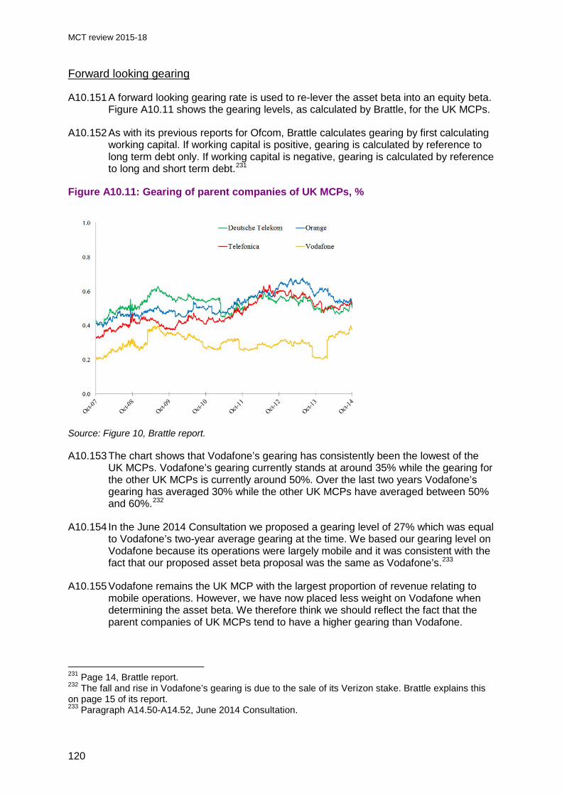
MCT review 2015-18

Forward looking gearing

A10.151 A forward looking gearing rate is used to re-lever the asset beta into an equity beta. Figure A10.11 shows the gearing levels, as calculated by Brattle, for the UK MCPs.

A10.152 As with its previous reports for Ofcom, Brattle calculates gearing by first calculating working capital. If working capital is positive, gearing is calculated by reference to long term debt only. If working capital is negative, gearing is calculated by reference to long and short term debt.231

Figure A10.11: Gearing of parent companies of UK MCPs, %

Source: Figure 10, Brattle report. A10.153 The chart shows that Vodafone’s gearing has consistently been the lowest of the

UK MCPs. Vodafone’s gearing currently stands at around 35% while the gearing for the other UK MCPs is currently around 50%. Over the last two years Vodafone’s gearing has averaged 30% while the other UK MCPs have averaged between 50% and 60%.232

A10.154 In the June 2014 Consultation we proposed a gearing level of 27% which was equal to Vodafone’s two-year average gearing at the time. We based our gearing level on Vodafone because its operations were largely mobile and it was consistent with the fact that our proposed asset beta proposal was the same as Vodafone’s.233

A10.155 Vodafone remains the UK MCP with the largest proportion of revenue relating to mobile operations. However, we have now placed less weight on Vodafone when determining the asset beta. We therefore think we should reflect the fact that the parent companies of UK MCPs tend to have a higher gearing than Vodafone.

231 Page 14, Brattle report. 232 The fall and rise in Vodafone’s gearing is due to the sale of its Verizon stake. Brattle explains this on page 15 of its report. 233 Paragraph A14.50-A14.52, June 2014 Consultation.

120

MCT review 2015-18

A10.156 Average gearing over the last two years for the UK MCPs varies between 30% (Vodafone) and 60% (Orange), although current gearing falls within a narrower range of 35% to 50%. The average across all four UK MCPs is just under 50%. Considering all the companies considered by Brattle that obtain more than half of their revenue from mobile operations, the average gearing level seen over the last two years is 40%, though the gearing rate can vary substantially as shown in Figure A10.12, from around 20% up to 60%. The variability within each comparator group (UK MCPs, EU mobile and US mobile) is also similar.

Figure A10.12: Average gearing over the last two years for companies obtaining more than half their revenues from mobile

Source: Brattle. Average gearing over two year period to 31 October 2014. A10.157 For the reasons explained above (at paragraphs A10.140-A10.141 and in the

Brattle report), in our estimation of asset beta we no longer place weight on the evidence from Vodafone in the way we did in the consultation. Therefore, we also consider it appropriate not to place significant weight on evidence from Vodafone in the estimation of gearing, but to consider evidence from a range of other companies with significant mobile operations.

A10.158 We have decided to use a gearing level of 40% in our WACC calculation. We consider that this level of gearing reflects the fact that gearing levels for other UK MCPs are above that of Vodafone and is around the average level of gearing observed for the comparator companies considered by Brattle which have significant mobile operations.

A10.159 We note that the overall WACC calculation is not very sensitive to the assumed forward looking gearing assumption. Assuming other parameters were held constant, the pre-tax real WACC would continue to be 7.0% for all forward looking gearing levels between 37% and 55%.234

Conclusion on equity beta

A10.160 Combining our asset beta estimate of 0.60, our forward looking gearing estimate of 40% and our debt beta estimate of 0.1 (see next section) we derive a forward looking equity beta for an average efficient MCP of 0.93. This is calculated using the following formula:

234 One reason for the relatively small effect of leverage on the WACC is the relatively low corporate tax rate of 20%.

121

MCT review 2015-18

𝛽𝛽𝑟𝑟𝑒𝑒𝑑𝑑𝑑𝑑𝑑𝑑𝑒𝑒 = β𝑟𝑟𝑑𝑑𝑑𝑑𝑟𝑟𝑑𝑑 − βdebt ∗ 𝐺𝐺𝑟𝑟𝑟𝑟𝑟𝑟𝑑𝑑𝑑𝑑𝑔𝑔

1 − 𝐺𝐺𝑟𝑟𝑟𝑟𝑟𝑟𝑑𝑑𝑑𝑑𝑔𝑔

Debt beta

A10.161 The debt beta is intended to measure the covariance of the return on debt to the return on the market. The debt beta is used to de-lever the equity beta in order to estimate the asset beta and, subsequently, to re-lever the asset beta to derive a forward looking equity beta.

Proposals in the June 2014 Consultation

A10.162 We used a debt beta of 0.1 in the June 2014 Consultation and noted that the overall WACC calculation was not very sensitive to the assumed debt beta.

Responses to the June 2014 Consultation

A10.163 No stakeholder commented on our debt beta proposal of 0.1.

Ofcom’s analysis of responses and conclusions

A10.164 We would associate a higher debt beta with relatively higher debt premia and gearing levels, and vice versa. We have decided to slightly reduce the debt premium from 1.2% in the June 2014 Consultation to 1.1% (see below), while our gearing assumption is somewhat higher (40% compared to 27% in the June 2014 Consultation). The lower debt premium reflects corporate debt spreads for the UK MCPs over the last 12 months while the higher gearing assumption reflects the fact we have put less weight on Vodafone’s gearing level and more weight on the gearing levels of the other UK MCPs, which tend to be higher. However, despite differences in gearing, all UK MCPs have similar credit ratings (see Table A10.19). We have therefore decided to maintain a debt beta of 0.1 as proposed in the June 2014 Consultation.

Debt premium

A10.165 In estimating the nominal cost of debt for an average efficient MCP, our approach involves summing together two parameters:

• the nominal RFR235 consistent with that underpinning the cost of equity; and

• the debt premium.

A10.166 The debt premium represents the extra return that investors require as a reward for investing in corporate debt rather than a risk-free asset.

Proposals in the June 2014 Consultation

A10.167 Based on data available at the time of the June 2014 Consultation, we considered that a reasonable range for the debt premium for an average efficient MCP was 1.0% - 1.6%.

235 As discussed earlier in this annex, the nominal RFR is estimated at 4.3%.

122

MCT review 2015-18

A10.168 We said we might place less weight on Telefonica’s debt premium since it appeared to be an outlier compared to the others, and place more weight on the average of the other three UK MCPs. The average debt premium of the other three UK MCPs was 1.2% over the year to April 2014.

A10.169 In light of the above, we considered that a debt premium slightly below the mid-point of the 1% to 1.6% range was appropriate. We therefore used a debt premium of 1.2% for our base case.

Responses to the June 2014 Consultation

A10.170 No respondents disagreed with our approach or commented on the proposed debt premium of 1.2%.

Ofcom’s conclusions

A10.171 In order to assess whether 1.2% remains a reasonable estimate of the debt premium for an average efficient MCP we have updated our analysis of the sterling denominated debt of each UK MCP to take into account data to the end of October 2014.

A10.172 Table A10.18 lists the debt we have considered alongside the average, minimum and maximum spread of this debt over nominal UK government gilts in the 12 months to 31 October 2014. The credit rating of each company as at October 2014 is included in brackets after the company name.236

236 Vodafone’s credit rating has been downgraded from A- at the time of the June 2014 Consultation to BBB+ at the time of this draft statement.

123

MCT review 2015-18

Table A10.18: Spread of sterling denominated debt over UK government gilts for European parents of UK MCPs, data to 31 October 2014

Maturity date

Years to maturity

12 month

average

12 month

min

12 month max

Current (October

2014) Vodafone (BBB+)

2017 2 0.9% 0.8% 1.1% 1.1% 2018 3 1.0% 0.8% 1.2% 1.0% 2025 10 1.1% 1.0% 1.2% 1.2% 2032 17 1.2% 1.0% 1.4% 1.4%

Deutsche Telekom (BBB+) 2019 4 1.0% 0.9% 1.1% 0.9% 2022 7 1.1% 0.9% 1.2% 1.1% 2028 13 1.2% 1.1% 1.3% 1.3% 2030 15 1.2% 1.0% 1.3% 1.3%

Orange (BBB+) 2016 1 0.8% 0.5% 0.9% 0.6% 2017 2 1.1% 1.0% 1.3% 1.0% 2020 5 1.2% 1.1% 1.3% 1.1% 2025 10 1.3% 1.2% 1.4% 1.3% 2028 13 1.4% 1.3% 1.5% 1.5% 2034 19 1.4% 1.2% 1.5% 1.5% 2050 35 1.4% 1.2% 1.6% 1.6%

Telefonica (BBB) 2018 3 1.3% 1.0% 2.0% 1.1% 2020 5 1.5% 1.1% 2.2% 1.3% 2022 7 1.7% 1.4% 2.2% 1.6% 2026 11 1.8% 1.5% 2.2% 1.8% 2029 14 1.8% 1.5% 2.2% 1.8%

Source: Bloomberg, Ofcom analysis. Company credit rating is the long term credit rating of the company and reflects the Bloomberg composite rating which takes into account the ratings of Moody’s, S&P and Fitch. Note that a rating of BBB- or higher indicates an investment grade bond.

A10.173 Table A10.19 shows the average, minimum and maximum debt spread for the parent companies of each of the UK MCPs taking into account all of the sterling-denominated debt in issue (the minima and maxima shown are therefore averaged over the maturities shown for each UK MCP).

124

MCT review 2015-18

Table A10.19: Average spread of sterling denominated debt over UK government gilts for European parent companies of UK MCPs, data to 31 October 2014

Average maturity (years)

12 month

average

12 month

min

12 month max

Current (October

2014)

Vodafone (BBB+) 8 1.1% 0.9% 1.2% 1.2% Deutsche Telekom (BBB+) 10 1.1% 1.0% 1.2% 1.1% Orange (BBB+) 12 1.2% 1.1% 1.3% 1.2% Telefonica (BBB) 8 1.6% 1.3% 2.1% 1.5%

Source: Bloomberg, Ofcom analysis. The 12 month minimum and maximum spreads represent the average across all maturities, not the very highest or the very lowest spread (which will be maturity specific – typically for debt at each end of the maturity spectrum).

A10.174 Figure A10.13 charts the spot spread (averaged over all maturities) of sterling denominated debt for the European parents of the UK MCPs up to October 2014.

Figure A10.13: Average spot spread of sterling denominated debt over benchmark yields for European parents of UK MCPs

Source: Bloomberg, Ofcom analysis. Data to 31 October 2014.

A10.175 The chart and preceding table show that the average debt spread for Vodafone and Deutsche Telekom continues to be around 1.1% (as we found in the June 2014 Consultation). The average debt spread for Orange has fallen a little and is now around 1.2%. The debt spread for these three parent companies is similar and averages 1.1% across the three over the 12 months to October 2014. This represents a slight reduction from the 1.2% 12 month average for these companies reported in the June 2014 Consultation.

A10.176 Telefonica’s average debt spread remains above that of the other UK MCPs, and its 12 month average stands at 1.6%. Although Telefonica’s average debt spread has converged to be closer to that of the other UK MCPs (it is now just within the range we considered for an average efficient MCP of 1.0% - 1.6% in the June 2014 Consultation) we consider that it remains somewhat of an outlier compared to the other UK MCPs (which may reflect Telefonica’s slightly lower credit rating). Consistent with the June 2014 Consultation we have therefore placed less weight on Telefonica’s debt spread.

125

MCT review 2015-18

A10.177 The more recent data to October 2014 suggests that the range for an average efficient MCP has reduced slightly. In the June 2014 Consultation the upper end of the range was bounded by the 12 month maximum debt spread for Orange which has now fallen from 1.6% to 1.3%. The lower end was bounded by the 12 month minimum debt spread for Vodafone which has now been as low as 0.9% over the last 12 months. Therefore, we remain of the view that it is appropriate to set a debt premium below the mid-point of the consultation range of 1% to 1.6%. As in the June 2014 Consultation, we prefer to place less weight on Telefonica’s debt spread and place more weight on the average of the other three parent companies. Taking the average of these three parent companies, the 12 month average is 1.1%. Therefore, we have used a debt premium of 1.1%.237

A10.178 The resulting pre-tax nominal cost of debt is 5.4%, representing the sum of the nominal RFR of 4.3% and the debt premium of 1.1%. This is above current yields to maturity on corporate debt issued by the UK MCPs because our preferred estimate of the real RFR is above current yields on index-linked gilts (and hence our estimate of the nominal RFR is above the yield on nominal gilts which provide the benchmark against which corporate bonds are typically compared to derive a spread). We have estimated the cost of debt in this way because we consider it appropriate to take a consistent approach in estimating the cost of equity and cost of debt by assuming the same real RFR for both. We are seeking to set an overall return on capital required by investors to finance significant, and in some cases risky or long-lived, investments. In doing so, we consider that arguments over the appropriate real RFR to use in the WACC should apply equally to debt and equity and we seek to maintain a consistent approach to estimating these – both through time and between market reviews.

Corporate tax

A10.179 In the Budget of April 2013, the UK Government announced its intention to reduce the corporate tax rate to 20% for 2015/16.238 We proposed to use a corporate tax rate of 20% since this represents the best estimate of what the tax rate will be on a long-run, forward-looking basis. This is consistent with the 20% tax rate used in the 2014 FAMR Statement.239

A10.180 No respondents commented on our proposals in relation to corporation tax and the Government has not announced any revisions to the rate of corporation tax for the period in question. We have therefore used a tax rate of 20% in the WACC calculation.

Conclusions: WACC estimate

A10.181 Table A10.20 sets out our decision relating to the WACC for an average efficient MCP. The pre-tax real rate (i.e. the pre-tax nominal rate deflated by CPI) of 7.0% is used in the 2015 MCT model from 2013/14 onwards. As explained in Annex 7, prior to that we have used the CPI adjusted real WACC consistent with previously determined values of the pre-tax nominal WACC for an average efficient MCP (which in the 2011 MCT model and earlier versions were deflated by RPI inflation so have now been adjusted to be consistent with deflating by CPI).

237 We note that, holding other parameters constant, the pre-tax real WACC would be 7.0% for all debt premium estimates between 1.00% and 1.24%. 238 Corporation tax rates available here: http://www.hmrc.gov.uk/rates/corp.htm 239 Paragraph A14.145, 2014 FAMR Statement.

126

MCT review 2015-18

Table A10.20: WACC estimates for an average efficient UK MCP

January 2015 (Statement)

WACC (pre-tax nominal) 9.1%

WACC (pre-tax real) (CPI deflation) 7.0% Source: Ofcom analysis.

127

MCT review 2015-18

Annex 11

11 Other modelling issues Introduction

A11.1 This annex explains the reasoning underlying our conclusions in relation to a number of other modelling issues in the 2015 MCT model. These issues are as follows and are addressed in turn in the following sub-sections:

• Spectrum bands, allocations and valuation

• Administrative costs

• HLR update costs

A11.2 Consistent with the approach taken in the 2011 MCT review, we do not consider that spectrum, administrative and HLR update costs would arise in the provision of MCT viewed as the final traffic increment. Therefore, these costs do not have a direct impact on the LRIC results of the 2015 MCT model that we have decided to use in setting the charge control.240 Nevertheless, we have sought information on these costs for the purposes of determining the LRIC+ of MCT.

Spectrum bands, allocations and valuation

Proposals in the June 2014 Consultation

Spectrum bands

A11.3 In the June 2014 Consultation we proposed to include the following spectrum bands in the 2014 MCT model:

• 800MHz spectrum, used for 4G technology;

• 1800MHz spectrum, used for 2G and 4G technologies;

• 2.1GHz spectrum, used for 3G technology; and

• 2.6GHz spectrum, used for 4G technology.

A11.4 By way of background information, the holdings of mobile spectrum currently held by the four national MCPs are shown in Figure A11.1 below.

240 However, the choice of spectrum bands and the quantity of spectrum assumed in each does have a bearing on the LRIC of MCT via the network dimensioning process.

128

MCT review 2015-18

Figure A11.1: Four largest MCPs’ spectrum holdings (MHz, paired)

Source: Ofcom.

Spectrum holdings

A11.5 In the June 2014 Consultation we proposed that the average efficient MCP had the spectrum holding set out in Table A11.1 below.

Table A11.1: Proposed spectrum holdings, uses and carrier sizes

Band Holding (paired

MHz) Technology Modelled carrier size (paired MHz)

800MHz 10 4G 5

900MHz 0 n/a n/a

1800MHz 30 20 2G 0.2

10 4G241 5

2.1GHz 10, increasing to 15 in 2012/13

3G 5

2.6GHz 10 4G 5 Source: Ofcom, 2014 MCT model.

241 Following refarming in 2012/13.

129

MCT review 2015-18

Spectrum for 2G services.

A11.6 We explained that we had used the spectrum holdings in the 2011 MCT model as our starting point, and the 2011 MCT model included 2 x 30 MHz of 1800 MHz spectrum which was used for 2G services.

A11.7 We detailed why we thought this formed part of a reasonable allocation of spectrum for the average efficient MCP. We also explained why we assumed that 2 x 10 MHz of 1800 MHz spectrum was refarmed for 4G use and how the timing of this change was consistent with Ofcom’s decision to allow EE to refarm its 1800 MHz spectrum for 4G use from 2012/13. The outcome of this process was to leave 2 x 20 MHz of 1800 MHz spectrum for use in the provision of 2G services from 2012/13 onwards.

Spectrum for 4G services

A11.8 We explained in the June 2014 Consultation that we had considered the inclusion of further spectrum for 4G services as a result of future spectrum releases, in particular following comments made by BT on the draft MCT model. We noted that Ofcom is currently planning the award of additional spectrum that could be used for 4G services, but that we considered that there was too much uncertainty surrounding the timing and use of this spectrum to allow robust modelling.242

Spectrum valuation

A11.9 The valuation of spectrum holdings influences the LRIC+ outputs of our modelling but does not affect the LRIC outputs. As we explained in the June 2014 Consultation, although LRIC could in principle include some contribution to spectrum costs, the modelling implementation means that it is not necessary to include an explicit estimate of spectrum costs.243

A11.10 For the purposes of calculating LRIC+ our approach in valuing the spectrum holdings of the average efficient MCP is to reflect the forward-looking economic value (i.e. opportunity cost) of the spectrum. In doing so in the June 2014 Consultation we drew on the most recently available evidence of the market value of spectrum from Ofcom’s consultation on ALF for 900 MHz and 1800 MHz spectrum (the ‘ALF Consultation’).244

A11.11 For the 800 MHz and 2.6 GHz spectrum we proposed to use recent market evidence from the 4G auction, based on Linear Reference Pricing (LRP) analysis of the auction data performed by DotEcon. This produced a valuation for 800 MHz spectrum of £29.9m per MHz, and for 2.6 GHz of £5m per MHz. These figures were doubled to calculate valuations per paired MHz and applied to the proposed spectrum holdings. We proposed to treat payments for these spectrum allocations as one-off capital expenditures in 2012/13, with no adjustment for inflation being necessary, and no gestation adjustment. We did, however, take account of the value of this spectrum following the initial period of 20 years, proxied by a capitalised value based on the auction prices, and discounted back to 2012/13. The

242 June 2014 Consultation, paragraph A15.18. 243 June 2014 Consultation, paragraphs A15.22 to A15.25, consistent with paragraphs A9.7 to A9.9 of the March 2011 Statement. 244 Ofcom, Annual licence fees for 900 MHz and 1800 MHz spectrum, consultation, 10 October 2013, http://stakeholders.ofcom.org.uk/binaries/consultations/900-1800-mhz-fees/summary/900-1800-fees.pdf.

130

MCT review 2015-18

outcome of this process was to produce 2012/13 capital expenditures of £755m in relation to the 2 x 10 MHz of 800 MHz spectrum and £126m for the 2 x 10 MHz of 2.6 GHz spectrum (both in 2012/13 prices).

A11.12 For the 2.1 GHz spectrum we proposed to treat payment in two lump sums; the first assumed to be incurred in 2004/5, and the second in 2012/13. The first lump sum was based on the valuation used in the 2011 MCT model, adjusted to reflect 2012/13 prices and the revised length of time for which it was assumed to apply. The second lump sum was based on a linear interpolation between the 2.6 GHz valuation of £5m per MHz explained above, and the ALF Consultation ‘best estimate’ of the value of 1800 MHz spectrum. The resulting valuation of £11.07m per MHz was then adjusted to account for its value after an initial period of 20 years in the manner described for 2.6 GHz spectrum above. The outcome of this process was a first lump sum of £313m and a second of £419m (both in 2012/13 prices) for the 2 x 15 MHz of 2.1 GHz spectrum.

A11.13 For the 1800 MHz spectrum we proposed a different approach to reflect the fact that fees are paid for this spectrum on an annual basis rather than as a lump sum. Although at the time of the June 2014 Consultation we were still considering the level and timing of introduction of the new ALF rates, we based our valuation on the proposed annual payments as the best available evidence of the market value of 1800 MHz spectrum at that time. We adjusted the valuation to reflect 2012/13 prices, resulting in an annual payment of £1.17m per MHz per year, or £70m for the modelled operator’s allocation of 2 x 30 MHz of 1800 MHz spectrum.

A11.14 Our proposals relating to the valuation of the spectrum for the 2014 MCT model are shown in Table A11.2 below.

Table A11.2: Proposed spectrum valuation summary

Methodology Treatment in model Valuation (2012/13 prices)

800MHz LRP analysis of 4G auction bid data Lump sum in 2012/13 £755m, incurred in 2012/13

900MHz n/a n/a n/a

1800MHz

Valuation consistent with 2011 MCT Model,

then updated from 2013/14

Annual fee

Historical figures to 2012/13, £70m per annum thereafter and split between 2G and

4G

2.1GHz

Adjusted historical valuation from 2004/5,

then interpolate between 1800 MHz and 2.6 GHz from 2012/13

Lump sum in 2004/5, second lump sum in

2012/13

£313m incurred in 2004/5 and £419m in 2012/13

2.6GHz LRP analysis of 4G auction bid data Lump sum in 2012/13 £126m, incurred in 2012/13

Source: Ofcom.

A11.15 We explained in the June 2014 Consultation that since our spectrum valuation was informed by our work on ALF, and this work was ongoing, we anticipated that it would require updating if changes were made to the ALF analysis.

131

MCT review 2015-18

Responses to the June 2014 Consultation

A11.16 We received a number of responses to the June 2014 Consultation on the subject of spectrum. Vodafone queried our choice of spectrum for 2G services, and Vodafone and EE suggested that we should include additional spectrum for 4G services. These topics are addressed below.

A11.17 BT, H3G and Telefonica did not comment on the specifics of our proposals in relation to spectrum bands, holdings or valuation.

Spectrum for 2G services

A11.18 Vodafone’s response to the consultation queried the use of 1800 MHz spectrum for 2G services.245 Vodafone argues that the use of 2 x 20 MHz of 1800 MHz spectrum for 2G services simply renews a decision originally made in 2007.246 At that time T-Mobile and Orange used 1800 MHz spectrum for 2G services, whereas Vodafone and O2 used 900/1800 MHz, and the unit costs of mobile services provided using the two spectrum scenarios were found to be similar.247

A11.19 Vodafone noted the following changes since 2007:

11.19.1 There is only one MCP with a 2G network using 1800 MHz spectrum (EE) and two using 900/1800 MHz (Telefonica and Vodafone); and

11.19.2 The focus of our modelling has shifted from LRIC+ to LRIC.

A11.20 Addressing these points in turn, Vodafone argued that modelling 2G services using 1800 MHz spectrum means that our average efficient MCP is based on a single ‘outlier’ observation rather than the two 900/1800 MHz MCPs running 2G networks (i.e. Vodafone and Telefonica). Noting that 900 MHz spectrum may be advantageous for providing coverage and 1800 MHz advantageous for capacity, Vodafone argued that this matters because LRIC is concerned with the costs of providing capacity, and the LRIC of MCT for a 900/1800 MHz operator will be higher than that of our modelled 1800 MHz operator.

A11.21 Vodafone calculated, based on adjustments to the 2014 MCT model, that the blended LRIC of an operator providing 2G services using 900 MHz is around 15% higher than if 1800 MHz spectrum is used.248

A11.22 Vodafone argued that this issue requires consideration and that at a minimum it is necessary to determine, by means of modelling, whether the costs of 2G services using 1800 MHz spectrum are representative of an average efficient MCP. Finally it added that another development in the 2014 MCT model is infrastructure sharing, but that in reality the only MCP using 1800 MHz spectrum for 2G has no operators to share this with (because EE’s network sharing agreement is with Three, which does not operate a 2G network).

245 Vodafone response to June 2014 Consultation, Section 2.3. 246 As explained above, 2 x 30 MHz is initially assumed, but 2 x 10 MHz is refarmed for 4G use in 2012/13. 247 See paragraphs 9.96 to 9.98 of the 2007 MCT Statement, http://www.ofcom.org.uk/static/LRIC_files/MCTStatement2007.pdf 248 Vodafone response to June 2014 Consultation, Section 3.6.

132

MCT review 2015-18

Spectrum for 4G services

A11.23 In its consultation response EE argued that the spectrum allocation assumed in the model failed to represent the likely availability of spectrum in future. In particular it noted that we have recently set out our proposals to make 700 MHz spectrum available from 2022, or possibly two years earlier. As a result it proposed to include 2 x 10 MHz of 700 MHz spectrum from 2022/23 onwards, and proxied the effect of this in the 2014 MCT model by including an additional 2 x 10 MHz of 800 MHz spectrum from that date. It found that this lead to an increase in the 2017/18 LRIC results of the model from 0.476pmm to 0.513ppm, an increase of 7.8%.249

A11.24 Vodafone commented that our proposed spectrum allocation ‘represents a fair spread of the available bands’, but noted that ‘it is not correct to assume a very considerable increase in data demand, as the model does, without also assuming an increase in spectrum’.250 Vodafone went on to explain its view that a lack of spectrum causes a surge in the number of 4G macrosites required to carry traffic.

A11.25 In order to rectify this perceived problem, Vodafone suggested a similar adjustment to that proposed by EE and explained above. Vodafone proxied the use of 2 x 10 MHz of 700 MHz spectrum by our average efficient MCP by assuming an additional 2 x 10 MHz of 800 MHz spectrum from 2019 onwards. As shown in Table 3.11 of Vodafone’s response, it found that this lead to a reduction in the LRIC+ results and an increase in the LRIC results of the model from 0.476pmm to 0.518ppm, an increase of 8.7%.

A11.26 BT queried the timing of the refarming of 1800 MHz spectrum for 4G use, and the consistency of this with the assumed timing of 4G network rollout and subscriber growth.251 This comment is addressed along with BT’s other comments on the modelling of traffic volumes in Annex 11 of this draft statement.

Spectrum valuation

A11.27 No stakeholders provided responses on the details of our approach to spectrum valuation in the 2014 MCT model, with Vodafone noting only that the outputs of the ALF Statement would need to be reflected.252

Ofcom’s analysis of responses and conclusions

Spectrum for 2G services

A11.28 In response to Vodafone’s argument that we should model a 900/1800 MHz network for 2G services we note that:

11.28.1 While a 900/1800 MHz operator would have a different coverage profile from an 1800 MHz only operator, we would expect any network cost difference to be eroded by market-based mechanisms for spectrum assignments.

249 EE response to June 2014 Consultation, Section 6.4. 250 Vodafone response to June 2014 Consultation, Section 2.2. 251 See page 13 of Annex 2 of BT’s response (the Deloitte report ‘Volume forecasts in the Ofcom MCT model’). 252 This comment was made in the context of 900 and 1800 MHz spectrum, see Vodafone response page 74.

133

MCT review 2015-18

11.28.2 Any cost disadvantage for a 900 MHz operator in providing termination services would be offset by lower coverage costs.

11.28.3 Not all MCPs have 900 MHz spectrum.

A11.29 The issue of a 900/1800 MHz operator was considered as part of the appeals of the 2011 MCT Statement.253 At that time Vodafone argued that we had not properly assessed whether 2G technology should be modelled at 900/1800 MHz or 1800 MHz for the purposes of the LRIC calculations. EE agreed with Vodafone, but noted that it was difficult to say that there was a difference between the two technologies when MCT is the final increment.

A11.30 The points set out in paragraph A11.28 are consistent with the arguments we presented in defending the appeals, and in the 2012 CC Determination the CC found that Vodafone had not demonstrated that Ofcom had erred in not modelling a 900/1800 MHz operator in calculating the LRIC of MCT. We remain of the view that the points in paragraph A11.28 above remain valid.

A11.31 Analysys Mason has reviewed Vodafone’s claim that the blended LRIC of MCT is 15% higher for a 900/1800 MHz operator than that for an 1800 MHz operator. As explained in Section 3.12 of Annex 8, it has replicated Vodafone’s result and has also improved it by rectifying a number of discrepancies. When Analysys Mason then recalibrated the model using information from the two 900/1800 MHz operators it found that the LRIC outputs are slightly lower than those in the 2015 MCT model base case. This leads us to find that even if modelling of a 900/1800 MHz operator were justified in principle, which we do not believe is the case, the impact is not necessarily of the direction or scale claimed by Vodafone.

A11.32 In addition to analysis of the LRIC unit outputs of the 2015 MCT model, we have examined overall costs measured by the NPV of total network costs254 and the cost of coverage implied by using different spectrum bands for 2G services.255 These analyses show both that the NPV of total network costs associated with an 1800 MHz operator is higher than that for a 900/1800 MHz and that the modelled unit costs of providing coverage using 900/1800 MHz spectrum are lower than when using 1800MHz spectrum only. Therefore, even if the 900/1800MHz operator faced a slightly higher LRIC of MCT, the 900/1800MHz operator would still have a competitive advantage in competing for subscribers as a result of its lower overall costs. These empirical findings reinforce the principled arguments we made in our defence of our 2011 MCT model, as reported in paragraph A11.28.2 above.

A11.33 In relation to Vodafone’s final point that the model assumes infrastructure sharing when there is now only one MCP providing 2G services using 1800 MHz spectrum our aim is to model the costs of providing MCT for an average efficient MCP. We do not aim to model the costs or infrastructure sharing arrangements of any particular MCP. We also note that the modelled operator has only 2 x 30 MHz of 1800 MHz spectrum out of a total of 2 x 72 MHz meaning that there is no reason why it could

253 See the 2012 CC Determination, paragraphs 3.553 to 3.571. 254 This information can be found on the ‘Selected ED results’ sheet of the ‘Economic’ module. 255 This analysis is explained in detail in Annex 8.

134

MCT review 2015-18

not engage in network sharing in principle.256 As a result we remain of the view that the position we adopted in the June 2014 Consultation is appropriate.

Spectrum for 4G services

Compatibility of spectrum allocation and traffic demand

A11.34 As explained in the consultation, we considered the inclusion of additional spectrum for 4G use in the 2014 MCT model following comments received from BT after the January 2014 industry workshop.257 Although we noted that Ofcom is planning future spectrum releases we considered that uncertainty surrounding the timing and use of this spectrum would not allow robust modelling of its use.

A11.35 We have analysed Vodafone’s claim that ‘the model very clearly shows the consequences of the failure to assume additional spectrum in a sudden surge in required 4G sites from 2020 onwards’.258 Vodafone’s response tabulates 4G macrocell site equipment from 2020/21 to 2025/26, but examination of the figures over a longer period shows relatively steady growth.

A11.36 This is shown in Figure A11.2 below, in which the blue line shows 4G macrocell equipment quantities from the 2014 MCT model and the dashed lines indicate the period in which Vodafone claims there is a ‘sudden surge’. The red line, indicating 4G macrocell equipment quantities from the 2015 MCT model shows that the outputs reach a considerably lower level. This change is primarily due to the modifications that Analysys Mason has made to the eNodeB and 4G carrier dimensioning, as explained in Section 3.2 of Annex 8.

256 We note that, as shown in Figure A11.1, EE has 2 x 45 MHz of 1800 MHz spectrum, which is well in excess of the 2 x 30MHz modelled. Since EE is larger than the other MCPs both in scale and spectrum holdings, and since EE was created by the merger of two MCPs, the merged entity is akin to infrastructure sharing between two MCPs with 2 x 45 MHz of 1800 MHz spectrum in total. With 2 x 30MHz of 1800 MHz spectrum our modelled MCP could, for example, infrastructure share with an MCP with 2 x 15 MHz of 1800 MHz spectrum, or more given the available 2 x 72 MHz. 257 See paragraphs A15.14 and A15.18 of the consultation. No comments were received at that stage from Vodafone, or from EE on the subject of additional spectrum for 4G services. 258 Vodafone response to June 2014 Consultation, page 49.

135

MCT review 2015-18

Figure A11.2: 4G macrocell equipment quantities

Source: 2014 MCT model, ‘Network’ module, ‘Summary’ sheet.

A11.37 In light of this analysis and the changes that have been made to the 4G dimensioning, we are not persuaded by Vodafone’s argument that there is a mismatch in the 2015 MCT model between the forecast traffic volumes and the availability of spectrum.

Inclusion of additional spectrum

A11.38 We have also reviewed the more general point of whether future spectrum releases should be included in our modelling. Specifically we have considered EE’s proposal that 2 x 10 MHz of 700 MHz spectrum should be included from 2022/23, and Vodafone’s proposal that this spectrum should be included from ‘2019 or so’.259 Both of these proposals involve the addition of spectrum after the end of the relevant charge control period, and EE’s suggestion in particular is close to the end of the period that is explicitly modelled. As explained in Annex 7, we aim to model the least cost means of delivering the regulated services using known technology, but recognising where an efficient national network would start from in terms of legacy network deployments. This principle extends to the spectrum assumptions.

A11.39 In the case of spectrum for 4G services Ofcom consulted on the use of 700 MHz spectrum for mobile broadband use in 2014.260 At that time we anticipated that 2 x 30 MHz of 700 MHz spectrum could be available for the provision of mobile

259 EE response to June 2014 Consultation, Section 6.4, Vodafone response to June 2014 Consultation, page 70. 260 See Ofcom, Consultation on future use of the 700 MHz band, 28 May 2014, http://stakeholders.ofcom.org.uk/binaries/consultations/700MHz/summary/main.pdf.

136

MCT review 2015-18

services from 2022 (or possibly up to two years earlier), but might be auctioned earlier than this, and possibly as early as 2016.

A11.40 More recently our 700 MHz Statement explained that 2020 is a likely date for the auction of this spectrum, making it available for mobile services from 2022.

A11.41 As we explained in the June 2014 Consultation, we consider that uncertainty around the timing and use of this spectrum hinders our ability to model its use in a robust manner. We also observe that spectrum auctions are complex processes, and their design and completion raises a range of technical, competition and implementation issues. Our experience suggests that stakeholder consultation can reveal issues in these areas that require further substantive work, all of which can introduce delay to the process.261

A11.42 A particular source of uncertainty in relation to the availability of 700 MHz spectrum is that it is currently used for digital terrestrial television (DTT) and Programme Making and Special Events (PMSE) services. The use of 700 MHz spectrum for mobile services therefore requires the clearance and re-planning of the existing DTT spectrum. Spectrum clearance is a costly process, and the re-planning of spectrum requires international cooperation. In relation to PMSE spectrum it is necessary to identify an alternative band for this use, and this remains to be done.

A11.43 This uncertainty about the date that 700 MHz spectrum might be used, and the length of time before this is likely, hinders our ability to model network costs in a robust manner. Although 700 MHz spectrum is used for the provision of mobile services in certain other countries, we anticipate that gathering information on its technical characteristics and equipment costs from UK operators would be challenging. This raises doubts about the robustness with which we could model traffic on a network which we do not anticipate will be used before 2022.

A11.44 Alongside our review of whether it would be appropriate to include 700 MHz spectrum in the 2015 model we have reconsidered whether other spectrum bands should be included. In early 2014 we consulted on technical issues related to spectrum in the 2.3 and 3.4 GHz bands,262, 263 More recently in our November 2014 consultation we explained that we anticipate an auction process taking place in late 2015 or early 2016.264

A11.45 However, the timing of the award of this spectrum is subject to the same sources of uncertainty as those explained in paragraph A11.41 above in the context of 700 MHz spectrum. We also note that while these bands may be of interest to the MCPs, the particular characteristics of the spectrum suggest it is likely to be

261 For example, when we first consulted on the 800MHz and 2.6GHz competition assessment and award proposals we anticipated the auction process beginning in Q1 2012. However, the need for further consultation meant that the award process was only concluded in February 2013, see http://media.ofcom.org.uk/news/2013/winners-of-the-4g-mobile-auction/. 262 See Ofcom, PSSR: Technical coexistence issues for the 2.3 and 3.4 GHz award, consultation, 19 February 2014, http://stakeholders.ofcom.org.uk/binaries/consultations/pssr-2014/summary/pssr.pdf. 263 We anticipate that these future spectrum releases will lead to an additional 2 x 30 MHz of 700 MHz spectrum, 40 MHz (unpaired) of 2.3 GHz spectrum, and 150 MHz (unpaired) of 3.4 GHz spectrum. In total this is equivalent to 2 x 125 MHz of spectrum in addition to the existing stock of 266.6 MHz, an increase of 47%. 264 See Ofcom, PSSR: Award of the 2.3 GHz and 3.4 GHz bands, consultation, 7 November 2014 http://stakeholders.ofcom.org.uk/binaries/consultations/2.3-3.4-ghz-auction-design/summary/2_3_and_3_4_GHz_award.pdf.

137

MCT review 2015-18

suitable for providing additional capacity or for backhaul, rather than for wide area coverage.265

A11.46 . We consider this to be consistent with the treatment of spectrum in the 2011 MCT model, which was produced at a time when the auction for 800MHz and 2.6GHz spectrum was anticipated but the spectrum was not included in the modelling.

Modelled impact of additional spectrum

A11.47 Notwithstanding our finding above that it would not be appropriate to include additional spectrum in the 2015 MCT model, we note that the adjustments proposed by both EE and Vodafone to increase spectrum holdings produce increases in the LRIC results of the model.

A11.48 Analysys Mason has investigated this result and found that the increase in the LRIC modelled by EE and by Vodafone is a modelling artefact caused as a result of the assumption that cell site numbers cannot fall over time, in combination with the site sharing assumptions and base case volume forecasts. The assumption that cell site numbers cannot fall over time was explained in the June 2014 Consultation,266 and is included to avoid a situation in which 2G and 3G site requirements fall in the short term (as a result of reductions in 2G and 3G traffic) only to increase again in the longer term as a result of 4G network deployments (which will require additional cell sites).

A11.49 The effect of this assumption in conjunction with other model inputs and assumptions is explained further by Analysys Mason in Annex 8. While the assumption that site numbers cannot fall over time can lead to counterintuitive results, as in the circumstances proposed by EE and Vodafone, it is nevertheless appropriate in order to avoid an unrealistic evolution of cell site numbers over time.

A11.50 A consequence of this is that even if we were to accept Vodafone and EE’s arguments about the inclusion of 700 MHz spectrum, which we do not, their calculations of the impact on the LRIC results of the model cannot be taken at face value.

Conclusions on spectrum bands and holdings

A11.51 In light of the analysis presented above we conclude that the spectrum bands and holdings modelled in the 2014 MCT model should be unchanged in the 2015 MCT model.

A11.52 We have reconsidered the question of what spectrum should be used to model 2G services following Vodafone’s argument that we should be modelling a 900/1800 MHz operator. We remain of the view that modelling a 2G network using 1800 MHz spectrum remains appropriate.

A11.53 We have also re-examined whether additional spectrum should be included in the 2015 MCT model for 4G services, in particular considering whether 700 MHz spectrum should be included. We find that the model does not suggest that 700 MHz spectrum is necessary to ensure consistency with traffic forecasts, and also

265 See Ofcom, PSSR: Award of the 2.3 GHz and 3.4 GHz bands, consultation, 7 November 2014, paragraph 1.5. 266 See paragraphs A16.9 to A16.11 of June 2014 Consultation.

138

MCT review 2015-18

that uncertainty surrounding the timing of release of 700 MHz spectrum means that its impact could not be modelled robustly, consistent with our arguments in the June 2014 Consultation.

A11.54 Based on this analysis the spectrum bands and holdings included in the 2015 MCT model are as shown in Table A11.3 below.

Table A11.3: Spectrum holdings, uses and carrier sizes in 2015 MCT model

Band Holding (paired

MHz) Technology Modelled carrier size (paired MHz)

800 MHz 10 4G 5

900 MHz 0 n/a n/a

1800 MHz 30 20 2G 0.2

10 4G267 5

2.1 GHz 10, increasing to 15 in 2012/13

3G 5

2.6 GHz 10 4G 5 Source: Ofcom, 2015 MCT model.

Spectrum valuation

A11.55 As noted above and in the June 2014 Consultation, our spectrum valuations in the 2014 MCT model were informed by our work on ALF at the time of publication. As such they require updating to reflect our Further Consultation on ALF.268

800 MHz and 2.6 GHz spectrum valuations

A11.56 Both 800 MHz and 2.6 GHz spectrum were included in Ofcom’s 4G auction, which concluded in February 2013. As a result, we have recent market evidence on the value of holdings in these spectrum bands and use this to inform the valuations for these spectrum bands in the 2015 MCT model.

A11.57 The marginal bidder analysis in the Further Consultation on ALF produces the following valuations for licences with a 20 year initial term:

• 800 MHz: £32.63m per MHz

• 2.6 GHz: £5.5m per MHz

A11.58 The 4G auction required payment for spectrum acquired by 21 February 2013 so we treat payments for 800MHz and 2.6GHz spectrum as one-off capital expenditures incurred in 2012/13. Since 2012/13 is the base year for costs in the 2014 MCT model, no adjustment is necessary to account for inflation. The figures

267 Following refarming in 2012/13. 268 See Ofcom, Annual licence fees for 900 MHz and 1800 MHz spectrum, further consultation, 1 August 2014 (the ‘Further Consultation on ALF’) http://stakeholders.ofcom.org.uk/binaries/consultations/annual-licence-fees-900-MHz-1800-MHz/summary/condoc.pdf.

139

MCT review 2015-18

explained above mean that a holding of 2 x 10 MHz of 800 MHz spectrum has a value of £653m and a holding of 2 x 10 MHz of 2.6 GHz spectrum has a value of £110m (both in 2012/13 prices).269

A11.59 We do not make a gestation adjustment for this spectrum, reflecting the speed with which it has been used to deploy 4G services. However, it is necessary to consider the value of this spectrum between 2032/33 and 2039/40 (the period after the initial period of 20 years until the end of the modelling period), also in light of the licence conditions requiring the licensees to pay the relevant fees as prescribed by Ofcom from 2033.270 For the purposes of the 2015 MCT model, we assume a capitalised value based on the auction prices paid in 2012/13 as a proxy as we did in the June 2014 Consultation, but annuitise this in a manner akin to our treatment of the 2.1 GHz valuation and use this annuity for each year after expiry of the initial licence until the end of the modelling period. These future payments are discounted back to 2012/13 and added to the initial outlay to produce 2012/13 total capital expenditures of £748m in relation to the 800MHz spectrum and £126m for the 2.6 GHz spectrum (both in 2012/13 prices).

2.1 GHz spectrum valuation

A11.60 The valuation of 2.1GHz spectrum is not as straightforward as for 800MHz and 2.6GHz because there is no recent direct market evidence of its value and the ALF Further Consultation does not seek to value it. However, the ALF Further Consultation does contain information that can be used in order to derive an estimate of the forward-looking economic value of 2.1GHz spectrum, as explained below.

A11.61 We treat 2.1GHz spectrum payments as two lump sums:

11.61.1 The first being incurred in 2004/5, relating to 2 x 10 MHz of 2.1GHz spectrum and based on adjustment to the 2004/5 valuation used in the 2011 MCT model.

11.61.2 The second being incurred in 2012/13, relating to the 2 x 15 MHz of 2.1 GHz spectrum assumed to be held from that point onwards and based on more recent evidence of spectrum values.

A11.62 The starting point for the first lump sum is the 2.1 GHz spectrum value of £451m (2008/9 prices) used in the 2011 MCT model. This was incurred in 2004/5 in relation to the 16 year period to 2021/22.271 In order for us to apply a second lump sum reflecting an updated valuation in 2012/13 it is necessary to adjust the lump sum incurred in 2004/5 in order to avoid double counting.

A11.63 Having first adjusted from 2004/5 to 2012/13 prices, we account for the change in the assumed length of time for which the 2004/5 lump sum applies by first annuitizing the 2004/5 lump sum using a discount rate of the WACC over the 16 year period for which the lump sum was assumed to apply in the 2011 MCT

269 Calculated as 32.63 x 2 x 10 = £653m and 5.5 x 2 x 10 = £110m respectively. 270 See paragraph 8 of the Template Spectrum Access 800 MHz/1800 MHz/2.6 GHz licence in Ofcom, The award of 800 MHz and 2.6 GHz spectrum – Annexes, Information Memorandum, 24 July 2012. http://stakeholders.ofcom.org.uk/binaries/consultations/award-800mhz/statement/IM2.pdf. 271 See footnotes 268 and 270 of the March 2011 Statement.

140

MCT review 2015-18

model272, and then discounting the resulting annual amounts over the eight year period to which we now assume the lump sum relates. This produces a revised lump sum for 2 x 10 MHz of 2.1 GHz spectrum of £313m (in 2012/13 prices), which is assumed to be incurred in 2004/5. This is supplemented by a second lump sum for 2.1 GHz spectrum incurred in 2012/13, as explained below.

A11.64 The starting point for the second lump sum is a linear interpolation between the 2.6 GHz spectrum valuation of £5.5m per MHz (2012/13 prices) explained above and the Further Consultation on ALF ‘best estimate’ of the value of 1800 MHz spectrum.273 This ‘best estimate’ for 1800 MHz spectrum was £14m per MHz in 2013/14 prices, or £13.7m per MHz in 2012/13 prices. This produces a valuation for 2.1 GHz spectrum of £10.64m per MHz, as shown in Figure A11.3 below.

Figure A11.3: Linear interpolation of 2.1GHz valuation

Source: Ofcom.

A11.65 The estimate explained in paragraph A11.64 implies that the modelled operator’s 2012/13 holding of 2 x 15 MHz of 2.1GHz spectrum has a valuation of £319m. The value of this spectrum beyond 2032/33 is accounted for in the same way as that described for 800 MHz and 2.6 GHz spectrum above, namely that the same lump sum valuation is assumed, annuitized and the values for the relevant years

272 Calculated as a geometric mean of the WACC forecast in the 2011 MCT model for the licence duration. 273 The ALF Further Consultation explains that the ‘best estimate’ of the value of 1800MHz spectrum takes into consideration the sums bid in the 4G auction, prices paid in other spectrum auctions abroad and the technical and commercial characteristics of the spectrum bands.

141

MCT review 2015-18

discounted to 2012/13 and added to the initial valuation.274 This produces a second lump sum of £366m to be incurred in 2012/13 (in 2012/13 prices).275

1800 MHz spectrum valuation

A11.66 As was the case in the June 2014 Consultation and the 2011 MCT model our approach to valuing 1800 MHz spectrum differs from that explained above because the fees paid for it are made on an annual basis rather than as a lump sum. However, our aim of reflecting the forward-looking opportunity cost of the spectrum is unchanged.

A11.67 For 1800 MHz spectrum we have updated the approach used in the 2011 MCT model by appending the historical stream of opex with updated assumptions derived from the ALF Further Consultation (both appropriately adjusted to be expressed in 2012/13 prices).

A11.68 The ALF Further Consultation derives an annual payment of £0.96m per MHz per year for 1800 MHz spectrum (2013/14 prices). We adjust this to 2012/13 prices to assume an annual payment of £0.94m per MHz per year, or £56m per year for the modelled operator’s allocation of 2 x 30 MHz.276 We assume that this valuation applies from 2015/16.

A11.69 The final element of the 1800 MHz calculation is to allocate part of this cost to 4G services, once 2 x 10 MHz of the modelled operator’s total holding of 2 x 30 MHz is refarmed for 4G use. As explained above we assume that re-farming occurs in 2012/13 and from this point onwards one third of the annual payment for 1800 MHz spectrum is allocated to 4G services, the remainder is recovered from 2G services.277

Summary of spectrum valuation

A11.70 Based on the analysis above our valuations of spectrum for the 2015 MCT model are summarised in Table A11.4 below.

274 We note that this approach is equivalent to taking a 20 year term from 12/13, truncating it in 21/22 and applying the annuity methodology thereafter. 275 Discounting this 2012/13 lump sum of £366m back to 2004/5 (using the 2015 MCT model WACC) and adding it to the 2004/5 lump sum of £313m gives a total valuation in 2004/5 of £490m (2012/13 prices). This is close to the 2004/5 valuation included in the 2011 MCT model, once it is adjusted to 2012/13 prices. 276 We note that the ALF calculations are based on post-tax modelling, and so use a post-tax WACC when discounting and a Tax Adjustment Factor, or TAF (see paragraph 5.62 of the ALF Consultation for an explanation). In essence, the TAF adjusts for the fact that the tax treatment of ALFs is more favourable than that for a lump sum licence payment, and hence the ALFs should be uplifted so as to leave the MCP in the same position as if it had paid a lump sum.) Taxes on inputs (such as labour) are typically captured in the cost inputs used for charge controls, not least because they are reflected in the regulated firm’s incremental cash flows. As a result we do not consider it necessary to adjust for this in drawing on the ALF calculations for the purposes of MCT modelling. 277 As a result of this assumption, the valuation of 1800 MHz spectrum used for 4G services in 2012/13 is based on the valuation from the 2011 MCT model before the revised valuation applies from 2015/16.

142

MCT review 2015-18

Table A11.4: Spectrum valuation summary

Methodology Treatment in model Valuation (2012/13 prices)

800 MHz Marginal bidder

analysis of 4G auction bid data

Lump sum in 2012/13 £748m, incurred in 2012/13

900 MHz n/a n/a n/a

1800 MHz

Valuation consistent with 2011 MCT Model,

then updated from 2015/16

Annual fee

Historical figures to 2014/15, £56m per annum thereafter and split between 2G and

4G

2.1 GHz

Adjusted historical valuation from 2004/5,

then interpolate between 1800MHz and 2.6GHz from 2012/13

Lump sum in 2004/5, second lump sum in

2012/13

£313m incurred in 2004/5 and £366m in 2012/13

2.6 GHz Marginal bidder

analysis of 4G auction bid data

Lump sum in 2012/13 £126m, incurred in 2012/13

Source: Ofcom.

Administrative costs

A11.71 In addition to network costs, other non-network costs are included in the 2015 MCT model in the form of administrative costs. However, consistent with the approach in the 2011 MCT review, administrative costs are considered common costs that are not sensitive to termination traffic. Therefore, the LRIC of MCT does not include an allowance for administrative costs.

A11.72 Nevertheless, under LRIC+ administrative costs have, in the past, been attributed to MCT and therefore we have outlined how these have been estimated in the 2015 MCT model in determining LRIC+ outputs.

A11.73 Non-network costs are classified under the following three categories:

• Customer acquisition, retention and service costs (CARs): comprising advertising and marketing, discounts and incentives, customer care, billing and bad debts.

• Administrative costs: comprising general overheads.

• Other costs: costs not relating to the running of the UK network nor either of the above two categories.278

A11.74 Of these three categories, we only include a contribution to administrative costs under LRIC+. This is consistent with the 2011 MCT Statement.279 Administrative

278 For the purposes of our LRIC+ calculations we apply the same methodology as that used in the 2011 MCT model. ‘Other costs’ are not considered as part of network costs and are not recoverable form network services. They are also not considered as part of ‘retail’ costs for the purposes of allocating administrative costs between network and retail, which we recognise will somewhat overstate the administrative cost mark-up for LRIC+.

143

MCT review 2015-18

costs include the overheads for non-network depreciation (IT, furniture and office equipment), property costs, human resources, finance and legal costs, and IT overheads.

Proposals in the June 2014 Consultation

A11.75 In the June 2014 Consultation we estimated that £241m in calendar year 2013 prices (£245m in 2012/13 prices) should be allocated to network activities as a share of administrative costs for the average efficient operator under LRIC+.

A11.76 The total administrative cost allocated to network activities was allocated to network services (e.g. incoming calls, outgoing calls and data) in proportion to their respective shares of network traffic costs. The ppm mark-up for administrative costs in the LRIC+ of MCT in 2017/18 was estimated by dividing the termination share of these network traffic costs (in £m) by the number of minutes terminating in that year. For 2017/18 the administrative cost contributed 0.10ppm (in 2012/13 prices) to the LRIC+ of MCT.

A11.77 We assumed that administrative costs (in £m, i.e. not in ppm terms) remained constant in real terms over the charge control period, meaning that the mark-up varied over time in ppm terms.

Ofcom’s updated analysis

A11.78 We did not receive any responses to the June 2014 Consultation on the details of the calculation or use of administrative costs in the 2014 MCT model. However, we sought clarification of the information provided by one of the four large MCPs and have updated our analysis in light of this.280 The resulting cost information is summarised in Table A11.5 below.

Table A11.5: Average non-network costs

Costs (£m, calendar year 2013)

CARs 1,703

Other 983

Administrative 543

Total 3,229 Source: Ofcom analysis based on information provided by the four largest MCPs in response to formal information requests.

A11.79 Table A11.6 below sets out our approach to estimating the share of total administrative costs that are allocated to network activities under LRIC+. This table has been created using accounting information for 2013, which is the latest full year available.281

279 See 2011 MCT Statement, paragraph 9.78. 280 This led to updates of the CARs and ‘Other’ costs. 281 In Table A11.6 the second column shows the calculation methodology and the third column contains the data and the results.

144

MCT review 2015-18

Table A11.6: Allocation of administrative costs to network activities

Calculation Costs (£m, calendar year 2013)

Network depreciation A 321

3G and 4G licence amortisation B 260

Network opex C 356

NBV of network assets D 1,455

NBV of 3G and 4G licences E 2,285

Cost of capital282 F 9.1%

Cost of capital on network assets and licences G=(E+D) x F 342

Total annual network costs H=A+B+C+G 1,279

Annual CARS costs I 1,703

Annual costs of "Other" activities J 983

Annual costs of Admin activities K 543

NBV of non-network assets L 688

Cost of capital on non-network assets M=L x F 63

Cost of capital on non-network assets attributable to CARS (Retail) N=M x I/(I+J+K) 33

Total CARS (Retail) costs O=I+N 1,736

Cost of capital on non-network costs attributable to Admin P=M x K/(I+J+K) 11

Total Admin costs Q=K+P 554

Total Network and Retail costs R=H+O 3,015

% Network costs S=H/R 42%

Administrative costs allocated to network activities T=S x Q 235

Source: Ofcom analysis based on information provided by the four largest MCPs in response to formal information requests. Data are averages of responses for 2G/3G/4G operators, where available and consistent with evidence underlying the 2011 MCT model.

A11.80 As shown in the final row of Table A11.6 we estimate that £235m in calendar year 2013 prices (£232m in 2012/13 prices) should be allocated to network activities as a share of administrative costs for the average efficient MCP under LRIC+.

A11.81 The total administrative cost allocated to network activities is allocated to network services (e.g. incoming calls, outgoing calls and data) in proportion to their respective shares of network traffic costs. The ppm mark-up for administrative costs in the LRIC+ of MCT in each year is estimated by dividing the termination share of

282 Pre-tax nominal based on the pre-tax real WACC (CPI deflated) of 7.0% explained in Annex 10 and assuming 2% CPI inflation.

145

MCT review 2015-18

administrative costs (in £m) by the number of minutes terminating in that year. For 2015/16, 2016/17 and 2017/18 administrative costs contribute 0.14ppm, 0.12ppm and 0.11pmm respectively to the base case LRIC+ of MCT (all in 2012/13 prices).

A11.82 We assume that administrative costs remain constant in real terms (£m) over the charge control period. As explained in the 2011 MCT Statement283 we accept that administrative costs may not necessarily remain fixed over time, but as a modelling simplification (and since we are not setting MTRs on the basis if LRIC+) we project administrative costs to be constant in real terms (£m) over time.

HLR update costs

A11.83 The Home Location Register (HLR) updates identify the location of subscribers on the network in order to efficiently route mobile services, including incoming voice calls, to them.

A11.84 In the 2014 MCT model, we proposed that HLR update costs were driven by the number of subscribers. As such, we considered that the increment of off-net termination traffic would not cause additional HLR update costs and therefore we proposed that HLR update costs should not be included in the LRIC of MCT. However, HLR update costs would be included in the LRIC+ of MCT.

A11.85 To determine the LRIC+ of MCT, the costs of HLR updates were allocated to incoming services based on the proportion of incoming service legs attributable to that service. This is added as a mark-up after the model has allocated the other network costs via routing factors.

A11.86 We did not receive any comments from stakeholders on this approach, and have maintained it in the 2015 MCT model. In the 2015 MCT model, for 2015/16, 2016/17 and 2017/18 HLR update costs contribute 0.01ppm, 0.02ppm and 0.02ppm respectively to the base case LRIC+ of MCT (all in 2012/13 prices).

283 See 2011 MCT Statement, paragraphs A9.91 to A9.98.

146

MCT review 2015-18

Annex 12

12 Model outputs and sensitivities Introduction

A12.1 We have used the 2015 MCT model to calculate the unit cost of MCT using a LRIC cost standard in order to inform the charge control calculations. The model is explained in Section 7 and details of the methodology, inputs and assumptions are provided in Annexes 7 to 13.

A12.2 This annex summarises the results of the model under a base case scenario and also under a range of alternative scenarios in order to provide a sensitivity analysis. We also construct high and low scenarios that show the range for the proposed benchmark efficient unit costs of MCT.

A12.3 In response to the model results and sensitivity analysis presented in the June 2014 Consultation we received comments from Vodafone. These are explained and accounted for in the relevant sub-sections below.

A12.4 This annex is structured as follows:

• We first describe the assumptions and inputs used in the base case scenario, and then present the corresponding base case results (the unit costs of incoming 2G, 3G and 4G voice calls).

• We then compare the model results against LRIC+ results and the results of the 2011 MCT model as a cross-check for historic cost recovery.

• We examine the sensitivity of the results to changes in demand assumptions.

• We test the sensitivity of the model outputs to changes in the network design, WACC and cost assumptions.

• Finally we combine the various scenarios to create high cost and low cost scenarios.

A12.5 As explained in Annex 7, all of the results of the model are presented in real terms, expressed in 2012/13 prices.

Model base case

A12.6 The base case scenario of the 2015 MCT model uses the following key assumptions and inputs284:

• an average efficient national MCP deploying 2G, 3G and 4G networks, including VoLTE services;

• our medium subscriber and traffic forecasts (as described in Annex 7);

284 A full list of the assumptions used in the base case can be found on the ‘Scenario’ sheet of the ‘Scenario Control’ module of the model.

147

MCT review 2015-18

• a long-term market share of 25%;

• infrastructure sharing (both passive and active);

• use of S-RAN technology;

• the spectrum allocations explained in Annex 11;

• the HSPA and backhaul upgrades as explained in Annex 8; and

• a real (CPI deflated) pre-tax WACC of 7.0%, as explained in Annex 10.

Results

A12.7 The base case LRIC unit costs of 2G, 3G, 4G and blended LRIC of MCT are shown in Figure A12.1 below. In 2017/18 the LRIC of MCT is 0.538 ppm for 2G, 0.485 ppm for 3G and 0.268 ppm for 4G. The blended LRIC of MCT in 2017/18 is 0.476 ppm.

Figure A12.1: LRIC of MCT (ppm, real 2012/13 prices)

Source: Ofcom 2015 MCT model.

A12.8 Figure A12.1 shows that the blended unit cost of MCT is generally declining over time. This is partly due to reductions in the unit costs of 2G technology and 3G technology over time, and partly due to migration between technologies, towards the lower cost 3G and 4G technologies.

A12.9 Figure A12.1 also shows an increase in the blended LRIC of MCT between 2009/10 and 2012/13. This is caused by the upwards adjustments to the capital and operating cost trends introduced as part of the model calibration process explained

148

MCT review 2015-18

in Annex 9. The reduction in the LRIC results in 2013/14 is driven by the introduction of active infrastructure sharing and S-RAN deployment in this year.

A12.10 As explained in Section 7 and Annex 7, the model is also capable of calculating LRIC+ results. The base case LRIC+ unit costs of 2G, 3G, 4G and blended MCT are shown in Figure A12.2 below. In 2017/18 the LRIC+ of MCT is 0.953 ppm for 2G, 0.812 ppm for 3G and 0.292 ppm for 4G. The blended LRIC+ of MCT in 2017/18 is 0.795 ppm.

Figure A12.2: LRIC+ of MCT (ppm, real 2012/13 prices)

Source: Ofcom 2015 MCT model.

A12.11 Figure 12.2 shows that the 3G LRIC+ exceeds the 2G LRIC+ results prior to 2012/13. The fact that this issue arises for the LRIC+ results but not the LRIC results indicates that this might be caused by costs that are common across services, and investigation shows that it is driven by 3G spectrum costs and 3G cell equipment costs.285 We have checked to ensure that, over the modelled period, costs are not under-recovered when compared to the 2011 MCT model as discussed below.

A12.12 The results of the 2015 MCT model are compared to those of the 2014 MCT model in Figure A12.3 below. The Scenario Control module of the 2015 MCT model allows the base case results of the 2014 MCT model to be replicated, along with controls for the 49 changes that have been made to the model. These changes have each

285 The Original ED algorithm has shifted some 3G cell equipment costs recovery into the past due to lower unit capex and unit opex levels in the future. These lower unit capex and unit opex values are brought about by infrastructure sharing and the implementation of S-RAN.

149

MCT review 2015-18

been allocated to one of five categories in Figure A12.3, which shows the cumulative effect of the changes.

Figure A12.3: Comparison of 2014 MCT model and 2015 MCT model blended LRIC results for 2017/18 (ppm, real 2012/13 prices)

Source: Ofcom 2014 MCT model, 2015 MCT model and Ofcom calculations.

A12.13 Figure A12.3 shows that the corrections we have made since the 2014 MCT model, the changes to traffic volumes and the network dimensioning each have the effect of increasing the blended LRIC result, while the changes to the cost inputs and the recalibration have the effect of reducing the blended LRIC result. The net impact of the changes is neutral compared to the result of the 2014 MCT model in 2017/18, although in 2015/16 and 2016/17 the 2015 MCT model LRIC is slightly lower than the 2014 MCT model LRIC.

Responses to the June 2014 Consultation

A12.14 In its response to the June 2014 Consultation Vodafone argued that the LRIC outputs of the model by technology are not reliable, and that it is only the blended result ‘that supplies a reliable output’. It noted that since the charge control is set on a blended basis, this ‘is not in itself a significant problem’.286 It argued that the problem is related to inconsistencies between cost causation and recovery.

Ofcom’s analysis and conclusions

A12.15 As Vodafone notes, the aim of the 2015 MCT model is to calculate a blended unit cost of MCT across the different technologies included in the model. On the reliability of the disaggregated results Analysys Mason addresses this point in

286 Vodafone response to June 2014 Consultation, page 65.

150

MCT review 2015-18

Section 5.1 of Annex 8. Analysys Mason find that the refinements that have been made in the 2015 MCT model have eliminated a number of anomalies to produce more robust results.287 We have discussed these issues with Analysys Mason and agree with its findings.

Comparison of 4G LRIC and LRIC+

A12.16 In the 2014 MCT model, the LRIC and LRIC+ of 4G MCT were very similar, with the LRIC+ only 0.7% higher than the LRIC result in 2017/18. We explained in the June 2014 Consultation that this effect was due to the ‘non-decreasing sites adjustment’ in the 2014 MCT model.288

A12.17 In developing the 2015 MCT model we have investigated this result in further detail with Analysys Mason, and this is explained in Sections 5.3 (and Section 3.8) of the Analysys Mason report in Annex 8. Annex 8 also explains the changes that we have made in the 2015 MCT model in order to avoid this phenomenon.

A12.18 In the 2015 MCT model, the difference between the LRIC and LRIC+ results in 2017/18 is 9%, which we consider to be a more reasonable outcome.

Comparison of results between the 2015 and 2011 MCT models

A12.19 A comparison of the blended LRIC results from the 2015 and 2011 MCT models is shown in Figure A12.4 below. This shows that the blended LRIC results of the 2015 MCT model lie below their equivalents from the 2011 MCT model throughout the period shown. This is the result of the updated demand forecasts showing greater traffic volumes, lower equipment prices and, towards the end of the period, the introduction of lower cost technologies such as 4G, S-RAN and active infrastructure sharing.

287 As an example to support its argument, Vodafone changed the 4G data downlift in the model to produce a 4G LRIC+ output that is below the 4G LRIC output. On this point we note that it is not surprising that the model produces anomalous results when unreasonable input assumptions are specified (in this instance to the 4G data downlift). 288 This assumption ensured that the modelled number of sites could not decrease over time in order to avoid a situation in which the 2G and 3G site requirements fall in the short term (as a result of reductions in 2G and 3G traffic) only to increase again in the longer term as a result of 4G network deployments.

151

MCT review 2015-18

Figure A12.4: Blended LRIC of MCT from 2015 and 2011 MCT models (ppm, real 2012/13 prices)

Source: Ofcom 2011 MCT model, 2015 MCT model and Ofcom calculations.

Sensitivity analysis: Introduction

A12.20 The June 2014 Consultation reported the results of a range of sensitivity tests performed on the 2014 MCT model. These showed the impact on the results of the model of flexing model inputs such as the demand inputs, technological choices, the WACC and cost trends. We also combined these sensitivities to produce overall high and low unit cost scenarios.

Responses to the June 2014 Consultation

A12.21 In response to the June 2014 Consultation we received high level comments on the sensitivity analysis from Vodafone. It argued that the range of sensitivities presented was ‘not as broad as possible’, that ‘some of the on/off alternatives are not real modelling choices’, and that ‘it focuses exclusively on scrutiny of the 2017/18 outputs, which is inconsistent with Ofcom’s provisional decision that the path of the charge control should involve an immediate drop to LRIC in 2015/16’.289

Ofcom’s analysis and conclusions

A12.22 The 2015 MCT model contains a large number of inputs and assumptions, only some of which were tested in the sensitivity analysis presented in the June 2014 Consultation. These were chosen on the basis of the sensitivities presented in the

289 Vodafone response to the June 2014 Consultation, page 79.

152

MCT review 2015-18

2011 MCT Statement, with the addition of tests in relation to the updates to the model to reflect technological progress.

A12.23 Although Vodafone has not specified what additional inputs and assumptions it would like to see tested in our sensitivity analysis we have reconsidered the sensitivities included and added sensitivities in relation to the assumed opex and capex trends and spectrum allocations.

A12.24 In relation to the argument that some sensitivities do not reflect real modelling choices, we assume that Vodafone is referring to the exclusion of 4G, VoLTE, infrastructure sharing and S-RAN deployment. While these features are all included in the model base case, they all reflect important technological changes seen since the last charge control, and hence are key changes to the model.290 We consider it informative for stakeholders to understand the implications of different developments on the outputs of the model.

A12.25 On Vodafone’s final point that the sensitivity analysis places undue emphasis on the results in 2017/18 we consider that the model results in earlier years are also important. As a result we have revised the presentation of our sensitivity analysis to show the impact on the LRIC results of the model over the charge control period.

Sensitivity analysis: Demand assumptions

A12.26 In order to test the 2015 MCT model we have performed sensitivity analysis to explore the impact of varying assumptions on the model results. For the demand assumptions we have used the low and high estimates explained in Annex 7 for each of:

• Handset penetration: the percentage of the population using mobile voice services;

• Voice usage: the minutes of use per subscriber;

• Data usage: the data usage per subscriber; and

• VoLTE handset availability: the share of 4G handsets that are VoLTE enabled.

A12.27 These changes are first made on an individual basis and presented in the following sub-sections in comparison to the results in the model base case. We then merge the changes in the main demand parameters to create combined high and low demand scenarios.

Handset penetration

A12.28 The impact of varying our handset penetration assumption on the blended LRIC of MCT is shown in Figure A12.5 below. Compared to the base case blended LRIC results, a lower level of handset penetration leads to a slightly higher LRIC and higher handset penetration to a slightly lower LRIC in each year of the charge control.

290 We use the sensitivity analysis to test how the model responds to a range of inputs, not just those changes that we might consider more likely.

153

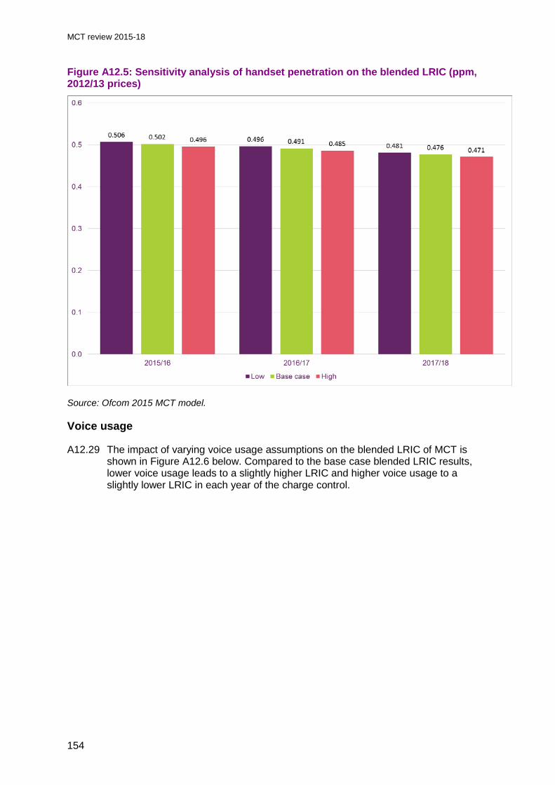
MCT review 2015-18

Figure A12.5: Sensitivity analysis of handset penetration on the blended LRIC (ppm, 2012/13 prices)

Source: Ofcom 2015 MCT model.

Voice usage

A12.29 The impact of varying voice usage assumptions on the blended LRIC of MCT is shown in Figure A12.6 below. Compared to the base case blended LRIC results, lower voice usage leads to a slightly higher LRIC and higher voice usage to a slightly lower LRIC in each year of the charge control.

154

MCT review 2015-18

Figure A12.6: Sensitivity analysis of voice usage on the blended LRIC (ppm, 2012/13 prices)

Source: Ofcom 2015 MCT model.

Data usage

A12.30 The impact of varying data usage assumptions on the LRIC of MCT is shown in Figure A12.7 below. Compared to the base case blended LRIC results, lower data usage leads to a slightly higher LRIC and higher data usage to a slightly lower LRIC in each year of the charge control.

155

MCT review 2015-18

Figure A12.7: Sensitivity analysis of data usage on the blended LRIC (ppm, 2012/13 prices)

Source: Ofcom 2015 MCT model.

Combined demand scenarios

A12.31 The impact of varying the demand parameters above in a combined manner is shown in Figure A12.8 below. This shows that the impact of our combined low demand forecasts on the blended LRIC of MCT is to increase it in all years of the charge control, relative to the base case. The corresponding combined high demand forecasts have the effect of reducing the LRIC of MCT.

A12.32 As was found in the sensitivity analysis of the 2011 MCT model and the 2014 MCT model, the LRIC of MCT is relatively insensitive to changes in demand forecasts. The greatest variation from the base case in any year of the charge control is 6% (which arises in the low demand scenarios).

156

MCT review 2015-18

Figure A12.8: Sensitivity analysis of combined low and high demand forecasts on the blended LRIC (ppm, 2012/13 prices)

Source: Ofcom 2015 MCT model.

Sensitivity analysis: technology, WACC and other assumptions

A12.33 We next test the sensitivity of the model results to non-demand assumptions and inputs, as follows:

• Exclude 4G: we exclude the deployment of the 4G network from the model.

• Vary VoLTE adoption: we vary the availability of VoLTE (4G voice) services in the model, but retain 4G data services unchanged.

• Exclude infrastructure sharing: we exclude the active infrastructure sharing assumptions in the model.

• Exclude S-RAN deployment: we exclude the use of S-RAN equipment in the model.

• WACC: we vary the value of the WACC ± 1 percentage point around the central estimate of 7.0% (pre-tax real).

• Cost trends: we vary the cost trend adjustments used for calibration in Annex 9.

A12.34 As before, these changes are first made on an individual basis and presented in the following sub-sections in comparison to the results in the model base case. We then combine these sensitivities with the demand sensitivities to create combined scenarios.

157

MCT review 2015-18

Exclude 4G

A12.35 The impact of excluding the 4G network on the blended LRIC of MCT is shown in Figure A12.9 below. It shows that excluding 4G technology slightly reduces the LRIC result in the first year of the charge control, but leads to a higher LRIC than that in the base case in subsequent years.

A12.36 We note that although the ability to exclude the 4G network is captured in the 2015 MCT model, the results of this test should be treated with caution. This is because a 2G/3G network would look very different to a 2G/3G/4G network and would, for example, be expected to have very different data traffic volumes. Although we have attempted to account for this by adjusting traffic volumes in the scenario excluding the 4G network, this is only an approximation. Since all four national MCPs have live 4G networks, we have no information on which to base forecasts for a world in which 4G technology has not been adopted.

A12.37 On the details of the LRIC results, in principle we would expect the inclusion of a newer and more efficient technology to cause the unit cost of existing services to fall. As a consequence we might not expect the exclusion of the 4G network to lead to a lower LRIC result in the first year of the charge control. However, examination of the LRIC results over a longer time period shows that this effect is transitory, with the blended LRIC of MCT in the absence of 4G technology being higher than that in the base case beyond the end of the charge control period.

A12.38 Additionally, we note that on an NPV basis, the exclusion of 4G technology increases total network expenditures, both on a forward-looking basis and over the whole life of the network. Overall, we are satisfied that the exclusion of 4G technology is behaving appropriately over the life of the modelled network.

158

MCT review 2015-18

Figure A12.9: Sensitivity analysis of excluding 4G on the blended LRIC (ppm, 2012/13 prices)

Source: Ofcom 2015 MCT model.

Vary VoLTE availability

A12.39 The impact of varying the availability of VoLTE on the blended LRIC of MCT is shown in Figure A12.10 below. As in the scenario excluding 4G technology, excluding VoLTE requires us to make additional assumptions around the traffic volumes to be carried by the 2G and 3G networks, in the absence of VoLTE.

A12.40 The impact of no VoLTE availability is to slightly reduce the blended LRIC result in first two years of the charge control, and to increase it in the final year, relative to the base case. The impact of high availability of VoLTE handsets is to increase the blended LRIC in all years of the charge control, relative to the base case.

A12.41 As we explained in the June 2014 Consultation,291 VoLTE has two offsetting effects on the components of the blended LRIC:

• 4G MCT has lower unit costs than 2G and 3G MCT so less 4G MCT increases the blended LRIC.

• Less traffic on the VoLTE network (in the limit none) typically leads to reductions in both the 2G and 3G unit LRIC of MCT because there is then higher utilisation of the 2G and 3G networks for voice traffic. This reduces the blended LRIC.

291 See paragraph A16.27 of the June 2014 Consultation.

159

MCT review 2015-18

A12.42 It appears somewhat counterintuitive that the 2015 MCT model produces a higher blended LRIC result when greater VoLTE availability is assumed. However, in much the same manner as the exclusion of 4G technology in the previous sensitivity, this effect is transitory and over a longer period the results are more intuitive. Specifically, the blended LRIC of MCT when VoLTE is excluded exceeds the blended LRIC in the base case (i.e. when VoLTE is included), which in turn exceeds the blended LRIC when VoLTE handset availability is assumed to be high.

A12.43 We also note that on an NPV basis, the greater the availability of VoLTE the lower are total network expenditures, both on a forward-looking basis and over the whole life of the network.

Figure A12.10: Sensitivity analysis of varying VoLTE availability on the blended LRIC (ppm, 2012/13 prices)

Source: Ofcom 2015 MCT model.

Exclude infrastructure sharing

A12.44 The impact of excluding infrastructure sharing on the LRIC of MCT is shown in Figure A12.11 below. This shows that compared to the base case blended LRIC, excluding infrastructure sharing leads to an increase in the blended LRIC of MCT in all years of the charge control.

160

MCT review 2015-18

Figure A12.11: Sensitivity analysis of excluding infrastructure sharing on the blended LRIC (ppm, 2012/13 prices)

Source: Ofcom 2015 MCT model.

Exclude S-RAN deployment

A12.45 The impact of excluding S-RAN deployment on the LRIC of MCT is shown in Figure A12.12 below. Compared to the base case blended LRIC result, excluding S-RAN technology increases the blended LRIC in all years of the charge control.

161

MCT review 2015-18

Figure A12.12: Sensitivity analysis of excluding S-RAN deployment on the blended LRIC (ppm, 2012/13 prices)

Source: Ofcom 2015 MCT model.

WACC

A12.46 The impact on the blended LRIC results of varying the WACC is shown in Figure A12.13 below. Relative to the base case blended LRIC, which uses a pre-tax real WACC (CPI deflated) of 7.0% (as explained in Annex 10), our low WACC assumption (6.0%) leads to a lower blended LRIC in all years of the charge control, and the high WACC assumption (8.0%) produces a higher blended LRIC in all years of the charge control.292

292 In testing the sensitivity of the results to changes in this parameter we have introduced the high and low WACC scenarios from 2009/10 (the point in time at which the WACC was changed in the 2011 MCT model), as we did in the 2014 MCT model. The reason for this is that the CPI-discounted real WACC in the 2014 MCT model for the period from 2006/7 to 2008/9 is 12.37% and that for 2009/10 to 2012/13 is 6.7%. As a result, were we not to make the WACC sensitivity change from 2009/10 onwards we would have a WACC time series that falls from 12.37% to 6.7% in 2009/10 only to increase markedly to our high WACC scenario of 8.0% in 2013/14. Large fluctuations such as this in the WACC can give rise to counterintuitive results due to the effect on economic depreciation.

162

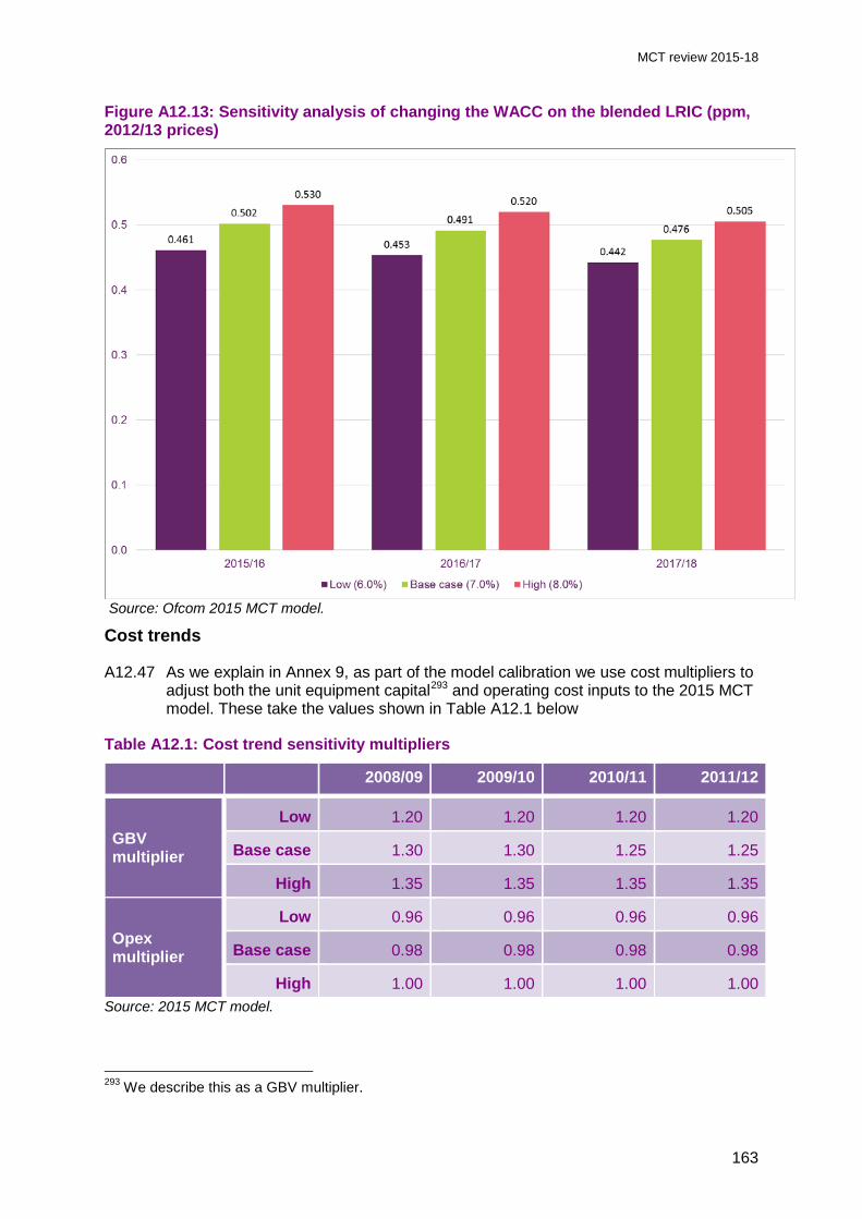
MCT review 2015-18

Figure A12.13: Sensitivity analysis of changing the WACC on the blended LRIC (ppm, 2012/13 prices)

Source: Ofcom 2015 MCT model.

Cost trends

A12.47 As we explain in Annex 9, as part of the model calibration we use cost multipliers to adjust both the unit equipment capital293 and operating cost inputs to the 2015 MCT model. These take the values shown in Table A12.1 below

Table A12.1: Cost trend sensitivity multipliers

2008/09 2009/10 2010/11 2011/12

GBV multiplier

Low 1.20 1.20 1.20 1.20

Base case 1.30 1.30 1.25 1.25

High 1.35 1.35 1.35 1.35

Opex multiplier

Low 0.96 0.96 0.96 0.96

Base case 0.98 0.98 0.98 0.98

High 1.00 1.00 1.00 1.00 Source: 2015 MCT model.

293 We describe this as a GBV multiplier.

163

MCT review 2015-18

A12.48 The impact on the blended LRIC results of varying the cost trends using the inputs in Table A12.1 is shown in Figure A12.14 below.

Figure A12.14: Sensitivity analysis of changing price trends on the blended LRIC (ppm, 2012/13 prices)

Source: Ofcom 2015 MCT model.

Base, high and low scenario: Summary of outputs

A12.49 In order to show the sensitivity of the 2015 MCT model to further combinations of parameter changes we use the sensitivities explained above to create overall high unit cost and low unit cost scenarios for the LRIC of MCT.

A12.50 The composition of these combined scenarios is shown in Table A12.2 below. We do not include our infrastructure sharing or S-RAN assumptions in the combined scenarios because these technologies are already deployed we do not consider their use to be uncertain.

164

MCT review 2015-18

Table A12.2: Assumptions used in the base case, high unit cost and low unit cost scenarios

Low unit cost scenario

Base case High unit cost scenario

Combined demand High Medium Low

WACC 6.0% 7.0% 8.0%

VoLTE availability None Medium High

Cost trends Low Medium High Source: Ofcom.

A12.51 The resulting LRIC unit costs under these combined scenarios are shown in Figure A12.15 below.

Figure A12.15: Sensitivity analysis for combined low and high cost scenarios on the blended LRIC (ppm, 2012/13 prices)

Source: Ofcom 2015 MCT model.

165

MCT review 2015-18

Annex 13

13 Brattle report This report is published separately

166