
May 2017 - ARAN - Access to Research at NUI Galway
302
Provided by the author(s) and NUI Galway in accordance with publisher policies. Please cite the published version when available. Downloaded 2022-07-12T09:35:50Z Some rights reserved. For more information, please see the item record link above. Title Experimental development and modelling of a novel auxiliary power unit for heavy trucks Author(s) Flannery, Barry Publication Date 2017-09-26 Item record http://hdl.handle.net/10379/6837
-
Upload
khangminh22 -
Category
Documents
-
view
2 -
download
0
Transcript of May 2017 - ARAN - Access to Research at NUI Galway

Provided by the author(s) and NUI Galway in accordance with publisher policies. Please cite the published
version when available.
Downloaded 2022-07-12T09:35:50Z
Some rights reserved. For more information, please see the item record link above.
Title Experimental development and modelling of a novel auxiliarypower unit for heavy trucks
Author(s) Flannery, Barry
PublicationDate 2017-09-26
Item record http://hdl.handle.net/10379/6837

1
EXPERIMENTAL DEVELOPMENT AND MODELLING OF A NOVEL
AUXILIARY POWER UNIT FOR HEAVY TRUCKS
By
BARRY FLANNERY
Supervised by
Dr. Rory Monaghan
Dr. Harald Berresheim
A thesis submitted to the National University of Ireland, Galway
in partial fulfilment for the degree of
DOCTOR OF PHILOSOPHY
Mechanical Engineering
May 2017

2
Abstract
This thesis identifies the key technical requirements for a heavy truck auxiliary power unit
(APU) and explores a potential alternative technology for use in a next-generation APU that could
eliminate key problems related to emissions, noise and maintenance experienced today by conventional
diesel engine-vapour compression APUs.
Through evaluation of alternative technologies, the work identified a free-piston Stirling engine
coupled to a zeolite-water adsorption chiller as being an effective technical solution to the range
challenges faced by the industry. A prototype test rig of this Stirling-adsorption system (SAS) was
constructed and experimentally characterised to investigated system integration dynamics and overall
performance. The adsorption chiller achieved an average COP of 0.42 ± 0.06 and 2.3 ± 0.1 kWt of
cooling capacity at the baseline test condition.
The behaviour of the Stirling and adsorption subsystems were investigated through semi-
empirical reduced order sub-models calibrated by measured experimental test data. These were
combined with fundamental physics-based sub-models of other components in the Mathworks
SimScape® environment. Using this system-level model, a series of duty cycle test scenarios were
simulated, which showed that the SAS has overall average electrical and cooling efficiencies of 8.7%
and 27.1%, respectively, compared to values of 4.7% and 11.0% for incumbent technology. The model
was also used to explore the impact of thermal coupling between the engine and chiller. The work
proposed a basic control scheme that dynamically prioritizes cooling or electrical demand in order to
meet the overall system requirements. Furthermore, the work identified that using the main truck
engine’s coolant volume as a thermal buffer tank could significantly reduce the negative impacts on
performance of low thermal buffering in the SAS architecture.
The results and experience obtained from the prototype SAS test rig demonstrates that there
appear to be no major technology barriers remaining that would prevent adoption of the SAS concept
in a next-generation APU. Although there are likely still commercial challenges facing the SAS
architecture relating to system capital cost and larger size and weight (albeit still feasible). Nonetheless,
such a system could offer reductions in exhaust emissions of greenhouse gases (GHGs), and ozone-
depleting substances, while producing less noise and requiring lower maintenance than incumbent
technologies. A system payback period is estimated to be 4.6 years.

3
Publications
Journal Publications
Development and experimental testing of a hybrid Stirling engine-adsorption chiller auxiliary power
unit for heavy trucks. B Flannery, R Lattin, O Finckh, H Berresheim, RFD Monaghan.
2017. Applied Thermal Engineering 112, 464-471
Hybrid Stirling engine-adsorption chiller for truck auxiliary power unit applications. B Flannery, R
Lattin, O Finckh, H Berresheim, RFD Monaghan. 2017. International Journal of Refrigeration 76,
356-366
System-level modelling and control of a hybrid Stirling engine-adsorption chiller auxiliary power unit
for heavy trucks B Flannery, R Lattin, O Finckh, H Berresheim, RFD Monaghan. 2017. Applied
Thermal Engineering [UNDER CONSIDERATION]
Conference Papers
B Flannery, R Lattin, O Finckh, H Berresheim, RFD Monaghan. Development and experimental
testing of a hybrid stirling engine-adsorption chiller auxiliary power unit for heavy trucks. 17th
International Stirling Engine Conference and Exhibition, Newcastle, United Kingdom, Aug 2016
B Flannery, O Finckh, H Berresheim, RFD Monaghan. Hybrid stirling engine-adsorption chiller
for truck auxiliary power unit applications. 12th IIR Gustav Lorentzen Natural Working Fluids
Conference, Edinburgh, United Kingdom, Aug 2016
Flannery B, Lattin R, Berresheim H, Monaghan RFD. Hybrid Stirling Engine‐Adsorption Chiller
for Truck APU Applications. International Stirling Engine Conference, Bilbao, Spain, Oct 2014
Poster Exhibitions
International Stirling Engine Conference 2016, Newcastle upon Tyne, UK.
NUI Galway Energy Night 2016 (1st place)
NUI Galway Energy Night 2015 (1st place)
Bernard Crossland Symposium, University of Limerick, 2014.
NUI Galway Energy Night 2014 (1st place)
International Stirling Engine Conference 2014, Bilbao, Spain (Best poster/idea award)

4
Table of Contents
Contents Abstract ................................................................................................................................................... 2
Publications ............................................................................................................................................. 3
Table of Contents .................................................................................................................................... 4
Table of Figures ...................................................................................................................................... 9
Nomenclature ........................................................................................................................................ 16
Acknowledgements ............................................................................................................................... 18
Chapter 1 – Introduction ....................................................................................................................... 19
1.1 Objectives ............................................................................................................................. 20
1.2 Thesis Layout ........................................................................................................................ 20
Chapter 2 – Finding an Alternative ....................................................................................................... 22
2.1 Chapter Overview ....................................................................................................................... 22
2.2 Background ................................................................................................................................. 22
2.3 Next-Generation APU Requirements .......................................................................................... 23
2.3.1 Cooling Capacity.................................................................................................................. 24
2.3.2 Heating Capacity .................................................................................................................. 24
2.3.3 Electrical Capacity ............................................................................................................... 25
2.3.4 Mass and Volume................................................................................................................. 25
2.3.5 Noise .................................................................................................................................... 26
2.3.6 Particulate Emissions ........................................................................................................... 27
2.3.7 Refrigerant Usage ................................................................................................................ 27
2.3.8 Fuel Type ............................................................................................................................. 28
2.3.9 Reliability and System Lifetime .......................................................................................... 29
2.3.10 System Cost and Payback .................................................................................................. 30
2.3.11 Summary ............................................................................................................................ 30
2.4 Alternative APU System Architectures ...................................................................................... 31
2.4.1 Power Generation ................................................................................................................. 32
2.4.1.1 Diesel engines ............................................................................................................... 33
2.4.1.2 Steam Engines ............................................................................................................... 34
2.4.1.3 Microturbines ................................................................................................................ 35
2.4.1.4 Organic Rankine cycle .................................................................................................. 36
2.4.1.5 Fuel Cells ...................................................................................................................... 37
2.4.1.6 Stirling engines ............................................................................................................. 40
2.4.1.7 Thermoelectric Power Generation ................................................................................ 44

5
2.4.2 Heating, Ventilation and Air Conditioning (HVAC) ........................................................... 45
2.4.2.1 Vapour-compression ..................................................................................................... 46
2.4.2.2 Stirling Cycle ................................................................................................................ 48
2.4.2.3 Air-cycle ....................................................................................................................... 50
2.4.2.4 Thermoelectric Cooling ................................................................................................ 51
2.4.2.5 Waste heat Technologies .............................................................................................. 52
2.4.3 Energy Storage ..................................................................................................................... 60
2.4.3.1 Flywheels ...................................................................................................................... 61
2.4.3.2 Lead-acid batteries ........................................................................................................ 63
2.4.3.3 Supercapacitors ............................................................................................................. 64
2.4.3.4 Flow batteries ................................................................................................................ 65
2.4.3.5 Lithium-ion batteries ..................................................................................................... 66
2.4.4 Summary .............................................................................................................................. 68
Chapter 3 – Literature Review .............................................................................................................. 71
3.1 Chapter Overview ....................................................................................................................... 71
3.2 Stirling Engine System Integration ............................................................................................. 71
3.3 Adsorption Chiller System Integration, Modelling and Testing ................................................. 76
3.4 Knowledge Gap .......................................................................................................................... 82
3.5 Research Methodology and Theoretical Framework .................................................................. 84
3.6 Motivation for this work ............................................................................................................. 85
3.7 Conclusion .................................................................................................................................. 86
Chapter 4 – Preliminary analysis of the Stirling-adsorption system ..................................................... 87
4.1 Chapter Overview ....................................................................................................................... 87
4.2 SAS Architecture ........................................................................................................................ 87
4.3 Performance of Commercially Available Hardware ................................................................... 88
4.4 Baseline Test Case ...................................................................................................................... 98
4.5 SAS Reduced Order model ......................................................................................................... 99
4.6 DEVC Reduced Order Model ................................................................................................... 101
4.7 Idling model .............................................................................................................................. 103
4.8 Sensitivity Analysis .................................................................................................................. 104
4.9 Results and Discussion ............................................................................................................. 106
4.10 Conclusion .............................................................................................................................. 106
Chapter 5 – Experimental Testing Program ........................................................................................ 108
5.1 Chapter Overview ..................................................................................................................... 108
5.1.1 Experimental Work Timeline ............................................................................................. 109
5.2 SAS Test Rig............................................................................................................................. 111

6
5.2.1 Experimental Objectives .................................................................................................... 112
5.2.2 Experimental Methodology ................................................................................................ 113
5.2.3 System Design ................................................................................................................... 115
5.2.4 Fabrication and Construction ............................................................................................. 116
5.2.5 Plumbing system ................................................................................................................ 120
5.4.5.1 Recooler Loop ............................................................................................................. 120
5.2.5.2 Chiller loop ................................................................................................................. 122
5.4.5.3 Drive loop ................................................................................................................... 124
5.2.5.4 Implementation ........................................................................................................... 127
5.2.6 Pump systems ..................................................................................................................... 131
5.2.6.1 Pump Selection ........................................................................................................... 131
5.4.6.2 Physical Implementation ............................................................................................. 131
5.4.6.3 Pump Control .............................................................................................................. 133
5.2.6.4 Electrical Systems Implementation ............................................................................. 136
5.2.6.5 Supplementary Booster Pumps ................................................................................... 137
5.2.7 Fans and Heat Exchangers ................................................................................................. 141
5.2.7.1 Air-Cooled Heat Exchangers ...................................................................................... 141
5.2.7.2 Fan Control ................................................................................................................. 143
5.2.7.3 Plate Heat Exchanger .................................................................................................. 147
5.2.8 Electric heater unit ............................................................................................................. 151
5.2.8.1 Electric Heater Version 1 ............................................................................................ 151
5.4.8.2 Electrical Heater Revision 2 ....................................................................................... 153
5.2.8.2 Electronics and Electrical Wiring ............................................................................... 156
5.2.9 Data Acquisition Systems and Programs ........................................................................... 163
5.2.9.1 Sensors ........................................................................................................................ 163
5.4.9.2 Data Acquisition Units ................................................................................................ 165
5.2.9.4 LabView ...................................................................................................................... 168
5.3 SAS Experimental Testing ........................................................................................................ 173
5.3.1 Test Methodology .............................................................................................................. 174
5.5.2 Sensor Calibration .............................................................................................................. 178
5.3.3 Error Analysis and Uncertainty .......................................................................................... 179
5.3.4 InvenSor Calibration data .................................................................................................. 180
5.3.5 Test Matrix ......................................................................................................................... 182
5.4 Results and Discussion ............................................................................................................. 185
5.4.1 Combined Stirling-adsorption system operation ................................................................ 187
5.4.2 Operation in High Ambient Conditions ............................................................................. 190
7
5.4.2.1 Heat Exchanger Sizing ................................................................................................ 190
5.4.3 Operation with Low Thermal Buffering Volume .............................................................. 196
5.5 Conclusion ................................................................................................................................ 202
Chapter 6 – System-level modelling of SAS ...................................................................................... 203
6.1 Chapter Overview ..................................................................................................................... 203
6.2 Modelling Objectives ................................................................................................................ 203
6.3 SimScape Modelling Methodology .......................................................................................... 203
6.4 DEVC SimScape Model ........................................................................................................... 206
6.5 SAS SimScape Model ............................................................................................................... 210
6.6 Truck Cabin Model ................................................................................................................... 215
6.7 Modelling Test Matrix .............................................................................................................. 216
6.8 Results and Discussion ............................................................................................................. 216
6.9 Conclusion ................................................................................................................................ 226
Chapter 7 – Discussion and Conclusion ............................................................................................. 227
7.1 Chapter Overview ..................................................................................................................... 227
7.2 CAD Modelling of SAS APU ................................................................................................... 227
7.2.1 SAS APU Physical Design ................................................................................................ 227
7.2.2 SAS APU Recooler Size .................................................................................................... 231
7.2.3 SAS APU Mass .................................................................................................................. 231
7.3 Cost Modelling of SAS APU .................................................................................................... 232
7.4 Particulate Emissions ................................................................................................................ 233
7.5 Knowledge Gap Addressed ....................................................................................................... 234
7.6 Future Work .............................................................................................................................. 236
7.7 Conclusions ............................................................................................................................... 237
Appendices .......................................................................................................................................... 239
Appendix I: Existential Threats to APUs ........................................................................................ 239
Driverless trucks ......................................................................................................................... 239
Electric APUs / Trucks ............................................................................................................... 239
Appendix II: Alternative Applications ............................................................................................ 241
Appendix III: LabView Programs................................................................................................... 242
Appendix IV: Arduino Code ........................................................................................................... 247
Appendix V: Comprehensive Test Results Matrix ......................................................................... 256
Appendix VI: Whispergen Test Rig ................................................................................................ 258
1.2.1 Whispergen Test Rig Objectives ........................................................................................ 259
1.2.2 Whispergen Test Rig Construction and Installation .......................................................... 259
1.2.3 Whispergen Data Acquisition ............................................................................................ 269

8
1.2.4 Whispergen Testing and Results ........................................................................................ 272
1.2.5 Whispergen Discussion and Conclusion ............................................................................ 275
Appendix VII .................................................................................................................................. 276
2.1 DEVC Test Rig ..................................................................................................................... 276
2.3.2 DEVC Test Rig Construction and Installation ................................................................... 277
2.3.3 DEVC Data Acquisition..................................................................................................... 284
2.3.4 Discussion and Conclusion ................................................................................................ 285
Appendix VIII ................................................................................................................................. 288
References and Bibliography .............................................................................................................. 289

9
Table of Figures Figure 1 Types of truck within the Class Eight designation. ©FHWA ............................................... 23
Figure 2 Thermo King TriPac Evolution DEVC APU. ©Thermo King .............................................. 23
Figure 3 TriPac Evolution mounted on a tractor frame rail. ©Thermo King....................................... 26
Figure 4 Truck parking lot. .................................................................................................................. 26
Figure 5 LNG fuel tank on a truck. ...................................................................................................... 29
Figure 6 DEVC APU System architecture. .......................................................................................... 31
Figure 7 Alternative APU system architectures. .................................................................................. 32
Figure 8 TriPac with DPF canister fitted onto rear of the unit. ©Thermo King .................................. 33
Figure 9 Cyclone power steam engine. ©Cyclone Power .................................................................... 34
Figure 10 MTT 3.8 kWe microturbine. ©MTT ................................................................................... 35
Figure 11 Scroll expander from a small-scale ORC machine. ©US DOE ........................................... 36
Figure 12 Eberspaecher prototype SOFC for truck APU applications. ©Eberspacher ........................ 39
Figure 13 Simplified diagram of an alpha-type KSE. .......................................................................... 40
Figure 14 Simplified diagram showing the configuration of a beta-type free-piston Stirling engine. . 41
Figure 15 The MEC 1 kWe free-piston Stirling engine. ©Microgen ................................................... 43
Figure 16 Cassini Probe GPHS-RTG. This TEG could deliver 300 W of electrical power. ©NASA 44
Figure 17 TM16 swash-plate compressor used in the Thermo King TriPac APU. The compressor
weighs only 4.9 kg without the clutch and can deliver up to 3.8 kW of cooling capacity at a COP of
1.4. ........................................................................................................................................................ 47
Figure 18 Ricor K508 tactical Stirling cryocooler with 440 mW of cooling capacity at 77 K. ©NASA
.............................................................................................................................................................. 49
Figure 19 Large turbofan engine on a modern aircraft. The main engine compressor section is an
ideal source of compressed air to drive a refrigeration cycle. In practical systems, a relatively small
quantity of compressed air is extracted through bleed valves. ©NASA ............................................... 50
Figure 20 Thermoelectric cooling devices for electronic chips. ©NASA ........................................... 51
Figure 21 Energy flow diagram comparing a DEVC system against a system utilizing waste heat ... 52
Figure 22 General overview of the absorption cooling process for lithium bromide-water © US
Department of Energy ........................................................................................................................... 55
Figure 23 Working principle of an adsorption chiller machine. .......................................................... 57
Figure 24 NASA G2 Flywheel has 525 Wh of energy storage and 1 kW output power. ©NASA ..... 61
Figure 25 Thermo King lead-acid battery used in their APU products. ©Thermo King ..................... 63
Figure 26 A range of supercapacitors from Maxwell Technologies. ©Maxwell Technologies .......... 64
Figure 27 Lithium-ion battery cost vs. energy density trends. ©JCESR ............................................. 66
Figure 28 Tesla Model S Battery Pack. ©Jason Hughes ..................................................................... 67
Figure 29 System-level architecture diagram of the SAS concept. This diagram is for illustrative
purposes only and does not depict minor plumbing.............................................................................. 69
Figure 30 Advanced prime mover architecture consisting of a SOFC driving a hermetically sealed
electric compressor. The refrigeration cycle would use either CO2 or a hydrocarbon as refrigerant. .. 69
Figure 31 Variation of Whispergen PPS16 Stirling engine electrical power output with temperature
difference [274]. .................................................................................................................................... 72
Figure 32 Variation of engine power output with changing cold-end temperature [275] .................... 73
Figure 33 Dynamic behaviour of an adsorption chiller's sorption beds [190]. .................................... 74
Figure 34 System architecture proposed by Verde et al [192, 193]. .................................................... 78
Figure 35 System-architecture proposed by Ali et. al [186]. ............................................................... 79
Figure 36 Truck engine exhaust heat driven adsorption system architecture proposed by Zhong et al
[280]. ..................................................................................................................................................... 80
Figure 37 Experimental data showing key adsorption chiller performance by Vasta et al [277]. ....... 81

10
Figure 38 TOPMACS system architecture as proposed by Verde et al [190]. .................................... 82
Figure 39 System-level architecture diagram of the SAS concept. This diagram is for illustrative
purposes only and does not depict minor plumbing. For a detailed overview of the adsorption chiller
internal plumbing, in particular with reference to heat recovery, the reader is directed to the system
characterised by Myat et al. [281]. ........................................................................................................ 88
Figure 40 View across part of the engine test facility at Microgen Engine Corporation’s R&D facility
in Peterborough, UK. © Barry Flannery ............................................................................................... 89
Figure 41 Cutaway of the MEC 1 kWe linear free-piston Stirling engine and CAD render showing the
full system and wiring. Note that the engine’s combustor is not installaed. © Microgen Engine
Corporation ........................................................................................................................................... 90
Figure 42 View of the Whispergen PPS16 kinematic Stirling engine test rig at NUI Galway set up as
part of the author’s B.Sc thesis. ............................................................................................................ 91
Figure 43 View of CS Centro Stirling, the Mondragon Corporation Stirling engine R&D facility, near
Bilbao, Spain. © Barry Flannery .......................................................................................................... 92
Figure 44 A prototype mockup of the 3 kWe kinematic Stirling is shown on the left and the 1 kWe
Mk.5 natural gas micro-CHP engine is shown on the right. Both machines were being developed by
Mondragon at CS Centro Stirling. ©Barry Flannery ............................................................................ 93
Figure 45 View of the building where InvenSor GmbH’s R&D facility is co-located with other small
businesses. © Barry Flannery ............................................................................................................... 94
Figure 46 View of two APU scale prototype adsorption chillers at InvenSor GmbH’s R&D facility in
Berlin, Germany. (a) is a 3 kW unit and measures 600 x 250 x 800mm and weighs 90 kg and (b) is
1000 x 550 x 450mm and has been integrated with a micro-organic Rankine cycle machine which is
very similar to the SAS architecture. .................................................................................................... 95
Figure 47 Diagrammatic overview of the general adsorption process that is used in the InvenSor
machines reproduced from Myat et al. ©Elsevier ................................................................................ 96
Figure 48 Detailed overview of each phase of the adsorption-desorption cycle within the InvenSor
machine reproduced from Myat et al. ©Elsevier. ................................................................................. 97
Figure 49 Energy flow diagrams for a DEVC and the SAS system utilizing waste heat. ................... 99
Figure 50 Logical structure of the DEVC APU model. ..................................................................... 102
Figure 51 Critical parameters defining the dynamic behaviour of the DEVC system. ...................... 102
Figure 52 Sensitivity analysis of the key variables affecting lifetime payback. ................................ 105
Figure 53 Overview of the three engine test rigs. The Microgen FPSE is visible on the left, the
Whispergen in the centre and TriPac Evolution APU on the right. Note that FPSE test rig was later
expanded into the SAS. ....................................................................................................................... 109
Figure 54 Overview of the full SAS test rig. ..................................................................................... 110
Figure 55 Overview of the SAS test rig. The key components visible are: (1) header tanks, (2)
propane fuel supply, (3) FPSE control electronics, (4) DC pump control box, (5) recooler heat
exchanger and blowers, (6) InvenSor adsorption chiller control panel, (7) free-piston Stirling engine
and (8) gas flowmeter. ........................................................................................................................ 111
Figure 56 Overview of the SAS test rig. The key components are: (1) DC pumps, (2) variable
frequency drives for three-phase pumps, (3) three-phase pumps, (4) free-piston Stirling engine, (5)
cab chiller heat exchanger and fans and (6) engine exhaust ducting. ................................................. 112
Figure 57 General architecture of the SAS experimental setup. ........................................................ 113
Figure 58 Adsorption chiller (left) and free-piston Stirling engine (right) as received from suppliers.
............................................................................................................................................................ 116
Figure 59 Initial SAS test rig concept (many auxiliary support systems not shown). ....................... 117
Figure 60 Revised SAS test rig design showing Stirling engine (left) and adsorption chiller (right) 118
Figure 61 Construction sequence for the SAS test rig frames. .......................................................... 119
Figure 62 Theoretical plumbing required in a final production SAS APU. ....................................... 120

11
Figure 63 Initial recooler plumbing circuit design. ............................................................................ 121
Figure 64 Final recooler loop plumbing design ................................................................................. 122
Figure 65 Initial design of the chiller loop. ........................................................................................ 123
Figure 66 Final chiller loop design. ................................................................................................... 123
Figure 67 SAS drive loop plumbing version 1. .................................................................................. 124
Figure 68 SAS drive loop plumbing version 2. .................................................................................. 125
Figure 69 SAS drive loop plumbing version 3. .................................................................................. 126
Figure 70 SAS drive loop plumbing final version. ............................................................................ 126
Figure 71 (top) right-angle fittings for pipe entry into pumping box, (middle) completed pumping
plumbing prior to insulation and (bottom) system header tanks. ........................................................ 128
Figure 72 (a) engine plumbing showing valves and copper pipework, (b) adsorption chiller bypass
valves, (c) central cable tray spine used to support header tanks, (d) pipes routed along spine. ........ 129
Figure 73 (a) primary plumbing connections with the adsorption chiller, (b) alternate view of primary
plumbing connections with adsorption chiller, (c) engine plumbing and valves and (d) recooler loop
valves and drainage point. Colour code: red (drive loop), blue (chiller loop) and green (recooler loop).
............................................................................................................................................................ 130
Figure 74 The pressure-flowrate curves for (left) Davies Craig EBP 25 and (right) Davies Craig EWP
80 pumps. ............................................................................................................................................ 131
Figure 75 CAD render of proposed pump installation ....................................................................... 132
Figure 76 Actual hardware implementation of the pumping system. ................................................ 133
Figure 77 (left) CAD Render of the pump drive electronics and (right) four separate Pololu 18V15
motor controllers. The key components are: (1) three 12V 3A PSUs, (2), 12V 10A PSU, (3) terminal
blocks, (4) Pololu motor controllers and (5) CR3000 datalogger. ...................................................... 134
Figure 78 Block diagram showing the operation and layout of the DC pump controller box. .......... 135
Figure 79 Construction of the pump controller box in the author’s electronics workshop. ............... 136
Figure 80 Actual layout of the DC pump controller box. Refer to Figure 81 for description of items.
............................................................................................................................................................ 136
Figure 82 Performance curve for Pedrollo pumps. Note discharge curve for CP130 and red region
showing the expected requirement for SAS test rig. ........................................................................... 137
Figure 83 (left) CAD render of proposed variable frequency drive enclosure and (right) actual
implementation of the three separate VFDs. ....................................................................................... 138
Figure 84 Block diagram showing the operation of the inverter drive system. ................................. 139
Figure 85 Actual implementation of the CP130 pumps. .................................................................... 140
Figure 86 Different types of heat exchangers available on-hand from the Thermo King factory in
Galway. ............................................................................................................................................... 141
Figure 87 Recooler air-cooled heat exchanger with blower fans. Note poor fan area coverage. ....... 142
Figure 88 Chiller loop air-cooled heat exchanger (lower centre) with blower fans. .......................... 143
Figure 89 CAD render of the fan control system. The major components are: (1) Omron PSU, (2)
Electromen motor drivers, (3) terminal blocks, (4) Arduino Mega 2560 and (5) terminal blocks. .... 143
Figure 90 Block diagram showing the control scheme for the chiller and recooler fans. .................. 145
Figure 91 (left) fan enclosure internals and (right) fan controller front panel controls. .................... 146
Figure 92 Low-cost 125 kW plate heat exchanger. ............................................................................ 147
Figure 93 Recooler loop temperature profile with air-cooled heat exchanger. Coolant flowrate is
approximately 1000 l/h and heat input to the system 6.5 kWt ............................................................ 148
Figure 94 Recooler loop temperature profile with the liquid cooled plate heat exchanger. Coolant
flowrate is approximately 1500 l/h and heat input to the system is 5 kW. ......................................... 148
Figure 95 Raw data showing variation in laboratory cold water supply. ........................................... 149
Figure 96 Raw data showing variation in solar PV output for author’s home solar panels. The time
period in this graph correlates with the period shown in Figure 95. .................................................. 150

12
Figure 97 (top left) CAD render of the heater core with the serpentine flow path through the heater
core, (top right) CAD render of the entire electric heater unit and (bottom) actual heater core with
heater elements visible to the left. The heater elements are inserted on the right-hand side of the
assembly. ............................................................................................................................................. 152
Figure 98 Characteristic “pin-hole” blowout failures on the immersion heater elements. This type of
failure is indicative of localized spot-heating caused by poor cooling flow. ...................................... 153
Figure 99 (left) CAD render of revised heater design (right) Large 12 kW immersion heater with
lower surface power flux. ................................................................................................................... 154
Figure 100 Schematic showing the design of the heater frame. ......................................................... 155
Figure 101 Fabrication of the revised electric heater unit. ................................................................. 156
Figure 102 Control scheme for varying the electric heater power output. ......................................... 157
Figure 103 (top) circuit diagram for the triac power control circuit and (bottom) physical breadboard
implementation. .................................................................................................................................. 158
Figure 104 Debugging phase of the heater power electronics. The key components are (1) single
phase heater, (2) triac power stage, (3) power electronics driver board and (4) oscilloscope. ........... 159
Figure 105 Overall electrical block diagram for the high power electric heater. ............................... 161
Figure 106 Physical layout of the electric heater internals. ............................................................... 162
Figure 107 (left) overview of the completed electric heater revision 2 and (right) electric heater
actually operating during a test. Note the current being pulled by each leg of phase on the panel meter
and green diagnostic LEDs. ................................................................................................................ 162
Figure 108 (left) external clamp on thermistors and (right) immersion type thermistors. ................. 164
Figure 109 (left) final installed external clamp on thermistor and (right) installed immersion
thermistor. ........................................................................................................................................... 164
Figure 110 Huba Control Type 210 DN15 flowmeter capable of reading liquid flow in the range of 3-
50 litres per minute. ............................................................................................................................ 165
Figure 111 U6P diaphragm gas flowmeter (front centre). ................................................................. 165
Figure 112 (left) Agilent 34972A data acquisition unit and (right) Campbell Scientific CR3000
datalogger. ........................................................................................................................................... 166
Figure 113 Lab test PC ....................................................................................................................... 167
Figure 114 Lab networking infrastructure and data acquisition layout.............................................. 168
Figure 115 Real-time display of data on Lab test PC. (Top-left) real time chiller capacity, (top-right)
heat rejection temperatures, (bottom-left) COP and (bottom-right) system temperatures. ................. 168
Figure 116 Microgen Engine Corporation LabView data acquisition program. Note that the author
made some minor modifications to the program so as to include thermal efficiency, fuel input and
overall system efficiency. ................................................................................................................... 169
Figure 117 Front panel display of the unified LabView data acquisition program............................ 170
Figure 118 Unified LabView data acquisition program block diagram. ............................................ 171
Figure 119 InvenSor GmbH adsorption machine physical front panel display. ................................ 172
Figure 120 Burner ceramic liner failure. The ceramic (visible in white on the left) has detached from
the shell house (right image). The remains of the ceramic collar at the exhaust vent is still visible in
the right hand photo where the failure occurred. ................................................................................ 173
Figure 121 DC Pump control box manual (left) and fan control box (right). The respective speeds are
adjusted using the front panel potentiometers. The fan control box also has a manual/auto selector that
can enable PID setpoint control. However this was not used during testing as manual control was
sufficient. ............................................................................................................................................ 174
Figure 122 (left) 12 kW electric heater in background, foreground shows the heater fans used to load
the chiller circuit of the adsorption chiller and (right) the manual lever valve controlling the flow of
water into the plate heat exchanger which controls the recooler inlet temperature. ........................... 175

13
Figure 123 Test data showing a period of local dynamic equilibrium. Single data-points are obtained
by taking an average of the data in this time window. ........................................................................ 176
Figure 124 Data showing the impact of building water temperature on recooler flowrate. The effect is
milder at high recooling temperatures. ............................................................................................... 177
Figure 125 Raw data of a particularly dire day of testing showing the extent of the variability in lab
water supply temperature. None the data obtained on this day was usable. ....................................... 177
Figure 126 Ice-bath calibration process for the temperature sensors. ................................................ 178
Figure 127 Data from chiller loop temperature sensor calibration. ................................................... 179
Figure 128 Initial InvenSor GmbH calibration data for the adsorption machine. .............................. 181
Figure 129 (left) Vacuum maintenance being performed on the adsorption machine and (right) the
vacuum purge valve. The vacuum pump is visible on top of the machine and is being used to remove
inert gases from the system. ................................................................................................................ 181
Figure 130 Variation of cooling capacity with increasing recooler inlet temperature. ...................... 182
Figure 131 Start-up dynamics of Stirling engine during independent operation. This test corresponds
to test C1 in the test matrix. ................................................................................................................ 185
Figure 132 Start-up dynamics of the Stirling engine as a part of the SAS. ........................................ 186
Figure 133 Adsorption chiller start-up dynamics when driven by electric heater. ............................ 187
Figure 134 (a) Stirling engine power spikes induced by thermal loading from the adsorption chiller
unit during coupled operation. This data was obtained using the Stirling engine independently without
the electric heater element. (b) Stirling engine efficiency spikes are the root cause of the power spikes
shown in (a)......................................................................................................................................... 188
Figure 135 Operation of the adsorption chiller when driven by the Stirling engine. Note that the Tri is
set very low simulating a cool ambient. Compare the similarities in graph with Figure 136 for a visual
comparison between Stirling engine and electric heater operation. .................................................... 189
Figure 137 Typical COP performance of adsorption chiller. Note that the breaks in the data, denoted
by grey bars are non-physical spikes which have been trimmed out for clarity. They are caused by
time lag between sensors. The average COP, shown as a red line is calculated at 0.42. .................... 190
Figure 138 Variation in cooling capacity with increasing ambient temperature for SAS and DEVC
systems. The adsorption chiller is undersized in comparison to the DEVC system. .......................... 196
Figure 139 Typical adsorption chiller performance characteristics. Note feedback pulsations on Tdi
loop. These data were obtained using the electric resistance heater. .................................................. 197
Figure 140 Experimental data showing high (a) and low (b) buffer adsorption chiller systems. ...... 198
Figure 141 Detailed buffering model of the SAS implemented in SimScape. Refer to [281] for a
comprehensive overview of the valve configuration used in the adsorption chiller submodel. ......... 199
Figure 142 Valve configuration within the adsorption chiller core plumbing submodel................... 199
Figure 143 Theoretical modelling results showing the impact of coolant volume on the recovery slope
of Tdi. ................................................................................................................................................... 200
Figure 144 The impact of buffering volume on temperature swing (a) and the impact of driving
temperature on capacity (b)................................................................................................................. 201

14
Figure 145 Critical parameters defining the dynamic behaviour of the DEVC system.
...... 208
Figure 146 Structure of the DEVC Simulink model. ......................................................................... 208
Figure 147 Implementation of the DEVC model within the Simulink environment. Note the orange
lines represent SimScape physical signals and the correlations are shown by “f(u)” blocks. ............ 209
Figure 148 Reduced-order model datasets for the Stirling engine and adsorption chiller subystems.
............................................................................................................................................................ 211
Figure 149 Structure of the SAS model. ............................................................................................ 212
Figure 150 SimScape block diagram of the recooler submodel showing the heat exchanger block. 213
Figure 151 High level overview of the SAS model within SimScape. .............................................. 214
Figure 152 SimScape Truck Cabin Model ......................................................................................... 215
Figure 153 Results of static external ambient temperature and electrical load input scenarios from
system-level model. ............................................................................................................................ 218
Figure 154 Impact of constantly increasing (a) and decreasing (b) external ambient temperatures on
fuel consumption and cab temperature. .............................................................................................. 220
Figure 155 High external ambient temperature sinusoidal profile with varying electrical load profiles.
............................................................................................................................................................ 222
Figure 156 Low external ambient temperature sinusoidal profile with varying electrical load profiles.
............................................................................................................................................................ 223
Figure 157 This figure shows the behaviour of the control algorithm for a specific scenario. Areas
shaded in grey indicate electrical prioritization and white areas indicate cooling prioritization. ....... 226
Figure 158 CAD Render of the proposed SAS APU. (1) electronics enclosure, (2) header tanks, (3)
circulation pumps, (4), flow control valves, (5) free-piston Stirling engine and (6) Stirling engine
blower and gas venturi assembly. ....................................................................................................... 228
Figure 159 CAD render of the SAS enclosure mounted on a tractor frame rail (left of fuel tank). ... 230
Figure 160 Engineering schematic of the SAS vs. DEVC APUs. ..................................................... 230
Figure 161 Comparison of the DEVC and SAS APU recooler and condenser sizes. The SAS recooler
is light grey rectangle and the DEVC condenser is the darker inset rectangle. The vehicle on the left is
a US Class-8 truck and the one on the right is a Euro truck. .............................................................. 231

15
Figure 162 Photograph of preliminary Whispergen test rig as part of the author’s undergraduate final
year project. Note untidy plumbing and immobility of the test rig. .................................................... 258
Figure 163 CAD render of the revised Whispergen test rig. .............................................................. 260
Figure 164 Flowchart outlining the back-end infrastructure that was required to fabricate the test rigs.
............................................................................................................................................................ 260
Figure 165 (top) delivery of welding table top plate, (left) conversion of manual mill to CNC mill,
(right) control electronics for CNC mill. ............................................................................................ 261
Figure 166 (top) three-phase electric power installation, (left) Stick/TIG welding and plasma cutting
system (right) construction of custom trolley cart for system ............................................................. 262
Figure 167 (top-left) drill press and bandsaw, (top-right) lathe and (bottom) general overview of
workshop where all test rigs were built. ............................................................................................. 263
Figure 168 (a) Niall Chambers receiving guidance on how to operate a horizontal band saw at the
author’s home workshop (b) partially completed Whispergen test rig frame ..................................... 264
Figure 169 Design drawing of the Whispergen test rig frame. .......................................................... 265
Figure 170 Overview of the plumbing connections on the Whispergen test rig. ............................... 267
Figure 171 Overview of the completed Whispergen PPS16 test rig. The major system components are
as follows; diesel header tank (1), coolant header tank (2), Whispergen PPS16 engine (3), electric
heater load (4), 24 VDC to 220 VAC inverter (5), lead-acid batteries (6), engine controller (7) and
plumbing connections (8). .................................................................................................................. 268
Figure 172 (a) silicone thermocouple seal and (b) epoxy resin thermocouple seal. .......................... 270
Figure 173 Block diagram of the Whispergen test rig LabView data acquisition program. .............. 271
Figure 174 Thermodynamic diagram of the Whispergen Stirling engine. © Niall Chambers[282] .. 272
Figure 175 Niall Chambers conducting experimental tests with the Whispergen engine. ................. 273
Figure 176 System start-up and shut down characteristics. ............................................................... 274
Figure 177 Variation in thermal heat output versus coolant loop temperature. ................................. 274
Figure 178 Bare APU engine as received requiring a test stand ........................................................ 277
Figure 179 CAD render of the proposed DEVC test stand. ............................................................... 278
Figure 180 Design drawing of the DEVC test rig. ............................................................................. 279
Figure 181 DEVC test rig frame during construction at the author’s workshop. .............................. 280
Figure 182 Complex APU accessories and harnesses undergoing installation. ................................. 281
Figure 183 Improved battery wiring setup using dedicated enclosures and cable entry glands. ....... 282
Figure 184 DEVC test rig front panel. The components are as follows; (1) condenser assembly, (2)
control electronics, (3) cab chiller intake, (4) cab chiller blowers, (5) cab heater blower duct, (6) HMI,
(7) refrigerant dryer and (8) DPF indicator and regeneration control switch. .................................... 283
Figure 185 Complete DEVC test rig. The key components are as follows: (1) diesel engine, (2)
condenser assembly, (3) cab evaporator assembly, (4) diesel fuel tank, (5) lead-acid batteries, (6)
HMI, (7) control electronics and (8) diesel fuelled heater. ................................................................. 283
Figure 186 Overview of the TriPac Evolution PC-based controller interface. .................................. 285
Figure 187 Design drawing for the ACS frame (sheet metal not included). ...................................... 287
Figure 188 Design drawing for the FPSE frame (sheet metal not included). .................................... 288

16
Nomenclature
Nomenclature Subscripts
di drive inlet Abbreviations do drive outlet
APU auxiliary power unit ri recooler inlet
DEVC diesel engine-vapour compression ro recooler outlet
SAS Stirling-adsorption system ci chiller inlet
COP coefficient of performance co chiller outlet
NTC negative temperature coefficient cab truck cab
LMTD log-mean temperature difference amb ambient
EPA Environmental Protection Agency cool cooling capacity
IPCC Intergovernmental Panel on Climate
Change
input heat input
SOFC Solid-oxide fuel cell c chiller flow
PEM Proton exchange membrane d drive flow
Q heat transfer (W) w water
ṁ mass flowrate (kg s-1) k kinetic
cp specific heat capacity (J kg-1 K-1) tot total l cab load
T temperature (°C) par parasitic Physical
Quantities e electrical
E f Fuel
i moment of inertia (kg m2) wh waste heat ω rotational speed (rad s-1) dr driving heat
C capacitance (F) com compressor
V voltage (V) alt alternator
P power (W) m mechanical
η efficiency pri Primary
I current (A) sec secondary
R resistance (Ω) p,pri primary specific heat
capacity
UA overall heat transfer coefficient (W
m-2)
p,sec secondary specific
heat capacity
k thermal conductivity (W m-1 K-1) net net
A area (m2) p,w Specific heat
capacity water p pressure (N m-2) r recooler
Nu Nusselt number input input
D Characteristic diameter (m) conv convective
g Gravitational acceleration (m s-2) cond conductive
Δz Change in height (m)
rad radiative
I’ Moment of inertia (kg m2) h total heat input

17

18
Acknowledgements
The author is extremely grateful for the continued support, patience and assistance of his two
advisors Dr. Rory Monaghan and Dr. Harald Berresheim without whom, this project would not have
taken place. The author also acknowledges and is thankful for the financial support of Ingersoll Rand
International and Thermo King for financially supporting this project and providing technical assistance
where needed. In particular the author would like to thank Ken Gleeson who has been instrumental
throughout the entire PhD and even the author’s undergraduate projects. The author also thanks Oliver
Finckh, Bernd Lipp, Robert Lattin Peter Loomis and Stephen DeLarosby for their support.
This research would not have been possible without the scholarship funding from the Irish
Research Council under the Enterprise Partnership Scheme (project reference: EPS/PG/579).
The author also offers thanks to Dave Clark and Adam Green of Microgen Engine Corporation
for their support over the years in seeing this research project through. Likewise, the author thanks Dr.
Niels Braunschweig, Makis Kontogeorgopolis and Robert Vieweg of InvenSor GmbH who also
provided extensive support for the project.
The author also thanks NUI Galway technicians Bonaventure Kennedy, Patrick Kelly and Aodh
Dalton for their support through the experimental phases of the research.
Finally, the author thanks his parents for their support throughout his research without whom
the author would not be in a position to take on the formidable burden of a PhD research program.

19
Chapter 1 – Introduction
Climate change is widely recognised as being one of the greatest challenges faced by mankind
today [1]. Manmade emissions of CO2 are having a direct measureable impact on the atmosphere and
are responsible for increasing the greenhouse effect which is raising average global temperatures
resulting in a shift in weather and climate patterns. The Intergovernmental Panel on Climate Change
(IPCC) expects that these shifts are contributing to more severe storms, longer droughts and increased
rainfall and flooding [1].
If unmitigated, climate change has the potential to displace hundreds of millions of people from
coastal regions, through rising sea levels, and cause massive disruption to marine and land ecosystems
such as corals and rainforests. The US Department of Defence has identified climate change as being a
major future threat to national security and global stability [2]. In fact, some scholars believe that many
of today’s conflicts in places such as Syria, Iraq and Sudan have underlying root causes related to water
and food scarcity, both of which are exacerbated by climate change [3].
It is clear that the scientific and engineering community have a clear role to play in tackling
climate change by developing cleaner next-generation technologies that will reduce the emissions of
CO2 and other harmful gases from industrial activity.
The World Energy Council (WEC) estimated that the global transport sector consumed about
19% of global energy supplies1, of which, heavy trucks accounted for 3.2% of global consumption [4].
The WEC also estimated that 96% of this energy was derived from oil. Consequently, increasing energy
efficiency and utilization within the heavy truck transportation sector will play an important role in
reducing greenhouse gas emissions and combatting climate change.
The Federal Motor Carrier Safety Administration imposes mandatory driving limits and rest
periods for truck drivers in the United States [5]. During these mandatory rest periods, truck drivers idle
the main truck engine on average for 1860 hours per year, to provide for “hotel loads” [6]. Typically,
this hotel load consists of a space heating load, cab air conditioning load and electrical power load for
appliances such as refrigerators, cookers and electronic devices within the cab. In many US states, idling
has been heavily restricted through legislation because it is highly fuel inefficient, polluting and adds
significant unnecessary wear to the main truck engine [7]. To avoid idling the main engine, a smaller,
more suitably sized diesel engine and vapour compression (DEVC) air conditioning system is used
instead. Such a system is known as an auxiliary power unit (APU). There are a number of alternative
idle reduction (IR) technologies to DEVC APUs such as fuel cells, direct-fired heaters, thermal storage,
1 Global energy supplies includes all forms of primary energy sources in use in the world today such as fossil
fuels and renewables.

20
battery-powered heating/air conditioning, truck stop electrification, shorepower2 solutions and truck
energy recovery systems. However, DEVC APUs have the widest adoption and can provide cab heating,
air conditioning and electrical power within a single package. For these reasons they are the main focus
of this research.
Diesel engine combustion is intrinsically noisy and produces relatively high levels of unwanted
emissions such as diesel particulates, carbon monoxide (CO) and oxides of nitrogen (NOx). Government
bodies, such as the California Air Resources Board, regulates these emissions and requires that all diesel
engine APUs incorporate expensive exhaust after-treatment systems such as diesel particulate filters
[8]. The cost of these aftermarket components is significant and can be up to 30% of the total APU cost.
DEVC APUs also use environmentally damaging hydrofluorocarbons (HFCs) such as R-134a
as refrigerants in the air conditioning subsystem which are in the process of being phased down by the
impending Montreal Protocol [9]. Alternative refrigerant technologies such as CO2 or hydrocarbons
face efficiency and safety challenges respectively meaning that the long-term viability of DEVC
technologies is uncertain.
1.1 Objectives
The purpose of this research is to identify a next-generation truck APU solution that addresses
the core existential challenges facing today’s diesel fuelled APU technology, namely emissions
compliance, refrigerant usage and noise. Additionally, the final chosen solution should offer superior
performance in terms of fuel saving compared to the leading DEVC solution used today.
The specific research objectives are to:
1. Derive system requirements for a next-generation APU.
2. Identify alternative APU system architectures that meet requirements.
3. Choose the best architecture.
4. Evaluate the potential performance of this architecture based on available data.
5. Construct and experimentally test a prototype system and measure its performance.
6. Model and extrapolate system performance across the APU operating envelope and
benchmark versus DEVC technology.
1.2 Thesis Layout
The thesis is broadly laid out to sequentially address each of the above objectives. Chapter 1 has
introduced the background and high level motivation for investigating alternative APU architectures.
Chapter 2 outlines the detailed technical requirements that a future system needs to meet in order to be
2 Shorepower refers to truck stop based solutions whereby electrical power is provided to the cab via a cable or
air conditioning is provided via a dedicated external duct.

21
viable and then eliminates many competing technologies that fail to meet the pre-defined criteria. The
Stirling-adsorption system (SAS) architecture is introduced at the conclusion of this chapter. Chapter 3
conducts a literature review into SAS related technology and research and clearly defines a gap in
knowledge in the current state of the art that will be addressed by the work presented in this thesis.
Chapter 4 presents preliminary modelling results that attempt to predict overall system performance
using a first-order analysis based on publicly available data. Chapter 5 discusses the extensive
experimental test program that was conducted to prove that the SAS concept is viable and also to
measure its actual performance. Chapter 6 presents system level modelling results that answer some
key remaining questions uncovered during experimental testing. Finally Chapter 7 provides an
overview of the proposed SAS APU along with some technical discussion related to geometric and cost
requirements followed by an overall conclusion to the research.

22
Chapter 2 – Finding an Alternative
2.1 Chapter Overview
The purpose of this chapter is to outline the requirements for a diesel-fuelled next-generation
APU for heavy trucks and to identify potentially suitable candidate technologies that could fulfil those
requirements. The chapter begins by clarifying what is meant by the term “heavy truck” and then
proceeds to list and discuss the diverse range of requirements that a future APU will need to meet. These
requirements are then used as a filtering mechanism to evaluate alternative prime-mover, HVAC and
energy storage technologies. Each respective technology is discussed and their key advantages and
disadvantages are listed in relation to the APU application. Finally, a summary decision is made which
identifies the most promising future architecture based on the requirements and available technologies.
2.2 Background
All aforementioned and subsequent references to “trucks” specifically relate to Class 8 heavy
goods vehicles as defined by the Federal Highways Administration in Figure 1, which is the single
largest use case for APUs and the target market in this research. The focus on the US market is due to
the fact that APUs are largely sold and marketed in the US. There are a number of potential reasons for
this, the most important of which is the availability of physical space on a typical US truck chassis to
house the APU system. Furthermore, the greater distances between US cities results in longer travel
times.
The reason for this lack of space on European trucks is that they have lower legal maximum
length than in the US. This is why many US trucks feature a nose cone style engine mounting whereas
European trucks feature cab-over style truck cabs. This more compact cab and tractor enables larger
trailers and thus increased payload and earning potential. A number of attempts have been made to
introduce APUs into the European market but the absence of space on the frame rail usually means that
a smaller fuel tank must be installed to accommodate the APU, thus reducing overall vehicle range.
This requirement does not appeal to most customers and European APUs have not been commercially
successful.
The second reason is that driver comfort is significantly more valuable in the US where driver
retention is a serious problem and the costs for training a new truck driver in the US can range from
$5,000-8,000. This places a tangible value on driver comfort as unhappy drivers are much more likely
to quit or move to alternative fleet operators.

23
Figure 1 Types of truck within the Class Eight designation. ©FHWA
2.3 Next-Generation APU Requirements
The DEVC APU market is mature with limited product differentiation between competing
manufacturers. All DEVC APUs are fundamentally the same, whereby they consist of a diesel engine,
alternator/generator, refrigeration compressor and lead acid battery. The only notable distinction
between DEVC APUs is the system architecture choice of direct drive versus diesel-electric. Direct
drive is where the compressor and auxiliary loads are mechanically driven by the engine whereas, in
diesel-electric APUs, the engine drives a large generator whose electrical power subsequently drives
the compressor and auxiliaries. There are benefits and disadvantages to both architectures. Direct drive
offers higher system efficiency but prevents the use of hermetically sealed compressors and also forces
the use of a small automotive alternator, which tends to have poorer efficiency when compared to a
larger permanent magnet generator. Electrified solutions have the advantage of being able to
independently power all auxiliary loads and the refrigeration compressor can have a greater amount of
operational flexibility as it is decoupled from the engine operating speed. The direct drive TriPac
Evolution, shown in Figure 2, manufactured by Thermo King is the market leading APU solution and
is used as the performance benchmark for evaluating alternative solutions.
Figure 2 Thermo King TriPac Evolution DEVC APU. ©Thermo King

24
2.3.1 Cooling Capacity
The amount of cooling capacity that an APU can deliver is crucial to overall driver comfort.
An APU system with insufficient cooling capacity will result in poor pull-down3 performance and
uncomfortably high cab temperatures in high outside temperature (high ambient) conditions. The
precise amount of cooling capacity needed depends strongly on the particular truck model. Differences
in insulation, window tinting, blinds and cab exterior paint colour can make a dramatic difference in
thermal loading. Significant research has been performance by the National Renewable Energy
Laboratory into truck cabin thermal modelling and the impact of various thermal load reduction
strategies [10, 11]. Improved insulation can reduce truck cabin thermal loading by up to 35% [12].
The TriPac Evolution has 3.8 kW of cooling capacity at the ARI STD 310/3804 condition of
35 °C ambient and 26.6 °C cabin [13]. The TriPace, an electric APU also offered by Thermo King has
a cooling capacity of 2.2 kW. The TriPace model has received customer complaints in relation to
insufficient capacity whereas no complaints have been received for the TriPac Evolution. This indicates
that the true capacity requirement for the majority of truck owners in somewhere between 2.2 - 3.8 kWt.
For purposes of developing a next-generation system, it is technically safer to aim for the higher end of
the capacity spectrum as excess capacity will not be noticed by the customer. In contrast, poor capacity
was a significant factor in the low commercial adoption of TriPace electric APUs. Therefore, it is
paramount that any alternative architectures be able to deliver sufficient capacity to match or exceed
the performance of TriPac Evolution.
2.3.2 Heating Capacity
Cab heating is typically provided by a supplementary diesel-fired air heater such as those
offered by Webasto and Eberspaecher [14]. Alternative strategies such as reverse-cycle air conditioning
or heat pumping are not implemented due to reasons of cost and unnecessary complexity. These units
typically provide 2 kW of heating capacity but higher power units (4 kW) are also available for arctic
applications. The efficiency of these heaters is typically 80%5. There are a number of alternative cab
heating solutions within the idle reduction umbrella such as heat storage materials and main engine heat
recovery, however, the focus of this research is on traditional APUs. Overall, heating capacity
requirements are generally not considered in this research as it is assumed that a similar fuel-fired air
heater solution will be implemented in any next-generation architecture as they are a proven and
extremely effective technology.
3 Pull-down refers to the act of cooling the truck cabin from an initial high temperature down to the setpoint. 4 Capacity must always be defined at a given cab and ambient condition as cooling capacity drops as ambient
temperature increases and, similarly, it can be inflated by choosing excessively high cab setpoint temperatures. 5 Based on data from Eberspaecher diesel-fired heater website. This is one of the most popular solutions.

25
2.3.3 Electrical Capacity
There are a wide number of discretionary electrical loads in the modern truck cabin such as
computers, TVs, microwaves, cookers and refrigerators. These loads can be powered from the main
truck engine’s battery bank for a certain duration however this practice is strongly rejected by truck
drivers as they do not want to risk being unable to start the main truck engine due to depleted battery
banks. Inability to restart the main truck engine can range from being a mild inconvenience to being
potentially life-threatening if the truck is operating in extremely remote and environmentally
challenging regions such as the Arctic. It is much more preferable to supply electrical loads from an
APU that has long runtime and that often replenishes the main truck engine’s batteries during rest
periods.
The variety and level of usage of such appliances make defining an electrical capacity
requirement extremely difficult but, once again, the TriPac Evolution serves as a useful reference. The
unit offers two alternator packages of 60 and 120 amps. This roughly equates to 1 – 1.8 kWe of gross
electrical capacity excluding parasitic loads. Any future architecture should be conservative and aim to
meet or exceed the current leading solution’s performance in order to ensure high customer adoption.
2.3.4 Mass and Volume
The maximum payload of a truck is regulated by law and any additional tractor mass, such as
an APU, results in a reduction in payload capacity. Many US states offer a 180kg (400 lbs) APU payload
exemption under US Code of Federal Regulations 23 CFR 658.17(n). Some states now offer up to 250
kg (550 lbs) exemption but an important exception to this rule is California, which does not offer any
payload exemption. In addition to the cost of potential payload reduction, additional tractor mass results
in a fuel economy penalty of about 0.15% per additional 50 kg or approximately $300 per 50 kg
additional fuel burn cost over the 1,000,000 mile truck lifetime assuming $2.2 per gallon diesel fuel
costs [15]. It is difficult to quantify the cost implications of payload reduction as there is such a wide
variability in truck payloads. However, it is not uncommon for trucks to be loaded up to their maximum
permissible load when carrying liquid loads or foodstuffs such as milk. The loss of earning potential
over the life of the truck caused by payload reduction in a scenario such as this is likely to exceed the
fuel consumption penalty cost. Therefore, minimizing APU weight, though not a technical limit, is
beneficial. In contrast, if APU maximum volume is exceeded, the APU would be unviable as it
physically would not fit on the tractor frame rail. The specific volumetric constraints vary depending
on the chosen tractor chassis but the broad physical homogeneity of APUs available on the market today
indicate that the TriPac Evolution’s physical dimensions are a useful reference. An example of an APU
mounted on a truck is shown below in Figure 3.

26
Figure 3 TriPac Evolution mounted on a tractor frame rail. ©Thermo King
2.3.5 Noise
The physical proximity of the APU to the sleeper berth shown above in Figure 3 (top right)
highlights the importance of noise in APU applications. APUs are, first and foremost, a driver comfort
product as their sole purpose is to provide for driver related electrical and air conditioning loads.
Excessively noisy APUs will negatively impact on driver comfort as the APU is typically operated
during rest periods when the driver is sleeping in the cab [16]. However, in some cases, drivers have
reported that the “white noise” generated by an APU can be a positive feature [17]. This counterintuitive
fact can be explained by understanding that trucks do not always park in isolation. Instead, truck drivers
will park side-by-side at designated truck stops as shown in Figure 4. In situations like these, each truck
is subjected to any noise generated by neighbouring trucks, whether from the main engine, refrigerated
transport units or APUs. The on-board APU can help to drown out these sources. Note that it is
technically straightforward to generate white noise in the truck cab through use of the APU cab blower
fans. Therefore, a next-generation low noise APU could satisfy both of these customer requirements.
Note that noise reduction regulations for trucks have been introduced in European cities and the US
could, potentially, start legislating against noise in urban areas in the future [18]. This would further
add to the need for quiet technologies.
Figure 4 Truck parking lot.

27
2.3.6 Particulate Emissions
Combustion within reciprocating diesel engines produces high levels of harmful exhaust
emissions such as oxides of nitrogen (NOx), carbon monoxide (CO), hydrocarbon emissions (HC) and
particulate emissions (PM). Each of these emissions have been associated with negative health
consequences in humans such as an increased risk of cardiac events, nausea, light-headedness decreased
lung function, irregular heartbeat, asthma, development of chronic bronchitis or even possibly death
[19-21]. Particulate emissions are perhaps the single greatest challenge facing todays APUs and
emissions regulations have been the sole force for change in APU development. Historically, “next-
generation” APUs have typically been the same overall system except the diesel engine has been
modified to meet the current US Environmental Protection Agency (EPA) standards such as the
migration from Tier 2 to Tier 4 engine compliance. The California Air Resources Board (CARB)
regulates the emissions from small non-road diesel engines and mandates that all diesel engines within
the state of California are equipped with a diesel particulate filter (DPF) [8]. The impact of this
regulation extends far beyond the borders of California as long-haul trucking by its nature traverses
many state boundaries. California is known as the “America’s salad bowl” due to its high production
of certain fruits and vegetables. This results in considerable amounts of transportation in and out of
California and, more importantly, it means that a majority of food transporters in the US are subject to
the laws imposed by CARB despite not being based in there.
The CARB regulations require all APUs to first meet a maximum PM emission limit and then
further reduce emissions by 90% through use of a DPF irrespective of the actual level of emission. This
effectively means that all APUs within California must be equipped with a DPF by default. This is a
significant additional cost for fleet operators as the DPF cost can be as much as 30% of the cost of a
new APU. In fact, many operators opt for electric storage based APUs in these regions to avoid using
diesel engines entirely. Not only do DPFs add a significant initial capital cost, they also require regular
maintenance and cleaning of ash after a certain number of regeneration events. In general, it can be
expected that internal combustion engine emissions legislation will continue to tighten the limits in
order to encourage manufacturers to opt for cleaner solutions. For these reasons, fundamentally
eliminating the need for expensive exhaust after-treatment should be a key next-generation requirement
for future APUs.
2.3.7 Refrigerant Usage
R-134a is widely used in conventional automotive air conditioning systems as it is a highly
effective refrigerant for the application. R-134a was introduced as an alternative to the CFC R-12, which
was banned due to high ozone depletion potential (ODP) by the Montreal Protocol in 1996 . However,
R-134a is still an extremely potent greenhouse gas with a global warming potential (GWP) of 1430.

28
Discussions are currently ongoing to implement an amendment to the Montreal Protocol to “phase
down” HFC refrigerants. This amendment will effective ban the use of HFC refrigerants in developed
nations and seek to curtail their usage in developing nations. Currently, there is no clear alternative to
R-134a as the alternatives such as CO2 and hydrocarbon refrigerants have challenges such as efficiency
and safety respectively. Manufacturers are waiting for impending legislative changes to be implemented
that will force the eventual adoption of these alternatives. Future APU architectures should not require
the use the HFC refrigerants and should be compatible with CO2, hydrocarbons or other natural working
fluids such as water. Industry has been shifting towards low-GWP blends and drop-in replacements for
R-134a as interim solutions while a longer term solution is identified [22].
2.3.8 Fuel Type
The choice of fuel is important when evaluating alternative technologies. Certain highly
promising technologies such as proton exchange membrane (PEM) fuel cells can offer electrical
efficiencies in excess of 60% [23]. However, PEM fuel cells require extremely pure hydrogen as their
feedstock and traces of sulfur can irreversibly damage the fuel cell. There have been a number of
proposals for a hydrogen fuel economy for heavy trucks but there have been few significant
developments in deploying the necessary infrastructure to make this a reality [23-26]. The immense
challenge of deploying widespread hydrogen infrastructure mean that it is unlikely to be a significant
source of fuel for the US trucking fleet in the medium term.
A number of alternative fuels such as liquefied natural gas (LNG), shown in Figure 5, and
compressed natural gas (CNG) have received increased attention in recent years as they offer a much
cleaner alternative to diesel engine combustion. Another important factor is that natural gas internal
combustion engine technology is relatively mature and no major technical breakthroughs are required
for implementation [27]. The recent boom in domestic natural gas production in the US caused by
fracking has strengthened the case for natural gas alternatives but there are still major infrastructure
investments required if it is to become widespread.

29
Figure 5 LNG fuel tank on a truck.
However, despite the recent interest in natural gas, diesel fuel is still the dominant source of
energy for the US trucking fleet and will continue to be so for the foreseeable future. The requirement
for a secondary fuel tank is unlikely to be feasible due to volumetric constraints. Additionally, the
complexity for the driver in terms of refuelling is a disadvantage. Any future APU must be able to
operate on diesel or whatever fuel source is available on the truck.
2.3.9 Reliability and System Lifetime
Reliability is the most important specification in the automotive world and particularly in the
trucking industry. Efficiency is often traded for improvements in reliability and durability in automotive
applications. Modern long-haul trucks are expected to provide 1.2 million miles of service over an 8
year lifetime. An APU is expected to last the life of the truck meaning that about 15,000 hours of
service6 would be expected from a typical unit. Poor reliability and excessive maintenance of an APU
will result in increased driver stress and lost earnings caused by preventable downtime. In terms of
maintenance, the APU should not require maintenance any more frequently than the main truck engine,
which is approximately every 50,000 miles or 600 hours of APU runtime7 as this will result in the cost
of an additional service. Note that excessively long APU lifetime has diminishing value due to
technological obsolescence. However, such a system will retain a higher residual value for resale and
second-hand applications.
6 Typical operating profile of 1860 hours per year over 8 years = 15,000 hours 7 Assuming 1,200,000 mile lifetime divided by 300 operating days per year for 8 years = 500 miles per day. 50,000
mile service interval divided by 500 miles per day = 100 day maintenance interval multiplied by 6 hours per day
APU runtime = 600 hours.

30
2.3.10 System Cost and Payback
The typical cost of an APU is around $9,000 excluding installation and additional extras like
higher power alternators, cab heaters, DPF and truck engine integration packages. The American
Trucking Association expects a payback of less than 2 years for any cost saving or efficiency measures
employed on heavy trucks [28]. Meeting the payback is critical to APU adoption as many major fleet
operators typically only operate their trucks for the warranty period before selling them on the second
hand market. It is these larger initial users that typically deploy APUs and if a payback cannot be
realised within the first two years then there is little incentive to install them. Truck drivers, with the
exception of owner operators, are seldom in charge of purchasing decisions for APUs. This is instead
done by fleet and purchasing managers who are most concerned with operational costs and payback
periods. This would imply that the most important technical requirements of a next generation APU are
fuel efficiency, weight and maintenance costs but this may not be true. Driver comfort, which is directly
related to noise, cooling capacity and electrical capacity represents an important and often overlooked
cost. Driver retention and turnover are a major issue in the long-haul trucking sector and driver comfort
plays an important role in retaining employees. Industry figures indicate it costs in the range of $5,000-
8,000 to train a new driver. Poor driver comfort and, consequently, low driver satisfaction, represents a
large potential cost for fleet operators. It is important to consider this significant preventable cost in
addition to fuel savings when analysing the payback period of an APU.
However, the fuel savings alone should still deliver a payback within the operational lifetime
of the APU. It should also be noted that high initial capital cost will reduce overall uptake of any new
system. Owner-operators in particular struggle to adopt new technologies in the trucking industry as
they do not have the capital reserves of large fleet operators.
2.3.11 Summary
The full list of proposed requirements for a next-generation APU are shown below in Table 1. It is
important to realise that the challenge of idle reduction has been solved by existing DEVC APUs and
they are an extremely effective solution. Any alternative proposed system must offer compelling
advantages over incumbent DEVC technology and not just simply address the idling problem. DEVC
technology is very mature and cost optimized meaning that any novel competitor technologies are likely
to be much more costly to implement than a traditional solution. This further reinforces the need for
significant improvements over the current state of the art. Marginal or incremental improvements
coupled with a new and unproven technology are unlikely to be a compelling value proposition to the
customer and the solution will receive low adoption.

31
Table 1 Summary of baseline next-generation APU requirements.
Cooling Capacity (kW) 3.5 – 4 *
Electrical Capacity (kW) 1-1.8
Heating Capacity (kW) 2-4
System Lifetime (hours) >15,000
Maintenance Interval (hours) >600
Noise (dBa) 60
PM Emissions (g/kWh) < 0.135
Weight (kg) ≈180
Volume (litres) 250
Payback Time (years) 2-3 years
Fuel Diesel** *Cooling capacity defined at cab/ambient of 26.6/35°C as per ANSI/AHRI Standard 301/300-2004 [13]
*Should be able to use main truck engine fuel to avoid a secondary APU-specific fuel tank.
2.4 Alternative APU System Architectures
In order to identify alternative APU system architectures it is first necessary to analyse what
constitutes an APU system. Figure 6 decomposes a DEVC APU into its fundamental sub-systems. All
APUs must have a HVAC element to perform temperature control, an electrical generator to meet
electrical loads and an element of energy storage for high transient loads or system starting.
Figure 6 DEVC APU System architecture.
Using Figure 6 as a reference, it is possible to further decompose the electrical generation aspect into
prime mover-generator processes and alternative direct electrical generation processes like
electrochemical fuel cells and thermoelectric generators. By decomposing a complex system into its
constituents, (as shown in Figure 7) it is possible to see a large number of potential alternative
technologies and an even greater number of different system permutations. However, once the next-
generation system requirements are imposed, the majority of these are disqualified or otherwise
unsuitable. Note that the technologies shown in Figure 7 are not an exhaustive list but any additional
technologies are very unlikely to be suitable for the APU application.

32
Figure 7 Alternative APU system architectures.
2.4.1 Power Generation
The starting point for choosing an alternative APU architecture begins with the power
generation subsystem or prime mover as it has the greatest number of system interfaces and overall
design implications. For example, the choice of certain lower efficiency prime movers will make
necessary the recovery of waste heat for cooling in order to comply with the next-generation system
requirements. Similarly, some prime movers, notably fuel cells and Stirling engines, have poor response
time to dynamic loads and have slow power ramp rates. This means that those systems will require fast-
acting energy storage and power electronics to meet instantaneous surges or changes in load. The key
criteria for evaluation of alternative prime movers are efficiency, power density and emissions.

33
2.4.1.1 Diesel engines
Small diesel engines typical have mechanical efficiencies in the range of 25-30% [29]. It is not
possible to simultaneously obtain high efficiency and low NOx formation from a diesel engine. High
efficiency is obtained when engine gas temperatures are high but this also aids in the formation of NOx.
Therefore, minimizing NOx formation will require lowering engine gas temperatures and sacrificing
efficiency. However, this has the additional negative effect of potentially causing incomplete
combustion and increasing the production of CO and unburned hydrocarbons (diesel particulates). High
levels of particulates are extremely undesirable as they force APUs to be equipped with a DPF as shown
in Figure 8. Diesel engine design becomes a complex trade-off between each form of emission and a
key challenge with diesel engines is that they are an extremely mature technology with few remaining
paths for optimization. Future systems will continue to be faced with this trade-off between performance
and emissions which, coupled with increasingly more stringent legislation, will force further reductions
in performance which will not benefit the customer.
Although diesel engines and their challenges have been discussed at length it is important to
recognise that they are still the most effective solution in today’s regulatory environment. The DPF is
an effective albeit costly solution that meets the needs of today’s APU. It will take legislative change
for diesel engines to be displaced from their current market dominance as all competing technologies
explored in this research cannot surpass diesel engine performance and cost in the current market
environment. The performance, cost and reliability diesel engines is a clear reason for their dominance
as a prime mover over the past one hundred years.
Figure 8 TriPac with DPF canister fitted onto rear of the unit. ©Thermo King

34
2.4.1.2 Steam Engines
The principle of the classical steam engine is as follows, a boiler heats water producing high
pressure steam which is then converted into mechanical work through some form of expansion process.
Historically, steam engine boilers posed significant safety hazards as the pressure vessels contained
large potential energy, which in the event of rupture, can be devastating [30]. Recent small-scale efforts
into building steam engines with modern technology have taken place. A recent experimental
investigation of a rotary steam engine demonstrated a 9% electrical efficiency and 2 kWe output [31].
Though impressive for steam engine technology, these figures are quite poor in the context of APUs.
Another proposal in the literature suggest that a rotary steam-engine based on a Wankel type mechanism
could achieve a cycle thermal efficiency of 25% [32]. However, this proposal does not appear to have
been advanced beyond theoretical simulation.
The most promising examples of modern steam technology are units such as the one shown in
Figure 9 being developed by Cyclone Power in the United States [33]. However, there are concerns
and uncertainty in relation to system lifetime and reliability. Cyclone Power claims to have only
demonstrated 1000 hours of operation across their engines, indicating that the technology still requires
significant development. More significantly and despite many marketing claims, Cyclone Power has
yet to deliver any working units to customers. In general, the suitability of steam engines in a modern
automotive environment could present some significant safety hazards in relation to the high pressure
boiler (220 bar in the case of Cyclone Power) whereby catastrophic failure could present a danger to
the truck driver. In summary, the lack of commercial development and academic interest in modern
steam engines suggest that they are not contenders for next generation prime mover.
Figure 9 Cyclone power steam engine. ©Cyclone Power
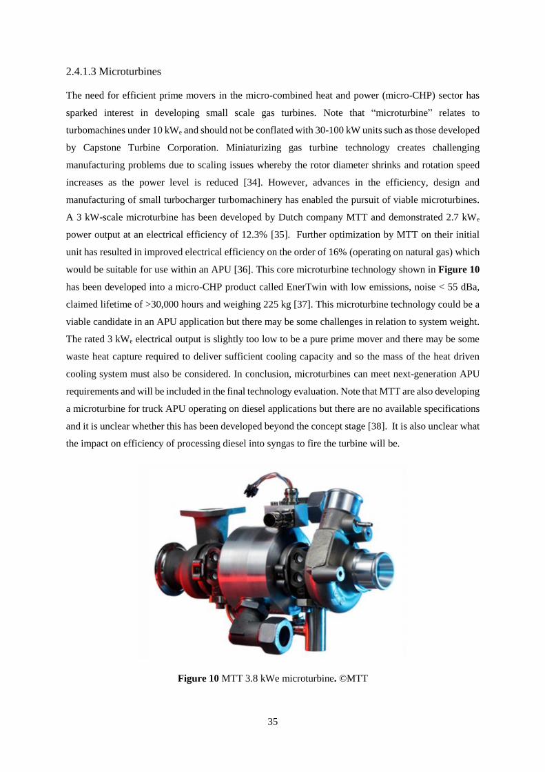
35
2.4.1.3 Microturbines
The need for efficient prime movers in the micro-combined heat and power (micro-CHP) sector has
sparked interest in developing small scale gas turbines. Note that “microturbine” relates to
turbomachines under 10 kWe and should not be conflated with 30-100 kW units such as those developed
by Capstone Turbine Corporation. Miniaturizing gas turbine technology creates challenging
manufacturing problems due to scaling issues whereby the rotor diameter shrinks and rotation speed
increases as the power level is reduced [34]. However, advances in the efficiency, design and
manufacturing of small turbocharger turbomachinery has enabled the pursuit of viable microturbines.
A 3 kW-scale microturbine has been developed by Dutch company MTT and demonstrated 2.7 kWe
power output at an electrical efficiency of 12.3% [35]. Further optimization by MTT on their initial
unit has resulted in improved electrical efficiency on the order of 16% (operating on natural gas) which
would be suitable for use within an APU [36]. This core microturbine technology shown in Figure 10
has been developed into a micro-CHP product called EnerTwin with low emissions, noise < 55 dBa,
claimed lifetime of >30,000 hours and weighing 225 kg [37]. This microturbine technology could be a
viable candidate in an APU application but there may be some challenges in relation to system weight.
The rated 3 kWe electrical output is slightly too low to be a pure prime mover and there may be some
waste heat capture required to deliver sufficient cooling capacity and so the mass of the heat driven
cooling system must also be considered. In conclusion, microturbines can meet next-generation APU
requirements and will be included in the final technology evaluation. Note that MTT are also developing
a microturbine for truck APU operating on diesel applications but there are no available specifications
and it is unclear whether this has been developed beyond the concept stage [38]. It is also unclear what
the impact on efficiency of processing diesel into syngas to fire the turbine will be.
Figure 10 MTT 3.8 kWe microturbine. ©MTT

36
2.4.1.4 Organic Rankine cycle
The organic Rankine cycle (ORC) is analogous to the conventional steam cycle except that an organic
working fluid is used instead of water [39]. There are a wide number of potential organic working fluids
such as hydrocarbons or refrigerants which can be used [40-47]. Choosing a specific working fluid
requires thermodynamically matching the fluid to the available heat resource temperature. ORC can be
advantageous over the conventional Rankine cycle as it eliminates several challenges experienced in
traditional steam turbines such as high operating pressures and turbine blade erosion [48]. Lower
pressure drop ratios also eliminate the need for complex and expensive multistage turbines that are only
practical in large-scale centralized power generation stations [49]. Commercial ORC systems have
typically been implemented in applications utilizing low-grade waste heat or similar low temperature
driving sources such as geothermal energy [50]. However, these systems are typically on the order of
>1 MW, which is not applicable to APUs. Conventional turbines, even single-stage, are generally not
suitable at low power scales (<10 kW) because of poor efficiency due to scaling effects. As a result,
finding a suitable expander technology has been a key focus of research for ORC applications [51].
Conventional refrigeration and compressor technologies such as rotary screw, piston and scroll
expander (which is illustrated in Figure 11) are instead used in the lower power <50 kWe regime. A
promising piston-based ORC technology developed by Amovis GmbH was recently acquired by the
major automotive supplier MAHLE who intend on implementing the technology as a bottoming cycle
for truck diesel engines by 2020 [52].There is considerable research into improving the efficiency of
large truck engines using ORC devices but all of these applications are waste heat recovery which is
fundamentally incompatible with the architecture of APUs [53-58]. In conclusion, there is a limited
availability of small-scale (<10 kWe) ORC devices due to challenges with expander technologies. The
prototype systems surveyed, which had appropriate power levels for an APU, typically achieved
electrical efficiencies in the 6-19% [51, 59-61]. More generally, the suitability of ORC as an APU prime
mover is questionable as they are typically intended for low-grade waste heat applications. In the
context of an APU, the heat source would be high temperature external diesel combustion, which may
be more appropriately utilized by a conventional Rankine cycle or alternative technology.
Figure 11 Scroll expander from a small-scale ORC machine. ©US DOE
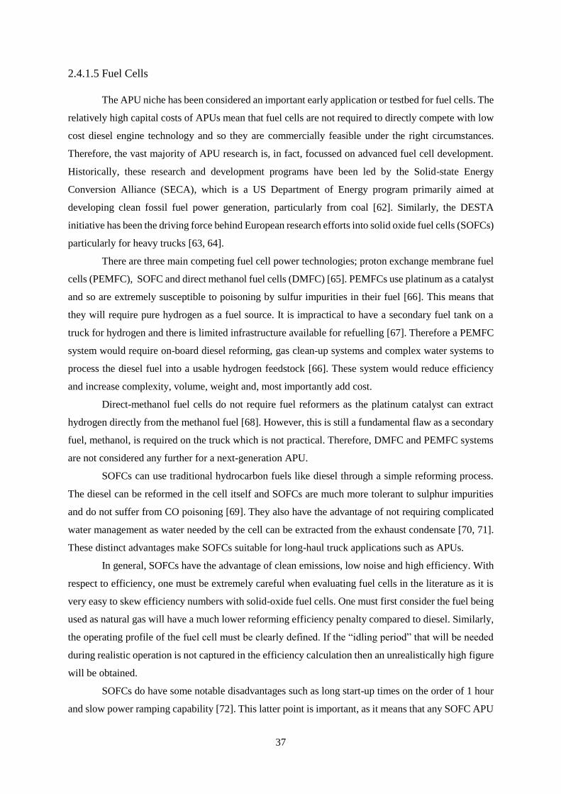
37
2.4.1.5 Fuel Cells
The APU niche has been considered an important early application or testbed for fuel cells. The
relatively high capital costs of APUs mean that fuel cells are not required to directly compete with low
cost diesel engine technology and so they are commercially feasible under the right circumstances.
Therefore, the vast majority of APU research is, in fact, focussed on advanced fuel cell development.
Historically, these research and development programs have been led by the Solid-state Energy
Conversion Alliance (SECA), which is a US Department of Energy program primarily aimed at
developing clean fossil fuel power generation, particularly from coal [62]. Similarly, the DESTA
initiative has been the driving force behind European research efforts into solid oxide fuel cells (SOFCs)
particularly for heavy trucks [63, 64].
There are three main competing fuel cell power technologies; proton exchange membrane fuel
cells (PEMFC), SOFC and direct methanol fuel cells (DMFC) [65]. PEMFCs use platinum as a catalyst
and so are extremely susceptible to poisoning by sulfur impurities in their fuel [66]. This means that
they will require pure hydrogen as a fuel source. It is impractical to have a secondary fuel tank on a
truck for hydrogen and there is limited infrastructure available for refuelling [67]. Therefore a PEMFC
system would require on-board diesel reforming, gas clean-up systems and complex water systems to
process the diesel fuel into a usable hydrogen feedstock [66]. These system would reduce efficiency
and increase complexity, volume, weight and, most importantly add cost.
Direct-methanol fuel cells do not require fuel reformers as the platinum catalyst can extract
hydrogen directly from the methanol fuel [68]. However, this is still a fundamental flaw as a secondary
fuel, methanol, is required on the truck which is not practical. Therefore, DMFC and PEMFC systems
are not considered any further for a next-generation APU.
SOFCs can use traditional hydrocarbon fuels like diesel through a simple reforming process.
The diesel can be reformed in the cell itself and SOFCs are much more tolerant to sulphur impurities
and do not suffer from CO poisoning [69]. They also have the advantage of not requiring complicated
water management as water needed by the cell can be extracted from the exhaust condensate [70, 71].
These distinct advantages make SOFCs suitable for long-haul truck applications such as APUs.
In general, SOFCs have the advantage of clean emissions, low noise and high efficiency. With
respect to efficiency, one must be extremely careful when evaluating fuel cells in the literature as it is
very easy to skew efficiency numbers with solid-oxide fuel cells. One must first consider the fuel being
used as natural gas will have a much lower reforming efficiency penalty compared to diesel. Similarly,
the operating profile of the fuel cell must be clearly defined. If the “idling period” that will be needed
during realistic operation is not captured in the efficiency calculation then an unrealistically high figure
will be obtained.
SOFCs do have some notable disadvantages such as long start-up times on the order of 1 hour
and slow power ramping capability [72]. This latter point is important, as it means that any SOFC APU

38
architecture must have a robust energy storage system, with significantly greater capacity than
conventional lead-acid battery solutions. SOFCs operate at very high temperatures (700-1000 °C), and,
therefore, the cell interconnects must be made of complex alloy materials which are expensive and
difficult to manufacture [73]. Furthermore, the high operating temperature, combined with thermal
cycling typical of an APU duty cycle, results in reliability issues caused by mechanical creep [74-77].
Additionally, current SOFC candidates experience cell degradation on the order of 1% per 1000 hours
of operation [78]. Perhaps the most significant challenge faced by SOFCs is their limited lifetime.
Systems currently under development have only demonstrated a lifetime of 2000 hours with a target
lifetime of 8000 hours for next-generation systems, which is about half of what is required for the APU
application [63, 79, 80]. The lifetime of a SOFC depends strongly upon the number of thermal cycles
that it undergoes [81, 82]. This has significant implications for a truck APU as it is expected that the
system would be cycled daily in accordance with current driver usage profiles. This behaviour is
unlikely to be compatible with current SOFC technology. In fact, many pre-commercial SOFC APUs
intend on effectively never being switched off [83]. As opposed to turning off, the system would throttle
down to a medium temperature idling state of 300 °C to reduce thermal loads. This will reduce
efficiency as the system will be consuming fuel to maintain a lower temperature and will require new
driver behaviour and acceptance. Although this is not a barrier to implementation, the fact of an idle-
reduction technology being forced to idle by design may impede use.
A state-of-the-art SOFC system demonstrated by Eberspaecher, shown in Figure 12, as part of
the DESTA program demonstrated 1.7 kWe output at a net electrical efficiency of 22% operating on
sulphur free diesel8 [63]. The SOFC developed by Delphi Power Systems as part of the SECA program
in the US demonstrated 1.5 kWe power output at 22% electrical efficiency with a specific power of 7
W/kg and 8 W/l power density [84]. Finally, an advanced SOFC system demonstrated by AVL systems
achieved 30% electrical efficiency and 2 kWe power output from a 90 kg prototype operating on road
diesel and has targets of 35% efficiency and 3 kWe for its next generation system [85].
In conclusion, SOFCs offer a completely different APU architecture to a waste-heat driven
solution assuming that they can demonstrate sufficient operational lifetimes and durability. SOFCs are
clean, quiet, high efficiency prime movers, making them suitable for driving vapour compression
refrigeration systems. A fuel cell-vapour compression APU would solve all of the key challenges faced
by conventional APUs related to noise, emissions and refrigerant usage. Note that implementing a waste
heat driven air conditioning system with a SOFC is not practical, due to overall system complexity, and
size.
However, given their insufficient lifetimes and durability challenges, they are not suitable for
a next-generation APU at present. SOFCs are not mature enough and require further development. One
8 Actual road diesel will contain sulphur and so there will be an efficiency penalty incurred when processing
this. Standard diesel has a sulphur limit of 500 ppm whereas ultra-low sulphur diesel has a limit of 15 ppm.

39
should be mindful however, that the magnitude of power required to move heavy trucks, means that, in
contrast to personal mobility, a battery-electric solution for heavy transport simply is not feasible for
the foreseeable future. Therefore, SOFCs are likely see continued research and development as the next-
generation prime mover technology to replace heavy duty diesel engines. Advancements in that field
should be watched closely as they will be directly applicable to the APU sector.
Figure 12 Eberspaecher prototype SOFC for truck APU applications. ©Eberspacher

40
2.4.1.6 Stirling engines
The Stirling engine (SE) is a reciprocating, externally‐heated engine. External heating via
combustion grants the SE considerable fuel flexibility and the potential for clean emissions and quiet
operation [86]. The Stirling engine has been known for nearly 200 years but has yet to achieve
mainstream adoption as a prime mover [87-89]. Recent developments in the distributed generation and
micro‐CHP sectors have sparked renewed interest in SEs as an alternative prime mover technology
[90]. As discussed previously, APUs are a niche application that are comparatively more lenient in
terms of system capital costs and are therefore a promising early market. There are two distinct variants
of SEs, namely, kinematic Stirling engines (KSEs) and free‐piston Stirling engines (FPSEs) and the key
differences between the two are discussed below.
KSEs have a crankshaft and a mechanical linkage to the power piston. Electrical power is
extracted from the engine using a rotary generation and the amplitude of the power-piston motion is
constrained by mechanical linkages. Furthermore, the amplitude and phasing of the displacer may also
be constrained by mechanical linkages. Consequently, KSEs are generally mechanically complex with
many moving parts, but relatively simple to analyse [87]. A simplified diagram of an alpha-type KSE
is shown in Figure 13 highlighting the mechanical complexity which can be further compounded with
the addition of more cylinders like the four-cylinder double-acting alpha type configuration used in the
Whispergen engine. Note that there are also beta and gamma type KSE configurations but these are
beyond the scope of this work.
Figure 13 Simplified diagram of an alpha-type KSE.
In contrast, FPSEs typically generate electric power with a linear alternator formed by the
oscillatory travel of the power piston in a magnetic field. The movement of the displacer and power
piston operate as a tuned spring-mass-damper system in response to pressure differences. FPSEs
typically only have two or three moving parts and so they are mechanically simple but dynamically and

41
thermodynamically complex. Figure 14 depicts the configuration of a beta-type FPSE, similar to the
Microgen Engine Corporation Stirling engine.
Figure 14 Simplified diagram showing the configuration of a beta-type free-piston Stirling engine.
The principle advantage of KSEs over FPSEs is their simplicity of operation. KSEs are
mechanically constrained by rigid linkages and the relationship between each phase of the cycle is fixed
and predictable. This results in KSEs being far easier to control and understand and their development
cycles are consequently much shorter and their performance is predictable. The second important
advantage of KSEs is that their output work is typically delivered via a rotating shaft and so they can
be coupled to any other machine that a traditional diesel engine would connect with, e.g., a compressor.
FPSEs, in contrast, require extremely complicated hydraulic or magnetic coupling and instead tend to
just drive a linear alternator that subsequently powers electro‐mechanical machines [91, 92]. This latter
point is a major challenge in relation to power density of free-piston engines as linear generators do not
scale in power as efficiently as rotary generators [93]. This limits the power output of a practical free-
piston Stirling engine to just several kilowatts.

42
The disadvantage of KSEs is that most designs incorporate a shaft seal between the crankcase
and the high pressure working gas to prevent leakage of oil from the crankcase into the working space,
and conversely, the leakage of working fluid into the crankcase. The shaft seal is a primary failure
mechanism for KSEs and has important implications for lifetime, reliability, efficiency and cost [94].
Additionally, the piston seals in the hot end of the engine must operate without lubrication. Thus, they
are subject to wear and failure over time [95, 96]. Mechanically induced lateral piston loading caused
by some KSE configurations further exacerbates these problems. Some novel KSE designs
incorporating pressurized crankcases and integrated generators eliminate these problems and bring them
more closely in line with FPSEs [97]. However none of this technology has comparable technical
maturity nor the availability of FPSEs. A key requirement of this study was the application of
commercial or near commercial technologies.
The advantages of the FPSE design is the elimination of the shaft seal allowing them to be fully
hermetically sealed and removes one of the key faults with KSE designs; the loss of working fluid over
time [92]. The linear configuration of FPSEs allows for the use of gas bearings which have very low
friction and do not suffer mechanical wear [98]. This increases the performance of the engine and vastly
increases its reliability in comparison to a KSE. FPSEs are mechanically simple and typically consist
of only 2 or 3 moving parts that require no lubrication [99]. This results in further increases of durability,
reliability and ultimately lifetime of the engine [9].
However, FPSEs have notable disadvantages. Though mechanically simple, the complex
interactions of dynamic mechanical and thermodynamic processes in FPSEs makes their analysis
extremely complex [100]. The development of FPSEs requires advanced, experimentally validated
modelling/simulation. First generation engine designs can fall short of expectations resulting in
extended engine development cycles and cost due to inadequate modelling and simulation [101]. In
contrast to KSEs, the engine cycle phases of FPSEs are not mechanically constrained and this leads to
considerable difficulty in predicting their operation and ensuring that they will operate stably [102].
Despite this, the aforementioned reliability and performance of FPSEs are the reason for choosing it
over KSEs as the prime‐mover in the proposed system.
The most heavily developed FPSE available today is the 1 kWe engine designed by Microgen
Engine Corporation (MEC) for micro-CHP applications shown in Figure 15 [103]. There have been
occasional developments and offerings of alternative FPSE designs over the years but none of these
proposed systems come close to the level of maturity of the MEC engine. The MEC system has received
$200m of development, demonstrated in excess of 5 million hours of cumulative operation and achieved
greater than 50,000 hours of reliability making it an extremely mature platform [104]. The engine offers
1 kWe of electrical output at an electrical efficiency of ~15% and weighs 49 kg. Note that the engine is
43
thermodynamically capable of producing up to 3 kW of power but is constrained by the size of its
alternator9. A 2 kWe FPSE based on the same platform is currently under development by MEC10.
In conclusion, free-piston Stirling engines are a promising future technology that meet the
emissions requirements and noise requirements of a next-generation APU whilst also offering
significantly reduced maintenance costs. However, the low power density and limited power output of
commercial or near commercial engines necessitates the use of waste-heat from the engine.
Furthermore, the novel nature of applying a Stirling engines to a real applications requires that a highly
mature platform is used.
Figure 15 The MEC 1 kWe free-piston Stirling engine. ©Microgen
9 Based on discussion with Microgen Engine Corporation design engineers. 10 This was conveyed during business discussions with MEC.

44
2.4.1.7 Thermoelectric Power Generation
Thermoelectric generators (TEGs) operate via the Seebeck effect which is the creation of a voltage
potential across a semiconductor when one side is heated and the other cooled [105]. Historically, the
most prominent application of TEGs has been for deep-space applications by NASA using the
radioisotope Pu-238 as a fuel source as shown in Figure 16 [106]. The electrical efficiency and power
density of this system is of 3-7% and 2.5 W kg-1 respectively [107], which is extremely low for an APU
application. TEGs are chosen for their extreme reliability and longevity (decades) where efficiency is
only a secondary concern. More broadly, TEGs typically have a low electrical efficiency on the order
of 5% [108]. TEGs are intended to be used as waste-heat recovery devices and several major large
automotive manufacturers like Honda [109], Renault [110], Ford [111] and BMW [112] have expressed
interest in engine exhaust heat recovery. Unfortunately, this architecture is incompatible with the APU
architecture as the APU runs when the main truck engine is not operating. However, a recent relatively
high power density TEG was developed that could be viable for an APU application and delivered 1
kWe while weighing only 30 kg [113]. Unfortunately, the electrical efficiency of this device was only
2.1%. Electrical efficiencies on this order of magnitude are not viable for an APU as the heat rejection
requirements would be too significant and the fuel consumption would not be competitive with today’s
technology. In conclusion, TEGs are unlikely to be a suitable candidate for a next-generation APU due
to insufficient electrical efficiency.
Figure 16 Cassini Probe GPHS-RTG. This TEG could deliver 300 W of electrical power. ©NASA

45
2.4.2 Heating, Ventilation and Air Conditioning (HVAC)
Heating, ventilation and air conditioning (HVAC) are the primary function of an auxiliary
power unit. It is critical to driver comfort that the proposed system can meet or surpass the performance
of current DEVC systems. Failure to meet capacity performance of current generation systems
disqualify any potential alternatives. Although future truck cabs are expected to have lower heating and
cooling requirements, due to improved insulation and design, this cannot be relied upon as justification
for reduce capacity performance. Anecdotal evidence from the electric APU sector which typically has
half the cooling capacity of diesel fuelled systems indicate that driver dissatisfaction with performance
was a major inhibitor to widespread market adoption11. This mistake should not be repeated.
The heating aspect of the climate control system is not considered in this research as it is
relatively straightforward to solve. In most of today’s APUs, a diesel fired heater is used to provide heat
to the cab. This is an extremely effective, quiet and clean way to produce heat, and, it is anticipated that
future solutions will likely incorporate a similar solution. However, there is scope for certain
architectures to utilize waste heat directly from the APU prime mover or the main truck engine to heat
the cab. This would enable higher efficiency cab heating if electrical power was also required and would
be analogous to a combined heat and power application. Capturing and redirecting hot water from the
engine cooling jacket would be the simplest way to achieve this heating effect but this architecture is
only possible with secondary heat exchangers using water-glycol as the transfer medium.
The key criteria for evaluation of a next-generation HVAC system is the cooling and air
conditioning system. It is essential that the refrigeration technology meets all current and future
regulatory constraints particularly in relation to refrigerant usage. HFCs are disqualified in the case of
traditional vapour-compression systems as they are being phased out. Safety is of paramount importance
in the air conditioning system as the driver cab is a confined space with a human occupant. For example,
hydrocarbon refrigerants represent an explosion hazard and similarly ammonia has toxicity issues in
the event of an evaporator coil leak. Both of these solutions should be avoided or, alternatively, a
secondary cooling loop should be employed to improve safety.
Finally, power density and overall efficiency12 should also be considered when evaluating
options. Low power density technologies are not viable in an automotive application like a truck APU
as there are rigid volumetric requirements that must be met.
11 This consensus was highlighted during internal company communications. 12 Refer to section 2.4.2.5 Waste-Heat Technologies for a more detailed discussion about overall system
efficiency. It is important not to conflate refrigeration COP with actual overall cooling efficiency as certain waste-
heat driven systems are capable of delivery highly efficient cooling from low COP sub-systems.

46
2.4.2.1 Vapour-compression
Vapour-compression refrigeration is a straightforward process to understand; when a gas is
compressed, its temperature rises. By allowing this gas to cool down while under pressure and rejecting
this heat to the ambient it is possible to reach a lower temperature than the starting temperature when
the gas is left expand back to its initial pressure. This basic process can be greatly enhanced by using
specific substances, called refrigerants, that are tailored to evaporate and condense at useful
temperatures and pressures. The latent heat of evaporation and condensation greatly increases the
cooling effect that can be generated from this process if the refrigerant condenses during the heat
rejection stage and evaporates during the heat acceptance stage [114]. Mechanical compression
refrigeration has been the backbone of refrigeration and air conditioning technology for many decades
and, consequently, it is very mature [115].
The advantages of automotive vapour compression technology are high COP and high cooling
power density of 2.1 and 500 W/kg respectively [116]. Figure 17 shows a compact compressor used in
a conventional APU. Vapour compression technology can be employed over a wide range of
temperatures from -40 to +60 °C by virtue of many different available refrigerants [114]. The ability to
obtain low evaporator and high condenser temperatures facilitates the use of more compact heat
exchangers which is extremely beneficial in an automotive application [117]. In fact, some automotive
air conditioning systems are operated at non-optimal thermodynamic conditions (such as elevated
condenser temperatures) in order to fit in compact spaces such as the engine bay of automobiles. The
higher temperature difference increases the heat rejection capacity of the heat exchanger enabling it to
be smaller at the expense of system performance.
However, the key challenges facing conventional vapour compression systems are in relation
to finding environmentally friendly refrigerants [118]. Traditional HCFC refrigerants have been largely
phased out by the Montreal Protocol due to their destructive ozone depletion potential (ODP) [119].
They have since been supplanted by HFC refrigerants which do not share this ODP property. However,
HFC refrigerants do exhibit an extremely large global warming potential (GWP), and persist in the
atmosphere for a very long time. R-134a, the most common refrigerant used in automotive air
conditioning applications, has a GWP of 1430 meaning that one kilogram of R-134a released to the
environment is equivalent to 1.4 tonnes of CO2 [120]. Therefore, HFC refrigerants are now being phased
down by the recent amendment to the Montreal Protocol and low-GWP alternatives such as
hydrocarbon or natural refrigerants are being explored [9]. Popular hydrocarbon refrigerant alternatives
such as R290 (propane) and R600a (Isobutane) pose certain safety challenges in relation to flammability
and explosion potential [121]. In the context of a truck APU this could present an explosion hazard to
the driver in the event of an evaporator coil leak within the sealed confines of the cab. Natural
refrigerants, for example CO2, do not have these flammability challenges but instead face different
engineering challenges such as requiring significantly higher operating pressures [122]. The higher

47
operating pressure results in more expensive and bulky compressors and pressure vessels both of which
increase system cost [123]. Natural refrigerants generally also offer lower efficiency and COP when
compared to traditional HFCs.
In conclusion, vapour compression technology will likely remain a strong contender
for a next generation APU even if there is no clear decision on the best future refrigerant from industry
[124] [125]. The decision on whether to use a mechanical compression refrigeration system depends
almost entirely on the availability of electrical or mechanical power from the APU. If high efficiency
electricity and mechanical work is available, whilst meeting emissions and noise requirements, then a
vapour compression system is very likely to offer superior performance and lower cost compared to
any alternative technology. The specific choice of refrigerant technology will likely be decided by other
high volume industrial sectors such as automobile air conditioning and then will then be applied to
APUs.
Figure 17 TM16 swash-plate compressor used in the Thermo King TriPac APU. The compressor weighs only 4.9 kg
without the clutch and can deliver up to 3.8 kW of cooling capacity at a COP of 1.4.

48
2.4.2.2 Stirling Cycle
Stirling cycle cooling at deep cryogenic temperatures has been the sole modern commercial
success of Stirling technology [103]. A Stirling cooler in principle is just a Stirling engine operating in
reverse whereby mechanical work is inputted into the engine resulting in a temperature increase on the
“cold end” of the engine and a temperature decrease on the “hot end”. Provided that the engine’s cold
end is maintained at a fixed temperature and heat is continually rejected, a cooling effect can be
generated from the engine’s hot end13. Note that the construction of an optimized Stirling cooler such
as the one shown in Figure 18 is physically quite different to a Stirling engine in order to reduce losses.
Generally speaking, Stirling coolers are only competitive at extremely low temperatures (< 200 K) and
low capacities (< 100 W) [126]. Cryogenic cooling is beyond the scope of this research and so will not
be discussed further.
Higher temperature Stirling coolers are somewhat competitive with vapour compression in low
power regimes such as domestic refrigeration but they still face major challenges related to power
density and cost [127]. Stirling cycle refrigerators have demonstrated COP on the order of 1.6 to 1.7 for
a 40 W machine maintaining a 20 °C temperature difference [128]. Another example of a 100 W
refrigerator achieved a COP of 1.6 while maintaining a 13 °C temperature difference. Interestingly, the
system COP dropped to 0.8 when the temperature difference was increased to 33 °C [129]. This could
present challenges in an APU application where the HVAC system would be subjected to extreme
environmental temperatures. Finally, perhaps the most interesting example of a high power Stirling
based refrigeration system is an ongoing project at ARPA-E (Advanced Research Project Agency –
Energy) in conjunction with the now defunct Infinia Technology Corporation (bought by Qnergy) who
are developing a ~4 – 8 kWt system which has a achieved a COP of 1 and expects to achieve a COP of
1.4 [130]. Unfortunately no power density or cost information is available for this project.
Although Stirling cycle performance can potentially exceed conventional vapour compression
systems in refrigerators it is questionable as to whether it is economically viable to displace them.
Stirling cycle machines are extremely niche products and produced very small quantities, which results
in high capital costs. In contrast, hermetically sealed compressors for domestic refrigerators are
manufactured in quantities of millions meaning that their costs are extremely optimized and
manufacturing capital costs can be amortized over many millions of units [131]. Similarly, there is
limited economic benefit to consumers in increasing the energy efficiency of refrigerators. A typical
modern refrigerator will only use about $50 per year worth of electricity and so even doubling the
efficiency will only result in savings of about $25 per year. This is an extremely low savings value to
merit introduction of a novel technology which will undoubtedly have high initial capital costs. For
reference, a conventional refrigerator compressor costs about $10 to manufacture. This is an challenging
price point to match with a novel low volume technology.
13 Note that the nomenclature seems reversed here but it is because it refers to an engine and not a cooler.
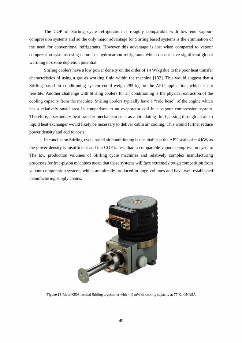
49
The COP of Stirling cycle refrigeration is roughly comparable with low end vapour-
compression systems and so the only major advantage for Stirling based systems is the elimination of
the need for conventional refrigerants. However this advantage is lost when compared to vapour
compression systems using natural or hydrocarbon refrigerants which do not have significant global
warming or ozone depletion potential.
Stirling coolers have a low power density on the order of 14 W/kg due to the poor heat transfer
characteristics of using a gas as working fluid within the machine [132]. This would suggest that a
Stirling based air conditioning system could weigh 285 kg for the APU application, which is not
feasible. Another challenge with Stirling coolers for air conditioning is the physical extraction of the
cooling capacity from the machine. Stirling coolers typically have a “cold head” of the engine which
has a relatively small area in comparison to an evaporator coil in a vapour compression system.
Therefore, a secondary heat transfer mechanism such as a circulating fluid passing through an air to
liquid heat exchanger would likely be necessary to deliver cabin air cooling. This would further reduce
power density and add to costs.
In conclusion Stirling-cycle based air conditioning is unsuitable at the APU scale of ~ 4 kWt as
the power density is insufficient and the COP is less than a comparable vapour-compression system.
The low production volumes of Stirling cycle machines and relatively complex manufacturing
processes for free-piston machines mean that these systems will face extremely tough competition from
vapour compression systems which are already produced in huge volumes and have well established
manufacturing supply chains.
Figure 18 Ricor K508 tactical Stirling cryocooler with 440 mW of cooling capacity at 77 K. ©NASA

50
2.4.2.3 Air-cycle
Air cycle refrigeration is a process whereby air is compressed causing its temperature to rise
and then heat is rejected to the surrounding ambient. Once the air has been sufficiently cooled, it is then
expanded resulting in a temperature drop and newly cooled air available for air conditioning. The
primary application for air-cycle refrigeration is in aviation as shown in Figure 19 where reliability and
weight are the most critical parameters. These systems are extremely effective in aircraft as there is
already a source of compressed air readily available from the turbofan engine compressor core thus
eliminating the need for additional compression equipment [133]. The power density is very high as the
jet engine compressor spins at extremely high speeds on the order of 60,000 rpm, which is over an order
of magnitude higher than conventional vapour compression system compressors. This results in an air
conditioning system that is typically half the weight of a comparable vapour compression system. Using
air as the working fluid also means that refrigerant leakage is tolerable in a sealed aircraft. The primary
disadvantage of air cycle refrigeration is poor COP on the order of 0.8 [134]. There is a near total
absence of research into air-cycle refrigeration applications outside of the aerospace industry which
possibly confirms that it is only suitable for this niche.
In conclusion, air-cycle refrigeration only makes sense in the context of aircraft where a source
of pressurized air is readily available via bleed mechanisms from the main turbofan engine compressors
In the context of a truck APU, it would not make sense to implement such a system as generating the
compressed air would result in an overall system with a very low COP and high weight.
Figure 19 Large turbofan engine on a modern aircraft. The main engine compressor section is an ideal source of compressed
air to drive a refrigeration cycle. In practical systems, a relatively small quantity of compressed air is extracted through bleed
valves. ©NASA

51
2.4.2.4 Thermoelectric Cooling
Thermoelectric cooling devices rely on the Peltier effect which is the creation of a temperature
difference between two dissimilar materials when a voltage is applied to them [135]. By rejecting heat
from the hot side, and maintaining a fixed temperature, it is possible to create a cooling effect. The main
applications for thermoelectric cooling are currently in the field of electronics cooling as shown in
Figure 20 where thermoelectric devices can offer high power density and compact size which meets
the requirements for single-chip package cooling. Thermoelectric devices can be cascaded into
multistage devices enabling very low temperatures for cryogenic applications typically involving
electronic chips to reduce thermally induced electronic noise [136]. A typical application of this is in
the field of optical sensor cooling for example in military grade thermal imaging systems [137].
Thermoelectric coolers are solid-state devices which makes them extremely rugged, highly reliable and
effectively silent [138]. Another potential benefit of thermoelectric cooling is that they require DC
electricity to operate and so can be directly coupled to solar photovoltaic panels or battery technologies
without any intermediate electronics which can be advantageous in military applications as it improves
reliability.
Thermoelectric cooling devices typically have a low COP in the range of 0.16-0.6 [139-144].
Similarly, they are associated with low cooling capacity although they can theoretically be scaled for
increased capacity. All of the thermoelectric cooling devices surveyed had a capacity in the 0-120 W
range which is an order of magnitude below what is required for an APU air conditioning application
[142, 143, 145-165]. An interesting comparison of thermoelectric cooling versus vapour-compression
system compared a high power 320 W thermoelectric cooler against a 2600 W vapour compressor
system, which is still an order of magnitude too small [166]. The COP for the thermoelectric device
was 0.38 versus 2.95 for vapour compression system. The cost of the thermoelectric system was $1385
compared to $500 for the conventional system.
In conclusion, thermoelectric cooling is not competitive against conventional vapour-
compression air conditioning systems as the devices are too expensive and their COP is too low to form
an efficient overall system. In contrast to heat driven cooling systems like sorption technologies,
thermoelectric cooling requires electricity to operate. Therefore, if electricity is available, it would be
more energy efficient to simply use this electricity to drive a hermetically sealed compressor and vapour
compression cycle using a natural or hydrocarbon refrigerant as they are available in the required
capacity and have significantly higher COP.
Figure 20 Thermoelectric cooling devices for electronic chips. ©NASA

52
2.4.2.5 Waste heat Technologies
All heat engines have an associated efficiency and, consequently, must reject some quantity of
heat during normal operation. The quantity and quality (temperature) of this waste heat varies
considerably depending on specific technologies but, in general, internal combustion engines have a
maximum efficiency of about 30% at the APU scale meaning that 70% of the heat input to the engine
is wasted. Stirling engines and organic Rankine cycle machines may need to reject up to 85-90% of
their inputted heat. This rejected heat is split between high temperature exhaust in the 400-600 °C range
and warm engine coolant water that is < 100 °C. For a typical diesel engine, a rule of thumb exists
whereby one third of the fuel input results in mechanical work, the next third as waste heat in the engine
cooling jacket and the final third as high temperature exhaust.
It is vitally important to consider the efficiency cost in generating mechanical work or
electricity when evaluating overall system architectures. One can easily be misled by choosing a high
efficiency refrigeration technology only to find that the effective system efficiency is in fact lower due
to the prime mover efficiency. A hypothetical worked example illustrating this is shown below in
Figure 21. In can be seen that combining two low efficiency technologies; a Stirling engine with 15%
net electrical efficiency and a zeolite-water adsorption chiller with a COP of 0.45 actually results in an
overall system with higher efficiency than the DEVC system.
Figure 21 Energy flow diagram comparing a DEVC system against a system utilizing waste heat
The temperature of the waste heat resource plays a very important role in choosing a
refrigeration technology. Higher temperature waste heat is preferred as it can be used to drive higher

53
COP cycles. However, again, this can be misleading and have disadvantages. Using waste heat from
the exhaust stream of an engine to heat a sorption cycle is non-trivial and requires close integration with
the engine manufacturer to ensure that emissions control systems are not compromised or interfered
with.
It is instead more preferable to capture waste heat from the engine cooling jacket. This is
advantageous for two reasons; firstly it is a lot simpler to do and only requires coolant hose and valves.
Secondly, exhaust heat can still be captured into the engine cooling jacket using conventional exhaust
heat exchanger technology that is used in micro-CHP systems. Avoiding direct heating of the sorption
bed greatly simplifies the engineering challenges associated with heat capture. By capturing exhaust
waste heat into the coolant jacket, it increases the overall quantity of waste heat available albeit reducing
its quality.
The most significant advantage of engine coolant waste heat capture is the ability to integrate
with the main truck engine. This can potentially grant access to a large quantity of waste heat when the
truck is operating and more importantly the practice is already accepted by truck engine manufacturers
(OEMs). A truck engine has a coolant volume of around 50-60 litres and will be heated to around 80
°C which is sufficient for driving a sorption system14. This latter point is vital as without the support of
truck OEMs, a next generation APU will likely have limited compatibility with truck engines and see
low adoption rates. In conventional DEVC APUs the coolant system is bridged with the main truck
engine in order to facilitate easier starting in cold conditions. Cold diesel has a tendency to gel and
precipitate wax particles which can thicken the fuel and clog injectors and fuel filters preventing the
engine from running. A technology that can harness waste heat from the main truck engine and the APU
with minimal modifications could potentially offer huge cost savings to truck drivers as it would enable
the APU air conditioning system to operate for a significantly higher number of hours each year. The
air conditioning provided during main engine operation would be of very high efficiency as no heat
input is required and the only energy input needed would be for running parasitic loads like pumps and
fans.
To summarise, engine waste heat capture is essential for low efficiency or low power-density
prime movers such as Stirling engines as there is not enough space or weight margin to put in a
sufficiently large engine to drive a vapour-compression system. Furthermore, capturing the waste heat
from the cooling water jacket is the most optimal solution as it is simpler, enables main truck engine
integration and provides a greater quantity of waste heat as the exhaust can also be captured. Therefore,
the temperature of the waste-heat resource in a next-generation APU is likely to be < 100 °C which
eliminates a number of more advanced sorption cycles and technologies.
14 There is also some heat available when the truck is parked. Assuming 60 litres of coolant volume at 80 °C, then
there is approximately 1.5 kWh of thermal heat available from the cooling jacket by cooling it from 80 to 60 C
(usable range for adsorption machine). Furthermore, treating the truck engine as a uniform 1.2 ton block of cast
iron, then an additional 3 kWh are available from the engine block.

54
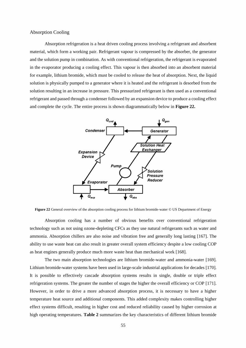
55
Absorption Cooling
Absorption refrigeration is a heat driven cooling process involving a refrigerant and absorbent
material, which form a working pair. Refrigerant vapour is compressed by the absorber, the generator
and the solution pump in combination. As with conventional refrigeration, the refrigerant is evaporated
in the evaporator producing a cooling effect. This vapour is then absorbed into an absorbent material
for example, lithium bromide, which must be cooled to release the heat of absorption. Next, the liquid
solution is physically pumped to a generator where it is heated and the refrigerant is desorbed from the
solution resulting in an increase in pressure. This pressurized refrigerant is then used as a conventional
refrigerant and passed through a condenser followed by an expansion device to produce a cooling effect
and complete the cycle. The entire process is shown diagrammatically below in Figure 22.
Figure 22 General overview of the absorption cooling process for lithium bromide-water © US Department of Energy
Absorption cooling has a number of obvious benefits over conventional refrigeration
technology such as not using ozone-depleting CFCs as they use natural refrigerants such as water and
ammonia. Absorption chillers are also noise and vibration free and generally long lasting [167]. The
ability to use waste heat can also result in greater overall system efficiency despite a low cooling COP
as heat engines generally produce much more waste heat than mechanical work [168].
The two main absorption technologies are lithium bromide-water and ammonia-water [169].
Lithium bromide-water systems have been used in large-scale industrial applications for decades [170].
It is possible to effectively cascade absorption systems results in single, double or triple effect
refrigeration systems. The greater the number of stages the higher the overall efficiency or COP [171].
However, in order to drive a more advanced absorption process, it is necessary to have a higher
temperature heat source and additional components. This added complexity makes controlling higher
effect systems difficult, resulting in higher cost and reduced reliability caused by higher corrosion at
high operating temperatures. Table 2 summarizes the key characteristics of different lithium bromide
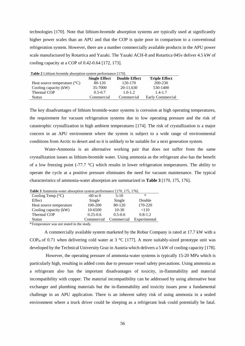
56
technologies [170]. Note that lithium-bromide absorption systems are typically used at significantly
higher power scales than an APU and that the COP is quite poor in comparison to a conventional
refrigeration system. However, there are a number commercially available products in the APU power
scale manufactured by Rotartica and Yazaki. The Yazaki ACH-8 and Rotartica 045v deliver 4.5 kW of
cooling capacity at a COP of 0.42-0.64 [172, 173].
Table 2 Lithium bromide absorption system performance [170].
Single Effect Double Effect Triple Effect Heat source temperature (°C) 80-120 120-170 200-230
Cooling capacity (kW) 35-7000 20-11,630 530-1400
Thermal COP 0.5-0.7 1.0-1.2 1.4-1.7
Status Commercial Commercial Early Commercial
The key disadvantages of lithium bromide-water systems is corrosion at high operating temperatures,
the requirement for vacuum refrigeration systems due to low operating pressure and the risk of
catastrophic crystallization in high ambient temperatures [174]. The risk of crystallization is a major
concern in an APU environment where the system is subject to a wide range of environmental
conditions from Arctic to desert and so it is unlikely to be suitable for a next generation system.
Water-Ammonia is an alternative working pair that does not suffer from the same
crystallization issues as lithium-bromide water. Using ammonia as the refrigerant also has the benefit
of a low freezing point (-77.7 °C) which results in lower refrigeration temperatures. The ability to
operate the cycle at a positive pressure eliminates the need for vacuum maintenance. The typical
characteristics of ammonia-water absorption are summarized in Table 3 [170, 175, 176].
Table 3 Ammonia-water absorption system performance [170, 175, 176].
Cooling Temp (°C) -60 to 0 5-10 *
Effect Single Single Double
Heat source temperature 100-200 80-120 170-220
Cooling capacity (kW) 10-6500 10-30 <110
Thermal COP 0.25-0.6 0.5-0.6 0.8-1.2
Status Commercial Commercial Experimental *Temperature was not stated in the study.
A commercially available system marketed by the Robur Company is rated at 17.7 kW with a
COPth of 0.71 when delivering cold water at 3 °C [177]. A more suitably-sized prototype unit was
developed by the Technical University Graz in Austria which delivers a 5 kW of cooling capacity [178].
However, the operating pressure of ammonia-water systems is typically 15-20 MPa which is
particularly high, resulting in added costs due to pressure vessel safety precautions. Using ammonia as
a refrigerant also has the important disadvantages of toxicity, in-flammability and material
incompatibility with copper. The material incompatibility can be addressed by using alternative heat
exchanger and plumbing materials but the in-flammability and toxicity issues pose a fundamental
challenge in an APU application. There is an inherent safety risk of using ammonia in a sealed
environment where a truck driver could be sleeping as a refrigerant leak could potentially be fatal.
57
Although this problem can be circumvented through use of a secondary heat exchanger system, it will
reduce efficiency, add cost and increase complexity.
In conclusion, absorption technology is unlikely to be viable in an APU application as the risk
of irreparable damage caused by crystallization presents a significant challenge in terms of APU
reliability. Alternative solutions using water-ammonia do not have a crystallization problem but do pose
a safety risk in an automotive environment.
Adsorption Cooling
Adsorption refrigeration differs from absorption as it is a solid-vapour process and relies on
desiccant materials that adsorb or desorb a refrigerant depending on whether they are cooled or heated
respectively. Figure 23 shows a practical adsorption machine. When the sealed, saturated, adsorption
chamber 1 is heated using waste heat, refrigerant is desorbed from the adsorber resulting in a pressure
increase forcing open the orange flap valve. This process is identical to the compression stage in a
vapour compression system except that it is thermally driven. The saturated vapour condenses when it
comes into contact with the condenser coil which is being externally cooled. This liquid refrigerant is
then siphoned to the low-pressure evaporator where it evaporates and creates a cooling effect. The
evaporator pressure is controlled adsorption chamber 2 which is being actively cooled causing
refrigerant to be adsorped into the bed reducing the surrounding pressure. This is analogous to the
suction created by a compressor intake. [179].
Figure 23 Working principle of an adsorption chiller machine.

58
Adsorption chillers share many of the same advantages as absorption technology such as the
elimination of CFC and HFC refrigerants, low noise and vibration, and long lifetimes [180]. The key
advantages of adsorption chillers over absorption technology is that they do not suffer from
crystallization problems and can tolerate wide variations in their driving temperatures, which is
particularly advantageous in an APU application where there is likely to be poor control over the input
temperature [167]. Using a benign refrigerant such as water also eliminates any potential corrosion
issues [181].
There are a number of different desiccant-refrigeration pairs available such as activated carbon-
methanol, silica gel-water, zeolite-water or calcium chloride-ammonia which must be chosen on the
basis of available driving temperature and required cooling temperature [181-184]. A key consideration
for the choice of refrigerant is whether ice or sub-zero cooling temperatures are required. Obviously,
water is not a viable refrigerant for those applications and so carbon-methanol or calcium chloride-
ammonia must be used instead. However, in the context of an APU, chilled water is sufficient as only
air conditioning is needed meaning that zeolite-water and silica gel-water could work. In contrast to
calcium chloride-ammonia and carbon methanol, silica gel and zeolite-water are better suited for low
temperature (<100°C) heat found in engine cooling jackets [185]. Moreover, zeolite-water offers
superior cooling power density compared to silica gel-water and so it was chosen as the most promising
adsorption technology [186].
However, adsorption chillers such as zeolite-water systems do have some notable disadvantages
such as low cooling power density and low COP [187]. Commercially available zeolite-water
adsorption chillers have displayed a COP of 0.6 and cooling power density of 40 W/kg [188]. Despite
the low COP, the quantity of waste heat available means that the overall system efficiency can exceed
conventional DEVC systems as evidenced by the hypothetical scenario shown previously in Figure 21.
There are a number of interesting waste-heat driven air conditioning concepts using adsorption
technology discussed in the literature [116, 132, 189-191]. A detailed design of an adsorption cooling
system for an automobile was presented by Lambert and highlights the advantages of using adsorption
such as the elimination of parasitic compressor loads and increased vehicle fuel economy [116, 132].
The key challenge with this proposed system was finding adequate space within the vehicle to house
the large bulky adsorption unit. Although the system would fit, it would consume a sizeable amount of
usable space within the vehicle (such as boot space) and negatively impact on the driver [192, 193].
Additionally, the waste-heat was high temperature exhaust and so required a rather complex heat
capture mechanism.
Another relevant concept called TOPMACS (Thermally Operated Mobile Air Conditioning
System) targeted at heavy trucks with sleeper cabs proposed a zeolite-water adsorption chiller air
conditioning system driven by waste heat from the truck engine. The system had a cooling power of 2-
3 kW and COP of 0.6 [190]. However, the system did had of critical flaws, such as only being able to
utilize waste heat from the main truck engine. This meant that the idling problem was not addressed the

59
truck would still require an APU in addition to the bulky adsorption chiller unit. The sheer size of an
adsorption chiller means that it would be impractical to fit both an APU and this adsorption chiller
system within the volume constraints of the truck.
In conclusion, zeolite-water adsorption refrigeration technology appears to be the most
promising next-generation air conditioning technology for APUs. Using a zeolite-water adsorption
cooling system could solve the refrigerant usage problem and offer higher overall system efficiency
compared to incumbent DEVC technology.
Despite the shortcomings experienced in the above concepts, adsorption technology has been
demonstrated in automotive applications and shown to deliver sufficient cooling capacity at a viable
COP. Fundamental challenges such as volume constraints can be addressed through an appropriate
system architecture such as the one that will be presented in this thesis.

60
2.4.3 Energy Storage
Energy storage is a relatively minor aspect of conventional DEVC APUs and is only necessary
for engine starting. However, many next-generation prime movers such as fuel cells, and Stirling
engines, will require increased energy storage buffering as they cannot instantaneously ramp their
power output like a diesel engine. A battery or alternative storage mechanism will be necessary to meet
loads during this interim period. It is technically possible to rely on the main truck batteries to support
loads during these periods and to also meet minor electrical loads when the truck is parked. However,
this practice is not favoured by truck drivers due to the risk of incurring main engine starting trouble
due to depleted batteries. Failure to restart the main truck engine can vary from being a mild
inconvenience to being potentially life-threatening in harsh and remote climates.
Energy storage represents the least important aspect of next-generation fuel driven APUs as it
has limited impact on the overall architecture. However, improvements in energy storage technology
such as reduced mass and increased cycle life do have the potential to deliver fuel economy savings and
reduced system life cycle costs. Conventional solutions using lead-acid batteries have a limited cycle
life and so must be replaced several times over the life the APU, which adds cost. It is very important
to consider this full life-cycle cost when evaluating energy storage systems. Although lead-acid batteries
are very cheap, their limited cycle life means that they must be replaced and can represent a false
economy. In contrast, lithium ion batteries are more expensive than lead-acid batteries but may last
several times longer and so the overall life cycle cost is lower despite the higher initial capital cost
[194].
The APU niche is not expected to be a technology driver for the adoption of a next-generation
battery solution as it is too small. Instead, developments with electric vehicles and consequent battery
advancements are likely to be what decides the future solution. Although, different technologies can be
made to be interoperable, it is obviously advantageous to use the same technology to reduce complexity
as the main truck battery as the APU and truck battery are typically placed in parallel.
The key evaluation criteria for energy storage are energy density, cost and lifetime. Historically,
safety has not been an issue with energy storage but alternative technologies such as lithium-ion
batteries, flywheels and flow batteries each have unique safety challenges which must be addressed and
considered.

61
2.4.3.1 Flywheels
Mechanical flywheels have been used for hundreds of years to maintain smooth operation of
engines from cycle to cycle. However, classic mechanical flywheels such as those found on diesel
engines have low energy storage capability and limited storage duration due to low rotation speeds and
mechanical bearing losses respectively. The kinetic energy stored in a flywheel, Ek, shown in Eq. (1) is
proportional to its moment of inertia, I’, and the square of its rotational speed, ω.
Ek =
1
2I′ω2 (1)
As per Eq. (1), increasing rotational speed of a flywheel has a much greater impact on energy
storage than increasing its mass. Modern high-tensile materials like carbon fibre have enabled the
manufacture of high power flywheels that can withstand the stresses of operation at speeds from 20,000
to over 50,000 rpm [195]. Additionally, advancements in magnetic bearing technology and vacuum
enclosure of the flywheel has enabled near frictionless operation of high performance flywheels
allowing them to store energy for extended durations [196-199]. The key advantage of flywheels over
alternative energy storage technologies is their effectively unlimited lifetime in terms of
charge/discharge cycles and their extremely rapid response times [200]. Flywheels can also discharge
their energy at extremely high power rates and are limited only by generator size. Unlike chemical
energy storage technologies such as batteries, FES are not negatively impacted by temperature and can
operate across a wide range of environments. Perhaps the most sophisticated flywheel energy storage
(FES) developed to date was the G2 Flywheel shown in Figure 24 developed by NASA for space power
applications, which could store 525 Wh of energy and deliver 1 kW of power [201].
Figure 24 NASA G2 Flywheel has 525 Wh of energy storage and 1 kW output power. ©NASA

62
Beacon power offer commercial FES systems in the 100-250 kWe with 3.3-25 kWh range [202].
Typical applications for commercial FES is frequency stabilization and voltage support of power grids
[195, 200, 203].
A potentially interesting application for APUs utilizing a flywheel on a truck is kinetic energy
recovery systems when the truck is operating. Although not strictly part of the traditional APU
requirements, the limited impact on flywheel lifetime make this an attractive additional benefit when
the truck is operating. Accelerating a large truck from standstill to highway speeds requires in excess
of 3.5 kWh in kinetic energy15. This energy must be dissipated in the brake pads when the truck comes
to a standstill. One alternative architecture is to incorporate a high power regenerative braking system
consisting of an integrated axle generator and fast acting energy storage device like a flywheel or
supercapacitors [204, 205]. Recovering the full energy of a truck would require power rates comparable
to the main truck engine i.e. 200-400 kW, which is at least two orders of magnitude above what chemical
battery technology can achieve in an APU. However, this application, though appealing, would have
immense engineering challenges related to safety and operation. The integrated, safety critical, nature
of an auxiliary braking system would require OEM integration and direct supervision meaning that it
could be a difficult product to implement across a diverse fleet of trucks.
The key challenges facing FES application to an APU are cost, overall system complexity and
safety. For example, a practical FES that is suitable for a truck would require; magnetic bearings,
catastrophic rotor failure protection system, vacuum vessel, power and control electronics and
potentially gyroscopic stabilisation. Each of these requirements would add weight, considerable cost
and unnecessary complexity compared to a lead-acid or lithium-ion battery. Capital costs for flywheels
range from $1000-5000 per kWh versus $200-400 for lead-acid batteries meaning that they are unlikely
to cost competitive in an APU application [206]. Additionally, the high amounts of kinetic energy stored
in the system could represent an unacceptable explosion risk to the driver in the event of catastrophic
rotor failure [207]. It is also unclear impact any gyroscopic effects caused by the flywheel would have
on the truck while driving. However, it is possible to eliminate these effects through the use of a gimbal
mechanism or by placing two flywheels in opposite rotation to each other but this adds additional
complexity.
To summarise, flywheel energy storage is not suitable for APU applications due to system
complexity, high cost and potential safety issues. Flywheels are currently only practical for applications
requiring extremely fast response times and discharge rates such as grid voltage stabilisation or extreme
lifetime and durability such as deep space applications [208].
15 This assumes a 20 tonne truck going accelerating from 0 to 100 km/h neglecting all losses and only
considering kinetic energy.

63
2.4.3.2 Lead-acid batteries
Lead-acid batteries such as the one show in Figure 25 have been the foundation of automotive
electrical systems for nearly 100 years [209]. It is an extremely popular choice due to its ruggedness,
low cost and inherent safety [210]. The key factor for the widespread implementation of lead acid
batteries is their low cost which is particularly important in an automotive context. This is largely due
to immense production volumes and high rates of recycling [211].
Lead-acid batteries are also simple to operate and are maintenance free. In contrast to alternative
battery technologies, lead-acid does not require any active control or management. Charging is
straightforward and largely self-regulating meaning that a basic charging algorithm can be used [212].
However, lead-acid batteries do have some notable disadvantages when compared to
alternatives. The specific energy and power density of lead-acid systems is low (50 Wh/kg) due to the
use of lead as the current collector [213]. Excessive overcharging during the battery charging procedure
can also potentially lead to the production and build-up of hydrogen gas which can present a safety
hazard in confined spaces [209]. Perhaps the greatest operational disadvantage of lead-acid batteries is
their limited cycle life (~600 cycles) which is strongly related to the depth of discharge [214]. In the
context of an APU, a deep depth of discharge is a favourable trait as it allows for longer durations of
operation without needing to operate the prime mover to recharge the battery. Though lead-acid
batteries are cheap, it is important to consider the entire life-cycle cost of an APU system. Their limited
cycle life can result in a need for multiple replacements throughout the APU lifetime which can be
costly. In certain situations, a more expensive technology such as lithium-ion can be more cost effective
over the life of the system.
In summary, lead-acid batteries are still an effective solution for a next-generation APU
although alternative technologies with superior lifetime could offer cost benefits. Depending on the next
generation system architecture, the battery system may be expected to perform significantly more work
than in the current DEVC system. If the battery is required to support loads during prime-mover ramp
up periods, the life cycle shortcomings of lead-acid batteries will be significantly exacerbated and an
alternative technology with better longevity will be necessary.
Figure 25 Thermo King lead-acid battery used in their APU products. ©Thermo King

64
2.4.3.3 Supercapacitors
Capacitors are an integral part of all modern electronic devices for short duration energy storage
and other useful electronic effects like filtering. Recently however, considerable work has been
performed on developing supercapacitors such as those shown in Figure 26 as a fast-acting high power
energy storage systems comparable to flywheels [215-220]. Capacitors store energy by maintaining a
voltage potential between two plates soaked in electrolyte and separated by an insulator. The energy
stored in a capacitor can be determined from its capacitance, C, and cell voltage, V using Eq. (2).
E =
1
2CV2 (2)
Supercapacitors have very poor energy density on the order of 1-10 Wh kg-1 versus 10-100 Wh kg-1 for
conventional batteries [221]. Supercapacitors are not intended to be used for their energy storage
capability but instead for their ability to deliver high power extremely quickly [220]. The power density
of supercapacitors is about 10 times higher than that of a battery and they are able to be cycled in excess
of 500,000 times [221]. The low energy storage density of supercapacitors could make them unsuitable
for an APU as conventional APUs incorporate a ~1 kWh lead-acid battery weighing ~36 kg. A
comparable supercapacitor based solution could weigh more than 360 kg which is twice as much as an
entire conventional APU system. However, depending on the APU system architecture, it may be
possible to significantly reduce the size of the battery if it is only required for ignition or starting of the
prime mover. Although, in current APUs, the prime mover typically cycles on and off to meet air
conditioning demand and to recharge the battery bank with the battery providing any electrical loads in
the interim period. This would not be possible with the limited energy reservoir of a supercapacitor. As
mentioned with flywheels, the high power density of supercapacitors may have potential uses as a truck
kinetic energy recovery system but this would face difficult aforementioned safety engineering
challenges.
In summary, supercapacitors are unlikely to be a feasible energy storage system for an APU
due to their poor energy density. Supercapacitors would only be a viable solution with a fast-acting
prime mover such as a diesel engine whereby the capacitor would be used solely for engine starting and
all operational loads would be met by the alternator.
Figure 26 A range of supercapacitors from Maxwell Technologies. ©Maxwell Technologies

65
2.4.3.4 Flow batteries
Redox flow batteries can be considered as an electrochemically regenerative fuel cell as they
utilize externally stored fuel and oxidant which are in the form of two soluble redox couples. These
couples can be used to generate electrical energy when they undergo oxidation and reduction reactions
at inert electrodes that are separated by an ion exchange membrane [222].
There are a wide range of competing redox flow chemistries [223-246]. In recent years, the
most promising technology appears to be the vanadium redox system as it offers good electrochemical
reversibility and high efficiency. Even within the Redox family, there are a number of competing
chemistries with different characteristics and properties [239, 247-259].
Redox flow batteries are advantageous when compared to lead-acid batteries as they have lower
costs at $180-250 per kWh versus $350-1500 lead-acid and offer potentially longer cycle lives of 5,000-
14,000 versus 200-1500 for lead-acid [260]. However, the energy density of flow batteries is poor and
comparable to lead-acid at 30-50 Wh per kg which is a disadvantage in the context of a next-generation
APU [261]. Redox flow batteries are clearly a superior solution to lead-acid batteries but perhaps not at
the APU scale of ~ 1 kWh. A conventional lead acid battery is a very simple solution and needs little
to no extraneous components. In contrast, a redox flow battery requires two external pumps and two
tanks and although the electrochemical stacks are not particularly large, the electrolyte storage tanks
can be bulky [256, 262]. The key application for redox flow batteries is in large scale stationary energy
storage where energy density is not particularly important. As the flow battery can be loosely considered
as analogous to a fuel cell, the system power output is limited by the stack size but its runtime or capacity
is limited only by the size of its electrolyte tanks. This enables extremely large scalability of redox flow
battery capacity at a very low cost making them a very compelling solution for long duration (3-4h)
energy storage like load levelling and peak shaving in grid-scale applications [263, 264].
Redox flow battery technology offers considerable promise in the large scale energy storage
sector but it is still a very early stage commercial technology and a number of challenges still remain.
Further work is required to improve electrolyte stability across wide temperature ranges, to develop
overcharge resistant electrode materials, and to mitigate the membrane degradation in low cost materials
[259].
In summary, redox flow batteries are unlikely to be suitable for an APU application as the
energy density is quite low and comparable to that of lead acid batteries. This technology is more
suitable for grid-scale stationary energy storage. They also have additional added complexity of
requiring pumps and storage tanks which introduces new potential failure mechanisms in an automotive
environment. Finally, there are potential driver safety and environmental concerns as some of the
electrolytes used pose serious toxicity issues [265, 266].
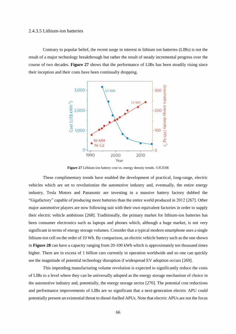
66
2.4.3.5 Lithium-ion batteries
Contrary to popular belief, the recent surge in interest in lithium ion batteries (LIBs) is not the
result of a major technology breakthrough but rather the result of steady incremental progress over the
course of two decades. Figure 27 shows that the performance of LIBs has been steadily rising since
their inception and their costs have been continually dropping.
Figure 27 Lithium-ion battery cost vs. energy density trends. ©JCESR
These complimentary trends have enabled the development of practical, long-range, electric
vehicles which are set to revolutionize the automotive industry and, eventually, the entire energy
industry. Tesla Motors and Panasonic are investing in a massive battery factory dubbed the
“Gigafactory” capable of producing more batteries than the entire world produced in 2012 [267]. Other
major automotive players are now following suit with their own equivalent factories in order to supply
their electric vehicle ambitions [268]. Traditionally, the primary market for lithium-ion batteries has
been consumer electronics such as laptops and phones which, although a huge market, is not very
significant in terms of energy storage volumes. Consider that a typical modern smartphone uses a single
lithium-ion cell on the order of 10 Wh. By comparison, an electric vehicle battery such as the one shown
in Figure 28 can have a capacity ranging from 20-100 kWh which is approximately ten thousand times
higher. There are in excess of 1 billion cars currently in operation worldwide and so one can quickly
see the magnitude of potential technology disruption if widespread EV adoption occurs [269].
This impending manufacturing volume revolution is expected to significantly reduce the costs
of LIBs to a level where they can be universally adopted as the energy storage mechanism of choice in
the automotive industry and, potentially, the energy storage sector [270]. The potential cost reductions
and performance improvements of LIBs are so significant that a next-generation electric APU could
potentially present an existential threat to diesel-fuelled APUs. Note that electric APUs are not the focus

67
of this research but please see Appendix 1 for a discussion on this and other outside factors that should
be considered in the context of a next generation APU.
The key advantages of LIBs are high energy density on the order of 140-200 Wh per kg and
longer cycle lives of 800-5000 cycle depending on specific chemistry. The cost of lithium-ion batteries
in 2014 was around $250-500 per kWh and is continuing to drop [213]. Lithium ion batteries also have
higher coulombic efficiencies meaning that they can be charged and discharged with greater efficiency
and can withstand deeper depths of discharge without serious degradation, unlike lead-acid batteries
[271].
However, LIBs do have some notable disadvantages when compared to conventional lead-acid
batteries. Lithium-ion batteries require complex control and management while operating and charging.
Great care must be taken to prevent overcharging or over-discharging of a lithium ion cell as doing so
can result in explosion [272].
There have been a number of high profile safety incidents with lithium-ion battery fires most
notably the 787 Dreamliner and, more recently, the Galaxy Note 7 [273]. These safety issues, although
firmly grounded in engineering, represent a major business and perception challenge to lithium-ion
batteries as a next-generation technology. A high profile failure of the energy management system in a
truck APU has the potential to permanently erode customer trust of the technology and could impact
the adoption of a new system even if the prime mover and HVAC subsystems operate optimally.
In conclusion, lithium-ion batteries represent an extremely promising next-generation solution
and have the potential to also make a compelling electric APU without the performance limitations of
today’s systems. The adoption of a lithium-ion battery in a next-generation APU will depend on cost
and the availability of a suitably-sized and safe system. These challenges are very likely to be met by
the automotive industry and simply adopted by the APU niche.
Figure 28 Tesla Model S Battery Pack. ©Jason Hughes

68
2.4.4 Summary
The only viable prime movers that meet the requirements are microturbines, free-piston Stirling
engines and SOFCs. Microturbines were not sufficiently developed when this research first began but
recent developments merit re-evaluation of the technology as an alternative to Stirling engines in any
future work. They offer similar performance to Stirling engines but likely at lower cost to due cost
efficiencies derived from using standard automotive technology and manufacturing processes. They do
not suffer from the power limitations of free-piston Stirling engines and so could, conceivably, directly
power a compressor or be used in a waste heat application. However, a high power unit, capable of
driving a compressor, is yet to be developed and will not have the level of maturity of current FPSE
technology and so will not be considered any further. SOFCs still face significant lifetime and durability
challenges but considering that they are the main focus of research and development in the APU sector
these challenges will likely be overcome.
We have evaluated vapour-compression, Stirling cycle, air-cycle, thermoelectric, absorption
and adsorption refrigeration technology as potential refrigeration candidates for a next generation APU.
The only two technologies that are feasible for a next generation APU are vapour compression and
adsorption. The decision between these two technologies represent major system architecture
implications for the prime mover as vapour compression technology requires a sizeable amount of
mechanical or electrical power to drive the compressor. This work is not available for certain prime
movers such as Stirling engines. Similarly, a microturbine would be at the limit of demonstrated
technology and would require a very high COP system to meet the APU capacity requirements.
Finally, the only viable future energy storage technologies are incumbent lead acid or lithium-
ion. SOFCs and Stirling engines will result in increased reliance on the battery during power ramp up
periods and for meeting transient loads. This increased duty cycle mean that lithium-ion batteries are
the only feasible solution as the increased wear and tear on lead-acid batteries will result in
uneconomically short lifetimes. A microturbine based solution could potentially operate on lead-acid
batteries similar to today’s diesel engine solutions.
In conclusion, there are two fundamentally different architectures available for a next-
generation fuel driven APU; the waste-heat architecture and the advanced prime mover architecture.
The waste heat architecture, shown schematically in Figure 29 consists of a 1-2 kWe free-piston
Stirling engine16 coupled to a 4 kWt zeolite-water adsorption chiller system. The adsorption chiller is
driven via waste heat from the Stirling engine’s cooling jacket. The adsorption system is also capable
of utilizing waste heat from the main truck engine cooling loop whilst driving. In conventional DEVC
systems, this infrastructure is already in place as the APU and main engine cooling circuits are often
bridged together to provide engine pre-heating for easy starting in cold climates. This will result in
higher efficiency air conditioning when the truck is driving and will offset some of the fuel consumption
16 Free-piston Stirling engines are chosen as they have demonstrated greater technical maturity than microturbines.

69
of running the truck’s air conditioning system. As a water-glycol mixture is circulated through the
external heat exchangers, it is possible to directly provide cab heating using engine waste thus
eliminating the need for a separate diesel fired heater which is commonly found in conventional DEVC
APUs.
The Stirling engine will charge the main truck batteries and any DC electrical cab loads will
be met through this battery bank buffer. An inverter will supply any alternating current (AC) cab loads.
Using a battery buffer before the Stirling engine allows it to operate in steady state conditions and
eliminates any potential issues with power load transients on the engine.
Figure 29 System-level architecture diagram of the SAS concept. This diagram is for illustrative purposes only and does not
depict minor plumbing.
The advanced prime mover (APM) architecture, shown in Figure 30 consists of a 3-4 kWe
diesel-fuelled SOFC powering an electric hermetically sealed compressor. The vapour compression
cycle would need to be high COP (>2) and utilize either CO2 or hydrocarbon refrigerants.
Figure 30 Advanced prime mover architecture consisting of a SOFC driving a hermetically sealed electric compressor. The
refrigeration cycle would use either CO2 or a hydrocarbon as refrigerant.
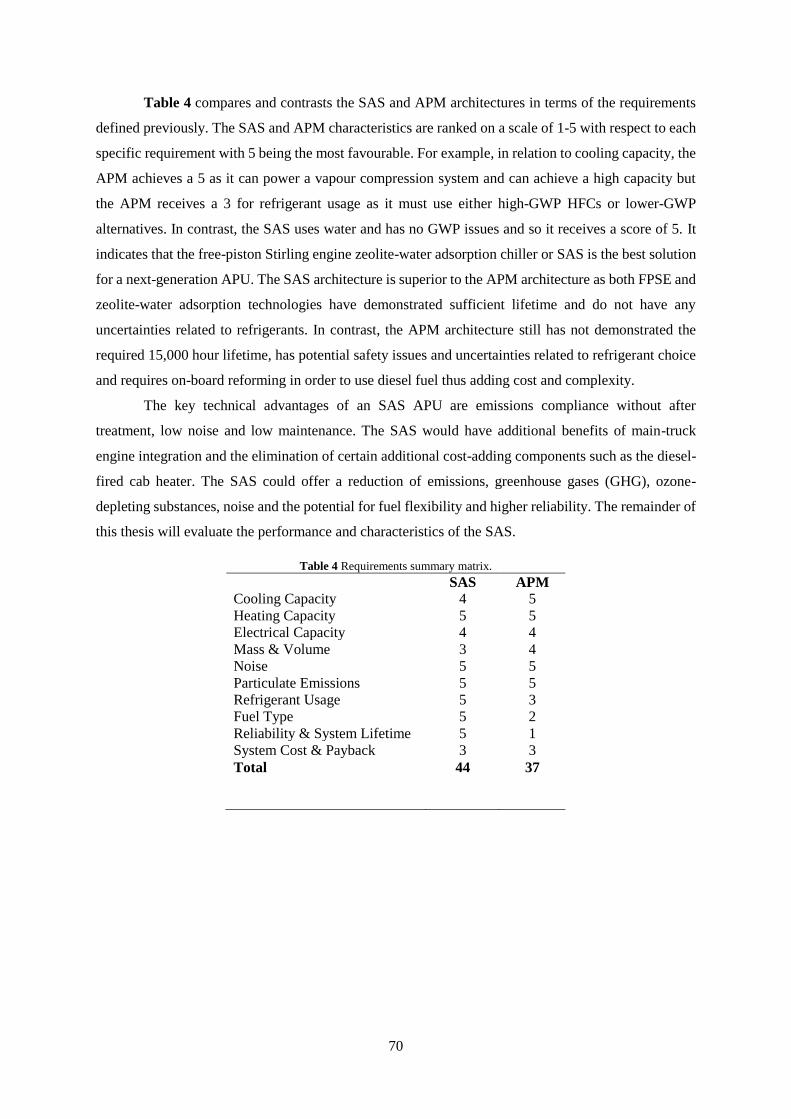
70
Table 4 compares and contrasts the SAS and APM architectures in terms of the requirements
defined previously. The SAS and APM characteristics are ranked on a scale of 1-5 with respect to each
specific requirement with 5 being the most favourable. For example, in relation to cooling capacity, the
APM achieves a 5 as it can power a vapour compression system and can achieve a high capacity but
the APM receives a 3 for refrigerant usage as it must use either high-GWP HFCs or lower-GWP
alternatives. In contrast, the SAS uses water and has no GWP issues and so it receives a score of 5. It
indicates that the free-piston Stirling engine zeolite-water adsorption chiller or SAS is the best solution
for a next-generation APU. The SAS architecture is superior to the APM architecture as both FPSE and
zeolite-water adsorption technologies have demonstrated sufficient lifetime and do not have any
uncertainties related to refrigerants. In contrast, the APM architecture still has not demonstrated the
required 15,000 hour lifetime, has potential safety issues and uncertainties related to refrigerant choice
and requires on-board reforming in order to use diesel fuel thus adding cost and complexity.
The key technical advantages of an SAS APU are emissions compliance without after
treatment, low noise and low maintenance. The SAS would have additional benefits of main-truck
engine integration and the elimination of certain additional cost-adding components such as the diesel-
fired cab heater. The SAS could offer a reduction of emissions, greenhouse gases (GHG), ozone-
depleting substances, noise and the potential for fuel flexibility and higher reliability. The remainder of
this thesis will evaluate the performance and characteristics of the SAS.
Table 4 Requirements summary matrix.
SAS APM
Cooling Capacity 4 5
Heating Capacity 5 5
Electrical Capacity 4 4
Mass & Volume 3 4
Noise 5 5
Particulate Emissions 5 5
Refrigerant Usage 5 3
Fuel Type 5 2
Reliability & System Lifetime 5 1
System Cost & Payback 3 3
Total 44 37

71
Chapter 3 – Literature Review
3.1 Chapter Overview
The purpose of this chapter is to evaluate existing literature on combined Stirling and adsorption
systems in terms of Stirling engine system integration, adsorption chiller system integration and overall
system modelling. This chapter differs from Chapter 2, which outlined the justifications for the Stirling-
adsorption system architecture. We believe that this is the first time that a Stirling engine and adsorption
chiller have been proposed for a truck auxiliary power unit, which means that there is no direct pre-
existing literature on the topic.
However, there are a range of studies on zeolite-water adsorption air conditioning using engine
waste heat recovery (not Stirling). Research has been done on applications for both truck and
automobile cabin cooling. The literature review has been expanded to include the automobile sector as
it will be relevant to the work done in this thesis as truck cabins and automobiles are broadly similar in
size and capacity requirements. Each of these major works are critically evaluated in terms of their
performance, general architecture and challenges related to the APU application. The chapter concludes
by identifying current gaps in the literature and highlighting the context for the proceeding work.
3.2 Stirling Engine System Integration
Combined operation of a Stirling and adsorption system – stability, pulsed thermal loading
As mentioned previously the proposed coupling of a Stirling engine and adsorption chiller in
truck APU appears to be entirely novel. Consequently, there is no information available on the potential
interaction between these two systems. Furthermore there appears be limited pre-existing literature on
the interaction of a Stirling engine and a dynamically varying waste heat load. However, previous work
by the author [274] in his B.Sc. thesis identified potentially important characteristics of Stirling engine
operation related to the variation in their power output with changing hot and cold end temperatures.
Figure 31 shown below shows the impact of engine temperature difference on the Stirling engine power
output. The engine power output, shown black, increases effectively linearly, with increasing exhaust
temperature (a proxy for hot end temperature). As the cold end is effectively fixed, the variation in
exhaust/hot end temperature is equivalent to overall engine temperature difference.

72
Figure 31 Variation of Whispergen PPS16 Stirling engine electrical power output with temperature difference [274].
The underlying reason for this is straightforward, Stirling engines are broadly analogous to
Carnot heat engines and so their efficiency, and consequently their power output, depends on the
temperature difference between the hot and cold end. This means that increasing the temperature at the
hot end of the engine whilst maintaining or reducing the cold end will result in an increase in efficiency
and power. Similarly, and perhaps more relevant to adsorption chiller integration, by decreasing the
cold end temperature and maintaining a fixed hot end temperature, the power output will also increase.
Such a scenario is already a thermal load case in the micro-CHP sector. Stirling engines are subjected
to a single instantaneous pulse of cold water through their cold end during normal operation in typical
households. This occurs when the radiator circuit in the house is switched into the boiler flow in order
to heat the whole house and not just a water tank. When this occurs, the Stirling engine is operating at
a nominal temperature of 50-70 °C but once the valve switches, a surge of cold water at 10-20 °C passes
through the engine resulting in a step-change in the engine ΔT. This causes a sudden spike in power
and efficiency which can be a challenge for free-piston Stirling engine operating stability.
Work by Bouvenot [275] in relation to experimental data driven modelling of a Stirling engine
for building energy simulation shows variation in power output for a 1 kWe Stirling with different inlet
temperatures. Though the core aims of this work are not directly related to the aims of this project, the
empirical approach to characterising the Stirling engine offers a valuable framework and methodology,
which could potentially be applied to this research. Additionally, a minor study from the same work,

73
reproduced below in Figure 32, offers important insight into the impact of varying the cold end
temperature of a Stirling engine on its overall performance and power output. Figure 32 shows that by
increasing the cold end temperature, the electrical power output will drop accordingly due to the
aforementioned reasons. A second, less significant effect is the impact of varying the flowrate through
the engine. The minor power gains in increasing flowrate are likely a result of improved efficiency of
the heat exchangers within the engine.
Figure 32 Variation of engine power output with changing cold-end temperature [275]
This data confirms the previous hypothesis derived from findings in Figure 31 and provides a
clear indication that dynamically varying engine temperatures will indeed cause corresponding power
fluctuations and potentially disrupt the stability of engine operation.
The change in engine cold end temperature is important for the adsorption chiller as the engine
cold end is the source of driving heat for the adsorption machine. In fact, the adsorption chiller can be
considered as the engine’s radiator or a source of thermal load. The heat demand of an adsorption chiller
is highly non-linear and work done by Verde et al. [190] on an adsorption chiller for truck cabin air
conditioning using waste heat from the main truck engine demonstrates this behaviour. A key figure
from the work, shown in Figure 33, shows the rapidly varying temperatures of the sorption beds which
is closely related to the overall driving temperature of the adsorption chiller which is, in effect, the cold
end of the Stirling engine. Using the purple line as an example, it is clear that coupled operation of
Stirling engine with an adsorption chiller will result in significant pulsed thermal loading.

74
Figure 33 Dynamic behaviour of an adsorption chiller's sorption beds [190].
The data shown in Figure 32 coupled with the adsorption behaviour shown in Figure 33
indicates that coupling a Stirling engine to an adsorption chiller will likely result in significant dynamic
interaction. It is unclear whether such a combination can operate with sufficient stability to be a practical
system. This is investigated in the work presented in this thesis.
Perhaps the most important distinction between the proposed Stirling engine-adsorption chiller
concept and previous efforts [116, 132, 189, 191-193, 276, 277] with waste-heat driven adsorption
chillers is the scale of the waste heat resource. All of the examples in the literature are large waste heat
sources such as truck, train and automobile engines. The quantity of waste heat produced by these
engines dwarfs the demand of the adsorption chiller and so the load placed on the engines is
comparatively small. The waste-heat output from the Stirling engine in the SAS configuration will
likely be closely matched to the adsorption chiller demand, meaning that there is no excess capacity
which will further amplify the interaction effects.
Similarly, in the micro-CHP sector, the engine or adsorption system are typically heavily
buffered through the use of a large storage tank of water with several hundred litres of capacity. This
tank dampens any interaction between the systems and the load. Obviously such a tank is unfeasible for
a mobile application like a truck APU as there are no space nor weight margins.
Therefore, there is a clear gap in the literature in relation to how Stirling engine will perform
when coupled to an adsorption chiller. More broadly, there does not appear to be any pre-existing
literature on how an adsorption chiller interacts with a similarly sized waste heat resource where
dynamic interaction will be very significant.

75
The key questions are:
Will the Stirling engine be able to operate stably with dynamic thermal loading on its cold end?
Will the adsorption chiller be able to operate with fluctuating drive temperatures?
What is the impact of low or no buffering on coupled Stirling-adsorption systems?
Stirling engine modelling
The analytical modelling of Stirling engines, in particular free-piston Stirling engines, is very
complex, and practically useful models require extensive calibration against real machines [86, 98].
Free-piston engines are kinematically simple but their overall operation is complicated by the
unconstrained phase angle relationship between each stage of thermodynamic cycle (hence free-piston).
Fundamental modelling of a free-piston Stirling engine is likely unnecessary and beyond the scope of
this research project’s aims as the key research questions and gaps in the academic literature lie at the
system level and the interaction between the Stirling engine and adsorption chiller. Consequently, a
higher level empirical approach such as the framework used by Bouvenot et al. implemented in an
appropriate modelling environment is likely sufficient to meet the needs of the project. A separate, yet
equally important reason, relates to product design and economics; as this research is co-funded by an
industrial sponsor, it is hoped that it will have real commercial applications. Therefore, the cost of the
Stirling engine will play a crucial role in the overall viability of the APU concept. Ergo, it is prudent
that the architecture leverage existing Stirling engine designs and, where possible, commercially
available technology. Reliance on a “common-platform” engine design that is used in other industries,
such as micro-CHP, will play an important role in minimizing engine costs through economies of scale.
In relation to engine modelling, this is important as any insights and optimizations discovered through
deep fundamental modelling of the core engine subsystem are unlikely to be implemented in a practical
system design for reasons of cost.
Bouvenot et al. has shown that the key criteria for characterising a Stirling engine’s
performance at the system level, namely the relationship of engine temperature difference to power
output and thermal efficiency can be characterised using experimental methods. This method is
analogous to “engine map” approaches used within the automotive industry whereby the performance
of an engine is measured across a wide range of conditions and a lookup table is generated that can be
used to estimate system performance for a given condition. A number of APU and micro-CHP (which
can be considered a stationary APU) system modelling studies utilize empirical “engine maps” within
dynamic modelling environments such as ADVISOR® or TRNSYS® [278, 279]. The use of such
experimentally-generated engine maps greatly simplifies subsystem modelling and therefore this
approach will be utilized in this research.
The key question related to the Stirling engine to be answered through system modelling is:
What is the optimum level of buffering required for the Stirling engine

76
3.3 Adsorption Chiller System Integration, Modelling and Testing
As mentioned previously, waste-heat driven adsorption cooling systems are not a novel idea.
For a comprehensive list of adsorption chiller systems driven via waste heat from engines the reader is
directed to work by Hamdy et. al [276]. However, work that specifically pertains to silica gel/zeolite –
water and truck/automobile cabin cooling are comparatively more niche and summarised below in
Table 5.
Table 5 Summary of relevant waste-heat air conditioning studies.
Author Adsorption modelling
approach
Sorption-
pair
Truck
application?
Ref Power COP
Verde et
al. (2016)
Non-equilibrium lumped
parameter adsorption model
based on previous
experimental
characterisation of sorbent
bed.
Silica gel-
water
Application is
automobiles
but still
similar to
truck APU.
[192,
193]
0.9 kW 0.4
Ali et al.
(2015)
Lumped parameter model.
Thermodynamic framework
of adsorption chiller is
developed from using mass
and energy balances of each
component of the system
and experimentally
confirmed isotherms and
kinetics data of various
adsorbent-adsorbate pairs.
Multiple Application is
automobiles
but still
similar to
truck APU
[186] 3 kW 0.38
Zhong et
al. (2011)
Lumped parameter model of
the system using linear
driving force model. Kinetic
properties of the zeolite
material are based on
previous experimental data.
Overall system results are
simulated
Zeolite-
water
Yes
specifically
related to
truck cabin
cooling.
[280] 0.3-0.8
kW
0.23-
0.5
Vasta et
al.
(2011)
System is characterised
experimentally and key
parameters such as cooling
power and COP measured
across range of condenser
(recooler) temperatures.
Zeolite-
water
Yes
specifically
related to
truck cabin
cooling
[277] 1-2.3
kW
0.25-
0.45
Verde et
al. (2010)
Lumped parameter
adsorption model based on
previous experimental
characterisation of sorbent
bed.
Zeolite-
water
Yes
specifically
related to
truck cabin
cooling.
[190] 5 kW 0.6

77
Extensive experimental
validation of model with
physical prototype
Jiangzhou
et al.
(2003)
System is characterised
experimentally and key
parameters such as cooling
power are measured for
specific adsorption,
desorption, condensing and
evaporating temperatures.
Zeolite-
water
Application is
locomotive
train cabin
which is
somewhat
similar to
truck
application.
[191] 3.2 kW N/A
Verde et al. (2016) [192, 193] proposed an adsorption chiller system for automobile cabin
cooling using waste-heat recovered from the vehicle’s engine. The system produced an average cooling
capacity of 925 W with a COP of 0.40 at a temperature of 17.5 °C. The overall proposed system
architecture is shown below in Figure 34 and consists of a two-bed adsorption chiller driven directly
by waste-heat from the vehicle engine. The modelling approach used in this study can be considered as
the most rigorous and robust method currently possible. The fundamental sorption kinetics and
isotherms for the silica-gel have been previously characterised experimentally. These parameters
underpin a non-equilibrium lumped parameter model of the adsorption process that has then been
validated using the experimental test rig. Fundamental modelling of the adsorption process enables high
fidelity dynamic simulation of key adsorption performance parameters such as COP and cooling
capacity. Though this approach provides the highest accuracy for predicting the adsorption subsystem’s
behaviour it necessitates the experimental characterisation of the sorbent material. This additional work
is significantly beyond the scope of the research aims of this project and the adsorption characteristics
of zeolites are significantly more non-linear than that of silica-gel making experimental characterisation
particularly essential.

78
Figure 34 System architecture proposed by Verde et al [192, 193].
Ali et al (2015) [186] proposed a waste-heat driven air conditioning system for an automobile
similar to that of Verde et al and generated simulated results for both silica gel and zeolite desiccants.
Verde’s results indicated that the proposed system could deliver 3 kW of cooling capacity at a maximum
COP of 0.38. The architecture proposed consists of a two-bed sorption system driven via waste-heat
derived from the main engine exhaust system and is shown below in Figure 35. The theoretical
approach utilized a lumped parameter model and the thermodynamic framework of adsorption chiller
was developed from using mass and energy balances of each component of the system and
experimentally confirmed isotherms and kinetics data of various adsorbent-adsorbate pairs. Though the
isotherms and kinetics were effectively validated through experimental confirmation, the overall system
model was not experimentally validated.

79
Figure 35 System-architecture proposed by Ali et. al [186].
Zhong et al. (2011) [280] proposed a zeolite-water adsorption chiller system for truck cabin
cooling using waste-heat derived from the main truck engine’s exhaust stream. The authors recognise
the complexity of exhaust heat capture and mention that heat capture from the cooling loop of the main
truck engine is simpler and potentially more effective due to the higher heat transfer coefficient of
liquids. Despite this, the focus of the study is on exhaust stream heat capture, and the proposed heat
exchanger design and system integration can be seen in Figure 36. The authors used a lumped parameter
model of the system using linear driving force model of the sorbent bed. The kinetic properties of the
zeolite material are based on previous experimental data and the overall system performance results are
simulated. The authors also recognise the advantages of potentially utilizing the APU but only mention
it in passing and do not propose a Stirling engine. Instead, a conventional APU is proposed and would
still face the emissions/noise problems which the authors acknowledge. Interestingly, the adsorption
system is viewed as an independent system and so the APU, truck engine and adsorption system are all
required in this architecture. The APU independent adsorption concept proposes a fuel fired heater for

80
truck engine independent operation and thus will not provide electric power to the cab which is a key
aspect of the hotel load.
Figure 36 Truck engine exhaust heat driven adsorption system architecture proposed by Zhong et al [280].
Vasta et al. 2011 [277] tested a zeolite-water adsorption chiller system for truck cabin cooling.
The system was powered via waste heat from the main engine coolant loop and achieved a COP of
0.25-0.45 and average cooling power of 1-2.3 kW. This work was part of the major EU-funded project
called Thermally Operated Mobile Air Conditioning System (TOPMACS). This work by the authors
probably represents the most advanced research in this field in terms of technology maturity as a fully
functional system was built and tested in an actual truck cabin. The TOPMACS proposal does not
address APUs as it is instead intended as a wholly independent system on the truck. This approach is
potentially disadvantageous as there will be insufficient space on the vehicle to accommodate both an
APU and the bulky adsorption chiller in applications where idling is a factor.
What is perhaps most interesting about this research is the empirical approach to characterising
the adsorption chiller system. The key system parameters such as COP and cooling capacity are
experimentally characterised across a range of ambient temperature (technically condenser) conditions.
This approach provides detailed performance characteristics and behaviour of an actual adsorption
chiller integrated with an engine but bypasses the need for detailed experimental characterisation of the

81
sorption material. Figure 37 shows the variation in COP over time with different condenser
temperatures. This method of characterising the adsorption chiller is similar to the “engine map”
approach discussed previously in relation to the Stirling engine. This approach is a very appealing
framework for the proposed research aims of this project as it avoids a considerable amount of
potentially tangential work. Crucially, these characteristic maps still capture sufficient dynamic
behaviour to provide sufficient accuracy to still meet the project aims.
Figure 37 Experimental data showing key adsorption chiller performance by Vasta et al [277].
Verde et al. (2010) [190] proposed a zeolite-water adsorption chiller system for truck cabin air
conditioning utilizing waste heat from the main truck engine. The architecture of their proposed system
is shown below in Figure 38. Experimental testing demonstrated that the adsorption chiller was capable
of generating 5 kW peak cooling power with a COP of 0.6. The authors employed a similar approach
as in their more recent (2016) work. They created a lumped parameter adsorption model based on
previous experimental characterisation of sorbent bed’s adsorption kinetics and isotherms. The overall
model was then extensively validated through experimental testing of a physical prototype. This work
represents the state-of-art in the truck cabin waste-heat driven adsorption cooling utilizing zeolites and
the theoretical framework employed is the most robust method available. However, in terms of
architecture, the overall concept suffers from similar challenges as the previous designs. The adsorption
chiller is an independent system and driven directly by the truck main engine. The idling problem is not
addressed and the system cannot operate independently of the main truck engine. However, as this
project was a European initiative related to TOPMACS, this is understandable as the APU is largely a
US phenomenon and the requirements of European trucks are different.

82
Figure 38 TOPMACS system architecture as proposed by Verde et al [190].
Jiangzhou et al. (2003) proposed a waste-heat driven adsorption chiller for a locomotive driver cabin.
Similar to Vasta et al. the authors took an empirical approach to characterising the system performance
and experimentally measured key parameters such as cooling power are measured for specific
adsorption, desorption, condensing and evaporating temperatures.
While wide-ranging, the literature surveyed above does not address a number of key questions related
to adsorption chiller behaviour and performance in the APU application namely:
How does cooling capacity change with increasing ambient temperature?
What is the realistic average COP an unbuffered adsorption chiller coupled to a Stirling engine?
How does the cooling efficiency compare to conventional DEVC systems across a range of
simulated conditions?
What are the physical dimensions and weight of an adsorption chiller capable of meeting the
requirements of a next generation APU system?
3.4 Knowledge Gap
None of the surveyed literature directly addresses the idea of integrating an adsorption chiller
within the APU itself. Only Zhong et al. [280] referenced the idea of using waste-heat from an APU in
addition the main truck engine but this concept viewed the adsorption chiller as an independent system

83
to the APU. Therefore, from an architecture standpoint, the proposed Stirling-adsorption system is
entirely novel and solves a number of key challenges related to the previous architectures. Implementing
the waste-heat adsorption chiller as a sub component of the APU potentially solves the space problem
as there is already a pre-existing footprint on the tractor frame rail. Similarly, direct APU integration
also addresses the idling challenge and permits operation independent of the main truck yet still retains
the ability to pull waste heat from the main engine during normal driving. Replacing the diesel engine
in the APU with a Stirling engine potentially solves the emission and noise problems with conventional
technology.
There is also a clear gap in the literature in relation to how adsorption chillers driven by similar
scale engine waste heat sources operate. In each of the above surveyed cases the prime mover is a car
engine or truck engine which is an order of magnitude larger waste-heat source than the waste-heat
load. Dynamic interaction will be much more significant with similarly sized heat load and generation
as in the proposed SAS. It is unclear how the adsorption chiller will perform in terms of steady state
COP and cooling capacity in this unbuffered configuration.
There appears to be no definitive experimental data showing the evolution of a zeolite-water
adsorption chiller’s cooling capacity with increasing ambient temperature above 35 °C. This data is of
critical importance to the overall feasibility of the SAS concept. The APU application requires
approximately 4 kW of cooling capacity at a cab temperature of 26.6 °C and 35 °C ambient. It is unclear
whether the adsorption chiller’s cooling capacity will degrade linearly or non-linearly with increasing
ambient temperature which is fundamental to overall sizing of the adsorption chiller. The system must
be sized to meet or exceed the conventional DEVC system’s performance across the entire operating
range and if the capacity degradation is so severe in high ambient temperatures as to make the adsorption
chiller impractically large then the overall concept will be technically unfeasible. From a product design
perspective, it is vital to be aware of any maximum ambient temperature limitations for the technology
as it could severely restrict potential market geographical deployment.
There is no experimental data showing the interaction of a Stirling engine with an adsorption
chiller in the literature. Some previous work does give an indication of what to expect with pulsed-
thermal loading but this has not been demonstrated in an experimental prototype.
Overall, the key question that this research seeks to answer is how the proposed SAS system
compares in terms of cooling and electrical efficiency to the incumbent DEVC system across a range
of realistic test conditions.
This research project will aim to add to the existing literature by answering the following
specific questions:
In relation to the Stirling engine subsystem:
Will the Stirling engine be able to operate stably with dynamic thermal loading on its cold end?
Will the adsorption chiller be able to operate with fluctuation drive temperatures?

84
What is the impact of low or no buffering similarly sized coupled Stirling-adsorption systems?
What is the optimum level of buffering required for the Stirling engine
In relation to the adsorption chiller subsystem:
How does cooling capacity change with increasing ambient temperature?
What is the actual average COP an unbuffered adsorption chiller coupled to a Stirling engine?
How does the cooling efficiency compare to conventional DEVC systems across a range of
simulated conditions?
What are the physical dimensions and weight of an adsorption chiller capable of meeting the
requirements of a next generation APU system?
In relation to overall SAS system:
How does it compare to the DEVC system in terms of cooling and electrical efficiency
3.5 Research Methodology and Theoretical Framework
The author has previously outlined the various theoretical approaches to predicting the key
performance metrics of both Stirling engine and adsorption chiller systems. He has established that an
empirical approach based on experimental testing or “engine maps” is the most suitable method for
characterising the Stirling engine as part of an overall APU system. The chosen methodology will be
similar to work done by Bouvenot et al. and these characteristic maps of engine performance will be
used as lookup tables within the dynamic physical modelling environment SimScape. SimScape, a
subset of Mathworks Simulink, is a physics-based modelling tool that facilitates the creation of hybrid
models that contain both physically accurate models of key components like pipes, valves, fluid flow
and heat transfer but also allows the inclusion of empirical lookup tables.
An empirical approach to characterising the adsorption chiller’s behaviour and performance
such as that used by Vasta et al. is also the most suitable approach for the research aims of this project
as it avoids the need for considerable background experimental work on characterising the adsorption
kinetics and isotherms of the zeolite-material which is only tangentially related to the research project.
As with the Stirling engine, the overall performance of the adsorption chiller will be captured using an
“engine map” approach for key parameters like cooling capacity versus increasing ambient temperature
and these relationships will be used as lookup tables within the SimScape environment.
The overall approach to answering the fundamental research question of how the SAS compares
to the DEVC system will consist of three phases which are effectively contained in Chapters 4, 5 and 6
respectively.

85
The first phase will be to create a preliminary reduced order model using known data from the
scientific literature and industrial community on commercially available or well developed Stirling
engines and adsorption chillers. The use of publicly available technology is essential for two reasons,
namely; the aforementioned importance of using common platform technology for economic reasons,
and, the more realistic performance of a commercial system which has undergone numerous
performance trade-offs to allow for manufacturability, acceptable cost and safety. A purely
experimental system is likely to provide unrealistically high performance compared to a system which
has been optimised into a viable product such as the incumbent DEVC system. However, as the
architecture is entirely novel, parts of the system will, by necessity, be experimental but the use of
commercially available technology where practical will make the comparison as realistic as is
reasonably possible. Once the basic models of the SAS and DEVC are created they will be compared
in terms of overall efficiency and estimated system costs. Though this approach will not capture many
of the unique dynamics that are expected when actual system integration occurs, it will provide a
satisfactory initial estimate of whether the architecture is worth pursuing further.
The second phase will consist of construction and testing of an experimental prototype. This
will facilitate the investigation of system integration issues and the measurement of key parameters
such as the degradation of cooling capacity with increasing ambient temperature and actual performance
of the adsorption chiller in terms of COP and capacity in low buffer scenarios. These measurements
will form the basis of empirical engine maps that will be used in the system modelling effort in phase
three.
The third phase of the research will be the construction of an overall system model in SimScape
using the empirical data recorded from the prototype. This system model will allow for comparison of
a theoretical full scale SAS against the DEVC across a range of relevant temperatures. It will also allow
for deeper investigation of any unique interaction effects such as the low buffering phenomenon. The
third phase will ultimately seek the answer the overall question of how the SAS compares against the
incumbent DEVC system in terms of efficiency, size, mass and cost.
3.6 Motivation for this work
The context for this work is that, although very interesting waste-heat truck cabin cooling
concepts have been proposed, they face fundamental architectural challenges that the SAS could
potentially address. The main justification for this research is because Chapter 2 identified the SAS as
potentially being the best technology architecture for a next generation APU and each of the
fundamental research questions outlined above represent the key technical challenges currently
preventing such a system from being implemented in the field. By addressing each of these questions,
the author will potentially remove all of the technical barriers preventing manufacturers from adopting

86
the SAS architecture and thus significantly reducing the environmental impact of APUs whilst
simultaneously increasing driver comfort and well-being.
3.7 Conclusion
The author has surveyed the most relevant literature related to the proposed SAS concept and, from
this, identified the key gaps in the scientific literature. Furthermore, through analysis of previous
approaches by the research community, the author has identified a semi-empirical approach utilizing
reduced-order models as the most suitable methodology and framework to meet the overall project aims.

87
Chapter 4 – Preliminary analysis of the Stirling-adsorption system
4.1 Chapter Overview
The purpose of this chapter is the reintroduce the SAS architecture and make a preliminary comparison
of its performance versus the incumbent DEVC APU in terms of cooling/electrical efficiency and
economic payback. The chapter begins by outlining the key players in adsorption and Stirling engine
technology and describes the technical performance of their respective commercially available (or near
commercial) systems. These technical parameters, based on proven technology, will then be used as the
basis for an empirical reduced order model that will be compared against pre-existing benchmark data
for a leading DEVC APU system, the TriPac Evolution, produced by Thermo King. The models will
compare the two systems under a baseline scenario of cooling and electrical loads and estimate the
overall fuel consumption required to meet these steady-state demands. Using the associated operating
fuel cost, along with expected maintenance and predicted capital costs, an overall lifetime payback for
each system will be calculated and compared. Finally a sensitivity analysis of the model will be
performed to identify the critical parameters that effect lifetime payback of the APU systems.
4.2 SAS Architecture
The proposed system, shown schematically in Figure 39, consists of a 1-2 kWe FPSE coupled to a
4 kWt zeolite-water adsorption chiller system. The adsorption chiller is driven via waste heat at Tdi from
the Stirling engine’s cooling jacket. Heat is rejected (Tro to Tri) from the adsorption chiller via a
secondary non-condensing heat exchanger known as a recooler, “Recooler HX” in Figure 39. Heat is
removed from the cab (Tco to Tci) via another secondary non-condensing heat exchanger, “Cab Chiller
HX” in Figure 39. As previously mentioned the adsorption system is also capable of utilizing waste
heat from the main truck engine cooling loop whilst driving. In conventional systems, this infrastructure
is already in place as the APU and main engine cooling circuits are often bridged together to provide
engine pre-heating for easy starting in cold climates. This could potentially result in high efficiency cab
air conditioning when the truck is driving and could offset the fuel consumption of running the truck’s
air conditioning system.

88
Figure 39 System-level architecture diagram of the SAS concept. This diagram is for illustrative purposes only and does not
depict minor plumbing. For a detailed overview of the adsorption chiller internal plumbing, in particular with reference to heat
recovery, the reader is directed to the system characterised by Myat et al. [281].
Functionally, the SAS can be decomposed into a Stirling subsystem and an adsorption chiller
subsystem. The remaining components such as piping, air cooled heat exchangers, valves and fans are
relatively trivial components and widely available commercially. In contrast, the Stirling engine and
adsorption chiller are extremely niche products as the technology is only in an early stage of
commercialization. In order to characterise the system using a reduced-order model it is first necessary
to identify an appropriately sized commercially available Stirling engine and adsorption chiller. For a
first order analysis the key global parameters needed from the commercial hardware are the Stirling
engine electrical efficiency, available waste heat, adsorption chiller COP and adsorption chiller heat
rejection load. It also necessary to estimate the fan blower and hydraulic pumping power required as
these are parasitic overhead for the Stirling engine’s electrical power output.
4.3 Performance of Commercially Available Hardware
There are occasional new entrants to the commercial Stirling engine market, however, a key
litmus test for these manufacturers is the level of development of their respective engine technologies.
Historically, the two major players in Stirling engine technology were New Zealand based
Whisper Tech and UK based Microgen Engine Corporation. Whisper Tech developed and marketed the
Whispergen 1 kWe kinematic Stirling engine which is a four-cylinder double-acting alpha type engine
that uses a wobble-yoke mechanism to drive a rotary alternator. Microgen developed and market the 1
kWe linear free-piston Stirling engine for domestic micro-CHP applications.

89
Microgen Engine Corporation
Microgen Engine Corporation (MEC) have a long history of Stirling engine development. Their
core engine technology was originally licensed from Sunpower in the US. Sunpower is notable in the
Stirling engine world as it was founded by William Beale, the inventor of the free-piston Stirling engine.
Microgen Engine Corporation began developing the Sunpower engine into a commercially viable
micro-CHP product in 1995. Subsequently, in 2001, the British Gas group bought out MEC and focused
development on gas-fuelled Stirling engines for domestic CHP. In 2007 a Dutch Investment consortium
bought out MEC and continued development of the core Stirling engine technology for gas-based CHP.
By 2013, more than 10,000 engines had been built and in 2014, 5 million cumulative run hours had
been demonstrated with the technology and over $200m had been invested in bringing the technology
to market.
The level of commercial development and technological maturity demonstrated by MEC is
significantly ahead on any potential competitors. In 2013, the author visited the MEC R&D facility in
Peterborough, UK as part of a fact finding mission and observed their engine testing facility (some of
which is shown below in Figure 40). In addition to numerous experimental test engines, the facility has
at least 30 engine test beds continuously running accumulating run-hours and reliability data.
Figure 40 View across part of the engine test facility at Microgen Engine Corporation’s R&D facility in Peterborough, UK.
© Barry Flannery
MECs core engine technology is a 1 kWe beta-type linear free-piston Stirling engine shown
below in Figure 41. The engine has a net electrical efficiency of ~15% and weighs 49 kg. The key
advantage of a free-piston Stirling engine over kinematic Stirling engines (and indeed diesel engines)
is its mechanical simplicity, which eliminates the need for gears, piston rods, flywheels, crankshafts,

90
bearings, piston rings and oil lubrication. Reducing the number of moving parts significantly improves
reliability and eliminates the need for maintenance. The integration of the linear alternator within the
pressure vessels also means that the whole engine can be hermetically sealed eliminating the generator
shaft seal and need for periodic gas recharging that stems from slow leakage of the working fluid out
of the engine in the case of kinematic machines like the Whispergen engine. Additional technical
parameters for the MEC engine are shown below in Table 6.
Figure 41 Cutaway of the MEC 1 kWe linear free-piston Stirling engine and CAD render showing the full system and
wiring. Note that the engine’s combustor is not installaed. © Microgen Engine Corporation
Table 6 Key technical specifications of the Microgen 1 kWe FPSE
Power output 1 kWe
Net electrical efficiency 15%
Weight (engine only) 49 kg
Voltage Min. 186 V, Max. 264 V, Nominal 230 V
Water flow Min. 7 l/min, Nominal 15 l/min
Frequency Min. 49.5 Hz, Max. 50.5 Hz, Nominal 50 Hz
Water temperatures 6 °C to 75 °C
Ambient temperatures 6 °C to 70 °C
Heat output to coolant 3±0.5 kW Nominal, Max. 5 kW
Heat output including exhaust HX Max. 6.5 kW
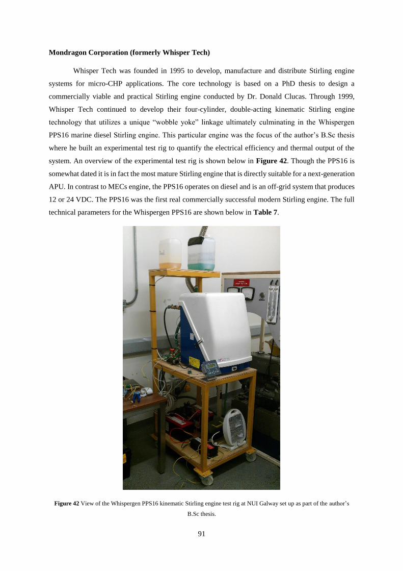
91
Mondragon Corporation (formerly Whisper Tech)
Whisper Tech was founded in 1995 to develop, manufacture and distribute Stirling engine
systems for micro-CHP applications. The core technology is based on a PhD thesis to design a
commercially viable and practical Stirling engine conducted by Dr. Donald Clucas. Through 1999,
Whisper Tech continued to develop their four-cylinder, double-acting kinematic Stirling engine
technology that utilizes a unique “wobble yoke” linkage ultimately culminating in the Whispergen
PPS16 marine diesel Stirling engine. This particular engine was the focus of the author’s B.Sc thesis
where he built an experimental test rig to quantify the electrical efficiency and thermal output of the
system. An overview of the experimental test rig is shown below in Figure 42. Though the PPS16 is
somewhat dated it is in fact the most mature Stirling engine that is directly suitable for a next-generation
APU. In contrast to MECs engine, the PPS16 operates on diesel and is an off-grid system that produces
12 or 24 VDC. The PPS16 was the first real commercially successful modern Stirling engine. The full
technical parameters for the Whispergen PPS16 are shown below in Table 7.
Figure 42 View of the Whispergen PPS16 kinematic Stirling engine test rig at NUI Galway set up as part of the author’s
B.Sc thesis.

92
Table 7 Key performance parameters of the Whispergen PPS16 diesel fuelled Stirling engine.
Power output 1 kWe
Net electrical efficiency 12%
Weight 90 kg
Overall efficiency 90%
Heat output including exhaust HX 6 kWt
Voltage 12 / 24 V DC
Whisper Tech subsequently developed an on-grid, natural gas fuelled variant of their engine
for domestic CHP applications. This engine was the predecessor to the system currently under
development by Mondragon Corporation and the core technology has been refined through successive
iterations. In 2011, Whisper Tech was dealt a devastating blow by the major earthquake that hit
Christchurch, New Zealand. This, coupled with a difficult market lead to the collapse of the company
and subsequent buyout by Mondragon Corporation of Spain.
In 2014, the author was invited to visit the Mondragon Stirling engine R&D facility, CS Centro
Stirling, near Bilbao, Spain shown below in Figure 43. Due to unsuccessful commercialization plans
caused by a key customer abandoning a major contract for strategic reasons, Mondragon Corporation
do not manufacture Stirling engines for sale at this time, but maintains an R&D presence.
Figure 43 View of CS Centro Stirling, the Mondragon Corporation Stirling engine R&D facility, near Bilbao, Spain. ©
Barry Flannery

93
The author was shown a Mk.5 natural gas fired kinematic Stirling engine and a mockup
showing the internals of a prototype 3 kWe Stirling engine design both of which are shown below in
Figure 44. There was a key disparity in the scale of research and development operations between
Mondragon and Microgen Engine Corporation. Only several engines were undergoing testing in a
relatively small-scale laboratory.
However, many of the key reliability challenges such as lateral piston seal loading of the
original Whispergen design appear to have been overcome through engineering advancements. The
Mk.5 Whispergen engine now demonstrates similar reliability to the MEC engine. However, it still
requires periodic gas refilling. Despite the MEC FPSE not requiring maintenance it is anticipated that
a diesel fuelled variant may require an annual burner maintenance to clean soot from the combustor.
Consequently, the advantage of not requiring a gas-refill is potentially moot as both engines will still
require an annual service. However, the key challenge for the Mondragon engine is not technical but
commercial as a they do not currently have any commercial sales to support their operations.
Figure 44 A prototype mockup of the 3 kWe kinematic Stirling is shown on the left and the 1 kWe Mk.5 natural gas micro-
CHP engine is shown on the right. Both machines were being developed by Mondragon at CS Centro Stirling. ©Barry Flannery

94
Table 8 Technical specifications of the Mondragon Mk.5 Stirling engine.
Power output 1 kW
Net electrical efficiency 12%
Weight 127 kg
Voltage 230-240 VAC
Frequency 50 / 60 Hz
Water temperatures 0-90 °C
Heat output to coolant 6 kWt
InvenSor GmbH
InvenSor GmbH was founded in 2006 with the aim of commercializing zeolite-water based
adsorption chiller units. Over the past decade, it has successfully commercialized small to medium scale
zeolite-water adsorption chiller in the 10-90 kW range and is one of the few suppliers on the market
currently manufacturing such systems and offering them for sale. In 2014, the author visited their main
R&D facility in Berlin, Germany, shown in Figure 45, to investigate the feasibility of a smaller scale
zeolite-water chiller. The author was shown a physical prototype of a 3 kWt adsorption chiller shown
below in Figure 46a. The optimized prototype unit broadly met the geometric and mass requirements
of the next generation APU and showed a considerable level of development based on underlying
technology used in their larger scale machines. A second prototype unit of similar scale shown in Figure
Figure 46b was also shown to the author that was driven by a micro-organic Rankine cycle machine,
an architecture that is extremely similar to the proposed SAS. InvenSor offer the highest power density
commercially available adsorption technology and has also demonstrated relevant scale prototypes
suitable for the next-generation APU.
Figure 45 View of the building where InvenSor GmbH’s R&D facility is co-located with other small businesses. © Barry
Flannery

95
(a) (b)
Figure 46 View of two APU scale prototype adsorption chillers at InvenSor GmbH’s R&D facility in Berlin, Germany. (a)
is a 3 kW unit and measures 600 x 250 x 800mm and weighs 90 kg and (b) is 1000 x 550 x 450mm and has been integrated
with a micro-organic Rankine cycle machine which is very similar to the SAS architecture.
InvenSor adsorption machines are two-bed zeolite-water designs that incorporate heat and mass
recovery. The zeolites used vary on specific machine design but the main technologies currently used
are AQSOA-FAMZ01 and AQSOA-FAMZ02 produced by Mitsubishi Chemicals17. A key strategic
decision by InvenSor is that it is sorbent material agnostic and has the ability to use new technologies.
This is in contrast to its main competitor SorTech which develops their own sorbent materials. This
approach enables InvenSor to rapidly adopt new technologies developed by the chemical industry for
wider applications. The internal operation of the machines is shown below in Figure 47 and Figure 48
by Myat et al [281]. The adsorber beds within the machine, Ads 1 and Ads 2, are heated and cooled out
of phase with each other. This facilitates concurrent cyclic desorption and adsorption of water
refrigerant enabling a refrigeration process. During switchover, a momentary connection is made
between the beds to equalise pressure and facilitate mass transfer and heat transfer. Similarly, in the
hydraulic loop, the warm water from the heated bed is physically transferred to the cold bed to further
aid in heat recovery thus increasing overall COP and efficiency.
17 The choice of either AQSOA-FAMZ01 and AQSOA-FAMZ02 depends on the operating temperature with the
latter being more suited to higher driving temperatures.
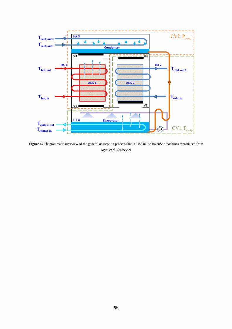
96
Figure 47 Diagrammatic overview of the general adsorption process that is used in the InvenSor machines reproduced from
Myat et al. ©Elsevier

97
Figure 48 Detailed overview of each phase of the adsorption-desorption cycle within the InvenSor machine reproduced from
Myat et al. ©Elsevier.
Extensive reliability testing and demonstrating technological maturity are critical criteria for
any new potential technology, especially a prime-mover that hopes to supplant the diesel engine. Major
OEMs, such as the manufactures of auxiliary power units, are risk averse and generally unwilling to
stake their reputations on an unproven technology. Therefore, the benchmark technology used for
preliminary modelling must have extensive development and reliability history to be considered feasible

98
for a next-generation APU. Consequently, the MEC engine provides the most realistic benchmark for a
future Stirling engine for a next-generation APU owing to its extensive development and proven
maturity. Though the engine is only rated at 1 kWe, MEC has indicated that a 2 kWe variant is currently
under development. From a technological standpoint, the existing engine design is thermodynamically
rated to deliver up to 3 kW of power but is limited by the size of the linear alternator which saturates at
approximately 1.4 kWe. Therefore, the performance, in terms of efficiency and heat output ratio, of a 2
kWe engine which is needed for the APU application is likely to be very similar to the 1 kWe engine.
In relation to adsorption cooling technology, InvenSor GmbH has successfully commercialized
several zeolite-water adsorption chiller products in the 10-90 kWt range and have demonstrated a 3 kW
scale prototype unit in a fact finding visit in 2014. More significantly, InvenSor have also demonstrated
coupled operation with an organic Rankine cycle engine which is very similar to the proposed SAS
architecture from a thermal standpoint. This experience, along with physical demonstration of a 3 kW
adsorption chiller that meets the geometric and weight constraints of the next-generation APU mean
that current InvenSor adsorption technology is an appropriate benchmark for future system
performance. According to InvenSor, the key performance parameters such as capacity and waste-heat
requirements scale linearly whilst maintaining the same COP with their machine designs meaning that
the LTC 10, a 10 kW adsorption chiller’s performance can be used as a reference in the SAS reduced
order model.
4.4 Baseline Test Case
The baseline test case used as inputs to the reduced order model are shown below in Table 9. The
cooling condition chosen is based on the ARI STD 310/380 which specifies an ambient temperature of
35 °C and cab condition of 26.6 °C. The electrical load of 0.8 kWe was estimated from typical use case
scenarios from the DEVC APU manufacturer. The actual cooling load is derived from the Thermo King
suction/discharge calculator that estimates the corresponding capacity requirement based on a given
ambient (condenser) and cab (evaporator) coil air-side condition.
Table 9 Reduced-order model inputs
Cooling Load (kW)*
Electrical Load (kWe)
Ambient Condition (°C)
Cab Condition (°C)
Fuel Cost ($/gal)
System Lifetime (years)
Running hours per year
Diesel calorific value (MJ/kg)
2.5
0.8
35.0
26.6
2.20
8
1860
42.80 *Calculation based on DEVC APU refrigeration sub-model

99
4.5 SAS Reduced Order model
Adsorption chiller
The adsorption chiller sub‐model is a simple steady state estimation based on a commercially
available 10 kW zeolite‐water adsorption chiller using a static COP of 0.518. The model does not account
for situations when there is insufficient waste heat available and the system must switch to “adsorption
chiller control” which is defined as when excess electrical power and waste heat is generated to drive
the chiller. Any excess electricity is diverted to the truck batteries or else dissipated in a resistive
element in the cooling loop i.e. converted into additional waste heat. The overall logic of the model is
closely approximated by the energy flow comparison diagram depicted in Figure 49.
Figure 49 Energy flow diagrams for a DEVC and the SAS system utilizing waste heat.
Free-piston Stirling engine
The FPSE model is based on empirical data from Microgen Engine Corporation. The system
electrical efficiency is estimated to be 15% and represents the efficiency of converting the thermal
power of the inputted fuel into an electrical power output. The waste heat capture efficiency is an
estimate as to how much waste heat by-product from electrical generation can be used for driving the
adsorption chiller. An estimate of 80% is used which is likely conservative as micro-CHP units typically
display overall system efficiencies of greater than 90%. The parasitic electrical requirements of the
18 Based on InvenSor LTC10 adsorption machine.

100
system are estimated to be 300 W based on experience with the Whispergen PPS16 test rig which
produces 1000 W of gross electrical power and 800 W net electrical.
The model operates on the basis of electrical demand whereby an electrical demand requirement
is provided as an input parameter and the model then calculates the required fuel input based on the
empirical electrical efficiency estimate of 15%.
Consider the following scenario of 0.8 kWe of electrical load and 2.5 kWt of cooling demand on the
hypothetical SAS system described above.
The total electrical demand, Ptot, is calculated using Eq. (3) and is equal to the sum of the actual demand,
Pl, and the parasitic electrical load Ppar.
𝑃𝑙 + 𝑃𝑝𝑎𝑟 = 𝑃𝑡𝑜𝑡 (3)
0.8 + 0.3 = 1.1 kWe
The required fuel input, Qf, to meet this demand is given by Eq. (4) and calculated from the total power
requirement Ptot divided by the empirical electrical efficiency ηe.
𝑃𝑡𝑜𝑡
𝜂𝑒= 𝑄𝑓
(4)
1.1
0.15= 7.3 𝑘𝑊𝑓
The amount of waste heat, Qwh, produced by the engine in this scenario is determined by calculating the
fraction of heat not used for electrical generation using Eq. (5).
𝑄𝑓(1 − 𝜂𝑒) = 𝑄𝑤ℎ (5)
7.3 (1 – 0.15) = 6.2 kWt
Not all of this waste heat is usable and so therefore a maximum waste heat capture efficiency, ηwh, must
be used to calculate the waste heat available for driving the adsorption chiller, Qdr using Eq. (6).
𝑄𝑤ℎ × 𝜂𝑤ℎ = 𝑄𝑑𝑟 (6)
6.2 × 0.8 = 5 kWt
The delivered cooling capacity is calculated from the estimated COP of 0.5 for the adsorption chiller
using Eq. (7).
𝑄𝑑𝑟 × 𝐶𝑂𝑃 = 𝑄𝑐𝑜𝑜𝑙 (7)
5 × 0.5 = 2.5 kWt
The overall cooling, ηcool and electrical efficiency ηelec can be calculated using Eq. (8) and Eq. (9)

101
𝑄𝑐𝑜𝑜𝑙
𝑄𝑓= 𝜂𝑐𝑜𝑜𝑙
(8)
2.5
7.3= 34.2%
𝑃𝑙
𝑄𝑓= 𝜂𝑒𝑙𝑒𝑐
(9)
0.8
7.3= 10.9%
Note that, in relation to electrical efficiency, it is incorrect to include the parasitic parameter in the
efficiency calculation as parasitics are not a desired output to the truck driver and do not form part of
the delivered electrical output.
The above example is carefully chosen as it is a simple case for calculations and represents a
typical usage scenario. However, there are extreme cases where the system will be required to produce
an excess of cooling or electrical power depending on the load configuration. For example, a high
cooling load coupled with a low or non-existent electrical load will decrease overall system efficiency
as excess electricity will need to be generated. In this scenario, the electricity can be dissipated in the
engine using an electrical clamp heater and converted back into waste heat. Likewise, in situations of
high electrical demand, there will be scenarios where cooling capacity could be generated if needed. If
cooling capacity is not required then the adsorption chiller could be placed in bypass mode and its
recooler used as a passive radiator as with conventional engines. In this scenario, certain parasitic loads
could be reduced by switching off the adsorption machine’s fans and pumps. It is important that the
excess fuel needed in these scenarios be accounted for in any model calculations.
4.6 DEVC Reduced Order Model
The APU model is based upon proprietary experimental data from the manufacturer of a leading
truck APU system. The logical structure of the model is shown in Figure 50. The model inputs are
relatable to a truck driver i.e. electrical load, cooling load. The model calculates the required fuel input
to meet these input conditions and, from this, generation efficiencies and running costs can be estimated.
Scheduled maintenance costs associated with the DEVC APU are based on the manufacturer’s
recommendations. Unscheduled maintenance costs related to break-downs, component failure such as
belts, drives, pulleys and shaft seals have not been accounted for but represent a significant maintenance
cost that could be eliminated with a high reliability system like the SAS.

102
Figure 50 Logical structure of the DEVC APU model.
The model for the DEVC system is based on performance equations extracted from three sets
of empirical data provided by the manufacturer; the overall refrigeration COP, the alternator efficiency
and the engine fuel consumption versus engine load. The latter two relations are shown graphically in
Figure 51a and Figure 51b respectively. A static refrigeration COP of 1.4 has been estimated from
experimental test data supplied by the manufacturer.
(a) (b)
Figure 51 Critical parameters defining the dynamic behaviour of the DEVC system.
Consider the following scenario of 0.8 kWe of electrical load. Pl, and 2.5 kWt of cooling demand, Qcool,
on the DEVC system.
The mechanical compressor load Pcom is calculated from the cooling capacity and the fixed COP using
Eq. (10).
𝑃𝑐𝑜𝑚 =𝑄𝑐𝑜𝑜𝑙
1.4
(10)
2.5
1.4= 1.8 𝑘𝑊𝑚
The efficiency of the alternator ηalt for a given electrical load is calculated from the electrical power Pe
using the empirical correlation shown in Eq. (11).
103
𝜂𝑎𝑙𝑡 = 0.0361𝑃𝑒2 − 0.1977𝑃𝑒 + 0.7576 (11)
0.0361(0.82) − 0.1977(0.8) + 0.7576 = 0.62
The alternator mechanical load Palt is calculated from ηalt and Pe using Eq. (12).
𝑃𝑎𝑙𝑡 =𝑃𝑒
𝜂𝑎𝑙𝑡
(12)
0.8
0.62= 1.3 𝑘𝑊𝑚
The total engine load Pm is calculated using Eq. (13).
𝑃𝑚 = 𝑃𝑎𝑙𝑡 + 𝑃𝑐𝑜𝑚 (13)
1.3+ 1.8 = 3.1 kWm
The fuel consumption, Qf is calculated from the total mechanical load Pm using the empirical
correlation shown in Eq. (14).
𝑄𝑓 = 0.0723 𝑃𝑚2 + 1.7685 𝑃𝑚 + 6.1787 (14)
0.0723(3.12) + 1.785(3.1) + 6.1787 = 12.3 𝑘𝑊𝑓
The overall cooling, ηcool and electrical efficiency ηelec can be calculated using Eq. (15) and Eq. (16)
𝑄𝑐𝑜𝑜𝑙
𝑄𝑓= 𝜂𝑐𝑜𝑜𝑙
(15)
2.5
12.3= 20.3%
𝑃𝑙
𝑄𝑓= 𝜂𝑒𝑙𝑒𝑐
(16)
0.8
12.3= 6.5%
4.7 Idling model
The number of hours spent idling by heavy-trucks and the associated fuel consumption varies
considerably. The baseline case of 1860 idling hours per year, 1 gal/hour (3.79 l/hour) fuel consumption
and $1.13 additional daily maintenance cost was taken from an Argonne National Laboratory report
into idling [6, 14]. It was assumed in the sub-model that, under this idling condition, the truck could
meet any electrical and/or air conditioning demand place upon it by the driver with the static fuel

104
consumption shown above which is equivalent to a fuel burn, Qf of 37.8 kW. The overall cooling, ηcool
and electrical efficiency ηelec can be calculated using Eq. (17) and Eq. (18)
𝑄𝑐𝑜𝑜𝑙
𝑄𝑓= 𝜂𝑐𝑜𝑜𝑙
(17)
2.5
37.8= 6.6%
𝑃𝑙
𝑄𝑓= 𝜂𝑒𝑙𝑒𝑐
(18)
0.8
37.8= 2.1%
4.8 Sensitivity Analysis
A sensitivity analysis of variables effecting lifetime payback, shown in Table 10, was
performed on the system level model and the results are shown below in Figure 52. Lifetime payback
was chosen as the dependent variable as it encapsulates all aspects of system efficiency and
performance. The rationale behind key variables such as system capital cost are that the existing system
costs approximately $8,000 and so represents a minimum value. The baseline cost case is based on the
system costing twice that of the existing system and finally the maximum cost case is 150% higher than
the baseline. The fuel cost was values were based on historical value of fuel prices. The cooling demand
is based on the existing DEVC operating range of 0-4 kWt and, likewise, so is the electrical demand.
The electrical efficiency of the Stirling engine is based on a range of actual engine performance values
of described in the literature [87]. The COP is based on observed performance of real systems.
Table 10 Sensitivity study variables
Baseline Min Max Fuel Cost ($/gal)
System Capital Cost ($)
Chiller COP
Electrical Demand (kWe)
Cooling Demand (kW)
Electrical Efficiency
2.2
16,000
0.50
0.80
2.32
0.15
1.5
8,000
0.20
0.10
0.50
0.08
4
24,000
0.80
1.80
4.00
0.20
As expected, fuel cost and system capital cost dominate lifetime payback. Fuel cost, obviously,
is largely uncontrollable but system capital cost can be managed to a certain extent. Free-piston Stirling
engines and adsorption chillers are low volume, new-to-market technologies and are still considerably
more expensive than conventional technology but they can be expected to decrease in cost as production
volumes increase. The Stirling engine efficiency and chiller COP have a strong non-linear effect above
a certain threshold which is caused by an imbalance of the waste-heat production to demand ratio. In
certain scenarios there is excess cooling capacity that is effectively of no value. In the case of the DEVC,

105
it can simply not produce the excess, whereas with the SAS the lower efficiency prime mover will suffer
and be forced to produce excess waste heat in high electrical/low cooling situations. This is primarily
due to the refrigeration load being perfectly matched to waste heat production of a lower efficiency
engine. The most important finding of the sensitivity analysis is the critical importance of COP to
lifetime payback. Adsorption chiller COP is expected to drop dramatically at higher ambient
temperatures and this is not currently captured in the system level model and is a key focus of work
described in Chapter 5.
Figure 52 Sensitivity analysis of the key variables affecting lifetime payback.

106
4.9 Results and Discussion
By avoiding the thermodynamic penalties of using mechanical engine work, the air
conditioning system was considerably more efficient if driven via waste heat than the incumbent. The
key outcome of this study shows that the proposed system has the potential to meet all of the next
generation requirements in addition to offering additional performance benefits shown in Table 11 over
the incumbent technology. However, it is important to highlight that the DEVC APU data is derived
from a real commercial system engineered to meet a wide-range of extreme conditions. Designing a
system that can operate in these extremes will incur performance penalties at the baseline conditions.
The proposed system will face similar reductions in performance if used in a real-world application but
the results in Table 11 are still significant enough to merit further investigation.
Table 11 Key Modelling Results
Idling DEVC APU SAS Cooling Efficiency
Electrical Efficiency
System Cost
Annual Maintenance Cost
Annual Running Cost
Lifetime Running Cost
Lifetime Saving vs. APU
6.6%
2.1%
$0
$339
$4,431
$38,160
$-25,802
20.3%
6.5%
$11,500
$214
$1,330
$12,358
-
34.0%
10.9%
$16,000*
$0
$794
$6,350
$1,507 *Estimated
The major underlying assumption in these results is the system capital cost which has been
estimated at $16,000. Varying the capital cost has a direct impact on lifetime payback. Free-piston
engines are low-volume products and current iterations of the technology are still prohibitively
expensive even for niche markets like APUs. Similarly, adsorption chillers at the required scale, are yet
to be commercialized and no pricing estimates are available. For both of these reasons, it is difficult to
make an accurate prediction of what a future prototype system may cost. For the purpose of this
analysis, it was assumed that the system would cost twice as much as the incumbent DEVC APU
without a DPF. The results indicate that for this scenario, the SAS offers a lifetime saving of $1,500
versus the conventional APU.
4.10 Conclusion
The purpose of this preliminary study is to provide an order of magnitude estimation of the
potential benefits of the proposed system versus conventional technology. As discussed already, some
critical parameters such as dynamic chiller COP performance, and Stirling engine part-load efficiency
have not been captured in this preliminary model. However, Stirling engines typically demonstrate good
part-load efficiency and so this effect is likely minor [86, 98]. Another assumption of the model is that
all 1860 of the running hours are steady-state summer months and do not reflect the changes in demand
during winter months. It is difficult to accurately capture this variation as it is heavily dependent on
geography and driving routes. The model of the SAS system, whilst semi-experimental, is still
essentially a steady-state, single-point estimation. In contrast, the DEVC APU sub-model is dynamic

107
across all conditions and set-points and has been experimentally validated using test hardware. In the
next chapter, a similar experimental characterisation campaign for the SAS is described.
The system level model that has been presented shows the performance of an SAS compared
to incumbent DEVC APU technology and the results indicate that the SAS technology will offer
significant performance advantages over the incumbent DEVC technology. An SAS based APU may
initially be considerably more expensive than current technology but even at double the cost of
incumbent technology, it will still provide a net return for the customer versus buying a DEVC. The
magnitude of this net return is uncertain and may decrease as the system is developed. However, the
size of the benefit is significant enough to assume that a fully optimized SAS is likely to be either
marginally cheaper or equivalent in cost to the DEVC. FPSE technology is anticipated to decrease in
cost as production volumes increase and so the magnitude of this return can be expected to increase as
the technology matures. Comparing the DEVC and SAS purely on the basis of efficiency and payback
is a false-equivalency as the SAS has unique characteristics like a reduction of emissions, greenhouse
gases (GHG), ozone-depleting substances, noise and the potential for fuel flexibility and higher
reliability. The environmental advantages of the architecture mean that it is more likely to be a
sustainable architecture in a future of increasingly more stringent emissions legislation.
The next chapter addresses the technical characteristics deficit highlighted in this chapter. It
describes an experimental test program to characterise key technical parameters that describe the
operation of the free-piston Stirling engine and adsorption chiller across a wide range of operating
conditions.

108
Chapter 5 – Experimental Testing Program
5.1 Chapter Overview
This chapter presents the construction of the experimental test rigs and outlines the extensive
experimental testing campaign conducted on the SAS. For completeness, the Whispergen and TriPac
(DEVC) test rigs have been included as an Appendix (VI and VII) but, in contrast to the SAS, key
experimental results related to the systems are self-contained with their relevant sub-sections (5.2 and
5.3 respectively). This format was chosen as the Whispergen and DEVC testing was relatively
tangential to the main focus of the project and distributing it across the main 5.6 Results & Discussion
section could potentially be confusing for the reader.
The broad format of Chapter 5 is as follows: the test rig is discussed in section 5.2, followed by
a detailed discussion of the methodology for testing the SAS in section 5.3 and then the experimental
results and discussion of the SAS results in section 5.4. The experimental design and fabrication of the
test rigs, shown in Figure 53 and Figure 54, is discussed extensively, particularly in Section 5.4, as
they represent a significant portion of the project research time. Furthermore, the vast majority of the
work was personally conducted by the author such as welding and fabrication, electronics design,
electrical wiring and installation, plumbing and general overall system design and implementation.
Many practical skills such as welding, plumbing and electrical were gained by the author during the
course of the experimental work and this was important to emphasise as it can be an overlooked learning
outcome of experimental research.
Chapter 5 concludes by presenting the key results, insights and learning obtained from testing
the SAS and the remaining research questions are highlighted in order to be addressed in Chapter 6.

109
5.1.1 Experimental Work Timeline
A key challenge for the experimental phase was a difficult timetable. The majority of the
practical work and fabrication commenced in November 2014 and all experimental testing had to be
concluded by 30th September 2015 as the adsorption chiller was subject to a fixed rental period from
InvenSor GmbH (which could not be extended). Initial test data was generated in May and June 2015
but major unexpected experimental difficulties were discovered with the original electric heater design
and test rig forcing a rapid redesign of the heater in July. Consequently a fully operational and functional
test rig was only available in early August and the first usable data was only generated late in the month.
The majority of the test data that is presented in this thesis was generated in late August, through the
month of September right up to the “11th hour” and all testing ceased by the 30th September 2015 to
allow return of the chiller. The original timeline, without the unforeseen experimental difficulties,
would have facilitated a far more extensive test matrix but unfortunately key tests had to be prioritized
and the test rig simplified to meet the September deadline. Also note that there were additional
responsibilities such as teaching duties and paper writing throughout this period which also required
attention and further exacerbated the lack of time.
Figure 53 Overview of the three engine test rigs. The Microgen FPSE is visible on the left, the Whispergen in the centre and
TriPac Evolution APU on the right. Note that FPSE test rig was later expanded into the SAS.

110
Figure 54 Overview of the full SAS test rig.

111
5.2 SAS Test Rig
The SAS test rig, shown in Figure 55 and Figure 56, consumed the majority of the PhD
research effort as the novelty, complexity and difficulty of getting a prototype system operational was
formidable. For this reason, a detailed account outlining the design process, implementation and
debugging of the test rig is presented below. This is to highlight the challenges encountered and
subsequently overcome in the effort to experimentally characterise the first known Stirling-adsorption
prototype system.
Figure 55 Overview of the SAS test rig. The key components visible are: (1) header tanks, (2) propane fuel supply, (3) FPSE
control electronics, (4) DC pump control box, (5) recooler heat exchanger and blowers, (6) InvenSor adsorption chiller control
panel, (7) free-piston Stirling engine and (8) gas flowmeter.
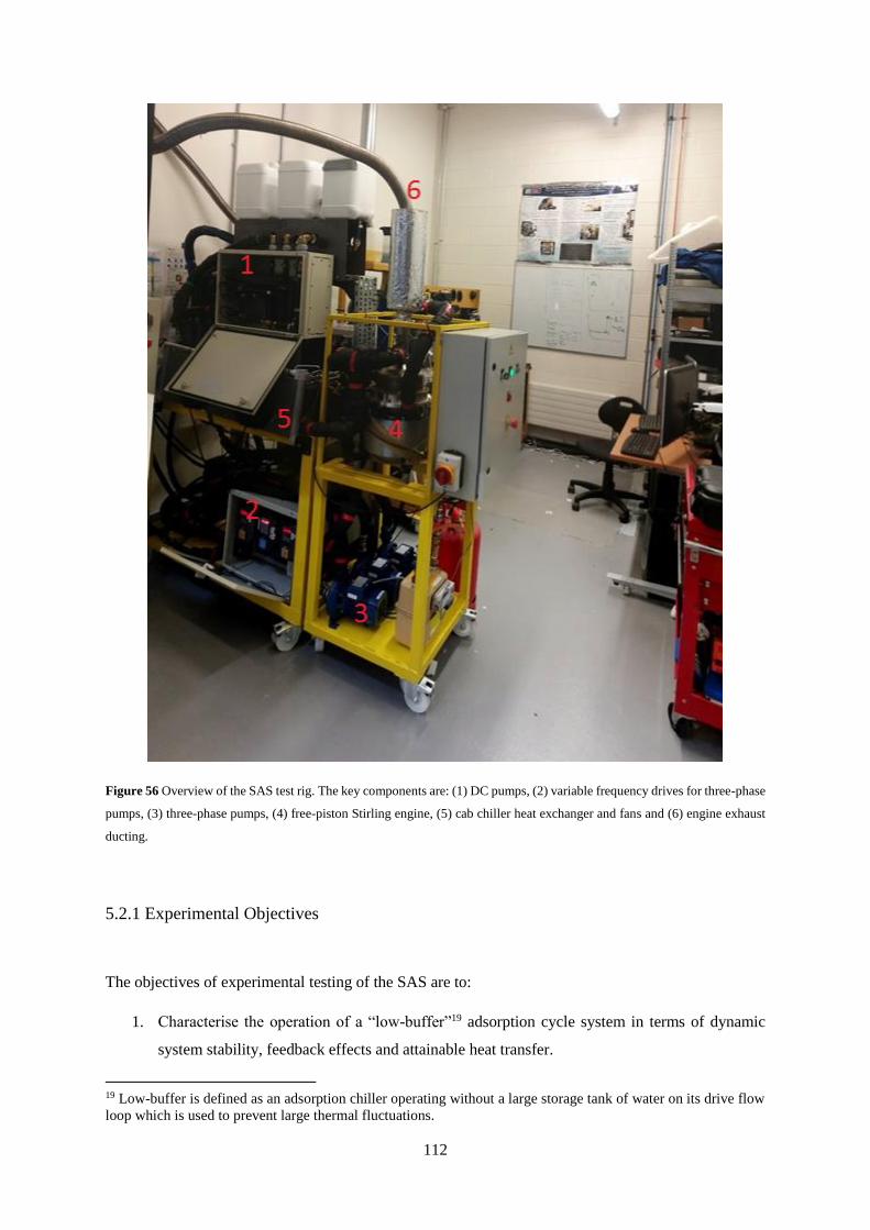
112
Figure 56 Overview of the SAS test rig. The key components are: (1) DC pumps, (2) variable frequency drives for three-phase
pumps, (3) three-phase pumps, (4) free-piston Stirling engine, (5) cab chiller heat exchanger and fans and (6) engine exhaust
ducting.
5.2.1 Experimental Objectives
The objectives of experimental testing of the SAS are to:
1. Characterise the operation of a “low-buffer”19 adsorption cycle system in terms of dynamic
system stability, feedback effects and attainable heat transfer.
19 Low-buffer is defined as an adsorption chiller operating without a large storage tank of water on its drive flow
loop which is used to prevent large thermal fluctuations.

113
2. Characterise the impact of pulsed thermal loading from the adsorption chiller on the free-piston
Stirling engine in terms of power spikes, controllability and dynamic system stability.
3. Investigate the variation of chiller capacity for high (> 40 °C) ambient temperature conditions.
4. Investigate the system COP and capacity at baseload condition. Baseload is defined as a cab
temperature of 26.6 °C and ambient temperature of 35 °C, Tcab/Text = 26.6/35 °C (80/95 °F as
per A.R.I. STD 310/380) [282].
5.2.2 Experimental Methodology
The above objectives require the measurement of cooling capacity, heat input and electrical power
output. The electrical characteristics of the FPSE are recorded by the engine’s microcontroller and the
data can be obtained using Microgen Engine Corporation LabView data acquisition program. The heat
input to the engine can be obtained by measuring the gas flow rate into the engine. Figure 57 shows
the experimental setup used for testing and characterising the SAS. This architecture differs from the
general SAS architecture presented previously which is the final APU implementation. In contrast,
Figure 57 has key differences such as FPSE electrical power being discharged into the electrical grid
for convenience. The condenser heat rejection is achieved using a plate heat exchanger and an open
flow of water from the laboratory water supply. Furthermore, the cooling system evaporator is thermally
loaded by blowing warm air over the air cooled cab chiller heat exchanger. The most significant
difference is the present of an electric heater in the system which serves the function of allowing the
adsorption chiller to be operated independently of the Stirling engine for extended durations.
Additionally, the 12 kW supplementary heater is used to boost the thermal output from the FPSE, which
is undersized for driving the adsorption chiller.
Figure 57 General architecture of the SAS experimental setup.
The drive heat input to the adsorption chiller, Qdr, is given calculated from the drive loop flowrate,
ṁd, the specific heat capacity of the coolant cp,w, the drive inlet temperature Tdi and the drive outlet
temperature Tdo using Eq. (19).

114
𝑄𝑑𝑟 = ṁ𝑑𝑐𝑝,𝑤(𝑇𝑑𝑖 − 𝑇𝑑𝑜) (19)
Similarly the chiller cooling capacity, Qcool is calculated from the chiller loop flowrate ṁc, the specific
heat capacity of the coolant cp,w, the chiller inlet temperature Tci and the chiller outlet temperature Tco
using Eq. (20).
𝑄𝑐𝑜𝑜𝑙 = ṁ𝑐𝑐𝑝,𝑤(𝑇𝑐𝑖 − 𝑇𝑐𝑜)
(20)
The adsorption chiller heat rejection, Qrej, is calculated from the recooler loop flowrate ṁr, the specific
heat capacity of the coolant cp,w, the recooler inlet temperature Tri and the recooler outlet temperature
Tro using Eq. (21). Due to sign conventions Qrej will appear as a negative value.
𝑄𝑟𝑒𝑗 = ṁ𝑟𝑐𝑝,𝑤(𝑇𝑟𝑖 − 𝑇𝑟𝑜)
(21)
The thermal, COPt, of the adsorption chiller is calculated from the chiller cooling capacity, Qcool, and
the chiller heat input Qdr using Eq. (22).
𝐶𝑂𝑃𝑡 =𝑄𝑐𝑜𝑜𝑙
𝑄𝑑𝑟
(22)
With respect to the Stirling engine, its electrical efficiency is calculated from its net electrical power,
Pel, obtained from the engine microcontroller and the thermal fuel input, Qf, obtained from the gas
flowmeter using Eq. (23).
𝜂𝑒 =𝑃𝑒𝑙
𝑄𝑓
(23)
The key parameters required to characterise the SAS have been outlined above in equations Eq.
(19) to (23). The required flowmeters and temperature sensors and their locations will be discussed in
section 5.4.5. The cooling capacity of any cooling system is obtained by measuring the cooling output
of the system when it is at the limit of maintaining a given setpoint. For example, to characterise the
SAS at the 26.6/35 °C (80/95 °F as per A.R.I. STD 310/380) condition the following would need to be
done.
First, the recooler inlet temperature would need to be maintained at 30 °C and the adsorption
machine’s controller would be set to maintain a chiller inlet temperature of 18 °C. The driving
temperature should also be maintained at a fixed inlet temperature of approximately 90 °C to keep

115
cooling capacity fixed. Note that the reasoning for choosing these temperature has not be discussed yet
and will be addressed in great detail in Section 5.6.2. The author has calculated that an airside cab
temperature of 26.6 °C corresponds to a chiller inlet temperature 18 °C for and the 35 °C airside ambient
temperature corresponds to a recooler inlet of 30 °C through sizing of the heat exchangers.
Next, the heat load on the chiller circuit is increased until the adsorption machine can just barely
maintain the 18 °C setpoint. Once the setpoint begins to shift upwards the machines maximum cooling
capacity at that point has been obtained. At this point, instantaneous values for Tci, Tco and ṁc are taken
and used to calculate Qcool using Eq. (20). Likewise, the instantaneous values for Tdi, Tdo and ṁd are also
taken at this point and used to calculate Qdr using Eq. (19). The COP at this point can then be calculated
using Eq. (22). Note that in practical tests, all of this is done in real-time using a LabView data
acquisition program and the cooling capacity point is taken by observing periods of relative stability in
cooling capacity at or as near to the 18 °C setpoint as possible.
5.2.3 System Design
Section 5.4.2 has outlined the key parameters that need to be measured in order to meet the
experimental objectives. In addition to these parameters, control systems need to be in place in order to
maintain and keep fixed critical parameters such as the drive inlet temperature, recooler inlet
temperature and system flowrates so that there is only a single dependent variable i.e. Qcool.
Consequently, the experimental design must have the ability to precisely modulate and control
the heat input on the drive loop, the heat rejection system on the recooler loop, and a controllable
temperature load on the chiller loop. Each of the circuit flowrates must also be controllable and held
fixed.
As shown previously in Figure 57, the author proposes a supplementary electric heater for the
drive loop which allows for continuous high temperature operation independent of the FPSE and also
precise control of the drive temperature. A bank of external fan heaters and controllable radiator fans
would allow for control of heat addition to the chiller loop to measure capacity and the recooler
temperature would be controlled by modulating the external open flow of water through a large plate
heat exchanger. Each of the plumbing circuit flowrates would be held fixed through electronic control
of the pumps in each loop.
All of these system operating in combination would allow for the system to be tested with only
a single dependent variable at a time such as cooling capacity.

116
5.2.4 Fabrication and Construction
As with the TriPac Evolution APU for the DEVC system, the core adsorption chiller and
Stirling engine were received as bare units as shown in Figure 58, and required numerous support
systems and test rig frames to be constructed around them in other to be used for meaningful tests.
Figure 58 Adsorption chiller (left) and free-piston Stirling engine (right) as received from suppliers.
A considerable amount of design effort was expended into designing an integrated test rig for
the combined Stirling engine and adsorption chiller. The initial test rig concept, shown in Figure 59
was intended to be loosely mimic the geometric requirements expected in a real truck APU and certain
fundamental design requirements such as the FPSE being situated above the chiller were imposed. The
initial test rig featured a large lower level that would house many of the support systems like fan and
pump controllers, data acquisition systems and the supplementary electric heater. A central cable tray
“spine” traverses the frame serving two purposes; mechanical support for the three header tanks and a
neater pathway for routing and securing plumbing lines. The Stirling engine was housed on a raised
gantry and its control box was situated immediately in front of it.
Though this design was workable, and all components can be accessed, the author felt that it
was unnecessarily restrictive and the overall design would not facilitate significant design modifications
in the event of unforeseen experimental challenges. Likewise, the initial motivation for making a
compact SAS test rig was to simulate the APU geometry but it was clear from the initial design that this
would not be possible with the prototype system due to un-optimised bulky support systems like the
header tanks and various enclosures. It was the author’s opinion that the system should either meet the
geometric requirements or not at all as partially fulfilling them was of no value and would only hamper
testing. Perhaps the most important factor in the decision to recycle the design process was the fixed
rental period of the adsorption chiller. The adsorption chiller was only going to be available for a limited

117
duration on a rental agreement from InvenSor GmbH but the FPSE was purchased outright from
Microgen Engine Corporation. This lead to an impetus to separate the FPSE and adsorption chiller into
separate test rigs so that the engine can be used in the future as a dedicated test bed once the research
has concluded like the Whispergen test rig was.
Figure 59 Initial SAS test rig concept (many auxiliary support systems not shown).
Consequently, a revised design shown below in Figure 60, was created that physically
separated the majority of the Stirling engine and its subsystems from the adsorption chiller and its own
subsystems. The FPSE test rig features an upper cage-like enclosure for the engine itself which is
mounted on two structural steel members via vibration dampeners. The cage-like design was deliberate
and intended to facilitate potential mounting of a dedicated header tank to grant it independence from
the adsorption chiller test rig. The vertical supports would also facilitate a Perspex enclosure around the
engine in the event of health and safety requiring it. The FPSE control box enclosure is externally
mounted on one side of the frame to facilitate ease of access and debugging. The fuel supply, a propane
cylinder, is mounted directly beneath the engine along with a gas flow meter. There is sufficient space
in the engine region to house the various engine auxiliaries such as the blower, gas injection venturi and
igniter.
The adsorption chiller test rig keeps some of the key design aspects from the initial frame design
such as a central cable tray spine to mount the header tanks and route the intricate plumbing for the
system. The main pump box is be mounted on top of the core adsorption chiller to the rear just below
the header tanks. The recooler heat exchanger would be mounted on one side of the frame with fans
(not shown) and, likewise, the cab chiller heat exchanger would be mounted on the other side with its
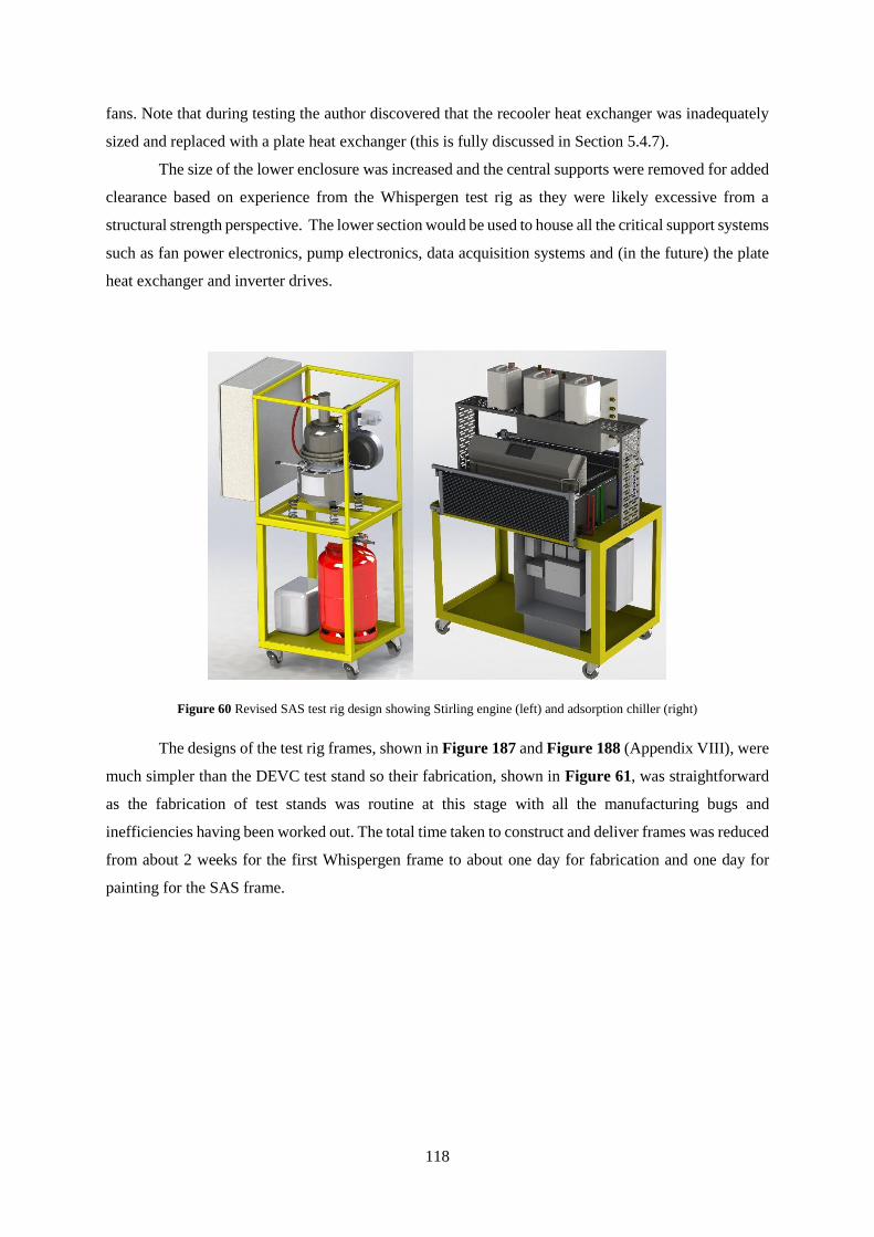
118
fans. Note that during testing the author discovered that the recooler heat exchanger was inadequately
sized and replaced with a plate heat exchanger (this is fully discussed in Section 5.4.7).
The size of the lower enclosure was increased and the central supports were removed for added
clearance based on experience from the Whispergen test rig as they were likely excessive from a
structural strength perspective. The lower section would be used to house all the critical support systems
such as fan power electronics, pump electronics, data acquisition systems and (in the future) the plate
heat exchanger and inverter drives.
Figure 60 Revised SAS test rig design showing Stirling engine (left) and adsorption chiller (right)
The designs of the test rig frames, shown in Figure 187 and Figure 188 (Appendix VIII), were
much simpler than the DEVC test stand so their fabrication, shown in Figure 61, was straightforward
as the fabrication of test stands was routine at this stage with all the manufacturing bugs and
inefficiencies having been worked out. The total time taken to construct and deliver frames was reduced
from about 2 weeks for the first Whispergen frame to about one day for fabrication and one day for
painting for the SAS frame.
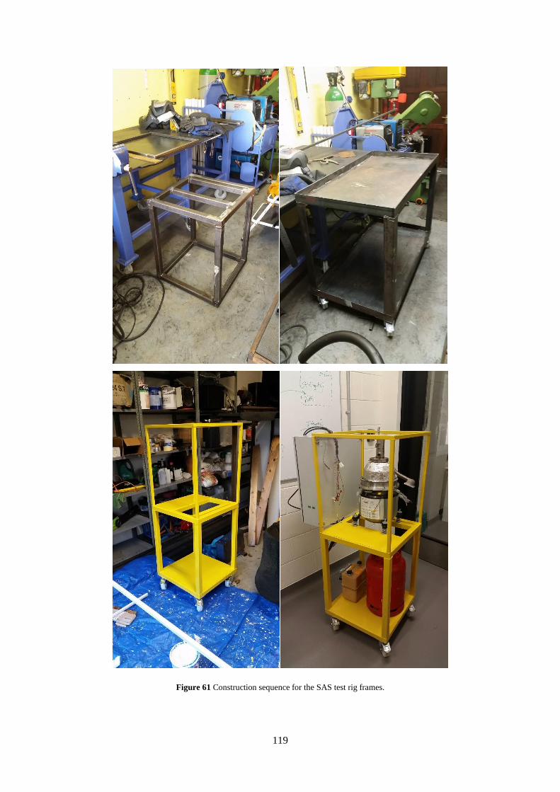
119
Figure 61 Construction sequence for the SAS test rig frames.

120
5.2.5 Plumbing system
In theory, the design of the SAS plumbing is relatively straightforward, there are three separate
fluid loops; the drive loop, the recooler loop and the chiller loop as shown in Figure 62. Each loop
requires a pump and the recooler and cab chiller loops require air-cooled heat exchangers. The drive
loop is simply a direct thermal connection between the engine and chiller and includes a pump.
However, this plumbing configuration is for a final production APU and is not conducive to
experimental testing and modification. The plumbing loops in the SAS test rig required numerous
sensors such as flowmeters and temperature sensors along with flow control devices like three-way
valves to divert flow and change the system configuration for example for engine only driving,
supplementary boost heating or a hybrid of the two. The boost heater was necessary for engine
independent operation as the engine was not rated for sustained high temperature operation. Similarly,
the experimental configuration required header tanks, safety pressure relief valves and drain/fill points.
Figure 62 Theoretical plumbing required in a final production SAS APU.
5.4.5.1 Recooler Loop
As with the mechanical design of the test rig frames, the plumbing system underwent several
evolutions due to shifts in requirements and attempts to reduce complexity. The preliminary design for
the recooler heat rejection circuit is shown in Figure 63. The major circuit elements consist of a closed
loop with the adsorption chiller (technically its internal condenser), a circulation pump and an air-cooled
heat exchanger (radiator) to reject heat. In terms of maintenance, the system has an expansion/header
tank for filling the system and a drain point for emptying it. With regard to sensors, the loop contains
temperature sensors before and after the adsorption chiller and a flowmeter. These three sensors are
used to calculate the heat rejection from the system. Also included in the initial design was a differential
pressure sensor for measuring the pressure drop of the plumbing loop to aid in hydraulic design and
optimization of the pumps.

121
The final major element in the initial recooler loop design was the three-way valve
configuration that allowed selection of the radiator or the controlled heat rejection system consisting of
and electric heater and high power heat rejection circuit such as a plate heat exchanger with open flow
of water on the secondary side. The intended purpose of this system was to enable precise control of
the returning recooler temperature into the adsorption for high precision characterisation of its
performance similar to how InvenSor GmbH benchmark their units. The electric heater would allow for
an increase of the recooler temperature and the heat rejection circuit would enable reduction in the
recooler temperature. The combination of both, along with flowmeters and temperature sensors would
be microprocessor controlled to maintain a fixed setpoint for testing. The ability to increase and
decrease the recooler loop temperature at will would simulate increases and decreases in external
ambient temperature.
Figure 63 Initial recooler plumbing circuit design.
However, due to limited time constraints, this precisely controlled recooler temperature system
was not implemented. The final design, shown in Figure 64 eliminated the electric heater aspect of the
temperature controlling system and the plate heat exchanger was manually controlled by varying the
flow of water on the open flow secondary side of the heat exchanger with a lever valve. The differential
pressure sensors were also omitted as they were deemed superfluous and unnecessary.
Precise control of the recooling temperature was hoped to be achieved through PID control of
the radiator blower fans using a microcontroller. However, during experimental testing, it was
discovered that the air-cooled heat exchanger was significantly undersized and incapable of controlling
the recooling temperature to within the 20-50 °C test range. Therefore, the plate heat exchanger became
the primary means of controlling the recooling temperature of the adsorption chiller. Also evident in

122
the recooler loop is an additional CP130 circulation pump which was added in to increase the flowrate
to the required value. A detailed discussion on the pumps is presented in section 5.4.6.
Figure 64 Final recooler loop plumbing design
5.2.5.2 Chiller loop
The initial chiller loop design was very similar to that of the initial recooler loop. It featured
the same pump, sensor configuration and maintenance filling and draining points. As with the recooler
circuit, the preliminary design envisaged precise chiller loop temperature control via an electric heater
which can be manually selected via a three-way valve. This electric heater would allow the chiller
circuit to be increased in temperature to simulate different cab temperature setpoint conditions.

123
Figure 65 Initial design of the chiller loop.
However, as with the recooler loop design, electric heater control had to be scaled back due to
time constraints and the final design, shown in Figure 66, and simply consisted of a radiator and two
pumps along with the necessary sensors for quantifying cooling capacity. The second pump was added
in to boost flowrate as the initial pumps were undersized for the application.
Figure 66 Final chiller loop design.

124
5.4.5.3 Drive loop
The drive circuit plumbing design was particularly complex due to the numerous permutations
of potential operating configurations. The drive loop needed to be designed in such a way as to enable:
1. Independent operation of the Stirling without the adsorption chiller
2. Independent operation of the adsorption chiller without the Stirling engine
3. Emergency heat dump to protect the Stirling engine
4. Precise drive loop temperature control
The initial design of the drive loop, shown in Figure 67, meets each of the above requirements and
also features a potential technical solution to low buffering issues via use of a bypass tank. The extensive
use of three-way valves enables multiple alternate configurations of the system. For example, the
adsorption chiller (ACS) can be bypassed entirely and the Stirling engine can be run in an engine only
configuration using the radiator in a conventional sense. Likewise, the adsorption chiller can be run
independently when the Stirling engine is dropped out of circuit via selection valves and driven
exclusively by a high power electric heater. The system also features a manually selectable emergency
dump plate heat exchanger that can rapidly chill the drive loop in emergency situations.
The external bypass tank was envisaged as a technical solution to capture the initial pulse of cold
water that originates from valve switchover during normal adsorption chiller operation. By diverting
the bulk of these pulses into an external bypass tank where it is captured and steadily reheated by the
main loop via the plate heat exchanger it was hoped that the spikes would dampened down significantly
and overall system performance would be increased.
Figure 67 SAS drive loop plumbing version 1.

125
An intermediate revision presented in Figure 68 preserved all of the key advantages of the previous
configuration but simplified it slightly. The radiator is eliminated from the system and instead replaced
by the emergency dump plate heat exchanger which would be oversized for the application. By
oversizing it, it would be serve dual functions of acting as the radiator during independent Stirling
engine operation and also as an emergency heat dump.
However, it is immediately obvious that both revision 1 and revision 2 are very complex and many
of the configurations are unlikely to be used in the limited testing period that was available.
Figure 68 SAS drive loop plumbing version 2.
Consequently, in version 3 shown in Figure 69, the drive loop plumbing design was greatly
simplified and only the high powered electric heater was preserved. This architecture would enable
operation of the adsorption chiller at full power and also independently of the Stirling engine which
was the most critical requirement. However, the ability to operate the Stirling engine independently was
sacrificed in favour of reduced complexity. The author felt that independent operation of the Stirling
engine was sufficiently well characterised by Microgen Engine Corporation and was unnecessary. The
system could always be reconfigured for independent operation after the project has concluded.
Revision 3 also featured a number of critical safety improvements such as the inclusion of pressure
relief valves at two points in the system. Essentially, all sources of heat that could be sealed such as the
engine and the electric heater now incorporated passive pressure relief valve that trigger at 3 bar
pressure. These were installed in the event of accidental mis-configuration of the three-way valves
resulting in a sealed pressure vessel that could explode. By placing the pressure relief valves in the

126
locations shown this risk can be mitigated. Another important safety feature is the pressure switch for
the high power electric heater that acts as a protection cut-out in the event of no water flow across the
heater element. The power of the electric heater and the small volume of circulating liquid would result
in extremely rapid boiling of the cooling system and destruction of the heater element.
The final revision, shown in Figure 70 is virtually unchanged from revision 3 and is only
included for completeness as it is homogenous with the other final schematics.
Figure 69 SAS drive loop plumbing version 3.
Figure 70 SAS drive loop plumbing final version.

127
5.2.5.4 Implementation
The SAS test rig plumbing is the most visually apparent aspect of the system and was also the
most laborious part of the installation due to the intricacy of the plumbing arrangements. The choice of
plumbing design was a hybrid mix of compression fittings where sharp right angle bends or three-way
valves were required and flexible ¾” automotive coolant line which was secured to copper pipe using
jubilee clips. The use of both these methods is readily apparent in the top and middle images in Figure
71. Also evident in bottom image of Figure 71 is the solution for the three system header tanks. Note
that the drive tank (left) and recooler tank (middle) are physically bridge at a high point. This was done
to prevent the tanks from overflowing during valve switchover. Due to pump imbalances caused by the
adsorption chiller not having direct control of the system pumps, the liquid from one loop could be
pushed excessively into another loop. Note that this is how the system is intended to operate during
switchover regeneration events. However due to the system being open vented and not pressurized, in
some situations the drive loop would dump too much liquid into the recooler tank causing it to overflow.
To combat this, the author installed the overflow bridge between the tanks and also increased the size
of the tanks from the initial containers which are visible in the top of the middle image in Figure 71.
A series of images showing construction and key elements of the plumbing system are
presented in Figure 72 and Figure 73. A description of each image is offered to the reader in the
captions of the figures. They are included as they clearly show the layout of the plumbing prior being
insulated (Figure 72) and after (Figure 73) which makes subsequent interpretation very difficult. Strips
of colour coded tape are visible in Figure 73 and the colour code is as follows; red (drive loop), blue
(chiller loop) and green (recooler loop).

128
Figure 71 (top) right-angle fittings for pipe entry into pumping box, (middle) completed pumping plumbing prior to insulation
and (bottom) system header tanks.

129
(a) (b)
(c) (d)
Figure 72 (a) engine plumbing showing valves and copper pipework, (b) adsorption chiller bypass valves, (c) central cable
tray spine used to support header tanks, (d) pipes routed along spine.

130
(a) (b)
(c) (d)
Figure 73 (a) primary plumbing connections with the adsorption chiller, (b) alternate view of primary plumbing connections
with adsorption chiller, (c) engine plumbing and valves and (d) recooler loop valves and drainage point. Colour code: red
(drive loop), blue (chiller loop) and green (recooler loop).

131
5.2.6 Pump systems
5.2.6.1 Pump Selection
The pump system should have been a relatively straightforward task to implement but a number
of design oversights and technical mistakes lead to the system requiring modification and the addition
of extra booster pumps. The SAS requires three pumps, one for each respective plumbing circuit; the
drive pump, recooler pump and chiller pump. InvenSor GmbH issued guidelines for the required
flowrates for each loop of the adsorption chiller machine. They recommend a drive flowrate of 1200
l/h, recooler flowrate of 1350 l/h and a chiller flowrate of 1000 l/h.
Achieving the required flowrate by any method other than trial and error would be difficult as
the final layout of the plumbing circuitry was uncertain and there was no simple way to calculate the
pressure drop of the respective loops as the pressure drop sensors were removed from the design to
simplify it. The author assumed that a Davies Craig EBP 25 circulation pump would be sufficient for
the recooler and chiller loops as these had lower pressure drop than the drive loop. The pressure drop
curve for the EBP 25 shown in Figure 74 and indicates a nominal flowrate of 1500 l/h at 0.1 bar pressure
drop. The author assumed that this would be sufficient for the chiller flowrate and added into a second
backup booster pump for the recooler circuit in the event of a single pump failing to achieve the required
flowrate. For the drive loop, the author chose the Davies Craig EWP 80 which has a flowrate of 4500
l/h at a 0.1 bar pressure drop according to the pressure drop curve shown in the right hand graph in
Figure 74. It was unclear at the time of design what the pressure drop would be without a means of
testing so the drive pump was significantly oversized for safety.
Figure 74 The pressure-flowrate curves for (left) Davies Craig EBP 25 and (right) Davies Craig EWP 80 pumps.
5.4.6.2 Physical Implementation

132
The proposed mounting arrangement for the circulation pumps and flowmeters was a dedicated
enclosure as shown in the CAD render in Figure 75. The three similar pumps are Davies Craig EBP 25
circulation pumps and the larger pump in the bottom right is the Davies Craig EWP 80 pump. On the
left-hand side of the enclosure there are four Huba Control Type 210 DN15 flowmeters. All of the
components are intended for high temperature automotive applications.
Figure 75 CAD render of proposed pump installation
The physical implementation of the pumping arrangement is shown in Figure 76 and evidence
of lessons learned from previous test rigs are apparent. The main method of pipe joining is direct
coupling of flexible ¾” coolant hose with ¾” copper pipe secured with jubilee clips. This method is
extremely reliable and faciliates quick reconfigurations or purging of air when necessary. The
flowmeters are all mounted together for ease of access and debugging. Huba Control Type 210
flowmeters also feature rapid disconnect fittings where the metal clip can simply be pulled out which
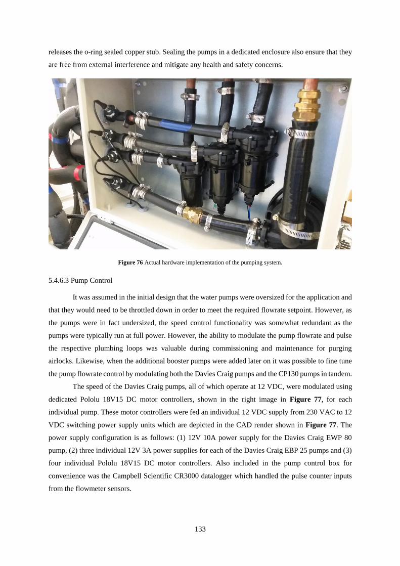
133
releases the o-ring sealed copper stub. Sealing the pumps in a dedicated enclosure also ensure that they
are free from external interference and mitigate any health and safety concerns.
Figure 76 Actual hardware implementation of the pumping system.
5.4.6.3 Pump Control
It was assumed in the initial design that the water pumps were oversized for the application and
that they would need to be throttled down in order to meet the required flowrate setpoint. However, as
the pumps were in fact undersized, the speed control functionality was somewhat redundant as the
pumps were typically run at full power. However, the ability to modulate the pump flowrate and pulse
the respective plumbing loops was valuable during commissioning and maintenance for purging
airlocks. Likewise, when the additional booster pumps were added later on it was possible to fine tune
the pump flowrate control by modulating both the Davies Craig pumps and the CP130 pumps in tandem.
The speed of the Davies Craig pumps, all of which operate at 12 VDC, were modulated using
dedicated Pololu 18V15 DC motor controllers, shown in the right image in Figure 77, for each
individual pump. These motor controllers were fed an individual 12 VDC supply from 230 VAC to 12
VDC switching power supply units which are depicted in the CAD render shown in Figure 77. The
power supply configuration is as follows: (1) 12V 10A power supply for the Davies Craig EWP 80
pump, (2) three individual 12V 3A power supplies for each of the Davies Craig EBP 25 pumps and (3)
four individual Pololu 18V15 DC motor controllers. Also included in the pump control box for
convenience was the Campbell Scientific CR3000 datalogger which handled the pulse counter inputs
from the flowmeter sensors.
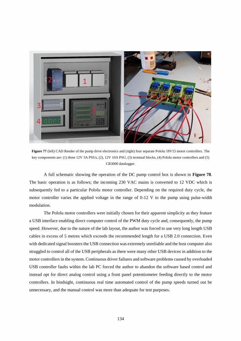
134
Figure 77 (left) CAD Render of the pump drive electronics and (right) four separate Pololu 18V15 motor controllers. The
key components are: (1) three 12V 3A PSUs, (2), 12V 10A PSU, (3) terminal blocks, (4) Pololu motor controllers and (5)
CR3000 datalogger.
A full schematic showing the operation of the DC pump control box is shown in Figure 78.
The basic operation is as follows; the incoming 230 VAC mains is converted to 12 VDC which is
subsequently fed to a particular Pololu motor controller. Depending on the required duty cycle, the
motor controller varies the applied voltage in the range of 0-12 V to the pump using pulse-width
modulation.
The Pololu motor controllers were initially chosen for their apparent simplicity as they feature
a USB interface enabling direct computer control of the PWM duty cycle and, consequently, the pump
speed. However, due to the nature of the lab layout, the author was forced to use very long length USB
cables in excess of 5 metres which exceeds the recommended length for a USB 2.0 connection. Even
with dedicated signal boosters the USB connection was extremely unreliable and the host computer also
struggled to control all of the USB peripherals as there were many other USB devices in addition to the
motor controllers in the system. Continuous driver failures and software problems caused by overloaded
USB controller faults within the lab PC forced the author to abandon the software based control and
instead opt for direct analog control using a front panel potentiometer feeding directly to the motor
controllers. In hindsight, continuous real time automated control of the pump speeds turned out be
unnecessary, and the manual control was more than adequate for test purposes.

135
Figure 78 Block diagram showing the operation and layout of the DC pump controller box.

136
5.2.6.4 Electrical Systems Implementation
The construction of the pump controller box, shown in Figure 79 was a new experience for the
author as it was his first experience of working with 230 VAC mains electricity and the most significant
electrical wiring project to date. The author used industry best practices when laying out the controller
box and opted to use DIN-rail components and terminal blocks at they provide the neatest, safest and
most reliable solution.
Figure 79 Construction of the pump controller box in the author’s electronics workshop.
The author was careful to ensure a neat, logical layout of the control box depicted in Figure 80
as it would greatly aid in troubleshooting and initial commissioning. The DC pump controller box was
completely successful and operated as expected on the first power up.
Figure 80 Actual layout of the DC pump controller box. Refer to Figure 81 for description of items.
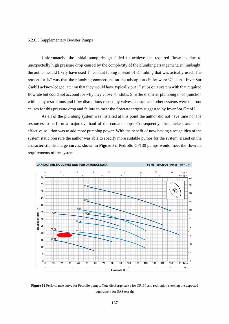
137
5.2.6.5 Supplementary Booster Pumps
Unfortunately, the initial pump design failed to achieve the required flowrates due to
unexpectedly high pressure drop caused by the complexity of the plumbing arrangement. In hindsight,
the author would likely have used 1” coolant tubing instead of ¾” tubing that was actually used. The
reason for ¾” was that the plumbing connections on the adsorption chiller were ¾” stubs. InvenSor
GmbH acknowledged later on that they would have typically put 1” stubs on a system with that required
flowrate but could not account for why they chose ¾” stubs. Smaller diameter plumbing in conjunction
with many restrictions and flow disruptions caused by valves, sensors and other systems were the root
causes for this pressure drop and failure to meet the flowrate targets suggested by InvenSor GmbH.
As all of the plumbing system was installed at this point the author did not have time nor the
resources to perform a major overhaul of the coolant loops. Consequently, the quickest and most
effective solution was to add more pumping power. With the benefit of now having a rough idea of the
system static pressure the author was able to specify more suitable pumps for the system. Based on the
characteristic discharge curves, shown in Figure 82, Pedrollo CP130 pumps would meet the flowrate
requirements of the system.
Figure 82 Performance curve for Pedrollo pumps. Note discharge curve for CP130 and red region showing the expected
requirement for SAS test rig.

138
The CP130 pumps are significantly more powerful than the Davies Craig EBP 25 and EWP80
pumps. The CP130 have a rated power of 370 Watts as compared to 120 W for the EWP80 and 45 W
for the EBP 25. The reason for the large increase in power requirement relates to the pump affinity laws
whereby flowrate for a given system has a cubic relationship in terms of power. Consequently a
doubling of flowrate could require eight times as much pumping power. In a real application the solution
is to reduce system static pressure through use of larger plumbing and less restriction but for these
experimental purposes the parasitic pumping losses are not relevant.
At this stage of the project, the author was significantly more comfortable with working with
230 VAC mains power and decided to opt for 3-phase circulation pumps to avoid the hassle of
implementing a DC power supply and motor controller system like in the DC pump control box. The
most straightforward solution was to use inverter drives that can take single phase power input and
output three-phase electric power at varying frequency to control the rotation speed of the pumps. The
author chose generic Huangyang 2.2 kW variable frequency inverter drives (VFDs), shown in Figure
83 for each pump. The inverter drives needed to be oversized by at least a factor of 3 as they are only
operating on single phase and the 2.2 kW version was the closest unit available.
Figure 83 (left) CAD render of proposed variable frequency drive enclosure and (right) actual implementation of the three
separate VFDs.
The installation of the inverter drives was very straightforward and a block diagram is given
in Figure 84. The drives are wired directly with single-phase 230 VAC mains which is subsequently
converted to 230 VAC three-phase power within the drive. The frequency of this AC voltage can be
modulated to control the speed of the pump rotation via the inverter control panel. Also shown in the
block diagram is a 12 VDC power supply for powering two blower fan units within the enclosure to
prevent overheating of the drives. The fans are manually controlled and feature an indicator LED
when operating.
The physical layout and location of the CP130 pumps is shown in Figure 85. The pumps were
positioned below the FPSE for convenience in place of where the propane cylinder was located. This

139
facilitated easy removal of the propane cylinder at the end of test periods for health and safety reasons.
A minor yet important part of the inverter drive installation was the choice of motor wiring. Shielded
wiring was used and installed in according with industrial inverter drive grounding best practices to
mitigate electromagnetic interference which could disrupt test measurements.
Figure 84 Block diagram showing the operation of the inverter drive system.
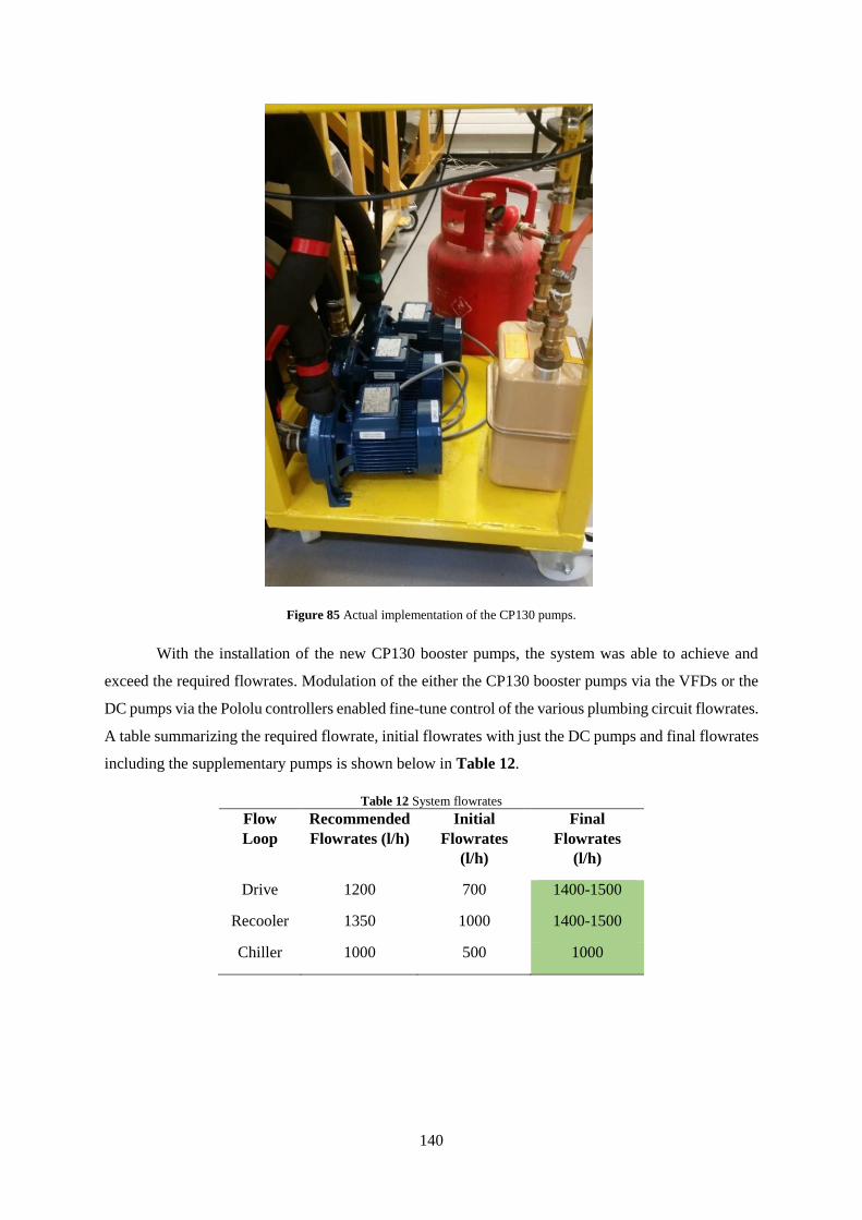
140
Figure 85 Actual implementation of the CP130 pumps.
With the installation of the new CP130 booster pumps, the system was able to achieve and
exceed the required flowrates. Modulation of the either the CP130 booster pumps via the VFDs or the
DC pumps via the Pololu controllers enabled fine-tune control of the various plumbing circuit flowrates.
A table summarizing the required flowrate, initial flowrates with just the DC pumps and final flowrates
including the supplementary pumps is shown below in Table 12.
Table 12 System flowrates
Flow
Loop
Recommended
Flowrates (l/h)
Initial
Flowrates
(l/h)
Final
Flowrates
(l/h)
Drive 1200 700 1400-1500
Recooler 1350 1000 1400-1500
Chiller 1000 500 1000

141
5.2.7 Fans and Heat Exchangers
5.2.7.1 Air-Cooled Heat Exchangers
The requirement for air-cooled heat rejection from the recooler and heat acceptance for the cab
chiller have been outlined previously in section 5.4.5. The adsorption chiller cooling capacity was
expected to be on the order of 2-3 kWt and the heat rejection requirement was expected to be on the
order of 12 kWt. Due to difficult time constraints, there was inadequate time to properly size and design
the recooler and cab chiller heat exchangers. Instead, a trial and error approach was chosen due to the
widespread availability of heat exchangers, as shown in Figure 86, and blower fans from the nearby
Thermo King (enterprise sponsor) factory.
Figure 86 Different types of heat exchangers available on-hand from the Thermo King factory in Galway.
The heat exchanger used for the recooler was a part used on Thermo King transport refrigeration
unit that had an approximate heat rejection capacity of 15 kW. However, the author made an oversight
when picking this heat exchanger and failed to realise that this capacity assumed a typical engine
cooling temperature of around 80 °C. In contrast, the adsorption chiller recooler, would be operating at
around 20-40 °C which corresponds to a significantly reduced temperature difference between the
ambient and the liquid within the heat exchanger resulting in dramatically reduced capacity. The author
also further compounded this problem by failing to adequately mount the fans on the heat exchanger.
Heat exchangers are intended to be enclosed in sheet metal enclosures so that the fans force air over the
entire heat exchanger face area. In the configuration shown in Figure 87 the author was only utilizing
about 60% of the overall heat exchanger area which further reduced its capacity.
The original requirement for air-cooled heat exchangers originated from the possibility of
testing the SAS test rig in a real calorimeter at Thermo King test facilities. Unfortunately, part way
through testing with the new deadline for return of the adsorption chiller, it became increasingly
apparent that this would not be possible due to insufficient time. With the benefit of hindsight, the

142
author would not have attempted to use an air-cooled heat exchanger and simply gone directly to a
water-cooled solution. An appropriately size heat exchanger in a proper enclosure would have most
likely been too large to fit on the side of the test rig within the existing lab footprint.
Figure 87 Recooler air-cooled heat exchanger with blower fans. Note poor fan area coverage.
The chiller loop heat exchanger depicted in Figure 88 suffered from the same problems as the
recooler heat exchanger implementation however the author was fortunate enough that the required
capacity was low enough for the system to be usable. By using external fan heaters in conjunction with
the radiator blower fans it was possible to force warm air over the heat exchanger and thermally load
the cooling circuit. The crudeness of this method was a fundamental root cause for the poor setpoint
temperature control of the chiller inlet temperature achieved in experimental testing. The electric heater
method described in section 5.4.5.2 would have vastly improved reproducibility of testing but there was
no time available to implement it.

143
Figure 88 Chiller loop air-cooled heat exchanger (lower centre) with blower fans.
5.2.7.2 Fan Control
Control of the flowrate of liquid through the heat exchangers has been outlined in section 5.4.6.
In order to control the air flow rate over the fans the two separate Electromen EM-241 DC motor
controllers were used to vary the voltage to the recooler fan bank and chiller fan bank via pulse-width
modulation. A CAD render of the fan control box is shown in Figure 89.
Figure 89 CAD render of the fan control system. The major components are: (1) Omron PSU, (2) Electromen motor drivers,
(3) terminal blocks, (4) Arduino Mega 2560 and (5) terminal blocks.

144
It is important to stress that the author was working under the assumption that the radiators
were adequately sized when designing the control system to precisely control the recooler and cab
chiller temperatures. With the intention of maintaining accurate and reproducible setpoints the author
implemented two separate PID control systems on the fan banks using an Arduino Mega 2560
microcontroller which received temperature feedback from an integrated thermistors within the
respective plumbing loops. The microcontroller attempted to maintain a designated temperature setpoint
by varying the duty cycle of the blower fans. Of course, with the recooler heat exchanger being
undersized, the PID control system could never reach setpoint and simply ran at maximum duty cycle
continuously. A block diagram showing the implementation of this control scheme is depicted in Figure
90. The operation of the system is straightforward, AC mains is converted into a high current 24 VDC
supply via the Omron 480W power supply, which is fed into the two Electromen EM-241 motor drivers.
The motor controllers vary the 24 VDC from 0-24 VDC in accordance with the analog control signal
from the Arduino Mega 2560 microcontoller. Also shown in the schematic is a manual override switch
which enables direct control of the motor drivers by sending them an analog control signal from front-
panel potentiometers. The need for manual override was an important lesson learned with the Pololu
pump system motor controllers.
The microcontroller code used to implement the PID control loop is also included in Appendix
IV to this thesis along with the relevant LabView control program.

145
Figure 90 Block diagram showing the control scheme for the chiller and recooler fans.

146
The fan control box was constructed using similar techniques to the pump control box. The
design was implemented using standard industrial best practices using DIN-rail components and
terminal blocks. The left hand side image in Figure 91 shows: (1) the Omron 480W PSU, (2) the
Electromen EM-241 motor controllers, (3) the DIN-rail terminal blocks, (4) Arduino Mega 2560
microcontroller and (5) linear regulator 12V power supply. During testing, the Omron 480W PSU
suffered from thermal-shutdown faults after extended durations of runtime. The author failed to account
for the heat rejected from the power supply which gradually overheated the internals of the enclosure.
An intake fan (6) was later added to mitigate this problem and a similar solution was retroactively added
to all other enclosures. The front panel shown in the right hand side image in Figure 91 consists of: (7)
emergency stop button, (8) mains power indicator LED, (9) manual over-ride toggle switches and
control potentiometers and (10) fan duty cycle indicator LEDs.
Figure 91 (left) fan enclosure internals and (right) fan controller front panel controls.

147
5.2.7.3 Plate Heat Exchanger
In order to address the insufficient cooling capacity of the recooler heat exchanger an oversized
plate heat exchanger shown in Figure 92 with an assumed of cooling capacity of 125 kW (based on
brochure) was purchased. The precise capacity is unknown as the rating condition was not given.
However the size of the heat exchanger and the fact that the heat exchanger would use an open flow of
cold water on one side meant that it would be more than adequate for the application. The author did
not wish to repeat the same mistake of undersizing the heat exchanger. There were no negative
implications for oversizing it as the cooling capacity could be controlled via the open side flowrate.
Figure 92 Low-cost 125 kW plate heat exchanger.
The old air-cooled heat exchanger system’s performance is shown in Figure 93 where the
following can be seen: (1) that the system has a very slow temperature recovery rate, (2) the minimum
temperature that can be achieved is approximately 30 °C, and (3) the system has still not reached
equilibrium as evidenced by the upward drift in temperature cycles. Note that the spikes are data
acquisition errors as these measurements were taken during initial setup tests.

148
Figure 93 Recooler loop temperature profile with air-cooled heat exchanger. Coolant flowrate is approximately 1000 l/h and
heat input to the system 6.5 kWt
In contrast with the air-cooled heat exchanger, the liquid-cooled plate heat exchanger has much
higher cooling capacity. Figure 94 shows the recooler loop reaching a very similar temperature to the
incoming cooling water when at maximum flowrate (in the external circuit). The pull-down rate is
significantly faster and the lower temperature is 17 °C in this example, which is sufficient for testing.
Figure 94 Recooler loop temperature profile with the liquid cooled plate heat exchanger. Coolant flowrate is approximately
1500 l/h and heat input to the system is 5 kW.
Although the plate heat exchanger offered an improvement in cooling performance and
reasonably steady manual control of the recooling temperature, it was reliant on the temperature of the
26
28
30
32
34
36
38
1500 1600 1700 1800 1900 2000 2100
Tem
per
ature
(°C
)
Time (seconds)
15
17
19
21
23
25
27
29
1500 1600 1700 1800 1900 2000 2100
Tem
per
ature
( °
C)
Time (s)

149
incoming lab water supply. The author believed that it was reasonable to assume that the incoming
water temperature would be relatively consistent and only vary moderately with ground temperatures
on the order of 10-20 °C. As these temperatures are all below the nominal minimum recooling test
point, the variations would not be an issue. However, in an unexpected discovery, the author learned
that the lab cold water supply could vary dramatically. An example of the variation in cooling
temperature is shown below in Figure 95 where the cooling water temperature can be seen to vary from
16 °C to 30 °C. In fact, during some tests, the author has seen momentary spikes in the cold water
temperature of up to 42 °C! Although these spikes rarely last more than 1 minute, they are capable of
ruining a test by suddenly disrupting the recooler setpoint control as the heat rejection circuit instead
becomes a heat source.
Figure 95 Raw data showing variation in laboratory cold water supply.
After further investigation, the author compared the temperature profile of the building water
supply with his home solar photovoltaic panels (several kilometres away) on the same day. Figure 96
shows the electric power output from the author’s solar panels. It is interesting to note that the solar
irradiance profile correlates with the building water supply temperature. The exponential decay
beginning at 7 hours in Figure 95 is due to large storage capacity within the building water supply. The
instantaneous changes in water temperature are likely caused by the university water supply system
switching storage tanks and occasionally supplying mains water supply which is at a fixed 15-16 °C.
The author was unable to obtain precise design schematics for the university water supply so any further
analysis is speculation.
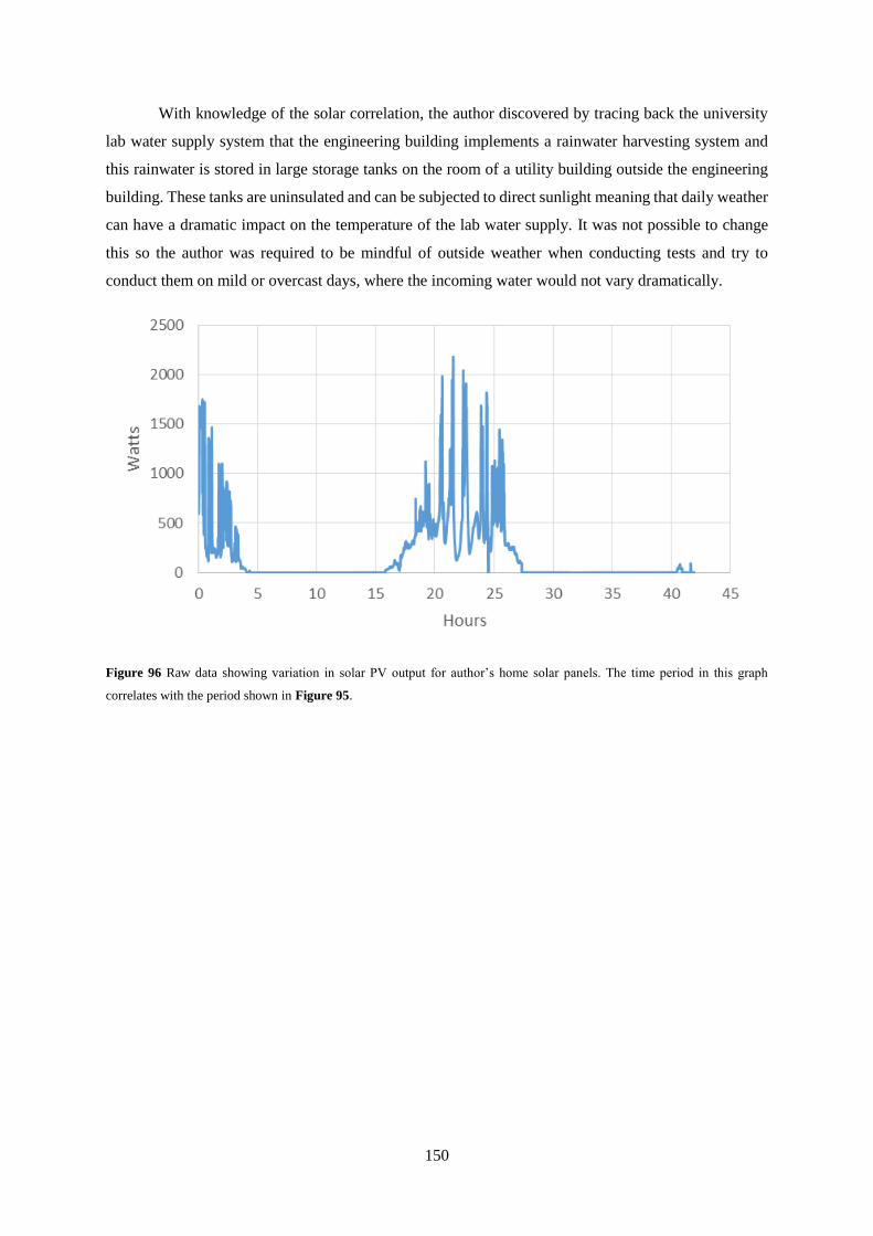
150
With knowledge of the solar correlation, the author discovered by tracing back the university
lab water supply system that the engineering building implements a rainwater harvesting system and
this rainwater is stored in large storage tanks on the room of a utility building outside the engineering
building. These tanks are uninsulated and can be subjected to direct sunlight meaning that daily weather
can have a dramatic impact on the temperature of the lab water supply. It was not possible to change
this so the author was required to be mindful of outside weather when conducting tests and try to
conduct them on mild or overcast days, where the incoming water would not vary dramatically.
Figure 96 Raw data showing variation in solar PV output for author’s home solar panels. The time period in this graph
correlates with the period shown in Figure 95.

151
5.2.8 Electric heater unit
The supplementary electric heater was the most technically challenging part of the PhD project
due to its complexity and numerous technical failures that forced major redesigns. The success of the
research project depended upon successful operation the electric heater. There was significant time
pressure to debug and fix the electric heater before the rental period for the adsorption chiller expired.
The author gained significant first-hand experience of detailed fault-tree diagnostic techniques and root-
cause analysis ultimately culminating in the successful operation of the electric heater.
As outlined in section 5.4.3, the electric heater was fundamental to the testing of the SAS as
the Stirling engine was incapable of providing sufficient heat to the chiller system nor was it capable of
operating at high (90 °C) temperatures for extended durations. It was therefore necessary to construct
an electric heater to act as a thermal analogue for the Stirling engine to boost its output and also
completely supplant it for extended duration high temperature tests.
The design of the electronics and control system are discussed after the physical design as it is
common to both revisions.
5.2.8.1 Electric Heater Version 1
There are a number of commercially available high power electric heaters which are marketed
as tankless water heaters for US applications. However, these systems universally have an upper
temperature safety limit of about 70 °C to prevent scalding and so they would be unsuitable for
application as the SAS supplementary heater. Industrial water heaters or custom tankless water heaters
were also unsuitable for the project as the lead time was too long and the cost was too high. The author
subsequently decided to design and build a custom heater unit using commercially available
components as a reference. The main design criteria for the electric heater was its electric power output
and so the initial heater had a rated power output of 16 kWt and was significantly oversized so as to
enable precise temperature control and rapid response to temperature pulsations during testing. The
design of the actual heater core is shown in the left CAD render in Figure 97. The author used three 5.5
kW immersion heater elements plumbed in series in a custom-built copper pipe assembly. The
immersion heaters are screwed into the assembly on its right hand side. The design is based on a near
universal design used by all tankless water heater manufactures. The author also hoped to avoid the
need for yet another test rig and frame to house the heater system, so it was designed to be completely
contained within a single enclosure box along with its electronics, just as commercial units are. This
enclosure would then be housed beneath the adsorption chiller test rig frame.
The requirement for compactness forced the use of small, and high surface power flux heater
elements. In hindsight this choice was a mistake and would lead to considerable experimental difficulty.
The surface power flux is a function of the total heater power output divided by its surface area.
Physically smaller heaters with high power outputs have a high surface power flux and require steady

152
and uniform cooling flow over the elements to prevent localized overheating of the heater element.
Turbulence, frothing and bubbling within the drive loop would all be detrimental to the required cooling
needed by the heater elements to ensure reliable operation.
Figure 97 (top left) CAD render of the heater core with the serpentine flow path through the heater core, (top right) CAD
render of the entire electric heater unit and (bottom) actual heater core with heater elements visible to the left. The heater
elements are inserted on the right-hand side of the assembly.
During experimental testing the first revision of the electric heater suffered continuous faults
and failures. In hindsight, the root cause of excess surface power flux is now obvious but an extensive
troubleshooting program had to be used to identify the root cause. From a test perspective the only
symptom was a continually tripping RCD circuit breaker within the lab power supply control panel. A
tripping RCD indicates that there is earth leakage present whereby some of the current is not returning
via the neutral wire but instead through protective earth. This is extremely dangerous as it means there
is a potential electrocution risk. The source of this earth leakage was unclear and the first investigation
focused on the author’s custom electronics as the most likely cause. However, after extensive
investigation these were not the source of the leakage and the heater elements themselves were causing

153
the fault. An immersion heater element displaying symptoms of earth leakage indicates a failure of the
heating element as the ceramic insulation around the heater wire has broken down and inner element is
shorting against the outer inconel sheath.
During inspection of the heater elements the author discovered characteristic pin-hole blowouts
on the heater elements shown in Figure 98. The author replaced the heater elements with new elements
on two separate occasions which would address the problem for several runs but the earth-leakage fault
would ultimately resurface. In each case, the heater elements themselves would display signs of weak
insulation and the pin-hole blowouts indicate that the root cause was most likely localized spot heating
caused by insufficient surface cooling.
Figure 98 Characteristic “pin-hole” blowout failures on the immersion heater elements. This type of failure is indicative of
localized spot-heating caused by poor cooling flow.
It was not possible to improve the quality of the water flow over the heater elements nor was
there time to perform additional analysis of the flow pattern over the units. It was therefore decided to
completely redesign the heater system and avoid the fundamental design flaw in the first revision.
5.4.8.2 Electrical Heater Revision 2
The problem with revision 1 was excessively high surface power flux for the heater elements.
With this new insight, the author later discovered that surface power flux is a fundamental design factor
in industrial electric heaters particularly in the milking and food industries. The use of excessively high
power heaters can burn and damage product that immediately contacts the heater element. The solution
was to both reduce the power output of the heater elements and to increase physical size of the element
so as to spread the heating power over a greater area. The author’s solution was to build a new test rig
that could accommodate a very large (approximately 1 metre) heating element shown in the right image
of Figure 99. This solution would be relatively quick to implement as the existing electronics and

154
controls could all still be used. A frame would need to be constructed to hold the heater tube vessel and
the power electronics enclosure and is shown in the left-hand CAD render in Figure 99.
Figure 99 (left) CAD render of revised heater design (right) Large 12 kW immersion heater with lower surface power flux.
After the previous fabrication work, the design and manufacture of the frame was
straightforward at this point in the project. The design is shown in Figure 100. Although the frame was
straightforward to manufacture (shown in Figure 101) the welding of water tight tubing was new to the
author and some mistakes were made during fabrication. The author fabricated the pipe end cap and
stub seals with standard MIG welds used to construct all of the metalwork to date. However, during
testing when the system was at maximum temperature and flowrate, evidence of minor pin-hole leakage
was discovered indicating that there was minute porosity in the welds. The magnitude of the leakage
was not serious enough to merit a repair and a small drip catching tray was instead placed under the
heater vessel. However, the author has learned that all future vessels should include a TIG welded root
pass to ensure water-tightness followed by subsequent filler welds over it.
Replacing the high surface flux power heater elements with the larger 12 kW immersion heater
completely eliminated the earth leakage faults and the heater did not have any subsequent faults or
failures during testing.

155
Figure 100 Schematic showing the design of the heater frame.

156
Figure 101 Fabrication of the revised electric heater unit.
5.2.8.2 Electronics and Electrical Wiring
The power dissipation of an immersion heater element is governed by Joule’s law shown in Eq. (24).
𝑃 = 𝐼2𝑅 (24)
Where the current flowing through the heater element is governed by the applied voltage in accordance
with Eq. (25).
𝐼 =𝑉
𝑅
(25)
Consequently, in order to control the heat output of the heater element, or its power dissipation,
it is necessary to vary the applied voltage. This is straightforward to do in the case of DC power and it
is achieved through pulse-width modulation particularly for motor control. However, in the case of
alternating current, it is slightly more complicated. The simplest solution is to chop sections of the AC
waveform in order to reduce the applied voltage. This method can be achieved using a solid-state device
called a triac, which is a type of switch that automatically turns off on voltage reversals. This is ideal in
the case of alternating voltage. In order to the control the AC voltage, it is necessary to simply trigger

157
the triac switch at precisely the right time to deliver the required amount of voltage and then the switch
will automatically switch off when the waveform crosses zero. Figure 102 outlines the process involved
in achieving this behaviour. The incoming AC power signal is passed through H11AA1 edge detection
integrated circuits that emit a sharp pulse indicating when the sinusoid has crossed zero. This acts as an
important event for timing when to trigger the triac switch. The microcontroller waits and calculates
the appropriate time delay required before emitting a firing signal pulse to the MOC3052 triac gate
driver integrated circuits. The gate driver circuits are basically isolated signal amplifiers that increase
the microcontroller signal’s power so that it can trigger the triac. Once the triac is switched on, the main
AC power is able to flow to the electric heater. By repeating this process rapidly and in a recurring
fashion is possible to achieve a controlled AC waveform and applied voltage to the heater thus
controlling its power output. For three-phase power, this process is repeated across each phase.
This method of power control is most commonly used in light dimmer switches. Note that an
alternative method to chopping sections of the sinusoid is to eliminate entire cycles from the 50 Hz
waveform. By eliminating 10 cycles from the 50 Hz waveform it is possible to reduce the power output
by 20%. This is preferred in industry as it prevents the creation of harmonic voltages and currents which
contribute to poor power quality. However, it is slightly more complex to implement and the author
chose the simpler solution as the heater would only be used for a limit period in a test environment.
The microcontroller code for implementing this control scheme has been included in the
appendix and the actual circuit diagram and breadboard implementation for the power electronics circuit
is shown in Figure 103.
Figure 102 Control scheme for varying the electric heater power output.

158
Figure 103 (top) circuit diagram for the triac power control circuit and (bottom) physical breadboard implementation.

159
A number of design flaws were discovered during testing (not represented in the final
schematics) and the root cause was identified to be incorrect resistor sizing on the edge detection
circuits. Thermally undersized resistors resulted in overheating and subsequent failure of the H11AA1
devices. Replacing the initial resistors with much larger resistors rated at 3 W was found to solve the
problem. The triac control electronics were deemed ready for full-scale testing when the power to the
single phase heater could be controlled using the potentiometer input to the Arduino Mega 2560
microcontroller as illustrated in Figure 104.
Figure 104 Debugging phase of the heater power electronics. The key components are (1) single phase heater, (2) triac power
stage, (3) power electronics driver board and (4) oscilloscope.
It is important to recognise that the power electronics were only one part of the overall electric
heater design and that the electrics were a much more significant part of the design in terms of ensuring
safety and reliability. As alluded to earlier, this was the author’s first experience working with high
power and high voltage electricity so numerous safety and troubleshooting systems were included in
the design to increase the likelihood of success and minimize risks. In fact, identification of the heater
element failure root cause was directly attributable to the extensive diagnostic indicators included in the
design that were originally thought to be superfluous and excessive.
The overall electrical layout block diagram is depicted in Figure 105. The power path through
the heater unit is as follows. First, the incoming three-phase 400 VAC mains passes through an RCBO
which provides protection in the event of earth-leakage and short-circuit current overload. The RCBO
also has a manual trip switch that can power down the heater if necessary. An indicator LED is
positioned up-stream of the RCBO to indicate whether there is power being supplied to the electric
heater from the lab building supply circuit. In the event of the main building RCBO being tripped by
earth leakage this light will go out to indicate a loss of supply.

160
Next, the power passes from the RCBO to the main power contactor. The purpose of the
contactor is to allow switches and control systems to turn on and off the power safely by interrupting
the contactor relay circuit and not the main power path. This is the preferred method of disconnecting
high power circuits. An LED is included to indicate whether or not the main contactor has closed or
not. Failure for the contactor to close could indicate that the one of the protection features is active. The
power then flows from the main contactor to the power electronics where it is controlled and modulated
to provide the required heating effect from the heater.
The main contactor has multiple series protection circuits on its control line; namely low
flowrate pressure switch, emergency stop disconnect and main on/off switch. Both the emergency stop
and the pressure switch have red fault LEDs on their normally open contacts to indicate when they are
active. Finally, each leg of modulated voltage outputted from the power electronics has an indicator
LED that will change in intensity based on the applied voltage. They also indicate a potential loss of
phase caused by a failure within the power electronics. The power output is controlled via a simple
front-panel potentiometer to the Arduino microcontroller. More sophisticated methods could have been
implemented such as computer control but the author felt that it was too risky to implement this in an
unproven design and manual control was the safest option.
The physical layout of the electric heater electrical systems is shown in Figure 106 and many
of the techniques used in previous electrical enclosure builds were applied to this design. As with
welding, at this point in the project, the construction and wiring of enclosures had become relatively
routine.
Not shown in the schematic is the front panel power meter that incorporates three current
clamps and voltage sensing to indicate how much heat is being delivered by the electric heater unit.
This front panel meter is visible in the right-hand photo in Figure 107.

161
Figure 105 Overall electrical block diagram for the high power electric heater.

162
Figure 106 Physical layout of the electric heater internals.
Figure 107 (left) overview of the completed electric heater revision 2 and (right) electric heater actually operating during a
test. Note the current being pulled by each leg of phase on the panel meter and green diagnostic LEDs.

163
5.2.9 Data Acquisition Systems and Programs
5.2.9.1 Sensors
As outlined previously the main measurements were temperature and flowrates of liquid throughout the
various plumbing loops. Based on experienced gained with the Whispergen test rig, a great deal of care
was put in choosing the temperature sensors in terms of reliability and ease of use. Figure 108 shows
two different devices for temperature measurements. The image on the left shows an external clamp on
thermistor and the image on the right shows an evolved method for obtained inflow measurements that
improves on the techniques used in the Whispergen unit. This method consisted of a 10 kΩ sealed
immersion thermistor (Vishay NTCAIMME3C90373) is inserted into a copper pipe stub section
through a drilled hole. The sensor is then sealed in place with epoxy to prevent leaks. This method
addressed all of the shortcomings of the techniques used for Whispergen sensors. Using a sealed
immersion thermistor eliminated the accumulation of scum and corrosion on the sensor and the epoxy
sealing prevented leaks. These types of sensors, although installed in the system, were ultimately not
used for system measurements and only for PID control loops for the fan controllers which were
typically manually overridden to run continuously due to undersized air cooled heat exchangers.
The left image in Figure 108 shows external clamp on 10 kΩ thermistors (Epcos
B57540G1103F000). These sensors relied upon physical contact with the bare copper pipe surface. In
order to ensure good connection, thermally conductive paste was placed on the pipe surface and the
sensor was securely pinned in place using a large tie-wrap and then enclosed with industrial grade
adhesive tack as depicted in the left image of Figure 109. The immersion type thermistors had the
advantage of high mechanical rigidity through their installation method and epoxy. Conversely, this
also meant they were difficult to move around the system and it was necessary to drain down the
respective loop to perform maintenance. The ease of maintenance was the deciding factor for using
external clamp-on thermistors and the author observed minimal difference in readings between the
internal and external sensors based on comparison between in-flow thermistors and the external
thermistors. As all differential temperature measurements were taken using similar sensors any
discrepancies would be common to both sensor and cancel out.
Thermistors, which are typically associated with lower accuracy, were chosen over
thermocouples or RTDs due to their rapid response times. The author believed that one of the key
behaviours under investigation was rapid temperature pulsations. Consequently, it was vital to be able
to measure these events with high fidelity.
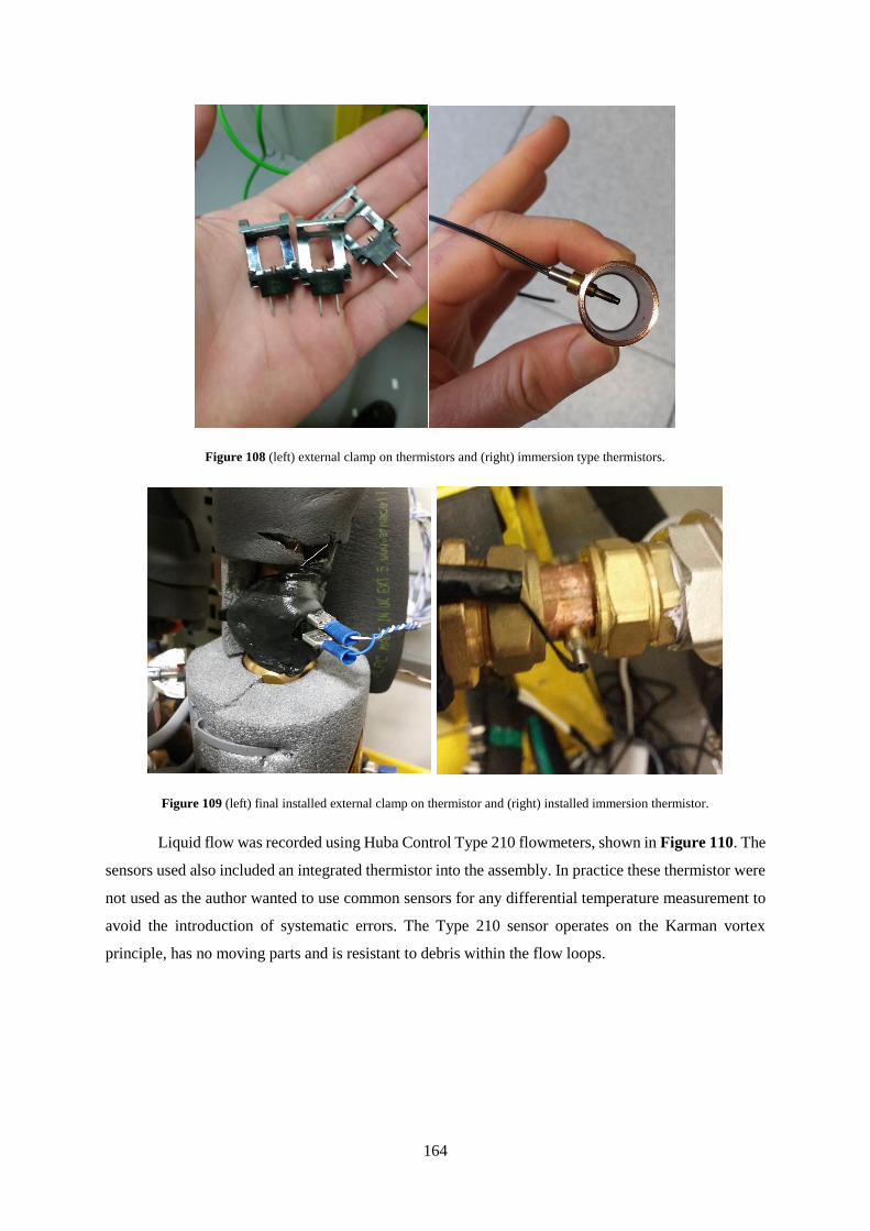
164
Figure 108 (left) external clamp on thermistors and (right) immersion type thermistors.
Figure 109 (left) final installed external clamp on thermistor and (right) installed immersion thermistor.
Liquid flow was recorded using Huba Control Type 210 flowmeters, shown in Figure 110. The
sensors used also included an integrated thermistor into the assembly. In practice these thermistor were
not used as the author wanted to use common sensors for any differential temperature measurement to
avoid the introduction of systematic errors. The Type 210 sensor operates on the Karman vortex
principle, has no moving parts and is resistant to debris within the flow loops.

165
Figure 110 Huba Control Type 210 DN15 flowmeter capable of reading liquid flow in the range of 3-50 litres per minute.
The gas flow to the Microgen FPSE was measured using a standard domestic diaphragm gas
flowmeter (U6P ITRON Diaphragm Gas Meter) shown in Figure 111. The flowmeter offers a
maximum capacity of 6 m3/h and offers a pulse output facility of 0.01 m3/pulse which was used to
provide a real time input to the LabView control program. By timing the interval between received
pulses it was possible to measure the heat input to the engine.
Figure 111 U6P diaphragm gas flowmeter (front centre).
5.4.9.2 Data Acquisition Units
An Agilent (now Keysight) 34972A data acquisition switch, shown in the left of Figure 112
was used for all temperature measurements (both thermistor and thermocouple for air temperature

166
sensing). The data acquisition unit had a 20 channel multiplexer for 2 wire temperature inputs. As the
Agilent 34972A could not accommodate pulse frequency inputs it was necessary to use a Campbell
Scientific CR3000 datalogger, shown on the right of Figure 112, which had 4 pulse input facilities. The
CR3000 could also provide temperature measurements but this was not used during testing as the
Agilent 34972A was easier to integrate with LabView.
Figure 112 (left) Agilent 34972A data acquisition unit and (right) Campbell Scientific CR3000 datalogger.
5.2.9.3 Networking and Communication
In addition to the external sensors and data acquisition units, the Microgen FPSE and InvenSor
adsorption chiller both had on-board microcontrollers which recorded data. With respect to the FPSE,
some of these measurements, such as electric power output were critical to obtain for making efficiency
estimates. For the adsorption chiller, each loop featured high accuracy RTD temperature sensor and
individual flowmeters. Though none of these would be used for final test measurements, they would
provide a useful comparison for highlighting faults. It was discovered during experimental testing that
the adsorption machine’s chiller flowrate temperature sensors were slightly skewed and would deliver
an artificially high cooling capacity measurement if used.
Data from the FPSE controller, adsorption machine controller, Agilent datalogger, CR3000
datalogger and Arduino fan PID controller were all collected and fused in a single integrated LabView
data acquisition program on the lab test PC shown in Figure 113.

167
Figure 113 Lab test PC
A network diagram describing all of the relevant protocols and interfaces for the entire lab data
acquisition infrastructure is shown below in Figure 114. With respect to the SAS, the chiller, CR3000
and Agilent were all interfaced with via ethernet through a switch connected to the PC. The FPSE and
Arduino fan PID controller were connected via an RS-232 serial connection which was subsequently
converted to USB to interface with the lab PC. Both the FPSE and the Whispergen engine were natively
RS-485 but this was converted to RS-232 via a converter module. Finally, the TriPac Evolution was
connected via a direct USB connection.

168
Figure 114 Lab networking infrastructure and data acquisition layout.
5.2.9.4 LabView
Due to the wide variety of data sources, it was essential to capture all data into a cohesive
unified environment so a LabView program was created that showed all of the relevant measurements
and data in real-time as illustrated in Figure 115.
Figure 115 Real-time display of data on Lab test PC. (Top-left) real time chiller capacity, (top-right) heat rejection
temperatures, (bottom-left) COP and (bottom-right) system temperatures.

169
Microgen Engine Corporation provided the author with a LabView program, shown in Figure
116 for interfacing with their engine microcontroller. This provided all of the relevant engine data and
the author modified the program slightly to also record the gas flowrate entering the engine which could
be used to calculate the thermal heat input, thermal efficiency and electrical efficiency. This was the
primary source of engine data although it was recorded into the unified LabView program also.
Figure 116 Microgen Engine Corporation LabView data acquisition program. Note that the author made some minor
modifications to the program so as to include thermal efficiency, fuel input and overall system efficiency.
The primary LabView program, depicted in Figure 117 and Figure 118 operated as follows.
Raw sensor data was read in from the Agilent datalogger and Campbell Datalogger and then converted
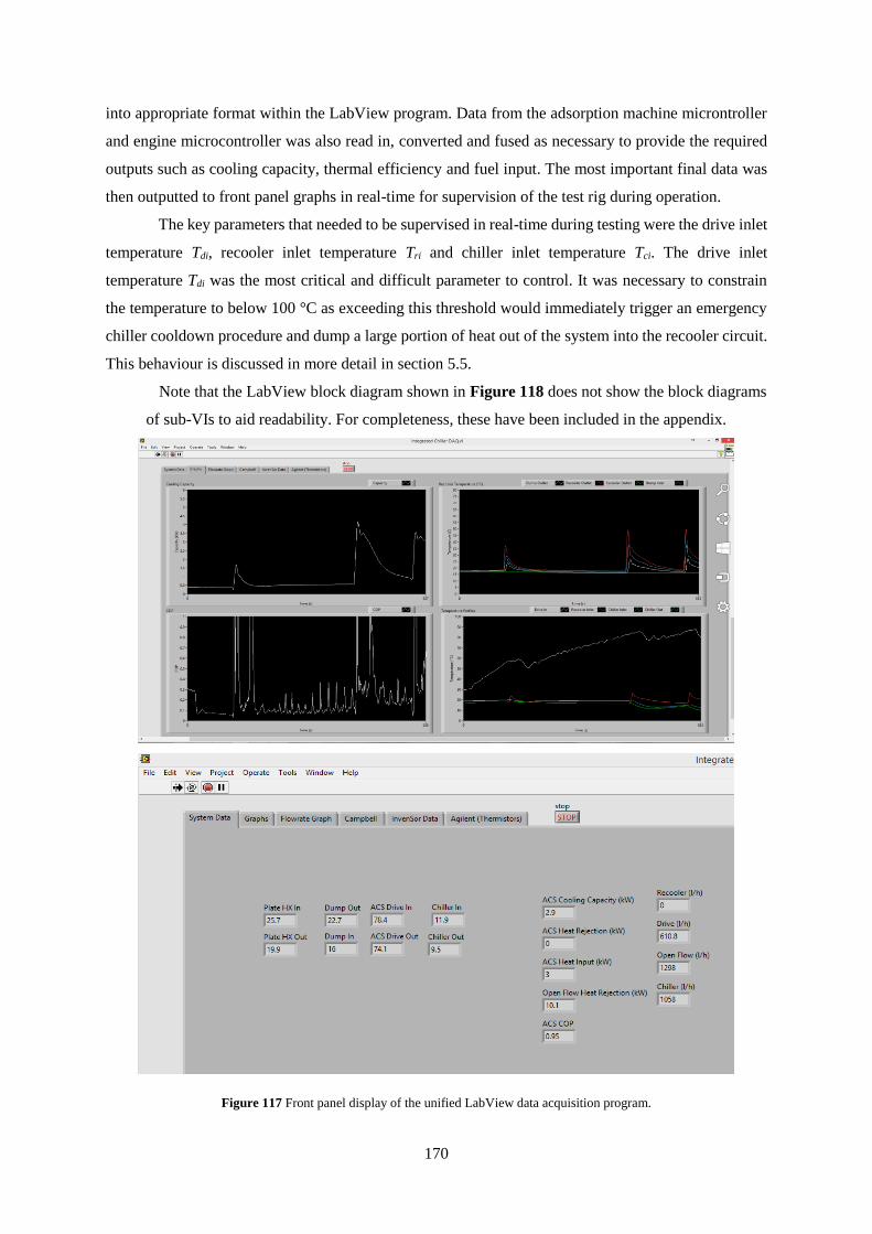
170
into appropriate format within the LabView program. Data from the adsorption machine microntroller
and engine microcontroller was also read in, converted and fused as necessary to provide the required
outputs such as cooling capacity, thermal efficiency and fuel input. The most important final data was
then outputted to front panel graphs in real-time for supervision of the test rig during operation.
The key parameters that needed to be supervised in real-time during testing were the drive inlet
temperature Tdi, recooler inlet temperature Tri and chiller inlet temperature Tci. The drive inlet
temperature Tdi was the most critical and difficult parameter to control. It was necessary to constrain
the temperature to below 100 °C as exceeding this threshold would immediately trigger an emergency
chiller cooldown procedure and dump a large portion of heat out of the system into the recooler circuit.
This behaviour is discussed in more detail in section 5.5.
Note that the LabView block diagram shown in Figure 118 does not show the block diagrams
of sub-VIs to aid readability. For completeness, these have been included in the appendix.
Figure 117 Front panel display of the unified LabView data acquisition program.

171
Figure 118 Unified LabView data acquisition program block diagram.
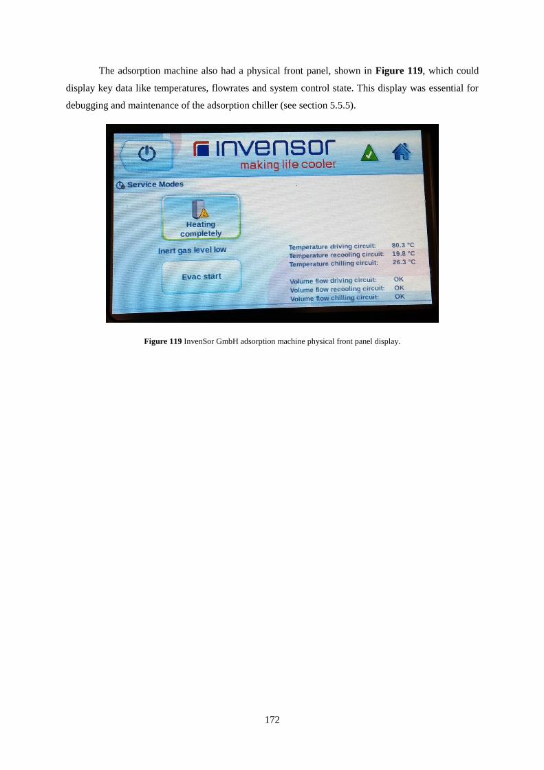
172
The adsorption machine also had a physical front panel, shown in Figure 119, which could
display key data like temperatures, flowrates and system control state. This display was essential for
debugging and maintenance of the adsorption chiller (see section 5.5.5).
Figure 119 InvenSor GmbH adsorption machine physical front panel display.

173
5.3 SAS Experimental Testing
With the construction phase of the experimental research completed it was possible to proceed with
testing of the adsorption chiller and the overall SAS architecture. The specific tests conduction and the
rationale behind them are discussed in section 5.5.6.
In addition to the experimental difficulty of conducting and controlling tests, as illustrated in
Section 5.5.2, the author also experienced a significant engine failure which is depicted in Figure 120.
The ceramic liner for the engine burner cracked at the collar and delaminated from the stainless steel
housing resulting in significantly reduced performance due to obstruction of flame circulation. The root-
cause for this fault was not investigated as there was no time and the engine related tests were minor in
comparison to the adsorption chiller testing that would be conducted with the electric heater. The burner
housing was returned to Microgen Engine Corporation for repair and the engine was subsequently put
back into service. The engine did not show any additional faults after this initial failure. It is unclear as
to whether the cracking was caused by a manufacturing flaw or mechanical strain during installation.
Another hypothesis is that the exhaust heat exchanger, situated immediately above the burner
shell, could have caused temperature cycling of the collar during pulsed thermal loading resulting in
fatigue cracking. The author personally does not believe this is the cause as the burner is designed to
undergo rapid heating from room temperature to in excess of 500 °C and the pulsed thermal load
temperature fluctuations are at most 50 °C.
Figure 120 Burner ceramic liner failure. The ceramic (visible in white on the left) has detached from the shell house (right
image). The remains of the ceramic collar at the exhaust vent is still visible in the right hand photo where the failure occurred.

174
5.3.1 Test Methodology
In order to perform controlled experimental test of the adsorption chiller, it is necessary to
constrain the drive inlet temperature, Tdi, recooler inlet temperature, Tri, system flowrates, ṁr, ṁc, ṁd,
and then varying the heat load on the chiller loop for a given chiller inlet temperature Tci.
The various system flowrates are manually set using the DC pump control box potentiometers,
depicted below in Figure 121, and the inverter drive control box. Once initially set, the system flowrate
remains constant throughout testing. Also visible in Figure 121 is the fan control box (right) which,
although was not used for the recooler temperature, it was vital for adding heat load to the chiller loop.
The airflow rate over the chiller air-cooled heat exchanger was varied by adjusting the voltage supplied
to the fans using the front-panel potentiometer on the fan control box.
Figure 121 DC Pump control box manual (left) and fan control box (right). The respective speeds are adjusted using the
front panel potentiometers. The fan control box also has a manual/auto selector that can enable PID setpoint control.
However this was not used during testing as manual control was sufficient.
The drive inlet temperature, Tdi, was controlled using the electric heater, shown in the rear
Figure 122. It was difficult to maintain a fixed driving temperature and the drive temperature was in a
constant state of dynamic equilibrium. In practical testing, the author seeked to maintain as close to 100
°C as possible without triggering an emergency heat dump in order to maximise capacity.
Also visible in Figure 122 (left) are the heater fans and chiller heat exchanger blowers this.
This method, although crude, was effective at supplying heat to the chiller loop. The exact heating effect
could be controlled by varying the fan speed, heater setting and the physical distance separating the
heaters from the radiator blowers. Finally, the image on the right of Figure 122 shows the lab water

175
supply lever valve. The flowrate through the external loop of the plate heat exchanger was modulated
by manually varying the position of this valve. This would directly control the recooler inlet
temperature, Tri, entering the adsorption chiller.
Figure 122 (left) 12 kW electric heater in background, foreground shows the heater fans used to load the chiller circuit of the
adsorption chiller and (right) the manual lever valve controlling the flow of water into the plate heat exchanger which controls
the recooler inlet temperature.
Careful adjustment and modulation of each of these control systems enables the operator to
perform tests to observe key system characteristics. However, the highly dynamic nature of adsorption
machine operation makes determination of fixed data points difficult. It is necessary to define a
measurement criterion for taking a measurement. The author chose the following method for estimating
system parameters; the system must achieve a minimum three or more sucessive periods of operation
and be in a local dynamic equilibrium for a data point to be valid. If longer periods are available then
this is more preferable as the data is more accurate as it represents a longer average.
An example of this local dynamic equilibrium is shown in Figure 123. It can be observed that
the system is in a constant regular repeating cycle and so for this sequence of data, in the 80 to 92 minute
range, a bulk average of each data point would be taken and used for later comparison. For example,
assume that the average Tdi temperature was 78 °C, the average Tri was 32 °C and the chiller inlet was
18 °C. The average capacity is approximately 2.5 kWt meaning that the system is capable of delivering
2.5 kWt at a Tri of 32 °C. This would be a single datapoint in the overall trend of the variation in cooling
capacity with increasing recooler temperature. Note that the driving temperature is somewhat lower

176
than typical in this test but for the purposes of comparison it would represent a minimum achievable
temperature. As the driving temperature is increased, the overall capacity would be increased. The
author attempted to maintain a high fixed driving temperature but this was difficult when trying to avoid
overtemperature emergency heat dumping. The final estimates produced will be conservative as the
system theoretically can provide a greater capacity that was achieved.
Figure 123 Test data showing a period of local dynamic equilibrium. Single data-points are obtained by taking an average of
the data in this time window.
As discussed in section 5.4.7, there was no control over the incoming water temperature and
the system could receive short-term pulses of high temperature cooling water which would cause a loss
of set-point. The unpredictability of incoming water temperature put an upper limit on the maximum
length of dynamic equilibrium that could be achieved. An example of a sudden change in incoming
cooling water temperature on overall system performance is depicted in Figure 124. The fluctuations
in incoming water cooling temperature, particularly beginning at 86 minutes cause an impact on the
recooler temperature control and break the dynamic equilibrium requirement for taking a test point.
This particular test is at very high recooler temperature so the impact is much weaker than when testing
at lower recooling temperatures.
0
1
2
3
4
5
6
7
8
0
10
20
30
40
50
60
70
80
90
100
80 82 84 86 88 90 92
Qco
ol (k
W)
Tem
per
ature
(°C
)
Time (mins)
Tri Tci Tdi Qcool (kW)

177
Figure 124 Data showing the impact of building water temperature on recooler flowrate. The effect is milder at high
recooling temperatures.
The impact when testing at lower recooling temperatures is shown in the raw data presented in
Figure 125. The rapid increase in temperature can be counter-acted by quickly increasing the flowrate
to compensate but, of course, if the cooling temperature exceeds the desired recooler temperature is it
thermodynamically impossible to maintain the setpoint. The fluctuating cooling water temperature
(blue) meant that test data obtained on this day was completely unusable for comparative analysis as no
periods of successive stability could be obtained. However, despite the difficulty presented by the
laboratory water supply temperature, it was possible to achieve a full range of datapoints through an
extensive and challenging test campaign which is presented in section 5.6.
Figure 125 Raw data of a particularly dire day of testing showing the extent of the variability in lab water supply temperature.
None the data obtained on this day was usable.
0
10
20
30
40
50
60
70
80
90
100
80 82 84 86 88 90 92 94 96 98 100
Tem
per
ature
(°C
)
Time (minutes)
Chiller Water In ACS Drive In (NTC10k)
ACS Recooler Inlet (NTC10k) ACS Chiller Inlet (NTC10k)

178
5.5.2 Sensor Calibration
In order to calibrate the thermistors, the sensors were placed on a pipe circulating water from a
large ice-bath. Figure 126 shows the calibration of the chiller inlet Tci and chiller out Tco sensors. The
sensors are placed on the exposed section of copper pipe and the pump is circulating the ice-water in a
closed loop with the large green bucket. It is assumed that the flowrate is sufficiently high to minimize
any losses and heat entering the pipes as the ice-water reaches the sensor. By placing the sensors side-
by-side, they should be providing the exact same measurement. Secondly, by circulating melting ice-
water through the system the temperature should be exactly 0 °C.
Figure 126 Ice-bath calibration process for the temperature sensors.
The experimental test data from this calibration process is shown in Figure 127. There are two
errors visible. The first is a relative error between the two sensors which is very important as the main
measurements they will be performing are differential measurements of temperature between the two.
The second error is an absolute error between the sensors and the true temperature of 0 °C. By measuring
these characteristics for each individual sensor it was possible to obtain unique calibration constants for
each sensor.

179
Figure 127 Data from chiller loop temperature sensor calibration.
The flowmeters were assumed to be accurate as they were in very close agreement with the
InvenSor flowmeters. In addition, the impact of minor deviations in flowrate were a lot less significant
on the overall results as compared to errors in temperature due to the very small temperature differences
being measured.
5.3.3 Error Analysis and Uncertainty
The largest source of error in the data presented originates from sub-optimal set point control. It
was not practically possible to test the system in a true calorimeter setting. Additionally, it was deemed
too risky to subject the core adsorption chiller and Stirling engine sub-systems to extreme ambient
conditions. Though both systems are technologically capable of operating at these conditions, guidance
from the respective manufacturers advised against it as certain sub-systems, such as electronics were
only designed for milder domestic applications.
Without a calorimeter, it was only possible to maintain Tci to ±1.8 °C of the 18.0 °C baseline
condition. The full list of errors are presented in Table 13.
As a result of the high system flowrates, the temperature differences (ΔT) being measured are
very small and on the order 2-3 °C. This means that a minor error in temperature measurement results
in a large propagating error in the cooling capacity and COP calculations. The chiller ΔT measurement
was calibrated by using an ice bath and observing the relative drift between the two thermistors as they
0
1
2
3
4
5
6
7
8
9
10
11
12
13
0 10 20 30 40 50 60 70
Tem
per
ature
(°C
)
Time (mins)
Chiller Out Chiller In

180
reached the 16-20 °C region where capacity measurements take place. This calibration method enabled
higher precision measurements with a standard deviation of ± 0.08 °C. It was not experimentally
possible to perform a similar calibration on the drive ΔT in the 90 °C region and so a larger extrapolated
drift error of ± 0.5 °C was used instead. This error is the source of the wide error range on the COP
estimation. A final source of error is the heat loss or gain in the plumbing that is not measured by
sensors. This is assumed to be negligible as the plumbing was heavily insulated and the sensors were
placed as close to the adsorption chiller as possible.
Table 13 List of experimental errors.
Parameter Symbol Error Unit Parameter Symbol Error Unit
Chiller ΔT ΔTc ±0.08 °C Recooler flowrate ṁr ±30 l h-1
Drive ΔT ΔTd ±0.5 °C Cooling capacity Qcool ±0.12 kW
Recooler ΔT ΔTr ±0.5 °C Heat input Qinput ±0.78 kW
Chiller
flowrate
ṁc ±30 l h-1 COP ±0.06 -
Drive flowrate ṁd ±30 l h-1
5.3.4 InvenSor Calibration data
Immediately prior to receiving the adsorption chiller, the author received some calibration test
data for the adsorption chiller operating at a nominal cooling capacity. This data is shown in Figure
128 and the variation in cooling capacity at a Tdi of 90 °C, Tri of 27 °C and Tci of 18 °C is shown. The
system offered by InvenSor GmbH was described as a 2 kWt adsorption machine but the system actually
achieves significantly higher capacity, almost 4 kWt at this particular condition. Although the capacity
drops at increasing ambient temperatures the author believes that the engineers at InvenSor were being
conservative and modest with the capacity values. This was one reason for the need for a supplementary
heater as the engine would not have been capable of driving the chiller at full power due to its limited
thermal output.
Another factor in the high performance of the adsorption chiller is the heavily buffered inputs.
The ability to maintain fixed input temperatures has a significant positive impact on overall performance
and cannot be readily achieved in the SAS architecture. This will be discussed at length in later sections.

181
Figure 128 Initial InvenSor GmbH calibration data for the adsorption machine.
The reduced cooling capacity obtained during initial tests lead the author to perform system
maintenance on the adsorption machine based on advice from InvenSor. As the adsorption machine
operates at partial vacuum it is susceptible to ingress of inert atmospheric gas which does not contribute
to the cooling effect. It is necessary to purge these gases from the system during annual maintenance
unless an active system is not already in place. The process for purging the gas was to connect a vacuum
pump to the chiller service valve, shown in the right image of Figure 129. The chiller would then be
operated at high temperature to dry the adsorption beds and a manual valve would be opened slightly
to release any non-condensable gases from the system until the front panel indicator indicated that the
system was operating nominally. They author successfully completed this process and some inert gas
was removed from the system resulting in a modest boost in capacity but the system still did not achieve
the performance obtained by InvenSor. This likely further confirmed the benefits of buffering for
overall system performance.
Figure 129 (left) Vacuum maintenance being performed on the adsorption machine and (right) the vacuum purge valve. The
vacuum pump is visible on top of the machine and is being used to remove inert gases from the system.
0
1000
2000
3000
4000
5000
6000
7000
0
10
20
30
40
50
60
70
80
90
100
0 1 2 3 4 5 6 7 8 9 10
Co
oli
ng C
apac
ity (
W)
Tem
per
ature
(°C
)
Time (mins)
Chiller Inlet Drive Inlet Recooler Inlet Cooling Capacity

182
After the experimental test period had concluded and the author returned the prototype chiller
to InvenSor, they performed a series of “high ambient” tests where the recooler inlet temperature was
varied in the range of 20 to 40 °C, shown in Figure 130, similar to what the author had done in order
to verify the overall trend. As with the initial calibration data, InvenSor achieved a higher capacity that
the author which is likely due to the benefits of high buffering and increased effective driving
temperature. Reassuringly, they also achieved the same temperature degradation profile but were unable
to test at extreme recooler temperatures due to experimental limitations of their calibration facility.
Figure 130 Variation of cooling capacity with increasing recooler inlet temperature.
5.3.5 Test Matrix
The primary focus of testing was the evaluation of system performance with increasing ambient
temperature (recooler temperature). Consequently, the bulk of the tests were concerned with increasing
the recooler inlet temperature, Tri from 22 – 55 °C and observing variations in cooling capacity, Qcool.
A test matrix showing the actual conditions is presented below in Table 14. The test conditions chosen
attempted to maintain a Tci of around 18 °C and then modulate the Tri across a range of 20-55 °C. The
Tdi was kept as high as possible without triggering over temperature heat dump from the adsorption
chiller. The flowrates were kept constant although certain tests required lower chiller flowrate (A-15
and A-10) to increase the chiller loop ΔT so that it was more easily measured and controlled. All of the
tests presented in this test matrix were conducted using the supplementary electric heater.
Table 14 Test Matrix of Conditions for recooler inlet temperature testing
Test Tri (°C) Tci (°C) Tdi (°C) Drive
Loop (l/h)
Recooler
(l/h)
Chiller
(l/h)
A-1 22.48 16.33 83.84 1491 1509 1057
A-2 25.10 17.98 84.27 1139 1502 1070
A-3 28.60 17.26 80.72 1309 1282 1069
0.0
0.5
1.0
1.5
2.0
2.5
3.0
3.5
4.0
4.5
5.0
15 20 25 30 35 40 45
Co
oli
ng C
apac
ity (
kW
t)
Recooler Inlet Temperature (°C)
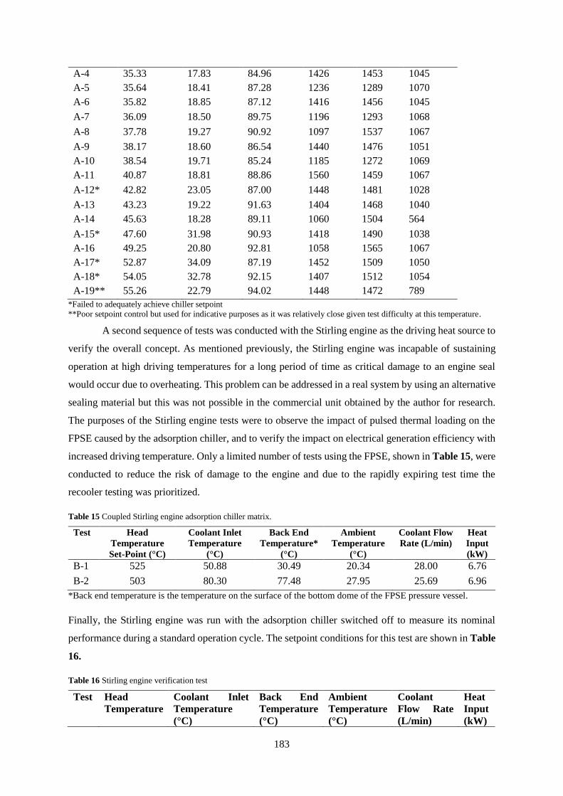
183
A-4 35.33 17.83 84.96 1426 1453 1045
A-5 35.64 18.41 87.28 1236 1289 1070
A-6 35.82 18.85 87.12 1416 1456 1045
A-7 36.09 18.50 89.75 1196 1293 1068
A-8 37.78 19.27 90.92 1097 1537 1067
A-9 38.17 18.60 86.54 1440 1476 1051
A-10 38.54 19.71 85.24 1185 1272 1069
A-11 40.87 18.81 88.86 1560 1459 1067
A-12* 42.82 23.05 87.00 1448 1481 1028
A-13 43.23 19.22 91.63 1404 1468 1040
A-14 45.63 18.28 89.11 1060 1504 564
A-15* 47.60 31.98 90.93 1418 1490 1038
A-16 49.25 20.80 92.81 1058 1565 1067
A-17* 52.87 34.09 87.19 1452 1509 1050
A-18* 54.05 32.78 92.15 1407 1512 1054
A-19** 55.26 22.79 94.02 1448 1472 789
*Failed to adequately achieve chiller setpoint
**Poor setpoint control but used for indicative purposes as it was relatively close given test difficulty at this temperature.
A second sequence of tests was conducted with the Stirling engine as the driving heat source to
verify the overall concept. As mentioned previously, the Stirling engine was incapable of sustaining
operation at high driving temperatures for a long period of time as critical damage to an engine seal
would occur due to overheating. This problem can be addressed in a real system by using an alternative
sealing material but this was not possible in the commercial unit obtained by the author for research.
The purposes of the Stirling engine tests were to observe the impact of pulsed thermal loading on the
FPSE caused by the adsorption chiller, and to verify the impact on electrical generation efficiency with
increased driving temperature. Only a limited number of tests using the FPSE, shown in Table 15, were
conducted to reduce the risk of damage to the engine and due to the rapidly expiring test time the
recooler testing was prioritized.
Table 15 Coupled Stirling engine adsorption chiller matrix.
Test Head
Temperature
Set-Point (°C)
Coolant Inlet
Temperature
(°C)
Back End
Temperature*
(°C)
Ambient
Temperature
(°C)
Coolant Flow
Rate (L/min)
Heat
Input
(kW)
B-1 525 50.88 30.49 20.34 28.00 6.76
B-2 503 80.30 77.48 27.95 25.69 6.96
*Back end temperature is the temperature on the surface of the bottom dome of the FPSE pressure vessel.
Finally, the Stirling engine was run with the adsorption chiller switched off to measure its nominal
performance during a standard operation cycle. The setpoint conditions for this test are shown in Table
16.
Table 16 Stirling engine verification test
Test Head
Temperature
Coolant Inlet
Temperature
(°C)
Back End
Temperature
(°C)
Ambient
Temperature
(°C)
Coolant
Flow Rate
(L/min)
Heat
Input
(kW)

184
Set-Point
(°C)
C-1 476 12.22 30.33 17.53 30.25 6.50

185
5.4 Results and Discussion
The start-up dynamics of the free-piston Stirling engine (FPSE) during a standard operating
profile independent of the adsorption chiller is depicted in Figure 131. The FPSE coolant loop is
approximately fixed at 18 °C. In contrast to the Whispergen kinematic Stirling engine start-up profile
presented in Section 5.2.4, the FPSE has a rapid start-up time likely owing to lower thermal mass in the
heater head and burner along with easier ignition of gas-burners when compared to the evaporative
diesel burner found in the Whispergen. The FPSE quickly reaches operating power and begins to
modulate the burner temperature at about 5 minutes to control the approach to the nominal 1 kWe output.
The engine controller then continuously modulates the heater head temperature by adjusting the burner
power to maintain a constant 1 kWe power output. The Stirling engine achieved an electrical efficiency
of 15.3% during this test.
Figure 131 Start-up dynamics of Stirling engine during independent operation. This test corresponds to test C1 in the test
matrix.
Figure 132 shows the start-up operation of the FPSE when coupled to the adsorption chiller.
The engine operates nominally from 3 minutes to around 30 minutes in a similar fashion to Figure 131.
However, note that the coolant loop temperature has been continually increasing in order to prepare for
the adsorption chiller operation. During this period, since the ACS is off, there is minimal heat rejection
from the coolant loop, leading to a increasing temperature. From the 30 minute point, it can be seen that
the FPSE can no longer maintain 1 kWe output as the reduction in efficiency caused by increased coolant
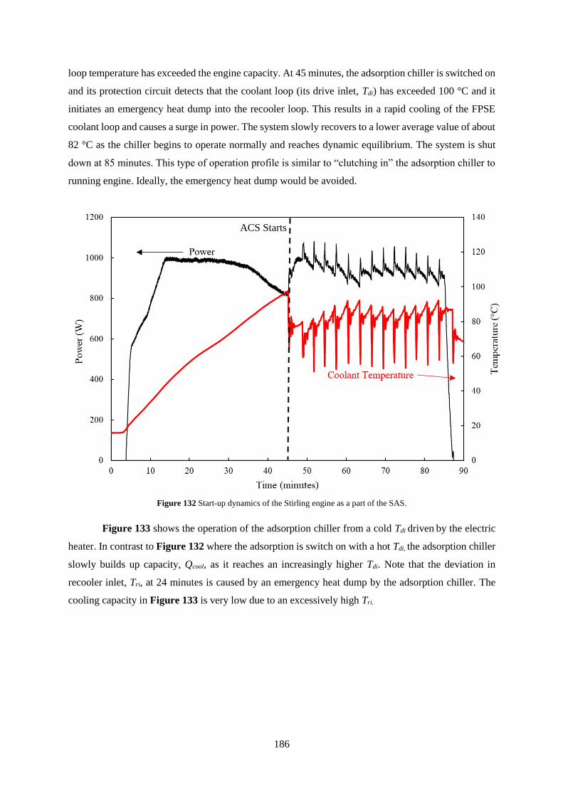
186
loop temperature has exceeded the engine capacity. At 45 minutes, the adsorption chiller is switched on
and its protection circuit detects that the coolant loop (its drive inlet, Tdi) has exceeded 100 °C and it
initiates an emergency heat dump into the recooler loop. This results in a rapid cooling of the FPSE
coolant loop and causes a surge in power. The system slowly recovers to a lower average value of about
82 °C as the chiller begins to operate normally and reaches dynamic equilibrium. The system is shut
down at 85 minutes. This type of operation profile is similar to “clutching in” the adsorption chiller to
running engine. Ideally, the emergency heat dump would be avoided.
Figure 132 Start-up dynamics of the Stirling engine as a part of the SAS.
Figure 133 shows the operation of the adsorption chiller from a cold Tdi driven by the electric
heater. In contrast to Figure 132 where the adsorption is switch on with a hot Tdi, the adsorption chiller
slowly builds up capacity, Qcool, as it reaches an increasingly higher Tdi. Note that the deviation in
recooler inlet, Tri, at 24 minutes is caused by an emergency heat dump by the adsorption chiller. The
cooling capacity in Figure 133 is very low due to an excessively high Tri.
ACS Starts

187
Figure 133 Adsorption chiller start-up dynamics when driven by electric heater.
5.4.1 Combined Stirling-adsorption system operation
In a waste heat application such as adsorption cooling, the operation of the chiller impacts the cold end
of the engine and can increase electrical efficiency by reducing the cooling temperature. Zeolite-water
adsorption chillers have high thermal demand during valve switchover and desorption events. These
short-term (<10 second) demands can be up to 10 times the steady state demand and cause rapid, short-
term cooling of the engine coolant loop flow, thus producing power spikes as shown in Figure 134a
resulting from the engine efficiency spikes shown in Figure 134b. The time scale of this thermal cooling
spike (several seconds) is far shorter than the thermal equilibration timescale of the hot end of the engine
(several minutes). Thus, it is not possible to compensate the resulting power pulsation by varying the
heat addition to the engine. Based on testing shown in Figure 134a the effect is significant with 10-
15% fluctuations in power output but, as the effect is regular and produces a surplus of energy, this
excess energy could easily be diverted to battery storage or simply dissipated in the engine’s coolant
loop using a resistive element. A simple linear relationship between temperature difference and power
output has been found to describe the impact of pulsed thermal loading on the engine. Every additional
1 °C of temperature difference produces approximately 3-4 W of power for cooling loop variations in
0
0.5
1
1.5
2
2.5
3
3.5
4
4.5
5
0
20
40
60
80
100
120
0 2 4 6 8 10 12 14 16 18 20 22 24 26 28
Qco
ol(k
Wt)
Tem
per
ature
(°C
)
Time (minutes)
Tdi
Tri
Tci
Qcool
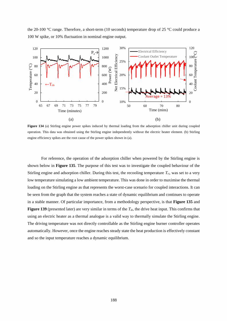
188
the 20-100 °C range. Therefore, a short-term (10 seconds) temperature drop of 25 °C could produce a
100 W spike, or 10% fluctuation in nominal engine output.
(a) (b)
Figure 134 (a) Stirling engine power spikes induced by thermal loading from the adsorption chiller unit during coupled
operation. This data was obtained using the Stirling engine independently without the electric heater element. (b) Stirling
engine efficiency spikes are the root cause of the power spikes shown in (a).
For reference, the operation of the adsorption chiller when powered by the Stirling engine is
shown below in Figure 135. The purpose of this test was to investigate the coupled behaviour of the
Stirling engine and adsorption chiller. During this test, the recooling temperature Tri, was set to a very
low temperature simulating a low ambient temperature. This was done in order to maximise the thermal
loading on the Stirling engine as that represents the worst-case scenario for coupled interactions. It can
be seen from the graph that the system reaches a state of dynamic equilibrium and continues to operate
in a stable manner. Of particular importance, from a methodology perspective, is that Figure 135 and
Figure 139 (presented later) are very similar in terms of the Tdi, the drive heat input. This confirms that
using an electric heater as a thermal analogue is a valid way to thermally simulate the Stirling engine.
The driving temperature was not directly controllable as the Stirling engine burner controller operates
automatically. However, once the engine reaches steady state the heat production is effectively constant
and so the input temperature reaches a dynamic equilibrium.
0
200
400
600
800
1000
1200
0
20
40
60
80
100
120
65 67 69 71 73 75 77 79
Po
wer
(W
)
Tem
per
ature
(°C
)
Time (minutes)
Pe→
0
20
40
60
80
100
120
10%
15%
20%
25%
30%
50 60 70 80
Co
ola
nt
Tem
per
ature
(°C
)
Net
Ele
ctri
cal
Eff
icie
ncy
Time (mins)
Electrical Efficiency
Coolant Outlet Temperature
Average = 13%
←Tdo

189
Figure 135 Operation of the adsorption chiller when driven by the Stirling engine. Note that the Tri is set very low
simulating a cool ambient. Compare the similarities in graph with Figure 136 for a visual comparison between Stirling
engine and electric heater operation.
An average COP, as defined in Eq. (26), of 0.42±0.06 was achieved at a Tri of 44.6 °C, Tci of
19.4 °C and Tdi of 81.0 °C. Figure 137 illustrates the highly dynamic real time COP of the adsorption
chiller system during operation. This value is lower than the figures achieved by the manufacturer
(≈0.6). This discrepancy can be explained by the absence of thermal buffering and reduced heat transfer
efficiency. The absence of buffering reduces the maximum attainable temperature difference between
the Tdi and Tdo during thedesorption phase. A large temperature difference between Tdi and Tdo can
however, be maintained in buffered systems as is shown in Figure 140a (shown later). This higher
temperature could result in improved heat transfer to the zeolite within the adsorber and thus increased
cooling capacity and COP. It is not possible to reproduce this behaviour in an APU using a fixed heat
source. Increasing the heat input will only increase the slopes of Tdi and Tdo shown Figure 140b (shown
later) and not the overall temperature difference. Additionally, in a mobile application with no buffering,
this sloping temperature profile of Tdi and Tdo results in a lower average effective driving temperature
as the system is limited to a peak temperature value to prevent boiling or over-pressurization of the
working fluid. Consequently, low buffer systems with their lower effective driving temperature, will
display a lower COP and cooling capacity when compared to a highly buffered system.
0
1
2
3
4
5
6
7
8
0
10
20
30
40
50
60
70
80
90
100
80 82 84 86 88 90 92
Qco
ol (k
W)
Tem
per
ature
(°C
)
Time (minutes)
Tri Tci Tdi Qcool (kW)

190
𝐶𝑂𝑃 =𝑄𝑐𝑜𝑜𝑙
𝑄𝑖𝑛𝑝𝑢𝑡=
ṁ𝑐𝐶𝑝,𝑤(𝑇𝑐𝑖−𝑇𝑐𝑜)
ṁ𝑑𝐶𝑝,𝑤(𝑇𝑑𝑖−𝑇𝑑𝑜)
(26)
Figure 137 Typical COP performance of adsorption chiller. Note that the breaks in the data, denoted by grey bars are non-
physical spikes which have been trimmed out for clarity. They are caused by time lag between sensors. The average COP,
shown as a red line is calculated at 0.42.
5.4.2 Operation in High Ambient Conditions
5.4.2.1 Heat Exchanger Sizing
The purpose of the heat exchanger design procedure is to correlate internal adsorption recooler
inlet temperature (Tri) with external air temperature (Text) and minimize this temperature difference ΔTr
= Tri - Text. A plain aluminium-finned copper tube air-cooled heat exchanger sized for the full scale (4
kWt) adsorption chiller, and that meets the overall APU design requirements was designed using the
sizing procedure described by [283]. The prototype system characterised experimentally in this work is
one-half scale (2 kWt cooling). A key challenge for the APU application relates to sizing of the heat
exchangers and whether there will be sufficient space on the truck to accommodate them. This heat
exchanger sizing exercise, estimates the size of the full-scale heat exchanger (for 4 kWt cooling) that
will be required for the real application as it is fundamental to overall feasibility. The key equations and
correlations that were used for sizing the heat exchanger are shown in Eq. (27) to Eq. (33). It is
necessary to perform an iterative process using these equations to find a design that meets the
requirements. As heat exchanger design is a well-documented process, and for the sake of brevity, some
minor equations have been omitted and instead their values have been given in Table 17. For a full
0.0
0.2
0.4
0.6
0.8
1.0
1.2
1.4
72 74 76 78 80 82 84 86 88 90
CO
P
Time (mins)

191
description of these equations and parameters, the reader is directed to the standard heat exchanger
design process presented by [283].
The overall heat transfer rate experienced by the heat exchanger (Q) can be calculated from the
log-mean temperature difference (LMTD) and heat transfer coefficient using Eq. (27). The target
variable ΔTr is proportional to the LMTD but it is not possible to minimize it arbitrarily as doing so will
force UA to become arbitrarily large according to Eq. (27). The heat exchanger design process was
performed iteratively to bring the LMTD to a minimum while keeping the heat exchanger within the
APU size and volume constraints.
𝑄 = 𝐿𝑀𝑇𝐷 ∗ 𝑈𝐴 (27)
Using Eq. (28), UA can be calculated using the fin effectiveness (ηo), the water side convective
heat transfer coefficient (hw), the air side convective heat transfer coefficient (ha), the total heat transfer
area (A), the wall and resistance (Rw), the fouling resistance (Rf) and from the geometrical properties of
the heat exchanger which are given in Table 17. The convective heat transfer coefficients for the air
and liquid sides can be calculated using the Nusselt number (NuD), thermal conductivity of water (kw),
characteristic length (D), Colburn heat transfer factor (jN), core mass velocity (G), specific heat capacity
of air (Cp,a) and the Prandtl number (Pr) using Eq. (29) and Eq. (30) respectively.
1
𝑈𝐴=
1
𝜂𝑜ℎ𝑤𝐴+
1
𝜂𝑜ℎ𝑎𝐴+ 𝑅𝑤 + 𝑅𝑓
(28)
ℎ𝑤 = (𝑁𝑢𝐷𝑘𝑤
𝐷) (29)
ℎ𝑎 = (𝑗𝑁𝐺𝑐𝑝,𝑎
𝑃𝑟23
) (30)
Calculating the air side convective heat transfer coefficient, ha, of a cross-flow tube and fin heat
exchanger is non-trivial and requires the use of empirical correlations. One method is the generalized
Colburn heat transfer factor (jN) shown in Eq. (31) where N is the number of tube rows and ReDc is
Reynolds number. The Colburn heat transfer factor for four tube rows (j4) is shown in Eq. (32) and is
calculated from the Reynolds number at the collar diameter (ReDc), transverse tube pitch (Pt)
longitudinal tube pitch (Pl), fin pitch (Pf) and the effective fin collar diameter (dc)
𝑗𝑁
𝑗4= 0.991 [2.24𝑅𝑒𝐷𝑐
−0.092 (𝑁
4)
−0.031]
0.607(4−𝑁)
(31)
𝑗4 = 0.14𝑅𝑒𝐷𝑐−0.328 (
𝑃𝑡
𝑃𝑙)
−0.502
(𝑃𝑓
𝑑𝑐)
0.0312
(32)

192
A critical parameter in air-cooled heat exchanger design is the overall pumping power required
to pass air over the tube bundle. This value must be kept within the heat exchanger design requirements
for the exchanger to be practical. The fan power (P) can be calculated from the mass flow rate of air
(ṁa), the density of air (𝜌a) and air-side pressure (Δp) given by Eq. (33). The air-side Fanning friction
factor, f, is an important parameter used for calculating the air-side pressure drop (Δp) and is calculated
using Eq. (33).
𝑃 =ṁ𝑎
𝜌𝑎𝛥𝑝 (33)
where 𝛥𝑝 ∝ 𝑓
𝑓 = 0.0267𝑅𝑒𝐷𝑐
𝑐7 (𝑃𝑡
𝑃𝑙)
𝑐8(
𝑃𝑓
𝑑𝑐)
𝑐9
(7)
𝑐7 = −0.764 + 0.739 (𝑃𝑡
𝑃𝑙) + 0.177 (
𝑃𝑓
𝑑𝑐) −
0.00758
𝑁
𝑐8 = −15.689 +64.021
𝑙𝑛𝑅𝑒𝐷𝑐 𝑐9 = 1.696 −
15.695
𝑙𝑛𝑅𝑒𝐷𝑐
In order to approximate the required heat rejection load, the COP can be used to derive the heat
input and, subsequently, the heat rejection. Taking the COP of 0.42 achieved previously, this implies
that the adsorption system would require 9.5 kWt (4 kWt / 0.42 = 9.5 kWt) of driving heat input and
would then need to reject approximately 13.5 kWt (9.5 kWt of driving heat plus 4 kWt of heat removed
from the cab) during normal operation. Therefore, a conservative 18 kW recooler design has been
developed to account for any reductions in COP that may be experienced during adverse operating
conditionings. This is shown in Table 17 and yields a recooler inlet-ambient temperature difference
(ΔTr = Tri – Text) of 6 °C. A similar analysis indicates that the difference between chiller in (Tci) and cab
temperatures (Tcab) (ΔTc = Tci – Tcab) of 8 °C is conservative. This latter analysis has not been shown for
the sake of brevity as it is identical to that shown in Table 17. Based on this analysis, the baseline cab
condition of Tcab/Text = 26.6/35 °C corresponds to a chiller inlet/recooler inlet of Tci/Tri = 18/41 °C. Note
that the heat exchanger has not been optimized at a system level nor for standard tooling and
manufacturing. This heat exchanger analysis indicates that the geometric size of the heat exchanger,
0.6m x 0.6m, is not unfeasibly large for the truck APU application. For reference the condenser used in
conventional DEVC systems is approximated 0.54m x 0.38m in size.
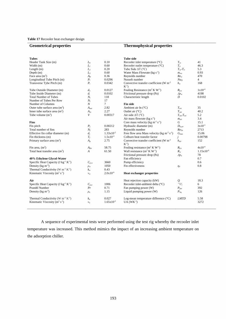
193
Table 17 Recooler heat exchanger design
Geometrical properties Thermophysical properties
Tubes Tube side
Header Tank Size (m) Lh 0.10 Recooler inlet temperature (°C) Tro 41 Width (m) L1 0.60 Recooler outlet temperature (°C) Tri 46.3
Length (m) L2 0.20 Tube Side ΔT (°C) Tro-Tri 5.3
Depth (m) L3 0.60 Water Mass Flowrate (kg s-1) ṁrec 0.93 Face area (m2) Afr 0.36 Reynolds number Rew 470
Longitudinal Tube Pitch (m) Pl 0.0296 Nusselt number NuD 4
Transverse Tybe Pitch (m) Pt 0.0342 Convective transfer coefficient (W m-2 K-1)
hw 168
Tube Outside Diameter (m) do 0.0127 Fouling Resistance (m2 K W-1) Rf,w 1x10⁻⁴
Tube Inside Diameter (m) di 0.0102 Frictional pressure drop (Pa) Δpw 4198 Total Number of Tubes Nt 118 Characteristic length D 0.0102
Number of Tubes Per Row Nl 17
Number of Columns N 7 Fin side
Outer tube surface area (m2) Aout 2.82 Ambient air In (°C) Text 35
Inner tube surface area (m2) Ain 2.27 Outlet air (°C) Tout 40.2
Tube volume (m3) V 0.00317 Air side ΔT (°C) Tout-Text 5.2
Air mass flowrate (kg s-1) ṁair 3.4
Fins Core mass velocity (kg m-2 s-1) G 15.1
Fin pitch Pf 0.00212 Hydraulic diameter (m) Dh,air 3x10⁻³
Total number of fins Nf 283 Reynolds number ReDc 2713
Effective fin collar diameter (m) dc 1.33x10⁻² Free flow area Mass velocity (kg m-2 s-1) Gmax 15.06
Fin thickness (m) Tf 1.5x10⁻⁴ Colburn heat transfer factor j 0.00798
Primary surface area (m2) Ap 2.75 Convective transfer coefficient (W m-2
K-1)
hair 152
Fin area, (m2) Afin 58.75 Fouling resistance (m2 K W-1) Rf,a 4x10⁻⁴
Total heat transfer area (m2) A 61.50 Wall resistance (m2 K W-1) Rw 1.15x10⁻⁶
Frictional pressure drop (Pa) Δpa 78
40% Ethylene Glycol-Water Fan efficiency 0.7
Specific Heat Capacity (J kg-1 K-1) Cp.w 3660 Pump efficiency 0.6
Density (kg m-3) ρw 1050 Fin effectiveness η0 0.8
Thermal Conductivity (W m-1 K-1) kw 0.43
Kinematic Viscosity (m2 s-1) νw 2.0x10⁻⁶ Heat exchanger properties
Air Heat rejection capacity (kW) Q 18.3
Specific Heat Capacity (J kg-1 K-1) Cp,a 1006 Recooler inlet-ambient delta (°C) r 6
Prandtl Number Pr 0.71 Fan pumping power (W) Pfan 392
Density (kg m-3) ρa 1.15 Liquid pumping power (W) Pliq
126
Thermal Conductivity (W m-1 K-1) ka 0.027 Log-mean temperature difference (°C) LMTD 5.58 Kinematic Viscosity (m2 s-1) νa 1.65x10⁻⁵ UA (WK-1) 3272
A sequence of experimental tests were performed using the test rig whereby the recooler inlet
temperature was increased. This method mimics the impact of an increasing ambient temperature on
the adsorption chiller.

194
Table 18 shows the lumped average results of a minimum of three cycles of dynamic stability.
The capacity data presented in Figure 138 was calculated using this table in conjunction with the Tri
offset described in previously in the heat exchanger sizing to correlate it to an ambient temperature.
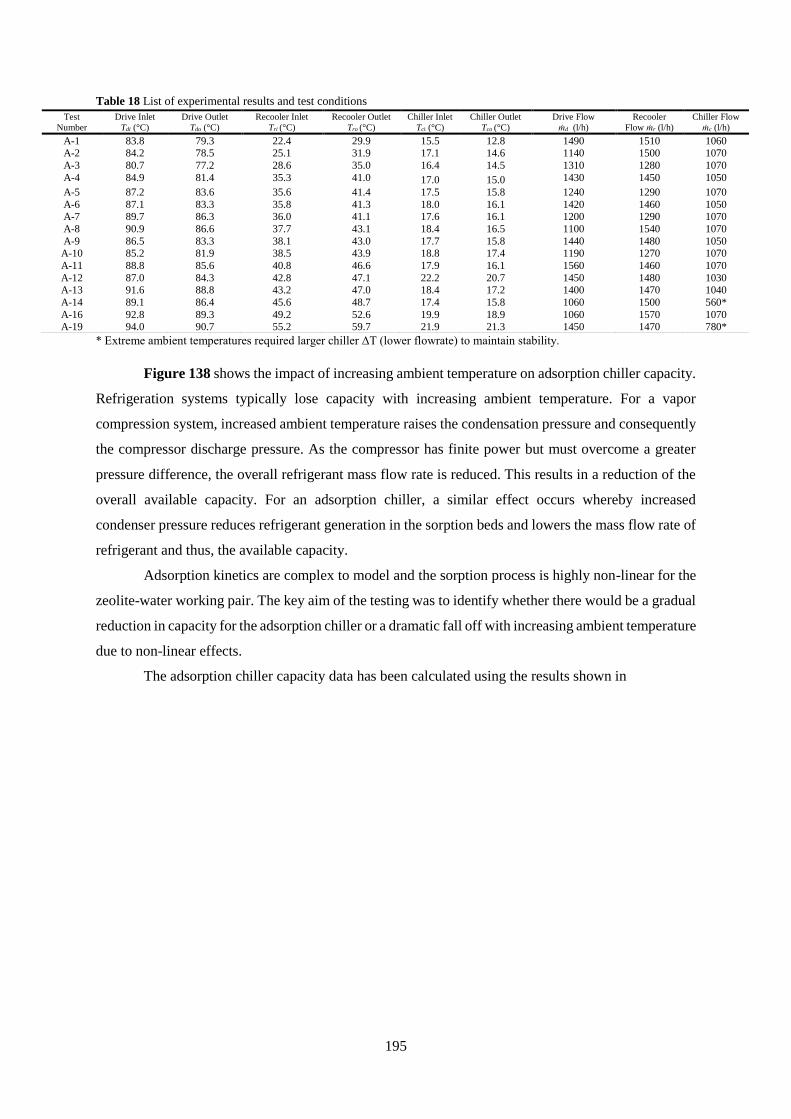
195
Table 18 List of experimental results and test conditions
* Extreme ambient temperatures required larger chiller ΔT (lower flowrate) to maintain stability.
Figure 138 shows the impact of increasing ambient temperature on adsorption chiller capacity.
Refrigeration systems typically lose capacity with increasing ambient temperature. For a vapor
compression system, increased ambient temperature raises the condensation pressure and consequently
the compressor discharge pressure. As the compressor has finite power but must overcome a greater
pressure difference, the overall refrigerant mass flow rate is reduced. This results in a reduction of the
overall available capacity. For an adsorption chiller, a similar effect occurs whereby increased
condenser pressure reduces refrigerant generation in the sorption beds and lowers the mass flow rate of
refrigerant and thus, the available capacity.
Adsorption kinetics are complex to model and the sorption process is highly non-linear for the
zeolite-water working pair. The key aim of the testing was to identify whether there would be a gradual
reduction in capacity for the adsorption chiller or a dramatic fall off with increasing ambient temperature
due to non-linear effects.
The adsorption chiller capacity data has been calculated using the results shown in
Test
Number Drive Inlet
Tdi (°C) Drive Outlet
Tdo (°C) Recooler Inlet
Tri (°C) Recooler Outlet
Tro (°C) Chiller Inlet
Tci (°C) Chiller Outlet
Tco (°C) Drive Flow
ṁd (l/h) Recooler
Flow ṁr (l/h) Chiller Flow
ṁc (l/h)
A-1 83.8 79.3 22.4 29.9 15.5 12.8 1490 1510 1060 A-2 84.2 78.5 25.1 31.9 17.1 14.6 1140 1500 1070
A-3 80.7 77.2 28.6 35.0 16.4 14.5 1310 1280 1070
A-4 84.9 81.4 35.3 41.0 17.0 15.0 1430 1450 1050
A-5 87.2 83.6 35.6 41.4 17.5 15.8 1240 1290 1070
A-6 87.1 83.3 35.8 41.3 18.0 16.1 1420 1460 1050 A-7 89.7 86.3 36.0 41.1 17.6 16.1 1200 1290 1070
A-8 90.9 86.6 37.7 43.1 18.4 16.5 1100 1540 1070
A-9 86.5 83.3 38.1 43.0 17.7 15.8 1440 1480 1050 A-10 85.2 81.9 38.5 43.9 18.8 17.4 1190 1270 1070
A-11 88.8 85.6 40.8 46.6 17.9 16.1 1560 1460 1070
A-12 87.0 84.3 42.8 47.1 22.2 20.7 1450 1480 1030 A-13 91.6 88.8 43.2 47.0 18.4 17.2 1400 1470 1040
A-14 89.1 86.4 45.6 48.7 17.4 15.8 1060 1500 560*
A-16 92.8 89.3 49.2 52.6 19.9 18.9 1060 1570 1070 A-19 94.0 90.7 55.2 59.7 21.9 21.3 1450 1470 780*

196
Table 18. This data is then compared with calorimeter test data of the leading DEVC APU
system. The graph indicates that, although the adsorption chiller is undersized, it appears to have lower
capacity degradation in high ambient conditions than the DEVC system, indicated by the relative slopes
of the trend lines. A zeolite-water adsorption chiller could potentially provide more stable cooling
capacity across its operating range compared to a DEVC system.
Figure 138 Variation in cooling capacity with increasing ambient temperature for SAS and DEVC systems. The adsorption
chiller is undersized in comparison to the DEVC system.
5.4.3 Operation with Low Thermal Buffering Volume
The majority of current adsorption applications are stationary and typically use a large buffer
storage tank with hundreds of litres of water to dampen peak thermal loads [284]. This is obviously not
practical in a truck application where space and weight are constrained. An APU application will be
forced to deal with rapid feedback pulsations as highlighted in Figure 139. Figure 139 shows 3
consecutive pulsations beginning at 111.6 minutes with the initial valve switchover causing a sudden
drop in Tdi from 90 °C to 70 °C. At 112.2 minutes the initial pulsation has recirculated around the system
and increased in temperature from 70 °C to 82 °C through mixing of the coolant fluid and heat input
from the engine. The initial major pulsation is almost completely dampened out by next recirculation
at 112.9 minutes and is barely noticeable. From 113 minutes to 114.1 minutes, the system is in the linear
recovery region whereby the difference between minimum and maximum temperature i.e. Tdi at 113
minutes and 114.1 minutes respectively, is defined as “recovery swing”, ΔTrs. The average effective Tdi
can be approximated by extrapolating the linear region back to the rising edge of the first pulsation. For
example, in Figure 139, extrapolating the Tdi at 117.5 minutes, which is 95 °C, back to the rising edge
R² = 0.8518R² = 0.9727
0.0
0.5
1.0
1.5
2.0
2.5
3.0
3.5
4.0
4.5
25 30 35 40 45 50
Cap
acit
y (
kW
)
Ambient Temperature (°C)
Proposed SAS
Current DEVC

197
of the first pulsation at 114.5 gives a lower temperature of approximately 80 °C. The average effective
temperature would be the average of these two values or 87.5 °C. The maximum temperature limit for
the SAS is under 100 °C to avoid boiling and pressurization. Consequently, the maximum average
effective driving temperature is governed by the amplitude of the recovery swing and therefore the
buffering volume. The pulsation behaviour also has a negative impact by lowering the effective driving
temperature.
Figure 139 Typical adsorption chiller performance characteristics. Note feedback pulsations on Tdi loop. These data were
obtained using the electric resistance heater.
Stirling-adsorption systems are subject to large instantaneous thermal loads caused by valve
switchover on the drive loop. However, in mobile applications, such as an APU, it is not practical to
incorporate a large buffer tank of several hundred litres, such as those found in stationary applications
[284]. For these reasons, all mobile systems, such as the SAS, are likely to experience an impact of Tdo
pulsations on Tdi, which in turn leads to further Tdo pulsations. Figure 140a shows Tdi and Tdo time
histories for an adsorption system with a large buffer volume defined as “high buffer”. The size of the
buffer volume ensure that Tdi is maintained at a constant value and that there is no secondary or tertiary
pulsations on Tdi. Tdi is completely decoupled from Tdo and no feedback mirroring of the Tdi profile on
the Tdo profile like what can be seen in Figure 140b. Figure 140a can achieve a higher average effective
Tdi as there is no recovery swing as in Figure 140b. In order to maintain the constant Tdi, shown in
Figure 140a, the waste heat source would need to rapidly and significantly modulate its heat output to
meet the peak demand. However, the heat output of a small engine waste heat source is effectively
constant and cannot change rapidly and so this behaviour can only be achieved through buffering.
Figure 140b shows the same temperature time histories for a system with no thermal buffering volume
0.0
0.5
1.0
1.5
2.0
2.5
3.0
3.5
4.0
4.5
5.0
0
10
20
30
40
50
60
70
80
90
100
110 111 112 113 114 115 116 117 118 119 120
Qco
ol(k
W)
Tem
per
ature
(°C
)
Time (minutes)
Tdi
Qcool→
Tci
Tri
Pulsations
Recovery Swing ΔTrs

198
other than the volume of water available in the drive loop defined as “low buffer”. Through comparison
of the two time histories, the interdependent nature of the relationship between Tdi and Tdo for systems
with small buffer volumes is apparent. The most important effect of low buffer volume is the reduction
in maximum average and peak temperatures in the Tdi that it cause due to the introduction of recovery
swing behaviour outlined previously in Figure 139. Both of these effects, lower peak and average
values for Tdi, dramatically reduce cooling capacity and also negatively impact COP.
(a) (b)
Figure 140 Experimental data showing high (a) and low (b) buffer adsorption chiller systems.
Investigation into optimum buffering volume
In order to investigate the dependence of recovery swing, ΔTrs, on total buffer volume available,
a model, highlighted in Figure 141, of the adsorption chiller plumbing circuitry was developed in
MathWorks SimScape® physical modelling environment. The model incorporates submodels of the
recooler heat exchanger which consists of a SimScape heat exchanger block [285] and thermal liquid
piping, the Stirling engine submodel which consists of a thermal liquid pipe with experimental derived
heat input parameters. The valve switchover timing and thermal load profiles of the sorption beds were
obtained from experimental testing. The valve configuration of the adsorption chiller, shown in Figure
142 implemented in the SimScape model is identical to the system described by [281] as was
implemented using physical valves within the thermal liquid network.
40
50
60
70
80
90
100
0 2 4 6 8 10
Tem
per
ature
(°C
)
Time (minutes)
Tdi
Tdo40
50
60
70
80
90
100
94 96 98 100 102 104 106 108 110
Tem
per
ature
(°C
)
Time (minutes)
Tdi
Tdo

199
Figure 141 Detailed buffering model of the SAS implemented in SimScape. Refer to [281] for a comprehensive overview of
the valve configuration used in the adsorption chiller submodel.
Figure 142 Valve configuration within the adsorption chiller core plumbing submodel.
The purpose of the study was to identify the minimum buffer volume required to reduce the
amplitude of ΔTrs to acceptable levels, and maximise average Tdi, within practical on-board mass and
volume constraints. Figure 143 shows the result of test cases for 5, 15, and 40 litres of buffer volume,
respectively. As would be expected, ΔTrs decreases as buffering volume increases. For example,

200
considering the 5 litre buffer case, the temperature swing is over 35 °C in amplitude at steady state and
can be obtained by subtracting the minimum and maximum Tdi after the main pulsation. Note that
secondary pulsations are captured by the model. This imposes a maximum effective drive temperature
limit of about 65 °C if the peak temperature is to be kept below 100 °C. The isotherm profile for zeolite-
water adsorption is highly non-linear and the water uptake has a distinct threshold temperature which
results in a dramatic loss in cooling capacity as driving temperature decreases.
Figure 143 Theoretical modelling results showing the impact of coolant volume on the recovery slope of Tdi.
A number of buffering volumes were modelled and the trend in swing reduction is plotted in
Figure 144a. It shows that there are increasingly diminishing returns beyond 30 litres of coolant
volume. The importance of driving temperature for zeolite-water adsorption chillers is evident in
Figure 144b, in which the variation in cooling capacity versus recooling temperature is plotted for a
number of driving temperatures based on experimental data from the chiller manufacturer [188]. For
example, at the 32 °C recooling point the system has approximately 6 kW of cooling capacity at a Tdi
of 70 °C as compared to approximately 19 kW of cooling capacity when driven at a Tdi of 95 °C. Using
this information, it is possible to infer that an adsorption chiller with 50 litres of buffering volume could
have three times higher capacity than a system with 5 litres of buffering due to the reduction in effective
driving temperature. Failure to optimize the plumbing circuit and buffer volume could result in an
unnecessarily large core adsorption chiller to achieve the required capacity, since tripling the size of the
adsorption chiller would add considerable mass in comparison to a modest buffering volume of water.
0
10
20
30
40
50
60
70
80
90
100
0 5 10 15 20 25 30 35 40
Tem
per
ature
(°C
)
Time (mins)
5 Litres
15 Litres
40 Litres
≈ 35 °C

201
(a) (b)
Figure 144 The impact of buffering volume on temperature swing (a) and the impact of driving temperature on capacity (b).
In order to provide 50 litres of buffer volume for the SAS, it is proposed to use the main truck
engine cooling circuit. Recall the system architecture whereby the SAS APU will be coupled to main
truck engine cooling circuit in order to utilize its waste heat when the truck is driving. This coupling is
already implemented with conventional DEVC systems to provide main engine pre-heating to aid cold-
starting of the large engine. A survey of major truck manufacturers’ engine cooling circuit volumes
presented in Table 19 indicates that the typical cooling system volume is on the order of 50 litres of
coolant. This means that the required buffer volume is already available to the SAS by coupling to the
main engine cooling system and using its volume as the buffer. We note that there may be some
engineering complexities associated with this strategy as the main truck engine cooling system will
have a high pressure drop as its coolant pump will not be operating when the truck is parked as it is
mechanically driven. However, considering that this integration is done in conventional DEVC systems,
this should not pose a barrier towards implementation.
Table 19 Survey of truck engine coolant volumes
Truck Manufacturer Market
Share
Coolant Volume
(litres)
Frieghtliner 40.4% 49.6
Kenworth (Paccar) 14.1% 55
Peterbilt (Paccar) 13.1% 55
International (Navistar) 11.2% n/a
Volvo 10.1% 41.3
Mack 8.6% 51.8
Western Star (Daimler) 2.5% n/a
Average: 50.5
0
5
10
15
20
25
30
35
40
45
0 10 20 30 40 50 60
Rec
over
y S
win
g (
°C)
Coolant Volume (litres)
0
3
6
9
12
15
18
21
24
26 28 30 32 34 36 38 40 42 44
Co
oli
ng C
apac
ity (
kW
)
Recooling Temperature (°C)
70°C75°C80°C85°C90°C
202
A comprehensive matrix of all test results has been included in Appendix V at the end of this
thesis. Please refer to this matrix of results for worked values for capacity, heat rejection, heat input…etc
for all tests conducted.
5.5 Conclusion
The experimental results presented above have addressed many of the key questions highlighted
in section 3.4 in relation to the knowledge gap in the current state of the art. A comprehensive
assessment outlining how these gaps have been addressed is presented later in section 7.5.
Furthermore, the successful construction, operation and testing of the SAS prototype system
has conclusively demonstrated that the SAS architecture works and can operate stably. However, a
number of open questions still exist and must be addressed through modelling as there was insufficient
time remaining to conduct further experimental investigations due to the expiration of the adsorption
chiller rental period. The most important outstanding question relates to adsorption chiller buffering.
An investigation into the optimum value of buffering needs to be conducted to identify an appropriate
drive loop buffer volume to maintain a more steady input temperature to mitigate the worst effects of
low buffering.
Additionally, a model-based study underpinned by the empirical data generated in this chapter
needs to be conducted to compare the cooling and electrical generation efficiency of the SAS versus
the DEVC across a wide range of operating profiles that more closely represent the actual APU
application.
Furthermore, modelling has shown that the negative effects of low thermal buffering
experienced in mobile applications can potentially be mitigated by using the main truck engine’s coolant
volume as a buffer. Alternatively, for APU truck applications a dedicated buffer tank could be
implemented as the optimum volume of approximately 50 litres is feasible to incorporate within the
current APU footprint or on the truck chassis.

203
Chapter 6 – System-level modelling of SAS
6.1 Chapter Overview
This chapter introduces the system-level modelling work conducted using Mathwork’s
SimScape. The purpose of this modelling was to identify the optimum buffering volume needed to
mitigate the worst of the low buffering effects in the Stirling-adsorption system. Furthermore, the
modelling investigates and compares the performance of the SAS versus the DEVC system across a
wide range of operating profiles in terms of cooling and electrical efficiency.
The chapter begins by outlining the objectives of the modelling work followed by discussing
the methodology and rationale for choosing SimScape as the modelling tool. Next, a brief background
discussion on SimScape is provided showing key aspects of its operation and some preliminary
modelling attempts.
The main modelling efforts are then presented in sections 6.5 and 6.6 where the DEVC and
SAS models are described. A modelling test matrix of load profiles is then presented in section 6.7 and
the results of which are given in section 6.8.
6.2 Modelling Objectives
The objectives of the system level modelling were as follows:
1. Compare the system-level cooling efficiency and electrical efficiency of the SAS versus the
DEVC across a range of different operating profiles and load scenarios.
2. Identify the optimum drive loop buffering volume for the SAS to reduce the negative impacts
of low thermal buffering.
6.3 SimScape Modelling Methodology
Simulink is a graphical programming environment developed by MathWorks for modelling,
simulating and analysing multi-domain dynamic systems. SimScape, which is a subset of the Simulink
environment is designed specifically for modelling physical systems across a broad range of domains
such as electrical, mechanical, thermal, thermal-liquid and hydraulic. Both Simulink and SimScape
enable the use of block libraries for common components such as pipes, heat exchangers and heat
transfer blocks. These pre-made blocks and libraries reduce the need for unnecessary replication of
common components. However, the programming environment does allow the creation of custom
components and standard library components are also highly customizable and configurable. Simulink

204
and SimScape are interoperable meaning that they can communicate to each other through the use of
conversion blocks that change convert signals into physical signals and vice-versa.
The nature of an APU system meant that the vast majority of the modelling work took place in
the thermal liquid and thermal physical domains and so a brief overview of their operation and key
blocks will be given. For the sake of brevity, the reader is directed towards Mathwork’s user manuals
which provide a full detailed description of the entire modelling framework and all equations
underpinning each block. The thermal liquid modelling framework is based upon the finite volume
method whereby the liquid system is discretized into a series of multiple control volumes that interact
through shared interfaces [285]. These interfaces enable the transfer of physical quantities such as mass,
heat, temperature and pressure. The rate of change of each of these parameters are governed by
momentum and energy conservation. The thermal liquid framework also implements a full flux scheme
meaning that the net heat flux through thermal liquid ports contain both convective and conductive flux
contributions which enables greater physical realism [286].
For example, heat transfer into and out of a pipe segment can be specified through the use of
conductive, convective or radiative heat transfer blocks. The conductive heat flow Qcond is calculated
using Eq. (34) from the material thermal conductivity, k1a, the area normal to the heat flow direction,
A, the distance between layers, D and the temperatures of the layers, TA TB.
𝑄𝑐𝑜𝑛𝑑 = 𝑘1
𝐴
𝐷(𝑇𝐴 − 𝑇𝐵)
(34)
The convective heat flow Qconv, is calculated from the convection heat transfer coefficient, k2, the surface
area, A, and the temperature of the bodies TA, TB using Eq. (35).
𝑄𝑐𝑜𝑛𝑣 = 𝑘2𝐴(𝑇𝐴 − 𝑇𝐵) (35)
Finally, the radiative heat flow Qrad is calculated using Eq. (36) from the radiation coefficient, k3, the
emitting body surface area A, and the temperatures of the bodies TA, TB.
𝑄𝑟𝑎𝑑 = 𝑘3𝐴(𝑇𝐴4 − 𝑇𝐵
4) (36)
In addition to physical heat transfer SimScape also enables the use of ideal heat transfer blocks that can
force the transfer of a specified number of joules through the thermal port. By forcing a fixed rate of
heat transfer the temperature and pressure within that block with evolve in accordance with the
conservation laws mentioned above. The temperatures of the external bodies or pipe wall can be
specified using an ideal temperature source block.
By connecting one of the above thermal heat transfer blocks to the thermal port of, for example,
a pipe segment it is possible to influence the temperature and pressure of the liquid in the pipe and
temperature of the pipe itself. The pipe block is perhaps the most important block in the SAS physical
model as it transfers energy around system and all critical parameters that define system performance

205
are based upon temperature and mass flowrates of liquids within the plumbing system. The pipe model
within SimScape accounts for viscous friction losses and heat transfer with the pipe wall. It is also
possible to model effects related to fluid inertia, dynamic compressibility and pipe wall compliance but
these are optional and were not used in this paper as they are particular relevant to this application. Note
that the pipe model assumes fully developed flow. The pipe model performs a mass, momentum, and
energy balance. The mass balance is relatively trivial in the absence of dynamic compressibility and is
based on a simple check using Eq. (37) between the mass flow rates into and out of the pipe which are
given by ṁA and ṁB respectively.
ṁ𝐴 + ṁ𝐵 = 0 (37)
The momentum balance is calculated using Eq. (38) from the pressure at the entrance to the pipe, pA,
the pressure at the exit of the pipe pB, the pressure losses at entrance and exit due to viscous friction
Δp,loss,A and Δp,loss,B and the cross-sectional area of the pipe, S. If there is a change in pipe elevation Δz
then this is accounted for using the potential energy term calculated from the change in pipe elevation
Δz, the fluid density, ρ, and gravitational acceleration, g.
𝑝𝐴 − 𝑝𝐵 = 𝛥𝑃𝑙𝑜𝑠𝑠,𝐴−𝛥𝑃𝑙𝑜𝑠𝑠,𝐵 + 𝜌𝑔𝛥𝑧 (38)
The energy balance is calculated using Eq. (39) from the energy flow rates into the pipe through the
pipe inlets given by ΦA and ΦB respectively, the heat flow rate into the pipe through the pipe wall ΦH
the average mass flow rate through the pipe, ṁ, and the total energy in of the fluid in the pipe, e.
𝑑𝑒
𝑑𝑡= 𝛷𝐴+𝛷𝐵+𝛷𝐻 − ṁ𝑔𝛥𝑧
(39)
The heat flow rate between the thermal liquid and the pipe wall are based on the convective heat transfer
coefficient using Eq. (40) and Eq. (41). It is calculated from the heat transfer coefficients at start and
end of the pipe, hA and hA, the Nusselt numbers NuA and NuB the fluid thermal conductivities kA and kB
and the characteristic diameter, D.
ℎ𝐴 =𝑁𝑢𝐴𝑘𝐴
𝐷 (40)
ℎ𝐵 =𝑁𝑢𝐵𝑘𝐵
𝐷 (41)
It is possible to obtain the Nusselt number for more complex geometries using heat transfer
parameterization correlations however this was not necessary for the SAS model piping.
Finally, the viscous friction losses for laminar flow are calculated using Eq. (42) and Eq. (43).
The viscous friction pressure loss, ΔPloss,A at the half pipe adjacent the entrance is calculated from the
fluid dynamic viscosities at entrance and exit, μA and μB, the pipe shape factor, λ, and the effective pipe
length, including the aggregate length of all pipe flow resistances, LEff.

206
𝛥𝑃𝑙𝑜𝑠𝑠,𝐴 =ṁ𝐴𝜇𝐴𝜆𝐿𝑒𝑓𝑓
4𝐷2𝜌𝐴𝑆 (42)
𝛥𝑃𝑙𝑜𝑠𝑠,𝐵 =ṁ𝐵𝜇𝐵𝜆𝐿𝑒𝑓𝑓
4𝐷2𝜌𝐵𝑆 (43)
For turbulent flows Eq. (44) and Eq. (45) are used where fTurb,A and fTurb,B are the Darcy friction factors
for turbulent flows.
𝛥𝑃𝑙𝑜𝑠𝑠,𝐴 =𝑓𝑇𝑢𝑟𝑏,𝐴𝐿𝑒𝑓𝑓ṁ𝐴|ṁ𝐴|
4𝐷𝜌𝐴𝑆2
(44)
𝛥𝑃𝑙𝑜𝑠𝑠,𝐵 =𝑓𝑇𝑢𝑟𝑏,𝐵𝐿𝑒𝑓𝑓ṁ𝐵|ṁ𝐵|
4𝐷𝜌𝐵𝑆2 (45)
It is possible to now build a significantly more complex system model using basic pipe blocks
as fundamental elements. The majority of the important parts of the SAS physical model can be
described using pipes and an appropriate heat transfer description. By appropriately initializing the
thermal liquid pipe with parameters that represent the SAS geometries, it is possible to then implement
mass flow rate sources to simulate pumps and ideal external temperature sinks to model the ambient
environment. The interaction of these ideal temperature sources can be controlled through use of the
heat transfer blocks described in Eq. (34), Eq. (35) and Eq. (36) along with thermal mass and resistance
blocks. The properties of the thermal liquid itself can be specified using a thermal properties block
which enables a wide-degree of customization and importing from the REFPROP database. A thermal
model within SimScape can now be constructed from these basic blocks and high level parameters can
be modified and calibrated to match the SAS system.
6.4 DEVC SimScape Model
The model for the DEVC system is based on performance equations extracted from three
sets of empirical data shown in Figure 145. These have been measured during calorimeter testing of a
well-characterised commercial system by leading truck APU manufacturer and provided for this work
shown later in Eq.(46)-(47) and Eq.(51). The DEVC model is implemented largely in Simulink® using
these empirical relations and only the truck cab model is physics-based. Figure 145a shows the
degradation in cooling capacity, Qcool with increasing ambient temperature, Text, Figure 145b shows the
relationship between alternator electrical generation efficiency, ηalt and output power, Pe and Figure
145c shows the engine fuel consumption, Qf, as a function of mechanical power output, Pm. Note that
Figure 145c does not decrease to zero at no load as all real engines will idle under no load whilst still
consuming fuel. Experimental data showing the variation in COP with Text for the DEVC was
unavailable from the manufacturer and so a single fixed point COP of 1.4 was used based on the test
data that was available from the compressor supplier [287]. Testing of COP versus Text of a similarly

207
sized mobile air conditioning system in the literature indicates that a COP degradation of 10% can be
expected in the operating ambient temperature range of 30-50 °C [288]. Therefore, assuming a fixed
COP gives an optimistic estimate of DEVC performance and therefore a conservative assessment of the
SAS.
The structure of the DEVC model is shown in Figure 146. The model requires three basic
inputs; electrical demand, Pe, ambient temperature, Text, and a cab setpoint Tset. From the Text, the
SimScape physical model of the truck cabin will generate a corresponding heat load requirement and
the truck cabin temperature will begin to rise unless cooling capacity is matched to balance the heat
load. The Text input also acts as an input to the Qcool correlation shown in Figure 145a and generates a
maximum available Qcool value. This maximum Qcool value acts as an upper limit to the PID dynamic
saturation controlling the resulting Qcool. The PID controller produces an instantaneous dynamically
limited Qcool value based on the current cab temperature (Tcab) and the target setpoint. In the next step,
the corresponding compressor mechanical load, Pcom, is calculated using the fixed COP of 1.4. The
mechanical load from the alternator, Palt is calculated from the Pe input using the efficiency correlation
shown in Figure 145b. and Eq. (47). The total engine load, Pm, is obtained using Eq. (50) by summing
the alternator Palt and compressor loads Pcom and this value is used as input to the third and final
correlation shown in Figure 145c and Eq. (51) which determines the corresponding thermal heat input,
Qf, to the engine. This heat input is the basis of comparison for the SAS and DEVC.

208
Figure 145 Critical parameters defining the dynamic behaviour of the DEVC system.
Figure 146 Structure of the DEVC Simulink model.
The implementation of this logical structure within Simulink is shown in Figure 147. Only the signals
shown in orange in the “Truck Cab Model” are physical signals. The remainder of the DEVC model is
based upon the mathematical relationships derived from experimental data shown in Eq.(46)-Eq.(51).
Maximum available Qcool can be calculated (in kW) from the Text (in °C) using the empirical correlation
shown Eq. (46). The actual delivered cooling capacity will be controlled by the PID controller and will
vary from 0 to Qcool depending on the heat load.
𝑄𝑐𝑜𝑜𝑙 = −0.1226 𝑇𝑒𝑥𝑡 + 7.2599 (46)
The efficiency of the alternator ηalt for a given electrical load is calculated from the electrical power Pe
using the empirical correlation shown in Eq. (47).
𝜂𝑎𝑙𝑡 = 0.0361𝑃𝑒2 − 0.1977𝑃𝑒 + 0.7576 (47)
The compressor load Pcom is calculated from the cooling capacity and the fixed COP using Eq. (48).
𝑃𝑐𝑜𝑚 =𝑄𝑐𝑜𝑜𝑙
1.4 (48)
The alternator mechanical load Palt is calculated from ηalt and Pe using Eq. (49).

209
𝑃𝑎𝑙𝑡 =𝑃𝑒
𝜂𝑎𝑙𝑡 (49)
The total engine load Pm is calculated using Eq. (50).
𝑃𝑚 = 𝑃𝑎𝑙𝑡 + 𝑃𝑐𝑜𝑚 (50)
The fuel consumption, Qf is calculated from the total mechanical load Pm using the empirical
correlation shown in Eq. (51).
𝑄𝑓 = 0.0723 𝑃𝑚2 + 1.7685 𝑃𝑚 + 6.1787 (51)
The PID control has been tuned to maintain the cab setpoint perfectly with no on/off behaviour. This
was done to aid in making direct performance comparisons with the SAS. In many traditional
refrigeration or air conditioning systems, it is more common to incorporate an on/off control structure
that is governed by a temperature dead band. However, it is physically possible to maintain continuous
temperature modulation through an electronic throttling valve although this is not usually done for cost
reasons.
Figure 147 Implementation of the DEVC model within the Simulink environment. Note the orange lines represent SimScape
physical signals and the correlations are shown by “f(u)” blocks.

210
6.5 SAS SimScape Model
The SAS model is a combined physics-based and reduced order model, calibrated using previously-
obtained experimental results in Chapter 5 (Section 5.6). This approach was chosen due to the
complexity of the Stirling and adsorption subsystems and the desire to deliver a practically useful
system model. The combined approach described here enables adequate description of component
performance and system dynamics with short times to solution. Free-piston Stirling engine analysis is
very complex and state-of-the-art models rely heavily on experimental calibration [102]. Furthermore,
commercially available Stirling engines are niche products and are likely to remain so for the
foreseeable future [87]. Therefore, the engine used in any future potential SAS applications should be
a commercially available common-platform20 engine that is also used in micro-combined heat and
power applications. This is essential to increase engine production volumes and reduce the per-unit cost
of engines to make an APU application economically viable.
Full physical modelling of the adsorption system requires the assembly of experimental datasets
of the sorbent material’s isothermal kinetics in order to characterise refrigerant uptake characteristics
[289, 290]. This data is often proprietary for commercial grade adsorption chillers and experimental
data across a wide range of test conditions for high power density zeolite-water pairs is not currently
available in the literature. Publicly available data is typical only available for a single or low number of
test conditions and not a wide map similar to those in which an APU would operate. It was therefore
deemed more practical to develop a sub-model of adsorption chiller system performance based on
experimental measurements.
A prototype zeolite-water adsorption chiller and commercially available free-piston Stirling
engine were coupled together and subjected to a matrix of tests to characterise the key performance
metrics of interest to the APU application. A summary of these tests results is presented in Figure 148.
Figure 148a and Figure 148b show the variation in cooling capacity Qcool and COP respectively with
recooler inlet temperature, Tri, which is a proxy for ambient temperature, Text. Figure 148c shows the
electrical generation efficiency for the Stirling engine as a function of drive outlet, Tdo, temperature. As
the model maintains a fixed drive inlet, Tdi temperature of 90 °C, a static value of 13% net electrical
generation efficiency, ηe, based on data in Figure 148c is used instead of a variable value (see Eq. (52)
for more details). The correlations presented in Figure 148 compartmentalize most of the subsystem
complexity associated with the Stirling engine and adsorption chiller without losing key dynamic
behaviour.
20 Common-platform refers to the use of a standard engine design used across sectors other than APUs such as
micro-CHP. The use of common-platform technology facilitates mass production and lower costs. A bespoke
Stirling engine design is unlikely to achieve the required production volume to be commercially competitive
against alternative systems due to the comparatively small size of the APU market.

211
Figure 148 Reduced-order model datasets for the Stirling engine and adsorption chiller subystems.
The structure of the SAS model is outlined in Figure 149. The overall model requires three main inputs;
ambient temperature, Text, cab setpoint, Tset, and electrical demand, Pe. Each of these inputs can vary
dynamically with time but the Tset is be expected to remain static in most situations. The electrical
demand input Pe is first converted into a total heat input Qh value using the correlation shown in Figure
148 c and using Eq. (52).
𝑄𝒉 =𝑷𝒆
𝜼𝒆 (52)
where 𝜂𝑒 = −0.0005𝑇𝑑𝑜 + 0.1782 = ~13% assuming fixed Tdo of 90 °C
The fraction of waste-heat Qwh available from this power generation activity is then calculated from the
electrical power output Pe, the electrical generation efficiency ηe and the overall system efficiency using
Eq. (53).
𝑄𝑤ℎ = 0.9 ((𝑃𝑒
𝜂𝑒) − 𝑃𝑒)
(53)
This assumes that the overall combined thermal and electrical efficiency of the system is 90% which is
a typical value for combined heat and power systems [90]. The electrical sub-model ultimately outputs
two values, one for the total heat input for pure electrical generation and also the waste heat quantity
both of which are denoted as Waste Heat [A] and Waste Heat [B] in Figure 149.

212
Figure 149 Structure of the SAS model.
The ambient temperature, Text, is used as an input to the SimScape physics-based models for
the recooler and cab respectively. Text, in conjunction with the current heat rejection load, is used to
calculate the instantaneous recooler inlet, Tri, and recooler outlet, Tro, temperatures. This sub-model
uses a fundamental cross-flow heat exchanger block within SimScape, shown in Figure 150, based on
the ε-NTU method for calculating heat transfer [291]. The parameters used for defining this block have
been obtained from the heat exchanger sizing conduction in Chapter 5.

213
Figure 150 SimScape block diagram of the recooler submodel showing the heat exchanger block.
Once the Tri is obtained, it is used as an input to the capacity correlation shown in Figure 148a to obtain
the maximum available capacity Qcool. The maximum available capacity is calculated from the recooler
inlet temperature, Tri, using the empirical correlation shown in Eq. (54).
𝑄𝑐𝑜𝑜𝑙 = −0.0782𝑇𝑟𝑖 + 4.9949 (54)
The ambient temperature also creates a heat load on the truck cabin based on the temperature difference
between the external ambient and current internal cab temperature in accordance with the physical
model described in Section 3.3. Next, a PID controller uses the target cab setpoint, Tset, and current cab
temperature, Tcab, values to calculate the requisite capacity required to reach the setpoint. This PID
output is dynamically limited and will saturate according the maximum capacity obtain from the
capacity correlation. Once the PID outputs a capacity value, this can be converted into a waste heat
input requirement [A] using the COP correlation shown in Figure 148b and Eq. (55). The amount of
waste heat, Qwh required to deliver a given capacity Qcool at a given recooler inlet temperature Tri can be
calculated from the empirical correlation shown in Eq. (54). This waste heat value can also be used to
reverse calculate the total required heat input to the system.

214
𝐶𝑂𝑃 = −0.0003𝑇𝑟𝑖2 + 0.0185𝑇𝑟𝑖 + 0.1623 (55)
As the electrical and cooling capacity are intrinsically linked, certain situations arise where
excess electrical capacity may be required to meet the cooling demands on the system. It is therefore
necessary to perform a “priority check” that measures whether there is sufficient waste heat available
from the electricity generation to provide the cooling. If there is insufficient waste heat available, the
total heat input [A] value calculated from the cooling sub-model is used as the fuel consumption. In this
scenario, the Stirling engine will be generating excess electrical power that exceeds the demand
requirement. It is assumed that this excess will be used to either charge batteries or dissipated in a dump
resistor. A high-level overview of the SAS model implemented in SimScape is shown in Figure 151.
Figure 151 High level overview of the SAS model within SimScape.

215
6.6 Truck Cabin Model
Extensive work has been performed on the thermal modelling of truck cabins by the
National Renewable Energy Laboratory in the United States [292, 293]. The focus of these studies has
been to characterise and reduce the thermal loads experienced by tractor sleeper cabins. For the purpose
of the study in this paper, the level of detail and implemented by such models was deemed unnecessary
as pull-down dynamics and precise cabin thermal characteristics were not the subject of this
investigation. The proposed SAS architecture has been sized to match the thermal performance of the
leading DEVC APU on the market today. Therefore, all pulldown characteristics will be very similar
as these are ultimately a function of cooling capacity. The purpose of the cab model in this study is to
simulate a source of ambient temperature-dependent thermal load with a modest amount of thermal
mass. A lumped thermal model of the cabin has been designed with a UA of 65 W K-1, 12 kg of cabin
air and an additional lumped thermal mass of 83740 J K-1 to account for the cabin walls and in cab
appliances [294]. This thermal mass is approximately seven times greater than the cabin air thermal
mass. It is assumed that the cabin air and in cab thermal masses are in equilibrium with each other.
Additionally, a radiative heat transfer term has also been included to account for direct solar insolation.
Improving the cab model will change the absolute value of any saving but should not change the relative
SAS versus DEVC values on a percentage basis. The cab model can be seen implemented in SimScape
in Figure 152.
Figure 152 SimScape Truck Cabin Model

216
6.7 Modelling Test Matrix
The models were subjected to range of different electrical and cooling load scenarios, summarized in
Table 20, consisted of a constant low external ambient temperature (Text = 22 oC) (Figure 153a),
constant high external ambient temperature (Text = 35 oC) (Figure 153b), constant low external ambient
with a constant low electrical load (Figure 153c), and constant low external ambient temperature with
high electrical load (Figure 153d). Finally, a dynamically changing low electrical load scenario (Figure
153e) was simulated in the model with the result shown in (Figure 153f). Next, a series of linearly
increasing and decreasing external ambient temperatures with no electrical load (Figure 154a) and
(Figure 154b) were tested to see the effects of basic dynamic external ambient temperature inputs. The
subsequently scenarios consisted of dynamic high external ambient temperatures using a sinusoidal
profile (Figure 155a, Figure 155c and Figure 155e) with a range of low, moderate and high
dynamically changing electrical loads. Finally, a set of scenarios for dynamic low external ambient
temperatures were tested (Figure 156a, Figure 156c, and Figure 156e) with the same range of low,
moderate and high dynamically changing electrical loads.
Table 20 Summary of test scenarios.
Scenario Average Text
(°C)
Average Electrical
Load (kWe)
Description
1 – Figure 153a 35.0 0 High Text / No Pe
2* - Figure 153b 22.0 0 Low Text / No Pe
3 – Figure 153c 22.0 0.250 Low Text / Low Pe
4 – Figure 153d 22.0 1.200 Low Text / High Pe
5 – Figure 154a 33.5 0 Linearly Increasing Text / No Pe
6 – Figure 154b 33.5 0 Linearly Decreasing Text / No Pe
7 – Figure 153e 22.0 0.073 Low Text / Low Pe (pulsed)
8 – Figure 155a 30.3 0.413 High Sinusoidal Text / Moderate Dynamic Pe
9 – Figure 155c 30.3 0.762 High Sinusoidal Text / High Dynamic Pe
10 – Figure 155e 30.3 0.081 High Sinusoidal Text / Low Dynamic Pe
11 – Figure 156a 29.3 0.413 Low Sinusoidal Text / Moderate Dynamic Pe
12 – Figure 156c 29.3 0.762 Low Sinusoidal Text / High Dynamic Pe
13 – Figure 156e 29.3 0.081 Low Sinusoidal Text / High Dynamic Pe
6.8 Results and Discussion
Impact of static external ambient temperature and basic electrical loads
The results of a number of the basic input scenarios are illustrated below in Figure 153 and the
corresponding fuel consumption outputs are quite predictable in each case and these test scenarios are
used solely to verify model behaviour and isolate the individual impacts of temperature and electrical
load on fuel consumption. The first scenario (Figure 153a) shows that the DEVC has significantly
higher fuel consumption than the SAS due to the fact that the DEVC is effectively idling under no load.
In contrast the SAS can deep throttle and solely provide the required waste heat. There are some very

217
short duration dynamics at the beginning of the test as the cab temperature pulls down to setpoint. These
dynamics are not of interest in this study as their duration (few minutes) is negligible over the full six-
hour duty cycle. In Figure 153b we see that the SAS and DEVC fuel profiles are closer as the SAS is
more heavily loaded due to increased refrigeration load resulting from a higher external ambient. Figure
153c is a very important test scenario for the SAS as it represents the worst possible condition for a
waste-heat application, such as the SAS. In this scenario there is heavy electrical demand but no
required cooling capacity (i.e. no use for waste heat). We see that, the SAS is still superior, albeit with
a fuel consumption saving of only 11%. Figure 153d is a significantly better case for the SAS as both
electrical and air conditioning loads are small and so the waste heat generation is matched to the load
and the SAS reduces fuel consumption by more than 72%. The input profile shown in Figure 153e
represents a simplified scenario assuming, for example, a small in-cab refrigerator cycling on and off
and a low external ambient temperature. Figure 153f shows that this load effectively results in a typical
static fuel consumption profile with the electrical load superimposed over it. This result is a valuable
reference when interpreting the more complex scenarios presented in Figure 155 and Figure 156. Note
that many vapour compression system cycle on and off in order to maintain a setpoint and typically
hold the setpoint temperature to within a certain tolerance that is determined by the specified dead band.
In order to aid direct comparison, the DEVC has been assumed to have perfect modulation and control
of its output. Such behaviour is physically possible in real systems through electronic throttling valves
in the refrigeration system, although this is not currently implemented on current APUs for reasons of
cost.

218
(a) Sc. 1 (b) Sc. 2 (c) Sc. 3
Figure 153 Results of static external ambient temperature and electrical load input scenarios from system-level model.
6.7.2 Impact of dynamic external ambient temperature profiles
The impact of increasing and decreasing external ambient temperature is shown in Figure 154.
A linearly varying input will result in a linear change in fuel consumption. However, an important
fundamental characteristic of air conditioning is evident in both Figure 154a and Figure 154b. All air
conditioning systems have finite capacity and therefore can only maintain a specific maximum
temperature difference between the cab and outdoor conditions. Additionally, all refrigeration systems
lose capacity and coefficient of performance (COP) as the external ambient temperature increases
relative to the cab temperature. This critical “loss of setpoint” event is highlighted in both figures and
occurs at approximately 40 °C for DEVC and 42 °C for the SAS, respectively. The DEVC and SAS
lose setpoint control at different external ambient temperatures because the adsorption system has lower
capacity degradation compared to the vapour compression system. In Figure 154a fuel consumption is
set to continuously increase for both SAS and DEVC as the air conditioning load and the cab/external
ambient temperature difference increase. The fuel consumption for SAS is slightly non-linear due to
the fact that a dynamic function for COP was available from experimental testing whereas a static COP
0
2
4
6
8
10
12
14
0
5
10
15
20
25
0 120 240 360
Fuel
Co
nsu
mp
tio
n (
kW
)
Tem
per
ature
(°C
)
Time (mins)
0
2
4
6
8
10
12
14
0
5
10
15
20
25
30
35
40
0 120 240 360
Fuel
Co
nsu
mp
tio
n (
kW
)
Tem
per
ature
(°C
)
Time (mins)
0
5
10
15
20
0
5
10
15
20
25
0 120 240 360
Fuel
Co
nsu
mp
tio
n (
kW
)
Tem
per
ature
(°C
)
Time (mins)
Constant 1200W
Electrical Load

219
was used for the DEVC as previous described. Loss of setpoint begins to occur at 300 minutes and fuel
consumption drops because there is less overall capacity available due to the extreme external ambient
temperature. Figure 154b is slightly more complicated as the impact of an elevated external ambient is
compounded by pull down dynamics. Here we see the cab actually increase in temperature as there is
insufficient capacity to pull it down from its initial temperature. As the external ambient temperature
decreases, there is eventually sufficient capacity to cool the cab and the setpoint can be maintained after
around 70 minutes. In both scenarios, the SAS system offers a fuel saving over the DEVC system.

220
(a) Scenario 5 (b) Scenario 6
Figure 154 Impact of constantly increasing (a) and decreasing (b) external ambient temperatures on fuel consumption and
cab temperature.
6.7.3 Impact of realistic dynamic electrical loads and external ambient temperature profiles
The following scenarios investigate the behaviour (Figure 155b, Figure 155d, Figure 155f)
of both the DEVC and SAS systems under conditions (Figure 155a, Figure 155c, Figure 155e) more
likely to be experienced in the actual operating scenario on truck. There is no standard temperature
profile available for truck cabin modelling or automotive testing. Similarly there is no standard
electrical load duty cycle available for in cab appliances. For these reasons, a matrix of plausible
scenarios was designed instead, which have been summarised in Table 20. Due to the aforementioned
loss of setpoint behaviour shown in Figure 154, the maximum external ambient temperature was
restricted to below 40 °C to ensure that the setpoint was maintained and to enable easy comparison. The
lowest temperature setpoint was restricted to 22 °C and implemented to ensure that there was always a
net cooling demand on the SAS and DEVC systems. Cab heating is a critical aspect of APU operations
but is not a focus of this study as it is expected that cab heating will be met by the same fuel fired diesel
heater that is implemented today in DEVC APUs. Reverse cycle air conditioning or heat pumping is
not implemented in mobile air conditioning systems and APUs due to added complexity and cost. The
authors expect this trend to continue to next-generation systems also21.
21 Based on internal communications with the current market leader for APUs.
0
2
4
6
8
10
12
14
0
5
10
15
20
25
30
35
40
45
50
0 60 120 180 240 300 360
Fuel
Co
nsu
mp
tio
n (
kW
)
Tem
per
ature
(°C
)
Time (mins)
Loss of setpoint
control
0
2
4
6
8
10
12
14
0
10
20
30
40
50
60
0 60 120 180 240 300 360
Fuel
Co
nsu
mp
tio
n (
kW
)
Tem
per
ature
(°C
)
Time (mins)
Loss of setpoint
control.

221
Figure 155 shows the behaviour of both systems when faced with a high sinusoidal external
ambient temperature variation and a range of moderate (Figure 155a), high (Figure 155c) and low
(Figure 155e) electrical load profiles. The electrical load profiles, assume realistic high impulse as in
Figure 155a at 180 minutes which, for example, would represent the switching on of a microwave
oven.
For each of the cases presented below the behaviour of the DEVC is very straightforward and
can be explained by re-examining Figure 153f. In all cases, the DEVC fuel consumption will result
from the superposition of the electrical and cooling loads. This is a fundamental difference between the
behaviour of the DEVC and SAS. The DEVC independently controls electrical and cooling generation
through a clutch mechanism. In contrast, the SAS cooling and electrical generation are intrinsically
coupled through the use of engine waste heat. In certain scenarios there may be insufficient waste heat
available to meet the cooling demand and therefore, excess electricity must be generated. This excess
electrical capacity can be used to charge batteries or simply dissipated into a dump resistor. The
inevitable generation of excess electrical capacity during unbalanced cooling and electrical load
scenarios is defined as “electrical prioritization” when the system is generating surplus waste heat that
could be used for cooling but is not needed. Likewise, the system is in “cooling prioritization” when
the system is generating excess electricity, in order to generate sufficient waste heat, to drive the
adsorption chiller. This “prioritization” behaviour results in fuel consumption profiles that have a
combined accumulation of a pure cooling or pure electrical loads. We can see in Figure 155b that the
SAS is prioritizing cooling capacity generation from 120 to 180 minutes and the electrical load is
effectively consumed by the sinusoidal external ambient load profile. However, in the 180 to 210 region,
the SAS switches to electrical generation prioritization to meet a heavy impulse load and this appears
as a superposition of the electrical demand on top of the cooling capacity sinusoid. In Figure 155d the
heavy electrical load profile produces contrasting behaviour in the same 120 to 300 minute region. The
SAS remains in electrical prioritization mode for virtually all of this region. The behaviour in Figure
155f is as expected as there is little electrical load but heavy cooling demand so the SAS remains in
cooling prioritization mode.
In each of these scenarios there is a clear advantage for utilizing waste heat. The SAS offers a
significant fuel saving over the incumbent DEVC system. It is important to note that the SAS will not
be able to instantly modulate its electrical generation as Stirling engine response times are on the order
of several minutes. This time delay is a characteristic trait of the Stirling engine and results from the
time delay in transferring heat from the combustor through the cylinder walls to the working fluid.
Consequently, these abrupt changes in load are expected to be met by the battery bank buffer and power
electronics. The Stirling engine would then run slightly out of phase with this to replenish the buffer.
Due to this disparity in time scales (several minutes of ramping versus several hours of load profile)
this added complexity was not included in the model as it would have negligible impact on the overall
results.

222
Figure 155 High external ambient temperature sinusoidal profile with varying electrical load profiles.
The sequence of profiles presented in Figure 156 represent a low dynamic external ambient
temperature profile such as a night time load or cool day. The electrical profiles implemented are the
same as those in Figure 155. In Figure 156b the impulse load at 180 minutes highlights the results
shown in Figure 153c as the SAS system is under a near worst case condition with a high electrical
load and no cooling load or use for the waste heat. However, the load profile also indicates that such a
scenario is unlikely to represent a base load condition and the SAS will still offer significant net savings

223
compared to the DEVC. Similarly in Figure 156d, the elevated electrical base load reduces the overall
savings offered by the SAS. As with Figure 155f, the scenario in Figure 156f is straightforward to
analyse and shows that the SAS is prioritizing cooling demand and offers significant savings over the
DEVC system, which is effectively idling.
Figure 156 Low external ambient temperature sinusoidal profile with varying electrical load profiles.

224
A summary test matrix is shown in Table 21 that describes each of the key parameters and
results from all of the previous test profiles. The most noteworthy result from this summary table is that
the SAS offers superior performances in every condition studied. The only conceivable scenario where
the DEVC would offer better performance than the SAS is an even more severe scenario than that shown
in Figure 153, in which there is no cooling demand and very high electrical demand. This would be a
highly unusual application for an APU and so it is likely that the SAS would offer better performance
in all practical cases. It is important to note that even in the outlier case of an extreme electrical load,
the SAS would nonetheless offer the intrinsic benefits of low noise, clean emissions and potentially
higher reliability.
Table 21 Summary results matrix
Scenario
Average Text
(°C)
Average Electrical
Load (kWe)
DEVC Cooling
Efficiency (%)
SAS Cooling
Efficiency (%)
DEVC Electrical
Efficiency (%)
SAS Electrical
Efficiency (%)
1 – Figure 153a 35.0 0 20.2 38.6 - -
2* - Figure 153b 22.0 0 3.6 38.6 - -
3 – Figure 153c 22.0 0.250 3.3 12.2 3.5 12.4 4 – Figure 153d 22.0 1.200 2.2 2.6 11.4 12.8
5 – Figure 154a 33.5 0 17.7 36.0 - -
6 –Figure 154b 33.5 0 17.6 35.9 - - 7 – Figure 153f 22.0 0.073 3.5 25.1 1.1 3.5
8 – Figure 155b 30.3 0.413 12.9 26.9 4.6 9.5
9 – Figure 155d 30.3 0.762 11.4 19.3 7.4 12.6
10 – Figure 155f 30.3 0.081 14.7 37.8 1.0 2.6
11 – Figure 156b 29.3 0.413 11.9 25.0 4.7 9.8 12 – Figure 156d 29.3 0.762 10.4 16.9 7.5 12.2
13 – Figure 156f 29.3 0.081 13.6 37.9 1.0 2.9
Avg. 28.4 0.31 11.0 27.1 4.7 8.7
*DEVC is essentially idling in this scenario, hence poor performance. System would likely cycle on and off in a
real application.
The SAS has a bulk average electrical and cooling efficiency of 8.7% and 27.1% respectively
whereas the DEVC has a corresponding electrical and cooling efficiency of 4.7% and 11.0%. Scenario
3 shown in Figure 153c demonstrates the importance of the application for waste heat utilization
systems. The results of this scenario show that the benefits of the SAS are less apparent when there is
no use for the waste heat or a significant imbalance between electrical and cooling demand
requirements. However, the overall key finding of these modelling scenarios is that the SAS system
could potentially be expected to deliver significant fuel savings over the incumbent DEVC system
across a wide range of load conditions. The impact of parasitic loads such as fans and pumps have been
omitted from the model for both the SAS and DEVC systems and these would be expected to reduce
efficiency for both systems. The SAS would be effected more than the DEVC as there are two additional
pumps in that system and the recooler heat exchanger would likely have larger blower fans. However,
there is a large enough efficiency margin between the SAS and DEVC to comfortably meet these
demands.
Although this modelling paper focuses on system efficiencies and fuel savings, additional
benefits of the SAS architecture over conventional DEVC systems must be considered. The elimination

225
of the diesel particulate filter, significant reduction in noise and emissions and the elimination of HFCs
offer long term advantages over DEVC systems. Conventional DEVC systems are extremely cost
optimized and their electrical and cooling performance could be significantly improved for example
through permanent magnet high efficiency alternators and higher COP air conditioning systems.
Potentially, a DEVC system could be designed that offers superior performance to the SAS system
presented here. Therefore, the APU systems should be evaluated on a holistic basis and not just
individual parameters such as efficiency.
6.7.4 SAS system control prioritization
As mentioned previously, a challenge with the SAS architecture was uncertainty relating to its
ability to maintain a fixed setpoint. This uncertainty stems from the intrinsic coupling of electrical and
cooling capacity generation which is in direct contrast to DEVC where cooling can be effectively
switched on and off via the compressor clutch mechanism. Figure 157 shows the aforementioned
dynamic prioritization of the control algorithm in the SAS model switching between cooling and
electrical capacity generation. The control algorithm is zero when the system is in cooling capacity
prioritization and is non-zero when prioritizing electrical generation. The specific methodology behind
this algorithm has been described in Figure 149. In Figure 157 the control algorithm can be seen to
largely prioritize electrical demand in the first 120 minutes of operation as the cab/external ambient
temperature difference is still relatively small. However, from 120 to 190 minutes during the peak of
the sinusoid, cooling capacity is prioritized except during the impulse electrical load. From 190 to 250
minutes, the peak cooling demand dominates and stays in control. For the remainder of the duty cycle
the electrical prioritization remains in control as the external ambient temperature decreases. The results
from the system-level modelling effort indicate that a simple control system can maintain a designated
setpoint with high stability.

226
Figure 157 This figure shows the behaviour of the control algorithm for a specific scenario. Areas shaded in grey indicate
electrical prioritization and white areas indicate cooling prioritization.
6.9 Conclusion
A system level model has been presented which shows that the SAS could provide superior
electrical and cooling efficiency across a wide range of ambient and electrical conditions when
compared to the conventional DEVC system. These results expand upon the previous experimental
work and fills the remaining gap outlined in the literature review on the performance of such a system
under plausible real world conditions. The model study also highlights the unique operational behaviour
and control challenges associated with waste-heat driven cooling. A basic control scheme has been
implemented which shows that a system with intrinsically coupled power generation and cooling can
in fact be operated to meet and maintain designated setpoint conditions. This new knowledge and
experience advances the state of the art of waste heat applications within APU systems which is a
relatively new concept.
227
Chapter 7 – Discussion and Conclusion
7.1 Chapter Overview
This chapter presents the overall conclusion and findings of the thesis and suggests potential
future work in the event that follow-on research is conducted. Furthermore, a number of outstanding
issues are addressed such as the feasibility study of the geometry of the proposed SAS APU in a full
scale system, cost estimates of a full-scale system and a comparison of particulate emissions between a
Stirling engine and diesel engine both operating on diesel. These supplementary points address the all
of the remaining questions outlined in the literature review assessment of the knowledge gap in the
current state of the art.
7.2 CAD Modelling of SAS APU
The system discussed hitherto has been a prototype laboratory scale system. However, to justify
continued investment from our enterprise sponsors, an effort had to be made to realise the system in a
more realistic product configuration similar to a conventional APU. The absence of a diesel engine,
conventional drivetrains and a compressor result in fundamental questions as to what an SAS APU
might look like.
7.2.1 SAS APU Physical Design
The author has generated CAD renders of a hypothetical SAS APU that comprise engineering
design and artistic impression. Detailed engineering design of an entire APU is well beyond the scope
of this research project and, most certainly, beyond the capability of a single individual. The SAS APU,
presented in Figure 158, shows the key elements of the system when subjected to the geometric
constraints of the APU application.
Beginning with the core shape of the adsorption system, the author envisages a novel
configuration of the chiller in order to maximise the available volume defined as “T-shaped” due to its
resemblance to an inverted “T”. The rationale behind the “T-shape” as opposed to a simpler “L-shape”
is that the conventional DEVC APU extends beneath the frame rail of the tractor and this volume is
usable. The author is unaware of any existing adsorption chiller designs in this configuration but, based
on discussion with InvenSor GmbH, the configuration in fundamentally possible to implement albeit
with minor performance degradation. The system is deliberately laid out with the condenser on top (red
box), adsorption beds on the bottom (orange) and evaporator immediately adjacent the beds (blue). The
size of the adsorption machine components have been linearly extrapolated based on performance data

228
obtained with the existing prototype system and then scaled up to meet the full capacity requirement of
3.8 kWt at the rating condition. In terms of adsorption machine design, it is critical to ensure maximum
contact face area between the adsorption beds and the evaporator and condenser to aid in refrigerant
transport. The condenser should also be placed on top to facilitate gravity flow of liquid refrigerant
down into the adsorption beds for re-adsorption.
The valves, header tank and plumbing for the machine have been included for completeness
but no engineering thought has been put into their positioning and this would almost certainly change
in a real design. For example, positioning the chiller header tank within the core APU enclosure would
decrease efficiency due to insulation losses. It may be more sensible to relocate the chiller header tank
and pump to the cab chiller enclosure which houses the heat exchanger. This would both free up space
and increase efficiency.
Likewise with the main drive electronics (shown in aluminium enclosure), the position is sub-
optimal and should realistically be outside the enclosure. It was placed in its current configuration
merely to highlight the key elements of the system.
The Stirling engine has been positioned in the only practical position to meet the geometric
requirements of the APU. It is positioned at the front for ease of access, along with its support systems
such as blower and gas venturi. Note that there is some merit to the idea of placing the engine in an
inverted configuration with the burner at the base as is done in some domestic CHP applications.
Provided that a secure mounting arrangement could be achieved, this would eliminate challenges with
exhaust condensate falling back into the engine onto the heater head causing damage.
Figure 158 CAD Render of the proposed SAS APU. (1) electronics enclosure, (2) header tanks, (3) circulation pumps, (4),
flow control valves, (5) free-piston Stirling engine and (6) Stirling engine blower and gas venturi assembly.

229
The SAS APU, shown above in Figure 158, has been placed in a sheet metal enclosure and then
installed in a standard APU mounting location on a Class-8 US truck shown below in the system render
depicted in Figure 159. The SAS APU is visible immediately to the left of the fuel tank on the tractor
frame rail. This CAD render shows that the geometric size of the proposed SAS is compatible with the
dimensional requirements of a truck APU.
For completeness, an engineering schematic highlighting the key dimensions of the SAS APU
are presented in Figure 160 and compared to the conventional DEVC APU. Note that the width of the
SAS APU is significantly larger than the DEVC APU. However, the author does not believe this will
be an issue as the critical dimension for an APU is the maximum width. In the DEVC APU, the radiator
fan blower and intake is situated on the right of the unit and the exhaust duct on the left of the unit both
acting as protrusions. One could argue that partially protruding components are potentially less
desirable than a bigger overall APU as they waste space on the frame rail. Figure 160 shows that the
SAS APU fits within the maximum width of the DEVC APU.
The author believes that the CAD model of the SAS APU is very conservative as low cooling
power density figures were use based on the un-optimized laboratory prototype. The size of the unit
could be reduced by optimizing the system, implementing the truck engine integration buffering
solution and a re-evaluating and potentially reducing capacity requirements.

230
Figure 159 CAD render of the SAS enclosure mounted on a tractor frame rail (left of fuel tank).
Figure 160 Engineering schematic of the SAS vs. DEVC APUs.

231
7.2.2 SAS APU Recooler Size
Finally, CAD comparison of the proposed SAS recooler heat exchanger versus the conventional
DEVC condenser is shown in Figure 161. This comparison shows that, although the SAS recooler
(larger rectangle) is deeper and has a larger face area it is not unfeasibly larger than the conventional
system’s condenser (smaller, inset rectangle). Note that this design is almost certain subject to change
as it has not been optimized for manufacturability and cost. This visual comparison was vital in
addressing concerns from the project’s enterprise sponsor in relation to the recooler size.
Figure 161 Comparison of the DEVC and SAS APU recooler and condenser sizes. The SAS recooler is light grey rectangle
and the DEVC condenser is the darker inset rectangle. The vehicle on the left is a US Class-8 truck and the one on the right is
a Euro truck.
7.2.3 SAS APU Mass
The mass of the SAS APU has been estimated below in Table 22 for two different scenarios, a
worst case scenario with low COP of 0.33 and a laboratory case scenario with a COP of 0.45, similar
to what was achieved in the lab and a marginally reduced capacity requirement from 3.8 kWt to 3.5
kWt. The adsorption machine is linearly scaled in mass with increased capacity based on guidance from
InvenSor GmbH. The comparative analysis shows that for the worst case scenario the core APU would
be 251 kg compared to 180 kg for the conventional DEVC system. System auxiliaries like the recooler
would and cab chiller would increase the total system mass to approximately 310 kg. This is about 30%
heavier than the conventional DEVC system (approx. 182 kg core system mass and 30 kg accessories).

232
An alternative scenario with a COP achieved in the lab and slightly relaxed capacity
requirements can reduce the total system mass to 232 kg which is broadly similar to the conventional
system. Through optimization and close attention to mitigation of buffering effects it is conceivable that
the system could achieve a closer to 0.55-0.6 that InvenSor GmbH have achieved with the same unit in
their own test facilities. An increase in COP to these levels would cause a significant reduction in mass
likely reducing the SAS APU to below what the DEVC APU currently weighs. The author believes that
there is significant scope for mass optimization of the SAS APU but this falls under commercial
development and no further work was done as part of the PhD research. In conclusion, it appears that
the SAS APU can realistically meet the required mass and geometric constraints of the APU
applications with minor optimization and commercial development.
Table 22 Estimates of SAS APU system mass under worst-case and medium case scenarios.
Worst Case Lab Case
Component Mass Mass
Adsorption Chiller 158 kg 103 kg
Core Stirling Engine 49 kg 49 kg
Housing 15 kg 15 kg
Miscellaneous Components 30 kg 30 kg
Core APU Mass 251 kg 197 kg
Recooler Assembly 50 kg 25 kg
Cab Chiller Assembly 10 kg 10 kg
Total SAS System Mass 310 kg 232 kg
Total DEVC System Mass 182 kg
7.3 Cost Modelling of SAS APU
It was necessary to estimate the potential cost of the SAS APU as part of project development
reviews in conjunction with our enterprise sponsor. The results of this exercise are shown in Table 23
which gives projected system prices to customers. This includes the project cost to the manufacturer
and a profit margin. Due to commercial sensitivity, the underlying basis for these estimates cannot be
described in this thesis. However, the enterprise sponsor believes that the overall price estimates
presented in Table 23 are realistic for such a system. Table 23 highlights the importance of
manufacturing volume for Stirling engine costs and the engine clearly represents a significant portion
of the SAS cost. Microgen Engine Corporation believe that the engine costs will be significantly
reduced, at high volumes, in their mass production engine currently under development.
The key findings are that the system even at maximum sales volume is likely to cost a significant
premium over the conventional system. The internal conclusion is that an SAS APU is unlikely to
achieve high volume penetration at the $16,000 capital cost. However, the system could still be feasible
in low volumes as a premium niche offering to meet strict environmental requirements and driver
comfort needs. Over time, and with improvements in technology, this niche offering could be reduced
in cost and eventually reach more widespread market penetration, further reducing cost.

233
Table 23 SAS APU projected price. Note that all accessory system costs are also included.
Sales Volume (Units) 100-200 200-500 500-1500 1500-3000 3000-8000
Adsorption Machine $ 5,241.80 $ 5,241.80 $ 5,241.80 $ 5,241.80 $ 5,241.80
Stirling Engine $ 15,528.00 $ 14,016.00 $ 12,741.60 $ 11,467.20 $ 10,473.60
Total Price $ 20,769.80 $ 19,257.80 $ 17,983.40 $ 16,709.00 $ 15,715.40
7.4 Particulate Emissions
Reduction of particulate emissions are a cornerstone of the rationale behind the SAS
architecture. External combustion at atmospheric pressure offers a dramatic reduction in the emission
of soot and diesel particulates when compared to diesel engines as evidenced by Table 24. Neither the
author nor undergraduate students under his supervision were able to complete conclusive experimental
results comparing the Whispergen Stirling engine against the TriPac Evolution APU (both operate on
diesel) due to a lack of suitable test equipment. Nonetheless, there are figures for particulate emissions
available in the literature [295] for a Whispergen Stirling engine and the emissions for the TriPac
Evolution are already available from the California Air Resources Board from the engine compliance
test certificate.
Table 24 compares the emissions from the Whispergen engine with a TriPac Evolution with
DPF installed. The results indicate that, even with the DPF installed, the Stirling engine achieves a 97%
reduction in the emissions of particulate matter. This data verifies that a Stirling engine will almost
certainly not require a costly DPF to be added to its exhaust system. The Stirling engine also offers a
reduction in NOx which is also regulated by the California Air Resources Board (CARB). Emissions of
CO were higher for the Stirling engine but it is unclear if the engine was correctly tuned and burning
completely. Regardless, emissions of CO are not currently regulated by CARB so it is not a deciding
factor in technical decision making.
Table 24 Engine exhaust emissions comparison based on mechanical shaft work.
CO
(g/kWhm)
NOx
(g/kWhm)
PM
(g/kWhm) CARB Limits - 8 0.4000
DEVC APU 1.2 6.2 0.0900
DEVC APU with DPF 1.2 6.2 0.0135*
Stirling Engine** 1.67 1.78 0.0004
*Assumed 85% PM reduction as mandated by law
**Based on testing done by Farra with a Whispergen PPS16 [295].

234
7.5 Knowledge Gap Addressed
The knowledge gaps outlined in Section 3.4 are reproduced below but with a description of how and
where they have been addressed.
In relation to the Stirling engine subsystem:
1. Will the Stirling engine be able to operate stably with dynamic thermal loading on its cold end?
Yes, it has been demonstrated in section 5.6.1 that the Stirling engine operates in a dynamic
equilibrium of regularly repeating temperature and power pulsations in actual physical testing.
Furthermore, the magnitude of these efficiency and power spikes is on the order 115%, which although
somewhat significant, can easily be dissipated using the engine’s internal load dump resistor to regulate
and maintain a fixed power output.
2. Will the adsorption chiller be able to operate with fluctuating drive temperatures?
Yes, this has been demonstrated in section 5.6.1. The chiller can operate with fluctuating drive
temperatures that are poorly buffered. However, the author believes that the absence of adequate
buffering will result in a dramatic loss of cooling capacity. Section 6.8 discusses in detail the importance
and benefits of having a relatively modest buffering volume of 50 litres, which can be largely obtained
for free by integrating with the main truck engine. It is clear from comparison between calibration data
from InvenSor GmbH and testing conducted by the author that operating in the low-buffer mobile
configuration will likely always deliver poorer performance than a stationary application. This is
important for initial system design as the capacity and COP should be de-rated for the application.
3. What is the impact of low or no buffering similarly sized coupled Stirling-adsorption systems?
Low or no buffering has an extremely significant effect on performance. Modelling work
described in Section 6.8 attempts to estimate the actual performance degradation caused by low
buffering. The model estimates that a poorly buffered system versus an optimally buffered system could
have approximately one-third the cooling capacity for the same size system. Alternatively, from a
design perspective, poor hydraulic design (insufficient liquid volume), of the system could result in the
need for a 300% oversizing of the core adsorption machine which would make the system unfeasibly
large for the application.
4. What is the optimum level of buffering required for the Stirling engine?
Based on modelling presented in Section 6.8, the author has predicted that the benefits of buffering
has strongly diminishing returns and that the optimum buffering value is approximately 50 litres. This
figure is significant as it is also approximately the same size as the main truck engine’s coolant loop

235
volume indicating that direct integration could provide a “free” source of buffering for the adsorption
chiller.
In relation to the adsorption chiller subsystem:
5. How does cooling capacity change with increasing ambient temperature?
The majority of this PhD research project’s effort was concerned with addressing this question.
The author has shown, with results presented in Section 6.8, that the cooling capacity of an adsorption
chiller appears to linearly degrade with increasing ambient temperature in a similar fashion to
conventional DEVC systems. Interestingly, the degradation is marginally less severe that for DEVC
systems. Most crucially, the adsorption cooling effect does not appear to abruptly stop at a critical
ambient temperature and can likely meet the entire truck APU operating profile including extreme
ambients.
6. What is the actual average COP an unbuffered adsorption chiller coupled to a Stirling engine?
Experimental testing presented in Section 5.6 indicate that a thermal COP of 0.42±0.06 are
realistic estimates for a real adsorption system operating in the SAS configuration. In contrast a DEVC
system has a refrigeration COP of 1.4 but the overall system cooling efficiency is around 0.3-0.4
depending on parasitic loads.
7. How does the cooling efficiency compare to conventional DEVC systems across a range of
simulated conditions?
Based on section 6.8, the SAS has a bulk average electrical and cooling efficiency of 8.7% and
27.1% respectively whereas the DEVC has a corresponding electrical and cooling efficiency of 4.7%
and 11.0%. These figures indicate that the SAS could potentially offer a 60% improvement in the
system cooling efficiency, when compared to the DEVC system across a range of simulated conditions.
8. What are the physical dimensions and weight of an adsorption chiller capable of meeting the
requirements of a next generation APU system?
Section 7.2 shows a direct comparison between an SAS APU and the conventional DEVC APU.
The estimates indicate that, although the SAS will be a heavier system, it will physically fit and be
approximately the same external dimensions as the DEVC APU. A heavier system, although
undesirable, is not a technical barrier to implementation. As discussed in Section 2.3.4, the impact of
heavier weight is loss of payload and increased fuel consumption. The benefits of the SAS APU
outweigh these negatives. Similarly the recooler heat exchanger sized for the system is not unfeasibly
large for the truck application. A direct comparison with the conventional DEVC condenser is also
presented in Section 7.2

236
In relation to overall SAS system:
9. How does the SAS compare to the DEVC system in terms of cooling and electrical efficiency?
The SAS architecture has the potential to beat the DEVC system in virtually every load case
condition. Modelling work presented in Section 6.8 indicates that the SAS offers approximately 60%
greater cooling efficiency than the DEVC system and 47% increased electrical efficiency when a wide
range of load scenarios are averaged.
7.6 Future Work
Although many of the technical challenges of the SAS APU architecture have been addressed
in this thesis, there are still a number of remaining tasks to be completed before the SAS can be
implemented in a commercial product. The author proposes a number of critical tasks that should be
done in any follow-up work on this concept but believes that they lie firmly under the scope of
commercial development and not academic research.
1. New Test Rig
The most significant future task is to construct a new test rig that meets the geometric
constraints of the APU application and that has been correctly packaged to be able to withstand the
harsh outdoor environment of a truck. The system must be completely independent of any supporting
lab infrastructure meaning that appropriate sized air-cooled heat exchanger need to be designed and
implemented as part of the system. Likewise, the plumbing system needs to be optimized and the
supplementary systems removed as they are unnecessary in the final system design.
With respect to the Stirling engine subsystem, the 2 kWe variant currently under development
by Microgen Engine Corporaiton should be installed and operate on diesel fuel using off-grid
electronics powering a DC battery bank. The Stirling engine should also be capable of operating at a
sustained high temperature up to 100 °C on its cooling loop.
2. Calorimeter Testing
The evolved SAS APU should be placed in a real calorimeter setting and tested head-to-head
against the DEVC system to conclusively verify whether it is superior to the DEVC under real world
conditions. Both systems should be tested across a wide-range of extreme ambient conditions, both high
and low.
3. Buffering Solution Validation
The proposed buffering solution identified in modelling should be empirically validated in
experimental testing and the diminishing effects of excessive buffering should also be proven by testing
a range of different buffer volumes.
237
4. Modelling Investigation into Benefit of Truck-Integration
A systematic investigation into the potential benefits of main-truck engine integration should be
conducted for a variety of different potential SAS use-cases. The lifetime payback should be calculated
for each of the typical driving scenarios. More subtle economic benefits like main-truck engine
integration are likely to play an important role in bridging the cost gap between the proposed SAS and
the conventional DEVC solution.
7.7 Conclusions
This thesis has identified a number of technical challenges facing today’s auxiliary power unit
systems and identified a promising alternative architecture that meets the extensive requirements
discussed in Chapter 2 and addresses these fundamental challenges. Gaps in the scientific literature
pertaining to this innovative Stirling-adsorption system architecture have been highlighted in Chapter
3 to guide the focus of the research. In Chapter 4, a preliminary analysis produced encouraging estimates
of potential system performance versus the incumbent DEVC system. These initial estimates were then
experimental investigated in Chapter 5 to identify the real system performance and also to study
complex dynamic interactions and strange buffering effects. The experimental phase of the project
answered key feasibility questions and validated that the underlying architecture is feasible and
physically works. Chapter 6 investigated a number of open questions stemming from the experimental
phase of the project such as the optimization of buffering and the performance of the SAS versus DEVC
system across a wide-range of simulated conditions. These tests concluded that the SAS offer superior
performance in virtually all test cases and that buffering can be addressed through use of the truck
engine coolant system. Chapter 7 addressed the final feasibility questions relating to geometric size and
weight of the proposed SAS APU and identified that the system would indeed fit on a truck. A basic
comparison of the particulate emissions also indicate that the SAS architecture will fundamentally solve
the emissions challenges faced by conventional DEVC APUs and represent a future-proof technical
solution.
An investigation in to the potential cost of the system indicates that there is still significant
work to be done on the commercial front but the author believes that the SAS architecture is sufficiently
mature to enter a proper product development cycle and further research is unlikely to produce any
further major insights. However, the architecture could benefit from continuing advances in new
technologies such as metal organic frameworks which are expected to considerably increase the power
density and performance of adsorption chiller technology. This will likely improve the commercial
attractiveness of the SAS but the architecture is still theoretically viable without these advancements.
In conclusion, this research project has identified a problem, proposed and demonstrated a
viable technical solution and addressed all major technical questions and barriers preventing full-scale
commercial development. The SAS architecture proposed in this study demonstrates a high efficiency
next-generation fuel driven APU solution which could potentially offer a major reduction of emissions,

238
ozone-depleting substances, greenhouse gases, noise and the potential for higher reliability and fuel
flexibility.

239
Appendices
Appendix I: Existential Threats to APUs
The purpose of this appendix is to show that the author acknowledges that his research has not
taken place in a vacuum and that there have been and continue to be major advancements in the heavy
truck transport sector. Certain advances like advanced lithium-ion batteries pose fundamental existential
threats to the choice of a future APU architecture and even the very need for an APU in the first place
such as driverless trucks. For obvious reasons, the author’s research at some point must diverge from
the needs of a product development which can and have changed dramatically in the 4 years since the
author began his research. Ultimately, the purpose of this research was to fulfil the main academic
objectives of achieving a PhD qualification and deliver novel insight and expand the state of the art.
Driverless trucks
Driverless trucks are becoming increasingly more likely as the underlying automation
technology matures [296]. Naturally, elimination of the driver from the cabin of the truck, and even the
truck cabin itself, removes the need for an APU in the first place. The author recognises this reality but
counters the point with the fact that, although driverless trucks are inevitable, they are unlikely to be a
universal solution to the trucking industry for a very long time. If anything, the creation of a human-
driver trucking niche may amplify the need for driver comfort systems like APUs in that niche.
Likewise, based on internal communications within our enterprise sponsor, there is likely to be
at least one more generation of APU systems before driverless trucks begin to start impacting the APU
market in a meaningful fashion. This means that the research presented in this thesis is still relevant but
its applicability is potentially finite and the solution should be implemented as soon as possible.
Electric APUs / Trucks
The electrification of trucks could present another existential threat to fuel driven APUs. The
magnitude of the APU load is negligible in comparison to the overall power requirements of a truck
meaning that any feasible electrified truck solution will have a large, likely lithium-ion, battery supply
capable of meeting the hotel load directly. The size of the battery will be so significant that the driver
will have no issue tapping into some storage capacity for driver comfort unlike present lead-acid truck
batteries. Consider a more familiar example of a modern internal combustion engine vehicle’s
headlights. All drivers are familiar with the danger of accidently leaving the headlights on while
shopping or away for several hours as it may hinder engine starting due depletion of the car battery. In
contrast, an electric Tesla Model S can leave its headlights on for about 3 months without depleting its
traction battery.

240
The mounting effort from the automotive industry to electrify their fleets is forcing rapid
advances in battery technology and reductions in cost. These advancements directly benefit the all-
electric APU solution and as time goes on, the author believes that fuel driven APUs will be forced into
an increasingly narrower niche. The SAS architecture still represents the best next-generation fuel
driven APU architecture but it is possible that this may be the final fuel driven APU before all systems
are supplanted by electric APUs in the 2025-2030 timeframe. Manufacturers are more likely to dedicate
resources to electric APUs as electrification represents the long-term future of mobility and
transportation. Investing resources into a fuel-driven solution is likely to be a poor use of engineering
resources for many companies and much of the engineering knowledge will not be applicable to future
technologies and much of the infrastructure and manufacturing capability are likely to become stranded
assets in the near future.
The author believes so strongly that electrification represents the future of transportation that
he is entering the energy storage and electrification industry after the conclusion of his studies.

241
Appendix II: Alternative Applications
Although the future prospects for the SAS architecture in the APU sector may be uncertain and
face difficult and potentially insurmountable challenges it is important to recognise that it is an
architecture and not an application specific product. Broadly speaking, the APU application is a micro-
trigeneration system and consequently the SAS is effectively a fuel agnostic micro-trigeneration system.
Micro-CHP has been the enabling application for Stirling engines to date but a key challenge for micro-
CHP applications is payback time which is directly proportional to the number of run-hours for the
prime mover. Each hour that there is a heating demand there is potential to generate “free” electricity
that can deliver a payback and offset the consumer’s electricity bill. Naturally, most modern houses in
developed nations do not require heating during the summer months thus eliminating a significant
portion of the year where the micro-CHP system could be delivering a payback. However, a micro-
trigeneration architecture like the SAS could deliver cooling, heating or a combination of both and meet
a much more diverse application profile. This increase in potential run-hours could be a game-changer
for conventional micro-CHP applications and also make such systems more feasible in other climates
like the US where air conditioning is much more common.
The SAS also has potential use in far more exotic applications. The ruggedness and long-life
of the architecture and virtual elimination of maintenance make it a very interesting solution for space
applications. Stirling engines represent the most likely advanced space-based nuclear
power/radioisotope solutions for future manned spaceflight and nuclear power is an essential part of
long-term viability of a manned Mars colony. The SAS architecture could provide, maintenance-free
nuclear or solar powered heating, cooling and electricity for the first humans on another world.

242
Appendix III: LabView Programs

243
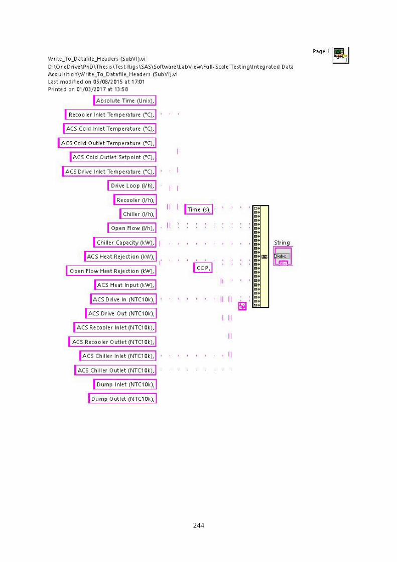
244

245

246

247
Appendix IV: Arduino Code
// FAN TEMPERATURE CONTROL SYSTEM
// BARRY FLANNERY
// BUILD 1.0
// 07/04/2015
//
// REVISION HISTORY
//
// Important References::
// Thermistor Guide: playground.arduino.cc/ComponentLib/Thermistor
// Thermistor Datasheet: http://www.farnell.com/datasheets/1756167.pdf
// MAX3232 TTL to RS232 level shifter datasheet:
http://pdfserv.maximintegrated.com/en/ds/MAX3222-MAX3241.pdf
// PROGRAM STRUCTURE
// The control system consists of 2 pairs of 10k immersion thermistors in two separate radiator
assemblies (a total of 4 thermistors) and an array of 24V DC fan blower units mounted on each
respective radiator.
// The motor controllers for these fans accepts a 0-5V analog signal corresponding to 0-100% duty
cycle output from the motor controller. When the control panel is switched to "auto", the Arduino
PWM output (used
// as analog 0-5V), is sent to each controller. A PID control system attempts to regulate the outlet
water temperature in each radiator to simulate different ambient temperature conditions. This is
achieved by
// monitoring the temperatures being read from the outlet thermistors and modulating the fan duty
cycle appropriately.
// VARIABLE INITIALIZATIONS AND HEADERS
//-------------------------------------------------------------------------------------------------------------------------
#include <PID_v1.h>
#define NTC_1 A0 //NTC (negative temperature coefficient) thermistor
1 is on Arduino Analog input 0 - Recooler Inlet Thermistor
#define NTC_2 A1 //NTC (negative temperature coefficient) thermistor
2 is on Arduino Analog input 1 - Recooler Outlet Thermistor
#define NTC_3 A2 //NTC (negative temperature coefficient) thermistor
3 is on Arduino Analog input 2 - Chiller Inlet Thermistor
#define NTC_4 A3 //NTC (negative temperature coefficient) thermistor
3 is on Arduino Analog input 3 - Chiller Outlet Thermistor
#define PWM_1 2 //Fan PWM duty cycle signal. This is a 0-5V signal
from the Arduino to the motor controller unit
#define PWM_2 3 //Fan PWM duty cycle signal. THis is a 0-5V signal
from the Arduino to the motor controller unit

248
long previousMillis = 0; //Used for the timing of the serial communication
printing
long currentMillis = 0;
int Recooler_In; //Variable assignment for NTC 1 (i.e. recooler inlet
temperature)
int Recooler_Out; //Variable assignment for NTC 2 (i.e. recooler outlet
temperature)
int Chiller_In; //Variable assignment for NTC 3 (i.e. chiller inlet
temperature)
int Chiller_Out; //Variable assignment for NTC 4 (i.e. chiller outlet
temperature)
double RecoolerSetpoint, RecoolerInput, RecoolerOutput; //Define PID variables
that we will be connecting
double ChillerSetpoint, ChillerInput, ChillerOutput; //Define PID variables that
we will be connecting
PID RecoolerPID(&RecoolerInput, &RecoolerOutput, &RecoolerSetpoint,2,5,1, REVERSE);
//Specify the links and initial tuning paramenters
PID ChillerPID(&ChillerInput, &ChillerOutput, &ChillerSetpoint,2,5,1, REVERSE); //Specify
the links and initial tuning paramenters
// ADJUSTABLE PARAMETERS
//-------------------------------------------------------------------------------------------------------------------------
long interval = 1000; //This variable controls how often the serial
communication will trigger (in milliseconds).
float Recooler_Setpoint = 12; //This is the setpoint variable for the PID system
(chiller side). Note this is technically redundant and only duplicated here for convenience and ease of
access.
float Chiller_Setpoint = 25; //This is the setpoint variable for the PID system
(recooler side). Note this is technically redundant and only duplicated here for convenience and ease
of access.
// VARIABLES/PARAMETERS
//-------------------------------------------------------------------------------------------------------------------------
// 10k THERMISTOR TEMPERATURE LOOK UP TABLE Refer to:
playground.arduino.cc/ComponentLib/Thermistor
//-------------------------------------------------------------------------------------------------------------------------
const static int temps[] PROGMEM = {
0, 1, 2, 3, 4, 6, 7, 8, 9, 10, 11, 12, 13, 14, 15, 16, 17, 18, 19, 20,
21, 22, 24, 25, 26, 27, 28, 29, 30, 31, 32, 33, 34, 35, 36, 37, 38, 39,
40, 41, 42, 43, 44, 45, 46, 47, 48, 49, 50, 51, 52, 53, 54, 55, 56, 57,
58, 59, 60, 61, 62, 63, 64, 65, 66, 67, 68, 68, 69, 70, 71, 72, 73, 74,
75, 76, 77, 78, 79, 80, 81, 82, 83, 84, 85, 86, 87, 88, 88, 89, 90, 91,
92, 93, 94, 95, 96, 97, 98, 99, 100, 101, 102, 102, 103, 104, 105, 106,
107, 108, 109, 110, 111, 112, 113, 114, 114, 115, 116, 117, 118, 119, 120,
121, 122, 123, 124, 124, 125, 126, 127, 128, 129, 130, 131, 132, 133, 134,
134, 135, 136, 137, 138, 139, 140, 141, 142, 143, 143, 144, 145, 146, 147,
148, 149, 150, 151, 151, 152, 153, 154, 155, 156, 157, 158, 159, 159, 160,
161, 162, 163, 164, 165, 166, 167, 167, 168, 169, 170, 171, 172, 173, 174,

249
175, 175, 176, 177, 178, 179, 180, 181, 182, 182, 183, 184, 185, 186, 187,
188, 189, 190, 190, 191, 192, 193, 194, 195, 196, 197, 197, 198, 199, 200,
201, 202, 203, 204, 205, 205, 206, 207, 208, 209, 210, 211, 212, 212, 213,
214, 215, 216, 217, 218, 219, 220, 220, 221, 222, 223, 224, 225, 226, 227,
228, 228, 229, 230, 231, 232, 233, 234, 235, 235, 236, 237, 238, 239, 240,
241, 242, 243, 243, 244, 245, 246, 247, 248, 249, 250, 251, 252, 252, 253,
254, 255, 256, 257, 258, 259, 260, 260, 261, 262, 263, 264, 265, 266, 267,
268, 269, 269, 270, 271, 272, 273, 274, 275, 276, 277, 278, 279, 279, 280,
281, 282, 283, 284, 285, 286, 287, 288, 289, 289, 290, 291, 292, 293, 294,
295, 296, 297, 298, 299, 300, 301, 301, 302, 303, 304, 305, 306, 307, 308,
309, 310, 311, 312, 313, 314, 315, 315, 316, 317, 318, 319, 320, 321, 322,
323, 324, 325, 326, 327, 328, 329, 330, 331, 332, 333, 334, 335, 335, 336,
337, 338, 339, 340, 341, 342, 343, 344, 345, 346, 347, 348, 349, 350, 351,
352, 353, 354, 355, 356, 357, 358, 359, 360, 361, 362, 363, 364, 365, 366,
367, 368, 369, 370, 371, 372, 373, 374, 375, 376, 377, 378, 379, 380, 381,
382, 383, 384, 385, 386, 387, 388, 389, 390, 392, 393, 394, 395, 396, 397,
398, 399, 400, 401, 402, 403, 404, 405, 406, 407, 408, 410, 411, 412, 413,
414, 415, 416, 417, 418, 419, 420, 422, 423, 424, 425, 426, 427, 428, 429,
430, 432, 433, 434, 435, 436, 437, 438, 439, 441, 442, 443, 444, 445, 446,
448, 449, 450, 451, 452, 453, 455, 456, 457, 458, 459, 460, 462, 463, 464,
465, 466, 468, 469, 470, 471, 472, 474, 475, 476, 477, 479, 480, 481, 482,
484, 485, 486, 487, 489, 490, 491, 492, 494, 495, 496, 498, 499, 500, 501,
503, 504, 505, 507, 508, 509, 511, 512, 513, 515, 516, 517, 519, 520, 521,
523, 524, 525, 527, 528, 530, 531, 532, 534, 535, 537, 538, 539, 541, 542,
544, 545, 547, 548, 550, 551, 552, 554, 555, 557, 558, 560, 561, 563, 564,
566, 567, 569, 570, 572, 574, 575, 577, 578, 580, 581, 583, 585, 586, 588,
589, 591, 593, 594, 596, 598, 599, 601, 603, 604, 606, 608, 609, 611, 613,
614, 616, 618, 620, 621, 623, 625, 627, 628, 630, 632, 634, 636, 638, 639,
641, 643, 645, 647, 649, 651, 653, 654, 656, 658, 660, 662, 664, 666, 668,
670, 672, 674, 676, 678, 680, 683, 685, 687, 689, 691, 693, 695, 697, 700,
702, 704, 706, 708, 711, 713, 715, 718, 720, 722, 725, 727, 729, 732, 734,
737, 739, 741, 744, 746, 749, 752, 754, 757, 759, 762, 764, 767, 770, 773,
775, 778, 781, 784, 786, 789, 792, 795, 798, 801, 804, 807, 810, 813, 816,
819, 822, 825, 829, 832, 835, 838, 842, 845, 848, 852, 855, 859, 862, 866,
869, 873, 877, 881, 884, 888, 892, 896, 900, 904, 908, 912, 916, 920, 925,
929, 933, 938, 942, 947, 952, 956, 961, 966, 971, 976, 981, 986, 991, 997,
1002, 1007, 1013, 1019, 1024, 1030, 1036, 1042, 1049, 1055, 1061, 1068, 1075,
1082, 1088, 1096, 1103, 1110, 1118, 1126, 1134, 1142, 1150, 1159, 1168, 1177,
1186, 1196, 1206, 1216, 1226, 1237, 1248, 1260, 1272, 1284, 1297, 1310, 1324,
1338, 1353, 1369, 1385, 1402, 1420, 1439, 1459, 1480, 1502 };
// VOID SETUP
//-------------------------------------------------------------------------------------------------------------------------
void setup()
{
Serial.begin(9600); //Initialize onboard USB serial
communication at 9600 baud.
Serial3.begin(9600); //Initialize serial 3 communication at
9600 baud. This serial output is passed through an RS-232 level shifter and and is being read by
LabView on a workstation
pinMode(A0, INPUT); //Define A0 as an input. A0 is
Recooler_In i.e. Recooler Inlet Thermistor
pinMode(A1, INPUT); //Define A1 as an input. A1 is
Recooler_Out i.e. Recooler Outlet Thermistor

250
pinMode(A2, INPUT); //Define A2 as an input. A2 is
Chiller_In i.e. Chiller Inlet Thermistor
pinMode(A3, INPUT); //Define A3 as an input. A3 is
Chiller_Out i.e. Chiller Outlet Thermistor
pinMode(2, OUTPUT); //Define 2 as an output. This is the 0-
5V PWM signal to control the fan duty cycle
pinMode(3, OUTPUT); //Define 3 as an output. This is the 0-
5V PWM signal to control the fan duty cycle
// PID
//-------------------------------------------------------------------------------------------------------------------------
RecoolerSetpoint = Recooler_Setpoint;
ChillerSetpoint = Chiller_Setpoint;
RecoolerPID.SetMode(AUTOMATIC);
ChillerPID.SetMode(AUTOMATIC);
delay(2000);
}
// MAIN LOOP
//-------------------------------------------------------------------------------------------------------------------------
void loop()
{
unsigned long currentMillis = millis();
if (Serial3.available()>0)
{
int x = Serial3.parseInt();
double RecoolerSetpoint = x;
}
// READ THERMISTORS AND CONVERT TO DECIMAL FLOATS FOR
DISPLAY/PROCESSING
//-------------------------------------------------------------------------------------------------------------------------
float Recooler_In_Temp = Recooler_In; //Assign float variable for
motor temperature 1
float Recooler_Out_Temp = Recooler_Out; //Assign float variable for
motor temperature 2
float Chiller_In_Temp = Chiller_In; //Assign float variable for
battery temperature
float Chiller_Out_Temp = Chiller_Out;
Recooler_In=analogRead(NTC_1)-238; //NTC 1 Thermistor Raw
reading
Recooler_In=pgm_read_word(&temps[Recooler_In]); //NTC 1 Thermistor
conversion to degrees celsius in format "192" = "19.2 C"
Recooler_Out=analogRead(NTC_2)-238; //NTC 2 Thermistor raw
reading
Recooler_Out=pgm_read_word(&temps[Recooler_Out]); //NTC 2
Thermistor conversion to degrees celsius in format "192" = "19.2 C"

251
Chiller_In=analogRead(NTC_3)-238; //NTC 3 Thermistor raw
reading
Chiller_In=pgm_read_word(&temps[Chiller_In]); //NTC 3 Thermistor
conversion to degrees celsius in format "192" = "19.2 C"
Chiller_Out=analogRead(NTC_4)-238; //NTC 4 Thermistor raw
reading
Chiller_Out=pgm_read_word(&temps[Chiller_Out]); //NTC 4 Thermistor
conversion to degrees celsius in format "192" = "19.2 C"
Recooler_In_Temp=Recooler_In_Temp/10; //Divide by 10 to go from
192 to 19.2 C
Recooler_Out_Temp=Recooler_Out_Temp/10; //Divide by 10 to go
from 192 to 19.2 C
Chiller_In_Temp=Chiller_In_Temp/10; //Divide by 10 to go from
192 to 19.2 C
Chiller_Out_Temp=Chiller_Out_Temp/10; //Divide by 10 to go from
192 to 19.2 C
// PID
//-------------------------------------------------------------------------------------------------------------------------
RecoolerInput = Recooler_Out_Temp;
ChillerInput = Chiller_Out_Temp;
RecoolerPID.Compute();
ChillerPID.Compute();
analogWrite(3,RecoolerOutput);
analogWrite(2,ChillerOutput);
//-------------------------------------------------------------------------------------------------------------------------
if(currentMillis - previousMillis > interval)
{
previousMillis = currentMillis;
Serial3.print(Recooler_In_Temp);
Serial3.print(" ");
Serial3.print(Recooler_Out_Temp);
Serial3.print(" ");
Serial3.print(Chiller_In_Temp);
Serial3.print(" ");
Serial3.print(Chiller_Out_Temp);
Serial3.print(" ");
Serial3.print(RecoolerInput);
Serial3.print(" ");
Serial3.print(RecoolerOutput);
Serial3.print(" ");
Serial3.print(RecoolerSetpoint);
Serial3.print(" ");
Serial3.print(ChillerInput);
Serial3.print(" ");
Serial3.print(ChillerOutput);
Serial3.print(" ");

252
Serial3.print(ChillerSetpoint);
Serial3.print(" ");
Serial3.println();
}
}
// High Powered Heater Control Algorithm
// by Barry Flannery
// 2015
// BUILD 0.0
// Arduino takes an input signal pulse from a H11AA1 AC zero-crossing detection IC, starts a timer
and then outputs a firing signal to a MOC3052 triac gate firing IC
//
// Key References: http://playground.arduino.cc/Main/ACPhaseControl
// http://letsmakerobots.com/node/28278
// VARIABLE INITIALIZATION
//-------------------------------------------------------------------------------------------------------------------------
int Zero_Cross_Detect1 = 2; //(INPUT) Zero-crossing event detection
output coming from H11AA1 IC. This output is being read on pin 2 of the Mega2560 (interrupt 0)
int Zero_Cross_Detect2 = 3; //(INPUT) Zero-crossing event detection
output coming from H11AA1 IC. This output is being read on pin 3 of the Mega2560 (interrupt 1)
int Zero_Cross_Detect3 = 21; //(INPUT) Zero-crossing event detection
output coming from H11AA1 IC. This output is being read on pin 21 of the Mega2560 (interrupt 2)
int GateFire1 = 9; //(OUTPUT) Triac #1 gate firing signal is on pin
9
int GateFire2 = 24; //(OUTPUT) Triac #2 gate firing signal is on pin
10
int GateFire3 = 5; //(OUTPUT) Triac #3 gate firing signal is on pin
11
int FiringPulseWidth = 8;
int i;
//-------------------------------------------------------------------------------------------------------------------------
// SETUP
//-------------------------------------------------------------------------------------------------------------------------
void setup()
{
Serial.begin(9600); //Start serial communication at 9600 baud
pinMode(Zero_Cross_Detect1,INPUT); //Zero_Cross_Detect1 (Pin 2) is an
input
pinMode(Zero_Cross_Detect2,INPUT); //Zero_Cross_Detect2 (Pin 3) is an
input
pinMode(Zero_Cross_Detect3,INPUT); //Zero_Cross_Detect3 (Pin 21) is an
input
digitalWrite(Zero_Cross_Detect1,HIGH); //Pull Pin 2 high using internall pull-
up
digitalWrite(Zero_Cross_Detect2,HIGH); //Pull Pin 3 high using internall pull-
up
digitalWrite(Zero_Cross_Detect3,HIGH); //Pull Pin 21 high using internall pull-
up
pinMode(GateFire1,OUTPUT); //GateFire1 (Pin 9) in an output

253
pinMode(GateFire2,OUTPUT); //GateFire2 (Pin 10) in an output
pinMode(GateFire3,OUTPUT); //GateFire3 (Pin 11) in an output
attachInterrupt(0,ZeroCrossingInterrupt1,RISING); //Attach zero-crossing event on pin
2 to interrupt 0
attachInterrupt(1,ZeroCrossingInterrupt2,RISING); //Attach zero-crossing event on pin
3 to interrupt 1
attachInterrupt(2,ZeroCrossingInterrupt3,RISING); //Attach zero-crossing event on pin
21 to interrupt 2
// TIMER 3,4,5 SETUP (REF:
http://playground.arduino.cc/Main/ACPhaseControl )
//-------------------------------------------------------------------------------------------------------------------------
OCR3A = 100; //Initialize the comparator
TIMSK3 = 0x03; //Enable comparator A and overflow interrupts
TCCR3A = 0x00; //Timer control registers set for
TCCR3B = 0x00; //Normal operation, timer disabled
OCR4A = 100; //Initialize the comparator
TIMSK4 = 0x03; //Enable comparator A and overflow interrupts
TCCR4A = 0x00; //Timer control registers set for
TCCR4B = 0x00; //Normal operation, timer disabled
OCR5A = 100; //Initialize the comparator
TIMSK5 = 0x03; //Enable comparator A and overflow interrupts
TCCR5A = 0x00; //Timer control registers set for
TCCR5B = 0x00; //Normal operation, timer disabled
}
//-------------------------------------------------------------------------------------------------------------------------
// INTERRUPT SERVICE ROUTINES
//-------------------------------------------------------------------------------------------------------------------------
void ZeroCrossingInterrupt1()
{
TCCR3B=0x04; //Start timer with divide by 256 input
TCNT3 = 0; //Reset timer - count from zero
}
void ZeroCrossingInterrupt2()
{
TCCR4B=0x04; //Start timer with divide by 256 input
TCNT4 = 0; //Reset timer - count from zero
}
void ZeroCrossingInterrupt3()
{
TCCR5B=0x04; //Start timer with divide by 256 input
TCNT5 = 0; //Reset timer - count from zero
}

254
//-------------------------------------------------------------------------------------------------------------------------
// TIMER 3,4,5 INTERRUPT SERVICE ROUTINES
//-------------------------------------------------------------------------------------------------------------------------
//TIMER 3 (Triac 1)
//----------------------------------------------------------------------
ISR(TIMER3_COMPA_vect) //Comparator match
{
digitalWrite(GateFire1,HIGH); //Set triac gate to high
TCNT3 = 65536-FiringPulseWidth; //Trigger pulse width
}
ISR(TIMER3_OVF_vect)
{ //Timer3 overflow
digitalWrite(GateFire1,LOW); //Turn off triac gate
TCCR3B = 0x00; //Disable timer stopd unintended triggers
}
//----------------------------------------------------------------------
//TIMER 4 (Triac 2)
//----------------------------------------------------------------------
ISR(TIMER4_COMPA_vect) //Comparator match
{
digitalWrite(GateFire2,HIGH); //Set triac gate to high
TCNT4 = 65536-FiringPulseWidth; //Trigger pulse width
}
ISR(TIMER4_OVF_vect)
{ //Timer4 overflow
digitalWrite(GateFire2,LOW); //Turn off triac gate
TCCR4B = 0x00; //Disable timer stopd unintended triggers
}
//----------------------------------------------------------------------
//TIMER 5 (Triac 3)
//----------------------------------------------------------------------
ISR(TIMER5_COMPA_vect) //Comparator match
{
digitalWrite(GateFire3,HIGH); //Set triac gate to high
TCNT5 = 65536-FiringPulseWidth; //Trigger pulse width
}
ISR(TIMER5_OVF_vect)
{ //Timer5 overflow
digitalWrite(GateFire3,LOW); //Turn off triac gate
TCCR5B = 0x00; //Disable timer stopd unintended triggers
}
//-------------------------------------------------------------------------------------------------------------------------
// MAIN LOOP
//-------------------------------------------------------------------------------------------------------------------------
void loop()
{

255
int val = 80;
val = map(val,0,100, 615, 0);
i--;
OCR3A = val; //set the compare register brightness desired.
if (i<10){i=615;}
OCR4A = val; //set the compare register brightness desired.
if (i<10){i=615;}
OCR5A = val; //set the compare register brightness desired.
if (i<10){i=615;}
delay(3);
}

256
Appendix V: Comprehensive Test Results Matrix
File
N
ote
sS
tab
ility (0
-5)
Data
Inte
rval
(min
s)
Inte
rval
Le
ng
th (m
ins)
Re
co
ole
r Inle
t
Te
mp
era
ture
(C
)
AC
S C
old
Inle
t
Te
mp
era
ture
(C
)
AC
S C
old
Ou
tlet
Te
mp
era
ture
(C
)
AC
S C
old
Ou
tlet S
etp
oin
t
(C
)
AC
S D
rive
Inle
t
Te
mp
era
ture
(C
)
Driv
e L
oo
p
(l/h)
Re
co
ole
r
(l/h)
Ch
iller
(l/h)
Op
en
Flo
w (l/h
)
Ch
iller
Cap
acity
(kW
)
D:\O
neD
rive\P
hD
\Fin
al D
ata
\Full-S
cale
Testin
g\R
aw
Data
\01-0
9-2
015.x
lsx4
10 - 2
010
39.7
119.0
316.8
19
87.8
21440
1476
1051
799
2.0
5
D:\O
neD
rive\P
hD
\Fin
al D
ata
\Full-S
cale
Testin
g\R
aw
Data
\01-0
9-2
015.x
lsx4
65 - 7
510
36.8
818.1
715.9
39
86.2
01426
1453
1045
770
2.1
4
D:\O
neD
rive\P
hD
\Fin
al D
ata
\Full-S
cale
Testin
g\R
aw
Data
\01-0
9-2
015.x
lsx3.5
110 - 1
25
15
44.7
419.7
118.1
39
92.9
91404
1468
1040
636
1.1
7
D:\O
neD
rive\P
hD
\Fin
al D
ata
\Full-S
cale
Testin
g\R
aw
Data
\01-0
9-2
015.x
lsx3.5
70 - 9
020
37.3
119.2
617.0
69
88.2
11416
1456
1045
797
2.0
3
D:\O
neD
rive\P
hD
\Fin
al D
ata
\Full-S
cale
Testin
g\R
aw
Data
\03-0
9-2
015.x
lsx4
45 - 5
813
24.0
816.6
813.7
99
85.1
91491
1509
1057
1317
2.9
8
D:\O
neD
rive\P
hD
\Fin
al D
ata
\Full-S
cale
Testin
g\R
aw
Data
\03-0
9-2
015.x
lsx3
100 - 1
10
10
55.5
732.9
831.9
29
93.5
11407
1512
1054
143
0.9
8
D:\O
neD
rive\P
hD
\Fin
al D
ata
\Full-S
cale
Testin
g\R
aw
Data
\03-0
9-2
015.x
lsx3.5
112 - 1
28
16
54.4
434.4
433.2
59
88.5
11452
1509
1050
141
0.9
4
D:\O
neD
rive\P
hD
\Fin
al D
ata
\Full-S
cale
Testin
g\R
aw
Data
\03-0
9-2
015.x
lsx3
165 - 1
72
748.5
832.3
830.6
99
92.3
41418
1490
1038
201
1.5
0
D:\O
neD
rive\P
hD
\Fin
al D
ata
\Full-S
cale
Testin
g\R
aw
Data
\03-0
9-2
015.x
lsx3
190 - 2
10
20
44.1
923.4
721.7
49
88.3
51448
1481
1028
203
1.4
4
D:\O
neD
rive\P
hD
\Fin
al D
ata
\Full-S
cale
Testin
g\R
aw
Data
\31-0
8-2
015.x
lsx4
40 - 5
010
30.1
417.6
715.5
09
81.6
91309
1282
1069
503
2.0
3
D:\O
neD
rive\P
hD
\Fin
al D
ata
\Full-S
cale
Testin
g\R
aw
Data
\31-0
8-2
015.x
lsx4
55 - 7
015
37.0
918.8
316.7
79
88.3
91236
1289
1070
308
1.9
0
D:\O
neD
rive\P
hD
\Fin
al D
ata
\Full-S
cale
Testin
g\R
aw
Data
\31-0
8-2
015.x
lsx4
115 - 1
25
10
39.7
420.0
218.4
29
86.5
51185
1272
1069
328
1.4
6
D:\O
neD
rive\P
hD
\Fin
al D
ata
\Full-S
cale
Testin
g\R
aw
Data
\31-0
8-2
015.x
lsx4
125 - 1
40
15
37.7
318.9
717.1
29
90.9
01196
1293
1068
377
1.5
7
..\Raw
Data
\06-0
8-2
015.x
lsx4
76 - 8
4
839.0
719.8
517.5
09
92.3
51097
1537
1067
350
2.0
7
..\Raw
Data
\06-0
8-2
015.x
lsx3
90 - 1
00
10
50.7
221.1
619.8
69
94.0
31058
1565
1067
155
1.0
4
..\Raw
Data
\06-0
8-2
015.x
lsx5
125 - 1
80
55
47.1
418.6
316.7
99
90.3
51060
1504
564
203
0.8
8
..\Raw
Data
\07-0
8-2
015.x
lsxS
tability
Poor d
rive in
520-4
020
26.4
418.3
415.5
79
85.4
71139
1502
1070
986
2.8
7
..\Raw
Data
\07-0
8-2
015.x
lsx2
50-6
010
56.4
323.0
322.3
59
95.5
51448
1472
789
160
0.3
7
..\Raw
Data
\07-0
8-2
015.x
lsx3
112-1
23
11
42.2
618.9
317.0
39
90.2
81560
1459
1067
334
2.0
4
Ch
iller Da
ta M
atrix
File
No
tes
Stability (0-5)
Data In
terval
(min
s)
Inte
rval Len
gth
(min
s)
He
ad
Tem
pe
rature
Set-
Po
int (°C
)
He
ad C
on
trol
Tem
pe
rature
(°C)
He
ad Lim
it
Tem
pe
rature
(°C)
Co
olan
t Inle
t
Tem
pe
rature
(°C)
Co
olan
t Ou
tlet
Tem
pe
rature
(°C)
Back En
d
Tem
pe
rature
(°C)
Am
bie
nt
Tem
pe
ratu
re (°C
)
Co
olan
t
Flow
Rate
(L/min
)
Po
we
r (W)
Vo
ltage (V
)
..\Raw
Data\FP
SE Data B
1922-PM
1-xxxx2-201509041011.xlsx5
14 - 2612
525529
55950.88
56.0330.49
20.3528.00
990236
..\Raw
Data\FP
SE Data B
1922-PM
1-xxxx2-201509041011.xlsx5
66 - 7812
503502
52980.30
81.0377.48
27.9525.69
942235
Stirling En
gine M
atrix

257
AC
S H
eat
Re
jectio
n
(kW
)
Op
en
Flo
w
He
at R
eje
ctio
n
(kW
)
CO
P
(Av
era
ge
Te
st)
CO
P
(Matrix
)
AC
S H
eat
Inp
ut (k
W)
AC
S D
rive
In
(NT
C1
0k
)
AC
S D
rive
Ou
t
(NT
C1
0k
)
AC
S
Re
co
ole
r
Inle
t
(NT
C1
0k
)
AC
S R
eco
ole
r
Ou
tlet
(NT
C1
0k
)
AC
S C
hille
r
Inle
t
(NT
C1
0k
)
AC
S C
hille
r
Ou
tlet (N
TC
10
k)
Du
mp
Inle
t
(NT
C1
0k
)
Du
mp
Ou
tlet
(NT
C1
0k
)
Calib
rate
d
Ch
iller
Inle
t
Calib
rate
d
Ch
iller O
utle
t
Calib
rate
d
Cap
acity
Ne
w C
OP
(Calib
rate
d
Cap
acity
+ O
ld H
eat In
pu
t)
Ne
w
CO
P
(Calc
ula
t
ed
Inp
ut)
He
at
Inp
ut
Erro
r
Bar
Ch
iller
Cap
acity
Me
asu
re
me
nt
Erro
r
Bar
CO
P
Pro
pag
atin
g
Erro
r
8.1
98.2
40.3
90.3
85.3
486.5
483.3
038.1
743.0
718.6
016.9
332.1
641.5
317.7
915.8
82.3
20.4
30.3
90.8
30.1
20.0
7
9.2
48.5
30.3
60.3
75.7
484.9
681.4
835.3
341.0
017.8
316.0
729.5
639.1
717.0
215.0
22.4
10.4
20.3
50.8
30.1
20.0
6
6.2
95.6
50.3
70.2
64.5
191.6
388.8
343.2
347.0
419.2
218.2
537.2
245.8
718.4
017.2
01.4
40.3
20.3
00.8
10.1
00.0
6
9.0
68.1
70.3
80.3
26.2
487.1
283.3
035.8
241.3
718.8
517.1
830.6
239.4
518.0
416.1
32.3
00.3
70.3
40.8
30.1
20.0
5
12.6
812.1
00.2
70.3
87.8
583.8
479.3
022.4
829.9
816.3
313.9
018.2
326.1
315.5
112.8
53.2
50.4
10.3
40.8
80.1
30.0
5
6.6
36.0
90.2
80.2
24.5
392.1
589.3
554.0
557.9
932.7
831.9
820.2
156.9
431.9
730.9
31.2
50.2
80.2
30.8
20.1
00.0
5
6.5
85.9
70.5
50.2
53.7
987.1
984.9
252.8
756.8
134.0
933.3
119.0
455.6
433.2
732.2
61.2
10.3
20.2
30.8
40.1
00.0
8
9.0
18.2
70.2
40.2
26.7
090.9
386.8
547.6
053.0
731.9
830.7
316.5
051.8
931.1
629.6
81.7
70.2
60.2
40.8
30.1
10.0
4
7.1
26.8
80.6
60.3
24.4
987.0
084.3
042.8
247.1
323.0
521.8
416.9
945.9
522.2
320.7
91.7
10.3
80.3
20.8
40.1
10.0
7
8.9
68.8
30.6
00.3
95.1
880.7
277.2
628.6
035.0
317.2
615.6
318.3
833.5
116.4
414.5
82.3
00.4
40.3
50.7
60.1
20.0
7
8.2
48.2
00.3
80.3
75.1
787.2
883.6
635.6
441.4
618.4
116.8
817.7
240.7
917.5
915.8
32.1
70.4
20.3
60.7
20.1
20.0
6
7.3
96.7
10.2
30.3
24.5
285.2
481.9
538.5
443.9
319.7
118.5
325.4
543.0
018.8
917.4
81.7
30.3
80.3
10.7
00.1
10.0
6
7.2
67.3
80.4
30.3
44.6
289.7
586.3
836.0
941.1
518.5
017.2
321.6
840.3
017.6
816.1
81.8
50.4
00.3
40.7
00.1
10.0
6
9.1
78.7
70.2
00.3
85.4
790.9
286.6
937.7
843.1
119.2
717.6
020.6
742.2
218.4
616.5
52.3
50.4
30.3
40.6
60.1
20.0
6
5.9
05.3
40.3
20.2
44.3
592.8
189.3
249.2
552.6
120.8
019.9
622.3
051.9
319.9
918.9
11.3
20.3
00.2
90.6
40.1
00.0
5
5.1
14.7
10.3
10.2
63.3
489.1
186.4
345.6
348.7
618.2
816.9
323.8
047.6
317.4
615.8
81.0
20.3
10.2
50.6
30.0
80.0
6
11.6
810.7
30.2
00.3
87.6
484.2
778.5
225.1
031.9
917.9
815.6
719.4
729.2
717.1
614.6
23.1
40.4
10.3
70.6
90.1
30.0
4
7.4
26.8
20.1
30.0
75.4
994.0
290.7
855.2
659.7
622.7
922.4
221.8
858.6
321.9
721.3
70.5
40.1
00.0
80.8
50.0
70.0
2
9.4
39.4
10.4
60.3
55.9
088.8
685.6
240.8
746.6
518.8
117.1
620.8
145.6
317.9
916.1
12.3
10.3
90.3
20.9
20.1
20.0
6
Cu
rren
t (A)
Freq
ue
ncy (H
z)P
hase
An
gle
(°)
Ene
rgy
Ge
ne
rated
(kWh
)
Fan Se
t-
Po
int (rp
m)
Fan Sp
ee
d
(rpm
)Fan
Drive
(%)
He
at Inp
ut
Rate
(s)H
eat In
pu
t (kW)
Electrical
Efficien
cy
4.2250.06
93.1111.61
26762694
30.67140.40
6.7714.6%
4.0750.04
6.2912.51
24942506
28.01136.41
6.9713.5%

258
Appendix VI: Whispergen Test Rig
A Whispergen PPS16 marine diesel Stirling engine was obtained during the course of the
author’s B.Sc undergraduate final year project. This was built into an initial test rig that achieved initial
operational capability just before the end of the designated project period [274]. Though the system
worked, and initial performance measurements were obtained, the test rig was hastily built, as illustrated
by Figure 162, due to the three-month time constraint of a final year Applied Physics project. The
Whispergen Stirling engine was the only piece of Stirling engine hardware available for testing for the
first year of the PhD research and it played a pivotal role in initial feasibility testing that formed the
basis of the proposal that ultimately lead to significant further investment from the project’s enterprise
partner for the acquisition and development of the SAS hardware. Note that this section’s technical
description related to the Whispergen test rig is not exhaustive and additional details may be found in
the theses of Niall Chambers and also the author’s [274, 297].
Figure 162 Photograph of preliminary Whispergen test rig as part of the author’s undergraduate final year project. Note untidy
plumbing and immobility of the test rig.
259
1.2.1 Whispergen Test Rig Objectives
The Whispergen test rig was used as an important learning test bed for developing metal
fabrication techniques and honing experimental testing skills related to data acquisition programming
and hardware installation. These skills are all practical-based and are rarely discussed in the scientific
literature as it is assumed to be implicit knowledge. Consequently, the only feasible way of obtaining
them was to use actually develop the Whispergen engine into a working test rig even though a kinematic
Stirling engine like the Whispergen is not intended to be used in the final SAS architecture.
In order to assist development of the Whispergen unit into a viable test rig, some of the work
was incorporated into an undergraduate engineering final year project conducted by Niall Chambers.
The author handled most of the tasks related to fabrication and major plumbing and offered instruction
to the undergraduate student for day-to-day operation and testing and provided close supervision [297].
The main objectives for the author with respect to the Whispergen test rig are summarized below:
1. Gain practical fabrication and plumbing experience for later use on SAS rig development
2. Measure system electrical and thermal efficiency of the Stirling engine and validate
experimental methodology for doing so.
3. Characterise system start-up time and shut down time
4. Measure variation in thermal heat output versus coolant loop temperature
5. Build a more robust test rig that can be safely utilized for further undergraduate teaching
activities
1.2.2 Whispergen Test Rig Construction and Installation
The key design criteria for the Whispergen test rig was that it needed to be mobile and self-
contained. The requirement for mobility stemmed from the potential event that the system might be
used in conjunction with adsorption hardware in the future and tested in a calorimeter at Thermo King
test facilities in Galway city. The initial test rig, shown previously in Figure 162, was immobile, untidy
and did not comply with health and safety best practices at NUI Galway.
A revised design, shown via CAD render in Figure 163, addressed many of the technical issues
with the initial temporary rig such as immobility and untidiness. The fuel and coolant header tanks are
securely positioned above the engine and move in conjunction with the frame. Similarly, the batteries,
inverter and electrical heater (not shown) are positioned in the lower shelf of the engine test stand. There
is additional space on the lower shelf for data acquisition hardware, engine specific consumables and
health and safety documentation. The engine itself is positioned on the middle shelf and can be easily
accessed from all sides. Crucially, there is sufficient space at the rear of the engine for making plumbing

260
connections and safely routing the exhaust duct. The entire system is mobile on castor wheels and the
only external connections required are the exhaust duct and external coolant loop. The flexible exhaust
duct can simply be removed from the lab extraction system and coiled up. Likewise, the external water
connection can simply be disconnected from the laboratory tap via quick release connector. The whole
system can then be easily moved around the lab or even to new locations as required.
Figure 163 CAD render of the revised Whispergen test rig.
The construction of the test rig presented significant challenges as the author had no previous
fabrication experience. Though limited fabrication services are offered by university technicians, the
scale of the work that would be required for the SAS development meant that the majority of future
work would need to be done by the author.
For brevity, a sequence of photographs showing just some of the key enabling hardware that
was developed to support the PhD research is shown below in Figure 165, Figure 166 and Figure 167.
This hardware was not only critical for enabling the construction of test rigs but it was often the initial
test bed for practicing fabrication techniques and also gaining electrical and electronics experience.
Figure 164 Flowchart outlining the back-end infrastructure that was required to fabricate the test rigs.
Figure 167 (top)
Figure 167 (left/right)
Figure 167
Figure 165
Figure 168

261
Figure 165 (top) delivery of welding table top plate, (left) conversion of manual mill to CNC mill, (right) control electronics
for CNC mill.

262
Figure 166 (top) three-phase electric power installation, (left) Stick/TIG welding and plasma cutting system (right)
construction of custom trolley cart for system

263
Figure 167 (top-left) drill press and bandsaw, (top-right) lathe and (bottom) general overview of workshop where all test
rigs were built.
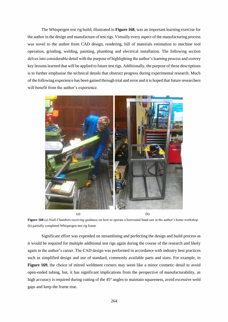
264
The Whispergen test rig build, illustrated in Figure 168, was an important learning exercise for
the author in the design and manufacture of test rigs. Virtually every aspect of the manufacturing process
was novel to the author from CAD design, rendering, bill of materials estimation to machine tool
operation, grinding, welding, painting, plumbing and electrical installation. The following section
delves into considerable detail with the purpose of highlighting the author’s learning process and convey
key lessons learned that will be applied to future test rigs. Additionally, the purpose of these descriptions
is to further emphasise the technical details that obstruct progress during experimental research. Much
of the following experience has been gained through trial and error and it is hoped that future researchers
will benefit from the author’s experience.
(a) (b)
Figure 168 (a) Niall Chambers receiving guidance on how to operate a horizontal band saw at the author’s home workshop
(b) partially completed Whispergen test rig frame
Significant effort was expended on streamlining and perfecting the design and build process as
it would be required for multiple additional test rigs again during the course of the research and likely
again in the author’s career. The CAD design was performed in accordance with industry best practices
such as simplified design and use of standard, commonly available parts and sizes. For example, in
Figure 169, the choice of mitred weldment corners may seem like a minor cosmetic detail to avoid
open-ended tubing, but, it has significant implications from the perspective of manufacturability, as
high accuracy is required during cutting of the 45° angles to maintain squareness, avoid excessive weld
gaps and keep the frame true.

265
Figure 169 Design drawing of the Whispergen test rig frame.

266
Another important aspect of the design process which is largely invisible in the end product is
the sequence of construction, particularly in relation to welding. Oftentimes, as much design effort goes
into designing for manufacturability as the core design itself. For example, during the development of
the CAD model, careful attention must be given to avoid creating unnecessarily difficult geometries
that will be ergonomically challenging to manufacture. In hindsight, the central support members in the
Whispergen frame were likely unnecessary from a structural strength perspective, and they were a
nuisance to manufacture as it required overhead welding while being crouch within the cage-like
confines of the frame.
The choice of using a plywood shelf on the test rig (visible in) was initially conceived for
convenience as the author had not yet mastered stitch-welding of sheet metal to square tube sections.
Yet-again, in hindsight, this turned out to be a poor choice. The choice of wood required numerous “L-
angle” brackets to be welded to the frame as support, often at inconvenient and difficult angles.
Similarly, the wood surface itself was a poor choice based on experience gained during experimental
testing as accidental coolant leaks or spillages would soak into the surface of the wood. Though this did
not impact structural strength, it did cause cosmetically unappealing staining and the irregular surface
of the plywood grain hampered efforts to clean up spillages by causing absorbent tissue to mechanically
disintegrate.
Perhaps the most time-consuming and maintenance heavy aspect of the Whispergen test rig
project was in relation to plumbing. Figure 170, shows a variety of different techniques provides a
visual timeline of advancements in the author’s plumbing experience and skill. For example, the
simplest plumbing connections are Qualpex push-fit connections whereby a clean section of appropriate
tubing can be cut and push into a special brass fitting. A Qualpex push-fit fitting is shown in the centre
of the photo immediately to the left of the lower red gate valve. The simplicity of Qualpex and push-fit
connections comes at the expense of reliability and ruggedness as any lateral stress on the fitting will
result in a leak. The flexibility of Qualpex can also be a disadvantage for the aforementioned reasons
as bends in the Qualpex piping can result in hidden stress in the overall system causing some push-fit
connections to leak. Lastly, though it is easy to work with, Qualpex is a nuisance to interface with
compression fittings as copper inserts are required for the compression seal and they do not always
work.
In contrast, the copper pipe and brass compression fittings are an extremely rugged method of
creating pipe joints. Although they require additional labour resulting from the requirement of PTFE
tape and inclusion of a compression olive they do not leak and can withstand tremendous mechanical
abuse. The author’s migration to compression fittings is evident in later additions to the plumbing (red
gate valves) and all future test rigs were designed and implemented using compression fittings. An
alternative solution for flexible piping is a direct connection of flexible coolant hose (green) over copper
pipe or even Qualpex and securing through use of a jubilee clip. This style of connection, despite its

267
appearance, is actually the most reliable, versatile and maintenance free solution for joining pipes and
was used extensively on the SAS test rig.
The final important lesson learned during the plumbing phase which was completely omitted
from the initial implementation was the inclusion of dedicated drain and vent points on the test rig for
airlock purging during coolant loop maintenance. The difficult of purging airlocks in the Whispergen
test rig was extremely important lesson learned for the design of the SAS test rig which would feature
four independent plumbing loops and substantially more complex plumbing infrastructure.
Figure 170 Overview of the plumbing connections on the Whispergen test rig.
The completed Whispergen test rig is shown below in Figure 171. The major system
components are as follows; diesel header tank (1), coolant header tank (2), Whispergen PPS16 engine
(3), electric heater load (4), 24 VDC to 220 VAC inverter (5), lead-acid batteries (6), engine controller
(7) and plumbing connections (8).

268
Figure 171 Overview of the completed Whispergen PPS16 test rig. The major system components are as follows; diesel header
tank (1), coolant header tank (2), Whispergen PPS16 engine (3), electric heater load (4), 24 VDC to 220 VAC inverter (5),
lead-acid batteries (6), engine controller (7) and plumbing connections (8).

269
1.2.3 Whispergen Data Acquisition
Difficulty related to data acquisition is often a major challenge for new test rigs and unfamiliar
students. The LabView program developed during the author’s undergraduate project, shown in Figure
173, formed the basis of the current data acquisition program developed by Niall Chambers. A number
of bugs and optimizations were eliminated from the original program related to data saving and
formatting of the output text file.
The Whispergen test rig has relatively simple sensor requirements and requires thermocouple
measurements and a pulse counter measurement facility for flowmeters. These measurements were
conducted using new hardware; an Agilent 34972A for thermocouple measurements and a National
Instruments USB-6009 for pulse counter measurements. Both of these data acquisition units would be
used during testing of the SAS so demonstrating their operation and developing a LabView interface
was critical to the project.
Various different techniques were tested and optimised in relation to measuring the temperature
of liquid circulating within the coolant loop. Many different attempts were made to measure in-flow
temperature, such as by physically inserting thermocouples down flexible pipes and sealing the joints
with silicone. These had varying degrees of success but, more often than not, resulted in leaks.
Alternative methods such as using a dedicated compression tee-fitting with thermocouple inserted
through a blanking cap which was then sealed with silicone were also tested as shown in Figure 172a.
These too, resulted in leaks at high temperatures but a final evolved solution using epoxy resin, shown
in Figure 172b to seal the thermocouple solved the leaking issue. However, periodic inspection of the
bare thermocouple wires during maintenance revealed corrosion on the thermocouples and build-ups of
scum and organic matter on the thermocouples. Similarly, the turbine type flowmeter used in the test
rig occasionally became blocked or clogged with debris circulating within the coolant loop such as
flecks of rubber from hoses, fragments of PTFE tape or corrosion from the engine internal plumbing.
These experiences were important lessons learned for the sensor hardware used in the SAS test rig.
Using external clamp-on thermistor on the copper pipes resulted in adequate thermal response times
while vastly simplifying the installation of sensors and simultaneously eliminating the corrosion and
scum issues. In relation to flowmeters, the SAS used Huba Control Type 210 piezoelectric Karman
vortex tail type sensors with no moving parts, and so could not easily clog. These sensors also had
integrated thermistors built into them although they were not necessary as external sensors were used.
The Whispergen was later retrofitted with these sensors also.

270
Figure 172 (a) silicone thermocouple seal and (b) epoxy resin thermocouple seal.
Figure 173 shows the block diagram for the LabView data acquisition program. This program read in
sensor data from the flowmeters and thermocouples in conjunction with Whispergen microcontroller
data and then performed system-level calculations related to efficiency, thermal and electrical output.

271
Figure 173 Block diagram of the Whispergen test rig LabView data acquisition program.

272
1.2.4 Whispergen Testing and Results
For a comprehensive discussion of the experimental testing of the Whispergen engine, the
reader is directed to work done by Niall Chambers as the experimental tests were conducted by him
[297]. The test results are summarized here, as the author was the primary technical supervisor of the
work. Experimental testing of the Whispergen PPS16 Stirling engine is described as follows. The
engine’s onboard microcontroller has dedicated interface software MicroMon, from which, the fuel
consumption and electrical power output can be obtained. However, in order to calculate the system
thermal efficiency it is necessary to also quantify the thermal heat output that requires measuring the
temperature difference across the marine plate heat exchanger and the mass flow rate of coolant through
it using external sensors and data acquisition equipment.
In theory, the heat lost by the primary coolant circuit, Qpri, should be equal to the heat gained
by the secondary coolant circuit Qsec, both of which are equivalent to the engines thermal output as
shown in Figure 174 and Eq. (56
Figure 174 Thermodynamic diagram of the Whispergen Stirling engine. © Niall Chambers[297]
𝑄𝑝𝑟𝑖 = 𝑄𝑠𝑒𝑐 (56)
Where Qpri can be calculated from the mass flow rate of coolant ṁpri, the heat exchanger inlet temperature
Tpri,in, outlet temperature Tpri,out and the specific heat capacity of the coolant cp,pri using Eq. (57)
𝑄𝑝𝑟𝑖 = ṁ𝑝𝑟𝑖𝑐𝑝,𝑝𝑟𝑖(𝑇𝑝𝑟𝑖,𝑖𝑛 − 𝑇𝑝𝑟𝑖,𝑜𝑢𝑡) (57)

273
The thermal efficiency of the engine is calculated from the fuel input, Qin and the heat output Qpri using
Eq. (58)
𝜂𝑡ℎ =𝑄𝑝𝑟𝑖
𝑄𝑖𝑛
(58)
Likewise the electrical efficiency is calculated from the useful electrical work Wnet using Eq. (59)
𝜂𝑒𝑙𝑒𝑐 =𝑊𝑛𝑒𝑡
𝑄𝑖𝑛
(59)
The experimental testing was conducted by Niall Chambers, shown in Figure 175 and his key
experimental findings are shown in Table 25 for completeness. The results achieved an very similar to
the manufacturer’s claims and Niall Chambers was successful in eliminating the original discrepancy
in the author’s B.Sc. project.
Figure 175 Niall Chambers conducting experimental tests with the Whispergen engine.
Table 25 Summary of experimental test results.
Test Electric
Power Wnet
(W)
Thermal
Power QR
(W)
Combined
Power Wnet
+ QR (W)
Electrical
Efficiency
ηelec (%)
Thermal
Efficiency
ηth (%)
Combined
Efficiency
ηth + ηelec
(%)
1 1125 6425 7551 12.58 71.85 84.43
2 1125 6630 7755 12.18 71.83 84.02
3 1106 6379 7485 12.50 72.07 84.57
Avg (1119) (6478) (7597) (12.42) (71.92) (84.34)

274
Chambers also investigated the engine start-up and shut-down times (shown in Figure 176) and the
variation in waste thermal output with increasing coolant temperature (Figure 177). Both of these
results are discussed in detail in the following section (5.2.5).
Figure 176 System start-up and shut down characteristics.
Figure 177 Variation in thermal heat output versus coolant loop temperature.

275
1.2.5 Whispergen Discussion and Conclusion
The Whispergen test rig, although not directly related to the development of the SAS, played a
pivotal role in experimental learning and was the forerunner to all future test rigs developed over the
course of this research. Numerous technical skills and insights which could not have been obtained from
the scientific literature originated directly from the development of this test rig. Furthermore, useful
information specifically pertaining to kinematic Stirling engines was also obtained such as start-up time
(Figure 176) and overall system efficiency. The latter data was provided a useful benchmark for
preliminary modelling and efficiency estimates. Another important subtle characteristic of waste heat
capture is the variation in the quantity of waste heat available at different temperatures shown previously
in Figure 177. In general, the higher the temperature of the waste heat resource, the less of it there is
available. This is important in the context of adsorption chillers requiring 90-100 °C driving temperature
as, for example with the Whispergen, there is only 4.75 kWt of heat available at 93 °C versus 6.3 kWt
at 52 °C. It is easiest to understand this behaviour when viewed as an inverse problem i.e. that you must
apply greater cooling effect on the engine to reduce its temperature. For example, in the Whispergen
experimental setup, in order to cool the engine from 90 °C to 50 °C it is necessary to increase the mass
flow rate of external cooling water through the marine heat exchanger open loop. This causes an
increase in the ΔT and the mass flow rate and, consequently, the overall heat removal. The physics of
this are perfectly understandable when interpreted in this manner but can be somewhat strange when
viewed in terms of increasing temperature.
The Whispergen test rig is now established as a self-contained operational Stirling engine test
bed that is available for future generations of students at NUI Galway and will provide them with a
unique Stirling engine learning opportunity.
Although, a kinematic Stirling engine is not intended to form part of the SAS architecture, the
physical presence and demonstration of a diesel-fuelled off-grid Stirling engine was a compelling
motivator for our enterprise sponsors during lab audits and was instrumental in their decision to commit
the required resources to develop the SAS architecture.

276
Appendix VII
2.1 DEVC Test Rig
A TriPac Evolution APU, the most popular APU on the market today, was obtained from the
project’s enterprise sponsors during the course of the research, and was subsequently developed into a
dedicated test rig. It was not the objective of this research to to perform detailed performance testing of
the TriPac Evolution, as extensive datasets obtained from calorimeter testing were available from our
enterprise sponsor. What therefore was the purpose of the TriPac Evolution test (DEVC) rig? The
DEVC test rig was used as a learning test bed to understand the installation process of a conventional
APU and understand all of the external components that are not immediately obvious from product
brochures such as the diesel particulate filter (DPF), inverter, cab heat exchanger, diesel fuel fired
heater, controller human-machine interfaces, APU electronics control boxes, DPF electronics control
boxes. From the outset, it was clear that the SAS would likely face difficult geometric constraints, and
so, having a detailed understanding of the existing true DEVC footprint is vital for a fair system
comparison, as brochure specifications typically only list the core APU dimensions. Chapter 7 addresses
some of the geometrical questions related to the SAS concept and having a physical DEVC APU on
hand was vital for creating CAD comparisons of the two systems.
Perhaps the most important role the DEVC played in this research was as a demonstrator for
visiting suppliers to gain a more clear understanding of what an APU is and how a conventional DEVC
system operates. The presence of DEVC system played a crucial role in the decision of InvenSor GmbH
and Microgen Engine Corporation to cooperate and provide engineering support to the project. This
project would have not possible without the technical support from the FPSE and adsorption chiller
suppliers. Likewise, during lab audits by senior engineers and managers from our enterprise sponsor,
the ability to run the DEVC system and then run the SAS was a compelling demonstration to encourage
their continued support. The dramatic reduction in noise from the SAS versus the DEVC system is
particularly impressive when witness in person as it is difficult to convey through figures such as dBa
measurements. The ability to show two fundamentally different systems operating side by side and both
delivering cooling greatly added to the demonstration of feasibility to the commercial interests of this
research.
5.3.1 DEVC Test Rig Objectives
The detailed objectives of the DEVC test rig are as follows:
Evaluate the installation process and physically set-up the APU
Identify useful techniques and best practices that can be applied to SAS test rig in relation to
wiring, harness design and system layout.

277
2.3.2 DEVC Test Rig Construction and Installation
The TriPac Evolution APU received from our enterprise sponsor was a development unit
from their test facility and arrived as a bare engine Figure 178. In order to operate the engine it was
necessary to build the engine into a DEVC test rig and mount the engine correctly in a hanging
configuration similar to how it is done on a tractor frame rail.
Figure 178 Bare APU engine as received requiring a test stand
The design of the DEVC test stand was done based on advice from engineers at our enterprise
sponsor’s R&D facility. As with the Whispergen test rig, the DEVC test rig had similar key
requirements such as mobility and being completed self-contained in the event of it needing to be moved
to a calorimeter test facility. Unlike the Whispergen test rig, which required an external water
connection the DEVC test rig could be implemented as a truly self-contained system as it rejected its
heat via radiators and a condenser with only an extended exhaust duct required to reach the lab
extraction system.
A CAD render showing the general design of the test stand can be seen in Figure 179 and
detailed plans are given in Figure 180. This test rig had significantly greater structural requirements
than the Whispergen test rig as the APU is hanging as a cantilever load on a main structural C-section
beam on the rear of the test stand. The test stand is open on one side to aid accessibility to the engine.
The right hand side of the test rig features an enclosed area for the batteries and diesel storage tank. The
choice of “L-angle” for the frame was deliberate as it would act as a minor bund in the case of any leaks
and also prevent the batteries from being knocked out of the frame. Based on experience gained with
the Whispergen test rig, wooden shelves were avoided and a sheet metal base was used instead and
stitch-welded to the angle sections. The use of sheet metal would vastly improve the ability to clean up
any spillages and also prevent staining.

278
The DEVC test stand features a second upper level above the battery enclosure zone to seat the
cab chiller heat exchanger box and also the diesel-fired heater unit. Lastly, a large upper panel is present
for mounting of all controls, refrigeration system components, the condenser and the main electronics.
The rear side of this upper sections is also intended to be used for additional mounting of components
like the DPF controller box, inverter and various air conditioning ducting. An important design decision
was making this upper section bolt-able and removable for transportation. The test stand had a strict
height requirement in order to fit into a van for transport.
Another minor design evolution from the Whispergen test rig was the mounting of the castor
wheels to the frame. The Whispergen frame featured dedicated mounting plates where the castor wheels
could be bolted to the frame. Though this was effective and worked well, it was difficult to manufacture
as 16 holes needed to be drilled through thick steel plate using a hand drill. For the DEVC frame, the
use of plates were avoid entirely and the castor wheel plates were simply welded directly to the frame.
The manufacturing of the test rig is shown in Figure 181.
Figure 179 CAD render of the proposed DEVC test stand.

279
Figure 180 Design drawing of the DEVC test rig.
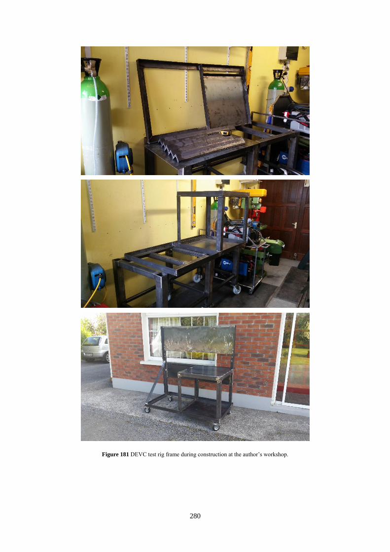
280
Figure 181 DEVC test rig frame during construction at the author’s workshop.

281
The fabrication of the test rig frame was relatively straightforward and experience gained
during the manufacturing of the Whispergen test rig significantly improved the quality of the final frame
and also reduced the time taken to construct it. However, the installation of the APU and all of its
auxiliary components and harnesses proved to be a laborious process due to its complexity as illustrated
by Figure 182. The author gained considerable experience installing the DEVC system in terms of
wiring and harness best practices which would be valuable for the SAS in creating a professional
looking test rig. Examples of best practice include the use of automotive style connectors to improve
reliability and ease of maintenance, the use of cable entry glands and enclosures.
Figure 182 Complex APU accessories and harnesses undergoing installation.

282
These lessons learned from observing a commercial system were directly applied to the DEVC
test rig and future rigs to improve safety and reliability. For example, in contrast with the Whispergen
test rig which had battery components like connection blocks and shunts exposed (albeit insulated), the
electrical systems on the DEVC test rig were contained in dedicated boxes and the cables strain relieved
using entry glands and the battery terminals insulated using silicone boots as shown in Figure 183. In
addition to being more cosmetically appealing this solution greatly improved the safety of the system
and reduced battery related risks in compliance with the University’s health and safety guidelines.
Figure 183 Improved battery wiring setup using dedicated enclosures and cable entry glands.
The finished DEVC test rig front panel is shown below in Figure 184. The refrigeration system
heat rejection is handled by (1) the condenser and the cool air is blown out the two side by side vents
in the centre (4). The third vent (5) is the heat blower vent for the independent fuel fired heater. The
HMI controller (6) is shown in the centre along with the DPF monitor and toggle switch (8). The main
engine controller (2) is housed in the enclosure on the right hand side and numerous harness are visible
terminating into it.

283
Figure 184 DEVC test rig front panel. The components are as follows; (1) condenser assembly, (2) control electronics, (3) cab
chiller intake, (4) cab chiller blowers, (5) cab heater blower duct, (6) HMI, (7) refrigerant dryer and (8) DPF indicator and
regeneration control switch.
The entire completed test rig is shown below in Figure 185 with the Whispergen test rig partially
visible in the left-hand side of the photograph.
Figure 185 Complete DEVC test rig. The key components are as follows: (1) diesel engine, (2) condenser assembly, (3) cab
evaporator assembly, (4) diesel fuel tank, (5) lead-acid batteries, (6) HMI, (7) control electronics and (8) diesel fuelled heater.

284
2.3.3 DEVC Data Acquisition
The TriPac Evolution has an on board microcontroller that monitors a number of variables such
as engine temperature, engine RPM, alarm status, various refrigeration switch statuses, battery voltages
and alternator currents. Data from this controller can be downloaded using a computer (Figure 186) but
it is of limited use to in terms of overall system testing as the engine fuel input is not available and, in
general, measuring diesel engine fuel consumption in real time is tremendously difficult to do without
very expensive sensors. Diesel engines have a high fuel bypass meaning that it is insufficient to simply
measure the fuel flowing into the engine as the fuel returning from the engine must also be measured
and the difference calculated. The fuel used to fuel returned or bypass ratio can be as high as 30:1
making measurement accuracy even more difficult. The key challenge with diesel engine fuel
measurement is the nature of the fuel flow. It is not steady state but instead it is pulsating back and
forward requiring the use of specialist sensors that can accommodate this such as Coriolis flow sensors
which are very expensive. The author has first-hand experience of the difficulty of measuring diesel
fuel consumption as he worked as test engineer at the Thermo King Development Centre for their large
transport refrigeration units. An alternative to measuring the fuel flow rate would be to periodically
weigh the fuel tank and measure the difference. This method would work but it would not provide the
real-time fuel consumption needed for useful comparison and vibration of the fuel tank and fuel lines
would hamper measurements due to the required sensitivity of the weighing scales.
The engine’s work output is similarly difficult to measure as specialist torque-speed sensors
would be required on the engine. The work output is not steady state either as the compressor clutches
in and out in accordance with refrigeration load. The cooling capacity of the system would also require
a calorimeter to accurately measure or, alternatively, water cooled heat exchangers would be needed.
This latter method was not implemented as the author felt that the value of having a fully functional
finished APU product for demonstration purposes outweighed the value of getting data that was already
available from the manufacturer.

285
Figure 186 Overview of the TriPac Evolution PC-based controller interface.
2.3.4 Discussion and Conclusion
Although no specific test data was generated from the DEVC test rig it played an important role
in the course of the research project. The primary objective of understanding the complete APU system
was completed as the author gained experience and understanding of how the DEVC APU operates.
This was the author’s first experience with the operation and maintenance of diesel engines and
refrigeration systems. It was particularly valuable from an engineering perspective to actually perform
an engine oil change, fuel filter installation and fine tuning of the engine’s RPM governor control. Oil
changes are regular maintenance activities performed by technicians in the field and this is eliminated
by the SAS architecture. Similarly, it was a valuable learning exercise for the author to install and
commission the air conditioning system and understand the maintenance required to do so. The use of
vacuum pumps and manifold gauges for the charging and discharging of the refrigeration system was
particularly insightful as periodic vacuum maintenance could potentially be required for the adsorption
chiller and was in fact necessary during commissioning of the SAS test rig.
The most significant realization from development of the DEVC test rig was the amount of
work that would be required to bring the SAS test rig from a prototype to a commercially viable product.
Considerable engineering effort would be required in the design of controllers, enclosures, packaging,
harnesses and weatherproofing to make a concept robust enough to survive the harsh realities of the
transport application. This is crucially important when making comparisons between the performance

286
of the SAS prototype and the TriPac Evolution APU. Although they are compared on an equal basis,
the TriPac Evolution has undoubtedly incurred efficiency and performance penalties in order to assure
overall system reliability and robustness as a commercial product.
Finally, as mentioned at the beginning of this sub-chapter, the DEVC test rig was instrumental
in educating suppliers on the APU application and showing their development engineers what a full
APU system looks like and how it operates. Likewise, the noise comparison demonstrations were
particularly effective at conveying the architectural advantages of the SAS versus conventional DEVC
technology to senior management within our enterprise sponsor.

287
Figure 187 Design drawing for the ACS frame (sheet metal not included).

288
Appendix VIII
Figure 188 Design drawing for the FPSE frame (sheet metal not included).

289
References and Bibliography
1. Pachauri, R. and A. Reisinger, IPCC fourth assessment report. IPCC, Geneva, 2007: p. 2007.
2. Barnett, J., Security and climate change. Global environmental change, 2003. 13(1): p. 7-17.
3. Nordås, R. and N.P. Gleditsch, Climate change and conflict. Political Geography, 2007.
26(6): p. 627-638.
4. World Energy Council, Global Transport Scenarios 2050. 2011.
5. FHWA Docket No 49, C.P., Hours of Service of Drivers.
6. EPRI, Truck Stop Electrification: A Cost-Effective Solution to Reducing Truck Idling (EPRI
Report Number 1008777). EPRI Report, 2004.
7. American Transportation Research Institute. Compendium of Idling Regulations 2013
01/03/2016]; Available from: www.atri-
online.org/research/idling/ATRI_Idling_Compendium.pdf.
8. California Air Resources Board. Final regulation order to reduce emissions of diesel
particulate matter, oxides of nitrogen, and other pollutants from in-use heavy-duty diesel-
fuelled vehicles. 2008; Available from:
http://www.arb.ca.gov/msprog/onrdiesel/documents/tbfinalreg.pdf.
9. United Nations. North American 2014 HFC Submission to the Montreal Protocol. 2014
01/03/2016]; Available from: http://www.state.gov/documents/organization/226046.pdf.
10. Levinson, R., et al., Potential benefits of solar reflective car shells: Cooler cabins, fuel
savings and emission reductions. Applied Energy, 2011. 88(12): p. 4343-4357.
11. Rugh, J.P., et al., Reduction in vehicle temperatures and fuel use from cabin ventilation,
solar-reflective paint, and a new solar-reflective glazing. 2007, SAE Technical Paper.
12. Proc, K., L. Chaney, and E. Sailor, Thermal Load Reduction of Truck Tractor Sleeper Cabins.
SAE Int. J. Commer. Veh., 2008. 1(1): p. 268-274.
13. Air-Conditioning Heating and Refrigeration Institute (AHRI), 2004 Standard for Standard for
Packaged Terminal Air-Conditioners And Heat Pumps. 2004, Canadian Standards
Association
14. Stodolsky, F., Gaines, L., Vyas, A. [Argonne National Lab], Analysis of Technology Options
to Reduce the Fuel Consumption of Idling Trucks. 2000.
15. Franzese, O., Effect of weight and roadway grade on the fuel economy of class-8 freight
trucks. Oak Ridge National Laboratory Technical Report (ORNL/TM-2011/471), 2011.
16. Mitler, M.M., et al., The sleep of long-haul truck drivers. New England Journal of Medicine,
1997. 337(11): p. 755-762.
17. Schweitzer, L., C.-J. Brodrick, and S.E. Spivey, Truck driver environmental and energy
attitudes–an exploratory analysis. Transportation Research Part D: Transport and
Environment, 2008. 13(3): p. 141-150.
18. Goevaers, R. PIEK low noise equipment, off peak hours transport. in Presentation at the
Transportation Research Board Annual Meeting, January, Washington, DC. 2011.
19. Kagawa, J., Health effects of diesel exhaust emissions—a mixture of air pollutants of
worldwide concern. Toxicology, 2002. 181: p. 349-353.
20. Ris, C., US EPA health assessment for diesel engine exhaust: a review. Inhalation
Toxicology, 2007. 19(sup1): p. 229-239.
21. Klein, S.G., et al., Endothelial responses of the alveolar barrier in vitro in a dose-controlled
exposure to diesel exhaust particulate matter. Particle and fibre toxicology, 2017. 14(1): p. 7.
22. Pham, H.M. and K. Monnier, Interim And Long-Term Low-GWP Refrigerant Solutions For
Air Conditioning. 2016.

290
23. Srinivasan, S., et al., High energy efficiency and high power density proton exchange
membrane fuel cells—electrode kinetics and mass transport. Journal of Power Sources, 1991.
36(3): p. 299-320.
24. Crabtree, G.W., M.S. Dresselhaus, and M.V. Buchanan, The hydrogen economy. Physics
Today, 2004. 57(12): p. 39-44.
25. Ogden, J.M., M.M. Steinbugler, and T.G. Kreutz, A comparison of hydrogen, methanol and
gasoline as fuels for fuel cell vehicles: implications for vehicle design and infrastructure
development. Journal of power sources, 1999. 79(2): p. 143-168.
26. Sharaf, O.Z. and M.F. Orhan, An overview of fuel cell technology: Fundamentals and
applications. Renewable and Sustainable Energy Reviews, 2014. 32: p. 810-853.
27. Weaver, C.S. and S.H. Turner, Dual fuel natural gas/diesel engines: technology,
performance, and emissions. 1994, SAE Technical Paper.
28. Brodrick, C.-J., et al., Evaluation of fuel cell auxiliary power units for heavy-duty diesel
trucks. Transportation Research Part D: Transport and Environment, 2002. 7(4): p. 303-315.
29. I. Knight, I.U., Review of existing residential cogeneration systems performance assessments
and evaluations. IEA/ECBCS Annex, 2007. 42.
30. Colburn, Z., Steam boiler explosions. 1873: D. Van Nostrand.
31. Alanne, K., et al., Thermo-economic analysis of a micro-cogeneration system based on a
rotary steam engine (RSE). Applied Thermal Engineering, 2012. 44: p. 11-20.
32. Antonelli, M. and L. Martorano, A study on the rotary steam engine for distributed generation
in small size power plants. Applied Energy, 2012. 97: p. 642-647.
33. Schoell, H., Steam generator in a heat regenerative engine. 2008, Google Patents.
34. Balje, O., Turbomachines: A Guide to Selection and Theory. 1981, New York: John Wiley &
Sons.
35. Visser, W., S. Shakariyants, and M. Oostveen, Development of a 3 kW Microturbine for CHP
Applications. Journal of Engineering for Gas Turbines and Power, 2011. 133(4): p. 042301.
36. Visser, W., et al. Performance optimization of a 3kw microturbine for chp applications. in
ASME Turbo Expo 2012: Turbine Technical Conference and Exposition. 2012. American
Society of Mechanical Engineers.
37. MTT. EnerTwin 3kW micro-CHP system specifications. 2016 [Last Accessed: 22/09/2016];
Available from:
http://www.enertwin.com/cms/files/EN__Specifications_EnerTwin_2016.pdf.
38. MTT. MTT Truck APU unit. 2016 [Last Accessed: 22/09/2016]; Available from:
http://www.epicos.com/EPCompanyProfileWeb/Content/MTT_Micro_Turbine_Technology/
MTT%20CAP%20unit%20sales%20presentation%20April%202010.pdf.
39. Macchi, E., 1 - Theoretical basis of the Organic Rankine Cycle, in Organic Rankine Cycle
(ORC) Power Systems. 2017, Woodhead Publishing. p. 3-24.
40. Maizza, V. and A. Maizza, Unconventional working fluids in organic Rankine-cycles for
waste energy recovery systems. Applied thermal engineering, 2001. 21(3): p. 381-390.
41. Borsukiewicz-Gozdur, A. and W. Nowak, Comparative analysis of natural and synthetic
refrigerants in application to low temperature Clausius–Rankine cycle. Energy, 2007. 32(4):
p. 344-352.
42. Angelino, G. and P.C. Di Paliano, Multicomponent working fluids for organic Rankine cycles
(ORCs). Energy, 1998. 23(6): p. 449-463.
43. Bruno, J.C., et al., Modelling and optimisation of solar organic rankine cycle engines for
reverse osmosis desalination. Applied Thermal Engineering, 2008. 28(17): p. 2212-2226.
44. Lee, M., D. Tien, and C. Shao, Thermophysical capability of ozone-safe working fluids for an
organic Rankine cycle system. Heat Recovery Systems and CHP, 1993. 13(5): p. 409-418.
45. Badr, O., P. O'Callaghan, and S. Probert, Thermodynamic and thermophysical properties of
organic working fluids for Rankine-cycle engines. Applied Energy, 1985. 19(1): p. 1-40.
46. Badr, O., S. Probert, and P. O'callaghan, Selecting a working fluid for a Rankine-cycle engine.
Applied Energy, 1985. 21(1): p. 1-42.
47. Papadopoulos, A.I., M. Stijepovic, and P. Linke, On the systematic design and selection of
optimal working fluids for Organic Rankine Cycles. Applied thermal engineering, 2010.
30(6): p. 760-769.
291
48. Staniša, B. and V. Ivušić, Erosion behaviour and mechanisms for steam turbine rotor blades.
Wear, 1995. 186: p. 395-400.
49. Drescher, U. and D. Brüggemann, Fluid selection for the Organic Rankine Cycle (ORC) in
biomass power and heat plants. Applied thermal engineering, 2007. 27(1): p. 223-228.
50. Spadacini, C., L.G. Xodo, and M. Quaia, 14 - Geothermal energy exploitation with Organic
Rankine Cycle technologies, in Organic Rankine Cycle (ORC) Power Systems. 2017,
Woodhead Publishing. p. 473-525.
51. Qiu, G., H. Liu, and S. Riffat, Expanders for micro-CHP systems with organic Rankine cycle.
Applied Thermal Engineering, 2011. 31(16): p. 3301-3307.
52. Claassen, D. and H. Wancura, Process and device for the recovery of energy. 2005, Google
Patents.
53. Wang, T., et al., A review of researches on thermal exhaust heat recovery with Rankine cycle.
Renewable and Sustainable Energy Reviews, 2011. 15(6): p. 2862-2871.
54. Teng, H., G. Regner, and C. Cowland, Achieving high engine efficiency for heavy-duty diesel
engines by waste heat recovery using supercritical organic-fluid Rankine cycle. 2006, SAE
Technical Paper.
55. Sprouse, C. and C. Depcik, Review of organic Rankine cycles for internal combustion engine
exhaust waste heat recovery. Applied thermal engineering, 2013. 51(1): p. 711-722.
56. Doyle, E., L. Dinanno, and S. Kramer, Installation of a diesel-organic Rankine compound
engine in a class 8 truck for a single-vehicle test. 1979, SAE Technical Paper.
57. Dolz, V., et al., HD Diesel engine equipped with a bottoming Rankine cycle as a waste heat
recovery system. Part 1: Study and analysis of the waste heat energy. Applied Thermal
Engineering, 2012. 36: p. 269-278.
58. Teng, H., G. Regner, and C. Cowland, Waste heat recovery of heavy-duty diesel engines by
organic Rankine cycle part I: hybrid energy system of diesel and Rankine engines. 2007, SAE
Technical Paper.
59. Bianchi, M., et al., Le tecnologie innovative ed efficienti nei sistemi di generazione in assetto
co-trigenerativo e nei sistemi integrati con unità a pompa di calore nelle applicazioni
industriali e del terziario. 2009, Report RSE/2009/18 ENEA-MSE.
60. Qiu, K. and A. Hayden, Integrated thermoelectric and organic Rankine cycles for micro-CHP
systems. Applied Energy, 2012. 97: p. 667-672.
61. Bianchi, M. and P. Spina, Integrazione di sistemi cogenerativi innovativi di piccolissima
taglia nelle reti di distribuzione dell’energia elettrica, termica e frigorifera. Report
RdS/2010/220; 2010. 2010.
62. Williams, M.C., J.P. Strakey, and W.A. Surdoval, The US department of energy, office of
fossil energy stationary fuel cell program. Journal of Power Sources, 2005. 143(1): p. 191-
196.
63. Rechberger, J., et al. DESTA: SOFC APUs for Heavy Duty Truck Idling-a Progress Report. in
11th European SOFC & SOE Forum 2014. 2014. Elektrochemische Verfahrenstechnik.
64. Rechberger, J., et al., Demonstration of the First European SOFC APU on a Heavy Duty
Truck. Transportation Research Procedia, 2016. 14: p. 3676-3685.
65. Blomen, L.J. and M.N. Mugerwa, Fuel cell systems. 2013: Springer Science & Business
Media.
66. Brodrick, C.-J., et al., Evaluation of fuel cell auxiliary power units for heavy-duty diesel
trucks. Transportation Research Part D: Transport and Environment, 2002. 7(4): p. 303-315.
67. Reddi, K., et al., Building a hydrogen infrastructure in the United States. Compendium of
Hydrogen Energy: Hydrogen Use, Safety and the Hydrogen Economy, 2015: p. 293.
68. Agnolucci, P., Prospects of fuel cell auxiliary power units in the civil markets☆. International
Journal of Hydrogen Energy, 2007. 32(17): p. 4306-4318.
69. O'hayre, R., et al., Fuel cell fundamentals. 2016: John Wiley & Sons.
70. Little, A., Conceptual design of POX/SOFC 5 kW net system. Morgantown, WV: Department
of Energy, National Energy Technology Laboratory, Final Report, 2001.
71. Baratto, F., U.M. Diwekar, and D. Manca, Impacts assessment and trade-offs of fuel cell-
based auxiliary power units: Part I: system performance and cost modeling. Journal of power
sources, 2005. 139(1): p. 205-213.
292
72. Singhal, S.C., Solid oxide fuel cells for stationary, mobile, and military applications. Solid
State Ionics, 2002. 152: p. 405-410.
73. Yang, Z., et al., Selection and evaluation of heat-resistant alloys for SOFC interconnect
applications. Journal of the Electrochemical Society, 2003. 150(9): p. A1188-A1201.
74. Liu, W.N., X. Sun, and M.A. Khaleel, Effect of Creep of Ferritic Interconnect on Long-Term
Performance of Solid Oxide Fuel Cell Stacks. Fuel Cells, 2010. 10(4): p. 703-717.
75. Greco, F., et al., Modelling the impact of creep on the probability of failure of a solid oxide
fuel cell stack. Journal of the European Ceramic Society, 2014. 34(11): p. 2695-2704.
76. Liu, W.N., X. Sun, and M.A. Khaleel, Effect of Creep of Ferritic Interconnect on Long‐Term
Performance of Solid Oxide Fuel Cell Stacks. Fuel Cells, 2010. 10(4): p. 703-717.
77. Laurencin, J., et al., Creep behaviour of porous SOFC electrodes: Measurement and
application to Ni-8YSZ cermets. Journal of the European Ceramic Society, 2011. 31(9): p.
1741-1752.
78. White, B., US DOE Solid Oxide Fuel Cell Program Status at Fuel Cell Seminar & Energy
Exposition. 2012.
79. Rechberger, J., M. Reissig, and M. Hauth, AVL SOFC Systems on the Way of
Industrialization. ECS Transactions, 2013. 57(1): p. 141-148.
80. Rechberger, J., et al., Fuel cell auxiliary power units for heavy duty truck anti-idling. SAE
International Journal of Commercial Vehicles, 2013. 6(2013-01-2470): p. 555-562.
81. Yokokawa, H., et al., Fundamental mechanisms limiting solid oxide fuel cell durability.
Journal of Power Sources, 2008. 182(2): p. 400-412.
82. Liu, L., G.-Y. Kim, and A. Chandra, Modeling of thermal stresses and lifetime prediction of
planar solid oxide fuel cell under thermal cycling conditions. Journal of Power Sources, 2010.
195(8): p. 2310-2318.
83. Christiansen, N., Fuel Cell Systems for APU. SOFC: Cell, Stack, and Systems. Fuel Cells:
Data, Facts, and Figures, 2016.
84. Lamp, P., et al., Development of an auxiliary power unit with solid oxide fuel cells for
automotive applications. Fuel Cells, 2003. 3(3): p. 146-152.
85. Christiansen, N., et al., Status of the Solid Oxide Fuel Cell Development at Topsoe Fuel Cell
A/S and DTU Energy Conversion. ECS Transactions, 2013. 57(1): p. 43-52.
86. Walker, G., Stirling engines. 1980.
87. EPRI, Stirling Engine Assessment (EPRI Report Number 1007317). EPRI Report, 2002.
88. Hargreaves, C.M., The Philips Stirling Engine 1991.
89. Organ, A., The Air Engine - Stirling Cycle Power For a Sustainable Future. 2007.
90. d’Accadia, M.D., et al., Micro-combined heat and power in residential and light commercial
applications. Applied Thermal Engineering, 2003. 23(10): p. 1247-1259.
91. Berchowitz, D.M., Lubricant free, reduced mass, free-piston, Stirling machine having
reciprocating piston drivingly linked to rotary electromagnetic transducer moving in
rotational oscillation. 2014, Google Patents.
92. Arthur D. Little Inc., Comparative Assessment of Free Piston and Kinematic Stirling Engine
Technologies (US DOE Report IEA-A11-5). 1988: Cambridge, MA 02140-2390.
93. Boldea, I. and S.A. Nasar, Linear Electric Actuators and Generators. 1997, Cambridge:
Cambridge University Press.
94. Martini, W.R., Stirling engine design manual. 1978: US Department of Energy, Office of
Conservation and Solar Applications, Division of Transportation Energy Conservation.
95. Johansson, S. and C. Domanski, Rod seal assembly for a stirling engine. 2013, Google
Patents.
96. Chang, J. Sealing performance analysis of Cap seal rings in the Stirling engine piston rod. in
Applied Mechanics and Materials. 2015. Trans Tech Publ.
97. Cotana, F., et al., Comparison of ORC Turbine and Stirling Engine to Produce Electricity
from Gasified Poultry Waste. Sustainability, 2014. 6(9): p. 5714-5729.
98. Walker, G. and J.R. Senft, Free-piston Stirling engines, in Free Piston Stirling Engines. 1985,
Springer. p. 23-99.
99. Lane, N.W. and W.T. Beale. Free-piston Stirling design features. in Eighth International
Stirling Engine Conference. 1997.
293
100. Urieli, I. and D.M. Berchowitz, Stirling cycle engine analysis. 1984: Taylor & Francis.
101. Ibrahim, M.B., et al., CFD modeling of free-piston Stirling engines. 2001.
102. Walker, G., Senft, J.R., Lecture Notes in Engineering - Free Piston Stirling Engines. 1985.
103. Lane, N.W. Commercialization status of free-piston Stirling machines. in 12th International
Stirling Engine Conference, Durham, UK September. 2005.
104. Corporation, M.E., Free-piston Stirling engine reliability B. Flannery, Editor. 2014.
105. Ioffe, A.F., Semiconductor thermoelements, and Thermoelectric cooling. 1957: Infosearch,
ltd.
106. Bennett, G.L., et al. The General-Purpose Heat Source Radioisotope Thermoelectric
Generator: Power for the Galileo and Ulysses Missions. in Proceedings of the 21st
intersociety energy conversion engineering conference. 1986.
107. Bennett, G., J. Lombardo, and B. Rock, Power performance of the general-purpose heat
source radioisotope thermoelectric generator. 1986.
108. Karri, M.A., E.F. Thacher, and B.T. Helenbrook, Exhaust energy conversion by
thermoelectric generator: Two case studies. Energy Conversion and Management, 2011.
52(3): p. 1596-1611.
109. Mori, M., et al., Simulation of fuel economy effectiveness of exhaust heat recovery system
using thermoelectric generator in a series hybrid. SAE International Journal of Materials and
Manufacturing, 2011. 4(2011-01-1335): p. 1268-1276.
110. Espinosa, N., et al., Modeling a thermoelectric generator applied to diesel automotive heat
recovery. Journal of Electronic materials, 2010. 39(9): p. 1446-1455.
111. Hussain, Q.E., D.R. Brigham, and C.W. Maranville, Thermoelectric exhaust heat recovery for
hybrid vehicles. SAE International Journal of Engines, 2009. 2(2009-01-1327): p. 1132-1142.
112. LaGrandeur, J., et al. Automotive waste heat conversion to electric power using skutterudite,
TAGS, PbTe and BiTe. in 2006 25th International Conference on Thermoelectrics. 2006.
IEEE.
113. Zhang, Y., et al., High-temperature and high-power-density nanostructured thermoelectric
generator for automotive waste heat recovery. Energy Conversion and Management, 2015.
105: p. 946-950.
114. Arora, C.P., Refrigeration and air conditioning. 2000: Tata McGraw-Hill Education.
115. Handbook, A., Fundamentals. American Society of Heating, Refrigerating and Air
Conditioning Engineers, Atlanta, 2001. 111.
116. Lambert, M.A. and B.J. Jones, Automotive adsorption air conditioner powered by exhaust
heat. Part 2: detailed design and analysis. Proceedings of the Institution of Mechanical
Engineers Part D-Journal of Automobile Engineering, 2006. 220(D7): p. 973-989.
117. Thulukkanam, K., Heat exchanger design handbook. 2013: CRC Press.
118. Calm, J.M., The next generation of refrigerants–Historical review, considerations, and
outlook. international Journal of Refrigeration, 2008. 31(7): p. 1123-1133.
119. Grubb, M., C. Vrolijk, and D. Brack, The Kyoto Protocol. A guide and assessment. 1999.
120. Solomon, S., Climate change 2007-the physical science basis: Working group I contribution
to the fourth assessment report of the IPCC. Vol. 4. 2007: Cambridge University Press.
121. Granryd, E., Hydrocarbons as refrigerants—an overview. International journal of
refrigeration, 2001. 24(1): p. 15-24.
122. Lorentzen, G., Revival of carbon dioxide as a refrigerant. International Journal of
Refrigeration, 1994. 17(5): p. 292-301.
123. Jang, K.S., Heat exchanger for CO2 refrigerant. 2004, Google Patents.
124. Devecioğlu, A.G. and V. Oruç, An analysis on the comparison of low-GWP refrigerants to
alternatively use in mobile air-conditioning systems. Thermal Science and Engineering
Progress, 2017. 1: p. 1-5.
125. Mota-Babiloni, A., et al., A review of refrigerant R1234ze (E) recent investigations. Applied
Thermal Engineering, 2016. 95: p. 211-222.
126. Thompson, D., Cryocoolers: edited by Graham Walker, Plenum, New York, 1983. Two
volumes: ISBN 0-306-40715-9 (v. 1), xxvi+ 365 pages, illustrated, hard-cover $49.50; ISBN
0-306-41219-5 (v. 2), xxvi+ 405 pages, illustrated, hard-cover $55.00. 1987, Elsevier.

294
127. Bansal, P., E. Vineyard, and O. Abdelaziz, Status of not-in-kind refrigeration technologies for
household space conditioning, water heating and food refrigeration. International Journal of
Sustainable Built Environment, 2012. 1(1): p. 85-101.
128. Berchowitz, D.M., J. McENTEE, and S. Welty. Design and testing of a 40 W free-piston
Stirling cycle cooling unit. in Proceedings of 20th International Congress of Refrigeration,
Sydney, Australia. 1999.
129. Ewert, M.K., et al. Experimental evaluation of a solar PV-refrigerator with Thermoelectric,
Stirling and Vapor Compression Heat Pumps. in Proceedings of Solar. 1998.
130. Infinia Technology Corporation (ITC) Stirling Air Conditioner for Compact Cooling. ARPA-
E Project (Free-Piston Zero Emissions Refrigeration (FREEZER). 2016 [30/09/2016];
Available from: https://arpa-e.energy.gov/?q=slick-sheet-project/high-efficiency-air-
conditioner.
131. Energy, U.D.o., Refrigerator Market Profile. 2009.
132. Lambert, M.A. and B.J. Jones, Automotive adsorption air conditioner powered by exhaust
heat. Part 1: conceptual and embodiment design. Proceedings of the Institution of
Mechanical Engineers Part D-Journal of Automobile Engineering, 2006. 220(D7): p. 959-
972.
133. Warner, J.L., Air cycle refrigeration system. 1984, Google Patents.
134. Prasad, M., Refrigeration and air conditioning. 2011: New Age International.
135. Barnard, R.D., Thermoelectricity in metals and alloys. 1972: Halsted Press.
136. Anderton, R.L. and S.E. Curtis, Apparatus for cooling charge coupled device imaging
systems. 1997, Google Patents.
137. Vollmer, M. and K.-P. Möllmann, Infrared thermal imaging: fundamentals, research and
applications. 2010: John Wiley & Sons.
138. Ghoshal, U.S., Highly reliable thermoelectric cooling apparatus and method. 2001, Google
Patents.
139. Hermes, C.J. and J.R. Barbosa, Thermodynamic comparison of Peltier, Stirling, and vapor
compression portable coolers. Applied Energy, 2012. 91(1): p. 51-58.
140. Jugsujinda, S., A. Vora-ud, and T. Seetawan, Analyzing of thermoelectric refrigerator
performance. Procedia Engineering, 2011. 8: p. 154-159.
141. Astrain, D., J. Vián, and J. Albizua, Computational model for refrigerators based on Peltier
effect application. Applied Thermal Engineering, 2005. 25(17): p. 3149-3162.
142. Vián, J. and D. Astrain, Development of a thermoelectric refrigerator with two-phase
thermosyphons and capillary lift. Applied Thermal Engineering, 2009. 29(10): p. 1935-1940.
143. Min, G. and D. Rowe, Experimental evaluation of prototype thermoelectric domestic-
refrigerators. Applied Energy, 2006. 83(2): p. 133-152.
144. Abdul-Wahab, S.A., et al., Design and experimental investigation of portable solar
thermoelectric refrigerator. Renewable Energy, 2009. 34(1): p. 30-34.
145. Lee, H., The Thomson effect and the ideal equation on thermoelectric coolers. Energy, 2013.
56: p. 61-69.
146. Jou, R.Y. Heat transfer enhancement of the liquid-cooled LED illumination module. in
Applied Mechanics and Materials. 2013. Trans Tech Publ.
147. Milani, D., et al., Evaluation of using thermoelectric coolers in a dehumidification system to
generate freshwater from ambient air. Chemical Engineering Science, 2011. 66(12): p. 2491-
2501.
148. Lineykin, S. and S. Ben-Yaakov, User-friendly and intuitive graphical approach to the design
of thermoelectric cooling systems. International Journal of Refrigeration, 2007. 30(5): p. 798-
804.
149. Xi, H., L. Luo, and G. Fraisse, Development and applications of solar-based thermoelectric
technologies. Renewable and Sustainable Energy Reviews, 2007. 11(5): p. 923-936.
150. Gillott, M., L. Jiang, and S. Riffat, An investigation of thermoelectric cooling devices for
small‐scale space conditioning applications in buildings. International Journal of Energy
Research, 2010. 34(9): p. 776-786.
295
151. Chen, M. and G.J. Snyder, Analytical and numerical parameter extraction for compact
modeling of thermoelectric coolers. International Journal of Heat and Mass Transfer, 2013.
60: p. 689-699.
152. Li, J., et al., Study on a cooling system based on thermoelectric cooler for thermal
management of high-power LEDs. Microelectronics Reliability, 2011. 51(12): p. 2210-2215.
153. Du, C.-Y. and C.-D. Wen, Experimental investigation and numerical analysis for one-stage
thermoelectric cooler considering Thomson effect. International Journal of Heat and Mass
Transfer, 2011. 54(23): p. 4875-4884.
154. Rahbar, N. and J. Esfahani, Experimental study of a novel portable solar still by utilizing the
heatpipe and thermoelectric module. Desalination, 2012. 284: p. 55-61.
155. Esfahani, J.A., N. Rahbar, and M. Lavvaf, Utilization of thermoelectric cooling in a portable
active solar still—an experimental study on winter days. Desalination, 2011. 269(1): p. 198-
205.
156. Shen, L., et al., Investigation of a novel thermoelectric radiant air-conditioning system.
Energy and buildings, 2013. 59: p. 123-132.
157. Xu, X., S. Van Dessel, and A. Messac, Study of the performance of thermoelectric modules
for use in active building envelopes. Building and Environment, 2007. 42(3): p. 1489-1502.
158. Nnanna, A.A., et al., Assessment of thermoelectric module with nanofluid heat exchanger.
Applied Thermal Engineering, 2009. 29(2): p. 491-500.
159. Zhu, L., H. Tan, and J. Yu, Analysis on optimal heat exchanger size of thermoelectric cooler
for electronic cooling applications. Energy Conversion and Management, 2013. 76: p. 685-
690.
160. Cosnier, M., G. Fraisse, and L. Luo, An experimental and numerical study of a thermoelectric
air-cooling and air-heating system. International Journal of Refrigeration, 2008. 31(6): p.
1051-1062.
161. Zhang, H., A general approach in evaluating and optimizing thermoelectric coolers.
international journal of refrigeration, 2010. 33(6): p. 1187-1196.
162. Van Dessel, S. and B. Foubert, Active thermal insulators: Finite elements modeling and
parametric study of thermoelectric modules integrated into a double pane glazing system.
Energy and Buildings, 2010. 42(7): p. 1156-1164.
163. Ahamat, M. and M. Tierney, Timewise temperature control with heat metering using a
thermoelectric module. Applied Thermal Engineering, 2011. 31(8): p. 1421-1426.
164. Chein, R. and Y. Chen, Performances of thermoelectric cooler integrated with microchannel
heat sinks. International Journal of Refrigeration, 2005. 28(6): p. 828-839.
165. Pérez–Aparicio, J., R. Palma, and R. Taylor, Finite element analysis and material sensitivity
of Peltier thermoelectric cells coolers. International Journal of Heat and Mass Transfer, 2012.
55(4): p. 1363-1374.
166. Riffat, S. and G. Qiu, Comparative investigation of thermoelectric air-conditioners versus
vapour compression and absorption air-conditioners. Applied Thermal Engineering, 2004.
24(14): p. 1979-1993.
167. Deng, J., R.Z. Wang, and G.Y. Han, A review of thermally activated cooling technologies for
combined cooling, heating and power systems. Progress in Energy and Combustion Science,
2011. 37(2): p. 172-203.
168. Flannery, B., Lattin, R., Berresheim, H., Monaghan, R.F.D Hybrid Stirling Engine-
Adsorption Chiller for Truck APU Applications. 16th International Stirling Engine
Conference, Bilbao, Spain. ISSN: 2409-0387, 2014.
169. Wu, D. and R. Wang, Combined cooling, heating and power: a review. progress in energy
and combustion science, 2006. 32(5): p. 459-495.
170. Srikhirin, P., S. Aphornratana, and S. Chungpaibulpatana, A review of absorption
refrigeration technologies. Renewable and sustainable energy reviews, 2001. 5(4): p. 343-
372.
171. Kang, Y.T., Y. Kunugi, and T. Kashiwagi, Review of advanced absorption cycles:
performance improvement and temperature lift enhancement. International journal of
refrigeration, 2000. 23(5): p. 388-401.

296
172. Izquierdo, M., et al., Air conditioning using an air-cooled single effect lithium bromide
absorption chiller: results of a trial conducted in Madrid in August 2005. Applied Thermal
Engineering, 2008. 28(8): p. 1074-1081.
173. Zogg, R.A., M.Y. Feng, and D. Westphalen, Guide to developing air-cooled LiBr absorption
for combined heat and power applications. TIAX LLC, 2005.
174. Horuz, I., A comparison between ammonia-water and water-lithium bromide solutions in
vapor absorption refrigeration systems. International communications in heat and mass
transfer, 1998. 25(5): p. 711-721.
175. ProEcoPolyNet. Polygeneration systems. [11/25/2009]; Available from:
http://www.proecopolynet.info/pdf_files/Polygeneration_brochure_final_D37_41.pdf.
176. ColibriBV., Ammonia absorption technology.
177. Häberle, A., et al. A linear concentrating Fresnel collector driving a NH3-H2O absorption
chiller. in Proceedings of the 2nd International Conference Solar Air-Conditioning,
Tarragona. 2007.
178. Moser, H. and R. Rieberer. Small-capacity ammonia/water absorption heat pump for heating
and cooling-used for solar cooling applications. in Proceedings of the 2nd International
Conference Solar Air-Conditioning. 2007.
179. Wang, R., L. Wang, and J. Wu, Adsorption refrigeration technology: theory and application.
2014: John Wiley & Sons.
180. Wang, R. and R. Oliveira, Adsorption refrigeration—an efficient way to make good use of
waste heat and solar energy. Progress in Energy and Combustion Science, 2006. 32(4): p.
424-458.
181. Wang, D., Z. Xia, and J. Wu, Design and performance prediction of a novel zeolite–water
adsorption air conditioner. Energy conversion and management, 2006. 47(5): p. 590-610.
182. Wang, L., et al., Compound adsorbent for adsorption ice maker on fishing boats. International
Journal of Refrigeration, 2004. 27(4): p. 401-408.
183. Wang, D., et al., Investigation of adsorption performance deterioration in silica gel–water
adsorption refrigeration. Energy Conversion and Management, 2012. 58: p. 157-162.
184. Wang, L., et al., Study of the performance of activated carbon–methanol adsorption systems
concerning heat and mass transfer. Applied Thermal Engineering, 2003. 23(13): p. 1605-
1617.
185. Askalany, A.A., et al., An overview on adsorption pairs for cooling. Renewable and
Sustainable Energy Reviews, 2013. 19(0): p. 565-572.
186. Ali, S.M. and A. Chakraborty, Thermodynamic modelling and performance study of an
engine waste heat driven adsorption cooling for automotive air-conditioning. Applied
Thermal Engineering, 2015. 90: p. 54-63.
187. Balaras, C.A., et al., Solar air conditioning in Europe—an overview. Renewable and
sustainable energy reviews, 2007. 11(2): p. 299-314.
188. InvenSor GmbH. InvenSor HTC18 Vario. Available from:
http://www.invensor.com/en/pdf/InvenSor_HTC18_Vario_Datasheet_EN.pdf [last accessed
02/01/2016]. Available from: http://www.invensor.com/en/products/htc-high-temperature-
chillers.htm.
189. Lambert, M.A. and B.J. Jones, Automotive adsorption heat pump. 2013, Google Patents.
190. Verde, M., et al., Modelling of an adsorption system driven by engine waste heat for truck
cabin A/C. Performance estimation for a standard driving cycle. Applied Thermal
Engineering, 2010. 30(13): p. 1511-1522.
191. Jiangzhou, S., et al., Locomotive driver cabin adsorption air-conditioner. Renewable Energy,
2003. 28(11): p. 1659-1670.
192. Verde, M., et al., Performance evaluation of a waste-heat driven adsorption system for
automotive air-conditioning: Part II - Performance optimization under different real driving
conditions. Energy, 2016. 115, Part 1: p. 996-1009.
193. Verde, M., et al., Performance evaluation of a waste-heat driven adsorption system for
automotive air-conditioning: Part I – Modeling and experimental validation. Energy, 2016.
116, Part 1: p. 526-538.

297
194. Albright, G., J. Edie, and S. Al-Hallaj, A comparison of lead acid to lithium-ion in stationary
storage applications. Published by AllCell Technologies LLC, 2012.
195. Suzuki, Y., et al., Novel applications of the flywheel energy storage system. Energy, 2005.
30(11): p. 2128-2143.
196. Koshizuka, N., et al., Present status of R&D on superconducting magnetic bearing
technologies for flywheel energy storage system. Physica C: Superconductivity, 2002. 378: p.
11-17.
197. Nagaya, S., et al., Study on high temperature superconducting magnetic bearing for 10 kWh
flywheel energy storage system. IEEE transactions on applied superconductivity, 2001. 11(1):
p. 1649-1652.
198. Miyagawa, Y., et al., A 0.5 kWh flywheel energy storage system using a high-T/sub
c/superconducting magnetic bearing. IEEE Transactions on Applied Superconductivity, 1999.
9(2): p. 996-999.
199. Filatov, A.V. and E.H. Maslen, Passive magnetic bearing for flywheel energy storage
systems. IEEE Transactions on Magnetics, 2001. 37(6): p. 3913-3924.
200. Lazarewicz, M. and J. Arseneaux. Flywheel-based frequency regulation demonstration
projects status. in Proceedings of EESAT conference, San Francisco, USA. 2005.
201. Jansen, R.H. and T.P. Dever, G2 flywheel module design. NASA Technical Note, CR-2006-
213862, 2006: p. 1-20.
202. Lazarewicz, M. A description of the beacon power high energy and high power composite
flywheel energy storage systems. in Electrical Energy Storage Systems Applications and
Technologies (EESAT) Conference Proceedings. 2002.
203. Weinstock, I.B., Recent advances in the US Department of Energy’s energy storage
technology research and development programs for hybrid electric and electric vehicles.
Journal of Power Sources, 2002. 110(2): p. 471-474.
204. Boretti, A., Comparison of fuel economies of high efficiency diesel and hydrogen engines
powering a compact car with a flywheel based kinetic energy recovery systems. International
Journal of hydrogen energy, 2010. 35(16): p. 8417-8424.
205. Cibulka, J., Kinetic energy recovery system by means of flywheel energy storage. Advanced
Engineering, 2009. 3(1): p. 27-38.
206. Chen, H., et al., Progress in electrical energy storage system: A critical review. Progress in
Natural Science, 2009. 19(3): p. 291-312.
207. Coppa, A.P. Flywheel containment and safety considerations. in An Assessment of Integrated
Flywheel System Technology. 1984.
208. Christopher, D.A. and R. Beach, Flywheel technology development program for aerospace
applications. IEEE Aerospace and Electronic Systems Magazine, 1998. 13(6): p. 9-14.
209. Moseley, P.T., et al., Valve-regulated lead-acid batteries. 2004: Elsevier.
210. Lukic, S.M., et al., Energy storage systems for automotive applications. IEEE Transactions on
industrial electronics, 2008. 55(6): p. 2258-2267.
211. Jolly, R. and C. Rhin, The recycling of lead-acid batteries: production of lead and
polypropylene. Resources, Conservation and Recycling, 1994. 10(1-2): p. 137-143.
212. Berndt, D., Valve-regulated lead-acid batteries. Journal of power sources, 2001. 100(1): p.
29-46.
213. Grothoff, J.M., Battery storage for renewables: market status and technology outlook. 2015,
Technical Report January, International Renewable Energy Agency (IRENA).
214. Bindner, H., et al., Lifetime modelling of lead acid batteries. 2005.
215. Honghai, K. and W. Zhengqiu. Research of super capacitor energy storage system based on
DG connected to power grid. in 2009 International Conference on Sustainable Power
Generation and Supply. 2009. IEEE.
216. Sahay, K. and B. Dwivedi, Supercapacitors energy storage system for power quality
improvement: An overview. J. Energy Sources, 2009. 10(10): p. 1-8.
217. Molina, M.G. Distributed energy storage systems for applications in future smart grids. in
Transmission and Distribution: Latin America Conference and Exposition (T&D-LA), 2012
Sixth IEEE/PES. 2012. IEEE.
218. Espinar, B. and D. Mayer, The role of energy storage for mini-grid stabilization. 2011.

298
219. Abbey, C. and G. Joos, Supercapacitor energy storage for wind energy applications. IEEE
Transactions on Industry Applications, 2007. 43(3): p. 769-776.
220. Miller, J.R. and P. Simon, Electrochemical capacitors for energy management. Science
Magazine, 2008. 321(5889): p. 651-652.
221. González, A., et al., Review on supercapacitors: Technologies and materials. Renewable and
Sustainable Energy Reviews, 2016. 58: p. 1189-1206.
222. Wang, W., et al., Recent progress in redox flow battery research and development. Advanced
Functional Materials, 2013. 23(8): p. 970-986.
223. Liu, C., R. Galasco, and R. Savinell, Operating Performance of an Fe‐Ti Stationary Redox
Battery in the Presence of Lead. Journal of The Electrochemical Society, 1982. 129(11): p.
2502-2505.
224. Liu, C., R. Galasco, and R. Savinell, Enhancing performance of the Ti (III)/Ti (IV) couple for
redox battery applications. Journal of The Electrochemical Society, 1981. 128(8): p. 1755-
1757.
225. Savinell, R., et al., Discharge Characteristics of a Soluble Iron‐Titanium Battery System.
Journal of the Electrochemical Society, 1979. 126(3): p. 357-360.
226. Sleightholme, A.E., et al., Non-aqueous manganese acetylacetonate electrolyte for redox flow
batteries. Journal of Power Sources, 2011. 196(13): p. 5742-5745.
227. Chakrabarti, M., R. Dryfe, and E. Roberts, Evaluation of electrolytes for redox flow battery
applications. Electrochimica Acta, 2007. 52(5): p. 2189-2195.
228. Zhang, L., et al., Study of zinc electrodes for single flow zinc/nickel battery application.
Journal of Power Sources, 2008. 179(1): p. 381-387.
229. Cheng, J., et al., Preliminary study of single flow zinc–nickel battery. Electrochemistry
Communications, 2007. 9(11): p. 2639-2642.
230. Xu, Y., et al., A study of tiron in aqueous solutions for redox flow battery application.
Electrochimica Acta, 2010. 55(3): p. 715-720.
231. Bae*, C., et al., All-chromium redox flow battery for renewable energy storage. International
Journal of Green Energy, 2011. 8(2): p. 248-264.
232. Chieng, S., M. Kazacos, and M. Skyllas-Kazacos, Modification of Daramic, microporous
separator, for redox flow battery applications. Journal of membrane science, 1992. 75(1-2):
p. 81-91.
233. Shirasaki, K., et al., Electrodeposition of uranium in dimethyl sulfoxide and its inhibition by
acetylacetone as studied by EQCM. Journal of alloys and compounds, 2006. 418(1): p. 217-
221.
234. Yamamura, T., et al., Electrochemical and spectroscopic investigations of uranium (III) with
N, N, N′, N′-tetramethylmalonamide in DMF. Journal of alloys and compounds, 2006. 418(1):
p. 139-144.
235. Yamamura, T., et al., Electrochemical investigation of tetravalent uranium β-diketones for
active materials of all-uranium redox flow battery. Journal of Nuclear Science and
Technology, 2002. 39(sup3): p. 445-448.
236. Yamamura, T., N. Watanabe, and Y. Shiokawa, Energy efficiency of neptunium redox battery
in comparison with vanadium battery. Journal of Alloys and compounds, 2006. 408: p. 1260-
1266.
237. Hasegawa, K., et al., Estimation of energy efficiency in neptunium redox flow batteries by the
standard rate constants. Journal of Physics and Chemistry of Solids, 2005. 66(2): p. 593-595.
238. Collins, J., et al., A novel flow battery: A lead acid battery based on an electrolyte with
soluble lead (II). Part IX: Electrode and electrolyte conditioning with hydrogen peroxide.
Journal of Power Sources, 2010. 195(9): p. 2975-2978.
239. Fang, B., et al., A study of the Ce (III)/Ce (IV) redox couple for redox flow battery
application. Electrochimica acta, 2002. 47(24): p. 3971-3976.
240. De Leon, C.P., et al., Redox flow cells for energy conversion. Journal of Power Sources, 2006.
160(1): p. 716-732.
241. Besenhard, J.O., Handbook of battery materials. 2008: John Wiley & Sons.
242. Linden, D., Handbook of batteries and fuel cells. New York, McGraw-Hill Book Co., 1984,
1075 p. No individual items are abstracted in this volume., 1984. 1.

299
243. Lex, P. and B. Jonshagen, The zinc/bromine battery system for utility and remote area
applications. Power Engineering Journal, 1999. 13(3): p. 142-148.
244. Lim, H., A. Lackner, and R. Knechtli, Zinc‐bromine secondary battery. Journal of the
Electrochemical Society, 1977. 124(8): p. 1154-1157.
245. Zhao, P., et al., Nickel foam and carbon felt applications for sodium polysulfide/bromine
redox flow battery electrodes. Electrochimica Acta, 2005. 51(6): p. 1091-1098.
246. Remick, R.J. and P.G. Ang, Electrically rechargeable anionically active reduction-oxidation
electrical storage-supply system. 1984, Google Patents.
247. Brushett, F.R., J.T. Vaughey, and A.N. Jansen, An All‐Organic Non‐aqueous Lithium‐Ion
Redox Flow Battery. Advanced Energy Materials, 2012. 2(11): p. 1390-1396.
248. Wen, Y., et al., Bifunctional redox flow battery: 2. V (III)/V (II)–l-cystine (O2) system.
Electrochimica Acta, 2008. 53(20): p. 6018-6023.
249. Wen, Y., et al., Bifunctional redox flow battery-1 V (III)/V (II)–glyoxal (O 2) system.
Electrochimica Acta, 2008. 53(9): p. 3514-3522.
250. Xia, X., H.-T. Liu, and Y. Liu, Studies of the Feasibility of a Ce4+/Ce3+ V 2+/V 3+ Redox
Cell. Journal of the Electrochemical Society, 2002. 149(4): p. A426-A430.
251. Paulenova, A., et al., Redox potentials and kinetics of the Ce 3+/Ce 4+ redox reaction and
solubility of cerium sulfates in sulfuric acid solutions. Journal of Power Sources, 2002.
109(2): p. 431-438.
252. Xue, F.-Q., et al., Investigation on the electrode process of the Mn (II)/Mn (III) couple in
redox flow battery. Electrochimica Acta, 2008. 53(22): p. 6636-6642.
253. Skyllas-Kazacos, M., Novel vanadium chloride/polyhalide redox flow battery. Journal of
Power Sources, 2003. 124(1): p. 299-302.
254. Jia, C., J. Liu, and C. Yan, A significantly improved membrane for vanadium redox flow
battery. Journal of Power Sources, 2010. 195(13): p. 4380-4383.
255. You, D., H. Zhang, and J. Chen, A simple model for the vanadium redox battery.
Electrochimica Acta, 2009. 54(27): p. 6827-6836.
256. Skyllas‐Kazacos, M., et al., Recent advances with UNSW vanadium‐based redox flow
batteries. International Journal of Energy Research, 2010. 34(2): p. 182-189.
257. Skyllas-Kazacos, M., Secondary batteries-flow systems, vanadium redox flow batteries. 2009,
Elsevier: Amsterdam. p. 444-453.
258. Skyllas‐Kazacos, M. and F. Grossmith, Efficient vanadium redox flow cell. Journal of the
Electrochemical Society, 1987. 134(12): p. 2950-2953.
259. Al-Fetlawi, H., A. Shah, and F. Walsh, Non-isothermal modelling of the all-vanadium redox
flow battery. Electrochimica Acta, 2009. 55(1): p. 78-89.
260. Skyllas-Kazacos, M., et al., Progress in flow battery research and development. Journal of
The Electrochemical Society, 2011. 158(8): p. R55-R79.
261. Divya, K. and J. Østergaard, Battery energy storage technology for power systems—An
overview. Electric Power Systems Research, 2009. 79(4): p. 511-520.
262. Shibata, A. and K. Sato, Development of vanadium redox flow battery for electricity storage.
Power Engineering Journal, 1999. 13(3): p. 130-135.
263. Li, L., et al., A Stable Vanadium Redox‐Flow Battery with High Energy Density for Large‐
Scale Energy Storage. Advanced Energy Materials, 2011. 1(3): p. 394-400.
264. Kear, G., A.A. Shah, and F.C. Walsh, Development of the all‐vanadium redox flow battery for
energy storage: a review of technological, financial and policy aspects. International journal
of energy research, 2012. 36(11): p. 1105-1120.
265. Rydh, C.J., Environmental assessment of vanadium redox and lead-acid batteries for
stationary energy storage. Journal of power sources, 1999. 80(1): p. 21-29.
266. Weber, A.Z., et al., Redox flow batteries: a review. Journal of Applied Electrochemistry,
2011. 41(10): p. 1137-1164.
267. Martin, C., Driving change in the battery industry. Nature nanotechnology, 2014. 9(5): p.
327-328.
268. Haughian, A., Winning the race to the bottom on battery cost. Translational Materials
Research, 2016. 3(2): p. 020201.

300
269. Tencer, D., Number of Cars Worldwide Surpasses 1 Billion; Can the World Handle This
Many Wheels. Huffington Post, 2011.
270. Nykvist, B. and M. Nilsson, Rapidly falling costs of battery packs for electric vehicles. Nature
Climate Change, 2015. 5(4): p. 329-332.
271. Nazri, G.-A. and G. Pistoia, Lithium batteries: science and technology. 2008: Springer
Science & Business Media.
272. Lu, L., et al., A review on the key issues for lithium-ion battery management in electric
vehicles. Journal of power sources, 2013. 226: p. 272-288.
273. Williard, N., et al., Lessons learned from the 787 Dreamliner issue on lithium-ion battery
reliability. Energies, 2013. 6(9): p. 4682-4695.
274. Flannery, B., Performance evaluation of a micro-CHP Stirling engine for domestic and
educational use. 2013.
275. Bouvenot, J.B., et al., Gas Stirling engine μCHP boiler experimental data driven model for
building energy simulation. Energy and Buildings, 2014. 84: p. 117-131.
276. Hamdy, M., et al., An overview on adsorption cooling systems powered by waste heat from
internal combustion engine. Renewable and Sustainable Energy Reviews, 2015. 51: p. 1223-
1234.
277. Vasta, S., et al., Development and lab-test of a mobile adsorption air-conditioner.
International Journal of Refrigeration, 2012. 35(3): p. 701-708.
278. Lutsey, N., C.-J. Brodrick, and T. Lipman, Analysis of potential fuel consumption and
emissions reductions from fuel cell auxiliary power units (APUs) in long-haul trucks. Energy,
2007. 32(12): p. 2428-2438.
279. Lee, H., et al., Modeling of micro-CHP (combined heat and power) unit and evaluation of
system performance in building application in United States. Energy, 2013. 58: p. 364-375.
280. Zhong, Y., T. Fang, and K.L. Wert, An adsorption air conditioning system to integrate with
the recent development of emission control for heavy-duty vehicles. Energy, 2011. 36(7): p.
4125-4135.
281. Myat, A., et al., Experimental investigation on the optimal performance of Zeolite–water
adsorption chiller. Applied Energy, 2013. 102(0): p. 582-590.
282. AHRI. 2004 Standard for Standard for Packaged Terminal Air-Conditioners And Heat
Pumps [last accessed 02/01/2016]. 2004; Available from:
http://www.ahrinet.org/App_Content/ahri/files/standards%20pdfs/ANSI%20standards%20pdf
s/ANSI.AHRI.CSA%20Standard%20310_380-2004.pdf
283. Kuppan, T., Heat exchanger design handbook, in Mechanical engineering. 2013, CRC Press,:
Boca Raton. p. 1216 p.
284. Zhai, X. and R. Wang, Experimental investigation and performance analysis on a solar
adsorption cooling system with/without heat storage. Applied Energy, 2010. 87(3): p. 824-
835.
285. Mathworks. Thermal Liquid Modelling Framework. 2016 [cited 2016 16/09/2016]; Available
from: http://uk.mathworks.com/help/physmod/simscape/ug/thermal-liquid-modeling-
framework.html.
286. Miller, S. and T. MathWorks. Modeling physical systems as physical networks with the
simscape language. in 6th Vienna International Conference on Mathematical Modelling
(MATHMOD 2009), Vienna, Austria, February. 2009.
287. Valeo-Compressors. Technical specifications: TM13 / TM15 / TM16 Swash-Plate
Compressor. 2017; Available from: http://www.valeocompressors.com/en/tm13-tm15-tm16.
288. Steven Brown, J., S.F. Yana-Motta, and P.A. Domanski, Comparitive analysis of an
automotive air conditioning systems operating with CO2 and R134a. International Journal of
Refrigeration, 2002. 25(1): p. 19-32.
289. Hong, S.W., et al., Characteristics of FAM-Z01 compared to silica gels in the performance of
an adsorption bed. Applied Thermal Engineering, 2016. 104: p. 24-33.
290. Goldsworthy, M.J., Measurements of water vapour sorption isotherms for RD silica gel,
AQSOA-Z01, AQSOA-Z02, AQSOA-Z05 and CECA zeolite 3A. Microporous and Mesoporous
Materials, 2014. 196: p. 59-67.

301
291. Mathworks. E-NTU Heat Transfer. 2016 [cited 2016 16/09/2016]; Available from:
http://uk.mathworks.com/help/physmod/hydro/ref/entuheattransfer.html.
292. Lustbader, J., Venson, T., Adelman, S., Dehart, C., Yeakel, S., Castillo, M., Application of
Sleeper Cab Thermal Management Technologies to Reduce Idle Climate Control Loads in
Long-Haul Trucks SAE 2012 Commercial Vehicle Engineering Congress, 2012.
293. Lustbader, J., Rugh, J., Rister, B., Venson, T., CoolCalc: A Long-Haul Truck Thermal Load
Estimation Tool SAE World Congress 2011 Detroit, Michigan, 2011.
294. Chaney, L., Proc, K., Sailor, E. , Thermal Load Reduction of Truck Tractor Sleeper Cabins
2008 SAE Commercial Vehicle Engineering Congress & Exhibition, 2008.
295. Farra, N., Efficiency and emissions study of a residential micro-cogeneration system based on
a Stirling engine and fuelled by diesel and ethanol, in Mechanical and Industrial
Engineering. 2010, University of Toronto. p. 128.
296. Wired Magazine. Uber’s Self-Driving Truck Makes Its First Delivery: 50,000 Beers. 2016
27-04-2017]; Available from: https://www.wired.com/2016/10/ubers-self-driving-truck-
makes-first-delivery-50000-beers/.
297. Chambers, N., Development of an Academic Assignment, Relating to a Micro-Combined Heat
and Power Unit with a Stirling Engine as its Prime Mover. PhD Thesis, 2014.