Mathematics for Computer Science - Internet Archive
519
1 Mathematics for Computer Science revised May 9, 2010, 770 minutes Prof. Albert R Meyer Massachusets Institute of Technology Creative Commons 2010, Prof. Albert R. Meyer.
-
Upload
khangminh22 -
Category
Documents
-
view
3 -
download
0
Transcript of Mathematics for Computer Science - Internet Archive

1
Mathematics for Computer Science
revised May 9, 2010, 770 minutes
Prof. Albert R MeyerMassachusets Institute of Technology
Creative Commons 2010, Prof. Albert R. Meyer.

2

Contents
1 What is a Proof? 131.1 Mathematical Proofs . . . . . . . . . . . . . . . . . . . . . . . . . . . . 13
1.1.1 Problems . . . . . . . . . . . . . . . . . . . . . . . . . . . . . . . 141.2 Propositions . . . . . . . . . . . . . . . . . . . . . . . . . . . . . . . . . 151.3 Predicates . . . . . . . . . . . . . . . . . . . . . . . . . . . . . . . . . . 181.4 The Axiomatic Method . . . . . . . . . . . . . . . . . . . . . . . . . . . 181.5 Our Axioms . . . . . . . . . . . . . . . . . . . . . . . . . . . . . . . . . 19
1.5.1 Logical Deductions . . . . . . . . . . . . . . . . . . . . . . . . 191.5.2 Patterns of Proof . . . . . . . . . . . . . . . . . . . . . . . . . . 20
1.6 Proving an Implication . . . . . . . . . . . . . . . . . . . . . . . . . . . 201.6.1 Method #1 . . . . . . . . . . . . . . . . . . . . . . . . . . . . . . 211.6.2 Method #2 - Prove the Contrapositive . . . . . . . . . . . . . . 221.6.3 Problems . . . . . . . . . . . . . . . . . . . . . . . . . . . . . . . 23
1.7 Proving an “If and Only If” . . . . . . . . . . . . . . . . . . . . . . . . 231.7.1 Method #1: Prove Each Statement Implies the Other . . . . . . 231.7.2 Method #2: Construct a Chain of Iffs . . . . . . . . . . . . . . . 23
1.8 Proof by Cases . . . . . . . . . . . . . . . . . . . . . . . . . . . . . . . . 241.8.1 Problems . . . . . . . . . . . . . . . . . . . . . . . . . . . . . . . 25
1.9 Proof by Contradiction . . . . . . . . . . . . . . . . . . . . . . . . . . . 261.9.1 Problems . . . . . . . . . . . . . . . . . . . . . . . . . . . . . . . 27
1.10 Good Proofs in Practice . . . . . . . . . . . . . . . . . . . . . . . . . . . 29
2 The Well Ordering Principle 312.1 Well Ordering Proofs . . . . . . . . . . . . . . . . . . . . . . . . . . . . 312.2 Template for Well Ordering Proofs . . . . . . . . . . . . . . . . . . . . 32
2.2.1 Problems . . . . . . . . . . . . . . . . . . . . . . . . . . . . . . . 332.3 Summing the Integers . . . . . . . . . . . . . . . . . . . . . . . . . . . 34
2.3.1 Problems . . . . . . . . . . . . . . . . . . . . . . . . . . . . . . . 352.4 Factoring into Primes . . . . . . . . . . . . . . . . . . . . . . . . . . . . 35
3 Propositional Formulas 373.1 Propositions from Propositions . . . . . . . . . . . . . . . . . . . . . . 38
3.1.1 “Not”, “And”, and “Or” . . . . . . . . . . . . . . . . . . . . . . 38
3

4 CONTENTS
3.1.2 “Implies” . . . . . . . . . . . . . . . . . . . . . . . . . . . . . . 393.1.3 “If and Only If” . . . . . . . . . . . . . . . . . . . . . . . . . . . 403.1.4 Problems . . . . . . . . . . . . . . . . . . . . . . . . . . . . . . . 40
3.2 Propositional Logic in Computer Programs . . . . . . . . . . . . . . . 413.2.1 Cryptic Notation . . . . . . . . . . . . . . . . . . . . . . . . . . 423.2.2 Logically Equivalent Implications . . . . . . . . . . . . . . . . 433.2.3 Problems . . . . . . . . . . . . . . . . . . . . . . . . . . . . . . . 46
4 Mathematical Data Types 514.1 Sets . . . . . . . . . . . . . . . . . . . . . . . . . . . . . . . . . . . . . . 51
4.1.1 Some Popular Sets . . . . . . . . . . . . . . . . . . . . . . . . . 524.1.2 Comparing and Combining Sets . . . . . . . . . . . . . . . . . 524.1.3 Complement of a Set . . . . . . . . . . . . . . . . . . . . . . . . 524.1.4 Power Set . . . . . . . . . . . . . . . . . . . . . . . . . . . . . . 534.1.5 Set Builder Notation . . . . . . . . . . . . . . . . . . . . . . . . 534.1.6 Proving Set Equalities . . . . . . . . . . . . . . . . . . . . . . . 544.1.7 Problems . . . . . . . . . . . . . . . . . . . . . . . . . . . . . . . 54
4.2 Sequences . . . . . . . . . . . . . . . . . . . . . . . . . . . . . . . . . . 554.3 Functions . . . . . . . . . . . . . . . . . . . . . . . . . . . . . . . . . . . 55
4.3.1 Function Composition . . . . . . . . . . . . . . . . . . . . . . . 574.4 Binary Relations . . . . . . . . . . . . . . . . . . . . . . . . . . . . . . . 574.5 Binary Relations and Functions . . . . . . . . . . . . . . . . . . . . . . 584.6 Images and Inverse Images . . . . . . . . . . . . . . . . . . . . . . . . 594.7 Surjective and Injective Relations . . . . . . . . . . . . . . . . . . . . . 60
4.7.1 Relation Diagrams . . . . . . . . . . . . . . . . . . . . . . . . . 604.8 The Mapping Rule . . . . . . . . . . . . . . . . . . . . . . . . . . . . . 614.9 The sizes of infinite sets . . . . . . . . . . . . . . . . . . . . . . . . . . 62
4.9.1 Infinities in Computer Science . . . . . . . . . . . . . . . . . . 654.9.2 Problems . . . . . . . . . . . . . . . . . . . . . . . . . . . . . . . 66
4.10 Glossary of Symbols . . . . . . . . . . . . . . . . . . . . . . . . . . . . 71
5 First-Order Logic 735.1 Quantifiers . . . . . . . . . . . . . . . . . . . . . . . . . . . . . . . . . . 73
5.1.1 More Cryptic Notation . . . . . . . . . . . . . . . . . . . . . . . 745.1.2 Mixing Quantifiers . . . . . . . . . . . . . . . . . . . . . . . . . 755.1.3 Order of Quantifiers . . . . . . . . . . . . . . . . . . . . . . . . 755.1.4 Negating Quantifiers . . . . . . . . . . . . . . . . . . . . . . . . 765.1.5 Validity . . . . . . . . . . . . . . . . . . . . . . . . . . . . . . . . 765.1.6 Problems . . . . . . . . . . . . . . . . . . . . . . . . . . . . . . . 78
5.2 The Logic of Sets . . . . . . . . . . . . . . . . . . . . . . . . . . . . . . 815.2.1 Russell’s Paradox . . . . . . . . . . . . . . . . . . . . . . . . . . 815.2.2 The ZFC Axioms for Sets . . . . . . . . . . . . . . . . . . . . . 815.2.3 Avoiding Russell’s Paradox . . . . . . . . . . . . . . . . . . . . 835.2.4 Power sets are strictly bigger . . . . . . . . . . . . . . . . . . . 835.2.5 Does All This Really Work? . . . . . . . . . . . . . . . . . . . . 84

CONTENTS 5
5.2.6 Large Infinities in Computer Science . . . . . . . . . . . . . . . 855.2.7 Problems . . . . . . . . . . . . . . . . . . . . . . . . . . . . . . . 85
5.3 Glossary of Symbols . . . . . . . . . . . . . . . . . . . . . . . . . . . . 89
6 Induction 916.1 Ordinary Induction . . . . . . . . . . . . . . . . . . . . . . . . . . . . . 92
6.1.1 Using Ordinary Induction . . . . . . . . . . . . . . . . . . . . . 926.1.2 A Template for Induction Proofs . . . . . . . . . . . . . . . . . 936.1.3 A Clean Writeup . . . . . . . . . . . . . . . . . . . . . . . . . . 946.1.4 Courtyard Tiling . . . . . . . . . . . . . . . . . . . . . . . . . . 946.1.5 A Faulty Induction Proof . . . . . . . . . . . . . . . . . . . . . 976.1.6 Problems . . . . . . . . . . . . . . . . . . . . . . . . . . . . . . . 98
6.2 Strong Induction . . . . . . . . . . . . . . . . . . . . . . . . . . . . . . 1026.2.1 Products of Primes . . . . . . . . . . . . . . . . . . . . . . . . . 1036.2.2 Making Change . . . . . . . . . . . . . . . . . . . . . . . . . . . 1046.2.3 The Stacking Game . . . . . . . . . . . . . . . . . . . . . . . . . 1046.2.4 Problems . . . . . . . . . . . . . . . . . . . . . . . . . . . . . . . 106
6.3 Induction versus Well Ordering . . . . . . . . . . . . . . . . . . . . . . 107
7 Partial Orders 1097.1 Axioms for Partial Orders . . . . . . . . . . . . . . . . . . . . . . . . . 1097.2 Representing Partial Orders by Set Containment . . . . . . . . . . . . 111
7.2.1 Problems . . . . . . . . . . . . . . . . . . . . . . . . . . . . . . . 1127.3 Total Orders . . . . . . . . . . . . . . . . . . . . . . . . . . . . . . . . . 113
7.3.1 Problems . . . . . . . . . . . . . . . . . . . . . . . . . . . . . . . 1147.4 Product Orders . . . . . . . . . . . . . . . . . . . . . . . . . . . . . . . 116
7.4.1 Problems . . . . . . . . . . . . . . . . . . . . . . . . . . . . . . . 1177.5 Scheduling . . . . . . . . . . . . . . . . . . . . . . . . . . . . . . . . . . 117
7.5.1 Parallel Task Scheduling . . . . . . . . . . . . . . . . . . . . . . 1197.6 Dilworth’s Lemma . . . . . . . . . . . . . . . . . . . . . . . . . . . . . 121
7.6.1 Problems . . . . . . . . . . . . . . . . . . . . . . . . . . . . . . . 122
8 Directed graphs 1298.1 Digraphs . . . . . . . . . . . . . . . . . . . . . . . . . . . . . . . . . . . 129
8.1.1 Paths in Digraphs . . . . . . . . . . . . . . . . . . . . . . . . . . 1308.2 Picturing Relational Properties . . . . . . . . . . . . . . . . . . . . . . 1308.3 Composition of Relations . . . . . . . . . . . . . . . . . . . . . . . . . 1318.4 Directed Acyclic Graphs . . . . . . . . . . . . . . . . . . . . . . . . . . 131
8.4.1 Problems . . . . . . . . . . . . . . . . . . . . . . . . . . . . . . . 132
9 State Machines 1359.1 State machines . . . . . . . . . . . . . . . . . . . . . . . . . . . . . . . . 135
9.1.1 Basic definitions . . . . . . . . . . . . . . . . . . . . . . . . . . 1359.1.2 Reachability and Preserved Invariants . . . . . . . . . . . . . . 1379.1.3 Sequential algorithm examples . . . . . . . . . . . . . . . . . . 140

6 CONTENTS
9.1.4 Derived Variables . . . . . . . . . . . . . . . . . . . . . . . . . . 1449.1.5 Problems . . . . . . . . . . . . . . . . . . . . . . . . . . . . . . . 145
9.2 The Stable Marriage Problem . . . . . . . . . . . . . . . . . . . . . . . 1569.2.1 The Problem . . . . . . . . . . . . . . . . . . . . . . . . . . . . . 1569.2.2 The Mating Ritual . . . . . . . . . . . . . . . . . . . . . . . . . 1589.2.3 A State Machine Model . . . . . . . . . . . . . . . . . . . . . . 1589.2.4 There is a Marriage Day . . . . . . . . . . . . . . . . . . . . . . 1599.2.5 They All Live Happily Every After... . . . . . . . . . . . . . . . 1599.2.6 ...Especially the Boys . . . . . . . . . . . . . . . . . . . . . . . . 1609.2.7 Applications . . . . . . . . . . . . . . . . . . . . . . . . . . . . . 1629.2.8 Problems . . . . . . . . . . . . . . . . . . . . . . . . . . . . . . . 163
10 Simple Graphs 16710.1 Degrees & Isomorphism . . . . . . . . . . . . . . . . . . . . . . . . . . 168
10.1.1 Definition of Simple Graph . . . . . . . . . . . . . . . . . . . . 16810.1.2 Sex in America . . . . . . . . . . . . . . . . . . . . . . . . . . . 16910.1.3 Handshaking Lemma . . . . . . . . . . . . . . . . . . . . . . . 17110.1.4 Some Common Graphs . . . . . . . . . . . . . . . . . . . . . . 17110.1.5 Isomorphism . . . . . . . . . . . . . . . . . . . . . . . . . . . . 17210.1.6 Problems . . . . . . . . . . . . . . . . . . . . . . . . . . . . . . . 174
10.2 Connectedness . . . . . . . . . . . . . . . . . . . . . . . . . . . . . . . . 17810.2.1 Paths and Simple Cycles . . . . . . . . . . . . . . . . . . . . . . 17810.2.2 Connected Components . . . . . . . . . . . . . . . . . . . . . . 18010.2.3 How Well Connected? . . . . . . . . . . . . . . . . . . . . . . . 18110.2.4 Connection by Simple Path . . . . . . . . . . . . . . . . . . . . 18110.2.5 The Minimum Number of Edges in a Connected Graph . . . . 18210.2.6 Problems . . . . . . . . . . . . . . . . . . . . . . . . . . . . . . . 183
10.3 Trees . . . . . . . . . . . . . . . . . . . . . . . . . . . . . . . . . . . . . 18710.3.1 Tree Properties . . . . . . . . . . . . . . . . . . . . . . . . . . . 18810.3.2 Spanning Trees . . . . . . . . . . . . . . . . . . . . . . . . . . . 18910.3.3 Problems . . . . . . . . . . . . . . . . . . . . . . . . . . . . . . . 190
10.4 Coloring Graphs . . . . . . . . . . . . . . . . . . . . . . . . . . . . . . . 19210.5 Modelling Scheduling Conflicts . . . . . . . . . . . . . . . . . . . . . . 192
10.5.1 Degree-bounded Coloring . . . . . . . . . . . . . . . . . . . . . 19310.5.2 Why coloring? . . . . . . . . . . . . . . . . . . . . . . . . . . . . 19410.5.3 Problems . . . . . . . . . . . . . . . . . . . . . . . . . . . . . . . 195
10.6 Bipartite Matchings . . . . . . . . . . . . . . . . . . . . . . . . . . . . . 19810.6.1 Bipartite Graphs . . . . . . . . . . . . . . . . . . . . . . . . . . 19810.6.2 Bipartite Matchings . . . . . . . . . . . . . . . . . . . . . . . . . 19910.6.3 The Matching Condition . . . . . . . . . . . . . . . . . . . . . . 20010.6.4 A Formal Statement . . . . . . . . . . . . . . . . . . . . . . . . 20210.6.5 Problems . . . . . . . . . . . . . . . . . . . . . . . . . . . . . . . 203
11 Recursive Data Types 20711.1 Strings of Brackets . . . . . . . . . . . . . . . . . . . . . . . . . . . . . 207

CONTENTS 7
11.2 Arithmetic Expressions . . . . . . . . . . . . . . . . . . . . . . . . . . . 21011.3 Structural Induction on Recursive Data Types . . . . . . . . . . . . . . 210
11.3.1 Functions on Recursively-defined Data Types . . . . . . . . . 21111.3.2 Recursive Functions on Nonnegative Integers . . . . . . . . . 21211.3.3 Evaluation and Substitution with Aexp’s . . . . . . . . . . . . 21411.3.4 Problems . . . . . . . . . . . . . . . . . . . . . . . . . . . . . . . 218
11.4 Games as a Recursive Data Type . . . . . . . . . . . . . . . . . . . . . 22311.4.1 Tic-Tac-Toe . . . . . . . . . . . . . . . . . . . . . . . . . . . . . . 22411.4.2 Infinite Tic-Tac-Toe Games . . . . . . . . . . . . . . . . . . . . . 22711.4.3 Two Person Terminating Games . . . . . . . . . . . . . . . . . 22711.4.4 Game Strategies . . . . . . . . . . . . . . . . . . . . . . . . . . . 22911.4.5 Problems . . . . . . . . . . . . . . . . . . . . . . . . . . . . . . . 230
11.5 Induction in Computer Science . . . . . . . . . . . . . . . . . . . . . . 231
12 Planar Graphs 23312.1 Drawing Graphs in the Plane . . . . . . . . . . . . . . . . . . . . . . . 23312.2 Continuous & Discrete Faces . . . . . . . . . . . . . . . . . . . . . . . 23512.3 Planar Embeddings . . . . . . . . . . . . . . . . . . . . . . . . . . . . . 23712.4 What outer face? . . . . . . . . . . . . . . . . . . . . . . . . . . . . . . 24012.5 Euler’s Formula . . . . . . . . . . . . . . . . . . . . . . . . . . . . . . . 24012.6 Number of Edges versus Vertices . . . . . . . . . . . . . . . . . . . . . 24112.7 Planar Subgraphs . . . . . . . . . . . . . . . . . . . . . . . . . . . . . . 24212.8 Planar 5-Colorability . . . . . . . . . . . . . . . . . . . . . . . . . . . . 24312.9 Classifying Polyhedra . . . . . . . . . . . . . . . . . . . . . . . . . . . 245
12.9.1 Problems . . . . . . . . . . . . . . . . . . . . . . . . . . . . . . . 247
13 Communication Networks 25313.1 Communication Networks . . . . . . . . . . . . . . . . . . . . . . . . . 25313.2 Complete Binary Tree . . . . . . . . . . . . . . . . . . . . . . . . . . . . 25313.3 Routing Problems . . . . . . . . . . . . . . . . . . . . . . . . . . . . . . 25413.4 Network Diameter . . . . . . . . . . . . . . . . . . . . . . . . . . . . . 255
13.4.1 Switch Size . . . . . . . . . . . . . . . . . . . . . . . . . . . . . 25513.5 Switch Count . . . . . . . . . . . . . . . . . . . . . . . . . . . . . . . . 25513.6 Network Latency . . . . . . . . . . . . . . . . . . . . . . . . . . . . . . 25613.7 Congestion . . . . . . . . . . . . . . . . . . . . . . . . . . . . . . . . . . 25613.8 2-D Array . . . . . . . . . . . . . . . . . . . . . . . . . . . . . . . . . . 25713.9 Butterfly . . . . . . . . . . . . . . . . . . . . . . . . . . . . . . . . . . . 25913.10Benes Network . . . . . . . . . . . . . . . . . . . . . . . . . . . . . . . 261
13.10.1 Problems . . . . . . . . . . . . . . . . . . . . . . . . . . . . . . . 266
14 Number Theory 27314.1 Divisibility . . . . . . . . . . . . . . . . . . . . . . . . . . . . . . . . . . 273
14.1.1 Facts About Divisibility . . . . . . . . . . . . . . . . . . . . . . 27414.1.2 When Divisibility Goes Bad . . . . . . . . . . . . . . . . . . . . 27614.1.3 Die Hard . . . . . . . . . . . . . . . . . . . . . . . . . . . . . . . 276

8 CONTENTS
14.2 The Greatest Common Divisor . . . . . . . . . . . . . . . . . . . . . . 27814.2.1 Linear Combinations and the GCD . . . . . . . . . . . . . . . . 27814.2.2 Properties of the Greatest Common Divisor . . . . . . . . . . . 27914.2.3 One Solution for All Water Jug Problems . . . . . . . . . . . . 28014.2.4 The Pulverizer . . . . . . . . . . . . . . . . . . . . . . . . . . . 28214.2.5 Problems . . . . . . . . . . . . . . . . . . . . . . . . . . . . . . . 283
14.3 The Fundamental Theorem of Arithmetic . . . . . . . . . . . . . . . . 28314.3.1 Problems . . . . . . . . . . . . . . . . . . . . . . . . . . . . . . . 286
14.4 Alan Turing . . . . . . . . . . . . . . . . . . . . . . . . . . . . . . . . . 28614.4.1 Turing’s Code (Version 1.0) . . . . . . . . . . . . . . . . . . . . 28714.4.2 Breaking Turing’s Code . . . . . . . . . . . . . . . . . . . . . . 289
14.5 Modular Arithmetic . . . . . . . . . . . . . . . . . . . . . . . . . . . . . 28914.5.1 Turing’s Code (Version 2.0) . . . . . . . . . . . . . . . . . . . . 29114.5.2 Problems . . . . . . . . . . . . . . . . . . . . . . . . . . . . . . . 292
14.6 Arithmetic with a Prime Modulus . . . . . . . . . . . . . . . . . . . . 29314.6.1 Multiplicative Inverses . . . . . . . . . . . . . . . . . . . . . . . 29314.6.2 Cancellation . . . . . . . . . . . . . . . . . . . . . . . . . . . . . 29414.6.3 Fermat’s Little Theorem . . . . . . . . . . . . . . . . . . . . . . 29514.6.4 Breaking Turing’s Code —Again . . . . . . . . . . . . . . . . . 29614.6.5 Turing Postscript . . . . . . . . . . . . . . . . . . . . . . . . . . 29714.6.6 Problems . . . . . . . . . . . . . . . . . . . . . . . . . . . . . . . 299
14.7 Arithmetic with an Arbitrary Modulus . . . . . . . . . . . . . . . . . . 29914.7.1 Relative Primality and Phi . . . . . . . . . . . . . . . . . . . . . 30014.7.2 Generalizing to an Arbitrary Modulus . . . . . . . . . . . . . . 30114.7.3 Euler’s Theorem . . . . . . . . . . . . . . . . . . . . . . . . . . 30114.7.4 RSA . . . . . . . . . . . . . . . . . . . . . . . . . . . . . . . . . . 30314.7.5 Problems . . . . . . . . . . . . . . . . . . . . . . . . . . . . . . . 303
15 Sums & Asymptotics 30715.1 The Value of an Annuity . . . . . . . . . . . . . . . . . . . . . . . . . . 307
15.1.1 The Future Value of Money . . . . . . . . . . . . . . . . . . . . 30815.1.2 Closed Form for the Annuity Value . . . . . . . . . . . . . . . 30915.1.3 Infinite Geometric Series . . . . . . . . . . . . . . . . . . . . . . 30915.1.4 Problems . . . . . . . . . . . . . . . . . . . . . . . . . . . . . . . 310
15.2 Book Stacking . . . . . . . . . . . . . . . . . . . . . . . . . . . . . . . . 31115.2.1 Formalizing the Problem . . . . . . . . . . . . . . . . . . . . . 31115.2.2 Evaluating the Sum—The Integral Method . . . . . . . . . . . 31315.2.3 More about Harmonic Numbers . . . . . . . . . . . . . . . . . 31515.2.4 Problems . . . . . . . . . . . . . . . . . . . . . . . . . . . . . . . 316
15.3 Finding Summation Formulas . . . . . . . . . . . . . . . . . . . . . . . 31715.3.1 Double Sums . . . . . . . . . . . . . . . . . . . . . . . . . . . . 319
15.4 Stirling’s Approximation . . . . . . . . . . . . . . . . . . . . . . . . . . 32015.4.1 Products to Sums . . . . . . . . . . . . . . . . . . . . . . . . . . 321
15.5 Asymptotic Notation . . . . . . . . . . . . . . . . . . . . . . . . . . . . 32215.5.1 Little Oh . . . . . . . . . . . . . . . . . . . . . . . . . . . . . . . 322

CONTENTS 9
15.5.2 Big Oh . . . . . . . . . . . . . . . . . . . . . . . . . . . . . . . . 32415.5.3 Theta . . . . . . . . . . . . . . . . . . . . . . . . . . . . . . . . . 32515.5.4 Pitfalls with Big Oh . . . . . . . . . . . . . . . . . . . . . . . . . 32615.5.5 Problems . . . . . . . . . . . . . . . . . . . . . . . . . . . . . . . 327
16 Counting 33116.1 Why Count? . . . . . . . . . . . . . . . . . . . . . . . . . . . . . . . . . 33116.2 Counting One Thing by Counting Another . . . . . . . . . . . . . . . 333
16.2.1 The Bijection Rule . . . . . . . . . . . . . . . . . . . . . . . . . 33316.2.2 Counting Sequences . . . . . . . . . . . . . . . . . . . . . . . . 33416.2.3 The Sum Rule . . . . . . . . . . . . . . . . . . . . . . . . . . . . 33516.2.4 The Product Rule . . . . . . . . . . . . . . . . . . . . . . . . . . 33516.2.5 Putting Rules Together . . . . . . . . . . . . . . . . . . . . . . . 33616.2.6 Problems . . . . . . . . . . . . . . . . . . . . . . . . . . . . . . . 337
16.3 The Pigeonhole Principle . . . . . . . . . . . . . . . . . . . . . . . . . . 34116.3.1 Hairs on Heads . . . . . . . . . . . . . . . . . . . . . . . . . . . 34216.3.2 Subsets with the Same Sum . . . . . . . . . . . . . . . . . . . . 34216.3.3 Problems . . . . . . . . . . . . . . . . . . . . . . . . . . . . . . . 343
16.4 The Generalized Product Rule . . . . . . . . . . . . . . . . . . . . . . . 34416.4.1 Defective Dollars . . . . . . . . . . . . . . . . . . . . . . . . . . 34616.4.2 A Chess Problem . . . . . . . . . . . . . . . . . . . . . . . . . . 34616.4.3 Permutations . . . . . . . . . . . . . . . . . . . . . . . . . . . . 347
16.5 The Division Rule . . . . . . . . . . . . . . . . . . . . . . . . . . . . . . 34716.5.1 Another Chess Problem . . . . . . . . . . . . . . . . . . . . . . 34816.5.2 Knights of the Round Table . . . . . . . . . . . . . . . . . . . . 34916.5.3 Problems . . . . . . . . . . . . . . . . . . . . . . . . . . . . . . . 350
16.6 Counting Subsets . . . . . . . . . . . . . . . . . . . . . . . . . . . . . . 35216.6.1 The Subset Rule . . . . . . . . . . . . . . . . . . . . . . . . . . . 35216.6.2 Bit Sequences . . . . . . . . . . . . . . . . . . . . . . . . . . . . 353
16.7 Sequences with Repetitions . . . . . . . . . . . . . . . . . . . . . . . . 35316.7.1 Sequences of Subsets . . . . . . . . . . . . . . . . . . . . . . . . 35316.7.2 The Bookkeeper Rule . . . . . . . . . . . . . . . . . . . . . . . . 35416.7.3 A Word about Words . . . . . . . . . . . . . . . . . . . . . . . . 35516.7.4 Problems . . . . . . . . . . . . . . . . . . . . . . . . . . . . . . . 355
16.8 Magic Trick . . . . . . . . . . . . . . . . . . . . . . . . . . . . . . . . . . 35616.8.1 The Secret . . . . . . . . . . . . . . . . . . . . . . . . . . . . . . 35716.8.2 The Real Secret . . . . . . . . . . . . . . . . . . . . . . . . . . . 35916.8.3 Same Trick with Four Cards? . . . . . . . . . . . . . . . . . . . 36016.8.4 Problems . . . . . . . . . . . . . . . . . . . . . . . . . . . . . . . 361
16.9 Counting Practice: Poker Hands . . . . . . . . . . . . . . . . . . . . . 36216.9.1 Hands with a Four-of-a-Kind . . . . . . . . . . . . . . . . . . . 36216.9.2 Hands with a Full House . . . . . . . . . . . . . . . . . . . . . 36316.9.3 Hands with Two Pairs . . . . . . . . . . . . . . . . . . . . . . . 36416.9.4 Hands with Every Suit . . . . . . . . . . . . . . . . . . . . . . . 36516.9.5 Problems . . . . . . . . . . . . . . . . . . . . . . . . . . . . . . . 366

10 CONTENTS
16.10Inclusion-Exclusion . . . . . . . . . . . . . . . . . . . . . . . . . . . . . 36816.10.1 Union of Two Sets . . . . . . . . . . . . . . . . . . . . . . . . . 36816.10.2 Union of Three Sets . . . . . . . . . . . . . . . . . . . . . . . . . 36916.10.3 Union of n Sets . . . . . . . . . . . . . . . . . . . . . . . . . . . 37116.10.4 Computing Euler’s Function . . . . . . . . . . . . . . . . . . . 37216.10.5 Problems . . . . . . . . . . . . . . . . . . . . . . . . . . . . . . . 373
16.11Binomial Theorem . . . . . . . . . . . . . . . . . . . . . . . . . . . . . 37616.11.1 Problems . . . . . . . . . . . . . . . . . . . . . . . . . . . . . . . 377
16.12Combinatorial Proof . . . . . . . . . . . . . . . . . . . . . . . . . . . . 38016.12.1 Boxing . . . . . . . . . . . . . . . . . . . . . . . . . . . . . . . . 38016.12.2 Finding a Combinatorial Proof . . . . . . . . . . . . . . . . . . 38116.12.3 Problems . . . . . . . . . . . . . . . . . . . . . . . . . . . . . . . 382
17 Generating Functions 38517.1 Operations on Generating Functions . . . . . . . . . . . . . . . . . . . 386
17.1.1 Scaling . . . . . . . . . . . . . . . . . . . . . . . . . . . . . . . . 38617.1.2 Addition . . . . . . . . . . . . . . . . . . . . . . . . . . . . . . . 38717.1.3 Right Shifting . . . . . . . . . . . . . . . . . . . . . . . . . . . . 38817.1.4 Differentiation . . . . . . . . . . . . . . . . . . . . . . . . . . . . 38817.1.5 Products . . . . . . . . . . . . . . . . . . . . . . . . . . . . . . . 390
17.2 The Fibonacci Sequence . . . . . . . . . . . . . . . . . . . . . . . . . . 39017.2.1 Finding a Generating Function . . . . . . . . . . . . . . . . . . 39117.2.2 Finding a Closed Form . . . . . . . . . . . . . . . . . . . . . . . 39217.2.3 Problems . . . . . . . . . . . . . . . . . . . . . . . . . . . . . . . 393
17.3 Counting with Generating Functions . . . . . . . . . . . . . . . . . . . 39817.3.1 Choosing Distinct Items from a Set . . . . . . . . . . . . . . . . 39817.3.2 Building Generating Functions that Count . . . . . . . . . . . 39817.3.3 Choosing Items with Repetition . . . . . . . . . . . . . . . . . 40017.3.4 Problems . . . . . . . . . . . . . . . . . . . . . . . . . . . . . . . 401
17.4 An “Impossible” Counting Problem . . . . . . . . . . . . . . . . . . . 40317.4.1 Problems . . . . . . . . . . . . . . . . . . . . . . . . . . . . . . . 405
18 Introduction to Probability 40918.1 Monty Hall . . . . . . . . . . . . . . . . . . . . . . . . . . . . . . . . . . 409
18.1.1 The Four Step Method . . . . . . . . . . . . . . . . . . . . . . . 41018.1.2 Clarifying the Problem . . . . . . . . . . . . . . . . . . . . . . . 41018.1.3 Step 1: Find the Sample Space . . . . . . . . . . . . . . . . . . . 41118.1.4 Step 2: Define Events of Interest . . . . . . . . . . . . . . . . . 41318.1.5 Step 3: Determine Outcome Probabilities . . . . . . . . . . . . 41418.1.6 Step 4: Compute Event Probabilities . . . . . . . . . . . . . . . 41618.1.7 An Alternative Interpretation of the Monty Hall Problem . . . 41718.1.8 Problems . . . . . . . . . . . . . . . . . . . . . . . . . . . . . . . 417
18.2 Set Theory and Probability . . . . . . . . . . . . . . . . . . . . . . . . . 41918.2.1 Probability Spaces . . . . . . . . . . . . . . . . . . . . . . . . . 42018.2.2 An Infinite Sample Space . . . . . . . . . . . . . . . . . . . . . 421

CONTENTS 11
18.2.3 Problems . . . . . . . . . . . . . . . . . . . . . . . . . . . . . . . 42318.3 Conditional Probability . . . . . . . . . . . . . . . . . . . . . . . . . . . 425
18.3.1 The “Halting Problem” . . . . . . . . . . . . . . . . . . . . . . 42618.3.2 Why Tree Diagrams Work . . . . . . . . . . . . . . . . . . . . . 42818.3.3 The Law of Total Probability . . . . . . . . . . . . . . . . . . . 42918.3.4 Medical Testing . . . . . . . . . . . . . . . . . . . . . . . . . . . 43018.3.5 Conditional Identities . . . . . . . . . . . . . . . . . . . . . . . 43218.3.6 Discrimination Lawsuit . . . . . . . . . . . . . . . . . . . . . . 43318.3.7 A Posteriori Probabilities . . . . . . . . . . . . . . . . . . . . . . 43418.3.8 Problems . . . . . . . . . . . . . . . . . . . . . . . . . . . . . . . 436
18.4 Independence . . . . . . . . . . . . . . . . . . . . . . . . . . . . . . . . 43818.4.1 Examples . . . . . . . . . . . . . . . . . . . . . . . . . . . . . . 43918.4.2 Working with Independence . . . . . . . . . . . . . . . . . . . 43918.4.3 Mutual Independence . . . . . . . . . . . . . . . . . . . . . . . 44018.4.4 Pairwise Independence . . . . . . . . . . . . . . . . . . . . . . 44018.4.5 Problems . . . . . . . . . . . . . . . . . . . . . . . . . . . . . . . 442
18.5 The Birthday Principle . . . . . . . . . . . . . . . . . . . . . . . . . . . 442
19 Random Processes 44519.1 Gamblers’ Ruin . . . . . . . . . . . . . . . . . . . . . . . . . . . . . . . 445
19.1.1 A Recurrence for the Probability of Winning . . . . . . . . . . 44719.1.2 Intuition . . . . . . . . . . . . . . . . . . . . . . . . . . . . . . . 44919.1.3 Problems . . . . . . . . . . . . . . . . . . . . . . . . . . . . . . . 449
19.2 Random Walks on Graphs . . . . . . . . . . . . . . . . . . . . . . . . . 45119.2.1 A First Crack at Page Rank . . . . . . . . . . . . . . . . . . . . 45219.2.2 Random Walk on the Web Graph . . . . . . . . . . . . . . . . . 45319.2.3 Stationary Distribution & Page Rank . . . . . . . . . . . . . . . 45419.2.4 Problems . . . . . . . . . . . . . . . . . . . . . . . . . . . . . . . 455
20 Random Variables 45920.1 Random Variable Examples . . . . . . . . . . . . . . . . . . . . . . . . 459
20.1.1 Indicator Random Variables . . . . . . . . . . . . . . . . . . . . 46020.1.2 Random Variables and Events . . . . . . . . . . . . . . . . . . 46020.1.3 Independence . . . . . . . . . . . . . . . . . . . . . . . . . . . . 461
20.2 Probability Distributions . . . . . . . . . . . . . . . . . . . . . . . . . . 46220.2.1 Bernoulli Distribution . . . . . . . . . . . . . . . . . . . . . . . 46420.2.2 Uniform Distribution . . . . . . . . . . . . . . . . . . . . . . . . 46420.2.3 The Numbers Game . . . . . . . . . . . . . . . . . . . . . . . . 46420.2.4 Binomial Distribution . . . . . . . . . . . . . . . . . . . . . . . 46720.2.5 Problems . . . . . . . . . . . . . . . . . . . . . . . . . . . . . . . 469
20.3 Average & Expected Value . . . . . . . . . . . . . . . . . . . . . . . . . 47120.3.1 Expected Value of an Indicator Variable . . . . . . . . . . . . . 47220.3.2 Conditional Expectation . . . . . . . . . . . . . . . . . . . . . . 47320.3.3 Mean Time to Failure . . . . . . . . . . . . . . . . . . . . . . . . 47420.3.4 Linearity of Expectation . . . . . . . . . . . . . . . . . . . . . . 475

12 CONTENTS
20.3.5 The Expected Value of a Product . . . . . . . . . . . . . . . . . 47920.3.6 Problems . . . . . . . . . . . . . . . . . . . . . . . . . . . . . . . 481
21 Deviation from the Mean 48921.1 Why the Mean? . . . . . . . . . . . . . . . . . . . . . . . . . . . . . . . 48921.2 Markov’s Theorem . . . . . . . . . . . . . . . . . . . . . . . . . . . . . 489
21.2.1 Applying Markov’s Theorem . . . . . . . . . . . . . . . . . . . 49121.2.2 Markov’s Theorem for Bounded Variables . . . . . . . . . . . 49121.2.3 Problems . . . . . . . . . . . . . . . . . . . . . . . . . . . . . . . 492
21.3 Chebyshev’s Theorem . . . . . . . . . . . . . . . . . . . . . . . . . . . 49221.3.1 Variance in Two Gambling Games . . . . . . . . . . . . . . . . 49321.3.2 Standard Deviation . . . . . . . . . . . . . . . . . . . . . . . . . 494
21.4 Properties of Variance . . . . . . . . . . . . . . . . . . . . . . . . . . . 49621.4.1 A Formula for Variance . . . . . . . . . . . . . . . . . . . . . . 49621.4.2 Variance of Time to Failure . . . . . . . . . . . . . . . . . . . . 49721.4.3 Dealing with Constants . . . . . . . . . . . . . . . . . . . . . . 49821.4.4 Variance of a Sum . . . . . . . . . . . . . . . . . . . . . . . . . . 49821.4.5 Problems . . . . . . . . . . . . . . . . . . . . . . . . . . . . . . . 499
21.5 Estimation by Random Sampling . . . . . . . . . . . . . . . . . . . . . 50121.5.1 Sampling . . . . . . . . . . . . . . . . . . . . . . . . . . . . . . . 50221.5.2 Matching Birthdays . . . . . . . . . . . . . . . . . . . . . . . . 50321.5.3 Pairwise Independent Sampling . . . . . . . . . . . . . . . . . 504
21.6 Confidence versus Probability . . . . . . . . . . . . . . . . . . . . . . . 50621.6.1 Problems . . . . . . . . . . . . . . . . . . . . . . . . . . . . . . . 507
Index 512

Chapter 1
What is a Proof?
1.1 Mathematical Proofs
A proof is a method of establishing truth. What constitutes a proof differs amongfields.
• Legal truth is decided by a jury based on allowable evidence presented attrial.
• Authoritative truth is specified by a trusted person or organization.
• Scientific truth1 is confirmed by experiment.
• Probable truth is established by statistical analysis of sample data.
• Philosophical proof involves careful exposition and persuasion typically basedon a series of small, plausible arguments. The best example begins with“Cogito ergo sum,” a Latin sentence that translates as “I think, therefore Iam.” It comes from the beginning of a 17th century essay by the mathemati-cian/philospher, Rene Descartes, and it is one of the most famous quotes inthe world: do a web search on the phrase and you will be flooded with hits.
Deducing your existence from the fact that you’re thinking about your exis-tence is a pretty cool and persuasive-sounding first axiom. However, withjust a few more lines of argument in this vein, Descartes goes on to concludethat there is an infinitely beneficent God. Whether or not you believe in abeneficent God, you’ll probably agree that any very short proof of God’s ex-istence is bound to be far-fetched. So even in masterful hands, this approachis not reliable.
1Actually, only scientific falsehood can be demonstrated by an experiment —when the experimentfails to behave as predicted. But no amount of experiment can confirm that the next experiment won’tfail. For this reason, scientists rarely speak of truth, but rather of theories that accurately predict past,and anticipated future, experiments.
13

14 CHAPTER 1. WHAT IS A PROOF?
Mathematics also has a specific notion of “proof.”
Definition. A formal proof of a proposition is a chain of logical deductions leading tothe proposition from a base set of axioms.
The three key ideas in this definition are highlighted: proposition, logical de-duction, and axiom. In the next sections, we’ll discuss these three ideas along withsome basic ways of organizing proofs.
1.1.1 Problems
Class Problems
Problem 1.1.Identify exactly where the bugs are in each of the following bogus proofs.2
(a) Bogus Claim: 1/8 > 1/4.
Bogus proof.
3 > 23 log10(1/2) > 2 log10(1/2)
log10(1/2)3 > log10(1/2)2
(1/2)3 > (1/2)2,
and the claim now follows by the rules for multiplying fractions. �
(b) Bogus proof : 1¢ = $0.01 = ($0.1)2 = (10¢)2 = 100¢ = $1. �
(c) Bogus Claim: If a and b are two equal real numbers, then a = 0.
Bogus proof.
a = b
a2 = ab
a2 − b2 = ab− b2
(a− b)(a+ b) = (a− b)ba+ b = b
a = 0.
�
2From Stueben, Michael and Diane Sandford. Twenty Years Before the Blackboard, Mathematical Asso-ciation of America, ©1998.

1.2. PROPOSITIONS 15
Problem 1.2.It’s a fact that the Arithmetic Mean is at least as large the Geometric Mean, namely,
a+ b
2≥√ab
for all nonnegative real numbers a and b. But there’s something objectionableabout the following proof of this fact. What’s the objection, and how would youfix it?
Bogus proof.
a+ b
2?≥√ab, so
a+ b?≥ 2√ab, so
a2 + 2ab+ b2?≥ 4ab, so
a2 − 2ab+ b2?≥ 0, so
(a− b)2 ≥ 0 which we know is true.
The last statement is true because a−b is a real number, and the square of a realnumber is never negative. This proves the claim. �
Problem 1.3.Albert announces that he plans a surprise 6.042 quiz next week. His students won-der if the quiz could be next Friday. The students realize that it obviously cannot,because if it hadn’t been given before Friday, everyone would know that there wasonly Friday left on which to give it, so it wouldn’t be a surprise any more.
So the students ask whether Albert could give the surprise quiz Thursday?They observe that if the quiz wasn’t given before Thursday, it would have to begiven on the Thursday, since they already know it can’t be given on Friday. Buthaving figured that out, it wouldn’t be a surprise if the quiz was on Thursdayeither. Similarly, the students reason that the quiz can’t be on Wednesday, Tuesday,or Monday. Namely, it’s impossible for Albert to give a surprise quiz next week.All the students now relax, having concluded that Albert must have been bluffing.
And since no one expects the quiz, that’s why, when Albert gives it on Tuesdaynext week, it really is a surprise!
What do you think is wrong with the students’ reasoning?
1.2 Propositions
Definition. A proposition is a statement that is either true or false.

16 CHAPTER 1. WHAT IS A PROOF?
This definition sounds very general, but it does exclude sentences such as,“Wherefore art thou Romeo?” and “Give me an A!”. But not all propositions aremathematical. For example, “Albert’s wife’s name is ‘Irene’ ” happens to be true,and could be proved with legal documents and testimony of their children, but it’snot a mathematical statement.
Mathematically meaningful propositions must be about well-defined mathe-matical objects like numbers, sets, functions, relations, etc., and they must be statedusing mathematically precise language. We can illustrate this with a few examples.
Proposition 1.2.1. 2 + 3 = 5.
This proposition is true.A prime is an integer greater than one that is not divisible by any integer greater
than 1 besides itself, for example, 2, 3, 5, 7, 11, . . . .
Proposition 1.2.2. For every nonnegative integer, n, the value of n2 + n+ 41 is prime.
Let’s try some numerical experimentation to check this proposition. Let 3
p(n) ::= n2 + n+ 41. (1.1)
We begin with p(0) = 41 which is prime. p(1) = 43 which is prime. p(2) = 47which is prime. p(3) = 53 which is prime. . . .p(20) = 461 which is prime. Hmmm,starts to look like a plausible claim. In fact we can keep checking through n = 39and confirm that p(39) = 1601 is prime.
But p(40) = 402 + 40 + 41 = 41 · 41, which is not prime. So it’s not true that theexpression is prime for all nonnegative integers. In fact, it’s not hard to show thatno nonconstant polynomial with integer coefficients can map all natural numbersinto prime numbers. The point is that in general you can’t check a claim about aninfinite set by checking a finite set of its elements, no matter how large the finiteset.
By the way, propositions like this about all numbers or other things are so com-mon that there is a special notation for it. With this notation, Proposition 1.2.2would be
∀n ∈ N. p(n) is prime. (1.2)
Here the symbol ∀ is read “for all”. The symbol N stands for the set of nonnegativeintegers, namely, 0, 1, 2, 3, . . . (ask your TA for the complete list). The symbol “∈”is read as “is a member of” or simply as “is in”. The period after the N is just aseparator between phrases.
Here are two even more extreme examples:
Proposition 1.2.3. a4 + b4 + c4 = d4 has no solution when a, b, c, d are positive integers.
Euler (pronounced “oiler”) conjectured this in 1769. But the proposition wasproven false 218 years later by Noam Elkies at a liberal arts school up Mass Ave.The solution he found was a = 95800, b = 217519, c = 414560, d = 422481.
3The symbol ::= means “equal by definition.” It’s always ok to simply write “=” instead of ::=, butreminding the reader that an equality holds by definition can be helpful.

1.2. PROPOSITIONS 17
In logical notation, Proposition 1.2.3 could be written,
∀a ∈ Z+ ∀b ∈ Z+ ∀c ∈ Z+ ∀d ∈ Z+. a4 + b4 + c4 6= d4.
Here, Z+ is a symbol for the positive integers. Strings of ∀’s like this are usuallyabbreviated for easier reading:
∀a, b, c, d ∈ Z+. a4 + b4 + c4 6= d4.
Proposition 1.2.4. 313(x3 + y3) = z3 has no solution when x, y, z ∈ Z+.
This proposition is also false, but the smallest counterexample has more than1000 digits!
Proposition 1.2.5. Every map can be colored with 4 colors so that adjacent4 regions havedifferent colors.
This proposition is true and is known as the “Four-Color Theorem”. However,there have been many incorrect proofs, including one that stood for 10 years in thelate 19th century before the mistake was found. An extremely laborious proof wasfinally found in 1976 by mathematicians Appel and Haken, who used a complexcomputer program to categorize the four-colorable maps; the program left a coupleof thousand maps uncategorized, and these were checked by hand by Haken andhis assistants—including his 15-year-old daughter. There was a lot of debate aboutwhether this was a legitimate proof: the proof was too big to be checked without acomputer, and no one could guarantee that the computer calculated correctly, nordid anyone have the energy to recheck the four-colorings of thousands of mapsthat were done by hand. Finally, about five years ago, a mostly intelligible proofof the Four-Color Theorem was found, though a computer is still needed to checkcolorability of several hundred special maps (see
http://www.math.gatech.edu/˜thomas/FC/fourcolor.html). 5
Proposition 1.2.6 (Goldbach). Every even integer greater than 2 is the sum of twoprimes.
No one knows whether this proposition is true or false. It is known as Goldbach’sConjecture, and dates back to 1742.
For a computer scientist, some of the most important things to prove are the“correctness” programs and systems —whether a program or system does whatit’s supposed to. Programs are notoriously buggy, and there’s a growing commu-nity of researchers and practitioners trying to find ways to prove program correct-ness. These efforts have been successful enough in the case of CPU chips that theyare now routinely used by leading chip manufacturers to prove chip correctnessand avoid mistakes like the notorious Intel division bug in the 1990’s.
Developing mathematical methods to verify programs and systems remains anactive research area. We’ll consider some of these methods later in the course.
4Two regions are adjacent only when they share a boundary segment of positive length. They arenot considered to be adjacent if their boundaries meet only at a few points.
5The story of the Four-Color Proof is told in a well-reviewed popular (non-technical) book: “FourColors Suffice. How the Map Problem was Solved.” Robin Wilson. Princeton Univ. Press, 2003, 276pp.ISBN 0-691-11533-8.

18 CHAPTER 1. WHAT IS A PROOF?
1.3 Predicates
A predicate is a proposition whose truth depends on the value of one or more vari-ables. Most of the propostions above were defined in terms of predicates. Forexample,
“n is a perfect square”
is a predicate whose truth depends on the value of n. The predicate is true forn = 4 since four is a perfect square, but false for n = 5 since five is not a perfectsquare.
Like other propositions, predicates are often named with a letter. Furthermore,a function-like notation is used to denote a predicate supplied with specific vari-able values. For example, we might name our earlier predicate P :
P (n) ::= “n is a perfect square”
Now P (4) is true, and P (5) is false.This notation for predicates is confusingly similar to ordinary function nota-
tion. If P is a predicate, then P (n) is either true or false, depending on the valueof n. On the other hand, if p is an ordinary function, like n2 + 1, then p(n) is anumerical quantity. Don’t confuse these two!
1.4 The Axiomatic Method
The standard procedure for establishing truth in mathematics was invented by Eu-clid, a mathematician working in Alexandria, Egypt around 300 BC. His idea wasto begin with five assumptions about geometry, which seemed undeniable based ondirect experience. (For example, “There is a straight line segment between everypair of points.) Propositions like these that are simply accepted as true are calledaxioms.
Starting from these axioms, Euclid established the truth of many additionalpropositions by providing “proofs”. A proof is a sequence of logical deductionsfrom axioms and previously-proved statements that concludes with the proposi-tion in question. You probably wrote many proofs in high school geometry class,and you’ll see a lot more in this course.
There are several common terms for a proposition that has been proved. Thedifferent terms hint at the role of the proposition within a larger body of work.
• Important propositions are called theorems.
• A lemma is a preliminary proposition useful for proving later propositions.
• A corollary is a proposition that follows in just a few logical steps from atheorem.

1.5. OUR AXIOMS 19
The definitions are not precise. In fact, sometimes a good lemma turns out to befar more important than the theorem it was originally used to prove.
Euclid’s axiom-and-proof approach, now called the axiomatic method, is thefoundation for mathematics today. In fact, just a handful of axioms, called theaxioms Zermelo-Frankel with Choice (ZFC), together with a few logical deductionrules, appear to be sufficient to derive essentially all of mathematics. We’ll examinethese in Chapter 4.
1.5 Our Axioms
The ZFC axioms are important in studying and justifying the foundations of math-ematics, but for practical purposes, they are much too primitive. Proving theoremsin ZFC is a little like writing programs in byte code instead of a full-fledged pro-gramming language —by one reckoning, a formal proof in ZFC that 2 + 2 = 4requires more than 20,000 steps! So instead of starting with ZFC, we’re going totake a huge set of axioms as our foundation: we’ll accept all familiar facts from highschool math!
This will give us a quick launch, but you may find this imprecise specificationof the axioms troubling at times. For example, in the midst of a proof, you mayfind yourself wondering, “Must I prove this little fact or can I take it as an axiom?”Feel free to ask for guidance, but really there is no absolute answer. Just be upfront about what you’re assuming, and don’t try to evade homework and examproblems by declaring everything an axiom!
1.5.1 Logical Deductions
Logical deductions or inference rules are used to prove new propositions using pre-viously proved ones.
A fundamental inference rule is modus ponens. This rule says that a proof of Ptogether with a proof that P IMPLIES Q is a proof of Q.
Inference rules are sometimes written in a funny notation. For example, modusponens is written:
Rule.P, P IMPLIES Q
Q
When the statements above the line, called the antecedents, are proved, then wecan consider the statement below the line, called the conclusion or consequent, toalso be proved.
A key requirement of an inference rule is that it must be sound: any assignmentof truth values that makes all the antecedents true must also make the consequenttrue. So if we start off with true axioms and apply sound inference rules, every-thing we prove will also be true.
There are many other natural, sound inference rules, for example:

20 CHAPTER 1. WHAT IS A PROOF?
Rule.P IMPLIES Q, Q IMPLIES R
P IMPLIES R
Rule.NOT(P ) IMPLIES NOT(Q)
Q IMPLIES P
On the other hand,
Rule.NOT(P ) IMPLIES NOT(Q)
P IMPLIES Q
is not sound: if P is assigned T and Q is assigned F, then the antecedent is trueand the consequent is not.
Note that a propositional inference rule is sound precisely when the conjunc-tion (AND) of all its antecedents implies its consequent.
As with axioms, we will not be too formal about the set of legal inference rules.Each step in a proof should be clear and “logical”; in particular, you should statewhat previously proved facts are used to derive each new conclusion.
1.5.2 Patterns of Proof
In principle, a proof can be any sequence of logical deductions from axioms andpreviously proved statements that concludes with the proposition in question.This freedom in constructing a proof can seem overwhelming at first. How doyou even start a proof?
Here’s the good news: many proofs follow one of a handful of standard tem-plates. Each proof has it own details, of course, but these templates at least provideyou with an outline to fill in. We’ll go through several of these standard patterns,pointing out the basic idea and common pitfalls and giving some examples. Manyof these templates fit together; one may give you a top-level outline while othershelp you at the next level of detail. And we’ll show you other, more sophisticatedproof techniques later on.
The recipes below are very specific at times, telling you exactly which words towrite down on your piece of paper. You’re certainly free to say things your ownway instead; we’re just giving you something you could say so that you’re never ata complete loss.
1.6 Proving an Implication
Propositions of the form “If P , then Q” are called implications. This implication isoften rephrased as “P IMPLIES Q.”
Here are some examples:

1.6. PROVING AN IMPLICATION 21
• (Quadratic Formula) If ax2 + bx+ c = 0 and a 6= 0, then
x =(−b±
√b2 − 4ac
)/2a.
• (Goldbach’s Conjecture) If n is an even integer greater than 2, then n is a sumof two primes.
• If 0 ≤ x ≤ 2, then −x3 + 4x+ 1 > 0.
There are a couple of standard methods for proving an implication.
1.6.1 Method #1
In order to prove that P IMPLIES Q:
1. Write, “Assume P .”
2. Show that Q logically follows.
Example
Theorem 1.6.1. If 0 ≤ x ≤ 2, then −x3 + 4x+ 1 > 0.
Before we write a proof of this theorem, we have to do some scratchwork tofigure out why it is true.
The inequality certainly holds for x = 0; then the left side is equal to 1 and1 > 0. As x grows, the 4x term (which is positive) initially seems to have greatermagnitude than −x3 (which is negative). For example, when x = 1, we have4x = 4, but −x3 = −1 only. In fact, it looks like −x3 doesn’t begin to dominateuntil x > 2. So it seems the −x3 + 4x part should be nonnegative for all x between0 and 2, which would imply that −x3 + 4x+ 1 is positive.
So far, so good. But we still have to replace all those “seems like” phrases withsolid, logical arguments. We can get a better handle on the critical −x3 + 4x partby factoring it, which is not too hard:
−x3 + 4x = x(2− x)(2 + x)
Aha! For x between 0 and 2, all of the terms on the right side are nonnegative. Anda product of nonnegative terms is also nonnegative. Let’s organize this blizzard ofobservations into a clean proof.
Proof. Assume 0 ≤ x ≤ 2. Then x, 2− x, and 2 + x are all nonnegative. Therefore,the product of these terms is also nonnegative. Adding 1 to this product gives apositive number, so:
x(2− x)(2 + x) + 1 > 0
Multiplying out on the left side proves that
−x3 + 4x+ 1 > 0
as claimed. �

22 CHAPTER 1. WHAT IS A PROOF?
There are a couple points here that apply to all proofs:
• You’ll often need to do some scratchwork while you’re trying to figure outthe logical steps of a proof. Your scratchwork can be as disorganized as youlike— full of dead-ends, strange diagrams, obscene words, whatever. Butkeep your scratchwork separate from your final proof, which should be clearand concise.
• Proofs typically begin with the word “Proof” and end with some sort ofdoohickey like � or “q.e.d”. The only purpose for these conventions is toclarify where proofs begin and end.
1.6.2 Method #2 - Prove the Contrapositive
An implication (“P IMPLIES Q”) is logically equivalent to its contrapositive
NOT(Q) IMPLIES NOT(P )
Proving one is as good as proving the other, and proving the contrapositive issometimes easier than proving the original statement. If so, then you can proceedas follows:
1. Write, “We prove the contrapositive:” and then state the contrapositive.
2. Proceed as in Method #1.
Example
Theorem 1.6.2. If r is irrational, then√r is also irrational.
Recall that rational numbers are equal to a ratio of integers and irrational num-bers are not. So we must show that if r is not a ratio of integers, then
√r is also not
a ratio of integers. That’s pretty convoluted! We can eliminate both not’s and makethe proof straightforward by considering the contrapositive instead.
Proof. We prove the contrapositive: if√r is rational, then r is rational.
Assume that√r is rational. Then there exist integers a and b such that:
√r =
a
b
Squaring both sides gives:
r =a2
b2
Since a2 and b2 are integers, r is also rational. �

1.7. PROVING AN “IF AND ONLY IF” 23
1.6.3 Problems
Homework Problems
Problem 1.4.Show that log7 n is either an integer or irrational, where n is a positive integer.Use whatever familiar facts about integers and primes you need, but explicitlystate such facts. (This problem will be graded on the clarity and simplicity of yourproof. If you can’t figure out how to prove it, ask the staff for help and they’ll tellyou how.)
1.7 Proving an “If and Only If”
Many mathematical theorems assert that two statements are logically equivalent;that is, one holds if and only if the other does. Here is an example that has beenknown for several thousand years:
Two triangles have the same side lengths if and only if two side lengthsand the angle between those sides are the same.
The phrase “if and only if” comes up so often that it is often abbreviated “iff”.
1.7.1 Method #1: Prove Each Statement Implies the Other
The statement “P IFF Q” is equivalent to the two statements “P IMPLIES Q” and“Q IMPLIES P”. So you can prove an “iff” by proving two implications:
1. Write, “We prove P implies Q and vice-versa.”
2. Write, “First, we show P implies Q.” Do this by one of the methods in Sec-tion 1.6.
3. Write, “Now, we show Q implies P .” Again, do this by one of the methodsin Section 1.6.
1.7.2 Method #2: Construct a Chain of Iffs
In order to prove that P is true iff Q is true:
1. Write, “We construct a chain of if-and-only-if implications.”
2. Prove P is equivalent to a second statement which is equivalent to a thirdstatement and so forth until you reach Q.
This method sometimes requires more ingenuity than the first, but the result canbe a short, elegant proof.

24 CHAPTER 1. WHAT IS A PROOF?
Example
The standard deviation of a sequence of values x1, x2, . . . , xn is defined to be:√(x1 − µ)2 + (x2 − µ)2 + · · ·+ (xn − µ)2
n(1.3)
where µ is the mean of the values:
µ ::=x1 + x2 + · · ·+ xn
n
Theorem 1.7.1. The standard deviation of a sequence of values x1, . . . , xn is zero iff allthe values are equal to the mean.
For example, the standard deviation of test scores is zero if and only if everyonescored exactly the class average.
Proof. We construct a chain of “iff” implications, starting with the statement thatthe standard deviation (1.3) is zero:√
(x1 − µ)2 + (x2 − µ)2 + · · ·+ (xn − µ)2
n= 0. (1.4)
Now since zero is the only number whose square root is zero, equation (1.4) holdsiff
(x1 − µ)2 + (x2 − µ)2 + · · ·+ (xn − µ)2 = 0. (1.5)
Now squares of real numbers are always nonnegative, so every term on the lefthand side of equation (1.5) is nonnegative. This means that (1.5) holds iff
Every term on the left hand side of (1.5) is zero. (1.6)
But a term (xi − µ)2 is zero iff xi = µ, so (1.6) is true iff
Every xi equals the mean.
�
1.8 Proof by Cases
Breaking a complicated proof into cases and proving each case separately is a use-ful, common proof strategy. Here’s an amusing example.
Let’s agree that given any two people, either they have met or not. If every pairof people in a group has met, we’ll call the group a club. If every pair of people ina group has not met, we’ll call it a group of strangers.
Theorem. Every collection of 6 people includes a club of 3 people or a group of 3 strangers.

1.8. PROOF BY CASES 25
Proof. The proof is by case analysis6. Let x denote one of the six people. There aretwo cases:
1. Among 5 other people besides x, at least 3 have met x.
2. Among the 5 other people, at least 3 have not met x.
Now we have to be sure that at least one of these two cases must hold,7 butthat’s easy: we’ve split the 5 people into two groups, those who have shaken handswith x and those who have not, so one the groups must have at least half thepeople.
Case 1: Suppose that at least 3 people did meet x.This case splits into two subcases:
Case 1.1: No pair among those people met each other. Then these peo-ple are a group of at least 3 strangers. So the Theorem holds in thissubcase.
Case 1.2: Some pair among those people have met each other. Thenthat pair, together with x, form a club of 3 people. So the Theoremholds in this subcase.
This implies that the Theorem holds in Case 1.Case 2: Suppose that at least 3 people did not meet x.This case also splits into two subcases:
Case 2.1: Every pair among those people met each other. Then thesepeople are a club of at least 3 people. So the Theorem holds in thissubcase.
Case 2.2: Some pair among those people have not met each other. Thenthat pair, together with x, form a group of at least 3 strangers. So theTheorem holds in this subcase.
This implies that the Theorem also holds in Case 2, and therefore holds in all cases.�
1.8.1 Problems
Class Problems
Problem 1.5.If we raise an irrational number to an irrational power, can the result be rational?
Show that it can by considering√
2√
2and arguing by cases.
6Describing your approach at the outset helps orient the reader.7Part of a case analysis argument is showing that you’ve covered all the cases. Often this is obvious,
because the two cases are of the form “P” and “not P”. However, the situation above is not stated quiteso simply.

26 CHAPTER 1. WHAT IS A PROOF?
Homework Problems
Problem 1.6.For n = 40, the value of polynomial p(n) ::= n2 + n + 41 is not prime, as notedin Chapter 1 of the Course Text. But we could have predicted based on generalprinciples that no nonconstant polynomial, q(n), with integer coefficients can mapeach nonnegative integer into a prime number. Prove it.
Hint: Let c ::= q(0) be the constant term of q. Consider two cases: c is notprime, and c is prime. In the second case, note that q(cn) is a multiple of c for alln ∈ Z. You may assume the familiar fact that the magnitude (absolute value) ofany nonconstant polynomial, q(n), grows unboundedly as n grows.
1.9 Proof by Contradiction
In a proof by contradiction or indirect proof, you show that if a proposition were false,then some false fact would be true. Since a false fact can’t be true, the propositionhad better not be false. That is, the proposition really must be true.
Proof by contradiction is always a viable approach. However, as the name sug-gests, indirect proofs can be a little convoluted. So direct proofs are generallypreferable as a matter of clarity.
Method: In order to prove a proposition P by contradiction:
1. Write, “We use proof by contradiction.”
2. Write, “Suppose P is false.”
3. Deduce something known to be false (a logical contradiction).
4. Write, “This is a contradiction. Therefore, P must be true.”
Example
Remember that a number is rational if it is equal to a ratio of integers. For example,3.5 = 7/2 and 0.1111 · · · = 1/9 are rational numbers. On the other hand, we’llprove by contradiction that
√2 is irrational.
Theorem 1.9.1.√
2 is irrational.
Proof. We use proof by contradiction. Suppose the claim is false; that is,√
2 isrational. Then we can write
√2 as a fraction n/d in lowest terms.
Squaring both sides gives 2 = n2/d2 and so 2d2 = n2. This implies that n is amultiple of 2. Therefore n2 must be a multiple of 4. But since 2d2 = n2, we know2d2 is a multiple of 4 and so d2 is a multiple of 2. This implies that d is a multipleof 2.
So the numerator and denominator have 2 as a common factor, which contra-dicts the fact that n/d is in lowest terms. So
√2 must be irrational. �

1.9. PROOF BY CONTRADICTION 27
1.9.1 Problems
Class Problems
Problem 1.7.Generalize the proof from lecture (reproduced below) that
√2 is irrational, for ex-
ample, how about 3√
2? Remember that an irrational number is a number thatcannot be expressed as a ratio of two integers.
Theorem.√
2 is an irrational number.
Proof. The proof is by contradiction: assume that√
2 is rational, that is,√
2 =n
d, (1.7)
where n and d are integers. Now consider the smallest such positiveinteger denominator, d. We will prove in a moment that the numerator,n, and the denominator, d, are both even. This implies that
n/2d/2
is a fraction equal to√
2 with a smaller positive integer denominator, acontradiction.
Since the assumption that√
2 is rational leads to this contradic-tion, the assumption must be false. That is,
√2 is indeed irrational.
This italicized comment on the implication of the contradic-tion normally goes without saying, but since this is the first6.042 exercise about proof by contradiction, we’ve said it.
To prove that n and d have 2 as a common factor, we start by squaringboth sides of (1.7) and get 2 = n2/d2, so
2d2 = n2. (1.8)
So 2 is a factor of n2, which is only possible if 2 is in fact a factor of n.
This means that n = 2k for some integer, k, so
n2 = (2k)2 = 4k2. (1.9)
Combining (1.8) and (1.9) gives 2d2 = 4k2, so
d2 = 2k2. (1.10)
So 2 is a factor of d2, which again is only possible if 2 is in fact also afactor of d, as claimed. �

28 CHAPTER 1. WHAT IS A PROOF?
Problem 1.8.Here is a different proof that
√2 is irrational, taken from the American Mathemat-
ical Monthly, v.116, #1, Jan. 2009, p.69:
Proof. Suppose for the sake of contradiction that√
2 is rational, and choose the leastinteger, q > 0, such that
(√2− 1
)q is a nonnegative integer. Let q′ ::=
(√2− 1
)q.
Clearly 0 < q′ < q. But an easy computation shows that(√
2− 1)q′ is a nonnega-
tive integer, contradicting the minimality of q. �
(a) This proof was written for an audience of college teachers, and is a little moreconcise than desirable at this point in 6.042. Write out a more complete versionwhich includes an explanation of each step.
(b) Now that you have justified the steps in this proof, do you have a preferencefor one of these proofs over the other? Why? Discuss these questions with yourteammates for a few minutes and summarize your team’s answers on your white-board.
Problem 1.9.Here is a generalization of Problem 1.7 that you may not have thought of:
Lemma 1.9.2. Let the coefficients of the polynomial a0+a1x+a2x2+· · ·+an−1x
m−1+xm
be integers. Then any real root of the polynomial is either integral or irrational.
(a) Explain why Lemma 1.9.2 immediately implies that m√k is irrational when-
ever k is not an mth power of some integer.
(b) Collaborate with your tablemates to write a clear, textbook quality proof ofLemma 1.9.2 on your whiteboard. (Besides clarity and correctness, textbook qual-ity requires good English with proper punctuation. When a real textbook writerdoes this, it usually takes multiple revisions; if you’re satisfied with your first draft,you’re probably misjudging.) You may find it helpful to appeal to the following:Lemma 1.9.3. If a prime, p, is a factor of some power of an integer, then it is a factor ofthat integer.You may assume Lemma 1.9.3 without writing down its proof, but see if you canexplain why it is true.
Homework Problems
Problem 1.10.The fact that that there are irrational numbers a, b such that ab is rational wasproved in Problem 1.5. Unfortunately, that proof was nonconstructive: it didn’treveal a specific pair, a, b, with this property. But in fact, it’s easy to do this: leta ::=
√2 and b ::= 2 log2 3.
We know√
2 is irrational, and obviously ab = 3. Finish the proof that this a, bpair works, by showing that 2 log2 3 is irrational.

1.10. GOOD PROOFS IN PRACTICE 29
1.10 Good Proofs in Practice
One purpose of a proof is to establish the truth of an assertion with absolute cer-tainty. Mechanically checkable proofs of enormous length or complexity can ac-complish this. But humanly intelligible proofs are the only ones that help someoneunderstand the subject. Mathematicians generally agree that important mathemat-ical results can’t be fully understood until their proofs are understood. That is whyproofs are an important part of the curriculum.
To be understandable and helpful, more is required of a proof than just logicalcorrectness: a good proof must also be clear. Correctness and clarity usually gotogether; a well-written proof is more likely to be a correct proof, since mistakesare harder to hide.
In practice, the notion of proof is a moving target. Proofs in a professionalresearch journal are generally unintelligible to all but a few experts who knowall the terminology and prior results used in the proof. Conversely, proofs in thefirst weeks of a beginning course like 6.042 would be regarded as tediously long-winded by a professional mathematician. In fact, what we accept as a good prooflater in the term will be different from what we consider good proofs in the firstcouple of weeks of 6.042. But even so, we can offer some general tips on writinggood proofs:
State your game plan. A good proof begins by explaining the general line of rea-soning, for example, “We use case analysis” or “We argue by contradiction.”
Keep a linear flow. Sometimes proofs are written like mathematical mosaics, withjuicy tidbits of independent reasoning sprinkled throughout. This is notgood. The steps of an argument should follow one another in an intellig-ble order.
A proof is an essay, not a calculation. Many students initially write proofs the waythey compute integrals. The result is a long sequence of expressions withoutexplanation, making it very hard to follow. This is bad. A good proof usuallylooks like an essay with some equations thrown in. Use complete sentences.
Avoid excessive symbolism. Your reader is probably good at understanding words,but much less skilled at reading arcane mathematical symbols. So use wordswhere you reasonably can.
Revise and simplify. Your readers will be grateful.
Introduce notation thoughtfully. Sometimes an argument can be greatly simpli-fied by introducing a variable, devising a special notation, or defining a newterm. But do this sparingly since you’re requiring the reader to remember allthat new stuff. And remember to actually define the meanings of new vari-ables, terms, or notations; don’t just start using them!
Structure long proofs. Long programs are usually broken into a hierarchy of smallerprocedures. Long proofs are much the same. Facts needed in your proof that

30 CHAPTER 1. WHAT IS A PROOF?
are easily stated, but not readily proved are best pulled out and proved inpreliminary lemmas. Also, if you are repeating essentially the same argu-ment over and over, try to capture that argument in a general lemma, whichyou can cite repeatedly instead.
Be wary of the “obvious”. When familiar or truly obvious facts are needed in aproof, it’s OK to label them as such and to not prove them. But rememberthat what’s obvious to you, may not be —and typically is not —obvious toyour reader.
Most especially, don’t use phrases like “clearly” or “obviously” in an attemptto bully the reader into accepting something you’re having trouble proving.Also, go on the alert whenever you see one of these phrases in someone else’sproof.
Finish. At some point in a proof, you’ll have established all the essential factsyou need. Resist the temptation to quit and leave the reader to draw the“obvious” conclusion. Instead, tie everything together yourself and explainwhy the original claim follows.
The analogy between good proofs and good programs extends beyond struc-ture. The same rigorous thinking needed for proofs is essential in the design ofcritical computer systems. When algorithms and protocols only “mostly work”due to reliance on hand-waving arguments, the results can range from problem-atic to catastrophic. An early example was the Therac 25, a machine that providedradiation therapy to cancer victims, but occasionally killed them with massiveoverdoses due to a software race condition. A more recent (August 2004) exam-ple involved a single faulty command to a computer system used by United andAmerican Airlines that grounded the entire fleet of both companies— and all theirpassengers!
It is a certainty that we’ll all one day be at the mercy of critical computer sys-tems designed by you and your classmates. So we really hope that you’ll developthe ability to formulate rock-solid logical arguments that a system actually doeswhat you think it does!

Chapter 2
The Well Ordering Principle
Every nonempty set of nonnegative integers has a smallest element.
This statement is known as The Well Ordering Principle. Do you believe it?Seems sort of obvious, right? But notice how tight it is: it requires a nonemptyset —it’s false for the empty set which has no smallest element because it has noelements at all! And it requires a set of nonnegative integers —it’s false for theset of negative integers and also false for some sets of nonnegative rationals —forexample, the set of positive rationals. So, the Well Ordering Principle capturessomething special about the nonnegative integers.
2.1 Well Ordering Proofs
While the Well Ordering Principle may seem obvious, it’s hard to see offhand whyit is useful. But in fact, it provides one of the most important proof rules in discretemathematics.
In fact, looking back, we took the Well Ordering Principle for granted in prov-ing that
√2 is irrational. That proof assumed that for any positive integers m and
n, the fraction m/n can be written in lowest terms, that is, in the form m′/n′ wherem′ and n′ are positive integers with no common factors. How do we know this isalways possible?
Suppose to the contrary that there were m,n ∈ Z+ such that the fraction m/ncannot be written in lowest terms. Now let C be the set of positive integers that arenumerators of such fractions. Then m ∈ C, so C is nonempty. Therefore, by WellOrdering, there must be a smallest integer, m0 ∈ C. So by definition of C, there isan integer n0 > 0 such that
the fractionm0
n0cannot be written in lowest terms.
31

32 CHAPTER 2. THE WELL ORDERING PRINCIPLE
This means that m0 and n0 must have a common factor, p > 1. But
m0/p
n0/p=m0
n0,
so any way of expressing the left hand fraction in lowest terms would also workfor m0/n0, which implies
the fractionm0/p
n0/pcannot be in written in lowest terms either.
So by definition of C, the numerator, m0/p, is in C. But m0/p < m0, which contra-dicts the fact that m0 is the smallest element of C.
Since the assumption that C is nonempty leads to a contradiction, it followsthat C must be empty. That is, that there are no numerators of fractions that can’tbe written in lowest terms, and hence there are no such fractions at all.
We’ve been using the Well Ordering Principle on the sly from early on!
2.2 Template for Well Ordering Proofs
More generally, there is a standard way to use Well Ordering to prove that someproperty, P (n) holds for every nonnegative integer, n. Here is a standard way toorganize such a well ordering proof:
To prove that “P (n) is true for all n ∈ N” using the Well Ordering Principle:
• Define the set, C, of counterexamples to P being true. Namely, definea
C ::= {n ∈ N | P (n) is false} .
• Assume for proof by contradiction that C is nonempty.
• By the Well Ordering Principle, there will be a smallest element, n, in C.
• Reach a contradiction (somehow) —often by showing how to use n to findanother member of C that is smaller than n. (This is the open-ended part ofthe proof task.)
• Conclude that C must be empty, that is, no counterexamples exist. QED
aThe notation {n | P (n)}means “the set of all elements n, for which P (n) is true.

2.2. TEMPLATE FOR WELL ORDERING PROOFS 33
2.2.1 Problems
Class Problems
Problem 2.1.The proof below uses the Well Ordering Principle to prove that every amount ofpostage that can be paid exactly using only 6 cent and 15 cent stamps, is divisibleby 3. Let the notation “j | k” indicate that integer j is a divisor of integer k, andlet S(n) mean that exactly n cents postage can be paid using only 6 and 15 centstamps. Then the proof shows that
S(n) IMPLIES 3 | n, for all nonnegative integers n. (*)
Fill in the missing portions (indicated by “. . . ”) of the following proof of (*).
Let C be the set of counterexamples to (*), namely1
C ::= {n | . . . }
Assume for the purpose of obtaining a contradiction thatC is nonempty.Then by the WOP, there is a smallest number, m ∈ C. This m must bepositive because. . . .
But if S(m) holds and m is positive, then S(m − 6) or S(m − 15) musthold, because. . . .
So suppose S(m− 6) holds. Then 3 | (m− 6), because. . .
But if 3 | (m− 6), then obviously 3 | m, contradicting the fact that m isa counterexample.
Next suppose S(m − 15) holds. Then the proof for m − 6 carries overdirectly for m−15 to yield a contradiction in this case as well. Since weget a contradiction in both cases, we conclude that. . .
which proves that (*) holds.
Problem 2.2.Euler’s Conjecture in 1769 was that there are no positive integer solutions to theequation
a4 + b4 + c4 = d4.
Integer values for a, b, c, d that do satisfy this equation, were first discovered in1986. So Euler guessed wrong, but it took more two hundred years to prove it.
Now let’s consider Lehman’s2 equation, similar to Euler’s but with some coef-ficients:
8a4 + 4b4 + 2c4 = d4 (2.1)1The notation “{n | . . . }” means “the set of elements, n, such that . . . .”2Suggested by Eric Lehman, a former 6.042 Lecturer.

34 CHAPTER 2. THE WELL ORDERING PRINCIPLE
Prove that Lehman’s equation (2.1) really does not have any positive integersolutions.
Hint: Consider the minimum value of a among all possible solutions to (2.1).
Homework Problems
Problem 2.3.Use the Well Ordering Principle to prove that any integer greater than or equal to8 can be represented as the sum of integer multiples of 3 and 5.
2.3 Summing the Integers
Let’s use this this template to prove
Theorem.1 + 2 + 3 + · · ·+ n = n(n+ 1)/2 (2.2)
for all nonnegative integers, n.
First, we better address of a couple of ambiguous special cases before they tripus up:
• If n = 1, then there is only one term in the summation, and so 1+2+3+· · ·+nis just the term 1. Don’t be misled by the appearance of 2 and 3 and thesuggestion that 1 and n are distinct terms!
• If n ≤ 0, then there are no terms at all in the summation. By convention, thesum in this case is 0.
So while the dots notation is convenient, you have to watch out for these specialcases where the notation is misleading! (In fact, whenever you see the dots, youshould be on the lookout to be sure you understand the pattern, watching out forthe beginning and the end.)
We could have eliminated the need for guessing by rewriting the left side of (2.2)with summation notation:
n∑i=1
i or∑
1≤i≤n
i.
Both of these expressions denote the sum of all values taken by the expression tothe right of the sigma as the variable, i, ranges from 1 to n. Both expressions makeit clear what (2.2) means when n = 1. The second expression makes it clear thatwhen n = 0, there are no terms in the sum, though you still have to know theconvention that a sum of no numbers equals 0 (the product of no numbers is 1, bythe way).
OK, back to the proof:

2.4. FACTORING INTO PRIMES 35
Proof. By contradiction. Assume that the theorem is false. Then, some nonnegativeintegers serve as counterexamples to it. Let’s collect them in a set:
C ::={n ∈ N | 1 + 2 + 3 + · · ·+ n 6= n(n+ 1)
2
}.
By our assumption that the theorem admits counterexamples, C is a nonempty setof nonnegative integers. So, by the Well Ordering Principle, C has a minimumelement, call it c. That is, c is the smallest counterexample to the theorem.
Since c is the smallest counterexample, we know that (2.2) is false for n = c buttrue for all nonnegative integers n < c. But (2.2) is true for n = 0, so c > 0. Thismeans c−1 is a nonnegative integer, and since it is less than c, equation (2.2) is truefor c− 1. That is,
1 + 2 + 3 + · · ·+ (c− 1) =(c− 1)c
2.
But then, adding c to both sides we get
1 + 2 + 3 + · · ·+ (c− 1) + c =(c− 1)c
2+ c =
c2 − c+ 2c2
=c(c+ 1)
2,
which means that (2.2) does hold for c, after all! This is a contradiction, and we aredone. �
2.3.1 Problems
Class Problems
Problem 2.4.Use the Well Ordering Principle to prove that
n∑k=0
k2 =n(n+ 1)(2n+ 1)
6. (2.3)
for all nonnegative integers, n.
2.4 Factoring into Primes
We’ve previously taken for granted the Prime Factorization Theorem that every inte-ger greater than one has a unique3 expression as a product of prime numbers. Thisis another of those familiar mathematical facts which are not really obvious. We’llprove the uniqueness of prime factorization in a later chapter, but well orderinggives an easy proof that every integer greater than one can be expressed as someproduct of primes.
Theorem 2.4.1. Every natural number can be factored as a product of primes.3. . . unique up to the order in which the prime factors appear

36 CHAPTER 2. THE WELL ORDERING PRINCIPLE
Proof. The proof is by Well Ordering.Let C be the set of all integers greater than one that cannot be factored as a
product of primes. We assume C is not empty and derive a contradiction.If C is not empty, there is a least element, n ∈ C, by Well Ordering. The n can’t
be prime, because a prime by itself is considered a (length one) product of primesand no such products are in C.
So nmust be a product of two integers a and bwhere 1 < a, b < n. Since a and bare smaller than the smallest element in C, we know that a, b /∈ C. In other words,a can be written as a product of primes p1p2 · · · pk and b as a product of primesq1 · · · ql. Therefore, n = p1 · · · pkq1 · · · ql can be written as a product of primes,contradicting the claim that n ∈ C. Our assumption that C 6= ∅ must therefore befalse. �

Chapter 3
Propositional Formulas
It is amazing that people manage to cope with all the ambiguities in the Englishlanguage. Here are some sentences that illustrate the issue:
1. “You may have cake, or you may have ice cream.”
2. “If pigs can fly, then you can understand the Chebyshev bound.”
3. “If you can solve any problem we come up with, then you get an A for thecourse.”
4. “Every American has a dream.”
What precisely do these sentences mean? Can you have both cake and ice creamor must you choose just one dessert? If the second sentence is true, then is theChebyshev bound incomprehensible? If you can solve some problems we comeup with but not all, then do you get an A for the course? And can you still get an Aeven if you can’t solve any of the problems? Does the last sentence imply that allAmericans have the same dream or might some of them have different dreams?
Some uncertainty is tolerable in normal conversation. But when we need to for-mulate ideas precisely —as in mathematics and programming —the ambiguitiesinherent in everyday language can be a real problem. We can’t hope to make anexact argument if we’re not sure exactly what the statements mean. So before westart into mathematics, we need to investigate the problem of how to talk aboutmathematics.
To get around the ambiguity of English, mathematicians have devised a spe-cial mini-language for talking about logical relationships. This language mostlyuses ordinary English words and phrases such as “or”, “implies”, and “for all”.But mathematicians endow these words with definitions more precise than thosefound in an ordinary dictionary. Without knowing these definitions, you mightsometimes get the gist of statements in this language, but you would regularly getmisled about what they really meant.
37

38 CHAPTER 3. PROPOSITIONAL FORMULAS
Surprisingly, in the midst of learning the language of logic, we’ll come acrossthe most important open problem in computer science —a problem whose solutioncould change the world.
3.1 Propositions from Propositions
In English, we can modify, combine, and relate propositions with words such as“not”, “and”, “or”, “implies”, and “if-then”. For example, we can combine threepropositions into one like this:
If all humans are mortal and all Greeks are human, then all Greeks are mortal.
For the next while, we won’t be much concerned with the internals of propo-sitions —whether they involve mathematics or Greek mortality —but rather withhow propositions are combined and related. So we’ll frequently use variables suchas P and Q in place of specific propositions such as “All humans are mortal” and“2 + 3 = 5”. The understanding is that these variables, like propositions, can takeon only the values T (true) and F (false). Such true/false variables are sometimescalled Boolean variables after their inventor, George —you guessed it —Boole.
3.1.1 “Not”, “And”, and “Or”
We can precisely define these special words using truth tables. For example, ifP denotes an arbitrary proposition, then the truth of the proposition “NOTP” isdefined by the following truth table:
P NOTPT FF T
The first row of the table indicates that when proposition P is true, the proposition“NOTP” is false. The second line indicates that when P is false, “NOTP” is true.This is probably what you would expect.
In general, a truth table indicates the true/false value of a proposition for eachpossible setting of the variables. For example, the truth table for the proposition“P ANDQ” has four lines, since the two variables can be set in four different ways:
P Q P AND QT T TT F FF T FF F F
According to this table, the proposition “P AND Q” is true only when P and Q areboth true. This is probably the way you think about the word “and.”

3.1. PROPOSITIONS FROM PROPOSITIONS 39
There is a subtlety in the truth table for “P OR Q”:
P Q P OR QT T TT F TF T TF F F
The third row of this table says that “P OR Q” is true when even if both P and Qare true. This isn’t always the intended meaning of “or” in everyday speech, butthis is the standard definition in mathematical writing. So if a mathematician says,“You may have cake, or you may have ice cream,” he means that you could haveboth.
If you want to exclude the possibility of having both having and eating, youshould use “exclusive-or” (XOR):
P Q P XOR QT T FT F TF T TF F F
3.1.2 “Implies”
The least intuitive connecting word is “implies.” Here is its truth table, with thelines labeled so we can refer to them later.
P Q P IMPLIES QT T T (tt)T F F (tf)F T T (ft)F F T (ff)
Let’s experiment with this definition. For example, is the following propositiontrue or false?
“If Goldbach’s Conjecture is true, then x2 ≥ 0 for every real number x.”
Now, we told you before that no one knows whether Goldbach’s Conjecture is trueor false. But that doesn’t prevent you from answering the question! This propo-sition has the form P −→ Q where the hypothesis, P , is “Goldbach’s Conjecture istrue” and the conclusion, Q, is “x2 ≥ 0 for every real number x”. Since the conclu-sion is definitely true, we’re on either line (tt) or line (ft) of the truth table. Eitherway, the proposition as a whole is true!
One of our original examples demonstrates an even stranger side of implica-tions.
“If pigs fly, then you can understand the Chebyshev bound.”

40 CHAPTER 3. PROPOSITIONAL FORMULAS
Don’t take this as an insult; we just need to figure out whether this proposition istrue or false. Curiously, the answer has nothing to do with whether or not you canunderstand the Chebyshev bound. Pigs do not fly, so we’re on either line (ft) orline (ff) of the truth table. In both cases, the proposition is true!
In contrast, here’s an example of a false implication:
“If the moon shines white, then the moon is made of white cheddar.”
Yes, the moon shines white. But, no, the moon is not made of white cheddar cheese.So we’re on line (tf) of the truth table, and the proposition is false.
The truth table for implications can be summarized in words as follows:
An implication is true exactly when the if-part is false or the then-part is true.
This sentence is worth remembering; a large fraction of all mathematical state-ments are of the if-then form!
3.1.3 “If and Only If”
Mathematicians commonly join propositions in one additional way that doesn’tarise in ordinary speech. The proposition “P if and only if Q” asserts that P and Qare logically equivalent; that is, either both are true or both are false.
P Q P IFF QT T TT F FF T FF F T
The following if-and-only-if statement is true for every real number x:
x2 − 4 ≥ 0 iff |x| ≥ 2
For some values of x, both inequalities are true. For other values of x, neither in-equality is true . In every case, however, the proposition as a whole is true.
3.1.4 Problems
Class Problems
Problem 3.1.When the mathematician says to his student, “If a function is not continuous, thenit is not differentiable,” then letting D stand for “differentiable” and C for contin-uous, the only proper translation of the mathematician’s statement would be
NOT(C) IMPLIES NOT(D),
or equivalently,D IMPLIES C.

3.2. PROPOSITIONAL LOGIC IN COMPUTER PROGRAMS 41
But when a mother says to her son, “If you don’t do your homework, thenyou can’t watch TV,” then letting T stand for “watch TV” and H for “do yourhomework,” a reasonable translation of the mother’s statement would be
NOT(H) IFF NOT(T ),
or equivalently,H IFF T.
Explain why it is reasonable to translate these two IF-THEN statements in dif-ferent ways into propositional formulas.
Problem 3.2.Prove by truth table that OR distributes over AND:
[P OR (Q AND R)] is equivalent to [(P OR Q) AND (P OR R)] (3.1)
Homework Problems
Problem 3.3.Describe a simple recursive procedure which, given a positive integer argument,n, produces a truth table whose rows are all the assignments of truth values to npropositional variables. For example, for n = 2, the table might look like:
T TT FF TF F
Your description can be in English, or a simple program in some familiar lan-guage (say Scheme or Java), but if you do write a program, be sure to include somesample output.
3.2 Propositional Logic in Computer Programs
Propositions and logical connectives arise all the time in computer programs. Forexample, consider the following snippet, which could be either C, C++, or Java:
if ( x > 0 || (x <= 0 && y > 100) )...
(further instructions)
The symbol || denotes “or”, and the symbol && denotes “and”. The further in-structions are carried out only if the proposition following the word if is true. Oncloser inspection, this big expression is built from two simpler propositions. Let A

42 CHAPTER 3. PROPOSITIONAL FORMULAS
be the proposition that x > 0, and let B be the proposition that y > 100. Thenwe can rewrite the condition this way:
A or ((not A) and B) (3.2)
A truth table reveals that this complicated expression is logically equivalent to
A or B. (3.3)
A B A or ((not A) and B) A or BT T T TT F T TF T T TF F F F
This means that we can simplify the code snippet without changing the program’sbehavior:
if ( x > 0 || y > 100 )...
(further instructions)
The equivalence of (3.2) and (3.3) can also be confirmed reasoning by cases:
A is T. Then an expression of the form (A or anything) will have truth value T.Since both expressions are of this form, both have the same truth value inthis case, namely, T.
A is F. Then (A or P ) will have the same truth value as P for any proposition, P .So (3.3) has the same truth value as B. Similarly, (3.2) has the same truthvalue as ((not F) and B), which also has the same value as B. So in this case,both expressions will have the same truth value, namely, the value of B.
Rewriting a logical expression involving many variables in the simplest formis both difficult and important. Simplifying expressions in software might slightlyincrease the speed of your program. But, more significantly, chip designers face es-sentially the same challenge. However, instead of minimizing && and || symbolsin a program, their job is to minimize the number of analogous physical devices ona chip. The payoff is potentially enormous: a chip with fewer devices is smaller,consumes less power, has a lower defect rate, and is cheaper to manufacture.
3.2.1 Cryptic Notation
Programming languages use symbols like && and ! in place of words like “and”and “not”. Mathematicians have devised their own cryptic symbols to representthese words, which are summarized in the table below.

3.2. PROPOSITIONAL LOGIC IN COMPUTER PROGRAMS 43
English Cryptic Notation
not P ¬P (alternatively, P )P and Q P ∧QP or Q P ∨QP implies Q P −→ Qif P then Q P −→ QP iff Q P ←→ Q
For example, using this notation, “If P and not Q, then R” would be written:
(P ∧Q) −→ R
This symbolic language is helpful for writing complicated logical expressionscompactly. But words such as “OR” and “IMPLIES,” generally serve just as well asthe cryptic symbols ∨ and −→, and their meaning is easy to remember. So we’lluse the cryptic notation sparingly, and we advise you to do the same.
3.2.2 Logically Equivalent Implications
Do these two sentences say the same thing?
If I am hungry, then I am grumpy.If I am not grumpy, then I am not hungry.
We can settle the issue by recasting both sentences in terms of propositional logic.Let P be the proposition “I am hungry”, and let Q be “I am grumpy”. The firstsentence says “P implies Q” and the second says “(not Q) implies (not P )”. Wecan compare these two statements in a truth table:
P Q P IMPLIES Q Q IMPLIES PT T T TT F F FF T T TF F T T
Sure enough, the columns of truth values under these two statements are the same,which precisely means they are equivalent. In general, “(NOTQ) IMPLIES (NOTP )”is called the contrapositive of the implication “P IMPLIES Q.” And, as we’ve justshown, the two are just different ways of saying the same thing.
In contrast, the converse of “P IMPLIES Q” is the statement “Q IMPLIES P”. Interms of our example, the converse is:
If I am grumpy, then I am hungry.

44 CHAPTER 3. PROPOSITIONAL FORMULAS
This sounds like a rather different contention, and a truth table confirms this sus-picion:
P Q P IMPLIES Q Q IMPLIES PT T T TT F F TF T T FF F T T
Thus, an implication is logically equivalent to its contrapositive but is not equiva-lent to its converse.
One final relationship: an implication and its converse together are equivalentto an iff statement, specifically, to these two statements together. For example,
If I am grumpy, then I am hungry.If I am hungry, then I am grumpy.
are equivalent to the single statement:
I am grumpy iff I am hungry.
Once again, we can verify this with a truth table:
P Q (P IMPLIES Q) AND (Q IMPLIES P ) Q IFF PT T T T T TT F F F T FF T T F F FF F T T T T
The underlined operators have the same column of truth values, proving that thecorresponding formulas are equivalent.

3.2. PROPOSITIONAL LOGIC IN COMPUTER PROGRAMS 45
SAT
A proposition is satisfiable if some setting of the variables makes the propositiontrue. For example, P AND Q is satisfiable because the expression is true when Pis true and Q is false. On the other hand, P AND P is not satisfiable because theexpression as a whole is false for both settings of P . But determining whether ornot a more complicated proposition is satisfiable is not so easy. How about thisone?
(P OR Q OR R) AND (P OR Q) AND (P OR R) AND (R OR Q)
The general problem of deciding whether a proposition is satisfiable is called SAT.One approach to SAT is to construct a truth table and check whether or not a Tever appears. But this approach is not very efficient; a proposition with n variableshas a truth table with 2n lines, so the effort required to decide about a propositiongrows exponentially with the number of variables. For a proposition with just 30variables, that’s already over a billion!
Is there a more efficient solution to SAT? In particular, is there some, presumablyvery ingenious, procedure that determines in a number of steps that grows polyno-mially —like n2 of n14 —instead of exponentially, whether any given propositionis satifiable or not? No one knows. And an awful lot hangs on the answer. An effi-cient solution to SAT would immediately imply efficient solutions to many, manyother important problems involving packing, scheduling, routing, and circuit ver-ification, among other things. This would be wonderful, but there would also beworldwide chaos. Decrypting coded messages would also become an easy task(for most codes). Online financial transactions would be insecure and secret com-munications could be read by everyone.
Recently there has been exciting progress on sat-solvers for practical applicationslike digital circuit verification. These programs find satisfying assignments withamazing efficiency even for formulas with millions of variables. Unfortunately,it’s hard to predict which kind of formulas are amenable to sat-solver methods,and for formulas that are NOT satisfiable, sat-solvers generally take exponentialtime to verify that.
So no one has a good idea how to solve SAT more efficiently or else to prove that noefficient solution exists —researchers are completely stuck. This is the outstandingunanswered question in theoretical computer science.

46 CHAPTER 3. PROPOSITIONAL FORMULAS
3.2.3 Problems
Class Problems
Problem 3.4.This problem1 examines whether the following specifications are satisfiable:
1. If the file system is not locked, then
(a) new messages will be queued.
(b) new messages will be sent to the messages buffer.
(c) the system is functioning normally, and conversely, if the system is func-tioning normally, then the file system is not locked.
2. If new messages are not queued, then they will be sent to the messages buffer.
3. New messages will not be sent to the message buffer.
(a) Begin by translating the five specifications into propositional formulas usingfour propositional variables:
L ::= file system locked,Q ::= new messages are queued,B ::= new messages are sent to the message buffer,N ::= system functioning normally.
(b) Demonstrate that this set of specifications is satisfiable by describing a singletruth assignment for the variables L,Q,B,N and verifying that under this assign-ment, all the specifications are true.
(c) Argue that the assignment determined in part (b) is the only one that does thejob.
Problem 3.5.Propositional logic comes up in digital circuit design using the convention that Tcorresponds to 1 and F to 0. A simple example is a 2-bit half-adder circuit. Thiscircuit has 3 binary inputs, a1, a0 and b, and 3 binary outputs, c, o1, o0. The 2-bitword a1a0 gives the binary representation of an integer, k, between 0 and 3. The3-bit word cs1s0 gives the binary representation of k + b. The third output bit, c, iscalled the final carry bit.
So if k and b were both 1, then the value of a1a0 would be 01 and the value ofthe output cs1s0 would 010, namely, the 3-bit binary representation of 1 + 1.
1From Rosen, 5th edition, Exercise 1.1.36

3.2. PROPOSITIONAL LOGIC IN COMPUTER PROGRAMS 47
In fact, the final carry bit equals 1 only when all three binary inputs are 1, thatis, when k = 3 and b = 1. In that case, the value of cs1s0 is 100, namely, the binaryrepresentation of 3 + 1.
This 2-bit half-adder could be described by the following formulas:
c0 = b
s0 = a0 XOR c0
c1 = a0 AND c0 the carry into column 1s1 = a1 XOR c1
c2 = a1 AND c1 the carry into column 2c = c2.
(a) Generalize the above construction of a 2-bit half-adder to an n + 1 bit half-adder with inputs an, . . . , a1, a0 and b for arbitrary n ≥ 0. That is, give simpleformulas for si and ci for 0 ≤ i ≤ n + 1, where ci is the carry into column i andc = cn+1.
(b) Write similar definitions for the digits and carries in the sum of two n + 1-bitbinary numbers an . . . a1a0 and bn . . . b1b0.
Visualized as digital circuits, the above adders consist of a sequence of single-digit half-adders or adders strung together in series. These circuits mimic ordinarypencil-and-paper addition, where a carry into a column is calculated directly fromthe carry into the previous column, and the carries have to ripple across all thecolumns before the carry into the final column is determined. Circuits with thisdesign are called ripple-carry adders. Ripple-carry adders are easy to understandand remember and require a nearly minimal number of operations. But the higher-order output bits and the final carry take time proportional to n to reach their finalvalues.(c) How many of each of the propositional operations does your adder from
part (b) use to calculate the sum?
Problem 3.6. (a) A propositional formula is valid iff it is equivalent to T. Verify bytruth table that
(P IMPLIES Q) OR (Q IMPLIES P )
is valid.
(b) Let P and Q be propositional formulas. Describe a single propositional for-mula, R, involving P and Q such that R is valid iff P and Q are equivalent.
(c) A propositional formula is satisfiable iff there is an assignment of truth valuesto its variables —an environment —which makes it true. Explain why
P is valid iff NOT(P ) is not satisfiable.

48 CHAPTER 3. PROPOSITIONAL FORMULAS
(d) A set of propositional formulas P1, . . . , Pk is consistent iff there is an environ-ment in which they are all true. Write a formula, S, so that the set P1, . . . , Pk is notconsistent iff S is valid.
Homework Problems
Problem 3.7.Considerably faster adder circuits work by computing the values in later columnsfor both a carry of 0 and a carry of 1, in parallel. Then, when the carry from theearlier columns finally arrives, the pre-computed answer can be quickly selected.We’ll illustrate this idea by working out the equations for an n+ 1-bit parallel half-adder.
Parallel half-adders are built out of parallel “add1” modules. An n+1-bit add1module takes as input the n+ 1-bit binary representation, an . . . a1a0, of an integer,s, and produces as output the binary representation, c pn . . . p1 p0, of s+ 1.(a) A 1-bit add1 module just has input a0. Write propositional formulas for its
outputs c and p0.
(b) Explain how to build an n + 1-bit parallel half-adder from an n + 1-bit add1module by writing a propositional formula for the half-adder output, oi, usingonly the variables ai, pi, and b.
We can build a double-size add1 module with 2(n+1) inputs using two single-size add1 modules with n+1 inputs. Suppose the inputs of the double-size moduleare a2n+1, . . . , a1, a0 and the outputs are c, p2n+1, . . . , p1, p0. The setup is illustratedin Figure 3.1.
Namely, the first single size add1 module handles the first n + 1 inputs. Theinputs to this module are the low-order n+ 1 input bits an, . . . , a1, a0, and its out-puts will serve as the first n + 1 outputs pn, . . . , p1, p0 of the double-size module.Let c(1) be the remaining carry output from this module.
The inputs to the second single-size module are the higher-order n + 1 inputbits a2n+1, . . . , an+2, an+1. Call its first n+ 1 outputs rn, . . . , r1, r0 and let c(2) be itscarry.(c) Write a formula for the carry, c, in terms of c(1) and c(2).
(d) Complete the specification of the double-size module by writing propositionalformulas for the remaining outputs, pi, for n + 1 ≤ i ≤ 2n + 1. The formula for pishould only involve the variables ai, ri−(n+1), and c(1).
(e) Parallel half-adders are exponentially faster than ripple-carry half-adders. Con-firm this by determining the largest number of propositional operations requiredto compute any one output bit of an n-bit add module. (You may assume n is apower of 2.)

3.2. PROPOSITIONAL LOGIC IN COMPUTER PROGRAMS 49
a 0a 1
a na 2
n+1
a n+1
a n+2
c (1)
c (2)
(n+1)‐bit ad
d1mod
ule
(n+1)‐bit ad
d1d
lmod
ule
mod
ule
r 0r 1
r nc
2(n+
2)‐bit add
1 mod
ule
p np 1
p 0p 2
n+1
p n+1
p n+2
n1
0n+
1n+
2
Figure 3.1: Structure of a Double-size Add1 Module.

50 CHAPTER 3. PROPOSITIONAL FORMULAS

Chapter 4
Mathematical Data Types
4.1 Sets
We’ve been assuming that the concepts of sets, sequences, and functions are al-ready familiar ones, and we’ve mentioned them repeatedly. Now we’ll do a quickreview of the definitions.
Informally, a set is a bunch of objects, which are called the elements of the set.The elements of a set can be just about anything: numbers, points in space, or evenother sets. The conventional way to write down a set is to list the elements insidecurly-braces. For example, here are some sets:
A = {Alex,Tippy, Shells, Shadow} dead petsB = {red, blue,yellow} primary colorsC = {{a, b} , {a, c} , {b, c}} a set of sets
This works fine for small finite sets. Other sets might be defined by indicating howto generate a list of them:
D = {1, 2, 4, 8, 16, . . . } the powers of 2
The order of elements is not significant, so {x, y} and {y, x} are the same setwritten two different ways. Also, any object is, or is not, an element of a givenset —there is no notion of an element appearing more than once in a set.1 Sowriting {x, x} is just indicating the same thing twice, namely, that x is in the set. Inparticular, {x, x} = {x}.
The expression e ∈ S asserts that e is an element of set S. For example, 32 ∈ Dand blue ∈ B, but Tailspin 6∈ A —yet.
Sets are simple, flexible, and everywhere. You’ll find some set mentioned innearly every section of this text.
1It’s not hard to develop a notion of multisets in which elements can occur more than once, butmultisets are not ordinary sets.
51

52 CHAPTER 4. MATHEMATICAL DATA TYPES
4.1.1 Some Popular Sets
Mathematicians have devised special symbols to represent some common sets.
symbol set elements∅ the empty set noneN nonnegative integers {0, 1, 2, 3, . . .}Z integers {. . . ,−3,−2,−1, 0, 1, 2, 3, . . .}Q rational numbers 1
2 , −53 , 16, etc.
R real numbers π, e, −9,√
2, etc.C complex numbers i, 19
2 ,√
2− 2i, etc.
A superscript “+” restricts a set to its positive elements; for example, R+ denotesthe set of positive real numbers. Similarly, R− denotes the set of negative reals.
4.1.2 Comparing and Combining Sets
The expression S ⊆ T indicates that set S is a subset of set T , which means thatevery element of S is also an element of T (it could be that S = T ). For example,N ⊆ Z and Q ⊆ R (every rational number is a real number), but C 6⊆ Z (not everycomplex number is an integer).
As a memory trick, notice that the ⊆ points to the smaller set, just like a ≤ signpoints to the smaller number. Actually, this connection goes a little further: thereis a symbol ⊂ analogous to <. Thus, S ⊂ T means that S is a subset of T , but thetwo are not equal. So A ⊆ A, but A 6⊂ A, for every set A.
There are several ways to combine sets. Let’s define a couple of sets for use inexamples:
X ::= {1, 2, 3}Y ::= {2, 3, 4}
• The union of sets X and Y (denoted X ∪ Y ) contains all elements appearingin X or Y or both. Thus, X ∪ Y = {1, 2, 3, 4}.
• The intersection of X and Y (denoted X ∩ Y ) consists of all elements thatappear in both X and Y . So X ∩ Y = {2, 3}.
• The set difference of X and Y (denoted X − Y ) consists of all elements thatare in X , but not in Y . Therefore, X − Y = {1} and Y −X = {4}.
4.1.3 Complement of a Set
Sometimes we are focused on a particular domain, D. Then for any subset, A, ofD, we define A to be the set of all elements of D not in A. That is, A ::=D−A. Theset A is called the complement of A.

4.1. SETS 53
For example, when the domain we’re working with is the real numbers, thecomplement of the positive real numbers is the set of negative real numbers to-gether with zero. That is,
R+ = R− ∪ {0} .It can be helpful to rephrase properties of sets using complements. For exam-
ple, two sets, A and B, are said to be disjoint iff they have no elements in common,that is, A ∩ B = ∅. This is the same as saying that A is a subset of the complementof B, that is, A ⊆ B.
4.1.4 Power Set
The set of all the subsets of a set, A, is called the power set, P(A), of A. So B ∈ P(A)iff B ⊆ A. For example, the elements of P({1, 2}) are ∅, {1} , {2} and {1, 2}.
More generally, if A has n elements, then there are 2n sets in P(A). For thisreason, some authors use the notation 2A instead of P(A).
4.1.5 Set Builder Notation
An important use of predicates is in set builder notation. We’ll often want to talkabout sets that cannot be described very well by listing the elements explicitly orby taking unions, intersections, etc., of easily-described sets. Set builder notationoften comes to the rescue. The idea is to define a set using a predicate; in particular,the set consists of all values that make the predicate true. Here are some examplesof set builder notation:
A ::= {n ∈ N | n is a prime and n = 4k + 1 for some integer k}B ::=
{x ∈ R | x3 − 3x+ 1 > 0
}C ::=
{a+ bi ∈ C | a2 + 2b2 ≤ 1
}The set A consists of all nonnegative integers n for which the predicate
“n is a prime and n = 4k + 1 for some integer k”
is true. Thus, the smallest elements of A are:
5, 13, 17, 29, 37, 41, 53, 57, 61, 73, . . . .
Trying to indicate the set A by listing these first few elements wouldn’t work verywell; even after ten terms, the pattern is not obvious! Similarly, the set B consistsof all real numbers x for which the predicate
x3 − 3x+ 1 > 0
is true. In this case, an explicit description of the set B in terms of intervals wouldrequire solving a cubic equation. Finally, set C consists of all complex numbersa+ bi such that:
a2 + 2b2 ≤ 1

54 CHAPTER 4. MATHEMATICAL DATA TYPES
This is an oval-shaped region around the origin in the complex plane.
4.1.6 Proving Set Equalities
Two sets are defined to be equal if they contain the same elements. That is, X = Ymeans that z ∈ X if and only if z ∈ Y , for all elements, z. (This is actually thefirst of the ZFC axioms.) So set equalities can be formulated and proved as “iff”theorems. For example:
Theorem 4.1.1 (Distributive Law for Sets). Let A, B, and C be sets. Then:
A ∩ (B ∪ C) = (A ∩B) ∪ (A ∩ C) (4.1)
Proof. The equality (4.1) is equivalent to the assertion that
z ∈ A ∩ (B ∪ C) iff z ∈ (A ∩B) ∪ (A ∩ C) (4.2)
for all z. Now we’ll prove (4.2) by a chain of iff’s.First we need a rule for distributing a propositional AND operation over an OR
operation. It’s easy to verify by truth-table that
Lemma 4.1.2. The propositional formula
P AND (Q OR R)
and(P AND Q) OR (P AND R)
are equivalent.
Now we have
z ∈ A ∩ (B ∪ C)iff (z ∈ A) AND (z ∈ B ∪ C) (def of ∩)iff (z ∈ A) AND (z ∈ B OR z ∈ C) (def of ∪)iff (z ∈ A AND z ∈ B) OR (z ∈ A AND z ∈ C) (Lemma 4.1.2)iff (z ∈ A ∩B) OR (z ∈ A ∩ C) (def of ∩)iff z ∈ (A ∩B) ∪ (A ∩ C) (def of ∪)
�
4.1.7 Problems
Homework Problems
Problem 4.1.Let A, B, and C be sets. Prove that:
A ∪B ∪ C = (A−B) ∪ (B − C) ∪ (C −A) ∪ (A ∩B ∩ C). (4.3)
Hint: P OR Q OR R is equivalent to
(P AND Q) OR (Q AND R) OR (R AND P ) OR (P AND Q AND R).

4.2. SEQUENCES 55
4.2 Sequences
Sets provide one way to group a collection of objects. Another way is in a sequence,which is a list of objects called terms or components. Short sequences are commonlydescribed by listing the elements between parentheses; for example, (a, b, c) is asequence with three terms.
While both sets and sequences perform a gathering role, there are several dif-ferences.
• The elements of a set are required to be distinct, but terms in a sequence canbe the same. Thus, (a, b, a) is a valid sequence of length three, but {a, b, a} isa set with two elements —not three.
• The terms in a sequence have a specified order, but the elements of a set donot. For example, (a, b, c) and (a, c, b) are different sequences, but {a, b, c}and {a, c, b} are the same set.
• Texts differ on notation for the empty sequence; we use λ for the empty se-quence.
The product operation is one link between sets and sequences. A product of sets,S1×S2×· · ·×Sn, is a new set consisting of all sequences where the first componentis drawn from S1, the second from S2, and so forth. For example, N×{a, b} is the setof all pairs whose first element is a nonnegative integer and whose second elementis an a or a b:
N× {a, b} = {(0, a), (0, b), (1, a), (1, b), (2, a), (2, b), . . . }
A product of n copies of a set S is denoted Sn. For example, {0, 1}3 is the set of all3-bit sequences:
{0, 1}3 = {(0, 0, 0), (0, 0, 1), (0, 1, 0), (0, 1, 1), (1, 0, 0), (1, 0, 1), (1, 1, 0), (1, 1, 1)}
4.3 Functions
A function assigns an element of one set, called the domain, to elements of anotherset, called the codomain. The notation
f : A→ B
indicates that f is a function with domain, A, and codomain, B. The familiarnotation “f(a) = b” indicates that f assigns the element b ∈ B to a. Here b wouldbe called the value of f at argument a.
Functions are often defined by formulas as in:
f1(x) ::=1x2

56 CHAPTER 4. MATHEMATICAL DATA TYPES
where x is a real-valued variable, or
f2(y, z) ::= y10yz
where y and z range over binary strings, or
f3(x, n) ::= the pair (n, x)
where n ranges over the nonnegative integers.A function with a finite domain could be specified by a table that shows the
value of the function at each element of the domain. For example, a functionf4(P,Q) where P and Q are propositional variables is specified by:
P Q f4(P,Q)T T TT F FF T TF F T
Notice that f4 could also have been described by a formula:
f4(P,Q) ::= [P IMPLIES Q].
A function might also be defined by a procedure for computing its value at anyelement of its domain, or by some other kind of specification. For example, definef5(y) to be the length of a left to right search of the bits in the binary string y untila 1 appears, so
f5(0010) = 3,f5(100) = 1,f5(0000) is undefined.
Notice that f5 does not assign a value to any string of just 0’s. This illustratesan important fact about functions: they need not assign a value to every element inthe domain. In fact this came up in our first example f1(x) = 1/x2, which does notassign a value to 0. So in general, functions may be partial functions, meaning thatthere may be domain elements for which the function is not defined. If a functionis defined on every element of its domain, it is called a total function.
It’s often useful to find the set of values a function takes when applied to theelements in a set of arguments. So if f : A → B, and S is a subset of A, we definef(S) to be the set of all the values that f takes when it is applied to elements of S.That is,
f(S) ::= {b ∈ B | f(s) = b for some s ∈ S} .
For example, if we let [r, s] denote the interval from r to s on the real line, thenf1([1, 2]) = [1/4, 1].

4.4. BINARY RELATIONS 57
For another example, let’s take the “search for a 1” function, f5. If we let X bethe set of binary words which start with an even number of 0’s followed by a 1,then f5(X) would be the odd nonnegative integers.
Applying f to a set, S, of arguments is referred to as “applying f pointwise toS”, and the set f(S) is referred to as the image of S under f .2 The set of values thatarise from applying f to all possible arguments is called the range of f . That is,
range (f) ::= f(domain (f)).
Some authors refer to the codomain as the range of a function, but they shouldn’t.The distinction between the range and codomain will be important in Sections 4.7and 4.8 when we relate sizes of sets to properties of functions between them.
4.3.1 Function Composition
Doing things step by step is a universal idea. Taking a walk is a literal example, butso is cooking from a recipe, executing a computer program, evaluating a formula,and recovering from substance abuse.
Abstractly, taking a step amounts to applying a function, and going step bystep corresponds to applying functions one after the other. This is captured by theoperation of composing functions. Composing the functions f and g means thatfirst f applied is to some argument, x, to produce f(x), and then g is applied tothat result to produce g(f(x)).
Definition 4.3.1. For functions f : A→ B and g : B → C, the composition, g ◦ f , ofg with f is defined to be the function h : A→ C defined by the rule:
(g ◦ f)(x) = h(x) ::= g(f(x)),
for all x ∈ A.
Function composition is familiar as a basic concept from elementary calculus,and it plays an equally basic role in discrete mathematics.
4.4 Binary Relations
Relations are another fundamental mathematical data type. Equality and “less-than” are very familiar examples of mathematical relations. These are called binaryrelations because they apply to a pair (a, b) of objects; the equality relation holds forthe pair when a = b, and less-than holds when a and b are real numbers and a < b.
In this chapter we’ll define some basic vocabulary and properties of binaryrelations.
2There is a picky distinction between the function f which applies to elements ofA and the functionwhich applies f pointwise to subsets ofA, because the domain of f isA, while the domain of pointwise-f is P(A). It is usually clear from context whether f or pointwise-f is meant, so there is no harm inoverloading the symbol f in this way.

58 CHAPTER 4. MATHEMATICAL DATA TYPES
4.5 Binary Relations and Functions
Binary relations are far more general than equality or less-than. Here’s the officialdefinition:
Definition 4.5.1. A binary relation, R, consists of a set, A, called the domain of R, aset, B, called the codomain of R, and a subset of A×B called the graph of R.
Notice that Definition 4.5.1 is exactly the same as the definition in Section 4.3of a function, except that it doesn’t require the functional condition that, for eachdomain element, a, there is at most one pair in the graph whose first coordinate isa. So a function is a special case of a binary relation.
A relation whose domain is A and codomain is B is said to be “between A andB”, or “from A to B.” When the domain and codomain are the same set, A, wesimply say the relation is “on A.” It’s common to use infix notation “a R b” tomean that the pair (a, b) is in the graph of R.
For example, we can define an “in-charge of” relation, T , for MIT in Spring ’10to have domain equal to the set, F , of names of the faculty and codomain equal toall the set, N , of subject numbers in the current catalogue. The graph of T containsprecisely the pairs of the form
(〈instructor-name〉 , 〈subject-num〉)
such that the faculty member named 〈instructor-name〉 is in charge of the subjectwith number 〈subject-num〉 in Spring ’10. So graph (T ) contains pairs like
(A. R. Meyer, 6.042),(A. R. Meyer, 18.062),(A. R. Meyer, 6.844),(T. Leighton, 6.042),(T. Leighton, 18.062),(G, Freeman, 6.011),(G, Freeman, 6.UAT),(G. Freeman, 6.881)(G. Freeman, 6.882)(T. Eng, 6.UAT)(J. Guttag, 6.00)
...
This is a surprisingly complicated relation: Meyer is in charge of subjects withthree numbers. Leighton is also in charge of subjects with two of these three num-bers —because the same subject, Mathematics for Computer Science, has two num-bers: 6.042 and 18.062, and Meyer and Leighton are co-in-charge of the subject.Freeman is in-charge of even more subjects numbers (around 20), since as Depart-ment Education Officer, he is in charge of whole blocks of special subject numbers.Some subjects, like 6.844 and 6.00 have only one person in-charge. Some faculty,

4.6. IMAGES AND INVERSE IMAGES 59
like Guttag, are in charge of only one subject number, and no one else is co-in-charge of his subject, 6.00.
Some subjects in the codomain, N , do not appear in the list —that is, they arenot an element of any of the pairs in the graph of T ; these are the Fall term onlysubjects. Similarly, there are faculty in the domain, F , who do not appear in thelist because all their in-charge subjects are Fall term only.
4.6 Images and Inverse Images
The faculty in charge of 6.UAT in Spring ’10 can be found by taking the pairs of theform
(〈instructor-name〉 , 6.UAT )
in the graph of the teaching relation, T , and then just listing the left hand sides ofthese pairs; these turn out to be just Eng and Freeman.
The introductory course 6 subjects have numbers that start with 6.0 . So wecan likewise find out all the instructors in-charge of introductory course 6 subjectsthis term, by taking all the pairs of the form (〈instructor-name〉 , 6.0 . . . ) and listthe left hand sides of these pairs. For example, from the part of the graph of Tshown above, we can see that Meyer, Leighton, Freeman, and Guttag are in-chargeof introductory subjects this term.
These are all examples of taking an inverse image of a set under a relation. IfR is a binary relation from A to B, and X is any set, define the inverse image ofX under R, written simply as RX to be the set elements of A that are related tosomething in X .
For example, let D be the set of introductory course 6 subject numbers. SoTD, the inverse image of the set D under the relation, T , is the set of all facultymembers in-charge of introductory course 6 subjects in Spring ’10. Notice that ininverse image notation, D gets written to the right of T because, to find the facultymembers in TD, we’re looking pairs in the graph of T whose right hand sides aresubject numbers in D.
Here’s a concise definition of the inverse image of a set X under a relation, R:
RX ::= {a ∈ A | aRx for some x ∈ X} .
Similarly, the image of a set Y under R, written Y R, is the set of elements of thecodomain, B, that are related to some element in Y , namely,
Y R ::= {b ∈ B | yRb for some y ∈ Y } .
So, {A. Meyer}T gives the subject numbers that Meyer is in charge of in Spring’09. In fact, {A. Meyer}T = {6.042, 18.062, 6.844}. Since the domain, F , is the setof all in-charge faculty, FT is exactly the set of all Spring ’09 subjects being taught.Similarly, TN is the set of people in-charge of a Spring ’09 subject.
It gets interesting when we write composite expressions mixing images, inverseimages and set operations. For example, (TD)T is the set of Spring ’09 subjects

60 CHAPTER 4. MATHEMATICAL DATA TYPES
that have people in-charge who also are in-charge of introductory subjects. So(TD)T−D are the advanced subjects with someone in-charge who is also in-chargeof an introductory subject. Similarly, TD ∩ T (N −D) is the set of faculty teachingboth an introductory and an advanced subject in Spring ’09.
Warning: When R happens to be a function, the pointwise application, R(Y ),of R to a set Y described in Section 4.3 is exactly the same as the image of Y underR. That means that when R is a function, R(Y ) = Y R —not RY . Both notationsare common in math texts, so you’ll have to live with the fact that they clash. Sorryabout that.
4.7 Surjective and Injective Relations
There are a few properties of relations that will be useful when we take up the topicof counting because they imply certain relations between the sizes of domains andcodomains. We say a binary relation R : A→ B is:
• total when every element of A is assigned to some element of B; more con-cisely, R is total iff A = RB.
• surjective when every element ofB is mapped to at least once3; more concisely,R is surjective iff AR = B.
• injective if every element of B is mapped to at most once, and
• bijective if R is total, surjective, and injective function.
Note that this definition ofR being total agrees with the definition in Section 4.3when R is a function.
If R is a binary relation from A to B, we define AR to to be the range of R. Soa relation is surjective iff its range equals its codomain. Again, in the case that Ris a function, these definitions of “range” and “total” agree with the definitions inSection 4.3.
4.7.1 Relation Diagrams
We can explain all these properties of a relation R : A → B in terms of a diagramwhere all the elements of the domain, A, appear in one column (a very long one ifA is infinite) and all the elements of the codomain, B, appear in another column,and we draw an arrow from a point a in the first column to a point b in the sec-ond column when a is related to b by R. For example, here are diagrams for twofunctions:
3 The names “surjective” and “injective” are unmemorable and nondescriptive. Some authors usethe term onto for surjective and one-to-one for injective, which are shorter but arguably no more memo-rable.

4.8. THE MAPPING RULE 61
A B
a - 1
b PPPPPPq2
c PPPPPPq
3
d ������3
4
e ������3
A B
a - 1
b PPPPPPq2
c QQQQQQs
3
d ������3
4
5
Here is what the definitions say about such pictures:
• “R is a function” means that every point in the domain column, A, has atmost one arrow out of it.
• “R is total” means that every point in theA column has at least one arrow out ofit. So if R is a function, being total really means every point in the A columnhas exactly one arrow out of it.
• “R is surjective” means that every point in the codomain column, B, has atleast one arrow into it.
• “R is injective” means that every point in the codomain column, B, has atmost one arrow into it.
• “R is bijective” means that every point in theA column has exactly one arrowout of it, and every point in the B column has exactly one arrow into it.
So in the diagrams above, the relation on the left is a total, surjective function(every element in the A column has exactly one arrow out, and every element intheB column has at least one arrow in), but not injective (element 3 has two arrowsgoing into it). The relation on the right is a total, injective function (every elementin theA column has exactly one arrow out, and every element in theB column hasat most one arrow in), but not surjective (element 4 has no arrow going into it).
Notice that the arrows in a diagram for R precisely correspond to the pairs inthe graph of R. But graph (R) does not determine by itself whether R is total orsurjective; we also need to know what the domain is to determine if R is total, andwe need to know the codomain to tell if it’s surjective.Example 4.7.1. The function defined by the formula 1/x2 is total if its domain isR+ but partial if its domain is some set of real numbers including 0. It is bijectiveif its domain and codomain are both R+, but neither injective nor surjective if itsdomain and codomain are both R.
4.8 The Mapping Rule
The relational properties above are useful in figuring out the relative sizes of do-mains and codomains.

62 CHAPTER 4. MATHEMATICAL DATA TYPES
If A is a finite set, we let |A| be the number of elements in A. A finite set mayhave no elements (the empty set), or one element, or two elements,. . . or any non-negative integer number of elements.
Now suppose R : A → B is a function. Then every arrow in the diagram forR comes from exactly one element of A, so the number of arrows is at most thenumber of elements in A. That is, if R is a function, then
|A| ≥ #arrows.
Similarly, if R is surjective, then every element of B has an arrow into it, so theremust be at least as many arrows in the diagram as the size of B. That is,
#arrows ≥ |B| .
Combining these inequalities implies that if R is a surjective function, then |A| ≥|B|. In short, if we write A surj B to mean that there is a surjective function fromA to B, then we’ve just proved a lemma: if A surj B, then |A| ≥ |B|. The followingdefinition and lemma lists include this statement and three similar rules relatingdomain and codomain size to relational properties.
Definition 4.8.1. Let A,B be (not necessarily finite) sets. Then
1. A surj B iff there is a surjective function from A to B.
2. A inj B iff there is a total injective relation from A to B.
3. A bij B iff there is a bijection from A to B.
4. A strict B iff A surj B, but not B surj A.
Lemma 4.8.2. [Mapping Rules] Let A and B be finite sets.
1. If A surj B, then |A| ≥ |B|.
2. If A inj B, then |A| ≤ |B|.
3. If R bij B, then |A| = |B|.
4. If R strict B, then |A| > |B|.
Mapping rule 2 can be explained by the same kind of “arrow reasoning” weused for rule 1. Rules 3 and 4 are immediate consequences of these first twomapping rules.
4.9 The sizes of infinite sets
Mapping Rule 1 has a converse: if the size of a finite set, A, is greater than or equalto the size of another finite set, B, then it’s always possible to define a surjective

4.9. THE SIZES OF INFINITE SETS 63
function from A to B. In fact, the surjection can be a total function. To see how thisworks, suppose for example that
A = {a0, a1, a2, a3, a4, a5}B = {b0, b1, b2, b3} .
Then define a total function f : A→ B by the rules
f(a0) ::= b0, f(a1) ::= b1, f(a2) ::= b2, f(a3) = f(a4) = f(a5) ::= b3.
In fact, if A and B are finite sets of the same size, then we could also define abijection from A to B by this method.
In short, we have figured out ifA andB are finite sets, then |A| ≥ |B| if and onlyif A surj B, and similar iff’s hold for all the other Mapping Rules:
Lemma 4.9.1. For finite sets, A,B,
|A| ≥ |B| iff A surj B,|A| ≤ |B| iff A inj B,|A| = |B| iff A bij B,|A| > |B| iff A strict B.
This lemma suggests a way to generalize size comparisons to infinite sets,namely, we can think of the relation surj as an “at least as big as” relation betweensets, even if they are infinite. Similarly, the relation bij can be regarded as a “samesize” relation between (possibly infinite) sets, and strict can be thought of as a“strictly bigger than” relation between sets.
Warning: We haven’t, and won’t, define what the “size” of an infinite is. Thedefinition of infinite “sizes” is cumbersome and technical, and we can get by justfine without it. All we need are the “as big as” and “same size” relations, surj andbij, between sets.
But there’s something else to watch out for. We’ve referred to surj as an “asbig as” relation and bij as a “same size” relation on sets. Of course most of the “asbig as” and “same size” properties of surj and bij on finite sets do carry over toinfinite sets, but some important ones don’t —as we’re about to show. So you have tobe careful: don’t assume that surj has any particular “as big as” property on infinitesets until it’s been proved.
Let’s begin with some familiar properties of the “as big as” and “same size”relations on finite sets that do carry over exactly to infinite sets:
Lemma 4.9.2. For any sets, A,B,C,
1. A surj B and B surj C, implies A surj C.
2. A bij B and B bij C, implies A bij C.
3. A bij B implies B bij A.

64 CHAPTER 4. MATHEMATICAL DATA TYPES
Lemma 4.9.2.1 and 4.9.2.2 follow immediately from the fact that compositionsof surjections are surjections, and likewise for bijections, and Lemma 4.9.2.3 fol-lows from the fact that the inverse of a bijection is a bijection. We’ll leave a proofof these facts to Problem 4.2.
Another familiar property of finite sets carries over to infinite sets, but this timeit’s not so obvious:
Theorem 4.9.3 (Schroder-Bernstein). For any sets A,B, if A surj B and B surj A,then A bij B.
That is, the Schroder-Bernstein Theorem says that if A is at least as big as Band conversely, B is at least as big as A, then A is the same size as B. Phrasedthis way, you might be tempted to take this theorem for granted, but that wouldbe a mistake. For infinite sets A and B, the Schroder-Bernstein Theorem is actuallypretty technical. Just because there is a surjective function f : A → B —whichneed not be a bijection —and a surjective function g : B → A —which also neednot be a bijection —it’s not at all clear that there must be a bijection e : A→ B. Theidea is to construct e from parts of both f and g. We’ll leave the actual constructionto Problem 4.7.
Infinity is different
A basic property of finite sets that does not carry over to infinite sets is that addingsomething new makes a set bigger. That is, if A is a finite set and b /∈ A, then|A ∪ {b}| = |A|+ 1, and so A and A ∪ {b} are not the same size. But if A is infinite,then these two sets are the same size!
Lemma 4.9.4. Let A be a set and b /∈ A. Then A is infinite iff A bij A ∪ {b}.
Proof. SinceA is not the same size asA∪{b}whenA is finite, we only have to showthat A ∪ {b} is the same size as A when A is infinite.
That is, we have to find a bijection between A ∪ {b} and A when A is infinite.Here’s how: since A is infinite, it certainly has at least one element; call it a0. Butsince A is infinite, it has at least two elements, and one of them must not be equalto a0; call this new element a1. But since A is infinite, it has at least three elements,one of which must not equal a0 or a1; call this new element a2. Continuing in theway, we conclude that there is an infinite sequence a0, a1, a2, . . . , an, . . . of differentelements of A. Now it’s easy to define a bijection e : A ∪ {b} → A:
e(b) ::= a0,
e(an) ::= an+1 for n ∈ N,e(a) ::= a for a ∈ A− {b, a0, a1, . . . } .
�
A set, C, is countable iff its elements can be listed in order, that is, the distinctelements is A are precisely
c0, c1, . . . , cn, . . . .

4.9. THE SIZES OF INFINITE SETS 65
This means that if we defined a function, f , on the nonnegative integers by the rulethat f(i) ::= ci, then f would be a bijection from N to C. More formally,
Definition 4.9.5. A set, C, is countably infinite iff N bij C. A set is countable iff it isfinite or countably infinite.
A small modification4 of the proof of Lemma 4.9.4 shows that countably infinitesets are the “smallest” infinite sets, namely, if A is a countably infinite set, thenA surj N.
Since adding one new element to an infinite set doesn’t change its size, it’sobvious that neither will adding any finite number of elements. It’s a commonmistake to think that this proves that you can throw in countably infinitely manynew elements. But just because it’s ok to do something any finite number of timesdoesn’t make it OK to do an infinite number of times. For example, starting from3, you can add 1 any finite number of times and the result will be some integergreater than or equal to 3. But if you add add 1 a countably infinite number oftimes, you don’t get an integer at all.
It turns out you really can add a countably infinite number of new elementsto a countable set and still wind up with just a countably infinite set, but anotherargument is needed to prove this:
Lemma 4.9.6. If A and B are countable sets, then so is A ∪B.
Proof. Suppose the list of distinct elements of A is a0, a1, . . . and the list of B isb0, b1, . . . . Then a list of all the elements in A ∪B is just
a0, b0, a1, b1, . . . an, bn, . . . . (4.4)
Of course this list will contain duplicates if A and B have elements in common,but then deleting all but the first occurrences of each element in list (4.4) leaves alist of all the distinct elements of A and B. �
4.9.1 Infinities in Computer Science
We’ve run into a lot of computer science students who wonder why they shouldcare about infinite sets: any data set in a computer memory is limited by the sizeof memory, and since the universe appears to have finite size, there is a limit onthe possible size of computer memory.
The problem with this argument is that universe-size bounds on data items areso big and uncertain (the universe seems to be getting bigger all the time), that it’ssimply not helpful to make use of possible bounds. For example, by this argumentthe physical sciences shouldn’t assume that measurements might yield arbitraryreal numbers, because there can only be a finite number of finite measurements ina universe of finite lifetime. What do you think scientific theories would look likewithout using the infinite set of real numbers?
4See Problem 4.3

66 CHAPTER 4. MATHEMATICAL DATA TYPES
Similary, in computer science, it simply isn’t plausible that writing a programto add nonnegative integers with up to as many digits as, say, the stars in the sky(billions of galaxies each with billions of stars), would be any different than writinga program that would add any two integers no matter how many digits they had.
That’s why basic programming data types like integers or strings, for example,can be defined without imposing any bound on the sizes of data items. Each datumof type string has only a finite number of letters, but there are an infinite numberof data items of type string. When we then consider string procedures of typestring-->string, not only are there an infinite number of such procedures, buteach procedure generally behaves differently on different inputs, so that a singlestring-->string procedure may embody an infinite number of behaviors.
In short, an educated computer scientist can’t get around having to understandinfinite sets.
4.9.2 Problems
Class Problems
Problem 4.2.Define a surjection relation, surj, on sets by the rule
Definition. A surj B iff there is a surjective function from A to B.
Define the injection relation, inj, on sets by the rule
Definition. A inj B iff there is a total injective relation from A to B.
(a) Prove that if A surj B and B surj C, then A surj C.
(b) Explain why A surj B iff B inj A.
(c) Conclude from (a) and (b) that if A inj B and B inj C, then A inj C.
Problem 4.3.

4.9. THE SIZES OF INFINITE SETS 67
Lemma 4.9.4. Let A be a set and b /∈ A. If A is infinite, then there is a bijection fromA ∪ {b} to A.
Proof. Here’s how to define the bijection: since A is infinite, it certainly has at leastone element; call it a0. But since A is infinite, it has at least two elements, and oneof them must not be equal to a0; call this new element a1. But since A is infinite,it has at least three elements, one of which must not equal a0 or a1; call this newelement a2. Continuing in the way, we conclude that there is an infinite sequencea0, a1, a2, . . . , an, . . . of different elements of A. Now we can define a bijectionf : A ∪ {b} → A:
f(b) ::= a0,
f(an) ::= an+1 for n ∈ N,f(a) ::= a for a ∈ A− {b, a0, a1, . . . } .
�
(a) Several students felt the proof of Lemma 4.9.4 was worrisome, if not circular.What do you think?
(b) Use the proof of Lemma 4.9.4 to show that if A is an infinite set, then there issurjective function from A to N, that is, every infinite set is “as big as” the set ofnonnegative integers.
Problem 4.4.Let R : A→ B be a binary relation. Use an arrow counting argument to prove thefollowing generalization of the Mapping Rule:
Lemma. If R is a function, and X ⊆ A, then
|X| ≥ |XR| .
Problem 4.5.Let A = {a0, a1, . . . , an−1} be a set of size n, and B = {b0, b1, . . . , bm−1} a set ofsize m. Prove that |A×B| = mn by defining a simple bijection from A × B to thenonnegative integers from 0 to mn− 1.
Problem 4.6.The rational numbers fill in all the spaces between the integers, so a first thought isthat there must be more of them than the integers, but it’s not true. In this problem

68 CHAPTER 4. MATHEMATICAL DATA TYPES
you’ll show that there are the same number of nonnegative rational as nonnegativeintegers. In short, the nonnegative rationals are countable.(a) Describe a bijection between all the integers, Z, and the nonnegative integers,
N.
(b) Define a bijection between the nonnegative integers and the set, N × N, of allthe ordered pairs of nonnegative integers:
(0, 0), (0, 1), (0, 2), (0, 3), (0, 4), . . .(1, 0), (1, 1), (1, 2), (1, 3), (1, 4), . . .(2, 0), (2, 1), (2, 2), (2, 3), (2, 4), . . .(3.0), (3, 1), (3, 2), (3, 3), (3, 4), . . .
...
(c) Conclude that N is the same size as the set, Q, of all nonnegative rationalnumbers.
Problem 4.7.Suppose sets A and B have no elements in common, and
• A is as small as B because there is a total injective function f : A→ B, and
• B is as small as A because there is a total injective function g : B → A.
Picturing the diagrams for f and g, there is exactly one arrow out of each ele-ment —a left-to-right f -arrow if the element in A and a right-to-left g-arrow if theelement in B. This is because f and g are total functions. Also, there is at most onearrow into any element, because f and g are injections.
So starting at any element, there is a unique, and unending path of arrows go-ing forwards. There is also a unique path of arrows going backwards, which mightbe unending, or might end at an element that has no arrow into it. These paths arecompletely separate: if two ran into each other, there would be two arrows into theelement where they ran together.
This divides all the elements into separate paths of four kinds:
i. paths that are infinite in both directions,
ii. paths that are infinite going forwards starting from some element of A.
iii. paths that are infinite going forwards starting from some element of B.
iv. paths that are unending but finite.
(a) What do the paths of the last type (iv) look like?
(b) Show that for each type of path, either

4.9. THE SIZES OF INFINITE SETS 69
• the f -arrows define a bijection between the A and B elements on the path, or
• the g-arrows define a bijection between B and A elements on the path, or
• both sets of arrows define bijections.
For which kinds of paths do both sets of arrows define bijections?
(c) Explain how to piece these bijections together to prove that A and B are thesame size.
Homework Problems
Problem 4.8.Let f : A → B and g : B → C be functions and h : A → C be their composition,namely, h(a) ::= g(f(a)) for all a ∈ A.(a) Prove that if f and g are surjections, then so is h.
(b) Prove that if f and g are bijections, then so is h.
(c) If f is a bijection, then define f ′ : B → A so that
f ′(b) ::= the unique a ∈ A such that f(a) = b.
Prove that f ′ is a bijection. (The function f ′ is called the inverse of f . The notationf−1 is often used for the inverse of f .)
Problem 4.9.In this problem you will prove a fact that may surprise you —or make you evenmore convinced that set theory is nonsense: the half-open unit interval is actuallythe same size as the nonnegative quadrant of the real plane!5 Namely, there is abijection from (0, 1] to [0,∞)2.(a) Describe a bijection from (0, 1] to [0,∞).
Hint: 1/x almost works.
(b) An infinite sequence of the decimal digits {0,1, . . . ,9} will be called long ifit has infinitely many occurrences of some digit other than 0. Let L be the set ofall such long sequences. Describe a bijection from L to the half-open real interval(0, 1].
Hint: Put a decimal point at the beginning of the sequence.
(c) Describe a surjective function from L to L2 that involves alternating digitsfrom two long sequences. a Hint: The surjection need not be total.
(d) Prove the following lemma and use it to conclude that there is a bijection fromL2 to (0, 1]2.
5The half open unit interval, (0, 1], is {r ∈ R | 0 < r ≤ 1}. Similarly, [0,∞) ::= {r ∈ R | r ≥ 0}.

70 CHAPTER 4. MATHEMATICAL DATA TYPES
Lemma 4.9.7. Let A and B be nonempty sets. If there is a bijection from A to B, thenthere is also a bijection from A×A to B ×B.
(e) Conclude from the previous parts that there is a surjection from (0, 1] and(0, 1]2. Then appeal to the Schroder-Bernstein Theorem to show that there is actu-ally a bijection from (0, 1] and (0, 1]2.
(f) Complete the proof that there is a bijection from (0, 1] to [0,∞)2.

4.10. GLOSSARY OF SYMBOLS 71
4.10 Glossary of Symbols
symbol meaning∈ is a member of⊆ is a subset of⊂ is a proper subset of∪ set union∩ set intersectionA complement of a set, AP(A) powerset of a set, A∅ the empty set, {}N nonnegative integersZ integersZ+ positive integersZ− negative integersQ rational numbersR real numbersC complex numbersλ the empty string/list

72 CHAPTER 4. MATHEMATICAL DATA TYPES

Chapter 5
First-Order Logic
5.1 Quantifiers
There are a couple of assertions commonly made about a predicate: that it is some-times true and that it is always true. For example, the predicate
“x2 ≥ 0”
is always true when x is a real number. On the other hand, the predicate
“5x2 − 7 = 0”
is only sometimes true; specifically, when x = ±√
7/5.There are several ways to express the notions of “always true” and “sometimes
true” in English. The table below gives some general formats on the left and spe-cific examples using those formats on the right. You can expect to see such phraseshundreds of times in mathematical writing!
Always True
For all n, P (n) is true. For all x ∈ R, x2 ≥ 0.P (n) is true for every n. x2 ≥ 0 for every x ∈ R.
Sometimes True
There exists an n such that P (n) is true. There exists an x ∈ R such that 5x2 − 7 = 0.P (n) is true for some n. 5x2 − 7 = 0 for some x ∈ R.P (n) is true for at least one n. 5x2 − 7 = 0 for at least one x ∈ R.
All these sentences quantify how often the predicate is true. Specifically, anassertion that a predicate is always true is called a universal quantification, and anassertion that a predicate is sometimes true is an existential quantification. Some-times the English sentences are unclear with respect to quantification:
73

74 CHAPTER 5. FIRST-ORDER LOGIC
“If you can solve any problem we come up with, then you get an A for thecourse.”
The phrase “you can solve any problem we can come up with” could reasonablybe interpreted as either a universal or existential quantification:
“you can solve every problem we come up with,”
or maybe
“you can solve at least one problem we come up with.”
In any case, notice that this quantified phrase appears inside a larger if-then state-ment. This is quite normal; quantified statements are themselves propositions andcan be combined with and, or, implies, etc., just like any other proposition.
5.1.1 More Cryptic Notation
There are symbols to represent universal and existential quantification, just asthere are symbols for “and” (∧), “implies” (−→), and so forth. In particular, tosay that a predicate, P , is true for all values of x in some set, D, one writes:
∀x ∈ D. P (x)
The symbol ∀ is read “for all”, so this whole expression is read “for all x in D, P (x)is true”. To say that a predicate P (x) is true for at least one value of x in D, onewrites:
∃x ∈ D. P (x)
The backward-E, ∃, is read “there exists”. So this expression would be read, “Thereexists an x in D such that P (x) is true.” The symbols ∀ and ∃ are always followedby a variable —usually with an indication of the set the variable ranges over —andthen a predicate, as in the two examples above.
As an example, let Probs be the set of problems we come up with, Solves(x) bethe predicate “You can solve problem x”, and G be the proposition, “You get an Afor the course.” Then the two different interpretations of
“If you can solve any problem we come up with, then you get an A forthe course.”
can be written as follows:
(∀x ∈ Probs. Solves(x)) IMPLIES G,
or maybe(∃x ∈ Probs. Solves(x)) IMPLIES G.

5.1. QUANTIFIERS 75
5.1.2 Mixing Quantifiers
Many mathematical statements involve several quantifiers. For example, Gold-bach’s Conjecture states:
“Every even integer greater than 2 is the sum of two primes.”
Let’s write this more verbosely to make the use of quantification clearer:
For every even integer n greater than 2, there exist primes p and q suchthat n = p+ q.
Let Evens be the set of even integers greater than 2, and let Primes be the set ofprimes. Then we can write Goldbach’s Conjecture in logic notation as follows:
∀n ∈ Evens︸ ︷︷ ︸for every eveninteger n > 2
∃p ∈ Primes ∃q ∈ Primes.︸ ︷︷ ︸there exist primesp and q such that
n = p+ q.
5.1.3 Order of Quantifiers
Swapping the order of different kinds of quantifiers (existential or universal) usu-ally changes the meaning of a proposition. For example, let’s return to one of ourinitial, confusing statements:
“Every American has a dream.”
This sentence is ambiguous because the order of quantifiers is unclear. LetA bethe set of Americans, let D be the set of dreams, and define the predicate H(a, d)to be “American a has dream d.”. Now the sentence could mean there is a singledream that every American shares:
∃ d ∈ D ∀a ∈ A. H(a, d)
For example, it might be that every American shares the dream of owning theirown home.
Or it could mean that every American has a personal dream:
∀a ∈ A ∃ d ∈ D. H(a, d)
For example, some Americans may dream of a peaceful retirement, while othersdream of continuing practicing their profession as long as they live, and still othersmay dream of being so rich they needn’t think at all about work.
Swapping quantifiers in Goldbach’s Conjecture creates a patently false state-ment that every even number ≥ 2 is the sum of the same two primes:
∃ p ∈ Primes ∃ q ∈ Primes︸ ︷︷ ︸there exist primesp and q such that
∀n ∈ Evens.︸ ︷︷ ︸for every eveninteger n > 2
n = p+ q.

76 CHAPTER 5. FIRST-ORDER LOGIC
Variables Over One Domain
When all the variables in a formula are understood to take values from the samenonempty set, D, it’s conventional to omit mention of D. For example, instead of∀x ∈ D ∃y ∈ D. Q(x, y) we’d write ∀x∃y. Q(x, y). The unnamed nonempty setthat x and y range over is called the domain of discourse, or just plain domain, of theformula.
It’s easy to arrange for all the variables to range over one domain. For exam-ple, Goldbach’s Conjecture could be expressed with all variables ranging over thedomain N as
∀n. n ∈ Evens IMPLIES (∃ p∃ q. p ∈ Primes ∧ q ∈ Primes ∧ n = p+ q).
5.1.4 Negating Quantifiers
There is a simple relationship between the two kinds of quantifiers. The followingtwo sentences mean the same thing:
It is not the case that everyone likes to snowboard.
There exists someone who does not like to snowboard.
In terms of logic notation, this follows from a general property of predicate formu-las:
NOT ∀x. P (x) is equivalent to ∃x. NOTP (x).
Similarly, these sentences mean the same thing:
There does not exist anyone who likes skiing over magma.
Everyone dislikes skiing over magma.
We can express the equivalence in logic notation this way:
(NOT ∃x. P (x)) IFF ∀x. NOTP (x). (5.1)
The general principle is that moving a “not” across a quantifier changes the kind ofquantifier.
5.1.5 Validity
A propositional formula is called valid when it evaluates to T no matter what truthvalues are assigned to the individual propositional variables. For example, thepropositional version of the Distributive Law is that P AND (Q ORR) is equivalentto (P AND Q) OR (P AND R). This is the same as saying that
[P AND (Q OR R)] IFF [(P AND Q) OR (P AND R)]
is valid.

5.1. QUANTIFIERS 77
The same idea extends to predicate formulas, but to be valid, a formula nowmust evaluate to true no matter what values its variables may take over any un-specified domain, and no matter what interpretation a predicate variable may begiven. For example, we already observed that the rule for negating a quantifier iscaptured by the valid assertion (5.1).
Another useful example of a valid assertion is
∃x∀y. P (x, y) IMPLIES ∀y∃x. P (x, y). (5.2)
Here’s an explanation why this is valid:
LetD be the domain for the variables and P0 be some binary predicate1
on D. We need to show that if
∃x ∈ D ∀y ∈ D. P0(x, y) (5.3)
holds under this interpretation, then so does
∀y ∈ D ∃x ∈ D. P0(x, y). (5.4)
So suppose (5.3) is true. Then by definition of ∃, this means that someelement d0 ∈ D has the property that
∀y ∈ D.P0(d0, y).
By definition of ∀, this means that
P0(d0, d)
is true for all d ∈ D. So given any d ∈ D, there is an element in D,namely, d0, such that P0(d0, d) is true. But that’s exactly what (5.4)means, so we’ve proved that (5.4) holds under this interpretation, asrequired.
We hope this is helpful as an explanation, but we don’t really want to call ita “proof.” The problem is that with something as basic as (5.2), it’s hard to seewhat more elementary axioms are ok to use in proving it. What the explanationabove did was translate the logical formula (5.2) into English and then appeal tothe meaning, in English, of “for all” and “there exists” as justification. So thiswasn’t a proof, just an explanation that once you understand what (5.2) means, itbecomes obvious.
In contrast to (5.2), the formula
∀y∃x. P (x, y) IMPLIES ∃x∀y. P (x, y). (5.5)
is not valid. We can prove this just by describing an interpretation where the hy-pothesis, ∀y∃x. P (x, y), is true but the conclusion, ∃x∀y. P (x, y), is not true. For
1That is, a predicate that depends on two variables.

78 CHAPTER 5. FIRST-ORDER LOGIC
example, let the domain be the integers and P (x, y) mean x > y. Then the hy-pothesis would be true because, given a value, n, for y we could choose the valueof x to be n + 1, for example. But under this interpretation the conclusion assertsthat there is an integer that is bigger than all integers, which is certainly false. Aninterpretation like this which falsifies an assertion is called a counter model to theassertion.
5.1.6 Problems
Class Problems
Problem 5.1.A media tycoon has an idea for an all-news television network called LNN: TheLogic News Network. Each segment will begin with a definition of the domain ofdiscourse and a few predicates. The day’s happenings can then be communicatedconcisely in logic notation. For example, a broadcast might begin as follows:
“THIS IS LNN. The domain of discourse is {Albert,Ben,Claire,David,Emily}.LetD(x) be a predicate that is true if x is deceitful. LetL(x, y) be a pred-icate that is true if x likes y. Let G(x, y) be a predicate that is true if xgave gifts to y.”
Translate the following broadcasted logic notation into (English) statements.(a)
(¬(D(Ben) ∨D(David))) −→ (L(Albert,Ben) ∧ L(Ben,Albert))
(b)
∀x (x = Claire ∧ ¬L(x,Emily)) ∨ (x 6= Claire ∧ L(x,Emily)) ∧∀x (x = David ∧ L(x,Claire)) ∨ (x 6= David ∧ ¬L(x,Claire))
(c)¬D(Claire) −→ (G(Albert,Ben) ∧ ∃ xG(Ben, x))
(d)∀x∃y∃z (y 6= z) ∧ L(x, y) ∧ ¬L(x, z)
(e) How could you express “Everyone except for Claire likes Emily” using justpropositional connectives without using any quantifiers (∀,∃)? Can you generalizeto explain how any logical formula over this domain of discourse can be expressedwithout quantifiers? How big would the formula in the previous part be if it wasexpressed this way?

5.1. QUANTIFIERS 79
Problem 5.2.The goal of this problem is to translate some assertions about binary strings intologic notation. The domain of discourse is the set of all finite-length binary strings:λ, 0, 1, 00, 01, 10, 11, 000, 001, . . . . (Here λ denotes the empty string.) In yourtranslations, you may use all the ordinary logic symbols (including =), variables,and the binary symbols 0, 1 denoting 0, 1.
A string like 01x0y of binary symbols and variables denotes the concatenationof the symbols and the binary strings represented by the variables. For example,if the value of x is 011 and the value of y is 1111, then the value of 01x0y is thebinary string 0101101111.
Here are some examples of formulas and their English translations. Names forthese predicates are listed in the third column so that you can reuse them in yoursolutions (as we do in the definition of the predicate NO-1S below).
Meaning Formula Namex is a prefix of y ∃z (xz = y) PREFIX(x, y)x is a substring of y ∃u∃v (uxv = y) SUBSTRING(x, y)x is empty or a string of 0’s NOT(SUBSTRING(1, x)) NO-1S(x)
(a) x consists of three copies of some string.
(b) x is an even-length string of 0’s.
(c) x does not contain both a 0 and a 1.
(d) x is the binary representation of 2k + 1 for some integer k ≥ 0.
(e) An elegant, slightly trickier way to define NO-1S(x) is:
PREFIX(x, 0x). (*)
Explain why (*) is true only when x is a string of 0’s.
Problem 5.3.For each of the logical formulas, indicate whether or not it is true when the do-main of discourse is N, (the nonnegative integers 0, 1, 2, . . . ), Z (the integers), Q(the rationals), R (the real numbers), and C (the complex numbers). Add a briefexplanation to the few cases that merit one.
∃x (x2 = 2)∀x ∃y (x2 = y)∀y ∃x (x2 = y)
∀x 6= 0 ∃y (xy = 1)∃x ∃y (x+ 2y = 2) ∧ (2x+ 4y = 5)

80 CHAPTER 5. FIRST-ORDER LOGIC
Problem 5.4.Show that
(∀x∃y. P (x, y)) −→ ∀z. P (z, z)is not valid by describing a counter-model.
Homework Problems
Problem 5.5.Express each of the following predicates and propositions in formal logic notation.The domain of discourse is the nonnegative integers, N. Moreover, in addition tothe propositional operators, variables and quantifiers, you may define predicatesusing addition, multiplication, and equality symbols, but no constants (like 0, 1,. . . )and no exponentiation (like xy). For example, the proposition “n is an even number”could be written
∃m. (m+m = n).(a) n is the sum of two fourth-powers (a fourth-power is k4 for some integer k).
Since the constant 0 is not allowed to appear explicitly, the predicate “x = 0”can’t be written directly, but note that it could be expressed in a simple way as:
x+ x = x.
Then the predicate x > y could be expressed
∃w. (y + w = x) ∧ (w 6= 0).
Note that we’ve used “w 6= 0” in this formula, even though it’s technically notallowed. But since “w 6= 0” is equivalent to the allowed formula “¬(w + w = w),”we can use “w 6= 0” with the understanding that it abbreviates the real thing. Andnow that we’ve shown how to express “x > y,” it’s ok to use it too.(b) x = 1.
(c) m is a divisor of n (notation: m | n)
(d) n is a prime number (hint: use the predicates from the previous parts)
(e) n is a power of 3.
Problem 5.6.Translate the following sentence into a predicate formula:
There is a student who has emailed exactly two other people in theclass, besides possibly herself.
The domain of discourse should be the set of students in the class; in addition,the only predicates that you may use are
• equality, and
• E(x, y), meaning that “x has sent e-mail to y.”

5.2. THE LOGIC OF SETS 81
5.2 The Logic of Sets
5.2.1 Russell’s Paradox
Reasoning naively about sets turns out to be risky. In fact, one of the earliest at-tempts to come up with precise axioms for sets by a late nineteenth century logicannamed Gotlob Frege was shot down by a three line argument known as Russell’sParadox:2 This was an astonishing blow to efforts to provide an axiomatic founda-tion for mathematics.
Let S be a variable ranging over all sets, and define
W ::= {S | S 6∈ S} .
So by definition,S ∈W iff S 6∈ S,
for every set S. In particular, we can let S be W , and obtain the contra-dictory result that
W ∈W iff W 6∈W.
A way out of the paradox was clear to Russell and others at the time: it’s un-justified to assume that W is a set. So the step in the proof where we let S be W hasno justification, because S ranges over sets, and W may not be a set. In fact, theparadox implies that W had better not be a set!
But denying that W is a set means we must reject the very natural axiom thatevery mathematically well-defined collection of elements is actually a set. So theproblem faced by Frege, Russell and their colleagues was how to specify whichwell-defined collections are sets. Russell and his fellow Cambridge University col-league Whitehead immediately went to work on this problem. They spent a dozenyears developing a huge new axiom system in an even huger monograph calledPrincipia Mathematica.
5.2.2 The ZFC Axioms for Sets
It’s generally agreed that, using some simple logical deduction rules, essentiallyall of mathematics can be derived from some axioms about sets called the Axiomsof Zermelo-Frankel Set Theory with Choice (ZFC).
We’re not going to be working with these axioms in this course, but we thought
2Bertrand Russell was a mathematician/logician at Cambridge University at the turn of the Twen-tieth Century. He reported that when he felt too old to do mathematics, he began to study and writeabout philosophy, and when he was no longer smart enough to do philosophy, he began writing aboutpolitics. He was jailed as a conscientious objector during World War I. For his extensive philosophicaland political writing, he won a Nobel Prize for Literature.

82 CHAPTER 5. FIRST-ORDER LOGIC
you might like to see them –and while you’re at it, get some practice reading quan-tified formulas:
Extensionality. Two sets are equal if they have the same members. In formal log-ical notation, this would be stated as:
(∀z. (z ∈ x IFF z ∈ y)) IMPLIES x = y.
Pairing. For any two sets x and y, there is a set, {x, y}, with x and y as its onlyelements:
∀x, y. ∃u. ∀z. [z ∈ u IFF (z = x OR z = y)]
Union. The union, u, of a collection, z, of sets is also a set:
∀z.∃u∀x. (∃y. x ∈ y AND y ∈ z) IFF x ∈ u.
Infinity. There is an infinite set. Specifically, there is a nonempty set, x, such thatfor any set y ∈ x, the set {y} is also a member of x.
Power Set. All the subsets of a set form another set:
∀x. ∃p. ∀u. u ⊆ x IFF u ∈ p.
Replacement. Suppose a formula, φ, of set theory defines the graph of a function,that is,
∀x, y, z. [φ(x, y) AND φ(x, z)] IMPLIES y = z.
Then the image of any set, s, under that function is also a set, t. Namely,
∀s∃t∀y. [∃x. φ(x, y) IFF y ∈ t].
Foundation. There cannot be an infinite sequence
· · · ∈ xn ∈ · · · ∈ x1 ∈ x0
of sets each of which is a member of the previous one. This is equivalentto saying every nonempty set has a “member-minimal” element. Namely,define
member-minimal(m,x) ::= [m ∈ x AND ∀y ∈ x. y /∈ m].
Then the Foundation axiom is
∀x. x 6= ∅ IMPLIES ∃m.member-minimal(m,x).
Choice. Given a set, s, whose members are nonempty sets no two of which haveany element in common, then there is a set, c, consisting of exactly one ele-ment from each set in s.

5.2. THE LOGIC OF SETS 83
5.2.3 Avoiding Russell’s Paradox
These modern ZFC axioms for set theory are much simpler than the system Russelland Whitehead first came up with to avoid paradox. In fact, the ZFC axioms areas simple and intuitive as Frege’s original axioms, with one technical addition: theFoundation axiom. Foundation captures the intuitive idea that sets must be builtup from “simpler” sets in certain standard ways. And in particular, Foundationimplies that no set is ever a member of itself. So the modern resolution of Russell’sparadox goes as follows: since S 6∈ S for all sets S, it follows that W , definedabove, contains every set. This means W can’t be a set —or it would be a memberof itself.
5.2.4 Power sets are strictly bigger
It turns out that the ideas behind Russell’s Paradox, which caused so much troublefor the early efforts to formulate Set Theory, lead to a correct and astonishing factabout infinite sets: they are not all the same size.
In particular,
Theorem 5.2.1. For any set, A, the power set, P(A), is strictly bigger than A.
Proof. First of all, P(A) is as big as A: for example, the partial function f : P(A)→A, where f({a}) ::= a for a ∈ A and f is only defined on one-element sets, is asurjection.
To show that P(A) is strictly bigger than A, we have to show that if g is a func-tion from A to P(A), then g is not a surjection. So, mimicking Russell’s Paradox,define
Ag ::= {a ∈ A | a /∈ g(a)} .Now Ag is a well-defined subset of A, which means it is a member of P(A). ButAg can’t be in the range of g, because if it were, we would have
Ag = g(a0)
for some a0 ∈ A, so by definition of Ag ,
a ∈ g(a0) iff a ∈ Ag iff a /∈ g(a)
for all a ∈ A. Now letting a = a0 yields the contradiction
a0 ∈ g(a0) iff a0 /∈ g(a0).
So g is not a surjection, because there is an element in the power set of A, namelythe set Ag , that is not in the range of g. �
Larger Infinities
There are lots of different sizes of infinite sets. For example, starting with the infi-nite set, N, of nonnegative integers, we can build the infinite sequence of sets
N, P(N), P(P(N)), P(P(P(N))), . . . .

84 CHAPTER 5. FIRST-ORDER LOGIC
By Theorem 5.2.1, each of these sets is strictly bigger than all the preceding ones.But that’s not all: the union of all the sets in the sequence is strictly bigger than eachset in the sequence (see Problem 5.7). In this way you can keep going, building stillbigger infinities.
So there is an endless variety of different size infinities.
5.2.5 Does All This Really Work?
So this is where mainstream mathematics stands today: there is a handful of ZFCaxioms from which virtually everything else in mathematics can be logically de-rived. This sounds like a rosy situation, but there are several dark clouds, suggest-ing that the essence of truth in mathematics is not completely resolved.
• The ZFC axioms weren’t etched in stone by God. Instead, they were mostlymade up by some guy named Zermelo. Probably some days he forgot hishouse keys.
So maybe Zermelo, just like Frege, didn’t get his axioms right and will beshot down by some successor to Russell who will use his axioms to provea proposition P and its negation NOTP . Then math would be broken. Thissounds crazy, but after all, it has happened before.
In fact, while there is broad agreement that the ZFC axioms are capable ofproving all of standard mathematics, the axioms have some further conse-quences that sound paradoxical. For example, the Banach-Tarski Theoremsays that, as a consequence of the Axiom of Choice, a solid ball can be di-vided into six pieces and then the pieces can be rigidly rearranged to givetwo solid balls, each the same size as the original!
• Georg Cantor was a contemporary of Frege and Russell who first developedthe theory of infinite sizes (because he thought he needed it in his study ofFourier series). Cantor raised the question whether there is a set whose sizeis strictly between the “smallest3” infinite set, N, and P(N); he guessed not:
Cantor’s Continuum Hypothesis: There is no set, A, such that P(N) is strictlybigger than A and A is strictly bigger than N.
The Continuum Hypothesis remains an open problem a century later. Itsdifficulty arises from one of the deepest results in modern Set Theory —discovered in part by Godel in the 1930’s and Paul Cohen in the 1960’s —namely, the ZFC axioms are not sufficient to settle the Continuum Hypoth-esis: there are two collections of sets, each obeying the laws of ZFC, and inone collection the Continuum Hypothesis is true, and in the other it is false.So settling the Continuum Hypothesis requires a new understanding of whatSets should be to arrive at persuasive new axioms that extend ZFC and arestrong enough to determine the truth of the Continuum Hypothesis one wayor the other.
3See Problem 4.3

5.2. THE LOGIC OF SETS 85
• But even if we use more or different axioms about sets, there are some un-avoidable problems. In the 1930’s, Godel proved that, assuming that an ax-iom system like ZFC is consistent —meaning you can’t prove both P andNOTP for any proposition, P —then the very proposition that the system isconsistent (which is not too hard to express as a logical formula) cannot beproved in the system. In other words, no consistent system is strong enoughto verify itself.
5.2.6 Large Infinities in Computer Science
If the romance of different size infinities and continuum hypotheses doesn’t appealto you, not knowing about them is not going to lower your professional abilitiesas a computer scientist. These abstract issues about infinite sets rarely come upin mainstream mathematics, and they don’t come up at all in computer science,where the focus is generally on “countable,” and often just finite, sets. In practice,only logicians and set theorists have to worry about collections that are too big tobe sets. In fact, at the end of the 19th century, the general mathematical communitydoubted the relevance of what they called “Cantor’s paradise” of unfamiliar setsof arbitrary infinite size.
But the proof that power sets are bigger gives the simplest form of what isknown as a “diagonal argument.” Diagonal arguments are used to prove manyfundamental results about the limitations of computation, such as the undecid-ability of the Halting Problem for programs (see Problem 5.8) and the inherent,unavoidable, inefficiency (exponential time or worse) of procedures for other com-putational problems. So computer scientists do need to study diagonal argumentsin order to understand the logical limits of computation.
5.2.7 Problems
Class Problems
Problem 5.7.There are lots of different sizes of infinite sets. For example, starting with the infi-nite set, N, of nonnegative integers, we can build the infinite sequence of sets
N, P(N), P(P(N)), P(P(P(N))), . . . .
By Theorem 5.2.1 from the Notes, each of these sets is strictly bigger4 than all thepreceding ones. But that’s not all: if we let U be the union of the sequence of setsabove, then U is strictly bigger than every set in the sequence! Prove this:
Lemma. Let Pn(N) be the nth set in the sequence, and
U ::=∞⋃n=0
Pn(N).
4Reminder: set A is strictly bigger than set B just means that A surj B, but NOT(B surj A).

86 CHAPTER 5. FIRST-ORDER LOGIC
Then
1. U surj Pn(N) for every n ∈ N, but
2. there is no n ∈ N for which Pn(N) surj U .
Now of course, we could take U,P(U),P(P(U)), . . . and can keep on indefi-nitely building still bigger infinities.
Problem 5.8.Let’s refer to a programming procedure (written in your favorite programminglanguage —C++, or Java, or Python, . . . ) as a string procedure when it is applicableto data of type string and only returns values of type boolean. When a stringprocedure, P , applied to a string, s, returns True, we’ll say that P recognizes s.IfR is the set of strings that P recognizes, we’ll call P a recognizer forR.(a) Describe how a recognizer would work for the set of strings containing only
lower case Roman letter —a,b,...,z —such that each letter occurs twice in arow. For example, aaccaabbzz, is such a string, but abb, 00bb, AAbb, and a arenot. (Even better, actually write a recognizer procedure in your favorite program-ming language).
A set of strings is called recognizable if there is a recognizer procedure for it.When you actually program a procedure, you have to type the program text
into a computer system. This means that every procedure is described by somestring of typed characters. If a string, s, is actually the typed description ofsome string procedure, let’s refer to that procedure as Ps. You can think of Ps asthe result of compiling s.5
In fact, it will be helpful to associate every string, s, with a procedure, Ps; wecan do this by defining Ps to be some fixed string procedure —it doesn’t matterwhich one —whenever s is not the typed description of an actual procedure thatcan be applied to string s. The result of this is that we have now defined a totalfunction, f , mapping every string, s, to the set, f(s), of strings recognized byPs. That is we have a total function,
f : string→ P(string). (5.6)
(b) Explain why the actual range of f is the set of all recognizable sets of strings.This is exactly the set up we need to apply the reasoning behind Russell’s Para-
dox to define a set that is not in the range of f , that is, a set of strings,N , that is notrecognizable.
5The string, s, and the procedure, Ps, have to be distinguished to avoid a type error: you can’t applya string to string. For example, let s be the string that you wrote as your program to answer part (a).Applying s to a string argument, say oorrmm, should throw a type exception; what you need to do isapply the procedure Ps to oorrmm. This should result in a returned value True, since oorrmm consistsof three pairs of lowercase roman letters

5.2. THE LOGIC OF SETS 87
(c) Let
N ::= {s ∈ string | s /∈ f(s)} .
Prove that N is not recognizable.
Hint: Similar to Russell’s paradox or the proof of Theorem 5.2.1.
(d) Discuss what the conclusion of part (c) implies about the possibility of writing“program analyzers” that take programs as inputs and analyze their behavior.
Problem 5.9.Though it was a serious challenge for set theorists to overcome Russells’ Paradox,the idea behind the paradox led to some important (and correct :-) ) results inLogic and Computer Science.
To show how the idea applies, let’s recall the formulas from Problem 5.2 thatmade assertions about binary strings. For example, one of the formulas in thatproblem was
NOT[∃y ∃z.s = y1z] (all-0s)
This formula defines a property of a binary string, s, namely that s has no occur-rence of a 1. In other words, s is a string of (zero or more) 0’s. So we can say thatthis formula describes the set of strings of 0’s.
More generally, whenG is any formula that defines a string property, let ok-strings(G)be the set of all the strings that have this property. A set of binary strings thatequals ok-strings(G) for some G is called a describable set of strings. So, for exam-ple, the set of all strings of 0’s is describable because it equals ok-strings(all-0s).
Now let’s shift gears for a moment and think about the fact that formula all-0sappears above. This happens because instructions for formatting the formula weregenerated by a computer text processor (in 6.042, we use the LATEX text processingsystem), and then an image suitable for printing or display was constructed ac-cording to these instructions. Since everybody knows that data is stored in com-puter memory as binary strings, this means there must have been some binarystring in computer memory —call it tall-0s —that enabled a computer to displayformula all-0s once tall-0s was retrieved from memory.
In fact, it’s not hard to find ways to represent any formula, G, by a correspond-ing binary word, tG, that would allow a computer to reconstruct G from tG. Weneedn’t be concerned with how this reconstruction process works; all that mattersfor our purposes is that every formula, G, has a representation as binary string, tG.
Now let
V ::= {tG | G defines a property of strings and tG /∈ ok-strings(G)} .
Use reasoning similar to Russell’s paradox to show that V is not describable.

88 CHAPTER 5. FIRST-ORDER LOGIC
Homework Problems
Problem 5.10.Let [N→ {1, 2, 3}] be the set of all sequences containing only the numbers 1, 2, and3, for example,
(1, 1, 1, 1...),(2, 2, 2, 2...),(3, 2, 1, 3...).
For any sequence, s, let s[m] be its mth element.Prove that [N→ {1, 2, 3}] is uncountable.Hint: Suppose there was a list
L = sequence0, sequence1, sequence2, . . .
of sequences in [N→ {1, 2, 3}] and show that there is a “diagonal” sequence diag ∈[N→ {1, 2, 3}] that does not appear in the list. Namely,
diag ::= r(sequence0[0]), r(sequence1[1]), r(sequence2[2]), . . . ,
where r : {1, 2, 3} → {1, 2, 3} is some function such that r(i) 6= i for i = 1, 2, 3.
Problem 5.11.For any sets, A, and B, let [A→ B] be the set of total functions from A to B. Provethat ifA is not empty andB has more than one element, then NOT(A surj [A→ B]).
Hint: Suppose there is a function, σ, that maps each element a ∈ A to a functionσa : A→ B. Pick any two elements of B; call them 0 and 1. Then define
diag(a) ::=
{0 if σa(a) = 1,1 otherwise.

5.3. GLOSSARY OF SYMBOLS 89
5.3 Glossary of Symbols
symbol meaning::= is defined to be∧ and∨ or−→ implies¬ not¬P not PP not P←→ iff←→ equivalent⊕ xor∃ exists∀ for all∈ is a member of⊆ is a subset of⊂ is a proper subset of∪ set union∩ set intersectionA complement of a set, AP(A) powerset of a set, A∅ the empty set, {}

90 CHAPTER 5. FIRST-ORDER LOGIC

Chapter 6
Induction
Induction is by far the most powerful and commonly-used proof technique in dis-crete mathematics and computer science. In fact, the use of induction is a definingcharacteristic of discrete —as opposed to continuous —mathematics. To understandhow it works, suppose there is a professor who brings to class a bottomless bag ofassorted miniature candy bars. She offers to share the candy in the following way.First, she lines the students up in order. Next she states two rules:
1. The student at the beginning of the line gets a candy bar.
2. If a student gets a candy bar, then the following student in line also gets acandy bar.
Let’s number the students by their order in line, starting the count with 0, as usualin Computer Science. Now we can understand the second rule as a short descrip-tion of a whole sequence of statements:
• If student 0 gets a candy bar, then student 1 also gets one.
• If student 1 gets a candy bar, then student 2 also gets one.
• If student 2 gets a candy bar, then student 3 also gets one....
Of course this sequence has a more concise mathematical description:
If student n gets a candy bar, then student n+ 1 gets a candy bar, for allnonnegative integers n.
So suppose you are student 17. By these rules, are you entitled to a miniature candybar? Well, student 0 gets a candy bar by the first rule. Therefore, by the second rule,student 1 also gets one, which means student 2 gets one, which means student 3gets one as well, and so on. By 17 applications of the professor’s second rule, youget your candy bar! Of course the rules actually guarantee a candy bar to everystudent, no matter how far back in line they may be.
91

92 CHAPTER 6. INDUCTION
6.1 Ordinary Induction
The reasoning that led us to conclude every student gets a candy bar is essentiallyall there is to induction.
The Principle of Induction.
Let P (n) be a predicate. If
• P (0) is true, and
• P (n) IMPLIES P (n+ 1) for all nonnegative integers, n,
then
• P (m) is true for all nonnegative integers, m.
Since we’re going to consider several useful variants of induction in later sec-tions, we’ll refer to the induction method described above as ordinary inductionwhen we need to distinguish it. Formulated as a proof rule, this would be
Rule. Induction Rule
P (0), ∀n ∈ N [P (n) IMPLIES P (n+ 1)]∀m ∈ N. P (m)
This general induction rule works for the same intuitive reason that all the stu-dents get candy bars, and we hope the explanation using candy bars makes it clearwhy the soundness of the ordinary induction can be taken for granted. In fact, therule is so obvious that it’s hard to see what more basic principle could be used tojustify it.1 What’s not so obvious is how much mileage we get by using it.
6.1.1 Using Ordinary Induction
Ordinary induction often works directly in proving that some statement aboutnonnegative integers holds for all of them. For example, here is the formula forthe sum of the nonnegative integer that we already proved (equation (2.2)) usingthe Well Ordering Principle:
Theorem 6.1.1. For all n ∈ N,
1 + 2 + 3 + · · ·+ n =n(n+ 1)
2(6.1)
1But see section 6.3.

6.1. ORDINARY INDUCTION 93
This time, let’s use the Induction Principle to prove Theorem 6.1.1.Suppose that we define predicate P (n) to be the equation (6.1). Recast in terms
of this predicate, the theorem claims that P (n) is true for all n ∈ N. This is great,because the induction principle lets us reach precisely that conclusion, providedwe establish two simpler facts:
• P (0) is true.
• For all n ∈ N, P (n) IMPLIES P (n+ 1).
So now our job is reduced to proving these two statements. The first is truebecause P (0) asserts that a sum of zero terms is equal to 0(0 + 1)/2 = 0, which istrue by definition. The second statement is more complicated. But remember thebasic plan for proving the validity of any implication: assume the statement on theleft and then prove the statement on the right. In this case, we assume P (n) in orderto prove P (n+ 1), which is the equation
1 + 2 + 3 + · · ·+ n+ (n+ 1) =(n+ 1)(n+ 2)
2. (6.2)
These two equations are quite similar; in fact, adding (n+ 1) to both sides of equa-tion (6.1) and simplifying the right side gives the equation (6.2):
1 + 2 + 3 + · · ·+ n+ (n+ 1) =n(n+ 1)
2+ (n+ 1)
=(n+ 2)(n+ 1)
2
Thus, if P (n) is true, then so is P (n + 1). This argument is valid for every non-negative integer n, so this establishes the second fact required by the inductionprinciple. Therefore, the induction principle says that the predicate P (m) is truefor all nonnegative integers, m, so the theorem is proved.
6.1.2 A Template for Induction Proofs
The proof of Theorem 6.1.1 was relatively simple, but even the most complicatedinduction proof follows exactly the same template. There are five components:
1. State that the proof uses induction. This immediately conveys the overallstructure of the proof, which helps the reader understand your argument.
2. Define an appropriate predicate P (n). The eventual conclusion of the in-duction argument will be that P (n) is true for all nonnegative n. Thus, youshould define the predicate P (n) so that your theorem is equivalent to (or fol-lows from) this conclusion. Often the predicate can be lifted straight from theclaim, as in the example above. The predicate P (n) is called the induction hy-pothesis. Sometimes the induction hypothesis will involve several variables,in which case you should indicate which variable serves as n.

94 CHAPTER 6. INDUCTION
3. Prove that P (0) is true. This is usually easy, as in the example above. Thispart of the proof is called the base case or basis step.
4. Prove that P (n) implies P (n + 1) for every nonnegative integer n. This iscalled the inductive step. The basic plan is always the same: assume that P (n)is true and then use this assumption to prove that P (n+1) is true. These twostatements should be fairly similar, but bridging the gap may require someingenuity. Whatever argument you give must be valid for every nonnegativeinteger n, since the goal is to prove the implications P (0) → P (1), P (1) →P (2), P (2)→ P (3), etc. all at once.
5. Invoke induction. Given these facts, the induction principle allows you toconclude that P (n) is true for all nonnegative n. This is the logical capstoneto the whole argument, but it is so standard that it’s usual not to mention itexplicitly,
Explicitly labeling the base case and inductive step may make your proofs clearer.
6.1.3 A Clean Writeup
The proof of Theorem 6.1.1 given above is perfectly valid; however, it contains alot of extraneous explanation that you won’t usually see in induction proofs. Thewriteup below is closer to what you might see in print and should be prepared toproduce yourself.
Proof. We use induction. The induction hypothesis, P (n), will be equation (6.1).Base case: P (0) is true, because both sides of equation (6.1) equal zero when
n = 0.Inductive step: Assume that P (n) is true, where n is any nonnegative integer.
Then
1 + 2 + 3 + · · ·+ n+ (n+ 1) =n(n+ 1)
2+ (n+ 1) (by induction hypothesis)
=(n+ 1)(n+ 2)
2(by simple algebra)
which proves P (n+ 1).So it follows by induction that P (n) is true for all nonnegative n. �
Induction was helpful for proving the correctness of this summation formula, butnot helpful for discovering it in the first place. Tricks and methods for finding suchformulas will appear in a later chapter.
6.1.4 Courtyard Tiling
During the development of MIT’s famous Stata Center, costs rose further and fur-ther over budget, and there were some radical fundraising ideas. One rumoredplan was to install a big courtyard with dimensions 2n × 2n:

6.1. ORDINARY INDUCTION 95
2n
2n
One of the central squares would be occupied by a statue of a wealthy potentialdonor. Let’s call him “Bill”. (In the special case n = 0, the whole courtyard consistsof a single central square; otherwise, there are four central squares.) A complica-tion was that the building’s unconventional architect, Frank Gehry, was alleged torequire that only special L-shaped tiles be used:
A courtyard meeting these constraints exists, at least for n = 2:
B
For larger values of n, is there a way to tile a 2n × 2n courtyard with L-shapedtiles and a statue in the center? Let’s try to prove that this is so.
Theorem 6.1.2. For all n ≥ 0 there exists a tiling of a 2n × 2n courtyard with Bill in acentral square.
Proof. (doomed attempt) The proof is by induction. Let P (n) be the proposition thatthere exists a tiling of a 2n × 2n courtyard with Bill in the center.
Base case: P (0) is true because Bill fills the whole courtyard.Inductive step: Assume that there is a tiling of a 2n × 2n courtyard with Bill in
the center for some n ≥ 0. We must prove that there is a way to tile a 2n+1 × 2n+1
courtyard with Bill in the center . . . . �
Now we’re in trouble! The ability to tile a smaller courtyard with Bill in thecenter isn’t much help in tiling a larger courtyard with Bill in the center. We haven’tfigured out how to bridge the gap between P (n) and P (n+ 1).

96 CHAPTER 6. INDUCTION
So if we’re going to prove Theorem 6.1.2 by induction, we’re going to needsome other induction hypothesis than simply the statement about n that we’re try-ing to prove.
When this happens, your first fallback should be to look for a stronger inductionhypothesis; that is, one which implies your previous hypothesis. For example,we could make P (n) the proposition that for every location of Bill in a 2n × 2n
courtyard, there exists a tiling of the remainder.This advice may sound bizarre: “If you can’t prove something, try to prove
something grander!” But for induction arguments, this makes sense. In the induc-tive step, where you have to prove P (n) IMPLIES P (n + 1), you’re in better shapebecause you can assume P (n), which is now a more powerful statement. Let’s seehow this plays out in the case of courtyard tiling.
Proof. (successful attempt) The proof is by induction. Let P (n) be the propositionthat for every location of Bill in a 2n × 2n courtyard, there exists a tiling of theremainder.
Base case: P (0) is true because Bill fills the whole courtyard.Inductive step: Assume that P (n) is true for some n ≥ 0; that is, for every
location of Bill in a 2n × 2n courtyard, there exists a tiling of the remainder. Dividethe 2n+1×2n+1 courtyard into four quadrants, each 2n×2n. One quadrant containsBill (B in the diagram below). Place a temporary Bill (X in the diagram) in each ofthe three central squares lying outside this quadrant:
X
X X
B
2n 2n
2n
a
2n
Now we can tile each of the four quadrants by the induction assumption. Re-placing the three temporary Bills with a single L-shaped tile completes the job.This proves that P (n) implies P (n + 1) for all n ≥ 0. The theorem follows as aspecial case. �
This proof has two nice properties. First, not only does the argument guaranteethat a tiling exists, but also it gives an algorithm for finding such a tiling. Second,we have a stronger result: if Bill wanted a statue on the edge of the courtyard,away from the pigeons, we could accommodate him!

6.1. ORDINARY INDUCTION 97
Strengthening the induction hypothesis is often a good move when an induc-tion proof won’t go through. But keep in mind that the stronger assertion mustactually be true; otherwise, there isn’t much hope of constructing a valid proof!Sometimes finding just the right induction hypothesis requires trial, error, and in-sight. For example, mathematicians spent almost twenty years trying to prove ordisprove the conjecture that “Every planar graph is 5-choosable”2. Then, in 1994,Carsten Thomassen gave an induction proof simple enough to explain on a nap-kin. The key turned out to be finding an extremely clever induction hypothesis;with that in hand, completing the argument is easy!
6.1.5 A Faulty Induction Proof
False Theorem. All horses are the same color.
Notice that no n is mentioned in this assertion, so we’re going to have to re-formulate it in a way that makes an n explicit. In particular, we’ll (falsely) provethat
False Theorem 6.1.3. In every set of n ≥ 1 horses, all are the same color.
This a statement about all integers n ≥ 1 rather ≥ 0, so it’s natural to use aslight variation on induction: prove P (1) in the base case and then prove that P (n)implies P (n+ 1) for all n ≥ 1 in the inductive step. This is a perfectly valid variantof induction and is not the problem with the proof below.
False proof. The proof is by induction on n. The induction hypothesis, P (n), willbe
In every set of n horses, all are the same color. (6.3)
Base case: (n = 1). P (1) is true, because in a set of horses of size 1, there’s onlyone horse, and this horse is definitely the same color as itself.
Inductive step: Assume that P (n) is true for some n ≥ 1. that is, assume thatin every set of n horses, all are the same color. Now consider a set of n+ 1 horses:
h1, h2, . . . , hn, hn+1
By our assumption, the first n horses are the same color:
h1, h2, . . . , hn,︸ ︷︷ ︸same color
hn+1
Also by our assumption, the last n horses are the same color:
h1, h2, . . . , hn, hn+1︸ ︷︷ ︸same color
25-choosability is a slight generalization of 5-colorability. Although every planar graph is 4-colorableand therefore 5-colorable, not every planar graph is 4-choosable. If this all sounds like nonsense, don’tpanic. We’ll discuss graphs, planarity, and coloring in a later chapter.

98 CHAPTER 6. INDUCTION
So h1 is the same color as the remaining horses besides hn+1, and likewise hn+1 isthe same color as the remaining horses besides h1. So h1 and hn+1 are the samecolor. That is, horses h1, h2, . . . , hn+1 must all be the same color, and so P (n+ 1) istrue. Thus, P (n) implies P (n+ 1).
By the principle of induction, P (n) is true for all n ≥ 1. �
We’ve proved something false! Is math broken? Should we all become poets?No, this proof has a mistake.
The error in this argument is in the sentence that begins, “So h1 and hn+1 arethe same color.” The “. . . ” notation creates the impression that there are someremaining horses besides h1 and hn+1. However, this is not true when n = 1. Inthat case, the first set is just h1 and the second is h2, and there are no remaininghorses besides them. So h1 and h2 need not be the same color!
This mistake knocks a critical link out of our induction argument. We provedP (1) and we correctly proved P (2) −→ P (3), P (3) −→ P (4), etc. But we failed toprove P (1) −→ P (2), and so everything falls apart: we can not conclude that P (2),P (3), etc., are true. And, of course, these propositions are all false; there are horsesof a different color.
Students sometimes claim that the mistake in the proof is because P (n) is falsefor n ≥ 2, and the proof assumes something false, namely, P (n), in order to proveP (n+ 1). You should think about how to explain to such a student why this claimwould get no credit on a 6.042 exam.
6.1.6 Problems
Class Problems
Problem 6.1.Use induction to prove that
13 + 23 + · · ·+ n3 =(n(n+ 1)
2
)2
. (6.4)
for all n ≥ 1.Remember to formally
1. Declare proof by induction.
2. Identify the induction hypothesis P (n).
3. Establish the base case.
4. Prove that P (n)⇒ P (n+ 1).
5. Conclude that P (n) holds for all n ≥ 1.
as in the five part template.

6.1. ORDINARY INDUCTION 99
Problem 6.2.Prove by induction on n that
1 + r + r2 + · · ·+ rn =rn+1 − 1r − 1
(6.5)
for all n ∈ N and numbers r 6= 1.
Problem 6.3.Prove by induction:
1 +14
+19
+ · · ·+ 1n2
< 2− 1n, (6.6)
for all n > 1.
Problem 6.4. (a) Prove by induction that a 2n× 2n courtyard with a 1× 1 statue ofBill in a corner can be covered with L-shaped tiles. (Do not assume or reprove the(stronger) result of Theorem 6.1.2 that Bill can be placed anywhere. The point ofthis problem is to show a different induction hypothesis that works.)
(b) Use the result of part (a) to prove the original claim that there is a tiling withBill in the middle.
Problem 6.5.Find the flaw in the following bogus proof that an = 1 for all nonnegative integersn, whenever a is a nonzero real number.
Bogus proof. The proof is by induction on n, with hypothesis
P (n) ::= ∀k ≤ n. ak = 1,
where k is a nonnegative integer valued variable.Base Case: P (0) is equivalent to a0 = 1, which is true by definition of a0. (By
convention, this holds even if a = 0.)Inductive Step: By induction hypothesis, ak = 1 for all k ∈ N such that k ≤ n.
But then
an+1 =an · an
an−1=
1 · 11
= 1,
which implies that P (n + 1) holds. It follows by induction that P (n) holds for alln ∈ N, and in particular, an = 1 holds for all n ∈ N.
�

100 CHAPTER 6. INDUCTION
Problem 6.6.We’ve proved in two different ways that
1 + 2 + 3 + · · ·+ n =n(n+ 1)
2But now we’re going to prove a contradictory theorem!
False Theorem. For all n ≥ 0,
2 + 3 + 4 + · · ·+ n =n(n+ 1)
2Proof. We use induction. Let P (n) be the proposition that 2 + 3 + 4 + · · · + n =n(n+ 1)/2.Base case: P (0) is true, since both sides of the equation are equal to zero. (Recallthat a sum with no terms is zero.)Inductive step: Now we must show that P (n) implies P (n + 1) for all n ≥ 0. Sosuppose that P (n) is true; that is, 2 + 3 + 4 + · · · + n = n(n + 1)/2. Then we canreason as follows:
2 + 3 + 4 + · · ·+ n+ (n+ 1) = [2 + 3 + 4 + · · ·+ n] + (n+ 1)
=n(n+ 1)
2+ (n+ 1)
=(n+ 1)(n+ 2)
2Above, we group some terms, use the assumption P (n), and then simplify. Thisshows that P (n) implies P (n + 1). By the principle of induction, P (n) is true forall n ∈ N. �
Where exactly is the error in this proof?
Homework Problems
Problem 6.7.
Claim 6.1.4. If a collection of positive integers (not necessarily distinct) has sum n ≥ 1,then the collection has product at most 3n/3.
For example, the collection 2, 2, 3, 4, 4, 7 has the sum:
2 + 2 + 3 + 4 + 4 + 7 = 22
On the other hand, the product is:
2 · 2 · 3 · 4 · 4 · 7 = 1344≤ 322/3
≈ 3154.2

6.1. ORDINARY INDUCTION 101
(a) Use strong induction to prove that n ≤ 3n/3 for every integer n ≥ 0.
(b) Prove the claim using induction or strong induction. (You may find it easier touse induction on the number of positive integers in the collection rather than inductionon the sum n.)
Problem 6.8.For any binary string, α, let num (α) be the nonnegative integer it represents inbinary notation. For example, num (10) = 2, and num (0101) = 5.
An n+1-bit adder adds two n+1-bit binary numbers. More precisely, an n+1-bitadder takes two length n+ 1 binary strings
αn ::= an . . . a1a0,
βn ::= bn . . . b1b0,
and a binary digit, c0, as inputs, and produces a length n+ 1 binary string
σn ::= sn . . . s1s0,
and a binary digit, cn+1, as outputs, and satisfies the specification:
num (αn) + num (βn) + c0 = 2n+1cn+1 + num (σn) . (6.7)
There is a straighforward way to implement an n + 1-bit adder as a digitalcircuit: an n+ 1-bit ripple-carry circuit has 1 + 2(n+ 1) binary inputs
an, . . . , a1, a0, bn, . . . , b1, b0, c0,
and n+ 2 binary outputs,cn+1, sn, . . . , s1, s0.
As in Problem 3.5, the ripple-carry circuit is specified by the following formulas:
si ::= ai XOR bi XOR ci (6.8)ci+1 ::= (ai AND bi) OR (ai AND ci) OR (bi AND ci), . (6.9)
for 0 ≤ i ≤ n.(a) Verify that definitions (6.8) and (6.9) imply that
an + bn + cn = 2cn+1 + sn. (6.10)
for all n ∈ N.
(b) Prove by induction on n that an n+ 1-bit ripple-carry circuit really is an n+ 1-bit adder, that is, its outputs satisfy (6.7).
Hint: You may assume that, by definition of binary representation of integers,
num (αn+1) = an+12n+1 + num (αn) . (6.11)

102 CHAPTER 6. INDUCTION
Problem 6.9.The 6.042 mascot, Theory Hippotamus, made a startling discovery while playingwith his prized collection of unit squares over the weekend. Here is what hap-pened.
First, Theory Hippotamus put his favorite unit square down on the floor as inFigure 6.1 (a). He noted that the length of the periphery of the resulting shape was4, an even number. Next, he put a second unit square down next to the first sothat the two squares shared an edge as in Figure 6.1 (b). He noticed that the lengthof the periphery of the resulting shape was now 6, which is also an even number.(The periphery of each shape in the figure is indicated by a thicker line.) TheoryHippotamus continued to place squares so that each new square shared an edgewith at least one previously-placed square and no squares overlapped. Eventually,he arrived at the shape in Figure 6.1 (c). He realized that the length of the peripheryof this shape was 36, which is again an even number.
Our plucky porcine pal is perplexed by this peculiar pattern. Use induction onthe number of squares to prove that the length of the periphery is always even, nomatter how many squares Theory Hippotamus places or how he arranges them.
(a) (b) (c)
Figure 6.1: Some shapes that Theory Hippotamus created.
6.2 Strong Induction
A useful variant of induction is called strong induction. Strong Induction and Ordi-nary Induction are used for exactly the same thing: proving that a predicate P (n)is true for all n ∈ N.

6.2. STRONG INDUCTION 103
Principle of Strong Induction. Let P (n) be a predicate. If
• P (0) is true, and
• for all n ∈ N, P (0), P (1), . . . , P (n) together imply P (n+ 1),
then P (n) is true for all n ∈ N.
The only change from the ordinary induction principle is that strong inductionallows you to assume more stuff in the inductive step of your proof! In an ordinaryinduction argument, you assume that P (n) is true and try to prove that P (n + 1)is also true. In a strong induction argument, you may assume that P (0), P (1), . . . ,and P (n) are all true when you go to prove P (n+ 1). These extra assumptions canonly make your job easier.
6.2.1 Products of Primes
As a first example, we’ll use strong induction to re-prove Theorem 2.4.1 which wepreviously proved using Well Ordering.
Lemma 6.2.1. Every integer greater than 1 is a product of primes.
Proof. We will prove Lemma 6.2.1 by strong induction, letting the induction hy-pothesis, P (n), be
n is a product of primes.
So Lemma 6.2.1 will follow if we prove that P (n) holds for all n ≥ 2.Base Case: (n = 2) P (2) is true because 2 is prime, and so it is a length one
product of primes by convention.Inductive step: Suppose that n ≥ 2 and that i is a product of primes for every
integer i where 2 ≤ i < n + 1. We must show that P (n + 1) holds, namely, thatn+ 1 is also a product of primes. We argue by cases:
If n+ 1 is itself prime, then it is a length one product of primes by convention,so P (n+ 1) holds in this case.
Otherwise, n+ 1 is not prime, which by definition means n+ 1 = km for someintegers k,m such that 2 ≤ k,m < n+ 1. Now by strong induction hypothesis, weknow that k is a product of primes. Likewise, m is a product of primes. it followsimmediately that km = n is also a product of primes. Therefore, P (n+ 1) holds inthis case as well.
So P (n + 1) holds in any case, which completes the proof by strong inductionthat P (n) holds for all nonnegative integers, n.
�

104 CHAPTER 6. INDUCTION
6.2.2 Making Change
The country Inductia, whose unit of currency is the Strong, has coins worth 3Sg(3 Strongs) and 5Sg. Although the Inductians have some trouble making smallchange like 4Sg or 7Sg, it turns out that they can collect coins to make change forany number that is at least 8 Strongs.
Strong induction makes this easy to prove for n+1 ≥ 11, because then (n+1)−3 ≥ 8, so by strong induction the Inductians can make change for exactly (n+1)−3Strongs, and then they can add a 3Sg coin to get (n+ 1)Sg. So the only thing to dois check that they can make change for all the amounts from 8 to 10Sg, which is nottoo hard to do.
Here’s a detailed writeup using the official format:
Proof. We prove by strong induction that the Inductians can make change for anyamount of at least 8Sg. The induction hypothesis, P (n) will be:
If n ≥ 8, then there is a collection of coins whose value is n Strongs.
Notice that P (n) is an implication. When the hypothesis of an implication isfalse, we know the whole implication is true. In this situation, the implication issaid to be vacuously true. So P (n) will be vacuously true whenever n < 8.3
We now proceed with the induction proof:Base case: P (0) is vacuously true.Inductive step: We assume P (i) holds for all i ≤ n, and prove that P (n + 1)
holds. We argue by cases:Case (n+ 1 < 8): P (n+ 1) is vacuously true in this case.Case (n + 1 = 8): P (8) holds because the Inductians can use one 3Sg coin and
one 5Sg coins.Case (n+ 1 = 9): Use three 3Sg coins.Case (n+ 1 = 10): Use two 5Sg coins.Case (n + 1 ≥ 11): Then n ≥ (n + 1) − 3 ≥ 8, so by the strong induction
hypothesis, the Inductians can make change for (n+1)−3 Strong. Now by addinga 3Sg coin, they can make change for (n+ 1)Sg.
So in any case, P (n + 1) is true, and we conclude by strong induction that forall n ≥ 8, the Inductians can make change for n Strong.
�
6.2.3 The Stacking Game
Here is another exciting 6.042 game that’s surely about to sweep the nation!You begin with a stack of n boxes. Then you make a sequence of moves. In
each move, you divide one stack of boxes into two nonempty stacks. The game
3Another approach that avoids these vacuous cases is to define
Q(n) ::= there is a collection of coins whose value is n+ 8Sg,
and prove that Q(n) holds for all n ≥ 0.

6.2. STRONG INDUCTION 105
ends when you have n stacks, each containing a single box. You earn points foreach move; in particular, if you divide one stack of height a + b into two stackswith heights a and b, then you score ab points for that move. Your overall score isthe sum of the points that you earn for each move. What strategy should you useto maximize your total score?
As an example, suppose that we begin with a stack of n = 10 boxes. Then thegame might proceed as follows:
Stack Heights Score105 5 25 points5 3 2 64 3 2 1 42 3 2 1 2 42 2 2 1 2 1 21 2 2 1 2 1 1 11 1 2 1 2 1 1 1 11 1 1 1 2 1 1 1 1 11 1 1 1 1 1 1 1 1 1 1
Total Score = 45 points
On each line, the underlined stack is divided in the next step. Can you find a betterstrategy?
Analyzing the Game
Let’s use strong induction to analyze the unstacking game. We’ll prove that yourscore is determined entirely by the number of boxes —your strategy is irrelevant!
Theorem 6.2.2. Every way of unstacking n blocks gives a score of n(n− 1)/2 points.
There are a couple technical points to notice in the proof:
• The template for a strong induction proof is exactly the same as for ordinaryinduction.
• As with ordinary induction, we have some freedom to adjust indices. In thiscase, we prove P (1) in the base case and prove that P (1), . . . , P (n) implyP (n+ 1) for all n ≥ 1 in the inductive step.
Proof. The proof is by strong induction. Let P (n) be the proposition that every wayof unstacking n blocks gives a score of n(n− 1)/2.
Base case: If n = 1, then there is only one block. No moves are possible, and sothe total score for the game is 1(1− 1)/2 = 0. Therefore, P (1) is true.
Inductive step: Now we must show that P (1), . . . , P (n) imply P (n+ 1) for alln ≥ 1. So assume that P (1), . . . , P (n) are all true and that we have a stack of n+ 1blocks. The first move must split this stack into substacks with positive sizes a and
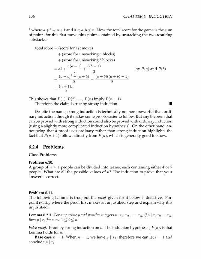
106 CHAPTER 6. INDUCTION
b where a+ b = n+ 1 and 0 < a, b ≤ n. Now the total score for the game is the sumof points for this first move plus points obtained by unstacking the two resultingsubstacks:
total score = (score for 1st move)+ (score for unstacking a blocks)+ (score for unstacking b blocks)
= ab+a(a− 1)
2+b(b− 1)
2by P (a) and P (b)
=(a+ b)2 − (a+ b)
2=
(a+ b)((a+ b)− 1)2
=(n+ 1)n
2
This shows that P (1), P (2), . . . , P (n) imply P (n+ 1).Therefore, the claim is true by strong induction. �
Despite the name, strong induction is technically no more powerful than ordi-nary induction, though it makes some proofs easier to follow. But any theorem thatcan be proved with strong induction could also be proved with ordinary induction(using a slightly more complicated induction hypothesis). On the other hand, an-nouncing that a proof uses ordinary rather than strong induction highlights thefact that P (n+ 1) follows directly from P (n), which is generally good to know.
6.2.4 Problems
Class Problems
Problem 6.10.A group of n ≥ 1 people can be divided into teams, each containing either 4 or 7people. What are all the possible values of n? Use induction to prove that youranswer is correct.
Problem 6.11.The following Lemma is true, but the proof given for it below is defective. Pin-point exactly where the proof first makes an unjustified step and explain why it isunjustified.
Lemma 6.2.3. For any prime p and positive integers n, x1, x2, . . . , xn, if p | x1x2 . . . xn,then p | xi for some 1 ≤ i ≤ n.
False proof. Proof by strong induction on n. The induction hypothesis, P (n), is thatLemma holds for n.
Base case n = 1: When n = 1, we have p | x1, therefore we can let i = 1 andconclude p | xi.

6.3. INDUCTION VERSUS WELL ORDERING 107
Induction step: Now assuming the claim holds for all k ≤ n, we must prove itfor n+ 1.
So suppose p | x1x2 . . . xn+1. Let yn = xnxn+1, so x1x2 . . . xn+1 = x1x2 . . . xn−1yn.Since the righthand side of this equality is a product of n terms, we have by induc-tion that p divides one of them. If p | xi for some i < n, then we have the desiredi. Otherwise p | yn. But since yn is a product of the two terms xn, xn+1, we haveby strong induction that p divides one of them. So in this case p | xi for i = n ori = n+ 1. �
Problem 6.12.Define the potential, p(S), of a stack of blocks, S, to be k(k − 1)/2 where k is thenumber of blocks in S. Define the potential, p(A), of a set of stacks, A, to be thesum of the potentials of the stacks in A.
Generalize Theorem 6.2.2 about scores in the stacking game to show that forany set of stacks, A, if a sequence of moves starting with A leads to another set ofstacks,B, then p(A) ≥ p(B), and the score for this sequence of moves is p(A)−p(B).
Hint: Try induction on the number of moves to get from A to B.
6.3 Induction versus Well Ordering
The Induction Axiom looks nothing like the Well Ordering Principle, but these twoproof methods are closely related. In fact, as the examples above suggest, we cantake any Well Ordering proof and reformat it into an Induction proof. Conversely,it’s equally easy to take any Induction proof and reformat it into a Well Orderingproof.
So what’s the difference? Well, sometimes induction proofs are clearer becausethey resemble recursive procedures that reduce handling an input of size n + 1 tohandling one of size n. On the other hand, Well Ordering proofs sometimes seemmore natural, and also come out slightly shorter. The choice of method is really amatter of style—but style does matter.

108 CHAPTER 6. INDUCTION

Chapter 7
Partial Orders
Partial orders are a kind of binary relation that come up a lot. The familiar≤ orderon numbers is a partial order, but so is the containment relation on sets and thedivisibility relation on integers.
Partial orders have particular importance in computer science because theycapture key concepts used, for example, in solving task scheduling problems, ana-lyzing concurrency control, and proving program termination.
7.1 Axioms for Partial Orders
The prerequisite structure among MIT subjects provides a nice illustration of par-tial orders. Here is a table indicating some of the prerequisites of subjects in thethe Course 6 program of Spring ’07:
Direct Prerequisites Subject18.01 6.04218.01 18.0218.01 18.038.01 8.026.001 6.0346.042 6.04618.03, 8.02 6.0026.001, 6.002 6.0046.001, 6.002 6.0036.004 6.0336.033 6.8576.046 6.840
Since 18.01 is a direct prerequisite for 6.042, a student must take 18.01 before6.042. Also, 6.042 is a direct prerequisite for 6.046, so in fact, a student has to takeboth 18.01 and 6.042 before taking 6.046. So 18.01 is also really a prerequisite for
109

110 CHAPTER 7. PARTIAL ORDERS
6.046, though an implicit or indirect one; we’ll indicate this by writing
18.01→ 6.046.
This prerequisite relation has a basic property known as transitivity: if subject ais an indirect prerequisite of subject b, and b is an indirect prerequisite of subject c,then a is also an indirect prerequisite of c.
In this table, a longest sequence of prerequisites is
18.01→ 18.03→ 6.002→ 6.004→ 6.033→ 6.857
so a student would need at least six terms to work through this sequence of sub-jects. But it would take a lot longer to complete a Course 6 major if the directprerequisites led to a situation1 where two subjects turned out to be prerequisitesof each other! So another crucial property of the prerequisite relation is that if a→ b,then it is not the case that b→ a. This property is called asymmetry.
Another basic example of a partial order is the subset relation, ⊆, on sets. Infact, we’ll see that every partial order can be represented by the subset relation.
Definition 7.1.1. A binary relation, R, on a set A is:
• transitive iff [a R b and b R c] IMPLIES a R c for every a, b, c ∈ A,
• asymmetric iff a R b IMPLIES NOT(b R a) for all a, b ∈ A,
• a strict partial order iff it is transitive and asymmetric.
So the prerequisite relation,→, on subjects in the MIT catalogue is a strict par-tial order. More familiar examples of strict partial orders are the relation,<, on realnumbers, and the proper subset relation, ⊂, on sets.
The subset relation, ⊆, on sets and ≤ relation on numbers are examples of re-flexive relations in which each element is related to itself. Reflexive partial ordersare called weak partial orders. Since asymmetry is incompatible with reflexivity,the asymmetry property in weak partial orders is relaxed so it applies only to twodifferent elements. This relaxation of the asymmetry is called antisymmetry:
Definition 7.1.2. A binary relation, R, on a set A, is
• reflexive iff a R a for all a ∈ A,
• antisymmetric iff a R b IMPLIES NOT(b R a) for all a 6= b ∈ A,
• a weak partial order iff it is transitive, reflexive and antisymmetric.
Some authors define partial orders to be what we call weak partial orders, butwe’ll use the phrase “partial order” to mean either a weak or strict one.
For weak partial orders in general, we often write an ordering-style symbol like� or v instead of a letter symbol like R. (General relations are usually denoted
1MIT’s Committee on Curricula has the responsibility of watching out for such bugs that mightcreep into departmental requirements.

7.2. REPRESENTING PARTIAL ORDERS BY SET CONTAINMENT 111
by a letter like R instead of a cryptic squiggly symbol, so � is kind of like themusical performer/composer Prince, who redefined the spelling of his name tobe his own squiggly symbol. A few years ago he gave up and went back to thespelling “Prince.”) Likewise, we generally use ≺ or @ to indicate a strict partialorder.
Two more examples of partial orders are worth mentioning:Example 7.1.3. Let A be some family of sets and define a R b iff a ⊃ b. Then R is astrict partial order.
For integers, m,n we write m | n to mean that m divides n, namely, there is aninteger, k, such that n = km.Example 7.1.4. The divides relation is a weak partial order on the nonnegative in-tegers.
7.2 Representing Partial Orders by Set Containment
Axioms can be a great way to abstract and reason about important properties ofobjects, but it helps to have a clear picture of the things that satisfy the axioms.We’ll show that every partial order can be pictured as a collection of sets related bycontainment. That is, every partial order has the “same shape” as such a collection.The technical word for “same shape” is “isomorphic.”
Definition 7.2.1. A binary relation, R, on a set, A, is isomorphic to a relation, S,on a set D iff there is a relation-preserving bijection from A to D. That is, there isbijection f : A→ D, such that for all a, a′ ∈ A,
a R a′ iff f(a) S f(a′).
Theorem 7.2.2. Every weak partial order, �, is isomorphic to the subset relation, on acollection of sets.
To picture a partial order, �, on a set, A, as a collection of sets, we simplyrepresent each element A by the set of elements that are � to that element, that is,
a ←→ {b ∈ A | b � a} .
For example, if � is the divisibility relation on the set of integers, {1, 3, 4, 6, 8, 12},then we represent each of these integers by the set of integers in A that divides it.So
1 ←→ {1}3 ←→ {1, 3}4 ←→ {1, 4}6 ←→ {1, 3, 6}8 ←→ {1, 4, 8}
12 ←→ {1, 3, 4, 6, 12}

112 CHAPTER 7. PARTIAL ORDERS
So, the fact that 3 | 12 corresponds to the fact that {1, 3} ⊆ {1, 3, 4, 6, 12}.In this way we have completely captured the weak partial order� by the subset
relation on the corresponding sets. Formally, we have
Lemma 7.2.3. Let � be a weak partial order on a set, A. Then � is isomorphic to thesubset relation on the collection of inverse images of elements a ∈ A under the � relation.
We leave the proof to Problem 7.3. Essentially the same construction shows thatstrict partial orders can be represented by set under the proper subset relation, ⊂.
7.2.1 Problems
Class Problems
Problem 7.1.
Direct Prerequisites Subject18.01 6.04218.01 18.0218.01 18.038.01 8.028.01 6.016.042 6.04618.02, 18.03, 8.02, 6.01 6.026.01, 6.042 6.0066.01 6.0346.02 6.004
(a) For the above table of MIT subject prerequisites, draw a diagram showing thesubject numbers with a line going down to every subject from each of its (direct)prerequisites.
(b) Give an example of a collection of sets partially ordered by the proper subsetrelation,⊂, that is isomorphic to (“same shape as”) the prerequisite relation amongMIT subjects from part (a).
(c) Explain why the empty relation is a strict partial order and describe a collec-tion of sets partially ordered by the proper subset relation that is isomorphic to theempty relation on five elements —that is, the relation under which none of the fiveelements is related to anything.
(d) Describe a simple collection of sets partially ordered by the proper subset rela-tion that is isomorphic to the ”properly contains” relation, ⊃, on P{1, 2, 3, 4}.
Problem 7.2.Consider the proper subset partial order, ⊂, on the power set P{1, 2, . . . , 6}.

7.3. TOTAL ORDERS 113
(a) What is the size of a maximal chain in this partial order? Describe one.
(b) Describe the largest antichain you can find in this partial order.
(c) What are the maximal and minimal elements? Are they maximum and mini-mum?
(d) Answer the previous part for the ⊂ partial order on the set P{1, 2, . . . , 6} − ∅.
Homework Problems
Problem 7.3.This problem asks for a proof of Lemma 7.2.3 showing that every weak partialorder can be represented by (is isomorphic to) a collection of sets partially orderedunder set inclusion (⊆). Namely,
Lemma. Let � be a weak partial order on a set, A. For any element a ∈ A, let
L(a) ::= {b ∈ A | b � a} ,L ::= {L(a) | a ∈ A} .
Then the function L : A → L is an isomorphism from the � relation on A, to the subsetrelation on L.
(a) Prove that the function L : A→ L is a bijection.
(b) Complete the proof by showing that
a � b iff L(a) ⊆ L(b) (7.1)
for all a, b ∈ A.
7.3 Total Orders
The familiar order relations on numbers have an important additional property:given two different numbers, one will be bigger than the other. Partial orders withthis property are said to be total2 orders.
Definition 7.3.1. Let R be a binary relation on a set, A, and let a, b be elements ofA. Then a and b are comparable with respect to R iff [a R b OR b R a]. A partialorder for which every two different elements are comparable is called a total order.
So < and ≤ are total orders on R. On the other hand, the subset relation isnot total, since, for example, any two different finite sets of the same size will beincomparable under ⊆. The prerequisite relation on Course 6 required subjects isalso not total because, for example, neither 8.01 nor 6.001 is a prerequisite of theother.
2“Total” is an overloaded term when talking about partial orders: being a total order is a muchstronger condition than being a partial order that is a total relation. For example, any weak partialorder such as ⊆ is a total relation.

114 CHAPTER 7. PARTIAL ORDERS
7.3.1 Problems
Practice Problems
Problem 7.4.For each of the binary relations below, state whether it is a strict partial order, aweak partial order, or neither. If it is not a partial order, indicate which of theaxioms for partial order it violates. If it is a partial order, state whether it is a totalorder and identify its maximal and minimal elements, if any.(a) The superset relation, ⊇ on the power set P{1, 2, 3, 4, 5}.
(b) The relation between any two nonegative integers, a, b that the remainder ofa divided by 8 equals the remainder of b divided by 8.
(c) The relation between propositional formulas, G, H , that G IMPLIES H is valid.
(d) The relation ’beats’ on Rock, Paper and Scissor (for those who don’t know thegame Rock, Paper, Scissors, Rock beats Scissors, Scissors beats Paper and Paperbeats Rock).
(e) The empty relation on the set of real numbers.
(f) The identity relation on the set of integers.
(g) The divisibility relation on the integers, Z.
Class Problems
Problem 7.5. (a) Verify that the divisibility relation on the set of nonnegative inte-gers is a weak partial order.
(b) What about the divisibility relation on the set of integers?
Problem 7.6.Consider the nonnegative numbers partially ordered by divisibility.(a) Show that this partial order has a unique minimal element.
(b) Show that this partial order has a unique maximal element.
(c) Prove that this partial order has an infinite chain.
(d) An antichain in a partial order is a set of elements such that any two elementsin the set are incomparable. Prove that this partial order has an infinite antichain.Hint: The primes.
(e) What are the minimal elements of divisibility on the integers greater than 1?What are the maximal elements?

7.3. TOTAL ORDERS 115
Problem 7.7.How many binary relations are there on the set {0, 1}?
How many are there that are transitive?, . . . asymmetric?, . . . reflexive?, . . . irreflexive?,. . . strict partial orders?, . . . weak partial orders?
Hint: There are easier ways to find these numbers than listing all the relationsand checking which properties each one has.
Problem 7.8.A binary relation, R, on a set, A, is irreflexive iff NOT(a R a) for all a ∈ A. Provethat if a binary relation on a set is transitive and irreflexive, then it is strict partialorder.
Problem 7.9.Prove that if R is a partial order, then so is R−1
Homework Problems
Problem 7.10.Let R and S be binary relations on the same set, A.
Definition 7.3.2. The composition, S ◦ R, of R and S is the binary relation on Adefined by the rule:3
a (S ◦R) c iff ∃b [a R b AND b S c].
Suppose both R and S are transitive. Which of the following new relationsmust also be transitive? For each part, justify your answer with a brief argumentif the new relation is transitive and a counterexample if it is not.(a) R−1
(b) R ∩ S
(c) R ◦R
(d) R ◦ S
Exam Problems
Problem 7.11.
3Note the reversal in the order ofR and S. This is so that relational composition generalizes functioncomposition, Composing the functions f and g means that f is applied first, and then g is applied tothe result. That is, the value of the composition of f and g applied to an argument, x, is g(f(x)). Toreflect this, the notation g ◦ f is commonly used for the composition of f and g. Some texts do defineg ◦ f the other way around.

116 CHAPTER 7. PARTIAL ORDERS
(a) For each row in the following table, indicate whether the binary relation, R,on the set, A, is a weak partial order or a total order by filling in the appropriateentries with either Y = YES or N = NO. In addition, list the minimal and maximalelements for each relation.
A a R b weak partial order total order minimal(s) maximal(s)
R− R+ a | b
P({1, 2, 3}) a ⊆ b
N ∪ {i} a > b
(b) What is the longest chain on the subset relation, ⊆, on P ({1, 2, 3})? (If there ismore than one, provide ONE of them.)
(c) What is the longest antichain on the subset relation,⊆, on P ({1, 2, 3})? (If thereis more than one, provide one of them.)
7.4 Product Orders
Taking the product of two relations is a useful way to construct new relations fromold ones.
Definition 7.4.1. The product, R1 ×R2, of relations R1 and R2 is defined to be therelation with
domain (R1 ×R2) ::= domain (R1)× domain (R2) ,codomain (R1 ×R2) ::= codomain (R1)× codomain (R2) ,
(a1, a2) (R1 ×R2) (b1, b2) iff [a1R1 b1 and a2R2 b2].
Example 7.4.2. Define a relation, Y , on age-height pairs of being younger and shorter.This is the relation on the set of pairs (y, h) where y is a nonnegative integer≤ 2400

7.5. SCHEDULING 117
which we interpret as an age in months, and h is a nonnegative integer ≤ 120 de-scribing height in inches. We define Y by the rule
(y1, h1)Y (y2, h2) iff y1 ≤ y2 AND h1 ≤ h2.
That is, Y is the product of the ≤-relation on ages and the ≤-relation on heights.
It follows directly from the definitions that products preserve the properties oftransitivity, reflexivity, irreflexivity, and antisymmetry, as shown in Problem 7.12.That is, if R1 and R2 both have one of these properties, then so does R1 ×R2. Thisimplies that if R1 and R2 are both partial orders, then so is R1 ×R2.
On the other hand, the property of being a total order is not preserved. Forexample, the age-height relation Y is the product of two total orders, but it is nottotal: the age 240 months, height 68 inches pair, (240,68), and the pair (228,72) areincomparable under Y .
7.4.1 Problems
Class Problems
Problem 7.12.LetR1,R2 be binary relations on the same set,A. A relational property is preservedunder product, if R1 × R2 has the property whenever both R1 and R2 have theproperty.(a) Verify that each of the following properties are preserved under product.
1. reflexivity,
2. antisymmetry,
3. transitivity.
(b) Verify that if either of R1 or R2 is irreflexive, then so is R1 ×R2.Note that it now follows immediately that if if R1 and R2 are partial orders and
at least one of them is strict, then R1 ×R2 is a strict partial order.
7.5 Scheduling
Scheduling problems are a common source of partial orders: there is a set, A, oftasks and a set of constraints specifying that starting a certain task depends onother tasks being completed beforehand. We can picture the constraints by draw-ing labelled boxes corresponding to different tasks, with an arrow from one box toanother if the first box corresponds to a task that must be completed before startingthe second one.

118 CHAPTER 7. PARTIAL ORDERS
Example 7.5.1. Here is a drawing describing the order in which you could put onclothes. The tasks are the clothes to be put on, and the arrows indicate what shouldbe put on directly before what.
left sock right sock
left shoe right shoe belt
pants
underwear shirt
sweater
jacket
When we have a partial order of tasks to be performed, it can be useful to havean order in which to perform all the tasks, one at a time, while respecting thedependency constraints. This amounts to finding a total order that is consistentwith the partial order. This task of finding a total ordering that is consistent with apartial order is known as topological sorting.
Definition 7.5.2. A topological sort of a partial order, ≺, on a set, A, is a total order-ing, @, on A such that
a ≺ b IMPLIES a @ b.
For example,
shirt @ sweater @ underwear @ leftsock @ rightsock @ pants@ leftshoe @ rightshoe @ belt @ jacket,
is one topological sort of the partial order of dressing tasks given by Example 7.5.1;there are several other possible sorts as well.
Topological sorts for partial orders on finite sets are easy to construct by startingfrom minimal elements:
Definition 7.5.3. Let� be a partial order on a set,A. An element a0 ∈ A is minimumiff it is � every other element of A, that is, a0 � b for all b 6= a0.
The element a0 is minimal iff no other element is � a0, that is, NOT(b � a0) forall b 6= a0.
There are corresponding definitions for maximum and maximal. Alternatively, amaximum(al) element for a relation, R, could be defined to be as a minimum(al)element for R−1.
In a total order, minimum and minimal elements are the same thing. But apartial order may have no minimum element but lots of minimal elements. Thereare four minimal elements in the clothes example: leftsock, rightsock, underwear,and shirt.

7.5. SCHEDULING 119
To construct a total ordering for getting dressed, we pick one of these minimalelements, say shirt. Next we pick a minimal element among the remaining ones.For example, once we have removed shirt, sweater becomes minimal. We con-tinue in this way removing successive minimal elements until all elements havebeen picked. The sequence of elements in the order they were picked will be atopological sort. This is how the topological sort above for getting dressed wasconstructed.
So our construction shows:
Theorem 7.5.4. Every partial order on a finite set has a topological sort.
There are many other ways of constructing topological sorts. For example, in-stead of starting “from the bottom” with minimal elements, we could build a totalstarting anywhere and simply keep putting additional elements into the total orderwherever they will fit. In fact, the domain of the partial order need not even befinite: we won’t prove it, but all partial orders, even infinite ones, have topologicalsorts.
7.5.1 Parallel Task Scheduling
For a partial order of task dependencies, topological sorting provides a way toexecute tasks one after another while respecting the dependencies. But what if wehave the ability to execute more than one task at the same time? For example, saytasks are programs, the partial order indicates data dependence, and we have aparallel machine with lots of processors instead of a sequential machine with onlyone. How should we schedule the tasks? Our goal should be to minimize the totaltime to complete all the tasks. For simplicity, let’s say all the tasks take the sameamount of time and all the processors are identical.
So, given a finite partially ordered set of tasks, how long does it take to dothem all, in an optimal parallel schedule? We can also use partial order conceptsto analyze this problem.
In the clothes example, we could do all the minimal elements first (leftsock,rightsock, underwear, shirt), remove them and repeat. We’d need lots of hands,or maybe dressing servants. We can do pants and sweater next, and then leftshoe,rightshoe, and belt, and finally jacket.
In general, a schedule for performing tasks specifies which tasks to do at succes-sive steps. Every task, a, has be scheduled at some step, and all the tasks that haveto be completed before task a must be scheduled for an earlier step.
Definition 7.5.5. A parallel schedule for a strict partial order, ≺, on a set, A, is a

120 CHAPTER 7. PARTIAL ORDERS
partition4 of A into sets A0, A1, . . . , such that for all a, b ∈ A, k ∈ N,
[a ∈ Ak AND b ≺ a] IMPLIES b ∈ Aj for some j < k.
The set Ak is called the set of elements scheduled at step k, and the length of theschedule is the number of sets Ak in the partition. The maximum number of el-ements scheduled at any step is called the number of processors required by theschedule.
So the schedule we chose above for clothes has four steps
A0 = {leftsock, rightsock, underwear, shirt} ,A1 = {pants, sweater} ,A2 = {leftshoe, rightshoe, belt} ,A3 = {jacket} .
and requires four processors (to complete the first step).Notice that the dependencies constrain the tasks underwear, pants, belt, and
jacket to be done in sequence. This implies that at least four steps are needed inevery schedule for getting dressed, since if we used fewer than four steps, two ofthese tasks would have to be scheduled at the same time. A set of tasks that mustbe done in sequence like this is called a chain.
Definition 7.5.6. A chain in a partial order is a set of elements such that any twodifferent elements in the set are comparable. A chain is said to end at an its maxi-mum element.
In general, the earliest step at which an element a can ever be scheduled mustbe at least as large as any chain that ends at a. A largest chain ending at a is calleda critical path to a, and the size of the critical path is called the depth of a. So in anypossible parallel schedule, it takes at least depth (a) steps to complete task a.
There is a very simple schedule that completes every task in this minimumnumber of steps. Just use a “greedy” strategy of performing tasks as soon as pos-sible. Namely, schedule all the elements of depth k at step k. That’s how we foundthe schedule for getting dressed given above.
Theorem 7.5.7. Let ≺ be a strict partial order on a set, A. A minimum length schedulefor ≺ consists of the sets A0, A1, . . . , where
Ak ::= {a | depth (a) = k} .
4Partitioning a set, A, means “cutting it up” into non-overlapping, nonempty pieces. The pieces arecalled the blocks of the partition. More precisely, a partition ofA is a setBwhose elements are nonemptysubsets of A such that
• if B,B′ ∈ B are different sets, then B ∩B′ = ∅, and
•SB∈B B = A.

7.6. DILWORTH’S LEMMA 121
We’ll leave to Problem 7.19 the proof that the sets Ak are a parallel scheduleaccording to Definition 7.5.5.
The minimum number of steps needed to schedule a partial order, ≺, is calledthe parallel time required by ≺, and a largest possible chain in ≺ is called a criticalpath for ≺. So we can summarize the story above by this way: with an unlimitednumber of processors, the minimum parallel time to complete all tasks is simplythe size of a critical path:
Corollary 7.5.8. Parallel time = length of critical path.
7.6 Dilworth’s Lemma
Definition 7.6.1. An antichain in a partial order is a set of elements such that anytwo elements in the set are incomparable.
Our conclusions about scheduling also tell us something about antichains.
Corollary 7.6.2. If the largest chain in a partial order on a set, A, is of size t, then A canbe partitioned into t antichains.
Proof. Let the antichains be the setsAk ::={a | depth (a) = k}. It is an easy exerciseto verify that each Ak is an antichain (Problem 7.19) �
Corollary 7.6.2 implies a famous result5 about partially ordered sets:
Lemma 7.6.3 (Dilworth). For all t > 0, every partially ordered set with n elements musthave either a chain of size greater than t or an antichain of size at least n/t.
Proof. Assume there is no chain of size greater than t, that is, the largest chain is ofsize ≤ t. Then by Corollary 7.6.2, the n elements can be partitioned into at most tantichains. Let ` be the size of the largest antichain. Since every element belongsto exactly one antichain, and there are at most t antichains, there can’t be morethan `t elements, namely, `t ≥ n. So there is an antichain with at least ` ≥ n/telements. �
Corollary 7.6.4. Every partially ordered set with n elements has a chain of size greaterthan
√n or an antichain of size at least
√n.
Proof. Set t =√n in Lemma 7.6.3. �
Example 7.6.5. In the dressing partially ordered set, n = 10.Try t = 3. There is a chain of size 4.Try t = 4. There is no chain of size 5, but there is an antichain of size 4 ≥ 10/4.
5Lemma 7.6.3 also follows from a more general result known as Dilworth’s Theorem which we willnot discuss.

122 CHAPTER 7. PARTIAL ORDERS
Example 7.6.6. Suppose we have a class of 101 students. Then using the productpartial order, Y , from Example 7.4.2, we can apply Dilworth’s Lemma to concludethat there is a chain of 11 students who get taller as they get older, or an antichainof 11 students who get taller as they get younger, which makes for an amusingin-class demo.
7.6.1 Problems
Practice Problems
Problem 7.13.What is the size of the longest chain that is guaranteed to exist in any partiallyordered set of n elements? What about the largest antichain?
Problem 7.14.Describe a sequence consisting of the integers from 1 to 10,000 in some order sothat there is no increasing or decreasing subsequence of size 101.
Problem 7.15.What is the smallest number of partially ordered tasks for which there can be morethan one minimum time schedule? Explain.
Class Problems
Problem 7.16.The table below lists some prerequisite information for some subjects in the MITComputer Science program (in 2006). This defines an indirect prerequisite relation,≺, that is a strict partial order on these subjects.
18.01→ 6.042 18.01→ 18.0218.01→ 18.03 6.046→ 6.8408.01→ 8.02 6.001→ 6.034
6.042→ 6.046 18.03, 8.02→ 6.0026.001, 6.002→ 6.003 6.001, 6.002→ 6.004
6.004→ 6.033 6.033→ 6.857
(a) Explain why exactly six terms are required to finish all these subjects, if youcan take as many subjects as you want per term. Using a greedy subject selectionstrategy, you should take as many subjects as possible each term. Exhibit yourcomplete class schedule each term using a greedy strategy.
(b) In the second term of the greedy schedule, you took five subjects including18.03. Identify a set of five subjects not including 18.03 such that it would be possi-

7.6. DILWORTH’S LEMMA 123
ble to take them in any one term (using some nongreedy schedule). Can you figureout how many such sets there are?
(c) Exhibit a schedule for taking all the courses —but only one per term.
(d) Suppose that you want to take all of the subjects, but can handle only two perterm. Exactly how many terms are required to graduate? Explain why.
(e) What if you could take three subjects per term?
Problem 7.17.A pair of 6.042 TAs, Liz and Oscar, have decided to devote some of their sparetime this term to establishing dominion over the entire galaxy. Recognizing this asan ambitious project, they worked out the following table of tasks on the back ofOscar’s copy of the lecture notes.
1. Devise a logo and cool imperial theme music - 8 days.
2. Build a fleet of Hyperwarp Stardestroyers out of eating paraphernalia swipedfrom Lobdell - 18 days.
3. Seize control of the United Nations - 9 days, after task #1.
4. Get shots for Liz’s cat, Tailspin - 11 days, after task #1.
5. Open a Starbucks chain for the army to get their caffeine - 10 days, after task#3.
6. Train an army of elite interstellar warriors by dragging people to see ThePhantom Menace dozens of times - 4 days, after tasks #3, #4, and #5.
7. Launch the fleet of Stardestroyers, crush all sentient alien species, and estab-lish a Galactic Empire - 6 days, after tasks #2 and #6.
8. Defeat Microsoft - 8 days, after tasks #2 and #6.
We picture this information in Figure 7.1 below by drawing a point for eachtask, and labelling it with the name and weight of the task. An edge betweentwo points indicates that the task for the higher point must be completed beforebeginning the task for the lower one.(a) Give some valid order in which the tasks might be completed.
Liz and Oscar want to complete all these tasks in the shortest possible time.However, they have agreed on some constraining work rules.
• Only one person can be assigned to a particular task; they can not work to-gether on a single task.

124 CHAPTER 7. PARTIAL ORDERS
v
v
v
v
v
v
v
v
�����������
�������QQQQQQQQ
AAAAAAA
PPPPPPPPPPPPPPPP
QQQQQQQQQ
�����������������������
EEEEEEEEEEEEEEEEEEEEEEE
BBBBBBBBBBB
6
seize control
open chain10
train army
devise logo build fleet
launch fleet 8
11
4
get shots
8 18
defeat Microsoft
9
Figure 7.1: Graph representing the task precedence constraints.

7.6. DILWORTH’S LEMMA 125
• Once a person is assigned to a task, that person must work exclusively onthe assignment until it is completed. So, for example, Liz cannot work onbuilding a fleet for a few days, run to get shots for Tailspin, and then returnto building the fleet.
(b) Liz and Oscar want to know how long conquering the galaxy will take. Oscarsuggests dividing the total number of days of work by the number of workers,which is two. What lower bound on the time to conquer the galaxy does this give,and why might the actual time required be greater?
(c) Liz proposes a different method for determining the duration of their project.He suggests looking at the duration of the “critical path”, the most time-consumingsequence of tasks such that each depends on the one before. What lower bounddoes this give, and why might it also be too low?
(d) What is the minimum number of days that Liz and Oscar need to conquer thegalaxy? No proof is required.
Problem 7.18. (a) What are the maximal and minimal elements, if any, of the powerset P({1, . . . , n}), where n is a positive integer, under the empty relation?
(b) What are the maximal and minimal elements, if any, of the set, N, of all non-negative integers under divisibility? Is there a minimum or maximum element?
(c) What are the minimal and maximal elements, if any, of the set of integersgreater than 1 under divisibility?
(d) Describe a partially ordered set that has no minimal or maximal elements.
(e) Describe a partially ordered set that has a unique minimal element, but no min-imum element. Hint: It will have to be infinite.
Homework Problems
Problem 7.19.Let ≺ be a partial order on a set, A, and let
Ak ::= {a | depth (a) = k}
where k ∈ N.(a) Prove that A0, A1, . . . is a parallel schedule for≺ according to Definition 7.5.5.
(b) Prove that Ak is an antichain.
Problem 7.20.Let S be a sequence of n different numbers. A subsequence of S is a sequence thatcan be obtained by deleting elements of S.

126 CHAPTER 7. PARTIAL ORDERS
For example, ifS = (6, 4, 7, 9, 1, 2, 5, 3, 8)
Then 647 and 7253 are both subsequences of S (for readability, we have droppedthe parentheses and commas in sequences, so 647 abbreviates (6, 4, 7), for exam-ple).
An increasing subsequence of S is a subsequence of whose successive elementsget larger. For example, 1238 is an increasing subsequence of S. Decreasing subse-quences are defined similarly; 641 is a decreasing subsequence of S.(a) List all the maximum length increasing subsequences of S, and all the maxi-
mum length decreasing subsequences.Now let A be the set of numbers in S. (So A = {1, 2, 3, . . . , 9} for the example
above.) There are two straightforward ways to totally order A. The first is to orderits elements numerically, that is, to order A with the < relation. The second is toorder the elements by which comes first in S; call this order<S . So for the exampleabove, we would have
6 <S 4 <S 7 <S 9 <S 1 <S 2 <S 5 <S 3 <S 8
Next, define the partial order ≺ on A defined by the rule
a ≺ a′ ::= a < a′ and a <S a′.
(It’s not hard to prove that ≺ is strict partial order, but you may assume it.)(b) Draw a diagram of the partial order, ≺, on A. What are the maximal ele-
ments,. . . the minimal elements?
(c) Explain the connection between increasing and decreasing subsequences of S,and chains and anti-chains under ≺.
(d) Prove that every sequence, S, of length n has an increasing subsequence oflength greater than
√n or a decreasing subsequence of length at least
√n.
(e) (Optional, tricky) Devise an efficient procedure for finding the longest increas-ing and the longest decreasing subsequence in any given sequence of integers.(There is a nice one.)
Problem 7.21.We want to schedule n partially ordered tasks.(a) Explain why any schedule that requires only p processors must take time at
least dn/pe.
(b) Let Dn,t be the strict partial order with n elements that consists of a chain oft− 1 elements, with the bottom element in the chain being a prerequisite of all theremaining elements as in the following figure:

7.6. DILWORTH’S LEMMA 127
. . .
. . . t - 1
n - (t - 1)
What is the minimum time schedule for Dn,t? Explain why it is unique. Howmany processors does it require?
(c) Write a simple formula, M(n, t, p), for the minimum time of a p-processorschedule to complete Dn,t.
(d) Show that every partial order with n vertices and maximum chain size, t, hasa p-processor schedule that runs in time M(n, t, p).
Hint: Induction on t.

128 CHAPTER 7. PARTIAL ORDERS

Chapter 8
Directed graphs
8.1 Digraphs
A directed graph (digraph for short) is formally the same as a binary relation, R, ona set, A —that is, a relation whose domain and codomain are the same set, A. Butwe describe digraphs as though they were diagrams, with elements of A picturedas points on the plane and arrows drawn between related points. The elementsof A are referred to as the vertices of the digraph, and the pairs (a, b) ∈ graph (R)are directed edges. Writing a→ b is a more suggestive alternative for the pair (a, b).Directed edges are also called arrows.
For example, the divisibility relation on {1, 2, . . . , 12} is could be pictured bythe digraph:
12 6 1
824 10
5
7
1193
Figure 8.1: The Digraph for Divisibility on {1, 2, . . . , 12}.
129

130 CHAPTER 8. DIRECTED GRAPHS
8.1.1 Paths in Digraphs
Picturing digraphs with points and arrows makes it natural to talk about followinga path of successive edges through the graph. For example, in the digraph of Fig-ure 8.1, a path might start at vertex 1, successively follow the edges from vertex 1to vertex 2, from 2 to 4, from 4 to 12, and then from 12 to 12 twice (or as many timesas you like). We can represent the path with the sequence of sucessive vertices itwent through, in this case:
1, 2, 4, 12, 12, 12.
So a path is just a sequence of vertices, with consecutive vertices on the path con-nected by directed edges. Here is a formal definition:
Definition 8.1.1. A path in a digraph is a sequence of vertices a0, . . . , ak with k ≥ 0such that ai → ai+1 is an edge of the digraph for i = 0, 1, . . . , k−1. The path is saidto start at a0, to end at ak, and the length of the path is defined to be k. The path issimple iff all the ai’s are different, that is, if i 6= j, then ai 6= aj .
Note that a single vertex counts as length zero path that begins and ends atitself.
It’s pretty natural to talk about the edges in a path, but technically, paths onlyhave points, not edges. So to instead, we’ll say a path traverses an edge a→ bwhena and b are consecutive vertices in the path.
For any digraph, R, we can define some new relations on vertices based onpaths, namely, the path relation, R∗, and the positive-length path relation, R+:
a R∗ b ::= there is a path in R from a to b,
a R+ b ::= there is a positive length path in R from a to b.
By the definition of path, both R∗ and R+ are transitive. Since edges count aslength one paths, the edges of R+ include all the edges of R. The edges of R∗ inturn include all the edges of R+ and, in addition include an edge (self-loop) fromeach vertex to itself. The self-loops get included in R∗ because of the a length zeropaths in R. So R∗ is reflexive. 1
8.2 Picturing Relational Properties
Many of the relational properties we’ve discussed have natural descriptions interms of paths. For example:
Reflexivity: All vertices have self-loops (a self-loop at a vertex is an arrow goingfrom the vertex back to itself).
Irreflexivity: No vertices have self-loops.
Antisymmetry: At most one (directed) edge between different vertices.
1In many texts, R+ is called the transitive closure and R∗ is called the reflexive transitive closure of R.

8.3. COMPOSITION OF RELATIONS 131
Asymmetry: No self-loops and at most one (directed) edge between different ver-tices.
Transitivity: Short-circuits—for any path through the graph, there is an arrowfrom the first vertex to the last vertex on the path.
Symmetry: A binary relation R is symmetric iff aRb implies bRa for all a, b in thedomain of R. That is, if there is an edge from a to b, there is also one in thereverse direction.
8.3 Composition of Relations
There is a simple way to extend composition of functions to composition of rela-tions, and this gives another way to talk about paths in digraphs.
Let R : B → C and S : A → B be relations. Then the composition of R with Sis the binary relation (R ◦ S) : A→ C defined by the rule
a (R ◦ S) c ::= ∃b ∈ B. (b R c) AND (a S b).
This agrees with the Definition 4.3.1 of composition in the special case whenR andS are functions.
Now when R is a digraph, it makes sense to compose R with itself. Then if welet Rn denote the composition of R with itself n times, it’s easy to check that Rn isthe length-n path relation:
a Rn b iff there is a length n path in R from a to b.
This even works for n = 0, if we adopt the convention that R0 is the identityrelation IdA on the set, A, of vertices. That is, (a IdA b) iff a = b.
8.4 Directed Acyclic Graphs
Definition 8.4.1. A cycle in a digraph is defined by a path that begins and ends atthe same vertex. This includes the cycle of length zero that begins and ends at thevertex. A directed acyclic graph (DAG) is a directed graph with no positive lengthcycles.
A simple cycle in a digraph is a cycle whose vertices are distinct except for thebeginning and end vertices.
DAG’s can be an economical way to represent partial orders. For example, thedirect prerequisite relation between MIT subjects in Chapter 7 was used to determinethe partial order of indirect prerequisites on subjects. This indirect prerequisitepartial order is precisely the positive length path relation of the direct prerequisites.
Lemma 8.4.2. If D is a DAG, then D+ is a strict partial order.

132 CHAPTER 8. DIRECTED GRAPHS
Proof. We know that D+ is transitive. Also, a positive length path from a vertex toitself would be a cycle, so there are no such paths. This means D+ is irreflexive,which implies it is a strict partial order (see problem 7.8). �
It’s easy to check that conversely, the graph of any strict partial order is a DAG.The divisibility partial order can also be more economically represented by the
path relation in a DAG. A DAG whose path relation is divisibility on {1, 2, . . . , 12}is shown in Figure 8.2; the arrowheads are omitted in the Figure, and edges areunderstood to point upwards.
����1
����4����8
����5����10����6
����3
����12
����7����11
����9
����2.........
................
.....
................
.............
................
.............
.............................
.............................
JJJJ
ZZ
ZZZZ
������
Figure 8.2: A DAG whose Path Relation is Divisibility on {1, 2, . . . , 12}.
If we’re using a DAG to represent a partial order —so all we care about is thethe path relation of the DAG —we could replace the DAG with any other DAGwith the same path relation. This raises the question of finding a DAG with thesame path relation but the smallest number of edges. This DAG turns out to beunique and easy to find (see problem 8.2).
8.4.1 Problems
Practice Problems
Problem 8.1.Why is every strict partial order a DAG?
Class Problems
Problem 8.2.If a and b are distinct nodes of a digraph, then a is said to cover b if there is an edge

8.4. DIRECTED ACYCLIC GRAPHS 133
from a to b and every path from a to b traverses this edge. If a covers b, the edgefrom a to b is called a covering edge.(a) What are the covering edges in the following DAG?
12 6 1
824 10
5
7
1193
(b) Let covering (D) be the subgraph of D consisting of only the covering edges.Suppose D is a finite DAG. Explain why covering (D) has the same positive pathrelation as D.Hint: Consider longest paths between a pair of vertices.
(c) Show that if two DAG’s have the same positive path relation, then they havethe same set of covering edges.
(d) Conclude that covering (D) is the unique DAG with the smallest number ofedges among all digraphs with the same positive path relation as D.
The following examples show that the above results don’t work in general fordigraphs with cycles.(e) Describe two graphs with vertices {1, 2} which have the same set of covering
edges, but not the same positive path relation (Hint: Self-loops.)
(f) (i) The complete digraph without self-loops on vertices 1, 2, 3 has edges be-tween every two distinct vertices. What are its covering edges?
(ii) What are the covering edges of the graph with vertices 1, 2, 3 and edges 1 →2, 2→ 3, 3→ 1?
(iii) What about their positive path relations?
Homework Problems
Problem 8.3.Let R be a binary relation on a set A. Then Rn denotes the composition of R with

134 CHAPTER 8. DIRECTED GRAPHS
itself n times. Let GR be the digraph associated with R. That is, A is the set ofvertices ofGR and R is the set of directed edges. Let R(n) denote the length n pathrelation GR, that is,
a R(n) b ::= there is a length n path from a to b in GR.
Prove thatRn = R(n) (8.1)
for all n ∈ N.
Problem 8.4. (a) Prove that if R is a relation on a finite set, A, then
a (R ∪ IA)n b iff there is a path in R of length length ≤ n from a to b.
(b) Conclude that if A is a finite set, then
R∗ = (R ∪ IA)|A|−1. (8.2)

Chapter 9
State Machines
9.1 State machines
State machines are an abstract model of step-by-step processes, and accordingly,they come up in many areas of computer science. You may already have seenthem in a digital logic course, a compiler course, or a probability course.
9.1.1 Basic definitions
A state machine is really nothing more than a binary relation on a set, except thatthe elements of the set are called “states,” the relation is called the transition relation,and a pair (p, q) in the graph of the transition relation is called a transition. Thetransition from state p to state q will be written p −→ q. The transition relation isalso called the state graph of the machine. A state machine also comes equippedwith a designated start state.
State machines used in digital logic and compilers usually have only a finitenumber of states, but machines that model continuing computations typically havean infinite number of states. In many applications, the states, and/or the transi-tions have labels indicating input or output values, costs, capacities, or probabili-ties, but for our purposes, unlabelled states and transitions are all we need.1
Example 9.1.1. A bounded counter, which counts from 0 to 99 and overflows at 100.The transitions are pictured in Figure 9.1, with start state zero. This machine isn’tmuch use once it overflows, since it has no way to get out of its overflow state.
Example 9.1.2. An unbounded counter is similar, but has an infinite state set. Thisis harder to draw :-)
Example 9.1.3. In the movie Die Hard 3: With a Vengeance, the characters played bySamuel L. Jackson and Bruce Willis have to disarm a bomb planted by the diaboli-cal Simon Gruber:
1We do name states, as in Figure 9.1, so we can talk about them, but the names aren’t part of thestate machine.
135

136 CHAPTER 9. STATE MACHINES
0 1 2 99 overflow
startstate
Figure 9.1: State transitions for the 99-bounded counter.
Simon: On the fountain, there should be 2 jugs, do you see them? A 5-gallon and a 3-gallon. Fill one of the jugs with exactly 4 gallons of waterand place it on the scale and the timer will stop. You must be precise;one ounce more or less will result in detonation. If you’re still alive in 5minutes, we’ll speak.
Bruce: Wait, wait a second. I don’t get it. Do you get it?
Samuel: No.
Bruce: Get the jugs. Obviously, we can’t fill the 3-gallon jug with 4 gallonsof water.
Samuel: Obviously.
Bruce: All right. I know, here we go. We fill the 3-gallon jug exactly to thetop, right?
Samuel: Uh-huh.
Bruce: Okay, now we pour this 3 gallons into the 5-gallon jug, giving usexactly 3 gallons in the 5-gallon jug, right?
Samuel: Right, then what?
Bruce: All right. We take the 3-gallon jug and fill it a third of the way...
Samuel: No! He said, “Be precise.” Exactly 4 gallons.
Bruce: Sh - -. Every cop within 50 miles is running his a - - off and I’m outhere playing kids games in the park.
Samuel: Hey, you want to focus on the problem at hand?
Fortunately, they find a solution in the nick of time. We’ll let the reader workout how.
The Die Hard series is getting tired, so we propose a final Die Hard Once and ForAll. Here Simon’s brother returns to avenge him, and he poses the same challenge,but with the 5 gallon jug replaced by a 9 gallon one.
We can model jug-filling scenarios with a state machine. In the scenario with a3 and a 5 gallon water jug, the states will be pairs, (b, l) of real numbers such that

9.1. STATE MACHINES 137
0 ≤ b ≤ 5, 0 ≤ l ≤ 3. We let b and l be arbitrary real numbers. (We can prove thatthe values of b and l will only be nonnegative integers, but we won’t assume this.)The start state is (0, 0), since both jugs start empty.
Since the amount of water in the jug must be known exactly, we will only con-sider moves in which a jug gets completely filled or completely emptied. There areseveral kinds of transitions:
1. Fill the little jug: (b, l) −→ (b, 3) for l < 3.
2. Fill the big jug: (b, l) −→ (5, l) for b < 5.
3. Empty the little jug: (b, l) −→ (b, 0) for l > 0.
4. Empty the big jug: (b, l) −→ (0, l) for b > 0.
5. Pour from the little jug into the big jug: for l > 0,
(b, l) −→
{(b+ l, 0) if b+ l ≤ 5,(5, l − (5− b)) otherwise.
6. Pour from big jug into little jug: for b > 0,
(b, l) −→
{(0, b+ l) if b+ l ≤ 3,(b− (3− l), 3) otherwise.
Note that in contrast to the 99-counter state machine, there is more than onepossible transition out of states in the Die Hard machine. Machines like the 99-counter with at most one transition out of each state are called deterministic. TheDie Hard machine is nondeterministic because some states have transitions to sev-eral different states.
Quick exercise: Which states of the Die Hard 3 machine have direct transitionsto exactly two states?
9.1.2 Reachability and Preserved Invariants
The Die Hard 3 machine models every possible way of pouring water among thejugs according to the rules. Die Hard properties that we want to verify can nowbe expressed and proved using the state machine model. For example, Bruce’scharacter will disarm the bomb if he can get to some state of the form (4, l).
A (possibly infinite) path through the state graph beginning at the start statecorresponds to a possible system behavior; such a path is called an execution of thestate machine. A state is called reachable if it appears in some execution. The bombin Die Hard 3 gets disarmed successfully because the state (4,3) is reachable.
A useful approach in analyzing state machine is to identify properties of statesthat are preserved by transitions.

138 CHAPTER 9. STATE MACHINES
Definition 9.1.4. A preserved invariant of a state machine is a predicate, P , on states,such that whenever P (q) is true of a state, q, and q −→ r for some state, r, thenP (r) holds.
The Invariant Principle
If a preserved invariant of a state machine is true for the start state,then it is true for all reachable states.
The Invariant Principle is nothing more than the Induction Principle reformu-lated in a convenient form for state machines. Showing that a predicate is true inthe start state is the base case of the induction, and showing that a predicate is apreserved invariant is the inductive step.2
Die Hard Once and For All
Now back to Die Hard Once and For All. This time there is a 9 gallon jug insteadof the 5 gallon jug. We can model this with a state machine whose states andtransitions are specified the same way as for the Die Hard 3 machine, with alloccurrences of “5” replaced by “9.”
Now reaching any state of the form (4, l) is impossible. We prove this using theInvariant Principle. Namely, we define the preserved invariant predicate, P (b, l),to be that b and l are nonnegative integer multiples of 3. So P obviously holds forthe state state (0, 0).
To prove that P is a preserved invariant, we assume P (b, l) holds for some state(b, l) and show that if (b, l) −→ (b′, l′), then P (b′, l′). The proof divides into cases,according to which transition rule is used. For example, suppose the transitionfollowed from the “fill the little jug” rule. This means (b, l) −→ (b, 3). But P (b, l)implies that b is an integer multiple of 3, and of course 3 is an integer multiple of3, so P still holds for the new state (b, 3). Another example is when the transitionrule used is “pour from big jug into little jug” for the subcase that b + l > 3. Thenstate is (b, l) −→ (b − (3 − l), 3). But since b and l are integer multiples of 3, so isb− (3− l). So in this case too, P holds after the transition.
We won’t bother to crank out the remaining cases, which can all be checkedjust as easily. Now by the Invariant Principle, we conclude that every reachable
2Preserved invariants are commonly just called “invariants” in the literature on program correct-ness, but we decided to throw in the extra adjective to avoid confusion with other definitions. Forexample, another subject at MIT uses “invariant” to mean “predicate true of all reachable states.” Let’scall this definition “invariant-2.” Now invariant-2 seems like a reasonable definition, since unreachablestates by definition don’t matter, and all we want to show is that a desired property is invariant-2. Butthis confuses the objective of demonstrating that a property is invariant-2 with the method for show-ing that it is. After all, if we already knew that a property was invariant-2, we’d have no need for anInvariant Principle to demonstrate it.

9.1. STATE MACHINES 139
state satisifies P . But since no state of the form (4, l) satisifies P , we have provedrigorously that Bruce dies once and for all!
By the way, notice that the state (1,0), which satisfies NOT(P ), has a transition to(0,0), which satisfies P . So it’s wrong to assume that the complement of a preservedinvariant is also a preserved invariant.
A Robot on a Grid
There is a robot. It walks around on a grid, and at every step it moves diagonallyin a way that changes its position by one unit up or down and one unit left or right.The robot starts at position (0, 0). Can the robot reach position (1, 0)?
To get some intuition, we can simulate some robot moves. For example, start-ing at (0,0) the robot could move northeast to (1,1), then southeast to (2,0), thensouthwest to (1,-1), then southwest again to (0,-2).
Let’s model the problem as a state machine and then find a suitable invariant.A state will be a pair of integers corresponding to the coordinates of the robot’sposition. State (i, j) has transitions to four different states: (i± 1, j ± 1).
The problem is now to choose an appropriate preserved invariant, P , that istrue for the start state (0, 0) and false for (1, 0). The Invariant Theorem then willimply that the robot can never reach (1, 0). A direct attempt for a preserved invari-ant is the predicate P (q) that q 6= (1, 0).
Unfortunately, this is not going to work. Consider the state (2, 1). ClearlyP (2, 1) holds because (2, 1) 6= (1, 0). And of course P (1, 0) does not hold. But(2, 1) −→ (1, 0), so this choice of P will not yield a preserved invariant.
We need a stronger predicate. Looking at our example execution you might beable to guess a proper one, namely, that the sum of the coordinates is even! If wecan prove that this is a preserved invariant, then we have proven that the robotnever reaches (1, 0) —because the sum 1 + 0 of its coordinates is odd, while thesum 0 + 0 of the coordinates of the start state is even.
Theorem 9.1.5. The sum of the robot’s coordinates is always even.
Proof. The proof uses the Invariant Principle.Let P (i, j) be the predicate that i+ j is even.First, we must show that the predicate holds for the start state (0, 0). Clearly,
P (0, 0) is true because 0 + 0 is even.Next, we must show that P is a preserved invariant. That is, we must show
that for each transition (i, j) −→ (i′, j′), if i + j is even, then i′ + j′ is even. Buti′ = i ± 1 and j′ = j ± 1 by definition of the transitions. Therefore, i′ + j′ is equalto i+ j or i+ j ± 2, all of which are even. �
Corollary 9.1.6. The robot cannot reach (1, 0).

140 CHAPTER 9. STATE MACHINES
Robert W. Floyd
The Invariant Principle was formulated by Robert Floyd at Carnegie Techa in 1967.Floyd was already famous for work on formal grammars which transformed thefield of programming language parsing; that was how he got to be a professoreven though he never got a Ph.D. (He was admitted to a PhD program as a teenageprodigy, but flunked out and never went back.)
In that same year, Albert R. Meyer was appointed Assistant Professor in theCarnegie Tech Computer Science Department where he first met Floyd. Floyd andMeyer were the only theoreticians in the department, and they were both delightedto talk about their shared interests. After just a few conversations, Floyd’s new ju-nior colleague decided that Floyd was the smartest person he had ever met.
Naturally, one of the first things Floyd wanted to tell Meyer about was his new,as yet unpublished, Invariant Principle. Floyd explained the result to Meyer, andMeyer wondered (privately) how someone as brilliant as Floyd could be excitedby such a trivial observation. Floyd had to show Meyer a bunch of examples be-fore Meyer understood Floyd’s excitement —not at the truth of the utterly obviousInvariant Principle, but rather at the insight that such a simple theorem could beso widely and easily applied in verifying programs.
Floyd left for Stanford the following year. He won the Turing award —the “Nobelprize” of computer science— in the late 1970’s, in recognition both of his workon grammars and on the foundations of program verification. He remained atStanford from 1968 until his death in September, 2001. You can learn more aboutFloyd’s life and work by reading the eulogy written by his closest colleague, DonKnuth.
aThe following year, Carnegie Tech was renamed Carnegie-Mellon Univ.
9.1.3 Sequential algorithm examples
Proving Correctness
Robert Floyd, who pioneered modern approaches to program verification, distin-guished two aspects of state machine or process correctness:
1. The property that the final results, if any, of the process satisfy system re-quirements. This is called partial correctness.You might suppose that if a result was only partially correct, then it mightalso be partially incorrect, but that’s not what he meant. The word “partial”comes from viewing a process that might not terminate as computing a partialfunction. So partial correctness means that when there is a result, it is correct,but the process might not always produce a result, perhaps because it getsstuck in a loop.

9.1. STATE MACHINES 141
2. The property that the process always finishes, or is guaranteed to producesome legitimate final output. This is called termination.
Partial correctness can commonly be proved using the Invariant Principle. Ter-mination can commonly be proved using the Well Ordering Principle. We’ll illus-trate Floyd’s ideas by verifying the Euclidean Greatest Common Divisor (GCD)Algorithm.
The Euclidean Algorithm
The Euclidean algorithm is a three-thousand-year-old procedure to compute thegreatest common divisor, gcd(a, b) of integers a and b. We can represent this al-gorithm as a state machine. A state will be a pair of integers (x, y) which we canthink of as integer registers in a register program. The state transitions are definedby the rule
(x, y) −→ (y, remainder(x, y))
for y 6= 0. The algorithm terminates when no further transition is possible, namelywhen y = 0. The final answer is in x.
We want to prove:
1. Starting from the state with x = a and y = b > 0, if we ever finish, then wehave the right answer. That is, at termination, x = gcd(a, b). This is a partialcorrectness claim.
2. We do actually finish. This is a process termination claim.
Partial Correctness of GCD First let’s prove that if GCD gives an answer, it is acorrect answer. Specifically, let d ::= gcd(a, b). We want to prove that if the proce-dure finishes in a state (x, y), then x = d.
Proof. Define the state predicate
P (x, y) ::= [gcd(x, y) = d and (x > 0 or y > 0)].
P holds for the start state (a, b), by definition of d and the requirement that b ispositive. Also, the preserved invariance of P follows immediately from
Lemma 9.1.7. For all m,n ∈ N such that n 6= 0,
gcd(m,n) = gcd(n, remainder(m,n)). (9.1)
Lemma 9.1.7 is easy to prove: let q be the quotient and r be the remainder of mdivided by n. Then m = qn+ r by definition. So any factor of both r and n will bea factor of m, and similarly any factor of both m and n will be a factor of r. So r, nand m,n have the same common factors and therefore the same gcd. Now by theInvariant Principle, P holds for all reachable states.

142 CHAPTER 9. STATE MACHINES
Since the only rule for termination is that y = 0, it follows that if (x, y) is aterminal state, then y = 0. If this terminal state is reachable, then the preservedinvariant holds for (x, y). This implies that gcd(x, 0) = d and that x > 0. Weconclude that x = gcd(x, 0) = d. �
Termination of GCD Now we turn to the second property, that the proceduremust terminate. To prove this, notice that y gets strictly smaller after any one tran-sition. That’s because the value of y after the transition is the remainder of x di-vided by y, and this remainder is smaller than y by definition. But the value of y isalways a nonnegative integer, so by the Well Ordering Principle, it reaches a mini-mum value among all its values at reachable states. But there can’t be a transitionfrom a state where y has its minimum value, because the transition would decreasey still further. So the reachable state where y has its minimum value is a state atwhich no further step is possible, that is, at which the procedure terminates.
Note that this argument does not prove that the minimum value of y is zero,only that the minimum value occurs at termination. But we already noted that theonly rule for termination is that y = 0, so it follows that the minimum value of ymust indeed be zero.
The Extended Euclidean Algorithm
An important fact about the gcd(a, b) is that it equals an integer linear combinationof a and b, that is,
gcd(a, b) = sa+ tb (9.2)
for some s, t ∈ Z. We’ll see some nice proofs of (9.2) later when we study NumberTheory, but now we’ll look at an extension of the Euclidean Algorithm that effi-ciently, if obscurely, produces the desired s and t. It is presented here simply asanother example of application of the Invariant Method (plus, we’ll need a proce-dure like this when we take up number theory based cryptography in a couple ofweeks).
Don’t worry if you find this Extended Euclidean Algorithm hard to follow, and youcan’t imagine where it came from. In fact, that’s good, because this will illustrate an im-portant point: given the right preserved invariant, you can verify programs you don’tunderstand.
In particular, given nonnegative integers x and y, with y > 0, we claim thefollowing procedure3 halts with registers S and T containing integers s and t satis-fying (9.2).
Inputs: a, b ∈ N, b > 0.Registers: X,Y,S,T,U,V,Q.Extended Euclidean Algorithm:
X := a; Y := b; S := 0; T := 1; U := 1; V := 0;loop:
3This procedure is adapted from Aho, Hopcroft, and Ullman’s text on algorithms.

9.1. STATE MACHINES 143
if Y divides X, then haltelse
Q := quotient(X,Y);;;the following assignments in braces are SIMULTANEOUS
{X := Y,Y := remainder(X,Y);U := S,V := T,S := U - Q * S,T := V - Q * T};
goto loop;
Note that X,Y behave exactly as in the Euclidean GCD algorithm in Section 9.1.3,except that this extended procedure stops one step sooner, ensuring that gcd(x, y)is in Y at the end. So for all inputs x, y, this procedure terminates for the samereason as the Euclidean algorithm: the contents, y, of register Y is a nonnegativeinteger-valued variable that strictly decreases each time around the loop.
The following properties are preserved invariants that imply partial correct-ness:
gcd(X,Y ) = gcd(a, b), (9.3)Sa+ Tb = Y, and (9.4)Ua+ V b = X. (9.5)
To verify that these are preserved invariants, note that (9.3) is the same onewe observed for the Euclidean algorithm. To check the other two properties, letx, y, s, t, u, v be the contents of registers X,Y,S,T,U,V at the start of the loop andassume that all the properties hold for these values. We must prove that (9.4)and (9.5) hold (we already know (9.3) does) for the new contents x′, y′, s′, t′, u′, v′
of these registers at the next time the loop is started.Now according to the procedure, u′ = s, v′ = t, x′ = y, so (9.5) holds for u′, v′, x′
because of (9.4) for s, t, y. Also,
s′ = u− qs, t′ = v − qt, y′ = x− qy
where q = quotient(x, y), so
s′a+ t′b = (u− qs)a+ (v − qt)b = ua+ vb− q(sa+ tb) = x− qy = y′,
and therefore (9.4) holds for s′, t′, y′.Also, it’s easy to check that all three preserved invariants are true just before
the first time around the loop. Namely, at the start:
X = a, Y = b, S = 0, T = 1 soSa+ Tb = 0a+ 1b = b = Y confirming (9.4).

144 CHAPTER 9. STATE MACHINES
Also,
U = 1, V = 0, soUa+ V b = 1a+ 0b = a = X confirming (9.5).
Now by the Invariant Principle, they are true at termination. But at termination,the contents, Y , of register Y divides the contents, X , of register X, so preservedinvariants (9.3) and (9.4) imply
gcd(a, b) = gcd(X,Y ) = Y = Sa+ Tb.
So we have the gcd in register Y and the desired coefficients in S, T.Now we don’t claim that this verification offers much insight. In fact, if you’re
not wondering how somebody came up with this concise program and invariant,you:
• are blessed with an inspired intellect allowing you to see how this programand its invariant were devised,
• have lost interest in the topic, or
• haven’t read this far.
If none of the above apply to you, we can offer some reassurance by repeating thatyou’re not expected to understand this program.
We’ve already observed that a preserved invariant is really just an inductionhypothesis. As with induction, finding the right hypothesis is usually the hardpart. We repeat:
Given the right preserved invariant, it can be easy to verify a programeven if you don’t understand it.
We expect that the Extended Euclidean Algorithm presented above illustrates thispoint.
9.1.4 Derived Variables
The preceding termination proofs involved finding a nonnegative integer-valuedmeasure to assign to states. We might call this measure the “size” of the state.We then showed that the size of a state decreased with every state transition. Bythe Well Ordering Principle, the size can’t decrease indefinitely, so when a mini-mum size state is reached, there can’t be any transitions possible: the process hasterminated.
More generally, the technique of assigning values to states —not necessarilynonnegative integers and not necessarily decreasing under transitions— is oftenuseful in the analysis of algorithms. Potential functions play a similar role in physics.In the context of computational processes, such value assignments for states arecalled derived variables.

9.1. STATE MACHINES 145
For example, for the Die Hard machines we could have introduced a derivedvariable, f : states → R, for the amount of water in both buckets, by settingf((a, b))::=a+b. Similarly, in the robot problem, the position of the robot along thex-axis would be given by the derived variable x-coord, where x-coord((i, j)) ::= i.
We can formulate our general termination method as follows:
Definition 9.1.8. Let ≺ be a strict partial order on a set, A. A derived variablef : states → A is strictly decreasing iff
q −→ q′ implies f(q′) ≺ f(q).
We confirmed termination of the GCD and Extended GCD procedures by find-ing derived variables, y and Y, respectively, that were nonnegative integer-valuedand strictly decreasing. We can summarize this approach to proving terminationas follows:
Theorem 9.1.9. If f is a strictly decreasing N-valued derived variable of a state machine,then the length of any execution starting at state q is at most f(q).
Of course we could prove Theorem 9.1.9 by induction on the value of f(q), butthink about what it says: “If you start counting down at some nonnegative integerf(q), then you can’t count down more than f(q) times.” Put this way, it’s obvious.
Weakly Decreasing Variables
In addition being strictly decreasing, it will be useful to have derived variableswith some other, related properties.
Definition 9.1.10. Let � be a weak partial order on a set, A. A derived variablef : Q→ A is weakly decreasing iff
q −→ q′ implies f(q′) � f(q).
Strictly increasing and weakly increasing derived variables are defined similarly.4
9.1.5 Problems
Homework Problems
Problem 9.1.You are given two buckets, A and B, a water hose, a receptacle, and a drain. Thebuckets and receptacle are initially empty. The buckets are labeled with their re-spectively capacities, positive integers a and b. The receptacle can be used to storean unlimited amount of water, but has no measurement markings. Excess watercan be dumped into the drain. Among the possible moves are:
4Weakly increasing variables are often also called nondecreasing. We will avoid this terminology toprevent confusion between nondecreasing variables and variables with the much weaker property ofnot being a decreasing variable.

146 CHAPTER 9. STATE MACHINES
1. fill a bucket from the hose,
2. pour from the receptacle to a bucket until the bucket is full or the receptacleis empty, whichever happens first,
3. empty a bucket to the drain,
4. empty a bucket to the receptacle,
5. pour from A to B until either A is empty or B is full, whichever happensfirst,
6. pour from B to A until either B is empty or A is full, whichever happensfirst.
(a) Model this scenario with a state machine. (What are the states? How does astate change in response to a move?)
(b) Prove that we can put k ∈ N gallons of water into the receptacle using theabove operations if and only if gcd(a, b) | k. Hint: Use the fact that if a, b arepositive integers then there exist integers s, t such that gcd(a, b) = sa + tb (seeNotes 9.1.3).
Problem 9.2.Here is a very, very fun game. We start with two distinct, positive integers writtenon a blackboard. Call them a and b. You and I now take turns. (I’ll let you decidewho goes first.) On each player’s turn, he or she must write a new positive integeron the board that is the difference of two numbers that are already there. If a playercan not play, then he or she loses.
For example, suppose that 12 and 15 are on the board initially. Your first playmust be 3, which is 15− 12. Then I might play 9, which is 12− 3. Then you mightplay 6, which is 15− 9. Then I can not play, so I lose.(a) Show that every number on the board at the end of the game is a multiple of
gcd(a, b).
(b) Show that every positive multiple of gcd(a, b) up to max(a, b) is on the boardat the end of the game.
(c) Describe a strategy that lets you win this game every time.
Problem 9.3.In the late 1960s, the military junta that ousted the government of the small repub-lic of Nerdia completely outlawed built-in multiplication operations, and also for-bade division by any number other than 3. Fortunately, a young dissident found away to help the population multiply any two nonnegative integers without riskingpersecution by the junta. The procedure he taught people is:

9.1. STATE MACHINES 147
procedure multiply(x, y: nonnegative integers)r := x;s := y;a := 0;while s 6= 0 do
if 3 | s thenr := r + r + r;s := s/3;
else if 3 | (s− 1) thena := a+ r;r := r + r + r;s := (s− 1)/3;
elsea := a+ r + r;r := r + r + r;s := (s− 2)/3;
return a;
We can model the algorithm as a state machine whose states are triples of non-negative integers (r, s, a). The initial state is (x, y, 0). The transitions are given bythe rule that for s > 0:
(r, s, a)→
(3r, s/3, a) if 3 | s(3r, (s− 1)/3, a+ r) if 3 | (s− 1)(3r, (s− 2)/3, a+ 2r) otherwise.
(a) List the sequence of steps that appears in the execution of the algorithm forinputs x = 5 and y = 10.
(b) Use the Invariant Method to prove that the algorithm is partially correct —thatis, if s = 0, then a = xy.
(c) Prove that the algorithm terminates after at most 1 + log3 y executions of thebody of the do statement.
Problem 9.4.A robot named Wall-E wanders around a two-dimensional grid. He starts out at(0, 0) and is allowed to take four different types of step:
1. (+2,−1)
2. (+1,−2)
3. (+1,+1)

148 CHAPTER 9. STATE MACHINES
4. (−3, 0)
Thus, for example, Wall-E might walk as follows. The types of his steps arelisted above the arrows.
(0, 0) 1→ (2,−1) 3→ (3, 0) 2→ (4,−2) 4→ (1,−2)→ . . .
Wall-E’s true love, the fashionable and high-powered robot, Eve, awaits at(0, 2).(a) Describe a state machine model of this problem.
(b) Will Wall-E ever find his true love? Either find a path from Wall-E to Eve oruse the Invariant Principle to prove that no such path exists.
Problem 9.5.A hungry ant is placed on an unbounded grid. Each square of the grid eithercontains a crumb or is empty. The squares containing crumbs form a path in which,except at the ends, every crumb is adjacent to exactly two other crumbs. The ant isplaced at one end of the path and on a square containing a crumb. For example, thefigure below shows a situation in which the ant faces North, and there is a trail offood leading approximately Southeast. The ant has already eaten the crumb uponwhich it was initially placed.
The ant can only smell food directly in front of it. The ant can only remembera small number of things, and what it remembers after any move only depends onwhat it remembered and smelled immediately before the move. Based on smelland memory, the ant may choose to move forward one square, or it may turn rightor left. It eats a crumb when it lands on it.
The above scenario can be nicely modelled as a state machine in which eachstate is a pair consisting of the “ant’s memory” and “everything else” —for exam-ple, information about where things are on the grid. Work out the details of such a

9.1. STATE MACHINES 149
model state machine; design the ant-memory part of the state machine so the antwill eat all the crumbs on any finite path at which it starts and then signal whenit is done. Be sure to clearly describe the possible states, transitions, and inputsand outputs (if any) in your model. Briefly explain why your ant will eat all thecrumbs.
Note that the last transition is a self-loop; the ant signals done for eternity. Onecould also add another end state so that the ant signals done only once.
Problem 9.6.Suppose that you have a regular deck of cards arranged as follows, from top tobottom:
A♥ 2♥ . . .K♥ A♠ 2♠ . . .K♠ A♣ 2♣ . . .K♣ A♦ 2♦ . . .K♦
Only two operations on the deck are allowed: inshuffling and outshuffling. Inboth, you begin by cutting the deck exactly in half, taking the top half into yourright hand and the bottom into your left. Then you shuffle the two halves togetherso that the cards are perfectly interlaced; that is, the shuffled deck consists of onecard from the left, one from the right, one from the left, one from the right, etc. Thetop card in the shuffled deck comes from the right hand in an outshuffle and fromthe left hand in an inshuffle.(a) Model this problem as a state machine.
(b) Use the Invariant Principle to prove that you can not make the entire first halfof the deck black through a sequence of inshuffles and outshuffles.
Note: Discovering a suitable invariant can be difficult! The standard approachis to identify a bunch of reachable states and then look for a pattern, some featurethat they all share.5
Problem 9.7.The following procedure can be applied to any digraph, G:
1. Delete an edge that is traversed by a directed cycle.
2. Delete edge u → v if there is a directed path from vertex u to vertex v thatdoes not traverse u→ v.
3. Add edge u→ v if there is no directed path in either direction between vertexu and vertex v.
Repeat these operations until none of them are applicable.This procedure can be modeled as a state machine. The start state is G, and the
states are all possible digraphs with the same vertices as G.
5If this does not work, consider twitching and drooling until someone takes the problem away.

150 CHAPTER 9. STATE MACHINES
(a) Let G be the graph with vertices {1, 2, 3, 4} and edges
{1→ 2, 2→ 3, 3→ 4, 3→ 2, 1→ 4}
What are the possible final states reachable from G?A line graph is a graph whose edges can all be traversed by a directed simple
path. All the final graphs in part (a) are line graphs.(b) Prove that if the procedure terminates with a digraph, H , then H is a line
graph with the same vertices as G.
Hint: Show that if H is not a line graph, then some operation must be applicable.
(c) Prove that being a DAG is a preserved invariant of the procedure.
(d) Prove that if G is a DAG and the procedure terminates, then the path relationof the final line graph is a topological sort of G.
Hint: Verify that the predicate
P (u, v) ::= there is a directed path from u to v
is a preserved invariant of the procedure, for any two vertices u, v of a DAG.
(e) Prove that if G is finite, then the procedure terminates.
Hint: Let s be the number of simple cycles, e be the number of edges, and p be thenumber of pairs of vertices with a directed path (in either direction) between them.Note that p ≤ n2 where n is the number of vertices of G. Find coefficients a, b, csuch that as+ bp+ e+ c is a strictly decreasing, N-valued variable.
Class Problems
Problem 9.8.In this problem you will establish a basic property of a puzzle toy called the FifteenPuzzle using the method of invariants. The Fifteen Puzzle consists of sliding squaretiles numbered 1, . . . , 15 held in a 4 × 4 frame with one empty square. Any tileadjacent to the empty square can slide into it.
The standard initial position is
1 2 3 45 6 7 89 10 11 1213 14 15
We would like to reach the target position (known in my youth as “the impossible”— ARM):
15 14 13 1211 10 9 87 6 5 43 2 1

9.1. STATE MACHINES 151
A state machine model of the puzzle has states consisting of a 4×4 matrix with16 entries consisting of the integers 1, . . . , 15 as well as one “empty” entry—likeeach of the two arrays above.
The state transitions correspond to exchanging the empty square and an adja-cent numbered tile. For example, an empty at position (2, 2) can exchange positionwith tile above it, namely, at position (1, 2):
n1 n2 n3 n4
n5 n6 n7
n8 n9 n10 n11
n12 n13 n14 n15
−→
n1 n3 n4
n5 n2 n6 n7
n8 n9 n10 n11
n12 n13 n14 n15
We will use the invariant method to prove that there is no way to reach thetarget state starting from the initial state.
We begin by noting that a state can also be represented as a pair consisting oftwo things:
1. a list of the numbers 1, . . . , 15 in the order in which they appear—readingrows left-to-right from the top row down, ignoring the empty square, and
2. the coordinates of the empty square—where the upper left square has coor-dinates (1, 1), the lower right (4, 4).
(a) Write out the “list” representation of the start state and the “impossible” state.Let L be a list of the numbers 1, . . . , 15 in some order. A pair of integers is an
out-of-order pair in L when the first element of the pair both comes earlier in the listand is larger, than the second element of the pair. For example, the list 1, 2, 4, 5, 3has two out-of-order pairs: (4,3) and (5,3). The increasing list 1, 2 . . . n has no out-of-order pairs.
Let a state, S, be a pair (L, (i, j)) described above. We define the parity of S to bethe mod 2 sum of the number, p(L), of out-of-order pairs in L and the row-numberof the empty square, that is the parity of S is p(L) + i (mod 2).(b) Verify that the parity of the start state and the target state are different.
(c) Show that the parity of a state is preserved under transitions. Conclude that“the impossible” is impossible to reach.
By the way, if two states have the same parity, then in fact there is a way to getfrom one to the other. If you like puzzles, you’ll enjoy working this out on yourown.
Problem 9.9.The most straightforward way to compute the bth power of a number, a, is tomultiply a by itself b times. This of course requires b − 1 multiplications. There isanother way to do it using considerably fewer multiplications. This algorithm iscalled fast exponentiation:

152 CHAPTER 9. STATE MACHINES
Given inputs a ∈ R, b ∈ N, initialize registers x, y, z to a, 1, b respectively, andrepeat the following sequence of steps until termination:
• if z = 0 return y and terminate
• r := remainder(z, 2)
• z := quotient(z, 2)
• if r = 1, then y := xy
• x := x2
We claim this algorithm always terminates and leaves y = ab.(a) Model this algorithm with a state machine, carefully defining the states and
transitions.
(b) Verify that the predicate P ((x, y, z)) ::= [yxz = ab] is a preserved invariant.
(c) Prove that the algorithm is partially correct: if it halts, it does so with y = ab.
(d) Prove that the algorithm terminates.
(e) In fact, prove that it requires at most 2 dlog2(b+ 1)emultiplications for the FastExponentiation algorithm to compute ab for b > 1.
Problem 9.10.A robot moves on the two-dimensional integer grid. It starts out at (0, 0), and isallowed to move in any of these four ways:
1. (+2,-1) Right 2, down 1
2. (-2,+1) Left 2, up 1
3. (+1,+3)
4. (-1,-3)
Prove that this robot can never reach (1,1).
Problem 9.11.The Massachusetts Turnpike Authority is concerned about the integrity of the newZakim bridge. Their consulting architect has warned that the bridge may collapseif more than 1000 cars are on it at the same time. The Authority has also beenwarned by their traffic consultants that the rate of accidents from cars speedingacross bridges has been increasing.
Both to lighten traffic and to discourage speeding, the Authority has decided tomake the bridge one-way and to put tolls at both ends of the bridge (don’t laugh, thisis Massachusetts). So cars will pay tolls both on entering and exiting the bridge,

9.1. STATE MACHINES 153
but the tolls will be different. In particular, a car will pay $3 to enter onto thebridge and will pay $2 to exit. To be sure that there are never too many cars on thebridge, the Authority will let a car onto the bridge only if the difference betweenthe amount of money currently at the entry toll booth minus the amount at the exittoll booth is strictly less than a certain threshold amount of $T0.
The consultants have decided to model this scenario with a state machine whosestates are triples of natural numbers, (A,B,C), where
• A is an amount of money at the entry booth,
• B is an amount of money at the exit booth, and
• C is a number of cars on the bridge.
Any state with C > 1000 is called a collapsed state, which the Authority dearlyhopes to avoid. There will be no transition out of a collapsed state.
Since the toll booth collectors may need to start off with some amount of moneyin order to make change, and there may also be some number of “official” carsalready on the bridge when it is opened to the public, the consultants must beready to analyze the system started at any uncollapsed state. So letA0 be the initialnumber of dollars at the entrance toll booth, B0 the initial number of dollars at theexit toll booth, and C0 ≤ 1000 the number of official cars on the bridge when it isopened. You should assume that even official cars pay tolls on exiting or enteringthe bridge after the bridge is opened.(a) Give a mathematical model of the Authority’s system for letting cars on and
off the bridge by specifying a transition relation between states of the form (A,B,C)above.
(b) Characterize each of the following derived variables
A,B,A+B,A−B, 3C −A, 2A− 3B,B + 3C, 2A− 3B − 6C, 2A− 2B − 3C
as one of the following
constant Cstrictly increasing SIstrictly decreasing SDweakly increasing but not constant WIweakly decreasing but not constant WDnone of the above N
and briefly explain your reasoning.The Authority has asked their engineering consultants to determine T and to
verify that this policy will keep the number of cars from exceeding 1000.The consultants reason that if C0 is the number of official cars on the bridge
when it is opened, then an additional 1000−C0 cars can be allowed on the bridge.So as long as A − B has not increased by 3(1000 − C0), there shouldn’t more than1000 cars on the bridge. So they recommend defining
T0 ::= 3(1000− C0) + (A0 −B0), (9.6)

154 CHAPTER 9. STATE MACHINES
where A0 is the initial number of dollars at the entrance toll booth, B0 is the initialnumber of dollars at the exit toll booth.(c) Use the results of part (b) to define a simple predicate, P , on states of the
transition system which is satisfied by the start state, that is P (A0, B0, C0) holds,is not satisfied by any collapsed state, and is a preserved invariant of the system.Explain why your P has these properties.
(d) A clever MIT intern working for the Turnpike Authority agrees that the Turn-pike’s bridge management policy will be safe: the bridge will not collapse. But shewarns her boss that the policy will lead to deadlock— a situation where traffic can’tmove on the bridge even though the bridge has not collapsed.
Explain more precisely in terms of system transitions what the intern means, andbriefly, but clearly, justify her claim.
Problem 9.12.Start with 102 coins on a table, 98 showing heads and 4 showing tails. There aretwo ways to change the coins:
(i) flip over any ten coins, or
(ii) let n be the number of heads showing. Place n+ 1 additional coins, all show-ing tails, on the table.
For example, you might begin by flipping nine heads and one tail, yielding 90heads and 12 tails, then add 91 tails, yielding 90 heads and 103 tails.(a) Model this situation as a state machine, carefully defining the set of states, the
start state, and the possible state transitions.
(b) Explain how to reach a state with exactly one tail showing.
(c) Define the following derived variables:
C ::= the number of coins on the table, H ::= the number of heads,T ::= the number of tails, C2 ::= remainder(C/2),H2 ::= remainder(H/2), T2 ::= remainder(T/2).
Which of these variables is
1. strictly increasing2. weakly increasing3. strictly decreasing4. weakly decreasing5. constant
(d) Prove that it is not possible to reach a state in which there is exactly one headshowing.

9.1. STATE MACHINES 155
Problem 9.13.In some terms when 6.042 is not taught in a TEAL room, students sit in a squarearrangement during recitations. An outbreak of beaver flu sometimes infects stu-dents in recitation; beaver flu is a rare variant of bird flu that lasts forever, withsymptoms including a yearning for more quizzes and the thrill of late night prob-lem set sessions.
Here is an example of a 6 × 6 recitation arrangement with the locations of in-fected students marked with an asterisk.
∗ ∗∗∗ ∗
∗∗ ∗
Outbreaks of infection spread rapidly step by step. A student is infected after astep if either
• the student was infected at the previous step (since beaver flu lasts forever),or
• the student was adjacent to at least two already-infected students at the pre-vious step.
Here adjacent means the students’ individual squares share an edge (front, back,left or right, but not diagonal). Thus, each student is adjacent to 2, 3 or 4 others.
In the example, the infection spreads as shown below.
∗ ∗∗∗ ∗
∗∗ ∗
⇒
∗ ∗ ∗∗ ∗ ∗∗ ∗ ∗∗∗ ∗∗ ∗ ∗ ∗
⇒
∗ ∗ ∗ ∗∗ ∗ ∗ ∗∗ ∗ ∗ ∗∗ ∗ ∗∗ ∗ ∗∗ ∗ ∗ ∗
In this example, over the next few time-steps, all the students in class becomeinfected.
Theorem. If fewer than n students among those in an n × n arrangment are initiallyinfected in a flu outbreak, then there will be at least one student who never gets infected inthis outbreak, even if students attend all the lectures.
Prove this theorem.Hint: Think of the state of an outbreak as an n× n square above, with asterisks
indicating infection. The rules for the spread of infection then define the transitionsof a state machine. Try to derive a weakly decreasing state variable that leads to aproof of this theorem.

156 CHAPTER 9. STATE MACHINES
9.2 The Stable Marriage Problem
Okay, frequent public reference to derived variables may not help your matingprospects. But they can help with the analysis!
9.2.1 The Problem
Suppose there are a bunch of boys and an equal number of girls that we wantto marry off. Each boy has his personal preferences about the girls —in fact, weassume he has a complete list of all the girls ranked according to his preferences,with no ties. Likewise, each girl has a ranked list of all of the boys.
The preferences don’t have to be symmetric. That is, Jennifer might like Bradbest, but Brad doesn’t necessarily like Jennifer best. The goal is to marry off boysand girls: every boy must marry exactly one girl and vice-versa—no polygamy.In mathematical terms, we want the mapping from boys to their wives to be abijection or perfect matching. We’ll just call this a “matching,” for short.
Here’s the difficulty: suppose every boy likes Angelina best, and every girl likesBrad best, but Brad and Angelina are married to other people, say Jennifer andBilly Bob. Now Brad and Angelina prefer each other to their spouses, which puts theirmarriages at risk: pretty soon, they’re likely to start spending late nights doing6.042 homework together.
This situation is illustrated in the following diagram where the digits “1” and“2” near a boy shows which of the two girls he ranks first and which second, andsimilarly for the girls:
Angelina
Jennifer
BillyBob
Brad2
1 2
1
2
1 2
1
More generally, in any matching, a boy and girl who are not married to eachother and who like each other better than their spouses, is called a rogue couple. Inthe situation above, Brad and Angelina would be a rogue couple.
Having a rogue couple is not a good thing, since it threatens the stability of themarriages. On the other hand, if there are no rogue couples, then for any boy andgirl who are not married to each other, at least one likes their spouse better thanthe other, and so won’t be tempted to start an affair.
Definition 9.2.1. A stable matching is a matching with no rogue couples.
The question is, given everybody’s preferences, how do you find a stable setof marriages? In the example consisting solely of the four people above, we could

9.2. THE STABLE MARRIAGE PROBLEM 157
let Brad and Angelina both have their first choices by marrying each other. Nowneither Brad nor Angelina prefers anybody else to their spouse, so neither will bein a rogue couple. This leaves Jen not-so-happily married to Billy Bob, but neitherJen nor Billy Bob can entice somebody else to marry them.
It is something of a surprise that there always is a stable matching among agroup of boys and girls, but there is, and we’ll shortly explain why. The surprisesprings in part from considering the apparently similar “buddy” matching prob-lem. That is, if people can be paired off as buddies, regardless of gender, thena stable matching may not be possible. For example, Figure 9.2 shows a situationwith a love triangle and a fourth person who is everyone’s last choice. In this figureMergatoid’s preferences aren’t shown because they don’t even matter.
BobbyJoeRobin
Alex
23
1
32 1
13
2
Mergatoid
Figure 9.2: Some preferences with no stable buddy matching.
Let’s see why there is no stable matching:
Lemma. There is no stable buddy matching among the four people in Figure 9.2.
Proof. We’ll prove this by contradiction.Assume, for the purposes of contradiction, that there is a stable matching. Then
there are two members of the love triangle that are matched. Since preferences inthe triangle are symmetric, we may assume in particular, that Robin and Alex arematched. Then the other pair must be Bobby-Joe matched with Mergatoid.
But then there is a rogue couple: Alex likes Bobby-Joe best, and Bobby-Joeprefers Alex to his buddy Mergatoid. That is, Alex and Bobby-Joe are a roguecouple, contradicting the assumed stability of the matching. �
So getting a stable buddy matching may not only be hard, it may be impossible.But when boys are only allowed to marry girls, and vice versa, then it turns outthat a stable matching is not hard to find.

158 CHAPTER 9. STATE MACHINES
9.2.2 The Mating Ritual
The procedure for finding a stable matching involves a Mating Ritual that takesplace over several days. The following events happen each day:
Morning: Each girl stands on her balcony. Each boy stands under the balconyof his favorite among the girls on his list, and he serenades her. If a boy has nogirls left on his list, he stays home and does his 6.042 homework.
Afternoon: Each girl who has one or more suitors serenading her, says to herfavorite among them, “We might get engaged. Come back tomorrow.” To the othersuitors, she says, “No. I will never marry you! Take a hike!”
Evening: Any boy who is told by a girl to take a hike, crosses that girl off hislist.
Termination condition: When every girl has at most one suitor, the ritual endswith each girl marrying her suitor, if she has one.
There are a number of facts about this Mating Ritual that we would like toprove:
• The Ritual has a last day.
• Everybody ends up married.
• The resulting marriages are stable.
9.2.3 A State Machine Model
Before we can prove anything, we should have clear mathematical definitions ofwhat we’re talking about. In this section we sketch how to define a rigorous statemachine model of the Marriage Problem.
So let’s begin by formally defining the problem.
Definition 9.2.2. A Marriage Problem consists of two disjoint sets of the same finitesize, called the-Boys and the-Girls. The members of the-Boys are called boys, andmembers of the-Girls are called girls. For each boy, B, there is a strict total order,<B , on the-Girls, and for each girl, G, there is a strict total order, <G, on the-Boys.If G1 <B G2 we say B prefers girl G2 to girl G1. Similarly, if B1 <G B2 we say Gprefers boy B2 to boy B1.
A marriage assignment or perfect matching is a bijection, w : the-Boys→ the-Girls.IfB ∈ the-Boys, thenw(B) is calledB’s wife in the assignment, and ifG ∈ the-Girls,then w−1(G) is called G’s husband. A rogue couple is a boy, B, and a girl, G, suchthat B prefers G to his wife, and G prefers B to her husband. An assignment isstable if it has no rogue couples. A solution to a marriage problem is a stable perfectmatching.
To model the Mating Ritual with a state machine, we make a key observation:to determine what happens on any day of the Ritual, all we need to know is whichgirls are still on which boys’ lists on the morning of that day. So we define a stateto be some mathematical data structure providing this information. For example,

9.2. THE STABLE MARRIAGE PROBLEM 159
we could define a state to be the “still-has-on-his-list” relation, R, between boysand girls, where B R G means girl G is still on boy B’s list.
We start the Mating Ritual with no girls crossed off. That is, the start state is thecomplete bipartite relation in which every boy is related to every girl.
According to the Mating Ritual, on any given morning, a boy will serenade thegirl he most prefers among those he has not as yet crossed out. Mathematically,the girl he is serenading is just the maximum among the girls on B’s list, orderedby <B . (If the list is empty, he’s not serenading anybody.) A girl’s favorite is justthe maximum, under her preference ordering, among the boys serenading her.
Continuing in this way, we could mathematically specify a precise Mating Rit-ual state machine, but we won’t bother. The intended behavior of the Mating Rit-ual is clear enough that we don’t gain much by giving a formal state machine, sowe stick to a more memorable description in terms of boys, girls, and their pref-erences. The point is, though, that it’s not hard to define everything using basicmathematical data structures like sets, functions, and relations, if need be.
9.2.4 There is a Marriage Day
It’s easy to see why the Mating Ritual has a terminal day when people finally getmarried. Every day on which the ritual hasn’t terminated, at least one boy crossesa girl off his list. (If the ritual hasn’t terminated, there must be some girl serenadedby at least two boys, and at least one of them will have to cross her off his list).So starting with n boys and n girls, each of the n boys’ lists initially has n girlson it, for a total of n2 list entries. Since no girl ever gets added to a list, the totalnumber of entries on the lists decreases every day that the Ritual continues, and sothe Ritual can continue for at most n2 days.
9.2.5 They All Live Happily Every After...
We still have to prove that the Mating Ritual leaves everyone in a stable marriage.To do this, we note one very useful fact about the Ritual: if a girl has a favoriteboy suitor on some morning of the Ritual, then that favorite suitor will still beserenading her the next morning —because his list won’t have changed. So she issure to have today’s favorite boy among her suitors tomorrow. That means she willbe able to choose a favorite suitor tomorrow who is at least as desirable to her astoday’s favorite. So day by day, her favorite suitor can stay the same or get better,never worse. In others words, a girl’s favorite is a weakly increasing variable withrespect to her preference order on the boys.
Now we can verify the Mating Ritual using a simple invariant predicate, P ,that captures what’s going on:
For every girl, G, and every boy, B, if G is crossed off B’s list, thenG has a suitor whom she prefers over B.
Why is P invariant? Well, we know that G’s favorite tomorrow will be at least

160 CHAPTER 9. STATE MACHINES
as desirable to her as her favorite today, and since her favorite today is more desir-able than B, tomorrow’s favorite will be too.
Notice that P also holds on the first day, since every girl is on every list. So bythe Invariant Theorem, we know that P holds on every day that the Mating Ritualruns. Knowing the invariant holds when the Mating Ritual terminates will let uscomplete the proofs.
Theorem 9.2.3. Everyone is married by the Mating Ritual.
Proof. Suppose, for the sake of contradiction, that it is the last day of the MatingRitual and some boy does not get married. Then he can’t be serenading anybody,and so his list must be empty. So by invariant P , every girl has a favorite boywhom she prefers to that boy. In particular, every girl has a favorite boy whomshe marries on the last day. So all the girls are married. What’s more there is nobigamy: a boy only serenades one girl, so no two girls have the same favorite.
But there are the same number of girls as boys, so all the boys must be marriedtoo. �
Theorem 9.2.4. The Mating Ritual produces a stable matching.
Proof. Let Brad be some boy and Jen be any girl that he is not married to on the lastday of the Mating Ritual. We claim that Brad and Jen are not a rogue couple. SinceBrad is an arbitrary boy, it follows that no boy is part of a rogue couple. Hence themarriages on the last day are stable.
To prove the claim, we consider two cases:Case 1. Jen is not on Brad’s list. Then by invariant P , we know that Jen prefers
her husband to Brad. So she’s not going to run off with Brad: the claim holds inthis case.
Case 2. Otherwise, Jen is on Brad’s list. But since Brad is not married to Jen, hemust be choosing to serenade his wife instead of Jen, so he must prefer his wife.So he’s not going to run off with Jen: the claim also holds in this case. �
9.2.6 ...Especially the Boys
Who is favored by the Mating Ritual, the boys or the girls? The girls seem to haveall the power: they stand on their balconies choosing the finest among their suitorsand spurning the rest. What’s more, we know their suitors can only change forthe better as the Ritual progresses. Similarly, a boy keeps serenading the girl hemost prefers among those on his list until he must cross her off, at which point heserenades the next most preferred girl on his list. So from the boy’s point of view,the girl he is serenading can only change for the worse. Sounds like a good dealfor the girls.
But it’s not! The fact is that from the beginning, the boys are serenading theirfirst choice girl, and the desirability of the girl being serenaded decreases onlyenough to give the boy his most desirable possible spouse. The mating algorithmactually does as well as possible for all the boys and does the worst possible jobfor the girls.

9.2. THE STABLE MARRIAGE PROBLEM 161
To explain all this we need some definitions. Let’s begin by observing thatwhile the mating algorithm produces one stable matching, there may be other sta-ble matchings among the same set of boys and girls. For example, reversing theroles of boys and girls will often yield a different stable matching among them.
But some spouses might be out of the question in all possible stable matchings.For example, Brad is just not in the realm of possibility for Jennifer, since if youever pair them, Brad and Angelina will form a rogue couple; here’s a picture:
Angelina
JenniferBrad2
1
1
1
Definition 9.2.5. Given any marriage problem, one person is in another person’srealm of possible spouses if there is a stable matching in which the two people aremarried. A person’s optimal spouse is their most preferred person within their realmof possibility. A person’s pessimal spouse is their least preferred person in theirrealm of possibility.
Everybody has an optimal and a pessimal spouse, since we know there is atleast one stable matching, namely the one produced by the Mating Ritual. Nowhere is the shocking truth about the Mating Ritual:
Theorem 9.2.6. The Mating Ritual marries every boy to his optimal spouse.
Proof. Assume for the purpose of contradiction that some boy does not get hisoptimal girl. There must have been a day when he crossed off his optimal girl—otherwise he would still be serenading her or some even more desirable girl.
By the Well Ordering Principle, there must be a first day when a boy, call him“Keith,” crosses off his optimal girl, Nicole.
According to the rules of the Ritual, Keith crosses off Nicole because Nicole hasa favorite suitor, Tom, and
Nicole prefers Tom to Keith (*)
(remember, this is a proof by contradiction :-) ).Now since this is the first day an optimal girl gets crossed off, we know Tom
hasn’t crossed off his optimal girl. So
Tom ranks Nicole at least as high as his optimal girl. (**)
By the definition of an optimal girl, there must be some stable set of marriages inwhich Keith gets his optimal girl, Nicole. But then the preferences given in (*)and (**) imply that Nicole and Tom are a rogue couple within this supposedlystable set of marriages (think about it). This is a contradiction. �

162 CHAPTER 9. STATE MACHINES
Theorem 9.2.7. The Mating Ritual marries every girl to her pessimal spouse.
Proof. Say Nicole and Keith marry each other as a result of the Mating Ritual. Bythe previous Theorem 9.2.6, Nicole is Keith’s optimal spouse, and so in any stableset of marriages,
Keith rates Nicole at least as high as his spouse. (+)
Now suppose for the purpose of contradiction that there is another stable set ofmarriages where Nicole does worse than Keith. That is, Nicole is married to Tom,and
Nicole prefers Keith to Tom (++)
Then in this stable set of marriages where Nicole is married to Tom, (+) and (++)imply that Nicole and Keith are a rogue couple, contradicting stability. We con-clude that Nicole cannot do worse than Keith. �
9.2.7 Applications
Not surprisingly, a stable matching procedure is used by at least one large datingagency. But although “boy-girl-marriage” terminology is traditional and makessome of the definitions easier to remember (we hope without offending anyone),solutions to the Stable Marriage Problem are widely useful.
The Mating Ritual was first announced in a paper by D. Gale and L.S. Shapleyin 1962, but ten years before the Gale-Shapley paper was appeared, and unknownby them, the Ritual was being used to assign residents to hospitals by the NationalResident Matching Program (NRMP). The NRMP has, since the turn of the twen-tieth century, assigned each year’s pool of medical school graduates to hospitalresidencies (formerly called “internships”) with hospitals and graduates playingthe roles of boys and girls. (In this case there may be multiple boys married to onegirl, but there’s an easy way to use the Ritual in this situation (see Problem 9.18).Before the Ritual was adopted, there were chronic disruptions and awkward coun-termeasures taken to preserve assignments of graduates to residencies. The Rit-ual resolved these problems so successfully, that it was used essentially withoutchange at least through 1989.6
MIT Math Prof. Tom Leighton, who regularly teaches 6.042 and also foundedthe internet infrastructure company, Akamai, reports another application. Akamaiuses a variation of the Gale-Shapley procedure to assign web traffic to servers. Inthe early days, Akamai used other combinatorial optimization algorithms that gotto be too slow as the number of servers and traffic increased. Akamai switched toGale-Shapley since it is fast and can be run in a distributed manner. In this case, theweb traffic corresponds to the boys and the web servers to the girls. The servershave preferences based on latency and packet loss; the traffic has preferences basedon the cost of bandwidth.
6Much more about the Stable Marriage Problem can be found in the very readable mathematicalmonograph by Dan Gusfield and Robert W. Irving, The Stable Marriage Problem: Structure and Algo-rithms, MIT Press, Cambridge, Massachusetts, 1989, 240 pp.

9.2. THE STABLE MARRIAGE PROBLEM 163
9.2.8 Problems
Practice Problems
Problem 9.14.Four Students want separate assignments to four VI-A Companies. Here are theirpreference rankings:
Student CompaniesAlbert: HP, Bellcore, AT&T, Draper
Rich: AT&T, Bellcore, Draper, HPMegumi: HP, Draper, AT&T, Bellcore
Justin: Draper, AT&T, Bellcore, HP
Company StudentsAT&T: Justin, Albert, Megumi, Rich
Bellcore: Megumi, Rich, Albert, JustinHP: Justin, Megumi, Albert, Rich
Draper: Rich, Justin, Megumi, Albert
(a) Use the Mating Ritual to find two stable assignments of Students to Compa-nies.
(b) Describe a simple procedure to determine whether any given stable marriageproblem has a unique solution, that is, only one possible stable matching.
Problem 9.15.Suppose that Harry is one of the boys and Alice is one of the girls in the MatingRitual. Which of the properties below are preserved invariants? Why?
a. Alice is the only girl on Harry’s list.
b. There is a girl who does not have any boys serenading her.
c. If Alice is not on Harry’s list, then Alice has a suitor that she prefers to Harry.
d. Alice is crossed off Harry’s list and Harry prefers Alice to anyone he is sere-nading.
e. If Alice is on Harry’s list, then she prefers to Harry to any suitor she has.
Class Problems
Problem 9.16.A preserved invariant of the Mating ritual is:
For every girl, G, and every boy, B, if G is crossed off B’s list, then Ghas a favorite suitor and she prefers him over B.

164 CHAPTER 9. STATE MACHINES
Use the invariant to prove that the Mating Algorithm produces stable mar-riages. (Don’t look up the proof in the Notes or slides.)
Problem 9.17.Consider a stable marriage problem with 4 boys and 4 girls and the followingpartial information about their preferences:
B1: G1 G2 – –B2: G2 G1 – –B3: – – G4 G3B4: – – G3 G4G1: B2 B1 – –G2: B1 B2 – –G3: – – B3 B4G4: – – B4 B3
(a) Verify that(B1, G1), (B2, G2), (B3, G3), (B4, G4)
will be a stable matching whatever the unspecified preferences may be.
(b) Explain why the stable matching above is neither boy-optimal nor boy-pessimaland so will not be an outcome of the Mating Ritual.
(c) Describe how to define a set of marriage preferences among n boys and n girlswhich have at least 2n/2 stable assignments.
Hint: Arrange the boys into a list of n/2 pairs, and likewise arrange the girls intoa list of n/2 pairs of girls. Choose preferences so that the kth pair of boys ranksthe kth pair of girls just below the previous pairs of girls, and likewise for the kthpair of girls. Within the kth pairs, make sure each boy’s first choice girl in the pairprefers the other boy in the pair.
Homework Problems
Problem 9.18.The most famous application of stable matching was in assigning graduating med-ical students to hospital residencies. Each hospital has a preference ranking of stu-dents and each student has a preference order of hospitals, but unlike the setupin the notes where there are an equal number of boys and girls and monogamousmarriages, hospitals generally have differing numbers of available residencies, andthe total number of residencies may not equal the number of graduating students.Modify the definition of stable matching so it applies in this situation, and explainhow to modify the Mating Ritual so it yields stable assignments of students toresidencies. No proof is required.

9.2. THE STABLE MARRIAGE PROBLEM 165
Problem 9.19.Give an example of a stable matching between 3 boys and 3 girls where no persongets their first choice. Briefly explain why your matching is stable.
Problem 9.20.In a stable matching between n boys and girls produced by the Mating Ritual, calla person lucky if they are matched up with one of their dn/2e top choices. We willprove:
Theorem. There must be at least one lucky person.
To prove this, define the following derived variables for the Mating Ritual:
q(B) = j, where j is the rank of the girl that boy B is courting. That is to say, boyB is always courting the jth girl on his list.
r(G) is the number of boys that girl G has rejected.
(a) LetS ::=
∑B∈the-Boys
q(B)−∑
G∈the-Girls
r(G). (9.7)
Show that S remains the same from one day to the next in the Mating Ritual.
(b) Prove the Theorem above. (You may assume for simplicity that n is even.)
Hint: A girl is sure to be lucky if she has rejected half the boys.

166 CHAPTER 9. STATE MACHINES

Chapter 10
Simple Graphs
Graphs in which edges are not directed are called simple graphs. They come up inall sorts of applications, including scheduling, optimization, communications, andthe design and analysis of algorithms. Two Stanford students even used graphtheory to become multibillionaires!
But we’ll start with an application designed to get your attention: we are goingto make a professional inquiry into sexual behavior. Namely, we’ll look at somedata about who, on average, has more opposite-gender partners, men or women.
Sexual demographics have been the subject of many studies. In one of thelargest, researchers from the University of Chicago interviewed a random sampleof 2500 people over several years to try to get an answer to this question. Theirstudy, published in 1994, and entitled The Social Organization of Sexuality foundthat on average men have 74% more opposite-gender partners than women.
Other studies have found that the disparity is even larger. In particular, ABCNews claimed that the average man has 20 partners over his lifetime, and the aver-age woman has 6, for a percentage disparity of 233%. The ABC News study, airedon Primetime Live in 2004, purported to be one of the most scientific ever done,with only a 2.5% margin of error. It was called ”American Sex Survey: A peekbetween the sheets,” —which raises some question about the seriousness of theirreporting.
Yet again, in August, 2007, the N.Y. Times reported on a study by the NationalCenter for Health Statistics of the U.S. government showing that men had sevenpartners while women had four. Anyway, whose numbers do you think are moreaccurate, the University of Chicago, ABC News, or the National Center? —don’tanswer; this is a setup question like “When did you stop beating your wife?” Usinga little graph theory, we’ll explain why none of these findings can be anywherenear the truth.
167

168 CHAPTER 10. SIMPLE GRAPHS
10.1 Degrees & Isomorphism
10.1.1 Definition of Simple Graph
Informally, a graph is a bunch of dots with lines connecting some of them. Here isan example:
A
B
C
D
E
F
G
H
I
For many mathematical purposes, we don’t really care how the points and linesare laid out —only which points are connected by lines. The definition of simplegraphs aims to capture just this connection data.
Definition 10.1.1. A simple graph, G, consists of a nonempty set, V , called the ver-tices of G, and a collection, E, of two-element subsets of V . The members of E arecalled the edges of G.
The vertices correspond to the dots in the picture, and the edges correspond tothe lines. For example, the connection data given in the diagram above can also begiven by listing the vertices and edges according to the official definition of simplegraph:
V = {A,B,C,D,E, F,G,H, I}E = {{A,B} , {A,C} , {B,D} , {C,D} , {C,E} , {E,F} , {E,G} , {H, I}} .
It will be helpful to use the notation A—B for the edge {A,B}. Note that A—Band B—A are different descriptions of the same edge, since sets are unordered.
So the definition of simple graphs is the same as for directed graphs, exceptthat instead of a directed edge v → w which starts at vertex v and ends at vertexw, a simple graph only has an undirected edge, v—w, that connects v and w.
Definition 10.1.2. Two vertices in a simple graph are said to be adjacent if they arejoined by an edge, and an edge is said to be incident to the vertices it joins. Thenumber of edges incident to a vertex is called the degree of the vertex; equivalently,the degree of a vertex is equals the number of vertices adjacent to it.
For example, in the simple graph above, A is adjacent to B and B is adjacent toD, and the edge A—C is incident to vertices A and C. Vertex H has degree 1, Dhas degree 2, and E has degree 3.

10.1. DEGREES & ISOMORPHISM 169
Graph Synonyms
A synonym for “vertices” is “nodes,” and we’ll use these words interchangeably.Simple graphs are sometimes called networks, edges are sometimes called arcs. Wemention this as a “heads up” in case you look at other graph theory literature; wewon’t use these words.
Some technical consequences of Definition 10.1.1 are worth noting right fromthe start:
1. Simple graphs do not have self-loops ({a, a} is not an undirected edge be-cause an undirected edge is defined to be a set of two vertices.)
2. There is at most one edge between two vertices of a simple graph.
3. Simple graphs have at least one vertex, though they might not have anyedges.
There’s no harm in relaxing these conditions, and some authors do, but we don’tneed self-loops, multiple edges between the same two vertices, or graphs with novertices, and it’s simpler not to have them around.
For the rest of this Chapter we’ll only be considering simple graphs, so we’lljust call them “graphs” from now on.
10.1.2 Sex in America
Let’s model the question of heterosexual partners in graph theoretic terms. To dothis, we’ll let G be the graph whose vertices, V , are all the people in America.Then we split V into two separate subsets: M , which contains all the males, and F ,which contains all the females.1 We’ll put an edge between a male and a female iffthey have been sexual partners. This graph is pictured in Figure 10.1 with maleson the left and females on the right.
M W
Figure 10.1: The sex partners graph
1For simplicity, we’ll ignore the possibility of someone being both, or neither, a man and a woman.

170 CHAPTER 10. SIMPLE GRAPHS
Actually, this is a pretty hard graph to figure out, let alone draw. The graphis enormous: the US population is about 300 million, so |V | ≈ 300M . Of these,approximately 50.8% are female and 49.2% are male, so |M | ≈ 147.6M , and |F | ≈152.4M . And we don’t even have trustworthy estimates of how many edges thereare, let alone exactly which couples are adjacent. But it turns out that we don’tneed to know any of this —we just need to figure out the relationship betweenthe average number of partners per male and partners per female. To do this,we note that every edge is incident to exactly one M vertex (remember, we’re onlyconsidering male-female relationships); so the sum of the degrees of theM verticesequals the number of edges. For the same reason, the sum of the degrees of the Fvertices equals the number of edges. So these sums are equal:∑
x∈Mdeg (x) =
∑y∈F
deg (y) .
Now suppose we divide both sides of this equation by the product of the sizes ofthe two sets, |M | · |F |:(∑
x∈M deg (x)|M |
)· 1|F |
=(∑
y∈F deg (y)|F |
)· 1|M |
The terms above in parentheses are the average degree of an M vertex and the averagedegree of a F vertex. So we know:
Avg. deg in M =|F ||M |·Avg. deg in F
In other words, we’ve proved that the average number of female partners ofmales in the population compared to the average number of males per female isdetermined solely by the relative number of males and females in the population.
Now the Census Bureau reports that there are slightly more females than malesin America; in particular |F | / |M | is about 1.035. So we know that on average,males have 3.5% more opposite-gender partners than females, and this tells usnothing about any sex’s promiscuity or selectivity. Rather, it just has to do with therelative number of males and females. Collectively, males and females have thesame number of opposite gender partners, since it takes one of each set for everypartnership, but there are fewer males, so they have a higher ratio. This meansthat the University of Chicago, ABC, and the Federal government studies are wayoff. After a huge effort, they gave a totally wrong answer.
There’s no definite explanation for why such surveys are consistently wrong.One hypothesis is that males exaggerate their number of partners —or maybe fe-males downplay theirs —but these explanations are speculative. Interestingly, theprincipal author of the National Center for Health Statistics study reported thatshe knew the results had to be wrong, but that was the data collected, and her jobwas to report it.
The same underlying issue has led to serious misinterpretations of other surveydata. For example, a couple of years ago, the Boston Globe ran a story on a survey

10.1. DEGREES & ISOMORPHISM 171
of the study habits of students on Boston area campuses. Their survey showedthat on average, minority students tended to study with non-minority studentsmore than the other way around. They went on at great length to explain why this“remarkable phenomenon” might be true. But it’s not remarkable at all —usingour graph theory formulation, we can see that all it says is that there are fewerminority students than non-minority students, which is, of course what “minority”means.
10.1.3 Handshaking Lemma
The previous argument hinged on the connection between a sum of degrees andthe number edges. There is a simple connection between these in any graph:
Lemma 10.1.3. The sum of the degrees of the vertices in a graph equals twice the numberof edges.
Proof. Every edge contributes two to the sum of the degrees, one for each of itsendpoints. �
Lemma 10.1.3 is sometimes called the Handshake Lemma: if we total up the num-ber of people each person at a party shakes hands with, the total will be twice thenumber of handshakes that occurred.
10.1.4 Some Common Graphs
Some graphs come up so frequently that they have names. The complete graph on nvertices, also called Kn, has an edge between every two vertices. Here is K5:
The empty graph has no edges at all. Here is the empty graph on 5 vertices:

172 CHAPTER 10. SIMPLE GRAPHS
Another 5 vertex graph is L4, the line graph of length four:
And here is C5, a simple cycle with 5 vertices:
10.1.5 Isomorphism
Two graphs that look the same might actually be different in a formal sense. Forexample, the two graphs below are both simple cycles with 4 vertices:
A B
CD
1 2
34

10.1. DEGREES & ISOMORPHISM 173
But one graph has vertex set {A,B,C,D}while the other has vertex set {1, 2, 3, 4}.If so, then the graphs are different mathematical objects, strictly speaking. But thisis a frustrating distinction; the graphs look the same!
Fortunately, we can neatly capture the idea of “looks the same” by adaptingDefinition 7.2.1 of isomorphism of digraphs to handle simple graphs.
Definition 10.1.4. If G1 is a graph with vertices, V1, and edges, E1, and likewisefor G2, then G1 is isomorphic to G2 iff there exists a bijection, f : V1 → V2, such thatfor every pair of vertices u, v ∈ V1:
u—v ∈ E1 iff f(u)—f(v) ∈ E2.
The function f is called an isomorphism between G1 and G2.
For example, here is an isomorphism between vertices in the two graphs above:
A corresponds to 1 B corresponds to 2D corresponds to 4 C corresponds to 3.
You can check that there is an edge between two vertices in the graph on the left ifand only if there is an edge between the two corresponding vertices in the graphon the right.
Two isomorphic graphs may be drawn very differently. For example, here aretwo different ways of drawing C5:
Isomorphism preserves the connection properties of a graph, abstracting outwhat the vertices are called, what they are made out of, or where they appear in adrawing of the graph. More precisely, a property of a graph is said to be preservedunder isomorphism if whenever G has that property, every graph isomorphic to Galso has that property. For example, since an isomorphism is a bijection betweensets of vertices, isomorphic graphs must have the same number of vertices. What’smore, if f is a graph isomorphism that maps a vertex, v, of one graph to the ver-tex, f(v), of an isomorphic graph, then by definition of isomorphism, every vertexadjacent to v in the first graph will be mapped by f to a vertex adjacent to f(v)in the isomorphic graph. That is, v and f(v) will have the same degree. So if onegraph has a vertex of degree 4 and another does not, then they can’t be isomorphic.

174 CHAPTER 10. SIMPLE GRAPHS
In fact, they can’t be isomorphic if the number of degree 4 vertices in each of thegraphs is not the same.
Looking for preserved properties can make it easy to determine that two graphsare not isomorphic, or to actually find an isomorphism between them, if there isone. In practice, it’s frequently easy to decide whether two graphs are isomorphic.However, no one has yet found a general procedure for determining whether twographs are isomorphic that is guaranteed to run much faster than an exhaustive(and exhausting) search through all possible bijections between their vertices.
Having an efficient procedure to detect isomorphic graphs would, for example,make it easy to search for a particular molecule in a database given the molecularbonds. On the other hand, knowing there is no such efficient procedure wouldalso be valuable: secure protocols for encryption and remote authentication can bebuilt on the hypothesis that graph isomorphism is computationally exhausting.
10.1.6 Problems
Class Problems
Problem 10.1. (a) Prove that in every graph, there are an even number of verticesof odd degree.
Hint: The Handshaking Lemma 10.1.3.
(b) Conclude that at a party where some people shake hands, the number of peo-ple who shake hands an odd number of times is an even number.
(c) Call a sequence of two or more different people at the party a handshake se-quence if, except for the last person, each person in the sequence has shaken handswith the next person in the sequence.
Suppose George was at the party and has shaken hands with an odd number ofpeople. Explain why, starting with George, there must be a handshake sequenceending with a different person who has shaken an odd number of hands.
Hint: Just look at the people at the ends of handshake sequences that start withGeorge.
Problem 10.2.For each of the following pairs of graphs, either define an isomorphism betweenthem, or prove that there is none. (We write ab as shorthand for a—b.)
(a)
G1 with V1 = {1, 2, 3, 4, 5, 6} , E1 = {12, 23, 34, 14, 15, 35, 45}G2 with V2 = {1, 2, 3, 4, 5, 6} , E2 = {12, 23, 34, 45, 51, 24, 25}

10.1. DEGREES & ISOMORPHISM 175
(b)
G3 with V3 = {1, 2, 3, 4, 5, 6} , E3 = {12, 23, 34, 14, 45, 56, 26}G4 with V4 = {a, b, c, d, e, f} , E4 = {ab, bc, cd, de, ae, ef, cf}
(c)
G5 with V5 = {a, b, c, d, e, f, g, h} , E5 = {ab, bc, cd, ad, ef, fg, gh, he, dh, bf}G6 with V6 = {s, t, u, v, w, x, y, z} , E6 = {st, tu, uv, sv, wx, xy, yz, wz, sw, vz}
Homework Problems
Problem 10.3.Determine which among the four graphs pictured in the Figures are isomorphic.If two of these graphs are isomorphic, describe an isomorphism between them. Ifthey are not, give a property that is preserved under isomorphism such that onegraph has the property, but the other does not. For at least one of the propertiesyou choose, prove that it is indeed preserved under isomorphism (you only needprove one of them).
1
2
34
56
7
8 9
10
(a) G1
1
2
34
56
7
8
9
10
(b) G2
1
2
3
4
56
7
8
9
10
(c) G3
1
2
34
56
7
8
9
10
(d) G4
Figure 10.2: Which graphs are isomorphic?

176 CHAPTER 10. SIMPLE GRAPHS
Problem 10.4. (a) For any vertex, v, in a graph, let N(v) be the set of neighbors ofv, namely, the vertices adjacent to v:
N(v) ::= {u | u—v is an edge of the graph} .
Suppose f is an isomorphism from graph G to graph H . Prove that f(N(v)) =N(f(v)).
Your proof should follow by simple reasoning using the definitions of isomor-phism and neighbors —no pictures or handwaving.
Hint: Prove by a chain of iff’s that
h ∈ N(f(v)) iff h ∈ f(N(v))
for every h ∈ VH . Use the fact that h = f(u) for some u ∈ VG.
(b) Conclude that if G and H are isomorphic graphs, then for each k ∈ N, theyhave the same number of degree k vertices.
Problem 10.5.Let’s say that a graph has “two ends” if it has exactly two vertices of degree 1 andall its other vertices have degree 2. For example, here is one such graph:
(a) A line graph is a graph whose vertices can be listed in a sequence with edgesbetween consecutive vertices only. So the two-ended graph above is also a linegraph of length 4.
Prove that the following theorem is false by drawing a counterexample.False Theorem. Every two-ended graph is a line graph.
(b) Point out the first erroneous statement in the following alleged proof of thefalse theorem. Describe the error as best you can.
False proof. We use induction. The induction hypothesis is that every two-endedgraph with n edges is a path.
Base case (n = 1): The only two-ended graph with a single edge consists of twovertices joined by an edge:

10.1. DEGREES & ISOMORPHISM 177
Sure enough, this is a line graph.
Inductive case: We assume that the induction hypothesis holds for some n ≥ 1and prove that it holds for n + 1. Let Gn be any two-ended graph with n edges.By the induction assumption, Gn is a line graph. Now suppose that we create atwo-ended graph Gn+1 by adding one more edge to Gn. This can be done in onlyone way: the new edge must join an endpoint of Gn to a new vertex; otherwise,Gn+1 would not be two-ended.
Gn
new edge
Clearly, Gn+1 is also a line graph. Therefore, the induction hypothesis holds for allgraphs with n+ 1 edges, which completes the proof by induction.
�
Exam Problems
Problem 10.6.There are four isomorphisms between these two graphs. List them.
Problem 10.7.A researcher analyzing data on heterosexual sexual behavior in a group ofmmalesand f females found that within the group, the male average number of femalepartners was 10% larger that the female average number of male partners.(a) Circle all of the assertions below that are implied by the above information on
average numbers of partners:

178 CHAPTER 10. SIMPLE GRAPHS
(i) males exaggerate their number of female partners
(ii) m = (9/10)f
(iii) m = (10/11)f
(iv) m = (11/10)f
(v) there cannot be a perfect matching with each male matched to one of his fe-male partners
(vi) there cannot be a perfect matching with each female matched to one of hermale partners
(b) The data shows that approximately 20% of the females were virgins, whileonly 5% of the males were. The researcher wonders how excluding virgins fromthe population would change the averages. If he knew graph theory, the researcherwould realize that the nonvirgin male average number of partners will be x(f/m)times the nonvirgin female average number of partners. What is x?
10.2 Connectedness
10.2.1 Paths and Simple Cycles
Paths in simple graphs are esentially the same as paths in digraphs. We just mod-ify the digraph definitions using undirected edges instead of directed ones. Forexample, the formal definition of a path in a simple graph is a virtually that sameas Definition 8.1.1 of paths in digraphs:
Definition 10.2.1. A path in a graph, G, is a sequence of k ≥ 0 vertices
v0, . . . , vk
such that vi—vi+1 is an edge of G for all i where 0 ≤ i < k . The path is said to startat v0, to end at vk, and the length of the path is defined to be k.
An edge, u—v, is traversed n times by the path if there are n different values ofi such that vi—vi+1 = u—v. The path is simple2 iff all the vi’s are different, that is,if i 6= j implies vi 6= vj .
For example, the graph in Figure 10.3 has a length 6 simple path A,B,C,D,E,F,G.This is the longest simple path in the graph.
As in digraphs, the length of a path is the total number of times it traversesedges, which is one less than its length as a sequence of vertices. For example, thelength 6 path A,B,C,D,E,F,G is actually a sequence of seven vertices.
2Heads up: what we call “paths” are commonly referred to in graph theory texts as “walks,” andsimple paths are referred to as just “paths”. Likewise, what we will call cycles and simple cycles arecommonly called “closed walks” and just “cycles”.

10.2. CONNECTEDNESS 179
A
B
C
D E
F GH
Figure 10.3: A graph with 3 simple cycles.
A cycle can be described by a path that begins and ends with the same vertex.For example, B,C,D,E,C,B is a cycle in the graph in Figure 10.3. This path suggeststhat the cycle begins and ends at vertex B, but a cycle isn’t intended to have abeginning and end, and can be described by any of the paths that go around it. Forexample, D,E,C,B,C,D describes this same cycle as though it started and ended atD, and D,C,B,C,E,D describes the same cycle as though it started and ended at Dbut went in the opposite direction. (By convention, a single vertex is a length 0cycle beginning and ending at the vertex.)
All the paths that describe the same cycle have the same length which is definedto be the length of the cycle. (Note that this implies that going around the same cycletwice is considered to be different than going around it once.)
A simple cycle is a cycle that doesn’t cross or backtrack on itself. For exam-ple, the graph in Figure 10.3 has three simple cycles B,H,E,C,B and C,D,E,C andB,C,D,E,H,B. More precisely, a simple cycle is a cycle that can be described by apath of length at least three whose vertices are all different except for the begin-ning and end vertices. So in contrast to simple paths, the length of a simple cycle isthe same as the number of distinct vertices that appear in it.
From now on we’ll stop being picky about distinguishing a cycle from a paththat describes it, and we’ll just refer to the path as a cycle. 3
Simple cycles are especially important, so we will give a proper definition ofthem. Namely, we’ll define a simple cycle in G to be a subgraph of G that looks likea cycle that doesn’t cross itself. Formally:
Definition 10.2.2. A subgraph, G′, of a graph, G, is a graph whose vertices, V ′, area subset of the vertices of G and whose edges are a subset of the edges of G.
Notice that since a subgraph is itself a graph, the endpoints of every edge of G′
3Technically speaking, we haven’t ever defined what a cycle is, only how to describe it with paths.But we won’t need an abstract definition of cycle, since all that matters about a cycle is which pathsdescribe it.

180 CHAPTER 10. SIMPLE GRAPHS
must be vertices in V ′.
Definition 10.2.3. For n ≥ 3, let Cn be the graph with vertices 1, . . . , n and edges
1—2, 2—3, . . . , (n− 1)—n, n—1.
A graph is a simple cycle of length n iff it is isomorphic to Cn for some n ≥ 3. Asimple cycle of a graph, G, is a subgraph of G that is a simple cycle.
This definition formally captures the idea that simple cycles don’t have direc-tion or beginnings or ends.
10.2.2 Connected Components
Definition 10.2.4. Two vertices in a graph are said to be connected when there isa path that begins at one and ends at the other. By convention, every vertex isconsidered to be connected to itself by a path of length zero.
The diagram in Figure 10.4 looks like a picture of three graphs, but is intendedto be a picture of one graph. This graph consists of three pieces (subgraphs). Eachpiece by itself is connected, but there are no paths between vertices in differentpieces.
Figure 10.4: One graph with 3 connected components.
Definition 10.2.5. A graph is said to be connected when every pair of vertices areconnected.
These connected pieces of a graph are called its connected components. A rigor-ous definition is easy: a connected component is the set of all the vertices connectedto some single vertex. So a graph is connected iff it has exactly one connected com-ponent. The empty graph on n vertices has n connected components.

10.2. CONNECTEDNESS 181
10.2.3 How Well Connected?
If we think of a graph as modelling cables in a telephone network, or oil pipelines,or electrical power lines, then we not only want connectivity, but we want connec-tivity that survives component failure. A graph is called k-edge connected if it takesat least k “edge-failures” to disconnect it. More precisely:
Definition 10.2.6. Two vertices in a graph are k-edge connected if they remain con-nected in every subgraph obtained by deleting k − 1 edges. A graph with at leasttwo vertices is k-edge connected4 if every two of its vertices are k-edge connected.
So 1-edge connected is the same as connected for both vertices and graphs. An-other way to say that a graph is k-edge connected is that every subgraph obtainedfrom it by deleting at most k − 1 edges is connected. For example, in the graph inFigure 10.3, vertices B and E are 2-edge connected, G and E are 1-edge connected,and no vertices are 3-edge connected. The graph as a whole is only 1-edge con-nected. More generally, any simple cycle is 2-edge connected, and the completegraph, Kn, is (n− 1)-edge connected.
If two vertices are connected by k edge-disjoint paths (that is, no two pathstraverse the same edge), then they are obviously k-edge connected. A fundamentalfact, whose ingenious proof we omit, is Menger’s theorem which confirms that theconverse is also true: if two vertices are k-edge connected, then there are k edge-disjoint paths connecting them. It even takes some ingenuity to prove this for thecase k = 2.
10.2.4 Connection by Simple Path
Where there’s a path, there’s a simple path. This is sort of obvious, but it’s easyenough to prove rigorously using the Well Ordering Principle.
Lemma 10.2.7. If vertex u is connected to vertex v in a graph, then there is a simple pathfrom u to v.
Proof. Since there is a path from u to v, there must, by the Well-ordering Principle,be a minimum length path from u to v. If the minimum length is zero or one, thisminimum length path is itself a simple path from u to v. Otherwise, there is aminimum length path
v0, v1, . . . , vk
from u = v0 to v = vk where k ≥ 2. We claim this path must be simple. Toprove the claim, suppose to the contrary that the path is not simple, that is, somevertex on the path occurs twice. This means that there are integers i, j such that0 ≤ i < j ≤ k with vi = vj . Then deleting the subsequence
vi+1, . . . vj
4The corresponding definition of connectedness based on deleting vertices rather than edges iscommon in Graph Theory texts and is usually simply called “k-connected” rather than “k-vertex con-nected.”

182 CHAPTER 10. SIMPLE GRAPHS
yields a strictly shorter path
v0, v1, . . . , vi, vj+1, vj+2, . . . , vk
from u to v, contradicting the minimality of the given path. �
Actually, we proved something stronger:
Corollary 10.2.8. For any path of length k in a graph, there is a simple path of length atmost k with the same endpoints.
10.2.5 The Minimum Number of Edges in a Connected Graph
The following theorem says that a graph with few edges must have many con-nected components.
Theorem 10.2.9. Every graph with v vertices and e edges has at least v − e connectedcomponents.
Of course for Theorem 10.2.9 to be of any use, there must be fewer edges thanvertices.
Proof. We use induction on the number of edges, e. Let P (e) be the propositionthat
for every v, every graph with v vertices and e edges has at least v − econnected components.
Base case:(e = 0). In a graph with 0 edges and v vertices, each vertex is itself aconnected component, and so there are exactly v = v − 0 connected components.So P (e) holds.
Inductive step: Now we assume that the induction hypothesis holds for everye-edge graph in order to prove that it holds for every (e + 1)-edge graph, wheree ≥ 0. Consider a graph, G, with e+ 1 edges and k vertices. We want to prove thatG has at least v − (e + 1) connected components. To do this, remove an arbitraryedge a—b and call the resulting graph G′. By the induction assumption, G′ hasat least v − e connected components. Now add back the edge a—b to obtain theoriginal graph G. If a and b were in the same connected component of G′, then Ghas the same connected components as G′, so G has at least v − e > v − (e + 1)components. Otherwise, if a and b were in different connected components of G′,then these two components are merged into one in G, but all other componentsremain unchanged, reducing the number of components by 1. Therefore, G has atleast (v−e)−1 = v−(e+1) connected components. So in either case, P (e+1) holds.This completes the Inductive step. The theorem now follows by induction. �
Corollary 10.2.10. Every connected graph with v vertices has at least v − 1 edges.

10.2. CONNECTEDNESS 183
A couple of points about the proof of Theorem 10.2.9 are worth noticing. First,we used induction on the number of edges in the graph. This is very commonin proofs involving graphs, and so is induction on the number of vertices. Whenyou’re presented with a graph problem, these two approaches should be amongthe first you consider. The second point is more subtle. Notice that in the inductivestep, we took an arbitrary (n+ 1)-edge graph, threw out an edge so that we couldapply the induction assumption, and then put the edge back. You’ll see this shrink-down, grow-back process very often in the inductive steps of proofs related tographs. This might seem like needless effort; why not start with an n-edge graphand add one more to get an (n + 1)-edge graph? That would work fine in thiscase, but opens the door to a nasty logical error called buildup error, illustrated inProblems 10.5 and 10.11. Always use shrink-down, grow-back arguments, andyou’ll never fall into this trap.
10.2.6 Problems
Class Problems
Problem 10.8.The n-dimensional hypercube, Hn, is a graph whose vertices are the binary stringsof length n. Two vertices are adjacent if and only if they differ in exactly 1 bit. Forexample, in H3, vertices 111 and 011 are adjacent because they differ only in thefirst bit, while vertices 101 and 011 are not adjacent because they differ at boththe first and second bits.
(a) Prove that it is impossible to find two spanning trees of H3 that do not sharesome edge.
(b) Verify that for any two vertices x 6= y of H3, there are 3 paths from x to y inH3, such that, besides x and y, no two of those paths have a vertex in common.
(c) Conclude that the connectivity of H3 is 3.
(d) Try extending your reasoning to H4. (In fact, the connectivity of Hn is n for alln ≥ 1. A proof appears in the problem solution.)
Problem 10.9.A set, M , of vertices of a graph is a maximal connected set if every pair of vertices inthe set are connected, and any set of vertices properly containing M will containtwo vertices that are not connected.
(a) What are the maximal connected subsets of the following (unconnected) graph?

184 CHAPTER 10. SIMPLE GRAPHS
(b) Explain the connection between maximal connected sets and connected com-ponents. Prove it.
Problem 10.10. (a) Prove that Kn is (n− 1)-edge connected for n > 1.Let Mn be a graph defined as follows: begin by taking n graphs with non-
overlapping sets of vertices, where each of the n graphs is (n− 1)-edge connected(they could be disjoint copies of Kn, for example). These will be subgraphs of Mn.Then pick n vertices, one from each subgraph, and add enough edges betweenpairs of picked vertices that the subgraph of the n picked vertices is also (n − 1)-edge connected.(b) Draw a picture of M4.
(c) Explain why Mn is (n− 1)-edge connected.
Problem 10.11.Definition 10.2.5. A graph is connected iff there is a path between every pair of itsvertices.
False Claim. If every vertex in a graph has positive degree, then the graph is connected.
(a) Prove that this Claim is indeed false by providing a counterexample.
(b) Since the Claim is false, there must be an logical mistake in the followingbogus proof. Pinpoint the first logical mistake (unjustified step) in the proof.
Bogus proof. We prove the Claim above by induction. Let P (n) be the propositionthat if every vertex in an n-vertex graph has positive degree, then the graph isconnected.
Base cases: (n ≤ 2). In a graph with 1 vertex, that vertex cannot have positivedegree, so P (1) holds vacuously.
P (2) holds because there is only one graph with two vertices of positive degree,namely, the graph with an edge between the vertices, and this graph is connected.

10.2. CONNECTEDNESS 185
Inductive step: We must show that P (n) implies P (n + 1) for all n ≥ 2. Consideran n-vertex graph in which every vertex has positive degree. By the assumptionP (n), this graph is connected; that is, there is a path between every pair of vertices.Now we add one more vertex x to obtain an (n+ 1)-vertex graph:
z
y
X
n − vertex graph
All that remains is to check that there is a path from x to every other vertex z. Sincex has positive degree, there is an edge from x to some other vertex, y. Thus, we canobtain a path from x to z by going from x to y and then following the path from yto z. This proves P (n+ 1).By the principle of induction, P (n) is true for all n ≥ 0, which proves the Claim.
�
Homework Problems
Problem 10.12.In this problem we’ll consider some special cycles in graphs called Euler circuits,named after the famous mathematician Leonhard Euler. (Same Euler as for theconstant e ≈ 2.718 —he did a lot of stuff.)
Definition 10.2.11. An Euler circuit of a graph is a cycle which traverses everyedge exactly once.
Does the graph in the following figure contain an Euler circuit?
A
B
C
DF
E
G

186 CHAPTER 10. SIMPLE GRAPHS
Well, if it did, the edge (E,F ) would need to be included. If the path does notstart at F then at some point it traverses edge (E,F ), and now it is stuck at F sinceF has no other edges incident to it and an Euler circuit can’t traverse (E,F ) twice.But then the path could not be a circuit. On the other hand, if the path starts at F ,it must then go to E along (E,F ), but now it cannot return to F . It again cannot bea circuit. This argument generalizes to show that if a graph has a vertex of degree1, it cannot contain an Euler circuit.
So how do you tell in general whether a graph has an Euler circuit? At firstglance this may seem like a daunting problem (the similar sounding problem offinding a cycle that touches every vertex exactly once is one of those million dollarNP-complete problems known as the Traveling Salesman Problem) —but it turns outto be easy.(a) Show that if a graph has an Euler circuit, then the degree of each of its vertices
is even.In the remaining parts, we’ll work out the converse: if the degree of every
vertex of a connected finite graph is even, then it has an Euler circuit. To do this,let’s define an Euler path to be a path that traverses each edge at most once.(b) Suppose that an Euler path in a connected graph does not traverse every edge.
Explain why there must be an untraversed edge that is incident to a vertex on thepath.
In the remaining parts, let W be the longest Euler path in some finite, connectedgraph.(c) Show that if W is a cycle, then it must be an Euler circuit.
Hint: part (b)
(d) Explain why all the edges incident to the end of W must already have beentraversed by W .
(e) Show that if the end of W was not equal to the start of W , then the degree ofthe end would be odd.
Hint: part (d)
(f) Conclude that if every vertex of a finite, connected graph has even degree,then it has an Euler circuit.
Homework Problems
Problem 10.13.An edge is said to leave a set of vertices if one end of the edge is in the set and theother end is not.(a) An n-node graph is said to be mangled if there is an edge leaving every set ofbn/2c or fewer vertices. Prove the following claim.Claim. Every mangled graph is connected.
An n-node graph is said to be tangled if there is an edge leaving every set ofdn/3e or fewer vertices.

10.3. TREES 187
(b) Draw a tangled graph that is not connected.
(c) Find the error in the proof of the followingFalse Claim. Every tangled graph is connected.
False proof. The proof is by strong induction on the number of vertices in the graph.Let P (n) be the proposition that if an n-node graph is tangled, then it is connected.In the base case, P (1) is true because the graph consisting of a single node is triv-ially connected.For the inductive case, assume n ≥ 1 and P (1), . . . , P (n) hold. We must proveP (n+ 1), namely, that if an (n+ 1)-node graph is tangled, then it is connected.So let G be a tangled, (n+ 1)-node graph. Choose dn/3e of the vertices and let G1
be the tangled subgraph of G with these vertices and G2 be the tangled subgraphwith the rest of the vertices. Note that since n ≥ 1, the graph G has a least twovertices, and so both G1 and G2 contain at least one vertex. Since G1 and G2 aretangled, we may assume by strong induction that both are connected. Also, sinceG is tangled, there is an edge leaving the vertices of G1 which necessarily connectsto a vertex of G2. This means there is a path between any two vertices of G: apath within one subgraph if both vertices are in the same subgraph, and a pathtraversing the connecting edge if the vertices are in separate subgraphs. Therefore,the entire graph, G, is connected. This completes the proof of the inductive case,and the Claim follows by strong induction.
�
Problem 10.14.Let G be the graph formed from C2n, the simple cycle of length 2n, by connectingevery pair of vertices at maximum distance from each other in C2n by an edge inG.(a) Given two vertices of G find their distance in G.
(b) What is the diameter of G, that is, the largest distance between two vertices?
(c) Prove that the graph is not 4-connected.
(d) Prove that the graph is 3-connected.
10.3 Trees
Trees are a fundamental data structure in computer science, and there are manykinds, such as rooted, ordered, and binary trees. In this section we focus on thepurest kind of tree. Namely, we use the term tree to mean a connected graph with-out simple cycles.
A graph with no simple cycles is called acyclic; so trees are acyclic connectedgraphs.

188 CHAPTER 10. SIMPLE GRAPHS
10.3.1 Tree Properties
Here is an example of a tree:
A vertex of degree at most one is called a leaf. In this example, there are 5 leaves.Note that the only case where a tree can have a vertex of degree zero is a graph witha single vertex.
The graph shown above would no longer be a tree if any edge were removed,because it would no longer be connected. The graph would also not remain a treeif any edge were added between two of its vertices, because then it would containa simple cycle. Furthermore, note that there is a unique path between every pairof vertices. These features of the example tree are actually common to all trees.
Theorem 10.3.1. Every tree has the following properties:
1. Any connected subgraph is a tree.
2. There is a unique simple path between every pair of vertices.
3. Adding an edge between two vertices creates a cycle.
4. Removing any edge disconnects the graph.
5. If it has at least two vertices, then it has at least two leaves.
6. The number of vertices is one larger than the number of edges.
Proof. 1. A simple cycle in a subgraph is also a simple cycle in the whole graph,so any subgraph of an acyclic graph must also be acyclic. If the subgraph isalso connected, then by definition, it is a tree.
2. There is at least one path, and hence one simple path, between every pair ofvertices, because the graph is connected. Suppose that there are two differentsimple paths between vertices u and v. Beginning at u, let x be the first vertexwhere the paths diverge, and let y be the next vertex they share. Then thereare two simple paths from x to y with no common edges, which defines asimple cycle. This is a contradiction, since trees are acyclic. Therefore, thereis exactly one simple path between every pair of vertices.

10.3. TREES 189
ux
yv
3. An additional edge u—v together with the unique path between u and vforms a simple cycle.
4. Suppose that we remove edge u—v. Since the tree contained a unique pathbetween u and v, that path must have been u—v. Therefore, when that edgeis removed, no path remains, and so the graph is not connected.
5. Let v1, . . . , vm be the sequence of vertices on a longest simple path in thetree. Then m ≥ 2, since a tree with two vertices must contain at least oneedge. There cannot be an edge v1—vi for 2 < i ≤ m; otherwise, verticesv1, . . . , vi would from a simple cycle. Furthermore, there cannot be an edgeu—v1 where u is not on the path; otherwise, we could make the path longer.Therefore, the only edge incident to v1 is v1—v2, which means that v1 is aleaf. By a symmetric argument, vm is a second leaf.
6. We use induction on the number of vertices. For a tree with a single vertex,the claim holds since it has no edges and 0 + 1 = 1 vertex. Now suppose thatthe claim holds for all n-vertex trees and consider an (n+1)-vertex tree, T . Letv be a leaf of the tree. You can verify that deleting a vertex of degree 1 (and itsincident edge) from any connected graph leaves a connected subgraph. Soby 1., deleting v and its incident edge gives a smaller tree, and this smallertree has one more vertex than edge by induction. If we re-attach the vertex,v, and its incident edge, then the equation still holds because the number ofvertices and number of edges both increase by 1. Thus, the claim holds for Tand, by induction, for all trees.
�
Various subsets of these properties provide alternative characterizations of trees,though we won’t prove this. For example, a connected graph with a number of ver-tices one larger than the number of edges is necessarily a tree. Also, a graph withunique paths between every pair of vertices is necessarily a tree.
10.3.2 Spanning Trees
Trees are everywhere. In fact, every connected graph contains a subgraph that isa tree with the same vertices as the graph. This is a called a spanning tree for the

190 CHAPTER 10. SIMPLE GRAPHS
graph. For example, here is a connected graph with a spanning tree highlighted.
Theorem 10.3.2. Every connected graph contains a spanning tree.
Proof. Let T be a connected subgraph of G, with the same vertices as G, and withthe smallest number of edges possible for such a subgraph. We show that T isacyclic by contradiction. So suppose that T has a cycle with the following edges:
v0—v1, v1—v2, . . . , vn—v0
Suppose that we remove the last edge, vn—v0. If a pair of vertices x and y wasjoined by a path not containing vn—v0, then they remain joined by that path. Onthe other hand, if x and y were joined by a path containing vn—v0, then they re-main joined by a path containing the remainder of the cycle. So all the vertices ofG are still connected after we remove an edge from T . This is a contradiction, sinceT was defined to be a minimum size connected subgraph with all the vertices ofG. So T must be acyclic. �
10.3.3 Problems
Class Problems
Problem 10.15.Procedure Mark starts with a connected, simple graph with all edges unmarkedand then marks some edges. At any point in the procedure a path that traversesonly marked edges is called a fully marked path, and an edge that has no fullymarked path between its endpoints is called eligible.
Procedure Mark simply keeps marking eligible edges, and terminates whenthere are none.
Prove that Mark terminates, and that when it does, the set of marked edgesforms a spanning tree of the original graph.
Problem 10.16.

10.3. TREES 191
Procedure create-spanning-tree
Given a simple graph G, keep applying the following operations to thegraph until no operation applies:
1. If an edge u—v of G is on a simple cycle, then delete u—v.
2. If vertices u and v of G are not connected, then add the edge u—v.
Assume the vertices of G are the integers 1, 2, . . . , n for some n ≥ 2. Procedurecreate-spanning-tree can be modeled as a state machine whose states are all possi-ble simple graphs with vertices 1, 2, . . . , n. The start state is G, and the final statesare the graphs on which no operation is possible.(a) Let G be the graph with vertices {1, 2, 3, 4} and edges
{1—2, 3—4}
What are the possible final states reachable from start state G? Draw them.
(b) Prove that any final state of must be a tree on the vertices.
(c) For any state, G′, let e be the number of edges in G′, c be the number of con-nected components it has, and s be the number of simple cycles. For each of thederived variables below, indicate the strongest of the properties that it is guaran-teed to satisfy, no matter what the starting graph G is and be prepared to brieflyexplain your answer.
The choices for properties are: constant, strictly increasing, strictly decreasing, weaklyincreasing, weakly decreasing, none of these. The derived variables are
(i) e
(ii) c
(iii) s
(iv) e− s(v) c+ e
(vi) 3c+ 2e
(vii) c+ s
(viii) (c, e), partially ordered coordinatewise (the product partial order, Ch. 7.4).
(d) Prove that procedure create-spanning-tree terminates. (If your proof dependson one of the answers to part (c), you must prove that answer is correct.)
Problem 10.17.Prove that a graph is a tree iff it has a unique simple path between any two vertices.

192 CHAPTER 10. SIMPLE GRAPHS
Homework Problems
Problem 10.18. (a) Prove that the average degree of a tree is less than 2.
(b) Suppose every vertex in a graph has degree at least k. Explain why the graphhas a simple path of length k.
Hint: Consider a longest simple path.
10.4 Coloring Graphs
In section 10.1.2, we used edges to indicate an affinity between two nodes, buthaving an edge represent a conflict between two nodes also turns out to be reallyuseful.
10.5 Modelling Scheduling Conflicts
Each term the MIT Schedules Office must assign a time slot for each final exam.This is not easy, because some students are taking several classes with finals, anda student can take only one test during a particular time slot. The Schedules Officewants to avoid all conflicts. Of course, you can make such a schedule by havingevery exam in a different slot, but then you would need hundreds of slots for thehundreds of courses, and exam period would run all year! So, the Schedules Officewould also like to keep exam period short. The Schedules Office’s problem is easyto describe as a graph. There will be a vertex for each course with a final exam, andtwo vertices will be adjacent exactly when some student is taking both courses.For example, suppose we need to schedule exams for 6.041, 6.042, 6.002, 6.003 and6.170. The scheduling graph might look like this:
002
041 042
003
170
6.002 and 6.042 cannot have an exam at the same time since there are students inboth courses, so there is an edge between their nodes. On the other hand, 6.042 and6.170 can have an exam at the same time if they’re taught at the same time (whichthey sometimes are), since no student can be enrolled in both (that is, no studentshould be enrolled in both when they have a timing conflict). Next, identify each

10.5. MODELLING SCHEDULING CONFLICTS 193
time slot with a color. For example, Monday morning is red, Monday afternoon isblue, Tuesday morning is green, etc.
Assigning an exam to a time slot is now equivalent to coloring the correspond-ing vertex. The main constraint is that adjacent vertices must get different colors —otherwise, some student has two exams at the same time. Furthermore, in orderto keep the exam period short, we should try to color all the vertices using as fewdifferent colors as possible. For our example graph, three colors suffice:
red
green blue
green
blue
This coloring corresponds to giving one final on Monday morning (red), twoMonday afternoon (blue), and two Tuesday morning (green). Can we use fewerthan three colors? No! We can’t use only two colors since there is a triangle in thegraph, and three vertices in a triangle must all have different colors.
This is an example of what is a called a graph coloring problem: given a graph G,assign colors to each node such that adjacent nodes have different colors. A colorassignment with this property is called a valid coloring of the graph —a “coloring,”for short. A graph G is k-colorable if it has a coloring that uses at most k colors.
Definition 10.5.1. The minimum value of k for which a graph, G, has a valid col-oring is called its chromatic number, χ(G).
In general, trying to figure out if you can color a graph with a fixed number ofcolors can take a long time. It’s a classic example of a problem for which no fastalgorithms are known. In fact, it is easy to check if a coloring works, but it seemsreally hard to find it (if you figure out how, then you can get a $1 million Clayprize).
10.5.1 Degree-bounded Coloring
There are some simple graph properties that give useful upper bounds on color-ings. For example, if we have a bound on the degrees of all the vertices in a graph,then we can easily find a coloring with only one more color than the degree bound.
Theorem 10.5.2. A graph with maximum degree at most k is (k + 1)-colorable.
Unfortunately, if you try induction on k, it will lead to disaster. It is not thatit is impossible, just that it is extremely painful and would ruin you if you tried

194 CHAPTER 10. SIMPLE GRAPHS
it on an exam. Another option, especially with graphs, is to change what you areinducting on. In graphs, some good choices are n, the number of nodes, or e, thenumber of edges.
Proof. We use induction on the number of vertices in the graph, which we denoteby n. Let P (n) be the proposition that an n-vertex graph with maximum degree atmost k is (k + 1)-colorable.
Base case: (n = 1) A 1-vertex graph has maximum degree 0 and is 1-colorable,so P (1) is true.
Inductive step: Now assume that P (n) is true, and let G be an (n + 1)-vertexgraph with maximum degree at most k. Remove a vertex v (and all edges incidentto it), leaving an n-vertex subgraph, H . The maximum degree of H is at most k,and so H is (k+ 1)-colorable by our assumption P (n). Now add back vertex v. Wecan assign v a color different from all its adjacent vertices, since there are at mostk adjacent vertices and k+ 1 colors are available. Therefore, G is (k+ 1)-colorable.This completes the inductive step, and the theorem follows by induction. �
Sometimes k + 1 colors is the best you can do. For example, in the completegraph, Kn, every one of its n vertices is adjacent to all the others, so all n mustbe assigned different colors. Of course n colors is also enough, so χ(Kn) = n.So Kk+1 is an example where Theorem 10.5.2 gives the best possible bound. Thismeans that Theorem 10.5.2 also gives the best possible bound for any graph withdegree bounded by k that hasKk+1 as a subgraph. But sometimes k+1 colors is farfrom the best that you can do. Here’s an example of an n-node star graph for n = 7:
In the n-node star graph, the maximum degree is n − 1, but the star only needs 2colors!
10.5.2 Why coloring?
One reason coloring problems come all the time is because scheduling conflictsare so common. For example, at Akamai, a new version of software is deployedover each of 20,000 servers every few days. The updates cannot be done at thesame time since the servers need to be taken down in order to deploy the software.Also, the servers cannot be handled one at a time, since it would take forever to

10.5. MODELLING SCHEDULING CONFLICTS 195
update them all (each one takes about an hour). Moreover, certain pairs of serverscannot be taken down at the same time since they have common critical functions.This problem was eventually solved by making a 20,000 node conflict graph andcoloring it with 8 colors – so only 8 waves of install are needed! Another examplecomes from the need to assign frequencies to radio stations. If two stations have anoverlap in their broadcast area, they can’t be given the same frequency. Frequen-cies are precious and expensive, so you want to minimize the number handed out.This amounts to finding the minimum coloring for a graph whose vertices are thestations and whose edges are between stations with overlapping areas.
Coloring also comes up in allocating registers for program variables. While avariable is in use, its value needs to be saved in a register, but registers can often bereused for different variables. But two variables need different registers if they arereferenced during overlapping intervals of program execution. So register alloca-tion is the coloring problem for a graph whose vertices are the variables; verticesare adjacent if their intervals overlap, and the colors are registers.
Finally, there’s the famous map coloring problem stated in Propostion 1.2.5.The question is how many colors are needed to color a map so that adjacent ter-ritories get different colors? This is the same as the number of colors needed tocolor a graph that can be drawn in the plane without edges crossing. A proof thatfour colors are enough for the planar graphs was acclaimed when it was discoveredabout thirty years ago. Implicit in that proof was a 4-coloring procedure that takestime proportional to the number of vertices in the graph (countries in the map).On the other hand, it’s another of those million dollar prize questions to find anefficient procedure to tell if a planar graph really needs four colors or if three willactually do the job. But it’s always easy to tell if an arbitrary graph is 2-colorable, aswe show in Section 10.6. Later in Chapter 12, we’ll develop enough planar graphtheory to present an easy proof at least that planar graphs are 5-colorable.
10.5.3 Problems
Class Problems
Problem 10.19.Let G be the graph below5. Carefully explain why χ(G) = 4.
5From Discrete Mathematics, Lovasz, Pelikan, and Vesztergombi. Springer, 2003. Exercise 13.3.1

196 CHAPTER 10. SIMPLE GRAPHS
Homework Problems
Problem 10.20.6.042 is often taught using recitations. Suppose it happened that 8 recitations wereneeded, with two or three staff members running each recitation. The assignmentof staff to recitation sections is as follows:
• R1: Eli, Megumi, Rich
• R2: Eli, Stephanie, David
• R3: Megumi, Stav
• R4: Liz, Stephanie, Oscar
• R5: Liz, Tom, David
• R6: Tom, Stav
• R7: Tom, Stephanie
• R8: Megumi, Stav, David
Two recitations can not be held in the same 90-minute time slot if some staffmember is assigned to both recitations. The problem is to determine the minimumnumber of time slots required to complete all the recitations.

10.5. MODELLING SCHEDULING CONFLICTS 197
(a) Recast this problem as a question about coloring the vertices of a particulargraph. Draw the graph and explain what the vertices, edges, and colors represent.
(b) Show a coloring of this graph using the fewest possible colors. What scheduleof recitations does this imply?
Problem 10.21.This problem generalizes the result proved Theorem 10.5.2 that any graph withmaximum degree at most w is (w + 1)-colorable.
A simple graph, G, is said to have width, w, iff its vertices can be arranged in asequence such that each vertex is adjacent to at most w vertices that precede it inthe sequence. If the degree of every vertex is at most w, then the graph obviouslyhas width at most w —just list the vertices in any order.(a) Describe an example of a graph with 100 vertices, width 3, but average degree
more than 5. Hint: Don’t get stuck on this; if you don’t see it after five minutes, askfor a hint.
(b) Prove that every graph with width at most w is (w + 1)-colorable.
(c) Prove that the average degree of a graph of width w is at most 2w.
Exam Problems
Problem 10.22.Recall that a coloring of a graph is an assignment of a color to each vertex such thatno two adjacent vertices have the same color. A k-coloring is a coloring that uses atmost k colors.
False Claim. Let G be a graph whose vertex degrees are all ≤ k. If G has a vertex ofdegree strictly less than k, then G is k-colorable.
(a) Give a counterexample to the False Claim when k = 2.
(b) Underline the exact sentence or part of a sentence where the following proofof the False Claim first goes wrong:
False proof. Proof by induction on the number n of vertices:
Induction hypothesis:
P (n)::= “Let G be an n-vertex graph whose vertex degrees are all ≤ k. If G alsohas a vertex of degree strictly less than k, then G is k-colorable.”
Base case: (n = 1)G has one vertex, the degree of which is 0. SinceG is 1-colorable,P (1) holds.
Inductive step:

198 CHAPTER 10. SIMPLE GRAPHS
We may assume P (n). To prove P (n + 1), let Gn+1 be a graph with n + 1 verticeswhose vertex degrees are all k or less. Also, supposeGn+1 has a vertex, v, of degreestrictly less than k. Now we only need to prove that Gn+1 is k-colorable.
To do this, first remove the vertex v to produce a graph, Gn, with n vertices. Let ube a vertex that is adjacent to v in Gn+1. Removing v reduces the degree of u by 1.So in Gn, vertex u has degree strictly less than k. Since no edges were added, thevertex degrees of Gn remain ≤ k. So Gn satisfies the conditions of the inductionhypothesis, P (n), and so we conclude that Gn is k-colorable.
Now a k-coloring of Gn gives a coloring of all the vertices of Gn+1, except forv. Since v has degree less than k, there will be fewer than k colors assigned tothe nodes adjacent to v. So among the k possible colors, there will be a color notused to color these adjacent nodes, and this color can be assigned to v to form ak-coloring of Gn+1. �
(c) With a slightly strengthened condition, the preceding proof of the False Claimcould be revised into a sound proof of the following Claim:Claim. LetG be a graph whose vertex degrees are all≤ k. If 〈statement inserted from below〉has a vertex of degree strictly less than k, then G is k-colorable.
Circle each of the statements below that could be inserted to make the Claim true.
• G is connected and
• G has no vertex of degree zero and
• G does not contain a complete graph on k vertices and
• every connected component of G
• some connected component of G
10.6 Bipartite Matchings
10.6.1 Bipartite Graphs
There were two kinds of vertices in the “Sex in America” graph —males and fe-males, and edges only went between the two kinds. Graphs like this come up sofrequently they have earned a special name —they are called bipartite graphs.
Definition 10.6.1. A bipartite graph is a graph together with a partition of its verticesinto two sets, L and R, such that every edge is incident to a vertex in L and to avertex in R.
So every bipartite graph looks something like this:

10.6. BIPARTITE MATCHINGS 199
Now we can immediately see how to color a bipartite graph using only twocolors: let all the L vertices be black and all the R vertices be white. Conversely, ifa graph is 2-colorable, then it is bipartite with L being the vertices of one color andR the vertices of the other color. In other words,
“bipartite” is a synonym for “2-colorable.”
The following Lemma gives another useful characterization of bipartite graphs.
Theorem 10.6.2. A graph is bipartite iff it has no odd-length cycle.
The proof of Theorem 10.6.2 is left to Problem 10.26.
10.6.2 Bipartite Matchings
The bipartite matching problem resembles the stable Marriage Problem in that itconcerns a set of girls and a set of at least as many boys. There are no preferencelists, but each girl does have some boys she likes and others she does not like. Inthe bipartite matching problem, we ask whether every girl can be paired up with aboy that she likes. Any particular matching problem can be specified by a bipartitegraph with a vertex for each girl, a vertex for each boy, and an edge between a boyand a girl iff the girl likes the boy. For example, we might obtain the followinggraph:

200 CHAPTER 10. SIMPLE GRAPHS
Martha
Alice
Sarah
JaneMergatroid
Chuck
Tom
John
Michael
Now a matching will mean a way of assigning every girl to a boy so that differ-ent girls are assigned to different boys, and a girl is always assigned to a boy shelikes. For example, here is one possible matching for the girls:
Martha
Alice
Sarah
JaneMergatroid
Chuck
Tom
John
Michael
Hall’s Matching Theorem states necessary and sufficient conditions for the ex-istence of a matching in a bipartite graph. It turns out to be a remarkably usefulmathematical tool.
10.6.3 The Matching Condition
We’ll state and prove Hall’s Theorem using girl-likes-boy terminology. Define theset of boys liked by a given set of girls to consist of all boys liked by at least one ofthose girls. For example, the set of boys liked by Martha and Jane consists of Tom,Michael, and Mergatroid. For us to have any chance at all of matching up the girls,the following matching condition must hold:
Every subset of girls likes at least as large a set of boys.

10.6. BIPARTITE MATCHINGS 201
For example, we can not find a matching if some 4 girls like only 3 boys. Hall’sTheorem says that this necessary condition is actually sufficient; if the matchingcondition holds, then a matching exists.
Theorem 10.6.3. A matching for a set of girls G with a set of boys B can be found if andonly if the matching condition holds.
Proof. First, let’s suppose that a matching exists and show that the matching con-dition holds. Consider an arbitrary subset of girls. Each girl likes at least the boyshe is matched with. Therefore, every subset of girls likes at least as large a set ofboys. Thus, the matching condition holds.
Next, let’s suppose that the matching condition holds and show that a matchingexists. We use strong induction on |G|, the number of girls.
Base Case: (|G| = 1) If |G| = 1, then the matching condition implies that thelone girl likes at least one boy, and so a matching exists.
Inductive Step: Now suppose that |G| ≥ 2. There are two cases:
Case 1: Every proper subset of girls likes a strictly larger set of boys. In this case, wehave some latitude: we pair an arbitrary girl with a boy she likes and sendthem both away. The matching condition still holds for the remaining boysand girls, so we can match the rest of the girls by induction.
Case 2: Some proper subset of girls X ⊂ G likes an equal-size set of boys Y ⊂ B.We match the girls in X with the boys in Y by induction and send them allaway. We can also match the rest of the girls by induction if we show thatthe matching condition holds for the remaining boys and girls. To check thematching condition for the remaining people, consider an arbitrary subset ofthe remaining girls X ′ ⊆ (G − X), and let Y ′ be the set of remaining boysthat they like. We must show that |X ′| ≤ |Y ′|. Originally, the combined setof girls X ∪ X ′ liked the set of boys Y ∪ Y ′. So, by the matching condition,we know:
|X ∪X ′| ≤ |Y ∪ Y ′|
We sent away |X| girls from the set on the left (leaving X ′) and sent awayan equal number of boys from the set on the right (leaving Y ′). Therefore, itmust be that |X ′| ≤ |Y ′| as claimed.
So there is in any case a matching for the girls, which completes the proof ofthe Inductive step. The theorem follows by induction. �
The proof of this theorem gives an algorithm for finding a matching in a bipar-tite graph, albeit not a very efficient one. However, efficient algorithms for findinga matching in a bipartite graph do exist. Thus, if a problem can be reduced tofinding a matching, the problem is essentially solved from a computational per-spective.

202 CHAPTER 10. SIMPLE GRAPHS
10.6.4 A Formal Statement
Let’s restate Hall’s Theorem in abstract terms so that you’ll not always be con-demned to saying, “Now this group of little girls likes at least as many little boys...”
A matching in a graph, G, is a set of edges such that no two edges in the setshare a vertex. A matching is said to cover a set, L, of vertices iff each vertex in Lhas an edge of the matching incident to it. In any graph, the set N(S), of neighbors6
of some set, S, of vertices is the set of all vertices adjacent to some vertex in S. Thatis,
N(S) ::= {r | s—r is an edge for some s ∈ S} .
S is called a bottleneck if|S| > |N(S)| .
Theorem 10.6.4 (Hall’s Theorem). LetG be a bipartite graph with vertex partition L,R.There is matching in G that covers L iff no subset of L is a bottleneck.
An Easy Matching Condition
The bipartite matching condition requires that every subset of girls has a certainproperty. In general, verifying that every subset has some property, even if it’s easyto check any particular subset for the property, quickly becomes overwhelmingbecause the number of subsets of even relatively small sets is enormous —over abillion subsets for a set of size 30. However, there is a simple property of vertexdegrees in a bipartite graph that guarantees a match and is very easy to check.Namely, call a bipartite graph degree-constrained if vertex degrees on the left are atleast as large as those on the right. More precisely,
Definition 10.6.5. A bipartite graphGwith vertex partitionL,R is degree-constrainedif deg (l) ≥ deg (r) for every l ∈ L and r ∈ R.
Now we can always find a matching in a degree-constrained bipartite graph.
Lemma 10.6.6. Every degree-constrained bipartite graph satisifies the matching condi-tion.
Proof. Let S be any set of vertices in L. The number of edges incident to verticesin S is exactly the sum of the degrees of the vertices in S. Each of these edges isincident to a vertex in N(S) by definition of N(S). So the sum of the degrees ofthe vertices in N(S) is at least as large as the sum for S. But since the degree ofevery vertex in N(S) is at most as large as the degree of every vertex in S, therewould have to be at least as many terms in the sum for N(S) as in the sum for S.So there have to be at least as many vertices in N(S) as in S, proving that S is not abottleneck. So there are no bottlenecks, proving that the degree-constrained graphsatisifies the matching condition. �
6An equivalent definition of N(S) uses relational notation: N(S) is simply the image, SR, of Sunder the adjacency relation, R, on vertices of the graph.

10.6. BIPARTITE MATCHINGS 203
Of course being degree-constrained is a very strong property, and lots of graphsthat aren’t degree-constrained have matchings. But we’ll see examples of degree-constrained graphs come up naturally in some later applications.
10.6.5 Problems
Class Problems
Problem 10.23.MIT has a lot of student clubs loosely overseen by the MIT Student Association.Each eligible club would like to delegate one of its members to appeal to the Deanfor funding, but the Dean will not allow a student to be the delegate of more thanone club. Fortunately, the Association VP took 6.042 and recognizes a matchingproblem when she sees one.(a) Explain how to model the delegate selection problem as a bipartite matching
problem.
(b) The VP’s records show that no student is a member of more than 9 clubs. TheVP also knows that to be eligible for support from the Dean’s office, a club musthave at least 13 members. That’s enough for her to guarantee there is a properdelegate selection. Explain. (If only the VP had taken 6.046, Algorithms, she couldeven have found a delegate selection without much effort.)
Problem 10.24.A Latin square is n × n array whose entries are the number 1, . . . , n. These en-tries satisfy two constraints: every row contains all n integers in some order, andalso every column contains all n integers in some order. Latin squares come upfrequently in the design of scientific experiments for reasons illustrated by a littlestory in a footnote7
7At Guinness brewery in the eary 1900’s, W. S. Gosset (a chemist) and E. S. Beavan (a “maltster”)were trying to improve the barley used to make the brew. The brewery used different varieties of barleyaccording to price and availability, and their agricultural consultants suggested a different fertilizer mixand best planting month for each variety.
Somewhat sceptical about paying high prices for customized fertilizer, Gosset and Beavan planned aseason long test of the influence of fertilizer and planting month on barley yields. For as many monthsas there were varieties of barley, they would plant one sample of each variety using a different one ofthe fertilizers. So every month, they would have all the barley varieties planted and all the fertilizersused, which would give them a way to judge the overall quality of that planting month. But they alsowanted to judge the fertilizers, so they wanted each fertilizer to be used on each variety during thecourse of the season. Now they had a little mathematical problem, which we can abstract as follows.
Suppose there are n barley varieties and an equal number of recommended fertilizers. Form an n×narray with a column for each fertilizer and a row for each planting month. We want to fill in the entriesof this array with the integers 1,. . . ,n numbering the barley varieties, so that every row contains all nintegers in some order (so every month each variety is planted and each fertilizer is used), and alsoevery column contains all n integers (so each fertilizer is used on all the varieties over the course of thegrowing season).

204 CHAPTER 10. SIMPLE GRAPHS
For example, here is a 4× 4 Latin square:
1 2 3 4
3 4 2 1
2 1 4 3
4 3 1 2
(a) Here are three rows of what could be part of a 5× 5 Latin square:
2 4 5 3 1
4 1 3 2 5
3 2 1 5 4
Fill in the last two rows to extend this “Latin rectangle” to a complete Latin square.
(b) Show that filling in the next row of an n × n Latin rectangle is equivalent tofinding a matching in some 2n-vertex bipartite graph.
(c) Prove that a matching must exist in this bipartite graph and, consequently, aLatin rectangle can always be extended to a Latin square.
Exam Problems
Problem 10.25.Overworked and over-caffeinated, the TAs decide to oust Albert and teach theirown recitations. They will run a recitation session at 4 different times in the sameroom. There are exactly 20 chairs to which a student can be assigned in each recita-tion. Each student has provided the TAs with a list of the recitation sessions herschedule allows and no student’s schedule conflicts with all 4 sessions. The TAsmust assign each student to a chair during recitation at a time she can attend, ifsuch an assignment is possible.(a) Describe how to model this situation as a matching problem. Be sure to specify
what the vertices/edges should be and briefly describe how a matching woulddetermine seat assignments for each student in a recitation that does not conflictwith his schedule. (This is a modeling problem; we aren’t looking for a descriptionof an algorithm to solve the problem.)
(b) Suppose there are 65 students. Given the information provided above, is amatching guaranteed? Briefly explain.

10.6. BIPARTITE MATCHINGS 205
Homework Problems
Problem 10.26.In this problem you will prove:
Theorem. A graph G is 2-colorable iff it contains no odd length cycle.
As usual with “iff” assertions, the proof splits into two proofs: part (a) asksyou to prove that the left side of the “iff” implies the right side. The other problemparts prove that the right side implies the left.(a) Assume the left side and prove the right side. Three to five sentences should
suffice.
(b) Now assume the right side. As a first step toward proving the left side, explainwhy we can focus on a single connected component H within G.
(c) As a second step, explain how to 2-color any tree.
(d) Choose any 2-coloring of a spanning tree, T , of H . Prove that H is 2-colorableby showing that any edge not in T must also connect different-colored vertices.
Problem 10.27.Take a regular deck of 52 cards. Each card has a suit and a value. The suit is one offour possibilities: heart, diamond, club, spade. The value is one of 13 possibilities,A, 2, 3, . . . , 10, J,Q,K. There is exactly one card for each of the 4 × 13 possiblecombinations of suit and value.
Ask your friend to lay the cards out into a grid with 4 rows and 13 columns.They can fill the cards in any way they’d like. In this problem you will show thatyou can always pick out 13 cards, one from each column of the grid, so that youwind up with cards of all 13 possible values.(a) Explain how to model this trick as a bipartite matching problem between the
13 column vertices and the 13 value vertices. Is the graph necessarily degree con-strained?
(b) Show that any n columns must contain at least n different values and provethat a matching must exist.
Problem 10.28.Scholars through the ages have identified twenty fundamental human virtues: hon-esty, generosity, loyalty, prudence, completing the weekly course reading-response,etc. At the beginning of the term, every student in 6.042 possessed exactly eight ofthese virtues. Furthermore, every student was unique; that is, no two studentspossessed exactly the same set of virtues. The 6.042 course staff must select one ad-ditional virtue to impart to each student by the end of the term. Prove that there is

206 CHAPTER 10. SIMPLE GRAPHS
a way to select an additional virtue for each student so that every student is uniqueat the end of the term as well.
Suggestion: Use Hall’s theorem. Try various interpretations for the vertices onthe left and right sides of your bipartite graph.

Chapter 11
Recursive Data Types
Recursive data types play a central role in programming. From a mathematical pointof view, recursive data types are what induction is about. Recursive data types arespecified by recursive definitions that say how to build something from its parts.These definitions have two parts:
• Base case(s) that don’t depend on anything else.
• Constructor case(s) that depend on previous cases.
11.1 Strings of Brackets
Let brkts be the set of all strings of square brackets. For example, the followingtwo strings are in brkts:
[ ] ] [ [ [ [ [ ] ] and [ [ [ ] ] [ ] ] [ ] (11.1)
Since we’re just starting to study recursive data, just for practice we’ll formulatebrkts as a recursive data type,
Definition 11.1.1. The data type, brkts, of strings of brackets is defined recur-sively:
• Base case: The empty string, λ, is in brkts.
• Constructor case: If s ∈ brkts, then s] and s[ are in brkts.
Here we’re writing s] to indicate the string that is the sequence of brackets (ifany) in the string s, followed by a right bracket; similarly for s[ .
A string, s ∈ brkts, is called a matched string if its brackets “match up” inthe usual way. For example, the left hand string above is not matched because itssecond right bracket does not have a matching left bracket. The string on the rightis matched.
207

208 CHAPTER 11. RECURSIVE DATA TYPES
We’re going to examine several different ways to define and prove propertiesof matched strings using recursively defined sets and functions. These propertiesare pretty straighforward, and you might wonder whether they have any partic-ular relevance in computer scientist —other than as a nonnumerical example ofrecursion. The honest answer is “not much relevance, any more.” The reason forthis is one of the great successes of computer science.
Expression Parsing
During the early development of computer science in the 1950’s and 60’s, creationof effective programming language compilers was a central concern. A key aspectin processing a program for compilation was expression parsing. The problem wasto take in an expression like
x+ y ∗ z2 ÷ y + 7
and put in the brackets that determined how it should be evaluated —should it be
[[x+ y] ∗ z2 ÷ y] + 7, or,
x+ [y ∗ z2 ÷ [y + 7]], or,
[x+ [y ∗ z2]]÷ [y + 7],
or . . . ?
The Turing award (the “Nobel Prize” of computer science) was ultimately be-stowed on Robert Floyd, for, among other things, being discoverer of a simpleprogram that would insert the brackets properly.
In the 70’s and 80’s, this parsing technology was packaged into high-levelcompiler-compilers that automatically generated parsers from expression gram-mars. This automation of parsing was so effective that the subject needed no longerdemanded attention. It largely disappeared from the computer science curriculumby the 1990’s.
One precise way to determine if a string is matched is to start with 0 and readthe string from left to right, adding 1 to the count for each left bracket and sub-tracting 1 from the count for each right bracket. For example, here are the counts

11.1. STRINGS OF BRACKETS 209
for the two strings above
[ ] ] [ [ [ [ [ ] ] ] ]0 1 0 −1 0 1 2 3 4 3 2 1 0
[ [ [ ] ] [ ] ] [ ]0 1 2 3 2 1 2 1 0 1 0
A string has a good count if its running count never goes negative and ends with 0.So the second string above has a good count, but the first one does not because itscount went negative at the third step.
Definition 11.1.2. Let
GoodCount ::= {s ∈ brkts | s has a good count} .
The matched strings can now be characterized precisely as this set of stringswith good counts. But it turns out to be really useful to characterize the matchedstrings in another way as well, namely, as a recursive data type:
Definition 11.1.3. Recursively define the set, RecMatch, of strings as follows:
• Base case: λ ∈ RecMatch.
• Constructor case: If s, t ∈ RecMatch, then
[ s ] t ∈ RecMatch.
Here we’re writing [ s ] t to indicate the string that starts with a left bracket,followed by the sequence of brackets (if any) in the string s, followed by a rightbracket, and ending with the sequence of brackets in the string t.
Using this definition, we can see that λ ∈ RecMatch by the Base case, so
[ λ] λ = [ ] ∈ RecMatch
by the Constructor case. So now,
[ λ] [ ] = [ ] [ ] ∈ RecMatch (letting s = λ, t = [ ] )
[ [ ] ] λ = [ [ ] ] ∈ RecMatch (letting s = [ ] , t = λ)
[ [ ] ] [ ] ∈ RecMatch (letting s = [ ] , t = [ ] )
are also strings in RecMatch by repeated applications of the Constructor case. Ifyou haven’t seen this kind of definition before, you should try continuing thisexample to verify that [ [ [ ] ] [ ] ] [ ] ∈ RecMatch
Given the way this section is set up, you might guess that RecMatch = GoodCount,and you’d be right, but it’s not completely obvious. The proof is worked out inProblem 11.6.

210 CHAPTER 11. RECURSIVE DATA TYPES
11.2 Arithmetic Expressions
Expression evaluation is a key feature of programming languages, and recognitionof expressions as a recursive data type is a key to understanding how they can beprocessed.
To illustrate this approach we’ll work with a toy example: arithmetic expres-sions like 3x2 + 2x+ 1 involving only one variable, “x.” We’ll refer to the data typeof such expressions as Aexp. Here is its definition:
Definition 11.2.1. • Base cases:
1. The variable, x, is in Aexp.
2. The arabic numeral, k, for any nonnegative integer, k, is in Aexp.
• Constructor cases: If e, f ∈ Aexp, then
3. (e+f) ∈ Aexp. The expression (e+f) is called a sum. The Aexp’s e andf are called the components of the sum; they’re also called the summands.
4. (e ∗ f) ∈ Aexp. The expression (e ∗ f) is called a product. The Aexp’se and f are called the components of the product; they’re also called themultiplier and multiplicand.
5. −(e) ∈ Aexp. The expression −(e) is called a negative.
Notice that Aexp’s are fully parenthesized, and exponents aren’t allowed. Sothe Aexp version of the polynomial expression 3x2 + 2x + 1 would officially bewritten as
((3 ∗ (x ∗ x)) + ((2 ∗ x) + 1)). (11.2)
These parentheses and ∗’s clutter up examples, so we’ll often use simpler expres-sions like “3x2 + 2x + 1” instead of (11.2). But it’s important to recognize that3x2 + 2x+ 1 is not an Aexp; it’s an abbreviation for an Aexp.
11.3 Structural Induction on Recursive Data Types
Structural induction is a method for proving some property, P , of all the elementsof a recursively-defined data type. The proof consists of two steps:
• Prove P for the base cases of the definition.
• Prove P for the constructor cases of the definition, assuming that it is true forthe component data items.
A very simple application of structural induction proves that the recursivelydefined matched strings always have an equal number of left and right brackets.To do this, define a predicate, P , on strings s ∈ brkts:
P (s) ::= s has an equal number of left and right brackets.

11.3. STRUCTURAL INDUCTION ON RECURSIVE DATA TYPES 211
Proof. We’ll prove that P (s) holds for all s ∈ RecMatch by structural induction onthe definition that s ∈ RecMatch, using P (s) as the induction hypothesis.
Base case: P (λ) holds because the empty string has zero left and zero rightbrackets.
Constructor case: For r = [ s ] t, we must show that P (r) holds, given that P (s)and P (t) holds. So let ns, nt be, respectively, the number of left brackets in s and t.So the number of left brackets in r is 1 + ns + nt.
Now from the respective hypotheses P (s) and P (t), we know that the numberof right brackets in s is ns, and likewise, the number of right brackets in t is nt. Sothe number of right brackets in r is 1 + ns + nt, which is the same as the numberof left brackets. This proves P (r). We conclude by structural induction that P (s)holds for all s ∈ RecMatch. �
11.3.1 Functions on Recursively-defined Data Types
Functions on recursively-defined data types can be defined recursively using thesame cases as the data type definition. Namely, to define a function, f , on a recur-sive data type, define the value of f for the base cases of the data type definition,and then define the value of f in each constructor case in terms of the values of fon the component data items.
For example, from the recursive definition of the set, RecMatch, of strings ofmatched brackets, we define:
Definition 11.3.1. The depth, d(s), of a string, s ∈ RecMatch, is defined recursivelyby the rules:
• d(λ) ::= 0.
• d([ s ] t) ::= max {d(s) + 1, d(t)}
Warning: When a recursive definition of a data type allows the same element tobe constructed in more than one way, the definition is said to be ambiguous. Afunction defined recursively from an ambiguous definition of a data type will notbe well-defined unless the values specified for the different ways of constructingthe element agree.
We were careful to choose an unambiguous definition of RecMatch to ensurethat functions defined recursively on the definition would always be well-defined.As an example of the trouble an ambiguous definition can cause, let’s consider yetanother definition of the matched strings.
Example 11.3.2. Define the set, M ⊆ brkts recursively as follows:
• Base case: λ ∈M ,
• Constructor cases: if s, t ∈M , then the strings [ s ] and st are also in M .

212 CHAPTER 11. RECURSIVE DATA TYPES
Quick Exercise: Give an easy proof by structural induction that M = RecMatch.
Since M = RecMatch, and the definition of M seems more straightforward,why didn’t we use it? Because the definition of M is ambiguous, while the trickierdefinition of RecMatch is unambiguous. Does this ambiguity matter? Yes it does.For suppose we defined
f(λ) ::= 1,
f( [ s ] ) ::= 1 + f(s),f(st) ::= (f(s) + 1) · (f(t) + 1) for st 6= λ.
Let a be the string [ [ ] ] ∈ M built by two successive applications of the firstM constructor starting with λ. Next let b ::=aa and c ::=bb, each built by successiveapplications of the second M constructor starting with a.
Alternatively, we can build ba from the second constructor with s = b and t = a,and then get to c using the second constructor with s = ba and t = a.
Now by these rules, f(a) = 2, and f(b) = (2 + 1)(2 + 1) = 9. This means thatf(c) = f(bb) = (9 + 1)(9 + 1) = 100.
But also f(ba) = (9+1)(2+1) = 27, so that f(c) = f(ba a) = (27+1)(2+1) = 84.The outcome is that f(c) is defined to be both 100 and 84, which shows that the
rules defining f are inconsistent.On the other hand, structural induction remains a sound proof method even
for ambiguous recursive definitions, which is why it was easy to prove that M =RecMatch.
11.3.2 Recursive Functions on Nonnegative Integers
The nonnegative integers can be understood as a recursive data type.
Definition 11.3.3. The set, N, is a data type defined recursivly as:
• 0 ∈ N.
• If n ∈ N, then the successor, n+ 1, of n is in N.
This of course makes it clear that ordinary induction is simply the special caseof structural induction on the recursive Definition 11.3.3, This also justifies thefamiliar recursive definitions of functions on the nonnegative integers. Here aresome examples.
The Factorial function. This function is often written “n!.” You will see a lot of itlater in the term. Here we’ll use the notation fac(n):
• fac(0) ::= 1.
• fac(n+ 1) ::= (n+ 1) · fac(n) for n ≥ 0.

11.3. STRUCTURAL INDUCTION ON RECURSIVE DATA TYPES 213
The Fibonacci numbers. Fibonacci numbers arose out of an effort 800 years agoto model population growth. They have a continuing fan club of peoplecaptivated by their extraordinary properties. The nth Fibonacci number, fib,can be defined recursively by:
fib(0) ::= 0,fib(1) ::= 1,fib(n) ::= fib(n− 1) + fib(n− 2) for n ≥ 2.
Here the recursive step starts at n = 2 with base cases for 0 and 1. This isneeded since the recursion relies on two previous values.
What is fib(4)? Well, fib(2) = fib(1) + fib(0) = 1, fib(3) = fib(2) + fib(1) = 2,so fib(4) = 3. The sequence starts out 0, 1, 1, 2, 3, 5, 8, 13, 21, . . . .
Sum-notation. Let “S(n)” abbreviate the expression “∑ni=1 f(i).” We can recur-
sively define S(n) with the rules
• S(0) ::= 0.
• S(n+ 1) ::= f(n+ 1) + S(n) for n ≥ 0.
Ill-formed Function Definitions
There are some blunders to watch out for when defining functions recursively.Below are some function specifications that resemble good definitions of functionson the nonnegative integers, but they aren’t.
f1(n) ::= 2 + f1(n− 1). (11.3)
This “definition” has no base case. If some function, f1, satisfied (11.3), so would afunction obtained by adding a constant to the value of f1. So equation (11.3) doesnot uniquely define an f1.
f2(n) ::=
{0, if n = 0,f2(n+ 1) otherwise.
(11.4)
This “definition” has a base case, but still doesn’t uniquely determine f2. Anyfunction that is 0 at 0 and constant everywhere else would satisfy the specification,so (11.4) also does not uniquely define anything.
In a typical programming language, evaluation of f2(1) would begin with arecursive call of f2(2), which would lead to a recursive call of f2(3), . . . with recur-sive calls continuing without end. This “operational” approach interprets (11.4) asdefining a partial function, f2, that is undefined everywhere but 0.

214 CHAPTER 11. RECURSIVE DATA TYPES
f3(n) ::=
0, if n is divisible by 2,1, if n is divisible by 3,2, otherwise.
(11.5)
This “definition” is inconsistent: it requires f3(6) = 0 and f3(6) = 1, so (11.5)doesn’t define anything.
A Mysterious Function
Mathematicians have been wondering about this function specification for a while:
f4(n) ::=
1, if n ≤ 1,f4(n/2) if n > 1 is even,f4(3n+ 1) if n > 1 is odd.
(11.6)
For example, f4(3) = 1 because
f4(3) ::= f4(10) ::= f4(5) ::= f4(16) ::= f4(8) ::= f4(4) ::= f4(2) ::= f4(1) ::= 1.
The constant function equal to 1 will satisfy (11.6), but it’s not known if anotherfunction does too. The problem is that the third case specifies f4(n) in terms off4 at arguments larger than n, and so cannot be justified by induction on N. It’sknown that any f4 satisfying (11.6) equals 1 for all n up to over a billion.
Quick exercise: Why does the constant function 1 satisfy (11.6)?
11.3.3 Evaluation and Substitution with Aexp’s
Evaluating Aexp’s
Since the only variable in an Aexp is x, the value of an Aexp is determined bythe value of x. For example, if the value of x is 3, then the value of 3x2 + 2x + 1is obviously 34. In general, given any Aexp, e, and an integer value, n, for thevariable, x, we can evaluate e to finds its value, eval(e, n). It’s easy, and useful, tospecify this evaluation process with a recursive definition.
Definition 11.3.4. The evaluation function, eval : Aexp × Z → Z, is defined recur-sively on expressions, e ∈ Aexp, as follows. Let n be any integer.
• Base cases:
1. Case[e is x]eval(x, n) ::= n.
(The value of the variable, x, is given to be n.)

11.3. STRUCTURAL INDUCTION ON RECURSIVE DATA TYPES 215
2. Case[e is k]eval(k, n) ::= k.
(The value of the numeral k is the integer k, no matter what value x has.)
• Constructor cases:
3. Case[e is (e1 + e2)]
eval((e1 + e2), n) ::= eval(e1, n) + eval(e2, n).
4. Case[e is (e1 ∗ e2)]
eval((e1 ∗ e2), n) ::= eval(e1, n) · eval(e2, n).
5. Case[e is −(e1)]eval(−(e1), n) ::=− eval(e1, n).
For example, here’s how the recursive definition of eval would arrive at thevalue of 3 + x2 when x is 2:
eval((3 + (x ∗ x)), 2) = eval(3, 2) + eval((x ∗ x), 2) (by Def 11.3.4.3)= 3 + eval((x ∗ x), 2) (by Def 11.3.4.2)= 3 + (eval(x, 2) · eval(x, 2)) (by Def 11.3.4.4)= 3 + (2 · 2) (by Def 11.3.4.1)= 3 + 4 = 7.
Substituting into Aexp’s
Substituting expressions for variables is a standard, important operation. For ex-ample the result of substituting the expression 3x for x in the (x(x− 1)) would be(3x(3x− 1). We’ll use the general notation subst(f, e) for the result of substitutingan Aexp, f , for each of the x’s in an Aexp, e. For instance,
subst(3x, x(x− 1)) = 3x(3x− 1).
This substitution function has a simple recursive definition:
Definition 11.3.5. The substitution function from Aexp × Aexp to Aexp is definedrecursively on expressions, e ∈ Aexp, as follows. Let f be any Aexp.
• Base cases:
1. Case[e is x]subst(f, x) ::= f.
(The result of substituting f for the variable, x, is just f .)

216 CHAPTER 11. RECURSIVE DATA TYPES
2. Case[e is k]subst(f, k) ::= k.
(The numeral, k, has no x’s in it to substitute for.)
• Constructor cases:
3. Case[e is (e1 + e2)]
subst(f, (e1 + e2))) ::= (subst(f, e1) + subst(f, e2)).
4. Case[e is (e1 ∗ e2)]
subst(f, (e1 ∗ e2))) ::= (subst(f, e1) ∗ subst(f, e2)).
5. Case[e is −(e1)]
subst(f,−(e1)) ::=−(subst(f, e1)).
Here’s how the recursive definition of the substitution function would find theresult of substituting 3x for x in the x(x− 1):
subst(3x, (x(x− 1))) = subst(3x, (x ∗ (x+−(1)))) (unabbreviating)= (subst(3x, x) ∗ subst(3x, (x+−(1)))) (by Def 11.3.5 4)= (3x ∗ subst(3x, (x+−(1)))) (by Def 11.3.5 1)= (3x ∗ (subst(3x, x) + subst(3x,−(1)))) (by Def 11.3.5 3)= (3x ∗ (3x+−(subst(3x, 1)))) (by Def 11.3.5 1 & 5)= (3x ∗ (3x+−(1))) (by Def 11.3.5 2)= 3x(3x− 1) (abbreviation)
Now suppose we have to find the value of subst(3x, (x(x − 1))) when x = 2.There are two approaches.
First, we could actually do the substitution above to get 3x(3x − 1), and thenwe could evaluate 3x(3x − 1) when x = 2, that is, we could recursively calculateeval(3x(3x − 1), 2) to get the final value 30. In programming jargon, this wouldbe called evaluation using the Substitution Model. Tracing through the steps inthe evaluation, we find that the Substitution Model requires two substitutions foroccurrences of x and 5 integer operations: 3 integer multiplications, 1 integer ad-dition, and 1 integer negative operation. Note that in this Substitution Model themultiplication 3 · 2 was performed twice to get the value of 6 for each of the twooccurrences of 3x.
The other approach is called evaluation using the Environment Model. Namely,we evaluate 3x when x = 2 using just 1 multiplication to get the value 6. Then weevaluate x(x − 1) when x has this value 6 to arrive at the value 6 · 5 = 30. So theEnvironment Model requires 2 variable lookups and only 4 integer operations: 1

11.3. STRUCTURAL INDUCTION ON RECURSIVE DATA TYPES 217
multiplication to find the value of 3x, another multiplication to find the value 6 · 5,along with 1 integer addition and 1 integer negative operation.
So the Environment Model approach of calculating
eval(x(x− 1), eval(3x, 2))
instead of the Substitution Model approach of calculating
eval(subst(3x, x(x− 1)), 2)
is faster. But how do we know that these final values reached by these two ap-proaches always agree? We can prove this easily by structural induction on thedefinitions of the two approaches. More precisely, what we want to prove is
Theorem 11.3.6. For all expressions e, f ∈ Aexp and n ∈ Z,
eval(subst(f, e), n) = eval(e, eval(f, n)). (11.7)
Proof. The proof is by structural induction on e.1
Base cases:
• Case[e is x]
The left hand side of equation (11.7) equals eval(f, n) by this base case inDefinition 11.3.5 of the substitution function, and the right hand side alsoequals eval(f, n) by this base case in Definition 11.3.4 of eval.
• Case[e is k].
The left hand side of equation (11.7) equals k by this base case in Defini-tions 11.3.5 and 11.3.4 of the substitution and evaluation functions. Likewise,the right hand side equals k by two applications of this base case in the Defi-nition 11.3.4 of eval.
Constructor cases:
• Case[e is (e1 + e2)]
By the structural induction hypothesis (11.7), we may assume that for allf ∈ Aexp and n ∈ Z,
eval(subst(f, ei), n) = eval(ei, eval(f, n)) (11.8)
for i = 1, 2. We wish to prove that
eval(subst(f, (e1 + e2)), n) = eval((e1 + e2), eval(f, n)) (11.9)
1This is an example of why it’s useful to notify the reader what the induction variable is—in thiscase it isn’t n.

218 CHAPTER 11. RECURSIVE DATA TYPES
But the left hand side of (11.9) equals
eval( (subst(f, e1) + subst(f, e2)), n)
by Definition 11.3.5.3 of substitution into a sum expression. But this equals
eval(subst(f, e1), n) + eval(subst(f, e2), n)
by Definition 11.3.4.3 of eval for a sum expression. By induction hypothe-sis (11.8), this in turn equals
eval(e1, eval(f, n)) + eval(e2, eval(f, n)).
Finally, this last expression equals the right hand side of (11.9) by Defini-tion 11.3.4.3 of eval for a sum expression. This proves (11.9) in this case.
• e is (e1 ∗ e2). Similar.
• e is −(e1). Even easier.
This covers all the constructor cases, and so completes the proof by structuralinduction.
�
11.3.4 Problems
Practice Problems
Problem 11.1.
Definition. Consider a new recursive definition, MB0, of the same set of “match-ing” brackets strings as MB (definition of MB is provided in the Appendix):
• Base case: λ ∈MB0.
• Constructor cases:
(i) If s is in MB0, then [s] is in MB0.(ii) If s, t ∈MB0, s 6= λ, and t 6= λ, then st is in MB0.
(a) Suppose structural induction was being used to prove that MB0 ⊆ MB. Cir-cle the one predicate below that would fit the format for a structural inductionhypothesis in such a proof.
• P0(n) ::= |s| ≤ n IMPLIES s ∈MB.• P1(n) ::= |s| ≤ n IMPLIES s ∈MB0.• P2(s) ::= s ∈MB.• P3(s) ::= s ∈MB0.• P4(s) ::= (s ∈MB IMPLIES s ∈MB0).
(b) The recursive definition MB0 is ambiguous. Verify this by giving two differentderivations for the string ”[ ][ ][ ]” according to MB0.

11.3. STRUCTURAL INDUCTION ON RECURSIVE DATA TYPES 219
Class Problems
Problem 11.2.The Elementary 18.01 Functions (F18’s) are the set of functions of one real variabledefined recursively as follows:
Base cases:
• The identity function, id(x) ::= x is an F18,
• any constant function is an F18,
• the sine function is an F18,
Constructor cases:If f, g are F18’s, then so are
1. f + g, fg, eg (the constant e),
2. the inverse function f (−1),
3. the composition f ◦ g.
(a) Prove that the function 1/x is an F18.
Warning: Don’t confuse 1/x = x−1 with the inverse, id(−1) of the identity functionid(x). The inverse id(−1) is equal to id.
(b) Prove by Structural Induction on this definition that the Elementary 18.01Functions are closed under taking derivatives. That is, show that if f(x) is an F18,then so is f ′ ::= df/dx. (Just work out 2 or 3 of the most interesting constructorcases; you may skip the less interesting ones.)
Problem 11.3.Here is a simple recursive definition of the set, E, of even integers:
Definition. Base case: 0 ∈ E.Constructor cases: If n ∈ E, then so are n+ 2 and −n.
Provide similar simple recursive definitions of the following sets:(a) The set S ::=
{2k3m5n | k,m, n ∈ N
}.
(b) The set T ::={
2k32k+m5m+n | k,m, n ∈ N}
.
(c) The set L ::={
(a, b) ∈ Z2 | 3 | (a− b)}
.Let L′ be the set defined by the recursive definition you gave for L in the pre-
vious part. Now if you did it right, then L′ = L, but maybe you made a mistake.So let’s check that you got the definition right.(d) Prove by structural induction on your definition of L′ that
L′ ⊆ L.

220 CHAPTER 11. RECURSIVE DATA TYPES
(e) Confirm that you got the definition right by proving that
L ⊆ L′.
(f) See if you can give an unambiguous recursive definition of L.
Problem 11.4.Let p be the string [ ] . A string of brackets is said to be erasable iff it can be reducedto the empty string by repeatedly erasing occurrences of p. For example, here’show to erase the string [ [ [ ] ] [ ] ] [ ] :
[ [ [ ] ] [ ] ] [ ] → [ [ ] ] → [ ] → λ.
On the other hand the string [ ] ] [ [ [ [ [ ] ] is not erasable because when we try toerase, we get stuck:
[ ] ] [ [ [ [ [ ] ] → ] [ [ [ [ ] → ] [ [ [ 6→
Let Erasable be the set of erasable strings of brackets. Let RecMatch be therecursive data type of strings of matched brackets given in Definition 11.3.7.(a) Use structural induction to prove that
RecMatch ⊆ Erasable.
(b) Supply the missing parts of the following proof that
Erasable ⊆ RecMatch.
Proof. We prove by induction on the length, n, of strings, x, that if x ∈ Erasable,then x ∈ RecMatch. The induction predicate is
P (n) ::= ∀x ∈ Erasable. (|x| ≤ n IMPLIES x ∈ RecMatch)
Base case:
What is the base case? Prove that P is true in this case.
Inductive step: To prove P (n+ 1), suppose |x| ≤ n+ 1 and x ∈ Erasable. We needonly show that x ∈ RecMatch. Now if |x| < n + 1, then the induction hypothesis,P (n), implies that x ∈ RecMatch, so we only have to deal with x of length exactlyn+ 1.
Let’s say that a string y is an erase of a string z iff y is the result of erasing a singleoccurrence of p in z.
Since x ∈ Erasable and has positive length, there must be an erase, y ∈ Erasable, ofx. So |y| = n− 1, and since y ∈ Erasable, we may assume by induction hypothesisthat y ∈ RecMatch.

11.3. STRUCTURAL INDUCTION ON RECURSIVE DATA TYPES 221
Now we argue by cases:
Case (y is the empty string).
Prove that x ∈ RecMatch in this case.
Case (y = [ s ] t for some strings s, t ∈ RecMatch.) Now we argue by subcases.
• Subcase (x is of the form [ s′ ] t where s is an erase of s′).Since s ∈ RecMatch, it is erasable by part (b), which implies that s′ ∈ Erasable.But |s′| < |x|, so by induction hypothesis, we may assume that s′ ∈ RecMatch.This shows that x is the result of the constructor step of RecMatch, and there-fore x ∈ RecMatch.
• Subcase (x is of the form [ s ] t′ where t is an erase of t′).Prove that x ∈ RecMatch in this subcase.
• Subcase(x = p[ s ] t).Prove that x ∈ RecMatch in this subcase.
The proofs of the remaining subcases are just like this last one. List these remain-ing subcases.
This completes the proof by induction on n, so we conclude that P (n) holds for alln ∈ N. Therefore x ∈ RecMatch for every string x ∈ Erasable. That is,
Erasable ⊆ RecMatch and hence Erasable = RecMatch.
�
Problem 11.5.
Definition. The recursive data type, binary-2PTG, of binary trees with leaf labels,L, is defined recursively as follows:
• Base case: 〈leaf, l〉 ∈ binary-2PTG, for all labels l ∈ L.
• Constructor case: If G1, G2 ∈ binary-2PTG, then
〈bintree, G1, G2〉 ∈ binary-2PTG.
The size, |G|, of G ∈ binary-2PTG is defined recursively on this definition by:
• Base case:|〈leaf, l〉| ::= 1, for all l ∈ L.
• Constructor case:
|〈bintree, G1, G2〉| ::= |G1|+ |G2|+ 1.

222 CHAPTER 11. RECURSIVE DATA TYPES
G
G11 win
G1,2win
lose win
Figure 11.1: A picture of a binary tree w.
For example, for the size of the binary-2PTG, G, pictured in Figure 11.1, is 7.(a) Write out (using angle brackets and labels bintree, leaf, etc.) the binary-2PTG,G, pictured in Figure 11.1.
The value of flatten(G) for G ∈ binary-2PTG is the sequence of labels in L ofthe leaves of G. For example, for the binary-2PTG, G, pictured in Figure 11.1,
flatten(G) = (win,lose,win,win).
(b) Give a recursive definition of flatten. (You may use the operation of concatena-tion (append) of two sequences.)
(c) Prove by structural induction on the definitions of flatten and size that
2 · length(flatten(G)) = |G|+ 1. (11.10)
Homework Problems
Problem 11.6.
Definition 11.3.7. The set, RecMatch, of strings of matching brackets, is definedrecursively as follows:
• Base case: λ ∈ RecMatch.

11.4. GAMES AS A RECURSIVE DATA TYPE 223
• Constructor case: If s, t ∈ RecMatch, then
[ s ] t ∈ RecMatch.
There is a simple test to determine whether a string of brackets is in RecMatch:starting with zero, read the string from left to right adding one for each left bracketand -1 for each right bracket. A string has a good count when the count never goesnegative and is back to zero by the end of the string. Let GoodCount be the bracketstrings with good counts.(a) Prove that GoodCount contains RecMatch by structural induction on the def-
inition of RecMatch.
(b) Conversely, prove that RecMatch contains GoodCount.
Problem 11.7.Fractals are example of a mathematical object that can be defined recursively. Inthis problem, we consider the Koch snowflake. Any Koch snowflake can be con-structed by the following recursive definition.
• Base Case: An equilateral triangle with a positive integer side length is aKoch snowflake.
• Recursive case: Let K be a Koch snowflake, and let l be a line segment onthe snowflake. Remove the middle third of l, and replace it with two linesegments of the same length as is done below:
The resulting figure is also a Koch snowflake.
Prove by structural induction that the area inside any Koch snowflake is of theform q
√3, where q is a rational number.
11.4 Games as a Recursive Data Type
Chess, Checkers, and Tic-Tac-Toe are examples of two-person terminating games ofperfect information, —2PTG’s for short. These are games in which two players al-ternate moves that depend only on the visible board position or state of the game.“Perfect information” means that the players know the complete state of the gameat each move. (Most card games are not games of perfect information because nei-ther player can see the other’s hand.) “Terminating” means that play cannot go onforever —it must end after a finite number of moves.2
2Since board positions can repeat in chess and checkers, termination is enforced by rules that preventany position from being repeated more than a fixed number of times. So the “state” of these games isthe board position plus a record of how many times positions have been reached.

224 CHAPTER 11. RECURSIVE DATA TYPES
We will define 2PTG’s as a recursive data type. To see how this will work, let’suse the game of Tic-Tac-Toe as an example.
11.4.1 Tic-Tac-Toe
Tic-Tac-Toe is a game for young children. There are two players who alternatelywrite the letters “X” and “O” in the empty boxes of a 3 × 3 grid. Three copies ofthe same letter filling a row, column, or diagonal of the grid is called a tic-tac-toe,and the first player who gets a tic-tac-toe of their letter wins the game.
We’re now going give a precise mathematical definition of the Tic-Tac-Toe gametree as a recursive data type.
Here’s the idea behind the definition: at any point in the game, the “boardposition” is the pattern of X’s and O’s on the 3× 3 grid. From any such Tic-Tac-Toepattern, there are a number of next patterns that might result from a move. Forexample, from the initial empty grid, there are nine possible next patterns, eachwith a single X in some grid cell and the other eight cells empty. From any of thesepatterns, there are eight possible next patterns gotten by placing an O in an emptycell. These move possibilities are given by the game tree for Tic-Tac-Toe indicatedin Figure 11.2.
Definition 11.4.1. A Tic-Tac-Toe pattern is a 3×3 grid each of whose 9 cells containseither the single letter, X, the single letter, O, or is empty.
A pattern, Q, is a possible next pattern after P , providing P has no tic-tac-toesand
• if P has an equal number of X’s and O’s, and Q is the same as P except thata cell that was empty in P has an X in Q, or
• if P has one more X than O’s, and Q is the same as P except that a cell thatwas empty in P has an O in Q.
If P is a Tic-Tac-Toe pattern, and P has no next patterns, then the terminatedTic-Tac-Toe game trees at P are
• 〈P, 〈win〉〉, if P has a tic-tac-toe of X’s.
• 〈P, 〈lose〉〉, if P has a tic-tac-toe of O’s.
• 〈P, 〈tie〉〉, otherwise.
The Tic-Tac-Toe game trees starting at P are defined recursively:Base Case: A terminated Tic-Tac-Toe game tree at P is a Tic-Tac-Toe game tree
starting at P .Constructor case: If P is a non-terminated Tic-Tac-Toe pattern, then the Tic-
Tac-Toe game tree starting at P consists of P and the set of all game trees startingat possible next patterns after P .

11.4. GAMES AS A RECURSIVE DATA TYPE 225
X XX X X
X X
X X X
X
X O…
X O X O…
O O
O X XX
Figure 11.2: The Top of the Game Tree for Tic-Tac-Toe.

226 CHAPTER 11. RECURSIVE DATA TYPES
For example, if
P0 =O X OX O XX
Q1 =O X OX O XX O
Q2 =O X OX O XX O
R =O X OX O XX O X
the game tree starting at P0 is pictured in Figure 11.3.
O
X
X X
XO
O
O
X
OO XO OX O
X X
O
O
O
<lose> XO
O
X
X
X
X
OXO
X
O
X
XO
O
O X
<tie>
X
X
Figure 11.3: Game Tree for the Tic-Tac-Toe game starting at P0.
Game trees are usually pictured in this way with the starting pattern (referred

11.4. GAMES AS A RECURSIVE DATA TYPE 227
to as the “root” of the tree) at the top and lines connecting the root to the game treesthat start at each possible next pattern. The “leaves” at the bottom of the tree (treesgrow upside down in computer science) correspond to terminated games. A pathfrom the root to a leaf describes a complete play of the game. (In English, “game”can be used in two senses: first we can say that Chess is a game, and second wecan play a game of Chess. The first usage refers to the data type of Chess gametrees, and the second usage refers to a “play.”)
11.4.2 Infinite Tic-Tac-Toe Games
At any point in a Tic-Tac-Toe game, there are at most nine possible next patterns,and no play can continue for more than nine moves. But we can expand Tic-Tac-Toe into a larger game by running a 5-game tournament: play Tic-Tac-Toe fivetimes and the tournament winner is the player who wins the most individualgames. A 5-game tournament can run for as many as 45 moves.
It’s not much of generalization to have an n-game Tic-Tac-Toe tournament. Butthen comes a generalization that sounds simple but can be mind-boggling: consol-idate all these different size tournaments into a single game we can call Tournament-Tic-Tac-Toe (T 4). The first player in a game of T 4 chooses any integer n > 0. Thenthe players play an n-game tournament. Now we can no longer say how long aT 4 play can take. In fact, there are T 4 plays that last as long as you might like: ifyou want a game that has a play with, say, nine billion moves, just have the firstplayer choose n equal to one billion. This should make it clear the game tree forT 4 is infinite.
But still, it’s obvious that every possible T 4 play will stop. That’s because afterthe first player chooses a value for n, the game can’t continue for more than 9nmoves. So it’s not possible to keep playing forever even though the game tree isinfinite.
This isn’t very hard to understand, but there is an important difference betweenany given n-game tournament and T 4: even though every play of T 4 must come toan end, there is no longer any initial bound on how many moves it might be beforethe game ends —a play might end after 9 moves, or 9(2001) moves, or 9(1010 + 1)moves. It just can’t continue forever.
Now that we recognize T 4 as a 2PTG, we can go on to a meta-T 4 game, wherethe first player chooses a number, m > 0, of T 4 games to play, and then the secondplayer gets the first move in each of the individual T 4 games to be played.
Then, of course, there’s meta-meta-T 4. . . .
11.4.3 Two Person Terminating Games
Familiar games like Tic-Tac-Toe, Checkers, and Chess can all end in ties, but forsimplicity we’ll only consider win/lose games —no “everybody wins”-type gamesat MIT. :-). But everything we show about win/lose games will extend easily togames with ties, and more generally to games with outcomes that have differentpayoffs.

228 CHAPTER 11. RECURSIVE DATA TYPES
Like Tic-Tac-Toe, or Tournament-Tic-Tac-Toe, the idea behind the definition of2PTG’s as a recursive data type is that making a move in a 2PTG leads to the startof a subgame. In other words, given any set of games, we can make a new gamewhose first move is to pick a game to play from the set.
So what defines a game? For Tic-Tac-Toe, we used the patterns and the rulesof Tic-Tac-Toe to determine the next patterns. But once we have a complete gametree, we don’t really need the pattern labels: the root of a game tree itself can playthe role of a “board position” with its possible “next positions” determined by theroots of its subtrees. So any game is defined by its game tree. This leads to thefollowing very simple —perhaps deceptively simple —general definition.
Definition 11.4.2. The 2PTG, game trees for two-person terminating games of perfectinformation are defined recursively as follows:
• Base cases:〈leaf,win〉 ∈ 2PTG, and〈leaf,lose〉 ∈ 2PTG.
• Constructor case: If G is a nonempty set of 2PTG’s, then G is a 2PTG, where
G ::= 〈tree,G〉 .
The game trees in G are called the possible next moves from G.
These games are called “terminating” because, even though a 2PTG may bea (very) infinite datum like Tournament2-Tic-Tac-Toe, every play of a 2PTG mustterminate. This is something we can now prove, after we give a precise definitionof “play”:
Definition 11.4.3. A play of a 2PTG,G, is a (potentially infinite) sequence of 2PTG’sstarting with G and such that if G1 and G2 are consecutive 2PTG’s in the play, thenG2 is a possible next move of G1.
If a 2PTG has no infinite play, it is called a terminating game.
Theorem 11.4.4. Every 2PTG is terminating.
Proof. By structural induction on the definition of a 2PTG, G, with induction hy-pothesis
G is terminating.
Base case: IfG = 〈leaf,win〉 orG = 〈leaf,lose〉 then the only possible playof G is the length one sequence consisting of G. Hence G terminates.
Constructor case: For G = 〈tree,G〉, we must show that G is terminating,given the Induction Hypothesis that every G′ ∈ G is terminating.
But any play of G is, by definition, a sequence starting with G and followed bya play starting with some G0 ∈ G. But G0 is terminating, so the play starting at G0
is finite, and hence so is the play starting at G.This completes the structural induction, proving that every 2PTG, G, is termi-
nating. �

11.4. GAMES AS A RECURSIVE DATA TYPE 229
11.4.4 Game Strategies
A key question about a game is whether a player has a winning strategy. A strategyfor a player in a game specifies which move the player should make at any pointin the game. A winning strategy ensures that the player will win no matter whatmoves the other player makes.
In Tic-Tac-Toe for example, most elementary school children figure out strate-gies for both players that each ensure that the game ends with no tic-tac-toes, thatis, it ends in a tie. Of course the first player can win if his opponent plays child-ishly, but not if the second player follows the proper strategy. In more complicatedgames like Checkers or Chess, it’s not immediately clear that anyone has a winningstrategy, even if we agreed to count ties as wins for the second player.
But structural induction makes it easy to prove that in any 2PTG, somebody hasthe winning strategy!
Theorem 11.4.5. Fundamental Theorem for Two-Person Games: For every two-person terminating game of perfect information, there is a winning strategy for one ofthe players.
Proof. The proof is by structural induction on the definition of a 2PTG, G. Theinduction hypothesis is that there is a winning strategy for G.
Base cases:
1. G = 〈leaf,win〉. Then the first player has the winning strategy: “make thewinning move.”
2. G = 〈leaf,lose〉. Then the second player has a winning strategy: “Let thefirst player make the losing move.”
Constructor case: Suppose G = 〈tree,G〉. By structural induction, we mayassume that some player has a winning strategy for each G′ ∈ G. There are twocases to consider:
• some G0 ∈ G has a winning strategy for its second player. Then the firstplayer in G has a winning strategy: make the move to G0 and then followthe second player’s winning strategy in G0.
• every G′ ∈ G has a winning strategy for its first player. Then the secondplayer inG has a winning strategy: if the first player’s move inG is toG0 ∈ G,then follow the winning strategy for the first player in G0.
So in any case, one of the players has a winning strategy for G, which completesthe proof of the constructor case.
It follows by structural induction that there is a winning strategy for every2PTG, G. �
Notice that although Theorem 11.4.5 guarantees a winning strategy, its proofgives no clue which player has it. For most familiar 2PTG’s like Chess, Go, . . . , noone knows which player has a winning strategy.3
3Checkers used to be in this list, but there has been a recent announcement that each player has a

230 CHAPTER 11. RECURSIVE DATA TYPES
11.4.5 Problems
Homework Problems
Problem 11.8.Define 2-person 50-point games of perfect information50-PG’s, recursively as follows:
Base case: An integer, k, is a 50-PG for −50 ≤ k ≤ 50. This 50-PG calledthe terminated game with payoff k. A play of this 50-PG is the length one integersequence, k.
Constructor case: If G0, . . . , Gn is a finite sequence of 50-PG’s for some n ∈ N,then the following game, G, is a 50-PG: the possible first moves in G are the choiceof an integer i between 0 and n, the possible second moves in G are the possiblefirst moves in Gi, and the rest of the game G proceeds as in Gi.
A play of the 50-PG, G, is a sequence of nonnegative integers starting with apossible move, i, of G, followed by a play of Gi. If the play ends at the gameterminated game, k, then k is called the payoff of the play.
There are two players in a 50-PG who make moves alternately. The objective ofone player (call him the max-player) is to have the play end with as high a payoffas possible, and the other player (called the min-player) aims to have play end withas low a payoff as possible.
Given which of the players moves first in a game, a strategy for the max-playeris said to ensure the payoff, k, if play ends with a payoff of at least k, no matterwhat moves the min-player makes. Likewise, a strategy for the min-player is saidto hold down the payoff to k, if play ends with a payoff of at most k, no matter whatmoves the max-player makes.
A 50-PG is said to have max value, k, if the max-player has a strategy that en-sures payoff k, and the min-player has a strategy that holds down the payoff to k,when the max-player moves first. Likewise, the 50-PG has min value, k, if the max-player has a strategy that ensures k, and the min-player has a strategy that holdsdown the payoff to k, when the min-player moves first.
The Fundamental Theorem for 2-person 50-point games of perfect informationis that is that every game has both a max value and a min value. (Note: the twovalues are usually different.)
What this means is that there’s no point in playing a game: if the max playergets the first move, the min-player should just pay the max-player the max valueof the game without bothering to play (a negative payment means the max-playeris paying the min-player). Likewise, if the min-player gets the first move, the min-player should just pay the max-player the min value of the game.(a) Prove this Fundamental Theorem for 50-valued 50-PG’s by structural induc-
tion.
(b) A meta-50-PG game has as possible first moves the choice of any 50-PG toplay. Meta-50-PG games aren’t any harder to understand than 50-PG’s, but thereis one notable difference, they have an infinite number of possible first moves. Wecould also define meta-meta-50-PG’s in which the first move was a choice of any
strategy that forces a tie. (reference TBA)

11.5. INDUCTION IN COMPUTER SCIENCE 231
50-PG or the meta-50-PG game to play. In meta-meta-50-PG’s there are an infinitenumber of possible first and second moves. And then there’s meta3 − 50-PG . . . .
To model such infinite games, we could have modified the recursive definition of50-PG’s to allow first moves that choose any one of an infinite sequence
G0, G1, . . . , Gn, Gn+1, . . .
of 50-PG’s. Now a 50-PG can be a mind-bendingly infinite datum instead of a finiteone.
Do these infinite 50-PG’s still have max and min values? In particular, do you thinkit would be correct to use structural induction as in part (a) to prove a FundamentalTheorem for such infinite 50-PG’s? Offer an answer to this question, and brieflyindicate why you believe in it.
11.5 Induction in Computer Science
Induction is a powerful and widely applicable proof technique, which is whywe’ve devoted two entire chapters to it. Strong induction and its special case ofordinary induction are applicable to any kind of thing with nonnegative integersizes –which is a awful lot of things, including all step-by-step computational pro-cesses.
Structural induction then goes beyond natural number counting by offeringa simple, natural approach to proving things about recursive computation andrecursive data types. This makes it a technique every computer scientist shouldembrace.

232 CHAPTER 11. RECURSIVE DATA TYPES

Chapter 12
Planar Graphs
12.1 Drawing Graphs in the Plane
Here are three dogs and three houses.
JJ�� JJ�� JJ��
Dog DogDogCan you find a path from each dog to each house such that no two paths inter-
sect?A quadapus is a little-known animal similar to an octopus, but with four arms.
Here are five quadapi resting on the seafloor:
� �� � � �
� �
� �.........................................................bbb%
%JJ
.....................................................................................................!!!
!!!ee((
��ee��
ll%
%........................................................................... .....................................................................................................!!!
!!!ee((
��ee��
.........................................................
@@��
bbb%
%JJ��@@
@@��
bbb%
%JJ��@@
JJJJ
����������.....................................................................................................
���.......................................................................................................
...........................................................................................HHHHhhhh
233

234 CHAPTER 12. PLANAR GRAPHS
Can each quadapus simultaneously shake hands with every other in such away that no arms cross?
Informally, a planar graph is a graph that can be drawn in the plane so that noedges cross, as in a map of showing the borders of countries or states. Thus, thesetwo puzzles are asking whether the graphs below are planar; that is, whether theycan be redrawn so that no edges cross. The first graph is called the complete bipartitegraph, K3,3, and the second is K5.
f ff
ff f
ff f
f f�������\\\\\\\
�������\
\\\\\\bb
bbbbbbbbbb
��
��
���
����
AAAAAA �
�����Z
ZZZ
ZZ���
���
��
��
���
������������ CCCCCCCCCCQ
In each case, the answer is, “No— but almost!” In fact, each drawing would bepossible if any single edge were removed.
Planar graphs have applications in circuit layout and are helpful in display-ing graphical data, for example, program flow charts, organizational charts, andscheduling conflicts. We will treat them as a recursive data type and use structuralinduction to establish their basic properties. Then we’ll be able to describe a simplerecursive procedure to color any planar graph with five colors, and also prove thatthere is no uniform way to place n satellites around the globe unless n = 4, 6, 8, 12,or 20.

12.2. CONTINUOUS & DISCRETE FACES 235
When wires are arranged on a surface, like a circuit board or microchip, crossingsrequire troublesome three-dimensional structures. When Steve Wozniak designedthe disk drive for the early Apple II computer, he struggled mightly to achieve anearly planar design:
For two weeks, he worked late each night to make a satisfactory design.When he was finished, he found that if he moved a connector he couldcut down on feedthroughs, making the board more reliable. To makethat move, however, he had to start over in his design. This time it onlytook twenty hours. He then saw another feedthrough that could beeliminated, and again started over on his design. ”The final design wasgenerally recognized by computer engineers as brilliant and was by en-gineering aesthetics beautiful. Woz later said, ’It’s something you canonly do if you’re the engineer and the PC board layout person yourself.That was an artistic layout. The board has virtually no feedthroughs.’”a
aFrom apple2history.org which in turn quotes Fire in the Valley by Freiberger and Swaine.
12.2 Continuous & Discrete Faces
Planar graphs are graphs that can be drawn in the plane —like familiar maps ofcountries or states. “Drawing” the graph means that each vertex of the graphcorresponds to a distinct point in the plane, and if two vertices are adjacent, theirvertices are connected by a smooth, non-self-intersecting curve. None of the curvesmay “cross” —the only points that may appear on more than one curve are thevertex points. These curves are the boundaries of connected regions of the planecalled the continuous faces of the drawing.
For example, the drawing in Figure 12.1 has four continuous faces. Face IV,which extends off to infinity in all directions, is called the outside face.
This definition of planar graphs is perfectly precise, but completely unsatis-fying: it invokes smooth curves and continuous regions of the plane to define aproperty of a discrete data type. So the first thing we’d like to find is a discretedata type that represents planar drawings.
The clue to how to do this is to notice that the vertices along the boundaryof each of the faces in Figure 12.1 form a simple cycle. For example, labeling thevertices as in Figure 12.2, the simple cycles for the face boundaries are
abca abda bcdb acda.
Since every edge in the drawing appears on the boundaries of exactly two contin-uous faces, every edge of the simple graph appears on exactly two of the simplecycles.
Vertices around the boundaries of states and countries in an ordinary map are

236 CHAPTER 12. PLANAR GRAPHS
IV IIIII
Figure 12.1: A Planar Drawing with Four Faces.
a
b
cd
Figure 12.2: The Drawing with Labelled Vertices.
always simple cycles, but oceans are slightly messier. The ocean boundary is the setof all boundaries of islands and continents in the ocean; it is a set of simple cycles(this can happen for countries too —like Bangladesh). But this happens becauseislands (and the two parts of Bangladesh) are not connected to each other. So wecan dispose of this complication by treating each connected component separately.
But general planar graphs, even when they are connected, may be a bit morecomplicated than maps. For example a planar graph may have a “bridge,” as inFigure 12.3. Now the cycle around the outer face is
abcefgecda.
This is not a simple cycle, since it has to traverse the bridge c—e twice.Planar graphs may also have “dongles,” as in Figure 12.4. Now the cycle
around the inner face isrstvxyxvwvtur,

12.3. PLANAR EMBEDDINGS 237
a
d
bc
g
f
e
Figure 12.3: A Planar Drawing with a Bridge.
rt
s
u
y x
wv
Figure 12.4: A Planar Drawing with a Dongle.
because it has to traverse every edge of the dongle twice —once “coming” and once“going.”
But bridges and dongles are really the only complications, which leads us tothe discrete data type of planar embeddings that we can use in place of continuousplanar drawings. Namely, we’ll define a planar embedding recursively to be theset of boundary-tracing cycles we could get drawing one edge after another.
12.3 Planar Embeddings
By thinking of the process of drawing a planar graph edge by edge, we can give auseful recursive definition of planar embeddings.
Definition 12.3.1. A planar embedding of a connected graph consists of a nonemptyset of cycles of the graph called the discrete faces of the embedding. Planar embed-

238 CHAPTER 12. PLANAR GRAPHS
dings are defined recursively as follows:
• Base case: If G is a graph consisting of a single vertex, v, then a planar em-bedding of G has one discrete face, namely the length zero cycle, v.
• Constructor Case: (split a face) SupposeG is a connected graph with a planarembedding, and suppose a and b are distinct, nonadjacent vertices of G thatappear on some discrete face, γ, of the planar embedding. That is, γ is a cycleof the form
a . . . b · · · a.Then the graph obtained by adding the edge a—b to the edges of G has aplanar embedding with the same discrete faces as G, except that face γ isreplaced by the two discrete faces1
a . . . ba and ab · · · a,
as illustrated in Figure 12.5.
a
z
y b
x
w
awxbyza → awxba, abyza
Figure 12.5: The Split a Face Case.
• Constructor Case: (add a bridge) Suppose G and H are connected graphswith planar embeddings and disjoint sets of vertices. Let a be a vertex on adiscrete face, γ, in the embedding of G. That is, γ is of the form
a . . . a.1 There is one exception to this rule. If G is a line graph beginning with a and ending with b, then
the cycles into which γ splits are actually the same. That’s because adding edge a—b creates a simplecycle graph, Cn, that divides the plane into an “inner” and an “outer” region with the same border. Inorder to maintain the correspondence between continuous faces and discrete faces, we have to allowtwo “copies” of this same cycle to count as discrete faces. But since this is the only situation in whichtwo faces are actually the same cycle, this exception is better explained in a footnote than mentionedexplicitly in the definition.

12.3. PLANAR EMBEDDINGS 239
Similarly, let b be a vertex on a discrete face, δ, in the embedding of H , so δ isof the form
b · · · b.
Then the graph obtained by connecting G and H with a new edge, a—b, hasa planar embedding whose discrete faces are the union of the discrete facesof G and H , except that faces γ and δ are replaced by one new face
a . . . ab · · · ba.
This is illustrated in Figure 12.6, where the faces of G and H are:
G : {axyza, axya, ayza} H : {btuvwb, btvwb, tuvt} ,
and after adding the bridge a—b, there is a single connected graph with faces
{axyzabtuvwba, axya, ayza, btvwb, tuvt} .
axyza, btuvwb → axyzabtuvwba
y
x
za
ut
b
vw
Figure 12.6: The Add Bridge Case.
An arbitrary graph is planar iff each of its connected components has a planarembedding.

240 CHAPTER 12. PLANAR GRAPHS
12.4 What outer face?
Notice that the definition of planar embedding does not distinguish an “outer”face. There really isn’t any need to distinguish one.
In fact, a planar embedding could be drawn with any given face on the outside.An intuitive explanation of this is to think of drawing the embedding on a sphereinstead of the plane. Then any face can be made the outside face by “puncturing”that face of the sphere, stretching the puncture hole to a circle around the rest ofthe faces, and flattening the circular drawing onto the plane.
So pictures that show different “outside” boundaries may actually be illustra-tions of the same planar embedding.
This is what justifies the “add bridge” case in a planar embedding: whateverface is chosen in the embeddings of each of the disjoint planar graphs, we can drawa bridge between them without needing to cross any other edges in the drawing,because we can assume the bridge connects two “outer” faces.
12.5 Euler’s Formula
The value of the recursive definition is that it provides a powerful technique forproving properties of planar graphs, namely, structural induction.
One of the most basic properties of a connected planar graph is that its num-ber of vertices and edges determines the number of faces in every possible planarembedding:
Theorem 12.5.1 (Euler’s Formula). If a connected graph has a planar embedding, then
v − e+ f = 2
where v is the number of vertices, e is the number of edges, and f is the number of faces.
For example, in Figure 12.1, |V | = 4, |E| = 6, and f = 4. Sure enough, 4−6+4 =2, as Euler’s Formula claims.
Proof. The proof is by structural induction on the definition of planar embeddings.Let P (E) be the proposition that v − e+ f = 2 for an embedding, E .
Base case: (E is the one vertex planar embedding). By definition, v = 1, e = 0,and f = 1, so P (E) indeed holds.
Constructor case: (split a face) Suppose G is a connected graph with a planarembedding, and suppose a and b are distinct, nonadjacent vertices ofG that appearon some discrete face, γ = a . . . b · · · a, of the planar embedding.
Then the graph obtained by adding the edge a—b to the edges ofG has a planarembedding with one more face and one more edge than G. So the quantity v −e + f will remain the same for both graphs, and since by structural induction thisquantity is 2 for G’s embedding, it’s also 2 for the embedding of G with the addededge. So P holds for the constructed embedding.

12.6. NUMBER OF EDGES VERSUS VERTICES 241
Constructor case: (add bridge) Suppose G and H are connected graphs withplanar embeddings and disjoint sets of vertices. Then connecting these two graphswith a bridge merges the two bridged faces into a single face, and leaves all otherfaces unchanged. So the bridge operation yields a planar embedding of a con-nected graph with vG + vH vertices, eG + eH + 1 edges, and fG + fH − 1 faces.But
(vG + vH)− (eG + eH + 1) + (fG + fH − 1)= (vG − eG + fG) + (vH − eH + fH)− 2= (2) + (2)− 2 (by structural induction hypothesis)= 2.
So v−e+f remains equal to 2 for the constructed embedding. That is, P also holdsin this case.
This completes the proof of the constructor cases, and the theorem follows bystructural induction. �
12.6 Number of Edges versus Vertices
Like Euler’s formula, the following lemmas follow by structural induction directlyfrom the definition of planar embedding.
Lemma 12.6.1. In a planar embedding of a connected graph, each edge is traversed onceby each of two different faces, or is traversed exactly twice by one face.
Lemma 12.6.2. In a planar embedding of a connected graph with at least three vertices,each face is of length at least three.
Corollary 12.6.3. Suppose a connected planar graph has v ≥ 3 vertices and e edges. Then
e ≤ 3v − 6.
Proof. By definition, a connected graph is planar iff it has a planar embedding. Sosuppose a connected graph with v vertices and e edges has a planar embeddingwith f faces. By Lemma 12.6.1, every edge is traversed exactly twice by the faceboundaries. So the sum of the lengths of the face boundaries is exactly 2e. Also byLemma 12.6.2, when v ≥ 3, each face boundary is of length at least three, so thissum is at least 3f . This implies that
3f ≤ 2e. (12.1)
But f = e− v + 2 by Euler’s formula, and substituting into (12.1) gives
3(e− v + 2) ≤ 2ee− 3v + 6 ≤ 0
e ≤ 3v − 6
�

242 CHAPTER 12. PLANAR GRAPHS
Corollary 12.6.3 lets us prove that the quadapi can’t all shake hands with-out crossing. Representing quadapi by vertices and the necessary handshakes byedges, we get the complete graph, K5. Shaking hands without crossing amountsto showing that K5 is planar. But K5 is connected, has 5 vertices and 10 edges, and10 > 3 · 5− 6. This violates the condition of Corollary 12.6.3 required for K5 to beplanar, which proves
Lemma 12.6.4. K5 is not planar.
Another consequence is
Lemma 12.6.5. Every planar graph has a vertex of degree at most five.
Proof. If every vertex had degree at least 6, then the sum of the vertex degrees isat least 6v, but since the sum equals 2e, we have e ≥ 3v contradicting the fact thate ≤ 3v − 6 < 3v by Corollary 12.6.3. �
12.7 Planar Subgraphs
If you draw a graph in the plane by repeatedly adding edges that don’t cross, youclearly could add the edges in any other order and still wind up with the samedrawing. This is so basic that we might presume that our recursively defined pla-nar embeddings have this property. But that wouldn’t be fair: we really need toprove it. After all, the recursive definition of planar embedding was pretty techni-cal —maybe we got it a little bit wrong, with the result that our embeddings don’thave this basic draw-in-any-order property.
Now any ordering of edges can be obtained just by repeatedly switching theorder of successive edges, and if you think about the recursive definition of em-bedding for a minute, you should realize that you can switch any pair of succes-sive edges if you can just switch the last two. So it all comes down to the followinglemma.
Lemma 12.7.1. Suppose that, starting from some embeddings of planar graphs with dis-joint sets of vertices, it is possible by two successive applications of constructor operationsto add edges e and then f to obtain a planar embedding, F . Then starting from the sameembeddings, it is also possible to obtain F by adding f and then e with two successiveapplications of constructor operations.
We’ll leave the proof of Lemma 12.7.1 to Problem 12.6.
Corollary 12.7.2. Suppose that, starting from some embeddings of planar graphs withdisjoint sets of vertices, it is possible to add a sequence of edges e0, e1, . . . , en by successiveapplications of constructor operations to obtain a planar embedding, F . Then startingfrom the same embeddings, it is also possible to obtain F by applications of constructoroperations that successively add any permutation2 of the edges e0, e1, . . . , en.
2If π : {0, 1, . . . , n} → {0, 1, . . . , n} is a bijection, then the sequence eπ(0), eπ(1), . . . , eπ(n) is calleda permutation of the sequence e0, e1, . . . , en.

12.8. PLANAR 5-COLORABILITY 243
Corollary 12.7.3. Deleting an edge from a planar graph leaves a planar graph.
Proof. By Corollary 12.7.2, we may assume the deleted edge was the last one addedin constructing an embedding of the graph. So the embedding to which this lastedge was added must be an embedding of the graph without that edge. �
Since we can delete a vertex by deleting all its incident edges, Corollary 12.7.3immediately implies
Corollary 12.7.4. Deleting a vertex from a planar graph, along with all its incident edgesof course, leaves another planar graph.
A subgraph of a graph, G, is any graph whose set of vertices is a subset of thevertices of G and whose set of edges is a subset of the set of edges of G. So we cansummarize Corollaries 12.7.3 and 12.7.4 and their consequences in a Theorem.
Theorem 12.7.5. Any subgraph of a planar graph is planar.
12.8 Planar 5-Colorability
We need to know one more property of planar graphs in order to prove that planargraphs are 5-colorable.
Lemma 12.8.1. Merging two adjacent vertices of a planar graph leaves another planargraph.
Here merging two adjacent vertices, n1 and n2 of a graph means deleting thetwo vertices and then replacing them by a new “merged” vertex, m, adjacent to allthe vertices that were adjacent to either of n1 or n2, as illustrated in Figure 12.7.
Lemma 12.8.1 can be proved by structural induction, but the proof is kind ofboring, and we hope you’ll be relieved that we’re going to omit it. (If you insist,we can add it to the next problem set.)
Now we’ve got all the simple facts we need to prove 5-colorability.
Theorem 12.8.2. Every planar graph is five-colorable.
Proof. The proof will be by strong induction on the number, v, of vertices, withinduction hypothesis:
Every planar graph with v vertices is five-colorable.
Base cases (v ≤ 5): immediate.Inductive case: Suppose G is a planar graph with v + 1 vertices. We will de-
scribe a five-coloring of G.First, choose a vertex, g, of G with degree at most 5; Lemma 12.6.5 guarantees
there will be such a vertex.Case 1 (deg (g) < 5): Deleting g from G leaves a graph, H , that is planar by
Lemma 12.7.4, and, since H has v vertices, it is five-colorable by induction hypoth-esis. Now define a five coloring of G as follows: use the five-coloring of H for all

244 CHAPTER 12. PLANAR GRAPHS
n11
n n2n1 m
n2
Figure 12.7: Merging adjacent vertices n1 and n2 into new vertex, m.

12.9. CLASSIFYING POLYHEDRA 245
the vertices besides g, and assign one of the five colors to g that is not the same asthe color assigned to any of its neighbors. Since there are fewer than 5 neighbors,there will always be such a color available for g.
Case 2 (deg (g) = 5): If the five neighbors of g in G were all adjacent to eachother, then these five vertices would form a nonplanar subgraph isomorphic toK5,contradicting Theorem 12.7.5. So there must be two neighbors, n1 and n2, of g thatare not adjacent. Now merge n1 and g into a new vertex, m, as in Figure 12.7. Inthis new graph, n2 is adjacent to m, and the graph is planar by Lemma 12.8.1. Sowe can then merge m and n2 into a another new vertex, m′, resulting in a newgraph, G′, which by Lemma 12.8.1 is also planar. Now G′ has v− 1 vertices and sois five-colorable by the induction hypothesis.
Now define a five coloring of G as follows: use the five-coloring of G′ for allthe vertices besides g, n1 and n2. Next assign the color of m′ in G′ to be the colorof the neighbors n1 and n2. Since n1 and n2 are not adjacent in G, this defines aproper five-coloring of G except for vertex g. But since these two neighbors of ghave the same color, the neighbors of g have been colored using fewer than fivecolors altogether. So complete the five-coloring of G by assigning one of the fivecolors to g that is not the same as any of the colors assigned to its neighbors.
�
A graph obtained from a graph, G, be repeatedly deleting vertices, deletingedges, and merging adjacent vertices is called a minor of G. Since K5 and K3,3 arenot planar, Lemmas 12.7.3, 12.7.4, and 12.8.1 immediately imply:
Corollary 12.8.3. A graph which has K5 or K3,3 as a minor is not planar.
We don’t have time to prove it, but the converse of Corollary 12.8.3 is also true.This gives the following famous, very elegant, and purely discrete characterizationof planar graphs:
Theorem 12.8.4 (Kuratowksi). A graph is not planar iff it has K5 or K3,3 as a minor.
12.9 Classifying Polyhedra
The Pythagoreans had two great mathematical secrets, the irrationality of√
2 anda geometric construct that we’re about to rediscover!
A polyhedron is a convex, three-dimensional region bounded by a finite numberof polygonal faces. If the faces are identical regular polygons and an equal numberof polygons meet at each corner, then the polyhedron is regular. Three examples ofregular polyhedra are shown below: the tetrahedron, the cube, and the octahedron.

246 CHAPTER 12. PLANAR GRAPHS
We can determine how many more regular polyhedra there are by thinkingabout planarity. Suppose we took any polyhedron and placed a sphere insideit. Then we could project the polyhedron face boundaries onto the sphere, whichwould give an image that was a planar graph embedded on the sphere, with theimages of the corners of the polyhedron corresponding to vertices of the graph.But we’ve already observed that embeddings on a sphere are the same as embed-dings on the plane, so Euler’s formula for planar graphs can help guide our searchfor regular polyhedra.
For example, planar embeddings of the three polyhedra above look like this:
�������SSSSSSS
���T
TT
��������LLLL@@@@``
`
%%%%%% e
eeeee
!!!!!
aaaaa
@@
��
@@
��
Let m be the number of faces that meet at each corner of a polyhedron, and letn be the number of sides on each face. In the corresponding planar graph, thereare m edges incident to each of the v vertices. Since each edge is incident to twovertices, we know:
mv = 2e
Also, each face is bounded by n edges. Since each edge is on the boundary of twofaces, we have:
nf = 2e
Solving for v and f in these equations and then substituting into Euler’s formulagives:
2em− e+
2en
= 2
which simplifies to1m
+1n
=1e
+12
(12.2)
This last equation (12.2) places strong restrictions on the structure of a polyhedron.Every nondegenerate polygon has at least 3 sides, so n ≥ 3. And at least 3 polygonsmust meet to form a corner, so m ≥ 3. On the other hand, if either n or m were 6or more, then the left side of the equation could be at most 1/3 + 1/6 = 1/2, which

12.9. CLASSIFYING POLYHEDRA 247
is less than the right side. Checking the finitely-many cases that remain turns uponly five solutions. For each valid combination of n and m, we can compute theassociated number of vertices v, edges e, and faces f . And polyhedra with theseproperties do actually exist:
n m v e f polyhedron3 3 4 6 4 tetrahedron4 3 8 12 6 cube3 4 6 12 8 octahedron3 5 12 30 20 icosahedron5 3 20 30 12 dodecahedron
The last polyhedron in this list, the dodecahedron, was the other great mathemat-ical secret of the Pythagorean sect. These five, then, are the only possible regularpolyhedra.
So if you want to put more than 20 geocentric satellites in orbit so that theyuniformly blanket the globe —tough luck!
12.9.1 Problems
Exam Problems
Problem 12.1.
k
n
l
o
m
gj
h
i
f
c
b
a
e
d
G1 G2 G3
(a) Describe an isomorphism between graphs G1 and G2, and another isomor-phism between G2 and G3.
(b) Why does part (a) imply that there is an isomorphism between graphsG1 andG3?
LetG andH be planar graphs. An embedding EG ofG is isomorphic to an embed-ding EH of H iff there is an isomorphism from G to H that also maps each face ofEG to a face of EH .

248 CHAPTER 12. PLANAR GRAPHS
(c) One of the embeddings pictured above is not isomorphic to either of the oth-ers. Which one? Briefly explain why.
(d) Explain why all embeddings of two isomorphic planar graphs must have thesame number of faces.
Class Problems
Problem 12.2.Figures 1–4 show different pictures of planar graphs.

12.9. CLASSIFYING POLYHEDRA 249
1
a
bc
d
Figure 1
a
b
c
d
Figure 2
a
bc
d
eFigure 3
a
b
c
d
eFigure 4
(a) For each picture, describe its discrete faces (simple cycles that define the re-gion borders).
(b) Which of the pictured graphs are isomorphic? Which pictures represent thesame planar embedding? – that is, they have the same discrete faces.

250 CHAPTER 12. PLANAR GRAPHS
(c) Describe a way to construct the embedding in Figure 4 according to the recur-sive Definition 12.3.1 of planar embedding. For each application of a constructorrule, be sure to indicate the faces (cycles) to which the rule was applied and thecycles which result from the application.
Problem 12.3. (a) Show that if a connected planar graph with more than two ver-tices is bipartite, then
e ≤ 2v − 4. (12.3)
Hint: Similar to the proof of Corollary 12.6.3 that for planar graphs e ≤ 3v − 6.
(b) Conclude that that K3,3 is not planar. (K3,3 is the graph with six vertices andan edge from each of the first three vertices to each of the last three.)
Problem 12.4.Prove the following assertions by structural induction on the definition of planarembedding.(a) In a planar embedding of a graph, each edge is traversed a total of two times
by the faces of the embedding.
(b) In a planar embedding of a connected graph with at least three vertices, eachface is of length at least three.
Homework Problems
Problem 12.5.A simple graph is triangle-free when it has no simple cycle of length three.(a) Prove for any connected triangle-free planar graph with v > 2 vertices and e
edges, e ≤ 2v − 4.
Hint: Similar to the proof that e ≤ 3v − 6. Use Problem 12.4.
(b) Show that any connected triangle-free planar graph has at least one vertex ofdegree three or less.
(c) Prove by induction on the number of vertices that any connected triangle-freeplanar graph is 4-colorable.
Hint: use part (b).
Problem 12.6. (a) Prove Lemma 12.7.1. Hint: There are four cases to analyze, de-pending on which two constructor operations are applied to add e and then f .Structural induction is not needed.

12.9. CLASSIFYING POLYHEDRA 251
(b) Prove Corollary 12.7.2.
Hint: By induction on the number of switches of adjacent elements needed to con-vert the sequence 0,1,. . . ,n into a permutation π(0), π(1), . . . , π(n).

252 CHAPTER 12. PLANAR GRAPHS

Chapter 13
Communication Networks
13.1 Communication Networks
Modeling communication networks is an important application of digraphs incomputer science. In this such models, vertices represent computers, processors,and switches; edges will represent wires, fiber, or other transmission lines throughwhich data flows. For some communication networks, like the internet, the corre-sponding graph is enormous and largely chaotic. Highly structured networks, bycontrast, find application in telephone switching systems and the communicationhardware inside parallel computers. In this chapter, we’ll look at some of the nicestand most commonly used structured networks.
13.2 Complete Binary Tree
Let’s start with a complete binary tree. Here is an example with 4 inputs and 4outputs.
253

254 CHAPTER 13. COMMUNICATION NETWORKS
IN OUT IN IN INOUT OUT OUT0 0 1 1 2 2 3 3
The kinds of communication networks we consider aim to transmit packets ofdata between computers, processors, telephones, or other devices. The term packetrefers to some roughly fixed-size quantity of data— 256 bytes or 4096 bytes orwhatever. In this diagram and many that follow, the squares represent terminals,sources and destinations for packets of data. The circles represent switches, whichdirect packets through the network. A switch receives packets on incoming edgesand relays them forward along the outgoing edges. Thus, you can imagine a datapacket hopping through the network from an input terminal, through a sequenceof switches joined by directed edges, to an output terminal.
Recall that there is a unique simple path between every pair of vertices in a tree.So the natural way to route a packet of data from an input terminal to an outputin the complete binary tree is along the corresponding directed path. For example,the route of a packet traveling from input 1 to output 3 is shown in bold.
13.3 Routing Problems
Communication networks are supposed to get packets from inputs to outputs,with each packet entering the network at its own input switch and arriving at itsown output switch. We’re going to consider several different communication net-work designs, where each network has N inputs and N outputs; for convenience,we’ll assume N is a power of two.
Which input is supposed to go where is specified by a permutation of {0, 1, . . . , N − 1}.So a permutation, π, defines a routing problem: get a packet that starts at input i tooutput π(i). A routing, P , that solves a routing problem, π, is a set of paths from eachinput to its specified output. That is, P is a set of n paths, Pi, for i = 0 . . . , N − 1,where Pi goes from input i to output π(i).

13.4. NETWORK DIAMETER 255
13.4 Network Diameter
The delay between the time that a packets arrives at an input and arrives at itsdesignated output is a critical issue in communication networks. Generally thisdelay is proportional to the length of the path a packet follows. Assuming it takesone time unit to travel across a wire, the delay of a packet will be the number ofwires it crosses going from input to output.
Generally packets are routed to go from input to output by the shortest pathpossible. With a shortest path routing, the worst case delay is the distance be-tween the input and output that are farthest apart. This is called the diameter ofthe network. In other words, the diameter of a network1 is the maximum length ofany shortest path between an input and an output. For example, in the completebinary tree above, the distance from input 1 to output 3 is six. No input and outputare farther apart than this, so the diameter of this tree is also six.
More generally, the diameter of a complete binary tree with N inputs and out-puts is 2 logN+2. (All logarithms in this lecture— and in most of computer science—are base 2.) This is quite good, because the logarithm function grows very slowly.We could connect up 210 = 1024 inputs and outputs using a complete binary treeand the worst input-output delay for any packet would be this diameter, namely,2 log(210) + 2 = 22.
13.4.1 Switch Size
One way to reduce the diameter of a network is to use larger switches. For exam-ple, in the complete binary tree, most of the switches have three incoming edgesand three outgoing edges, which makes them 3 × 3 switches. If we had 4 × 4switches, then we could construct a complete ternary tree with an even smaller di-ameter. In principle, we could even connect up all the inputs and outputs via asingle monster N ×N switch.
This isn’t very productive, however, since we’ve just concealed the original net-work design problem inside this abstract switch. Eventually, we’ll have to designthe internals of the monster switch using simpler components, and then we’re rightback where we started. So the challenge in designing a communication networkis figuring out how to get the functionality of an N × N switch using fixed size,elementary devices, like 3× 3 switches.
13.5 Switch Count
Another goal in designing a communication network is to use as few switches aspossible. The number of switches in a complete binary tree is 1+2+4+8+ · · ·+N ,since there is 1 switch at the top (the “root switch”), 2 below it, 4 below those, and
1The usual definition of diameter for a general graph (simple or directed) is the largest distance be-tween any two vertices, but in the context of a communication network we’re only interested in thedistance between inputs and outputs, not between arbitrary pairs of vertices.

256 CHAPTER 13. COMMUNICATION NETWORKS
so forth. By the formula (6.5) for geometric sums, the total number of switches is2N − 1, which is nearly the best possible with 3× 3 switches.
13.6 Network Latency
We’ll sometimes be choosing routings through a network that optimize some quan-tity besides delay. For example, in the next section we’ll be trying to minimizepacket congestion. When we’re not minimizing delay, shortest routings are not al-ways the best, and in general, the delay of a packet will depend on how it is routed.For any routing, the most delayed packet will be the one that follows the longestpath in the routing. The length of the longest path in a routing is called its latency.
The latency of a network depends on what’s being optimized. It is measuredby assuming that optimal routings are always chosen in getting inputs to theirspecified outputs. That is, for each routing problem, π, we choose an optimal rout-ing that solves π. Then network latency is defined to be the largest routing latencyamong these optimal routings. Network latency will equal network diameter ifroutings are always chosen to optimize delay, but it may be significantly larger ifroutings are chosen to optimize something else.
For the networks we consider below, paths from input to output are uniquelydetermined (in the case of the tree) or all paths are the same length, so networklatency will always equal network diameter.
13.7 Congestion
The complete binary tree has a fatal drawback: the root switch is a bottleneck. Atbest, this switch must handle an enormous amount of traffic: every packet travel-ing from the left side of the network to the right or vice-versa. Passing all thesepackets through a single switch could take a long time. At worst, if this switchfails, the network is broken into two equal-sized pieces.
For example, if the routing problem is given by the identity permutation, Id(i)::=i, then there is an easy routing, P , that solves the problem: let Pi be the path frominput i up through one switch and back down to output i. On the other hand, ifthe problem was given by π(i) ::= (N − 1) − i, then in any solution, Q, for π, eachpath Qi beginning at input i must eventually loop all the way up through the rootswitch and then travel back down to output (N − 1) − i. These two situations areillustrated below.

13.8. 2-D ARRAY 257
IN OUT IN IN INOUT OUT OUT0 0 1 1 2 2 3 3 IN OUT IN IN INOUT OUT OUT0 0 1 1 2 2 3 3
We can distinguish between a “good” set of paths and a “bad” set based oncongestion. The congestion of a routing, P , is equal to the largest number of pathsin P that pass through a single switch. For example, the congestion of the routingon the left is 1, since at most 1 path passes through each switch. However, thecongestion of the routing on the right is 4, since 4 paths pass through the rootswitch (and the two switches directly below the root). Generally, lower congestionis better since packets can be delayed at an overloaded switch.
By extending the notion of congestion to networks, we can also distinguish be-tween “good” and “bad” networks with respect to bottleneck problems. For eachrouting problem, π, for the network, we assume a routing is chosen that optimizescongestion, that is, that has the minimum congestion among all routings that solveπ. Then the largest congestion that will ever be suffered by a switch will be themaximum congestion among these optimal routings. This “maximin” congestionis called the congestion of the network.
So for the complete binary tree, the worst permutation would be π(i) ::= (N −1) − i. Then in every possible solution for π, every packet, would have to follow apath passing through the root switch. Thus, the max congestion of the completebinary tree is N —which is horrible!
Let’s tally the results of our analysis so far:
network diameter switch size # switches congestioncomplete binary tree 2 logN + 2 3× 3 2N − 1 N
13.8 2-D Array
Let’s look at an another communication network. This one is called a 2-dimensionalarray or grid.

258 CHAPTER 13. COMMUNICATION NETWORKS
IN
IN
IN
IN
0
1
2
3
OUT OUT OUT OUT0 1 2 3
Here there are four inputs and four outputs, so N = 4.The diameter in this example is 8, which is the number of edges between input
0 and output 3. More generally, the diameter of an array withN inputs and outputsis 2N , which is much worse than the diameter of 2 logN +2 in the complete binarytree. On the other hand, replacing a complete binary tree with an array almosteliminates congestion.
Theorem 13.8.1. The congestion of an N -input array is 2.
Proof. First, we show that the congestion is at most 2. Let π be any permutation.Define a solution, P , for π to be the set of paths, Pi, where Pi goes to the right frominput i to column π(i) and then goes down to output π(i). Thus, the switch in rowi and column j transmits at most two packets: the packet originating at input i andthe packet destined for output j.
Next, we show that the congestion is at least 2. This follows because in anyrouting problem, π, where π(0) = 0 and π(N − 1) = N − 1, two packets must passthrough the lower left switch. �
As with the tree, the network latency when minimizing congestion is the sameas the diameter. That’s because all the paths between a given input and output arethe same length.
Now we can record the characteristics of the 2-D array.
network diameter switch size # switches congestioncomplete binary tree 2 logN + 2 3× 3 2N − 1 N
2-D array 2N 2× 2 N2 2
The crucial entry here is the number of switches, which isN2. This is a major defectof the 2-D array; a network of sizeN = 1000 would require a million 2×2 switches!Still, for applications where N is small, the simplicity and low congestion of thearray make it an attractive choice.

13.9. BUTTERFLY 259
13.9 Butterfly
The Holy Grail of switching networks would combine the best properties of thecomplete binary tree (low diameter, few switches) and of the array (low conges-tion). The butterfly is a widely-used compromise between the two.
A good way to understand butterfly networks is as a recursive data type. Therecursive definition works better if we define just the switches and their connec-tions, omitting the terminals. So we recursively define Fn to be the switches andconnections of the butterfly net with N ::= 2n input and output switches.
The base case is F1 with 2 input switches and 2 output switches connected asin Figure 13.1.
2 inputs 2 outputs
N = 21N = 21
Figure 13.1: F1, the Butterfly Net switches with N = 21.
In the constructor step, we construct Fn+1 with 2n+1 inputs and outputs outof two Fn nets connected to a new set of 2n+1 input switches, as shown in as inFigure 13.2. That is, the ith and 2n + ith new input switches are each connectedto the same two switches, namely, to the ith input switches of each of two Fncomponents for i = 1, . . . , 2n. The output switches of Fn+1 are simply the outputswitches of each of the Fn copies.
So Fn+1 is laid out in columns of height 2n+1 by adding one more column ofswitches to the columns in Fn. Since the construction starts with two columnswhen n = 1, the Fn+1 switches are arrayed in n + 1 columns. The total numberof switches is the height of the columns times the number of columns, namely,2n+1(n+1). Remembering that n = logN , we conclude that the Butterfly Net with

260 CHAPTER 13. COMMUNICATION NETWORKS
⎧⎨ F⎨⎩
2n Fn
2n 1 t t⎩⎧⎨ F
2n+1 outputs
⎨⎩
2n Fn
Fnew inputs⎩
Fn+1
Figure 13.2: Fn+1, the Butterfly Net switches with 2n+1 inputs and outputs.
N inputs has N(logN + 1) switches.Since every path in Fn+1 from an input switch to an output is the same length,
namely, n+ 1, the diameter of the Butterfly net with 2n+1 inputs is this length plustwo because of the two edges connecting to the terminals (square boxes) —oneedge from input terminal to input switch (circle) and one from output switch tooutput terminal.
There is an easy recursive procedure to route a packet through the ButterflyNet. In the base case, there is obviously only one way to route a packet from one ofthe two inputs to one of the two outputs. Now suppose we want to route a packetfrom an input switch to an output switch in Fn+1. If the output switch is in the“top” copy of Fn, then the first step in the route must be from the input switch tothe unique switch it is connected to in the top copy; the rest of the route is deter-mined by recursively routing the rest of the way in the top copy of Fn. Likewise,if the output switch is in the “bottom” copy of Fn, then the first step in the routemust be to the switch in the bottom copy, and the rest of the route is determined byrecursively routing in the bottom copy of Fn. In fact, this argument shows that therouting is unique: there is exactly one path in the Butterfly Net from each input toeach output, which implies that the network latency when minimizing congestionis the same as the diameter.

13.10. BENES NETWORK 261
The congestion of the butterfly network is about√N , more precisely, the con-
gestion is√N if N is an even power of 2 and
√N/2 if N is an odd power of 2. A
simple proof of this appears in Problem13.8.Let’s add the butterfly data to our comparison table:
network diameter switch size # switches congestioncomplete binary tree 2 logN + 2 3× 3 2N − 1 N
2-D array 2N 2× 2 N2 2butterfly logN + 2 2× 2 N(log(N) + 1)
√N or
√N/2
The butterfly has lower congestion than the complete binary tree. And it usesfewer switches and has lower diameter than the array. However, the butterflydoes not capture the best qualities of each network, but rather is a compromisesomewhere between the two. So our quest for the Holy Grail of routing networksgoes on.
13.10 Benes Network
In the 1960’s, a researcher at Bell Labs named Benes had a remarkable idea. Heobtained a marvelous communication network with congestion 1 by placing twobutterflies back-to-back. This amounts to recursively growing Benes nets by addingboth inputs and outputs at each stage. Now we recursively define Bn to be theswitches and connections (without the terminals) of the Benes net with N ::= 2n
input and output switches.The base case, B1, with 2 input switches and 2 output switches is exactly the
same as F1 in Figure 13.1.In the constructor step, we construct Bn+1 out of two Bn nets connected to a
new set of 2n+1 input switches and also a new set of 2n+1 output switches. This isillustrated in Figure 13.3.
Namely, the ith and 2n+ ith new input switches are each connected to the sametwo switches, namely, to the ith input switches of each of two Bn components fori = 1, . . . , 2n, exactly as in the Butterfly net. In addition, the ith and 2n + ith newoutput switches are connected to the same two switches, namely, to the ith outputswitches of each of two Bn components.
Now Bn+1 is laid out in columns of height 2n+1 by adding two more columnsof switches to the columns in Bn. So the Bn+1 switches are arrayed in 2(n + 1)columns. The total number of switches is the number of columns times the heightof the columns, namely, 2(n+ 1)2n+1.
All paths in Bn+1 from an input switch to an output are the same length,namely, 2(n + 1) − 1, and the diameter of the Benes net with 2n+1 inputs is thislength plus two because of the two edges connecting to the terminals.
So Benes has doubled the number of switches and the diameter, of course, butcompletely eliminates congestion problems! The proof of this fact relies on a cleverinduction argument that we’ll come to in a moment. Let’s first see how the Benes

262 CHAPTER 13. COMMUNICATION NETWORKS
⎧ ⎫⎧⎨⎩
2n ⎫⎪
Bn
⎩⎧
⎪⎬⎪
2n+1
⎧⎨⎩
2n ⎪⎭
Bn
⎩ ⎭Bnew inputs new outputsBn+1
p p
Figure 13.3: Bn+1, the Benes Net switches with 2n+1 inputs and outputs.
network stacks up:
network diameter switch size # switches congestioncomplete binary tree 2 logN + 2 3× 3 2N − 1 N
2-D array 2N 2× 2 N2 2butterfly logN + 2 2× 2 N(log(N) + 1)
√N or
√N/2
Benes 2 logN + 1 2× 2 2N logN 1
The Benes network has small size and diameter, and completely eliminates con-gestion. The Holy Grail of routing networks is in hand!
Theorem 13.10.1. The congestion of the N -input Benes network is 1.
Proof. By induction on n where N = 2n. So the induction hypothesis is

13.10. BENES NETWORK 263
P (n) ::= the congestion of Bn is 1.
Base case (n = 1): B1 = F1 and the unique routings in F1 have congestion 1.Inductive step: We assume that the congestion of an N = 2n-input Benes net-
work is 1 and prove that the congestion of a 2N -input Benes network is also 1.Digression. Time out! Let’s work through an example, develop some intu-
ition, and then complete the proof. In the Benes network shown below with N = 8inputs and outputs, the two 4-input/output subnetworks are in dashed boxes.
OUT
OUT
OUT
OUT
OUT
OUT0
1
OUT3
2OUT
4
5
6
7
IN
IN
IN
IN
IN
IN
IN
IN
0
1
2
3
4
5
6
7
By the inductive assumption, the subnetworks can each route an arbitrary per-mutation with congestion 1. So if we can guide packets safely through just the firstand last levels, then we can rely on induction for the rest! Let’s see how this worksin an example. Consider the following permutation routing problem:
π(0) = 1 π(4) = 3π(1) = 5 π(5) = 6π(2) = 4 π(6) = 0π(3) = 7 π(7) = 2
We can route each packet to its destination through either the upper subnet-work or the lower subnetwork. However, the choice for one packet may constrainthe choice for another. For example, we can not route both packet 0 and packet 4through the same network since that would cause two packets to collide at a singleswitch, resulting in congestion. So one packet must go through the upper networkand the other through the lower network. Similarly, packets 1 and 5, 2 and 6, and 3

264 CHAPTER 13. COMMUNICATION NETWORKS
and 7 must be routed through different networks. Let’s record these constraints ina graph. The vertices are the 8 packets. If two packets must pass through differentnetworks, then there is an edge between them. Thus, our constraint graph lookslike this:
1
2
3
4
5
6
7
0
Notice that at most one edge is incident to each vertex.The output side of the network imposes some further constraints. For example,
the packet destined for output 0 (which is packet 6) and the packet destined foroutput 4 (which is packet 2) can not both pass through the same network; thatwould require both packets to arrive from the same switch. Similarly, the packetsdestined for outputs 1 and 5, 2 and 6, and 3 and 7 must also pass through differentswitches. We can record these additional constraints in our graph with gray edges:
1
2
3
4
5
6
7
0
Notice that at most one new edge is incident to each vertex. The two linesdrawn between vertices 2 and 6 reflect the two different reasons why these packetsmust be routed through different networks. However, we intend this to be a simplegraph; the two lines still signify a single edge.
Now here’s the key insight: a 2-coloring of the graph corresponds to a solution tothe routing problem. In particular, suppose that we could color each vertex eitherred or blue so that adjacent vertices are colored differently. Then all constraintsare satisfied if we send the red packets through the upper network and the bluepackets through the lower network.
The only remaining question is whether the constraint graph is 2-colorable,which is easy to verify:

13.10. BENES NETWORK 265
Lemma 13.10.2. Prove that if the edges of a graph can be grouped into two sets such thatevery vertex has at most 1 edge from each set incident to it, then the graph is 2-colorable.
Proof. Since the two sets of edges may overlap, let’s call an edge that is in both setsa doubled edge.
We know from Theorem 10.6.2 that all we have to do is show that every cyclehas even length. There are two cases:
Case 1: [The cycle contains a doubled edge.] No other edge can be incidentto either of the endpoints of a doubled edge, since that endpoint would then beincident to two edges from the same set. So a cycle traversing a doubled edge hasnowhere to go but back and forth along the edge an even number of times.
Case 2: [No edge on the cycle is doubled.] Since each vertex is incident toat most one edge from each set, any path with no doubled edges must traversesuccessive edges that alternate from one set to the other. In particular, a cycle musttraverse a path of alternating edges that begins and ends with edges from differentsets. This means the cycle has to be of even length. �
For example, here is a 2-coloring of the constraint graph:
1
2
3
4
5
6
7
0
redblue
red
red
red
blueblue
blue
The solution to this graph-coloring problem provides a start on the packet rout-ing problem:
We can complete the routing in the two smaller Benes networks by induction!Back to the proof. End of Digression.
Let π be an arbitrary permutation of {0, 1, . . . , N − 1}. Let G be the graphwhose vertices are packet numbers 0, 1, . . . , N − 1 and whose edges come fromthe union of these two sets:
E1::= {u—v | |u− v| = N/2} , andE2::= {u—w | |π(u)− π(w)| = N/2} .
Now any vertex, u, is incident to at most two edges: a unique edge u—v ∈ E1 anda unique edge u—w ∈ E2. So according to Lemma 13.10.2, there is a 2-coloringfor the vertices of G. Now route packets of one color through the upper subnet-work and packets of the other color through the lower subnetwork. Since for each

266 CHAPTER 13. COMMUNICATION NETWORKS
edge in E1, one vertex goes to the upper subnetwork and the other to the lowersubnetwork, there will not be any conflicts in the first level. Since for each edgein E2, one vertex comes from the upper subnetwork and the other from the lowersubnetwork, there will not be any conflicts in the last level. We can complete therouting within each subnetwork by the induction hypothesis P (n). �
13.10.1 Problems
Exam Problems
Problem 13.1.Consider the following communication network:
IN0 IN1 IN2
OUT0 OUT1 OUT2
(a) What is the max congestion?
(b) Give an input/output permutation, π0, that forces maximum congestion:
π0(0) = π0(1) = π0(2) =
(c) Give an input/output permutation, π1, that allows minimum congestion:
π1(0) = π1(1) = π1(2) =
(d) What is the latency for the permutation π1? (If you could not find π1, justchoose a permutation and find its latency.)
Class Problems
Problem 13.2.The Benes network has a max congestion of 1; that is, every permutation can berouted in such a way that a single packet passes through each switch. Let’s workthrough an example. A Benes network of size N = 8 is attached.(a) Within the Benes network of size N = 8, there are two subnetworks of sizeN = 4. Put boxes around these. Hereafter, we’ll refer to these as the upper andlower subnetworks.

13.10. BENES NETWORK 267
(b) Now consider the following permutation routing problem:
π(0) = 3 π(4) = 2π(1) = 1 π(5) = 0π(2) = 6 π(6) = 7π(3) = 5 π(7) = 4
Each packet must be routed through either the upper subnetwork or the lowersubnetwork. Construct a graph with vertices 0, 1, . . . , 7 and draw a dashed edgebetween each pair of packets that can not go through the same subnetwork becausea collision would occur in the second column of switches.
(c) Add a solid edge in your graph between each pair of packets that can not gothrough the same subnetwork because a collision would occur in the next-to-lastcolumn of switches.
(d) Color the vertices of your graph red and blue so that adjacent vertices getdifferent colors. Why must this be possible, regardless of the permutation π?
(e) Suppose that red vertices correspond to packets routed through the uppersubnetwork and blue vertices correspond to packets routed through the lower sub-network. On the attached copy of the Benes network, highlight the first and lastedge traversed by each packet.
(f) All that remains is to route packets through the upper and lower subnetworks.One way to do this is by applying the procedure described above recursively oneach subnetwork. However, since the remaining problems are small, see if you cancomplete all the paths on your own.

268 CHAPTER 13. COMMUNICATION NETWORKS
OU
T
OU
T
OU
T
OU
T
OU
T
OU
T0 1
OU
T32
OU
T
4 5 6 7
ININININ IN ININ IN
0 1 2 3 4 5 6 7

13.10. BENES NETWORK 269
Problem 13.3.A multiple binary-tree network has n inputs and n outputs, where n is a power of 2.Each input is connected to the root of a binary tree with n/2 leaves and with edgespointing away from the root. Likewise, each output is connected to the root of abinary tree with n/2 leaves and with edges pointing toward the root.
Two edges point from each leaf of an input tree, and each of these edges pointsto a leaf of an output tree. The matching of leaf edges is arranged so that for everyinput and output tree, there is an edge from a leaf of the input tree to a leaf of theoutput tree, and every output tree leaf has exactly two edges pointing to it.(a) Draw such a multiple binary-tree net for n = 4.
(b) Fill in the table, and explain your entries.
# switches switch size diameter max congestion
Problem 13.4.The n-input 2-D Array network was shown to have congestion 2. An n-input 2-Layer Array consisting of two n-input 2-D Arrays connected as pictured below forn = 4.
IN0
IN1
IN2
IN3
OUT0 OUT1 OUT2 OUT3
In general, an n-input 2-Layer Array has two layers of switches, with each layerconnected like an n-input 2-D Array. There is also an edge from each switch in thefirst layer to the corresponding switch in the second layer. The inputs of the 2-Layer Array enter the left side of the first layer, and the n outputs leave from thebottom row of either layer.(a) For any given input-output permutation, there is a way to route packets that
achieves congestion 1. Describe how to route the packets in this way.
(b) What is the latency of a routing designed to minimize latency?

270 CHAPTER 13. COMMUNICATION NETWORKS
(c) Explain why the congestion of any minimum latency (CML) routing of pack-ets through this network is greater than the network’s congestion.
Problem 13.5.A 5-path communication network is shown below. From this, it’s easy to see whatan n-path network would be. Fill in the table of properties below, and be preparedto justify your answers.
IN0 IN1 IN2 IN3 IN4
OUT0 OUT1 OUT2 OUT3 OUT4
5-Path
network # switches switch size diameter max congestion5-pathn-path
Problem 13.6.Tired of being a TA, Megumi has decided to become famous by coming up with anew, better communication network design. Her network has the following spec-ifications: every input node will be sent to a Butterfly network, a Benes networkand a 2D Grid network. At the end, the outputs of all three networks will convergeon the new output.
In the Megumi-net a minimum latency routing does not have minimum con-gestion. The latency for min-congestion (LMC) of a net is the best bound on latencyachievable using routings that minimize congestion. Likewise, the congestion formin-latency (CML) is the best bound on congestion achievable using routings thatminimize latency.

13.10. BENES NETWORK 271
......
...
...
...
...
...
...
......
I1
I2
I3
IN
O1
O2
O3
ON
Butterfly
Benes
2-D
Fill in the following chart for Megumi’s new net and explain your answers.
network diameter # switches congestion LMC CMLMegumi’s net
Homework Problems
Problem 13.7.Louis Reasoner figures that, wonderful as the Benes network may be, the butterflynetwork has a few advantages, namely: fewer switches, smaller diameter, and aneasy way to route packets through it. So Louis designs an N -input/output net-work he modestly calls a Reasoner-net with the aim of combining the best featuresof both the butterfly and Benes nets:
The ith input switch in a Reasoner-net connects to two switches, ai andbi, and likewise, the jth output switch has two switches, yj and zj ,connected to it. Then the Reasoner-net has an N -input Benes networkconnected using the ai switches as input switches and the yj switchesas its output switches. The Reasoner-net also has an N -input butterflynet connected using the bi switches as inputs and¡ the zj switches asoutputs.
In the Reasoner-net a minimum latency routing does not have minimum con-gestion. The latency for min-congestion (LMC) of a net is the best bound on latencyachievable using routings that minimize congestion. Likewise, the congestion formin-latency (CML) is the best bound on congestion achievable using routings thatminimize latency.

272 CHAPTER 13. COMMUNICATION NETWORKS
Fill in the following chart for the Reasoner-net and briefly explain your an-swers.
diameter switch size(s) # switches congestion LMC CML
Problem 13.8.Show that the congestion of the butterfly net, Fn, is exactly
√N when n is even.
Hint:
• There is a unique path from each input to each output, so the congestion isthe maximum number of messages passing through a vertex for any routingproblem.
• If v is a vertex in column i of the butterfly network, there is a path from ex-actly 2i input vertices to v and a path from v to exactly 2n−i output vertices.
• At which column of the butterfly network must the congestion be worst?What is the congestion of the topmost switch in that column of the network?

Chapter 14
Number Theory
Number theory is the study of the integers. Why anyone would want to study theintegers is not immediately obvious. First of all, what’s to know? There’s 0, there’s1, 2, 3, and so on, and, oh yeah, -1, -2, . . . . Which one don’t you understand? Sec-ond, what practical value is there in it? The mathematician G. H. Hardy expressedpleasure in its impracticality when he wrote:
[Number theorists] may be justified in rejoicing that there is one sci-ence, at any rate, and that their own, whose very remoteness from or-dinary human activities should keep it gentle and clean.
Hardy was specially concerned that number theory not be used in warfare; hewas a pacifist. You may applaud his sentiments, but he got it wrong: NumberTheory underlies modern cryptography, which is what makes secure online com-munication possible. Secure communication is of course crucial in war —whichmay leave poor Hardy spinning in his grave. It’s also central to online commerce.Every time you buy a book from Amazon, check your grades on WebSIS, or use aPayPal account, you are relying on number theoretic algorithms.
14.1 Divisibility
Since we’ll be focussing on properties of the integers, we’ll adopt the default con-vention in this chapter that variables range over integers, Z.
The nature of number theory emerges as soon as we consider the divides relation
a divides b iff ak = b for some k.
The notation, a | b, is an abbreviation for “a divides b.” If a | b, then we also say thatb is a multiple of a. A consequence of this definition is that every number divideszero.
This seems simple enough, but let’s play with this definition. The Pythagore-ans, an ancient sect of mathematical mystics, said that a number is perfect if it equals
273

274 CHAPTER 14. NUMBER THEORY
the sum of its positive integral divisors, excluding itself. For example, 6 = 1+2+3and 28 = 1 + 2 + 4 + 7 + 14 are perfect numbers. On the other hand, 10 is notperfect because 1 + 2 + 5 = 8, and 12 is not perfect because 1 + 2 + 3 + 4 + 6 = 16.Euclid characterized all the even perfect numbers around 300 BC. But is there anodd perfect number? More than two thousand years later, we still don’t know! Allnumbers up to about 10300 have been ruled out, but no one has proved that thereisn’t an odd perfect number waiting just over the horizon.
So a half-page into number theory, we’ve strayed past the outer limits of humanknowledge! This is pretty typical; number theory is full of questions that are easyto pose, but incredibly difficult to answer. Interestingly, we’ll see that computerscientists have found ways to turn some of these difficulties to their advantage.
Don’t Panic —we’re going to stick to some relatively benign parts of numbertheory. We rarely put any of these super-hard unsolved problems on exams :-)
14.1.1 Facts About Divisibility
The lemma below states some basic facts about divisibility that are not difficult toprove:
Lemma 14.1.1. The following statements about divisibility hold.
1. If a | b, then a | bc for all c.
2. If a | b and b | c, then a | c.
3. If a | b and a | c, then a | sb+ tc for all s and t.
4. For all c 6= 0, a | b if and only if ca | cb.
Proof. We’ll prove only part 2.; the other proofs are similar.Proof of 2.: Since a | b, there exists an integer k1 such that ak1 = b. Since b | c,
there exists an integer k2 such that bk2 = c. Substituting ak1 for b in the secondequation gives (ak1)k2 = c. So a(k1k2) = c, which implies that a | c.
�
A number p > 1 with no positive divisors other than 1 and itself is called aprime. Every other number greater than 1 is called composite. For example, 2, 3, 5,7, 11, and 13 are all prime, but 4, 6, 8, and 9 are composite. Because of its specialproperties, the number 1 is considered to be neither prime nor composite.

14.1. DIVISIBILITY 275
Famous Problems in Number Theory
Fermat’s Last Theorem Do there exist positive integers x, y, and z such that
xn + yn = zn
for some integer n > 2? In a book he was reading around 1630, Fermatclaimed to have a proof, but not enough space in the margin to write it down.Wiles finally gave a proof of the theorem in 1994, after seven years of workingin secrecy and isolation in his attic. His proof did not fit in any margin.
Goldbach Conjecture Is every even integer greater than two equal to the sum oftwo primes? For example, 4 = 2 + 2, 6 = 3 + 3, 8 = 3 + 5, etc. The conjectureholds for all numbers up to 1016. In 1939 Schnirelman proved that every evennumber can be written as the sum of not more than 300,000 primes, whichwas a start. Today, we know that every even number is the sum of at most 6primes.
Twin Prime Conjecture Are there infinitely many primes p such that p + 2 is alsoa prime? In 1966 Chen showed that there are infinitely many primes p suchthat p+ 2 is the product of at most two primes. So the conjecture is known tobe almost true!
Primality Testing Is there an efficient way to determine whether n is prime? Anaive search for factors of n takes a number of steps proportional to
√n,
which is exponential in the size of n in decimal or binary notation. All knownprocedures for prime checking blew up like this on various inputs. Finally in2002, an amazingly simple, new method was discovered by Agrawal, Kayal,and Saxena, which showed that prime testing only required a polynomialnumber of steps. Their paper began with a quote from Gauss emphasizingthe importance and antiquity of the problem even in his time— two centuriesago. So prime testing is definitely not in the category of infeasible problemsrequiring an exponentially growing number of steps in bad cases.
Factoring Given the product of two large primes n = pq, is there an efficient wayto recover the primes p and q? The best known algorithm is the “numberfield sieve”, which runs in time proportional to:
e1.9(lnn)1/3(ln lnn)2/3
This is infeasible when n has 300 digits or more.

276 CHAPTER 14. NUMBER THEORY
14.1.2 When Divisibility Goes Bad
As you learned in elementary school, if one number does not evenly divide an-other, you get a “quotient” and a “remainder” left over. More precisely:
Theorem 14.1.2 (Division Theorem). 1 Let n and d be integers such that d > 0. Thenthere exists a unique pair of integers q and r, such that
n = q · d+ r AND 0 ≤ r < d. (14.1)
The number q is called the quotient and the number r is called the remainder of ndivided by d. We use the notation qcnt(n, d) for the quotient and rem(n, d) for theremainder.
For example, qcnt(2716, 10) = 271 and rem(2716, 10) = 6, since 2716 = 271 ·10 + 6. Similarly, rem(−11, 7) = 3, since −11 = (−2) · 7 + 3. There is a remainderoperator built into many programming languages. For example, the expression“32 % 5” evaluates to 2 in Java, C, and C++. However, all these languages treatnegative numbers strangely.
We’ll take this familiar Division Theorem for granted without proof.
14.1.3 Die Hard
We’ve previously looked at the Die Hard water jug problem with jugs of sizes 3and 5, and 3 and 9. A little number theory lets us solve all these silly water jugquestions at once. In particular, it will be easy to figure out exactly which amountsof water can be measured out using jugs with capacities a and b.
Finding an Invariant Property
Suppose that we have water jugs with capacities a and b with b ≥ a. The state ofthe system is described below with a pair of numbers (x, y), where x is the amountof water in the jug with capacity a and y is the amount in the jug with capacity b.Let’s carry out sample operations and see what happens, assuming the b-jug is bigenough:
(0, 0)→ (a, 0) fill first jug→ (0, a) pour first into second→ (a, a) fill first jug→ (2a− b, b) pour first into second (assuming 2a ≥ b)→ (2a− b, 0) empty second jug→ (0, 2a− b) pour first into second→ (a, 2a− b) fill first→ (3a− 2b, b) pour first into second (assuming 3a ≥ 2b)
1This theorem is often called the “Division Algorithm,” even though it is not what we would call analgorithm.

14.1. DIVISIBILITY 277
What leaps out is that at every step, the amount of water in each jug is of the form
s · a+ t · b (14.2)
for some integers s and t. An expression of the form (14.2) is called an integer linearcombination of a and b, but in this chapter we’ll just call it a linear combination, sincewe’re only talking integers. So we’re suggesting:
Lemma 14.1.3. Suppose that we have water jugs with capacities a and b. Then the amountof water in each jug is always a linear combination of a and b.
Lemma 14.1.3 is easy to prove by induction on the number of pourings.
Proof. The induction hypothesis, P (n), is the proposition that after n steps, theamount of water in each jug is a linear combination of a and b.Base case: (n = 0). P (0) is true, because both jugs are initially empty, and 0 · a+ 0 ·b = 0.Inductive step. We assume by induction hypothesis that after n steps the amountof water in each jug is a linear combination of a and b. There are two cases:
• If we fill a jug from the fountain or empty a jug into the fountain, then that jugis empty or full. The amount in the other jug remains a linear combination ofa and b. So P (n+ 1) holds.
• Otherwise, we pour water from one jug to another until one is empty or theother is full. By our assumption, the amount in each jug is a linear combina-tion of a and b before we begin pouring:
j1 = s1 · a+ t1 · bj2 = s2 · a+ t2 · b
After pouring, one jug is either empty (contains 0 gallons) or full (contains aor b gallons). Thus, the other jug contains either j1 + j2 gallons, j1 + j2−a, orj1 +j2−b gallons, all of which are linear combinations of a and b. So P (n+1)holds in this case as well.
So in any case, P (n+ 1) follows, completing the proof by induction. �
This theorem has an important corollary:
Corollary 14.1.4. Bruce dies.
Proof. In Die Hard 6, Bruce has water jugs with capacities 3 and 6 and must form4 gallons of water. However, the amount in each jug is always of the form 3s + 6tby Lemma 14.1.3. This is always a multiple of 3 by Lemma 14.1.1.3, so he cannotmeasure out 4 gallons. �
But Lemma 14.1.3 isn’t very satisfying. We’ve just managed to recast a prettyunderstandable question about water jugs into a complicated question about linearcombinations. This might not seem like progress. Fortunately, linear combinationsare closely related to something more familiar, namely greatest common divisors,and these will help us solve the water jug problem.

278 CHAPTER 14. NUMBER THEORY
14.2 The Greatest Common Divisor
We’ve already examined the Euclidean Algorithm for computing gcd(a, b), thegreatest common divisor of a and b. This quantity turns out to be a very valu-able piece of information about the relationship between a and b. We’ll be makingarguments about greatest common divisors all the time.
14.2.1 Linear Combinations and the GCD
The theorem below relates the greatest common divisor to linear combinations.This theorem is very useful; take the time to understand it and then remember it!
Theorem 14.2.1. The greatest common divisor of a and b is equal to the smallest positivelinear combination of a and b.
For example, the greatest common divisor of 52 and 44 is 4. And, sure enough,4 is a linear combination of 52 and 44:
6 · 52 + (−7) · 44 = 4
Furthermore, no linear combination of 52 and 44 is equal to a smaller positiveinteger.
Proof. By the Well Ordering Principle, there is a smallest positive linear combi-nation of a and b; call it m. We’ll prove that m = gcd(a, b) by showing bothgcd(a, b) ≤ m and m ≤ gcd(a, b).
First, we show that gcd(a, b) ≤ m. Now any common divisor of a and b —thatis, any c such that c | a and c | b —will divide both sa and tb, and therefore alsodivides sa+ tb. The gcd(a, b) is by definition a common divisor of a and b, so
gcd(a, b) | sa+ tb (14.3)
every s and t. In particular, gcd(a, b) | m, which implies that gcd(a, b) ≤ m.Now, we show that m ≤ gcd(a, b). We do this by showing that m | a. A
symmetric argument shows that m | b, which means that m is a common divisorof a and b. Thus, m must be less than or equal to the greatest common divisor of aand b.
All that remains is to show that m | a. By the Division Algorithm, there exists aquotient q and remainder r such that:
a = q ·m+ r (where 0 ≤ r < m)
Recall that m = sa+ tb for some integers s and t. Substituting in for m gives:
a = q · (sa+ tb) + r, sor = (1− qs)a+ (−qt)b.
We’ve just expressed r as a linear combination of a and b. However, m is thesmallest positive linear combination and 0 ≤ r < m. The only possibility is thatthe remainder r is not positive; that is, r = 0. This implies m | a. �

14.2. THE GREATEST COMMON DIVISOR 279
Corollary 14.2.2. An integer is linear combination of a and b iff it is a multiple ofgcd(a, b).
Proof. By (14.3), every linear combination of a and b is a multiple of gcd(a, b). Con-versely, since gcd(a, b) is a linear combination of a and b, every multiple of gcd(a, b)is as well. �
Now we can restate the water jugs lemma in terms of the greatest commondivisor:
Corollary 14.2.3. Suppose that we have water jugs with capacities a and b. Then theamount of water in each jug is always a multiple of gcd(a, b).
For example, there is no way to form 2 gallons using 1247 and 899 gallon jugs,because 2 is not a multiple of gcd(1247, 899) = 29.
14.2.2 Properties of the Greatest Common Divisor
We’ll often make use of some basic gcd facts:
Lemma 14.2.4. The following statements about the greatest common divisor hold:
1. Every common divisor of a and b divides gcd(a, b).
2. gcd(ka, kb) = k · gcd(a, b) for all k > 0.
3. If gcd(a, b) = 1 and gcd(a, c) = 1, then gcd(a, bc) = 1.
4. If a | bc and gcd(a, b) = 1, then a | c.
5. gcd(a, b) = gcd(b, rem(a, b)).
Here’s the trick to proving these statements: translate the gcd world to the lin-ear combination world using Theorem 14.2.1, argue about linear combinations,and then translate back using Theorem 14.2.1 again.
Proof. We prove only parts 3. and 4.Proof of 3. The assumptions together with Theorem 14.2.1 imply that there
exist integers s, t, u, and v such that:
sa+ tb = 1ua+ vc = 1
Multiplying these two equations gives:
(sa+ tb)(ua+ vc) = 1
The left side can be rewritten as a · (asu + btu + csv) + bc(tv). This is a linearcombination of a and bc that is equal to 1, so gcd(a, bc) = 1 by Theorem 14.2.1.

280 CHAPTER 14. NUMBER THEORY
Proof of 4. Theorem 14.2.1 says that gcd(ac, bc) is equal to a linear combinationof ac and bc. Now a | ac trivially and a | bc by assumption. Therefore, a dividesevery linear combination of ac and bc. In particular, a divides gcd(ac, bc) = c ·gcd(a, b) = c · 1 = c. The first equality uses part 2. of this lemma, and the seconduses the assumption that gcd(a, b) = 1. �
Lemma 14.2.4.5 is the preserved invariant from Lemma 9.1.7 that we used toprove partial correctness of the Euclidean Algorithm.
Now let’s see if it’s possible to make 3 gallons using 21 and 26-gallon jugs.Using Euclid’s algorithm:
gcd(26, 21) = gcd(21, 5) = gcd(5, 1) = 1.
Now 3 is a multiple of 1, so we can’t rule out the possibility that 3 gallons can beformed. On the other hand, we don’t know it can be done.
14.2.3 One Solution for All Water Jug Problems
Can Bruce form 3 gallons using 21 and 26-gallon jugs? This question is not so easyto answer without some number theory.
Corollary 14.2.2 says that 3 can be written as a linear combination of 21 and 26,since 3 is a multiple of gcd(21, 26) = 1. In other words, there exist integers s and tsuch that:
3 = s · 21 + t · 26
We don’t know what the coefficients s and t are, but we do know that they exist.Now the coefficient s could be either positive or negative. However, we can
readily transform this linear combination into an equivalent linear combination
3 = s′ · 21 + t′ · 26 (14.4)
where the coefficient s′ is positive. The trick is to notice that if we increase s by26 in the original equation and decrease t by 21, then the value of the expressions · 21 + t · 26 is unchanged overall. Thus, by repeatedly increasing the value of s(by 26 at a time) and decreasing the value of t (by 21 at a time), we get a linearcombination s′ · 21 + t′ · 26 = 3 where the coefficient s′ is positive. Notice that thent′ must be negative; otherwise, this expression would be much greater than 3.
Now here’s how to form 3 gallons using jugs with capacities 21 and 26:Repeat s′ times:
1. Fill the 21-gallon jug.
2. Pour all the water in the 21-gallon jug into the 26-gallon jug. Whenever the26-gallon jug becomes full, empty it out.
At the end of this process, we must have have emptied the 26-gallon jug exactly|t′| times. Here’s why: we’ve taken s′ · 21 gallons of water from the fountain, andwe’ve poured out some multiple of 26 gallons. If we emptied fewer than |t′| times,

14.2. THE GREATEST COMMON DIVISOR 281
then by (14.4), the big jug would be left with at least 3 + 26 gallons, which is morethan it can hold; if we emptied it more times, the big jug would be left containingat most 3− 26 gallons, which is nonsense. But once we have emptied the 26-gallonjug exactly |t′| times, equation (14.4) implies that there are exactly 3 gallons left.
Remarkably, we don’t even need to know the coefficients s′ and t′ in order touse this strategy! Instead of repeating the outer loop s′ times, we could just repeatuntil we obtain 3 gallons, since that must happen eventually. Of course, we have tokeep track of the amounts in the two jugs so we know when we’re done. Here’sthe solution that approach gives:
(0, 0) fill 21−−−→ (21, 0)pour 21 into 26−−−−−−−−→ (0, 21)
fill 21−−−→ (21, 21)pour 21 into 26−−−−−−−−→ (16, 26)
empty 26−−−−−→ (16, 0)pour 21 into 26−−−−−−−−→ (0, 16)
fill 21−−−→ (21, 16)pour 21 into 26−−−−−−−−→ (11, 26)
empty 26−−−−−→ (11, 0)pour 21 into 26−−−−−−−−→ (0, 11)
fill 21−−−→ (21, 11)pour 21 into 26−−−−−−−−→ (6, 26)
empty 26−−−−−→ (6, 0)pour 21 into 26−−−−−−−−→ (0, 6)
fill 21−−−→ (21, 6)pour 21 into 26−−−−−−−−→ (1, 26)
empty 26−−−−−→ (1, 0)pour 21 into 26−−−−−−−−→ (0, 1)
fill 21−−−→ (21, 1)pour 21 into 26−−−−−−−−→ (0, 22)
fill 21−−−→ (21, 22)pour 21 into 26−−−−−−−−→ (17, 26)
empty 26−−−−−→ (17, 0)pour 21 into 26−−−−−−−−→ (0, 17)
fill 21−−−→ (21, 17)pour 21 into 26−−−−−−−−→ (12, 26)
empty 26−−−−−→ (12, 0)pour 21 into 26−−−−−−−−→ (0, 12)
fill 21−−−→ (21, 12)pour 21 into 26−−−−−−−−→ (7, 26)
empty 26−−−−−→ (7, 0)pour 21 into 26−−−−−−−−→ (0, 7)
fill 21−−−→ (21, 7)pour 21 into 26−−−−−−−−→ (2, 26)
empty 26−−−−−→ (2, 0)pour 21 into 26−−−−−−−−→ (0, 2)
fill 21−−−→ (21, 2)pour 21 into 26−−−−−−−−→ (0, 23)
fill 21−−−→ (21, 23)pour 21 into 26−−−−−−−−→ (18, 26)
empty 26−−−−−→ (18, 0)pour 21 into 26−−−−−−−−→ (0, 18)
fill 21−−−→ (21, 18)pour 21 into 26−−−−−−−−→ (13, 26)
empty 26−−−−−→ (13, 0)pour 21 into 26−−−−−−−−→ (0, 13)
fill 21−−−→ (21, 13)pour 21 into 26−−−−−−−−→ (8, 26)
empty 26−−−−−→ (8, 0)pour 21 into 26−−−−−−−−→ (0, 8)
fill 21−−−→ (21, 8)pour 21 into 26−−−−−−−−→ (3, 26)
empty 26−−−−−→ (3, 0)pour 21 into 26−−−−−−−−→ (0, 3)
The same approach works regardless of the jug capacities and even regardlessthe amount we’re trying to produce! Simply repeat these two steps until the de-sired amount of water is obtained:
1. Fill the smaller jug.
2. Pour all the water in the smaller jug into the larger jug. Whenever the largerjug becomes full, empty it out.
By the same reasoning as before, this method eventually generates every mul-tiple of the greatest common divisor of the jug capacities —all the quantities wecan possibly produce. No ingenuity is needed at all!

282 CHAPTER 14. NUMBER THEORY
14.2.4 The Pulverizer
We saw that no matter which pair of integers a and b we are given, there is alwaysa pair of integer coefficients s and t such that
gcd(a, b) = sa+ tb.
The previous subsection gives a roundabout and not very efficient method of find-ing such coefficients s and t. In Chapter 9.1.3 we defined and verified the “Ex-tended Euclidean GCD algorithm,” which is a much more efficient way to findthese coefficients. In this section we finally explain where the obscure procedurein Chapter 9.1.3 came from by describing it in a way that dates to sixth-centuryIndia, where it was called kuttak, which means “The Pulverizer.”
Suppose we use Euclid’s Algorithm to compute the GCD of 259 and 70, forexample:
gcd(259, 70) = gcd(70, 49) since rem(259, 70) = 49= gcd(49, 21) since rem(70, 49) = 21= gcd(21, 7) since rem(49, 21) = 7= gcd(7, 0) since rem(21, 7) = 0= 7.
The Pulverizer goes through the same steps, but requires some extra bookkeepingalong the way: as we compute gcd(a, b), we keep track of how to write each ofthe remainders (49, 21, and 7, in the example) as a linear combination of a and b(this is worthwhile, because our objective is to write the last nonzero remainder,which is the GCD, as such a linear combination). For our example, here is thisextra bookkeeping:
x y (rem(x, y)) = x− q · y259 70 49 = 259− 3 · 7070 49 21 = 70− 1 · 49
= 70− 1 · (259− 3 · 70)= −1 · 259 + 4 · 70
49 21 7 = 49− 2 · 21= (259− 3 · 70)− 2 · (−1 · 259 + 4 · 70)= 3 · 259− 11 · 70
21 7 0
We began by initializing two variables, x = a and y = b. In the first two columnsabove, we carried out Euclid’s algorithm. At each step, we computed rem(x, y),which can be written in the form x− q · y. (Remember that the Division Algorithmsays x = q·y+r, where r is the remainder. We get r = x−q·y by rearranging terms.)Then we replaced x and y in this equation with equivalent linear combinations ofa and b, which we already had computed. After simplifying, we were left with alinear combination of a and b that was equal to the remainder as desired. The finalsolution is boxed.

14.3. THE FUNDAMENTAL THEOREM OF ARITHMETIC 283
14.2.5 Problems
Class Problems
Problem 14.1.A number is perfect if it is equal to the sum of its positive divisors, other than itself.For example, 6 is perfect, because 6 = 1 + 2 + 3. Similarly, 28 is perfect, because28 = 1 + 2 + 4 + 7 + 14. Explain why 2k−1(2k − 1) is perfect when 2k − 1 is prime.2
Problem 14.2. (a) Use the Pulverizer to find integers x, y such that
x · 50 + y · 21 = gcd(50, 21).
(b) Now find integers x′, y′ with y′ > 0 such that
x′ · 50 + y′ · 21 = gcd(50, 21)
Problem 14.3.For nonzero integers, a, b, prove the following properties of divisibility and GCD’S.(You may use the fact that gcd(a, b) is an integer linear combination of a and b. Youmay not appeal to uniqueness of prime factorization because the properties beloware needed to prove unique factorization.)(a) Every common divisor of a and b divides gcd(a, b).
(b) If a | bc and gcd(a, b) = 1, then a | c.
(c) If p | ab for some prime, p, then p | a or p | b.
(d) Let m be the smallest integer linear combination of a and b that is positive.Show that m = gcd(a, b).
14.3 The Fundamental Theorem of Arithmetic
We now have almost enough tools to prove something that you probably alreadyknow.
Theorem 14.3.1 (Fundamental Theorem of Arithmetic). Every positive integer n canbe written in a unique way as a product of primes:
n = p1 · p2 · · · pj (p1 ≤ p2 ≤ · · · ≤ pj)2Euclid proved this 2300 years ago. About 250 years ago, Euler proved the
converse: every even perfect number is of this form (for a simple proof seehttp://primes.utm.edu/notes/proofs/EvenPerfect.html). As is typical in numbertheory, apparently simple results lie at the brink of the unknown. For example, it is not known if thereare an infinite number of even perfect numbers or any odd perfect numbers at all.

284 CHAPTER 14. NUMBER THEORY
Notice that the theorem would be false if 1 were considered a prime; for exam-ple, 15 could be written as 3 ·5 or 1 ·3 ·5 or 12 ·3 ·5. Also, we’re relying on a standardconvention: the product of an empty set of numbers is defined to be 1, much as thesum of an empty set of numbers is defined to be 0. Without this convention, thetheorem would be false for n = 1.
There is a certain wonder in the Fundamental Theorem, even if you’ve knownit since you were in a crib. Primes show up erratically in the sequence of integers.In fact, their distribution seems almost random:
2, 3, 5, 7, 11, 13, 17, 19, 23, 29, 31, 37, 41, 43, . . .
Basic questions about this sequence have stumped humanity for centuries. Andyet we know that every natural number can be built up from primes in exactly oneway. These quirky numbers are the building blocks for the integers. The Funda-mental Theorem is not hard to prove, but we’ll need a couple of preliminary facts.
Lemma 14.3.2. If p is a prime and p | ab, then p | a or p | b.
Proof. The greatest common divisor of a and pmust be either 1 or p, since these arethe only positive divisors of p. If gcd(a, p) = p, then the claim holds, because a is amultiple of p. Otherwise, gcd(a, p) = 1 and so p | b by Lemma 14.2.4.4. �
A routine induction argument extends this statement to:
Lemma 14.3.3. Let p be a prime. If p | a1a2 · · · an, then p divides some ai.
Now we’re ready to prove the Fundamental Theorem of Arithmetic.
Proof. Theorem 2.4.1 showed, using the Well Ordering Principle, that every posi-tive integer can be expressed as a product of primes. So we just have to prove thisexpression is unique. We will use Well Ordering to prove this too.
The proof is by contradiction: assume, contrary to the claim, that there existpositive integers that can be written as products of primes in more than one way.By the Well Ordering Principle, there is a smallest integer with this property. Callthis integer n, and let
n = p1 · p2 · · · pj= q1 · q2 · · · qk
be two of the (possibly many) ways to write n as a product of primes. Then p1 | nand so p1 | q1q2 · · · qk. Lemma 14.3.3 implies that p1 divides one of the primes qi.But since qi is a prime, it must be that p1 = qi. Deleting p1 from the first productand qi from the second, we find that n/p1 is a positive integer smaller than n thatcan also be written as a product of primes in two distinct ways. But this contradictsthe definition of n as the smallest such positive integer. �

14.3. THE FUNDAMENTAL THEOREM OF ARITHMETIC 285
The Prime Number Theorem
Let π(x) denote the number of primes less than or equal to x. For example, π(10) =4 because 2, 3, 5, and 7 are the primes less than or equal to 10. Primes are veryirregularly distributed, so the growth of π is similarly erratic. However, the PrimeNumber Theorem gives an approximate answer:
limx→∞
π(x)x/ lnx
= 1
Thus, primes gradually taper off. As a rule of thumb, about 1 integer out of everylnx in the vicinity of x is a prime.
The Prime Number Theorem was conjectured by Legendre in 1798 and proved acentury later by de la Vallee Poussin and Hadamard in 1896. However, after hisdeath, a notebook of Gauss was found to contain the same conjecture, which heapparently made in 1791 at age 15. (You sort of have to feel sorry for all the other-wise “great” mathematicians who had the misfortune of being contemporaries ofGauss.)
In late 2004 a billboard appeared in various locations around the country:{first 10-digit prime foundin consecutive digits of e
}. com
Substituting the correct number for the expression in curly-braces produced theURL for a Google employment page. The idea was that Google was interested inhiring the sort of people that could and would solve such a problem.
How hard is this problem? Would you have to look through thousands or millionsor billions of digits of e to find a 10-digit prime? The rule of thumb derived fromthe Prime Number Theorem says that among 10-digit numbers, about 1 in
ln 1010 ≈ 23
is prime. This suggests that the problem isn’t really so hard! Sure enough, the first10-digit prime in consecutive digits of e appears quite early:
e =2.7182818284590452353602874713526624977572470936999595749669676277240766303535475945713821785251664274274663919320030599218174135966290435729003342952605956307381323286279434 . . .

286 CHAPTER 14. NUMBER THEORY
14.3.1 Problems
Class Problems
Problem 14.4. (a) Let m = 295241171712 and n = 2372211211131179192. What is thegcd(m,n)? What is the least common multiple, lcm(m,n), of m and n? Verify that
gcd(m,n) · lcm(m,n) = mn. (14.5)
(b) Describe in general how to find the gcd(m,n) and lcm(m,n) from the primefactorizations of m and n. Conclude that equation (14.5) holds for all positive inte-gers m,n.
14.4 Alan Turing
The man pictured above is Alan Turing, the most important figure in the historyof computer science. For decades, his fascinating life story was shrouded by gov-ernment secrecy, societal taboo, and even his own deceptions.
At age 24, Turing wrote a paper entitled On Computable Numbers, with an Ap-plication to the Entscheidungsproblem. The crux of the paper was an elegant way tomodel a computer in mathematical terms. This was a breakthrough, because it al-lowed the tools of mathematics to be brought to bear on questions of computation.For example, with his model in hand, Turing immediately proved that there existproblems that no computer can solve— no matter how ingenious the programmer.Turing’s paper is all the more remarkable because he wrote it in 1936, a full decadebefore any electronic computer actually existed.
The word “Entscheidungsproblem” in the title refers to one of the 28 mathe-matical problems posed by David Hilbert in 1900 as challenges to mathematicians

14.4. ALAN TURING 287
of the 20th century. Turing knocked that one off in the same paper. And perhapsyou’ve heard of the “Church-Turing thesis”? Same paper. So Turing was obviouslya brilliant guy who generated lots of amazing ideas. But this lecture is about oneof Turing’s less-amazing ideas. It involved codes. It involved number theory. Andit was sort of stupid.
Let’s look back to the fall of 1937. Nazi Germany was rearming under AdolfHitler, world-shattering war looked imminent, and— like us— Alan Turing waspondering the usefulness of number theory. He foresaw that preserving militarysecrets would be vital in the coming conflict and proposed a way to encrypt com-munications using number theory. This is an idea that has ricocheted up to our owntime. Today, number theory is the basis for numerous public-key cryptosystems,digital signature schemes, cryptographic hash functions, and electronic paymentsystems. Furthermore, military funding agencies are among the biggest investorsin cryptographic research. Sorry Hardy!
Soon after devising his code, Turing disappeared from public view, and half acentury would pass before the world learned the full story of where he’d gone andwhat he did there. We’ll come back to Turing’s life in a little while; for now, let’sinvestigate the code Turing left behind. The details are uncertain, since he neverformally published the idea, so we’ll consider a couple of possibilities.
14.4.1 Turing’s Code (Version 1.0)
The first challenge is to translate a text message into an integer so we can performmathematical operations on it. This step is not intended to make a message harderto read, so the details are not too important. Here is one approach: replace eachletter of the message with two digits (A = 01, B = 02, C = 03, etc.) and string allthe digits together to form one huge number. For example, the message “victory”could be translated this way:
“v i c t o r y”→ 22 09 03 20 15 18 25
Turing’s code requires the message to be a prime number, so we may need to padthe result with a few more digits to make a prime. In this case, appending thedigits 13 gives the number 2209032015182513, which is prime.
Now here is how the encryption process works. In the description below, mis the unencoded message (which we want to keep secret), m∗ is the encryptedmessage (which the Nazis may intercept), and k is the key.
Beforehand The sender and receiver agree on a secret key, which is a large primek.
Encryption The sender encrypts the message m by computing:
m∗ = m · k

288 CHAPTER 14. NUMBER THEORY
Decryption The receiver decrypts m∗ by computing:
m∗
k=m · kk
= m
For example, suppose that the secret key is the prime number k = 22801763489and the message m is “victory”. Then the encrypted message is:
m∗ = m · k= 2209032015182513 · 22801763489= 50369825549820718594667857
There are a couple of questions that one might naturally ask about Turing’scode.
1. How can the sender and receiver ensure that m and k are prime numbers, asrequired?
The general problem of determining whether a large number is prime orcomposite has been studied for centuries, and reasonably good primalitytests were known even in Turing’s time. In 2002, Manindra Agrawal, NeerajKayal, and Nitin Saxena announced a primality test that is guaranteed towork on a number n in about (log n)12 steps, that is, a number of stepsbounded by a twelfth degree polynomial in the length (in bits) of the in-put, n. This definitively places primality testing way below the problemsof exponential difficulty. Amazingly, the description of their breakthroughalgorithm was only thirteen lines long!
Of course, a twelfth degree polynomial grows pretty fast, so the Agrawal, etal. procedure is of no practical use. Still, good ideas have a way of breedingmore good ideas, so there’s certainly hope further improvements will leadto a procedure that is useful in practice. But the truth is, there’s no practi-cal need to improve it, since very efficient probabilistic procedures for prime-testing have been known since the early 1970’s. These procedures have someprobability of giving a wrong answer, but their probability of being wrong isso tiny that relying on their answers is the best bet you’ll ever make.
2. Is Turing’s code secure?
The Nazis see only the encrypted message m∗ = m · k, so recovering theoriginal messagem requires factoringm∗. Despite immense efforts, no reallyefficient factoring algorithm has ever been found. It appears to be a funda-mentally difficult problem, though a breakthrough someday is not impossi-ble. In effect, Turing’s code puts to practical use his discovery that there arelimits to the power of computation. Thus, provided m and k are sufficientlylarge, the Nazis seem to be out of luck!
This all sounds promising, but there is a major flaw in Turing’s code.

14.5. MODULAR ARITHMETIC 289
14.4.2 Breaking Turing’s Code
Let’s consider what happens when the sender transmits a second message usingTuring’s code and the same key. This gives the Nazis two encrypted messages tolook at:
m∗1 = m1 · k and m∗2 = m2 · k
The greatest common divisor of the two encrypted messages, m∗1 and m∗2, is thesecret key k. And, as we’ve seen, the GCD of two numbers can be computed veryefficiently. So after the second message is sent, the Nazis can recover the secret keyand read every message!
It is difficult to believe a mathematician as brilliant as Turing could overlooksuch a glaring problem. One possible explanation is that he had a slightly differentsystem in mind, one based on modular arithmetic.
14.5 Modular Arithmetic
On page 1 of his masterpiece on number theory, Disquisitiones Arithmeticae, Gaussintroduced the notion of “congruence”. Now, Gauss is another guy who managedto cough up a half-decent idea every now and then, so let’s take a look at this one.Gauss said that a is congruent to b modulo n iff n | (a− b). This is written
a ≡ b (mod n).
For example:29 ≡ 15 (mod 7) because 7 | (29− 15).
There is a close connection between congruences and remainders:
Lemma 14.5.1 (Congruences and Remainders).
a ≡ b (mod n) iff rem(a, n) = rem(b, n).
Proof. By the Division Theorem, there exist unique pairs of integers q1, r1 and q2, r2such that:
a = q1n+ r1 where 0 ≤ r1 < n,
b = q2n+ r2 where 0 ≤ r2 < n.
Subtracting the second equation from the first gives:
a− b = (q1 − q2)n+ (r1 − r2) where −n < r1 − r2 < n.
Now a ≡ b (mod n) if and only if n divides the left side. This is true if and onlyif n divides the right side, which holds if and only if r1 − r2 is a multiple of n.Given the bounds on r1 − r2, this happens precisely when r1 = r2, that is, whenrem(a, n) = rem(b, n). �

290 CHAPTER 14. NUMBER THEORY
So we can also see that
29 ≡ 15 (mod 7) because rem(29, 7) = 1 = rem(15, 7).
This formulation explains why the congruence relation has properties like an equal-ity relation. Notice that even though (mod 7) appears over on the right side the ≡symbol, it isn’t any more strongly associated with the 15 than with the 29. It wouldreally be clearer to write 29 ≡ mod 7 15 for example, but the notation with the mod-ulus at the end is firmly entrenched and we’ll stick to it.
We’ll make frequent use of the following immediate Corollary of Lemma 14.5.1:
Corollary 14.5.2.a ≡ rem(a, n) (mod n)
Still another way to think about congruence modulo n is that it defines a partitionof the integers into n sets so that congruent numbers are all in the same set. For example,suppose that we’re working modulo 3. Then we can partition the integers into 3sets as follows:
{ . . . , −6, −3, 0, 3, 6, 9, . . . }{ . . . , −5, −2, 1, 4, 7, 10, . . . }{ . . . , −4, −1, 2, 5, 8, 11, . . . }
according to whether their remainders on division by 3 are 0, 1, or 2. The upshotis that when arithmetic is done modulo n there are really only n different kindsof numbers to worry about, because there are only n possible remainders. In thissense, modular arithmetic is a simplification of ordinary arithmetic and thus is agood reasoning tool.
There are many useful facts about congruences, some of which are listed in thelemma below. The overall theme is that congruences work a lot like equations, thoughthere are a couple of exceptions.
Lemma 14.5.3 (Facts About Congruences). The following hold for n ≥ 1:
1. a ≡ a (mod n)
2. a ≡ b (mod n) implies b ≡ a (mod n)
3. a ≡ b (mod n) and b ≡ c (mod n) implies a ≡ c (mod n)
4. a ≡ b (mod n) implies a+ c ≡ b+ c (mod n)
5. a ≡ b (mod n) implies ac ≡ bc (mod n)
6. a ≡ b (mod n) and c ≡ d (mod n) imply a+ c ≡ b+ d (mod n)
7. a ≡ b (mod n) and c ≡ d (mod n) imply ac ≡ bd (mod n)

14.5. MODULAR ARITHMETIC 291
Proof. Parts 1.–3. follow immediately from Lemma 14.5.1. Part 4. follows immedi-ately from the definition that a ≡ b (mod n) iff n | (a− b). Likewise, part 5. followsbecause if n | (a− b) then it divides (a− b)c = ac− bc. To prove part 6., assume
a ≡ b (mod n) (14.6)
andc ≡ d (mod n). (14.7)
Then
a+ c ≡ b+ c (mod n) (by part 4. and (14.6)),c+ b ≡ d+ b (mod n) (by part 4. and (14.7)), sob+ c ≡ b+ d (mod n) and thereforea+ c ≡ b+ d (mod n) (by part 3.)
Part 7. has a similar proof. �
14.5.1 Turing’s Code (Version 2.0)
In 1940 France had fallen before Hitler’s army, and Britain alone stood against theNazis in western Europe. British resistance depended on a steady flow of sup-plies brought across the north Atlantic from the United States by convoys of ships.These convoys were engaged in a cat-and-mouse game with German “U-boats” —submarines —which prowled the Atlantic, trying to sink supply ships and starveBritain into submission. The outcome of this struggle pivoted on a balance of in-formation: could the Germans locate convoys better than the Allies could locateU-boats or vice versa?
Germany lost.But a critical reason behind Germany’s loss was made public only in 1974: Ger-
many’s naval code, Enigma, had been broken by the Polish Cipher Bureau (seehttp://en.wikipedia.org/wiki/Polish Cipher Bureau) and the secrethad been turned over to the British a few weeks before the Nazi invasion of Polandin 1939. Throughout much of the war, the Allies were able to route convoys aroundGerman submarines by listening in to German communications. The British gov-ernment didn’t explain how Enigma was broken until 1996. When it was finallyreleased (by the US), the story revealed that Alan Turing had joined the secretBritish codebreaking effort at Bletchley Park in 1939, where he became the leaddeveloper of methods for rapid, bulk decryption of German Enigma messages.Turing’s Enigma deciphering was an invaluable contribution to the Allied victoryover Hitler.
Governments are always tight-lipped about cryptography, but the half-centuryof official silence about Turing’s role in breaking Enigma and saving Britain maybe related to some disturbing events after the war.
Let’s consider an alternative interpretation of Turing’s code. Perhaps we hadthe basic idea right (multiply the message by the key), but erred in using conven-tional arithmetic instead of modular arithmetic. Maybe this is what Turing meant:

292 CHAPTER 14. NUMBER THEORY
Beforehand The sender and receiver agree on a large prime p, which may be madepublic. (This will be the modulus for all our arithmetic.) They also agree ona secret key k ∈ {1, 2, . . . , p− 1}.
Encryption The message m can be any integer in the set {0, 1, 2, . . . , p− 1}; in par-ticular, the message is no longer required to be a prime. The sender encryptsthe message m to produce m∗ by computing:
m∗ = rem(mk, p) (14.8)
Decryption (Uh-oh.)
The decryption step is a problem. We might hope to decrypt in the same wayas before: by dividing the encrypted message m∗ by the key k. The difficulty isthat m∗ is the remainder when mk is divided by p. So dividing m∗ by k might noteven give us an integer!
This decoding difficulty can be overcome with a better understanding of arith-metic modulo a prime.
14.5.2 Problems
Class Problems
Problem 14.5.The following properties of equivalence mod n follow directly from its definitionand simple properties of divisibility. See if you can prove them without lookingup the proofs in the text.
(a) If a ≡ b (mod n), then ac ≡ bc (mod n).
(b) If a ≡ b (mod n) and b ≡ c (mod n), then a ≡ c (mod n).
(c) If a ≡ b (mod n) and c ≡ d (mod n), then ac ≡ bd (mod n).
(d) rem(a, n) ≡ a (mod n).
Problem 14.6. (a) Why is a number written in decimal evenly divisible by 9 if andonly if the sum of its digits is a multiple of 9? Hint: 10 ≡ 1 (mod 9).
(b) Take a big number, such as 37273761261. Sum the digits, where every otherone is negated:
3 + (−7) + 2 + (−7) + 3 + (−7) + 6 + (−1) + 2 + (−6) + 1 = −11
Explain why the original number is a multiple of 11 if and only if this sum is amultiple of 11.

14.6. ARITHMETIC WITH A PRIME MODULUS 293
Problem 14.7.At one time, the Guinness Book of World Records reported that the “greatest hu-man calculator” was a guy who could compute 13th roots of 100-digit numbersthat were powers of 13. What a curious choice of tasks . . . .(a) Prove that
d13 ≡ d (mod 10) (14.9)
for 0 ≤ d < 10.
(b) Now prove thatn13 ≡ n (mod 10) (14.10)
for all n.
14.6 Arithmetic with a Prime Modulus
14.6.1 Multiplicative Inverses
The multiplicative inverse of a number x is another number x−1 such that:
x · x−1 = 1
Generally, multiplicative inverses exist over the real numbers. For example, themultiplicative inverse of 3 is 1/3 since:
3 · 13
= 1
The sole exception is that 0 does not have an inverse.On the other hand, inverses generally do not exist over the integers. For exam-
ple, 7 can not be multiplied by another integer to give 1.Surprisingly, multiplicative inverses do exist when we’re working modulo a
prime number. For example, if we’re working modulo 5, then 3 is a multiplicativeinverse of 7, since:
7 · 3 ≡ 1 (mod 5)
(All numbers congruent to 3 modulo 5 are also multiplicative inverses of 7; forexample, 7 · 8 ≡ 1 (mod 5) as well.) The only exception is that numbers congruentto 0 modulo 5 (that is, the multiples of 5) do not have inverses, much as 0 does nothave an inverse over the real numbers. Let’s prove this.
Lemma 14.6.1. If p is prime and k is not a multiple of p, then k has a multiplicativeinverse.
Proof. Since p is prime, it has only two divisors: 1 and p. And since k is not amultiple of p, we must have gcd(p, k) = 1. Therefore, there is a linear combinationof p and k equal to 1:
sp+ tk = 1

294 CHAPTER 14. NUMBER THEORY
Rearranging terms gives:sp = 1− tk
This implies that p | (1− tk) by the definition of divisibility, and therefore tk ≡ 1(mod p) by the definition of congruence. Thus, t is a multiplicative inverse of k. �
Multiplicative inverses are the key to decryption in Turing’s code. Specifically,we can recover the original message by multiplying the encoded message by theinverse of the key:
m∗ · k−1 = rem(mk, p) · k−1 (the def. (14.8) of m∗)
≡ (mk)k−1 (mod p) (by Cor. 14.5.2)≡ m (mod p).
This shows that m∗k−1 is congruent to the original message m. Since m was inthe range 0, 1, . . . , p− 1, we can recover it exactly by taking a remainder:
m = rem(m∗k−1, p)
So now we can decrypt!
14.6.2 Cancellation
Another sense in which real numbers are nice is that one can cancel multiplicativeterms. In other words, if we know that m1k = m2k, then we can cancel the k’s andconclude that m1 = m2, provided k 6= 0. In general, cancellation is not valid inmodular arithmetic. For example,
2 · 3 ≡ 4 · 3 (mod 6),
cancelling the 3’s leads to the false conclusion that 2 ≡ 4 (mod 6). The fact thatmultiplicative terms can not be cancelled is the most significant sense in whichcongruences differ from ordinary equations. However, this difference goes awayif we’re working modulo a prime; then cancellation is valid.
Lemma 14.6.2. Suppose p is a prime and k is not a multiple of p. Then
ak ≡ bk (mod p) IMPLIES a ≡ b (mod p).
Proof. Multiply both sides of the congruence by k−1. �
We can use this lemma to get a bit more insight into how Turing’s code works.In particular, the encryption operation in Turing’s code permutes the set of possiblemessages. This is stated more precisely in the following corollary.
Corollary 14.6.3. Suppose p is a prime and k is not a multiple of p. Then the sequence:
rem((1 · k), p), rem((2 · k), p), . . . , rem(((p− 1) · k) , p)

14.6. ARITHMETIC WITH A PRIME MODULUS 295
is a permutation3 of the sequence:
1, 2, . . . , (p− 1).
Proof. The sequence of remainders contains p−1 numbers. Since i·k is not divisibleby p for i = 1, . . . p − 1, all these remainders are in the range 1 to p − 1 by thedefinition of remainder. Furthermore, the remainders are all different: no twonumbers in the range 1 to p − 1 are congruent modulo p, and by Lemma 14.6.2,i · k ≡ j · k (mod p) if and only if i ≡ j (mod p). Thus, the sequence of remaindersmust contain all of the numbers from 1 to p− 1 in some order. �
For example, suppose p = 5 and k = 3. Then the sequence:
rem((1 · 3), 5)︸ ︷︷ ︸=3
, rem((2 · 3), 5)︸ ︷︷ ︸=1
, rem((3 · 3), 5)︸ ︷︷ ︸=4
, rem((4 · 3), 5)︸ ︷︷ ︸=2
is a permutation of 1, 2, 3, 4. As long as the Nazis don’t know the secret key k,they don’t know how the set of possible messages are permuted by the process ofencryption and thus can’t read encoded messages.
14.6.3 Fermat’s Little Theorem
A remaining challenge in using Turing’s code is that decryption requires the in-verse of the secret key k. An effective way to calculate k−1 follows from the proofof Lemma 14.6.1, namely
k−1 = rem(t, p)
where s, t are coefficients such that sp + tk = 1. Notice that t is easy to find usingthe Pulverizer.
An alternative approach, about equally efficient and probably more memo-rable, is to rely on Fermat’s Little Theorem, which is much easier than his famousLast Theorem.
Theorem 14.6.4 (Fermat’s Little Theorem). Suppose p is a prime and k is not a multipleof p. Then:
kp−1 ≡ 1 (mod p)
3A permutation of a sequence of elements is a sequence with the same elements (including repeats)possibly in a different order. More formally, if
~e ::= e1, e2, . . . , en
is a length n sequence, and π : {1, . . . , n} → {1, . . . , n} is a bijection, then
eπ(1), eπ(2), . . . , eπ(n),
is a permutation of ~e.

296 CHAPTER 14. NUMBER THEORY
Proof. We reason as follows:
(p− 1)! ::= 1 · 2 · · · (p− 1)= rem(k, p) · rem(2k, p) · · · rem((p− 1)k, p) (by Cor 14.6.3)≡ k · 2k · · · (p− 1)k (mod p) (by Cor 14.5.2)
≡ (p− 1)! · kp−1 (mod p) (rearranging terms)
Now (p−1)! is not a multiple of p because the prime factorizations of 1, 2, . . . , (p−1) contain only primes smaller than p. So by Lemma 14.6.2, we can cancel (p− 1)!from the first and last expressions, which proves the claim. �
Here is how we can find inverses using Fermat’s Theorem. Suppose p is a primeand k is not a multiple of p. Then, by Fermat’s Theorem, we know that:
kp−2 · k ≡ 1 (mod p)
Therefore, kp−2 must be a multiplicative inverse of k. For example, suppose thatwe want the multiplicative inverse of 6 modulo 17. Then we need to computerem(615, 17), which we can do by successive squaring. All the congruences belowhold modulo 17.
62 ≡ 36 ≡ 2
64 ≡ (62)2 ≡ 22 ≡ 4
68 ≡ (64)2 ≡ 42 ≡ 16
615 ≡ 68 · 64 · 62 · 6 ≡ 16 · 4 · 2 · 6 ≡ 3
Therefore, rem(615, 17) = 3. Sure enough, 3 is the multiplicative inverse of 6 mod-ulo 17, since:
3 · 6 ≡ 1 (mod 17)
In general, if we were working modulo a prime p, finding a multiplicative in-verse by trying every value between 1 and p− 1 would require about p operations.However, the approach above requires only about log p operations, which is farbetter when p is large.
14.6.4 Breaking Turing’s Code —Again
The Germans didn’t bother to encrypt their weather reports with the highly-secureEnigma system. After all, so what if the Allies learned that there was rain off thesouth coast of Iceland? But, amazingly, this practice provided the British with acritical edge in the Atlantic naval battle during 1941.
The problem was that some of those weather reports had originally been trans-mitted using Enigma from U-boats out in the Atlantic. Thus, the British obtainedboth unencrypted reports and the same reports encrypted with Enigma. By com-paring the two, the British were able to determine which key the Germans were

14.6. ARITHMETIC WITH A PRIME MODULUS 297
using that day and could read all other Enigma-encoded traffic. Today, this wouldbe called a known-plaintext attack.
Let’s see how a known-plaintext attack would work against Turing’s code. Sup-pose that the Nazis know both m and m∗ where:
m∗ ≡ mk (mod p)
Now they can compute:
mp−2 ·m∗ = mp−2 · rem(mk, p) (def. (14.8) of m∗)
≡ mp−2 ·mk (mod p) (by Cor 14.5.2)
≡ mp−1 · k (mod p)≡ k (mod p) (Fermat’s Theorem)
Now the Nazis have the secret key k and can decrypt any message!This is a huge vulnerability, so Turing’s code has no practical value. Fortu-
nately, Turing got better at cryptography after devising this code; his subsequentdeciphering of Enigma messages surely saved thousands of lives, if not the wholeof Britain.
14.6.5 Turing Postscript
A few years after the war, Turing’s home was robbed. Detectives soon determinedthat a former homosexual lover of Turing’s had conspired in the robbery. So theyarrested him —that is, they arrested Alan Turing —because homosexuality wasa British crime punishable by up to two years in prison at that time. Turing wassentenced to a hormonal “treatment” for his homosexuality: he was given estrogeninjections. He began to develop breasts.
Three years later, Alan Turing, the founder of computer science, was dead. Hismother explained what happened in a biography of her own son. Despite herrepeated warnings, Turing carried out chemistry experiments in his own home.Apparently, her worst fear was realized: by working with potassium cyanide whileeating an apple, he poisoned himself.
However, Turing remained a puzzle to the very end. His mother was a de-voutly religious woman who considered suicide a sin. And, other biographershave pointed out, Turing had previously discussed committing suicide by eatinga poisoned apple. Evidently, Alan Turing, who founded computer science andsaved his country, took his own life in the end, and in just such a way that hismother could believe it was an accident.
Turing’s last project before he disappeared from public view in 1939 involvedthe construction of an elaborate mechanical device to test a mathematical conjec-ture called the Riemann Hypothesis. This conjecture first appeared in a sketchypaper by Berhard Riemann in 1859 and is now one of the most famous unsolvedproblem in mathematics.

298 CHAPTER 14. NUMBER THEORY
The Riemann Hypothesis
The formula for the sum of an infinite geometric series says:
1 + x+ x2 + x3 + · · · = 11− x
Substituting x = 12s , x = 1
3s , x = 15s , and so on for each prime number gives a
sequence of equations:
1 +12s
+1
22s+
123s
+ · · · = 11− 1/2s
1 +13s
+1
32s+
133s
+ · · · = 11− 1/3s
1 +15s
+1
52s+
153s
+ · · · = 11− 1/5s
etc.
Multiplying together all the left sides and all the right sides gives:
∞∑n=1
1ns
=∏
p∈primes
(1
1− 1/ps
)
The sum on the left is obtained by multiplying out all the infinite series and apply-ing the Fundamental Theorem of Arithmetic. For example, the term 1/300s in thesum is obtained by multiplying 1/22s from the first equation by 1/3s in the secondand 1/52s in the third. Riemann noted that every prime appears in the expressionon the right. So he proposed to learn about the primes by studying the equiva-lent, but simpler expression on the left. In particular, he regarded s as a complexnumber and the left side as a function, ζ(s). Riemann found that the distributionof primes is related to values of s for which ζ(s) = 0, which led to his famousconjecture:
The Riemann Hypothesis: Every nontrivial zero of the zeta function ζ(s)lies on the line s = 1/2 + ci in the complex plane.
Researchers continue to work intensely to settle this conjecture, as they have forover a century. A proof would immediately imply, among other things, a strongform of the Prime Number Theorem —and earn the prover a $1 million prize!(We’re not sure what the cash would be for a counter-example, but the discovererwould be wildly applauded by mathematicians everywhere.)

14.7. ARITHMETIC WITH AN ARBITRARY MODULUS 299
14.6.6 Problems
Class Problems
Problem 14.8.Two nonparallel lines in the real plane intersect at a point. Algebraically, thismeans that the equations
y = m1x+ b1
y = m2x+ b2
have a unique solution (x, y), provided m1 6= m2. This statement would be false ifwe restricted x and y to the integers, since the two lines could cross at a nonintegerpoint:
However, an analogous statement holds if we work over the integers modulo aprime, p. Find a solution to the congruences
y ≡ m1x+ b1 (mod p)y ≡ m2x+ b2 (mod p)
when m1 6≡ m2 (mod p). Express your solution in the form x ≡? (mod p) andy ≡? (mod p) where the ?’s denote expressions involving m1, m2, b1, and b2. Youmay find it helpful to solve the original equations over the reals first.
Problem 14.9.Let Sk = 1k+2k+. . .+(p−1)k, where p is an odd prime and k is a positive multipleof p− 1. Use Fermat’s theorem to prove that Sk ≡ −1 (mod p).
Homework Problems
Problem 14.10. (a) Use the Pulverizer to find the inverse of 13 modulo 23 in therange {1, . . . , 22}.
(b) Use Fermat’s theorem to find the inverse of 13 modulo 23 in the range {1, . . . , 22}.
14.7 Arithmetic with an Arbitrary Modulus
Turing’s code did not work as he hoped. However, his essential idea— using num-ber theory as the basis for cryptography— succeeded spectacularly in the decadesafter his death.

300 CHAPTER 14. NUMBER THEORY
In 1977, Ronald Rivest, Adi Shamir, and Leonard Adleman at MIT proposed ahighly secure cryptosystem (called RSA) based on number theory. Despite decadesof attack, no significant weakness has been found. Moreover, RSA has a majoradvantage over traditional codes: the sender and receiver of an encrypted mes-sage need not meet beforehand to agree on a secret key. Rather, the receiver hasboth a secret key, which she guards closely, and a public key, which she distributesas widely as possible. The sender then encrypts his message using her widely-distributed public key. Then she decrypts the received message using her closely-held private key. The use of such a public key cryptography system allows you andAmazon, for example, to engage in a secure transaction without meeting up be-forehand in a dark alley to exchange a key.
Interestingly, RSA does not operate modulo a prime, as Turing’s scheme mayhave, but rather modulo the product of two large primes. Thus, we’ll need to knowa bit about how arithmetic works modulo a composite number in order to under-stand RSA. Arithmetic modulo an arbitrary positive integer is really only a littlemore painful than working modulo a prime —though you may think this is likethe doctor saying, “This is only going to hurt a little,” before he jams a big needlein your arm.
14.7.1 Relative Primality and Phi
First, we need a new definition. Integers a and b are relatively prime iff gcd(a, b) = 1.For example, 8 and 15 are relatively prime, since gcd(8, 15) = 1. Note that, exceptfor multiples of p, every integer is relatively prime to a prime number p.
We’ll also need a certain function that is defined using relative primality. Let nbe a positive integer. Then φ(n) denotes the number of integers in {1, 2, . . . , n− 1}that are relatively prime to n. For example, φ(7) = 6, since 1, 2, 3, 4, 5, and 6 are allrelatively prime to 7. Similarly, φ(12) = 4, since only 1, 5, 7, and 11 are relativelyprime to 12. If you know the prime factorization of n, then computing φ(n) is apiece of cake, thanks to the following theorem. The function φ is known as Euler’sφ function; it’s also called Euler’s totient function.
Theorem 14.7.1. The function φ obeys the following relationships:
(a) If a and b are relatively prime, then φ(ab) = φ(a)φ(b).
(b) If p is a prime, then φ(pk) = pk − pk−1 for k ≥ 1.
Here’s an example of using Theorem 14.7.1 to compute φ(300):
φ(300) = φ(22 · 3 · 52)
= φ(22) · φ(3) · φ(52) (by Theorem 14.7.1.(a))
= (22 − 21)(31 − 30)(52 − 51) (by Theorem 14.7.1.(b))= 80.
The proof of Theorem 14.7.1.(a) requires a few more properties of modulararithmetic worked out in the next section (see Problem 14.15). We’ll also give an-other a proof in a few weeks based on rules for counting things.

14.7. ARITHMETIC WITH AN ARBITRARY MODULUS 301
To prove Theorem 14.7.1.(b), notice that every pth number among the pk num-bers in the interval from 0 to pk − 1 is divisible by p, and only these are divisibleby p. So 1/pth of these numbers are divisible by p and the remaining ones are not.That is,
φ(pk) = pk − (1/p)pk = pk − pk−1.
14.7.2 Generalizing to an Arbitrary Modulus
Let’s generalize what we know about arithmetic modulo a prime. Now, insteadof working modulo a prime p, we’ll work modulo an arbitrary positive integern. The basic theme is that arithmetic modulo n may be complicated, but the in-tegers relatively prime to n remain fairly well-behaved. For example, the proof ofLemma 14.6.1 of an inverse for k modulo p extends to an inverse for k relativelyprime to n:
Lemma 14.7.2. Let n be a positive integer. If k is relatively prime to n, then there existsan integer k−1 such that:
k · k−1 ≡ 1 (mod n)
As a consequence of this lemma, we can cancel a multiplicative term from bothsides of a congruence if that term is relatively prime to the modulus:
Corollary 14.7.3. Suppose n is a positive integer and k is relatively prime to n. If
ak ≡ bk (mod n)
thena ≡ b (mod n)
This holds because we can multiply both sides of the first congruence by k−1
and simplify to obtain the second.
14.7.3 Euler’s Theorem
RSA essentially relies on Euler’s Theorem, a generalization of Fermat’s Theoremto an arbitrary modulus. The proof is much like the proof of Fermat’s Theorem,except that we focus on integers relatively prime to the modulus. Let’s start witha lemma.
Lemma 14.7.4. Suppose n is a positive integer and k is relatively prime to n. Let k1, . . . , krdenote all the integers relatively prime to n in the range 1 to n− 1. Then the sequence:
rem(k1 · k, n), rem(k2 · k, n), rem(k3 · k, n), . . . , rem(kr · k, n)
is a permutation of the sequence:
k1, k2, . . . , kr.

302 CHAPTER 14. NUMBER THEORY
Proof. We will show that the remainders in the first sequence are all distinct andare equal to some member of the sequence of kj ’s. Since the two sequences havethe same length, the first must be a permutation of the second.
First, we show that the remainders in the first sequence are all distinct. Supposethat rem(kik, n) = rem(kjk, n). This is equivalent to kik ≡ kjk (mod n), whichimplies ki ≡ kj (mod n) by Corollary 14.7.3. This, in turn, means that ki = kjsince both are between 1 and n− 1. Thus, none of the remainder terms in the firstsequence is equal to any other remainder term.
Next, we show that each remainder in the first sequence equals one of the ki.By assumption, gcd(ki, n) = 1 and gcd(k, n) = 1, which means that
gcd(n, rem(kik, n)) = gcd(kik, n) (by Lemma 14.2.4.5)= 1 (by Lemma 14.2.4.3).
Now rem(kik, n) is in the range from 0 to n− 1 by the definition of remainder, butsince it is relatively prime to n, it is actually in the range 0 to n − 1. The kj ’s aredefined to be the set of all such integers, so rem(kik, n) must equal some kj . �
We can now prove Euler’s Theorem:
Theorem 14.7.5 (Euler’s Theorem). Suppose n is a positive integer and k is relativelyprime to n. Then
kφ(n) ≡ 1 (mod n)
Proof. Let k1, . . . , kr denote all integers relatively prime to n such that 0 ≤ ki < n.Then r = φ(n), by the definition of the function φ. Now we can reason as follows:
k1 · k2 · · · kr= rem(k1 · k, n) · rem(k2 · k, n) · · · rem(kr · k, n) (by Lemma 14.7.4)≡ (k1 · k) · (k2 · k) · · · · (kr · k) (mod n) (by Cor 14.5.2)≡ (k1 · k2 · · · kr) · kr (mod n) (rearranging terms)
Lemma 14.2.4.3. implies that k1 · k2 · · · kr is prime relative to n. So by Corol-lary 14.7.3, we can cancel this product from the first and last expressions. Thisproves the claim. �
We can find multiplicative inverses using Euler’s theorem as we did with Fer-mat’s theorem: if k is relatively prime to n, then kφ(n)−1 is a multiplicative inverseof k modulo n. However, this approach requires computing φ(n). Unfortunately,finding φ(n) is about as hard as factoring n, and factoring is hard in general. How-ever, when we know how to factor n, we can use Theorem 14.7.1 to compute φ(n)efficiently. Then computing kφ(n)−1 to find inverses is a competitive alternative tothe Pulverizer.

14.7. ARITHMETIC WITH AN ARBITRARY MODULUS 303
14.7.4 RSA
Finally, we are ready to see how the RSA public key encryption scheme works:
RSA Public Key Encryption
Beforehand The receiver creates a public key and a secret key as follows.
1. Generate two distinct primes, p and q.
2. Let n = pq.
3. Select an integer e such that gcd(e, (p− 1)(q − 1)) = 1.The public key is the pair (e, n). This should be distributed widely.
4. Compute d such that de ≡ 1 (mod (p− 1)(q − 1)).The secret key is the pair (d, n). This should be kept hidden!
Encoding The sender encrypts message m to produce m′ using the public key:
m′ = rem(me, n).
Decoding The receiver decrypts message m′ back to message m using the secretkey:
m = rem((m′)d, n).
We’ll explain why this way of Decoding works in Problem 14.14.
14.7.5 Problems
Practice Problems
Problem 14.11. (a) Prove that 2212001 has a multiplicative inverse modulo 175.
(b) What is the value of φ(175), where φ is Euler’s function?
(c) What is the remainder of 2212001 divided by 175?
Problem 14.12. (a) Use the Pulverizer to find integers s, t such that
40s+ 7t = gcd(40, 7).
Show your work.
(b) Adjust your answer to part (a) to find an inverse modulo 40 of 7 in the range{1, . . . , 39}.

304 CHAPTER 14. NUMBER THEORY
Class Problems
Problem 14.13.Let’s try out RSA! There is a complete description of the algorithm at the bottomof the page. You’ll probably need extra paper. Check your work carefully!
(a) As a team, go through the beforehand steps.
• Choose primes p and q to be relatively small, say in the range 10-40. In prac-tice, p and q might contain several hundred digits, but small numbers areeasier to handle with pencil and paper.
• Try e = 3, 5, 7, . . . until you find something that works. Use Euclid’s algorithmto compute the gcd.
• Find d (using the Pulverizer —see appendix for a reminder on how the Pul-verizer works —or Euler’s Theorem).
When you’re done, put your public key on the board. This lets another team sendyou a message.
(b) Now send an encrypted message to another team using their public key. Selectyour message m from the codebook below:
• 2 = Greetings and salutations!
• 3 = Yo, wassup?
• 4 = You guys are slow!
• 5 = All your base are belong to us.
• 6 = Someone on our team thinks someone on your team is kinda cute.
• 7 = You are the weakest link. Goodbye.
(c) Decrypt the message sent to you and verify that you received what the otherteam sent!
RSA Public Key Encryption

14.7. ARITHMETIC WITH AN ARBITRARY MODULUS 305
Beforehand The receiver creates a public key and a secret key as follows.
1. Generate two distinct primes, p and q.
2. Let n = pq.
3. Select an integer e such that gcd(e, (p− 1)(q − 1)) = 1.The public key is the pair (e, n). This should be distributed widely.
4. Compute d such that de ≡ 1 (mod (p− 1)(q − 1)).The secret key is the pair (d, n). This should be kept hidden!
Encoding The sender encrypts messagem, where 0 ≤ m < n, to producem′ usingthe public key:
m′ = rem(me, n).
Decoding The receiver decrypts message m′ back to message m using the secretkey:
m = rem((m′)d, n).
Problem 14.14.A critical fact about RSA is, of course, that decrypting an encrypted message al-ways gives back the original message! That is, that rem((md)e, pq) = m. This willfollow from something slightly more general:
Lemma 14.7.6. Let n be a product of distinct primes and a ≡ 1 (mod φ(n)) for somenonnegative integer, a. Then
ma ≡ m (mod n). (14.11)
(a) Explain why Lemma 14.7.6 implies that k and k5 have the same last digit. Forexample:
25 = 32 795 = 3077056399
Hint: What is φ(10)?
(b) Explain why Lemma 14.7.6 implies that the original message,m, equals rem((me)d, pq).(c) Prove that if p is prime, then
ma ≡ m (mod p) (14.12)
for all nonnegative integers a ≡ 1 (mod p− 1).
(d) Prove that if n is a product of distinct primes, and a ≡ b (mod p) for all primefactors, p, of n, then a ≡ b (mod n).
(e) Combine the previous parts to complete the proof of Lemma 14.7.6.

306 CHAPTER 14. NUMBER THEORY
Homework Problems
Problem 14.15.Suppose m,n are relatively prime. In the problem you will prove the key propertyof Euler’s function that φ(mn) = φ(m)φ(n).(a) Prove that for any a, b, there is an x such that
x ≡ a (mod m), (14.13)x ≡ b (mod n). (14.14)
Hint: Congruence (14.13) holds iff
x = jm+ a. (14.15)
for some j. So there is such an x only if
jm+ a ≡ b (mod n). (14.16)
Solve (14.16) for j.
(b) Prove that there is an x satisfying the congruences (14.13) and (14.14) such that0 ≤ x < mn.
(c) Prove that the x satisfying part (b) is unique.
(d) For an integer k, let k∗ be the integers between 1 and k − 1 that are relativelyprime to k. Conclude from part (c) that the function
f : (mn)∗ → m∗ × n∗
defined byf(x) ::= (rem(x,m), rem(x, n))
is a bijection.
(e) Conclude from the preceding parts of this problem that
φ(mn) = φ(m)φ(n).
Exam Problems
Problem 14.16.Find the remainder of 261818181 divided by 297. Hint: 1818181 = (180 · 10101) + 1;Euler’s theorem
Problem 14.17.Find an integer k > 1 such that n and nk agree in their last three digits whenevern is divisible by neither 2 nor 5. Hint: Euler’s theorem.

Chapter 15
Sums & Asymptotics
15.1 The Value of an Annuity
Would you prefer a million dollars today or $50,000 a year for the rest of your life?On the one hand, instant gratification is nice. On the other hand, the total dollarsreceived at $50K per year is much larger if you live long enough.
Formally, this is a question about the value of an annuity. An annuity is a finan-cial instrument that pays out a fixed amount of money at the beginning of everyyear for some specified number of years. In particular, an n-year, m-payment an-nuity pays m dollars at the start of each year for n years. In some cases, n is finite,but not always. Examples include lottery payouts, student loans, and home mort-gages. There are even Wall Street people who specialize in trading annuities.
A key question is what an annuity is worth. For example, lotteries often payout jackpots over many years. Intuitively, $50, 000 a year for 20 years ought to beworth less than a million dollars right now. If you had all the cash right away, youcould invest it and begin collecting interest. But what if the choice were between$50, 000 a year for 20 years and a half million dollars today? Now it is not clearwhich option is better.
In order to answer such questions, we need to know what a dollar paid outin the future is worth today. To model this, let’s assume that money can be in-vested at a fixed annual interest rate p. We’ll assume an 8% rate1 for the rest of thediscussion.
Here is why the interest rate p matters. Ten dollars invested today at interestrate p will become (1 + p) · 10 = 10.80 dollars in a year, (1 + p)2 · 10 ≈ 11.66 dollarsin two years, and so forth. Looked at another way, ten dollars paid out a year fromnow are only really worth 1/(1+p)·10 ≈ 9.26 dollars today. The reason is that if we
1U.S. interest rates have dropped steadily for several years, and ordinary bank deposits now earnaround 1.5%. But just a few years ago the rate was 8%; this rate makes some of our examples a littlemore dramatic. The rate has been as high as 17% in the past thirty years.
In Japan, the standard interest rate is near zero%, and on a few occasions in the past few years haseven been slightly negative. It’s a mystery why the Japanese populace keeps any money in their banks.
307

308 CHAPTER 15. SUMS & ASYMPTOTICS
had the $9.26 today, we could invest it and would have $10.00 in a year anyway.Therefore, p determines the value of money paid out in the future.
15.1.1 The Future Value of Money
So for an n-year, m-payment annuity, the first payment of m dollars is truly worthm dollars. But the second payment a year later is worth only m/(1 + p) dollars.Similarly, the third payment is worth m/(1 + p)2, and the n-th payment is worthonly m/(1 + p)n−1. The total value, V , of the annuity is equal to the sum of thepayment values. This gives:
V =n∑i=1
m
(1 + p)i−1
= m ·n−1∑j=0
(1
1 + p
)j(substitute j ::= i− 1)
= m ·n−1∑j=0
xj (substitute x =1
1 + p). (15.1)
The summation in (15.1) is a geometric sum that has a closed form, making theevaluation a lot easier, namely2,
n−1∑i=0
xi =1− xn
1− x. (15.2)
(The phrase “closed form” refers to a mathematical expression without any sum-mation or product notation.)
Equation (15.2) was proved by induction in problem 6.2, but, as is often thecase, the proof by induction gave no hint about how the formula was found in thefirst place. So we’ll take this opportunity to explain where it comes from. The trickis to let S be the value of the sum and then observe what −xS is:
S = 1 +x +x2 +x3 + · · · +xn−1
−xS = −x −x2 −x3 − · · · −xn−1 − xn.
Adding these two equations gives:
S − xS = 1− xn,
so
S =1− xn
1− x.
We’ll look further into this method of proof in a few weeks when we introducegenerating functions in Chapter 16.
2To make this equality hold for x = 0, we adopt the convention that 00 ::= 1.

15.1. THE VALUE OF AN ANNUITY 309
15.1.2 Closed Form for the Annuity Value
So now we have a simple formula for V , the value of an annuity that paysm dollarsat the start of each year for n years.
V = m1− xn
1− x(by (15.1) and (15.2)) (15.3)
= m1 + p− (1/(1 + p))n−1
p(x = 1/(1 + p)). (15.4)
The formula (15.4) is much easier to use than a summation with dozens of terms.For example, what is the real value of a winning lottery ticket that pays $50, 000per year for 20 years? Plugging in m = $50, 000, n = 20, and p = 0.08 givesV ≈ $530, 180. So because payments are deferred, the million dollar lottery isreally only worth about a half million dollars! This is a good trick for the lotteryadvertisers!
15.1.3 Infinite Geometric Series
The question we began with was whether you would prefer a million dollars todayor $50, 000 a year for the rest of your life. Of course, this depends on how long youlive, so optimistically assume that the second option is to receive $50, 000 a yearforever. This sounds like infinite money! But we can compute the value of anannuity with an infinite number of payments by taking the limit of our geometricsum in (15.2) as n tends to infinity.
Theorem 15.1.1. If |x| < 1, then
∞∑i=0
xi =1
1− x.
Proof.
∞∑i=0
xi ::= limn→∞
n−1∑i=0
xi
= limn→∞
1− xn
1− x(by (15.2))
=1
1− x.
The final line follows from that fact that limn→∞ xn = 0 when |x| < 1. �

310 CHAPTER 15. SUMS & ASYMPTOTICS
In our annuity problem, x = 1/(1 + p) < 1, so Theorem 15.1.1 applies, and weget
V = m ·∞∑j=0
xj (by (15.1))
= m · 11− x
(by Theorem 15.1.1)
= m · 1 + p
p(x = 1/(1 + p)).
Plugging in m = $50, 000 and p = 0.08, the value, V , is only $675, 000. Amazingly,a million dollars today is worth much more than $50, 000 paid every year forever!Then again, if we had a million dollars today in the bank earning 8% interest, wecould take out and spend $80, 000 a year forever. So on second thought, this answerreally isn’t so amazing.
15.1.4 Problems
Class Problems
Problem 15.1.You’ve seen this neat trick for evaluating a geometric sum:
S = 1 + z + z2 + . . .+ zn
zS = z + z2 + . . .+ zn + zn+1
S − zS = 1− zn+1
S =1− zn+1
1− z
Use the same approach to find a closed-form expression for this sum:
T = 1z + 2z2 + 3z3 + . . .+ nzn
Homework Problems
Problem 15.2.Is a Harvard degree really worth more than an MIT degree?! Let us say that aperson with a Harvard degree starts with $40,000 and gets a $20,000 raise everyyear after graduation, whereas a person with an MIT degree starts with $30,000,but gets a 20% raise every year. Assume inflation is a fixed 8% every year. That is,$1.08 a year from now is worth $1.00 today.(a) How much is a Harvard degree worth today if the holder will work for n years
following graduation?
(b) How much is an MIT degree worth in this case?

15.2. BOOK STACKING 311
(c) If you plan to retire after twenty years, which degree would be worth more?
Problem 15.3.Suppose you deposit $100 into your MIT Credit Union account today, $99 in onemonth from now, $98 in two months from now, and so on. Given that the interestrate is constantly 0.3% per month, how long will it take to save $5,000?
15.2 Book Stacking
Suppose you have a pile of books and you want to stack them on a table in someoff-center way so the top book sticks out past books below it. How far past theedge of the table do you think you could get the top book to go without having thestack fall over? Could the top book stick out completely beyond the edge of table?
Most people’s first response to this question—sometimes also their second andthird responses—is “No, the top book will never get completely past the edge ofthe table.” But in fact, you can get the top book to stick out as far as you want: onebooklength, two booklengths, any number of booklengths!
15.2.1 Formalizing the Problem
We’ll approach this problem recursively. How far past the end of the table can weget one book to stick out? It won’t tip as long as its center of mass is over the table,so we can get it to stick out half its length, as shown in Figure 15.1.
table
1
2
center of massof book
Figure 15.1: One book can overhang half a book length.
Now suppose we have a stack of books that will stick out past the table edgewithout tipping over—call that a stable stack. Let’s define the overhang of a stablestack to be the largest horizontal distance from the center of mass of the stack tothe furthest edge of a book. If we place the center of mass of the stable stack at theedge of the table as in Figure 15.2, that’s how far we can get a book in the stack tostick out past the edge.

312 CHAPTER 15. SUMS & ASYMPTOTICS
table
center of massof the whole stack
overhang
Figure 15.2: Overhanging the edge of the table.
So we want a formula for the maximum possible overhang,Bn, achievable witha stack of n books.
We’ve already observed that the overhang of one book is 1/2 a book length.That is,
B1 =12.
Now suppose we have a stable stack of n+ 1 books with maximum overhang.If the overhang of the n books on top of the bottom book was not maximum, wecould get a book to stick out further by replacing the top stack with a stack of nbooks with larger overhang. So the maximum overhang, Bn+1, of a stack of n + 1books is obtained by placing a maximum overhang stable stack of n books on topof the bottom book. And we get the biggest overhang for the stack of n + 1 booksby placing the center of mass of the n books right over the edge of the bottom bookas in Figure 15.3.
So we know where to place the n + 1st book to get maximum overhang, andall we have to do is calculate what it is. The simplest way to do that is to let thecenter of mass of the top n books be the origin. That way the horizontal coordinateof the center of mass of the whole stack of n + 1 books will equal the increasein the overhang. But now the center of mass of the bottom book has horizontalcoordinate 1/2, so the horizontal coordinate of center of mass of the whole stack ofn+ 1 books is
0 · n+ (1/2) · 1n+ 1
=1
2(n+ 1).
In other words,
Bn+1 = Bn +1
2(n+ 1), (15.5)
as shown in Figure 15.3.

15.2. BOOK STACKING 313
table
}
2( n+1)
1
ntop books}center of massof top booksn
center of massof all +1 booksn
Figure 15.3: Additional overhang with n+ 1 books.
Expanding equation (15.5), we have
Bn+1 = Bn−1 +1
2n+
12(n+ 1)
= B1 +1
2 · 2+ · · ·+ 1
2n+
12(n+ 1)
=12
n+1∑i=1
1i. (15.6)
The nth Harmonic number, Hn, is defined to be
Definition 15.2.1.
Hn ::=n∑i=1
1i.
So (15.6) means that
Bn =Hn
2.
The first few Harmonic numbers are easy to compute. For example, H4 =1 + 1
2 + 13 + 1
4 = 2512 . The fact that H4 is greater than 2 has special significance; it
implies that the total extension of a 4-book stack is greater than one full book! Thisis the situation shown in Figure 15.4.
15.2.2 Evaluating the Sum—The Integral Method
It would be nice to answer questions like, “How many books are needed to build astack extending 100 book lengths beyond the table?” One approach to this question

314 CHAPTER 15. SUMS & ASYMPTOTICS
Table
1/2
1/4
1/6
1/8
Figure 15.4: Stack of four books with maximum overhang.
would be to keep computing Harmonic numbers until we found one exceeding200. However, as we will see, this is not such a keen idea.
Such questions would be settled if we could express Hn in a closed form. Un-fortunately, no closed form is known, and probably none exists. As a second best,however, we can find closed forms for very good approximations to Hn using theIntegral Method. The idea of the Integral Method is to bound terms of the sumabove and below by simple functions as suggested in Figure 15.5. The integrals ofthese functions then bound the value of the sum above and below.
1
0 1 2 3 4 5 6 7 8
1 / x
1 / (x + 1)
Figure 15.5: This figure illustrates the Integral Method for bounding a sum. The areaunder the “stairstep” curve over the interval [0, n] is equal to Hn =
∑ni=1 1/i. The
function 1/x is everywhere greater than or equal to the stairstep and so the integral of 1/xover this interval is an upper bound on the sum. Similarly, 1/(x + 1) is everywhere lessthan or equal to the stairstep and so the integral of 1/(x+ 1) is a lower bound on the sum.
The Integral Method gives the following upper and lower bounds on the har-

15.2. BOOK STACKING 315
monic number Hn:
Hn ≤ 1 +∫ n
1
1xdx = 1 + lnn (15.7)
Hn ≥∫ n
0
1x+ 1
dx =∫ n+1
1
1xdx = ln(n+ 1). (15.8)
These bounds imply that the harmonic number Hn is around lnn.But lnn grows —slowly —but without bound. That means we can get books to
overhang any distance past the edge of the table by piling them high enough! Forexample, to build a stack extending three book lengths beyond the table, we needa number of books n so that Hn ≥ 6. By inequality (15.8), this means we want
Hn ≥ ln(n+ 1) ≥ 6,
so n ≥ e6− 1 books will work, that is, 403 books will be enough to get a three bookoverhang. Actual calculation of H6 shows that 227 books is the smallest numberthat will work.
15.2.3 More about Harmonic Numbers
In the preceding section, we showed that Hn is about lnn. An even better approx-imation is known:
Hn = lnn+ γ +1
2n+
112n2
+ε(n)
120n4
Here γ is a value 0.577215664 . . . called Euler’s constant, and ε(n) is between 0 and1 for all n. We will not prove this formula.
Asymptotic Equality
The shorthand Hn ∼ lnn is used to indicate that the leading term of Hn is lnn.More precisely:
Definition 15.2.2. For functions f, g : R → R, we say f is asymptotically equal to g,in symbols,
f(x) ∼ g(x)
ifflimx→∞
f(x)/g(x) = 1.
It’s tempting to might write Hn ∼ lnn + γ to indicate the two leading terms,but it is not really right. According to Definition 15.2.2, Hn ∼ lnn + c where cis any constant. The correct way to indicate that γ is the second-largest term isHn − lnn ∼ γ.

316 CHAPTER 15. SUMS & ASYMPTOTICS
The reason that the∼ notation is useful is that often we do not care about lowerorder terms. For example, if n = 100, then we can compute H(n) to great precisionusing only the two leading terms:
|Hn − lnn− γ| ≤∣∣∣∣ 1200− 1
120000+
1120 · 1004
∣∣∣∣ < 1200
.
15.2.4 Problems
Class Problems
Problem 15.4.An explorer is trying to reach the Holy Grail, which she believes is located in adesert shrine d days walk from the nearest oasis. In the desert heat, the explorermust drink continuously. She can carry at most 1 gallon of water, which is enoughfor 1 day. However, she is free to make multiple trips carrying up to a gallon eachtime to create water caches out in the desert.
For example, if the shrine were 2/3 of a day’s walk into the desert, then shecould recover the Holy Grail after two days using the following strategy. Sheleaves the oasis with 1 gallon of water, travels 1/3 day into the desert, caches 1/3gallon, and then walks back to the oasis— arriving just as her water supply runsout. Then she picks up another gallon of water at the oasis, walks 1/3 day into thedesert, tops off her water supply by taking the 1/3 gallon in her cache, walks theremaining 1/3 day to the shrine, grabs the Holy Grail, and then walks for 2/3 of aday back to the oasis— again arriving with no water to spare.
But what if the shrine were located farther away?(a) What is the most distant point that the explorer can reach and then return to
the oasis if she takes a total of only 1 gallon from the oasis?
(b) What is the most distant point the explorer can reach and still return to theoasis if she takes a total of only 2 gallons from the oasis? No proof is required; justdo the best you can.
(c) The explorer will travel using a recursive strategy to go far into the desert andback drawing a total of n gallons of water from the oasis. Her strategy is to buildup a cache of n − 1 gallons, plus enough to get home, a certain fraction of a day’sdistance into the desert. On the last delivery to the cache, instead of returninghome, she proceeds recursively with her n−1 gallon strategy to go farther into thedesert and return to the cache. At this point, the cache has just enough water leftto get her home.
Prove that with n gallons of water, this strategy will get her Hn/2 days into thedesert and back, where Hn is the nth Harmonic number:
Hn ::=11
+12
+13
+ · · ·+ 1n.
Conclude that she can reach the shrine, however far it is from the oasis.

15.3. FINDING SUMMATION FORMULAS 317
(d) Suppose that the shrine is d = 10 days walk into the desert. Use the asymp-totic approximation Hn ∼ lnn to show that it will take more than a million yearsfor the explorer to recover the Holy Grail.
Problem 15.5.There is a number a such that
∑∞i=1 i
p converges iff p < a. What is the value of a?Prove it.
Homework Problems
Problem 15.6.There is a bug on the edge of a 1-meter rug. The bug wants to cross to the otherside of the rug. It crawls at 1 cm per second. However, at the end of each second,a malicious first-grader named Mildred Anderson stretches the rug by 1 meter. As-sume that her action is instantaneous and the rug stretches uniformly. Thus, here’swhat happens in the first few seconds:
• The bug walks 1 cm in the first second, so 99 cm remain ahead.
• Mildred stretches the rug by 1 meter, which doubles its length. So now thereare 2 cm behind the bug and 198 cm ahead.
• The bug walks another 1 cm in the next second, leaving 3 cm behind and 197cm ahead.
• Then Mildred strikes, stretching the rug from 2 meters to 3 meters. So thereare now 3 · (3/2) = 4.5 cm behind the bug and 197 · (3/2) = 295.5 cm ahead.
• The bug walks another 1 cm in the third second, and so on.
Your job is to determine this poor bug’s fate.(a) During second i, what fraction of the rug does the bug cross?
(b) Over the first n seconds, what fraction of the rug does the bug cross alto-gether? Express your answer in terms of the Harmonic number Hn.
(c) The known universe is thought to be about 3 · 1010 light years in diameter.How many universe diameters must the bug travel to get to the end of the rug?
15.3 Finding Summation Formulas
The Integral Method offers a way to derive formulas like those for the sum ofconsecutive integers,
n∑i=1
i = n(n+ 1)/2,

318 CHAPTER 15. SUMS & ASYMPTOTICS
or for the sum of squares,
n∑i=1
i2 =(2n+ 1)(n+ 1)n
6
=n3
3+n2
2+n
6. (15.9)
These equations appeared in Chapter 2 as equations (2.2) and (2.3) where theywere proved using the Well-ordering Principle. But those proofs did not explainhow someone figured out in the first place that these were the formulas to prove.
Here’s how the Integral Method leads to the sum-of-squares formula, for ex-ample. First, get a quick estimate of the sum:∫ n
0
x2 dx ≤n∑i=1
i2 ≤∫ n
0
(x+ 1)2 dx,
so
n3/3 ≤n∑i=1
i2 ≤ (n+ 1)3/3− 1/3. (15.10)
and the upper and lower bounds (15.10) imply that
n∑i=1
i2 ∼ n3/3.
To get an exact formula, we then guess the general form of the solution. Where weare uncertain, we can add parameters a, b, c, . . . . For example, we might make theguess:
n∑i=1
i2 = an3 + bn2 + cn+ d.
If the guess is correct, then we can determine the parameters a, b, c, and d byplugging in a few values for n. Each such value gives a linear equation in a, b,c, and d. If we plug in enough values, we may get a linear system with a uniquesolution. Applying this method to our example gives:
n = 0 implies 0 = d
n = 1 implies 1 = a+ b+ c+ d
n = 2 implies 5 = 8a+ 4b+ 2c+ d
n = 3 implies 14 = 27a+ 9b+ 3c+ d.
Solving this system gives the solution a = 1/3, b = 1/2, c = 1/6, d = 0. Therefore,if our initial guess at the form of the solution was correct, then the summation isequal to n3/3 + n2/2 + n/6, which matches equation (15.9).

15.3. FINDING SUMMATION FORMULAS 319
The point is that if the desired formula turns out to be a polynomial, then onceyou get an estimate of the degree of the polynomial —by the Integral Method orany other way —all the coefficients of the polynomial can be found automatically.
Be careful! This method let’s you discover formulas, but it doesn’t guaranteethey are right! After obtaining a formula by this method, it’s important to go backand prove it using induction or some other method, because if the initial guess atthe solution was not of the right form, then the resulting formula will be com-pletely wrong!
15.3.1 Double Sums
Sometimes we have to evaluate sums of sums, otherwise known as double sum-mations. This can be easy: evaluate the inner sum, replace it with a closed form,and then evaluate the outer sum which no longer has a summation inside it. Forexample,∞∑n=0
(yn
n∑i=0
xi
)
=∞∑n=0
(yn
1− xn+1
1− x
)(geometric sum formula (15.2))
=∑∞n=0 y
n
1− x−∑∞n=0 y
nxn+1
1− x
=1
(1− y)(1− x)−x∑∞n=0 (xy)n
1− x(infinite geometric sum, Theorem 15.1.1)
=1
(1− y)(1− x)− x
(1− xy)(1− x)(infinite geometric sum, Theorem 15.1.1)
=(1− xy)− x(1− y)
(1− xy)(1− y)(1− x)
=1− x
(1− xy)(1− y)(1− x)
=1
(1− xy)(1− y).
When there’s no obvious closed form for the inner sum, a special trick that isoften useful is to try exchanging the order of summation. For example, suppose wewant to compute the sum of the harmonic numbers
n∑k=1
Hk =n∑k=1
k∑j=1
1/j
For intuition about this sum, we can try the integral method:n∑k=1
Hk ≈∫ n
1
lnx dx ≈ n lnn− n.

320 CHAPTER 15. SUMS & ASYMPTOTICS
Now let’s look for an exact answer. If we think about the pairs (k, j) over whichwe are summing, they form a triangle:
j1 2 3 4 5 . . . n
k 1 12 1 1/23 1 1/2 1/34 1 1/2 1/3 1/4
. . .n 1 1/2 . . . 1/n
The summation above is summing each row and then adding the row sums. In-stead, we can sum the columns and then add the column sums. Inspecting thetable we see that this double sum can be written as
n∑k=1
Hk =n∑k=1
k∑j=1
1/j
=n∑j=1
n∑k=j
1/j
=n∑j=1
1/jn∑k=j
1
=n∑j=1
1j
(n− j + 1)
=n∑j=1
n− j + 1j
=n∑j=1
n+ 1j−
n∑j=1
j
j
= (n+ 1)n∑j=1
1j−
n∑j=1
1
= (n+ 1)Hn − n. (15.11)
15.4 Stirling’s Approximation
The familiar factorial notation, n!, is an abbreviation for the product
n∏i=1
i.

15.4. STIRLING’S APPROXIMATION 321
This is by far the most common product in discrete mathematics. In this section wedescribe a good closed-form estimate of n! called Stirling’s Approximation. Unfor-tunately, all we can do is estimate: there is no closed form for n! —though provingso would take us beyond the scope of 6.042.
15.4.1 Products to Sums
A good way to handle a product is often to convert it into a sum by taking thelogarithm. In the case of factorial, this gives
ln(n!) = ln(1 · 2 · 3 · · · (n− 1) · n)= ln 1 + ln 2 + ln 3 + · · ·+ ln(n− 1) + lnn
=n∑i=1
ln i.
We’ve not seen a summation containing a logarithm before! Fortunately, one toolthat we used in evaluating sums is still applicable: the Integral Method. We canbound the terms of this sum with lnx and ln(x + 1) as shown in Figure 15.6. Thisgives bounds on ln(n!) as follows:∫ n
1
lnx dx ≤∑ni=1 ln i ≤
∫ n
0
ln(x+ 1) dx
n ln(n
e) + 1 ≤
∑ni=1 ln i ≤ (n+ 1) ln
(n+ 1e
)+ 1
(ne
)ne ≤ n! ≤
(n+ 1e
)n+1
e.
The second line follows from the first by completing the integrations. The thirdline is obtained by exponentiating.
So n! behaves something like the closed form formula (n/e)n. A more carefulanalysis yields an unexpected closed form formula that is asymptotically exact:
Lemma (Stirling’s Formula).
n! ∼(ne
)n√2πn, (15.12)
Stirling’s Formula describes how n! behaves in the limit, but to use it effec-tively, we need to know how close it is to the limit for different values of n. Thatinformation is given by the bounding formulas:
Fact (Stirling’s Approximation).
√2πn
(ne
)ne1/(12n+1) ≤ n! ≤
√2πn
(ne
)ne1/12n.

322 CHAPTER 15. SUMS & ASYMPTOTICS
ln(x + 1)
ln(x)
Figure 15.6: This figure illustrates the Integral Method for bounding the sum∑ni=1 ln i.
Stirling’s Approximation implies the asymptotic formula (15.12), since e1/(12n+1)
and e1/12n both approach 1 as n grows large. These inequalities can be verified byinduction, but the details are nasty.
The bounds in Stirling’s formula are very tight. For example, if n = 100, thenStirling’s bounds are:
100! ≥√
200π(
100e
)100
e1/1201
100! ≤√
200π(
100e
)100
e1/1200
The only difference between the upper bound and the lower bound is in thefinal term. In particular e1/1201 ≈ 1.00083299 and e1/1200 ≈ 1.00083368. As aresult, the upper bound is no more than 1 + 10−6 times the lower bound. This isamazingly tight! Remember Stirling’s formula; we will use it often.
15.5 Asymptotic Notation
Asymptotic notation is a shorthand used to give a quick measure of the behaviorof a function f(n) as n grows large.
15.5.1 Little Oh
The asymptotic notation, ∼, of Definition 15.2.2 is a binary relation indicating thattwo functions grow at the same rate. There is also a binary relation indicating thatone function grows at a significantly slower rate than another. Namely,
Definition 15.5.1. For functions f, g : R → R, with g nonnegative, we say f is

15.5. ASYMPTOTIC NOTATION 323
asymptotically smaller than g, in symbols,
f(x) = o(g(x)),
ifflimx→∞
f(x)/g(x) = 0.
For example, 1000x1.9 = o(x2), because 1000x1.9/x2 = 1000/x0.1 and since x0.1
goes to infinity with x and 1000 is constant, we have limx→∞ 1000x1.9/x2 = 0. Thisargument generalizes directly to yield
Lemma 15.5.2. xa = o(xb) for all nonnegative constants a < b.
Using the familiar fact that log x < x for all x > 1, we can prove
Lemma 15.5.3. log x = o(xε) for all ε > 0 and x > 1.
Proof. Choose ε > δ > 0 and let x = zδ in the inequality log x < x. This implies
log z < zδ/δ = o(zε) by Lemma 15.5.2. (15.13)
�
Corollary 15.5.4. xb = o(ax) for any a, b ∈ R with a > 1.
Proof. From (15.13),log z < zδ/δ
for all z > 1, δ > 0. Hence
(eb)log z < (eb)zδ/δ
zb <(elog a(b/ log a)
)zδ/δ= a(b/δ log a)zδ
< az
for all z such that(b/δ log a)zδ < z.
But choosing δ < 1, we know zδ = o(z), so this last inequality holds for all largeenough z. �
Lemma 15.5.3 and Corollary 15.5.4 can also be proved easily in several otherways, for example, using L’Hopital’s Rule or the McLaurin Series for log x and ex.Proofs can be found in most calculus texts.

324 CHAPTER 15. SUMS & ASYMPTOTICS
15.5.2 Big Oh
Big Oh is the most frequently used asymptotic notation. It is used to give an upperbound on the growth of a function, such as the running time of an algorithm.
Definition 15.5.5. Given nonnegative functions f, g : R→ R, we say that
f = O(g)
ifflim supx→∞
f(x)/g(x) <∞.
This definition3 makes it clear that
Lemma 15.5.6. If f = o(g) or f ∼ g, then f = O(g).
Proof. lim f/g = 0 or lim f/g = 1 implies lim f/g <∞. �
It is easy to see that the converse of Lemma 15.5.6 is not true. For example,2x = O(x), but 2x 6∼ x and 2x 6= o(x).
The usual formulation of Big Oh spells out the definition of lim sup withoutmentioning it. Namely, here is an equivalent definition:
Definition 15.5.7. Given functions f, g : R→ R, we say that
f = O(g)
iff there exists a constant c ≥ 0 and an x0 such that for all x ≥ x0, |f(x)| ≤ cg(x).
This definition is rather complicated, but the idea is simple: f(x) = O(g(x))means f(x) is less than or equal to g(x), except that we’re willing to ignore a con-stant factor, namely, c, and to allow exceptions for small x, namely, x < x0.
We observe,
Lemma 15.5.8. If f = o(g), then it is not true that g = O(f).
Proof.
limx→∞
g(x)f(x)
=1
limx→∞ f(x)/g(x)=
10
=∞,
so g 6= O(f).�
3We can’t simply use the limit as x → ∞ in the definition of O(), because if f(x)/g(x) oscil-lates between, say, 3 and 5 as x grows, then f = O(g) because f ≤ 5g, but limx→∞ f(x)/g(x)does not exist. So instead of limit, we use the technical notion of lim sup. In this oscillating case,lim supx→∞ f(x)/g(x) = 5.
The precise definition of lim sup is
lim supx→∞
h(x) ::= limx→∞
luby≥xh(y),
where “lub” abbreviates “least upper bound.”

15.5. ASYMPTOTIC NOTATION 325
Proposition 15.5.9. 100x2 = O(x2).
Proof. Choose c = 100 and x0 = 1. Then the proposition holds, since for all x ≥ 1,∣∣100x2∣∣ ≤ 100x2. �
Proposition 15.5.10. x2 + 100x+ 10 = O(x2).
Proof. (x2 + 100x + 10)/x2 = 1 + 100/x + 10/x2 and so its limit as x approachesinfinity is 1+0+0 = 1. So in fact, x2+100x+10 ∼ x2, and therefore x2+100x+10 =O(x2). Indeed, it’s conversely true that x2 = O(x2 + 100x+ 10). �
Proposition 15.5.10 generalizes to an arbitrary polynomial:
Proposition 15.5.11. For ak 6= 0, akxk + ak−1xk−1 + · · ·+ a1x+ a0 = O(xk).
We’ll omit the routine proof.Big Oh notation is especially useful when describing the running time of an al-
gorithm. For example, the usual algorithm for multiplying n×n matrices requiresproportional to n3 operations in the worst case. This fact can be expressed con-cisely by saying that the running time is O(n3). So this asymptotic notation allowsthe speed of the algorithm to be discussed without reference to constant factorsor lower-order terms that might be machine specific. In this case there is another,ingenious matrix multiplication procedure that requires O(n2.55) operations. Thisprocedure will therefore be much more efficient on large enough matrices. Un-fortunately, the O(n2.55)-operation multiplication procedure is almost never usedbecause it happens to be less efficient than the usual O(n3) procedure on matricesof practical size.
15.5.3 Theta
Definition 15.5.12.
f = Θ(g) iff f = O(g) and g = O(f).
The statement f = Θ(g) can be paraphrased intuitively as “f and g are equal towithin a constant factor.”
The value of these notations is that they highlight growth rates and allow sup-pression of distracting factors and low-order terms. For example, if the runningtime of an algorithm is
T (n) = 10n3 − 20n2 + 1,
thenT (n) = Θ(n3).
In this case, we would say that T is of order n3 or that T (n) grows cubically.Another such example is
π23x−7 +(2.7x113 + x9 − 86)4√
x− 1.083x = Θ(3x).

326 CHAPTER 15. SUMS & ASYMPTOTICS
Just knowing that the running time of an algorithm is Θ(n3), for example, isuseful, because if n doubles we can predict that the running time will by and large4
increase by a factor of at most 8 for large n. In this way, Theta notation preserves in-formation about the scalability of an algorithm or system. Scalability is, of course,a big issue in the design of algorithms and systems.
15.5.4 Pitfalls with Big Oh
There is a long list of ways to make mistakes with Big Oh notation. This sectionpresents some of the ways that Big Oh notation can lead to ruin and despair.
The Exponential Fiasco
Sometimes relationships involving Big Oh are not so obvious. For example, onemight guess that 4x = O(2x) since 4 is only a constant factor larger than 2. Thisreasoning is incorrect, however; actually 4x grows much faster than 2x.
Proposition 15.5.13. 4x 6= O(2x)
Proof. 2x/4x = 2x/(2x2x) = 1/2x. Hence, limx→∞ 2x/4x = 0, so in fact 2x = o(4x).We observed earlier that this implies that 4x 6= O(2x). �
Constant Confusion
Every constant is O(1). For example, 17 = O(1). This is true because if we letf(x) = 17 and g(x) = 1, then there exists a c > 0 and an x0 such that |f(x)| ≤ cg(x).In particular, we could choose c = 17 and x0 = 1, since |17| ≤ 17 · 1 for all x ≥ 1.We can construct a false theorem that exploits this fact.
False Theorem 15.5.14.n∑i=1
i = O(n)
False proof. Define f(n) =∑ni=1 i = 1 + 2 + 3 + · · ·+ n. Since we have shown that
every constant i is O(1), f(n) = O(1) +O(1) + · · ·+O(1) = O(n). �
Of course in reality∑ni=1 i = n(n+ 1)/2 6= O(n).
The error stems from confusion over what is meant in the statement i = O(1).For any constant i ∈ N it is true that i = O(1). More precisely, if f is any constantfunction, then f = O(1). But in this False Theorem, i is not constant but rangesover a set of values 0,1,. . . ,n that depends on n.
And anyway, we should not be adding O(1)’s as though they were numbers.We never even defined what O(g) means by itself; it should only be used in thecontext “f = O(g)” to describe a relation between functions f and g.
4Since Θ(n3) only implies that the running time, T (n), is between cn3 and dn3 for constants 0 <c < d, the time T (2n) could regularly exceed T (n) by a factor as large as 8d/c. The factor is sure to beclose to 8 for all large n only if T (n) ∼ n3.

15.5. ASYMPTOTIC NOTATION 327
Lower Bound Blunder
Sometimes people incorrectly use Big Oh in the context of a lower bound. Forexample, they might say, “The running time, T (n), is at least O(n2),” when theyprobably mean something like “O(T (n)) = n2,” or more properly, “n2 = O(T (n)).”
Equality Blunder
The notation f = O(g) is too firmly entrenched to avoid, but the use of “=” is reallyregrettable. For example, if f = O(g), it seems quite reasonable to write O(g) = f .But doing so might tempt us to the following blunder: because 2n = O(n), we cansay O(n) = 2n. But n = O(n), so we conclude that n = O(n) = 2n, and thereforen = 2n. To avoid such nonsense, we will never write “O(f) = g.”
15.5.5 Problems
Practice Problems
Problem 15.7.Let f(n) = n3. For each function g(n) in the table below, indicate which of theindicated asymptotic relations hold.
g(n) f = O(g) f = o(g) g = O(f) g = o(f)6− 5n− 4n2 + 3n3
n3 log n(sin (πn/2) + 2)n3
nsin(πn/2)+2
log n!e0.2n − 100n3
Homework Problems
Problem 15.8. (a) Prove that log x < x for all x > 1 (requires elementary calculus).
(b) Prove that the relation, R, on functions such that f R g iff f = o(g) is a strictpartial order.
(c) Prove that f ∼ g iff f = g + h for some function h = o(g).
Problem 15.9.Indicate which of the following holds for each pair of functions (f(n), g(n)) inthe table below. Assume k ≥ 1, ε > 0, and c > 1 are constants. Pick the fourtable entries you consider to be the most challenging or interesting and justifyyour answers to these.

328 CHAPTER 15. SUMS & ASYMPTOTICS
f(n) g(n) f = O(g) f = o(g) g = O(f) g = o(f) f = Θ(g) f ∼ g2n 2n/2√n nsinnπ/2
log(n!) log(nn)nk cn
logk n nε
Problem 15.10.Let f , g be nonnegative real-valued functions such that limx→∞ f(x) = ∞ andf ∼ g.(a) Give an example of f, g such that NOT(2f ∼ 2g).
(b) Prove that log f ∼ log g.
(c) Use Stirling’s formula to prove that in fact
log(n!) ∼ n log n
Class Problems
Problem 15.11.Give an elementary proof (without appealing to Stirling’s formula) that log(n!) =Θ(n log n).
Problem 15.12.Recall that for functions f, g on N, f = O(g) iff
∃c ∈ N∃n0 ∈ N ∀n ≥ n0 c · g(n) ≥ |f(n)| . (15.14)
For each pair of functions below, determine whether f = O(g) and whetherg = O(f). In cases where one function is O() of the other, indicate the smallestnonegative integer, c, and for that smallest c, the smallest corresponding nonegativeinteger n0 ensuring that condition (15.14) applies.(a) f(n) = n2, g(n) = 3n.
f = O(g) YES NO If YES, c = , n0 =
g = O(f) YES NO If YES, c = , n0 =
(b) f(n) = (3n− 7)/(n+ 4), g(n) = 4
f = O(g) YES NO If YES, c = , n0 =
g = O(f) YES NO If YES, c = , n0 =

15.5. ASYMPTOTIC NOTATION 329
(c) f(n) = 1 + (n sin(nπ/2))2, g(n) = 3n
f = O(g) YES NO If yes, c = n0 =
g = O(f) YES NO If yes, c = n0 =
Problem 15.13.
False Claim.2n = O(1). (15.15)
Explain why the claim is false. Then identify and explain the mistake in thefollowing bogus proof.
Bogus proof. The proof by induction on n where the induction hypothesis, P (n), isthe assertion (15.15).
base case: P (0) holds trivially.inductive step: We may assume P (n), so there is a constant c > 0 such that
2n ≤ c · 1. Therefore,2n+1 = 2 · 2n ≤ (2c) · 1,
which implies that 2n+1 = O(1). That is, P (n+1) holds, which completes the proofof the inductive step.
We conclude by induction that 2n = O(1) for all n. That is, the exponentialfunction is bounded by a constant.
�
Problem 15.14.
(a) Define a function f(n) such that f = Θ(n2) and NOT(f ∼ n2).
(b) Define a function g(n) such that g = O(n2), g 6= Θ(n2) and g 6= o(n2).

330 CHAPTER 15. SUMS & ASYMPTOTICS

Chapter 16
Counting
16.1 Why Count?
Are there two different subsets of the ninety 25-digit numbers shown below thathave the same sum —for example, maybe the sum of the numbers in the first col-umn is equal to the sum of the numbers in the second column?
0020480135385502964448038 31710048321735013941130175763257331083479647409398 82473310000429953116460210489445991866915676240992 32082344215973686470192655800949123548989122628663 84962439971234759227663101082662032430379651370981 34372546563551578648691136042900801199280218026001 85183991406760026607474771178480894769706178994993 35748833930586539237113656116171789137737896701405 85436912834701914523337631253127351683239693851327 36449099460404801899691496144868973001582369723512 86753092583741370924613521301505129234077811069011 37900441327370840944172466247314593851169234746152 86943211123639968672966651311567111143866433882194 38703321274379713553228156814428944266874963488274 87723212036084772458511541470029452721203587686214 40805058045778014513631006870852945543886849147881 87914221617225825463410911578271047286257499433886 41672834610257023481249206914955508120950093732397 90626280245921262839732851638243921852176243192354 42359968311237777882112496949632451365987152423541 91378455669255263498977941763580219131985963102365 46709394457494390421112207128211143613619828415650 91537629668031892919344191826227795601842231029694 48153793518653842796134277173920083651862307925394 92708801940776364069842491843971862675102037201420 48370529482129226044421907215654874211755676220587 93243014807221034903792042396951193722134526177237 51063894238550185506715307256932847164391040233050 94360908321466951471405812781394568268599801096354 51423681920047692180699107332822657075235431620317 94753081597345382490132382796605196713610405408019 51812340961301440840418567426441829541573444964139 94923766239174869749232022931016394761975263190347 51982673981256179943913487632198126531809327186321 95119725587798802882529792933458058294405155197296 53175929403162312197583727712154432211912882310511 96024134246191871125522643075514410490975920315348 5384358126771794128356947
331

332 CHAPTER 16. COUNTING
7858918664240262356610010 96312171149061292194611118149436716871371161932035 31576931053251112843219933111474985252793452860017 54392117122489019954234417898156786763212963178679 99081898531027533359813193145621587936120118438701 56103798260928381927604588147591017037573337848616 99132374763417642998139873148901255628881103198549 56323175554652286776760445692168374637019617423712 8176063831682536571306791
Finding two subsets with the same sum may seem like an silly puzzle, butsolving problems like this turns out to be useful, for example in finding good waysto fit packages into shipping containers and in decoding secret messages.
The answer to the question turns out to be “yes.” Of course this would be easyto confirm just by showing two subsets with the same sum, but that turns out to bekind of hard to do. So before we put a lot of effort into finding such a pair, it wouldbe nice to be sure there were some. Fortunately, it is very easy to see why there issuch a pair —or at least it will be easy once we have developed a few simple rulesfor counting things.
The Contest to Find Two Sets with the Same Sum
One term, Eric Lehman, a 6.042 instructor who contributed to many parts of thisbook, offered a $100 prize for being the first 6.042 student to actually find twodifferent subsets of the above ninety 25-digit numbers that have the same sum.Eric didn’t expect to have to pay off this bet, but he underestimated the ingenuityand initiative of 6.042 students.
One computer science major wrote a program that cleverly searched only amonga reasonably small set of “plausible” sets, sorted them by their sums, and actuallyfound a couple with the same sum. He won the prize. A few days later, a mathmajor figured out how to reformulate the sum problem as a “lattice basis reduc-tion” problem; then he found a software package implementing an efficient basisreduction procedure, and using it, he very quickly found lots of pairs of subsetswith the same sum. He didn’t win the prize, but he got a standing ovation fromthe class —staff included.
Counting seems easy enough: 1, 2, 3, 4, etc. This direct approach works well forcounting simple things —like your toes —and may be the only approach for ex-tremely complicated things with no identifiable structure. However, subtler meth-ods can help you count many things in the vast middle ground, such as:
• The number of different ways to select a dozen doughnuts when there arefive varieties available.
• The number of 16-bit numbers with exactly 4 ones.

16.2. COUNTING ONE THING BY COUNTING ANOTHER 333
Counting is useful in computer science for several reasons:
• Determining the time and storage required to solve a computational problem—a central objective in computer science —often comes down to solving acounting problem.
• Counting is the basis of probability theory, which plays a central role in allsciences, including computer science.
• Two remarkable proof techniques, the “pigeonhole principle” and “combi-natorial proof,” rely on counting. These lead to a variety of interesting anduseful insights.
We’re going to present a lot of rules for counting. These rules are actually the-orems, but most of them are pretty obvious anyway, so we’re not going to focuson proving them. Our objective is to teach you simple counting as a practical skill,like integration.
16.2 Counting One Thing by Counting Another
How do you count the number of people in a crowded room? You could countheads, since for each person there is exactly one head. Alternatively, you couldcount ears and divide by two. Of course, you might have to adjust the calculationif someone lost an ear in a pirate raid or someone was born with three ears. Thepoint here is that you can often count one thing by counting another, though somefudge factors may be required.
In more formal terms, every counting problem comes down to determining thesize of some set. The size or cardinality of a finite set, S, is the number of elementsin it and is denoted |S|. In these terms, we’re claiming that we can often find thesize of one set by finding the size of a related set. We’ve already seen a generalstatement of this idea in the Mapping Rule of Lemma 4.8.2.
16.2.1 The Bijection Rule
We’ve already implicitly used the Bijection Rule of Lemma 3 a lot. For example,when we studied Stable Marriage and Bipartite Matching, we assumed the obviousfact that if we can pair up all the girls at a dance with all the boys, then there mustbe an equal number of each. If we needed to be explicit about using the BijectionRule, we could say that A was the set of boys, B was the set of girls, and thebijection between them was how they were paired.
The Bijection Rule acts as a magnifier of counting ability; if you figure out thesize of one set, then you can immediately determine the sizes of many other setsvia bijections. For example, let’s return to two sets mentioned earlier:
A = all ways to select a dozen doughnuts when five varieties are availableB = all 16-bit sequences with exactly 4 ones

334 CHAPTER 16. COUNTING
Let’s consider a particular element of set A:
0 0︸︷︷︸chocolate
︸︷︷︸lemon-filled
0 0 0 0 0 0︸ ︷︷ ︸sugar
0 0︸︷︷︸glazed
0 0︸︷︷︸plain
We’ve depicted each doughnut with a 0 and left a gap between the different vari-eties. Thus, the selection above contains two chocolate doughnuts, no lemon-filled,six sugar, two glazed, and two plain. Now let’s put a 1 into each of the four gaps:
0 0︸︷︷︸chocolate
1 ︸︷︷︸lemon-filled
1 0 0 0 0 0 0︸ ︷︷ ︸sugar
1 0 0︸︷︷︸glazed
1 0 0︸︷︷︸plain
We’ve just formed a 16-bit number with exactly 4 ones— an element of B!This example suggests a bijection from set A to set B: map a dozen doughnuts
consisting of:
c chocolate, l lemon-filled, s sugar, g glazed, and p plain
to the sequence:
0 . . . 0︸ ︷︷ ︸c
1 0 . . . 0︸ ︷︷ ︸l
1 0 . . . 0︸ ︷︷ ︸s
1 0 . . . 0︸ ︷︷ ︸g
1 0 . . . 0︸ ︷︷ ︸p
The resulting sequence always has 16 bits and exactly 4 ones, and thus is anelement of B. Moreover, the mapping is a bijection; every such bit sequence ismapped to by exactly one order of a dozen doughnuts. Therefore, |A| = |B| by theBijection Rule!
This demonstrates the magnifying power of the bijection rule. We managedto prove that two very different sets are actually the same size— even though wedon’t know exactly how big either one is. But as soon as we figure out the size ofone set, we’ll immediately know the size of the other.
This particular bijection might seem frighteningly ingenious if you’ve not seenit before. But you’ll use essentially this same argument over and over, and soonyou’ll consider it routine.
16.2.2 Counting Sequences
The Bijection Rule lets us count one thing by counting another. This suggests ageneral strategy: get really good at counting just a few things and then use bijec-tions to count everything else. This is the strategy we’ll follow. In particular, we’llget really good at counting sequences. When we want to determine the size of someother set T , we’ll find a bijection from T to a set of sequences S. Then we’ll use oursuper-ninja sequence-counting skills to determine |S|, which immediately gives us|T |. We’ll need to hone this idea somewhat as we go along, but that’s pretty muchthe plan!

16.2. COUNTING ONE THING BY COUNTING ANOTHER 335
16.2.3 The Sum Rule
Linus allocates his big sister Lucy a quota of 20 crabby days, 40 irritable days, and60 generally surly days. On how many days can Lucy be out-of-sorts one wayor another? Let set C be her crabby days, I be her irritable days, and S be thegenerally surly. In these terms, the answer to the question is |C ∪ I ∪ S|. Nowassuming that she is permitted at most one bad quality each day, the size of thisunion of sets is given by the Sum Rule:
Rule 1 (Sum Rule). If A1, A2, . . . , An are disjoint sets, then:
|A1 ∪A2 ∪ . . . ∪An| = |A1|+ |A2|+ . . .+ |An|
Thus, according to Linus’ budget, Lucy can be out-of-sorts for:
|C ∪ I ∪ S| = |C|+ |I|+ |S|= 20 + 40 + 60= 120 days
Notice that the Sum Rule holds only for a union of disjoint sets. Finding thesize of a union of intersecting sets is a more complicated problem that we’ll takeup later.
16.2.4 The Product Rule
The Product Rule gives the size of a product of sets. Recall that if P1, P2, . . . , Pn aresets, then
P1 × P2 × . . .× Pnis the set of all sequences whose first term is drawn from P1, second term is drawnfrom P2 and so forth.
Rule 2 (Product Rule). If P1, P2, . . . Pn are sets, then:
|P1 × P2 × . . .× Pn| = |P1| · |P2| · · · |Pn|
Unlike the sum rule, the product rule does not require the sets P1, . . . , Pn to bedisjoint. For example, suppose a daily diet consists of a breakfast selected from setB, a lunch from set L, and a dinner from set D:
B = {pancakes, bacon and eggs, bagel,Doritos}L = {burger and fries,garden salad,Doritos}D = {macaroni,pizza, frozen burrito,pasta,Doritos}
ThenB×L×D is the set of all possible daily diets. Here are some sample elements:
(pancakes, burger and fries,pizza)(bacon and eggs,garden salad,pasta)
(Doritos,Doritos, frozen burrito)

336 CHAPTER 16. COUNTING
The Product Rule tells us how many different daily diets are possible:
|B × L×D| = |B| · |L| · |D|= 4 · 3 · 5= 60
16.2.5 Putting Rules Together
Few counting problems can be solved with a single rule. More often, a solutionis a flurry of sums, products, bijections, and other methods. Let’s look at someexamples that bring more than one rule into play.
Counting Passwords
The sum and product rules together are useful for solving problems involvingpasswords, telephone numbers, and license plates. For example, on a certain com-puter system, a valid password is a sequence of between six and eight symbols.The first symbol must be a letter (which can be lowercase or uppercase), and theremaining symbols must be either letters or digits. How many different passwordsare possible?
Let’s define two sets, corresponding to valid symbols in the first and subse-quent positions in the password.
F = {a, b, . . . , z, A,B, . . . , Z}S = {a, b, . . . , z, A,B, . . . , Z, 0, 1, . . . , 9}
In these terms, the set of all possible passwords is:
(F × S5) ∪ (F × S6) ∪ (F × S7)
Thus, the length-six passwords are in set F×S5, the length-seven passwords are inF ×S6, and the length-eight passwords are in F ×S7. Since these sets are disjoint,we can apply the Sum Rule and count the total number of possible passwords asfollows:∣∣(F × S5) ∪ (F × S6) ∪ (F × S7)
∣∣ =∣∣F × S5
∣∣+∣∣F × S6
∣∣+∣∣F × S7
∣∣ Sum Rule
= |F | · |S|5 + |F | · |S|6 + |F | · |S|7 Product Rule
= 52 · 625 + 52 · 626 + 52 · 627
≈ 1.8 · 1014 different passwords
Subsets of an n-element Set
How many different subsets of an n-element set X are there? For example, the setX = {x1, x2, x3} has eight different subsets:
∅ {x1} {x2} {x1, x2}{x3} {x1, x3} {x2, x3} {x1, x2, x3}

16.2. COUNTING ONE THING BY COUNTING ANOTHER 337
There is a natural bijection from subsets ofX to n-bit sequences. Let x1, x2, . . . , xnbe the elements ofX . Then a particular subset ofX maps to the sequence (b1, . . . , bn)where bi = 1 if and only if xi is in that subset. For example, if n = 10, then thesubset {x2, x3, x5, x7, x10}maps to a 10-bit sequence as follows:
subset: { x2, x3, x5, x7, x10 }sequence: ( 0, 1, 1, 0, 1, 0, 1, 0, 0, 1 )
We just used a bijection to transform the original problem into a question aboutsequences —exactly according to plan! Now if we answer the sequence question,then we’ve solved our original problem as well.
But how many different n-bit sequences are there? For example, there are 8different 3-bit sequences:
(0, 0, 0) (0, 0, 1) (0, 1, 0) (0, 1, 1)(1, 0, 0) (1, 0, 1) (1, 1, 0) (1, 1, 1)
Well, we can write the set of all n-bit sequences as a product of sets:
{0, 1} × {0, 1} × . . .× {0, 1}︸ ︷︷ ︸n terms
= {0, 1}n
Then Product Rule gives the answer:
|{0, 1}n| = |{0, 1}|n
= 2n
This means that the number of subsets of an n-element set X is also 2n. We’llput this answer to use shortly.
16.2.6 Problems
Practice Problems
Problem 16.1.How many ways are there to select k out of n books on a shelf so that there arealways at least 3 unselected books between selected books? (Assume n is largeenough for this to be possible.)
Class Problems
Problem 16.2.A license plate consists of either:
• 3 letters followed by 3 digits (standard plate)
• 5 letters (vanity plate)

338 CHAPTER 16. COUNTING
• 2 characters – letters or numbers (big shot plate)
Let L be the set of all possible license plates.(a) Express L in terms of
A = {A,B,C, . . . , Z}D = {0, 1, 2, . . . , 9}
using unions (∪) and set products (×).
(b) Compute |L|, the number of different license plates, using the sum and prod-uct rules.
Problem 16.3. (a) How many of the billion numbers in the range from 1 to 109
contain the digit 1? (Hint: How many don’t?)
(b) There are 20 books arranged in a row on a shelf. Describe a bijection betweenways of choosing 6 of these books so that no two adjacent books are selected and15-bit strings with exactly 6 ones.
Problem 16.4.
(a) Let Sn,k be the possible nonnegative integer solutions to the inequality
x1 + x2 + · · ·+ xk ≤ n. (16.1)
That isSn,k ::=
{(x1, x2, . . . , xk) ∈ Nk | (16.1) is true
}.
Describe a bijection between Sn,k and the set of binary strings with n zeroes and kones.
(b) Let Ln,k be the length k weakly increasing sequences of nonnegative integers≤ n. That is
Ln,k ::={
(y1, y2, . . . , yk) ∈ Nk | y1 ≤ y2 ≤ · · · ≤ yk ≤ n}.
Describe a bijection between Ln,k and Sn,k.
Problem 16.5.An n-vertex numbered tree is a tree whose vertex set is {1, 2, . . . , n} for some n > 2.We define the code of the numbered tree to be a sequence of n − 2 integers from 1to n obtained by the following recursive process:

16.2. COUNTING ONE THING BY COUNTING ANOTHER 339
If there are more than two vertices left, write down the father of the largest leafa,delete this leaf, and continue this process on the resulting smaller tree.
If there are only two vertices left, then stop —the code is complete.
aThe necessarily unique node adjacent to a leaf is called its father.
For example, the codes of a couple of numbered trees are shown in the Fig-ure 16.2.
Figure 16.1:
(a) Describe a procedure for reconstructing a numbered tree from its code.
(b) Conclude there is a bijection between the n-vertex numbered trees and {1, . . . , n}n−2,and state how many n-vertex numbered trees there are.

340 CHAPTER 16. COUNTING
Homework Problems
Problem 16.6.Answer the following questions with a number or a simple formula involving fac-torials and binomial coefficients. Briefly explain your answers.(a) How many ways are there to order the 26 letters of the alphabet so that no two
of the vowels a, e, i, o, u appear consecutively and the last letter in the orderingis not a vowel?
Hint: Every vowel appears to the left of a consonant.
(b) How many ways are there to order the 26 letters of the alphabet so that thereare at least two consonants immediately following each vowel?
(c) In how many different ways can 2n students be paired up?
(d) Two n-digit sequences of digits 0,1,. . . ,9 are said to be of the same type if thedigits of one are a permutation of the digits of the other. For n = 8, for example,the sequences 03088929 and 00238899 are the same type. How many types ofn-digit integers are there?
Problem 16.7.In a standard 52-card deck, each card has one of thirteen ranks in the set, R, andone of four suits in the set, S, where
R ::= {A, 2, . . . , 10, J,Q,K} ,S ::= {♣,♦,♥,♠} .
A 5-card hand is a set of five distinct cards from the deck.For each part describe a bijection between a set that can easily be counted using
the Product and Sum Rules of Ch. 16.2, and the set of hands matching the specifi-cation. Give bijections, not numerical answers.
For instance, consider the set of 5-card hands containing all 4 suits. Each suchhand must have 2 cards of one suit. We can describe a bijection between suchhands and the set S × R2 × R3 where R2 is the set of two-element subsets of R.Namely, an element
(s, {r1, r2} , (r3, r4, r5)) ∈ S ×R2 ×R3
indicates
1. the repeated suit, s ∈ S,
2. the set, {r1, r2} ∈ R2, of ranks of the cards of suit, s, and
3. the ranks (r3, r4, r5) of remaining three cards, listed in increasing suit orderwhere ♣ ≺ ♦ ≺ ♥ ≺ ♠.

16.3. THE PIGEONHOLE PRINCIPLE 341
For example,
(♣, {10, A} , (J, J, 2)) ←→ {A♣, 10♣, J♦, J♥, 2♠} .
(a) A single pair of the same rank (no 3-of-a-kind, 4-of-a-kind, or second pair).
(b) Three or more aces.
16.3 The Pigeonhole Principle
Here is an old puzzle:
A drawer in a dark room contains red socks, green socks, and bluesocks. How many socks must you withdraw to be sure that you have amatching pair?
For example, picking out three socks is not enough; you might end up with onered, one green, and one blue. The solution relies on the Pigeonhole Principle, whichis a friendly name for the contrapositive of the injective case 2 of the Mapping Ruleof Lemma 4.8.2. Let’s write it down:
If |X| > |Y |, then no total function1 f : X → Y is injective.
And now rewrite it again to eliminate the word “injective.”
Rule 3 (Pigeonhole Principle). If |X| > |Y |, then for every total function f : X → Y ,there exist two different elements of X that are mapped to the same element of Y .
What this abstract mathematical statement has to do with selecting footwearunder poor lighting conditions is maybe not obvious. However, let A be the setof socks you pick out, let B be the set of colors available, and let f map each sockto its color. The Pigeonhole Principle says that if |A| > |B| = 3, then at least twoelements of A (that is, at least two socks) must be mapped to the same element ofB (that is, the same color). For example, one possible mapping of four socks tothree colors is shown below.
A f B
1st sock
2nd sock
3rd sock
4th sock
red
green
blue
-
-
-
������3
1This Mapping Rule actually applies even if f is a total injective relation.

342 CHAPTER 16. COUNTING
Therefore, four socks are enough to ensure a matched pair.Not surprisingly, the pigeonhole principle is often described in terms of pi-
geons:
If there are more pigeons than holes they occupy, then at least two pigeonsmust be in the same hole.
In this case, the pigeons form set A, the pigeonholes are set B, and f describeswhich hole each pigeon flies into.
Mathematicians have come up with many ingenious applications for the pi-geonhole principle. If there were a cookbook procedure for generating such argu-ments, we’d give it to you. Unfortunately, there isn’t one. One helpful tip, though:when you try to solve a problem with the pigeonhole principle, the key is to clearlyidentify three things:
1. The set A (the pigeons).
2. The set B (the pigeonholes).
3. The function f (the rule for assigning pigeons to pigeonholes).
16.3.1 Hairs on Heads
There are a number of generalizations of the pigeonhole principle. For example:
Rule 4 (Generalized Pigeonhole Principle). If |X| > k · |Y |, then every total functionf : X → Y maps at least k + 1 different elements of X to the same element of Y .
For example, if you pick two people at random, surely they are extremely un-likely to have exactly the same number of hairs on their heads. However, in theremarkable city of Boston, Massachusetts there are actually three people who haveexactly the same number of hairs! Of course, there are many bald people in Boston,and they all have zero hairs. But we’re talking about non-bald people; say a personis non-bald if they have at least ten thousand hairs on their head.
Boston has about 500,000 non-bald people, and the number of hairs on a per-son’s head is at most 200,000. Let A be the set of non-bald people in Boston, letB = {10, 000, 10, 001, . . . , 200, 000}, and let f map a person to the number of hairson his or her head. Since |A| > 2 |B|, the Generalized Pigeonhole Principle impliesthat at least three people have exactly the same number of hairs. We don’t knowwho they are, but we know they exist!
16.3.2 Subsets with the Same Sum
We asserted that two different subsets of the ninety 25-digit numbers listed on thefirst page have the same sum. This actually follows from the Pigeonhole Principle.Let A be the collection of all subsets of the 90 numbers in the list. Now the sum ofany subset of numbers is at most 90·1025, since there are only 90 numbers and every

16.3. THE PIGEONHOLE PRINCIPLE 343
25-digit number is less than 1025. So letB be the set of integers{
0, 1, . . . , 90 · 1025}
,and let f map each subset of numbers (in A) to its sum (in B).
We proved that an n-element set has 2n different subsets. Therefore:
|A| = 290
≥ 1.237× 1027
On the other hand:
|B| = 90 · 1025 + 1
≤ 0.901× 1027
Both quantities are enormous, but |A| is a bit greater than |B|. This means that fmaps at least two elements of A to the same element of B. In other words, by thePigeonhole Principle, two different subsets must have the same sum!
Notice that this proof gives no indication which two sets of numbers have thesame sum. This frustrating variety of argument is called a nonconstructive proof.
Sets with Distinct Subset Sums
How can we construct a set of n positive integers such that all its subsets havedistinct sums? One way is to use powers of two:
{1, 2, 4, 8, 16}
This approach is so natural that one suspects all other such sets must involve largernumbers. (For example, we could safely replace 16 by 17, but not by 15.) Remark-ably, there are examples involving smaller numbers. Here is one:
{6, 9, 11, 12, 13}
One of the top mathematicans of the Twentieth Century, Paul Erdos, conjecturedin 1931 that there are no such sets involving significantly smaller numbers. Moreprecisely, he conjectured that the largest number must be > c2n for some constantc > 0. He offered $500 to anyone who could prove or disprove his conjecture, butthe problem remains unsolved.
16.3.3 Problems
Class Problems
Problem 16.8.Solve the following problems using the pigeonhole principle. For each problem,

344 CHAPTER 16. COUNTING
try to identify the pigeons, the pigeonholes, and a rule assigning each pigeon to apigeonhole.(a) Every MIT ID number starts with a 9 (we think). Suppose that each of the 75
students in 6.042 sums the nine digits of his or her ID number. Explain why twopeople must arrive at the same sum.
(b) In every set of 100 integers, there exist two whose difference is a multiple of37.
(c) For any five points inside a unit square (not on the boundary), there are twopoints at distance less than 1/
√2.
(d) Show that if n + 1 numbers are selected from {1, 2, 3, . . . , 2n}, two must beconsecutive, that is, equal to k and k + 1 for some k.
Homework Problems
Problem 16.9.Pigeon Huntin’(a) Show that any odd integer x in the range 109 < x < 2 · 109 containing all ten
digits 0, 1, . . . , 9 must have consecutive even digits. Hint: What can you concludeabout the parities of the first and last digit?
(b) Show that there are 2 vertices of equal degree in any finite undirected graphwith n ≥ 2 vertices. Hint: Cases conditioned upon the existence of a degree zerovertex.
Problem 16.10.Show that for any set of 201 positive integers less than 300, there must be twowhose quotient is a power of three (with no remainder).
16.4 The Generalized Product Rule
We realize everyone has been working pretty hard this term, and we’re consideringawarding some prizes for truly exceptional coursework. Here are some possiblecategories:
Best Administrative Critique We asserted that the quiz was closed-book. On thecover page, one strong candidate for this award wrote, “There is no book.”
Awkward Question Award “Okay, the left sock, right sock, and pants are in anantichain, but how— even with assistance— could I put on all three at once?”
Best Collaboration Statement Inspired by a student who wrote “I worked alone”on Quiz 1.

16.4. THE GENERALIZED PRODUCT RULE 345
In how many ways can, say, three different prizes be awarded to n people? Thisis easy to answer using our strategy of translating the problem about awards intoa problem about sequences. Let P be the set of n people in 6.042. Then there is abijection from ways of awarding the three prizes to the set P 3 ::= P × P × P . Inparticular, the assignment:
“person x wins prize #1, y wins prize #2, and z wins prize #3”
maps to the sequence (x, y, z). By the Product Rule, we have∣∣P 3∣∣ = |P |3 = n3, so
there are n3 ways to award the prizes to a class of n people.But what if the three prizes must be awarded to different students? As before,
we could map the assignment
“person x wins prize #1, y wins prize #2, and z wins prize #3”
to the triple (x, y, z) ∈ P 3. But this function is no longer a bijection. For example, novalid assignment maps to the triple (Dave, Dave, Becky) because Dave is not al-lowed to receive two awards. However, there is a bijection from prize assignmentsto the set:
S ={
(x, y, z) ∈ P 3 | x, y, and z are different people}
This reduces the original problem to a problem of counting sequences. Unfortu-nately, the Product Rule is of no help in counting sequences of this type because theentries depend on one another; in particular, they must all be different. However,a slightly sharper tool does the trick.
Rule 5 (Generalized Product Rule). Let S be a set of length-k sequences. If there are:
• n1 possible first entries,
• n2 possible second entries for each first entry,
• n3 possible third entries for each combination of first and second entries, etc.
then:|S| = n1 · n2 · n3 · · ·nk
In the awards example, S consists of sequences (x, y, z). There are n ways tochoose x, the recipient of prize #1. For each of these, there are n−1 ways to choosey, the recipient of prize #2, since everyone except for person x is eligible. For eachcombination of x and y, there are n− 2 ways to choose z, the recipient of prize #3,because everyone except for x and y is eligible. Thus, according to the GeneralizedProduct Rule, there are
|S| = n · (n− 1) · (n− 2)
ways to award the 3 prizes to different people.

346 CHAPTER 16. COUNTING
16.4.1 Defective Dollars
A dollar is defective if some digit appears more than once in the 8-digit serial num-ber. If you check your wallet, you’ll be sad to discover that defective dollars areall-too-common. In fact, how common are nondefective dollars? Assuming thatthe digit portions of serial numbers all occur equally often, we could answer thisquestion by computing:
fraction dollars that are nondefective =# of serial #’s with all digits different
total # of serial #’s
Let’s first consider the denominator. Here there are no restrictions; there are are 10possible first digits, 10 possible second digits, 10 third digits, and so on. Thus, thetotal number of 8-digit serial numbers is 108 by the Product Rule.
Next, let’s turn to the numerator. Now we’re not permitted to use any digittwice. So there are still 10 possible first digits, but only 9 possible second digits,8 possible third digits, and so forth. Thus, by the Generalized Product Rule, thereare
10 · 9 · 8 · 7 · 6 · 5 · 4 · 3 =10!2
= 1, 814, 400
serial numbers with all digits different. Plugging these results into the equationabove, we find:
fraction dollars that are nondefective =1, 814, 400
100, 000, 000= 1.8144%
16.4.2 A Chess Problem
In how many different ways can we place a pawn (p), a knight (k), and a bishop(b) on a chessboard so that no two pieces share a row or a column? A valid config-uration is shown below on the left, and an invalid configuration is shown on theright.
k
b
p
p
b k
valid invalid

16.5. THE DIVISION RULE 347
First, we map this problem about chess pieces to a question about sequences. Thereis a bijection from configurations to sequences
(rp, cp, rk, ck, rb, cb)
where rp, rk, and rb are distinct rows and cp, ck, and cb are distinct columns. Inparticular, rp is the pawn’s row, cp is the pawn’s column, rk is the knight’s row, etc.Now we can count the number of such sequences using the Generalized ProductRule:
• rp is one of 8 rows• cp is one of 8 columns• rk is one of 7 rows (any one but rp)• ck is one of 7 columns (any one but cp)• rb is one of 6 rows (any one but rp or rk)• cb is one of 6 columns (any one but cp or ck)
Thus, the total number of configurations is (8 · 7 · 6)2.
16.4.3 Permutations
A permutation of a set S is a sequence that contains every element of S exactly once.For example, here are all the permutations of the set {a, b, c}:
(a, b, c) (a, c, b) (b, a, c)(b, c, a) (c, a, b) (c, b, a)
How many permutations of an n-element set are there? Well, there are n choicesfor the first element. For each of these, there are n − 1 remaining choices for thesecond element. For every combination of the first two elements, there are n − 2ways to choose the third element, and so forth. Thus, there are a total of
n · (n− 1) · (n− 2) · · · 3 · 2 · 1 = n!
permutations of an n-element set. In particular, this formula says that there are3! = 6 permuations of the 3-element set {a, b, c}, which is the number we foundabove.
Permutations will come up again in this course approximately 1.6 bazilliontimes. In fact, permutations are the reason why factorial comes up so often andwhy we taught you Stirling’s approximation:
n! ∼√
2πn(ne
)n16.5 The Division Rule
Counting ears and dividing by two is a silly way to count the number of people ina room, but this approach is representative of a powerful counting principle.
A k-to-1 function maps exactly k elements of the domain to every element of thecodomain. For example, the function mapping each ear to its owner is 2-to-1:

348 CHAPTER 16. COUNTING
ear 1
ear 2
ear 3
ear 4
ear 5
ear 6
person A
person B
person C
-
PPPPPPq������3
PPPPPPq-
�������
Similarly, the function mapping each finger to its owner is 10-to-1, and the func-tion mapping each finger and toe to its owner is 20-to-1. The general rule is:
Rule 6 (Division Rule). If f : A→ B is k-to-1, then |A| = k · |B|.
For example, suppose A is the set of ears in the room and B is the set of people.There is a 2-to-1 mapping from ears to people, so by the Division Rule |A| = 2 · |B|or, equivalently, |B| = |A| /2, expressing what we knew all along: the numberof people is half the number of ears. Unlikely as it may seem, many countingproblems are made much easier by initially counting every item multiple times andthen correcting the answer using the Division Rule. Let’s look at some examples.
16.5.1 Another Chess Problem
In how many different ways can you place two identical rooks on a chessboard sothat they do not share a row or column? A valid configuration is shown below onthe left, and an invalid configuration is shown on the right.
r
r
r
r
valid invalid
Let A be the set of all sequences
(r1, c1, r2, c2)
where r1 and r2 are distinct rows and c1 and c2 are distinct columns. Let B bethe set of all valid rook configurations. There is a natural function f from set A toset B; in particular, f maps the sequence (r1, c1, r2, c2) to a configuration with onerook in row r1, column c1 and the other rook in row r2, column c2.

16.5. THE DIVISION RULE 349
But now there’s a snag. Consider the sequences:
(1, 1, 8, 8) and (8, 8, 1, 1)
The first sequence maps to a configuration with a rook in the lower-left corner anda rook in the upper-right corner. The second sequence maps to a configuration witha rook in the upper-right corner and a rook in the lower-left corner. The problem isthat those are two different ways of describing the same configuration! In fact, thisarrangement is shown on the left side in the diagram above.
More generally, the function f maps exactly two sequences to every board con-figuration; that is f is a 2-to-1 function. Thus, by the quotient rule, |A| = 2 · |B|.Rearranging terms gives:
|B| = |A|2
=(8 · 7)2
2
On the second line, we’ve computed the size of A using the General Product Rulejust as in the earlier chess problem.
16.5.2 Knights of the Round Table
In how many ways can King Arthur seat n different knights at his round table?Two seatings are considered equivalent if one can be obtained from the other byrotation. For example, the following two arrangements are equivalent:
"!# k1
k2
k3
k4 "!# k3
k4
k1
k2
Let A be all the permutations of the knights, and let B be the set of all possibleseating arrangements at the round table. We can map each permutation in set A toa circular seating arrangement in set B by seating the first knight in the permuta-tion anywhere, putting the second knight to his left, the third knight to the left ofthe second, and so forth all the way around the table. For example:
(k2, k4, k1, k3) −→ "!# k2
k4
k1
k3

350 CHAPTER 16. COUNTING
This mapping is actually an n-to-1 function from A to B, since all n cyclic shifts ofthe original sequence map to the same seating arrangement. In the example, n = 4different sequences map to the same seating arrangement:
(k2, k4, k1, k3)
(k4, k1, k3, k2)
(k1, k3, k2, k4)
(k3, k2, k4, k1)
−→ "!# k2
k4
k1
k3
Therefore, by the division rule, the number of circular seating arrangements is:
|B| = |A|n
=n!n
= (n− 1)!
Note that |A| = n! since there are n! permutations of n knights.
16.5.3 Problems
Class Problems
Problem 16.11.Your 6.006 tutorial has 12 students, who are supposed to break up into 4 groupsof 3 students each. Your TA has observed that the students waste too much timetrying to form balanced groups, so he decided to pre-assign students to groupsand email the group assignments to his students.(a) Your TA has a list of the 12 students in front of him, so he divides the list into
consecutive groups of 3. For example, if the list is ABCDEFGHIJKL, the TA woulddefine a sequence of four groups to be ({A,B,C} , {D,E, F} , {G,H, I} , {J,K,L}).This way of forming groups defines a mapping from a list of twelve students to asequence of four groups. This is a k-to-1 mapping for what k?
(b) A group assignment specifies which students are in the same group, but notany order in which the groups should be listed. If we map a sequence of 4 groups,
({A,B,C} , {D,E, F} , {G,H, I} , {J,K,L}),
into a group assignment
{{A,B,C} , {D,E, F} , {G,H, I} , {J,K,L}} ,
this mapping is j-to-1 for what j?

16.5. THE DIVISION RULE 351
(c) How many group assignments are possible?
(d) In how many ways can 3n students be broken up into n groups of 3?
Problem 16.12.A pizza house is having a promotional sale. Their commercial reads:
We offer 9 different toppings for your pizza! Buy 3 large pizzas at theregular price, and you can get each one with as many different toppingsas you wish, absolutely free. That’s 22, 369, 621 different ways to chooseyour pizzas!
The ad writer was a former Harvard student who had evaluated the formula(29)3/3! on his calculator and gotten close to 22, 369, 621. Unfortunately, (29)3/3! isobviously not an integer, so clearly something is wrong. What mistaken reasoningmight have led the ad writer to this formula? Explain how to fix the mistake andget a correct formula.
Problem 16.13.Answer the following quesions using the Generalized Product Rule.(a) Next week, I’m going to get really fit! On day 1, I’ll exercise for 5 minutes. On
each subsequent day, I’ll exercise 0, 1, 2, or 3 minutes more than the previous day.For example, the number of minutes that I exercise on the seven days of next weekmight be 5, 6, 9, 9, 9, 11, 12. How many such sequences are possible?
(b) An r-permutation of a set is a sequence of r distinct elements of that set. Forexample, here are all the 2-permutations of {a, b, c, d}:
(a, b) (a, c) (a, d)(b, a) (b, c) (b, d)(c, a) (c, b) (c, d)(d, a) (d, b) (d, c)
How many r-permutations of an n-element set are there? Express your answerusing factorial notation.
(c) How many n×nmatrices are there with distinct entries drawn from {1, . . . , p},where p ≥ n2?
Exam Problems
Problem 16.14.Suppose that two identical 52-card decks are mixed together. Write a simple for-mula for the number of 104-card double-deck mixes that are possible.

352 CHAPTER 16. COUNTING
16.6 Counting Subsets
How many k-element subsets of an n-element set are there? This question arisesall the time in various guises:
• In how many ways can I select 5 books from my collection of 100 to bring onvacation?
• How many different 13-card Bridge hands can be dealt from a 52-card deck?
• In how many ways can I select 5 toppings for my pizza if there are 14 avail-able toppings?
This number comes up so often that there is a special notation for it:(n
k
)::= the number of k-element subsets of an n-element set.
The expression(n
k
)is read “n choose k.” Now we can immediately express
the answers to all three questions above:
• I can select 5 books from 100 in(
1005
)ways.
• There are(
5213
)different Bridge hands.
• There are(
145
)different 5-topping pizzas, if 14 toppings are available.
16.6.1 The Subset Rule
We can derive a simple formula for the n-choose-k number using the DivisionRule. We do this by mapping any permutation of an n-element set {a1, . . . , an}into a k-element subset simply by taking the first k elements of the permutation.That is, the permutation a1a2 . . . an will map to the set {a1, a2, . . . , ak}.
Notice that any other permutation with the same first k elements a1, . . . , akin any order and the same remaining elements n − k elements in any order willalso map to this set. What’s more, a permutation can only map to {a1, a2, . . . , ak}if its first k elements are the elements a1, . . . , ak in some order. Since there arek! possible permutations of the first k elements and (n − k)! permutations of theremaining elements, we conclude from the Product Rule that exactly k!(n − k)!permutations of the n-element set map to the the particular subset, S. In otherwords, the mapping from permutations to k-element subsets is k!(n− k)!-to-1.
But we know there are n! permutations of an n-element set, so by the DivisionRule, we conclude that
n! = k!(n− k)!(n
k
)

16.7. SEQUENCES WITH REPETITIONS 353
which proves:
Rule 7 (Subset Rule). The number, (n
k
),
of k-element subsets of an n-element set is
n!k! (n− k)!
.
Notice that this works even for 0-element subsets: n!/0!n! = 1. Here we use thefact that 0! is a product of 0 terms, which by convention equals 1. (A sum of zeroterms equals 0.)
16.6.2 Bit Sequences
How many n-bit sequences contain exactly k ones? We’ve already seen the straight-forward bijection between subsets of an n-element set and n-bit sequences. Forexample, here is a 3-element subset of {x1, x2, . . . , x8} and the associated 8-bit se-quence:
{ x1, x4, x5 }( 1, 0, 0, 1, 1, 0, 0, 0 )
Notice that this sequence has exactly 3 ones, each corresponding to an elementof the 3-element subset. More generally, the n-bit sequences corresponding to ak-element subset will have exactly k ones. So by the Bijection Rule,
The number of n-bit sequences with exactly k ones is(n
k
).
16.7 Sequences with Repetitions
16.7.1 Sequences of Subsets
Choosing a k-element subset of an n-element set is the same as splitting the setinto a pair of subsets: the first subset of size k and the second subset consisting ofthe remaining n − k elements. So the Subset Rule can be understood as a rule forcounting the number of such splits into pairs of subsets.
We can generalize this to splits into more than two subsets. Namely, let A bean n-element set and k1, k2, . . . , km be nonnegative integers whose sum is n. A(k1, k2, . . . , km)-split of A is a sequence
(A1, A2, . . . , Am)
where the Ai are pairwise disjoint2 subsets of A and |Ai| = ki for i = 1, . . . ,m.
2That is Ai ∩ Aj = ∅ whenever i 6= j. Another way to say this is that no element appears in morethan one of the Ai’s.

354 CHAPTER 16. COUNTING
The same reasoning used to explain the Subset Rule extends directly to a rulefor counting the number of splits into subsets of given sizes.
Rule 8 (Subset Split Rule). The number of (k1, k2, . . . , km)-splits of an n-element set is(n
k1, . . . , km
)::=
n!k1! k2! · · · km!
The proof of this Rule is essentially the same as for the Subset Rule. Namely,we map any permutation a1a2 . . . an of an n-element set, A, into a (k1, k2, . . . , km)-split by letting the 1st subset in the split be the first k1 elements of the permutation,the 2nd subset of the split be the next k2 elements, . . . , and the mth subset of thesplit be the final km elements of the permutation. This map is a k1! k2! · · · km!-to-1from the n! permutations to the (k1, k2, . . . , km)-splits of A, and the Subset SplitRule now follows from the Division Rule.
16.7.2 The Bookkeeper Rule
We can also generalize our count of n-bit sequences with k-ones to counting lengthn sequences of letters over an alphabet with more than two letters. For example,how many sequences can be formed by permuting the letters in the 10-letter wordBOOKKEEPER?
Notice that there are 1 B, 2 O’s, 2 K’s, 3 E’s, 1 P, and 1 R in BOOKKEEPER. Thisleads to a straightforward bijection between permutations of BOOKKEEPER and(1,2,2,3,1,1)-splits of {1, . . . , n}. Namely, map a permutation to the sequence of setsof positions where each of the different letters occur.
For example, in the permutation BOOKKEEPER itself, the B is in the 1st posi-tion, the O’s occur in the 2nd and 3rd positions, K’s in 4th and 5th, the E’s in the6th, 7th and 9th, P in the 8th, and R is in the 10th position, so BOOKKEEPER mapsto
({1} , {2, 3} , {4, 5} , {6, 7, 9} , {8} , {10}).From this bijection and the Subset Split Rule, we conclude that the number of waysto rearrange the letters in the word BOOKKEEPER is:
total letters︷︸︸︷10!
1!︸︷︷︸B’s
2!︸︷︷︸O’s
2!︸︷︷︸K’s
3!︸︷︷︸E’s
1!︸︷︷︸P’s
1!︸︷︷︸R’s
This example generalizes directly to an exceptionally useful counting principlewhich we will call the
Rule 9 (Bookkeeper Rule). Let l1, . . . , lm be distinct elements. The number of sequenceswith k1 occurrences of l1, and k2 occurrences of l2, . . . , and km occurrences of lm is
(k1 + k2 + . . .+ km)!k1! k2! . . . km!

16.7. SEQUENCES WITH REPETITIONS 355
Example. 20-Mile Walks.I’m planning a 20-mile walk, which should include 5 northward miles, 5 east-
ward miles, 5 southward miles, and 5 westward miles. How many different walksare possible?
There is a bijection between such walks and sequences with 5 N’s, 5 E’s, 5 S’s,and 5 W’s. By the Bookkeeper Rule, the number of such sequences is:
20!5!4
16.7.3 A Word about Words
Someday you might refer to the Subset Split Rule or the Bookkeeper Rule in frontof a roomful of colleagues and discover that they’re all staring back at you blankly.This is not because they’re dumb, but rather because we made up the name “Book-keeper Rule”. However, the rule is excellent and the name is apt, so we suggestthat you play through: “You know? The Bookkeeper Rule? Don’t you guys knowanything???”
The Bookkeeper Rule is sometimes called the “formula for permutations withindistinguishable objects.” The size k subsets of an n-element set are sometimescalled k-combinations. Other similar-sounding descriptions are “combinations withrepetition, permutations with repetition, r-permutations, permutations with indis-tinguishable objects,” and so on. However, the counting rules we’ve taught youare sufficient to solve all these sorts of problems without knowing this jargon, sowe won’t burden you with it.
16.7.4 Problems
Class Problems
Problem 16.15.The Tao of BOOKKEEPER: we seek enlightenment through contemplation of theword BOOKKEEPER.
(a) In how many ways can you arrange the letters in the word POKE?
(b) In how many ways can you arrange the letters in the wordBO1O2K? Observethat we have subscripted the O’s to make them distinct symbols.
(c) Suppose we map arrangements of the letters in BO1O2K to arrangementsof the letters in BOOK by erasing the subscripts. Indicate with arrows how thearrangements on the left are mapped to the arrangements on the right.

356 CHAPTER 16. COUNTING
O2BO1KKO2BO1
O1BO2KKO1BO2
BO1O2KBO2O1K. . .
BOOKOBOKKOBO. . .
(d) What kind of mapping is this, young grasshopper?
(e) In light of the Division Rule, how many arrangements are there of BOOK?
(f) Very good, young master! How many arrangements are there of the letters inKE1E2PE3R?
(g) Suppose we map each arrangement of KE1E2PE3R to an arrangement ofKEEPER by erasing subscripts. List all the different arrangements ofKE1E2PE3Rthat are mapped to REPEEK in this way.
(h) What kind of mapping is this?
(i) So how many arrangements are there of the letters in KEEPER?
(j) Now you are ready to face the BOOKKEEPER!
How many arrangements of BO1O2K1K2E1E2PE3R are there?
(k) How many arrangements of BOOK1K2E1E2PE3R are there?
(l) How many arrangements of BOOKKE1E2PE3R are there?
(m) How many arrangements of BOOKKEEPER are there?
Remember well what you have learned: subscripts on, subscripts off.This is the Tao of Bookkeeper.
(n) How many arrangements of V OODOODOLL are there?
(o) How many length 52 sequences of digits contain exactly 17 two’s, 23 fives,and 12 nines?
16.8 Magic Trick
There is a Magician and an Assistant. The Assistant goes into the audience with adeck of 52 cards while the Magician looks away.3
3 There are 52 cards in a standard deck. Each card has a suit and a rank. There are four suits:
♠( spades) ♥( hearts) ♣( clubs) ♦( diamonds)

16.8. MAGIC TRICK 357
Five audience members each select one card from the deck. The Assistant thengathers up the five cards and holds up four of them so the Magician can see them.The Magician concentrates for a short time and then correctly names the secret,fifth card!
Since we don’t really believe the Magician can read minds, we know the As-sistant has somehow communicated the secret card to the Magician. Since realMagicians and Assistants are not to be trusted, we can expect that the Assistantwould illegitimately signal the Magician with coded phrases or body language,but they don’t have to cheat in this way. In fact, the Magician and Assistant couldbe kept out of sight of each other while some audience member holds up the 4cards designated by the Assistant for the Magician to see.
Of course, without cheating, there is still an obvious way the Assistant cancommunicate to the Magician: he can choose any of the 4! = 24 permutations ofthe 4 cards as the order in which to hold up the cards. However, this alone won’tquite work: there are 48 cards remaining in the deck, so the Assistant doesn’t haveenough choices of orders to indicate exactly what the secret card is (though hecould narrow it down to two cards).
16.8.1 The Secret
The method the Assistant can use to communicate the fifth card exactly is a niceapplication of what we know about counting and matching.
The Assistant really has another legitimate way to communicate: he can choosewhich of the five cards to keep hidden. Of course, it’s not clear how the Magician coulddetermine which of these five possibilities the Assistant selected by looking at thefour visible cards, but there is a way, as we’ll now explain.
The problem facing the Magician and Assistant is actually a bipartite matchingproblem. Put all the sets of 5 cards in a collection, X , on the left. And put all thesequences of 4 distinct cards in a collection, Y , on the right. These are the two setsof vertices in the bipartite graph. There is an edge between a set of 5 cards anda sequence of 4 if every card in the sequence is also in the set. In other words, ifthe audience selects a set of cards, then the Assistant must reveal a sequence ofcards that is adjacent in the bipartite graph. Some edges are shown in the diagrambelow.
And there are 13 ranks, listed here from lowest to highest:
AceA , 2 , 3 , 4 , 5 , 6 , 7 , 8 , 9 ,
JackJ ,
QueenQ ,
KingK
Thus, for example, 8♥ is the 8 of hearts and A♠ is the ace of spades.

358 CHAPTER 16. COUNTING
X =all sets of
5 cards
•
•
•
•
{8♥,K♠, Q♠, 2♦, 6♦}
•
•
{8♥,K♠, Q♠, 9♣, 6♦}
•
Y = allsequences of 4
distinct cards
•
•
•
(8♥,K♠, Q♠, 2♦)
(K♠, 8♥, Q♠, 2♦)
(K♠, 8♥, 6♦, Q♠)
•
•
•
����
��
hhhhhhhhhhhhh
PPPPPP
����
��
((((((((
(((
For example,{8♥,K♠, Q♠, 2♦, 6♦} (16.2)
is an element of X on the left. If the audience selects this set of 5 cards, thenthere are many different 4-card sequences on the right in set Y that the Assis-tant could choose to reveal, including (8♥,K♠, Q♠, 2♦), (K♠, 8♥, Q♠, 2♦), and(K♠, 8♥, 6♦, Q♠).
What the Magician and his Assistant need to perform the trick is a matching fortheX vertices. If they agree in advance on some matching, then when the audienceselects a set of 5 cards, the Assistant reveals the matching sequence of 4 cards. TheMagician uses the reverse of the matching to find the audience’s chosen set of 5cards, and so he can name the one not already revealed.
For example, suppose the Assistant and Magician agree on a matching contain-ing the two bold edges in the diagram above. If the audience selects the set
{8♥,K♠, Q♠, 9♣, 6♦} , (16.3)
then the Assistant reveals the corresponding sequence
(K♠, 8♥, 6♦, Q♠). (16.4)
Using the matching, the Magician sees that the hand (16.3) is matched to the se-quence (16.4), so he can name the one card in the corresponding set not alreadyrevealed, namely, the 9♣. Notice that the fact that the sets are matched, that is, thatdifferent sets are paired with distinct sequences, is essential. For example, if theaudience picked the previous hand (16.2), it would be possible for the Assistantto reveal the same sequence (16.4), but he better not do that: if he did, then theMagician would have no way to tell if the remaining card was the 9♣ or the 2♦.
So how can we be sure the needed matching can be found? The reason is thateach vertex on the left has degree 5 · 4! = 120, since there are five ways to selectthe card kept secret and there are 4! permutations of the remaining 4 cards. Inaddition, each vertex on the right has degree 48, since there are 48 possibilities forthe fifth card. So this graph is degree-constrained according to Definition 10.6.5, andtherefore satisfies Hall’s matching condition.

16.8. MAGIC TRICK 359
In fact, this reasoning show that the Magician could still pull off the trick if 120cards were left instead of 48, that is, the trick would work with a deck as large as124 different cards —without any magic!
16.8.2 The Real Secret
But wait a minute! It’s all very well in principle to have the Magician and hisAssistant agree on a matching, but how are they supposed to remember a matchingwith
(525
)= 2, 598, 960 edges? For the trick to work in practice, there has to be a
way to match hands and card sequences mentally and on the fly.We’ll describe one approach. As a running example, suppose that the audience
selects:10♥ 9♦ 3♥ Q♠ J♦
• The Assistant picks out two cards of the same suit. In the example, the assis-tant might choose the 3♥ and 10♥.
• The Assistant locates the ranks of these two cards on the cycle shown below:
A 2
3
4
5
678
9
10
J
Q
K
For any two distinct ranks on this cycle, one is always between 1 and 6 hopsclockwise from the other. For example, the 3♥ is 6 hops clockwise from the10♥.
• The more counterclockwise of these two cards is revealed first, and the otherbecomes the secret card. Thus, in our example, the 10♥ would be revealed,and the 3♥would be the secret card. Therefore:
– The suit of the secret card is the same as the suit of the first card revealed.– The rank of the secret card is between 1 and 6 hops clockwise from the
rank of the first card revealed.
• All that remains is to communicate a number between 1 and 6. The Magicianand Assistant agree beforehand on an ordering of all the cards in the deckfrom smallest to largest such as:
A♣ A♦ A♥ A♠ 2♣ 2♦ 2♥ 2♠ . . . K♥K♠

360 CHAPTER 16. COUNTING
The order in which the last three cards are revealed communicates the num-ber according to the following scheme:
( small, medium, large ) = 1( small, large, medium ) = 2( medium, small, large ) = 3( medium, large, small ) = 4( large, small, medium ) = 5( large, medium, small ) = 6
In the example, the Assistant wants to send 6 and so reveals the remainingthree cards in large, medium, small order. Here is the complete sequence thatthe Magician sees:
10♥ Q♠ J♦ 9♦
• The Magician starts with the first card, 10♥, and hops 6 ranks clockwise toreach 3♥, which is the secret card!
So that’s how the trick can work with a standard deck of 52 cards. On theother hand, Hall’s Theorem implies that the Magician and Assistant can in principleperform the trick with a deck of up to 124 cards. It turns out that there is a methodwhich they could actually learn to use with a reasonable amount of practice for a124 card deck (see The Best Card Trick by Michael Kleber).
16.8.3 Same Trick with Four Cards?
Suppose that the audience selects only four cards and the Assistant reveals a se-quence of three to the Magician. Can the Magician determine the fourth card?
Let X be all the sets of four cards that the audience might select, and let Y beall the sequences of three cards that the Assistant might reveal. Now, on one hand,we have
|X| =(
524
)= 270, 725
by the Subset Rule. On the other hand, we have
|Y | = 52 · 51 · 50 = 132, 600
by the Generalized Product Rule. Thus, by the Pigeonhole Principle, the Assistantmust reveal the same sequence of three cards for at least⌈
270, 725132, 600
⌉= 3
different four-card hands. This is bad news for the Magician: if he sees that se-quence of three, then there are at least three possibilities for the fourth card whichhe cannot distinguish. So there is no legitimate way for the Assistant to communi-cate exactly what the fourth card is!

16.8. MAGIC TRICK 361
16.8.4 Problems
Class Problems
Problem 16.16. (a) Show that the Magician could not pull off the trick with a decklarger than 124 cards.
Hint: Compare the number of 5-card hands in an n-card deck with the number of4-card sequences.
(b) Show that, in principle, the Magician could pull off the Card Trick with a deckof 124 cards.
Hint: Hall’s Theorem and degree-constrained (10.6.5) graphs.
Problem 16.17.The Magician can determine the 5th card in a poker hand when his Assisant revealsthe other 4 cards. Describe a similar method for determining 2 hidden cards in ahand of 9 cards when your Assisant reveals the other 7 cards.
Homework Problems
Problem 16.18.Section 16.8.3 explained why it is not possible to perform a four-card variant of thehidden-card magic trick with one card hidden. But the Magician and her Assistantare determined to find a way to make a trick like this work. They decide to changethe rules slightly: instead of the Assistant lining up the three unhidden cards forthe Magician to see, he will line up all four cards with one card face down and theother three visible. We’ll call this the face-down four-card trick.
For example, suppose the audience members had selected the cards 9♥, 10♦,A♣, 5♣. Then the Assistant could choose to arrange the 4 cards in any order solong as one is face down and the others are visible. Two possibilities are:
A♣ ? 10♦ 5♣
? 5♣ 9♥ 10♦
(a) Explain why there must be a bipartite matching which will in theory allow theMagician and Assistant to perform the face-down four-card trick.
(b) There is actually a simple way to perform the face-down four-card trick.

362 CHAPTER 16. COUNTING
Case 1. there are two cards with the same suit: Say there are two♠ cards. The Assistantproceeds as in the original card trick: he puts one of the ♠ cards face up as the firstcard. He will place the second ♠ card face down. He then uses a permutation of theface down card and the remaining two face up cards to code the offset of the facedown card from the first card.
Case 2. all four cards have different suits: Assign numbers 0, 1, 2, 3 to the four suits insome agreed upon way. The Assistant computes, s, the sum modulo 4 of the ranksof the four cards, and chooses the card with suit s to be placed face down as the firstcard. He then uses a permutation of the remaining three face-up cards to code therank of the face down card.a
aThis elegant method was devised in Fall ’09 by student Katie E Everett.
Explain how in Case 2. the Magician can determine the face down card from thecards the Assistant shows her.
(c) Explain how any method for performing the face-down four-card trick can beadapted to perform the regular (5-card hand, show 4 cards) with a 52-card deckconsisting of the usual 52 cards along with a 53rd card call the joker.
16.9 Counting Practice: Poker Hands
Five-Card Draw is a card game in which each player is initially dealt a hand, asubset of 5 cards. (Then the game gets complicated, but let’s not worry aboutthat.) The number of different hands in Five-Card Draw is the number of 5-elementsubsets of a 52-element set, which is 52 choose 5:
total # of hands =(
525
)= 2, 598, 960
Let’s get some counting practice by working out the number of hands with variousspecial properties.
16.9.1 Hands with a Four-of-a-Kind
A Four-of-a-Kind is a set of four cards with the same rank. How many differenthands contain a Four-of-a-Kind? Here are a couple examples:
{ 8♠, 8♦, Q♥, 8♥, 8♣ }{ A♣, 2♣, 2♥, 2♦, 2♠ }
As usual, the first step is to map this question to a sequence-counting problem. Ahand with a Four-of-a-Kind is completely described by a sequence specifying:

16.9. COUNTING PRACTICE: POKER HANDS 363
1. The rank of the four cards.
2. The rank of the extra card.
3. The suit of the extra card.
Thus, there is a bijection between hands with a Four-of-a-Kind and sequences con-sisting of two distinct ranks followed by a suit. For example, the three hands aboveare associated with the following sequences:
(8, Q,♥) ↔ { 8♠, 8♦, 8♥, 8♣, Q♥ }(2, A,♣) ↔ { 2♣, 2♥, 2♦, 2♠, A♣ }
Now we need only count the sequences. There are 13 ways to choose the first rank,12 ways to choose the second rank, and 4 ways to choose the suit. Thus, by theGeneralized Product Rule, there are 13 · 12 · 4 = 624 hands with a Four-of-a-Kind.This means that only 1 hand in about 4165 has a Four-of-a-Kind; not surprisingly,this is considered a very good poker hand!
16.9.2 Hands with a Full House
A Full House is a hand with three cards of one rank and two cards of another rank.Here are some examples:
{ 2♠, 2♣, 2♦, J♣, J♦ }{ 5♦, 5♣, 5♥, 7♥, 7♣ }
Again, we shift to a problem about sequences. There is a bijection between FullHouses and sequences specifying:
1. The rank of the triple, which can be chosen in 13 ways.
2. The suits of the triple, which can be selected in(43
)ways.
3. The rank of the pair, which can be chosen in 12 ways.
4. The suits of the pair, which can be selected in(42
)ways.
The example hands correspond to sequences as shown below:
(2, {♠,♣,♦} , J, {♣,♦}) ↔ { 2♠, 2♣, 2♦, J♣, J♦ }(5, {♦,♣,♥} , 7, {♥,♣}) ↔ { 5♦, 5♣, 5♥, 7♥, 7♣ }
By the Generalized Product Rule, the number of Full Houses is:
13 ·(
43
)· 12 ·
(42
)We’re on a roll— but we’re about to hit a speedbump.

364 CHAPTER 16. COUNTING
16.9.3 Hands with Two Pairs
How many hands have Two Pairs; that is, two cards of one rank, two cards ofanother rank, and one card of a third rank? Here are examples:
{ 3♦, 3♠, Q♦, Q♥, A♣ }{ 9♥, 9♦, 5♥, 5♣, K♠ }
Each hand with Two Pairs is described by a sequence consisting of:
1. The rank of the first pair, which can be chosen in 13 ways.
2. The suits of the first pair, which can be selected(42
)ways.
3. The rank of the second pair, which can be chosen in 12 ways.
4. The suits of the second pair, which can be selected in(42
)ways.
5. The rank of the extra card, which can be chosen in 11 ways.
6. The suit of the extra card, which can be selected in(41
)= 4 ways.
Thus, it might appear that the number of hands with Two Pairs is:
13 ·(
42
)· 12 ·
(42
)· 11 · 4
Wrong answer! The problem is that there is not a bijection from such sequences tohands with Two Pairs. This is actually a 2-to-1 mapping. For example, here are thepairs of sequences that map to the hands given above:
(3, {♦,♠} , Q, {♦,♥} , A,♣) ↘{ 3♦, 3♠, Q♦, Q♥, A♣ }
(Q, {♦,♥} , 3, {♦,♠} , A,♣) ↗
(9, {♥,♦} , 5, {♥,♣} ,K,♠) ↘{ 9♥, 9♦, 5♥, 5♣, K♠ }
(5, {♥,♣} , 9, {♥,♦} ,K,♠) ↗
The problem is that nothing distinguishes the first pair from the second. A pair of5’s and a pair of 9’s is the same as a pair of 9’s and a pair of 5’s. We avoided thisdifficulty in counting Full Houses because, for example, a pair of 6’s and a tripleof kings is different from a pair of kings and a triple of 6’s.
We ran into precisely this difficulty last time, when we went from countingarrangements of different pieces on a chessboard to counting arrangements of twoidentical rooks. The solution then was to apply the Division Rule, and we can do thesame here. In this case, the Division rule says there are twice as many sequencesas hands, so the number of hands with Two Pairs is actually:
13 ·(42
)· 12 ·
(42
)· 11 · 4
2

16.9. COUNTING PRACTICE: POKER HANDS 365
Another Approach
The preceding example was disturbing! One could easily overlook the fact that themapping was 2-to-1 on an exam, fail the course, and turn to a life of crime. Youcan make the world a safer place in two ways:
1. Whenever you use a mapping f : A → B to translate one counting problemto another, check that the same number elements in A are mapped to eachelement in B. If k elements of A map to each of element of B, then apply theDivision Rule using the constant k.
2. As an extra check, try solving the same problem in a different way. Multipleapproaches are often available— and all had better give the same answer!(Sometimes different approaches give answers that look different, but turnout to be the same after some algebra.)
We already used the first method; let’s try the second. There is a bijection be-tween hands with two pairs and sequences that specify:
1. The ranks of the two pairs, which can be chosen in(132
)ways.
2. The suits of the lower-rank pair, which can be selected in(42
)ways.
3. The suits of the higher-rank pair, which can be selected in(42
)ways.
4. The rank of the extra card, which can be chosen in 11 ways.
5. The suit of the extra card, which can be selected in(41
)= 4 ways.
For example, the following sequences and hands correspond:
({3, Q} , {♦,♠} , {♦,♥} , A,♣) ↔ { 3♦, 3♠, Q♦, Q♥, A♣ }({9, 5} , {♥,♣} , {♥,♦} ,K,♠) ↔ { 9♥, 9♦, 5♥, 5♣, K♠ }
Thus, the number of hands with two pairs is:(132
)·(
42
)·(
42
)· 11 · 4
This is the same answer we got before, though in a slightly different form.
16.9.4 Hands with Every Suit
How many hands contain at least one card from every suit? Here is an example ofsuch a hand:
{ 7♦, K♣, 3♦, A♥, 2♠ }
Each such hand is described by a sequence that specifies:
1. The ranks of the diamond, the club, the heart, and the spade, which can beselected in 13 · 13 · 13 · 13 = 134 ways.

366 CHAPTER 16. COUNTING
2. The suit of the extra card, which can be selected in 4 ways.
3. The rank of the extra card, which can be selected in 12 ways.
For example, the hand above is described by the sequence:
(7,K,A, 2,♦, 3) ↔ { 7♦, K♣, A♥, 2♠, 3♦ }
Are there other sequences that correspond to the same hand? There is one more!We could equally well regard either the 3♦ or the 7♦ as the extra card, so thisis actually a 2-to-1 mapping. Here are the two sequences corresponding to theexample hand:
(7,K,A, 2,♦, 3) ↘{ 7♦, K♣, A♥, 2♠, 3♦ }
(3,K,A, 2,♦, 7) ↗
Therefore, the number of hands with every suit is:
134 · 4 · 122
16.9.5 Problems
Class Problems
Problem 16.19.Solve the following counting problems by defining an appropriate mapping (bijec-tive or k-to-1) between a set whose size you know and the set in question.(a) How many different ways are there to select a dozen donuts if four varieties
are available?
(b) In how many ways can Mr. and Mrs. Grumperson distribute 13 identicalpieces of coal to their two —no, three! —children for Christmas?
(c) How many solutions over the nonnegative integers are there to the inequality:
x1 + x2 + . . .+ x10 ≤ 100
(d) We want to count step-by-step paths between points in the plane with integercoordinates. Ony two kinds of step are allowed: a right-step which increments thex coordinate, and an up-step which increments the y coordinate.
(i) How many paths are there from (0, 0) to (20, 30)?
(ii) How many paths are there from (0, 0) to (20, 30) that go through the point(10, 10)?

16.9. COUNTING PRACTICE: POKER HANDS 367
(iii) How many paths are there from (0, 0) to (20, 30) that do not go through eitherof the points (10, 10) and (15, 20)?Hint: Let P be the set of paths from (0, 0) to (20, 30), N1 be the paths in P thatgo through (10, 10) and N2 be the paths in P that go through (15, 20).
Problem 16.20.Solve the following counting problems. Define an appropriate mapping (bijectiveor k-to-1) between a set whose size you know and the set in question.(a) An independent living group is hosting nine new candidates for member-
ship. Each candidate must be assigned a task: 1 must wash pots, 2 must clean thekitchen, 3 must clean the bathrooms, 1 must clean the common area, and 2 mustserve dinner. Write a multinomial coefficient for the number of ways this can bedone.
(b) Write a multinomial coefficient for the number of nonnegative integer solu-tions for the equation:
x1 + x2 + x3 + x4 + x5 = 8. (16.5)
(c) How many nonnegative integers less than 1,000,000 have exactly one digitequal to 9 and have a sum of digits equal to 17?
Exam Problems
Problem 16.21.Here are the solutions to the next 10 problem parts, in no particular order.
nm mn n!(n−m)!
(n+m
m
) (n− 1 +m
m
) (n− 1 +m
n
)2mn
(a) How many solutions over the natural numbers are there to the inequalityx1 + x2 + · · ·+ xn ≤ m?
(b) How many length m words can be formed from an n-letter alphabet, if noletter is used more than once?
(c) How many length m words can be formed from an n-letter alphabet, ifletters can be reused?

368 CHAPTER 16. COUNTING
(d) How many binary relations are there from set A to set B when |A| = mand |B| = n?
(e) How many injections are there from set A to set B, where |A| = m and|B| = n ≥ m?
(f) How many ways are there to place a total of m distinguishable balls inton distinguishable urns, with some urns possibly empty or with severalballs?
(g) How many ways are there to place a total of m indistinguishable balls inton distinguishable urns, with some urns possibly empty or with severalballs?
(h) How many ways are there to put a total of m distinguishable balls into ndistinguishable urns with at most one ball in each urn?
16.10 Inclusion-Exclusion
How big is a union of sets? For example, suppose there are 60 math majors, 200EECS majors, and 40 physics majors. How many students are there in these threedepartments? Let M be the set of math majors, E be the set of EECS majors, and Pbe the set of physics majors. In these terms, we’re asking for |M ∪ E ∪ P |.
The Sum Rule says that the size of union of disjoint sets is the sum of their sizes:
|M ∪ E ∪ P | = |M |+ |E|+ |P | (if M , E, and P are disjoint)
However, the sets M , E, and P might not be disjoint. For example, there might bea student majoring in both math and physics. Such a student would be countedtwice on the right side of this equation, once as an element of M and once as anelement of P . Worse, there might be a triple-major4 counted three times on the rightside!
Our last counting rule determines the size of a union of sets that are not neces-sarily disjoint. Before we state the rule, let’s build some intuition by consideringsome easier special cases: unions of just two or three sets.
16.10.1 Union of Two Sets
For two sets, S1 and S2, the Inclusion-Exclusion Rule is that the size of their unionis:
|S1 ∪ S2| = |S1|+ |S2| − |S1 ∩ S2| (16.6)
4. . . though not at MIT anymore.

16.10. INCLUSION-EXCLUSION 369
Intuitively, each element of S1 is accounted for in the first term, and each elementof S2 is accounted for in the second term. Elements in both S1 and S2 are countedtwice— once in the first term and once in the second. This double-counting iscorrected by the final term.
We can capture this double-counting idea in a precise way by decomposing theunion of S1 and S2 into three disjoint sets, the elements in each set but not theother, and the elements in both:
S1 ∪ S2 = (S1 − S2) ∪ (S2 − S1) ∪ (S1 ∩ S2). (16.7)
Similarly, we can decompose each of S1 and S2 into the elements exclusively ineach set and the elements in both:
S1 = (S1 − S2) ∪ (S1 ∩ S2), (16.8)S2 = (S2 − S1) ∪ (S1 ∩ S2). (16.9)
Now we have from (16.8) and (16.9)
|S1|+ |S2| = (|S1 − S2|+ |S1 ∩ S2|) + (|S2 − S1|+ |S1 ∩ S2|)= |S1 − S2|+ |S2 − S1|+ 2 |S1 ∩ S2| , (16.10)
which shows the double-counting of S1 ∩ S2 in the sum. On the other hand, wehave from (16.7)
|S1 ∪ S2| = |S1 − S2|+ |S2 − S1|+ |S1 ∩ S2| . (16.11)
Subtracting (16.11) from (16.10), we get
(|S1|+ |S2|)− |S1 ∪ S2| = |S1 ∩ S2|
which proves (16.6).
16.10.2 Union of Three Sets
So how many students are there in the math, EECS, and physics departments? Inother words, what is |M ∪ E ∪ P | if:
|M | = 60|E| = 200|P | = 40
The size of a union of three sets is given by a more complicated Inclusion-Exclusionformula:
|S1 ∪ S2 ∪ S3| = |S1|+ |S2|+ |S3|− |S1 ∩ S2| − |S1 ∩ S3| − |S2 ∩ S3|+ |S1 ∩ S2 ∩ S3|

370 CHAPTER 16. COUNTING
Remarkably, the expression on the right accounts for each element in the union ofS1, S2, and S3 exactly once. For example, suppose that x is an element of all threesets. Then x is counted three times (by the |S1|, |S2|, and |S3| terms), subtracted offthree times (by the |S1 ∩ S2|, |S1 ∩ S3|, and |S2 ∩ S3| terms), and then counted oncemore (by the |S1 ∩ S2 ∩ S3| term). The net effect is that x is counted just once.
So we can’t answer the original question without knowing the sizes of the var-ious intersections. Let’s suppose that there are:
4 math - EECS double majors3 math - physics double majors
11 EECS - physics double majors2 triple majors
Then |M ∩ E| = 4 + 2, |M ∩ P | = 3 + 2, |E ∩ P | = 11 + 2, and |M ∩ E ∩ P | = 2.Plugging all this into the formula gives:
|M ∪ E ∪ P | = |M |+ |E|+ |P | − |M ∩ E| − |M ∩ P | − |E ∩ P |+ |M ∩ E ∩ P |= 60 + 200 + 40− 6− 5− 13 + 2= 278
Sequences with 42, 04, or 60
In how many permutations of the set {0, 1, 2, . . . , 9} do either 4 and 2, 0 and 4, or 6and 0 appear consecutively? For example, none of these pairs appears in:
(7, 2, 9, 5, 4, 1, 3, 8, 0, 6)
The 06 at the end doesn’t count; we need 60. On the other hand, both 04 and 60appear consecutively in this permutation:
(7, 2, 5, 6, 0, 4, 3, 8, 1, 9)
Let P42 be the set of all permutations in which 42 appears; define P60 and P04
similarly. Thus, for example, the permutation above is contained in both P60 andP04. In these terms, we’re looking for the size of the set P42 ∪ P04 ∪ P60.
First, we must determine the sizes of the individual sets, such as P60. We canuse a trick: group the 6 and 0 together as a single symbol. Then there is a naturalbijection between permutations of {0, 1, 2, . . . 9} containing 6 and 0 consecutivelyand permutations of:
{60, 1, 2, 3, 4, 5, 7, 8, 9}
For example, the following two sequences correspond:
(7, 2, 5, 6, 0, 4, 3, 8, 1, 9) ↔ (7, 2, 5, 60, 4, 3, 8, 1, 9)
There are 9! permutations of the set containing 60, so |P60| = 9! by the BijectionRule. Similarly, |P04| = |P42| = 9! as well.
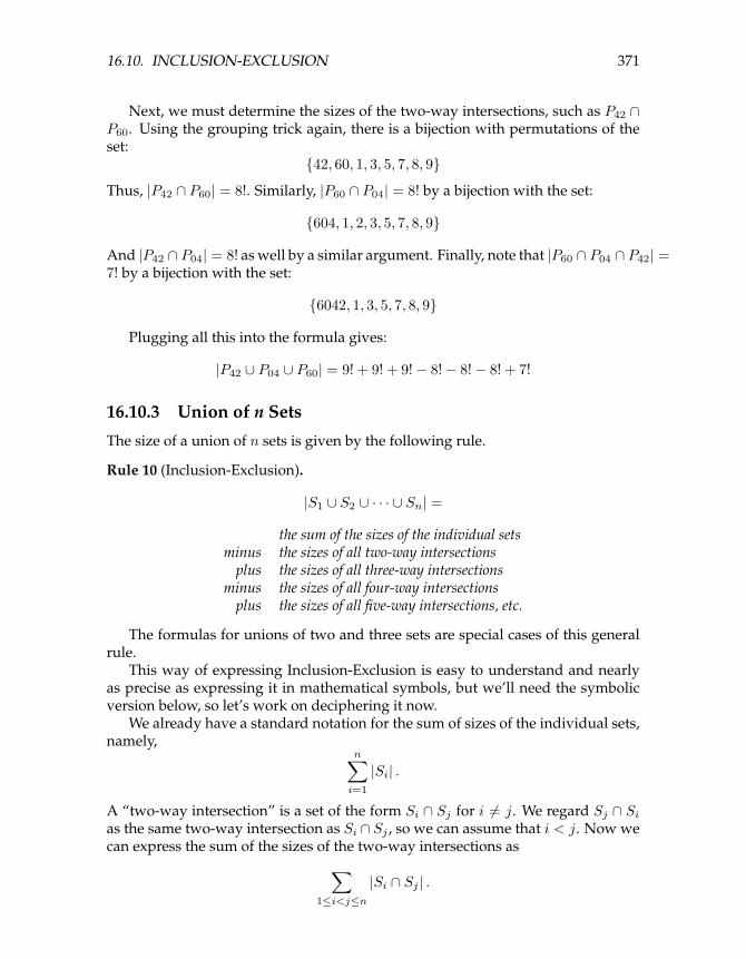
16.10. INCLUSION-EXCLUSION 371
Next, we must determine the sizes of the two-way intersections, such as P42 ∩P60. Using the grouping trick again, there is a bijection with permutations of theset:
{42, 60, 1, 3, 5, 7, 8, 9}
Thus, |P42 ∩ P60| = 8!. Similarly, |P60 ∩ P04| = 8! by a bijection with the set:
{604, 1, 2, 3, 5, 7, 8, 9}
And |P42 ∩ P04| = 8! as well by a similar argument. Finally, note that |P60 ∩ P04 ∩ P42| =7! by a bijection with the set:
{6042, 1, 3, 5, 7, 8, 9}
Plugging all this into the formula gives:
|P42 ∪ P04 ∪ P60| = 9! + 9! + 9!− 8!− 8!− 8! + 7!
16.10.3 Union of n Sets
The size of a union of n sets is given by the following rule.
Rule 10 (Inclusion-Exclusion).
|S1 ∪ S2 ∪ · · · ∪ Sn| =
the sum of the sizes of the individual setsminus the sizes of all two-way intersections
plus the sizes of all three-way intersectionsminus the sizes of all four-way intersections
plus the sizes of all five-way intersections, etc.
The formulas for unions of two and three sets are special cases of this generalrule.
This way of expressing Inclusion-Exclusion is easy to understand and nearlyas precise as expressing it in mathematical symbols, but we’ll need the symbolicversion below, so let’s work on deciphering it now.
We already have a standard notation for the sum of sizes of the individual sets,namely,
n∑i=1
|Si| .
A “two-way intersection” is a set of the form Si ∩ Sj for i 6= j. We regard Sj ∩ Sias the same two-way intersection as Si ∩ Sj , so we can assume that i < j. Now wecan express the sum of the sizes of the two-way intersections as∑
1≤i<j≤n
|Si ∩ Sj | .

372 CHAPTER 16. COUNTING
Similarly, the sum of the sizes of the three-way intersections is∑1≤i<j<k≤n
|Si ∩ Sj ∩ Sk| .
These sums have alternating signs in the Inclusion-Exclusion formula, with thesum of the k-way intersections getting the sign (−1)k−1. This finally leads to asymbolic version of the rule:
Rule (Inclusion-Exclusion).∣∣∣∣∣n⋃i=1
Si
∣∣∣∣∣ =n∑i=1
|Si|
−∑
1≤i<j≤n
|Si ∩ Sj |
+∑
1≤i<j<k≤n
|Si ∩ Sj ∩ Sk|+ · · ·
+ (−1)n−1
∣∣∣∣∣n⋂i=1
Si
∣∣∣∣∣ .16.10.4 Computing Euler’s Function
We will now use Inclusion-Exclusion to calculate Euler’s function, φ(n). By defini-tion, φ(n) is the number of nonnegative integers less than a positive integer n thatare relatively prime to n. But the set, S, of nonnegative integers less than n that arenot relatively prime to n will be easier to count.
Suppose the prime factorization of n is pe11 · · · pemm for distinct primes pi. Thismeans that the integers in S are precisely the nonnegative integers less than n thatare divisible by at least one of the pi’s. So, letting Ci be the set of nonnegativeintegers less than n that are divisible by pi, we have
S =m⋃i=1
Ci.
We’ll be able to find the size of this union using Inclusion-Exclusion becausethe intersections of the Ci’s are easy to count. For example, C1 ∩ C2 ∩ C3 is theset of nonnegative integers less than n that are divisible by each of p1, p2 and p3.But since the pi’s are distinct primes, being divisible by each of these primes is thatsame as being divisible by their product. Now observe that if r is a positive divisorof n, then exactly n/r nonnegative integers less than n are divisible by r, namely,0, r, 2r, . . . , ((n/r) − 1)r. So exactly n/p1p2p3 nonnegative integers less than n aredivisible by all three primes p1, p2, p3. In other words,
|C1 ∩ C2 ∩ C3| =n
p1p2p3.

16.10. INCLUSION-EXCLUSION 373
So reasoning this way about all the intersections among the Ci’s and applyingInclusion-Exclusion, we get
|S| =
∣∣∣∣∣m⋃i=1
Ci
∣∣∣∣∣=
m∑i=1
|Ci| −∑
1≤i<j≤m
|Ci ∩ Cj |+∑
1≤i<j<k≤m
|Ci ∩ Cj ∩ Ck| − · · ·+ (−1)m−1
∣∣∣∣∣m⋂i=1
Ci
∣∣∣∣∣=
m∑i=1
n
pi−
∑1≤i<j≤m
n
pipj+
∑1≤i<j<k≤m
n
pipjpk− · · ·+ (−1)m−1 n
p1p2 · · · pn
= n
m∑i=1
1pi−
∑1≤i<j≤m
1pipj
+∑
1≤i<j<k≤m
1pipjpk
− · · ·+ (−1)m−1 1p1p2 · · · pn
But φ(n) = n− |S| by definition, so
φ(n) = n
1−m∑i=1
1pi
+∑
1≤i<j≤m
1pipj
−∑
1≤i<j<k≤m
1pipjpk
+ · · ·+ (−1)m1
p1p2 · · · pn
= n
m∏i=1
(1− 1
pi
). (16.12)
Notice that in case n = pk for some prime, p, then (16.12) simplifies to
φ(pk) = pk(
1− 1p
)= pk − pk−1
as claimed in chapter 14.Quick Question: Why does equation (16.12) imply that
φ(ab) = φ(a)φ(b)
for relatively prime integers a, b > 1, as claimed in Theorem 14.7.1.(a)?
16.10.5 Problems
Practice Problems
Problem 16.22.The working days in the next year can be numbered 1, 2, 3, . . . , 300. I’d like toavoid as many as possible.
• On even-numbered days, I’ll say I’m sick.
• On days that are a multiple of 3, I’ll say I was stuck in traffic.

374 CHAPTER 16. COUNTING
• On days that are a multiple of 5, I’ll refuse to come out from under the blan-kets.
In total, how many work days will I avoid in the coming year?
Class Problems
Problem 16.23.A certain company wants to have security for their computer systems. So theyhave given everyone a name and password. A length 10 word containing each ofthe characters:
a, d, e, f, i, l, o, p, r, s,
is called a cword. A password will be a cword which does not contain any of thesubwords ”fails”, ”failed”, or ”drop”.
For example, the following two words are passwords:
adefiloprs, srpolifeda,
but the following three cwords are not:
adropeflis, failedrops, dropefails.
(a) How many cwords contain the subword “drop”?
(b) How many cwords contain both “drop” and “fails”?
(c) Use the Inclusion-Exclusion Principle to find a simple formula for the numberof passwords.
Homework Problems
Problem 16.24.How many paths are there from point (0, 0) to (50, 50) if every step incrementsone coordinate and leaves the other unchanged? How many are there when thereare impassable boulders sitting at points (10, 11) and (21, 20)? (You do not haveto calculate the number explicitly; your answer may be an expression involvingbinomial coefficients.)
Hint: Count the number of paths going through (10, 11), the number through(21, 20), and use Inclusion-Exclusion.
Problem 16.25.A derangement is a permutation (x1, x2, . . . , xn) of the set {1, 2, . . . , n} such thatxi 6= i for all i. For example, (2, 3, 4, 5, 1) is a derangement, but (2, 1, 3, 5, 4) is notbecause 3 appears in the third position. The objective of this problem is to countderangements.

16.10. INCLUSION-EXCLUSION 375
It turns out to be easier to start by counting the permutations that are not de-rangements. Let Si be the set of all permutations (x1, x2, . . . , xn) that are not de-rangements because xi = i. So the set of non-derangements is
n⋃i=1
Si.
(a) What is |Si|?
(b) What is |Si ∩ Sj |where i 6= j?
(c) What is |Si1 ∩ Si2 ∩ · · · ∩ Sik |where i1, i2, . . . , ik are all distinct?
(d) Use the inclusion-exclusion formula to express the number of non-derangementsin terms of sizes of possible intersections of the sets S1, . . . , Sn.
(e) How many terms in the expression in part (d) have the form |Si1 ∩ Si2 ∩ · · · ∩ Sik |?
(f) Combine your answers to the preceding parts to prove the number of non-derangements is:
n!(
11!− 1
2!+
13!− · · · ± 1
n!
).
Conclude that the number of derangements is
n!(
1− 11!
+12!− 1
3!+ · · · ± 1
n!
).
(g) As n goes to infinity, the number of derangements approaches a constant frac-tion of all permutations. What is that constant? Hint:
ex = 1 + x+x2
2!+x3
3!+ · · ·
Problem 16.26.How many of the numbers 2, . . . , n are prime? The Inclusion-Exclusion Principleoffers a useful way to calculate the answer when n is large. Actually, we will useInclusion-Exclusion to count the number of composite (nonprime) integers from 2to n. Subtracting this from n− 1 gives the number of primes.
Let Cn be the set of composites from 2 to n, and let Am be the set of numbersin the range m+ 1, . . . , n that are divisible by m. Notice that by definition, Am = ∅for m ≥ n. So
Cn =n−1⋃i=2
Ai. (16.13)
(a) Verify that if m | k, then Am ⊇ Ak.

376 CHAPTER 16. COUNTING
(b) Explain why the right hand side of (16.13) equals⋃primes p≤
√n
Ap. (16.14)
(c) Explain why |Am| = bn/mc − 1 for m ≥ 2.
(d) Consider any two relatively prime numbers p, q ≤ n. What is the one numberin (Ap ∩Aq)−Ap·q?
(e) Let P be a finite set of at least two primes. Give a simple formula for∣∣∣∣∣∣⋂p∈P
Ap
∣∣∣∣∣∣ .(f) Use the Inclusion-Exclusion principle to obtain a formula for |C150| in terms
the sizes of intersections among the setsA2, A3, A5, A7, A11. (Omit the intersectionsthat are empty; for example, any intersection of more than three of these sets mustbe empty.)
(g) Use this formula to find the number of primes up to 150.
16.11 Binomial Theorem
Counting gives insight into one of the basic theorems of algebra. A binomial is asum of two terms, such as a+ b. Now consider its 4th power, (a+ b)4.
If we multiply out this 4th power expression completely, we get
(a+ b)4 = aaaa + aaab + aaba + aabb+ abaa + abab + abba + abbb+ baaa + baab + baba + babb+ bbaa + bbab + bbba + bbbb
Notice that there is one term for every sequence of a’s and b’s. So there are 24
terms, and the number of terms with k copies of b and n− k copies of a is:
n!k! (n− k)!
=(n
k
)by the Bookkeeper Rule. Now let’s group equivalent terms, such as aaab = aaba =abaa = baaa. Then the coefficient of an−kbk is
(nk
). So for n = 4, this means:
(a+ b)4 =(
40
)· a4b0 +
(41
)· a3b1 +
(42
)· a2b2 +
(43
)· a1b3 +
(44
)· a0b4
In general, this reasoning gives the Binomial Theorem:

16.11. BINOMIAL THEOREM 377
Theorem 16.11.1 (Binomial Theorem). For all n ∈ N and a, b ∈ R:
(a+ b)n =n∑k=0
(n
k
)an−kbk
The expression(n
k
)is often called a “binomial coefficient” in honor of its ap-
pearance here.This reasoning about binomials extends nicely to multinomials, which are sums
of two or more terms. For example, suppose we wanted the coefficient of
bo2k2e3pr
in the expansion of (b+o+k+e+p+r)10. Each term in this expansion is a productof 10 variables where each variable is one of b, o, k, e, p, or r. Now, the coefficientof bo2k2e3pr is the number of those terms with exactly 1 b, 2 o’s, 2 k’s, 3 e’s, 1 p, and1 r. And the number of such terms is precisely the number of rearrangments of theword BOOKKEEPER: (
101, 2, 2, 3, 1, 1
)=
10!1! 2! 2! 3! 1! 1!
.
The expression on the left is called a “multinomial coefficient.” This reasoningextends to a general theorem.
Definition 16.11.2. For n, k1, . . . , km ∈ naturals, such that k1 + k2 + · · ·+ km = n,define the multinomial coefficient(
n
k1, k2, . . . , km
)::=
n!k1! k2! . . . km!
.
Theorem 16.11.3 (Multinomial Theorem). For all n ∈ N and z1, . . . zm ∈ R:
(z1 + z2 + · · ·+ zm)n =∑
k1,...,km∈Nk1+···+km=n
(n
k1, k2, . . . , km
)zk11 zk22 · · · zkmm
You’ll be better off remembering the reasoning behind the Multinomial Theo-rem rather than this ugly formal statement.
16.11.1 Problems
Practice Problems
Problem 16.27.Find the coefficients of x10y5 in (19x+ 4y)15

378 CHAPTER 16. COUNTING
Class Problems
Problem 16.28.Find the coefficients of(a) x5 in (1 + x)11
(b) x8y9 in (3x+ 2y)17
(c) a6b6 in (a2 + b3)5
Problem 16.29. (a) Use the Multinomial Theorem 16.11.3 to prove that
(x1 + x2 + · · ·+ xn)p ≡ xp1 + xp2 + · · ·+ xpn (mod p) (16.15)
for all primes p. (Do not prove it using Fermat’s “little” Theorem. The point of thisproblem is to offer an independent proof of Fermat’s theorem.)
Hint: Explain why(
pk1,k2,...,kn
)is divisible by p if all the ki’s are positive integers
less than p.
(b) Explain how (16.15) immediately proves Fermat’s Little Theorem 14.6.4: np−1 ≡1 (mod p) when n is not a multiple of p.
Homework Problems
Problem 16.30.The degree sequence of a simple graph is the weakly decreasing sequence of de-grees of its vertices. For example, the degree sequence for the 5-vertex num-bered tree pictured in the Figure 16.2 is (2, 2, 2, 1, 1) and for the 7-vertex tree itis (3, 3, 2, 1, 1, 1, 1).
We’re interested in counting how many numbered trees there are with a givendegree sequence. We’ll do this using the bijection defined in Problem 16.5 betweenn-vertex numbered trees and length n−2 code words whose characters are integersbetween 1 and n.
The occurrence number for a character in a word is the number of times thatthe character occurs in the word. For example, in the word 65622, the occur-rence number for 6 is two, and the occurrence number for 5 is one. The occurrencesequence of a word is the weakly decreasing sequence of occurrence numbers ofcharacters in the word. The occurrence sequence for this word is (2, 2, 1) becauseit has two occurrences of each of the characters 6 and 2, and one occurrence of 5.(a) There is simple relationship between the degree sequence of an n-vertex num-
bered tree and the occurrence sequence of its code. Describe this relationship andexplain why it holds. Conclude that counting n-vertex numbered trees with agiven degree sequence is the same as counting the number of length n − 2 codewords with a given occurrence sequence.
Hint: How many times does a vertex of degree, d, occur in the code?

16.11. BINOMIAL THEOREM 379
Figure 16.2:
For simplicity, let’s focus on counting 9-vertex numbered trees with a givendegree sequence. By part (a), this is the same as counting the number of length 7code words with a given occurrence sequence.
Any length 7 code word has a pattern, which is another length 7 word over thealphabet a,b,c,d,e,f,g that has the same occurrence sequence.(b) How many length 7 patterns are there with three occurrences of a, two occur-
rences of b, and one occurrence of c and d?(c) How many ways are there to assign occurrence numbers to integers 1, 2, . . . , 9
so that a code word with those occurrence numbers would have the occurrencesequence 3, 2, 1, 1, 0, 0, 0, 0, 0?In general, to find the pattern of a code word, list its characters in decreasing or-der by number of occurrences, and list characters with the same number of occur-rences in decreasing order. Then replace successive characters in the list by suc-cessive letters a,b,c,d,e,f,g. The code word 2468751, for example, has thepattern fecabdg, which is obtained by replacing its characters 8,7,6,5,4,2,1by a,b,c,d,e,f,g, respectively. The code word 2449249 has pattern caabcab,which is obtained by replacing its characters 4,9,2 by a,b,c, respectively.

380 CHAPTER 16. COUNTING
(d) What length 7 code word has three occurrences of 7, two occurrences of 8, oneoccurrence each of 2 and 9, and pattern abacbad?
(e) Explain why the number of 9-vertex numbered trees with degree sequence(4, 3, 2, 2, 1, 1, 1, 1, 1) is the product of the answers to parts (b) and (c).
16.12 Combinatorial Proof
Suppose you have n different T-shirts, but only want to keep k. You could equallywell select the k shirts you want to keep or select the complementary set of n − kshirts you want to throw out. Thus, the number of ways to select k shirts fromamong n must be equal to the number of ways to select n− k shirts from among n.Therefore: (
n
k
)=(
n
n− k
)This is easy to prove algebraically, since both sides are equal to:
n!k! (n− k)!
But we didn’t really have to resort to algebra; we just used counting principles.Hmm.
16.12.1 Boxing
Jay, famed 6.042 TA, has decided to try out for the US Olympic boxing team. Afterall, he’s watched all of the Rocky movies and spent hours in front of a mirror sneer-ing, “Yo, you wanna piece a’ me?!” Jay figures that n people (including himself)are competing for spots on the team and only k will be selected. As part of maneu-vering for a spot on the team, he needs to work out how many different teams arepossible. There are two cases to consider:
• Jay is selected for the team, and his k−1 teammates are selected from amongthe other n−1 competitors. The number of different teams that can be formedin this way is: (
n− 1k − 1
)• Jay is not selected for the team, and all k team members are selected from
among the other n− 1 competitors. The number of teams that can be formedthis way is: (
n− 1k
)

16.12. COMBINATORIAL PROOF 381
All teams of the first type contain Jay, and no team of the second type does;therefore, the two sets of teams are disjoint. Thus, by the Sum Rule, the total num-ber of possible Olympic boxing teams is:(
n− 1k − 1
)+(n− 1k
)Jeremy, equally-famed 6.042 TA, thinks Jay isn’t so tough and so he might as
well also try out. He reasons that n people (including himself) are trying out for kspots. Thus, the number of ways to select the team is simply:(
n
k
)Jeremy and Jay each correctly counted the number of possible boxing teams;
thus, their answers must be equal. So we know:(n− 1k − 1
)+(n− 1k
)=(n
k
)This is called Pascal’s Identity. And we proved it without any algebra! Instead, werelied purely on counting techniques.
16.12.2 Finding a Combinatorial Proof
A combinatorial proof is an argument that establishes an algebraic fact by relying oncounting principles. Many such proofs follow the same basic outline:
1. Define a set S.
2. Show that |S| = n by counting one way.
3. Show that |S| = m by counting another way.
4. Conclude that n = m.
In the preceding example, S was the set of all possible Olympic boxing teams. Jaycomputed
|S| =(n− 1k − 1
)+(n− 1k
)by counting one way, and Jeremy computed
|S| =(n
k
)by counting another. Equating these two expressions gave Pascal’s Identity.
More typically, the set S is defined in terms of simple sequences or sets ratherthan an elaborate story. Here is less colorful example of a combinatorial argument.

382 CHAPTER 16. COUNTING
Theorem 16.12.1.n∑r=0
(n
r
)(2nn− r
)=(
3nn
)Proof. We give a combinatorial proof. Let S be all n-card hands that can be dealtfrom a deck containing n red cards (numbered 1, . . . , n) and 2n black cards (num-bered 1, . . . , 2n). First, note that every 3n-element set has
|S| =(
3nn
)n-element subsets.
From another perspective, the number of hands with exactly r red cards is(n
r
)(2nn− r
)since there are
(nr
)ways to choose the r red cards and
(2nn−r)
ways to choose then− r black cards. Since the number of red cards can be anywhere from 0 to n, thetotal number of n-card hands is:
|S| =n∑r=0
(n
r
)(2nn− r
)Equating these two expressions for |S| proves the theorem. �
Combinatorial proofs are almost magical. Theorem 16.12.1 looks pretty scary,but we proved it without any algebraic manipulations at all. The key to construct-ing a combinatorial proof is choosing the set S properly, which can be tricky. Gen-erally, the simpler side of the equation should provide some guidance. For exam-ple, the right side of Theorem 16.12.1 is
(3nn
), which suggests choosing S to be all
n-element subsets of some 3n-element set.
16.12.3 Problems
Class Problems
Problem 16.31.According to the Multinomial theorem, (w+x+ y+ z)n can be expressed as a sumof terms of the form (
n
r1, r2, r3, r4
)wr1xr2yr3zr4 .
(a) How many terms are there in the sum?
(b) The sum of these multinomial coefficients has an easily expressed value. Whatis it? ∑
r1+r2+r3+r4=n,ri∈N
(n
r1, r2, r3, r4
)=? (16.16)

16.12. COMBINATORIAL PROOF 383
Hint: How many terms are there when (w + x + y + z)n is expressed as a sum ofmonomials inw, x, y, z before terms with like powers of these variables are collectedtogether under a single coefficient?
Homework Problems
Problem 16.32.Prove the following identity by algebraic manipulation and by giving a combina-torial argument: (
n
r
)(r
k
)=(n
k
)(n− kr − k
)
Problem 16.33. (a) Find a combinatorial (not algebraic) proof that
n∑i=0
(n
i
)= 2n.
(b) Below is a combinatorial proof of an equation. What is the equation?
Proof. Stinky Peterson owns n newts, t toads, and s slugs. Conveniently, he livesin a dorm with n + t + s other students. (The students are distinguishable, butcreatures of the same variety are not distinguishable.) Stinky wants to put onecreature in each neighbor’s bed. Let W be the set of all ways in which this can bedone.
On one hand, he could first determine who gets the slugs. Then, he could decidewho among his remaining neighbors has earned a toad. Therefore, |W | is equal tothe expression on the left.
On the other hand, Stinky could first decide which people deserve newts and slugsand then, from among those, determine who truly merits a newt. This shows that|W | is equal to the expression on the right.
Since both expressions are equal to |W |, they must be equal to each other. �
(Combinatorial proofs are real proofs. They are not only rigorous, but also con-vey an intuitive understanding that a purely algebraic argument might not reveal.However, combinatorial proofs are usually less colorful than this one.)
Problem 16.34.According to the Multinomial Theorem 16.11.3, (x1+x2+...+xk)n can be expressedas a sum of terms of the form(
n
r1, r2, ..., rk
)xr11 x
r22 ...x
rkk .

384 CHAPTER 16. COUNTING
(a) How many terms are there in the sum?
(b) The sum of these multinomial coefficients has an easily expressed value:
∑r1+r2+...+rk=n,
ri∈N
(n
r1, r2, ..., rk
)= kn (16.17)
Give a combinatorial proof of this identity.
Hint: How many terms are there when (x1 + x2 + ...+ xk)n is expressed as a sumof monomials in xi before terms with like powers of these variables are collectedtogether under a single coefficient?
Problem 16.35.Give combinatorial proofs of the identities below. Use the following structure foreach proof. First, define an appropriate set S. Next, show that the left side ofthe equation counts the number of elements in S. Then show that, from anotherperspective, the right side of the equation also counts the number of elements inset S. Conclude that the left side must be equal to the right, since both are equal to|S|.(a) (
2nn
)=
n∑k=0
(n
k
)·(
n
n− k
)(b)
r∑i=0
(n+ i
i
)=(n+ r + 1
r
)Hint: consider a set of binary strings that could be counted using the right side ofthe equation, then try partitioning them into subsets countable by the elements ofthe sum on the left.

Chapter 17
Generating Functions
Generating Functions are one of the most surprising and useful inventions in Dis-crete Math. Roughly speaking, generating functions transform problems aboutsequences into problems about functions. This is great because we’ve got piles ofmathematical machinery for manipulating functions. Thanks to generating func-tions, we can apply all that machinery to problems about sequences. In this way,we can use generating functions to solve all sorts of counting problems. There is ahuge chunk of mathematics concerning generating functions, so we will only get ataste of the subject.
In this chapter, we’ll put sequences in angle brackets to more clearly distinguishthem from the many other mathematical expressions floating around.
The ordinary generating function for 〈g0, g1, g2, g3 . . . 〉 is the power series:
G(x) = g0 + g1x+ g2x2 + g3x
3 + · · · .
There are a few other kinds of generating functions in common use, but ordinarygenerating functions are enough to illustrate the power of the idea, so we’ll stickto them. So from now on generating function will mean the ordinary kind.
A generating function is a “formal” power series in the sense that we usuallyregard x as a placeholder rather than a number. Only in rare cases will we actu-ally evaluate a generating function by letting x take a real number value, so wegenerally ignore the issue of convergence.
Throughout this chapter, we’ll indicate the correspondence between a sequenceand its generating function with a double-sided arrow as follows:
〈g0, g1, g2, g3, . . . 〉 ←→ g0 + g1x+ g2x2 + g3x
3 + · · ·
For example, here are some sequences and their generating functions:
〈0, 0, 0, 0, . . . 〉 ←→ 0 + 0x+ 0x2 + 0x3 + · · · = 0
〈1, 0, 0, 0, . . . 〉 ←→ 1 + 0x+ 0x2 + 0x3 + · · · = 1
〈3, 2, 1, 0, . . . 〉 ←→ 3 + 2x+ 1x2 + 0x3 + · · · = 3 + 2x+ x2
385

386 CHAPTER 17. GENERATING FUNCTIONS
The pattern here is simple: the ith term in the sequence (indexing from 0) is thecoefficient of xi in the generating function.
Recall that the sum of an infinite geometric series is:
1 + z + z2 + z3 + · · · = 11− z
This equation does not hold when |z| ≥ 1, but as remarked, we don’t worry aboutconvergence issues. This formula gives closed form generating functions for awhole range of sequences. For example:
〈1, 1, 1, 1, . . . 〉 ←→ 1 + x+ x2 + x3 + · · · =1
1− x
〈1,−1, 1,−1, . . . 〉 ←→ 1− x+ x2 − x3 + x4 − · · · =1
1 + x⟨1, a, a2, a3, . . .
⟩←→ 1 + ax+ a2x2 + a3x3 + · · · =
11− ax
〈1, 0, 1, 0, 1, 0, . . . 〉 ←→ 1 + x2 + x4 + x6 + · · · =1
1− x2
17.1 Operations on Generating Functions
The magic of generating functions is that we can carry out all sorts of manipu-lations on sequences by performing mathematical operations on their associatedgenerating functions. Let’s experiment with various operations and characterizetheir effects in terms of sequences.
17.1.1 Scaling
Multiplying a generating function by a constant scales every term in the associatedsequence by the same constant. For example, we noted above that:
〈1, 0, 1, 0, 1, 0, . . . 〉 ←→ 1 + x2 + x4 + x6 + · · · = 11− x2
Multiplying the generating function by 2 gives
21− x2
= 2 + 2x2 + 2x4 + 2x6 + · · ·
which generates the sequence:
〈2, 0, 2, 0, 2, 0, . . . 〉

17.1. OPERATIONS ON GENERATING FUNCTIONS 387
Rule 11 (Scaling Rule). If
〈f0, f1, f2, . . . 〉 ←→ F (x),
then〈cf0, cf1, cf2, . . . 〉 ←→ c · F (x).
The idea behind this rule is that:
〈cf0, cf1, cf2, . . . 〉 ←→ cf0 + cf1x+ cf2x2 + · · ·
= c · (f0 + f1x+ f2x2 + · · · )
= cF (x)
17.1.2 Addition
Adding generating functions corresponds to adding the two sequences term byterm. For example, adding two of our earlier examples gives:
〈 1, 1, 1, 1, 1, 1, . . . 〉 ←→ 11− x
+ 〈 1, −1, 1, −1, 1, −1, . . . 〉 ←→ 11 + x
〈 2, 0, 2, 0, 2, 0, . . . 〉 ←→ 11− x
+1
1 + x
We’ve now derived two different expressions that both generate the sequence 〈2, 0, 2, 0, . . . 〉.They are, of course, equal:
11− x
+1
1 + x=
(1 + x) + (1− x)(1− x)(1 + x)
=2
1− x2
Rule 12 (Addition Rule). If
〈f0, f1, f2, . . . 〉 ←→ F (x), and〈g0, g1, g2, . . . 〉 ←→ G(x),
then〈f0 + g0, f1 + g1, f2 + g2, . . . 〉 ←→ F (x) +G(x).
The idea behind this rule is that:
〈f0 + g0, f1 + g1, f2 + g2, . . . 〉 ←→∞∑n=0
(fn + gn)xn
=
( ∞∑n=0
fnxn
)+
( ∞∑n=0
gnxn
)= F (x) +G(x)

388 CHAPTER 17. GENERATING FUNCTIONS
17.1.3 Right Shifting
Let’s start over again with a simple sequence and its generating function:
〈1, 1, 1, 1, . . . 〉 ←→ 11− x
Now let’s right-shift the sequence by adding k leading zeros:
〈0, 0, . . . , 0︸ ︷︷ ︸k zeroes
, 1, 1, 1, . . . 〉 ←→ xk + xk+1 + xk+2 + xk+3 + · · ·
= xk · (1 + x+ x2 + x3 + · · · )
=xk
1− x
Evidently, adding k leading zeros to the sequence corresponds to multiplying thegenerating function by xk. This holds true in general.
Rule 13 (Right-Shift Rule). If 〈f0, f1, f2, . . . 〉 ←→ F (x), then:
〈0, 0, . . . , 0︸ ︷︷ ︸k zeroes
, f0, f1, f2, . . . 〉 ←→ xk · F (x)
The idea behind this rule is that:
〈k zeroes︷ ︸︸ ︷
0, 0, . . . , 0, f0, f1, f2, . . . 〉 ←→ f0xk + f1x
k+1 + f2xk+2 + · · ·
= xk · (f0 + f1x+ f2x2 + f3x
3 + · · · )= xk · F (x)
17.1.4 Differentiation
What happens if we take the derivative of a generating function? As an example,let’s differentiate the now-familiar generating function for an infinite sequence of1’s.
d
dx(1 + x+ x2 + x3 + x4 + · · · ) =
d
dx
(1
1− x
)1 + 2x+ 3x2 + 4x3 + · · · =
1(1− x)2
(17.1)
〈1, 2, 3, 4, . . . 〉 ←→ 1(1− x)2
We found a generating function for the sequence 〈1, 2, 3, 4, . . . 〉 of positive integers!In general, differentiating a generating function has two effects on the corre-
sponding sequence: each term is multiplied by its index and the entire sequence isshifted left one place.

17.1. OPERATIONS ON GENERATING FUNCTIONS 389
Rule 14 (Derivative Rule). If
〈f0, f1, f2, f3, . . . 〉 ←→ F (x),
then〈f1, 2f2, 3f3, . . . 〉 ←→ F ′(x).
The idea behind this rule is that:
〈f1, 2f2, 3f3, . . . 〉 ←→ f1 + 2f2x+ 3f3x2 + · · ·
=d
dx(f0 + f1x+ f2x
2 + f3x3 + · · · )
=d
dxF (x)
The Derivative Rule is very useful. In fact, there is frequent, independent needfor each of differentiation’s two effects, multiplying terms by their index and left-shifting one place. Typically, we want just one effect and must somehow cancel outthe other. For example, let’s try to find the generating function for the sequence ofsquares, 〈0, 1, 4, 9, 16, . . . 〉. If we could start with the sequence 〈1, 1, 1, 1, . . . 〉 andmultiply each term by its index two times, then we’d have the desired result:
〈0 · 0, 1 · 1, 2 · 2, 3 · 3, . . . 〉 = 〈0, 1, 4, 9, . . . 〉
A challenge is that differentiation not only multiplies each term by its index, butalso shifts the whole sequence left one place. However, the Right-Shift Rule 13 tellshow to cancel out this unwanted left-shift: multiply the generating function by x.
Our procedure, therefore, is to begin with the generating function for 〈1, 1, 1, 1, . . . 〉,differentiate, multiply by x, and then differentiate and multiply by x once more.
〈1, 1, 1, 1, . . . 〉 ←→ 11− x
〈1, 2, 3, 4, . . . 〉 ←→ d
dx
11− x
=1
(1− x)2
〈0, 1, 2, 3, . . . 〉 ←→ x · 1(1− x)2
=x
(1− x)2
〈1, 4, 9, 16, . . . 〉 ←→ d
dx
x
(1− x)2=
1 + x
(1− x)3
〈0, 1, 4, 9, . . . 〉 ←→ x · 1 + x
(1− x)3=x(1 + x)(1− x)3
Thus, the generating function for squares is:
x(1 + x)(1− x)3
(17.2)

390 CHAPTER 17. GENERATING FUNCTIONS
17.1.5 Products
Rule 15 ( Product Rule). If
〈a0, a1, a2, . . . 〉 ←→ A(x), and 〈b0, b1, b2, . . . 〉 ←→ B(x),
then〈c0, c1, c2, . . . 〉 ←→ A(x) ·B(x),
wherecn ::= a0bn + a1bn−1 + a2bn−2 + · · ·+ anb0.
To understand this rule, let
C(x) ::=A(x) ·B(x) =∞∑n=0
cnxn.
We can evaluate the product A(x) · B(x) by using a table to identify all thecross-terms from the product of the sums:
b0x0 b1x
1 b2x2 b3x
3 . . .
a0x0 a0b0x
0 a0b1x1 a0b2x
2 a0b3x3 . . .
a1x1 a1b0x
1 a1b1x2 a1b2x
3 . . .
a2x2 a2b0x
2 a2b1x3 . . .
a3x3 a3b0x
3 . . .
... . . .
Notice that all terms involving the same power of x lie on a /-sloped diagonal.Collecting these terms together, we find that the coefficient of xn in the product isthe sum of all the terms on the (n+ 1)st diagonal, namely,
a0bn + a1bn−1 + a2bn−2 + · · ·+ anb0. (17.3)
This expression (17.3) may be familiar from a signal processing course; the se-quence 〈c0, c1, c2, . . . 〉 is called the convolution of sequences 〈a0, a1, a2, . . . 〉 and 〈b0, b1, b2, . . . 〉.
17.2 The Fibonacci Sequence
Sometimes we can find nice generating functions for more complicated sequences.For example, here is a generating function for the Fibonacci numbers:
〈0, 1, 1, 2, 3, 5, 8, 13, 21, . . . 〉 ←→ x
1− x− x2

17.2. THE FIBONACCI SEQUENCE 391
The Fibonacci numbers may seem like a fairly nasty bunch, but the generatingfunction is simple!
We’re going to derive this generating function and then use it to find a closedform for the nth Fibonacci number. The techniques we’ll use are applicable to alarge class of recurrence equations.
17.2.1 Finding a Generating Function
Let’s begin by recalling the definition of the Fibonacci numbers:
f0 = 0f1 = 1fn = fn−1 + fn−2 (for n ≥ 2)
We can expand the final clause into an infinite sequence of equations. Thus, theFibonacci numbers are defined by:
f0 =0f1 =1f2 =f1 + f0
f3 =f2 + f1
f4 =f3 + f2
...
Now the overall plan is to define a function F (x) that generates the sequence onthe left side of the equality symbols, which are the Fibonacci numbers. Then wederive a function that generates the sequence on the right side. Finally, we equatethe two and solve for F (x). Let’s try this. First, we define:
F (x) = f0 + f1x+ f2x2 + f3x
3 + f4x4 + · · ·
Now we need to derive a generating function for the sequence:
〈0, 1, f1 + f0, f2 + f1, f3 + f2, . . . 〉
One approach is to break this into a sum of three sequences for which we knowgenerating functions and then apply the Addition Rule:
〈 0, 1, 0, 0, 0, . . . 〉 ←→ x〈 0, f0, f1, f2, f3, . . . 〉 ←→ xF (x)
+ 〈 0, 0, f0, f1, f2, . . . 〉 ←→ x2F (x)〈 0, 1 + f0, f1 + f0, f2 + f1, f3 + f2, . . . 〉 ←→ x+ xF (x) + x2F (x)
This sequence is almost identical to the right sides of the Fibonacci equations. Theone blemish is that the second term is 1 + f0 instead of simply 1. However, thisamounts to nothing, since f0 = 0 anyway.

392 CHAPTER 17. GENERATING FUNCTIONS
Now if we equate F (x) with the new function x+ xF (x) + x2F (x), then we’reimplicitly writing down all of the equations that define the Fibonacci numbers inone fell swoop:
F (x) = f0 + f1 x + f2 x2 + f3 x3 + · · ·q q q q q
x+ xF (x) + x2F (x) = 0 + (1 + f0) x + (f1 + f0) x2 + (f2 + f1) x3 + · · ·
Solving for F (x) gives the generating function for the Fibonacci sequence:
F (x) = x+ xF (x) + x2F (x)
soF (x) =
x
1− x− x2.
Sure enough, this is the simple generating function we claimed at the outset.
17.2.2 Finding a Closed Form
Why should one care about the generating function for a sequence? There are sev-eral answers, but here is one: if we can find a generating function for a sequence,then we can often find a closed form for the nth coefficient— which can be prettyuseful! For example, a closed form for the coefficient of xn in the power series forx/(1− x− x2) would be an explicit formula for the nth Fibonacci number.
So our next task is to extract coefficients from a generating function. There areseveral approaches. For a generating function that is a ratio of polynomials, wecan use the method of partial fractions, which you learned in calculus. Just as theterms in a partial fraction expansion are easier to integrate, the coefficients of thoseterms are easy to compute.
Let’s try this approach with the generating function for Fibonacci numbers.First, we factor the denominator:
1− x− x2 = (1− α1x)(1− α2x)
where α1 = 12 (1+
√5) and α2 = 1
2 (1−√
5). Next, we find A1 and A2 which satisfy:
x
1− x− x2=
A1
1− α1x+
A2
1− α2x
We do this by plugging in various values of x to generate linear equations in A1
and A2. We can then find A1 and A2 by solving a linear system. This gives:
A1 =1
α1 − α2=
1√5
A2 =−1
α1 − α2= − 1√
5

17.2. THE FIBONACCI SEQUENCE 393
Substituting into the equation above gives the partial fractions expansion ofF (x):
x
1− x− x2=
1√5
(1
1− α1x− 1
1− α2x
)Each term in the partial fractions expansion has a simple power series given by thegeometric sum formula:
11− α1x
= 1 + α1x+ α21x
2 + · · ·
11− α2x
= 1 + α2x+ α22x
2 + · · ·
Substituting in these series gives a power series for the generating function:
F (x) =1√5
(1
1− α1x− 1
1− α2x
)=
1√5
((1 + α1x+ α2
1x2 + · · · )− (1 + α2x+ α2
2x2 + · · · )
),
so
fn =αn1 − αn2√
5
=1√5
((1 +√
52
)n−
(1−√
52
)n)
This formula may be scary and astonishing —it’s not even obvious that itsvalue is an integer —but it’s very useful. For example, it provides (via the re-peated squaring method) a much more efficient way to compute Fibonacci num-bers than crunching through the recurrence, and it also clearly reveals the expo-nential growth of these numbers.
17.2.3 Problems
Class Problems
Problem 17.1.The famous mathematician, Fibonacci, has decided to start a rabbit farm to fill uphis time while he’s not making new sequences to torment future college students.Fibonacci starts his farm on month zero (being a mathematician), and at the startof month one he receives his first pair of rabbits. Each pair of rabbits takes a monthto mature, and after that breeds to produce one new pair of rabbits each month.Fibonacci decides that in order never to run out of rabbits or money, every time abatch of new rabbits is born, he’ll sell a number of newborn pairs equal to the totalnumber of pairs he had three months earlier. Fibonacci is convinced that this wayhe’ll never run out of stock.

394 CHAPTER 17. GENERATING FUNCTIONS
(a) Define the number, rn, of pairs of rabbits Fibonacci has in month n, using arecurrence relation. That is, define rn in terms of various ri where i < n.
(b) Let R(x) be the generating function for rabbit pairs,
R(x) ::= r0 + r1x+ r2x2 + ·.
Express R(x) as a quotient of polynomials.
(c) Find a partial fraction decomposition of the generating function R(x).
(d) Finally, use the partial fraction decomposition to come up with a closed formexpression for the number of pairs of rabbits Fibonacci has on his farm on monthn.
Problem 17.2.Less well-known than the Towers of Hanoi —but no less fascinating —are the Tow-ers of Sheboygan. As in Hanoi, the puzzle in Sheboygan involves 3 posts and ndisks of different sizes. Initially, all the disks are on post #1:
Post #1 Post #2 Post #3
The objective is to transfer all n disks to post #2 via a sequence of moves. Amove consists of removing the top disk from one post and dropping it onto an-other post with the restriction that a larger disk can never lie above a smaller disk.Furthermore, a local ordinance requires that a disk can be moved only from a post tothe next post on its right —or from post #3 to post #1. Thus, for example, moving adisk directly from post #1 to post #3 is not permitted.(a) One procedure that solves the Sheboygan puzzle is defined recursively: to
move an initial stack of n disks to the next post, move the top stack of n − 1 disksto the furthest post by moving it to the next post two times, then move the big, nthdisk to the next post, and finally move the top stack another two times to land ontop of the big disk. Let sn be the number of moves that this procedure uses. Writea simple linear recurrence for sn.
(b) Let S(x) be the generating function for the sequence 〈s0, s1, s2, . . . 〉. Show thatS(x) is a quotient of polynomials.

17.2. THE FIBONACCI SEQUENCE 395
(c) Give a simple formula for sn.
(d) A better (indeed optimal, but we won’t prove this) procedure to solve theTowers of Sheboygan puzzle can be defined in terms of two mutually recursiveprocedures, procedure P1(n) for moving a stack of n disks 1 pole forward, andP2(n) for moving a stack of n disks 2 poles forward. This is trivial for n = 0. Forn > 0, define:
P1(n): Apply P2(n− 1) to move the top n− 1 disks two poles forward to the thirdpole. Then move the remaining big disk once to land on the second pole. Thenapply P2(n− 1) again to move the stack of n− 1 disks two poles forward from thethird pole to land on top of the big disk.
P2(n): Apply P2(n − 1) to move the top n − 1 disks two poles forward to landon the third pole. Then move the remaining big disk to the second pole. Thenapply P1(n − 1) to move the stack of n − 1 disks one pole forward to land on thefirst pole. Now move the big disk 1 pole forward again to land on the third pole.Finally, apply P2(n − 1) again to move the stack of n − 1 disks two poles forwardto land on the big disk.
Let tn be the number of moves needed to solve the Sheboygan puzzle using proce-dure P1(n). Show that
tn = 2tn−1 + 2tn−2 + 3, (17.4)
for n > 1.
Hint: Let sn be the number of moves used by procedure P2(n). Express each of tnand sn as linear combinations of tn−1 and sn−1 and solve for tn.
(e) Derive values a, b, c, α, β such that
tn = aαn + bβn + c.
Conclude that tn = o(sn).
Homework Problems
Problem 17.3.Taking derivatives of generating functions is another useful operation. This is donetermwise, that is, if
F (x) = f0 + f1x+ f2x2 + f3x
3 + · · · ,
thenF ′(x) ::= f1 + 2f2x+ 3f3x2 + · · · .
For example,1
(1− x)2=(
1(1− x)
)′= 1 + 2x+ 3x2 + · · ·

396 CHAPTER 17. GENERATING FUNCTIONS
soH(x) ::=
x
(1− x)2= 0 + 1x+ 2x2 + 3x3 + · · ·
is the generating function for the sequence of nonegative integers. Therefore
1 + x
(1− x)3= H ′(x) = 1 + 22x+ 32x2 + 42x3 + · · · ,
sox2 + x
(1− x)3= xH ′(x) = 0 + 1x+ 22x2 + 32x3 + · · ·+ n2xn + · · ·
is the generating function for the nonegative integer squares.(a) Prove that for all k ∈ N, the generating function for the nonnegative integerkth powers is a quotient of polynomials in x. That is, for all k ∈ N there arepolynomials Rk(x) and Sk(x) such that
[xn](Rk(x)Sk(x)
)= nk. (17.5)
Hint: Observe that the derivative of a quotient of polynomials is also a quotient ofpolynomials. It is not necessary work out explicit formulas for Rk and Sk to provethis part.
(b) Conclude that if f(n) is a function on the nonnegative integers defined recur-sively in the form
f(n) = af(n− 1) + bf(n− 2) + cf(n− 3) + p(n)αn
where the a, b, c, α ∈ C and p is a polynomial with complex coefficients, then thegenerating function for the sequence f(0), f(1), f(2), . . . will be a quotient of poly-nomials in x, and hence there is a closed form expression for f(n).
Hint: ConsiderRk(αx)Sk(αx)
Problem 17.4.Generating functions provide an interesting way to count the number of strings ofmatched parentheses. To do this, we’ll use the description of these strings givenin Definition 11.1.2 as the set, GoodCount, of strings of parentheses with a goodcount. Let cn be the number of strings in GoodCount with exactly n left parenthe-ses, and let C(x) be the generating function for these numbers:
C(x) ::= c0 + c1x+ c2x2 + · · · .

17.2. THE FIBONACCI SEQUENCE 397
(a) The wrap of a string, s, is the string, (s), that starts with a left parenthesisfollowed by the characters of s, and then ends with a right parenthesis. Explainwhy the generating function for the wraps of strings with a good count is xC(x).
Hint: The wrap of a string with good count also has a good count that starts andends with 0 and remains positive everywhere else.
(b) Explain why, for every string, s, with a good count, there is a unique sequenceof strings s1, . . . , sk that are wraps of strings with good counts and s = s1 · · · sk.For example, the string r ::= (())()(()()) ∈ GoodCount equals s1s2s3 where s1 =(()), s2 = (), s3 = (()()), and this is the only way to express r as a sequence ofwraps of strings with good counts.
(c) Conclude that
C = 1 + xC + (xC)2 + · · ·+ (xC)n + · · · , (17.6)
so
C =1
1− xC, (17.7)
and hence
C =1±√
1− 4x2x
. (17.8)
Let D(x) ::= 2xC(x). Expressing D as a power series
D(x) = d0 + d1x+ d2x2 + · · · ,
we have
cn =dn+1
2. (17.9)
(d) Use (17.12), (17.13), and the value of c0 to conclude that
D(x) = 1−√
1− 4x.
(e) Prove that
dn =(2n− 3) · (2n− 5) · · · 5 · 3 · 1 · 2n
n!.
Hint: dn = D(n)(0)/n!
(f) Conclude that
cn =1
n+ 1
(2nn
).

398 CHAPTER 17. GENERATING FUNCTIONS
Exam Problems
Problem 17.5.Define the sequence r0, r1, r2, . . . recursively by the rule that r0 = r1 = 0 and
rn = 7rn−1 + 4rn−2 + (n+ 1),
for n ≥ 2. Express the generating function of this sequence as a quotient of poly-nomials or products of polynomials. You do not have to find a closed form forrn.
17.3 Counting with Generating Functions
Generating functions are particularly useful for solving counting problems. In par-ticular, problems involving choosing items from a set often lead to nice generatingfunctions by letting the coefficient of xn be the number of ways to choose n items.
17.3.1 Choosing Distinct Items from a Set
The generating function for binomial coefficients follows directly from the Bino-mial Theorem:⟨(
k
0
),
(k
1
),
(k
2
), . . . ,
(k
k
), 0, 0, 0, . . .
⟩←→
(k
0
)+(k
1
)x+
(k
2
)x2 + · · ·+
(k
k
)xk
= (1 + x)k
Thus, the coefficient of xn in (1+x)k is(kn
), the number of ways to choose n dis-
tinct items from a set of size k. For example, the coefficient of x2 is(k2
), the number
of ways to choose 2 items from a set with k elements. Similarly, the coefficient ofxk+1 is the number of ways to choose k + 1 items from a size k set, which is zero.(Watch out for this reversal of the roles that k and n played in earlier examples;we’re led to this reversal because we’ve been using n to refer to the power of x ina power series.)
17.3.2 Building Generating Functions that Count
Often we can translate the description of a counting problem directly into a gen-erating function for the solution. For example, we could figure out that (1 + x)k
generates the number of ways to select n distinct items from a k-element set with-out resorting to the Binomial Theorem or even fussing with binomial coefficients!
Here is how. First, consider a single-element set {a1}. The generating functionfor the number of ways to select n elements from this set is simply 1+x: we have 1way to select zero elements, 1 way to select one element, and 0 ways to select morethan one element. Similarly, the number of ways to select n elements from the set{a2} is also given by the generating function 1+x. The fact that the elements differin the two cases is irrelevant.
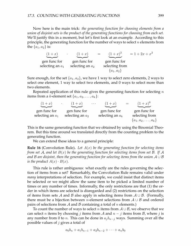
17.3. COUNTING WITH GENERATING FUNCTIONS 399
Now here is the main trick: the generating function for choosing elements from aunion of disjoint sets is the product of the generating functions for choosing from each set.We’ll justify this in a moment, but let’s first look at an example. According to thisprinciple, the generating function for the number of ways to select n elements fromthe {a1, a2} is:
(1 + x)︸ ︷︷ ︸gen func for
selecting an a1
· (1 + x)︸ ︷︷ ︸gen func for
selecting an a2
= (1 + x)2︸ ︷︷ ︸gen func for
selecting from{a1, a2}
= 1 + 2x+ x2
Sure enough, for the set {a1, a2}, we have 1 way to select zero elements, 2 ways toselect one element, 1 way to select two elements, and 0 ways to select more thantwo elements.
Repeated application of this rule gives the generating function for selecting nitems from a k-element set {a1, a2, . . . , ak}:
(1 + x)︸ ︷︷ ︸gen func for
selecting an a1
· (1 + x)︸ ︷︷ ︸gen func for
selecting an a2
· · · (1 + x)︸ ︷︷ ︸gen func for
selecting an ak
= (1 + x)k︸ ︷︷ ︸gen func for
selecting from{a1, a2, . . . , ak}
This is the same generating function that we obtained by using the Binomial Theo-rem. But this time around we translated directly from the counting problem to thegenerating function.
We can extend these ideas to a general principle:
Rule 16 (Convolution Rule). Let A(x) be the generating function for selecting itemsfrom set A, and let B(x) be the generating function for selecting items from set B. If Aand B are disjoint, then the generating function for selecting items from the union A ∪ Bis the product A(x) ·B(x).
This rule is rather ambiguous: what exactly are the rules governing the selec-tion of items from a set? Remarkably, the Convolution Rule remains valid undermany interpretations of selection. For example, we could insist that distinct itemsbe selected or we might allow the same item to be picked a limited number oftimes or any number of times. Informally, the only restrictions are that (1) the or-der in which items are selected is disregarded and (2) restrictions on the selectionof items from sets A and B also apply in selecting items from A ∪ B. (Formally,there must be a bijection between n-element selections from A ∪ B and orderedpairs of selections from A and B containing a total of n elements.)
To count the number of ways to select n items from A ∪ B, we observe that wecan select n items by choosing j items from A and n − j items from B, where j isany number from 0 to n. This can be done in ajbn−j ways. Summing over all thepossible values of j gives a total of
a0bn + a1bn−1 + a2bn−2 + · · ·+ anb0

400 CHAPTER 17. GENERATING FUNCTIONS
ways to select n items from A∪ B. By the Product Rule, this is precisely the coeffi-cient of xn in the series for A(x)B(x).
17.3.3 Choosing Items with Repetition
The first counting problem we considered was the number of ways to select adozen doughnuts when five flavors were available. We can generalize this ques-tion as follows: in how many ways can we select n items from a k-element set ifwe’re allowed to pick the same item multiple times? In these terms, the doughnutproblem asks in how many ways we can select n = 12 doughnuts from the set ofk = 5 flavors
{chocolate, lemon-filled, sugar,glazed,plain}
where, of course, we’re allowed to pick several doughnuts of the same flavor. Let’sapproach this question from a generating functions perspective.
Suppose we make n choices (with repetition allowed) of items from a set con-taining a single item. Then there is one way to choose zero items, one way tochoose one item, one way to choose two items, etc. Thus, the generating functionfor choosing n elements with repetition from a 1-element set is:
〈1, 1, 1, 1, . . . 〉 ←→ 1 + x+ x2 + x3 + · · ·
=1
1− x
The Convolution Rule says that the generating function for selecting items froma union of disjoint sets is the product of the generating functions for selecting itemsfrom each set:
11− x︸ ︷︷ ︸
gen func forchoosing a1’s
· 11− x︸ ︷︷ ︸
gen func forchoosing a2’s
· · · 11− x︸ ︷︷ ︸
gen func forchoosing ak’s
=1
(1− x)k︸ ︷︷ ︸gen func for
repeated choice from{a1, a2, . . . , ak}
Therefore, the generating function for choosing items from a k-element set withrepetition allowed is 1/(1− x)k.
Now the Bookkeeper Rule tells us that the number of ways to choose n itemswith repetition from an k element set is(
n+ k − 1n
),
so this is the coefficient of xn in the series expansion of 1/(1− x)k.On the other hand, it’s instructive to derive this coefficient algebraically, which
we can do using Taylor’s Theorem:

17.3. COUNTING WITH GENERATING FUNCTIONS 401
Theorem 17.3.1 (Taylor’s Theorem).
f(x) = f(0) + f ′(0)x+f ′′(0)
2!x2 +
f ′′′(0)3!
x3 + · · ·+ f (n)(0)n!
xn + · · · .
This theorem says that the nth coefficient of 1/(1−x)k is equal to its nth deriva-tive evaluated at 0 and divided by n!. Computing the nth derivative turns out notto be very difficult (Problem 17.7).
17.3.4 Problems
Practice Problems
Problem 17.6.You would like to buy a bouquet of flowers. You find an online service that willmake bouquets of lilies, roses and tulips, subject to the following constraints:
• there must be at most 3 lilies,
• there must be an odd number of tulips,
• there can be any number of roses.
Example: A bouquet of 3 tulips, 5 roses and no lilies satisfies the constraints.Let fn be the number of possible bouquets with n flowers that fit the service’s
constraints. ExpressF (x), the generating function corresponding to 〈f0, f1, f2, . . . 〉,as a quotient of polynomials (or products of polynomials). You do not need to sim-plify this expression.
Class Problems
Problem 17.7.Let A(x) =
∑∞n=0 anx
n. Then it’s easy to check that
an =A(n)(0)n!
,
whereA(n) is the nth derivative ofA. Use this fact (which you may assume) insteadof the Convolution Counting Principle, to prove that
1
(1− x)k=∞∑n=0
(n+ k − 1k − 1
)xn.
So if we didn’t already know the Bookkeeper Rule, we could have proved itfrom this calculation and the Convolution Rule for generating functions.

402 CHAPTER 17. GENERATING FUNCTIONS
Problem 17.8.We are interested in generating functions for the number of different ways to com-pose a bag of n donuts subject to various restrictions. For each of the restrictionsin (a)-(e) below, find a closed form for the corresponding generating function.(a) All the donuts are chocolate and there are at least 3.
(b) All the donuts are glazed and there are at most 2.
(c) All the donuts are coconut and there are exactly 2 or there are none.
(d) All the donuts are plain and their number is a multiple of 4.
(e) The donuts must be chocolate, glazed, coconut, or plain and:
• there must be at least 3 chocolate donuts, and
• there must be at most 2 glazed, and
• there must be exactly 0 or 2 coconut, and
• there must be a multiple of 4 plain.
(f) Find a closed form for the number of ways to select n donuts subject to theconstraints of the previous part.
Problem 17.9. (a) Let
S(x) ::=x2 + x
(1− x)3.
What is the coefficient of xn in the generating function series for S(x)?
(b) Explain why S(x)/(1 − x) is the generating function for the sums of squares.That is, the coefficient of xn in the series for S(x)/(1− x) is
∑nk=1 k
2.
(c) Use the previous parts to prove that
n∑k=1
k2 =n(n+ 1)(2n+ 1)
6.
Homework Problems
Problem 17.10.We will use generating functions to determine how many ways there are to usepennies, nickels, dimes, quarters, and half-dollars to give n cents change.(a) Write the sequence Pn for the number of ways to use only pennies to changen cents. Write the generating function for that sequence.
(b) Write the sequence Nn for the number of ways to use only nickels to change ncents. Write the generating function for that sequence.

17.4. AN “IMPOSSIBLE” COUNTING PROBLEM 403
(c) Write the generating function for the number of ways to use only nickels andpennies to change n cents.
(d) Write the generating function for the number of ways to use pennies, nickels,dimes, quarters, and half-dollars to give n cents change.
(e) Explain how to use this function to find out how many ways are there tochange 50 cents; you do not have to provide the answer or actually carry out theprocess.
Exam Problems
Problem 17.11.The working days in the next year can be numbered 1, 2, 3, . . . , 300. I’d like toavoid as many as possible.
• On even-numbered days, I’ll say I’m sick.
• On days that are a multiple of 3, I’ll say I was stuck in traffic.
• On days that are a multiple of 5, I’ll refuse to come out from under the blan-kets.
In total, how many work days will I avoid in the coming year?
Problem 17.12.Define the sequence r0, r1, r2, . . . recursively by the rule that r0 = r1 = 0 and
rn = 7rn−1 + 4rn−2 + (n+ 1),
for n ≥ 2. Express the generating function of this sequence as a quotient of poly-nomials or products of polynomials. You do not have to find a closed form forrn.
Problem 17.13.Find the coefficients of x10y5 in (19x+ 4y)15
17.4 An “Impossible” Counting Problem
So far everything we’ve done with generating functions we could have done an-other way. But here is an absurd counting problem— really over the top! In howmany ways can we fill a bag with n fruits subject to the following constraints?
• The number of apples must be even.

404 CHAPTER 17. GENERATING FUNCTIONS
• The number of bananas must be a multiple of 5.
• There can be at most four oranges.
• There can be at most one pear.
For example, there are 7 ways to form a bag with 6 fruits:
Apples 6 4 4 2 2 0 0Bananas 0 0 0 0 0 5 5Oranges 0 2 1 4 3 1 0
Pears 0 0 1 0 1 0 1
These constraints are so complicated that the problem seems hopeless! But let’ssee what generating functions reveal.
Let’s first construct a generating function for choosing apples. We can choose aset of 0 apples in one way, a set of 1 apple in zero ways (since the number of applesmust be even), a set of 2 apples in one way, a set of 3 apples in zero ways, and soforth. So we have:
A(x) = 1 + x2 + x4 + x6 + · · · = 11− x2
Similarly, the generating function for choosing bananas is:
B(x) = 1 + x5 + x10 + x15 + · · · = 11− x5
Now, we can choose a set of 0 oranges in one way, a set of 1 orange in one way,and so on. However, we can not choose more than four oranges, so we have thegenerating function:
O(x) = 1 + x+ x2 + x3 + x4 =1− x5
1− xHere we’re using the geometric sum formula. Finally, we can choose only zero orone pear, so we have:
P (x) = 1 + x
The Convolution Rule says that the generating function for choosing from amongall four kinds of fruit is:
A(x)B(x)O(x)P (x) =1
1− x2
11− x5
1− x5
1− x(1 + x)
=1
(1− x)2
= 1 + 2x+ 3x2 + 4x3 + · · ·
Almost everything cancels! We’re left with 1/(1 − x)2, which we found a powerseries for earlier: the coefficient of xn is simply n+ 1. Thus, the number of ways toform a bag of n fruits is just n+ 1. This is consistent with the example we workedout, since there were 7 different fruit bags containing 6 fruits. Amazing!

17.4. AN “IMPOSSIBLE” COUNTING PROBLEM 405
17.4.1 Problems
Homework Problems
Problem 17.14.Miss McGillicuddy never goes outside without a collection of pets. In particular:
• She brings a positive number of songbirds, which always come in pairs.
• She may or may not bring her alligator, Freddy.
• She brings at least 2 cats.
• She brings two or more chihuahuas and labradors leashed together in a line.
Let Pn denote the number of different collections of n pets that can accompanyher, where we regard chihuahuas and labradors leashed up in different orders asdifferent collections, even if there are the same number chihuahuas and labradorsleashed in the line.
For example, P6 = 4 since there are 4 possible collections of 6 pets:
• 2 songbirds, 2 cats, 2 chihuahuas leashed in line
• 2 songbirds, 2 cats, 2 labradors leashed in line
• 2 songbirds, 2 cats, a labrador leashed behind a chihuahua
• 2 songbirds, 2 cats, a chihuahua leashed behind a labrador
And P7 = 16 since there are 16 possible collections of 7 pets:
• 2 songbirds, 3 cats, 2 chihuahuas leashed in line
• 2 songbirds, 3 cats, 2 labradors leashed in line
• 2 songbirds, 3 cats, a labrador leashed behind a chihuahua
• 2 songbirds, 3 cats, a chihuahua leashed behind a labrador
• 4 collections consisting of 2 songbirds, 2 cats, 1 alligator, and a line of 2 dogs
• 8 collections consisting of 2 songbirds, 2 cats, and a line of 3 dogs.
(a) LetP (x) ::= P0 + P1x+ P2x
2 + P3x3 + · · ·
be the generating function for the number of Miss McGillicuddy’s pet collections.Verify that
P (x) =4x6
(1− x)2(1− 2x).
(b) Find a simple formula for Pn.

406 CHAPTER 17. GENERATING FUNCTIONS
Problem 17.15.Generating functions provide an interesting way to count the number of strings ofmatched parentheses. To do this, we’ll use the description of these strings givenin Definition 11.1.2 as the set, GoodCount, of strings of parentheses with a goodcount. Let cn be the number of strings in GoodCount with exactly n left parenthe-ses, and let C(x) be the generating function for these numbers:
C(x) ::= c0 + c1x+ c2x2 + · · · .
(a) The wrap of a string, s, is the string, (s), that starts with a left parenthesisfollowed by the characters of s, and then ends with a right parenthesis. Explainwhy the generating function for the wraps of strings with a good count is xC(x).Hint: The wrap of a string with good count also has a good count that starts andends with 0 and remains positive everywhere else.
(b) Explain why, for every string, s, with a good count, there is a unique sequenceof strings s1, . . . , sk that are wraps of strings with good counts and s = s1 · · · sk.For example, the string r ::= (())()(()()) ∈ GoodCount equals s1s2s3 where s1 =(()), s2 = (), s3 = (()()), and this is the only way to express r as a sequence ofwraps of strings with good counts.
(c) Conclude that
C = 1 + xC + (xC)2 + · · ·+ (xC)n + · · · , (17.10)
soC =
11− xC
, (17.11)
and hence
C =1±√
1− 4x2x
. (17.12)
Let D(x) ::= 2xC(x). Expressing D as a power series
D(x) = d0 + d1x+ d2x2 + · · · ,
we havecn =
dn+1
2. (17.13)
(d) Use (17.12), (17.13), and the value of c0 to conclude that
D(x) = 1−√
1− 4x.
(e) Prove that
dn =(2n− 3) · (2n− 5) · · · 5 · 3 · 1 · 2n
n!.
Hint: dn = D(n)(0)/n!
(f) Conclude that
cn =1
n+ 1
(2nn
).

17.4. AN “IMPOSSIBLE” COUNTING PROBLEM 407
Exam Problems
Problem 17.16.T-Pain is planning an epic boat trip and he needs to decide what to bring with him.
• He definitely wants to bring burgers, but they only come in packs of 6.
• He and his two friends can’t decide whether they want to dress formally orcasually. He’ll either bring 0 pairs of flip flops or 3 pairs.
• He doesn’t have very much room in his suitcase for towels, so he can bringat most 2.
• In order for the boat trip to be truly epic, he has to bring at least 1 nautical-themed pashmina afghan.
(a) Let gn be the the number of different ways for T-Pain to bring n items (burgers,pairs of flip flops, towels, and/or afghans) on his boat trip. Express the generatingfunction G(x) ::=
∑∞n=0 gnx
n as a quotient of polynomials.
(b) Find a closed formula in n for the number of ways T-Pain can bring exactly nitems with him.

408 CHAPTER 17. GENERATING FUNCTIONS

Chapter 18
Introduction to Probability
Probability plays a key role in the sciences —”hard” and social —including com-puter science. Many algorithms rely on randomization. Investigating their cor-rectness and performance requires probability theory. Moreover, computer sys-tems designs, such as memory management, branch prediction, packet routing,and load balancing are based on probabilistic assumptions and analyses. Probabil-ity is central as well in related subjects such as information theory, cryptography,artificial intelligence, and game theory. But we’ll start with a more down-to-earthapplication: getting a prize in a game show.
18.1 Monty Hall
In the September 9, 1990 issue of Parade magazine, the columnist Marilyn vos Sa-vant responded to this letter:
Suppose you’re on a game show, and you’re given the choice of three doors.Behind one door is a car, behind the others, goats. You pick a door, say number1, and the host, who knows what’s behind the doors, opens another door, saynumber 3, which has a goat. He says to you, ”Do you want to pick doornumber 2?” Is it to your advantage to switch your choice of doors?
Craig. F. WhitakerColumbia, MD
The letter describes a situation like one faced by contestants on the 1970’s gameshow Let’s Make a Deal, hosted by Monty Hall and Carol Merrill. Marilyn repliedthat the contestant should indeed switch. She explained that if the car was behindeither of the two unpicked doors —which is twice as likely as the the car beingbehind the picked door —the contestant wins by switching. But she soon receiveda torrent of letters, many from mathematicians, telling her that she was wrong. Theproblem generated thousands of hours of heated debate.
409

410 CHAPTER 18. INTRODUCTION TO PROBABILITY
This incident highlights a fact about probability: the subject uncovers lots ofexamples where ordinary intuition leads to completely wrong conclusions. So un-til you’ve studied probabilities enough to have refined your intuition, a way toavoid errors is to fall back on a rigorous, systematic approach such as the FourStep Method.
18.1.1 The Four Step Method
Every probability problem involves some sort of randomized experiment, process,or game. And each such problem involves two distinct challenges:
1. How do we model the situation mathematically?
2. How do we solve the resulting mathematical problem?
In this section, we introduce a four step approach to questions of the form, “Whatis the probability that —– ?” In this approach, we build a probabilistic modelstep-by-step, formalizing the original question in terms of that model. Remark-ably, the structured thinking that this approach imposes provides simple solutionsto many famously-confusing problems. For example, as you’ll see, the four stepmethod cuts through the confusion surrounding the Monty Hall problem like aGinsu knife. However, more complex probability questions may spin off chal-lenging counting, summing, and approximation problems— which, fortunately,you’ve already spent weeks learning how to solve.
18.1.2 Clarifying the Problem
Craig’s original letter to Marilyn vos Savant is a bit vague, so we must make someassumptions in order to have any hope of modeling the game formally:
1. The car is equally likely to be hidden behind each of the three doors.
2. The player is equally likely to pick each of the three doors, regardless of thecar’s location.
3. After the player picks a door, the host must open a different door with a goatbehind it and offer the player the choice of staying with the original door orswitching.
4. If the host has a choice of which door to open, then he is equally likely toselect each of them.
In making these assumptions, we’re reading a lot into Craig Whitaker’s letter.Other interpretations are at least as defensible, and some actually lead to differ-ent answers. But let’s accept these assumptions for now and address the question,“What is the probability that a player who switches wins the car?”

18.1. MONTY HALL 411
18.1.3 Step 1: Find the Sample Space
Our first objective is to identify all the possible outcomes of the experiment. Atypical experiment involves several randomly-determined quantities. For exam-ple, the Monty Hall game involves three such quantities:
1. The door concealing the car.
2. The door initially chosen by the player.
3. The door that the host opens to reveal a goat.
Every possible combination of these randomly-determined quantities is called anoutcome. The set of all possible outcomes is called the sample space for the experi-ment.
A tree diagram is a graphical tool that can help us work through the four stepapproach when the number of outcomes is not too large or the problem is nicelystructured. In particular, we can use a tree diagram to help understand the sam-ple space of an experiment. The first randomly-determined quantity in our ex-periment is the door concealing the prize. We represent this as a tree with threebranches:
carlocation
C
A
B
In this diagram, the doors are called A, B, and C instead of 1, 2, and 3 becausewe’ll be adding a lot of other numbers to the picture later.
Now, for each possible location of the prize, the player could initially chooseany of the three doors. We represent this in a second layer added to the tree. Then athird layer represents the possibilities of the final step when the host opens a doorto reveal a goat:

412 CHAPTER 18. INTRODUCTION TO PROBABILITY
carlocation
player’sinitial guess
doorrevealed
C
C
C
A
B
A
B
A
B
C
A
B
C
A
B
A
C
A
CC
B
A
B
outcome
B
(A,A,B)
(A,A,C)
(A,B,C)
(B,A,C)
(B,B,A)
(B,B,C)
(B,C,A)
(C,A,B)
(C,B,A)
(C,C,A)
(C,C,B)
(A,C,B)
Notice that the third layer reflects the fact that the host has either one choiceor two, depending on the position of the car and the door initially selected by theplayer. For example, if the prize is behind door A and the player picks door B, thenthe host must open door C. However, if the prize is behind door A and the playerpicks door A, then the host could open either door B or door C.
Now let’s relate this picture to the terms we introduced earlier: the leaves of thetree represent outcomes of the experiment, and the set of all leaves represents thesample space. Thus, for this experiment, the sample space consists of 12 outcomes.For reference, we’ve labeled each outcome with a triple of doors indicating:
(door concealing prize, door initially chosen, door opened to reveal a goat)
In these terms, the sample space is the set:{(A,A,B), (A,A,C), (A,B,C), (A,C,B), (B,A,C), (B,B,A),(B,B,C), (B,C,A), (C,A,B), (C,B,A), (C,C,A), (C,C,B)
}The tree diagram has a broader interpretation as well: we can regard the wholeexperiment as following a path from the root to a leaf, where the branch taken ateach stage is “randomly” determined. Keep this interpretation in mind; we’ll useit again later.

18.1. MONTY HALL 413
18.1.4 Step 2: Define Events of Interest
Our objective is to answer questions of the form “What is the probability that . . . ?”,where the missing phrase might be “the player wins by switching”, “the playerinitially picked the door concealing the prize”, or “the prize is behind door C”,for example. Each of these phrases characterizes a set of outcomes: the outcomesspecified by “the prize is behind door C” is:
{(C,A,B), (C,B,A), (C,C,A), (C,C,B)}
A set of outcomes is called an event. So the event that the player initially pickedthe door concealing the prize is the set:
{(A,A,B), (A,A,C), (B,B,A), (B,B,C), (C,C,A), (C,C,B)}
And what we’re really after, the event that the player wins by switching, is the setof outcomes:
{(A,B,C), (A,C,B), (B,A,C), (B,C,A), (C,A,B), (C,B,A)}
Let’s annotate our tree diagram to indicate the outcomes in this event.
carlocation
player’sinitial guess
doorrevealed
switchwins?
C
C
C
A
B
A
B
A
B
C
A
B
C
A
B
A
C
A
CC
B
A
B
outcome
X
X
X
X
X
X
B
(A,A,B)
(A,A,C)
(A,B,C)
(B,A,C)
(B,B,A)
(B,B,C)
(B,C,A)
(C,A,B)
(C,B,A)
(C,C,A)
(C,C,B)
(A,C,B)

414 CHAPTER 18. INTRODUCTION TO PROBABILITY
Notice that exactly half of the outcomes are marked, meaning that the player winsby switching in half of all outcomes. You might be tempted to conclude that aplayer who switches wins with probability 1/2. This is wrong. The reason is thatthese outcomes are not all equally likely, as we’ll see shortly.
18.1.5 Step 3: Determine Outcome Probabilities
So far we’ve enumerated all the possible outcomes of the experiment. Now wemust start assessing the likelihood of those outcomes. In particular, the goal of thisstep is to assign each outcome a probability, indicating the fraction of the time thisoutcome is expected to occur. The sum of all outcome probabilities must be one,reflecting the fact that there always is an outcome.
Ultimately, outcome probabilities are determined by the phenomenon we’remodeling and thus are not quantities that we can derive mathematically. How-ever, mathematics can help us compute the probability of every outcome based onfewer and more elementary modeling decisions. In particular, we’ll break the task ofdetermining outcome probabilities into two stages.
Step 3a: Assign Edge Probabilities
First, we record a probability on each edge of the tree diagram. These edge-probabilitiesare determined by the assumptions we made at the outset: that the prize is equallylikely to be behind each door, that the player is equally likely to pick each door,and that the host is equally likely to reveal each goat, if he has a choice. Noticethat when the host has no choice regarding which door to open, the single branchis assigned probability 1.

18.1. MONTY HALL 415
carlocation
player’sinitial guess
doorrevealed
switchwins?
C
C
C
A
B
A
B
A
B
C
A
B
C
A
B
A
C
A
CC
1/3
1/3
1/3
1/3
1/3
1/3
1/3
1/3
1/3
1/3
1/3
1/3
1
1
1
1
1
1
1/2 B
1/2
1/2
1/2
A
B
1/2
1/2
outcome
X
X
X
X
X
X
B
(A,A,B)
(A,A,C)
(A,B,C)
(B,A,C)
(B,B,A)
(B,B,C)
(B,C,A)
(C,A,B)
(C,B,A)
(C,C,A)
(C,C,B)
(A,C,B)
Step 3b: Compute Outcome Probabilities
Our next job is to convert edge probabilities into outcome probabilities. This is apurely mechanical process: the probability of an outcome is equal to the product of theedge-probabilities on the path from the root to that outcome. For example, the probabilityof the topmost outcome, (A,A,B) is
13· 1
3· 1
2=
118.
There’s an easy, intuitive justification for this rule. As the steps in an experi-ment progress randomly along a path from the root of the tree to a leaf, the proba-bilities on the edges indicate how likely the walk is to proceed along each branch.For example, a path starting at the root in our example is equally likely to go downeach of the three top-level branches.
Now, how likely is such a walk to arrive at the topmost outcome, (A,A,B)?Well, there is a 1-in-3 chance that a walk would follow the A-branch at the toplevel, a 1-in-3 chance it would continue along the A-branch at the second level,and 1-in-2 chance it would follow the B-branch at the third level. Thus, it seemsthat about 1 walk in 18 should arrive at the (A,A,B) leaf, which is precisely theprobability we assign it.
Anyway, let’s record all the outcome probabilities in our tree diagram.

416 CHAPTER 18. INTRODUCTION TO PROBABILITY
carlocation
player’sinitial guess
doorrevealed
switchwins?
C
C
C
A
B
A
B
A
B
C
A
B
C
A
B
A
C
A
CC
1/3
1/3
1/3
1/3
1/3
1/3
1/3
1/3
1/3
1/3
1/3
1/3
1
1
1
1
1
1
1/2 B
1/2
1/2
1/2
A
B
1/2
1/2
outcome
X
X
X
X
X
X
probability
1/18
1/18
1/9
1/9
1/9
1/18
1/18
1/9
1/9
1/9
1/18
1/18
B
(A,A,B)
(A,A,C)
(A,B,C)
(B,A,C)
(B,B,A)
(B,B,C)
(B,C,A)
(C,A,B)
(C,B,A)
(C,C,A)
(C,C,B)
(A,C,B)
Specifying the probability of each outcome amounts to defining a function thatmaps each outcome to a probability. This function is usually called Pr. In theseterms, we’ve just determined that:
Pr {(A,A,B)} =118
Pr {(A,A,C)} =118
Pr {(A,B,C)} =19
etc.
18.1.6 Step 4: Compute Event Probabilities
We now have a probability for each outcome, but we want to determine the prob-ability of an event which will be the sum of the probabilities of the outcomes in it.The probability of an event, E, is written Pr {E}. For example, the probability of

18.1. MONTY HALL 417
the event that the player wins by switching is:
Pr {switching wins} = Pr {(A,B,C)}+ Pr {(A,C,B)}+ Pr {(B,A,C)}+Pr {(B,C,A)}+ Pr {(C,A,B)}+ Pr {(C,B,A)}
=19
+19
+19
+19
+19
+19
=23
It seems Marilyn’s answer is correct; a player who switches doors wins the carwith probability 2/3! In contrast, a player who stays with his or her original doorwins with probability 1/3, since staying wins if and only if switching loses.
We’re done with the problem! We didn’t need any appeals to intuition or inge-nious analogies. In fact, no mathematics more difficult than adding and multiply-ing fractions was required. The only hard part was resisting the temptation to leapto an “intuitively obvious” answer.
18.1.7 An Alternative Interpretation of the Monty Hall Problem
Was Marilyn really right? Our analysis suggests she was. But a more accurateconclusion is that her answer is correct provided we accept her interpretation of thequestion. There is an equally plausible interpretation in which Marilyn’s answeris wrong. Notice that Craig Whitaker’s original letter does not say that the hostis required to reveal a goat and offer the player the option to switch, merely thathe did these things. In fact, on the Let’s Make a Deal show, Monty Hall sometimessimply opened the door that the contestant picked initially. Therefore, if he wantedto, Monty could give the option of switching only to contestants who picked thecorrect door initially. In this case, switching never works!
18.1.8 Problems
Class Problems
Problem 18.1.[A Baseball Series]The New York Yankees and the Boston Red Sox are playing a two-out-of-threeseries. (In other words, they play until one team has won two games. Then thatteam is declared the overall winner and the series ends.) Assume that the Red Soxwin each game with probability 3/5, regardless of the outcomes of previous games.
Answer the questions below using the four step method. You can use the sametree diagram for all three problems.(a) What is the probability that a total of 3 games are played?
(b) What is the probability that the winner of the series loses the first game?
(c) What is the probability that the correct team wins the series?

418 CHAPTER 18. INTRODUCTION TO PROBABILITY
Problem 18.2.To determine which of two people gets a prize, a coin is flipped twice. If the flipsare a Head and then a Tail, the first player wins. If the flips are a Tail and then aHead, the second player wins. However, if both coins land the same way, the flipsdon’t count and whole the process starts over.
Assume that on each flip, a Head comes up with probability p, regardless ofwhat happened on other flips. Use the four step method to find a simple formulafor the probability that the first player wins. What is the probability that neitherplayer wins?
Suggestions: The tree diagram and sample space are infinite, so you’re not go-ing to finish drawing the tree. Try drawing only enough to see a pattern. Summingall the winning outcome probabilities directly is difficult. However, a neat tricksolves this problem and many others. Let s be the sum of all winning outcomeprobabilities in the whole tree. Notice that you can write the sum of all the winningprobabilities in certain subtrees as a function of s. Use this observation to write anequation in s and then solve.
Problem 18.3.[The Four-Door Deal]
Let’s see what happens when Let’s Make a Deal is played with four doors. Aprize is hidden behind one of the four doors. Then the contestant picks a door.Next, the host opens an unpicked door that has no prize behind it. The contestantis allowed to stick with their original door or to switch to one of the two unopened,unpicked doors. The contestant wins if their final choice is the door hiding theprize.
Use The Four Step Method of Section 18.1 to find the following probabilities.The tree diagram may become awkwardly large, in which case just draw enoughof it to make its structure clear.
(a) Contestant Stu, a sanitation engineer from Trenton, New Jersey, stays with hisoriginal door. What is the probability that Stu wins the prize?
(b) Contestant Zelda, an alien abduction researcher from Helena, Montana, switchesto one of the remaining two doors with equal probability. What is the probabilitythat Zelda wins the prize?
Problem 18.4.[Simulating a fair coin] Suppose you need a fair coin to decide which door tochoose in the 6.042 Monty Hall game. After making everyone in your group emptytheir pockets, all you managed to turn up is some crumpled bubble gum wrappers,a few used tissues, and one penny. However, the penny was from Prof. Meyer’spocket, so it is not safe to assume that it is a fair coin.
How can we use a coin of unknown bias to get the same effect as a fair coin

18.2. SET THEORY AND PROBABILITY 419
of bias 1/2? Draw the tree diagram for your solution, but since it is infinite, drawonly enough to see a pattern.
Suggestion: A neat trick allows you to sum all the outcome probabilities thatcause you to say ”Heads”: Let s be the sum of all ”Heads” outcome probabilitiesin the whole tree. Notice that you can write the sum of all the ”Heads” outcome proba-bilities in certain subtrees as a function of s. Use this observation to write an equationin s and then solve.
Homework Problems
Problem 18.5.I have a deck of 52 regular playing cards, 26 red, 26 black, randomly shuffled. Theyall lie face down in the deck so that you can’t see them. I will draw a card off thetop of the deck and turn it face up so that you can see it and then put it aside. Iwill continue to turn up cards like this but at some point while there are still cardsleft in the deck, you have to declare that you want the next card in the deck to beturned up. If that next card turns up black you win and otherwise you lose. Eitherway, the game is then over.(a) Show that if you take the first card before you have seen any cards, you then
have probability 1/2 of winning the game.
(b) Suppose you don’t take the first card and it turns up red. Show that you havethen have a probability of winning the game that is greater than 1/2.
(c) If there are r red cards left in the deck and b black cards, show that the proba-bility of winning in you take the next card is b/(r + b).
(d) Either,
1. come up with a strategy for this game that gives you a probability of winningstrictly greater than 1/2 and prove that the strategy works, or,
2. come up with a proof that no such strategy can exist.
18.2 Set Theory and Probability
Let’s abstract what we’ve just done in this Monty Hall example into a generalmathematical definition of probability. In the Monty Hall example, there wereonly finitely many possible outcomes. Other examples in this course will have acountably infinite number of outcomes.
General probability theory deals with uncountable sets like the set of real num-bers, but we won’t need these, and sticking to countable sets lets us define theprobability of events using sums instead of integrals. It also lets us avoid somedistracting technical problems in set theory like the Banach-Tarski “paradox” men-tioned in Chapter 5.2.5.

420 CHAPTER 18. INTRODUCTION TO PROBABILITY
18.2.1 Probability Spaces
Definition 18.2.1. A countable sample space, S, is a nonempty countable set. Anelement w ∈ S is called an outcome. A subset of S is called an event.
Definition 18.2.2. A probability function on a sample space, S, is a total functionPr {} : S → R such that
• Pr {w} ≥ 0 for all w ∈ S, and
•∑w∈S Pr {w} = 1.
The sample space together with a probability function is called a probability space.For any event, E ⊆ S, the probability of E is defined to be the sum of the proba-
bilities of the outcomes in E:
Pr {E} ::=∑w∈E
Pr {w} .
An immediate consequence of the definition of event probability is that for dis-joint events, E,F ,
Pr {E ∪ F} = Pr {E}+ Pr {F} .
This generalizes to a countable number of events. Namely, a collection of sets ispairwise disjoint when no element is in more than one of them —formally,A∩B = ∅for all sets A 6= B in the collection.
Rule (Sum Rule). If {E0, E1, . . . } is collection of pairwise disjoint events, then
Pr
{⋃n∈N
En
}=∑n∈N
Pr {En} .
The Sum Rule1 lets us analyze a complicated event by breaking it down intosimpler cases. For example, if the probability that a randomly chosen MIT studentis native to the United States is 60%, to Canada is 5%, and to Mexico is 5%, thenthe probability that a random MIT student is native to North America is 70%.
Another consequence of the Sum Rule is that Pr {A} + Pr{A}
= 1, which fol-lows because Pr {S} = 1 and S is the union of the disjoint sets A and A. Thisequation often comes up in the form
1If you think like a mathematician, you should be wondering if the infinite sum is really necessary.Namely, suppose we had only used finite sums in Definition 18.2.2 instead of sums over all naturalnumbers. Would this imply the result for infinite sums? It’s hard to find counterexamples, but there aresome: it is possible to find a pathological “probability” measure on a sample space satisfying the SumRule for finite unions, in which the outcomesw0, w1, . . . each have probability zero, and the probabilityassigned to any event is either zero or one! So the infinite Sum Rule fails dramatically, since the wholespace is of measure one, but it is a union of the outcomes of measure zero.
The construction of such weird examples is beyond the scope of this text. You can learn more aboutthis by taking a course in Set Theory and Logic that covers the topic of “ultrafilters.”

18.2. SET THEORY AND PROBABILITY 421
Rule (Complement Rule).
Pr{A}
= 1− Pr {A} .
Sometimes the easiest way to compute the probability of an event is to computethe probability of its complement and then apply this formula.
Some further basic facts about probability parallel facts about cardinalities offinite sets. In particular:
Pr {B −A} = Pr {B} − Pr {A ∩B} , (Difference Rule)Pr {A ∪B} = Pr {A}+ Pr {B} − Pr {A ∩B} , (Inclusion-Exclusion)Pr {A ∪B} ≤ Pr {A}+ Pr {B} . (Boole’s Inequality)
The Difference Rule follows from the Sum Rule because B is the union of the dis-joint sets B − A and A ∩ B. Inclusion-Exclusion then follows from the Sum andDifference Rules, becauseA∪B is the union of the disjoint setsA andB−A. Boole’sinequality is an immediate consequence of Inclusion-Exclusion since probabilitiesare nonnegative.
The two event Inclusion-Exclusion equation above generalizes to n events inthe same way as the corresponding Inclusion-Exclusion rule for n sets. Boole’sinequality also generalizes to
Pr {E1 ∪ · · · ∪ En} ≤ Pr {E1}+ · · ·+ Pr {En} . (Union Bound)
This simple Union Bound is actually useful in many calculations. For example,suppose that Ei is the event that the i-th critical component in a spacecraft fails.ThenE1∪· · ·∪En is the event that some critical component fails. The Union Boundcan give an adequate upper bound on this vital probability.
Similarly, the Difference Rule implies that
If A ⊆ B, then Pr {A} ≤ Pr {B} . (Monotonicity)
18.2.2 An Infinite Sample Space
Suppose two players take turns flipping a fair coin. Whoever flips heads first isdeclared the winner. What is the probability that the first player wins? A treediagram for this problem is shown below:

422 CHAPTER 18. INTRODUCTION TO PROBABILITY
1/21/2
1/21/2
1/21/2
1/21/2
etc.
HH
HHT
TT
T
firstplayer
secondplayer
firstplayer
secondplayer
1/21/4
1/81/16
The event that the first player wins contains an infinite number of outcomes,but we can still sum their probabilities:
Pr {first player wins} =12
+18
+132
+1
128+ · · ·
=12
∞∑n=0
(14
)n=
12
(1
1− 1/4
)=
23.
Similarly, we can compute the probability that the second player wins:
Pr {second player wins} =14
+116
+164
+1
256+ · · ·
=13.
To be formal about this, sample space is the infinite set
S ::= {TnH | n ∈ N}
where Tn stands for a length n string of T’s. The probability function is
Pr {TnH} ::=1
2n+1.
Since this function is obviously nonnegative, To verify that this is a probabilityspace, we just have to check that all the probabilities sum to 1. But this followsdirectly from the formula for the sum of a geometric series:∑
TnH∈SPr {TnH} =
∑n∈N
12n+1
=12
∑n∈N
12n
= 1.
Notice that this model does not have an outcome corresponding to the possi-bility that both players keep flipping tails forever —in the diagram, flipping for-ever corresponds to following the infinite path in the tree without ever reaching

18.2. SET THEORY AND PROBABILITY 423
a leaf/outcome. If leaving this possibility out of the model bothers you, you’rewelcome to fix it by adding another outcome, wforever, to indicate that that’s whathappened. Of course since the probabililities of the other outcomes already sum to1, you have to define the probability of wforever to be 0. Now outcomes with prob-ability zero will have no impact on our calculations, so there’s no harm in addingit in if it makes you happier. On the other hand, there’s also no harm in simplyleaving it out as we did, since it has no impact.
The mathematical machinery we’ve developed is adequate to model and ana-lyze many interesting probability problems with infinite sample spaces. However,some intricate infinite processes require uncountable sample spaces along withmore powerful (and more complex) measure-theoretic notions of probability. Forexample, if we generate an infinite sequence of random bits b1, b2, b3, . . ., then whatis the probability that
b121
+b222
+b323
+ · · ·
is a rational number? Fortunately, we won’t have any need to worry about suchthings.
18.2.3 Problems
Class Problems
Problem 18.6.Suppose there is a system with n components, and we know from past experiencethat any particular component will fail in a given year with probability p. That is,letting Fi be the event that the ith component fails within one year, we have
Pr {Fi} = p
for 1 ≤ i ≤ n. The system will fail if any one of its components fails. What can wesay about the probability that the system will fail within one year?
Let F be the event that the system fails within one year. Without any additionalassumptions, we can’t get an exact answer for Pr {F}. However, we can give usefulupper and lower bounds, namely,
p ≤ Pr {F} ≤ np. (18.1)
We may as well assume p < 1/n, since the upper bound is trivial otherwise. Forexample, if n = 100 and p = 10−5, we conclude that there is at most one chance in1000 of system failure within a year and at least one chance in 100,000.
Let’s model this situation with the sample space S ::=P({1, . . . , n}) whose out-comes are subsets of positive integers ≤ n, where s ∈ S corresponds to the indicesof exactly those components that fail within one year. For example, {2, 5} is theoutcome that the second and fifth components failed within a year and none of theother components failed. So the outcome that the system did not fail correspondsto the emptyset, ∅.

424 CHAPTER 18. INTRODUCTION TO PROBABILITY
(a) Show that the probability that the system fails could be as small as p by de-scribing appropriate probabilities for the outcomes. Make sure to verify that thesum of your outcome probabilities is 1.
(b) Show that the probability that the system fails could actually be as large as npby describing appropriate probabilities for the outcomes. Make sure to verify thatthe sum of your outcome probabilities is 1.
(c) Prove inequality (18.1).
Problem 18.7.Here are some handy rules for reasoning about probabilities that all follow directlyfrom the Disjoint Sum Rule in the Appendix. Prove them.
Pr {A−B} = Pr {A} − Pr {A ∩B} (Difference Rule)
Pr{A}
= 1− Pr {A} (Complement Rule)
Pr {A ∪B} = Pr {A}+ Pr {B} − Pr {A ∩B} (Inclusion-Exclusion)
Pr {A ∪B} ≤ Pr {A}+ Pr {B} . (2-event Union Bound)
If A ⊆ B, then Pr {A} ≤ Pr {B} . (Monotonicity)
Problem 18.8.Suppose Pr {} : S → [0, 1] is a probability function on a sample space, S , and letB be an event such that Pr {B} > 0. Define a function PrB {·} on events outcomesw ∈ S by the rule:
PrB {w} ::=
{Pr {w} /Pr {B} if w ∈ B,0 if w /∈ B.
(18.2)
(a) Prove that PrB {·} is also a probability function on S according to Defini-tion 18.2.2.
(b) Prove that
PrB {A} =Pr {A ∩B}
Pr {B}
for all A ⊆ S.

18.3. CONDITIONAL PROBABILITY 425
18.3 Conditional Probability
Suppose that we pick a random person in the world. Everyone has an equal chanceof being selected. Let A be the event that the person is an MIT student, and let Bbe the event that the person lives in Cambridge. What are the probabilities of theseevents? Intuitively, we’re picking a random point in the big ellipse shown belowand asking how likely that point is to fall into region A or B:
AB
set of all peoplein the world
set of people wholive in Cambridge
set of MITstudents
The vast majority of people in the world neither live in Cambridge nor are MITstudents, so events A and B both have low probability. But what is the probabilitythat a person is an MIT student, given that the person lives in Cambridge? Thisshould be much greater— but what is it exactly?
What we’re asking for is called a conditional probability; that is, the probabilitythat one event happens, given that some other event definitely happens. Questionsabout conditional probabilities come up all the time:
• What is the probability that it will rain this afternoon, given that it is cloudythis morning?
• What is the probability that two rolled dice sum to 10, given that both areodd?
• What is the probability that I’ll get four-of-a-kind in Texas No Limit Hold’Em Poker, given that I’m initially dealt two queens?
There is a special notation for conditional probabilities. In general, Pr {A | B}denotes the probability of eventA, given that eventB happens. So, in our example,Pr {A | B} is the probability that a random person is an MIT student, given thathe or she is a Cambridge resident.
How do we compute Pr {A | B}? Since we are given that the person lives inCambridge, we can forget about everyone in the world who does not. Thus, alloutcomes outside event B are irrelevant. So, intuitively, Pr {A | B} should be thefraction of Cambridge residents that are also MIT students; that is, the answer

426 CHAPTER 18. INTRODUCTION TO PROBABILITY
should be the probability that the person is in set A ∩ B (darkly shaded) dividedby the probability that the person is in set B (lightly shaded). This motivates thedefinition of conditional probability:
Definition 18.3.1.
Pr {A | B} ::=Pr {A ∩B}
Pr {B}
If Pr {B} = 0, then the conditional probability Pr {A | B} is undefined.Pure probability is often counterintuitive, but conditional probability is worse!
Conditioning can subtly alter probabilities and produce unexpected results in ran-domized algorithms and computer systems as well as in betting games. Yet, themathematical definition of conditional probability given above is very simple andshould give you no trouble— provided you rely on formal reasoning and not intu-ition.
18.3.1 The “Halting Problem”
The Halting Problem was the first example of a property that could not be testedby any program. It was introduced by Alan Turing in his seminal 1936 paper.The problem is to determine whether a Turing machine halts on a given . . . yaddayadda yadda . . . what’s much more important, it was the name of the MIT EECSdepartment’s famed C-league hockey team.
In a best-of-three tournament, the Halting Problem wins the first game withprobability 1/2. In subsequent games, their probability of winning is determinedby the outcome of the previous game. If the Halting Problem won the previousgame, then they are invigorated by victory and win the current game with proba-bility 2/3. If they lost the previous game, then they are demoralized by defeat andwin the current game with probablity only 1/3. What is the probability that theHalting Problem wins the tournament, given that they win the first game?
This is a question about a conditional probability. Let A be the event that theHalting Problem wins the tournament, and let B be the event that they win thefirst game. Our goal is then to determine the conditional probability Pr {A | B}.
We can tackle conditional probability questions just like ordinary probabilityproblems: using a tree diagram and the four step method. A complete tree diagramis shown below, followed by an explanation of its construction and use.

18.3. CONDITIONAL PROBABILITY 427
2/3
L1/2
W1/2
W 1/3
L2/3
L 1/3
W2/3
LL 1/3
W2/3
W1/3
1st gameoutcome 2nd game
outcome3rd gameoutcome probability
outcome
1/3
1/18
1/9
1/9
1/18
1/3
event B:win the
1st game?
event A:win theseries?
WW
WLW
WLL
LWW
LWL
LL
outcome
Step 1: Find the Sample Space
Each internal vertex in the tree diagram has two children, one corresponding to awin for the Halting Problem (labeled W ) and one corresponding to a loss (labeledL). The complete sample space is:
S = {WW, WLW, WLL, LWW, LWL, LL}
Step 2: Define Events of Interest
The event that the Halting Problem wins the whole tournament is:
T = {WW, WLW, LWW}
And the event that the Halting Problem wins the first game is:
F = {WW,WLW,WLL}
The outcomes in these events are indicated with checkmarks in the tree diagram.
Step 3: Determine Outcome Probabilities
Next, we must assign a probability to each outcome. We begin by labeling edgesas specified in the problem statement. Specifically, The Halting Problem has a 1/2chance of winning the first game, so the two edges leaving the root are each as-signed probability 1/2. Other edges are labeled 1/3 or 2/3 based on the outcome

428 CHAPTER 18. INTRODUCTION TO PROBABILITY
of the preceding game. We then find the probability of each outcome by multiply-ing all probabilities along the corresponding root-to-leaf path. For example, theprobability of outcome WLL is:
12· 1
3· 2
3=
19
Step 4: Compute Event Probabilities
We can now compute the probability that The Halting Problem wins the tourna-ment, given that they win the first game:
Pr {A | B} =Pr {A ∩B}
Pr {B}
=Pr {{WW,WLW}}
Pr {{WW,WLW,WLL}}
=1/3 + 1/18
1/3 + 1/18 + 1/9
=79
We’re done! If the Halting Problem wins the first game, then they win the wholetournament with probability 7/9.
18.3.2 Why Tree Diagrams Work
We’ve now settled into a routine of solving probability problems using tree dia-grams. But we’ve left a big question unaddressed: what is the mathematical justi-fication behind those funny little pictures? Why do they work?
The answer involves conditional probabilities. In fact, the probabilities thatwe’ve been recording on the edges of tree diagrams are conditional probabilities.For example, consider the uppermost path in the tree diagram for the Halting Prob-lem, which corresponds to the outcome WW . The first edge is labeled 1/2, whichis the probability that the Halting Problem wins the first game. The second edgeis labeled 2/3, which is the probability that the Halting Problem wins the secondgame, given that they won the first— that’s a conditional probability! More gener-ally, on each edge of a tree diagram, we record the probability that the experimentproceeds along that path, given that it reaches the parent vertex.
So we’ve been using conditional probabilities all along. But why can we mul-tiply edge probabilities to get outcome probabilities? For example, we concludedthat:
Pr {WW} =12· 2
3
=13

18.3. CONDITIONAL PROBABILITY 429
Why is this correct?The answer goes back to Definition 18.3.1 of conditional probability which
could be written in a form called the Product Rule for probabilities:
Rule (Product Rule for 2 Events). If Pr {E1} 6= 0, then:
Pr {E1 ∩ E2} = Pr {E1} · Pr {E2 | E1}
Multiplying edge probabilities in a tree diagram amounts to evaluating theright side of this equation. For example:
Pr {win first game ∩win second game}= Pr {win first game} · Pr {win second game | win first game}
=12· 2
3
So the Product Rule is the formal justification for multiplying edge probabilities toget outcome probabilities! Of course to justify multiplying edge probabilities alonglonger paths, we need a Product Rule for n events. The pattern of the n event ruleshould be apparent from
Rule (Product Rule for 3 Events).
Pr {E1 ∩ E2 ∩ E3} = Pr {E1} · Pr {E2 | E1} · Pr {E3 | E2 ∩ E1}
providing Pr {E1 ∩ E2} 6= 0.
This rule follows from the definition of conditional probability and the trivialidentity
Pr {E1 ∩ E2 ∩ E3} = Pr {E1} ·Pr {E2 ∩ E1}
Pr {E1}· Pr {E3 ∩ E2 ∩ E1}
Pr {E2 ∩ E1}
18.3.3 The Law of Total Probability
Breaking a probability calculation into cases simplifies many problems. The ideais to calculate the probability of an event A by splitting into two cases based onwhether or not another event E occurs. That is, calculate the probability of A ∩ Eand A∩E. By the Sum Rule, the sum of these probabilities equals Pr {A}. Express-ing the intersection probabilities as conditional probabilities yields
Rule (Total Probability).
Pr {A} = Pr {A | E} · Pr {E}+ Pr{A∣∣ E} · Pr
{E}.
For example, suppose we conduct the following experiment. First, we flip acoin. If heads comes up, then we roll one die and take the result. If tails comes up,then we roll two dice and take the sum of the two results. What is the probability

430 CHAPTER 18. INTRODUCTION TO PROBABILITY
that this process yields a 2? Let E be the event that the coin comes up heads,and let A be the event that we get a 2 overall. Assuming that the coin is fair,Pr {E} = Pr
{E}
= 1/2. There are now two cases. If we flip heads, then we rolla 2 on a single die with probabilty Pr {A | E} = 1/6. On the other hand, if weflip tails, then we get a sum of 2 on two dice with probability Pr
{A∣∣ E} = 1/36.
Therefore, the probability that the whole process yields a 2 is
Pr {A} =12· 1
6+
12· 1
36=
772.
There is also a form of the rule to handle more than two cases.
Rule (Multicase Total Probability). If E1, . . . , En are pairwise disjoint events whoseunion is the whole sample space, then:
Pr {A} =n∑i=1
Pr {A | Ei} · Pr {Ei} .
18.3.4 Medical Testing
There is an unpleasant condition called BO suffered by 10% of the population.There are no prior symptoms; victims just suddenly start to stink. Fortunately,there is a test for latent BO before things start to smell. The test is not perfect,however:
• If you have the condition, there is a 10% chance that the test will say you donot. (These are called “false negatives”.)
• If you do not have the condition, there is a 30% chance that the test will sayyou do. (These are “false positives”.)
Suppose a random person is tested for latent BO. If the test is positive, thenwhat is the probability that the person has the condition?
Step 1: Find the Sample Space
The sample space is found with the tree diagram below.

18.3. CONDITIONAL PROBABILITY 431
personhas BO?
test result outcomeprobability event A B?
yes
no
pos
neg
pos
neg
.1
.9
.9
.1
.3
.7
.09
.01
.27
.63event A: event B:
hasBO?
testpositive?
Step 2: Define Events of Interest
Let A be the event that the person has BO. Let B be the event that the test waspositive. The outcomes in each event are marked in the tree diagram. We wantto find Pr {A | B}, the probability that a person has BO, given that the test waspositive.
Step 3: Find Outcome Probabilities
First, we assign probabilities to edges. These probabilities are drawn directly fromthe problem statement. By the Product Rule, the probability of an outcome is theproduct of the probabilities on the corresponding root-to-leaf path. All probabili-ties are shown in the figure.
Step 4: Compute Event Probabilities
p
Pr {A | B} =Pr {A ∩B}
Pr {B}
=0.09
0.09 + 0.27
=14
If you test positive, then there is only a 25% chance that you have the condition!

432 CHAPTER 18. INTRODUCTION TO PROBABILITY
This answer is initially surprising, but makes sense on reflection. There aretwo ways you could test positive. First, it could be that you are sick and the testis correct. Second, it could be that you are healthy and the test is incorrect. Theproblem is that almost everyone is healthy; therefore, most of the positive resultsarise from incorrect tests of healthy people!
We can also compute the probability that the test is correct for a random person.This event consists of two outcomes. The person could be sick and the test positive(probability 0.09), or the person could be healthy and the test negative (probability0.63). Therefore, the test is correct with probability 0.09 + 0.63 = 0.72. This is arelief; the test is correct almost three-quarters of the time.
But wait! There is a simple way to make the test correct 90% of the time: alwaysreturn a negative result! This “test” gives the right answer for all healthy peopleand the wrong answer only for the 10% that actually have the condition. The beststrategy is to completely ignore the test result!
There is a similar paradox in weather forecasting. During winter, almost alldays in Boston are wet and overcast. Predicting miserable weather every day maybe more accurate than really trying to get it right!
18.3.5 Conditional Identities
The probability rules above extend to probabilities conditioned on the same event.For example, the Inclusion-Exclusion formula for two sets holds when all proba-bilities are conditioned on an event C:
Pr {A ∪B | C} = Pr {A | C}+ Pr {B | C} − Pr {A ∩B | C} .
This follows from the fact that if Pr {C} 6= 0 and we define
PrC {A} ::= Pr {A | C}
then PrC {} satisfies the definition of being probability function.It is important not to mix up events before and after the conditioning bar. For
example, the following is not a valid identity:
False Claim.
Pr {A | B ∪ C} = Pr {A | B}+ Pr {A | C} − Pr {A | B ∩ C} . (18.3)
A counterexample is shown below. In this case, Pr {A | B} = 1, Pr {A | C} = 1,and Pr {A | B ∪ C} = 1. However, since 1 6= 1 + 1, the equation above does nothold.

18.3. CONDITIONAL PROBABILITY 433
sample space
A
BC
So you’re convinced that this equation is false in general, right? Let’s see if youreally believe that.
18.3.6 Discrimination Lawsuit
Several years ago there was a sex discrimination lawsuit against Berkeley. A femaleprofessor was denied tenure, allegedly because she was a woman. She argued thatin every one of Berkeley’s 22 departments, the percentage of male applicants ac-cepted was greater than the percentage of female applicants accepted. This soundsvery suspicious!
However, Berkeley’s lawyers argued that across the whole university the per-centage of male tenure applicants accepted was actually lower than the percentageof female applicants accepted. This suggests that if there was any sex discrimi-nation, then it was against men! Surely, at least one party in the dispute must belying.
Let’s simplify the problem and express both arguments in terms of conditionalprobabilities. Suppose that there are only two departments, EE and CS, and con-sider the experiment where we pick a random applicant. Define the followingevents:
• Let A be the event that the applicant is accepted.
• Let FEE the event that the applicant is a female applying to EE.
• Let FCS the event that the applicant is a female applying to CS.
• Let MEE the event that the applicant is a male applying to EE.
• Let MCS the event that the applicant is a male applying to CS.
Assume that all applicants are either male or female, and that no applicant appliedto both departments. That is, the events FEE , FCS , MEE , and MCS are all disjoint.
In these terms, the plaintiff is make the following argument:
Pr {A | FEE} < Pr {A | MEE}Pr {A | FCS} < Pr {A | MCS}

434 CHAPTER 18. INTRODUCTION TO PROBABILITY
That is, in both departments, the probability that a woman is accepted for tenure isless than the probability that a man is accepted. The university retorts that overalla woman applicant is more likely to be accepted than a man:
Pr {A | FEE ∪ FCS} > Pr {A | MEE ∪MCS}
It is easy to believe that these two positions are contradictory. In fact, we mighteven try to prove this by adding the plaintiff’s two inequalities and then arguingas follows:
Pr {A | FEE}+ Pr {A | FCS} < Pr {A | MEE}+ Pr {A | MCS}⇒ Pr {A | FEE ∪ FCS} < Pr {A | MEE ∪MCS}
The second line exactly contradicts the university’s position! But there is a bigproblem with this argument; the second inequality follows from the first only ifwe accept the false identity (18.3). This argument is bogus! Maybe the two partiesdo not hold contradictory positions after all!
In fact, the table below shows a set of application statistics for which the asser-tions of both the plaintiff and the university hold:
CS 0 females accepted, 1 applied 0%50 males accepted, 100 applied 50%
EE 70 females accepted, 100 applied 70%1 male accepted, 1 applied 100%
Overall 70 females accepted, 101 applied ≈ 70%51 males accepted, 101 applied ≈ 51%
In this case, a higher percentage of males were accepted in both departments, butoverall a higher percentage of females were accepted! Bizarre!
18.3.7 A Posteriori Probabilities
Suppose that we turn the hockey question around: what is the probability that theHalting Problem won their first game, given that they won the series?
This seems like an absurd question! After all, if the Halting Problem won theseries, then the winner of the first game has already been determined. Therefore,who won the first game is a question of fact, not a question of probability. How-ever, our mathematical theory of probability contains no notion of one event pre-ceding another— there is no notion of time at all. Therefore, from a mathemati-cal perspective, this is a perfectly valid question. And this is also a meaningfulquestion from a practical perspective. Suppose that you’re told that the HaltingProblem won the series, but not told the results of individual games. Then, fromyour perspective, it makes perfect sense to wonder how likely it is that The HaltingProblem won the first game.
A conditional probability Pr {B | A} is called a posteriori if event B precedesevent A in time. Here are some other examples of a posteriori probabilities:

18.3. CONDITIONAL PROBABILITY 435
• The probability it was cloudy this morning, given that it rained in the after-noon.
• The probability that I was initially dealt two queens in Texas No Limit Hold’Em poker, given that I eventually got four-of-a-kind.
Mathematically, a posteriori probabilities are no different from ordinary probabil-ities; the distinction is only at a higher, philosophical level. Our only reason fordrawing attention to them is to say, “Don’t let them rattle you.”
Let’s return to the original problem. The probability that the Halting Problemwon their first game, given that they won the series is Pr {B | A}. We can computethis using the definition of conditional probability and our earlier tree diagram:
Pr {B | A} =Pr {B ∩A}
Pr {A}
=1/3 + 1/18
1/3 + 1/18 + 1/9
=79
This answer is suspicious! In the preceding section, we showed that Pr {A | B}was also 7/9. Could it be true that Pr {A | B} = Pr {B | A} in general? Somereflection suggests this is unlikely. For example, the probability that I feel uneasy,given that I was abducted by aliens, is pretty large. But the probability that I wasabducted by aliens, given that I feel uneasy, is rather small.
Let’s work out the general conditions under which Pr {A | B} = Pr {B | A}.By the definition of conditional probability, this equation holds if an only if:
Pr {A ∩B}Pr {B}
=Pr {A ∩B}
Pr {A}
This equation, in turn, holds only if the denominators are equal or the numeratoris 0:
Pr {B} = Pr {A} or Pr {A ∩B} = 0
The former condition holds in the hockey example; the probability that the HaltingProblem wins the series (event A) is equal to the probability that it wins the firstgame (event B). In fact, both probabilities are 1/2.
Such pairs of probabilities are related by Bayes’ Rule:
Theorem 18.3.2 (Bayes’ Rule). If Pr {A} and Pr {B} are nonzero, then:
Pr {A | B} · Pr {B}Pr {A}
= Pr {B | A} (18.4)
Proof. When Pr {A} and Pr {B} are nonzero, we have
Pr {A | B} · Pr {B} = Pr {A ∩B} = Pr {B | A} · Pr {A}
by definition of conditional probability. Dividing by Pr {A} gives (18.4).�

436 CHAPTER 18. INTRODUCTION TO PROBABILITY
In the hockey problem, the probability that the Halting Problem wins the firstgame is 1/2 and so is the probability that the Halting Problem wins the series.Therefore, Pr {A} = Pr {B} = 1/2. This, together with Bayes’ Rule, explains whyPr {A | B} and Pr {B | A} turned out to be equal in the hockey example.
18.3.8 Problems
Practice Problems
Problem 18.9.Dirty Harry places two bullets in the six-shell cylinder of his revolver. He givesthe cylinder a random spin and says “Feeling lucky?” as he holds the gun againstyour heart.(a) What is the probability that you will get shot if he pulls the trigger?
(b) Suppose he pulls the trigger and you don’t get shot. What is the probabilitythat you will get shot if he pulls the trigger a second time?
(c) Suppose you noticed that he placed the two shells next to each other in thecylinder. How does this change the answers to the previous two questions?
Class Problems
Problem 18.10.There are two decks of cards. One is complete, but the other is missing the ace ofspades. Suppose you pick one of the two decks with equal probability and thenselect a card from that deck uniformly at random. What is the probability thatyou picked the complete deck, given that you selected the eight of hearts? Use thefour-step method and a tree diagram.
Problem 18.11.There are three prisoners in a maximum-security prison for fictional villains: theEvil Wizard Voldemort, the Dark Lord Sauron, and Little Bunny Foo-Foo. Theparole board has declared that it will release two of the three, chosen uniformlyat random, but has not yet released their names. Naturally, Sauron figures that hewill be released to his home in Mordor, where the shadows lie, with probability2/3.
A guard offers to tell Sauron the name of one of the other prisoners who will bereleased (either Voldemort or Foo-Foo). Sauron knows the guard to be a truthfulfellow. However, Sauron declines this offer. He reasons that if the guard says,for example, “Little Bunny Foo-Foo will be released”, then his own probabilityof release will drop to 1/2. This is because he will then know that either he orVoldemort will also be released, and these two events are equally likely.
Using a tree diagram and the four-step method, either prove that the Dark LordSauron has reasoned correctly or prove that he is wrong. Assume that if the guard

18.3. CONDITIONAL PROBABILITY 437
has a choice of naming either Voldemort or Foo-Foo (because both are to be re-leased), then he names one of the two uniformly at random.
Homework Problems
Problem 18.12.There is a course —not 6.042, naturally —in which 10% of the assigned problemscontain errors. If you ask a TA whether a problem has an error, then he or she willanswer correctly 80% of the time. This 80% accuracy holds regardless of whetheror not a problem has an error. Likewise when you ask a lecturer, but with only 75%accuracy.
We formulate this as an experiment of choosing one problem randomly andasking a particular TA and Lecturer about it. Define the following events:
E ::= “the problem has an error,”T ::= “the TA says the problem has an error,”L ::= “the lecturer says the problem has an error.”
(a) Translate the description above into a precise set of equations involving con-ditional probabilities among the events E, T , and L
(b) Suppose you have doubts about a problem and ask a TA about it, and shetells you that the problem is correct. To double-check, you ask a lecturer, who saysthat the problem has an error. Assuming that the correctness of the lecturers’ answerand the TA’s answer are independent of each other, regardless of whether there is an error2,what is the probability that there is an error in the problem?
(c) Is the event that “the TA says that there is an error”, independent of the eventthat “the lecturer says that there is an error”?
Problem 18.13. (a) Suppose you repeatedly flip a fair coin until you see the se-quence HHT or the sequence TTH. What is the probability you will see HHT first?Hint: Symmetry between Heads and Tails.
(b) What is the probability you see the sequence HTT before you see the sequenceHHT? Hint: Try to find the probability that HHT comes before HTT conditioning onwhether you first toss an H or a T. The answer is not 1/2.
Problem 18.14.A 52-card deck is thoroughly shuffled and you are dealt a hand of 13 cards.(a) If you have one ace, what is the probability that you have a second ace?
2This assumption is questionable: by and large, we would expect the lecturer and the TA’s to spotthe same glaring errors and to be fooled by the same subtle ones.

438 CHAPTER 18. INTRODUCTION TO PROBABILITY
(b) If you have the ace of spades, what is the probability that you have a secondace?
Remarkably, the two answers are different. This problem will test your count-ing ability!
Problem 18.15.You are organizing a neighborhood census and instruct your census takers to knockon doors and note the sex of any child that answers the knock. Assume that thereare two children in a household and that girls and boys are equally likely to bechildren and to open the door.
A sample space for this experiment has outcomes that are triples whose first el-ement is either B or G for the sex of the elder child, likewise for the second elementand the sex of the younger child, and whose third coordinate is E or Y indicatingwhether the elder child or younger child opened the door. For example, (B, G, Y) isthe outcome that the elder child is a boy, the younger child is a girl, and the girlopened the door.(a) Let T be the event that the household has two girls, and O be the event that a
girl opened the door. List the outcomes in T and O.
(b) What is the probability Pr {T | O}, that both children are girls, given that agirl opened the door?
(c) Where is the mistake in the following argument?
If a girl opens the door, then we know that there is at least one girl in thehousehold. The probability that there is at least one girl is
1− Pr {both children are boys} = 1− (1/2× 1/2) = 3/4. (18.5)
So,
Pr {T | there is at least one girl in the household} (18.6)
=Pr {T ∩ there is at least one girl in the household}
Pr {there is at least one girl in the household}(18.7)
=Pr {T}
Pr {there is at least one girl in the household}(18.8)
= (1/4)/(3/4) = 1/3. (18.9)
Therefore, given that a girl opened the door, the probability that thereare two girls in the household is 1/3.
18.4 Independence
Suppose that we flip two fair coins simultaneously on opposite sides of a room.Intuitively, the way one coin lands does not affect the way the other coin lands.

18.4. INDEPENDENCE 439
The mathematical concept that captures this intuition is called independence:
Definition. Events A and B are independent if and only if:
Pr {A ∩B} = Pr {A} · Pr {B}
Generally, independence is something you assume in modeling a phenomenon—or wish you could realistically assume. Many useful probability formulas onlyhold if certain events are independent, so a dash of independence can greatly sim-plify the analysis of a system.
18.4.1 Examples
Let’s return to the experiment of flipping two fair coins. Let A be the event thatthe first coin comes up heads, and let B be the event that the second coin is heads.If we assume that A and B are independent, then the probability that both coinscome up heads is:
Pr {A ∩B} = Pr {A} · Pr {B}
=12· 1
2
=14
On the other hand, let C be the event that tomorrow is cloudy and R be theevent that tomorrow is rainy. Perhaps Pr {C} = 1/5 and Pr {R} = 1/10 aroundhere. If these events were independent, then we could conclude that the probabil-ity of a rainy, cloudy day was quite small:
Pr {R ∩ C} = Pr {R} · Pr {C}
=15· 1
10
=150
Unfortunately, these events are definitely not independent; in particular, everyrainy day is cloudy. Thus, the probability of a rainy, cloudy day is actually 1/10.
18.4.2 Working with Independence
There is another way to think about independence that you may find more intu-itive. According to the definition, events A and B are independent if and only ifPr {A ∩B} = Pr {A}·Pr {B}. This equation holds even if Pr {B} = 0, but assumingit is not, we can divide both sides by Pr {B} and use the definition of conditionalprobability to obtain an alternative formulation of independence:
Proposition. If Pr {B} 6= 0, then events A and B are independent if and only if
Pr {A | B} = Pr {A} . (18.10)

440 CHAPTER 18. INTRODUCTION TO PROBABILITY
Equation (18.10) says that events A and B are independent if the probabilityof A is unaffected by the fact that B happens. In these terms, the two coin tossesof the previous section were independent, because the probability that one coincomes up heads is unaffected by the fact that the other came up heads. Turning toour other example, the probability of clouds in the sky is strongly affected by thefact that it is raining. So, as we noted before, these events are not independent.
Warning: Students sometimes get the idea that disjoint events are independent.The opposite is true: if A ∩ B = ∅, then knowing that A happens means you knowthat B does not happen. So disjoint events are never independent —unless one ofthem has probability zero.
18.4.3 Mutual Independence
We have defined what it means for two events to be independent. But how can wetalk about independence when there are more than two events? For example, howcan we say that the orientations of n coins are all independent of one another?
Events E1, . . . , En are mutually independent if and only if for every subset of theevents, the probability of the intersection is the product of the probabilities. Inother words, all of the following equations must hold:
Pr {Ei ∩ Ej} = Pr {Ei} · Pr {Ej} for all distinct i, jPr {Ei ∩ Ej ∩ Ek} = Pr {Ei} · Pr {Ej} · Pr {Ek} for all distinct i, j, k
Pr {Ei ∩ Ej ∩ Ek ∩ El} = Pr {Ei} · Pr {Ej} · Pr {Ek} · Pr {El} for all distinct i, j, k, l. . .
Pr {E1 ∩ · · · ∩ En} = Pr {E1} · · ·Pr {En}
As an example, if we toss 100 fair coins and let Ei be the event that the ith coinlands heads, then we might reasonably assume that E1, . . . , E100 are mutually in-dependent.
18.4.4 Pairwise Independence
The definition of mutual independence seems awfully complicated— there are somany conditions! Here’s an example that illustrates the subtlety of independencewhen more than two events are involved and the need for all those conditions.Suppose that we flip three fair, mutually-independent coins. Define the followingevents:
• A1 is the event that coin 1 matches coin 2.
• A2 is the event that coin 2 matches coin 3.
• A3 is the event that coin 3 matches coin 1.
Are A1, A2, A3 mutually independent?

18.4. INDEPENDENCE 441
The sample space for this experiment is:
{HHH, HHT, HTH, HTT, THH, THT, TTH, TTT}
Every outcome has probability (1/2)3 = 1/8 by our assumption that the coins aremutually independent.
To see if events A1, A2, and A3 are mutually independent, we must check asequence of equalities. It will be helpful first to compute the probability of eachevent Ai:
Pr {A1} = Pr {HHH}+ Pr {HHT}+ Pr {TTH}+ Pr {TTT}
=18
+18
+18
+18
=12
By symmetry, Pr {A2} = Pr {A3} = 1/2 as well. Now we can begin checking allthe equalities required for mutual independence.
Pr {A1 ∩A2} = Pr {HHH}+ Pr {TTT}
=18
+18
=14
=12· 1
2= Pr {A1}Pr {A2}
By symmetry, Pr {A1 ∩A3} = Pr {A1} · Pr {A3} and Pr {A2 ∩A3} = Pr {A2} ·Pr {A3}must hold also. Finally, we must check one last condition:
Pr {A1 ∩A2 ∩A3} = Pr {HHH}+ Pr {TTT}
=18
+18
=14
6= Pr {A1}Pr {A2}Pr {A3} =18
The three events A1, A2, and A3 are not mutually independent even though anytwo of them are independent! This not-quite mutual independence seems weird atfirst, but it happens. It even generalizes:
Definition 18.4.1. A set A0, A1, . . . of events is k-way independent iff every set ofk of these events is mutually independent. The set is pairwise independent iff it is2-way independent.

442 CHAPTER 18. INTRODUCTION TO PROBABILITY
So the sets A1, A2, A3 above are pairwise independent, but not mutually in-dependent. Pairwise independence is a much weaker property than mutual in-dependence, but it’s all that’s needed to justify a standard approach to makingprobabilistic estimates that will come up later.
18.4.5 Problems
Class Problems
Problem 18.16.Suppose that you flip three fair, mutually independent coins. Define the followingevents:
• Let A be the event that the first coin is heads.
• Let B be the event that the second coin is heads.
• Let C be the event that the third coin is heads.
• Let D be the event that an even number of coins are heads.
(a) Use the four step method to determine the probability space for this experi-ment and the probability of each of A,B,C,D.
(b) Show that these events are not mutually independent.
(c) Show that they are 3-way independent.
18.5 The Birthday Principle
There are 85 students in a class. What is the probability that some birthday isshared by two people? Comparing 85 students to the 365 possible birthdays, youmight guess the probability lies somewhere around 1/4 —but you’d be wrong: theprobability that there will be two people in the class with matching birthdays isactually more than 0.9999.
To work this out, we’ll assume that the probability that a randomly chosen stu-dent has a given birthday is 1/d, where d = 365 in this case. We’ll also assumethat a class is composed of n randomly and independently selected students, withn = 85 in this case. These randomness assumptions are not really true, since morebabies are born at certain times of year, and students’ class selections are typi-cally not independent of each other, but simplifying in this way gives us a starton analyzing the problem. More importantly, these assumptions are justifiable inimportant computer science applications of birthday matching. For example, thebirthday matching is a good model for collisions between items randomly insertedinto a hash table. So we won’t worry about things like Spring procreation prefer-ences that make January birthdays more common, or about twins’ preferences totake classes together (or not).

18.5. THE BIRTHDAY PRINCIPLE 443
Selecting a sequence of n students for a class yields a sequence of n birthdays.Under the assumptions above, the dn possible birthday sequences are equallylikely outcomes. Let’s examine the consequences of this probability model by fo-cussing on the ith and jth elements in a birthday sequence, where 1 ≤ i 6= j ≤ n.It makes for a better story if we refer to the ith birthday as “Alice’s” and the jth as“Bob’s.”
Now since Bob’s birthday is assumed to be independent of Alice’s, it followsthat whichever of the d birthdays Alice’s happens to be, the probability that Bobhas the same birthday 1/d. Next, If we look at two other birthdays —call them“Carol’s” and “Don’s” —then whether Alice and Bob have matching birthdayshas nothing to do with whether Carol and Don have matching birthdays. Thatis, the event that Alice and Bob have matching birthdays is independent of theevent that Carol and Don have matching birthdays. In fact, for any set of non-overlapping couples, the events that a couple has matching birthdays are mutuallyindependent.
In fact, it’s pretty clear that the probability that Alice and Bob have matchingbirthdays remains 1/d whether or not Carol and Alice have matching birthdays.That is, the event that Alice and Bob match is also independent of Alice and Carolmatching. In short, the set of all events in which a couple has macthing birthdaysis pairwise independent, despite the overlapping couples. This will be importantin Chapter 21 because pairwise independence will be enough to justify some con-clusions about the expected number of matches. However, it’s obvious that thesematching birthday events are not mutually independent, not even 3-way indepen-dent: if Alice and Bob match and also Alice and Carol match, then Bob and Carolwill match.
We could justify all these assertions of independence routinely using the fourstep method, but it’s pretty boring, and we’ll skip it.
It turns out that as long as the number of students is noticeably smaller thanthe number of possible birthdays, we can get a pretty good estimate of the birth-day matching probabilities by pretending that the matching events are mutuallyindependent. (An intuitive justification for this is that with only a small numberof matching pairs, it’s likely that none of the pairs overlap.) Then the probabilityof no matching birthdays would be the same as rth power of the probability that acouple does not have matching birthdays, where r ::=
(n2
)is the number of couples.
That is, the probability of no matching birthdays would be
(1− 1/d)(n2). (18.11)
Using the fact that ex > 1 + x for all x,3 we would conclude that the probability ofno matching birthdays is at most
e−
(n2
)d . (18.12)
3This approximation is obtained by truncating the Taylor series e−x = 1− x+ x2/2!− x3/3! + · · · .The approximation e−x ≈ 1− x is pretty accurate when x is small.

444 CHAPTER 18. INTRODUCTION TO PROBABILITY
The matching birthday problem fits in here so far as a nice example illustrat-ing pairwise and mutual independence. But it’s actually not hard to justify thebound (18.12) without any pretence or any explicit consideration of independence.Namely, there are d(d − 1)(d − 2) · · · (d − (n − 1)) length n sequences of distinctbirthdays. So the probability that everyone has a different birthday is:
d(d− 1)(d− 2) · · · (d− (n− 1))dn
=d
d· d− 1
d· d− 2
d· · · d− (n− 1)
d
=(
1− 0d
)(1− 1
d
)(1− 2
d
)· · ·(
1− n− 1d
)< e0 · e−1/d · e−2/d · · · e−(n−1)/d (since 1 + x < ex)
= e−(Pn−1i=1 i/d)
= e−(n(n−1)/2d)
= the bound (18.12).
For n = 85 and d = 365, (18.12) is less than 1/17, 000, which means the probabil-ity of having some pair of matching birthdays actually is more than 1−1/17, 000 >0.9999. So it would be pretty astonishing if there were no pair of students in theclass with matching birthdays.
For d ≤ n2/2, the probability of no match turns out to be asymptotically equalto the upper bound (18.12). For d = n2/2 in particular, the probability of no matchis asymptotically equal to 1/e. This leads to a rule of thumb which is useful inmany contexts in computer science:
The Birthday Principle
If there are d days in a year and√
2d people in a room, then the probability thattwo share a birthday is about 1− 1/e ≈ 0.632.
For example, the Birthday Principle says that if you have√
2 · 365 ≈ 27 peoplein a room, then the probability that two share a birthday is about 0.632. The actualprobability is about 0.626, so the approximation is quite good.
Among other applications, the Birthday Principle famously comes into play asthe basis of “birthday attacks” that crack certain cryptographic systems.

Chapter 19
Random Processes
Random Walks are used to model situations in which an object moves in a sequenceof steps in randomly chosen directions. For example in Physics, three-dimensionalrandom walks are used to model Brownian motion and gas diffusion. In this chap-ter we’ll examine two examples of random walks. First, we’ll model gambling asa simple 1-dimensional random walk —a walk along a straight line. Then we’llexplain how the Google search engine used random walks through the graph ofworld-wide web links to determine the relative importance of websites.
19.1 Gamblers’ Ruin
a Suppose a gambler starts with an initial stake of n dollars and makes a sequenceof $1 bets. If he wins an individual bet, he gets his money back plus another $1. Ifhe loses, he loses the $1.
We can model this scenario as a random walk between integer points on thereall line. The position on the line at any time corresponds to the gambler’s cash-on-hand or capital. Walking one step to the right (left) corresponds to winning(losing) a $1 bet and thereby increasing (decreasing) his capital by $1. The gamblerplays until either he is bankrupt or increases his capital to a target amount of Tdollars. If he reaches his target, then he is called an overall winner, and his profit,m, will be T − n dollars. If his capital reaches zero dollars before reaching histarget, then we say that he is “ruined” or goes broke. We’ll assume that the gamblerhas the same probability, p, of winning each individual $1 bet and that the bets aremutually independent. We’d like to find the probability that the gambler wins.
The gambler’s situation as he proceeds with his $1 bets is illustrated in Fig-ure 19.1. The random walk has boundaries at 0 and T . If the random walk everreaches either of these boundary values, then it terminates.
In a fair game, the gambler is equally likely to win or lose each bet, that is p =1/2. The corresponding random walk is called unbiased. The gambler is more likelyto win if p > 1/2 and less likely to win if p < 1/2; these random walks are called
445

446 CHAPTER 19. RANDOM PROCESSES
capitalgambler’s
n
T = n + m
time
bet outcomes:WLLWLWWLLL
Figure 19.1: This is a graph of the gambler’s capital versus time for one possible sequenceof bet outcomes. At each time step, the graph goes up with probability p and down withprobability 1− p. The gambler continues betting until the graph reaches either 0 or T .
biased. We want to determine the probability that the walk terminates at boundaryT , namely, the probability that the gambler is a winner. We’ll do this by showingthat the probability satisfies a simple linear recurrence and solving the recurrence,but before we derive the probability, let’s just look at what it turns out to be.
Let’s begin by supposing the coin is fair, the gambler starts with 100 dollars,and he wants to double his money. That is, he plays until he goes broke or reachesa target of 200 dollars. Since he starts equidistant from his target and bankruptcy,it’s clear by symmetry that his probability of winning in this case is 1/2.
We’ll show below that starting with n dollars and aiming for a target of T ≥ ndollars, the probability the gambler reaches his target before going broke is n/T .For example, suppose he want to win the same $100, but instead starts out with$500. Now his chances are pretty good: the probability of his making the 100dollars is 5/6. And if he started with one million dollars still aiming to win $100dollars he almost certain to win: the probability is 1M/(1M + 100) > .9999.
So in the fair game, the larger the initial stake relative to the target, the higherthe probability the gambler will win, which makes some intuitive sense. But notethat although the gambler now wins nearly all the time, the game is still fair. Whenhe wins, he only wins $100; when he loses, he loses big: $1M. So the gambler’saverage win is actually zero dollars.
Now suppose instead that the gambler chooses to play roulette in an Americancasino, always betting $1 on red. A roulette wheel has 18 black numbers, 18 rednumbers, and 2 green numbers, designed so that each number is equally likelyto appear. So this game is slightly biased against the gambler: the probabilityof winning a single bet is p = 18/38 ≈ 0.47. It’s the two green numbers that

19.1. GAMBLERS’ RUIN 447
slightly bias the bets and give the casino an edge. Still, the bets are almost fair, andyou might expect that starting with $500, the gambler has a reasonable chance ofwinning $100 —the 5/6 probability of winning in the unbiased game surely getsreduced, but perhaps not too drastically.
Not so! The gambler’s odds of winning $100 making one dollar bets against the“slightly” unfair roulette wheel are less than 1 in 37,000. If that seems surprising,listen to this: no matter how much money the gambler has to start —$5000, $50,000,$5 · 1012 —his odds are still less than 1 in 37,000 of winning a mere 100 dollars!
Moral: Don’t play!The theory of random walks is filled with such fascinating and counter-intuitive
conclusions.
19.1.1 A Recurrence for the Probability of Winning
The probability the gambler wins is a function of his initial capital, n, his target,T ≥ n, and the probability, p, that he wins an individual one dollar bet. Let’s let pand T be fixed, and letwn be the gambler’s probabiliity of winning when his initialcapital is n dollars. For example, w0 is the probability that the gambler will wingiven that he starts off broke and wT is the probability he will win if he starts offwith his target amount, so clearly
w0 = 0, (19.1)wT = 1. (19.2)
Otherwise, the gambler starts with n dollars, where 0 < n < T . Consider theoutcome of his first bet. The gambler wins the first bet with probability p. In thiscase, he is left with n+ 1 dollars and becomes a winner with probability wn+1. Onthe other hand, he loses the first bet with probability q ::=1−p. Now he is left withn−1 dollars and becomes a winner with probability wn−1. By the Total ProbabilityRule, he wins with probability wn = pwn+1 + qwn−1. Solving for wn+1 we have
wn+1 =wnp− rwn−1 (19.3)
wherer ::=
q
p.
This recurrence holds only for n+ 1 ≤ T , but there’s no harm in using (19.3) todefine wn+1 for all n+ 1 > 1. Now, letting
W (x) ::= w0 + w1x+ w2x2 + · · ·
be the generating function for the wn, we derive from (19.3) and (19.1) using ourgenerating function methods that
xW (x) =w1x
(1− x)(1− rx), (19.4)

448 CHAPTER 19. RANDOM PROCESSES
so if p 6= q, then using partial fractions we can calculate that
W (x) =w1
r − 1
(1
1− rx− 1
1− x
),
which implies
wn = w1rn − 1r − 1
. (19.5)
Now we can use (19.5) to solve for w1 by letting n = T to get
w1 =r − 1rT − 1
.
Plugging this value of w1 into (19.5), we finally arrive at the solution:
wn =rn − 1rT − 1
. (19.6)
The expression (19.6) for the probability that the Gambler wins in the biasedgame is a little hard to interpret. There is a simpler upper bound which is nearlytight when the gambler’s starting capital is large and the game is biased against thegambler. Then both the numerator and denominator in the quotient in (19.6) arepositive, and the quotient is less than one. This implies that
wn <rn
rT= rT−n,
which proves:
Corollary 19.1.1. In the Gambler’s Ruin game with probability p < 1/2 of winning eachindividual bet, with initial capital, n, and target, T ,
Pr {the gambler is a winner} <(p
q
)T−n(19.7)
The amount T − n is called the Gambler’s intended profit. So the gambler gainshis intended profit before going broke with probability at most p/q raised to theintended-profit power. Notice that this upper bound does not depend on the gam-bler’s starting capital, but only on his intended profit. This has the amazing conse-quence we announced above: no matter how much money he starts with, if he makes$1 bets on red in roulette aiming to win $100, the probability that he wins is lessthan (
18/3820/38
)100
=(
910
)100
<1
37, 648.
The bound (19.7) is exponential in the intended profit. So, for example, dou-bling his intended profit will square his probability of winning. In particular, the

19.1. GAMBLERS’ RUIN 449
probability that the gambler’s stake goes up 200 dollars before he goes broke play-ing roulette is at most
(9/10)200 = ((9/10)100)2 =(
137, 648
)2
,
which is about 1 in 70 billion.The solution (19.6) only applies to biased walks, but the method above works
just as well in getting a formula for the unbiased case (except that the partial frac-tions involve a repeated root). But it’s simpler settle the fair case simply by takingthe limit as r approaches 1 of (19.6). By L’Hopital’s Rule this limit is n/T , as weclaimed above.
19.1.2 Intuition
Why is the gambler so unlikely to make money when the game is slightly biasedagainst him? Intuitively, there are two forces at work. First, the gambler’s capi-tal has random upward and downward swings due to runs of good and bad luck.Second, the gambler’s capital will have a steady, downward drift, because the neg-ative bias means an average loss of a few cents on each $1 bet. The situation isshown in Figure 19.2.
Our intuition is that if the gambler starts with, say, a billion dollars, then he issure to play for a very long time, so at some point there should be a lucky, upwardswing that puts him $100 ahead. The problem is that his capital is steadily driftingdownward. If the gambler does not have a lucky, upward swing early on, then he isdoomed. After his capital drifts downward a few hundred dollars, he needs a hugeupward swing to save himself. And such a huge swing is extremely improbable.As a rule of thumb, drift dominates swings in the long term.
19.1.3 Problems
Homework Problems
Problem 19.1.A drunken sailor wanders along main street, which conveniently consists of thepoints along the x axis with integral coordinates. In each step, the sailor movesone unit left or right along the x axis. A particular path taken by the sailor can bedescribed by a sequence of “left” and “right” steps. For example, 〈left,left,right〉describes the walk that goes left twice then goes right.
We model this scenario with a random walk graph whose vertices are the in-tegers and with edges going in each direction between consecutive integers. Alledges are labelled 1/2.
The sailor begins his random walk at the origin. This is described by an initialdistribution which labels the origin with probability 1 and all other vertices withprobability 0. After one step, the sailor is equally likely to be at location 1 or −1,

450 CHAPTER 19. RANDOM PROCESSES
T = n + m
time
gambler’scapital
n
downwarddrift
swingupward
(too late!)
Figure 19.2: In an unfair game, the gambler’s capital swings randomly up and down, butsteadily drifts downward. If the gambler does not have a winning swing early on, then hiscapital drifts downward, and later upward swings are insufficient to make him a winner.
so the distribution after one step gives label 1/2 to the vertices 1 and−1 and labelsall other vertices with probability 0.(a) Give the distributions after the 2nd, 3rd, and 4th step by filling in the table
of probabilities below, where omitted entries are 0. For each row, write all thenonzero entries so they have the same denominator.
location-4 -3 -2 -1 0 1 2 3 4
initially 1after 1 step 1/2 0 1/2after 2 steps ? ? ? ? ?after 3 steps ? ? ? ? ? ? ?after 4 steps ? ? ? ? ? ? ? ? ?
(b)
1. What is the final location of a t-step path that moves right exactly i times?
2. How many different paths are there that end at that location?
3. What is the probability that the sailor ends at this location?
(c) Let L be the random variable giving the sailor’s location after t steps, and letB ::=(L+t)/2. Use the answer to part (b) to show thatB has an unbiased binomialdensity function.

19.2. RANDOM WALKS ON GRAPHS 451
(d) Again let L be the random variable giving the sailor’s location after t steps,where t is even. Show that
Pr{|L| <
√t
2
}<
12.
So there is a better than even chance that the sailor ends up at least√t/2 steps from
where he started.
Hint: Work in terms of B. Then you can use an estimate that bounds the binomialdistribution. Alternatively, observe that the origin is the most likely final locationand then use the asymptotic estimate
Pr {L = 0} = Pr {B = t/2} ∼√
2πt.
19.2 Random Walks on Graphs
The hyperlink structure of the World Wide Web can be described as a digraph. Thevertices are the web pages with a directed edge from vertex x to vertex y if x hasa link to y. For example, in the following graph the vertices x1, . . . , xn correspondto web pages and xi → xj is a directed edge when page xi contains a hyperlink topage xj .
x1
x3 x4
x7
x6
x2x5
The web graph is an enormous graph with many billions and probably eventrillions of vertices. At first glance, this graph wouldn’t seem to be very inter-esting. But in 1995, two students at Stanford, Larry Page and indexBrin, SergeySergey Brin realized that the structure of this graph could be very useful in build-ing a search engine. Traditional document searching programs had been aroundfor a long time and they worked in a fairly straightforward way. Basically, youwould enter some search terms and the searching program would return all doc-uments containing those terms. A relevance score might also be returned for eachdocument based on the frequency or position that the search terms appeared in

452 CHAPTER 19. RANDOM PROCESSES
the document. For example, if the search term appeared in the title or appeared100 times in a document, that document would get a higher score. So if an authorwanted a document to get a higher score for certain keywords, he would put thekeywords in the title and make it appear in lots of places. You can even see thistoday with some bogus web sites.
This approach works fine if you only have a few documents that match a searchterm. But on the web, there are billions of documents and millions of matches to atypical search.
For example, a few years ago a search on Google for “math for computer sci-ence notes” gave 378,000 hits! How does Google decide which 10 or 20 to showfirst? It wouldn’t be smart to pick a page that gets a high keyword score because ithas “math math . . . math” across the front of the document.
One way to get placed high on the list is to pay Google an advertising fees—and Google gets an enormous revenue stream from these fees. Of course anearly listing is worth a fee only if an advertiser’s target audience is attracted to thelisting. But an audience does get attracted to Google listings because its rankingmethod is really good at determining the most relevant web pages. For example,Google demonstrated its accuracy in our case by giving first rank to the Fall 2002open courseware page for 6.042 :-) . So how did Google know to pick 6.042 to befirst out of 378, 000?
Well back in 1995, Larry and Sergey got the idea to allow the digraph structureof the web to determine which pages are likely to be the most important.
19.2.1 A First Crack at Page Rank
Looking at the web graph, any idea which vertex/page might be the best to rank1st? Assume that all the pages match the search terms for now. Well, intuitively,we should choose x2, since lots of other pages point to it. This leads us to their firstidea: try defining the page rank of x to be the number of links pointing to x, thatis, indegree(x). The idea is to think of web pages as voting for the most importantpage —the more votes, the better rank.
Of course, there are some problems with this idea. Suppose you wanted to haveyour page get a high ranking. One thing you could do is to create lots of dummypages with links to your page.
+n

19.2. RANDOM WALKS ON GRAPHS 453
There is another problem —a page could become unfairly influential by havinglots of links to other pages it wanted to hype.
+1
+1
+1
+1
+1
So this strategy for high ranking would amount to, “vote early, vote often,”which is no good if you want to build a search engine that’s worth paying fees for.So, admittedly, their original idea was not so great. It was better than nothing, butcertainly not worth billions of dollars.
19.2.2 Random Walk on the Web Graph
But then Sergey and Larry thought some more and came up with a couple of im-provements. Instead of just counting the indegree of a vertex, they considered theprobability of being at each page after a long random walk on the web graph. Inparticular, they decided to model a user’s web experience as following each linkon a page with uniform probability. That is, they assigned each edge x → y of theweb graph with a probability conditioned on being on page x:
Pr {follow link x→ y | at page x} ::=1
outdegree(x).
The user experience is then just a random walk on the web graph.For example, if the user is at page x, and there are three links from page x, then
each link is followed with probability 1/3.We can also compute the probability of arriving at a particular page, y, by sum-
ming over all edges pointing to y. We thus have
Pr {go to y} =∑
edges x→y
Pr {follow link x→ y | at page x} · Pr {at page x}
=∑
edges x→y
Pr {at x}outdegree(x)
(19.8)
For example, in our web graph, we have
Pr {go to x4} =Pr {at x7}
2+
Pr {at x2}1
.

454 CHAPTER 19. RANDOM PROCESSES
One can think of this equation as x7 sending half its probability to x2 and the otherhalf to x4. The page x2 sends all of its probability to x4.
There’s one aspect of the web graph described thus far that doesn’t mesh withthe user experience —some pages have no hyperlinks out. Under the currentmodel, the user cannot escape these pages. In reality, however, the user doesn’tfall off the end of the web into a void of nothingness. Instead, he restarts his webjourney.
To model this aspect of the web, Sergey and Larry added a supervertex to theweb graph and had every page with no hyperlinks point to it. Moreover, the su-pervertex points to every other vertex in the graph, allowing you to restart thewalk from a random place. For example, below left is a graph and below right isthe same graph after adding the supervertex xN+1.
x1
x2
x3
11/2
1/2
xN+1
x1
x2
x3
The addition of the supervertex also removes the possibility that the value1/outdegree(x) might involve a division by zero.
19.2.3 Stationary Distribution & Page Rank
The basic idea of page rank is just a stationary distribution over the web graph, solet’s define a stationary distribution.
Suppose each vertex is assigned a probability that corresponds, intuitively, tothe likelihood that a random walker is at that vertex at a randomly chosen time.We assume that the walk never leaves the vertices in the graph, so we require that∑
vertices x
Pr {at x} = 1. (19.9)
Definition 19.2.1. An assignment of probabililties to vertices in a digraph is a sta-tionary distribution if for all vertices x
Pr {at x} = Pr {go to x at next step}
Sergey and Larry defined their page ranks to be a stationary distribution. Theydid this by solving the following system of linear equations: find a nonnegativenumber, PR(x), for each vertex, x, such that

19.2. RANDOM WALKS ON GRAPHS 455
PR(x) =∑
edges y→x
PR(y)outdegree(y)
, (19.10)
corresponding to the intuitive equations given in (19.8). These numbers must alsosatisfy the additional constraint corresponding to (19.9):∑
vertices x
PR(x) = 1. (19.11)
So if there are n vertices, then equations (19.10) and (19.11) provide a systemof n + 1 linear equations in the n variables, PR(x). Note that constraint (19.11)is needed because the remaining constraints (19.10) could be satisfied by lettingPR(x) ::= 0 for all x, which is useless.
Sergey and Larry were smart fellows, and they set up their page rank algorithmso it would always have a meaningful solution. Their addition of a supervertexensures there is always a unique stationary distribution. Moreover, starting fromany vertex and taking a sufficiently long random walk on the graph, the probabilityof being at each page will get closer and closer to the stationary distribution. Notethat general digraphs without supervertices may have neither of these properties:there may not be a unique stationary distribution, and even when there is, theremay be starting points from which the probabilities of positions during a randomwalk do not converge to the stationary distribution.
Now just keeping track of the digraph whose vertices are billions of web pagesis a daunting task. That’s why Google is building power plants. Indeed, Larryand Sergey named their system Google after the number 10100 —which called a“googol” —to reflect the fact that the web graph is so enormous.
Anyway, now you can see how 6.042 ranked first out of 378,000 matches. Lotsof other universities used our notes and presumably have links to the 6.042 opencourseware site, and the university sites themselves are legitimate, which ulti-mately leads to 6.042 getting a high page rank in the web graph.
19.2.4 Problems
Class Problems
Problem 19.2.Consider the following random-walk graph:
x y
1
1

456 CHAPTER 19. RANDOM PROCESSES
(a) Find a stationary distribution.
(b) If you start at node x and take a (long) random walk, does the distributionover nodes ever get close to the stationary distribution? Explain.
Consider the following random-walk graph:
w z
1
0.9
0.1
(c) Find a stationary distribution.
(d) If you start at node w and take a (long) random walk, does the distributionover nodes ever get close to the stationary distribution? We don’t want you toprove anything here, just write out a few steps and see what’s happening.
Consider the following random-walk graph:
a b1 c
1/2
1/2
1/21d
1/2
(e) Describe the stationary distributions for this graph.
(f) If you start at node b and take a long random walk, the probability you are atnode d will be close to what fraction? Explain.
Homework Problems
Problem 19.3.A digraph is strongly connected iff there is a directed path between every pair ofdistinct vertices. In this problem we consider a finite random walk graph that isstrongly connected.(a) Let d1 and d2 be distinct distributions for the graph, and define the maximum
dilation, γ, of d1 over d2 to be
γ ::= maxx∈V
d1(x)d2(x)
.
Call a vertex, x, dilated if d1(x)/d2(x) = γ. Show that there is an edge, y → z, froman undilated vertex y to a dilated vertex, z. Hint: Choose any dilated vertex, x, and

19.2. RANDOM WALKS ON GRAPHS 457
consider the set, D, of dilated vertices connected to x by a directed path (going tox) that only uses dilated vertices. Explain why D 6= V , and then use the fact thatthe graph is strongly connected.
(b) Prove that the graph has at most one stationary distribution. (There always isa stationary distribution, but we’re not asking you prove this.) Hint: Let d1 be astationary distribution and d2 be a different distribution. Let z be the vertex frompart (a). Show that starting from d2, the probability of z changes at the next step.That is, d2(z) 6= d2(z).
Exam Problems
Problem 19.4.For which of the following graphs is the uniform distribution over nodes a station-ary distribution? The edges are labeled with transition probabilities. Explain yourreasoning.
0.5
0.5
0.50.5
0.5
0.5
0.5
0.5
0.5
0.5
1
1
1
0.5
0.5
1

458 CHAPTER 19. RANDOM PROCESSES

Chapter 20
Random Variables
So far we focused on probabilities of events —that you win the Monty Hall game;that you have a rare medical condition, given that you tested positive; . . . . Now wefocus on quantitative questions: How many contestants must play the Monty Hallgame until one of them finally wins? . . . How long will this condition last? Howmuch will I lose playing 6.042 games all day? Random variables are the mathemat-ical tool for addressing such questions.
20.1 Random Variable Examples
Definition 20.1.1. A random variable, R, on a probability space is a total functionwhose domain is the sample space.
The codomain of R can be anything, but will usually be a subset of the realnumbers. Notice that the name “random variable” is a misnomer; random vari-ables are actually functions!
For example, suppose we toss three independent, unbiased coins. Let C be thenumber of heads that appear. Let M = 1 if the three coins come up all heads or alltails, and letM = 0 otherwise. Now every outcome of the three coin flips uniquelydetermines the values of C and M . For example, if we flip heads, tails, heads, thenC = 2 and M = 0. If we flip tails, tails, tails, then C = 0 and M = 1. In effect, Ccounts the number of heads, and M indicates whether all the coins match.
Since each outcome uniquely determines C and M , we can regard them asfunctions mapping outcomes to numbers. For this experiment, the sample spaceis:
S = {HHH,HHT,HTH,HTT, THH, THT, TTH, TTT} .
Now C is a function that maps each outcome in the sample space to a number as
459

460 CHAPTER 20. RANDOM VARIABLES
follows:C(HHH) = 3 C(THH) = 2C(HHT ) = 2 C(THT ) = 1C(HTH) = 2 C(TTH) = 1C(HTT ) = 1 C(TTT ) = 0.
Similarly, M is a function mapping each outcome another way:
M(HHH) = 1 M(THH) = 0M(HHT ) = 0 M(THT ) = 0M(HTH) = 0 M(TTH) = 0M(HTT ) = 0 M(TTT ) = 1.
So C and M are random variables.
20.1.1 Indicator Random Variables
An indicator random variable is a random variable that maps every outcome to ei-ther 0 or 1. These are also called Bernoulli variables. The random variable M is anexample. If all three coins match, then M = 1; otherwise, M = 0.
Indicator random variables are closely related to events. In particular, an in-dicator partitions the sample space into those outcomes mapped to 1 and thoseoutcomes mapped to 0. For example, the indicator M partitions the sample spaceinto two blocks as follows:
HHH TTT︸ ︷︷ ︸M = 1
HHT HTH HTT THH THT TTH︸ ︷︷ ︸M = 0
.
In the same way, an event, E, partitions the sample space into those outcomesin E and those not in E. So E is naturally associated with an indicator randomvariable, IE , where IE(p) = 1 for outcomes p ∈ E and IE(p) = 0 for outcomesp /∈ E. Thus, M = IF where F is the event that all three coins match.
20.1.2 Random Variables and Events
There is a strong relationship between events and more general random variablesas well. A random variable that takes on several values partitions the sample spaceinto several blocks. For example, C partitions the sample space as follows:
TTT︸ ︷︷ ︸C = 0
TTH THT HTT︸ ︷︷ ︸C = 1
THH HTH HHT︸ ︷︷ ︸C = 2
HHH︸ ︷︷ ︸C = 3
.
Each block is a subset of the sample space and is therefore an event. Thus, wecan regard an equation or inequality involving a random variable as an event. Forexample, the event that C = 2 consists of the outcomes THH , HTH , and HHT .The event C ≤ 1 consists of the outcomes TTT , TTH , THT , and HTT .

20.1. RANDOM VARIABLE EXAMPLES 461
Naturally enough, we can talk about the probability of events defined by prop-erties of random variables. For example,
Pr {C = 2} = Pr {THH}+ Pr {HTH}+ Pr {HHT}
=18
+18
+18
=38.
20.1.3 Independence
The notion of independence carries over from events to random variables as well.Random variables R1 and R2 are independent iff for all x1 in the codomain of R1,and x2 in the codomain of R2, we have:
Pr {R1 = x1 AND R2 = x2} = Pr {R1 = x1} · Pr {R2 = x2} .
As with events, we can formulate independence for random variables in an equiv-alent and perhaps more intuitive way: random variables R1 and R2 are indepen-dent if for all x1 and x2
Pr {R1 = x1 | R2 = x2} = Pr {R1 = x1} .
whenever the lefthand conditional probability is defined, that is, whenever Pr {R2 = x2} >0.
As an example, are C and M independent? Intuitively, the answer should be“no”. The number of heads, C, completely determines whether all three coinsmatch; that is, whether M = 1. But, to verify this intuition, we must find somex1, x2 ∈ R such that:
Pr {C = x1 AND M = x2} 6= Pr {C = x1} · Pr {M = x2} .
One appropriate choice of values is x1 = 2 and x2 = 1. In this case, we have:
Pr {C = 2 AND M = 1} = 0 6= 14· 3
8= Pr {M = 1} · Pr {C = 2} .
The first probability is zero because we never have exactly two heads (C = 2) whenall three coins match (M = 1). The other two probabilities were computed earlier.
On the other hand, let H1 be the indicator variable for event that the first flip isa Head, so
[H1 = 1] = {HHH,HTH,HHT,HTT} .
Then H1 is independent of M , since
Pr {M = 1} = 1/4 = Pr {M = 1 | H1 = 1} = Pr {M = 1 | H1 = 0}Pr {M = 0} = 3/4 = Pr {M = 0 | H1 = 1} = Pr {M = 0 | H1 = 0}
This example is an instance of a simple lemma:
Lemma 20.1.2. Two events are independent iff their indicator variables are independent.

462 CHAPTER 20. RANDOM VARIABLES
As with events, the notion of independence generalizes to more than two ran-dom variables.
Definition 20.1.3. Random variables R1, R2, . . . , Rn are mutually independent iff
Pr {R1 = x1 AND R2 = x2 AND · · · AND Rn = xn}= Pr {R1 = x1} · Pr {R2 = x2} · · ·Pr {Rn = xn} .
for all x1, x2, . . . , xn.
It is a simple exercise to show that the probability that any subset of the variablestakes a particular set of values is equal to the product of the probabilities that theindividual variables take their values. Thus, for example, if R1, R2, . . . , R100 aremutually independent random variables, then it follows that:
Pr {R1 = 7 AND R7 = 9.1 AND R23 = π} = Pr {R1 = 7}·Pr {R7 = 9.1}·Pr {R23 = π} .
20.2 Probability Distributions
A random variable maps outcomes to values, but random variables that show upfor different spaces of outcomes wind up behaving in much the same way becausethey have the same probability of taking any given value. Namely, random vari-ables on different probability spaces may wind up having the same probabilitydensity function.
Definition 20.2.1. Let R be a random variable with codomain V . The probabilitydensity function (pdf) of R is a function PDFR : V → [0, 1] defined by:
PDFR(x) ::=
{Pr {R = x} if x ∈ range (R) ,0 if x /∈ range (R) .
A consequence of this definition is that∑x∈range(R)
PDFR(x) = 1.
This follows becauseR has a value for each outcome, so summing the probabilitiesover all outcomes is the same as summing over the probabilities of each value inthe range of R.
As an example, let’s return to the experiment of rolling two fair, independentdice. As before, let T be the total of the two rolls. This random variable takes onvalues in the set V = {2, 3, . . . , 12}. A plot of the probability density function isshown below:

20.2. PROBABILITY DISTRIBUTIONS 463
-
66/36
3/36PDFR(x)
x ∈ V
2 3 4 5 6 7 8 9 10 11 12
The lump in the middle indicates that sums close to 7 are the most likely. The totalarea of all the rectangles is 1 since the dice must take on exactly one of the sums inV = {2, 3, . . . , 12}.
A closely-related idea is the cumulative distribution function (cdf) for a randomvariable R whose codomain is real numbers. This is a function CDFR : R → [0, 1]defined by:
CDFR(x) = Pr {R ≤ x}As an example, the cumulative distribution function for the random variable T isshown below:
-
61
1/2
0
CDFR(x)
x ∈ V
2 3 4 5 6 7 8 9 10 11 12
The height of the i-th bar in the cumulative distribution function is equal to thesum of the heights of the leftmost i bars in the probability density function. Thisfollows from the definitions of pdf and cdf:
CDFR(x) = Pr {R ≤ x}
=∑y≤x
Pr {R = y}
=∑y≤x
PDFR(y)
In summary, PDFR(x) measures the probability that R = x and CDFR(x) mea-sures the probability that R ≤ x. Both the PDFR and CDFR capture the same

464 CHAPTER 20. RANDOM VARIABLES
information about the random variable R— you can derive one from the other—but sometimes one is more convenient. The key point here is that neither theprobability density function nor the cumulative distribution function involves thesample space of an experiment.
We’ll now look at three important distributions and some applications.
20.2.1 Bernoulli Distribution
Indicator random variables are perhaps the most common type because of theirclose association with events. The probability density function of an indicator ran-dom variable, B, is always
PDFB(0) = p
PDFB(1) = 1− p
where 0 ≤ p ≤ 1. The corresponding cumulative distribution function is:
CDFB(0) = p
CDFB(1) = 1
20.2.2 Uniform Distribution
A random variable that takes on each possible value with the same probability iscalled uniform. For example, the probability density function of a random variableU that is uniform on the set {1, 2, . . . , N} is:
PDFU (k) =1N
And the cumulative distribution function is:
CDFU (k) =k
N
Uniform distributions come up all the time. For example, the number rolled on afair die is uniform on the set {1, 2, . . . , 6}.
20.2.3 The Numbers Game
Let’s play a game! I have two envelopes. Each contains an integer in the range0, 1, . . . , 100, and the numbers are distinct. To win the game, you must determinewhich envelope contains the larger number. To give you a fighting chance, I’ll letyou peek at the number in one envelope selected at random. Can you devise astrategy that gives you a better than 50% chance of winning?
For example, you could just pick an envelope at random and guess that it con-tains the larger number. But this strategy wins only 50% of the time. Your challengeis to do better.

20.2. PROBABILITY DISTRIBUTIONS 465
So you might try to be more clever. Suppose you peek in the left envelope andsee the number 12. Since 12 is a small number, you might guess that that othernumber is larger. But perhaps I’m sort of tricky and put small numbers in bothenvelopes. Then your guess might not be so good!
An important point here is that the numbers in the envelopes may not be ran-dom. I’m picking the numbers and I’m choosing them in a way that I think willdefeat your guessing strategy. I’ll only use randomization to choose the numbersif that serves my end: making you lose!
Intuition Behind the Winning Strategy
Amazingly, there is a strategy that wins more than 50% of the time, regardless ofwhat numbers I put in the envelopes!
Suppose that you somehow knew a number x between my lower number andhigher numbers. Now you peek in an envelope and see one or the other. If it isbigger than x, then you know you’re peeking at the higher number. If it is smallerthan x, then you’re peeking at the lower number. In other words, if you know anumber x between my lower and higher numbers, then you are certain to win thegame.
The only flaw with this brilliant strategy is that you do not know x. Oh well.But what if you try to guess x? There is some probability that you guess cor-
rectly. In this case, you win 100% of the time. On the other hand, if you guessincorrectly, then you’re no worse off than before; your chance of winning is still50%. Combining these two cases, your overall chance of winning is better than50%!
Informal arguments about probability, like this one, often sound plausible, butdo not hold up under close scrutiny. In contrast, this argument sounds completelyimplausible— but is actually correct!
Analysis of the Winning Strategy
For generality, suppose that I can choose numbers from the set {0, 1, . . . , n}. Callthe lower number L and the higher number H .
Your goal is to guess a number x between L andH . To avoid confusing equalitycases, you select x at random from among the half-integers:{
12, 1
12, 2
12, . . . , n− 1
2
}But what probability distribution should you use?
The uniform distribution turns out to be your best bet. An informal justificationis that if I figured out that you were unlikely to pick some number— say 50 1
2—then I’d always put 50 and 51 in the evelopes. Then you’d be unlikely to pick an xbetween L and H and would have less chance of winning.
After you’ve selected the number x, you peek into an envelope and see somenumber p. If p > x, then you guess that you’re looking at the larger number. If

466 CHAPTER 20. RANDOM VARIABLES
p < x, then you guess that the other number is larger.All that remains is to determine the probability that this strategy succeeds. We
can do this with the usual four step method and a tree diagram.Step 1: Find the sample space. You either choose x too low (< L), too high (> H),or just right (L < x < H). Then you either peek at the lower number (p = L) or thehigher number (p = H). This gives a total of six possible outcomes.
x just right
1/2
1/2
1/2
1/2
1/2
1/2
L/n
(H−L)/n
(n−H)/n
choice of x
# peeked at result probability
win
win
x too high
x too lowwin
lose
win
lose
L/2n
L/2n
(H−L)/2n
(H−L)/2n
(n−H)/2n
(n−H)/2n
p=H
p=L
p=H
p=L
p=H
p=L
Step 2: Define events of interest. The four outcomes in the event that you winare marked in the tree diagram.Step 3: Assign outcome probabilities. First, we assign edge probabilities. Yourguess x is too low with probability L/n, too high with probability (n−H)/n, andjust right with probability (H −L)/n. Next, you peek at either the lower or highernumber with equal probability. Multiplying along root-to-leaf paths gives the out-come probabilities.Step 4: Compute event probabilities. The probability of the event that you winis the sum of the probabilities of the four outcomes in that event:
Pr {win} =L
2n+H − L
2n+H − L
2n+n−H
2n
=12
+H − L
2n
≥ 12
+1
2n
The final inequality relies on the fact that the higher number H is at least 1 greaterthan the lower number L since they are required to be distinct.
Sure enough, you win with this strategy more than half the time, regardlessof the numbers in the envelopes! For example, if I choose numbers in the range0, 1, . . . , 100, then you win with probability at least 1
2 + 1200 = 50.5%. Even better, if
I’m allowed only numbers in the range 0, . . . , 10, then your probability of winningrises to 55%! By Las Vegas standards, those are great odds!

20.2. PROBABILITY DISTRIBUTIONS 467
20.2.4 Binomial Distribution
The binomial distribution plays an important role in Computer Science as it does inmost other sciences. The standard example of a random variable with a binomialdistribution is the number of heads that come up in n independent flips of a coin;call this random variable Hn. If the coin is fair, then Hn has an unbiased binomialdensity function:
PDFHn(k) =(n
k
)2−n.
This follows because there are(nk
)sequences of n coin tosses with exactly k heads,
and each such sequence has probability 2−n.Here is a plot of the unbiased probability density function PDFHn(k) corre-
sponding to n = 20 coins flips. The most likely outcome is k = 10 heads, and theprobability falls off rapidly for larger and smaller values of k. These falloff regionsto the left and right of the main hump are usually called the tails of the distribution.
0
0.02
0.04
0.06
0.08
0.1
0.12
0.14
0.16
0.18
0 5 10 15 20
In many fields, including Computer Science, probability analyses come down togetting small bounds on the tails of the binomial distribution. In the context of aproblem, this typically means that there is very small probability that somethingbad happens, which could be a server or communication link overloading or arandomized algorithm running for an exceptionally long time or producing thewrong result.
As an example, we can calculate the probability of flipping at most 25 heads in100 tosses of a fair coin and see that it is very small, namely, less than 1 in 3,000,000.
In fact, the tail of the distribution falls off so rapidly that the probability offlipping exactly 25 heads is nearly twice the probability of flipping fewer than 25

468 CHAPTER 20. RANDOM VARIABLES
heads! That is, the probability of flipping exactly 25 heads —small as it is —isstill nearly twice as large as the probability of flipping exactly 24 heads plus theprobability of flipping exactly 23 heads plus . . . the probability of flipping no heads.
The General Binomial Distribution
Now let J be the number of heads that come up on n independent coins, each ofwhich is heads with probability p. Then J has a general binomial density function:
PDFJ(k) =(n
k
)pk(1− p)n−k.
As before, there are(nk
)sequences with k heads and n− k tails, but now the prob-
ability of each such sequence is pk(1− p)n−k.As an example, the plot below shows the probability density function PDFJ(k)
corresponding to flipping n = 20 independent coins that are heads with probabiltyp = 0.75. The graph shows that we are most likely to get around k = 15 heads,as you might expect. Once again, the probability falls off quickly for larger andsmaller values of k.
0
0.05
0.1
0.15
0.2
0.25
0 5 10 15 20

20.2. PROBABILITY DISTRIBUTIONS 469
20.2.5 Problems
Class Problems
Guess the Bigger Number Game
Team 1:
• Write different integers between 0 and 7 on two pieces of paper.
• Put the papers face down on a table.
Team 2:
• Turn over one paper and look at the number on it.
• Either stick with this number or switch to the unseen other number.
Team 2 wins if it chooses the larger number.
Problem 20.1.In section 20.2.3, Team 2 was shown to have a strategy that wins 4/7 of the timeno matter how Team 1 plays. Can Team 2 do better? The answer is “no,” becauseTeam 1 has a strategy that guarantees that it wins at least 3/7 of the time, no matterhow Team 2 plays. Describe such a strategy for Team 1 and explain why it works.
Problem 20.2.Suppose X1, X2, and X3 are three mutually independent random variables, eachhaving the uniform distribution
Pr {Xi = k} equal to 1/3 for each of k = 1, 2, 3.
Let M be another random variable giving the maximum of these three randomvariables. What is the density function of M?
Homework Problems
Problem 20.3.A drunken sailor wanders along main street, which conveniently consists of thepoints along the x axis with integral coordinates. In each step, the sailor movesone unit left or right along the x axis. A particular path taken by the sailor can be

470 CHAPTER 20. RANDOM VARIABLES
described by a sequence of “left” and “right” steps. For example, 〈left,left,right〉describes the walk that goes left twice then goes right.
We model this scenario with a random walk graph whose vertices are the in-tegers and with edges going in each direction between consecutive integers. Alledges are labelled 1/2.
The sailor begins his random walk at the origin. This is described by an initialdistribution which labels the origin with probability 1 and all other vertices withprobability 0. After one step, the sailor is equally likely to be at location 1 or −1,so the distribution after one step gives label 1/2 to the vertices 1 and−1 and labelsall other vertices with probability 0.(a) Give the distributions after the 2nd, 3rd, and 4th step by filling in the table
of probabilities below, where omitted entries are 0. For each row, write all thenonzero entries so they have the same denominator.
location-4 -3 -2 -1 0 1 2 3 4
initially 1after 1 step 1/2 0 1/2after 2 steps ? ? ? ? ?after 3 steps ? ? ? ? ? ? ?after 4 steps ? ? ? ? ? ? ? ? ?
(b)
1. What is the final location of a t-step path that moves right exactly i times?
2. How many different paths are there that end at that location?
3. What is the probability that the sailor ends at this location?
(c) Let L be the random variable giving the sailor’s location after t steps, and letB ::=(L+t)/2. Use the answer to part (b) to show thatB has an unbiased binomialdensity function.
(d) Again let L be the random variable giving the sailor’s location after t steps,where t is even. Show that
Pr{|L| <
√t
2
}<
12.
So there is a better than even chance that the sailor ends up at least√t/2 steps from
where he started.
Hint: Work in terms of B. Then you can use an estimate that bounds the binomialdistribution. Alternatively, observe that the origin is the most likely final locationand then use the asymptotic estimate
Pr {L = 0} = Pr {B = t/2} ∼√
2πt.

20.3. AVERAGE & EXPECTED VALUE 471
20.3 Average & Expected Value
The expectation of a random variable is its average value, where each value isweighted according to the probability that it comes up. The expectation is alsocalled the expected value or the mean of the random variable.
For example, suppose we select a student uniformly at random from the class,and let R be the student’s quiz score. Then E [R] is just the class average —the firstthing everyone wants to know after getting their test back! For similar reasons,the first thing you usually want to know about a random variable is its expectedvalue.
Definition 20.3.1.
E [R] ::=∑
x∈range(R)
x · Pr {R = x} (20.1)
=∑
x∈range(R)
x · PDFR(x).
Let’s work through an example. Let R be the number that comes up on a fair,six-sided die. Then by (20.1), the expected value of R is:
E [R] =6∑k=1
k · 16
= 1 · 16
+ 2 · 16
+ 3 · 16
+ 4 · 16
+ 5 · 16
+ 6 · 16
=72
This calculation shows that the name “expected value” is a little misleading; therandom variable might never actually take on that value. You don’t ever expect toroll a 3 1
2 on an ordinary die!There is an even simpler formula for expectation:
Theorem 20.3.2. If R is a random variable defined on a sample space, S, then
E [R] =∑ω∈S
R(ω) Pr {ω} (20.2)
The proof of Theorem 20.3.2, like many of the elementary proofs about expec-tation in this chapter, follows by judicious regrouping of terms in the definingsum (20.1):

472 CHAPTER 20. RANDOM VARIABLES
Proof.
E [R] ::=∑
x∈range(R)
x · Pr {R = x} (Def 20.3.1 of expectation)
=∑
x∈range(R)
x
∑ω∈[R=x]
Pr {ω}
(def of Pr {R = x})
=∑
x∈range(R)
∑ω∈[R=x]
xPr {ω} (distributing x over the inner sum)
=∑
x∈range(R)
∑ω∈[R=x]
R(ω) Pr {ω} (def of the event [R = x])
=∑ω∈S
R(ω) Pr {ω}
The last equality follows because the events [R = x] for x ∈ range (R) partition thesample space, S, so summing over the outcomes in [R = x] for x ∈ range (R) is thesame as summing over S. �
In general, the defining sum (20.1) is better for calculating expected values andhas the advantage that it does not depend on the sample space, but only on thedensity function of the random variable. On the other hand, the simpler sum overall outcomes (20.2)is sometimes easier to use in proofs about expectation.
20.3.1 Expected Value of an Indicator Variable
The expected value of an indicator random variable for an event is just the proba-bility of that event.
Lemma 20.3.3. If IA is the indicator random variable for event A, then
E [IA] = Pr {A} .
Proof.
E [IA] = 1 · Pr {IA = 1}+ 0 · Pr {IA = 0}= Pr {IA = 1}= Pr {A} . (def of IA)
�
For example, if A is the event that a coin with bias p comes up heads, E [IA] =Pr {IA = 1} = p.

20.3. AVERAGE & EXPECTED VALUE 473
20.3.2 Conditional Expectation
Just like event probabilities, expectations can be conditioned on some event.
Definition 20.3.4. The conditional expectation, E [R | A], of a random variable, R,given event, A, is:
E [R | A] ::=∑
r∈range(R)
r · Pr {R = r | A} . (20.3)
In other words, it is the average value of the variableRwhen values are weightedby their conditional probabilities given A.
For example, we can compute the expected value of a roll of a fair die, given,for example, that the number rolled is at least 4. We do this by letting R be theoutcome of a roll of the die. Then by equation (20.3),
E [R | R ≥ 4] =6∑i=1
i ·Pr {R = i | R ≥ 4} = 1 ·0 + 2 ·0 + 3 ·0 + 4 · 13 + 5 · 13 + 6 · 13 = 5.
The power of conditional expectation is that it lets us divide complicated ex-pectation calculations into simpler cases. We can find the desired expectation bycalculating the conditional expectation in each simple case and averaging them,weighing each case by its probability.
For example, suppose that 49.8% of the people in the world are male and therest female —which is more or less true. Also suppose the expected height of arandomly chosen male is 5′ 11′′, while the expected height of a randomly chosenfemale is 5′ 5′′. What is the expected height of a randomly chosen individual? Wecan calculate this by averaging the heights of men and women. Namely, let H bethe height (in feet) of a randomly chosen person, and let M be the event that theperson is male and F the event that the person is female. We have
E [H] = E [H |M ] Pr {M}+ E [H | F ] Pr {F}= (5 + 11/12) · 0.498 + (5 + 5/12) · 0.502= 5.665
which is a little less that 5’ 8”.The Law of Total Expectation justifies this method.
Theorem 20.3.5. Let A1, A2, . . . be a partition of the sample space. Then
Rule (Law of Total Expectation).
E [R] =∑i
E [R | Ai] Pr {Ai} .

474 CHAPTER 20. RANDOM VARIABLES
Proof.
E [R] ::=∑
r∈range(R)
r · Pr {R = r} (Def 20.3.1 of expectation)
=∑r
r ·∑i
Pr {R = r | Ai}Pr {Ai} (Law of Total Probability)
=∑r
∑i
r · Pr {R = r | Ai}Pr {Ai} (distribute constant r)
=∑i
∑r
r · Pr {R = r | Ai}Pr {Ai} (exchange order of summation)
=∑i
Pr {Ai}∑r
r · Pr {R = r | Ai} (factor constant Pr {Ai})
=∑i
Pr {Ai}E [R | Ai] . (Def 20.3.4 of cond. expectation)
�
20.3.3 Mean Time to Failure
A computer program crashes at the end of each hour of use with probability p, if ithas not crashed already. What is the expected time until the program crashes?
If we let C be the number of hours until the crash, then the answer to ourproblem is E [C]. Now the probability that, for i > 0, the first crash occurs in theith hour is the probability that it does not crash in each of the first i − 1 hoursand it does crash in the ith hour, which is (1 − p)i−1p. So from formula (20.1) forexpectation, we have
E [C] =∑i∈N
i · Pr {R = i}
=∑i∈N+
i(1− p)i−1p
= p∑i∈N+
i(1− p)i−1
= p1
(1− (1− p))2(by (17.1))
=1p
A simple alternative derivation that does not depend on the formula (17.1)(which you remembered, right?) is based on conditional expectation. Given thatthe computer crashes in the first hour, the expected number of hours to the firstcrash is obviously 1! On the other hand, given that the computer does not crashin the first hour, then the expected total number of hours till the first crash is the

20.3. AVERAGE & EXPECTED VALUE 475
expectation of one plus the number of additional hours to the first crash. So,
E [C] = p · 1 + (1− p) E [C + 1] = p+ E [C]− pE [C] + 1− p,
from which we immediately calculate that E [C] = 1/p.So, for example, if there is a 1% chance that the program crashes at the end of
each hour, then the expected time until the program crashes is 1/0.01 = 100 hours.As a further example, suppose a couple really wants to have a baby girl. For
simplicity assume there is a 50% chance that each child they have is a girl, and thegenders of their children are mutually independent. If the couple insists on havingchildren until they get a girl, then how many baby boys should they expect first?
This is really a variant of the previous problem. The question, “How manyhours until the program crashes?” is mathematically the same as the question,“How many children must the couple have until they get a girl?” In this case, acrash corresponds to having a girl, so we should set p = 1/2. By the precedinganalysis, the couple should expect a baby girl after having 1/p = 2 children. Sincethe last of these will be the girl, they should expect just one boy.
Something to think about: If every couple follows the strategy of having chil-dren until they get a girl, what will eventually happen to the fraction of girls bornin this world?
20.3.4 Linearity of Expectation
Expected values obey a simple, very helpful rule called Linearity of Expectation. Itssimplest form says that the expected value of a sum of random variables is the sumof the expected values of the variables.
Theorem 20.3.6. For any random variables R1 and R2,
E [R1 +R2] = E [R1] + E [R2] .
Proof. Let T ::=R1 +R2. The proof follows straightforwardly by rearranging termsin the sum (20.2)
E [T ] =∑ω∈S
T (ω) · Pr {ω} (Theorem 20.3.2)
=∑ω∈S
(R1(ω) +R2(ω)) · Pr {ω} (def of T )
=∑ω∈S
R1(ω) Pr {ω}+∑ω∈S
R2(ω) Pr {ω} (rearranging terms)
= E [R1] + E [R2] . (Theorem 20.3.2)
�
A small extension of this proof, which we leave to the reader, implies

476 CHAPTER 20. RANDOM VARIABLES
Theorem 20.3.7 (Linearity of Expectation). For random variablesR1,R2 and constantsa1, a2 ∈ R,
E [a1R1 + a2R2] = a1 E [R1] + a2 E [R2] .
In other words, expectation is a linear function. A routine induction extendsthe result to more than two variables:
Corollary 20.3.8. For any random variables R1, . . . , Rk and constants a1, . . . , ak ∈ R,
E
[k∑i=1
aiRi
]=
k∑i=1
ai E [Ri] .
The great thing about linearity of expectation is that no independence is required.This is really useful, because dealing with independence is a pain, and we oftenneed to work with random variables that are not independent.
Expected Value of Two Dice
What is the expected value of the sum of two fair dice?Let the random variable R1 be the number on the first die, and let R2 be the
number on the second die. We observed earlier that the expected value of one dieis 3.5. We can find the expected value of the sum using linearity of expectation:
E [R1 +R2] = E [R1] + E [R2] = 3.5 + 3.5 = 7.
Notice that we did not have to assume that the two dice were independent.The expected sum of two dice is 7, even if they are glued together (provided eachindividual die remainw fair after the gluing). Proving that this expected sum is7 with a tree diagram would be a bother: there are 36 cases. And if we did notassume that the dice were independent, the job would be really tough!
The Hat-Check Problem
There is a dinner party where nmen check their hats. The hats are mixed up duringdinner, so that afterward each man receives a random hat. In particular, each mangets his own hat with probability 1/n. What is the expected number of men whoget their own hat?
Letting G be the number of men that get their own hat, we want to find theexpectation of G. But all we know about G is that the probability that a man getshis own hat back is 1/n. There are many different probability distributions of hatpermutations with this property, so we don’t know enough about the distributionof G to calculate its expectation directly. But linearity of expectation makes theproblem really easy.
The trick is to express G as a sum of indicator variables. In particular, let Gi bean indicator for the event that the ith man gets his own hat. That is, Gi = 1 if he

20.3. AVERAGE & EXPECTED VALUE 477
gets his own hat, and Gi = 0 otherwise. The number of men that get their own hatis the sum of these indicators:
G = G1 +G2 + · · ·+Gn. (20.4)
These indicator variables are not mutually independent. For example, if n− 1 menall get their own hats, then the last man is certain to receive his own hat. But, sincewe plan to use linearity of expectation, we don’t have worry about independence!
Now sinceGi is an indicator, we know 1/n = Pr {Gi = 1} = E [Gi] by Lemma 20.3.3.Now we can take the expected value of both sides of equation (20.4) and apply lin-earity of expectation:
E [G] = E [G1 +G2 + · · ·+Gn]= E [G1] + E [G2] + · · ·+ E [Gn]
=1n
+1n
+ · · ·+ 1n
= n
(1n
)= 1.
So even though we don’t know much about how hats are scrambled, we’ve figuredout that on average, just one man gets his own hat back!
Expectation of a Binomial Distribution
Suppose that we independently flip n biased coins, each with probability p of com-ing up heads. What is the expected number that come up heads?
Let J be the number of heads after the flips, so J has the (n, p)-binomial dis-tribution. Now let Ik be the indicator for the kth coin coming up heads. ByLemma 20.3.3, we have
E [Ik] = p.
But
J =n∑k=1
Ik,
so by linearity
E [J ] = E
[n∑k=1
Ik
]=
n∑k=1
E [Ik] =n∑k=1
p = pn.
In short, the expectation of an (n, p)-binomially distributed variable is pn.
The Coupon Collector Problem
Every time I purchase a kid’s meal at Taco Bell, I am graciously presented witha miniature “Racin’ Rocket” car together with a launching device which enablesme to project my new vehicle across any tabletop or smooth floor at high velocity.Truly, my delight knows no bounds.
There are n different types of Racin’ Rocket car (blue, green, red, gray, etc.). Thetype of car awarded to me each day by the kind woman at the Taco Bell register

478 CHAPTER 20. RANDOM VARIABLES
appears to be selected uniformly and independently at random. What is the ex-pected number of kid’s meals that I must purchase in order to acquire at least oneof each type of Racin’ Rocket car?
The same mathematical question shows up in many guises: for example, whatis the expected number of people you must poll in order to find at least one personwith each possible birthday? Here, instead of collecting Racin’ Rocket cars, you’recollecting birthdays. The general question is commonly called the coupon collectorproblem after yet another interpretation.
A clever application of linearity of expectation leads to a simple solution to thecoupon collector problem. Suppose there are five different types of Racin’ Rocket,and I receive this sequence:
blue green green red blue orange blue orange gray
Let’s partition the sequence into 5 segments:
blue︸︷︷︸X0
green︸ ︷︷ ︸X1
green red︸ ︷︷ ︸X2
blue orange︸ ︷︷ ︸X3
blue orange gray︸ ︷︷ ︸X4
The rule is that a segment ends whenever I get a new kind of car. For example, themiddle segment ends when I get a red car for the first time. In this way, we canbreak the problem of collecting every type of car into stages. Then we can analyzeeach stage individually and assemble the results using linearity of expectation.
Let’s return to the general case where I’m collecting n Racin’ Rockets. Let Xk
be the length of the kth segment. The total number of kid’s meals I must purchaseto get all n Racin’ Rockets is the sum of the lengths of all these segments:
T = X0 +X1 + · · ·+Xn−1
Now let’s focus our attention on Xk, the length of the kth segment. At thebeginning of segment k, I have k different types of car, and the segment ends whenI acquire a new type. When I own k types, each kid’s meal contains a type that Ialready have with probability k/n. Therefore, each meal contains a new type of carwith probability 1 − k/n = (n − k)/n. Thus, the expected number of meals untilI get a new kind of car is n/(n − k) by the “mean time to failure” formula. So wehave:
E [Xk] =n
n− k
Linearity of expectation, together with this observation, solves the coupon col-

20.3. AVERAGE & EXPECTED VALUE 479
lector problem:
E [T ] = E [X0 +X1 + · · ·+Xn−1]= E [X0] + E [X1] + · · ·+ E [Xn−1]
=n
n− 0+
n
n− 1+ · · ·+ n
3+n
2+n
1
= n
(1n
+1
n− 1+ · · ·+ 1
3+
12
+11
)n
(11
+12
+13
+ · · ·+ 1n− 1
+1n
)= nHn ∼ n lnn.
Let’s use this general solution to answer some concrete questions. For example,the expected number of die rolls required to see every number from 1 to 6 is:
6H6 = 14.7 . . .
And the expected number of people you must poll to find at least one person witheach possible birthday is:
365H365 = 2364.6 . . .
20.3.5 The Expected Value of a Product
While the expectation of a sum is the sum of the expectations, the same is usuallynot true for products. But it is true in an important special case, namely, when therandom variables are independent.
For example, suppose we throw two independent, fair dice and multiply thenumbers that come up. What is the expected value of this product?
Let random variables R1 and R2 be the numbers shown on the two dice. Wecan compute the expected value of the product as follows:
E [R1 ·R2] = E [R1] · E [R2] = 3.5 · 3.5 = 12.25. (20.5)
Here the first equality holds because the dice are independent.At the other extreme, suppose the second die is always the same as the first.
Now R1 = R2, and we can compute the expectation, E[R2
1
], of the product of the

480 CHAPTER 20. RANDOM VARIABLES
dice explicitly, confirming that it is not equal to the product of the expectations.
E [R1 ·R2] = E[R2
1
]=
6∑i=1
i2 · Pr{R2
1 = i2}
=6∑i=1
i2 · Pr {R1 = i}
=12
6+
22
6+
32
6+
42
6+
52
6+
62
6= 15 1/66= 12 1/4= E [R1] · E [R2] .
Theorem 20.3.9. For any two independent random variables R1, R2,
E [R1 ·R2] = E [R1] · E [R2] .
Proof. The event [R1 · R2 = r] can be split up into events of the form [R1 =r1 and R2 = r2] where r1 · r2 = r. So
E [R1 ·R2]
::=∑
r∈range(R1·R2)
r · Pr {R1 ·R2 = r}
=∑
ri∈range(Ri)
r1r2 · Pr {R1 = r1 and R2 = r2}
=∑
r1∈range(R1)
∑r2∈range(R2)
r1r2 · Pr {R1 = r1 and R2 = r2} (ordering terms in the sum)
=∑
r1∈range(R1)
∑r2∈range(R2)
r1r2 · Pr {R1 = r1} · Pr {R2 = r2} (indep. of R1, R2)
=∑
r1∈range(R1)
r1 Pr {R1 = r1} ·∑
r2∈range(R2)
r2 Pr {R2 = r2}
(factoring out r1 Pr {R1 = r1})
=∑
r1∈range(R1)
r1 Pr {R1 = r1} · E [R2] (def of E [R2])
= E [R2] ·∑
r1∈range(R1)
r1 Pr {R1 = r1} (factoring out E [R2])
= E [R2] · E [R1] . (def of E [R1])
�
Theorem 20.3.9 extends routinely to a collection of mutually independent vari-ables.

20.3. AVERAGE & EXPECTED VALUE 481
Corollary 20.3.10. If random variables R1, R2, . . . , Rk are mutually independent, then
E
[k∏i=1
Ri
]=
k∏i=1
E [Ri] .
20.3.6 Problems
Practice Problems
Problem 20.4.MIT students sometimes delay laundry for a few days. Assume all random valuesdescribed below are mutually independent.(a) A busy student must complete 3 problem sets before doing laundry. Each
problem set requires 1 day with probability 2/3 and 2 days with probability 1/3.Let B be the number of days a busy student delays laundry. What is E [B]?
Example: If the first problem set requires 1 day and the second and third problemsets each require 2 days, then the student delays for B = 5 days.
(b) A relaxed student rolls a fair, 6-sided die in the morning. If he rolls a 1, then hedoes his laundry immediately (with zero days of delay). Otherwise, he delays forone day and repeats the experiment the following morning. Let R be the numberof days a relaxed student delays laundry. What is E [R]?
Example: If the student rolls a 2 the first morning, a 5 the second morning, and a 1the third morning, then he delays for R = 2 days.
(c) Before doing laundry, an unlucky student must recover from illness for a num-ber of days equal to the product of the numbers rolled on two fair, 6-sided dice.Let U be the expected number of days an unlucky student delays laundry. What isE [U ]?
Example: If the rolls are 5 and 3, then the student delays for U = 15 days.
(d) A student is busy with probability 1/2, relaxed with probability 1/3, and un-lucky with probability 1/6. LetD be the number of days the student delays laundry.What is E [D]?
Problem 20.5.Each 6.042 final exam will be graded according to a rigorous procedure:
• With probability 47 the exam is graded by a TA,with probability 2
7 it is gradedby a lecturer, and with probability 1
7 , it is accidentally dropped behind theradiator and arbitrarily given a score of 84.
• TAs score an exam by scoring each problem individually and then taking thesum.

482 CHAPTER 20. RANDOM VARIABLES
– There are ten true/false questions worth 2 points each. For each, fullcredit is given with probability 3
4 , and no credit is given with probability14 .
– There are four questions worth 15 points each. For each, the score isdetermined by rolling two fair dice, summing the results, and adding 3.
– The single 20 point question is awarded either 12 or 18 points with equalprobability.
• Lecturers score an exam by rolling a fair die twice, multiplying the results,and then adding a “general impression”score.
– With probability 410 , the general impression score is 40.
– With probability 310 , the general impression score is 50.
– With probability 310 , the general impression score is 60.
Assume all random choices during the grading process are independent.(a) What is the expected score on an exam graded by a TA?
(b) What is the expected score on an exam graded by a lecturer?
(c) What is the expected score on a 6.042 final exam?
Class Problems
Problem 20.6.Let’s see what it takes to make Carnival Dice fair. Here’s the game with payoffparameter k: make three independent rolls of a fair die. If you roll a six
• no times, then you lose 1 dollar.
• exactly once, then you win 1 dollar.
• exactly twice, then you win two dollars.
• all three times, then you win k dollars.
For what value of k is this game fair?
Problem 20.7.A classroom has sixteen desks arranged as shown below.

20.3. AVERAGE & EXPECTED VALUE 483
If there is a girl in front, behind, to the left, or to the right of a boy, then the two ofthem flirt. One student may be in multiple flirting couples; for example, a studentin a corner of the classroom can flirt with up to two others, while a student in thecenter can flirt with as many as four others. Suppose that desks are occupied byboys and girls with equal probability and mutually independently. What is theexpected number of flirting couples? Hint: Linearity.
Problem 20.8.Here are seven propositions:
x1 OR x3 OR x7
x5 OR x6 OR x7
x2 OR x4 OR x6
x4 OR x5 OR x7
x3 OR x5 OR x8
x9 OR x8 OR x2
x3 OR x9 OR x4
Note that:
1. Each proposition is the disjunction (OR) of three terms of the form xi or theform xi.
2. The variables in the three terms in each proposition are all different.
Suppose that we assign true/false values to the variables x1, . . . , x9 indepen-dently and with equal probability.

484 CHAPTER 20. RANDOM VARIABLES
(a) What is the expected number of true propositions?
Hint: Let Ti be an indicator for the event that the i-th proposition is true.
(b) Use your answer to prove that for any set of 7 propositions satisfying the con-ditions 1. and 2., there is an assignment to the variables that makes all 7 of thepropositions true.
Problem 20.9. (a) Suppose we flip a fair coin until two Tails in a row come up.What is the expected number, NTT, of flips we perform? Hint: Let D be the treediagram for this process. Explain why D = H ·D + T · (H ·D + T ). Use the Lawof Total Expectation 20.3.5
(b) Suppose we flip a fair coin until a Tail immediately followed by a Head comeup. What is the expected number, NTH, of flips we perform?
(c) Suppose we now play a game: flip a fair coin until either TT or TH first occurs.You win if TT comes up first, lose if TH comes up first. Since TT takes 50% longeron average to turn up, your opponent agrees that he has the advantage. So youtell him you’re willing to play if you pay him $5 when he wins, but he merely paysyou a 20% premium, that is, $6, when you win.
If you do this, you’re sneakily taking advantage of your opponent’s untrained in-tuition, since you’ve gotten him to agree to unfair odds. What is your expectedprofit per game?
Problem 20.10.Justify each line of the following proof that if R1 and R2 are independent, then
E [R1 ·R2] = E [R1] · E [R2] .

20.3. AVERAGE & EXPECTED VALUE 485
Proof.
E [R1 ·R2]
=∑
r∈range(R1·R2)
r · Pr {R1 ·R2 = r}
=∑
ri∈range(Ri)
r1r2 · Pr {R1 = r1 and R2 = r2}
=∑
r1∈range(R1)
∑r2∈range(R2)
r1r2 · Pr {R1 = r1 and R2 = r2}
=∑
r1∈range(R1)
∑r2∈range(R2)
r1r2 · Pr {R1 = r1} · Pr {R2 = r2}
=∑
r1∈range(R1)
r1 Pr {R1 = r1} ·∑
r2∈range(R2)
r2 Pr {R2 = r2}
=
∑r1∈range(R1)
r1 Pr {R1 = r1} · E [R2]
= E [R2] ·∑
r1∈range(R1)
r1 Pr {R1 = r1}
= E [R2] · E [R1] .
�
Problem 20.11.Here are seven propositions:
x1 ∨ x3 ∨ ¬x7
¬x5 ∨ x6 ∨ x7
x2 ∨ ¬x4 ∨ x6
¬x4 ∨ x5 ∨ ¬x7
x3 ∨ ¬x5 ∨ ¬x8
x9 ∨ ¬x8 ∨ x2
¬x3 ∨ x9 ∨ x4
Note that:
1. Each proposition is the OR of three terms of the form xi or the form ¬xi.
2. The variables in the three terms in each proposition are all different.
Suppose that we assign true/false values to the variables x1, . . . , x9 independentlyand with equal probability.(a) What is the expected number of true propositions?

486 CHAPTER 20. RANDOM VARIABLES
(b) Use your answer to prove that there exists an assignment to the variables thatmakes all of the propositions true.
Problem 20.12.A literal is a propositional variable or its negation. A k-clause is an OR of k literals,with no variable occurring more than once in the clause. For example,
P OR Q OR R OR V,
is a 4-clause, butV OR Q OR X OR V,
is not, since V appears twice.Let S be a set of n distinct k-clauses involving v variables. The variables in
different k-clauses may overlap or be completely different, so k ≤ v ≤ nk.A random assignment of true/false values will be made independently to each
of the v variables, with true and false assignments equally likely. Write formulasin n, k, and v in answer to the first two parts below.(a) What is the probability that the last k-clause in S is true under the random
assignment?
(b) What is the expected number of true k-clauses in S?
(c) A set of propositions is satisfiable iff there is an assignment to the variablesthat makes all of the propositions true. Use your answer to part (b) to prove that ifn < 2k, then S is satisfiable.
Problem 20.13.A gambler bets $10 on “red” at a roulette table (the odds of red are 18/38 whichslightly less than even) to win $10. If he wins, he gets back twice the amount of hisbet and he quits. Otherwise, he doubles his previous bet and continues.(a) What is the expected number of bets the gambler makes before he wins?
(b) What is his probability of winning?
(c) What is his expected final profit (amount won minus amount lost)?
(d) The fact that the gambler’s expected profit is positive, despite the fact thatthe game is biased against him, is known as the St. Petersberg paradox. The para-dox arises from an unrealistic, implicit assumption about the gambler’s money.Explain.
Hint: What is the expected size of his last bet?

20.3. AVERAGE & EXPECTED VALUE 487
Homework Problems
Problem 20.14.Let R and S be independent random variables, and f and g be any functions suchthat domain (f) = codomain (R) and domain (g) = codomain (S). Prove that f(R)and g(S) are independent random variables. Hint: The event [f(R) = a] is thedisjoint union of all the events [R = r] for r such that f(r) = a.

488 CHAPTER 20. RANDOM VARIABLES

Chapter 21
Deviation from the Mean
21.1 Why the Mean?
In the previous chapter we took it for granted that expectation is important, andwe developed a bunch of techniques for calculating expected (mean) values. Butwhy should we care about the mean? After all, a random variable may never takea value anywhere near its expected value.
The most important reason to care about the mean value comes from its con-nection to estimation by sampling. For example, suppose we want to estimate theaverage age, income, family size, or other measure of a population. To do this, wedetermine a random process for selecting people —say throwing darts at censuslists. This process makes the selected person’s age, income, and so on into a ran-dom variable whose mean equals the actual average age or income of the population.So we can select a random sample of people and calculate the average of peoplein the sample to estimate the true average in the whole population. Many fun-damental results of probability theory explain exactly how the reliability of suchestimates improves as the sample size increases, and in this chapter we’ll examinea few such results.
In particular, when we make an estimate by repeated sampling, we need toknow how much confidence we should have that our estimate is OK. Technically,this reduces to finding the probability that an estimate deviates a lot from its ex-pected value. This topic of deviation from the mean is the focus of this final chapter.
21.2 Markov’s Theorem
Markov’s theorem is an easy result that gives a generally rough estimate of theprobability that a random variable takes a value much larger than its mean.
The idea behind Markov’s Theorem can be explained with a simple example ofintelligence quotient, IQ. This quantity was devised so that the average IQ measure-ment would be 100. Now from this fact alone we can conclude that at most 1/3 the
489

490 CHAPTER 21. DEVIATION FROM THE MEAN
population can have an IQ of 300 or more, because if more than a third had an IQof 300, then the average would have to be more than (1/3)300 = 100, contradictingthe fact that the average is 100. So the probability that a randomly chosen personhas an IQ of 300 or more is at most 1/3. Of course this is not a very strong con-clusion; in fact no IQ of over 300 has ever been recorded. But by the same logic,we can also conclude that at most 2/3 of the population can have an IQ of 150 ormore. IQ’s of over 150 have certainly been recorded, though again, a much smallerfraction than 2/3 of the population actually has an IQ that high.
But although these conclusions about IQ are weak, they are actually the strongestgeneral conclusions that can be reached about a random variable using only the factthat it is nonnegative and its mean is 100. For example, if we choose a random vari-able equal to 300 with probability 1/3, and 0 with probability 2/3, then its mean is100, and the probability of a value of 300 or more really is 1/3. So we can’t hope toget a better upper bound based solely on this limited amount of information.
Theorem 21.2.1 (Markov’s Theorem). If R is a nonnegative random variable, then forall x > 0
Pr {R ≥ x} ≤ E [R]x
.
Proof. For any x > 0
E [R] ::=∑
y∈range(R)
y Pr {R = y}
≥∑y≥x,
y∈range(R)
y Pr {R = y} (because R ≥ 0)
≥∑y≥x,
y∈range(R)
xPr {R = y}
= x∑y≥x,
y∈range(R)
Pr {R = y}
= xPr {R ≥ x} . (21.1)
Dividing the first and last expression (21.1) by x gives the desired result. �
Our focus is deviation from the mean, so it’s useful to rephrase Markov’s The-orem this way:
Corollary 21.2.2. If R is a nonnegative random variable, then for all c ≥ 1
Pr {R ≥ c · E [R]} ≤ 1c. (21.2)
This Corollary follows immediately from Markov’s Theorem(21.2.1) by lettingx be c · E [R].

21.2. MARKOV’S THEOREM 491
21.2.1 Applying Markov’s Theorem
Let’s consider the Hat-Check problem again. Now we ask what the probability isthat x or more men get the right hat, this is, what the value of Pr {G ≥ x} is.
We can compute an upper bound with Markov’s Theorem. Since we knowE [G] = 1, Markov’s Theorem implies
Pr {G ≥ x} ≤ E [G]x
=1x.
For example, there is no better than a 20% chance that 5 men get the right hat,regardless of the number of people at the dinner party.
The Chinese Appetizer problem is similar to the Hat-Check problem. In thiscase, n people are eating appetizers arranged on a circular, rotating Chinese ban-quet tray. Someone then spins the tray so that each person receives a randomappetizer. What is the probability that everyone gets the same appetizer as before?
There are n equally likely orientations for the tray after it stops spinning. Ev-eryone gets the right appetizer in just one of these n orientations. Therefore, thecorrect answer is 1/n.
But what probability do we get from Markov’s Theorem? Let the random vari-able, R, be the number of people that get the right appetizer. Then of courseE [R] = 1 (right?), so applying Markov’s Theorem, we find:
Pr {R ≥ n} ≤ E [R]n
=1n.
So for the Chinese appetizer problem, Markov’s Theorem is tight!On the other hand, Markov’s Theorem gives the same 1/n bound for the prob-
ability everyone gets their hat in the Hat-Check problem in the case that all per-mutations are equally likely. But the probability of this event is 1/(n!). So for thiscase, Markov’s Theorem gives a probability bound that is way off.
21.2.2 Markov’s Theorem for Bounded Variables
Suppose we learn that the average IQ among MIT students is 150 (which is nottrue, by the way). What can we say about the probability that an MIT student hasan IQ of more than 200? Markov’s theorem immediately tells us that no more than150/200 or 3/4 of the students can have such a high IQ. Here we simply appliedMarkov’s Theorem to the random variable, R, equal to the IQ of a random MITstudent to conclude:
Pr {R > 200} ≤ E [R]200
=150200
=34.
But let’s observe an additional fact (which may be true): no MIT student has anIQ less than 100. This means that if we let T ::=R− 100, then T is nonnegative andE [T ] = 50, so we can apply Markov’s Theorem to T and conclude:
Pr {R > 200} = Pr {T > 100} ≤ E [T ]100
=50100
=12.

492 CHAPTER 21. DEVIATION FROM THE MEAN
So only half, not 3/4, of the students can be as amazing as they think they are. Abit of a relief!
More generally, we can get better bounds applying Markov’s Theorem to R− linstead of R for any lower bound l > 0 on R.
Similarly, if we have any upper bound, u, on a random variable, S, then u − Swill be a nonnegative random variable, and applying Markov’s Theorem to u− Swill allow us to bound the probability that S is much less than its expectation.
21.2.3 Problems
Class Problems
Problem 21.1.A herd of cows is stricken by an outbreak of cold cow disease. The disease lowersthe normal body temperature of a cow, and a cow will die if its temperature goesbelow 90 degrees F. The disease epidemic is so intense that it lowered the averagetemperature of the herd to 85 degrees. Body temperatures as low as 70 degrees,but no lower, were actually found in the herd.(a) Prove that at most 3/4 of the cows could have survived.
Hint: Let T be the temperature of a random cow. Make use of Markov’s bound.
(b) Suppose there are 400 cows in the herd. Show that the bound of part (a) isbest possible by giving an example set of temperatures for the cows so that theaverage herd temperature is 85, and with probability 3/4, a randomly chosen cowwill have a high enough temperature to survive.
21.3 Chebyshev’s Theorem
There’s a really good trick for getting more mileage out of Markov’s Theorem:instead of applying it to the variable, R, apply it to some function of R. One usefulchoice of functions to use turns out to be taking a power of |R|.
In particular, since |R|α is nonnegative, Markov’s inequality also applies to theevent [|R|α ≥ xα]. But this event is equivalent to the event [|R| ≥ x], so we have:
Lemma 21.3.1. For any random variable R, α ∈ R+, and x > 0,
Pr {|R| ≥ x} ≤ E [|R|α]xα
.
Rephrasing (21.3.1) in terms of the random variable, |R− E [R]|, that measuresR’s deviation from its mean, we get
Pr {|R− E [R]| ≥ x} ≤ E [(R− E [R])α]xα
. (21.3)
The case when α = 2 is turns out to be so important that numerator of the righthand side of (21.3) has been given a name:

21.3. CHEBYSHEV’S THEOREM 493
Definition 21.3.2. The variance, Var [R], of a random variable, R, is:
Var [R] ::= E[(R− E [R])2
].
The restatement of (21.3) for α = 2 is known as Chebyshev’s Theorem.
Theorem 21.3.3 (Chebyshev). Let R be a random variable and x ∈ R+. Then
Pr {|R− E [R]| ≥ x} ≤ Var [R]x2
.
The expression E[(R− E [R])2
]for variance is a bit cryptic; the best approach
is to work through it from the inside out. The innermost expression, R − E [R], isprecisely the deviation of R above its mean. Squaring this, we obtain, (R−E [R])2.This is a random variable that is near 0 when R is close to the mean and is a largepositive number when R deviates far above or below the mean. So if R is alwaysclose to the mean, then the variance will be small. If R is often far from the mean,then the variance will be large.
21.3.1 Variance in Two Gambling Games
The relevance of variance is apparent when we compare the following two gam-bling games.
Game A: We win $2 with probability 2/3 and lose $1 with probability 1/3.Game B: We win $1002 with probability 2/3 and lose $2001 with probability
1/3.Which game is better financially? We have the same probability, 2/3, of win-
ning each game, but that does not tell the whole story. What about the expectedreturn for each game? Let random variables A and B be the payoffs for the twogames. For example, A is 2 with probability 2/3 and -1 with probability 1/3. Wecan compute the expected payoff for each game as follows:
E [A] = 2 · 23
+ (−1) · 13
= 1,
E [B] = 1002 · 23
+ (−2001) · 13
= 1.
The expected payoff is the same for both games, but they are obviously verydifferent! This difference is not apparent in their expected value, but is capturedby variance. We can compute the Var [A] by working “from the inside out” asfollows:
A− E [A] ={
1 with probability 23
−2 with probability 13
(A− E [A])2 ={
1 with probability 23
4 with probability 13
E[(A− E [A])2
]= 1 · 2
3+ 4 · 1
3Var [A] = 2.

494 CHAPTER 21. DEVIATION FROM THE MEAN
Similarly, we have for Var [B]:
B − E [B] ={
1001 with probability 23
−2002 with probability 13
(B − E [B])2 ={
1, 002, 001 with probability 23
4, 008, 004 with probability 13
E[(B − E [B])2
]= 1, 002, 001 · 2
3+ 4, 008, 004 · 1
3Var [B] = 2, 004, 002.
The variance of Game A is 2 and the variance of Game B is more than twomillion! Intuitively, this means that the payoff in Game A is usually close to theexpected value of $1, but the payoff in Game B can deviate very far from thisexpected value.
High variance is often associated with high risk. For example, in ten roundsof Game A, we expect to make $10, but could conceivably lose $10 instead. Onthe other hand, in ten rounds of game B, we also expect to make $10, but couldactually lose more than $20,000!
21.3.2 Standard Deviation
Because of its definition in terms of the square of a random variable, the variance ofa random variable may be very far from a typical deviation from the mean. For ex-ample, in Game B above, the deviation from the mean is 1001 in one outcome and-2002 in the other. But the variance is a whopping 2,004,002. From a dimensionalanalysis viewpoint, the “units” of variance are wrong: if the random variable is indollars, then the expectation is also in dollars, but the variance is in square dollars.For this reason, people often describe random variables using standard deviationinstead of variance.
Definition 21.3.4. The standard deviation, σR, of a random variable, R, is the squareroot of the variance:
σR ::=√
Var [R] =√
E [(R− E [R])2].
So the standard deviation is the square root of the mean of the square of thedeviation, or the root mean square for short. It has the same units —dollars in ourexample —as the original random variable and as the mean. Intuitively, it mea-sures the average deviation from the mean, since we can think of the square rooton the outside as canceling the square on the inside.Example 21.3.5. The standard deviation of the payoff in Game B is:
σB =√
Var [B] =√
2, 004, 002 ≈ 1416.
The random variable B actually deviates from the mean by either positive 1001or negative 2002; therefore, the standard deviation of 1416 describes this situationreasonably well.

21.3. CHEBYSHEV’S THEOREM 495
mean
0 100stdev
Figure 21.1: The standard deviation of a distribution indicates how wide the “mainpart” of it is.
Intuitively, the standard deviation measures the “width” of the “main part” ofthe distribution graph, as illustrated in Figure 21.1.
It’s useful to rephrase Chebyshev’s Theorem in terms of standard deviation.
Corollary 21.3.6. Let R be a random variable, and let c be a positive real number.
Pr {|R− E [R]| ≥ cσR} ≤1c2.
Here we see explicitly how the “likely” values of R are clustered in an O(σR)-sized region around E [R], confirming that the standard deviation measures howspread out the distribution of R is around its mean.
Proof. Substituting x = cσR in Chebyshev’s Theorem gives:
Pr {|R− E [R]| ≥ cσR} ≤Var [R](cσR)2
=σ2R
(cσR)2=
1c2.
�
The IQ Example
Suppose that, in addition to the national average IQ being 100, we also know thestandard deviation of IQ’s is 10. How rare is an IQ of 300 or more?
Let the random variable, R, be the IQ of a random person. So we are sup-posing that E [R] = 100, σR = 10, and R is nonnegative. We want to computePr {R ≥ 300}.
We have already seen that Markov’s Theorem 21.2.1 gives a coarse bound,namely,
Pr {R ≥ 300} ≤ 13.

496 CHAPTER 21. DEVIATION FROM THE MEAN
Now we apply Chebyshev’s Theorem to the same problem:
Pr {R ≥ 300} = Pr {|R− 100| ≥ 200} ≤ Var [R]2002
=102
2002=
1400
.
So Chebyshev’s Theorem implies that at most one person in four hundred hasan IQ of 300 or more. We have gotten a much tighter bound using the additionalinformation, namely the variance of R, than we could get knowing only the expec-tation.
21.4 Properties of Variance
The definition of variance of R as E[(R− E [R])2
]may seem rather arbitrary. A
direct measure of average deviation would be E [ |R− E [R]| ]. But the direct mea-sure doesn’t have the many useful properties that variance has, which is what thissection is about.
21.4.1 A Formula for Variance
Applying linearity of expectation to the formula for variance yields a convenientalternative formula.
Lemma 21.4.1.Var [R] = E
[R2]− E2 [R] ,
for any random variable, R.
Here we use the notation E2 [R] as shorthand for (E [R])2.
Proof. Let µ = E [R]. Then
Var [R] = E[(R− E [R])2
](Def 21.3.2 of variance)
= E[(R− µ)2
](def of µ)
= E[R2 − 2µR+ µ2
]= E
[R2]− 2µE [R] + µ2 (linearity of expectation)
= E[R2]− 2µ2 + µ2 (def of µ)
= E[R2]− µ2
= E[R2]− E2 [R] . (def of µ)
�
For example, if B is a Bernoulli variable where p ::= Pr {B = 1}, then
Lemma 21.4.2.Var [B] = p− p2 = p(1− p). (21.4)
Proof. By Lemma 20.3.3, E [B] = p. But since B only takes values 0 and 1, B2 = B.So Lemma 21.4.2 follows immediately from Lemma 21.4.1. �

21.4. PROPERTIES OF VARIANCE 497
21.4.2 Variance of Time to Failure
According to section 20.3.3, the mean time to failure is 1/p for a process that failsduring any given hour with probability p. What about the variance? That is, letC be the hour of the first failure, so Pr {C = i} = (1 − p)i−1p. We’d like to find aformula for Var [C].
By Lemma 21.4.1,
Var [C] = E[C2]− (1/p)2 (21.5)
so all we need is a formula for E[C2]:
E[C2]
::=∑i≥1
i2(1− p)i−1p
= p∑i≥1
i2xi−1 (where x = 1− p). (21.6)
But (17.2) gives the generating function x(1+x)/(1−x)3 for the nonnegative integersquares, and this implies that the generating function for the sum in (21.6) is (1 +x)/(1− x)3. So,
E[C2]
= p(1 + x)(1− x)3
(where x = 1− p)
= p2 + p
p3
=1− pp2
+1p2, (21.7)
Combining (21.5) and (21.7) gives a simple answer:
Var [C] =1− pp2
. (21.8)
It’s great to be able apply generating function expertise to knock off equa-tion (21.8) mechanically just from the definition of variance, but there’s a moreelementary, and memorable, alternative. In section 20.3.3 we used conditional ex-pectation to find the mean time to failure, and a similar approach works for thevariance. Namely, the expected value of C2 is the probability, p, of failure in thefirst hour times 12, plus (1− p) times the expected value of (C + 1)2. So
E[C2]
= p · 12 + (1− p) E[(C + 1)2
]= p+ (1− p)
(E[C2]
+2p
+ 1),
which directly simplifies to (21.7).

498 CHAPTER 21. DEVIATION FROM THE MEAN
21.4.3 Dealing with Constants
It helps to know how to calculate the variance of aR+ b:
Theorem 21.4.3. Let R be a random variable, and a a constant. Then
Var [aR] = a2 Var [R] . (21.9)
Proof. Beginning with the definition of variance and repeatedly applying linearityof expectation, we have:
Var [aR] ::= E[(aR− E [aR])2
]= E
[(aR)2 − 2aRE [aR] + E2 [aR]
]= E
[(aR)2
]− E [2aRE [aR]] + E2 [aR]
= a2 E[R2]− 2 E [aR] E [aR] + E2 [aR]
= a2 E[R2]− a2E2 [R]
= a2(E[R2]− E2 [R]
)= a2 Var [R] (by Lemma 21.4.1)
�
It’s even simpler to prove that adding a constant does not change the variance,as the reader can verify:
Theorem 21.4.4. Let R be a random variable, and b a constant. Then
Var [R+ b] = Var [R] . (21.10)
Recalling that the standard deviation is the square root of variance, this impliesthat the standard deviation of aR + b is simply |a| times the standard deviation ofR:
Corollary 21.4.5.σaR+b = |a|σR.
21.4.4 Variance of a Sum
In general, the variance of a sum is not equal to the sum of the variances, butvariances do add for independent variables. In fact, mutual independence is notnecessary: pairwise independence will do. This is useful to know because there aresome important situations involving variables that are pairwise independent butnot mutually independent.
Theorem 21.4.6. If R1 and R2 are independent random variables, then
Var [R1 +R2] = Var [R1] + Var [R2] . (21.11)

21.4. PROPERTIES OF VARIANCE 499
Proof. We may assume that E [Ri] = 0 for i = 1, 2, since we could always replaceRi by Ri−E [Ri] in equation (21.11). This substitution preserves the independenceof the variables, and by Theorem 21.4.4, does not change the variances.
Now by Lemma 21.4.1, Var [Ri] = E[R2i
]and Var [R1 +R2] = E
[(R1 +R2)2
],
so we need only prove
E[(R1 +R2)2
]= E
[R2
1
]+ E
[R2
2
]. (21.12)
But (21.12) follows from linearity of expectation and the fact that
E [R1R2] = E [R1] E [R2] (21.13)
since R1 and R2 are independent:
E[(R1 +R2)2
]= E
[R2
1 + 2R1R2 +R22
]= E
[R2
1
]+ 2 E [R1R2] + E
[R2
2
]= E
[R2
1
]+ 2 E [R1] E [R2] + E
[R2
2
](by (21.13))
= E[R2
1
]+ 2 · 0 · 0 + E
[R2
2
]= E
[R2
1
]+ E
[R2
2
]�
An independence condition is necessary. If we ignored independence, then wewould conclude that Var [R+R] = Var [R] + Var [R]. However, by Theorem 21.4.3,the left side is equal to 4 Var [R], whereas the right side is 2 Var [R]. This implies thatVar [R] = 0, which, by the Lemma above, essentially only holds if R is constant.
The proof of Theorem 21.4.6 carries over straightforwardly to the sum of anyfinite number of variables. So we have:
Theorem 21.4.7. [Pairwise Independent Additivity of Variance] If R1, R2, . . . , Rn arepairwise independent random variables, then
Var [R1 +R2 + · · ·+Rn] = Var [R1] + Var [R2] + · · ·+ Var [Rn] . (21.14)
Now we have a simple way of computing the variance of a variable, J , thathas an (n, p)-binomial distribution. We know that J =
∑nk=1 Ik where the Ik are
mutually independent indicator variables with Pr {Ik = 1} = p. The variance ofeach Ik is p(1− p) by Lemma 21.4.2, so by linearity of variance, we have
Lemma (Variance of the Binomial Distribution). If J has the (n, p)-binomial distribu-tion, then
Var [J ] = nVar [Ik] = np(1− p). (21.15)
21.4.5 Problems
Practice Problems
Problem 21.2.A gambler plays 120 hands of draw poker, 60 hands of black jack, and 20 hands of

500 CHAPTER 21. DEVIATION FROM THE MEAN
stud poker per day. He wins a hand of draw poker with probability 1/6, a hand ofblack jack with probability 1/2, and a hand of stud poker with probability 1/5.(a) What is the expected number of hands the gambler wins in a day?
(b) What would the Markov bound be on the probability that the gambler willwin at least 108 hands on a given day?
(c) Assume the outcomes of the card games are pairwise independent. What isthe variance in the number of hands won per day?
(d) What would the Chebyshev bound be on the probability that the gamblerwill win at least 108 hands on a given day? You may answer with a numericalexpression that is not completely evaluated.
Class Problems
Problem 21.3.The hat-check staff has had a long day serving at a party, and at the end of theparty they simply return people’s hats at random. Assume that n people checkedhats at the party.(a) What is the expected number of people who get their own hat back?
Let Xi = 1 be the indicator variable for the ith person getting their own hatback. Let Sn =
∑ni=1Xi, so Sn is the total number of people who get their own hat
back.(b) Write a simple formula for E [XiXj ] for i 6= j. Hint: What is Pr {Xj = 1 | Xi = 1}?
(c) Explain why you cannot use the variance of sums formula to calculate Var [Sn].
(d) Show that E[S2n
]= 2. Hint: X2
i = Xi.
(e) What is the variance of Sn?
(f) Use the Chebyshev bound to show that the probability that 11 or more peopleget their own hat back is at most 0.01.
Problem 21.4.For any random variable, R, with mean, µ, and standard deviation, σ, the Cheby-shev Bound says that for any real number x > 0,
Pr {|R− µ| ≥ x} ≤(σx
)2
.
Show that for any real number, µ, and real numbers x ≥ σ > 0, there is an R forwhich the Chebyshev Bound is tight, that is,
Pr {|R| ≥ x} =(σx
)2
. (21.16)

21.5. ESTIMATION BY RANDOM SAMPLING 501
Hint: First assume µ = 0 and let R only take values 0,−x, and x.
Problem 21.5.Let R be a positive integer valued random variable such that
fR(n) =1cn3
,
where
c ::=∞∑n=1
1n3.
(a) Prove that E [R] is finite.
(b) Prove that Var [R] is infinite.
Homework Problems
Problem 21.6.There is a “one-sided” version of Chebyshev’s bound for deviation above the mean:
Lemma (One-sided Chebyshev bound).
Pr {R− E [R] ≥ x} ≤ Var [R]x2 + Var [R]
.
Hint: Let Sa ::= (R − E [R] + a)2, for 0 ≤ a ∈ R. So R − E [R] ≥ x impliesSa ≥ (x+a)2. Apply Markov’s bound to Pr
{Sa ≥ (x+ a)2
}. Choose a to minimize
this last bound.
Problem 21.7.A man has a set of n keys, one of which fits the door to his apartment. He triesthe keys until he finds the correct one. Give the expectation and variance for thenumber of trials until success if(a) he tries the keys at random (possibly repeating a key tried earlier)
(b) he chooses keys randomly from among those he has not yet tried.
21.5 Estimation by Random Sampling
Polling again
Suppose we had wanted an advance estimate of the fraction of the Massachusettsvoters who favored Scott Brown over everyone else in the recent Democratic pri-mary election to fill Senator Edward Kennedy’s seat.

502 CHAPTER 21. DEVIATION FROM THE MEAN
Let p be this unknown fraction, and let’s suppose we have some random pro-cess —say throwing darts at voter registration lists —which will select each voterwith equal probability. We can define a Bernoulli variable, K, by the rule thatK = 1 if the random voter most prefers Brown, and K = 0 otherwise.
Now to estimate p, we take a large number, n, of random choices of voters1
and count the fraction who favor Brown. That is, we define variables K1,K2, . . . ,where Ki is interpreted to be the indicator variable for the event that the ith cho-sen voter prefers Brown. Since our choices are made independently, the Ki’s areindependent. So formally, we model our estimation process by simply assumingwe have mutually independent Bernoulli variablesK1,K2, . . . , each with the sameprobability, p, of being equal to 1. Now let Sn be their sum, that is,
Sn ::=n∑i=1
Ki. (21.17)
So Sn has the binomial distribution with parameter n, which we can choose, andunknown parameter p.
The variable Sn/n describes the fraction of voters we will sample who favorScott Brown. Most people intuitively expect this sample fraction to give a usefulapproximation to the unknown fraction, p —and they would be right. So we willuse the sample value, Sn/n, as our statistical estimate of p and use the PairwiseIndependent Sampling Theorem 21.5.1 to work out how good an estinate this is.
21.5.1 Sampling
Suppose we want our estimate to be within 0.04 of the Brown favoring fraction, p,at least 95% of the time. This means we want
Pr{∣∣∣∣Snn − p
∣∣∣∣ ≤ 0.04}≥ 0.95 . (21.18)
So we better determine the number, n, of times we must poll voters so that inequal-ity (21.18) will hold.
Now Sn is binomially distributed, so from (21.15) we have
Var [Sn] = n(p(1− p)) ≤ n · 14
=n
4
The bound of 1/4 follows from the fact that p(1− p) is maximized when p = 1− p,that is, when p = 1/2 (check this yourself!).
1We’re choosing a random voter n times with replacement. That is, we don’t remove a chosen voterfrom the set of voters eligible to be chosen later; so we might choose the same voter more than once inn tries! We would get a slightly better estimate if we required n different people to be chosen, but doingso complicates both the selection process and its analysis, with little gain in accuracy.

21.5. ESTIMATION BY RANDOM SAMPLING 503
Next, we bound the variance of Sn/n:
Var[Snn
]=(
1n
)2
Var [Sn] (by (21.9))
≤(
1n
)2n
4(by (21.5.1))
=1
4n(21.19)
Now from Chebyshev and (21.19) we have:
Pr{∣∣∣∣Snn − p
∣∣∣∣ ≥ 0.04}≤ Var [Sn/n]
(0.04)2=
14n(0.04)2
=156.25n
(21.20)
To make our our estimate with 95% confidence, we want the righthand sideof (21.20) to be at most 1/20. So we choose n so that
156.25n
≤ 120,
that is,n ≥ 3, 125.
A more exact calculation of the tail of this binomial distribution shows that theabove sample size is about four times larger than necessary, but it is still a feasiblesize to sample. The fact that the sample size derived using Chebyshev’s Theoremwas unduly pessimistic should not be surprising. After all, in applying the Cheby-shev Theorem, we only used the variance of Sn. It makes sense that more detailedinformation about the distribution leads to better bounds. But working throughthis example using only the variance has the virtue of illustrating an approach toestimation that is applicable to arbitrary random variables, not just binomial vari-ables.
21.5.2 Matching Birthdays
There are important cases where the relevant distributions are not binomial be-cause the mutual independence properties of the voter preference example do nothold. In these cases, estimation methods based on the Chebyshev bound maybe the best approach. Birthday Matching is an example. We already saw in Sec-tion 18.5 that in a class of 85 students it is virtually certain that two or more stu-dents will have the same birthday. This suggests that quite a few pairs of studentsare likely to have the same birthday. How many?
So as before, suppose there are n students and d days in the year, and let D bethe number of pairs of students with the same birthday. Now it will be easy tocalculate the expected number of pairs of students with matching birthdays. Thenwe can take the same approach as we did in estimating voter preferences to get

504 CHAPTER 21. DEVIATION FROM THE MEAN
an estimate of the probability of getting a number of pairs close to the expectednumber.
Unlike the situation with voter preferences, having matching birthdays for dif-ferent pairs of students are not mutually independent events, but the matchingsare pairwise independent, as explained in Section 18.5. as we did for voter preference.Namely, letB1, B2, . . . , Bn be the birthdays of n independently chosen people, andlet Ei,j be the indicator variable for the event that the ith and jth people chosenhave the same birthdays, that is, the event [Bi = Bj ]. So our probability model,the Bi’s are mutually independent variables, the Ei,j ’s are pairwise independent.Also, the expectations of Ei,j for i 6= j equals the probability that Bi = Bj , namely,1/d.
Now, D, the number of matching pairs of birthdays among the n choices issimply the sum of the Ei,j ’s:
D ::=∑
1≤i<j≤n
Ei,j . (21.21)
So by linearity of expectation
E [D] = E
∑1≤i<j≤n
Ei,j
=∑
1≤i<j≤n
E [Ei,j ] =(n
2
)· 1d.
Similarly,
Var [D] = Var
∑1≤i<j≤n
Ei,j
=
∑1≤i<j≤n
Var [Ei,j ] (by Theorem 21.4.7)
=(n
2
)· 1d
(1− 1
d
). (byLemma 21.4.2)
In particular, for a class of n = 85 students with d = 365 possible birthdays, wehave E [D] ≈ 9.7 and Var [D] < 9.7(1− 1/365) < 9.7. So by Chebyshev’s Theorem
Pr {|D − 9.7| ≥ x} < 9.7x2.
Letting x = 5, we conclude that there is a better than 50% chance that in aclass of 85 students, the number of pairs of students with the same birthday willbe between 5 and 14.
21.5.3 Pairwise Independent Sampling
The reasoning we used above to analyze voter polling and matching birthdays isvery similar. We summarize it in slightly more general form with a basic result we

21.5. ESTIMATION BY RANDOM SAMPLING 505
call the Pairwise Independent Sampling Theorem. In particular, we do not needto restrict ourselves to sums of zero-one valued variables, or to variables with thesame distribution. For simplicity, we state the Theorem for pairwise independentvariables with possibly different distributions but with the same mean and vari-ance.
Theorem 21.5.1 (Pairwise Independent Sampling). Let G1, . . . , Gn be pairwise inde-pendent variables with the same mean, µ, and deviation, σ. Define
Sn ::=n∑i=1
Gi. (21.22)
Then
Pr{∣∣∣∣Snn − µ
∣∣∣∣ ≥ x} ≤ 1n
(σx
)2
.
Proof. We observe first that the expectation of Sn/n is µ:
E[Snn
]= E
[∑ni=1Gin
](def of Sn)
=∑ni=1 E [Gi]n
(linearity of expectation)
=∑ni=1 µ
n
=nµ
n= µ.
The second important property of Sn/n is that its variance is the variance of Gidivided by n:
Var[Snn
]=(
1n
)2
Var [Sn] (by (21.9))
=1n2
Var
[n∑i=1
Gi
](def of Sn)
=1n2
n∑i=1
Var [Gi] (pairwise independent additivity)
=1n2· nσ2 =
σ2
n. (21.23)
This is enough to apply Chebyshev’s Theorem and conclude:
Pr{∣∣∣∣Snn − µ
∣∣∣∣ ≥ x} ≤ Var [Sn/n]x2
. (Chebyshev’s bound)
=σ2/n
x2(by (21.23))
=1n
(σx
)2
.

506 CHAPTER 21. DEVIATION FROM THE MEAN
�
The Pairwise Independent Sampling Theorem provides a precise general state-ment about how the average of independent samples of a random variable ap-proaches the mean. In particular, it proves what is known as the Law of LargeNumbers2 : by choosing a large enough sample size, we can get arbitrarily accu-rate estimates of the mean with confidence arbitrarily close to 100%.
Corollary 21.5.2. [Weak Law of Large Numbers] LetG1, . . . , Gn be pairwise independentvariables with the same mean, µ, and the same finite deviation, and let
Sn ::=∑ni=1Gin
.
Then for every ε > 0,limn→∞
Pr {|Sn − µ| ≤ ε} = 1.
21.6 Confidence versus Probability
So Chebyshev’s Bound implies that sampling 3,125 voters will yield a fraction that,95% of the time, is within 0.04 of the actual fraction of the voting population whoprefer Brown.
Notice that the actual size of the voting population was never considered be-cause it did not matter. People who have not studied probability theory often insistthat the population size should matter. But our analysis shows that polling a littleover 3000 people people is always sufficient, whether there are ten thousand, ormillion, or billion . . . voters. You should think about an intuitive explanation thatmight persuade someone who thinks population size matters.
Now suppose a pollster actually takes a sample of 3,125 random voters to es-timate the fraction of voters who prefer Brown, and the pollster finds that 1250 ofthem prefer Brown. It’s tempting, but sloppy, to say that this means:
False Claim. With probability 0.95, the fraction, p, of voters who prefer Brown is 1250/3125±0.04. Since 1250/3125− 0.04 > 1/3, there is a 95% chance that more than a third of thevoters prefer Brown to all other candidates.
What’s objectionable about this statement is that it talks about the probabilityor “chance” that a real world fact is true, namely that the actual fraction, p, ofvoters favoring Brown is more than 1/3. But p is what it is, and it simply makes nosense to talk about the probability that it is something else. For example, supposep is actually 0.3; then it’s nonsense to ask about the probability that it is within 0.04of 1250/3125 —it simply isn’t.
This example of voter preference is typical: we want to estimate a fixed, un-known real-world quantity. But being unknown does not make this quantity a randomvariable, so it makes no sense to talk about the probability that it has some property.
2This is the Weak Law of Large Numbers. As you might suppose, there is also a Strong Law, but it’soutside the scope of 6.042.

21.6. CONFIDENCE VERSUS PROBABILITY 507
A more careful summary of what we have accomplished goes this way:
We have described a probabilistic procedure for estimating the value ofthe actual fraction, p. The probability that our estimation procedure willyield a value within 0.04 of p is 0.95.
This is a bit of a mouthful, so special phrasing closer to the sloppy language iscommonly used. The pollster would describe his conclusion by saying that
At the 95% confidence level, the fraction of voters who prefer Brown is1250/3125± 0.04.
So confidence levels refer to the results of estimation procedures for real-worldquantities. The phrase “confidence level” should be heard as a reminder that somestatistical procedure was used to obtain an estimate, and in judging the credibilityof the estimate, it may be important to learn just what this procedure was.
21.6.1 Problems
Practice Problems
Problem 21.8.You work for the president and you want to estimate the fraction p of voters inthe entire nation that will prefer him in the upcoming elections. You do this byrandom sampling. Specifically, you select n voters independently and randomly,ask them who they are going to vote for, and use the fraction P of those that saythey will vote for the President as an estimate for p.(a) Our theorems about sampling and distributions allow us to calculate how con-
fident we can be that the random variable, P , takes a value near the constant, p.This calculation uses some facts about voters and the way they are chosen. Whichof the following facts are true?
1. Given a particular voter, the probability of that voter preferring the Presidentis p.
2. Given a particular voter, the probability of that voter preferring the Presidentis 1 or 0.
3. The probability that some voter is chosen more than once in the sequence goesto zero as n increases.
4. All voters are equally likely to be selected as the third in our sequence of nchoices of voters (assuming n ≥ 3).
5. The probability that the second voter chosen will favor the President, giventhat the first voter chosen prefers the President, is greater than p.
6. The probability that the second voter chosen will favor the President, giventhat the second voter chosen is from the same state as the first, may not equalp.

508 CHAPTER 21. DEVIATION FROM THE MEAN
(b) Suppose that according to your calculations, the following is true about yourpolling:
Pr {|P − p| ≤ 0.04} ≥ 0.95.
You do the asking, you count how many said they will vote for the President, youdivide by n, and find the fraction is 0.53. You call the President, and . . . what doyou say?
1. Mr. President, p = 0.53!
2. Mr. President, with probability at least 95 percent, p is within 0.04 of 0.53.
3. Mr. President, either p is within 0.04 of 0.53 or something very strange (5-in-100) has happened.
4. Mr. President, we can be 95% confident that p is within 0.04 of 0.53.
Class Problems
Problem 21.9.A recent Gallup poll found that 35% of the adult population of the United Statesbelieves that the theory of evolution is “well-supported by the evidence.” Galluppolled 1928 Americans selected uniformly and independently at random. Of these,675 asserted belief in evolution, leading to Gallup’s estimate that the fraction ofAmericans who believe in evolution is 675/1928 ≈ 0.350. Gallup claims a marginof error of 3 percentage points, that is, he claims to be confident that his estimate iswithin 0.03 of the actual percentage.(a) What is the largest variance an indicator variable can have?
(b) Use the Pairwise Independent Sampling Theorem to determine a confidencelevel with which Gallup can make his claim.
(c) Gallup actually claims greater than 99% confidence in his estimate. Howmight he have arrived at this conclusion? (Just explain what quantity he couldcalculate; you do not need to carry out a calculation.)
(d) Accepting the accuracy of all of Gallup’s polling data and calculations, canyou conclude that there is a high probability that the number of adult Americanswho believe in evolution is 35± 3 percent?
Problem 21.10.Suppose there are n students and d days in the year, and let D be the number ofpairs of students with the same birthday. Let B1, B2, . . . , Bn be the birthdays of nindependently chosen people, and let Ei,j be the indicator variable for the event[Bi = Bj ].(a) What are E [Ei,j ] and Var [Ei,j ]?

21.6. CONFIDENCE VERSUS PROBABILITY 509
(b) What is E [D]?
(c) What is Var [D]?
(d) In a 6.01 class of 500 students, the youngest student was born in 1995 and theoldest in 1975. Let S be the number of students in the class who were born onexactly the same day. What is the probability that 4 ≤ S ≤ 32? (For simplicity,assume that the distribution of birthdays is uniform over the 7305 days in the twodecade interval from 1975 to 1995.)
Problem 21.11.A defendent in traffic court is trying to beat a speeding ticket on the grounds that—since virtually everybody speeds on the turnpike —the police have unconstitu-tional discretion in giving tickets to anyone they choose. (By the way, we don’trecommend this defense :-) )
To support his argument, the defendent arranged to get a random sample oftrips by 3,125 cars on the turnpike and found that 94% of them broke the speedlimit at some point during their trip. He says that as a consequence of samplingtheory (in particular, the Pairwise Independent Sampling Theorem), the court canbe 95% confident that the actual percentage of all cars that were speeding is 94±4%.
The judge observes that the actual number of car trips on the turnpike wasnever considered in making this estimate. He is skeptical that, whether there werea thousand, a million, or 100,000,000 car trips on the turnpike, sampling only 3,125is sufficient to be so confident.
Suppose you were were the defendent. How would you explain to the judgewhy the number of randomly selected cars that have to be checked for speedingdoes not depend on the number of recorded trips? Remember that judges are not trainedto understand formulas, so you have to provide an intuitive, nonquantitative ex-planation.
Problem 21.12.The proof of the Pairwise Independent Sampling Theorem 21.5.1 was given fora sequence R1, R2, . . . of pairwise independent random variables with the samemean and variance.
The theorem generalizes straighforwardly to sequences of pairwise indepen-dent random variables, possibly with different distributions, as long as all theirvariances are bounded by some constant.
Theorem (Generalized Pairwise Independent Sampling). Let X1, X2, . . . be a se-quence of pairwise independent random variables such that Var [Xi] ≤ b for some b ≥ 0

510 CHAPTER 21. DEVIATION FROM THE MEAN
and all i ≥ 1. Let
An ::=X1 +X2 + · · ·+Xn
n,
µn ::= E [An] .
Then for every ε > 0,
Pr {|An − µn| > ε} ≤ b
ε2· 1n. (21.24)
(a) Prove the Generalized Pairwise Independent Sampling Theorem.
(b) Conclude that the following holds:Corollary (Generalized Weak Law of Large Numbers). For every ε > 0,
limn→∞
Pr {|An − µn| ≤ ε} = 1.
Problem 21.13.An International Journal of Epidemiology has a policy that they will only publishthe results of a drug trial when there were enough patients in the drug trial to besure that the conclusions about the drug’s effectiveness hold at the 95% confidencelevel. The editors of the Journal reason that under this policy, their readership canbe confident that at most 5% of the published studies will be mistaken.
Later, the editors are astonished and embarrassed to learn that every one of the20 drug trial results they published during the year was wrong. This happenedeven though the editors and reviewers had carefully checked the submitted data,and every one of the trials was properly performed and reported in the publishedpaper.
The editors thought the probability of this was negligible (namely, (1/20)20 <10−25). Explain what’s wrong with their reasoning and how it could be that all 20published studies were wrong.
Exam Problems
Problem 21.14.Yesterday, the programmers at a local company wrote a large program. To estimatethe fraction, b, of lines of code in this program that are buggy, the QA team willtake a small sample of lines chosen randomly and independently (so it is possible,though unlikely, that the same line of code might be chosen more than once). Foreach line chosen, they can run tests that determine whether that line of code isbuggy, after which they will use the fraction of buggy lines in their sample as theirestimate of the fraction b.
The company statistician can use estimates of a binomial distribution to calcu-late a value, s, for a number of lines of code to sample which ensures that with97% confidence, the fraction of buggy lines in the sample will be within 0.006 ofthe actual fraction, b, of buggy lines in the program.

21.6. CONFIDENCE VERSUS PROBABILITY 511
Mathematically, the program is an actual outcome that already happened. Thesample is a random variable defined by the process for randomly choosing s linesfrom the program. The justification for the statistician’s confidence depends onsome properties of the program and how the sample of s lines of code from theprogram are chosen. These properties are described in some of the statementsbelow. Indicate which of these statements are true, and explain your answers.
1. The probability that the ninth line of code in the program is buggy is b.
2. The probability that the ninth line of code chosen for the sample is defective,is b.
3. All lines of code in the program are equally likely to be the third line chosenin the sample.
4. Given that the first line chosen for the sample is buggy, the probability thatthe second line chosen will also be buggy is greater than b.
5. Given that the last line in the program is buggy, the probability that the next-to-last line in the program will also be buggy is greater than b.
6. The expectation of the indicator variable for the last line in the sample beingbuggy is b.
7. Given that the first two lines of code selected in the sample are the same kindof statement —they might both be assignment statements, or both be condi-tional statements, or both loop statements,. . . —the probability that the firstline is buggy may be greater than b.
8. There is zero probability that all the lines in the sample will be different.

Index
−, set difference, 52(k1, k2, . . . , km)-split of A, 353<B , 158<G, 158Cn, 180IE , indicator for event E, 460K3,3, 234, 245K5, 234, 242, 245Kn, 171Θ(), 325bij, 62|S| (size of set S), 333C, 52| (divides relation), 273∅, 52::=, 16≡ (mod n), 289∃, 74E [R], expectation of R, 471E2 [R], 496∀, 16∈, 16inj, 62, 66Z, 52∩, 52λ, 55N, 16, 52A, 52Z+, 17P(A), 53Q, 52R, 52R−, 52R+, 52∼, 322
∼ (asymptotic equality), 315strict, 62⊂, 52⊆, 52surj, 62∪, 52k-coloring, 197k-combinations, 355k-to-1 function, 347k-way independent, 441n+ 1-bit adder, 101r-permutation, 351IQ, 489, 4952-D Array, 2692-Layer Array, 2692-colorable, 1992-dimensional array, 2575-Colorability, 243
acyclic, 187Addition Rule (for generating func-
tions), 387adjacent, 168Adleman, 300Agrawal, 275annuity, 307antecedents, 19antichain, 114, 116, 121a posteriori, 434approximations, 314arrows, 129asymmetry, 110asymptotically equal, 315asymptotically smaller, 323asymptotic relations, 327
512

INDEX 513
average, 489average degree, 170, 192axiomatic method, 19Axiom of Choice, 84axioms, 14, 18
Banach-Tarski, 84base case, 94basis step, 94Bayes’ Rule, 435Benes nets, 261Bernoulli variable, 496Bernoulli variables, 460biased, 446Big Oh, 326bijection, 378Bijection Rule, 333bijective, 60binary predicate, 77binary relation, 58binary relations, 57binary trees, 221binomial, 376binomial coefficient, 377binomial coefficients, 340binomial distribution, 467, 477, 499Binomial Theorem, 377, 398bipartite graph, 198, 199, 206bipartite matching, 199birthday principle, 444Bookkeeper Rule, 401Book Stacking, 311Boole’s inequality, 421Boolean variables, 38bottleneck, 202bridge, 236buildup error, 183busy, 481butterfly, 259butterfly net, 272
Cancellation, 294Cantor, 84Cantor’s paradise, 85cardinality, 333
carry bit, 46chain, 116, 120chain of “iff”, 24Chebyshev’s bound, 501Chebyshev’s Theorem, 493, 503, 505Chebyshev bound, 500Chinese Appetizer problem, 491Choice axiom, 82chromatic number, 193Church-Turing thesis, 287closed form, 308, 314, 386, 392CML, 270, 271codomain, 55, 58Cohen, 84colorable, 193coloring, 193, 197combinatorial proof, 333, 381, 384complement, 52Complement Rule, 421complete binary tree, 253complete bipartite, 159complete bipartite graph, 234complete digraph, 133complete graph, 171components, 55composing, 57composite, 274composition, 57, 115, 131conclusion, 19, 39conditional expectation, 473, 474conditional probability, 425confidence level, 507congestion, 257, 272congestion for min-latency, 270, 271congestion of the network, 257congruence, 289congruent, 289connected, 180, 184connected components, 180consequent, 19consistent, 85Continuum Hypothesis, 84contrapositive, 22, 43convergence, 385converse, 43

514 INDEX
convolution, 390Convolution Counting Principle, 401Convolution Rule, 399corollary, 18countable, 64, 65, 85countably infinite, 65counter model, 78coupon collector problem, 478cover, 132covering edge, 133critical path, 120, 121cumulative distribution function (cdf),
463cycle, 131, 179
DAG, 133degree, 168degree-constrained, 202, 358, 361degree sequence, 378depth, 120derivative, 388Derivative Rule, 389describable, 87deviation from the mean, 489diagonal argument, 85diameter, 255Difference Rule, 421digraph, 129directed acyclic graph (DAG), 131directed edges, 129directed graph, 129discrete faces, 237disjoint, 53Distributive Law, 54, 76divides, 273Division Rule, 348Division Theorem, 276domain, 55, 58, 76domain of discourse, 76dongles, 236double summations, 319
edge connected, 181edges, 168elements, 51
Elkies, 16empty graph, 171empty relation, 112, 114, 125empty sequence, 55empty string, 79, 207end of chain, 120end of path, 178Enigma, 291erasable, 220Euclid, 18, 274, 283Euclid’s Algorithm, 282Euclidean algorithm, 141Euler, 16, 283Euler’s φ function, 300Euler’s constant, 315Euler’s Formula, 240Euler’s formula, 246Euler’s Theorem, 301, 302Euler’s theorem, 306Euler circuits, 185evaluation function, 214event, 413, 420events, 459execution, 137existential, 73expectation, 471expected value, 471, 472exponentially, 45exponential time, 85Extended Euclidean GCD, 282Extensionality, 82
face-down four-card trick, 361factorial, 320factorials, 340Factoring, 275fair game, 445fast exponentiation, 151father, 339favorite, 159Fermat’s Last Theorem, 275Fermat’s Little Theorem, 295Fermat’s theorem, 299Fibonacci, 390Fifteen Puzzle, 150

INDEX 515
formal proof, 14Foundation, 82Four-Color Theorem, 17four-step method, 436Frege, 81, 84function, 55Fundamental Theorem of Arithmetic,
283
Godel, 84, 85Gale, 162game tree, 224Gauss, 275, 289GCD, 278GCD algorithm, 141Generalized Pigeonhole Principle, 342Generalized Product Rule, 345generating function, 394, 401Generating Functions, 385geometric series, 386geometric sum, 308Goldbach’s Conjecture, 17, 75, 76Goldbach Conjecture, 275good count, 209, 223, 396, 406Google, 445graph coloring problem, 193graph of R, 58Greatest Common Divisor, 279grid, 257
half-adder, 46Hall’s matching condition, 358Hall’s Matching Theorem, 200Hall’s Theorem, 202, 361Hall’s theorem, 206Halting Problem, 85Handshake Lemma, 171Hardy, 273, 287Harmonic number, 313Hat-Check problem, 491hypothesis, 39
identity relation, 114image, 57, 59implications, 20incident, 168
Inclusion-Exclusion, 369, 371inclusion-exclusion for probabilities,
421Inclusion-Exclusion Rule, 368increasing subsequence, 126independence, 439independent, 498independent random variables, 461indicator random variable, 460indicator variable, 464, 472indicator variables, 461indirect proof, 26Induction, 91Induction Axiom, 107induction hypothesis, 93inductive step, 94inefficiency, 85inference rules, 19Infinity axiom, 82infix notation, 58injection relation, 66injective, 60integer linear combination, 277Integral Method, 313, 321interest rate, 311intersection, 52Invariant, 276inverse image, 59isomorphic, 111, 173isomorphism, 173
Kayal, 275known-plaintext attack, 297Kuratowksi, 245
latency, 256latency for min-congestion, 270, 271Latin square, 203lattice basis reduction, 332Law of Large Numbers, 506leaf, 188Lehman, 332lemma, 18length of path, 178length of the cycle, 179

516 INDEX
linear combination, 277Linear Combinations, 278Linearity of Expectation, 475, 476line graph, 172literal, 486LMC, 270, 271logarithm, 321logical deductions, 14lowest terms, 31
Mapping Rule, 333, 341Markov’s bound, 501Markov’s Theorem, 489, 490marriage assignment, 158Marriage Problem, 158matched string, 207matching, 200, 202matching birthdays, 504matching condition, 200matrix multiplication, 325maximal, 118maximum, 118maximum dilation, 456mean, 24, 471, 489Menger, 181minimal, 118minimum, 118minor, 245modulo, 289modus ponens, 19multinomial coefficient, 377multinomials, 377Multinomial Theorem, 383multiple, 273multiplicative inverse, 293Multiplicative Inverses, 293multisets, 51mutual independence, 498mutually independent, 440, 443, 462,
504mutually recursive, 395
neighbors, 176, 202network latency, 256nodes, 169
nonconstructive proof, 343numbered tree, 338numbered trees, 378number of processors, 120Number theory, 273
o(), asymptotically smaller, 323O(), big oh, 324o(), little oh, 322one-sided Chebyshev bound, 501onto, 60optimal spouse, 161ordinary generating function, 385ordinary induction, 92outcome, 411, 420outer face, 240outside face, 235overhang, 311
packet, 254Page, Larry, 451page rank, 452, 454Pairing, 82pairwise disjoint, 420pairwise independence, 498pairwise independent, 441, 443, 499,
504Pairwise Independent Additivity, 499Pairwise Independent Sampling, 505,
509parallel schedule, 119parallel time, 121parity, 151partial fractions, 392partial functions, 56Pascal’s Identity, 381path, 130, 178, 186, 449, 469perfect matching, 158perfect number, 273, 283permutation, 242, 295, 340, 347pessimal spouse, 161Pigeonhole Principle, 341pigeonhole principle, 333planar, 239planar embedding, 237

INDEX 517
planar embeddings, 237planar graph, 234planar subgraph, 243pointwise, 57Polyhedra, 245polyhedron, 245population size, 506potential, 107power set, 53, 83Power Set axiom, 82Power sets, 83predicate, 18prefers, 158preserved invariant, 138preserved under isomorphism, 173Primality, 275prime, 16, 274prime factorization, 283Prime Factorization Theorem, 35Prime Number Theorem, 298probability density function (pdf), 462probability function, 420, 424probability of an event, 420probability space, 420product of sets, 55Product Rule, 335, 429Product Rule (for generating functions),
390proof, 18proof by contradiction, 26proposition, 14, 15public key, 300public key cryptography, 300Pulverizer, 282, 283, 299Pythagoreans, 245
quotient, 276
random variable, 459random variables, 460random walk, 449, 453, 470Random Walks, 445range, 57rank, 340rational, 26
reachable, 137recognizer, 86recognizes, 86Recursive data types, 207recursive definitions, 207reflexive transitive closure, 130regular polyhedron, 245relation on a set, 58Relations, 57relatively prime, 300relaxed, 481remainder, 276Replacement axiom, 82Riemann Hypothesis, 298right-shift, 388Right-Shift Rule, 388ripple-carry, 47ripple-carry circuit, 101Rivest, 300rogue couple, 158root mean square, 494routing, 254
routing problem, 254
RSA, 300, 301, 305RSA public key encryption scheme,
303Russell, 81, 84Russell’s Paradox, 81, 83
same size, 63sample space, 411, 420SAT, 45satisfiable, 46, 486sat-solvers, 45Saxena, 275Scaling Rule, 387scheduled at step k, 120Schroder-Bernstein, 64secret key, 300sequence, 55serenade, 159set, 51set difference, 52Shamir, 300

518 INDEX
Shapley, 162simple, 178simple cycle, 131, 172, 179, 180simple cycle of a graph, 180simple graph, 168simple graphs, 167size, 333smallest counterexample, 35solution, 158solves, 254sound, 19spanning tree, 189St. Petersberg paradox, 486stable, 158stable matching, 156standard deviation, 494, 495, 498start of path, 178state graph, 135stationary distribution, 454Stirling’s Approximation, 321, 322Stirling’s Formula, 321strictly bigger, 63, 83, 84, 85string, 66string-->string, 66string procedure, 86strong induction, 102strongly connected, 456subgraph, 179, 243subsequence, 125subset, 52substitution function, 215suit, 340summation notation, 34Sum Rule, 335, 420surjection relation, 66surjective, 60switches, 254symmetric, 131
tails, 467tails of the distribution, 467terminals, 254terms, 55theorems, 18The Riemann Hypothesis, 298
topological sort, 118total, 60Total Expectation, 473total function, 56totient, 300Towers of Hanoi, 394transition, 135transition relation, 135transitive closure, 130transitivity, 110Traveling Salesman Problem, 186traversed, 178traverses, 130tree, 187tree diagram, 411, 436truth tables, 38Turing, 286, 287, 297Turing’s code, 287, 291, 296Twin Prime Conjecture, 275
unbiased, 445uniform, 464union, 52Union axiom, 82Union Bound, 421unique factorization, 283universal, 73unlucky, 481
valid, 47, 76valid coloring, 193value of an annuity, 309variance, 493, 500, 503vertices, 168
Weak Law of Large Numbers, 506, 510Well Ordering, 103Well Ordering Principle, 31, 92, 107,
181width, 197wrap, 397, 406
Zermelo, 84Zermelo-Frankel, 19Zermelo-Frankel Set Theory, 81ZFC, 19, 81, 84, 85

INDEX 519
ZFC axioms, 84