Digital Object Identifier (DOI):10.1007/s00285-005-0363-1

J. Math. Biol. 52, 571–594 (2006) Mathematical Biology

Greg Lemon · John R. King · Helen M. Byrne · Oliver E. JensenKevin M. Shakesheff

Mathematical modelling of engineered tissue growthusing a multiphase porous flow mixture theory

Received: 29 November 2004 / Revised version: 24 June 2005 /Published online: 7 February 2006 – c© Springer-Verlag 2006

Abstract. This paper outlines the framework of a porous flow mixture theory for themathematical modelling of in vitro tissue growth, and gives an application of this theoryto an aspect of tissue engineering. The problem is formulated as a set of partial differentialequations governing the space and time dependence of the amounts of each component of thetissue (phase), together with the physical stresses in each component. The theory requiresconstitutive relations to specify the material properties of each phase, and also requiresrelations to specify the stresses developed due to mechanical interactions, both within eachphase and between different phases. An application of the theory is given to the study of themobility and aggregation of a population of cells seeded into an artificial polymeric scaffold.Stability analysis techniques show that the interplay of the forces between the tissue constit-uents results in two different regimes: either the cells form aggregates or disperse throughthe scaffold.

1. Introduction

Therapeutic tissue engineering is a means of ameliorating the increasing incidenceof degeneration and damage to tissue [37], which is mainly due to increased lon-gevity in society [52] and contributed to by increased levels of physical activity inthe aged population [29]. Although promising to be one of the most fertile areas formedical advance in the 21st century, the field is still in its early stages of develop-ment [63]. Many tissue engineering therapies and procedures are developed usingpurely empirical approaches. A major factor limiting the development of improvedtechniques, is an incomplete understanding of the complex mechanisms by whichcells assemble themselves into tissue [12]. Mathematical modelling may have animportant role in elucidating these mechanisms, and identifying key parameters bywhich a therapeutic device or procedure could be improved [43,25].

Mathematical modelling of tissue growth and function is problematic becauseit involves complex phenomena occurring over vastly disparate length scales, from

G. Lemon, J. R. King, H. M. Byrne, O. E. Jensen: Centre for Mathematical Medicine, Schoolof Mathematical Sciences, University of Nottingham, Nottingham, NG7 2RD, UK.e-mail: greg.lemon@maths.nottingham.ac.uk

K. M. Shakesheff: Tissue Engineering Group, School of Pharmacy, University of Notting-ham, Nottingham, NG7 2RD, UK.

Key words or phrases: Tissue engineering – Cell motility – Multiphase – Porous flow –Mixture theory – Continuum mechanics

572 G. Lemon et al.

the organism scale (of order 0.1 m and greater) down to the sub-cellular scale(of order 1 µm and less). Moreover, biological tissue exhibits a high degree ofstructural complexity at all scales. For example, at the microscopic (sub-millime-tre) level, individual cells exert forces on other cells and on extra-cellular materialsin the tissue. This occurs both passively (in reaction to forces exerted on them byother tissue constituents) and actively (due to mechanical forces generated by thecells). Simultaneously, the composition of the tissue can change with time as aresult of naturally occurring processes such as metabolism, mitosis, apoptosis andcell differentiation. A large number of distinct phases in the tissue may thus needto be considered.

Many different approaches have been used by authors to model tissue mechanicsand growth, with each method usually motivated by the application being consid-ered. Some authors favour simulating the collective behaviour of large numbersof individual cells using cellular automata techniques, for example [41,20]. Thecollective behaviour of migrating cells can also be modelled using well-establishedreaction-diffusion formulations, which describe the evolution of cell density inspace and time [51,25]. This latter approach, however, typically ignores the inter-action between individual cells and is therefore inappropriate to describe tissueswhere cells occupy a significant fraction of the available space. For these situa-tions various soft tissue continuum macroscopic models have been developed; fora review, see [27]. Examples of these include models to describe growth of tissueinto an artificial scaffold where cell proliferation occurs at a free boundary [23] andmodels to study stress and deformation developed in soft tissues in situ [50].

The approach taken in this paper is to use a continuum macroscale (> 1 mm)model of tissue growth and dynamics that can incorporate the complex processesinvolved without the need to resolve explicitly the dynamics of individual cells andother materials at the microscopic level. The model is based on mixture theory,whereby each tissue component is treated on the macroscale as a continuum thatoccupies the same region of space. The model comprises mass and force balanceequations for each tissue component, together with constitutive relations definingthe material deformations in response to stress. Attention will be restricted to tis-sue materials that can be modelled with fluid-like constitutive assumptions. Themechanical interactions between tissue constituents at the microscopic level areassumed to give rise to interphase and intraphase pressure terms, which are them-selves specified via constitutive relations.

Since the seminal work of Truesdell [65], the general continuum theory of mix-tures has been studied extensively, see also [30,6,3]. The mixture theory approachhas been used extensively by many authors for modelling tissue growth and mechan-ics. Examples include models for tumour growth [42,10,8], the mechanics of softhydrated tissues [57], triphasic models for cartilage mechanics [35,64] and cellmotion [1,16,4]. The use of fluid models for tissue growth has also been triedpreviously, particularly for modelling tumour growth [42,11,9,8]. However, thesemodels tend to differ from each other with regard to how the forces between theinteracting continua are specified, this being done to suit the particular applicationbeing considered. The distinguishing feature of the model presented in this paperis in the special form chosen for the interphase forces, the generality of which

Mathematical modelling of engineered tissue growth 573

potentially gives the model a wide scope of applicability, and will prove useful infuture work.

The remainder of this paper is divided into three parts. In §2, the mixture theorymodel is presented in its complete generality. It must be emphasised that the basicmethodology is not new, but will serve as a recapitulation of the mixture theoryapproach used by many authors for tissue modelling, albeit in a general form, withan arbitrary number of phases. In §3 and §4, the model is applied to an aspect ofthe process of tissue engineering, specifically, where motile cells are seeded into aporous artificial scaffold. Further discussion of the model and the application, arethen given in §5, together with suggestions for extensions to the model, and othertissue engineering applications.

2. Continuum mechanics

In this section, the framework of the porous flow mixture theory for tissue growthis presented. The model is based on the general theory of multiphase porous flow,which is developed in greater detail in [18,45,7].

2.1. Continuity and momentum equations

Let the volume fraction, velocity and density of tissue constituent (phase) i bedenoted θi, vi and ρi respectively, where i = 1, . . . , N . The phases are assumedto be incompressible and to have fixed density.

The equation of mass transfer in the ith phase is then

ρi

{∂θi

∂t+ ∇ · (viθi)

}=∑j

kij ρj θj −∑

j

kji

ρiθi, (1)

where kij is the volume conversion rate of material from phase j to phase i andsuch summations are taken over all the phases. The quantity kii has no physicalmeaning and will be defined to be zero, although the right-hand side of (1) impliesthat kii in any case contributes no net mass change in phase i.

The kij may be functions of quantities defined in the mixture, such as the volumefractions or the concentration of a diffusible messenger or nutrient. If the phases areonly cells and water, then, since cells are themselves mainly comprised of water,all the densities can be considered to be the same, and can be divided out from (1).However, in some cases mass transfer between phases can involve non-negligiblechanges in density, such as in the secretion of bone matrix materials by osteoblasts[44].

A conservation condition can be derived by summing (1) over all the phases,the sum of the right hand side being zero. Thus the summation of (1) leads to theoverall conservation condition

∑i

ρi

{∂θi

∂t+ ∇ · (viθi)

}= 0. (2)

574 G. Lemon et al.

Application of the divergence theorem to this equation in the usual way impliesthat any net change in mass of tissue within some bounded region must be dueto transport of mass across its boundaries, for example by advection or diffusionthrough the edges of the domain of metabolites dissolved in a liquid phase. Anotherconservation condition arises from the no-voids constraint that the volume fractionsmust sum to unity,

∑i

θi = 1. (3)

The dynamics of the phases at any point in the tissue will be described using aporous flow model, whereby the motion of each phase is in response to the stresswithin that phase and the pressures exerted by the other component phases. Theapplication of porous flow models to tissue growth has been employed in can-cer modelling [42,36,11,10], and is justified by the similarities of growing tissuewith moving fluids [21,22]. The method for deriving the momentum equations isbased on a two-phase flow model [17,19], which is extended here to the case of anarbitrary number of phases.

Neglecting inertial effects, including the momentum change caused by inter-change of mass between the phases, the momentum balance equation for phase i is

∇ · (θiΨ i )+∑j �=i

fij = 0. (4)

The quantity Ψ i is the macroscopic (averaged) stress tensor associated with phasei. The quantity fij denotes the interphase force which is exerted by the j th phaseon the ith phase and, by Newton’s third law, is taken have the property fij = −fji .

2.2. Interphase forces

The interphase forces in (4) represent the forces acting at the interfaces betweenpairs of phases. Many different relations have been proposed for these by variousauthors; for a review, see [47]. A simplified approach is used in this paper, in partfollowing [19], whereby these forces are expressed in terms of interphase pressureand drag components. Thus the force exerted by the j th phase on the ith phase ispostulated to be of the form

fij = pij θj∇θi − pjiθi∇θj + βij θiθj (vj − vi ). (5)

The first term in the right hand side of (5) models the interfacial force exerted bythe j th phase on the ith phase. The form of this term reflects that, on the micro-scale, an element of the ith phase experiences a higher force from the j th phaseon those parts of its interface that present a higher degree of contact to the latter.The net effect of the resulting force differential across the element’s surface willbe a force in the direction of increasing interfacial contact, which is modelled onthe macroscale as being proportional to the gradient of θi . The second term can beinterpreted as the reaction to the corresponding force which is exerted by the ithphase on the j th phase. The final term in (5) models the effects of viscous drag

Mathematical modelling of engineered tissue growth 575

between the phases, where βij = βji is the drag coefficient, which may depend onθi and θj . It follows from (5) that fij = −fji , as required. The quantity pij is theinterphase pressure exerted on the ith phase by the j th phase, where pij = pji .

Taking the βij to be constant, each term in (5) scales linearly with each of θiand θj . This takes into account the necessary dependence of the interfacial forceon the degree of contact between the constituents, which is assumed to depend alsoon their volume fractions. This linear scaling would be expected (in particular) forinterfacial forces in a mixture that comprises identical particles, so that the area ofcontact between two phases scales with the probability that any two particles of therespective phases are in contact, which in turn scales with the respective volumefractions.

When the mixture comprises only two phases, fij takes the same form as theinterphase force relation given in [19] (see equation 3.15 of that paper, for the caseof there being no inertia and surface tension). Note that since θi + θj = 1, the twointerphase pressure terms in the right hand side of (5) become

pij θj∇θi − pjiθi∇(−θi) = pij (θi + θj )∇θi = pij∇θi,which has the same form as equation 3.14 of [19].

Taking the sum of (4) over all the phases and using the properties of the inter-phase pressure and drag coefficients discussed above it can be shown that

∇ ·(∑

i

θiΨ i

)= 0, (6)

which is a statement that the total momentum of the mixture is conserved.

2.3. Constitutive relations

The stress tensors Ψ i need to be prescribed as functions of the state of strain in thetissue. These quantities depend on the material properties of each of the phases.Systematic approaches to devising constitutive relations for the components ofmixtures are discussed in [17,19].

For the sake of generality, Ψ i , will be decomposed into the following form

Ψ i = −pi I + Ψ i,d , (7)

where pi is the locally averaged (intraphase) pressure for phase i, withpi = − 1

3 tr Ψ i , Ψ i,d is the deviatoric part of the stress tensor and I is the IdentityTensor.

As an example, motile cells can be modelled as a viscous fluid phase implying

Ψ i,d = µi

(∇vi + ∇v T

i − 23 (∇ · vi )I

), (8)

where the coefficient µi is the shear viscosity. This viscosity arises mainly due tothe resistance to cell motion due to the presence of the cytoskeletal network insidethe cell.

576 G. Lemon et al.

The water component of the tissue can typically be modelled on the macroscaleas an inviscid fluid, in which case

Ψ i,d = 0. (9)

Solid components of the tissue, such as the structural proteins that comprise theextracellular matrix (ECM) in connective tissues can also be included within themodelling framework. If a phase is sufficiently rigid that its elastic deformationsare negligible, then that phase can be taken to have zero velocity, vi = 0. In thiscase (4) is redundant for that phase.

The restriction to fluid-like assumptions allows considerable simplification tothe modelling of tissue growth due to local changes in tissue composition. With thisrestriction, interconversion of mass between phases does not intrinsically generatestress, unlike for the case of growth involving elastic deformations. Modelling of tis-sue growth involving elastic constituents is significantly more complicated [13,62,26] and is beyond the scope of the present work. Examples of continuum models fortissue mechanics and growth incorporating elastic effects can be found in [2,24,28].

2.4. Extra pressures

For a mixture comprised entirely of passive constituents, the intraphase pressureswill tend to equilibrate. However, mechanically active components, such as cellsundergoing chemotaxis, can generate interphase and intraphase forces. In the cur-rent framework these forces will result in pressure differences between the phases.The approach taken in this paper is to give constitutive relations that will specifythese pressure differences. However, rather than postulating the form of pi − pjdirectly, it is more instructive instead to specify the pressure contribution, or extrapressure, that one phase makes to the pressure in another. These extra pressuresare derived from consideration of the form of the interfacial pressures between thephases.

The interphase pressure pij , is assumed to comprise a ‘contact-independent’pressure, common to all components of the mixture, and an extra pressure due tothe tractions between the ith and j th phases,

pij = p + ψij , (10)

for i �= j , where ψij = ψji . In (10), p = p(x, t) is the overall mixture pressure,which is to be determined.

The additional pressure in phase i due to the interphase pressure ψij is takento be θjψij , being weighted according to the degree of contact of phase j . There isan additional intraphase pressure, φi , which may also be written in the form θiψii ,being due to interactions between constituent elements of the ith phase. In the caseof a cellular phase, φi may include contributions due to intracellular effects such asosmotic stress and surface tension in the cell membranes. Surface tension withinthe interface between phases i and j could be modelled as an additional pressureθiθj�ij in phase i. The quantity �ij depends on the surface tension within the inter-face and the typical mean curvature of that part of the interface of phase i which isin contact with phase j . These effects will be neglected in the present work.

Mathematical modelling of engineered tissue growth 577

The total pressure in the ith phase, pi , is then the sum of the extra pressuresand the mixture pressure,

pi = p + φi +∑j �=i

θjψij . (11)

Gradients of any of the quantities appearing in the right hand side of (11) will causea gradient in pi and thereby generate a flow in phase i. Further discussion of howthe φi and ψij should be specified is given in the following section, in the contextof an application to tissue engineering.

The assumptions (10) and (11) are completely general in that they involve noreduction in the number of variables; the decomposition (11) will, however, provevery valuable in interpreting subsequent constitutive assumptions on the variouspressures.

Substitution of (10)–(11), together with (7) and (5), into (4) yields the followingform of the force balance equation for phase i,

−θi∇p − ∇(φiθi)+ ∇ · (θiΨ i,d

)−∑j �=i

{θiθj∇ψij + 2θiψij∇θj

}

+∑j �=i

βij θiθj (vj − vi ) = 0. (12)

Similarly, the overall conservation of momentum expression (6) becomes

−∇p +∑i

−∇(θiφi)− ∇

θi∑

j �=iθjψij

+ ∇ · (θiΨ i,d )

= 0. (13)

The mixture model is posed in terms of 2N +1 unknown variables, these beingthe θi, vi and p, and comprises 2N + 1 independent equations relating these vari-ables. The fundamental equations are the the mass transfer equation for each phase(1), the no-voids constraint (3), and the momentum balance equation for each phase(4) (or equivalently (12)). It may be convenient to employ the overall conserva-tion of mass condition (2) or the total conservation of momentum equation (6) (orequivalently (13)), although these are not independent equations, being a combi-nation of (1), (3) and (4). There remains to specify the constitutive relation Ψ i,d

for each phase, and relations to specify the extra pressures, that is, the φi’s andthe ψij ’s. Once this is done, the model equations, given appropriate boundary andinitial conditions, can be solved to determine the θi, vi and p.

3. Application to tissue engineering: the dynamics of motile cells and waterinside a rigid scaffold

3.1. Preamble

In this section, application of the mixture theory described in §2 above is given tothe study of certain in vitro tissue growth processes relevant to tissue engineering.

Much effort in the field has focused on the development of ex vivo implants,whereby artificial matrix materials are seeded with cells compatible with the native

578 G. Lemon et al.

tissue and then surgically implanted into the tissue defect [39,37]. Scaffolds usedin tissue engineering can take many forms, including solid porous meshes andinjectable gels [58]. Methods for seeding solid porous scaffolds with cells includeshaking or perfusing an aqueous suspension of cells through the scaffold [5]. Thetissue sample must be kept immersed in a fluid containing oxygen and nutrients,to keep existing cells alive and support the growth of new tissue. The scaffold maybe kept stationary in the growth medium, or the medium may be perfused throughit using either unidirectional flow or rotating flow induced around the sample in abioreactor [46].

The interactions between cells and the water and scaffold phases are complex.Motile cells, for example fibroblasts, generate tractions on the scaffold, thereby giv-ing rise to cell crawling motions. The direction of cell movement can be in responseto the presence of other cells, or of a chemoattractant (either dissolved in the wateror impregnated in the scaffold itself). The cells may also move in response to alocal pressure gradient in the surrounding mixture.

A current problem in tissue engineering is achieving, after the initial seeding,sufficient penetration of cells through the scaffold [53,32,31]. This motivates thedevelopment of a mathematical model to describe the behaviour of the cells withinthe scaffold. Such a model could be used to help predict the cell distributionsthrough the scaffold under a given set of experimental conditions.

In this section a simplified three-phase tissue system is considered, consisting ofmotile cells and water inside a rigid porous scaffold material that is held stationary.The subscripts c,w and s will be used to indicate quantities associated with cells,water and scaffold, respectively. The extra pressures are assumed to be solely dueto the effects of tractions generated by cells as they move through the scaffold. Itwill be assumed that the tractions exerted by the cells on the water (and vice versa)are negligible compared to the effects of tractions exerted on other cells and on thescaffold, so that ψcw = 0. Also, water, being a passive phase, is assumed not toexert any extra pressure on the scaffold, thus ψws = 0.

Under these assumptions the relations for the pressures and extra pressures,equations (11) and (10), reduce to

pc = p + φc + θsψcs, ps = p + θcψcs, pw = p, pcs = p + ψcs,

pws = p, pcw = p. (14)

Consistent with the approach discussed in §2.3, the cell phase will be modelledas an incompressible viscous fluid with shear viscosity µc, the water phase will bemodelled as an inviscid fluid, and the scaffold will be treated as a rigid solid. Forsimplicity, modification of the scaffold substrate by the cells will be ignored andthe scaffold will be treated as having a volume fraction θs , which is constant withrespect to space and time.

3.2. Correspondence with two-phase porous-flow

Before investigating the detailed dynamics of cells within the scaffold, it is instruc-tive to see how the model equations compare with those of existing porous-flowmodels for tissue growth.

Mathematical modelling of engineered tissue growth 579

For the case of there being two phases, cells and water, and no scaffold, θs=0,the momentum equation (12) for the water is

−(1 − θc)∇p + βcwθcθw(vc − vw) = 0, (15)

where θw has been replaced by 1 − θc, and the total momentum equation (13) is

−∇p − ∇(θcφc)+ ∇ ·(θcµc

[∇vc + ∇v T

c − 23 (∇ · vc)I

])= 0. (16)

Equations (15) and (16) are identical to those used in two-phase poroviscous modelsof tumour growth [11], [10]. Equation (15) defines a Darcy-type law for deform-able media that relates the relative velocities in the mixture to the local pressuregradient.

For the three-phase case, where the scaffold material is included, the sum ofequations (12) for the cell and water phases is

−(1 − θs)∇p − ∇(θcφc)+ ∇ ·(θcµc

[∇vc + ∇v T

c − 23 (∇ · vc)I

])−θcθs∇ψcs − βcsθcθsvc − βwsθwθsvw = 0, (17)

where the relations θw + θc = 1 − θs and ∇θs = 0 have been used.It is instructive to draw an analogy of the three-phase case with the case of flow

of a single fluid fluid through a porous solid. To do this, it is necessary to makethe temporary assumption that the constitutive properties of the cell and waterphases are indistinguishable. It is also necessary to assume the cell phase is invis-cid,µc = 0, and the scaffold-water and scaffold-cell drag coefficients are the same,βcs = βws = βs . The average mixture velocity is defined to be

vav = θcvc + θwvw.

Substituting these relations into (17) it follows that

vav = −1 − θs

βsθs∇p − 1

βsθs∇(θcφc)− θc

βs∇ψcs, (18)

for θs, βs �= 0.The first term in the right hand side of (18) represents the tendency of the mix-

ture to flow down the mixture pressure gradient, and is analogous to the classicalDarcy law term in porous-flow models. This term can be eliminated using (13),which in the present case becomes

−∇p − ∇(θcφc)− 2θs∇(θcψcs) = 0,

to obtain

vav = − 1

βs[φc − 2(1 − θs)ψcs] ∇θc − θc

βs[∇φc − (1 − 2θs)∇ψcs] . (19)

This equation shows that the mixture flows in response to the concentration gradient,∇θc, and the gradients of the extra pressures.

580 G. Lemon et al.

It should be noted that the assumption that the cell phase is inviscid is highlyunrealistic, the viscosity arising mainly from the behaviour of the cytoskeleton.In the case when cell viscosity is reintroduced into the model, but the assumptionβcs = βws = βs is again made, so that the drag terms in (17) can be written interms of vav , it can be shown that an extra term appears in the right hand side of(19), this being

1

βs∇ ·

(θcµc

[∇vc + ∇v T

c − 23 (∇ · vc)I

]).

This term describes how the cellular flow generated by the scaffold-motile cell dragforce results in viscous stresses in the mixture.

3.3. Specification of extra pressures

The intraphase extra pressure φc is assumed to be completely due to cell-cell inter-actions, and to scale linearly with θc must be of the form θcψcc. Following theapproach taken for postulating the form of the extra pressures in some two-phasemixture models [8,11], an appropriate expression for φc is,

φc = θc

(−ν + δφ θ

nc

(1 − θs − θc)n

), (20)

for constants ν, δφ, n > 0. The first term in (20) models the tendency for cells toaggregate at low cell densities, that is, when θc is sufficiently small. The secondterm curtails this aggregation at higher cell densities due to repulsive forces betweencells when they come into close contact. This repulsion will become large whenthe cells have filled a significant portion of the pores in the scaffold, and this isreflected in the singularity of (20) that occurs when θc = 1 − θs . For simplicity thesame exponent, n, has been used in the numerator and denominator in the secondterm of (20).

It is assumed that the cells exhibit an affinity for the scaffold and hence the cell-scaffold extra pressure, ψcs is negative for sufficiently small θc. Again, however, asecond term is included to model the forces that bring about net repulsion of cellsfor sufficiently large θc, thus

ψcs = −χ + δψ θnc

(1 − θs − θc)n, (21)

for constants χ, δψ, n > 0.For simplicity the same parameter n has been used in (20) and (21). Study of the

detailed cell dynamics would be required to derive φc andψcs from first principles;alternatively they could be estimated from suitable experimental investigations.Both are, however, beyond the scope of the present work.

4. Linear stability

In this section a first step is made towards understanding the properties of theformulation described in the previous section by investigating its linear stabilitybehaviour.

Mathematical modelling of engineered tissue growth 581

4.1. Analysis

Consideration is now given to the dynamical stability of a constant homogeneousdistribution of motile cells seeded into a porous scaffold. The equations upon whichthe analysis is performed are those for the three-phase case of motile cells and waterin a rigid scaffold, under the assumptions given in §3.1. These equations are sum-marised as follows.

The mass transfer and momentum equations for the cells, become, from (1) and(12) respectively,

∂θc

∂t+ ∇ · (vcθc) = 0, (22)

and

−θc∇p − ∇(θcφc)+ ∇ ·(θcµc

[∇vc + ∇v T

c − 23 (∇ · vc)I

])−θcθs∇ψcs − βcsθcθsvc + βcwθcθw(vw − vc) = 0. (23)

The equation for conservation of momentum of the mixture, (13), becomes

−∇p − ∇(θcφc)− 2θs∇(θcψcs)+∇ ·(θcµc

[∇vc + ∇v T

c − 23 (∇ · vc)I

])= 0,

(24)

and the equation for the conservation of volume, (3), is

θc + θs + θw = 1. (25)

Assuming the densities of the water and cells to be approximately the same, theequation for the total conservation of mass, (2), reduces to

∇ · (vcθc + vwθw) = 0. (26)

The five equations (22)–(26), given appropriate boundary and initial conditions,determine the five unknown quantities θc, θw, vc, vw and p.

To establish whether or not aggregation of cells into clusters can be expectedto occur, a linear stability analysis about a constant homogeneous solution is per-formed of (22)–(26). Formation of an initially spherical cluster of cells at r = 0is studied by considering a radially symmetric perturbation to a spatially homoge-neous steady state. The effects of the boundary condition imposed by the edges ofthe scaffold are not considered, the domain treated as being of infinite extent. Per-turbations with polar and azimuthal components are not considered because theydo not correspond to aggregation per se; however, non-radial perturbations need tobe included when analysing the stability of multi-cell spheroids [9], and may alsowarrant attention in the current context.

Any set of values of the variables θc, θw, vc, vw and p that are constant in spaceand time are a solution for (22)–(26), provided that (25) is satisfied and, from (23),(βcsθs + βcwθw)vc = βcwθwvw holds. Attention will be restricted to perturbationsof such solutions in which the cells and water are stationary, that is vc = vw = 0at leading order.

582 G. Lemon et al.

With vc = vc r̂ and vw = vw r̂ , the variables θc, θw, vc, vw and p are expandedin a regular power series in terms of the small parameter ε � 1 in the usual manner,

θc = θc,0 + ε θc,1 + . . . ,

θw = θw,0 + ε θw,1 + . . . ,

vc = ε vc,1 + . . . ,

vw = ε vw,1 + . . . ,

p = p0 + ε p1 + . . . .

The quantities θc,0, θw,0 and p0 represent the spatially homogeneous steady state(with vc,0 = vw,0 = 0) and the perturbations θc,1, θw,1, vc,1, vw,1 and p1 are func-tions of the radial displacement, r , and time. In the analysis, the values of θc,0 andp0 are specified a priori, the former by the average cell seeding density within thescaffold. Equation (25) then gives

θw,0 = 1 − θc,0 − θs. (27)

Symmetry of the solutions about the origin implies that

vc(0, t) = vw(0, t) = 0, (28)

thus vc,1 = vw,1 = 0 at r = 0. The equation for the total conservation of mass (26)becomes

1

r2

∂

∂r

{r2(vcθc + vwθw)

}= 0,

which, upon integration and applying the boundary conditions (28) implies

vcθc + vwθw = 0. (29)

To solve for the higher-order perturbations, (22)–(26) are expanded to order ε1.From (22),

∂θc,1

∂t+ θc,0

1

r2

∂

∂r

(r2vc,1

)= 0. (30)

Expanding (20) and (21) in powers of ε gives

φc = φc,0 + εφ′c,0θc,1 + . . . ,

ψcs = ψcs,0 + εψ ′cs,0θc,1 + . . . ,

where φc,0 =φc(θc,0), φ′c,0 = ∂φc

∂θc(θc,0), ψcs,0 =ψcs(θc,0) and ψ ′

cs,0 = ∂ψcs

∂θc(θc,0).

These are substituted into (23) which is expanded to obtain, at order ε1,

−θc,0 ∂p1

∂r− (φc,0 + θc,0φ

′c,0 + θc,0θsψ

′cs,0

) ∂θc,1∂r

+4

3µcθc,0

{1

r2

∂

∂r

(r2 ∂vc,1

∂r

)− 2vc,1

r2

}

−[βcsθs + βcw(1 − θs)]θc,0vc,1 = 0, (31)

Mathematical modelling of engineered tissue growth 583

where (29) has been used to eliminate vw. Similarly, (24) becomes at order ε1,

−∂p1

∂r− [φc,0 + θc,0φ

′c,0 + 2θs(ψcs,0 + θc,0ψ

′cs,0)

] ∂θc,1∂r

+4

3µcθc,0

{1

r2

∂

∂r

(r2 ∂vc,1

∂r

)− 2vc,1

r2

}= 0. (32)

Notice that in (31) and (32) the terms involving p0 have dropped out, meaningthat the constant homogeneous component of the mixture pressure has no effect onstability. The terms involving p1 are eliminated by subtracting the product of (32)with θc,0 from (31) giving

[(θc,0 − 1)(φc,0 + θc,0φ

′c,0)+ θsθc,0

(2ψcs,0 + [2θc,0 − 1]ψ ′

cs,0

)] ∂θc,1∂r

+4

3µcθc,0(1 − θc,0)

{1

r2

∂

∂r

(r2 ∂vc,1

∂r

)− 2vc,1

r2

}

−[βcsθs + βcw(1 − θs)]θc,0vc,1 = 0. (33)

Stability is determined by seeking solutions of (33) that grow or decay expo-nentially in time. Thus θc,1(r, t) = θ̂c,1(r)e

λt and vc,1(r, t) = v̂c,1(r)eλt , where λ

is an eigenvalue to be determined, are substituted into (30) to give

λθ̂c,1 + θc,01

r2

∂

∂r

(r2v̂c,1

)= 0. (34)

This is substituted into (33) to obtain an equation depending only on v̂c,1, namely,

∂2v̂c,1

∂r2 + 2

r

∂v̂c,1

∂r+(γ − 2

r2

)v̂c,1 = 0, (35)

where

γ = −[βcsθs + βcw(1 − θs)]

− [(θc,0−1)(φc,0+θc,0φ′c,0)+θsθc,0

(2ψcs,0+[2θc,0−1]ψ ′

cs,0

)]λ−1+ 4

3µc(1−θc,0).

(36)

The solution of (35) involves spherical Bessel functions, see for example [49], thegeneral solution being v̂c,1 = C1r

−1/2J3/2(γ1/2r) + C2r

−1/2J−3/2(γ1/2r), for

constants C1 and C2. Explicit formulae for these Bessel functions are

J3/2(z) = (2/π)1/2(z−3/2 sin z− z−1/2 cos z),

J−3/2(z) = −(2/π)1/2(z−3/2 cos z+ z−1/2 sin z),

which imply limz→0

J3/2(z) = 0 and J−3/2(z) = O(z−2) as z → 0. Hence, the

constantC2 = 0 must hold to satisfy the symmetry condition limr→0

v̂c,1 = 0, leaving

v̂c,1 = C1r−1/2J3/2(γ

1/2r).

584 G. Lemon et al.

This equation defines the amplitude function with respect to r , of all possible radiallysymmetric motile cell velocity perturbations. The parameter γ is analogous to thewave number of the perturbation. If there exists real γ for which λ, satisfying thedispersion relation (36), is positive, the perturbation for that value of γ will grow,implying the onset of aggregation of cells. If λ < 0 for all values of real γ theconstant, spatially homogeneous state is stable. Inverting (36) gives λ as a functionof γ :

λ(γ ) =(θc,0 − 1)(φc,0 + θc,0φ

′c,0)+ θsθc,0

(2ψcs,0 + [2θc,0 − 1]ψ ′

cs,0

)[βcsθs + βcw(1 − θs)] γ−1 + 4

3µc(1 − θc,0).

(37)

Since the denominator of (37) is always positive, it follows that the sign of λ(γ )does not change with γ , and |λ(γ )| < |λ∞|, where λ∞ = lim

γ→∞ λ(γ ) is the maxi-

mum growth rate, which occurs for perturbations of vanishingly small wavelength.The value of the cell viscosity parameter µc does not influence the sign of λ, but isimportant in that it ensures that the (positive) growth rates of modes are boundedin the limit of vanishingly small wavelengths.

4.2. Results

The linear stability theory developed in §4.1 is now applied to the specific choicesfor the extra pressures given in §3.3.

Using the definitions for the extra pressures φc and ψcs , given by (20) and (21)respectively, the numerator of (37) can be written in the form

2θc,0[(1 − θc,0)ν − χθs

]− θnc,0

(1 − θs − θc,0)n+1

{n(1 − θs)

[δφθc,0(1 − θc,0)

+δψθs(1 − 2θc,0)]+ 2θc,0(1 − θs − θc,0)(δφ(1 − θc,0)− δψθs)

}.

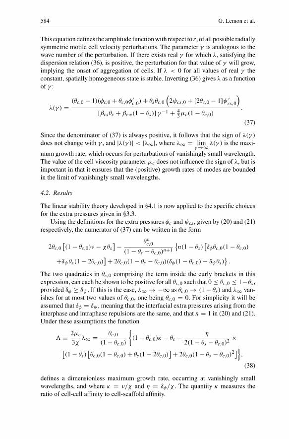
The two quadratics in θc,0 comprising the term inside the curly brackets in thisexpression, can each be shown to be positive for all θc,0 such that 0 ≤ θc,0 ≤ 1−θs ,provided δφ ≥ δψ . If this is the case, λ∞ → −∞ as θc,0 → (1 − θs) and λ∞ van-ishes for at most two values of θc,0, one being θc,0 = 0. For simplicity it will beassumed that δφ = δψ , meaning that the interfacial extra pressures arising from theinterphase and intraphase repulsions are the same, and that n = 1 in (20) and (21).Under these assumptions the function

� ≡ 2µc3χ

λ∞ = θc,0

(1 − θc,0)

{(1 − θc,0)κ − θs − η

2(1 − θs − θc,0)2×

[(1 − θs)

[θc,0(1 − θc,0)+ θs(1 − 2θc,0)

]+ 2θc,0(1 − θs − θc,0)2]},

(38)

defines a dimensionless maximum growth rate, occurring at vanishingly smallwavelengths, and where κ = ν/χ and η = δφ/χ . The quantity κ measures theratio of cell-cell affinity to cell-scaffold affinity.

Mathematical modelling of engineered tissue growth 585

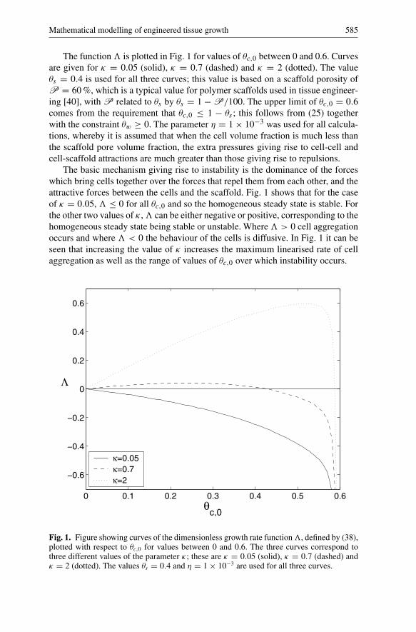
The function� is plotted in Fig. 1 for values of θc,0 between 0 and 0.6. Curvesare given for κ = 0.05 (solid), κ = 0.7 (dashed) and κ = 2 (dotted). The valueθs = 0.4 is used for all three curves; this value is based on a scaffold porosity ofP = 60 %, which is a typical value for polymer scaffolds used in tissue engineer-ing [40], with P related to θs by θs = 1 − P/100. The upper limit of θc,0 = 0.6comes from the requirement that θc,0 ≤ 1 − θs ; this follows from (25) togetherwith the constraint θw ≥ 0. The parameter η = 1 × 10−3 was used for all calcula-tions, whereby it is assumed that when the cell volume fraction is much less thanthe scaffold pore volume fraction, the extra pressures giving rise to cell-cell andcell-scaffold attractions are much greater than those giving rise to repulsions.

The basic mechanism giving rise to instability is the dominance of the forceswhich bring cells together over the forces that repel them from each other, and theattractive forces between the cells and the scaffold. Fig. 1 shows that for the caseof κ = 0.05, � ≤ 0 for all θc,0 and so the homogeneous steady state is stable. Forthe other two values of κ ,� can be either negative or positive, corresponding to thehomogeneous steady state being stable or unstable. Where� > 0 cell aggregationoccurs and where � < 0 the behaviour of the cells is diffusive. In Fig. 1 it can beseen that increasing the value of κ increases the maximum linearised rate of cellaggregation as well as the range of values of θc,0 over which instability occurs.

0 0.1 0.2 0.3 0.4 0.5 0.6

−0.6

−0.4

−0.2

0

0.2

0.4

0.6

θc,0

Λ

κ=0.05κ=0.7κ=2

Fig. 1. Figure showing curves of the dimensionless growth rate function�, defined by (38),plotted with respect to θc,0 for values between 0 and 0.6. The three curves correspond tothree different values of the parameter κ; these are κ = 0.05 (solid), κ = 0.7 (dashed) andκ = 2 (dotted). The values θs = 0.4 and η = 1 × 10−3 are used for all three curves.

586 G. Lemon et al.

Such dynamical instabilities can be expected to result in the break up of thehomogeneous steady state into aggregates in which the value of the cell volumefraction is such that � ≤ 0. In the case of κ = 0.7, the stable region for valuesof θc,0 above about 0.43 corresponds to a cell aggregate; the unstable region lessthan this value can be associated with an area of the scaffold that becomes devoidof cells.

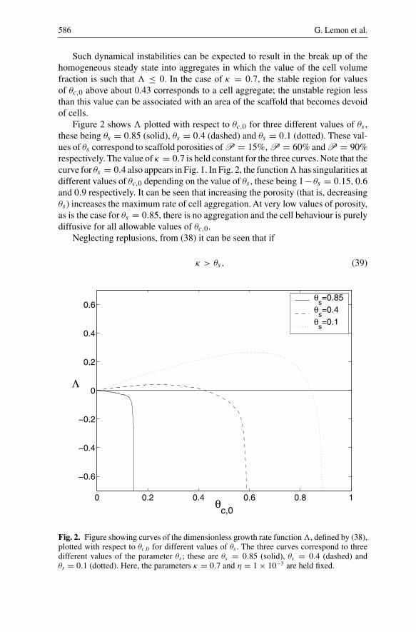
Figure 2 shows � plotted with respect to θc,0 for three different values of θs ,these being θs = 0.85 (solid), θs = 0.4 (dashed) and θs = 0.1 (dotted). These val-ues of θs correspond to scaffold porosities of P = 15%,P = 60% and P = 90%respectively. The value of κ = 0.7 is held constant for the three curves. Note that thecurve for θs = 0.4 also appears in Fig. 1. In Fig. 2, the function� has singularities atdifferent values of θc,0 depending on the value of θs , these being 1−θs = 0.15, 0.6and 0.9 respectively. It can be seen that increasing the porosity (that is, decreasingθs) increases the maximum rate of cell aggregation. At very low values of porosity,as is the case for θs = 0.85, there is no aggregation and the cell behaviour is purelydiffusive for all allowable values of θc,0.

Neglecting replusions, from (38) it can be seen that if

κ > θs, (39)

0 0.2 0.4 0.6 0.8 1

−0.6

−0.4

−0.2

0

0.2

0.4

0.6

θc,0

Λ

θs=0.85

θs=0.4

θs=0.1

Fig. 2. Figure showing curves of the dimensionless growth rate function�, defined by (38),plotted with respect to θc,0 for different values of θs . The three curves correspond to threedifferent values of the parameter θs ; these are θs = 0.85 (solid), θs = 0.4 (dashed) andθs = 0.1 (dotted). Here, the parameters κ = 0.7 and η = 1 × 10−3 are held fixed.

Mathematical modelling of engineered tissue growth 587

then� > 0 for sufficiently small values of θc,0, and hence cell aggregation occurs.As θc,0 increases, crowding effects of cells on each other decreases the contributionto the rate of aggregation by cell-cell interactions. This effect is represented by the(1 − θc,0) factor appearing inside the curly brackets in (38). The −θs term, alsoinside the brackets, represents the negative contribution to the growth rate by cell-scaffold interactions, and at sufficiently large θc,0 this dominates. As θc,0 increasestowards the volume fraction of pores in the scaffold, the repulsive forces begin todominate, further decreasing �.

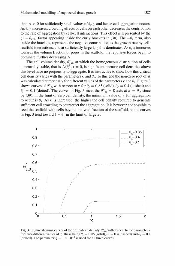
The cell volume density, θ∗c,0, at which the homogeneous distribution of cells

is neutrally stable, that is �(θ∗c,0) = 0, is significant because cell densities above

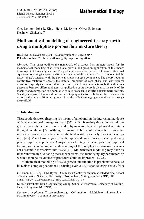
this level have no propensity to aggregate. It is instructive to show how this criticalcell density varies with the parameters κ and θs . To this end the non-zero root of�was calculated numerically for different values of the parameters κ and θs . Figure 3shows curves of θ∗

c,0 with respect to κ for θs = 0.85 (solid), θs = 0.4 (dashed) andθs = 0.1 (dotted). The curves in Fig. 3 meet the θ∗

c,0 = 0 axis at κ = θs , sinceby (39), in the limit of zero cell density, the minimum value of κ for aggregationto occur is θs . As κ is increased, the higher the cell density required to generatesufficient cell crowding to counteract the aggregation. It is however not possible toseed the scaffold with cells beyond the void fraction of the scaffold, so the curvesin Fig. 3 tend toward 1 − θs in the limit of large κ .

0 0.5 1 1.5 20

0.1

0.2

0.3

0.4

0.5

0.6

0.7

0.8

0.9

1

κ

θc,0*

θs=0.85

θs=0.4

θs=0.1

Fig. 3. Figure showing curves of the critical cell density, θ∗c,0, with respect to the parameter κ

for three different values of θs , these being θs = 0.85 (solid), θs = 0.4 (dashed) and θs = 0.1(dotted). The parameter η = 1 × 10−3 is used for all three curves.

588 G. Lemon et al.

The parameter θs is a property of the scaffold material that can be modifiedrelatively easily during its manufacture. The parameter κ , however, through itsdependence on ν and χ , depends on both the characteristics of the cells and thoseof the surface of the scaffold. In principle, its value could be changed by altering thechemistry or physics of the scaffold surface. Indeed, low cell-scaffold affinity dueto scaffold hydrophobicity is a serious drawback to the use of polylactic acid (PLA)scaffolds for tissue engineering applications, since this results in a preference forcells to aggregate. From the analysis presented above, aggregation of cells can becurbed by using a scaffold with sufficiently low porosity and/or a sufficiently lowvalue of κ . However, lower porosity makes initial penetration of the scaffold withcells more difficult. Aggregation can also be curbed using a cell seeding densityabove the critical density.

The ultimate distribution of cell aggregates and cell voids in the steady state islikely to depend both on the form of the initial perturbation to the spatially homoge-neous steady state and the effects of nonlinear terms. Thus the model predicts that, inexperiments, the ultimate size of the aggregates and their morphology and distribu-tion, depend critically upon the initial distribution of cells seeded into the scaffold.Given that the initial seeding distribution exhibits a high degree of randomness, thisis reflected in the wide variation in the characteristics of the cell aggregates seenin some experiments. A detailed simulation of cell aggregate formation requiresnumerical solution of the model equations. This is beyond the scope of the presentwork and will be the subject of a forthcoming publication.

When λ > 0, the initial growth of a perturbation to the homogeneous steadystate is dominated by the mode with the largest positive growth rate, this being λ∞.Using (38), λ∞ can be estimated for the case of a sparse distribution of cells, whereθc,0 � 1, this being

λ∞ = 3θc,02µc

(ν − χθs),

where the assumption δφ � ν, χ has been used.When λ < 0, the higher the wave number of a mode, the more rapidly it will

decay. Thus the damping of an initial perturbation to the homogeneous steady stateis determined by the lower wave number modes. If consideration is restricted tomodes with wave numbers such that

43µc(1 − θc,0) γ � [βcsθs + βcw(1 − θs)] ,

(37) reduces to a dispersion relation of the form

λ = −Dvγ.

This is identical to the dispersion relation for the diffusion equation in sphericallysymmetric polar coordinates,

∂u

∂t= D

r2

∂

∂t

(r2 ∂u

∂r

),

Mathematical modelling of engineered tissue growth 589

which has eigenmodes of the form

u = eλtJ0(γ1/2r),

where λ = −Dγ . Thus from (37),

Dv = θc,0

[βcsθs + βcw(1 − θs)]

{2[χθs − (1 − θc,0)ν

]+ δφ

(1 − θc,0 − θs)2

×[(1 − θs)[θc,0(1 − θc,0)+ θs(1 − 2θc,0)

]+ 2θc,0(1 − θs − θc,0)2]}

can be identified as the diffusion coefficient. The classical diffusion coefficient,D,relates the perturbed cell velocity, εvc,1, to gradients in the cell density, or equiva-lently, to ε∇θc,1. However, since the flux of cells in terms of their volume fractionis to first order, εvc,1θc,0, it follows that the diffusion coefficient is Dv = θc,0D.The case of a sparse collection of cells moving on a substrate corresponds to avanishingly small volume fraction, θc,0 � 1, from which there is obtained

D = 2(χθs − ν)

βcsθs + βcw(1 − θs), (40)

where the assumption δφ � ν, χ has again been used. Experimental values of D,for example 10 µm2 min−1 for osteoblasts [15], could be used to estimate valuesfor the parameters in (40).

From (40), increasing the drag coefficients βcw and βcs lowers the diffusioncoefficient, D. The parameter βcs depends not only on the nature of the interfacebetween the surface of the scaffold and the membrane of each cell, but also thetopography and topology of the scaffold itself. The void space in many types ofmacroporous scaffolds consists of a set of pores, typically of diameter in the rangetens to hundreds ofµm, interconnected by window-like openings or ‘fenestrations’[40]. The ability of cells to migrate through the scaffold depends on the degree ofconnectivity between the pores and the size of the fenestrations; thus, the smallerthe fenestration size, the higher the value of βcs . One approach to obtaining a quan-titative relation between βcs and the scaffold surface topography would be to treatflow through a bundle of sinusoidal shaped capillaries, see for example [59].

5. Discussion

In this paper a mixture theory is presented for the purposes of modelling in vitrotissue growth processes relevant to tissue engineering. In the first part of the paper,the general theory is presented, and in the second part, application of the theoryis given to the initial stages of aggregation of cells seeded into artificial polymericscaffolds.

This application requires a three-phase model comprising cells, water and asolid scaffold material. The dynamics of the different components of the mix-ture were analysed using linear-stability techniques. The interplay between thestresses induced by cell-cell interactions and cell-scaffold tractions results in differ-ent dynamical regimes, depending on the values of the parameters. There are shown

590 G. Lemon et al.

to be two essentially different regimes: either the cells form aggregates or theydiffuse and spread out to become uniformly distributed through the scaffold. Theseresults agree qualitatively with those of experiments where cells are seeded ontopolymeric surfaces [55] and into hydrogels [34]. In those studies it was shown thatwhether or not cells spread or form aggregates depended on the relative strengthsof cell-cell forces and cell-substrate forces.

The existence and extent of these regimes is governed by parameters that dependon the material properties of the scaffold. This suggests that the characteristics ofthe scaffold could be engineered so as to make the seeded cells behave in specificways. A major current concern in tissue engineering is to ensure that an artificialmatrix material is seeded uniformly with cells [14]. The methodology presented inthis paper demonstrates how parameter regimes can be determined where this ispossible.

Other applications may require some control over the seeding density of cellsin the scaffold. It has been demonstrated that the cell density in an aggregate canbe manipulated by varying the values of the parameters (see Fig. 3). This princi-ple could be applied to where a gradient in the cell density is required, such aswhen there is a need to bind a non-biodegradable material to native tissue [54,60].Scaffolds for these applications have a gradient in biodegradability and cells seededinto them need to be directed to migrate preferentially to the more biodegradableparts of the scaffold.

Theoretical analysis can be performed on direct extensions of the present three-phase model. For example, growth terms describing the contact inhibition of prolif-eration of cells [33] can be added to the right hand side of (1), in order to investigatethe pattern of growth of cell aggregates and colonies. Also, the effect on thecell dynamics of an ambient fluid flow could be investigated, this being relevantto where liquid is being perfused through the tissue sample inside a bioreactor[48,38,56]. Such an analysis is again beyond the scope of the present study; how-ever, it is instructive to combine (23) and (24) to eliminate the cell viscosity term,giving

(βcsθcθs + βcwθcθw)vc = (1 − θc)∇p + 2θs∇(θcψcs)−θcθs∇ψcs + βcwθcθwvw.

This equation shows that in the absence of cell-scaffold drag, the cell-water dragforce will tend to make the cells travel with the same velocity as the ambient flow,but their motion is impeded in the presence of cell-scaffold drag. It is reasonableto assume that βcw << βcs , implying that the cells travel at a much lower speedthan that of the liquid.

It is the intention also to apply the theory given in this paper to more spe-cific applications in tissue engineering. Consideration is currently being given toits application to the engineering of cartilage. Articular cartilage has extremelylimited capacity for self repair in vivo, and this has prompted much effort in thedevelopment of ex vivo implants, whereby artificial matrix materials are seededwith chondrocytes and surgically implanted into the joint cartilage defect [37,61].At present, insufficient penetration of chondrocytes into the scaffolds, as discussed

Mathematical modelling of engineered tissue growth 591

above, is a serious impediment to the production of engineered tissue that possessesthe same characteristics as native tissue. Modelling of the growth and developmentof the artificial cartilage could help improve the quality of the implants. Such amodel must include extra phases, in particular the extra cellular matrix (ECM)components, as well as growth terms in (1) that represent interconversion of massbetween phases, such as the degradation of scaffold by enzymes released by thecells and its replacement with ECM. The general multiphase framework outlinedin this paper will be applicable in studying a wide range of such issues.

Acknowledgements. The authors gratefully acknowledge the financial support of theEPSRC. They also wish to thank Felicity Rose and Marta Silva for helpful discussions.

References

1. Alt, W., Dembo, M.: Cytoplasm dynamics and cell motion: two-phase flow models.Math. Biosci. 156, 207–228 (1999)

2. Araujo, R.P., McElwain, D.L.S.: A mixture theory for the genesis of residual stresses ingrowing tissues I: A general formulation. SIAM J Appl. Math. 65, 1261–1284 (2005)

3. Atkin, R.J., Craine, R.E.: Continuum theories of mixtures: basic theory and historicaldevelopment. Q. J. Mech. Appl. Math. 29, 209–244 (1976)

4. Barocas, V.H., Tranquillo, R.T.: An anisotropic biphasic theory of tissue-equivalentmechanics: the interplay among cell traction, fibrillar network deformation, fibril align-ment, and cell contact guidance. J. Biomech. Eng. 119, 137–145 (1997)

5. Bhati, R.S., Mukherjee, D.P., McCarthy, K.J., Rogers, S.H., Smith, D.F., Shalaby, S.W.:The growth of chondrocytes into a fibronectin-coated biodegradable scaffold. J. Biomed.Mater. Res. 56 (1), 74–82 (2001)

6. Bowen, R.M.: Theory of mixtures. In: A. C. Eringen (ed.), Continuum physics, pp.1–127 Academic Press, 1976

7. Bowen, R.M.: Incompressible porous media models by use of the theory of mixtures.Int. J. Engng Sci. 18, 1129–1148 (1980)

8. Breward, C.J.W., Byrne, H.M., Lewis, C.E.: The role of cell-cell interactions in a two-phase model for avascular tumour growth J. Math. Biol. 45, 125–152 (2002)

9. Byrne, H., Chaplain, M.A.J.: Free boundary value problems associated with the growthand development of multicellular spheroids. Eur. J. Appl. Math. 8 (6), 639–658 (1997)

10. Byrne, H., Preziosi, L.: Modelling solid tumour growth using the theory of mixtures.Math. Med. Biol. 20 (4), 341–366 (2003)

11. Byrne, H.M., King, J.R., McElwain, D.L.S., Preziosi, L.: A two-phase model of tumourgrowth. Appl. Math. Lett. 16, 567–573 (2003)

12. Cowin, S.C.: How is a tissue built? J. Biomech. Eng. 122, 553–569 (2000)13. Cowin, S.C.: Tissue growth and remodeling.Annu. Rev. Biomed. Eng. 6, 77–107 (2004)14. Dar, A., Shachar, M., Leor, J., Cohen, S.: Optimization of cardiac cell seeding and

distribution in 3D porous alginate scaffolds. Biotechnol. Bioeng. 80, 305–312 (2002)15. Dee, K.C., Andersen, T.T., Bizios, R.: Osteoblast population migration characteristics

on substrates modified with immobilized adhesive peptides. Biomaterials 20, 221–227(1999)

16. Dembo, M., Harlow, F.: Cell motion contractile networks and the physics of interpene-trating reactive flow. Biophys. J. 50, 109–121 (1986)

17. Drew, D.A.: Mathematical modeling of two-phase flow. Ann. Rev. Fluid Mech. 15,261–291 (1983)

592 G. Lemon et al.

18. Drew, D.A., Passman, S.L.: Theory of multicomponent fluids. Springer, 199919. Drew, D.A., Segel, L.A.: Averaged equations for two-phase flows. Stud. Appl. Math. L

3, 205–231 (1971)20. Ermentrout, G.B., Edelstein-Keshet, L.: Cellular automata approaches to biological

modeling. J. Theor. Biol. 160, 97–133 (1993)21. Forgacs, G., Foty, R.A., Shafrir, Y., Steinberg, M.S.: Viscoelastic properties of living

embryonic tissues: a quantitative study. Biophys. J. 74, 2227–2234 (1998)22. Foty, R.A., Forgacs, G., Pfleger, C.M., Steinberg, M.S.: Liquid properties of embry-

onic-tissues - measurement of interfacial-tensions. Phys. Rev. Lett. 72 (14), 2298–2301(1994)

23. Galban, C.J., Locke, B.R.: Analysis of cell growth in a polymer scaffold using a movingboundary approach. Biotechnol. Bioeng. 56 (4), 422–432 (1997)

24. Garikipati, K.,Arruda, E.M., Grosh K., Narayanan H., Calve, S.:A continuum treatmentof growth in biological tissue: the coupling of mass transport and mechanics. J. Mech.Phys. Solids. 52, 1595–1625 (2004)

25. Grodzinsky,A.J., Kamm, R.D., Lauffenburger, D.A.: Quantitative aspects of tissue engi-neering: basic issues in kinetics transport and mechanics. In: R Lanzer and R Langer andW Chick (ed.), Principles of Tissue Engineering. pp. 193–207 R.G. Landes Company,1997

26. Hoger, A.: Virtual configurations and constitutive equations for residually stressed bod-ies with material symmetry. J. Elast. 48 (2), 125–144 (1997)

27. Humphrey, J.D.: Continuum biomechanics of soft biological tissues. Proc. R. Soc. Lond.A 459, 3–46 (2003)

28. Humphrey, J.D., Rajagopal, K.R.: A constrained mixture model for growth and remod-eling of soft tissues. Math. Mod. Meth. Appl. S. 12, 407–430 (2002)

29. Hunter, D.J., March, L., Sambrook, P.N.: Knee osteoarthritis: The influence of environ-mental factors. Clin. Exp. Rheumatol. 20 (1), 93–100 (2002)

30. Ingram, J.D., Eringen, A.C.: A continuum theory of chemically reacting media - IIConstitutive equations of reacting fluid mixtures. Int. J. Engng Sci. 5, 289–322 (1967)

31. Ishuag-Riley, S.L., Crane-Kruger, G.M., Miller, M.J., Yasko, A.W., Yaszemski, M.J.,Mikos, A.G.: Bone formation by three-dimensional stromal osteoblast culture in biode-gradable polymer scaffolds. J. Biomed. Mater. Res. 36, 17–28 (1997)

32. Ishuag-Riley, S.L., Crane-Kruger, G.M., Yaszemski, M.J., Mikos, A.G.: Three-dimen-sional culture of rat calvarial osteoblasts in porous biodegradable polymers. Biomate-rials 19, 1405–1412 (1998)

33. Itano, N., Atsumi, F., Sawai, T., Yamada, Y., Miyaishi, O., Senga, T., Hamaguchi, M.,Kimata, K.: Abnormal accumulation of hyaluronan matrix diminishes contact inhibitionof cell growth and promotes cell migration. P. Natl. Acad. Sci. USA 99 (6), 3609–3614(2002)

34. Jakab, K., Neagu, A., Mironov, V., Markwald, R.R., Forgacs, G.: Engineering biologi-cal structures of prescribed shape using self-assembling multicellular systems. P. Natl.Acad. Sci. USA. 101 (9), 2864–2869 (2004)

35. Lai, W.M., Hou, J.S., Mow, V.C.: A triphasic theory for the swelling and deformationalbehaviours of articular cartilage. J. Biomech. Eng. 113, 245–258 (1991)

36. Landman, K.A., Please, C.P.: Tumour dynamics and necrosis: surface tension and sta-bility. Math. Med. Biol. 18, 131–158 (2001)

37. Langer, R., Vacanti, J.P.: Tissue Engineering. Science 260, 920–926 (1993)38. Lappa, M.: Organic tissues in rotating bioreactors: fluid-mechanical aspects dynamic

growth models, and morphological evolution. Biotechnol. Bioeng. 84 (5), 518–532(2003)

Mathematical modelling of engineered tissue growth 593

39. Levenberg, S., Langer, R.: Advances in tissue engineering. In: Current topics in devel-opmental biology, Elsevier 61, (2004)

40. Li, S.H., de Wijn, J.R., Layrolle, P., de Groot, K.: Macroporous biphasic calcium phos-phate scaffold with high permeability/porosity ratio. Tissue Eng. 9 (3), 535–548 (2003)

41. Longo, D., Peirce, S.A., Skalak, T.C., Davidson, L., Marsden, M., Dzamba, B., DeSi-mone, D.W.: Multicellular computer simulation of morphogenesis: blastocoel roof thin-ning and matrix assembly in Xenopus laevis. Dev. Biol. 271 (1), 210–222 (2004)

42. Lubkin, S.R., Jackson, T.: Multiphase mechanics of capsule formation in tumors.J. Biomech. Eng. 124 (2), 237–243 (2002)

43. MacArthur, B.D., Please, C.P., Taylor, M., Oreffo, R.O.C.: Mathematical modelling ofskeletal repair. Biochem. Bioph. Res. Co. 313, 825–833 (2004)

44. Mackie, E.J.: Osteoblasts: novel roles in orchestration of skeletal architecture. Int. J.Biochem. Cell. B. 35 (9), 1301–1305 (2003)

45. Marle, C.M.: On macroscopic equations governing multiphase flow with diffusion andchemical reactions in porous media. Int. J. Engng Sci. 20 (5), 643–662 (1982)

46. Martin, I., Wendt, D., Heberer, M.: The role of bioreactors in tissue engineering. TrendsBiotechnol. 22, 80–86 (2004)

47. Massoudi, M.: Constitutive relations for the interaction force in multicomponent par-ticulate flows. Int. J. Nonlinear. Mech. 38 (3), 313–336 (2003)

48. Mizuno, S., Alleman, F., Glowacki, J.: Effects of medium perfusion on matrix produc-tion by bovine chondrocytes in three-dimensional collagen sponges. J. Biomed. Mater.Res. 56 (3), 368–375 (2001)

49. Morse, P.M., Feshbach, H.: Methods of theoretical physics. Vol 1. McGraw-Hill, 195350. Mow, V.C., Kuei, S.C., Lai, W.M., Armstrong, C.G.: Biphasic creep and stress relaxa-

tion of articular cartilage in compression: theory and experiment. J. Biomech. Eng. 102,73–84 (1980)

51. Murray, J.D.: Mathematical Biology. Springer, 3rd edn. 200252. Palferman, T.G.: Bone and joint diseases around the world. The UK perspective.

J. Rheumatol. 30, 33–35 (2003)53. Rose, F.R., Cyster, L.A., Grant, D.M., Scotchford, C.A., Howdle, S.M., Shakesheff,

K.M.: In vitro assessment of cell penetration into porous hydroxyapatite scaffolds witha central aligned channel. Biomaterials 25 (24), 5507–5514 (2004)

54. Roy, T.D., Simon, J.L., Ricci, J.L., Rekow, E.D., Thompson, V.P., Parsons, J.R.: Per-formance of degradable composite bone repair products made via three-dimensionalfabrication techniques. J. Biomed. Mater. Res. A 66, 283–291 (2003)

55. Ryan, P.L., Foty, R.A., Kohn, J., Steinberg, M.S.: Tissue spreading on implantable sub-strates is a competitive outcome of cell-cell vs. cell-substratum adhesivity. P. Natl.Acad.Sci. USA. 98 (8), 4323–4327 (2001)

56. Saini, S., Wick, T.M.: Concentric cylinder bioreactor for production of tissue engineeredcartilage: Effect of seeding density and hydrodynamic loading on construct develop-ment. Biotechnol. Prog. 19 (2), 510–521 (2003)

57. Sengers, B.G., Oomens, C.W.J., Baaijens, F.P.T.: An integrated finite-element approachto mechanics transport and biosynthesis in tissue engineering. J. Biomech. Eng. 126,82–90 (2004)

58. Sharma, B., Elisseeff, J.H.: Engineering structurally organized cartilage and bone tis-sues. Ann. Biomed. Eng. 32 (1), 148–159 (2004)

59. Sheffield, R.E., Metzner, A.B.: Flows of nonlinear fluids through porous media. AIChEJ. 22 (4), 736–744 (1976)

60. Sherwood, J.K., Riley, S.L., Palazzolo, R., Brown, S.C., Monkhouse, D.C., Coates, M.,Griffith, L.G., Landeen, L.K., Ratcliffe, A.: A three-dimensional osteochondral com-posite scaffold for articular cartilage repair. Biomaterials 23, 4739–4751 (2002)

594 G. Lemon et al.

61. Sittinger, M., Perka, C., Schultz, O., Haupl, T., Burmester, G.R.: Joint cartilage regen-eration by tissue engineering. Z. Rheumatol. 58 (3), 130–135 (1999)

62. Skalak, R., Zargaryan. S., Jain, R.K., Netti, P.A., Hoger, A.: Compatibility and thegenesis of residual stress by volumetric growth. J. Math. Biol. 34 (8), 889–914 (1996)

63. Stock, U.A., Vacanti, J.P.: Tissue engineering: current state and prospects. Annu. Rev.Med. 52, 443–451 (2001)

64. Sun, D.N., Gu, W.Y., Guo, X.E., Lai, W.M., Mow, V.C.: A mixed finite element formu-lation of triphasic mechano-electrochemical theory for charged hydrated biological softtissues. Int. J. Numer. Meth. Eng. 45, 1375–1402 (1999)

65. Truesdell, C., Noll, W.: The nonlinear field theory of mechanics. In: S. Flugge (ed.),Handbuch der Physik, Springer, 1960