MATHEMATICAL MODELING CONSIDERING AIR POLLUTION OF TRANSPORTATION: AN URBAN ENVIRONMENTAL PLANNING,...

Hadipour M., Pourebrahim S. and Mahmmud A. R.

MATHEMATICAL MODELING CONSIDERING AIR POLLUTION OF TRANSPORTATION: AN URBAN ENVIRONMENTAL PLANNING, CASE STUDY IN PETALING JAYA, MALAYSIA

75

Theoretical and Empirical Researches in Urban Management

Num

ber 4(13) / November 2009

MATHEMATICAL MODELING CONSIDERING

AIR POLLUTION OF TRANSPORTATION: AN

URBAN ENVIRONMENTAL PLANNING, CASE

STUDY IN PETALING JAYA, MALAYSIA

Mehrdad HADIPOUR Department of Environment, Arak University

Shahid Beheshti Ave, Arak, Iran [email protected]

Sharareh POUREBRAHIM

Department of Environment, Arak University Shahid Beheshti Ave, Arak, Iran

[email protected]

Ahmad Rodzi MAHMMUD Department of Civil Engineering, University Putra Malaysia,

4300, Serdang,Selangor, Malaysia [email protected]

Abstract This paper provides the findings on a project undertaken to develop a geo-spatial mathematical model relating landuse, road type and air quality. The model shows how spatial elements and issues were quantified to accurately represent the usual and unusual urban environment in the development of residential land-use. The mathematical relationship was based on the optimum distance between residential area and urban transportation network. This mathematical analysis would provide a better planning for urban transportation. The spatial data (urban land-use and urban network development) were generated using satellite images, aerial photos and land use maps. Geospatial analyses were performed to find the effect and impact of urban air quality with respect to urban transportation networks. The output of the study would assist the task to reduce negative transport environmental impacts particularly in the field of air pollution. It would also be useful in identifying the potential residential area with respect to urban transportation network towards achieving sustainable development.

Keywords: Transportation, Model, Air pollution, urban environment, land use

1. Introduction

Air quality, regarded a main infrastructure element in urban transportation system, is considered as a

major criterion for human settlement. Therefore transport emitted air pollution appears related to the

establishment of urban landuse in proportion to urban transportation network. Increasing demand for

76

Hadipour M., Pourebrahim S. AND Mahmmud A. R.



Num


residential areas, along with this development of cities, has given rise to some environmental issues

(Bell and Blake, 2000; Ranjan, 2001). More than half of the world’s population lives in urban areas

(Colesca S., 2009), therefore increasing urban land-uses resulted in several impacts on various fields

such as air quality, accessibility and land use. Air quality has been considered as one of the major

environmental elements by many urban planners (Colvile et al. 2000; Nicolas et al. 2005). Therefore,

there is a need to look into urban transportation planning together with landuse development.

With respect to above note, paper presents development of a mathematical model to find suitable

locations for landuses and urban transportation network for the urban transportation system of Petaling

Jaya Municipal Council (MPPJ). The model essentially investigated the best air quality for residential

area. It was based on the optimum distance from residential zones to urban networks as main element

avoiding transport emitted air pollution.

Petaling Jaya Municipal Council (MPPJ), a developing city in Malaysia, was chosen as study area, Its

based on choices of environmental factors such as: several routes to access to important public

facilities, High transportation activities, Efforts to maintain its "garden city" concept, Efforts to establish

well-developed infrastructures and excellent investment opportunities.

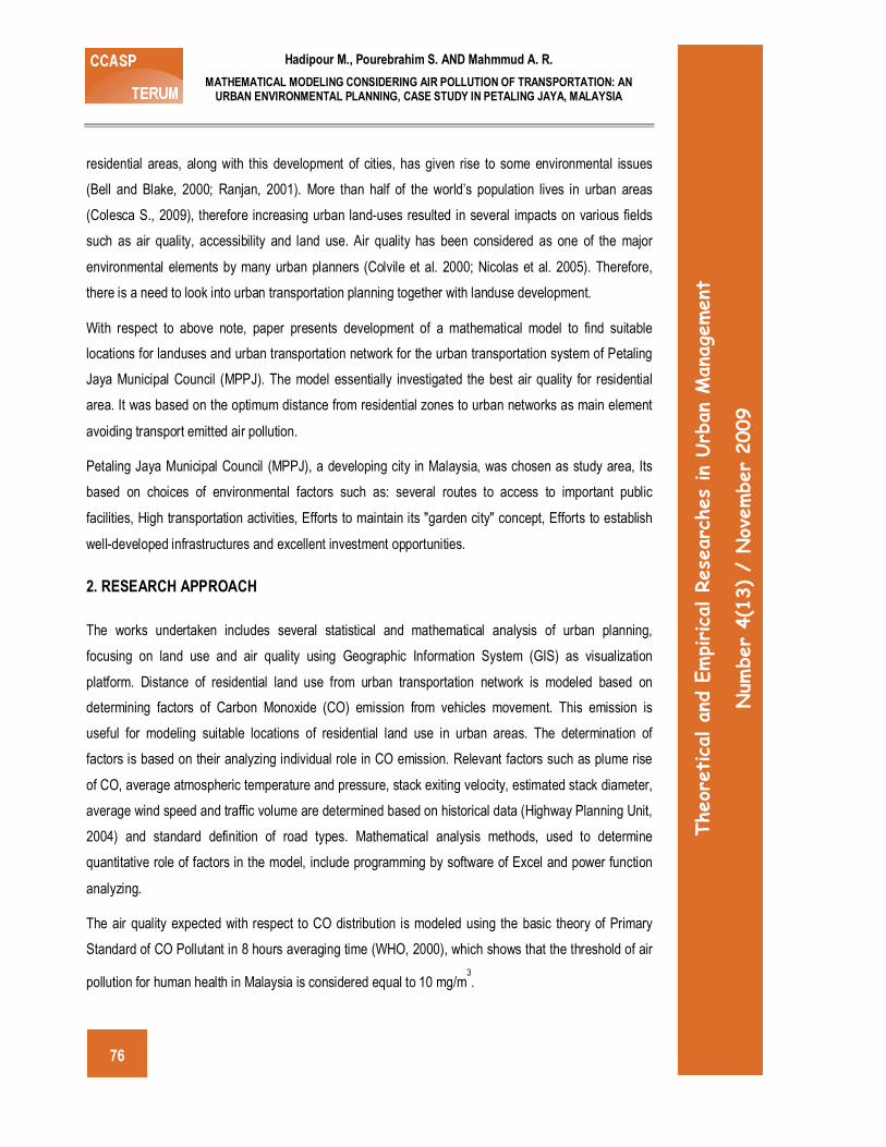
2. RESEARCH APPROACH

The works undertaken includes several statistical and mathematical analysis of urban planning,

focusing on land use and air quality using Geographic Information System (GIS) as visualization

platform. Distance of residential land use from urban transportation network is modeled based on

determining factors of Carbon Monoxide (CO) emission from vehicles movement. This emission is

useful for modeling suitable locations of residential land use in urban areas. The determination of

factors is based on their analyzing individual role in CO emission. Relevant factors such as plume rise

of CO, average atmospheric temperature and pressure, stack exiting velocity, estimated stack diameter,

average wind speed and traffic volume are determined based on historical data (Highway Planning Unit,

2004) and standard definition of road types. Mathematical analysis methods, used to determine

quantitative role of factors in the model, include programming by software of Excel and power function

analyzing.

The air quality expected with respect to CO distribution is modeled using the basic theory of Primary

Standard of CO Pollutant in 8 hours averaging time (WHO, 2000), which shows that the threshold of air

pollution for human health in Malaysia is considered equal to 10 mg/m3

.



77


Num


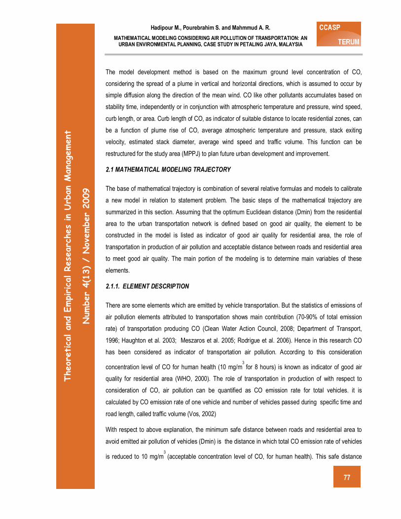
The model development method is based on the maximum ground level concentration of CO,

considering the spread of a plume in vertical and horizontal directions, which is assumed to occur by

simple diffusion along the direction of the mean wind. CO like other pollutants accumulates based on

stability time, independently or in conjunction with atmospheric temperature and pressure, wind speed,

curb length, or area. Curb length of CO, as indicator of suitable distance to locate residential zones, can

be a function of plume rise of CO, average atmospheric temperature and pressure, stack exiting

velocity, estimated stack diameter, average wind speed and traffic volume. This function can be

restructured for the study area (MPPJ) to plan future urban development and improvement.

2.1 MATHEMATICAL MODELING TRAJECTORY

The base of mathematical trajectory is combination of several relative formulas and models to calibrate

a new model in relation to statement problem. The basic steps of the mathematical trajectory are

summarized in this section. Assuming that the optimum Euclidean distance (Dmin) from the residential

area to the urban transportation network is defined based on good air quality, the element to be

constructed in the model is listed as indicator of good air quality for residential area, the role of

transportation in production of air pollution and acceptable distance between roads and residential area

to meet good air quality. The main portion of the modeling is to determine main variables of these

elements.

2.1.1. ELEMENT DESCRIPTION

There are some elements which are emitted by vehicle transportation. But the statistics of emissions of

air pollution elements attributed to transportation shows main contribution (70-90% of total emission

rate) of transportation producing CO (Clean Water Action Council, 2008; Department of Transport,

1996; Haughton et al. 2003; Meszaros et al. 2005; Rodrigue et al. 2006). Hence in this research CO

has been considered as indicator of transportation air pollution. According to this consideration

concentration level of CO for human health (10 mg/m3

for 8 hours) is known as indicator of good air

quality for residential area (WHO, 2000). The role of transportation in production of with respect to

consideration of CO, air pollution can be quantified as CO emission rate for total vehicles. it is

calculated by CO emission rate of one vehicle and number of vehicles passed during specific time and

road length, called traffic volume (Vos, 2002)

With respect to above explanation, the minimum safe distance between roads and residential area to

avoid emitted air pollution of vehicles (Dmin) is the distance in which total CO emission rate of vehicles

is reduced to 10 mg/m3

(acceptable concentration level of CO, for human health). This safe distance

78




Num


depends on a plume in vertical and horizontal directions is assumed to occur by simple diffusion along

the direction of the mean wind, total CO emission rate of vehicles as expressed in Equation (1),

developed by Turner (1995).

1

1/2 1/2x

y z z y

Q H YC e e

Uπσ σ σ σ

−

− −

=

(1)

Hence for calculating of this distance, it is required to apply total CO emission rate of vehicles, rise

distance of emitted CO, mean wind speed and standard deviation of vertical and horizontal wind

direction.

2.1.2. QUANTIFICATION OF ELEMENTS

CO pollution is very sensitive and traffic volume changes over times are considerably unpredictable.

Therefore, for calculating total CO emission rate of vehicles, it is better to consider road capacity

(maximum possible traffic volume) replacing traffic volume, as expressed in Equation (2)

( ) cQ RC q= (2)

Where

Q = Total CO emission rate of vehicles

RC = Possible road capacity in stability time of CO

qc = Possible average CO emission rate for one vehicle

A simple Equation to calculate road capacity is developed by Li (1998) as follow:

( )

=m

tp

C

VWL

RC (3)

Where,

W= Road width based on road type (m),

Lp= Passed road length by vehicle,



79


Num


Cm = one vehicle’s normal Average space time usage (m2

) and

Vt = average Vehicle speed based on road type (m/s) = Average passed length by car per second (m).

Since, the concentration of pollutant reaches a peak value within5 minutes of the gas injection, the

maximum reasonable specific time for calculating the number of passed car is considered as less than

15 minutes (Colorado Department of Public Health and Environment, 2006)

Cm is calculated for the study area, based on percentage of vehicle types (according to historical data

of traffic volume) and their actual size. W and Vt were applied based on road types (table1). Lp (passed

road length by vehicle) refers to selected greed size to investigate and study of air pollution. And qc was

obtained trough mathematical process, considering some important elements like percentage of vehicle

types, average fuel consumption of foreign and domestic employing vehicles, average normal age of

employing vehicles, percentage of different ages of employing vehicles.

For computing rise distance of emitted CO by vehicle transportation (∆h), Equations (4) and (5)

developed by Wayson (2000) were used as follows:

Where,

∆h = Rise distance (m),

F0 = Buoyancy factor (m4

/s3

),

t = Time (s),

U = Ambient horizontal wind speed (m/s),

g = Gravitational constant = 9.81 m/s2

,

vs = Exit velocity (m/s),

rs = Exit radius (m),

Ta = Ambient temperature (K) and

Ts = Exit temperature (K).

The parameters and also mean wind speed could easily be obtained through annual reports of the study

area (DOE, 2004) actual measurement with respect to various vehicle types, standards and guidelines.

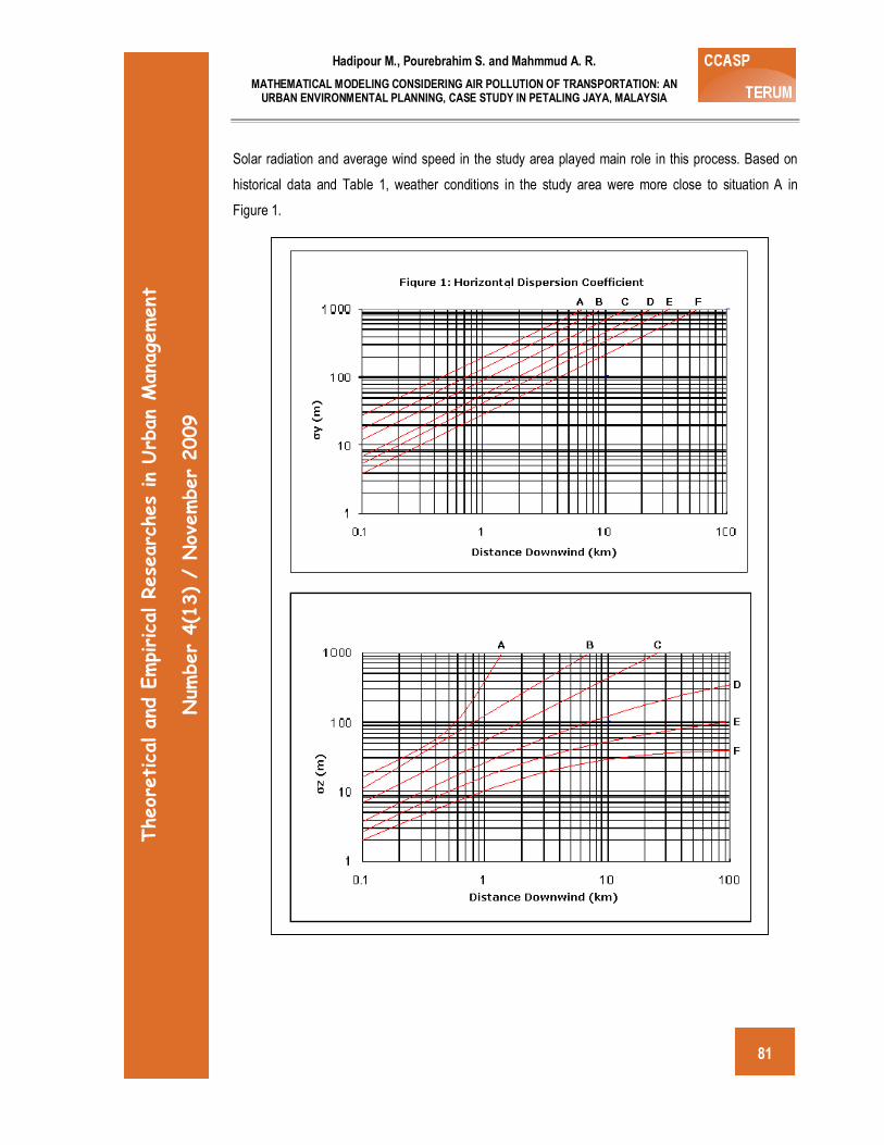
Horizontal and vertical dispersion (σy and σz) are determined from the graphs found in the Figure1 and

in the attributes written in Table 1. In these figures vertical and horizontal dispersion coefficients for

3/12

06.1

=∆

U

tFh

(4)

2

01 a

s s

s

TF gv r

T

= −

(5)

80




Num


different areas have been categorized in 6 weather stability classes (A, B, C for day and D, E, F for

night). It is based on 3 atmospheric factors of wind speed, incoming solar radiation and thinly overcast.

2.1.3 FINALIZATION OF MODEL

By applying amount of Cx = 0.01g/m3

(primary standard of CO pollutant in 8 hours), Equation (1) can be

rewritten as follow:

( )2

3 19.3y z

Q h

Uσ σ

∆=

(6)

Where is Dmin? In Equation (7), σy and σz were replaced by a mathematical function of Dmin.

( ) ( )3

min y zF D σ σ= (7)

Therefore, based on Equation (6)

( )2

min

19.3Q hF D

U

∆=

(8)

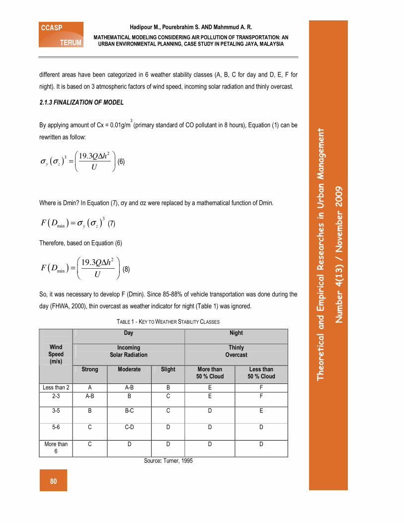
So, it was necessary to develop F (Dmin). Since 85-88% of vehicle transportation was done during the

day (FHWA, 2000), thin overcast as weather indicator for night (Table 1) was ignored.

TABLE 1 - KEY TO WEATHER STABILITY CLASSES

Day Night

Incoming Solar Radiation

Thinly Overcast

Wind Speed (m/s)

Strong Moderate Slight More than 50 % Cloud

Less than 50 % Cloud

Less than 2 A A-B B E F

2-3 A-B B C E F

3-5 B B-C C D E

5-6 C C-D D D D

More than 6

C D D D D

Source: Turner, 1995



81


Num


Solar radiation and average wind speed in the study area played main role in this process. Based on

historical data and Table 1, weather conditions in the study area were more close to situation A in

Figure 1.

Figure 1: Horizontal and Vertical Dispersion Coefficients (Turner, 1995)

Note: Definition of A, B, C, D, E, and F are shown in Table 1.

82




Num


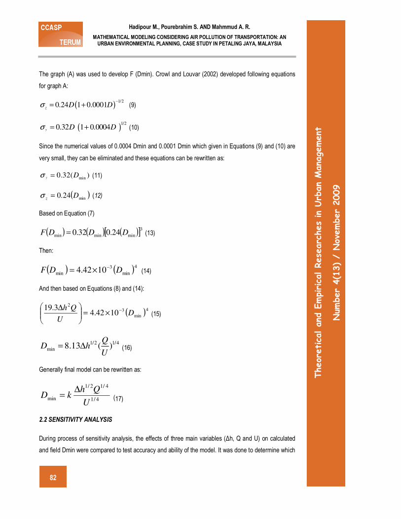
The graph (A) was used to develop F (Dmin). Crowl and Louvar (2002) developed following equations

for graph A:

( )1/2

0.24 1 0.0001z D Dσ−

= + (9)

( )1/2

0.32 1 0.0004y D Dσ = + (10)

Since the numerical values of 0.0004 Dmin and 0.0001 Dmin which given in Equations (9) and (10) are

very small, they can be eliminated and these equations can be rewritten as:

min0.32( )y Dσ = (11)

( )min24.0 Dz =σ (12)

Based on Equation (7)

( ) ( ) ( )[ ]3minminmin 24.032.0 DDDF = (13)

Then:

( ) ( )4

min

3

min1042.4 DDF

−×= (14)

And then based on Equations (8) and (14):

( )4

min

3

2

1042.43.19

DU

Qh −×=

∆ (15)

1/2 1/4

min 8.13 ( )Q

D hU

= ∆ (16)

Generally final model can be rewritten as:

4/1

4/12/1

minU

QhkD

∆= (17)

2.2 SENSITIVITY ANALYSIS

During process of sensitivity analysis, the effects of three main variables (∆h, Q and U) on calculated

and field Dmin were compared to test accuracy and ability of the model. It was done to determine which



83


Num


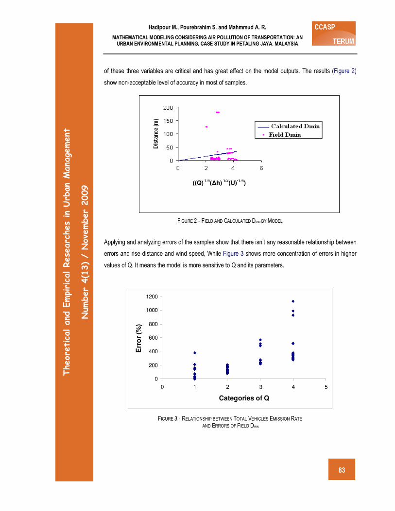
of these three variables are critical and has great effect on the model outputs. The results (Figure 2)

show non-acceptable level of accuracy in most of samples.

Figures 2: Mathematical Effect of the Main Parameters on

FIGURE 2 - FIELD AND CALCULATED DMIN BY MODEL

Applying and analyzing errors of the samples show that there isn’t any reasonable relationship between

errors and rise distance and wind speed, While Figure 3 shows more concentration of errors in higher

values of Q. It means the model is more sensitive to Q and its parameters.

0

200

400

600

800

1000

1200

0 1 2 3 4 5

Categories of Q

Err

or

(%)

FIGURE 3 - RELATIONSHIP BETWEEN TOTAL VEHICLES EMISSION RATE AND ERRORS OF FIELD DMIN

((Q) 1/4

(∆h) 1/2

(U)-1/4

)

84




Num


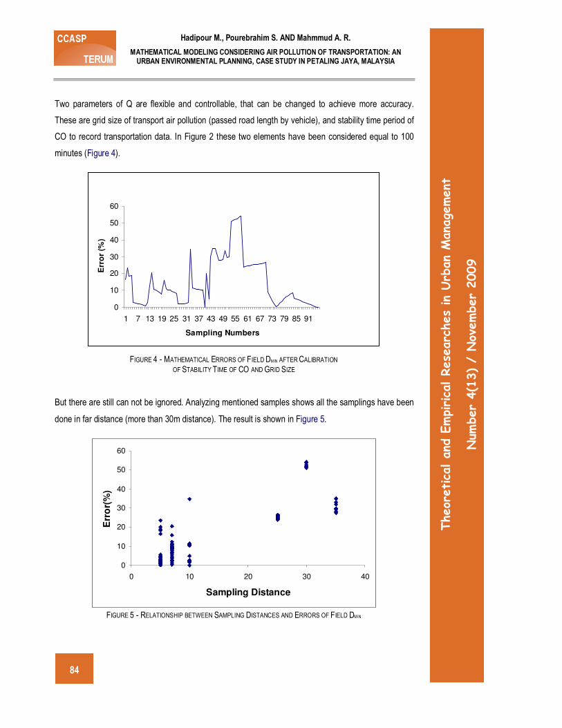
Two parameters of Q are flexible and controllable, that can be changed to achieve more accuracy.

These are grid size of transport air pollution (passed road length by vehicle), and stability time period of

CO to record transportation data. In Figure 2 these two elements have been considered equal to 100

minutes (Figure 4).

0

10

20

30

40

50

60

1 7 13 19 25 31 37 43 49 55 61 67 73 79 85 91

Sampling Numbers

Err

or

(%)

FIGURE 4 - MATHEMATICAL ERRORS OF FIELD DMIN AFTER CALIBRATION OF STABILITY TIME OF CO AND GRID SIZE

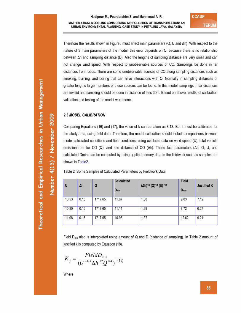
But there are still can not be ignored. Analyzing mentioned samples shows all the samplings have been

done in far distance (more than 30m distance). The result is shown in Figure 5.

0

10

20

30

40

50

60

0 10 20 30 40

Sampling Distance

Err

or(

%)

FIGURE 5 - RELATIONSHIP BETWEEN SAMPLING DISTANCES AND ERRORS OF FIELD DMIN



85


Num


Therefore the results shown in Figure5 must affect main parameters (Q, U and ∆h). With respect to the

nature of 3 main parameters of the model, this error depends on Q, because there is no relationship

between ∆h and sampling distance (D). Also the lengths of sampling distance are very small and can

not change wind speed. With respect to unobservable sources of CO, Samplings be done in far

distances from roads. There are some unobservable sources of CO along sampling distances such as

smoking, burning, and boiling that can have interactions with Q. Normally in sampling distances of

greater lengths larger numbers of these sources can be found. In this model samplings in far distances

are invalid and sampling should be done in distance of less 30m. Based on above results, of calibration

validation and testing of the model were done.

2.3 MODEL CALIBRATION

Comparing Equations (16) and (17), the value of k can be taken as 8.13. But it must be calibrated for

the study area, using field data. Therefore, the model calibration should include comparisons between

model-calculated conditions and field conditions, using available data on wind speed (U), total vehicle

emission rate for CO (Q), and rise distance of CO (∆h). These four parameters (∆h, Q, U, and

calculated Dmin) can be computed by using applied primary data in the fieldwork such as samples are

shown in Table2.

Table 2: Some Samples of Calculated Parameters by Fieldwork Data

U ∆h Q

Calculated

Dmin

(∆h)1/2 (Q)1/4 (U) -1/4

Field

Dmin

Justified K

10.53 0.15 1717.65 11.07 1.38 9.83 7.12

10.80 0.15 1717.65 11.11 1.39 8.72 6.27

11.08 0.15 1717.65 10.98 1.37 12.62 9.21

Field Dmin also is interpolated using amount of Q and D (distance of sampling). In Table 2 amount of

justified k is computed by Equation (18).

min

1/ 4 1/2 1/ 4( )

j

FieldDK

U h Q−

=∆

(18)

Where

86




Num


∆h = Rise distance of CO,

Q = Total vehicle emission rate for CO,

U = Wind speed, and

Kj = Justified constant value for every sample.

After calculating Kj for all the samples, justified constant value for final model is calculated by averaging

total amounts of Kj. The results show average total amount of Kj is equal to 8.68. Hence the model for

study area can be written as follow:

1/2 1/4

min 1/48.68

h QD

U

∆= (19)

Where,

∆h = Rise distance of CO,

Q = Total vehicle emission rate for CO,

U = Wind speed, and

Kj = Justified constant value for every sample.

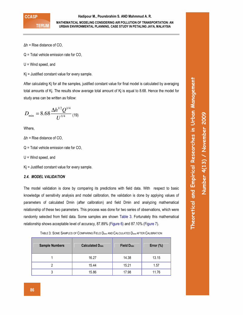
2.4. MODEL VALIDATION

The model validation is done by comparing its predictions with field data. With respect to basic

knowledge of sensitivity analysis and model calibration, the validation is done by applying values of

parameters of calculated Dmin (after calibration) and field Dmin and analyzing mathematical

relationship of these two parameters. This process was done for two series of observations, which were

randomly selected from field data. Some samples are shown Table 3. Fortunately this mathematical

relationship shows acceptable level of accuracy, 87.89% (Figure 6) and 87.10% (Figure 7).

TABLE 3: SOME SAMPLES OF COMPARING FIELD DMIM AND CALCULATED DMIM AFTER CALIBRATION

Sample Numbers Calculated Dmin Field Dmin Error (%)

1 16.27 14.38 13.15

2 15.44 15.21 1.57

3 15.86 17.98 11.76



87


Num


0

5

10

15

20

25

1 4 7 10 13 16 19 22 25 28 31 34 37 40

Samle Numbers

Dis

tan

ce (

m)

Field Dmin

Calculated Dmin

FIGURE 6 - MATHEMATICAL ERROR BETWEEN FIELD AND

CALCULATED DMIN BY MODEL (SERI 1)

0

5

10

15

20

25

1 4 7 10 13 16 19 22 25 28 31 34 37

Sample Numbers

Dis

tan

ce (

m)

Field Dmin

Calculated Dmin

FIGURE 7 - MATHEMATICAL ERROR BETWEEN FIELD AND

CALCULATED DMIN BY MODEL (SERI 2)

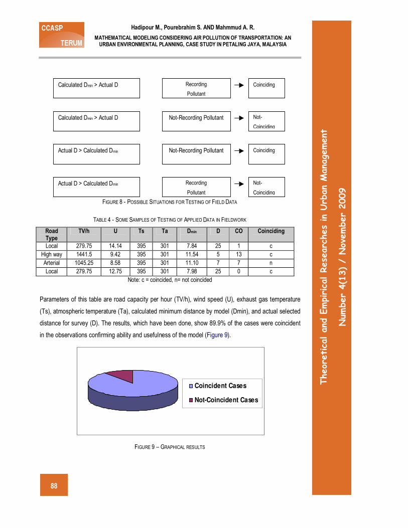
2.5. MODEL TESTING

In the analysis of data, field and calculated values were compared to verify model for a range of

idealized and real condition with respect of model purposed. For example, if the calculated minimum

safe distance for one station was more than the actual distance, the sensors monitored some pollution

in this station. Also, if the calculated distance was less than the field distance, there should not be any

pollution. Four possible situations in the mentioned process are shown in Figure 8. Some samples of

applied data in fieldwork are shown in Table 4.

88




Num


FIGURE 8 - POSSIBLE SITUATIONS FOR TESTING OF FIELD DATA

TABLE 4 - SOME SAMPLES OF TESTING OF APPLIED DATA IN FIELDWORK

Road Type

TV/h U Ts Ta Dmin

D CO Coinciding

Local 279.75 14.14 395 301 7.84 25 1 c

High way 1441.5 9.42 395 301 11.54 5 13 c

Arterial 1045.25 8.58 395 301 11.10 7 7 n

Local 279.75 12.75 395 301 7.98 25 0 c

Note: c = coincided, n= not coincided

Parameters of this table are road capacity per hour (TV/h), wind speed (U), exhaust gas temperature

(Ts), atmospheric temperature (Ta), calculated minimum distance by model (Dmin), and actual selected

distance for survey (D). The results, which have been done, show 89.9% of the cases were coincident

in the observations confirming ability and usefulness of the model (Figure 9).

Figures 9: Results of Model Testing

FIGURE 9 – GRAPHICAL RESULTS

Calculated Dmin > Actual D Recording

Pollutant

Coinciding

Calculated Dmin > Actual D Not-Recording Pollutant Not-

Coinciding

Actual D > Calculated Dmin Not-Recording Pollutant Coinciding

Actual D > Calculated Dmin Recording

Pollutant

Not-

Coinciding

Coincident Cases

Not-Coincident Cases



89


Num


3. CONTRIBUTION OF MODEL FOR THE STUDY AREA

The model when applied with the generalized values for the components of transportation system and

weather condition had found to be fit for the study area. The main constants used are:

a) Ts (General average exiting gas temperature from exhaust) = 395° k,

b) Vs (General average CO exiting velocity from exhaust) = 0.4 m/sec,

c) Ta (Average annual atmospheric temperature for MPPJ) = 301° k,

d) P (Average annual atmospheric pressure for MPPJ) =1000 and

e) Cm

(Average single vehicle’s normal space time usage) =7.3 m2

After applying these generalized values in the model, the Dmin were calculated for road types in MPPJ,

the results are shown in Table 5.

In this research, determination of residential landuse was done with determination of polluted areas of

urban transportation. Areas with good air quality were obtained through overlaying analysis and

deselecting of effective polluted zones by road types. Based on the standard road types (FHWA, 2000;

PBD, 1998), potential polluted zones were sub-divided into five zones: potential polluted zones by

collector roads, local roads, arterial roads, sub-arterial roads and highways. Applying the appropriate

Dmin values indicated in Table 5, five polluted areas have been zoned and presented in maps of

varying road types.

TABLE 5 - CALCULATED DMIN FOR ROAD TYPES OF MPPJ

Road type Dmin

Local 18.32

Collector 17.14

Sub-arterial 16.35 Arterial 15.43

Highway 12.77

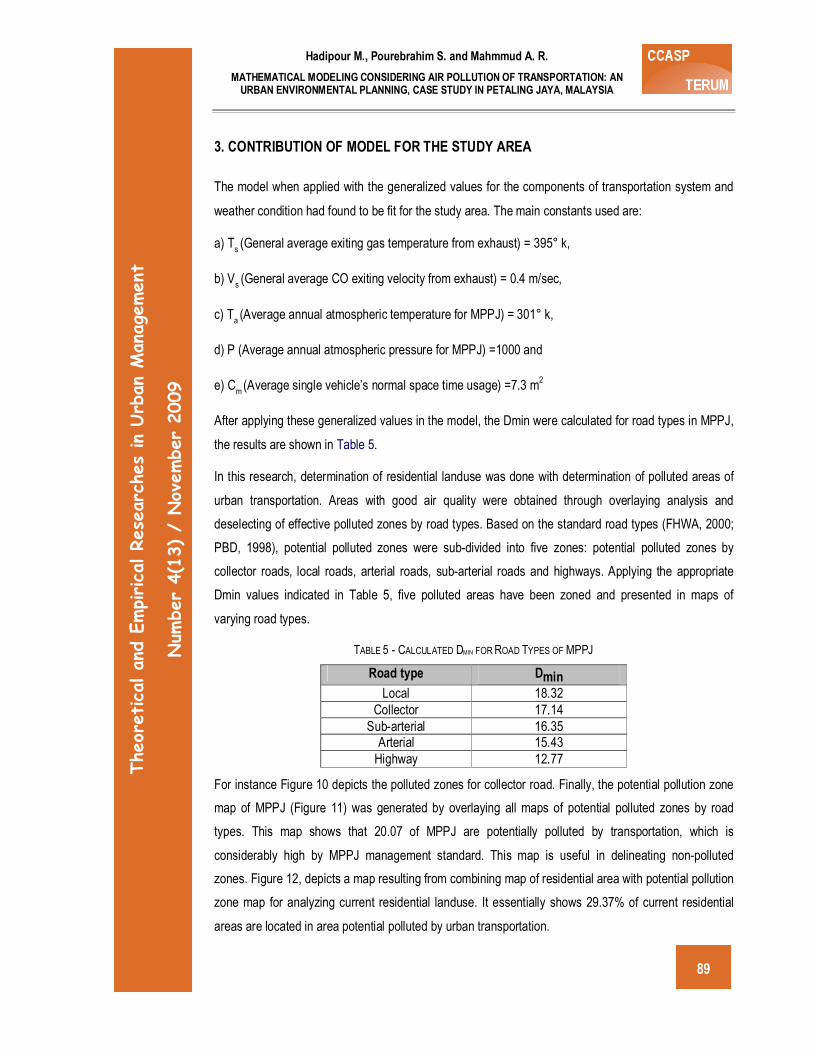
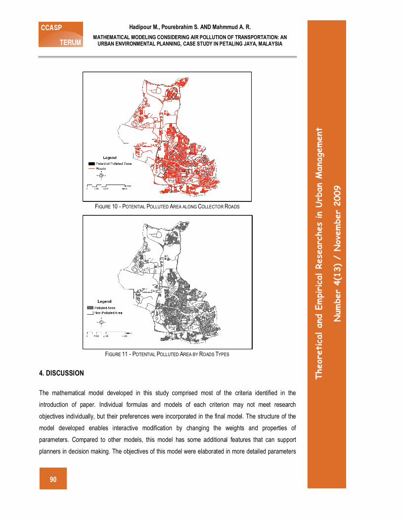
For instance Figure 10 depicts the polluted zones for collector road. Finally, the potential pollution zone

map of MPPJ (Figure 11) was generated by overlaying all maps of potential polluted zones by road

types. This map shows that 20.07 of MPPJ are potentially polluted by transportation, which is

considerably high by MPPJ management standard. This map is useful in delineating non-polluted

zones. Figure 12, depicts a map resulting from combining map of residential area with potential pollution

zone map for analyzing current residential landuse. It essentially shows 29.37% of current residential

areas are located in area potential polluted by urban transportation.

90




Num


FIGURE 10 - POTENTIAL POLLUTED AREA ALONG COLLECTOR ROADS

FIGURE 11 - POTENTIAL POLLUTED AREA BY ROADS TYPES

4. DISCUSSION

The mathematical model developed in this study comprised most of the criteria identified in the

introduction of paper. Individual formulas and models of each criterion may not meet research

objectives individually, but their preferences were incorporated in the final model. The structure of the

model developed enables interactive modification by changing the weights and properties of

parameters. Compared to other models, this model has some additional features that can support

planners in decision making. The objectives of this model were elaborated in more detailed parameters



91


Num


and parameters indicators were determined. Indicators are driven data to satisfy the purpose of the

model. This detailed classification strengthens analysis of any situation and the result is normally more

reliable. In this model, constraints were also considered for instance planners should avoid selecting a

site which was defined as effective polluted area by transportation. This model also is used more

friendly and easier than other models; it structured in simple mathematical formula and does not need to

train any other skim.

It is expected that the urban planners who are studying the spatial distribution of transportation network

and landuse will utilize the model. A user must be aware of the limitations of the model. Moreover, the

result will depend on the quality of data that are used in this model. It is important to note that this model

supports the planners by providing alternative sites in urban development plans.

5. CONCLUSION

This research has successfully managed to identify and develop a scientific based method

understanding the relationship between landuse and urban network location, by modeling for

transportation air pollution and analyzing the successful and non-successful development of landuses

and urban networks based on the developed model. The research strategy is able to support urban

planners with a range of options. Implementation of the model suggests that some areas can be more

suitable than others for residential landuse and urban transportation network development, if

performances and criteria are considered carefully. This suitability largely depends on the goals of the

transportation projects, but importance of the main negative element (air quality) can not be ignored in

all of transportation projects. The operational model can handle multiple types of transportation sources,

by corresponding and averaging conditions, where each condition includes some important elements

with respect to human health, all economic. The model was not sensitive to small changes of the values

of input parameters. Therefore under specific meteorological conditions, areas far away from the

emission sources (roads) can also be highly polluted.

REFERENCES

Bell, M. C. and Blake, M. (2000). Forecasting the Pattern of Urban Growth with PUP: a Web-based Model Interfaced with GIS and 3D Animation. Journal of Environment and Urban Systems, 24(6), 559-581.

Clean Water Action Council, (2008). Environmental Impacts of Transportation. USA.

Colesca S. (2009). Editorial note. Urban issues in Asia. Theoretical and Empirical Researches in Urban Management, Special number 1S, Urban Issues in Asia, April, 2009

92




Num


Colorado Department of Public Health and Environment, (2006). Standard Method for Determination of Nitrogen Oxides, Carbon Monoxide and Oxygen Emissions from Natural Gas-fired Reciprocating Engines, Combustion Turbines, Boilers, and Process Heaters using Portable Analyzers, USA.

Colvile, R. N., Kaur, S., Britter, R., Robins, A., Bell, M. C., Shallcross, D. and Belcher, S. E. (2000). High-resolution Integrated Modeling of the Spatial Dynamics of Urban and Regional Systems. Journal of Environment and Urban Systems, 24(5), 383-400.

Crowl, A. D. and Louvar, J. F. (2002). Chemical Process Safety. Prentice Hall PTR, USA.

Department of Transport, (1996). Transport Statistics Great Britain. UK.

DOE (Department of Environment), (2004). Annual Report of Air Quality Data. Ministry of Natural Resource and Environment, Malaysia.

FHWA (Federal Highway Administration), (2000). Functional Classification Guidelines. US Department of Transportation, USA.

Haughton, G., Hunter, C. and Haughton, H. (2003). Sustainable Cities. Routledge publisher, UK.

Highway Planning Unit, (2004). Road Traffic Volume in Malaysia (1998- 2004). Ministry of work, Malaysia.

JPBD (Department of town and country planning), (1998). Guidelines and Geometric Standards on Road Network Systems. Ministry of work, Malaysia.

Li, S. (1998). A Study on the Macro Capacity Model of Urban Road Network and its Application. Retrived 2005, from http://www.inro.ca/en/pres_pap/asian/asi99/paper4.doc

Meszaros, T., Haszpra, L. and Gelencser, A. (2005). Tracking Changes in Carbon Monoxide Budget over Europe between 1995 and 2000. Journal of Atmospheric

Nicolas, J. P., Duprez, F., Durand, S., Poisson, F., Aubert, P. L., Chiron, M., Crozet, Y. and Lambert, J. (2005). Local Impact of Air Pollution: lessons from Recent Practices in Economics and in Public Policies in the Transport Sector, Journal of Atmospheric Environment, 39(13), 2475-2482.

Ranjan, K. (2001). Development of Spatial and Attribute Database for Planning and Managing Rural Service Centers in Kendrapara District, Orissa, India: A GIS Based Information. Journal of Applied Gerontology, 3(1), 99-105.

Rodrigue, J. P., Comtois, C. and Slack, B. (2006). The Geography of Transport Systems. Taylor and Francis group publisher, USA.

Turner, D. B. (1995). Atmospheric Dispersion Estimates, An Introduction to Dispersion Modeling. Lewis, USA publisher.

Vos, J. (2002). Trends in the Emission of Air Pollutants from On-road Motor Vehicles in Florida. Florida Department of Transportation, USA.

Wayson, R. (2000). Predicting Air Quality Near Roadways through the Application of a Gaussian Puff

Model to Moving Sources. Proceeding of 93rd

Annual Conference and Exhibition of the Air and Waste Management Association. USA.

WHO, (2000). Air Quality Guidelines. Regional Office for Europe, Copenhagen, Denmark.

MATHEMATICAL MODELING CONSIDERING AIR POLLUTION OF TRANSPORTATION: AN URBAN ENVIRONMENTAL PLANNING,...

Documents

Transcript of MATHEMATICAL MODELING CONSIDERING AIR POLLUTION OF TRANSPORTATION: AN URBAN ENVIRONMENTAL PLANNING,...