F A C U L T Y O F S C I E N C E

U N I V E R S I T Y O F C O P E N H A G E N

Department of Plant and Environmental Sciences

Kyriaki Adelais Boulata

Supervisors

Kristian Thorup-Kristensen

Dorte Bodin Dresbøll

Corentin Clement

Master thesis

Root growth in different soil depths and

sap flow of barley (Hordeum vulgare L.)

and pea (Pisum sativum L.) under

drought

2

Abstract

Root systems that proliferate in deep soil domains, when the upper most layers are

progressively drying, have been proposed to confer crop drought resistance through the

utilisation of deep water. A greenhouse study was conducted to identify root growth dynamics

in three soil layers (0-26, 36-62 and 71-97 cm) and to relate them to sap flow rates and soil

water content under mild drought. To that end, two crops with different root systems, peas

(dicot) and barley (monocot), were grown in a loamy sand soil in 14x100 cm transparent pots

and subjected to intermittent and terminal drought. In peas, no increased root proliferation

(measured as root length) was observed in the lowest soil layers when the topsoil was dry and

sap flow rates, during terminal drought, were similar in the control and the water stressed

treatment. However, barley showed an enhanced root growth in the 36-62 cm layer due to the

intermittent drought and in the 71-97 cm layer due to terminal drought. Moreover, sap flow

rates, as measured during terminal drought, demonstrated increased water use in barley during

the early stages of the drought. Our findings show the importance of the drought characteristics

(timing, duration and severity) in plant response to drought and highlight the need for

development of genotypes with increased root length in deeper soil domains under drought

conditions.

Table of contents

Abstract………………………………………………………………………………….…… 2

Introduction…………………………………………………………………………….……. 4

-Water scarcity in crop production…………………………………………………….…… 4

-Drought stress characteristics…………………………………………………………..… 4

-Role of roots under water stress conditions……………………………………………… 5

--Deep rootedness and root length………………………………………………………… 5

--Root length is important for water extraction……………………………………………. 6

-Monocotyledonous vs dicotyledonous root systems………………………………….… 7

-Transpiration and sap flow under water stress……………………………………….…. 7

-Aim of research……………………………………………………………………………… 10

Materials and methods……………………………………………………………….…… 11

-Study site and experimental setup…………………………………………………….…. 11

-Water treatments & fertilization……………………………………………………….…… 12

-Soil water content………………………………………………………………………..…. 13

3

-Canopy cover and plant height………………………………………………………..…… 13

-Root growth……………………………………………………………………………..….... 14

-Stomatal conductance………………………….…………………………………............... 15

-Sap flow………………………………………………………………………………….….… 16

-Data analysis…………………………………………………………………………............ 16

Results…………………………………………………………………………………….…… 17

-Soil water content………………………………………………………………………….…. 17

-Canopy cover and plant height……………………………………………………………… 19

-Root length………………………………………………………………………………..…... 21

-Stomatal conductance…………………………………………………………………..…… 24

-Sap flow…………………………………………………………………………………..…… 25

-Hourly sap flow rates and stomatal conductance………………………………..….……. 26

Discussion………………………………………………………………………………..…… 28

-Deep rootedness……………………………………………………………………………... 28

-Root length……………………………………………………………………………………. 28

-Sap flow and stomatal conductance………………………………………………………... 31

-Water saving and water spending strategies………………………………………………. 32

-Significance of findings and general considerations………………………………………. 33

-Study limitations…………………………………………………………………………….… 34

Acknowledgements………………………………………………………………………….. 34

References…………………………………………………………………………………………….. 36

4

Introduction

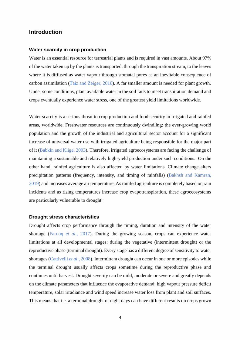
Water scarcity in crop production

Water is an essential resource for terrestrial plants and is required in vast amounts. About 97%

of the water taken up by the plants is transported, through the transpiration stream, to the leaves

where it is diffused as water vapour through stomatal pores as an inevitable consequence of

carbon assimilation (Taiz and Zeiger, 2010). A far smaller amount is needed for plant growth.

Under some conditions, plant available water in the soil fails to meet transpiration demand and

crops eventually experience water stress, one of the greatest yield limitations worldwide.

Water scarcity is a serious threat to crop production and food security in irrigated and rainfed

areas, worldwide. Freshwater resources are continuously dwindling: the ever-growing world

population and the growth of the industrial and agricultural sector account for a significant

increase of universal water use with irrigated agriculture being responsible for the major part

of it (Babkin and Klige, 2003). Therefore, irrigated agroecosystems are facing the challenge of

maintaining a sustainable and relatively high-yield production under such conditions. On the

other hand, rainfed agriculture is also affected by water limitations. Climate change alters

precipitation patterns (frequency, intensity, and timing of rainfalls) (Bakhsh and Kamran,

2019) and increases average air temperature. As rainfed agriculture is completely based on rain

incidents and as rising temperatures increase crop evapotranspiration, these agroecosystems

are particularly vulnerable to drought.

Drought stress characteristics

Drought affects crop performance through the timing, duration and intensity of the water

shortage (Farooq et al., 2017). During the growing season, crops can experience water

limitations at all developmental stages: during the vegetative (intermittent drought) or the

reproductive phase (terminal drought). Every stage has a different degree of sensitivity to water

shortages (Cattivelli et al., 2008). Intermittent drought can occur in one or more episodes while

the terminal drought usually affects crops sometime during the reproductive phase and

continues until harvest. Drought severity can be mild, moderate or severe and greatly depends

on the climate parameters that influence the evaporative demand: high vapour pressure deficit

temperature, solar irradiance and wind speed increase water loss from plant and soil surfaces.

This means that i.e. a terminal drought of eight days can have different results on crops grown

5

in different locations due to the differences in the above-mentioned parameters. Furthermore,

drought severity is also determined by the speed at which the soil moisture recedes. During a

mild drought, soil water would recede slowly and a fraction of it would still be available for

plant use. The combined effects of timing, duration and intensity of drought influence the

extent of yield loss.

Intermittent drought is hardly ever lethal to the plant but can diminish plant growth and thus

yield capacity. Terminal drought can result in big yield reductions in rainfed systems (Richard

et al., 2015). As several yield components are sensitive to drought, water shortages during their

formation adversely affects yield. Pollen infertility (Yu et al., 2019), seed weight (Muñoz-

Perea et al., 2006), seed number (Jamieson et al., 1995), number of pods (Gorim and

Vandenberg, 2017), tiller density (Cai et al., 2018) call all be adversely influenced by water

shortage.

Role of roots under water stress conditions

Improvement of drought tolerance has primarily come from efforts focusing on the above

ground plant characteristics. Roots are concealed within the soil, which cause technical and

experimental difficulties in studying them. However, during the last decades, there has been an

increased interest in root studies and there is growing evidence that root systems are important

for drought tolerance.

In the absence of rain events, the soil dries gradually from the top layers due to drainage and

evapotranspiration. This results in deeper soil strata maintaining higher moisture contents at

the end of the growing season and rainfed crops, under these circumstances, could exploit the

stored soil water to cover their needs during the reproductive phase. By capturing this untapped

water during drought events plants could alleviated the consequent stress or delay the onset of

a more severe one (Hurd, 1968), and indeed there are numerous studies which demonstrated

the role of deep and vigorous roots during droughts.

Deep rootedness and root length

Root system architecture plays an essential role in plant productivity under limited soil water

conditions (Lynch, 1995). Its role in plant adaptation to drought environments has been

outlined in Manschadi et al. (2006) who showed that a relatively dense and deep root system

in wheat increased water access to deeper soil strata during the grain-filling period. Moreover,

root length (RL) was greater in the deeper soil layers. They also suggested that the extra water

extracted during the grain-filling period can positively influence yield. This is supported by

6

Kirkegaard et al (2007) who found that even relatively small amounts of deep water contribute

significantly to grain yield in wheat under moderate terminal drought.

The angle of early roots seems to influence rooting depth (Wasson et al., 2012). Steeper root

angles result in deeper root systems and, in rice, this trait has been demonstrated to allow

drought avoidance (Uga et al., 2013). On the other hand, shallower roots resulting from

narrower root angles can be of importance for e.g. phosphorus foraging from the upper soil

layers (Ho et al., 2005; Rubio et al., 2003).

Besides cereals, deep rootedness has also been found to play a role in vegetable and legume

performance under drought. In an experiment with lettuce, Johnson et al. (2000) found that

QTL’s for taproot length, found in a wild relative, enhanced water uptake from deep soil layers.

Deep roots alleviated stress in groundnut (Reddy et al., 2003), soybean (Prince et al., 2015)

and common bean (Polania et al., 2017).

Root length is important for water extraction

Soil water depletion from the soil profile, over a growing season, is highly correlated with

maximum rooting depth and root length density (RLD), with the former having a stronger

correlation (Hamblin and Tennant, 1987).

RLD is an important trait for water and nutrient uptake. The greater its value is in a given

volume of soil, the greater the rates of water uptake will be (Passioura, 1983). However, there

is an upper limit of RLD that is valuable for water extraction. Ludlow and Muchow (1990)

argue that a RLD of 0.5 cm cm-3 and more is sufficient to extract all plant available water and

variation in RLD between 0.3 to 6 does not induce variation in the extracted water. In chickpea,

RLDs of more than 0.4 cm cm-3 did not contribute in extra water extraction (Gregory, 1988).

These findings suggest that there is an additional metabolic cost for roots that, in the long term,

do not contribute significantly to water uptake. However, within a shorter time scale of

consideration, an increase in RLD can be beneficial for water uptake, especially under soil

water deficits. According to Zhan et al (2015) this cost is avoided in plants with reduced lateral

root branching density which results in deeper root systems that can utilise deep water

resources and reduce the yield penalty. Therefore, alterations to root architecture towards

deeper roots can contribute to enhanced water acquisition from deeper soil domains.

Roots tend to proliferate to a greater extend in soil domains with higher nutrient and water

content (Johnson et al., 2000). Under drying topsoil conditions (i.e. terminal drought), maize

root proliferation was observed to be restricted in the upper soil layers but increased in the

7

lower layers where roots extracted water at greater rates per unit length when compared to the

well-watered plants (Sharp and Davies, 1985). Similarly, soybean, increased its RL deeper in

the soil in response to drier upper layers (Hoogenboom et al., 1987). Thus, the development of

greater root densities deeper in the soil under terminal drought events can increase water

foraging.

Monocotyledonous vs dicotyledonous root systems

Monocotyledonous species, such as cereals, develop fibrous root systems. The embryo in the

seed gives rise to one or more “primary” roots and the mesocotyl to “basal” roots. Both root

types branch into successive orders of “laterals”. On the other hand, dicotyledonous species,

such as legumes, have root systems comprising of a single primary root, the “taproot” which

originates from the embryo and can also give rise to different orders of “lateral” roots. “Shoot-

borne” roots can be found in both plant types and are created from aerial parts of the plant

(Rich and Watt, 2013; Zobel and Waisel, 2010).

Cereal crops typically develop greater total RL per area than grain legumes and in some cases

this difference can be 5 or even 10-fold (Hamblin and Tennant, 1987). On the other hand,

legumes extract more water per unit RL than cereals (Katayama et al., 2000). However,

legumes continue to expand their root densities after the pod-filling phase (at a slower pace

than before) while most cereals stop even earlier (anthesis phase) (Gregory, 1988).

Differences in root system architecture between legumes and cereals may be attributed to the

different types of vegetative growth, which is indeterminate and determinate, respectively

(Gregory, 1988) however the majority of modern grain legume crops have a determinate

growth pattern.

Transpiration and sap flow under water stress

Transpiration reflects plant water use and is directly affected by drought. To adapt under water

stress conditions, plants, through a series of regulatory events, induce stomatal closure

(Osakabe et al., 2014). This in turn affects the amount of water vapour diffusing out of the

leaves hence transpiration rates are inhibited.

A direct measure of transpiration is obtained by monitoring sap flow rates on intact plant stems:

the mass of sap ascending through a stem section per unit time is determined (usually g h-1).

This method is based on the heat-balance theory that was developed by Sakuratani (1981) and

Baker and van Bavel (1987). A brief description follows below:

8

According to the heat-balance, a constant and steady state heat flows from a heater strip to a

stem segment as seen in Figure 1. This heat is partitioned to the sap, the stem and the outer

environment (if no heat storage is assumed):

Pin = Qf + Qu + Qd+ Qr (Equation 1)

where:

Pin= power input from the heater

Qf= energy convection carried by the sap flow

Qu, Qd= the two components of the axial heat conduction;

energies transferred upwards and downwards along the

stem

Qr= radial energy loss by conduction to the ambient

Figure 1 An annular heater on a stem section and heat fluxes of the heat balance theory. A constant and

steady state energy input is applied (Pin) to the stem section which results in heat fluxes radially to the

ambient (Qr), vertically in the stem (Qu, Qd) and the one carried by the sap flow (Qf).

The rate of sap flow is then calculated using the following relation:

F= Qf/ Cp * dT= (Pin – Qu – Qd - Qr)/ Cp * dT (Equation 2)

where:

Cp= specific heat of water (4.186 J/g*C)

dT= temperature increase in sap

The axial (Qu + Qd) and radial (Qr) heat losses are measured through thermocouples and

thermopiles and F is being calculated from equation (2).

9

Sap flow sensors have successfully been used to monitor sap flow rates in many plant species.

Most of the research has been conducted on trees, however this method has also been used in

many agricultural crops (Table 1). Sap flow sensors can also be applied in thin stems

(microsensors) with stem diameters ranging from 2.1 to 7 mm (Dynamax, Inc.) but literature

on the lowest end of this range is very rare.

Table 1. Examples of herbaceous crops in which sap flow measurements based on the heat balance

theory were performed.

Crop References

Cereals

Winter wheat (Triticum aestivum L.) Cai et al, 2018; Rafi et al, 2019

Corn (Zea mays L.) Han et al, 2018

Legumes

Soybean (Glycine max (L.) Merr.) Cohen et al, 1993; Sauer et at, 2007

Vegetable crops

Tomato De Swaef et al, 2012

Potato (Solanum tuberosum L.) Gordon et al, 1997; Byrd et al, 2015

Industrial crops

Cotton (Gossypium hirsutum L.) Dugas et al, 1990; Isoda and Wang, 2002

Sunflower (Heliantus annus L.) Zhang and Kirkham, 1995

Ornamental crops

Rose (Rosa hybrida L.) Rose and Rose, 1994

In Zhang and Kirkham (1995) the sap flow of sorghum (monocotyledon) is compared to that

of sunflower (dicotyledon) under well-watered and water stressed conditions. In the well-

watered treatment sunflower showed much higher rates of sap flow than sorghum. During

water stress both crops exhibited lower sap flow rates but in sunflower the difference between

the water treatments was more pronounced. They also noted that in sorghum, radial heat

conduction dominated the energy balance under all water treatments while this was only true

for water stressed sunflower (except midday). Finally, they concluded that the gauges were

reliable only when sap flow rates exceed that of 20 g h-1. In another study, an effect of soil

texture on sap flow rates was found under drought as no differences were detected among

control and watered stressed plants in a silty soil but noted in the stony (Cai et al, 2018).

10

Some authors underline the problems arising when sap flow sensors are used under specific

circustances. Langensiepen et al. (2014) experimented in wheat under field conditions and

found that the heat fluxes of the heat-balance theory did not allow enough energy to be carried

by the sap resulting in noisy sap flow measurements. This is also noticed in Gordon et al.

(1997) where at very low sap flow rates in potato stems most of the energy was lost radially.

They concluded that under these circumstances, a considerable amount of heat is stored in the

stem. This agrees well with Grime et al. (1995) who suggest that a heat storage term (Qs) should

be included in the heat balance equation, especially under low sap flow rates (Groot and King,

1992).

Aim of research

The aim of this research was to study the root growth of a monocotyledonous (barley) and a

dicotyledonous (pea) species, in different soil depths in relation to soil water depletion and

transpiration under intermittent and terminal drought. It is hypothesised that under drought

conditions, root length increases in the lowest soil layers in response to drying in the topsoil

layer. Furthermore, it is hypothesized that this increase in root length will be accompanied by

maintenance in transpiration rates.

11

Materials and methods

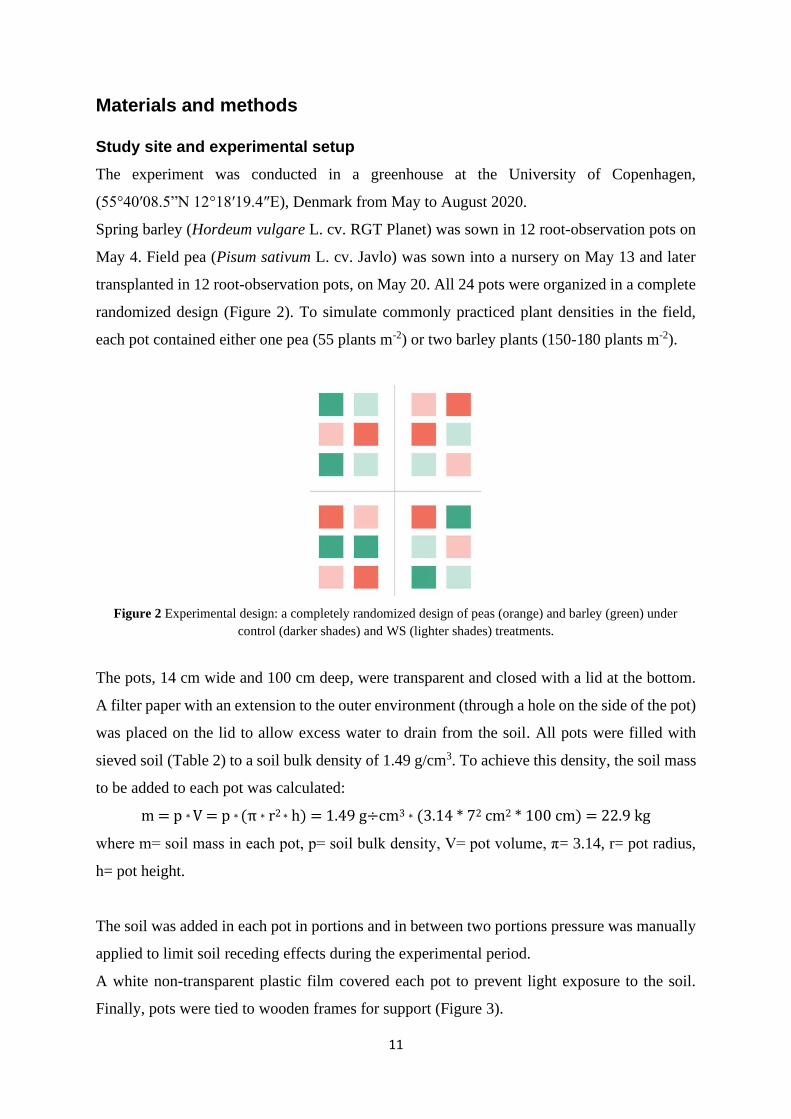
Study site and experimental setup

The experiment was conducted in a greenhouse at the University of Copenhagen,

(55°40′08.5”N 12°18′19.4″E), Denmark from May to August 2020.

Spring barley (Hordeum vulgare L. cv. RGT Planet) was sown in 12 root-observation pots on

May 4. Field pea (Pisum sativum L. cv. Javlo) was sown into a nursery on May 13 and later

transplanted in 12 root-observation pots, on May 20. All 24 pots were organized in a complete

randomized design (Figure 2). To simulate commonly practiced plant densities in the field,

each pot contained either one pea (55 plants m-2) or two barley plants (150-180 plants m-2).

Figure 2 Experimental design: a completely randomized design of peas (orange) and barley (green) under

control (darker shades) and WS (lighter shades) treatments.

The pots, 14 cm wide and 100 cm deep, were transparent and closed with a lid at the bottom.

A filter paper with an extension to the outer environment (through a hole on the side of the pot)

was placed on the lid to allow excess water to drain from the soil. All pots were filled with

sieved soil (Table 2) to a soil bulk density of 1.49 g/cm3. To achieve this density, the soil mass

to be added to each pot was calculated:

m = p * V = p * (π * r2 * h) = 1.49 g÷cm3 * (3.14 * 72 cm2 * 100 cm) = 22.9 kg

where m= soil mass in each pot, p= soil bulk density, V= pot volume, π= 3.14, r= pot radius,

h= pot height.

The soil was added in each pot in portions and in between two portions pressure was manually

applied to limit soil receding effects during the experimental period.

A white non-transparent plastic film covered each pot to prevent light exposure to the soil.

Finally, pots were tied to wooden frames for support (Figure 3).

12

Table 2 Chemical composition and physical characteristics of the soil (*Source: USDA)

Chemical composition & pH

Mg (mg/100 g) P (mg/100 g) K (mg/100 g) Organic matter (%) pH

3.5 3.2 9.5 1.9 6.9

Physical characteristics

Soil type Clay

<0.002 mm

Silt

0.002 – 0.02 mm

Fine sand

0.02 – 0.2 mm

Coarse sand

0.2 – 2.0 mm

Loamy sand* 7.7% 6.1% 42.2% 42.2%

Figure 3 Root observation-pots (24) attached to wooden pallets for support. The white plastic film is wrapped

around the pots to prevent light exposure to the soil.

Water treatments & fertilization

Two water treatments were applied in both plant species: 1) a control treatment, where pots

were continuously provided with water (0.2 L/24 h) through an irrigation system of a clay cone

(Blumat, Easy, Telfs, Austria) inserted into a 0.5 L plastic bottle containing water, and 2) a

water stressed (WS) treatment, where the irrigation system was withdrawn from the pots at

selected drought stress periods.

Drought was imposed in two cycles. Six randomly selected pots per species were given the WS

treatment during both cycles (Figure 2). In both crops, the first drought event occurred during

the vegetative phase (21 DAS) and lasted for 22 days. In peas, however, the end of the cycle

concurred with the first pod formation. The second drought cycle took place during the

reproductive phase for both crops. It started at 51 and 60 DAS in peas and barley, respectively,

and lasted until harvest. A recovery phase took place between the drought cycles where the WS

pots were receiving the same amount of water as the control pots. An additional 400 ml was

added daily in each pot, 3 days before the onset of the second drought event, to allow initiation

of the second drought cycle with relatively high soil water content. The treatments and their

corresponding dates are shown in Figure 4.

13

Due to progressive drying of the topsoil layer of some pots of the control treatment that was

observed at around 36 and 45 DAS (peas and barley, respectively), 100 mL of additional tap

water was added daily on the soil of the control pots (and the WS pots during recovery) from

the above mentioned dates until the end of the experimental period.

Shortly after sowing, 70 ml of liquid fertilizer (5-1-4) (Min have næring) was mixed with 1.4

L of tap water to create a solution of which 60 ml was added to each irrigation bottle.

Figure 4 Water treatments flow. The second drought cycle continued until harvest. Green shade represents

barley and orange represents peas.

Soil water content

Soil volumetric water content (VWC%) was monitored using time-domain reflectometry

sensors (TDR-310S, Acclima, Inc., Meridian, ID, USA). Three sensors were vertically inserted

into each pot (n=24) at three different depths: the top sensor was placed at 10-20 cm, the middle

at 50-60 cm and the bottom at 80-90 cm from the top of the pot. All sensors were connected to

a CR6 datalogger (Campbell Scientific, Inc., Logan, USA) and the data were logged every 24

h from sowing until harvest.

Canopy cover and plant height

Plant growth was measured in terms of canopy cover and plant height. Canopy cover was

estimated as a percentage of green areas on a picture, using the Canopeo App (1.1.7, Oklahoma

State University, USA). Images of every pot (n=24) were taken on 7-day intervals using a

smartphone camera, from two fixed locations: the top view pictures, taken from a 120 cm

distance from pot level and the side view pictures, 150 cm from ground level and 60 cm from

the pot level. The pictures were taken from these two angles to catch the canopy growth in both

14

the horizontal and vertical direction. Black backgrounds were used to avoid green areas not

belonging to the plant(s) of interest. All images were later edited with Paint (Windows 10), to

cover most of the background in black, and processed by the app using the 50% adjustment

function (Figure 5).

Plant height was measured in all plants (n=24) from the soil level using a ruler. One main tiller

was selected out of every barley pot whereas in peas height was measured on the main stem.

a) b) c)

Figure 5 Canopy images used for canopy cover estimation in Canopeo a) original image b) processed image

in Paint and c) Canopeo output image.

Root growth

Root growth was estimated non-invasively by taking weekly images of the pot sides and later

extracting RL from the pictures using an image analysis software (Smith et al., 2020). A

‘’PhotoBox’’ consisting of a camera lens (Sony, DSC-QX10) and LED lights (Figure 6) was

used to take images of roots growing at the pot-soil interface. Every pot was divided into three

horizontal layers (measured from the top of the pot): 1) top layer 0-26 cm, 2) middle layer 36-

62 cm and 3) bottom layer 71-97 cm. From each pot (n=24), one image was taken from each

layer on 7-day intervals. All images from one pot were aligned on a randomly selected vertical

axis around the pot.

a) b)

Figure 6 The PhotoBox used for obtaining root images from the pot-soil interface as seen

from a) the side view and the b) front view where the lens and the LED lights are shown.

15

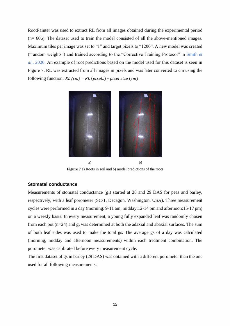
RootPainter was used to extract RL from all images obtained during the experimental period

(n= 606). The dataset used to train the model consisted of all the above-mentioned images.

Maximum tiles per image was set to “1” and target pixels to “1200”. A new model was created

(“random weights”) and trained according to the “Corrective Training Protocol” in Smith et

al., 2020. An example of root predictions based on the model used for this dataset is seen in

Figure 7. RL was extracted from all images in pixels and was later converted to cm using the

following function: RL (cm) = 𝑅𝐿 (𝑝𝑖𝑥𝑒𝑙𝑠) ∗ 𝑝𝑖𝑥𝑒𝑙 𝑠𝑖𝑧𝑒 (𝑐𝑚)

a) b)

Figure 7 a) Roots in soil and b) model predictions of the roots

Stomatal conductance

Measurements of stomatal conductance (gs) started at 28 and 29 DAS for peas and barley,

respectively, with a leaf porometer (SC-1, Decagon, Washington, USA). Three measurement

cycles were performed in a day (morning: 9-11 am, midday:12-14 pm and afternoon:15-17 pm)

on a weekly basis. In every measurement, a young fully expanded leaf was randomly chosen

from each pot (n=24) and gs was determined at both the adaxial and abaxial surfaces. The sum

of both leaf sides was used to make the total gs. The average gs of a day was calculated

(morning, midday and afternoon measurements) within each treatment combination. The

porometer was calibrated before every measurement cycle.

The first dataset of gs in barley (29 DAS) was obtained with a different porometer than the one

used for all following measurements.

16

Sap flow

To determine sap flow rates (g h-1), a Flow32A-1K sap flow system (Dynamax Inc., Houston,

TX, USA) with SGA2 gauges, suitable for 2.1-3.5 mm stem diameters, and a CR1000 data

logger (Campbell Scientific, Inc., Logan, UT, USA) was used. Eight gauges were installed in

two random plants/tillers per treatment at the beginning of the second drought cycle. A 2.3 V

input voltage was applied to all gauge heaters. Stem thermal conductivity (Kst) was set to 0.54

W/m*K for peas and 0.28 W/m*K for barley which are typical for herbaceous and hollow

stems, respectively. Initial Ksh was set at 0.2 and for later calculations an auto zero algorithm

was running every other day between 3-5 am.

Sap flow calculations were performed every 15 minutes using the average of sensor

measurements made every 60 seconds. When the temperature difference above and below the

heater was less than 0.5 all data were ignored.

Data analysis

The statistical analysis was performed with IBM SPSS Statistics 26. To detect differences

between the control and the WS treatment (traits: canopy cover, height, gs, RL) within

consecutive measurements a two-way ANOVA was performed. An independent samples t-test

was used to determine differences between the control and the WS treatment, within single

measurements (DAS). For all tests, significance level (a) was set to 0.05. To summarize data,

averages and standard errors were used in figures and tables.

17

Results

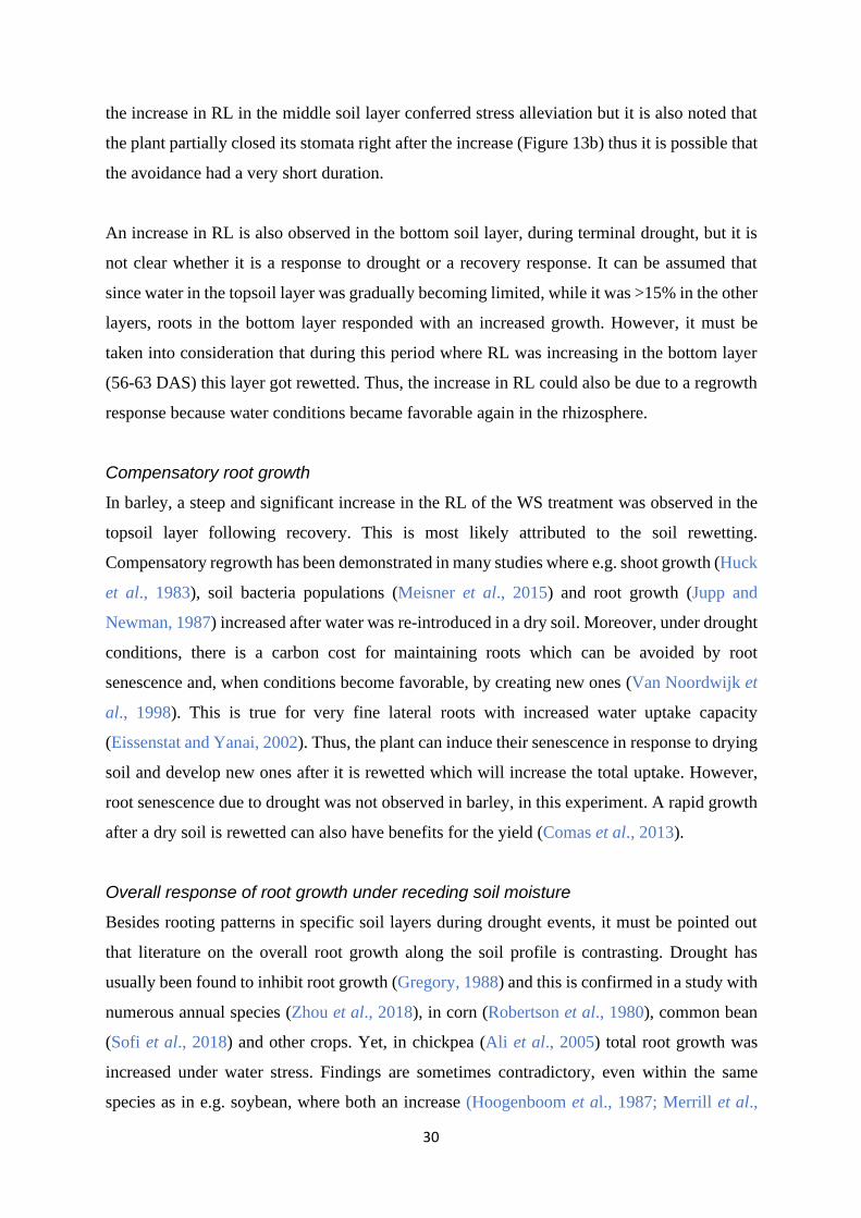
Soil water content

Drought influenced the soil volumetric water content (VWC) in all soil layers, as by the end of

each drought cycle a difference between the water treatments is noted (Figure 8 & 9).

The VWC of both crops followed the same trend within all soil layers: during drought events,

it remained constant (control) or declined (control and WS) down to a minimum value.

Peas

The effect of the first drought cycle on the VWC was noticed: a) in the topsoil layer (Figure

8a) between 22-44 DAS where the VWC fell from 14 to 5% (control remained stable at 15%),

b) in the middle soil layer (Figure 8b) between 28-48 DAS where the VWC decreased from 16

to 5% (control from 17 to 8%) and c) in the bottom soil layer (Figure 8c) between 31-49 DAS

as the VWC dropped from 24 to 5% (control from 26 to 10%). Thus, the first drought event

caused the VWC in the WS treatment to reach a minimum of 5% in all soil layers, although at

different dates. It was observed that from the onset of the drought to the appearance of its effect

in the top, middle and bottom soil layer, a period of 1, 7 and 10 days elapsed, respectively.

The recovery period between the two drought cycles restored VWC in both treatments at about

27% in the top, 18% in the middle and 20% in the bottom soil layer. The top, middle and bottom

soil layer got rewetted 2, 6 and 7 days, respectively, after the initiation of the recovery.

The second drought cycle decreased the VWC of the WS treatment until 64 DAS to a) 7% in

the topsoil layer (19% in the control) , b) 8% in the middle soil layer (14% in the control) and

c) 9% in the bottom soil layer (17% in the control).

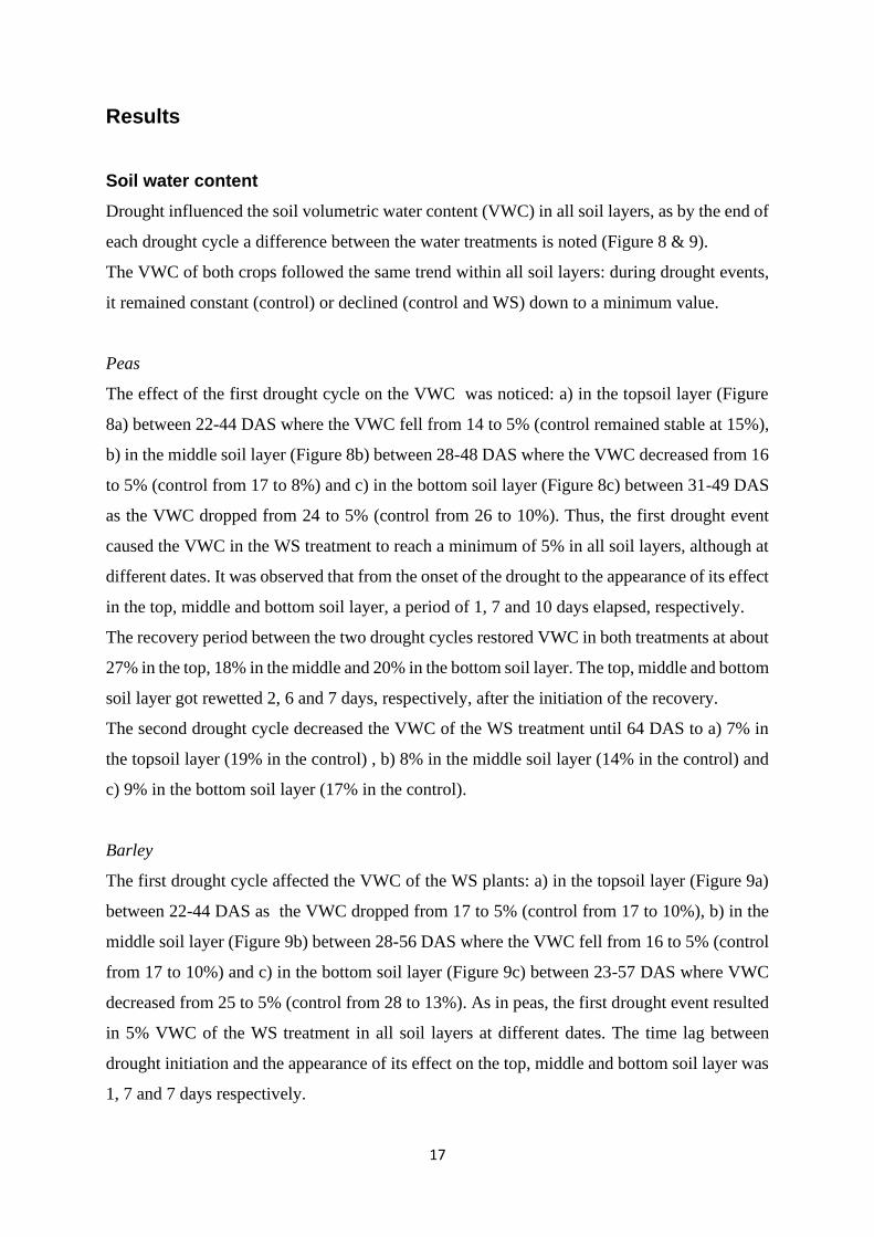
Barley

The first drought cycle affected the VWC of the WS plants: a) in the topsoil layer (Figure 9a)

between 22-44 DAS as the VWC dropped from 17 to 5% (control from 17 to 10%), b) in the

middle soil layer (Figure 9b) between 28-56 DAS where the VWC fell from 16 to 5% (control

from 17 to 10%) and c) in the bottom soil layer (Figure 9c) between 23-57 DAS where VWC

decreased from 25 to 5% (control from 28 to 13%). As in peas, the first drought event resulted

in 5% VWC of the WS treatment in all soil layers at different dates. The time lag between

drought initiation and the appearance of its effect on the top, middle and bottom soil layer was

1, 7 and 7 days respectively.

18

The recovery period between the two drought events raised VWC up to 27% in the top, 19%

in the middle and 20-25% in the bottom soil layer.

During the second drought cycle, the VWC of the WS treatment, decreased until 73 DAS to a)

8% in the topsoil (control reached 19%), b) 13% in the middle soil layer (control to 17%) and

c)15% in the bottom soil layer (control at 25%).

a)

b)

VW

C%

c)

Days after sowing

Figure 8 Soil volumetric water content (VWC) (%) of control (C) and water stressed (WS) peas in the a) topsoil,

b) middle soil and c) bottom soil. Solid lines represent averages and dotted lines standard errors (n= 6).

19

a)

b)

VW

C%

c)

Days after sowing

Figure 9 Soil volumetric water content (VWC) (%) of control (C) and water stressed (WS) barley in the a)

topsoil, b) middle soil and c) bottom soil. Solid lines represent averages and dotted lines standard errors (n= 6).

Canopy cover and plant height

Considering the whole experimental period, drought did not have an impact on the canopy

cover of peas but did reduce the canopy cover of barley (P= 0.001) (Figure 3). When control

plants were compared to the WS at the same DAS, no differences were found in either plant

species. Plant height was also not affected by drought in peas or barley.

20

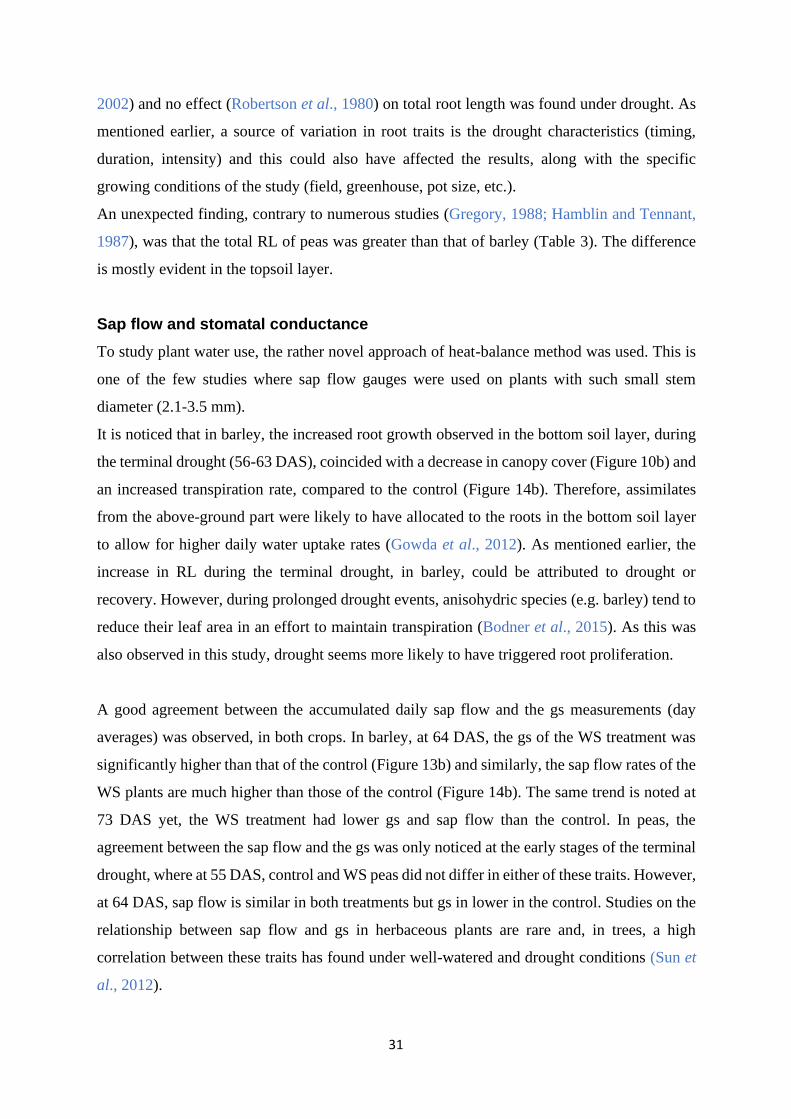
Peas

The canopy cover of both treatments increased until 49 DAS and then 56 DAS (onset of 2nd

drought) it started to decrease (Figure 10a).

Canopy cover was not affected by either drought events. A small, however non-significant,

difference between the treatments was observed between 56 and 63 DAS.

Barley

The canopy cover of the control treatment increased until 44 DAS and showed a slight decrease

65 DAS (Figure 10b). In the WS treatment, canopy cover peaked a little later, at 51 DAS, and

started to markedly decrease until 72 DAS.

The first drought event had an impact on canopy cover which was observed during the early

days of recovery. At 44 DAS, control plants showed a 56 % increase in canopy cover,

compared to the previous measurement, as opposed to the 3% of the WS plants (Figure 10b).

The second drought cycle had a stronger influence on canopy cover than the first (P=0.04). At

65 (P= 0.184) and 72 DAS (P= 0.099) the difference between the control and the WS plants

was noticeable.

a)

b)

Figure 10 Canopy cover (%) and plant height (cm) of control (C) and water stressed (WS) a) peas and b)

barley. Bars represent canopy cover (n=3-6 ±SEM) and lines plant height (n= 5-6 ±SEM).

21

Root length

Pea had a more extensive root system than barley. This is mostly noticed at the top and middle

soil layers. At the bottom soil layer, there were no significant differences in RL between the

plant species (Table 3).

Considering the whole experimental period, within each soil layer, RL did not differ

significantly between the treatments in both crops (Table 3). When RL was compared between

the treatments during drought cycles (as defined by VWC, see Soil water content section)

significant differences were found in barley in all three soil layers whereas in peas, no such

differences were detected.

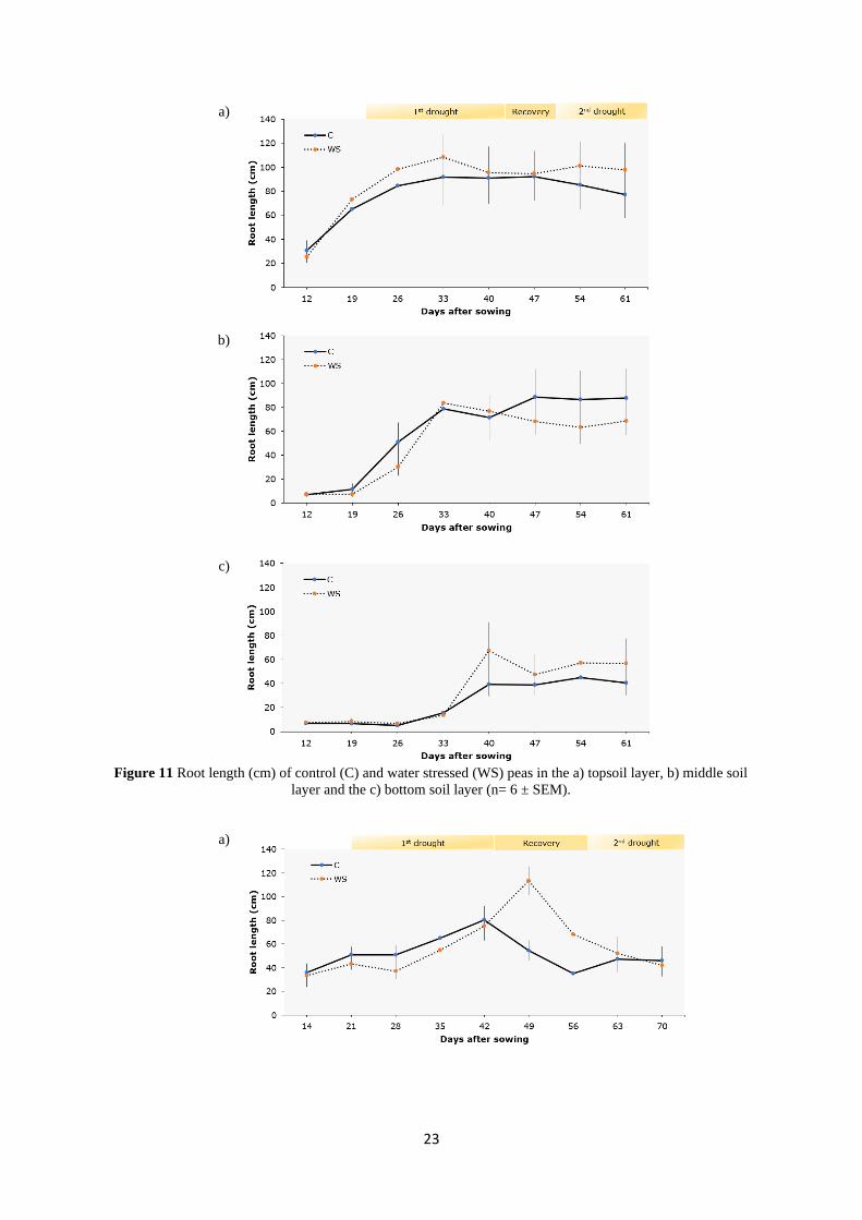
Peas

Root growth was more prominent in the topsoil layer where the RL of both treatments averaged

82 cm (Table 3). Fewest roots were observed in the middle (55 cm) and even fewer in the

bottom soil layer (29 cm).

In the topsoil layer (Figure 11a), RL increased until 26 DAS from where it remained constant

until the last measurement. The same trend is noticed in the middle and bottom soil layer

(Figure 11a, 11b), only here the increase seemed to stop at 33 and 40 DAS, respectively.

Within each soil layer, neither of the drought events seemed to significantly influence root

proliferation and there were no significant differences in RL within single dates.

In the topsoil layer, a small rise, however non-significant, in the RL of the WS treatment was

observed after the onset of both drought cycles.

In the middle soil layer, a small but not significant difference between the treatments is

observed between 40-47 DAS, as control plants seem to have higher RL than the stressed

plants. This difference is maintained throughout the second drought cycle.

In the bottom soil layer, the RL of both treatments seemed similar until 33 DAS. At 40 DAS,

a rise in the RL of the WS treatment is observed. At 47, 54 and 61 DAS WS peas had higher,

but non-significant, RL than the control.

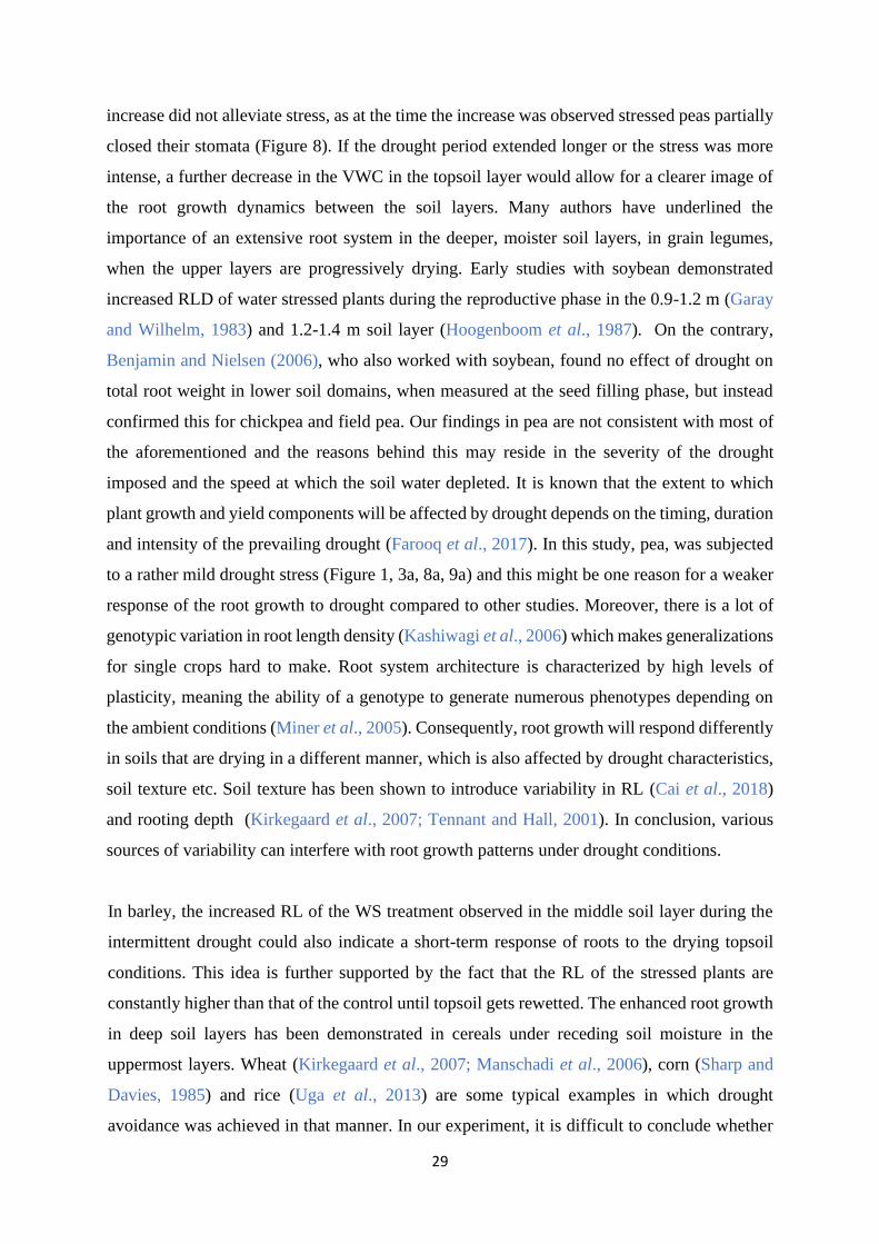
Barley

Roots proliferated more in the topsoil (55 cm on average) than in the middle and the bottom

(35 and 31 cm, respectively). Moreover, there were no significant differences in the RL

between the middle and the bottom soil layer (Table 3).

22

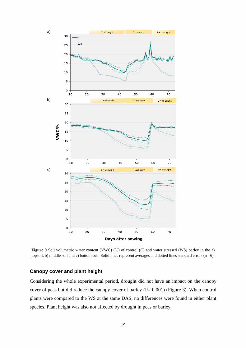
In the topsoil layer, RL gradually increased and peaked at 42 DAS in the control and 49 DAS

in the WS treatment. A decrease followed in both treatments and at 63 and 70 DAS RL

remained constant and similar.

In the middle soil layer, the RL of the control treatment reached a maximum value at 21-35

DAS, then decreased between 35 and 42 DAS and decreased again between 56-63 DAS. On

the other hand, the RL of the WS treatment peaked at 35 DAS and was gradually decreasing

until the last measurement, at 70 DAS.

In the bottom soil layer, the RL of the control treatment increased until 35 DAS, then it

decreased between 42-56 DAS and was stable at 56-70 DAS. The RL of the WS treatment

exhibited two peaks: one, 35 DAS and another at 63-70 DAS.

Significant differences in RL were found between the treatments during both drought events

and recovery. Shortly after the end of the first drought, at 49 DAS, a significant difference (P=

0.003) was noticeable as the roots of the WS treatment had more than double the length of that

of the control (113.3 and 54.7 cm, respectively). The same pattern was also observed at 56

DAS at the following measurement, although the difference was not significant (P=0.082). The

second drought cycle had no influence on RL of the topsoil layer.

In the middle soil layer, at 35-49 DAS the RL of the WS treatment was significantly higher

from that of the control (P= 0.03)

In the bottom soil layer, at 63-70 DAS (second drought event), the RL of the WS plants was

significantly higher than the control (P= 0.007).

Table 3 Root length (cm) of peas and barley [(npeas =47-48, nbarley= 52-53) ± SEM] under different water

treatments in three soil sections. Values are drawn from all root length measurements (peas: 12-61 DAS,

barley: 14-70)

Plant species Water treatment Soil section

Top Middle Bottom

Peas

Control 77 ± 7 60 ± 8 25 ± 3

Water stressed 87 ± 7 51 ± 5 33 ± 6

Total 82 ± 5 55 ± 5 29 ± 4

Barley

Control 52 ± 3 32 ± 4 28 ± 3

Water stressed 58 ± 5 37 ± 4 34.6 ± 4.0

Total 55 ± 3 35 ± 3 31.4 ± 2.5

23

a)

c)

Figure 11 Root length (cm) of control (C) and water stressed (WS) peas in the a) topsoil layer, b) middle soil

layer and the c) bottom soil layer (n= 6 ± SEM).

a)

b)

24

b)

c)

Figure 12 Root length (cm) of control (C) and water stressed (WS) barley in the a) topsoil layer, b) middle

soil layer and the c) bottom soil layer (n= 6 ± SEM).

Stomatal conductance

Peas had higher stomatal conductance (gs) than barley: the control peas had an average gs of

733 mmol m-2 s-1 while the corresponding barley had 340 mmol m-2 s-1, during the experimental

period.

Peas

An effect of drought on gs was observed at 41 DAS (end of 1st drought), where WS plants had

a 23.2 % lower gs than the control (P= 0.004). In the recovery phase, 50 DAS, gs was restored

to a similar value (around 700 mmol m-2 s-1) in both treatments. The second drought cycle was

observed to affect gs at 64 DAS (P= 0.04).

Barley

The impact of water limitation on the gs was also noticeable towards the end of the first drought

event, at 43 DAS (P= 0.005). During the recovery phase no differences between the treatments

were observed. A noteworthy change occurred at the beginning of the second drought event:

WS plants had higher gs than the control plants (P= 0.012). This pattern reversed as drought

progressed and, at 73 DAS, WS plants had again lower gs than the control (P= 0.001).

25

a)

b)

Figure 13 Stomatal conductance (gs) (mmol m-2 s-1) of control (C) and water stressed (WS) a) peas and b)

barley (n=6 ± SEM). Stars represent statistically significant differences between the C and the WS treatment.

Sap flow

Pea had higher daily sap flow rates than barley (Figure 14, 15). However, it should be noted

that in each barley pot there were about 10 stems (5 per plant) as opposed to pea pots that

contained 1-3 stems each.

Peas

The effect of terminal drought on the sap flow rate of pea was not evident. For most days shown

in Figure 14a and 15a, the sap flow rates of the control plants slightly exceeded that of the WS

plants. An exception to that, occurred at 60-61 and 69-70 DAS (Figure 14a) where the sap flow

rates of the WS plants, was slightly higher. A downward trend, started at 58 DAS, was noticed

in the control treatment until the sap flow rates became zero. Similarly, the same trend was

observed in the WS treatment but with a lag time of 3 days.

Barley

26

In barley, there was an apparent impact of water limitation to the sap flow (Figure 14b and

15b). Τhis was observed between 69-81 DAS, where the sap flow rates of the stressed plants

were lower than the control and continued to decrease until 77 DAS to zero. In the control

treatment, the sap flow rates started to fall later, at 76 DAS, and came close to zero at 82 DAS.

However, at the beginning of the terminal drought, the WS treatment exhibited higher sap flow

rates than the control. This is noted during a 3-day period at 62-65 DAS.

a)

b)

Figure 14 Accumulated sap flow rates (g day-1) of control and WS a) pea and b) barley during terminal

drought (n=2)

Hourly sap flow rates and stomatal conductance

Examples of hourly fluctuations in sap flow rates and gs within a day, during terminal drought,

are shown in Figure 15 and 17&18, respectively. In both crops, the daily sap flow pattern was

similar to that of solar radiation (Figure 16) as peaks and troughs in solar radiation are noted,

shortly after, in the sap flow rates as well.

In both crops, between 9.00-15.00, gs did not fluctuate much (Figure 17,18). This was observed

in both treatments, but it was not always in agreement with sap flow measurements: in peas, at

64 DAS, there is an apparent difference between the sap flow rates at 9.00 and 12.00, which is

not reflected in gs. Similarly, in WS barley at 73 DAS, the difference in the flow between 12.00

and 15.00 is not seen in gs.

27

a)

Sap

flo

w r

ate

(g

h-1

)

b)

c)

d)

Time (hhmm)

Figure 15 Sap flow rates (g h-1) of a) peas at 55 DAS and b) peas at 64 DAS, c) barley at 64 DAS and d)

barley at 73 DAS (n=2).

a)

RH

(%

)

b

SR

(μ

mo

l)

Time (hhmm)

Figure 16 Relative humidity (RH) (%) and solar radiation (SR) (μmol) at a) 7/7 (peas=55, barley=64 DAS)

and b) 16/7 (peas=64, barley=73 DAS).

a)

a)

b)

b)

Figure 17 Stomatal conductance (gs) (mmol

m-2 s-1) of control and water stressed (WS) a)

peas at 55 DAS and b) barley at 64 DAS,

presented at three different times within a day

(n=6 ± SEM).

Figure 18 Stomatal conductance (gs) (mmol

m-2 s-1) of control and water stressed (WS) a)

peas at 64 DAS and b) barley at 73 DAS,

presented at three different times within a day

(n=6 ± SEM).

28

Discussion

To cope with adverse water availability and to maintain their tissues hydrated, plants develop

mechanisms to enhance water acquisition from the soil and limit water loss (Blum et al., 2005).

Numerous studies have showed the benefits of deep and vigorous root systems in water

acquisition under various types of drought (Uga et al., 2013; Kirkegaard et al., 2007;

Manschandi et al., 2006). In the present study, we investigated whether two plant species, with

different root systems, could exploit water deeper in the soil in response to topsoil drying, in

order to alleviate water stress and yield penalties. The results show that, in pea, roots of the

water stressed plants (WS) did not enhance their proliferation in lower soil layers in response

to topsoil drying conditions whereas, in barley there was an increased root growth in the 36-62

cm and 71-97 layers when exposed to drought. Furthermore, sap flow measurements revealed

differences in plant water use between the treatments and confirmed the role of enhanced root

proliferation in water acquisition from the lowest soil layer.

Deep rootedness

The effect of water shortages on rooting depth was not evaluated in this study due to the limited

size of the pots. The pots used were 100 cm long and since roots of both crops usually grow

longer, we were not able to determine whether water stressed plants could explore deeper soil

domains to acquire water when upper layers were drier. Instead, we studied whether roots that

were already established in the lowest soil layers (36-62 and 71-97 cm) could proliferate more

in response to drought in the upper layer.

Root length

When water shortages occur, an extensive root growth in the deep soil layers, where water is

available, would be an advantage for sustaining relatively high yields (Comas et al., 2013). In

this study, pea, showed a slight increase in RL in the bottom soil layer during the late stages of

the intermittent drought and while the VWC of the upper layers (top and bottom) was less than

10%. After the topsoil layer got rewetted, RL in the bottom layer decreased and no difference

between the treatments was noted. It can be speculated that this increase was a short term

response to drought in the upper soil layers, as there was more water in the bottom to be

exploited (Hoogenboom et al., 1987) but the data cannot confirm this, as the increase is not

very evident and the variability in the data is big. Furthermore, it can be assumed that this

29

increase did not alleviate stress, as at the time the increase was observed stressed peas partially

closed their stomata (Figure 8). If the drought period extended longer or the stress was more

intense, a further decrease in the VWC in the topsoil layer would allow for a clearer image of

the root growth dynamics between the soil layers. Many authors have underlined the

importance of an extensive root system in the deeper, moister soil layers, in grain legumes,

when the upper layers are progressively drying. Early studies with soybean demonstrated

increased RLD of water stressed plants during the reproductive phase in the 0.9-1.2 m (Garay

and Wilhelm, 1983) and 1.2-1.4 m soil layer (Hoogenboom et al., 1987). On the contrary,

Benjamin and Nielsen (2006), who also worked with soybean, found no effect of drought on

total root weight in lower soil domains, when measured at the seed filling phase, but instead

confirmed this for chickpea and field pea. Our findings in pea are not consistent with most of

the aforementioned and the reasons behind this may reside in the severity of the drought

imposed and the speed at which the soil water depleted. It is known that the extent to which

plant growth and yield components will be affected by drought depends on the timing, duration

and intensity of the prevailing drought (Farooq et al., 2017). In this study, pea, was subjected

to a rather mild drought stress (Figure 1, 3a, 8a, 9a) and this might be one reason for a weaker

response of the root growth to drought compared to other studies. Moreover, there is a lot of

genotypic variation in root length density (Kashiwagi et al., 2006) which makes generalizations

for single crops hard to make. Root system architecture is characterized by high levels of

plasticity, meaning the ability of a genotype to generate numerous phenotypes depending on

the ambient conditions (Miner et al., 2005). Consequently, root growth will respond differently

in soils that are drying in a different manner, which is also affected by drought characteristics,

soil texture etc. Soil texture has been shown to introduce variability in RL (Cai et al., 2018)

and rooting depth (Kirkegaard et al., 2007; Tennant and Hall, 2001). In conclusion, various

sources of variability can interfere with root growth patterns under drought conditions.

In barley, the increased RL of the WS treatment observed in the middle soil layer during the

intermittent drought could also indicate a short-term response of roots to the drying topsoil

conditions. This idea is further supported by the fact that the RL of the stressed plants are

constantly higher than that of the control until topsoil gets rewetted. The enhanced root growth

in deep soil layers has been demonstrated in cereals under receding soil moisture in the

uppermost layers. Wheat (Kirkegaard et al., 2007; Manschadi et al., 2006), corn (Sharp and

Davies, 1985) and rice (Uga et al., 2013) are some typical examples in which drought

avoidance was achieved in that manner. In our experiment, it is difficult to conclude whether

30

the increase in RL in the middle soil layer conferred stress alleviation but it is also noted that

the plant partially closed its stomata right after the increase (Figure 13b) thus it is possible that

the avoidance had a very short duration.

An increase in RL is also observed in the bottom soil layer, during terminal drought, but it is

not clear whether it is a response to drought or a recovery response. It can be assumed that

since water in the topsoil layer was gradually becoming limited, while it was >15% in the other

layers, roots in the bottom layer responded with an increased growth. However, it must be

taken into consideration that during this period where RL was increasing in the bottom layer

(56-63 DAS) this layer got rewetted. Thus, the increase in RL could also be due to a regrowth

response because water conditions became favorable again in the rhizosphere.

Compensatory root growth

In barley, a steep and significant increase in the RL of the WS treatment was observed in the

topsoil layer following recovery. This is most likely attributed to the soil rewetting.

Compensatory regrowth has been demonstrated in many studies where e.g. shoot growth (Huck

et al., 1983), soil bacteria populations (Meisner et al., 2015) and root growth (Jupp and

Newman, 1987) increased after water was re-introduced in a dry soil. Moreover, under drought

conditions, there is a carbon cost for maintaining roots which can be avoided by root

senescence and, when conditions become favorable, by creating new ones (Van Noordwijk et

al., 1998). This is true for very fine lateral roots with increased water uptake capacity

(Eissenstat and Yanai, 2002). Thus, the plant can induce their senescence in response to drying

soil and develop new ones after it is rewetted which will increase the total uptake. However,

root senescence due to drought was not observed in barley, in this experiment. A rapid growth

after a dry soil is rewetted can also have benefits for the yield (Comas et al., 2013).

Overall response of root growth under receding soil moisture

Besides rooting patterns in specific soil layers during drought events, it must be pointed out

that literature on the overall root growth along the soil profile is contrasting. Drought has

usually been found to inhibit root growth (Gregory, 1988) and this is confirmed in a study with

numerous annual species (Zhou et al., 2018), in corn (Robertson et al., 1980), common bean

(Sofi et al., 2018) and other crops. Yet, in chickpea (Ali et al., 2005) total root growth was

increased under water stress. Findings are sometimes contradictory, even within the same

species as in e.g. soybean, where both an increase (Hoogenboom et al., 1987; Merrill et al.,

31

2002) and no effect (Robertson et al., 1980) on total root length was found under drought. As

mentioned earlier, a source of variation in root traits is the drought characteristics (timing,

duration, intensity) and this could also have affected the results, along with the specific

growing conditions of the study (field, greenhouse, pot size, etc.).

An unexpected finding, contrary to numerous studies (Gregory, 1988; Hamblin and Tennant,

1987), was that the total RL of peas was greater than that of barley (Table 3). The difference

is mostly evident in the topsoil layer.

Sap flow and stomatal conductance

To study plant water use, the rather novel approach of heat-balance method was used. This is

one of the few studies where sap flow gauges were used on plants with such small stem

diameter (2.1-3.5 mm).

It is noticed that in barley, the increased root growth observed in the bottom soil layer, during

the terminal drought (56-63 DAS), coincided with a decrease in canopy cover (Figure 10b) and

an increased transpiration rate, compared to the control (Figure 14b). Therefore, assimilates

from the above-ground part were likely to have allocated to the roots in the bottom soil layer

to allow for higher daily water uptake rates (Gowda et al., 2012). As mentioned earlier, the

increase in RL during the terminal drought, in barley, could be attributed to drought or

recovery. However, during prolonged drought events, anisohydric species (e.g. barley) tend to

reduce their leaf area in an effort to maintain transpiration (Bodner et al., 2015). As this was

also observed in this study, drought seems more likely to have triggered root proliferation.

A good agreement between the accumulated daily sap flow and the gs measurements (day

averages) was observed, in both crops. In barley, at 64 DAS, the gs of the WS treatment was

significantly higher than that of the control (Figure 13b) and similarly, the sap flow rates of the

WS plants are much higher than those of the control (Figure 14b). The same trend is noted at

73 DAS yet, the WS treatment had lower gs and sap flow than the control. In peas, the

agreement between the sap flow and the gs was only noticed at the early stages of the terminal

drought, where at 55 DAS, control and WS peas did not differ in either of these traits. However,

at 64 DAS, sap flow is similar in both treatments but gs in lower in the control. Studies on the

relationship between sap flow and gs in herbaceous plants are rare and, in trees, a high

correlation between these traits has found under well-watered and drought conditions (Sun et

al., 2012).

32

Finally, it is confirmed that the greatest part of the energy applied on barley stems was

partitioned to radial heat conduction, as expected from studies with cereals (Langensiepen et

al., 2014). It has been argued that under both field and greenhouse conditions low sap flow

rates (<20 g h-1) are the main cause (Zhang and Kirkham, 1995).

a)

Pow

er (

Watt

)

b)

Time (hh.mm)

Figure 19 Energy fluxes of the heat-balance theory in a) peas at 55 DAS and b) barley at 64 DAS (n=1). Pin=

power input from the heater, Qf= energy convection carried by the sap flow, Qv= axial heat conduction, Qr=

radial energy loss by conduction to the ambient

Water saving and water spending strategies

To cope with water stress, plants have developed three key strategies: drought escape, drought

avoidance and drought tolerance (Verma et al., 2018). Drought escape is achieved by rapid

plant development in such a way that flowering, or maturation occurs before the onset of

drought. By using this strategy plants finalize much of their development before adverse

conditions arise. Although this is desirable for some types of plants (e.g. desert plants), it would

not always be of an advantage for crops, as a diminished above-ground mass may not be able

to meet the productivity demand. Drought escape is often found in native populations (e.g.

crops in the Mediterranean region where terminal drought scenarios are frequent) and can also

be manipulated by agricultural practices (early sowing). The intermittent drought in this study

did not hasten the flowering time in any of the two crops. Drought avoidance involves a

complex of mechanisms which allow the plant to keep its water status and is further classified

into water saving and water spending strategies (Basu et al., 2016). In this study, both crops

have demonstrated mostly water saving strategies as, in an effort to minimize water loss, they

reduced their leaf area (barley) and gs (peas and barley). The water spending strategy is utilized

by crops to enhance water uptake from the soil. In this way, by maintaining relatively high

transpiration rates under drought, plants might be able to accumulate more assimilates in the

stem and relocate them in the grain (Lopes and Reynolds, 2010). In this experiment, barley has

33

demonstrated an ability to utilize the water spending strategy as well. As mentioned earlier,

barley roots proliferated more in the bottom soil layer during terminal drought, which was

followed by increased sap flow rates. Thus, WS plants seemed to have utilized this strategy for

increased water acquisition. Finally, the third strategy employed by plants for drought

resistance is drought tolerance and involves osmotic regulation (solute accumulation in the

cell), protection from oxidative stress and desiccation tolerance (Zhang, 2007) but it is out of

the scope of this research.

Significance of findings and general considerations

In order to maintain relatively high yields under drought conditions, plants must have access

to and utilize water from layers of soil that have not yet dried. Similarly, Lynch (2013)

mentioned that for optimal water uptake “root foraging and resource availability should

coincide in space and time”. Several root traits have been proposed to confer drought tolerance

(Watt et al., 2013) and in this study we focused mainly on the root length. It has been found

that there is high variability for root length within plant species, and screening trials revealed

drought tolerant genotypes with increased root proliferation at depths (Ali et al., 2005;

Kashiwagi et al., 2006). Moreover, root length is highly heritable (Kashiwagi et al., 2006)

which makes it a suitable trait for plant breeding. Thus, in drought-prone environments where

plants mature while there is still water in depth, the approach of choosing the appropriate

genotype that could reach and use this water could be adopted. From our experiment it was not

fully understood whether these cultivars (Pisum sativum L. cv. Javlo and Hordeum vulgare L.

cv. RGT Planet) would be suitable for drought-prone environments but future research, such

as those of Kashiwagi et al. (2006), could focus on finding and developing new genotypes with

enhanced water acquisition. Wild relatives have shown to be a gene pool of root traits valuable

for drought tolerance (Johnson et al., 2000).

Crops that can forage for deep water under drought can be used in crop rotations with crops

with shallower roots (Cutforth et al., 2013). As there is high variability among crops for total

water depletion from the soil profile over the growing season, the amount of available water

left for a crop in a rotation system will depend on the choice of the preceding crop. A shallow-

rooted species (e.g. field pea) will leave water available in the subsoil for the following deep-

rooted species (e.g. wheat) to use which can be beneficial, as mentioned earlier, especially in

drought prone areas.

34

The study of deep roots involves many parameters that must be taken into consideration. The

penetration and proliferation of roots in the subsoil can face several restrictions (Lynch and

Wojciechowski, 2015) such as mineral toxicity, low temperatures and low oxygen levels.

Moreover, plant resources are often stratified within the soil profile creating contrasting needs

for root growth. A good example is phosphorus acquisition in drying soils as water may be

located deeper in the soil while phosphorus resides in the upper most layers (Ho et al., 2005).

This study underlines the importance of genotype and drought characteristics (timing, duration,

intensity) in drought avoidance.

Study limitations

A better understanding of the dynamics between soil water depletion and transpiration during

the vegetative phase would have achieved if sap flow measurements were conducted then. The

use of SGA2 gauges is only applicable to stems with diameter ranging from 2.1 to 3.5mm. In

barley, this diameter range was reached relatively high in the stem during the recovery phase.

The diameter of pea stems was, for the most part of the growth cycle, within the limits but in

order to get a good signal from the gauges a substantial transpiring leaf area should exist above

them. This was achieved during the recovery phase as well.

The use of longer pots would allow the comparison of rooting depth and the proliferation of

roots to that depth between the control and the water stress treatment.

Acknowledgements

I would like to thank Corentin Clément for his continuous guidance and support throughout the

project and for helping me develop my critical thinking skills through our conversations.

Furthermore, I acknowledge George Statiris who helped me with the measurements and

constantly encouraging me, Dimitris Statiris for the illustrations, and Abraham Smith for

teaching me how to use RootPainter. Lastly, I would like to thank Kristian Thorup-Kristensen

and Dorte Bodin Dresbøll who trusted me with the project and coordinated the whole process.

The study was part of the DeepFrontier project which is funded by the Villum Funden.

35

36

References

Ali MY, Johansen C, Krishnamurthy L, Hamid A. 2005. Genotypic variation in root systems of

chickpea (Cicer arietinum L.) across environments. Journal of Agronomy and Crop Science, 191, 464–

472.

Babkin VI, Klige RK. 2003. The earth and its physical features. In: Shiklomanov IA, Rodda JC (eds.),

World Water Resources at the Beginning of the Twenty-first Century (p. 17), Cambridge University

Press

Baker JM, van Bavel CHM. 1987. Measurement of mass flow of water in the stems of herbaceous

plants. Plant, Cell & Environment, 10, 777–782.

Bakhsh K, Kamran MA. 2019. Adaptation to climate change in rain-fed farming system in Punjab,

Pakistan. International Journal of the Commons, 13, 833–847.

Basu S, Ramegowda V, Kumar A, Pereira A. 2016. Plant adaptation to drought stress.

F1000Research, 5, 1–10.

Benjamin JG, Nielsen DC. 2006. Water deficit effects on root distribution of soybean, field pea and

chickpea. Field Crops Research, 97, 248–253.

Blum A. 2005. Drought resistance , water-use efficiency , and yield potential — are they compatible ,

dissonant , or mutually exclusive ? Australian Journal of Agricultural research, 56, 1159–1168.

Bodner G, Nakhforoosh A, Kaul HP. 2015. Management of crop water under drought: a review.

Agronomy for Sustainable Development, 35, 401–442.

Byrd SA, Rowland DL, Bennett J, Zotarelli L, Wright D, Alva A, Nordgaard J. 2015. The

Relationship Between Sap Flow and Commercial Soil Water Sensor Readings in Irrigated Potato

(Solanum tuberosum L.) Production. American Journal of Potato Research, 92, 582–592.

Cai G, Vanderborght J, Langensiepen M, Schnepf A, Hüging H, Vereecken H. 2018. Root growth,

water uptake, and sap flow of winter wheat in response to different soil water conditions. Hydrology

and Earth System Sciences, 22, 2449-2470.

Cattivelli L, Rizza F, Badeck FW, Mazzucotelli E, Mastrangelo AM, Francia E, Marè C, Tondelli

A, Stanca AM. 2008. Drought tolerance improvement in crop plants: An integrated view from breeding

to genomics. Field Crops Research, 105, 1–14.

Cohen Y, Takeuchi S, Nozaka J, Yano T. 1993. Accuracy of sap flow measurement using heat balance

and heat pulse methods. Agronomy Journal, 85, 1080–1086.

Comas LH, Becker SR, Cruz VMV, Byrne PF, Dierig DA. 2013. Root traits contributing to plant

productivity under drought. Frontiers in Plant Science, 4:442.

Cutforth HW, Angadi SV, McConkey BG, Miller PR, Ulrich D, Gulden R, Volkmar KM, Entz

MH, Brandt SA. 2013. Comparing rooting characteristics and soil water withdrawal patterns of wheat

with alternative oilseed and pulse crops grown in the semiarid Canadian prairie. Canadian Journal of

Soil Science, 93, 147–160.

de Swaef T, Verbist K, Cornelis W, Steppe K. 2012. Tomato sap flow, stem and fruit growth in

relation to water availability in rockwool growing medium. Plant and Soil, 350, 237–252.

Dugas WA. 1990. Comparative Measurement of Stem Flow and Transpiration in Cotton. Theoretical

and Applied ClimatoIogy, 42, 215-221

37

Eissenstat D, Yanai RD. 2002. Root lifespan, turnover and efficiency. In: Waisel Y, Eshel A, Kafkafi

U (eds.), Plant Roots: The Hidden Half (third edition), pp. 221–238, Marcel Dekker, Inc.

Farooq M, Gogoi N, Barthakur S, Baroowa B, Bharadwaj N, Alghamdi SS, Siddique KHM. 2017.

Drought Stress in Grain Legumes during Reproduction and Grain Filling. Journal of Agronomy and

Crop Science, 203, 81–102.

Garay AF, Wilhelm WW. 1983. Root System Characteristics of Two Soybean Isolines Undergoing

Water Stress Conditions . Agronomy Journal, 75, 973–977.

Gorim LY, Vandenberg A. 2017. Evaluation of wild lentil species as genetic resources to improve

drought tolerance in cultivated lentil. Frontiers in Plant Science, 8:1129.

Gowda VRP, Henry A, Vadez V, Sashidhar HE, Serraj R. 2012. Water uptake dynamics under

progressive drought stress in diverse accessions of the OryzaSNP panel of rice (Oryza sativa).

Functional Plant Biology, 39, 402-411

Gregory PJ. 1988. Root growth of chickpea, faba bean, lentil, and pea and effects of water and salt

stresses. In: Summerfield RJ (eds), World crops: Cool season food legumes (pp. 857-867), Springer.

Grime VL, Morison JIL, Simmonds LP. 1995. Including the heat storage term in sap flow

measurements with the stem heat balance method. Agricultural and Forest Meteorology, 74, 1–25.

Groot A, King KM. 1992. Measurement of sap flow by the heat balance method: numerical analysis

and application to coniferous seedlings. Agricultural and Forest Meteorology, 59, 289–308.

Gordon R, Dixon M.A, Brown DM. 1997. Verification of sap flow by heat balance method on three

potato cultivars. Potato Research, 40, 267–276.

Hamblin A, Tennant D. 1987. Root length density and water uptake in cereals and grain legumes:

How well are they correlated? Australian Journal of Agricultural Research, 38, 513–527.

Han M, Zhang H, DeJonge KC, Comas LH, Gleason S. 2018. Comparison of three crop water stress

index models with sap flow measurements in maize. Agricultural Water Management, 203, 366–375.

Ho MD, Rosas JC, Brown KM, Lynch JP. 2005. Root architectural tradeoffs for water and

phosphorus acquisition. Functional Plant Biology, 32, 737–748.

Hoogenboom G, Huck MG, Peterson CM. 1987. Root Growth Rate of Soybean as Affected by

Drought Stress 1 . Agronomy Journal, 79, 607–614.

Huck MG, Ishihara K, Peterson CM, Ushijima T. 1983. Soybean Adaptation to Water Stress at

Selected Stages of Growth. Plant Physiology, 73, 422–427.

Hurd EA. 1968. Growth of Roots of Seven Varieties of Spring Wheat at High and Low Moisture Levels

1 . Agronomy Journal, 60, 201–205.

Isoda A, Wang P. 2002. Leaf temperature and transpiration of field grown cotton and soybean under

arid and humid conditions. Plant Production Science, 5, 224–228.

Jamieson PD, Martin RJ, Francis GS. 1995. Drought influences on grain yield of barley, wheat, and

maize. New Zealand Journal of Crop and Horticultural Science, 23,55-66

Johnson WC, Jackson LE, Ochoa O, Van Wijk R, Peleman J, St. Clair DA, Michelmore, RW.

2000. Lettuce, a shallow-rooted crop, and Lactuca serriola, its wild progenitor, differ at QTL

determining root architecture and deep soil water exploitation. Theoretical and Applied Genetics, 101,

1066–1073.

38

Jupp AP, Newman EI. 1987. Morphological and anatomical effects of severe drougth in the roots of

Lolium perrene L. New Phytologist, 105, 393-402

Kashiwagi J, Krishnamurthy L, Crouch JH, Serraj R. 2006. Variability of root length density and

its contributions to seed yield in chickpea (Cicer arietinum L.) under terminal drought stress. Field

Crops Research, 95, 171–181.

Katayama K, Ito O, Adu-Gyamfi JJ, Rao TP. 2000. Analysis of relationship between root length

density and water uptake by roots of five crops using minirhizotron in the semi-arid tropics. Japan

Agricultural Research Quarterly, 34, 81–86.

Kirkegaard JA, Lilley JM, Howe GN, Graham JM. 2007. Impact of subsoil water use on wheat

yield. Australian Journal of Agricultural Research, 58, 303–315.

Langensiepen M, Kupisch M, Graf A, Schmidt M, Ewert F. 2014. Improving the stem heat balance

method for determining sap-flow in wheat. Agricultural and Forest Meteorology, 186, 34–42.

Lopes M, Reynolds M. 2010. Partitioning of assimilates to deeper roots is associated with cooler

canopies and increased yield under drought in wheat. Functional Plant Biology, 37, 147–156.

Ludlow MM, Muchow RC. 1990. A critical evaluation of traits for improving crop yields in water-

limited environments. Advances in Agronomy, 43, 107-153.

Lynch JP. 1995. Root architecture and plant productivity. Plant Physiology, 109, 7–13.

Lynch JP. 2013. Steep, cheap and deep: An ideotype to optimize water and N acquisition by maize

root systems. Annals of Botany, 112, 347–357.

Lynch JP, Wojciechowski T. 2015. Opportunities and challenges in the subsoil: Pathways to deeper

rooted crops. Journal of Experimental Botany, 66, 2199–2210.

Manschadi AM, Christopher J, Devoil P, Hammer GL. 2006. The role of root architectural traits in

adaptation of wheat to water-limited environments. Functional Plant Biology, 33, 823–837.

Meisner A, Rousk J, Bååth E. 2015. Prolonged drought changes the bacterial growth response to

rewetting. Soil Biology and Biochemistry, 88, 314–322.

Merrill SD, Tanaka DL, Hanson JD. 2002. Root Length Growth of Eight Crop Species in Haplustoll

Soils. Soil Science Society of America Journal, 66, 913–923.

Miner BG, Sultan SE, Morgan SG, Padilla DK, Relyea RA. 2005. Ecological consequences of

phenotypic plasticity. Trends in Ecology and Evolution, 20, 685–692.

Muñoz-Perea CG, Terán H, Allen RG, Wright JL, Westermann DT, Singh SP. 2006. Selection for

drought resistance in dry bean landraces and cultivars. Crop Science, 46, 2111–2120.

Osakabe Y, Osakabe K, Shinozaki K, Tran LSP. 2014. Response of plants to water stress. Frontiers

in Plant Science, 5:86.

Passioura JB. 1983. Roots and drought resistance. Agricultural Water Management, 7, 265–280.

Polania J, Rao IM, Cajiao C, Grajales M, Rivera M, Velasquez F, Raatz B, Beebe SE. 2017. Shoot

and root traits contribute to drought resistance in recombinant inbred lines of MD 23–24 × SEA 5 of

common bean. Frontiers in Plant Science, 8:296.

Prince SJ, Song L, Qiu D, Maldonado dos Santos JV, Chai C, Joshi T, Patil G, Valliyodan B,

Vuong TD, Murphy M, Krampis K, Tucker DM, Biyashev R, Dorrance AE, Maroof SAS, Xu D,

Shannon JG, Nguyen HT. 2015. Genetic variants in root architecture-related genes in a Glycine soja

39

accession, a potential resource to improve cultivated soybean. BMC Genomics, 16:132

Rafi Z, Merli O, Le Dantec V, Khabba S, Mordelet P, Er-Raki S, Amazirh A, Olivera-Guerra L,

Ait Hssaine B, Simonneaux V, Ezzahar J, Ferrer F. 2019. Partitioning evapotranspiration of a drip-

irrigated wheat crop: Inter-comparing eddy covariance-, sap flow-, lysimeter- and FAO-based methods.

Agricultural and Forest Meteorology, 265, 310–326.

Reddy TY, Reddy VR, Anbumozhi V. 2003. Physiological responses of groundnut (Arachis hypogaea

L.) to drought stress and its amelioration: A critical review. Plant Growth Regulation, 41, 75-88.

Rich SM, Watt M. 2013. Soil conditions and cereal root system architecture: Review and

considerations for linking Darwin and Weaver. Journal of Experimental Botany, 64, 1193–1208.

Richard CAI, Hickey LT, Fletcher S, Jennings R, Chenu K, Christopher JT. 2015. High-

throughput phenotyping of seminal root traits in wheat. Plant Methods, 11, 13.

Robertson WK, Hammond LC, Johnson JT, Boote KJ. 1980. Effects of Plant-Water Stress on Root

Distribution of Corn, Soybeans, and Peanuts in Sandy Soil1. Agronomy Journal, 72, 548-550.

Rose MA, Rose MA. 1994. Oscillatory transpiration may complicate stomatal conductance of gas-

exchange measurements. HortScience, 29, 693–694.

Rubio G, Liao H, Yan X, Lynch JP. 2003. Topsoil foraging and its role in plant competitiveness for

phosphorus in common bean. Crop Science, 43, 598–607.

Sakuratani T. 1981. A Heat Balance Method for Measuring Water Flux in the Stem of Intact Plants.

Journal of Agricultural Meteorology, 37, 9–17.

Sauer TJ, Singer JW, Prueger JH, DeSutter TM, Hatfield JL. 2007. Radiation balance and

evaporation partitioning in a narrow-row soybean canopy. Agricultural and Forest Meteorology, 145,

206–214.

Sharp RE, Davies WJ. 1985. Root growth and water uptake by maize plants in drying soil. Journal of

Experimental Botany, 36, 1441–1456.

Smith AG, Han E, Petersen J, Olsen NAF, Giese C, Athmann M, Dresbøll DB, Thorup-Kristensen

K. 2020. RootPainter: Deep learning Segmantation of Biological Images with Corrective Annotation.

BioRχin, 1-16.

Sofi PA, Djanaguiraman M, Siddique KHM, Prasad PVV. 2018. Reproductive fitness in common

bean (Phaseolus vulgaris L.) under drought stress is associated with root length and volume. Indian

Journal of Plant Physiology, 23, 796–809.

Sun XP, Yan HL, Ma P, Liu BH, Zou YJ, Liang D, Ma FW, Li PM. 2012. Responses of young

“Pink lady” apple to alternate deficit irrigation following long-term drought: Growth, photosynthetic

capacity, water-use efficiency, and sap flow. Photosynthetica, 50, 501–507.

Taiz L, Zeiger E. 2012. Plant physiology, 3, Water and Plant Cells (p. 82), Utopia, first greek edition.

Tennant D, Hall D. 2001. Improving water use of annual crops and pastures - Limitations and

opportunities in Western Australia. Australian Journal of Agricultural Research, 52, 171–182.

Uga Y, Sugimoto K, Ogawa S, Rane J, Ishitani M, Hara N, Kitomi Y, Inukai Y, Ono K, Kanno

N, Inoue H, Takehisa H, Motoyama R, Nagamura Y, Wu J, Matsumoto T, Takai T, Okuno K,

Yano M. 2013. Control of root system architecture by DEEPER ROOTING 1 increases rice yield under

drought conditions. Nature Genetics, 45, 1097–1102.

Van Noordwijk M, Martikainen P, Bottner P, Cuevas E, Rouland C, Dhillion SS. 1998. Global

40

change and root function. Global Change Biology, 4, 759–772.

Wasson AP, Richards RA, Chatrath R, Misra SC, Prasad SVS, Rebetzke GJ, Kirkegaard JA,

Christopher J, Watt M. 2012. Traits and selection strategies to improve root systems and water uptake

in water-limited wheat crops. Journal of Experimental Botany, 63, 3485–3498.

Watt M, Wasson AP, Chochois V. 2013. Root-Based Solutions to Increasing Crop Productivity. In:

Eshel A, Beeckman T (eds.), Plant Roots: the hidden half (21, pp. 1-17), CRC Press.

Yu J, Jiang M, Guo C. 2019. Crop pollen development under drought: From the phenotype to the

mechanism. International Journal of Molecular Sciences, 20:1550.

Zhan A, Schneider H, Lynch JP. 2015. Reduced lateral root branching density improves drought

tolerance in maize. Plant Physiology, 168, 1603–1615.

Zhang J, Kirkham MB. 1995. Sap Flow in a Dicotyledon (Sunflower) and a Monocotyledon

(Sorghum) by the Heat-Balance Method. Agronomy Journal, 87, 1106–1114.

Zhang Q. 2007. Strategies for developing green super rice. Proceedings of the National Academy of

Sciences of the USA, 104, 16402–16409.

Zhou G, Zhou X, Nie Y, Bai SH, Zhou L, Shao J, Cheng W, Wang J, Hu F, Fu Y. 2018. Drought-

induced changes in root biomass largely result from altered root morphological traits: Evidence from a

synthesis of global field trials. Plant Cell and Environment, 41, 2589–2599.

Zobel RW, Waisel Y. 2010. A plant root system architectural taxonomy: A framework for root

nomenclature. Plant Biosystems, 144, 507–512.