Marker-trait-sensor association in a multi-parent advanced ...

Institut für Nutzpflanzenwissenschaften und Ressourcenschutz

Professur für Pflanzenzüchtung

Prof. Dr. J. Léon

Marker-trait-sensor association in a multi-parent advanced generation

intercross (MAGIC) population in barley (Hordeum vulgare ssp. vulgare)

Inaugural-Dissertation

zur

Erlangung des Grades

Doktor der Agrarwissenschaften

(Dr. agr.)

der

Landwirtschaftlichen Fakultät

der Rheinischen Friedrich-Wilhelms-Universität Bonn

vorgelegt am 07.06.2013

von

Wiebke Sannemann

aus Bielefeld

Referent: Prof. Dr. Jens Léon

Korreferent: Prof. Dr. Heiner Goldbach

Tag der mündlichen Prüfung: 25.10.2013

Erscheinungsjahr 2013

„Prepare for awesomeness“

(Kung Fu Panda)

ABSTRACT I

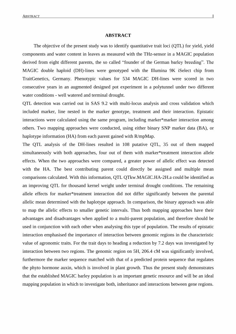
ABSTRACT

The objective of the present study was to identify quantitative trait loci (QTL) for yield, yield

components and water content in leaves as measured with the THz-sensor in a MAGIC population

derived from eight different parents, the so called “founder of the German barley breeding”. The

MAGIC double haploid (DH)-lines were genotyped with the Illumina 9K iSelect chip from

TraitGenetics, Germany. Phenotypic values for 534 MAGIC DH-lines were scored in two

consecutive years in an augmented designed pot experiment in a polytunnel under two different

water conditions - well watered and terminal drought.

QTL detection was carried out in SAS 9.2 with multi-locus analysis and cross validation which

included marker, line nested in the marker genotype, treatment and their interaction. Epistatic

interactions were calculated using the same program, including marker*marker interaction among

others. Two mapping approaches were conducted, using either binary SNP marker data (BA), or

haplotype information (HA) from each parent gained with R/mpMap.

The QTL analysis of the DH-lines resulted in 108 putative QTL, 35 out of them mapped

simultaneously with both approaches, four out of them with marker*treatment interaction allele

effects. When the two approaches were compared, a greater power of allelic effect was detected

with the HA. The best contributing parent could directly be assigned and multiple mean

comparisons calculated. With this information, QTL QTkw.MAGIC.HA-2H.a could be identified as

an improving QTL for thousand kernel weight under terminal drought conditions. The remaining

allele effects for marker*treatment interaction did not differ significantly between the parental

allelic mean determined with the haplotype approach. In comparison, the binary approach was able

to map the allelic effects to smaller genetic intervals. Thus both mapping approaches have their

advantages and disadvantages when applied to a multi-parent population, and therefore should be

used in conjunction with each other when analysing this type of population. The results of epistatic

interaction emphasised the importance of interaction between genomic regions in the characteristic

value of agronomic traits. For the trait days to heading a reduction by 7.2 days was investigated by

interaction between two regions. The genomic region on 5H, 206.4 cM was significantly involved,

furthermore the marker sequence matched with that of a predicted protein sequence that regulates

the phyto hormone auxin, which is involved in plant growth. Thus the present study demonstrates

that the established MAGIC barley population is an important genetic resource and will be an ideal

mapping population in which to investigate both, inheritance and interactions between gene regions.

ABSTRACT II

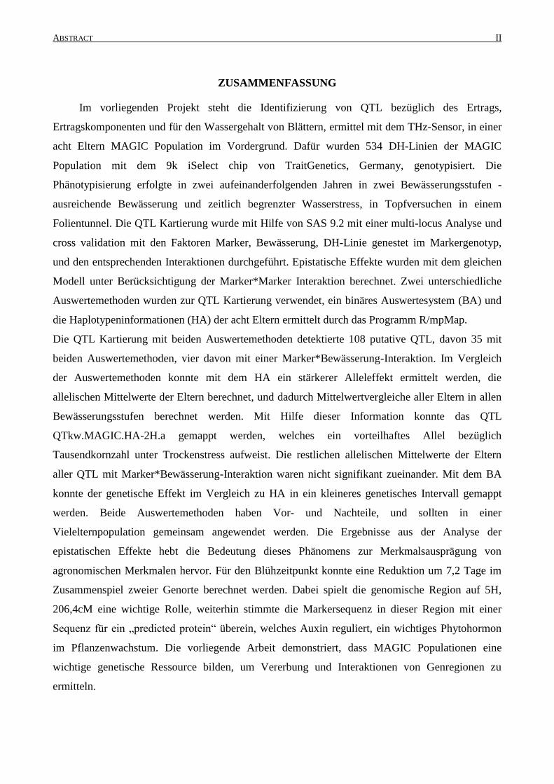
ZUSAMMENFASSUNG

Im vorliegenden Projekt steht die Identifizierung von QTL bezüglich des Ertrags,

Ertragskomponenten und für den Wassergehalt von Blättern, ermittel mit dem THz-Sensor, in einer

acht Eltern MAGIC Population im Vordergrund. Dafür wurden 534 DH-Linien der MAGIC

Population mit dem 9k iSelect chip von TraitGenetics, Germany, genotypisiert. Die

Phänotypisierung erfolgte in zwei aufeinanderfolgenden Jahren in zwei Bewässerungsstufen -

ausreichende Bewässerung und zeitlich begrenzter Wasserstress, in Topfversuchen in einem

Folientunnel. Die QTL Kartierung wurde mit Hilfe von SAS 9.2 mit einer multi-locus Analyse und

cross validation mit den Faktoren Marker, Bewässerung, DH-Linie genestet im Markergenotyp,

und den entsprechenden Interaktionen durchgeführt. Epistatische Effekte wurden mit dem gleichen

Modell unter Berücksichtigung der Marker*Marker Interaktion berechnet. Zwei unterschiedliche

Auswertemethoden wurden zur QTL Kartierung verwendet, ein binäres Auswertesystem (BA) und

die Haplotypeninformationen (HA) der acht Eltern ermittelt durch das Programm R/mpMap.

Die QTL Kartierung mit beiden Auswertemethoden detektierte 108 putative QTL, davon 35 mit

beiden Auswertemethoden, vier davon mit einer Marker*Bewässerung-Interaktion. Im Vergleich

der Auswertemethoden konnte mit dem HA ein stärkerer Alleleffekt ermittelt werden, die

allelischen Mittelwerte der Eltern berechnet, und dadurch Mittelwertvergleiche aller Eltern in allen

Bewässerungsstufen berechnet werden. Mit Hilfe dieser Information konnte das QTL

QTkw.MAGIC.HA-2H.a gemappt werden, welches ein vorteilhaftes Allel bezüglich

Tausendkornzahl unter Trockenstress aufweist. Die restlichen allelischen Mittelwerte der Eltern

aller QTL mit Marker*Bewässerung-Interaktion waren nicht signifikant zueinander. Mit dem BA

konnte der genetische Effekt im Vergleich zu HA in ein kleineres genetisches Intervall gemappt

werden. Beide Auswertemethoden haben Vor- und Nachteile, und sollten in einer

Vielelternpopulation gemeinsam angewendet werden. Die Ergebnisse aus der Analyse der

epistatischen Effekte hebt die Bedeutung dieses Phänomens zur Merkmalsausprägung von

agronomischen Merkmalen hervor. Für den Blühzeitpunkt konnte eine Reduktion um 7,2 Tage im

Zusammenspiel zweier Genorte berechnet werden. Dabei spielt die genomische Region auf 5H,

206,4cM eine wichtige Rolle, weiterhin stimmte die Markersequenz in dieser Region mit einer

Sequenz für ein „predicted protein“ überein, welches Auxin reguliert, ein wichtiges Phytohormon

im Pflanzenwachstum. Die vorliegende Arbeit demonstriert, dass MAGIC Populationen eine

wichtige genetische Ressource bilden, um Vererbung und Interaktionen von Genregionen zu

ermitteln.

ABSTRACT III

TABLE OF CONTENT

1. INTRODUCTION .................................................................................................................. 1

1.1 HORDEUM VULGARE SSP. VULGARE (BARLEY) ..................................................................................... 1

1.2 BARLEY GENETICS .............................................................................................................................. 2

1.3 BARLEY LANDRACES ........................................................................................................................... 3

1.4 PHENOTYPING WITH SENSOR TECHNOLOGY ........................................................................................ 4

1.5 DROUGHT AND DROUGHT TOLERANCE ............................................................................................... 6

1.6 QUANTITATIVE TRAIT LOCI (QTL) MAPPING ...................................................................................... 7

1.7 MULTI-PARENT MAPPING POPULATIONS ............................................................................................. 9

1.8 SINGLE NUCLEOTIDE POLYMORPHISM (SNP) .................................................................................... 10

1.9 HAPLOTYPES ..................................................................................................................................... 12

1.10 EPISTASIS .......................................................................................................................................... 13

1.11 OBJECTIVE AND HYPOTHESES ........................................................................................................... 14

2. MATERIALS UND METHODS ........................................................................................ 16

2.1 PLANT MATERIAL ............................................................................................................................. 16

2.2 PHENOTYPING ANALYSES ................................................................................................................. 19

2.3 GENOTYPING ..................................................................................................................................... 23

2.4 STATISTICAL ANALYSES .................................................................................................................... 25

3. RESULTS.............................................................................................................................. 30

3.1 PRELIMINARY PHENOTYPING EXPERIMENT: TRAITS AND ANALYSIS OF VARIANCE .......................... 30

3.2 PHENOTYPIC VARIATION IN MAGIC DH-LINES ............................................................................... 33

3.3 GENETIC CHARACTERISATION OF THE MAGIC POPULATION ........................................................... 39

3.4 QTL DETERMINATION IN THE MAGIC POPULATION ........................................................................ 43

3.5 EPISTATIC EFFECTS ........................................................................................................................... 54

3.6 MULTIPLE COMPARISON OF PARENTAL MEANS FROM HAPLOTYPE APPROACH ................................ 55

3.7 PYRAMIDISATION OF QTL................................................................................................................. 63

4. DISCUSSION ....................................................................................................................... 66

4.1 CHARACTERIZATION OF THE MAGIC POPULATION .......................................................................... 66

4.2 THZ-MEASUREMENT ......................................................................................................................... 68

4.3 COMPARISON OF THE TWO MAPPING APPROACHES ........................................................................... 69

4.4 DISTRIBUTION OF QTL WITHIN THE GENOME ................................................................................... 84

4.5 CONFIRMED AND NOVEL QTL: COMPARISON WITH KNOWN QTL AND CANDIDATE GENES ............. 87

4.6 GENOTYPE AND TREATMENT INTERACTION – DROUGHT TOLERANCE .............................................. 95

ABSTRACT IV

4.7 EPISTASIS IN THE MAGIC POPULATION .......................................................................................... 101

4.8 COMBINATION OF POSITIVE ALLELE EFFECTS ................................................................................. 104

4.9 MAGIC POPULATION AS MAPPING POPULATION ............................................................................ 109

5. SUMMARY AND CONCLUSION ................................................................................... 111

6. REFERENCES ................................................................................................................... 113

7. LIST OF FIGURES ........................................................................................................... 127

8. LIST OF TABLES ............................................................................................................. 128

9. LIST OF ABBREVIATIONS............................................................................................ 130

10. APPENDIX ......................................................................................................................... 131

INTRODUCTION 1

1. Introduction

Global agriculture is and will be facing declining water availability, a reduction in arable land,

competition between the cultivation of bio fuel, feedstock or food, and strongly increasing demand

for harvested products (Tardieu, 2012). Predictions of climate change indicate an increased

variability of rainfall in the next 40 years and an increased risk of high temperature (IPCC) that will

cause appreciable limitations of yield due to abiotic stresses (Brisson et al., 2010; Tebaldi and

Lobell, 2008). Cereal grain yields alone must increase by at least 70% before 2050. Rice demand

has already exceeded supply for the years 2007 and 2008 (Furbank et al., 2009). To face this

problem it is necessary to develop crops that are tolerant to drought. Unfortunately, drought is made

complex by variations in its severity, duration, and timing. The responses to drought are complex;

therefore drought tolerance is a complex trait. Barley is a genetically wide adapted crop species and

model crop, which is known to be drought tolerant, with established genomic resources and is

suitable for mapping of complex traits. Bi-parental crosses are grateful when used for individual

traits, like resistances to abiotic stresses. But when it comes to identify the genetic control of

complex multigenic traits like yield, and especially in complex environments like drought stress,

there is a need to move from ‘purpose-build’ bi-parental populations to those with a broader genetic

and phenotypic base (Huang et al., 2012). Therefore, a more complex breeding design was formed

and the barley MAGIC population, derived from eight German barley landraces/cultivar, was

established.

Understanding how to maximise water use efficiency of cultivated plants is a promising strategy to

remedy the above mentioned global water shortages (Hadjiloucas et al., 2002). Measuring the water

content of plants invasively would be a major gain in the overcoming of high-throughput

phenotyping of plants. This can be perfectly addressed with the terahertz (THz) spectroscopy,

whereas point measurements on leaves can determine the water content of leaves.

Adding it all together, the MAGIC population, the established genotyping facility with 7800 SNP

data points and the use of the THz-sensor to measure water content leads to the main objective of

this work, the detection of favourable allele effects for yield and yield component and water content

in plants under terminal drought stress.

1.1 Hordeum vulgare ssp. vulgare (Barley)

Barley (Hordeum vulgare L.) belongs to the tribe of Triticeae in the family of grass, Poaceae,

representing the largest family of monocotyledonous plants. The genus Hordeum contains 32

species and 45 taxa, including diploid, polyploid, perennial and annual types, distributed throughout

the world (Bothmer et al., 2003).

INTRODUCTION 2

Barley is one of the first crop domesticated, approximately 7500 B.C.E. as archaeological remains

emphasize. It is assumed that the domestication of barley took place from two-rowed wild barley

(Hordeum vulgare ssp. spontaneum, in the following written as Hordeum spontaneum) in the Near

East, the Fertile Crescent. Wild barley is still broadly distributed in these regions. But there are

ongoing debates among researchers about the evidence of multiple barley domestication sites

(Molina-Cano et al., 2005; Tanno et al., 2002).

Barley is one of the most important cereal crop species in food production. It is ranking fifth in the

world after wheat, maize, rice and soya in terms of acreage (FAO 2010, http://faostat.fao.org).

Approximately 75% of global production is used for animal livestock feed, 20% is malted for use in

alcoholic and non-alcoholic beverages, and 5% as use in human food products (Blake et al., 2011).

Barley is widely adapted to different environmental conditions, and is more stress tolerant to cold,

drought, alkalinity and salinity then its close relative wheat (Nevo et al., 2012).

1.2 Barley genetics

Barley is a diploid, self-pollinating, highly homozygous crop with a high degree of

inbreeding. Compared with the plant models Arabidopsis (135 Mb) and rice (430 Mb) the genome

of barley is very large, but with 7 chromosomes (2n=14) it is one of the smallest genome regarding

the tribe of Triticeae, turning barley into a highly investigated model for classical genetics, with

genetic and genomic resources being established over the last years (Stein et al., 2007). These

contain geographically diverse elite varieties, landraces and wild accessions, a comprehensive

number of well-characterized genetic stocks and mutant collections (Caldwell et al., 2004),

containing alleles that could ameliorate the effect of climate change (Lundqvist et al., 1996). Large

numbers of expressed sequence tags (EST) have been developed, providing resources for

microarray design that in turn establish routine functional genomics (Close et al., 2004; Druka et al.,

2006). Several (high density) maps based upon different genetic marker techniques were published

over the last decade (Close et al., 2009; Potokina et al., 2008; Ramsay et al., 2000; Stein et al.,

2007; Varshney et al., 2007; Wenzl et al., 2006). The same sequences were used to develop and

implement high-throughput single nucleotide polymorphism (SNP) genotyping and to construct the

first high-density gene map (Close et al., 2009), containing 2,943 SNP loci in 975 marker bins

covering a genetic distance of 1099 cM. This technology enables to dissect genetically agronomical

important traits (Wang et al., 2010; Wang et al., 2012). Recently genotyping by sequencing (GBS)

has been developed as a tool for association studies and genomics-assisted breeding, being able to

detect and locate thousands of SNPs on the genome.

INTRODUCTION 3

A major step towards understanding and exploitation of these resources mentioned above and the

amount of genetic data available is the publication of the barley genome gene space by Mayer et al.

(2012), a resource that provides access to the majority of barley genes in a highly structured

physical and genetic framework. The consortium released a physical map, representing more than

95% of the barley genome with a size of 4.98 gigabases (Gb), and more than 3.9 Gb anchored to a

high-resolution genetic map. The physical map was constructed of the barley cultivar Morex by

high-information-content fingerprinting (Luo et al., 2003) and contig assembly (Soderlund et al.,

2000) of 571,000 bacterial artificial chromosome (BAC) clones originated from six independent

BAC libraries. Consistent with the genome sequence of maize (Schnable et al., 2009) the

pericentromeric and centromeric regions of the barley chromosomes present significantly reduced

recombination frequency, an attribute that hampers the utilization of genetic diversity and impedes

plant breeding. Approximately 1.9 Gb or 48% of the genetically anchored physical map (3.9 Gb)

was assigned to these regions (Mayer et al., 2012). The barley genome is characterized by high

amount of repetitive DNA, as known from Maize (Schnable et al., 2009). Approximately 84% of

the genome consists of mobile elements or other repeat structures. The majority of this repeat

structure (76%) consists of retrotransposons; out of them 99.6% are long terminal repeat

retrotransposons (LTR). Concerning the assembly along the chromosome, there is reduced

repetitive DNA content within the terminal 10% of the physical map of each barley chromosome

(Mayer et al., 2012). A total of 24,154 high-confidence genes could be associated and positioned in

the physical/genetic framework, averaged gene density of five genes per Mb, proximal and distal

ends of chromosomes being more gene-rich, with a mean of 13 genes per Mb (Mayer et al., 2012).

Approximately 175,000 in exons located single-nucleotide variants (SNVs), out of 15 million

detected non-redundant SNVs by sequencing four diverse barley cultivars (Bowman, Barke, Igri,

Haruna Nijo) and one Hordeum spontaneum accession, were integrated into the genetic/physical

framework. This provides a source material to establish true genome-wide marker technology for

high-resolution genetics and genome-assisted breeding (Mayer et al., 2012).

1.3 Barley landraces

Landraces evolved directly from their wild progenitor through natural and human selection

and are still used as a main source of seeds in a lot of countries. They are often highly variable in

their appearance and often get local names from farmers. They can be classified by certain

characteristics, for example early or late maturing or by their use, for animal food, human food or

constructing material. Landraces are adapted to certain climate conditions and biotic stresses. But

most important, they are genetically diverse populations – variable, in equilibrium with both

INTRODUCTION 4

environment and pathogens and genetically dynamic (Harlan, 1975). The beginning of barley

breeding in Germany accompanied with defined rules and requirements concerning the Seed

Marketing Act changed the demand of a “variety”. A variety has to be homogeneous and invariable

to be on the market for sale. This was not in accordance with the structure of landraces. Landraces

were used as primary material for the breeding process in Germany. That’s why modern varieties

available right now on the market have always landraces as ancestors in their pedigree, so there are

landraces in Germany that can be called founder of the German barley breeding.

1.4 Phenotyping with sensor technology

To benefit from all the information from genomics for agricultural application, it has to be

carefully and comprehensively linked to phenotypes (Furbank and Tester, 2011). Phenotyping

populations, e.g. for QTL-studies, is a labour and time intense part of research and main work for

breeders, releasing new varieties through phenotyping thousands of genotypes each year.

Conventional phenotyping methods are often destructive, and involve the removal of plant biomass

for analysis, especially for water status in plants or part of plants. Alternative phenotyping methods

enable the researcher to obtain multiple images of the same plant during a time series and whole

plant developmental stages, offering a new dimension of quantitative data, and possibilities for

screening genotypes under abiotic stresses (Berger et al., 2010). One of these new phenotyping

approaches, TeraHertz time-domain spectroscopy (THz-TDS), will be introduced in this research

project.

1.4.1 THz-TDS system

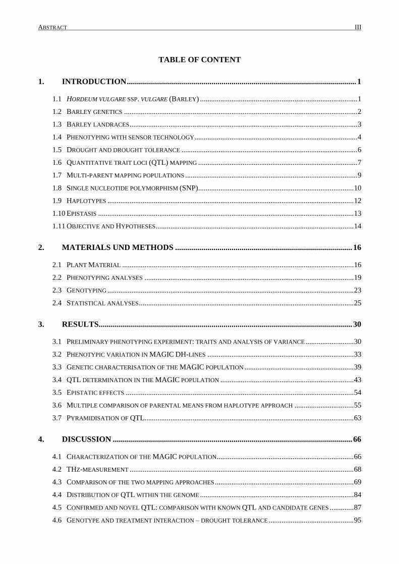
In physics, terahertz radiation consists of electromagnetic waves at frequency ranging from

0.1 to 10 terahertz (THz). With this range it comprises the high-frequency edge of microwave band

to long-wavelength edge of far infrared light as seen in Fig. 1. For a long time, THz radiation was a

black hole of the spectroscopic portfolio; neither electronic nor optical sources could illuminate that

shadowy region (Jansen et al., 2010). But the potential of the THz technology, the power and

efficiency of cost-effective emitter and detector from microwave and near infrared technology

helped to enlighten the frequency region. THz systems are now used in several fields of application,

ranging from medical technique, security check at airports, characterisation and quality inspection

of material (building material, polymers), and spectroscopy at the molecular level and in biological

systems.

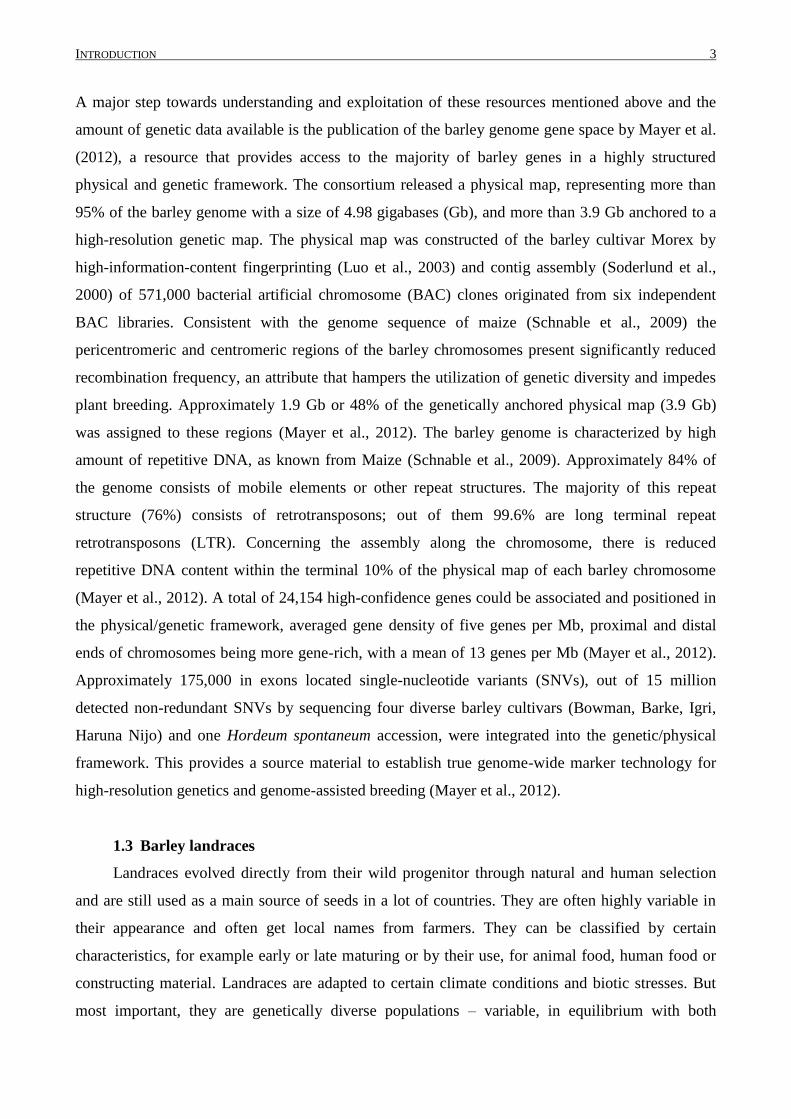
INTRODUCTION 5

Fig. 1: Frequency range of THz and others

There are two categories of optoelectronic THz spectrometer systems suitable for different

approaches: Spectrometer with continuous waves at constant frequency (“continuous wave” (CW)-

systems) or with a THz-TDS system. The CW-systems offers sharp spectral features and a

frequency resolution down to one Megahertz (MHz), the time domain spectroscopy offers broad

spectral information from a single scan in the timescale of seconds (Karpowicz et al., 2005).

THz radiation is highly absorbed by water. Therefore measuring the moisture status of a plant leaf

was one of the first applications in THz imaging a drying leaf (Hu and Nuss, 1995), providing a non

destructive method for the instantaneous monitoring of the water status in living tissues. Other

contactless measurements were developed, for example infrared radiation (Tucker, 1980) and

microwaves (Matzler, 1994). Concerning the infrared technology there is still ongoing discussions

of the suitability of the employed spectral indices (Eitel et al., 2006). The relatively large wave

length of the microwave is strongly affected by the salinity of the water in the leaves, picturing one

disadvantage of this technique. THz radiation provides lots of advantages compared to other

techniques. Due to the smaller THz wavelength compared with microwaves it offers a better spatial

resolution. Furthermore, the influence of dissolved salt on the permittivity of water is low. With a

technical setup shown in Fig. 2 the average measuring time is less than ten seconds per sample,

leading the way to a high-throughput phenotyping of the water status in leaves. Consequently,

physiological studies of a leaf hydration status are possible and diverse approaches to estimate the

water status were conducted (Hadjiloucas et al., 2002; Hadjiloucas et al., 1999; Jordens et al., 2009;

Mittleman et al., 1996). Evaluation of leaf water status or leaf water content as a non-invasive

measurement is of great importance for researchers and plant breeders.

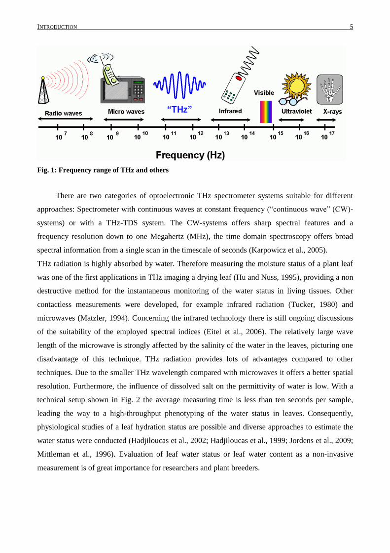
INTRODUCTION 6

Fig. 2: Schematic installation of a pulsed THz system

1.5 Drought and drought tolerance

Among different abiotic stresses, drought is by far the most complex and devastating one on a

global scale. Worldwide it is one of the major limitations to food production (Pennisi, 2008). Jian-

Kang Zhu, a molecular geneticist at the University of California, Riverside, says: “Drought stress is

as complicated and difficult to plant biology as cancer is to mammalian biology“ (Pennisi, 2008).

Blum defines “agricultural drought” as insufficient moisture for maximum or potential growth of

crops. This condition can arise, even in times of average precipitation, owing to specific soil

conditions, topography or biotic factors. It follows that agricultural drought can be expressed on

very wide range of plant growth reductions up to complete crop failures. It does not necessarily

imply that plants must wilt or die or fail in any spectacular manner. By definition, agricultural

drought can cause small reductions in yield when it is mild (Blum, 2010). Passioura defines drought

as circumstances in which plants suffer reduced growth or yield because of insufficient water

supply, or because of too large humidity deficit despite there being seemingly adequate water in the

soil (Passioura, 1996; Pennisi, 2008).

As the definition of drought itself seems to be similar between researchers, the definition of drought

tolerance and drought tolerance traits in plants is more difficult. “There is not a single, magical

drought-tolerance trait” says Mark Tester, plant physiologist at the Australian Centre for Plant

Functional Genomics (Pennisi, 2008).

Up to the late 1970’s, defining criteria for improving yield under drought stress was a haphazard

affair. There was no great deal of attention given to the complex nature of drought or to separate

productivity under drought, which was important for agricultural plants, from survival mechanisms,

which characterize xerophytes. Yet, many adaptations favouring survival tend to reduce economic

INTRODUCTION 7

yield (Richards, 1996). Passioura (1996) pictured the same concept in the article “Drought and

drought tolerance”. It is well known, that a cactus is more drought tolerant than a carnation. But

regarding crops, drought tolerance cannot only concern survival during drought periods. In crops

one is concerned with production. The term “drought tolerance” in an agricultural context, only

gives a meaning when defined in terms of yield in relation to a limiting water supply. In the late

1970’s there was a change in identifying criteria for improving yield under drought. Maximising the

economic product when water is limited was and still is the main aim, pioneered by Passioura

(1977). Several scientists worked on the mechanisms underlying drought tolerance and the

strategies that can improve yield under such conditions (Blum, 1996; Blum, 2011a; Mir et al., 2012;

Passioura, 2007; Passioura, 1996; Passioura and Angus, 2010; Reynolds and Tuberosa, 2008;

Richards, 1996; Richards et al., 2010).

The years of breeding activities have led to yield increase in drought environments for many crop

plants. Meanwhile, fundamental research has provided significant gains in the understanding of the

physiological and molecular response of plants to water deficits, but there is still a large gap

between yields in optimal and in stress conditions (Cattivelli et al., 2008). Minimizing the yield gap

and maximising yield stability are the main tasks for the future. With this challenging task in mind,

molecular approaches (Ashraf, 2010; Bohnert et al., 2006; Deikman et al., 2012; Forster et al.,

2000; Tuberosa and Salvi, 2006; Vij and Tyagi, 2007) offer novel opportunities for the dissection

and more targeted manipulation of the genetic and functional basis of yield under drought stress

(Tuberosa, 2012).

1.6 Quantitative trait loci (QTL) mapping

A quantitative trait is one that has measurable phenotypic variation owing to genetic and/or

environmental influences (Abiola et al., 2003). In crop plants most traits of biological or economic

interest are of quantitative nature and under polygenetic control (Falconer and Mackay, 1996), and

therefore display continuous variation within or between species and have complex inheritance, e.g.

flowering time, yield.

The term “quantitative trait loci (QTL)” was introduced by Geldermann to describe those regions of

the genome underlying a continuous trait (Geldermann, 1975). Quantitative trait loci play an

important role in understanding complex traits, whether in human, animal or plant genetic.

Detection of QTL by conventional phenotyping is not possible. The breakthrough of developing

genetic markers in the 1980s paved the way for characterising QTL. These enabled to build a

linkage map of the experimental mapping population that shows the position of genetic markers

relative to each other. The process of constructing a linkage map and associate phenotypic traits

INTRODUCTION 8

with genomic regions is known as QTL mapping (also ‘genetic’, ‘gene’ or ‘genome’ mapping)

(Mccouch and Doerge, 1995). A traditional QTL mapping approach involves (1) the development

of a mapping population out of parents segregating for the trait of interest, (2) genotyping the

population with polymorphic markers, (3) accurate phenotyping for the traits of interest, (4)

construction of a linkage map, (5) QTL mapping by combining phenotypic values and genotypic

data (Mir et al., 2012).

The first whole genome QTL mapping was performed in tomato (Paterson et al., 1991; Paterson et

al., 1988), followed by soy bean (Keim et al., 1990) and maize (Beavis et al., 1991). The first QTL

analysis in barley was conducted by Heun (1992) and Hayes et al. (1993). Since a lot of QTL

analysis in barley have been performed, focusing on different traits (yield, resistance etc.), on

different populations (advanced backcross, recombinant inbred lines (RILs), near isogenic lines

(NILs)) and on different environments (drought, salinity). Progresses in statistical methods play an

important role in the improvement of QTL detection. The three commonly used methods are single

– marker analysis, interval mapping and composite interval mapping.

(1) The statistical methods for single-marker analysis include t-test, analysis of variance

(ANOVA) and regression. The major advantage of this method is that it does not require a linkage

map. Furthermore it is flexible concerning different mapping populations, different experimental

designs with further factors (environments, treatments) and epistatic effects. The disadvantage of

underestimating QTL (Tanksley, 1993) with the single-marker methods will be minimized trough a

dense genotypic marker approach (Collard et al., 2005).

(2) The interval mapping method was first proposed by Lander and Botstein (1989) and is

based on maximum likelihood methods or multiple regressions. It makes use of linkage maps and

analyses intervals between adjacent pairs of linked markers along the chromosome simultaneously

and is considered statistically more powerful compared to the single-marker method (Lander and

Botstein, 1989). With a high density map of genetic markers, as available now, the advantages are

negligible.

(3) Composite interval mapping (Jansen, 1993; Rodolphe and Lefort, 1993; Zeng, 1994)

includes partial regression coefficients from markers (cofactors) in other regions of the genome.

The main advantage is the more precise and effective QTL mapping, especially when linked

markers are involved. Unfortunately epistatic effects cannot be calculated as well as

genotype*environment interactions (Collard et al., 2005).

Teulat et al. (1997) were the first one to use QTL analysis to identify genomic segments related to

drought tolerance. Since then six different mapping populations with drought stress tolerant parents

were under investigation by different scientist (Chen et al., 2010; Diab et al., 2004; Guo et al., 2008;

INTRODUCTION 9

Mardi et al., 2005; Peighambari et al., 2005; Teulat et al., 2001a; Teulat et al., 2001b; Teulat et al.,

1998; Teulat et al., 2003; Zhang et al., 2005). Altogether 117 QTL were detected in 12 studies for a

variety of drought related traits, for example days to heading, grain yield, plant height and thousand

seed weight (Li et al., 2013). These traits and the corresponding QTL that affect yield in drought

environments can be categorized as constitutive (i.e., also expressed under well-watered conditions)

or drought-responsive (i.e., expressed only water shortage) traits (Lafitte and Edmeades, 1995).

1.7 Multi-parent mapping populations

Most of the QTL studies in plants were conducted in individual bi-parental populations.

Highly diverse parents, segregating for the trait of interest were crossed with each other and the

offspring, F2, DH-lines or RILs were analyzed for QTL. Bi-parental mapping populations are

grateful with respect to population development and the high power of QTL detection (Doerge,

2002). But their soft spot is the mapping with low resolution (large genetic intervals) as a result of

limited opportunity of recombination (Huang et al., 2012). Inferences from bi-parental studies

suggested that plant populations segregate for a limited set of small-effect QTL plus a very few

QTL that have large effects. This is due to genetic heterogeneity between the mapping populations,

if a trait is controlled by many genes, different subsets can segregate in different mapping

populations (Holland, 2007). Researchers started to study complex traits in larger populations

because small populations biased the effects of QTL with statistical artefacts by sampling (Salvi and

Tuberosa, 2005). The results detected in a very large maize population concerning seed oil content

(Laurie et al., 2004) and grain yield (Schön et al., 2004), relative large numbers of QTL but low

genetic effects, were consistent with QTL analysis in mouse population (Valdar et al., 2006) and

Drosophila (Mackay, 2004). A concept to overcome the low explained genetic variation through the

QTL in bi-parental crosses, to reduce linkage disequilibrium (LD) and to improve mapping

resolution, was proposed by Darvasi and Soller (1995) with the advanced intercross (AIC). It is an

extension of RILs and consists of a repeatedly random intermated F2 population from a bi-parental

cross, followed by generations of selfing, with the effect of reducing the level of LD and increasing

the precision of QTL mapping (Cavanagh et al., 2008). But QTL mapping in purpose build bi-

parental crosses reveals only a slice of the genetic architecture of a complex trait, because only

alleles that differ between the parents will segregate within the offspring (Holland, 2007). In

contrast, association panels (Core Collections etc.) enclose a high genetic variation, due to large

number of recombination events in the past and therefore promise a high resolution of QTL (Myles

et al., 2009). One major disadvantage from QTL mapping with association panels is the variation in

pairwise relationships of genotypes, leading to a genetic structure within the panel that hampers the

INTRODUCTION 10

differentiation of true-positive and false-positive QTL. A different way to enhance the genetic

variation and to avoid limitations of genetic structure within a population was spurred by Mott et al.

(2000). The AIC approach was extended by Mott et al. (2000) to produce highly recombinant

outbred populations in mice from multiple parents, so called heterogeneous stocks (HS). The

application of HS in research increased the power to detect and localise QTL, and to fine map QTL

controlling complex traits in mice to small confidence intervals (Yalcin et al., 2005). The use of HS

is cost intensive and time consuming because each individual genome is exclusive and

heterozygous and requires genotyping each time it is phenotyped.

A strategy to overcome this problem is to produce RILs from several parents (Churchill et al., 2004)

which has been termed multi-parent populations in crops (Cavanagh et al., 2008). These populations

combine the high mapping resolution exhibited by multiple generations of recombination with the

high mapping power afforded by linkage-based design (King et al., 2012). Four multi-parent

population have been described in plants, the Arabidopsis multi-parent recombinant inbreed line

(AMPRIL) population (Huang et al., 2011), the Arabidopsis multi-parent advanced generation

intercross (MAGIC) (Kover et al., 2009), the maize nested associated mapping population (NAM)

(Buckler et al., 2009; McMullen et al., 2009) and the four parent MAGIC population in wheat

(Huang et al., 2012). These populations are composed of a series of homozygous, genotyped RILs,

they represent stable genetic reference panels that facilitate systems-level analyses of genetic

architecture (King et al., 2012).

The aspired high mapping resolution was achieved in the four parent MAGIC population of Huang

et al. (2012). The mean LD dropped down to <0.8 within ~5 cM and to <0.2 within 40 cM. The

average LD between markers on different chromosomes was 0.0037. In the multi-parent population

in Arabidopsis from Huang et al. (2011) the mean correlation between SNPs decayed to 0.17 by

about 0.5 Mb. Minimal LD between the chromosomes was detected, the mean R² value was 0.04. A

population structured implied a low chance of ghost QTL (Huang et al., 2011).

1.8 Single nucleotide polymorphism (SNP)

Molecular markers have become increasingly important during the last decades to investigate

and dissect the genetic fraction underlying quantitative traits. Different classes of DNA markers

were develop and implemented over time. Co-dominant restriction fragment length polymorphism

(RFLP), implemented in 1980 (Botstein et al., 1980), were the first molecular markers widely used.

Random amplified polymorphic DNA (RAPD) markers were developed in 1990 and first described

by Williams et al. (1990). In the following, amplified fragment length polymorphism (AFLP)

marker (Vos et al., 1995) and single sequence repeat (SSR) marker were developed which were

INTRODUCTION 11

used in plant studies in 1993 (Morgante and Olivieri, 1993) for the first time. With the development

of diversity array technology (DArT) by Jaccoud et al. (2001) the first generic whole genome

genotyping technology was implemented which allows genome profiling and diversity analysis.

These marker techniques differ in costs, work, range of use and repeatability and need to be chosen

in respect to the investigated population and application area.

A SNP is an individual nucleotide base difference between two DNA sequences. Every SNP within

the genome could be used as a genetic marker. In the last years SNP markers gained a lot of interest

in the scientific community across all species and its power is clearly represented in the human

genome analysis (Sachidanandam et al., 2001). In plants, SNP in genic regions are abundant with

the preliminary estimate ranging from 1 SNP per 60 bp in out breeding maize (Ching et al., 2002) to

ca. 1 SNP per 300 bp for inbreeding rice and Arabidopsis (Schmid et al., 2003; Yu et al., 2005).

SNPs offer an important source of molecular markers that can be utilized in genetic mapping, map-

based position cloning, detection of marker-trait gene associations through linkage and linkage

disequilibrium mapping and the estimation of genetic relationships between individuals (Oraguzie,

2007). SNPs underlie a low mutation rate, which makes them excellent, stable markers for

dissecting complex traits and a tool for the understanding of the genome (Syvanen, 2001). The

abundance of SNPs within the genome largely offers the greatest level of genetic resolution. This

offsets the disadvantage of SNPs being biallelic and makes them the most attractive molecular

system so far. Complementary approaches for the detection of SNP in barley have been explored,

i.e. searching for electronic SNPs in expressed sequence tags (EST) assemblies (Kota et al., 2003)

and resequencing selected sets of unigens in different barley accessions (Rostoks et al., 2005). SNPs

are of potential functional relevance and they are also well suited to high throughput analytical

methods (Rostoks et al., 2005). Several barley linkage maps (Close et al., 2009; Comadran et al.,

2012; Sato et al., 2009; Stein et al., 2007) and a SNP based map featuring gene sequences expressed

differentially in response to various abiotic stresses have been published (Rostoks et al., 2005).

QTL mapping or association mapping in barley were effectively conducted with SNP recently

(Burris et al., 1998; Cockram et al., 2010; Comadran et al., 2011a; Comadran et al., 2011b; Wang et

al., 2012). International collaborators subsequently initiated the development of a highly multiplex

unigene-based SNP assay platform for barley (Rostoks et al., 2006) and chose Illumina’s oligo pool

assay (OPA) as a marker platform (Waugh et al., 2009). The latest development, the 9K iSelect chip

contains 7864 SNPs (Comadran et al., 2012).

INTRODUCTION 12

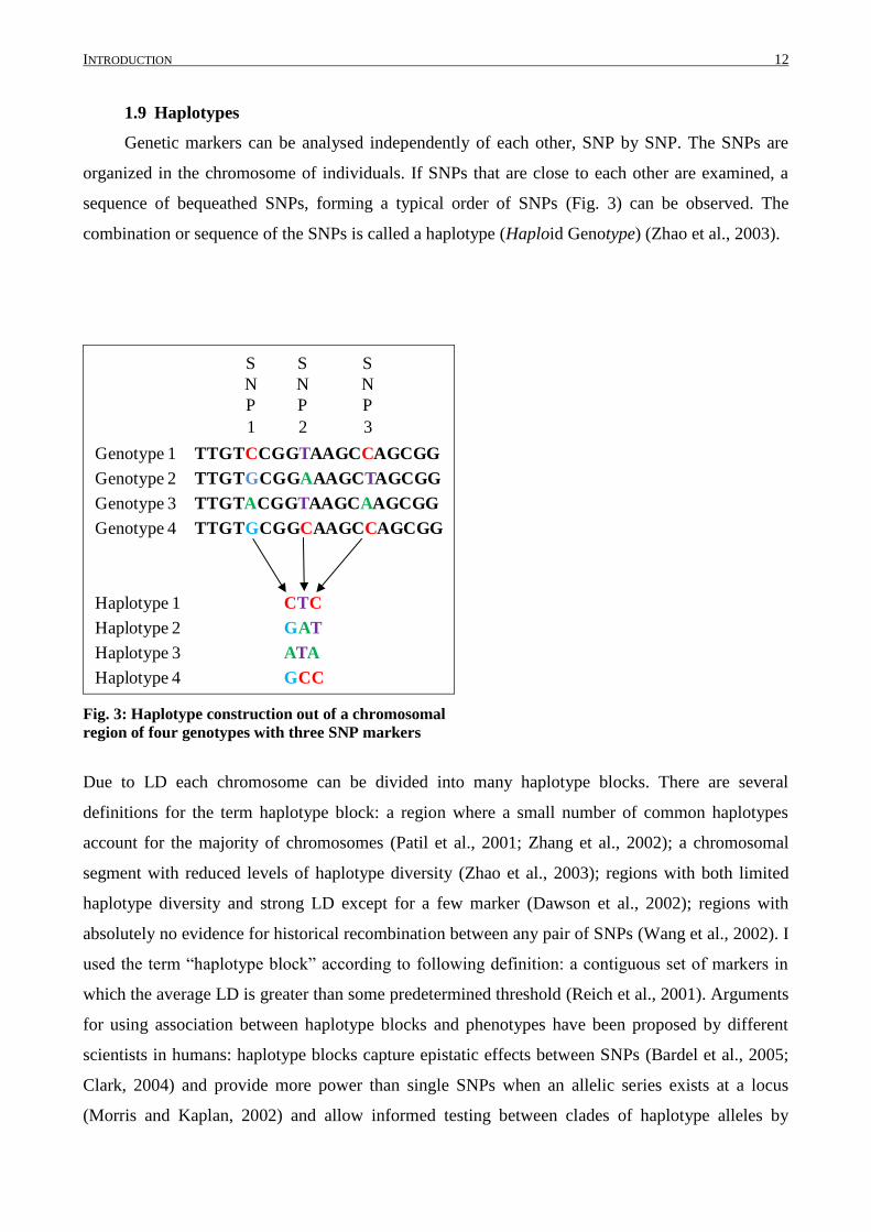
1.9 Haplotypes

Genetic markers can be analysed independently of each other, SNP by SNP. The SNPs are

organized in the chromosome of individuals. If SNPs that are close to each other are examined, a

sequence of bequeathed SNPs, forming a typical order of SNPs (Fig. 3) can be observed. The

combination or sequence of the SNPs is called a haplotype (Haploid Genotype) (Zhao et al., 2003).

Genotype 1

Genotype 2

Genotype 3

Genotype 4

TTGTCCGGTAAGCCAGCGG

TTGTACGGTAAGCAAGCGG

TTGTGCGGCAAGCCAGCGG

TTGTGCGGAAAGCTAGCGG

Haplotype 3

Haplotype 1

Haplotype 2

Haplotype 4

ATA

CTC

GAT

GCC

S

N

P

1

S

N

P

2

S

N

P

3

Fig. 3: Haplotype construction out of a chromosomal

region of four genotypes with three SNP markers

Due to LD each chromosome can be divided into many haplotype blocks. There are several

definitions for the term haplotype block: a region where a small number of common haplotypes

account for the majority of chromosomes (Patil et al., 2001; Zhang et al., 2002); a chromosomal

segment with reduced levels of haplotype diversity (Zhao et al., 2003); regions with both limited

haplotype diversity and strong LD except for a few marker (Dawson et al., 2002); regions with

absolutely no evidence for historical recombination between any pair of SNPs (Wang et al., 2002). I

used the term “haplotype block” according to following definition: a contiguous set of markers in

which the average LD is greater than some predetermined threshold (Reich et al., 2001). Arguments

for using association between haplotype blocks and phenotypes have been proposed by different

scientists in humans: haplotype blocks capture epistatic effects between SNPs (Bardel et al., 2005;

Clark, 2004) and provide more power than single SNPs when an allelic series exists at a locus

(Morris and Kaplan, 2002) and allow informed testing between clades of haplotype alleles by

INTRODUCTION 13

capturing information from evolutionary history in Drosophila (Templeton et al., 1987).

Comparison of “haplotype block” and “single-marker based” approaches were conducted in human

and livestock with contrasting results. Single-marker based approaches with greater power were

detected by Long and Langley (1999) in human population genetics. Results from simulation in

livestock populations by Hayes et al. (2007) and others (Calus et al., 2009; Grapes et al., 2004)

resulted in greater QTL detection power and mapping accuracy with “haplotype blocks” then with

the “single-marker based” approach. Zhao et al. (2007) detected no differences between the two

approaches in conducting simulations designed to resemble the demography and population history

of livestock.

A comparison of the two approaches in plants was conducted in barley by Lorenz et al. (2010). In

his research the “haplotype block” approach performed better, when QTL were simulated as

polymorphisms that arose subsequent to marker variants and in the analysis of empirical heading

date. The results from the study demonstrate that the information content of haplotype blocks is

dependent on the recombinational history of the QTL and the nearby markers. The analysis of the

empirical data confirmed that the use of haplotype information can capture association that is

neglected by the “single-marker SNP” approach (Lorenz et al., 2010).

1.10 Epistasis

Epistatic effects are statistically defined as interactions on a phenotype between effects of

alleles from two or more genetic loci which do not correspond to the sum of their separate effects

(Fisher, 1918). The existence of epistatic interactions in barley populations was already

demonstrated by Fasoulas and Allard (1962) before the age of molecular marker. The advent of

molecular markers was supposed to make analysis of epistatic effects on the basis of a genome-

wide scale possible. Early efforts using molecular markers were not really successful or did not

provide evidence for important epistatic effects (Tanksley, 1993) for example in maize (Blanc et al.,

2006; Edwards et al., 1987; Melchinger et al., 1998; Mihaljevic et al., 2005; Schön et al., 2004). But

studies in self-pollinated crops have been more successful in given evidence for important epistasis,

for example concerning yield in rice (Li et al., 1997; Mei et al., 2005; Yu et al., 1997), Arabidopsis

(Malmberg et al., 2005) and in barley (Thomas et al., 1995). The contrasting results might be due

partly to the differences in breeding scheme of the species discussed above (inbreeding and out-

crossing) and partly to differences in the statistical model used in the determination of the epistatic

effects.

Statistical methods for detecting epistasis in QTL studies are improving (Holland, 2001), searching

for effects throughout the genome (Wang et al., 1999) while other methods just test the interactions

INTRODUCTION 14

of QTL with significant main effects (Holland, 2001). Recent results have demonstrated the power

and importance of epistatic interactions in the studied domestication-related traits heading date,

plant height and yield (von Korff et al., 2010), where the interaction of QTL with background loci,

as promoted by Wang et al. (1999) were tested. Strong epistatic effects were detected in BC2DH

lines between a QTL on chromosome 4H and the Vrn-H1 gene where genotypes carrying the exotic

allele from the wild barley accession ISR42-8 on both markers flowered eight days earlier than the

lines with the elite allele from variety Scarlett at both loci. This identification of the epistatic effects

is important in prospects of marker assisted selection and gene cloning (von Korff et al., 2010).

Tanksley (1993) suggested that the power to detected epistatic effects not only depends on the trait

but as well on the mapping population, making NILs a powerful tool due to a stabilized genetic

background compared to first approaches using F2 populations. The MAGIC DH-lines with the high

amount of recombination during the crossing procedure and the 100% homozygosity is assumed to

be a favourable population to dissect complex traits and to measure epistatic effects precisely.

1.11 Objective and Hypotheses

QTL mapping for yield and yield related traits under drought conditions was conducted in

different research projects with different populations as mentioned above. A MAGIC population

instead is a new kind of mapping population, adapted from mouse genetic and only established so

far in Arabidopsis (Huang et al., 2011; Kover et al., 2009) and wheat (Huang et al., 2012). QTL

analyses under drought conditions have not been conducted in a MAGIC population. The

application of sensor technology for precise phenotyping is an emerging research field in

agriculture and especially in plant breeding. The non invasive measurement of water content in

leaves has been conducted in coffee (Jordens et al., 2009) and Catalpa (Hadjiloucas et al., 1999).

The determination of the water content in an agricultural important crop, the application of the THz-

sensor in a segregating population, and the estimation of QTL for water content in barley has not

been conducted so far. The use of a dense genetic map and a large amount of genotypes in a

segregating population are good source for a QTL mapping approach. The combination of the

integration of cross validation to estimate the performance of the model and multi-locus analysis to

reduce the number of false-positive QTL and the estimation of epistatic effect will enable a precise

QTL detection and localisation. The primary aim of this project is the detection of QTL in a

MAGIC population in spring barley. Relevant traits are yield and yield related traits under drought

conditions, using the combination of classical phenotypic traits and THz-sensor as a non-invasive

approach for measuring water content in leaves. Specific objectives of the study are listed below.

INTRODUCTION 15

The THz-Sensor is able to measure the water content in living leaves.

The MAGIC population is suitable for QTL mapping concerning its population structure and

decay of linkage disequilibrium.

The information content from the genotypic data enables to estimate haplotypes.

The QTL will be calculated with two approaches, with the SNP data and the haplotype data.

The approaches differ from each other concerning information content, cover ratio and

estimation of the allele effect.

QTL for yield, yield related traits and water content of leaves from THz-sensor and their

interaction with a drought stress environment will be determined with both approaches.

The MAGIC population and the QTL program are a perfect source to identify epistatic effects

between genomic regions for the traits of interest due to a high number of meiosis and

therefore smaller genomic fragments along the chromosomes.

MATERIAL AND METHODS 16

2. Materials und Methods

This chapter outlines the phenotypic and genotypic studies of the MAGIC DH-lines and their

parents as well as the materials and methods for the THz sensor.

2.1 Plant Material

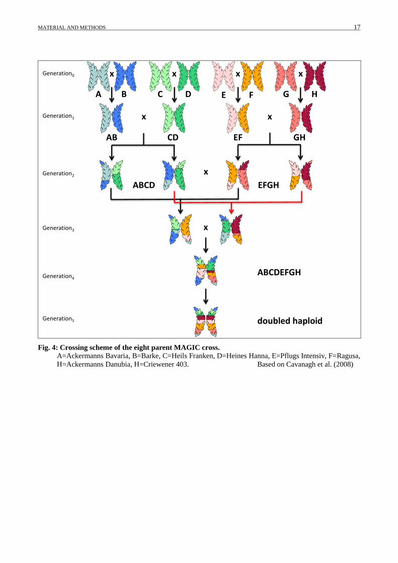
To create the genetic material used in this research, eight spring barley genotypes

(Ackermanns Bavaria, Ackermanns Danubia, Barke, Criewener 403, Heils Franken, Heines Hanna,

Pflugs Intensiv, Ragusa (Table 1) (hereinafter named: parents)) were intermated in an eight-way-

cross. The parental genotypes were selected due to their contribution to the German barley

breeding. Seven of them are old landraces and so called founder of the German barley breeding,

contributing as a crossing partner in the pedigree of most German spring barley cultivars. The

eighth genotype is ‘Barke’, a modern German spring barley variety, released in 1996, and important

model in barley genetics. The parental genotypes can be traced back to a single plant. They were

crossed in G0 in four pairs to produce F1 seeds (Fig. 4): Ack. Bavaria x Barke (AB), Heils Franken x

Heines Hanna (CD) Pflugs Intensiv x Ragusa (EF) Ack. Danubia x Criewener 403 (GH).

In G1 the two-way-crosses were intermated with each other to a four-way-cross, (AB x CD) and (EF

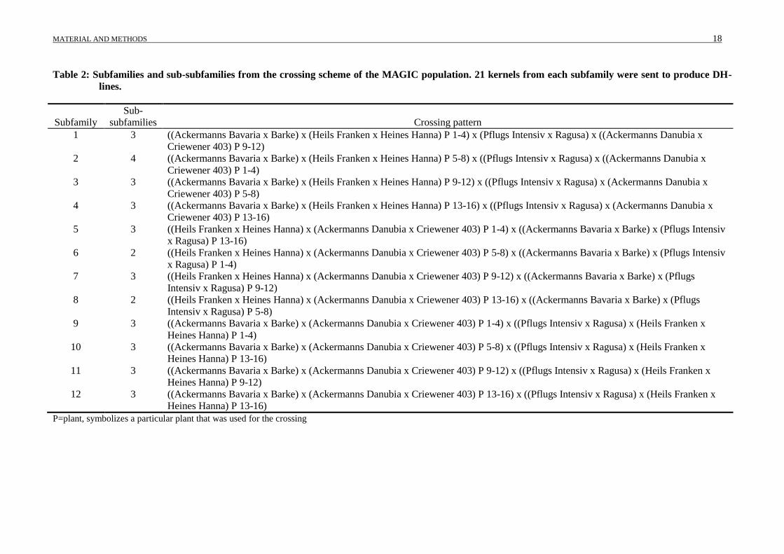
x GH). The crosses G1 and further crosses can be traced back to subfamilies and sub-subfamilies

(Table 2); more than one crossing per combination was conducted to reduce the loss of alleles.

Starting from G2 the double crosses segregated, replicated crosses involving more recombinant

plants were required. At G3 the progenies of G2 are intercrossed to effect the eight-way

intercrossing to produce F1 seeds for (ABCDEFGH). Each ABCDEFG F1 seed was harvested and

252 seeds from twelve subfamilies were sent to Saaten-Union Biotec GmbH, Leopoldshöhe,

Germany. Doubled haploid lines were produced via anther and microspore culture to shorten the

breeding cycle. 534 MAGIC DH-lines were selected out of approximately 5000 DH-lines to be

investigated in this thesis.

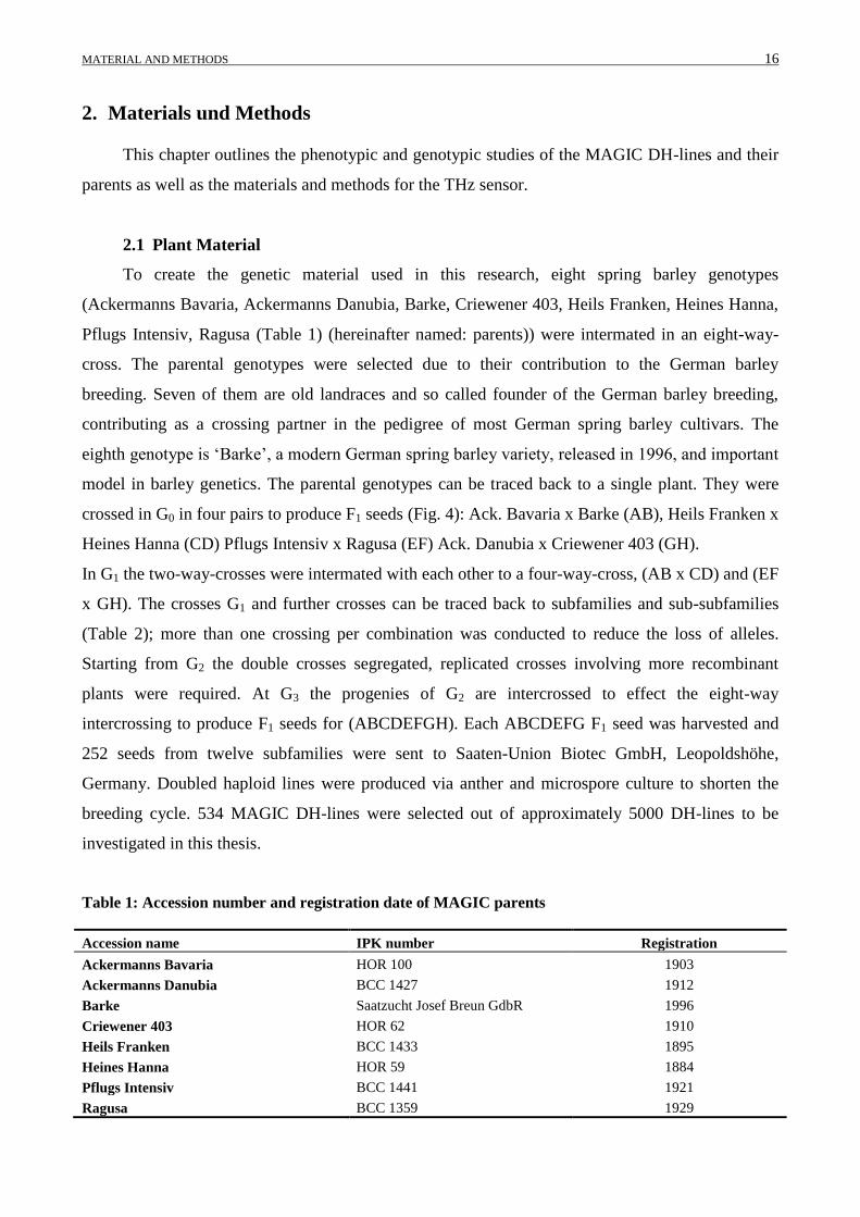
Table 1: Accession number and registration date of MAGIC parents

Accession name IPK number Registration

Ackermanns Bavaria HOR 100 1903

Ackermanns Danubia BCC 1427 1912

Barke Saatzucht Josef Breun GdbR 1996

Criewener 403 HOR 62 1910

Heils Franken BCC 1433 1895

Heines Hanna HOR 59 1884

Pflugs Intensiv BCC 1441 1921

Ragusa BCC 1359 1929


x x x x

A B C D E F G H

AB CD EF GH

x x

ABCD EFGH

x

ABCDEFGH

x

doubled haploid

Generation0

Generation1

Generation2

Generation3

Generation4

Generation5

Fig. 4: Crossing scheme of the eight parent MAGIC cross.

A=Ackermanns Bavaria, B=Barke, C=Heils Franken, D=Heines Hanna, E=Pflugs Intensiv, F=Ragusa,

H=Ackermanns Danubia, H=Criewener 403. Based on Cavanagh et al. (2008)


Table 2: Subfamilies and sub-subfamilies from the crossing scheme of the MAGIC population. 21 kernels from each subfamily were sent to produce DH-

lines.

Subfamily

Sub-

subfamilies Crossing pattern

1 3 ((Ackermanns Bavaria x Barke) x (Heils Franken x Heines Hanna) P 1-4) x (Pflugs Intensiv x Ragusa) x ((Ackermanns Danubia x

Criewener 403) P 9-12)

2 4 ((Ackermanns Bavaria x Barke) x (Heils Franken x Heines Hanna) P 5-8) x ((Pflugs Intensiv x Ragusa) x ((Ackermanns Danubia x


3 3 ((Ackermanns Bavaria x Barke) x (Heils Franken x Heines Hanna) P 9-12) x ((Pflugs Intensiv x Ragusa) x (Ackermanns Danubia x


4 3 ((Ackermanns Bavaria x Barke) x (Heils Franken x Heines Hanna) P 13-16) x ((Pflugs Intensiv x Ragusa) x (Ackermanns Danubia x


5 3 ((Heils Franken x Heines Hanna) x (Ackermanns Danubia x Criewener 403) P 1-4) x ((Ackermanns Bavaria x Barke) x (Pflugs Intensiv

x Ragusa) P 13-16)

6 2 ((Heils Franken x Heines Hanna) x (Ackermanns Danubia x Criewener 403) P 5-8) x ((Ackermanns Bavaria x Barke) x (Pflugs Intensiv

x Ragusa) P 1-4)

7 3 ((Heils Franken x Heines Hanna) x (Ackermanns Danubia x Criewener 403) P 9-12) x ((Ackermanns Bavaria x Barke) x (Pflugs

Intensiv x Ragusa) P 9-12)

8 2 ((Heils Franken x Heines Hanna) x (Ackermanns Danubia x Criewener 403) P 13-16) x ((Ackermanns Bavaria x Barke) x (Pflugs

Intensiv x Ragusa) P 5-8)

9 3 ((Ackermanns Bavaria x Barke) x (Ackermanns Danubia x Criewener 403) P 1-4) x ((Pflugs Intensiv x Ragusa) x (Heils Franken x

Heines Hanna) P 1-4)







P=plant, symbolizes a particular plant that was used for the crossing


2.2 Phenotyping analyses

The phenotypic experiments were carried out at the experimental research station at

University of Bonn, Poppelsdorf, Institute for Plant Breeding in 2010, 2011 and 2012. A

preliminary test for drought tolerance was conducted in 2010, characterising a set of spring barley

genotypes including the parents of the MAGIC population under well watered and terminal drought

conditions. The MAGIC DH-lines and the parents were tested under well watered and terminal

drought conditions in the vegetation period of 2011 and 2012.

2.2.1 Preliminary experiment 2010

The experiment was set up in a polytunnel which enables natural growth behaviour under

water controlled conditions. 30 spring barley genotypes were selected to be phenotyped at terminal

drought and well watered conditions. The experiment was conducted in 22 x 22 cm plastic pots

containing 11.5 l of Terrasoil® (a mixture of top soil, silica sand, milled lava and peat dust,

Terrasoil®, Cordel & Sohn, Salm, Germany). The pots were arranged in a split plot design with

four replications. Twelve seeds per pot were sown on the 7th

of April 2010 to simulate a plant

population within the pot. Water was supplied with a computer mediated drip irrigation system

three times a day (6:15 am, 0:15 pm, 6:15 pm) to hold the volumetric water content (VWC) at 40%.

Terminal drought stress started 30 days after sowing (DAS). It was aimed to reduce the water

content in the pots during 21 days to the permanent wilting point (15% VWC) and to stabilize it at

15% for seven days. Subsequently the pots under terminal drought were re-watered after 28 days of

reduced water supply to gain approximately 40% VWC within a few hours. The well watered

treatment was continuously kept at 40% VWC. Weather data was collected by HOBO U30 weather

station measuring the following parameters every 15 minutes:

volumetric water content with HOBO soil moisture smart sensors S-SMB-M003

soil temperature with HOBO soil temperature smart sensor S-TMB-M006

air temperature and radiation with HOBO smart sensor S-THB-M002

Fertilizer, fungicides and insecticides were applied referring to agricultural practice. The recorded

traits, the method and dates of measurement in days after sowing (DAS) are listed in Table 3.


Table 3: List of phenotypic traits and their abbreviations, measured unit, methods and time after

sowing (DAS) investigated in preliminary experiment in 2010

Trait Abbr. Unit Methods of measurement DAS

repeated measurements

number of tillers NT no/plant number of tillers 33-82

number of leaves NL no/plant number of fully developed leaves 33-82

number of green leaves NGL no/plant number of leaves with at least 50%

photosynthetic activity

33-82

number of yellow leaves NYL no/plant number of leaves with less than 50%

photosynthetic activity

33-82

plant height PLH cm distance between soil ground level and tip of

awns in cm

33-82

SPAD value SPAD value measured with SPAD-502plus (Konica

Minolta)

33-61

wilting score WS 0 – 9 Dedatta et al., 1988 33-61

invasive measurements

plant fresh biomass PFB g/plant amount of fresh biomass 61

plant dry biomass PDB g/plant amount of dry biomass 61

water content WC % gravimetric measured % of water in plant 61

root biomass RB g/plant amount of dry root biomass 61

root length RL cm root length starting from nod 61

leaf area LA cm² whole leaf area/plant 61

green leaf area GLA cm² green leaf area/plant 61

yield and yield components

straw biomass SB g/plant amount of dry straw biomass harvest

number of ears NE no/plant number of ears harvest

number of ripe ears NRE no/plant number of ripe ears harvest

number of green ears NGE no/plant number of green ears harvest

number of kernels NK no/ear amount of kernels per ear harvest

grain yield YLD g/plant weight of barley grain harvest

thousand kernel weight TKW gram weight of 1000 kernels harvest

harvest index HI 0 – 1 ratio of generative to vegetative biomass harvest

DAS=days after sowing

Abbr.=abbreviation


Seven of these traits were repeatedly scored (listed in Table 3 as repeated measurements) to

evaluate the most significant trait and date*trait interaction for drought tolerance phenotyping,

starting from 33 DAS (before water supply was reduced), 40 DAS, 47 DAS, 54 DAS, 61 DAS and

82 DAS. SPAD value and wilting score could not be scored at 82 DAS due to reduced chlorophyll

content and advanced ripening progress in the plants. Yield and yield components were scored after

harvest (listed in Table 3 as yield and yield components).

2.2.2 Phenotyping experimental setup 2011 and 2012

The trial in 2011 and 2012 was located at the same experimental site like 2010. 534 MAGIC DH-

lines, the parents of the MAGIC cross and a set of check varieties of spring barley were sown into

19.5 x 25.5 cm plastic pots, filled with 5.5 l of Terrasoil®. Two water treatments were evaluated,

well watered and terminal drought. Four seeds per genotype for each treatment were sown at the 4th

of April 2011 and 3rd

of April 2012. The experiment was arranged in an augmented experimental

block design in the polytunnel, using 20 varieties as checks, providing replicates every 20 pots. The

experiments contained 1184 pots, 1068 pots with MAGIC DH-Lines, 116 pots with check varieties.

The terminal drought conditions started 35 DAS and extended to five weeks. It was aimed to reduce

the water content in the pots during 21 days to the permanent wilting point (15% VWC) and

stabilize it at 15% for seven days. At 65 DAS the pots under terminal drought conditions were re-

watered slowly to 30% VWC, and re-watered to 40% VWC at 73 DAS. The recorded traits, the

method and dates of measurement for 2011 and 2012 are listed in Table 4. Leaf senescence was

measured repeatedly and evaluated as area under drought progress curve (AUDPC), which was

calculated from leaf senescence taking time between measuring dates into account.


Table 4: List of phenotypic traits and their abbreviations, measured unit, methods and time after

sowing (DAS) investigated in the MAGIC population in 2011 and 2012

Trait Abbr. Unit Methods of measurement

sum of area under

drought progress curve AUDPC Shaner and Finney, 1977

above ground biomass AGB g/plant amount of dry above-ground biomass

days to heading DHE D number of days from sowing until emergence of 3 cm of awns

grain filling period DGF D number of days from heading to hard dough ripening

floret abortion FA no/ear amount of sterile fully developed florets

number of ears NE no/plant number of ripe ears

number of kernels NK no/ear amount of kernels per ear

plant height PLH cm distance between soil ground level and tip of awns in cm

thousand kernel

weight TKW gram weight of 1000 kernels

grain yield YLD g/plant weight of barley grain

Abbr. = abbreviation

2.2.3 Time domain spectroscopy

The THz-TDS used in this research project was built at University of Marburg, Department of

Physics, Fachbereich Experimentelle Halbleiterphysik, Prof. Koch, Germany, and will be explained

in details hereafter.

The measurements were conducted using a THz-TDS system based on an ER:Fiber laser providing

around 65 fs pulses with a central wavelength of 1550 nanometre (nm) at a repetition rate of around

80 MHz. A fraction of this pulse was sent through a polarization maintaining fiber-piezo-driven

fiber stretcher producing a delay of around 15 ps at 10 THz. The pulses were used to excite a LT-

InGaAs stripline photoconductive emitter. The remaining fraction of the pulse was used to gate an

LT-InGaAs dipole photoconductive detector. After emission, the THz radiation was collected and

refocused by a pair of polyethylene lenses producing an around 3 mm focus where the sample was

placed (Fig. 2).

Measuring a reference first, a pulse without sample in the THz beam path and second a pulse with

the sample allowed for the simultaneous extraction of the refractive index, the absorption

coefficient (a), the thickness of the sample (b) providing detailed information of the object (Scheller

et al., 2009).


The measurements with the THz sensor were carried out on plants grown in a climate chamber, to

rely on accurately defined climate terms during weeks of cultivation and measurements.

Einheitserde Typ VM, Werkverband E.V., Germany, was filled into 96 QuickPot plates,

HerkuPlast, Kubern GmbH, Germany. Each pot was 7.8 * 3.8 * 3.8 cm in size, with a soil volume

of 75 cc. Two seeds of each genotype were sown into the soil, watered and cultivated in the climate

chamber. Ten DAS the weaker seedling was removed from the soil. The 96 QuickPot plate was

placed into a water bath 16 DAS to reach maximum water content. Afterwards the plate was

removed after eleven hours and left in the climate chamber for two hours. Subsequently the plants

were removed from the 96 QuickPot plate into 7 * 8 cm pots from Pöppelmann, Lohne, Germany to

assure uniform drying. These pots were lined with a 17.5 * 10 cm Crispac, cut to 12 * 10 cm from

Baumann Saatzuchtbedarf, Waldenburg, Germany preventing the soil from rapid drying. The plants

were left in the climate chamber for 96 hours and were only removed from the climate chamber for

the measurement with the THz sensor every 24 hours. The measurements took place at INRES,

department of Crop Genetics and Biotechnology, Plant Breeding in Bonn. The leaves of the plants

were marked with an ink pen and measured every 24 hours at the same position of the leaves. The

two oldest leaves per plant were used for measurement. A program to process the measured data

was written in MATLAB (The MathWorks Inc.) by Ralf Gente, University Marburg. The measured

THz value was automatically recalculated into following values taking the leaf thickness into

account: water volume (%), water content (%), plant material (%). The values for water content

were used to calculate the traits listed in Table 5, that were used in QTL mapping.

Table 5: Calculated values measured with THz-TDS-System used for marker-trait-sensor association

Trait Abbr. Unit Methods of measurement

water content WCT % water content after 96 hours of not watering

water loss WL % difference between basic and final water content value

Abbr. = abbreviation

2.3 Genotyping

The DNA isolation from the MAGIC DH lines and their parents was conducted in the lab at

University of Bonn, Institute of Plant Breeding in Bonn. TraitGenetis in Gatersleben, Germany was

commissioned to genotype the DNA with the Illumina 9K iSelect-SNP chip (Comadran et al.,

2012).


2.3.1 Extraction of genomic DNA

For the isolation, frozen leaf material of 2-week-old seedlings grown in the greenhouse was

harvested for each MAGIC DH-line. Per line, leaf material from three MAGIC DH-lines was

pooled. 30 to 50 mg of fresh leaf material was transferred into a 96well Collection Microtube from

Qiagen, Hilden, Germany. One tungsten bead (Qiagen) per well was added. Leaf samples were

homogenized using a TissueLyser bead mill (Qiagen) at 20 Hz for one minute and centrifuged at

3000 rpm for two minutes. 300 µl of fresh buffer working solution was added, shaken gently. The

samples were incubated for one hour at 65°C, gently shaken every 15 minutes. Afterwards the

samples were cooled down for five minutes on ice. 300 µl of chloroform/isoamyl alcohol (24:1)

was added to each sample and mixed well for 15 minutes under the hood. The samples were

centrifuged for ten minutes at 6000 rpm. 150 µl of the supernatant was transferred into a new set of

96well Collection Microtubes, which was prepared with 150 µl of ice cold isopropanol and stored

in the freezer. The tubes were inverted 10 times and centrifuged for 30 minutes at 6000 rpm. The

supernatant was discarded and the DNA-pellets washed with 300 µl of 70% ETOH. The samples

were centrifuged again for ten minutes at 6000 rpm, and the supernatant was discarded. The DNA-

pellets were dried and dissolved in 100 µl of TE-Buffer (modified protocol for DArT marker

analysis: www.diversityarrays.com). DNA concentration was measured with Nanodrop

spectrophotometer 2000c, Thermo Fisher Scientific Inc, and rechecked on a 2% agarose gel to

check the quality and to quantify the amount of DNA by staining with ethidium bromide after

electrophoresis. If required, samples were diluted to achieve a final concentration of 50 ng/µl. A

sample volume of 25 µl was provided for TraitGenetics for SNP genotyping.

Buffer and solutions

Buffers and solutions used in the DNA extraction will be itemised.

Extraction buffer for 96 samples

Sorbitol 350 mM

TrisHCl 100 mM

EDTA 500 mM

Lysis Buffer Stock for 96 samples

Tris 20 mM

EDTA 5 mM

NaCl 200 mM

CTAB 2%


Sarcosyl stock 5%

Lauryl sarcosine 170.42 mM

H2O (high ourity) ad 500 ml

Fresh buffer working solution for 96 samples

Sodiumdisulfite 0.5 g

PVP-40 2.0 g

Extraction buffer 41.6 ml

Lysis buffer 41.6 ml

Sarcosyl stock 16.6 ml

Chloroform/isoamyl alcohol 24:1

24 volumes chloroform and one volume isoamyl alcohol

2.3.2 Molecular maker genotyping and data cleaning

The Illumina 9k iSelect chip from TraitGenetics was used to genotype 542 barley genotypes

(534 MAGIC DH-lines, eight parents) with 7864 SNP markers. The Data was transcribed into a

binary matrix, for each genotype the minor represented allele was defined as zero, the major

represented allele was defined as one.

Data cleaning included the following steps: Monomorphic markers were removed from the dataset.

Markers with missing data for the parents were removed. Markers with a minor allele frequency

(MAF) < 5% were removed. Heterozygous scores were scored as missing data. Since the MAGIC

DH-lines where doubled haploid lines and 100% inbred, the genotypic data were treated as

effectively haploid.

2.4 Statistical analyses

The statistical analyses were conducted using the software SAS version 9.2 (SAS Institute

2008) and R 2.15.1, using the package R/mpMap (Huang and George, 2011).

2.4.1 Preliminary phenotyping experiments

The means of the data, their variance and covariance were modelled using a mixed linear

model with the Proc mixed procedure in SAS 9.2. The unknown covariance parameters were


estimated with the maximum likelihood method. Asymptotic tests were requested for all covariance

parameters.

Yijkl = μ + Gi + Dj + Tk + Gi*Dj + Gi*Tk + Dj*Tk + Gi*Dj*Tk + Bl+Єijkl

Where Yijkl is response variable; μ is general mean; Gi is the random effect of i-th genotype; Dj is

the fixed effect of j-th sampling date; Tk is the fixed effect of k-th treatment; Gi*Dj is the random

interaction effect of i-th genotype with j-th sampling date; Gi*Tk is the random interaction effect of

i-th genotype with k-th treatment; Dj*Tk is the fixed interaction effect of j-th sampling date with k-th

treatment; Gi*Dj*Tk is the random interaction effect of i-th genotype with j-th sampling date and

with k-th treatment; Bl is the random effect of the l-th block and Єijkl is random errors.

Significant differences between treatments, genotypes, sampling dates and their interactions were

calculated using pair-wise contrasts, using the LSMEANS statement with the DIFF option in Proc

mixed.

2.4.2 Phenotyping experiments of MAGIC DH-lines 2011 and 2012

Due to the augmented experimental design, the data was analyzed by restricted maximum

likelihood (REML) to fit a mixed model with check varieties as fixed effects and non-replicated

MAGIC DH-lines as random effect (Comadran et al., 2008). Best linear unbiased predictors were

requested. The mean, variance and covariance were modelled using the following mixed linear

model with Proc mixed procedure in SAS 9.2.

Yijk = μ + Li + Tj + Ck + Li*Tj + Єijk

Where Yijk is response variable; μ is general mean; Li is the random effect of i-th DH-line; Tj is the

fixed effect of j-th treatment; Ck is the random effect of the k-th calendar year; Li*Tj is the random

interaction effect of i-th DH-line with j-th treatment and Єijk is the random error.

2.4.3 Genetic correlation of MAGIC DH-lines

Genetic correlations between trait values were calculated with Proc corr procedure for each

treatment. Lsmeans were used to calculate the Pearson’s coefficient (r).

2.4.4 Population structure

The principal component analysis (PCA) was conducted as in Price et al. (2006) using Proc

princomp in SAS 9.2 to clarify population structure in the MAGIC DH-lines. The PCA was

calculated with 5117 SNP markers and 533 MAGIC DH-lines using the SNP markers as covariance

matrix. Significant principal components were identified according to Franklin et al. (1995).


2.4.5 Linkage disequilibrium

Pair-wise measures of linkage disequilibrium (LD) were calculated (R²) for the established

SNP set and after data cleaning using SAS 9.2. Information about linkage groups and genetic

position of the SNPs were used from Comadran et al. (2012). Values were plotted for each linkage

group by genetic distance. R/LDheatmap was used to construct heat maps for each linkage group.

The same procedure was conducted with the number of SNP marker that was used to construct the

genetic map with R/mpMap.

2.4.6 Genetic map construction for the MAGIC DH-lines

The genetic map of the seven linkage groups of barley was constructed using R/mpMap

(Huang and George, 2011). Altogether 1416 SNP markers and 533 MAGIC DH-lines were

considered in map construction during the following steps: Recombination fraction between all pair

of loci was calculated using the function ‘mpestrf’. The markers were grouped into linkage groups

based on the estimated recombination fraction and logarithm of the odds (LOD) score using

‘mpgroup’. Within each linkage group, markers were ordered with ‘mporder’, minimizing the total

chromosome length based on the maximum likelihood estimates of recombination fractions (Huang

et al., 2012). Map positions were computed using ‘computemap’ as the sum of adjacent

recombination fractions transformed by the Kosambi map function. The haplotypes are constructed

from marker data by identifying the parental origin of the marker alleles (Huang and George, 2011).

Recombination events for all MAGIC DH-lines were estimated using ‘mpprob’. It calculates the

multipoint probability at each locus that the observed genotype is inherited from each of the eight

founders, using the information from flanking markers with the outcome of haplotype blocks

(Huang et al., 2012).

2.4.7 QTL mapping

The QTL detection was carried out as a multiple QTL model in SAS 9.2 using proc mixed.

Forward/backward selection or so called multi-locus analysis, according to Bauer et al. (2009) a

very effective selection strategy was applied within the model to reduce the number of false-

positive QTL. The multi-locus selection strategy was described by Sillanpaa and Corander (2002)

and applied by Kilpikari and Sillanpaa (2003). During the first round of multi-locus analysis a

single-locus analysis was conducted. According from these results, the marker with the most

significant effect (in regards to the P value) was chosen as fixed cofactor in the model for the

following estimation. With the information from the extended model the marker effects are

estimated again, markers were included or excluded from the model, regarding their performance.


This procedure was repeated until no further significant markers were found (Bauer et al., 2009).

Beside incorporation of the control of the QTL false-discovery rate into statistical model the multi-

locus analysis should provide a better balance declaring too many false-positive QTL and

sacrificing power to detect QTL that have small effects (Benjamini and Yekutieli, 2005). Cross

validation was used to reduce high bias of explained variance. QTL were calculated using two

different approaches, common “binary” approach (BA) and “haplotype” approach (HA). The

genetic marker information from the binary matrix was used for the BA, resulting in two allele

information per marker. The calculated haplotype probabilities for each parent, or haplotype blocks,

were used in the HA, resulting in an allele information for each parent if present in the genome. The

following model was used:

Yijkl = μ + Mi + Lj(Mi) + Tk + Cl + Mi*Tk + Lj(Mi*Tk) + Єijkl

Where Yijkl is response variable; μ is general mean; Mi is the fixed effect of i-th marker; Lj(Mi) is

the random effect of j-th MAGIC DH-line nested in the i-th marker genotype; Tk is the fixed effect

of k-th treatment; Cl is the random effect of the l-th calendar year; Mi*Tk is the fixed interaction

effect of i-th marker genotype with the k-th treatment, Lj(Mi*Tk) is the random effect of the of j-th

MAGIC DH-line nested in the i-th marker genotype interaction with the k-th treatment and Єijkl is

the residual of Yijkl.

Significant main marker effects and marker*treatment interactions with p≤0.05 or 0.001 (depending

on the trait) were accepted as putative QTL and included in the next iteration of the cross validation

leading to the final hierarchical model with applied multi-locus analysis:

Yijkl = μ + ∑QTL+ Mi + Lj(Mi) + Tk + Cl + Mi*Tk + Lj(Mi*Tk) + Єijkl

Where ∑QTL represents the detected QTL from multi-locus analysis.

2.4.8 Epistatic interaction model

Digenic epistatic interactions were tested with SAS 9.2 using the cross validation multi-locus

approach and resulted in the following hierarchical model:

Yijklm = μ + ∑QTL+ M1i + M2j + M1i*M2j + Lk(M1i*M2j) + Tl + Cm + M1i*M2j*Tl +

Lk(M1i*M2j*Tl) + Єijklm

Where Yijklm is response variable, μ is general mean, ∑QTL represents the detected QTL from multi-

locus analysis, M1i and M2j are fixed effects of the i-th marker and the j-th marker, respectively;

M1i*M2j is the fixed interaction effect of the i-th M1 marker genotype with the j-th M2 marker

genotype; Lk (M1i*M2j) is the random effect of the k-th DH-line nested in the i-th M1 marker

genotype and j-th M2 marker genotype interaction; Tl is the fixed effect of l-th treatment; Cm is the

random effect of the m-th calendar year; M1i*M2j*Tl is the fixed interaction of the i-th M1 marker


genotype with the j-th M2 marker genotype and the l-th treatment, Lk(M1i*M2j*Tl) is the random

effect of the k-th DH-line nested in the i-th M1 marker genotype, j-th M2 marker genotype and l-th

treatment interaction and Єijklm is the residual of Yijklm.

2.4.9 Multiple mean comparison

Multiple mean comparison were conducted with SAS 9.2 within the QTL mapping approach

for a selected group of allele effects from the HA. Pairwise differences of the Lsmeans were

calculated with Proc mixed using the Diff statement.

RESULTS 30

3. Results

First, the results from the preliminary phenotyping and the resultant traits for phenotyping the

MAGIC population are described. Subsequently the phenotypic variations within the MAGIC

population and in comparison with the parents are characterized for the traits of interest including

the THz-values. The genetic constitution of the MAGIC population is characterized through

analysis of population structure and linkage disequilibrium. The results for genetic linkage map and

haplotype block building are presented. The detected QTL with both approaches and finally the

results for digenic marker interactions for the traits are presented.

3.1 Preliminary phenotyping experiment: traits and analysis of variance

The parents of the MAGIC population were characterized with 22 agronomical traits under 2

water treatments (well watered and terminal drought) in the polytunnel in 2010. The results from

analysis of variance for the repeated measurements are listed in Table 6, the ones from destructive

measurements and yield and yield component related traits in Table 7. Based on the results from

Table 6 significant differences between the genotype, treatment and genotype*treatment interaction

were scored starting from 47 DAS to 61 DAS. The evaluation of SPAD was time consuming and

less significant. The same accounted to the leaf orientated traits (NL, NGL, NYL), the cost-

significant benefit analysis has no justifiable ratio. These traits will therefore not be scored in the

MAGIC DH-lines. NT and PLH are the most distinctive traits concerning significant differences

between genotypes, treatment as well as genotype*treatment interaction already at early stage of

plant development (33 DAS). Root related traits (RB, RL) listed in Table 7 showed no significant

results for the listed effects and plant biomass related traits (FB, PB, WC) showed no significant

genotype*treat interaction. The destructive measurements were highly time consuming and will not

be scored in the MAGIC DH-lines despite to significant results in leaf related traits (LA, GLA). All

traits evaluated at harvest (Table 7), except NGE and HI, show significant results for the effects and

will be scored in the MAGIC DH-Lines.

RESULTS 31

Table 6: Degrees of freedom, F and p value of fixed effects in the analysis of variance for the parents of MAGIC population for repeated traits

33 DAS 40 DAS 47 DAS 54 DAS 61 DAS 82 DAS

Trait Effect DF F P F P F P F P F P F P

NT genotype 7 2.95 0.0255 4.54 0.0032 8.08 0.0001 3.72 0.0090 18.22 <0.0001 8.35 0.0060

treat 1 0.29 0.6280 2.58 0.2065 2.17 0.2374 63.92 0.0041 236.29 0.0006 51.50 0.0056

genotype*treat 7 2.44 0.0538 0.72 0.6560 1.03 0.4370 16.20 <0.0001 3.74 0.0088 5.52 0.0390

NL genotype 7 1.99 0.1054 1.66 0.1725 2.42 0.0555 3.04 0.0226 3.55 0.0112 0.13 0.9921

treat 1 9.51 0.0540 8.78 0.0594 10.29 0.0490 114.34 0.0017 149.83 0.0012 23.53 0.0167

genotype*treat 7 2.33 0.0631 1.20 0.3475 2.29 0.0665 2.24 0.0720 4.79 0.0024 1.11 0.4712

NGL genotype 7 1.99 0.1054 1.54 0.2071 1.75 0.1512 4.02 0.0061 4.96 0.0019 8.04 0.0067

treat 1 9.51 0.0540 7.07 0.0764 15.99 0.0280 182.08 0.0009 178.29 0.0009 0.00 1.0000

genotype*treat 7 2.33 0.0631 0.82 0.5780 2.07 0.0927 3.89 0.0072 3.87 0.0074 0.23 0.9592

NYL genotype 7 NA NA 6.45 0.0004 4.91 0.0021 1.53 0.2116 2.25 0.0713 1.96 0.1967

treat 1 NA NA 0.07 0.8105 1.95 0.2570 0.05 0.8380 29.61 0.0122 53.29 0.0053

genotype*treat 7 NA NA 0.94 0.4990 2.59 0.0432 0.60 0.7495 2.23 0.0737 3.06 0.1181

PLH genotype 7 10.94 <0.0001 8.30 0.0001 6.98 0.0002 3.50 0.0120 7.03 0.0002 0.35 0.9052

treat 1 0.80 0.4358 2.16 0.2380 3.13 0.1752 16.40 0.0271 77.17 0.0031 10.84 0.0460

genotype*treat 7 0.56 0.7806 1.25 0.3206 5.25 0.0014 3.50 0.0120 1.96 0.1102 1.13 0.4634

SPAD genotype 7 1.93 0.1148 1.46 0.2338 10.57 <0.0001 7.66 0.0001 6.99 0.0002 8.04 0.0067

treat 1 1.67 0.2868 0.03 0.8777 34.76 0.0097 56.56 0.0049 122.03 0.0016 0.00 1.0000

genotype*treat 7 0.95 0.4893 1.37 0.2685 0.31 0.9415 1.11 0.3904 3.59 0.0107 0.23 0.9592

WS genotype 7 NA NA NA NA 2.90 0.0277 6.37 0.0004 1.07 0.4162 0.35 0.9052

treat 1 NA NA NA NA 155.50 0.0011 766.97 0.0001 44.27 0.0069 10.84 0.0460

genotype*treat 7 NA NA NA NA 5.51 0.0010 0.85 0.5618 0.80 0.5983 1.13 0.4634

Where: P= P value with *: 0.01 < P < 0.05 level, ** : 0.001 < P < 0.01, *** P < 0.001, F=F value, DF=degree of freedom, NA=data not available

DAS= days after sowing

Genotype = Ackermanns Bavaria, Ackermanns Danubia, Barke, Criewener, Heils Franken, Heines Hanna, Pflugs Intensiv, Ragusa

Treat= treatment: ww (well watered), td (terminal drought)

Traits: NT (number of tillers), NL (number of leaves), NGL (number of green leaves), NYL (number of yellow leaves), PLH (plant height), SPAD (SPAD value), WS (wilting

score.

RESULTS 32

Table 7: Degrees of freedom, F and p value of fixed effects in the analysis of variance for the parents of

MAGIC population for non-recurrent traits

61 DAS Harvest

Trait Effect DF F P Trait Effect DF F P

PFB genotype 7 13.65 0.0014 SB genotype 7 8.23 0.0063

treat 1 563.02 0.0002 treat 1 545.98 0.0002

genotype*treat 7 2.32 0.1861 genotype*treat 7 3.06 0.1185

PB genotype 7 0.99 0.5073 NE genotype 7 12.80 0.0017

treat 1 61.28 0.0043 treat 1 241.36 0.0006


WC genotype 7 3.67 0.0540 NRE genotype 7 12.66 0.0017

treat 1 33.93 0.0101 treat 1 337.37 0.0004


RB genotype 7 3.93 0.0457 NGE genotype 7 0.00 1.0000

treat 1 5.79 0.0953 treat 1 0.00 1.0000


RL genotype 7 0.14 0.9913 NK genotype 7 86.98 <0.0001

treat 1 2.15 0.2385 treat 1 5.23 0.1063


LA genotype 7 14.39 0.0011 YLD genotype 7 2.71 0.1055

treat 1 99.04 0.0022 treat 1 766.16 0.0001


GLA genotype 7 8.97 0.0049 TKW genotype 7 29.96 0.0001

treat 1 272.67 0.0005 treat 1 253.05 0.0005


HI genotype 7 3.86 0.0477

treat 1 4.84 0.1151

genotype*treat 7 0.33 0.9090

Where: P= P value with *: 0.01 < P < 0.05 level, ** : 0,001 < P < 0.01, *** P < 0.001, F=F value, DF=degree of

freedom

DAS=days after sowing

Genotype=Ackermanns Bavaria, Ackermanns Danubia, Barke, Criewener, Heils Franken, Heines Hanna, Pflugs

Intensiv, Ragusa

Treat=Treatment: ww=well watered, td=terminal drought

Traits: PFB (plant fresh biomass), PB (plant dry biomass), WC (water content), RB (root biomass), RL (root length),

LA (leaf area), GLA (green leaf area), SB (straw biomass), NE (number of ears), NRE (number of ripe ears), NGE

(number of green ears), NK (number of kernels), YLD (grain yield), TKW (thousand kernel weight), HI (harvest index)

RESULTS 33

3.2 Phenotypic variation in MAGIC DH-lines

The 534 MAGIC DH-lines and their parents were investigated in an augmented experimental

design in pots for two consecutive years. Environmental and phenotypic results are listed in the

following chapter.

3.2.1 Environmental factors

The soil moisture condition in the pots for both water treatments in both years in the poly tunnel is

shown in Fig. 5. The water supply via the irrigation system was accurately used and allowed a

similar soil moisture trend, making both experimental years comparable for environmental effects.

The blue line represents the soil moisture content under well watered conditions, the red line under

terminal drought conditions in years 2011 and 2012.

Fig. 5 Soil moisture content (%) for well watered (blue) and terminal drought (red) treatment in 2011

and 2012

3.2.2 Means and analysis of variance for phenotypic traits

Based on the results from preliminary investigation of the MAGIC parental genotypes in 2010

the 534 MAGIC DH-lines were investigated for 10 traits related to yield at two different water

treatments in two consecutive years (Table 4). The phenotypic values for the traits of interest were

investigated with multiple comparisons between the parents within each treatment (Table 8). The

parents showed significant differences within each treatment for all traits, except AUDPC, DGF and

YLD under terminal drought conditions. At most of the traits the parents clustered into two groups

which were significant from each other. Multiple comparisons at the traits NK and PLH under well

watered conditions revealed the clustering of the parents into four groups.

RESULTS 34

Table 8: Multiple mean comparisons of the phenotype values between the MAGIC parents

Trait Treat AB AD B C HF HH PI R

AUDPC ww 33.50 b 37.88 a 38.50 a 37.63 a 42.63 a 28.38 b 41.13 a 33.63 b

td 62.25 a 64.00 a 58.00 a 64.00 a 64.00 a 65.50 a 63.13 a 59.63 a

AGB ww 14.17 a 12.06 a 9.09 b 11.53 a 10.53 b 11.28 a 9.94 b 13.83 a

td 10.30 a 6.41 b 6.11 b 6.82 a 6.44 b 5.36 b 5.88 b 6.97 a

DHE ww 55.00 b 56.25 b 56.50 a 54.25 b 54.50 b 53.25 b 54.50 b 56.75 a

td 54.00 b 56.75 a 56.00 b 55.00 a 53.00 b 55.00 a 55.25 a 56.25 a

DGF ww 41.50 a 39.75 a 40.00 a 37.00 b 37.25 b 38.00 b 35.75 b 38.00 b

td 40.00 a 37.00 a 40.00 a 37.25 a 38.25 a 36.75 a 36.25 a 37.50 a

FA ww 1.43 b 0.98 b 2.55 b 1.67 b 3.98 b 1.43 b 1.98 b 13.83 a

td 2.03 b 0.99 b 0.47 b 2.17 b 3.78 b 2.84 b 2.58 b 11.89 a

NE ww 5.38 b 4.44 b 4.38 b 4.06 a 4.31 b 4.44 b 4.06 a 2.81 a

td 4.85 b 2.94 b 3.38 b 3.00 b 3.13 b 2.50 a 2.81 a 1.63 a

NK ww 20.43 bc 23.94 b 17.26 c 23.71 bc 19.89 c 21.48 bc 22.10 bc 49.37 a

td 17.77 b 18.98 b 16.19 b 18.25 b 18.12 b 17.27 b 19.53 b 36.17 a

PLH ww 100.75 bc 98.00 bc 69.50 a 104.00 bc 85.75 a 93.00 c 95.50 bc 106.00 b

td 96.75 a 84.50 a 69.00 b 88.25 a 84.50 a 77.75 b 78.50 b 94.75 a

TKW ww 54.76 a 50.54 b 51.46 a 51.15 a 56.34 a 52.63 a 49.19 b 52.28 a

td 48.41 b 46.24 b 55.18 a 48.34 b 55.55 a 49.11 b 45.95 b 55.18 a

YLD ww 6.31 a 5.38 b 4.09 b 5.09 b 4.89 b 5.31 b 4.75 b 7.33 a

td 4.29 a 2.71 a 3.20 a 2.91 a 3.06 a 2.30 a 2.66 a 3.17 a

Traits: AUDPC (area under drought progress curve), AGB (above ground biomass), DHE (days to heading), DFG

(grain filling period), FA (floret abortion), NE (number of ears), NK (number of kernels), PLH (plant height), TKW

(thousand kernel weight), YLD (grain yield)

Treat: ww=well watered, td=terminal drought

AB=Ackermanns Bavaria, AD=Ackermanns Danubia, B=Barke, C=Criewener 403, HF=Heils Franken, HH=Heines

Hanna, PF=Pflugs Intensiv, R=Ragusa

Different letter indicate significant differences (p<0.05)

The mean values for scored traits under well watered and terminal drought conditions were

calculated for the parents and the MAGIC DH-lines to investigate significant differences within the

parents and the MAGIC DH-lines between the watering conditions (Table 9). The parents differed

significantly between the watering conditions for the traits AUDPC, AGB, NE, NK, PLH and YLD.

The MAGIC DH-lines were significantly different between the watering conditions for traits listed

above and additional for DGF and TKW.

The mean between the parents and the MAGIC DH-lines was significantly different within each

watering condition for DHE, NE, NK, TKW for terminal drought and well watered and additionally

for PLH under terminal drought (Table 10).

RESULTS 35

Table 9: Mean values and comparison for scored traits under both watering conditions for the mean of

the eight parents and for the MAGIC DH-lines

Parents MAGIC DH-lines

Trait ww td ww td

AUDPC 36.70 63.00 *** 36.50 65.60 ***

AGB 11.60 6.70 *** 12.40 6.70 ***

DHE 54.90 55.10

56.90 56.80

DGF 38.20 38.00

38.50 38.00 ***

FA 3.60 3.60

4.40 4.50

NE 4.20 2.90 *** 5.30 3.40 ***

NK 25.50 20.80 *** 21.00 17.00 ***

PLH 95.90 85.00 *** 92.10 79.50 ***

TKW 52.20 50.30

49.70 46.80 *

YLD 5.40 3.00 *** 5.60 2.80 ***

With: *: 0.01 < P < 0.05, ** : 0.001 < P < 0.01, ***: P < 0.001,





Parents: mean of AB=Ackermanns Bavaria, AD=Ackermanns Danubia, B=Barke, C=Criewener 403, HF=Heils

Franken, HH=Heines Hanna, PF=Pflugs Intensiv, R=Ragusa

Table 10: Mean comparison for scored traits within each treatment (well watered and terminal

drought) between the mean of the MAGIC DH-lines and the mean of the parents

MAGIC DH-lines Parents MAGIC DH-lines Parents

Trait ww ww td td

AUDPC 36.0 36.7

65.6 63.0

AGB 12.4 11.6

6.7 6.7

DHE 56.0 54.9 *** 56.8 55.1 ***

DGF 38.5 38.2

38.0 38.0

FA 4.4 3.6

4.5 3.6

NE 5.3 4.2 *** 3.4 2.9 ***

NK 21.0 25.5 *** 17.0 20.8 ***

PLH 92.1 95.9

79.5 85.0 ***

TKW 49.7 52.2 *** 46.8 50.3 ***

YLD 5.6 5.4

2.8 3.0

With: *: 0.01 < P < 0.05, ** : 0.001 < P < 0.01, ***: P < 0.001,





Parents: mean of AB=Ackermanns Bavaria, AD=Ackermanns Danubia, B=Barke, C=Criewener 403, HF=Heils

Franken, HH=Heines Hanna, PF=Pflugs Intensiv, R=Ragusa

Analysis of variance was calculated for all traits and treatment within the MAGIC DH-lines

(Table 11) to investigate the differences within the MAGIC DH-lines. Genotypes, treatment and

their interaction are in most traits highly significantly different. No significantly different effects are

RESULTS 36

found in FA and DHE which are only significant for genotypes and in DGF which are not

significant for the genotype*treatment interaction (Table 11).

Table 11: Degrees of freedom, F and p value of fixed effects in the analysis of variance 534 MAGIC

DH-lines over two years for non-recurrent traits

Trait effect DF F P Trait Effect DF F P

AUDPC genotype 533 3.79 <0.0001 NE genotype 533 4.16 <0.0001

treat 1 18176.14 <0.0001 treat 1 2352.16 <0.0001

genotype*treat 533 1.38 <0.0001 genotype*treat 533 1.49 <0.0001

AGB genotype 533 3.22 <0.0001 NK genotype 533 8.74 <0.0001

treat 1 8072.32 <0.0001 treat 1 822.93 <0.0001

genotype*treat 533 1.97 <0.0001 genotype*treat 533 2.59 <0.0001

DHE genotype 533 14.92 <0.0001 PLH genotype 533 7.15 <0.0001

treat 1 0.96 0.3265 treat 1 2123.14 <0.0001

genotype*treat 533 0.5 1 genotype*treat 533 1.63 <0.0001

DGF genotype 533 4.44 <0.0001 TKW genotype 533 11.18 <0.0001

treat 1 63.98 <0.0001 treat 1 561.77 <0.0001

genotype*treat 533 0.9 0.9089 genotype*treat 533 1.68 <0.0001

FA genotype 533 14.07 <0.0001 YLD genotype 533 2.95 <0.0001

treat 1 0.31 0.5791 treat 1 5921.31 <0.0001

genotype*treat 533 1.1 0.0923 genotype*treat 533 1.95 <0.0001

Where: P= P value with *: 0.01 < P < 0.05, **: 0.001 < P < 0.01, *** P < 0.001, F=F value, DF=degree of freedom

Genotype = 533 MAGIC DH-lines

Treat= treatment: ww=well watered, td=terminal drought




3.2.3 Time Domain Spectroscopy

The 534 MAGIC DH-lines and the parents were measured with the THz-TDS-Sensor to

testify the water content and dehydration in leaves over time. Multiple comparisons of the MAGIC

parents revealed Ackermanns Danubia as significantly different to Heines Hanna at trait WCT.

Pflugs Intensiv was significantly different to Ackermanns Bavaria, Barke, Heils Franken and

Heines Hanna for the trait WL. Ragusa was as well significantly different to Barke (Table 12).

RESULTS 37

Table 12: Multiple comparisons of MAGIC parents for two traits evaluated with the THz-sensor

Trait AB AD B C HF HH PI R

WCT 80.39 ab 85.54 a 83.12 ab 82.44 ab 80.52 ab 77.83 b 81.65 ab 78.91 ab

WL 6.14 bc 3.72 abc 9.58 b 4.43 abc 7.80 bc 6.90 bc 0.00 ac 0.35 ac

Traits: WCT=water content in leaves after 96 hours without irrigation, WL= water loss, difference in water content

within the leaves between 0 and 96 hours of no irrigation

AB=Ackermanns Bavaria, AD=Ackermanns Danubia, B=Barke, C=Criewener 403, HF=Heils Franken, HH=Heines

Hanna, PF=Pflugs Intensiv, R=Ragusa


The mean, minimum and maximum values for the traits were calculated to compare the

performance of the MAGIC DH-lines with their parents (Table 13). The minimum – maximum

range for WCT increased in the MAGIC DH-lines compared to their parents. A water content of

100% was measured after 96 hours without irrigation within the MAGIC population. Differences

between the population and the parents were also evaluated with the WL. Interestingly Pflugs

Intensiv is the only parent that showed no water loss in the leaves during 96 hours without

irrigation. Ragusa as a second parent showed low water loss (Table 13).

Table 13: Mean, minimum (min) and maximum (max) values for THz traits for mean of MAGIC DH-

lines and their parents

WCT WL

mean min max mean min max

MAGIC DH-lines 75.5 19.8 100.0 5.1 0.0 51.2

Ackermanns Bavaria 80.4 75.8 85.0 6.1 4.7 7.6

Ackermanns Danubia 85.5 84.0 87.1 3.7 2.3 5.1

Barke 83.1 82.2 84.1 9.6 3.2 15.9

Criewener 82.4 78.9 86.0 4.4 3.3 5.5

Heils Franken 80.5 77.7 83.3 7.8 5.5 10.1

Heines Hanna 77.8 73.0 82.7 6.9 0.5 13.3

Pflugs Intensiv 81.6 80.0 83.3 0.0 0.0 0.0

Ragusa 78.9 77.1 80.7 0.4 0.0 5.9

mean parents 81.3 73.0 87.1 4.6 0.0 15.9

Traits: WCT=water content in leaves after 96 hours without irrigation, WL= water loss, difference in water content

within the leaves between 0 and 96 hours of no irrigation

RESULTS 38

3.2.4 Phenotypic correlations

The genetic correlations between the traits were calculated with Lsmeans for each treatment.

A total of 74 significant correlations (37 for ww and 37 for td) were calculated. The strongest

positive correlation under well watered conditions was found between AGB and YLD with r=0.89,

and with AGB and PLH, and AGB and NE r=0.72 and r=0.68, respectively, all highly significant.

Except from correlations between YLD and NE and PLH with r=0.74 and r=0.58, respectively,

other correlations between traits were rather low but still mostly highly significant.

The strongest positive correlation under terminal drought conditions was found as well between

AGB and YLD with r=0.90 and highly significant. The correlation pattern did not change much

under terminal drought conditions, detecting the highest values between AGB and NE and AGB

and PLH with r=0.70 and r=0.59, respectively (Table 14).

Table 14: Pearson correlation coefficient (r) for traits measured in MAGIC DH-lines. Values in italic

show correlations between traits under ww, others under td conditions; high correlations

are bold.

AUDPC AGB DHE DGF FA NE NK PLH TKW YLD

AUDPC

-0.15 -0.09 -0.13 0.06 -0.08 0.01 -0.04 -0.09 -0.12

*** ** *** * **

** ***

AGB 0.28

-0.23 0.10 -0.11 0.68 0.28 0.72 0.42 0.89

***

*** *** *** *** *** *** *** ***

DHE -0.44 -0.39

0.01 0.03 -0.13 -0.11 -0.37 -0.23 -0.23

*** ***

*** *** *** *** ***

DGF -0.39 -0.11 0.12

-0.05 0.05 0.02 -0.01 0.12 0.14

*** *** ***

*** ***

FA 0.14 0.06 -0.04 -0.11

-0.14 0.28 -0.07 -0.49 -0.11

***

***

*** *** * *** ***

NE 0.15 0.70 -0.21 -0.05 -0.03

-0.12 0.35 0.21 0.74

*** *** ***

*** *** *** ***

NK 0.34 0.27 -0.31 -0.17 0.32 -0.02

0.27 -0.19 0.41

*** *** *** *** ***

*** *** ***

PLH 0.26 0.59 -0.25 -0.09 0.05 0.27 0.27

0.39 0.58

*** *** *** ***

*** ***

*** ***

TKW 0.03 0.10 -0.17 0.07 -0.37 -0.15 -0.24 0.22

0.39

*** * *** *** *** ***

***

YLD 0.33 0.90 -0.42 -0.12 0.06 0.78 0.42 0.49 0.03

*** *** *** *** * *** *** ***

Where: *: 0.01 < P < 0.05, **: 0.001 < P < 0.01, *** P < 0.001




RESULTS 39

The values from THz-sensor were correlated with AUDPC, AGB and YLD, to search for

correlations between the water content in leaves and the phenotypic traits mostly affected by the

drought treatment. The result in Table 15 pointed out that there is no correlation between the water

status of leaves and the traits AUDPC, AGB and yield under both water treatments.

Table 15: Pearson correlation coefficient (r) for traits measured with the THz-sensor and AUDPC,

AGB and YLD. Values in italic are correlations between traits under ww, others under td

conditions; high correlations are bold.

AUDPC AGB YLD WCT WL

AUDPC

-0.15 -0.12 0.02 0.00

*** ***

AGB 0.28

0.89 -0.06 -0.04

***

***

YLD 0.33 0.90

-0.01 -0.07

*** ***

*

WCT 0.02 -0.06 -0.01

-0.28

***

WL 0.01 0.00 -0.03 -0.27

***

Where: *: 0.01 < P < 0.05, **: 0.001 < P < 0.01, *** P < 0.001

Traits: AUDPC (area under drought progress curve), AGB (above ground biomass), YLD (grain yield), WCT=water

content in leaves after 96 hours without irrigation, WL= water loss, difference in water content within the leaves

between 0 and 96 hours of no irrigation

3.3 Genetic characterisation of the MAGIC population

The Illumina 9k iSelect SNP chip was chosen for genotyping the MAGIC population and the

parents. It is the most informative and highly reproducible genotyping method with the most data

points available to date. The following chapters include the results from genotyping and the

classification of the MAGIC population as a mapping population.

3.3.1 Data cleaning

Genotyping with the Illumina 9k iSelect chip resulted in 7864 SNP information for 534

MAGIC DH-lines and eight parents. 866 SNP markers were removed due to missing value for all

eight parents. 1666 SNP markers were monomorphic for the same allele for all eight parents.

Another 215 markers were dismissed from the dataset due to minor allele frequency (MAF). One

genotype from the MAGIC DH-lines was removed from the data set due to poor genotyping results.

After removing all undesirable SNPs and genotypes, the final data set consisted of 5117 SNPs in

541 genotypes (8 parents, 533 MAGIC DH-lines). With the information about the location of the

SNP markers (Comadran et al., 2012), downloadable from http://bioinf.hutton.ac.uk/waugh/iselect,

http://bioinf.hutton.ac.uk/waugh/iselect

RESULTS 40

the remaining markers could be grouped to linkage groups and ordered within the linkage groups.

With this information 1906 SNP marker were not assigned to any linkage group. 5117 SNPs were

used to calculate population structure and linkage disequilibrium. The 5117 SNPs were partly

mapped to the same position. Only one marker was used from positions with doubled mapped SNP

markers to reduce the programming complexity and to maximize the correlation between the

marker order and position of the iSelect marker assay and the map results from the R program

‘mpMap’ (Huang and George, 2011).

3.3.2 Population structure

Population structure was calculated with 5117 SNP marker using principal component

analysis (PCA) with SAS 9.2. The first principal component explained 6.8%; the second explained

4.1% of the variation within the population (Fig. 6). No significant principal components according

to Franklin et al. (1995) could be identified. The MAGIC population is unstructured.

Fig. 6: Principal component analysis with 5117 SNP markers and 533 MAGIC DH-lines

The first principal component (PC 1) represents 6.8% of the variation, the second principal

component (PC 2) only 4.1%, this refers to no structure within the MAGIC DH-lines.

3.3.3 Linkage disequilibrium

The analysis of LD decay in Fig. 7 showed the genome-wide LD with R2 values plotted

against the genetic distance in cM. The figure showed that the strongest and significant LD is

RESULTS 41

observed at very short distance, around 5 cM. Beyond 5 cM, LD became constant at a value of

R2=0.1 which allowed a precise genetic analysis. Low intra-chromosomal linkage along the barley

chromosomes is shown in Fig. 7 for the mean of all chromosomes. The LD for each chromosome in

comparison of the two datasets is shown in the Appendix 1 as heat maps.

cM

0 20 40 60 80 100 120 140 160

R2

0,0

0,2

0,4

0,6

0,8

1,0

Fig. 7: LD as a function of genetic distance.

Mean of all chromosomes (1H to 7H) with 5117 SNP markers.

3.3.4 Genetic map with R/mpMap

In total 1416 SNP markers were used to construct the genetic map with 541 genotypes (8

parents, 533 MAGIC DH-lines) across 7 chromosomes. The total genome size measured 1714 cM

in length (Table 16). The highest density of genetic markers was located on chromosome 6H with a

SNP marker each 0.9 cM, the lowest density with a marker every 1.52 cM was investigated on

chromosome 4H. On average, one marker was mapped each 1.2 cM on the chromosome. The

biggest gap between two markers was determined on chromosome 1H with 23.91 cM distance

between two SNP markers, located at the end of the long arm of chromosome 1H. The full list of

SNP markers and genetic positions is attached as Appendix 2.

RESULTS 42

Table 16: Summary of MAGIC genetic linkage map

Chromosome nr SNP Length (cM)

1H 184 225

2H 238 283

3H 225 281

4H 137 206

5H 272 292

6H 179 160

7H 181 267

total 1416 1714

SNP=single nucleotide polymorphism, 1H to 7H are the linkage groups of barley

3.3.5 Haplotype probability

On the basis of the map results the multipoint probability at each locus to be inherited from

each of the eight parents could be calculated with ‘mpprob’ from the program R/mpMap. The

calculated percentages are listed in Table 17 for every parent for each chromosome and the mean of

each parent for all chromosomes. The parents Ackermanns Bavaria, Barke, Heils Franken, Heines

Hanna and Ragusa were equally distributed within each chromosome and on average over all

chromosomes. The probability of the parents Pflugs Intensiv and Criewener 403 were compared to

the theoretical approach underrepresented on chromosome 2H, 3H, 4H, 5H, 6H, 7H and 1H, 2H,

3H, 4H, 5H, 6H, 7H, respectively (Table 17). Ackermanns Danubia was underrepresented for 1H,

2H, 4H, 5H, 6H and 7H, too. The unexplained probability for each chromosome was quite high

with a mean of 37.8%.

Table 17: Percentage of each chromosome with each founder ancestry

Parent Chromosome

1H 2H 3H 4H 5H 6H 7H mean

Ackermanns Bavaria 10.1 11.4 9.9 10.5 9.9 13.2 14.2 11.3

Barke 14.9 9.7 11.7 8.7 14.3 14.7 10.7 12.1

Heils Franken 9.4 12.7 13.6 5.5 8.3 11.1 7.9 9.8

Heines Hanna 12.1 3.7 15.4 20.5 9.3 10.5 7.4 11.3

Pflugs Intensiv 10.0 0.0 2.6 0.0 0.1 0.0 0.0 1.8

Ragusa 9.2 8.6 8.9 10.3 12.1 10.4 9.8 9.9

Ackermanns Danubia 3.9 6.3 9.9 6.2 5.0 2.5 8.2 6.0

Criewener 403 0.2 0.0 0.2 0.0 0.0 0.0 0.0 0.6

unexplained 30.4 47.5 27.9 38.4 41.1 37.6 41.8 37.8

total 100 100 100 100 100 100 100 100

RESULTS 43

3.4 QTL determination in the MAGIC population

The QTL mapping with multi-locus analysis and cross validation was conducted with two

QTL mapping approaches (BA, HA) for 12 traits with p<0.001 or p<0.05. If the analysis of

variance for the phenotypic trait showed significant results for treatment or genotype*treatment

interaction the QTL mapping was conducted for genotype*treatment interaction, too. 143 QTL for

twelve traits were detected with both approaches.

A total of 78 QTL were detected for twelve traits with the binary approach. The main marker effect

was significant at 61 QTL, the marker*treatment interaction was significant at twelve QTL and the

main marker and the marker*treatment interaction was significant at five QTL. The results for the

putative QTL are presented separately for each trait and are listed in Table 18.

A total of 65 QTL were detected for twelve traits with the haplotype approach. The main marker

effect was significant at 57 QTL, the marker*treatment interaction was significant at eight QTL and

the main marker and the marker*treatment interaction was significant at three QTL. The results for

the putative QTL are presented separately for each trait and are listed in Table 19.

3.4.1 Above ground biomass (AGB)

Altogether 16 QTL for the trait AGB were detected with BA. Eight putative QTL for main

marker effects were located on chromosome 2H, 3H, 4H, 5H and 7H with p<0.05. Six putative QTL

with marker*treatment interaction were assigned to chromosome 1H, 2H, 3H, 5H and 6H with

p<0.05. Two QTL were significant for main marker and marker*treatment interaction, located on

chromosome 4H and 5H. The strongest probability for a main marker QTL was investigated on

chromosome 7H (SNP marker: i_12_10979) genotypes carrying the less frequent allele had a

reduced above ground biomass by 6.4% (-0.6 g). The QTL with the strongest effect for

marker*treatment interaction was located on chromosome 1H (SNP marker: i_SCRI_RS_120053).

Genotypes with the less frequent allele produced a higher above ground biomass by 5.2% under

well watered, but had no effect under terminal drought conditions.

Altogether eleven QTL for ABG were detected with HA. Eight putative QTL with main marker

effects were detected on all chromosomes except 6H with p<0.05. Three additional QTL were

detected for marker*treatment interaction on chromosome 1H, 2H and 6H. The QTL with the

strongest probability for a main marker effect was located on chromosome 2H (SNP marker:

i_11_21242), the allele from Barke increased the AGB to 10.3 g/plant, the allele from Ragusa

decreased the AGB to 9.5 g/plant. The strongest probability for marker*treatment interaction was

located on chromosome 6H (SNP marker: i_SCRI_RS_151280), the allele from Ragusa increased

the AGB to 13.1 g/ plant and the allele from Heils Franken decreased the AGB to 11.7 g/ plant

RESULTS 44

under well watered conditions. Under terminal drought conditions the lowest AGB with 6.5 g/ plant

was detected at genotypes carrying the allele from Heines Hanna, the highest AGB with 6.9 g/ plant

from Ragusa.

3.4.2 Leaf senescence (AUDPC)

Altogether seven QTL for the trait leaf senescence (AUDPC) were detected with the BA. Five

putative QTL for main marker effects were detected on chromosome 1H, 2H, 3H, 4H, and 6H with

p<0.05. Two different QTL were detected for marker*treatment interaction on chromosome 5H and

7H. The strongest probability for the main marker QTL was detected on chromosome 4H (SNP

marker: i_12_30718), genotypes carrying the less frequent allele showed intensified leaf senescence

by 13.4%. The strongest probability for a marker*treatment interaction effect was detected on

chromosome 5H (SNP marker: i_SCRI_RS_173583), genotypes carrying the less frequent allele

showed less leaf senescence (3.6%) under well watered conditions, but intensified leaf senescence

(1.5%) under terminal drought conditions.

Altogether six QTL for AUDPC were detected with HA. Five putative QTL with main marker

effects were detected on chromosome 1H, 2H, two on 4H and one on 5H with p<0.05. One QTL on

chromosome 5H was detected for marker*treatment interaction. The strongest probability for main

marker effects was located on chromosome 4H (SNP marker: i_11_11470), genotypes carrying the

allele from Heines Hanna showed the lowest leaf senescence; the one carrying the allele from Barke

showed the highest leaf senescence. The marker*treatment interaction effect on chromosome 5H

(SNP marker: i_SCRI_RS_173583) resulted in lowest leaf senescence in genotypes carrying the

allele from Barke, the highest leaf senescence was detected at genotypes carrying the allele from

Pflugs Intensiv under well watered conditions. Under terminal drought conditions the lowest leaf

senescence was detected with the allele from Heils Franken, the highest with the allele from Pflugs

Intensiv.

3.4.3 Days to heading (DHE)

The genotype*treatment interaction was not significant in the analysis of variance and

therefore not considered in the QTL mapping approaches. The BA QTL model detected eight

putative QTL for days to heading on chromosomes 3H, 4H, 5H and 7H for p<0.001. The strongest

F value was detected on chromosome 7H (SNP marker: i_11_20126), the less represented allele

resulted in a reduction till heading by up to 6.5% (-3.7 days).

RESULTS 45

Seven putative QTL were detected on chromosome 3H, 4H, 5H and 7H for p<0.001 with the HA.

The strongest F value was detected on 7H (SNP marker: i_11_11348), the allele from Ackermanns

Bavaria reduced DHE to 53.7 days, and the allele from Ragusa extended DHE to 59.7 days.

3.4.4 Grain filling period (DGF)

Four QTL with main marker effects were detected with BA for days to grain filling on

chromosome 3H, two on 5H and 6H for p<0.001. No significant marker*treatment interaction was

detected. The strongest probability was measured on chromosome 5H (SNP marker: i_11_20713),

the less represented allele resulted in an elongation of grain filling by 3.2% (1.2 days).

Three putative QTL with main marker effects were detected with HA, one on chromosome 2H, one

on 5H and one on 6H with p<0.001. No significant marker*treatment interaction was detected. The

marker with the strongest F value was located on chromosome 2H (SNP marker:

i_SCRI_RS_153693), the allele from Ragusa shortened the grain filling period to 34.5 days, the

allele from Barke extended the grain filling period to 39.3 days.

3.4.5 Flower abortion (FA)

The genotype*treatment interaction was not significant in the analysis of variance and

therefore not considered in the QTL mapping approaches. Two putative QTL with BA for main

marker effects were detected on chromosome 2H and 3H with p<0.001. The strongest probability

was located on chromosome 2H (SNP marker: i_11_10287), genotypes carrying the less

represented allele had an enhanced flower abortion by over 100% (25.2 flowers).

One putative QTL with HA was detected for main marker effect on chromosome 2H at the same

region like the one detected with BA with p<0.05. The strongest probability was detected at SNP

marker i_SCRI_RS_196270; the allele from Heils Franken resulted in 1.5 sterile flowers/ear, the

allele from Ragusa in 29.9 sterile flowers/ear.

3.4.6 Number of ears per plant (NE)

Four putative QTL with BA for main marker effects were detected on chromosome 2H, 3H

and 5H with p<0.001. No significant marker*treatment interaction was detected. The strongest

probability was located on chromosome 5H (SNP marker: i_11_10146), genotypes carrying the less

represented allele enhanced the number of ears per plant by 14.5% compared to the more frequent

allele. No significant QTL for marker*treatment interaction were detected.

Two putative QTL with the HA for main marker effects were detected on chromosome 5H with

p<0.05. No significant marker*treatment interaction was detected. The strongest F value was

RESULTS 46

located the short arm of chromosome 5H (SNP marker: i_12_30975), the allele from Ragusa

resulted in 3.7 ears per plant and the allele from Heils Franken in 4.7 ears per plant.

3.4.7 Number of kernels per ear (NK)

Altogether two QTL for the trait NK were detected with BA. One putative QTL for main

marker effect was detected on chromosome 4H for p<0.001. One QTL was significant for main

marker and marker*treatment interaction, located on chromosome 2H. At the position of SNP

marker i_12_30897 the strongest F value was detected, genotypes carrying the less represented

allele produced 59.4% (10.4) more kernels per ear. The marker*treatment interaction allele effects

at 2H increased the number of kernels by 70.1% under well watered and by 41.9% by terminal

drought conditions compared to the more represented allele.

Altogether two QTL for the trait NK were detected with the HA at the same position as with the

BA. The marker with the strongest F value for main marker and marker*treatment interaction was

located on chromosome 2H (SNP marker: i_SCRI_RS_160958), the allele from Ackermanns

Bavaria reduced the number of NK to 17.6; the allele from Ragusa increased the NK to 28.4 as

main marker effect. The allele from Ackermanns Bavaria reduced the number of kernels to 19.2; the

allele from Ragusa increased the NK to 33.7 under well watered conditions. The same pattern was

detected under terminal drought conditions with 16 kernels per ear and 22.4 kernels per ear,

respectively.

3.4.8 Plant height (PLH)

Altogether six QTL for the trait PLH were detected with BA. Five putative QTL for main

marker effects were detected on chromosome 3H, 4H, 5H and 7H and one with marker *treatment

interaction on chromosome 3H with p<0.001. The QTL with the strongest F value for a main

marker QTL was located on 3H (SNP marker: i_SCRI_RS_121052), genotypes carrying the less

frequent allele reduced plant height by 15.3% (-13.3 cm). The less frequent allele for the QTL for

marker*treatment interaction on 3H (SNP marker: i_11_11086) increased plant height by 8.6% (7.7

cm) under well watered and 4.5% (3.6 cm) under terminal drought conditions.

Altogether eight QTL for the trait PLH were detected with HA on all chromosomes except 4H with

p<0.05. The QTL with the strongest F value for a main marker QTL was detected on 3H (SNP

marker: i_11_10312), position 161.6 cM. The effect was based on the allele from Pflugs Intensiv,

which increased the plant height to 90.2 cm, and the allele from Barke which reduced it to 73.9 cm.

Compared to the BA no marker*treatment interaction effects were detected with the HA.

RESULTS 47

3.4.9 Thousand kernel weight (TKW)

Altogether three QTL for the trait TKW were detected with the BA. Two putative QTL for

main marker effects were detected on chromosome 5H and 6H for p<0.001. One significant main

marker and marker*treatment interaction was detected on chromosome 2H. This was the region

(SNP marker: i_11_10287) with the strongest probability for the main marker and marker*treatment

interaction and reduced the thousand kernel weight by 22.8% (-11.2 g), decreasing the thousand

kernel weight under well watered conditions by 25.9% (-13.2 g) and under terminal drought

conditions by 19.6% (-9.3 g).

Altogether five QTL for TKW were detected with the HA. Five putative main QTL effects on

chromosome 2H, 4H, 5H and 6H were detected with p<0.05. One marker*treatment QTL effect

was detected on 2H, which was at the same position as the main marker effect on 2H. This position

(SNP marker: i_11_10214) also inhibited the strongest statistical probability; the highest TKW was

assigned to the parent Barke (50.3g), the lowest to the parent Ragusa (37.8 g). The same parental

pattern was detected under well watered and terminal drought conditions for the marker*treatment

interaction effect.

3.4.10 Grain yield (YLD)

Altogether eleven QTL for the trait YLD were detected with the BA. Eight putative QTL for

main marker effects for grain yield were detected on chromosome 2H, 5H, 6H and 7H with p<0.05.

Three QTL were detected for a significant marker*treatment interaction on chromosome 1H and

2H. One QTL was detected for significant main marker and significant marker*treatment

interaction effect on chromosome 4H. The strongest probability for the main effects was located on

chromosome 2H (SNP marker: i_SCRI_RS_15537), genotypes carrying the minor frequent allele

yielded higher by 9.2% (0.4 g). The strongest effect for the marker*treatment interaction was

located on chromosome 2H (SNP marker: i_11_10429) and increases the kernel yield under well

watered conditions by 8.7% (0.5 g), and under terminal drought conditions by 2.4% (0.1 g).

Altogether six QTL for the trait YLD were detected with the HA. Five putative QTL for main

marker effects were detected on chromosome 1H, 4H and two on 5H with p<0.05. One significant

QTL for marker*treatment interaction was detected on chromosome 6H. One QTL on 2H was

significant for main marker and marker*treatment interaction effects. This was the strongest QTL

main marker effect (SNP marker: i_SCRI_RS_179555), the highest yield with 4.8 g/plant was

detected in genotypes carrying the allele from Ragusa, the lowest with 4.1 g/plant in genotypes

carrying the allele from Barke. The strongest probability for a marker*treatment interaction was

detected on chromosome 6H (SNP marker: i_11_10175), under well watered conditions the highest

RESULTS 48

yield with 6.0g/plant resulted from the allele from Barke, the lowest yield with 5.2 g/plant from

allele from Heines Hanna. Under terminal drought conditions the highest yield with 2.9 g/ plant the

derived from the allele from Ackermanns Bavaria, the lowest with 2.7 g/plant derived from the

allele from Heines Hanna.

3.4.11 THz: water content after 96 hours of not watering (WCT)

Eight putative QTL with the BA for main marker effects were detected on chromosome 1H,

2H, 4H, 5H and 6H with p<0.05. The QTL with the strongest F value was detected on 5H (SNP

marker: i_SCRI_RS_145275), genotypes carrying the less frequent allele had a reduced water

content by 12.1%.

Seven putative QTL with HA for main marker effects were detected on chromosome 2H, 5H and

6H with p<0.05. The QTL with the highest probability was detected on 5H (SNP marker:

i_SCRI_RS_174091), the allele from Ackermanns Bavaria resulted in a water content of 80.6% in

the leaves, the allele from Barke in 67.5%.

3.4.12 THz: Difference between day1 and day5 (WL)

Seven putative QTL with BA for main marker effects were detected on chromosome 3H, 4H

and 5H with p<0.05. The QTL with the strongest probability was detected on 5H (SNP marker:

i_SCRI_RS_184564); genotypes carrying the allele 1 had a 98.1% lower difference between water

content at day 1 and day 5.

Seven putative QTL with main marker effects were mapped with the HA with p<0.05, located on

chromosome 1H, 3H, 4H, 5H and 6H. The strongest probability was detected on 4H

(i_SCRI_RS_229116), the allele from Heils Franken had the lowest, the allele from Ragusa the

highest differences between the water contents at day 1 and day 5. For both approaches no

marker*treatment interaction was calculated and no epistatic effects were detected.

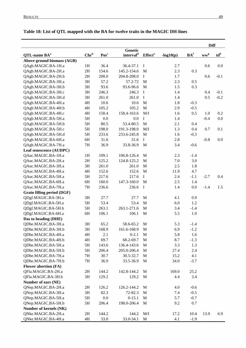
RESULTS 49

Table 18: List of QTL mapped with the BA for twelve traits in the MAGIC DH-lines

Diff

QTL-name BAa Chr

b Pos

c

Genetic

intervald Effect

e -log10(p) BA

f ww

g td

h

Above ground biomass (AGB)

QAgb.MAGIC.BA-1H.a 1H 36.4 36.4-37.1 I 2.7

0.6 0.0

QAgb.MAGIC.BA-2H.a 2H 154.6 145.2-154.6 M 2.3 0.3

QAgb.MAGIC.BA-2H.b 2H 208.0 204.8-208.0 I 1.7

0.6 -0.1

QAgb.MAGIC.BA-3H.a 3H 57.2 57.2-72 M 2.3 0.5

QAgb.MAGIC.BA-3H.b 3H 93.6 93.6-96.6 M 1.5 0.3

QAgb.MAGIC.BA-3H.c 3H 246.3 246.3 I 1.4

0.4 -0.1

QAgb.MAGIC.BA-3H.d 3H 261.0 261.0 I 1.4

0.5 -0.2

QAgb.MAGIC.BA-4H.a 4H 10.6 10.6 M 1.8 -0.3

QAgb.MAGIC.BA-4H.b 4H 105.2 105.2 M 2.9 -0.5

QAgb.MAGIC.BA-4H.c 4H 158.4 158.4-163.6 M/I 1.6 0.5 1.0 0.2

QAgb.MAGIC.BA-5H.a 5H 0.0 0.0 I 1.4

-0.4 0.0


QAgb.MAGIC.BA-5H.c 5H 198.0 191.3-198.0 M/I 1.3 0.4 0.7 0.1

QAgb.MAGIC.BA-5H.d 5H 233.6 233.6-245.8 M 1.6 -0.3

QAgb.MAGIC.BA-6H.a 6H 31.6 31.6 I 2.8

-0.8 0.0

QAgb.MAGIC.BA-7H.a 7H 36.9 33.8-36.9 M 3.4 -0.6

Leaf senescence (AUDPC)

QAuc.MAGIC.BA-1H.a 1H 109.1 106.8-126.4 M 2.3 -1.4

QAuc.MAGIC.BA-2H.a 2H 125.2 124.8-125.2 M 7.0 3.0

QAuc.MAGIC.BA-3H.a 3H 261.0 261.0 M 2.5 1.8


QAuc.MAGIC.BA-5H.a 5H 217.6 217.6 I 2.4 -1.1 -2.7 0.4


QAuc.MAGIC.BA-7H.a 7H 236.6 236.6 I 1.4 0.0 -1.4 1.5

Grain filling period (DGF)

QDgf.MAGIC.BA-3H.a 3H 27.7 27.7 M 4.1 0.9


QDgf.MAGIC.BA-5H.b 5H 263.1 263.1-271.6 M 3.4 -1.4


Das to heading (DHE)

QDhe.MAGIC.BA-3H.a 3H 65.2 58.6-65.2 M 5.3 -1.4

QDhe.MAGIC.BA-3H.b 3H 168.9 161.6-168.9 M 6.9 -1.2

QDhe.MAGIC.BA-4H.a 4H 2.1 0-2.1 M 5.8 1.6


QDhe.MAGIC.BA-5H.a 5H 143.6 136.4-143.6 M 3.3 1.3

QDhe.MAGIC.BA-5H.b 5H 206.4 205.0-206.4 M 27.4 2.4



Flower abortion (FA)

QFla.MAGIC.BA-2H.a 2H 144.2 142.8-144.2 M 169.0 25.2

QFla.MAGIC.BA-3H.b 3H 129.2 129.2 M 4.4 3.4

Number of ears (NE)

QNep.MAGIC.BA-2H.a 2H 126.2 126.2-144.2 M 4.0 -0.6

QNep.MAGIC.BA-3H.a 3H 82.3 72-82.3 M 7.4 -0.5

QNep.MAGIC.BA-5H.a 5H 0.0 0-15.1 M 5.7 -0.7

QNep.MAGIC.BA-5H.b 5H 206.4 198.0-206.4 M 9.2 0.7

Number of kernels (NK)

QNke.MAGIC.BA-2H.a 2H 144.2 144.2 M/I 17.2 10.4 13.9 6.9

QNke.MAGIC.BA-4H.a 4H 33.0 33.0-34.1 M 4.1 -1.9

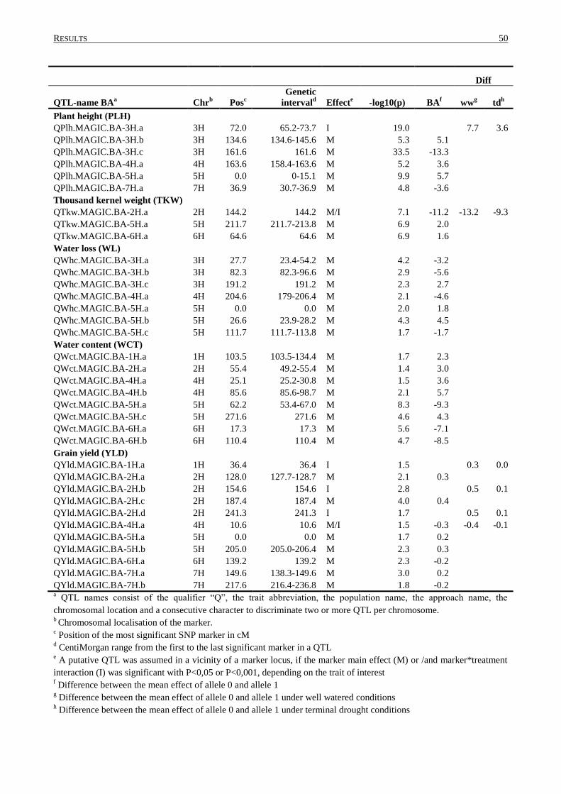
RESULTS 50

Diff

QTL-name BAa Chr

b Pos

c

Genetic

intervald Effect

e -log10(p) BA

f ww

g td

h

Plant height (PLH)

QPlh.MAGIC.BA-3H.a 3H 72.0 65.2-73.7 I 19.0

7.7 3.6

QPlh.MAGIC.BA-3H.b 3H 134.6 134.6-145.6 M 5.3 5.1

QPlh.MAGIC.BA-3H.c 3H 161.6 161.6 M 33.5 -13.3

QPlh.MAGIC.BA-4H.a 4H 163.6 158.4-163.6 M 5.2 3.6

QPlh.MAGIC.BA-5H.a 5H 0.0 0-15.1 M 9.9 5.7

QPlh.MAGIC.BA-7H.a 7H 36.9 30.7-36.9 M 4.8 -3.6

Thousand kernel weight (TKW)

QTkw.MAGIC.BA-2H.a 2H 144.2 144.2 M/I 7.1 -11.2 -13.2 -9.3

QTkw.MAGIC.BA-5H.a 5H 211.7 211.7-213.8 M 6.9 2.0

QTkw.MAGIC.BA-6H.a 6H 64.6 64.6 M 6.9 1.6

Water loss (WL)

QWhc.MAGIC.BA-3H.a 3H 27.7 23.4-54.2 M 4.2 -3.2

QWhc.MAGIC.BA-3H.b 3H 82.3 82.3-96.6 M 2.9 -5.6

QWhc.MAGIC.BA-3H.c 3H 191.2 191.2 M 2.3 2.7

QWhc.MAGIC.BA-4H.a 4H 204.6 179-206.4 M 2.1 -4.6

QWhc.MAGIC.BA-5H.a 5H 0.0 0.0 M 2.0 1.8

QWhc.MAGIC.BA-5H.b 5H 26.6 23.9-28.2 M 4.3 4.5

QWhc.MAGIC.BA-5H.c 5H 111.7 111.7-113.8 M 1.7 -1.7

Water content (WCT)

QWct.MAGIC.BA-1H.a 1H 103.5 103.5-134.4 M 1.7 2.3



QWct.MAGIC.BA-4H.b 4H 85.6 85.6-98.7 M 2.1 5.7

QWct.MAGIC.BA-5H.a 5H 62.2 53.4-67.0 M 8.3 -9.3

QWct.MAGIC.BA-5H.c 5H 271.6 271.6 M 4.6 4.3

QWct.MAGIC.BA-6H.a 6H 17.3 17.3 M 5.6 -7.1

QWct.MAGIC.BA-6H.b 6H 110.4 110.4 M 4.7 -8.5

Grain yield (YLD)

QYld.MAGIC.BA-1H.a 1H 36.4 36.4 I 1.5

0.3 0.0

QYld.MAGIC.BA-2H.a 2H 128.0 127.7-128.7 M 2.1 0.3

QYld.MAGIC.BA-2H.b 2H 154.6 154.6 I 2.8

0.5 0.1

QYld.MAGIC.BA-2H.c 2H 187.4 187.4 M 4.0 0.4

QYld.MAGIC.BA-2H.d 2H 241.3 241.3 I 1.7

0.5 0.1

QYld.MAGIC.BA-4H.a 4H 10.6 10.6 M/I 1.5 -0.3 -0.4 -0.1

QYld.MAGIC.BA-5H.a 5H 0.0 0.0 M 1.7 0.2

QYld.MAGIC.BA-5H.b 5H 205.0 205.0-206.4 M 2.3 0.3

QYld.MAGIC.BA-6H.a 6H 139.2 139.2 M 2.3 -0.2


QYld.MAGIC.BA-7H.b 7H 217.6 216.4-236.8 M 1.8 -0.2

a QTL names consist of the qualifier “Q”, the trait abbreviation, the population name, the approach name, the

chromosomal location and a consecutive character to discriminate two or more QTL per chromosome. b Chromosomal localisation of the marker.

c Position of the most significant SNP marker in cM

d CentiMorgan range from the first to the last significant marker in a QTL

e A putative QTL was assumed in a vicinity of a marker locus, if the marker main effect (M) or /and marker*treatment

interaction (I) was significant with P<0,05 or P<0,001, depending on the trait of interest f Difference between the mean effect of allele 0 and allele 1

g Difference between the mean effect of allele 0 and allele 1 under well watered conditions

h Difference between the mean effect of allele 0 and allele 1 under terminal drought conditions

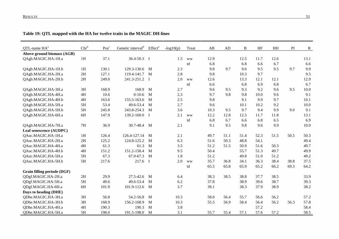
RESULTS 51

Table 19: QTL mapped with the HA for twelve traits in the MAGIC DH-lines

QTL-name HAa Chr

b Pos

c Genetic interval

d Effect

e -log10(p) Treat AB AD B HF HH PI R


QAgb.MAGIC.HA-1H.a 1H 37.1 36.4-50.3 I 1.5 ww 12.9

12.5 11.7 12.6

13.1

td 6.8

6.8 6.6 6.7

6.6

QAgb.MAGIC.HA-1H.b 1H 130.1 129.3-130.6 M 2.3

9.8 9.7 9.6 9.5 9.5 9.7 9.9

QAgb.MAGIC.HA-2H.a 2H 127.1 119.4-141.7 M 2.8

9.8

10.3 9.7

9.5

QAgb.MAGIC.HA-2H.b 2H 249.0 241.3-251.2 I 2.0 ww 12.6

13.3 12.1 12.1

12.9

td 6.6

6.8 6.9 6.8

6.7

QAgb.MAGIC.HA-3H.a 3H 168.9 168.9 M 2.7

9.6 9.5 9.3 9.2 9.6 9.5 10.0

QAgb.MAGIC.HA-4H.a 4H 10.6 0-10.6 M 2.3

9.7 9.8 9.8 10.0 9.6

9.1


9.8

9.1 9.9 9.7

10.1


9.6

10.1 10.2 9.2

10.0


10.3 9.5 9.7 9.4 9.9 9.0 9.1

QAgb.MAGIC.HA-6H.a 6H 147.9 139.2-160.0 I 2.1 ww 12.2 12.8 12.5 11.7 11.8

13.1

td 6.8 6.7 6.6 6.8 6.5

6.9


9.1 9.5 9.8 9.6 9.9

10.0


QAuc.MAGIC.HA-1H.a 1H 126.4 126.4-127.14 M 2.1

49.7 51.1 51.4 52.3 51.5 50.5 50.3


51.6 50.3 48.8 54.1

49.4

QAuc.MAGIC.HA-4H.a 4H 61.3 61.3 M 3.5

51.2 51.5 50.9 51.6 50.3

49.7

QAuc.MAGIC.HA-4H.b 4H 151.2 151.2-158.4 M 9.5

50.4

55.7 51.3 49.7

49.9


51.2

49.8 51.0 51.2

49.2

QAuc.MAGIC.HA-5H.b 5H 217.6 217.6 I 2.0 ww 35.7 36.8 34.1 36.3 38.4 38.8 37.5

td 65.5 65.8 65.9 65.2 66.2 69.3 64.2

Grain filling periode (DGF)

QDgf.MAGIC.HA-2H.a 2H 29.9 27.5-42.6 M 6.4

38.3 38.5 38.8 37.7 38.5

33.9


37.8

38.9 39.6 38.7

39.3


39.1

38.3 37.9 38.9

38.2

Days to heading (DHE)

QDhe.MAGIC.HA-3H.a 3H 56.8 54.2-56.8 M 10.3

58.0 56.4 55.7 56.6 56.2

57.2

QDhe.MAGIC.HA-3H.b 3H 168.9 156.2-168.9 M 10.3

55.5 56.9 58.4 56.4 56.2 56.3 57.8

QDhe.MAGIC.HA-4H.a 4H 190.3 190.3 M 3.8

57.2

58.4


55.7 55.4 57.1 57.6 57.2

58.5

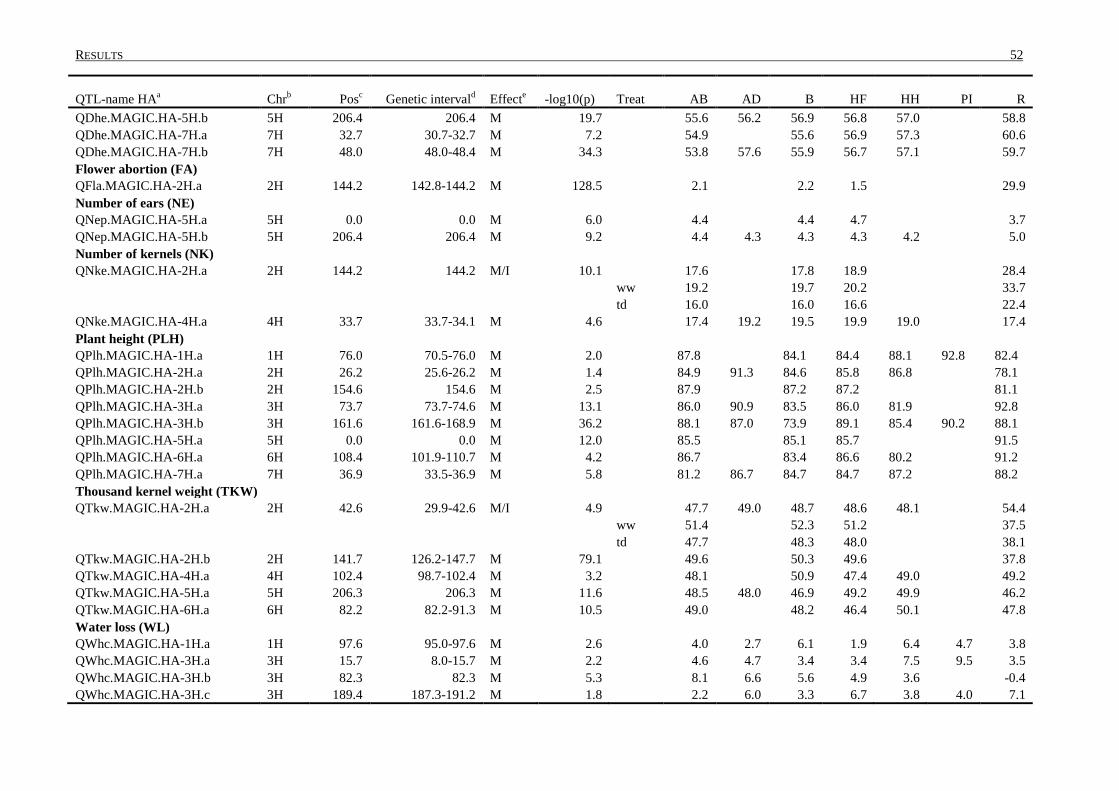
RESULTS 52

QTL-name HAa Chr

b Pos

c Genetic interval

d Effect


QDhe.MAGIC.HA-5H.b 5H 206.4 206.4 M 19.7

55.6 56.2 56.9 56.8 57.0

58.8


54.9

55.6 56.9 57.3

60.6

QDhe.MAGIC.HA-7H.b 7H 48.0 48.0-48.4 M 34.3

53.8 57.6 55.9 56.7 57.1

59.7


QFla.MAGIC.HA-2H.a 2H 144.2 142.8-144.2 M 128.5

2.1

2.2 1.5

29.9

Number of ears (NE)

QNep.MAGIC.HA-5H.a 5H 0.0 0.0 M 6.0

4.4

4.4 4.7

3.7

QNep.MAGIC.HA-5H.b 5H 206.4 206.4 M 9.2

4.4 4.3 4.3 4.3 4.2

5.0


QNke.MAGIC.HA-2H.a 2H 144.2 144.2 M/I 10.1

17.6

17.8 18.9

28.4

ww 19.2

19.7 20.2

33.7

td 16.0

16.0 16.6

22.4

QNke.MAGIC.HA-4H.a 4H 33.7 33.7-34.1 M 4.6

17.4 19.2 19.5 19.9 19.0

17.4

Plant height (PLH)

QPlh.MAGIC.HA-1H.a 1H 76.0 70.5-76.0 M 2.0

87.8

84.1 84.4 88.1 92.8 82.4


84.9 91.3 84.6 85.8 86.8

78.1

QPlh.MAGIC.HA-2H.b 2H 154.6 154.6 M 2.5

87.9

87.2 87.2

81.1


86.0 90.9 83.5 86.0 81.9

92.8

QPlh.MAGIC.HA-3H.b 3H 161.6 161.6-168.9 M 36.2

88.1 87.0 73.9 89.1 85.4 90.2 88.1

QPlh.MAGIC.HA-5H.a 5H 0.0 0.0 M 12.0

85.5

85.1 85.7

91.5


86.7

83.4 86.6 80.2

91.2


81.2 86.7 84.7 84.7 87.2

88.2


QTkw.MAGIC.HA-2H.a 2H 42.6 29.9-42.6 M/I 4.9

47.7 49.0 48.7 48.6 48.1

54.4

ww 51.4

52.3 51.2

37.5

td 47.7

48.3 48.0

38.1

QTkw.MAGIC.HA-2H.b 2H 141.7 126.2-147.7 M 79.1

49.6

50.3 49.6

37.8

QTkw.MAGIC.HA-4H.a 4H 102.4 98.7-102.4 M 3.2

48.1

50.9 47.4 49.0

49.2

QTkw.MAGIC.HA-5H.a 5H 206.3 206.3 M 11.6

48.5 48.0 46.9 49.2 49.9

46.2

QTkw.MAGIC.HA-6H.a 6H 82.2 82.2-91.3 M 10.5

49.0

48.2 46.4 50.1

47.8

Water loss (WL)

QWhc.MAGIC.HA-1H.a 1H 97.6 95.0-97.6 M 2.6

4.0 2.7 6.1 1.9 6.4 4.7 3.8


4.6 4.7 3.4 3.4 7.5 9.5 3.5

QWhc.MAGIC.HA-3H.b 3H 82.3 82.3 M 5.3

8.1 6.6 5.6 4.9 3.6

-0.4

QWhc.MAGIC.HA-3H.c 3H 189.4 187.3-191.2 M 1.8

2.2 6.0 3.3 6.7 3.8 4.0 7.1

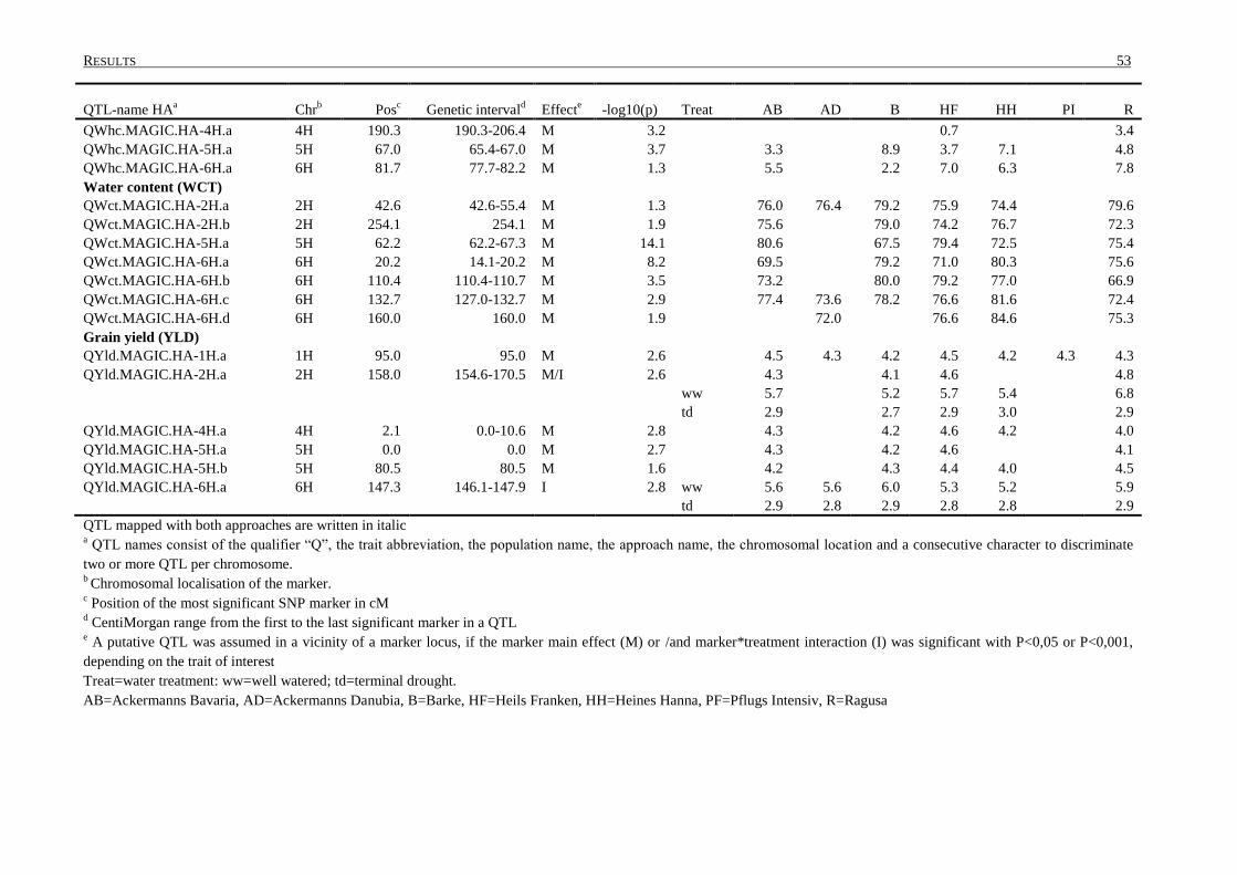
RESULTS 53

QTL-name HAa Chr

b Pos

c Genetic interval

d Effect



0.7

3.4


3.3

8.9 3.7 7.1

4.8


5.5

2.2 7.0 6.3

7.8

Water content (WCT)

QWct.MAGIC.HA-2H.a 2H 42.6 42.6-55.4 M 1.3

76.0 76.4 79.2 75.9 74.4

79.6

QWct.MAGIC.HA-2H.b 2H 254.1 254.1 M 1.9

75.6

79.0 74.2 76.7

72.3


80.6

67.5 79.4 72.5

75.4


69.5

79.2 71.0 80.3

75.6

QWct.MAGIC.HA-6H.b 6H 110.4 110.4-110.7 M 3.5

73.2

80.0 79.2 77.0

66.9

QWct.MAGIC.HA-6H.c 6H 132.7 127.0-132.7 M 2.9

77.4 73.6 78.2 76.6 81.6

72.4

QWct.MAGIC.HA-6H.d 6H 160.0 160.0 M 1.9

72.0

76.6 84.6

75.3

Grain yield (YLD)

QYld.MAGIC.HA-1H.a 1H 95.0 95.0 M 2.6

4.5 4.3 4.2 4.5 4.2 4.3 4.3

QYld.MAGIC.HA-2H.a 2H 158.0 154.6-170.5 M/I 2.6

4.3

4.1 4.6

4.8

ww 5.7

5.2 5.7 5.4

6.8

td 2.9

2.7 2.9 3.0

2.9

QYld.MAGIC.HA-4H.a 4H 2.1 0.0-10.6 M 2.8

4.3

4.2 4.6 4.2

4.0

QYld.MAGIC.HA-5H.a 5H 0.0 0.0 M 2.7

4.3

4.2 4.6

4.1

QYld.MAGIC.HA-5H.b 5H 80.5 80.5 M 1.6

4.2

4.3 4.4 4.0

4.5

QYld.MAGIC.HA-6H.a 6H 147.3 146.1-147.9 I 2.8 ww 5.6 5.6 6.0 5.3 5.2

5.9

td 2.9 2.8 2.9 2.8 2.8

2.9

QTL mapped with both approaches are written in italic a QTL names consist of the qualifier “Q”, the trait abbreviation, the population name, the approach name, the chromosomal location and a consecutive character to discriminate

two or more QTL per chromosome. b Chromosomal localisation of the marker.



e A putative QTL was assumed in a vicinity of a marker locus, if the marker main effect (M) or /and marker*treatment interaction (I) was significant with P<0,05 or P<0,001,

depending on the trait of interest

Treat=water treatment: ww=well watered; td=terminal drought.

AB=Ackermanns Bavaria, AD=Ackermanns Danubia, B=Barke, HF=Heils Franken, HH=Heines Hanna, PF=Pflugs Intensiv, R=Ragusa

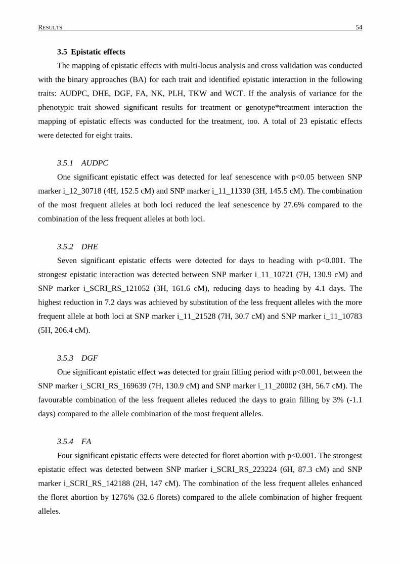
RESULTS 54

3.5 Epistatic effects

The mapping of epistatic effects with multi-locus analysis and cross validation was conducted

with the binary approaches (BA) for each trait and identified epistatic interaction in the following

traits: AUDPC, DHE, DGF, FA, NK, PLH, TKW and WCT. If the analysis of variance for the

phenotypic trait showed significant results for treatment or genotype*treatment interaction the

mapping of epistatic effects was conducted for the treatment, too. A total of 23 epistatic effects

were detected for eight traits.

3.5.1 AUDPC

One significant epistatic effect was detected for leaf senescence with p<0.05 between SNP

marker i_12_30718 (4H, 152.5 cM) and SNP marker i_11_11330 (3H, 145.5 cM). The combination

of the most frequent alleles at both loci reduced the leaf senescence by 27.6% compared to the

combination of the less frequent alleles at both loci.

3.5.2 DHE

Seven significant epistatic effects were detected for days to heading with p<0.001. The

strongest epistatic interaction was detected between SNP marker i_11_10721 (7H, 130.9 cM) and

SNP marker i_SCRI_RS_121052 (3H, 161.6 cM), reducing days to heading by 4.1 days. The

highest reduction in 7.2 days was achieved by substitution of the less frequent alleles with the more

frequent allele at both loci at SNP marker i_11_21528 (7H, 30.7 cM) and SNP marker i_11_10783

(5H, 206.4 cM).

3.5.3 DGF

One significant epistatic effect was detected for grain filling period with p<0.001, between the

SNP marker i_SCRI_RS_169639 (7H, 130.9 cM) and SNP marker i_11_20002 (3H, 56.7 cM). The

favourable combination of the less frequent alleles reduced the days to grain filling by 3% (-1.1

days) compared to the allele combination of the most frequent alleles.

3.5.4 FA

Four significant epistatic effects were detected for floret abortion with p<0.001. The strongest

epistatic effect was detected between SNP marker i_SCRI_RS_223224 (6H, 87.3 cM) and SNP

marker i_SCRI_RS_142188 (2H, 147 cM). The combination of the less frequent alleles enhanced

the floret abortion by 1276% (32.6 florets) compared to the allele combination of higher frequent

alleles.

RESULTS 55

3.5.5 NK

Two significant epistatic interactions were detected for number of kernels with p<0.001. The

strongest effect was detected between SNP marker i_SCRI_RS_197190 (7H, 217.3 cM) and SNP

marker i_SCRI_RS_156323 (2H, 125.1 cM). The combination of the less frequent alleles enhanced

the number of kernels by 36.6% (6.7 kernels) compared to the combination of the most frequent

alleles.

3.5.6 PLH

Two significant epistatic interactions were detected for plant height with p<0.001. The

strongest effect was detected between SNP marker i_SCRI_RS_98225 (6H, 113.3 cM) and SNP

marker i_11_10005 (3H, 70.7 cM). The combination of the most frequent alleles reduced the plant

height by 6.7% (5.5 cm) compared to the combination of less frequent alleles.

3.5.7 TKW

Two significant epistatic effects for thousand kernel weight were detected with p<0.001. The

strongest effect was detected between SNP marker i_11_11250 (2H, 144.2 cM) and SNP marker

i_SCRI_RS_159503 (2H, 8.1 cM). The reduction in thousand kernel weight by 10.3% (4.6 g) was

exhibited by lines carrying the more frequent allele at marker i_11_11250 and the less frequent

allele at marker i_SCRI_RS_159503.

3.5.8 WCT

Four significant effects were detected with p<0.05. The strongest effect was detected between

SNP marker i_12_30329 (7H, 217.3 cM) and SNP marker i_SCRI_RS_8671 (2H, 259.4 cM). The

reduction of water content by 14.9% was exhibited by lines carrying the more frequent allele at

SNP marker i_12_30329 and the less frequent allele at SNP marker i_SCRI_RS_8671.

3.6 Multiple comparison of parental means from haplotype approach

Main marker effects

Not only the allele effect between the contrasting parents can be calculated as significant, the

further parental means can be evaluated regarding to their significant differences as well. Therefore

a selected group of eighteen allele effects were tested for multiple comparisons from traits except

FA and NK (Table 20).

The multiple comparison of QAgb.MAGIC.HA-5H.b determined three groups of allelic means: the

alleles from Ackermanns Bavaria and Heines Hanna were significantly different to Ragusa and

RESULTS 56

Heines Hanna. The means of Ackermanns Danubia, Barke and Pflugs Intensiv were not significant

different to both groups.

Two allele effects for AUDPC were evaluated (QAuc.MAGIC.HA-4H.a and QAuc.MAGIC.HA-

4H.b). QAuc.MAGIC.HA-4H.a revealed three groups of significant allelic means; the mean of

Heils Franken was significantly different to Ragusa, the remaining allelic means were not

significantly different from any mean. The further analysis of QAuc.MAGIC.HA-4H.b showed that

the allelic mean of Barke was significantly higher compared to all other allelic means from the

parents.

Three allele effects for DHE were investigated (QDhe.MAGIC.HA-5H.b, QDhe.MAGIC.HA-7H.a

and QDhe.MAGIC.HA-7H.b). QDhe.MAGIC.HA-5H.b resulted in three groups of allelic means

that were significantly different from each other; the allelic mean of Ragusa was significantly

different from all other parental means at that position. The mean of Ackermanns Bavaria was

significantly different to the mean of Barke and the mean of Heines Hanna. The further analysis of

the multiple comparisons of the allelic means of QDhe.MAGIC.HA-7H.a resulted in three groups as

well. The allelic mean of Ragusa was significantly different to all other parents, and the mean of

Ackermanns Bavaria and Barke were significant from the means of Ragusa, Heils Franken and

Heines Hanna. The third QTL for DHE which was investigated (QDhe.MAGIC.HA-7H.b) showed

significant differences for the mean of Ragusa to all other parents and the allelic mean of

Ackermanns Bavaria and Barke was significantly different from Ackermanns Danubia, Heils

Franken and Heines Hanna.

QNep.MAGIC.HA-5H.b was investigated for multiple comparisons for number of ears (NE). The

parental mean of Ragusa was significantly different to all means of the other parental means at this

position.

Five QTL for plant height were investigated for multiple comparisons of the parental alleles. The

allelic effects at QPlh.MAGIC.HA-1H.a resulted in two clusters. The means of Pflugs Intensiv was

significantly different to Ragusa, Barke and Heils Franken, but not to Ackermanns Bavaria and

Heines Hanna. The mean of Heines Hanna and Ackermanns Bavaria were significant different to

the parental mean of Barke, Heils Franken and Ragusa. Two allele effects on chromosome 3H for

plant height were investigated for their parental mean, QPlh.MAGIC.HA-3H.a and

QPlh.MAGIC.HA-3H.b. At QTL QPlh.MAGIC.HA-3H.a the allelic mean of Ragusa and

Ackermanns Danubia were significantly different to all allelic parental means but not to each other.

The low allelic mean of Heines Hanna was significantly different to the mean of Ackermanns

Bavaria and Heils Franken and Heils Franken to Barke. Multiple comparisons of the allelic means

resulted in three clusters. At QPlh.MAGIC.HA-3H.b the mean of Barke was significantly different

RESULTS 57

to all other parental means at that position. The mean of Heines Hanna was significant to all others

as well except to the mean of Ackermanns Bavaria. At QPlh.MAGIC.HA-6H.a the allelic effect of

Ragusa was significantly different to all other parents at that position. The parental mean of Heines

Hanna was significant to the mean of Ackermanns Bavaria, Heils Franken and Ragusa. The mean of

Barke was significant to the mean of Ackermanns Bavaria. Multiple comparisons of the allelic

means resulted in three clusters. The last multiple comparison for a QTL for plant height was

investigated at QPlh.MAGIC.HA-7H.a. The allelic mean of Ackermanns Bavaria was significantly

different to all parental means at that position. The mean of Ragusa was significantly different to

Barke as well. Multiple comparisons of the allelic means resulted in four clusters.

The multiple comparisons for one QTL for TKW were investigated. At QTKW.MAGIC.HA-2H.a

all parental means were significantly different to Ragusa, but not among each other.

One QTL for water loss was investigated for multiple comparisons of the parental means. The mean

of Barke at QWhc.MAGIC.HA-5H.a was significant to the mean of Ackermanns Bavaria, Heils

Franken and Ragusa. The mean of Heines Hanna was only significant to the mean of Ackermanns

Bavaria. Distinct differences between the means are shown exemplary in Fig. 8.

Two QTL for water content (WCT) were investigated concerning their parental means. The parental

means of QWct.MAGIC.HA-5H.a clustered in three groups. The mean of Barke was significantly

different to all other parental means. The mean of Ackermanns Bavaria was significantly different

to Heines Hanna and Ragusa. And additionally the mean of Heines Hanna was significant to the

mean of Heils Franken. The allelic means of the second QTL, QWct.MAGIC.HA-6H.c, clustered

into two groups. The means of Heines Hanna, Barke and Ackermanns Bavaria were significant to

the mean of Ackermanns Danubia, Heils Franken and Ragusa.

The two QTL for grain yield which were investigated for multiple comparisons of the parental

alleles showed clear clustering for the significance. At QYld.MAGIC.HA-4H.a the allelic mean of

Heils Franken was significant to all other parental means. At QYld.MAGIC.HA-5H.b the allelic

means of Heils Franken and Barke were significantly different from the other parental means.

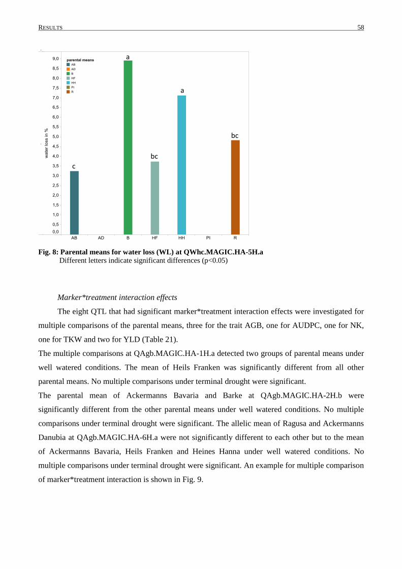
RESULTS 58

c

a

bc

a

bc

Fig. 8: Parental means for water loss (WL) at QWhc.MAGIC.HA-5H.a

Different letters indicate significant differences (p<0.05)

Marker*treatment interaction effects

The eight QTL that had significant marker*treatment interaction effects were investigated for

multiple comparisons of the parental means, three for the trait AGB, one for AUDPC, one for NK,

one for TKW and two for YLD (Table 21).

The multiple comparisons at QAgb.MAGIC.HA-1H.a detected two groups of parental means under

well watered conditions. The mean of Heils Franken was significantly different from all other

parental means. No multiple comparisons under terminal drought were significant.

The parental mean of Ackermanns Bavaria and Barke at QAgb.MAGIC.HA-2H.b were

significantly different from the other parental means under well watered conditions. No multiple

comparisons under terminal drought were significant. The allelic mean of Ragusa and Ackermanns

Danubia at QAgb.MAGIC.HA-6H.a were not significantly different to each other but to the mean

of Ackermanns Bavaria, Heils Franken and Heines Hanna under well watered conditions. No

multiple comparisons under terminal drought were significant. An example for multiple comparison

of marker*treatment interaction is shown in Fig. 9.

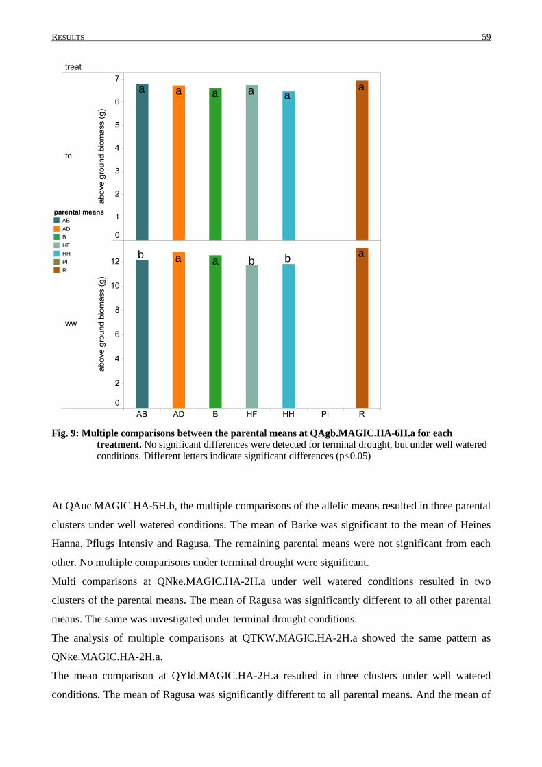
RESULTS 59

a aaaaa

b a aa

b b

Fig. 9: Multiple comparisons between the parental means at QAgb.MAGIC.HA-6H.a for each

treatment. No significant differences were detected for terminal drought, but under well watered

conditions. Different letters indicate significant differences (p<0.05)

At QAuc.MAGIC.HA-5H.b, the multiple comparisons of the allelic means resulted in three parental

clusters under well watered conditions. The mean of Barke was significant to the mean of Heines

Hanna, Pflugs Intensiv and Ragusa. The remaining parental means were not significant from each

other. No multiple comparisons under terminal drought were significant.

Multi comparisons at QNke.MAGIC.HA-2H.a under well watered conditions resulted in two

clusters of the parental means. The mean of Ragusa was significantly different to all other parental

means. The same was investigated under terminal drought conditions.

The analysis of multiple comparisons at QTKW.MAGIC.HA-2H.a showed the same pattern as

QNke.MAGIC.HA-2H.a.

The mean comparison at QYld.MAGIC.HA-2H.a resulted in three clusters under well watered

conditions. The mean of Ragusa was significantly different to all parental means. And the mean of

RESULTS 60

Barke was significant to the mean of Heils Franken. No multiple comparisons under terminal

drought were significant.

The last investigated QTL was located on chromosome 6H, QYld.MAGIC.HA-6H.a. The allelic

mean of Barke was significant to all other parental means except to Ragusa under well watered

conditions. The parental means of Ragusa and Ackermanns Danubia were not significant to each

other, but to the means of Heils Franken and Heines Hanna. No multiple comparisons under

terminal drought were significant.

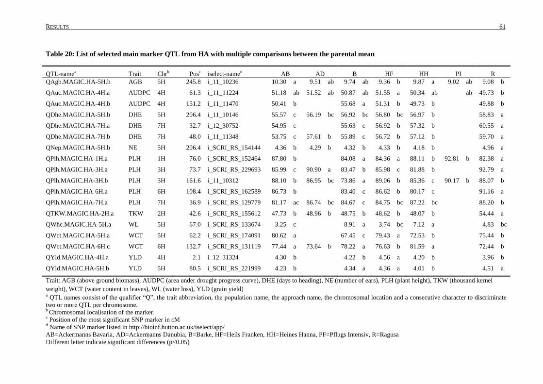
RESULTS 61

Table 20: List of selected main marker QTL from HA with multiple comparisons between the parental mean

QTL-namea Trait Chr

b Pos

c iselect-name

d AB AD B HF HH PI R

QAgb.MAGIC.HA-5H.b AGB 5H 245.8 i_11_10236 10.30 a 9.51 ab 9.74 ab 9.36 b 9.87 a 9.02 ab 9.08 b

QAuc.MAGIC.HA-4H.a AUDPC 4H 61.3 i_11_11224 51.18 ab 51.52 ab 50.87 ab 51.55 a 50.34 ab ab 49.73 b

QAuc.MAGIC.HA-4H.b AUDPC 4H 151.2 i_11_11470 50.41 b 55.68 a 51.31 b 49.73 b 49.88 b

QDhe.MAGIC.HA-5H.b DHE 5H 206.4 i_11_10146 55.57 c 56.19 bc 56.92 bc 56.80 bc 56.97 b 58.83 a

QDhe.MAGIC.HA-7H.a DHE 7H 32.7 i_12_30752 54.95 c 55.63 c 56.92 b 57.32 b 60.55 a

QDhe.MAGIC.HA-7H.b DHE 7H 48.0 i_11_11348 53.75 c 57.61 b 55.89 c 56.72 b 57.12 b 59.70 a

QNep.MAGIC.HA-5H.b NE 5H 206.4 i_SCRI_RS_154144 4.36 b 4.29 b 4.32 b 4.33 b 4.18 b 4.96 a

QPlh.MAGIC.HA-1H.a PLH 1H 76.0 i_SCRI_RS_152464 87.80 b 84.08 a 84.36 a 88.11 b 92.81 b 82.38 a

QPlh.MAGIC.HA-3H.a PLH 3H 73.7 i_SCRI_RS_229693 85.99 c 90.90 a 83.47 b 85.98 c 81.88 b 92.79 a

QPlh.MAGIC.HA-3H.b PLH 3H 161.6 i_11_10312 88.10 b 86.95 bc 73.86 a 89.06 b 85.36 c 90.17 b 88.07 b

QPlh.MAGIC.HA-6H.a PLH 6H 108.4 i_SCRI_RS_162589 86.73 b 83.40 c 86.62 b 80.17 c 91.16 a

QPlh.MAGIC.HA-7H.a PLH 7H 36.9 i_SCRI_RS_129779 81.17 ac 86.74 bc 84.67 c 84.75 bc 87.22 bc 88.20 b

QTKW.MAGIC.HA-2H.a TKW 2H 42.6 i_SCRI_RS_155612 47.73 b 48.96 b 48.75 b 48.62 b 48.07 b 54.44 a

QWhc.MAGIC.HA-5H.a WL 5H 67.0 i_SCRI_RS_133674 3.25 c 8.91 a 3.74 bc 7.12 a 4.83 bc

QWct.MAGIC.HA-5H.a WCT 5H 62.2 i_SCRI_RS_174091 80.62 a 67.45 c 79.43 a 72.53 b 75.44 b

QWct.MAGIC.HA-6H.c WCT 6H 132.7 i_SCRI_RS_131119 77.44 a 73.64 b 78.22 a 76.63 b 81.59 a 72.44 b

QYld.MAGIC.HA-4H.a YLD 4H 2.1 i_12_31324 4.30 b 4.22 b 4.56 a 4.20 b 3.96 b

QYld.MAGIC.HA-5H.b YLD 5H 80.5 i_SCRI_RS_221999 4.23 b 4.34 a 4.36 a 4.01 b 4.51 a

Trait: AGB (above ground biomass), AUDPC (area under drought progress curve), DHE (days to heading), NE (number of ears), PLH (plant height), TKW (thousand kernel

weight), WCT (water content in leaves), WL (water loss), YLD (grain yield) a QTL names consist of the qualifier “Q”, the trait abbreviation, the population name, the approach name, the chromosomal location and a consecutive character to discriminate



d Name of SNP marker listed in http://bioinf.hutton.ac.uk/iselect/app/



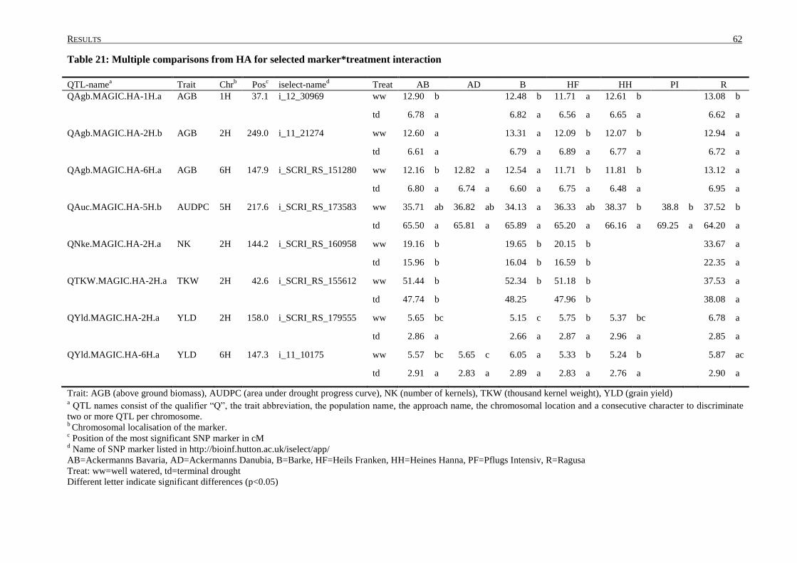
RESULTS 62

Table 21: Multiple comparisons from HA for selected marker*treatment interaction

QTL-namea Trait Chr

b Pos

c iselect-name

d Treat AB AD B HF HH PI R

QAgb.MAGIC.HA-1H.a AGB 1H 37.1 i_12_30969 ww 12.90 b 12.48 b 11.71 a 12.61 b 13.08 b

td 6.78 a 6.82 a 6.56 a 6.65 a 6.62 a

QAgb.MAGIC.HA-2H.b AGB 2H 249.0 i_11_21274 ww 12.60 a 13.31 a 12.09 b 12.07 b 12.94 a

td 6.61 a 6.79 a 6.89 a 6.77 a 6.72 a

QAgb.MAGIC.HA-6H.a AGB 6H 147.9 i_SCRI_RS_151280 ww 12.16 b 12.82 a 12.54 a 11.71 b 11.81 b 13.12 a

td 6.80 a 6.74 a 6.60 a 6.75 a 6.48 a 6.95 a

QAuc.MAGIC.HA-5H.b AUDPC 5H 217.6 i_SCRI_RS_173583 ww 35.71 ab 36.82 ab 34.13 a 36.33 ab 38.37 b 38.8 b 37.52 b

td 65.50 a 65.81 a 65.89 a 65.20 a 66.16 a 69.25 a 64.20 a

QNke.MAGIC.HA-2H.a NK 2H 144.2 i_SCRI_RS_160958 ww 19.16 b 19.65 b 20.15 b 33.67 a

td 15.96 b 16.04 b 16.59 b 22.35 a

QTKW.MAGIC.HA-2H.a TKW 2H 42.6 i_SCRI_RS_155612 ww 51.44 b 52.34 b 51.18 b 37.53 a

td 47.74 b 48.25 47.96 b 38.08 a

QYld.MAGIC.HA-2H.a YLD 2H 158.0 i_SCRI_RS_179555 ww 5.65 bc 5.15 c 5.75 b 5.37 bc 6.78 a

td 2.86 a 2.66 a 2.87 a 2.96 a 2.85 a

QYld.MAGIC.HA-6H.a YLD 6H 147.3 i_11_10175 ww 5.57 bc 5.65 c 6.05 a 5.33 b 5.24 b 5.87 ac

td 2.91 a 2.83 a 2.89 a 2.83 a 2.76 a 2.90 a

Trait: AGB (above ground biomass), AUDPC (area under drought progress curve), NK (number of kernels), TKW (thousand kernel weight), YLD (grain yield) a QTL names consist of the qualifier “Q”, the trait abbreviation, the population name, the approach name, the chromosomal location and a consecutive character to discriminate



d Name of SNP marker listed in http://bioinf.hutton.ac.uk/iselect/app/




RESULTS 63

3.7 Pyramidisation of QTL

The MAGIC DH-lines were analysed for the accumulation of favourable QTL within each

trait in single DH-lines and in combination of favourable QTL of different traits in single DH-lines

for each mapping approach.

Within each trait: BA

Seven traits were investigated for the binary approach, the remaining four traits only showed

one favourable QTL.

Six QTL mapped for main marker effects for AGB were investigated for pyramidisation within the

MAGIC DH-lines. No combination of all six favourable QTL (high AGB was defined as

favourable) in a DH-line was detected. Two DH-lines (211 and 459) carried five favourable alleles;

but only the mean of line 211 was greater than the population mean. Lines that carried four

favourable alleles and had a greater mean than the population were: 232, 280, 328, 390, 468, from

which line 390 had the greatest mean.

Four QTL for DHE were mapped with favourable effect (reduced DHE). Four DH-lines (153, 171,

431 and 552) were detected to carry the combination of the favourable QTL, three of those had a

mean lower than the population mean. DH-line 171 had the lowest mean with 49 DHE.

Two positive effects for PLH were detected. 41 DH-lines combined the positive effects. However,

the mean of 20 DH-lines was smaller than the population mean.

Two QTL for TKW had positive effects on the trait (higher TKW). 26 DH-lines carried the

combination of these favourable QTL. The mean for TKW of half of the 26 DH-lines was higher

than the mean of the population. DH-line 549 was outranging with a mean of 53.8 g for TKW.

Four QTL with favourable effects (reduced water loss) were mapped for the trait WL. No DH-line

combined all four favourable alleles, three favourable QTL were mapped in DH-lines 76, 92 and

397. Out of these, only DH-lines 76 and 92 had a smaller value for WL than the population mean.

Five QTL with favourable effects (high amount of water content) were detected for the trait WCT.

No DH-line combined all five favourable alleles. Fifteen DH-lines combined four out of five

favourable alleles and thirteen of them had a greater mean for WCT than the population mean.

Five QTL with favourable effects were mapped for YLD. No DH-line was detected that combined

all five favourable alleles. Only two DH-lines (145, 468) combined four favourable alleles and their

mean was greater than the population mean.

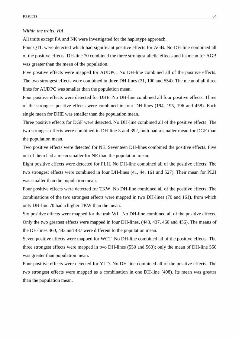
RESULTS 64

Within the traits: HA

All traits except FA and NK were investigated for the haplotype approach.

Four QTL were detected which had significant positive effects for AGB. No DH-line combined all

of the positive effects. DH-line 70 combined the three strongest allelic effects and its mean for AGB

was greater than the mean of the population.

Five positive effects were mapped for AUDPC. No DH-line combined all of the positive effects.

The two strongest effects were combined in three DH-lines (31, 100 and 554). The mean of all three

lines for AUDPC was smaller than the population mean.

Four positive effects were detected for DHE. No DH-line combined all four positive effects. Three

of the strongest positive effects were combined in four DH-lines (194, 195, 196 and 458). Each

single mean for DHE was smaller than the population mean.

Three positive effects for DGF were detected. No DH-line combined all of the positive effects. The

two strongest effects were combined in DH-line 3 and 392, both had a smaller mean for DGF than

the population mean.

Two positive effects were detected for NE. Seventeen DH-lines combined the positive effects. Five

out of them had a mean smaller for NE than the population mean.

Eight positive effects were detected for PLH. No DH-line combined all of the positive effects. The

two strongest effects were combined in four DH-lines (41, 44, 161 and 527). Their mean for PLH

was smaller than the population mean.

Four positive effects were detected for TKW. No DH-line combined all of the positive effects. The

combinations of the two strongest effects were mapped in two DH-lines (70 and 161), from which

only DH-line 70 had a higher TKW than the mean.

Six positive effects were mapped for the trait WL. No DH-line combined all of the positive effects.

Only the two greatest effects were mapped in four DH-lines, (443, 437, 460 and 456). The means of

the DH-lines 460, 443 and 437 were different to the population mean.

Seven positive effects were mapped for WCT. No DH-line combined all of the positive effects. The

three strongest effects were mapped in two DH-lines (550 and 563); only the mean of DH-line 550

was greater than population mean.

Four positive effects were detected for YLD. No DH-line combined all of the positive effects. The

two strongest effects were mapped as a combination in one DH-line (408). Its mean was greater

than the population mean.

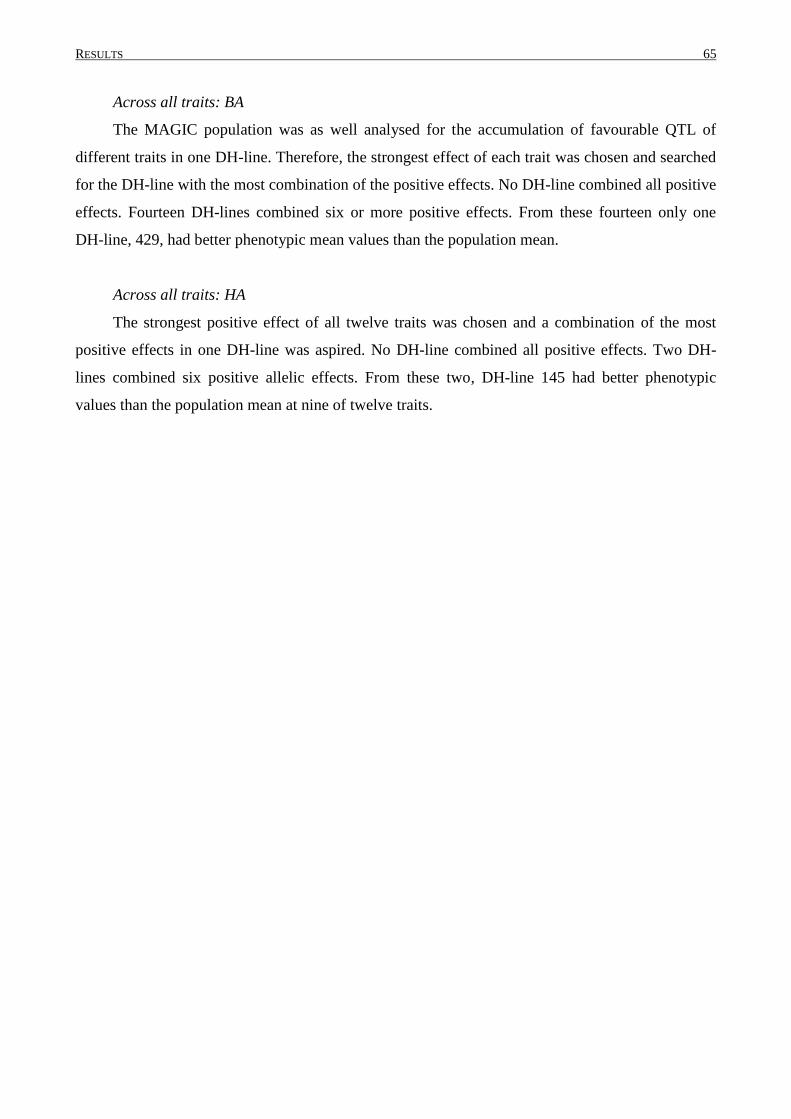
RESULTS 65

Across all traits: BA

The MAGIC population was as well analysed for the accumulation of favourable QTL of

different traits in one DH-line. Therefore, the strongest effect of each trait was chosen and searched

for the DH-line with the most combination of the positive effects. No DH-line combined all positive

effects. Fourteen DH-lines combined six or more positive effects. From these fourteen only one

DH-line, 429, had better phenotypic mean values than the population mean.

Across all traits: HA

The strongest positive effect of all twelve traits was chosen and a combination of the most

positive effects in one DH-line was aspired. No DH-line combined all positive effects. Two DH-

lines combined six positive allelic effects. From these two, DH-line 145 had better phenotypic

values than the population mean at nine of twelve traits.

DISCUSSION 66

4. Discussion

The aim of the present MAGIC DH-line analysis was to use the advantage of the crossing

scheme for a multi-parent cross to identify QTL for yield and yield components under two water

scenarios. In addition, epistatic effects within the barley genome were identified. The discussion

will be structured as following: First, the genetic characterization of the MAGIC population is

discussed. Second, the advantages and drawbacks of the THz-sensor as a measurement for water

content in leaves are analysed. Third, the mapped QTL with the two approaches are compared with

each. Fourth, the clustering of QTL in the genome will be elucidated. Fifth, the mapped QTL are

compared with QTL and genes known from literature. Sixth, the appropriateness of the chosen traits

to investigate drought tolerance and the detected QTL are discussed in comparison with literature.

Seventh, the investigated epistatic effects and their role in the expression of quantitative traits are

outlined. Eight, the pyramidisation of positive allelic effects in DH-lines is elucidated. Finally, the

MAGIC population as mapping population will be discussed.

4.1 Characterization of the MAGIC population

Population structure

The population structure was measured with a PCA to determine if the variability within the

population was biased. It was expected that no correction would be needed if the crossing scheme

was well conducted and balanced. With the low first and second principal component, which

explained 6.8% and 4.1%, respectively, the variability within the population was low and needed

no further correction.

Linkage disequilibrium

A detailed knowledge of LD has been considered a prerequisite for effective population-

based, high-resolution gene mapping (Caldwell et al., 2006). Population history, breeding systems

and the species of interest have an influence on the decay of LD. The analysis of LD in the

MAGIC population showed a rapid decay of LD within the first 5 cM. This decay had been known

from barley and reported by different researchers. It was more rapid then the decay of LD reported

by Stracke et al. (2003) measured in an association panel of spring and winter barley. And it was

close to the LD extent that had recently been reported (2.5-3.5 cM) by Comadran et al. (2009) in

an association panel of 192 barley accessions from the Mediterranean basin. These reference

populations are association panel, with a different population history and structure than the

MAGIC population. In comparison with the four parent MAGIC population in wheat, where the

DISCUSSION 67

mean LD dropped down to <0.8 within the ~5 cM (Huang et al., 2012), the decay of LD in the

barley MAGIC population formed an excellent base for QTL mapping.

Haplotype construction

The chance of each parent to be inherited to the offspring was theoretically equal. Therefore

each parent was supposed to be represented by 12.5% on each chromosome of the offspring. The

real distribution of each parent of the MAGIC population is listed in Table 17 and showed unequal

distribution of the parents. First of all, the value of not explained regions of the chromosomes with

an average of 37.81% was quite high. More than one third of the chromosomes of the offspring

cannot be explained by any parent and therefore was handled as missing values. Genetic positions

with a missing haplotype value were neglected in respect to allelic effect. Therefore, more than

one third of the genome and at 2H nearly 50%, of the genetic positions did not present any results

for the haplotype mapping approach. Time, effort and enhanced statistical methods are needed to

improve the haplotype mapping approach.

The distribution of each parent within each chromosome was as well not consistent with the

theory (Table 17). The mean distribution ranged from 0.05% (Criewener 403) to 12.1% (Barke).

The parents Ackermanns Bavaria (11.3%), Barke (12.1%), Heils Franken (9.8%), Heines Hanna

(11.3%) and Ragusa (9.9%) were inherited to the offspring like expected. The parents Pflugs

Intensiv (1.8%), Ackermanns Danubia (6.0%) and Criewener 403 (0.1%) were underrepresented.

Especially the parent Criewener 403 can be appointed as not represented within the MAGIC

population. The analysis of the genetic data with the program Flapjack (Copyright © 2007-2012,

Information & Computational Sciences, JHI.) (Milne et al., 2010) revealed that the parents

Criewener 403 and Pflugs Intensiv genetically did not differ from each other (Fig. 10) and parent

Ackermanns Danubia was 88.6% similar to them. Further genetic and phenotypic analysis about

the similarity of these two barley landraces need to be conducted to reassure the contribution of

the parents to the MAGIC population.

DISCUSSION 68

Fig. 10: Similarity of Pflugs Intensiv and Ackermanns Bavaria to parent Criewener 403 based on 5117

SNP markers used in the analysis.

Z583=Criewener 403, Z591=Pflugs Intensiv and Z579=Ackermanns Danubia. Criewener 403 and

Pflugs Intensiv are to 100% similar and both to 88.6% similar to Ackermanns Danubia.

Genetic map

Recombination and crossing over happened during the crossing of the eight parents and

within the following generations of crossing. Therefore, a genetic map for the offspring needed to

be constructed. R/mpMap is the only program that allows a genetic map construction of a multi-

parental population and was written by Huang and George (2011) and used by Huang et al. (2012)

within the four parents MAGIC population in wheat. Unfortunately, in the barley MAGIC

population no equal distribution of the SNP markers over the genome was achieved. On average

one SNP marker was located every 1.2 cM, but big gaps between SNP markers and doubling of

SNPs at one position were detected. Compared to the equal distribution of the SNP marker on the

genetic map build by Comadran et al. (2012), the genetic map established with R/mpMap lacks

power and precision. But compared with the genetic map of the wheat MAGIC population with a

marker density of 3.3, 2.4 and 8.7 cM (Huang et al., 2012) respectively to the three genomes, the

genetic map for this MAGIC population had a dense distribution of genetic markers.

4.2 THz-measurement

The multiple comparisons between the parents for the two traits measured with the THz-

sensor revealed low significant differences between the parents for trait WCT. There, only two of

the eight parents differed from each other. For trait WL Pflugs Intensiv was the parent with the

lowest water loss value. Consequently, Ackermanns Bavaria, Barke, Heils Franken and Heines

Hanna differed significantly to Pflugs Intensiv. Therefore, a high variability within the parents was

detected. This high variability could not be confirmed through the mean comparisons of the

inherited alleles at the detected QTL positions between the parental allelic means. No correlation

has been detected between traits evaluated with the THz-Sensor and yield and yield components.

DISCUSSION 69

It is known from literature that the water status of leaves can be measured with a THz-sensor

(Federici, 2012). One of the first applications of a THz-sensor was to measure the moisture content

of tobacco products (Chan et al., 2007). Monitoring of hydration state in leaves was successfully

conducted (Jordens et al., 2009; Mittleman et al., 1996). The THz-sensor was able to measure time

dynamics of water transport in a leaf (Mittleman et al., 1996) and to distinguish between fully

watered leaves and drying leaves. The experiments were conducted on houseplants (Mittleman et

al., 1996) or on single coffee plants (Jordens et al., 2009). The following research was mostly

conducted from the engineering site and focused on optimising the permittivity model. No water

status measurement was ever conducted on barley before. Neither the time of plant development

during drought stress nor the compensating strategies of a growing plant were taken into account,

nor focused any research project on the determination of differences in water content between

genotypes of the same species by the THz-sensor. Therefore, no comparison with results from

literature can be undertaken. This clarifies the novelty of this study.

4.3 Comparison of the two mapping approaches

A total of 78 QTL for twelve traits were detected with the BA, a total of 65 QTL with the HA.

The following chapter will discuss the simultaneously mapped QTL with both approaches and the

advantages and drawbacks of each mapping approach.

4.3.1 Above ground biomass, leaf senescence and plant height

Above ground biomass

The two mapping approaches revealed 16 QTL for BA and eleven QTL for HA for above

ground biomass (AGB) with p<0.05, of which five were mapped with both approaches. The QTL

on 4H (QAgb.MAGIC.BA-4H.a and QAgb.MAGIC.HA-4H.a), mapped with both approaches, had

the same most significant SNP marker position in common (10.6 cM), but the HA mapped the QTL

in a wider genetic interval of 10 cM. The strength of the allelic effect was double with the HA, the

strongest effect was measured between the alleles from Ragusa (9.1 g AGB) and Heils Franken (10

g AGB). The BA is not able to address the effect to a certain parent, this approach is lacking power.

The same accounted for the second QTL mapped with both approaches on 4H (QAgb.MAGIC.BA-

4H.c and QAgb.MAGIC.HA-4H.b), where the allele effect with BA is calculated to 0.4 g and to ±1

g with the HA. The information from the raw binary data identified Ragusa as the parent carrying

the less frequent allele and the increase in AGB can be assigned to Ragusa. The results from the HA

disclosed the contrasting parents Ackermanns Bavaria (9.1 g AGB) and Ragusa (10.1 g AGB) as

the main allele effect.

DISCUSSION 70

The two QTL QAgb.MAGIC.BA-5H.d and QAgb.MAGIC.HA-5H.b were mapped into the same

genetic interval but to different most significant SNP marker position, which were 12.2 cM apart.

Due to the overlapping genetic intervals they were considered as same QTL. As mentioned above,

the BA had less power to dissect the QTL effect compared to the HA, in this particular case the

effect was four times smaller. This lack of power in the BA was particular strong if more than one

parent carried the less frequent allele. This can be identified with the raw data. In case of

QAgb.MAGIC.BA-5H.d, Ragusa, Pflugs Intensiv and Criewener 403 were assigned to the less

frequent allele, the other parents to the more frequent allele. The allelic mean of the genotypes from

different parents which carried the same alleles, due to the binary code, can interfere with each

other and neutralise the effect between allele 0 and 1.

The position of the most significant marker for the QTL mapped to 7H (QAgb.MAGIC.BA-7H.a

and QAgb.MAGIC.HA-7H.a) with both approaches were the same (36.9 cM), but the HA mapped

the QTL into a wider genetic interval. The QTL effect was slightly higher with the HA, reason for

that are mentioned above.

The only marker*treatment interaction, mapped parallel with both approaches was located with a

distance of 0.7 cM between the most significant markers to chromosome 1H. The genetic interval of

the QTL mapped with HA (QAgb.MAGIC.HA-1H.a) was greater (13.9 cM) than the one mapped

with BA (QAgb.MAGIC.BA-1H.a) (0.7 cM). The observed differences in the QTL effect (BA= 0.6;

HA= ±1.4 under well watered and BA=0; HA= ±0.2 under terminal drought) resulted from the lack

of power mentioned above in the BA.

Ten QTL detected with the BA were not detected with the HA, six QTL detected with the HA but

not with the BA. Two of them were overlapping with the genetic interval in which they were

mapped, but the most significant SNP markers were 27.5 cM (chromosome 2H) and 27.1 cM

(chromosome 5H) apart and will therefore not be counted as the same QTL.

Therefore 22 different QTL for AGB were mapped with the two mapping approaches.

Leaf senescence

The two mapping approaches revealed seven QTL for BA and six QTL for HA for leaf

senescence (AUDPC), of which four could be mapped with both approaches. The QTL on 1H,

QAuc.MAGIC.HA-1H.a and QAuc.MAGIC.BA-1H.a, were mapped with the most significant SNP

marker 17.3 cM apart, but mapped into overlapping genetic intervals and therefore considered as

the same QTL. The other parallel mapped QTL on 2H, 125.2 cM, QAuc.MAGIC.HA-2H.a and

QAuc.MAGIC.BA-2H.a, and 5H, 217.6 cM, QAuc.MAGIC.HA-5H.b and QAuc.MAGIC.BA-5H.a,

were mapped to the same marker position and at the QTL mapped with both approaches on 4H with

DISCUSSION 71

a distance of 1.4 cM. The allele effect of the HA was stronger for all parallel mapped QTL. The

allelic effects came from different parents, at 1H, the biggest difference in AUDPC is measured

between the allele from Ackermanns Bavaria (49.7) and Heils Franken (52.3), whereas at

chromosome 2H between Barke (48.8) and Heils Franken (54.1). The only QTL with

marker*treatment interaction which was mapped with both approaches was located on 5H, 217.6

cM. The HA identified the allele from Barke as the one with lowest leaf senescence under well

watered conditions. The same was detected using the raw binary data. Under terminal drought

conditions genotypes with the allele from Ragusa had the lowest leaf senescence. This effect could

not be detected with the BA.

All the QTL that was not mapped simultaneously with both approaches have small effects and can

maybe therefore not be mapped with the other approach.

Therefore, nine different QTL for AUDPC were mapped with the two mapping approaches.

Plant height

The two mapping approaches revealed six QTL for BA and eight QTL for HA for plant height

(PLH), of which four could be mapped with both approaches. Three of them were main marker

QTL effects, mapped to the same most significant SNP marker position with both approaches,

respectively. In all cases the HA detected a stronger QTL effect than the BA and could address, in

case of the QTL on 3H, QPlh.MAGIC.HA-3H.b and QPlh.MAGIC.BA-3H.c Pflugs Intensiv (90.2

cm) and Barke (73.9 cm) as the parents with most contrasting alleles. At chromosome 5H,

QPlh.MAGIC.HA-5H.a and QPlh.MAGIC.BA-5H.a, Ragusa (91.5 cm) and Barke (85.1 cm) carried

the most contrasting alleles. Ragusa (88.2 cm) and Ackermanns Bavaria (81.2 cm) at the QTL on

7H, QPlh.MAGIC.HA-7H.a and QPlh.MAGIC.BA-7H.a were defined as most contrasting parents.

No marker*treatment interaction effects were detected with the HA, but a main marker effect at the

same position like a marker*treatment interaction effect mapped with the BA on chromosome 3H,

around 72 cM, QPlh.MAGIC.HA-3H.a and QPlh.MAGIC.BA-3H.a. The main marker effect from

the HA can be explained by the differences from contrasting alleles from Ragusa (92.8 cm) and

Heines Hanna (81.9 cm). The QTL effect from the marker*treatment interaction is 7.7 cm under

well watered conditions and 3.6 cm under terminal drought between genotypes carrying the less

frequent and the more frequent allele.

Ten different QTL for plant height (PLH) were mapped with the two mapping approaches.

DISCUSSION 72

4.3.2 Days to heading and grain filling period

Days to heading

The two mapping approaches revealed eight QTL for BA and seven QTL for HA for days to

heading (DHE), of which only three could be mapped with both approaches. The three QTL that

were mapped with both approaches are located on chromosome 3H with the most significant SNP

marker mapped to 168.9 cM, on 5H at 206.4 cM and on 7H in a genetic interval of 30.5-32.7 cM.

The comparison of the allele effects between the approaches, BA= -1.2 days and HA= -2.9, on

chromosome 3H (QDhe.MAGIC.HA-3H.b and QDhe.MAGIC.BA-3H.b) pointed out the power of

the HA. Not only the QTL effect was higher with the HA, but also the contribution of each parent to

the effect can be assigned. The differences between the alleles from Ackermanns Bavaria and Barke

were responsible for the strong QTL effect.

The same accounted for the QTL mapped to 5H, 206.4 cM (QDhe.MAGIC.HA-5H.b and

QDhe.MAGIC.BA-5H.b). Information from the binary raw data assigned Ragusa as the only parent

carrying the less frequent allele, which enhanced DHE by 2.4 days. The allele effect is stronger with

the HA (3.2 days) and revealed the biggest differences between the allele from Ragusa (58.8 DHE)

and the allele from Ackermanns Bavaria (55.6 DHE). Fig. 11 pictured the differences in the mean

allelic effects as an example for the haplotype approach. Due to the raw data the mean value for

allele 0 (grey) from the BA coincided with the parental allelic mean from Ragusa (blue) as seen on

Fig. 11. The loss of power in the BA derived from the biased mean for allele 0 (black) which low

information content compared to the parental allelic mean of Ackermanns Bavaria (red) was

explicit visible in Fig. 11. This figure demonstrated as well, that the parental allelic mean, for

example from Barke (orange) changed along the chromosome (here on chromosome 5H). This

allowed a precise allocation of the best contributing parent. The same parental allele pattern like at

QDhe.MAGIC.HA-5H.b and QDhe.MAGIC.BA-5H.b was found for the QTL on 7H, 30.5-32.7

cM. The QTL QDhe.MAGIC.HA-3H.a mapped on 3H by HA could be identical with

QDhe.MAGIC.BA-3H.a, but the most significant SNPs were 8.4 cM apart and the genetic intervals

were not overlapping. The rather small QTL effects on 4H and 5H detected by BA were not

detected with HA and vice versa. The strong effect of QDhe.MAGIC.BA-7H.b at 36.9 cM could not

be validated with the HA, a QTL at 48.0 cM, QDhe.MAGIC.HA-7H.b, was detected instead. But

this QTL showed the same tendency with greater effect in DHE between Ackermanns Bavaria (53.8

DHE) and Ragusa (59.7 DHE). If these are two different QTL or the same, needs to be clarified.

Therefore, twelve different QTL for DHE were mapped with the two mapping approaches.

DISCUSSION 73

Grain filling period

For the trait grain filling period (DGF) four QTL were mapped with the BA and three with the

HA, of which two were mapped with both programs. Whereas the two QTL were mapped with only

one significant SNP marker by the BA to chromosome 5H, 53.4 cM and 6H, 106.1 cM, the HA

mapped the QTL into genetic intervals of 3.8 cM and 10.7 cM, respectively. The allele effect

calculated with the HA was stronger in both cases than the one from BA.

Interestingly at chromosome 5H, QDgf.MAGIC.HA-5H.a and QDgf.MAGIC.BA-5H.a, the two

contrasting alleles came from Ackermanns Bavaria (37.8 DGF) and Heils Franken (39.6 DGF). At

chromosome 6H, QDgf.MAGIC.HA-6H.a and QDgf.MAGIC.BA-6H.a, the pattern was vice versa,

the allele from Ackermanns Bavaria led to 39.1 DGF and the one from Heils Franken to 37.9 DGF.

QDgf.MAGIC.HA-2H.a, the QTL with the strongest effect, 4.9 days difference between Ragusa

(33.9 DGF) and Barke (38.8 DGF), was not detected by BA. The rather small effects detected with

the BA on 3H and 5H were not detected with the HA. Interaction with water treatment was

calculated, but no genotype*treatment interaction was detected.

Therefore, five different QTL for DGF were mapped with the two mapping approaches.

DISCUSSION 74

Fig. 11: Differences between the mapping power of the allelic parental means.

Ragusa (blue), Ackermanns Bavaria (red) and Barke (orange) from HA and allelic means for 0 (grey) and 1 (black) from BA for QDhe.MAGIC.HA-

5H.b (QDhe.MAGIC.BA-5H.b).

DISCUSSION 75

4.3.3 Number of ears/ plant, number of kernels/ear and flower abortion

Number of ears/plant

Four QTL were detected with the BA on chromosome 2H, 3H and two on 5H for the trait

number of ears, both on 5H were mapped with the HA as well. The HA mapped the QTL to a single

significant marker at 0 cM, QNep.MAGIC.HA-5H.a and QNep.MAGIC.HA-5H.b at 206.4 cM,

whereas the BA located the QTL QNep.MAGIC.BA-5H.a and QNep.MAGIC.BA-5H.b into a

genetic interval of 15 cM and 8 cM, respectively. The effects of the alleles were similar with both

approaches, HA enabled to address the allele from Ragusa as the one being responsible for a

reduction in number of ears for QNep.MAGIC.HA-5H.a and increased number of ears for

QNep.MAGIC.HA-5H.b. Therefore, four different QTL for NE were mapped with the two mapping

approaches.

Number of kernels/ear

The two mapping approaches detected the same QTL at the same position or the same genetic

interval for number of kernels. The most significant SNP markers were different, due to the fact that

more than one marker was mapped to the same position.

Both approaches resulted in similar QTL effects for the QTL mapped to 2H, 144.2 cM,

QNke.MAGIC.HA-2H.a and QNke.MAGIC.BA-2H.a. The HA addressed at the main effect the

biggest differences between the alleles to the parents Ragusa and Ackermanns Bavaria. The same

parental and effect pattern appeared for the marker*treatment interaction.

The allele effect mapped to 4H, QNke.MAGIC.HA-4H.a and QNke.MAGIC.BA-4H.a, differed

nearly twice in its strength between the approaches but was not as strong as the one detected on 2H.

The HA discovered the alleles from Ackermanns Bavaria and Ragusa as responsible for the smaller

number of kernels (17.4), and from the remaining parents for a higher number of kernels (19.0 to

19.9). Due to the lower information content of the BA it underestimated the QTL effect at

chromosome 4H.

Therefore, two different QTL for NK were mapped with the two mapping approaches.

Flower abortion

The number of detected QTL for flower abortion was low, two with the BA and one identical

one with the HA on chromosome 2H, mapped in a genetic interval of 1.4 cM with the most

significant marker at 144.2 cM, the same genetic region that was significant for a QTL for number

of kernels. The effects of the QTL QFla.MAGIC.HA-2H.a and QFla.MAGIC.BA-2H.a from both

DISCUSSION 76

approaches were similar in their strength; the effect can be addressed with the information content

from the HA to the allele from parent Ragusa.

Therefore, two different QTL for FA were mapped with the two mapping approaches.

4.3.4 Thousand kernel weight and grain yield

Thousand kernel weight

Three QTL were detected with the BA for the trait thousand kernel weight (TKW). Five QTL

were detected with the HA, of which two were mapped parallel with both approaches. The parallel

mapped QTL were both main marker QTL effects mapped on 2H, 141.7 cM and 5H, 206.3 cM. The

QTL mapped with both approaches on 2H, QTkw.MAGIC.HA-2H.b and QTkw.MAGIC.BA-2H.a,

were mapped as a main marker and marker*treatment interaction effect with the BA and only for as

a main marker effect with HA. The effect for the main marker was stronger with the HA, assigning

the allele from Ragusa with the lowest TKW (37.8 g) and the allele from Barke with the highest

TKW (50.3 g). For the first time the information rate for the identification of a marker*treatment

effect was lower in the HA compared to the BA, which detected a marker*treatment interaction

with significant different allelic effects between the two water treatments. The second parallel

mapped QTL, QTkw.MAGIC.HA-5H.a and QTkw.MAGIC.BA-5H.a, was a main marker effect in

both approaches, the information rate with the HA was greater than with the BA.

Therefore, 6 different QTL for TKW were mapped with the two mapping approaches.

Grain yield

Eleven QTL were detected with the BA for grain yield (YLD). Six QTL were detected with

the HA, of which three were mapped parallel with both approaches. The only QTL with main

marker effect mapped at the same position with both approaches was on 5H at 0 cM,

QYld.MAGIC.HA-5H.a and QYld.MAGIC.BA-5H.a. The HA had a greater QTL effect, addressing

the alleles from Heils Franken and Ragusa for the differences in grain yield by 0.6 g.

The most significant SNP markers for the parallel mapped QTL on 2H were 4.6 cM apart, the

genetic intervals of both approaches were overlapping and the QTL therefore considered as the

same QTL. QYld.MAGIC.BA-2H.b was significant for a marker*treatment interaction, whereas the

parallel mapped QTL with HA, QYld.MAGIC.HA-2H.a, was significant for main marker and

marker*treatment interaction. The HA was able to assign the allele from Barke as the responsible

one for the reduction of yield for the main QTL effect and the marker*treatment interaction under

both watering treatments. The allele for the highest yield under well watered conditions came from

DISCUSSION 77

Ragusa, but the allele from Heines Hanna had a greater effect on increasing yield under terminal

drought conditions.

Similar characteristics were detected on chromosome 4H, QYld.MAGIC.HA-4H.a and

QYld.MAGIC.BA-4H.a the most significant markers are 8.5 cM apart, the HA mapped the QTL in

a larger genetic interval of 10.6 cM, whereas the most significant marker of the BA represented the

upper interval border. A main marker effect with HA and a main marker and marker*interaction

effect with BA was detected. The alleles from Ragusa and Heils Franken were responsible for the

reduced and increased yield, respectively. Further eight QTL with BA, two of them with

marker*treatment interaction were detected, as well as three more with the HA, one with

marker*treatment interaction.

Therefore, 14 different QTL for YLD were mapped with the two mapping approaches.

4.3.5 Water content and water loss

Water content

Eight QTL were detected with the BA for water content (WCT). Seven QTL were detected

with the HA, of which four were mapped parallel with both approaches. The parallel mapped QTL

on chromosome 2H, QWct.MAGIC.HA-2H.a and QWct.MAGIC.BA-2H.a, had the most

significant SNP markers located 12.8 cM apart, but the location of the QTL overlapped in large

genetic intervals and was therefore considered as the same QTL. The other parallel mapped QTL

were located with the most significant SNP marker at the same position or 2.9 cM apart like on

chromosome 6H, QWct.MAGIC.HA-6H.a and QWct.MAGIC.BA-6H.a, QWct.MAGIC.HA-6H.b

and QWct.MAGIC.BA-6H.b. The allele effect explained with the HA was higher in all parallel

mapped QTL, due to the greater power of detecting the contrasting alleles. But the allelic effect was

not consistent to one parent, at 2H the allele from Ragusa caused the highest and in

QWct.MAGIC.HA-6H.b and QWct.MAGIC.BA-6H.b, the lowest water content of all parental

alleles. The same could be observed with the allele from Ackermanns Bavaria at the QTL on 5H,

QWct.MAGIC.HA-5H.a and QWct.MAGIC.BA-5H.a, and QWct.MAGIC.HA-6H.a and

QWct.MAGIC.BA-6H.a. Four QTL mapped with the BA and three with the HA were mapped

additionally but they all had smaller effects on the trait.

Therefore, eleven different QTL for WCT were mapped with the two mapping approaches.

Water loss

Seven QTL were detected with the BA for water loss (WL). Seven QTL were detected with

the HA, of which three were mapped parallel with both approaches. The position of the most

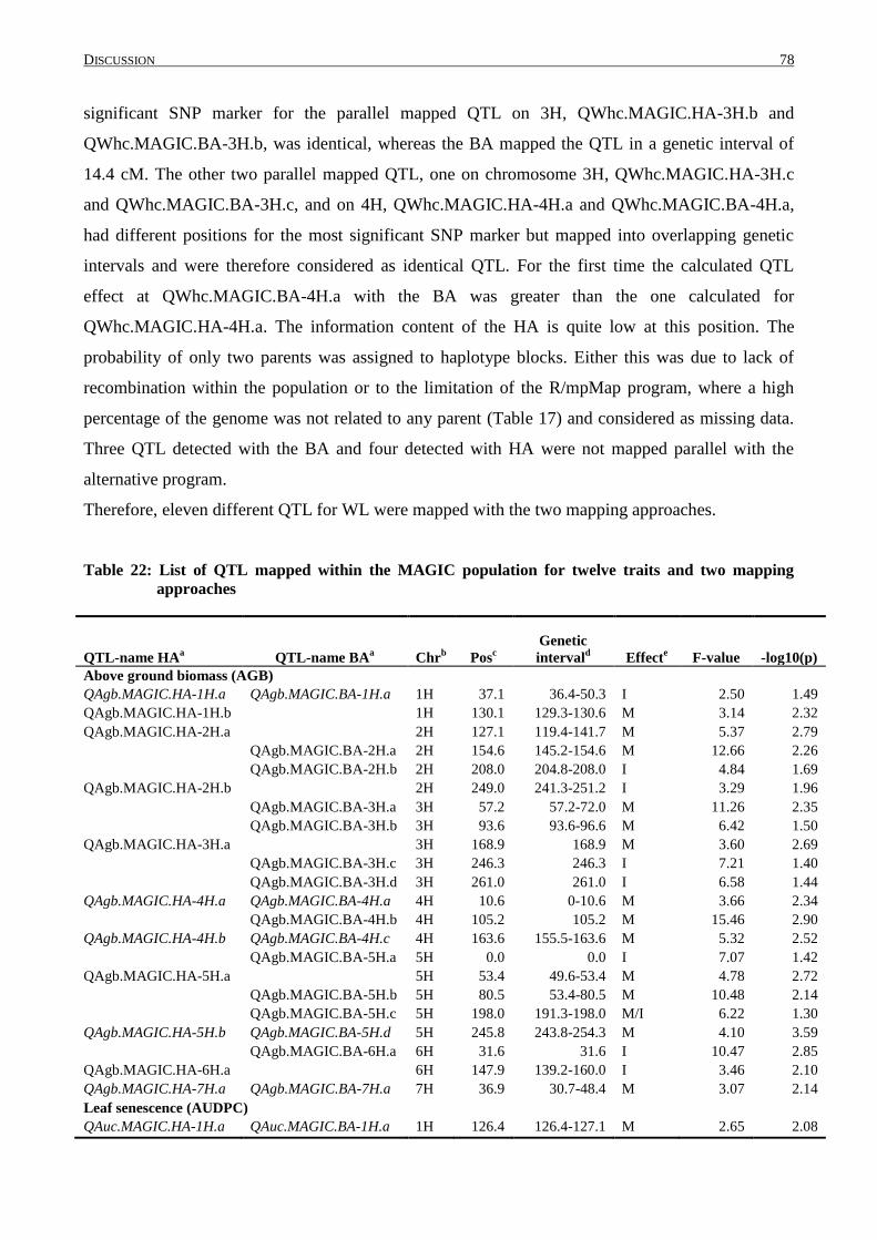
DISCUSSION 78

significant SNP marker for the parallel mapped QTL on 3H, QWhc.MAGIC.HA-3H.b and

QWhc.MAGIC.BA-3H.b, was identical, whereas the BA mapped the QTL in a genetic interval of

14.4 cM. The other two parallel mapped QTL, one on chromosome 3H, QWhc.MAGIC.HA-3H.c

and QWhc.MAGIC.BA-3H.c, and on 4H, QWhc.MAGIC.HA-4H.a and QWhc.MAGIC.BA-4H.a,

had different positions for the most significant SNP marker but mapped into overlapping genetic

intervals and were therefore considered as identical QTL. For the first time the calculated QTL

effect at QWhc.MAGIC.BA-4H.a with the BA was greater than the one calculated for

QWhc.MAGIC.HA-4H.a. The information content of the HA is quite low at this position. The

probability of only two parents was assigned to haplotype blocks. Either this was due to lack of

recombination within the population or to the limitation of the R/mpMap program, where a high

percentage of the genome was not related to any parent (Table 17) and considered as missing data.

Three QTL detected with the BA and four detected with HA were not mapped parallel with the

alternative program.

Therefore, eleven different QTL for WL were mapped with the two mapping approaches.

Table 22: List of QTL mapped within the MAGIC population for twelve traits and two mapping

approaches

QTL-name HAa QTL-name BA

a Chr

b Pos

c

Genetic

intervald Effect

e F-value -log10(p)


QAgb.MAGIC.HA-1H.a QAgb.MAGIC.BA-1H.a 1H 37.1 36.4-50.3 I 2.50 1.49

QAgb.MAGIC.HA-1H.b 1H 130.1 129.3-130.6 M 3.14 2.32

QAgb.MAGIC.HA-2H.a 2H 127.1 119.4-141.7 M 5.37 2.79


QAgb.MAGIC.BA-2H.b 2H 208.0 204.8-208.0 I 4.84 1.69

QAgb.MAGIC.HA-2H.b 2H 249.0 241.3-251.2 I 3.29 1.96



QAgb.MAGIC.HA-3H.a 3H 168.9 168.9 M 3.60 2.69

QAgb.MAGIC.BA-3H.c 3H 246.3 246.3 I 7.21 1.40

QAgb.MAGIC.BA-3H.d 3H 261.0 261.0 I 6.58 1.44

QAgb.MAGIC.HA-4H.a QAgb.MAGIC.BA-4H.a 4H 10.6 0-10.6 M 3.66 2.34

QAgb.MAGIC.BA-4H.b 4H 105.2 105.2 M 15.46 2.90

QAgb.MAGIC.HA-4H.b QAgb.MAGIC.BA-4H.c 4H 163.6 155.5-163.6 M 5.32 2.52

QAgb.MAGIC.BA-5H.a 5H 0.0 0.0 I 7.07 1.42

QAgb.MAGIC.HA-5H.a 5H 53.4 49.6-53.4 M 4.78 2.72


QAgb.MAGIC.BA-5H.c 5H 198.0 191.3-198.0 M/I 6.22 1.30

QAgb.MAGIC.HA-5H.b QAgb.MAGIC.BA-5H.d 5H 245.8 243.8-254.3 M 4.10 3.59

QAgb.MAGIC.BA-6H.a 6H 31.6 31.6 I 10.47 2.85

QAgb.MAGIC.HA-6H.a 6H 147.9 139.2-160.0 I 3.46 2.10

QAgb.MAGIC.HA-7H.a QAgb.MAGIC.BA-7H.a 7H 36.9 30.7-48.4 M 3.07 2.14


QAuc.MAGIC.HA-1H.a QAuc.MAGIC.BA-1H.a 1H 126.4 126.4-127.1 M 2.65 2.08

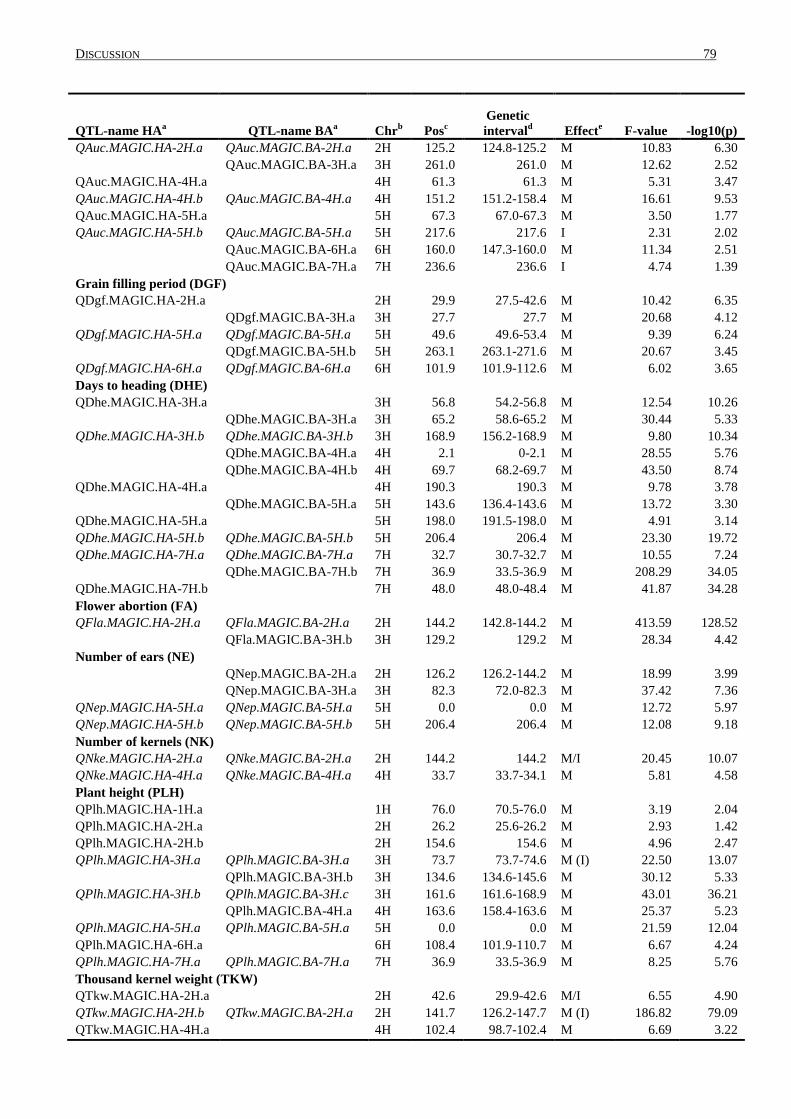
DISCUSSION 79


a Chr

b Pos

c

Genetic

intervald Effect

e F-value -log10(p)

QAuc.MAGIC.HA-2H.a QAuc.MAGIC.BA-2H.a 2H 125.2 124.8-125.2 M 10.83 6.30


QAuc.MAGIC.HA-4H.a 4H 61.3 61.3 M 5.31 3.47

QAuc.MAGIC.HA-4H.b QAuc.MAGIC.BA-4H.a 4H 151.2 151.2-158.4 M 16.61 9.53

QAuc.MAGIC.HA-5H.a 5H 67.3 67.0-67.3 M 3.50 1.77

QAuc.MAGIC.HA-5H.b QAuc.MAGIC.BA-5H.a 5H 217.6 217.6 I 2.31 2.02


QAuc.MAGIC.BA-7H.a 7H 236.6 236.6 I 4.74 1.39

Grain filling period (DGF)

QDgf.MAGIC.HA-2H.a 2H 29.9 27.5-42.6 M 10.42 6.35


QDgf.MAGIC.HA-5H.a QDgf.MAGIC.BA-5H.a 5H 49.6 49.6-53.4 M 9.39 6.24

QDgf.MAGIC.BA-5H.b 5H 263.1 263.1-271.6 M 20.67 3.45

QDgf.MAGIC.HA-6H.a QDgf.MAGIC.BA-6H.a 6H 101.9 101.9-112.6 M 6.02 3.65


QDhe.MAGIC.HA-3H.a 3H 56.8 54.2-56.8 M 12.54 10.26


QDhe.MAGIC.HA-3H.b QDhe.MAGIC.BA-3H.b 3H 168.9 156.2-168.9 M 9.80 10.34

QDhe.MAGIC.BA-4H.a 4H 2.1 0-2.1 M 28.55 5.76


QDhe.MAGIC.HA-4H.a 4H 190.3 190.3 M 9.78 3.78


QDhe.MAGIC.HA-5H.a 5H 198.0 191.5-198.0 M 4.91 3.14

QDhe.MAGIC.HA-5H.b QDhe.MAGIC.BA-5H.b 5H 206.4 206.4 M 23.30 19.72

QDhe.MAGIC.HA-7H.a QDhe.MAGIC.BA-7H.a 7H 32.7 30.7-32.7 M 10.55 7.24


QDhe.MAGIC.HA-7H.b 7H 48.0 48.0-48.4 M 41.87 34.28


QFla.MAGIC.HA-2H.a QFla.MAGIC.BA-2H.a 2H 144.2 142.8-144.2 M 413.59 128.52

QFla.MAGIC.BA-3H.b 3H 129.2 129.2 M 28.34 4.42

Number of ears (NE)

QNep.MAGIC.BA-2H.a 2H 126.2 126.2-144.2 M 18.99 3.99

QNep.MAGIC.BA-3H.a 3H 82.3 72.0-82.3 M 37.42 7.36

QNep.MAGIC.HA-5H.a QNep.MAGIC.BA-5H.a 5H 0.0 0.0 M 12.72 5.97

QNep.MAGIC.HA-5H.b QNep.MAGIC.BA-5H.b 5H 206.4 206.4 M 12.08 9.18


QNke.MAGIC.HA-2H.a QNke.MAGIC.BA-2H.a 2H 144.2 144.2 M/I 20.45 10.07

QNke.MAGIC.HA-4H.a QNke.MAGIC.BA-4H.a 4H 33.7 33.7-34.1 M 5.81 4.58

Plant height (PLH)

QPlh.MAGIC.HA-1H.a 1H 76.0 70.5-76.0 M 3.19 2.04


QPlh.MAGIC.HA-2H.b 2H 154.6 154.6 M 4.96 2.47

QPlh.MAGIC.HA-3H.a QPlh.MAGIC.BA-3H.a 3H 73.7 73.7-74.6 M (I) 22.50 13.07

QPlh.MAGIC.BA-3H.b 3H 134.6 134.6-145.6 M 30.12 5.33

QPlh.MAGIC.HA-3H.b QPlh.MAGIC.BA-3H.c 3H 161.6 161.6-168.9 M 43.01 36.21

QPlh.MAGIC.BA-4H.a 4H 163.6 158.4-163.6 M 25.37 5.23

QPlh.MAGIC.HA-5H.a QPlh.MAGIC.BA-5H.a 5H 0.0 0.0 M 21.59 12.04


QPlh.MAGIC.HA-7H.a QPlh.MAGIC.BA-7H.a 7H 36.9 33.5-36.9 M 8.25 5.76


QTkw.MAGIC.HA-2H.a 2H 42.6 29.9-42.6 M/I 6.55 4.90

QTkw.MAGIC.HA-2H.b QTkw.MAGIC.BA-2H.a 2H 141.7 126.2-147.7 M (I) 186.82 79.09

QTkw.MAGIC.HA-4H.a 4H 102.4 98.7-102.4 M 6.69 3.22

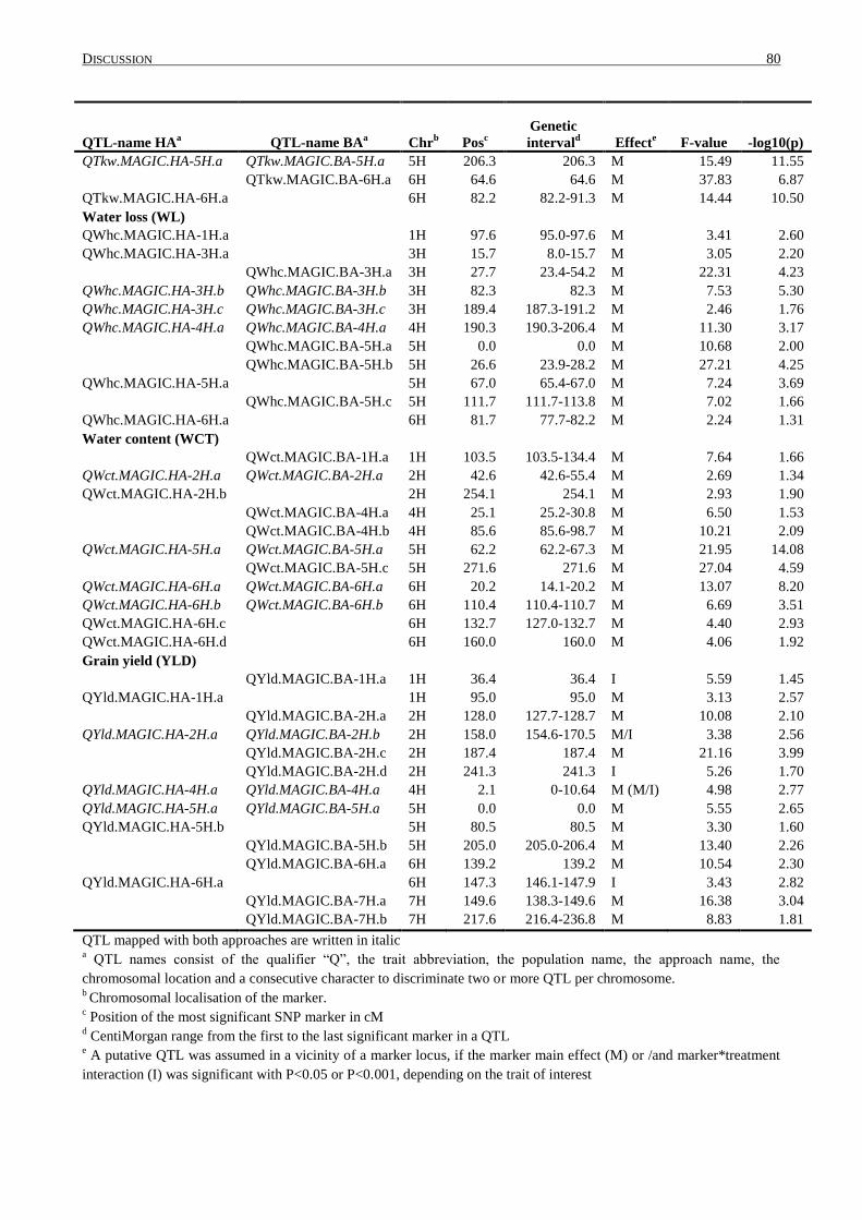
DISCUSSION 80


a Chr

b Pos

c

Genetic

intervald Effect

e F-value -log10(p)

QTkw.MAGIC.HA-5H.a QTkw.MAGIC.BA-5H.a 5H 206.3 206.3 M 15.49 11.55

QTkw.MAGIC.BA-6H.a 6H 64.6 64.6 M 37.83 6.87

QTkw.MAGIC.HA-6H.a 6H 82.2 82.2-91.3 M 14.44 10.50

Water loss (WL)

QWhc.MAGIC.HA-1H.a 1H 97.6 95.0-97.6 M 3.41 2.60


QWhc.MAGIC.BA-3H.a 3H 27.7 23.4-54.2 M 22.31 4.23

QWhc.MAGIC.HA-3H.b QWhc.MAGIC.BA-3H.b 3H 82.3 82.3 M 7.53 5.30

QWhc.MAGIC.HA-3H.c QWhc.MAGIC.BA-3H.c 3H 189.4 187.3-191.2 M 2.46 1.76

QWhc.MAGIC.HA-4H.a QWhc.MAGIC.BA-4H.a 4H 190.3 190.3-206.4 M 11.30 3.17

QWhc.MAGIC.BA-5H.a 5H 0.0 0.0 M 10.68 2.00

QWhc.MAGIC.BA-5H.b 5H 26.6 23.9-28.2 M 27.21 4.25


QWhc.MAGIC.BA-5H.c 5H 111.7 111.7-113.8 M 7.02 1.66


Water content (WCT)


QWct.MAGIC.HA-2H.a QWct.MAGIC.BA-2H.a 2H 42.6 42.6-55.4 M 2.69 1.34

QWct.MAGIC.HA-2H.b 2H 254.1 254.1 M 2.93 1.90


QWct.MAGIC.BA-4H.b 4H 85.6 85.6-98.7 M 10.21 2.09


QWct.MAGIC.BA-5H.c 5H 271.6 271.6 M 27.04 4.59


QWct.MAGIC.HA-6H.b QWct.MAGIC.BA-6H.b 6H 110.4 110.4-110.7 M 6.69 3.51

QWct.MAGIC.HA-6H.c 6H 132.7 127.0-132.7 M 4.40 2.93

QWct.MAGIC.HA-6H.d 6H 160.0 160.0 M 4.06 1.92

Grain yield (YLD)

QYld.MAGIC.BA-1H.a 1H 36.4 36.4 I 5.59 1.45

QYld.MAGIC.HA-1H.a 1H 95.0 95.0 M 3.13 2.57


QYld.MAGIC.HA-2H.a QYld.MAGIC.BA-2H.b 2H 158.0 154.6-170.5 M/I 3.38 2.56

QYld.MAGIC.BA-2H.c 2H 187.4 187.4 M 21.16 3.99

QYld.MAGIC.BA-2H.d 2H 241.3 241.3 I 5.26 1.70

QYld.MAGIC.HA-4H.a QYld.MAGIC.BA-4H.a 4H 2.1 0-10.64 M (M/I) 4.98 2.77

QYld.MAGIC.HA-5H.a QYld.MAGIC.BA-5H.a 5H 0.0 0.0 M 5.55 2.65

QYld.MAGIC.HA-5H.b 5H 80.5 80.5 M 3.30 1.60


QYld.MAGIC.BA-6H.a 6H 139.2 139.2 M 10.54 2.30

QYld.MAGIC.HA-6H.a 6H 147.3 146.1-147.9 I 3.43 2.82



QTL mapped with both approaches are written in italic a QTL names consist of the qualifier “Q”, the trait abbreviation, the population name, the approach name, the

chromosomal location and a consecutive character to discriminate two or more QTL per chromosome. b Chromosomal localisation of the marker.



e A putative QTL was assumed in a vicinity of a marker locus, if the marker main effect (M) or /and marker*treatment

interaction (I) was significant with P<0.05 or P<0.001, depending on the trait of interest

DISCUSSION 81

The contribution of each parent at the genetic position of interest was examined through the

calculated allelic mean at the QTL position. This provides an additional information content gained

through the haplotype approach as mentioned in 4.3. The comparisons between the allelic means of

the parents were conducted as multiple comparisons to investigate the significant differences of all

parental means to each other. From the eighteen investigated QTL only one, QAuc.MAGIC.HA-

4H.a, was discovered were only two of the parents, Heils Franken and Ragusa, the most contrasting

ones, were significant to each other. All the remaining parents were not significant different to Heils

Franken with the highest AUDPC value or Ragusa, with the lowest AUDPC value.

The multiple comparisons at four QTL discovered that one parental mean was significant to all

other parental mean. This was detected at QNep.MAGIC.HA-5H.b and QTKW.MAGIC.HA-2H.a,

were the parental mean of Ragusa was identified as the extreme value. The inclusion of Ragusa as a

parent into the MAGIC population enhanced the allelic diversity within the population due to a

different origin of Ragusa compared to the other seven parents. The extreme values identified at the

other two QTL, QAuc.MAGIC.HA-4H.b and QYld.MAGIC.HA-4H.a can be assigned to Barke and

Heils Franken, respectively. The mean of Barke had a high allelic effect at that position on the trait

AUDPC. Barke was the only modern variety that contributed to the crossing scheme of the MAGIC

population. Barke was genetically separated from the remaining parents, which are all landraces, by

approximately 90 years of active barley breeding. This is illustrated in the breeding success as in the

shorter phenotype of Barke with higher biomass at shorter tillers. This could lead to a tendency of

higher AUDPC scores. At QYld.MAGIC.HA-4H.a, the allelic mean of Heils Franken outranged all

other parental means. The parental mean for yield at this position was higher than the one from

Barke, which was expected to have a higher effect on yield, due to the status as a modern variety.

The QTL for DHE under investigation for multi comparisons showed nearly the same parental

pattern. The allelic effect from Ragusa was always the highest, with the longest time until heading.

The allelic effect from Ackermanns Bavaria was always the lowest. Therefore, the allelic effect for

the QTL was significant between these two parental means. The multiple comparisons of DHE

unravelled further significant differences. The parental mean of Heines Hanna was always

significant different to the mean of Ragusa and the mean of Ackermanns Bavaria. The distinct

groups were investigated in all three QTL, which indicates a stable contribution of the parents to

this trait DHE.

In summary, 35 QTL were detected with both approaches. Additionally, 43 QTL were

detected with the binary approach and 30 with the haplotype approach (Table 22). Both approaches

showed advantages and drawbacks. Rating the approaches by their strength of the -log10 (p) and

DISCUSSION 82

mean allelic effects the haplotype approach performed better in all except one of the 35 QTL (Fig.

12). This allows the conclusion that the haplotype approach is more precise in calculating the actual

effect of a QTL. Rating the approaches by the size of the genetic interval in which the QTL was

mapped, the binary approach shows advantages due to the specification of a smaller genetic

interval. This is clearly demonstrated in Fig. 11.

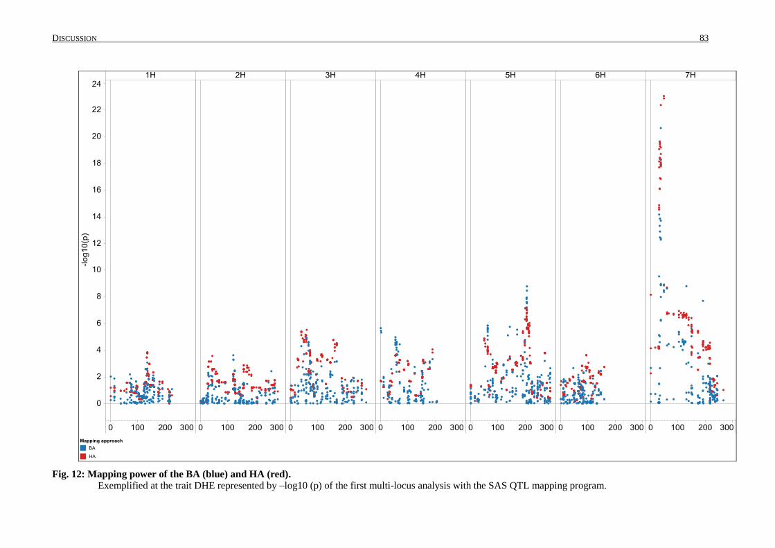
DISCUSSION 83

Fig. 12: Mapping power of the BA (blue) and HA (red).

Exemplified at the trait DHE represented by –log10 (p) of the first multi-locus analysis with the SAS QTL mapping program.

DISCUSSION 84

4.4 Distribution of QTL within the genome

The distribution of the QTL was not random within the genome for agronomic traits. The

majority of the QTL was detected on chromosome 2H, 3H and 5H (Fig. 13). Several QTL for

different traits were found in genetic proximity to each other and were considered as QTL cluster.

The QTL were mapped at the same position or within genetic intervals. Cluster for the traits YLD

and AGB were found on 1H, three on 2H, 4H, 5H and 6H, of which the cluster on 1H, 2H (around

141 cM) and 6H showed traits with marker*treatment interaction effects. A strong and highly

significant correlation between these traits was detected under both watering conditions which

support the idea that these traits are controlled by the same locus (McKay et al., 2003).

A second interesting group of traits clustered including QTL related to water status of leaves (WCT

or WL). Two clusters were detected on 1H, the first one included QTL for YLD and WL. Due to the

results from the haplotype approach, the allele from Heils Franken at this locus can be assigned as

the allele for an increase in grain yield and the lowest water loss during the drying period measured

with the THz sensor. A second cluster, including QTL for WCT, AUDPC and AGB was detected

close by (around 103-130 cM). Unfortunately, the QTL for WCT was only detected by the BA; the

alleles leading to high water content in leaves are common in Ackermanns Bavaria, Heines Hanna

and Ragusa. The remaining two QTL of the cluster were mapped with the HA and assigned the

positive effects, low AUDPC despite high AGB to the allele from Ackermanns Bavaria, too.

Summarizing, the allele from Ackermanns Bavaria had a positive effect on the QTL in a cluster on

chromosome 1H.

A group of QTL clustered on chromosome 5H, 0.0 cM for different traits, among these was a QTL

for WL and YLD. Again, the QTL for WL was only mapped by the BA; the more frequent allele

had a significant lower water loss over time in the leaves and was inherited by Ackermanns

Bavaria, Barke, Heils Franken and Ragusa. The allele from Heils Franken was responsible for the

highest allelic effect for the trait yield, mapped at the same position on the chromosome.

Summarizing, the allele from Heils Franken had a positive QTL effect on water loss and grain yield.

Another cluster of QTL was detected on 5H, around 62-80 cM, including QTL for WCT, WL,

AUDPC and AGB. Except for the effect for AGB all were mapped with the HA. But the raw data

from the BA assigned Barke as the sole parent inheriting the less frequent allele and increasing the

AGB by 0.5 g. Interestingly, the allele from Barke was responsible for the second lowest leaf

senescence (AUDPC) but for the lowest water content after 96 hours of drying (WCT). A

comparison between the parents for the mean of AUDPC over two years showed that Barke had a

quite low leaf senescence under well watered, and the lowest under terminal drought conditions.

This could be due to the breeding process of the last 90 years, Barke as the only modern variety in

DISCUSSION 85

this set of parents could also be characterized by the QTL effect for AUDPC as a “stay green”

genotype, representing the improvement in plant breeding. But that does not legitimate the high

effect of the allele from Barke for the high water loss (WL) or the low water content (WCT), the

other way round: a low effect on leaf senescence would expect a low water loss. This requires

further analysis.

A similar pattern was detected on chromosome 6H, 160 cM with a cluster of two QTL of AUDPC

and WCT. Unfortunately, the allelic effect for AUDPC was only mapped with BA, but the raw data

results showed the parent Ackermanns Danubia and Heines Hanna carried the less frequent allele

which was responsible for a higher AUDPC compared to the more frequent allele. The QTL effect

from WCT assigned the most contrasting effects coming from the allele from Heines Hanna, which

increased the water content after 96 hours of drying to 84.6%, and to the allele from Ackermanns

Danubia (72%). This implied that AUDPC and water content or water loss are contrasting traits.

Genotypes with low water loss during their juvenile stage cannot be selected for low AUDPC. The

determination of water loss cannot be used a selection criteria for leaf senescence in the later

growing stage of the plant.

Several QTL studies have reported clustering of QTL (Li et al., 2007; McCartney et al., 2006; Pillen

et al., 2003). Results from the QTL analysis of the MAGIC population from Arabidopsis showed

clustering of a QTL for days to germination within a nitrilase gene cluster on chromosome 3H

(Kover et al., 2009). This cluster phenomenon could be considered as “multifactorial linkages”

followed by natural selection favouring co-adapted traits. Further it is possible, that the clustering is

based on pleiotropy of unknown key factors controlling various traits through diverse metabolic

pathways (Cai and Morishima, 2002). In barley as an inbreeding species, natural hybridisation may

have played an important role during the domestication process, preserving chromosome blocks

carrying co-adapted genes.

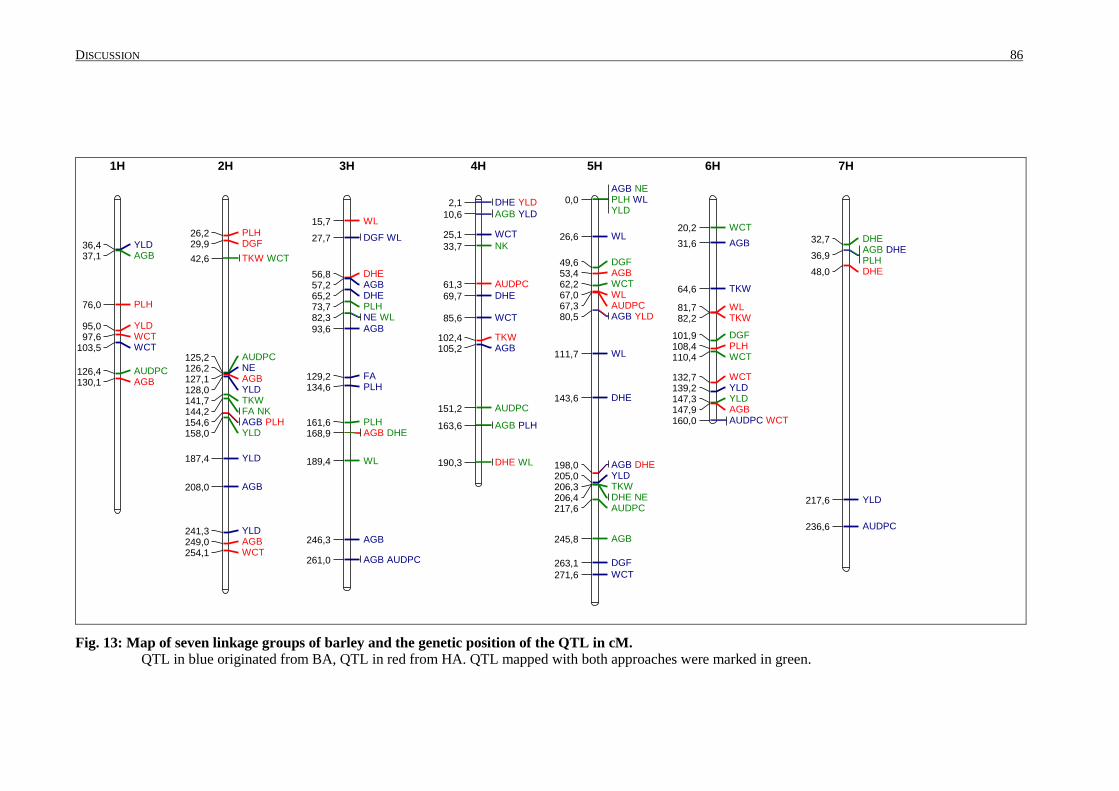
DISCUSSION 86

YLD36,4AGB37,1

PLH76,0

YLD95,0WCT97,6WCT103,5

AUDPC126,4AGB130,1

1H

PLH26,2DGF29,9

TKW WCT42,6

AUDPC125,2NE126,2AGB127,1YLD128,0TKW141,7FA NK144,2AGB PLH154,6YLD158,0

YLD187,4

AGB208,0

YLD241,3AGB249,0WCT254,1

2H

WL15,7

DGF WL27,7

DHE56,8AGB57,2DHE65,2PLH73,7NE WL82,3AGB93,6

FA129,2PLH134,6

PLH161,6AGB DHE168,9

WL189,4

AGB246,3

AGB AUDPC261,0

3H

DHE YLD2,1AGB YLD10,6

WCT25,1NK33,7

AUDPC61,3DHE69,7

WCT85,6

TKW102,4AGB105,2

AUDPC151,2

AGB PLH163,6

DHE WL190,3

4H

AGB NEPLH WLYLD

0,0

WL26,6

DGF49,6AGB53,4WCT62,2WL67,0AUDPC67,3AGB YLD80,5

WL111,7

DHE143,6

AGB DHE198,0YLD205,0TKW206,3DHE NE206,4AUDPC217,6

AGB245,8

DGF263,1WCT271,6

5H

WCT20,2

AGB31,6

TKW64,6

WL81,7TKW82,2

DGF101,9PLH108,4WCT110,4

WCT132,7YLD139,2YLD147,3AGB147,9AUDPC WCT160,0

6H

DHE32,7AGB DHEPLH

36,9

DHE48,0

YLD217,6

AUDPC236,6

7H

YLD36,4AGB37,1

PLH76,0


AUDPC126,4AGB130,1

1H

PLH26,2DGF29,9

TKW WCT42,6


YLD187,4

AGB208,0

YLD241,3AGB249,0WCT254,1

2H

WL15,7

DGF WL27,7


FA129,2PLH134,6


WL189,4

AGB246,3

AGB AUDPC261,0

3H


WCT25,1NK33,7

AUDPC61,3DHE69,7

WCT85,6

TKW102,4AGB105,2

AUDPC151,2

AGB PLH163,6

DHE WL190,3

4H

AGB NEPLH WLYLD

0,0

WL26,6


WL111,7

DHE143,6


AGB245,8

DGF263,1WCT271,6

5H

WCT20,2

AGB31,6

TKW64,6

WL81,7TKW82,2

DGF101,9PLH108,4WCT110,4


6H

DHE32,7AGB DHEPLH

36,9

DHE48,0

YLD217,6

AUDPC236,6

7H

Fig. 13: Map of seven linkage groups of barley and the genetic position of the QTL in cM.

QTL in blue originated from BA, QTL in red from HA. QTL mapped with both approaches were marked in green.

DISCUSSION 87

4.5 Confirmed and novel QTL: comparison with known QTL and candidate genes

The results from QTL mapping for yield and yield related traits in the MAGIC population

were compared with studies of candidate genes and other QTL and association mapping approaches

in barley, in particular to Pasam et al. (2012), Comadran et al. (2011b), Wang et al. (2010),

Schmalenbach et al. (2009) von Korff et al. (2008) and von Korff et al. (2006). The results were

compared to Varshney et al. (2012), Comadran et al. (2008), Talame et al. (2004), Forster et al.

(2004), Baum et al. (2003) and Teulat et al. (2001b) under the aspect of drought environments and

the identification of QTL and genes responsible for drought tolerance. The mapping populations

used in the compared studies had different genetic approaches for the detection of drought tolerant

QTL or genes. Baum et al. (2003), von Korff et al. (2006), Schmalenbach et al. (2009), Talame et

al. (2004) and Wang et al. (2010) used populations or advanced backcrosses of a genotype with a

wild barley accession (Hordeum vulgare ssp. spontaneum), Forster et al. (2004) used a doubled

haploid population from a cross of two genotypes, Derkado and B83-12/21/5, von Korff et al.

(2008) and Teulat et al. (2001b) used progenies from the cross of Tadmor and ER/Apm to test their

performance in QTL mapping and under drought stress conditions. Comadran et al. (2008), Pasam

et al. (2012) and Varshney et al. (2012) tested association panels under abiotic stress conditions to

investigate QTL under drought stress and to study the performance of association mapping. Table

23 and Fig. 14 displays the QTL detected in the MAGIC DH-lines as main marker and

marker*treatment interaction and coinciding gene candidates from BLASTn and candidate genes

and QTL from studied literature. Comparing the exact genetic position between the coinciding QTL

is not feasible, different genetic maps were used for the QTL studies. The QTL from the MAGIC

population listed in Table 23 as coinciding were mapped in the same genetic region. Altogether, 26

of the QTL detected in the MAGIC population corresponded to QTL and genes found in literature

or in a database. Comparing the QTL effects is not feasible as well; different crossing schemes,

different parents and different statistical programs were used within the studies. With the exception

of the association studies, bi-parental crossings were used for QTL mapping. In cases of populations

with a Hordeum spontaneum parent, the contribution of the exotic allele to the QTL was calculated.

Only if the QTL was mapped with the HA, a direct contribution from a single parent can be

assigned to the QTL effect. The most coinciding QTL were detected for plant height, yield and

above ground biomass. No QTL could be validated for leaf senescence (AUDPC) or water status

and water loss, measured with the THz-Sensor. Each trait will be discussed below.

DISCUSSION 88

4.5.1 Days to heading

Heading date is a critical trait for adaption to different environments and cultivation areas. It

is the result of the interaction of different environmental factors and genes, including vernalization,

photoperiodic response or earliness per se. Most QTL mapping populations in the past used a cross

between a winter and spring barley, to investigate the vernalization and photoperiodic genes. The

parents of the MAGIC population are all spring barley, with the exception of Ragusa, which can be

assigned as a semi-type. Therefore, out of the classical studied flowering genes only Vrn-H3 could

be of interest in the MAGIC population. The QTL QDhe.MAGIC.HA-7H.a was mapped with both

approaches to the short arm of chromosome 7H. This position corresponded to the barley

vernalization gene Vrn-H3 (Laurie et al., 1995; Yan et al., 2006), which was confirmed among

others by Schmalenbach et al. (2009) (QHea.S42IL-7H.a) and mapped recently to chromosome 7H,

28.8 cM, by Comadran et al. (2012). QDhe.MAGIC.HA-7H.a (QDhe.MAGIC.BA-7H.a) for days to

heading corresponded to the gene HvGI, mapped by Wang et al. (2010). Ten unique QTL for days

to heading were detected in the MAGIC population.

4.5.2 Plant height

The most QTL could be confirmed for the trait plant height, which is a well a studied trait in

barley. QPlh.MAGIC.HA-1H.a could be confirmed by Schmalenbach et al. (2009) to Qhei.S4IL-

1H.a and QPlh.MAGIC.HA-2H.b to QHt.StMo-2H.2 was mapped by Hayes et al. (1993) on

chromosome 2H. One QTL on chromosome 3H, QPlh.MAGIC.HA-3H.a (QPlh.MAGIC.BA-3H.a),

coincided with a QTL detected by Baum et al. (2003), PH.3H-4, and Pasam et al. (2012),

QTL7_PHT. A second QTL on 3H, QPlh.MAGIC.BA-3H.b coincided with the dwarfing gene

swd1/denso from Laurie et al. (1995), which was detected in several studies. The

QPlh.MAGIC.HA-3H.b (QPlh.MAGIC.BA-3H.c) coincided with QTL QTL.9_PHT and QTL

QPlh.MAGIC.HA-6H.a matched with QTL17_PHT, both mapped by Pasam et al. (2012). The QTL

QPlh.MAGIC.HA-7H.a (QPlh.MAGIC.BA-7H.a) for plant height was confirmed by a mapped

QTL von Korff et al. (2008) (Qhei.S42.-7H.b). Three unique QTL for plant height were mapped in

the MAGIC population.

4.5.3 Grain yield and yield components

Grain yield is well known as a complex trait, especially in interaction with drought

conditions. It has always been one of the most important breeding goals and therefore is a well

studied trait. Dissecting the complex trait grain yield into components which may be under simpler

genetic control has been one of the approaches to understand the trait. Therefore, in this study not

DISCUSSION 89

only grain yield was analysed, but as well above ground biomass, flower abortion, number of ears,

number of kernels per ear and the thousand kernel weight.

Above ground biomass (ABG)

Five QTL for above ground biomass coincided with known QTL from literature; one QTL

from the MAGIC population, QAgb.MAGIC.BA-5H.b matched with BYnb.5H-4 mapped by Baum

et al. (2003). Three QTL, QAgb.MAGIC.HA-3H.a, QAgb.MAGIC.BA-4H.b and

QAgb.MAGIC.HA-4H.b (QAgb.MAGIC.BA-4H.c) were already mapped in von Korff et al. (2006)

as Qmas.S42-3H.a, Qmas.S42-4H.a and Qmas.S42-4H.b. respectively.

The first marker*treatment interaction QTL QAgb.MAGIC.HA-1H.a (QAgb.MAGIC.BA-1H.a)

detected for above ground biomass was confirmed by the QTL BYnb.1H-1 in the study from Baum

et al. (2003), in which a set of AB-QTL RILs were phenotyped under two rain fed levels, based on

the location of the research station. In the AB-QTL study, the exotic allele from Hordeum

spontaneum had a positive effect of the biomass under drought conditions. The marker*treatment

effect in the MAGIC population was detected by both approaches. Under well watered conditions,

the allele from Ragusa had the biggest effect on the above ground biomass, enhancing it by 0.6

g/plant compared to the modern variety Barke. But under terminal drought conditions, the positive

effect to produce high amount of biomass was assigned to the genotype Ackermanns Bavaria,

which had the highest effect on the trait. Seventeen additional QTL were mapped in the MAGIC

population, which were not mentioned in barley literature before.

Flower abortion (FA) number of ears (NE), number of kernels (NK) and thousand kernel

weight (TKW)

One QTL, QFla.MAGIC.HA-2H.a (QFla.MAGIC.BA-2H.a), matched via BLASTn of the

most significant SNP marker sequence with the vrs1 gene for row-type (Komatsuda et al., 2007).

The detected QTL QNke.MAGIC.HA-2H.a (QNke.MAGIC.BA-2H.a) and QTkw.MAGIC.HA-

2H.b (QTkw.MAGIC.BA-2H.a) were mapped at the same position and therefore confirm the vrs1

gene as well. The QTL for number of kernels, QNke.MAGIC.HA-2H.a (QNke.MAGIC.BA-2H.a),

mapped in the MAGIC population on chromosome 2H, 144.2 cM had main marker and

marker*treatment interaction effects and was mapped parallel with both approaches. This QTL

coincided with detected QTL by Comadran et al. (2011) under drought environments.

A second QTL for number of kernels, QNke.MAGIC.HA-4H.a (QNke.MAGIC.BA-4H.a) matched

with the region of the gene int-c (Waugh et al., 2009) and coincided with a QTL mapped by

DISCUSSION 90

Comadran et al. (2011) in the association panel. All these allelic effects pointed out the influence of

row type number to these traits. One QTL in the MAGIC population, QNep.MAGIC.HA-5H.a

(QNep.MAGIC.BA-5H.a), for number of ears, as a component trait for yield, was mapped by von

Korff et al. (2006) as the QTL Qear.S42-5H.a and as SNP 11_20553 by Comadran et al. (2011) at

the beginning of the short arm of chromosome 5H. Besides the one QTL for TKW mentioned above

all remaining QTL mapped in the MAGIC DH-lines for TKW were mapped in other populations as

well.

The main marker and marker*treatment interaction effect in the MAGIC population,

QTkw.MAGIC.HA-2H.a, was mapped as QTL4_TGW by Pasam et al. (2012), and as a interaction

effect with drought environment as tkw_br (bPb_4875) by Varshney et al. (2012), who tested an

association panel on two contrasting experimental sites in Syria, concerning the amount of rainfall.

Three more allele effects for thousand kernel weight, QTkw.MAGIC.HA-4H.a,

QTkw.MAGIC.HA-5H.a (QTkw.MAGIC.BA-5H.a) and QTkw.MAGIC.HA-6H.a were detected on

4H, 5H and 6H, all coincided with QTL mapped by Baum et al. (2003) (KW.4H-3) on 4H, Pillen et

al. (2003) (QTgw.pil-5H.4), Pasam et al. (2012) (QTL16_TGW) and Forster et al. (2004) (TGW*)

on 5H and Forster et al. (2004) on 6H (TGW). QTkw.MAGIC.BA-6H.a mapped in the MAGIC

population by the BA coincided with the QTL Qkw-tera_6H.a by von Korff et al. (2008),

BCD348B by Teulat et al. (2001b) and KW.6H-2 by Baum et al. (2003) on 6H. One unique QTL

was mapped in the MAGIC population for flower abortion, three unique ones for number of ears.

The QTL mapped for number of kernels and thousand kernel weight were all mapped in literature

before.

For grain yield, five QTL could be confirmed with known QTL from literature. The QTL

QYld.MAGIC.HA-5H.b coincided with Qyld.S42-5H.b detected by von Korff et al. (2006),

HvUDPGPPxYLD by Pillen et al. (2003), CDO344 by Teulat et al. (2001b), GY.5H-4 by Baum et

al. (2003) and Forster et al. (2004) on chromosome 5H. The second one, QYld.MAGIC.BA-7H.b

on chromosome 7H, matched with QTL S5D, A5D, T5D detected by Comadran et al. (2008) and

WG380 Teulat et al. (2001b). One QTL for marker*treatment interaction, QYld.MAGIC.BA-1H.a

was located on chromosome 1H and coincided with a QTL for grain yield detected by Talame et al.

(2004) in a doubled haploid population from Barke and HOR11508, a wild barley accession, grown

under water deficit in three Mediterranean countries. For all three locations, the allele from Barke

increased the yield in his study. The QTL in the MAGIC population was only detected with the BA;

a favourable parent for that trait cannot be assigned, neither with the raw data. The second QTL for

marker*treatment interaction, QYld.MAGIC.BA-4H.a, coincided with a QTL from Comadran et al.

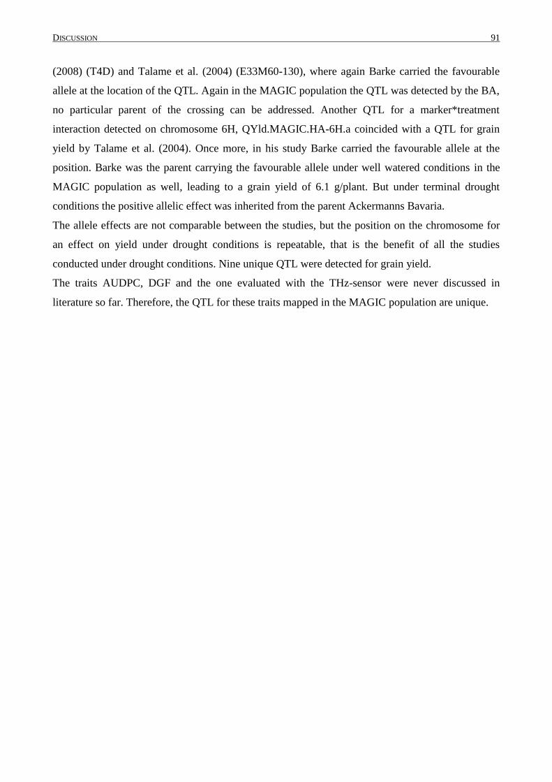
DISCUSSION 91

(2008) (T4D) and Talame et al. (2004) (E33M60-130), where again Barke carried the favourable

allele at the location of the QTL. Again in the MAGIC population the QTL was detected by the BA,

no particular parent of the crossing can be addressed. Another QTL for a marker*treatment

interaction detected on chromosome 6H, QYld.MAGIC.HA-6H.a coincided with a QTL for grain

yield by Talame et al. (2004). Once more, in his study Barke carried the favourable allele at the

position. Barke was the parent carrying the favourable allele under well watered conditions in the

MAGIC population as well, leading to a grain yield of 6.1 g/plant. But under terminal drought

conditions the positive allelic effect was inherited from the parent Ackermanns Bavaria.

The allele effects are not comparable between the studies, but the position on the chromosome for

an effect on yield under drought conditions is repeatable, that is the benefit of all the studies

conducted under drought conditions. Nine unique QTL were detected for grain yield.

The traits AUDPC, DGF and the one evaluated with the THz-sensor were never discussed in

literature so far. Therefore, the QTL for these traits mapped in the MAGIC population are unique.

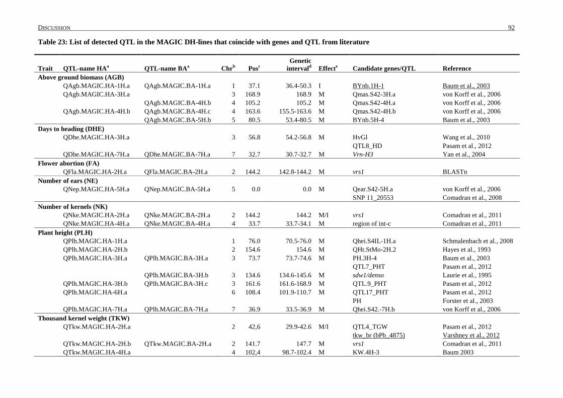
DISCUSSION 92

Table 23: List of detected QTL in the MAGIC DH-lines that coincide with genes and QTL from literature

Trait QTL-name HAa QTL-name BA

a Chr

b Pos

c

Genetic

intervald Effect

e Candidate genes/QTL Reference


QAgb.MAGIC.HA-1H.a QAgb.MAGIC.BA-1H.a 1 37.1 36.4-50.3 I BYnb.1H-1 Baum et al., 2003

QAgb.MAGIC.HA-3H.a

3 168.9 168.9 M Qmas.S42-3H.a von Korff et al., 2006

QAgb.MAGIC.BA-4H.b 4 105.2 105.2 M Qmas.S42-4H.a von Korff et al., 2006

QAgb.MAGIC.HA-4H.b QAgb.MAGIC.BA-4H.c 4 163.6 155.5-163.6 M Qmas.S42-4H.b von Korff et al., 2006

QAgb.MAGIC.BA-5H.b 5 80.5 53.4-80.5 M BYnb.5H-4 Baum et al., 2003


QDhe.MAGIC.HA-3H.a

3 56.8 54.2-56.8 M HvGl Wang et al., 2010

QTL8_HD Pasam et al., 2012

QDhe.MAGIC.HA-7H.a QDhe.MAGIC.BA-7H.a 7 32.7 30.7-32.7 M Vrn-H3 Yan et al., 2004


QFla.MAGIC.HA-2H.a QFla.MAGIC.BA-2H.a 2 144.2 142.8-144.2 M vrs1 BLASTn

Number of ears (NE)

QNep.MAGIC.HA-5H.a QNep.MAGIC.BA-5H.a 5 0.0 0.0 M Qear.S42-5H.a von Korff et al., 2006

SNP 11_20553 Comadran et al., 2008


QNke.MAGIC.HA-2H.a QNke.MAGIC.BA-2H.a 2 144.2 144.2 M/I vrs1 Comadran et al., 2011

QNke.MAGIC.HA-4H.a QNke.MAGIC.BA-4H.a 4 33.7 33.7-34.1 M region of int-c Comadran et al., 2011

Plant height (PLH)

QPlh.MAGIC.HA-1H.a

1 76.0 70.5-76.0 M Qhei.S4IL-1H.a Schmalenbach et al., 2008

QPlh.MAGIC.HA-2H.b

2 154.6 154.6 M QHt.StMo-2H.2 Hayes et al., 1993

QPlh.MAGIC.HA-3H.a QPlh.MAGIC.BA-3H.a 3 73.7 73.7-74.6 M PH.3H-4 Baum et al., 2003

QTL7_PHT Pasam et al., 2012

QPlh.MAGIC.BA-3H.b 3 134.6 134.6-145.6 M sdw1/denso Laurie et al., 1995

QPlh.MAGIC.HA-3H.b QPlh.MAGIC.BA-3H.c 3 161.6 161.6-168.9 M QTL.9_PHT Pasam et al., 2012

QPlh.MAGIC.HA-6H.a

6 108.4 101.9-110.7 M QTL17_PHT Pasam et al., 2012

PH Forster et al., 2003

QPlh.MAGIC.HA-7H.a QPlh.MAGIC.BA-7H.a 7 36.9 33.5-36.9 M Qhei.S42.-7H.b von Korff et al., 2006


QTkw.MAGIC.HA-2H.a 2 42,6 29.9-42.6 M/I QTL4_TGW Pasam et al., 2012

tkw_br (bPb_4875) Varshney et al., 2012

QTkw.MAGIC.HA-2H.b QTkw.MAGIC.BA-2H.a 2 141.7 147.7 M vrs1 Comadran et al., 2011

QTkw.MAGIC.HA-4H.a 4 102,4 98.7-102.4 M KW.4H-3 Baum 2003

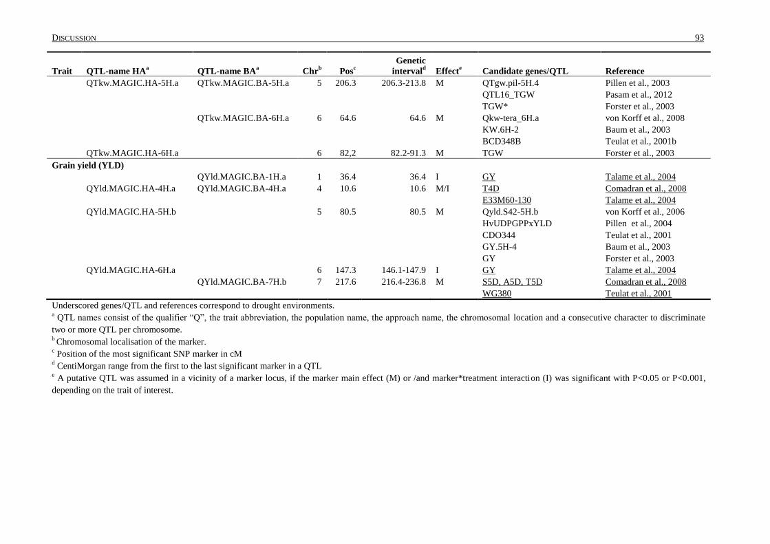
DISCUSSION 93


a Chr

b Pos

c

Genetic

intervald Effect

e Candidate genes/QTL Reference

QTkw.MAGIC.HA-5H.a QTkw.MAGIC.BA-5H.a 5 206.3 206.3-213.8 M QTgw.pil-5H.4 Pillen et al., 2003

QTL16_TGW Pasam et al., 2012

TGW* Forster et al., 2003

QTkw.MAGIC.BA-6H.a 6 64.6 64.6 M Qkw-tera_6H.a von Korff et al., 2008

KW.6H-2 Baum et al., 2003

BCD348B Teulat et al., 2001b

QTkw.MAGIC.HA-6H.a 6 82,2 82.2-91.3 M TGW Forster et al., 2003

Grain yield (YLD)

QYld.MAGIC.BA-1H.a 1 36.4 36.4 I GY Talame et al., 2004

QYld.MAGIC.HA-4H.a QYld.MAGIC.BA-4H.a 4 10.6 10.6 M/I T4D Comadran et al., 2008

E33M60-130 Talame et al., 2004

QYld.MAGIC.HA-5H.b

5 80.5 80.5 M Qyld.S42-5H.b von Korff et al., 2006

HvUDPGPPxYLD Pillen et al., 2004

CDO344 Teulat et al., 2001

GY.5H-4 Baum et al., 2003

GY Forster et al., 2003

QYld.MAGIC.HA-6H.a

6 147.3 146.1-147.9 I GY Talame et al., 2004

QYld.MAGIC.BA-7H.b 7 217.6 216.4-236.8 M S5D, A5D, T5D Comadran et al., 2008

WG380 Teulat et al., 2001

Underscored genes/QTL and references correspond to drought environments. a QTL names consist of the qualifier “Q”, the trait abbreviation, the population name, the approach name, the chromosomal location and a consecutive character to discriminate




e A putative QTL was assumed in a vicinity of a marker locus, if the marker main effect (M) or /and marker*treatment interaction (I) was significant with P<0.05 or P<0.001,

depending on the trait of interest.

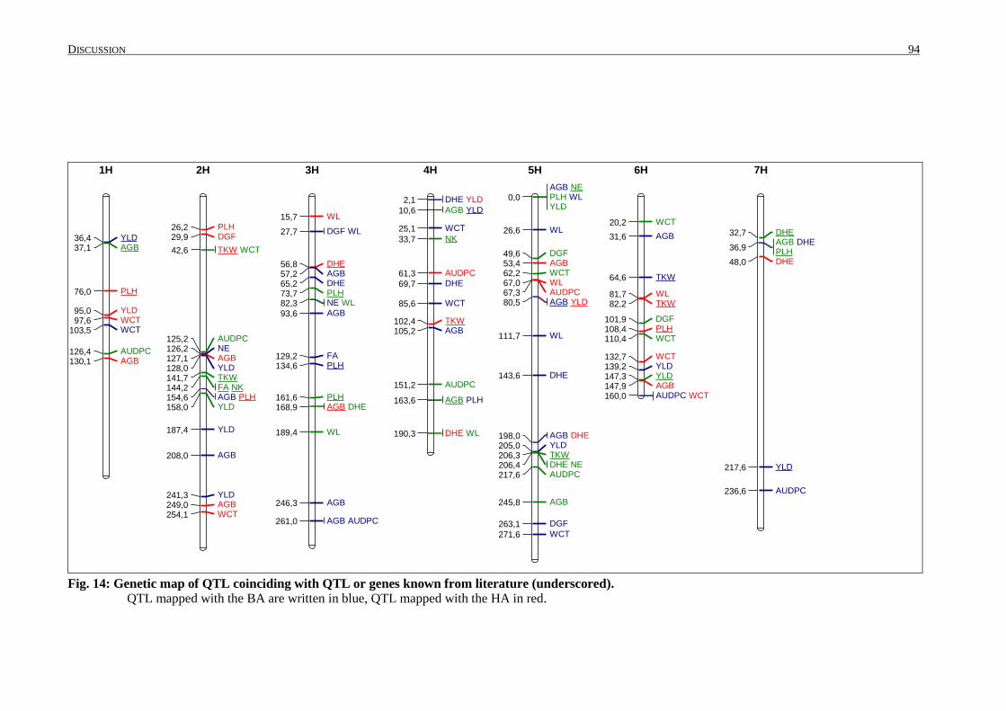
DISCUSSION 94

YLD36,4AGB37,1

PLH76,0


AUDPC126,4AGB130,1

1H

PLH26,2DGF29,9

TKW WCT42,6


YLD187,4

AGB208,0

YLD241,3AGB249,0WCT254,1

2H

WL15,7

DGF WL27,7


FA129,2PLH134,6


WL189,4

AGB246,3

AGB AUDPC261,0

3H


WCT25,1NK33,7

AUDPC61,3DHE69,7

WCT85,6

TKW102,4AGB105,2

AUDPC151,2

AGB PLH163,6

DHE WL190,3

4H

AGB NEPLH WLYLD

0,0

WL26,6


WL111,7

DHE143,6


AGB245,8

DGF263,1WCT271,6

5H

WCT20,2

AGB31,6

TKW64,6

WL81,7TKW82,2

DGF101,9PLH108,4WCT110,4


6H

DHE32,7AGB DHEPLH

36,9

DHE48,0

YLD217,6

AUDPC236,6

7H

YLD36,4AGB37,1

PLH76,0


AUDPC126,4AGB130,1

1H

PLH26,2DGF29,9

TKW WCT42,6


YLD187,4

AGB208,0

YLD241,3AGB249,0WCT254,1

2H

WL15,7

DGF WL27,7


FA129,2PLH134,6


WL189,4

AGB246,3

AGB AUDPC261,0

3H


WCT25,1NK33,7

AUDPC61,3DHE69,7

WCT85,6

TKW102,4AGB105,2

AUDPC151,2

AGB PLH163,6

DHE WL190,3

4H

AGB NEPLH WLYLD

0,0

WL26,6


WL111,7

DHE143,6


AGB245,8

DGF263,1WCT271,6

5H

WCT20,2

AGB31,6

TKW64,6

WL81,7TKW82,2

DGF101,9PLH108,4WCT110,4


6H

DHE32,7AGB DHEPLH

36,9

DHE48,0

YLD217,6

AUDPC236,6

7H

Fig. 14: Genetic map of QTL coinciding with QTL or genes known from literature (underscored).

QTL mapped with the BA are written in blue, QTL mapped with the HA in red.

DISCUSSION 95

4.6 Genotype and treatment interaction – drought tolerance

Yield was and still is the traditional target of breeding programs and breeding for high

yielding genotypes under drought stress environments is even more challenging. Therefore, yield

and yield components were investigated in 534 MAGIC DH-lines for ten different traits in the

polytunnel in 2011 and 2012 under two water treatments (well watered and terminal drought), as

well as for two traits, WCT and WL, evaluated with the THz-sensor to detected the water status in

leaves. The results from the ANOVA (Table 11) documented, that the traits DHE and FA had no

significant treatment effects as well as genotype*treatment effects. Therefore, no marker*treatment

interaction was calculated for these traits in the QTL mapping approaches. The remaining eight

traits were tested among the main marker effect for the marker*treatment interaction effects as well.

Only five of the traits, AGB, AUDPC, NK, TKW and YLD, had significant marker*treatment

interaction allele effects.

The most marker*treatment interaction allele effects were mapped in the traits AGB, nine out of 27

QTL effects were significant for marker*treatment interaction. One QTL was mapped with both

approaches, QAgb.MAGIC.HA-1H.a and QAgb.MAGIC.BA-1H.a, (chromosome 1H, 37.1 cM),

two more were mapped with the HA, six were mapped with the BA. The allelic effects estimated by

the BA for the marker*treatment interaction were rather low; the reason was already explained in

chapter 4.3. For three QTL in AGB, QAgb.MAGIC.BA-1H.a, QAgb.MAGIC.BA-5H.a and

QAgb.MAGIC.BA-6H.a the effect under terminal drought conditions was estimated to 0, which

means no allelic effect between the parents was detected under drought conditions. Interestingly,

one of this QTL (QAgb.MAGIC.BA-1H.a) was detected with the HA (QAgb.MAGIC.HA-1H.a) as

well, and in contrast to the BA the approach was able to detect an allelic effect under terminal

drought as well. The HA addressed the allele effect under the two treatments to different parents,

under well watered to Ragusa (13.1 g) and Heils Franken (11.7 g), and under terminal drought to

Barke (6.8 g) and Heils Franken (6.6 g). First, this result showed the advantage of the HA over the

BA concerning the information content and detecting of differences between the parents. Second,

the high information content from the HA enabled to identify different favourable alleles under

different watering conditions. The allele from Ragusa was not able to produce high amounts of

above ground biomass under terminal drought conditions although it clearly had the highest impact

under well watered conditions. This pattern of difference of the allelic effect between the watering

conditions of the same trait was detected for eight out of ten marker*treatment interactions with the

HA. Only the allelic effects for marker*interaction of NK, QNke.MAGIC.HA-2H.a, and TKW,

QTkw.MAGIC.HA-2H.a, were constant under both treatments, the highest NK was assigned to the

allele from Ragusa and the lowest NK to Ackermanns Bavaria. For TKW, the lowest weight was

DISCUSSION 96

inherited from Ragusa, the highest from Barke. The allelic effects for QNke.MAGIC.HA-2H.a and

QTkw.MAGIC.HA-2H.a under terminal drought were smaller than under well watered conditions.

This result implied that the allelic effect from Ragusa was strong enough to have a significant

impact on the trait, under well watered and terminal drought conditions. On the other hand, the

results implied that the selection environment for a trait like NK and TKW would be irrelevant to

the selection successes for this trait under drought.

Two out of ten mapped QTL for AUDPC had a marker*treatment interaction. Pflugs Intensiv was

the parent inheriting the allele for high leaf senescence under both treatments for the QTL mapped

to 5H; QAuc.MAGIC.HA-5H.b and QAuc.MAGIC.BA-5H.a. Reduced leaf senescence under well

watered and terminal drought conditions is a favourable trait in crops. The good phenotypic

performance of Barke under controlled conditions caved in under drought, the allele from Ragusa

performed the lowest AUDPC under drought conditions. Only 1/5 of the detected QTL for AUDPC

interacted with water treatment. For a trait like AUDPC, which is a selection criterion for the ability

of a plant to tolerate water limitation in the breeding process, a higher number of QTL with

marker*treatment interaction was expected.

Five QTL with marker*treatment interaction effect were mapped out of 14 QTL for grain yield.

Here as well a higher number of interaction effects were expected. The effects mapped with the BA

were quite small, especially for the effect under terminal drought, ranging from 0 g at QTL

QYld.MAGIC.BA-1H.a to -0.10 g at QYld.MAGIC.BA-4H.a. The effects calculated with the HA

were slightly higher, settled between 0.2 g (QYld.MAGIC.HA-6H.a) and 0.3 g (QYld.MAGIC.HA-

2H.a). This implied not only the higher power of the approach using haplotype blocks, it also

showed that the performance of all parents to drought tolerance for grain yield was rather low.

There was no outstanding allelic effect for grain yield under drought stress discovered.

Eight QTL for marker*treatment interaction were investigated with multiple mean comparisons.

The QTL for AGB, AUDPC and YLD had in common, that no significant differences were detected

between the parental means under terminal drought. Only the QTL concerning number of kernels

(QNke.MAGIC.HA-2H.a) and thousand kernel weight (QTkw.MAGIC.HA-2H.a) had significant

differences between the parents under terminal drought conditions. These significant differences

showed the same pattern as under well watered conditions, the mean of Ragusa was significantly

different to the mean of the other parents. The remaining parents differed not from each other.

Under this circumstances Ragusa could be named drought tolerant concerning number of kernels

and thousand kernel weight. Unfortunately, the effect of significant differences between the mean

of Ragusa and the remaining parents relied on the spike morphology of Ragusa. It was the only six

DISCUSSION 97

rowed barley of all parents and therefore had a significant higher amount of kernels and a

significant lower thousand kernel weight. These results were expected. As Comadran et al. (2011)

mentioned the 2- and 6-rowed barley phenotypes are under control of two major genes (Komatsuda

and Mano, 2002) both of which have already been cloned. Vrs1 on the long arm of chromosome 2H

(Pourkheirandish et al., 2007) and int-c on the short arm of chromosome 4H (Waugh et al. 2009).

The QTL QNke.MAGIC.HA-2H.a with its position on 2H, 144.2 cM matched with the gene vrs1

(Pourkheirandish et al., 2007) and therefore cannot be named an improving QTL under terminal

drought. The QTL QTkw.MAGIC.HA-2H.a was mapped as well by Pasam et al. (2012) as

QTL4_TGW and Varshney et al. (2012) as tkw_br (bPb_4875), but did not coincide with any gene

mapped before. Therefore, the QTL QTkw.MAGIC.HA-2H.a can be named as an improving QTL

for thousand kernel weight under drought with a positive allelic effect derived from parent Barke.

However, under well watered conditions the parental means for all detected marker*treatment

interactions were significantly different from each other and depending on the trait clustered in

different groups. The parental means at QYld.MAGIC.HA-2H.a clustered in four groups, where the

mean of Ragusa had the greatest amount of yield/plant and was significantly different to the variety

Barke. This effect might be dependent on the fact that Ragusa is six rowed barley landrace and has

a higher number of kernels and therefore could have a high yield. The second QTL for yield

investigated for multiple comparisons, QYld.MAGIC.HA-6H.a, showed with five clusters

significant differences between the parents within the well watered conditions. This signified that

the parents differed a lot for the trait yield between each other. This implied that the genetic

potential between the parents concerning yield is quite different and that they were well chosen as

parents for the MAGIC population. But the multiple comparisons between the parents under

terminal drought conditions revealed no significant differences, except for the two QTL for NK and

TKW mentioned above.

Except for the QTL QTkw.MAGIC.HA-2H.a and QNke.MAGIC.HA-2H.a no significant allelic

effect under terminal drought conditions could be detected. This could be due to the starting time,

the duration and severity of the terminal drought. The average yield reduction was around 45%

between well watered and terminal drought conditions. In dependence on Blum (2006), who defines

severe drought stress as a yield reduction of more than 70% compared to yield under well watered

conditions, the applied drought stress would be defined as a moderate water shortage. Yield under

more moderate water shortage reflects closely yield under favourable conditions (Blum 2006).

Therefore the applied drought stress might not have been severe enough to target the drought

tolerant genetic regions. The choice of parents could be a second drawback for the detection of QTL

under drought conditions. The eight parents differed significantly for all traits under well watered

DISCUSSION 98

conditions as seen in Table 8. Only for the traits AUDPC, DGF and YLD no significant differences

were detected under terminal drought conditions, a higher QTL potential under terminal drought

conditions was expected. The MAGIC population was not established with the only perspective of

QTL mapping under terminal drought. None of the genotypes was a drought tolerant genotype per

definition. They were chosen due to their contribution to German plant breeding.

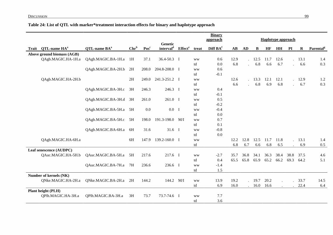
DISCUSSION 99

Table 24: List of QTL with marker*treatment interaction effects for binary and haplotype approach

Binary

approach

Haplotype approach


a Chr

b Pos

c

Genetic

intervald Effect

e treat Diff BA

f

AB AD B HF HH PI R Parentalg


QAgb.MAGIC.HA-1H.a QAgb.MAGIC.BA-1H.a 1H 37.1 36.4-50.3 I ww 0.6

12.9 . 12.5 11.7 12.6 . 13.1 1.4

td 0.0

6.8 . 6.8 6.6 6.7 . 6.6 0.3

QAgb.MAGIC.BA-2H.b 2H 208.0 204.8-208.0 I ww 0.6

td -0.1

QAgb.MAGIC.HA-2H.b

2H 249.0 241.3-251.2 I ww

12.6 . 13.3 12.1 12.1 . 12.9 1.2

td

6.6 . 6.8 6.9 6.8 . 6.7 0.3

QAgb.MAGIC.BA-3H.c 3H 246.3 246.3 I ww 0.4

td -0.1

QAgb.MAGIC.BA-3H.d 3H 261.0 261.0 I ww 0.5

td -0.2

QAgb.MAGIC.BA-5H.a 5H 0.0 0.0 I ww -0.4

td 0.0

QAgb.MAGIC.BA-5H.c 5H 198.0 191.3-198.0 M/I ww 0.7

td 0.1

QAgb.MAGIC.BA-6H.a 6H 31.6 31.6 I ww -0.8

td 0.0

QAgb.MAGIC.HA-6H.a

6H 147.9 139.2-160.0 I ww

12.2 12.8 12.5 11.7 11.8 . 13.1 1.4

td

6.8 6.7 6.6 6.8 6.5 . 6.9 0.5


QAuc.MAGIC.HA-5H.b QAuc.MAGIC.BA-5H.a 5H 217.6 217.6 I ww -2.7

35.7 36.8 34.1 36.3 38.4 38.8 37.5 4.6

td 0.4

65.5 65.8 65.9 65.2 66.2 69.3 64.2 5.1

QAuc.MAGIC.BA-7H.a 7H 236.6 236.6 I ww -1.4

td 1.5


QNke.MAGIC.HA-2H.a QNke.MAGIC.BA-2H.a 2H 144.2 144.2 M/I ww 13.9

19.2 . 19.7 20.2 . . 33.7 14.5

td 6.9

16.0 . 16.0 16.6 . . 22.4 6.4

Plant height (PLH)

QPlh.MAGIC.HA-3H.a QPlh.MAGIC.BA-3H.a 3H 73.7 73.7-74.6 I ww 7.7

td 3.6

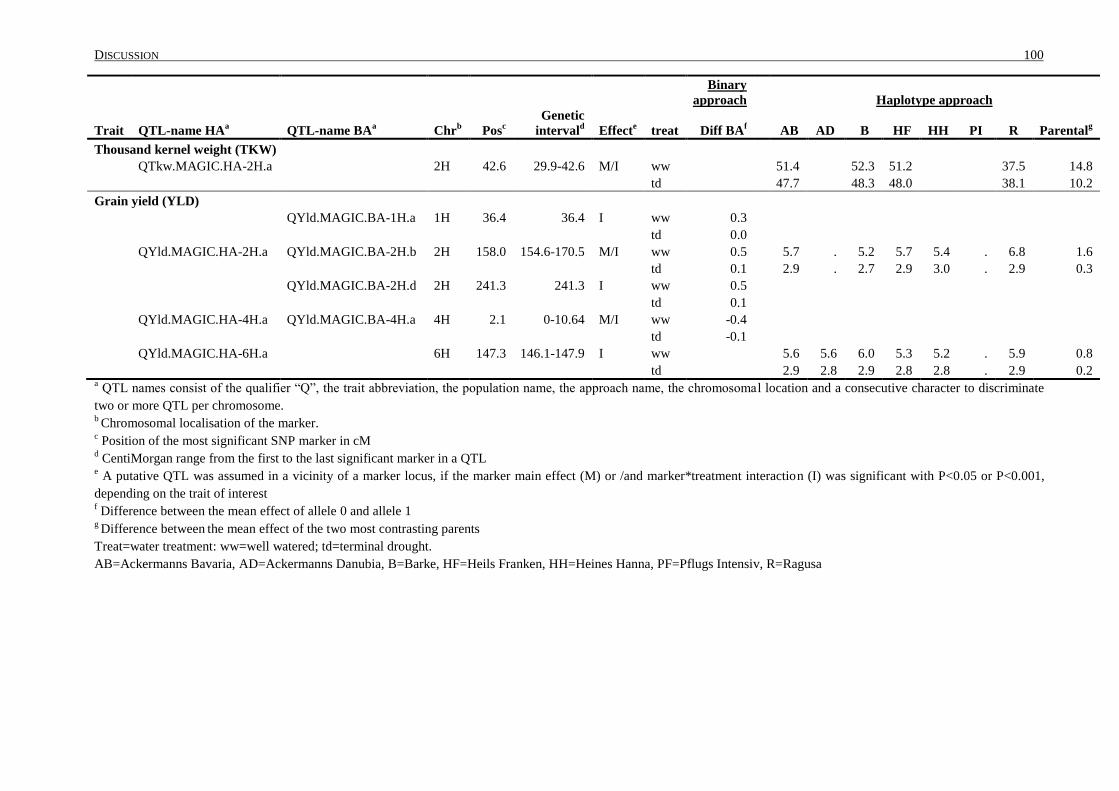
DISCUSSION 100

Binary

approach

Haplotype approach


a Chr

b Pos

c

Genetic

intervald Effect

e treat Diff BA

f

AB AD B HF HH PI R Parentalg


QTkw.MAGIC.HA-2H.a

2H 42.6 29.9-42.6 M/I ww

51.4

52.3 51.2

37.5 14.8

td

47.7

48.3 48.0

38.1 10.2

Grain yield (YLD)

QYld.MAGIC.BA-1H.a 1H 36.4 36.4 I ww 0.3

td 0.0

QYld.MAGIC.HA-2H.a QYld.MAGIC.BA-2H.b 2H 158.0 154.6-170.5 M/I ww 0.5

5.7 . 5.2 5.7 5.4 . 6.8 1.6

td 0.1

2.9 . 2.7 2.9 3.0 . 2.9 0.3

QYld.MAGIC.BA-2H.d 2H 241.3 241.3 I ww 0.5

td 0.1

QYld.MAGIC.HA-4H.a QYld.MAGIC.BA-4H.a 4H 2.1 0-10.64 M/I ww -0.4

td -0.1

QYld.MAGIC.HA-6H.a

6H 147.3 146.1-147.9 I ww

5.6 5.6 6.0 5.3 5.2 . 5.9 0.8

td

2.9 2.8 2.9 2.8 2.8 . 2.9 0.2

a QTL names consist of the qualifier “Q”, the trait abbreviation, the population name, the approach name, the chromosomal location and a consecutive character to discriminate




e A putative QTL was assumed in a vicinity of a marker locus, if the marker main effect (M) or /and marker*treatment interaction (I) was significant with P<0.05 or P<0.001,

depending on the trait of interest f Difference between the mean effect of allele 0 and allele 1

g Difference between

the mean effect of the two most contrasting parents

Treat=water treatment: ww=well watered; td=terminal drought.


DISCUSSION 101

4.7 Epistasis in the MAGIC population

In this study, diallelic epistatic interactions were calculated using a model which tested all

pairwise marker combinations. The analysis demonstrated that epistatic interactions play an

important role in quantitative traits. The calculation of epistatic effects was conducted with the

binary approach and resulted into 23 significant interactions for eight phenotypic traits. From all 46

mapped genomic positions within the epistatic effects, only twelve were mapped as main marker

allelic effects with the multi-locus analysis of the binary QTL mapping approach. In many studies,

only epistatic effects were tested between loci with significant main marker effects. The

determination of epistatic interaction in this study was specially designed to test all marker*marker

interaction. The result in Table 25 illustrates, that a large number of significant epistatic interactions

would be undiscovered, as already mentioned by von Korff et al. (2010), and Li et al. (1997).

The most epistatic interactions were detected in the trait DHE. A reduction of DHE from 2.9 to 7.2

days was detected by the combination of the favourable alleles in different epistatic interactions. A

“hotspot” region was the interaction between chromosome 7H, 30.5-36.9 cM and chromosome 5H,

206.4 cM. Three out of seven epistatic effects for DHE were mapped to this positional combination

and explain the strongest effects among the seven interactions. Interestingly, two epistatic effects

(DHE_4, DHE_5) were mapped with different SNP markers to 7H, position wise only 0.2 cM apart

and 5H, 206.4 cM. Both of these epistatic effects were strong, resulting in reduced DHE by 5.3

(DHE_4) and 7.2 (DHE_5) days Fig. 15. But the favourable combinations of alleles varied. The

favourable allele combination to reduce the DHE for DHE_4 was marker1=1 (1=more frequent

allele) marker2=0 (0=less frequent allele), whereas DHE_5 required for the reduction of DHE a

marker combination of 1/1. The third close by epistatic effect, DHE_6, showed the same pattern

concerning the favourable allele like DHE_4, mapped to position of a main marker effect

determined by the BA at chromosome 7H, 36.9 cM. Due to the binary QTL mapping approach a

particular parent could not be assigned in this epistatic effect, but the raw data results clarified the

avoidance of the alleles from parent Ragusa in concern with early DHE.

Two epistatic effects clustered for two traits, NK_2 and FA_4. The position for the first marker

differed by 0.5 cM, 7H, 217.3 cM and 7H, 217.8 cM, respectively. The position of the second

marker was exactly the same, 2H, 125.2 cM. The high number of sterile flowers was inherited by

the parent Ragusa, with a significant higher number of flower abortion compared to the remaining

parents. The unfavourable and less frequent allele was inherited by Ragusa. This explained the

combination of alleles (1/1) for the epistatic effect for the lowest number of fertile abortion. The

epistatic interaction for NK at the same locus for the first marker preferred the allele from Ragusa

for a high number of kernels. Ragusa, due to its six-row-type inherited the tendency to produce a

DISCUSSION 102

high number of kernels. However, it was evident from the raw data, that favourable allele for an

increase of NK for the second marker was not addressed to Ragusa or Heils Franken. A more

precise conclusion cannot be made with the binary approach.

The trait flower abortion (FA) resulted only in two main marker effects mapped with the binary

approach (Table 22). But four significant epistatic effects were mapped for this trait; all mapped

with stronger effects than the main marker allele effect from QTL mapping. This suggested that

epistatic effects play a large role in certain agronomic traits and enable the understanding and

dissection of complex traits. The genetic position for both markers of the epistatic interaction of

FA_1 were mapped closely together, further analysis is required to verify the results.

Four epistatic interaction effects were mapped for the estimation of the water content (WCT) of

leaves. All of the interaction effects were greater than the main marker effects mapped with the

binary approach. Cluster of epistatic effects for WCT with other traits was not discovered.

To my knowledge the work from von Korff et al. (2010) was the only one till now working on

epistatic interaction in yield components. The two way epistatic interaction was conducted in a

BC2DH population S42, a cross between Scarlett and the Israeli wild barley accession ISR42-8, for

heading date, plant height and yield. None of the epistatic effects mapped in the MAGIC population

could be confirmed by the results from von Korff et al. (2010) for days to heading and plant height.

Table 25: Significant M1*M2 epistatic interactions determined with the BA in the MAGIC DH-lines

SNP marker1 SNP marker2 Allele combination

Namea chr

b pos

c chr

b pos

c

00d

01d

10d

11d Diff

e

AUDPC_1 4H 152.6 3H 145.6 64.5 50.9 53.1 50.5 13.9

DGF_1 7H 130.9 3H 56.8 36.6 38.9 37.7 37.8 2.3

DHE_1 3H 70.8 3H 58.6 55.3 58.2 57.6 57.1 3.0

DHE_2 4H 179.7 4H 69.7 59.4 55.5 57.4 57.3 3.9

DHE_3 5H 170.5 5H 143.6 57.5 58.9 58.1 56.0 2.9

DHE_4 7H 30.5 5H 206.4 56.3 60.9 55.6 57.1 5.3

DHE_5 7H 30.7 5H 206.4 63.4 56.8 58.3 56.2 7.2

DHE_6 7H 36.9 5H 206.4 55.1 60.8 54.8 57.1 6.1

DHE_7 7H 130.9 3H 161.6 57.7 58.6 60.5 56.4 4.1

FA_1 2H 144.2 2H 142.8 29.9 19.1 2.8 2.3 27.6

FA_2 3H 111.5 2H 144.2 35.4 24.1 2.1 2.2 33.3

FA_3 6H 87.3 2H 147.7 35.2 10.9 4.1 2.6 32.6

FA_4 7H 217.8 2H 125.2 33.6 9.8 8.1 2.9 30.6

NK_1 6H 139.2 2H 147.7 22.0 28.3 17.8 19.0 10.4

NK_2 7H 217.3 2H 125.2 25.0 32.5 18.2 18.3 14.3

PLH_1 3H 56.8 3H 43.9 90.3 82.0 87.5 86.6 8.3

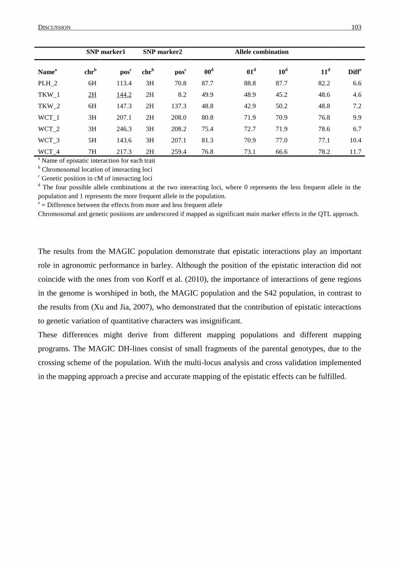
DISCUSSION 103

SNP marker1 SNP marker2 Allele combination

Namea chr

b pos

c chr

b pos

c

00d

01d

10d

11d Diff

e

PLH_2 6H 113.4 3H 70.8 87.7 88.8 87.7 82.2 6.6

TKW_1 2H 144.2 2H 8.2 49.9 48.9 45.2 48.6 4.6

TKW_2 6H 147.3 2H 137.3 48.8 42.9 50.2 48.8 7.2

WCT_1 3H 207.1 2H 208.0 80.8 71.9 70.9 76.8 9.9

WCT_2 3H 246.3 3H 208.2 75.4 72.7 71.9 78.6 6.7

WCT_3 5H 143.6 3H 207.1 81.3 70.9 77.0 77.1 10.4

WCT_4 7H 217.3 2H 259.4 76.8 73.1 66.6 78.2 11.7 a Name of epistatic interaction for each trait

b Chromosomal location of interacting loci

c Genetic position in cM of interacting loci

d The four possible allele combinations at the two interacting loci, where 0 represents the less frequent allele in the

population and 1 represents the more frequent allele in the population. e = Difference between the effects from more and less frequent allele

Chromosomal and genetic positions are underscored if mapped as significant main marker effects in the QTL approach.

The results from the MAGIC population demonstrate that epistatic interactions play an important

role in agronomic performance in barley. Although the position of the epistatic interaction did not

coincide with the ones from von Korff et al. (2010), the importance of interactions of gene regions

in the genome is worshiped in both, the MAGIC population and the S42 population, in contrast to

the results from (Xu and Jia, 2007), who demonstrated that the contribution of epistatic interactions

to genetic variation of quantitative characters was insignificant.

These differences might derive from different mapping populations and different mapping

programs. The MAGIC DH-lines consist of small fragments of the parental genotypes, due to the

crossing scheme of the population. With the multi-locus analysis and cross validation implemented

in the mapping approach a precise and accurate mapping of the epistatic effects can be fulfilled.

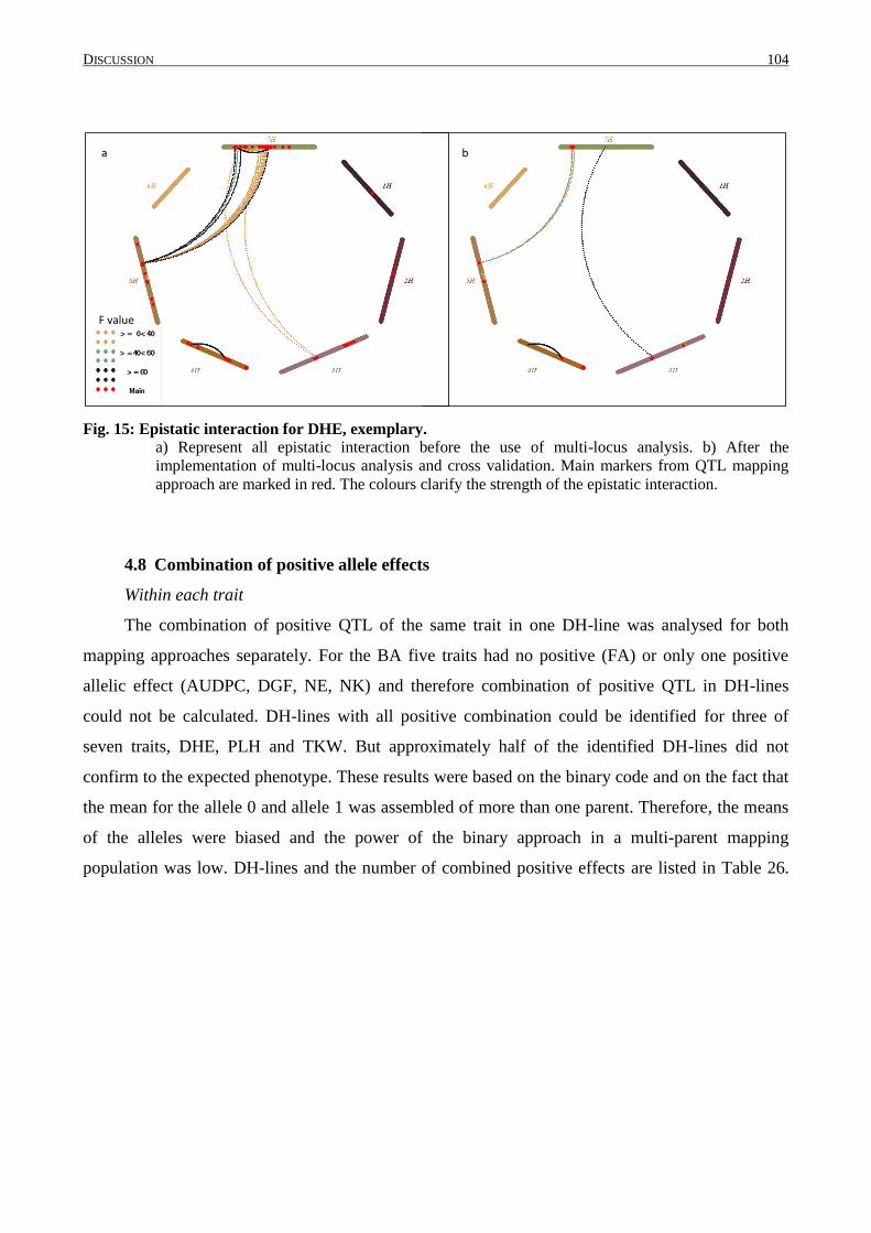
DISCUSSION 104

F value

a b

Fig. 15: Epistatic interaction for DHE, exemplary.

a) Represent all epistatic interaction before the use of multi-locus analysis. b) After the

implementation of multi-locus analysis and cross validation. Main markers from QTL mapping

approach are marked in red. The colours clarify the strength of the epistatic interaction.

4.8 Combination of positive allele effects

Within each trait

The combination of positive QTL of the same trait in one DH-line was analysed for both

mapping approaches separately. For the BA five traits had no positive (FA) or only one positive

allelic effect (AUDPC, DGF, NE, NK) and therefore combination of positive QTL in DH-lines

could not be calculated. DH-lines with all positive combination could be identified for three of

seven traits, DHE, PLH and TKW. But approximately half of the identified DH-lines did not

confirm to the expected phenotype. These results were based on the binary code and on the fact that

the mean for the allele 0 and allele 1 was assembled of more than one parent. Therefore, the means

of the alleles were biased and the power of the binary approach in a multi-parent mapping

population was low. DH-lines and the number of combined positive effects are listed in Table 26.

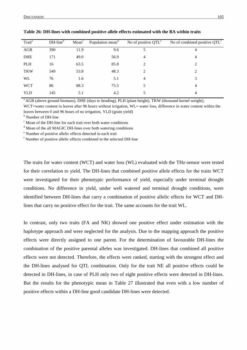
DISCUSSION 105

Table 26: DH-lines with combined positive allele effects estimated with the BA within traits

Traita DH-line

b Mean

c Population mean

d No of positive QTL

e No of combined positive QTL

f

AGB 390 11.9 9.6 5 4

DHE 171 49.0 56.9 4 4

PLH 16 63.5 85.8 2 2

TKW 549 53.8 48.3 2 2

WL 76 1.6 5.1 4 3

WCT 86 88.3 75.5 5 4

YLD 145 5.1 4.2 5 4

a AGB (above ground biomass), DHE (days to heading), PLH (plant height), TKW (thousand kernel weight),

WCT=water content in leaves after 96 hours without irrigation, WL= water loss, difference in water content within the

leaves between 0 and 96 hours of no irrigation, YLD (grain yield) b Number of DH-line

c Mean of the DH-line for each trait over both water conditions

d Mean of the all MAGIC DH-lines over both watering conditions

e Number of positive allelic effects detected in each trait

f Number of positive allelic effects combined in the selected DH-line

The traits for water content (WCT) and water loss (WL) evaluated with the THz-sensor were tested

for their correlation to yield. The DH-lines that combined positive allele effects for the traits WCT

were investigated for their phenotypic performance of yield, especially under terminal drought

conditions. No difference in yield, under well watered and terminal drought conditions, were

identified between DH-lines that carry a combination of positive allelic effects for WCT and DH-

lines that carry no positive effect for the trait. The same accounts for the trait WL.

In contrast, only two traits (FA and NK) showed one positive effect under estimation with the

haplotype approach and were neglected for the analysis. Due to the mapping approach the positive

effects were directly assigned to one parent. For the determination of favourable DH-lines the

combination of the positive parental alleles was investigated. DH-lines that combined all positive

effects were not detected. Therefore, the effects were ranked, starting with the strongest effect and

the DH-lines analysed for QTL combination. Only for the trait NE all positive effects could be

detected in DH-lines, in case of PLH only two of eight positive effects were detected in DH-lines.

But the results for the phenotypic mean in Table 27 illustrated that even with a low number of

positive effects within a DH-line good candidate DH-lines were detected.

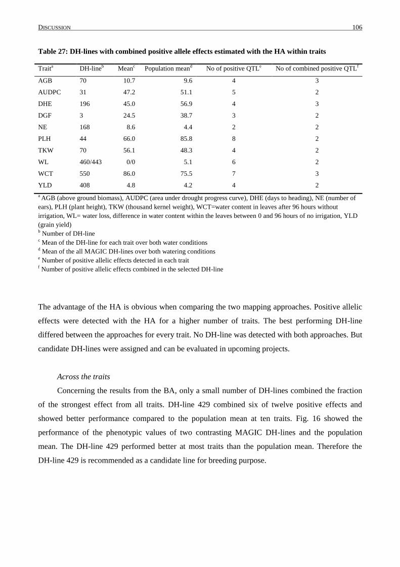
DISCUSSION 106

Table 27: DH-lines with combined positive allele effects estimated with the HA within traits

Traita DH-line

b Mean

c Population mean

d No of positive QTL

e No of combined positive QTL

f

AGB 70 10.7 9.6 4 3

AUDPC 31 47.2 51.1 5 2

DHE 196 45.0 56.9 4 3

DGF 3 24.5 38.7 3 2

NE 168 8.6 4.4 2 2

PLH 44 66.0 85.8 8 2

TKW 70 56.1 48.3 4 2

WL 460/443 0/0 5.1 6 2

WCT 550 86.0 75.5 7 3

YLD 408 4.8 4.2 4 2

a AGB (above ground biomass), AUDPC (area under drought progress curve), DHE (days to heading), NE (number of

ears), PLH (plant height), TKW (thousand kernel weight), WCT=water content in leaves after 96 hours without

irrigation, WL= water loss, difference in water content within the leaves between 0 and 96 hours of no irrigation, YLD

(grain yield) b Number of DH-line

c Mean of the DH-line for each trait over both water conditions

d Mean of the all MAGIC DH-lines over both watering conditions

e Number of positive allelic effects detected in each trait

f Number of positive allelic effects combined in the selected DH-line

The advantage of the HA is obvious when comparing the two mapping approaches. Positive allelic

effects were detected with the HA for a higher number of traits. The best performing DH-line

differed between the approaches for every trait. No DH-line was detected with both approaches. But

candidate DH-lines were assigned and can be evaluated in upcoming projects.

Across the traits

Concerning the results from the BA, only a small number of DH-lines combined the fraction

of the strongest effect from all traits. DH-line 429 combined six of twelve positive effects and

showed better performance compared to the population mean at ten traits. Fig. 16 showed the

performance of the phenotypic values of two contrasting MAGIC DH-lines and the population

mean. The DH-line 429 performed better at most traits than the population mean. Therefore the

DH-line 429 is recommended as a candidate line for breeding purpose.

DISCUSSION 107

AGB

AUDPC

DGF

DHE

FA

NE

NK

PLH

TKW

WL

WW96

YLD

DH 429

Population mean

Fig. 16: Radar chart of the MAGIC DH-line 429 (blue) and the MAGIC population mean (black) for

the phenotypic mean resulting from the BA at twelve traits. (WW96=WCT)

For the results from the HA approach, only two DH-lines (145 and 161) were detected which

carried the combination of six positive effects within their genome. DH-line 145 was the only one

that showed a better mean performance than the population mean for all these traits, for which it

carried the positive allelic effect. In addition three more traits had a higher phenotypic mean than

the population mean without being inherited by the parent with the strongest allelic effect. The

outranging of DH-line 145 over the population mean is shown in Fig. 17.

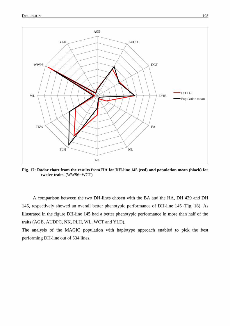
DISCUSSION 108

AGB

AUDPC

DGF

DHE

FA

NE

NK

PLH

TKW

WL

WW96

YLD

DH 145

Population mean

Fig. 17: Radar chart from the results from HA for DH-line 145 (red) and population mean (black) for

twelve traits. (WW96=WCT)

A comparison between the two DH-lines chosen with the BA and the HA, DH 429 and DH

145, respectively showed an overall better phenotypic performance of DH-line 145 (Fig. 18). As

illustrated in the figure DH-line 145 had a better phenotypic performance in more than half of the

traits (AGB, AUDPC, NK, PLH, WL, WCT and YLD).

The analysis of the MAGIC population with haplotype approach enabled to pick the best

performing DH-line out of 534 lines.

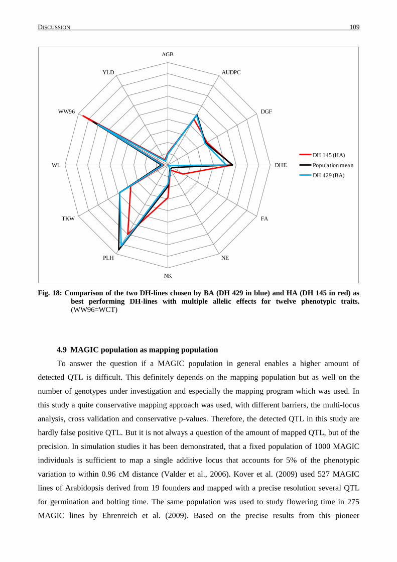
DISCUSSION 109

AGB

AUDPC

DGF

DHE

FA

NE

NK

PLH

TKW

WL

WW96

YLD

DH 145 (HA)

Population mean

DH 429 (BA)

Fig. 18: Comparison of the two DH-lines chosen by BA (DH 429 in blue) and HA (DH 145 in red) as

best performing DH-lines with multiple allelic effects for twelve phenotypic traits.

(WW96=WCT)

4.9 MAGIC population as mapping population

To answer the question if a MAGIC population in general enables a higher amount of

detected QTL is difficult. This definitely depends on the mapping population but as well on the

number of genotypes under investigation and especially the mapping program which was used. In

this study a quite conservative mapping approach was used, with different barriers, the multi-locus

analysis, cross validation and conservative p-values. Therefore, the detected QTL in this study are

hardly false positive QTL. But it is not always a question of the amount of mapped QTL, but of the

precision. In simulation studies it has been demonstrated, that a fixed population of 1000 MAGIC

individuals is sufficient to map a single additive locus that accounts for 5% of the phenotypic

variation to within 0.96 cM distance (Valder et al., 2006). Kover et al. (2009) used 527 MAGIC

lines of Arabidopsis derived from 19 founders and mapped with a precise resolution several QTL

for germination and bolting time. The same population was used to study flowering time in 275

MAGIC lines by Ehrenreich et al. (2009). Based on the precise results from this pioneer

DISCUSSION 110

populations, several multi-parent populations are being created right now, including the one in

Arabidopsis (Kover et al., 2009) and wheat (Huang et al. 2012), one in winter wheat

(http://www.niab.com/pages/id/93/MAGIC_Populations_in_Wheat) and in rice (Bandillo et al.,

2010, Leung et al., 2011). Unfortunately, the multi-parent populations differ in their crossing

schemes and are not easily comparable.

However, the statistical complexity in the analysis of MAGIC populations is far higher than

compared to bi-parental mapping population. But in the combination of the two mapping

approaches discussed in this thesis and the use of the SAS 9.2 QTL mapping program, the complex

statistical needs can be negotiated. This is shown in the results, especially in the outcome from the

calculation of the epistatic interaction. To my knowledge there is no publication including so many

strong epistatic interaction in barley. This is one huge advantage of the MAGIC population, which

enables through a high number of crossover events (Broman, 2005) a dissection of epistatic

interactions of complex traits. It might be highly probable to obtain useful MAGIC DH-lines

combining favourable value of agronomic traits, which might directly be used in breeding

programs.

SUMMARY AND CONCLUSION 111

5. Summary and Conclusion

The MAGIC DH-lines investigated in this research showed no population structure within the

DH-lines and enabled with a strong decay of LD a precise mapping of genetic regions of interest.

The terminal drought treatment applied in the early developmental stages of barley resulted in

significant differences for the traits of interest between the well watered and the stress scenario.

The search for genetic regions with an influence on yield and yield components on the traits

evaluated in this work was successful. QTL with main marker effects and marker*treatment

interaction effects were discovered for twelve traits with two different mapping approaches. The

two approaches mapped 35 allelic effects simultaneously. Both approaches showed advantages and

drawbacks, the strength of the allelic effect was greater when calculated with the HA and the real

parental allelic effect could be calculated only with the haplotype approach. But the binary

approach was able to locate the region of interest in much smaller genetic intervals.

The comparison of the detected QTL with the known ones from literature revealed new genetic

regions of interest for each investigated trait. Especially a gene region with association to days to

heading on chromosome 5H, 206.4 cM, is of superior interest. The sequence of the most significant

SNP marker matched with the sequence of a predicted protein in a databse, which regulates the

phyto hormone auxin.

The output of allele effects for marker*treatment interaction was rather low. Multi comparisons

between the parental allelic mean for the haplotype approach revealed only two genetic regions,

QNke.MAGIC.HA-2H.a and QTkw.MAGIC.HA-2H.a, with significant differences between the

parental allelic mean. Of these QTL QTkw.MAGIC.HA-2H.a can be named as a QTL with positive

effect under terminal drought conditions, derived from parent Barke.

The use of the THz-sensor to determine water content in leaves is one of the novelties of this

research project. Differences between the parents were detected; Ackermanns Danubia had the

highest water content in leaves after five days of drought. Pflugs Intensiv was the most stable parent

concerning water content under drought. QTL for water content and water holding capability were

detected in the MAGIC population. No correlation of THz values with phenotypic values of yield or

yield related trait was discovered, but clustering of QTL from water content and yield on 1H and

6H, with thousand kernel weight on 2H and with leaf senescence on 6H. Clusters for water holding

capability were mapped on 5H with yield and biomass and with leaf senescence.

Not only epistatic interactions between main markers but between all possible markers were

conducted and detected. The strength of the allelic effect was higher than the main marker effect,

e.g. one epistatic interaction explained the reduction of DHE by 7.2 days. The results for epistatic

interactions demonstrated the value of the interaction of gen regions in the agronomic performance

SUMMARY AND CONCLUSION 112

in barley. But they also explain the value of the MAGIC population, which enabled the detection of

small genetic fragments with a high number of recombination during the crossing process.

In general, a MAGIC population comprised new challenging assignment to QTL mapping. Almost

no commercial statistical programs that handle multi-parent populations are available. The

application of a haplotype QTL mapping approach is contemporary and enables the direct

investigation of multi-parent populations. But due to the mentioned drawbacks I recommend a

routine use of both mapping approaches for QTL mapping, the binary and haplotype approach.

Results from this study can be used as a starting block, the genetic map and the haplotype

probability of each parent to be inherited to the offspring has to be pursued in the future. The

MAGIC population proofed its importance as genetic resource and will be an ideal tool for

investigating inheritance and interactions of genetic regions.

REFERENCES 113

6. References

Abiola O., Angel J.M., Avner P., Bachmanov A.A., Belknap J.K., Bennett B., Blankenhorn E.P.,

Blizard D.A., Bolivar V., Brockmann G.A., Buck K.J., Bureau J.F., Casley W.L., Chesler

E.J., Cheverud J.M., Churchill G.A., Cook M., Crabbe J.C., Crusio W.E., Darvasi A., de

Haan G., Demant P., Doerge R.W., Elliott R.W., Farber C.R., Flaherty L., Flint J.,

Gershenfeld H., Gu J.P.G.J., Gu W.K., Himmelbauer H., Hitzemann R., Hsu H.C., Hunter

K., Iraqi F.A., Jansen R.C., Johnson T.E., Jones B.C., Kempermann G., Lammert F., Lu L.,

Manly K.F., Matthews D.B., Medrano J.F., Mehrabian M., Mittleman G., Mock B.A., Mogil

J.S., Montagutelli X., Morahan G., Mountz J.D., Nagase H., Nowakowski R.S., O'Hara

B.R., Osadchuk A.V., Paigen B., Palmer A.A., Peirce J.L., Pomp D., Rosemann M., Rosen

G.D., Schalkwyk L.C., Seltzer Z., Settle S., Shimomura K., Shou S.M., Sikela J.M.,

Siracusa L.D., Spearow J.L., Teuscher C., Threadgill D.W., Toth L.A., Toye A.A., Vadasz

C., Van Zant G., Wakeland E., Williams R.W., Zhang H.G., Zou F., Consortium C.T.

(2003) The nature and identification of quantitative trait loci: a community's view. Nature

Reviews Genetics 4:911-916. DOI: Doi 10.1038/Nrg1206.

Ashraf M. (2010) Inducing drought tolerance in plants: Recent advances. Biotechnology Advances

28:169-183. DOI: DOI 10.1016/j.biotechadv.2009.11.005.

Bandillo N., Muyco P.A., Caspillo C., Laza M., Sajise A.G., Singh R.K. et al. (2010) Development

of multiparent advanced generation intercross (magic) populations for gene discovery in rice

(Oryza sativa L. ) Philippine Journal of Crop Science 35:suppl 1, 96.

Bardel C., Danjean V., Hugot J.P., Darlu P., Genin E. (2005) On the use of haplotype phylogeny to

detect disease susceptibility loci. BMC Genet 6:24. DOI: 10.1186/1471-2156-6-24.

Bauer A.M., Hoti F., von Korff M., Pillen K., Leon J., Sillanpaa M.J. (2009) Advanced backcross-

QTL analysis in spring barley (H. vulgare ssp. spontaneum) comparing a REML versus a

Bayesian model in multi-environmental field trials. Theoretical and Applied Genetics

119:105-23. DOI: 10.1007/s00122-009-1021-6.

Baum M., Grando S., Backes G., Jahoor A., Sabbagh A., Ceccarelli S. (2003) QTLs for agronomic

traits in the Mediterranean environment identified in recombinant inbred lines of the cross

'Arta' x H-spontaneum 41-1. Theoretical and Applied Genetics 107:1215-1225. DOI: DOI

10.1007/s00122-003-1357-2.

Beavis W.D., Grant D., Albertsen M., Fincher R. (1991) Quantitative Trait Loci for Plant Height in

4 Maize Populations and Their Associations with Qualitative Genetic-Loci. Theoretical and

Applied Genetics 83:141-145.

Benjamini Y., Yekutieli D. (2005) Quantitative trait Loci analysis using the false discovery rate.

Genetics 171:783-90. DOI: 10.1534/genetics.104.036699.

Berger B., Parent B., Tester M. (2010) High-throughput shoot imaging to study drought responses.

Journal of Experimental Botany 61:3519-3528. DOI: Doi 10.1093/Jxb/Erq201.

Broman H.W. (2005) The genomes of recombinant inbred lines. Genetics 169:1133-1146

Blake T., Blake V., Bowman J., Abdel-Haleem H. (2011) Barley Feed Uses and Quality

Improvement. In: Ullrich S. E. (ed.) Barley: Productio, Improvement and Uses. Wiley-

Blackwell.: 522-531.

Blanc G., Charcosset A., Mangin B., Gallais A., Moreau L. (2006) Connected populations for

detecting quantitative trait loci and testing for epistasis: an application in maize. Theoretical

and Applied Genetics 113:206-24. DOI: 10.1007/s00122-006-0287-1.

Blum A. (1996) Crop responses to drought and the interpretation of adaptation. Plant Growth

Regulation 20:135-148.

Blum A. (2006) Drought adaption in cereal crops: a prologue. In: Ribaut J.M. (ed) Drought

adaption in cereals. Binghamton, NY: the Haworth Press, Inc: 3-15.

Blum A. (2011a) Drought resistance - is it really a complex trait? Functional Plant Biology 38:753-

757. DOI: Doi 10.1071/Fp11101.

REFERENCES 114

Blum A. (2011b) Plant Breeding for Water-Limited Environments. Springer.

Bohnert H.J., Gong Q., Li P., Ma S. (2006) Unraveling abiotic stress tolerance mechanisms –

getting genomics going. Current Opinion in Plant Biology 9:180-188. DOI:

http://dx.doi.org/10.1016/j.pbi.2006.01.003.

Botstein D., White R.L., Skolnick M., Davis R.W. (1980) Construction of a Genetic-Linkage Map

in Man Using Restriction Fragment Length Polymorphisms. American Journal of Human

Genetics 32:314-331.

Brisson N., Gate P., Gouache D., Charmet G., Oury F.X., Huard F. (2010) Why are wheat yields

stagnating in Europe? A comprehensive data analysis for France. Field Crops Research

119:201-212. DOI: 10.1016/j.fcr.2010.07.012.

Buckler E.S., Holland J.B., Bradbury P.J., Acharya C.B., Brown P.J., Browne C., Ersoz E., Flint-

Garcia S., Garcia A., Glaubitz J.C., Goodman M.M., Harjes C., Guill K., Kroon D.E.,

Larsson S., Lepak N.K., Li H.H., Mitchell S.E., Pressoir G., Peiffer J.A., Rosas M.O.,

Rocheford T.R., Romay M.C., Romero S., Salvo S., Villeda H.S., da Silva H.S., Sun Q.,

Tian F., Upadyayula N., Ware D., Yates H., Yu J.M., Zhang Z.W., Kresovich S., McMullen

M.D. (2009) The Genetic Architecture of Maize Flowering Time. Science 325:714-718.

DOI: DOI 10.1126/science.1174276.

Burris H.A., 3rd, Raymond E., Awada A., Kuhn J.G., O'Rourke T.J., Brentzel J., Lynch W., King

S.Y., Brown T.D., Von Hoff D.D. (1998) Pharmacokinetic and phase I studies of brequinar

(DUP 785; NSC 368390) in combination with cisplatin in patients with advanced

malignancies. Invest New Drugs 16:19-27.

Cai W., Morishima H. (2002) QTL clusters reflect character associations in wild and cultivated rice.

Theoretical and Applied Genetics 104:1217-1228. DOI: 10.1007/s00122-001-0819-7.

Caldwell D.G., McCallum N., Shaw P., Muehlbauer G.J., Marshall D.F., Waugh R. (2004) A

structured mutant population for forward and reverse genetics in Barley (Hordeum vulgare

L.). Plant Journal 40:143-150. DOI: DOI 10.1111/j.1365-313X.2004.02190.x.

Caldwell K.S., Russell J., Langridge P., Powell W. (2006) Extreme population-dependent linkage

disequilibrium detected in an inbreeding plant species, Hordeum vulgare. Genetics 172:557-

67. DOI: 10.1534/genetics.104.038489.

Calus M.P., Meuwissen T.H., Windig J.J., Knol E.F., Schrooten C., Vereijken A.L., Veerkamp R.F.

(2009) Effects of the number of markers per haplotype and clustering of haplotypes on the

accuracy of QTL mapping and prediction of genomic breeding values. Genet Sel Evol

41:11. DOI: 10.1186/1297-9686-41-11.

Cattivelli L., Rizza F., Badeck F.W., Mazzucotelli E., Mastrangelo A.M., Francia E., Mare C.,

Tondelli A., Stanca A.M. (2008) Drought tolerance improvement in crop plants: An

integrated view from breeding to genomics. Field Crops Research 105:1-14. DOI: DOI

10.1016/j.fcr.2007.07.004.

Cavanagh C., Morell M., Mackay I., Powell W. (2008) From mutations to MAGIC: resources for

gene discovery, validation and delivery in crop plants. Current Opinion in Plant Biology

11:215-221. DOI: DOI 10.1016/j.pbi.2008.01.002.

Chan W.L., Deibel J., Mittleman D.M. (2007) Imaging with terahertz radiation. Reports on Progress

in Physics 70:1325-1379. DOI: Doi 10.1088/0034-4885/70/8/R02.

Chen G.X., Krugman T., Fahima T., Chen K.G., Hu Y.G., Roder M., Nevo E., Korol A. (2010)

Chromosomal regions controlling seedling drought resistance in Israeli wild barley,

Hordeum spontaneum C. Koch. Genetic Resources and Crop Evolution 57:85-99. DOI: DOI

10.1007/s10722-009-9453-z.

Ching A., Caldwell K.S., Jung M., Dolan M., Smith O.S., Tingey S., Morgante M., Rafalski A.J.

(2002) SNP frequency, haplotype structure and linkage disequilibrium in elite maize inbred

lines. Bmc Genetics 3:19.

Churchill G., Airey D.C., Allayee H., Angel J.M., Attie A.D., Beatty J., Beavis W.D., Belknap J.K.,

Bennett B., Berrettini W., Bleich A., Bogue M., Broman K.W., Buck K.J., Buckler E.,

REFERENCES 115

Burmeister M., Chesler E.J., Cheverud J.M., Clapcote S., Cook M.N., Cox R.D., Crabbe

J.C., Crusio W.E., Darvasi A., Deschnepper C.F., Doerge R.W., Farber C.R., Forejt J., Gaile

D., Garlow S.J., Geiger H., Gershenfeld H., Gordon T., Gu J., Gu W.K., de Haan G., Hayes

N.L., Heller C., Himmelbauer H., Hitzemann R., Hunter K., Hsu H.C., Iraqi F.A., Ivandic

B., Jacob H.J., Jansen R.C., Jjepsen K.J., Johnson D.K., Johnson T.E., Kempermann G.,

Kendziorski C., Kotb M., Kooy R.F., Llamas B., Lammert F., Lassalle J.M., Lowenstein

P.R., Lu L., Lusiss A., Manly K.F., Marcucio R., Matthews D., Medrano J.F., Miller D.R.,

Mittleman G., Mock B.A., Mogil J.S., Montagutelli X., Morahan G., Morris D.G., Mott R.,

Nadeau J.H., Nagase H., Nowakowski R.S., O'Hara B.F., Osadchuk A.V., Page G.P., Paigen

B., Paigen K., Palmer A.A., Pan H.J., Peltonen-Palotie L., Peirce J., Pomp D., Pravenec M.,

Prows D.R., Qi Z.H., Reeves R.H., Roder J., Rosen G.D., Schadt E.E., Schalkwyk L.C.,

Seltzer Z., Shimomura K., Shou S.M., Sillanpaa M.J., Siracusa L.D., Snoeck H.W., Spearow

J.L., Svenson K., et al. (2004) The Collaborative Cross, a community resource for the

genetic analysis of complex traits. Nat Genet 36:1133-1137.

Clark A.G. (2004) The role of haplotypes in candidate gene studies. Genetic Epidemiology 27:321-

33. DOI: 10.1002/gepi.20025.

Close T.J., Bhat P.R., Lonardi S., Wu Y.H., Rostoks N., Ramsay L., Druka A., Stein N., Svensson

J.T., Wanamaker S., Bozdag S., Roose M.L., Moscou M.J., Chao S.A.M., Varshney R.K.,

Szucs P., Sato K., Hayes P.M., Matthews D.E., Kleinhofs A., Muehlbauer G.J., DeYoung J.,

Marshall D.F., Madishetty K., Fenton R.D., Condamine P., Graner A., Waugh R. (2009)

Development and implementation of high-throughput SNP genotyping in barley. Bmc

Genomics 10. DOI: Artn 582 Doi 10.1186/1471-2164-10-582.

Close T.J., Wanamaker S.I., Caldo R.A., Turner S.M., Ashlock D.A., Dickerson J.A., Wing R.A.,

Muehlbauer G.J., Kleinhofs A., Wise R.P. (2004) A new resource for cereal genomics: 22K

barley GeneChip comes of age. Plant Physiol 134:960-8. DOI: 10.1104/pp.103.034462.

Cockram J., White J., Zuluaga D.L., Smith D., Comadran J., Macaulay M., Luo Z.W., Kearsey

M.J., Werner P., Harrap D., Tapsell C., Liu H., Hedley P.E., Stein N., Schulte D.,

Steuernagel B., Marshall D.F., Thomas W.T.B., Ramsay L., Mackay I., Balding D.J.,

Waugh R., O'Sullivan D.M., Consortium A. (2010) Genome-wide association mapping to

candidate polymorphism resolution in the unsequenced barley genome. Proceedings of the

National Academy of Sciences of the United States of America 107:21611-21616. DOI:

DOI 10.1073/pnas.1010179107.

Collard B.C.Y., Jahufer M.Z.Z., Brouwer J.B., Pang E.C.K. (2005) An introduction to markers,

quantitative trait loci (QTL) mapping and marker-assisted selection for crop improvement:

The basic concepts. Euphytica 142:169-196. DOI: 10.1007/s10681-005-1681-5.

Comadran J., Kilian B., Russell J., Ramsay L., Stein N., Ganal M., Shaw P., Bayer M., Thomas W.,

Marshall D., Hedley P., Tondelli A., Pecchioni N., Francia E., Korzun V., Walther A.,

Waugh R. (2012) Natural variation in a homolog of Antirrhinum CENTRORADIALIS

contributed to spring growth habit and environmental adaptation in cultivated barley. Nat

Genet advance online publication. DOI:

http://www.nature.com/ng/journal/vaop/ncurrent/abs/ng.2447.html#supplementary-

information.

Comadran J., Ramsay L., MacKenzie K., Hayes P., Close T.J., Muehlbauer G., Stein N., Waugh R.

(2011a) Patterns of polymorphism and linkage disequilibrium in cultivated barley.

Theoretical and Applied Genetics 122:523-531. DOI: DOI 10.1007/s00122-010-1466-7.

Comadran J., Russell J.R., Booth A., Pswarayi A., Ceccarelli S., Grando S., Stanca A.M., Pecchioni

N., Akar T., Al-Yassin A., Benbelkacem A., Ouabbou H., Bort J., van Eeuwijk F.A.,

Thomas W.T., Romagosa I. (2011b) Mixed model association scans of multi-environmental

trial data reveal major loci controlling yield and yield related traits in Hordeum vulgare in

Mediterranean environments. Theoretical and Applied Genetics 122:1363-73. DOI:

10.1007/s00122-011-1537-4.

REFERENCES 116

Comadran J., Russell J.R., van Eeuwijk F.A., Ceccarelli S., Grando S., Baum M., Stanca A.M.,

Pecchioni N., Mastrangelo A.M., Akar T., Al-Yassin A., Benbelkacem A., Choumane W.,

Ouabbou H., Dahan R., Bort J., Araus J.L., Pswarayi A., Romagosa I., Hackett C.A.,

Thomas W.T.B. (2008) Mapping adaptation of barley to droughted environments. Euphytica

161:35-45. DOI: DOI 10.1007/s10681-007-9508-1.

Comadran J., Thomas W.T., van Eeuwijk F.A., Ceccarelli S., Grando S., Stanca A.M., Pecchioni

N., Akar T., Al-Yassin A., Benbelkacem A., Ouabbou H., Bort J., Romagosa I., Hackett

C.A., Russell J.R. (2009) Patterns of genetic diversity and linkage disequilibrium in a highly

structured Hordeum vulgare association-mapping population for the Mediterranean basin.

Theor Appl Genet 119:175-87. DOI: 10.1007/s00122-009-1027-0.

Darvasi A., Soller M. (1995) Advanced Intercross Lines, an Experimental Population for Fine

Genetic-Mapping. Genetics 141:1199-1207.

Dawson E., Abecasis G.R., Bumpstead S., Chen Y., Hunt S., Beare D.M., Pabial J., Dibling T.,

Tinsley E., Kirby S., Carter D., Papaspyridonos M., Livingstone S., Ganske R., Lohmussaar

E., Zernant J., Tonisson N., Remm M., Magi R., Puurand T., Vilo J., Kurg A., Rice K.,

Deloukas P., Mott R., Metspalu A., Bentley D.R., Cardon L.R., Dunham I. (2002) A first-

generation linkage disequilibrium map of human chromosome 22. Nature 418:544-8. DOI:

10.1038/nature00864.

Dedatta S.K., Malabuyoc J.A., Aragon E.L. (1988) A Field Screening Technique for Evaluating

Rice Germplasm for Drought Tolerance during the Vegetative Stage. Field Crops Research

19:123-134. DOI: Doi 10.1016/0378-4290(88)90050-0.

Deikman J., Petracek M., Heard J.E. (2012) Drought tolerance through biotechnology: improving

translation from the laboratory to farmers’ fields. Current Opinion in Biotechnology 23:243-

250. DOI: http://dx.doi.org/10.1016/j.copbio.2011.11.003.

Diab A.A., Teulat-Merah B., This D., Ozturk N.Z., Benscher D., Sorrells M.E. (2004) Identification

of drought-inducible genes and differentially expressed sequence tags in barley. Theoretical

and Applied Genetics 109:1417-1425. DOI: DOI 10.1007/s00122-004-1755-0.

Doerge R.W. (2002) Mapping and analysis of quantitative trait loci in experimental populations.

Nature Reviews Genetics 3:43-52. DOI: 10.1038/nrg703.

Druka A., Muehlbauer G., Druka I., Caldo R., Baumann U., Rostoks N., Schreiber A., Wise R.,

Close T., Kleinhofs A., Graner A., Schulman A., Langridge P., Sato K., Hayes P., McNicol

J., Marshall D., Waugh R. (2006) An atlas of gene expression from seed to seed through

barley development. Funct Integr Genomics 6:202-11. DOI: 10.1007/s10142-006-0025-4.

Edwards M.D., Stuber C.W., Wendel J.F. (1987) Molecular-marker-facilitated investigations of

quantitative-trait loci in maize. I. Numbers, genomic distribution and types of gene action.

Genetics 116:113-25.

Ehrenreich I.M., Hanzawa Y., Chou L., Roe J.L., Kover P.X., Purugganan M.D. (2009) Candidate

gene association mapping of Arabidopsis flowering time. Genetics 183:325-335

Eitel J.U.H., Gessler P.E., Smith A.M.S., Robberecht R. (2006) Suitability of existing and novel

spectral indices to remotely detect water stress in Populus spp. Forest Ecology and

Management 229:170-182. DOI: DOI 10.1016/j.foreco.2006.03.027.

Falconer and Mackay (1996) Introduction to Quantitative Genetics. Benjamin Cummings; 4 edition.

Fasoulas A.C., Allard R.W. (1962) Nonallelic Gene Interactions in the Inheritance of Quantitative

Characters in Barley. Genetics 47:899-907.

Federici J.F. (2012) Review of Moisture and Liquid Detection and Mapping using Terahertz

Imaging. Journal of Infrared Millimeter and Terahertz Waves 33:97-126. DOI: DOI

10.1007/s10762-011-9865-7.

Fisher R.A. (1918) The correlation between relatives on the supposition of mendalien inheritance.

Transaction of the Royal Society of Endinburgh 52:399-433

Forster B.P., Ellis R.P., Moir J., Talame V., Sanguineti M.C., Tuberosa R., This D., Teulat-Merah

B., Ahmed I., Mariy S.A.E.E., Bahri H., El Ouahabi M., Zoumarou-Wallis N., El-Fellah M.,

REFERENCES 117

Ben Salem M. (2004) Genotype and phenotype associations with drought tolerance in barley

tested in North Africa. Annals of Applied Biology 144:157-168. DOI: DOI 10.1111/j.1744-

7348.2004.tb00329.x.

Forster B.P., Ellis R.P., Thomas W.T., Newton A.C., Tuberosa R., This D., el-Enein R.A., Bahri

M.H., Ben Salem M. (2000) The development and application of molecular markers for

abiotic stress tolerance in barley. Journal of Experimental Botany 51:19-27.

Franklin S.B., Gibson D.J., Robertson P.A., Pohlmann J.T., Fralish J.S. (1995) Parallel Analysis: a

method for determining significant principal components. Journal of Vegetation Science

6:99-106. DOI: 10.2307/3236261.

Furbank R.T., Tester M. (2011) Phenomics - technologies to relieve the phenotyping bottleneck.

Trends in Plant Science 16:635-644. DOI: DOI 10.1016/j.tplants.2011.09.005.

Furbank R.T., von Caemmerer S., Sheehy J., Edwards G. (2009) C4 rice: a challenge for plant

phenomics. Functional Plant Biology 36:845-856. DOI: http://dx.doi.org/10.1071/FP09185.

Geldermann H. (1975) Investigations on Inheritance of Quantitative Characters in Animals by Gene

Markers .1. Methods. Theoretical and Applied Genetics 46:319-330.

Grapes L., Dekkers J.C., Rothschild M.F., Fernando R.L. (2004) Comparing linkage

disequilibrium-based methods for fine mapping quantitative trait loci. Genetics 166:1561-

70.

Guo P.G., Baum M., Varshney R.K., Graner A., Grando S., Ceccarelli S. (2008) QTLs for

chlorophyll and chlorophyll fluorescence parameters in barley under post-flowering drought.

Euphytica 163:203-214. DOI: DOI 10.1007/s10681-007-9629-6.

Hadjiloucas S., Galvao R.K.H., Bowen J.W. (2002) Analysis. of spectroscopic measurements of

leaf water content at terahertz frequencies using linear transforms. Journal of the Optical

Society of America a-Optics Image Science and Vision 19:2495-2509.

Hadjiloucas S., Karatzas L.S., Bowen J.W. (1999) Measurements of leaf water content using

terahertz radiation. Ieee Transactions on Microwave Theory and Techniques 47:142-149.

Harlan J. R. (1975) Our vanishing genetc resources. Science188: 618-621

Hayes B.J., Chamberlain A.J., McPartlan H., Macleod I., Sethuraman L., Goddard M.E. (2007)

Accuracy of marker-assisted selection with single markers and marker haplotypes in cattle.

Genet Res 89:215-20. DOI: 10.1017/S0016672307008865.

Hayes P.M., Liu B.H., Knapp S.J., Chen F., Jones B., Blake T., Franckowiak J., Rasmusson D.,

Sorrells M., Ullrich S.E., Wesenberg D., Kleinhofs A. (1993) Quantitative Trait Locus

Effects and Environmental Interaction in a Sample of North-American Barley Germ Plasm.

Theoretical and Applied Genetics 87:392-401. DOI: Doi 10.1007/Bf01184929.

Heun M. (1992) Mapping Quantitative Powdery Mildew Resistance of Barley Using a Restriction-

Fragment-Length-Polymorphism Map. Genome 35:1019-1025.

Holland J.B. (2001) Epistasis and Plant Breeding. In: Janick J. (ed) Plant Breeding Reviews

21.DOI: 10.1002/9780470650196.ch2

Holland J.B. (2007) Genetic architecture of complex traits in plants. Curr Opin Plant Biol 10:156-

61. DOI: 10.1016/j.pbi.2007.01.003.

Hu B.B., Nuss M.C. (1995) Imaging with Terahertz Waves. Optics Letters 20:1716-&.

Huang B.E., George A.W. (2011) R/mpMap: a computational platform for the genetic analysis of

multiparent recombinant inbred lines. Bioinformatics 27:727-729. DOI: DOI

10.1093/bioinformatics/btq719.

Huang B.E., George A.W., Forrest K.L., Kilian A., Hayden M.J., Morell M.K., Cavanagh C.R.

(2012) A multiparent advanced generation inter-cross population for genetic analysis in

wheat. Plant Biotechnol J 10:826-39. DOI: 10.1111/j.1467-7652.2012.00702.x.

Huang X., Paulo M.-J., Boer M., Effgen S., Keizer P., Koornneef M., van Eeuwijk F.A. (2011)

Analysis of natural allelic variation in Arabidopsis using a multiparent recombinant inbred

line population. Proceedings of the National Academy of Sciences 108:4488-4493. DOI:

10.1073/pnas.1100465108.

REFERENCES 118

Jaccoud D., Peng K., Feinstein D., Kilian A. (2001) Diversity arrays: a solid state technology for

sequence information independent genotyping. Nucleic Acids Research 29:E25.

Jansen C., Wietzke S., Peters O., Scheller M., Vieweg N., Salhi M., Krumbholz N., Jordens C.,

Hochrein T., Koch M. (2010) Terahertz imaging: applications and perspectives. Applied

Optics 49:E48-E57.

Jansen R.C. (1993) Interval Mapping of Multiple Quantitative Trait Loci. Genetics 135:205-211.

Jordens C., Scheller M., Breitenstein B., Selmar D., Koch M. (2009) Evaluation of leaf water status

by means of permittivity at terahertz frequencies. J Biol Phys 35:255-64. DOI:

10.1007/s10867-009-9161-0.

Karpowicz N., Zhong H., Xu J.Z., Lin K.I., Hwang J.S., Zhang X.C. (2005) Comparison between

pulsed terahertz time-domain imaging and continuous wave terahertz imaging.

Semiconductor Science and Technology 20:S293-S299. DOI: Doi 10.1088/0268-

1242/20/7/021.

Keim P., Diers B.W., Shoemaker R.C. (1990) Genetic-Analysis of Soybean Hard Seededness with

Molecular Markers. Theoretical and Applied Genetics 79:465-469.

Kilpikari R., Sillanpaa M.J. (2003) Bayesian analysis of multilocus association in quantitative and

qualitative traits. Genet Epidemiol 25:122-35. DOI: 10.1002/gepi.10257.

King E.G., Merkes C.M., McNeil C.L., Hoofer S.R., Sen S., Broman K.W., Long A.D., Macdonald

S.J. (2012) Genetic dissection of a model complex trait using the Drosophila Synthetic

Population Resource. Genome Research 22:1558-1566. DOI: DOI 10.1101/gr.134031.111.

Komatsuda T., Mano Y. (2002) Molecular mapping of the intermedium spike-c (int-c) and non-

brittle rachis 1 (btr1) loci in barley (Hordeum vulgare L.). Theoretical and Applied Genetics

105:85-90. DOI: DOI 10.1007/s00122-001-0858-0.

Komatsuda T., Pourkheirandish M., He C., Azhaguvel P., Kanamori H., Perovic D., Stein N.,

Graner A., Wicker T., Tagiri A., Lundqvist U., Fujimura T., Matsuoka M., Matsumoto T.,

Yano M. (2007) Six-rowed barley originated from a mutation in a homeodomain-leucine

zipper I-class homeobox gene. Proc Natl Acad Sci U S A 104:1424-9. DOI:

10.1073/pnas.0608580104.

Kota R., Rudd S., Facius A., Kolesov G., Thiel T., Zhang H., Stein N., Mayer K., Graner A. (2003)

Snipping polymorphisms from large EST collections in barley (Hordeum vulgare L.).

Molecular Genetics and Genomics 270:24-33. DOI: 10.1007/s00438-003-0891-6.

Kover P.X., Valdar W., Trakalo J., Scarcelli N., Ehrenreich I.M., Purugganan M.D., Durrant C.,

Mott R. (2009) A Multiparent Advanced Generation Inter-Cross to fine-map quantitative

traits in Arabidopsis thaliana. PLoS Genet 5:e1000551. DOI:

10.1371/journal.pgen.1000551.

Lafitte H.R., Edmeades G.O. (1995) Stress Tolerance in Tropical Maize Is Linked to Constitutive

Changes in Ear Growth-Characteristics. Crop Science 35:820-826.

Lander E.S., Botstein D. (1989) Mapping mendelian factors underlying quantitative traits using

RFLP linkage maps. Genetics 121:185-99.

Laurie C.C., Chasalow S.D., LeDeaux J.R., McCarroll R., Bush D., Hauge B., Lai C., Clark D.,

Rocheford T.R., Dudley J.W. (2004) The genetic architecture of response to long-term

artificial selection for oil concentration in the maize kernel. Genetics 168:2141-55. DOI:

10.1534/genetics.104.029686.

Laurie D.A., Pratchett N., Bezant J.H., Snape J.W. (1995) Rflp Mapping of 5 Major Genes and 8

Quantitative Trait Loci Controlling Flowering Time in a Winterxspring Barley (Hordeum-

Vulgare L) Cross. Genome 38:575-585.

Leung H., McNally K., Thomson M., Bandillo N., Muyco P., Singh R.K. (2011) Expandinf and

fine-tuning genetic resources for discovery of gene functions in rice. Plant and animal

genome conference, San Diego.

REFERENCES 119

Li S., Jia J., Wei X., Zhang X., Li L., Chen H., Fan Y., Sun H., Zhao X., Lei T., Xu Y., Jiang F.,

Wang H., Li L. (2007) A intervarietal genetic map and QTL analysis for yield traits in

wheat. Molecular Breeding 20:167-178. DOI: 10.1007/s11032-007-9080-3.

Li W.T., Liu C.J., Liu Y.X., Pu Z.E., Dai S.F., Wang J.R., Lan X.J., Zheng Y.L., Wei Y.M. (2013)

Meta-analysis of QTL associated with tolerance to abiotic stresses in barley. Euphytica

189:31-49. DOI: DOI 10.1007/s10681-012-0683-3.

Li Z., Pinson S.R., Park W.D., Paterson A.H., Stansel J.W. (1997) Epistasis for three grain yield

components in rice (Oryza sativa L.). Genetics 145:453-65.

Long A.D., Langley C.H. (1999) The power of association studies to detect the contribution of

candidate genetic loci to variation in complex traits. Genome Res 9:720-31.

Lorenz A.J., Hamblin M.T., Jannink J.L. (2010) Performance of Single Nucleotide Polymorphisms

versus Haplotypes for Genome-Wide Association Analysis in Barley. Plos One 5. DOI:

ARTN e14079 DOI 10.1371/journal.pone.0014079.

Lundqvist U., Franckowiak J., Konishi T. (1996) New and revised descriptions of barley genes.

Barley Genetic Newsleter 26: 22-43.

Luo M.-C., Thomas C., You F.M., Hsiao J., Ouyang S., Buell C.R., Malandro M., McGuire P.E.,

Anderson O.D., Dvorak J. (2003) High-throughput fingerprinting of bacterial artificial

chromosomes using the snapshot labeling kit and sizing of restriction fragments by capillary

electrophoresis. Genomics 82:378-389. DOI: 10.1016/s0888-7543(03)00128-9.

Mackay T.F. (2004) The genetic architecture of quantitative traits: lessons from Drosophila. Curr

Opin Genet Dev 14:253-7. DOI: 10.1016/j.gde.2004.04.003.

Malmberg R.L., Held S., Waits A., Mauricio R. (2005) Epistasis for fitness-related quantitative

traits in Arabidopsis thaliana grown in the field and in the greenhouse. Genetics 171:2013-

2027. DOI: DOI 10.1534/genetics.105.046078.

Mardi M., Buerstmayr H., Ghareyazie B., Lemmens M., Mohammadi S.A., Nolz R., Ruckenbauer

P. (2005) QTL analysis of resistance to Fusarium head blight in wheat using a

'Wangshuibai'-derived population. Plant Breeding 124:329-333. DOI: DOI 10.1111/j.1439-

0523.2005.01103.x.

Matzler C. (1994) Microwave (1-100 GHz) dielectric model of leaves. Geoscience and Remote

Sensing, IEEE Transactions on 32:947-949. DOI: 10.1109/36.298024.

Mayer K.F., Waugh R., Langridge P., Close T.J., Wise R.P., Graner A., Matsumoto T., Sato K.,

Schulman A., Muehlbauer G.J., Stein N., Ariyadasa R., Schulte D., Poursarebani N., Zhou

R., Steuernagel B., Mascher M., Scholz U., Shi B., Madishetty K., Svensson J.T., Bhat P.,

Moscou M., Resnik J., Hedley P., Liu H., Morris J., Frenkel Z., Korol A., Berges H.,

Taudien S., Felder M., Groth M., Platzer M., Himmelbach A., Lonardi S., Duma D., Alpert

M., Cordero F., Beccuti M., Ciardo G., Ma Y., Wanamaker S., Cattonaro F., Vendramin V.,

Scalabrin S., Radovic S., Wing R., Morgante M., Nussbaumer T., Gundlach H., Martis M.,

Poland J., Spannagl M., Pfeifer M., Moisy C., Tanskanen J., Zuccolo A., Russell J., Druka

A., Marshall D., Bayer M., Swarbreck D., Sampath D., Ayling S., Febrer M., Caccamo M.,

Tanaka T., Wannamaker S., Schmutzer T., Brown J.W., Fincher G.B. (2012) A physical,

genetic and functional sequence assembly of the barley genome. Nature. DOI:

10.1038/nature11543.

McCartney C.A., Somers D.J., Lukow O., Ames N., Noll J., Cloutier S., Humphreys D.G.,

McCallum B.D. (2006) QTL analysis of quality traits in the spring wheat cross

RL4452 × ‘AC Domain’. Plant Breeding 125:565-575. DOI: 10.1111/j.1439-

0523.2006.01256.x.

Mccouch S.R., Doerge R.W. (1995) Qtl Mapping in Rice. Trends in Genetics 11:482-487.

McKay J.K., Richards J.H., Mitchell-Olds T. (2003) Genetics of drought adaptation in Arabidopsis

thaliana: I. Pleiotropy contributes to genetic correlations among ecological traits. Molecular

Ecology 12:1137-1151. DOI: 10.1046/j.1365-294X.2003.01833.x.

REFERENCES 120

McMullen M.D., Kresovich S., Villeda H.S., Bradbury P., Li H.H., Sun Q., Flint-Garcia S.,

Thornsberry J., Acharya C., Bottoms C., Brown P., Browne C., Eller M., Guill K., Harjes

C., Kroon D., Lepak N., Mitchell S.E., Peterson B., Pressoir G., Romero S., Rosas M.O.,

Salvo S., Yates H., Hanson M., Jones E., Smith S., Glaubitz J.C., Goodman M., Ware D.,

Holland J.B., Buckler E.S. (2009) Genetic Properties of the Maize Nested Association

Mapping Population. Science 325:737-740. DOI: DOI 10.1126/science.1174320.

Mei H.W., Li Z.K., Shu Q.Y., Guo L.B., Wang Y.P., Yu X.Q., Ying C.S., Luo L.J. (2005) Gene

actions of QTLs affecting several agronomic traits resolved in a recombinant inbred rice

population and two backcross populations. Theoretical and Applied Genetics 110:649-659.

DOI: DOI 10.1007/s00122-004-1890-7.

Melchinger A.E., Utz H.F., Schon C.C. (1998) Quantitative trait locus (QTL) mapping using

different testers and independent population samples in maize reveals low power of QTL

detection and large bias in estimates of QTL effects. Genetics 149:383-403.

Mihaljevic R., Utz H.F., Melchinger A.E. (2005) No evidence for epistasis in hybrid and per se

performance of elite European flint maize inbreds from generation means and QTL

analyses. Crop Science 45:2605-2613. DOI: DOI 10.2135/cropsci2004.0760.

Milne I., Shaw P., Stephen G., Bayer M., Cardle L., Thomas W.T., Flavell A.J., Marshall D. (2010)

Flapjack--graphical genotype visualization. Bioinformatics 26:3133-4. DOI:

10.1093/bioinformatics/btq580.

Mir R.R., Zaman-Allah M., Sreenivasulu N., Trethowan R., Varshney R.K. (2012) Integrated

genomics, physiology and breeding approaches for improving drought tolerance in crops.


Mittleman D.M., Jacobsen R.H., Nuss M.C. (1996) T-ray imaging. Ieee Journal of Selected Topics

in Quantum Electronics 2:679-692.

Molina-Cano J.L., Russell J.R., Moralejo M.A., Escacena J.L., Arias G., Powell W. (2005)

Chloroplast DNA microsatellite analysis supports a polyphyletic origin for barley.


Morgante M., Olivieri A.M. (1993) PCR-amplified microsatellites as markers in plant genetics.

Plant J 3:175-82.

Morris R.W., Kaplan N.L. (2002) On the advantage of haplotype analysis in the presence of

multiple disease susceptibility alleles. Genetic Epidemiology 23:221-233. DOI: Doi

10.1002/Gepi.10200.

Mott R., Talbot C.J., Turri M.G., Collins A.C., Flint J. (2000) A method for fine mapping

quantitative trait loci in outbred animal stocks. Proceedings of the National Academy of

Sciences of the United States of America 97:12649-12654.

Myles S., Peiffer J., Brown P.J., Ersoz E.S., Zhang Z., Costich D.E., Buckler E.S. (2009)

Association mapping: critical considerations shift from genotyping to experimental design.

Plant Cell 21:2194-202. DOI: 10.1105/tpc.109.068437.

Nevo E., Fu Y.B., Pavlicek T., Khalifa S., Tavasi M., Beiles A. (2012) Evolution of wild cereals

during 28 years of global warming in Israel. Proc Natl Acad Sci U S A 109:3412-5. DOI:

10.1073/pnas.1121411109.

Oraguzie N.C., Rikkerink E.H.A., Gardiner S.E., Nihal de Silva H. (2007) Association mapping in

plants. Springer.

Pasam R.K., Sharma R., Malosetti M., van Eeuwijk F.A., Haseneyer G., Kilian B., Graner A.

(2012) Genome-wide association studies for agronomical traits in a world wide spring

barley collection. Bmc Plant Biology 12:16. DOI: 10.1186/1471-2229-12-16.

Passioura J. (2007) The drought environment: physical, biological and agricultural perspectives.

Journal of Experimental Botany 58:113-117. DOI: Doi 10.1093/Jxb/Erl212.

Passioura J.B. (1977) Grain-Yield, Harvest Index, and Water-Use of Wheat. Journal of the

Australian Institute of Agricultural Science 43:117-120.

REFERENCES 121

Passioura J.B. (1996) Drought and drought tolerance. Plant Growth Regulation 20:79-83. DOI: Doi

10.1007/Bf00024003.

Passioura J.B., Angus J.F. (2010) Improving Productivity of Crops in Water-Limited Environments.

Advances in Agronomy, Vol 106 106:37-75. DOI: Doi 10.1016/S0065-2113(10)06002-5.

Paterson A.H., Damon S., Hewitt J.D., Zamir D., Rabinowitch H.D., Lincoln S.E., Lander E.S.,

Tanksley S.D. (1991) Mendelian factors underlying quantitative traits in tomato: comparison

across species, generations, and environments. Genetics 127:181-97.

Paterson A.H., Lander E.S., Hewitt J.D., Peterson S., Lincoln S.E., Tanksley S.D. (1988)

Resolution of quantitative traits into Mendelian factors by using a complete linkage map of

restriction fragment length polymorphisms. Nature 335:721-6. DOI: 10.1038/335721a0.

Patil N., Berno A.J., Hinds D.A., Barrett W.A., Doshi J.M., Hacker C.R., Kautzer C.R., Lee D.H.,

Marjoribanks C., McDonough D.P., Nguyen B.T., Norris M.C., Sheehan J.B., Shen N.,

Stern D., Stokowski R.P., Thomas D.J., Trulson M.O., Vyas K.R., Frazer K.A., Fodor S.P.,

Cox D.R. (2001) Blocks of limited haplotype diversity revealed by high-resolution scanning

of human chromosome 21. Science 294:1719-23. DOI: 10.1126/science.1065573.

Peighambari S.A., Samadi B.Y., Nabipour A., Charmet G., Sarrafi A. (2005) QTL analysis for

agronomic traits in a barley doubled haploids population grown in Iran. Plant Science

169:1008-1013. DOI: DOI 10.1016/j.plantsci.2005.05.018.

Pennisi E. (2008) Plant genetics: The blue revolution, drop by drop, gene by gene. Science 320:171-

173.

Pillen K., Zacharias A., Leon J. (2003) Advanced backcross QTL analysis in barley (Hordeum

vulgare L.). Theoretical and Applied Genetics 107:340-52. DOI: 10.1007/s00122-003-1253-

9.

Potokina E., Druka A., Luo Z., Wise R., Waugh R., Kearsey M. (2008) Gene expression

quantitative trait locus analysis of 16 000 barley genes reveals a complex pattern of genome-

wide transcriptional regulation. Plant J 53:90-101. DOI: 10.1111/j.1365-

313X.2007.03315.x.

Pourkheirandish M., Wicker T., Stein N., Fujimura T., Komatsuda T. (2007) Analysis of the barley

chromosome 2 region containing the six-rowed spike gene vrs1 reveals a breakdown of rice-

barley micro collinearity by a transposition. Theoretical and Applied Genetics 114:1357-

1365. DOI: DOI 10.1007/s00122-007-0522-4.

Price A.L., Patterson N.J., Plenge R.M., Weinblatt M.E., Shadick N.A., Reich D. (2006) Principal

components analysis corrects for stratification in genome-wide association studies. Nat

Genet 38:904-909. DOI:

http://www.nature.com/ng/journal/v38/n8/suppinfo/ng1847_S1.html.

Ramsay L., Macaulay M., degli Ivanissevich S., MacLean K., Cardle L., Fuller J., Edwards K.J.,

Tuvesson S., Morgante M., Massari A., Maestri E., Marmiroli N., Sjakste T., Ganal M.,

Powell W., Waugh R. (2000) A simple sequence repeat-based linkage map of barley.

Genetics 156:1997-2005.

Reich D.E., Cargill M., Bolk S., Ireland J., Sabeti P.C., Richter D.J., Lavery T., Kouyoumjian R.,

Farhadian S.F., Ward R., Lander E.S. (2001) Linkage disequilibrium in the human genome.

Nature 411:199-204. DOI: 10.1038/35075590.

Reynolds M., Tuberosa R. (2008) Translational research impacting on crop productivity in drought-

prone environments. Current Opinion in Plant Biology 11:171-179. DOI:

10.1016/j.pbi.2008.02.005.

Richards R.A. (1996) Defining selection criteria to improve yield under drought. Plant Growth

Regulation 20:157-166.

Richards R.A., Rebetzke G.J., Watt M., Condon A.G., Spielmeyer W., Dolferus R. (2010) Breeding

for improved water productivity in temperate cereals: phenotyping, quantitative trait loci,

markers and the selection environment. Functional Plant Biology 37:85-97. DOI: Doi

10.1071/Fp09219.

REFERENCES 122

Rodolphe F., Lefort M. (1993) A Multi-Marker Model for Detecting Chromosomal Segments

Displaying Qtl Activity. Genetics 134:1277-1288.

Rostoks N., Mudie S., Cardle L., Russell J., Ramsay L., Booth A., Svensson J.T., Wanamaker S.I.,

Walia H., Rodriguez E.M., Hedley P.E., Liu H., Morris J., Close T.J., Marshall D.F., Waugh

R. (2005) Genome-wide SNP discovery and linkage analysis in barley based on genes

responsive to abiotic stress. Molecular Genetics and Genomics 274:515-527. DOI: DOI

10.1007/s00438-005-0046-z.

Rostoks N., Ramsay L., MacKenzie K., Cardle L., Bhat P.R., Roose M.L., Svensson J.T., Stein N.,

Varshney R.K., Marshall D.F., Graner A., Close T.J., Waugh R. (2006) Recent history of

artificial outcrossing facilitates whole-genome association mapping in elite inbred crop

varieties. Proceedings of the National Academy of Sciences 103:18656-18661. DOI:

10.1073/pnas.0606133103.

Sachidanandam R., Weissman D., Schmidt S.C., Kakol J.M., Stein L.D., Marth G., Sherry S.,

Mullikin J.C., Mortimore B.J., Willey D.L., Hunt S.E., Cole C.G., Coggill P.C., Rice C.M.,

Ning Z., Rogers J., Bentley D.R., Kwok P.Y., Mardis E.R., Yeh R.T., Schultz B., Cook L.,

Davenport R., Dante M., Fulton L., Hillier L., Waterston R.H., McPherson J.D., Gilman B.,

Schaffner S., Van Etten W.J., Reich D., Higgins J., Daly M.J., Blumenstiel B., Baldwin J.,

Stange-Thomann N., Zody M.C., Linton L., Lander E.S., Altshuler D. (2001) A map of

human genome sequence variation containing 1.42 million single nucleotide

polymorphisms. Nature 409:928-33. DOI: 10.1038/35057149.

Salvi S., Tuberosa R. (2005) To clone or not to clone plant QTLs: present and future challenges.

Trends in Plant Science 10:297-304. DOI: 10.1016/j.tplants.2005.04.008.

Sato K., Nankaku N., Takeda K. (2009) A high-density transcript linkage map of barley derived

from a single population. Heredity (Edinb) 103:110-7. DOI: 10.1038/hdy.2009.57.

Scheller M., Jansen C., Koch M. (2009) Analyzing sub-100-mu m samples with transmission

terahertz time domain spectroscopy. Optics Communications 282:1304-1306. DOI: DOI

10.1016/j.optcom.2008.12.061.

Schmalenbach I., Leon J., Pillen K. (2009) Identification and verification of QTLs for agronomic

traits using wild barley introgression lines. Theoretical and Applied Genetics 118:483-497.

DOI: DOI 10.1007/s00122-008-0915-z.

Schmid K.J., Sorensen T.R., Stracke R., Torjek O., Altmann T., Mitchell-Olds T., Weisshaar B.

(2003) Large-scale identification and analysis of genome-wide single-nucleotide

polymorphisms for mapping in Arabidopsis thaliana. Genome Research 13:1250-7. DOI:

10.1101/gr.728603.

Schnable P.S., Ware D., Fulton R.S., Stein J.C., Wei F.S., Pasternak S., Liang C.Z., Zhang J.W.,

Fulton L., Graves T.A., Minx P., Reily A.D., Courtney L., Kruchowski S.S., Tomlinson C.,

Strong C., Delehaunty K., Fronick C., Courtney B., Rock S.M., Belter E., Du F.Y., Kim K.,

Abbott R.M., Cotton M., Levy A., Marchetto P., Ochoa K., Jackson S.M., Gillam B., Chen

W.Z., Yan L., Higginbotham J., Cardenas M., Waligorski J., Applebaum E., Phelps L.,

Falcone J., Kanchi K., Thane T., Scimone A., Thane N., Henke J., Wang T., Ruppert J.,

Shah N., Rotter K., Hodges J., Ingenthron E., Cordes M., Kohlberg S., Sgro J., Delgado B.,

Mead K., Chinwalla A., Leonard S., Crouse K., Collura K., Kudrna D., Currie J., He R.F.,

Angelova A., Rajasekar S., Mueller T., Lomeli R., Scara G., Ko A., Delaney K., Wissotski

M., Lopez G., Campos D., Braidotti M., Ashley E., Golser W., Kim H., Lee S., Lin J.K.,

Dujmic Z., Kim W., Talag J., Zuccolo A., Fan C., Sebastian A., Kramer M., Spiegel L.,

Nascimento L., Zutavern T., Miller B., Ambroise C., Muller S., Spooner W., Narechania A.,

Ren L.Y., Wei S., Kumari S., Faga B., Levy M.J., McMahan L., Van Buren P., Vaughn

M.W., et al. (2009) The B73 Maize Genome: Complexity, Diversity, and Dynamics.

Science 326:1112-1115. DOI: DOI 10.1126/science.1178534.

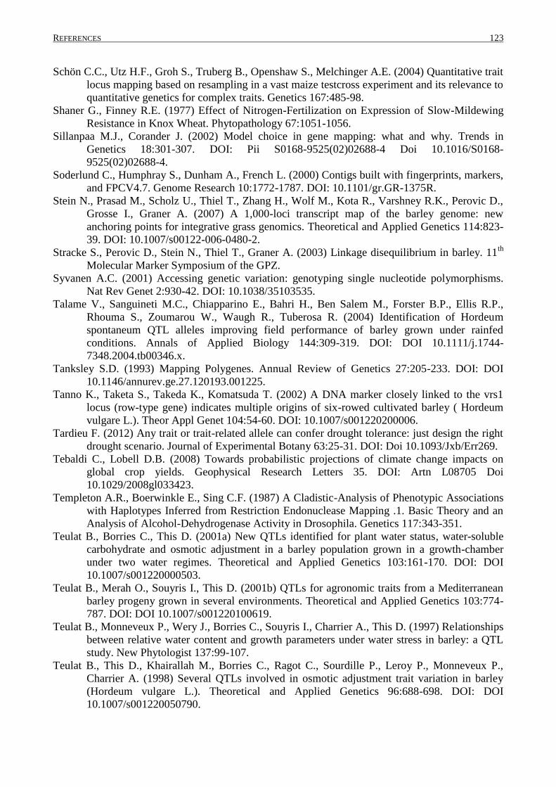
REFERENCES 123

Schön C.C., Utz H.F., Groh S., Truberg B., Openshaw S., Melchinger A.E. (2004) Quantitative trait

locus mapping based on resampling in a vast maize testcross experiment and its relevance to

quantitative genetics for complex traits. Genetics 167:485-98.

Shaner G., Finney R.E. (1977) Effect of Nitrogen-Fertilization on Expression of Slow-Mildewing

Resistance in Knox Wheat. Phytopathology 67:1051-1056.

Sillanpaa M.J., Corander J. (2002) Model choice in gene mapping: what and why. Trends in

Genetics 18:301-307. DOI: Pii S0168-9525(02)02688-4 Doi 10.1016/S0168-

9525(02)02688-4.

Soderlund C., Humphray S., Dunham A., French L. (2000) Contigs built with fingerprints, markers,

and FPCV4.7. Genome Research 10:1772-1787. DOI: 10.1101/gr.GR-1375R.

Stein N., Prasad M., Scholz U., Thiel T., Zhang H., Wolf M., Kota R., Varshney R.K., Perovic D.,

Grosse I., Graner A. (2007) A 1,000-loci transcript map of the barley genome: new

anchoring points for integrative grass genomics. Theoretical and Applied Genetics 114:823-

39. DOI: 10.1007/s00122-006-0480-2.

Stracke S., Perovic D., Stein N., Thiel T., Graner A. (2003) Linkage disequilibrium in barley. 11th

Molecular Marker Symposium of the GPZ.

Syvanen A.C. (2001) Accessing genetic variation: genotyping single nucleotide polymorphisms.

Nat Rev Genet 2:930-42. DOI: 10.1038/35103535.

Talame V., Sanguineti M.C., Chiapparino E., Bahri H., Ben Salem M., Forster B.P., Ellis R.P.,

Rhouma S., Zoumarou W., Waugh R., Tuberosa R. (2004) Identification of Hordeum

spontaneum QTL alleles improving field performance of barley grown under rainfed

conditions. Annals of Applied Biology 144:309-319. DOI: DOI 10.1111/j.1744-

7348.2004.tb00346.x.

Tanksley S.D. (1993) Mapping Polygenes. Annual Review of Genetics 27:205-233. DOI: DOI

10.1146/annurev.ge.27.120193.001225.

Tanno K., Taketa S., Takeda K., Komatsuda T. (2002) A DNA marker closely linked to the vrs1

locus (row-type gene) indicates multiple origins of six-rowed cultivated barley ( Hordeum

vulgare L.). Theor Appl Genet 104:54-60. DOI: 10.1007/s001220200006.

Tardieu F. (2012) Any trait or trait-related allele can confer drought tolerance: just design the right

drought scenario. Journal of Experimental Botany 63:25-31. DOI: Doi 10.1093/Jxb/Err269.

Tebaldi C., Lobell D.B. (2008) Towards probabilistic projections of climate change impacts on

global crop yields. Geophysical Research Letters 35. DOI: Artn L08705 Doi

10.1029/2008gl033423.

Templeton A.R., Boerwinkle E., Sing C.F. (1987) A Cladistic-Analysis of Phenotypic Associations

with Haplotypes Inferred from Restriction Endonuclease Mapping .1. Basic Theory and an

Analysis of Alcohol-Dehydrogenase Activity in Drosophila. Genetics 117:343-351.

Teulat B., Borries C., This D. (2001a) New QTLs identified for plant water status, water-soluble

carbohydrate and osmotic adjustment in a barley population grown in a growth-chamber

under two water regimes. Theoretical and Applied Genetics 103:161-170. DOI: DOI

10.1007/s001220000503.

Teulat B., Merah O., Souyris I., This D. (2001b) QTLs for agronomic traits from a Mediterranean

barley progeny grown in several environments. Theoretical and Applied Genetics 103:774-

787. DOI: DOI 10.1007/s001220100619.

Teulat B., Monneveux P., Wery J., Borries C., Souyris I., Charrier A., This D. (1997) Relationships

between relative water content and growth parameters under water stress in barley: a QTL

study. New Phytologist 137:99-107.

Teulat B., This D., Khairallah M., Borries C., Ragot C., Sourdille P., Leroy P., Monneveux P.,

Charrier A. (1998) Several QTLs involved in osmotic adjustment trait variation in barley

(Hordeum vulgare L.). Theoretical and Applied Genetics 96:688-698. DOI: DOI

10.1007/s001220050790.

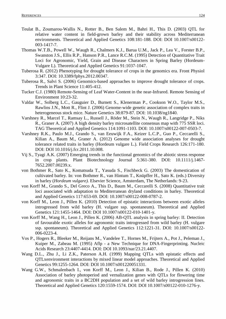
REFERENCES 124

Teulat B., Zoumarou-Wallis N., Rotter B., Ben Salem M., Bahri H., This D. (2003) QTL for

relative water content in field-grown barley and their stability across Mediterranean

environments. Theoretical and Applied Genetics 108:181-188. DOI: DOI 10.1007/s00122-

003-1417-7.

Thomas W.T.B., Powell W., Waugh R., Chalmers K.J., Barua U.M., Jack P., Lea V., Forster B.P.,

Swanston J.S., Ellis R.P., Hanson P.R., Lance R.C.M. (1995) Detection of Quantitative Trait

Loci for Agronomic, Yield, Grain and Disease Characters in Spring Barley (Hordeum-

Vulgare L). Theoretical and Applied Genetics 91:1037-1047.

Tuberosa R. (2012) Phenotyping for drought tolerance of crops in the genomics era. Front Physiol

3:347. DOI: 10.3389/fphys.2012.00347.

Tuberosa R., Salvi S. (2006) Genomics-based approaches to improve drought tolerance of crops.

Trends in Plant Science 11:405-412.

Tucker C.J. (1980) Remote-Sensing of Leaf Water-Content in the near-Infrared. Remote Sensing of

Environment 10:23-32.

Valdar W., Solberg L.C., Gauguier D., Burnett S., Klenerman P., Cookson W.O., Taylor M.S.,

Rawlins J.N., Mott R., Flint J. (2006) Genome-wide genetic association of complex traits in

heterogeneous stock mice. Nature Genetics 38:879-87. DOI: 10.1038/ng1840.

Varshney R., Marcel T., Ramsay L., Russell J., Röder M., Stein N., Waugh R., Langridge P., Niks

R., Graner A. (2007) A high density barley microsatellite consensus map with 775 SSR loci.

TAG Theoretical and Applied Genetics 114:1091-1103. DOI: 10.1007/s00122-007-0503-7.

Varshney R.K., Paulo M.J., Grando S., van Eeuwijk F.A., Keizer L.C.P., Guo P., Ceccarelli S.,

Kilian A., Baum M., Graner A. (2012) Genome wide association analyses for drought

tolerance related traits in barley (Hordeum vulgare L.). Field Crops Research 126:171-180.

DOI: DOI 10.1016/j.fcr.2011.10.008.

Vij S., Tyagi A.K. (2007) Emerging trends in the functional genomics of the abiotic stress response

in crop plants. Plant Biotechnology Journal 5:361-380. DOI: 10.1111/j.1467-

7652.2007.00239.x.

von Bothmer R., Sato K., Komatsuda T., Yasuda S., Fischbeck G. (2003) The domestication of

cultivated barley. In: von Bothmer R., van Hintum T., Knüpffer H., Sato K. (eds.) Diversity

in barley (Hordeum vulgare). Elsevier Science, Amsterdam, The Netherlands: 9-23.

von Korff M., Grando S., Del Greco A., This D., Baum M., Ceccarelli S. (2008) Quantitative trait

loci associated with adaptation to Mediterranean dryland conditions in barley. Theoretical

and Applied Genetics 117:653-69. DOI: 10.1007/s00122-008-0787-2.

von Korff M., Leon J., Pillen K. (2010) Detection of epistatic interactions between exotic alleles

introgressed from wild barley (H. vulgare ssp. spontaneum). Theoretical and Applied

Genetics 121:1455-1464. DOI: DOI 10.1007/s00122-010-1401-y.

von Korff M., Wang H., Leon J., Pillen K. (2006) AB-QTL analysis in spring barley: II. Detection

of favourable exotic alleles for agronomic traits introgressed from wild barley (H. vulgare

ssp. spontaneum). Theoretical and Applied Genetics 112:1221-31. DOI: 10.1007/s00122-

006-0223-4.

Vos P., Hogers R., Bleeker M., Reijans M., Vandelee T., Hornes M., Frijters A., Pot J., Peleman J.,

Kuiper M., Zabeau M. (1995) Aflp - a New Technique for DNA-Fingerprinting. Nucleic

Acids Research 23:4407-4414. DOI: DOI 10.1093/nar/23.21.4407.

Wang D.L., Zhu J., Li Z.K., Paterson A.H. (1999) Mapping QTLs with epistatic effects and

QTLxenvironment interactions by mixed linear model approaches. Theoretical and Applied

Genetics 99:1255-1264. DOI: DOI 10.1007/s001220051331.

Wang G.W., Schmalenbach I., von Korff M., Leon J., Kilian B., Rode J., Pillen K. (2010)

Association of barley photoperiod and vernalization genes with QTLs for flowering time

and agronomic traits in a BC2DH population and a set of wild barley introgression lines.

Theoretical and Applied Genetics 120:1559-1574. DOI: DOI 10.1007/s00122-010-1276-y.

REFERENCES 125

Wang M.H., Jiang N., Jia T.Y., Leach L., Cockram J., Waugh R., Ramsay L., Thomas B., Luo Z.W.

(2012) Genome-wide association mapping of agronomic and morphologic traits in highly

structured populations of barley cultivars. Theoretical and Applied Genetics 124:233-246.

DOI: DOI 10.1007/s00122-011-1697-2.

Wang N., Akey J.M., Zhang K., Chakraborty R., Jin L. (2002) Distribution of recombination

crossovers and the origin of haplotype blocks: the interplay of population history,

recombination, and mutation. American Journal of Human Genetics 71:1227-34. DOI:

10.1086/344398.

Waugh R., Jannink J.L., Muehlbauer G.J., Ramsay L. (2009) The emergence of whole genome

association scans in barley. Current Opinion in Plant Biology 12:218-222. DOI: DOI

10.1016/j.pbi.2008.12.007.

Wenzl P., Li H., Carling J., Zhou M., Raman H., Paul E., Hearnden P., Maier C., Xia L., Caig V.,

Ovesna J., Cakir M., Poulsen D., Wang J., Raman R., Smith K., Muehlbauer G., Chalmers

K., Kleinhofs A., Huttner E., Kilian A. (2006) A high-density consensus map of barley

linking DArT markers to SSR, RFLP and STS loci and agricultural traits. Bmc Genomics

7:206.

Williams J.G.K., Kubelik A.R., Livak K.J., Rafalski J.A., Tingey S.V. (1990) DNA Polymorphisms

Amplified by Arbitrary Primers Are Useful as Genetic-Markers. Nucleic Acids Research

18:6531-6535. DOI: DOI 10.1093/nar/18.22.6531.

Xu S.Z., Jia Z.Y. (2007) Genomewide analysis of epistatic effects for quantitative traits in barley.

Genetics 175:1955-1963. DOI: DOI 10.1534/genetics.106.066571.

Yalcin B., Flint J., Mott R. (2005) Using progenitor strain information to identify quantitative trait

nucleotides in outbred mice. Genetics 171:673-681.

Yan L., Fu D., Li C., Blechl A., Tranquilli G., Bonafede M., Sanchez A., Valarik M., Yasuda S.,

Dubcovsky J. (2006) The wheat and barley vernalization gene VRN3 is an orthologue of FT.

Proceedings of the National Academy of Sciences of the United States of America

103:19581-19586. DOI: DOI 10.1073/pnas.0607142103.

Yu J., Wang J., Lin W., Li S., Li H., Zhou J., Ni P., Dong W., Hu S., Zeng C., Zhang J., Zhang Y.,

Li R., Xu Z., Li X., Zheng H., Cong L., Lin L., Yin J., Geng J., Li G., Shi J., Liu J., Lv H.,

Li J., Deng Y., Ran L., Shi X., Wang X., Wu Q., Li C., Ren X., Li D., Liu D., Zhang X., Ji

Z., Zhao W., Sun Y., Zhang Z., Bao J., Han Y., Dong L., Ji J., Chen P., Wu S., Xiao Y., Bu

D., Tan J., Yang L., Ye C., Xu J., Zhou Y., Yu Y., Zhang B., Zhuang S., Wei H., Liu B., Lei

M., Yu H., Li Y., Xu H., Wei S., He X., Fang L., Huang X., Su Z., Tong W., Tong Z., Ye J.,

Wang L., Lei T., Chen C., Chen H., Huang H., Zhang F., Li N., Zhao C., Huang Y., Li L.,

Xi Y., Qi Q., Li W., Hu W., Tian X., Jiao Y., Liang X., Jin J., Gao L., Zheng W., Hao B.,

Liu S., Wang W., Yuan L., Cao M., McDermott J., Samudrala R., Wong G.K., Yang H.

(2005) The Genomes of Oryza sativa: a history of duplications. PLoS Biol 3:e38. DOI:

10.1371/journal.pbio.0030038.

Yu S.B., Li J.X., Xu C.G., Tan Y.F., Gao Y.J., Li X.H., Zhang Q., Saghai Maroof M.A. (1997)

Importance of epistasis as the genetic basis of heterosis in an elite rice hybrid. Proc Natl

Acad Sci U S A 94:9226-31.

Zeng Z.B. (1994) Precision Mapping of Quantitative Trait Loci. Genetics 136:1457-1468.

Zhang F., Chen G., Huang Q., Orion O., Krugman T., Fahima T., Korol A.B., Nevo E., Gutterman

Y. (2005) Genetic basis of barley caryopsis dormancy and seedling desiccation tolerance at

the germination stage. Theoretical and Applied Genetics 110:445-53. DOI: 10.1007/s00122-

004-1851-1.

Zhang K., Deng M., Chen T., Waterman M.S., Sun F. (2002) A dynamic programming algorithm

for haplotype block partitioning. Proc Natl Acad Sci U S A 99:7335-9. DOI:

10.1073/pnas.102186799.

REFERENCES 126

Zhao H.H., Fernando R.L., Dekkers J.C. (2007) Power and precision of alternate methods for

linkage disequilibrium mapping of quantitative trait loci. Genetics 175:1975-86. DOI:

10.1534/genetics.106.066480.

Zhao H.Y., Pfeiffer R., Gail M.H. (2003) Haplotype analysis in population genetics and association

studies. Pharmacogenomics 4:171-178.

FIGURE LISTING 127

7. List of figures

FIG. 1: FREQUENCY RANGE OF THZ AND OTHERS ................................................................................................................ 5

FIG. 2: SCHEMATIC INSTALLATION OF A PULSED THZ SYSTEM ............................................................................................ 6

FIG. 3: HAPLOTYPE CONSTRUCTION OUT OF CHROMOSOMAL ............................................................................................ 12

FIG. 4: CROSSING SCHEME OF THE EIGHT PARENT MAGIC CROSS. .................................................................................... 17

FIG. 5 SOIL MOISTURE CONTENT (%) FOR WELL WATERED (BLUE) AND TERMINAL DROUGHT (RED) TREATMENT IN 2011

AND 2012 ................................................................................................................................................................. 33

FIG. 6: PRINCIPAL COMPONENT ANALYSIS WITH 5117 SNP MARKER AND 533 MAGIC DH-LINES ................................... 40

FIG. 7: LD AS A FUNCTION OF GENETIC DISTANCE. ............................................................................................................ 41

FIG. 8: PARENTAL MEANS FOR WATER LOSS (WL) AT QWHC.MAGIC.HA-5H.A ............................................................. 58

FIG. 9: MULTIPLE COMPARISONS BETWEEN THE PARENTAL MEANS AT QAGB.MAGIC.HA-6H.A FOR EACH TREATMENT.

NO SIGNIFICANT DIFFERENCES WERE DETECTED FOR TERMINAL DROUGHT, BUT UNDER WELL WATERED

CONDITIONS. DIFFERENT LETTER INDICATE SIGNIFICANT DIFFERENCES (P<0.05) .................................................... 59

FIG. 10: SIMILARITY OF PFLUGS INTENSIV AND ACKERMANNS BAVARIA TO PARENT CRIEWENER 403 BASED ON THE

AMOUNT OF MARKERS USED IN THE ANALYSIS. ........................................................................................................ 68

FIG. 11: DIFFERENCES BETWEEN THE MAPPING POWER OF THE ALLELIC PARENTAL MEANS. ............................................. 74

FIG. 12: MAPPING POWER OF THE BA (BLUE) AND HA (RED). ........................................................................................... 83

FIG. 13: MAP OF SEVEN LINKAGE GROUPS OF BARLEY AND THE GENETIC POSITION OF THE QTL IN CM. ........................... 86

FIG. 14: GENETIC MAP OF QTL COINCIDING WITH QTL OR GENES KNOWN FROM LITERATURE (UNDERSCORED). ............. 94

FIG. 15: EPISTATIC INTERACTION FOR DHE, EXEMPLARY. .............................................................................................. 104

FIG. 16: RADAR CHART OF THE MAGIC DH-LINE 429 (BLUE) AND THE MAGIC POPULATION MEAN (BLACK) FOR THE

PHENOTYPIC MEAN RESULTING FROM THE BA AT TWELVE TRAITS. ....................................................................... 107

FIG. 17: RADAR CHART FROM THE RESULTS FROM HA FOR DH-LINE 145 (RED) AND POPULATION MEAN (BLACK) FOR

TWELVE TRAITS. ..................................................................................................................................................... 108

FIG. 18: COMPARISON OF THE TWO DH-LINES CHOSEN BY BA (DH 429 IN BLUE) AND HA (DH 145 IN RED) AS BEST

PERFORMING DH-LINES WITH MULTIPLE ALLELIC EFFECTS FOR TWELVE PHENOTYPIC TRAITS. ............................. 109

TABLE LISTING 128

8. List of tables

TABLE 1: ACCESSION NUMBER AND REGISTRATION DATE OF MAGIC PARENTS ............................................................... 16

TABLE 2: SUBFAMILIES AND SUB-SUBFAMILIES FROM THE CROSSING SCHEME OF THE MAGIC POPULATION. 21 KERNELS

FROM EACH SUBFAMILY WERE SENT TO PRODUCE DH-LINES. .................................................................................. 18

TABLE 3: LIST OF PHENOTYPIC TRAITS AND THEIR ABBREVIATIONS, MEASURED UNIT AND METHOD AND TIME AFTER

SOWING (DAS) INVESTIGATED IN PRELIMINARY EXPERIMENT IN 2010 .................................................................... 20

TABLE 4: LIST OF PHENOTYPIC TRAITS AND THEIR ABBREVIATIONS, MEASURED UNIT AND METHOD AND TIME AFTER

SOWING (DAS) INVESTIGATED IN THE MAGIC POPULATION IN 2011 AND 2012 ..................................................... 22

TABLE 5: CALCULATED VALUES MEASURED WITH THZ-TDS-SYSTEM USED FOR MARKER-TRAIT-SENSOR ASSOCIATION . 23

TABLE 6: DEGREES OF FREEDOM, F AND P VALUE OF FIXED EFFECTS IN THE ANALYSIS OF VARIANCE FOR THE PARENTS OF

MAGIC POPULATION FOR REPEATED TRAITS ........................................................................................................... 31

TABLE 7: DEGREES OF FREEDOM, F AND P VALUE OF FIXED EFFECTS IN THE ANALYSIS OF VARIANCE FOR THE PARENTS OF

MAGIC POPULATION FOR NON-RECURRENT TRAITS ................................................................................................ 32

TABLE 8: MULTIPLE MEAN COMPARISONS OF THE PHENOTYPE VALUES BETWEEN THE MAGIC PARENTS ........................ 34

TABLE 9: MEANS VALUES AND COMPARISON FOR SCORED TRAITS UNDER BOTH WATERING CONDITIONS FOR THE MEAN OF

THE EIGHT PARENTS AND FOR THE MAGIC DH-LINES ............................................................................................. 35

TABLE 10: MEAN COMPARISON FOR SCORED TRAITS WITHIN EACH TREATMENT (WELL WATERED AND TERMINAL

DROUGHT) BETWEEN THE MEAN OF THE MAGIC DH-LINES AND THE MEAN OF THE PARENTS ................................ 35

TABLE 11: DEGREES OF FREEDOM, F AND P VALUE OF FIXED EFFECTS IN THE ANALYSIS OF VARIANCE 534 MAGIC DH-

LINES OVER TWO YEARS FOR NON-RECURRENT TRAITS ............................................................................................ 36

TABLE 12: MULTIPLE COMPARISONS OF MAGIC PARENTS FOR TWO TRAITS EVALUATED WITH THE THZ-SENSOR ........... 37

TABLE 13: MEAN, MINIMUM (MIN) AND MAXIMUM (MAX) VALUES FOR THZ TRAITS FOR MEAN OF MAGIC DH-LINES AND

THEIR PARENTS ........................................................................................................................................................ 37

TABLE 14: PEARSON CORRELATION COEFFICIENT FOR TRAITS MEASURED IN MAGIC DH-LINES. VALUES IN ITALIC ARE

CORRELATIONS BETWEEN TRAITS UNDER WW OTHERS UNDER TD CONDITIONS; HIGH CORRELATIONS ARE BOLD..... 38

TABLE 15: PEARSON CORRELATION COEFFICIENT FOR TRAITS MEASURED WITH THE THZ-SENSOR AND AUDPC, AGB AND

YLD. VALUES IN ITALIC ARE CORRELATIONS BETWEEN TRAITS UNDER WW OTHERS UNDER TD CONDITIONS; HIGH

CORRELATIONS ARE BOLD. ....................................................................................................................................... 39

TABLE 16: SUMMARY OF MAGIC GENETIC LINKAGE MAP ................................................................................................ 42

TABLE 17: PERCENTAGE OF EACH CHROMOSOME WITH EACH FOUNDER ANCESTRY .......................................................... 42

TABLE 18: LIST OF QTL MAPPED WITH THE BA FOR TWELVE TRAITS IN THE MAGIC DH-LINES ..................................... 49

TABLE 19: QTL MAPPED WITH THE HA FOR TWELVE TRAITS IN THE MAGIC H-LINES ..................................................... 51

TABLE 20: LIST OF SELECTED MAIN MARKER QTL FROM HA WITH MULTIPLE COMPARISONS BETWEEN THE PARENTAL

MEAN ....................................................................................................................................................................... 61

TABLE 21: MULTIPLE COMPARISONS FROM HA FOR SELECTED MARKER*TREATMENT INTERACTION ............................... 62

TABLE 22: LIST OF QTL MAPPED WITHIN THE MAGIC POPULATION FOR TWELVE TRAITS AND TWO MAPPING APPROACHES

................................................................................................................................................................................. 78

TABLE 23: LIST OF DETECTED QTL IN THE MAGIC DH-LINES THAT COINCIDE WITH GENES AND QTL FROM LITERATURE

................................................................................................................................................................................. 92

TABLE 24: LIST OF QTL WITH MARKER*TREATMENT INTERACTION EFFECTS FOR BINARY AND HAPLOTYPE APPROACH ... 99

ABBILDUNGS- UND TABELLENVERZEICHNIS 129

TABLE 25: SIGNIFICANT M1*M2 EPISTATIC INTERACTIONS DETERMINED WITH THE BA IN THE MAGIC DH-LINES ...... 102

TABLE 26: DH-LINES WITH COMBINED POSITIVE ALLELE EFFECTS ESTIMATED WITH THE BA WITHIN TRAITS ................. 105

TABLE 27: DH-LINES WITH COMBINED POSITIVE ALLELE EFFECTS ESTIMATED WITH THE HA WITHIN TRAITS ................ 106

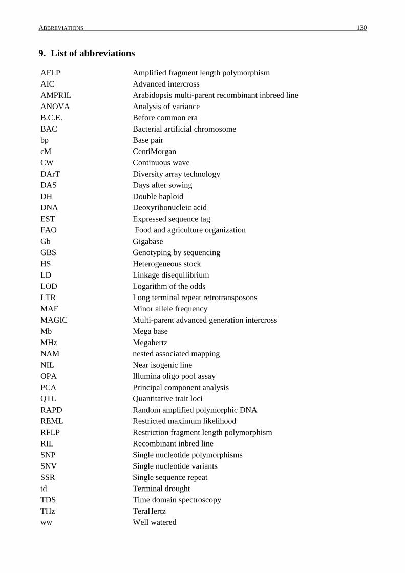
ABBREVIATIONS 130

9. List of abbreviations

AFLP Amplified fragment length polymorphism

AIC Advanced intercross

AMPRIL Arabidopsis multi-parent recombinant inbreed line

ANOVA Analysis of variance

B.C.E. Before common era

BAC Bacterial artificial chromosome

bp Base pair

cM CentiMorgan

CW Continuous wave

DArT Diversity array technology

DAS Days after sowing

DH Double haploid

DNA Deoxyribonucleic acid

EST Expressed sequence tag

FAO Food and agriculture organization

Gb Gigabase

GBS Genotyping by sequencing

HS Heterogeneous stock

LD Linkage disequilibrium

LOD Logarithm of the odds

LTR Long terminal repeat retrotransposons

MAF Minor allele frequency

MAGIC Multi-parent advanced generation intercross

Mb Mega base

MHz Megahertz

NAM nested associated mapping

NIL Near isogenic line

OPA Illumina oligo pool assay

PCA Principal component analysis

QTL Quantitative trait loci

RAPD Random amplified polymorphic DNA

REML Restricted maximum likelihood

RFLP Restriction fragment length polymorphism

RIL Recombinant inbred line

SNP Single nucleotide polymorphisms

SNV Single nucleotide variants

SSR Single sequence repeat

td Terminal drought

TDS Time domain spectroscopy

THz TeraHertz

ww Well watered

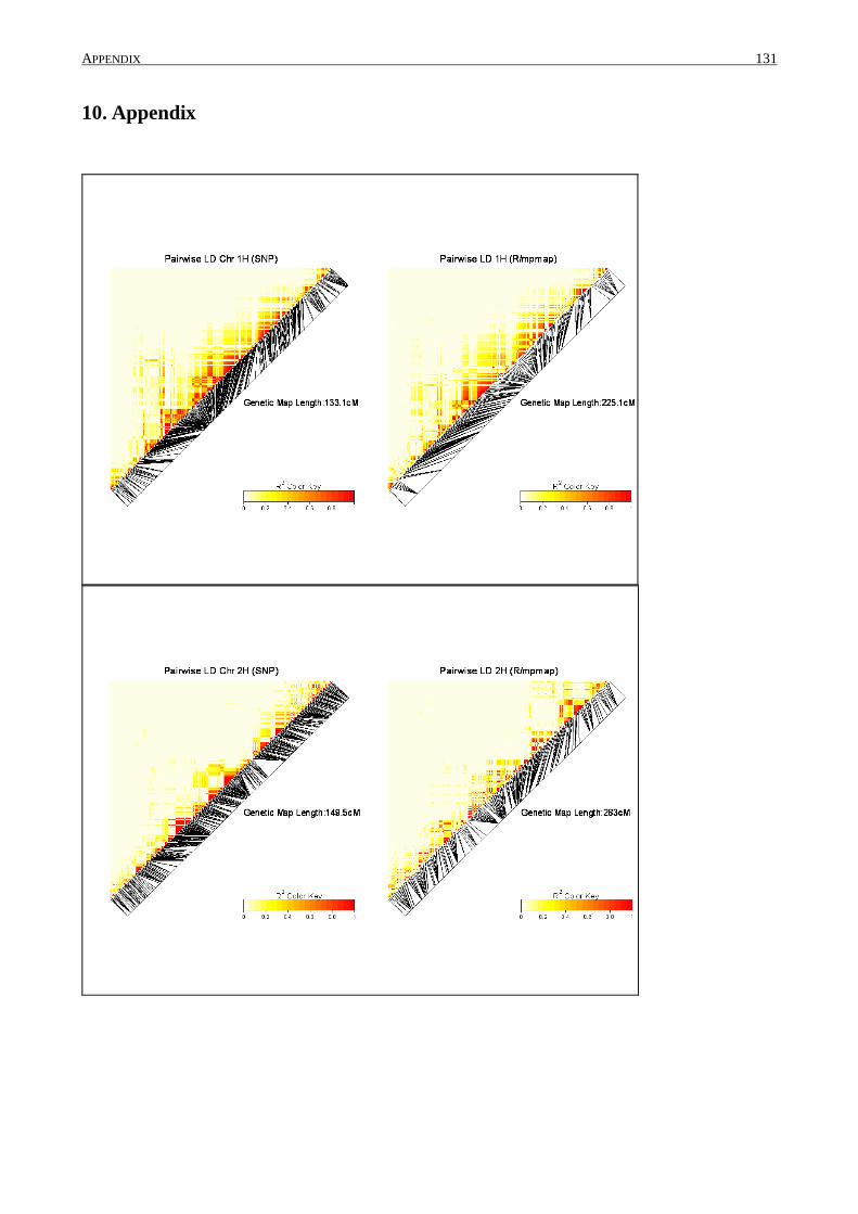
APPENDIX 131

10. Appendix

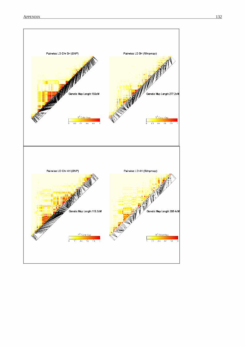
APPENDIX 132

APPENDIX 133

APPENDIX 134

Appendix 1: Heat maps of linkage disequilibrium for each chromosome and each approach.

SNP=Binary approach, R/mpmap=Haplotype approach

APPENDIX 135

Appendix 2: List of SNP markers with their locus name and chromosome and position in cM constructed from

R/mpMap

Locus name Chr Pos BOPAMARK BOPA OLDNAME POPA123S POPA

12_11011 1H 0,0 12_11011 12_0233 12_11011 931-681 1_1011

12_30918 1H 0,0 12_30918 12_1144 12_30918 SCRI_abc15612_01_1 3_0918

11_20502 1H 13,4 11_20502 11_0481 3220-723 3220-723 2_0502

11_21174 1H 13,4 11_21174 11_1079 6949-895 6949-895 2_1174

11_21226 1H 13,4 11_21226 11_1126 7372-1253 7372-1253 2_1226

SCRI_RS_148560 1H 13,4

SCRI_RS_148733 1H 13,4 SCRI_RS_130592 1H 13,4 SCRI_RS_205669 1H 13,4

SCRI_RS_120053 1H 36,4

12_30969 1H 37,1 12_30969 12_1184 12_30969 SCRI_bbc15015_01_164 3_0969

11_10419 1H 37,1 11_10419 11_0453 3101-111 3101-111 1_0419

11_21067 1H 50,3 11_21067 11_0992 6195-2137 6195-2137 2_1067

12_30715 1H 50,3 12_30715 12_0994 12_30715 U32_7636_1701 3_0715

SCRI_RS_184274 1H 58,1 11_20712 1H 58,1 11_20712 11_0683 4226-570 4226-570 2_0712

SCRI_RS_119312 1H 61,6

SCRI_RS_157757 1H 70,5

12_30948 1H 70,5 12_30948 12_1166 12_30948 SCRI_bbc04473_01_2 3_0948

11_20371 1H 70,5 11_20371 11_0346 2496-1916 2496-1916 2_0371

12_30241 1H 70,5 12_30241 12_0726 12_30241 ABC15164_2_387 3_0241

SCRI_RS_124926 1H 75,4

SCRI_RS_14227 1H 75,4 11_10760 1H 75,9 11_10760 11_0879 5346-1587 5346-1587 1_0760

SCRI_RS_152464 1H 76,0

11_10030 1H 76,0 11_10030 11_0042 10922-503 10922-503 1_0030

SCRI_RS_155382 1H 76,0 12_31276 1H 76,0 12_31276 12_1385 12_31276 U35_19740_954 3_1276

SCRI_RS_189483 1H 76,0

12_10506 1H 76,0 12_10506 12_0118 12_10506 3640-2807 1_0506

12_11169 1H 76,0 12_11169 12_0284 12_11169 ABC07427-1-1-329 1_1169

11_10764 1H 76,4 11_10764 11_0883 5381-1950 5381-1950 1_0764

SCRI_RS_140837 1H 76,4

11_21134 1H 76,4 11_21134 11_1052 6720-641 6720-641 2_1134

11_20855 1H 76,4 11_20855 11_0819 5019-879 5019-879 2_0855

11_20514 1H 83,5 11_20514 11_0491 3277-446 3277-446 2_0514

11_11287 1H 83,5 11_11287 11_1422 ABC11913-1-1-104 ABC11913-1-1-104 1_1287

12_30336 1H 89,3 12_30336 12_0773 12_30336 U32_11789_202 3_0336

11_10526 1H 89,3 11_10526 11_0579 3710-852 3710-852 1_0526

11_11064 1H 89,3 11_11064 11_1326 ABC02639-1-4-370 ABC02639-1-4-370 1_1064

11_20660 1H 89,3 11_20660 11_0629 4020-643 4020-643 2_0660

SCRI_RS_221759 1H 92,9

12_30683 1H 92,9 12_30683 12_0975 12_30683 U32_7097_198 3_0683

11_10985 1H 92,9 11_10985 11_1229 8613-278 8613-278 1_0985

11_10075 1H 92,9 11_10075 11_0112 1294-473 1294-473 1_0075

SCRI_RS_165811 1H 95,0

SCRI_RS_11615 1H 95,0 SCRI_RS_160545 1H 95,0 11_10275 1H 95,0 11_10275 11_0307 2314-1412 2314-1412 1_0275

SCRI_RS_199178 1H 95,0

SCRI_RS_132461 1H 95,0

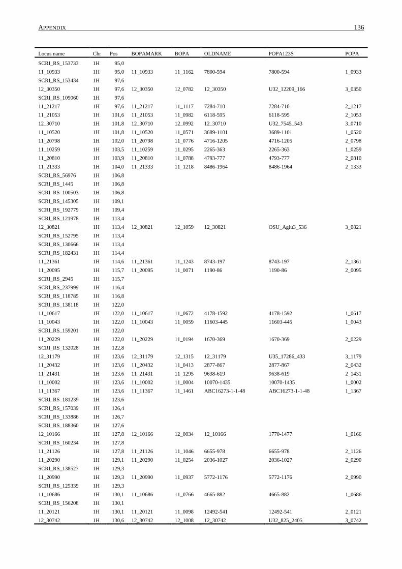
APPENDIX 136


SCRI_RS_153733 1H 95,0 11_10933 1H 95,0 11_10933 11_1162 7800-594 7800-594 1_0933

SCRI_RS_153434 1H 97,6

12_30350 1H 97,6 12_30350 12_0782 12_30350 U32_12209_166 3_0350

SCRI_RS_109060 1H 97,6 11_21217 1H 97,6 11_21217 11_1117 7284-710 7284-710 2_1217

11_21053 1H 101,6 11_21053 11_0982 6118-595 6118-595 2_1053

12_30710 1H 101,8 12_30710 12_0992 12_30710 U32_7545_543 3_0710

11_10520 1H 101,8 11_10520 11_0571 3689-1101 3689-1101 1_0520

11_20798 1H 102,0 11_20798 11_0776 4716-1205 4716-1205 2_0798

11_10259 1H 103,5 11_10259 11_0295 2265-363 2265-363 1_0259

11_20810 1H 103,9 11_20810 11_0788 4793-777 4793-777 2_0810

11_21333 1H 104,0 11_21333 11_1218 8486-1964 8486-1964 2_1333

SCRI_RS_56976 1H 106,8

SCRI_RS_1445 1H 106,8

SCRI_RS_100503 1H 106,8

SCRI_RS_145305 1H 109,1 SCRI_RS_192779 1H 109,4

SCRI_RS_121978 1H 113,4

12_30821 1H 113,4 12_30821 12_1059 12_30821 OSU_Aglu3_536 3_0821

SCRI_RS_152795 1H 113,4 SCRI_RS_130666 1H 113,4

SCRI_RS_182431 1H 114,4

11_21361 1H 114,6 11_21361 11_1243 8743-197 8743-197 2_1361

11_20095 1H 115,7 11_20095 11_0071 1190-86 1190-86 2_0095

SCRI_RS_2945 1H 115,7

SCRI_RS_237999 1H 116,4

SCRI_RS_118785 1H 116,8

SCRI_RS_138118 1H 122,0 11_10617 1H 122,0 11_10617 11_0672 4178-1592 4178-1592 1_0617

11_10043 1H 122,0 11_10043 11_0059 11603-445 11603-445 1_0043

SCRI_RS_159201 1H 122,0

11_20229 1H 122,0 11_20229 11_0194 1670-369 1670-369 2_0229

SCRI_RS_132028 1H 122,8

12_31179 1H 123,6 12_31179 12_1315 12_31179 U35_17286_433 3_1179

11_20432 1H 123,6 11_20432 11_0413 2877-867 2877-867 2_0432

11_21431 1H 123,6 11_21431 11_1295 9638-619 9638-619 2_1431

11_10002 1H 123,6 11_10002 11_0004 10070-1435 10070-1435 1_0002

11_11367 1H 123,6 11_11367 11_1461 ABC16273-1-1-48 ABC16273-1-1-48 1_1367

SCRI_RS_181239 1H 123,6

SCRI_RS_157039 1H 126,4 SCRI_RS_133886 1H 126,7

SCRI_RS_188360 1H 127,6

12_10166 1H 127,8 12_10166 12_0034 12_10166 1770-1477 1_0166

SCRI_RS_160234 1H 127,8 11_21126 1H 127,8 11_21126 11_1046 6655-978 6655-978 2_1126

11_20290 1H 129,1 11_20290 11_0254 2036-1027 2036-1027 2_0290

SCRI_RS_138527 1H 129,3

11_20990 1H 129,3 11_20990 11_0937 5772-1176 5772-1176 2_0990

SCRI_RS_125339 1H 129,3

11_10686 1H 130,1 11_10686 11_0766 4665-882 4665-882 1_0686

SCRI_RS_156208 1H 130,1

11_20121 1H 130,1 11_20121 11_0098 12492-541 12492-541 2_0121

12_30742 1H 130,6 12_30742 12_1008 12_30742 U32_825_2405 3_0742

APPENDIX 137


SCRI_RS_9158 1H 132,1 11_20434 1H 132,1 11_20434 11_0415 2881-935 2881-935 2_0434

SCRI_RS_166168 1H 132,1

SCRI_RS_181353 1H 132,5

11_20550 1H 134,2 11_20550 11_0516 3404-2470 3404-2470 2_0550

11_10830 1H 134,2 11_10830 11_0999 6250-1056 6250-1056 1_0830

SCRI_RS_162524 1H 134,4

11_10006 1H 134,4 11_10006 11_0011 1016-376 1016-376 1_0006

SCRI_RS_135092 1H 134,4 11_10433 1H 134,4 11_10433 11_0473 3201-603 3201-603 1_0433

11_21373 1H 134,4 11_21373 11_1251 8867-459 8867-459 2_1373

SCRI_RS_157246 1H 135,4

SCRI_RS_121048 1H 135,4 11_20475 1H 135,4 11_20475 11_0451 3087-1763 3087-1763 2_0475

SCRI_RS_197263 1H 135,4

12_31163 1H 135,4 12_31163 12_1303 12_31163 U35_1704_1053 3_1163

SCRI_RS_188218 1H 135,4 11_10396 1H 135,4 11_10396 11_0425 2935-1634 2935-1634 1_0396

11_11277 1H 139,6 11_11277 11_1419 ABC11290-sfp44-06 ABC11290-sfp44-06 1_1277

SCRI_RS_194371 1H 139,6

12_31319 1H 139,6 12_31319 12_1415 12_31319 U35_21782_494 3_1319

SCRI_RS_199689 1H 139,6

11_20169 1H 142,0 11_20169 11_0143 14371-423 14371-423 2_0169

11_10522 1H 142,2 11_10522 11_0575 3702-982 3702-982 1_0522

11_20754 1H 142,2 11_20754 11_0733 4499-1364 4499-1364 2_0754

11_10357 1H 142,4 11_10357 11_0387 2711-234 2711-234 1_0357

11_20840 1H 142,4 11_20840 11_0805 4927-1340 4927-1340 2_0840

SCRI_RS_235724 1H 143,1

SCRI_RS_130139 1H 143,6 SCRI_RS_188909 1H 146,7

SCRI_RS_136856 1H 146,7

SCRI_RS_235968 1H 147,4

SCRI_RS_189168 1H 147,4 SCRI_RS_171501 1H 150,1

SCRI_RS_213675 1H 154,5

12_20187 1H 154,5 12_20187 12_0428 12_20187 1498-596 2_0187

11_10111 1H 154,5 11_10111 11_0157 1497-628 1497-628 1_0111

SCRI_RS_106754 1H 154,5

SCRI_RS_154528 1H 154,5

12_10905 1H 154,5 12_10905 12_0209 12_10905 7389-555 1_0905

SCRI_RS_143810 1H 156,5 SCRI_RS_175646 1H 156,5

SCRI_RS_192730 1H 156,5

SCRI_RS_238125 1H 156,5

11_21392 1H 159,7 11_21392 11_1265 9105-497 9105-497 2_1392

SCRI_RS_224392 1H 159,7

11_11481 1H 159,7 11_11481 11_1508 ConsensusGBS0361-5 ConsensusGBS0361-5 1_1481

SCRI_RS_169881 1H 159,7

SCRI_RS_216088 1H 159,7 BK_01 1H 159,7

11_20021 1H 175,0 11_20021 11_0023 10360-563 10360-563 2_0021

SCRI_RS_155997 1H 175,0

11_20908 1H 175,0 11_20908 11_0868 5283-1090 5283-1090 2_0908

SCRI_RS_170110 1H 175,3

APPENDIX 138


SCRI_RS_147611 1H 175,3 SCRI_RS_155758 1H 175,3

11_20220 1H 179,1 11_20220 11_0185 1625-303 1625-303 2_0220

11_10854 1H 179,1 11_10854 11_1036 6547-1363 6547-1363 1_0854

SCRI_RS_159031 1H 179,1 SCRI_RS_165588 1H 179,1

SCRI_RS_120481 1H 190,2

SCRI_RS_127646 1H 190,2

11_10586 1H 190,2 11_10586 11_0632 4027-1814 4027-1814 1_0586

11_21140 1H 190,2 11_21140 11_1057 677-411 677-411 2_1140

11_21038 1H 210,3 11_21038 11_0972 6026-1949 6026-1949 2_1038

12_11443 1H 215,1 12_11443 12_0368 12_11443 ConsensusGBS0103-1 1_1443

11_20383 1H 215,1 11_20383 11_0358 2572-986 2572-986 2_0383

SCRI_RS_162628 1H 215,1

SCRI_RS_10956 1H 215,1

11_10590 1H 215,1 11_10590 11_0641 4057-2114 4057-2114 1_0590

SCRI_RS_199945 1H 215,1 11_10443 1H 215,1 11_10443 11_0487 3263-2865 3263-2865 1_0443

12_30934 1H 215,1 12_30934 12_1158 12_30934 SCRI_bbc01078_01_1 3_0934

12_10693 1H 217,8 12_10693 12_0167 12_10693 472-1376 1_0693

11_20138 1H 217,8 11_20138 11_0119 13095-187 13095-187 2_0138

SCRI_RS_176006 1H 217,8

SCRI_RS_175218 1H 217,8

11_20772 1H 217,8 11_20772 11_0748 4592-118 4592-118 2_0772

SCRI_RS_196025 1H 225,1 SCRI_RS_166806 2H 0,0

SCRI_RS_139708 2H 0,0

SCRI_RS_135585 2H 4,3

SCRI_RS_184395 2H 4,3 SCRI_RS_133377 2H 7,7

SCRI_RS_169758 2H 7,7

SCRI_RS_192463 2H 7,7

SCRI_RS_165171 2H 8,2 SCRI_RS_136200 2H 8,2

SCRI_RS_122 2H 8,2

SCRI_RS_168604 2H 8,2

SCRI_RS_88391 2H 8,2 12_10592 2H 8,2 12_10592 12_0138 12_10592 4063-677 1_0592

SCRI_RS_159503 2H 8,2

SCRI_RS_231057 2H 8,2

SCRI_RS_141564 2H 8,2 SCRI_RS_10642 2H 10,0

SCRI_RS_141753 2H 10,0

SCRI_RS_155957 2H 12,2

SCRI_RS_213799 2H 12,4 SCRI_RS_204158 2H 20,6

SCRI_RS_209516 2H 20,6

SCRI_RS_144545 2H 20,6

SCRI_RS_188511 2H 20,6 SCRI_RS_152744 2H 20,6

SCRI_RS_153226 2H 20,8

SCRI_RS_192440 2H 21,2

SCRI_RS_226348 2H 25,6 12_31284 2H 25,6 12_31284 12_1393 12_31284 U35_20027_279 3_1284

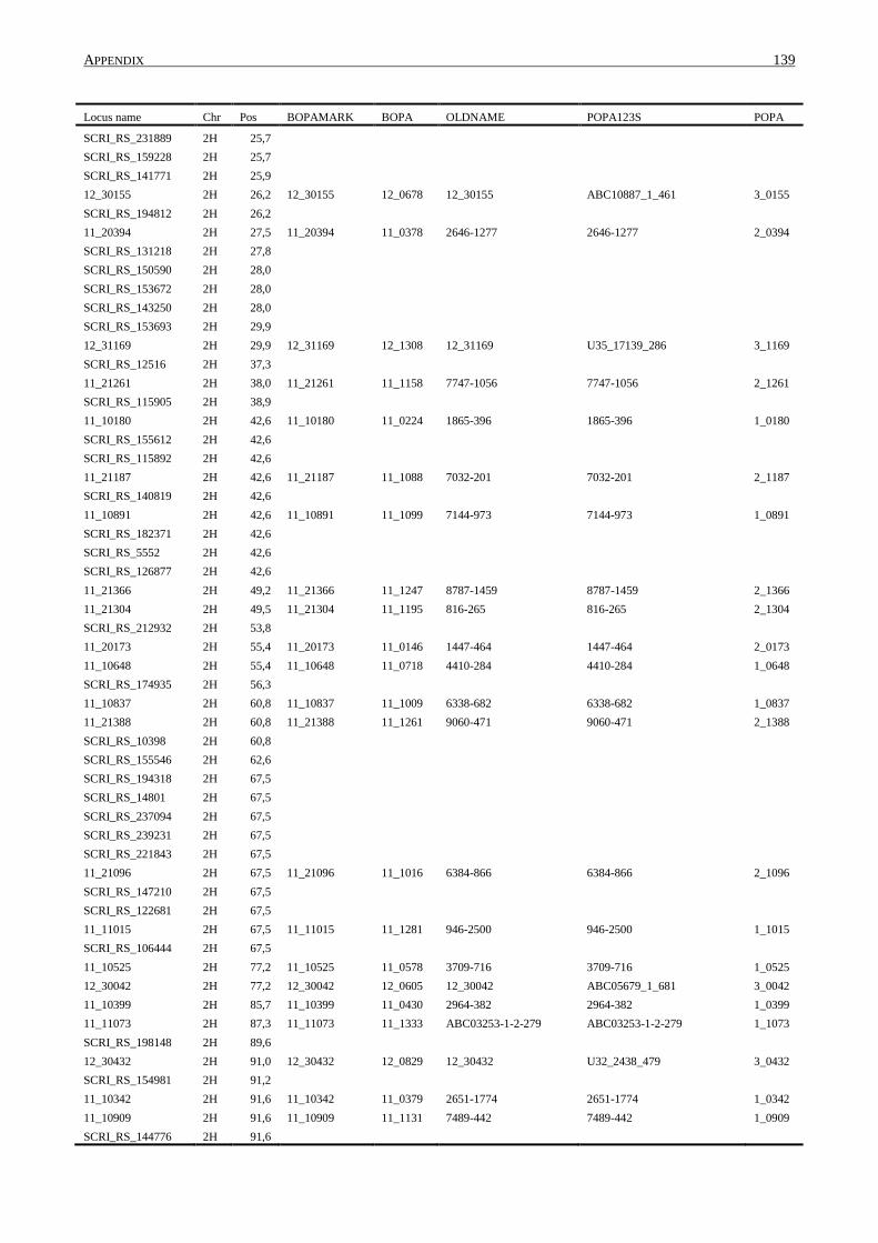
APPENDIX 139


SCRI_RS_231889 2H 25,7 SCRI_RS_159228 2H 25,7

SCRI_RS_141771 2H 25,9

12_30155 2H 26,2 12_30155 12_0678 12_30155 ABC10887_1_461 3_0155

SCRI_RS_194812 2H 26,2 11_20394 2H 27,5 11_20394 11_0378 2646-1277 2646-1277 2_0394

SCRI_RS_131218 2H 27,8

SCRI_RS_150590 2H 28,0

SCRI_RS_153672 2H 28,0 SCRI_RS_143250 2H 28,0

SCRI_RS_153693 2H 29,9

12_31169 2H 29,9 12_31169 12_1308 12_31169 U35_17139_286 3_1169

SCRI_RS_12516 2H 37,3 11_21261 2H 38,0 11_21261 11_1158 7747-1056 7747-1056 2_1261

SCRI_RS_115905 2H 38,9

11_10180 2H 42,6 11_10180 11_0224 1865-396 1865-396 1_0180

SCRI_RS_155612 2H 42,6 SCRI_RS_115892 2H 42,6

11_21187 2H 42,6 11_21187 11_1088 7032-201 7032-201 2_1187

SCRI_RS_140819 2H 42,6

11_10891 2H 42,6 11_10891 11_1099 7144-973 7144-973 1_0891

SCRI_RS_182371 2H 42,6

SCRI_RS_5552 2H 42,6

SCRI_RS_126877 2H 42,6

11_21366 2H 49,2 11_21366 11_1247 8787-1459 8787-1459 2_1366

11_21304 2H 49,5 11_21304 11_1195 816-265 816-265 2_1304

SCRI_RS_212932 2H 53,8

11_20173 2H 55,4 11_20173 11_0146 1447-464 1447-464 2_0173

11_10648 2H 55,4 11_10648 11_0718 4410-284 4410-284 1_0648

SCRI_RS_174935 2H 56,3

11_10837 2H 60,8 11_10837 11_1009 6338-682 6338-682 1_0837

11_21388 2H 60,8 11_21388 11_1261 9060-471 9060-471 2_1388

SCRI_RS_10398 2H 60,8 SCRI_RS_155546 2H 62,6

SCRI_RS_194318 2H 67,5

SCRI_RS_14801 2H 67,5

SCRI_RS_237094 2H 67,5 SCRI_RS_239231 2H 67,5

SCRI_RS_221843 2H 67,5

11_21096 2H 67,5 11_21096 11_1016 6384-866 6384-866 2_1096

SCRI_RS_147210 2H 67,5 SCRI_RS_122681 2H 67,5

11_11015 2H 67,5 11_11015 11_1281 946-2500 946-2500 1_1015

SCRI_RS_106444 2H 67,5

11_10525 2H 77,2 11_10525 11_0578 3709-716 3709-716 1_0525

12_30042 2H 77,2 12_30042 12_0605 12_30042 ABC05679_1_681 3_0042

11_10399 2H 85,7 11_10399 11_0430 2964-382 2964-382 1_0399

11_11073 2H 87,3 11_11073 11_1333 ABC03253-1-2-279 ABC03253-1-2-279 1_1073

SCRI_RS_198148 2H 89,6 12_30432 2H 91,0 12_30432 12_0829 12_30432 U32_2438_479 3_0432

SCRI_RS_154981 2H 91,2

11_10342 2H 91,6 11_10342 11_0379 2651-1774 2651-1774 1_0342

11_10909 2H 91,6 11_10909 11_1131 7489-442 7489-442 1_0909

SCRI_RS_144776 2H 91,6

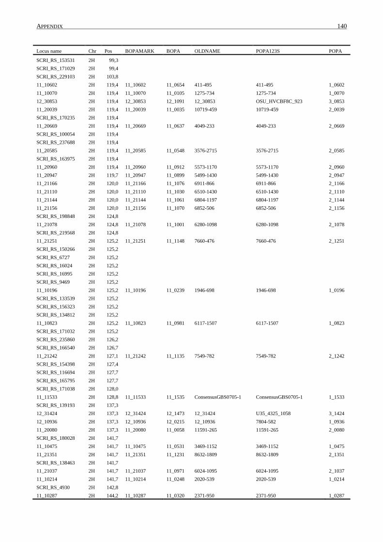
APPENDIX 140


SCRI_RS_153531 2H 99,3 SCRI_RS_171029 2H 99,4

SCRI_RS_229103 2H 103,8

11_10602 2H 119,4 11_10602 11_0654 411-495 411-495 1_0602

11_10070 2H 119,4 11_10070 11_0105 1275-734 1275-734 1_0070

12_30853 2H 119,4 12_30853 12_1091 12_30853 OSU_HVCBF8C_923 3_0853

11_20039 2H 119,4 11_20039 11_0035 10719-459 10719-459 2_0039

SCRI_RS_170235 2H 119,4

11_20669 2H 119,4 11_20669 11_0637 4049-233 4049-233 2_0669

SCRI_RS_100054 2H 119,4

SCRI_RS_237688 2H 119,4

11_20585 2H 119,4 11_20585 11_0548 3576-2715 3576-2715 2_0585

SCRI_RS_163975 2H 119,4 11_20960 2H 119,4 11_20960 11_0912 5573-1170 5573-1170 2_0960

11_20947 2H 119,7 11_20947 11_0899 5499-1430 5499-1430 2_0947

11_21166 2H 120,0 11_21166 11_1076 6911-866 6911-866 2_1166

11_21110 2H 120,0 11_21110 11_1030 6510-1430 6510-1430 2_1110

11_21144 2H 120,0 11_21144 11_1061 6804-1197 6804-1197 2_1144

11_21156 2H 120,0 11_21156 11_1070 6852-506 6852-506 2_1156

SCRI_RS_198848 2H 124,8

11_21078 2H 124,8 11_21078 11_1001 6280-1098 6280-1098 2_1078

SCRI_RS_219568 2H 124,8

11_21251 2H 125,2 11_21251 11_1148 7660-476 7660-476 2_1251

SCRI_RS_150266 2H 125,2

SCRI_RS_6727 2H 125,2 SCRI_RS_16024 2H 125,2

SCRI_RS_16995 2H 125,2

SCRI_RS_9469 2H 125,2

11_10196 2H 125,2 11_10196 11_0239 1946-698 1946-698 1_0196

SCRI_RS_133539 2H 125,2

SCRI_RS_156323 2H 125,2

SCRI_RS_134812 2H 125,2

11_10823 2H 125,2 11_10823 11_0981 6117-1507 6117-1507 1_0823

SCRI_RS_171032 2H 125,2

SCRI_RS_235860 2H 126,2

SCRI_RS_166540 2H 126,7

11_21242 2H 127,1 11_21242 11_1135 7549-782 7549-782 2_1242

SCRI_RS_154398 2H 127,4

SCRI_RS_116694 2H 127,7

SCRI_RS_165795 2H 127,7

SCRI_RS_171038 2H 128,0 11_11533 2H 128,8 11_11533 11_1535 ConsensusGBS0705-1 ConsensusGBS0705-1 1_1533

SCRI_RS_139193 2H 137,3

12_31424 2H 137,3 12_31424 12_1473 12_31424 U35_4325_1058 3_1424

12_10936 2H 137,3 12_10936 12_0215 12_10936 7804-582 1_0936

11_20080 2H 137,3 11_20080 11_0058 11591-265 11591-265 2_0080

SCRI_RS_180028 2H 141,7

11_10475 2H 141,7 11_10475 11_0531 3469-1152 3469-1152 1_0475

11_21351 2H 141,7 11_21351 11_1231 8632-1809 8632-1809 2_1351

SCRI_RS_138463 2H 141,7

11_21037 2H 141,7 11_21037 11_0971 6024-1095 6024-1095 2_1037

11_10214 2H 141,7 11_10214 11_0248 2020-539 2020-539 1_0214

SCRI_RS_4930 2H 142,8 11_10287 2H 144,2 11_10287 11_0320 2371-950 2371-950 1_0287

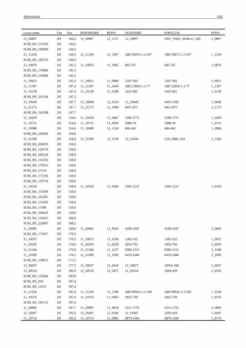
APPENDIX 141


12_30897 2H 144,2 12_30897 12_1127 12_30897 OSU_VRS1_HvHox1_260 3_0897

SCRI_RS_137263 2H 144,2

SCRI_RS_160958 2H 144,2

11_11250 2H 144,2 11_11250 11_1407 ABC10472-1-2-247 ABC10472-1-2-247 1_1250

SCRI_RS_196270 2H 144,2 11_10876 2H 145,2 11_10876 11_1065 682-767 682-767 1_0876

SCRI_RS_159484 2H 145,2

SCRI_RS_150494 2H 145,2

11_20923 2H 145,2 11_20923 11_0880 5347-585 5347-585 2_0923

11_11307 2H 147,4 11_11307 11_1430 ABC12856-1-1-77 ABC12856-1-1-77 1_1307

11_10138 2H 147,4 11_10138 11_0188 1635-691 1635-691 1_0138

SCRI_RS_195164 2H 147,5

12_10649 2H 147,7 12_10649 12_0154 12_10649 4419-1392 1_0649

11_21175 2H 147,7 11_21175 11_1080 6951-875 6951-875 2_1175

SCRI_RS_142188 2H 147,7

11_10429 2H 154,6 11_10429 11_0467 3180-1771 3180-1771 1_0429

11_10731 2H 154,6 11_10731 11_0830 5088-59 5088-59 1_0731

11_10988 2H 154,6 11_10988 11_1234 866-442 866-442 1_0988

SCRI_RS_109266 2H 154,6

12_31506 2H 154,6 12_31506 12_1518 12_31506 U35_6860_433 3_1506

SCRI_RS_200033 2H 158,0 SCRI_RS_129178 2H 158,0

SCRI_RS_209218 2H 158,0

SCRI_RS_116193 2H 158,0

SCRI_RS_179555 2H 158,0 SCRI_RS_15119 2H 158,0

SCRI_RS_172136 2H 158,0

SCRI_RS_119718 2H 158,0

11_10329 2H 158,0 11_10329 11_0366 2592-1237 2592-1237 1_0329

SCRI_RS_170209 2H 158,0

SCRI_RS_161281 2H 158,0

SCRI_RS_151056 2H 158,0

SCRI_RS_13386 2H 158,0 SCRI_RS_206020 2H 158,0

SCRI_RS_134252 2H 168,0

SCRI_RS_223897 2H 168,2

11_20681 2H 168,6 11_20681 11_0650 4100-1047 4100-1047 2_0681

SCRI_RS_173017 2H 170,5

11_10072 2H 170,5 11_10072 11_0106 1283-332 1283-332 1_0072

11_20293 2H 170,6 11_20293 11_0258 2052-792 2052-792 2_0293

11_21346 2H 170,9 11_21346 11_1227 8586-1221 8586-1221 2_1346

11_21099 2H 176,1 11_21099 11_1020 6419-1680 6419-1680 2_1099

SCRI_RS_158072 2H 177,5

12_20027 2H 177,5 12_20027 12_0410 12_20027 10503-360 2_0027

12_20518 2H 185,9 12_20518 12_0471 12_20518 3294-439 2_0518

SCRI_RS_152664 2H 185,9

SCRI_RS_918 2H 187,4

SCRI_RS_15537 2H 187,4

11_11236 2H 187,4 11_11236 11_1398 ABC09941-1-1-100 ABC09941-1-1-100 1_1236

11_10376 2H 187,4 11_10376 11_0403 2822-739 2822-739 1_0376

SCRI_RS_181112 2H 187,4

11_20895 2H 187,7 11_20895 11_0854 5211-1755 5211-1755 2_0895

12_10447 2H 192,6 12_10447 12_0100 12_10447 3292-418 1_0447

11_10714 2H 192,6 11_10714 11_0802 4879-1560 4879-1560 1_0714

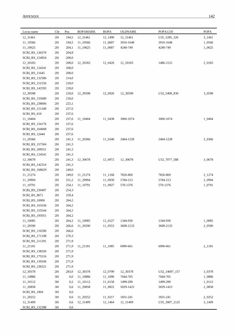
APPENDIX 142


12_31461 2H 194,5 12_31461 12_1490 12_31461 U35_5285_326 3_1461

11_10566 2H 194,5 11_10566 11_0607 3910-1648 3910-1648 1_0566

11_10625 2H 204,1 11_10625 11_0687 4240-749 4240-749 1_0625

SCRI_RS_136379 2H 204,8

SCRI_RS_154954 2H 208,0 12_20183 2H 208,0 12_20183 12_0426 12_20183 1486-1515 2_0183

SCRI_RS_134241 2H 208,0

SCRI_RS_11645 2H 208,0

SCRI_RS_132586 2H 214,0 SCRI_RS_151556 2H 218,0

SCRI_RS_142593 2H 218,0

12_30598 2H 218,0 12_30598 12_0926 12_30598 U32_5408_830 3_0598

SCRI_RS_155689 2H 218,0 SCRI_RS_238606 2H 223,1

SCRI_RS_151349 2H 237,6

SCRI_RS_610 2H 237,6

11_10404 2H 237,6 11_10404 11_0438 3000-1074 3000-1074 1_0404

SCRI_RS_154176 2H 237,6

SCRI_RS_164608 2H 237,6

SCRI_RS_12444 2H 237,6

11_20366 2H 241,3 11_20366 11_0340 2464-1228 2464-1228 2_0366

SCRI_RS_157504 2H 241,3

SCRI_RS_209551 2H 241,3

SCRI_RS_124541 2H 241,3

12_30678 2H 241,3 12_30678 12_0972 12_30678 U32_7077_588 3_0678

SCRI_RS_142314 2H 241,3

SCRI_RS_168629 2H 249,0

11_21274 2H 249,0 11_21274 11_1168 7826-869 7826-869 2_1274

11_20994 2H 251,2 11_20994 11_0939 5784-213 5784-213 2_0994

11_10791 2H 254,1 11_10791 11_0927 570-1376 570-1376 1_0791

SCRI_RS_230497 2H 254,3

SCRI_RS_8671 2H 259,4

SCRI_RS_10006 2H 264,2 SCRI_RS_161636 2H 264,2

SCRI_RS_155544 2H 264,2

SCRI_RS_195051 2H 264,2

11_10085 2H 264,2 11_10085 11_0127 1344-930 1344-930 1_0085

11_20590 2H 266,6 11_20590 11_0553 3608-2133 3608-2133 2_0590

SCRI_RS_116590 2H 266,6

SCRI_RS_171198 2H 270,3

SCRI_RS_211291 2H 271,9 11_21181 2H 271,9 11_21181 11_1085 6990-661 6990-661 2_1181

SCRI_RS_138320 2H 271,9

SCRI_RS_175216 2H 271,9

SCRI_RS_139106 2H 271,9 SCRI_RS_236521 2H 271,9

12_30378 2H 283,0 12_30378 12_0799 12_30378 U32_14697_157 3_0378

11_10886 3H 0,0 11_10886 11_1090 7044-705 7044-705 1_0886

11_10112 3H 0,2 11_10112 11_0158 1499-290 1499-290 1_0112

11_20858 3H 0,6 11_20858 11_0822 5029-1423 5029-1423 2_0858

SCRI_RS_1804 3H 0,6

11_20252 3H 0,6 11_20252 11_0217 1831-241 1831-241 2_0252

12_31409 3H 0,6 12_31409 12_1464 12_31409 U35_3907_2125 3_1409

SCRI_RS_132388 3H 0,6

APPENDIX 143


11_20595 3H 0,6 11_20595 11_0557 3646-1984 3646-1984 2_0595

SCRI_RS_173491 3H 1,6


11_20529 3H 8,0 11_20529 11_0500 3344-1147 3344-1147 2_0529

SCRI_RS_184857 3H 8,0 SCRI_RS_239142 3H 14,4

12_10103 3H 15,7 12_10103 12_0020 12_10103 1453-346 1_0103

SCRI_RS_97417 3H 15,7

SCRI_RS_192352 3H 15,7 11_20742 3H 23,4 11_20742 11_0720 4443-1835 4443-1835 2_0742

SCRI_RS_214280 3H 25,5

11_10565 3H 25,6 11_10565 11_0606 3906-558 3906-558 1_0565

SCRI_RS_155475 3H 27,7 SCRI_RS_130264 3H 27,7

SCRI_RS_153718 3H 27,7

SCRI_RS_151808 3H 27,7

SCRI_RS_177084 3H 27,7 11_20794 3H 29,4 11_20794 11_0772 4701-2395 4701-2395 2_0794

11_10559 3H 39,0 11_10559 11_0603 3886-313 3886-313 1_0559

SCRI_RS_189757 3H 39,0

SCRI_RS_144410 3H 39,0 SCRI_RS_222975 3H 39,0

SCRI_RS_4528 3H 43,9

12_31475 3H 45,4 12_31475 12_1498 12_31475 U35_5532_765 3_1475

SCRI_RS_230486 3H 48,6 SCRI_RS_119697 3H 48,6

SCRI_RS_115045 3H 48,6

11_11002 3H 48,6 11_11002 11_1258 9018-522 9018-522 1_1002

11_20193 3H 54,2 11_20193 11_0163 15141-257 15141-257 2_0193

SCRI_RS_211943 3H 54,2

SCRI_RS_194531 3H 56,8

SCRI_RS_6922 3H 56,8

SCRI_RS_199987 3H 56,8 12_30785 3H 56,8 12_30785 12_1039 12_30785 U32_9354_684 3_0785

11_20002 3H 56,8 11_20002 11_0002 10012-1239 10012-1239 2_0002

11_10224 3H 56,8 11_10224 11_0262 2066-1133 2066-1133 1_0224

SCRI_RS_124607 3H 56,8 SCRI_RS_115423 3H 57,2

SCRI_RS_231261 3H 57,2

SCRI_RS_136959 3H 57,2

SCRI_RS_237761 3H 57,2 SCRI_RS_141171 3H 57,2

11_21109 3H 57,2 11_21109 11_1029 6491-295 6491-295 2_1109

11_10672 3H 58,6 11_10672 11_0749 4593-2007 4593-2007 1_0672

SCRI_RS_1627 3H 65,2 SCRI_RS_151299 3H 65,2

11_10710 3H 65,2 11_10710 11_0795 4844-1737 4844-1737 1_0710

SCRI_RS_175314 3H 65,2

11_20410 3H 65,2 11_20410 11_0394 2765-406 2765-406 2_0410

11_10601 3H 65,2 11_10601 11_0652 4105-1417 4105-1417 1_0601

12_30609 3H 65,2 12_30609 12_0933 12_30609 U32_5641_239 3_0609

12_31122 3H 65,2 12_31122 12_1281 12_31122 U35_15712_1129 3_1122

SCRI_RS_189045 3H 65,2 SCRI_RS_219247 3H 65,2

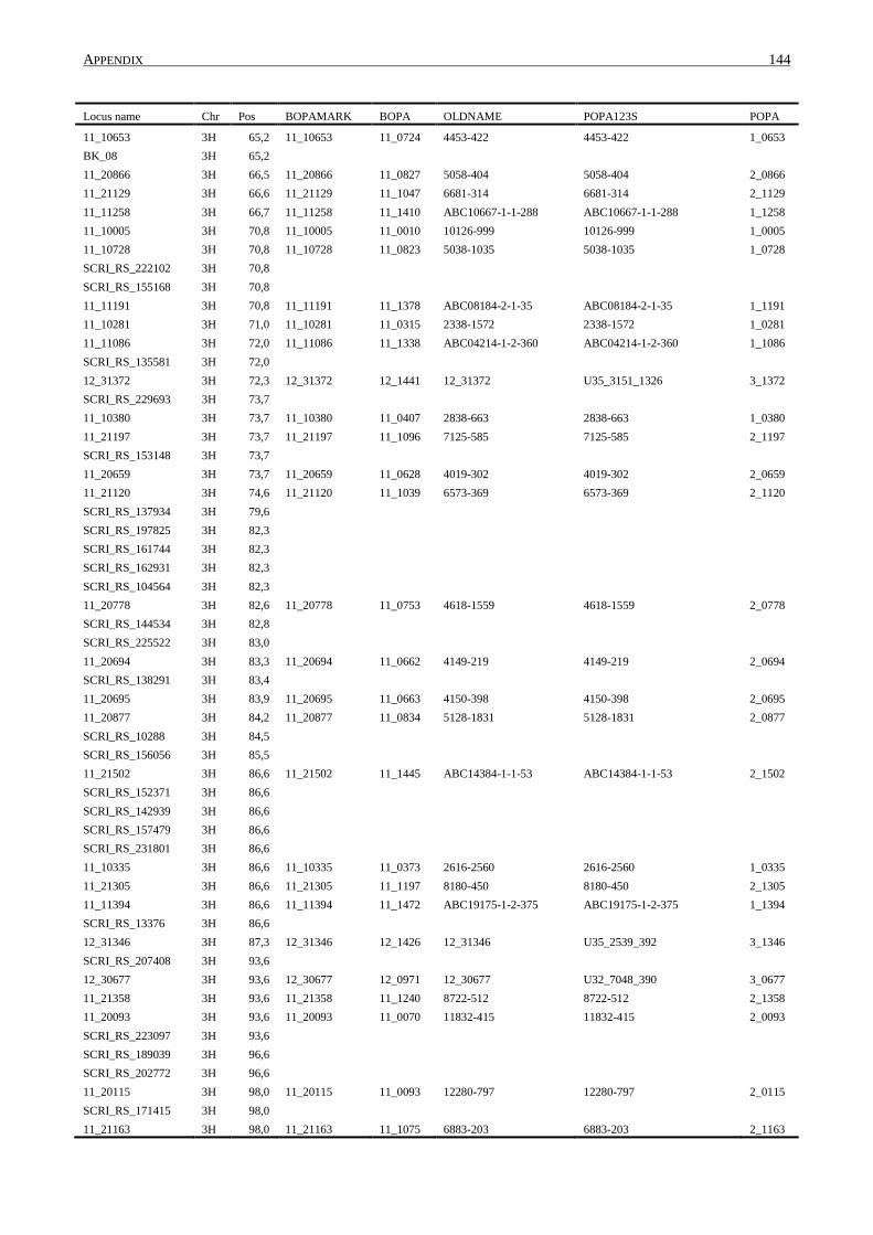
APPENDIX 144


11_10653 3H 65,2 11_10653 11_0724 4453-422 4453-422 1_0653

BK_08 3H 65,2

11_20866 3H 66,5 11_20866 11_0827 5058-404 5058-404 2_0866

11_21129 3H 66,6 11_21129 11_1047 6681-314 6681-314 2_1129

11_11258 3H 66,7 11_11258 11_1410 ABC10667-1-1-288 ABC10667-1-1-288 1_1258

11_10005 3H 70,8 11_10005 11_0010 10126-999 10126-999 1_0005

11_10728 3H 70,8 11_10728 11_0823 5038-1035 5038-1035 1_0728

SCRI_RS_222102 3H 70,8

SCRI_RS_155168 3H 70,8 11_11191 3H 70,8 11_11191 11_1378 ABC08184-2-1-35 ABC08184-2-1-35 1_1191

11_10281 3H 71,0 11_10281 11_0315 2338-1572 2338-1572 1_0281

11_11086 3H 72,0 11_11086 11_1338 ABC04214-1-2-360 ABC04214-1-2-360 1_1086

SCRI_RS_135581 3H 72,0 12_31372 3H 72,3 12_31372 12_1441 12_31372 U35_3151_1326 3_1372

SCRI_RS_229693 3H 73,7

11_10380 3H 73,7 11_10380 11_0407 2838-663 2838-663 1_0380

11_21197 3H 73,7 11_21197 11_1096 7125-585 7125-585 2_1197

SCRI_RS_153148 3H 73,7

11_20659 3H 73,7 11_20659 11_0628 4019-302 4019-302 2_0659

11_21120 3H 74,6 11_21120 11_1039 6573-369 6573-369 2_1120

SCRI_RS_137934 3H 79,6 SCRI_RS_197825 3H 82,3

SCRI_RS_161744 3H 82,3

SCRI_RS_162931 3H 82,3

SCRI_RS_104564 3H 82,3 11_20778 3H 82,6 11_20778 11_0753 4618-1559 4618-1559 2_0778

SCRI_RS_144534 3H 82,8

SCRI_RS_225522 3H 83,0

11_20694 3H 83,3 11_20694 11_0662 4149-219 4149-219 2_0694

SCRI_RS_138291 3H 83,4

11_20695 3H 83,9 11_20695 11_0663 4150-398 4150-398 2_0695

11_20877 3H 84,2 11_20877 11_0834 5128-1831 5128-1831 2_0877

SCRI_RS_10288 3H 84,5 SCRI_RS_156056 3H 85,5

11_21502 3H 86,6 11_21502 11_1445 ABC14384-1-1-53 ABC14384-1-1-53 2_1502

SCRI_RS_152371 3H 86,6

SCRI_RS_142939 3H 86,6 SCRI_RS_157479 3H 86,6

SCRI_RS_231801 3H 86,6

11_10335 3H 86,6 11_10335 11_0373 2616-2560 2616-2560 1_0335

11_21305 3H 86,6 11_21305 11_1197 8180-450 8180-450 2_1305

11_11394 3H 86,6 11_11394 11_1472 ABC19175-1-2-375 ABC19175-1-2-375 1_1394

SCRI_RS_13376 3H 86,6

12_31346 3H 87,3 12_31346 12_1426 12_31346 U35_2539_392 3_1346

SCRI_RS_207408 3H 93,6 12_30677 3H 93,6 12_30677 12_0971 12_30677 U32_7048_390 3_0677

11_21358 3H 93,6 11_21358 11_1240 8722-512 8722-512 2_1358

11_20093 3H 93,6 11_20093 11_0070 11832-415 11832-415 2_0093

SCRI_RS_223097 3H 93,6 SCRI_RS_189039 3H 96,6

SCRI_RS_202772 3H 96,6

11_20115 3H 98,0 11_20115 11_0093 12280-797 12280-797 2_0115

SCRI_RS_171415 3H 98,0 11_21163 3H 98,0 11_21163 11_1075 6883-203 6883-203 2_1163

APPENDIX 145


SCRI_RS_219894 3H 98,0 SCRI_RS_238157 3H 98,0

11_20063 3H 98,0 11_20063 11_0050 11116-257 11116-257 2_0063

SCRI_RS_167410 3H 98,0

SCRI_RS_146347 3H 98,0 SCRI_RS_199922 3H 109,7

SCRI_RS_138193 3H 111,5

11_21294 3H 112,8 11_21294 11_1183 8020-87 8020-87 2_1294

12_30325 3H 112,8 12_30325 12_0768 12_30325 U32_10917_237 3_0325

SCRI_RS_826 3H 115,5

11_11021 3H 115,5 11_11021 11_1294 963-386 963-386 1_1021

SCRI_RS_198609 3H 115,5

SCRI_RS_159006 3H 116,0 11_20136 3H 116,0 11_20136 11_0118 13081-199 13081-199 2_0136

11_21438 3H 116,0 11_21438 11_1299 9683-140 9683-140 2_1438

11_20999 3H 116,0 11_20999 11_0944 5797-777 5797-777 2_0999

SCRI_RS_146429 3H 129,2 SCRI_RS_192761 3H 129,2

11_20628 3H 129,2 11_20628 11_0593 3791-1525 3791-1525 2_0628

11_10515 3H 129,2 11_10515 11_0565 3674-1352 3674-1352 1_0515

12_30663 3H 134,6 12_30663 12_0964 12_30663 U32_6715_250 3_0663

SCRI_RS_235849 3H 134,6

SCRI_RS_227472 3H 134,6

SCRI_RS_231007 3H 134,6

11_21381 3H 134,6 11_21381 11_1257 8984-579 8984-579 2_1381

SCRI_RS_115925 3H 134,6

12_10344 3H 134,6 12_10344 12_0077 12_10344 2660-678 1_0344

12_30342 3H 134,6 12_30342 12_0777 12_30342 U32_12072_133 3_0342

11_21083 3H 145,6 11_21083 11_1003 6302-250 6302-250 2_1083

SCRI_RS_164704 3H 145,6

11_20023 3H 145,6 11_20023 11_0025 1038-754 1038-754 2_0023

SCRI_RS_133339 3H 145,6

12_30423 3H 145,6 12_30423 12_0823 12_30423 U32_2291_275 3_0423

11_10753 3H 145,6 11_10753 11_0864 5253-1318 5253-1318 1_0753

SCRI_RS_149566 3H 145,6

SCRI_RS_114333 3H 145,6

SCRI_RS_116542 3H 145,6 11_20168 3H 145,6 11_20168 11_0142 1435-670 1435-670 2_0168

SCRI_RS_153519 3H 145,6

12_30927 3H 145,6 12_30927 12_1153 12_30927 SCRI_aj420778_01_1 3_0927

SCRI_RS_14857 3H 145,6 11_11330 3H 145,6 11_11330 11_1440 ABC13753-1-2-167 ABC13753-1-2-167 1_1330

SCRI_RS_163092 3H 153,0

SCRI_RS_162929 3H 156,2

SCRI_RS_3125 3H 156,8 11_10312 3H 161,6 11_10312 11_0347 2500-1514 2500-1514 1_0312

SCRI_RS_131897 3H 161,6

SCRI_RS_206510 3H 161,6

SCRI_RS_121052 3H 161,6 SCRI_RS_151711 3H 168,9

12_31220 3H 168,9 12_31220 12_1343 12_31220 U35_18257_694 3_1220

12_30274 3H 168,9 12_30274 12_0741 12_30274 ABC19616_1_756 3_0274

12_31525 3H 168,9 12_31525 12_1530 12_31525 U35_835_1187 3_1525

11_11172 3H 168,9 11_11172 11_1370 ABC07496-pHv1343-02 ABC07496-pHv1343-02 1_1172

APPENDIX 146


11_10754 3H 168,9 11_10754 11_0866 5260-462 5260-462 1_0754

11_20650 3H 168,9 11_20650 11_0615 3965-353 3965-353 2_0650

12_31238 3H 168,9 12_31238 12_1358 12_31238 U35_18691_432 3_1238

11_10867 3H 187,3 11_10867 11_1050 6716-823 6716-823 1_0867

SCRI_RS_146012 3H 187,3 12_30960 3H 187,3 12_30960 12_1177 12_30960 SCRI_bbc09200_01_110 3_0960

12_30972 3H 189,4 12_30972 12_1185 12_30972 SCRI_bbc21998_01_388 3_0972

SCRI_RS_167755 3H 189,4

11_20612 3H 191,2 11_20612 11_0581 3718-1026 3718-1026 2_0612

11_20527 3H 191,2 11_20527 11_0498 3340-1042 3340-1042 2_0527

11_20085 3H 191,2 11_20085 11_0063 11657-398 11657-398 2_0085

SCRI_RS_180027 3H 191,6

SCRI_RS_13871 3H 191,6 SCRI_RS_208297 3H 194,5

12_31251 3H 195,5 12_31251 12_1366 12_31251 U35_19018_419 3_1251

11_20409 3H 200,2 11_20409 11_0393 2754-1027 2754-1027 2_0409

SCRI_RS_175038 3H 207,1 SCRI_RS_194148 3H 207,1

12_21386 3H 207,1 12_21386 12_0555 12_21386 9040-492 2_1386

SCRI_RS_167698 3H 207,1

SCRI_RS_144559 3H 207,1 SCRI_RS_14107 3H 207,1


SCRI_RS_169325 3H 208,2

SCRI_RS_183550 3H 212,7 SCRI_RS_231382 3H 220,7

SCRI_RS_49693 3H 220,7

11_10681 3H 220,7 11_10681 11_0760 4643-867 4643-867 1_0681

11_10570 3H 224,3 11_10570 11_0614 3949-1560 3949-1560 1_0570

SCRI_RS_180847 3H 224,3

11_11410 3H 224,3 11_11410 11_1480 ABC36454-pHv2499-01 ABC36454-pHv2499-01 1_1410


SCRI_RS_205592 3H 231,7 SCRI_RS_115755 3H 231,7

SCRI_RS_208633 3H 231,7

11_21272 3H 231,7 11_21272 11_1166 7818-967 7818-967 2_1272

SCRI_RS_135155 3H 231,7 SCRI_RS_189710 3H 231,7

SCRI_RS_205957 3H 231,7

SCRI_RS_172357 3H 231,7

12_31500 3H 231,7 12_31500 12_1515 12_31500 U35_6520_551 3_1500

SCRI_RS_126369 3H 231,7

11_10646 3H 241,5 11_10646 11_0716 4403-885 4403-885 1_0646

SCRI_RS_168360 3H 246,3

SCRI_RS_173623 3H 246,3 SCRI_RS_230023 3H 246,3

11_10694 3H 246,3 11_10694 11_0780 4737-368 4737-368 1_0694

SCRI_RS_216141 3H 260,6

SCRI_RS_128254 3H 260,6 SCRI_RS_236603 3H 260,6

11_20605 3H 261,0 11_20605 11_0567 3682-556 3682-556 2_0605

12_30736 3H 261,0 12_30736 12_1006 12_30736 U32_8179_620 3_0736

11_21267 3H 261,0 11_21267 11_1161 7782-410 7782-410 2_1267

SCRI_RS_203164 3H 261,0

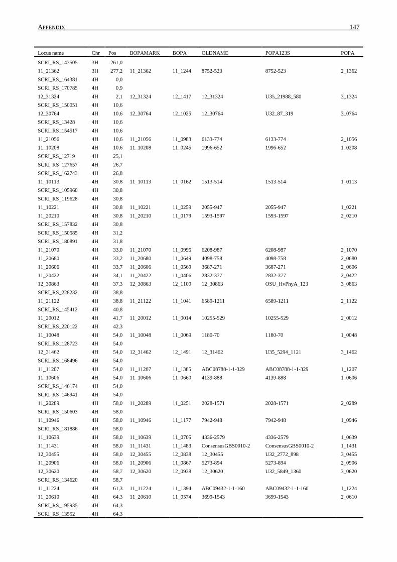
APPENDIX 147


SCRI_RS_143505 3H 261,0 11_21362 3H 277,2 11_21362 11_1244 8752-523 8752-523 2_1362

SCRI_RS_164381 4H 0,0

SCRI_RS_170785 4H 0,9

12_31324 4H 2,1 12_31324 12_1417 12_31324 U35_21988_580 3_1324

SCRI_RS_150051 4H 10,6

12_30764 4H 10,6 12_30764 12_1025 12_30764 U32_87_319 3_0764

SCRI_RS_13428 4H 10,6

SCRI_RS_154517 4H 10,6 11_21056 4H 10,6 11_21056 11_0983 6133-774 6133-774 2_1056

11_10208 4H 10,6 11_10208 11_0245 1996-652 1996-652 1_0208

SCRI_RS_12719 4H 25,1

SCRI_RS_127657 4H 26,7 SCRI_RS_162743 4H 26,8

11_10113 4H 30,8 11_10113 11_0162 1513-514 1513-514 1_0113

SCRI_RS_105960 4H 30,8

SCRI_RS_119628 4H 30,8 11_10221 4H 30,8 11_10221 11_0259 2055-947 2055-947 1_0221

11_20210 4H 30,8 11_20210 11_0179 1593-1597 1593-1597 2_0210

SCRI_RS_157832 4H 30,8

SCRI_RS_150585 4H 31,2 SCRI_RS_180891 4H 31,8

11_21070 4H 33,0 11_21070 11_0995 6208-987 6208-987 2_1070

11_20680 4H 33,2 11_20680 11_0649 4098-758 4098-758 2_0680

11_20606 4H 33,7 11_20606 11_0569 3687-271 3687-271 2_0606

11_20422 4H 34,1 11_20422 11_0406 2832-377 2832-377 2_0422

12_30863 4H 37,3 12_30863 12_1100 12_30863 OSU_HvPhyA_123 3_0863

SCRI_RS_228232 4H 38,8

11_21122 4H 38,8 11_21122 11_1041 6589-1211 6589-1211 2_1122

SCRI_RS_145412 4H 40,8

11_20012 4H 41,7 11_20012 11_0014 10255-529 10255-529 2_0012

SCRI_RS_220122 4H 42,3

11_10048 4H 54,0 11_10048 11_0069 1180-70 1180-70 1_0048

SCRI_RS_128723 4H 54,0

12_31462 4H 54,0 12_31462 12_1491 12_31462 U35_5294_1121 3_1462

SCRI_RS_168496 4H 54,0

11_11207 4H 54,0 11_11207 11_1385 ABC08788-1-1-329 ABC08788-1-1-329 1_1207

11_10606 4H 54,0 11_10606 11_0660 4139-888 4139-888 1_0606

SCRI_RS_146174 4H 54,0

SCRI_RS_146941 4H 54,0

11_20289 4H 58,0 11_20289 11_0251 2028-1571 2028-1571 2_0289

SCRI_RS_150603 4H 58,0

11_10946 4H 58,0 11_10946 11_1177 7942-948 7942-948 1_0946

SCRI_RS_181886 4H 58,0

11_10639 4H 58,0 11_10639 11_0705 4336-2579 4336-2579 1_0639


12_30455 4H 58,0 12_30455 12_0838 12_30455 U32_2772_898 3_0455

11_20906 4H 58,0 11_20906 11_0867 5273-894 5273-894 2_0906

12_30620 4H 58,7 12_30620 12_0938 12_30620 U32_5849_1360 3_0620

SCRI_RS_134620 4H 58,7

11_11224 4H 61,3 11_11224 11_1394 ABC09432-1-1-160 ABC09432-1-1-160 1_1224

11_20610 4H 64,3 11_20610 11_0574 3699-1543 3699-1543 2_0610

SCRI_RS_195935 4H 64,3 SCRI_RS_13552 4H 64,3

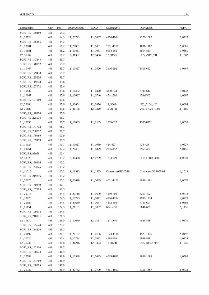
APPENDIX 148


SCRI_RS_189180 4H 64,3 11_20723 4H 64,3 11_20723 11_0697 4276-1082 4276-1082 2_0723

SCRI_RS_135365 4H 64,3

11_20001 4H 68,2 11_20001 11_0001 1001-1187 1001-1187 2_0001

11_10881 4H 68,2 11_10881 11_1081 6954-861 6954-861 1_0881

12_31362 4H 68,2 12_31362 12_1436 12_31362 U35_2917_591 3_1362

SCRI_RS_143144 4H 69,7

SCRI_RS_148392 4H 69,7

11_10467 4H 69,7 11_10467 11_0520 3416-692 3416-692 1_0467

SCRI_RS_179438 4H 69,7

SCRI_RS_155536 4H 69,7

SCRI_RS_119778 4H 85,6

SCRI_RS_157072 4H 85,6 11_10432 4H 85,6 11_10432 11_0470 3190-644 3190-644 1_0432

11_10667 4H 85,6 11_10667 11_0740 454-1502 454-1502 1_0667

SCRI_RS_101389 4H 85,6

12_30684 4H 85,6 12_30684 12_0976 12_30684 U32_7104_420 3_0684

12_31186 4H 85,6 12_31186 12_1320 12_31186 U35_17521_1003 3_1186

SCRI_RS_128974 4H 85,9

SCRI_RS_225074 4H 98,7

11_10093 4H 98,7 11_10093 11_0135 1385-827 1385-827 1_0093

SCRI_RS_147712 4H 98,7

SCRI_RS_200957 4H 98,7

SCRI_RS_179489 4H 100,9

SCRI_RS_159159 4H 100,9 11_10627 4H 101,7 11_10627 11_0689 424-423 424-423 1_0627

11_20451 4H 102,4 11_20451 11_0429 2955-452 2955-452 2_0451

SCRI_RS_89959 4H 102,4

12_30328 4H 105,2 12_30328 12_0769 12_30328 U32_11103_408 3_0328

SCRI_RS_139806 4H 105,2

SCRI_RS_143825 4H 105,2


SCRI_RS_219816 4H 105,2 11_20670 4H 105,2 11_20670 11_0639 4051-1101 4051-1101 2_0670

SCRI_RS_140349 4H 110,1

SCRI_RS_137903 4H 110,3

11_20718 4H 124,5 11_20718 11_0690 4250-402 4250-402 2_0718

11_10723 4H 124,5 11_10723 11_0811 4986-1214 4986-1214 1_0723

11_20689 4H 124,5 11_20689 11_0657 4133-601 4133-601 2_0689

11_21151 4H 124,5 11_21151 11_1067 6841-637 6841-637 2_1151

SCRI_RS_129218 4H 124,5 SCRI_RS_210971 4H 126,5

12_10670 4H 129,0 12_10670 12_0161 12_10670 4555-499 1_0670

SCRI_RS_125524 4H 129,7

SCRI_RS_184126 4H 129,7 11_20197 4H 130,1 11_20197 11_0166 1523-1136 1523-1136 2_0197

11_10724 4H 130,4 11_10724 11_0812 4988-858 4988-858 1_0724

12_31246 4H 130,8 12_31246 12_1363 12_31246 U35_18847_967 3_1246

SCRI_RS_162410 4H 138,7 SCRI_RS_168074 4H 146,9

11_10588 4H 146,9 11_10588 11_0635 4039-1686 4039-1686 1_0588

SCRI_RS_157760 4H 146,9

SCRI_RS_168399 4H 146,9 11_20732 4H 146,9 11_20732 11_0709 4361-1867 4361-1867 2_0732

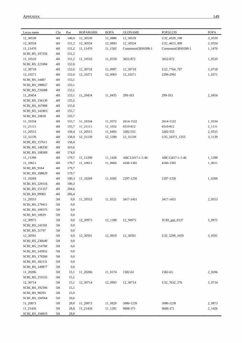
APPENDIX 149


12_30539 4H 146,9 12_30539 12_0886 12_30539 U32_4329_198 3_0539

12_30554 4H 151,2 12_30554 12_0893 12_30554 U32_4613_499 3_0554


SCRI_RS_197256 4H 151,2

11_10510 4H 151,2 11_10510 11_0559 3652-872 3652-872 1_0510

SCRI_RS_121084 4H 152,6

12_30718 4H 152,6 12_30718 12_0997 12_30718 U32_7764_707 3_0718

12_10271 4H 152,6 12_10271 12_0063 12_10271 2299-2992 1_0271

SCRI_RS_14487 4H 153,1 SCRI_RS_188827 4H 153,1

SCRI_RS_235688 4H 153,1

11_20454 4H 153,1 11_20454 11_0435 299-163 299-163 2_0454

SCRI_RS_156130 4H 155,5 SCRI_RS_167808 4H 155,6

SCRI_RS_141803 4H 155,7

SCRI_RS_10818 4H 155,7

11_10334 4H 155,7 11_10334 11_0372 2614-1522 2614-1522 1_0334

11_21111 4H 155,7 11_21111 11_1032 6519-812 6519-812 2_1111

11_20515 4H 158,4 11_20515 11_0492 3282-555 3282-555 2_0515

12_31139 4H 158,4 12_31139 12_1290 12_31139 U35_16371_1353 3_1139

SCRI_RS_157611 4H 158,4 SCRI_RS_148330 4H 163,6

SCRI_RS_108369 4H 174,0

11_11299 4H 179,7 11_11299 11_1428 ABC12417-1-1-46 ABC12417-1-1-46 1_1299

11_10611 4H 179,7 11_10611 11_0666 4160-1365 4160-1365 1_0611

SCRI_RS_9164 4H 179,7

SCRI_RS_188829 4H 179,7

11_10269 4H 190,3 11_10269 11_0305 2297-1250 2297-1250 1_0269

SCRI_RS_229116 4H 190,3 SCRI_RS_151357 4H 204,6

SCRI_RS_99965 4H 206,4

11_20553 5H 0,0 11_20553 11_0521 3417-1451 3417-1451 2_0553

SCRI_RS_179411 5H 0,0 SCRI_RS_109375 5H 0,0

SCRI_RS_10929 5H 0,0

12_30975 5H 0,0 12_30975 12_1188 12_30975 SCRI_gsp_0137 3_0975

SCRI_RS_141591 5H 0,0 SCRI_RS_31797 5H 0,0

12_30591 5H 0,0 12_30591 12_0919 12_30591 U32_5299_1659 3_0591

SCRI_RS_236640 5H 0,0

SCRI_RS_214760 5H 0,0 SCRI_RS_143952 5H 0,0

SCRI_RS_179260 5H 0,0

SCRI_RS_182131 5H 0,0

SCRI_RS_149877 5H 0,0 11_20206 5H 15,1 11_20206 11_0174 1582-63 1582-63 2_0206

SCRI_RS_155555 5H 15,1

12_30714 5H 15,1 12_30714 12_0993 12_30714 U32_7632_376 3_0714

SCRI_RS_192396 5H 15,1 SCRI_RS_98293 5H 23,9

SCRI_RS_184564 5H 26,6

11_20873 5H 28,8 11_20873 11_0829 5086-1239 5086-1239 2_0873

11_21426 5H 28,8 11_21426 11_1291 9608-371 9608-371 2_1426

SCRI_RS_194819 5H 28,8

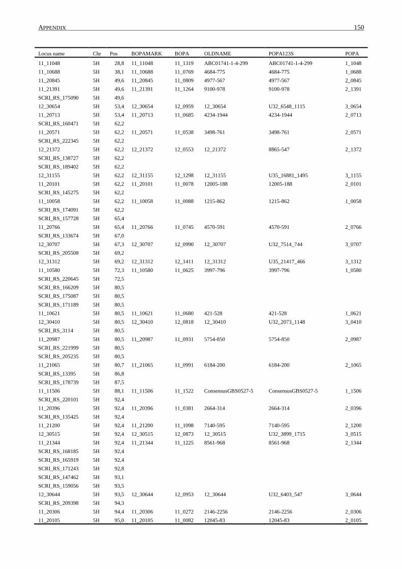
APPENDIX 150


11_11048 5H 28,8 11_11048 11_1319 ABC01741-1-4-299 ABC01741-1-4-299 1_1048

11_10688 5H 38,1 11_10688 11_0769 4684-775 4684-775 1_0688

11_20845 5H 49,6 11_20845 11_0809 4977-567 4977-567 2_0845

11_21391 5H 49,6 11_21391 11_1264 9100-978 9100-978 2_1391

SCRI_RS_175090 5H 49,6 12_30654 5H 53,4 12_30654 12_0959 12_30654 U32_6548_1115 3_0654

11_20713 5H 53,4 11_20713 11_0685 4234-1944 4234-1944 2_0713

SCRI_RS_160471 5H 62,2

11_20571 5H 62,2 11_20571 11_0538 3498-761 3498-761 2_0571

SCRI_RS_222345 5H 62,2

12_21372 5H 62,2 12_21372 12_0553 12_21372 8865-547 2_1372

SCRI_RS_138727 5H 62,2

SCRI_RS_189402 5H 62,2 12_31155 5H 62,2 12_31155 12_1298 12_31155 U35_16881_1495 3_1155

11_20101 5H 62,2 11_20101 11_0078 12005-188 12005-188 2_0101

SCRI_RS_145275 5H 62,2

11_10058 5H 62,2 11_10058 11_0088 1215-862 1215-862 1_0058

SCRI_RS_174091 5H 62,2

SCRI_RS_157728 5H 65,4

11_20766 5H 65,4 11_20766 11_0745 4570-591 4570-591 2_0766

SCRI_RS_133674 5H 67,0 12_30707 5H 67,3 12_30707 12_0990 12_30707 U32_7514_744 3_0707

SCRI_RS_205508 5H 69,2

12_31312 5H 69,2 12_31312 12_1411 12_31312 U35_21417_466 3_1312

11_10580 5H 72,3 11_10580 11_0625 3997-796 3997-796 1_0580

SCRI_RS_220645 5H 72,5

SCRI_RS_166209 5H 80,5

SCRI_RS_175087 5H 80,5

SCRI_RS_171189 5H 80,5 11_10621 5H 80,5 11_10621 11_0680 421-528 421-528 1_0621

12_30410 5H 80,5 12_30410 12_0818 12_30410 U32_2073_1148 3_0410

SCRI_RS_3114 5H 80,5

11_20987 5H 80,5 11_20987 11_0931 5754-850 5754-850 2_0987

SCRI_RS_221999 5H 80,5

SCRI_RS_205235 5H 80,5

11_21065 5H 80,7 11_21065 11_0991 6184-200 6184-200 2_1065

SCRI_RS_13395 5H 86,8 SCRI_RS_178739 5H 87,5


SCRI_RS_220101 5H 92,4

11_20396 5H 92,4 11_20396 11_0381 2664-314 2664-314 2_0396

SCRI_RS_135425 5H 92,4

11_21200 5H 92,4 11_21200 11_1098 7140-595 7140-595 2_1200

12_30515 5H 92,4 12_30515 12_0873 12_30515 U32_3899_1715 3_0515

11_21344 5H 92,4 11_21344 11_1225 8561-968 8561-968 2_1344

SCRI_RS_168185 5H 92,4

SCRI_RS_165919 5H 92,4

SCRI_RS_171243 5H 92,8

SCRI_RS_147462 5H 93,1 SCRI_RS_159056 5H 93,5

12_30644 5H 93,5 12_30644 12_0953 12_30644 U32_6403_547 3_0644

SCRI_RS_209398 5H 94,3

11_20306 5H 94,4 11_20306 11_0272 2146-2256 2146-2256 2_0306

11_20105 5H 95,0 11_20105 11_0082 12045-83 12045-83 2_0105

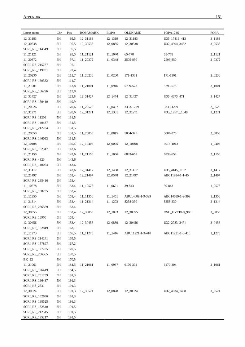
APPENDIX 151


12_31183 5H 95,5 12_31183 12_1319 12_31183 U35_17419_413 3_1183

12_30538 5H 95,5 12_30538 12_0885 12_30538 U32_4304_3452 3_0538

SCRI_RS_114549 5H 95,5

11_21121 5H 95,5 11_21121 11_1040 65-778 65-778 2_1121

11_20372 5H 97,1 11_20372 11_0348 2505-850 2505-850 2_0372

SCRI_RS_215787 5H 97,1

SCRI_RS_119781 5H 97,4

11_20236 5H 111,7 11_20236 11_0200 171-1301 171-1301 2_0236

SCRI_RS_160332 5H 111,7 11_21001 5H 113,8 11_21001 11_0946 5799-578 5799-578 2_1001

SCRI_RS_166296 5H 113,8

12_31427 5H 113,8 12_31427 12_1474 12_31427 U35_4373_471 3_1427

SCRI_RS_150410 5H 119,9 11_20526 5H 120,6 11_20526 11_0497 3333-1209 3333-1209 2_0526

12_31271 5H 120,6 12_31271 12_1381 12_31271 U35_19573_1049 3_1271

SCRI_RS_11206 5H 131,5

SCRI_RS_140487 5H 131,5 SCRI_RS_212784 5H 131,5

11_20850 5H 131,5 11_20850 11_0815 5004-375 5004-375 2_0850

SCRI_RS_146093 5H 131,5

12_10408 5H 136,4 12_10408 12_0095 12_10408 3018-1012 1_0408

SCRI_RS_152347 5H 143,6

11_21150 5H 143,6 11_21150 11_1066 6833-658 6833-658 2_1150

SCRI_RS_4923 5H 143,6

SCRI_RS_140054 5H 143,6 12_31417 5H 143,6 12_31417 12_1468 12_31417 U35_4145_1152 3_1417

12_21497 5H 153,4 12_21497 12_0578 12_21497 ABC11984-1-1-45 2_1497

SCRI_RS_235416 5H 153,4

11_10578 5H 153,4 11_10578 11_0621 39-843 39-843 1_0578

SCRI_RS_158235 5H 153,4

11_11350 5H 153,4 11_11350 11_1451 ABC14689-1-9-399 ABC14689-1-9-399 1_1350

11_21314 5H 153,4 11_21314 11_1203 8258-330 8258-330 2_1314

SCRI_RS_236569 5H 153,4 12_30855 5H 153,4 12_30855 12_1093 12_30855 OSU_HVCBF9_988 3_0855

SCRI_RS_13960 5H 153,4

12_30456 5H 153,4 12_30456 12_0839 12_30456 U32_2783_2471 3_0456

SCRI_RS_152849 5H 163,1 11_11273 5H 165,5 11_11273 11_1416 ABC11221-1-3-410 ABC11221-1-3-410 1_1273

SCRI_RS_214241 5H 165,5

SCRI_RS_157897 5H 167,2

SCRI_RS_127785 5H 170,5 SCRI_RS_206565 5H 170,5

BK_22 5H 170,5

11_21061 5H 184,5 11_21061 11_0987 6170-304 6170-304 2_1061

SCRI_RS_126419 5H 184,5 SCRI_RS_231239 5H 191,3

SCRI_RS_196437 5H 191,3

SCRI_RS_2831 5H 191,3

12_30524 5H 191,3 12_30524 12_0878 12_30524 U32_4034_1438 3_0524

SCRI_RS_162696 5H 191,3

SCRI_RS_198525 5H 191,3

SCRI_RS_182540 5H 191,5

SCRI_RS_212515 5H 191,5 SCRI_RS_195217 5H 191,5

APPENDIX 152


12_30377 5H 198,0 12_30377 12_0798 12_30377 U32_14622_323 3_0377

SCRI_RS_189371 5H 198,0

11_20347 5H 198,0 11_20347 11_0318 2352-277 2352-277 2_0347

SCRI_RS_150691 5H 198,0

SCRI_RS_149088 5H 198,0 11_20300 5H 198,0 11_20300 11_0266 211-259 211-259 2_0300

SCRI_RS_1501 5H 198,0

11_20883 5H 198,4 11_20883 11_0841 5154-117 5154-117 2_0883

11_10805 5H 198,4 11_10805 11_0950 5844-1011 5844-1011 1_0805

SCRI_RS_165331 5H 198,5

SCRI_RS_165569 5H 199,3

SCRI_RS_150232 5H 199,8

11_10705 5H 204,2 11_10705 11_0789 4795-782 4795-782 1_0705

SCRI_RS_78626 5H 204,5

SCRI_RS_51000 5H 205,0

11_20003 5H 205,0 11_20003 11_0003 10047-338 10047-338 2_0003

12_30611 5H 205,0 12_30611 12_0934 12_30611 U32_5714_470 3_0611

11_20188 5H 205,0 11_20188 11_0159 1501-353 1501-353 2_0188

11_10901 5H 205,0 11_10901 11_1121 7337-388 7337-388 1_0901

11_10820 5H 205,0 11_10820 11_0976 6054-1050 6054-1050 1_0820

11_21041 5H 205,0 11_21041 11_0974 603-72 603-72 2_1041

BK_17 5H 205,0

11_21203 5H 205,5 11_21203 11_1102 7167-466 7167-466 2_1203

12_31237 5H 205,5 12_31237 12_1357 12_31237 U35_18649_1027 3_1237

SCRI_RS_166218 5H 206,3 SCRI_RS_188785 5H 206,3

12_30067 5H 206,3 12_30067 12_0622 12_30067 ABC07029_1_290 3_0067

SCRI_RS_130992 5H 206,3

11_10095 5H 206,3 11_10095 11_0140 1394-1222 1394-1222 1_0095

SCRI_RS_188141 5H 206,3

SCRI_RS_154144 5H 206,4

11_10146 5H 206,4 11_10146 11_0198 1697-636 1697-636 1_0146

11_10783 5H 206,4 11_10783 11_0911 5571-640 5571-640 1_0783

SCRI_RS_166857 5H 210,5

SCRI_RS_168544 5H 210,5

SCRI_RS_4658 5H 210,5

SCRI_RS_230112 5H 211,2 SCRI_RS_148120 5H 211,7

SCRI_RS_140356 5H 211,7

SCRI_RS_149936 5H 211,7

SCRI_RS_188572 5H 211,7 12_30635 5H 213,8 12_30635 12_0947 12_30635 U32_6188_1308 3_0635

SCRI_RS_214130 5H 213,8

11_20551 5H 213,8 11_20551 11_0518 3412-579 3412-579 2_0551

SCRI_RS_161534 5H 213,8 11_10658 5H 213,8 11_10658 11_0731 447-88 447-88 1_0658

SCRI_RS_105705 5H 213,8

12_30580 5H 215,4 12_30580 12_0911 12_30580 U32_5092_965 3_0580

SCRI_RS_208686 5H 215,7 11_20568 5H 216,0 11_20568 11_0534 3477-1248 3477-1248 2_0568

12_30400 5H 216,1 12_30400 12_0811 12_30400 U32_1794_707 3_0400

SCRI_RS_225632 5H 216,5

12_31206 5H 217,1 12_31206 12_1332 12_31206 U35_17942_828 3_1206

SCRI_RS_173583 5H 217,6

APPENDIX 153


11_10217 5H 218,4 11_10217 11_0253 203-1128 203-1128 1_0217

SCRI_RS_161614 5H 218,5

11_20104 5H 218,6 11_20104 11_0081 1204-1104 1204-1104 2_0104

SCRI_RS_13262 5H 218,6

12_10904 5H 218,7 12_10904 12_0208 12_10904 7382-626 1_0904

SCRI_RS_138608 5H 218,7

SCRI_RS_167426 5H 218,7

SCRI_RS_138735 5H 219,9

SCRI_RS_153575 5H 219,9 11_10536 5H 219,9 11_10536 11_0586 3759-1385 3759-1385 1_0536

11_20560 5H 220,5 11_20560 11_0525 3443-1234 3443-1234 2_0560

SCRI_RS_230034 5H 222,6

SCRI_RS_181376 5H 222,6 11_20676 5H 224,7 11_20676 11_0646 407-259 407-259 2_0676

12_31165 5H 224,7 12_31165 12_1305 12_31165 U35_17121_1510 3_1165

SCRI_RS_155999 5H 225,3

11_10363 5H 225,3 11_10363 11_0391 2746-1501 2746-1501 1_0363

SCRI_RS_235550 5H 225,5

11_21077 5H 225,5 11_21077 11_1000 6260-183 6260-183 2_1077

12_30062 5H 225,5 12_30062 12_0618 12_30062 ABC06870_1_371 3_0062

SCRI_RS_157026 5H 225,7 BK_04 5H 225,7

SCRI_RS_168534 5H 233,6

SCRI_RS_138029 5H 233,6

12_30183 5H 233,6 12_30183 12_0693 12_30183 ABC11767_1_299 3_0183

11_21355 5H 233,6 11_21355 11_1236 8682-406 8682-406 2_1355


SCRI_RS_173935 5H 233,6

11_10336 5H 233,6 11_10336 11_0374 2617-1234 2617-1234 1_0336

SCRI_RS_204570 5H 233,6

SCRI_RS_155322 5H 243,8

11_20334 5H 244,5 11_20334 11_0303 2290-796 2290-796 2_0334

SCRI_RS_19741 5H 245,6 12_30165 5H 245,6 12_30165 12_0683 12_30165 ABC11168_1_163 3_0165

11_20829 5H 245,6 11_20829 11_0799 485-1369 485-1369 2_0829

12_30666 5H 245,6 12_30666 12_0966 12_30666 U32_6903_1480 3_0666

SCRI_RS_123668 5H 245,6 11_10161 5H 245,8 11_10161 11_0206 1761-804 1761-804 1_0161

11_20078 5H 245,8 11_20078 11_0057 11470-478 11470-478 2_0078

SCRI_RS_131479 5H 245,8

11_20988 5H 245,8 11_20988 11_0932 5757-248 5757-248 2_0988

11_20826 5H 245,8 11_20826 11_0796 4845-123 4845-123 2_0826

SCRI_RS_102066 5H 245,8

SCRI_RS_157318 5H 245,8

11_10236 5H 245,8 11_10236 11_0271 2144-852 2144-852 1_0236

SCRI_RS_178615 5H 245,8

SCRI_RS_134358 5H 253,6

SCRI_RS_165835 5H 253,6

11_20934 5H 254,3 11_20934 11_0888 5428-146 5428-146 2_0934

SCRI_RS_195241 5H 256,0

11_10254 5H 256,5 11_10254 11_0290 2244-3247 2244-3247 1_0254

SCRI_RS_130982 5H 257,4

SCRI_RS_192640 5H 260,1 SCRI_RS_199694 5H 260,1

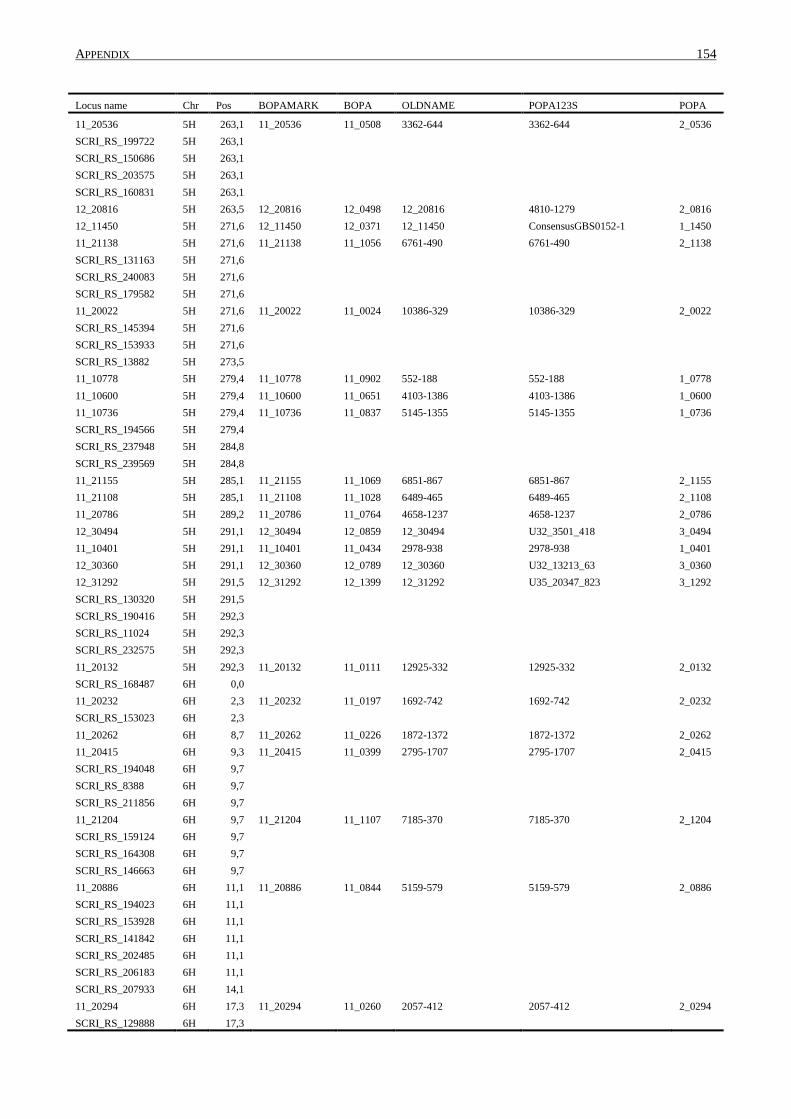
APPENDIX 154


11_20536 5H 263,1 11_20536 11_0508 3362-644 3362-644 2_0536

SCRI_RS_199722 5H 263,1

SCRI_RS_150686 5H 263,1

SCRI_RS_203575 5H 263,1

SCRI_RS_160831 5H 263,1 12_20816 5H 263,5 12_20816 12_0498 12_20816 4810-1279 2_0816

12_11450 5H 271,6 12_11450 12_0371 12_11450 ConsensusGBS0152-1 1_1450

11_21138 5H 271,6 11_21138 11_1056 6761-490 6761-490 2_1138

SCRI_RS_131163 5H 271,6 SCRI_RS_240083 5H 271,6

SCRI_RS_179582 5H 271,6

11_20022 5H 271,6 11_20022 11_0024 10386-329 10386-329 2_0022

SCRI_RS_145394 5H 271,6 SCRI_RS_153933 5H 271,6

SCRI_RS_13882 5H 273,5

11_10778 5H 279,4 11_10778 11_0902 552-188 552-188 1_0778

11_10600 5H 279,4 11_10600 11_0651 4103-1386 4103-1386 1_0600

11_10736 5H 279,4 11_10736 11_0837 5145-1355 5145-1355 1_0736

SCRI_RS_194566 5H 279,4

SCRI_RS_237948 5H 284,8

SCRI_RS_239569 5H 284,8 11_21155 5H 285,1 11_21155 11_1069 6851-867 6851-867 2_1155

11_21108 5H 285,1 11_21108 11_1028 6489-465 6489-465 2_1108

11_20786 5H 289,2 11_20786 11_0764 4658-1237 4658-1237 2_0786

12_30494 5H 291,1 12_30494 12_0859 12_30494 U32_3501_418 3_0494

11_10401 5H 291,1 11_10401 11_0434 2978-938 2978-938 1_0401

12_30360 5H 291,1 12_30360 12_0789 12_30360 U32_13213_63 3_0360

12_31292 5H 291,5 12_31292 12_1399 12_31292 U35_20347_823 3_1292

SCRI_RS_130320 5H 291,5 SCRI_RS_190416 5H 292,3

SCRI_RS_11024 5H 292,3

SCRI_RS_232575 5H 292,3

11_20132 5H 292,3 11_20132 11_0111 12925-332 12925-332 2_0132

SCRI_RS_168487 6H 0,0

11_20232 6H 2,3 11_20232 11_0197 1692-742 1692-742 2_0232

SCRI_RS_153023 6H 2,3

11_20262 6H 8,7 11_20262 11_0226 1872-1372 1872-1372 2_0262

11_20415 6H 9,3 11_20415 11_0399 2795-1707 2795-1707 2_0415

SCRI_RS_194048 6H 9,7

SCRI_RS_8388 6H 9,7

SCRI_RS_211856 6H 9,7 11_21204 6H 9,7 11_21204 11_1107 7185-370 7185-370 2_1204

SCRI_RS_159124 6H 9,7

SCRI_RS_164308 6H 9,7

SCRI_RS_146663 6H 9,7 11_20886 6H 11,1 11_20886 11_0844 5159-579 5159-579 2_0886

SCRI_RS_194023 6H 11,1

SCRI_RS_153928 6H 11,1

SCRI_RS_141842 6H 11,1 SCRI_RS_202485 6H 11,1

SCRI_RS_206183 6H 11,1

SCRI_RS_207933 6H 14,1

11_20294 6H 17,3 11_20294 11_0260 2057-412 2057-412 2_0294

SCRI_RS_129888 6H 17,3

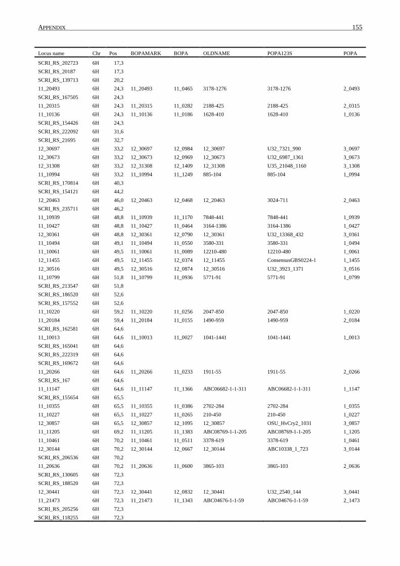
APPENDIX 155


SCRI_RS_202723 6H 17,3 SCRI_RS_20187 6H 17,3

SCRI_RS_139713 6H 20,2

11_20493 6H 24,3 11_20493 11_0465 3178-1276 3178-1276 2_0493

SCRI_RS_167505 6H 24,3 11_20315 6H 24,3 11_20315 11_0282 2188-425 2188-425 2_0315

11_10136 6H 24,3 11_10136 11_0186 1628-410 1628-410 1_0136

SCRI_RS_154426 6H 24,3

SCRI_RS_222092 6H 31,6 SCRI_RS_21695 6H 32,7

12_30697 6H 33,2 12_30697 12_0984 12_30697 U32_7321_990 3_0697

12_30673 6H 33,2 12_30673 12_0969 12_30673 U32_6987_1361 3_0673

12_31308 6H 33,2 12_31308 12_1409 12_31308 U35_21048_1160 3_1308

11_10994 6H 33,2 11_10994 11_1249 885-104 885-104 1_0994

SCRI_RS_170814 6H 40,3

SCRI_RS_154121 6H 44,2

12_20463 6H 46,0 12_20463 12_0468 12_20463 3024-711 2_0463

SCRI_RS_235711 6H 46,2

11_10939 6H 48,8 11_10939 11_1170 7848-441 7848-441 1_0939

11_10427 6H 48,8 11_10427 11_0464 3164-1386 3164-1386 1_0427

12_30361 6H 48,8 12_30361 12_0790 12_30361 U32_13368_432 3_0361

11_10494 6H 49,1 11_10494 11_0550 3580-331 3580-331 1_0494

11_10061 6H 49,5 11_10061 11_0089 12210-480 12210-480 1_0061

12_11455 6H 49,5 12_11455 12_0374 12_11455 ConsensusGBS0224-1 1_1455

12_30516 6H 49,5 12_30516 12_0874 12_30516 U32_3923_1371 3_0516

11_10799 6H 51,8 11_10799 11_0936 5771-91 5771-91 1_0799

SCRI_RS_213547 6H 51,8

SCRI_RS_186520 6H 52,6

SCRI_RS_157552 6H 52,6 11_10220 6H 59,2 11_10220 11_0256 2047-850 2047-850 1_0220

11_20184 6H 59,4 11_20184 11_0155 1490-959 1490-959 2_0184

SCRI_RS_162581 6H 64,6

11_10013 6H 64,6 11_10013 11_0027 1041-1441 1041-1441 1_0013

SCRI_RS_165041 6H 64,6

SCRI_RS_222319 6H 64,6

SCRI_RS_169672 6H 64,6

11_20266 6H 64,6 11_20266 11_0233 1911-55 1911-55 2_0266

SCRI_RS_167 6H 64,6

11_11147 6H 64,6 11_11147 11_1366 ABC06682-1-1-311 ABC06682-1-1-311 1_1147

SCRI_RS_155654 6H 65,5

11_10355 6H 65,5 11_10355 11_0386 2702-284 2702-284 1_0355

11_10227 6H 65,5 11_10227 11_0265 210-450 210-450 1_0227

12_30857 6H 65,5 12_30857 12_1095 12_30857 OSU_HvCry2_1031 3_0857

11_11205 6H 69,2 11_11205 11_1383 ABC08769-1-1-205 ABC08769-1-1-205 1_1205

11_10461 6H 70,2 11_10461 11_0511 3378-619 3378-619 1_0461

12_30144 6H 70,2 12_30144 12_0667 12_30144 ABC10338_1_723 3_0144

SCRI_RS_206536 6H 70,2

11_20636 6H 70,2 11_20636 11_0600 3865-103 3865-103 2_0636

SCRI_RS_130605 6H 72,3 SCRI_RS_188520 6H 72,3

12_30441 6H 72,3 12_30441 12_0832 12_30441 U32_2540_144 3_0441

11_21473 6H 72,3 11_21473 11_1343 ABC04676-1-1-59 ABC04676-1-1-59 2_1473

SCRI_RS_205256 6H 72,3 SCRI_RS_118255 6H 72,3

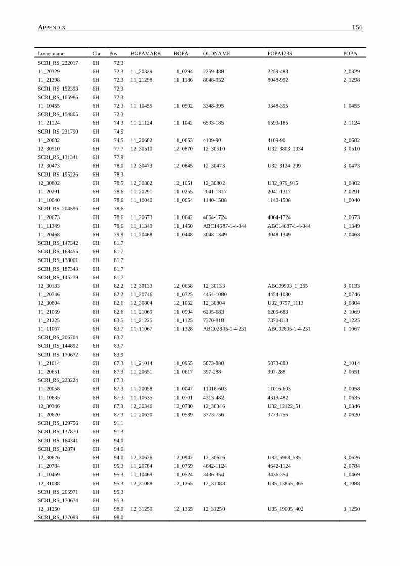
APPENDIX 156


SCRI_RS_222017 6H 72,3 11_20329 6H 72,3 11_20329 11_0294 2259-488 2259-488 2_0329

11_21298 6H 72,3 11_21298 11_1186 8048-952 8048-952 2_1298

SCRI_RS_152393 6H 72,3

SCRI_RS_165986 6H 72,3 11_10455 6H 72,3 11_10455 11_0502 3348-395 3348-395 1_0455

SCRI_RS_154805 6H 72,3

11_21124 6H 74,3 11_21124 11_1042 6593-185 6593-185 2_1124

SCRI_RS_231790 6H 74,5 11_20682 6H 74,5 11_20682 11_0653 4109-90 4109-90 2_0682

12_30510 6H 77,7 12_30510 12_0870 12_30510 U32_3803_1334 3_0510

SCRI_RS_131341 6H 77,9

12_30473 6H 78,0 12_30473 12_0845 12_30473 U32_3124_299 3_0473

SCRI_RS_195226 6H 78,3

12_30802 6H 78,5 12_30802 12_1051 12_30802 U32_979_915 3_0802

11_20291 6H 78,6 11_20291 11_0255 2041-1317 2041-1317 2_0291

11_10040 6H 78,6 11_10040 11_0054 1140-1508 1140-1508 1_0040

SCRI_RS_204596 6H 78,6

11_20673 6H 78,6 11_20673 11_0642 4064-1724 4064-1724 2_0673

11_11349 6H 78,6 11_11349 11_1450 ABC14687-1-4-344 ABC14687-1-4-344 1_1349

11_20468 6H 79,9 11_20468 11_0448 3048-1349 3048-1349 2_0468

SCRI_RS_147342 6H 81,7

SCRI_RS_168455 6H 81,7

SCRI_RS_138001 6H 81,7

SCRI_RS_187343 6H 81,7 SCRI_RS_145279 6H 81,7

12_30133 6H 82,2 12_30133 12_0658 12_30133 ABC09903_1_265 3_0133

11_20746 6H 82,2 11_20746 11_0725 4454-1080 4454-1080 2_0746

12_30804 6H 82,6 12_30804 12_1052 12_30804 U32_9797_1113 3_0804

11_21069 6H 82,6 11_21069 11_0994 6205-683 6205-683 2_1069

11_21225 6H 83,5 11_21225 11_1125 7370-818 7370-818 2_1225

11_11067 6H 83,7 11_11067 11_1328 ABC02895-1-4-231 ABC02895-1-4-231 1_1067

SCRI_RS_206704 6H 83,7 SCRI_RS_144892 6H 83,7

SCRI_RS_170672 6H 83,9

11_21014 6H 87,3 11_21014 11_0955 5873-880 5873-880 2_1014

11_20651 6H 87,3 11_20651 11_0617 397-288 397-288 2_0651

SCRI_RS_223224 6H 87,3

11_20058 6H 87,3 11_20058 11_0047 11016-603 11016-603 2_0058

11_10635 6H 87,3 11_10635 11_0701 4313-482 4313-482 1_0635

12_30346 6H 87,3 12_30346 12_0780 12_30346 U32_12122_51 3_0346

11_20620 6H 87,3 11_20620 11_0589 3773-756 3773-756 2_0620

SCRI_RS_129756 6H 91,1

SCRI_RS_137870 6H 91,3

SCRI_RS_164341 6H 94,0 SCRI_RS_12874 6H 94,0

12_30626 6H 94,0 12_30626 12_0942 12_30626 U32_5968_585 3_0626

11_20784 6H 95,3 11_20784 11_0759 4642-1124 4642-1124 2_0784

11_10469 6H 95,3 11_10469 11_0524 3436-354 3436-354 1_0469

12_31088 6H 95,3 12_31088 12_1265 12_31088 U35_13855_365 3_1088

SCRI_RS_205971 6H 95,3

SCRI_RS_170674 6H 95,3

12_31250 6H 98,0 12_31250 12_1365 12_31250 U35_19005_402 3_1250

SCRI_RS_177093 6H 98,0

APPENDIX 157


SCRI_RS_736 6H 101,9 11_21025 6H 104,7 11_21025 11_0961 5926-798 5926-798 2_1025

SCRI_RS_149165 6H 105,0

SCRI_RS_169374 6H 106,1

SCRI_RS_164037 6H 106,3 SCRI_RS_10932 6H 107,8

SCRI_RS_184453 6H 108,0

SCRI_RS_162589 6H 108,4

11_20996 6H 110,4 11_20996 11_0941 578-587 578-587 2_0996

SCRI_RS_182637 6H 110,4

11_10595 6H 110,4 11_10595 11_0647 4076-1056 4076-1056 1_0595

11_20972 6H 110,7 11_20972 11_0922 5684-601 5684-601 2_0972

SCRI_RS_124224 6H 110,7 11_10734 6H 112,6 11_10734 11_0832 5124-1707 5124-1707 1_0734

SCRI_RS_120442 6H 112,6

12_31432 6H 113,4 12_31432 12_1477 12_31432 U35_4470_378 3_1432

SCRI_RS_98225 6H 113,4 SCRI_RS_151574 6H 118,2

SCRI_RS_224910 6H 118,2

11_10015 6H 118,2 11_10015 11_0028 10425-725 10425-725 1_0015

12_31044 6H 118,2 12_31044 12_1243 12_31044 UCI_Dhn7_1221 3_1044

SCRI_RS_8034 6H 118,2

11_20036 6H 118,2 11_20036 11_0034 10687-540 10687-540 2_0036

11_20467 6H 118,2 11_20467 11_0447 3047-1400 3047-1400 2_0467

SCRI_RS_6720 6H 118,2 SCRI_RS_189619 6H 124,4

SCRI_RS_135063 6H 127,0

SCRI_RS_213956 6H 127,0

SCRI_RS_149269 6H 127,0 SCRI_RS_169022 6H 132,7

SCRI_RS_147455 6H 132,7

SCRI_RS_162836 6H 132,7


SCRI_RS_131119 6H 132,7

SCRI_RS_138295 6H 139,2

11_20029 6H 139,2 11_20029 11_0030 10535-217 10535-217 2_0029

SCRI_RS_206827 6H 139,2 11_20005 6H 139,2 11_20005 11_0005 1007-651 1007-651 2_0005

11_20211 6H 139,5 11_20211 11_0181 1597-158 1597-158 2_0211

SCRI_RS_152414 6H 146,1

11_10828 6H 146,1 11_10828 11_0988 617-167 617-167 1_0828

11_10175 6H 147,3 11_10175 11_0219 1852-509 1852-509 1_0175

SCRI_RS_235672 6H 147,3

SCRI_RS_10655 6H 147,3

12_31283 6H 147,3 12_31283 12_1392 12_31283 U35_19999_392 3_1283

11_20687 6H 147,3 11_20687 11_0656 4126-1180 4126-1180 2_0687

11_21112 6H 147,3 11_21112 11_1033 6523-1691 6523-1691 2_1112

SCRI_RS_151280 6H 147,9

11_20537 6H 160,0 11_20537 11_0509 3363-1795 3363-1795 2_0537

12_30956 6H 160,0 12_30956 12_1173 12_30956 SCRI_bbc07676_02_30 3_0956

11_10327 7H 0,0 11_10327 11_0364 2585-2901 2585-2901 1_0327

SCRI_RS_187827 7H 0,0

SCRI_RS_219349 7H 0,0 SCRI_RS_155795 7H 16,6

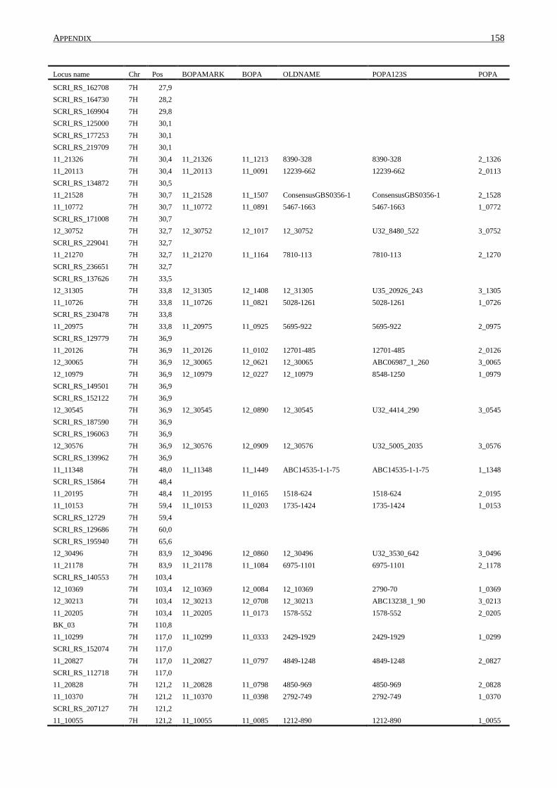
APPENDIX 158


SCRI_RS_162708 7H 27,9 SCRI_RS_164730 7H 28,2

SCRI_RS_169904 7H 29,8

SCRI_RS_125000 7H 30,1

SCRI_RS_177253 7H 30,1 SCRI_RS_219709 7H 30,1

11_21326 7H 30,4 11_21326 11_1213 8390-328 8390-328 2_1326

11_20113 7H 30,4 11_20113 11_0091 12239-662 12239-662 2_0113

SCRI_RS_134872 7H 30,5 11_21528 7H 30,7 11_21528 11_1507 ConsensusGBS0356-1 ConsensusGBS0356-1 2_1528

11_10772 7H 30,7 11_10772 11_0891 5467-1663 5467-1663 1_0772

SCRI_RS_171008 7H 30,7

12_30752 7H 32,7 12_30752 12_1017 12_30752 U32_8480_522 3_0752

SCRI_RS_229041 7H 32,7

11_21270 7H 32,7 11_21270 11_1164 7810-113 7810-113 2_1270

SCRI_RS_236651 7H 32,7

SCRI_RS_137626 7H 33,5 12_31305 7H 33,8 12_31305 12_1408 12_31305 U35_20926_243 3_1305

11_10726 7H 33,8 11_10726 11_0821 5028-1261 5028-1261 1_0726

SCRI_RS_230478 7H 33,8

11_20975 7H 33,8 11_20975 11_0925 5695-922 5695-922 2_0975

SCRI_RS_129779 7H 36,9

11_20126 7H 36,9 11_20126 11_0102 12701-485 12701-485 2_0126

12_30065 7H 36,9 12_30065 12_0621 12_30065 ABC06987_1_260 3_0065

12_10979 7H 36,9 12_10979 12_0227 12_10979 8548-1250 1_0979

SCRI_RS_149501 7H 36,9

SCRI_RS_152122 7H 36,9

12_30545 7H 36,9 12_30545 12_0890 12_30545 U32_4414_290 3_0545

SCRI_RS_187590 7H 36,9 SCRI_RS_196063 7H 36,9

12_30576 7H 36,9 12_30576 12_0909 12_30576 U32_5005_2035 3_0576

SCRI_RS_139962 7H 36,9

11_11348 7H 48,0 11_11348 11_1449 ABC14535-1-1-75 ABC14535-1-1-75 1_1348

SCRI_RS_15864 7H 48,4

11_20195 7H 48,4 11_20195 11_0165 1518-624 1518-624 2_0195

11_10153 7H 59,4 11_10153 11_0203 1735-1424 1735-1424 1_0153

SCRI_RS_12729 7H 59,4 SCRI_RS_129686 7H 60,0

SCRI_RS_195940 7H 65,6

12_30496 7H 83,9 12_30496 12_0860 12_30496 U32_3530_642 3_0496

11_21178 7H 83,9 11_21178 11_1084 6975-1101 6975-1101 2_1178

SCRI_RS_140553 7H 103,4

12_10369 7H 103,4 12_10369 12_0084 12_10369 2790-70 1_0369

12_30213 7H 103,4 12_30213 12_0708 12_30213 ABC13238_1_90 3_0213

11_20205 7H 103,4 11_20205 11_0173 1578-552 1578-552 2_0205

BK_03 7H 110,8

11_10299 7H 117,0 11_10299 11_0333 2429-1929 2429-1929 1_0299

SCRI_RS_152074 7H 117,0

11_20827 7H 117,0 11_20827 11_0797 4849-1248 4849-1248 2_0827

SCRI_RS_112718 7H 117,0

11_20828 7H 121,2 11_20828 11_0798 4850-969 4850-969 2_0828

11_10370 7H 121,2 11_10370 11_0398 2792-749 2792-749 1_0370

SCRI_RS_207127 7H 121,2 11_10055 7H 121,2 11_10055 11_0085 1212-890 1212-890 1_0055

APPENDIX 159


11_20314 7H 124,8 11_20314 11_0281 2183-227 2183-227 2_0314

12_30563 7H 126,8 12_30563 12_0899 12_30563 U32_4768_190 3_0563

11_10073 7H 127,7 11_10073 11_0108 1290-729 1290-729 1_0073

SCRI_RS_150768 7H 130,7

11_10721 7H 130,9 11_10721 11_0808 497-386 497-386 1_0721

SCRI_RS_169639 7H 130,9

BK_07 7H 130,9

12_31211 7H 138,3 12_31211 12_1337 12_31211 U35_18063_1739 3_1211

12_30419 7H 139,2 12_30419 12_0821 12_30419 U32_2166_347 3_0419

SCRI_RS_207246 7H 139,2

SCRI_RS_181727 7H 149,6

11_20485 7H 149,6 11_20485 11_0460 3140-491 3140-491 2_0485

SCRI_RS_225636 7H 149,6 SCRI_RS_104566 7H 149,6

SCRI_RS_127791 7H 149,6

12_30806 7H 149,6 12_30806 12_1053 12_30806 U32_9828_126 3_0806

SCRI_RS_204256 7H 149,6 SCRI_RS_193197 7H 149,6

12_31440 7H 149,6 12_31440 12_1479 12_31440 U35_4712_928 3_1440

12_31294 7H 149,6 12_31294 12_1401 12_31294 U35_20364_468 3_1294

SCRI_RS_172243 7H 149,6 SCRI_RS_168994 7H 152,5

SCRI_RS_136586 7H 152,5

SCRI_RS_124251 7H 152,5

SCRI_RS_152752 7H 152,5 11_10169 7H 173,5 11_10169 11_0214 1800-1101 1800-1101 1_0169

SCRI_RS_112204 7H 173,5

11_20092 7H 173,5 11_20092 11_0068 1178-279 1178-279 2_0092

11_20247 7H 173,5 11_20247 11_0212 1789-782 1789-782 2_0247

SCRI_RS_1347 7H 173,5

SCRI_RS_141732 7H 174,4

SCRI_RS_182503 7H 174,4

SCRI_RS_139808 7H 179,7 SCRI_RS_162966 7H 179,7

SCRI_RS_219260 7H 179,7

SCRI_RS_150049 7H 191,1

SCRI_RS_149645 7H 191,1 SCRI_RS_223021 7H 191,8

11_20192 7H 191,8 11_20192 11_0161 1511-545 1511-545 2_0192

12_10652 7H 191,8 12_10652 12_0156 12_10652 445-1199 1_0652

12_30362 7H 191,8 12_30362 12_0791 12_30362 U32_13417_246 3_0362

12_30797 7H 191,8 12_30797 12_1049 12_30797 U32_9614_416 3_0797

11_20103 7H 192,1 11_20103 11_0080 12027-128 12027-128 2_0103

SCRI_RS_127224 7H 193,2

12_31261 7H 193,2 12_31261 12_1374 12_31261 U35_19382_606 3_1261

11_20495 7H 200,9 11_20495 11_0469 3187-1073 3187-1073 2_0495

SCRI_RS_179528 7H 203,1

SCRI_RS_148318 7H 203,4

11_10451 7H 204,1 11_10451 11_0494 3313-1443 3313-1443 1_0451

SCRI_RS_150053 7H 209,7

11_10851 7H 210,8 11_10851 11_1031 6517-602 6517-602 1_0851

SCRI_RS_222330 7H 210,8

12_31351 7H 211,3 12_31351 12_1428 12_31351 U35_2705_1795 3_1351

SCRI_RS_174285 7H 211,3

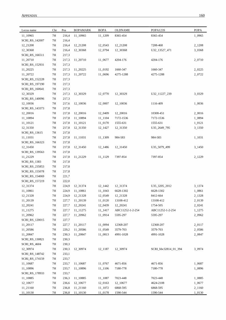
APPENDIX 160


11_10965 7H 216,4 11_10965 11_1209 8365-454 8365-454 1_0965

SCRI_RS_142007 7H 216,4

12_21208 7H 216,4 12_21208 12_0543 12_21208 7208-468 2_1208

12_30368 7H 216,4 12_30368 12_0794 12_30368 U32_13527_471 3_0368

SCRI_RS_166511 7H 217,3 11_20710 7H 217,3 11_20710 11_0677 4204-176 4204-176 2_0710

SCRI_RS_152931 7H 217,3

11_20225 7H 217,3 11_20225 11_0192 1660-347 1660-347 2_0225

11_20722 7H 217,3 11_20722 11_0696 4275-1288 4275-1288 2_0722

SCRI_RS_152228 7H 217,3

SCRI_RS_197190 7H 217,3

SCRI_RS_160641 7H 217,3

12_30329 7H 217,3 12_30329 12_0770 12_30329 U32_11227_239 3_0329

SCRI_RS_140096 7H 217,3

12_10036 7H 217,6 12_10036 12_0007 12_10036 1116-409 1_0036

SCRI_RS_143373 7H 217,8

12_20016 7H 217,8 12_20016 12_0409 12_20016 10308-451 2_0016

11_10894 7H 217,8 11_10894 11_1104 7172-1536 7172-1536 1_0894

11_10121 7H 217,8 11_10121 11_0170 1555-631 1555-631 1_0121

12_31350 7H 217,8 12_31350 12_1427 12_31350 U35_2649_795 3_1350

SCRI_RS_13615 7H 217,8 11_11031 7H 217,8 11_11031 11_1309 984-583 984-583 1_1031

SCRI_RS_166323 7H 217,8

12_31450 7H 217,8 12_31450 12_1486 12_31450 U35_5079_499 3_1450

SCRI_RS_139563 7H 217,8 11_21229 7H 217,8 11_21229 11_1129 7397-854 7397-854 2_1229

SCRI_RS_1383 7H 217,8

SCRI_RS_235853 7H 217,8

SCRI_RS_155078 7H 217,8 SCRI_RS_154069 7H 221,7

SCRI_RS_157219 7H 222,0

12_31374 7H 224,9 12_31374 12_1442 12_31374 U35_3205_2012 3_1374

11_10861 7H 224,9 11_10861 11_1043 6628-1302 6628-1302 1_0861

12_21328 7H 224,9 12_21328 12_0549 12_21328 8412-664 2_1328

11_20139 7H 227,7 11_20139 11_0120 13108-412 13108-412 2_0139

12_20241 7H 227,7 12_20241 12_0439 12_20241 1754-505 2_0241

11_11275 7H 227,7 11_11275 11_1417 ABC11252-1-2-254 ABC11252-1-2-254 1_1275

11_20962 7H 227,7 11_20962 11_0914 5595-297 5595-297 2_0962

SCRI_RS_120015 7H 227,7

11_20117 7H 227,7 11_20117 11_0094 12368-207 12368-207 2_0117

11_20586 7H 229,2 11_20586 11_0549 3579-703 3579-703 2_0586

11_20847 7H 230,3 11_20847 11_0813 4991-1028 4991-1028 2_0847

SCRI_RS_130821 7H 230,3

SCRI_RS_4604 7H 230,3

12_30974 7H 230,3 12_30974 12_1187 12_30974 SCRI_bbc32814_01_394 3_0974

SCRI_RS_148742 7H 233,1

SCRI_RS_174159 7H 233,7

11_10687 7H 233,7 11_10687 11_0767 4671-856 4671-856 1_0687

11_10896 7H 233,7 11_10896 11_1106 7180-778 7180-778 1_0896

SCRI_RS_178933 7H 233,7

11_10885 7H 236,3 11_10885 11_1087 7023-448 7023-448 1_0885

12_10677 7H 236,6 12_10677 12_0163 12_10677 4624-2108 1_0677

11_21160 7H 236,8 11_21160 11_1072 6868-595 6868-595 2_1160

11_10130 7H 236,8 11_10130 11_0178 1590-544 1590-544 1_0130

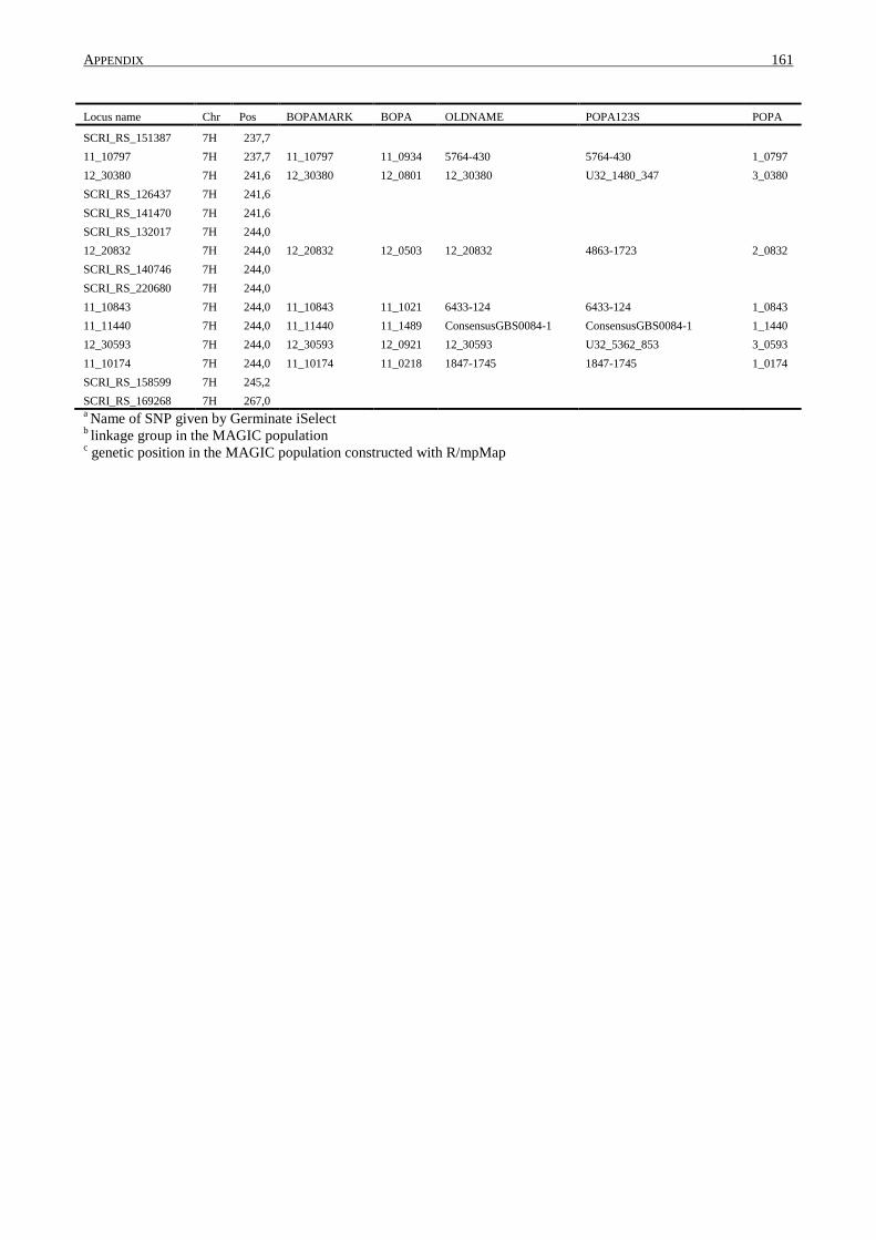
APPENDIX 161


SCRI_RS_151387 7H 237,7 11_10797 7H 237,7 11_10797 11_0934 5764-430 5764-430 1_0797

12_30380 7H 241,6 12_30380 12_0801 12_30380 U32_1480_347 3_0380

SCRI_RS_126437 7H 241,6

SCRI_RS_141470 7H 241,6 SCRI_RS_132017 7H 244,0

12_20832 7H 244,0 12_20832 12_0503 12_20832 4863-1723 2_0832

SCRI_RS_140746 7H 244,0

SCRI_RS_220680 7H 244,0 11_10843 7H 244,0 11_10843 11_1021 6433-124 6433-124 1_0843


12_30593 7H 244,0 12_30593 12_0921 12_30593 U32_5362_853 3_0593

11_10174 7H 244,0 11_10174 11_0218 1847-1745 1847-1745 1_0174

SCRI_RS_158599 7H 245,2

SCRI_RS_169268 7H 267,0

a Name of SNP given by Germinate iSelect

b linkage group in the MAGIC population

c genetic position in the MAGIC population constructed with R/mpMap

Acknowledgements

First of all my deepest thanks go to Prof. Jens Léon for supervising me, providing me with

resources and a lot of questions. I thank him for his idea to develop a MAGIC population, his

enthusiasm in this project, his encouragement and time for all the little questions. But most of all I

thank him for his trust in me and for the opportunity to work independently and with fullest possible

autonomy knowing he would always support me with discussion and advices.

My thanks go to Prof. Heiner Goldbach, who did not hesitate to take over the role of co-referee in

the examination committee and his willingness to critical review this manuscript.

I thank Merle Noschinski, the friendliest, reliable and tireless assistance one can think of. She never

got lost in all the samples.

I thank Ralf Gente from University Marburg, who spent lots of time explaining the world of the

THz-sensor to a non-professional.

My special thanks go to technicians Josef Höckling and Petra Rings, nothing would work without

them. I thank all my colleagues from the Institute, especially Karola Müller, who patiently crossed

the MAGIC population over several years, Anne Reinders for her help with SAS and the

organization of the pot experiments. Karin Woitoil, Heike Sodtke and all students for the help of

data collecting. My thanks go to Agim Ballvora for constructive discussion and his charming

personality, which made work joyful.

Furthermore I thank all PhD candidates, comrade-in-arms, and newly graduates, first of all Boby

Mathew for his help in R, Melanie Herker, Tobias Kox, Alex Bothe for cheerful company during

long days of work and evenings. Especially I like to thank Tiegist Abebe for our friendship,

discussions and Ethiopian coffee and food.

I want to thank my friends for their support, sympathy, patience and interest in my work. Thank

you, Simon, for the makeover of the abstract.

Sarah, you make my life significantly different.

Finally I want to thank my family and especially my parents for their supported, trust and interest in

my life. Ohne euch wäre ich nicht hier.

Marker-trait-sensor association in a multi-parent advanced ...

Documents

Transcript of Marker-trait-sensor association in a multi-parent advanced ...