Uw

Sa

b

c

d

a

ARRA

KTWVI

1

rvfewarfiwsa

(

h1

Europ. J. Agronomy 59 (2014) 67–77

Contents lists available at ScienceDirect

European Journal of Agronomy

j ourna l h o mepage: www.elsev ier .com/ locate /e ja

se of soil and vegetation spectroradiometry to investigate cropater use efficiency of a drip irrigated tomato

. Marinoa,∗, M. Ariab, B. Bassod, A.P. Leonec, A. Alvinoa

Department of Agricultural, Environmental and Food Sciences (DAEFS), University of Molise, Via De Sanctis, I-86100 Campobasso, ItalyDepartment of Economics and Statistics, University of Study of Napoli Federico II, via Cintia 26, 80126 Napoli, ItalyDepartment of Geological Sciences, Michigan State University, 206 Natural Science Building, East Lansing, MI 48824-1115, United StatesCNR — Institute for Mediterranean Agriculture and Forest Systems (ISAFoM), via Patacca 85, 80056 Ercolano, Italy

r t i c l e i n f o

rticle history:eceived 17 June 2013eceived in revised form 14 May 2014ccepted 24 May 2014

eywords:omato yieldater use efficiency

egetation indicesrrigation management

a b s t r a c t

An agronomic research was conducted in Tuscany (Central Italy) to evaluate the effects of an advancedirrigation system on the water use efficiency (WUE) of a tomato crop and to investigate the ability of soiland vegetation spectroradiometry to detect and map WUE. Irrigation was applied following an innovativeapproach based on CropSense system. Soil water content was monitored at four soil depths (10, 20,30 and 50 cm) by a probe. Rainfall during the crop cycle reached 162 mm and irrigation water appliedwith a drip system amounted to 207 mm, distributed with 16 irrigation events. Tomato yield variedfrom 7.10 to 14.4 kg m−2, with a WUE ranging from 19.1 to 38.9 kg m−3. The irrigation system alloweda high yield levels and a low depth of water applied, as compared to seasonal ET crop estimated withHargraves’ formula and with the literature data on irrigated tomato. Measurements were carried outon geo-referenced points to gather information on crop (crop yield, eighteen Vegetation indices, leafarea index) and on soil (spectroradiometric and traditional analysis). Eight VIs, out of nineteen ones

analyzed, showed a significant relationship with georeferenced yield data; PVI maps seemed able toreturn the best response, before harvesting, to improve the knowledge of the area of cultivation andirrigation system. CropSense irrigation system reduced seasonal irrigation volumes. Some vegetationindexes were significantly correlated to tomato yield and well identify, a posteriori, crop area with lowWUE; spectroradiometry can be a valuable tool to improve irrigated tomato field management.

. Introduction

Agricultural water use plays the most critical role in wateresources management all around the world (Köksal, 2008). Thealue of water will go up in the century for the severe competitionor water from human beings, intensive agriculture, flora and fauna,tc. (Bouwer, 2000). Irrigated agriculture is a major consumer ofater and accounts for about two thirds of the total fresh water

ssigned to human uses (Fereres and Evans, 2006). As a generalule, agriculture show often a low irrigation water use efficiency,or this reason irrigation scientists are forced to develop water sav-ng irrigation strategies (Payero et al., 2009). Sustainable irrigation

ater management should simultaneously achieve two objectives:ustaining irrigated agriculture for food security and preserving thessociated natural environment. A stable relationship should be

∗ Corresponding author. Tel.: +39 0874404709; fax: +39 0874404713.E-mail addresses: stefanomarino@unimol.it, stefanomarino@gmail.com

S. Marino).

ttp://dx.doi.org/10.1016/j.eja.2014.05.012161-0301/© 2014 Elsevier B.V. All rights reserved.

© 2014 Elsevier B.V. All rights reserved.

maintained between these two objectives now and in the future,while potential conflicts between these objectives should be miti-gated through appropriate irrigation practices. The sustainable useof water in agriculture has become a priority and the adoptionof irrigation strategies which may allow saving irrigation waterand maintaining satisfactory yields, thus improving water use effi-ciency (WUE), may contribute to the preservation of this even morerestricted resource (Parry et al., 2005; Topcu et al., 2007).

Efficient use of water in any irrigation system is becomingimportant particularly in arid and semiarid region where wateris a scarce commodity; in this area maximizing water productiv-ity may be more profitable to the farmer than maximizing cropyield (Pereira et al., 2002). The economic and environmental bene-fits of improving the volumetric efficiency of irrigation are obviousin both the value of the water saved and the additional produc-tion possible with this water. Hence, there is a triple bonus for

improving irrigation precision including: (a) maximizing yield andquality of production, (b) reducing water losses below the rootzone, and (c) conserving the resource base, by minimizing the riskof groundwater salinity and thus enhancing sustainability. These

6 J. Agro

ga1

t(ama

eii2fbapIwd

stHa1saI

eboMttsrswmVntopaw2

pitigtoatauw2

a

8 S. Marino et al. / Europ.

ains can only be achieved when all elements of precision oper-te synergistically within a given environment (Painter and Carren,978).

For improving WUE, Batchelor (1999) suggested several ways athe farm level, improving crop husbandry and cropping strategiesagronomic), installing an advanced irrigation system (technical),dopting demand-based irrigation scheduling systems and betteraintaining equipment (managerial), introducing water pricing

nd improving the legal environment (institutional).Water Use Efficiency can be optimized by the adoption of more

fficient irrigation practices (Costa et al., 2007), in this regard, driprrigation has contributed to improve WUE by significantly reduc-ng runoff and crop evapotranspiration losses (Stanghellini et al.,003; Jones, 2004; Kirnak and Demirtas, 2006). Drip irrigation inact is one of the best techniques to use in applying water to vegeta-les and orchards (C etin and Uygan, 2008). Proper irrigation timingnd amount increases the water use efficiency; consequently theroduction per unit of water will be increased (Ismail et al., 2008).

mproper irrigation timing can lead to the development of cropater deficit resulting in reduced yield due to water and nutrienteficiencies (Wright, 2002).

However, irrespective of the strategy employed, the benefits ofcheduling will only be realized if the irrigation system can be con-rolled sufficiently well to apply only the exact amount required.ence, control is a necessary component of any irrigation systemiming to apply water in precise amounts (Hoffman and Martin,993): “the accurate and precise application of water to meet thepecific requirements of individual plants or management unitsnd minimize adverse environmental impact” is defined Precisionrrigation (Raine et al., 2007).

Usually irrigation treatments are carried out following thevapotranspiration criterion according to the simplified soil wateralance (Doorenbons and Pruitt, 1977), with a complete restorationf the calculated ETc (Hanson and May, 2004; Favati et al., 2009).onitoring the water use and plant status in the field is important

o develop effective precautions and for this purpose some indica-ors are required (Köksal et al., 2008). A very large body of research,panning almost four decades, has demonstrated that much of theequired agricultural information can be derived from remotelyensed data (Pinter et al., 2003). The ability to accurately assessater stress symptoms in vegetation using spectral reflectanceeasurements is an important goal for research (Jackson, 1986).egetation and water stress indices calculated based on visible-ear infrared (vis-NIR) spectral reflectance and infrared surfaceemperature measurements from either the long (remote sensing)r short distance (proximal sensing) can provide spatial and tem-oral information to improve WUE. There are numerous studiesddressing the use of spectral reflectance to obtain the leaf/canopyater status and water stress (Leone et al., 2007; Ceccato et al.,

001; Penuelas et al., 1993, 1997).Besides the new technologies to improve WUE, JDW has pro-

osed CropSense® Soil Moisture Monitoring, a new near-real-timenstrument to measure in-depth soil moisture levels from fac-ors encompassing growth stage to environmental conditions. Thenstrument delivers data for a precision control of soil moisture,ives customizable reports, which accurately measure soil mois-ure levels in the field. By understanding the movement of waterver time for the crop, provides information to determine the rightmount of water to apply to properly fill the root zone and optimizehe applied nutrients and to make decisions on irrigation programsnd fertigation. The goal of JDW sensor is to increase crop waterse efficiency (WUE) by reducing the amount of water applied by

atering and by reducing the number of irrigation events (Kirda,

002).During the next years, simulation model development and

pplication should (Consoli et al., 2006; D’Urso et al., 2010) focus

nomy 59 (2014) 67–77

on agricultural water savings, increase crop water productivity,monitoring of crop conditions (Bastianssen et al., 2007). The useof remote and proximal sensing has proved to be very importantin monitoring the growth of agricultural crops and in irrigationscheduling. Spectral VIs, resulting from the combination of two ormore spectral bands, are commonly used to enhance the vegeta-tion signal, while minimizing solar irradiance and soil backgroundeffects (Jackson and Huete, 1991). They are indirectly related toplant stress, biomass, leaf area index, yield, N content, leaf chloro-phyll concentration (Leone et al., 2007, 2001a; Penuelas et al., 1997;Baret and Guyot, 1991; Basso et al., 2011; Marino and Alvino, 2014).

Tomato, an important crop in Mediterranean countries, is a highwater demanding crop, thus requiring irrigation throughout thegrowing season in arid and semiarid areas (Patanè et al., 2011).Several comparisons between VIs reliability are presented in recentliterature. However, to our knowledge, no indications are availablefor tomato WUE (Gianquinto et al., 2011). Furthermore water stresshad a significant reduction yield (Pulupol et al., 1996; May andGonzalerz, 1999) then the frequency and amount of irrigation playa crucial role on growth and yield of tomato (Obreza et al., 1996).The present paper reports the spatial variability of a tomato crop,drip irrigated by an automated system which maintained the soilwater content within specific intervals. The aims were (i) to test theautomated irrigation system as a tool to reduce seasonal irrigationwater applied related to the Hargreaves method; (ii) assess the spa-tial variability, at field scale, of a tomato crop; (iii) to identify theVegetation Indices significantly related to WUE.

2. Materials and methods

2.1. Experimental set-up

The studies were carried out in 2009 at Abbadia of Montepul-ciano (Central Italy), in a farm called Agrichiana Farming (Latitude N43.15216, Longitude E 11.88747). The tomato cultivar Perfectpeelwas transplanted on the 22nd of May in a twin row spacing of150 cm, with a final plant density of 33,500 plants ha−1 (50 cmbetween rows and 20 cm plants on the row).

Fertilization was performed using fertilizers and doses com-monly used for the cultivation of tomato in central Italy and weedswere controlled with recommended chemical herbicides.

The crop was drip irrigated by T-Tape® 708-30-250, a John DeereWater drip tape with spacing between drippers of 30 cm and a flowrate of 0.75 l/h at 0.55 bar. A CropSense® Soil Moisture Monitoring(by John Deere Water) was installed on 26th of June; CropSense®

is a near-real-time soil moisture monitoring system, character-ized by multilevel capacitance sensors that monitors water contentchanges at the soil depths of 10, 20, 30 and 50 cm. The system allowto optimize irrigation management at each crop stage, especiallyprovides information so that it is possible to determine the rightamount of water to apply to properly fill the root zone. A Graph isgenerated by collecting data from four depths; limits can be set onthis graph (full point, full point warning, re-fill point warning, andre-fill point); these zones on the graph to help determine when andhow often to irrigate, in order to ameliorate irrigations taking intoaccount rainfall. The seasonal irrigation volume was 2070 m3 ha−1

applied with 16 irrigation as reported in Fig. 1.

2.2. Meteorological and agronomic measurements

Daily maximum and minimum temperatures and rainfall

were recorded through a standard agro-meteorological station byARSIAT, the Extension Service of the Tuscany Region, and a fewkilometers away from the farm. Crop yields and total seasonalirrigation water applied under the described irrigation technique

S. Marino et al. / Europ. J. Agronomy 59 (2014) 67–77 69

F ollecte3

waTawalOmb0

tI2

2

A(sbTat6ABtb2sa2aSfi

tsr

aomRteod1i

ig. 1. CropSense® Soil Moisture Monitoring stacked graph which shows the data c0 and 50 cm) from 27th June to tomato harvest.

ere recorded. Irrigation water use efficiency is generally defineds crop yield per water used to produce the yield (Viets, 1962).hus, WUE (Lovelli et al., 2007; Patanè et al., 2011) was calculateds fresh fruit weight (kg ha−1) obtained per unit volume of totalater use (ETc m3 ha−1). The ETc was measured with Hargreaves

nd Samani equation (1982, 1985) and the crop coefficients uti-ized were those obtained in a similar environment (Tarantino andnofri, 1991), with values of 0.35 from transplant up to establish-ent, 0.55 up to the early stages of blooming; 0.90 in the phase

looming-setting; 1.1 in the phase of berry growth-veraison, and.95 from the beginning of ripening up to the end of the cycle.

Sixty-four georeferred yield samples (1 m2 each) were collectedhe day before harvesting, the 24th of September 2009. Leaf Areandex (LAI) was measured by means of a portable system (LI-COR000, Biosciences, Lincoln, NE, USA) at the 20th of August.

.3. Crop and soil spectral measurements (proximal sensing)

The radiance over tomato canopy was measured with anSD FieldSpec Hand-Held Pro portable hyperspectral radiometer

Analytical Spectral Device, Boudler, CO, USA), and converted topectral reflectance by dividing the radiance reflected by the targety that reflected by a standard white reference plate (spectralon).his instrument covers the portion of the spectrum between 350nd 1100 nm, with a spectral sampling distance of <1.5 nm. Spec-ral reflectance was measured at nadir in cloud-free days. A total of4 georeferred spectral measurements were taken on August 20th.

FieldSpec Pro spectroradiometer (Analytical Spectral Device,oudler, CO, USA) was used to both describe the general charac-eristics of the investigated soil and predict soil properties on thease of existing statistically-based predictive models (Leone et al.,012). Twenty geo-referred soil samples were air dried and 2 mmieved to determine in the laboratory soil texture and CEC capacity,ccording to the Italian Official Methods for Soil Analysis (MIPAF,000). To improve the quality of both canopy and soil the spectra,

10-point Savitzky–Golay filter was applied to these spectra. Theavitzky–Golay (1964) filter is based on least squares polynomialtting across a moving window within the data.

After filtering, the majority VIs reported in the scientific litera-ure were calculated from canopy spectra according to the formulashown in Table 1. For a detailed discussion of these indices, theeader is referred to the references cited in this table.

After filtering, soil reflectance spectra (R) were converted tobsorbance spectra (A = log 1/R), and the second derivative spectraf the latter were then calculated, and analyzed to extract infor-ation on the mineralogical assemblage of the investigated soils.

eflectance spectra (R) result from the superposition of absorp-ion bands at different wavelengths, corresponding to the variouslectronic or vibrational transitions in the atoms and molecules

f minerals. These bands can be enhanced by plotting the seconderivative of absorbance against wavelength (Malengreau et al.,994). The position of an absorption band is indicated by the min-

mum on the second derivative curve (Huguenin and Jones, 1986),

d from the soil moisture sensors at each depth represented by a single line (10, 20,

and allows identifying either individual or groups of minerals. Theamplitude of an absorption band is determined by the difference inordinate between the minimum and the following maximum, andis related to the abundance of a mineral or a group of minerals.

Further information was derived from the transformation of vis-ible reflectance (350–780 nm) Munsell color notations (Leone et al.,2012). The Munsell system is the most definite colors in terms ofhue (H), chroma (C), and value (V). Hue refers to the dominantwavelength, chroma expresses the saturation of the color, and valueis the overall brightness.

2.4. Statistical analysis

The 64 yield data were analyzed by a clustering method, usingHierarchical clustering Ward’s minimum variance approach.

Cluster analysis is a collection of statistical methods that iden-tifies groups of samples that behave similarly or show similarcharacteristics. Cluster analysis classifies a set of observations intotwo or more mutually exclusive unknown groups on the basis ofcombinations of interval variables. The purpose of cluster analysisis to discover a system that can classify observations into groups, inwhich the group members have properties in common. Agglomer-ative hierarchical cluster methods produce a hierarchy of clustersfrom small clusters of very similar items to large clusters thatinclude more dissimilar items. Hierarchical methods usually pro-duce a graphical output known as a dendrogram, or tree, that showsthis hierarchical clustering structure (Ward, 1963). Agglomerativeclustering begins by finding the most similar two groups, based onthe distance matrix, and subsequently merging them into a singlegroup. This procedure is repeated, step by step, until all the sampleshave been added to a single large cluster. The final partition is iden-tified by a distance criterion (Fernández and Gómez, 2008). Startingfrom the bottom part of the dendrogram, the researcher decides tostop the agglomeration process when successive clusters are toofar apart to be merged.

2.4.1. Assessing normalityShapiro-Wilk method (1965), Lilliefors method (1967),

Anderson–Darling method (1954) and D’Agostino et al. (1990)method were used to check the normality assumption. The rejec-tion of one or more of this test is a symptom of non normalitydistribution.

2.4.2. Non-parametric ANOVA by Kruskal–WallisThe Kruskal–Wallis test (1952) is most commonly used when

there is one nominal variable and one measurement variable, andthe measurement variable does not meet the normality assump-tion. It is can interpreted as the non-parametric alternative toclassical one-way Analysis of Variance test.

A one-way ANOVA may yield inaccurate estimates of the P-value when the data are very far from normally distributed. TheKruskal–Wallis test does not make assumptions about normality.Like most non-parametric tests, it is performed on ranked data, so

70 S. Marino et al. / Europ. J. Agronomy 59 (2014) 67–77

Table 1Reflectance index, acronym, formulation and references of eighteen vegetation indices.

Reflectance index Acronym Formulation References

Water Index WI (R900/R970) Penuelas et al. (1993, 1997)Structure Intensive Pigment Index SIPI (R800 − R445)/(R800 + R680) Penuelas et al. (1995)Plant Senescence Reflectance Index PSRI (R680 − R550)/R750 Merzlyak et al. (1999)Photochemical Reflectance Index PRI (R531 − R570)/(R531 + R570) Gamon et al. (1990, 1992, 1997)Weighted difference vegetation index WDVI R800 − (1.2344 × R670) Clevers (1989)Perpendicular Vegetation Index PVI 1/RADQ(1.23442 + 1 × (R800 − 1.2344 ×

R670 − 0.0183))Richardson and Wiegand (1977)

Soil-Adjusted Vegetation Index SAVI (R800 − R670)/(R800 + R670 + 0.5)) ×(1 + 0.5) Huete (1988)Transformed Soil-Adjusted Vegetation

IndexTSAVI (1.2344 × (R800 − 1.2344 ×

R670 − 0.0183))/(1.2344 ×R800 + R670 − 1.2344 × 0.0183)

Baret et al. (1989)

Second Soil-Adjusted Vegetation Index SAVI2 R800/(R670 + 0.0183/1.2344) Major et al. (1990)Modified Soil-Adjusted Vegetation

IndexMSAVI (R800 − R670)/(R800 + R670 + (1 + (1–1.2342 × R800

− (1.2344 ×R670) × (R800 − R670)/(R800 + R670))))

Qi et al. (1994)

Optimized Soil-Adjusted VegetationIndex

OSAVI (1 + 0.16) × (R800 − R670)/(R800 + R670 + 0.16) Rondeaux et al. (1996)

Normalized Difference VegetationIndex

NDVI (R800 − R670)/(R800 + R670) Rouse et al. (1974)

Green Normalized DifferenceVegetation Index

GNDVI (R800 − R550)/(R800 + R670) Gitelson et al. (1996)

Transformed Chlorophyll Absorption inReflectance Index

TCARI 3 × ((R700 − R670) − 0.2 ×(R700 − R550) × (R700/R670))

Kim et al. (1994)

Transformed Chlorophyll Absorption inReflectance Index/OptimizedSoil-Adjusted Vegetation Index

TCARI/OSAVI 3 × ((R700 − R670) − 0.2 × (R700 − R550) ×(R700/R670))/(1 + 0.16) ×(R800 − R670)/(R800 + R670 + 0.16)

Haboudane et al. (2002)

Chlorophyll Index CL (R750 − R705)/(R750 + R705) Gitelson and Merzlyak (1994, 1996)Modified Chlorophyll Absorption in MCARI ((R700 − R670) − 0.2 ×

550) ×Daughtry et al., 2000

0)/(R

to

huP

2

P

tsuTccc

2

at

bia

2

Vosp

Reflectance Index (R700 − RWater Index/Normalized Difference

Vegetation IndexWI/NDVI (R900/R97

he measurement observations are converted to their ranks in theverall data set.

The KW test verifies whether three or more independent groupsave same distribution. All statistical procedures were computedsing the statistical packages IBM SPSS 21 (IBM Inc. USA) and OriginRO 8 (Origin Lab Corporation, Northampton, MA 01060, USA).

.4.3. Factorial analysisThe multiple correlation among variables has been measured by

rincipal Component Analysis.Principal component analysis (PCA, Hotelling 1933) is a statis-

ical procedure that uses orthogonal transformation to convert aet of observations of possibly correlated variables into a set of val-es of linearly uncorrelated variables called principal components.his transformation is defined in such a way that the first principalomponent has the largest possible variance, and each succeedingomponent in turn has the highest variance possible under theonstraint that it is orthogonal to the preceding components.

.4.4. Regression analysisThe main applications of PCA are: to reduce the number of vari-

bles and to detect structure in the relationships between variables,hat is to classify variables.

Regression analysis was used to assess the relationshipsetween canopy variables and those derived from the parameter-

zation of soil reflectance spectra (i.e. Color notation and depth ofbsorption bands in the second derivative spectra).

.5. Geostatistical analysis

Geostatistical analysis to map the spatial variability of selected

is was used. Ordinary kriging is a commonly-used linear methodf spatial prediction to provide estimates of variables at unvisitedites. The procedure uses information from neighboring points toredict at a target point; weights are assigned to these points based

(R700/670))800 − R670)/(R800 + R670) Penuelas et al. (1997)

on their distance from the target. Weights are assigned to eachsample such that the estimation or the kriging variance is mini-mized and the estimates are unbiased (Webster and Oliver, 2007).The weights depend on the relative positions of the samples in theneighboring both to one another and to the target point, and on thevariogram. The latter describes the spatial correlation and covari-ance structure between data points for each variable. The variogramcan be computed by Matheron’s (1965) usual method of moments.The best variogram model for each parameter was selected basedcross validation. Cross validation (Delhomme, 1978; Merino et al.,2001) is performed using Mean Error (ME), Root Mean Square(RMSE) and Standardized Mean Squared Error (SMSE) (Table 2). Thesemivariograms was computed using GS+ version 8 while krigingwas performed using surfer version 9 (Golden software, Golden,Colorado, USA) according to Selvaraja et al. (2012).

3. Results and discussion

Decadal minimum and maximum air temperature, decadal EToand rainfall, and watering depths during the study period are pre-sented in Fig. 2. The minimum mean temperature was recordedin September (7.1 ◦C), and the maximum one in July (34.3 ◦C). Inthe crop cycle (May–September), ETo amounted to 650 mm, ran-ging from 110 mm in September to 186 in July. The 21% of ETo wasin June (157 mm) and in August (151 mm), while the highest rate(25%) was recorded in July.

The total ETc reached about 500 mm, with about the 40% in Julyand the 25% in August. Precipitation amounted to 163 mm, with adry period (50 days) from the third decade of June to the first oneof August. Irrigation started in June, with one water application of9 mm.

The water distributed with JDW CropSense (207 mm) wasabout 32% lower than the amount estimated with Hargraves,304 mm. Nine irrigations were applied in July (142 mm, 67% of theseasonal irrigation depth), characterized by lack of rainfall and by

S. Marino et al. / Europ. J. Agronomy 59 (2014) 67–77 71

Table 2Semivariogram parameters (model, Nugget effect, sill, range) and cross validation (mean square ME, root mean square error RMSE and Standardized mean squared error)used to WUE, and Vegetation indexes kriging map.

Model Nugget Sill Range ME RMSE SMSE

WUE Spherical 9.508 22.219 60.586 3.0105 1.7351 1.0046PVI Spherical 0.000617 0.002717 61.594 0.0023 0.0481 1.0005SAVI Spherical 0.00526 0.02612

WDVI Spherical 0.0114 0.1203

OSAVI Spherical 0.000162 0.002594

Fp

toa

(rt(oCpcopw

Fotce

use on numerous field and greenhouse crops. As common to agro-

ig. 2. Ten-day averages rainfall (rain), maximum (Tmax) and minimum (Tmin) tem-eratures, evapotranspiration (ETo) and irrigation amount (Irr) during crop seasons.

he highest evaporative demand during the cycle. The 18% and 11%f the total irrigation depth was applied in August (4 irrigation)nd in September (2 irrigation), respectively.

The investigated soils show a homogeneous olive-brown coloron average 2.24Y 4.41/3.32), with Munsell H, V and C ranging,espectively, from 1.79 Y to 2.87Y, from 4.25 to 5.00, and from 3.05o 3.48, and a coefficient of variation (CV) had been always low<20%). The moderate V may be attributed to the moderate contentf organic matter and carbonates (Leone and Escadafal, 2001b). The, always >2.00, indicated the absence, in the investigated soils, ofrolonged conditions of reductions (or, in the other word, of goodonditions of oxygenation). The values of H indicated the presence

f iron oxi-hydroxides, very likely of goethite. The diagnosis of theresence of goethite is confirmed from the analysis of Fig. 3, fromhich it appears evident that all the investigated soil samples falls

ig. 3. Distribution of Montepulciano soil samples (Soil Mont) compared with thosef pure iron oxi-hydroxides (hematite, ferrihydrite, lepidocrocite and goethite) onhe space defined Munsell chroma and hue (polar diagram of chromaticity). Thehromaticity diagram of pure iron oxi-hydroxides refers to a recent work of Leonet al. (2012), build up using data published by Schwertmann and Cornell (2000).

49.88 0.0159 0.126 1.007150.3 0.1005 0.317 1.037050.2 0.0065 0.081 1.0153

within the range of variation of the Munsell H of the above iron-hydroxide. However, the relatively low C indicated that content ofgoethite is low.

The low presence of goethite is further confirmed by the pres-ence of a band, relatively shallow, on the second derived spectra(Fig. 4), cantered at around 482 nm, produced by pairs of electronictransitions in the Fe present in the crystal structure of the aboveiron-oxide (Sherman and Waite, 1985). The analysis of the secondderivative spectra shows also the presence of three major bandsassociated with the presence of clay minerals, at around 1409 and1906 nm (mainly determined by the presence of smectite), 2202 nm(determined by the presence of kaolinite, but also influenced bythe presence of other clay minerals, mainly smectite and illite) and2341 nm (determined by the presence of carbonates). The bandaround 2002 nm is associated with a doublet, at around 2162 nm,which is diagnostic of the presence of kaolinite (Leone and Sommer,2000).

The average yield of tomato was 10.4 kg m−2, similar(10.6 kg m−2) to the result of a four-year test carried out onthe same hybrid and in the same Region by ARSIA (the extensionservice of Tuscany) and according to other experiment reportson Perfectpeel hybrid (e.g. Siviero et al., 2000; Riahi et al., 2009;Giorio et al., 2007).

In the present experiment, the extreme fruit yield valueswere 14.4 kg m−2 and 7.1 kg m−2, and thus the water use efficien-cies (WUE) ranged from 19.1 to 38.9 kg m−3 with an average of28.1 kg m−3.

The literature shows many papers on the efficiency of water

nomic studies, papers on tomato differed each other for severalfactors, such as climatic conditions, variety/hybrid, and agronomic

Fig. 4. Mean second derivative spectra of abosrbance of the experimental soils. Theposition of the main absorption bands is shown.

72 S. Marino et al. / Europ. J. Agronomy 59 (2014) 67–77

F e. Thes

tWiUffift(

Wp(HWTaW

tmbHsfi(fiat

coiwH

o

TCtc

2200 nm), soil particle size distribution, cation exchange capac-ity (CEC), and subsequently among the above soil properties andtomato yield. These relationships were effectively proved by fac-tor analysis (FA) (Hair et al., 1995). The projection of the above

ig. 5. Cluster analysis: dendrogram, or tree, with hierarchical clustering structurmall clusters of very similar items to large clusters that include dissimilar items.

reatments in combination with irrigation. Authors have computedUE taking or not into consideration rainfall (IWUE), and without

ndicating any possible contribution from the water table. C etin andygan (2008), in Central Anatolian (Turkey) from 2003 to 2005,

ound values of WUE ranging from 14.3 to 25.8 kg m−3 in a tomatoeld hybrid (Dual Large F1) which gave a marketable yield ranging

rom 6.4 to 13.1 kg m−2. Patanè et al. (2011) obtained values closeo those of the present experiment when applying deficit irrigation50% of the ETc) to cv. Brigade.

Yield data were analyzed by hierarchical cluster analysis, usingard’s method. The cluster selection procedure identifies the best

artition (BSS ratio 0.864, Gap 0.093) formed by three clustersFig. 5): cluster n◦1 (25 items – Low value (L)), cluster n◦2 (10 itemsigh value (H)) and cluster n◦3 (29 items Medium value (M)). TheUE and yield mean value of the three clusters were reported in

able 3, the H cluster mean was 35.1 kg m−3, the M cluster showedn average WUE of 29.9 kg m−3 and L cluster showed an averageUE of 23.1 kg m−3.Georeferenced WUE data were spatialized with geostatistich

echnique to assess the spatial variability of tomato crop and theaps are presented in Fig. 6, as reported by cluster analysis have

een identified three different zones: Low (L), Medium (M) andigh (H). Two H zones were detected, one near the probe and the

econd one near the upper edge of the field (550 m from the lowereld hedge), along with three little surfaces, for a total of 4800 m2

Table 4). A L area appeared as a long strip on the right side of theeld and as two small spots on the left side, for a total surface ofbout 7200 m2. The remaining large area showed M WUE with aotal surface of 23,640 m2.

The mean values of WUE and data relating to tomato crop wateronsumption along the crop cycle have shown good effectivenessf the irrigation system and probe measuring. As a whole, therrigation system allowed a high yield levels and a low depth of

ater applied, as compared to seasonal ET crop estimated with

argraves’ formula and with the literature data on irrigated tomato.

A factor analysis was used the to investigate the possible impactn tomato WUE due to soil spectroradiometric measurements and

able 3luster centroids: mean (StdDev) of 64 georeferenced yield data and WUE, split intohree different clusters: low (L), medium (M) and high (H) according to hierarchicallustering analysis with Euclidean distance and Ward’s link aggregation.

L M H

Yield 8.57 (0.78) 11.08 (0.53) 13.0 (0.65)WUE 23.1 (2.09) 29.9 (1.4) 35.1 (1.8)

agglomerative hierarchical cluster methods produce a hierarchy of clusters from

soil analytical measurements. It is well known that the clay miner-alogy of a soil affects other important properties of soil, such as theparticle distribution in the fine earth and the net negative charge(Brady and Weil, 2002). Therefore, relationships may be expectedamong the 1096 nm and other main clay absorption bands (1400,

Fig. 6. Spatial distribution of tomato WUE (kg m−3), divided into High (H), Medium(M) and Low (L) zones, as modeled by ordinary kriging.

S. Marino et al. / Europ. J. Agronomy 59 (2014) 67–77 73

Table 4Area (m2) and percent incidence of Water Use Efficiency, PVI, WDVI SAVI and OSAVI indexes from each zone (H, M, L from WUE). Within each zone, the degree of discriminationof an index, expressed as percentual difference respect to WUE surface.

Area (m2) Incidence (%) Differences from WUE (%)

H M L H M L H M L

WUE 4819 23,640 7181 13.5 66.3 20.1 – – –PVI 3961 23,808 7871 11.12 66.8 22.1 −21.6 0.7 8.8

v(aacAtaipeto

lfificps

1sa2f(e

FoBC

WDVI 1611 21,501 12,528 4.52SAVI 19,525 13,407 2708 54.8

OSAVI 0 30,194 5446 0

ariables on the factorial plan defined by the first (F1) and secondF2) factorial axes (Fig. 7) revealed that clay is close to the depth ofbsorption band of clay minerals, particularly with that of smectite,nd in the opposite side of the clay, thus confirming that as clay andlay minerals content in soil increase, the tomato yield decreases.lso the CEC is in the opposite direction of yield, thus indicating

hat an increase of CEC lead to a decrease of yield. This result couldppear strange, considering that CEC is and indicator of soil chem-cal fertility. Evidently, more than the chemical fertility are the soilhysical conditions, especially soil areation, that affect yield. Thisxplain also the position of sand in the scatterplot, which is posi-ively related with yield (both yield and sand are far from the originf axes and in highly loaded to the first principal axis).

The analysis of the data related to the WUE maps has high-ighted that the best management of certain areas (L area) of theeld can enhance the average value of WUE. Therefore, the identi-cation during the cultural cycle of the area with the lowest WUEould allow proper management of the field resulting in increasedroduction and optimization of WUE and improve the irrigationystem.

Given that several studies (e.g. Pinter et al., 1981; Ma et al.,996; Teal et al., 2006; Elwadie et al., 2005; Marino et al., 2013)howed VIs ability to predict yield on Maize, Corn, Wheat, Barleynd Onion and previous studies on tomato (Koller and Upadhyay,005) hypothesized the use of VIs based upon plant greenness

or the evaluation of tomato yield. On tomato Gianquinto et al.2011) have found NIR/R560 as the most suitable index for thevaluation of the crop nutritional status, spectroradiometric curves

ig. 7. Ordination of soil chemical, physical and spectroscopic properties and yieldn the F1-F2 axes resulting from the application of factor analysis (FA).1400, 1906, B2200 = depth of absorption bands at 1400, 1906 and 2200 nm;EC = cation exchange capacity.

60.3 35.2 −199.1 −9.9 42.737.6 7.6 75.3 −76.3 −165.284.8 15.3 – 21.7 −31.9

and vegetation indices were tested to evaluate the goodness of VIsto detect different zones WUE.

For this reason were collected and analyzed 64 spectroradio-metric measures vegetation (geo-referenced points), to evaluatethe possibility to characterize the tomato crop variability and WUEbefore harvest and to identify the best Vegetation Indices signifi-cantly related to WUE.

The first step was to assess any differences in the spectra veg-etational curves, the mean of all the georeferenced spectra of thethree areas (L, M, and H) are presented in Fig. 8.

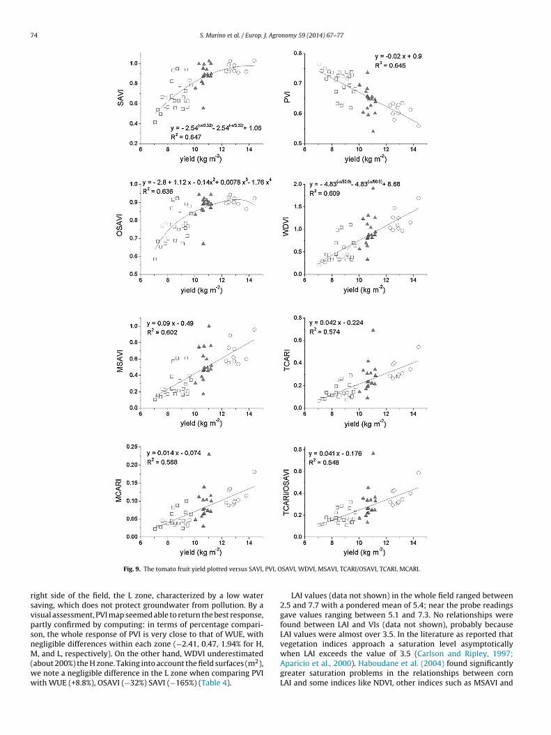
The curves, which overlapped each other in the visible range, dif-fered markedly from 725 nm on; the peak value of L curve was 10%lower than the others. In fact as reported by Penuelas et al. (1997)plant reflectance is governed by leaf surface properties and internalstructure, as well as by the concentration and distribution of bio-chemical components, and thus remote analysis of reflected lightcan be used to assess both the biomass and the physiological statusof a plant. As a result of the differences in the curves, Vegetationindices collected before harvest, were calculated and georeferreddata of all VIs were correlated to the equivalent tomato yield val-ues collected at harvest. Eight VIs (Fig. 9), out of eighteen ones,showed significant regression curves (R2 0.568–0.647). The bestrelation was found by SAVI, PVI and OSAVI indices (R2 = 0.647, 0.645and 0.636 respectively), followed by WDVI and MSAVI indexes(R2 = 0.609 and 0.601 respectively); TCARI/OSAVI, TCARI and MCARIshowed an R2 ranged between 0.568 and 0.581. In Fig. 9 were alsoreported the three different cluster clusters selection zones com-puted by Kruskal–Wallis one-way analysis-of-variance, to evaluateall VIs. As reported in Table 5, PSRI did not discriminate amongthe three zones; three indexes (CL, WI and WI/NDVI) discriminatedamong zones with p value <0.05, while fourteen VIs showed differ-ences (p < 0.01) among cluster. The clusters were created on theyield basis and statistical tests was used to verify (a posteriori)

dependence conditioning of the different variables, compared tothe three clusters.

Fig. 10 shows four significative maps derived from the abovesaid indexes, which look like the WUE map: they all show, on the

Fig. 8. Spectral reflectance at vis-NIR Wavelength of tomato crop at High (H),Medium (M) and Low (L) yield fruit level.

74 S. Marino et al. / Europ. J. Agronomy 59 (2014) 67–77

PVI, O

rsvpsnM(ww

Fig. 9. The tomato fruit yield plotted versus SAVI,

ight side of the field, the L zone, characterized by a low wateraving, which does not protect groundwater from pollution. By aisual assessment, PVI map seemed able to return the best response,artly confirmed by computing: in terms of percentage compari-on, the whole response of PVI is very close to that of WUE, withegligible differences within each zone (−2.41, 0.47, 1.94% for H,

, and L, respectively). On the other hand, WDVI underestimated

about 200%) the H zone. Taking into account the field surfaces (m2),e note a negligible difference in the L zone when comparing PVIith WUE (+8.8%), OSAVI (−32%) SAVI (−165%) (Table 4).

SAVI, WDVI, MSAVI, TCARI/OSAVI, TCARI, MCARI.

LAI values (data not shown) in the whole field ranged between2.5 and 7.7 with a pondered mean of 5.4; near the probe readingsgave values ranging between 5.1 and 7.3. No relationships werefound between LAI and VIs (data not shown), probably becauseLAI values were almost over 3.5. In the literature as reported thatvegetation indices approach a saturation level asymptotically

when LAI exceeds the value of 3.5 (Carlson and Ripley, 1997;Aparicio et al., 2000). Haboudane et al. (2004) found significantlygreater saturation problems in the relationships between cornLAI and some indices like NDVI, other indices such as MSAVI and

S. Marino et al. / Europ. J. Agronomy 59 (2014) 67–77 75

Fig. 10. Spatial distribution of PVI, SAVI, WDVI and OSAVI indexes divided into H

Table 5Mean of 64 georeferenced yield data, WUE and VIs data, split into three differentzones: low (L), medium (M) and high (H) processed by Kruskal–Wallis one-wayanalysis of variance.

L M H Kruskal–Wallis KW (corr.ties)

WDVI 0.501 0.947 1.192 ** **

PVI 0.709 0.641 0.610 ** **

SAVI 0.674 0.895 0.957 ** **

SAVI2 10.42 12.82 13.92 ** **

MSAVI 0.271 0.537 0.675 ** **

OSAVI 0.769 0.89 0.906 ** **

TCARI 0.14 0.261 0.34 ** **

TCARI/OSAVI 0.177 0.29 0.375 ** **

MCARI 0.047 0.087 0.113 ** **

TSAVI 0.857 0.868 0.884 ** **

GNDVI 0.731 0.739 0.755 ** **

SIPI 0.872 0.823 0.894 ** **

PRI 0.032 0.035 0.042 ** **

CL 0.619 0.62 0.647 * *

NDVI 0.868 0.89 0.874 ** **

WI 1.208 1.223 1.229 * *

PSRI −0.092 −0.089 −0.088 n.s. n.s.WI/NDVI 1.394 1.375 1.407 * *

n

Scs

4

tsn

* Significant at the 0.05 probability level.** Significant at the 0.01 probability level..s., not significant.

AVI exhibited better performances, but they were still affected byhanges at moderate chlorophyll levels, and tended to noticeableaturation for high LAI levels.

. Conclusion

The irrigation system adopted, which was based on a soil mois-ure probe measuring tomato crop water consumption at differentoil depths along the crop cycle, proved to be effective from agro-omic and environmental point of view. The crop yield was superior

igh (H), Medium (M) and Low (L) zones, as modeled by ordinary kriging.

to Italian peak values. The depth of water applied was lower thanthose calculated with Hargraves’ formula and those derived fromthe literature data on irrigated tomato. The steady values of watercontent registered by the probe at 50 cm depth along whole cropcycle, pointed out no water leaching.

To characterize crop variability, the georeferenced data weresplit into three clusters with increasing productivity (Low, Medium,High), with the latter zone hosting the soil probe. The consequencewas an average WUE quite elevated (28 kg m−3); the WUE in theH zones was very high: 35.1 kg m−3. Even the less productive zone(Low, 20% of the total surface) showed an appreciable WUE value(23.1 kg m−3), well above the few data available in the literatureand the average.

Some vegetation indices (PVI, SAVI, WDVI, OSAVI) were signif-icantly related to tomato crop yield. PVI proved to be a useful toolfor (i) a better understanding of the different field productive areasand for (ii) the adoption of variable water rate application accordingto the different PVI values.

Acknowledgements

This research has been supported by PRIN 2008 (Spatial and tem-poral relationships between N2O emissions, NO3 leaching and yield inproduction and bioenergetic cropping system – research units Nitrateleaching and precision irrigation in tomato crop). Marino and Alvinowrote the paper.

References

Analytical Spectral Devices, Incorporated, 1995. FieldSpec FR User’s Guide, ManualRelease 2, Boulder, Colorado.

Aparicio, N., Viellegas, D., Casadesus, J., Araus, J.L., Royo, C., 2000. Spectral vegetationindices as non-destructive tools for determining durum wheat yield. Agron. J.92, 83–91.

7 J. Agro

A

B

B

B

B

B

B

B

C

C

C

C

C

C

D

D

D

DD

E

F

F

F

G

G

G

G

G

G

G

H

6 S. Marino et al. / Europ.

RSIA Regione Toscana, 2009. Azienda Agraria di Cesa, Arezzo, Prova confrontovarietale Pomodoro Industria - Risultati produttivi e qualitativi, from 2006 to2009.

aret, F., Guyot, G., 1991. Potential and limitations of vegetation indices for LAI andAPAR assessment. Remote Sens. Environ. 104, 88–95.

aret, F., Guyot, G., Major, D., 1989. TSAVI: a vegetation index which minimizes soilbrightness effects on LAI and APAR estimation. In: Proceedings of 12th CanadianSymposium on Remote Sensing and IGARSS’89, Canada, 10-14 July 1989, pp.1355–1358.

asso, B., Cammarano, D., Cafiero, G., Marino, S., Alvino, A., 2011. Cultivar discrimina-tion at different site elevations with remotely sensed vegetation indices. ItalianJ. Agron. 6, e1.

astianssen, W.G.M., Allen, R.G., Droogers, P., D’Urso, G., Steduto, P., 2007. Twenty-five years modeling irrigated and drained soils: state of the art. Agric. WaterManage. 92, 111–125.

atchelor, C., 1999. Improving water use efficiency as part of integrated catchmentmanagement. Agric. Water Manage. 40, 249–263.

ouwer, H., 2000. Integrated water management emerging issues and challenges.Agric. Water Manage. 45, 217–228.

rady, N.C., Weil, R.R., 2002. The Nature and Properties of Soils. Prentice Hall, UpperSaddle River, New Jersey, pp. 960.

arlson, T.N., Ripley, D.A., 1997. On the relation between NDVI, fractional vegetationcover, and leaf area index. Remote Sens. Environ. 62, 241–252.

eccato, P., Flasse, S., Tarantola, S., Jacquemoud, S., Gregoire, J.M., 2001. Detectingvegetation leaf water content using reflectance in the optical domain. RemoteSens. Environ. 77, 22–33.

etin, O., Uygan, D., 2008. The effect of drip line spacing, irrigation regimes andplanting geometries of tomato on yield, irrigation water use efficiency and netreturn. Agric. Water Manage. 95, 949–958.

levers, J.G.P.W., 1989. The application of a weighted infrared-red vegetation indexfor estimating leaf area index by correcting soil moisture. Remote Sens. Environ.29, 25–37.

onsoli, S., D’Urso, G., Toscano, A., 2006. Remote sensing to estimate ET-fluxes andthe performance of an irrigation district in southern Italy. Agric. Water Manage.81, 295–314.

osta, J.M., Ortuno, M.F., Chaves, M.M., 2007. Deficit irrigation as a strategy to savewater: physiology and potential application to horticulture. J. Integr. Plant Biol.49, 1421–1434.

’Agostino, R.B., Belanger, A., D’Agostino Jr., R.B., 1990. A suggestion for usingpowerful and informative tests of normality”. American Statistician 44 (4),316–321.

’Urso, G., Richter, K., Calera, A., Osann, M.A., Escadafal, R., Garatuza-Pajan, J., Hanich,L., Perdigão, A., Tapia, J.B., Vuolo, F., 2010. Earth Observation products for oper-ational irrigation management in the context of the PLEIADeS project. Agric.Water Manage. 98, 271–282.

aughtry, C.S.T., Walthall, C.L., Kim, M.S., Brown de Colstoun, E., McMurtrey III,J.E., 2000. Estimating corn leaf chlorophyll concentration from leaf and canopyreflectance. Remote Sens. Environ. 74, 229–285.

elhomme, J.P., 1978. Kriging in the hydrosciences. Adv. Water Resour. 1, 251–266.oorenbons, J., Pruitt, W.O., 1977. Guidelines for Predicting Crop Water Require-

ments. Irrigation and Drainage Paper 24. Food and Agriculture Organization ofUnited Nations, Rome, Italy, pp. 36–45.

lwadie, M.E., Pierce, F.J., Qi, J., 2005. Remote sensing of canopy dynamics and bio-physical variables estimation of corn in Michigan. Agron. J. 97, 99–105.

avati, F., Lovelli, S., Galgano, F., Miccolis, V., Di Tommaso, T., Candido, V., 2009.Processing tomato quality as affected by irrigation scheduling. Sci. Hort. 122,562–571.

ereres, E., Evans, R.G., 2006. Irrigation of fruit trees and vines. Irrigation Sci. 24,55–57.

ernández, A., Gómez, S., 2008. Solving non-uniqueness in agglomerative hierarchi-cal clustering using multidendrograms. J. Classification 25 (1), 43–65.

amon, J.A., Penuelas, J., Field, C.B., 1992. A narrow-waveband spectral index thattracks diurnal changes in photosynthetic efficiency. Remote Sens. Environ. 41,35–44.

amon, J.A., Field, C.B., Bilger, W., Bjorkman, O., Fredeen, A.L., Penuelas, J., 1990.Remote sensing of the xanthophyll cycle and chlorophyll fluorescence in sun-flower leaves and canopies. Oecologia 85, 1–7.

amon, J.A., Serrano, L., Surfus, J.S., 1997. The photochemical reflectance index:an optical indicator of photosynthetic radiation use efficiency across species,functional types, and nutrient level. Oecologia 112, 492–501.

ianquinto, G., Orsini, F., Fecondini, M., Mezzetti, M., Sambo, P., Bona, S., 2011.A methodological approach for defining spectral indices for assessing tomatonitrogen status and yield. Eur. J. Agron. 35, 135–143.

iorio, G., Stigliani, A.L., D’Ambrosio, C., 2007. Agronomic performance and trans-criptional analysis of carotenoid biosynthesis in fruits of transgenic HighCaroand control tomato lines under field conditions. Transgenic Res. February 16(1), 15–28.

itelson, A., Merzlyak, M.N., 1994. Spectral reflectance changes associated withautumn senescence of Aesculus hippocastanum L. and Acer platanoides L. leaves:spectral features and relation to chlorophyll estimation. J. Plant Physiol. 143,286–292.

itelson, A.A., Merzlyak, M.N., 1996. Signature analysis of leaf reflectance spectra:algorithm development for remote sensing of chlorophyll. J. Plant Physiol. 148,94–500.

aboudane, D., Miller, J.R., Pattey, E., Zarco-Tejada, P.J., Strachan, I.B., 2004. Hyper-spectral vegetation indices and novel algorithms for predicting green LAI of

nomy 59 (2014) 67–77

crop canopies: modeling and validation in the context of precision agriculture.Remote Sens. Environ. 90, 337–352.

Haboudane, D., Miller, J.R., Tremblay, N., Zarco-Tejada, P.J., Dextraze, L., 2002.Integrated narrow-band vegetation indices for prediction of crop chlorophyllcontent for application to precision agriculture. Remote Sens. Environ. 81,416–426.

Hair, J.F., Andrson, R.E., Tatham, R.L., Black, W.C., 1995. Multivariate Data Analysis.Prentice Hall, Englewoods Cliffs, New Jersey, pp. 745.

Hanson, B., May, D., 2004. Effect of subsurface drip irrigation on processing tomatoyield, water table depth, soil salinity, and profitability. Agric. Water Manage. 68,1–17.

Hargreaves, G.H., Samani, Z.A., 1982. Estimating potential evapotranspiration. J. Irrig.Drain. Engr., ASCE 108, 223–230.

Hargreaves, G.H., Samani, Z.A., 1985. Reference crop evapotranspiration from tem-perature. Trans. ASAE 1, 96–99.

Hoffman, G.J., Martin, D.L., 1993. Engineering systems to enhance irrigation perfor-mance. Irrigation Sci. 14, 53–63.

Huete, A.R., 1988. A soil-adjusted vegetation index (SAVI). Remote Sens. Environ. 25,295–309.

Huguenin, R.L., Jones, J.L., 1986. Intelligent information extraction from reflectancespectra: absorption band positions. J. Geophys. Res. 91, 9585–9598.

Ismail, S.M., Ozawa, K., Nur, A.K., 2008. Influence of single and multiple water appli-cation timings on yield and water use efficiency in tomato (var.First power).Agric. Water Manage. 95, 116–122.

Jackson, R.D., 1986. Remote sensing of biotic and abiotic plant stress. Ann. Rev.Phytopathol. 4, 289–297.

Jackson, R.D., Huete, A.H., 1991. Interpreting vegetation indices. Preventive Vet. Med.11, 185–200.

Jones, H.G., 2004. Irrigation scheduling: advantages and pitfalls of plant-based meth-ods. J. Exp. Bot. 55, 2427–2436.

Kim, M.S., Daughtry, C.S.T., Chappelle, E.W., McMurtrey III, J.E., Walthall, C.L., 1994.The use of high spectral resolution bands for estimating absorbed photosynthet-ically active radiation (Apar). In: Proceedings of the 6th Symposium on PhysicalMeasurements and Signatures in Remote Sensing, January 17–21, 1994, France,pp. 299–306.

Kirda, C., 2002. Deficit irrigation scheduling based on plant growth stages showingwater stress tolerance. Deficit irrigation practices. FAO Corp. Doc. Rep. 22, Rome,pp. 3–10.

Kirnak, H., Demirtas, M.N., 2006. Effects of different irrigation regimes and mulcheson yield and macronutrition levels of drip-irrigated cucumber under open fieldconditions. J. Plant Nutr. 29, 1675–1690.

Köksal, E.S., Kara, T., Apan, M., Üstün, H., Ilbeyi, A., 2008. Estimation of green beanyield, water deficiency and productivity using spectral indexes during the grow-ing season. Irrig. Drainage Syst. 22, 209–223.

Koller, M., Upadhyay, S.K., 2005. Prediction of processing tomato yield using a cropgrowth model and remotely sensed aerial image. Trans. ASAE 48, 2335.

Kruskal, W.H., Wallis, W.A., 1952. Use of ranks in one-criterion variance analysis. J.Am. Stat. Assoc. 47 (260), 583–621.

Leone, A.P., Escadafal, R., 2001b. Statistical analysis of soil colour and spectrora-diometric data for hyperspectral remote sensing of soil properties (examplein a southern Italy Mediterranean ecosystem). Int. J. Remote Sens. 12,2311–2328.

Leone, A.P., Menenti, M., Buondonno, A., Letizia, A., Maffei, C., Sorrentino, G., 2007. Afield experiment on spectrometry of crop response to soil salinity. Agric. WaterManage. 80 (12), 39–48.

Leone, A.P., Menenti, M., Sorrentino, G., 2001a. Reflectance spectroscopy to studycrop response to soil salinity. Italian J. Agron. 4 (2), 75–85.

Leone, A.P., Sommer, S., 2000. Multivariate analysis of laboratory spectra for theassessment of soil development and soil degradation in the southern Apennines(Italy). Remote Sens. Environ. 72 (3), 346–359.

Leone, A.P., Viscarra-Rossel, R., Amenta, P., Buondonno, A., 2012. Prediction of soilproperties with PLSR and vis-NIR spectroscopy: application to Mediterraneansoils from southern Italy. Curr. Anal. Chem. 8, 283–299.

Lilliefors, H., 1967. On the Kolmogorov–Smirnov test for normality with mean andvariance unknown. J. Am. Stat. Assoc. 62, 399–402.

Lovelli, S., Perniola, M., Ferrara, A., Di Tommaso, T., 2007. Yield response factorto water (Ky) and water use efficiency of Carthamus tinctorius L. and Solanummelongena L. Agric. Water Manage. 92, 73–80.

Ma, B.L., Morrison, M.J., Dwyer, L.M., 1996. Canopy light reflectance and fieldgreenness to assess nitrogen fertilization and yield of maize. Agron. J. 88,915–920.

Major, D.J., Baret, F., Guyot, G., 1990. A ratio vegetation index adjusted for soil bright-ness. Int. J. Remote Sens. 11, 727–740.

Malengreau, N., Muller, J.-P., Calas, G., 1994. Fe-speciation in kaolins: a diffusereflectance study. Clays Clay Miner. 42, 137–147.

Marino, S., Alvino, A., 2014. Proximal sensing and vegetation indices for site-specific evaluation on an irrigated crop tomato. Eur. J. Remote Sens. 47,271–283.

Marino, S., Basso, B., Leone, A.P., Alvino, A., 2013. Agronomic traits and vegetationindices of two onion hybrids. Sci. Hortic. 155, 56–64.

Matheron, G., 1965. Les variables regionalisees et leur estimation: une application

de la theorie de fonctions aleatoires aux sciences de la nature. Masson et Cie,Paris.

May, D.M., Gonzalerz, J., 1999. Major California processing tomato cultivars responddifferentially in yield and fruit quality to various levels of moisture stress. ActaHort. 487, 525–529.

J. Agro

M

M

M

O

PP

P

P

P

P

P

P

P

P

P

Q

S. Marino et al. / Europ.

erino, G.G., Jones, D., Stooksbury, D.E., Hubbard, K.G., 2001. Determination of semi-variogram models to krige hourly and daily solar irradiance in western Nebraska.J. Appl. Meteorol. 40, 1085–1094.

erzlyak, J.R., Gitelson, A.A., Chivkunova, O.B., Rakitin, V.Y., 1999. Non-destructiveoptical detection of pigment changes during leaf senescence and fruit ripening.Physiol. Plant. 106, 135–141.

IPAF, Ministero delle Politiche Agricole e Forestali, 2000. Metodi di Analisi Chimicadel Suolo. Franco Angeli.

breza, T.A., Pitts, D.J., McFgovern, R.J., Spreen, T.H., 1996. Deficit irrigation of microirrigated tomato affects yield, fruit quality and disease severity. J. Prod. Agric. 9,270–275.

ainter, D., Carren, P., 1978. What is irrigation efficiency? Soil Water 14, 15–22.arry, M.A.J., Flexas, J., Medrano, H., 2005. Prospects for crop production under

drought: research priorities and future directions. Ann. Appl. Biol. 147, 211–226.atanè, C., Tringali, S., Sortino, O., 2011. Effects of deficit irrigation on biomass,

yield, water productivity and fruit quality of processing tomato under semi-aridMediterranean climate conditions. Sci. Hort. 129, 590–596.

ayero, J.O., Tarkalson, D.D., Irmak, S., Davison, D., Petersen, J.L., 2009. Effect of timingof a deficit-irrigation allocation on corn evapotranspiration, yield, water useefficiency and dry mass. Agric. Water Manage. 96, 1387–1397.

enuelas, J., Baret, F., Filella, I., 1995. Semi-empirical indices to assesscarotenoids/chlorophyll-a ratio from leaf spectral reflectance. Photosynthetica31, 221–230.

enuelas, J., Filella, I., Briel, C., Serrano, L., Savé, R., 1993. The reflectance at the 950-970 nm region as an indicator of plant water status. Int. J. Remote Sens. 14,1887–1905.

enuelas, J., Pinol, J., Ogaya, R., Filella, I., 1997. Estimation of plant water concen-tration by the reflectance Water Index WI (R900/R970). Int. J. Remote Sens. 18,2869–2875.

ereira, L.S., Oweis, T., Zairi, A., 2002. Irrigation management under water scarcity.Agric. Water Manage. 57, 175–206.

inter Jr., P.J., Hatfield, J.L., Schepers, J.S., Barners, E.M., Moran, M.S., Daughtry, C.S.T.,2003. Remote sensing for crop management. Photog. Eng. Remote Sens. 69,647–664.

inter Jr., P.J., Jackson, R.D., Idso, S.B., Reginato, R.J., 1981. Multidate spectralreflectance as predictors of yield in water stressed wheat and barley. Int. J.Remote Sens. 2, 43–48.

ulupol, L.U., Behboudian, M.H., Fisher, K.J., 1996. Growth, yield and postharvestattributes of glasshouse tomatoes produced under deficit irrigation. Hort. Sci.31, 926–929.

i, J., Chehbouni, A., Huete, A.R., Kerr, Y.H., Sorooshian, S., 1994. A modified soiladjusted vegetation index. Remote Sens. Environ. 48, 119–126.

nomy 59 (2014) 67–77 77

Raine, S.R., Meyer, W.S., Rassam, D.W., Hutson, J.L., Cook, F.J., 2007. Soil–water andsolute movement under precision irrigation: knowledge gaps for managing sus-tainable root zones. Irrigation Sci. 26, 91–100.

Riahi, A., Hdider, C., Sanaa, M., Tarchoun, N., Ben Kheder, M., Guezal, I., 2009.Effect of conventional and organic production systems on the yield and qual-ity of field tomato cultivars grown in Tunisia. J. Sci. Food Agric. 89, 2275–2282.

Richardson, A.J., Wiegand, C.L., 1977. Distinguishing vegetation from soil backgroundinformation. Photogramm. Eng. Remote Sens. 43, 1541–1552.

Rondeaux, G., Steven, M., Baret, F., 1996. Optimization of soil-adjusted vegetationindices. Remote Sens. Environ. 55, 95–107.

Rouse, J.W., Haas Jr., R.H., Schell, J.A., Deering, D.W., 1974. Monitoring vegetationsystems in the Great Plains with ERTS. In: Proc. ERTS-1 Symp., 3rd, Greenbelt,MD, 1 09-317.

Savitzky, A., Golay, M.J.E., 1964. Smoothing and differentiation of data by simplifiedleast squares procedures. Anal. Chem. 36 (8), 1627–1639.

Selvaraja, S., Balasundram, S.K., Vadamalai, G., Husni, M.H.A., 2012. Spatial variabilityof orange spotting disease in oil palm. J. Biol. Sci. 12, 232–238.

Shapiro, S.S., Wilk, M.B., 1965. An analysis of variance test for normality (completesamples). Biometrika 52, 591–611.

Sherman, D.M., Waite, T.D., 1985. Electronic spectra of Fe3* oxides and oxide hydrox-ides in the near IR to near UV. Am. Mineralogist 70, 1262–1269.

Siviero, P., Sandei, L., Zanotti, G., 2000. Comparison of mid-late and late tomatohybrids. Informatore Agrario. 56, 49–51.

Stanghellini, C., Kempkes, F.L.K., Knies, P., 2003. Enhancing environmental qualityin agricultural systems. Acta Hort. 609, 277–283.

Tarantino, E., Onofri, M., 1991. Determinazione dei coefficienti colturali mediantelisimetri. Bonifica 8, 119–136.

Teal, R.K., Tubana, B., Girma, K., Freeman, K.W., Arnall, D.B., Walsh, O., Raun, W.R.,2006. In-season prediction of corn grain yield potential using normalized dif-ference vegetation index. Agric. J. 98, 1488–1494.

Topcu, S., Kirda, C., Dasgan, Y., Kaman, H., Cetin, M., Yazici, A., Bacon, M.A., 2007. Yieldresponse and N-fertiliser recovery of tomato grown under deficit irrigation. Eur.J. Agron. 26, 64–70.

Viets Jr., F.G., 1962. Fertilizer and the efficient use of water. Adv. Agron. 14, 223–264.

Ward Jr., J.H., 1963. Hierarchical grouping to optimize an objective function. J. Am.

Stat. Assoc. 58, 236–244.

Webster, R., Oliver, M.A., 2007. Geostatistics for Environmental Scientists, 2nd ed.John Wiley Sons Ltd., England, 315 p.

Wright, J., 2002. Irrigation Scheduling Checkbook Method. Communication and Edu-cational Technology Services. University of Minnesota, USA.