Sensors 2011, 11, 7095-7109; doi:10.3390/s110707095

sensors ISSN 1424-8220

www.mdpi.com/journal/sensors

Article

Mapping Wide Row Crops with Video Sequences Acquired

from a Tractor Moving at Treatment Speed

Nadir Sainz-Costa 1, Angela Ribeiro

1,*, Xavier P. Burgos-Artizzu

2, María Guijarro

3 and

Gonzalo Pajares 3

1 Centre for Automation and Robotics, CSIC-UPM, Arganda del Rey, 28500 Madrid, Spain;

E-Mail: nadir.sainz@car.upm-csic.es 2 Computation and Neural Systems, 136-93, California Institute of Technology, 1200 East California

Boulevard, Pasadena, CA 91125, USA; E-Mail: xpburgos@gmail.com 3 Department of Software Engineering and Artificial Intelligence, Faculty of Computer Science,

Complutense University, 28040 Madrid, Spain; E-Mails: mguijarro@fdi.ucm.es (M.G.);

pajares@fdi.ucm.es (G.P.)

* Author to whom correspondence should be addressed; E-Mail: angela.ribeiro@car.upm-csic.es;

Tel.: +34-91-871-1900 ext. 261; Fax: +34-91-871-5070.

Received: 6 April 2011; in revised form: 4 July 2011 / Accepted: 6 July 2011 /

Published: 11 July 2011

Abstract: This paper presents a mapping method for wide row crop fields. The resulting

map shows the crop rows and weeds present in the inter-row spacing. Because field videos

are acquired with a camera mounted on top of an agricultural vehicle, a method for image

sequence stabilization was needed and consequently designed and developed. The proposed

stabilization method uses the centers of some crop rows in the image sequence as features

to be tracked, which compensates for the lateral movement (sway) of the camera and

leaves the pitch unchanged. A region of interest is selected using the tracked features, and

an inverse perspective technique transforms the selected region into a bird’s-eye view that

is centered on the image and that enables map generation. The algorithm developed has

been tested on several video sequences of different fields recorded at different times and

under different lighting conditions, with good initial results. Indeed, lateral displacements

of up to 66% of the inter-row spacing were suppressed through the stabilization process,

and crop rows in the resulting maps appear straight.

OPEN ACCESS

Sensors 2011, 11

7096

Keywords: crop mapping; video stabilization; inverse perspective mapping; video

processing; precision agriculture

1. Introduction

Precision Agriculture aims to optimize field management and increase agricultural efficiency and

sustainability; that is, to reduce the operating costs and ecological footprint traditionally associated

with agriculture by matching resource application and agronomic practices with soil and crop

requirements.

For instance, most herbicides are usually applied uniformly in fields, but strong evidence suggests

that weeds occur in patches rather than in homogenous distributions within crop fields. Marshall et al.

investigated the presence of three different species of grass in arable fields and showed that between

24% and 80% of the sample area was free of grass weeds [1]. According to [2], an average of 30% of

the sample area for 12 fields (seven maize and five soybean fields) was free of broadleaf weeds, and

70% was free of grass weeds in the inter-row spacing where no herbicide was previously applied. In

these situations, accurate maps showing both weed location and density could have (and indeed have

had) numerous uses including monitoring the effectiveness of past or current weed management

strategies, understanding weed population dynamics and verifying model predictions. In particular,

they can be the data source for sprayers, which can determine their location using a GPS receiver and

apply treatments where data recommends it. These spatial information systems have the potential to

allow farmers to fine-tune the locations and rates of herbicide application, thereby achieving

sustainability and reducing treatment costs [3]. In [3,4] the authors report that by using site-specific

weed control, reductions of between 42% (soybean and maize) and 84% (maize) in the amount of

applied herbicide could be achieved, depending on the patchiness and weed pressure in the sample

fields. These herbicide savings translated into an average of 33 €/ha per year that would be available to

apply to the additional costs for sampling, data processing and precision spraying [5].

Two main approaches to the data-collection step exist: sampling from the air and from ground level.

Aerial imagery and satellite data lack the necessary spatial resolution, and their acquisition depends

heavily on weather conditions (e.g., lack of clouds and fog). In the mid-late’90 these aerial methods

fell in disuse due to the appearance of more advanced computers that permitted direct photo analysis,

though nowadays are experiencing a resurgence due to the use of hyper and multispectral cameras, that

facilitate and potentiate the reckoning of each species [6]. Still, these methods continue to show clear

disadvantages like their high economic costs and low resolution due to the height from which images

is taken, causing each pixel to represent more than a square meter of area.

At the ground level, data collection can be accomplished by sampling on foot or with mobile platforms.

Sampling on foot is a highly time-consuming task and requires a high number of skilled workers to

cover the large treatment areas and even doing so, only discrete data are obtained (using sampling

grids) [7]. Colliver et al. calculated the time needed to manually map the presence of wild oats in a

field as 3.75 h/ha [8]. Depending on the size of the sampling grid, the required time can vary between

Sensors 2011, 11

7097

4.36 h/ha for a 20 m × 20 m grid [9] and 2.5 h/ha using a 36 m × 50 m grid [10]. Thus, the cost of

manually mapping the weeds in a field would exceed the savings gained from the reduced herbicide use.

On the other hand, data gathering using a tractor or vehicle as a mobile platform requires only one

operator and enables continuous sampling. In continuous sampling, data are collected over the entire

sample area, whereas with discrete sampling, data are collected only from pre-defined points

throughout an area. Interpolation methods are then used to estimate the densities in the intervening

areas. Continuous data can provide a qualitative description of abundance (i.e., presence or absence, or

zero, low, medium, or high) rather than the quantitative plant counts usually generated from discrete

sampling [1]. Moreover, acquiring video from a mobile platform may become a good opportunity to

obtain accurate weed and crop maps, which is our objective in this paper, and also crop row location in

real time has often been an important goal in the autonomous guidance of agricultural vehicles [11],

which increments the advantages of the ground level approach.

Mounting cameras on top of tractors or mobile platforms presents problems because the roughness

of the terrain transfers to the camera mounting system and causes it to acquire images that are difficult

to process (even to the human eye). Image sequence stabilization is the process of removing (totally or

partially) the effects of this unwanted motion from an input video sequence. It is a key pre-processing

step in any serious application of computer vision, especially when images are acquired from a mobile

platform. Based on the particular roughness of the terrain, motion in Precision Agriculture video

sequences can include vibration, sway, roll and pitch.

The problem of image stabilization has been assessed by a number of researchers [12-18]. Different

techniques are used in the literature and are primarily based on sparse feature tracking; some of them

use Kalman filters to predict the motion of features from frame to frame [12]. The authors of [13] use

Kalman filters to estimate the camera velocity and acceleration vectors for each frame using linear

camera motion models. Both [14] and [15] estimate the optical flow field and compute the required

affine transformation using Laplacian pyramid images. In [16], the 3D motion of the camera is

computed by first calculating the image flow of a 2D planar region and then subtracting it from the

whole image flow, resulting in a rotationless optical flow. This rotationless image sequence is

considered to be stabilized for relevant purposes. In [17], almost vertical segments in the frames are

used to compute the transformation needed to make them real vertical lines and thus correct the

camera rotation. In [18] block motion vectors are used to estimate the motion between consecutive

frames. These methods attempt to compensate for all motion and are rather complex and

computationally demanding. Most of them use discrete features (i.e., corners or segments) and attempt

to keep these features fixed in relation to a reference frame. These solutions are not possible in our

case, where there are no permanent features or even a constant reference frame, because the portion of

the field recorded by the camera is constantly changing as the vehicle travels through it. In the context

of wide row crops (see Figure 1(b)), we can exploit some characteristics of the images, particularly the

fact that crop fields present an approximately constant pattern of evenly spaced parallel rows. In this

paper, we present a method to stabilize the sway and roll motion in crop field video sequences using

the crop rows as features and inverse perspective mapping to focus on a region of interest. This method

is implemented as a first step in the mapping of crop fields using OpenCV [19].

After stabilization, a map containing all vegetation cover (crop rows and weeds) was built. In this

map, crop rows are quite straight regardless of the camera movements that, without stabilization,

Sensors 2011, 11

7098

would make them appear as S-shaped lines. Generation of weed maps has been reported in the

literature. In [20], weeds are mapped automatically using three bi-spectral cameras mounted in front of

a prototype carrier vehicle. This is a rather expensive system due to the specialized cameras and the

dedicated mobile platform. The idea behind our proposal is to use a good quality domestic camera

mounted on top of an agricultural vehicle that is likely dedicated to some other field task and therefore

presents a more cost effective solution. Tian et al. developed a real-time precision spraying system that

releases herbicide only over weed patches based on the information gathered by two to four cameras

mounted in front of the sprayer. Instead of building a weed map, the system acts in real-time [3].

Although this presents certain advantages, we argue that the information contained in a map is a very

powerful tool because it can be used to measure the effectiveness of the treatments from season to

season, to extract global information about weed coverage in the field or to distribute tasks among a

robot fleet.

Unfortunately, none of these studies thus far have resulted in the commercialization of the

technologies developed. The major obstacles to commercialization concern the high computing and

economic costs involved, as well as the difficulties of correctly representing all of the possible

situations present in real and outdoor conditions [21].

2. Materials and Methods

2.1. Frame Segmentation Process

All frames used for presenting and testing our proposal have a 720 × 576 pixel resolution and were

taken with a commercial video camera (Sony DCR PC110E) that was placed directly on the roof of the

tractor, at a height of 2.15 m from the ground, with a 10° pitch angle [Figure 1(a)]. The images were

acquired during a treatment operation at an approximate speed of 6 km/h. In the crop images, our

interest focused on the central three rows because they are present in every frame (even when the

camera sways laterally) and they can be seen with moderate resolution. Closer to the upper corners of

the frame, the crop rows become difficult to distinguish from one another due to the perspective in the

image and the camera optics [as seen in Figure 1(b)]. To avoid these effects, the image was divided in

half, and the upper half was discarded [Figure 1(c)].

Figure 1. (a) The emplacement of the video camera onboard the tractor; (b) The original

crop field image. Closer to the corners, crop rows become difficult to distinguish from one

another; (c) Half of the original image, where crop rows are clearly identifiable.

Sensors 2011, 11

7099

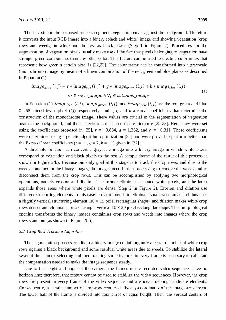
The first step in the proposed process segments vegetation cover against the background. Therefore

it converts the input RGB image into a binary (black and white) image and showing vegetation (crop

rows and weeds) in white and the rest as black pixels (Step 1 in Figure 2). Procedures for the

segmentation of vegetation pixels usually make use of the fact that pixels belonging to vegetation have

stronger green components than any other color. This feature can be used to create a color index that

represents how green a certain pixel is [22,23]. The color frame can be transformed into a grayscale

(monochrome) image by means of a linear combination of the red, green and blue planes as described

in Equation (1):

𝑖𝑚𝑎𝑔𝑒𝑔𝑟𝑎𝑦 𝑖, 𝑗 = 𝑟 ∗ 𝑖𝑚𝑎𝑔𝑒𝑟𝑒𝑑 𝑖, 𝑗 + 𝑔 ∗ 𝑖𝑚𝑎𝑔𝑒𝑔𝑟𝑒𝑒𝑛 𝑖, 𝑗 + 𝑏 ∗ 𝑖𝑚𝑎𝑔𝑒𝑏𝑙𝑢𝑒 𝑖, 𝑗

∀𝑖 ∈ 𝑟𝑜𝑤𝑠_𝑖𝑚𝑎𝑔𝑒 ∧ ∀𝑗 ∈ 𝑐𝑜𝑙𝑢𝑚𝑛𝑠_𝑖𝑚𝑎𝑔𝑒 (1)

In Equation (1), 𝑖𝑚𝑎𝑔𝑒𝑟𝑒𝑑 (𝑖, 𝑗), 𝑖𝑚𝑎𝑔𝑒𝑔𝑟𝑒𝑒𝑛 (𝑖, 𝑗), and 𝑖𝑚𝑎𝑔𝑒𝑏𝑙𝑢𝑒 (𝑖, 𝑗) are the red, green and blue

0–255 intensities at pixel (i,j) respectively, and r, g and b are real coefficients that determine the

construction of the monochrome image. These values are crucial in the segmentation of vegetation

against the background, and their selection is discussed in the literature [22-25]. Here, they were set

using the coefficients proposed in [25], r = −0.884, g = 1.262, and b = −0.311. These coefficients

were determined using a genetic algorithm optimization [24] and were proved to perform better than

the Excess Green coefficients (r = −1, g = 2, b = −1) given in [22].

A threshold function can convert a grayscale image into a binary image in which white pixels

correspond to vegetation and black pixels to the rest. A sample frame of the result of this process is

shown in Figure 2(b). Because our only goal at this stage is to track the crop rows, and due to the

weeds contained in the binary images, the images need further processing to remove the weeds and to

disconnect them from the crop rows. This can be accomplished by applying two morphological

operations, namely erosion and dilation. The former eliminates isolated white pixels, and the latter

expands those areas where white pixels are dense (Step 2 in Figure 2). Erosion and dilation use

different structuring elements in this case: erosion intends to eliminate small weed areas and thus uses

a slightly vertical structuring element (10 × 15 pixel rectangular shape), and dilation makes white crop

rows denser and eliminates breaks using a vertical 10 × 20 pixel rectangular shape. This morphological

opening transforms the binary images containing crop rows and weeds into images where the crop

rows stand out [as shown in Figure 2(c)].

2.2. Crop Row Tracking Algorithm

The segmentation process results in a binary image containing only a certain number of white crop

rows against a black background and some residual white areas due to weeds. To stabilize the lateral

sway of the camera, selecting and then tracking some features in every frame is necessary to calculate

the compensation needed to make the image sequence steady.

Due to the height and angle of the camera, the frames in the recorded video sequences have no

horizon line; therefore, that feature cannot be used to stabilize the video sequences. However, the crop

rows are present in every frame of the video sequence and are ideal tracking candidate elements.

Consequently, a certain number of crop-row centers at fixed y-coordinates of the image are chosen.

The lower half of the frame is divided into four strips of equal height. Then, the vertical centers of

Sensors 2011, 11

7100

those strips are selected as the y-coordinates of the points to be tracked. The x-coordinates of these

points are calculated as the average horizontal centers of the crop rows in those strips.

We added all pixel intensity values (0 or 255) for every column in every frame strip and divided

that total column value by the strip height. This yielded an average intensity for every column of the

strip that corresponds to a certain gray level. The darkness of this gray level indicates the vegetation

content of that column: darker columns indicate lower vegetation content, and lighter ones indicate

higher vegetation content. Because we need to separate the crop rows (highest vegetation content,

close to 100 %) from the rest (weeds and soil with little or no vegetation presence), it seems adequate

to apply a threshold on the resulting image (Step 3 in Figure 2). This generates a binary image in

which the widest white blocks correspond to the crop rows and the narrower ones (if any) correspond

to weed patches that seldom extend over any appreciable vertical distance [Figure 2(d)].

The algorithm uses these wide or narrow characteristics of the white blocks to classify them as crop

rows or weeds and then extracts the x-coordinates from the centers of the three central wide blocks,

which correspond to crop rows (Step 4 in Figure 2). In the first frame, the algorithm searches for these

centers in a window around some known positions (the horizontal center of the image ± the

approximated row distance in the image of 140 pixels) and stores them in an array. These centers are

distributed over the three central rows of crops [as shown in Figure 2(e)]. Line equations (slope and

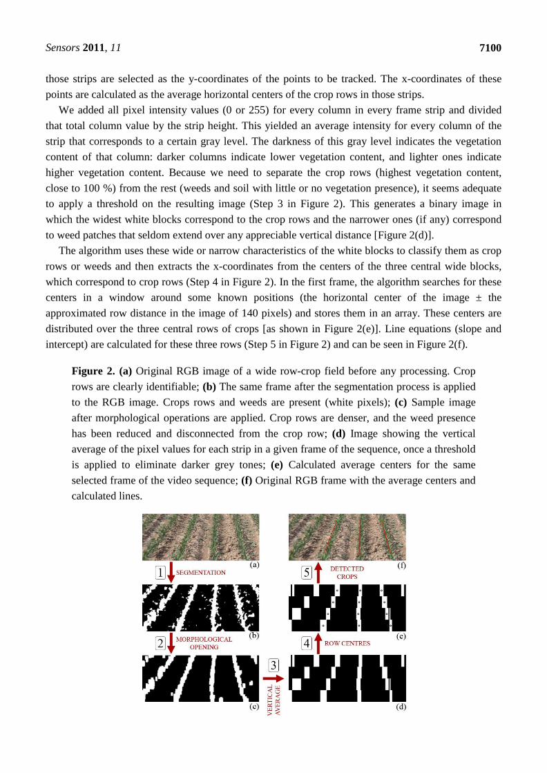
intercept) are calculated for these three rows (Step 5 in Figure 2) and can be seen in Figure 2(f).

Figure 2. (a) Original RGB image of a wide row-crop field before any processing. Crop

rows are clearly identifiable; (b) The same frame after the segmentation process is applied

to the RGB image. Crops rows and weeds are present (white pixels); (c) Sample image

after morphological operations are applied. Crop rows are denser, and the weed presence

has been reduced and disconnected from the crop row; (d) Image showing the vertical

average of the pixel values for each strip in a given frame of the sequence, once a threshold

is applied to eliminate darker grey tones; (e) Calculated average centers for the same

selected frame of the video sequence; (f) Original RGB frame with the average centers and

calculated lines.

Sensors 2011, 11

7101

The straightforward feature tracking mechanism stores the crop-row centers in an array after the

first frame calculations. A new frame is then processed similarly but using the stored centers from the

previous frame as the origins around which the system searches for new crop-row centers. This enables

the algorithm to search for a given center only in a window of a certain width around the last known

position of that same center. Furthermore the system can find the centers of the same crop rows in

every frame even if they move laterally from frame to frame. To a certain extent, abrupt feature

displacements from one frame to the next may disable the algorithm from finding the same feature in

subsequent frames. However, frame to frame displacements are generally small, given that video

sequences recording at 25 fps (or 40 ms per frame) generate them.

2.3. Inverse Perspective Mapping

The images taken with cameras are 2D projections of the 3D world, and the recovery of 3D

information such as depth, length or area requires a model of the projection transformation. The correct

model for human vision and cameras is the central projective model (or perspective). Images formed

under this model disable the calculation of distance measurements because perspective is a non-linear

transformation. Light rays passing through one unique point (the focal point) form the projected

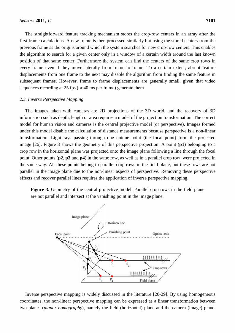
image [26]. Figure 3 shows the geometry of this perspective projection. A point (p1) belonging to a

crop row in the horizontal plane was projected onto the image plane following a line through the focal

point. Other points (p2, p3 and p4) in the same row, as well as in a parallel crop row, were projected in

the same way. All these points belong to parallel crop rows in the field plane, but these rows are not

parallel in the image plane due to the non-linear aspects of perspective. Removing these perspective

effects and recover parallel lines requires the application of inverse perspective mapping.

Figure 3. Geometry of the central projective model. Parallel crop rows in the field plane

are not parallel and intersect at the vanishing point in the image plane.

Inverse perspective mapping is widely discussed in the literature [26-29]. By using homogeneous

coordinates, the non-linear perspective mapping can be expressed as a linear transformation between

two planes (planar homography), namely the field (horizontal) plane and the camera (image) plane.

Sensors 2011, 11

7102

According to [27], a point (P) with homogeneous coordinates 𝒖 = (𝑢, 𝑣, 𝑤) in the field plane can be

projected into the image plane using Equation 2:

𝒖′ = 𝑠𝐻𝒖 (2)

where s is a scale factor, 𝒖′ are the homogeneous coordinates of the image point, 𝒖 are the coordinates

of that same point in the field plane and H is the 3 × 3 homography matrix. The determination of H

allows the computation of the projections of points from one plane to the other or even the

modification of the whole image for a bird’s-eye view of the scene. A common method in computer

vision based on point correspondences calculates this homography matrix. We define correspondences

as sets of n pairs of points (𝒖𝒊,𝒖′𝒊) such that a point (𝒖𝒊 ) in the field plane corresponds to 𝒖𝒊′ in the

image plane. The following homogeneous system of linear equations requires a solution for H and the

scale factors si (Equation 3):

𝑠𝑖𝒖′𝒊 = 𝐻𝒖𝒊, 𝑖 = 1, … , 𝑛 (3)

The system has 𝑛(𝑑 + 1) equations and 𝑛 + 𝑑 + 1 2 − 1 unknowns. H can be determined up to an

overall scale factor by using 𝑛 = 𝑑 + 2 point correspondences as long as no more than d of them are

collinear. For 2D planar images, this means that four point correspondences are needed, of which no

more than two are collinear.

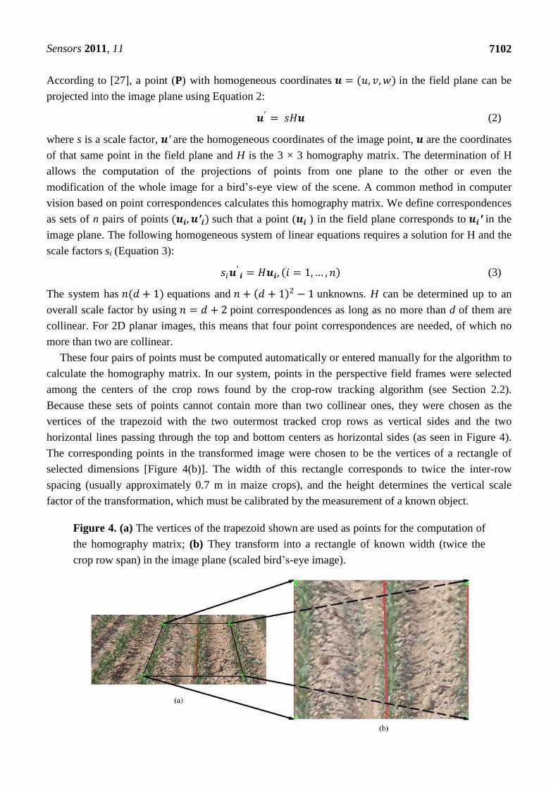
These four pairs of points must be computed automatically or entered manually for the algorithm to

calculate the homography matrix. In our system, points in the perspective field frames were selected

among the centers of the crop rows found by the crop-row tracking algorithm (see Section 2.2).

Because these sets of points cannot contain more than two collinear ones, they were chosen as the

vertices of the trapezoid with the two outermost tracked crop rows as vertical sides and the two

horizontal lines passing through the top and bottom centers as horizontal sides (as seen in Figure 4).

The corresponding points in the transformed image were chosen to be the vertices of a rectangle of

selected dimensions [Figure 4(b)]. The width of this rectangle corresponds to twice the inter-row

spacing (usually approximately 0.7 m in maize crops), and the height determines the vertical scale

factor of the transformation, which must be calibrated by the measurement of a known object.

Figure 4. (a) The vertices of the trapezoid shown are used as points for the computation of

the homography matrix; (b) They transform into a rectangle of known width (twice the

crop row span) in the image plane (scaled bird’s-eye image).

Sensors 2011, 11

7103

After computing the homography matrix, warping the whole image by applying the inverse

perspective mapping to each pixel produces a planar crop field image (or a bird’s-eye view) in which

parallel rows remain parallel and, once calibrated, distances can be measured.

2.4. Map Generation

Because our work aims to build a map of the crop field using recorded video sequences, we need to

integrate the information contained in each segmented bird’s-eye frame into a complete map of the

entire field length. This map consists of a matrix of specific dimensions, with each of its elements

corresponding to a cell of a given size in the real field. Moreover we must select an adequate scale

factor depending on the precision and field size needed. The values of the matrix elements are

determined by how many times weeds are found in the cell that the element represents. Higher values

correspond to those cells where weeds were found in a larger number of frames. When a white pixel is

found in the segmented frame, the matrix element corresponding to that field location (cell) is

increased by one unit. Because the vehicle on top of which the camera is mounted moves forward,

each new frame covers a slightly different field area, and the map’s frame of reference must be

updated. The distance in pixels that the reference moves between frames depends on the speed of the

vehicle, and (due to working with recorded sequences) this has been estimated using the characteristic

speed of 6 km/h (1.667 m/s). Once a particular field area has been mapped, the map contains different

values (ranging from zero to some certain maximum) that each refer to the number of frames

containing vegetation cover (weeds and crops) in the corresponding field cell. In this manner, a higher

number implies a higher level of certainty that the corresponding field cell contains vegetation.

After mapping, the matrix can be converted into a grayscale image in which higher values are

lighter (white) colors and darker grey or black pixels represent lower values. Applying a threshold here

retains only those cells in the map in which vegetation definitely occurs. To select an adequate value

for this threshold, we analyzed the map matrix for the video sequence tested. Typical values for the

matrix elements (the number of frames where weeds were present in a particular cell) ranged from

0 (no weeds in that area in any frame) to 17. To eliminate false weeds in the map due to segmentation

errors in some particular frames, we selected a threshold corresponding to approximately 25% of the

maximum value. Thus, any value below 4 in the map matrix was not considered in the final map. This

graphical representation offers a quick view of the complete length of the field covered by the map

represented in the matrix.

3. Results and Discussion

As previously stated, the algorithm was tested with different video sequences recorded from an

autonomous tractor in an actual spraying operation (at speeds of approximately 6 km/h or 1.667 m/s).

Its general performance was satisfactory, and crop rows were successfully detected and tracked for

most frames in the sequences. The videos were also stabilized. Some detection errors were present due

to the misidentification of weeds and crops in areas in which one of the crop rows thinned down and

weeds became the major green zone, but these cases occurred in less than 7% of the frames.

As a measure of the importance of video-sequence stabilization, we measured the distance between

the image horizontal center and the calculated position of the central crop row in the lower part of each

Sensors 2011, 11

7104

frame (y = 215 pixels) for one of the sequences in which unwanted motion was more evident. In this

area, the central crop row of a stabilized sequence should remain close to the horizontal center of the

frame (even in the context of perspective). However, the measured deviations usually vary from

26 pixels to the left of the center to 93 pixels to the right (as shown in Table 1).

Table 1. Distances between the central crop row and the real center of the image on the

horizontal axis for 306 frames.

Variable Value in pixels

Distance average 20

Standard deviation 28.5

Maximum distance to the right 93

Maximum distance to the left 26

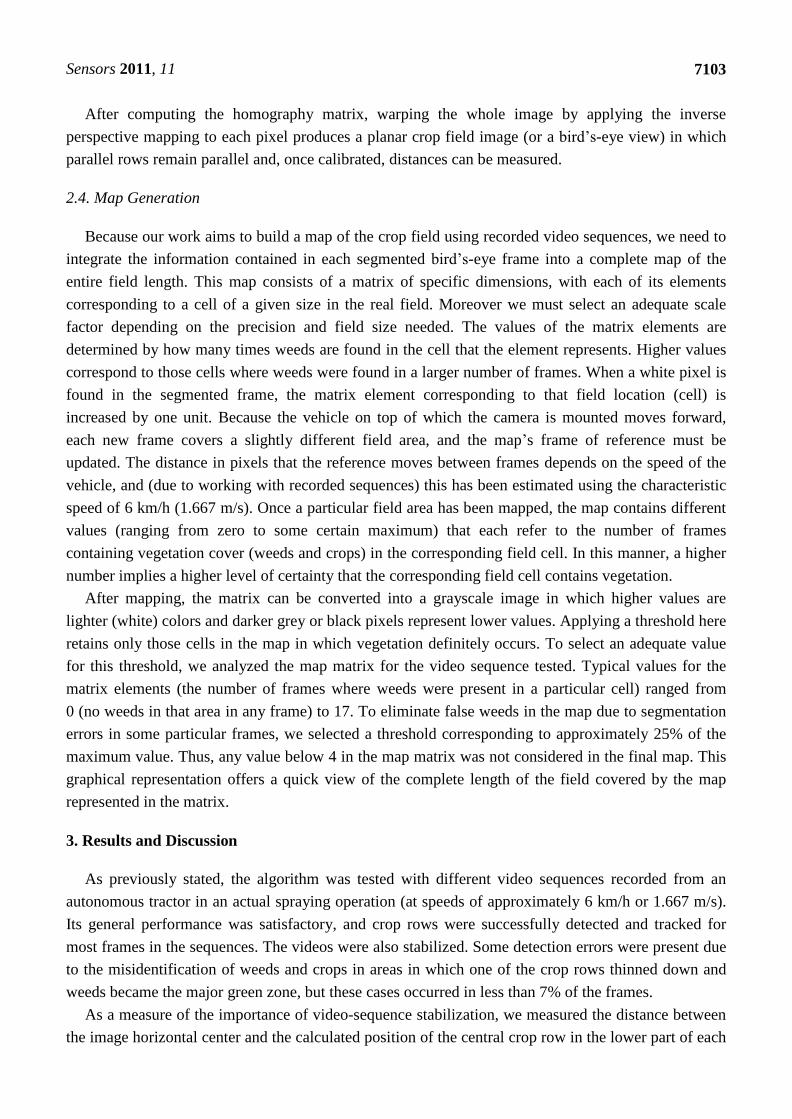
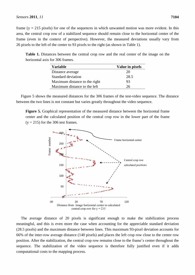
Figure 5 shows the measured distances for the 306 frames of the test-video sequence. The distance

between the two lines is not constant but varies greatly throughout the video sequence.

Figure 5. Graphical representation of the measured distance between the horizontal frame

center and the calculated position of the central crop row in the lower part of the frame

(y = 215) for the 306 test frames.

The average distance of 20 pixels is significant enough to make the stabilization process

meaningful, and this is even more the case when accounting for the appreciable standard deviation

(28.5 pixels) and the maximum distance between lines. This maximum 93-pixel deviation accounts for

66% of the inter-row average distance (140 pixels) and places the left crop row close to the center row

position. After the stabilization, the central crop row remains close to the frame’s center throughout the

sequence. The stabilization of the video sequence is therefore fully justified even if it adds

computational costs to the mapping process.

Sensors 2011, 11

7105

Figures 6 and 7 show the maps made before and after the stabilization process for two test video

sequences that were recorded at different times of day and in different fields. Figure 6 corresponds to a

crop field with low weed cover that was recorded on a partly cloudy day over rough terrain; these

conditions contribute to the noticeable crop-row twisting along the moving direction. A tracking error

occurred in this first sequence around the middle of the crop field. In this area, the plant density in the

left crop row is reduced due to sowing errors, and some isolated weed patches were misidentified as

the real crop row, causing the tracking error.

Figure 6. (a) Grayscale image of the generated field map for a video sequence without

stabilization. The crop rows meander along the moving direction; (b) After the stabilization

process, the crop rows remain straight despite the camera sway. The area where the left

row twists is due to a tracking error.

Figure 7. In this case, the sequence corresponds to a sunny day on a field with low weed

cover. (a) The grayscale image of the generated map for the video sequence without

stabilization depicts crop rows meandering slightly along the moving direction; (b) After

the stabilization process, the crop rows stay completely straight despite the slight sway of

the camera.

In Figure 7, the tested video sequence was taken on a smoother surface, and thus, the crop rows in

the unstabilized map present less twisting [Figure 7(a)]. The rows in the stabilized map are almost

completely straight [Figure 7(b)], and weed occurrences are lower than in the previous case.

Because the maps have a rather large horizontal scale factor (the maps correspond to either 18 or 20 m

of terrain), the presence of weeds cannot be seen without applying the proper resolution to the obtained

images. For example, Figure 8 shows a small portion of the whole field in the first test video in which

weeds were detected between the crop rows.

Sensors 2011, 11

7106

Figure 8. Crop area in the first video sequence in which weeds are present. Due to the

large scale of the maps, a more appropriate resolution is needed in order to detect the

occurrence of weeds.

4. Conclusions

Crop mapping is a crucial stage in the Precision Agriculture process. Accurate information is

needed to use autonomous vehicles that apply treatments in the field or that perform other agricultural

tasks. Fields must be mapped, and weeds must be precisely located. Given that the most adequate

information-gathering method currently consists of cameras mounted on autonomous vehicles, some

amount of instability and noise in the recorder images must be expected. To generate precise maps,

these disturbances should be addressed, and the stabilization process plays an important role in

this effort.

To compensate for camera motion and stabilize the sequence, many stabilization systems make use

of point features that are present and that maintain a stable position in all or most of the images in the

sequence. In crop fields, this problem remains important given the constant motion and slightly

downward tilt of the cameras (which eliminates the horizon line in every image) and due to the

absence of permanent features.

The crop-row detection and tracking algorithm presented here for video-sequence stabilization

works successfully for various fields and sequences. Crop rows were detected and tracked, and the

lateral camera sway and roll were removed by keeping a region of interest centered on the screen.

Trials were conducted for various sequences that were recorded in different fields at different times

and under different lighting conditions, with generally promising results. The distances between some

reference features, such as the central crop row and the horizontal center of the frame, remained

invariant once the video sequence was stabilized. Lateral displacements of up to 66% of the inter-row

spacing were suppressed.

As seen in the images, the generated maps give graphical proof of the importance of the

stabilization process. Unstabilized maps present zigzagging crop rows that differ significantly from the

real crop rows. Straight crops should remain straight despite the lateral sway of the camera (due to the

terrain roughness), and the generated stabilized maps depict this feature for all tested video sequences.

In areas where weed infestation was high and the inter-row space was covered with green weeds,

the stabilization algorithm had problems separating crops from weeds. The detection and tracking of

crop rows could also be improved to deal with isolated absences of plants in the rows (sowing errors)

Sensors 2011, 11

7107

to prevent the mischaracterization by the algorithm of the presence of weeds elsewhere in the images

as crop rows. This leads to incorrect crop-row center-line calculations and to stabilization errors as

well [as shown in the first map in Figure 6(b)]. However, from the test presented in this paper, we can

conclude that the algorithm is robust and that to affect its performance, gaps in the crop rows (sowing

errors) must be quite significant or must be coupled with appreciable camera sway.

A memory method could be developed to use the lines calculated in good frames as a reference or

prediction in the line calculation in frames with sowing errors or with high vegetation density. This

would reduce the weaknesses of the proposed approach. These modifications are high on our list of

future improvements that also includes suppressing vibrations by means of a mechanical compensating

device in the camera support.

Acknowledgements

The Spanish Ministry of Science and Innovation and the European Union have provided full and

continuing support for this research work through projects PLAN NACIONAL AGL2008-04670-C03-

02/AGR and the RHEA project, which is funded by the EU 7th Framework Programme under contract

number NMP2-LA-2010-245986.

References

1. Marshall, E.J.P. Field-scale estimates of grass weed populations in arable land. Weed Res. 1988,

28, 191-198.

2. Johnson, G.A.; Mortensen, D.A.; Martin, A.R. A simulation of herbicide use based on weed

spatial distribution. Weed Res. 1995, 35, 197-205.

3. Tian, L.; Reid, J.F.; Hummel, J.W. Development of a precision sprayer for site-specific weed

management. Trans. Am. Soc. Agr. Eng. 1999, 42, 893-900.

4. Medlin, C.R.; Shaw, D.R. Economic comparison of broadcast and site-specific herbicide

applications in nontransgenic and glyphosate-tolerant Glycine max. Weed Sci. 2000, 48, 653-661.

5. Timmermann, C.; Gerhards, R.; Kühbauch, W. The economic impact of site-specific weed

control. Precis. Agr. 2003, 4, 249-260.

6. López Granados, F.; Jurado-Expósito, M.; Atenciano Núez, S.; García-Ferrer, A.;

Sánchez de la Orden, M.; García-Torres, L. Spatial variability of agricultural soils in parameters

southern Spain. Plant Soil 2002, 246, 97-105

7. Rew L.J.; Cousens R.D. Spatial distribution of weeds in arable crops: Are current sampling and

analytical methods appropriate? Weed Res. 2001, 41, 1-18.

8. Colliver, C.T.; Maxwell B.D.; Tyler D.A.; Roberts D.W.; Long D.S. Georeferencing Wild Oat

(Avena fatua) Infestations in Small Grains (wheat and barley): Accuracy and Efficiency of Three

Weed Survey Techniques. In Proceedings 3rd International Conference on Precision Agriculture;

Roberts, P.C., Rust, R.H., Larson, W.E., Eds.; Minneapolis, MN, USA, 23–26 June 1996;

pp. 453-463.

9. Murphy, D.P.L.; Oestergaard, H.; Schnug, E. Lokales Ressourcen Management-Ergebnisse Und

Ausblick (Local Resources Management–Results and Outlook); ATB/KTBL-Kolloquium Technik

für Kleinräumige Bewirtschaftung: Potsdam-Borhim, Germany, 1994; pp. 90-101.

Sensors 2011, 11

7108

10. Schwartz, J.; Wartenberg, G. Wirtschaftlichkeit der teilflächenspecifischen Herbizidanwendung

(Economic benefit of site-specific weed control). Landtechnik 1999, 54, 334-335.

11. Billingsley, J.; Schoenfisch, M. The successful development of a vision guidance system for

agriculture. Comput. Electron. Agr. 1997, 16, 147-163.

12. Censi, A.; Fusiello, A.; Roberto, V. Image Stabilization by Features Tracking. In Proceedings of

the International Conference on Image Analysis and Processing, Venice, Italy, 27–29 Sepember

1999; pp. 665-670.

13. Ertürk, S. Real-time digital image stabilization using Kalman filters. Real-Time Imag. 2002, 8,

317-328.

14. Morimoto, C.; Chellappa, R. fast electronic digital image stabilization for off-road navigation.

Real-Time Imag. 1996, 2, 285-296.

15. Hansen, P.; Anandan, P.; Dana, K.; VanDer Wal, G.; Burt, P. Real-Time Scene Stabilization and

Mosaic Construction. In Proceedings of the Second IEEE Workshop on Applications of Computer

Vision, Sarasota, FL , USA, 5–7 December 1994; pp. 54-62.

16. Irani, M.; Rousso, B.; Peleg, S. Recovery of Ego-Motion Using Image Stabilization. In

Proceedings of the 1994 IEEE Computer Society Conference on Computer Vision and Pattern

Recognition, Seattle, WA, USA, 21–23 June 1994; pp. 454-460.

17. Viéville, T.; Clergue, E.; Dos Santos Facao, P.E. Computation of ego motion using the vertical

cue. Mach. Vis. Appl. 1995, 8, 41-56.

18. Vella, F.; Castorina, A.; Mancuso, M.; Messina, G. Digital image stabilization by adaptive Block

Motion Vectors filtering. IEEE Trans. Consum. Electron. 2002, 48, 796-801.

19. Bradsky, G.; Kaehler, A. Learning OpenCV, 1st ed.; O’Reilly Media Inc.: Sebastopol, CA, USA,

2008.

20. Gerhards, R.; Oebel, H. Practical experiences with a system for site-specific weed control in

arable crops using real-time image analysis and GPS-controlled patch spraying. Weed Res. 2006,

46, 185-193.

21. Slaughter, D.C.; Giles, D.K.; Downey, D. Autonomous robotic weed control systems: A review.

Comput. Electron. Agr. 2008, 61, 63-78.

22. Woebbecke, D.; Meyer, G.; Vonbargen, K.; Mortensen, D. Colour indices for weed identification

under various soil, residue and lighting conditions. Trans. Am. Soc. Agr. Eng. 1995, 38, 271-281.

23. Ribeiro, A.; Fernández-Quintanilla, C.; Barroso, J.; García-Alegre, M.C. Development of an

Image Analysis System for Estimation of Weed. In Proceedings of the Fifth European

Conference on Precision Agriculture, Uppsala, Sweden, 9–12 June 2005; pp. 169-174.

24. Burgos-Artizzu, X.P.; Ribeiro, A.; Tellaeche, A.; Pajares, G.; Fernandez-Qunitanilla, C. Analysis

of natural images processing for the extraction of agricultural elements. Image Vis. Comput. 2010,

28, 138-149.

25. Burgos-Artizzu, X.P.; Ribeiro, A.; Guijarro, M.; Pajares, G. Real-time image processing for

crop/weed discrimination in maize fields. Comput. Electron. Agr. 2011, 75, 337-346.

26. Sonka, M.; Glavac, V.; Boyle, R. Image Processing, Analysis, and Machine Vision, 3rd ed.;

Thomson Learning: Toronto, ON, Canada, 2008; pp. 553-565.

27. Barnard, S.T. Interpreting perspective images. Artif. Intell. 1983, 21, 435-462.

Sensors 2011, 11

7109

28. Mallot, H.A.; Bülthoff, H.H.; Little, J.J.; Bohrer, S. Inverse perspective mapping simplifies

optical flow computation and obstacle detection. Biol. Cybern. 1991, 64, 177-185.

29. Bevilacqua, A.; Gherardi, A.; Carozza, L. Automatic Perspective Camera Calibration Based on an

Incomplete Set of Chessboard Markers. In Proceedings of the Sixth Indian Conference on

Computer Vision, Graphics & Image Processing, ICVGIP’08, Bhubaneswar, India,

16–19 December 2008; pp. 126-133.

© 2011 by the authors; licensee MDPI, Basel, Switzerland. This article is an open access article

distributed under the terms and conditions of the Creative Commons Attribution license

(http://creativecommons.org/licenses/by/3.0/).