Manipulação e Visualização de Dados - a abordagem tidyverse

Manipulação e Visualização de Dadosa abordagem tidyverse

Prof. Walmes [email protected]

Laboratório de Estatística e GeoinformaçãoDepartamento de Estatística

Universidade Federal do Paraná

Walmes Zeviani · UFPR Manipulação e Visualização de Dados 1

http://leg.ufpr.br/~walmes

mailto:[email protected]

Motivação


Manipulação e visualização de dados

I Manipular e visualizar dados são tarefas obrigatórias emData Science (DS).

I O conhecimento sobre dados determina o sucesso das etapasseguintes.

I Fazer isso de forma eficiente requer:I Conhecer o processo e suas etapas.I Dominar a tecnologia para isso.

I Existem inúmeros softwares voltados para isso.I R se destaca em DS por ser free & open source, ter muitos

recursos e uma ampla comunidade.


O tempo gasto em DS

5%4%3%

9%

60%

19%

25

50

75

0/100 5%4%

10%3%

57%

21%

25

50

75

0/100

Tempo gasto Menos divertido

Atividade

1. Coletar dados

2. Limpar e organizar dados

3. Minerar de dados

4. Construir dados de treino

5. Refinar algorítmos

6. Outros

O que os cientistas de dados mais gastam tempofazendo e como gostam disso?

Figura 1. Tempo gasto e diversão em atividades. Fonte: Gil Press, 2016.


https://www.forbes.com/sites/gilpress/2016/03/23/data-preparation-most-time-consuming-least-enjoyable-data-science-task-survey-says

O ambiente R para manipulação de dados

I O R é a lingua franca da Estatística.I Desde o princípio oferece recursos para manipulação de

dados.I O data.frame é a estrutura base para dados tabulares.I base, utils, stats, reshape, etc com recursos para importar,

transformar, modificar, filtrar, agregar, data.frames.I Porém, existem “algumas imperfeições” ou espaço para

melhorias:I Coerções indesejadas de data.frame/matriz para vetor.I Ordem/nome irregular/inconsistente dos argumentos nas

funções.I Dependência de pacotes apenas em cascata.


A abordagem tidyverse


O tidyverse

I Oferece uma reimplementação e extensão dasfuncionalidades para manipulação e visualização.

I É uma coleção 8 de pacotes R que operam em harmonia.I Eles foram planejados e construídos para trabalhar em

conjunto.I Possuem gramática, organização, filosofia e estruturas de

dados mais clara.I Maior facilidade de desenvolvimento de código e

portabilidade.I Outros pacotes acoplam muito bem com o tidyverse.I Pacotes: https://www.tidyverse.org/packages/.I R4DS: https://r4ds.had.co.nz/.I Cookbook: https://rstudio-education.github.io/

tidyverse-cookbook/program.html.


https://www.tidyverse.org/packages/

https://r4ds.had.co.nz/

https://rstudio-education.github.io/tidyverse-cookbook/program.html

https://rstudio-education.github.io/tidyverse-cookbook/program.html

O que o tidyverse contém

library(tidyverse) 1ls("package:tidyverse") 2

## [1] "tidyverse_conflicts" "tidyverse_deps" "tidyverse_logo"## [4] "tidyverse_packages" "tidyverse_update"

tidyverse_packages() 1

## [1] "broom" "cli" "crayon" "dplyr"## [5] "dbplyr" "forcats" "ggplot2" "haven"## [9] "hms" "httr" "jsonlite" "lubridate"## [13] "magrittr" "modelr" "purrr" "readr"## [17] "readxl\n(>=" "reprex" "rlang" "rstudioapi"## [21] "rvest" "stringr" "tibble" "tidyr"## [25] "xml2" "tidyverse"


Os pacotes do tidyverse

Figura 2. Pacotes que fazer parte do tidyverse.


Mas na realidade

Figura 3. Em um universo pararelo.


A anatomia do tidyverse

tibble

I Uma reimplementação do data.frame com muitas melhorias.I Método print() enxuto.I Documentação: https://tibble.tidyverse.org/.

readr

I Leitura de dados tabulares: csv, tsv, fwf.I Recursos “inteligentes” que determinam tipo de variável.I Ex: importar campos de datas como datas!I Documentação: https://readr.tidyverse.org/.


https://tibble.tidyverse.org/

https://readr.tidyverse.org/


tidyr

I Suporte para criação de dados no formato tidy (tabular).I Cada variável está em uma coluna.I Cada observação (unidade amostral) é uma linha.I Cada valor é uma cédula.

I Documentação: https://tidyr.tidyverse.org/.

dplyr

I Oferece uma gramática extensa pra manipulação de dados.I Operações de split-apply-combine.I Na maior parte da manipulação é usado o dplyr.I Documentação: https://dplyr.tidyverse.org/.


https://tidyr.tidyverse.org/

https://dplyr.tidyverse.org/

A anatomia do tidyverseggplot2

I Criação de gráficos baseado no The Grammar of Graphics(WILKINSON et al., 2013).

I Claro mapeamento das variáveis do BD em variáveis visuais econstrução baseada em camadas.

I Documentação: https://ggplot2.tidyverse.org/.I WICKHAM (2016): ggplot2 - Elegant Graphics for Data

Analysis.I TEUTONICO (2015): ggplot2 Essentials.

forcats

I Para manipulação de variáveis categóricas/fatores.I Renomenar, reordenar, transformar, aglutinar.

I Documentação: https://forcats.tidyverse.org/.


https://ggplot2.tidyverse.org/

https://forcats.tidyverse.org/


stringr

I Recursos coesos construídos para manipulação de strings.I Feito sobre o stringi.I Documentação: https://stringr.tidyverse.org/.

purrr

I Recursos para programação funcional.I Funções que aplicam funções em lote varrendo objetos:

vetores, listas, etc.I Documentação: https://purrr.tidyverse.org/.


https://stringr.tidyverse.org/

https://purrr.tidyverse.org/

Harmonizam bem com o tidyverse

I magrittr: operadores pipe → %>%.I rvest: web scraping.I httr: requisições HTTP e afins.I xml2: manipulação de XML.I lubridate e hms: manipulação de dados cronológicos.


https://magrittr.tidyverse.org/

https://rvest.tidyverse.org/

https://cran.r-project.org/package=httr

https://cran.r-project.org/package=xml2

https://lubridate.tidyverse.org/

https://hms.tidyverse.org/

Estruturas de dados do tibble


Anatomia do tibble

I Aperfeiçoamento do data.frame.I A classe tibble.I Formas ágeis de criar tibbles.I Formas ágeis de modificar objetos das classes.I Método print mais enxuto e informativo.


# packageVersion("tibble") 1ls("package:tibble") 2

## [1] "add_case" "add_column"## [3] "add_row" "as_data_frame"## [5] "as_tibble" "as.tibble"## [7] "column_to_rownames" "data_frame"## [9] "data_frame_" "deframe"## [11] "enframe" "frame_data"## [13] "frame_matrix" "glimpse"## [15] "has_name" "has_rownames"## [17] "is_tibble" "is.tibble"## [19] "is_vector_s3" "knit_print.trunc_mat"## [21] "lst" "lst_"## [23] "new_tibble" "obj_sum"## [25] "remove_rownames" "repair_names"## [27] "rowid_to_column" "rownames_to_column"## [29] "set_tidy_names" "tbl_sum"## [31] "tibble" "tibble_"## [33] "tidy_names" "tribble"## [35] "trunc_mat" "type_sum"


Figura 4. Uso do tibble.


Leitura de dados com readr


Anatomia do readr

I Importação de dados no formato texto.I Funções de importação: read_*().I Funções de escrita: write_*().I Funções de parsing: parse_*.

I Conseguem identificar campos de data.I Muitas opções de controle de importação:

I Encoding.I Separador de campo e decimal.I Aspas, comentários, etc.

I Cartão de leitura com o readr e arrumação com o tidyr: https://rawgit.com/rstudio/cheatsheets/master/data-import.pdf.

I Exemplos do curso de leitura de dados com o readr:http://leg.ufpr.br/~walmes/cursoR/data-vis/99-datasets.html.


https://rawgit.com/rstudio/cheatsheets/master/data-import.pdf

https://rawgit.com/rstudio/cheatsheets/master/data-import.pdf

http://leg.ufpr.br/~walmes/cursoR/data-vis/99-datasets.html

# packageVersion("readr") 1ls("package:readr") %>% 2

str_subset("(read|parse|write)_") %>% 3sort() 4

## [1] "parse_character" "parse_date" "parse_datetime"## [4] "parse_double" "parse_factor" "parse_guess"## [7] "parse_integer" "parse_logical" "parse_number"## [10] "parse_time" "parse_vector" "read_csv"## [13] "read_csv2" "read_csv2_chunked" "read_csv_chunked"## [16] "read_delim" "read_delim_chunked" "read_file"## [19] "read_file_raw" "read_fwf" "read_lines"## [22] "read_lines_chunked" "read_lines_raw" "read_log"## [25] "read_rds" "read_table" "read_table2"## [28] "read_tsv" "read_tsv_chunked" "write_csv"## [31] "write_delim" "write_excel_csv" "write_file"## [34] "write_lines" "write_rds" "write_tsv"


read_*(file, col_names = TRUE, col_types = NULL, locale = default_locale(), na = c("", "NA"), quoted_na = TRUE, comment = "", trim_ws = TRUE, skip = 0, n_max = Inf, guess_max = min(1000, n_max), progress = interactive())

Try one of the following packages to import other types of files

• haven - SPSS, Stata, and SAS files • readxl - excel files (.xls and .xlsx) • DBI - databases • jsonlite - json • xml2 - XML • httr - Web APIs • rvest - HTML (Web Scraping)

Save Data

Data Import : : CHEAT SHEET Read Tabular Data - These functions share the common arguments: Data types

USEFUL ARGUMENTS

OTHER TYPES OF DATA

Comma delimited file write_csv(x, path, na = "NA", append = FALSE,

col_names = !append) File with arbitrary delimiter

write_delim(x, path, delim = " ", na = "NA", append = FALSE, col_names = !append)

CSV for excel write_excel_csv(x, path, na = "NA", append =

FALSE, col_names = !append) String to file

write_file(x, path, append = FALSE) String vector to file, one element per line

write_lines(x,path, na = "NA", append = FALSE) Object to RDS file

write_rds(x, path, compress = c("none", "gz", "bz2", "xz"), ...)

Tab delimited files write_tsv(x, path, na = "NA", append = FALSE,

col_names = !append)

Save x, an R object, to path, a file path, as:

Skip lines read_csv(f, skip = 1)

Read in a subset read_csv(f, n_max = 1)

Missing Values read_csv(f, na = c("1", "."))

Comma Delimited Files read_csv("file.csv")

To make file.csv run: write_file(x = "a,b,c\n1,2,3\n4,5,NA", path = "file.csv")

Semi-colon Delimited Files read_csv2("file2.csv")

write_file(x = "a;b;c\n1;2;3\n4;5;NA", path = "file2.csv")

Files with Any Delimiter read_delim("file.txt", delim = "|")

write_file(x = "a|b|c\n1|2|3\n4|5|NA", path = "file.txt")

Fixed Width Files read_fwf("file.fwf", col_positions = c(1, 3, 5))

write_file(x = "a b c\n1 2 3\n4 5 NA", path = "file.fwf")

Tab Delimited Files read_tsv("file.tsv") Also read_table().

write_file(x = "a\tb\tc\n1\t2\t3\n4\t5\tNA", path = "file.tsv")

a,b,c 1,2,3 4,5,NA

a;b;c 1;2;3 4;5;NA

a|b|c 1|2|3 4|5|NA

a b c 1 2 3 4 5 NA

A B C1 2 3

A B C1 2 34 5 NA

x y zA B C1 2 34 5 NA

A B CNA 2 34 5 NA

1 2 3

4 5 NA

A B C1 2 34 5 NA

A B C1 2 34 5 NA

A B C1 2 34 5 NA

A B C1 2 34 5 NA

a,b,c 1,2,3 4,5,NA

Example file write_file("a,b,c\n1,2,3\n4,5,NA","file.csv") f <- "file.csv"

No header read_csv(f, col_names = FALSE)

Provide header read_csv(f, col_names = c("x", "y", "z"))

Read a file into a single string read_file(file, locale = default_locale())

Read each line into its own string read_lines(file, skip = 0, n_max = -1L, na = character(),

locale = default_locale(), progress = interactive())

Read a file into a raw vector read_file_raw(file)

Read each line into a raw vector read_lines_raw(file, skip = 0, n_max = -1L,

progress = interactive())

Read Non-Tabular Data

Read Apache style log files read_log(file, col_names = FALSE, col_types = NULL, skip = 0, n_max = -1, progress = interactive())

## Parsed with column specification: ## cols( ## age = col_integer(), ## sex = col_character(), ## earn = col_double() ## )

1. Use problems() to diagnose problems. x <- read_csv("file.csv"); problems(x)

2. Use a col_ function to guide parsing. • col_guess() - the default • col_character() • col_double(), col_euro_double() • col_datetime(format = "") Also

col_date(format = ""), col_time(format = "") • col_factor(levels, ordered = FALSE) • col_integer() • col_logical() • col_number(), col_numeric() • col_skip() x <- read_csv("file.csv", col_types = cols( A = col_double(), B = col_logical(), C = col_factor()))

3. Else, read in as character vectors then parse with a parse_ function.

• parse_guess() • parse_character() • parse_datetime() Also parse_date() and

parse_time() • parse_double() • parse_factor() • parse_integer() • parse_logical() • parse_number() x$A <- parse_number(x$A)

readr functions guess the types of each column and convert types when appropriate (but will NOT convert strings to factors automatically).

A message shows the type of each column in the result.

earn is a double (numeric)sex is a

character

age is an integer

RStudio® is a trademark of RStudio, Inc. • CC BY SA RStudio • [email protected] • 844-448-1212 • rstudio.com • Learn more at tidyverse.org • readr 1.1.0 • tibble 1.2.12 • tidyr 0.6.0 • Updated: 2017-01

R’s tidyverse is built around tidy data stored in tibbles, which are enhanced data frames.

The front side of this sheet shows how to read text files into R with readr.

The reverse side shows how to create tibbles with tibble and to layout tidy data with tidyr.

Figura 5. Cartão de referência importação de dados com o readr.Walmes Zeviani · UFPR Manipulação e Visualização de Dados 23

Figura 6. Leitura com o readr.


Figura 7. Parsing de valores com readr.


Dados no formato tidy com tidyr


Anatomia do tidyr

I Para fazer arrumação dos dados.I Mudar a disposição dos dados: long wide.I Partir uma variável em vários campos.I Concatenar vários campos para criar uma variável.I Remover ou imputar os valores ausentes: NA.I Aninhar listas em tabelas: tribble.


# packageVersion("tidyr") 1ls("package:tidyr") 2

## [1] "%>%" "complete" "complete_"## [4] "crossing" "crossing_" "drop_na"## [7] "drop_na_" "expand" "expand_"## [10] "extract" "extract_" "extract_numeric"## [13] "fill" "fill_" "full_seq"## [16] "gather" "gather_" "nest"## [19] "nest_" "nesting" "nesting_"## [22] "population" "replace_na" "separate"## [25] "separate_" "separate_rows" "separate_rows_"## [28] "smiths" "spread" "spread_"## [31] "table1" "table2" "table3"## [34] "table4a" "table4b" "table5"## [37] "uncount" "unite" "unite_"## [40] "unnest" "unnest_" "who"


separate_rows(data, ..., sep = "[^[:alnum:].]+", convert = FALSE) Separate each cell in a column to make several rows. Also separate_rows_().

Handle Missing Values

Reshape Data - change the layout of values in a table

gather(data, key, value, ..., na.rm = FALSE, convert = FALSE, factor_key = FALSE) gather() moves column names into a key column, gathering the column values into a single value column.

spread(data, key, value, fill = NA, convert = FALSE, drop = TRUE, sep = NULL) spread() moves the unique values of a key column into the column names, spreading the values of a value column across the new columns.

Use gather() and spread() to reorganize the values of a table into a new layout.

gather(table4a, `1999`, `2000`, key = "year", value = "cases") spread(table2, type, count)

valuekey

table4acountry 1999 2000

A 0.7K 2KB 37K 80KC 212K 213K

country year casesA 1999 0.7KB 1999 37KC 1999 212KA 2000 2KB 2000 80KC 2000 213K

valuekey

country year cases popA 1999 0.7K 19MA 2000 2K 20MB 1999 37K 172MB 2000 80K 174MC 1999 212K 1TC 2000 213K 1T

table2country year type count

A 1999 cases 0.7KA 1999 pop 19MA 2000 cases 2KA 2000 pop 20MB 1999 cases 37KB 1999 pop 172MB 2000 cases 80KB 2000 pop 174MC 1999 cases 212KC 1999 pop 1TC 2000 cases 213KC 2000 pop 1T

unite(data, col, ..., sep = "_", remove = TRUE) Collapse cells across several columns to make a single column.

drop_na(data, ...) Drop rows containing NA’s in … columns.

fill(data, ..., .direction = c("down", "up")) Fill in NA’s in … columns with most recent non-NA values.

replace_na(data, replace = list(), ...) Replace NA’s by column.

Use these functions to split or combine cells into individual, isolated values.

country year rateA 1999 0.7K/19MA 2000 2K/20MB 1999 37K/172MB 2000 80K/174MC 1999 212K/1TC 2000 213K/1T

country year cases popA 1999 0.7K 19MA 2000 2K 20MB 1999 37K 172B 2000 80K 174C 1999 212K 1TC 2000 213K 1T

table3

separate(data, col, into, sep = "[^[:alnum:]]+", remove = TRUE, convert = FALSE, extra = "warn", fill = "warn", ...) Separate each cell in a column to make several columns.

country century yearAfghan 19 99Afghan 20 0Brazil 19 99Brazil 20 0China 19 99China 20 0

country yearAfghan 1999Afghan 2000Brazil 1999Brazil 2000China 1999China 2000

table5

separate(table3, rate, into = c("cases", "pop"))

separate_rows(table3, rate)

unite(table5, century, year, col = "year", sep = "")

x1 x2A 1B NAC NAD 3E NA

x1 x2A 1D 3

xx1 x2A 1B NAC NAD 3E NA

x1 x2A 1B 1C 1D 3E 3

xx1 x2A 1B NAC NAD 3E NA

x1 x2A 1B 2C 2D 3E 2

x

drop_na(x, x2) fill(x, x2) replace_na(x, list(x2 = 2))

country year rateA 1999 0.7KA 1999 19MA 2000 2KA 2000 20MB 1999 37KB 1999 172MB 2000 80KB 2000 174MC 1999 212KC 1999 1TC 2000 213KC 2000 1T

table3country year rate

A 1999 0.7K/19MA 2000 2K/20MB 1999 37K/172MB 2000 80K/174MC 1999 212K/1TC 2000 213K/1T

Tidy data is a way to organize tabular data. It provides a consistent data structure across packages.

CBAA * B -> C*A B C

Each observation, or case, is in its own row

A B C

Each variable is in its own column

A B C

&A table is tidy if: Tidy data:

Makes variables easy to access as vectors

Preserves cases during vectorized operations

complete(data, ..., fill = list()) Adds to the data missing combinations of the values of the variables listed in … complete(mtcars, cyl, gear, carb)

expand(data, ...) Create new tibble with all possible combinations of the values of the variables listed in … expand(mtcars, cyl, gear, carb)

The tibble package provides a new S3 class for storing tabular data, the tibble. Tibbles inherit the data frame class, but improve three behaviors:

• Subsetting - [ always returns a new tibble, [[ and $ always return a vector.

• No partial matching - You must use full column names when subsetting

• Display - When you print a tibble, R provides a concise view of the data that fits on one screen

RStudio® is a trademark of RStudio, Inc. • CC BY SA RStudio • [email protected] • 844-448-1212 • rstudio.com • Learn more at tidyverse.org • readr 1.1.0 • tibble 1.2.12 • tidyr 0.6.0 • Updated: 2017-01

Tibbles - an enhanced data frame Split Cells

• Control the default appearance with options: options(tibble.print_max = n,

tibble.print_min = m, tibble.width = Inf)

• View full data set with View() or glimpse() • Revert to data frame with as.data.frame()

data frame display

tibble display

tibble(…) Construct by columns. tibble(x = 1:3, y = c("a", "b", "c"))

tribble(…) Construct by rows. tribble( ~x, ~y, 1, "a", 2, "b", 3, "c")

A tibble: 3 × 2 x y <int> <chr> 1 1 a 2 2 b 3 3 c

Both make this

tibble

ww

# A tibble: 234 × 6 manufacturer model displ <chr> <chr> <dbl> 1 audi a4 1.8 2 audi a4 1.8 3 audi a4 2.0 4 audi a4 2.0 5 audi a4 2.8 6 audi a4 2.8 7 audi a4 3.1 8 audi a4 quattro 1.8 9 audi a4 quattro 1.8 10 audi a4 quattro 2.0 # ... with 224 more rows, and 3 # more variables: year <int>, # cyl <int>, trans <chr>

156 1999 6 auto(l4) 157 1999 6 auto(l4) 158 2008 6 auto(l4) 159 2008 8 auto(s4) 160 1999 4 manual(m5) 161 1999 4 auto(l4) 162 2008 4 manual(m5) 163 2008 4 manual(m5) 164 2008 4 auto(l4) 165 2008 4 auto(l4) 166 1999 4 auto(l4) [ reached getOption("max.print") -- omitted 68 rows ]A large table

to display

as_tibble(x, …) Convert data frame to tibble.

enframe(x, name = "name", value = "value") Convert named vector to a tibble

is_tibble(x) Test whether x is a tibble.

CONSTRUCT A TIBBLE IN TWO WAYS

Expand Tables - quickly create tables with combinations of values

Tidy Data with tidyr

Figura 8. Cartão de referência arrumação de dados com tidyr.Walmes Zeviani · UFPR Manipulação e Visualização de Dados 29

Figura 9. A definição de tidy data ou formato tabular.


Figura 10. Modificação da disposição dos dados com o tidyr.


Figura 11. Recursos para lidar com dados ausentes do tidyr.


Figura 12. Partir e concatenar valores com tidyr.


Agregação com dplyr


Anatomia do dplyr

I O dplyr é a gramática para manipulação de dados.I Tem um conjunto consistente de verbos para atuar sobre

tabelas.I Verbos: mutate(), select(), filter(), arrange(),

summarise(), slice(), rename(), etc.I Sufixos: _at(), _if(), _all(), etc.I Agrupamento: group_by() e ungroup().I Junções: inner_join(), full_join(), left_join() e

right_join().I Funções resumo: n(), n_distinct(), first(), last(), nth(),

etc.I E muito mais no cartão de referência.

I Cartão de referência: https://github.com/rstudio/cheatsheets/raw/master/data-transformation.pdf.

I É sem dúvida o pacote mais importante do tidyverse.


https://github.com/rstudio/cheatsheets/raw/master/data-transformation.pdf

https://github.com/rstudio/cheatsheets/raw/master/data-transformation.pdf

# library(dplyr) 1ls("package:dplyr") %>% str_c(collapse = ", ") %>% strwrap() 2

## [1] "%>%, add_count, add_count_, add_row, add_rownames, add_tally,"## [2] "add_tally_, all_equal, all_vars, anti_join, any_vars, arrange,"## [3] "arrange_, arrange_all, arrange_at, arrange_if, as_data_frame,"## [4] "as.tbl, as.tbl_cube, as_tibble, auto_copy, band_instruments,"## [5] "band_instruments2, band_members, bench_tbls, between,"## [6] "bind_cols, bind_rows, case_when, changes, check_dbplyr,"## [7] "coalesce, collapse, collect, combine, common_by, compare_tbls,"## [8] "compare_tbls2, compute, contains, copy_to, count, count_,"## [9] "cumall, cumany, cume_dist, cummean, current_vars, data_frame,"## [10] "data_frame_, db_analyze, db_begin, db_commit, db_create_index,"## [11] "db_create_indexes, db_create_table, db_data_type, db_desc,"## [12] "db_drop_table, db_explain, db_has_table, db_insert_into,"## [13] "db_list_tables, db_query_fields, db_query_rows, db_rollback,"## [14] "db_save_query, db_write_table, dense_rank, desc, dim_desc,"## [15] "distinct, distinct_, do, do_, dr_dplyr, ends_with, enexpr,"## [16] "enexprs, enquo, enquos, ensym, ensyms, eval_tbls, eval_tbls2,"## [17] "everything, explain, expr, failwith, filter, filter_,"## [18] "filter_all, filter_at, filter_if, first, frame_data, full_join,"## [19] "funs, funs_, glimpse, group_by, group_by_, group_by_all,"## [20] "group_by_at, group_by_if, group_by_prepare, grouped_df,"## [21] "group_indices, group_indices_, groups, group_size, group_vars,"## [22] "id, ident, if_else, inner_join, intersect, is_grouped_df,"## [23] "is.grouped_df, is.src, is.tbl, lag, last, lead, left_join,"## [24] "location, lst, lst_, make_tbl, matches, min_rank, mutate,"## [25] "mutate_, mutate_all, mutate_at, mutate_each, mutate_each_,"## [26] "mutate_if, n, na_if, nasa, n_distinct, near, n_groups, nth,"## [27] "ntile, num_range, one_of, order_by, percent_rank,"## [28] "progress_estimated, pull, quo, quo_name, quos, rbind_all,"## [29] "rbind_list, recode, recode_factor, rename, rename_, rename_all,"## [30] "rename_at, rename_if, rename_vars, rename_vars_, right_join,"## [31] "row_number, rowwise, same_src, sample_frac, sample_n, select,"## [32] "select_, select_all, select_at, select_if, select_var,"## [33] "select_vars, select_vars_, semi_join, setdiff, setequal,"## [34] "show_query, slice, slice_, sql, sql_escape_ident,"## [35] "sql_escape_string, sql_join, sql_select, sql_semi_join,"## [36] "sql_set_op, sql_subquery, sql_translate_env, src, src_df,"## [37] "src_local, src_mysql, src_postgres, src_sqlite, src_tbls,"## [38] "starts_with, starwars, storms, summarise, summarise_,"## [39] "summarise_all, summarise_at, summarise_each, summarise_each_,"## [40] "summarise_if, summarize, summarize_, summarize_all,"## [41] "summarize_at, summarize_each, summarize_each_, summarize_if,"## [42] "sym, syms, tally, tally_, tbl, tbl_cube, tbl_df,"## [43] "tbl_nongroup_vars, tbl_sum, tbl_vars, tibble, top_n, transmute,"## [44] "transmute_, transmute_all, transmute_at, transmute_if, tribble,"## [45] "trunc_mat, type_sum, ungroup, union, union_all, vars,"## [46] "with_order, wrap_dbplyr_obj"


w

Summarise Cases

group_by(.data, ..., add = FALSE) Returns copy of table grouped by … g_iris <- group_by(iris, Species)

ungroup(x, …) Returns ungrouped copy of table. ungroup(g_iris)

wwwwwww

Use group_by() to create a "grouped" copy of a table. dplyr functions will manipulate each "group" separately and then combine the results.

mtcars %>% group_by(cyl) %>% summarise(avg = mean(mpg))

These apply summary functions to columns to create a new table of summary statistics. Summary functions take vectors as input and return one value (see back).

VARIATIONS summarise_all() - Apply funs to every column. summarise_at() - Apply funs to specific columns. summarise_if() - Apply funs to all cols of one type.

wwwwww

summarise(.data, …)Compute table of summaries. summarise(mtcars, avg = mean(mpg))

count(x, ..., wt = NULL, sort = FALSE)Count number of rows in each group defined by the variables in … Also tally().count(iris, Species)

RStudio® is a trademark of RStudio, Inc. • CC BY SA RStudio • [email protected] • 844-448-1212 • rstudio.com • Learn more with browseVignettes(package = c("dplyr", "tibble")) • dplyr 0.7.0 • tibble 1.2.0 • Updated: 2017-03

Each observation, or case, is in its own row

Each variable is in its own column

&

dplyr functions work with pipes and expect tidy data. In tidy data:

pipes

x %>% f(y) becomes f(x, y) filter(.data, …) Extract rows that meet logical

criteria. filter(iris, Sepal.Length > 7)

distinct(.data, ..., .keep_all = FALSE) Remove rows with duplicate values. distinct(iris, Species)

sample_frac(tbl, size = 1, replace = FALSE, weight = NULL, .env = parent.frame()) Randomly select fraction of rows. sample_frac(iris, 0.5, replace = TRUE)

sample_n(tbl, size, replace = FALSE, weight = NULL, .env = parent.frame()) Randomly select size rows. sample_n(iris, 10, replace = TRUE)

slice(.data, …) Select rows by position. slice(iris, 10:15)

top_n(x, n, wt) Select and order top n entries (by group if grouped data). top_n(iris, 5, Sepal.Width)

Row functions return a subset of rows as a new table.

See ?base::logic and ?Comparison for help.> >= !is.na() ! &< <= is.na() %in% | xor()

arrange(.data, …) Order rows by values of a column or columns (low to high), use with desc() to order from high to low. arrange(mtcars, mpg) arrange(mtcars, desc(mpg))

add_row(.data, ..., .before = NULL, .after = NULL) Add one or more rows to a table. add_row(faithful, eruptions = 1, waiting = 1)

Group Cases

Manipulate CasesEXTRACT VARIABLES

ADD CASES

ARRANGE CASES

Logical and boolean operators to use with filter()

Column functions return a set of columns as a new vector or table.

contains(match) ends_with(match) matches(match)

:, e.g. mpg:cyl -, e.g, -Species

num_range(prefix, range) one_of(…) starts_with(match)

pull(.data, var = -1) Extract column values as a vector. Choose by name or index. pull(iris, Sepal.Length)

Manipulate Variables

Use these helpers with select (), e.g. select(iris, starts_with("Sepal"))

These apply vectorized functions to columns. Vectorized funs take vectors as input and return vectors of the same length as output (see back).

mutate(.data, …) Compute new column(s). mutate(mtcars, gpm = 1/mpg)

transmute(.data, …)Compute new column(s), drop others. transmute(mtcars, gpm = 1/mpg)

mutate_all(.tbl, .funs, …) Apply funs to every column. Use with funs(). Also mutate_if().mutate_all(faithful, funs(log(.), log2(.))) mutate_if(iris, is.numeric, funs(log(.)))

mutate_at(.tbl, .cols, .funs, …) Apply funs to specific columns. Use with funs(), vars() and the helper functions for select().mutate_at(iris, vars( -Species), funs(log(.)))

add_column(.data, ..., .before = NULL, .after = NULL) Add new column(s). Also add_count(), add_tally(). add_column(mtcars, new = 1:32)

rename(.data, …) Rename columns. rename(iris, Length = Sepal.Length)

MAKE NEW VARIABLES

EXTRACT CASES

wwwwwwwwwwwwwwwwww

wwwwww

wwwwww

wwwwww

wwww

wwwww

wwwwwwwwwwwwww

wwwwww

summary function

vectorized function

Data Transformation with dplyr : : CHEAT SHEET

A B CA B C

select(.data, …) Extract columns as a table. Also select_if(). select(iris, Sepal.Length, Species)wwww

dplyr

Figura 13. Cartão de referência de operações em dados com tabulares com dplyr.Walmes Zeviani · UFPR Manipulação e Visualização de Dados 37

OFFSETS dplyr::lag() - Offset elements by 1 dplyr::lead() - Offset elements by -1

CUMULATIVE AGGREGATES dplyr::cumall() - Cumulative all() dplyr::cumany() - Cumulative any()

cummax() - Cumulative max() dplyr::cummean() - Cumulative mean()

cummin() - Cumulative min() cumprod() - Cumulative prod() cumsum() - Cumulative sum()

RANKINGS dplyr::cume_dist() - Proportion of all values <= dplyr::dense_rank() - rank with ties = min, no gaps dplyr::min_rank() - rank with ties = min dplyr::ntile() - bins into n bins dplyr::percent_rank() - min_rank scaled to [0,1] dplyr::row_number() - rank with ties = "first"

MATH +, - , *, /, ^, %/%, %% - arithmetic ops log(), log2(), log10() - logs <, <=, >, >=, !=, == - logical comparisons

dplyr::between() - x >= left & x <= right dplyr::near() - safe == for floating point numbers

MISC dplyr::case_when() - multi-case if_else() dplyr::coalesce() - first non-NA values by element across a set of vectors dplyr::if_else() - element-wise if() + else() dplyr::na_if() - replace specific values with NA

pmax() - element-wise max() pmin() - element-wise min()

dplyr::recode() - Vectorized switch() dplyr::recode_factor() - Vectorized switch()for factors

mutate() and transmute() apply vectorized functions to columns to create new columns. Vectorized functions take vectors as input and return vectors of the same length as output.

Vector FunctionsTO USE WITH MUTATE ()

vectorized function

Summary FunctionsTO USE WITH SUMMARISE ()

summarise() applies summary functions to columns to create a new table. Summary functions take vectors as input and return single values as output.

COUNTS dplyr::n() - number of values/rows dplyr::n_distinct() - # of uniques

sum(!is.na()) - # of non-NA’s

LOCATION mean() - mean, also mean(!is.na()) median() - median

LOGICALS mean() - Proportion of TRUE’s sum() - # of TRUE’s

POSITION/ORDER dplyr::first() - first value dplyr::last() - last value dplyr::nth() - value in nth location of vector

RANK quantile() - nth quantile min() - minimum value max() - maximum value

SPREAD IQR() - Inter-Quartile Range mad() - median absolute deviation sd() - standard deviation var() - variance

Row NamesTidy data does not use rownames, which store a variable outside of the columns. To work with the rownames, first move them into a column.

RStudio® is a trademark of RStudio, Inc. • CC BY SA RStudio • [email protected] • 844-448-1212 • rstudio.com • Learn more with browseVignettes(package = c("dplyr", "tibble")) • dplyr 0.7.0 • tibble 1.2.0 • Updated: 2017-03

rownames_to_column() Move row names into col. a <- rownames_to_column(iris, var = "C")

column_to_rownames() Move col in row names. column_to_rownames(a, var = "C")

summary function

C A B

Also has_rownames(), remove_rownames()

Combine TablesCOMBINE VARIABLES COMBINE CASES

Use bind_cols() to paste tables beside each other as they are.

bind_cols(…) Returns tables placed side by side as a single table. BE SURE THAT ROWS ALIGN.

Use a "Mutating Join" to join one table to columns from another, matching values with the rows that they correspond to. Each join retains a different combination of values from the tables.

left_join(x, y, by = NULL, copy=FALSE, suffix=c(“.x”,“.y”),…) Join matching values from y to x.

right_join(x, y, by = NULL, copy = FALSE, suffix=c(“.x”,“.y”),…) Join matching values from x to y.

inner_join(x, y, by = NULL, copy = FALSE, suffix=c(“.x”,“.y”),…) Join data. Retain only rows with matches.

full_join(x, y, by = NULL, copy=FALSE, suffix=c(“.x”,“.y”),…) Join data. Retain all values, all rows.

Use by = c("col1", "col2", …) to specify one or more common columns to match on. left_join(x, y, by = "A")

Use a named vector, by = c("col1" = "col2"), to match on columns that have different names in each table. left_join(x, y, by = c("C" = "D"))

Use suffix to specify the suffix to give to unmatched columns that have the same name in both tables. left_join(x, y, by = c("C" = "D"), suffix = c("1", "2"))

Use bind_rows() to paste tables below each other as they are.

bind_rows(…, .id = NULL) Returns tables one on top of the other as a single table. Set .id to a column name to add a column of the original table names (as pictured)

intersect(x, y, …) Rows that appear in both x and y.

setdiff(x, y, …) Rows that appear in x but not y.

union(x, y, …) Rows that appear in x or y. (Duplicates removed). union_all() retains duplicates.

Use a "Filtering Join" to filter one table against the rows of another.

semi_join(x, y, by = NULL, …) Return rows of x that have a match in y. USEFUL TO SEE WHAT WILL BE JOINED.

anti_join(x, y, by = NULL, …)Return rows of x that do not have a match in y. USEFUL TO SEE WHAT WILL NOT BE JOINED.

Use setequal() to test whether two data sets contain the exact same rows (in any order).

EXTRACT ROWS

A B1 a t2 b u3 c v

1 a t2 b u3 c v

A B1 a t2 b u3 c v

A B C1 a t2 b u3 c v

x yA B Ca t 1b u 2c v 3

A B Da t 3b u 2d w 1

+ =A B Ca t 1b u 2c v 3


A B C Da t 1 3b u 2 2c v 3 NA

A B C Da t 1 3b u 2 2d w NA 1

A B C Da t 1 3b u 2 2

A B C Da t 1 3b u 2 2c v 3 NA

d w NA 1

A B.x C B.y Da t 1 t 3b u 2 u 2c v 3 NA NA

A.x B.x C A.y B.ya t 1 d wb u 2 b uc v 3 a t

A1 B1 C A2 B2a t 1 d wb u 2 b uc v 3 a t

x

y

A B Ca t 1b u 2c v 3

A B CC v 3d w 4+

DF A B Cx a t 1x b u 2x c v 3z c v 3z d w 4

A B Cc v 3

A B Ca t 1b u 2c v 3d w 4

A B Ca t 1b u 2

x yA B Ca t 1b u 2c v 3


+ =

A B Cc v 3

A B Ca t 1b u 2

dplyr

Figura 14. Cartão de referência de operações em dados com tabulares com dplyr.Walmes Zeviani · UFPR Manipulação e Visualização de Dados 38

Programação funcional com purrr


Anatomia do purrr

I O purrr fornece um conjunto completo e consistente paraprogramação funcional.

I São uma sofisticação da família apply.I Várias função do tipo map para cada tipo de input/output.I Percorrem vetores, listas, colunas, linhas, etc.I Permitem filtar, concatenar, parear listas, etc.I Tem funções para tratamento de exceções: falhas/erros, avisos.I Cartão de referência:

https://github.com/rstudio/cheatsheets/raw/master/purrr.pdf.


https://github.com/rstudio/cheatsheets/raw/master/purrr.pdf

# library(purrr) 1ls("package:purrr") %>% str_c(collapse = ", ") %>% strwrap() 2

## [1] "%>%, %||%, %@%, accumulate, accumulate_right, array_branch,"## [2] "array_tree, as_function, as_mapper, as_vector, at_depth,"## [3] "attr_getter, auto_browse, compact, compose, cross, cross2,"## [4] "cross3, cross_d, cross_df, cross_n, detect, detect_index,"## [5] "discard, every, flatten, flatten_chr, flatten_dbl, flatten_df,"## [6] "flatten_dfc, flatten_dfr, flatten_int, flatten_lgl,"## [7] "has_element, head_while, imap, imap_chr, imap_dbl, imap_dfc,"## [8] "imap_dfr, imap_int, imap_lgl, invoke, invoke_map,"## [9] "invoke_map_chr, invoke_map_dbl, invoke_map_df, invoke_map_dfc,"## [10] "invoke_map_dfr, invoke_map_int, invoke_map_lgl, is_atomic,"## [11] "is_bare_atomic, is_bare_character, is_bare_double,"## [12] "is_bare_integer, is_bare_list, is_bare_logical,"## [13] "is_bare_numeric, is_bare_vector, is_character, is_double,"## [14] "is_empty, is_formula, is_function, is_integer, is_list,"## [15] "is_logical, is_null, is_numeric, is_scalar_atomic,"## [16] "is_scalar_character, is_scalar_double, is_scalar_integer,"## [17] "is_scalar_list, is_scalar_logical, is_scalar_numeric,"## [18] "is_scalar_vector, is_vector, iwalk, keep, lift, lift_dl,"## [19] "lift_dv, lift_ld, lift_lv, lift_vd, lift_vl, list_along,"## [20] "list_merge, list_modify, lmap, lmap_at, lmap_if, map, map2,"## [21] "map2_chr, map2_dbl, map2_df, map2_dfc, map2_dfr, map2_int,"## [22] "map2_lgl, map_at, map_call, map_chr, map_dbl, map_df, map_dfc,"## [23] "map_dfr, map_if, map_int, map_lgl, modify, modify_at,"## [24] "modify_depth, modify_if, negate, partial, pluck, pmap,"## [25] "pmap_chr, pmap_dbl, pmap_df, pmap_dfc, pmap_dfr, pmap_int,"## [26] "pmap_lgl, possibly, prepend, pwalk, quietly, rbernoulli,"## [27] "rdunif, reduce, reduce2, reduce2_right, reduce_right,"## [28] "rep_along, rerun, safely, set_names, simplify, simplify_all,"## [29] "some, splice, tail_while, transpose, update_list, vec_depth,"## [30] "walk, walk2, when"


JOIN (TO) LISTSappend(x, values, after = length(x)) Add to end of list. append(x, list(d = 1))

prepend(x, values, before = 1) Add to start of list. prepend(x, list(d = 1))

splice(…) Combine objects into a list, storing S3 objects as sub-lists. splice(x, y, "foo")

+

+

++

WORK WITH LISTSarray_tree(array, margin = NULL) Turn array into list. Also array_branch. array_tree(x, margin = 3)

cross2(.x, .y, .filter = NULL) All combinations of .x and .y. Also cross, cross3, cross_df. cross2(1:3, 4:6)

set_names(x, nm = x) Set the names of a vector/list directly or with a function. set_names(x, c("p", "q", "r")) set_names(x, tolower)

pqr

abc

+

abcd

abcd

abcd

abcd

abcd

abcd

TRANSFORM LISTSmodify(.x, .f, ...) Apply function to each element. Also map, map_chr, map_dbl, map_dfc, map_dfr, map_int, map_lgl. modify(x, ~.+ 2)

modify_at(.x, .at, .f, ...) Apply function to elements by name or index. Also map_at. modify_at(x, "b", ~.+ 2)

modify_if(.x, .p, .f, ...) Apply function to elements that pass a test. Also map_if. modify_if(x, is.numeric,~.+2)

modify_depth(.x,.depth,.f,...) Apply function to each element at a given level of a list. modify_depth(x, 1, ~.+ 2)

Map functions apply a function iteratively to each element of a list or vector.

RStudio® is a trademark of RStudio, Inc. • CC BY SA RStudio • [email protected] • 844-448-1212 • rstudio.com • Learn more at purrr.tidyverse.org • purrr 0.2.3 • Updated: 2017-09

Reduce Lists

Work with Lists

Apply functions with purrr : : CHEAT SHEET

Modify function behavior

abcd

b

abc

ac

ab

abcd

FILTER LISTSpluck(.x, ..., .default=NULL) Select an element by name or index, pluck(x,"b") ,or its attribute with attr_getter. pluck(x,"b",attr_getter("n"))

keep(.x, .p, …) Select elements that pass a logical test. keep(x, is.na)

discard(.x, .p, …) Select elements that do not pass a logical test. discard(x, is.na)

compact(.x, .p = identity)Drop empty elements. compact(x)

head_while(.x, .p, …) Return head elements until one does not pass. Also tail_while. head_while(x, is.character)

NULLab

NULLc

b

RESHAPE LISTS

flatten(.x) Remove a level of indexes from a list. Also flatten_chr, flatten_dbl, flatten_dfc, flatten_dfr, flatten_int, flatten_lgl. flatten(x)

transpose(.l, .names = NULL) Transposes the index order in a multi-level list. transpose(x)

abc

x yabc

x y

abc

abc

x y z 2

abc

FALSE

abc

TRUE

abc

TRUE

SUMMARISE LISTS

abc

c

abc

3

every(.x, .p, …) Do all elements pass a test? every(x, is.character)

some(.x, .p, …) Do some elements pass a test? some(x, is.character)

has_element(.x, .y) Does a list contain an element? has_element(x, "foo")

detect(.x, .f, ..., .right=FALSE, .p) Find first element to pass. detect(x, is.character)

detect_index(.x, .f, ..., .right = FALSE, .p) Find index of first element to pass. detect_index(x, is.character)

vec_depth(x) Return depth (number of levels of indexes). vec_depth(x)

Apply Functions

map(.x, .f, …) Apply a function to each element of a list or vector. map(x, is.logical)

map2(.x, ,y, .f, …) Apply a function to pairs of elements from two lists, vectors. map2(x, y, sum)

pmap(.l, .f, …) Apply a function to groups of elements from list of lists, vectors. pmap(list(x, y, z), sum, na.rm = TRUE)

invoke_map(.f, .x = list(NULL), …, .env=NULL) Run each function in a list. Also invoke. l <- list(var, sd); invoke_map(l, x = 1:9)

lmap(.x, .f, ...) Apply function to each list-element of a list or vector. imap(.x, .f, ...) Apply .f to each element of a list or vector and its index.

reduce(.x, .f, ..., .init) Apply function recursively to each element of a list or vector. Also reduce_right, reduce2, reduce2_right. reduce(x, sum)

accumulate(.x, .f, ..., .init) Reduce, but also return intermediate results. Also accumulate_right. accumulate(x, sum)

compose() Compose multiple functions.

lift() Change the type of input a function takes. Also lift_dl, lift_dv, lift_ld, lift_lv, lift_vd, lift_vl.

rerun() Rerun expression n times.

negate() Negate a predicate function (a pipe friendly !)

partial() Create a version of a function that has some args preset to values.

safely() Modify func to return list of results and errors.

quietly() Modify function to return list of results, output, messages, warnings.

possibly() Modify function to return default value whenever an error occurs (instead of error).

a bfunc( , )

func( , )c

func( , )d

a b c dfunc +

func( , )func( , )

c

func( , )d

a b c dfunc +

fun( ,…) fun( ,…) fun( ,…)

map( , fun, …)

fun( , ,…) fun( , ,…) fun( , ,…)

map2( , ,fun,…)

fun( , , ,…) fun( , , ,…) fun( , , ,…)

pmap( ,fun,…)

fun

funfun

( ,…) ( ,…) ( ,…)

invoke_map( , ,…)fun

funfun

~ .x becomes function(x) x, e.g. map(l, ~ 2 +.x) becomes map(l, function(x) 2 + x )

"name" becomes function(x) x[["name"]], e.g. map(l, "a") extracts a from each element of l

map(), map2(), pmap(), imap and invoke_map each return a list. Use a suffixed version to return the results as a specific type of flat vector, e.g. map2_chr, pmap_lgl, etc.

Use walk, walk2, and pwalk to trigger side effects. Each return its input invisibly.

OUTPUT

SHORTCUTS - within a purrr function:

~ .x .y becomes function(.x, .y) .x .y, e.g. map2(l, p, ~ .x +.y ) becomes map2(l, p, function(l, p) l + p )

~ ..1 ..2 etc becomes function(..1, ..2, etc) ..1 ..2 etc, e.g. pmap(list(a, b, c), ~ ..3 + ..1 - ..2) becomes pmap(list(a, b, c), function(a, b, c) c + a - b)

function returnsmap listmap_chr character vectormap_dbl double (numeric) vectormap_dfc data frame (column bind)map_dfr data frame (row bind)map_int integer vectormap_lgl logical vectorwalk triggers side effects, returns

the input invisibly

abc

b

Figura 15. Cartão de referência de programação funcional com purrr.Walmes Zeviani · UFPR Manipulação e Visualização de Dados 42

purrr::map_lgl(.x, .f, ...) Apply .f element-wise to .x, return a logical vector n_iris %>% transmute(n = map_lgl(data, is.matrix))

purrr::map_int(.x, .f, ...) Apply .f element-wise to .x, return an integer vector n_iris %>% transmute(n = map_int(data, nrow))

RStudio® is a trademark of RStudio, Inc. • CC BY SA RStudio • [email protected] • 844-448-1212 • rstudio.com • Learn more at purrr.tidyverse.org • purrr 0.2.3 • Updated: 2017-09

A nested data frame stores individual tables within the cells of a larger, organizing table.

Use a nested data frame to: • preserve relationships

between observations and subsets of data

• manipulate many sub-tables at once with the purrr functions map(), map2(), or pmap().

Use a two step process to create a nested data frame: 1. Group the data frame into groups with dplyr::group_by() 2. Use nest() to create a nested data frame

with one row per group

Species S.L S.W P.L P.Wsetosa 5.1 3.5 1.4 0.2setosa 4.9 3.0 1.4 0.2setosa 4.7 3.2 1.3 0.2setosa 4.6 3.1 1.5 0.2setosa 5.0 3.6 1.4 0.2versi 7.0 3.2 4.7 1.4versi 6.4 3.2 4.5 1.5versi 6.9 3.1 4.9 1.5versi 5.5 2.3 4.0 1.3versi 6.5 2.8 4.6 1.5

virgini 6.3 3.3 6.0 2.5virgini 5.8 2.7 5.1 1.9virgini 7.1 3.0 5.9 2.1virgini 6.3 2.9 5.6 1.8virgini 6.5 3.0 5.8 2.2

Species datasetos <tibble [50x4]>versi <tibble [50x4]>virgini <tibble [50x4]>

Species S.L S.W P.L P.Wsetosa 5.1 3.5 1.4 0.2setosa 4.9 3.0 1.4 0.2setosa 4.7 3.2 1.3 0.2setosa 4.6 3.1 1.5 0.2setosa 5.0 3.6 1.4 0.2versi 7.0 3.2 4.7 1.4versi 6.4 3.2 4.5 1.5versi 6.9 3.1 4.9 1.5versi 5.5 2.3 4.0 1.3versi 6.5 2.8 4.6 1.5virgini 6.3 3.3 6.0 2.5virgini 5.8 2.7 5.1 1.9virgini 7.1 3.0 5.9 2.1virgini 6.3 2.9 5.6 1.8virgini 6.5 3.0 5.8 2.2

S.L S.W P.L P.W5.1 3.5 1.4 0.24.9 3.0 1.4 0.24.7 3.2 1.3 0.24.6 3.1 1.5 0.25.0 3.6 1.4 0.2

S.L S.W P.L P.W7.0 3.2 4.7 1.46.4 3.2 4.5 1.56.9 3.1 4.9 1.55.5 2.3 4.0 1.36.5 2.8 4.6 1.5

S.L S.W P.L P.W6.3 3.3 6.0 2.55.8 2.7 5.1 1.97.1 3.0 5.9 2.16.3 2.9 5.6 1.86.5 3.0 5.8 2.2n_iris <- iris %>% group_by(Species) %>% nest()

tidyr::nest(data, ..., .key = data) For grouped data, moves groups into cells as data frames.

Unnest a nested data frame with unnest():

Species datasetos <tibble [50x4]>versi <tibble [50x4]>virgini <tibble [50x4]>

Species S.L S.W P.L P.Wsetosa 5.1 3.5 1.4 0.2setosa 4.9 3.0 1.4 0.2setosa 4.7 3.2 1.3 0.2setosa 4.6 3.1 1.5 0.2versi 7.0 3.2 4.7 1.4versi 6.4 3.2 4.5 1.5versi 6.9 3.1 4.9 1.5versi 5.5 2.3 4.0 1.3

virgini 6.3 3.3 6.0 2.5virgini 5.8 2.7 5.1 1.9virgini 7.1 3.0 5.9 2.1virgini 6.3 2.9 5.6 1.8

n_iris %>% unnest()

tidyr::unnest(data, ..., .drop = NA, .id=NULL, .sep=NULL) Unnests a nested data frame.

1 Make a list column 3 Simplify

the list column

2 Work with list columns

Species S.L S.W P.L P.Wsetosa 5.1 3.5 1.4 0.2setosa 4.9 3.0 1.4 0.2setosa 4.7 3.2 1.3 0.2setosa 4.6 3.1 1.5 0.2versi 7.0 3.2 4.7 1.4versi 6.4 3.2 4.5 1.5versi 6.9 3.1 4.9 1.5versi 5.5 2.3 4.0 1.3virgini 6.3 3.3 6.0 2.5virgini 5.8 2.7 5.1 1.9virgini 7.1 3.0 5.9 2.1virgini 6.3 2.9 5.6 1.8

Species datasetos <tibble [50x4]>versi <tibble [50x4]>

virgini <tibble [50x4]>

S.L S.W P.L P.W5.1 3.5 1.4 0.24.9 3.0 1.4 0.24.7 3.2 1.3 0.24.6 3.1 1.5 0.2

S.L S.W P.L P.W7.0 3.2 4.7 1.46.4 3.2 4.5 1.56.9 3.1 4.9 1.55.5 2.3 4.0 1.3

S.L S.W P.L P.W6.3 3.3 6.0 2.55.8 2.7 5.1 1.97.1 3.0 5.9 2.16.3 2.9 5.6 1.8

Species datasetosa <tibble [50 x 4]>

versicolor <tibble [50 x 4]>virginica <tibble [50 x 4]>

Sepal.L Sepal.W Petal.L Petal.W5.1 3.5 1.4 0.24.9 3.0 1.4 0.24.7 3.2 1.3 0.24.6 3.1 1.5 0.25.0 3.6 1.4 0.2



nested data frame

"cell" contents

n_iris

n_iris$data[[1]]

n_iris$data[[2]]

n_iris$data[[3]]

Species data modelsetosa <tibble [50x4]> <S3: lm>versi <tibble [50x4]> <S3: lm>

virgini <tibble [50x4]> <S3: lm>

Call: lm(S.L ~ ., df) Coefs: (Int) S.W P.L P.W 2.3 0.6 0.2 0.2

Call: lm(S.L ~ ., df)

Coefs: (Int) S.W P.L P.W 1.8 0.3 0.9 -0.6

Call: lm(S.L ~ ., df) Coefs: (Int) S.W P.L P.W 0.6 0.3 0.9 -0.1

Species betasetos 2.35versi 1.89virgini 0.69

n_iris <- iris %>% group_by(Species) %>% nest()

mod_fun <- function(df) lm(Sepal.Length ~ ., data = df)

m_iris <- n_iris %>% mutate(model = map(data, mod_fun))

b_fun <- function(mod) coefficients(mod)[[1]]

m_iris %>% transmute(Species, beta = map_dbl(model, b_fun))

tibble::tibble(…) Saves list input as list columns tibble(max = c(3, 4, 5), seq = list(1:3, 1:4, 1:5))

tibble::enframe(x, name="name", value="value") Converts multi-level list to tibble with list cols enframe(list('3'=1:3, '4'=1:4, '5'=1:5), 'max', 'seq')

tibble::tribble(…) Makes list column when needed tribble( ~max, ~seq, 3, 1:3, 4, 1:4, 5, 1:5)

max seq3 <int [3]>4 <int [4]>5 <int [5]>

dplyr::mutate(.data, …) Also transmute() Returns list col when result returns list. mtcars %>% mutate(seq = map(cyl, seq))

dplyr::summarise(.data, …) Returns list col when result is wrapped with list() mtcars %>% group_by(cyl) %>% summarise(q = list(quantile(mpg)))

data<tibble [50x4]><tibble [50x4]><tibble [50x4]>

model<S3: lm><S3: lm><S3: lm>

pmap(list( , , ), fun, …)funs

coefAICBIC

fun( , , ,…) fun( , , ,…) fun( , , ,…)



funscoefAICBIC

resultresult 1result 2result 3


map2( , , fun, …)data

<tibble [50x4]><tibble [50x4]><tibble [50x4]>


fun( , ,…) fun( , ,…) fun( , ,…)



map( , fun, …)data

<tibble [50x4]><tibble [50x4]><tibble [50x4]>

fun( , …) fun( , …) fun( , …)



purrr::map(.x, .f, ...) Apply .f element-wise to .x as .f(.x) n_iris %>% mutate(n = map(data, dim))

purrr::map2(.x, .y, .f, ...) Apply .f element-wise to .x and .y as .f(.x, .y) m_iris %>% mutate(n = map2(data, model, list))

purrr::pmap(.l, .f, ...) Apply .f element-wise to vectors saved in .l m_iris %>% mutate(n = pmap(list(data, model, data), list))

Use the purrr functions map_lgl(), map_int(), map_dbl(), map_chr(), as well as tidyr’s unnest() to reduce a list column into a regular column.

purrr::map_dbl(.x, .f, ...) Apply .f element-wise to .x, return a double vector n_iris %>% transmute(n = map_dbl(data, nrow))

purrr::map_chr(.x, .f, ...) Apply .f element-wise to .x, return a character vector n_iris %>% transmute(n = map_chr(data, nrow))

Nested Data List Column Workflow Nested data frames use a list column, a list that is stored as a column vector of a data frame. A typical workflow for list columns:

3. SIMPLIFY THE LIST COLUMN (into a regular column)

2. WORK WITH LIST COLUMNS - Use the purrr functions map(), map2(), and pmap() to apply a function that returns a result element-wise to the cells of a list column. walk(), walk2(), and pwalk() work the same way, but return a side effect.

1. MAKE A LIST COLUMN - You can create list columns with functions in the tibble and dplyr packages, as well as tidyr’s nest()

Figura 16. Cartão de referência de programação funcional com purrr.Walmes Zeviani · UFPR Manipulação e Visualização de Dados 43

Gráficos com ggplot2


Anatomia do ggplot2

I O ggplot2 é o pacote gráfico mais adotado em ciência dedados.

I Sua implementação é baseada no The Gammar of Graphics(WILKINSON et al., 2013).

I A gramática faz com que a construção dos gráficos seja porcamadas.

I Cartão de referência: https://github.com/rstudio/cheatsheets/raw/master/data-visualization-2.1.pdf.

I Um tutorial de ggplot2 apresentado no R Day:http://rday.leg.ufpr.br/materiais/intro_ggplo2_tomas.pdf.


https://github.com/rstudio/cheatsheets/raw/master/data-visualization-2.1.pdf

https://github.com/rstudio/cheatsheets/raw/master/data-visualization-2.1.pdf

http://rday.leg.ufpr.br/materiais.html

http://rday.leg.ufpr.br/materiais/intro_ggplo2_tomas.pdf

Data Visualization with ggplot2 : : CHEAT SHEET

ggplot2 is based on the grammar of graphics, the idea that you can build every graph from the same components: a data set, a coordinate system, and geoms—visual marks that represent data points.

BasicsGRAPHICAL PRIMITIVES

a + geom_blank()(Useful for expanding limits)

b + geom_curve(aes(yend = lat + 1,xend=long+1,curvature=z)) - x, xend, y, yend, alpha, angle, color, curvature, linetype, size

a + geom_path(lineend="butt", linejoin="round", linemitre=1)x, y, alpha, color, group, linetype, size

a + geom_polygon(aes(group = group))x, y, alpha, color, fill, group, linetype, size

b + geom_rect(aes(xmin = long, ymin=lat, xmax= long + 1, ymax = lat + 1)) - xmax, xmin, ymax, ymin, alpha, color, fill, linetype, size

a + geom_ribbon(aes(ymin=unemploy - 900, ymax=unemploy + 900)) - x, ymax, ymin, alpha, color, fill, group, linetype, size

+ =

To display values, map variables in the data to visual properties of the geom (aesthetics) like size, color, and x and y locations.

+ =

data geom x = F · y = A

coordinate system

plot

data geom x = F · y = A color = F size = A

coordinate system

plot

Complete the template below to build a graph.required

ggplot(data = mpg, aes(x = cty, y = hwy)) Begins a plot that you finish by adding layers to. Add one geom function per layer.

qplot(x = cty, y = hwy, data = mpg, geom = “point") Creates a complete plot with given data, geom, and mappings. Supplies many useful defaults.

last_plot() Returns the last plot

ggsave("plot.png", width = 5, height = 5) Saves last plot as 5’ x 5’ file named "plot.png" in working directory. Matches file type to file extension.

F M A

F M A

aesthetic mappings data geom

LINE SEGMENTS

b + geom_abline(aes(intercept=0, slope=1)) b + geom_hline(aes(yintercept = lat)) b + geom_vline(aes(xintercept = long))

common aesthetics: x, y, alpha, color, linetype, size

b + geom_segment(aes(yend=lat+1, xend=long+1)) b + geom_spoke(aes(angle = 1:1155, radius = 1))

a <- ggplot(economics, aes(date, unemploy)) b <- ggplot(seals, aes(x = long, y = lat))

ONE VARIABLE continuousc <- ggplot(mpg, aes(hwy)); c2 <- ggplot(mpg)

c + geom_area(stat = "bin")x, y, alpha, color, fill, linetype, size

c + geom_density(kernel = "gaussian")x, y, alpha, color, fill, group, linetype, size, weight

c + geom_dotplot() x, y, alpha, color, fill

c + geom_freqpoly() x, y, alpha, color, group, linetype, size

c + geom_histogram(binwidth = 5) x, y, alpha, color, fill, linetype, size, weight

c2 + geom_qq(aes(sample = hwy)) x, y, alpha, color, fill, linetype, size, weight

discreted <- ggplot(mpg, aes(fl))

d + geom_bar() x, alpha, color, fill, linetype, size, weight

e + geom_label(aes(label = cty), nudge_x = 1, nudge_y = 1, check_overlap = TRUE) x, y, label, alpha, angle, color, family, fontface, hjust, lineheight, size, vjust

e + geom_jitter(height = 2, width = 2) x, y, alpha, color, fill, shape, size

e + geom_point(), x, y, alpha, color, fill, shape, size, stroke

e + geom_quantile(), x, y, alpha, color, group, linetype, size, weight

e + geom_rug(sides = "bl"), x, y, alpha, color, linetype, size

e + geom_smooth(method = lm), x, y, alpha, color, fill, group, linetype, size, weight

e + geom_text(aes(label = cty), nudge_x = 1, nudge_y = 1, check_overlap = TRUE), x, y, label, alpha, angle, color, family, fontface, hjust, lineheight, size, vjust

discrete x , continuous y f <- ggplot(mpg, aes(class, hwy))

f + geom_col(), x, y, alpha, color, fill, group, linetype, size

f + geom_boxplot(), x, y, lower, middle, upper, ymax, ymin, alpha, color, fill, group, linetype, shape, size, weight

f + geom_dotplot(binaxis = "y", stackdir = "center"), x, y, alpha, color, fill, group

f + geom_violin(scale = "area"), x, y, alpha, color, fill, group, linetype, size, weight

discrete x , discrete y g <- ggplot(diamonds, aes(cut, color))

g + geom_count(), x, y, alpha, color, fill, shape, size, stroke

THREE VARIABLES seals$z <- with(seals, sqrt(delta_long^2 + delta_lat^2))l <- ggplot(seals, aes(long, lat))

l + geom_contour(aes(z = z))x, y, z, alpha, colour, group, linetype, size, weight

l + geom_raster(aes(fill = z), hjust=0.5, vjust=0.5, interpolate=FALSE)x, y, alpha, fill

l + geom_tile(aes(fill = z)), x, y, alpha, color, fill, linetype, size, width

h + geom_bin2d(binwidth = c(0.25, 500))x, y, alpha, color, fill, linetype, size, weight

h + geom_density2d()x, y, alpha, colour, group, linetype, size

h + geom_hex()x, y, alpha, colour, fill, size

i + geom_area()x, y, alpha, color, fill, linetype, size

i + geom_line()x, y, alpha, color, group, linetype, size

i + geom_step(direction = "hv")x, y, alpha, color, group, linetype, size

j + geom_crossbar(fatten = 2)x, y, ymax, ymin, alpha, color, fill, group, linetype, size

j + geom_errorbar(), x, ymax, ymin, alpha, color, group, linetype, size, width (also geom_errorbarh())

j + geom_linerange()x, ymin, ymax, alpha, color, group, linetype, size

j + geom_pointrange()x, y, ymin, ymax, alpha, color, fill, group, linetype, shape, size

continuous function i <- ggplot(economics, aes(date, unemploy))

visualizing error df <- data.frame(grp = c("A", "B"), fit = 4:5, se = 1:2) j <- ggplot(df, aes(grp, fit, ymin = fit-se, ymax = fit+se))

maps data <- data.frame(murder = USArrests$Murder,state = tolower(rownames(USArrests)))map <- map_data("state")k <- ggplot(data, aes(fill = murder))

k + geom_map(aes(map_id = state), map = map) + expand_limits(x = map$long, y = map$lat), map_id, alpha, color, fill, linetype, size

Not required, sensible defaults supplied

Geoms Use a geom function to represent data points, use the geom’s aesthetic properties to represent variables. Each function returns a layer.

TWO VARIABLES continuous x , continuous y e <- ggplot(mpg, aes(cty, hwy))

continuous bivariate distribution h <- ggplot(diamonds, aes(carat, price))

RStudio® is a trademark of RStudio, Inc. • CC BY SA RStudio • [email protected] • 844-448-1212 • rstudio.com • Learn more at http://ggplot2.tidyverse.org • ggplot2 3.1.0 • Updated: 2018-12

ggplot (data = <DATA> ) + <GEOM_FUNCTION> (mapping = aes( <MAPPINGS> ), stat = <STAT> , position = <POSITION> ) + <COORDINATE_FUNCTION> + <FACET_FUNCTION> + <SCALE_FUNCTION> + <THEME_FUNCTION>

Figura 17. Cartão de referência de gráficos com ggplot2.Walmes Zeviani · UFPR Manipulação e Visualização de Dados 46

Scales Coordinate SystemsA stat builds new variables to plot (e.g., count, prop).

Stats An alternative way to build a layer

+ =data geom

x = x ·y = ..count..

coordinate system

plot

fl cty cyl

x ..count..

stat

Visualize a stat by changing the default stat of a geom function, geom_bar(stat="count") or by using a stat function, stat_count(geom="bar"), which calls a default geom to make a layer (equivalent to a geom function). Use ..name.. syntax to map stat variables to aesthetics.

i + stat_density2d(aes(fill = ..level..), geom = "polygon")

stat function geommappings

variable created by stat

geom to use

c + stat_bin(binwidth = 1, origin = 10)x, y | ..count.., ..ncount.., ..density.., ..ndensity.. c + stat_count(width = 1) x, y, | ..count.., ..prop.. c + stat_density(adjust = 1, kernel = “gaussian") x, y, | ..count.., ..density.., ..scaled..

e + stat_bin_2d(bins = 30, drop = T)x, y, fill | ..count.., ..density.. e + stat_bin_hex(bins=30) x, y, fill | ..count.., ..density.. e + stat_density_2d(contour = TRUE, n = 100)x, y, color, size | ..level.. e + stat_ellipse(level = 0.95, segments = 51, type = "t")

l + stat_contour(aes(z = z)) x, y, z, order | ..level.. l + stat_summary_hex(aes(z = z), bins = 30, fun = max)x, y, z, fill | ..value.. l + stat_summary_2d(aes(z = z), bins = 30, fun = mean)x, y, z, fill | ..value..

f + stat_boxplot(coef = 1.5) x, y | ..lower.., ..middle.., ..upper.., ..width.. , ..ymin.., ..ymax.. f + stat_ydensity(kernel = "gaussian", scale = “area") x, y | ..density.., ..scaled.., ..count.., ..n.., ..violinwidth.., ..width..

e + stat_ecdf(n = 40) x, y | ..x.., ..y.. e + stat_quantile(quantiles = c(0.1, 0.9), formula = y ~ log(x), method = "rq") x, y | ..quantile.. e + stat_smooth(method = "lm", formula = y ~ x, se=T, level=0.95) x, y | ..se.., ..x.., ..y.., ..ymin.., ..ymax..

ggplot() + stat_function(aes(x = -3:3), n = 99, fun = dnorm, args = list(sd=0.5)) x | ..x.., ..y.. e + stat_identity(na.rm = TRUE) ggplot() + stat_qq(aes(sample=1:100), dist = qt, dparam=list(df=5)) sample, x, y | ..sample.., ..theoretical.. e + stat_sum() x, y, size | ..n.., ..prop.. e + stat_summary(fun.data = "mean_cl_boot") h + stat_summary_bin(fun.y = "mean", geom = "bar") e + stat_unique()

Scales map data values to the visual values of an aesthetic. To change a mapping, add a new scale.

(n <- d + geom_bar(aes(fill = fl)))

n + scale_fill_manual( values = c("skyblue", "royalblue", "blue", “navy"), limits = c("d", "e", "p", "r"), breaks =c("d", "e", "p", “r"), name = "fuel", labels = c("D", "E", "P", "R"))

scale_aesthetic to adjust

prepackaged scale to use

scale-specific arguments

title to use in legend/axis

labels to use in legend/axis

breaks to use in legend/axis

range of values to include

in mapping

GENERAL PURPOSE SCALES Use with most aesthetics scale_*_continuous() - map cont’ values to visual ones scale_*_discrete() - map discrete values to visual ones scale_*_identity() - use data values as visual ones scale_*_manual(values = c()) - map discrete values to manually chosen visual ones scale_*_date(date_labels = "%m/%d"), date_breaks = "2 weeks") - treat data values as dates. scale_*_datetime() - treat data x values as date times. Use same arguments as scale_x_date(). See ?strptime for label formats.

X & Y LOCATION SCALES Use with x or y aesthetics (x shown here) scale_x_log10() - Plot x on log10 scale scale_x_reverse() - Reverse direction of x axis scale_x_sqrt() - Plot x on square root scale

COLOR AND FILL SCALES (DISCRETE) n <- d + geom_bar(aes(fill = fl)) n + scale_fill_brewer(palette = "Blues") For palette choices: RColorBrewer::display.brewer.all() n + scale_fill_grey(start = 0.2, end = 0.8, na.value = "red")

COLOR AND FILL SCALES (CONTINUOUS) o <- c + geom_dotplot(aes(fill = ..x..))

o + scale_fill_distiller(palette = "Blues") o + scale_fill_gradient(low="red", high="yellow") o + scale_fill_gradient2(low="red", high=“blue", mid = "white", midpoint = 25) o + scale_fill_gradientn(colours=topo.colors(6)) Also: rainbow(), heat.colors(), terrain.colors(), cm.colors(), RColorBrewer::brewer.pal()

SHAPE AND SIZE SCALES p <- e + geom_point(aes(shape = fl, size = cyl)) p + scale_shape() + scale_size() p + scale_shape_manual(values = c(3:7))

p + scale_radius(range = c(1,6)) p + scale_size_area(max_size = 6)

r <- d + geom_bar() r + coord_cartesian(xlim = c(0, 5)) xlim, ylimThe default cartesian coordinate system r + coord_fixed(ratio = 1/2) ratio, xlim, ylimCartesian coordinates with fixed aspect ratio between x and y units r + coord_flip() xlim, ylimFlipped Cartesian coordinates r + coord_polar(theta = "x", direction=1 ) theta, start, directionPolar coordinates r + coord_trans(ytrans = “sqrt") xtrans, ytrans, limx, limyTransformed cartesian coordinates. Set xtrans and ytrans to the name of a window function.

π + coord_quickmap() π + coord_map(projection = "ortho", orientation=c(41, -74, 0))projection, orienztation, xlim, ylim Map projections from the mapproj package (mercator (default), azequalarea, lagrange, etc.)

Position AdjustmentsPosition adjustments determine how to arrange geoms that would otherwise occupy the same space.

s <- ggplot(mpg, aes(fl, fill = drv)) s + geom_bar(position = "dodge")Arrange elements side by side s + geom_bar(position = "fill")Stack elements on top of one another, normalize height e + geom_point(position = "jitter")Add random noise to X and Y position of each element to avoid overplotting e + geom_label(position = "nudge")Nudge labels away from points

s + geom_bar(position = "stack")Stack elements on top of one another

Each position adjustment can be recast as a function with manual width and height arguments s + geom_bar(position = position_dodge(width = 1))

AB

Themesr + theme_bw()White backgroundwith grid lines r + theme_gray()Grey background (default theme) r + theme_dark()dark for contrast

r + theme_classic() r + theme_light() r + theme_linedraw() r + theme_minimal()Minimal themes r + theme_void()Empty theme

FacetingFacets divide a plot into subplots based on the values of one or more discrete variables.

t <- ggplot(mpg, aes(cty, hwy)) + geom_point()

t + facet_grid(cols = vars(fl))facet into columns based on fl t + facet_grid(rows = vars(year))facet into rows based on year t + facet_grid(rows = vars(year), cols = vars(fl))facet into both rows and columns t + facet_wrap(vars(fl))wrap facets into a rectangular layout

Set scales to let axis limits vary across facets

t + facet_grid(rows = vars(drv), cols = vars(fl), scales = "free")x and y axis limits adjust to individual facets"free_x" - x axis limits adjust"free_y" - y axis limits adjust

Set labeller to adjust facet labels

t + facet_grid(cols = vars(fl), labeller = label_both)

t + facet_grid(rows = vars(fl), labeller = label_bquote(alpha ^ .(fl)))

fl: c fl: d fl: e fl: p fl: r

↵c↵d ↵e ↵p ↵r

Labelst + labs( x = "New x axis label", y = "New y axis label",title ="Add a title above the plot", subtitle = "Add a subtitle below title",caption = "Add a caption below plot", <aes> = "New <aes> legend title") t + annotate(geom = "text", x = 8, y = 9, label = "A")

Use scale functions to update legend labels

<AES>

geom to place manual values for geom’s aesthetics

<AES>

Legendsn + theme(legend.position = "bottom")Place legend at "bottom", "top", "left", or "right" n + guides(fill = "none")Set legend type for each aesthetic: colorbar, legend, or none (no legend) n + scale_fill_discrete(name = "Title", labels = c("A", "B", "C", "D", "E"))Set legend title and labels with a scale function.

ZoomingWithout clipping (preferred) t + coord_cartesian(xlim = c(0, 100), ylim = c(10, 20)) With clipping (removes unseen data points) t + xlim(0, 100) + ylim(10, 20) t + scale_x_continuous(limits = c(0, 100)) + scale_y_continuous(limits = c(0, 100))

RStudio® is a trademark of RStudio, Inc. • CC BY SA RStudio • [email protected] • 844-448-1212 • rstudio.com • Learn more at http://ggplot2.tidyverse.org • ggplot2 3.1.0 • Updated: 2018-12

60

long

lat

Figura 18. Cartão de referência de gráficos com ggplot2.Walmes Zeviani · UFPR Manipulação e Visualização de Dados 47

u <- ls("package:ggplot2") 1u %>% str_subset("^geom_") 2

## [1] "geom_abline" "geom_area" "geom_bar"## [4] "geom_bin2d" "geom_blank" "geom_boxplot"## [7] "geom_col" "geom_contour" "geom_count"## [10] "geom_crossbar" "geom_curve" "geom_density"## [13] "geom_density2d" "geom_density_2d" "geom_dotplot"## [16] "geom_errorbar" "geom_errorbarh" "geom_freqpoly"## [19] "geom_hex" "geom_histogram" "geom_hline"## [22] "geom_jitter" "geom_label" "geom_line"## [25] "geom_linerange" "geom_map" "geom_path"## [28] "geom_point" "geom_pointrange" "geom_polygon"## [31] "geom_qq" "geom_qq_line" "geom_quantile"## [34] "geom_raster" "geom_rect" "geom_ribbon"## [37] "geom_rug" "geom_segment" "geom_sf"## [40] "geom_sf_label" "geom_sf_text" "geom_smooth"## [43] "geom_spoke" "geom_step" "geom_text"## [46] "geom_tile" "geom_violin" "geom_vline"

u %>% str_subset("^theme_") 1

## [1] "theme_bw" "theme_classic" "theme_dark" "theme_get"## [5] "theme_gray" "theme_grey" "theme_light" "theme_linedraw"## [9] "theme_minimal" "theme_replace" "theme_set" "theme_test"## [13] "theme_update" "theme_void"


u %>% str_subset("^stat_") 1

## [1] "stat_bin" "stat_bin2d" "stat_bin_2d"## [4] "stat_binhex" "stat_bin_hex" "stat_boxplot"## [7] "stat_contour" "stat_count" "stat_density"## [10] "stat_density2d" "stat_density_2d" "stat_ecdf"## [13] "stat_ellipse" "stat_function" "stat_identity"## [16] "stat_qq" "stat_qq_line" "stat_quantile"## [19] "stat_sf" "stat_sf_coordinates" "stat_smooth"## [22] "stat_spoke" "stat_sum" "stat_summary"## [25] "stat_summary2d" "stat_summary_2d" "stat_summary_bin"## [28] "stat_summary_hex" "stat_unique" "stat_ydensity"

u %>% str_subset("^(scale|coord)_") 1

## [1] "coord_cartesian" "coord_equal"## [3] "coord_fixed" "coord_flip"## [5] "coord_map" "coord_munch"## [7] "coord_polar" "coord_quickmap"## [9] "coord_sf" "coord_trans"## [11] "scale_alpha" "scale_alpha_continuous"## [13] "scale_alpha_date" "scale_alpha_datetime"## [15] "scale_alpha_discrete" "scale_alpha_identity"## [17] "scale_alpha_manual" "scale_alpha_ordinal"## [19] "scale_color_brewer" "scale_color_continuous"## [21] "scale_color_discrete" "scale_color_distiller"## [23] "scale_color_gradient" "scale_color_gradient2"## [25] "scale_color_gradientn" "scale_color_grey"## [27] "scale_color_hue" "scale_color_identity"## [29] "scale_color_manual" "scale_color_viridis_c"## [31] "scale_color_viridis_d" "scale_colour_brewer"## [33] "scale_colour_continuous" "scale_colour_date"## [35] "scale_colour_datetime" "scale_colour_discrete"## [37] "scale_colour_distiller" "scale_colour_gradient"## [39] "scale_colour_gradient2" "scale_colour_gradientn"## [41] "scale_colour_grey" "scale_colour_hue"## [43] "scale_colour_identity" "scale_colour_manual"## [45] "scale_colour_ordinal" "scale_colour_viridis_c"## [47] "scale_colour_viridis_d" "scale_continuous_identity"## [49] "scale_discrete_identity" "scale_discrete_manual"## [51] "scale_fill_brewer" "scale_fill_continuous"## [53] "scale_fill_date" "scale_fill_datetime"## [55] "scale_fill_discrete" "scale_fill_distiller"## [57] "scale_fill_gradient" "scale_fill_gradient2"## [59] "scale_fill_gradientn" "scale_fill_grey"## [61] "scale_fill_hue" "scale_fill_identity"## [63] "scale_fill_manual" "scale_fill_ordinal"## [65] "scale_fill_viridis_c" "scale_fill_viridis_d"## [67] "scale_linetype" "scale_linetype_continuous"## [69] "scale_linetype_discrete" "scale_linetype_identity"## [71] "scale_linetype_manual" "scale_radius"## [73] "scale_shape" "scale_shape_continuous"## [75] "scale_shape_discrete" "scale_shape_identity"## [77] "scale_shape_manual" "scale_shape_ordinal"## [79] "scale_size" "scale_size_area"## [81] "scale_size_continuous" "scale_size_date"## [83] "scale_size_datetime" "scale_size_discrete"## [85] "scale_size_identity" "scale_size_manual"## [87] "scale_size_ordinal" "scale_type"## [89] "scale_x_continuous" "scale_x_date"## [91] "scale_x_datetime" "scale_x_discrete"## [93] "scale_x_log10" "scale_x_reverse"## [95] "scale_x_sqrt" "scale_x_time"## [97] "scale_y_continuous" "scale_y_date"## [99] "scale_y_datetime" "scale_y_discrete"## [101] "scale_y_log10" "scale_y_reverse"## [103] "scale_y_sqrt" "scale_y_time"


Manipulação de strings com stringr


Anatomia do stringr

I O stringr é uma coleção de funções para operações comstrings.

I Ele foi construído sobre o stringi.I Cartão de referência:

https://github.com/rstudio/cheatsheets/raw/master/strings.pdf.


https://github.com/rstudio/cheatsheets/raw/master/strings.pdf

ls("package:stringr") 1

## [1] "%>%" "boundary" "coll"## [4] "fixed" "fruit" "invert_match"## [7] "regex" "sentences" "str_c"## [10] "str_conv" "str_count" "str_detect"## [13] "str_dup" "str_extract" "str_extract_all"## [16] "str_flatten" "str_glue" "str_glue_data"## [19] "str_interp" "str_length" "str_locate"## [22] "str_locate_all" "str_match" "str_match_all"## [25] "str_order" "str_pad" "str_remove"## [28] "str_remove_all" "str_replace" "str_replace_all"## [31] "str_replace_na" "str_sort" "str_split"## [34] "str_split_fixed" "str_squish" "str_sub"## [37] "str_sub<-" "str_subset" "str_to_lower"## [40] "str_to_title" "str_to_upper" "str_trim"## [43] "str_trunc" "str_view" "str_view_all"## [46] "str_which" "str_wrap" "word"## [49] "words"


Join and Splitstr_c(..., sep = "", collapse = NULL) Join multiple strings into a single string. str_c(letters, LETTERS)

str_c(..., sep = "", collapse = NULL) Collapse a vector of strings into a single string. str_c(letters, collapse = "")

str_dup(string, times) Repeat strings times times. str_dup(fruit, times = 2)

str_split_fixed(string, pattern, n) Split a vector of strings into a matrix of substrings (splitting at occurrences of a pattern match). Also str_split to return a list of substrings. str_split_fixed(fruit, " ", n=2)

str_glue(…, .sep = "", .envir = parent.frame()) Create a string from strings and {expressions} to evaluate. str_glue("Pi is {pi}")

str_glue_data(.x, ..., .sep = "", .envir = parent.frame(), .na = "NA") Use a data frame, list, or environment to create a string from strings and {expressions} to evaluate. str_glue_data(mtcars, "{rownames(mtcars)} has {hp} hp")

{xx} {yy}a string

A STRING

A STRING

a string

Mutate Stringsstr_sub() <- value. Replace substrings by identifying the substrings with str_sub() and assigning into the results. str_sub(fruit, 1, 3) <- "str"

str_replace(string, pattern, replacement) Replace the first matched pattern in each string. str_replace(fruit, "a", "-")

str_replace_all(string, pattern, replacement) Replace all matched patterns in each string. str_replace_all(fruit, "a", "-")

str_to_lower(string, locale = "en")1 Convert strings to lower case. str_to_lower(sentences)

str_to_upper(string, locale = "en")1 Convert strings to upper case. str_to_upper(sentences)

str_to_title(string, locale = "en")1 Convert strings to title case. str_to_title(sentences)

a string

A String

str_conv(string, encoding) Override the encoding of a string. str_conv(fruit,"ISO-8859-1")

str_view(string, pattern, match = NA) View HTML rendering of first regex match in each string. str_view(fruit, "[aeiou]")

str_view_all(string, pattern, match = NA) View HTML rendering of all regex matches. str_view_all(fruit, "[aeiou]")

str_wrap(string, width = 80, indent = 0, exdent = 0) Wrap strings into nicely formatted paragraphs. str_wrap(sentences, 20)

RStudio® is a trademark of RStudio, Inc. • CC BY SA RStudio • [email protected] • 844-448-1212 • rstudio.com • Learn more at stringr.tidyverse.org • Diagrams from @LVaudor ! • stringr 1.2.0 • Updated: 2017-10

String manipulation with stringr : : CHEAT SHEET Detect Matches

str_detect(string, pattern) Detect the presence of a pattern match in a string. str_detect(fruit, "a")

str_which(string, pattern) Find the indexes of strings that contain a pattern match. str_which(fruit, "a")

str_count(string, pattern) Count the number of matches in a string. str_count(fruit, "a")

str_locate(string, pattern) Locate the positions of pattern matches in a string. Also str_locate_all. str_locate(fruit, "a")

Manage LengthsTRUETRUEFALSE

TRUE

124

0312

start end

2 44 7

NA NA3 4

str_length(string) The width of strings (i.e. number of code points, which generally equals the number of characters). str_length(fruit)

str_pad(string, width, side = c("left", "right", "both"), pad = " ") Pad strings to constant width. str_pad(fruit, 17)

str_trunc(string, width, side = c("right", "left", "center"), ellipsis = "...") Truncate the width of strings, replacing content with ellipsis. str_trunc(fruit, 3)

str_trim(string, side = c("both", "left", "right")) Trim whitespace from the start and/or end of a string. str_trim(fruit)

4623

Helpers

str_order(x, decreasing = FALSE, na_last = TRUE, locale = "en", numeric = FALSE, ...)1 Return the vector of indexes that sorts a character vector. x[str_order(x)]

str_sort(x, decreasing = FALSE, na_last = TRUE, locale = "en", numeric = FALSE, ...)1 Sort a character vector. str_sort(x)

4132

Order Strings

The stringr package provides a set of internally consistent tools for working with character strings, i.e. sequences of characters surrounded by quotation marks.

NA NA

Subset Stringsstr_sub(string, start = 1L, end = -1L) Extract substrings from a character vector. str_sub(fruit, 1, 3); str_sub(fruit, -2)

str_subset(string, pattern) Return only the strings that contain a pattern match. str_subset(fruit, "b")

str_extract(string, pattern) Return the first pattern match found in each string, as a vector. Also str_extract_all to return every pattern match. str_extract(fruit, "[aeiou]")

str_match(string, pattern) Return the first pattern match found in each string, as a matrix with a column for each ( ) group in pattern. Also str_match_all. str_match(sentences, "(a|the) ([^ ]+)")

NA

1 See bit.ly/ISO639-1 for a complete list of locales.

Figura 19. Cartão de referência para manipulação de strings com stringr.Walmes Zeviani · UFPR Manipulação e Visualização de Dados 53

2 ...1 nn ... m

regexp matches example

a? zero or one quant("a?") .a.aa.aaaa* zero or more quant("a*") .a.aa.aaaa+ one or more quant("a+") .a.aa.aaaa{n} exactly n quant("a{2}") .a.aa.aaaa{n, } n or more quant("a{2,}") .a.aa.aaaa{n, m} between n and m quant("a{2,4}") .a.aa.aaa

string (type this)

regexp (to mean this)

matches (which matches this)

example (the result is the same as ref("abba"))

\\1 \1 (etc.) first () group, etc. ref("(a)(b)\\2\\1") abbaab


â start of string anchor("â") aaaa$ end of string anchor("a$") aaa


ab|d or alt("ab|d") abcde[abe] one of alt("[abe]") abcde[âbe] anything but alt("[âbe]") abcde[a-c] range alt("[a-c]") abcde

regex(pattern, ignore_case = FALSE, multiline = FALSE, comments = FALSE, dotall = FALSE, ...) Modifies a regex to ignore cases, match end of lines as well of end of strings, allow R comments within regex's , and/or to have . match everything including \n. str_detect("I", regex("i", TRUE))

fixed() Matches raw bytes but will miss some characters that can be represented in multiple ways (fast). str_detect("\u0130", fixed("i"))

coll() Matches raw bytes and will use locale specific collation rules to recognize characters that can be represented in multiple ways (slow). str_detect("\u0130", coll("i", TRUE, locale = "tr"))

boundary() Matches boundaries between characters, line_breaks, sentences, or words. str_split(sentences, boundary("word"))

Special Character Represents\\ \\" "\n new line

Need to Know Regular Expressions -Pattern arguments in stringr are interpreted as regular expressions after any special characters have been parsed.

In R, you write regular expressions as strings, sequences of characters surrounded by quotes ("") or single quotes('').

Some characters cannot be represented directly in an R string . These must be represented as special characters, sequences of characters that have a specific meaning., e.g.

RStudio® is a trademark of RStudio, Inc. • CC BY SA RStudio • [email protected] • 844-448-1212 • rstudio.com • Learn more at stringr.tidyverse.org • Diagrams from @LVaudor ! • stringr 1.2.0 • Updated: 2017-10

Run ?"'" to see a complete list

Because of this, whenever a \ appears in a regular expression, you must write it as \\ in the string that represents the regular expression.

Use writeLines() to see how R views your string after all special characters have been parsed.

writeLines("\\.") # \.

writeLines("\\ is a backslash") # \ is a backslash

MATCH CHARACTERS

quant <- function(rx) str_view_all(".a.aa.aaa", rx)QUANTIFIERS

anchor <- function(rx) str_view_all("aaa", rx)ANCHORS

GROUPSUse parentheses to set precedent (order of evaluation) and create groups

Use an escaped number to refer to and duplicate parentheses groups that occur earlier in a pattern. Refer to each group by its order of appearance

ref <- function(rx) str_view_all("abbaab", rx)

alt <- function(rx) str_view_all("abcde", rx)ALTERNATES

look <- function(rx) str_view_all("bacad", rx)LOOK AROUNDS

INTERPRETATION

Patterns in stringr are interpreted as regexs To change this default, wrap the pattern in one of:

regexp matches example (ab|d)e sets precedence alt("(ab|d)e") abcde

see <- function(rx) str_view_all("abc ABC 123\t.!?\$){}\n", rx)

Regular expressions, or regexps, are a concise language for describing patterns in strings.

a b c d e f

g h i j k l

m n o p q r

s t u v w x

z

[:lower:]

A B C D E F

G H I J K L

M N O P Q R

S T U V W X

Z

[:upper:]

[:alpha:]

0 1 2 3 4 5 6 7 8 9

[:digit:]

[:alnum:]

[:punct:]

. , : ; ? ! \ | / ` = * + - ^

_ ~ " ' [ ] { } ( ) < > @ # $

[:graph:]

.[:blank:]

[:space:]

spacetab

new line"

1 Many base R functions require classes to be wrapped in a second set of [ ], e.g. [[:digit:]]

string (type this)

regexp (to mean this)

matches (which matches this)

example

a (etc.) a (etc.) see("a") abc ABC 123 .!?\(){}\\. \. . see("\\.") abc ABC 123 .!?\(){}\\! \! ! see("\\!") abc ABC 123 .!?\(){}\\? \? ? see("\\?") abc ABC 123 .!?\(){}\\\\ \\ \ see("\\\\") abc ABC 123 .!?\(){}\\( \( ( see("\\(") abc ABC 123 .!?\(){}\$ \) ) see("\\)") abc ABC 123 .!?\(){}\\{ \{ { see("\\{") abc ABC 123 .!?\(){}\\} \} } see( "\\}") abc ABC 123 .!?\(){}\\n \n new line (return) see("\\n") abc ABC 123 .!?\(){}\\t \t tab see("\\t") abc ABC 123 .!?\(){}\\s \s any whitespace (\S for non-whitespaces) see("\\s") abc ABC 123 .!?\(){}\\d \d any digit (\D for non-digits) see("\\d") abc ABC 123 .!?\(){}\\w \w any word character (\W for non-word chars) see("\\w") abc ABC 123 .!?\(){}\\b \b word boundaries see("\\b") abc ABC 123 .!?\(){}

[:digit:] digits see("[:digit:]") abc ABC 123 .!?\(){}[:alpha:] letters see("[:alpha:]") abc ABC 123 .!?\(){}[:lower:] lowercase letters see("[:lower:]") abc ABC 123 .!?\(){}[:upper:] uppercase letters see("[:upper:]") abc ABC 123 .!?\(){}[:alnum:] letters and numbers see("[:alnum:]") abc ABC 123 .!?\(){}[:punct:] punctuation see("[:punct:]") abc ABC 123 .!?\(){}[:graph:] letters, numbers, and punctuation see("[:graph:]") abc ABC 123 .!?\(){}[:space:] space characters (i.e. \s) see("[:space:]") abc ABC 123 .!?\(){}[:blank:] space and tab (but not new line) see("[:blank:]") abc ABC 123 .!?\(){}. every character except a new line see(".") abc ABC 123 .!?\(){}

1 1 1 1 1

1 1 1 1

1 2 ... n


a(?=c) followed by look("a(?=c)") bacada(?!c) not followed by look("a(?!c)") bacad(?<=b)a preceded by look("(?<=b)a") bacad(?<!b)a not preceded by look("(?<!b)a") bacad

Figura 20. Cartão de referência para manipulação de strings com stringr.Walmes Zeviani · UFPR Manipulação e Visualização de Dados 54

Manipulação de fatores com forcats


Anatomia do forcats

I O forcats é uma coleção de funções para operações comfatores.

I Permite renomear, reordenar, aglutinar níveis, etc.I Cartão de referência:

https://github.com/rstudio/cheatsheets/raw/master/factors.pdf.

ls("package:forcats") 1

## [1] "%>%" "as_factor" "fct_anon"## [4] "fct_c" "fct_collapse" "fct_count"## [7] "fct_drop" "fct_expand" "fct_explicit_na"## [10] "fct_infreq" "fct_inorder" "fct_lump"## [13] "fct_other" "fct_recode" "fct_relabel"## [16] "fct_relevel" "fct_reorder" "fct_reorder2"## [19] "fct_rev" "fct_shift" "fct_shuffle"## [22] "fct_unify" "fct_unique" "gss_cat"## [25] "last2" "lvls_expand" "lvls_reorder"## [28] "lvls_revalue" "lvls_union"


https://github.com/rstudio/cheatsheets/raw/master/factors.pdf

1 = 2 =

1 = 2 = 3 = x

1 = 2 = 3 =

1 = 2 =

x

1 = 2 = 3 =

NA

1 = 2 =

x

1 = 2 =

1 = 2 = 3 =

x

1 = 2 = 3 =

1 = 2 = 3 =

v

1 = 2 =

1 = 2 =

1 = 2 = 3 =

1 = 2 = 3 =

2ac

Factors with forcats : : CHEAT SHEET Change the value of levels

The forcats package provides tools for working with factors, which are R's data structure for categorical data.

R represents categorical data with factors. A factor is an integer vector with a levels attribute that stores a set of mappings between integers and categorical values. When you view a factor, R displays not the integers, but the values associated with them.

fct_c(…) Combine factors with different levels. f1 <- factor(c("a", "c")) f2 <- factor(c("b", "a")) fct_c(f1, f2)

fct_unify(fs, levels = lvls_union(fs)) Standardize levels across a list of factors. fct_unify(list(f2, f1))

Inspect Factors

RStudio® is a trademark of RStudio, Inc. • CC BY SA RStudio • [email protected] • 844-448-1212 • rstudio.com • Learn more at forcats.tidyverse.org • Diagrams inspired by @LVaudor ! • forcats 0.3.0 • Updated: 2019-02

Factors

Create a factor with factor() factor(x = character(), levels, labels = levels, exclude = NA, ordered = is.ordered(x), nmax = NA) Convert a vector to a factor. Also as_factor. f <- factor(c("a", "c", "b", "a"), levels = c("a", "b", "c"))

Return its levels with levels() levels(x) Return/set the levels of a factor. levels(f); levels(f) <- c("x","y","z")

Use unclass() to see its structure

Add or drop levelsCombine Factorsfct_drop(f, only) Drop unused levels. f5 <- factor(c("a","b"),c("a","b","x")) f6 <- fct_drop(f5)

fct_expand(f, …) Add levels to a factor. fct_expand(f6, "x")

fct_explicit_na(f, na_level="(Missing)") Assigns a level to NAs to ensure they appear in plots, etc. fct_explicit_na(factor(c("a", "b", NA)))

fct_count(f, sort = FALSE) Count the number of values with each level. fct_count(f)

fct_unique(f) Return the unique values, removing duplicates. fct_unique(f)

fct_recode(.f, ...) Manually change levels. Also fct_relabel which obeys purrr::map syntax to apply a function or expression to each level. fct_recode(f, v = "a", x = "b", z = "c") fct_relabel(f, ~ paste0("x", .x))

fct_anon(f, prefix = "")) Anonymize levels with random integers. fct_anon(f)

fct_collapse(.f, ...) Collapse levels into manually defined groups. fct_collapse(f, x = c("a", "b"))

fct_lump(f, n, prop, w = NULL, other_level = "Other", ties.method = c("min", "average", "first", "last", "random", "max")) Lump together least/most common levels into a single level. Also fct_lump_min. fct_lump(f, n = 1)

fct_other(f, keep, drop, other_level = "Other") Replace levels with "other." fct_other(f, keep = c("a", "b"))

1

1

32

1 = 2 = 3 =

integer vector

levels

1 = 2 = 3 =

stored displayed

1 = 2 = 3 =

1 = 2 = 3 =

1 = 2 = 3 =

1 = 2 = 3 =

f n211

1 = 2 = 3 =

1 = 2 = 3 =

1 = 2 =

1 = 2 =

+ =

2

2

13

1 = 2 2 = 1 3 = 3

1 = 2 = 3 =

1 = 2 = 3 =

1 = 2 = 3 = Other

Other

1 = 2 = 3 =

Other

Other

1 = 2 = Other

1 = 2 = 3 =

1 = 2 = 3 =

1 = 2 = 3 =

1 = 2 = 3 =

1 = 2 = 3 =

1 = 2 = 3 =

Change the order of levelsfct_relevel(.f, ..., after = 0L) Manually reorder factor levels. fct_relevel(f, c("b", "c", "a"))

fct_infreq(f, ordered = NA) Reorder levels by the frequency in which they appear in the data (highest frequency first). f3 <- factor(c("c", "c", "a")) fct_infreq(f3)

fct_inorder(f, ordered = NA) Reorder levels by order in which they appear in the data. fct_inorder(f2)

fct_rev(f) Reverse level order. f4 <- factor(c("a","b","c")) fct_rev(f4)

fct_shift(f) Shift levels to left or right, wrapping around end. fct_shift(f4)

fct_shuffle(f, n = 1L) Randomly permute order of factor levels. fct_shuffle(f4)

fct_reorder(.f, .x, .fun=median, ..., .desc = FALSE) Reorder levels by their relationship with another variable. boxplot(data = iris, Sepal.Width ~ fct_reorder(Species, Sepal.Width))

fct_reorder2(.f, .x, .y, .fun = last2, ..., .desc = TRUE) Reorder levels by their final values when plotted with two other variables. ggplot(data = iris, aes(Sepal.Width, Sepal.Length, color = fct_reorder2(Species, Sepal.Width, Sepal.Length))) + geom_smooth()

1 = 2 = 3 =

1 = 2 = 3 =

1 = 2 =

1 = 2 =

1 = 2 = 3 =

1 = 2 = 3 =

1 = 2 =

1 = 2 =

1 = 2 = 3 =

1 = 2 = 3 =

b c a

ab

ab c

ab

ab

ab

ab

ab

ab

x

x

cx

a

a

cb

ab

ca

ab

ac

acb

a

a

cb

a

a

cb

a

a

cb

c

ab

a

a

cb

a

a

cb

ac

ba

a

a

cb

vzx

a

a

cb

a

a

cb

a

ab

a

a

cb

a

a

abc

abc

a

a

cb

a

a

cb

cca

cca

abc

abc

ba

ba

abc

abc

a

a

cb

ba

ba

ba

x

ba

ba

ba

ba

cba

ba

c

a

ba

c

ba

c

ba

cxv

z

c

ba

ccb

a

ca

ba

ab

ac

ba

c

ba

c

ba

c

bc

a

ac

b

ca

b

ba

ccb

a

ba

ccb

a

ba

cba

c

ba

c

ba

cba

c

ba

c

ba

cba

c

ca

bca a

b

ba

ba

c

ba

c

ac

Figura 21. Cartão de referência para manipulação de factores com forcats.Walmes Zeviani · UFPR Manipulação e Visualização de Dados 57

Dados cronológicos com lubridate e hms


Anatomia dos pacotes

I Recursos para manipulação de dados date-time.I Fácil decomposição de datas: dia, mês, semana, dia da

semana, etc.I Lida com fusos horários, horários de verão, etc.I Extende para outras classes de dados baseados em date-time:

duração, período, intervalos.I Cartão de referência:

https://rawgit.com/rstudio/cheatsheets/master/lubridate.pdf.I Não é carregado junto com o tidyverse.


https://rawgit.com/rstudio/cheatsheets/master/lubridate.pdf

library(lubridate) 1ls("package:lubridate") %>% str_c(collapse = ", ") %>% strwrap() 2

## [1] "%--%, add_with_rollback, am, Arith, as_date, as_datetime,"## [2] "as.difftime, as.duration, as.interval, as.period, ceiling_date,"## [3] "Compare, date, date<-, date_decimal, day, day<-, days,"## [4] "days_in_month, ddays, decimal_date, dhours, dmicroseconds,"## [5] "dmilliseconds, dminutes, dmy, dmy_h, dmy_hm, dmy_hms,"## [6] "dnanoseconds, dpicoseconds, dseconds, dst, duration, dweeks,"## [7] "dyears, dym, edays, ehours, emicroseconds, emilliseconds,"## [8] "eminutes, enanoseconds, epicoseconds, epiweek, epiyear,"## [9] "eseconds, eweeks, eyears, fast_strptime, fit_to_timeline,"## [10] "floor_date, force_tz, force_tzs, guess_formats, here, hm, hms,"## [11] "hour, hour<-, hours, int_aligns, int_diff, int_end, int_end<-,"## [12] "intersect, interval, int_flip, int_length, int_overlaps,"## [13] "int_shift, int_standardize, int_start, int_start<-, is.Date,"## [14] "is.difftime, is.duration, is.instant, is.interval, isoweek,"## [15] "isoyear, is.period, is.POSIXct, is.POSIXlt, is.POSIXt,"## [16] "is.timepoint, is.timespan, lakers, leap_year, local_time, %m-%,"## [17] "%m+%, make_date, make_datetime, make_difftime, mday, mday<-,"## [18] "mdy, mdy_h, mdy_hm, mdy_hms, microseconds, milliseconds,"## [19] "minute, minute<-, minutes, month, month<-, ms, myd,"## [20] "nanoseconds, new_difftime, new_duration, new_interval,"## [21] "new_period, now, olson_time_zones, origin, parse_date_time,"## [22] "parse_date_time2, period, period_to_seconds, picoseconds, pm,"## [23] "pretty_dates, qday, qday<-, quarter, reclass_date,"## [24] "reclass_timespan, rollback, round_date, second, second<-,"## [25] "seconds, seconds_to_period, semester, setdiff, show, stamp,"## [26] "stamp_date, stamp_time, time_length, today, tz, tz<-, union,"## [27] "wday, wday<-, week, week<-, weeks, %within%, with_tz, yday,"## [28] "yday<-, ydm, ydm_h, ydm_hm, ydm_hms, year, year<-, years, ymd,"## [29] "ymd_h, ymd_hm, ymd_hms, yq"Walmes Zeviani · UFPR Manipulação e Visualização de Dados 60

J F M A MJ A S O N

JD

x

J F M A MJ A S O N

JD

x

2018-01-31 11:59:59

2018-01-31 11:59:59

2018-01-31 11:59:59

2018-01-31 11:59:59

2018-01-31 11:59:59

2018-01-31 11:59:59

2018-01-31 11:59:59

2017-11-28 12:00:00

RStudio® is a trademark of RStudio, Inc. • CC BY SA RStudio • [email protected] • 844-448-1212 • rstudio.com • Learn more at lubridate.tidyverse.org • lubridate 1.6.0 • Updated: 2017-12

Dates and times with lubridate : : CHEAT SHEET Date-times

2017-11-28 12:00:00 A date-time is a point on the timeline, stored as the number of seconds since 1970-01-01 00:00:00 UTC

dt <- as_datetime(1511870400) ## "2017-11-28 12:00:00 UTC"

1. Identify the order of the year (y), month (m), day (d), hour (h), minute (m) and second (s) elements in your data.

2. Use the function below whose name replicates the order. Each accepts a wide variety of input formats.

PARSE DATE-TIMES (Convert strings or numbers to date-times)

date_decimal(decimal, tz = "UTC") date_decimal(2017.5)

now(tzone = "") Current time in tz (defaults to system tz). now()

today(tzone = "") Current date in a tz (defaults to system tz). today()

fast_strptime() Faster strptime. fast_strptime('9/1/01', '%y/%m/%d')

parse_date_time() Easier strptime. parse_date_time("9/1/01", "ymd")

ymd_hms(), ymd_hm(), ymd_h(). ymd_hms("2017-11-28T14:02:00")

ydm_hms(), ydm_hm(), ydm_h(). ydm_hms("2017-22-12 10:00:00")

mdy_hms(), mdy_hm(), mdy_h(). mdy_hms("11/28/2017 1:02:03")

dmy_hms(), dmy_hm(), dmy_h(). dmy_hms("1 Jan 2017 23:59:59")

ymd(), ydm(). ymd(20170131)

mdy(), myd(). mdy("July 4th, 2000")

dmy(), dym(). dmy("4th of July '99")

yq() Q for quarter. yq("2001: Q3")

hms::hms() Also lubridate::hms(), hm() and ms(), which return periods.* hms::hms(sec = 0, min= 1, hours = 2)

2017-11-28T14:02:00

2017-22-12 10:00:00

11/28/2017 1:02:03

1 Jan 2017 23:59:59

20170131

July 4th, 20004th of July '99

2001: Q3

2:01

2017.5

2016 2017 2018 2019 2020

J F M A MJ A S O N

JD

x

2017-11-28 A date is a day stored as the number of days since 1970-01-01

d <- as_date(17498) ## "2017-11-28"

12:00:00 An hms is a time stored as the number of seconds since 00:00:00

t <- hms::as.hms(85) ## 00:01:25

GET AND SET COMPONENTS

date(x) Date component. date(dt)

year(x) Year. year(dt) isoyear(x) The ISO 8601 year. epiyear(x) Epidemiological year.

month(x, label, abbr) Month. month(dt)

day(x) Day of month. day(dt) wday(x,label,abbr) Day of week. qday(x) Day of quarter.

hour(x) Hour. hour(dt)

minute(x) Minutes. minute(dt)

second(x) Seconds. second(dt)

week(x) Week of the year. week(dt) isoweek() ISO 8601 week. epiweek() Epidemiological week.

quarter(x, with_year = FALSE) Quarter. quarter(dt)

semester(x, with_year = FALSE) Semester. semester(dt)

am(x) Is it in the am? am(dt) pm(x) Is it in the pm? pm(dt)

dst(x) Is it daylight savings? dst(d)

leap_year(x) Is it a leap year? leap_year(d)

update(object, ..., simple = FALSE) update(dt, mday = 2, hour = 1)

Use an accessor function to get a component. Assign into an accessor function to change a component in place.

d ## "2017-11-28" day(d) ## 28 day(d) <- 1 d ## "2017-11-01"

January

xxxxxxxx

Time ZonesR recognizes ~600 time zones. Each encodes the time zone, Daylight Savings Time, and historical calendar variations for an area. R assigns one time zone per vector.

Use the UTC time zone to avoid Daylight Savings.

OlsonNames() Returns a list of valid time zone names. OlsonNames()

with_tz(time, tzone = "") Get the same date-time in a new time zone (a new clock time). with_tz(dt, "US/Pacific")

force_tz(time, tzone = "") Get the same clock time in a new time zone (a new date-time). force_tz(dt, "US/Pacific")

PTMT CT ET

7:00 Eastern

6:00 Central

5:00 Mountain4:00

Pacific

7:00 Eastern

7:00 Central

7:00 Mountain

7:00 Pacific

stamp() Derive a template from an example string and return a new function that will apply the template to date-times. Also stamp_date() and stamp_time().

1. Derive a template, create a function sf <- stamp("Created Sunday, Jan 17, 1999 3:34")

2. Apply the template to dates sf(ymd("2010-04-05")) ## [1] "Created Monday, Apr 05, 2010 00:00"

Tip: use a date with day > 12

Stamp Date-times

Round Date-timesfloor_date(x, unit = "second") Round down to nearest unit. floor_date(dt, unit = "month")

round_date(x, unit = "second") Round to nearest unit. round_date(dt, unit = "month")

ceiling_date(x, unit = "second", change_on_boundary = NULL) Round up to nearest unit. ceiling_date(dt, unit = "month")

rollback(dates, roll_to_first = FALSE, preserve_hms = TRUE) Roll back to last day of previous month. rollback(dt)

Jan Feb Mar Apr

Jan Feb Mar Apr

Jan Feb Mar Apr

Figura 22. Cartão de referência para manipulação de *date-time* com lubridate

e hms.Walmes Zeviani · UFPR Manipulação e Visualização de Dados 61

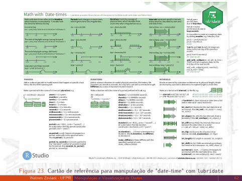
Make an interval with interval() or %--%, e.g.

i <- interval(ymd("2017-01-01"), d) ## 2017-01-01 UTC--2017-11-28 UTC j <- d %--% ymd("2017-12-31") ## 2017-11-28 UTC--2017-12-31 UTC

PERIODS DURATIONS

RStudio® is a trademark of RStudio, Inc. • CC BY SA RStudio • [email protected] • 844-448-1212 • rstudio.com • Learn more at lubridate.tidyverse.org • lubridate 1.6.0 • Updated: 2017-12

years(x = 1) x years. months(x) x months. weeks(x = 1) x weeks. days(x = 1) x days. hours(x = 1) x hours. minutes(x = 1) x minutes. seconds(x = 1) x seconds. milliseconds(x = 1) x milliseconds. microseconds(x = 1) x microseconds nanoseconds(x = 1) x nanoseconds. picoseconds(x = 1) x picoseconds.

period(num = NULL, units = "second", ...) An automation friendly period constructor. period(5, unit = "years")

as.period(x, unit) Coerce a timespan to a period, optionally in the specified units. Also is.period(). as.period(i)

period_to_seconds(x) Convert a period to the "standard" number of seconds implied by the period. Also seconds_to_period(). period_to_seconds(p)

Add or subtract periods to model events that happen at specific clock times, like the NYSE opening bell.

dyears(x = 1) 31536000x seconds. dweeks(x = 1) 604800x seconds. ddays(x = 1) 86400x seconds. dhours(x = 1) 3600x seconds. dminutes(x = 1) 60x seconds. dseconds(x = 1) x seconds. dmilliseconds(x = 1) x x 10-3 seconds. dmicroseconds(x = 1) x x 10-6 seconds. dnanoseconds(x = 1) x x 10-9 seconds. dpicoseconds(x = 1) x x 10-12 seconds.

duration(num = NULL, units = "second", ...) An automation friendly duration constructor. duration(5, unit = "years")

as.duration(x, …) Coerce a timespan to a duration. Also is.duration(), is.difftime(). as.duration(i)

make_difftime(x) Make difftime with the specified number of units. make_difftime(99999)

Make a period with the name of a time unit pluralized, e.g.

p <- months(3) + days(12) p "3m 12d 0H 0M 0S"

Make a duration with the name of a period prefixed with a d, e.g.

dd <- ddays(14) dd "1209600s (~2 weeks)"

Add or subtract durations to model physical processes, like battery life. Durations are stored as seconds, the only time unit with a consistent length. Difftimes are a class of durations found in base R.

Number of days etc.Number

of monthsExact

length in seconds

Equivalent in common

units

INTERVALSDivide an interval by a duration to determine its physical length, divide an interval by a period to determine its implied length in clock time.

Math with Date-times — Lubridate provides three classes of timespans to facilitate math with dates and date-times

a %within% b Does interval or date-time a fall within interval b? now() %within% i

int_start(int) Access/set the start date-time of an interval. Also int_end(). int_start(i) <- now(); int_start(i)

int_aligns(int1, int2) Do two intervals share a boundary? Also int_overlaps(). int_aligns(i, j)

int_diff(times) Make the intervals that occur between the date-times in a vector. v <-c(dt, dt + 100, dt + 1000); int_diff(v)

int_flip(int) Reverse the direction of an interval. Also int_standardize(). int_flip(i)

int_length(int) Length in seconds. int_length(i)

int_shift(int, by) Shifts an interval up or down the timeline by a timespan. int_shift(i, days(-1))

as.interval(x, start, …) Coerce a timespans to an interval with the start date-time. Also is.interval(). as.interval(days(1), start = now())

l

Start Date

End Date

Math with date-times relies on the timeline, which behaves inconsistently. Consider how the timeline behaves during:

A normal day nor <- ymd_hms("2018-01-01 01:30:00",tz="US/Eastern")

The start of daylight savings (spring forward) gap <- ymd_hms("2018-03-11 01:30:00",tz="US/Eastern")

The end of daylight savings (fall back) lap <- ymd_hms("2018-11-04 00:30:00",tz="US/Eastern")

Leap years and leap seconds leap <- ymd("2019-03-01")

12:00 1:00 2:00 3:00

2019 2020 2021

1:00 2:00 3:00 4:00

1:00 2:00 3:00 4:00

Durations track the passage of physical time, which deviates from clock time when irregularities occur.

nor + dminutes(90)

gap + dminutes(90)

lap + dminutes(90)

leap + dyears(1)

12:00 1:00 2:00 3:00

2019 2020 2021

1:00 2:00 3:00 4:00

1:00 2:00 3:00 4:00

Periods track changes in clock times, which ignore time line irregularities.

nor + minutes(90)

gap + minutes(90)

lap + minutes(90)

leap + years(1)

12:00 1:00 2:00 3:00

1:00 2:00 3:00 4:00

1:00 2:00 3:00 4:00

2019 2020 2021

Intervals represent specific intervals of the timeline, bounded by start and end date-times.

interval(nor, nor + minutes(90))

interval(gap, gap + minutes(90))

interval(lap, lap + minutes(90))

interval(leap, leap + years(1))

12:00 1:00 2:00 3:00

1:00 2:00 3:00 4:00

1:00 2:00 3:00 4:00

2019 2020 2021

Not all years are 365 days due to leap days. Not all minutes are 60 seconds due to leap seconds. It is possible to create an imaginary date by adding months, e.g. February 31st jan31 <- ymd(20180131) jan31 + months(1) ## NA %m+% and %m-% will roll imaginary dates to the last day of the previous month. jan31 %m+% months(1) ## "2018-02-28" add_with_rollback(e1, e2, roll_to_first = TRUE) will roll imaginary dates to the first day of the new month. add_with_rollback(jan31, months(1), roll_to_first = TRUE) ## "2018-03-01"

Figura 23. Cartão de referência para manipulação de *date-time* com lubridate

e hms.Walmes Zeviani · UFPR Manipulação e Visualização de Dados 62

Encadeando com operadores do magrittr


Anatomia

I O operador permite expressar de forma mais direta asoperações.

I É uma ideia inspirada no Shell.I A lógica é bem simples:

I x %>% f é o mesmo que f(x).I x %>% f(y) é o mesmo que f(x, y).I x %>% f %>% g %>% h é o mesmo que h(g(f(x))).


Anatomia do magrittrlibrary(magrittr) 1

2# Operadores "pipe". 3ls("package:magrittr") %>% 4

str_subset("%") 5

## [1] "%<>%" "%>%" "%$%" "%T>%"

# Outras funções/objetos. 1ls("package:magrittr") %>% 2

str_subset("^[^%]*$") 3

## [1] "add" "and"## [3] "debug_fseq" "debug_pipe"## [5] "divide_by" "divide_by_int"## [7] "equals" "extract"## [9] "extract2" "freduce"## [11] "functions" "inset"## [13] "inset2" "is_greater_than"## [15] "is_in" "is_less_than"## [17] "is_weakly_greater_than" "is_weakly_less_than"## [19] "mod" "multiply_by"## [21] "multiply_by_matrix" "n'est pas"## [23] "not" "or"## [25] "raise_to_power" "set_colnames"## [27] "set_names" "set_rownames"## [29] "subtract" "undebug_fseq"## [31] "use_series"Walmes Zeviani · UFPR Manipulação e Visualização de Dados 65

Exemplos do uso do pipe (1)

x <- precip 1mean(sqrt(x - min(x))) 2

## [1] 5.020078

x <- x - min(x) 1x <- sqrt(x) 2mean(x) 3

## [1] 5.020078

precip %>% 1`-`(min(.)) %>% # o mesmo que subtract(min(.)) 2sqrt() %>% 3mean() 4

## [1] 5.020078


Exemplos de uso do pipe (2)

x <- precip 1x <- sqrt(x) 2x <- x[x > 5] 3x <- mean(x) 4x 5

## [1] 6.364094

precip %>% 1sqrt() %>% 2.[is_greater_than(., 5)] %>% # o mesmo que .[`>`(., 5)] 3mean() 4

## [1] 6.364094


Mãos à obra!


Instalar o tidyverse

# Do CRAN. 1install.packages("tidyverse") 2

3# Do GitHub. 4# install.packages("devtools") 5devtools::install_github("hadley/tidyverse") 6

7# Atualizar caso já tenha instalado. 8tidyverse_update() 9


O que vem agora?

I Uma visão aprofundada de cada pacote do tidyverse.I Exemplos didáticos seguidos de desafios práticos.I Happy coding.


Referências

TEUTONICO, D. Ggplot2 essentials. Packt Publishing, 2015.

WICKHAM, H. Ggplot2: Elegant graphics for data analysis.Springer International Publishing, 2016.

WILKINSON, L.; WILLS, D.; ROPE, D.; NORTON, A.; DUBBS, R.The grammar of graphics. Springer New York, 2013.


Manipulação e Visualização de Dados - a abordagem tidyverse

Documents

Transcript of Manipulação e Visualização de Dados - a abordagem tidyverse