Manhattan Path Based RWP Mobility Models: Spatial Node Distribution, Smooth Movement, and...

SUBMITTED TO IEEE TRANSACTIONS ON MOBILE COMPUTING (SEPTEMBER 2009) 1

Manhattan Path Based RWP Mobility Models:Spatial Node Distribution, Smooth Movement,

and Connectivity PropertiesPilu Crescenzi, Miriam Di Ianni, Andrea Marino, Donatella Merlini, Gianluca Rossi, and Paola Vocca

Abstract—In this paper, we study the spatial node stationary distribution and connectivity properties of two variations of the RandomWaypoint (in short, RWP) mobility model. In particular, differently from the RWP mobility model that connects the source points to thedestination ones by straight lines, our models make use of one of the two Manhattan paths connecting the given points whose selectionis based on a random choice between the two paths. In both models a node randomly chooses a destination point and a randompositive velocity value v. In the first model, called the random Manhattan RWP mobility model (in short, rMRWP), the node travels atconstant velocity v, while in the second model, called the acceleration/deceleration random Manhattan RWP mobility model (in short,AC/DC-rMRWP), the node starts with velocity zero, travels according to a uniformly accelerated motion until it reaches the mid-pointof the first segment of the Manhattan path at velocity v, then it travels according to a uniformly decelerated motion until it reachesthe turning point of the Manhattan path, and then it repeats the process on the second segment of the Manhattan path. We provideanalytical results for the spatial node stationary distribution of the two Manhattan based RWP mobility models. As an application, weexploit these results to derive upper bounds on the transmission range of the nodes of a MANET, moving according to these models,that guarantees the connectivity of the communication graph with high probability.

Index Terms—MANET, mobility model, Manhattan path, smooth movement.

F

1 INTRODUCTION

The Random WayPoint (in short, RWP) mobility model isone of the most commonly used models for evaluatingthe performance of a communication protocol and/orapplication based on a mobile wireless ad hoc network (inshort, MANET) [?]. According to this model, each nodemoves by selecting a random destination point D withina specified movement region (typically a square) anda random velocity value v (usually chosen uniformlywithin a specified interval), and by traveling from itscurrent position S to D at constant velocity v along thesegment joining S to D (for a survey on mobility modelsfor MANET research, see [?]).

Due to its simplicity, the RWP model has been widelyanalyzed in the literature, from both an experimentaland a theoretical point of view. In particular, in the lastfew years several papers studied and tried to estimatethe spatial node stationary distribution of the model [?],[?], [?], [?]. Obtaining an exact closed formula for thisdistribution might turn out to be very useful in or-der to derive analytical results concerning, for instance,

• P. Crescenzi, A. Marino, and D. Merlini are with the Dipartimento diSistemi e Informatica, Universita degli Studi di Firenze, Firenze, Italy.

• M. Di Ianni and G. Rossi are with Dipartimento di Matematica, Univer-sita degli Studi di Roma “Tor Vergata”, Roma, Italy.

• P. Vocca is with Dipartimento di Matematica “Ennio De Giorgi”, Univer-sita del Salento, Lecce, Italy.

Part of the results contained in this paper have been presented at 16thInternational Colloquium on Structural Information and CommunicationComplexity, May 25-27, 2009, Piran, Slovenia. This work was partiallysupported by the EU under the EU/IST Project 15964 AEOLUS.

topological properties of the communication graph of aMANET and the performance of specific protocols thatdepend on these properties. As an example, one coulddetermine upper and lower bounds on the transmissionrange of the nodes of the MANET, moving according tothe RWP model, that with high probability1 guaranteesthe connectivity of the communication graph (similarlyto what has been done in the case of static networksin [?]), once the nodes have reached the spatial stationarydistribution. More ambitiously, one could also determineupper and lower bounds on the completion time ofspecific information spreading protocols (such as theflooding one) as a function of the number of nodes andof the transmission range (similarly to what has beendone in the case of geometric random graphs in [?], [?]).

As far as we know, two main approaches have beenused in the literature in order to compute a closedformula for the RWP spatial node stationary distribution.The first one is based on relatively simple geometricprobability arguments [?], [?], [?]: however, this approachled to the necessity of computing very difficult integralsand, for this reason, allowed the authors to obtain onlyapproximations of the exact formula (even though quitegood ones). The second approach [?], instead, producesan exact formula by using a more sophisticated tool, thatis, the Palm calculus which is a set of formulas that relatetime averages to event averages [?] and which is notwidely used or even known in applied areas.

1. Recall that a series of events En holds with high probability ifPr (En) ≥ 1−O

`1

nα

´for some α > 0.


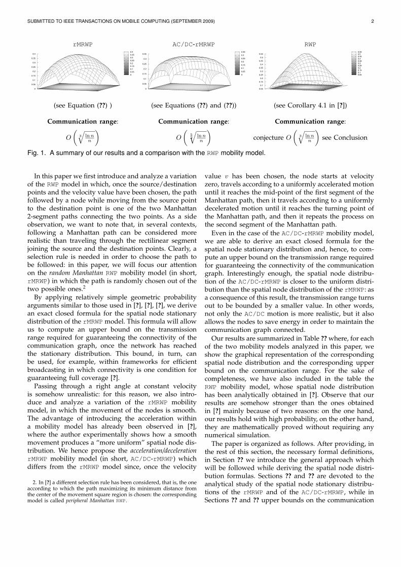
rMRWP AC/DC-rMRWP RWP

0

0.05

0.1

0.15

0.2

0.25

0.3

0.35

0.4

0

0.05

0.1

0.15

0.2

0.25

0.3

0.35

0.4

0

0.05

0.1

0.15

0.2

0.25

0.3

0.35

0

0.05

0.1

0.15

0.2

0.25

0.3

0.35

0.05

0.1

0.15

0.2

0.25

0.3

0.35

0.4

0.45

0.5

0.55

0.05

0.1

0.15

0.2

0.25

0.3

0.35

0.4

0.45

0.5

0.55

(see Equation (??) ) (see Equations (??) and (??)) (see Corollary 4.1 in [?])

Communication range: Communication range: Communication range:

O

(3

√lnnn

)O

(52

√lnnn

)conjecture O

(3

√lnnn

)see Conclusion

Fig. 1. A summary of our results and a comparison with the RWP mobility model.

In this paper we first introduce and analyze a variationof the RWP model in which, once the source/destinationpoints and the velocity value have been chosen, the pathfollowed by a node while moving from the source pointto the destination point is one of the two Manhattan2-segment paths connecting the two points. As a sideobservation, we want to note that, in several contexts,following a Manhattan path can be considered morerealistic than traveling through the rectilinear segmentjoining the source and the destination points. Clearly, aselection rule is needed in order to choose the path tobe followed: in this paper, we will focus our attentionon the random Manhattan RWP mobility model (in short,rMRWP) in which the path is randomly chosen out of thetwo possible ones.2

By applying relatively simple geometric probabilityarguments similar to those used in [?], [?], [?], we derivean exact closed formula for the spatial node stationarydistribution of the rMRWP model. This formula will allowus to compute an upper bound on the transmissionrange required for guaranteeing the connectivity of thecommunication graph, once the network has reachedthe stationary distribution. This bound, in turn, canbe used, for example, within frameworks for efficientbroadcasting in which connectivity is one condition forguaranteeing full coverage [?].

Passing through a right angle at constant velocityis somehow unrealistic: for this reason, we also intro-duce and analyze a variation of the rMRWP mobilitymodel, in which the movement of the nodes is smooth.The advantage of introducing the acceleration withina mobility model has already been observed in [?],where the author experimentally shows how a smoothmovement produces a “more uniform” spatial node dis-tribution. We hence propose the acceleration/decelerationrMRWP mobility model (in short, AC/DC-rMRWP) whichdiffers from the rMRWP model since, once the velocity

2. In [?] a different selection rule has been considered, that is, the oneaccording to which the path maximizing its minimum distance fromthe center of the movement square region is chosen: the correspondingmodel is called peripheral Manhattan RWP.

value v has been chosen, the node starts at velocityzero, travels according to a uniformly accelerated motionuntil it reaches the mid-point of the first segment of theManhattan path, then it travels according to a uniformlydecelerated motion until it reaches the turning point ofthe Manhattan path, and then it repeats the process onthe second segment of the Manhattan path.

Even in the case of the AC/DC-rMRWP mobility model,we are able to derive an exact closed formula for thespatial node stationary distribution and, hence, to com-pute an upper bound on the transmission range requiredfor guaranteeing the connectivity of the communicationgraph. Interestingly enough, the spatial node distribu-tion of the AC/DC-rMRWP is closer to the uniform distri-bution than the spatial node distribution of the rMRWP: asa consequence of this result, the transmission range turnsout to be bounded by a smaller value. In other words,not only the AC/DC motion is more realistic, but it alsoallows the nodes to save energy in order to maintain thecommunication graph connected.

Our results are summarized in Table ?? where, for eachof the two mobility models analyzed in this paper, weshow the graphical representation of the correspondingspatial node distribution and the corresponding upperbound on the communication range. For the sake ofcompleteness, we have also included in the table theRWP mobility model, whose spatial node distributionhas been analytically obtained in [?]. Observe that ourresults are somehow stronger than the ones obtainedin [?] mainly because of two reasons: on the one hand,our results hold with high probability, on the other hand,they are mathematically proved without requiring anynumerical simulation.

The paper is organized as follows. After providing, inthe rest of this section, the necessary formal definitions,in Section ?? we introduce the general approach whichwill be followed while deriving the spatial node distri-bution formulas. Sections ?? and ?? are devoted to theanalytical study of the spatial node stationary distribu-tions of the rMRWP and of the AC/DC-rMRWP, while inSections ?? and ?? upper bounds on the communication


range are proved whenever nodes move according tothese models. Finally, we conclude in Section ??.

1.1 Formal definitionsLet S = (xS , yS) and D = (xD, yD) be two pointsin the square Q = [0, 2] × [0, 2] of center Z = (1, 1).The Manhattan paths from S to D are mhv(S,D) andmvh(S,D), where mhv(S,D) is the horizontal path fromS to H = (xD, yS) followed by the vertical path fromH to D, and mvh(S,D) is the vertical path from S toK = (xS , yD) followed by the horizontal path from K toD.

The mobility models studied in this paper are allderived by the Random Waypoint mobility model. Eachnode is initially positioned at a point S, randomly cho-sen within Q. Successively, the node chooses a randomdestination point D ∈ Q, and a random velocity valuev ∈ [vm, vM] with vm > 0. Then,• in the rMRWP mobility model the node travels at

constant velocity v along a path randomly chosenbetween mhv(S,D) and mvh(S,D);

• in the AC/DC-rMRWP mobility model the nodetravels along a path randomly chosen betweenmhv(S,D) and mvh(S,D) according to the followingAC/DC motion rule: if the chosen path is mhv(S,D),then (1) the node travels at constant accelerationalong the segment SH until it reaches its mid-pointwith velocity v, (2) the node travels at constantdeceleration along the second half of segment SHuntil it reaches H with velocity 0, (3) the nodetravels at constant acceleration along the segmentHD until it reaches its mid-point at velocity v, and(4) the node travels at constant deceleration alongthe second half of segment HD until it reaches Dwith velocity 0. The case in which the chosen pathis mvh(S,D) is defined similarly.

Once the destination point D is reached, the nodeimmediately starts the traveling process again.3

2 THE GENERAL APPROACH

In this section, we describe the approach that will befollowed while deriving the explicit formula for thespatial node stationary distribution of the Manhattanbased mobility models. Observe that, since nodes moveindependently, we can limit ourselves to analyze themovement of a single node.

For any p and q with 0 ≤ p, q ≤ 2, letR be the rectangle[0, p]× [0, q], and let F = (p, q) be the top right vertex ofR. Moreover, let X be the random variable describingthe location of the node, and let T and Tp,q be the tworandom variables describing, respectively, the time spentby the node while moving between the source and the

3. In the RWP mobility model it is also assumed that, once a nodereaches its destination, it stays there for a pause time tp, randomlychosen within a specified interval. In this paper, we assume that tp = 0:the case in which tp > 0 can be dealt with similarly to what has beendone in [?].

destination point and the time spent within R whilemoving between these two points. As proved in [?],

Pr(X ∈ R) =E[Tp,q]E[T ]

. (1)

In other words, the problem of computing the cumula-tive distribution function (in short, cdf) Pr(X ∈ R) hasbeen reduced to the problem of computing the valuesE[Tp,q] and E[T ].

Let S denote the location of a node at the beginningof its movement period and D denote the location ofthe same node at the end of the same movement period.Hence, the value of E[Tp,q] is equal to

1∆v

∫ vM

vm

∫S∈Q

∫D∈Q

f(S)f(D)tR(S,D, v)dDdSdv,

where f(.) denotes the probability density function4 (inshort, pdf) of a point location, 1

∆v= 1vM−vm

is the pdf ofthe chosen velocity value v, and tR(S,D, v) denotes theexpected time spent within R while moving between Sand D. The computation of the above integral will beperformed by distinguishing the three cases in which (i)both S and D are contained in R or (ii) S is containedin R while D is outside of R (or vice versa) or (iii) bothS and D are outside of R. In particular, the value ofthe above integral can be obtained by computing thefollowing four integrals:

Σ1 =1

16∆v

∫ vM

vm

∫S∈R

∫D∈R

tR(S,D, v)dDdSdv,

Σ2 =1

16∆v

∫ vM

vm

∫S∈R

∫D∈Q−R

tR(S,D, v)dDdSdv,

Σ3 =1

16∆v

∫ vM

vm

∫S∈Q−R

∫D∈R

tR(S,D, v)dDdSdv,

and

Σ4 =1

16∆v

∫ vM

vm

∫S∈Q−R

∫D∈Q−R

tR(S,D, v)dDdSdv

(note that, due to symmetry reasons, Σ2 = Σ3).5 Insummary, we have that

E[Tp,q] = Σ1 + 2Σ2 + Σ4. (2)

The goal of the Sections ?? and ?? will be to compute thethree integrals Σ1, Σ2, and Σ4.

In order to compute E[T ], instead, we need to dis-tinguish the case in which the nodes move at constantvelocity from the case in which the motion is the AC/DCone. In the first case, E[T ] = E

[LV

]where L is the

random variable denoting the path length and V is the

4. The probability density function of a random variable is a functionwhich describes the density of probability at each point in the samplespace: it is well-known that this function is the derivative of the cdf.

5. For i = 1, 2, 3, 4, Σi is indeed a function Σi(p, q): however, for thesake of brevity, we will always avoid to explicitly state the dependencyon p and q.


random variable denoting the velocity value. Since L

and V are independent, we have that E[T ] = E[L]E[V ] : it is

known that E[L] = 43 (see [?]) while E[V ] = ∆v/ ln vM

vm=

c (see [?]). Hence, in the case of uniform motion, we havethat

E[T ] =43c. (3)

In the AC/DC motion case, instead, we proceed byfirst proving a simple preliminary result computing thetime spent by a node traveling along a segment withendpoints A and B according to the AC/DC motion rule.To this aim, denote as M the midpoint of AB, denote as vthe maximum velocity to be reached during the AC/DCmotion, denote as a the acceleration, and denote as t`the time spent by a node to cover a segment `. Observenow that tAM is equal to the time necessary to reach themaximum velocity v. Since |AM | = 1

2vtAM , we have that

tAM =|AB|v

. (4)

Clearly, tAB = 2tAM : hence,

tAB = 2|AB|v

. (5)

Observe now that

E[T ] =1

∆v

∫ vM

vm

∫S∈Q

∫D∈Q

tv(S,D)16

dDdSdv

where tv(S,D) denotes the time spent by a node travel-ing along one of the two Manhattan paths from S to Daccording to the AC/DC motion rule. On the ground ofEquation (??), we have that

tv(S,D) = 2|xS − xD|+ |yS − yD|

v.

Hence,

E[T ] =

∫S∈Q

∫D∈Q 2 (|xS − xD|+ |yS − yD| ) dDdS

16c.

The above integral is equal to 32 times the expected Man-hattan distance between two points randomly chosenwithin the square Q: it is known that this latter valueis equal to 4

3 (see [?]). In conclusion, in the case of theAC/DC motion, we have that

E[T ] =83c. (6)

3 THE RANDOM MANHATTAN RWP MODEL

Recall that

Σi =1

16∆v

∫ vM

vm

∫S∈Ai

∫D∈Bi

tR(S,D, v)dDdSdv

where Ai and Bi denote two regions included in Q, Rdenotes the rectangle [0, p]×[0, q], and tR(S,D, v) denotesthe expected time spent within R while moving between

S and D. Since in the case of the rMRWP model, the nodesmove according to the uniform motion rule, we have that

tR(S,D) =lR(S,D)

v,

where lR(S,D) denotes the expected length of the in-tersection between the chosen path from S to D and R.Hence,

Σi =1

16c

∫S∈Ai

∫D∈Bi

lR(S,D)dDdS =1

16cΓi. (7)

The next subsections are then devoted to the computa-tion of Γi. To this aim, we will make use of the followingnotation: given two points α = (xα, yα) and β = (xβ , yβ),∆α,βx = xα − xβ and ∆α,β

y = yα − yβ .

3.1 Computing Γ1: A1 = B1 = RThis case corresponds to computing the following inte-gral: ∫

S∈R

∫D∈R

(|xS − xD|+ |yS − yD|) dDdS.

It is known (see [?]) that the value of this integral is equalto

p2q2 p+ q

3. (8)

3.2 Computing Γ2: A2 = R and B2 = Q−RAccording to the left part of Figure ??, it is easy tocompute Γ2 by distinguishing five cases: for example,the value of lR(S,D) whenever D is above S and on itsleft, is equal to (∆S,D

x +∆F,Sy )+∆F,S

y

2 = ∆S,Dx

2 + ∆F,Sy .

Γ2 =∫ p

0

∫ q

0

[∫ xS

0

∫ 2

q

(xS − xD

2+ q − yS

)dyDdxDdySdxS

+∫ p

xS

∫ 2

q

(xD − xS

2+ q − yS

)dyDdxDdySdxS

+∫ 2

p

∫ 2

q

p− xS + q − yS2

dyDdxDdySdxS

+∫ 2

p

∫ q

yS

(yD − yS

2+ p− xS

)dyDdxDdySdxS

+∫ 2

p

∫ yS

0

(yS − yD

2+ p− xS

)dyDdxD

]dySdxS .

After having evaluated the above integral6 and doubledthe result, we obtain that Γ2 is equal to

−5p3q2

12− 5p2q3

12+ p2q2 − 1

6p3q − 1

6pq3 + p2q + pq2. (9)

6. All the integral computations included in this paper have beenperformed by using the Mathematica tool, version 5.2.


S

F

∆S,Dx2 + ∆F,Sy

∆D,S

x 2+

∆F,Sy

∆F,Sx +∆F,Sy2

∆D,Sy2 + ∆F,Sx

∆S,Dy2 + ∆F,Sx

S

D

F

Fig. 2. The second and the third cases of the rMRWP mobility model.

3.3 Computing Γ4: A4 = Q−R and B4 = Q−RObserve that only two situations giving raise to a nonempty intersection with R may occur: either S is in theregion above R and D is in the region at its right or viceversa. Since the two cases are symmetric, we can limitourselves to analyse only the first one (see the right partof Figure ??). Clearly, for any such pair of points S andD, the value of lR(S,D) is equal to

(∆F,Sx + ∆F,D

y ) + 02

=∆F,Sx + ∆F,D

y

2Hence, Γ4 is equal to

2∫ p

0

∫ 2

q

∫ 2

p

∫ q

0

p− xS + q − yD2

dyDdxDdySdxS .

After having evaluated the above integral, we obtain thatΓ4 is equal to

12pq(p+ q)(2− p)(2− q). (10)

3.4 The spatial node distributionBy applying Equations (??)-(??) and by using Equa-tions (??)-(??), we get

Pr(X ∈ R) =116pq(3p− p2 + 3q − q2

).

The pdf can be finally obtained by computing the deriva-tive of the cdf (in doing so, for the sake of readability,we replace p and q with x and y, respectively). We havethat

f1(x, y) =316(2x− x2 + 2y − y2

). (11)

The first row of Table ?? shows the behaviour of f1(x, y).Observe how the central part of the domain squareis visited more often due to the border effect of themodel [?] (similarly to the standard RWP model).

4 CONNECTIVITY IN THE RMRWP MODEL

In this section, we exploit our analytical results on thespatial node distribution of the rMRWP model to derivean upper bound on the transmission range to be assignedto the nodes of a MANET, moving according to thismodel, in order to guarantee its connectivity with high

probability. In the following, N = {1, . . . , n} will denotethe set of n nodes moving in the square Q according tothe rMRWP mobility model and transmitting with ranger, while G(N, t) will denote the communication graphinduced by N at time t, in which two nodes are adjacentif and only if they are within the transmission range ofeach other. Our result in this section is the following one.

Theorem 1: There exists a positive constant γ such that

if r = r(n) ≥ γ 3

√lnnn , then there exist two positive

constants α and β such that

Pr (G(N, t) is not connected ) <β

nα.

Proof: In order to prove the theorem, we will followthe same approach which has been used in the case of(static) geometric random graphs (see, for example, [?]).

Let r = r(n) = γ 3

√lnnn be the transmission range of the

nodes. By tessellating the square Q into k2 square cellsof size z = 2/k, with k =

√5/r(n), it is not difficult

to prove that, in order to guarantee the connectivity ofthe communication graph, it suffices to choose γ so that,with high probability, every cell is not empty. For any cellC of Q, let Xi(C, t) be the random variable whose valueis 1 if, at time t, node i is in C and 0 otherwise. Moreover,let X(C, t) = X1(C, t) + . . . + Xn(C, t) be the randomvariable describing the total number of nodes in C. Bylooking at the analytical expression of the pdf relativeto the rMRWP mobility model derived in the previoussection (and as it clearly appears by observing the leftpart of Figure ??), it follows that only the cells at thecorners of Q have to be analyzed. Let CO be the cell atthe bottom left corner of Q (the other corner cells can beanalyzed similarly). Then

Pr[Xi(CO, t) = 1] =∫Y ∈CO

f1(Y )dY

=38z3 − 1

8z4 ≥ 1

4z3.

For any cell C, let us denote by µ(C, t) the expected valueof X(C, t). We have that

µ(C, t) ≥ µ(CO, t) ≥n

4z3.

We can now apply the well-known Chernoff bound thatstates that if U1, . . . , Um are m independent random bi-nary variables such that Pr [Ui = 1] = pi, if U =

∑mi=1 Ui,


and if µU is the expected value of U , then, for any δ > 0,

Pr [U < (1− δ)µU ] <(

e−δ

(1− δ)1−δ

)µU.

By applying this bound to the variables Xi(C, t) withδ = µ(C,t)−1

µ(C,t) , we obtain that

Pr[X(C, t) < 1] < µ(C)e1−µ(C).

Hence, the probability that G(N, t) is not connected isbounded by

∑C

Pr[X(C, t) < 1] < k2µ(C)e1−µ(C)

≤ k2n

4z3e1−n4 z

3= k2n

48k3e1−n4

8k3

=2nke1− 2n

k3 =2nr(n)√

5e

1− 2nr3(n)5√

5

=2γn2/3 ln1/3 n√

5e

1− 2γ3 lnn5√

5

<2γn√

5e

1− 2γ3 lnn5√

5 =2eγn√

51

n2γ3

5√

5

.

By choosing γ > 3√

5√

52 , we obtain that

Pr (G(N, t) is not connected ) <c

nα

where c and α are two positive constants.The above theorem implies that, whenever r(n) ≥

γ 3

√lnnn , the probability that the graph G(N, t) is con-

nected is greater than 1− βnα , that is, the communication

graph is connected with high probability.

5 THE AC/DC RANDOM MANHATTAN RWPMODEL

Due to the symmetry of the AC/DC-rMRWP model, in thissection we can limit ourselves to compute E[Tp,q] forp, q < 1. Indeed, once we have computed the cdf and,hence, the pdf fp,q<1

2 (x, y) relative to this case, we havethat the value of f2(x, y) is equal to

fp,q<12 (x, y) if x ∈ [0, 1] ∧ y ∈ [0, 1],fp,q<1

2 (2− x, y) if x ∈ [1, 2] ∧ y ∈ [0, 1],fp,q<1

2 (x, 2− y) if x ∈ [0, 1] ∧ y ∈ [1, 2],fp,q<1

2 (2− x, 2− y) if x ∈ [1, 2] ∧ y ∈ [1, 2].

(12)

In order to compute fp,q<12 (x, y), we have to compute,

for i = 1, 2, 4, the values

Σi =1

16∆v

∫ vM

vm

∫S∈Ai

∫D∈Bi

tR(S,D, v)dDdSdv

where Ai and Bi denote two regions included in Q, Rdenotes the rectangle [0, p]× [0, q] with 0 < p, q < 1, andtR(S,D, v) denotes the expected time spent within Rwhile moving between S and D. To compute tR(S,D, v),for each pair of points S and D, we find the intersection

between R and the chosen Manhattan path from S to D,and we then take the same approach used in Section ??for deriving Equations (??) and (??). To this aim, weconsider a segment with endpoints A and B and withmid-point M and we denote as v the maximum velocityto be reached during the AC/DC motion, we denote as athe acceleration, and we denote as t` the time spent bya node to cover a segment `. Let I be a generic point inAB, then the following three cases arise.

• I coincides with M or I coincides with B. In this case,tAI is computed by means of Equation (??) or (??).

• I lies between A and M . Since{|AI| = 1

2at2AI

a = vtAM

= v2

|AB| ,

then

tAI =

√2|AI|a

=1v

√2|AI| · |AB|. (13)

• I lies between M and B. Since tAI = tAB − tIB ,then it is sufficient to compute tIB . Similarly to theprevious case, we can show that

tIB =1v

√2|IB| · |AB|.

Hence,

tAI = 2|AB|v− 1v

√2|IB| · |AB|. (14)

An easy exploitation of Equations (??), (??), (??) and (??)allows to compute the value of tR.

5.1 Computing Σ1: A1 = B1 = R

In this case, the entire Manhattan path from S to D iscontained in R. Hence, if H denotes the turning pointof the path, we can apply Equation (??) obtaining thattR(S,D, v) = 2

(|SH|v + |HD|

v

). Hence, the value of Σ1 is

equal to

116c

∫S∈R

∫D∈R

2 (|SH|+ |HD|) dDdS.

After having evaluated the above integral, we have that

Σ1 =1

16c23(p3q2 + p2q3

). (15)

5.2 Computing Σ2: A2 = R and B2 = Q−R

In order to deal with this case, we decompose Q−R intotwelve regions as shown in the following figure, whereR is shown in grey.


Integrand function

D ∈ I J Implicit Explicit

R1 (xD, q) (xS , q) |SH|+ 2|HD| −p

2|ID||HD| (xS − xD) + 2(yD − yS)−p

2(yD − q)(yD − yS)

R2 (xD, q) (xS , q) |SH|+p

2|HI||HD| (xS − xD) +p

2(q − yS)(yD − yS)

R9 (p, yS) (xS , q) |SH|+ |SK| −√

2|IH||SH|+√

2|JK||SK|2

(xD − xS) + (yD − yS)−√

2(xD−p)(xD−xS)+√

2(yD−q)(yD−yS)

2

R10 (p, yS) (xS , q) |SH| −√

2|IH||SH|−√

2|SJ||SK|2

(xD − xS)−√

2(xD−p)(xD−xS)−√

2(q−yS)(yD−yS)

2

R12 (p, yS) (xS , q)

√2|SI||SH|+

√2|SJ||SK|

2

√2(p−xS)(xD−xS)+

√2(q−yS)(yD−yS)

2

TABLE 1Computing Σ2 in the case of the AC/DC movement: recall that H = (xD, yS) and K = (xS , yD).

S

p 2p − xS

q

2q − yS

2

2

R1

R2

R3

R4

R9

R10

R11

R12

R5

R6

R7

R8

Let us consider, as an example, the case in which Dis contained in R1: in this case, we can apply Equa-tions (??) and (??). If H and K denote the turning pointof mhv(S,D) and mvh(S,D) respectively, and if I andJ are the intersection of the line y = q with mhv(S,D)and mvh(S,D) respectively, we have that the value oftR(S,D, v) is equal to(

2|SH|v + 2|HD|−

√2|ID||HD|v

)+ 2|SK|−

√2|JK||SK|v

2.

Since |HD| = |SK| and |ID| = |JK|, it follows that

tR(S,D, v) =|SH|+ 2|HD| −

√2|ID||HD|

v.

This implies that the contribution to Σ2 given by thiscase is equal to∫

S∈R∫D∈R1

(|SH|+ 2|HD| −

√2|ID||HD|

)dDdS

16c.

Observe now that, since D ∈ R1, then

|SH| = xS − xD, |HD| = yD − yS , and |ID| = yD − q.

After having substituted these expressions into the in-tegrand function and after having evaluated the aboveintegral, we have that the contribution to Σ2 given bythis case is equal to

σ2,1(p, q) =1

16cp2q2

48

(4p+

√2q ln

(2√

2 + 3)

+ 12q).

We can deal with the other eleven regions in a sim-ilar way (see Table ?? where both the implicit andthe explicit integrand functions are indicated). Not thatonly the contributions corresponding to R1, R2, R9,R10, and R12 have to be explicitly computed, since,due to symmetry, we have that σ2,3(p, q) = σ2,1(p, q),σ2,4(p, q) = σ2,2(p, q), σ2,5(p, q) = σ2,1(q, p), σ2,6(p, q) =σ2,1(q, p), σ2,7(p, q) = σ2,2(q, p), σ2,8(p, q) = σ2,2(q, p), andσ2,10(p, q) = σ2,11(q, p).

After having evaluated all these contributions, weobtain that

Σ2 =1

16c

(−

(3p+ 2)(p− 6)(q + 2)q√p

36

−(3q + 2)(q − 6)(p+ 2)p

√q

36

+pq(p2(10− 19q) + q2(10− 19p)

)36

+pq(p2(2 + q) + q2(2 + p)

)12√

2ln(

1 +√

2)

(16)

+(p− 2)3(q + 2)q

24√

2ln

(√2 +√p

√2−√p

)

+(q − 2)3(p+ 2)p

24√

2ln

(√2 +√q

√2−√q

))

5.3 Computing Σ4: A4 = B4 = Q−R

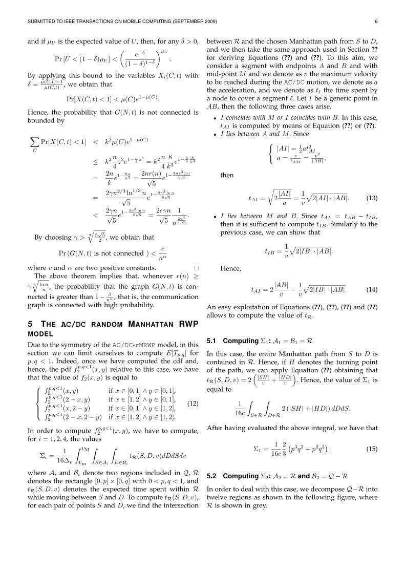
Similarly to the analysis of the rMRWP mobility model,we have to consider only the case in which D is in theregion above R and S is in the region at its right, that is,the case in which only the path mhv(S,D) intersects R.To this aim, we distinguish the case in which p < xS < 2pfrom the case in which 2p < xS < 2. In the first case, wedecompose the region including D into four regions asshown in the following figure.


Integrand function

S ∈ D ∈ Implicit Explicit

R1 R3 |SH|+ |HD| −√

2|SI||SH|+√

2|JD||HD|2

(xS − xD) + (yD − yS)−√

2(xS−p)(xS−xD)+√

2(yD−q)(yD−yS)

2

R1 R4 |SH| −√

2|SI||SH|−√

2|HJ||HD|2

(xS − xD)−√

2(xS−p)(xS−xD)−√

2(q−yS)(yD−yS)

2

R1 R5 |HD|+√

2|IH||SH|−√

2|JD||HD|2

(yt − yS) +

√2(p−xD)(xS−xD)−

√2(yD−q)(yD−yS)

2

R1 R6

√2|IH||SH|+

√2|HJ||HD|

2

√2(p−xD)(xS−xD)+


2

R2 R7 |HD|+√

2|IH||SH|−√

2|JD||HD|2

(yt − yS) +

√2(p−xD)(xS−xD)−

√2(yD−q)(yD−yS)

2

R2 R8

√2|IH||SH|+

√2|HJ||HD|

2

√2(p−xD)(xS−xD)+


2

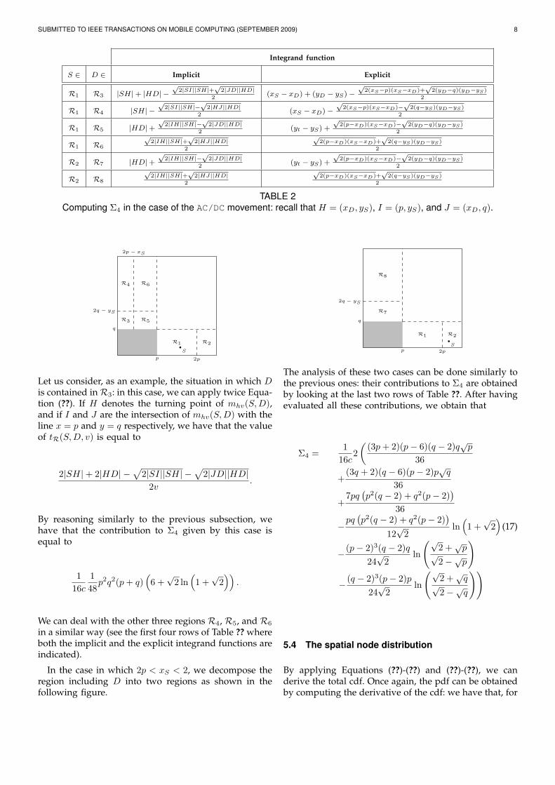
TABLE 2Computing Σ4 in the case of the AC/DC movement: recall that H = (xD, yS), I = (p, yS), and J = (xD, q).

S

2p − xS

p

q

2p

2q − yS

R1 R2

R3

R4

R5

R6

Let us consider, as an example, the situation in which Dis contained inR3: in this case, we can apply twice Equa-tion (??). If H denotes the turning point of mhv(S,D),and if I and J are the intersection of mhv(S,D) with theline x = p and y = q respectively, we have that the valueof tR(S,D, v) is equal to

2|SH|+ 2|HD| −√

2|SI||SH| −√

2|JD||HD|2v

.

By reasoning similarly to the previous subsection, wehave that the contribution to Σ4 given by this case isequal to

116c

148p2q2(p+ q)

(6 +√

2 ln(

1 +√

2))

.

We can deal with the other three regions R4, R5, and R6

in a similar way (see the first four rows of Table ?? whereboth the implicit and the explicit integrand functions areindicated).

In the case in which 2p < xS < 2, we decompose theregion including D into two regions as shown in thefollowing figure.

Sp

q

2p

2q − yS

R1 R2

R7

R8

The analysis of these two cases can be done similarly tothe previous ones: their contributions to Σ4 are obtainedby looking at the last two rows of Table ??. After havingevaluated all these contributions, we obtain that

Σ4 =1

16c2(

(3p+ 2)(p− 6)(q − 2)q√p

36

+(3q + 2)(q − 6)(p− 2)p

√q

36

+7pq

(p2(q − 2) + q2(p− 2)

)36

−pq(p2(q − 2) + q2(p− 2)

)12√

2ln(

1 +√

2)

(17)

− (p− 2)3(q − 2)q24√

2ln

(√2 +√p

√2−√p

)

− (q − 2)3(p− 2)p24√

2ln

(√2 +√q

√2−√q

))

5.4 The spatial node distribution

By applying Equations (??)-(??) and (??)-(??), we canderive the total cdf. Once again, the pdf can be obtainedby computing the derivative of the cdf: we have that, for


0 < x, y < 1,

fp,q<12 (x, y) =

10√x− 3x3/2 − x2

64

+10√y − 3y3/2 − y2

64

+3√

2(x2 + y2

)128

ln(

1 +√

2)

+3√

2(x− 2)2

256ln

(√2 +√x√

2−√x

)(18)

+3√

2(y − 2)2

256ln

(√2 +√y

√2−√y

)The central part of Figure ?? shows the behavior off2(x, y), obtained by combining the above equation andEquation (??).

6 CONNECTIVITY IN THE AC/DC MRWPMODEL

The computation of an upper bound on the commu-nication range in the case of the AC/DC-rMRWP modelproceeds similarly to the case of the rMRWP mobilitymodel analyzed in Section ??. In particular, our resultin this section is the following one.

Theorem 2: There exists a positive constant γ such that

if r = r(n) ≥ γ52

√lnnn , then there exist two positive

constants α and β such that

Pr (G(N, t) is not connected ) <β

nα.

Proof: As it can be verified by analyzing the proofof Theorem ??, in order to obtain an upper bound in thecase of the AC/DC-rMRWP model it suffices to compute alower bound for the following value:∫

Y ∈COf2(Y )dY

where CO is the square at the bottom left corner of Qwhose side is equal to z = 2/k with k =

√5/r(n). This

value is equal to the value g(z) of the cdf computed withinput (z, z), that is,

g(z) =1

384z((

6√

2 ln(1 +√

2)− 4)z3

−4(−6 + z)(2 + 3z)√z

+3√

2(−2 + z)3 ln

(√2 +√z√

2−√z

)).

We now prove that, for any z ∈ [0, 1],

g(z) ≥ 16z5/2.

For the sake of simplicity, we study the following equiv-alent problem:

g(z2)− 16z5 ≥ 0. (19)

After some simplifications, we obtain that

g(z2) =1

192z8(−2 + 3

√2 ln

(1 +√

2))

+1

192z3(−6z4 + 32z2 + 24

)+√

2128

z2(−2 + z2)3 ln

(√2 + z√2− z

)The logarithm in the above expression can be developedinto series as follows:

ln

(√2 + z√2− z

)=∑k≥0

akz2k+1,

where ak =√

22k(2k+1)

. Therefore, if we consider theoperator [zn] which acts on a formal power series h(z) =∑k≥0 hkz

k by extracting the coefficient of zn, that is[zn]h(z) = hn (see, for example, [?], [?]), we have that,for n = 2k + 1 ≥ 6:

bk = [zn](−2 + z2)3∑k≥0

akz2k+1

= [zn](−8 + 12z2 − 6z4 + z6)∑k≥0

akz2k+1

= −8[zn]∑k≥0

akz2k+1 + 12[zn−2]

∑k≥0

akz2k+1

−6[zn−4]∑k≥0

akz2k+1 + [zn−6]

∑k≥0

akz2k+1

= −8ak + 12ak−1 − 6ak−2 + ak−3.

After some simplifications, we have that, for k ≥ 3,

bk =384√

2(2k − 5)(2k − 3)(2k − 1)(2k + 1)2k

. (20)

Consequently, we have that

(−2 + z2)3∑k≥0

akz2k+1 =

∑k≥3

bkz2k+1

−8√

2 +323

√2z3 − 22

5

√2z5.

The function g(z2) can be hence rewritten as follows:

g(z2) =

(√2

64ln(1 +

√2)− 1

96

)z8 − z7

10+z5

3

+√

2128

z2∑k≥3

bkz2k+1. (21)

Now, it can be easily proved that the coefficients bkdefined in Equation (??) are positive for k ≥ 3. Hencein Equation (??) the series

∑k≥3 bkz

2k+1 gives a positivecontribution when computed in z ∈ [0, 1]. Therefore, inorder to prove Equation (??) it is sufficient to prove thefollowing inequality:(√

264

ln(1 +√

2)− 196

)z8 − z7

10+z5

3− 1

6z5 ≥ 0,


or, equivalently,

Q(z) = 5(−2 + 3

√2 ln

(1 +√

2))

z3 − 96z2 + 160 ≥ 0.

Now, the derivative Q′(z) of Q(z) is negative betweenz = 0 and z = 64

5

(3√

2 ln(1 +√

2)− 2)−1 ≈ 7.36. Hence,

the polynomial Q(z) is a decreasing function for z ∈[0, 1]. Since Q(0) = 160 and Q(1) ≈ 72.7, we have thatEquation (??) holds.

We now continue the proof by reasoning exactly as in

the proof of Theorem ??. Let r = r(n) = γ52

√lnnn . For

any cell C, let us denote by µ(C, t) the expected valueof X(C, t). We have that

µ(C, t) ≥ µ(CO, t) ≥n

6z

52 .

By applying the Chernoff bound, we obtain that

Pr[X(C, t) < 1] < µ(C)e1−µ(C).

Hence, the probability that G(N, t) is not connected isbounded by

∑C

Pr[X(C, t) < 1] < k2µ(C)e1−µ(C)

≤ k2n

6z

52 e1−n6 z

52

= k2n

64√

2k

52e

1−n64√

2

k52

=2√

2n3√ke

1− 2√

2n

3k52

=2√

2n√r(n)

3 · 5 14

e1− 2

√2nr

52 (n)

3·554

=2γ

12n4/5 ln1/5 n

3 · 5 14

e1− 2

√2γ

52 lnn

3·554

<2γ

12n

3 · 5 14e

1− 2√

2γ52 lnn

3·554

=2eγ

12n

3 · 5 14

1

n2√

2γ52

3·554

.

By choosing γ > 2.29, we obtain that

Pr (G(N, t) is not connected ) <c

nα

where c and α are two positive constants.Once again, the above theorem implies that, whenever

r(n) ≥ γ 52

√lnnn , the probability that the graph G(N, t) is

connected is greater than 1 − βnα , that is, the communi-

cation graph is connected with high probability.

7 CONCLUSION AND FURTHER RESEARCH

In this paper, we have analyzed the spatial node station-ary distribution of two Manhattan path based variationsof the RWP mobility model. We have then applied theseanalytical results to the computation of upper bounds

on the transmission range guaranteeing, with high prob-ability, the connectivity of the communication graph ofa MANET, whose nodes move according to one of thesetwo models.

From an algorithmic point of view, the main questionleft open by this paper is whether these upper boundsare tight. To this aim, it seems that, unfortunately, thesecond moment method (see, for example, [?]), whichis usually applied to the case of random geometricgraphs, leads, in the case of both the rMRWP and theAC/DC-rMRWP model, to the computation of very dif-ficult integrals. Another very interesting open questionconcerns the possibility of proving similar bounds in thecase of the RWP mobility model. As we have alreadynoticed, the cdf corresponding to this model has a verycomplex expression: indeed, we were not able to proveanalytically that the value h(z) of this function withinput (z, z) is at least equal to 1

6z3 for any z ∈ [0, 1]

(similarly to what we have done in the case of therMRWP model). However, we verified numerically thatthis inequality holds for z = 1/2i, with 1 ≤ i ≤ 200, byusing very high precision computations. On the otherhand, by using similar numerical arguments and variousconstants k = h(1) ≤ 1

4 , we found that the inequalityh(z) ≥ kz 5

2 does not hold for all z ∈ [0, 1]. For this reason,we conjecture that the upper bound on the transmissionrange necessary for guaranteeing connectivity (with highprobability) in the case of the RWP model is equal to

O

(3

√lnnn

). Finally, it would be interesting to obtain

analytical results about the completion time of specificinformation spreading protocols based on MANETs whosenodes move according to one of these two mobilitymodels.

From a mobility model point of view, instead, themain question left open by this paper is whether thegeometric probability arguments that we have used forthe analysis of the rMRWP and the AC/DC-rMRWP modelscan be applied to the RWP model. Even though quitecomplicated integrals might arise, we believe it wouldbe worth deeply analyzing this approach.

REFERENCES

[1] N. Alon and J. H. Spencer. The probabilistic method, Wiley, 2008.[2] F. Baccelli and P. Bremaud. Palm Probabilities and Stationary Queues,

Springer-Verlag, 1987.[3] C. Bettstetter. Mobility Modeling in Wireless Networks: Cate-

gorization, Smooth Movement, and Border Effects. ACM MobileComputing and Communications Review, 5 (2001), 55–67.

[4] C. Bettstetter, H. Hartenstein, and X. Perez-Costa. Stochastic Prop-erties of the Random Waypoint Mobility Model. Wireless Netwroks,10 (2004), 555–567.

[5] C. Bettstetter, G. Resta, and P. Santi. The Node Distribution of theRandom Waypoint Mobility Model for Wireless Ad Hoc Networks.IEEE Transactions on Mobile Computing, 2 (2003), 257–269.

[6] C. Bettstetter and C. Wagner. The Spatial Node Distribution of theRandom Waypoint Mobility Model. In WMAN 2002 (March 25 -26, 2002), 41–58.

[7] T. Camp, J. Boleng, and V. Davies. A Survey of Mobility Modelsfor Ad Hoc Network Research. Wireless Communication and MobileComputing, 2 (2002), 483–502.


[8] A. Clementi, A. Monti, F. Pasquale, and R. Silvestri. InformationSpreading in Stationary Markovian Evolving Graphs. In IPDPS2009 (May 23-29, 2009).

[9] A. Clementi, F. Pasquale, and R. Silvestri. MANETS: High mobilitycan make up for low transmission power. In ICALP 2009 (July 5-12,2009), 387–398.

[10] P. Crescenzi, M. Di Ianni, A. Marino, G. Rossi, and P. Vocca. Spa-tial Node Distribution of Manhattan Path Based Random WaypointMobility Models with Applications. In Sirocco 2009, to appear.

[11] R.B. Ellis, X. Jia, and C. Yan. On random points in the unit disk.Random Structures and Algorithms, 29 (2005), 14–25.

[12] G. Farin. Curves and Surfaces for Computer-Aided Geometric Design:A Practical Guide, Academic Press, 1996.

[13] Gaboune B., G. Laporte, and F. Soumis. Expected Distancesbetween Two Uniformly Distributed Random Points in Rectanglesand Rectangular Parallelepipeds. Journal of the Operational ResearchSociety 44 (1993), 513–519.

[14] P. Gupta and P. R. Kumar. Critical power for asymptotic con-nectivity in wireless networks. In W. M. McEneaney, G. G. Yin,and Q. Zhang (eds.), Stochastic Analysis, Control, Optimization andApplications: A Volume in Honor of W. H. Fleming1999, Birkhauser,1999, 547–566.

[15] D. B. Johnson and D. A. Maltz. Dynamic source routing in adhoc wireless networks. In T. Imielinski and H. Korth (eds.), MobileComputing, Kluwer Academic Publishers, 1996.

[16] E. Hyytia, P. Lassila, and J. Virtamo. Spatial Node Distributionof the Random Waypoint Mobility Model with Applications. IEEETransactions on Mobile Computing 5 (2006), 680–694.

[17] P. Lassila, E. Hyytia, and H. Koskinen. Connectivity properties ofrandom waypoint mobility model for ad hoc networks, Med-Hoc-Net 2005 (June 2005).

[18] J. Le Boudec. Understanding the simulation of mobility modelswith Palm calculus. Performance Evaluation, 64 (2007), 126–147.

[19] D. Merlini, R. Sprugnoli, and M. C. Verri. The method of coeffi-cients. American Mathematical Monthly, 114 (2007), 40–57.

[20] R. Sedgewick and P. Flajolet. An introduction to the analysis ofalgorithms. Addison-Wesley, Reading, MA, 1996.

[21] J. Wu and F. Dai. Efficient broadcasting with guaranteed coveragein mobile ad hoc networks. IEEE Transactions on Mobile Computing4 (2005), 259–270.

Manhattan Path Based RWP Mobility Models: Spatial Node Distribution, Smooth Movement, and...

Documents

Transcript of Manhattan Path Based RWP Mobility Models: Spatial Node Distribution, Smooth Movement, and...