Male students' augmented underperformance with teacher ...

Male students’ augmented underperformancewith teacher-perceived gender stereotypes asscore markers : natural experimental evidencefrom rural Philippines

著者 Okabe Masayoshi権利 Copyrights 日本貿易振興機構（ジェトロ）アジア

経済研究所 / Institute of DevelopingEconomies, Japan External Trade Organization(IDE-JETRO) http://www.ide.go.jp

journal orpublication title

IDE Discussion Paper

volume 734year 2019-01URL http://doi.org/10.20561/00050664

INSTITUTE OF DEVELOPING ECONOMIES

IDE Discussion Papers are preliminary materials circulated to stimulate discussions and critical comments

Keywords: Male-effect Heterogeneity; Supply-side Bias; Test Scores; Human Capital; Philippines JEL classification: D91; I21; I24; I25; I32; J16; O15; O53 * Overseas Research Fellow (Manila) IDE; Visiting Research Fellow, School of Labor and Industrial Relaations, University of the Philippines Diliman ([email protected])

IDE DISCUSSION PAPER No. 734

Male Students’ Augmented Underperformance with Teacher-Perceived Gender Stereotypes as Score Markers: Natural Experimental Evidence from Rural Philippines MASAYOSHI OKABE* January 2019

Abstract Schoolboys in the Philippines are said to be underperforming in human capital accumulation, particularly education, compared to their female counterparts, especially in rural regions. Although existing literature has analyzed the sources of this bias, further research is required to understand its background. Thus, by combining our unique primary data from our own field survey using tailored questionnaires conducted in Marinduque Province and administrative data on the National Achievement Tests (NATs), we compare sources of the persistence of a negative male effect on test scores. We avail of the variations of blindness in rating systems between the NATs and teacher-rating report cards (RCs). Results of sensitivity analysis in regressions support the hypothesis that male students are systematically more likely to receive lower scores when they are evaluated in a non-blind rating system in which teachers know who the examinees are. The paper empirically presents an insightful perspective about Filipino schoolboys’ underperformance being further augmented through gender stereotypes perceived by the evaluators, in this case, the school teachers.

The Institute of Developing Economies (IDE) is a semigovernmental,

nonpartisan, nonprofit research institute, founded in 1958. The Institute merged

with the Japan External Trade Organization (JETRO) on July 1, 1998. The

Institute conducts basic and comprehensive studies on economic and related

affairs in all developing countries and regions, including Asia, the Middle East,

Africa, Latin America, Oceania, and Eastern Europe. The views expressed in this publication are those of the author(s). Publication does not imply endorsement by the Institute of Developing Economies of any of the views expressed within.

INSTITUTE OF DEVELOPING ECONOMIES (IDE), JETRO 3-2-2, WAKABA, MIHAMA-KU, CHIBA-SHI CHIBA 261-8545, JAPAN ©2019 by Institute of Developing Economies, JETRO No part of this publication may be reproduced without the prior permission of the IDE-JETRO.

1

MALE STUDENTS’ AUGMENTED UNDERPERFORMANCE WITH TEACHER-PERCEIVED GENDER STEREOTYPES AS SCORE MARKERS: NATURAL EXPERIMENTAL EVIDENCE

FROM RURAL PHILIPPINES* 1

Masayoshi OKABE** Institute of Developing Economies, Japan External Trade Organization (IDE-JETRO), Chiba, Japan;

University of the Philippines Diliman, Quezon City, Philippines

January 2019

Abstract: Schoolboys in the Philippines are said to be underperforming in human capital accumulation, particularly education, compared to their female counterparts, especially in rural regions. Although existing literature has analyzed the sources of this bias, further research is required to understand its background. Thus, by combining our unique primary data from our own field survey using tailored questionnaires conducted in Marinduque Province and administrative data on the National Achievement Tests (NATs), we compare sources of the persistence of a negative male effect on test scores. We avail of the variations of blindness in rating systems between the NATs and teacher-rating report cards (RCs). Results of sensitivity analysis in regressions support the hypothesis that male students are systematically more likely to receive lower scores when they are evaluated in a non-blind rating system in which teachers know who the examinees are. The paper empirically presents an insightful perspective about Filipino schoolboys’ underperformance being further augmented through gender stereotypes perceived by the evaluators, in this case, the school teachers.

Keywords: Male-effect Heterogeneity; Supply-side Bias; Test Scores; Human Capital;

Philippines

JEL classifications: D91; I21; I24; I25; I32; J16; O15; O53

* This paper is a part of the research output of the author’s current term of the overseas research fellowship in the Philippines. ** Masayoshi Okabe: Overseas Research Fellow (Manila), IDE-JETRO; Visiting Research Fellow, School of Labor and Industrial Relations/Senior Lecturer, College of Education, University of the Philippines, Diliman (concurrent positions). Contact at: +63–921–621–4290; [email protected]; [email protected].

2

ACKNOWLEDGMENT

I wish to express my appreciation to the 2016 research grant program (program ID: D16-R-0798) funded by the Toyota Foundation (Toyota Zaidan), Tokyo, Japan (Grantee: Masayoshi Okabe, with the accepted research title: “A Socioeconomic Analysis on Reversed Gender Disparity in Education from Development Studies Perspective: A case from the Philippines”) for much of my fieldwork activities. I am indebted to Yasuyuki Sawada, the Chief Economist and Director-General, Asian Development Bank and Professor, University of Tokyo, for his invaluable suggestions on the issue setting of the current study. It is under my terms as overseas and visiting research fellow that I have been able to commit long-term preparations and household survey in a rural area in the Philippines till now. I thank the faculty of the University of the Philippines Diliman’s School of Labor and Industrial Relations (UP-SOLAIR) for hosting me (among others, to Maragtas Amante, Ronahlee Asuncion, Emily Cabegin, and Rebecca Gaddi) and the IDE-JETRO (among others, to Takesi Aida for suggesting an empirical approach, Tomohiro Machikita for continuous advice, and Momoe Makino for insightful comments on time-allocation survey designs). In addition, I received invaluable cooperation from the local people of Marinduque Province in the Philippines (among others, Ms. Lolita Natal and Mr. Delfin Natal Jr). The administrative data of score information of the National Achievement Tests (NATs) was provided by the Bureau of Education Assessment (BEA), Department of Education (DepED). Special thanks go to the BEA-DepED (particularly its specialist Ann Legarte and its statistician Ricky Totañes). A part of this study was presented at the 4th Philippine Studies Conference in Japan, held at Hiroshima University, Japan, on November 18, 2018, and I thank Kim Allen, Takeshi Kawanaka, and other participants who gave me comments and suggestions. All possible and potential errors are solely on the author, and the contents and discussions in the current paper do not represent those of any third parties, including the author’s affiliations.

3

CONTENTS

I. INTRODUCTION ............................................................................................................................. 5

II. LITERATURE REVIEW .................................................................................................................... 6

A. On Supply-side Attributes as a Source of Disparities in Education ....................................... 6 B. Teachers’ Stereotypes or Bias that Teachers Have toward Some Students ........................... 8 C. Philippine Settings ........................................................................................................................ 9 D. Reinforcements by Local Representations through Field Observations .............................. 10

III. DATA ............................................................................................................................................ 10

A. Research Site and Sampling ....................................................................................................... 10 B. Collected Information ................................................................................................................. 14 C. Information of Test Scores ......................................................................................................... 16

IV. EMPIRICAL ANALYSES ........................................................................................................... 18

A. Analytical Framework ................................................................................................................ 18 B. Sensitivity Analysis in Benchmark Models ............................................................................. 19

V. RESULTS .......................................................................................................................................... 21

A. Benchmark Results ...................................................................................................................... 21 B. The Same-student Comparisons by Subtracting Blind and Non-blind Scores ................... 24 C. What More Do We Need to Consider? ..................................................................................... 28

VI. CONCLUION .............................................................................................................................. 34

REFERENCE ............................................................................................................................................ 36

APPENDIX I ............................................................................................................................................. 40

APPENDIX II ........................................................................................................................................... 43

4

TABLES

Table 1: Industrial Characteristics of Marinduque Province in Regional and National Contexts

(%, 2015)............................................................................................................................................ 14

Table 2: Descriptive Statistics of z Scores on RC and NATs ............................................................... 17

Table 3: Single Regression of Male Effect on Scores by Test Type and Subject ............................... 20

Table 4: Results of Sensitivity Analysis (Covariates = Individual/household characteristics) ...... 21

Table 5: Results of Sensitivity Analysis (Covariates = Individual and household characteristics +

Region effect) ................................................................................................................................... 22


Region effect + School effect) ......................................................................................................... 23


Region effect + School effect + Male-specific School effect) ....................................................... 24

Table 8: Descriptive Statistics of the Differences between the Two Scores by Subject ................... 25

Table 9: Sensitivity Analysis of Differences between Scores on RC and on NAT by Subject ........ 27

Table 10: Probit Analysis (Probability of the tracking scores on NATs) ........................................... 28

Table 11: Sensitivity Analysis of Differences between Scores on RC and on NAT by Subjects

(Covariates = Specification (5) in the Table 9 + Time-allocation Patterns) ............................... 31

Table 12: Teachers’ Gender Ratios by School Levels and Subjects (Sample Schools) ..................... 32

Table 13: Sensitivity Analysis, Difference Between Scores on RC and on NAT by Subject

(Covariates = Specification (5) in Table 12 + TGRs of each school subject) .............................. 33

Table 14: Sensitivity Analysis, Difference between Scores on RC and on NAT by subject

(Covariates = Specification (5) in Table 11 + Interaction term of male indicator with the

TGRs of each own school subject) ................................................................................................. 34

FIGURES Figure 1: Location of Marinduque Province on the National Map ................................................... 11

Figure 2: Provincial Map of Marinduque ............................................................................................. 12

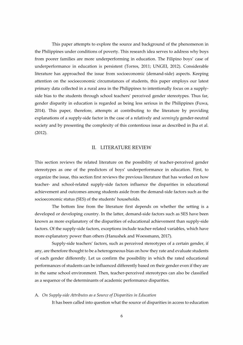
Figure 3: Gender Disparities in Net Enrollment Rates at the Secondary Level .............................. 13

Figure 4: Response Rates of RC Scores (by subjects) and Tracking Rate of NATs Scores .............. 16

Figure 5: Distributions of Differences Between the Two Scores by Subject ..................................... 26

5

I. INTRODUCTION

he long-standing significance of empowerment of females in developing countries is

undoubtable, as women in these parts of the world have been lagging behind their male

counterparts in reaping the benefits of human development. This global issue has continued

to require the mobilization of human wisdom. However, in some developing countries, an

issue has begun to remerge regarding boys’ underperformance in education2 compared to

their female counterparts (UNGEI, 2012).

UNGEI (2012) directly highlights this issue with cases in four East and Southeast

Asian countries: the Philippines, Thailand, Malaysia, and Mongolia. It determined boys’

underperformance from indices not only of access to education but also of quality or

outcomes of education. Furthermore, Cambodia and Bangladesh, referred to as even lower

income countries than UNGEI’s (2012) four countries, have also been reported as regions

where females have started to overtake their male counterparts in education (Zimmermann

and Williams, 2016; Asadullah and Chaudhury, 2009; Khandker et al., 2003).3

Outside the Asia and Pacific region, the same issue has been found in some Latin

American countries (Kitamura, 2015). Surprisingly, though it is considered a patriarchal

region, some Sub-Saharan African countries such as Lesotho and Malawi are reported to

have experienced the same situation (Jha et al. 2012). These were reported with some sense

of astonishment, whereas the school subject-based underperformance of one gender has

been reported in developed countries (OECD, 2014).

If the boys’ underperformance in education merely meant the catch-ups of girls in

those regions over time, we could interpret it as female outperformance of males, which is

welcome. However, the situation is not that optimistic. Difficulties and barriers specific to

male children have not been studied as much as in female cases (UNGEI, 2012). The literature

dealing with boys’ issues is still developing, as the issues are “a more complex phenomenon

than female disadvantages” in education because the male issue “coexists with higher social

and economic positioning, and privileging within family” (Jha et al. 2012: 12). The issue

leading to male underachievement in human capital accumulation processes, if it emerges

more broadly, not only poses an obstacle to males’ own capability development but also can

be of harm for women from a postfeminist perspective (Miralao, 2008).

2 In this paper the author uses the term “’boys’ underperformance’ in education.” The terms “underperform” and “boy” rather than “male” or “man” are derived from the terminology used by UNGEI (2012). 3 According to Asadullah and Chaudhury (2009) and Khandker et al. (2003), the Bangladeshi government introduced an affirmative action called the female secondary stipend (FSS) program in 1994, which has been reported to increase girls’ secondary education.

T

6

This paper attempts to explore the source and background of the phenomenon in

the Philippines under conditions of poverty. This research idea serves to address why boys

from poorer families are more underperforming in education. The Filipino boys’ case of

underperformance in education is persistent (Torres, 2011; UNGEI, 2012). Considerable

literature has approached the issue from socioeconomic (demand-side) aspects. Keeping

attention on the socioeconomic circumstances of students, this paper employs our latest

primary data collected in a rural area in the Philippines to intentionally focus on a supply-

side bias to the students through school teachers’ perceived gender stereotypes. Thus far,

gender disparity in education is regarded as being less serious in the Philippines (Fuwa,

2014). This paper, therefore, attempts at contributing to the literature by providing

explanations of a supply-side factor in the case of a relatively and seemingly gender-neutral

society and by presenting the complexity of this contentious issue as described in Jha et al.

(2012).

II. LITERATURE REVIEW

This section reviews the related literature on the possibility of teacher-perceived gender

stereotypes as one of the predictors of boys’ underperformance in education. First, to

organize the issue, this section first reviews the previous literature that has worked on how

teacher- and school-related supply-side factors influence the disparities in educational

achievement and outcomes among students aside from the demand-side factors such as the

socioeconomic status (SES) of the students’ households.

The bottom line from the literature first depends on whether the setting is a

developed or developing country. In the latter, demand-side factors such as SES have been

known as more explanatory of the disparities of educational achievement than supply-side

factors. Of the supply-side factors, exceptions include teacher-related variables, which have

more explanatory power than others (Hanushek and Woessmann, 2017).

Supply-side teachers’ factors, such as perceived stereotypes of a certain gender, if

any, are therefore thought to be a heterogeneous bias on how they rate and evaluate students

of each gender differently. Let us confirm the possibility in which the rated educational

performances of students can be influenced differently based on their gender even if they are

in the same school environment. Then, teacher-perceived stereotypes can also be classified

as a sequence of the determinants of academic performance disparities.

A. On Supply-side Attributes as a Source of Disparities in Education

It has been called into question what the source of disparities in access to education

7

and educational outcomes across individuals is, not only limited to gender disparities but

also in general. A dichotomy between demand and supply sides of education is a primary

and straightforward framework. On one hand, it was believed that the school attributes as

supply-side factors served as a key predictor of educational outcomes of students.

Heyneman and Loxley (1983) argued that in developing countries, school- and teacher-

related variables accounted for a greater proportion of variance of student achievements than

demand-side (individual- and household-level) SES did. It was called the “HL effect”

(Huang, 2010). This was offset by the so-called Coleman Report, which reported low

explanation powers of school-resource attributes for educational outcomes of students in the

United States (Coleman et al., 1966). Relationships between demand- and school-side factors

on educational outcomes have then been a big issue in related fields (Baker et al., 2002;

Bouhlila, 2015; White, 1982).4

Nonetheless, later literature seems to converge toward denial of the HL effect.5 It

admits the demand-side SES in developing countries accounts for much more than the

supply-side variables6 (Hanushek, 2006; Hanushek and Woessmann, 2017). The pros and

cons of the HL effect have still been a central question in the fields of education and

development because the supply-side variations are the (possibly only) policy variables on

which governments can intervene directly by arranging educational improvement through

public policies.7 A more recent study by Hanushek and Woessmann (2017) surveyed the

4 Some scholars do not sufficiently emphasize the supply side factors but place considerable importance in demand side factors. There emerged a controversy regarding Heyneman (1989) and Riddell (1989a and 1989b) in a developing country setting. 5 For example, Baker et al. (2002) conducted a comparative analysis of over 29 developing and developed countries using the Trends in International Mathematics and Science Study [TIMSS] ; Riddell (1997) for cases of Botswana, Brazil, Columbia, Egypt, Honduras, India, Jordan, Namibia, Pakistan, the Philippines, Thailand, and Zimbabwe; Huang (2010) for the Philippines; Bouhlila (2015) confirming Baker et al. (2002) for the TIMSS case in the Middle East and North African (MENA) countries. Meta-analysis covering 96 studies on the school-side effects on educational outcome found inconsistency in the explanation powers of the school-side variables in developing countries (Hanushek, 2006). 6 Regarding the background of a weakened and vanishing HL effect, Baker et al. (2002) interpreted that “[i]nvestment in mass schooling by nation-states and multilateral agencies, backed by an ideology of providing some minimum level of school quality throughout the nation, has shifted the potential toward greater direct family SES effects in the social stratification process,” “[t]he macroprocess of mass schooling across a large part of the world may have achieved a resource threshold in the quality of schooling,” and “[t]his is one very plausible explanation for a shifting HL effect over time” (Baker et al. 2002: 310). 7 I do not mean that demand-side–centered interventions of governments to livelihoods of poor students and families, e.g., school subsidy programs, are not a policy option to contribute to educational improvement. Here, it must be noted that the betterments of access to education and of quality of education differ from each other.

8

later literature and confirmed the same trends that the surveyed studies found regarding

little significant explanatory power of the supply-side attributes, with exceptions such as the

attributes of school teachers.

In the literature, variations of school-side factors have been gauged as overall effects

that are homogeneous for male and female students. Yet, the supply-side factors can be

transvalued if introducing the perspective of heterogeneity of the ways in which supply-side

factors influence different groups of students. In the context of the current study, the

interactions of gender-based stereotypes are thought to be one of such typical heterogeneous

examples.

B. Teachers’ Stereotypes or Bias that Teachers Have toward Some Students

School teachers are almost always near their students. As confirmed in Subsection

A of this section, teachers’ variations are said to be an exceptionally stronger predictor than

other school-related inputs (Hanusheck and Woessmann, 2017). At the same time, teachers

are also occasionally reported to perpetrate stereotyping, which in turn affects students’

educational outcomes (Lavy, 2008; Torres, 2011; UNGEI, 2012). Emerging literature by Lavy

(2008) and its successors, such as Cornwell et al. (2013) and Lavy and Sand (2018), opened a

new approach to empirically study the effect of teachers as a source of stereotypes perceived

against some students. Teachers had already been thought by educational psychology to be

the source of unfavorable stereotypes of female students in particular school subjects such

as math (Dusek and Joseph, 1983; Riegle-Crumb and Humphries, 2012; Tiedemann, 2000;

Tiedemann, 2002).

Lavy (2008) deals with an Israeli case and Cornwell et al. (2013) with a US case and

find such teachers’ stereotypes treat male students more unfavorably than females. In turn,

Lavy and Sand (2018) studied the same Israeli case by more directly focusing on the

consequences of such stereotypes on female students’ progress in the advanced science track

in senior high schools and find that there are unfavorable stereotypes for female progress to

the advanced tracks. Unfavorable female stereotypes are also found consistently in a French

case (Terrier, 2015) and an Italian case (Carlana, 2017). As every study states, the direction

toward females is strongly observed on the science track since it has been believed that math

and sciences are male-dominated subjects in general (OECD, 2014).

Yet, these studies tested cases mostly in developed countries. 8 In developing

8 The term “developed countries” is gauged here as OECD member countries. Israel is one. Based on the literature survey by Lavy and Sand (2018), the applications of the initial study by Lavy (2008) range from teachers’ gendered stereotypes to racial discriminations in UK high schools

9

countries, there are few studies of the case. Data accessibility is possibly one of biggest

obstacles because the documentation storage methods of schools and central governments

differ greatly from those of developed countries. It can also fall afoul of privacy issues.

However, given that the Philippines is one emerging country where boys’

underperformance is prevailing, it is highly relevant to study this by applying the

aforementioned research framework to the country.

C. Philippine Settings

A desk review by Torres (2011) lists concerns regarding Filipino boys’

underperformance in education: higher dropout rates; earlier linkage to economic activities;

lower functional literacy rates; and lower scores across subjects and on NATs. She also

mentions that Filipino boys are prone to be victims of corporal punishment. Some mode like

hidden curriculum in classrooms can also unconsciously be exercised in an explicit curriculum

but can be perceived to be a certain mode of messages by learners like prejudicial.

According to the UNGEI (2012), teachers are described as a stereotyping factor.

Torres (2011) warns that the school environment nature is not gender-neutral in the

Philippines and stereotypes impede boys’ potential and achievement in education. She adds

that the teachers’ perceived stereotypes in a school environment are often perpetuated by

inadequate male role models and guidance process (e.g., due to lack of male teachers).

However, what has been lacking is data, particularly data disaggregated by gender, regional

and geographical locations, socioeconomic background, and ethnicity. Without this data, the

existence of stereotypes and bias embedded in learning environment remains hardly tested.

It is then good to question whether the stereotypes are a source of the Filipino boys’

persisting underperformance in education. In the HL effect literature, the country was not

included in the developing countries that Heyneman and Loxley (1983) studied. Later,

Riddell (1997) included the Philippines in her case studies and showed that the HL effect

was not confirmed in the Philippine case along with cases of Botswana, Brazil, Columbia,

Egypt, Honduras, India, Jordan, Namibia, Pakistan, Thailand, and Zimbabwe. Huang (2010)

also denied the HL effect by employing the household survey that was conducted by the

government in Cebu, Philippines, through closed analysis to Riddell (1989a). Yet, as said by

Hanushek and Woessmann (2017), teachers are one exceptional variable in testing the HL

effect.

(Burgess and Greaves, 2013), discriminatory influences on black students in Brazilian schools (Botelho et al.,2015), and foreign students in Swedish high schools (Björn et al. (2011)

10

D. Reinforcements by Local Representations through Field Observations

Our observations in the fields also confirm that some male youths can be

stereotyped by adults including teachers (see also a Western Visayas case in Okabe, 2018).

For example, the inclination of male youths to be lazy was often raised by local adults as a

primary reason why they think male youths tend to lag behind their female counterparts in

education. More surprisingly, not few mothers that we encountered in our current study

area in Marinduque boldly stated that their sons had low IQs (intelligence quotients):

––“Oo naman, tamad nga kasi ang mga lalaki namen.” (Yeah certainly, because our boys

are lazy.)

––“Mababa din kasi ang IQ nila.” (In addition, because their IQ is low.)

According to them, however, the sons’ IQs had not ever been actually measured.

Our interviewees, public school teachers, added that male students were much more out of

their control in classes. They described that some male students came to be much more

violent as they grew.

By combining the above related perspectives from the literature and some local

representations and observations, this study aims to fill the literature gap by working on the

question on the gender-heterogenetic stereotypes from school teachers, which has not been

satisfactorily addressed so far. The local representations provided an eloquently reinforced

hypothesis that the adults’ perceptions can sometimes be a negative bias against youths.

The structure of the paper is as follows: Section III provides the data, explaining the

choice and characteristics of research site, the sampling technique, and the collected

information. Section IV explains our analytical framework and empirical analysis. Section V

shows the research results, by beginning with the benchmark results then reaching some

additional analyses for robustness checks. Finally, Section VI spells out the conclusion and

limitations for future study. Appendices I and II provide some supplementary information

for the readers’ references.

III. DATA

A. Research Site and Sampling

The data employed in the current study comes from our tailor-made questionnaire-

based household survey. The data collection was prepared from August 2017, and then the

household survey was intensively conducted from January to March in 2018. Approximately

11

150 households with information of around 300 children were covered from nine barangays

(the local government unit in the Philippines) in three municipalities, say, Boac, Gasan, and

Buenavista, in the Province of Marinduque (see Fig. 1 and Fig. 2). The municipalities,

barangays, and households were randomly chosen through the stratified random sampling

technique based on the master list from the Community-based Monitoring System (CBMS) that

the local government units provided.9

Figure 1: Location of Marinduque Province on the National Map

Source: Adapted from http://www.freemap.jp

9 In August 2017, the author paid courtesy calls to every municipality hall to see mayors/representative of three municipalities. In this occasion, the barangay lists were collected from the municipalities. The collection of CBMS information at a barangay level was also helped by the author’s local counterparts.

12

Figure 2: Provincial Map of Marinduque

Notes: The circles A–I represent the nine sampled barangays.

Source: Hand-drawn by the author.

Marinduque Province belongs to the Region IV-B (MIMAROPA). Because Filipino

male youths start to lag behind females typically in secondary-level education, one of the

regions with the largest gender gap in access to secondary-level education was first chosen.

It is the Region IV-B, called MIMAROPA Region (Fig. 3). According to Fig. 3, male youths

lag behind their female counterparts more in rural regions outside of Luzon Island than

regions on Luzon Island. The regions in MIMAROPA, Visayas, and Mindanao are opposition

to Metro Manila and Central Luzon where boys’ underperformance is much less severe.

Region IV-B, MIMAROPA, used to be referred to as the Southern Tagalog Region.

Marinduque Province is considered the geographical center of the Philippine archipelago; it

is a heart-shaped island with a total land area of 952.58 square kilometers (Gaddi, 2018). The

municipality Gasan is where purok Quatis in the barangay Masiga (the circle D in the Fig. 2)

can be found.10 The purok Quatis has been the author’s research stronghold, whereby our

preparatory fieldworks and observations and data collection works, including dry runs of

questionnaire survey, have been spread to the other sites in order. There are no major cities

10 A purok is a Filipino term meaning a district within a barangay.

13

in Marinduque Province, which is comprised of only municipalities. Most of our study

barangays are remote from poblacion, referring to central and commercial zones, in each

municipality. Out of nine barangays, two barangays are classified as poblacion in two

municipalities.

Figure 3: Gender Disparities in Net Enrollment Rates at the Secondary Level

Note: “(Female–Male)/Enrl(Male & Female)” means the proportion of differences of female-to-

male enrollment rates over the total enrollment rates. “Enrl(Male & Female)” means the total enrollment rates of both males and females.

Source: FLEMSS 2013, PSA.

Marinduque’s regional economy depends on primary industries such as agriculture

(mainly palay [paddy rice] and coconut), horticulture (vegetables), and fishery. It also

depends on craftworks and micro-business. The province’s economy is outstanding in the

regional and national contexts in terms of the dominance of self-employment (Table 1).

According to Table 1, the occupational rate of self-employment is dominant, reaching 45.80%

in Marinduque Province compared to 37.42% in the MIMAROPA Region and 32.94% on

average nationally in rural areas. The province’s high self-employment rate comes at the

expense of the rate of private establishment, which is much lower in the province at 26.72%

than the regional and national rural averages of 34.24% and 38.11%, respectively. These

imply that the private firm-driven sectors are, by and large, yet far from developing in the

0 10 20 30 40 50 60 70 80

Country’s AverageMetro Manila (NCR)

Illocos RegionCordillera Administrative Region

Cagayan Valley RegionCentral Luzon Region

CALABARZON RegionMIMAROPA Region

Bicol RegionWestern Visayas RegionCentral Visayas Region

Zamboanga Peninsula RegionNorthern Mindanao Region

Davao RegionSOCSARGEN Region

Caraga RegionAutonomous Region in Muslim Mindanao

(Female -Male) / Enrl (Male & Female) Enrl (Male & Female)

14

province. In exchange of its underdeveloped private sector, the governmental (public) sector

absorbs more workers than regional and national rural average.11

Table 1: Industrial Characteristics of Marinduque Province in Regional and National

Contexts (%, 2015)

Occupation Categories National

Region Province Urban Rural

Private household 6.66 4.38 4.43 4.58

Private establishment 53.30 38.11 34.24 26.72

Governmental corporation 9.38 8.62 9.62 12.21

Self-employed 23.08 32.94 37.42 45.80

Employer 2.64 4.73 4.31 1.53

With pay (family-owned business) 0.43 0.29 0.46 0.00

Without pay (family-owned business) 4.51 10.94 9.53 9.16

Number of observations (persons) 28,814 49,734 2,392 262

Note: Region = MIMAROPA region (Region IV-B); Province = Marinduque province.

Source: LFS 2015, PSA.

B. Collected Information

Our intensive survey collected information in the three categories: (1) individual

characteristics of the sampled children who are mainly teenaged/in high school, (2) schooling

and education profiles of the children, (3) basic information about their families, and (4) time-

allocation patterns of two selected children per household. (1), (2), and (4) were directly

asked to the children (siblings), whereas (3) was asked to one of their parents or grandparents

(adult guardians). In a few cases where the guardians were not available at the timing of our

household survey, relatives (uncles/aunts or grandparents) responded on their behalf. A

detailed summary of variables in the empirical analyses is presented in Appendix I.

The first category, children’s characteristics, is a set of data that includes names, sex,

birthday, birth order, and number of siblings. The second category is regarding enrollment

status and school-related information if enrolled or reasons for quitting schooling if not

11 In this sense, Marinduque Province is similar to Bukidnon Province (which Chapters 2 and 3 discuss) in terms of the nature of underdevelopment of private sectors within the provincial economy and in the correspondingly substituting role by the public sector.

15

enrolled. For the third category on basic family information, we collected the demographic,

educational, working, and earning information of parents, including the home addresses.

These deserve control variables and are reported in summary statistics in Appendix I. The fourth category, a time-allocation survey, is a collection of the allocations of (1)

home time and (2) working time, based on classifications of Lam and McHale (2015). It

collected daily information for a week (7 days) to attempt to mitigate time-variant incidents

and then collect information based on their usual (average) patterns of activities.12 The home

time includes sleep/rest and leisure activities such as playing. The children’s working time

in a day includes studying at home and laboring for family members (e.g., helping with

parents’ work and household chores). Combining the classifications of activities by Lam and

McHale (2015) in our own preliminary observations as to how the children spend their time

every day, the questionnaire of daily activities (like a diary) was semi-structured, meaning

that most of the questionnaire was structured while leaving an unstructured (free-style) part.

In the structured part, the children were asked how much time (in minutes) they

spent on the following activities: sleeping, schooling, helping their father and mother with

their respective work, household chores, studying at home, playing outside/with friends,

and going to a computer game shop. They were also asked the number of times they attended

schooling in a week (namely, number of absences). In the unstructured part, we asked what

other activities they did and for how long, if at all (free description).13 The questionnaires

were self-administered. After collecting the filled questionnaires in 7 days, the author

checked if there were unclear parts to modify. If critical contradictions and/or completely

unclear answers were found, we did not allow the survey to be completed and asked the

12 Each set of questionnaire consists of seven sheets, from the first to the seventh day. Although the start date of the first day is not shared across individuals, the date of the first day was recorded in the questionnaire sheet to control for timing variations as well as to identify whether it was a working day or weekend/holidays and to note the day of week (e.g., Sunday, Monday, etc.). 13 As unstructured parts of activities, children could also report their extra activities such as magsimba (going to church to attend a Christian Mass particularly on Sundays) and out-of-school practices (e.g., group dance practices) and/or irregular events (e.g., funeral, marriage parties), if any. However, this information is not actually used for our quantitative analysis, because their answers seem to suffer from selection problem (a distinct difference between children who are providing detailed information and children who do not provide any information on these extra activities) and because interpretations of this information are difficult, both coming from the truncated response frequencies. The author checked and moved to the structured part if some of the activities reported in the free descriptions were indicated in structured parts. Nonetheless, there seems to have still remained an issue of selection. We lack judgment as to whether some children kept some activities reported and others unreported, but they actually did. Yet, the contents were very helpful to know and learn how and for what the youths in our sample spent their time qualitatively.

16

child to refill with the correct information. If minor errors were found, the author would

manually check and correct these by contacting the children and conduct follow-up

confirmations by additional contacts. The mean comparisons tell us that there are clearly

gendered patterns in the time-allocation patterns (see Section D in Appendix I for details).

C. Information of Test Scores

The test scores of students were collected via the following two channels: direct

interviews and administrative data provided by the government. The sample children were

asked their latest scores on the teacher-based report card (hereafter, scores on RC) regarding

seven school subjects: national language (Filipino), math, English, science, social studies14,

MAPEH (music, arts, physical education, and health), and TLE (technology and livelihood

education). When asking about the RC scores, we carefully explained to each child using

both an oral and written explanation that the collected information would be immediately

encoded into numerical and anonymous data which would keep individuals unidentifiable,

and their proper names would never appear in the analyses and results. This dedicated

explanation let the respondents feel at ease to answer the questions and thus achieve high

rates of response regarding RC scores (see Fig. 4).

Figure 4: Response Rates of RC Scores (by subjects) and Tracking Rate of NATs Scores

Note: The rate of scores on NATs is based on the number of students who are in

Grade 7 or above. Source: Author’s own calculation.

In turn, the score information of NATs was provided as the administrative data by

14 It is locally called HeKaSi or Araling Panlipunan. The former initials the Heograpiya, Kasaysayan at Sibika, meaning Geography, History, and Civics, and the latter means the social studies (aralin means study, -(n)g serves as a linker connecting with another word, and panlipunan means social).

0.00%

20.00%

40.00%

60.00%

80.00%

100.00%

Filipino Math English Science SocialStudies

MAPEH TLE NATs (5subjects)

17

the national government (DepED) with respect to the same children in our sample who are

in or above the seventh grade (students lower than grade 6 do not yet have their own NAT

scores). The office in charge is the BEA in the DepED, and we made a formal request to the

office for the NAT data. The BEA-DepED took a considerably long time to try tracing the

sample students listed in the request before finally providing us with the NAT score data of

55% of the children from our sample children. The NAT is the Nationwide Achievement Test

supervised by the DepED comprising five subjects: Filipino, English, math, science, and

social studies (HeKaSi or Araling Panlipunan).

Table 2: Descriptive Statistics of z Scores on RC and NATs

Non-blind score (RC)Filipino 275 0.34 -0.38 0.72Math 274 0.26 -0.30 0.56English 274 0.40 -0.47 0.87Science 270 0.33 -0.39 0.72Social Studies 259 0.34 -0.38 0.72MAPEH 269 0.32 -0.38 0.71TLE 240 0.28 -0.35 0.63

Blind score (NAT)Filipino 135 0.00 0.00 0.00Math 135 -0.01 0.02 -0.03English 135 0.04 -0.06 0.10Science 135 0.04 -0.07 0.11Social Studies 135 0.06 -0.10 0.16

Scores and Subjects Δ(F - M)Obs Female (F) Male (M)

Notes: MAPEH = Music, Arts, Physical Education and Health; TLE = Technology and Livelihood Education. Source: Author’s own calculations.

Both RC and NAT scores are standardized into z scores: 𝑧𝑧𝑖𝑖𝑖𝑖 = (𝑅𝑅𝑖𝑖𝑖𝑖 − 𝑅𝑅𝑖𝑖��) 𝑠𝑠𝑖𝑖⁄ , where

𝑅𝑅𝑖𝑖𝑖𝑖 means the individual percentage scores of child 𝑖𝑖, the 𝑅𝑅𝑖𝑖�� is the mean score of the subject

set 𝑆𝑆, and 𝑠𝑠𝑖𝑖 means the standard deviations of the subject set 𝑆𝑆. The raw scores on RC are

rated as if they had the nonzero minimum score because they range mostly from 75 to 100,

unlike the raw percentage scores on NATs that can range from 0 to 100, due to the education

system of the Philippines. Scores on RC contain information through which teachers provide

18

evaluation, that is, “fail,” if under 75 or “pass,” if above 75. Those students who performed

really poorly enough to be judged as “failure” (a factor to repetition) would get scores on RC

lower than 75 (but this proportion is actually low). The standardization into z scores is useful

in this sense that it will be more comparable across the scores from different tests and exams.

Theoretically, the mean values of z scores take zero. The difference from zero is interpreted

as a size of standard deviation (SD).

Table 2 shows the descriptive statistics of z scores on NATs and on RC by school

subject. Obviously, male students receive lower scores on RC (non-blind scores) across all

subjects. The gaps between male and female averages range from 0.56 SD for math to 0.87

SD for English. This means that even in math, which is generally assumed to be a subject that

male students perform better at, male students are underperforming compared to their

female counterparts.

Intriguingly, the scores on NATs show much smaller gender gaps in contrast to the

RC scores. The gaps are largest in social studies with a 0.16 SD size and smallest (not

detected) in Filipino with a 0.00 SD size. In math, the female students received slightly lower

scores on average than their male counterparts. The mean comparisons deliver two key

points: The gender gap is much more prominent on the non-blind scores than on the blind

scores, and the subject-base variations are also large depending on the subject.

IV. EMPIRICAL ANALYSES

A. Analytical Framework

The rating system of NATs is conducted blindly and is done mechanically on the

basis of numbers of questions correctly answered by external markers who do not know

about the examinees. In contrast, the scores on RC are rated in a non-blind way by school

teachers, who know about the evaluated (i.e., their students). The classification into “blind”

and “non-blind” rating systems refers to what Lavy (2008) did. Applying the framework of

Lavy (2008), who focused on the blind and non-blind rating settings of matriculation exams

in Israeli public high schools, we hypothesize that the bias and perceptions of teachers

toward some of their students, if any, will influence the rating of RC scores (non-blind scores)

compared to NAT scores (blind scores). We also hypothesize that such stereotyping can be

exercised even unconsciously and unintentionally by teachers. Lavy (2008) empirically

regards the situation of having both blind and non-blind rating manners as a natural

experimental setting where only the blindness in the evaluations changes and the blindness

in the rating system is not a choice variable (i.e., examinees cannot choose or change the

19

blindness setting endogenously).

As expected, the mean comparisons shown in Table 2 exhibit larger gender gaps on

RC scores but much smaller or insignificant gender gaps on NAT scores in the same school

subject sets (Subsection C in Section III). Our research aims to examine the channel through

which the boys’ persisting underperformance in education can be explained by their

evaluators, namely, their school teachers.

B. Sensitivity Analysis in Benchmark Models

To test the bias and stereotype, we rely on the regression analysis, not merely on

two-dimensional comparisons of mean values and descriptive statistics, because the effect of

being male should be interpreted as a marginal effect or partial derivative, where other

possible variables are controlled at constant (ceteris paribus).

In particular, we explore the sensitivity analysis by which we check the extent to

which the effect of variable of interest is sensitive or stable through various specifications as

other explanatory variables are included. This approach is relevant to a proposed method in

recent works by Oster (2017) or in the original works by Altonji et al. (2005) and Bellows and

Miguel (2009). Oster (2017) propounds exploring the sensitivity of coefficient stability when

and after other controls are additionally included in regression equations and the transitive

changes in R2, to examine the robustness of treatment effect in order to cope with the

situation in which the observed variables do not fully capture the omitted unobserved

characteristics. The discussions in Section II require incorporation of the SES variables as

explanatory variables before supply-side factors. Therefore, by transitive changes from a

very simple model to complex models where more SES-related covariates are controlled, our

focus is on the persistence of the gender variable.

The econometric models are built as follows. To begin with, the simplest model is

given by:

𝑆𝑆𝑖𝑖𝑖𝑖𝑖𝑖 = 𝛼𝛼0𝑖𝑖𝑖𝑖 + 𝛼𝛼1𝑖𝑖𝑖𝑖𝑀𝑀𝑖𝑖 + 𝑒𝑒𝑖𝑖𝑖𝑖𝑖𝑖, (1)

where the dependent variables 𝑆𝑆𝑖𝑖𝑖𝑖𝑖𝑖 are the standardized z scores of the student 𝑖𝑖, on the

test type 𝑗𝑗 = {NATs, RC}, and the set of school subject areas 𝑠𝑠 = {Filipino, math, English,

science, social studies, MAPEH, TLE}; 𝛼𝛼0 is the intercept; 𝑀𝑀𝑖𝑖 is the male indicator taking 1

if the individual 𝑖𝑖 is male and 0 otherwise. In Eq. (1), no covariates are controlled. 15 Table

3 shows the results. This simple regression reconfirms the results in Table 2.

15 On the NATs, MAPEH and TLE are not examined.

20

Table 3: Single Regression of Male Effect on Scores by Test Type and Subject Filipino Math English Science Soc. Stu. MAPEH TLE

Scores on NATs:

Male (=1) 0.12 0.34** 0.16 0.07 0.12 n.a. n.a.

[0.18] [0.14] [0.15] [0.15] [0.14] n.a. n.a.

Adj. R2 0.08 0.41 0.35 0.36 0.37 n.a. n.a.

No. of Obs. 128 128 128 128 128 n.a. n.a.

Scores on RC:

Male (=1) -0.72*** -0.56*** -0.87*** -0.72*** -0.72*** -0.71*** -0.63***

[0.11] [0.12] [0.11] [0.11] [0.12] [0.12] [0.12]

Adj. R2 0.13 0.08 0.18 0.12 0.12 0.12 0.10

No. of Obs. 275 274 274 270 259 269 240 *** 𝑝𝑝 < 0.01; ** 𝑝𝑝 < 0.05; * 𝑝𝑝 < 0.01. Notes: 1. Soc. Stu. = Social Studies; MAPEH = Music, Arts, Physical Education and Health; TLE = Technology and Livelihood Education.. Numbers in brackets are robust standard errors. 2. Coefficients of other covariates are omitted in this report for space and visual purposes. Source: Authors’ own calculation.

Then, we need to put the vector 𝐗𝐗 containing individual characteristics and

household-level SES. Appendix Table 1 provides the summary statistics of the dependent

and independent variables, and Appendix I describes the variables that are used as covariates.

Whereas these variables are gradually added as covariates into the regression models by

specifications, the main part of this paper shall omit reporting the coefficients of the other

covariates in the tables for the sake of space and visuality. The full report corresponding to

the full model is available in Appendix II.

Next, we put some fixed effects in the models to further control for some

unobservable factors: 𝜌𝜌 denotes the school year (SY) effect capturing difficulty levels of

NATs in each SY that can vary in some SYs; 𝜔𝜔 denotes the region-specific effect to control

for unobservable heterogeneity across the barangays; and 𝜑𝜑 denotes the school effect to

control for unobservable heterogeneity in attributes of teachers and schools. Particularly, 𝜑𝜑

is decomposed into the overall part, 𝜑𝜑𝑎𝑎𝑎𝑎𝑎𝑎, and the male-specific part, 𝜑𝜑𝑀𝑀 (i.e., 𝜑𝜑 = 𝜑𝜑𝑎𝑎𝑎𝑎𝑎𝑎 +

𝜑𝜑𝑀𝑀). The model is now rewritten as:

𝑆𝑆𝑖𝑖𝑖𝑖𝑖𝑖 = 𝛿𝛿𝑖𝑖𝑖𝑖𝑀𝑀𝑖𝑖 + 𝐗𝐗𝐢𝐢𝐢𝐢𝛃𝛃𝐢𝐢𝐣𝐣 + 𝜌𝜌 + 𝜔𝜔 + 𝜑𝜑 + 𝑢𝑢𝑖𝑖𝑖𝑖𝑖𝑖. (2)

The idea of exploring sensitivity is like this: Expected signs of 𝛿𝛿s are negative, but

when 𝛿𝛿s are negative, the extent of the persistence of 𝛿𝛿 is of our interest. If the individual

characteristics and household-level SES already capture sufficiently the influences of being

male, then the insignificant relation 𝛿𝛿 = 0 can no longer be rejected. If the added covariates

21

do not yet capture them, 𝛿𝛿 is still expected to be statistically significant and negative. In turn,

if the sources of male effect mainly include regional heterogeneity, 𝛿𝛿 will be

indistinguishable from taking zero once the region-specific effects are controlled for.

Likewise, if the teachers’ in-school factors play highly as the source of male effect, here 𝛿𝛿

will be indistinguishable from taking zero once those school effects are controlled for. In sum,

sensitive analysis allows to check the persistence of the male effect as other covariates and

fixed effects are added in the specifications.

V. RESULTS

A. Benchmark Results

1. Male effect when other individual and household characteristics are controlled

To begin, Table 4 shows the result of regression analysis when individual and

household characteristics are controlled as covariates. The male effects do not qualitatively

change from the result of single regression in Table 3. The male effect is not detected on the

scores on NATs, except for math where the male effect is positive, but it is robustly persistent

on the scores on RC through all the subjects. Whereas male students perform well in math

relative to their female counterparts on the blind scores, they underperform on the non-blind

scores across all subjects including math, MAPEH, and TLE.

Table 4: Results of Sensitivity Analysis (Covariates = Individual/household characteristics) Filipino Math English Science Soc. Stu. MAPEH TLE

Scores on NATs:Male (=1) 0.00 0.29* 0.05 0.02 0.08 n.a. n.a.

[0.19] [0.15] [0.15] [0.16] [0.16] n.a. n.a.

Adj. R2 0.23 0.49 0.46 0.44 0.47 n.a. n.a.No. of Obs. 128 128 128 128 128 n.a. n.a.

Scores on RC:Male (=1) -0.69*** -0.66*** -0.86*** -0.85*** -0.59*** -0.62*** -0.68***

[0.17] [0.17] [0.15] [0.15] [0.18] [0.16] [0.17]

Adj. R2 0.23 0.30 0.35 0.35 0.29 0.32 0.31No. of Obs. 256 255 255 251 241 250 221

*** 𝑝𝑝 < 0.01; ** 𝑝𝑝 < 0.05; * 𝑝𝑝 < 0.01. Notes: 1. Soc. Stu. = Social Studies; MAPEH = Music, Arts, Physical Education and Health; TLE = Technology and Livelihood Education.. Numbers in brackets are robust standard errors. 2. Coefficients of other covariates are omitted in this report for space and visual purposes. Source: Authors’ own calculation.

22

2. Male effect when the region effect is additionally controlled

Estimations in the results of Table 5 further add the barangay-level region effect to

control for unobserved heterogeneity across the living places. The adjusted R2 increases in

all the subjects in Table 4, and so the regional heterogeneity has some explanation power on

the scores. Yet, the patterns of marginal effect of being male on both scores remain persistent

and are qualitatively the same as in Table 4.

Table 5: Results of Sensitivity Analysis (Covariates = Individual and household

characteristics + Region effect)

Filipino Math English Science Soc. Stu. MAPEH TLEScores on NATs:

Male (=1) 0.00 0.29* 0.05 0.02 0.08 n.a. n.a.[0.19] [0.15] [0.15] [0.16] [0.16] n.a. n.a.


Scores on RC:Male (=1) -0.77*** -0.61*** -0.94*** -0.83*** -0.63*** -0.74*** -0.64***

[0.15] [0.13] [0.13] [0.13] [0.15] [0.14] [0.15]

Adj. R2 0.25 0.35 0.37 0.38 0.33 0.31 0.30No. of Obs. 256 255 255 251 241 250 221


3. Male effect when the school effect is additionally controlled

Next, estimations in the results of Table 6 further add the school effect to control for

unobserved heterogeneity on school attributes. As compared to Table 5, the positive male

effect on math on the blind scores turns out to be insignificant here. Yet, the male effect still

remains persistently negative through all subjects on the non-blind scores.

4. Male effect when male-specific part of school effect is isolated and additionally controlled

Furthermore, to isolate unobserved heterogeneity that can affect selectively on male

students in schools, the male-specific part of school effect, 𝜑𝜑𝑀𝑀, is set apart and added in the

23

equation. The results are shown in Table 7. There are two noteworthy changes in Table 7.

First, the male effect on NATs (blind scores) here becomes positive once again for math and

positive recently for English and science (in the upper stage of Table 7). Second, the male

effect is consistently negative so far, but vanishes on scores on RC regardless of the subject

(in the lower stage of Table 7).

Initially, there was minor gender difference on the scores on NATs when comparing

the mean values. This has remained even after other individual- and household-level

characteristics, unobserved heterogeneities across living places and schools, and some school

year-specific difficulty levels are controlled at constant. However, once 𝜑𝜑𝑀𝑀 is also controlled,

the male effect becomes positive on math, English, and science in Table 7.

Table 7 shows that, if 𝜑𝜑𝑀𝑀, say, male-specific but directly unobserved environment

for male students in schools, gets controlled at constant, being male alone would predict

higher scores of math, English, and science on the NAT than their female counterparts.

However, the estimation including 𝜑𝜑𝑀𝑀 indicated the “underestimation” of the male effect

until the previous specifications without 𝜑𝜑𝑀𝑀 toward the direction to zero unless the former

effect is controlled. Namely, some sort of within-school environment selectively to male

students may be masking such potentiality of male students. In other words, the source of

the considerable part of the negative male effect that has been persistently detected on the

RC scores is in the schools.


characteristics + Region effect + School effect) Filipino Math English Science Soc. Stu. MAPEH TLE

Scores on NATs:Male (=1) -0.18 0.16 -0.07 -0.07 -0.01 n.a. n.a.

[0.20] [0.16] [0.17] [0.17] [0.15] n.a. n.a.


Scores on RC:Male (=1) -0.69*** -0.66*** -0.86*** -0.85*** -0.59*** -0.62*** -0.68***

[0.17] [0.17] [0.15] [0.15] [0.18] [0.16] [0.17]

Adj. R2 0.28 0.29 0.38 0.40 0.25 0.30 0.29No. of Obs. 236 235 236 231 221 231 207


24


characteristics + Region effect + School effect + Male-specific School effect) Filipino Math English Science Soc. Stu. MAPEH TLE

Scores on NATs:Male (=1) 1.30 1.47*** 1.29* 1.23** 0.87 n.a. n.a.

[0.82] [0.55] [0.71] [0.49] [0.66] n.a. n.a.


Scores on RC:Male (=1) 1.15 0.02 1.08 1.03 -0.77 0.39 0.14

[0.83] [0.92] [0.75] [0.78] [0.90] [0.99] [1.00]

Adj. R2 0.24 0.26 0.37 0.41 0.22 0.27 0.25No. of Obs. 236 235 236 231 221 231 207


Likewise, on the teacher-based scores on RC, being male alone would no longer

predict a negative or a positive consequence when controls include 𝜑𝜑𝑀𝑀, regardless of the

subject. Given the persistence of negative coefficients of being male until the previous

specifications without 𝜑𝜑𝑀𝑀, the male effect alone, until the previous specification, has been

“underestimated” toward a downward direction from zero to negative. Eventually, the

results in Table 7 consistently explain that the male-specific part of school effect represents a

considerable part of the 𝛿𝛿s, say, male effect that was estimated to be persistently negative

until the last specification. This finding further supports that the male students are selectively

facing some sort of unfavorable bias in schools.

B. The Same-student Comparisons by Subtracting Blind and Non-blind Scores

The benchmark analyses in the previous subsection yield the results that the male

students are significantly underperforming in the non-blind scores but are not doing so in

the blind scores with various specifications to put additional controls. The results come from

the separate estimations of the scores on NATs and on RC, respectively. Whereas the separate

estimations indicate the features of each score, it is more straightforward to directly look at

the differences between the two score of the same individuals. To do so, by taking advantage

of statistical properties of standardized z scores, we subtract the scores on RC from the scores

on NATs to get the differences and directly use the variable for regression analysis. This

25

subsection further explores the robustness checks of additional possible arrangements to test

whether the obtained results drastically change qualitatively. The model rewrites:

Δ𝑆𝑆𝑖𝑖𝑖𝑖 = 𝛿𝛿𝑖𝑖′𝑀𝑀𝑖𝑖 + 𝐗𝐗𝛃𝛃𝐣𝐣′ + 𝜌𝜌 + 𝜔𝜔 + 𝜑𝜑 + 𝑢𝑢𝑖𝑖𝑖𝑖′ . (3)

where Δ𝑆𝑆𝑖𝑖𝑖𝑖 ≡ 𝑆𝑆𝑖𝑖,𝑅𝑅𝑅𝑅,𝑖𝑖 − 𝑆𝑆𝑖𝑖,𝑁𝑁𝑁𝑁𝑁𝑁,𝑖𝑖. Each coefficient means:

𝛿𝛿𝑖𝑖′ = 𝛿𝛿𝑅𝑅𝑅𝑅,𝑖𝑖 − 𝛿𝛿𝑁𝑁𝑁𝑁𝑁𝑁,𝑖𝑖 and 𝛃𝛃𝐣𝐣′ = 𝛃𝛃𝐑𝐑𝐑𝐑,𝐣𝐣 − 𝛃𝛃𝐍𝐍𝐍𝐍𝐍𝐍,𝐣𝐣, (4)

where we are continuously interested in the significance and signs of 𝛿𝛿𝑖𝑖′ . If 𝛿𝛿𝑖𝑖′ ⋚ 0, then

𝛿𝛿𝑅𝑅𝑅𝑅,𝑖𝑖 ⋚ 𝛿𝛿𝑁𝑁𝑁𝑁𝑁𝑁,𝑖𝑖.

Table 8 summarizes the descriptive statistics of Δ𝑆𝑆, and the distributions of Δ𝑆𝑆 by

school subjects are drawn in Fig. 5 for the visual information. The differences can only be

calculated on the subsample whose scores on NATs were tracked. If Δ𝑆𝑆𝑖𝑖𝑖𝑖 > 0, it means that

the individual 𝑖𝑖 takes higher z score on RC on the subject 𝑆𝑆 than that on NATs, and if

Δ𝑆𝑆𝑖𝑖𝑖𝑖 < 0, it means vice versa. This Table 8 still shows that Δ𝑆𝑆 of female individuals are

higher than Δ𝑆𝑆 of males across all five subjects.16 It should be noted here that the properties

of Δ𝑆𝑆 are not totally the same as z scores because Δ𝑆𝑆𝑖𝑖𝑖𝑖 ≡ 𝑆𝑆𝑖𝑖,𝑅𝑅𝑅𝑅,𝑖𝑖 − 𝑆𝑆𝑖𝑖,𝑁𝑁𝑁𝑁𝑁𝑁,𝑖𝑖 , not necessarily

guaranteeing that the means of Δ𝑆𝑆 become zero and SDs of Δ𝑆𝑆 become one.

Table 8: Descriptive Statistics of the Differences between the Two Scores by Subject

Δ Score (RD - NAT)Filipino 125 0.35 -0.10 0.46Math 123 0.30 -0.09 0.39English 125 0.34 -0.12 0.46Science 121 0.47 0.05 0.42Social Studies 114 0.31 0.10 0.21

Scores and Subjects Δ(F - M)Obs Female (F) Male (M)

Source: Author’s own calculations.

Table 9 displays the results of estimating Δ𝑆𝑆 as dependent variables by

specifications similar to the ones in the benchmark analyses: Specification (1) is the single

16 MAPEH and TLE are no longer available because these subjects are not examined in the NATs.

26

regression only with the male indicator, corresponding to Table 3. Specification (2) adds the

individual and household characteristics as the covariates, corresponding to Table 4.

Specification (3) further adds the region effect, corresponding to Table 5, and likewise,

specification (4) additionally controls for the school effect, corresponding to Table 6. Finally,

specification (5) adds the 𝜑𝜑𝑀𝑀, corresponding to Table 7.

Figure 5: Distributions of Differences Between the Two Scores by Subject


Results in Table 9 show that the male effect in specifications (1) and (2) are

significantly negative except for social studies. In turn, in specifications (3) and (4), the signs

of male effect estimated remain significantly negative for English and science. Then, in

specification (5), it is noteworthy that the male effects are detected as negative across all the

subjects, including social studies.

Based on the logic in interpreting the transitive change from Table 6 to Table 7, the

results from the benchmark analysis are qualitatively confirmed also by more

straightforward estimations using the differences between the two scores and are the case

for English and science. In contrast to the benchmark analyses of separate estimations, such

05

10Fr

eque

ncy

-2 0 2 4 RC - NAT (Filipino)

Δ Filipino0

510

Freq

uenc

y

-2 0 2 4 RC - NAT (Math)

Δ Math

05

1015

Freq

uenc

y

-4 -2 0 2 4 RC - NAT (English)

Δ English

05

10Fr

eque

ncy

-2 -1 0 1 2 3 RC - NAT (Science)

Δ Science

02

46

8Fr

eque

ncy

-2 -1 0 1 2 3 RC - NAT (Social Studies)

Δ Social Studies

Female Male

27

unfavorable treatments against male students remain or become negative across all subjects

even when 𝜑𝜑𝑀𝑀 is controlled for.

Table 9: Sensitivity Analysis of Differences between Scores on RC and on NAT by Subject Filipino Math English Science Soc. Stu.

(1) Covariates = NoneMale (=1) -0.47** -0.40* -0.51*** -0.45** -0.28

[0.20] [0.22] [0.19] [0.19] [0.20]

Adj. R2 0.04 0.03 0.11 0.04 0.14No. of Obs. 125 123 125 121 114

(2) Covariates = Individual, Household SESMale (=1) -0.52* -0.50* -0.89*** -0.66*** -0.46

[0.27] [0.29] [0.23] [0.24] [0.28]

Adj. R2 0.17 0.19 0.22 0.17 0.22No. of Obs. 118 116 118 114 107

(3) Covariates = (2) + Region effectMale (=1) -0.43 -0.46 -0.87*** -0.64** -0.42

[0.30] [0.33] [0.25] [0.25] [0.30]

Adj. R2 0.16 0.14 0.20 0.17 0.21No. of Obs. 118 116 118 114 107

(4) Covariates = (3) + School effectMale (=1) -0.29 -0.40 -0.81*** -0.79*** -0.44

[0.31] [0.37] [0.28] [0.26] [0.33]

Adj. R2 0.27 0.23 0.27 0.25 0.20No. of Obs. 118 116 118 114 107

(5) Covariates = (4) + Male-specific School effectMale (=1) -1.32* -3.23*** -1.41** -1.95*** -2.24***

[0.76] [0.70] [0.69] [0.57] [0.66]

Adj. R2 0.22 0.25 0.25 0.24 0.19No. of Obs. 118 116 118 114 107

Specifications

*** 𝑝𝑝 < 0.01; ** 𝑝𝑝 < 0.05; * 𝑝𝑝 < 0.01. Notes: 1. Soc. Stu. = Social Studies. Numbers in brackets are robust standard errors. 2. Coefficients of other covariates are omitted in this report for space and visual purposes. Source: Authors’ own calculation.

Unlike the separate estimations of blind scores and non-blind scores, the direct

estimations of Δ𝑆𝑆 (or joint estimations of two scores by subtractions) now show that even

an inclusion of 𝜑𝜑𝑀𝑀 does not sufficiently capture the male effect estimated to be negative.

The two-score differences are assumed to more directly capture the effect brought by the

score markers (teachers) who know who the evaluated are. In contrast to the results from the

benchmark analyses, the results in Table 9 reinforce our hypothesis that male (female)

28

students are more likely to be treated relatively unfavorably (favorably) when students are

rated in a non-blind rating system in which teachers know who the evaluated are. C. What More Do We Need to Consider?

So far, the benchmark analyses and direct estimations of two-score differences

imply supportive results of our hypothesis. This subsection explores and examines the

obtained results from some critical perspectives, to ascertain the arguments. Let us

specifically discuss the selection bias, the students’ studiousness, and the teachers’ genders

as alternative factors.

Table 10: Probit Analysis (Probability of the tracking scores on NATs)

Independent Variables Coef.

Male (=1) 1.21[1.54]

Grade -0.08[0.07]

Male×Grade -0.08[0.10]

z score on RC, Filipino -0.07[0.20]

Male×z score on RC, Filipino 0.01[0.29]

z score on RC, math -0.14[0.18]

Male×z score on RC, math -0.3[0.29]

z score on RC, Englsih -0.48**[0.24]

Male×z score on RC, English 0.89***[0.34]

z score on RC, science 0.43*[0.23]

Male×z score on RC, science -0.14[0.35]

z score on RC, social studies 0.2[0.21]

Male×z score on RC, social studies 0.06[0.30]

Intercept 1.5[1.12]

Regional effect Yes

Pseudo R 2 0.17No. of Obs. 202

Note: Numbers in brackets are robust standard errors. Source: Author’s own calculation.

29

1. Would the tracking of scores on NATs matter?

In directly estimating the two-score differences, the subsample whose Δ𝑆𝑆 are

observed is used. This subsample is the one whose scores on NATs were tracked. As in

Section III, the scores on NATs were tracked by the BEA-DepED at their best efforts in

correspondence with the author’s data request. Admittedly, when tracking students, the

BEA-DepED had neither any intention nor incentive to omit and exclude specific students.

In this sense, the success or failure of tracking the students is out of our control and choice.

Nevertheless, the ex post outcome implies that the gender gaps (ΔF − M) get smaller in the

Table 8 than those in Table 2. Possible reasons may include the following: (1) the non-tracked

students recently migrated to our study areas in Marinduque Province as the tracking was

done based on the individual names and current home address, or (2) some students did not

take the NATs.

For (1), it is least possible according to our field observations. Our sampling

framework was based on the master list information on the CBMS conducted in 2015, and

our own household survey was conducted in 2018. We found only four households that were

not listed in the CBMS out of all the sample households. Moreover, out of those four

households, only one household’s children’s NAT scores were not tracked by the BEA-

DepED. The migration profile is thus thought to be least associated with the tracking rates.

In turn, the possibility of (2) can be more considerable than (1). In principle, it is an

obligation for every eligible student to take the NAT regardless if he/she is enrolled in a

public or private school. In practice, however, some local teachers reported to the author that

some students might not take the NAT because they were absent on the date of the

examination. Teachers let the students take the NAT, but there is no explicit penalty even if

a student did not take it.

Therefore, by probit analysis, the probability of the NAT scores being tracked is

estimated. The male indicator is an independent variable. In addition, the score information

on RC of the same school subject (Filipino, math, English, science, and social studies) is also

used as independent variables to consider the possibility of associations with lower academic

performances. Additionally, the interaction terms of male indicator with each score

information on RC are also used in the independent variables.

Table 10 shows the results. They do not support that neither sex influences the

probability of NAT scores being tracked, yet there is a gender-heterogenetic association in

English performance. The scores on NATs of those male students better performing English

are more likely to be tracked than the female students who perform similarly. For science

performance, there is a gender-homogeneous association, as the scores on NATs of those

30

students performing better in science are more likely to be tracked regardless of gender.

In any case, given the estimated results, the probability of the NAT scores being

tracked or untracked, even if it is a bias, would not do harm to the interpretations of the

results in Table 9 because the probability only works for the negative male effects to be more

weakly detected than in the counterfactual situation where NAT scores of all the students

were tracked. If the potentiality had the opponent property, namely, if the scores on NATs

of those better-performing students were less likely to be tracked, our results could be

overestimated. However, our logical inference and the probit analysis do not support the

opponent case, and so we can interpret the current results as existing at the very least.

Counterfactually, the male effects in our results could have been more significant. Eventually,

these reconfirm that the negative male effects in the counterfactual situation could have been

statistically significant no less than our current results in Table 9 but that they could not have

been weaker than our current results in the same table.

2. Would the studiousness of students matter?

Aside from the potentiality of NAT score-related selection bias, there is another

issue to be considered. Some may criticize that the NATs are the object-test-based

examinations and the numbers of correct answers really matter, but in contrast, the scores

on RC are calculated more holistically depending not only on the objective performance but

also on the attitudinal factors of student learning. The author has two arguments against this

possible criticism.

First, students’ attitude- and mentality-based “observed values,” such as maka-diyos

(piety), makatao (humane personality), maka-kalikasan (friendliness to the environment and

nature), and makabansa (nationalism and citizenship), are also evaluated on the RC separately

from the subject learning performances. Even if attitudinal factors matter, the teachers are

assumed to distinguishably rate the scores because academic performances and such value-

based attitudinal proactivity bases are evaluated separately.

Second, on the contrary, in their rating policy circulated to all the school teachers,

the DepED certainly asks the teachers to rely not only on objective basis but also on others.

DepED (2015) figures out three criteria to rate the scores on RC: (1) performance tasks, (2)

written works, and (3) quarterly assessment. The quarterly assessment is to evaluate the

achievement in the semester exams. The (1) and (2) would add routine attitudinal factors in

student learning; attendance and the extent of accomplishing projects (a kind of homework)

matter. Some would say that there can be a gender difference in the routine-based factors

between male and female students before talking about the teacher-perceived stereotypes.

In case a student’s attitudinal factors cannot be captured by his/her RC parts in

31

maka-diyos, makatao, maka-kalikasan, and makabansa, the current study also tries an alternative

way to control for such attitudinal factors as much as possible. Thus, our data collected the

information of the weekly time-allocation patterns of children. As explained in Subsection B

in Section III, we have information on children’s time allocation regarding time at home and

time spent working plus the weekly frequency of going to schools. The pattern differences

are additionally controlled just as additional covariates of proxies of their real attitudinal

factors.

Table 11 shows the estimation of Δ𝑆𝑆 additionally with the information of time-

allocation patterns as covariates to specification (5) in Table 9. Even when such time-

allocation patterns are controlled for, the male effect on Δ𝑆𝑆 remains negative. These results

reconfirm that the male students are still more likely to be treated unfavorably in the non-

blind scores even when time-allocation patterns as proxies of students’ studiousness are

additionally controlled for.

Table 11: Sensitivity Analysis of Differences between Scores on RC and on NAT by Subjects

(Covariates = Specification (5) in the Table 9 + Time-allocation Patterns) Filipino Math English Science Soc. Stu.

Male (=1) -1.28 -3.27*** -1.84** -1.82** -1.86**[0.90] [0.89] [0.85] [0.71] [0.76]

Adj. R2 0.24 0.27 0.26 0.28 0.26No. of Obs. 117 115 117 113 106 *** 𝑝𝑝 < 0.01; ** 𝑝𝑝 < 0.05; * 𝑝𝑝 < 0.01. Notes: 1. Soc. Stu. = Social Studies. Numbers in brackets are robust standard errors. 2. Coefficients of other covariates are omitted in this report for space and visual purposes. 3. Information on the time-allocation patterns is added as covariates to the specification (5)

in Table 9. Source: Authors’ own calculation.

3. Teachers’ Gender Matters?

When considering the teachers as a source of stereotyping, teachers’ attributes

would matter. The teachers’ gender is a potentially key variable (Torres, 2011). Indeed, the

labor market of school teachers in the Philippines is highly predominated by female teachers,

said to count for 80% or 90%. Actually, the teacher gender ratios (TGRs) of the sample schools

present the high predominance of female teachers regardless of school subject and education

level.

Table 12 summarizes the TGRs of the sampled schools. Overall, 81.7% of school

32

teachers are females. At the elementary and secondary levels, 87.1% and 72.0% of teachers

are females, respectively. This shows that majority of the school teachers are females, which

is a feature quite unique to the Philippines. By school subjects, more female teachers teach

the five NAT-covered subjects (Filipino, math, English, science, and social studies) than the

two non-NAT subjects (MAPEH and TLE; 79.3% vs 57.4%). Compatibility between own-sex

teachers and cross-sex teachers for a student can be a source of supply-side-originated

stereotypes or bias. Therefore, in addition to the studiousness of students, the TGRs of the

said school subject in the student’s school shall be used in the analyses as additional set of

controlling variables.

Table 12: Teachers’ Gender Ratios by School Levels and Subjects (Sample Schools)

Male teachers 18.3%

Female teachers 81.7%

Male teachers 12.9%


Male teachers 28.0%


Male teachers 20.7%


Male teachers 42.6%


TGR

Elementary Level

Secondary Level

General 5 Subjects (Filipino, Math, English, Science, SocialStudies)

MAPEH + TLE

Overall

School Levels and Subjects

Source: DepED Basic Education Information System (BEIS).

Table 13 reports the estimation results with the TGRs of each school subject in the

enrolled school as additional set of controlling variables to the covariates in specification (5)

of Table 9. Comparing with Table 11, after the TGRs are controlled, the negative signs turn

to be insignificant in Table 13, except for math. Combining the results of Table 9, Table 11,

and Table 13, we can interpret as follows: The male effect is estimated to be negative in Table

9, and Table 11 implies that the additional controlling variables such as the time-allocation

patterns as proxies of students’ studiousness did not yet sufficiently represent the marginally

lower scores on the two-score differences. However, the male effect which turns to be

insignificant in Table 13 indicates that the teachers’ attribute such as their gender variations

now considerably represents the marginally lower scores on the two-score differences.

If the male students were lazy, irresponsible in learning, and underperforming as

33

compared to their female counterparts determinately, inclusion of a teachers’ attribute, such

as gender, would not matter in the sensitivity of the male effect on the two-score difference.

Nonetheless, Table 13 presents that the persistent male effect vanishes when the own-subject

teachers’ gender variations are controlled, and thus, the negative male effect on the two-score

differences is interpreted to be highly represented by such a teacher-side attribute.

Incorporating the empirical framework focusing on the difference between blind and non-

blind rating systems, it is thought to be most likely reasonable to interpret that the “boys’

underperformance” is augmented by the score markers, namely, teachers, through a mode

of stereotyping or bias against male students.

Table 13: Sensitivity Analysis, Difference Between Scores on RC and on NAT by Subject

(Covariates = Specification (5) in Table 12 + TGRs of each school subject)

Filipino Math English Science Soc. Stu.Male (=1) 2.02 1.29 0.20 0.88 1.27

[1.69] [1.19] [1.36] [1.01] [1.18]Adj. R2 0.20 0.28 0.20 0.37 0.30No. of Obs. 115 113 115 111 104 *** 𝑝𝑝 < 0.01; ** 𝑝𝑝 < 0.05; * 𝑝𝑝 < 0.01. Notes: 1. Soc. Stu. = social studies. Numbers in brackets are robust standard errors. 2. Coefficients of other covariates are omitted in this report for spaces and visual purposes.

Appendix Table 3 provides the full reports. Source: Authors’ own calculation.

Furthermore, Table 14 supports the results from Table 13. Table 14 presents the

results of estimating the model including interaction term of male indicator with the TGRs

of each own school subject (𝑀𝑀𝑖𝑖 ∗ 𝑇𝑇𝑇𝑇𝑅𝑅𝑖𝑖,𝑖𝑖 for the own subject 𝑠𝑠), or in a math expression:

Δ𝑆𝑆𝑖𝑖𝑖𝑖 = 𝛿𝛿𝑖𝑖′′𝑀𝑀𝑖𝑖 + 𝛿𝛿𝑁𝑁𝑇𝑇𝑅𝑅�𝑀𝑀𝑖𝑖 ∗ 𝑇𝑇𝑇𝑇𝑅𝑅𝑖𝑖,𝑖𝑖� + 𝐗𝐗𝛃𝛃𝐣𝐣′′ + 𝜌𝜌 + 𝜔𝜔 + 𝜑𝜑𝑎𝑎𝑎𝑎𝑎𝑎 + 𝜑𝜑𝑀𝑀 + 𝑢𝑢𝑖𝑖𝑖𝑖′′ . (5)

The coefficients of male indicator shift to be statistically positive for math, science, and social

studies (for Filipino and English, point estimates are positive but not statistically significant).

The coefficients of interaction term for the same set of subjects are estimated to be negative.

Yet, the overall effect of female TGRs is insignificant over all the subjects. These mean that

being male would potentially predict positive effect on 𝛥𝛥𝑆𝑆, but actually, as the female TGRs

increase, male students selectively receive lower non-blind scores. However, even when the

34

female TGRs increase, it does not influence the female students.

Table 14: Sensitivity Analysis, Difference between Scores on RC and on NAT by subject

(Covariates = Specification (5) in Table 11 + Interaction term of male indicator with the

TGRs of each own school subject)

Filipino Math English Science Soc. Stu.Male (=1) 13.04 68.25*** 5.66 44.59** 207.28**

[22.41] [20.92] [17.65] [17.53] [82.82]Female TGR (own subject) -0.10 -7.85 -10.13 -24.06 -88.34

[15.18] [19.81] [14.16] [20.72] [113.39]Male × Female TGR (own subject) -12.68 -94.32*** -5.94 -53.31** -239.54**

[24.27] [28.69] [20.23] [20.73] [95.54]Adj. R2 0.20 0.28 0.20 0.37 0.30No. of Obs. 115 113 115 111 104 *** 𝑝𝑝 < 0.01; ** 𝑝𝑝 < 0.05; * 𝑝𝑝 < 0.01. Notes: 1. Soc. Stu. = social studies. Numbers in brackets are robust standard errors. 2. Coefficients of other covariates are omitted in this report for space and visual purposes.

Appendix Table 3 provides the full reports. Source: Authors’ own calculation.

VI. CONCLUION

Section V provides various findings from sensitivity analysis to support the hypothesis that

students of one gender are stereotyped when school teachers know who the evaluated are or

when students are rated in a non-blind rating system. School teachers may, even

unconsciously, believe some unfavorable stereotypes toward one of the genders (Torres,

2011). Our identification strategy is similar to that of Lavy (2008). Our results of the

benchmark analyses and the direct (joint) estimations of two-score differences among the

same students support the statement that male students are more likely to systematically get

evaluated lower than their female counterparts when teachers know who the evaluated are.

Some further investigations regarding robustness by sensitivity analysis (Oster, 2017) also

serve to confirm whether the results remain the same qualitatively as what was obtained

previously. Particularly, the sensitivity explorations support our hypothesis because the

persistently negative male effect vanishes when variations of teachers’ attributes are

controlled for. The conclusions include the notion that the existing and persistent Filipino

boys’ “underperformance in education” is augmented or amplified by evaluators who know

35

who the evaluated are.

More than a dozen explorations of sensitivities of male effect with respect to added

controls done in this study quantitatively pin down the possible source(s) of persistent

negative male effect. For example, according to the increasing adjusted R2, as more controls

are added, some individual- and household-level characteristics are already significant

predictors of academic achievement and disparities. What we need to recall, however, is the

persistence of male effect staying negative even when they are added. The persistence has

lasted until male-specific school effect and, more explicitly, the female TGR information are

controlled. Considerable parts of the persistent negative male effect on the difference

capturing the blind vs. non-blind rating system are therefore represented not by individual-,

household-, or region-level variations but by school-side variations, particularly of teachers.

Yet, it should be noted here that this paper does not intend to blame teachers who would

stereotype in the end. It requires a more nuanced attitude to consider the background if such

stereotype can even potentially, unconsciously, and unintentionally be exercised.

The findings are also relevant to the controversy in the literature on the HL effect.

Whereas the previous literature tends to deny the HL effect, the current study obtains the

results to reappraise the HL effect captured by school teachers that work heterogeneously

over genders. This is consistent with the latest studies (Hanushek and Woesmann, 2017) that

attach an exceptional status to teachers out of other school-resource variables in explaining

disparities of academic performances among students. Needless to say, children and their

parents face barriers and obstacles contingent with their SES–––demand-side factors.

Situations of extreme poverty and instability, for instance, would require children to spend

their time contributing to their households’ livelihood rather than stay in school. It has been

widely documented that parents facing financial constraints stop sending their son(s) to

school more frequently compared to their daughters because parents know that sons tend to

receive lower evaluations from schools.

A social significance of being stereotyped was spelled out in the literature. For

example, the risk of being stereotyped was warned by sociology and sociopsychology as

“stereotype threat” (Steele and Aronson, 1995), with a study of relations between African

Americans and their test performances. If the stereotype threat holds, the stereotype and the

set of stereotyped behaviors will be in a recursive, recurrent relation: People are stereotyped

by others because of their certain behaviors, and, in turn, people will behave in that way

because of that very stereotype.

The “boys’ underperformance in education” is a puzzle in the setting of developing

countries because poorer countries are generally more challenged by the issue of provision

of girls’ education. Previous literature working on the Philippine case provided us with some

36

empirically sound perspectives to explain the backgrounds of the issue, including focuses on

poverty as a driving force of boys’ immediate contributions to family livelihoods as labor

forces rather than as student learning in schools, especially upon reaching physical maturity

(Torres, 2011); on the comparative advantage between men and women with respect to

agricultural occupations that are less profitable than jobs in non-agricultural sectors

(Estudillo et al. 2008); on some parental egalitarian behaviors with respect to either inheriting

lands to sons as a bequest or investing as its compensation in daughters’ human capital

(Estudillo et al. 2001); willingness or “pro-girl” intra-household bias of parents in rural

Philippines in treating their daughters more favorably than their sons (Fuwa, 2014); on

pressure for female to more achieve human capital accumulation in a reflection of the

pressures and wage penalties in Philippine labor markets toward women (Yamauchi and

Tiongco, 2013); or on the boys’ laziness and irresponsibility to learning as if they are their

inherent habitudes (Bouis et al. 1998), among others. These perspectives basically suggest

demand-side interventions to achieve the more gender-equal educational achievement.

However, this study, through a channel of school-side factors, suggests supply-side

interventions regarding the same issue. For instance, the high female dominance of teacher

labor markets in the Philippines is of interest. If the “chemistry” of female teachers with male

students is one of the stated sources, informing female (and also male) teachers of the

possible bias in evaluating male and female students can be one option we can begin with in

addition to enriching demand-side focus on interventions.

Yet, the current study still does have some limitations to be addressed in the future.

Firstly, the tracking rates of scores on NATs should have been higher. Indeed, it is generally

strictly restricted for the government to provide individual-based score information.

Additionally, in most cases, it must be an especially difficult task to match every individual

between our own prepared list and the information in the government’s storage. Yet, tighter

collaborations of academic researchers and the government before designing and planning

researches could enable a broader coverage of matching information. Secondly, it is more

desirable for more detailed information on teachers’ backgrounds to be collected so that the

robustness of the obtained results can be further proven. Finally, explorations of additional

possible factors on students to the routine-work-based evaluations on RC are a future

challenge to be incorporated.

REFERENCE

Altonji, Joseph G.; Todd E. Elder; and Christopher R. Taber. 2005. “An Evaluation of

Instrumental Variable Strategies for Estimating the Effects of Catholic Schooling.”

37

Journal of Human Resources 40: 791–821.

Asadullah, Mohammad Niaz, and Nazmul Chaudhury. 2009. “Reverse Gender Gap in

Schooling in Bangladesh: Insights from Urban and Rural Households.” Journal of

Development Studies 45, no. 8: 1360–1380.

Baker, David P.; Brian Goesling; and Gerald K. LeTendre. 2002. “Socioeconomic Status,

School Quality, and National Economic Development: A Cross-National Analysis of the

‘Heyneman–Loxley Effect’ on Mathematics and Science Achievement.” Comparative

Education Review 46, no. 3: 291–312.

Bellows, John, and Edward Miguel. 2009. “War and Local Collective Action in Sierra Leone.”

Journal of Public Economics 93: 1144–157.

Björn, T.H., Höglin, E. and M. Johannesson. 2011. “Are Boys Discriminated in Swedish High

Schools?" Economics of Education Review 30, no. 4: 682–690.

Bouhlila, Donia Smaali. 2015. “The Heyneman–Loxley Effect Revisited in the Middle East

and North Africa: Analysis using TIMSS 2007 Database.” International Journal of

Educational Development 42: 85–95.

Bouis, Howarth. E.; Marilou Palabrica-Costello; Orville Solon; Daniel Westbrook; and

Azucena B. Limbo. 1998. Gender equality and investments in adolescents in the rural

Philippines. Research Report 108. International Food Policy Research Institute,

Washington, DC.

Carlana, Michela. 2017. "Stereotypes and Self-Stereotypes: Evidence from Teachers’ Gender

Bias." mimeo, http://www.aiel.it/cms/cms-files/submission/all20170822084159.pdf

(Retrieved on September 25, 2018).

Coleman, J.S.; Campbell, E.Q.; Hobson, C.J.; McPartland, J.; Mood, A.M.; Weinfeld, A.D.; and

York, R.L. 1966. Equality of Educational Opportunity. Washington, DC: US Government

Printing Office.

Cornwell, Christopher; David B. Mustard; and Jessica Van Parys. 2013. “Noncognitive Skills

and the Gender Disparities in Test Scores and Teacher Assessments: Evidence from

Primary School.” Journal of Human Resources 48, no. 1: 236–264.

Dusek, Jerome B., and Gail Joseph. 1983. “The Bases of Teacher Expectancies: A meta-

analysis.” Journal of Educational Psychology 75, no. 3: 327–346.

Estudillo, Jonna P.; Agnes R. Quisumbing; and Keijiro Otsuka. 2001. “Gender Differences in

Land Inheritance and Schooling Investment in the Rural Philippines.” Land Economics

77, no. 1: 130–143.

38

Estudillo, Jonna P.; Yasuyuki Sawada; and Keijiro Otsuka. 2008. “Poverty and Income

Dynamics in Philippine Villages, 1985–2004.” Review of Development Economics 12, no. 4:

877–890.

Fuwa, Nobuhiko. 2014. “Pro-Girl Bias in Intra-Household Allocation in the Rural

Philippines.” Review of Development Economics 18, no. 4: 727–740.

Gaddi, Rebecca S. 2018. “Integrating the Saemaul Undong Spirit: Stimulating Capacity for

Rural Development.” Philippine Journal of Labor and Industrial Relations 35: 39–71.

Hanushek, Eric A. 2006. “School Resources.” In Handbook of the Economics of Education, Vol. 2,

edited by Eric A. Hanushek and Finis Welch. Amsterdam: North Holland.

Hanushek, Eric A., and Ludger Woessmann. 2017. “School Resources and Student

Achievement: A Review of Cross-Country Economic Research.” In Cognitive Abilities and

Educational Outcomes: A Festschrift in Honour of Jan-Eric Gustafsson, edited by Monica

Rosén, Kajsa Yang Hansen, and Ulrika Wolff. Cham: Springer International Publishing.

Heyneman, Stephen P. 1989. “Multilevel Methods for Analyzing School Effects in

Developing Countries.” Comparative Education Review 33, no. 4: 498–504.

Heyneman, Stephen P., and William A. Loxley. 1983. “The Effect of Primary-School Quality

on Academic Achievement across Twenty-Nine High- and Low-Income Countries."

American Journal of Sociology 88, no. .6: 1162–194.

Huang, Francis L. 2010. “The Role of Socioeconomic Status and School Quality in the

Philippines: Revisiting the Heyneman-Loxley Effect.” International Journal of Educational

Development 30, no.3: 288–296.

Jha, Jyotsna; Shubhashansha Bakshi; and Ernesto Martins Faria. 2012. “Understanding and

Challenging Boys’ Disadvantage in Secondary Education in Developing Countries.”

Background paper prepared for the Education for All Global Monitoring Report 2012. Paris:

UNESCO.

Khandker, Shahidur; Mark Pitt; and Nobuhiko Fuwa. 2003. “Subsidy to Promote Girls'

Secondary Education: The Female Stipend Program in Bangladesh.” MPRA Paper 23688,

Munich: University Library of Munich.

Kitamura, Yuto. 2015. The Scope of International Educational Development Studies. (in Japanese)

Tokyo: Toshindo Press.

Lam, Chun Bun, and Susan M. McHale. 2015. “Time Use as Cause and Consequence of Youth

Development.” Child Development Perspectives 9, no. 1: 20–25.

Lavy, Victor. 2008. “Do Gender Stereotypes Reduce Girls’ or Boys’ Human Capital

Outcomes? Evidence from a Natural Experiment.” Journal of Public Economics 92: 2083–

105.

39

Lavy, Victor, and Edith Sand. 2018. “On the Origins of the Gender Gaps on Human Capital:

Short- and Long-Term Consequences of Teachers’ Biases.” Journal of Public Economics

167: 263–279. Miralao, Virginia A. 2008. “Towards Post-Feminism in Philippine Education.” In The Paradox

of Philippine Education and Education Reform: Social Scientific Perspectives, edited by Allan

Bernado. Quezon City: Philippine Social Science Council.

OECD. 2014. Are Boys and Girls Equally Prepared For Life? Paris: OECD (Retrieved

http://www.oecd.org/pisa/pisaproducts/PIF-2014-gender-international-version.pdf).

Okabe, Masayoshi. 2018. “’Under-Performing’ or Resilient Filipino Boys in Education?

Listening to Students' and Adults' Perspectives and Backgrounds: A Western Visayas

Case.” IDE Discussion Paper Series 705.

Oster, Emily. 2017. “Unobservable Selection and Coefficient Stability: Theory and Evidence.”

Journal of Business and Economic Statistics, 1–18, DOI: 10.1080/07350015.2016.1227711

Philippine Statistics Authority (PSA). 2015. Labor Force Survey 2015.

Riddell, Abby Rubin. 1989a. “An Alternative Approach to the Study of School Effectiveness

in Third World Countries.” Comparative Education Review 33, no.4: 481–497.

–––––––––. 1989b. “Response to Heyneman.” Comparative Education Review 33, 505–506.

–––––––––. 1997. “Assessing Designs for School Effectiveness Research and School

Improvement in Developing Countries.” Comparative Education Review 41, no. 2: 178–204.

Riegle-Crumb, Catherine, and Melissa Humphries. 2012. “Exploring Bias in Math Teachers’

Perceptions of Students’ Ability by Gender and Race/Ethnicity.” Gender and Society 26,

no. 2: 290–322.

Steele, Claude, and Joshua Aronson. 1995. “Stereotype Threat and the Intellectual Test

Performance of African Americans.” Journal of Personality and Social Psychology 69: no. 5:

797–811.

Terrier, Camille. 2014. “Giving a Little Help to Girls? Evidence on Grade Discrimination and

its Effect on Students’ Achievement.” CEP Discussion Papers, no. 1341.

Tiedemann, Joachim. 2000. “Parents’ Gender Stereotypes and Teachers’ Beliefs as Predictors

of Children’s Concept of their Mathematical Ability in Elementary School.” Journal of

Educational Psychology 92, no. 1: 144–151.

–––––––––. 2002. “Teachers’ Gender Stereotypes as Determinants of Teacher Perceptions in

Elementary School Mathematics." Educational Studies in Mathematics 50, no. 1: 49–62.

Torres, Amaryllis. 2011. “Analysis on Why Boys Do Poorly: Philippines Case Study.” mimeo,

UNGEI.

UNGEI. 2012. Why are Boys Under-performing in Education? Gender Analysis of Four Asia-Pacific

Countries. United Nations.

40

White, Karl R. 1982. “The Relation between Socioeconomic Status and Academic

Achievement.” Psychological Bulletin 91, no. 3: 461–81.

Zimmermann, Thomas, and James H. Williams. 2016. “Parents’ Educational Expectations,

Their Determinants, and Consequences in Explaining Students’ Dropout in an Area in

Cambodia.” In The Political Economy of Schooling in Cambodia: Issues of Quality and Equity,

edited by Yuto Kitamura, D. Brent EdwardsJr., Chhinh Sitha, and James H. Williams.

Hampshire: Palgrave MacMillan.

Administrative Document

DepED Order No. 8. s. 2015. Policy Guidelines on Classroom Assessment for the K to 12 Basic

Education Program. Department of Education.

Database

Functional Literacy, Education and Mass Media Survey (FLEMMS) 2013. Quezon City:

Philippine Statistics Authority (PSA).

Labor Force Survey (LFS) 2015. Quezon City: Philippine Statistics Authority (PSA).

APPENDIX I

This Appendix I provides the sample characteristics based on the summary statistics of the

dependent and independent variables, based on our full model. Appendix Table 1 provides

the summary statistics of the dependent and independent variables.

A. Individual Characteristics

The male indicator variable shows that 48% of children in our sample are males (the

remaining 52% are females). The birth-order information uses the indicators of being

firstborn (panganay) and being last-born (bunso) children, and the numbers of younger

siblings and of older siblings show that 17% and 22% of children are firstborn and last-born,

respectively. Firstborn sons and last-born sons account for 7% and 10%, respectively. On

average, a child has 1.76 younger siblings and 2.64 elder siblings, which imply that the

average total number of siblings is around 5.4 (=1.76 (younger siblings) + 2.64 (elder siblings)

+ 1.0 (oneself)). Among the siblings, the birth order of a child on average is thus around

second to third. Out of the sample size, 48% of children have some sort of role model in their

community whom he or she admires and wants to be like in the future. The information on

the time-allocation patterns is standardized into z scores for comparability.

41

Appendix Table 1: Summary Statistics

Obs Mean Std. Dev. Min MaxIndependent variables:

Individual charactersticsMale indicator 310 0.48 0.50 0.00 1.00Eldest 313 0.17 0.38 0.00 1.00Eldest × Male 310 0.07 0.26 0.00 1.00Youngest 313 0.22 0.41 0.00 1.00Youngest × Male 310 0.10 0.30 0.00 1.00No. of younger siblings 310 1.76 1.42 0.00 7.00No. of elder siblings 310 2.64 2.32 0.00 11.00Having role-modelled person 310 0.48 0.50 0.00 1.00

Time-allocation patterns (in z scores)Studying at home 303 0.00 1.00 -1.06 5.20Playing 303 0.00 1.00 -0.76 7.07Weekly frequency of going to school 303 0.00 1.00 -2.67 1.67Helping for father's job 303 0.00 1.00 -0.43 6.75Helping for mother's job 303 0.00 1.00 -0.43 5.35Helping for household chores 303 0.00 1.00 -1.23 4.04Computer-game shop usage 303 0.00 1.00 -0.42 9.34

Household characteristicsFather's education 294 8.92 3.18 1.00 14.00Mother's education 308 9.01 3.17 2.00 14.00log per capita income 310 6.90 1.16 0.00 9.72Father's age 310 46.97 7.72 31.00 74.00Mother's age 292 40.91 6.81 31.00 73.00Having mobile phone 310 0.61 0.49 0.00 1.00Income share by mother's earning 308 0.20 0.28 0.00 1.00Income share by remmittance 308 0.13 0.24 0.00 0.89CCT beneficiary indicator 310 0.38 0.49 0.00 1.00Female-headed indicator 310 0.09 0.29 0.00 1.00Father not living together indicator 313 0.12 0.33 0.00 1.00Mother not living together indicator 313 0.09 0.28 0.00 1.00Father is land owning farmer 313 0.05 0.22 0.00 1.00Father is contruct farmer 313 0.04 0.21 0.00 1.00Father is agricultural wage laborer 313 0.08 0.28 0.00 1.00Father is fisherman 313 0.14 0.35 0.00 1.00Father is proprietor 313 0.01 0.11 0.00 1.00Working mother indicator (=1) 292 0.49 0.50 0.00 1.00Mother is land owning farmer 313 0.01 0.08 0.00 1.00Mother is proprietor 313 0.00 0.00 0.00 0.00

School variables: Public school indicator (=1) 282 0.92 0.27 0.00 1.00Filipino: Female teacher gender ratio 275 0.81 0.16 0.50 1.00Math: Female teacher gender ratio 275 0.68 0.16 0.00 1.00English: Female teacher gender ratio 275 0.91 0.11 0.50 1.00Science: Female teacher gender ratio 275 0.88 0.12 0.00 1.00Social Studies: Female teacher gender ratio 275 0.84 0.08 0.50 1.00MAPEH: Female teacher gender ratio 275 0.65 0.19 0.00 1.00TLE: Female teacher gender ratio 275 0.72 0.23 0.00 1.00

Variables


42

B. Household Characteristics

On average, parents completed the third grade out of the four-year secondary

education and thus did not complete their secondary education in full.17 Mothers generally

completed more years of education than fathers did. On average, fathers are older than

mothers (their wives). Out of all households, 61% have at least one mobile phone, i.e., 39%

do not have any mobile phones. Contributions of mothers’ earnings account for 20% of their

household incomes on average, with remittances from other family members living

separately contributing to 13%. The beneficiary households of conditional cash transfer

account for 38%, implying that these households are poorer than otherwise. The coresidential

status shows that 9% of households are female-headed due to the death of husbands (fathers)

or to separation,18 and fathers and mothers live separately in 12% and 9% of households due

to working in another place or in a foreign country, respectively.

The parental job category indicators are used, letting non-primary-sector and

proprietorial jobs be reference categories. Out of the fathers, 5%, 4%, and 8% are land-owner

farmers, tenant farmers, and agricultural wage laborers, respectively, whereas 14% are

fishermen and 1% are in proprietorial positions such as management. Out of the mothers,

49% work, with most being self-employed or in the service sector. Only 1% worked in

agriculture and none were in proprietorial positions.

C. School Variables

School variables include the public school indicator (1 if the school is public) and

female TGRs for each school subject. In the sample, 92% of the schools children enrolled in

are public schools. According to the subject-level TGRs, the majority of teachers, ranging

from 65% (MAPEH) to 91% (English), are female.

D. Time-allocation Patterns between Male and Female Children

Appendix Table 2 further decomposes the mean values of z scores of time-allocation

patterns by male and female. There are clearly gender differences between male and female

children. Female children are more likely to spend more time studying at home and at school

as well as helping with household chores compared to their male counterparts. In contrast,

male children are more likely to spend more time playing, helping with their fathers’ work,

and using computer game shops. Interestingly, given that more male youths are expected to

17 In the parents’ generation, the secondary education was for only 4 years. 18 In the Philippines, legal divorce is not common due to the country’s adherence to Catholic rules. People report their marital status as “separated” if it is substantially similar to the situation of divorced couples.

43

contribute to their household livelihood in accordance with social norms, there is no gender

difference on the time allocated for helping with their mothers’ work.

Appendix Table 2: Mean Comparisons, Time-allocation Patterns

Time-use variables (in z scores) Female MaleStudying at home 0.25 -0.29Weekly frequency of going to school 0.23 -0.26Playing -0.39 0.44Helping for father's job -0.25 0.28Helping for mother's job 0.00 0.01Helping for household chores 0.21 -0.24Computer-game shop usage -0.13 0.15


APPENDIX II

Appendix II provides supplementary information about the full reports of the estimations of

the scores on the difference between NAT and RC scores. Appendix Table 3 presents the full

report of results for full-model estimations in which the region effect, school effect, male-

specific part of school effect, time-allocation patterns, own-subject female TGRs and their

interaction term with the male indicator, as well as individual and household characteristics

are controlled for (corresponding to the results reported in Table 13 and Table 14). Let us

overview the associations of other individual and household characteristics and time-

allocation patterns aside from male indicators.

A. Individual and Household Characteristics

There are some variables capturing statistically significant individual and

household characteristics, as follows. The birth-order variations do not seem to be effective

except for being the eldest son, but children with more siblings, especially more older

siblings, are more likely to score better on RC than on NAT; children who have role models

within the community are more likely to score better on RC than on NAT; students who go

to school more times per week are more likely to score better RC than on NAT; higher

logarithmic per capita incomes predict better scores on RC than on NAT; higher income

shares by remittances predict negative scores on RC compared to those on NATs (this can be

44

related to the instability of their livelihoods because their household livelihoods rely more

on remittances, not on their breadwinners’ earnings); an indicator of conditional cash

transfer beneficiary predicts slightly better scores on RC than on NAT; households with

fathers or mothers living separately predict slightly better scores on RC than on NAT

compared to households with cohabitating fathers or mothers; children whose fathers are

land-owning farmers or in proprietorial positions are more likely to score better on RC than

on NAT compared to their counterparts with fathers who are self-employed or in

manufacturing occupations.

These relations show that, before mentioning teacher-perceived stereotypes, the

above characteristics would partially predict the factors of better engagement with routine-

based school activities that can affect teachers’ evaluations on the RC scores.

B. School Variables

Aside from school fixed effects, the following school variables are used as

covariates: the public-school indicator (1 if the school is public), the mode of transportation

to schools (1 if walking and 0 otherwise), school-distance information (kilometers and

minutes from each house), female TGRs of own subjects, and their interaction terms with

male indicator. Firstly, children enrolled in public schools are more likely to score lower

compared to NAT than children enrolled in private schools. The results regarding the TGRs

were interpreted in Subsection C of Section V.

45

Appendix Table 3: Full Report of Estimations

Filipino Math English Science AP Filipino Math English Science APIndividual characteristics:

Male indicator (=1) 2.02 1.29 0.20 0.88 1.27 13.04 68.25*** 5.66 44.59** 207.28**[1.69] [1.19] [1.36] [1.01] [1.18] [22.41] [20.92] [17.65] [17.53] [82.82]

Eldest indicator 0.26 0.44 -0.15 0.25 0.04 0.26 0.44 -0.15 0.25 0.04[0.62] [0.61] [0.55] [0.39] [0.58] [0.62] [0.61] [0.55] [0.39] [0.58]

Eldest son indicator -1.50 -1.94** -0.13 -1.80** -0.09 -1.50 -1.94** -0.13 -1.80** -0.09[1.03] [0.92] [0.85] [0.82] [0.95] [1.03] [0.92] [0.85] [0.82] [0.95]

Youngest indicator -0.27 -0.72 -0.44 0.13 0.36 -0.27 -0.72 -0.44 0.13 0.36[0.60] [0.50] [0.56] [0.41] [0.49] [0.60] [0.50] [0.56] [0.41] [0.49]

Youngest son indicator 0.84 0.79 0.86 0.77 0.29 0.84 0.79 0.86 0.77 0.29[0.83] [1.00] [0.88] [0.78] [0.94] [0.83] [1.00] [0.88] [0.78] [0.94]

No. of elder siblings 0.22** 0.22** 0.21** 0.22** 0.22** 0.22** 0.22** 0.21** 0.22** 0.22**[0.09] [0.10] [0.09] [0.09] [0.09] [0.09] [0.10] [0.09] [0.09] [0.09]

Male * No. of elder siblings -0.21 -0.37** -0.16 -0.32** -0.14 -0.21 -0.37** -0.16 -0.32** -0.14[0.14] [0.17] [0.15] [0.13] [0.16] [0.14] [0.17] [0.15] [0.13] [0.16]

No. of younger siblings 0.21 0.16 0.19 0.28** 0.38** 0.21 0.16 0.19 0.28** 0.38**[0.19] [0.16] [0.14] [0.12] [0.15] [0.19] [0.16] [0.14] [0.12] [0.15]

Male * No. of younger siblings 0.08 0.09 -0.24 0.01 -0.38 0.08 0.09 -0.24 0.01 -0.38[0.34] [0.37] [0.30] [0.28] [0.27] [0.34] [0.37] [0.30] [0.28] [0.27]

Role-model indicator 0.55 0.43 0.74* 0.90*** 0.34 0.55 0.43 0.74* 0.90*** 0.34[0.33] [0.32] [0.39] [0.25] [0.36] [0.33] [0.32] [0.39] [0.25] [0.36]

Z scores, Time-allocation patterns:Studying at home -0.28* -0.16 -0.18 -0.24* -0.03 -0.28* -0.16 -0.18 -0.24* -0.03

[0.17] [0.19] [0.18] [0.14] [0.15] [0.17] [0.19] [0.18] [0.14] [0.15]Playing -0.64** -0.1 -0.12 -0.02 -0.50** -0.64** -0.1 -0.12 -0.02 -0.50**

[0.27] [0.25] [0.25] [0.22] [0.22] [0.27] [0.25] [0.25] [0.22] [0.22]Weekly frequency of going to schools 0.18 0.83* 0.06 0.62* -0.1 0.18 0.83* 0.06 0.62* -0.1

[0.46] [0.43] [0.33] [0.34] [0.37] [0.46] [0.43] [0.33] [0.34] [0.37]Helping for fathers' jobs 0.24 0.33 -0.19 -0.07 -0.08 0.24 0.33 -0.19 -0.07 -0.08

[0.18] [0.23] [0.18] [0.19] [0.20] [0.18] [0.23] [0.18] [0.19] [0.20]Helping for mothers' jobs 0.04 -0.27 0.24 0.29 0.06 0.04 -0.27 0.24 0.29 0.06

[0.17] [0.20] [0.16] [0.18] [0.21] [0.17] [0.20] [0.16] [0.18] [0.21]Helping for household chores 0.03 0.22 -0.27 -0.01 0.05 0.03 0.22 -0.27 -0.01 0.05

[0.26] [0.22] [0.19] [0.16] [0.22] [0.26] [0.22] [0.19] [0.16] [0.22]Computer-game shop usage -0.25 -0.23 0.07 -0.05 0.72** -0.25 -0.23 0.07 -0.05 0.72**

[0.31] [0.27] [0.19] [0.19] [0.29] [0.31] [0.27] [0.19] [0.19] [0.29]Household characteristics

Fathers' education 0.05 0.02 0.00 0.02 0.06 0.05 0.02 0.00 0.02 0.06[0.05] [0.05] [0.06] [0.05] [0.06] [0.05] [0.05] [0.06] [0.05] [0.06]

Mothers' education -0.09 0.12 0.04 0.05 0.02 -0.09 0.12 0.04 0.05 0.02[0.08] [0.07] [0.06] [0.05] [0.06] [0.08] [0.07] [0.06] [0.05] [0.06]

log per capita income 0.25 0.18 0.14 0.31* 0.54** 0.25 0.18 0.14 0.31* 0.54**[0.21] [0.24] [0.21] [0.17] [0.26] [0.21] [0.24] [0.21] [0.17] [0.26]

Fathers' age 0.01 0.01 0.00 -0.02 -0.03 0.01 0.01 0.00 -0.02 -0.03[0.02] [0.03] [0.03] [0.02] [0.02] [0.02] [0.03] [0.03] [0.02] [0.02]

Mothers' age -0.05 -0.04 -0.02 0.03 0.05 -0.05 -0.04 -0.02 0.03 0.05[0.04] [0.04] [0.04] [0.03] [0.04] [0.04] [0.04] [0.04] [0.03] [0.04]

Having mobile phone -0.26 -0.22 0.07 0.12 -0.06 -0.26 -0.22 0.07 0.12 -0.06[0.36] [0.34] [0.32] [0.27] [0.35] [0.36] [0.34] [0.32] [0.27] [0.35]

Income share by mothers 0.18 -1.41 -0.25 -1.36 -1.32 0.18 -1.41 -0.25 -1.36 -1.32[1.01] [1.36] [0.89] [0.93] [0.92] [1.01] [1.36] [0.89] [0.93] [0.92]

Income share by remittance -2.02** -1.30 -2.30*** -2.11** -1.03 -2.02** -1.30 -2.30*** -2.11** -1.03[0.98] [1.09] [0.85] [0.80] [0.99] [0.98] [1.09] [0.85] [0.80] [0.99]

CCT beneficiary indicator -0.21 0.28 -0.07 0.10 0.59* -0.21 0.28 -0.07 0.10 0.59*[0.37] [0.35] [0.32] [0.27] [0.31] [0.37] [0.35] [0.32] [0.27] [0.31]

Female-headed indicator -0.51 1.85 -1.06 -1.55 0.72 -0.51 1.85 -1.06 -1.55 0.72[1.17] [1.76] [1.44] [1.37] [1.66] [1.17] [1.76] [1.44] [1.37] [1.66]

Separated father indicator -0.99 -0.44 -1.24** -0.39 -0.95 -0.99 -0.44 -1.24** -0.39 -0.95[0.64] [0.68] [0.55] [0.42] [0.62] [0.64] [0.68] [0.55] [0.42] [0.62]

Independent variablesΔz (zNAT - zRC) without Male*TGR interactions Δz (zNAT - zRC) with Male*TGR interactions

(Continued to next page)

46

Appendix Table 3: Full Report of Estimations (Cont.)

Filipino Math English Science AP Filipino Math English Science APSeparated mother indicator -0.14 -0.04 -0.19 -0.72* 0.62 -0.14 -0.04 -0.19 -0.72* 0.62

[0.70] [0.69] [0.60] [0.43] [0.59] [0.70] [0.69] [0.60] [0.43] [0.59]Father: land-owning farmer 1.43** 1.69* 0.43 1.71** 1.20* 1.43** 1.69* 0.43 1.71** 1.20*

[0.60] [0.94] [0.77] [0.69] [0.60] [0.60] [0.94] [0.77] [0.69] [0.60]Father: tenant farmer 0.31 -0.48 0.28 0.57 0.25 0.31 -0.48 0.28 0.57 0.25

[0.53] [0.61] [0.49] [0.51] [0.60] [0.53] [0.61] [0.49] [0.51] [0.60]Father: agricultural wage laborer -0.56 -0.38 0.33 0.02 0.70 -0.56 -0.38 0.33 0.02 0.70

[0.61] [0.66] [0.42] [0.43] [0.48] [0.61] [0.66] [0.42] [0.43] [0.48]Father: fisherman -0.16 -0.58 -0.14 -0.27 0.14 -0.16 -0.58 -0.14 -0.27 0.14

[0.47] [0.42] [0.45] [0.36] [0.54] [0.47] [0.42] [0.45] [0.36] [0.54]Father: proprietor 1.41 1.61* 1.16 1.31 0.81 1.41 1.61* 1.16 1.31 0.81

[1.03] [0.88] [1.00] [0.80] [0.94] [1.03] [0.88] [1.00] [0.80] [0.94]Working mother indicator 0.1 0.82 0.09 0.25 0.22 0.1 0.82 0.09 0.25 0.22

[0.58] [0.64] [0.50] [0.45] [0.48] [0.58] [0.64] [0.50] [0.45] [0.48]Mother: land-owning farmer 0.97 0.49 1.82 1.13 0.09 0.97 0.49 1.82 1.13 0.09

[0.81] [1.02] [1.19] [0.86] [0.84] [0.81] [1.02] [1.19] [0.86] [0.84]School variables

Public school indicator (=1) -1.78 -3.61*** -2.77** -2.33** -1.62 -1.78 -3.61*** -2.77** -2.33** -1.62[1.32] [1.27] [1.25] [1.12] [1.24] [1.32] [1.27] [1.25] [1.12] [1.24]

Indiactor of walking to school (=1) 0.57 0.24 0.13 0.69 -0.55 0.57 0.24 0.13 0.69 -0.55[0.50] [0.49] [0.44] [0.46] [0.46] [0.50] [0.49] [0.44] [0.46] [0.46]

Distance to school (km) -0.03 0.01 0.05 0.02 -0.09 -0.03 0.01 0.05 0.02 -0.09[0.07] [0.06] [0.05] [0.05] [0.08] [0.07] [0.06] [0.05] [0.05] [0.08]

Minutes to schools (min.) -0.01 0.00 -0.01 -0.02 0.04 -0.01 0.00 -0.01 -0.02 0.04[0.02] [0.02] [0.01] [0.01] [0.02] [0.02] [0.02] [0.01] [0.01] [0.02]

Female TGR (own subject) -0.10 -7.85 -10.13 -24.06 -88.34 -0.10 -7.85 -10.13 -24.06 -88.34[15.18] [19.81] [14.16] [20.72] [113.39] [15.18] [19.81] [14.16] [20.72] [113.39]

Male × Female TGR (own subject) -12.68 -94.32*** -5.94 -53.31** -239.54**[24.27] [28.69] [20.23] [20.73] [95.54]

Constant 1.49 6.21 10.29 17.55 70.22 1.49 6.21 10.29 17.55 70.22[14.21] [15.05] [12.48] [17.55] [97.77] [14.21] [15.05] [12.48] [17.55] [97.77]

Adj. R 2 0.20 0.28 0.20 0.37 0.30 0.20 0.28 0.20 0.37 0.30No. of Obs. 115 113 115 111 104 115 113 115 111 104

Independent variablesΔz (zNAT - zRC) without Male×TGR interactions Δz (zNAT - zRC) with Male×TGR interactions

*** 𝑝𝑝 < 0.01; ** 𝑝𝑝 < 0.05; * 𝑝𝑝 < 0.01. Notes: Numbers in brackets are robust standard errors. The full-model estimations in which the

region effect, school effect, male-specific part of school effect, and time-allocation patterns are controlled for.


Male students' augmented underperformance with teacher ...

Documents

Transcript of Male students' augmented underperformance with teacher ...